Full-Text PDF - MDPI

applied sciences

Article

Implementation and Experimental Verification ofFlow Rate Control Based on Differential Flatness in aTilting-Ladle-Type Automatic Pouring Machine

Yoshiyuki Noda *Page 1 of 1

2019/02/19file:///C:/Users/noda/Desktop/5008697/ORCID-iD_icon-vector.svg

and Yuta SuekiPage 1 of 1

2019/02/19file:///C:/Users/noda/Desktop/5008697/ORCID-iD_icon-vector.svg

Course of Mechanical Engineering, Integrated Graduate School of Medicine, Engineering, and AgriculturalSciences, University of Yamanashi, 4-3-11, Takeda, Kofu 400-8511, Japan; [email protected]* Correspondence: [email protected]

Received: 18 March 2019; Accepted: 9 May 2019; Published: 14 May 2019�����������������

Abstract: In this paper, we study an advanced pouring control system using a tilting-ladle-typeautomatic pouring machine. In such a machine, it is difficult to precisely pour the molten metalinto the pouring basin of the mold, as the outflow from the ladle can be indirectly controlled bycontrolling its tilt. Therefore, model-based pouring control systems have been developed as a partof conventional studies to solve this problem. In the results of a recent study, the efficacy of apouring flow rate control system based on differential flatness has been verified, by performing asimulation. In this study, we apply the flow rate control system based on differential flatness to atilting-ladle-type automatic pouring machine, using experiments to verify the efficacy of the flowrate control system in suppressing any disturbances. In these experiments, the tracking performanceusing the developed flow rate control system was better than the performance obtained using aconventional feed-forward-type flow rate control system.

Keywords: flow rate control; automatic pouring machine; casting process; differential flatness; modelbased control design; flow rate estimation

1. Introduction

In the casting industry, the pouring process creates a dangerous working environment, involvinghigh-temperature molten metal. Therefore, automatic pouring systems have been developed andapplied to keep workers away from the pouring site [1,2]. Recently, a tilting-ladle-type automaticpouring system has been developed, which is simple to construct and which allows the molten metalin the ladle to be easily changed [3]. An automatic pouring machine must be able to precisely andquickly pour molten metal into a mold, to ensure the quality of the cast product and to ensure safetyin the working environment. However, it is difficult to precisely pour molten metal into the pouringbasin of a mold, as the outflow from the ladle can be indirectly controlled by controlling its tilt [4–7].

Pouring control systems which can be used to precisely pour a liquid by tilting the liquid containerhave been proposed in previous studies. A mathematical model that represents the pouring processusing an automatic pouring system has been derived, and a feed-forward flow rate control system,based on the inverse model, has been developed by the present authors [8]. Furthermore, feed-forwardflow rate control has been applied to control the liquid level in the tundish of a strip-caster [9]. Thesupervisory control of an automatic pouring system with a fan-shaped ladle was proposed, in order toperform multiple tasks: To ensure that the liquid in the pouring basin was maintained at a constantlevel; that the total quantity of the liquid that was poured into the mold was achieved precisely atthe target quantity; and that sloshing of the liquid in the ladle was suppressed [10]; in this approach,flow rate control was achieved using feed-forward control based on the inverse pouring model. The

Appl. Sci. 2019, 9, 1978; doi:10.3390/app9101978 www.mdpi.com/journal/applsci

Appl. Sci. 2019, 9, 1978 2 of 18

parameters of the inverse pouring model in the feed-forward control have been adaptively tuned,using the on-line model parameters identification method [11]. Additionally, the motion of the liquidcontainer was optimized using a computer fluid dynamics simulation based on the Navier-Stokesmodel [12,13]. Recently, the model-based pouring control system was applied to a pouring robot,which was constructed with a parallel mechanism [14]. Other recent pouring control approacheshave noted that the falling position and flow rate of the outflow liquid from the ladle can be directlymanipulated from a remote location [15]. In the previously-described approaches, various pouringcontrol systems have been proposed with model-based designs, and feed-forward control approachesare employed in most of them.

As for pouring control using model-free approaches, various feedback control systems have beenproposed to ensure that the liquid volume in the target container can be achieved at the target volume,using a vision system [16,17]. More recently, the liquid poured from an unknown container, whichhas a simple and symmetric shape, has been controlled by estimating the geometry of the containershape, using the model learning approach [18,19]. These approaches are robust with respect to theshape of the source container, and specialize in ensuring that the total liquid volume poured fromthe source container is achieved precisely at the target volume. However, flow rate control is veryimportant for designing a high-precision automatic pouring machine in the casting field, as the flowrate influences the pouring conditions, including the falling position of the outflow liquid, the liquidlevel in the target container, and the total outflow.

Some pouring control systems have been proposed based on the model-based feedback approach.A real-time flow rate estimation system was developed, using an extended Kalman filter based on thepouring model [20]. Additionally, an un-scented Kalman filter was applied to realize real-time flowrate estimation for a ladle with a complicated shape [21]. To construct a flow rate feedback controlsystem, the present authors developed a flow rate control based on differential flatness [22]. A cascadecontrol system, exhibiting flow rate feedback control and liquid level control in the pouring basin, wasproposed in a recent study [23]. In previous studies, the efficacy of flow rate feedback control wasverified using only simulation. To the best of our knowledge, the implementation and experimentalverification of flow rate control systems using the feedback approach have not been previously studied.

Therefore, in this study, pouring flow rate control based on differential flatness is implementedfor a tilting-ladle-type automatic pouring machine, and the efficacy of flow rate control is verifiedthrough experiments. During the implementation of the flow rate control, an extended Kalman filterbased on the pouring model is applied for estimating the state variables of the automatic pouringmachine, and these variables are used to achieve flow rate control. In the control design, based ondifferential flatness, a two degree-of-freedom control system can be constructed for a control objectexhibiting non-linear characteristics. This study addresses the problem in the implementation of flowrate feedback control [22] that the load cell data is perturbed by the vertical motion of ladle. In theexperiments, the flow rate control system developed in this study is compared with a conventionalfeed-forward-type pouring flow rate control system.

The remainder of this study is organized as follows. The second section provides an overview ofthe tilting-ladle-type automatic pouring machine. The modeling of the tilting-ladle-type automaticpouring machine is presented in the third section. Further, the fourth section presents the design of thepouring flow rate control based on differential flatness. Then, the implementation of the developedsystem is described in the fifth section. The efficacy of the system is verified through experiments, asdescribed in the sixth section. Finally, we summarize our observations.

2. Tilting-Ladle-Type Automatic Pouring Machine

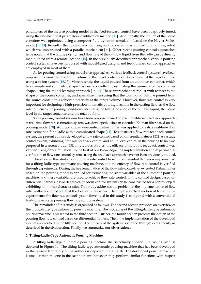
A tilting-ladle-type automatic pouring machine that is actually applied in a casting plant isdepicted in Figure 1a. The tilting-ladle-type automatic pouring machine that has been developedin the present laboratory of the authors is depicted in Figure 1b. The developed pouring machineis smaller than the one in the casting plant; however, they perform similar functions with respect

Appl. Sci. 2019, 9, 1978 3 of 18

to their drive and sensor systems. The ladles in both the pouring machines can be moved in thefront–back, up–down, and rotational directions, for three degrees-of-freedom of motion. In thisstudy, the front–back, up–down, and rotational directions are denoted as the X-, Z-, and Θ-directions,respectively. Further, each drive system in the X- and Z-directions is comprised of linear guides, aball screw, and a servomotor. The drive system in the Θ-direction is comprised of a gear reducerand servomotor. The positions of the ladle in the X- and Z-directions and the angle of the ladle inΘ-direction can be detected, using the rotary encoders in the servomotor systems. The specificationsof the drive systems in the pouring machine developed in our laboratory are presented in Table 1.Additionally, the weight of the liquid in the ladle can be measured, using the load cell installed in thebase of the machine. Therefore, the total weight of the outflow liquid from the ladle can be obtained,based on the difference between the initial and the current weights of the liquid in the ladle. Thecombined error of the load cell is 0.1 kg.

The command signals to the drive systems are calculated by a PC-based controller, in whichthe CPU is an Intel Core i7-4790 (Intel Corporation, Santa Clara, CA, USA) and the memory is 8 GBDDR3-1600 (Corsair Corporation, Fermon, CA, USA). The sampling period in the control systemis 0.02 s. The signals between the controller and the drive systems are transferred by a controllerarea network (CAN) communication method, and the signal from the load cell to the controller istransferred by a serial communication method for reducing noise in the communication.

Load cell

Ladle

Outflow liquid

DC servomotor in Q-direction

Z-direction

X-direction

Q-direction

Linear guides, Ball screw, and DC servomotor in Z-direction

Linear guides, Ball screw, and DC servomotor in X-direction

(a) (b)

Pouring Mouth

Figure 1. Photos of tilting-ladle-type automatic pouring machines. (a) An automatic pouring machinethat is actually applied in a casting plant, and (b) the automatic pouring machine that has beendeveloped in the present laboratory of the authors.

Table 1. Specifications of drive systems in the tilting-ladle-type automatic pouring machine developedby the authors.

X-Direction Z-Direction Θ-Direction

Type of motor Brushless DC motor Brushless DC motor Brushless DC motorControl mode in servo amplifier Velocity mode Velocity mode Velocity modeMotion range 0–0.3 m 0–0.4 m 0–70 degMaximum torque of motor 1.22 Nm 1.22 Nm 11.5 NmPitch of ball screw 0.02 m 0.02 m -Maximum velocity of motor 0.77 m/s 0.38 m/s 371 deg/s

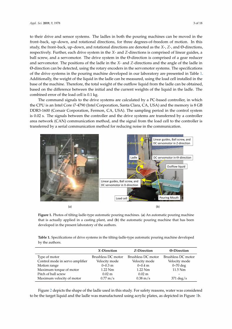
Figure 2 depicts the shape of the ladle used in this study. For safety reasons, water was consideredto be the target liquid and the ladle was manufactured using acrylic plates, as depicted in Figure 1b.

Appl. Sci. 2019, 9, 1978 4 of 18

190

125

115.5

25030

200

Unit: mm

Figure 2. Shape of ladle used in this study.

3. Modeling of the Tilting-Ladle-Type Automatic Pouring Machine

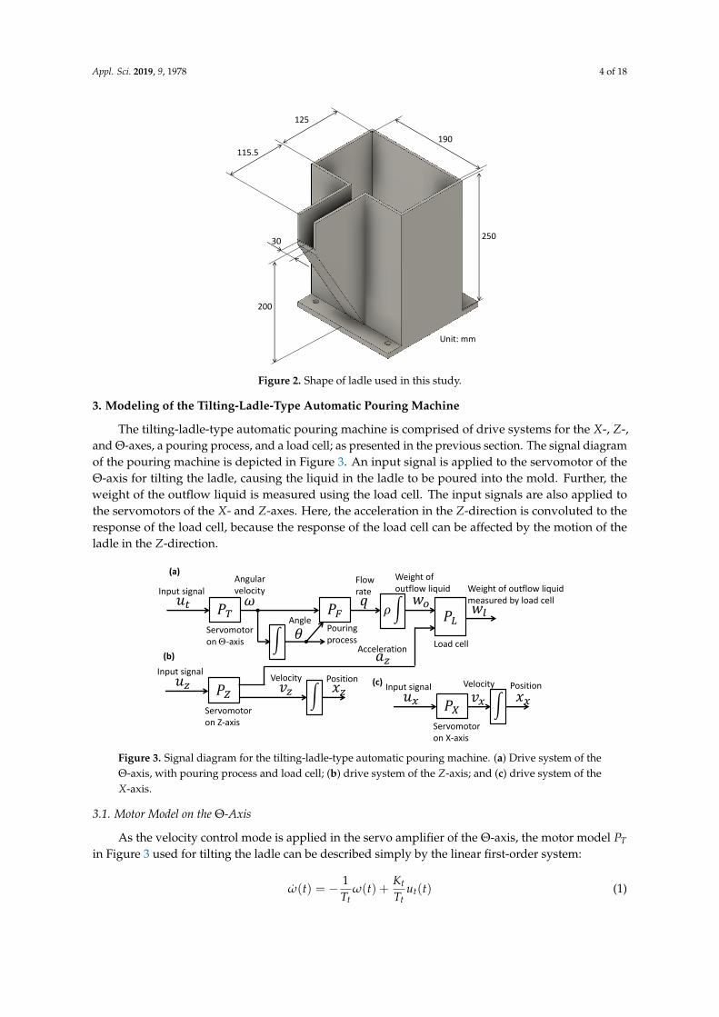
The tilting-ladle-type automatic pouring machine is comprised of drive systems for the X-, Z-,and Θ-axes, a pouring process, and a load cell; as presented in the previous section. The signal diagramof the pouring machine is depicted in Figure 3. An input signal is applied to the servomotor of theΘ-axis for tilting the ladle, causing the liquid in the ladle to be poured into the mold. Further, theweight of the outflow liquid is measured using the load cell. The input signals are also applied tothe servomotors of the X- and Z-axes. Here, the acceleration in the Z-direction is convoluted to theresponse of the load cell, because the response of the load cell can be affected by the motion of theladle in the Z-direction.

Servomotor on Q-axis

𝑃𝑇

Input signal

න

Angularvelocity

Angle

𝑢𝑡 𝜔

𝜃

Servomotor on X-axis

𝑃𝑋

Input signal

න

Velocity Position

𝑢𝑥 𝑣𝑥 𝑥𝑥Servomotor on Z-axis

𝑃𝑍

Input signal

න

Velocity Position𝑢𝑧 𝑣𝑧 𝑥𝑧

Pouring process

𝑃𝐹𝑞

Flow rate

𝜌න 𝑃𝐿

Weight of outflow liquid

𝑤𝑜 𝑤𝑙

Weight of outflow liquid measured by load cell

Load cell

(a)

(c)

(b) 𝑎𝑧Acceleration

Figure 3. Signal diagram for the tilting-ladle-type automatic pouring machine. (a) Drive system of theΘ-axis, with pouring process and load cell; (b) drive system of the Z-axis; and (c) drive system of theX-axis.

3.1. Motor Model on the Θ-Axis

As the velocity control mode is applied in the servo amplifier of the Θ-axis, the motor model PTin Figure 3 used for tilting the ladle can be described simply by the linear first-order system:

ω(t) = − 1Tt

ω(t) +Kt

Ttut(t) (1)

Appl. Sci. 2019, 9, 1978 5 of 18

where ω deg/s denotes the angular velocity of the tilting ladle, ut denotes the input signal applied tothe motor, Tt s denotes the time constant, and Kt deg/s denotes the gain. The tilt angle, θ (in deg), isgiven as

θ(t) = ω(t), (2)

and can be measured using the rotary encoder fitted to the servomotor.

3.2. Motor Models on the X- and Z-Axes

As the velocity control mode is applied in the servo amplifiers of the X- and Z-axes, the motormodels PX and PZ depicted in Figure 3 for transferring the ladle on the X- and Z-axes, respectively,can be described simply by a linear first-order system:

vi(t) = −1Ti

vi(t) +KiTi

ui(t), (i = x, z), (3)

where vi m/s denotes the velocity of the transferring ladle on each axis, ui denotes the input signalapplied to each motor, Ti s denotes the time constant, and Ki m/s denotes the gain. The subscript irepresents the drive direction. The positions xx and xz m of the ladle are given as

xi(t) = vi(t), (i = x, z), (4)

and can be measured using the rotary encoder fitted to each servomotor.

3.3. Pouring Process Model

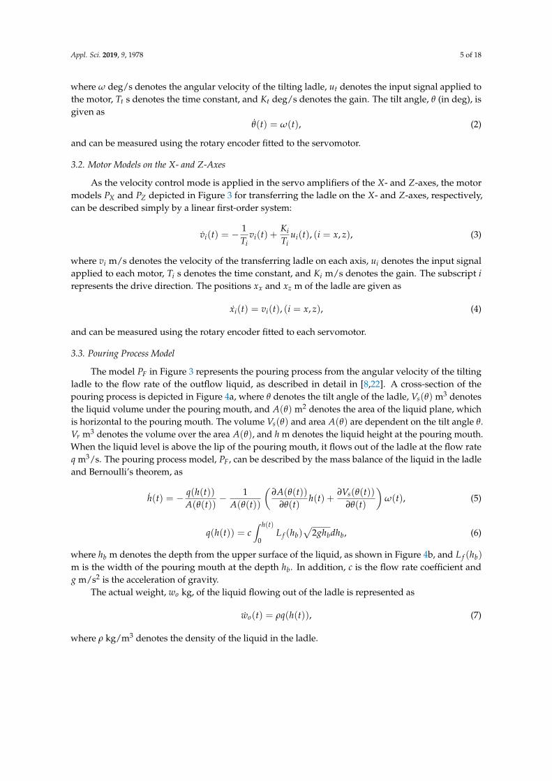
The model PF in Figure 3 represents the pouring process from the angular velocity of the tiltingladle to the flow rate of the outflow liquid, as described in detail in [8,22]. A cross-section of thepouring process is depicted in Figure 4a, where θ denotes the tilt angle of the ladle, Vs(θ) m3 denotesthe liquid volume under the pouring mouth, and A(θ) m2 denotes the area of the liquid plane, whichis horizontal to the pouring mouth. The volume Vs(θ) and area A(θ) are dependent on the tilt angle θ.Vr m3 denotes the volume over the area A(θ), and h m denotes the liquid height at the pouring mouth.When the liquid level is above the lip of the pouring mouth, it flows out of the ladle at the flow rateq m3/s. The pouring process model, PF, can be described by the mass balance of the liquid in the ladleand Bernoulli’s theorem, as

h(t) = − q(h(t))A(θ(t))

− 1A(θ(t))

(∂A(θ(t))

∂θ(t)h(t) +

∂Vs(θ(t))∂θ(t)

)ω(t), (5)

q(h(t)) = c∫ h(t)

0L f (hb)

√2ghbdhb, (6)

where hb m denotes the depth from the upper surface of the liquid, as shown in Figure 4b, and L f (hb)

m is the width of the pouring mouth at the depth hb. In addition, c is the flow rate coefficient andg m/s2 is the acceleration of gravity.

The actual weight, wo kg, of the liquid flowing out of the ladle is represented as

wo(t) = ρq(h(t)), (7)

where ρ kg/m3 denotes the density of the liquid in the ladle.

Appl. Sci. 2019, 9, 1978 6 of 18

L (h )f

hb

m

m

Ladle

Pouring mouth

Outflow liquid

Width of pouring mouth at depth hb

Depth from liquid upper surface

b

Liquid volume under pouring mouth Vs m3

Liquid volume over pouringmouth Vr m3

Area of liquid planewhich is horizontally located on pouring mouth A m2

Pouring mouth

degTilt angle Ladle

θ

Flow rateq m /s3

h mLiquid height at pouring mouth

(a) (b)

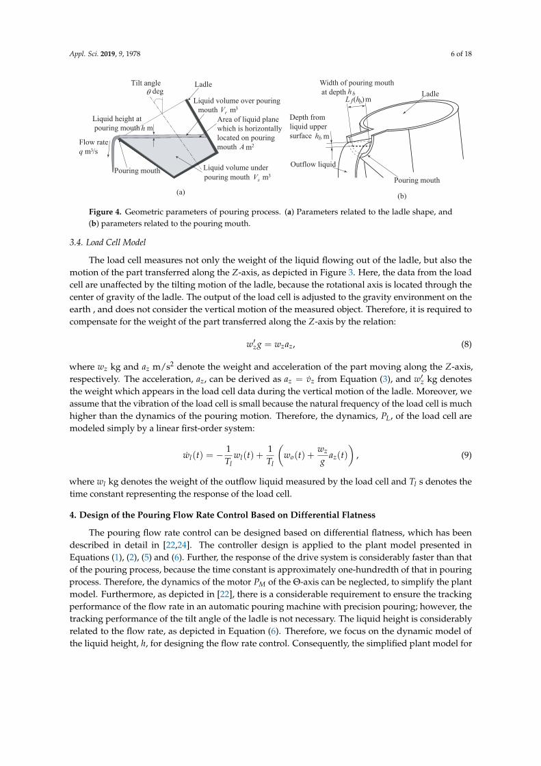
Figure 4. Geometric parameters of pouring process. (a) Parameters related to the ladle shape, and(b) parameters related to the pouring mouth.

3.4. Load Cell Model

The load cell measures not only the weight of the liquid flowing out of the ladle, but also themotion of the part transferred along the Z-axis, as depicted in Figure 3. Here, the data from the loadcell are unaffected by the tilting motion of the ladle, because the rotational axis is located through thecenter of gravity of the ladle. The output of the load cell is adjusted to the gravity environment on theearth , and does not consider the vertical motion of the measured object. Therefore, it is required tocompensate for the weight of the part transferred along the Z-axis by the relation:

w′zg = wzaz, (8)

where wz kg and az m/s2 denote the weight and acceleration of the part moving along the Z-axis,respectively. The acceleration, az, can be derived as az = vz from Equation (3), and w′z kg denotesthe weight which appears in the load cell data during the vertical motion of the ladle. Moreover, weassume that the vibration of the load cell is small because the natural frequency of the load cell is muchhigher than the dynamics of the pouring motion. Therefore, the dynamics, PL, of the load cell aremodeled simply by a linear first-order system:

wl(t) = −1Tl

wl(t) +1Tl

(wo(t) +

wz

gaz(t)

), (9)

where wl kg denotes the weight of the outflow liquid measured by the load cell and Tl s denotes thetime constant representing the response of the load cell.

4. Design of the Pouring Flow Rate Control Based on Differential Flatness

The pouring flow rate control can be designed based on differential flatness, which has beendescribed in detail in [22,24]. The controller design is applied to the plant model presented inEquations (1), (2), (5) and (6). Further, the response of the drive system is considerably faster than thatof the pouring process, because the time constant is approximately one-hundredth of that in pouringprocess. Therefore, the dynamics of the motor PM of the Θ-axis can be neglected, to simplify the plantmodel. Furthermore, as depicted in [22], there is a considerable requirement to ensure the trackingperformance of the flow rate in an automatic pouring machine with precision pouring; however, thetracking performance of the tilt angle of the ladle is not necessary. The liquid height is considerablyrelated to the flow rate, as depicted in Equation (6). Therefore, we focus on the dynamic model ofthe liquid height, h, for designing the flow rate control. Consequently, the simplified plant model for

Appl. Sci. 2019, 9, 1978 7 of 18

the design of the flow rate control is represented as a single input and single output (SISO)-nonlinearfirst-order dynamic system:

h(t) = − 1A(θ)

q(h(t))− 1A(θ)

(∂Vs(θ)

∂θ+

∂A(θ)

∂θh(t)

)Ktut(t). (10)

The flat output F to Equation (10) is given as follows:

F = h(t). (11)

Additionally, the input ut can be derived by the flat output, as follows:

ut(t) = −A(θ)F(t) + q(F(t))

Kt

(∂Vs(θ)

∂θ + ∂A(θ)∂θ F(t)

) . (12)

Further, the new input ν is introduced by the following transformation:

ut(t) = −A(θ)ν(t) + q(F(t))

Kt

(∂Vs(θ)

∂θ + ∂A(θ)∂θ F(t)

) . (13)

Subsequently, the pouring process, using the new input ν, can be described as a single integrator:

F = ν. (14)

Based on Equation (14), the linear feedback tracking controller can be set up using theproportional–integral–derivative (PID) scheme:

ν(t) = F∗ − β1(F− F∗)− β0

∫(F− F∗)dt, (15)

which includes the reference trajectory F∗(t) = h∗(t) of the liquid height and the control parametersβ0 and β1. Then, the dynamics of the tracking error e, which is given as e = F− F∗, can be derived as

e + β1 e + β0e = 0, (16)

using the characteristic polynomial

ϕ(s) = s2 + β1s + β0. (17)

The coefficients β0 and β1 are arranged for satisfying the exponential stability of the closed-loopsystem as follows:

β0 = ω2n, β1 = 2ζωn, (ζ ≥ 1, ωn > 0), (18)

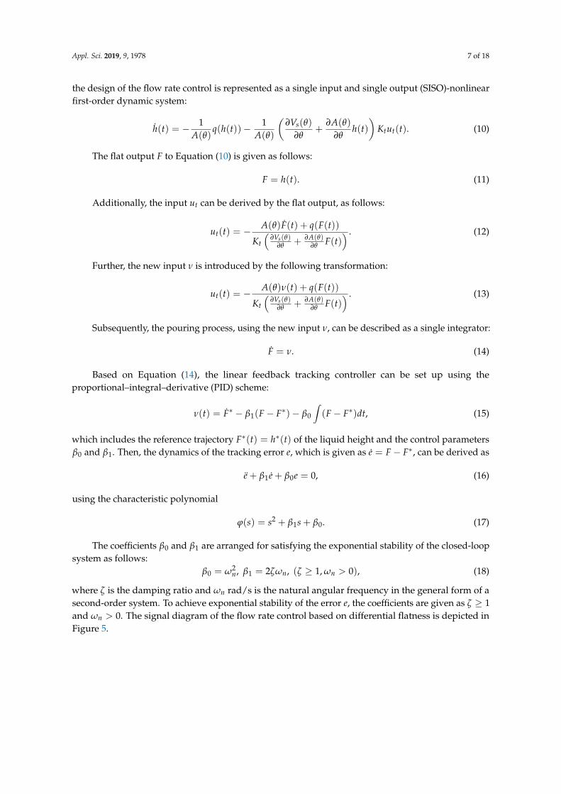
where ζ is the damping ratio and ωn rad/s is the natural angular frequency in the general form of asecond-order system. To achieve exponential stability of the error e, the coefficients are given as ζ ≥ 1and ωn > 0. The signal diagram of the flow rate control based on differential flatness is depicted inFigure 5.

Appl. Sci. 2019, 9, 1978 8 of 18

Pouring process with motor

Input signal for tilting ladle

𝑢𝑡−𝐴 𝜃 𝜈 + 𝑞(ℎ)

𝐾𝑡𝜕𝑉𝑠(𝜃)𝜕𝜃

+𝜕𝐴(𝜃)𝜕𝜃

ℎ𝛽1

න 𝛽0

𝑑

𝑑𝑡𝐹∗ = ℎ∗ 𝜈 𝑞Flow rate

+

+ +

-Angle of tilting ladle

𝜃Liquid height on pouring mouth

ℎ

Reference trajectory

Figure 5. Signal diagram of flow rate control based on differential flatness.

The control input, ut, can be decomposed into a feed-forward term ut f f and a feedback term ut f b,as follows:

ut f f (t) = −A(θ)h(t) + q(h(t))

Kt

(∂Vs(θ)

∂θ + ∂A(θ)∂θ h(t)

) , (19)

ut f b(t) = −A(θ)

{β1e(t) + β0

∫e(t)dt

}+ q(h(t))

Kt

(∂Vs(θ)

∂θ + ∂A(θ)∂θ h(t)

) . (20)

Therefore, the control approach based on differential flatness can derive a two degree-of-freedomcontrol system with a feed-forward term consisting of the inverse dynamics of the pouring model anda feedback term consisting of the feedback linearization and the proportional-integral (PI) control.

This flow rate control system must satisfy the following conditions for stability:

• Kt 6= 0, ∂Vs(θ)∂θ + ∂A(θ)

∂θ F 6= 0;• β0,1 > 0;• the reference trajectory is set as F∗ = 0, within finite time;• the control input is switched to ut = 0 at F∗ = 0;• the control input is within the limitations utlower ≤ ut ≤ utupper, where utlower and utupper are the

lower and the upper bounds in the control input, respectively.

By satisfying the aforementioned conditions, the equilibrium point of the liquid height h isasymptotically stable and that of the tilt angle θ is stable. The stability analysis of this control systemhas been described, in detail, in [22].

The reference trajectory, h∗(=F∗), of the liquid height is required in the flow rate control system.The reference trajectory, h∗(t), is a C1-function. It is set up using a time polynomial for a transientbetween the stationary states h∗i m and h∗f m:

h∗(t) = h∗i + (h∗f − h∗i )2n+1

∑j=n+1

aj(t− tit f − ti

)j, t ∈ [ti, t f ], (21)

where h∗i and h∗f denote the initial and terminal liquid heights on transition, respectively. Further, tis and t f s are the initial and terminal times of transition, respectively. The order n = 1 defines the(2n + 1 = 3) degree of the polynomial, because of the required smoothness h∗ ∈ C1 of the referencetrajectory. The coefficients aj are given as a2 = 3 and a3 = −2.

In the reference trajectory planning, the initial and terminal liquid heights, h∗i, f , are obtainedas follows:

h∗i, f = f−1q (q∗i, f ), (22)

where f−1q represents the inverse function of Equation (6). Here, q∗i m3/s denotes the initial flow rate

and q∗f m3/s denotes the terminal flow rate of transition. We assume that the relation between the flowrate q and liquid height h at pouring mouth is uniquely derived.

Appl. Sci. 2019, 9, 1978 9 of 18

5. Implementation of the Flow Rate Control System

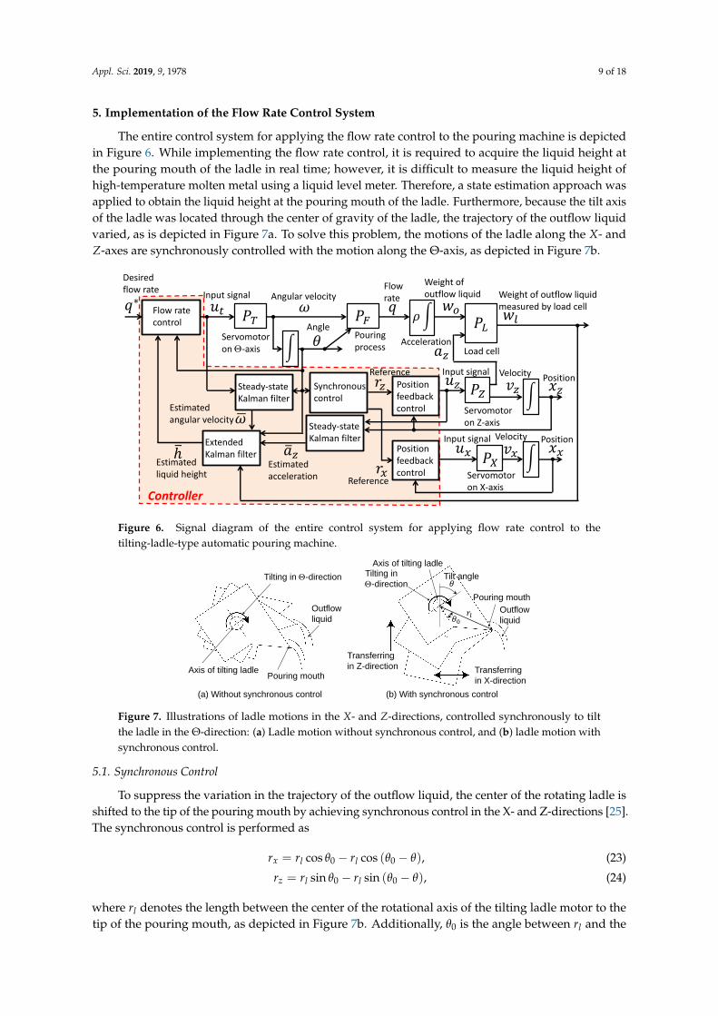
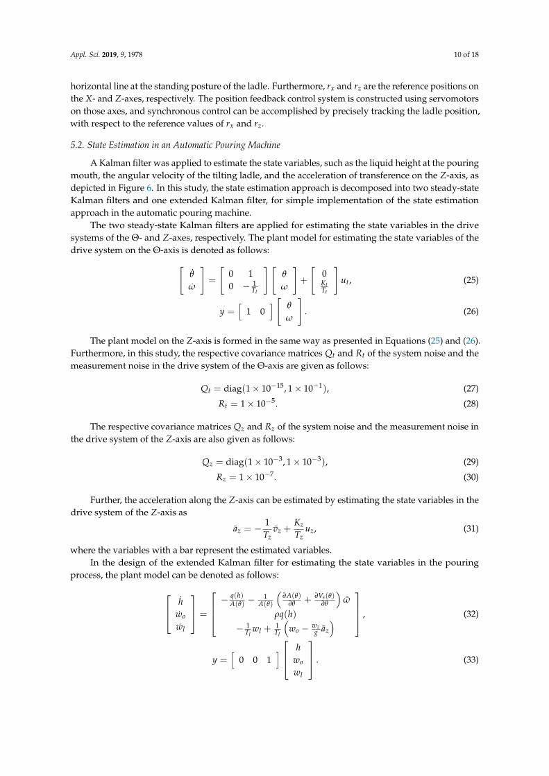
The entire control system for applying the flow rate control to the pouring machine is depictedin Figure 6. While implementing the flow rate control, it is required to acquire the liquid height atthe pouring mouth of the ladle in real time; however, it is difficult to measure the liquid height ofhigh-temperature molten metal using a liquid level meter. Therefore, a state estimation approach wasapplied to obtain the liquid height at the pouring mouth of the ladle. Furthermore, because the tilt axisof the ladle was located through the center of gravity of the ladle, the trajectory of the outflow liquidvaried, as is depicted in Figure 7a. To solve this problem, the motions of the ladle along the X- andZ-axes are synchronously controlled with the motion along the Θ-axis, as depicted in Figure 7b.

Servomotor on Q-axis

𝑃𝑇

Input signal

න

Angular velocity

Angle

𝑢𝑡

Servomotor on X-axis

𝑃𝑋

Input signal

න

Velocity Position𝑢𝑥 𝑣𝑥 𝑥𝑥

Servomotor on Z-axis

𝑃𝑍

Input signal

න

Velocity Position𝑢𝑧 𝑣𝑧 𝑥𝑧

Pouring process

𝑃𝐹𝑞

Flow rate

𝜌න 𝑃𝐿

Weight of outflow liquid

𝑤𝑜 𝑤𝑙

Weight of outflow liquid measured by load cell

Load cell𝑎𝑧Acceleration

Synchronous control

Flow ratecontrol

Steady-stateKalman filter

Steady-stateKalman filterExtended

Kalman filterതℎEstimatedliquid height

Estimatedangular velocity ഥ𝜔

ത𝑎𝑧Estimatedacceleration

Controller

𝜔

𝜃

Position feedback control

Position feedback control

𝑟𝑧

𝑟𝑥

Reference

Reference

𝑞∗

Desired flow rate

Figure 6. Signal diagram of the entire control system for applying flow rate control to thetilting-ladle-type automatic pouring machine.

Axis of tilting ladlePouring mouth

(a) Without synchronous control

Transferring

in Z-direction

(b) With synchronous control

Transferring

in X-direction

Axis of tilting ladle

Pouring mouth

Outflow

liquid

Outflow

liquid

Tilting in Q-direction Tilting in

Q-direction

𝑟𝑙𝜃0

𝜃Tilt angle

Figure 7. Illustrations of ladle motions in the X- and Z-directions, controlled synchronously to tiltthe ladle in the Θ-direction: (a) Ladle motion without synchronous control, and (b) ladle motion withsynchronous control.

5.1. Synchronous Control

To suppress the variation in the trajectory of the outflow liquid, the center of the rotating ladle isshifted to the tip of the pouring mouth by achieving synchronous control in the X- and Z-directions [25].The synchronous control is performed as

rx = rl cos θ0 − rl cos (θ0 − θ), (23)

rz = rl sin θ0 − rl sin (θ0 − θ), (24)

where rl denotes the length between the center of the rotational axis of the tilting ladle motor to thetip of the pouring mouth, as depicted in Figure 7b. Additionally, θ0 is the angle between rl and the

Appl. Sci. 2019, 9, 1978 10 of 18

horizontal line at the standing posture of the ladle. Furthermore, rx and rz are the reference positions onthe X- and Z-axes, respectively. The position feedback control system is constructed using servomotorson those axes, and synchronous control can be accomplished by precisely tracking the ladle position,with respect to the reference values of rx and rz.

5.2. State Estimation in an Automatic Pouring Machine

A Kalman filter was applied to estimate the state variables, such as the liquid height at the pouringmouth, the angular velocity of the tilting ladle, and the acceleration of transference on the Z-axis, asdepicted in Figure 6. In this study, the state estimation approach is decomposed into two steady-stateKalman filters and one extended Kalman filter, for simple implementation of the state estimationapproach in the automatic pouring machine.

The two steady-state Kalman filters are applied for estimating the state variables in the drivesystems of the Θ- and Z-axes, respectively. The plant model for estimating the state variables of thedrive system on the Θ-axis is denoted as follows:[

θ

ω

]=

[0 10 − 1

Tt

] [θ

ω

]+

[0KtTt

]ut, (25)

y =[

1 0] [ θ

ω

]. (26)

The plant model on the Z-axis is formed in the same way as presented in Equations (25) and (26).Furthermore, in this study, the respective covariance matrices Qt and Rt of the system noise and themeasurement noise in the drive system of the Θ-axis are given as follows:

Qt = diag(1× 10−15, 1× 10−1), (27)

Rt = 1× 10−5. (28)

The respective covariance matrices Qz and Rz of the system noise and the measurement noise inthe drive system of the Z-axis are also given as follows:

Qz = diag(1× 10−3, 1× 10−3), (29)

Rz = 1× 10−7. (30)

Further, the acceleration along the Z-axis can be estimated by estimating the state variables in thedrive system of the Z-axis as

az = −1Tz

vz +Kz

Tzuz, (31)

where the variables with a bar represent the estimated variables.In the design of the extended Kalman filter for estimating the state variables in the pouring

process, the plant model can be denoted as follows:

hwo

wl

=

− q(h)

A(θ)− 1

A(θ)

(∂A(θ)

∂θ + ∂Vs(θ)∂θ

)ω

ρq(h)− 1

Tlwl +

1Tl

(wo − wz

g az

) , (32)

y =[

0 0 1] h

wo

wl

. (33)

Appl. Sci. 2019, 9, 1978 11 of 18

In this study, the respective covariance matrices Q f and R f of the system noise and themeasurement noise in the pouring process are given as follows:

Q f = diag(2.5× 10−10, 1× 10−11, 1× 10−11), (34)

R f = 5× 10−4. (35)

5.3. Model Parameter Identification

The model parameters of the drive systems of the X-, Z-, and Θ-axes in the automatic pouringmachine, as depicted in Figure 1b, were identified by fitting the simulations of the drive system modelsto the experimental data. The identified model parameters are presented in Table 2.

Table 2. Identified model parameters for the drive systems of the X-, Z-, and Θ-axes.

X-Axis Z-Axis Θ-Axis

Gain, K 1.00 1.00 1.00Time constant, T 0.050 s 0.050 s 0.022 s

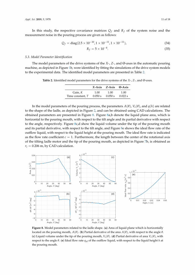
In the model parameters of the pouring process, the parameters A(θ), Vs(θ), and q(h) are relatedto the shape of the ladle, as depicted in Figure 2, and can be obtained using CAD calculations. Theobtained parameters are presented in Figure 8. Figure 8a,b denote the liquid plane area, which ishorizontal to the pouring mouth, with respect to the tilt angle and its partial derivative with respectto the angle, respectively. Figure 8c,d show the liquid volume under the tip of the pouring mouthand its partial derivative, with respect to the tilt angle, and Figure 8e shows the ideal flow rate of theoutflow liquid, with respect to the liquid height at the pouring mouth. The ideal flow rate is indicatedas the flow rate coefficient c = 1. Furthermore, the length between the center of the rotational axisof the tilting ladle motor and the tip of the pouring mouth, as depicted in Figure 7b, is obtained asrl = 0.206 m, by CAD calculation.

(a)

(b)

(c)

(d)

(e)

Figure 8. Model parameters related to the ladle shape. (a) Area of liquid plane which is horizontallylocated on the pouring mouth, A(θ). (b) Partial derivative of the area A(θ), with respect to the angle θ.(c) Liquid volume under the tip of the pouring mouth, Vs(θ). (d) Partial derivative of area Vs(θ), withrespect to the angle θ. (e) Ideal flow rate qid of the outflow liquid, with respect to the liquid height h atthe pouring mouth.

Appl. Sci. 2019, 9, 1978 12 of 18

The flow rate coefficient, c, in the pouring process can be identified by fitting the simulation tothe experimental data using the pouring model. In this study, the flow rate coefficient was obtained asc = 0.75. The density of the liquid is given as ρ = 103 kg/m3, as water is considered to be the targetliquid in this study.

In the load cell model, the weight of the part transferred along the Z-axis is wz = 18.6 kg.Additionally, the time constant in the load cell was identified as Tl = 0.16 s.

5.4. Control Parameters

In the design of the flow rate control, the damping ratio in Equation (18) is given as ζ = 1 for hightracking performance with suppressed vibration. In addition, we adjust the natural angular frequencyωn in Equation (18). Further, the tracking performance can be improved by increasing the naturalangular frequency. However, this can also increase the signal noise in the control loop. The naturalangular frequency was determined as ωn = 2 rad/s, in this study.

5.5. Design of the Reference Trajectory

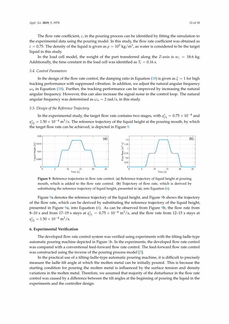
In the experimental study, the target flow rate contains two stages, with q∗f 1 = 0.75× 10−4 and

q∗f 2 = 1.50× 10−4 m3/s. The reference trajectory of the liquid height at the pouring mouth, by whichthe target flow rate can be achieved, is depicted in Figure 9.

(a) (b)

Figure 9. Reference trajectories in flow rate control. (a) Reference trajectory of liquid height at pouringmouth, which is added to the flow rate control. (b) Trajectory of flow rate, which is derived bysubstituting the reference trajectory of liquid height, presented in (a), into Equation (6).

Figure 9a denotes the reference trajectory of the liquid height, and Figure 9b shows the trajectoryof the flow rate, which can be derived by substituting the reference trajectory of the liquid height,presented in Figure 9a, into Equation (6). As can be observed from Figure 9b, the flow rate from8–10 s and from 17–19 s stays at q∗f 1 = 0.75× 10−4 m3/s, and the flow rate from 12–15 s stays at

q∗f 2 = 1.50× 10−4 m3/s.

6. Experimental Verification

The developed flow rate control system was verified using experiments with the tilting-ladle-typeautomatic pouring machine depicted in Figure 1b. In the experiments, the developed flow rate controlwas compared with a conventional feed-forward flow rate control. The feed-forward flow rate controlwas constructed using the inverse of the pouring process model [3].

In the practical use of a tilting-ladle-type automatic pouring machine, it is difficult to preciselymeasure the ladle tilt angle at which the molten metal can be initially poured. This is because thestarting condition for pouring the molten metal is influenced by the surface tension and densityvariations in the molten metal. Therefore, we assumed that majority of the disturbance in the flow ratecontrol was caused by a difference between the tilt angles at the beginning of pouring the liquid in theexperiments and the controller design.

Appl. Sci. 2019, 9, 1978 13 of 18

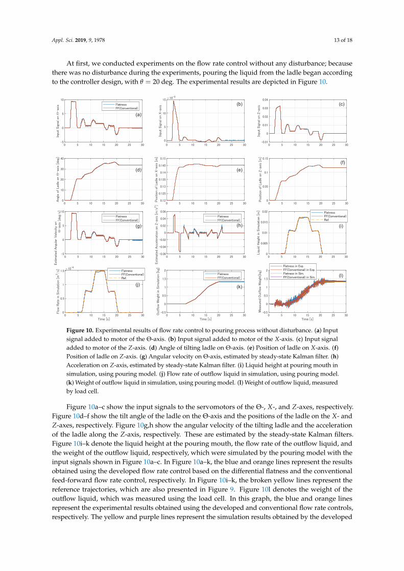
At first, we conducted experiments on the flow rate control without any disturbance; becausethere was no disturbance during the experiments, pouring the liquid from the ladle began accordingto the controller design, with θ = 20 deg. The experimental results are depicted in Figure 10.

(a)

(b) (c)

(d) (e)(f)

(g) (h) (i)

(j) (k)

(l)

Figure 10. Experimental results of flow rate control to pouring process without disturbance. (a) Inputsignal added to motor of the Θ-axis. (b) Input signal added to motor of the X-axis. (c) Input signaladded to motor of the Z-axis. (d) Angle of tilting ladle on Θ-axis. (e) Position of ladle on X-axis. (f)Position of ladle on Z-axis. (g) Angular velocity on Θ-axis, estimated by steady-state Kalman filter. (h)Acceleration on Z-axis, estimated by steady-state Kalman filter. (i) Liquid height at pouring mouth insimulation, using pouring model. (j) Flow rate of outflow liquid in simulation, using pouring model.(k) Weight of outflow liquid in simulation, using pouring model. (l) Weight of outflow liquid, measuredby load cell.

Figure 10a–c show the input signals to the servomotors of the Θ-, X-, and Z-axes, respectively.Figure 10d–f show the tilt angle of the ladle on the Θ-axis and the positions of the ladle on the X- andZ-axes, respectively. Figure 10g,h show the angular velocity of the tilting ladle and the accelerationof the ladle along the Z-axis, respectively. These are estimated by the steady-state Kalman filters.Figure 10i–k denote the liquid height at the pouring mouth, the flow rate of the outflow liquid, andthe weight of the outflow liquid, respectively, which were simulated by the pouring model with theinput signals shown in Figure 10a–c. In Figure 10a–k, the blue and orange lines represent the resultsobtained using the developed flow rate control based on the differential flatness and the conventionalfeed-forward flow rate control, respectively. In Figure 10i–k, the broken yellow lines represent thereference trajectories, which are also presented in Figure 9. Figure 10l denotes the weight of theoutflow liquid, which was measured using the load cell. In this graph, the blue and orange linesrepresent the experimental results obtained using the developed and conventional flow rate controls,respectively. The yellow and purple lines represent the simulation results obtained by the developed

Appl. Sci. 2019, 9, 1978 14 of 18

and conventional flow rate controls, respectively. As can be observed from Figure 10l, because thesimulation results were fitted with the experimental results, the pouring process in the tilting-ladle-typeautomatic pouring machine can be precisely represented by using the pouring model derived in thisstudy. Therefore, we observe the simulation results in Figure 10i–k as actual states in the automaticpouring machine. In the experiments on the pouring process without any disturbance, the liquidheight at the pouring mouth and the flow rate of the outflow liquid in each flow rate control wereprecisely tracked to the reference trajectory.

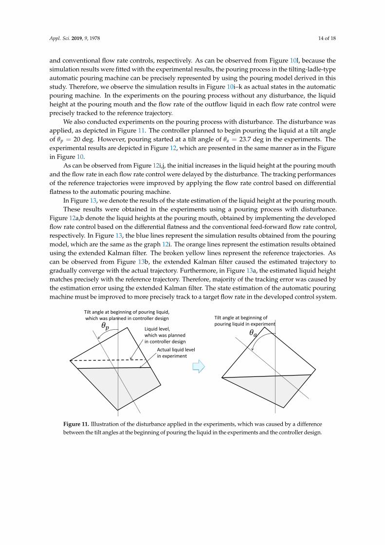
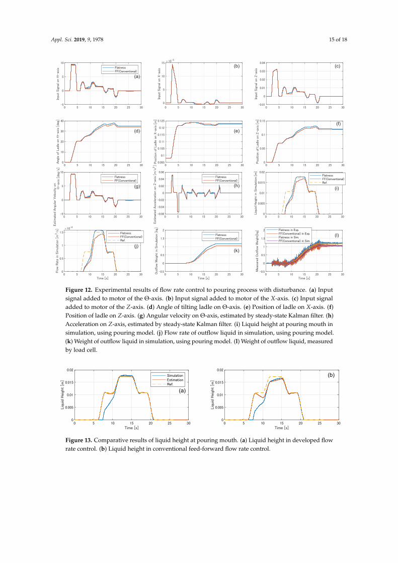
We also conducted experiments on the pouring process with disturbance. The disturbance wasapplied, as depicted in Figure 11. The controller planned to begin pouring the liquid at a tilt angleof θp = 20 deg. However, pouring started at a tilt angle of θa = 23.7 deg in the experiments. Theexperimental results are depicted in Figure 12, which are presented in the same manner as in the Figurein Figure 10.

As can be observed from Figure 12i,j, the initial increases in the liquid height at the pouring mouthand the flow rate in each flow rate control were delayed by the disturbance. The tracking performancesof the reference trajectories were improved by applying the flow rate control based on differentialflatness to the automatic pouring machine.

In Figure 13, we denote the results of the state estimation of the liquid height at the pouring mouth.These results were obtained in the experiments using a pouring process with disturbance.

Figure 12a,b denote the liquid heights at the pouring mouth, obtained by implementing the developedflow rate control based on the differential flatness and the conventional feed-forward flow rate control,respectively. In Figure 13, the blue lines represent the simulation results obtained from the pouringmodel, which are the same as the graph 12i. The orange lines represent the estimation results obtainedusing the extended Kalman filter. The broken yellow lines represent the reference trajectories. Ascan be observed from Figure 13b, the extended Kalman filter caused the estimated trajectory togradually converge with the actual trajectory. Furthermore, in Figure 13a, the estimated liquid heightmatches precisely with the reference trajectory. Therefore, majority of the tracking error was caused bythe estimation error using the extended Kalman filter. The state estimation of the automatic pouringmachine must be improved to more precisely track to a target flow rate in the developed control system.

Tilt angle at beginning of pouring liquid,which was planned in controller design

𝜃𝑝 Liquid level, which was planned in controller design

Actual liquid level in experiment

𝜃𝑎

Tilt angle at beginning of pouring liquid in experiment

Figure 11. Illustration of the disturbance applied in the experiments, which was caused by a differencebetween the tilt angles at the beginning of pouring the liquid in the experiments and the controller design.

Appl. Sci. 2019, 9, 1978 15 of 18

(a)

(b) (c)

(d) (e)(f)

(g) (h) (i)

(j)(k)

(l)

Figure 12. Experimental results of flow rate control to pouring process with disturbance. (a) Inputsignal added to motor of the Θ-axis. (b) Input signal added to motor of the X-axis. (c) Input signaladded to motor of the Z-axis. (d) Angle of tilting ladle on Θ-axis. (e) Position of ladle on X-axis. (f)Position of ladle on Z-axis. (g) Angular velocity on Θ-axis, estimated by steady-state Kalman filter. (h)Acceleration on Z-axis, estimated by steady-state Kalman filter. (i) Liquid height at pouring mouth insimulation, using pouring model. (j) Flow rate of outflow liquid in simulation, using pouring model.(k) Weight of outflow liquid in simulation, using pouring model. (l) Weight of outflow liquid, measuredby load cell.

(a)

(b)

Figure 13. Comparative results of liquid height at pouring mouth. (a) Liquid height in developed flowrate control. (b) Liquid height in conventional feed-forward flow rate control.

Appl. Sci. 2019, 9, 1978 16 of 18

7. Conclusions and Future Works

In this study, we addressed the manner in which flow rate control based on differential flatnesscan be applied to a tilting-ladle-type automatic pouring machine, and verified the efficacy of thedeveloped flow rate control through various experiments. The following conclusions can be obtained:

1. From the viewpoint of practical application, a SISO-nonlinear-type controller design based ondifferential flatness was applied, to ensure the flow rate control of the automatic pouring machine;

2. while implementing the flow rate control using the feedback control scheme, it was necessary tomeasure the states of the automatic pouring machine—however, it is difficult to directly measurethe states of high-temperature molten metal. Therefore, in this study, the Kalman filter approachwas applied for estimating the state variables of the automatic pouring machine;

3. the steady-state and extended Kalman filters were decomposed for simple construction of thestate estimate of the automatic pouring machine;

4. in the experiments related to the pouring process without disturbance, both the feed-forward flowrate control based on the inverse pouring model, and the flow rate control based on differentialflatness, achieved a flow rate by which the outflow liquid precisely tracked with the referencetrajectory: We conclude that the pouring model described in this study could precisely representthe actual pouring process in the automatic pouring machine;

5. in the experiments on a pouring process with disturbance, the tracking performance of the flowrate in the pouring machine could be improved by implementing flow rate control based ondifferential flatness; and

6. a majority of the tracking errors of the flow rate control based on differential flatness were causedby the estimation errors of the extended Kalman filter.

Furthermore, the following recommendations for future work can be obtained:

1. To obtain high tracking performance, the state estimation approach of the pouring machine shouldbe improved in future studies;

2. in the developed flow rate control, the flow rate of the outflow liquid was indirectly controlled,based on the liquid height at the pouring mouth. If any disturbances were observed in the relationbetween the flow rate and the liquid height at the pouring mouth, the tracking performance ofthe flow rate control may have degraded. Further, direct flow rate control must be achieved toconstruct a high-precision automatic pouring machine; and

3. in practical pouring processes, the characteristics of the pouring material are variable withtemperature, the added substance, and so on. Therefore, a control approach with computationalintelligence, such that the controller can be adapted autonomously to the pouring environment,should be developed in the future work.

Author Contributions: Conceptualization, Y.N.; Methodology, Y.N.; software, Y.N. and Y.S.; Validation, Y.N.and Y.S.; Formal analysis, Y.N.; Investigation, Y.N.; Resources, Y.N.; Data curation, Y.N.; Writing—original draftpreparation, Y.N.; Writing—review and editing, Y.N. and Y.S.; Visualization, Y.N.; Supervision, Y.N.; Projectadministration, Y.N.; Funding acquisition, Y.N.

Funding: This study was funded by JKA foundation, grant number 2018M-177; and the Adaptable and SeamlessTechnology Transfer Program through Target-driven R&D, JST, project “Development of measurement system forpouring process by sensor-fusion”.

Conflicts of Interest: The authors declare no conflict of interest.

Abbreviations

The following abbreviation is used in this manuscript:

SISO Single input and single output.

Appl. Sci. 2019, 9, 1978 17 of 18

References

1. Lindsay, W. Automatic pouring and metal distribution systems. Foundry Trade J. 1983, 10, 151–176.2. Terashima, K.; Miyoshi, T.; Noda, Y. Innovative automation technologies and IT applications of the metal

casting process necessary for the foundries of the 21st century. Int. J. Autom. Technol. 2008, 2, 229–240.[CrossRef]

3. Noda, Y.; Nishida, T. Precision analysis of automatic pouring machines for the casting industry. Int. J.Autom. Technol. 2008, 2, 241–246. [CrossRef]

4. Neumann, E.; Trauzeddel, D. Pouring systems for ferrous applications. Foundry Trade J. 2002, 23–24.5. Tayode, A.; Chitre, A.; Rahulkar, A. PLC based hydraulic auto ladle system. Int. J. Eng. Res. Appl. 2014,

4, 19–22.6. Rajput, N.; Patil, N.; Sutar, M. Precision analysis and control of automatic pouring machine to control the

flow ability to minimize the porosity of SG200 casting for foundry. Int. J. Res. Adv. Technol. 2015, 3, 22–24.7. Voss, T. Optimization and control of modern ladle pouring process. In Proceedings of the 73rd World

Foundry Congress, Cracow, Poland, 23–27 September 2018; pp. 497–498.8. Noda, Y.; Terashima, K. Modeling and feedforward flow rate control of automatic pouring system with real

ladle. Int. J. Robot. Mechatron. 2007, 19, 205–211. [CrossRef]9. Noda, Y.; Watari, H.; Yamazaki, T. Control of liquid level in tundish of strip caster with automatic pouring

system. Mater. Sci. Forum 2008, 575–578, 147–153. [CrossRef]10. Yano, K.; Terashima, K. Supervisory control of automatic pouring machine. Control Eng. Pract. 2010,

18, 230–241. [CrossRef]11. Tsuji, T.; Noda, Y. High-precision pouring control using online model parameters identification in automatic

pouring robot with cylindrical ladle. In Proceedings of the 2014 IEEE International Conference on Systems,Man, and Cybernetics, San Diego, CA, USA, 5–8 October 2014; pp. 2593–2598.

12. Kuriyama, Y.; Yano, K.; Nishido, S. Optimization of pouring velocity for aluminium gravity casting. In FluidDynamics, Computational Modeling and Applications; Juarez, L., Ed.; InTech: Rijeka, Croatia, 2012; pp. 575–588.

13. Pan, Z.; Park, C.; Manocha, D. Robot motion planning for pouring liquids. In Proceedings of the 26thInternational Conference on Automated Planning and Scheduling, London, UK, 12–17 June 2016; pp. 518–526.

14. Li, L.; Wang, C.; Wu, H. Research on kinematics and pouring law of a mobile heavy load pouring robot.Math. Prob. Eng. 2018, 2018, 8790575. [CrossRef]

15. Sueki, Y.; Noda, Y. Operational assistance system with direct manipulation of flow rate and falling positionof outflow liquid in tilting-ladle-type pouring machine. In Proceedings of the 73rd World Foundry Congress,Cracow, Poland, 23–27 September 2018; pp. 325–326.

16. Schenck, C.; Fox, D. Visual closed-loop control for pouring liquids. In Proceedings of the IEEE InternationalConference on Robotics and Automation, Singapore, 29 May–3 June 2017; pp. 2629–2636.

17. Do, C.; Burgard, W. Accurate pouring with an autonomous robot using an RGB-D camera. In IntelligentAutonomous Systems 15, Proceedings of the International Conference on Intelligent Autonomous Systems,Baden-Baden, Germany, 11–15 June 2018; Springer: Cham, Switzerland, 2018; pp. 210–221.

18. Kennedy, M.; Schmeckpeper, K.; Thakur, D.; Jiang, C.; Kumar, V.; Daniilidis, K. Autonomous PrecisionPouring From Unknown Containers. IEEE Robot. Autom. Lett. 2019, 4, 2317–2324. [CrossRef]

19. Kennedy, M.; Queen, K.; Thakur, D.; Daniilidis, K.; Kumar, V. Precise dispensing of liquids using visualfeedback. In Proceedings of the 2017 IEEE/RSJ International Conference on Intelligent Robots and Systems,Vancouver, BC, Canada, 24–28 September 2017. [CrossRef]

20. Noda, Y.; Terashima, K. Estimation of flow rate in automatic pouring system with real ladle used in industry.In Proceedings of the ICROS-SICE Internaonal Conference, Fukuoka, Japan, 18–21 August 2009; pp. 354–359.

21. Noda, Y.; Birkhold, M.; Terashima, K.; Sawodny, O.; Verl, A. Flow rate estimation using UnscentedKalman Filter in automatic pouring robot. In Proceedings of the SICE Annual Conference, Tokyo, Japan,13–18 September 2011; pp. 769–774.

22. Noda, Y.; Zeitz, M.; Sawodny, O.; Terashima, K. Flow rate control based on differential flatness inautomatic pouring robot. In Proceedings of the IEEE International Conference on Control Applications,Denver, CO, USA, 3–5 March 2011; pp. 1468–1475.

Appl. Sci. 2019, 9, 1978 18 of 18

23. Ito, A.; Oetinger, P.; Tasaki, R.; Sawodny, O.; Terashima, K. Visual nonlinear feedback control of liquid levelin mold sprue cup by cascade system with flow rate control for tilting-ladle-type automatic pouring system.Mater. Sci. Forum 2018, 925, 483–490. [CrossRef]

24. Ramirez, H.; Agrawal, S. SISO nonlinear systems. In Differentially Flat Systems; Lewis, F., Ed.; CRC Press:Boca Raton, FL, USA, 2004; pp. 191–220.

25. Terashima, K.; Yano, K.; Sugimoto, Y.; Watanabe, M. Position control of ladle tip and sloshing suppressionduring tilting motion in automatic pouring machine. In Proceedings of the 10th IFAC symposium onAutomation in Mining, Mineral and Metal Processing, Tokyo, Japan, 4–6 September 2001; pp. 182–187.

c© 2019 by the authors. Licensee MDPI, Basel, Switzerland. This article is an open accessarticle distributed under the terms and conditions of the Creative Commons Attribution(CC BY) license (http://creativecommons.org/licenses/by/4.0/).