CONTENTS Volume 4, Number 4, Autumn 2010 1. Biosurfactants and heir Use in Upgrading Petroleum Vacuum Distillation Residue: A Review 549 Mazaheri Assadi, M . and Tabatabaee, M. S.( Iran) 2. Multi-Criteria Decision-based Model for Road Network Process 573 Sadeghi-Niaraki, A . and Kim, K . and Varshosaz, M . (Korea) 3. Water and Wastewater Minimization in Tehran Oil Refinery using Water Pinch Analysis 583 Nabi Bidhendi, Gh. R., Mehrdadi, N. and Mohammadnejad, S. (Iran) 4. Genotoxic Effects of Electromagnetic Fields from High Voltage Power Lines on Some Plants 595 Aksoy, H., Unal, F. and Ozcan, S.(Turkey) 5. Adsorption of fluoride from water by Al 3+ and Fe 3+ pretreated natural Iranian zeolites 607 Rahmani, A., Nouri, J., Kamal Ghadiri, S., Mahvi, A. H., Zare M. R. (Iran) 6. Recyclable Rubber Sheets Impregnated with Potassium Oxalate doped TiO 2 and their uses in Decolorization of Dye-Polluted Waters 615 Suwanchawalit, Ch., Sriwong, Ch. and Wongnawa, S. (Thailand) 7. Heavy Metal Pollution in Kabini River Sediments 629 Taghinia Hejabi, A., Basavarajappa, H.T. and Qaid Saeed, A. M.( India) 8. Corporations Response to the Energy Saving and Pollution Abatement Policy 637 Xing, L., Shi, L. and Hussain, A.(China) 9. Distribution of Heavy Metals around the Dashkasan Au Mine 647 Rafiei, B., Bakhtiari Nejad, M ., Hashemi, M. and Khodaei, A . S. (Iran) 10. Enhancement Biodegradation of n-alkanes from Crude Oil Contaminated Seawater 655 Zahed, M. A., Aziz , H. A., Isa, M. H. and Mohajeri, L. (Malaysia) 11. Preparation of Pellets by Urban Waste Compost 665 Mavaddati, S., Kianmehr , M . H ., Allahdadi , I. and Chegini , G . R.(Iran) 12. Land Reclamation and Ecological Restoration in a Marine Area 673 Zagas, T., Tsitsoni, T., Ganatsas, P., Tsakaldimi, M., Skotidakis, T. and Zagas D. (Greece) 13. Role of E-shopping Management Strategy in Urban Environment 681 Tehrani, S. M. , Karbassi, A. R., Monavari, S. M. and Mirbagheri S. A.(Iran) 14. Spatial Variability and Contamination of Heavy Metals in the Inter-tidal Systems of a Tropical Environment 691 Ratheesh Kumar, C. S., Joseph, M. M., Gireesh Kumar, T. R., Renjith, K.R., Manju, M. N. and Chandramohanakumar, N.(India) 15. A GIS Based Assessment Tool for Biodiversity Conservation 701 Monavari , S. M. and Momen Bellah Fard, S.(Iran) 16. Flow Regulation for Water Quality (chlorophyll a) Improvement 713 Jeong, K. S., Kim, D. K., Shin, H. S., Kim, H. W., Cao, H., Jang, M. H. and Joo, G. J.( Korea) 17. Ecological Impact Analysis on Mahshahr Petrochemical Industries Using Analytic Hierarchy Process Method 725 Malmasi, S. , Jozi, S . A. , Monavari, S .M., Jafarian, M. E .(Iran) 18. Precipitation Chelation of Cyanide Complexes in Electroplating Industry Wastewater 735 Naim, R., Kisay , L., Park , J. , Qaisar, M., Zulfiqar, A . B., Noshin, M. and Jamil, K. (Korea) Continues…

Welcome message from author
This document is posted to help you gain knowledge. Please leave a comment to let me know what you think about it! Share it to your friends and learn new things together.
Transcript
CONTENTS
Volume 4, Number 4, Autumn 2010
1. Biosurfactants and heir Use in Upgrading Petroleum Vacuum Distillation Residue: A Review 549 Mazaheri Assadi, M . and Tabatabaee, M. S.( Iran)
2. Multi-Criteria Decision-based Model for Road Network Process 573 Sadeghi-Niaraki, A . and Kim, K . and Varshosaz, M . (Korea)
3. Water and Wastewater Minimization in Tehran Oil Refinery using Water Pinch Analysis 583 Nabi Bidhendi, Gh. R., Mehrdadi, N. and Mohammadnejad, S. (Iran)
4. Genotoxic Effects of Electromagnetic Fields from High Voltage Power Lines on Some Plants 595 Aksoy, H., Unal, F. and Ozcan, S.(Turkey)
5. Adsorption of fluoride from water by Al3+ and Fe3+ pretreated natural Iranian zeolites 607 Rahmani, A., Nouri, J., Kamal Ghadiri, S., Mahvi, A. H., Zare M. R. (Iran)
6. Recyclable Rubber Sheets Impregnated with Potassium Oxalate doped TiO2 and their uses in Decolorization of Dye-Polluted Waters
615
Suwanchawalit, Ch., Sriwong, Ch. and Wongnawa, S. (Thailand)
7. Heavy Metal Pollution in Kabini River Sediments 629 Taghinia Hejabi, A., Basavarajappa, H.T. and Qaid Saeed, A. M.( India)
8. Corporations Response to the Energy Saving and Pollution Abatement Policy 637 Xing, L., Shi, L. and Hussain, A.(China)
9. Distribution of Heavy Metals around the Dashkasan Au Mine 647 Rafiei, B., Bakhtiari Nejad, M ., Hashemi, M. and Khodaei, A . S. (Iran)
10. Enhancement Biodegradation of n-alkanes from Crude Oil Contaminated Seawater 655 Zahed, M. A., Aziz , H. A., Isa, M. H. and Mohajeri, L. (Malaysia)
11. Preparation of Pellets by Urban Waste Compost 665 Mavaddati, S., Kianmehr , M . H ., Allahdadi , I. and Chegini , G . R.(Iran)
12. Land Reclamation and Ecological Restoration in a Marine Area 673 Zagas, T., Tsitsoni, T., Ganatsas, P., Tsakaldimi, M., Skotidakis, T. and Zagas D. (Greece)
13. Role of E-shopping Management Strategy in Urban Environment 681 Tehrani, S. M. , Karbassi, A. R., Monavari, S. M. and Mirbagheri S. A.(Iran)
14. Spatial Variability and Contamination of Heavy Metals in the Inter-tidal Systems of a Tropical Environment 691 Ratheesh Kumar, C. S., Joseph, M. M., Gireesh Kumar, T. R., Renjith, K.R., Manju, M. N. and Chandramohanakumar, N.(India)
15. A GIS Based Assessment Tool for Biodiversity Conservation 701 Monavari , S. M. and Momen Bellah Fard, S.(Iran)
16. Flow Regulation for Water Quality (chlorophyll a) Improvement 713 Jeong, K. S., Kim, D. K., Shin, H. S., Kim, H. W., Cao, H., Jang, M. H. and Joo, G. J.( Korea)
17. Ecological Impact Analysis on Mahshahr Petrochemical Industries Using Analytic Hierarchy Process Method 725 Malmasi, S. , Jozi, S . A. , Monavari, S .M., Jafarian, M. E .(Iran)
18. Precipitation Chelation of Cyanide Complexes in Electroplating Industry Wastewater 735 Naim, R., Kisay , L., Park , J. , Qaisar, M., Zulfiqar, A . B., Noshin, M. and Jamil, K. (Korea)
Continues…

CONTENTS
Volume 4, Number 4, Autumn 2010
19. Efficiency of Landsat ETM+ Thermal Band for Land Cover Classification of the Biosphere Reserve “Eastern Carpathians” (Central Europe)Using SMAP and ML Algorithms
741
Ehsani, A . H . and Quiel, F. (Iran)
20. Improving Competitive Advantage with Environmental Infrastructure Sharing: A Case Study of China-Singapore Suzhou Industrial Park
751
Yuan, Z., Zhang, L., Zhang, B., Huang, L., Bi, J. and Liu, B.(China)
21. Approaching Zero-discharge with Cleaner Production: Case Study of a Sulfide Mine Flotation Plant in China 759 Yuan, Z ., Sun, Sh . and Bi, J.(China)
22. Simulating Multi-Objective Spatial Optimization Allocation of Land Use Based on the Integration of Multi-Agent System and Genetic Algorithm
765
Zhang, H. H ., Zeng, Y. N. and Bian, L.(China)
23. Stormwater Quality from Gas Stations in Tijuana, Mexico 777 Mijangos-Montiel, J. L., Wakida F.T. and Temores-Pea, J.( México)
24. An Investigation on Heavy Metals in an Industrial Area in Greece 785 Razos, P. and Christides, A. (Greece)
25. Management of Urban Solid Waste Pollution in Developing Countries 795 Firdaus, G. and Ahmad , A .(India)
26. Model Simulation of Biodegradation of Polycyclic aromatic Hydrocarbon in a Microcosm 807 Owabor, C. N., Ogbeide, S . E . and Susu, A . A.( Nigeria)
27. Equilibrium and Kinetic Studies on Sorption of Malachite Green using Hydrilla Verticillata Biomass 817 Rajesh Kannan, R., Rajasimman, M., Rajamohan, N. and Sivaprakash, B. (India)
28. Effect of Sludge Initial Depth on the Fate of Pathogens in Sand Drying Beds in the Eastern Province of Saudi Arabia
825
Al-Malack, M. H.( Arabia)
29. A new Fuzzy-LOGIC based Model for Chlorophyll-a in Pulicat Lagoon, India 837 Santhanam, H. and Amal Raj, S. (India)
30. Effect of the Ammonium Chloride Concentration on the Mineral Medium Composition – Biodegradation of Phenol by a Microbial Consortium
849
Hamitouche, A. , Amrane, A. , Bendjama, Z. and Kaouah, F. (Algeria)
31. Adsorption and Stabilization of Phenol by Modified Local Clay 855 Belarbi, H. and Al-Malack, M. H. (Algeria)
32. Geochemistry of Core Sediments from Gulf of Mannar, India 861 Sundararajan, M. and Srinivasalu, S.(India)
33. Vertical Distribution of Heavy Metals and Enrichment in the South China Sea Sediment Cores 877 Rezaee, Kh., Saion, E. B. , Yap, C. K. , Abdi, M. R. and Riyahi Bakhtiari, A.(Iran)
34. Trihalomethanes Concentration in Different Components of Water Treatment Plant and Water Distribution System in the North of Iran
887
Hassani, A. H. , Jafari, M. A. and Torabifar, B.(Iran)
35.Dissolved Methane Fluctuations in Relation to Hydrochemical Parameters in Tapi Estuary, Gulf of Cambay, India
893
Nirmal Kumar, J. I. , Kumar, R. N. and Viyol, S.(India)
36. Municipal Waste Reduction Potential and Related Strategies in Tehran 901 Abduli, M . A . and Azimi, E.(Iran)
Int. J. Environ. Res., 4(4):549-572, Autumn 2010ISSN: 1735-6865
Received 10 Feb. 2010; Revised 7 May 2010; Accepted 17 May 2010
*Corresponding author E-mail: [email protected]
549
Biosurfactants and their Use in Upgrading Petroleum Vacuum DistillationResidue: A Review
Mazaheri Assadi, M . 1* and Tabatabaee, M. S.2
1 Environmental Biotechnology, Biotechnology Department, Iranian Research Organization forScience and Technology , Tehran,Iran
2 Faculty of science, Azad University, Central Tehran Branch, Tehran, Iran
ABSTRACT: It has been known for years that microbial surface active agents have a wide range of applica-tions not only in oil spill environment but also in many industries. Their properties including: (i) changingsurface active phenomena, such as lowering of surface and interfacial tensions, (ii) wetting and penetratingactions, (iii) spreading, (iv) hydrophylicity and hydrophobicity actions, (v) microbial growth enhancement,(vi) metal sequestration and (vii) anti-microbial action attract the biotechnologist’s attention to be substitutedinstead of synthetic ones. There are many advantages of biosurfacants in comparison with chemically synthe-sized counterparts like biodegradability, generally low toxicity, biocompatibility and digestibility, availability ofcheap raw materials, acceptable production economics, use in environmental control, specificity and Effective-ness at extreme temperatures, pH and Salinity. Hydrophobic petroleum hydrocarbons require solubilizationbefore degradation by microbial cells. Surfactants can increase the surface area of hydrophobic materials, suchas oil spills in soil and water environment, thereby increasing their water solubility. Hence, the presence ofsurfactants would increase biodegradation of complex hydrocarbons like asphaltenes and resins. Increasingsupply of heavy crude oils, bitumens, distillation vacuum residue in most of oil producing countries hasincreased the interest in transportation and conversion of the high-molecular weight fractions of these materi-als into refined fuels and petrochemicals and also the interest of conversion of heavy fraction of crude oil likevacuum distillation residue to more valuable components.
Key words: Vacuum Bottom Residue, Biosurfactant, Heavy crude oil, Microorganisms
INTRODUCTIONRecent BP’s catastrophic oil spill has been a mas-
sive one. World experts believes this is the largestever spill in the Gulf of Mexico, they have come to thisconclusion after studying the oil flow for more thantwo months. That is why pressure is mounting on theoil giant to halt the gusher that has done immense dam-age to the environment, businesses and sea species inthe region. It is estimated that in the last two and a halfmonths more than 140 million gallon crude oil has leakedfrom a blown-out well in the Gulf, endangering speciesand plants deep in the sea. Crude oil spills results ofcovering soil or water surfaces, the oxygen supply tothe bulk of the soil or water is cut off causing environ-mental disasters such as the death of oxygen-depen-dent organisms. The use of surfactants is among themost effective ways of removing hydrocarbons fromthe environment. Oil spills can be removed using dif-ferent mixtures of surfactants.
Originally, biosurfactants attracted attention as hy-drocarbon dissolving agents in the late 1960s, andtheir applications have been greatly extended in thepast five decades as an improved alternative to chemi-cal surfactants (carboxylates, sulphonates and sul-phate acid esters), especially in food, pharmaceuticaland oil industry (Deisi et al., 1997; Banat et al., 2000;Nasrollahzadeh, et al., 2007). The reason for their popu-larity as high value microbial products is primarilybecause of their specific action, low toxicity, higherbiodegradability, effectiveness at extremes of tempera-ture, pH, salinity and widespread applicability, andtheir unique structures which provide new propertiesthat classical surfactants may lack (Cooper et al.,1984;Kosaric et al.,1992). Biosurfactants possess the char-acteristic property of reducing the surface and inter-facial tension using the same mechanisms as chemicalsurfactants. Unlike chemical surfactants, which aremostly derived from petroleum feedstock, these mol-

550
Mazaheri Assadi, M . and Tabatabaee, M. S.
ecules can be produced by microbial fermentation pro-cesses using cheaper agro-based substrates and wastematerials (Muthusamy et al., 2008). Hydrophobic pol-lutants present in petroleum hydrocarbons, and soiland water environment require solubilization beforebeing degraded by microbial cells. Mineralization isgoverned by desorption of hydrocarbons from soil.Surfactants can increase the surface area of hydro-phobic materials, such as oil spills in soil and waterenvironment, thereby increasing their water solubility.Hence, the presence of surfactants may increase mi-crobial degradation of pollutants. Use of biosurfactantsfor degradation of oil in soil and water environmenthas gained importance only recently (Karanth et al.,2008). Bacteria degrade and use n-Alkanes and poly-cyclic hydrocarbons (PAHs) as carbon substrates inpresence of synthetic surfactants more efficiently thanwithout surfactants (Edwards et al, 1991; Tiehm, 1994);biosurfactants may likewise facilitate biodegradationof hydrocarbons (Zhang and Miller, 1992, 1995; VanDyke et al., 1993). Microorganisms utilize a variety oforganic compounds as the source of carbon and en-ergy for their growth. When the carbon source is aninsoluble substrate like a hydrocarbon (CxHy), micro-organisms facilitate their diffusion into the cell by pro-ducing a variety of substances, the biosurfactants.Some bacteria and yeasts excrete ionic surfactantswhich emulsify the CxHy substrate in the growth me-dium. Some examples of this group of biosurfactantsare rhamnolipids which are produced by differentPseudomonas sp.(Mazaheri Assadi et al., 2004;Mazaheri Assadi and Tabatabaee, 2008), or thesophorolipids which are produced by several Toru-lopsis sp (Cooper et al.,1984). Some other microorgan-isms are capable of changing the structure of their cellwall, which they achieve by synthesizing lipopolysac-charides or nonionic surfactants in their cell wall. Ex-amples of this group are: Candida lipolytica and C.tropicalis which produce cell wall-bound lipopolysac-charides when growing on n-alkanes; andRhodococcus erythropolis, and many Mycobacteriumsp. and Arthrobacter sp. which synthesize nonionictrehalose corynomycolates (Kretschmer et al.,1982;Rosenberg et al.,1979). There are lipopolysaccharides,such as Emulsan, synthesized by Acinetobacter sp.( Rosenberg et al.,1979; Chamanrokh et al., 2010), andlipoproteins or lipopeptides, such as Surfactin andSubtilisin, produced by Bacillus subtilis (Arima etal.,1968; Haghighat et al., 2008). Other effective BSare: (i) Mycolates and Corynomycolates which are pro-duced by Rhodococcus sp., Corynebacteria sp., My-cobacteria sp., and Nocardia sp.; and (ii)ornithinlipids, which are produced by Pseudomonasrubescens, Gluconobacter cerinus, and Thiobacillusferroxidans. Biosurfactant produced by various mi-
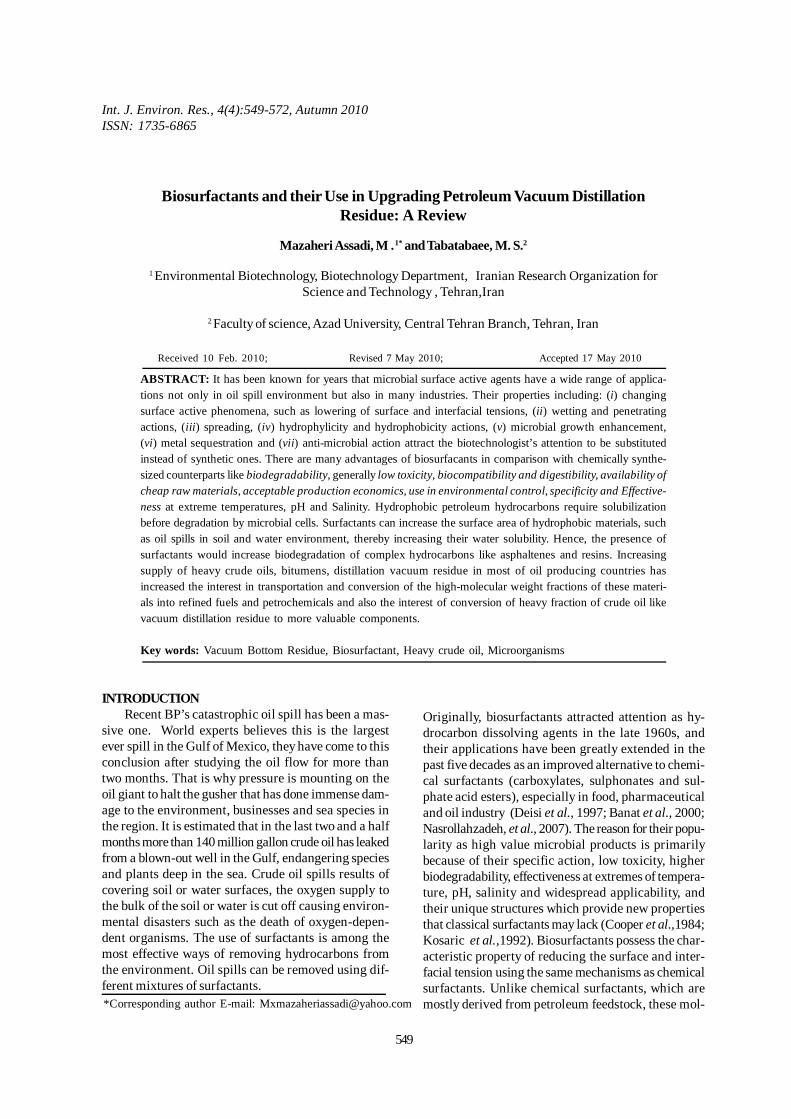
croorganisms together with their properties are listedin Table 1. (Das et al.,2008, Karanth et al.,2008).
The bioavailibity of many organic compounds suchas petroleum hydrocarbons is limited by their watersolubility (leathy and colwell, 1990; Atlas andBartha,1992). Surfactants and emulsifiers facilitate deg-radation of hydrophobic materials by making them morebioavailable to microorganisms. Therefore, they mayhave application in oil spill remediation, as well as inthe textile, pharmaceutical, cosmetic, and paper indus-tries. All surfactants possess both hydrophilic and hy-drophobic domains and thus can interact with bothaqueous and nonpolar materials (Georgiou et al., 1992;Desai and Desai, 1993). They facilitate dispersion ofhydrophobic materials into aqueous phases (MazaheriAssadi et al.,2004).
BiosurfactantsBiosurfactants are microbially produced surface-
active compounds have amphiphilic molecules. Theseamphiphilic molecules have both hydrophilic and hy-drophobic regions causing them to aggregate at inter-faces between fluids with different polarities such aswater and hydrocarbons (Banat, 1995a; Fiechter, 1992;Georgiou, 1992; Kosaric, 1993; Karanth et al., 1999)hence, decreases interfacial surface tension (Fiechter,1992; Georgiou et al., 1992;Rouse et al., 1994 ; Lin,1996; Shafi and Khanna, 1995; Volkering et al.,1998;Karanth et al., 1999). It has been proved that thesesecondary metabolites enhance nutrient transportacross membranes and affect in various host-microbeinteractions. Usually provide biocidal and fungicidalprotection to the producing organism (Banat, 1995a;Banat,1995b; Lin,1996). The ability of these specificbiomolecule is to reduce interfacial surface tension,which has important role in petrolrum industry like intertiary oil recovery and bioremediation consequencesor upgrading the heavy crude oil (Rouse et al., 1994;Lin, 1996; Volkering et al., 1998). Many of thebiosurfactant producing microorganisms are also hy-drocarbon-degraders (Rouse et al., 1994; Willumsenand Karlson, 1997; Volkering et al., 1998). However inthe past decades, many studies have showed the ef-fects of microbially produced surfactants not only onbioremediation but also on enhanced oil recovery(Jenneman et al., 1984; Jack, 1988; Volkering et al., 1998,Tabatabaee et al., 2005). Most of these studies typi-cally involved a single microbe or group of microbesisolated and identified in a laboratory and then appliedto either ex situ soil core experiments or injected intoexisting oil reservoirs for observation. In addition, themajority of biosurfactant production, hydrocarbonrecovery, heavy crude oil and vaccum residueupgradingwere conducted with known species such
Int. J. Environ. Res., 4(4):549-572 , Autumn 2010
551
Biosurfactants Microbial origin
Bacteria Fungi
Surfactin Bacillus subtilis (Arima et al. 1968)
Bacillus licheniformis F2.2(Thaniyavarn et al. 2003) Bacillus subtilis ATCC 21332(Nitschke and Pastore, 2003) Bacillus subtilis LB5a(Nitschke and Pastore, 2006) Bacillus subtilis MTCC 1427 and MTCC 2423 (Makkar and Cameotra, 1999)
Surfactant BL86 Bacillus licheniformis 86 (Horowitz and Currie, 1990) Arthrofactin Arthrobacter sp.MIS38 (Morikawa et al. 1993) Viscosin Pseudomonas fluorescens (Neu and Poralla, 1990) Plipastatin Bacillus licheniformis F2.2 (Thaniyavarn et al. 2003) Massetolides Pseudomonas fluorescens SS101 (Tran et al. 2007) Iturin B. amyloliquefaciens B94 (Yu et al. 2002) -
Bacillus subtilis RB14 (Rahman et al. 2006) Lichenysin A Bacillus licheniformis BAS50 (Yakimov et al. 1995) Lichenysin B, C Bacillus sp. (Yakimov et al. 1995, Yakimov et al. -1998, Yakimov et al. 1999)
Bamylomycin B. amyloliquefaciens (Lee et al. 2007) Halobacillin Marine Bacillus sp. (Trischmann et al. 1994)
Isohalobacillin Bacillus sp. A1238 (Hasumi et al. 1995) Bioemulsifier Bacillus stearothermophilus VR-8 Candida lipolytica
(Gurjar et al. 1995) IA 1055 (Vance-Harrop et al. 2003)
Flavolipid Flavobacterium sp. MTN11 -(Bodour et al. 2004) Mannosylerthritol Candida antarctica lipid (MEL)
(Kitamoto et al. 1990a) Candida sp. KSM-1529 (Kobayashi et al. 1987) Pseudozyma antarctica JCM 10317T (Morita et al. 2007)
Rhamnolipids Rl and R2
Pseudomonas aeruginosa (Guerra-Santos et al. 1986)
Rhamnolipid P. aeruginosa EM1 (Wu et al. 2008) Pseudomonas aeruginosa GS3 (Patel and Desai 1997) Pseudomonas aeruginosa BS2 (Dubey and Juwarkar 2001) P. putida 300-B mutant (obtained from Pseudomonas putida 33 wild strain by gamma ray mutagenesis) (Robert et al. 1989) Pseudomonas aerogiosa MM1011 (Mazaheri Assadi M., et al.2004)
Rhamnolipid RL1 Pseudomonas sp. 47T2 NCIB 400044 and RL2 (Mercade et al. 1993)
Rhamnolipids (RLLBI)
Pseudomonas aeruginosa strain LBI (Benincasa et al. 2002)
Emulsan Acinetobacter calcoaceticus ATCC 31012 -(RAG-1) (Shabtai 1990) Acinetobacter venetianus RAG-1 (Panilaitis et al.2006)
Liposan - C. lipolytica (Cirigliano and Carman 1985)
Biodispersan A. calcoaceticus A2 (Shabtai 1990) -
Lactonic sophorose lipid
T. bombicola KSM-36 (Ito et al. 1980)
Fructose-lipids Arthrobacter sp. , Corynebacterium sp., - Nocardia sp., Mycobacterium sp. (Itoh and Suzuki, 1974)
Sophorolipids Candida bombicola (Deshpande and Daniels 1995)
Bioemulsan Gordonia sp. BS29 (Franzetti et al. 2008) Circulocin Bacillus circulans, J2154 (He et al. 2001)
AP-6 Pseudomonas fluorescens 378 (Persson et al. 1988)
Table 1. Biosurfactants with their microbial sources

552
as Pseudomonas aeruginosa., Pseudomonasfluorescens., Bacillus licheniformis strain JF-2, Bacil-lus subtilis, or Acinetobacter calcoaceticus and manyunknown ones either reservoir indigenous ones or fromother hydrocarbon recourses and hydrocarbon con-taminated sites(Adkins et al., 1992; Banat, 1995a;Banat, 1995b; Lin, 1998, McInerney et al.,300 Proceed-ings of the 2000 Conference on Hazardous Waste Re-search 1990, Jenning and Tanner.,2000; Tahzibi etal.,2004; Tabatabaee et al.,2005).
Classification and chemical nature of biosurfactantsBiosurfactants are specific molecules covering a
wide range of chemical types including peptides, fattyacids, phospholipids, glycolipids, antibiotics,lipopeptides, etc. (Fig. 1 to 4). Usually structurally elu-cidated surfactants were obtained by a procedure ofprecise purification processes. The high molecularweight biosurfactants are generally polyanionicheteropolysaccharides containing both polysaccha-rides and proteins which are more effective at stabiliz-ing oil-in-water ((Rosenberg and Ron 1999;Chamanrokh et al., 2008).
Mechanisms proposed for the enhancement ofaqueous solubility of hydrophobic substances by sur-factants include solubilization in the hydrophobic coreof multimolecular surfactant structures formed atabove-aggregation concentrations, such as micelles(Edwards et al.,1991; Volkering et al.,1995, Jordan etal.,1999, Schippers et al.,2000 ) and liposomes (Millerand Bartha, 1989); decreased surface tension of thesolvent ; and interaction with hydrophobic tails of sur-factant monomers(Barkay et al.,1999).
The low molecular weight biosurfactants whichlower surface and interfacial tensions are often gly-colipids such as trehalose lipids, sophorolipids andrhamnolipids, or lipopeptides, such as surfactin, grami-cidin S and polymyxin (Rosenberg and Ron1999,Tahzibi et al., 2004); and ones with low (micro-grams per milliliter) critical micelle concentrations(CMC) can increase the apparent solubility of hydro-
carbons by incorporating them into the hydrophobiccavity of micelles (Miller and Zhang ,1997).
Three main roles for biosurfactants are supposedto be: (i) increasing the surface area of hydrophobicwater-insoluble growth substrates; (ii) increasing thebioavailability of hydrophobic substrates by increas-ing their apparent solubility or desorbing them fromsurfaces; (iii) regulating the attachment and detach-ment of microorganisms to and from surfaces(Rosenberg and Ron, 1999).The yield of microbial sur-factants varies with the environmental requirement i.eincluding their nutrition requirements. Intact microbialcells that have high cell surface hydrophobicity arethemselves surfactants. In some cases, surfactantsthemselves play a natural role in growth of microbialcells on water-insoluble substrates like CxHy, sulphur,etc. Exocellular surfactants are involved in cell adhe-sion, emulsification, dispersion, flocculation, cell ag-gregation, and desorption phenomena. Biosurfactantsgenerally classified into six major groups:Glycolipids,Fatty acids, Phospholipids, Surface activeantibiotics, Polymeric microbial surfactants and par-ticulate surfactants. (Karanth et al.,2008; Gautam andTyagi, 2006, Shakerifard et al., 2009).
GlycolipidsThe most common types of biosurfactant are gly-
colipids which constituent mono-, di-, tri- andtetrasaccharides include glucose, mannose, galactose,glucuronic acid, rhamnose, and galactose sulphate.The composition of fatty acid has a similar structureto that of the phospholipids of the same microorgan-ism. The glycolipids usually are classified as:Trehalose lipids: The production of trehalose lipidsseen in many members of the genus Mycobacterium.The typical structure is due to the presence of treha-lose esters on the cell surface (Asselineau et al.,1978)from different species of Mycobacteria (Asselineauet al.,1978), Corynebacteria, Nocardia, andBrevibacteria differ in size and structure of the my-colic acid esters.
Fig.1. Different chemical Structure of Trehalose lipids (Marqués et al., 2009)
Biosurfactants

Int. J. Environ. Res., 4(4):549-572 , Autumn 2010
553
Sophorolipids: Torulopsis bombicola are major specisof yeast which are capable of producing glycolipids(Rosenberg et al.,1979). There are several yeasts suchas: T. petrophilum and T. apicola consist of a dimericcarbohydrate sophorose linked to a long-chain hy-droxyl fatty acid by glycosidic linkage.Usuallysophorolipids occur as a mixture of macrolactones andfree acid form. The lactone form of the sophorolipid ismost important molecules, known for many applica-tions. According to Muthusamy et al.(2008), thesebiosurfactants are a mixture of at least 6-9 differenthydrophobic sophorolipids
Fig. 2. chemical Structure Sophorolipid(Van Bogaert, et al., 2007)
Rhamnolipids: Genus Pseudomonas are one ofthe most important producers of large quantities of aglycolipid, consisting of two molecules of rhamnoseand two molecules of b-hydroxydecanoic acid(Jarvisand Johnson1949; Edward and Hayashi1965;Reiling etal., 1986,). In glycosidic linkage, the OH groupof one of the acids is involved with the reducing endof the rhamnose disaccharide, the OH group of the
Fig. 3. chemical Structure of Rhamnolipid(Tazhibi et al., 2005)
Mannosylerythritol and Cellobiose LipidsThe yeast Candida (Pseudozyma) antarctica secretesan extracellular mannosylerythritol lipid (4-O-(2’,6’-di-O-acyl-β-D-mannopyranosyl)-D-erythritol), withbiosurfactant properties, when grown on a vegetableoil substrate. When grown on glucose, the same lipidaccumulates intra-cellularly as an energy store until itamounts to 10% or more of the dry weight of the cell.
second acids is involved in ester formation. Since oneof the carboxylic acid is free, the rhamnolipids areanions above pH 4.0((Karanth etal., 2008, Hisatsukaatal1971). Formation of rhamnolipids by Pseudomonasspecies was greatly increased by nitrogen limitations(Mazaheri Assadi etal., 2004) . The pure rhamnolipidlowered the interfacial tension against n-hexadecanein water to about 1 mN/m and had a critical micellarconcentration (cmc) of 10 to 30 mg/L depending on thepH and salt conditions (Karanth et al., 2008).
Fig. 4. Chemical structure of Mannosylerythritol and Cellobiose Lipids (Arutchelv, et al., 2008)

554
One or two of the hydroxyls on the mannoseresidue are acetylated, and there are two esterified fattyacids, which are both are odd- and even-numberedfrom C8 to C12 in chain-length (longer in related species).While this organism gives the greatest yields of theselipids, they were first found in the fungus Ustilagomaydis and termed ‘ustilipids’. In this instance, the 2-hydroxyl group of the mannose residue is esterifiedwith a C2 to C8 fatty acid, while the 3-hydroxyl group isesterified by a C12 to C20 fatty acid. Several other speciesof the genus Pseudozyma are now known to producesimilar lipids in which the nature, number and positionsof the acyl groups vary. As with other biosurfactants,these compounds are believed to facilitate dissolutionof organic hydrophobic compounds so that they canbe consumed by the organism. Mannosylerythritollipids have been shown to have a number of profoundbiological effects in animals, but especially to inducethe differentiation of certain cancer cells.
Ustilago maydis also contains distinctivecellobiose lipids (or ‘ustilagic acid’), consisting of thedisaccharide cellobiose linked O-glycosidically to theω-hydroxyl group of the unusual long-chain fatty acid15,16-dihydroxyhexadecanoic acid or 2,15,16-trihydroxyhexadecanoic acid. Others of the hydroxylgroups are esterified either to acetate or a medium-chain 3-hydroxy fatty acid. A further unusual cellobioselipid is produced by the fungal biocontrol agent,Pseudozyma flocculosa, and has been show to be 2-(2',4'-diacetoxy-5'-carboxy-pentanoyl)octadecylcellobioside (flocculosin), the compound responsiblefor the antifungal activities of the organism
Fatty acidsUsing alkanes as substrates, the fatty acids
produced by microbial oxidations, have receivedhighest attention as biosurfactants. Straight-chainacids, microorganisms produce mixed fatty acidscontaining OH groups and alkyl branches(Figs.5 &6).Some of these mixed acids, are corynomucolic acids,which are considered as surfactants (Kretschmer etal.,1982; Cooper et al., 1984; Karanth et al.,2008).
PhospholipidsPhospholipids are major components of microbial
membranes. When certain CxHy-degrading bacteria oryeast are grown on alkane substrates, the level ofphospholipids increases greatly. Phospholipids fromhexadecane-grown Acinetobacter sp. have potentsurfactant properties. Phospholipids produced byThiobacillus thiooxidans have been reported to beresponsible for wetting elemental sulphur, which isnecessary for growth ( Kappeli et al ., 1979; Karanth etal.,2008).
Surface active antibioticsGramicidin S: Many bacteria produce a
cyclosymmetric decapeptide antibiotic, gramicidin S.Spore preparations of Brevibacterium brevis containlarge amounts of gramicidin S bound strongly to theouter surface of the spores. Mutants lacking gramicidinS germinate rapidly and do not have a lipophilic surface.The antibacterial activity of gramicidin S is due to itshigh surface activity (Karanth et al.,2008).
Polymixins: A group of antibiotics produced byBrevibacterium polymyxa and related to bacilli species.A decapeptide known as Polymixin B contain aminoacids 3 through 10 form a cyclic octapeptide.Polymixins are able to solubilize certain membraneenzymes(Karanth et al.,2008).
Surfactin (subtilysin): One of the most activebiosurfactants produced by B. subtilis is a cycliclipopeptide surfactin (Arima etal1968). The yield ofsurfactin produced by B. subtilis can be improved toaround 0.8 g/l by continuously removing the surfactantby foam fractionation and addition of either iron ormanganese salts to the growth medium (Karanth etal.,2008).
Fig. 5.Chemical structure of Surfactin( López, et al., 2009)
Antibiotic TA: Myxococcus xanthus producesantibiotic TA which inhibits peptidoglycan synthesisby interfering with polymerization of the lipiddisaccharide pentapeptide. Antibiotic TA hasinteresting chemotherapeutic applications (Karanth etal.,2008).
Polymeric microbial surfactantsMost of these are polymeric heterosaccharidecontaining proteins.Acinetobacter calcoaceticus RAG-1 (ATCC 31012)emulsan: A bacterium, RAG-1, was isolated during aninvestigation of a factor that limited the degradationof crude oil in sea water. This bacterium efficientlyemulsified CxHy in water. This bacterium, Acinetobactercalcoaceticus, was later successfully used to clear a
Mazaheri Assadi, M . and Tabatabaee, M. S.

555
Int. J. Environ. Res., 4(4):549-572 , Autumn 2010
cargo compartment of an oil tanker during its ballastvoyage. The cleaning phenomenon was due to theproduction of an extracellular, high molecular weightemulsifying factor, emulsan(Karanth et al.,2008,Amiryan at al.,2004).
Fig. 6.Chemical structure of Emulsan(Amiryan, et al., 2004)
Emulsan has potential applications in the petro-leum industry, including formation of heavy oil-wateremulsions for viscosity reduction during pipelinetransport and production of fuel oil-water emulsionsfor direct combustion with dewatering(7; M. E. Hayes,K. R. Hrebenar, P. L. Murphy, L. E. Futch, Jr., and J. F.Deal, U.S. patent 4,618,348, October 1986). The affinityof emulsan for the oil-water interface suggests that itmight affect microbial degradation of emulsified oils.This has implications both for the stability of the oilemulsions during storage and transport and for theirbiodegradability should the emulsions accidentally bespilled in the environment(Foght et al.,1989; Amiryanat al.,2004).The polysaccharide protein complex of Acinetobactercalcoaceticus BD413: A mutant of A. calcoaceticusBD4, excreted large amounts of polysaccharide togetherwith proteins. The emulsifying activity required thepresence of both polysaccharide and proteins.Other Acinetobacter emulsifiers: Extracellular emulsi-fier production is widespread in the genusAcinetobacter. In one survey, 8 to 16 strains of A.calcaoceticus produced high amounts of emulsifierfollowing growth on ethanol medium. This extracellu-lar fraction was extremely active in breaking (de-emul-sifying) kerosene/ water emulsion stabilized by a mix-ture of Tween 60 and Span 60.Polysaccharide-lipid complexes from yeast: The par-tially purified emulsifier, liposan, was reported to con-tain about 95% carbohydrate and 5% protein. A CxHy-degrading yeast, Endomycopsis lipolytica YM, pro-duced an unstable alkane-solubilizing factor. Torulop-sis petrophilum produced different types of surfac-
tants depending on the growth medium (Copper andPaddock1984). On water-insoluble substrates, the yeastproduced glycolipids which were incapable of stabi-lizing emulsions. When glucose was the substrate, theyeast produced a potent emulsifier.Emulsifying protein (PA) from Pseudomonasaeruginosa: The bacterium P. aeruginosa has beenobserved to excrete a protein emulsifier. This proteinPA is produced from long-chain n-alkanes, 1-hexadecane, and acetyl alcohol substrates; but not fromglucose, glycerol or palmitic acid. The protein has aMW of 14,000 Da and is rich in serine and threonine(Hisatsuka et al.,1971, Kappeli et al.,1979).Surfactants from Pseudomonas PG-1: PseudomonasPG-1 is an extremely efficient hydrocarbon-solubiliz-ing bacterium. It utilizes a wide range of CxHy includ-ing gaseous volatile and liquid alkanes, alkenes, pris-tane, and alkyl benzenes.Bioflocculant and emulcyan from the filamentousCyanobacterium phormidium J-1: The change in cellsurface hydrophobicity of Cyanobacteriumphormidium was correlated with the production of anemulsifying agent, emulcyan. The partially purifiedemulcyan has a MW greater than 10,000 Da and con-tains carbohydrate, protein and fatty acid esters. Ad-dition of emulcyan to adherent hydrophobic cells re-sulted in their becomeing hydrophilic and detach fromhexadecane droplets or phenyl sepharose beads(Karanth et al.,2008).
Alasan, the bioemulsifier complex of A.radioresistens KA53: Alasan is made of a polysaccha-ride (apo-alasan) containing covalently bound alanineand proteins. The proteins of alasan plays an essen-tial role in both the structure and surface activity ofthe complex, because in contrast with alasan, apo-alasan had no emulsifying activity and did not showthe large temperature-induced hydrodynamic shapechanges while alasan emulsifying activity increasedgreatly after exposure to high temperature under neu-tral or alkaline conditions(Navon-Venezia et al.,1995).Bioemulsifier alasan can increases the solubility ofsome PAHs, that this activity is likely due to a revers-ible binding of these compounds, and that it enhancesthe biodegradation of PAHs. As the mechanism of solu-bilization by high-molecular-weight polymers may befundamentally different than that of small micelle-form-ing biosurfactants, research on the nature of this pro-cess might lead to the development of new approachesand tools for environmental management and indus-trial applications (Toren et al.,2001). The hydrophobicregions in alasan are the most plausible explanationfor the mechanism of solubilizing compounds with lim-ited aqueous solubility. Recently (Chamanrokh et al.,2010) isolated two autochthonous strains which are
556
capable of producing an extracellular, emulsifying agentwhen grown in Mineral Salt Medium containing Soyoil, ethanol or local crude oil. Analysis of purifiedemulsion was performed to prove the molecular struc-ture by 13CarbonNuclear Magnetic Resonance(13CNMR), Proton1Nuclear Magnetic (1HNMR) Reso-nance and Fourier Transform Infrared Radiation (FTIR)methods. These investigations showed that the mo-lecular weight of emulsion produced by species iso-lated from Iranian crude oil reservoirs are comparablewith Acinetobacter calcoaceticus PTCC 1318.
Particulate surfactantsExtracellular vesicles from Acinetobacter sp.
H01-N: Acinetobacter sp. when grown on hexadecane,accumulated extracellular vesicles of 20 to 50 mm diam-eter with a buoyant density of 1.158 g/cm3. Thesevesicles appear to play a role in the uptake of alkanesby Acinetobacter sp. HO1-N.Microbial cells with high cell surface hydrophobici-ties: Most hydrocarbon-degrading microorganisms,many nonhydrocarbon degraders, some species ofCyanobacteria, and some pathogens have a strongaffinity for hydrocarbon-water and air-water interfaces.In such cases, the microbial cell itself is a surfactant(Karanth et al.,2008).
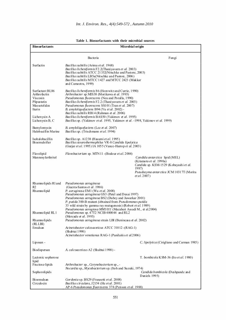
Biosurfactants in oil industryBiorefinery currently use biosurfactant of differ-
ent forms and therefore face the increasing environ-mental awareness and tightening of regulations in thisregard (Fig. 7). Microorganisms have long been knownto be able to produce a variety of surface active com-pounds that display properties and activities compa-
• Reservoirs wettability modification • Oil viscosity reduction • Drilling mud • Paraffin/ asphalt deposition control • Oil displacement increase • Oil viscosity reduction
• Oil viscosity reduction • Oil emulsion stabilization • Paraffin/ asphalt deposition
control
• Oil viscosity reduction • Oily sludge emulsification • Hydrocarbon dispersion
Oil extraction Oil transportation Oiltank/container cleaning
Biosurfactant in the petroleum industry
Tehran refinery
rable to those of synthetic surfactants. (Daisi andBanat, 1979; Singh eal., 2007). Biological surface ac-tive molecules can potentially replace chemical ana-logue compounds, even offering additional advan-tages, all through the chain of petroleum processingincluding; Extraction, Transportation, Upgrading andrefining and Petrochemical manufacturing (Van Dykeetal.,1991, Tabatabaee et al., 2005; Tabatabaee et al.,2006; Haghighat et al., 2008, Planckaert, 2005). Appli-cation and activity attributed to use of biosurfactantin oil industry is presented in fig.8.
Heavy fractions of crude oil and Distillation VacuumResidue
Increasing supply of heavy crude oils, bitumens,distillation vacuum residue in most of oil producingcountries has increased the interest in transportationand conversion of the high-molecular weight fractionsof these materials into refined fuels and petrochemi-cals.
In refineries crude oil is first preheated in a heatexchanger network en then heated up to 350°C in a gasfired heater. Hot crude oil is then separated in an atmo-spheric distillation column (CDU) into different frac-tions (naphtha, kerosene, gasoline). Heavy fuel oil re-lated streams produced by atmospheric distillationcomprise fractions of crude oil separated by heating(650-700 degrees °F) at atmospheric pressure. Theyinclude atmospheric distillates (heavy gas oils) andthe heavier residual materials (The Petroleum HPV Test-ing Group, 2004).The bottom stream of the column isfurther separated in a vacuum distillation column intoother fractions. vacuum residual refinery streams com-
Fig. 7. Biosurfactant application in petroleum industry
Biosurfactants
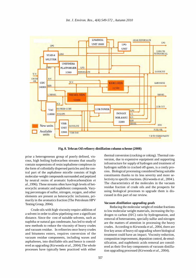
Fig. 8. Tehran Oil refinery distillation column scheme (2008)
prise a heterogeneous group of poorly defined, vis-cous, high boiling hydrocarbon streams that usuallycontain suspensions of resin/asphaltene complexes inthe form of colloidally dispersed particles and the cen-tral part of the asphaltene micelle consists of highmolecular-weight compounds surrounded and peptizedby neutral resins of aromatic hydrocarbons(kim etal.,1996). These streams often have high levels of het-erocyclic aromatic and naphthenic compounds. Vary-ing percentages of sulfur, nitrogen, oxygen, and otherelements are present as heterocyclic inclusions, pri-marily in the aromatics fraction (The Petroleum HPVTesting Group, 2004).
Crude oils with high viscosity require addition ofa solvent in order to allow pipelining over a significantdistance. Since the cost of suitable solvents, such asnaphtha or natural gas condensate, has led to study ofnew methods to reduce the viscosity of heavy crudesand vacuum residue. In refineries once heavy crudesand bitumens enters, requires conversion of thevacuum residue components, including waxes andasphaltenes, into distillable oils and hence is consid-ered as upgrading (Kirwooda et al., 2004).The wholeprocesses have typically been practiced with either
thermal conversion (cracking or coking). Thermal con-version, due to expensive equipment and supportinginfrastructure for supply of hydrogen and treatment ofhydrogen sulfide in cracked off-gases, is a costly pro-cess. Biological processing considered being suitableconstituents thanks to its less severity and more se-lectivity to specific reactions. (Kirwooda et al., 2004 ).The characteristics of the molecules in the vacuumresidue fraction of crude oils and the prospects forusing biological processes to upgrade them is dis-cussed in this part of our review.
Vacuum distillation upgrading goalsReducing the molecular weight of residue fractions
to low molecular weight materials, increasing the hy-drogen to carbon (H/C) ratio by hydrogenation, andremoval of heteroatoms, specially sulfur and nitrogenare the matters of attention in processing the heavycrudes. According to Kirwooda et al., 2004, there arefive key areas of heavy oil upgrading where biologicaltreatment could have an impact. Viscosity reduction,composition improvement, deposition control, de-emul-sification, and naphthenic acids removal are consid-ered as their five key components of vacuum distilla-tion upgrading processed (Kirwooda et al., 2004).
Int. J. Environ. Res., 4(4):549-572 , Autumn 2010
557
New units
Available units

Oxidation of aliphatic and aromatic carbon groups,oxidation of naphthenic acids, and oxidation and des-ulfurization of aromatic and aliphatic sulfur groups arestudied interactions between microbes and the highmolecular weight components of crude oils. Hydroge-nation and dehydrogenation reactions have been dem-onstrated only on lower-molecular weight components.All of these reactions are of potential interest for up-grading heavy crude oils and bitumens, but a majorbarrier is the transport of reactants to the active site ofreaction, particularly for intracellular enzymes in bac-teria. Although membranes may give significant barri-ers for bioprocessing of heavy hydrocarbons, the in-teractions of cell membranes with oil/water interfacesmay be of interest in deemulsifying oil and in dispers-ing asphaltenic material to prevent deposition(Kirwooda et al., 2004).
Vacuum distillation residue contentsThe asphaltene content of petroleum is an impor-
tant aspect of fluid processability (Fig. 9). ThereforeSARA method is conveniently used to separate thecrude oil into four major fractions: saturates (includ-ing waxes), aromatics, resins and asphaltenes (SARA),based on their solubility and polarity as shown in Fig.10 (Harald Auflem, 2002).
Fig. 9. Typical scheme for separating crude oil intosaturate, aromatic, resin and asphaltene (SARA)
components (Harald Auflem, 2002)
Asphaltene and resin fraction of VR:Asphaltenes with a heavy polar structure, are insolublein low normal alkanes (nC5 nC8) and soluble in suchsolvents as benzene and toluene and so on (Fig.10).Generally crudes have a dynamic stable system ofasphaltenes, resins and petroleum alkanes, similar to acolloidal system, in which the petroleum alkanes actas solvents, the asphaltenes as micelle and the resinsas stabilizers (Spight ,1996;Spight and Long,1996,Storm, 1995). Resins in crude oil consist mainly ofnaphthenic aromatic hydrocarbons, generally aromatic
ring systems with alicyclic chains. The resins are to adegree interfacially active in crude oils and they areeffective as a dispersant of tensions of asphaltenes(Schorling 1999) leading to formation of micelles withdifferent polarities, which can further aggregate toform supermicelles and molecular solutions( Fig.11).This process is summarized in Fig. 9 (Premutzic Andlin,1999; Schorling et al.,1999). Any changes in dy-namic stable system of crude oil like changes of tem-perature, pressure and/or compositions in crude oilsmay couse asphal tene precipi tation . (Spight,1996;Spight and Long,1996; Leontaritis,1996; Zewenand ansung, 2000, Harald Auflem at al.,2002).
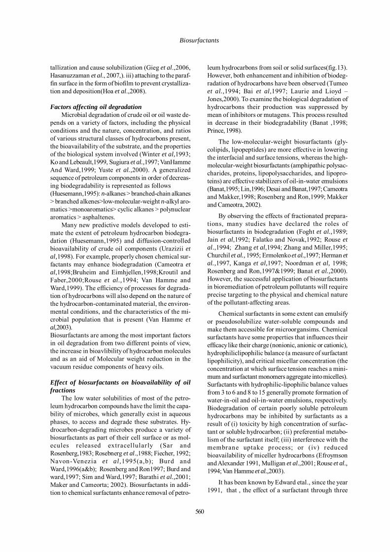
Paraffin and naphthenic of VRThe petroleum crudes typically consists of par-
affin hydrocarbons (C18 - C36) known as paraffinwax and naphthenic hydrocarbons (C30 - C60) whichare straight chain saturated hydrocarbons (Hoa etal., 2008). Hydrocarbon components of wax can ex-ist in various states of matter (gas, liquid o r solid)depending on their temperature and pressure. Whenthe wax freezes it forms crystals. The crystals formedof paraffin wax are known as macrocrystalline wax.Those formed from naphthenes are known as micro-crystalline wax (Himran et al., 1994; Mansoori et al.,2003).
Fig. 10. Formation of molecular solutions. Darkcircles represent heteroatoms and active sites
(Harald Auflem at al.,2002)
Mazaheri Assadi, M . and Tabatabaee, M. S.
558
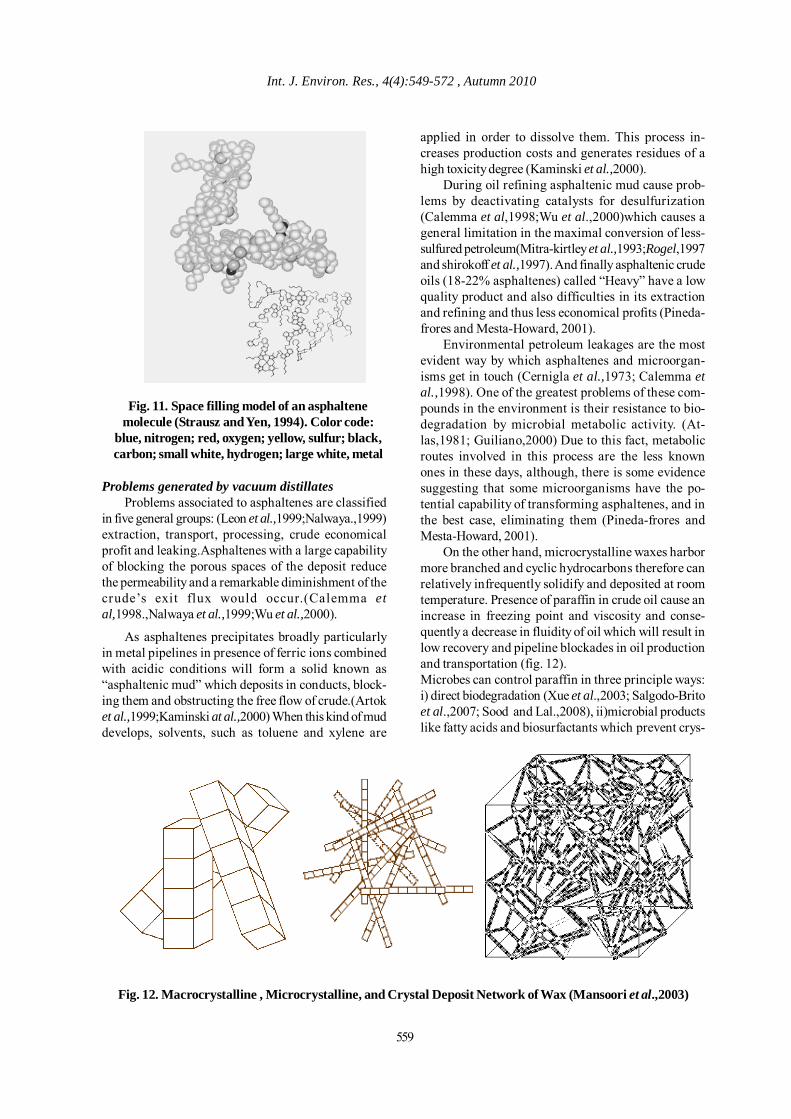
Fig. 11. Space filling model of an asphaltenemolecule (Strausz and Yen, 1994). Color code:
blue, nitrogen; red, oxygen; yellow, sulfur; black,carbon; small white, hydrogen; large white, metal
Fig. 12. Macrocrystalline , Microcrystalline, and Crystal Deposit Network of Wax (Mansoori et al.,2003)
Problems generated by vacuum distillatesProblems associated to asphaltenes are classified
in five general groups: (Leon et al.,1999;Nalwaya.,1999)extraction, transport, processing, crude economicalprofit and leaking.Asphaltenes with a large capabilityof blocking the porous spaces of the deposit reducethe permeability and a remarkable diminishment of thecrude’s exit flux would occur.(Calemma etal,1998.,Nalwaya et al.,1999;Wu et al.,2000).
As asphaltenes precipitates broadly particularlyin metal pipelines in presence of ferric ions combinedwith acidic conditions will form a solid known as“asphaltenic mud” which deposits in conducts, block-ing them and obstructing the free flow of crude.(Artoket al.,1999;Kaminski at al.,2000) When this kind of muddevelops, solvents, such as toluene and xylene are
applied in order to dissolve them. This process in-creases production costs and generates residues of ahigh toxicity degree (Kaminski et al.,2000).
During oil refining asphaltenic mud cause prob-lems by deactivating catalysts for desulfurization(Calemma et al,1998;Wu et al.,2000)which causes ageneral limitation in the maximal conversion of less-sulfured petroleum(Mitra-kirtley et al.,1993;Rogel,1997and shirokoff et al.,1997). And finally asphaltenic crudeoils (18-22% asphaltenes) called “Heavy” have a lowquality product and also difficulties in its extractionand refining and thus less economical profits (Pineda-frores and Mesta-Howard, 2001).
Environmental petroleum leakages are the mostevident way by which asphaltenes and microorgan-isms get in touch (Cernigla et al.,1973; Calemma etal.,1998). One of the greatest problems of these com-pounds in the environment is their resistance to bio-degradation by microbial metabolic activity. (At-las,1981; Guiliano,2000) Due to this fact, metabolicroutes involved in this process are the less knownones in these days, although, there is some evidencesuggesting that some microorganisms have the po-tential capability of transforming asphaltenes, and inthe best case, eliminating them (Pineda-frores andMesta-Howard, 2001).
On the other hand, microcrystalline waxes harbormore branched and cyclic hydrocarbons therefore canrelatively infrequently solidify and deposited at roomtemperature. Presence of paraffin in crude oil cause anincrease in freezing point and viscosity and conse-quently a decrease in fluidity of oil which will result inlow recovery and pipeline blockades in oil productionand transportation (fig. 12).Microbes can control paraffin in three principle ways:i) direct biodegradation (Xue et al.,2003; Salgodo-Britoet al.,2007; Sood and Lal.,2008), ii)microbial productslike fatty acids and biosurfactants which prevent crys-
Int. J. Environ. Res., 4(4):549-572 , Autumn 2010
559
tallization and cause solubilization (Gieg et al.,2006,Hasanuzzaman et al., 2007,). iii) attaching to the paraf-fin surface in the form of biofilm to prevent crystalliza-tion and deposition(Hoa et al.,2008).
Factors affecting oil degradationMicrobial degradation of crude oil or oil waste de-
pends on a variety of factors, including the physicalconditions and the nature, concentration, and ratiosof various structural classes of hydrocarbons present,the bioavailability of the substrate, and the propertiesof the biological system involved (Winter et al,1993;Ko and Lebeault,1999, Sugiura et al.,1997; VanHammeAnd Ward,1999; Yuste et al.,2000). A generalizedsequence of petroleum components in order of decreas-ing biodegradability is represented as follows(Huesemann,1995): n-alkanes > branched-chain alkanes> branched alkenes>low-molecular-weight n-alkyl aro-matics >monoaromatics> cyclic alkanes > polynucleararomatics > asphaltenes.
Many new predictive models developed to esti-mate the extent of petroleum hydrocarbon biodegra-dation (Huesemann,1995) and diffusion-controlledbioavailability of crude oil components (Urazizii etal,1998). For example, properly chosen chemical sur-factants may enhance biodegradation (Cameotra etal,1998;Bruheim and Eimhjellen,1998;Kroutil andFaber,2000;Rouse et al.,1994; Van Hamme andWard,1999). The efficiency of processes for degrada-tion of hydrocarbons will also depend on the nature ofthe hydrocarbon-contaminated material, the environ-mental conditions, and the characteristics of the mi-crobial population that is present (Van Hamme etal,2003).Biosurfactants are among the most important factorsin oil degradation from two different points of view,the increase in bioavlibility of hydrocarbon moleculesand as an aid of Molecular weight reduction in thevacuum residue components of heavy oils.
Effect of biosurfactants on bioavailability of oilfractions
The low water solubilities of most of the petro-leum hydrocarbon compounds have the limit the capa-bility of microbes, which generally exist in aqueousphases, to access and degrade these substrates. Hy-drocarbon-degrading microbes produce a variety ofbiosurfactants as part of their cell surface or as mol-ecules released extracellularly (Sar andRosenberg,1983; Rosebnerg et al.,1988; Fiecher, 1992;Navon-Venezia et al,1995(a,b); Burd andWard,1996(a&b); Rosenberg and Ron1997; Burd andward,1997; Sim and Ward,1997; Barathi et al.,2001;Maker and Cameorta; 2002). Biosurfactants in addi-tion to chemical surfactants enhance removal of petro-
leum hydrocarbons from soil or solid surfaces(fig.13).However, both enhancement and inhibition of biodeg-radation of hydrocarbons have been observed (Tumeoet al.,1994; Bai et al,1997; Laurie and Lioyd –Jones,2000). To examine the biological degradation ofhydrocarbons their production was suppressed bymean of inhibitors or mutagens. This process resultedin decrease in their biodegradability (Banat ,1998;Prince, 1998).
The low-molecular-weight biosurfactants (gly-colipids, lipopeptides) are more effective in loweringthe interfacial and surface tensions, whereas the high-molecular-weight biosurfactants (amphipathic polysac-charides, proteins, lipopolysaccharides, and lipopro-teins) are effective stabilizers of oil-in-water emulsions(Banat,1995; Lin,1996; Desai and Banat,1997; Cameotraand Makker,1998; Rosenberg and Ron,1999; Makkerand Cameotra, 2002).
By observing the effects of fractionated prepara-tions, many studies have declared the roles ofbiosurfactants in biodegradation (Foght et al.,1989;Jain et al,1992; Falatko and Novak,1992; Rouse etal.,1994; Zhang et al,1994; Zhang and Miller,1995;Churchil et al., 1995; Ermolenko et al.,1997; Herman etal.,1997, Kanga et al,1997; Noordman et al, 1998;Rosenberg and Ron,1997&1999; Banat et al.,2000).However, the successful application of biosurfactantsin bioremediation of petroleum pollutants will requireprecise targeting to the physical and chemical natureof the pollutant-affecting areas.
Chemical surfactants in some extent can emulsifyor pseudosolubilize water-soluble compounds andmake them accessible for microorgansims. Chemicalsurfactants have some properties that influences theirefficacy like their charge (nonionic, anionic or cationic),hydrophiliclipophilic balance (a measure of surfactantlipophilicity), and critical micellar concentration (theconcentration at which surface tension reaches a mini-mum and surfactant monomers aggregate into micelles).Surfactants with hydrophilic-lipophilic balance valuesfrom 3 to 6 and 8 to 15 generally promote formation ofwater-in-oil and oil-in-water emulsions, respectively.Biodegradation of certain poorly soluble petroleumhydrocarbons may be inhibited by surfactants as aresult of (i) toxicity by high concentration of surfac-tant or soluble hydrocarbon; (ii) preferential metabo-lism of the surfactant itself; (iii) interference with themembrane uptake process; or (iv) reducedbioavailability of miceller hydrocarbons (Efroymsonand Alexander 1991, Mulligan et al.,2001; Rouse et al.,1994; Van Hamme et al.,2003).
It has been known by Edward etal., since the year1991, that , the effect of a surfactant through three
Biosurfactants
560

mechanisms can increase availability of organic com-pounds: dispersion of nonaqueous-phase liquid(NAPL) organics, leading to an increase in contact areacaused by a reduction in the interfacial tension be-tween the aqueous phase and the nonaqueous phase;increased apparent solubility of the pollutant, causedby the presence of micelles that contain high concen-trations of HOCs (Edwards et al., 1991); and facilitatedtransport of the pollutant from the solid phase, whichcan be caused by lowering of the surface tension ofthe soil particle pore water, interaction of the surfac-tant with solid interfaces, and interaction of the pollut-ant with single surfactant molecules. The first mecha-nism is involved only when there is nonaqueous-phaseliquid organics . Because both of the latter two mecha-nisms can cause an increase in the rate of mass trans-fer to the aqueous phase, the relative contributions ofthese two mechanisms to the enhancement ofbioavailability of the substrate are confounded bySchippers et al. (Schippers, 2000), they gave threesuppositions for the promotion of the biodegradationof PAHs by surfactants. In their comments, the firstproposed pathway by bacteria were able to take up thehydrocarbons from the micellar core (Miller andBartha,1989). In the second pathway, biosurfactantsincreased the mass transfer of hydrophobic organiccompounds to the aqueous phase to make them ac-cessible for microbes. In the third approached, the di-rect contact between cells and NALP facilitates bymaking changes in hydrophobicity by mean of surfac-tants (Randhir et al.,2003).
In another proposed mechanism, surfactants helpmicrobes to be adsorbed to soil particles occupied byHydrocarbon compounds, thus decreasing the diffu-sion path length between the site of adsorption and
Fig. 13. The bioavailability model for syrfactant-enhanced biodegradation (Jordan et al.,1999)
site of bio-uptake by the microbe (Tang et al.,1998;Poeton et al,1999; Randhir et al.,2003).Effect of biosurfactants on Molecular weight of oilVR fractions
Molecular weight reduction in the residue frac-tion of heavy oils by a biological agent has been re-ported (Miller et al.,1989; Widdel and Rabus, 2001).There are few bacterial strains reported that act onparaffines and functionalize them. British Petroleumcoined the concept of biological dewaxing in 1970 withsome value added as a by product (Hamer and Al-Awadhi, 2000). Microbes can help in deposition con-trol by producing metabolites (from carbon sourcesother than the oil) that improve the solubility of eitherwaxes or asphaltenes, biotransform waxes andasphaltenes to more soluble products (through mo-lecular weight reduction or functionalization), and bio-degrade to remove the problematic compounds eitherfrom the oil or from existing deposits (lazer et al,1999).Rocha et al. Disclosed a method for preparingbiosurfactants for use in making emulsions of highviscosity hydrocarbons such as high viscosity crudeoil wherein the biosurfactant is a metabolite ofPseudomonas aeruginosa (USB-CS1). The resultingbiosurfactant can be used to produce emulsion hav-ing a viscosity below about 500 centipoise and, morepreferably, below about 100 centipoise at ambienttemperatures.The production of biosurfactants in situby microbial organisms grown in the presence of crudeoil has also been reported in literature (Iqbal et al.,1995;Abalos et al,2004;
Mazaheri et al., 2004; Amirian et al., 2004;Chamanrokh et al., 2010). Mostly the microbial pro-duced biosurfactants assisted in the dispersal of crudeoil in aquatic environment, thus facilitating thebioremediation of oil spills and chronic petroleum pol-
Int. J. Environ. Res., 4(4):549-572 , Autumn 2010
561

lution. Of special authochthonous microorganisms or/and genetically modified microorganisms used forbioremediation purposes, however, are not generallycompatible with petroleum extraction and refining pro-cesses because they also attack and catabolize (de-stroy) combustible hydrocarbons(Leon andKumar,2005; Chamanrokh et al., 2008).
Undesirable water in oil (W/O) emulsions occursthroughout oil production, transportation, and process-ing, and represents a major problem in heavy crude oil.Crude oil emulsions are complex and the emulsifyingagents may be amphiphilic molecules from the oil, es-pecially the resin fraction, including naphthenic acids,asphaltenes, fine solids, including clays, scale, waxcrystals or by microorganisms. De-emulsification in theoil industry is challenging due to the variety of pos-sible emulsion properties, and treatments are currentlytailored to each site and adapted over time. Variousmicrobes including Nocardia amarare, Pseudomonassp., Corynebacterium petrophilum, Rhodococcusauranticus, Bacillus subtilis, and Micrococcus sp. areknown to exhibit demulsification activity. Some bio-logically produced agents like glycolipids, polysac-charide, glycolipids, glycoproteins, phospholipids andrhamnolipids destabilize petroleum emulsions.
Since 1982, it have been proven that , the bacterialcell surface is responsible for major demulsifying ac-tivity of some microorganisms (Cairns et al.,1982, Coo-per 1982). It is more than three decades of research onbiosurfactant but till today, the applicability of bio-technology to asphaltene- or solids- stabilized emul-sions have not been studied throughly. There is a workdone by (Leon and Kumar,2005) proved that, biologi-cally produced molecules may be effective in remov-ing or dispersing asphaltenes or wax crystals, particu-larly in combination with suitable cell-surface proper-ties to aid in dispersion of the heavy crude oil or inaiding flocculation. Further more, not much workimplemented in this regards.
Biosurfactant Genetic engineering supporting theconcept of ‘‘biorefining’’
Genetic engineering consists in modifying in a de-terminate way the genetic material of microorganismsof industrial interest so that they acquire new or en-hanced capabilities.For this, novel DNA sequences are created by artifi-cially joining together strands of DNA from differentorganisms through the use of recombinant DNA tech-nology. The design of recombinant microorganismsfor petroleum biorefining includes the construction ofmicroorganisms:• able to transform the different types of compoundspresent in petroleum,
• possessing higher activities compatible with the de-sign of efficient and economically viable processes,• capable to secrete biosurfactants to increase thebioavailability of hydrocarbons to be transformed,• stable under process conditions (e.g. solvent-resis-tant microorganisms)(Borgne and Quintero, 2003).
One of the main purposes of microbial genetic en-gineering in oil industry is to increase the biosurfactantsecretion to promote the bioavailability of hydrocar-bons particularly the heavy fractions, to be transformed;or to be used in bioremediation of hydrocarbon con-taminated soils or MEOR.
Among all the biosurfactants reported till date,the molecular biosynthetic regulation of rhamnolipid,a glycolipid type biosurfactant produced byPseudomonas aeruginosa and a lipopeptidebiosurfactant called surfactin produced by Bacillussubtilis were the first to be famous. Otherbiosurfactants whose molecular genetics have beenintroduced in later years included arthrofactin fromPseudomonas species, iturin and lichenysin from Ba-cillus species, mannosylerythritol lipids (MEL) fromCandida and emulsan from Acinetobacter species( Mazaheri et al.,2004).
Quorum sensing, a cell density dependent generegulation process allowing bacterial cells to expresscertain specific genes on attaining high cell density,regulates the production of some biosurfactants. It hadbeen reported that low-molecular-mass signal molecules(such as the furanosyl borate diester AI-2) are involvedin biosurfactant production from different bacteria(Daniels et al., 2004). However, whether quorum sens-ing is the environmental cue to biosurfactant produc-tion in general is not known(Das et al.,2008).
The yield of all biotechnological products reliesupon the producer’s genetic that cause the type andamount of the metabolite production. Furthermore, toeconomize further the production process and toobtain products with better commercially importantproperties, recombinant and mutant hyperproducersseems necessary (Mukherjee et al.,2006). Various meth-ods and agents have been reported in literature to pro-duce biosurfactant hyperproducers. A summery someexamples of these mutants are given in Table 2.
CONCLUSIONOil spill has been a massive catastrophic effect on
the environment. World experts believes Crude oil spillhave done immense damage to the biodiversity, envi-ronment and businesses. The use of surfactants isamong the most effective ways of removing hydrocar-bons from the environment. Oil spills can be removedusing different mixtures of surfactants. These bioactive
Mazaheri Assadi, M . and Tabatabaee, M. S.
562
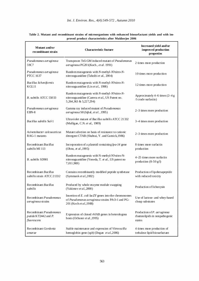
Table 2. Mutant and recombinant strains of microorganisms with enhanced biosurfactant yields and with im-proved product characteristics after Mukherjee 2006
Mutant and/or recombinant strain
Characteristic feature Increased yield and/or improved production
properties
Pseudomonas aeruginosa 59C7
Transposon Tn5-GM induced mutant of Pseudomonas aeruginosa PG201(Koch., et al. 1991)
2 times more production
Pseudomonas aeruginosa PTCC 1637
Random mutagenesis with N-methyl-N?-nitro-N-nitrosoguanidine (Tahzibi et al., 2004)
10 times more production
Bacillus licheniformis KGL11
Random mutagenesis with N-methyl-N?-nitro-N-nitrosoguanidine (Lin et al., 1998) 12 times more production
B. subtilis ATCC 55033 Random mutagenesis with N-methyl-N?-nitro-N-nitrosoguanidine (Carrera et al., US Patent no. 5,264,363 & 5,227,294)
Approximately 4–6 times (2–4 g /l crude surfactin)
Pseudomonas aeruginosa EBN-8
Gamma ray induced mutant of Pseudomonas aeruginosa S8 (Iqbal, et al. ,1995) 2–3 times more production
Bacillus subtilis Suf-1 Ultraviolet mutant of Bacillus subtilis ATCC 21332 (Mulligan, C.N. et al., 1989)
3–4 times more production
Acinetobacter calcoaceticus RAG-1 mutants
Mutant selection on basis of resistance to cationic detergent CTAB (Shabtai, Y. and Gutnick,1986)
2–3 times more production
Recombinant Bacillus subtilis MI 113
Incorporation of a plasmid containing lpa-14 gene (Ohno, et al.,1995)
8 times more surfactin production
B. subtilis SD901 Random mutagenesis with N-methyl-N?-nitro-N-nitrosoguanidine (Yoneda, T. et al. , US patent no 7,011,969)
4–25 times more surfactin production (8–50 g/l)
Recombinant Bacillus subtilis strain ATCC 21332
Contains recombinantly modified peptide synthetase (Symmank et al.,2002)
Production of lipohexapeptide with reduced toxicity
Recombinant Bacillus subtilis
Produced by whole enzyme module swapping (Yakimov et al.,2000) Production of lichenysin
Recombinant Pseudomonas aeruginosa strains
Insertion of E. coli lacZY genes into the chromosomes of Pseudomonas aeruginosa strains PAO-1 and PG-201 (Koch et al.,1988)
Use of lactose- and whey-based cheap substrates
Recombinant Pseudomonas putida KT2442 and P. fluorescens
Expression of cloned rhlAB genes in heterologous hosts (Ochsner et al.,1995)
Production of P. aeruginosa rhamnolipids in nonpathogenic stains
Recombinant Gordonia amarae
Stable maintenance and expression of Vitreoscilla hemoglobin gene (vgb) (Dogan et al.,2006)
4 times more production of trehalose lipid biosurfactant
Int. J. Environ. Res., 4(4):549-572 , Autumn 2010
563

material applications have been greatly extended inthe past five decades as an improved alternative tochemical surfactants (carboxylates, sulphonates andsulphate acid esters), especially in food, pharmaceuti-cal and oil industry The development of new surfac-tants has long been acknowledged to need continu-ous technology improvement and adoption for maxi-mum economic benefit.
A part from environment, in refineries crude oil isfirst preheated in a heat exchanger network. Hot crudeoil is then separated in an atmospheric distillation col-umn (CDU) into different fractions (naphtha, kerosene,gasoline). Heavy fuel oil related streams produced byatmospheric distillation comprise fractions of crude oilseparated by heating at atmospheric pressure. Thevacuum residual refinery streams comprise a hetero-geneous group of poorly defined, viscous, high boil-ing hydrocarbon streams that usually contain suspen-sions of resin/asphalting complexes in the form of col-loidal dispersed particles. These streams often havehigh levels of heterocyclic aromatic and naphtheniccompounds using special biosurfactant produced byspecific strain of genetically engineered. Usually novelDNA sequences are created by artificially joining to-gether strands of DNA from different organismsthrough the use of recombinant DNA technology. Thisreview has focused on the identification of emergingand developing biosurfactant technologies that can,when fully developed, either be applied directly to notonly cleaning the environment but also upgradeVacuum bottom residue and very heavy crudes, or areintegral to new approaches to upgrading. This ap-proach can have some important and economically at-tractive side benefits in the main vacuum bottom resi-due upgrading process selection.
REFERENCESAbalos, A., M. Vinas, J. Sabate, M. A. Manresa, and SolanasA. M. (2004). Enhanced biodegradation of Casablanca crudeoil by a microbial consortium in presence of a rhamnolipidproduced by Pseudomonas aeruginosa AT10. Biodegrada-tion, 15, 249-260.
Adkins, J.P., R.S. Tanner, E.O. Udegbunam, M.J. McInerney,and. Knapp, R. M. (1992). Microbially enhanced oil recov-ery from unconsolidated limestone cores.” GeomicrobiologyJournal, 10, 77-86.
Amiriyan A., Mazaheri Assadi M, Saggadian V.A. and NoohiA. (2004). Bioemulsan production by Iranian oil reservoirsmicroorganisms, Iranain Journal of Environmental HealthScience Engineering, 1(2), 28-35.
Arima, K., Kakinuma, A. and Tamura, G. (1968). Surfactin,a crystalline peptide lipid surfactant produced by Bacillussubtilis: isolation, characterization and its inhibition of fi-
brin clot formation. Biochemical Biophysical Research Com-munications, 31, 488-494.
Artok, L., Su, Y., Hirose, Y., Hosokawa, M., Murata, S. andMomura, M. (1999). Structure and reactivity of petroleum-derived asphaltene. Energy & Fuel, 13, 287-296.
Arutchelvi, J.I., Bhaduri, S., Uppara, P.V. and Doble, M.(2008). Mannosylerythritol lipids: a review. Journal of In-dustrial Microbiology & Biotechnology, 35, 1559-1570 .
Arutchelvi, J.I., Bhaduri, S., Uppara, P.V. and Doble, M.(2008). Mannosylerythritol lipids: a review. Journal of In-dustrial Microbiology & Biotechnology, 35, 1559-1570
Asselineau, C. and Asselineau, J. (1978). Trehalose con-taining glycolipids. Progress Chemistry Fats Lipids, 16,59 – 99.
Atlas, R. M. (1981). Micro bial degradation of petroleumhydrocarbons: an environmental perspective. MicrobialReview, 45, 180-209.
Atlas,R.M and Bartha, R. (1992). Hydrocarbon biodegra-dation and oil spill bioremediation, Advances in MicrobialEcology, 2, 287-338
Bagherzadeh-Namazi, A.; Shojaosadati, S. A. and Hashemi-Najafabadi, S.(2008). Biodegradation of Used Engine OilUsing Mixed and Isolated Cultures. Int. J. Environ. Res.,2(4), 431-440.
Bai, G. Y., M. L. Brusseau, and Miller R. M. (1997).Biosurfactant enhanced removal of residual hydrocarbonfrom soil. Journal of Contaminant Hydrology. 25,157 -170.
Baltzis, B. C. (1998). Biofiltration of volatile organic carbonvapors, p. 119–150. In G. A. Lewandowski and L. J. DeFilippi(ed.), Biological treatment of hazardous wastes. John Wiley,New York, N.Y.
Banat, I. M. (1995a). Biosurfactant production and pos-sible uses in microbial enhanced oil recovery and oil pollu-tion remediation. Bioresource Technology. 51, 1–12.
Banat, I.M., (1995b). “Characterization of Biosurfactantsand Their Use in Pollution Removal– State of the Art (Re-view).” Acta Biotechnology, 3, 251-267.
Banat, I. M., Makkar R. S. and Cameotra S. S. (2000). Po-tential commercial applications of microbial surfactants.Appl. Microbiol. Biotechnol. 53, 495– 508.
Barathi, S. and Vasudevan, N. (2001). Utilization of petro-leum hydrocarbons by Pseudomonas fluorescens isolatedfrom a petroleum-contaminated soil. Environment Interna-tional. 26, 413-416.
Barkay T., Navon-Venezia S., Ron E. Z. and Rosenberg,E.,(1999), Enhancement of Solubilization and Biodegrada-tion of Polyaromatic Hydrocarbons by the Bioemulsifier
Biosurfactants
564
Alasan. Applied & Environmental Microbiology, 65, 2697–2702.
Benincasa, M., Contiero, J., Manresa, M.A. and Moreaes,I.O. (2002). Rhamnolipid production by Pseudomonasaeruginosa LBI growing on soapstock as the sole carbonsource. Journal of Food Engineering 54, 283-288.
Bodour, A. A., Guerrero-Barajas, C., Jiorle, B.V., Malcomson,M.E., Paull, A.K., Somogyi, A., Trinh, L.N., Bates, R.B.and Maier, R.M. (2004). Structure and characterization offlavolipids, a novel class of biosurfactants produced by Fla-vobacterium sp. strain MTN11. Applied & EnvironmentalMicrobiology, 70(1),114-120.
Borgne S. L. and Quintero, R. (2003). Biotechnological pro-cesses for the refining of petroleum. Fuel Processing Tech-nology, 81, 155– 169.
Bruheim, P. and Eimhjellen, K. (1998). Chemically emulsi-fied crude oil as substrate for bacterial oxidation: differencesin species response. Canadian Journal of Microbiology, 44,638–646.
Bruheim, P., Bredholt, H. and Eimhjellen. K. (1997). Bacte-rial degradation of emulsified crude oil and the effect ofvarious surfactants. Canadian Journal of Microbiology,43,17–22.
Burd, G., and Ward. O. P. (1996a). Physico-chemical prop-erties of PM-factor, a surface active agent produced byPseudomonas marginalis. Canadian Journal of Microbiol-ogy, 42,243-251.
Burd, G., and Ward. O. P. (1996 b). Bacterial degradation ofpolycyclic aromatic hydrocarbons on agar plates: the roleof biosurfactants. Biotechnology, 10, 371–374.
Burd, G., and Ward. O. P.(1997). Energy-dependent pro-duction of particulate biosurfactant by Pseudomonasmarginalis. Canadian Journal of Microbiology, 43, 391–394.
Cairns, W. L.,. Cooper, D. G., Zajic, J. E., Wood, J. M. andKosaric, N. (1982). Characterization of Nocardia amarae asa potent biological coalescing agent of water-oil emulsions.Applied Environmental Microbiology. 43, 362-366.
Calemma, V., Rausa, R., D´Antona, P. and MontanariL.(1998). Characterization of asphaltenes molecular struc-ture. Energy &. Fuel, 12, 422-428.
Cameotra, S. S., and Makkar.R. S. (1998). Synthesis ofbiosurfactants in extreme conditions. Applied. Microbiol-ogy &. Biotechnology, 50, 520–529.
Carrera P., Cosmina P. and Grandi G. (1993). EniricercheS.p.A., Milan, Italy. Mutant of Bacillus subtilis, US Patentno. 5, 264-363.
Carrera P., Cosmina P., Grandi G.. Eniricerche S. P. A. (1993),Method of producing surfactin with the use of mutant ofBacillus subtilis, US Patent no.5, 227,294.
Carrera P., Cosmina P., Grandi G.. Eniricerche S.P.A.(1993).Method of producing surfactin with the use of mutant ofBacillus subtilis, US Patent no. 5, 227-294 .
Cerniglia, C. E. and Perry, J. J. (1973). Crude oil degradationby microorganisms isolated from the marine environment.Zeitschrift Für Allg. Mikrobiologie, 13, 299-306.
Chamanrokh, P., Mazaheri Assadi, M. and Amouabedini,Gh. (2010). Cleaning of oil contaminated vessel by emulsanproducers(Authochthonous Bacteria). Iranian Journal ofEnvironmental Health Science & Engineering (In press).
Chamanrokh,P., Mazaheri Assadi M., Noohi A. and YahyaiS. (2008), Emulsan Analysis Produced by Locally IsolatedBacteria and Acinetobacter calcoaceticus, Journal of Envi-ronmental Health Science & Engineering, 5,101-108.
Churchill, S. A., Griffin, R. A., Jones, L. P. and Churchill,P.F. (1995). Biodegradation rate enhancement of hydrocar-bons by an oleophilic fertilizer and a rhamnolipidbiosurfactant. Journal. Environmental Quality, 24,19–28.
Cirigliano, M.C. and Carman, G.M. (1985). Purification andcharacterizafton of liposan: a bioemulsifier from Candidalipolytica. Applied and Environmental Microbiology, 50, 846-850.
Cooper, D. G. (1982). Biosurfactants and Enhanced OilRecovery. pp. 112-114. Proceedings of International Con-ferences on Microbial Enhanced Oil Recovery, May 16-21,Afton, UK.
Cooper, D. G. and Paddock, D. A. (1984). Production ofbiosurfactants from Torulopsis bombicola. Applied Envi-ronmental Microbiology, 47, 173–176.
Cooper, D. G., MacDonald, C. R., Duff, S. J. B. and Kosaric,N.(1981). Enhanced production of surfactin from B. subtilisby continuous product removal and metal cation additions.Applied Environmental Microbiology, 42, 408–412.
Daniels, R., Vanderleyden, J. and Michiels, J. (2004). Quo-rum sensing and swarming migration in bacteria. FEMSMicrobiology Reviews 28, 261-289.
Das P., Mukherjee S. and Sen, R. (2008). Genetic Regula-tions of the Biosynthesis of Microbial Surfactants: An Over-view. Biotechnology and Genetic Engineering Reviews, 25,165-186.
Desai J. and Banat I.M. (1997). Microbial production ofsurfactants and their commercial potential. Microbiology& Molecular Biology Review, 61, 47-64.
Desai, J. and Desai, A. J . (1993). Prodauction ofbiosurfactants. In N.Kosaric(editor), Biosurfactants, pro-duction, properties, applications. M. Dekker,Inc., New York,4, 865-79.
Deshpande, M. and Daniels, L. (1995) Evaluation ofsophorolipid biosurfactant production by Cand ida
Int. J. Environ. Res., 4(4):549-572 , Autumn 2010
565
bombicola using animal fat. Bioresource Technology, 54,143-150.Dogan I., Pagilla K. R., Webster D. A. and Stark B. C. (2006),Expression of Vitreoscilla haemoglobin in Gordonia amaraeenhances biosurfactant production. Journal of IndustrialMicrobiology & Biotechnology, 33, 693–700.
Dubey, K. and Juwarkar, A. (2001), Distillery and curdwhey wastes as viable alternative sources for biosurfactantproduction. World Journal of Microbiology and Biotech-nology 17, 61-69.
Edward, J. R. and Hayashi, J. A.,(1965). Structure ofrhamnolipid from Pseudomonas aeruginosa. ArchiveBiochem. Biophysic., 111, 415–421.
Edwards, D., Luthy, R. and Liu, Z. (1991). Solubilization ofpolycyclic aromatic hydrocarbons in micellar non-ionic sur-factant solutions. Environmental Science & Technology,25,127-133.
Efroymson, R. A. and Alexander.M.(1991). Biodegradationby an Arthrobacter species of hydrocarbons partitioned intoan organic solvent. Applied Environmental Microbiology,57,1441-1444.
Ermolenko, Z. M., Kholodenko, V. A., Chugunov, N. A.,Zhirkova, A. and Raulova.G. E.( 1997). A Mycobacteriastrain isolated from Ukhtinske oil field, identification anddegradative properties. Microbiology, 66, 542–554.
Falatko, D. M. and Novak, J. T. (1992). Effects of biologi-cally produced surfactants on mobility and biodegradationof petroleum hydrocarbons. Water Environment Research,64,163–169.
Fiechter, A. (1992). Biosurfactants: moving towards indus-trial application. Trends in Biotechnology, 10, 208–217.
Foght J. M., Gutnick, D. L. and Westlake, D.W.S. (1989).Effect of Emulsan on Biodegradation of Crude Oil by Pureand Mixed Bacterial Cultures. Applied and EnvironmentalMicrobiology, 55(1), 36-42.
Foght, J. M., Gutnick, D. L. and Westlake. D. W. S. (1989).Effect of emulsan on biodegradation of crude oil by pureand mixed bacterial cultures. Applied and EnvironmentalMicrobiology, 55, 36–42.
Franzett I, A., Bestett , G., Caredd A. P., La Colla P. andTamb urini, E. (2008). Surfaceactive compounds and theirrole in the access to hydrocarbons in Gordonia strains. FEMSMicrobiology Ecology, 63(2), 238-248.
Gautam K.K. and Tyagi,V.K.(2006). Microbial surfactants:A review. Journal of Science, 55(4),155-166.
Georgiou,G., Lin, S-C. and Sharma. M. M. (1992). Surfaceactive compounds from microorganisms. Biotechnology, 10,60-65.
Gieg, L. M., Duncan, K. E. and Suflita, J.M. (2006). Anaero-bic Paraffin Biodegradation. In:Abstracts of the 11th Inter-national Symposium on Microbial Ecology, Vienna, Aus-tria, August 20 – 25 (poster presentation).
Guerra-Santos, L.H., Kapp eli, O. and Fiechter, A. (1986).Dependence of Pseudomonas aeruginosa continuous cul-ture biosurfactant production on nutritional and environ-mental factors. Applied Microbiology Biotechnology 24,443–448.
Guiliano, M., Boukir, A., Doumenq, P. and Mille, G. (2000).Supercritical fluid extraction of bal 150 crude oil asphaltenes.Energ. Fuel. 14, 89-94.
Gurjar, M., Khire, J.M. and Khan, M.I. (1995) Bioemulsifierproduction by Bacillus stearothermophilus VR-8 isolate.Letters in Applied Microbiology 21(2), 83-86.
Hamer, G. and Al-Awadhi, N. (2000). Biotechnological ap-plications in the oil industry. Acta Biotechnology, 20, 335-350.
Hao D-H., Lin J-Q., Song X., Lin J-Q., Su Y-J., and Qu Y-B.(2008). Isolation, Identification, and performance studiesof a Novel Paraffin-degrading Bacterium of Gordoniaamicalis LH3, Biotechnology & Bioprocess Engineering,13,61-68.
Harald A. I. (2002), Influence of Asphaltene Aggregationand Pressure on Crude Oil Emulsion Stability, PhD Thesis,Department of Chemical Engineering Norwegian Univer-sity of Science and Technology.
Hasanuzzaman, M., Ueno, A., Ito, H., Ito, Y., Yamamoto,Y., Yumoto, I. and Okuyama, H. (2007). Degradation oflong-chain n-alkanes (C36 and C40) by Pseudomonasaeruginosa strain. International. Biodeterioration. & Bio-degradation, 59, 40–43.
Hasumi, K., Takizawa, K., Takahashi, F., Park, J.K. andEndo, A. (1995). Inhibition Acyl CoA: Cholestrolacyltransferase by isohalobacillin, a complex of novel cyclicacylpeptides produced by Bacillus sp. A1238. Journal ofAntibiotics, 48, 1419-1424.
He, H., Shen, B., Korshalla J. and Carter, G.T. (2001).Circulocins, new antibacterial lipopeptides from Bacilluscirculans, J2154. Tetrahedron 57, 1189-1195.
Heavy Fuel Oils Category (2004). Submitted to the US EPABy The Petroleum HPV Testing Groupwww.petroleumhpv.org ,Consortium Registration #1100997.
Herman, D. C., Zhang, Y. M. and. Miller, R. M. (1997).Rhamnolipid (biosurfactants) effects on cell aggregation andbiodegradation of residual hexadecane under saturated flowconditions. Applied Environmental Microbiology, 63, 3622–3627.
Mazaheri Assadi, M . and Tabatabaee, M. S.
566
Himran S., Suwono A. and Mansoori G. A.( 1994). Charac-terization of alkanes and paraffin waxes for application asphase change energy storage medium. EnergySources,16,117-128.
Hisatsuka, K., Nakahara, T., Sano, N. and Yamada, K. (1971).Formation of rhamnolipid by Pseudomonas aeruginosa: Itsfunction in hydrocarbon fermentations. Agricultural Biol-ogy &. Chemistry, 35, 686–692.
Horowitz , S. and Currie, J.K. (1990). Novel dispersants ofsilicon and aluminum nitride. Journal of Dispersion Scienceand Technology, 11, 637-59.
Huesemann, M. H. (1995). Predictive model for estimatingthe extent of petroleum hydrocarbon biodegradation in con-taminated soils. Environmental Science & Technology, 29,7–18.
Iqbal S., Khalid Z..M., Malik K.A. (1995). Enhanced bio-degradation and emulsification of crude oil andhyperproduction of biosurfactants by a gamma ray inducedmutant of Pseudomonas aeruginosa. Letters in AppliedMicrobiology, 21,176–179.
Ito, S., Kinta, M. and Inoue, S. (1980) Growth of yeasts onn-alkanes: Inhibition by a lactonic sophorolipid producedby Torulopsis bombicola. Agricultural Biological Chemis-try, 44, 2221-2223.
Jack, T.R.(1998). Microbially Enhanced Oil Recovery.Biorecovery, 1, 59-73.
Jain, D. K., H. Lee, and Trevors. J.T. (1992). Effect ofaddition of Pseudomonas aeruginosa UG2 inocula orbiosurfactants on biodegradation of selected hydrocarbonsin soil. Journal of Industrial Microbiology, 10, 87–93.
Jarvis, F. G. and Johnson, M. J.(1949). A glycolipid pro-duced by Pseudomonas aeruginosa. Journal of AmericanOil Chemical Society, 71, 4124–4126.
Jennings E.M. and Tanner R.S. (2000), Biosurfactant pro-ducing bacteria found in contaminated and uncontaminatedsoils, Proceedings of the 2000 Conference on HazardousWaste Research, pp299-306.
Jordan R.N., E. P. Nichold and Cunningham, A. B. (1999).The role of Biosurfactant sorption in promoting thebioavailability of nutrients localized at the solid-water in-terface, Water Science Technology, 39(7), 91-98.
Kaminski, T., Fogler, H. S., Wolf, N., Wattana, P. and Mairal,A. (2000). Classification of asphaltenes via fractionationand the effect of heteroatomic content on dissolution kinet-ics. Energy Fuel, 14, 25-30.
Kanga, S. A., J. S. Bonner, C. A. Page, M. A. Mills, andAutenrieth R.L. (1997). Solubilization of naphthalene andmethyl substituted naphthalenes from crude oil withbiosurfactants. Environmental Science Technology, 31, 556–561.
Kappeli, O. and Finnerty, W. R.(1979). Partition of alkaneby an extracellular vesicle derived from hexadecane grownAcinetobacter. Journal of Bacteriology, 140,707–712.
Karanth, N.G.K., P.G. Deo, and Veenanadig. N.K.(1999).Microbial Production of Biosurfactants and Their Impor-tance. Current Science, 77,116 – 126.
Kim H. H., Chung K-B. and Kim M-N., 1996, Measure-ment of the Asphaltene and resin content of crude oils, Jour-nal of Industrial & Engineering Chemistry, 2(1),72-78.
Kirkwooda K.M., J.M. Foghtb, and Gray, M.R. (2004).Petroleum Biotechnology. Elsevier B.V. ISBN: 0 444 516999, ISSN: 0167 2991 (Series) 151(4),113-142.
Kitamoto, D., Akiba, S., Hioki, C. and Tabuchi, T. (1990a)Extracellular accumulation of mannosylerythritol lipids bya strain of Candida antarctica. Agricultural and BiologicalChemistry, 54 (1),31-36.
Ko, S. H., and Lebeault, J.M. (1999). Effect of a mixedculture on cooxidation during the degradation of saturatedhydrocarbon mixture. Journal of Applied Microbiology,87,72–79.
Kobayashi, T., Ito, S. and Okamoto, K. (1987). Productionof Mannosylerythritol by Candida sp. KSM-1529. Agri-cultural Biological Chemistry, 51, 171-175.
Koch, A. K, Reiser J., Käppeli O. and Fiechter A., (1988)Genetic construction of lactose-utilizing strains ofPseudomonas aeruginosa and their application inbiosurfactant production. Nature Biotechnology, 6, 1335–1339.
Koch, A.K. Käppeli. O., Fiechter A. and Reiser J., (1991)Hydrocarbon assimilation and biosurfactant production inPseudomonas aeruginosa mutants. Journal of Bacteriology,173,4212–4219.
Kosaric, N., (1992), Biosurfactants in industry. Pure &Applied Chemistry, 11, 1731–1737.
Kosaric, N. (1993). Biosurfactants— Production, Proper-ties, Applications, New York, Marcel Dekker, Inc.
Kretschmer, A., Bock, H. and Wagner, F., 1982, Chemicaland physical characterization of interfacial active lipids fromRhodococcus erythropolis grown on n-alkane. Appl. Environ.Microbiol., , 44, 864–870.
Kretschmer, A., Bock, H. and Wagner, F., (1982). Chemicaland physical characterization of interfacial active lipids fromRhodococcus erythropolis grown on n-alkane. Applied En-vironmental. Microbiology, 44, 864–870.
Kroutil, W., and K. Faber. 2000. Stereoselective syntheseswith microbial epoxide hydrolases, p. 205–237. In R. N.Patel (ed.), Stereoselective biocatalysis. Marcel Dekker, NewYork, N.Y.
Langworthy D. E., R. D. Stapleton, G. S. Sayler, and Findlay,R.H. (1998). Genotypic and phenotypic responses of ariverine microbial community to polycyclic aromatic hy-
Int. J. Environ. Res., 4(4):549-572 , Autumn 2010
567
drocarbon contamination. Applied Environmental Microbi-ology, 64, 3422–3428.
Laurie, A. D., and G. Lloyd-Jones, G. (2000). Quantifica-tion of phnAc and nahAc in contaminated New Zealand soilsby competitive PCR. Applied Environmental Microbiol-ogy, 66,1814-1817.
Lazar, I., A. Voicu, C. Nicolescu, D. Mucenica, S. Dobrota,I. G. Petrisor, M. Stefanescu, and Sandulescu, L. (1999).The use of naturally occurring selectively isolated bacteriafor inhibiting paraffin deposition. Journal of PetroleumScience &. Engineering, 22,161-169.
Leathy,J.G. and Colwell,R.R. (1990). Microbial degrada-tion of Hydrocarbons in the environment, Microbialogicalreviews, 54, 305-315.
Lee, A.S., Sadeghi, M.A., Yen, T.F. (1986). The role of per-oxides reacting with asphaltic oil in micellar inversion pro-cess. PREPRINTS, American Chemical Society’s 21stIECEC, pp. 25–29.
Lee, A.S., Xu, X.W., Yen, T.F. (1989). Upgrading of heavycrude oils at low temperature and ambient atmosphere. Pro-ceeding of. 4th UNITAR-UNDP International Conferenceon Heavy Crude and Tar Sands: Extraction Upgrading Trans-portation, 5,109–116.
Lee, S.C., Kim, S.H., Park, I.H., Chung, S.Y. and Choi, Y.L.(2007). Isolation and structural analysis of bamylocin A,novel lipopeptide from Bacillus amyloliquefaciens LP03having antagonistic and crude oil-emulsifying activity. Ar-chives of Microbiology, 188, 307–312.
Leon V. and M.Kumar, (2005), Biological upgrading of heavycrude oil, Biotechnology and Bioprocess Engineering, 10( 6), 471-481.
León, O., Rogel, E. Urbina, A., Andújar, A. and Lucas, A.(1999). Study of the adsorption of alkyl benzene-derivedamphiphiles on asphaltene particles. Langmuir 15, 7653-7657.
Leontaritis, K.J.(1996) The asphaltene and wax depositionenvelopes, Fuel Science and Technology Int’ L., 14(1&2),13.
Lian, H., Lin, J.R., Yen, T.F.(1994). Peptization studies ofasphaltene and solubility parameter spectra Fuel, (3),423–428.
Lin S-C., Lin K-G., Lo C-Ch. and Lin Y-M. (1998) En-hanced biosurfactant production by a Bacillus licheniformismutant. Enzyme Microbial Technology, 23, 267–273.
Lin, S. (1996). Biosurfactants: Recent Reviews. Journal ofChemical Technology & Biotechnology,66,109-120.
López D., Fischbach M. A., Chu F., Losick, R., Kolter R.(2009). Structurally diverse natural products that causepotassium leakage trigger multicellularity in Bacillus subtilis,PNAS, 106 (1), 280-285.
Makkar, R. S., and Cameotra, S.S. (2002). An update on theuse of unconventional substrates for biosurfactant produc-tion and their new applications. Applied Microbiology andBiotechnology, 58,428–434.
Makkar, R.S. and Cameotra, S.C. (1999) Biosurfactant pro-duction by microorganisms on unconventional carbonsources. Journal of Surfactants and Detergents, 2(2), 237–241.
Mansoori G. A., Lindsey Barnes H. and Webster G. M.(2003). Petroleum Waxes, Chapter 19, Fuels and LubricantsHandbook , PA, Pages 525-558, ASTM Int’ l, WestConshohocken.
Marqués AM, Pinazo A, Farfan M, Aranda FJ, Teruel JA,Ortiz A, Manresa A, Espuny M J.(2009). The physico-chemical properties and chemical composition of trehaloselipids produced by Rhodococcus erythropolis 51T7. Chem-istry and Physics of Lipids, 158(2),110-7.
Mazaheri Assadi M., Amirian, A. (2008). Emulsan produc-tion by indigenous bacteria of Iranian oil field. A reportsubmitted to the Department of biotechnology,IROST.Tehran, Iran.
Mazaheri Assadi M., Arabian., D. (2008). Polysaccharideproducers of indigenous bacteria (Iranian oil field). A reportsubmitted to the Department of biotechnology, IROST.Tehran, Iran.
Mazaheri Assadi M., Arbab-Soleimani, (2008). Sulfur Re-ducing bacteria of Iranian oil reservoir. A report submittedto the Department of biotechnology, IROST. Tehran, Iran.Mazaheri Assadi M., M. Rostamza, A.S.Noohi, M. Levinand M. Shahamati, (2004). Rhamnolipid production byPseudomonas aerogiosa MM1011 from sugar beet molas-ses, Asian Journal of microbial Environmental Science, 6(2),203-207.
Mazaheri Assadi M., Mohaghegh, S., (2008). Indigenousanaerobic bacteria of Iranian oil reservoir. A report submit-ted to the Department of biotechnology, IROST. Tehran,Iran.
Mazaheri Assadi M., Tabatabaee M, (2008). Methane pro-ducers of Iranian oil reservoir. A report submitted to theDepartment of biotechnology, IROST. Tehran, Iran.
Mazaheri Assadi M., Tabatabaee, A., (2008). Surfactant pro-duction (Rhamnolipid) by indigenous bacteria of Iranian oilfield. A report submitted to the Department of biotechnol-ogy, IROST. Tehran, Iran.
McInerney et al.,300 Proceedings of the 2000 Conferenceon Hazardous Waste Research 1990Oil Recovery and OilPollution Remediation: A Review.” Bioresource Technol-ogy, 51, 1-12.
Mercade, M.E., Manresa, M.A., Robert, M., Espuny, M.J.,de Andres. C. and Guinea, J. (1993) Olive oil mill effluent(OOME). New substrate for biosurfactant production.
Biosurfactants
568

Mesarch, M. B., C. H. Nakatsu, and Nies, L. (2000). Devel-opment of catechol 2,3 dioxygenase-specific primers formonitoring bioremediation by competitive quantitative PCR.Applied Environmental Microbiology, 66,678–683.
Miller R., and Bartha, R. (1989). Evidence from liposomeencapsulation for transport-limited microbial metabolismof solid alkanes. Applied Environmental Microbiology, 55,269–274.
Miller R.M. and Zhang, Y. (1997). Measurement ofbiosurfactant-enhanced solubilization and biodegradation ofhydrocarbons, Methods in Biotechnology, 2, 1186-1188.
Miller, R. M. and R. Bartha (1989). Evidence from lipo-some encapsulation for transport limited microbial metabo-lism of solid alkanes. Applied Environmental Microbiol-ogy, 55, 269-274.
Mitra-Kirtley, S., Mullins, C. O., Elp, J. V., George, J. S.,Chen, J. and Cramer, P. S. (1993). Determination of thenitrogen chemical structures in petroleum asphaltenes usingXANES spectroscopy. Journal of American Chemical Soci-ety, 115, 252-258.
Morikawa, M., Daido, H., Takao, T., Murata, S., Shimonishi,Y. and Imanaka, T. (1993). A new lipopeptide biosurfactantproduced by Arthrobacter sp. strain MIS38. Journal ofBacteriology 175(20), 6459-6466.
Morita, T., Konishi, M., Fukuoka, T., Imura, T. andKitamoto, D. (2007) Microbial conversion of glycerol intoglycolipid biosurfactants, mannosylerythritol lipids, by abasidiomycete yeast, Pseudozyma antarctica JCM 10317T.Journal of Bioscience and Bioengineering, 104 (1), 78–81.
Mulligan, C. N., Yong, R. N. and Gibbs, B.F.(2001). Sur-factant-enhanced remediation of contaminated soil: a review.Engineering Geology, 60, 371–380.
MulliganC.N., Chow T. Y. -K. and Gibbs B. F. (1989). En-hanced biosurfactant production by a mutant Bacillussubtilis strain. Applied Microbiology & Biotechnology,31,486–489.
Muthusamy K., S. Gopalakrishnan, T. Kochupappy Raviand Sivachidambaram, P. (2008), Biosurfactants: Proper-ties, commercial production and application, Current Sci-ence, 94( 6), 736-747.
Nalwaya, V., Tangtayakom, V., Piumsomboon, P. and Fogler,S. (1999). Studies on asphaltenes through analysis of polarfractions. Industrial Engineering Chemical Research, 38, 964-972.
Nasrollahzadeh, H. S., Najafpour, G. D. andAghamohammadi, N. (2007). Biodegradation of Phenanthreneby Mixed Culture Consortia in Batch Bioreactor using Cen-tral Composite Face-Entered Design. International Journalof Environmental Research, 1(2), 80-87.
Navon-Venezia, S., E. Banin, E. Z. Ron, and Rosenberg, E.(b)1995. The bioemulsifier Alasan: role of protein in main-taining structure and activity. Applied Microbiology andBiotechnology, 49,382–384.
Navon-Venezia, S., Z. Zoshin, A. Gottlieb, R. Leggmann, S.Carmeli, E. Z. Ron, and E. Rosenberg. (a)1995. Alasan, anew bioemulsifier from Acinetobacter radioresistens. Ap-plied Environmental Microbiology, 61, 3240–3244.
Neu, T.R. and Poralla, K. (1990) Emulsifying agents frombacteria isolated during screening for cells with hydropho-bic surfaces. Applied Microbiology Biotechnology 32, 521–525.
Nitschke, M. and Pastore, G.M. (2003). Cassava flour waste-water as a substrate for biosurfactant production. AppliedBiochemistry Biotechnology, 106, 295–302.
Nitschke, M. and Pastore, G.M. (2006). Production andproperties of a surfactant obtained from Bacillus subtilisgrown on cassava wastewater. Bioresource Technology, 97,336–341.
Noordman, W. H., Brusseau,W. Ji, M. L. and Janssen, D.B.(1998). Effects of rhamnolipid biosurfactants on removalof phenanthrene from soil. Environmental Science & Tech-nology, 32,1806–1812.
Ochsner U.A., Reiser J., Fiechter A. and Witholt Ochsner,B. (1995).Production of Pseudomonas aeruginosarhamnolipid biosurfactants in heterologous hosts. AppliedEnvironmental Microbiology, 61, 4503-4506.
Ohno, A., Ano, T. and Shoda, M. (1995). Production of alipopeptide antibiotic, surfactin,by recombinant Bacillussubtilis in solid-state fermentation. Biotechnology &.Bioengineering, 47, 209–214.
Othner, K. (1981). Encyclopedia of chemical technologyVol 2, 12 & 17. 3ed, John Wiley & Sons, USA, 700-703,890, 124 p.
Panilaitis, B., Castro, G.R., Solaiman D. and Kaplan, D.L.(2006). Biosynthesis of emulsan biopolymers from agro-based feedstocks. Journal of Applied Microbiology.
Patel, R.M. and Desai, A.J. (1997) Biosurfactant produc-tion by Pseudomonas aeruginosa GS3 from molasses. Let-ters in Applied Microbiology, 25, 91–94.
Persson, A., Osterberg, E. and Dostalek, M. (1988)Biosurfactant production by Pseudomonas fluorescens 378:growth and product characteristics. Applied MicrobiologyBiotechnology 29, 1-4.
Pineda-Flores, G. aned Mesta-Howard, A. M. (2001) Pe-troleum asphaltenes: generated problematic and possiblebiodegradation mechanisms, Rev Latinoam Microbiology,43(3),143–150.
Int. J. Environ. Res., 4(4):549-572 , Autumn 2010
569
Planckaert, M. (2005) Oil reservoirs and oil production.Petroleum Microbiology, ASM Press, Washington, DC.
Poeton, T. Stensel H, Strand S. (1999). Biodegradation ofpolyaromatic hydrocarbons by marine bacteria: Effects ofsolid phase on degradation kinetics. Water Research, 33,868-880.
Premuzic E. T. , Lin, M. S.(1999). Induced biochemicalconversions of heavy crude oils, Journal of Petroleum Sci-ence and Engineering 22 ,171–180.
Prince, R. C. (1998). Bioremediation, In Encyclopedia ofChemical Technology, supplement to 4th ed. Wiley, NewYork, N.Y, 48–89.
Rahman, M.S., Ano, T. and Shoda, M. (2006). Second stageproduction of iturin A by induced germination of Bacillussubtilis RB14. Journal of Biotechnology, 125(4), 513-515.
Randhir S. Makkar And Karl J. Rockne, J. (2003). Compari-son Of Synthetic Surfactants And Biosurfactants In En-hancing Biodegradation Of Polycyclic Aromatic Hydrocar-bons, Environmental Toxicology and Chemistry, 22(10),2280–2292.
Rashedi H., jamshidi E., Mazaheri Assadi M. (2006).Biosurfactant production with glucose as a carbon source,Chemical & Biochemical Engineering Q., 20(1), 99-106.
Reiling H. E., Thanei-Wyss T U., Guerra-Santos L. H., HirtT R., Kappelio., And Fiechter A., (1986). Pilot Plant Pro-duction of Rhamnolipid Biosurfactant by Pseudomonasaeruginosa, Applied And Environmental Microbiology,51(5), 985-989.
Robert, M., Mercade, M.E., Bosch, M.P., Parra, J.L.,Espuny, M.J., Manresa, M.A. and Guinea, J. (1989). Effectof the carbon source on biosurfactant production byPseudomonas aeruginosa 44Ti. Biotechnology Letters,11,871–874.
Rocha, C. A., D. Gonzalez, M. L. Iturralde, U. L. Lacoa,and Morales, F. A. (2000). Production of oily emulsionsmediated by a microbial tenso-active agent. US Patent 6,060,287.
Rogel, E. (1997). Theorical estimation of the solubilityparameter istribution of asphaltenes, resins and oils fromcrude oils and related materials. Energy & Fuel. 11, 920-925.
Rosenberg, E., and Ron. E. Z.1997. Bioemulsans: microbialpolymeric emulsifiers. Current. Opinion in Biotechnology,8, 313–316.
Rosenberg, E., and Ron. E. Z.(1999). High- and low-mo-lecular-mass microbial surfactants. Appl. Microbiol.Biotechnol. 52,154–162.
Rosenberg, E., C. Rubinovitz, A. Gottlieb, S. Rosenhak,and Ron, E. Z.(1988). Production of biodispersan by
Acinetobacter calcoaceticus A2. Applied EnvironmentalMicrobiology, 54, 317- 322.
Rosenberg, E., Zuckerberg, A., Rubinovitz, C. and Gutinck,D. L. (1979). Emulsifier ArthrobacterRAG-1: Isolation andemulsifying properties. Applied Environmental Microbiol-ogy, 37, 402–408.
Rouse, J.D., Sabatini, D.A. Suflita, J . M.and J .H.andHarwell. J.H.(1994). Influence of surfactants on Micro-bial degradation of organic compounds.” Critical Reviews inEnvironmental Science and Technology, 24, 325-370.
Salgado-Brito R. , Neria M. I., Mesta-Howard A. M., DíazCedillo F., Wang E., (2007). Oxidation of solid paraffin(C
11-40) by Pseudomonas aeruginosa MGP-1, Annals of Mi-
crobiology, 57(3), 321-328.
Sar, N., and Rosenberg, E. (1983). Emulsifier production byAcinetobacter calcoaeticus strains. Current Microbiology,9, 309–314.
Schippers C, Gessner K, Mueller T, Scheper T. (2000).Microbial degradation of phenanthrene by addition of asophorolipid mixture. Journal of Biotechnology, 83,189–198.
Schorling P.-C., Kessel D.G., Rahimian, I.(1999). Influenceof the crude oil resin/asphaltene ratio on the stability of oil/water emulsions, Colloids Surfaces A: Physicochemical En-gineering Aspects, 152, 95–102.
Shabt ai, Y. (1990). Production of exopolysaccharides byAcinetobacter strains in a controlled fed-batch fermentationprocess using soap stock oil (SSO) as carbon source. Inter-national Journal of Biological Macromolecules. 12,145-152.
Shabtai, Y. and Gutnick, D.L. (1986). Enhanced emulsanproduction in mutants of Acinetobacter calcoaceticus RAG-1 selected for resistance to cetyltrimethylammonium bro-mide. Applied. Environmental Microbiology, 52,146–151.
Shafi, R., and Khanna, S.(1995). Biosurfactants, IndianJournal of Microbiology, 35, 165-184.
Shahidi Bonjar, G. H. (2007). Potential Hazards of GasolineAdditives in Altering Soil Environment in Favor of HarmfulMicroorganisms. International Journal of EnvironmentalResearch, 1(1),1-4.
Shirokoff, W. J., Siddiqui, N. M. and Ali, F. M. (1997).Characterization of the structure of Saudi crude asphaltenesby x-ray diffraction. Energy & Fuel, 11, 561-565.
Sim, L., and Ward, O. P. (1997). Production and character-ization of a biosurfactant isolated from Pseudomonasaeruginosa UW-1. Journal of Industrial Microbiology &Biotechnology, 19, 232- 238.
Singh A., Van Hamme J.D. and Ward O.P. (2007). Surfac-tants in microbiology and biotechnology: Part 2. Applica-tion aspects” Biotechnology Advance, 25, 99-121.
Mazaheri Assadi, M . and Tabatabaee, M. S.
570

Sood N., Lal, B. (2008). Isolation and characterization of apotential paraffin-wax degrading thermophilic bacterial strainGeobacillus kaustophilus TERI NSM for application in oilwells with paraffin deposition problems, Chemosphere,70,1445–1451.
Soumen Mukherjee, Palashpriya Das and RamkrishnaS.(2006). Towards commercial production of microbial sur-factants, Trends in Biotechnology, 24,11.
Speight, J.G. (1996). Asphaltenes in crude oil and bitumen:structure and dispersion, Advance in. Chemical Series, 251,377.
Speight, J.G., Long, R.B. (1996). The concept of asphaltenesrevisited, Fuel Science and Technology Int’ L., 14(1&2), 1.
Storm, D. A. and Sheu, E.Y. (1995). Characterization ofcolloidal asphaltenic particles in heavy oil. Fuel, 74(8), 1140.
Sugiura, K., M. Ishihara, Toshitsugu T., and HarayamaS.(1997). Physicochemical properties and biodegradabilityof crude oil. Environmental Science & Technology, 31, 45–51.
Symmank H., Franke P., Saenger W. and Bernhard F. (2002).Modification of biologically active peptides: production ofa novel lipohexapeptide after engineering of Bacillus subtilissurfactin synthetase. Protein Engineering, 15, 913–921.
Tabatabaee M.S., Mazaheri Assadi,M.(2006). Methanogeniclife under extreme conditions in the oil reservoir, Environ-mental Science, 10,51-58.
Tabatabaee, A., Mazaheri Assadi, M., Noohi A. A., Sajadian,V. A. (2005). Isolation of Biosurfactant Producing Bacteriafrom Oil Reservoirs. Iranian J. Environ. Health Science &Engineering, 2 (1), 6-12.
Tahzibi, A., Kamal F., Mazaheri Assadi, M. (2004). Im-proved Production of Rhamnolipids by a Pseudomonasaeruginosa Mutant,.Biomedical Journal, 8, 25-31.
Tang, W. White, J. Alexander, M. (1998). Utilization ofsorbed compounds by microorganisms specifically isolatedfor that purpose. Applied Microbiology & Biotechnology,49,117 -121.
Tang, W. White, J. Alexander, M. (1998). Utilization ofsorbed compounds by microorganisms specifically isolatedfor that purpose. Applied Microbiology & Biotechnology,49,117- 121.
Thaniyavarn, J., Roongsawang, N., Kameyama, T., Haruki,M., Imanaka, T., Morikawa, M. and Kanaya, S. (2003).Production and characterization of biosurfactants from Ba-cillus licheniformis F2.2. Bioscience Biotechnology Biochem-istry 67(6), 1239-1244.
Toren A., Navon-Venezia S.,. Ron E. Z, And Rosenberg,E.(2001). Emulsifying Activities of Purified Alasan Proteins
from Acinetobacter radioresistens KA53. Applied And En-vironmental Microbiology, 67(3),1102–1106.
Tran, H., Ficke, A., Asiimw e, T., Höft e, M. and Raaijmakers, J.M. (2007). Role of the cyclic lipopeptide massetolideA in biological control of Phytophthora infestans and in colo-nization of tomato plants by Pseudomonas fluorescens. NewPhytologist, 175(4),731-742.
Trischmann, J.A., Jensen, P.R. and Fenical, W. (1994).Halobacillin: a cytotoxic cyclic acylpeptide of the iturinclass produced by a marine Bacillus. Tetrahedron Letters35, 5571-5574.
Tumeo, M., Bradock, J. Venator,T. Rog, S.and Owens, D.(1994). Effectiveness of biosurfactants in removing weath-ered crude oil from subsurface beach material. Spill Science& Technology Bulletin, 1, 53–59.
Uraizee, F. A., Venosa, A. D.and Suidan, M.T. (1998). Amodel for diffusion controlled bioavailability of crude oilcomponents. Biodegradation, 8, 287–296.
Van Bogaert, I.N.A., Saerens, K., De Muynck, C., Develter,D., Soetaert, W. and Vandamme, E.J.(2007). Microbial pro-duction and application of sophorolipids. AppliedMicrobioogy & Biotechnology, 76, 23-34.
Van Dyke, M. I., Lee, H.and Trevors. J. T. (1991). Appli-cations of microbial surfactants. Biotechnology Advance, 9,241–252.
Van Dyke, M.L.P. Couture, M. Brouer, H. lee, andTrevors,J .T.(1993). Pseudomunas aeroginosa UG2rhamnolipid biosurfactants: structural characterization andtheir use in removing hydrophobic compounds from soil.Canadian Journal of Microbiology, 39,1071-1078.
Van Hamme J. D., Singh, A.and Ward, O. P. (2003). RecentAdvances in Petroleum Microbiology, Microbiology AndMolecular Biology Reviews, 67(4), 503–549.
Van Hamme, J., and Ward. O. P. (1999). Influence of chemi-cal surfactants on the biodegradation of crude oil by a mixedbacterial culture. Canadian Journal of Microbiology, 45,130–137.
Vance Harrop, M.H., de Gusmão, N.B. and de Campos-Takaki, G.M. (2003). New bioemulsifiers produced byCandida lipolytica using D-Glucose and Babassu oil as car-bon sources. Brazilian Journal of Microbiology, 34,120-123.
Venkateswaran, K., and Harayama, S. (1995). Sequentialenrichment of microbial populations exhibiting enhancedbiodegradation of crude oil. Canadian Journal of Microbiol-ogy. 41,767 775.
Volkering, F., Breure, A.M. and Rulkens, W.H. (1998). “Mi-crobiological aspects of surfactant use for biological soilremediation. Biodegradation, 8, 401-417.
Int. J. Environ. Res., 4(4):549-572 , Autumn 2010
571
Volkering, F., Breure, A. M., van Andel J. G., and Rulkens,W. H. (1995).Influence of nonionic surfactants onbioavailability and biodegradation of polycyclic aromatichydrocarbons.Applied Environmental Microbiology,61,1699–1705.
Widdel, F. and Rabus, R. (2001). Anaerobic biodegradationof saturated and aromatic hydrocarbons. Current OpinionBiotechnology, 12, 259-276.
Willumsen, P.A., and Karlson, U. (1997). Screening ofbacteria, isolated from PAH contaminated soils, for produc-tion of biosurfactants and bioemulsifiers.” Biodegradation,7, 415-423.
Winter, J. D., Meyers, J. E.and. Deever, W.R.(1993).Process for treating oily sludge. U.S. patent no. 5, 207,912.
Wu, J., Prausnitz, M. J. and Firoozabadi, A. (2000).Molecular thermodynamics of asphaltene precipitation inreservoir fluids. AICh.E Journal, 46, 197-206.
Wu, J.Y., Yeh, K.L., Lu, W.B., Lin, C.L. and Chang, J.S.(2008). Rhamnolipid production with indigenous Pseudomo-nas aeruginosa EM1 isolated from oil-contaminated site.Bioresource Technology, 99,1157-1164.
Yakimov, M.M., KroÈger, A., Slepak, T.N., Giuliano, L.,Timm is, K.N. and Golyshin, P.N. (1998). A putativelichenysin A synthetase operon in Bacillus licheniformis:initial characterization. Biochimica Biophysica Acta,139(9),141-53.
Yakimov, M.M., Abraham, W.R., Meyer, H., Giuliano, L.and Golyshin, P.N. (1999). Structural characterization oflichenysin A components by fast atom bombardment tan-dem mass spectrometry. Biochimica Biophysica Acta, 1438,273-80.
Yakimov M.M., Giuliano L., Tim.mis K.N., Golyshin,P.N.(2000) Recombinant acylheptapeptide lichenysin: highlevel of production by Bacillus subtilis cells. Journal ofMolecular Microbiology and Biotechnology, 2, 217–224.
Yen, T.F.(1975). The Role of Trace Metals in Petroleum,Ann Arbor Science Publishers, Ann Arbor, MI.
Yen, T.F. (1994). Meso-scaled structure and membrane mi-metic chemistry. In: Yen, T.F., Gilbert, R.D., Fendler, J.H._Eds..,”Advances in the Applications of Membrane Mi-metic Chemistry”, Plenum, New York. 255–279.
Yoneda T., Miyota Y., Furuya K., Tsuzuki, T. (2006). Pro-duction process of surfactin. Showa Denko K.K., Tokyo,Japan., US patent no 7, 011,969.
Yu, G.Y., Sinclair, J.B., Hartm an, G.L. and Bertagnolli, B.L.(2002). Production of iturin A by Bacillus amyloliquefacienssuppressing Rhizoctonia solani. Soil Biology and Biochem-istry 7, 955-963.
Yuste, L., M. E. Corbella, M. J. Turiegano, U. Karlson, A.Puyet, and F.Rojo. 2000. Characterization of bacterial strainsable to grow on high molecular mass residues from crude oilprocessing. FEMS Microbiol. Ecol. 32,69–75.
Yuste, L., M. E. Corbella, M. J. Turiegano, U. Karlson, A.Puyet, and Rojo, F. (2000). Characterization of bacterialstrains able to grow on high molecular mass residues fromcrude oil processing. FEMS Microbial Ecology, 32,69–75.
Zewen L. & Ansong G., 2000 Asphaltenes in oil reservoirrecovery, Chinese Science Bulletin, 45 (8),682-687.
Zhang, Y., and Miller, R. M. (1994). Effect of Pseudomo-nas rhamnolipid biosurfactant on cell hydrophobicity andbiodegradation of octadecane. Applied Environmental Mi-crobiology, 60, 2101–2106.
Zhang, Y., and Miller, R. M. (1995). Effect of rhamnolipidstructure on solubilization and biodegradation of n-alkanes.Applied Environmental Microbiology, 61, 2247–2251.
Biosurfactants
572
Int. J. Environ. Res., 4(4):573-582 , Autumn 2010ISSN: 1735-6865
Received 12 Sep. 2009; Revised 5 April 2010; Accepted 15 April 2010
*Corresponding author E-mail: [email protected]
573
Multi-Criteria Decision-based Model for Road Network Process
Sadeghi-Niaraki, A . 1 , Kim, K . 1 and Varshosaz, M . 2*
1Department of Geoinformatic Engineering, Inha University, Incheon, South Korea2Department of Photogrammetry and Remote Sensing, Faculty of Geodesy and Geomatics Engineering,
K.N. Toosi University of Technology, Tehran, Iran
ABSTRACT: This paper addresses a multi-criteria decision based methodology to develop a road networkcost function for route finding analysis in a Geographic Information System (GIS). Over the years, severalstudies relating to route planning process in GIS and Intelligent Transportation Systems (ITS) have beenconducted, most of which rely on the use of one-dimensional variables like distance or time as a cost function.This paper, in contrast, investigates multi-dimensional variables to define the cost function using a multi-criteria decision making approach. To this end, first additional realistic variables which have quantitative aswell as qualitative characteristics are taken into account. These include climate, sight-seeing information, roadtype, and so on. Second, they are combined using a Multi-Dimensional Cost Model (MDCM) using theAnalytical Hierarchical Process (AHP). The models developed were implemented and closely evaluated innorthern parts of Iran. The resulting routs showed to be more accurate than those obtained utilizingone-dimensional cost functions.
Key words:GIS, AHP, Multi-Dimensional Cost Model, Route finding analysis
INTRODUCTIONDecision support systems have been widely used
in analyzing different urban and environmental affairs(Gharakhlou et al., 2010; Vafaei and Harati, 2010;Goswami, 2009; Monavari and Mirsaeed, 2008; Alam etal., 2008; Mahiny and Gholamalifard, 2007; Faryadi andTaheri, 2009; Shobeiri et al., 2007; Pijanowski et al.,2009). A common process in Geographic InformationSystems (GIS) is route finding which is directly relatedto recent developments in Intelligent TransportationSystems (ITS), and to the field of in-vehicle Route Guid-ance Systems in particular (Fu & Rilett, 1998). In thisprocess, each segment of a road is evaluated based onits direction and a measure of impedance/cost alongthe network. Being crucial in route finding, the mea-sure is usually defined using a cost model/function,which refers to the amount of impedance, or resistancethat can be expected through a network link from theorigin to the destination node. Accurate definition ofthe cost model which is issued to each segment of thenetwork leads to accurate route finding results.
Typically, the “cost” or the “impedance” of indi-vidual segments of the network is estimated using one-dimensional variables like time (Orda & Rom, 1990;Ziliaskopoulos, 1993), distance (Ben-Akiva et al., 1984),
and traffic (Shadewald et al., 2001). However, the useof one-dimensional cost models can easily lead to,unrealistic results where different factors affect a user’sdecision in determining the most favorable path. Byfar, there have been some works that have positedmore than a single variable to estimate a segment’scost. Unfortunately, most of these studies have notused a combination of multi-dimensional quantitativeand qualitative variables. As a result, their approachesdo not take qualitative variables into account, whichleads to unrealistic outcomes. In addition, many re-searches have focused on urban roads instead of in-ter-city roads. For instance, Jun et al. (2004) proposedthe use of regional supply, distance, the road network,and construction cost variables. Furthermore,Thirumalaivasan and Guruswamy (2003) reported vari-ous cost factors that play significant roles in deter-mining the travel time, such as the traffic volume, thetype of road, the road width, and the number of junc-tions and turns. However, their method was based onan empirical rather than a mathematical or generalmethod.
To obtain a suitable and practical result with a GISusing a route finding algorithm, a methodology thatcan take various variables into consideration is

574
Sadeghi-Niaraki, A . et al.
required. This methodology should determine severalspecifications of the road network that correspond withreality in order to achieve user satisfaction. Therefore,to yield appropriate route finding results in GIS, thepresent study first has determined several efficientvariables that require more than the distance or timerequirements for each road segment. Next, the Analyti-cal Hierarchical Process (AHP) developed by ThomasL. Saaty was employed to weight all variables of thecost model. The AHP enables a hierarchical formula-tion and allows the combination of both qualitativeand quantitative characteristics in the decision mak-ing process (Vahidnia et al., 2009). The AHP has beenapplied extensively in decision-making problems(Saaty, & Vargas, 2001; Saaty, 1988; Saaty, 1980;Zahedi, 1986; Vargas, 1990; Souder, 1986). AHP pre-sents an easy way for making complex decisions, us-ing simple mathematics (Forman & Selly, 2001) TheAHP procedure will be further explained in the subse-quent section. Additionally, the cost model was deter-mined using a linear combination of several weightedvariables.
The objective of this research is to present amethod of performing an optimal path analysis usingseveral variables instead of a single variable on roadsegments. The main emphasis is to investigate the in-fluence of multi-dimensional factors using a multi-cri-teria decision analysis on optimum path finding.
MATERIALS & METHODSIn this section, a number of efficient variables es-
sential for route finding in GIS are obtained. In addi-tion, an efficient method is then used to combine thesevariables in a unique function. In this research, theroad network between Tehran and Mashhad cities wasselected as a study area; Tehran is the capital andMashhad is one of the largest cities in Iran (Fig. 1).The total area and length of the GIS based road net-work data (with a scale of 1:250,000) in the study areaare approximately 482,000 square kilometers and 13,495kilometers, respectively. This study uses some of theaccessible and independent road variables that willhave a major influence on the road network (Table 1).
Fig. 1. Portion of Iranian inter-city road network used for study area
Table 1. The variables for the cost model of each road segment

Int. J. Environ. Res., 4(4):573-582 , Autumn 2010
575
In general, multi-criteria decision making methodsrequire information about the relative importance ofcriteria. The relative importance is typically establishedby a set of preference weights (Alesheikh et. al, 2008).The AHP is one of the most developed multi-criteriadecision making methods. In Schomaker, and Waid(1992) and Zaperto, Smith, and Weistroffer (1997), AHPwas compared with five other techniques, includingthe utility theory method and multiple regression tech-nique. The results showed that AHP is the least diffi-cult to implement and the most accurate.
In the AHP process, the first step is decomposi-tion, or structuring of the problem into a hierarchy.This hierarchic structuring reflects the natural tendencyof the mind to sort elements of a system into differentlevels and to group like elements in each level (Stewart,2005). In this study, the AHP structure addresses twolevels. The elements of the first level are the main vari-ables and those of the second level are composed ofthe sub-variables of each main variables (Table 1). Acomparative judgment matrix is the next step of theAHP process. Basic scales of absolute numbers areconsidered in a reciprocal matrix in the AHP pairedcomparison judgments. Their numerical values are: 1 =equal, 3 = moderately dominant, 5 = strongly domi-nant, 7 = very strongly dominant and 9 = extremelydominant, along with intermediate values for inversejudgments (Saaty, 2005). Decimals are employed tocompare uniform criteria whose comparison falls withinone unit.
Since the AHP analysis of this research was de-signed for cost modeling for an inter-city road net-work, pairwise comparisons were conducted using thejudgment of 35 Road Maintenance and Transport Or-ganization (RMTO) experts who are professionals inthe transportation and traffic field. RMTO is a part ofthe Road and Transportation Ministry and is respon-sible for the inter-city road network in Iran. The knowl-edge of these experts is the most reliable informationin this research. The AHP process was explained indetail to all of these experts before asking questionsfor the pairwise comparisons process. Indeed, it wasfound that the pairwise comparisons of all variables toderive the cost model in this study are more complex;attaining a clear understanding of the concepts of thesevariables and their relationships is not a trivial task. Inaddition, the experts were asked to avoid personal opin-ions and to determine the best options for comparisonjudgments.
The next step of the AHP process is a comparativejudgment matrix. The elements on the first level arearranged into a matrix and the decision maker makesjudgments concerning the relative importance of theelements with respect to the overall goal (Saaty, &
Vargas, 1991). In the present research, it was assumedthat passenger cars are used in the cost modeling, asopposed to the use of other vehicles such as buses ortrucks. It was found that some variables and sub-vari-ables have different relative importance levels to eachother in different seasons and for different goals (suchas tourist trips in the summer or non-tourist trips in thewinter). For example, the weather conditions in thesummer are the worst possible conditions for travelingin the desert area whilst it is more pleasant to travelcompared to in cold weather conditions in the winter.The tourism variable for non-tourist travel has the leastimportance for travelers, while on tourist trips this isvery important. Therefore, in this research the goal ofthe AHP method can be delineated into the followingfour categories, allowing four MDCM goals to be de-fined: MDCM for the summer season and tourist trips(MDCM-ST), MDCM for the winter season and tour-ist trips (MDCM-WT), MDCM for the summer seasonand non-tourist trips (MDCM-SNT), and MDCM forthe winter season and non-tourist trips (MDCM-WNT).Designing the MDCM in four different situations hasmany advantages such as simplification of the pairwisecomparisons for experts due to very clear categoriza-tion of each variable, flexibility in choosing the prefer-able cost model for route finding based on the users’situation and their preferences.
Additionally, because the AHP is a multi-criteriadecision making technique, combination of the priori-ties of the alternatives, derived under different criteria,is crucial. For this, after multiplying the weight of eachvariable by its variable, the results are summed togetherto find the cost function. This cost function is thenemployed to obtain the final ranking of the alterna-tives. In the present study, alternatives are the pathsfound between the origin and destination in the studyarea.
RESULTS & DISCUSSIONAs explained in the preceding section, in order to
create the models after designing the AHP structureand the comparative judgment matrixes, relevant vari-ables in the same level were compared to each other byRMTO experts. The AHP process was explained indetail to all of the RMTO experts before asking ques-tions for the pairwise comparisons process. As statedearlier, the judgment processes were performed in twolevels, where first and second level modeling includesmain variables and sub-variables, respectively. For theaforesaid MDCM situations, four and eight pairwisecomparisons in the first and second levels of the AHPstructure were performed, respectively. For this, Equa-tion (1) shows the general MDCM formula of the afore-mentioned AHP processes after performing thepairwise comparisons by RMTO experts. Thus, the cost

576
Decision-based Model for Road Network
model of each segment is a linear combination of allweighted variables and sub-variables in two levels. Theweights in the equations were normalized, implying thatthe aggregate of the weights is equal to 1. In the caseof n variables, a set of weights can be written as (2).Since the length variable ( iL ) of each segment has aspecial behavior compared with other variables, it hasa reverse relationship with other variables.
)...(1332211
1)(
nni
XKXKXKXKL
n
i iLiXiK
MDCMF
+++
⎟⎟⎠
⎞⎜⎜⎝
⎛=∑
==
(1)
),...,,,( 321 nKKKKK =
where
11
=∑=
n
jjK (2)
where )(MDCMF demonstrates a general aspect of theMDCM model, iX presents the variables/sub-vari-
ables, and iK denotes the variables/sub-variables
weight. The detailed process for determining iK in thedifferent AHP models in both noted levels will be ad-dressed in the following sections. Since the MDCMAHP structure was designed in two levels, the model-ing process was similarly performed in two parts, whichare described in the following.
As previously noted, the MDCM model for theroad network encompasses four different situations:MDCM-ST, MDCM-WT, MDCM-SNT, and MDCM-WNT, where (1) is the general equation of these mod-els and (2), (3), (4), and (5) demonstrate specific situa-tions of the cost model at the first level. The differencebetween these four models is only the weights of thevariables, which have been derived from AHP pairwisecomparisons in any situation from the first level of theAHP structure. Equation (2) presents the MDCM-STmodel, where it is assumed that the goal of route find-ing is a tourist trip in the summer. In this equation, dueto the high importance of the tourism variable and theroad traffic, these are given the highest values. Equa-tion (1) states the MDCM-SNT condition. In this equa-tion, as the tourism variable has the least importancefor travelers, the given value for this variable is nearlyzero. Due to the importance of the road traffic variablefor travelers in summer and assuming that non-tourist
travelers and drivers want to reach their destinationsas soon as possible, road traffic has the highest weight.Furthermore, in the MDCM-WT scenario (4), the tour-ism and traffic variables are the most important vari-ables and the climate variable is relatively high as well.The traffic variable is the most important factor in theMDCM-WNT situation (5), while the value given tothe tourism variable is nearly zero.
)5F0.1874F0.1753F0.193
2F0.2961F(0.149iL
1STF
++
++=(3)
)5F0130.4F0190.3F9610.
2F00.1F007(0.iL
1TSF
++
++=N(4)
)5F1790.4F1790.3F2140.
2F2340.1F195(0.iL
1TF
++
++=W(5)
)5F0270.4F0320.3F9010.
2F00.1F040(0.iL
1TF
++
++=WN(6)
where STF , SNTF , WTF , and WNTF present theMDCM-ST, MDCM-SNT, MDCM-WT, and MDCM-WNT models, respectively, 1F is the effect of the cli-
mate variable, 2F is the number of tourist places, 3F is
the extent of road traffic, 4F is the security of the
road, 5F is the facilities around the road, and iL is thelength of the individual road segment.
Additionally, to verify the above models, incon-sistency ratio (IR) analyses were performed for eachmodel. The proper IR reveals the appropriate pairwisecomparison process of RMTO experts to determinethe given models. The results of IRs have been statedin the model evaluation section. Furthermore, a com-prehensive explanation of the process to quantify allmain variables and sub-variables of the above modelsis presented in the following sections.
Subsequent to obtaining the MDCM models inthe first level, the modelling of the sub-variables weredesigned in second level. Quantification of these sub-
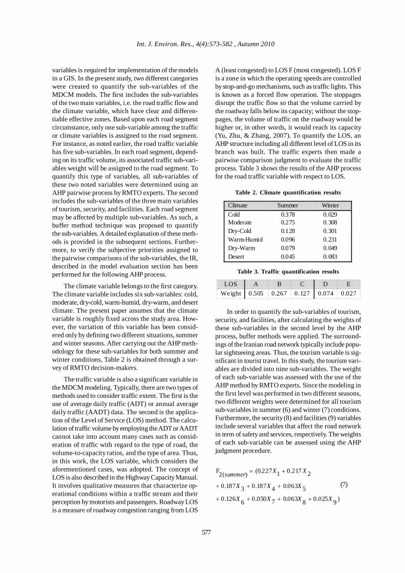
Int. J. Environ. Res., 4(4):573-582 , Autumn 2010
577
variables is required for implementation of the modelsin a GIS. In the present study, two different categorieswere created to quantify the sub-variables of theMDCM models. The first includes the sub-variablesof the two main variables, i.e. the road traffic flow andthe climate variable, which have clear and differen-tiable effective zones. Based upon each road segmentcircumstance, only one sub-variable among the trafficor climate variables is assigned to the road segment.For instance, as noted earlier, the road traffic variablehas five sub-variables. In each road segment, depend-ing on its traffic volume, its associated traffic sub-vari-ables weight will be assigned to the road segment. Toquantify this type of variables, all sub-variables ofthese two noted variables were determined using anAHP pairwise process by RMTO experts. The secondincludes the sub-variables of the three main variablesof tourism, security, and facilities. Each road segmentmay be affected by multiple sub-variables. As such, abuffer method technique was proposed to quantifythe sub-variables. A detailed explanation of these meth-ods is provided in the subsequent sections. Further-more, to verify the subjective priorities assigned tothe pairwise comparisons of the sub-variables, the IR,described in the model evaluation section has beenperformed for the following AHP process.
The climate variable belongs to the first category.The climate variable includes six sub-variables: cold,moderate, dry-cold, warm-humid, dry-warm, and desertclimate. The present paper assumes that the climatevariable is roughly fixed across the study area. How-ever, the variation of this variable has been consid-ered only by defining two different situations, summerand winter seasons. After carrying out the AHP meth-odology for these sub-variables for both summer andwinter conditions, Table 2 is obtained through a sur-vey of RMTO decision-makers.
The traffic variable is also a significant variable inthe MDCM modeling. Typically, there are two types ofmethods used to consider traffic extent. The first is theuse of average daily traffic (ADT) or annual averagedaily traffic (AADT) data. The second is the applica-tion of the Level of Service (LOS) method. The calcu-lation of traffic volume by employing the ADT or AADTcannot take into account many cases such as consid-eration of traffic with regard to the type of road, thevolume-to-capacity ratios, and the type of area. Thus,in this work, the LOS variable, which considers theaforementioned cases, was adopted. The concept ofLOS is also described in the Highway Capacity Manual.It involves qualitative measures that characterize op-erational conditions within a traffic stream and theirperception by motorists and passengers. Roadway LOSis a measure of roadway congestion ranging from LOS
A (least congested) to LOS F (most congested). LOS Fis a zone in which the operating speeds are controlledby stop-and-go mechanisms, such as traffic lights. Thisis known as a forced flow operation. The stoppagesdisrupt the traffic flow so that the volume carried bythe roadway falls below its capacity; without the stop-pages, the volume of traffic on the roadway would behigher or, in other words, it would reach its capacity(Yu, Zhu, & Zhang, 2007). To quantify the LOS, anAHP structure including all different level of LOS in itsbranch was built. The traffic experts then made apairwise comparison judgment to evaluate the trafficprocess. Table 3 shows the results of the AHP processfor the road traffic variable with respect to LOS.
Table 2. Climate quantification results
Winter Summer Climate 0.029 0.378 Cold 0.308 0.275 Moderate 0.301 0.128 Dry-Cold 0.231 0.096 Warm-Humid 0.049 0.079 Dry-Warm 0.083 0.045 Desert
Table 3. Traffic quantification results
E D C B A LOS 0.027 0.074 0.127 0.267 0.505 Weight
In order to quantify the sub-variables of tourism,
security, and facilities, after calculating the weights ofthese sub-variables in the second level by the AHPprocess, buffer methods were applied. The surround-ings of the Iranian road network typically include popu-lar sightseeing areas. Thus, the tourism variable is sig-nificant in tourist travel. In this study, the tourism vari-ables are divided into nine sub-variables. The weightof each sub-variable was assessed with the use of theAHP method by RMTO experts. Since the modeling inthe first level was performed in two different seasons,two different weights were determined for all tourismsub-variables in summer (6) and winter (7) conditions.Furthermore, the security (8) and facilities (9) variablesinclude several variables that affect the road networkin term of safety and services, respectively. The weightsof each sub-variable can be assessed using the AHPjudgment procedure.
)90250.80630.70500.61260.50630.41870.31870.
22170.1227(0.)(2F
XXXX
XXX
XXsummer
++++
+++
+=
(7)
578
)90990.80480.71180.62560.
50480.42070.31820.
21940.1145(0.)int(2F
XXXX
XXX
XXerw
+++
+++
++=
(8)
where 8,7654321 ,,,,,, XXXXXXXX and 9X denote the sea,recreational places, jungle, mountain regions, rivers/streams, ski resorts, historical places, pisciculture sta-tions, and dikes/lakes, respectively.
)0170.0690.2980.4060.0330.0880.088(0.F
7654
3214
YYYYYYY
+++
+++=(9)
where 4F presents the security variable,654321 ,,,,, YYYYYY and 7Y show the number of police sta-
tions, road maintenance offices, urban/rural pointsaround the road, side-road parking places, car-servicepoints, medical treatment service locations, and tele-phone boxes, respectively.
)37730.20930.1134(0 .5F ZZZ ++= (10)
where 1Z is the number of gas stations, 2Z is the num-ber of car/passenger terminals, and 3Z is service cen-ters.
In fact, the value of the equation (1) demonstratesa general aspect of the MDCM models (equation 2-5).The value of equation (2-5) includes several sub-equa-tions (6-9) and two tables (2 and 3). In fact, equation(1) is a combination of multiplying the inverse
distance )1(iL and a polynomial
)...( 332211 nn XKXKXKXK +++ . The value of inverse dis-tance is inverse length. Because the polynomial is onlythe combination of multiplying some coefficients andsome numbers without value, it does not have anyvalue. Thus, the value of equation (1) as well as thefinal value of all equations (2-5) is inverse length. Itshould be noted that the models can be implementedin any route-finding algorithm. This study utilizes theroute-finding algorithm of the ArcView software pack-age. ArcView utilizes a modified Dijkstra algorithm(Dijkstra, 1959) implemented using d-heap’s with d = 2(Weiss, 1997).
A number of issues relating to the evaluation of anovel model are raised at the time of its determination.Typically, two elements of a decision support system
evaluation are verification and validation. Model veri-fication is to ensure that the model is correctly builtfrom a formal point of view, while model validation as-sesses the model’s effectiveness to the user, i.e. itsability to improve the decision-making process andimprove the ability of the decision-making process(Sojda, 2007; Qureshi, Harrison, & Wegener, 1999). Inthe present study, after the model verification, valida-tion of the models was considered to verify the weightdeterminations and selection of variables for themodels.
A measure termed IR is used to verify the consis-tency of the decision makers’ judgment for model veri-fication. Inconsistency of judgment likely occurs whendecision-makers make mistakes during the process ofpairwise comparisons. The IR examines subjective pri-orities assigned for the pairwise comparisons and de-termines the extent to which all the pairwise judgmentsdiffer from ideal consistency among all comparisons.The IR provides a useful reference about how to inter-pret information returned from an individual or a group.IR in the AHP is a unique tool that can evaluate theinconsistency of each individual decision maker. Aspreviously mentioned, the 35 RMTO experts surveyedhere were the decision makers in this work. IR of vari-ous pairwise comparisons, which were explained inprevious sections in different levels, were evaluatedfor each expert opinion separately. If the IR of eachexpert’s evaluation was greater than 0.1, then his/herassessment can be deemed inconsistent. In this case,the decision-maker has to constantly reassess theirjudgment until an IR of smaller than 0.1 is achieved.The following discusses how this research deals withthe inconsistency issue.
If the IR of the MDCM models was greater than0.1, then the experts were asked to constantly re-evalu-ate their judgments in the pairwise matrix until an IR ofless than 0.1 was achieved. In the first level of theMDCM models, consistency was evaluated as follows:The final IRs of MDCM-ST, MDCM-WT, MDCM-SNT,and MDCM-WNT models were approximately 0.075,0.087, 0.0756, and 0.084, respectively. Thus, all of theseratios were smaller than 0.1 and reflect a fairly coher-ent set of assessments for modeling in level one of theAHP structure. In addition, in the second level of mod-eling, the IR measurement of each individual evaluatorfor each sub-variable was no greater than 0.1 in thefinal re-evaluations. The ratios show that the incon-sistency of the AHP process for the sub-variables cli-mate (winter situation), climate (summer situation), traf-fic, tourism (winter situation), tourism (summer condi-tion), security, and facilities were 0.045, 0.039, 0.098,0.075, 0.080, 0.034, and 0.041 respectively, which all aregenerally quite acceptable for practical purposes.
Sadeghi-Niaraki, A . et al.
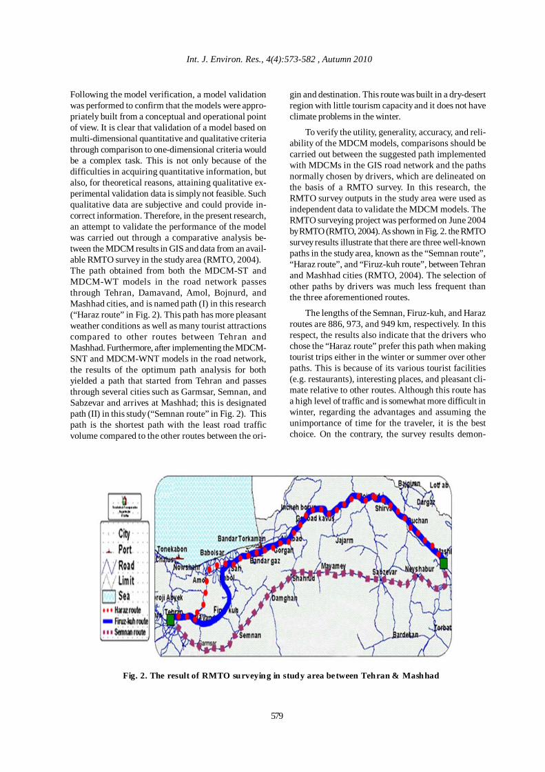
579
Int. J. Environ. Res., 4(4):573-582 , Autumn 2010
Following the model verification, a model validationwas performed to confirm that the models were appro-priately built from a conceptual and operational pointof view. It is clear that validation of a model based onmulti-dimensional quantitative and qualitative criteriathrough comparison to one-dimensional criteria wouldbe a complex task. This is not only because of thedifficulties in acquiring quantitative information, butalso, for theoretical reasons, attaining qualitative ex-perimental validation data is simply not feasible. Suchqualitative data are subjective and could provide in-correct information. Therefore, in the present research,an attempt to validate the performance of the modelwas carried out through a comparative analysis be-tween the MDCM results in GIS and data from an avail-able RMTO survey in the study area (RMTO, 2004).The path obtained from both the MDCM-ST andMDCM-WT models in the road network passesthrough Tehran, Damavand, Amol, Bojnurd, andMashhad cities, and is named path (I) in this research(“Haraz route” in Fig. 2). This path has more pleasantweather conditions as well as many tourist attractionscompared to other routes between Tehran andMashhad. Furthermore, after implementing the MDCM-SNT and MDCM-WNT models in the road network,the results of the optimum path analysis for bothyielded a path that started from Tehran and passesthrough several cities such as Garmsar, Semnan, andSabzevar and arrives at Mashhad; this is designatedpath (II) in this study (“Semnan route” in Fig. 2). Thispath is the shortest path with the least road trafficvolume compared to the other routes between the ori-
gin and destination. This route was built in a dry-desertregion with little tourism capacity and it does not haveclimate problems in the winter.
To verify the utility, generality, accuracy, and reli-ability of the MDCM models, comparisons should becarried out between the suggested path implementedwith MDCMs in the GIS road network and the pathsnormally chosen by drivers, which are delineated onthe basis of a RMTO survey. In this research, theRMTO survey outputs in the study area were used asindependent data to validate the MDCM models. TheRMTO surveying project was performed on June 2004by RMTO (RMTO, 2004). As shown in Fig. 2. the RMTOsurvey results illustrate that there are three well-knownpaths in the study area, known as the “Semnan route”,“Haraz route”, and “Firuz-kuh route”, between Tehranand Mashhad cities (RMTO, 2004). The selection ofother paths by drivers was much less frequent thanthe three aforementioned routes.
The lengths of the Semnan, Firuz-kuh, and Harazroutes are 886, 973, and 949 km, respectively. In thisrespect, the results also indicate that the drivers whochose the “Haraz route” prefer this path when makingtourist trips either in the winter or summer over otherpaths. This is because of its various tourist facilities(e.g. restaurants), interesting places, and pleasant cli-mate relative to other routes. Although this route hasa high level of traffic and is somewhat more difficult inwinter, regarding the advantages and assuming theunimportance of time for the traveler, it is the bestchoice. On the contrary, the survey results demon-
Fig. 2. The result of RMTO surveying in study area between Tehran & Mashhad
580
This paper considers the conventional one-di-mensional results to demonstrate the advantages ofthe suggested multi-dimensional method over thestandard single dimensional approach. In this step,the differences between the implementation of thefour MDCMs and a conventional method based on asingle variable such as distance are evaluated. Theroute finding result, based only on distance, passesthrough Tehran, Firuz-kuh, Semnan, Sabzevar, andMashhad. After considering the results given by theexperts, a major problem was found in this path interms of the real world; drivers almost certainly wouldnot select this path. For more information regardingthis problem and for determining why drivers do notuse this route, a topographic map of the area isshown. This route has many twisting gorges that aredifficult to pass. Therefore, this example underscoresa major problem associated with the use of the con-ventional method.
The analysis between the MDCM outputs (pathsI and II) and the conventional approach results withthe RMTO survey results revealed the following. Path(I) was adapted to the path that is chosen by travelerson tourist trips in both summer and winter, i.e. both theMDCM-ST and MDCM-WT models have been de-signed with high precision in terms of correspondingwith reality. In contrast, the conventional model re-sults showed major differences with the path selectedby the tourist travelers. Additionally, path (II), theMDCM-SNT and MDCM-WNT models outputs, co-incided with the path selected by drivers on businesstrips in both summer and winter. On the contrary, thepath of the conventional model based on distance didnot accord with reality. The results of the evaluationanalysis showed that there are no differences betweenthe MDCM models outputs and the path chosen bytravelers in reality. In general, the models provide anaccurate picture of the road network in the study area.Hence, it can be concluded that taking into account ofvarious qualitative and quantitative criteria affectedon each road segment in reality, leads to the result ofroute finding analysis are more close to reality. This
result coincides with what the driver choose their pathto get to the destination. Since the accurate path ofroute finding analysis is based on the user’ prefer-ence, the validation process of the result of MDCMmodels is complex. In this research, the result of thesurveying performed based on asking many driversfrom origin and destination was utilized to validate theresult of MDCM modeling.
CONCLUSIONAiming to resolve problems of one dimensional
cost functions used in network analysis, this paperproposed a new model based on the use of a multi-dimensional cost function in GIS. For this, a modelwas developed by assessing, weighting, and combin-ing several variables (travel, climatic conditions, sea-son, road characteristics, and so forth) into a singlecost model. The model was, then implemented in theIranian road network and evaluated within GIS for itsaccuracy and reliability. The results indicated that,compared to the current techniques, the model leadsto results which fit more precisely to the real routsselected by the users. An important advantage of theproposed approach over the others is that it incorpo-rates quantitative along qualitative parameters affect-ing a user’s decision, all in a single model. . Therefore,it can be concluded that this modeling approach ap-pears to be adequate for the designed purpose, and itis applicable to GIS based route finding analysis. How-ever, it is suggested that the use of multi-decisionmaking techniques other than AHP to be also studiedin the future. Furthermore, using the MDCM throughWEBGIS would greatly enhance tourist services andtourist infrastructure. This will contribute further tothe development of the tourist industry, as a large num-ber of users would be able to utilize the MDCM resultsfrom any place in the world.
ACKNOWLEDGEMENTSThis work was supported by an INHA UNIVER-
SITY Research Grant. Furthermore, the authors wouldlike to thank the Iranian Road Maintenance and Trans-port Organization.
REFERENCESAlam, J. B., Nahar, T. and Shaha, B. (2008). Evaluation ofNational Highway by Geographical Information System.Int. Journal. Environ. Res., 2 (4), 365-370.
Alesheikh, A. A., Soltani, M. J., Nouri, N. and Khalilzadeh,M. (2008). Land Assessment for Flood Spreading Site Se-lection Using Geospatial Information System. InternationalJournal of Environmental Science and Technology, 5 (4),455-462.
strated that in reality most drivers on non-tourist tripschoose the “Semnan route” in both summer and win-ter when on business trips. These reasons for this in-clude the fact that it is the shortest route and it has thelowest road traffic rate and the fewest climate-relatedproblems in winter. Furthermore, this trip is not a tour-ist trip, thus implying that the tourism variable is notof high importance for travelers. Lastly, the above re-sults demonstrated that the MDCM models outputcorrespond well with the findings of the RMTOsurvey.
Decision-based Model for Road Network
Ben-Akiva, M., Bergman, M. J., Daly, A. J. and Ramaswamy,R. (1984). Modeling Inter Urban Route Choice Behavior.Ninth International Symposium on Transportation and Traf-fic Theory, VNU Science Press, Utrecht, 299-330.
Dijkstra, E. W. (1959). A Note on Two Problems in Connec-tion With Graphs. Numerische Mathematik,1, 269-271.
Faryadi, Sh. and Taheri, Sh. (2009). Interconnections ofUrban Green Spaces and Environmental Quality of Tehran.Int. Journal. Environ. Res., 3 (2), 199-208.
Forman, E. and Selly, M.A. (2001). Decisions by Objec-tives, Expert Choice Inc. Available at: http://www.expertchoice.com.
Fu, L., and Rilett, L.R. (1998). Expected shortest paths indynamic and stochastic traffic networks. Transportationresearch Part B, Methodological, 32 (7), 499-516.
Gharakhlou, M., Faraji Sabokbar, H. A. and Givehchi, S.(2010). Access Enhancement by Making Changes in theRoute Network to Facilitate Rescue Operations in UrbanDisasters. Int. Journal. Environ. Res., 4 (2), 183-192.
Goswami, Sh. (2009). Road Traffic Noise: A Case Study ofBalasore Town, Orissa, India. Int. Journal. Environ. Res., 3(2), 309-316.
Jun, C., Koo, J., and Koh, J. (2004). Developing a WaterPipe Management System in Seoul Using the GIS. Inter-national Archives of Photogrammetry. Remote Sensing andSpatial Information Sciences, ISPRS, 35 (2), 290-293.
Mahiny, A. S. and Gholamalifard, M. (2007). Dynamic Spa-tial Modeling of Urban Growth through Cellular Automatain a GIS Environment. Int. Journal. Environ. Res., 1 (3),272-279.
Monavari, M. and Mirsaeed, Sh.G. (2008). Ecological Im-pact Assessment of Highways on National Parks: Tehran -Pardis Highway (Iran). Int. Journal. Environ. Res., 2 (2),133-138.
Orda, A., and Rom, R. (1990). Shortest-path and minimum-delay algorithms in networks with time-dependent edge-length. Journal of the Association for Computing Machin-ery, 37 (3), 607-625.
Pijanowski, B. C., Tayyebi, A., Delavar, M. R. andYazdanpanah, M. J. (2009). Urban Expansion SimulationUsing Geospatial Information System and Artificial NeuralNetworks. Int. Journal. Environ. Res., 3 (4), 493-502.
Qureshi, M. E., Harrison, S. R., and Wegener, M. K. (1999).Validation of multicriteria analysis models. Agricultural Sys-tems, 62, 105-116.
RMTO (2004). Origin-destination surveying for transpor-tation analyses in Iranian road networks. Iranian Road Main-tenance and Transport Organization project report, 2, pp.70-90.
Saaty, T.L. (1988). Decision making for leaders. RWS Pub-lications, Pittsburgh, USA, 27-33.
Saaty, T. L. (1980). The analytic hierarchy process: Plan-ning, priority setting, resource allocation. McGraw-Hill, 97-98.
Saaty, T. L., and Vargas, L. G. (1991). Prediction, Projectionand Forecasting. Boston, Kluwer Academic Publishers, 118-119.
Saaty, T. L., and Vargas, L. G. (2001). Models, methods,concepts & applications of the analytic hierarchy process.Kluwer Academic Publishers, Dordrecht, MA, 45-51.
Saaty, T. L. (2005). Theory and Applications of the Ana-lytic Network Process. RWS Publications, Pittsburgh,USA.
Schomaker, P. J. H., and Waid, C. C. (1992). An experimen-tal comparison of different approaches to determiningweights in additive utility models. Management Science, 28(2), 182-195.
Shadewald, J., Hallmark, K. S., and Souleyrette, R. R. (2001).Visualizing System-Wide Economic Impacts of Transpor-tation Projects. Journal of Urban Planning and Develop-ment, 127 (4), 158-168.
Shobeiri, S. M. , Omidvar, B. and Prahallada, N. N. (2007).Digital Change Detection Using Remotely Sensed Data forMonitoring Green Space Destruction in Tabriz. Int. J.Environ. Res., 1 (1), 35-41.
Sojda, R. (2007). Empirical evaluation of decision supportsystems: Needs, definitions, potential methods, and an ex-ample pertaining to waterfowl management. EnvironmentalModelling and Software, 22, 269-277.
Souder, W.E., and Mandakovic, T. (1986). R&D projectselection models. Research Management, 24 (4), 36-42.
Stewart, W. (2005). Using the AHP and Expert Choice toSupport the MSC Fisheries Certification Process. MarineStewardship Council Hartley McMaster Ltd, 62-69.
Thirumalaivasan, D. and Guruswamy, V., (2003). OptimalRoute Analysis Using GIS. 1-2. Available at http://www.gisdevelopment.net/application/Utility/transport/utilitytr 0004a.htm.
Vafaei, F. and Harati, A. N. (2010). Strategic Management inDecision Support System for Coastal Flood Management.Int. Journal. Environ. Res., 4 (1), 169-176.
Vahidnia, M. H. Alesheikh, A. A. and Alimohammadi, A.(2009). Hospital Site Selection Using Fuzzy AHP and ItsDerivatives. Journal of Environmental Management, 90 (10),3048-3056.
Vargas, L. G. (1990). An overview of the analytic hierarchyprocess and its applications. European Journal of Opera-tional Research, 48, 2-8.
Int. J. Environ. Res., 4(4):573-582 , Autumn 2010
581

Weiss, M. A. (1997). Data Structures and AlgorithmAnalysis in C, Addison-Wesley Longman Inc. 2nd ed.,295-304.
Yu, G., Zhu, J.-S., and Zhang, N. (2007). Study of theCapacity of a Road Network Basing on the Level of Ser-vice. Management Science and Engineering, 2241 (2246),20-22.
Zahedi, F. (1986). The analytic hierarchy process-a sur-vey of the method and its application. Interface, 16 (4),96-108.
Zaperto, E. G., Smith, C. H., and Weistroffer, H. R. (1997).Evaluating multi-attribute decision support systems. Jour-nal of Multi-Criteria Decision Analysis, 6, 201-214.
Ziliaskopoulos, A. K. (1993). Time-dependent, shortest-path algorithm for real-time intelligent vehicle highwaysystem applications. Transportation research record, 1408,94-100.
Sadeghi-Niaraki, A . et al.
582
Int. J. Environ. Res., 4(4):583-594 , Autumn 2010ISSN: 1735-6865
Received 12 March 2009; Revised 17 June 2010; Accepted 25 June 2010
*Corresponding author E-mail: [email protected]
583
Water and Wastewater Minimization in Tehran Oil Refinery using Water PinchAnalysis
Nabi Bidhendi, Gh. R. , Mehrdadi, N. and Mohammadnejad , S .*
Graduate Faculty of Environment, University of Tehran, P.O. Box: 14155-6135, Tehran, Iran
ABSTRACT: This study aimed to find an appropriate way to minimize water utility in the petrochemical andpetroleum industries. For this purpose, Tehran oil refinery was chosen to analyze feasibilities of regeneration,reuse and recycling in the water network. In this research, two key contaminants including COD and hardnesswere analyzed. Amount of freshwater was reduced about 180 m3/h (53%) and 216.88 m3/h (63%) regardingCOD and hardness respectively. In the next stage, two mentioned contaminants were analyzed simultaneouslybased on the mass transfer constraints. Results showed that the amount of required water was reduced from340 m3/h to 197.12 m3/h that was about 42%. Analyzing both methods clearly demonstrated that amount ofrequired water would be determined by mass transfer of COD. In addition, the method based on multiplecontaminants gave more precise results rather than single contaminant.
Key words: Water utility, Water reuse, Minimization, Mass transfer, Regeneration
INTRODUCTIONGenerally, water is used as raw material in most of
the industries and generated wastewater is dischargedin to the environment. Increasing freshwater utility isdue to economical and industrial growth, considerably(Rajakumar and Meenambal, 2008; Rajasimman andKarthikeyan, 2009; Yoochatchaval et al., 2008; Biati etal., 2010; Aminzadeh et al., 2010; Bagherzadeh-Namaziet al., 2008; Mehrdadi et al., 2007; Abduli et al., 2007;Dabhade et al., 2009). On the one hand, the price ofwater is increased which consequently raises the priceof products. On the other hand, the environmental lawsdo not allow discharging wastewater in to theenvironment. (Karbassi, et al., 2008; Praveena, et al.,2010; Vargas-Vargas, et al., 2010; Biati, et al., 2010).Therefore, industries have to use some strategiesrelated to water utility minimization. Industrialwastewater management through different methods hasbeen taken into consideration during recent years inIran (Ataei and Yoo, 2010; Saeedi and Amini, 2007;Sarparastzadeh et al., 2007; Nabi Bidhendi et al., 2007;Hassani et al., 2008; Amini et al., 2008; Kabir andOgbeide, 2008; Hassani et al., 2009; Moayed Salehiand Mirbagheri, 2010). Nowadays, different techniquesand methods have been developed to design waterallocation system so that water utility is reduced in anacceptable level. Water pinch technology is asystematic technique for analyzing water networks andreducing expenditures related to different water usingprocesses (Manan, et al., 2006; Hallale, et al., 2001;
Ataei, et al., 2010 ; Ahmed, et al., 2009 and Gomez, etal., 2006; Omran et al., 2009; Khezri et al., 2010). El-Halwagi (1992) propounded the theory of massexchange networks. This theory was based on a two-stage solution; first, Mixed Integer NonlinearProgramming and then Mixed Integer LinerProgramming. Most of the methods used in water pinchanalysis are based on the mass exchange of one orseveral contaminants (Ataei and Panjehshahi ,2009).If the mass exchange is based on mass transferring ofone contaminant, the problem will be solved as asingle contaminant. Nevertheless, if it includes masstransferring of two or more key contaminants, theproblem will be solved as multiple contaminants.Graphical, mathematical and computer-based methodsmay be used for both cases. Each method has someadvantages and disadvantages. Graphical methods areso practical to solve single contaminant problems.However, they are complicated and sometimeimpossible for multiple contaminants problems.(Alizadeh, et al., 2010; Bhatnagar, et al., 2009; Hassani,et al., 2009). Wang and Smith (1994) used limitingcomposite curve to solve multiple contaminantsproblems. Kuo and Smith (1997) applied a new methodto reduce complexity of graphical method based onbreaking the operations. Majozi, et al. (2005) Presenteda graphical technique for freshwater and wastewaterminimization in completely batch operations. Waterminimization was achieved through the exploitationof inter- and intra-process water reuses and recycles
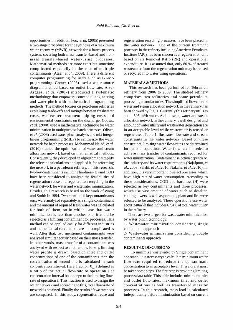
584
Nabi Bidhendi, Gh. R. et al.
opportunities. In addition, Foo, et al. (2005) presenteda two-stage procedure for the synthesis of a maximumwater recovery (MWR) network for a batch processsystem, covering both mass transfer-based and non-mass transfer-based water-using processes.Mathematical methods are more exact but sometimecomplicated especially in the case of multiplecontaminants (Ataei, et al., 2009). There is differentcomputer programming for users such as GAMSprogramming. Gomez (2006) used a water sourcediagram method based on outlet flow-rate. Alva-Argaez, et al. (2007) introduced a systematicmethodology that empowers conceptual engineeringand water-pinch with mathematical programmingmethods. The method focuses on petroleum refineriesexplaining trade-offs and savings between freshwatercosts, wastewater treatment, piping costs andenvironmental constraints on the discharge. Gouws,et al. (2008) used a mathematical technique for waterminimization in multipurpose batch processes. Oliver,et al. (2008) used water pinch analysis and mix integerlinear programming (MILP) to synthesize the waternetwork for batch processes. Mohammad Nejad, et al.(2010) studied the optimization of water and steamallocation network based on mathematical methods.Consequently, they developed an algorithm to simplifythe relevant calculations and applied it for reformingthe network in a petroleum refinery. In this research,two key contaminants including hardness (H) and CODhave been considered to analyze the feasibilities ofregeneration reuse and regeneration recycling in thewater network for water and wastewater minimization.Besides, this research is based on the work of Wangand Smith in 1994. Two mentioned key contaminantsonce were analyzed separately as a single contaminantand the amount of required fresh water was calculatedfor both of them, so in which case that waterminimization is less than another one, it could beselected as a limiting contaminant for processes. Thismethod can be applied easily for different industriesand mathematical calculations are not complicated aswell. After that, two mentioned contaminants wereanalyzed simultaneously based on their mass transfer.In other words, mass transfer of a contaminant wasanalyzed with respect to another one. Firstly, limitingwater profile is drawn based on inlet and outletconcentrations of one of the contaminants then theconcentration of second one is calculated in eachconcentration interval. Here, fraction θi.nis defined asa ratio of the actual flow-rate to operation i atconcentration interval boundary n to the limiting flow-rate of operation i. This fraction is used to design thewater network and according to this, total flow-rate ofnetwork is obtained. Finally, the results of two methodsare compared. In this study, regeneration reuse and
regeneration recycling processes have been placed inthe water network. One of the current treatmentprocesses in the refinery including American PetroleumInstitute (API) has been chosen as a regeneration unitbased on its Removal Ratio (RR) and operationalexpenditure. It is assumed that, only 80 % of treatedwastewater from the regeneration unit may be reusedor recycled into water using operations.
MATERIALS & METHODSThis research has been performed for Tehran oil
refinery from 2006 to 2009. The studied refinerycomprises two refineries and some petroleumprocessing manufactories. The simplified flowchart ofwater and steam allocation network in the refinery hasbeen showed by Fig. 1. Currently this refinery utilizesabout 505 m3/h water. As it is seen, water and steamallocation network in the refinery is well designed andamount of water utility and wastewater generation arein an acceptable level while wastewater is reused orregenerated. Table 1 illustrates flow-rate and streamconstraints in the water network. Based on theseconstraints, limiting water flow-rates are determinedfor optional operations. Water flow-rate is needed toachieve mass transfer of contaminants required forwater minimization. Contaminant selection depends onthe industry and its water requirements (Najafpour, etal., 2008; Salehi, et al., 2010; Nakane, et al., 2010). Inaddition, it is very important to select processes, whichhave high rate of water consumption. According tothese considerations, COD and hardness (H) wereselected as key contaminants and three processes,which use vast amount of water such as desalter,cooling towers as well as portable; plant and fire wereselected to be analyzed. These operations use waterabout 340m3/h that includes 67.4% of total water utilityin the refinery. There are two targets for wastewater minimizationby water pinch technology:1- Wastewater minimization considering singlecontaminant approach2- Wastewater minimization considering doublecontaminants approach
RESULTS & DISCUSSIONS To minimize wastewater by Single contaminantapproach, it is necessary to calculate minimum waterflow-rate required to reduce the contaminantconcentration to an acceptable level. Therefore, it mustbe taken some steps. The first step is providing limitingprocess data table. This table includes minimum inletand outlet flow-rates, maximum inlet and outletconcentrations as well as transferred mass byprocesses. In this research, mass load is calculatedindependently before minimization based on current
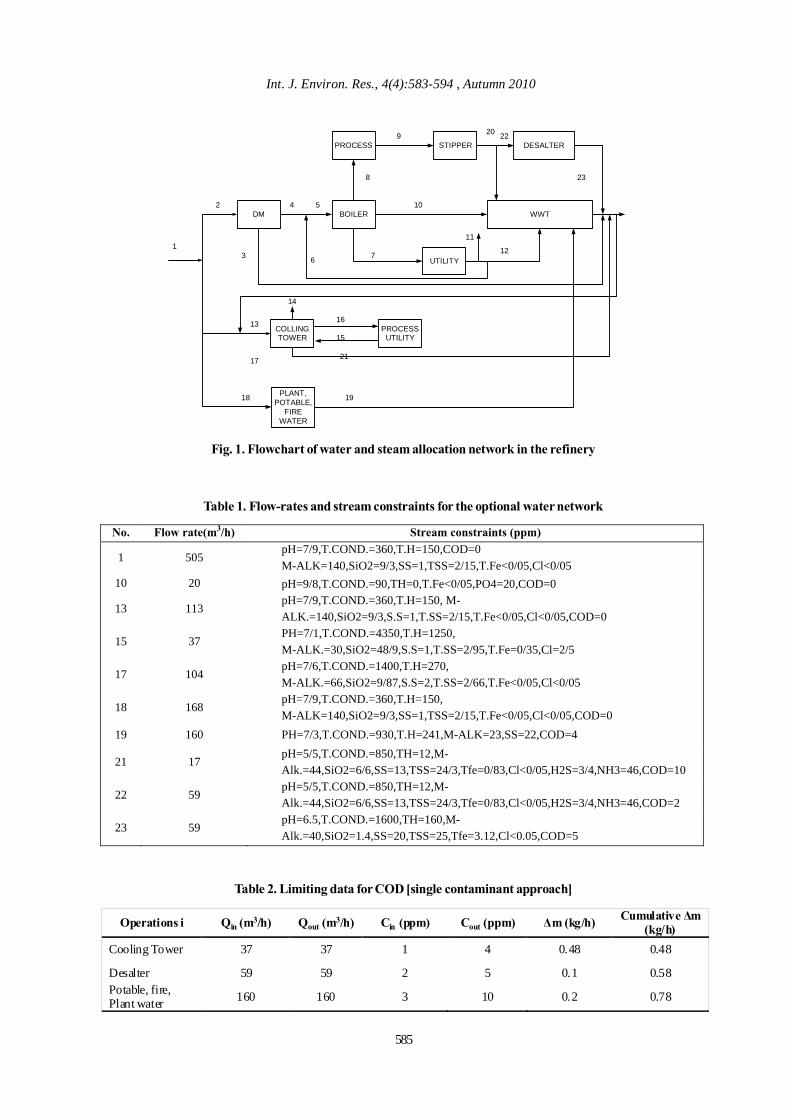
Int. J. Environ. Res., 4(4):583-594 , Autumn 2010
585
DM BOILER
PROCESS STIPPER DESALTER
WWT
UTILITY
COLLING TOWER
PROCESS UTILITY
PLANT, POTABLE,
FIRE WATER
1
2 4 5
3 6 7
8
10
9 20 22
23
12
11
14
13
17
16
15
21
18 19
Fig. 1. Flowchart of water and steam allocation network in the refinery
Table 1. Flow-rates and stream constraints for the optional water network
No. Flow rate(m3/h) Stream constraints (ppm)
1 505 pH=7/9,T.COND.=360,T.H=150,COD=0 M-ALK=140,SiO2=9/3,SS=1,TSS=2/15,T.Fe<0/05,Cl<0/05
10 20 pH=9/8,T.COND.=90,TH=0,T.Fe<0/05,PO4=20,COD=0
13 113 pH=7/9,T.COND.=360,T.H=150, M-ALK.=140,SiO2=9/3,S.S=1,T.SS=2/15,T.Fe<0/05,Cl<0/05,COD=0
15 37 PH=7/1,T.COND.=4350,T.H=1250, M-ALK.=30,SiO2=48/9,S.S=1,T.SS=2/95,T.Fe=0/35,Cl=2/5
17 104 pH=7/6,T.COND.=1400,T.H=270, M-ALK.=66,SiO2=9/87,S.S=2,T.SS=2/66,T.Fe<0/05,Cl<0/05
18 168 pH=7/9,T.COND.=360,T.H=150, M-ALK=140,SiO2=9/3,SS=1,TSS=2/15,T.Fe<0/05,Cl<0/05,COD=0
19 160 PH=7/3,T.COND.=930,T.H=241,M-ALK=23,SS=22,COD=4
21 17 pH=5/5,T.COND.=850,TH=12,M-Alk.=44,SiO2=6/6,SS=13,TSS=24/3,Tfe=0/83,Cl<0/05,H2S=3/4,NH3=46,COD=10
22 59 pH=5/5,T.COND.=850,TH=12,M-Alk.=44,SiO2=6/6,SS=13,TSS=24/3,Tfe=0/83,Cl<0/05,H2S=3/4,NH3=46,COD=2
23 59 pH=6.5,T.COND.=1600,TH=160,M-Alk.=40,SiO2=1.4,SS=20,TSS=25,Tfe=3.12,Cl<0.05,COD=5
Table 2. Limiting data for COD [single contaminant approach]
Operations i Qin (m3/h) Qout (m3/h) Cin (ppm) Cout (ppm) ∆m (kg/h) Cumulative ∆m (kg/h)
Cooling Tower 37 37 1 4 0.48 0.48
Desalter 59 59 2 5 0.1 0.58 Potable, fire, Plant water 160 160 3 10 0.2 0.78
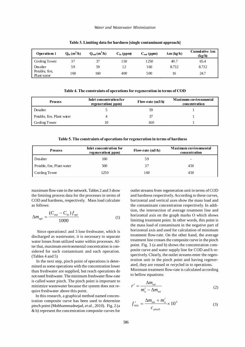
586
Water and Wastewater Minimization
maximum flow-rate in the network. Tables 2 and 3 showthe limiting process data for the processes in terms ofCOD and hardness, respectively. Mass load calculateas follows:
1000)( opiinout
opi
fCCm
−=∆ (1)
Since operations1 and 3 lose freshwater, which isdischarged as wastewater, it is necessary to separatewater losses from utilized water within processes. Af-ter that, maximum environmental concentration is con-sidered for each contaminant and each operation.(Tables 4 and 5) In the next step, pinch point of operations is deter-mined as some operations with the concentration lowerthan freshwater are supplied, but reach operations donot need freshwater. The minimum freshwater flow-rateis called water pinch. The pinch point is important tominimize wastewater because the system does not re-quire freshwater above this point. In this research, a graphical method named concen-tration composite curve has been used to determinepinch point (Mohhammadnejad, et al., 2010). Fig. 2 (a& b) represent the concentration composite curves for
Table 3. Limiting data for hardness [single contaminant approach]
Operations i Qin (m3/h) Qout (m3/h) Cin (ppm) Cout (ppm) ∆m (kg/h) Cumulative ∆m (kg/h)
Cooling Tower 37 37 150 1250 40.7 65.4 Desalter 59 59 12 160 8.732 8.732 Potable, fire, Plant water 160 160 400 500 16 24.7
Table 4. The constraints of operations for regeneration in terms of COD
Maximum environmental concentration Flow-rate (m3/h) Inlet concentration for
regeneration( ppm) Process
1 59 5 Desalter
1 37 4 Potable, fire, Plant water 1 160 10 Cooling Tower
Table 5. The constraints of operations for regeneration in terms of hardness
Maximum environmental concentration Flow-rate (m3/h) Inlet concentration for
regeneration( ppm) Process
- 59 160 Desalter
450 37 500 Potable, fire, Plant water
450 160 1250 Cooling Tower
outlet streams from regeneration unit in terms of CODand hardness respectively. According to these curves,horizontal and vertical axes show the mass load andthe contaminant concentration respectively. In addi-tion, the intersection of average treatment line andhorizontal axis on the graph marks O which showslimiting treatment point. In other words, this point isthe mass load of contaminant in the negative part ofhorizontal axis and used for calculation of minimumtreatment flow-rate. On the other hand, the averagetreatment line crosses the composite curve in the pinchpoint. Fig. 3 (a and b) shows the concentration com-posite curve and water supply line for COD and h re-spectively. Clearly, the outlet streams enter the regen-eration unit in the pinch point and having regener-ated, they are reused or recycled in to operations.Minimum treatment flow-rate is calculated accordingto bellow equations:
totio
toti
mmmr∆−
∆= (2)
3min 10×
+∆=
pinch
iototi
cmm
f (3)
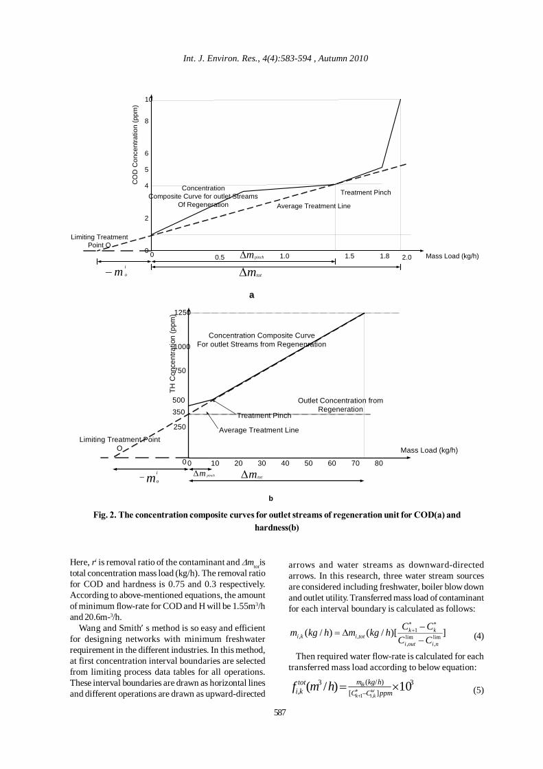
Int. J. Environ. Res., 4(4):583-594 , Autumn 2010
0 0.5 1.0 1.5 2.00
2
4
6
8
10
Mass Load (kg/h)
CO
D C
once
ntra
tion
(ppm
)
Concentration Composite Curve for outlet Streams
Of Regeneration Average Treatment Line
Treatment Pinch
5
1.8
Limiting Treatment Point O
m i
o−mpinch∆
mtot∆
a
0
250
500
750
1000
1250
0 10 20 30 40 50 60 70 80
Mass Load (kg/h)
TH C
once
ntra
tion
(ppm
)
Limiting Treatment PointO
Treatment Pinch
mi
o− m pinch∆ mtot∆
Average Treatment Line
Concentration Composite CurveFor outlet Streams from Regenenration
350Outlet Concentration from
Regeneration
b
Fig. 2. The concentration composite curves for outlet streams of regeneration unit for COD(a) andhardness(b)
Here, ri is removal ratio of the contaminant and ∆mtotistotal concentration mass load (kg/h). The removal ratiofor COD and hardness is 0.75 and 0.3 respectively.According to above-mentioned equations, the amountof minimum flow-rate for COD and H will be 1.55m3/hand 20.6m-3/h. Wang and Smith′ s method is so easy and efficientfor designing networks with minimum freshwaterrequirement in the different industries. In this method,at first concentration interval boundaries are selectedfrom limiting process data tables for all operations.These interval boundaries are drawn as horizontal linesand different operations are drawn as upward-directed
arrows and water streams as downward-directedarrows. In this research, three water stream sourcesare considered including freshwater, boiler blow downand outlet utility. Transferred mass load of contaminantfor each interval boundary is calculated as follows:
])[/()/( lim,
lim,
1,,
niouti
kktotiki CC
CChkgmhkgm−−
∆=∗∗
+ (4)
Then required water flow-rate is calculated for eachtransferred mass load according to below equation:
3][
)/(3, 10)/(
,1×=
−∗+ ppmCC
hkgmtotki w
kik
ikhmf (5)
587
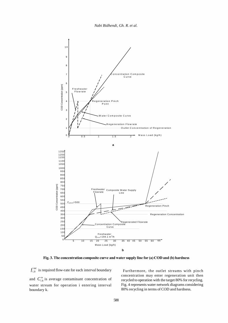
588
Nabi Bidhendi, Gh. R. et al.
0 0
1
2
3
4
5
6
7
8
0 .5 1 1 .5 2 M a s s L o a d (k g /h )
CO
D C
once
ntra
tion
(ppm
)
9
1 0
W a te r C o m p o s ite C u rv e
C o n c e n tra tio n C o m p o s iteC u rv e
R e g e n e ra tio n P in c hP o in t
F re s h w a te rF lo w ra te
R e g e n e ra tio n F lo w ra teO u tle t C o n c e n tra tio n o f R e g e n e ra tio n
a
050
100150200250300350400450500550600650700750800850900950
1000
10501100115012001250
5 10 15 20 25 30 35 40 45 50 55 60 65
CO
D C
once
ntra
tion
(ppm
)
M ass Load (kg/h)
Com posite W ater SupplyL ine
Concentration Com positeC urve
C pinch=500
FreshwaterQ m in=194.1 m 3/h
Regeneration Concentra tion
Regeneration P inch
Freshw aterFlow rate
R egenerated Flow rate
b
Fig. 3. The concentration composite curve and water supply line for (a) COD and (b) hardness
totkif , is required flow-rate for each interval boundary
and wkiC . is average contaminant concentration of
water stream for operation i entering intervalboundary k.
Furthermore, the outlet streams with pinchconcentration may enter regeneration unit thenrecycled to operation with the target 80% for recycling.Fig. 4 represents water network diagrams considering80% recycling in terms of COD and hardness.
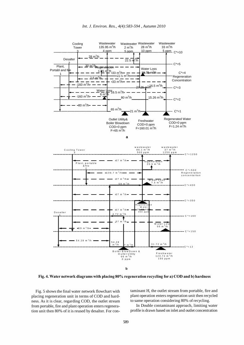
589
Int. J. Environ. Res., 4(4):583-594 , Autumn 2010
16.5 m3/h
15.26 m3/h
22.5 m3/h
65 m3/h 21 m3/h
80 m3/h
80 m3/h
160 m3/h
160 m3/h
16.5 m3/h
33 m3/h
33 m3/h
Outlet Utility&Boiler Blowdown
COD=0 ppmF=65 m3/h
FreshwaterCOD=0 ppm
F=160.01 m3/h
Regenerated WaterCOD=0 ppmF=1.24 m3/h
27.25 m3/h
22.5 m3/h
Regeneration1.55 m3/h
28 m3/h
30 m3/h
7.5 m3/h
Water Loss6 m3/h
Water Loss19.75 m3/h
Plant,Portabl and fire
1
Desalter2
Wastewater135.95 m3/h
4 ppm
Wastewater2 m3/h5 ppm
Wastewater28 m3/h10 ppm
Wastewater33 m3/h5 ppm
C*=1
C*=2
C*=3
C*=4Regeneration Concentration
C*=5
C*=10
Cooling Tower
3
a
5 4 . 2 8 m 3 / h
5 9 m 3 /h
3 7 m 3 / h
3 7 m 3 / h
3 7 m 3 / h
3 7 m 3 / h
3 7 m 3 / h
1 0 6 .7 m 3 / h
D e s a l te r 1
P la n t , p o r ta b le& f i r e
2
C o o l in g T o w e r 3
r e g e n e r a t io n2 0 . 6 m 3 /h
w a s te w a te r8 6 . 1 m 3 /h5 0 0 p p m
w a s te w a te r3 7 m 3 / h
1 2 5 0 p p m
W a te r L o s s7 . 5 m 3 /h5 9 m 3 /h
W a te r L o s s5 5 m 3 /h
3 1 .7 2 m 3 /h7 m 3 / h
4 .7 2 m 3 / h
5 4 .2 8m 3 / h
B o i le r B lo w D o w n &O u t le t U t i l i ty
6 6 m 3 /h0 p p m
R e g e n e r a t e d W a t e r
1 6 . 4 8 m 3 / h3 5 0 p p m
F r e s h w a te r1 2 3 .7 2 m 3 /h
1 5 0 p p m
C * = 1 2
C * = 1 5 0
C * = 1 6 0
C * = 3 5 0
C * = 4 0 0
C * = 5 0 0R e g e n e r a t io n c o n c e n ta r t io n
C * = 1 2 5 0
b
Fig. 4. Water network diagrams with placing 80% regeneration recycling for a) COD and b) hardness
Fig. 5 shows the final water network flowchart withplacing regeneration unit in terms of COD and hard-ness. As it is clear, regarding COD, the outlet streamfrom portable, fire and plant operation enters regenera-tion unit then 80% of it is reused by desalter. For con-
taminant H, the outlet stream from portable, fire andplant operation enters regeneration unit then recycledto same operation considering 80% of recycling.
In Double contaminant approach, limiting waterprofile is drawn based on inlet and outlet concentration
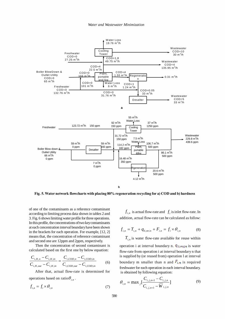
590
Water and Wastewater Minimization
Plant, portable and fire
Regeneration
Desalter
Cooling Tower
Boiler BlowDown &Outlet Utility
COD=065 m 3/h
FreshwaterCOD=0
132.76 m3/h
COD=0166 m 3/h
COD=0101 m 3/h
COD=031.76 m 3/h
COD=11.24 m 3/h
COD=0.0533 m 3/h
COD=41.55 m3/h
W astewaterCOD=533 m 3/h
FreshwaterCOD=0
27.25 m 3/h
W astewaterCOD=1030 m 3/h
W astewaterCOD=4
135.95 m3/h
COD=1.849.75 m3/h
COD=422.5 m 3/h
0.31 m 3/h
W ater Loss19.76 m 3/h
W ater Loss6 m 3/h
a
DesalterPlant,
portable&fire
Rgeneration
Cooling Tower
Freshwater 123.72 m3/h 150 ppm
31.72 m3/h 150 ppm
92 m3/h 150 ppm
59 m3/h 160 ppm
7 m3/h 0 ppm
16.48 m3/h 350 ppm
20.6 m3/h 500 ppm
114.2 m3/h 182 ppm
106.7 m3/h 500 ppm
86.1 m3/h 500 ppm
37 m3/h 1250 ppm
59 m3/h 0 ppm
Boiler Blow down & Outlet Utility
66 m3/h 0 ppm
Wastewater229.8 m3/h 439.6 ppm
4.12 m3/h
b
55 m3/h Water Loss
7.5 m3/h Water Loss
Fig. 5. Water network flowcharts with placing 80% regeneration recycling for a) COD and b) hardness
of one of the contaminants as a reference contaminantaccording to limiting process data shown in tables 2 and3. Fig. 6 shows limiting water profile for three operations.In this profile, the concentrations of two key contaminantsat each concentration interval boundary have been shownin the brackets for each operation. For example, [12, 2]means that, the concentration of reference contaminantand second one are 12ppm and 2ppm, respectively. Then the concentration of second contaminant iscalculated based on the first one by below equation:
inCODioutCODi
inCODinCODi
inHioutHi
inHinHi
CCCC
CCCC
,,,,
,,,,
,,,,
,,,,
−
−=
−
− (6)
After that, actual flow-rate is determined for
operations based on ratio ni.θ .
niini ff ,, θ×= (7)
nif , is actual flow-rate and if is inlet flow-rate. Inaddition, actual flow-rate can be calculated as follow:
niininmlinini fFqTf ,.,,, θ×=++= ≤ (8)
niT , is water flow-rate available for reuse within
operation i at interval boundary n. is waterflow-rate from operation i at interval boundary n thatis supplied by (or reused from) operation l at intervalboundary m smaller than n and is requiredfreshwater for each operation in each interval boundary. is obtained by following equation:
(9)][max,,1,,
,,1,,,
njinji
njinjijni WC
CC
−
−=
+
+θ

Int. J. Environ. Res., 4(4):583-594 , Autumn 2010
is flow-rate weighted average concentration of thecurrent water sources and is calculated as:
Wi,j,n+1is outlet concentration of each operation and inletconcentration of next one. To design the water network, at first concentrationinterval boundaries are drawn. Then water flow-rate iscalculated for each operation in each interval boundarybased on mass transfer of key contaminants (COD andH) by above- mentioned equations. For example, the water flow-rate for intervalboundary1 and operation1 is calculated as follow:
1. Determining ni.θ
92.0]3.0,92.0max[]15.19
135.19,0150
12150[max1,1 ==−−
−−
=θ
2. Calculating required flow-rate
hmfi /28.545992.0 31, =×=
∑∑
++
×+×=
≤
≤≤
lninmlini
lnmljnmlinjini
njiFqT
WqWTW
,,,
,,,,,
,,
1,
,,1,,,,1,,
)(
+
++
−×+=
ni
njinjiinjinji T
CCfWW
(10)
(11)
0
12
150
160
400
500
1250
Con
cent
ratio
n H
(ppm
)
Op1 [160,5]
[12,2]
[150,3]
[500,4]
[400,1]
Op 2
[1250,10]
Op 3
[150,4.8]
[160,3.1]
[400,4.6]
[500,5.2]
Fig. 6. Limiting water profile
3. Calculating outlet concentration
Likewise, water flow-rate and outlet concentration arecalculated for the rest of the operations in each intervalboundary. Unfortunately, there is no reasonable rule forplacing regeneration processes in a water network anddrawing the diagrams as well. This research provides amethod based on analysis of single contaminantconsideration for regeneration placement (Mann andLiu, 1999). Accordingly, at first, the minimum treatmentflow-rate is calculated for each contaminant by Eqs. 1and 2. After that, the greatest value is considered as a totalminimum treatment flow-rate:
Therefore:
Although the minimum treatment flow-rate is 20.6m3/h,the regeneration unit could regenerate water more, so thewhole outlet flow-rate from cooling tower is transferredinto regeneration unit and regenerated into portable; plantand fire operation. Next step is selection of some streamsfor treatment. Minimum flow-rate is deducted from flow-rate of the most polluted stream and the rest is consideredfor other polluted streams. Therefore, the cleanest streamremains as a last alternative for treatment. In this method,contaminants are treated to get appropriate concentrationfor using by all processes. In this research, outletregeneration concentration is determined based on thespecification of regeneration unit, which could be anadvantage compared to Mann and Liu ′s method. In otherwords, outlet treatment concentration may not be usablefor all processes, so this concentration is used by process,in which inlet contaminant concentration is equal orgreater than outlet treatment concentration. Accordingly,although the maximum treatment flow-rate is consideredfor regeneration, it can be less, more or equal to actualflow-rate. Fig. 7 and 8 illustrate the final water networkdiagram and the final flowchart for three optionaloperations considering 80% regeneration recycling As itis seen, desalter does not require freshwater and justreuses water from outlet utility and boiler blow down.Potable, plant and firewater is supplied by water reusefrom desalter. In Addition, the whole outlet flow-rate fromcooling tower is transferred into regeneration unit. Table
ppmW
ppmW
H
SS
15028.54
)12150(591
1.828.54
)135.19(591
2,,1
2,,1
=−×
+=
=−×
+=
(12){ }CODHSS fffh
mf min,min,min,
3
min ,,max)( =
55.1)(3
.min =h
mf COD
591
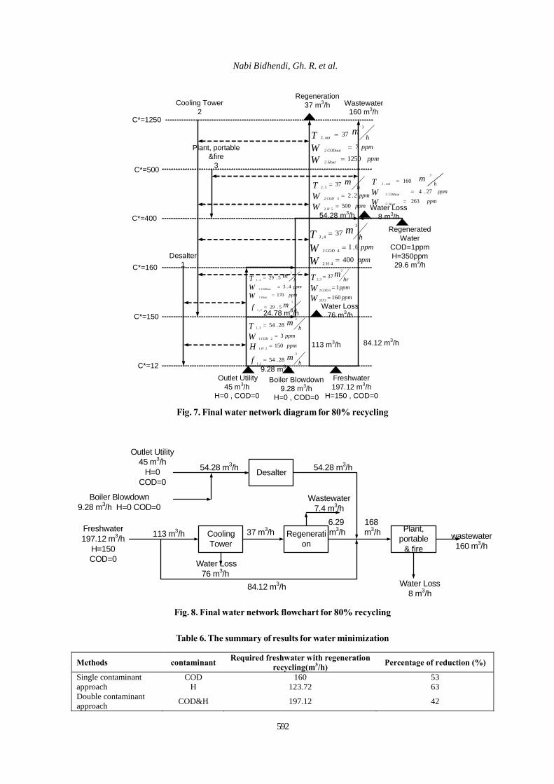
Nabi Bidhendi, Gh. R. et al.
Desalter 1
Cooling Tower 2
Plant, portable&fire
3
Regeneration37 m3/h
Outlet Utility45 m3/h
H=0 , COD=0
Boiler Blowdown9.28 m3/h
H=0 , COD=0
Freshwater197.12 m3/h
H=150 , COD=0
84.12 m3/h113 m3/h
9.28 m3/h
24.78 m3/h
54.28 m3/h
RegeneratedWater
COD=1ppmH=350ppm29.6 m3/h
Water Loss76 m3/h
Water Loss8 m3/h
Wastewater160 m3/h
h
ppm
ppmh
mfHW
mT
H
COD
3
1,1
21
21
3
2,1
28.54
150
3
28.54
=
=
=
=
h
ppm
ppmh
mfWW
mT
Hout
CODout
3
2,1
1
1
3
2,1
5.29
170
4.3
5.29
=
=
=
=
ppm
ppmhr
WW
mT
H
COD
160
1
37
32
32
3
3,2
=
=
=
ppm
ppmh
WW
mT
H
COD
400
6.1
37
42
42
3
4,2
=
=
=
ppm
ppmh
WW
mT
H
COD
500
2.2
37
52
52
3
5,2
=
=
=
ppm
ppmh
WW
mT
Hout
CODout
out
1250
7
37
2
2
3
,2
=
=
=
ppm
ppmh
WW
mT
Hout
CODout
out
263
27.4
160
3
3
3
,3
=
=
=
C*=12
C*=150
C*=160
C*=400
C*=500
C*=1250
Fig. 7. Final water network diagram for 80% recycling
Desalter
Cooling Tower
Regeneration
Plant, portable
& fire
Outlet Utility 45 m3/h
H=0COD=0
Boiler Blowdown9.28 m3/h H=0 COD=0
Freshwater197.12 m3/h
H=150COD=0
84.12 m3/h
54.28 m3/h 54.28 m3/h
113 m3/h 37 m3/h29.6
m3/h
Wastewater7.4 m3/h
168 m3/h
Water Loss8 m3/h
wastewater160 m3/h
Water Loss76 m3/h
Fig. 8. Final water network flowchart for 80% recycling
Table 6. The summary of results for water minimization
Methods contaminant Required freshwater with regeneration recycling(m3/h) Percentage of reduction (%)
COD 160 53 Single contaminant approach H 123.72 63 Double contaminant approach COD&H 197.12 42
592
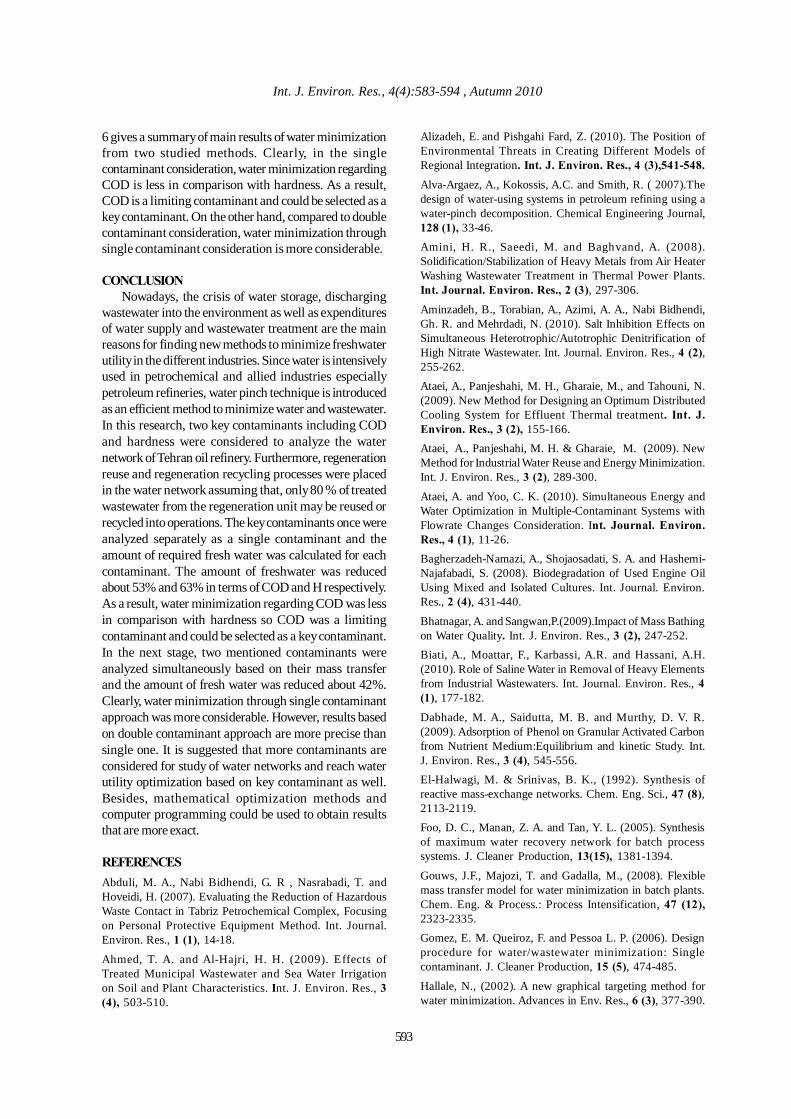
Int. J. Environ. Res., 4(4):583-594 , Autumn 2010
6 gives a summary of main results of water minimizationfrom two studied methods. Clearly, in the singlecontaminant consideration, water minimization regardingCOD is less in comparison with hardness. As a result,COD is a limiting contaminant and could be selected as akey contaminant. On the other hand, compared to doublecontaminant consideration, water minimization throughsingle contaminant consideration is more considerable.
CONCLUSION Nowadays, the crisis of water storage, dischargingwastewater into the environment as well as expendituresof water supply and wastewater treatment are the mainreasons for finding new methods to minimize freshwaterutility in the different industries. Since water is intensivelyused in petrochemical and allied industries especiallypetroleum refineries, water pinch technique is introducedas an efficient method to minimize water and wastewater.In this research, two key contaminants including CODand hardness were considered to analyze the waternetwork of Tehran oil refinery. Furthermore, regenerationreuse and regeneration recycling processes were placedin the water network assuming that, only 80 % of treatedwastewater from the regeneration unit may be reused orrecycled into operations. The key contaminants once wereanalyzed separately as a single contaminant and theamount of required fresh water was calculated for eachcontaminant. The amount of freshwater was reducedabout 53% and 63% in terms of COD and H respectively.As a result, water minimization regarding COD was lessin comparison with hardness so COD was a limitingcontaminant and could be selected as a key contaminant.In the next stage, two mentioned contaminants wereanalyzed simultaneously based on their mass transferand the amount of fresh water was reduced about 42%.Clearly, water minimization through single contaminantapproach was more considerable. However, results basedon double contaminant approach are more precise thansingle one. It is suggested that more contaminants areconsidered for study of water networks and reach waterutility optimization based on key contaminant as well.Besides, mathematical optimization methods andcomputer programming could be used to obtain resultsthat are more exact.
REFERENCESAbduli, M. A., Nabi Bidhendi, G. R , Nasrabadi, T. andHoveidi, H. (2007). Evaluating the Reduction of HazardousWaste Contact in Tabriz Petrochemical Complex, Focusingon Personal Protective Equipment Method. Int. Journal.Environ. Res., 1 (1), 14-18.
Ahmed, T. A. and Al-Hajri, H. H. (2009). Effects ofTreated Municipal Wastewater and Sea Water Irrigationon Soil and Plant Characteristics. Int. J. Environ. Res., 3(4), 503-510.
Alizadeh, E. and Pishgahi Fard, Z. (2010). The Position ofEnvironmental Threats in Creating Different Models ofRegional Integration. Int. J. Environ. Res., 4 (3),541-548.
Alva-Argaez, A., Kokossis, A.C. and Smith, R. ( 2007).Thedesign of water-using systems in petroleum refining using awater-pinch decomposition. Chemical Engineering Journal,128 (1), 33-46.Amini, H. R., Saeedi, M. and Baghvand, A. (2008).Solidification/Stabilization of Heavy Metals from Air HeaterWashing Wastewater Treatment in Thermal Power Plants.Int. Journal. Environ. Res., 2 (3), 297-306.
Aminzadeh, B., Torabian, A., Azimi, A. A., Nabi Bidhendi,Gh. R. and Mehrdadi, N. (2010). Salt Inhibition Effects onSimultaneous Heterotrophic/Autotrophic Denitrification ofHigh Nitrate Wastewater. Int. Journal. Environ. Res., 4 (2),255-262.Ataei, A., Panjeshahi, M. H., Gharaie, M., and Tahouni, N.(2009). New Method for Designing an Optimum DistributedCooling System for Effluent Thermal treatment. Int. J.Environ. Res., 3 (2), 155-166.Ataei, A., Panjeshahi, M. H. & Gharaie, M. (2009). NewMethod for Industrial Water Reuse and Energy Minimization.Int. J. Environ. Res., 3 (2), 289-300.
Ataei, A. and Yoo, C. K. (2010). Simultaneous Energy andWater Optimization in Multiple-Contaminant Systems withFlowrate Changes Consideration. Int. Journal. Environ.Res., 4 (1), 11-26.Bagherzadeh-Namazi, A., Shojaosadati, S. A. and Hashemi-Najafabadi, S. (2008). Biodegradation of Used Engine OilUsing Mixed and Isolated Cultures. Int. Journal. Environ.Res., 2 (4), 431-440.
Bhatnagar, A. and Sangwan,P.(2009).Impact of Mass Bathingon Water Quality. Int. J. Environ. Res., 3 (2), 247-252.Biati, A., Moattar, F., Karbassi, A.R. and Hassani, A.H.(2010). Role of Saline Water in Removal of Heavy Elementsfrom Industrial Wastewaters. Int. Journal. Environ. Res., 4(1), 177-182.
Dabhade, M. A., Saidutta, M. B. and Murthy, D. V. R.(2009). Adsorption of Phenol on Granular Activated Carbonfrom Nutrient Medium:Equilibrium and kinetic Study. Int.J. Environ. Res., 3 (4), 545-556.El-Halwagi, M. & Srinivas, B. K., (1992). Synthesis ofreactive mass-exchange networks. Chem. Eng. Sci., 47 (8),2113-2119.Foo, D. C., Manan, Z. A. and Tan, Y. L. (2005). Synthesisof maximum water recovery network for batch processsystems. J. Cleaner Production, 13(15), 1381-1394.
Gouws, J.F., Majozi, T. and Gadalla, M., (2008). Flexiblemass transfer model for water minimization in batch plants.Chem. Eng. & Process.: Process Intensification, 47 (12),2323-2335.Gomez, E. M. Queiroz, F. and Pessoa L. P. (2006). Designprocedure for water/wastewater minimization: Singlecontaminant. J. Cleaner Production, 15 (5), 474-485.
Hallale, N., (2002). A new graphical targeting method forwater minimization. Advances in Env. Res., 6 (3), 377-390.
593

Water and Wastewater Minimization
Hassani, A. H., Otadi, N., Javid, A. H., Khiabani, F. F. andHoshyaripour, G. (2009). Improving the performance ofPars Oil Refinery Wastewater Treatment System. Int.Journal. Environ. Res., 3 (4), 653-662.
Hassani, A. H., Seif, S., Javid A. H. and Borghei, M. (2008).Comparison of Adsorption Process by GAC with NovelFormulation ofCoagulation – Flocculation for Color Removalof Textile Wastewater. Int. Journal. Environ. Res., 2 (3),239-248.Kabir, G . and Ogbeide, S. E. (2008). Removal of Chromatein Trace Concentration Using Ion Exchange From TanneryWastewater. Int. Journal. Environ. Res., 2 (4), 377-384.
Karbassi, A. R., Abduli, M. A. and Neshastehriz, S.(2008).Energy Saving in Tehran International FlowerExhibition’s Building. Int. J. Environ. Res., 2 (1), 75-86.Khezri, S. M., Lotfi, F., Tabibian, S. and Erfani, Z. (2010).Application of water pinch technology for water andwastewater minimization in aluminum anodizing industries.Int. Journal. Environ. Sci. Tech., 7 (2), 281-290.Kuo, K. and smith, R. (1997). Effluent treatment systemdesign, chem. Eng. Sci., 23, 4273-4290.
Majozi, T. (2005). An effective technique for wastewaterminimization in batch processes. J. Cleaner Production, 13(15), 1374-1380.Mann, G. and Liu, Y. A. (1999). Industrial water reuse andwastewater minimization. McGrew hill.
Manan, Z.A., Wan Alwi, S.R. and Ujang, Z. (2006). Waterpinch analysis for an urban system: a case study on theSultan Ismail Mosque at the University TechnologyMalaysia (UTM). Desalination, 194, 52-68.Mehrdadi, N., Joshi, S. G., Nasrabadi, T. and Hoveidi, H.(2007). Aplication of Solar Energy for Drying of Sludgefrom Pharmaceutical Industrial Waste Water and ProbableReuse. Int. Journal. Environ. Res., 1 (1), 42-48.
Moayed Salehi M. and Mirbagheri, S. A. (2010).Determination of Kinetic Constants and BiologicalTreatment of Automobile Industries Wastewater. Int.Journal. Environ. Res., 4 (1), 131-136.Mohammadnejad, S., Nabi Bidhendi, G. R. and Mehrdadi,N. (2010). A New Algorithm for Water and WastewaterOptimization in Multiple Contaminants Network using WaterPinch Technology. Res. J. Environ. Sci., 4 (3), 193-208.Nabi Bidhendi, Gh. R., Torabian, A., Ehsani, H., Razmkhah,N. and Abbasi, M. (2007). Evaluation of Industrial DyeingWastewater Treatment with Coagulants. Int. Journal.Environ. Res., 1 (3), 242-247.
Najafpour, Sh., Alkarkhi, A. F. M., Kadir, M. O. A. andNajafpour, Gh. D. (2008). Evaluation of Spatial andTemporal Variation in River Water Quality. Int. J. Environ.Res., 2 (4), 349-358.Nakane, K. and Haidary, A. (2010). Sensitivity Analysis ofStream Water Quality and Land Cover Linkage Models UsingMonte Carlo Method. Int. J. Environ. Res., 4 (1), 121-130.
Oliver, P., Rodriguez, R. and Udaquiola, S. (2008). Wateruse optimization in batch process industries. Part 1: designof the water network. J. Cleaner Production, 16 (12), 1275-1286.
Omran, A., Mahmood, A. and Abdul Aziz, H. (2009). NewMethod for Industrial Water Reuse and Energy Minimization.Int. Journal. Environ. Res., 3 (2), 289-300.Praveena, S. M., Abdullah, M. H. and Aris, A. Z. (2010).Modeling for Equitable Groundwater Management. Int. J.Environ. Res., 4 (3), 415-426.
Rajakumar, R. and Meenambal, T. (2008). Comparative Studyon Start - Up Performance of HUASB and AF ReactorsTreating Poultry Slaughterhouse Wastewater. Int. Journal.Environ. Res., 2 (4), 401-410.Rajasimman, M. and Karthikeyan, C. (2009). Optimizationstudies in an Inverse Fluidized Bed Bioreactor for StarchWastewater Treatment. Int. Journal. Environ. Res., 3 (4),569-574.Saeedi, M. and Amini, H. R. (2007). Chemical, Physical,Mineralogical, Morphology and Leaching Characteristics ofa Thermal Power Plant Air Heater Washing Waste. Int.Journal. Environ. Res., 1 (1), 74-79.
Salehi, F., Monavari, S. M., Arjomandi, R., Dabiri, F. andSamadi , R. (2010). A New Approach TowardsEnvironmental Monitoring Plan in Steam Power Plants. Int.J. Environ. Res., 4 (3), 433-438.Sarparastzadeh, H., Saeedi, M., Naeimpoor, F. andAminzadeh, B. (2007). Pretreatment of MunicipalWastewater by Enhanced Chemical Coagulation. Int. Journal.Environ. Res.,1 (2), 104-113.
Vargas-Vargas, M., Meseguer-Santamaría, M. L., Mondéjar- J iménez, J. and Mondéjar Jiménez, J . A. (2010).Environmental Protection Expenditure for Companies: ASpanish Regional Analysis. Int. J. Environ. Res., 4 (3), 373-378.Wang, Y. P. and Smith, R. (1994). Wastewater minimization.Chem. Eng. Sci., 49, 981-1006.
Yoochatchaval, W., Ohashi, A., Harada, H., Yamaguchi, T.and Syutsubo, K. (2008). Intermittent Effluent Recirculationfor the Efficient Treatment ofLow Strength Wastewater byan EGSB Reactor. Int. Journal. Environ. Res., 2 (3), 231-238.
594
Int. J. Environ. Res., 4(4):595-606 , Autumn 2010ISSN: 1735-6865
Received 10 Feb. 2010; Revised 2 June 2010; Accepted 12 June 2010
*Corresponding author E-mail: [email protected]
595
Genotoxic Effects of Electromagnetic Fields from High Voltage Power Lineson Some Plants
Aksoy, H.1*, Unal, F.2 and Ozcan, S.3
1Sakarya University, Science Faculty, Department of Biology, Sakarya, Turkey2Gazi University, Science Faculty, Department of Biology, Ankara, Turkey
3Ankara University, Faculty of Agriculture, Department of Field Crops, Ankara, Turkey
ABSTRACT: Allium cepa bulbs were germinated in pots for three days on treatment area on which 380 kVhigh voltage power lines are passing. Ten bulbs were set up for each treatment area (0 m (meter), 10 m, 25 m,50 m and 100+ m for control from power lines). Triticum baeoticum Boiss. subsp. baeoticum seeds werecollected at same distance from power lines on planted field. Ten seeds from each area were germinated in Petridishes for three days in laboratory. The treatment groups were compared with the control group for mitoticindex and chromosome aberrations. Data obtained showed that electromagnetic fields from high voltage powerlines increased the mitotic index and chromosome aberrations.
Keywords: Electromagnetic Fields, High Voltage Power Lines, Chromosome aberrations
INTRODUCTIONIndustrial development has widely affected the
environment during recent decades (Nabi Bidhendi etal., 2007; Abduli et al., 2007; Mehrdadi et al., 2007;Motesaddi Zarandi et al., 2008; Ahmad et al., 2009;Sadashiva Murthy et al., 2009; Javid and Lak, 2007). Itis a modern fact of life that we are all exposed to EMFs(electromagnetic fields) produced by generation,transmission, and use of electricity. EMFs are producedby power lines, electrical wiring, and electricalequipments. EMFs are invisible lines of force thatsurround any electrical device. As various chemicalseffects living organisms in different ways, various formsof electromagnetic energy can have very differentbiological effects. However, the mechanism leading tochanges in the biosynthesis has been elusive. Low-frequency electric fields do not penetrate cells veryeffectively, but low-frequency magnetic fields dopenetrate (Blank and Goodman, 1997).
The possible effects of EMFs on health, especially,were begun discussed after the Wertheimer and Leeper’s(1979) publication. They reported that an associationwas found between living near high voltage power linesand childhood cancer. Current researches on EMFs aredivided into two general categories; epidemiologicaland laboratory studies. While a majority of theepidemiological studies have focused to reveal that
relation between EMFs exposure and cancer (Floderuset al., 1993; Coogan et al., 1996; Kheifets et al., 1997;Feychting et al., 1997; McElroy et al.,2001; Draper etal., 2005), laboratory studies has focused onchromosomal aberration in human blood cells whichexposed to EMFs (Khalil and Qassem, 1991; Garcia-Sagredo and Monteagudo, 1991; Valjus et al., 1993;Skyberg et al., 1993; Antonopoulos et al., 1995; Erdalet al., 1998; Cho and Chung, 2003). On the other hand,cellular damage (Veiga et al., 2000; Belyavskaya, 2001),plant chromosome aberrations (Rapley et al., 1998) andplant grow up (Kocacaliskan, 1990; Soja et al., 2003;Kobayashi et al., 2004; Fischer et al., 2004) have beeninvestigated in the same condition.
According to some epidemiologic studies, whilethere is a relationship between EMFs and variouscancer types (Floderus et al., 1993; Dockerty et al.,1998; Zhu et al., 2003), according to some other studies,there is no relationship (Zheng et al., 2000; McElroyet al., 2001; Forssen et al., 2005). Even though someresearchers reported that EMFs increased frequencyof chromosomal aberrations in cultured humanlymphocytes (Khalil and Qassem, 1991; Erdal et al.,1998; Erdal et al., 1999), some of them reported thatEMFs did not induce any cytogenetic damage incultured human lymphocytes (Rosenthal and Obe,1989; Garcia-Sagredo et al., 1990; Skyberg et al., 1993;Scarfi et al., 1994).
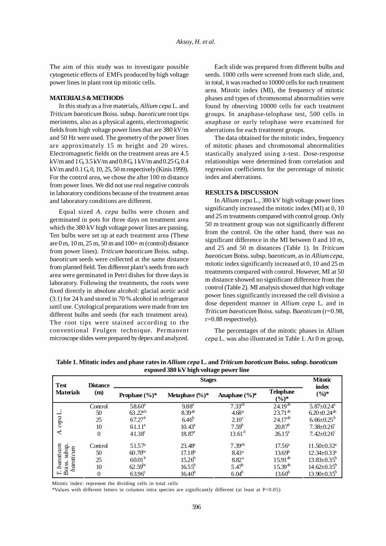
596
Aksoy, H. et al.
The aim of this study was to investigate possiblecytogenetic effects of EMFs produced by high voltagepower lines in plant root tip mitotic cells.
MATERIALS & METHODSIn this study as a live materials, Allium cepa L. and
Triticum baeoticum Boiss. subsp. baeoticum root tipsmeristems, also as a physical agents, electromagneticfields from high voltage power lines that are 380 kV/mand 50 Hz were used. The geometry of the power linesare approximately 15 m height and 20 wires.Electromagnetic fields on the treatment areas are 4.5kV/m and 1 G, 3.5 kV/m and 0.8 G, 1 kV/m and 0.25 G, 0.4kV/m and 0.1 G, 0, 10, 25, 50 m respectively (Kinis 1999).For the control area, we chose the after 100 m distancefrom power lines. We did not use real negative controlsin laboratory conditions because of the treatment areasand laboratory conditions are different.
Equal sized A. cepa bulbs were chosen andgerminated in pots for three days on treatment areawhich the 380 kV high voltage power lines are passing.Ten bulbs were set up at each treatment area (Theseare 0 m, 10 m, 25 m, 50 m and 100+ m (control) distancefrom power lines). Triticum baeoticum Boiss. subsp.baeoticum seeds were collected at the same distancefrom planted field. Ten different plant’s seeds from eacharea were germinated in Petri dishes for three days inlaboratory. Following the treatments, the roots werefixed directly in absolute alcohol: glacial acetic acid(3:1) for 24 h and stored in 70 % alcohol in refrigeratoruntil use. Cytological preparations were made from tendifferent bulbs and seeds (for each treatment area).The root tips were stained according to theconventional Feulgen technique. Permanentmicroscope slides were prepared by depex and analyzed.
Each slide was prepared from different bulbs andseeds. 1000 cells were screened from each slide, and,in total, it was reached to 10000 cells for each treatmentarea. Mitotic index (MI), the frequency of mitoticphases and types of chromosomal abnormalities werefound by observing 10000 cells for each treatmentgroups. In anaphase-telophase test, 500 cells inanaphase or early telophase were examined foraberrations for each treatment groups.
The data obtained for the mitotic index, frequencyof mitotic phases and chromosomal abnormalitiesstastically analyzed using z-test. Dose-responserelationships were determined from correlation andregression coefficients for the percentage of mitoticindex and aberrations.
RESULTS & DISCUSSIONIn Allium cepa L., 380 kV high voltage power lines
significantly increased the mitotic index (MI) at 0, 10and 25 m treatments compared with control group. Only50 m treatment group was not significantly differentfrom the control. On the other hand, there was nosignificant difference in the MI between 0 and 10 m,and 25 and 50 m distances (Table 1). In Triticumbaeoticum Boiss. subsp. baeoticum, as in Allium cepa,mitotic index significantly increased at 0, 10 and 25 mtreatments compared with control. However, MI at 50m distance showed no significant difference from thecontrol (Table 2). MI analysis showed that high voltagepower lines significantly increased the cell division adose dependent manner in Allium cepa L. and inTriticum baeoticum Boiss. subsp. Baeoticum (r=0.98,r=0.88 respectively).
The percentages of the mitotic phases in Alliumcepa L. was also illustrated in Table 1. At 0 m group,
Table 1. Mitotic index and phase rates in Allium cepa L. and Triticum baeoticum Boiss. subsp. baeoticumexposed 380 kV high voltage power line
Stages Test Materials
Distance (m) Prophase (%)* Metaphase (%)* Anaphase (%)* Telophase
(%)*
Mitotic index (%)*
Control 58.60a 9.88a 7.33ab 24.19ab 5.87±0.24a 50 63.22ab 8.39ab 4.68a 23.71ab 6.20±0.24ab 25 67.27b 6.46b 2.10c 24.17ab 6.66±0.25b 10 61.11a 10.43a 7.59b 20.87b 7.38±0.26c
A. c
epa
L.
0 41.38c 18.87c 13.61d 26.15a 7.42±0.26c
Control 51.57a 23.48a 7.39ab 17.56a 11.50±0.32a 50 60.70bc 17.18b 8.43a 13.69b 12.34±0.33a 25 60.01b 15.26b 8.82a 15.91ab 13.83±0.35b 10 62.59bc 16.55b 5.47b 15.39ab 14.62±0.35b
T. b
aeot
icum
B
oiss
. sub
sp.
baeo
ticum
0 63.96c 16.40b 6.04b 13.60b 13.90±0.35b Mitotic index: represent the dividing cells in total cells*Values with different letters in columns intra species are significantly different (at least at P<0.05)

Int. J. Environ. Res., 4(4):595-606 , Autumn 2010
597
Table 2. Types and rates of abnormalities in Allium cepa L. and Triticum baeoticum Boiss. subsp. baeoticumexposed 380 kV high voltage power lines
Abnormalities (%) Test Materials
Distance (m)
Dividing cells
Mn St F Cm Im M B Lc
AC / DC (%)*
AC / TC (%)*
Control 587 - - - - - 0.17 0.34 0.17 0.68±0.34a 0.04±0.02a 50 620 0.01 - - 0.16 - - 0.32 0.16 0.64±0.32a 0.05±0.02a 25 666 0.02 - - 0.30 - - - 0.30 0.60±0.30a 0.06±0.02a 10 738 0.02 - 0.41 - - 0.14 0.41 0.27 1.23±0.41a 0.11±0.03a
A. c
epa
L.
0 742 0.08 0.94 0.54 0.67 0.27 0.94 1.08 1.08 5.52±0.84b 0.48±0.07b
Control 1150 - 0.09 - - - - - - 0.09±0.09a 0.01±0.01a 50 1234 0.01 - 0.16 - - - - - 0.16±0.11a 0.03±0.02a 25 1383 0.01 - 0.07 0.07 - - 0.07 0.15 0.36±0.16ab 0.06±0.02a 10 1462 0.07 - 0.21 - - 0.21 0.27 0.21 0.90±0.25b 0.19±0.04b
T. b
aeot
icum
B
oiss
. sub
sp.
baeo
ticum
0 1390 0.01 0.29 0.86 0.22 0.07 0.14 0.14 0.22 1.94±0.37c 0.28±0.05b Mn: Micronuclei, St: Stickiness, F: Fragment, Cm: C-mitosis, Im: Irregular metaphase, M: Multipolarity,B: Bridge, Lc: Lagging chromosome, AC: Abnormal cells, DC: Dividing cells, TC: Total cells*Values with different letters in columns intra species are significantly different (at least at P<0.05)
high voltage power lines significantly decreased thepercentage of prophase and increased the percentageof metaphase and telophase stage when compared tothe control group. Decrease at prophase and increaseat metaphase and anaphase was also significantlydifferent from the other treatment groups. At 10 mtreatments, cells at anaphase stages were increasedand at telophase stages were decreased as comparedto the control. On the other hand, at 25 m treatmentgroups, there were a significantly increase in thepercentage at prophase and a significantly decrease inthe percentage of metaphase and anaphase. Thepercentage of cells at different stages, at the 50 mtreatments, was not different from the control.
The percentages of the mitotic phases of Triticumbaeoticum Boiss. subsp. baeoticum was illustrated inTable 2. The results showed a significant increase inall treatment groups from the control for prophasestages and a significant decrease for metaphase stages.At anaphase, while 0 and 10 m treatments showed asignificant decrease from the control, 25 and 50 mtreatments did not. At telophase stage, 0 and 50 mtreatments showed a significant decrease but 10 and25 m. High voltage power lines at 380 kV were inducedsome abnormalities in mitotic cells in both Allium cepaL. and Triticum baeoticum Boiss. subsp. baeoticum(Table 3 and 4).The abnormalities observed at mitoticstage were bridges, multipolarity, fragment, laggingchromosome, c-mitosis, stickiness, irregular metaphaseand micronuclei at interphase (Fig. 1 & 2).
In Allium cepa, lagging chromosome was presentin all treatment groups as well as control. Bridge wasobserved in all treatment groups and control but 25 m.Again, multipolarity was detected at 0 and 10 mtreatment and in control roots. C-mitosis was observedat 0, 25 and 50 m treatment groups. Fragment was
detected in 0 and 10 m treatment groups. Stickinessand irregular metaphase were present at only 0 mtreatment root tips. At interphase, all treatment groupshad micronuclei. Abnormal cells/dividing cells andabnormal cells/total cells ratios in Allium cepa weresignificantly different from the control at only 0 mtreatment group. This ratio was not significantlydifferent from the control in all the other treatments(Table 3). On the other hand, the increases are dosedependent manner in abnormal cells/dividing cells andabnormal cells/total cells ratios (r=0.76, r=0.79respectively).
In Triticum baeoticum Boiss. subsp. baeoticum,fragment was observed in all treatment groups. Laggingchromosome and bridge were detected in all treatmentgroups except 50 m. Multipolarity was present at 0 and10 m treatment groups. While irregular metaphase wasobserved at only 0 m treatment group, c-mitosis wasobserved at 0 and 25 m treatment groups. On the otherhand, stickiness was present at 0 m treatment group aswell as control. All treatment groups had micronucleiat interphase. Abnormal cells/dividing cells ratio inTriticum baeoticum Boiss. subsp. baeoticum, wassignificantly different from the control at 0 and 10 mtreatment groups. Similarly, abnormal cells/total cellsratio was also significantly different from the controlat 0 and 10 m treatments (Table 4). In abnormal cells/dividing cells and abnormal cells/total cells ratios theincreases are dose dependent manner (r=0.92, r=0.95respectively).
In anaphase-telophase test, the most commonabnormal i t ies were br idges. Fragmen t wasobserved in all treatment groups and control in bothspecies. Lagging chromosome was detected in alltreatment groups but control. Multipolarity was
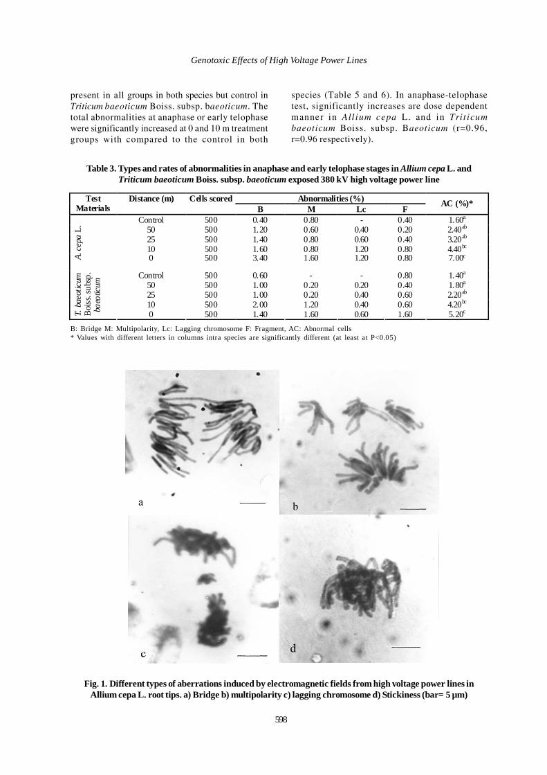
598
Genotoxic Effects of High Voltage Power Lines
Table 3. Types and rates of abnormalities in anaphase and early telophase stages in Allium cepa L. andTriticum baeoticum Boiss. subsp. baeoticum exposed 380 kV high voltage power line
Abnormalities (%) Test Materials
Distance (m) Cells scoredB M Lc F
AC (%)*
Control 500 0.40 0.80 - 0.40 1.60a 50 500 1.20 0.60 0.40 0.20 2.40ab 25 500 1.40 0.80 0.60 0.40 3.20ab 10 500 1.60 0.80 1.20 0.80 4.40bc
A. c
epa
L.
0 500 3.40 1.60 1.20 0.80 7.00c
Control 500 0.60 - - 0.80 1.40a 50 500 1.00 0.20 0.20 0.40 1.80a 25 500 1.00 0.20 0.40 0.60 2.20ab 10 500 2.00 1.20 0.40 0.60 4.20bc
T. b
aeot
icum
B
oiss
. sub
sp.
baeo
ticum
0 500 1.40 1.60 0.60 1.60 5.20c B: Bridge M: Multipolarity, Lc: Lagging chromosome F: Fragment, AC: Abnormal cells* Values with different letters in columns intra species are significantly different (at least at P<0.05)
Fig. 1. Different types of aberrations induced by electromagnetic fields from high voltage power lines inAllium cepa L. root tips. a) Bridge b) multipolarity c) lagging chromosome d) Stickiness (bar= 5 µm)
present in all groups in both species but control inTriticum baeoticum Boiss. subsp. baeoticum. Thetotal abnormalities at anaphase or early telophasewere significantly increased at 0 and 10 m treatmentgroups with compared to the control in both
species (Table 5 and 6). In anaphase-telophasetest, significantly increases are dose dependentmanner in All ium cepa L. and in Tri t icumbaeoticum Boiss. subsp. Baeoticum (r=0.96,r=0.96 respectively).
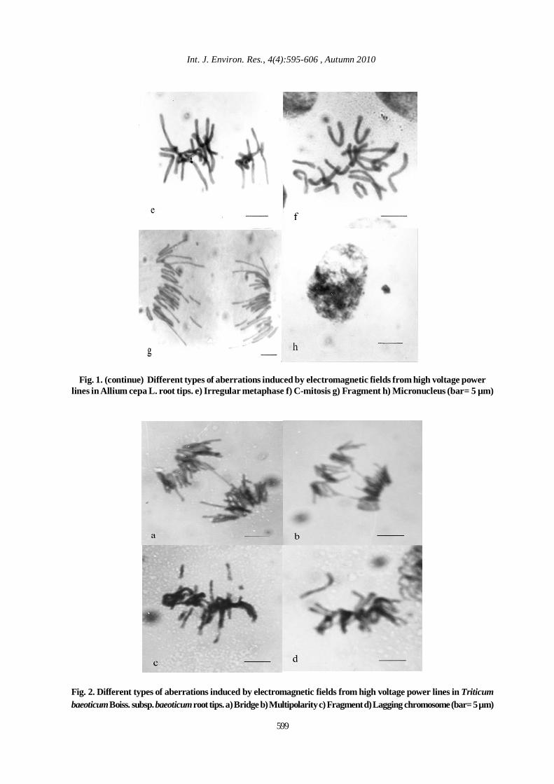
Int. J. Environ. Res., 4(4):595-606 , Autumn 2010
Fig. 1. (continue) Different types of aberrations induced by electromagnetic fields from high voltage powerlines in Allium cepa L. root tips. e) Irregular metaphase f) C-mitosis g) Fragment h) Micronucleus (bar= 5 µm)
Fig. 2. Different types of aberrations induced by electromagnetic fields from high voltage power lines in Triticumbaeoticum Boiss. subsp. baeoticum root tips. a) Bridge b) Multipolarity c) Fragment d) Lagging chromosome (bar= 5 µm)
599
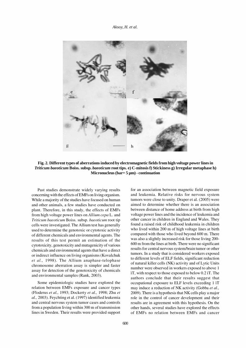
600
Aksoy, H. et al.
Fig. 2. Different types of aberrations induced by electromagnetic fields from high voltage power lines inTriticum baeoticum Boiss. subsp. baeoticum root tips. e) C-mitosis f) Stickiness g) Irregular metaphase h)
Micronucleus (bar= 5 µm) - continuation
Past studies demonstrate widely varying resultsconcerning with the effects of EMFs on living organism.While a majority of the studies have focused on humanand other animals, a few studies have conducted onplant. Therefore, in this study, the effects of EMFsfrom high voltage power lines on Allium cepa L. andTriticum baeoticum Boiss. subsp. baeoticum root tipcells were investigated. The Allium test has generallyused to determine the genotoxic or cytotoxic activityof different chemicals and environmental agents. Theresults of this test permit an estimation of thecytotoxicity, genotoxicity and mutagenicity of variouschemicals and environmental agents that have a director indirect influence on living organisms (Kovalchuket al., 1998). The Allium anaphase-telophasechromosome aberration assay is simpler and fasterassay for detection of the genotoxicity of chemicalsand environmental samples (Rank, 2003).
Some epidemiologic studies have explored therelation between EMFs exposure and cancer types(Floderus et al., 1993; Dockerty et al., 1998; Zhu etal., 2003). Feychting et al. (1997) identified leukemiaand central nervous system tumor cases and controlsfrom a population living within 300 m of transmissionlines in Sweden. Their results were provided support
for an association between magnetic field exposureand leukemia. Relative risks for nervous systemtumors were close to unity. Draper et al. (2005) wereaimed to determine whether there is an associationbetween distance of home address at birth from highvoltage power lines and the incidence of leukemia andother cancer in children in England and Wales. Theyfound a raised risk of childhood leukemia in childrenwho lived within 200 m of high voltage lines at birthcompared with those who lived beyond 600 m. Therewas also a slightly increased risk for those living 200-600 m from the lines at birth. There were no significantresults for central nervous system/brain tumor or othertumors. In a study that is considered workers exposedto different levels of ELF fields, significant reductionof natural killer cells (NK) activity and of Lytic Unitsnumber were observed in workers exposed to above 1ìT, with respect to those exposed to below 0.2 ìT. Theauthors conclude that their results suggest thatoccupational exposure to ELF levels exceeding 1 ìTmay induce a reduction of NK activity (Gobba et al.,2009). There is a hypothesis that NK cells play a majorrole in the control of cancer development and theirresults are in agreement with this hypothesis. On theother hands, several studies have explored the effectsof EMFs no relation between EMFs and cancer
601
Int. J. Environ. Res., 4(4):595-606 , Autumn 2010
(Theriault et al., 1994; Laden et al., 2000; Zheng etal., 2000; McElroy et al., 2001; Minder and Pfluger,2001). Tynes et al. (1994) were investigated the braintumor and leukemia in railway workers that exposureto EMFs on Norwegian railways. Their results were nosupport an association between exposure to electricand magnetic fields and the risk for leukemia or braintumors. Forssen et al. (2005) were found no evidencefor an increased risk of breast cancer among womenworking in occupations with high magnetic fieldexposure.EMFs do not act directly on the cell components (Blankand Goodman, 1997). The effects of EMFs on chemicalreaction have caused to occurring the free radicals(Adey, 1993; Tuncel et al., 1999). Although the energyassociated with environmental EMFs is too low to causedirect changes to the structure of DNA, EMFs mightaffect the production of agents such as free radicals,which themselves can react with DNA, or of otheragents that cause chromosomal damage, instigatingtranslocation by inducing DNA breaks or by formationof unnatural DNA structures. Interfering with themechanisms of DNA repair or chromosomal replicationand segregation can also cause DNA damage orincrease the probability that a particular DNA sequencewill be lost from the genome (Lacy-Hulbert et al., 1998).Another effective mechanism of EMFs is on ion flux inthe cell membrane. The transmembrane ion flux isregulated by voltage-dependent changes in theconformation of channel proteins, and that perturb ionflux will cause profound changes in the metabolismand fate of effected cells. When the organism exposureto EMFs, EMFs can perturb the transmembranemovement of cations such as K+, Na+ or Ca+2 throughtheir respective channels, thus producing biologicaleffects (Balcavage et al., 1996; Stange et. al., 2002).Paksu et al. (1999) investigated the effects of EMFs onthe erythrocyte membrane proteins of people workingin and living near high voltage power lines. Theypointed that there was significant difference betweenassay and control groups about proteins amount.
The rats in different groups were exposed to MF (B=5mT) for 165 min every day for 30 days. Their resultswere revealed the exposure to modulation MFdecreased the glucose levels in streptozotocin-induceddiabetic rats. The authors were determined that thehypoglycemic effect of modulation MF was similar tothat of insulin treatment. Also, the hypoglycemic effectof combined insulin treatment and exposure ofmodulation MF on the glucose levels was the lowest.The authors suggested that the hypoglycemic effectof MF on the function of â cells may be able to helpincrease insulin concentration and sensitivity toglucose metabolism. At the same time, in a
streptozotocin-induced diabetic rat model, MF wasincreased the blood-brain barrier permeability(Gulturk et al., 2010). In another research, it wasconcluded that 50 Gauss EMF was raised the numberof follicoles but the number of corpora lutei in rats(Solaeymanirad et al., 2003).
During the cell cycle, the order of events ismaintained by controls termed checkpoints. Twocheckpoints are sensitive to DNA damage, one actbefore mitosis and a second acts before DNAreplication. The checkpoint mutants show geneticinstability, and such instability is characteristic ofmany cancers. Studies of checkpoints in normal andcancer cells suggest a mechanistic relationship to thecentral cell cycle control p34CDC2 and its regulators.The researchers suggested that mutations in thesegenes and those with a role in DNA metabolism mayaffect the function at G
1-S checkpoint (Weinert and
Lydall, 1993). Regard the literatures and present study,it says that the EMFs may effect the proteins which isactivate the cell division and checkpoints in cell cyclebecause of increase not only chromosome aberrations,but also mitotic index in plant cells that exposed byEMFs.
The present study shows that a clear effects ofEMFs from high voltage power lines on cell divisionand chromosomes. The mitotic index has risen in bothplants as the distance gets decreased toward the powerlines. These results are in agreement with previousreport (Cossarizza et al., 1989; Scarfi et al., 1994). Tkalecet al. (2009) investigated that the effects of exposureto radiofrequency electromagnetic fields (RF-EMFs)on seed germination, primary root growth as well asmitotic activity and mitotic aberrations in rootmeristematic cells were examined in Allium cepa L.They reported that, exposures to EMFs of higher fieldstrengths (41 and 120 V/m) showed a significantincrease of the mitotic index compared with controls.Racuciu (2009), conclude that the low intensity 900MHz electromagnetic radiation was increased themitotic index for increasing exposure theelectromagnetic field and the mitotic index is higherfor all samples under the radiofrequency field compareto the control in Zea mays root tip. Also, it was provideda low percentage of chromosomal aberrations and thechromosomal aberrations are micronucleus,interchromatin bridges, retard chromosomes andchromosome fragments, combinations of retardchromosomes or chromosome fragments with inter-chromatin bridges. Ichim et al. (2007), were focusedon cell proliferation in meristematic tissues ofEchinacea purpurea’s young vegetal organism (in itsvery early ontogenetic stages) to exposure that thecontrolled electrostatic stress (10–17 V; (5, 10, 15, 20,
602
Genotoxic Effects of High Voltage Power Lines
30, 40 pulses; 5s) and their results were revealed thatthe mitotic index was increased statisticallysignificant for 20, 30, 40 pulses. In their research,higher changes were found in the metaphase andtelophase percentages and the highest increase ofmetaphase cell number was recorded for 15 pulseswhile the lowest number of telophase cells were alsofound for 15 pulses. Vicia faba beans were germinatedand grown in vermiculite granules in a controlledenvironment laboratory and seedlings were subjectedto different magnetic fields. In particular, all treatmentsincreased the length of prophase significantly inmeristematic root tip cells compared with the controls(Rapley et al., 1998). Our results indicate that theduration of prophase is increased in the root meristemof all the experimental groups when compared withthe control in both plants but 0 m treatment in Alliumcepa. According to Rapley et al. (1998), duringprophase, it may be possible that the EMFs play a rolein the unwinding process, causing some slowing downof winding mechanism and resulting in a longerprophase. The durations of other stages also indicatevariability in the effects of the EMFs. Researchers whoobserving the same results suggested that these arevery difficult to interpret because of the apparenthaphazard nature of the magnetic field effects andbiological explanations for these differences remainelusive. At metaphase and anaphase, especially at 0m treatment group, the phase ratio was increased a lotin Allium cepa. In Triticum baeoticum Boiss. subsp.Baeoticum, on the other hands, there was significantlydecreased in all treatment groups compared withcontrol at metaphase but anaphase. In this study,different results are shown both in stages and in twodifferent plants. These differences might be resultedfrom the genetic composition, growing conditions andexposure period of these two species. At the same time,observing the differentiations in phase frequencieshave been shown as an evidence of electromagneticfields that effective on not only interphase stage butalso during whole cell cycle.
EMFs induced abnormalities in mitotic cells inboth plant species investigated in this study. Theseare bridges, multipolarity, fragments, laggingchromosomes, c-mitosis, stickiness, irregularmetaphase and micronuclei. Pavela and Creanga (2005),were studied the influence of a petroleum magneticfluid upon the cell proliferation in young plants ofagricultural interest and Zea mays plants, in their earlyontogenetic stages were treated with magnetic fluid(10, 60 and 100 µL/L - ferrophase weight was of theorder of magnitude of µg/L of culture medium) androot meristem was investigated by cytogeneticalmethods. In this study, they were found that the cellproliferation rate was significantly enhanced as well
as the percentage of chromosomal aberrations and theyexplained that the petroleum magnetic fluid was ableto stimulate the plant proliferation (up to 30%) and toinduce various types of chromosomal aberrations:micronuclei, bridges, chromosome fragments. Hanafyet al., (2006) were used the two exposure systems of anextremely low frequency electric field, the first was anexperimental model (50 Hz, 6 kV/m strength) and thesecond was the high voltage transmission lines passingthrough an open agricultural field (50 Hz, 66 kV/11 m =6 kV/m). They were used for the controls that after 100m distance in both systems. Their results indicatedthat the electric field of both systems showed a highfrequency of chromosomal abnormalities. Each of thetwo systems induced a wide range of chromosomalabnormalities covering all mitotic stages. Among themitotic irregularities induced by the applied electricfield were stickiness, disturbed phases, laggards,bridges, fragment and micronuclei in interphase cells.The results also indicated that the molecular structureof the extracted water soluble protein changed theamount of protein in the bands of exposed grainsdecreased and their molecular weights changed. Afterthese results, they suggested that the potentiality ofthe applied electric field to induce mitotic irregularities.Tkalec et al. (2009) pointed that higher numbers ofmitotic abnormalities were found after exposure tomodulated EMF as well as after exposure to EMFs ofhigher strengths (41 and 120 V/m) at 400 MHz, whilethe percentage of mitotic abnormalities increased afterall exposure treatments at 900 MHz compared with thecontrol in Allium cepa. Major abnormalities found afterexposure at both frequencies were laggingchromosomes, vagrants, disturbed anaphases andchromosome stickiness. They suggested that mitoticeffects of RF-EMF could be due to impairment of themitotic spindle. Malfunction of the spindle mechanismcould be connected with the effect of RFR on calcium-ion homeostasis in cells (Penafiel et al., 1997). The totalpercentage of aberrant cells was not considerablychanged by the electrostatic exposure except for thetwo highest pulse numbers. The main types ofchromosomal aberrations were retard and expulsedchromosomes, micronuclei and chromosome bridges.It was also been observed such as retard chromosomescombined with bridges. After these results, authorspointed that the young vegetal organisms are quitesensitive to external stress factors and therefore E.purpurea plantlets during their early ontogeneticstages can be influenced by electrostatic stress (up to40 consecutive applied pulses) 15 kV amplitude, 4 msduration, negative polarity, as the cytogenetic testswere revealed (Ichim et al., 2007). Ghotbi Kohan andMorgan (2007), the result of their research, haverevealed the direct relation between increase of
Int. J. Environ. Res., 4(4):595-606 , Autumn 2010
pollution and the level of stress protein. Theyexplained that stress proteins have high sensitivity tochanges in the environment. Today, we know thatelectromagnetic field is also an environmentalpollution. Maybe electromagnetic fields can increasethe stress protein too and it can affect the livingorganism.
Haider et al. (1994) were used the Tradescantiamicronucleus bioassay in an in situ experiment to findout whether short wave electromagnetic fields usedfor broadcasting and they were observed that theresults at all exposure sites except one were statisticallysignificant. Fatigoni et al. (2005) were investigated thepossible genotoxicity of ELF-MF by Tradescantiamicronucleus assay and their results indicated that a50 Hz MF of 1 mT field strength is genotoxic. Feulgenstained chromosome spreads of colchicine treated roottips from control and experimental plants were examinedin detail for structural aberrations, such as chromosomeor chromatid breakage, anaphase bridges, or abnormalconfigurations. But, researchers were observed onlychromosome and chromatid breakages and the resultsshowed that no significant relationship between thefrequency of chromosome and chromatid breakscompared with the control (Rapley et al., 1998). Thereason of the no significant relation that compared thecontrol of investigation results of researchers, it mightbe only study at metaphase for structural aberrations.
Some researchers explained that an association wasfound between cancer risks and increasing thechromosomal aberrations and micronucleus frequency(Bonassi, 2006; El-Zein et al., 2006). In this case, itmust take into consideration the high voltage powerlines that are important source that of EMFs causedthe chromosomal aberrations.
Previous in vitro studies have indicated thatunrepaired DNA lession exist in mutagen-treated cellsuntil the cells enter mitosis. The repair of these lesionscan be effectively inhibited in G
2 stage (Palitti et al.,
1984). Kihlman and Andersson (1986) have suggestedthat chromosome aberration as such cause delay orblock in the G
2 stage. Robison et al. (2002) were found
that the rate of DNA repair for EMFs exposed HL-60and HL-60R cultures were significantly decreased whencompared to non-exposed cultures.
The reason of the some aberration such asmultipolarity, lagging chromosome and fragment whichare resulting micronuclei and then chromosome losing,and c-mitosis might be the damage to mitotic spindleswhich is caused by radicals. Because, mitotic spindleshave important roles the chromosomes which aremovement toward the poles during cell division. Ahmadand Yasmin (1992) reported that micronuclei may
originate from lagging chromosomes and fragmentsoccurred in mitotic stage. The physical adhesion ofchromatin proteins may be cause the stickiness (Patiland Bhat, 1992). Fragments usually producemicronuclei and then genetic material is lost.Chromosomal stickiness and sister chromatid unionare result in bridges.
CONCLUSIONDespite many epidemiological investigations, the
association between high voltage power lines andsome form of cancer or other some diseases is not clear,yet. However, from present and previous studies, itseems that EMFs may be capable of producingchromosome aberration and effecting mitotic index.We think that the main reason of increased number ofchromosome aberrations and mitotic index are due todamaging in various proteins and DNA in interphasestage which is caused by free radicals and defect inthe processing of the signals occurring because ofEMFs from high voltage. In conclusion, in theliterature and this study, it seems that EMFs may beeffect the living organism and long exposure timemust be avoided. More investigation is required toeffectively understand the mechanisms associated withEMFs.
ACKNOWLEDGEMENTThe authors thank to Gazi University for financial
support under grant no. 05/2003-71.
REFERENCESAbduli, M. A., Nabi Bidhendi, G. R , Nasrabadi, T. andHoveidi, H. (2007). Evaluating the Reduction of HazardousWaste Contact in Tabriz Petrochemical Complex, Focusingon Personal Protective Equipment Method. Int. J. Environ.Res., 1(1), 14-18.
Adey, W. R. (1993). Biological effects of electromagneticfield. J. of Cell Biochem. 51,410-416.
Ahmad, S. and Yasmin, R. (1992). Effects of methyl parationand tri-miltox on the mitosis of Allium cepa. Cytologia, 57,155-160.
Ahmad, A., Othman, M. R. and Latif, M. T. (2009). Earlystudy of Surfactants in Indoor Dust and Their ConnectionWith Street Dust. Int. J. Environ. Res., 3(3), 403-410.
Antonopoulos, A., Yang, B., Stamm, A., Heller, W.D. andObe, G. (1995). Cytological effects of 50 Hz electromagneticfields on human lymphocytes in vitro. Mutat. Res., 346,151-157.
Balcavage, W. X., Alvager, T., Swez, J., Goff, C. W., Fox,M. T., Abdullyava, S. and King, M. W. (1996). A mechanismfor action of extremely low frequency electromagnetic fieldson biological systems. Biochem. and Biophys. Res. Com.,222, 374-378.
603

Aksoy, H. et al.
Belyavskaya, N. A. (2001). Ultrastructure and calciumbalance in meristem cells of pea roots exposed to extremelylow magnetic fields. Adv. Space Res., 28 (4), 645-650.
Blank, M. and Goodman, R. (1997). Do electromagneticfields interact directly with DNA?. Bioelectromagnetics, 18,111-115.
Bonassi, S. (2006, July). Predictivity of micronuclei in cancerrisk and chromosomal aberrations for quantitative analysisfor cancer risk. Paper resented at the O-046th. In: FromGenes to Molecular Epidemiology. 36th Annual Meeting ofthe EEMS, Prague
Cho, Y. H. and Chung, H. W. (2003). The effects of extremelylow frequency electromagnetic fields (ELF-EMF) on thefrequency of micronuclei and sister chromatid exchange inhuman lymphocytes induced by benzo(a)pyrene. Toxicol.Let., 143, 37-44.
Coogan, P. F., Clapp, R. W., Newcomb, P. A., Wenzl, T. B.,Bogdan, G., Mittendorf, R., Baron J. A. and Longnecker, M.P. (1996). Occupational exposure to 60-hertz magnetic fieldsand risk of breast cancer in women. Epidemiology, 7, 459-464.
Cossarizza, A., Monti, D., Bersani, F., Cantini, M., Cadossi,R., Sacchi, A. and Franceschi, C. (1989). Extremely lowfrequency pulsed electromagnetic fields increase cellproliferation in lymphocytes from young and aged subjects.Biochem. Biophys. Res. Commun., 160 (2), 692-698.
Dockerty, J. D., Elwood, J. M., Skegg, D. C. G. and Herbison,G. P. (1998). Electromagnetic field exposures and childhoodcancers in New Zealand. Cancer Cause Control, 9, 299-309.
Draper, G., Vincent, T., Kroll, M. E. and Swanson, J. (2005).Childhood cancer in relation to distance from high voltagepower lines in England and Wales: a case-control study.BMJ., 330, 1290-1295.
El-Zein, R., Schabath, M.B., Etzel, C. J., Lopez, M. S.,Franklin, J. and Spitz, M. R. (2006, July). The cytokinesis-blocked micronucleus assay as a novel biomarker for lungcancer risk. Paper resented at the O-050th. In: From Genesto Molecular Epidemiology. 36th Annual Meeting of theEEMS, Prague.
Erdal, M. E., Erdal, N. and Oguzkan, S. (1999).Chromosomal aberrations in peripheral lymphocytes of ahigh-voltage power lineman exposed to electromagneticfields. Tr. J. of Medical Sciences, 29, 335-336.
Erdal, M. E., Erdal, N., Oguzkan, S. and Paksu, C. (1998).Elektrik alanýnýn insan kromozomlarýna in vitro etkisi.C.U. Tip Fak. Dergisi, 23 (13), 141-144.
Fatigoni, C., Dominici, L., Moretti, M., Villarini, M. andMonarca, S. (2005). Genotoxic effects of extremely low frequency(ELF) magnetic fields (MF) evaluated by the Tradescantia-micronucleus assay. Environ. Toxicol., 20, 585-591.
Feychting, M., Forssen, U. and Floderus, B. (1997).Occupational and residential magnetic field exposure andleukemia and central nervous system tumors. Epidemiology,8(4), 384-389.
Fischer, G., Tausz, M., Köck, M. and Grill, D. (2004).Effects of weak 16*2/3 Hz magnetic fields on growthparameters of young sunflower and wheat seedlings.Bioelectromagnetics, 25, 638–641.
Floderus, B., Persson, T., Stenlund, C., Linder, G.,Johansson, C., Kiriranta, J., Parsman, H., Lindblöm, M.,Wennberg, A., Öst, A. and Knave, B. (1993). Occupationalexposure to electromagnetic fields in relation to leukemiaand brain tumor: a case-control study in Sweden. CancerCause Control, 4, 465-476.
Forssen, U.M., Rutqvist, L.E., Ahlbom, A. and Feychting,M. (2005). Occupational magnetic fields and female breastcancer: A case control study using Swedish registers andnew exposure data. Am. J. of Epidemiol., 161(3), 250-259.
Garcia-Sagredo, J. M. and Monteagudo, J. L. (1991). Effectof low-level pulsed electromagnetic fields on humanchromosomes in vitro: analysis of chromosomal aberrations.Hereditas, 115, 9-11.
Garcia-Sagredo, J. M., Parada, L. A. and Monteagudo, J. L.(1990). Effect on SCE in human chromosome in vitro oflow-level pulsed magnetic field. Environ. and Mol. Mutagen.,16, 185-188.
Ghotbi Kohan, K. and Morgan, W. A. (2007). Stress proteinsas a suitable biomarker of environmental pollution. Int. J.Environ. Res., 1 (4), 290-29.
Gobba, F., Bargellini, A., Scaringi, M., Bravo, G. and Borella,P. (2009). Extremely low frequency-magnetic fields (ELF-EMF) occupational exposure and natural killer activity inperipheral blood lymphocytes. Sci. Total Environ., 407,1218-1223.
Gulturk, S., Demirkazik, A., Kosar, I., Cetin, A., Dokmetas,H. S. and Demir, T. (2010). Effect of exposure to 50 Hzmagnetic field with or without insulin on blood-brain barrierpermeability in streptozotocin-induced diabetic rats.Bioelectromagnetics, 31, 262-269.
Haider, T., Knasmueller, S., Kundi, M. and Haider, M.(1994). clastogenic effects of radiofrequency radiations onchromosomes of Tradescantia. Mutat. Res., 324 (1-2), 65-68.
Hanafy, M. S., Mohamed, H. A. and Abd El-Hady, E. A.(2006). Effect of low frequency electric field on growthcharacteristics and protein molecular structure of wheatplant. Romanian j. Biophys., 16 (4), 253-271.
Ichim, D., Creanga D. and Rapa, A. (2007). The influence ofthe electrostatic stress on cell proliferation in plants. J. ofElectrostatics, 65, 408-413.
Javid, A. H and Lak, P. (2007). Dynamic Optimization ofAir Treatment Systems for Fundries. Int. J. Environ. Res.,1(4), 347-353.
Khalil, A. M. and Qassem, W. (1991). Cytogenetic effectsof pulsing electromagnetic field on human lymphocytes invitro: Chromosome aberrations, sister-chromatide exchangesand cell cinetics. Mutat. Res., 247, 141-146.
604
Int. J. Environ. Res., 4(4):595-606 , Autumn 2010
Kheifets, L. I., Kavet, R. and Sussman, S. S. (1997). Wirecodes, magnetic fields, and childhood cancer.Bioelectromagnetics, 18, 99-110.
Kihlman, B. A. and Andersson, H. C. (1986). Effects ofinhibitor of DNA repair on the frequencies of chromosomalaberrations induced by x-rays or alkylating agents in culturehuman lymphocytes. Prog. Clin. Biol. Res., 209, 395-402.
Kinis, A. (1999, November). Yüksek gerilimli enerji iletimhatlari ve trafo istasyonlari. (Paper resented at the pp 145-149. Bilisim Toplumuna Giderken Elektromanyetik KirlilikEtkileri Sempozyumu, Ankara)
Kobayashi, M., Soda, N., Miyo, T. and Ueda, Y. (2004).Effects of combined DC and AC magnetic fields ongermination of Hornwort seeds. Bioelectromagnetics, 25,552–559.
Kocacaliskan, I. (1990). Effectiveness of electrical currentsin breaking potato tuber dormancy compared with othermethods. J. of Horticultural Science, 65 (6), 683-687.
Kovalchuk, O., Kovalchuk, I., Arkhipov, A., Telyuk, P.,Hohn, B. and Kovalchuk, L. (1998). The Allium cepachromosome aberration test reliably measures genotoxicityof soils of inhabited areas in the Ukraine contaminated bythe Chernobyl accident. Mutat. Res., 415, 47-57.
Lacy-Hulbert, A., Metcalfe, J. C. and Hesketh, R. (1998).Biological responses to electromagnetic fields. The FASEBJournal, 12, 395-420.
Laden, F., Neas, L. M., Tolbert, P. E., Holmes, M. D.,Hankinson, S. E., Spiegelman, D., Speizer, F. E. and Hunter,D. J. (2000). Electric blanket use and breast cancer in nurses’health study. Am. J. of Epidemiol., 152 (1), 41-49.
McElroy, J., Newcomb, P. A., Remington, P. L., Egan, K.M., Titus-Ernstoff, L., Trentham-Dietz, A., Hampton, J.M., Baron, J. A., Stampfer, M. J. and Willett, W. C. (2001).Electric blanket or mattress cover use and breast cancerincidence in women 50-79 years of age. Epidemiology, 12,613-617.
Mehrdadi, N., Joshi, S. G., Nasrabadi, T. and Hoveidi, H.(2007). Aplication of Solar Energy for Drying of Sludgefrom Pharmaceutical Industrial Waste Water and ProbableReuse. Int. J. Environ. Res., 1(1), 42-48.
Minder, C. E. and Pfluger, D. H. (2001). Leukemia, braintumor, and exposure to extremely low frequencyelectromagnetic fields in Swiss railway employees. Am. J.of Epidemiol., 153 (9), 825-835.
Motesaddi Zarandi, S., Khajevandi, M., Damez –Fontaine,D. and Ardestani, M. (2008). Determination of Air PollutionMonitoring Stations. Int. J. Environ. Res., 2(3), 313-318.
Nabi Bidhendi, G. R., Karbassi, A. R., Nasrabadi, T. andHoveidi, H. (2007). Influence of copper mine on surfacewater quality. Int. Journal. Environ. Sci. Tech., 4(1), 85-91.
Paksu, C., Erdal, N., Erdal, M. E. and Oguzkan, S. (1999).Yüksek gerilim hattýnda çalýsan ve yakýnýnda yaþayanbireylerin eritrosit membran proteinlerinin sodyum dodesil
sülfat poliakrilamid jel disk elektroforez yöntemi ilearaºtýrýlmasý. Tr. J. of Biology., 23, 23-30.
Palitti, F., Tanzarella, C., Degrassi, F., De Salvia, R. andFiore, M. (1984). Enhencement of induced sister chromatidexchange and chromosomal aberrations by inhibitors of DNArepair processes. Toxicol. Pathol., 12, 269-273.
Patil, B. C. and Bhat, G. L. (1992). A comparative study ofMH and EMS in the induction of chromosomal aberrationson lateral root meristem in Clitoria ternata L. Cytologia, 57,259-264.
Pavela, A. and Creanga, D. E. (2005). Chromosomalaberrations in plants under magnetic fluid influence, J. Magn.Magn. Mater., 289, 469-472.
Penafiel, L. M., Litovitz, T., Krause, D., Desta, A. andMullins, J. M. (1997) Role of modulation on the effect ofmicrowaves on ornithine decarboxylase activity in L929 cells.Bioelectromagnetics, 18, 132-141.
Racuciu, M. (2009). Effects of radiofrequency radiation onroot tip cells of Zea mays. Roumanian Biotech. Letters, 14(3), 4365-4369.
Rank, J. (2003). The method of Allium anaphase-telophasechromosome aberration assay. Ekologija, 1,38-42.
Rapley, B. I., Rowland, R. E., Page, W. H. and Podd, J. V.(1998). Influence of extremely low frequency magnetic fieldson chromosomes and the mitotic cycle in Vicia faba L., thebroad bean. Bioelectromagnetics, 19 (3), 152-161.
Robison, J. G., Pendleton, A. R., Monson, K. O., Murray,B. K. and O’neill, L. (2002). Decreased DNA repair ratesand protection from heat induced apoptosis mediated byelectromagnetic field exposure. Bioelectromagnetics, 23, 106-112.
Rosenthal, M. and Obe, G. (1989). Effects of 50-Hertzelectromagnetic fields on proliferation and on chromosomalalterations in human peripheral lymphocytes untreated orpretreated with chemical mutagens. Mutat. Res., 210, 329-335.
Sadashiva Murthy, B.M., Ramesh, H.S. andMahadevaswamy, M. (2009). Pollution Migration Study inSubsurface Environment. Int. J. Environ. Res., 3(4), 545-556.
Scarfi, M. R., Lioi, M. R., Zeni, O., Franceschetti, G.,Franceschi, C. and Bersani, F. (1994). Lack of chromosomalaberration and micronucleus induction in human lymphocytesexposed pulsed magnetic fields. Mutat. Res., 306 (2), 129-133.
Skyberg, K., Hansteen, I. L. and Vistnes, A. I. (1993).Chromosome aberrations in lymphocytes of high-voltagelaboratory cable splicers exposed to electromagnetic fields.Scand. J. Work Environ. Health, 19, 29-34.
Solaeymanirad, J., Rowshanger, L. and Karimi, K. (2003).The effect of electromagnetic field on follicogenesis in ovary.J. of Iranian Anat. Sci., 1 (1), 47-51.
605

Genotoxic Effects of High Voltage Power Lines
Soja, G., Kunsch, B., Gerzabek, M., Reichenauer, T., Soja,A. M., Rippar, G. and Bolhar-Nordenkampf, H. R. (2003).Growth and yield of winter wheat (Triticum aestivum L.)and corn (Zea mays L.) near a high voltage transmissionline. Bioelectromagnetics, 24, 91-102.
Stange, B.C., Rowland, R. E., Rapley, B. I. and Podd, J. V.(2002). ELF magnetic fields increase amino acid uptake intoVicia faba L. roots and alter ion movement across the plasmamembrane. Bioelectromagnetics, 23, 347-354.
Theriault, G., Goldberg, M., Miller, A. B., Armstrong, B.,Guenel, P., Deadman, J., Imbernon, E., To, T., Chevalier, A.,Cyr, D. and Wall, C. (1994). Cancer risks associated withoccupational exposure to magnetic fields among electricutility workers in Ontario and Quebec, Canada, and France:1970-1989. Am. J. of Epidemiol., 139 (6), 550-572.
Tkalec, M., Malari’c, K., Pavlica, M., Pevalek-Kozlina, B.and Vidakovi’c-Cifrek, Z. (2009). Effects of radiofrequencyelectromagnetic fields on seed germination and rootmeristematic cells of Allium cepa L. Mutat. Res., 672, 76-81.
Tuncel, H., Kalkan, T., Göksel, S., Özaydýn, A., Onaran, I.,Kömürcü, O., Tuncel, N., Türker, A. and Önen, S. (1999).50 Hz frekanslý manyetik alan etkisinin kolon tümörümodelinde SOD aktivitesi ve histopatolojik açýdanincelenmesi. Paper resented at the pp 97-105. BilisimToplumuna Giderken Elektromanyetik Kirlilik EtkileriSempozyumu, Ankara.
Tynes, T., Jynge, H. and Vistnes, A. I. (1994). Leukemiaand brain tumors in Norwegian railway workers, a nestedcase-control study. Am. J. of Epidemiol., 139 (7), 645-653.
Valjus, J., Norppa, H., Jarventaus, H., Sorsa, M., Nykyri,E., Salomaa, S., Jarvinen, P. and Kajander, J. (1993).Analysis of chromosomal aberrations, sister chromatidexchanges and micronuclei among power linesmen with long-term exposure to 50-Hz electromagnetic fields. Radiat.Environ. Biophys., 32, 325-336.
Veiga, V. F., Holandino, C., Rodrigues, M. L., Capella, M.A. M., Menezes, S. and Alviano, C. S. (2000). Cellulardamage and altered carbohydrate expression in P815 tumorcells induced by direct electric current: An in vitro analysis.Bioelectromagnetics, 21, 597-607.
Weinert, T. and Lydall, D. (1993). Cell cycle checkpoints,genetic instability and cancer. Semin. Cancer Biol., 4 (2),129-140.
Wertheimer, N. and Leeper, E. (1979). Electrical wiringconfigurations and childhood cancer. Am. J. Epidemiol., 109,273-284.
Zheng, T., Holford, T. R., Mayne, S. T., Owens, P. H.,Zhang, B., Boyle, P., Carter, D., Ward, B., Zhang, Y. andZahm, S. H. (2000). Exposure to electromagnetic fields fromuse of electric blankets and other in-home electricalappliances and breast cancer risk. Am. J. of Epidemiol., 151(11), 1103-1111.
Zhu, K., Hunter, S., Payne-Wilks, K., Roland, C. L. andForbes, D. S. (2003). Use of electric bedding devices andrisk of breast cancer in African-American women. Am. J. ofEpidemiol., 158 (8), 798-806.
606
Rahmani. A. et al.
ABSTRACT: Besides human dental and skeletal fluorosis, drinking water above permissible levels of fluorideis known to cause a wide range of adverse health effects. In this study, the adsorption of Fluoride fromaqueous solution onto pretreated zeolite has been studied by using batch test. The large surface area of naturalzeolite (i. e., clinoptilolite from Miyaneh region, Iran) was utilized to create active sites for fluoride sorptionby exchanging Na+-bound zeolite with Fe3+ and Al3+ ions. In this study, the effects of variables such as contacttime, and Fluoride concentration have been investigated. Since the chemistry quality of groundwater variesfrom point to point, the effects of pH and electrolytes such as bicarbonate, chloride and sulfate on fluorideuptake are studied too. The performances of the Fluoride adsorption with the natural zeolite (i. e., nonmodified zeolite) were compared with the pretreated zeolite. Factors from the solution chemistry that affectedfluoride removal from water were the solution pH and bicarbonate content. Acidic pH was the better conditionfor fluoride adsorption and the bicarbonate content cause higher pH values and thus diminished the affinity ofthe adsorption sites for fluoride. Comparing natural and deionized water with each other it was observed thatthe existence of onions in natural samples has an intervening effect on absorption rate of fluoride. In overall,among the aforementioned Pretreated Zeolites (i. e., Al3+ and Fe3+ -modified zeolites), Al3+ was particularlyfound to create adsorption media with high capacity and specificity for fluoride.
Key words: Fluoride; Adsorption; Solution chemistry; Al3+ and Fe3+; Modified zeolite
Received 8 March 2010; Revised 25 June 2010; Accepted 10 July 2010
*Corresponding author E-mail: [email protected]
607
Adsorption of fluoride from water by Al3+ and Fe3+ pretreated naturalIranian zeolites
1Department of Environmental Health Engineering, School of Public Health, Tehran University ofMedical Sciences, Tehran, Iran
2Department of Environmental Management, Graduate School of the Environment and Energy,Science and Research Branch, Islamic Azad University, Tehran, Iran
3National Institute of Health Research, Ministry of Health, Tehran, Iran
INTRODUCTIONFluorides are released into the environment natu-
rally through the weathering and dissolution of miner-als, in emissions from volcanoes and in marine aero-sols (WHO, 2002; Ahmad et al., 2010; Zvinowanda etal., 2009). Fluorides are also released into the environ-ment via coal combustion and process waters and wastefrom various industrial processes, including steel manu-facture, primary aluminium, copper and nickel produc-tion, phosphate ore processing, phosphate fertilizerproduction and use, glass, brick and ceramic manufac-turing and glue and adhesive production (WHO, 2002;Nouri, 2006; Goyal et al., 2008). The presence of fluo-ride concentration in drinking water in Iran is one ofthe most problems of water quality (Dobaradaran et al.,2008a; Rahmani Boldaji et al., 2009; Dobaradaran et al.,2009; Dobaradaran et al., 2008b; Mahvi et al., 2006;
Shams, et al., 2010; Vasanthavigar et al., 2009). Dentaland bone florosis are major problem of high concen-tration fluoride in drinking water. Persons sufferingfrom fluorosis manifest discolored teeth and deformedbones. Besides damaging bones and teeth, excessiveintake of fluoride cause a wide range of adverse healtheffects (Shivarajashankara et al., 2001; Rzeusk et al.,1998; Wu et al., 2006). The United States Public HealthService has established the optimum concentrationfor fluoride in the water with the range of 0.7 mg/L to1.2 mg/L while World Health Organization recommen-dation for fluoride permissible limit is 1.5 mgF/L (CDCP,2001); WHO, 2008). There are several techniques thathave been used for treatment of fluoride-contaminatedwater. These techniques include: coagulation/precipi-tation, the use of membranes, ion exchange, electrodi-alysis and adsorption. Among the aforementioned
Int. J. Environ. Res., 4(4): 607-614, Autumn 2010ISSN: 1735-6865
Rahmani, A.1*, Nouri, J.2, Kamal Ghadiri, S.1, Mahvi, A. H.1, 3 and Zare M. R.1
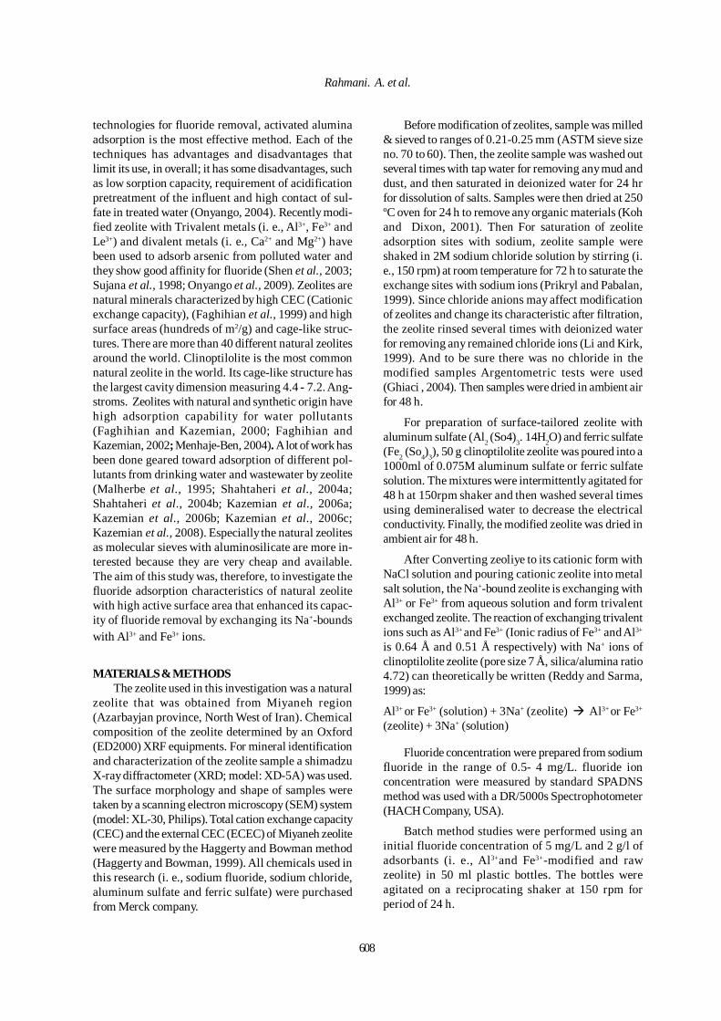
Rahmani. A. et al.
608
technologies for fluoride removal, activated aluminaadsorption is the most effective method. Each of thetechniques has advantages and disadvantages thatlimit its use, in overall; it has some disadvantages, suchas low sorption capacity, requirement of acidificationpretreatment of the influent and high contact of sul-fate in treated water (Onyango, 2004). Recently modi-fied zeolite with Trivalent metals (i. e., Al3+, Fe3+ andLe3+) and divalent metals (i. e., Ca2+ and Mg2+) havebeen used to adsorb arsenic from polluted water andthey show good affinity for fluoride (Shen et al., 2003;Sujana et al., 1998; Onyango et al., 2009). Zeolites arenatural minerals characterized by high CEC (Cationicexchange capacity), (Faghihian et al., 1999) and highsurface areas (hundreds of m2/g) and cage-like struc-tures. There are more than 40 different natural zeolitesaround the world. Clinoptilolite is the most commonnatural zeolite in the world. Its cage-like structure hasthe largest cavity dimension measuring 4.4 - 7.2. Ang-stroms. Zeolites with natural and synthetic origin havehigh adsorption capability for water pollutants(Faghihian and Kazemian, 2000; Faghihian andKazemian, 2002; Menhaje-Ben, 2004). A lot of work hasbeen done geared toward adsorption of different pol-lutants from drinking water and wastewater by zeolite(Malherbe et al., 1995; Shahtaheri et al., 2004a;Shahtaheri et al., 2004b; Kazemian et al., 2006a;Kazemian et al., 2006b; Kazemian et al., 2006c;Kazemian et al., 2008). Especially the natural zeolitesas molecular sieves with aluminosilicate are more in-terested because they are very cheap and available.The aim of this study was, therefore, to investigate thefluoride adsorption characteristics of natural zeolitewith high active surface area that enhanced its capac-ity of fluoride removal by exchanging its Na+-boundswith Al3+ and Fe3+ ions.
MATERIALS & METHODSThe zeolite used in this investigation was a natural
zeolite that was obtained from Miyaneh region(Azarbayjan province, North West of Iran). Chemicalcomposition of the zeolite determined by an Oxford(ED2000) XRF equipments. For mineral identificationand characterization of the zeolite sample a shimadzuX-ray diffractometer (XRD; model: XD-5A) was used.The surface morphology and shape of samples weretaken by a scanning electron microscopy (SEM) system(model: XL-30, Philips). Total cation exchange capacity(CEC) and the external CEC (ECEC) of Miyaneh zeolitewere measured by the Haggerty and Bowman method(Haggerty and Bowman, 1999). All chemicals used inthis research (i. e., sodium fluoride, sodium chloride,aluminum sulfate and ferric sulfate) were purchasedfrom Merck company.
Before modification of zeolites, sample was milled& sieved to ranges of 0.21-0.25 mm (ASTM sieve sizeno. 70 to 60). Then, the zeolite sample was washed outseveral times with tap water for removing any mud anddust, and then saturated in deionized water for 24 hrfor dissolution of salts. Samples were then dried at 250ºC oven for 24 h to remove any organic materials (Kohand Dixon, 2001). Then For saturation of zeoliteadsorption sites with sodium, zeolite sample wereshaked in 2M sodium chloride solution by stirring (i.e., 150 rpm) at room temperature for 72 h to saturate theexchange sites with sodium ions (Prikryl and Pabalan,1999). Since chloride anions may affect modificationof zeolites and change its characteristic after filtration,the zeolite rinsed several times with deionized waterfor removing any remained chloride ions (Li and Kirk,1999). And to be sure there was no chloride in themodified samples Argentometric tests were used(Ghiaci , 2004). Then samples were dried in ambient airfor 48 h.
For preparation of surface-tailored zeolite withaluminum sulfate (Al2 (So4)3. 14H2O) and ferric sulfate(Fe2 (So4)3), 50 g clinoptilolite zeolite was poured into a1000ml of 0.075M aluminum sulfate or ferric sulfatesolution. The mixtures were intermittently agitated for48 h at 150rpm shaker and then washed several timesusing demineralised water to decrease the electricalconductivity. Finally, the modified zeolite was dried inambient air for 48 h.
After Converting zeoliye to its cationic form withNaCl solution and pouring cationic zeolite into metalsalt solution, the Na+-bound zeolite is exchanging withAl3+ or Fe3+ from aqueous solution and form trivalentexchanged zeolite. The reaction of exchanging trivalentions such as Al3+ and Fe3+ (Ionic radius of Fe3+ and Al3+
is 0.64 Å and 0.51 Å respectively) with Na+ ions ofclinoptilolite zeolite (pore size 7 Å, silica/alumina ratio4.72) can theoretically be written (Reddy and Sarma,1999) as:
Al3+ or Fe3+ (solution) + 3Na+ (zeolite) Al3+ or Fe3+
(zeolite) + 3Na+ (solution)
Fluoride concentration were prepared from sodiumfluoride in the range of 0.5- 4 mg/L. fluoride ionconcentration were measured by standard SPADNSmethod was used with a DR/5000s Spectrophotometer(HACH Company, USA).
Batch method studies were performed using aninitial fluoride concentration of 5 mg/L and 2 g/l ofadsorbants (i. e., Al3+and Fe3+-modified and rawzeolite) in 50 ml plastic bottles. The bottles wereagitated on a reciprocating shaker at 150 rpm forperiod of 24 h.
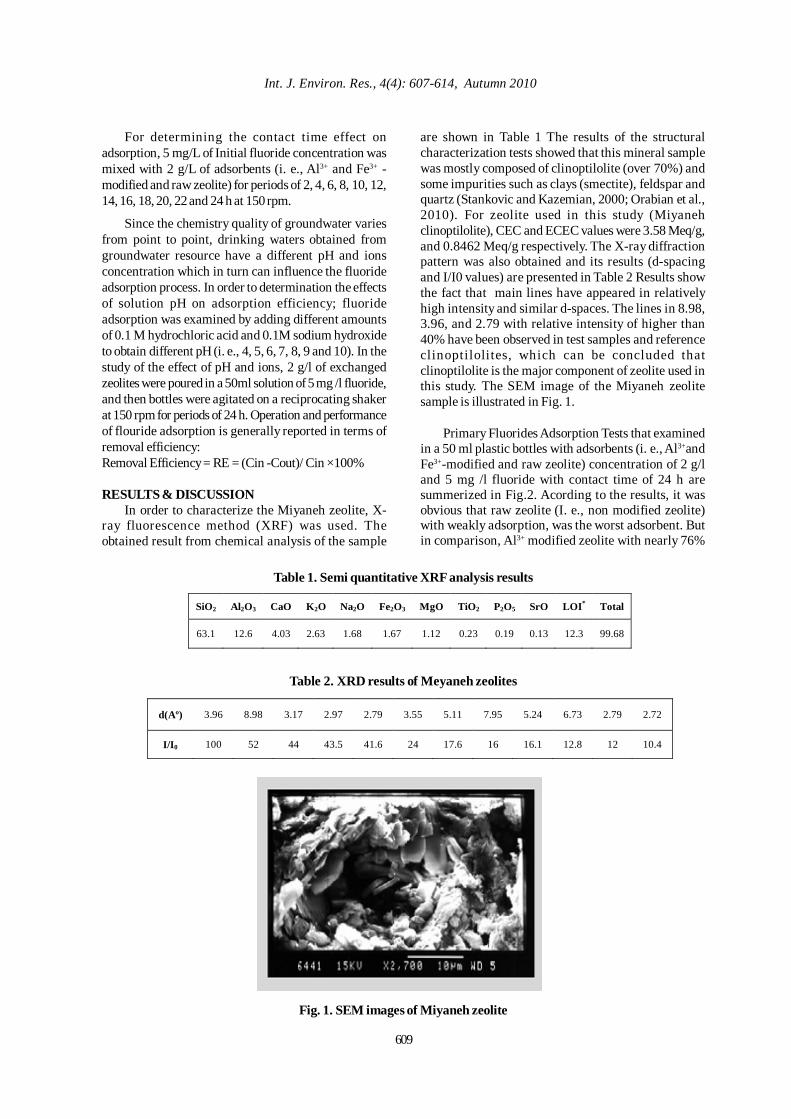
Rahmani. A. et al.
609
For determining the contact time effect onadsorption, 5 mg/L of Initial fluoride concentration wasmixed with 2 g/L of adsorbents (i. e., Al3+ and Fe3+ -modified and raw zeolite) for periods of 2, 4, 6, 8, 10, 12,14, 16, 18, 20, 22 and 24 h at 150 rpm.
Since the chemistry quality of groundwater variesfrom point to point, drinking waters obtained fromgroundwater resource have a different pH and ionsconcentration which in turn can influence the fluorideadsorption process. In order to determination the effectsof solution pH on adsorption efficiency; fluorideadsorption was examined by adding different amountsof 0.1 M hydrochloric acid and 0.1M sodium hydroxideto obtain different pH (i. e., 4, 5, 6, 7, 8, 9 and 10). In thestudy of the effect of pH and ions, 2 g/l of exchangedzeolites were poured in a 50ml solution of 5 mg /l fluoride,and then bottles were agitated on a reciprocating shakerat 150 rpm for periods of 24 h. Operation and performanceof flouride adsorption is generally reported in terms ofremoval efficiency:Removal Efficiency = RE = (Cin -Cout)/ Cin ×100%
RESULTS & DISCUSSIONIn order to characterize the Miyaneh zeolite, X-
ray fluorescence method (XRF) was used. Theobtained result from chemical analysis of the sample
are shown in Table 1 The results of the structuralcharacterization tests showed that this mineral samplewas mostly composed of clinoptilolite (over 70%) andsome impurities such as clays (smectite), feldspar andquartz (Stankovic and Kazemian, 2000; Orabian et al.,2010). For zeolite used in this study (Miyanehclinoptilolite), CEC and ECEC values were 3.58 Meq/g,and 0.8462 Meq/g respectively. The X-ray diffractionpattern was also obtained and its results (d-spacingand I/I0 values) are presented in Table 2 Results showthe fact that main lines have appeared in relativelyhigh intensity and similar d-spaces. The lines in 8.98,3.96, and 2.79 with relative intensity of higher than40% have been observed in test samples and referenceclinoptilolites, which can be concluded thatclinoptilolite is the major component of zeolite used inthis study. The SEM image of the Miyaneh zeolitesample is illustrated in Fig. 1.
Primary Fluorides Adsorption Tests that examinedin a 50 ml plastic bottles with adsorbents (i. e., Al3+andFe3+-modified and raw zeolite) concentration of 2 g/land 5 mg /l fluoride with contact time of 24 h aresummerized in Fig.2. Acording to the results, it wasobvious that raw zeolite (I. e., non modified zeolite)with weakly adsorption, was the worst adsorbent. Butin comparison, Al3+ modified zeolite with nearly 76%
Int. J. Environ. Res., 4(4): 607-614, Autumn 2010
Table 1. Semi quantitative XRF analysis results
SiO2 Al2O3 CaO K2O Na2O Fe2O3 MgO TiO2 P2O5 SrO LOI* Total
63.1 12.6 4.03 2.63 1.68 1.67 1.12 0.23 0.19 0.13 12.3 99.68
Table 2. XRD results of Meyaneh zeolites
d(Aº) 3.96 8.98 3.17 2.97 2.79 3.55 5.11 7.95 5.24 6.73 2.79 2.72
I/I0 100 52 44 43.5 41.6 24 17.6 16 16.1 12.8 12 10.4
Fig. 1. SEM images of Miyaneh zeolite

Rahmani A.. et al.
610
Production of PHB from coir industrial wasteAdsorption of fluoride from water
perform the highest adsorption of fluoride and Fe3+
modified zeolite whit 65% adsorption was the nexthighest adsorbent.
For assessment of contact time effect on fluorideadsorbtion, periods of 2, 4, 6, 8, 10, 12, 14, 16, 18, 20, 22and 24 h were investigated. as illustrated in Fig. 3 itwas obvious that approximately 20h is enough to reachequilibrium conditions for fluoride adsorbtion.
For determining the effect of fluoride concentrationon its adsorption, mixture of fluoride solution andadsorbrnts (i. e., Al3+and Fe3+-modified and raw zeolite)were shaked for 24 h at 150 rpm with the fluoride initialconcentrations from 2 to 20 mg/L. The results arepresented at Fig. 4. As expected, with increasing offluoride concentration, the adsorption potential willdecrease. Again the Al3+ modified zeolite was the bestadsorbant for fluoride adsorbtion.
Effect of solution pH value and electrolytes suchas bicarbonate, chloride and sulfate on fluoride uptakewas studied. Experiments were carried out by taking50 ml of fluoride-ions-spiked aqueous solution of initialconcentration 5 mg/L fluoride and adsorbents (i. e.,Al3+and Fe3+-modified and raw zeolite) dose of 2 g/l. Inthis study, the pH values were varied from 4 to 10while the effects of ions were studied with neutral pH.The investigation was limited to allowable ranges ofthe concentration of electrolytes in drinking water. Theimpact of pH is illustrated in Fig. 5 and the impact ofbicarbonate, chloride and sulfate concentrations onfluoride adsorption are presented in Fig. 6.
Natural samples used in this study obtained ofsupply groundwater in the Dashtestan area of theBushehr Province in Iran. The method of sampling wasclusture. Anionic and cationic Characters of thesesamples showed in Table 3.
Fig. 2. Fluoride adsorption with different adsorbents
Fig. 3. Effect of contact time on fluoride adsorption
00.10.20.30.40.50.60.70.8
Al3+ zeo Fe3+zeo raw zeolite
Adsorbent type
Rem
oval
(%)
00.10.20.30.40.50.60.70.8
0 2 4 6 8 101214 161820 2224
Contact time (h)
Rem
oval
(%) Al3+
zeo
Fe3+zeo
rawzeolite
00.10.20.30.40.50.60.70.80.9
2 4 6 8 10 12 14 16 18 20
Fluoride concentration (mg/l)
Fluo
ride
rem
oval
(%)
Al3+ zeo
Fe3+zeo
rawzeolite
Fig. 4. Effect of fluoride concentration on its adsorption
Fig. 5. Effect of pH on fluoride uptake by raw andmodified clinoptilolites
00.10.20.30.40.50.60.70.80.9
4 5 6 7 8 9 10
initial solution pH
Rem
oval
(%)
Al3+ zeo
Fe3+zeo
rawzeolite
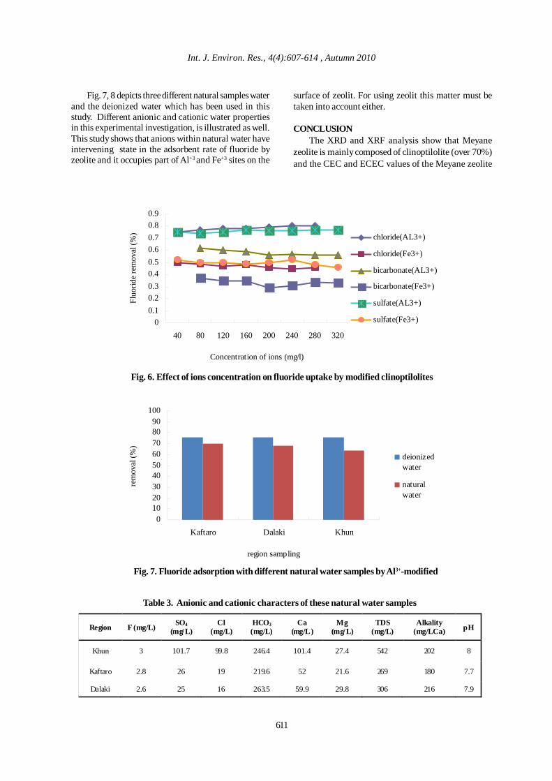
Rahmani. A. et al.Int. J. Environ. Res., 4(4):607-614 , Autumn 2010
611
Fig. 7, 8 depicts three different natural samples waterand the deionized water which has been used in thisstudy. Different anionic and cationic water propertiesin this experimental investigation, is illustrated as well.This study shows that anions within natural water haveintervening state in the adsorbent rate of fluoride byzeolite and it occupies part of Al+3 and Fe+3 sites on the
surface of zeolit. For using zeolit this matter must betaken into account either.
CONCLUSIONThe XRD and XRF analysis show that Meyane
zeolite is mainly composed of clinoptilolite (over 70%)and the CEC and ECEC values of the Meyane zeolite
00.10.20.30.40.50.60.70.80.9
40 80 120 160 200 240 280 320
Concentration of ions (mg/l)
Fluo
ride
rem
oval
(%) chloride(AL3+)
chloride(Fe3+)
bicarbonate(AL3+)
bicarbonate(Fe3+)
sulfate(AL3+)
sulfate(Fe3+)
Fig. 6. Effect of ions concentration on fluoride uptake by modified clinoptilolites
Fig. 7. Fluoride adsorption with different natural water samples by Al3+-modified
Table 3. Anionic and cationic characters of these natural water samples
Region F (mg/L) SO4 (mg/L)
Cl (mg/L)
HCO3 (mg/L)
Ca (mg/L)
Mg (mg/L)
TDS (mg/L)
Alkality (mg/LCa) pH
Khun 3 101.7 99.8 246.4 101.4 27.4 542 202 8
Kaftaro 2.8 26 19 219.6 52 21.6 269 180 7.7
Dalaki 2.6 25 16 263.5 59.9 29.8 306 216 7.9
0102030405060708090
100
Kaftaro Dalaki Khun
region sampling
rem
oval
(%)
deionized water
natural water
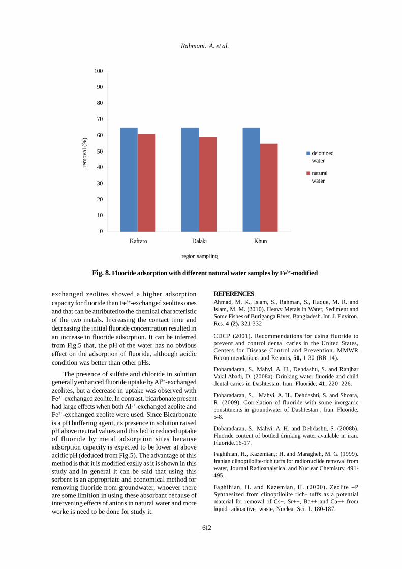
Rahmani. A. et al.
612
exchanged zeolites showed a higher adsorptioncapacity for fluoride than Fe3+-exchanged zeolites onesand that can be attributed to the chemical characteristicof the two metals. Increasing the contact time anddecreasing the initial fluoride concentration resulted inan increase in fluoride adsorption. It can be inferredfrom Fig.5 that, the pH of the water has no obviouseffect on the adsorption of fluoride, although acidiccondition was better than other pHs.
The presence of sulfate and chloride in solutiongenerally enhanced fluoride uptake by Al3+-exchangedzeolites, but a decrease in uptake was observed withFe3+-exchanged zeolite. In contrast, bicarbonate presenthad large effects when both Al3+-exchanged zeolite andFe3+-exchanged zeolite were used. Since Bicarbonateis a pH buffering agent, its presence in solution raisedpH above neutral values and this led to reduced uptakeof fluoride by metal adsorption sites becauseadsorption capacity is expected to be lower at aboveacidic pH (deduced from Fig.5). The advantage of thismethod is that it is modified easily as it is shown in thisstudy and in general it can be said that using thissorbent is an appropriate and economical method forremoving fluoride from groundwater, whoever thereare some limition in using these absorbant because ofintervening effects of anions in natural water and moreworke is need to be done for study it.
Fig. 8. Fluoride adsorption with different natural water samples by Fe3+-modified
0
10
20
30
40
50
60
70
80
90
100
Kaftaro Dalaki Khun
region sampling
rem
oval
(%)
deionized water
natural water
REFERENCESAhmad, M. K., Islam, S., Rahman, S., Haque, M. R. andIslam, M. M. (2010). Heavy Metals in Water, Sediment andSome Fishes of Buriganga River, Bangladesh. Int. J. Environ.Res. 4 (2), 321-332
CDCP (2001). Recommendations for using fluoride toprevent and control dental caries in the United States,Centers for Disease Control and Prevention. MMWRRecommendations and Reports, 50, 1-30 (RR-14).
Dobaradaran, S., Mahvi, A. H., Dehdashti, S. and RanjbarVakil Abadi, D. (2008a). Drinking water fluoride and childdental caries in Dashtestan, Iran. Fluoride, 41, 220–226.
Dobaradaran, S., Mahvi, A. H., Dehdashti, S. and Shoara,R. (2009). Correlation of fluoride with some inorganicconstituents in groundwater of Dashtestan , Iran. Fluoride,5-8.
Dobaradaran, S., Mahvi, A. H. and Dehdashti, S. (2008b).Fluoride content of bottled drinking water available in iran.Fluoride.16-17.
Faghihian, H., Kazemian,; H. and Maragheh, M. G. (1999).Iranian clinoptilolite-rich tuffs for radionuclide removal fromwater, Journal Radioanalytical and Nuclear Chemistry. 491-495.
Faghihian, H. and Kazemian, H. (2000). Zeolite –PSynthesized from clinoptilolite rich- tuffs as a potentialmaterial for removal of Cs+, Sr++, Ba++ and Ca++ fromliquid radioactive waste, Nuclear Sci. J. 180-187.
Rahmani. A. et al.Int. J. Environ. Res., 4(4):607-614 , Autumn 2010
Faghihian, H. and Kazemian, H. (2002). Ion exchange ofPb2+, Ag+1, Ni2+ and Zn2+ in natural clinoptilolite, studyof some parameters. Iran J. Sci.Tech., 357 - 361.
Ghiaci, M., Abbaspour, A., Kia, R. and Seyedeyn-Azad, F.(2004). Equilibrium isotherm studies for the sorption ofbenzene, toluene, and phenol onto organo-zeolites and as-synthesized MCM-41, Sep. Purification and Tech., 40, 217– 229.
Goyal, P., Sharma , A., Srivastava, S. and Srivastava, M. M.(2008). Saraca indica leaf powder for decontamination ofPb: removal, recovery, adsorbent characterization andequilibrium modeling. Int. J. Environ. Sci. Tech., 5 (1), 27-34.
Haggerty, G. M. and Bowman, R. S. (1994). Sorption ofChromate and other inorganic anions by organo-zeolite,Environ. Sci. Tech., 452-458.
Kazemian, H., Darybi, K. P., Mallah, M. H. and Khani, M.R. (2006a). Vitrification of Cs and Sr loaded Iranian Naturaland synthetic Zeolites, J. Radioanalytical Nuclear Chem.219-223.
Kazemian, H., Zakeri, H. and Rabbani, M. S. (2006b). Csand Sr removal from solution using potassium nickelhexacyanoferrate impregnated zeolites. J. RadioanalyticalNuclear Chem., 231-236.
Kazemian, H. and Mallah, M. H. (2006c). Elimination ofCd2+ and Mn2+ from wastewaters using naturalclinoptilolite and synthetic zeolite-P. Iranian J.chem.chemical Eng., 91-94.
Kazemian, H. and Mallah, M. H. (2008). Removal ofChromate ion from synthetic water using MCM-41/ZSM-5 composite. Iran J. Environ. Health Sci. Eng., 73-77.
Koh, S. M., Dixon, J. B. (2001). Preparation and applicationof organo-minerals as Sorbents of phenol, benzene andtoluene. Applied Clay Sci., 111-122.
Li, Z., Robert, B. and Kirk, J. (1999). Enhanced Reductionof chromate and pelletized surfactant-modified zeolite/zerovalent iron, Environ. Sci. Tech., 33, 4326-4330.
Mahvi, A. H., Zazoli, M. A., Younecian, M. and Esfandiari,Y. (2006). Fluoride content of Iranian black tea and tea liquor.Fluoride 39, 266-268.
Menhaje-Bena, R., Kazemian, H., Ghazi-Khonsari, M.,Hosseini, M. and Shahtaheri, S. J. (2004). Evaluation ofsome Iranian natural zeolites and their relevant syntheticzeolites as sorbents for removal of arsenate from drinkingwater. Iran J. Public Health. 36 - 44.
Malherbe, R., Fernandez, L. L. and Colado, L. ( 1995). Phsico– chemical properties of natural zeolites used for adsorptionof water. In: Ming DW, Munpton FA, Eds. Int. comm. naturalzeolite. 299- 308.
Nouri J., Mahvi A. H., Babaei A. and Ahmadpour, E. (2006).Regional pattern distribution of groundwater fluoride in theShush aquifer of Khuzestan County, Iran. Fluoride, 39 (4),321-325.
Orabian, T. A., Kazemian, H., Seifi, L., Bidhendi, G. N. andGhadiri, S. K. (2010). Removal of petroleum aromatichydrocarbons by surfactant-modified natural zeolite. CleanSoil, Air, Water, 38, 1.
Onyango, M. S., Leswifi, T. Y., Ochieng, A., Kuchar, D. F.O. and Otieno, H. (2009). Matsuda, Breakthrough analysisfor water defluoridation using surface-tailored zeolite in afixed bed column. Industrial and Engineering ChemistryResearch, 48, 931–937.
Onyango, M. S., Kojima, Y., Aoyi, O., Bernardo, E. C. andMatsuda, H. (2004). Adsorption equilibrium modeling andsolution chemistry dependence of fluoride removal fromwater by trivalent-cation-exchanged zeolite F-9. J. ColloidInterface Sci., 341–350.
Rahmani Boldaji, M., Mahvi, A. H., Dobaradaran, S. andHosseini, S. S. (2009). Evaluating the effectiveness of ahybrid sorbent resin in removing fluoride from water.International Journal Environment Science Technology, 6,(4), 629-632.
Reddy, B. J. and Sarma, K. B. N. (1980). Optical absorptionspectrum of Fe3+ In orthoclase feldspar, Proc IndianNational Science Academ. 176-180.
Rzeusk, R., Chlubek, D. and Machoy, Z. (1988). Interactionsbetween fluoride and biological free radical reactions, Fluoride31, 43-45.
Shivarajashankara, Y. M., Shivashankara, A. R., Bhat, P. G.and Rao, S. H. (2001). Effect of fluoride intoxication onlipid peroxidation and antioxidant systems in rats. Fluoride,34, 108-113.
Shahtaheri, S. J., Kazemian, H., Ghazi-Khonsari, M. andMenhaje-Bena, R. (2004a) Selective adsorption and removalof arsenic compounds from drinking water using natural andsynthetic zeolites. ICTX 2004 Conference ExposureAssessment in a Changing Environment to Utrecht.
Shahtaheri, S. J., Kazemian, H. and Menhaje-Bena, R.(2004b). Removal of arsenic species from drinking water byIranian natural and synthetic zeolites. Studies in SurfaceScience and Catalysis,1892-1899.
Shen, F., Chen, X., Gao, P. and Chen, G. (2003).Electrochemical Removal of fluoride ions from industrialwastewater. Chemical Engineering Science, 58, 987.
Shams, M., Nodehi, R. N., Dehghani, M. H., Younesian, M.and Mahvi, A. H. (2010). Efficiency of granular ferrichydroxide (GFH) for removal of fluoride from water.Fluoride, 43 (1), 61-66.
Stankovic, J. and Kazemian, H. (2000). Clinoptilolite fromzeolite deposits semnan, Meyaneh and Firouzkooh in Iran.Mineral, 31–32 (in Slovak).
Sujana, M. G., Thakur, R. S. and Rao, S. B. (1998). Removalof fluoride from aqueous solution by using alum sludge,Journal of Colloid Interface Science, 94, 206.
Prikryl, J. D.; Pabalan, R. T. (1999). Sorption of uranium6+and neptunium5+ by surfactant-modified natural zeolites.Mater. Res. Soc. Symp. Proc. 556.
613

Rahmani. A. et al.Adsorption of fluoride from water
614
Vasanthavigar, M., Srinivasamoorthy, K., Vijayaragavan, K.,Rajiv Ganthi, R., Chidambaram, S., Sarama, V. S., Anandhan,P., Manivannan, R. and Vasudevan, S. (2009).Hydrogeochemistry Of Thirumanimuttar Basin: AnIndication Of Weathering and Anthropogenic Impact. Int. J.Environ. Res., 3 (4), 617-628.
Wu, C., Gu, X., Ge, Y., Zhang, J. and Wang, J. (2006).Effects of fluoride and arsenic on brain biochemical indexesand learning-memory in rats. Fluoride, 39, 274-279.
WHO (2002). Fluorides. Environmental Health Criteria 227.World Health Organization, Geneva.
WHO (2008). Guidelines for drinking-water quality, 3rdEd., Vol. 1, World Health Organization, Geneva.
Zvinowanda, C. M., Okonkwo, J. O., Shabalala, P. N. andAgyei, N. M., (2009). A novel adsorbent for heavy metalremediation in aqueous environments. Int. J. Environ. Sci.Tech., 6 (3), 425-434.
Int. J. Environ. Res., 4(4):615-628 , Autumn 2010ISSN: 1735-6865
Received 12 Aug. 2009; Revised 5 April 2010; Accepted 15 April 2010
*Corresponding author E-mail: [email protected]
615
Recyclable Rubber Sheets Impregnated with Potassium Oxalate doped TiO2
and their uses in Decolorization of Dye-Polluted Waters
Suwanchawalit, Ch., Sriwong, Ch. and Wongnawa, S.*
Department of Chemistry and Center for Innovation in Chemistry, Faculty of Science, Prince of SongklaUniversity, Hat Yai, Songkhla 90112, Thailand
ABSTRACT: Two potassium oxalate doped TiO2 samples, designated as K1-TiO2 and K2-TiO2, weresynthesized by the base-catalyzed sol-gel process. These samples were impregnated into rubber sheets. Twocommercial TiO2 samples, anatase and Degussa P25, were used as reference materials with which the synthesizedsamples were to be compared. Anatase and P25 were also impregnated into rubber sheets and designated asImp-Ana and Imp-P25, respectively. Methylene blue solution was effectively decolorized by these fourimpregnated sheets. Imp-K1 and Imp-K2 sheets could turn dye solutions to colorless in 3 h and remained atthat point until reaching 6h. For the Imp-Ana and Imp-P25 sheets the decolorization rate was slower butincreased continually until reaching their maximum at 6h (colorless). The mode of decolorization for the Imp-synthesized TiO2 was mainly based on adsorption with a small contribution from the photocatalytic reactionwhile the reverse was observed for the Imp-commercial TiO2. The surface of the used Imp-synthsized TiO2sheets became covered with dye after several uses but it could be cleaned by regeneration with H2O2 and UVlight. After recycling the cleaned sheets could be reused many times to decolorize the dye solution.
Key words: Immobilized titanium dioxide, Titanium dioxide thin film, Methylene blue, Dye decolorization
INTRODUCTIONDifferent methods have been utilized in industrial
waste treatment for dye decolorization (Sreedhar Reddyand Kotaiah, 2005; Gong et al., 2010; Binupriya et al.,2009; Nagda and Ghole, 2008; Hassani et al., 2008; NabiBidhendi et al., 2007). In the field of environmentalchemistry, semiconductor mediated photocatalysis hasbeen the focus of recent attention since it aims todestroy contaminants in water and air by non-toxicprocesses. Following the the pioneering work ofFujishima and Honda in 1972 titanium dioxide (TiO2),has become an important photocatalyst forenvironmental applications due to its high activity,absence of toxicity, low cost, and excellent durability( Legrini et al.,1993; Lisebigler et al., 1995 andKonstantinou and Albanis, 2004). When TiO2 isirradiated with UV light (λ < 380 nm), electron–holepairs are formed which immediately generate free photoelectrons and holes that are able to interact with organicmatter present at the TiO2 surface. The O2 moleculescavenges an electron from the conduction band ofTiO2 to form a superoxide radical (O2") because theenergy of the conduction band edge is close to thereduction potential of oxygen. This superoxide reactswith a proton and forms a hydroperoxyl radical (HO2•).
These O2" and HO2• species interact with organicpollutants and degrade them to CO2 and water whichare harmless products (Houas et al, 2001 and Djaouedet al., 2008). Several studies have dealt with thesynthesis of ultrafine TiO2 nanoparticles and theirapplications in water purification. However, if used inthe powder form, photocatalysts have to be separatedfrom the liquid phase after water treatment and theprocess for the separation of ultrafine nanoscale particlesis tedious and costly (Neppolian et al., 2002). The after-used separation process, is one problem that hinders theuse of powder photocatalysts to photodegrade toxic ornon-biodegradable organic compounds in solution( Zhiyong et al., 2008 and Zhiyong et al., 2008). Thesedisadvantages could be overcome by using supportedphotocatalysts for example by fixing TiO2 on glass(Losito et al., 2005), ITO glass (Sankapal and Steiner,2005), polymer films (Yang et al., 2006), and plastic (Kwonet al., 2004). TiO2 thin films have been prepared by varioustechniques such as chemical vapor deposition (Ding etal., 2001), spray pyrolysis deposition (Weng et al., 2005),flame synthesis (Partsinis, 1996), and sol-gel dip coating(Sen et al., 2005 and Guo et al., 2005),however, thesetechniques need expensive equipment and complexprocedures.
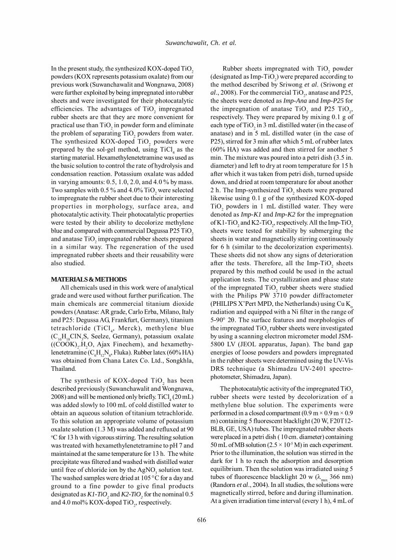
616
Suwanchawalit, Ch. et al.
In the present study, the synthesized KOX-doped TiO2powders (KOX represents potassium oxalate) from ourprevious work (Suwanchawalit and Wongnawa, 2008)were further exploited by being impregnated into rubbersheets and were investigated for their photocatalyticefficiencies. The advantages of TiO2 impregnatedrubber sheets are that they are more convenient forpractical use than TiO2 in powder form and eliminatethe problem of separating TiO2 powders from water.The synthesized KOX-doped TiO2 powders wereprepared by the sol-gel method, using TiCl4 as thestarting material. Hexamethylenetetramine was used asthe basic solution to control the rate of hydrolysis andcondensation reaction. Potassium oxalate was addedin varying amounts: 0.5, 1.0, 2.0, and 4.0 % by mass.Two samples with 0.5 % and 4.0% TiO2 were selectedto impregnate the rubber sheet due to their interestingproperties in morphology, surface area, andphotocatalytic activity. Their photocatalytic propertieswere tested by their ability to decolorize methyleneblue and compared with commercial Degussa P25 TiO2and anatase TiO2 impregnated rubber sheets preparedin a similar way. The regeneration of the usedimpregnated rubber sheets and their reusability werealso studied.
MATERIALS & METHODSAll chemicals used in this work were of analytical
grade and were used without further purification. Themain chemicals are commercial titanium dioxidepowders (Anatase: AR grade, Carlo Erba, Milano, Italyand P25: Degussa AG, Frankfurt, Germany), titaniumtetrachloride (TiCl4, Merck), methylene blue(C16H18ClN3S, Seelze, Germany), potassium oxalate((COOK)2.H2O, Ajax Finechem), and hexamethy-lenetetramine (C6H12N4, Fluka). Rubber latex (60% HA)was obtained from Chana Latex Co. Ltd., Songkhla,Thailand.
The synthesis of KOX-doped TiO2 has beendescribed previously (Suwanchawalit and Wongnawa,2008) and will be mentioned only briefly. TiCl4 (20 mL)was added slowly to 100 mL of cold distilled water toobtain an aqueous solution of titanium tetrachloride.To this solution an appropriate volume of potassiumoxalate solution (1.3 M) was added and refluxed at 90oC for 13 h with vigorous stirring. The resulting solutionwas treated with hexamethylenetetramine to pH 7 andmaintained at the same temperature for 13 h. The whiteprecipitate was filtered and washed with distilled wateruntil free of chloride ion by the AgNO3 solution test.The washed samples were dried at 105 °C for a day andground to a fine powder to give final productsdesignated as K1-TiO2 and K2-TiO2 for the nominal 0.5and 4.0 mol% KOX-doped TiO2, respectively.
Rubber sheets impregnated with TiO2 powder(designated as Imp-TiO2) were prepared according tothe method described by Sriwong et al. (Sriwong etal., 2008). For the commercial TiO2, anatase and P25,the sheets were denoted as Imp-Ana and Imp-P25 forthe impregnation of anatase TiO2 and P25 TiO2,respectively. They were prepared by mixing 0.1 g ofeach type of TiO2 in 3 mL distilled water (in the case ofanatase) and in 5 mL distilled water (in the case ofP25), stirred for 3 min after which 5 mL of rubber latex(60% HA) was added and then stirred for another 5min. The mixture was poured into a petri dish (3.5 in.diameter) and left to dry at room temperature for 15 hafter which it was taken from petri dish, turned upsidedown, and dried at room temperature for about another2 h. The Imp-synthesized TiO2 sheets were preparedlikewise using 0.1 g of the synthesized KOX-dopedTiO2 powders in 1 mL distilled water. They weredenoted as Imp-K1 and Imp-K2 for the impregnationof K1-TiO2 and K2-TiO2, respectively. All the Imp-TiO2sheets were tested for stability by submerging thesheets in water and magnetically stirring continuouslyfor 6 h (similar to the decolorization experiments).These sheets did not show any signs of deteriorationafter the tests. Therefore, all the Imp-TiO2 sheetsprepared by this method could be used in the actualapplication tests. The crystallization and phase stateof the impregnated TiO2 rubber sheets were studiedwith the Philips PW 3710 powder diffractometer(PHILIPS X’Pert MPD, the Netherlands) using Cu Kα
radiation and equipped with a Ni filter in the range of5-90° 2θ. The surface features and morphologies ofthe impregnated TiO2 rubber sheets were investigatedby using a scanning electron micrometer model JSM-5800 LV (JEOL apparatus, Japan). The band gapenergies of loose powders and powders impregnatedin the rubber sheets were determined using the UV-VisDRS technique (a Shimadzu UV-2401 spectro-photometer, Shimadzu, Japan).
The photocatalytic activity of the impregnated TiO2rubber sheets were tested by decolorization of amethylene blue solution. The experiments wereperformed in a closed compartment (0.9 m × 0.9 m × 0.9m) containing 5 fluorescent blacklight (20 W, F20T12-BLB, GE, USA) tubes. The impregnated rubber sheetswere placed in a petri dish ( 10 cm. diameter) containing50 mL of MB solution (2.5 × 10⁻⁵ M) in each experiment.Prior to the illumination, the solution was stirred in thedark for 1 h to reach the adsorption and desorptionequilibrium. Then the solution was irradiated using 5tubes of fluorescence blacklight 20 w (λmax 366 nm)(Randorn et al., 2004). In all studies, the solutions weremagnetically stirred, before and during illumination.At a given irradiation time interval (every 1 h), 4 mL of

Int. J. Environ. Res., 4(4):615-628 , Autumn 2010
617
the sample was collected and measured for theremaining concentration of MB by observing thechange in absorbance at 665 nm using the UV-Visspectrophotometer (Specord S100, Analytik JenaGmbH, Germany). The concentration of MB solutionwas determined quantitatively through the calibrationgraph constructed from standard solutions of MB atvarious concentrations (R2 = 0.9983). The percentageof decolorization was calculated by Eq. (1),
100 x C
tC - C tion Decoloriza %
0
0= (1)
where C0 is the initial concentration of MB solutionand Ct is the concentration of MB solution at specifictime interval for the collected sample. Controlledexperiments, without light or without TiO2, wereperformed to demonstrate that the degradation of thedye was dependent on the presence of both light andTiO2.
RESULTS & DISCUSSIONK1-TiO2 and K2-TiO2 were synthesized by the sol-
gel method and, without calcinations, were impregnatedinto rubber sheets by the method previously described
(Sriwong et al., 2008). Prior to the impregnation stage,the loose powders were characterized by XRD andcompared with the commercial ones as shown in Fig. 1.For the two commercial TiO2 samples, anatase and rutilephases are clearly seen, denoted by “A” and “R”,respectively. In the synthesized samples, K1-TiO2appears to be mainly in its amorphous form with a verysmall amount of the anatase phase (Fig. 1a); while K2-TiO2 does not show any characteristic patterns ofanatase or rutile but mixed phases of several potassiumcontaining compounds can be observed (Fig. 1b),notably, potassium acetate hydrate (C2H3KO2.xH2O),potassium titanium oxide (K2Ti4O9 2.2H2O), andtitanium oxide (Ti3O5). Some physicochemicalproperties of K1-TiO2 and K2-TiO2 are given in Table 1including the titanium and potassium contents.
When the loose powders were incorporated intothe rubber sheets, the XRD was also used to examinetheir identities in the new environment and the resultsare shown in Fig. 2. A well-crystallized anatase formshows up in the Imp-Ana sheet as shown in Fig 2e.The same result is observed for the Imp-P25 sheet asshown in Fig 2d. The pristine rubber sheet shows aclean base line throughout the spectrum except for a
Table 1. Typical physicochemical properties of as-prepared TiO2 samples
Surface area Amount of element Sample Crystallite phase (m2/g) Tia (%) Ka (%) K1- TiO2 Amorphous 336.7 14.08 2.44 K2- TiO2 Mixed phase* 8.8 7.67 19.55
* Data from XRD: mixed phases are potassium acetate hydrate (C2H3KO2.xH2O),potassium titanium oxide (K2Ti4O9 2.2H2O), and titanium oxide (Ti3O5).a Determined by XRF using the calibration graph method.
Fig. 1. XRD patterns of TiO2 powders (a) K1- TiO2, (b) K2-TiO2, (c) P25, and (d) anatase.
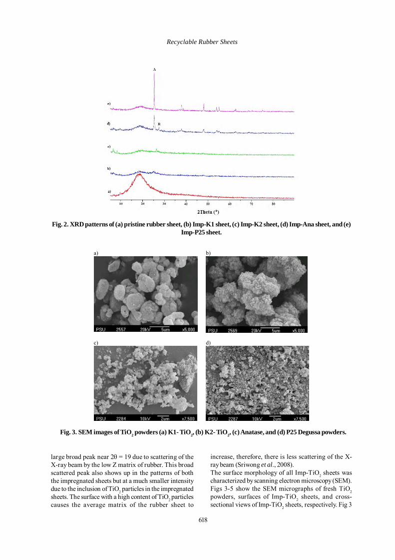
618
Fig. 2. XRD patterns of (a) pristine rubber sheet, (b) Imp-K1 sheet, (c) Imp-K2 sheet, (d) Imp-Ana sheet, and (e)Imp-P25 sheet.
a)
b)
c)
d)
Fig. 3. SEM images of TiO2 powders (a) K1- TiO2, (b) K2- TiO2, (c) Anatase, and (d) P25 Degussa powders.
large broad peak near 2θ = 19 due to scattering of theX-ray beam by the low Z matrix of rubber. This broadscattered peak also shows up in the patterns of boththe impregnated sheets but at a much smaller intensitydue to the inclusion of TiO2 particles in the impregnatedsheets. The surface with a high content of TiO2 particlescauses the average matrix of the rubber sheet to
increase, therefore, there is less scattering of the X-ray beam (Sriwong et al., 2008).The surface morphology of all Imp-TiO2 sheets wascharacterized by scanning electron microscopy (SEM).Figs 3-5 show the SEM micrographs of fresh TiO2powders, surfaces of Imp-TiO2 sheets, and cross-sectional views of Imp-TiO2 sheets, respectively. Fig 3
Recyclable Rubber Sheets
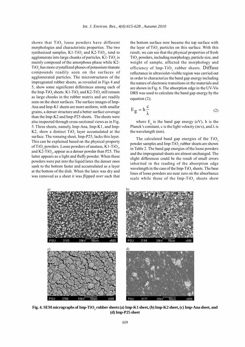
Int. J. Environ. Res., 4(4):615-628 , Autumn 2010
shows that TiO2 loose powders have differentmorphologies and characteristic properties. The twosynthesized samples, K1-TiO2 and K2-TiO2, tend toagglomerate into large chunks of particles. K1-TiO2 ismainly composed of the amorphous phase while K2-TiO2 has more crystallized phases of potassium titanatecompounds readily seen on the surfaces ofagglomerated particles. The microstructures of theimpregnated rubber sheets, as revealed in Figs 4 and5, show some significant differences among each ofthe Imp-TiO2 sheets. K1-TiO2 and K2-TiO2 still remainas large chunks in the rubber matrix and are readilyseen on the sheet surfaces. The surface images of Imp-Ana and Imp-K1 sheets are more uniform, with smallergrains, a denser structure and a better surface coveragethan the Imp-K2 and Imp-P25 sheets. The sheets werealso inspected through cross-sectional views as in Fig.5. Three sheets, namely, Imp-Ana, Imp-K1, and Imp-K2, show a distinct TiO2 layer accumulated at thesurface. The remaing sheet, Imp-P25, lacks this layer.This can be explained based on the physical propertyof TiO2 powders. Loose powders of anatase, K1-TiO2,and K2-TiO2, appear as a denser powder than P25. Thelatter appears as a light and fluffy powder. When thesepowders were put into the liquid latex the denser onessank to the bottom faster and accumulated as a layerat the bottom of the dish. When the latex was dry andwas removed as a sheet it was flipped over such that
the bottom surface now became the top surface withthe layer of TiO2 particles on this surface. With thisresult, we can see that the physical properties of freshTiO2 powders, including morphology, particle size, andweight of sample, affected the morphology andefficiency of Imp-TiO2 rubber sheets. Diffusereflectance in ultraviolet-visible region was carried outin order to characterize the band gap energy includingthe nature of electronic transitions in the materials andare shown in Fig. 6. The absorption edge in the UV-VisDRS was used to calculate the band gap energy by theequation (2);
λchgE = (2)
where Eg is the band gap energy (eV), h is thePlanck’s constant, c is the light velocity (m/s), and λ isthe wavelength (nm).
The calculated band gap energies of the TiO2powder samples and Imp-TiO2 rubber sheets are shownin Table 2. The band gap energies of the loose powdersand the impregnated sheets are almost unchanged. Theslight differences could be the result of small errorsinherited in the reading of the absorption edgewavelength in the case of the Imp-TiO2 sheets. The baselines of loose powders are near zero on the absorbancescale while those of the Imp-TiO2 sheets show
a)
b)
c)
d)
Fig. 4. SEM micrographs of Imp-TiO2 rubber sheets (a) Imp-K1 sheet, (b) Imp-K2 sheet, (c) Imp-Ana sheet, and(d) Imp-P25 sheet
619
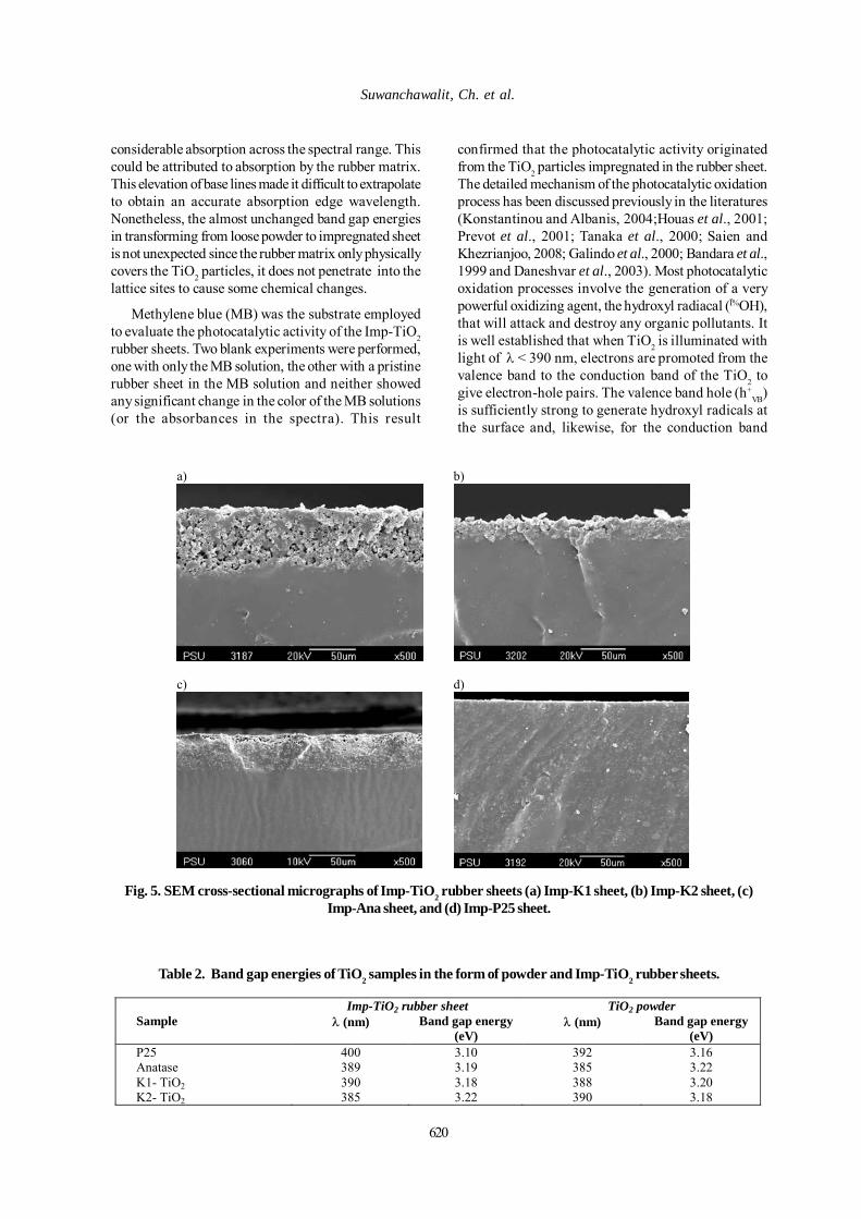
620
Suwanchawalit, Ch. et al.
considerable absorption across the spectral range. Thiscould be attributed to absorption by the rubber matrix.This elevation of base lines made it difficult to extrapolateto obtain an accurate absorption edge wavelength.Nonetheless, the almost unchanged band gap energiesin transforming from loose powder to impregnated sheetis not unexpected since the rubber matrix only physicallycovers the TiO2 particles, it does not penetrate into thelattice sites to cause some chemical changes.
Methylene blue (MB) was the substrate employedto evaluate the photocatalytic activity of the Imp-TiO2rubber sheets. Two blank experiments were performed,one with only the MB solution, the other with a pristinerubber sheet in the MB solution and neither showedany significant change in the color of the MB solutions(or the absorbances in the spectra). This result
a)
b)
c)
d)
Fig. 5. SEM cross-sectional micrographs of Imp-TiO2 rubber sheets (a) Imp-K1 sheet, (b) Imp-K2 sheet, (c)Imp-Ana sheet, and (d) Imp-P25 sheet.
Table 2. Band gap energies of TiO2 samples in the form of powder and Imp-TiO2 rubber sheets. Imp-TiO2 rubber sheet TiO2 powder
Sample λ (nm)
Band gap energy (eV)
λ (nm)
Band gap energy (eV)
P25 Anatase K1- TiO2 K2- TiO2
400 389 390 385
3.10 3.19 3.18 3.22
392 385 388 390
3.16 3.22 3.20 3.18
confirmed that the photocatalytic activity originatedfrom the TiO2 particles impregnated in the rubber sheet.The detailed mechanism of the photocatalytic oxidationprocess has been discussed previously in the literatures(Konstantinou and Albanis, 2004;Houas et al., 2001;Prevot et al., 2001; Tanaka et al., 2000; Saien andKhezrianjoo, 2008; Galindo et al., 2000; Bandara et al.,1999 and Daneshvar et al., 2003). Most photocatalyticoxidation processes involve the generation of a verypowerful oxidizing agent, the hydroxyl radiacal (Ï%OH),that will attack and destroy any organic pollutants. Itis well established that when TiO2 is illuminated withlight of λ < 390 nm, electrons are promoted from thevalence band to the conduction band of the TiO2 togive electron-hole pairs. The valence band hole (h+
VB)is sufficiently strong to generate hydroxyl radicals atthe surface and, likewise, for the conduction band
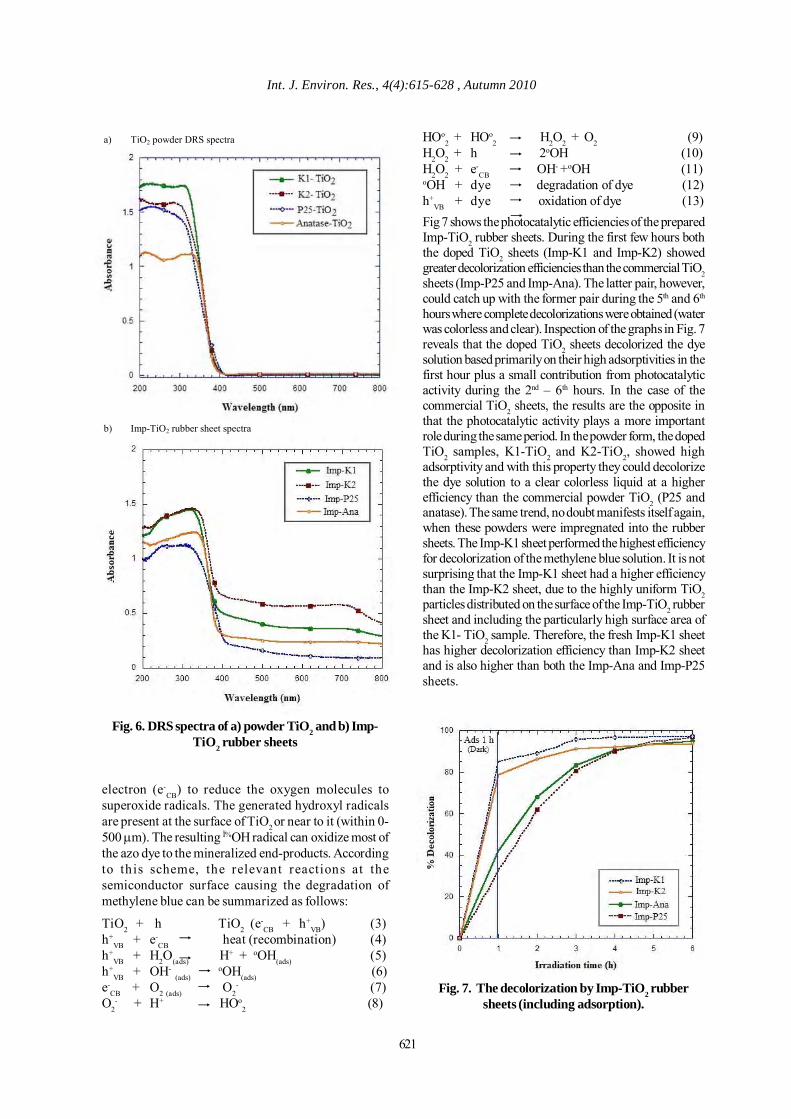
621
Int. J. Environ. Res., 4(4):615-628 , Autumn 2010
a) TiO2 powder DRS spectra
b) Imp-TiO2 rubber sheet spectra
Fig. 6. DRS spectra of a) powder TiO2 and b) Imp-TiO2 rubber sheets
electron (e-CB) to reduce the oxygen molecules to
superoxide radicals. The generated hydroxyl radicalsare present at the surface of TiO2 or near to it (within 0-500 µm). The resulting Ï%OH radical can oxidize most ofthe azo dye to the mineralized end-products. Accordingto this scheme, the relevant reactions at thesemiconductor surface causing the degradation ofmethylene blue can be summarized as follows:
TiO2 + h TiO2 (e-CB + h+
VB) (3)h+
VB + e-CB heat (recombination) (4)
h+VB + H2O(ads) H+ + oOH(ads) (5)
h+VB + OH- (ads)
oOH(ads) (6)e-
CB + O2 (ads) O2- (7)
O2- + H+ HOo
2 (8)
HOo2 + HOo
2 H2O2 + O2 (9)H2O2 + h 2oOH (10)H2O2 + e-
CB OH- +oOH (11)oOH + dye degradation of dye (12)h+
VB + dye oxidation of dye (13)Fig 7 shows the photocatalytic efficiencies of the preparedImp-TiO2 rubber sheets. During the first few hours boththe doped TiO2 sheets (Imp-K1 and Imp-K2) showedgreater decolorization efficiencies than the commercial TiO2sheets (Imp-P25 and Imp-Ana). The latter pair, however,could catch up with the former pair during the 5th and 6th
hours where complete decolorizations were obtained (waterwas colorless and clear). Inspection of the graphs in Fig. 7reveals that the doped TiO2 sheets decolorized the dyesolution based primarily on their high adsorptivities in thefirst hour plus a small contribution from photocatalyticactivity during the 2nd – 6th hours. In the case of thecommercial TiO2 sheets, the results are the opposite inthat the photocatalytic activity plays a more importantrole during the same period. In the powder form, the dopedTiO2 samples, K1-TiO2 and K2-TiO2, showed highadsorptivity and with this property they could decolorizethe dye solution to a clear colorless liquid at a higherefficiency than the commercial powder TiO2 (P25 andanatase). The same trend, no doubt manifests itself again,when these powders were impregnated into the rubbersheets. The Imp-K1 sheet performed the highest efficiencyfor decolorization of the methylene blue solution. It is notsurprising that the Imp-K1 sheet had a higher efficiencythan the Imp-K2 sheet, due to the highly uniform TiO2particles distributed on the surface of the Imp-TiO2 rubbersheet and including the particularly high surface area ofthe K1- TiO2 sample. Therefore, the fresh Imp-K1 sheethas higher decolorization efficiency than Imp-K2 sheetand is also higher than both the Imp-Ana and Imp-P25sheets.
Fig. 7. The decolorization by Imp-TiO2 rubbersheets (including adsorption).
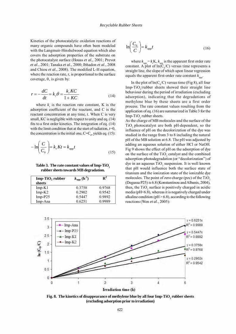
622
Kinetics of the photocatalytic oxidation reactions ofmany organic compounds have often been modeledwith the Langmuir-Hinshelwood equation which alsocovers the adsorption properties of the substrate onthe photocatalyst surface (Houas et al., 2001; Prevotet al., 2001; Tanaka et al., 2000; Ibhadon et al., 2008and Chiou et al., 2008). The modified L-H equation,where the reaction rate, r, is proportional to the surfacecoverage, θ, is given by:
KCKCkk
dtdCr r
r +==−=
1θ (14)
where kr is the reaction rate constant, K is theadsorption coefficient of the reactant, and C is thereactant concentration at any time, t. When C is verysmall, KC is negligible with respect to unity and eq. (14)fits to a first order kinetics. The integration of eq. (14)with the limit condition that at the start of radiation, t=0,the concentration is the initial one, C=C0, yields eq. (15):
tkKtkCC
appr ==⎟⎟⎠
⎞⎜⎜⎝
⎛−
0
ln (15)
tkCC
app=⎟⎠⎞
⎜⎝⎛ 0ln (16)
where kapp = krK, kapp is the apparent first order rateconstant. A plot of ln(C0/C) versus time represents astraight line, the slope of which upon linear regressionequals the apparent first-order rate constant kapp.
In the plot of ln(C0/C) versus time (Fig 8), all fourImp-TiO2/rubber sheets showed their straight linebehaviour during the period of irradiation (excludingadsorption), indicating that the degradations ofmethylene blue by these sheets are a first orderprocess. The rate constant values resulting from theapplication of eq. (16) are summarized in Table 3 for theImp-TiO2 rubber sheets.As the charge of MB molecules and the surface of theTiO2 photocatalyst are both pH-dependent, so theinfluence of pH on the decolorization of the dye wasstudied in the range from 3 to 8 including the naturalpH of the MB solution at 6.8. The pH was adjusted byadding an aqueous solution of either HCl or NaOH.Fig 9 shows the effect of pH on the adsorption of dyeon the surface of the TiO2 catalyst and the combinedadsorption-photodegradation (or “decolorization”) ofdye in an aqueous TiO2 suspension. It is well knownthat pH would influence both the surface state oftitanium and the ionization state of the ionizable dyemolecules. The point of zero charge (pzc) of the TiO2(Degussa P25) is 6.8 (Konstantinou and Albanis, 2004),thus, the TiO2 surface is positively charged in acidicmedia (pH<6.8), whereas it is negatively charged underalkaline condition (pH > 6.8), according to the followingreactions (Wen et al., 2005):
Fig. 8. The kinetics of disappearance of methylene blue by all four Imp-TiO2 rubber sheets(excluding adsorption prior to irradiation)
Table 3. The rate constant values of Imp-TiO2rubber sheets towards MB degradation.
Imp-TiO2 rubber sheets
kapp (h-1) R2
Imp-K1 Imp-K2 Imp-P25 Imp-Ana
0.3758 0.2902 0.5447 0.6251
0.9768 0.9542 0.9892 0.9989
Recyclable Rubber Sheets

Int. J. Environ. Res., 4(4):615-628 , Autumn 2010
pH < pzc: Ti-OH + H+ → TiOH2+ (17)
pH > pzc: Ti-OH + OH- → TiO- + H2O (18)
Since the parent fragment of MB has a positive charge,the adsorption on a negatively charged surface of TiO2is favored at high pH. Increasing the pH caused thesurface of TiO2 to become less positive or even turnedto negative once the pH exceeded pzc. Hence, we expectthat the repulsive force to operate is stronger at lowpH, therefore there is less adsorption of dye onto theTiO2 surface. This fact is borne out as the adsorptiontrend from pH 3 to 8 of the Imp-TiO2 sheets gradually
a) Adsorption
b) Decolorization (adsorption + photodegradation)
Fig. 9. Effect of pH on a) adsorption of MB on the rubber sheet surface, and b) the combined adsorption-
photodegradation of MB by the rubber sheet. (Condition: Imp-TiO2 sheet , 50 mL MB solution, adsorption inthe dark 1 h (a) and under UV irradiation 5 h. (b))
increases as shown in Fig 9a. The decolorizations (Fig9b) also gradually increased when increasing the pHvalues due to higher concentrations of the •OH radical,hence, the high decolorization efficiencies. So, the orderof the efficiency of decolorization by all Imp-TiO2 rubbersheets at different pH values is pH 8 > pH 6.8 > pH3.To determine the recyclability of the rubber sheets,all Imp-TiO2 rubber sheets were used in repeatedconsecutive photocatalytic runs. After the first roundof photocatalytic experiment, the rubber sheet wasseparated and used in the next round without anytreatment. The results in Fig. 10 show that the activity
623
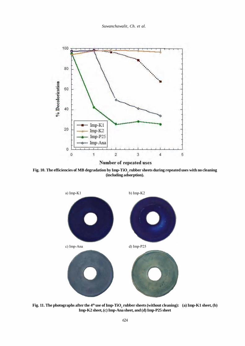
Suwanchawalit, Ch. et al.
Fig. 10. The efficiencies of MB degradation by Imp-TiO2 rubber sheets during repeated uses with no cleaning(including adsorption).
a) Imp-K1
b) Imp-K2
c) Imp-Ana
d) Imp-P25
Fig. 11. The photographs after the 4th use of Imp-TiO2 rubber sheets (without cleaning): (a) Imp-K1 sheet, (b)Imp-K2 sheet, (c) Imp-Ana sheet, and (d) Imp-P25 sheet
624

Int. J. Environ. Res., 4(4):615-628 , Autumn 2010
Before regeneration
After regeneration
Imp-Ana
Imp-Ana
Imp-K1
Imp-K2
Fig. 12. The photographs of Imp-TiO2 rubber sheets: before and after regeneration.
Fig. 13. The efficiencies of MB decolorization by the regenerated Imp-TiO2 rubber sheets after repeating uses(including adsorption)
of the Imp-commercial TiO2 rubber sheets decreasedgreatly in successive uses by up to four times. On theother hand, the activity of the Imp-synthesized TiO2rubber sheets decreased only slightly for the Imp-K1and the Imp-K2 sheet produced excellent performance
throughout. When freshly prepared and being usedfor the first time the Imp-K1 sheet showed a higherphotocatalytic efficiency than the Imp-K2 sheet, asshown in Fig 10 (data on the y-axis). However, in thefollowing repeated uses the Imp-K2 sheet maintained
625
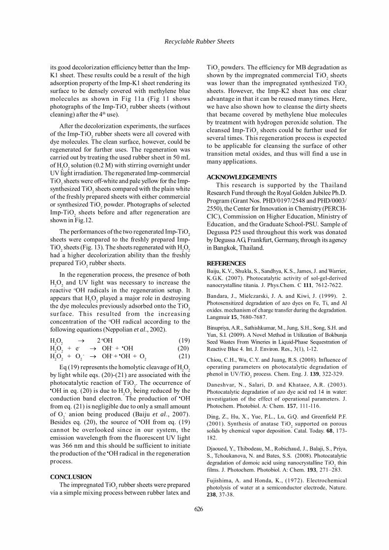
its good decolorization efficiency better than the Imp-K1 sheet. These results could be a result of the highadsorption property of the Imp-K1 sheet rendering itssurface to be densely covered with methylene bluemolecules as shown in Fig 11a (Fig 11 showsphotographs of the Imp-TiO2 rubber sheets (withoutcleaning) after the 4th use).
After the decolorization experiments, the surfacesof the Imp-TiO2 rubber sheets were all covered withdye molecules. The clean surface, however, could beregenerated for further uses. The regeneration wascarried out by treating the used rubber sheet in 50 mLof H2O2 solution (0.2 M) with stirring overnight underUV light irradiation. The regenerated Imp-commercialTiO2 sheets were off-white and pale yellow for the Imp-synthesized TiO2 sheets compared with the plain whiteof the freshly prepared sheets with either commercialor synthesized TiO2 powder. Photographs of selectedImp-TiO2 sheets before and after regeneration areshown in Fig.12.
The performances of the two regenerated Imp-TiO2sheets were compared to the freshly prepared Imp-TiO2 sheets (Fig. 13). The sheets regenerated with H2O2had a higher decolorization ability than the freshlyprepared TiO2 rubber sheets.
In the regeneration process, the presence of bothH2O2 and UV light was necessary to increase thereactive oOH radicals in the regeneration setup. Itappears that H2O2 played a major role in destroyingthe dye molecules previously adsorbed onto the TiO2surface. This resulted from the increasingconcentration of the oOH radical according to thefollowing equations (Neppolian et al., 2002).
H2O2 → 2 oOH (19)H2O2 + e- → OH- + •OH (20)H2O2 + O2
- → OH- + •OH + O2 (21)
Eq (19) represents the homolytic cleavage of H2O2by light while eqs. (20)-(21) are associated with thephotocatalytic reaction of TiO2. The occurrence of•OH in eq. (20) is due to H2O2 being reduced by theconduction band electron. The production of •OHfrom eq. (21) is negligible due to only a small amountof O2
- anion being produced (Baiju et al., 2007).Besides eq. (20), the source of •OH from eq. (19)cannot be overlooked since in our system, theemission wavelength from the fluorescent UV lightwas 366 nm and this should be sufficient to initiatethe production of the •OH radical in the regenerationprocess.
CONCLUSIONThe impregnated TiO2 rubber sheets were prepared
via a simple mixing process between rubber latex and
TiO2 powders. The efficiency for MB degradation asshown by the impregnated commercial TiO2 sheetswas lower than the impregnated synthesized TiO2sheets. However, the Imp-K2 sheet has one clearadvantage in that it can be reused many times. Here,we have also shown how to cleanse the dirty sheetsthat became covered by methylene blue moleculesby treatment with hydrogen peroxide solution. Thecleansed Imp-TiO2 sheets could be further used forseveral times. This regeneration process is expectedto be applicable for cleansing the surface of othertransition metal oxides, and thus will find a use inmany applications.
ACKNOWLEDGEMENTSThis research is supported by the Thailand
Research Fund through the Royal Golden Jubilee Ph.D.Program (Grant Nos. PHD/0197/2548 and PHD/0003/2550), the Center for Innovation in Chemistry (PERCH-CIC), Commission on Higher Education, Ministry ofEducation, and the Graduate School-PSU. Sample ofDegussa P25 used throughout this work was donatedby Degussa AG, Frankfurt, Germany, through its agencyin Bangkok, Thailand.
REFERENCESBaiju, K.V., Shukla, S., Sandhya, K.S., James, J. and Warrier,K.G.K. (2007). Photocatalytic activity of sol-gel-derivednanocrystalline titania. J. Phys.Chem. C 111, 7612-7622.
Bandara, J., Mielczarski, J. A. and Kiwi, J. (1999). 2.Photosensitized degradation of azo dyes on Fe, Ti, and Aloxides. mechanism of charge transfer during the degradation.Langmuir 15, 7680-7687.
Binupriya, A.R., Sathishkumar, M., Jung, S.H., Song, S.H. andYun, S.I. (2009). A Novel Method in Utilization of BokbunjaSeed Wastes From Wineries in Liquid-Phase Sequestration ofReactive Blue 4. Int. J. Environ. Res., 3(1), 1-12.
Chiou, C.H., Wu, C.Y. and Juang, R.S. (2008). Influence ofoperating parameters on photocatalytic degradation ofphenol in UV/TiO2 process. Chem. Eng. J. 139, 322-329.
Daneshvar, N., Salari, D. and Khataee, A.R. (2003).Photocatalytic degradation of azo dye acid red 14 in water:investigation of the effect of operational parameters. J.Photochem. Photobiol. A: Chem. 157, 111-116.
Ding, Z., Hu, X., Yue, P.L., Lu, G.Q. and Greenfield P.F.(2001). Synthesis of anatase TiO2 supported on poroussolids by chemical vapor deposition. Catal. Today. 68, 173-182.
Djaoued, Y., Thibodeau, M., Robichaud, J., Balaji, S., Priya,S., Tchoukanova, N. and Bates, S.S. (2008). Photocatalyticdegradation of domoic acid using nanocrystalline TiO2 thinfilms. J. Photochem. Photobiol. A: Chem. 193, 271–283.
Fujishima, A. and Honda, K., (1972). Electrochemicalphotolysis of water at a semiconductor electrode, Nature.238, 37-38.
Recyclable Rubber Sheets
626
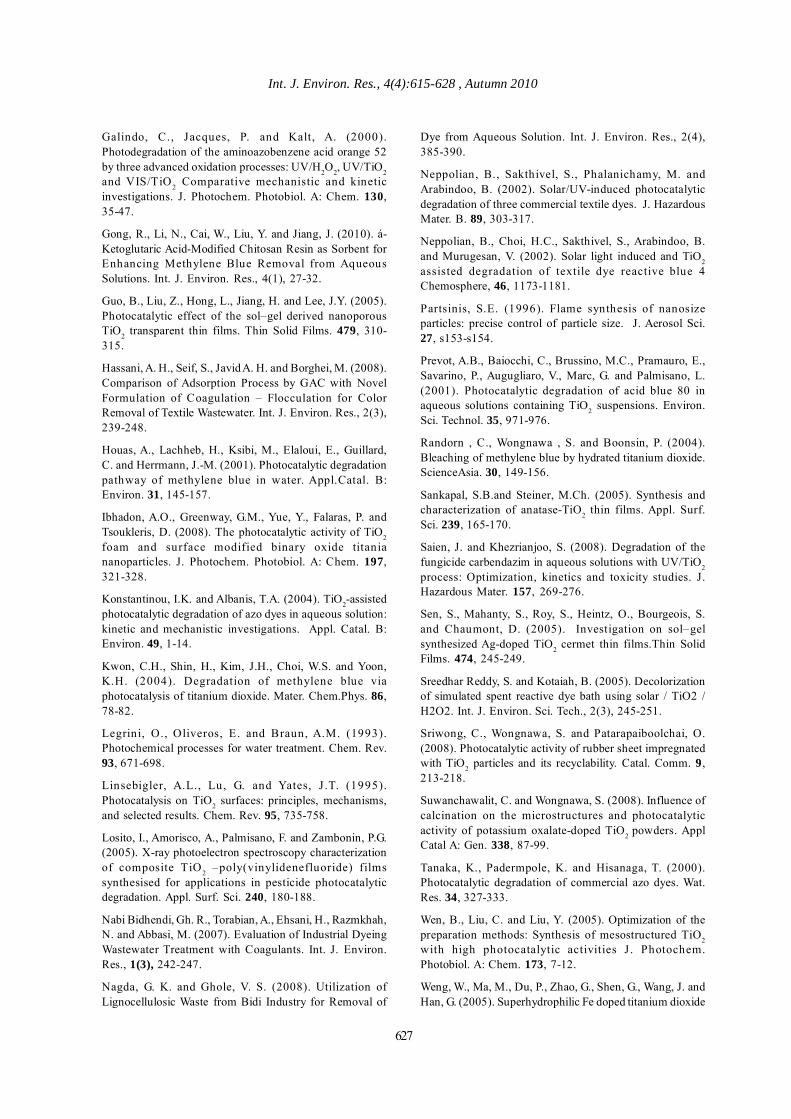
Galindo, C., Jacques, P. and Kalt, A. (2000).Photodegradation of the aminoazobenzene acid orange 52by three advanced oxidation processes: UV/H2O2, UV/TiO2and VIS/TiO2 Comparative mechanistic and kineticinvestigations. J. Photochem. Photobiol. A: Chem. 130,35-47.
Gong, R., Li, N., Cai, W., Liu, Y. and Jiang, J. (2010). á-Ketoglutaric Acid-Modified Chitosan Resin as Sorbent forEnhancing Methylene Blue Removal from AqueousSolutions. Int. J. Environ. Res., 4(1), 27-32.
Guo, B., Liu, Z., Hong, L., Jiang, H. and Lee, J.Y. (2005).Photocatalytic effect of the sol–gel derived nanoporousTiO2 transparent thin films. Thin Solid Films. 479, 310-315.
Hassani, A. H., Seif, S., Javid A. H. and Borghei, M. (2008).Comparison of Adsorption Process by GAC with NovelFormulation of Coagulation – Flocculation for ColorRemoval of Textile Wastewater. Int. J. Environ. Res., 2(3),239-248.
Houas, A., Lachheb, H., Ksibi, M., Elaloui, E., Guillard,C. and Herrmann, J.-M. (2001). Photocatalytic degradationpathway of methylene blue in water. Appl.Catal. B:Environ. 31, 145-157.
Ibhadon, A.O., Greenway, G.M., Yue, Y., Falaras, P. andTsoukleris, D. (2008). The photocatalytic activity of TiO2foam and surface modified binary oxide titaniananoparticles. J. Photochem. Photobiol. A: Chem. 197,321-328.
Konstantinou, I.K. and Albanis, T.A. (2004). TiO2-assistedphotocatalytic degradation of azo dyes in aqueous solution:kinetic and mechanistic investigations. Appl. Catal. B:Environ. 49, 1-14.
Kwon, C.H., Shin, H., Kim, J.H., Choi, W.S. and Yoon,K.H. (2004). Degradation of methylene blue viaphotocatalysis of titanium dioxide. Mater. Chem.Phys. 86,78-82.
Legrini, O., Oliveros, E. and Braun, A.M. (1993).Photochemical processes for water treatment. Chem. Rev.93, 671-698.
Linsebigler, A.L., Lu, G. and Yates, J .T. (1995).Photocatalysis on TiO2 surfaces: principles, mechanisms,and selected results. Chem. Rev. 95, 735-758.
Losito, I., Amorisco, A., Palmisano, F. and Zambonin, P.G.(2005). X-ray photoelectron spectroscopy characterizationof composite TiO2 –poly(vinylidenefluoride) filmssynthesised for applications in pesticide photocatalyticdegradation. Appl. Surf. Sci. 240, 180-188.
Nabi Bidhendi, Gh. R., Torabian, A., Ehsani, H., Razmkhah,N. and Abbasi, M. (2007). Evaluation of Industrial DyeingWastewater Treatment with Coagulants. Int. J. Environ.Res., 1(3), 242-247.
Nagda, G. K. and Ghole, V. S. (2008). Utilization ofLignocellulosic Waste from Bidi Industry for Removal of
Dye from Aqueous Solution. Int. J. Environ. Res., 2(4),385-390.
Neppolian, B., Sakthivel, S., Phalanichamy, M. andArabindoo, B. (2002). Solar/UV-induced photocatalyticdegradation of three commercial textile dyes. J. HazardousMater. B. 89, 303-317.
Neppolian, B., Choi, H.C., Sakthivel, S., Arabindoo, B.and Murugesan, V. (2002). Solar light induced and TiO2assisted degradation of textile dye reactive blue 4Chemosphere, 46, 1173-1181.
Partsinis, S.E. (1996). Flame synthesis of nanosizeparticles: precise control of particle size. J. Aerosol Sci.27, s153-s154.
Prevot, A.B., Baiocchi, C., Brussino, M.C., Pramauro, E.,Savarino, P., Augugliaro, V., Marc, G. and Palmisano, L.(2001). Photocatalytic degradation of acid blue 80 inaqueous solutions containing TiO2 suspensions. Environ.Sci. Technol. 35, 971-976.
Randorn , C., Wongnawa , S. and Boonsin, P. (2004).Bleaching of methylene blue by hydrated titanium dioxide.ScienceAsia. 30, 149-156.
Sankapal, S.B.and Steiner, M.Ch. (2005). Synthesis andcharacterization of anatase-TiO2 thin films. Appl. Surf.Sci. 239, 165-170.
Saien, J. and Khezrianjoo, S. (2008). Degradation of thefungicide carbendazim in aqueous solutions with UV/TiO2process: Optimization, kinetics and toxicity studies. J.Hazardous Mater. 157, 269-276.
Sen, S., Mahanty, S., Roy, S., Heintz, O., Bourgeois, S.and Chaumont, D. (2005). Investigation on sol–gelsynthesized Ag-doped TiO2 cermet thin films.Thin SolidFilms. 474, 245-249.
Sreedhar Reddy, S. and Kotaiah, B. (2005). Decolorizationof simulated spent reactive dye bath using solar / TiO2 /H2O2. Int. J. Environ. Sci. Tech., 2(3), 245-251.
Sriwong, C., Wongnawa, S. and Patarapaiboolchai, O.(2008). Photocatalytic activity of rubber sheet impregnatedwith TiO2 particles and its recyclability. Catal. Comm. 9,213-218.
Suwanchawalit, C. and Wongnawa, S. (2008). Influence ofcalcination on the microstructures and photocatalyticactivity of potassium oxalate-doped TiO2 powders. ApplCatal A: Gen. 338, 87-99.
Tanaka, K., Padermpole, K. and Hisanaga, T. (2000).Photocatalytic degradation of commercial azo dyes. Wat.Res. 34, 327-333.
Wen, B., Liu, C. and Liu, Y. (2005). Optimization of thepreparation methods: Synthesis of mesostructured TiO2with high photocatalytic activities J . Photochem.Photobiol. A: Chem. 173, 7-12.
Weng, W., Ma, M., Du, P., Zhao, G., Shen, G., Wang, J. andHan, G. (2005). Superhydrophilic Fe doped titanium dioxide
Int. J. Environ. Res., 4(4):615-628 , Autumn 2010
627

thin films prepared by a spray pyrolysis deposition. Surf.Coat. Tech. 198, 340-344.
Yang, J.H., Han, Y.S. and Choy, J.H. (2006). TiO2 thin-films on polymer substrates and their photocatalyticactivity. Thin Solid Films. 495, 266-271.
Zhiyong, Y., Laub, D., Bensimon, M. and Kiwi, J. (2008).Flexible polymer TiO2 modified film photocatalysts activein the photodegradation of azo-dyes in solution. Inorg.Chim. Acta. 361, 589–594.
Zhiyong, Y., Keppner, H., Laub, D., Mielczarski, E.,Mielczarski, J., Kiwi-Minsker, L., Renken, A. and Kiwi, J.(2008). Photocatalytic discoloration of Methyl Orange oninnovative parylene–TiO2 flexible thin films under simulatedsunlight. Appl.Catal. B: Environ. 79, 63-71.
Suwanchawalit, Ch. et al.
628

Int. J. Environ. Res., 4(4):629-636 , Autumn 2010ISSN: 1735-6865
Received 22 Feb. 2008; Revised 15 April 2010; Accepted 25 April 2010
*Corresponding author E-mail: [email protected]
629
Heavy Metal Pollution in Kabini River Sediments
Taghinia Hejabi, A.*, Basavarajappa, H.T. and Qaid Saeed, A. M.
Department of Studies in geology, University of Mysore, MGM-06, Karnataka, India
ABSTRACT: The river Kabini which is tributary of Cauvery drains through industrial area at Nanjangud,Karnataka. Out of the sediment load carried by the river, 2micron the clay fraction was analyzed for totalheavy metal contents and advanced statistical techniques such as cluster analysis and correlation matrix wereapplied in order to investigate the source of heavy metal concentration in the sediments. The river carriesnatural and anthropogenic pollutants, mainly heavy metal concentration of Cd, Cr, Cu, Fe, Mn, Ni, Pb and Znwhich are released from industrial effluents, agricultural return flows and domestic sewage. The heavy metalsfind their residence in the colloidal form in water and in 2micron clay fraction in the river bed sediments.Systematic sampling of the river bed sediments at predefined locations has revealed that the metal accumulationis very close to normal and also beyond threshold limits. Compared with the maximum background values inKabini river sediment, Pb was the highest in terms of contamination level, especially at point of influx of papermill effluents, followed by Zn and Cu.
Key words: Kabini River, Sediments, Heavy Metals, Physico-Chemical, Accumulation
INTRODUCTIONHeavy metals in aquatic system and sediments have
natural and anthropogenic origin; distribution andaccumulation of metals are influenced by mineralogicalcomposition, sediment texture, adsorption, desorptionprocesses and oxidation - reduction state and physicaltransport. Moreover, metals can be adsorbed from thewater column into/on fine particle surfaces and laterreside and move thereafter towards sediment matrices.Metals also participate in various biogeochemicalprocesses, have significant mobility, can affect theecosystems through bio-accumulation and bio-magnification processes and are potentially toxic forenvironment and for human life (Manahan, 2000; AbdulAziz et al., 2010; Hasan et al., 2010; Resmi et al., 2010;Ahmad et al., 2010; Ahmed and Al-Hajri, 2009; Gaur andDhankhar, 2009). As a combined result of these factors,metal concentrations in sediments change, with spaceand time. In fact, during the last few decades, industrialand urban activities have contributed to the increase ofmetal contamination into aquatic environment and havedirectly influenced the coastal ecosystems. Variousstudies have demonstrated that aquatic sediments arecontaminated by heavy metals from industrialized coastalareas; therefore, the evaluation of metal distribution insurface sediments is useful to assess pollution in theaquatic environment (Solomons and Forstner, 1984;
Zonta et al., 1994, Bellucci et al., 2002). Different studieshave widely confirmed the serious contamination ofriver sediment by heavy metals (Priju and Narayana,2007; Nabi Bidhendi et al., 2007; Dixit and Tiwari, 2008;Mumba et al., 2008; Kashulin et al., 2008; Mensi et al.,2008; Akoto et al., 2008; Venugopal et al., 2009; Biati etal., 2010; Nouri et al., 2010; Øygard and Gjengedal, 2009).Further studies have been conducted to evaluate thedistribution and speciation of heavy metals insediments. (Buccolieri et al. ,2006; Carman et al. ,2006;Acevedo-Figueroa et al. ,2006; Karbassi et al. ,2007;Yang et al.,2009; Cuculic et al. ,2009). Furthermore, lotsof bioassays have indicated the influence of heavymetals on various organisms from different points ofview (Murugesan et al., 2008; Opuene and Agbozu,2008; Vinodhini and Narayanan, 2009; Shetty andRajkumar, 2009; Abdullahi et al., 2009; Uba et al., 2009;Rahmani et al., 2009). In India, previous studies in MuleHole, Cauvery and Brahmaputra and Cauvery riverbasins have focused on mineralogical, geochemical andgeophysical studies and chemical composition ofsediments (Subramanian et al., 1988; Dekov et al., 1998;Braun et al., 2009). In Mysore, Karnataka the KabiniRiver is a good example of a site where contributions ofpollutants from natural (lithogenic) sources andanthropogenic activity and contribute pollutants twoto three fold over values.

630
Taghinia Hejabi, A. et al.
The purpose of this paper is to determine thegeochemistry, physico-chemical properties and heavymetal thresholds in the Kabini river sediments with anaim to provide additional data and investigate thepresent level of metal in the area. The Kabini river, aconfluence of the tributaries from Panamaram andMananthavady area originate from western Ghats inthe Wynad district of Kerala and passes through theNanjangud industrial area and flows into the main riverCauvery with its confluence at T.Narasipura downstream. The area lies between north latitude 11° 45-12° 30 and east longitude 75° 45- 77° 00.
MATERIALS & METHODSRiver bed sediments were collected from the surface
along its main stream in the month of April 2009 atseventeen predetermined locations based on GPS (Fig1). Sampling stations were chosen to provide goodarea coverage of the background and anthropogenicinput values. After sampling, sediments were stored ina plastic vials and frozen at -20° C pending analytical
procedures. In the laboratory, sediment samples weredefrosted at room temperature, dried at 40 °C up to aconstant weight, ground and homogenized in a mortarto a fine powder. Total metals (Cd++, Cr+3, Cu++, Mn++,Ni++ ,Pb++, Fe+3and Zn++) were determined by AtomicAbsorption Spectrophotometer technique after aciddigestion. For digestion, 2 g of dried sample was putinto a PTFE vessel with 4 ml of nitric acid, 2 ml ofhydrochloric acid and 2 ml of hydrofluoric acid. Foreach digestion program, a blank was prepared with thesame amount of acids. After digestion and coolingbelow extractor hood, samples were filtered and dilutedto 100 ml with distilled water and analyzed (Minoia etal., 1993; Daskalova and Boevski, 1999; Mermet, 2001;Bettinelli et al., 2000). Physico-Chemical characteristicsincluding pH, electrical conductivity, Ca++, Mg++, Na+,K+ were analyzed by standard methods given byTrivedy and Goel (1986), APHA (1992).
To identify the association between metals, basicstatistical tools such as cluster analysis (CA) wasexploited on raw data through using MVSP software.
Study area
2 315
4
6 78
9 10
11
12
13
14
15
16 17
76°
40
45
50
55
12°15
10
5
40
45
50
55
76°
5
10
12° 15
Fig.1. Sample location map of the study area

Int. J. Environ. Res., 4(4):629-636 , Autumn 2010
631
Table 1. Physico-Chemical Characteristics of water at sampling point in Kabini river-April 2009
No. Location pH Ec Hardness (mg/lit)
Ca (mg/lit)
Mg (mg/lit)
Na (mg/lit) K (mg/lit)
1 N.Kattavadipura 8.48 250 544 400 144 31.3 34 2 Chikkayyana Chatra 7.70 327 448 288 160 10.7 12.7 3 Paper mills 7.95 396 740 524 216 16.7 10.8 4 Bridge 8.67 67 188 184 4 8.8 4.9 5 E.Kattavadipura 9.04 82 256 120 136 16.8 5.7 6 Byalaru 8.49 78 220 132 88 9.1 19.5 7 Deburu 8.24 124 432 208 224 21.9 24.7 8 Kallahalli 8.41 68 172 124 48 7.8 6.4 9 Nanjangud Temple 8.76 62 180 148 32 16.7 7.8 10 Hejijige 8.5 135 400 184 216 33.8 30.4 11 Mullur 7.91 64 204 168 36 20.6 4.8 12 Suttur 7.31 64 280 172 108 7.4 10.6 13 Thayur 8.29 112 400 188 212 19.6 35.8 14 Bilagale 8.27 74 208 92 116 1.5 3.8 15 T.Narasipura 8.41 240 220 132 88 5.6 3.4 16 Kabini 8.40 238 400 60 340 6.7 1.2 17 Confluence Cavery &
Kabini river 8.46 233 168 100 68 1 1.4
Parameter Level (mg/Kg) Arsenic 41.6 Cadmium 4.21 Chromium 160 Copper 108 Lead 112 Mercury 0.7 Zinc 271
RESULTS & DISCUSSIONThere were obvious differences in several
measured parameters when the resul ts werecompared from site to site. The results of measuredphysico-chemical parameters are presented in Table2. The pH of the river sediments vary from 7.31 to9.04, indicating alkaline nature of the Kabini River.There was also significant difference in electricalconductivity values between the sampling sites (62-396 µmho). High concentrations of exchangeablecations were found in all the samples without anysignificant difference in the obtained values, exceptfor station 10. There was significant difference incalcium and magnesium values between thesampling sites. However, the calcium values werefound higher than magnesium in most of the samplingsites .The highest value of the calcium was observedat station 1 (400 mg/lit). Generally, the higher calciumcontents are attributable to microorganisms whichplay an important role in the calcium exchange atthe interface between sediment and overlying water(Elewa, 1988). The value of sodium contents were (1to 33.8 mg/lit) and significant difference wasobserved in sodium values. High concentrations ofpotassium is noticed in the station 1 (34 mg/lit) withsignificant difference in the obtained values indifferent station.
Table 3 shows the SQGs guideline that it is veryuseful to screen sediment contaminat ion bycomparing sediment contaminant concentration withthe corresponding quality guideline.(Caeiro etal.,2005). Bottom sediments have a high absorptioncapacity with regard to trace elements, and in fact, itis the bottom sediment that is one of the main factors
of water body self-purification from heavy metalcompounds. Fig. 2 represents bottom sediment heavymetal parameters. Transitional metals, in particular,Fe and Mn, play a very impor tan t role asmicronutrients in the biochemistry of plants andanimals. At the same time, they are classified as basictechnogenic elements. Accumulation levels of theseelements are taken into account in estimating thetechnogenic pollution (Khazheeva et al., 2004). Themaximum concentration of Fe (1381 mg/kg) wasobserved at station 3, in station 1 this value did notexceeded 1360 mg/kg and 1327 mg/kg at station 7,for the rest of the station, the value ranging of Fe is(928-1315 mg/kg). Much of the Fe content are fixedwithin the crystalline structure of primary andsecondary minerals and are totally non reactive. Alarge portion may be soluble under reducedcondition of typical anaerobic sediments and floodsoils, but essentially all of the potentially reactiveFe would be oxidized to sparingly soluble ferricoxyhydroxide under upland conditions (Gambrell etal., 1983). The maximum concentration of Mn in the
Table 2. PEL classification of Sediment qualityguideline- quotient (SQG-Q)

632
Metal Pollution in Sediments
0
50
100
150
200
250
Cu (ppm) 69.1 59.1 152.8 141.6 71.8 107.8 102.9 86.3 91.4 120.6 122.6 99.5 94.1 71.8 100 94.9 47.2Zn (ppm) 36.9 30.1 191.6 26.4 40.8 25.6 32.5 28.2 31.5 39.8 41.5 43 32 17.2 37.1 23.1 12.9Pb(ppm) 8.3 6.5 265.4 3.6 40.2 5.2 4.2 3.9 1 10.3 5.8 5.1 3.8 4.3 4.4 2.8 0
Cd (ppm) 7.75 0 0 0 0.1 0 0 0 0 0 0 0 0 0 0 0 0Cr (ppm) 24.1 23.3 48 8.6 24.6 14.9 21.9 12.4 31.8 16.4 22 16.2 50.3 48 15.7 9.4 60.7Ni (ppm) 20.6 12 21.2 3.8 4.4 3.8 13.3 4.5 6.5 6.9 11.2 10.4 11.2 7 12.1 4.5 1.2
1 2 3 4 5 6 7 8 9 10 11 12 13 14 15 16 17
1-17: Measured Stations
ppm
Fig. 2. Heavy metal Characteristics of sediments at sampling points in Kabini river April 2009
bottom sediment (435.64 mg/kg) was determined atstation 2, as well as in station 1 (227.55 mg/kg) andstation 10 ( 204 mg/kg).
Copper is an essential nutrient for plants growth,but may be toxic under certain conditions. Station 3showed significant higher concentration of copper(152.8 mg/kg) compared to that of other stations.The lowest concentration of copper is at station 7(47.2 mg/kg). As is known, the concentration of Cuin non-contaminated sea and river bottom sedimentsdoes not exceed 20 mg/kg .
The maximum value of Pb concentration in station3 (265.4) mg/kg was observed that is exceeds the SQG
Table3. Correlation matrix between metal concentrations in the area of study
Pearson Correlations CU ZN PB CD CR NI MN FE
CU 1 ZN 0.58 1 PB 0.50 0.99 1 CD -0.26 -0.024 -0.056 1 CR -0.30 0.26 0.34 -0.038 1 NI 0.25 0.63 0.54 0.52 0.14 1 MN -0.37 -0.057 -0.093 0.28 -0.097 0.27 1 FE 0.27 0.49 0.36 0.31 -0.004 0.73 0.31 1
* Correlation is significant at the 0.05 level (2-tailed). ** Correlation is significant at the 0.01 level (2-tailed).
standard level. Highest appreciable values of Znconcentration (191.6 mg/kg ) is also observed at station3,in other stations the concentration of Zn varied from12.9 to 43 mg/kg, relatively high concentration of Crwas observed at station 16 (60.7 mg/kg) whereas inother stations this value varies from 8.6-50.3 mg/kg.The concentration of Nickel at station 3 was the highestwith value of 21.2 mg/kg the lowest Ni concentrationwas at station 17 with a value of 1.2 mg/kg, value rangingfrom 3.8-20.6 mg/kg.
In the present study CA was carried out onsediment samples in order to identify similarities inmetal contents between the analyzed sediment samples.The aim in performing CA was to identify the samples
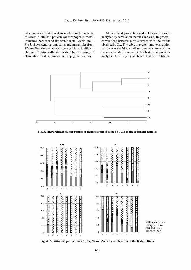
Int. J. Environ. Res., 4(4): 629-636, Autumn 2010
which represented different areas where metal contentsfollowed a similar pattern (anthropogenic metalinfluence, background lithogenic metal levels, etc.).Fig.3. shows dendrograms summarizing samples from17 sampling sites which were grouped into significantclusters of statistically similarity. The clustering ofelements indicates common anthropogenic sources.
Metal–metal properties and relationships wereanalyzed by correlation matrix (Tables 3).In general,correlations between metals agreed with the resultsobtained by CA. Therefore in present study correlationmatrix was useful to confirm some new associationsbetween metals that were not clearly stated in previousanalysis. Thus, Cu ,Zn and Pb were highly correlatable,
Fig. 3. Hierarchical cluster results or dendrogram obtained by CA of the sediment samples
Fig. 4. Partitioning patterns of Cu, Cr, Ni and Zn in 8 samples sites of the Kabini River
633

634
Taghinia Hejabi, A. et al.
which shows that Cu content in sediment was not onlydue to its presence in the parent rocks but also due toanthropogenic effluents of industrial area, andconfirms the combination of metal affiliation of variedorigin . Besides, Cd and Pb also correlated with Ni. Ithas been shown that the concentration of Pb insediments is contribution of effluents from a particularindustry involving manufacture of paints and pigmentsand on the other hand, Cd and Ni may result from avariety of industrial activities.
Metal fractionationChemical partitioning patterns for each metal and
sampling point are shown in Fig. 4. In the present study,the resistant ion was predominant for Cu, Cr, Ni andZn in most sites. For Cu and Zn, the very differentpartitioning patterns in various samples can beobserved. These metals were mostly concentrated atthe resistant ion at points 6 (39.9% for Cu) and 7 (50.7%for Zn) both in lower reaches, while at points 3 therelative percentage values in this fraction were 11.3%for Cu and 19.6% for Zn respectively. The nextimportant phase of detective was, Cu as the loose ion.Cr showed a homogeneous distribution in all samples.Cr was mostly bound to resistant ion (72.7 to 97.6%)and to loose ion (13.3– 63.6%). Only small amounts ofCr were bound to the organic fraction (1.3–18.4%). Theloose ions and sulfide ion account for less than 10%of total Cr with the exception of points 1.
The dominance of the resistant ion for Ni is clearover the other fractions (25–92%), with exception ofsampling point 4 where the loose ion fraction is
predominant (49%). The next Important phase of thiselement in the samples was the organic fraction (1.3–18.4%). The other fractions were found associated withloose ion, 3.3 49%; sulfide ion fraction, 0-21.9%.
CONCLUSIONThe major sources of pollution of the Kabini river
are the industrial effluents, (return flows), agriculturalrunoff, domestic and municipal sewage besidespedogenic background contributions. A case studywhere contamination of coconut trees by heavy metalsreleased by industrial effluents soaking soils anddraining into river Kabini near Nanjangud is on record.(Fazeli et.al.,1991). The provenance or source of heavymetals in Kabini river bed sediments (RBS) is normallyenvisaged as additional inputs from anthropogenicsources over and above natural or lithogenic sources.The heavy metal averages of RBS are above and moreconcentrated than the combined averages contributedby lithogenic sources .Table 4 gives the sources ofheavy metals, the matrices involved and the mechanismof pollutants entering various matrices. Kabini Riveris degraded in quality due to the industrial dischargeand anthropogenic effluents. In this study, hierarchicalclustered analysis helped to show that groups ofelements were significantly interrelated. Also,partitioning study indicate the metals under study werepresent mostly in the least mobilized fraction to theoverlying water and it is assumed that trace metals inthese sediments are to a great extent derived fromderived from multisource anthropogenic inputs besidesgeochemical background contributions . In addition,
Source category
Pollutant types
Provenance (source) point Non point
Cu Cd Cr Ni Co Pb Zn Fe Mn
Matrices involved
Mechanism of pollution
A. NATURAL (LITHOGENIC) Amphibolites Granites, Gneisses, Ultra basic rocks & Carbonates
River water, Suspended load, bed sediment Soil, Ground water, Biomass
Dissolution Suspension Deposition Reprecipitation
B. ANTHROPOGENIC 1- Industrial a) Textile b) Paper c) Distil lery d) Miscellaneous
Soil, Suspended load Bed Sediment Biomass
Flows, Land spreading, Soaking, Sorption, CEC, Seepage, Plumes, Suspension
2- Municipal a) Sewage effluent b) Sewage sludge c) Garbage dumps
Suspended load Bed sediment Soil, Ground water
Mixing, Dispersion, Soaking, Sorption, Seepage
3- Agricultural a) Return flows b) Stockpiles
Table 4. Sources of heavy metals in river bed sediments of Kabini River
635
Int. J. Environ. Res., 4(4):629-636 , Autumn 2010
analysis indicates that Cu was not only due to weatheringof parent rocks but also due to anthropogenic effluentof industrial area and other pollutants contributed to theriver. Whereas Zn originated from the discharge at pointsources pollutants along the river, particularly in theindustrial area, Pb showed the anthropogenic sourcesof heavy metal in the sediments. It could have comefrom non- point sources such as atmospheric deposition(aerosols carrying insecticides and pesticides) andsurface draining toxic chemicals within industrial areas.Although total amounts of the heavy metals investigatedwere found to be normal, those station showingaccumulation beyond threshold limits presented by SQGstandard level, assumes greater significance. Somemeasured stations show anomalies in heavy metal levelsaccumulations beyond threshold limits posing potentialdanger and contamination and possibility reentering intoaquatic and solid food chain. It may, however be addedthat higher metal values might also be contributions fromthe already adsorbed metals in the deposited sedimentsdue to turbulence generated by scavenging organismsat the sediment water interface.
ACKNOWLEDGEMENTSThe authors are thankful to the Department of
Studies in Geology, University of Mysore for theencouragement extended for this study. Special thanksto Dr.Karbassi for guidance during the course of thispaper and Prof. Sathyanarayan for useful discussionalso Mr.B.M. Prakash, Mr.H.M.ShivaKumar and Mr.S.Mohan Kumar in Karnataka State Pollution ControlBoard for their assistance in the analytical techniques.
REFERENCESAbdul Aziz, H., Omran, A. and Zakaria, W. R. (2010). H2O2Oxidation of Pre-Coagulated Semi Aerobic Leachate. Int. J.Environ. Res., 4 (2), 209-216.
Abdullahi, M. S., Uzairu, A. and Okunola, O. J. (2009).Quantitative Determination of Heavy Metal Concentrations inOnion Leaves. Int. J. Environ. Res., 3 (2), 271-274.Acevedo-Figueroa, D. (2006). Trace metals in sediments oftwo estuarine lagoons from Puerto Rico. Environmentalpollution, 141 (2), 336-342.
Ahmad, M. K., Islam, S., Rahman, S., Haque, M. R. and Islam,M. M. (2010). Heavy Metals in Water, Sediment and SomeFishes of Buriganga River, Bangladesh. Int. J. Environ. Res., 4(2), 321-332.
Ahmed, T. A. and Al-Hajri, H. H. (2009). Effects of TreatedMunicipal Wastewater and Sea Water Irrigation on Soil andPlant Characteristics. Int. J. Environ. Res., 3 (4), 503-510.
Akoto, O., Ephraim, J. H. and Darko, G. (2008). Heavy MetalsPollution in Surface Soils in the Vicinity of Abundant RailwayServicing Workshop in Kumasi, Ghana. Int. J. Environ. Res., 2(4), 359-364.
APHA. (1992). Standard Methods for the Examination ofWater and Wastewater. American Public Health Asociation,Washington, DC.
Bellucci, L.G., Frignani, M., Paolucci, D. and Ravanelli, M.(2002). Distribution of heavy metals in sediments of the VeniceLagoon: the role of the industrial area. The Science of the TotalEnvironment, 295, 35– 49.Bettinelli, M., Beone, G.M., Spezia, S. and Baffi, C. (2000).Determination of heavy metals in soils and sediments bymicrowave-assisted digestion and inductively coupled plasmaoptical emission spectrometry analysis. Analytica ChimicaActa , 424, 289– 296.
Biati, A., Moattar, F., Karbassi, A.R. and Hassani, A.H. (2010).Role of Saline Water in Removal of Heavy Elements fromIndustrial Wastewaters. Int. J. Environ. Res., 4 (1), 177-182.Braun, jean-jacques, Descloîtres, Marc, Riotte, Jean, Fleury,S., Barbiero, Laurent, Boeglin, Jean-loup, Violette, A., Lacarce,E., Ruiz, Laurent, Sekhar, M., Kumar, M. S. M., Subramanian,S. and Dupré, Bernard (2009). Regolith mass balance inferredfrom combined mineralogical, geochemical and geophysicalstudies: Mule Hole gneissic watershed, South India.Geochemical et Cosmochimica Acta,73 (4), 935-961.Buccolieri, A., Buccolieri, G., Cardellicchio, N., Dell’Atti, A.,Di Leo, A. and Maci, A. (2006). Heavy metals in marinesediments of Taranto Gulf (Ionian Sea, Southern Italy). MarineChemistry journal , 99, 227–235.
Caeiro, S., Costa, M. H., Barros, T. B., Fernandes, F., Silveira,N., Coimbra, A., Medeiros, G. and Painho, M. (2005).Assessing heavy metal contamination in Sado Estuarysediment: An index analysis approach. Ecological Indicatorsjournal, 5, 151–169.Cuculic, Vlado, Cukrov, Neven, Kwokal, Zeljko and Mlakar,Marina (2009).Natural and anthropogenic sources of Hg, Cd,Pb, Cu and Zn in seawater and sediment of Mljet NationalPark, Croatia Estuarine. Coastal and Shelf Science journal ,81, 311–320
Daskalova, N. and Boevski, I. (1999). Spectral interferences inthe determination of trace elements in environmental materialsby inductively coupled plasma atomic emission spectrometry.Spectrochimica Acta, Part B 54, 1099– 1122.Dixit, S. and Tiwari, S. (2008). Impact Assessment of HeavyMetal Pollution of Shahpura Lake, Bhopal, India. Int. J.Environ. Res., 2 (1), 37-42.
Dekov, V. M. (1998). Chemical composition of sediments andsuspended matter from the Cauvery and Brahmaputra rivers(India). The Science of The Total Environment, 212 (2-3), 89-105.Elewa, A. A. (1988). Influence of oxidation reduction potentialin the water environmental of Aswan High Dam Reservoir.Water Res. Development., 4 (3),184-190.Fazeli, M.S., Sathyanarayan, S., Satish, P.N. and Lata,Muthanna (1991). Effect of paper mill effluents onaccumulation of heavy metals in coconut trees near Nanjangud,Maysore district ,Karnataka ,India. Environmental geologyand water science, 17 (1),47-50.
Gambrell,. R.P, Reddy, C.N. and Khalid, R.A. (1983).Characterization of trace and toxic materials in sediments of a
636
Metal Pollution in Sediments
lake being restored. Journal of Water Pollution ControlFederation, 55 (9),121– 1210.
Gaur, N. and Dhankhar, R. (2009). Removal of Zn+2 ionsfrom aqueous solution using Anabaena variabilis. Equilibriumand Kinetic studies. Int. J. Environ. Res., 3 (4), 605-616.
Hasan, M.A.A., Ahmed, M.K., Akhand, A. A., Ahsan, N. andIslam, M.M. (2010). Toxicological Effects and Molecular ChangesDue to Mercury Toxicity in Freshwater Snakehead ( Channapunctatus Bloch, 1973). Int. J. Environ. Res., 4 (1), 91-98.
Ip, C. C. M., Li, X. D., Zhang, G., Wai, O. W. H. and Li, Y. S.(2007). Trace metal distribution in sediments of the Pearl RiverEstuary and the surrounding coastal area, South China.Environmental Pollution journal, 147, 311-323.
Karbassi, A. R, Monavari, S. M., Nabi Bidhendi, Gh. R. ,Nouri ,J. and Nematpour , K. (2008). Metal pollutionassessment of sediment and water in the Shur River. Environ.Monit. Assess. journal, 147, 107–116.
Kashulin, N. A., Terentiev, P. M. and Koroleva, I. M. (2008).The status of whitefish population from Chuna Lake in theLapland Biosphere Reserve Russia. Int. J. Environ. Res., 2 (2),111-124.
Khazheeva, Z. I., Urbazaeva, S. D., Bodoev, N. V., Radnaeva,L. D. and Kalinin Y. O. (2004). Heavy Metals in the Water andBottom Sediments of the Selenga River Delta. Water Resources,31 (1), 64-67.
Linnik, P. N. and Nabivanets, B.I. (1986). Formy MigratsiiMetallovv Presnykh Poverkhnostnykh Vodakh (Forms ofMigration of Metals in Fresh Surface Waters). Leningrad,Gidrometeoizdat.
MacDonald, D. D., Carr, S., Clader, F. D., Long, E. D. andIngersoll, C. G. (1996). Development and evaluation of sedimentquality guidelines for Florida coastal waters. Ecotoxicology, 5,253–27.
Manahan, S. E. (2000). Environmental Chemistry. SeventhEdition, Lewis Publishers, CRC Press LLC, 898.
Mensi, Gh. S., Moukha, S., Creppy, E. E. and Maaroufi, K.(2008). Metals Accumulation in Marine Bivalves and Seawaterfrom theLagoon of Boughrara in Tunisia (North Africa). Int. J.Environ. Res., 2 (3), 279-284.
Mermet, J. M. (2001). Qualities related to spectra acquisitionin inductively coupled plasma–atomic emission spectrometry.Spectrochimica Acta, Part B 56, 1657–1672.
Minoia, C., Bettinelli, M. and Sabbioni, E. (1993). Applicazionidell’ICP– AES nel laboratorio chimico e tossicologico. MorganEdizioni Tecniche, Milan, Italy, 860.
Moor, J. and Ramamoorthy, S. (1984).Heavy Metals in NaturalWaters, Applied Monitoring and Impact Assessment. NewYork, Springer.
Mumba, P. P., Chibambo, B. Q. and Kadewa, W. (2008). AComparison of The Levels of Heavy Metals in CabbagesIrrigated With Reservoir and Tap Water. Int. J.. Environ. Res.,2 (1), 61-64.
Murugesan, A. G., Maheswari, S. and Bagirath, G. (2008).Biosorption of Cadmium by Live and Immobilized Cells ofSpirulina Platensis. Int. J. Environ. Res., 2 (3), 307-312.
Nabi Bidhendi, G. R., Karbassi, A. R., Nasrabadi, T. and Hoveidi,H. (2007). Influence of copper mine on surface water quality.Int. Journal. Environ. Sci. Tech., 4 (1), 85-91.
Nouri, J., Mahvi, A. H. and Bazrafshan, E. (2010). Applicationof Electrocoagulation Process in Removal of Zinc and CopperFrom Aqueous Solutions by Aluminum Electrodes. Int. Journal.Environ. Res., 4 (2), 201-208.
Ong,. M. C. and Kamaruzzaman, B. Y. (2009). An Assessmentof Metals (Pb and Cu) Contamination in Bottom Sedimentfrom South China Sea Coastal Waters, Malaysia. AmericanJournal of Applied Sciences, 6 (7),1418-1423.
Opuene, K. and Agbozu, I. E. (2008). Relationships BetweenHeavy Metals in Shrimp ( Macrobrachium felicinum and MetalLevels in The Water Column and Sediments of Taylor Creek.Int. J. Environ. Res., 2 (4), 343-348.
Øygard, J. K. and Gjengedal, E. (2009). Uranium in MunicipalSolid Waste Landfill Leachate. Int. J. Environ. Res., 3 (1), 61-68.
Priju, C. P. and Narayana, A. C. (2007). Heavy and TraceMetals in Vembanad Lake Sediments. Int. J. Environ. Res., 1(4), 280-289.
Rahmani, K., Mahvi, A. H., Vaezi, F., Mesdaghinia, A.R.,Nabizade, R. and Nazmara, Sh. (2009). Bioremoval of Lead byUse of Waste Activated Sludge. Int. J. Environ. Res., 3(3), 471-476.
Resmi, G., Thampi, S. G. and Chandrakaran, S. (2010).Brevundimonas vesicularis. A Novel Bio-sorbent for Removalof Lead from Wastewater. Int. J. Environ. Res., 4 (2), 281-288.
Shetty, R. and Rajkumar, Sh. (2009). Biosorption of Cu (II) byMetal Resistant Pseudomonas sp. Int. J. Environ. Res., 3 (1),121-128.
Solomons, W. and Forstner, U. (1984). Metals in theHydrocycle. Springer Verlag, Berlin, 349.
Subramanian, V., Grieken R.V. and Dack, L.V. (1988). Heavymetals distribution in the sediments of Ganges and Brahmaputrarivers. Environ. Geol. Water Sci., 9, 93-103.
Trivedy, R. K. and Goel, P. K. (1986). Chemical and BiologicalMethods for Water Pollution Studies. EnvironmentalPublications, Karad.
Uba, S., Uzairu, A. and Okunola, O. J. (2009). Content ofHeavy Metals in Lumbricus Terrestris and Associated Soils inDump Sites. Int. J. Environ. Res., 3 (3), 353-358.
Venugopal, T., Giridharan, L. and Jayaprakash, M. (2009).Characterization and Risk Assessment Studies of Bed Sedimentsof River Adyar-An Application of Speciation Study. Int. J.Environ. Res., 3 (4), 581-598.
Vinodhini, R. and Narayanan, M. (2009). Heavy Metal InducedHistopathological Alterations in Selected Organs of theCyprinus carpio L.(Common Carp). Int. J. Environ. Res., 3(1), 95-100.
Zonta, R., Zaggia, L. and Argese, E. (1994). Heavy metal andgrain-size distribution in estuarine shallow water sediments ofthe Cona Marsh (Venice, Lagoon, Italy). The Science of theTotal Environment, 151, 19– 28.
Int. J. Environ. Res., 4(4):637-646 , Autumn 2010ISSN: 1735-6865
Received 4 Aug. 2009; Revised 15 Dec. 2009; Accepted 12 April 2010
*Corresponding author E-mail: [email protected]
637
Corporations Response to the Energy Saving and Pollution Abatement Policy
Xing, L.1, Shi, L.2* and Hussain, A.3
1School of Environment and Natural Resources, Renmin University of China, Beijing 100872, P. R. China& Asia Research Centre, The London School of Economics and Political Science,
London WC2A 2AE, UK2School of Environment and Natural Resources, Renmin University of China, Beijing 100872, P. R. China
3Asia Research Centre, the London School of Economics and Political Science, London WC2A 2AE, UK
ABSTRACT: As the main actor of implementing energy saving and pollution abatement, corporations andtheir response to the policy are studied in this paper. We find that corporate properties as scale, ownership,current environmental performance on energy using and pollution, target market and listed situation haveimpact on the corporate responding conduct and progress. Especially, current environmental performance hasstrong relationship with corporate policy responding performance, corporations with low energy efficiencyperformed poorly to energy saving and those with heavy pollution level performed below average for pollutionabatement. It implicates that the national policy could contribute a lot to outdating production facilities lessenvironment-friendly under strict implementation.
Key words: Energy saving, pollution abatement, corporation, environmental performance, Qingdao, China
INTRODUCTIONMaking benefit of opportunities for sustainable
development through optimization in energy use hasbeen considered in lots of studies during recent years(Ataei and Yoo, 2010; Atabi, 2006; Rehman et al., 2009;Saffarinia and Dellavar, 2009; Lau et al., 2008; Karbassiet al., 2008; Shafie-Pour et al., 2007; Masnavi, 2007;Mehrdadi et al., 2007; Shafie-Pour Motlagh andFarsiabi, 2007). In the three decades after China’sopening, remarkable economic growth has helped Chinato be one of the most important emerging powers in theworld. However, it has not come without prices. Forexample, as the world largest emitter of wastewater, allthe seven major watersheds in China were mediallypolluted in 2007, 50.1% of which contained waterdeemed unsafe for human consumption. China is nowthe second largest energy-consuming country in theworld after the USA, consuming in total 26.5 billiontons of standard coal equivalent in 2007 (Zhang et al,2009; National Bureau of Statistics of China, 2008) withhigh energy intensity, that’s 3 times more than that ofUS, and about 7 times as that of Japanese (Hong, 2009).Due to the coal-dominated energy consumption, Chinabecomes the second source of global CO2 emission(Guan et al, 2009) as well as the largest contributor to
global SO2 emission, which makes China one of thethree major acid rain polluted area in the world (Larssenet al., 1999; Shi et al, 2008).
Therefore, to reduce pollutants emission andimprove energy efficiency is inevitable course forChina to achieve sustainable development. “Energysaving and pollution abatement policy” was approvedas two legal-bounding targets for the 11th Five Yearplanning (2006-2010) in 2006: (1) energy saving-energy intensity per GDP needs to be reduced by 20%at the end of the 11th Five-Year Plan; (2) pollutionabatement- both the emission of SO2 and COD needsto be abated by 10% at the end of the 11th Five-YearPlan.
China’s energy saving and pollution abatementhave been investigated by a number of decompositionstudies (Ma et al., 2009; Lin and Cao, 2008; Shi, 2008;Cornelius and Story, 2007; McMichael, 2007;Crompton and Wu, 2005; Karen et al., 2004; Wang,2002). Besides literatures from engineeringperspective, many studies are mainly focused onanalysis and evaluation of related management andpolicies. Philip (2009) introduced China’s energy-saving targets and evaluated related energy policies

638
Xing, L. et al.
at national level; Shi et al (2008) evaluated the potentialSO2 abatement at provincial level in China from 1990-2005 by data envelopment analysis; Wang et al (2008)and Zhang et al (2008) analyzed the implementationeffect of energy saving and pollution reduction basedon economics model; Fang and Zeng (2007) analyzedeffect and perspective of management instruments inChina for energy saving and pollution reduction andthen provided suggestions; Yang (2007) also analyzedmain barriers to energy saving in China fromgovernment’s perspective; Ma et al (2007) presented alasting effect mechanisms for China’s implementingpolicy of pollution abatement at central governmentlevel. However, existing literatures are mainly from theperspective of government, few are about analysis ofother stakeholders. Moreover, little literature focuseson corporation, which is the real power that plays animportant role in achieving the targets of energy savingand pollution abatement.
In this study, 120 corporations were surveyed inQingdao at the end of 2008 to analyze corporations’awareness, attitude and actions to the policy of energysaving and pollution abatement. Sample analysis wasin Sector 2 of this paper. Sector 3 discussed how thesecorporations thought about the importance and impactof the policy, and to what extent they did for it. InSector 4, the relationships between policy performanceand corporate properties such as scale and ownershipwere discussed. Conclusion and policy suggestion wereproposed in Sector 5 based on former results.
MATERIALS & METHODSQingdao is selected as target city in our study. As
one of the fourteen coastal cities of open economyendorsed by State Council in China, Qingdao is theproduction base of electronic equipment in China, andpetro chemistry and machinery production are othertwo dominant industries of this city. Advantageousgeographic factors together with preferential policiesattract abundant foreign investment, especially fromJapan and South Korea, in food and textile wearingapparel manufacture.With the assistance of QingdaoBureau of Environmental Protection (QBEP), 200corporations were randomly selected from database.Except for those newly closing down and rejecting theinterview, 120 samples were finally collected by face toface interview with managers and staff in charge ofenvironment related issues in surveyed corporations.Table 1 is a classification of samples, according to theirindustrial categories, scales and ownerships.
RESULTS & DISCUSSIONThe 120 corporations cover 24 industr ies
according to the secondary industrial classification inChina (since some food manufacturers also produce
beverages, the two industries “manufacture of foods”and “manufacture of beverages” were combined). Theyconsist of 25 Chinese state-owned corporations, 32Chinese private corporations, 35 foreign corporationsand 28 joint ventures. 98 corporations belong to smallscaled corporation, mainly because their capital assertsare lower than 40 million Yuan. Large corporations withcapital assert over 400 million, employment over 2000and annual sale over 300 million Yuan account 7.5%.Other 13 corporations in between are medium sized.The proportion of medium scaled corporation is veryconsistent with the statistics from Qingdao StatisticBook 2007; while the proportion of large corporationis somewhat higher, mainly because none of thoseselected large corporations rejected interview.
From the economic perspective, energy saving andpollution abatement have different impact on businesscost. However, it is hard to say which costs more-reducing energy intensity by 20% or abating SO2 andCOD emissions by 10%. It may depend on theinvestment required and marginal reduction cost toeach corporation. In this research, on one hand, thepolicy was considered as a whole in the interview ofcorporate awareness and attitude to it; on the otherhand, the authors considered their performance onenergy-saving and pollution abatement separately tomake their current situation and policy response moreaccurate.
79 corporations thought it was hindering or veryhindering to their business, in which 24 thought thenegative impact was serious. Only 18 corporationsconsidered the policy was good to the long-termdevelopment of business. See fig. 1.
Among the 18 corporations which welcomed thestricter environmental requirement, 9 are foreigncorporations (3 from US, 5 from EU and 1 from Japan);6 are joint ventures, 5 of which are dominated byAmerican, German and Japanese investment, 1 is Sino-South Korean corporation; the other 3 are all largescaled Chinese state-owned corporations. Significantgap is shown between foreign and domesticinvestment. These 18 corporations also do well inenergy using and polluting control: 12 of them haveworld advanced energy using efficiency and the other6 are leading in China; 15 corporations are slightlypolluting and the other 3 are polluting averagely.
In contrast, the most discouraged 24 corporationsare mainly small sized private ones, see fig. 1. Theyperformed poorly on energy using and pollutioncontrol. Half of these corporations have energyefficiency at or below national average, 9 of them saidthey had no idea of what level they were. According tothe staff from QBEP, they are mainly poor at it. Except

Int. J. Environ. Res., 4(4):637-646 , Autumn 2010
639
Industrial Category Number of samples Ownership Scalec
S (state-owned) a 1 P (Chinese private) 1 F (foreign invested)b 2 Processing of Food from Agricultural Products 7
J (joint venture) 3
L (large) M (medium) S (small)
0 0 7
S 4 P 2 F 5 Manufacture of Foods and Beverages 12 J 1
L S
1 11
S 3 P 2 F 7 Manufacture of Textile Wearing Apparel, Footware and Caps 14 J 2
L S
1 13
S 1 Manufacture of Wood, Bamboo, Rattan, Palm and Straw Products 2 P 1 S 2 Manufacture of Paper and Paper Products 1 P 1 S 1
F 2 Manufacture of Articles For Culture, Educat ion and Sport Activities 3 J 1 S 3
Processing of Petroleum, Coking, Processing of Nuclear Fuel 2 S 2 L 2 S 3 P 5 F 5 Manufacture of Raw Chemical Materials and Chemical Products 18 J 5
M S
8 10
Manufacture of Medicines 1 P 1 S 1 P 4 F 2 Manufacture of Chemical Fibers 9 J 3
S 9
P 2 F 1 Manufacture of Rubber 4 J 1
S 4
P 1 F 1 Manufacture of Plast ics 3 J 1
S 3
Manufacture of Non-metallic Mineral Products 1 J 1 S 1 Smelting and Pressing of Ferrous Metals 1 S 1 L 1
S 1 Smelting and Pressing of Non-ferrous Metals 2 J 1 M S
1 1
Manufacture of Metal Products 1 J 1 S 1 Manufacture of General Purpose Machinery 3 P 3 M
S 1 2
S 2 P 2 F 2 Manufacture of Special Purpose Machinery 9
J 3
S 9
Manufacture of Transport Equipment 1 S 1 L 1 S 1 P 4 F 2 Manufacture of Electrical Machinery and Equipment 8
J 1
M S
1 7
S 3 P 3 F 5
Manufacture of Communication Equipment, Computers and Other Electronic Equipment 14
J 3
L M S
2 2 10
Manufacture of Measuring Instruments and Machinery for Cultural Activity and Office Work 1 S 1 S 1
F 1 Manufacture of Artwork and Other Manufacturing 2 J 1 S 2
Production and Supply of Electric Power and Heat Power 1 S 1 L 1 Total 120
Table 1. Industrial category, ownership and scale of samples
a State-owned corporation in China is fully invested and controlled by the national or local government.b Foreign corporation here only refers to that wholly owned by foreign capital.c Classification of scale answers to the classification of corporations published by National Statistic Bureau in 2003, that is: largecorporation- total asserts >= 400 million Yuan, employees >= 2000, and annual sells >= 300 million Yuan (they are allnecessary conditions); medium- total asserts from 40 to 400 million Yuan, employees from 300 to 2000 and annual sellsbetween 30 to 300 million (all necessary conditions); others are all small corporations. If any of the 3 condition can notachieve the required standard for Large or Medium, the corporation will be classified as small one.

640
Pollution Abatement Policy
Very hindering tocorporate development,
24
Hindering to corporatedevelopment, 55
Good to the long-termcorporate development,
18No impact, 23
Scale: 23 small and 1 medium
Ownership: 18 Chinese private
Energy efficiency: 21 at national average or below
Polluting: 23 are polluting heavily or very heavily
Fig. 1. How will the policy impact my business?
Table 2. Correlation matrix of four variables
Impact Importance Energy efficiency Pollution level Impact 1.00 0.70 0.73 0.76 Importance 0.70 1.00 0.80 0.76 Energy efficiency 0.73 0.80 1.00 0.68 Pollution level 0.76 0.76 0.68 1.00
for one corporation, all other 23 corporations admittedthat they were polluting heavily or very heavily. All ofthem have to pay the pollution discharging fee, 23 ofthem has been fined for environmental pollution.
More than 75% of surveyed corporations said theenergy saving and pollution abatement policy was veryimportant or important to them. For the 29 corporationsignoring the policy importance, they all considered thepolicy was hindering or very hindering to theirbusiness. Similar to the result above, these 29corporations are all small sized: 6 of them are state-owned, 20 ones are Chinese private, 2 are South Koreancorporations and 1 is a Taiwan corporation. Also, theirperformances on energy using and pollution controlare mainly at or below the national average.Since the factors of policy impact, policy importance,current energy using efficiency and polluting levelseem to have close relationships with each other, wepresent the correlation matrix in table 2 to show theircorrelation.
High and positive correlation exists amongst thesefour variables. One reasonable hypothesis is that the
***, **, * refer to significant level at 1%, 5% and 10%; - indicates the nonzero coefficient is denied by z-test.
higher current environmental performance acorporation has, the more possible it will consider thepolicy positive and important to its business, as theenvironmental performance would contribute to itscompetition advantage. Another hypothesis is basedon the correlation between energy efficiency andpollution level- corporations having high energyefficiency is more likely to have lower pollutionemission. It is acceptable because they share manydeterminants, such as technical level, investment,managing level and environmental awareness. Besides,scale has little correlation with them.
Among 120 surveyed corporations, 40corporations had not taken any actions for energysaving, and 22.5% of surveyed corporations were no-responding to pollution abatement. One reason mightexplain the lower responding rate for energy saving is,national and local Development and ReformCommissions (DRCs), who are in charge of monitoringenergy saving process, are a sort of comprehensivedecision-making administration without enforcementpower. While pollution emission is regularly monitored
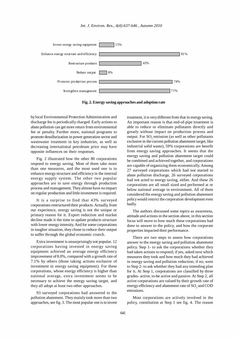
Int. J. Environ. Res., 4(4):637-646 , Autumn 2010
71%
74%
8%
43%
81%
15%
St rengthen management
Promote product ion process
Reduce out put
Restructure products
Enhance energy structure and efficiency
Invest energy saving equipment
Fig. 2. Energy saving approaches and adoption rate
by local Environmental Protection Administration anddischarge fee is periodically charged. Early actions toabate pollution can get more return from environmentalfee or penalty. Further more, national programs topromote desulfurization in power generation sector andwastewater treatment in key industries, as well asdecreasing international petroleum price may haveopposite influences on their responses.
Fig. 2 illustrated how the other 80 corporationsrespond to energy saving. Most of them take morethan one measures, and the most used one is toenhance energy structure and efficiency in the internalenergy supply system. The other two popularapproaches are to save energy through productionprocess and management. They almost have no impacton regular production and little investment is required.
It is a surprise to find that 43% surveyedcorporations restructured their products. Actually, fromour experience, energy saving is not the unique orprimary reason for it. Export reduction and marketdecline made it the time to update products structurewith lower energy intensity. And for some corporationsin tougher situation, they chose to reduce their outputto suffer through the global economic crunch.
Extra investment is unsurprisingly not popular. 12corporations having invested in energy savingequipment achieved an average energy efficiencyimprovement of 8.0%, compared with a growth rate of7.1% by others (those taking actions exclusive ofinvestment in energy saving equipment). For thesecorporations, whose energy efficiency is higher thannational average, extra investment seems to benecessary to achieve the energy saving target, andthey all adopt at least two other approaches.
93 surveyed corporations had answered to thepollution abatement. They mainly took more than twoapproaches, see fig. 3. The most popular one is to invest
treatment, it is very different from that in energy saving.An important reason is that end-of-pipe treatment isable to reduce or eliminate pollutants directly andgreatly without impact on production process andoutput. For SO2 emission (as well as other pollutantsexclusive in the current pollution abatement target, likeindustrial solid waste), 59% corporations are benefitfrom energy saving approaches. It seems that theenergy saving and pollution abatement target couldbe combined and achieved together, and corporationsare capable of organizing them economically. Among27 surveyed corporations which had not started toabate pollution discharge, 26 surveyed corporationshad not acted to energy saving, either. And these 26corporations are all small sized and performed at orbelow national average in environment. All of themconsidered the energy saving and pollution abatementpolicy would restrict the corporation development evenbadly.
The authors discussed some topics as awareness,attitude and actions in the section above, in this sectionfocus will move to how much these corporations haddone to answer to the policy, and how the corporateproperties impacted their performance.
There are two steps to assess how corporationsanswer to the energy saving and pollution abatementpolicy. Step 1- to ask the corporations whether theyhad taken actions to respond; if yes, asked next whichmeasures they took and how much they had achievedin energy saving and pollution reduction; if no, wentto Step 2- to ask whether they had any intending planfor it. At Step 1, corporations are classified by threegrades- active, to-be active and passive. At Step 2, allactive corporations are valued by their growth rate ofenergy efficiency and abatement rate of SO2 and CODemissions.
Most corporations are actively involved in thepolicy, constitution at Step 1 see fig. 4. The reason
641
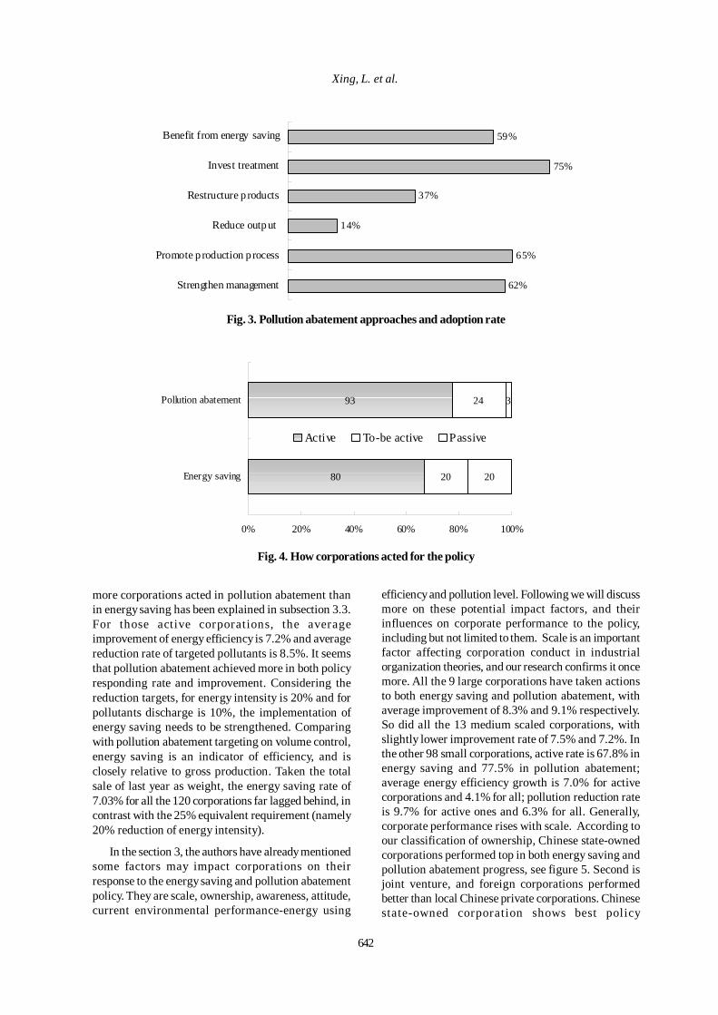
642
Xing, L. et al.
62%
65%
14%
37%
75%
59%
Strengthen management
Promote production process
Reduce output
Restructure products
Invest treatment
Benefit from energy saving
Fig. 3. Pollution abatement approaches and adoption rate
80
93
20
24
20
3
0% 20% 40% 60% 80% 100%
Energy saving
Pollution abatement
Active To-be active Passive
Fig. 4. How corporations acted for the policy
more corporations acted in pollution abatement thanin energy saving has been explained in subsection 3.3.For those active corporations, the averageimprovement of energy efficiency is 7.2% and averagereduction rate of targeted pollutants is 8.5%. It seemsthat pollution abatement achieved more in both policyresponding rate and improvement. Considering thereduction targets, for energy intensity is 20% and forpollutants discharge is 10%, the implementation ofenergy saving needs to be strengthened. Comparingwith pollution abatement targeting on volume control,energy saving is an indicator of efficiency, and isclosely relative to gross production. Taken the totalsale of last year as weight, the energy saving rate of7.03% for all the 120 corporations far lagged behind, incontrast with the 25% equivalent requirement (namely20% reduction of energy intensity).
In the section 3, the authors have already mentionedsome factors may impact corporations on theirresponse to the energy saving and pollution abatementpolicy. They are scale, ownership, awareness, attitude,current environmental performance-energy using
efficiency and pollution level. Following we will discussmore on these potential impact factors, and theirinfluences on corporate performance to the policy,including but not limited to them. Scale is an importantfactor affecting corporation conduct in industrialorganization theories, and our research confirms it oncemore. All the 9 large corporations have taken actionsto both energy saving and pollution abatement, withaverage improvement of 8.3% and 9.1% respectively.So did all the 13 medium scaled corporations, withslightly lower improvement rate of 7.5% and 7.2%. Inthe other 98 small corporations, active rate is 67.8% inenergy saving and 77.5% in pollution abatement;average energy efficiency growth is 7.0% for activecorporations and 4.1% for all; pollution reduction rateis 9.7% for active ones and 6.3% for all. Generally,corporate performance rises with scale. According toour classification of ownership, Chinese state-ownedcorporations performed top in both energy saving andpollution abatement progress, see figure 5. Second isjoint venture, and foreign corporations performedbetter than local Chinese private corporations. Chinesestate-owned corporation shows best policy
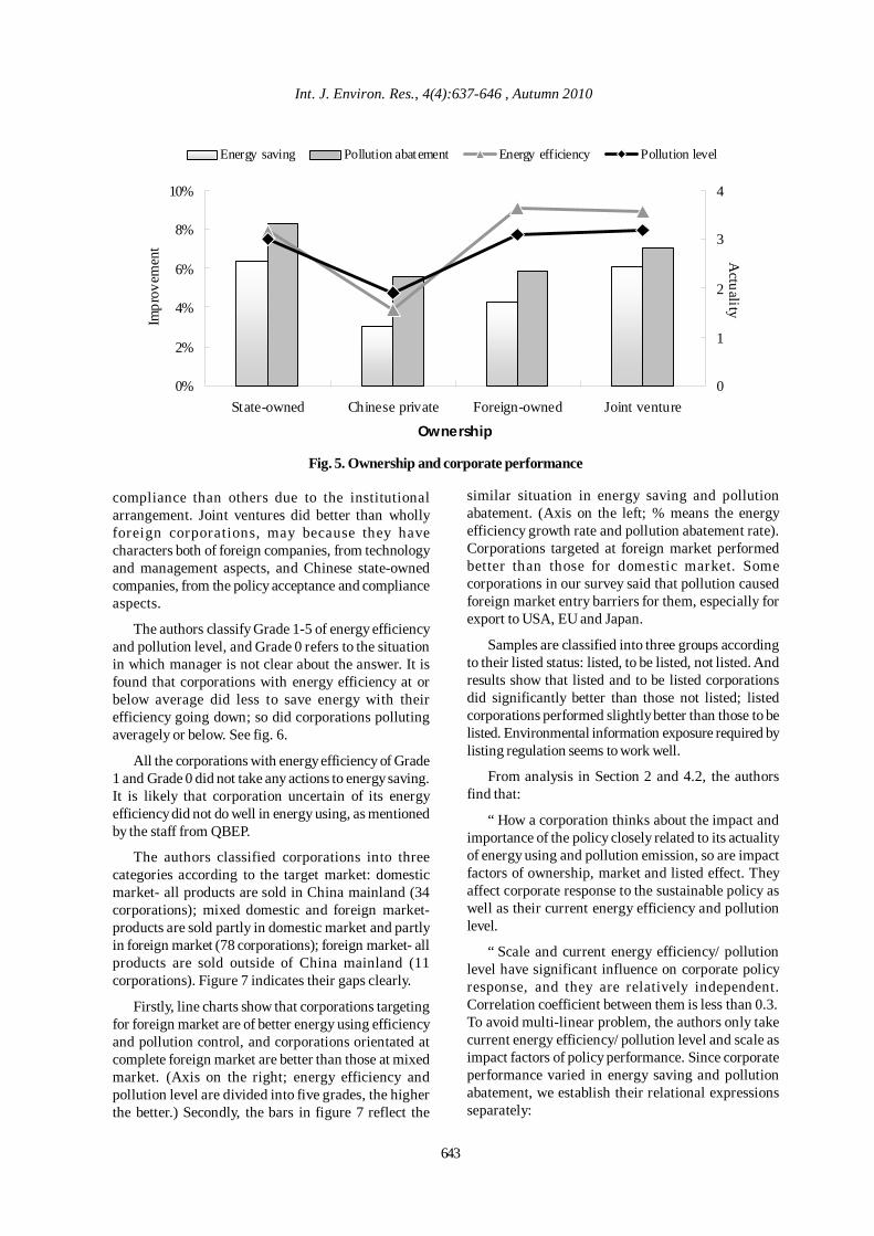
643
Int. J. Environ. Res., 4(4):637-646 , Autumn 2010
0%
2%
4%
6%
8%
10%
State-owned Chinese private Foreign-owned Joint venture
Ownership
Impr
ovem
ent
0
1
2
3
4
Actuality
Energy saving Pollution abatement Energy efficiency Pollution level
Fig. 5. Ownership and corporate performance
compliance than others due to the institutionalarrangement. Joint ventures did better than whollyforeign corporations, may because they havecharacters both of foreign companies, from technologyand management aspects, and Chinese state-ownedcompanies, from the policy acceptance and complianceaspects.
The authors classify Grade 1-5 of energy efficiencyand pollution level, and Grade 0 refers to the situationin which manager is not clear about the answer. It isfound that corporations with energy efficiency at orbelow average did less to save energy with theirefficiency going down; so did corporations pollutingaveragely or below. See fig. 6.
All the corporations with energy efficiency of Grade1 and Grade 0 did not take any actions to energy saving.It is likely that corporation uncertain of its energyefficiency did not do well in energy using, as mentionedby the staff from QBEP.
The authors classified corporations into threecategories according to the target market: domesticmarket- all products are sold in China mainland (34corporations); mixed domestic and foreign market-products are sold partly in domestic market and partlyin foreign market (78 corporations); foreign market- allproducts are sold outside of China mainland (11corporations). Figure 7 indicates their gaps clearly.
Firstly, line charts show that corporations targetingfor foreign market are of better energy using efficiencyand pollution control, and corporations orientated atcomplete foreign market are better than those at mixedmarket. (Axis on the right; energy efficiency andpollution level are divided into five grades, the higherthe better.) Secondly, the bars in figure 7 reflect the
similar situation in energy saving and pollutionabatement. (Axis on the left; % means the energyefficiency growth rate and pollution abatement rate).Corporations targeted at foreign market performedbetter than those for domestic market. Somecorporations in our survey said that pollution causedforeign market entry barriers for them, especially forexport to USA, EU and Japan.
Samples are classified into three groups accordingto their listed status: listed, to be listed, not listed. Andresults show that listed and to be listed corporationsdid significantly better than those not listed; listedcorporations performed slightly better than those to belisted. Environmental information exposure required bylisting regulation seems to work well.
From analysis in Section 2 and 4.2, the authorsfind that:
“ How a corporation thinks about the impact andimportance of the policy closely related to its actualityof energy using and pollution emission, so are impactfactors of ownership, market and listed effect. Theyaffect corporate response to the sustainable policy aswell as their current energy efficiency and pollutionlevel.
“ Scale and current energy efficiency/ pollutionlevel have significant influence on corporate policyresponse, and they are relatively independent.Correlation coefficient between them is less than 0.3.To avoid multi-linear problem, the authors only takecurrent energy efficiency/ pollution level and scale asimpact factors of policy performance. Since corporateperformance varied in energy saving and pollutionabatement, we establish their relational expressionsseparately:
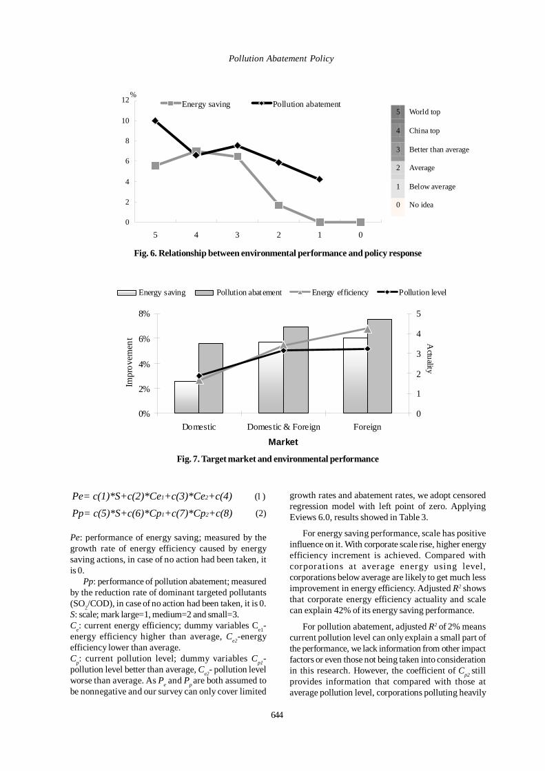
644
Pollution Abatement Policy
0
2
4
6
8
10
12
5 4 3 2 1 0
%Energy saving Pollution abatement
5 World top
4 China top
3 Better than average
2 Average
1 Below average
0 No idea
Fig. 6. Relationship between environmental performance and policy response
0%
2%
4%
6%
8%
Domestic Domes tic & Foreign Foreign
Market
Impr
ovem
ent
0
1
2
3
4
5
Actuality
Energy saving Pollution abatement Energy efficiency Pollution level
Fig. 7. Target market and environmental performance
1 2Pe= c(1)*S+c(2)*Ce +c(3)*Ce +c(4) (1)
1 2Pp= c(5)*S+c(6)*Cp +c(7)*Cp +c(8) (2)
Pe: performance of energy saving; measured by thegrowth rate of energy efficiency caused by energysaving actions, in case of no action had been taken, itis 0.
Pp: performance of pollution abatement; measuredby the reduction rate of dominant targeted pollutants(SO2/COD), in case of no action had been taken, it is 0.S: scale; mark large=1, medium=2 and small=3.Ce: current energy efficiency; dummy variables Ce1-energy efficiency higher than average, Ce2-energyefficiency lower than average.Cp: current pollution level; dummy variables Cp1-pollution level better than average, Ce2- pollution levelworse than average. As Pe and Pp are both assumed tobe nonnegative and our survey can only cover limited
growth rates and abatement rates, we adopt censoredregression model with left point of zero. ApplyingEviews 6.0, results showed in Table 3.
For energy saving performance, scale has positiveinfluence on it. With corporate scale rise, higher energyefficiency increment is achieved. Compared withcorporations at average energy using level,corporations below average are likely to get much lessimprovement in energy efficiency. Adjusted R2 showsthat corporate energy efficiency actuality and scalecan explain 42% of its energy saving performance.
For pollution abatement, adjusted R2 of 2% meanscurrent pollution level can only explain a small part ofthe performance, we lack information from other impactfactors or even those not being taken into considerationin this research. However, the coefficient of Cp2 stillprovides information that compared with those ataverage pollution level, corporations polluting heavily

Int. J. Environ. Res., 4(4):637-646 , Autumn 2010
Table 3. Regression results for equation (1) and (2)
Dependent variable Coefficients of parameters Adjusted R2 c(1)- S c(2)- Ce1 c(3)- Ce2 C(4)- C Pe 1.17* - -11.58*** 4.77*** 0.42
c(5)- S c(6)- Cp1 c(7)- Cp2 C(8)- C Pp - - -2.86** 5.45*** 0.02
***, **, * refer to significant level at 1%, 5% and 10%; - indicates the nonzero coefficient is denied by z-test.
achieve less pollution abatement in average. Theconclusion is similar to that of energy saving.
In spite of some missing information for whollyexplaining corporate performance, the regressionresults implicate assuredly that the energy saving andpollution abatement policy and its allocation tocorporations will help to outdate production facilitiesof low energy efficiency and high pollution level, sincethese manufacturers are more likely to fail to implementtheir required targets.
CONCLUSIONThis paper analyzed corporate response to the
energy saving and pollution abatement policy bysampling. The authors firstly analyzed awareness,attitude and actions of the 120 surveyed corporationsto the energy saving and pollution abatement policy,and found that:
“ More than half corporations thought the policywould constrain their development, especially thosesmall corporations performing poorly in environment;only a few Chinese state-owned and foreigncorporations with good environmental performanceconsidered it was good to long-term development.
“ In general, corporations responded to pollutionabatement more actively than energy saving due todifferent monitoring authorities. And 26 in 27corporations taking no action were small corporationswith poor environmental performance.
“ Environmental performance and howcorporations thought about the policy impact andimportance are highly correlated with each other. Itseems foreign investment from USA, EU and Japanhas better environmental awareness generally. Smallsized Chinese corporations as well as a few smallforeign corporations from South Korea and Taiwanconsist of the most passive part answering to thepolicy. No significant difference appears amongindustrial categories.
“ Most corporations took more than two measuresin action, and measures in promoting productionprocess and management are commonly adopted.Investing in equipment is the most popular approachfor pollution abatement while not for energy saving.The policy meanwhile provides drive and
environmental direction for adjusting productsstructure and outdating disadvantaged productionfacilities.
Further research found that corporate propertiesas scale, ownership, current environmentalperformance on energy using and pollution, targetmarket and listed situation have impact on the corporateresponding conduct and progress. Summarize theseimpact factors, we found that current environmentalperformance has strong relationship with their policyresponding performance. Corporations with low energyefficiency performed poorly to energy saving, whilethose with high pollution level performed belowaverage for pollution abatement.
It implicates that the national policy of energysaving and pollution abatement and its task allocationto corporations could contribute to outdatingproduction facilities less environment-friendlysignificantly under the condition of str ictimplementation. And the given environmentalrequirements also drive corporations to achieve targetsby various approaches, with which also helpcorporations to gain other benefits, such as updatingand adjusting product structures, lowering pollutiondischarge fee. That may be the co-benefit for China’seconomic transformation.
ACKNOWLEDGEMENTThis paper is supported by Graduate Research
Project Fund of Renmin University of China(08XNH080) and Joint Ph.D. Education Program ofChinese Scholarship Council. It also receives financialsupport from the National Key Technology R&DProgram in the 11th Five year Plan of China(2007BAC03A07).
REFERENCES
Atabi, F. (2006). Review Paper- Renewable energy in Iran:Challenges and opportunities for sustainable development.Int. J. Environ. Sci. Tech., 1 (1), 69-80.
Ataei, A. and Yoo, C. K. (2010). Simultaneous Energy andWater Optimization in Multiple-Contaminant Systems withFlowrate Changes Consideration. Int. J. Environ. Res., 4(1), 11-26.
Cornelius, P. and Story, J. (2007) China and Global EnergyMarkets. Orbis, 51 (1), 4-20.
645

Xing, L. et al.
Crompton, P. and Wu, Y. (2005). Energy consumption inChina: Past trends and future directions. Energy Economics,27 (1), 195-208.
Fang, Y.P. and Zeng, Y. (2007). Balancing energy andenvironment: The effect and perspective of managementinstruments in China. Energy, 32 (12), 2247-2261.
Fisher-Vanden, K., Jefferson, G. H., Liu, H. M. and Tao, Q.(2004). What is driving China’s decline in energy intensity?Resource and Energy Economics, 26 (1), 77-97.
Guan, D.B., Hubacek, K., Weber, L.C., Peters, P.G. andReiner, M.D. (2008). Accounting for energy-related CO2emission in China, 1991–2006. Global EnvironmentalChange, 18 (4), 626–634.
Hong, T.Z. (2009). A close look at the China Design Standardfor Energy Efficiency of Public Buildings. Energy andBuildings, 41 (4), 426–435.
Karbassi, A. R., Abduli, M. A. and Neshastehriz, S. (2008).Energy Saving in Tehran International Flower Exhibition’sBuilding. Int. J. Environ. Res., 2 (1), 75-86.
Larssen, T., Seip, H. M., Semb, A., Mulder, J., Muniz, I. P.,Vogt, R. D., Lydersen, E., Angell, V., Tang, D. and Eilertsen,O. (1999). Acid rain and its effects in China- an overview.Environmental Science and Policy, 2 (1), 9-24.
Lau, H. H., Whyte, A. and Law, P. L. (2008). Compositionand Characteristics of Construction Waste Generated byResidential Housing Project. Int. J. Environ. Res., 2 (3),261-268.
Lin, H. and Cao, M. (2008). Plant energy storage strategyand caloric value. Ecological Modelling, 217 (1-2), 132-138.
Ma, H.Y., Oxley, L. and Gibson, J. (2009). Substitutionpossibilities and determinants of energy intensity for China.Energy Policy, 37 (5), 1793-1804.
Ma, Z., Wu, J., Wei, X. And Zhang, H. L. (2007). LastingEffect Mechanisms based on effectiveness and efficiency.Environmental Protection (in Chinese), 24, 20-22.
Masnavi, M. R. (2007). Measuring Urban Sustainability:Developing a Conceptual Framework for Bridging the GapBetween theoretical Levels and the Operational Levels. Int.J. Environ. Res., 1 (2), 179-187.
McMichael, J.A. (2007). Seeing clearly: tackling air pollutionin China. The Lancet, 370 (9591), 927-928.
Mehrdadi, N., Joshi, S. G., Nasrabadi, T. and Hoveidi, H.(2007). Aplication of Solar Energy for Drying of Sludgefrom Pharmaceutical Industrial Waste Water and ProbableReuse. Int. J. Environ. Res., 1 (1), 42-48.
National Bureau of Statistics of China (2008). ChinaStatistical Yearbook. Beijing: China Statistics Press.
Philip Andrews-Speed (2009). China’s ongoing energyefficiency drive: Origins, progress and prospects. EnergyPolicy, 37 (4), 1331-1344.
Rehman, A., Pandey, R. K., Dixit, S. and Sarviya, R. M.(2009). Performance and Emission Evaluation of DieselEngine Fueled with Vegetable Oil. Int. J. Environ. Res., 3(3), 463-470.
Saffarinia, M. and Dellavar, A. (2009). ApplyingConservation Psychology in Decreasing Electrical EnergyConsumption and Preserving Environment by Students. Int.J. Environ. Res., 3 (3), 373-378.
Shafie-Pour, M., Ardestani, M. and Sarraf, M. (2007). FuelsPrice Structuring; A Tool for Integration of EnvironmentalConcerns into Energy Sector. Int. J. Environ. Res., 1 (4),358-367.
Shafie-Pour Motlagh, M. and Farsiabi, M. M. (2007). AnEnvironmental & Economic Analysis for Reducing EnergySubsidies. Int. J. Environ. Res., 1 (2), 150-162.
Shi, L., Xing L., Zou J. and Lu G. F. (2008). Evaluation ofrational industrial solid waste abatement in China.International Journal of Environment and WasteManagement, 2 (1-2), 187-199.
Shi, L., Xing, L., Lu, G.F. and Zou, J. (2008). Evaluation ofrational sulphur dioxide abatement in China. Int. J.Environment and Pollution, 35 (1), 42-57.
Wang, G.H., Wang, Y.X. and Zhao T. (2008). Analysis ofinteractions among the barriers to energy saving in China,Energy Policy, 36 (6), 1879-1889.
Wang, H. (2002). Pollution regulation and abatement efforts:evidence from China. Ecological Economics, 41 (1), 85-94.
Yang, M. Y. (2007). Analysis of the main problems thatinfluence the realization of energy conservation. EnergySaving of Non-ferrous metallurgy (in Chinese), 2, 7-11.
Zhang, L. and Jiang, Y. (2008). Research on the Policy ofPromoting Energy Saving and Emissions Reduction. Journalof Central University of Finance & Economics (in Chinese),8, 6-11.
Zhang, M., Hu, H. L. and Ning, Y. D. (2009). Accountingfor energy-related CO2 emission in China, 1991–2006.Energy Policy, 37 (3), 767-773.
646
Int. J. Environ. Res., 4(4):647-654 , Autumn 2010ISSN: 1735-6865
Received 19 Feb. 2010; Revised 25 April 2010; Accepted 5 June 2010
*Corresponding author E-mail: [email protected]
647
Distribution of Heavy Metals around the Dashkasan Au Mine
Rafiei, B.1, Bakhtiari Nejad, M .1*, Hashemi, M. 2 and Khodaei, A . S. 1
1 Department of Geology, Bu Ali Sina University, Mahdieh St., Hamedan, Iran2 Faculty of Chemistry, Bu Ali Sina University, Mahdieh St., Hamedan, Iran
ABSTRACT: The aim of the study is to determine the major source and extent of metal pollution in thevicinity of Dashkasan gold mine. Dashkasan mine has resulted in extensive contamination of soils by Arsenic(As) and potentially toxic ore-related elements including Mercury (Hg), Antimony (Sb) and Cadmium (Cd).Soils samples were collected and analyzed for As, Cd, Hg, Pb and Sb. The concentration of each heavy metalis controlled by different parameters (soil pH, iron and aluminum oxide content, clay content, organic matterand cation exchange capacity). The maximum content in the soils were 485, 3.2, 100, 2710 and 640 mg/kg forAs, Cd, Hg, Pb and Sb, respectively. In particular, the extracted concentration of As, Cd, Hg and Sb are inexcess of the tolerable levels. Positive correlation with organic matter and clay content but not with pH hasbeen observed for most of elements analyzed in this study. Enrichment factor (EF) analysis and clusteranalysis (CA) highlighted the lithogenic origin of heavy metals. It also revealed the need for detailed geochemicalsurveys in the future in order to decrease the uncertainty of discrimination between lithogenic and anthropogenicorigin of metals of interest.
Key words: Arsenic, Heavy metals, Contamination, Dashkasan, Gold mine
INTRODUCTIONThe problem of soil pollution by heavy metal has
been receiving an increasing attention in the last fewdecades (Hasan et al., 2010; Mumba et al., 2008;Kashulin et al., 2008; Mensi et al., 2008; Venugopal etal., 2009; Dixit and Tiwari, 2008; Biati et al., 2010; Nouriet al., 2010; Abdul Aziz et al., 2010; Gaur and Dhankhar,2009; Akoto et al., 2008; Dauvalter et al., 2009; Uba etal., 2009; Ahmad et al., 2010). Soils can act as a scavengeragent for heavy metal and an adsorptive sink incontaminated environments (Priju & Narayana, 2007;Ahmed and Al-Hajri, 2009; Øygard and Gjengedal, 2009)It is therefore considered to be an appropriate indicatorof heavy metal pollution. Metals accumulate in soil fromboth natural and anthropogenic sources occur in thesame manner, and this makes it difficult to identify anddetermine the origin of heavy metal present in soil.Contaminated soils from various sources, however,contain significant levels of the elements. Averageconcentrations of As, Cd, Hg, Pb and Sb in the Earth’scrust are 1.5, 0.2, 0.08, 13 and 0.2 mg /kg1 respectively(Mason & Moore, 1982). Because pollution of the soilenvironment may affect human health directly andindirectly (Deckers et al., 2000; Opuene and Agbozu,2008; Nabi Bidhendi et al., 2007; Resmi et al., 2010), aproper estimation of the potential hazard of pollutedarea is essential. Many studies have examined
relationships among elements and between elementalconcentrations and other soil properties (clay content,cation exchange capacity, pH, soil texture, carbonatecontent) in non-contaminated soils (Navas & Machin,2002; Burt et al., 2003; Vega et al., 2004; Covelo et al.,2007; Dragovic et al., 2008; Praveena et al., 2008).Methods of multivariate analysis have been widelyused in these investigations to identify pollutionsources and to apportion natural vs. anthropogeniccontribution (Facchinelli et al., 2001; Slavkoviæ et al.,2004; Micó et al., 2006; Luo et al., 2007; Shetty andRajkumar, 2009; Murugesan et al., 2008; Vinodhini andNarayanan, 2009; Abdullahi et al., 2009; Uba et al.,2009; Rahmani et al., 2009).
The present study was carried out as a preliminarysurvey on soil contamination of Dashkasan area. Thereare only a few studies on level of soil pollution in thisarea (Sayyareh et al., 2005). The aims of this studyare: (i) to determine concentrations of five heavy metals(As, Cd, Hg, Pb and Sb) in soils of investigated areaas a basis for future geochemical surveys; (ii) to revealtheir relationships with physico-chemicalcharacteristics of the soil; (iii) to analyze their intra-relationships and (iv) to highlight their lithogenic oranthropogenic origin by both enrichment factoranalysis and cluster analysis (CA).
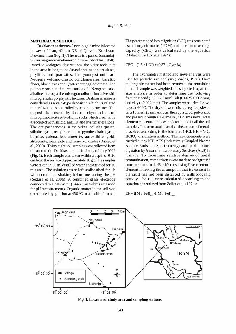
648
Rafiei, B. et al.
MATERIALS & METHODSDashkasan antimony-Arsenic-gold mine is located
in west of Iran, 42 km NE of Qorveh, KordestanProvince, Iran (Fig. 1). The area is a part of Sanandaj-Sirjan magmatic-metamorphic zone (Stocklin, 1968).Based on geological observations, the oldest rock unitsin the area belong to the Jurassic series and are slates,phyllites and quartzites. The youngest units areNeogene volcano-clastic conglomerates, basalticflows, block lavas and Quaternary agglomerates. Theplutonic rocks in the area consist of a Neogene, calc-alkaline microgranite-microgranodiorite intrusive withmicrogranular porphyritic textures. Dashkasan mine isconsidered as a vein-type deposit in which its relatedmineralization is controlled by tectonic structures. Thedeposit is hosted by dacite, rhyodacite andmicrogranodiorite subvolcanic rocks which are mainlyassociated with silicic, argillic and pyritic alterations.The ore parageneses in the veins includes quartz,stibnite, pyrite, realgar, orpiment, pyrotite, chalcopyrite,bornite, galena, boulangerite, aurostibite, gold,stibiconite, kermesite and iron-hydroxides (Rastad etal., 2000). Thirty eight soil samples were collected fromthe around the Dashkasan mine in June and July 2007(Fig. 1). Each sample was taken within a depth of 0-20cm from the surface. Approximately 10 g of the sampleswere taken in 50 ml distilled water and agitated for 10minutes. The solutions were left undisturbed for 1hwith occasional shaking before measuring the pH(Segura et al. 2006). A combined glass electrodeconnected to a pH-meter (744&! metrohm) was usedfor pH measurements. Organic matter in the soil wasdetermined by ignition at 450 oC in a muffle furnace.
The percentage of loss of ignition (LOI) was consideredas total organic matter (TOM) and the cation exchangecapacity (CEC) was calculated by the equation(Malakouti & Homaie, 1994):
CEC = (2.5 × LOI) + (0.57 × Clay %)
The hydrometry method and sieve analysis wereused for particle size analysis (Bowles, 1978). Oncethe organic matter had been removed, the remainingmineral sample was weighted and subjected to particlesize analysis in order to determine the followingfractions: sand (2-0.0625 mm), silt (0.0625-0.002 mm)and clay (<0.002 mm). The samples were dried for twodays at 60 oC. The dry soil were disaggregated, sievedon a 10 mesh (2 mm) screen, then quartered, pulverizedand passed through a 120 mesh (<125 ìm) sieve. Totalelement concentrations were determined in all the soilsamples. The term total is used as the amount of metalsdissolved according to the four acid (HCl, HF, HNO3,HClO4) dissolution method. The measurements werecarried out by ICP-AES (Inductively Coupled PlasmaAtomic Emission Spectrometry) and acid mixturedigestion by Australian Laboratory Services (ALS) inCanada. To determine relative degree of metalcontamination, comparisons were made to backgroundconcentrations in the Earth’s crust using Fe as referenceelement following the assumption that its content inthe crust has not been disturbed by anthropogenicactivity. The EFs were calculated according to theequation generalized from Zoller et al. (1974):
EF = ([M]/[Fe])soil /([M]/[Fe])crust
Fig. 1. Location of study area and sampling stations.

Int. J. Environ. Res., 4(4):647-654 , Autumn 2010
where [M] is the concentration of any element, [Fe] isthe concentration of Fe, and the subscripts “soil” and“crust” indicate which medium the concentration refersto. Multivariate analysis was performed using SPSS 16software for windows. An agglomerative hierarchicalcluster analysis (CA) based on between-groups linkagemethod and correlation matrix was performed. Resultsare shown in a dendrogram where steps in thehierarchical clustering solution and values of thedistance between clusters (Pearson correlation) arerepresented. Details on cluster analysis can be foundin standard chemometric textbooks (Brereton, 2003).
RESULTS & DISCUSSIONDescriptive statistics for heavy metal contents,
physico-chemical soil characteristics of analyzed soilare summarized in Table 1. Soil texture estimated to besandy mud according to soil textural triangle (Folk,1980) (Fig. 2). Most soils were brown in color. The pHdid not vary much and was slightly basic (7.15–7.75),which suggests neutral to sub-alkaline conditions forall the soil samples. At low pH (ca. 6.5), the mobilityand leaching of toxic metals increase, and their mobilityand availability decrease as the pH approaches neutralor rises above seven. Organic matter content in thesoils ranged from 3.4% to 8%. Cation exchange capacity(CEC) shows broad variation ranging from 18.08 to43.81 meq/100g. The correlation between heavy metalcontent and soil physico-chemical characteristics isshown in Table 2. Soil pH was not correlated with heavymetal content of analyzed soils. Organic matter wascorrelated positively (p < 0.01) with As. The cationexchange capacity exhibited a significant relationshipwith As and Sb (r = 0.649, r = 0.533, p < 0.01) and with
Cd, Hg and Pb (p < 0.05).Strong positive correlationwere found between clay content and As and Sbconcentration (p < 0.01). Inter element relationshipsprovide information on heavy metal sources andpathways. According to the values of Pearsoncorrelation coefficient (Table 2) all metals are highlycorrelated (p < 0.01). Arsenic showed strong positivecorrelation with Sb (r = 0.851, p < 0.01). Basic statisticsfor total concentrations of heavy metals in surface soilsamples are shown in Table 1. The maximumconcentrations of heavy metals in surface soils were485, 3.2, 100, 2710 and 640 mg/kg for As, Cd, Hg, Pb
Range
467.00
2.70
99.99
2684.00
635.00
4.60
26.54
0.60
31.11
37.38
41.98
Maximum
485.00
3.20
100.00
2710.00
640.00
8.00
43.81
7.75
41.77
61.75
57.68
Minimum
18.00
0.50
0.01
26.00
5.00
3.40
17.27
7.15
10.66
24.37
15.70
Kurtosis
7.66
7.08
8.86
19.99
14.74
-0.45
0.72
0.10
1.43
-0.49
0.13
Skewness
2.38
2.67
3.20
4.18
3.60
0.06
0.60
1.13
1.02
0.76
-0.60
Std. deviation
91.07
0.65
26.54
474.92
119.51
1.08
5.81
0.15
6.79
10.35
10.07
Median
80.50
0.50
0.46
111.50
27.50
5.80
26.70
7.29
20.78
37.13
42.14
Mean
106.53
0.80
9.03
255.03
65.63
5.75
26.73
7.35
21.70
39.99
40.45
As (mg/kg)
Cd (mg/kg)
Hg (mg/kg)
Pb (mg/kg)
Sb (mg/kg)
Org.M (%)
CEC (meq/100g)
pH
Clay (%)
Silt (%)
Sand (%)
Table 1. Basic statistics for heavy metal contents, physico-chemical soil characteristic of the around
Dashkasan mine
Fig. 2. Ternary diagram of the mine soil texture(After Folk, 1980)
S: Sand, Sc: Clayey Sand, Sm: Mudy Sand, Sz: SiltySand, Cs: Sandy Clay, Ms: Sandy Mud, Zs: Sandy
Silt, C: Clay, M: Mud, Z: Silt
649

650
Heavy Metals around Gold Mine
Table 2. Correlation between elements, organic matter, cation exchange capacity , pH and grain sizedistributions in the studied soils
* Correlation is significant at the 0.05 level.** Correlation is significant at the 0.01 level.
Sand
1
Silt
1
-0.454**
Clay
1
0.102
-0.368*
CEC
1
0.878**
-0.0931
-0.319
pH
1
0.170
0.038
-0.162
0.071
Org.M
1
-0.059
0.135**
-0.024
-0.023*
0.189
Sb
1
0.232
0.032
0.533**
0.553**
-0.111
0.169
Pb
1
0.334**
0.294
0.282
0.337*
0.209
0.171
-0.165
Hg
1
0.716**
0.635**
0.213
0.042
0.362*
0.302
0.205
-0.069
Cd
1
0.794**
0.835**
0.600**
0.220
0.191
0.409*
0.307
0.111
-0.033
As
1
0.689**
0.585**
0.517**
0.851**
0.331*
0.127
0.649**
0.588**
-0.232
0.131
As
Cd
Hg
Pb
Sb
Org.M
pH
CEC
Clay
Silt
Sand
and Sb, respectively. These values were significantlyhigher than those in natural soil (Bowen, 1979), andalso higher than the tolerable levels, which areconsidered as phytotoxically excessive, 20 mg/kg ofAs, 200 mg/kg of Pb, 3 mg/kg of Cd (Ross, 1994; Singh& Steinnes, 1994), 3 mg/kg of Hg and 5 mg/kg of Sb(Kabata- Pendias & Pendias, 1992). A very wide rangebetween minimum and maximum values was observed.This could be due to either a marker variation in themineralogical composition of the different soils in thestudied area and/or different amounts of heavy metalsthat have been released to the various soils fromvarious sources (Idris et al., 2007). Distribution mapsfor As, Cd, Hg and Sb concentrations in surface soilsamples are shown in Fig. 3.
Significant concentrations of As and Sb werefound in the sites around mine due to mineralizationassociated with those metalloids, with the averagevalues of 106.5 and 65.6 mg/kg1, respectively. Most Asin the soils of Dashkasan area is relatively immobile,bound to iron and manganese oxyhydroxides, organicmatter and carbonates or found in the residual mineralfraction, i.e. in refractory minerals. The concentrationsof the metals however, were relatively low in a nearbycontrol area with the same geology as the mine.However, it can be expected that soils in the study areaare highly contaminated. Therefore large area in thevicinity of the mine would not be useful for agriculturalactivities due to the due to contamination of As.
Basic statistics for EFs of all analyzed metals isshown in Table 3. The values of EFs were calculatedtaking into account the following values of
concentrations of metals in upper continental crust,0.102 mg/kg for Cd, 17 mg/kg for Pb, 2 mg/kg for As,0.056 mg/kg for Hg and 0.31 mg/kg for Sb (Wedepohl,1995). The EF values show the enrichment for As andSb. There is no accepted pollution ranking system orcategorization of degree of pollution on the EF analysis.It cannot provide a reliable assessment of the degreeof human interference with the global environment(Reimann and Caritat 2005) but only indicate lithogenicor anthropogenic origin of the contaminations. Theresults obtained by cluster analysis are presented bydendrogram where the distance axis represents thedegree of association between-groups of variable, i.e.the lower the value on the axis, the more significantthe association (Fig. 4). As can be seen Cd, Pb and Hgare grouped into one branch, while As and Sb are intoother branch. In the study area soils, two distinctclusters can be identified. Cluster I: contained CEC,clay content, organic matter content and silt. ClusterII: contained studied heavy metals as well as pH andsand content. Comparison of the average values ofheavy metal concentrations obtained in this study(Table 1) with the values available from literatureindicate that As and Sb are higher than the meanvalues established for uncultivated area worldwide.The higher content of As and Sb are probably due toparent material, i.e. dacite, rhyodacite andmicrogranodiorite subvolcanic rocks common inDashkasan area which are mainly associated withsilicic, argillic and pyretic alterations. No significantcorrelation between soil pH and heavy metal contentwas observed for analyzed soils (Table 2). These

Int. J. Environ. Res., 4(4):647-654 , Autumn 2010
Fig.
3. D
istri
butio
n m
aps o
f As,
Cd,
Hg,
Pb
and
Sb (m
g/kg
) in
the s
oils
of a
roun
d D
ashk
asan
min
e
651
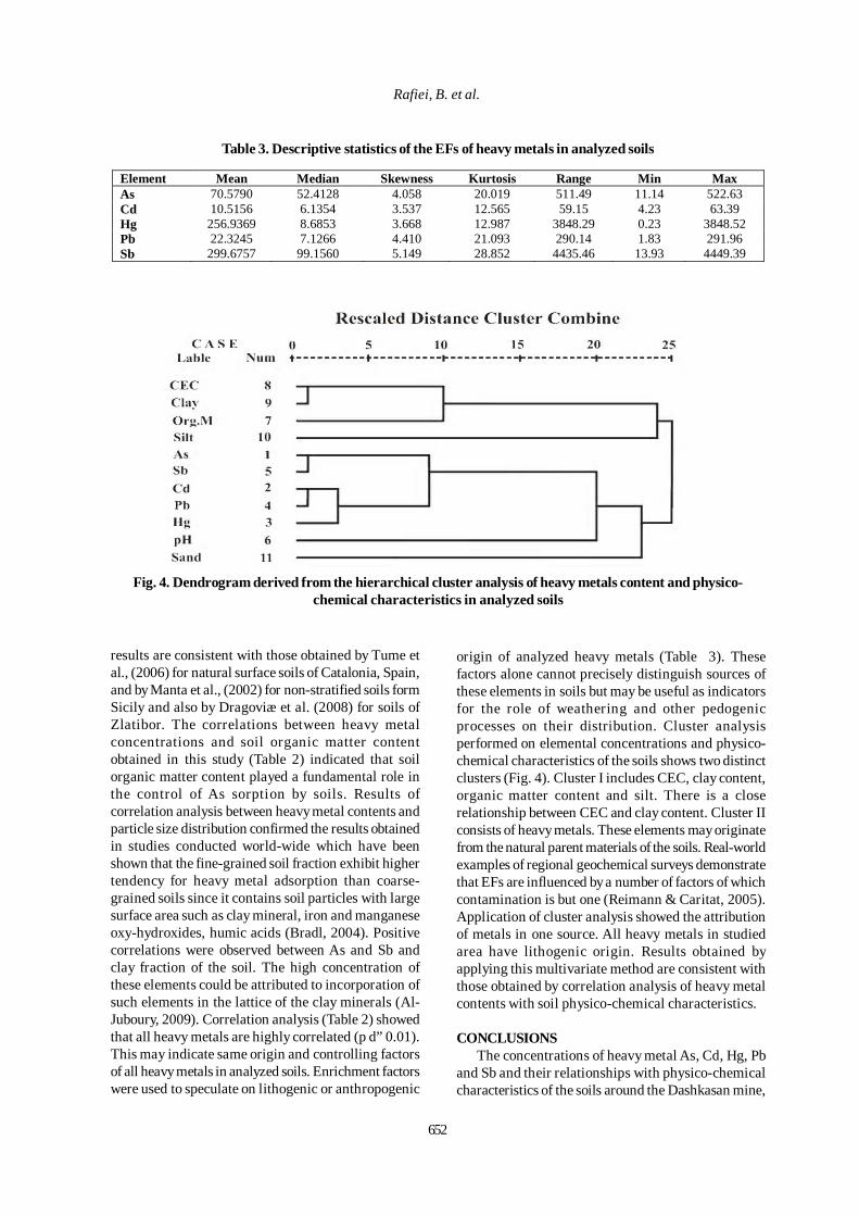
652
Rafiei, B. et al.
Table 3. Descriptive statistics of the EFs of heavy metals in analyzed soils
Element Mean Median Skewness Kurtosis Range Min Max As 70.5790 52.4128 4.058 20.019 511.49 11.14 522.63 Cd 10.5156 6.1354 3.537 12.565 59.15 4.23 63.39 Hg 256.9369 8.6853 3.668 12.987 3848.29 0.23 3848.52 Pb 22.3245 7.1266 4.410 21.093 290.14 1.83 291.96 Sb 299.6757 99.1560 5.149 28.852 4435.46 13.93 4449.39
Fig. 4. Dendrogram derived from the hierarchical cluster analysis of heavy metals content and physico-chemical characteristics in analyzed soils
results are consistent with those obtained by Tume etal., (2006) for natural surface soils of Catalonia, Spain,and by Manta et al., (2002) for non-stratified soils formSicily and also by Dragoviæ et al. (2008) for soils ofZlatibor. The correlations between heavy metalconcentrations and soil organic matter contentobtained in this study (Table 2) indicated that soilorganic matter content played a fundamental role inthe control of As sorption by soils. Results ofcorrelation analysis between heavy metal contents andparticle size distribution confirmed the results obtainedin studies conducted world-wide which have beenshown that the fine-grained soil fraction exhibit highertendency for heavy metal adsorption than coarse-grained soils since it contains soil particles with largesurface area such as clay mineral, iron and manganeseoxy-hydroxides, humic acids (Bradl, 2004). Positivecorrelations were observed between As and Sb andclay fraction of the soil. The high concentration ofthese elements could be attributed to incorporation ofsuch elements in the lattice of the clay minerals (Al-Juboury, 2009). Correlation analysis (Table 2) showedthat all heavy metals are highly correlated (p d” 0.01).This may indicate same origin and controlling factorsof all heavy metals in analyzed soils. Enrichment factorswere used to speculate on lithogenic or anthropogenic
origin of analyzed heavy metals (Table 3). Thesefactors alone cannot precisely distinguish sources ofthese elements in soils but may be useful as indicatorsfor the role of weathering and other pedogenicprocesses on their distribution. Cluster analysisperformed on elemental concentrations and physico-chemical characteristics of the soils shows two distinctclusters (Fig. 4). Cluster I includes CEC, clay content,organic matter content and silt. There is a closerelationship between CEC and clay content. Cluster IIconsists of heavy metals. These elements may originatefrom the natural parent materials of the soils. Real-worldexamples of regional geochemical surveys demonstratethat EFs are influenced by a number of factors of whichcontamination is but one (Reimann & Caritat, 2005).Application of cluster analysis showed the attributionof metals in one source. All heavy metals in studiedarea have lithogenic origin. Results obtained byapplying this multivariate method are consistent withthose obtained by correlation analysis of heavy metalcontents with soil physico-chemical characteristics.
CONCLUSIONSThe concentrations of heavy metal As, Cd, Hg, Pb
and Sb and their relationships with physico-chemicalcharacteristics of the soils around the Dashkasan mine,
653
Int. J. Environ. Res., 4(4):647-654 , Autumn 2010
west of Iran have been studied. The concentration ofAs, Cd, Hg, Pb and Sb in mine soils ranges from 18 to485, 0.5 to 3.2, 0.01 to 100, 26 to 2710 and 5 to 640 mg/kg, with an arithmetic mean of 106.53, 0.80, 9.03, 255.03and 65.63 mg/kg, respectively. The highestconcentrations of the heavy metals were recorded intopsoil near the mine. There is a progressive decreaseof heavy element concentrations with increasingdistance from the mine. The application of EF analysisand CA pointed out lithogenic origin of all heavymetals in soils around Dashkasan mine. The mean EFthat is more than 5 is clearly indicative of metalsenrichment in soils of area of study.This study alsohighlighted the need for further research includingdetailed geochemical surveys in this area. Thepreliminary compilation of As distribution in soilsshows the role of geology as the main governing factor.
REFERENCES
Abdul Aziz, H., Omran, A. and Zakaria, W. R. (2010). H2O2Oxidation of Pre-Coagulated Semi Aerobic Leachate. Int. Journal.Environ. Res., 4 (2), 209-216.
Abdullahi, M. S., Uzairu, A. and Okunola, O. J. (2009).Quantitative Determination of Heavy Metal Concentrations inOnion Leaves. Int. Journal. Environ. Res., 3 (2), 271-274.
Ahmad, M. K., Islam, S., Rahman, S., Haque, M. R. and Islam,M. M. (2010). Heavy Metals in Water, Sediment and SomeFishes of Buriganga River, Bangladesh. Int. J. Environ. Res., 4(2), 321-332.
Ahmed, T. A. and Al-Hajri, H. H. (2009). Effects of TreatedMunicipal Wastewater and Sea Water Irrigation on Soil andPlant Characteristics. Int. Journal. Environ. Res., 3 (4), 503-510.
Akoto, O., Ephraim, J. H. and Darko, G. (2008). Heavy MetalsPollution in Surface Soils in the Vicinity of Abundant RailwayServicing Workshop in Kumasi, Ghana. Int. J. Environ. Res., 2(4), 359-364.
Al-Juboury, A. I. (2009). Natural Pollution By Some HeavyMetals in the Tigris River, Northern Iraq. Int. J. Environ. Res.,3 (2), 189-198.
Biati, A., Moattar, F., Karbassi, A. R. and Hassani, A. H. (2010).Role of Saline Water in Removal of Heavy Elements fromIndustrial Wastewaters. Int. Journal. Environ. Res., 4 (1), 177-182.
Bowen, H .J. M. (1979). Environmental chemistry of theelements. New York: Academic Press. (333pp).
Bowles, J. E. (1978). Engineering properties of soils and theirmeasurement. McGraw-Hill Book Co. 218p.
Bradl, H. B. (2004). Adsorption of heavy metal ions on soilsand soils constituents. J. Colloid Interf. Sci., 277, 1-18.
Brereton, R. G. (2003). Data Analysis for the Laboratory andChemical Plant. John Wiley & Sons, Ltd., West Sussex, UnitedKingdom.
Burt, R., Wilson, M. A., Mays, M. D. and Lee, C. W. (2003).Major and trace elements of selected pedons in the USA. J.Environ. Qual., 32, 2109-2121.
Covelo, E. F., Vega, F. A. and Andrade, M. L. (2007).Simultaneous sorption and desorption of Cd, Cr, Cu, Ni, Pband Zn in acid soils II: soil ranking and influence of soilcharacteristics. J. Hazard. Mater., 147, 862-870.
Dauvalter, V. A., Kashulin, N. A., Lehto, J. and Jernström, J.(2009). Chalcophile elements Hg, Cd, Pb, As in LakeUmbozero, Murmansk Region, Russia. Int. J. Environ. Res., 3(3), 411-428.
Deckers, J., Laker, M., Vanherreweghe, S., Vanclooster, M.,Swennen, R. and Cappuyns, V. (2000). State of the art on soilrelated geomedical issues in the world. Gepmedical problemsin developing countries. International Symposium of theNorwegian Academy of Science and Letters. 23- 42.
Dragovic, S., Mihailovic, N. and Gajic, B. (2008). Heavy metalsin soils: Distribution, relationship with soil characteristics andradionuclides and multivariate assessment of contaminationsources. Chemosphere, 72, 491-495.
Dixit, S. and Tiwari, S. (2008). Impact Assessment of HeavyMetal Pollution of Shahpura Lake, Bhopal, India. Int. Journal.Environ. Res., 2 (1), 37-42.
Facchinelli, A., Sacchi, E. and Mallen, L. (2001). Multivariatestatistical and GIS-based approach to identify heavy metalsources in soils. Environ. Pollut., 114, 313-324.
Folk, R. L. (1980). Petrology of sedimentary rocks. HemphillPublishing Co., Texas.
Gaur, N. and Dhankhar, R. (2009). Removal of Zn+2 ionsfrom aqueous solution using Anabaena variabilis. Equilibriumand Kinetic studies. Int. Journal. Environ. Res., 3 (4), 605-616.
Hasan, M. A. A., Ahmed, M. K., Akhand, A. A., Ahsan, N. andIslam, M. M. (2010). Toxicological Effects and MolecularChanges Due to Mercury Toxicity in Freshwater Snakehead(Channa punctatus Bloch, 1973). Int. Journal. Environ. Res., 4(1), 91-98.
Idris, A. M., Eltayeb, M. A. H., Potgieter-Vermaak, S. S.,Grieken, R. V. and Potgieter, J. H. (2007). Assessment of heavymetals pollution in Sudanese harbours along the Red Sea Coast.Micro chemical Journal, 87, 104-112.
Kabata- Pendias, A. and Pendias, H. (1992). Trace elements insoils and plants, 2 nd ed. London: CRC. Press. (413pp).
Kashulin, N. A., Terentiev, P. M. and Koroleva, I. M. (2008).The status of whitefish population from Chuna Lake in theLapland Biosphere Reserve Russia. Int. Journal. Environ. Res.,2 (2), 111-124.
Luo, W., Wang, T., Lu, Y., Giesy, H., Shi, Y., Zheng, Y., Xing, Y.and Wu, G. (2007). Landscape ecology of the GuantingReservoir, Beijing, China: multivariate and geostatisticalanalyses of metals in soils. Environ. Pollut. 146, 567-576.
Malakouti, M. and Homaie, M. (1994). Fertility of arid regionsoils (Problems & solutions), Trbiat Modarres Univ.Press.
654
Heavy Metals around Gold Mine
Manta, D. S., Angelone, M., Bellance, A., Neri, R. and Sprovieri,M. (2002). Heavy metals in urban soils: a case study from thecity of Palermo (Sicily), Italy. Sci. Total Environ., 30, 229-243.
Mason, B. and Moore, C. B. (1982). Principles ofGeochemistry. John Wiley and Sons. (344p).
Mensi, Gh. S., Moukha, S., Creppy, E. E. and Maaroufi, K.(2008). Metals Accumulation in Marine Bivalves and Seawaterfrom theLagoon of Boughrara in Tunisia (North Africa). Int.Journal. Environ. Res., 2 (3), 279-284.
Micó, C., Recatala, L., Peris, M. and Sanchez, J. (2006).Assessing heavy metal sources in agricultural soils of anEuropean Mediterranean area by multivariate analysis.Chemosphere, 65, 863-872.
Mumba, P. P., Chibambo, B. Q. and Kadewa, W. (2008). AComparison of The Levels of Heavy Metals in CabbagesIrrigated With Reservoir and Tap Water. Int. Journal. Environ.Res., 2 (1), 61-64.
Murugesan, A.G., Maheswari, S. and Bagirath, G. (2008).Biosorption of Cadmium by Live and Immobilized Cells ofSpirulina Platensis . Int. Journal. Environ. Res., 2 (3), 307-312.
Nabi Bidhendi, G. R., Karbassi, A. R., Nasrabadi, T. and Hoveidi,H. (2007). Influence of copper mine on surface water quality.Int. J. Environ. Sci. Tech., 4 (1), 85-91.
Navas, A. and Machin, J. (2002). Spatial distribution of heavymetals and arsenic in soils of Aragon (northeast Spain):controlling factors and environmental implications. Appl.Geochem., 17, 961-973.
Nouri, J., Mahvi, A. H. and Bazrafshan, E. (2010). Applicationof Electrocoagulation Process in Removal of Zinc and CopperFrom Aqueous Solutions by Aluminum Electrodes. Int. Journal.Environ. Res., 4 (2), 201-208.
Opuene, K. and Agbozu, I. E. (2008). Relationships BetweenHeavy Metals in Shrimp ( Macrobrachium felicinum) and MetalLevels in The Water Column and Sediments of Taylor Creek.Int. Journal. Environ. Res., 2 (4), 343-348.
Øygard, J. K. and Gjengedal, E. (2009). Uranium in MunicipalSolid Waste Landfill Leachate. Int. Journal. Environ. Res., 3(1), 61-68.
Praveena, S. M., Ahmed, A., Radojevic, M., Abdullah, M. H.and Aris, A. Z. (2008). Heavy Metals in Mangrove SurfaceSediment of Mengkabong Lagoon, Sabah: Multivariate and Geo-Accumulation Index Approaches. Int. J. Environ. Res., 2 (2),139-148.
Priju, C. P. and Narayana, A.C. (2007). Heavy and Trace Metalsin Vembanad Lake Sediments. Int. J. Environ. Res., 1(4): 280-289.
Rahmani, K., Mahvi, A. H., Vaezi, F., Mesdaghinia, A. R.,Nabizade, R. and Nazmara, Sh. (2009). Bioremoval of Lead byUse of Waste Activated Sludge. Int. Journal. Environ. Res., 3(3), 471-476.
Rastad, E., Niroomand, Sh., Emami, M. H. and Rashid NezhadOmran, N. (2000). Genesis of Sb-As-Au deposit in volcano-plautonic complex of Dash-kasan (East Qorveh, KordestanProvince). Geosciences: Iranian scientific Quaterly Journal, 9(37-38), 2-9.
Reimann, C. and de Caritat, P. (2005). Distinguishing betweennatural and anthropogenic sources for elements in theenvironment: regional geochemical surveys versus enrichmentfactors. Sci. Total Environ., 337, 91-107.
Resmi, G., Thampi, S. G. and Chandrakaran, S. (2010).Brevundimonas vesicularis: A Novel Bio-sorbent for Removalof Lead from Wastewater. Int. Journal. Environ. Res., 4 (2),281-288.
Ross, S. M. (1994). Sources and forms of potentially toxicmetals in soil-planet system. In: Ross, S.M., editor. Toxic metalsin soil-plant system. Chichester, John Wiley and Sons LTD, 3-25.
Sayyareh, A., Fonoudi, M. and Dadsetan, A. (2005).Environmental geology study in Qorveh-Bijar area (Preliminaryreport). Geological & Environmental management, GeologicalSurvey of Iran.
Segura, R., Arancibia, V., Zuniga, M. C. and Pasten, P. (2006).Distribution of copper, zinc, lead and cadmium concentrationsin stream sediments from the Mapocho River in Santiago, Chile,Journal of Geochemical Exploration, 91, 71-80.
Shetty, R. and Rajkumar, Sh. (2009). Biosorption of Cu (II) byMetal Resistant Pseudomonas sp. Int. Journal. Environ. Res.,3 (1), 121-128.
Singh, B. R. and Steinnes, E. (1994). Soil and watercontamination b heavy metals. In: Lal, R. and Stewart, A.,editors. Soil processes and water quality, advances in soilscience. Boca Raton, Florida: Lewis Publishers, 233-271.
Slavkoviæ, L., Škrbiæ, B., Miljeviæ, N. and Onjia, A. (2004).Principal Component analysis of trace elements in industrialsoils. Environ. Chem. Lett., 2, 105-108.
Stocklin, J. (1968). Structural history and tectonics of Iran.Amer. Assoc. Petro. Geol. Bull., 52, 1229-1258.
Tume, P., Bech, J., Longan, L., Tume, L., Reverter, F. &Sepulveda, B. (2006). Trace elements in natural surface soils inSant Climent (Catalonia, Spain). Ecol. Eng., 27, 145-152.
Uba, S., Uzairu, A. and Okunola, O. J. (2009). Content ofHeavy Metals in Lumbricus Terrestris and Associated Soils inDump Sites. Int. J. Environ. Res., 3 (3), 353-358.
Vega, F. A., Covelo, E. F., Andrade, M. L. and Marcet, P.(2004). Relationship between heavy metals content and soilproperties in minesoils. Anal. Chim. Acta, 524, 141-150.
Venugopal, T., Giridharan, L. and Jayaprakash, M. (2009).Characterization and Risk Assessment Studies of Bed Sedimentsof River Adyar-An Application of Speciation Study. Int. Journal.Environ. Res., 3 (4), 581-598.
Vinodhini, R. and Narayanan, M. (2009). Heavy Metal InducedHistopathological Alterations in Selected Organs of theCyprinus carpio L.(Common Carp). Int. Journal. Environ. Res.,3 (1), 95-100.
Wedepohl, K. H. (1995). The composition of the continentalcrust. Geochimica et Cosmochimica Acta, 59 (7), 1217-1232.
Zoller, W. H., Gladney, E. S. and Duce, R. A. (1974).Atmosphere concentrations and sources of trace metals at theSouth Pole. Science, 183, 199-201.
Int. J. Environ. Res., 4(4):655-664, Autumn 2010ISSN: 1735-6865
Received 12 Oct. 2009; Revised 27 April 2010; Accepted 10 May 2010
*Corresponding author E-mail: [email protected]
655
Enhancement Biodegradation of n-alkanes from Crude OilContaminated Seawater
Zahed, M. A . 1, Aziz , H. A.1*, Isa, M. H. 2 and Mohajeri, L. 1
1 School of Civil Engineering, Universiti Sains Malaysia, 14300 Nibong Tebal, Penang, Malaysia
2 Civil Engineering Department, Universiti Teknologi PETRONAS, 31750 Tronoh, Perak, Malaysia
ABSTRACT: The aim of this research was to optimize bioremediation of seawater samples spiked with 1000mg/L crude oil for removal of n-alkanes (C12H26 to C34H70). Bioaugmentation experiments were performed atlaboratory scale: each bioreactor contained 250 ml dispersed crude-oil-contaminated seawater, indigenousacclimatized microorganism and nitrogen and phosphorus at concentrations based on central composite design(CCD) calculations. Three independent variables, time, nitrogen and phosphorus, were investigated and theexperimental data obtained were fitted to a second-order polynomial mathematical model with multipleregressions. The obtained Model F-value of 97.12 and probability F <0.0001 implies the model is significant.Hydrocarbon analyses were carried out using a gas chromatograph equipped with flame ionization detector(GC/FID). During 28 days of experimentation, a maximum of 85.35% total n-alkane removal was observed.Numerical optimization was achieved based on desirability functions. Using 188.71 mg/L nitrogen and 18.99mg/L phosphorus, design of experiment (DOE) software predicted 91.00% removal. A removal of 92.04% wasobserved experimentally, in close agreement with the predicted value.
Key words: Bioremediation, Bioaugmentation, Paraffines, Petroleum, Marine pollution
INTRODUCTIONCrude oil is a complex mixture of many compounds
including alkanes, aromatics, resins and asphalteneswhich potentially could be eliminated from contami-nated environments by microbial degradation. Differ-ent components of crude oil are degraded at differentrates: n-alkanes, also known as n-paraffins, are oxidizedmore rapidly than either aromatics or naphthenes (Ijahand Antai, 2003; Fingas, 2001). Crude oil and hydrocar-bon fuels (jet fuel, kerosene, gasoline, diesel fuel, ect.)contain large amounts of n-alkanes. Therefore, en-hanced biodegradation of these compounds is ex-tremely important in the case of hydrocarbonspills.Several factors may affect hydrocarbon degrada-tion and, in particular, the oil concentration is an impor-tant consideration in determining whetherbioremediation is a viable option. Very low concentra-tions of hydrocarbons may be ineffectually attackedby microorganisms (Foght and Westlake, 1987). In con-trast, high concentrations of hydrocarbons can causeinhibition of biodegradation due to toxic effects, al-though the inhibitory concentration varies with oil com-position. Hence, there is an optimum oil concentrationrange for bioremediation applications (Zhu, 2001).
Different types of nutrients (primarily nitrogen andphosphorus) have been applied to improve petroleumhydrocarbon degradation, including classic (watersoluble) nutrients and oleophilic and slow-release fer-tilizers. Application of nutrients for hydrocarbon bio-degradation has been widely investigated (Delille etal., 2009; Ruberto et al, 2009; Kim et al., 2008; Ramirezet al., 2008; Bagherzadeh-Namazi et al., 2008;Nikolopouloua and Kalogerakis, 2008; Salas et al., 2006Knezevich et al., 2006), and each nutrient type exhib-its various advantages and disadvantages (Jean etal., 2008; Onwurah et al., 2007; Das and Mukherjee,2007). However, the literature is still inconclusive re-garding what nutrient conditions are sufficient for dif-ferent environments.
Low nutrient concentrations reduce the rate ofbiodegradation; whereas, high nutrient concentrationmay be toxic for marine biota and cause eutrophica-tion and red tide. Hydrocarbon-utilizing microorgan-isms are ubiquitously distributed in marine ecosys-tems following oil spills (Atlas, 1995). For ex-situbioremediation, addition of acclimatized naturally oc-curring microorganisms (bioaugmentation) enhancesbiodegradation of hydrocarbons. As dissolved hy-
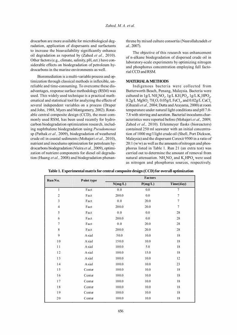
656
Zahed, M. A. et al.
drocarbon are more available for microbiological deg-radation, application of dispersants and surfactantsto increase the bioavailability significantly enhanceoil degradation as reported by (Zahed et al., 2010).Other factors (e.g., climate, salinity, pH, ect.) have con-siderable effects on biodegradation of petroleum hy-drocarbons in the marine environments as well.
Bioremediation is a multi-variable process and op-timization through classical methods is inflexible, un-reliable and time-consuming. To overcome these dis-advantages, response surface methodology (RSM) wasused. This widely used technique is a practical math-ematical and statistical tool for analyzing the effects ofseveral independent variables on a process (Draperand John, 1988, Myers and Montgomery, 2002). Rotat-able central composite design (CCD), the most com-monly used RSM, has been used recently for hydro-carbon biodegradation optimization research, includ-ing naphthalene biodegradation using Pseudomonassp (Pathak et al., 2009), biodegradation of weatheredcrude oil in coastal sediments (Mohajeri et al., 2010),nutrient and inoculums optimization for petroleum hy-drocarbons biodegradation (Vieira et al., 2009), optimi-zation of nutrient components for diesel oil degrada-tion (Huang et al., 2008) and biodegradation phenan-
threne by mixed culture consortia (Nasrollahzadeh etal., 2007).
The objective of this research was enhancementof n-alkane biodegradation of dispersed crude oil inlaboratory-scale experiments by optimizing nitrogenand phosphorus concentration employing full facto-rial CCD and RSM.
MATERIAL & METHODSIndigenous bacteria were collected from
Butterworth Beach, Penang, Malaysia. Bacteria werecultured in 1g/L NH4NO3, 1g/L KH2PO4, 1g/L K2HPO4,0.2g/L MgSO4·7H2O, 0.05g/L FeCl3, and 0.02g/L CaCl2(Ghazali et al., 2004; Dutta and Arayama, 2000) at roomtemperature under natural light conditions and pH 7.0-7.8 with stirring and aeration. Bacterial inoculums char-acteristics were reported before (Mohajeri et al., 2009;Zahed et al., 2010). Erlenmeyer flasks (bioreactors)contained 250 ml seawater with an initial concentra-tion of 1000 mg/l light crude oil (Shell, Port Dickson,Malaysia) and the dispersant Corexit 9500 in a ratio of20:1 (w/w) as well as the amounts of nitrogen and phos-phorus listed in Table 1. Run 21 (an extra test) wascarried out to determine the amount of removal fromnatural attenuation. NH4NO3 and K2HPO4 were usedas nitrogen and phosphorus sources, respectively.
Table 1. Experimental matrix for central composite design (CCD) for overall optimizationFactors
Run No. Point type N(mg/L) P(mg/L) Time(day)
1 Fact 0 .0 0.0 7
2 Fact 200.0 0.0 7 3 Fact 0 .0 20.0 7
4 Fact 200.0 20.0 7
5 Fact 0 .0 0.0 28
6 Fact 200.0 0.0 28 7 Fact 0 .0 20.0 28
8 Fact 200.0 20.0 28
9 Axial 50.0 10.0 18
10 Axial 150.0 10.0 18 11 Axial 100.0 5.0 18
12 Axial 100.0 15.0 18
13 Axial 100.0 10.0 12
14 Axial 100.0 10.0 23 15 Center 100.0 10.0 18
16 Center 100.0 10.0 18
17 Center 100.0 10.0 18
18 Center 100.0 10.0 18 19 Center 100.0 10.0 18
20 Center 100.0 10.0 18
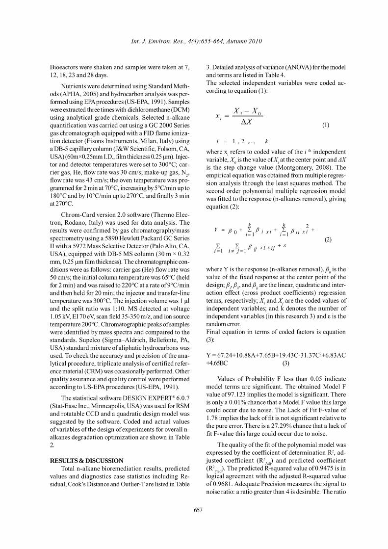
Int. J. Environ. Res., 4(4):655-664, Autumn 2010
657
Bioeactors were shaken and samples were taken at 7,12, 18, 23 and 28 days.
Nutrients were determined using Standard Meth-ods (APHA, 2005) and hydrocarbon analysis was per-formed using EPA procedures (US-EPA, 1991). Sampleswere extracted three times with dichloromethane (DCM)using analytical grade chemicals. Selected n-alkanequantification was carried out using a GC 2000 Seriesgas chromatograph equipped with a FID flame ioniza-tion detector (Fisons Instruments, Milan, Italy) usinga DB-5 capillary column (J&W Scientific, Folsom, CA,USA) (60m×0.25mm I.D., film thickness 0.25 µm). Injec-tor and detector temperatures were set to 300°C; car-rier gas, He, flow rate was 30 cm/s; make-up gas, N2,flow rate was 43 cm/s; the oven temperature was pro-grammed for 2 min at 70°C, increasing by 5°C/min up to180°C and by 10°C/min up to 270°C, and finally 3 minat 270°C.
Chrom-Card version 2.0 software (Thermo Elec-tron, Rodano, Italy) was used for data analysis. Theresults were confirmed by gas chromatography/massspectrometry using a 5890 Hewlett Packard GC SeriesII with a 5972 Mass Selective Detector (Palo Alto, CA,USA), equipped with DB-5 MS column (30 m × 0.32mm, 0.25 µm film thickness). The chromatographic con-ditions were as follows: carrier gas (He) flow rate was50 cm/s; the initial column temperature was 65°C (heldfor 2 min) and was raised to 220°C at a rate of 9°C/minand then held for 20 min; the injector and transfer-linetemperature was 300°C. The injection volume was 1 µland the split ratio was 1:10. MS detected at voltage1.05 kV, EI 70 eV, scan field 35-350 m/z, and ion sourcetemperature 200°C. Chromatographic peaks of sampleswere identified by mass spectra and compaired to thestandards. Supelco (Sigma–Aldrich, Bellefonte, PA,USA) standard mixture of aliphatic hydrocarbons wasused. To check the accuracy and precision of the ana-lytical procedure, triplicate analysis of certified refer-ence material (CRM) was occasionally performed. Otherquality assurance and quality control were performedaccording to US-EPA procedures (US-EPA, 1991).
The statistical software DESIGN EXPERT® 6.0.7(Stat-Ease Inc., Minneapolis, USA) was used for RSMand rotatable CCD and a quadratic design model wassuggested by the software. Coded and actual valuesof variables of the design of experiments for overall n-alkanes degradation optimization are shown in Table2.
RESULTS & DISCUSSIONTotal n-alkane bioremediation results, predicted
values and diagnostics case statistics including Re-sidual, Cook’s Distance and Outlier-T are listed in Table
3. Detailed analysis of variance (ANOVA) for the modeland terms are listed in Table 4.The selected independent variables were coded ac-cording to equation (1):
where xi refers to coded value of the i th independentvariable, X0 is the value of Xi at the center point and ∆Xis the step change value (Montgomery, 2008). Theempirical equation was obtained from multiple regres-sion analysis through the least squares method. Thesecond order polynomial multiple regression modelwas fitted to the response (n-alkanes removal), givingequation (2):
where Y is the response (n-alkanes removal), β0 is thevalue of the fixed response at the center point of thedesign; βi, βii, and βij are the linear, quadratic and inter-action effect (cross product coefficients) regressionterms, respectively; Xi and Xj are the coded values ofindependent variables; and k denotes the number ofindependent variables (in this research 3) and ε is therandom error.Final equation in terms of coded factors is equation(3):
Y = 67.24+10.88A+7.65B+19.43C-31.37C2+6.83AC+4.65BC (3)
Values of Probability F less than 0.05 indicatemodel terms are significant. The obtained Model Fvalue of 97.123 implies the model is significant. Thereis only a 0.01% chance that a Model F value this largecould occur due to noise. The Lack of Fit F-value of1.78 implies the lack of fit is not significant relative tothe pure error. There is a 27.29% chance that a lack offit F-value this large could occur due to noise.
The quality of the fit of the polynomial model wasexpressed by the coefficient of determination R2, ad-justed coefficient (R2
Adj) and predicted coefficient(R2
Pred). The predicted R-squared value of 0.9475 is inlogical agreement with the adjusted R-squared valueof 0.9681. Adequate Precision measures the signal tonoise ratio: a ratio greater than 4 is desirable. The ratio
εβ
βββ
+∑=≠
∑=
+∑=
+∑=
+=
x i jx iji iji
x ik
i i ix ik
i iY
11
2110
(2)
XXXx i
i ∆−= 0
ki ,. ..,2,1=
(1)
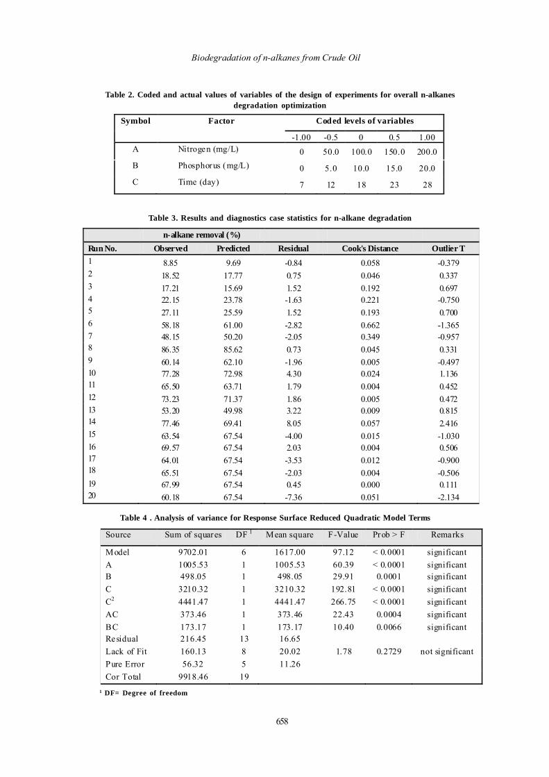
658
Biodegradation of n-alkanes from Crude Oil
n-alkane removal (%) Run No. Observed Predicted Residual Cook's Distance Outlier T 1 8.85 9.69 -0.84 0.058 -0.379 2 18.52 17.77 0.75 0.046 0.337 3 17.21 15.69 1.52 0.192 0.697 4 22.15 23.78 -1.63 0.221 -0.750 5 27.11 25.59 1.52 0.193 0.700 6 58.18 61.00 -2.82 0.662 -1.365 7 48.15 50.20 -2.05 0.349 -0.957 8 86.35 85.62 0.73 0.045 0.331 9 60.14 62.10 -1.96 0.005 -0.497 10 77.28 72.98 4.30 0.024 1.136 11 65.50 63.71 1.79 0.004 0.452 12 73.23 71.37 1.86 0.005 0.472 13 53.20 49.98 3.22 0.009 0.815 14 77.46 69.41 8.05 0.057 2.416 15 63.54 67.54 -4.00 0.015 -1.030 16 69.57 67.54 2.03 0.004 0.506 17 64.01 67.54 -3.53 0.012 -0.900 18 65.51 67.54 -2.03 0.004 -0.506 19 67.99 67.54 0.45 0.000 0.111 20 60.18 67.54 -7.36 0.051 -2.134
Table 3. Results and diagnostics case statistics for n-alkane degradation
Table 4 . Analysis of variance for Response Surface Reduced Quadratic Model Terms
Source Sum of squares DF 1 Mean square F-Value Prob > F Remarks
Model 9702.01 6 1617.00 97.12 < 0.0001 significant A 1005.53 1 1005.53 60.39 < 0.0001 significant B 498.05 1 498.05 29.91 0.0001 significant C 3210.32 1 3210.32 192.81 < 0.0001 significant C2 4441.47 1 4441.47 266.75 < 0.0001 significant AC 373.46 1 373.46 22.43 0.0004 significant BC 173.17 1 173.17 10.40 0.0066 significant Residual 216.45 13 16.65 Lack of Fit 160.13 8 20.02 1.78 0.2729 not significant Pure Error 56.32 5 11.26 Cor Total 9918.46 19
1 DF= Degree of freedom
Table 2. Coded and actual values of variables of the design of experiments for overall n-alkanesdegradation optimization
Coded levels of variables Symbol Factor
-1.00 -0.5 0 0.5 1.00 A Nitrogen (mg/L) 0 50.0 100.0 150.0 200.0 B Phosphorus (mg/L) 0 5.0 10.0 15.0 20.0 C Time (day) 7 12 18 23 28
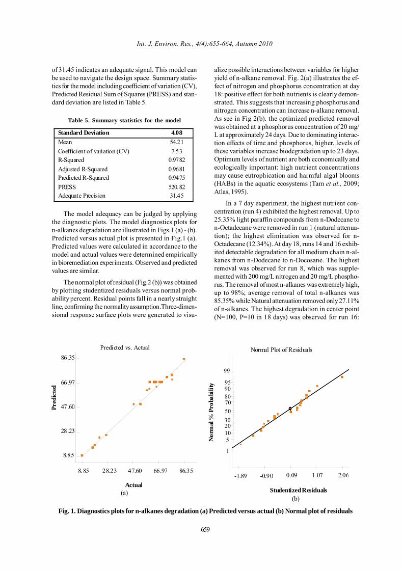
Int. J. Environ. Res., 4(4):655-664, Autumn 2010
659
of 31.45 indicates an adequate signal. This model canbe used to navigate the design space. Summary statis-tics for the model including coefficient of variation (CV),Predicted Residual Sum of Squares (PRESS) and stan-dard deviation are listed in Table 5.
Table 5. Summary statistics for the model
Standard Deviation 4.08 Mean 54.21 Coefficient of variation (CV) 7.53 R-Squared 0.9782 Adjusted R-Squared 0.9681 Predicted R-Squared 0.9475 PRESS 520.82 Adequate Precision 31.45
The model adequacy can be judged by applying
the diagnostic plots. The model diagnostics plots forn-alkanes degradation are illustrated in Figs.1 (a) - (b).Predicted versus actual plot is presented in Fig.1 (a).Predicted values were calculated in accordance to themodel and actual values were determined empiricallyin bioremediation experiments. Observed and predictedvalues are similar.
The normal plot of residual (Fig.2 (b)) was obtainedby plotting studentized residuals versus normal prob-ability percent. Residual points fall in a nearly straightline, confirming the normality assumption.Three-dimen-sional response surface plots were generated to visu-
Actual
Pred
icte
d
Predicted vs. Actual
8.85
28.23
47.60
66.97
86.35
8.85 28.23 47.60 66.97 86.35
(a) Studentized Residuals
Nor
mal
% P
roba
bilit
y
Normal Plot of Residuals
-1.89 -0.90 0.09 1.07 2.06
99
95908070503020105
1
(b)
Fig. 1. Diagnostics plots for n-alkanes degradation (a) Predicted versus actual (b) Normal plot of residuals
alize possible interactions between variables for higheryield of n-alkane removal. Fig. 2(a) illustrates the ef-fect of nitrogen and phosphorus concentration at day18: positive effect for both nutrients is clearly demon-strated. This suggests that increasing phosphorus andnitrogen concentration can increase n-alkane removal.As see in Fig 2(b). the optimized predicted removalwas obtained at a phosphorus concentration of 20 mg/L at approximately 24 days. Due to dominating interac-tion effects of time and phosphorus, higher, levels ofthese variables increase biodegradation up to 23 days.Optimum levels of nutrient are both economically andecologically important: high nutrient concentrationsmay cause eutrophication and harmful algal blooms(HABs) in the aquatic ecosystems (Tam et al., 2009;Atlas, 1995).
In a 7 day experiment, the highest nutrient con-centration (run 4) exhibited the highest removal. Up to25.35% light paraffin compounds from n-Dodecane ton-Octadecane were removed in run 1 (natural attenua-tion); the highest elimination was observed for n-Octadecane (12.34%). At day 18, runs 14 and 16 exhib-ited detectable degradation for all medium chain n-al-kanes from n-Dodecane to n-Docosane. The highestremoval was observed for run 8, which was supple-mented with 200 mg/L nitrogen and 20 mg/L phospho-rus. The removal of most n-alkanes was extremely high,up to 98%; average removal of total n-alkanes was85.35% while Natural attenuation removed only 27.11%of n-alkanes. The highest degradation in center point(N=100, P=10 in 18 days) was observed for run 16:
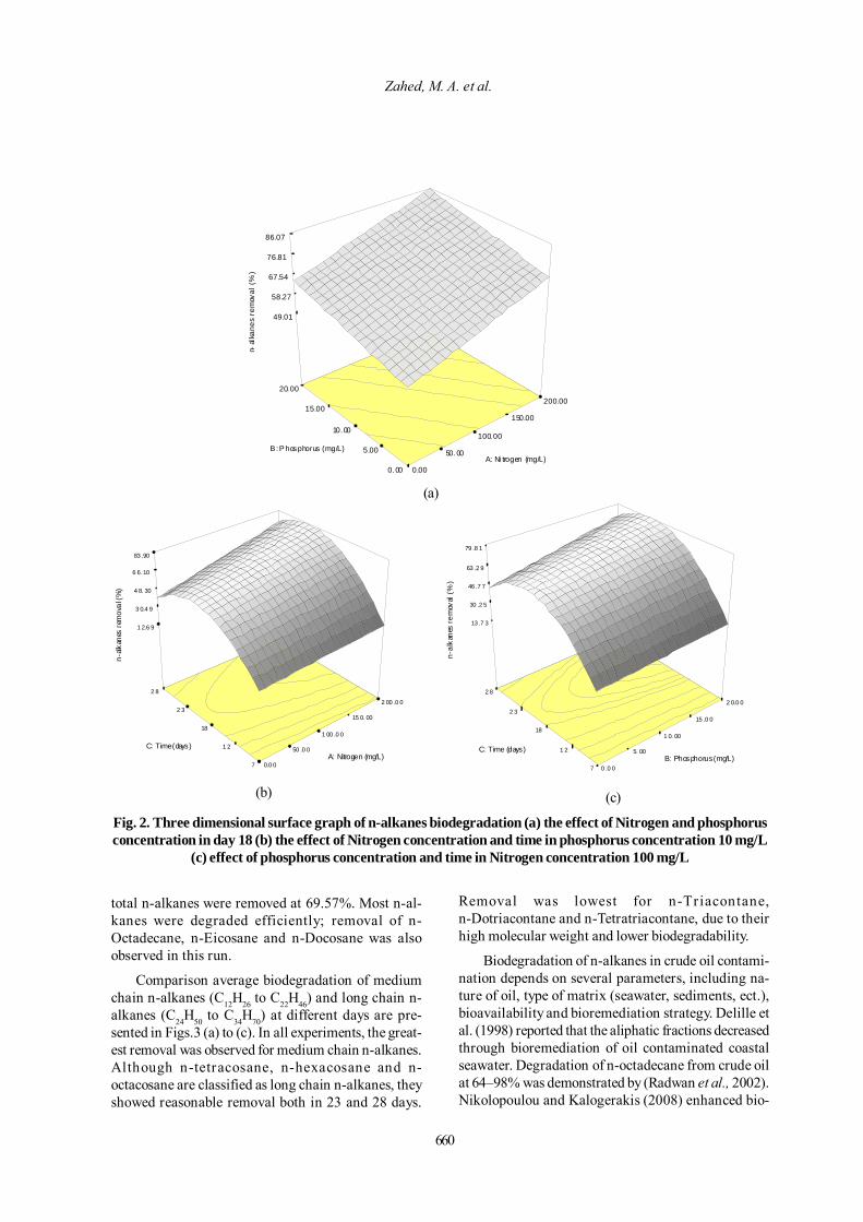
660
49.01
58.27
67.54
76.81
86.07
n-a
lkan
es r
emov
al (
%)
0.00
50.00
100.00
150.00
200.00
0.00
5.00
10.00
15.00
20.00
A: Ni trogen (mg/L) B : P hosphorus (mg/L)
1 2.6 9
3 0.4 9
4 8. 30
6 6. 10
83 .90
n-a
lkan
es re
mov
al (%
)
0.0 0
50 .0 0
1 00 .0 0
15 0. 00
2 00 .0 0
7
1 2
18
2 3
2 8
A: Nitrogen (mg/L) C: Time (days)
13 .7 3
30 .2 5
46 .7 7
63 .2 9
79 .8 1
n-a
lkan
es re
mov
al (%
)
0 .0 0
5. 00
1 0. 00
15 .0 0
2 0.0 0
7
1 2
18
2 3
2 8
B: Phosphorus (mg/L) C: Time (days)
(a)
(b) (c)
Fig. 2. Three dimensional surface graph of n-alkanes biodegradation (a) the effect of Nitrogen and phosphorusconcentration in day 18 (b) the effect of Nitrogen concentration and time in phosphorus concentration 10 mg/L
(c) effect of phosphorus concentration and time in Nitrogen concentration 100 mg/L
total n-alkanes were removed at 69.57%. Most n-al-kanes were degraded efficiently; removal of n-Octadecane, n-Eicosane and n-Docosane was alsoobserved in this run.
Comparison average biodegradation of mediumchain n-alkanes (C12H26 to C22H46) and long chain n-alkanes (C24H50 to C34H70) at different days are pre-sented in Figs.3 (a) to (c). In all experiments, the great-est removal was observed for medium chain n-alkanes.Although n-tetracosane, n-hexacosane and n-octacosane are classified as long chain n-alkanes, theyshowed reasonable removal both in 23 and 28 days.
Removal was lowest for n-Triacontane,n-Dotriacontane and n-Tetratriacontane, due to theirhigh molecular weight and lower biodegradability.
Biodegradation of n-alkanes in crude oil contami-nation depends on several parameters, including na-ture of oil, type of matrix (seawater, sediments, ect.),bioavailability and bioremediation strategy. Delille etal. (1998) reported that the aliphatic fractions decreasedthrough bioremediation of oil contaminated coastalseawater. Degradation of n-octadecane from crude oilat 64–98% was demonstrated by (Radwan et al., 2002).Nikolopoulou and Kalogerakis (2008) enhanced bio-
Zahed, M. A. et al.
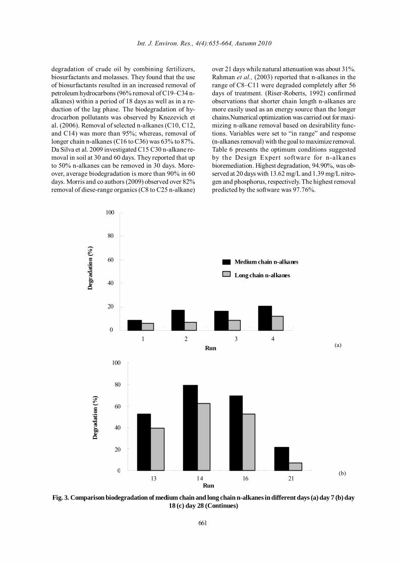
661
Int. J. Environ. Res., 4(4):655-664, Autumn 2010
degradation of crude oil by combining fertilizers,biosurfactants and molasses. They found that the useof biosurfactants resulted in an increased removal ofpetroleum hydrocarbons (96% removal of C19–C34 n-alkanes) within a period of 18 days as well as in a re-duction of the lag phase. The biodegradation of hy-drocarbon pollutants was observed by Knezevich etal. (2006). Removal of selected n-alkanes (C10, C12,and C14) was more than 95%; whereas, removal oflonger chain n-alkanes (C16 to C36) was 63% to 87%.Da Silva et al. 2009 investigated C15 C30 n-alkane re-moval in soil at 30 and 60 days. They reported that upto 50% n-alkanes can be removed in 30 days. More-over, average biodegradation is more than 90% in 60days. Morris and co authors (2009) observed over 82%removal of diese-range organics (C8 to C25 n-alkane)
over 21 days while natural attenuation was about 31%.Rahman et al., (2003) reported that n-alkanes in therange of C8–C11 were degraded completely after 56days of treatment. (Riser-Roberts, 1992) confirmedobservations that shorter chain length n-alkanes aremore easily used as an energy source than the longerchains.Numerical optimization was carried out for maxi-mizing n-alkane removal based on desirability func-tions. Variables were set to “in range” and response(n-alkanes removal) with the goal to maximize removal.Table 6 presents the optimum conditions suggestedby the Design Expert software for n-alkanesbioremediation. Highest degradation, 94.90%, was ob-served at 20 days with 13.62 mg/L and 1.39 mg/L nitro-gen and phosphorus, respectively. The highest removalpredicted by the software was 97.76%.
0
20
40
60
80
100
1 2 3 4Run
Deg
rada
tion
(%)
Medium chain n-alkanes
Long chain n-alkanes
(a)
0
20
40
60
80
100
13 14 16 21
Deg
rada
tion
(%)
Run
(b)
Fig. 3. Comparison biodegradation of medium chain and long chain n-alkanes in different days (a) day 7 (b) day18 (c) day 28 (Continues)
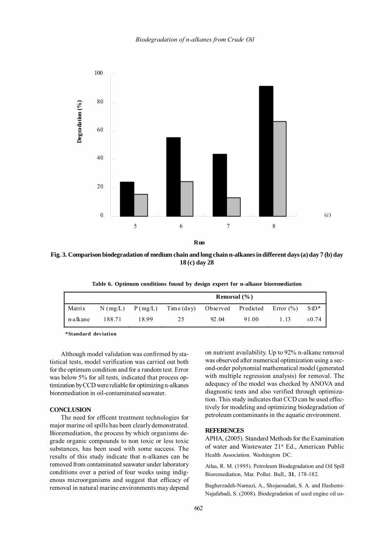
662
0
20
40
60
80
100
5 6 7 8
Deg
rada
tion
(%)
Run
Fig. 3. Comparison biodegradation of medium chain and long chain n-alkanes in different days (a) day 7 (b) day18 (c) day 28
Table 6. Optimum conditions found by design expert for n-alkane bioremediation
Removal (%)
Matrix N (mg/L) P (mg/L) Time (day) Observed Predicted Error (%) StD*
n-a lkane 188.71 18.99 25 92.04 91.00 1.13 ±0.74
*Standard deviation
CONCLUSIONThe need for efficent treatment technologies for
major marine oil spills has been clearly demonstrated.Bioremediation, the process by which organisms de-grade organic compounds to non toxic or less toxicsubstances, has been used with some success. Theresults of this study indicate that n-alkanes can beremoved from contaminated seawater under laboratoryconditions over a period of four weeks using indig-enous microorganisms and suggest that efficacy ofremoval in natural marine environments may depend
on nutrient availability. Up to 92% n-alkane removalwas observed after numerical optimization using a sec-ond-order polynomial mathematical model (generatedwith multiple regression analysis) for removal. Theadequacy of the model was checked by ANOVA anddiagnostic tests and also verified through optimiza-tion. This study indicates that CCD can be used effec-tively for modeling and optimizing biodegradation ofpetroleum contaminants in the aquatic environment.
REFERENCESAPHA, (2005). Standard Methods for the Examinationof water and Wastewater 21st Ed., American PublicHealth Association. Washington DC.
Atlas, R. M. (1995). Petroleum Biodegradation and Oil SpillBioremediation, Mar. Pollut. Bull., 31, 178-182.
Bagherzadeh-Namazi, A., Shojaosadati, S. A. and Hashemi-Najafabadi, S. (2008). Biodegradation of used engine oil us-
(c)
Biodegradation of n-alkanes from Crude Oil
Although model validation was confirmed by sta-tistical tests, model verification was carried out bothfor the optimum condition and for a random test. Errorwas below 5% for all tests, indicated that process op-timization by CCD were reliable for optimizing n-alkanesbioremediation in oil-contaminated seawater.
ing mixed and isolated cultures. Int. J. Environ. Res., 2, 431-440.
Da Silva, A. C., Oliveira, F. J., Bernardes, D. S., Franca, F. P.(2009). Bioremediation of Marine Sediments Impacted byPetroleum. Appl. Biochem. Biotechnol., 153, 58-66.
Das, K. and Mukherjee, A. K. (2007). Crude petroleum-oilbiodegradation efficiency of Bacillus subtilis and Pseudomo-nas aeruginosa strains isolated from a petroleum-oil con-taminated soil from North-East India. Bioresource Technol.,98, 1339-1345.
Delille, D., BasseÌres, A. and Dessommes, A. (1998). Effec-tiveness of bioremediation for oil-polluted antarctic seawa-ter. Polar Biol., 19, 237-241.
Delille, D., Pelletier, E., Rodriguez-Blanco, A. and Ghiglione,J. (2009). Effects of nutrient and temperature on degrada-tion of petroleum hydrocarbons in sub-Antarctic coastalseawater, Polar Biol., 32, 1521-1528.
Dutta, T. K., and Arayama, S. (2000). Fate of Crude Oil bythe Combination of Photooxidation and Biodegradation.Environ. Sci. Technol., 34, 1500-1505.
Fingas, M. (2001). The Basics of Oil Spill Cleanup. CRCPress, Boca Raton, FL.
Ghazali, F. M., Rahman, R. N., Salleh, Z. A., A. B. andBasri, M. (2004). Biodegradation of hydrocarbons in soilby microbial consortium. Int. Biodete. Biodegr., 54, 61- 67.
Huang, L., Ma, T., Li, D., Liang, F., Liu, R.-. and Li, G.(2008). Optimization of nutrient component for diesel oildegradation by Rhodococcus erythropolis, Mar. Pollut. Bull,56, 1714-1718.
Ijah, U. J. J., Antai, S. P. (2003). Removal of Nigerian lightcrude oil in soil over a 12-month period. Int. biodeterior.Biodegrade., 51, 93-99.
Jean, J., M., Lee, Sh., Wang, Chattopadhyay, P. and Maity,J. (2008). Effects of inorganic nutrient levels on the biodeg-radation of benzene, toluene, and xylene (BTX) byPseudomonas spp. in a laboratory porous media sand aqui-fer model. Bioresource Technol., 99, 7807-7815.
Kim, M., Bae, S. S., Seol, M., Lee, J. and Oh, Y. (2008).Monitoring nutrient impact on bacterial community com-position during bioremediation of anoxic PAH-contaminatedsediment. J. Microbiol, 46, 615-623.
Knezevich, V., O., Koren, E., Ron, Z. and Rosenberg, E.(2006). Petroleum bioremediation in seawater using guanoas the fertilizer. Bioremediation J., 10, 83-91.
Lee K. and Merlin F. X. (1999). Bioremediation of oil onshoreline environments: development of techniques andguidelines. Pure Appl. Chem., 71, 161–172.
Mohajeri L., H. A. Aziz, M. A. Zahed, M. H. (2009) Petro-leum hydrocarbon degrading potentials of microbial consor-tia isolated from coastal water and sediments of PenangIsland, Malaysia, 5th civil engineering conference (AWAM09), Kuala Lumpur, Malaysia.
Mohajeri, L., Aziz H. A., Isa M. H., Zahed, M. A. (2010). Astatistical experiment design approach for optimizing bio-degradation of weathered crude oil in coastal sediments,Bioresource Technol., 101, 893-900.
Montgomery, D. C. (2008). Design and Analysis of Experi-ments 7th edition, John Wiley and Sons, Inc., New York.
Morris, J. M., Jin, S., Crimi B., and Pruden A. (2009). Mi-crobial fuel cell in enhancing anaerobic biodegradation ofdiesel. Chem. Eng. J., 146, 161-167.
Nasrollahzadeh, H. S., Najafpour, G. D. andAghamohammadi, N. (2007). Biodegradation of Phenan-threne by mixed culture consortia in batch bioreactor usingcentral composite face-entered design. Int. J. Environ. Res.,1, 80-87.
Nikolopouloua, M. and Kalogerakis, N. (2008). Enhancedbioremediation of crude oil utilizing lipophilic fertilizerscombined with biosurfactants and molasses. Mar. Pollut.Bull., 56, 1855-1861.
Onwurah, I. N. E., Ogugua, V. N., Onyike, N. B., Ochonogor,A. E. and Otitoju, O. F. (2007). Crude oils spills in theenvironment, effects and some innovative clean-up biotech-nologies. Int. J. Environ. Res., 1, 307-320.
OTA, (1991). Bioremediation of Marine Oil Spills: An Analy-sis of Oil Spill Response Technologies, OTA-BP-O-70,Office of Technology Assessment, Washington, DC.
Pathak, H., Kantharia, D., Malpani, A., Madamwar, D.(2009). Naphthalene biodegradation using Pseudomonas sp.HOB1: In vitro studies and assessment of naphthalene deg-radation efficiency in simulated microcosms. J. Hazard.Mater., 166, 1466-1473.
Radwan, S. S., Al-Hasan, R. H., Salamah, S. and Al-Dabbous,S. (2002). Bioremediation of oily sea water by bacteria im-mobilized in biofilms coating macroalgae. Int. biodeterior.Biodegrade., 50, 55-59.
Rahman, K. S. M., Rahman, T. J., Kourkoutas, Y., Petsas,I., Marchant, R. and Banat, I. M. (2003). Enhancedbioremediation of n-alkane in petroleum sludge using bacte-rial consortium amended with rhamnolipid and micronutri-ents. Bioresource Technol., 90, 159-168.
Ramirez, L. C., Iturbe, R. and Torres, L. G. (2008). Effect ofnutrient and surfactant addition on polyaromatic hydrocar-bon (PAH) biodegradation in contaminated soils. Land Con-tamination and Reclamation, 16, 1-11.
Int. J. Environ. Res., 4(4):655-664, Autumn 2010
663
Riser-Roberts, E. (1992). Bioremediation of petroleum-con-taminated sites. CRC Press, Inc., Boca Raton, FL.
Ruberto, L., Dias, R., Lo Balbo, A., Vazquez, S. C.,Hernandez, E. A. and Mac Cormack, W. P. (2009). Influenceof nutrients addition and bioaugmentation on the hydrocar-bon biodegradation of a chronically contaminated Antarcticsoil. J. appl. microbiol., 106, 1101-1110.
Salas, N., Ortiz, L., Gilcoto, M., Varela, M., Bayona, J. M.,Groom, S., Álvarez-Salgado, X. A. and Albaigés, J. (2006).Fingerprinting petroleum hydrocarbons in plankton andsurface sediments during the spring and early summer bloomsin the galician coast (NW spain) after the prestige oil spill.Mar. Environ. Res., 62, 388-413.
Tam, N. F. Y., Wong, Y. S. and Wong, M. H. (2009). Noveltechnology in pollutant removal at source andbioremediation. Ocean Coast. Manage., 52, 368-373.
US-EPA, (1991). Test Methods for Evaluating Solid Waste-SW 846, US-Environmental Protection Agency, Cincinnati.OH.
Zahed, M. A. et al.
Vieira, P. A., Faria, S. R., Vieira B., De Franca, F. P., Cardoso,V. L. (2009). Statistical analysis and optimization of nitro-gen, phosphorus, and inoculum concentrations for the bio-degradation of petroleum hydrocarbons by response sur-face methodology. J. Microbiol. Biotechnol., 25, 427–438.
Zahed, M. A., Aziz H. A., Isa M. H., Mohajeri L. (2010).Effect of initial oil concentration and dispersant on crude oilbiodegradation in contaminated seawater. Bull. Environ.Contam. Toxicol., 84, 438-442.
Zhu, X, Venosa, A.D., Suidan, M. T. and Lee, K. (2001).Guidelines for the bioremediation of marine shorelines andfreshwaters Office of Research and Development NationalRisk Management Research Laboratory Land Remediationand Pollution Control Division US. Environmental Protec-tion Agency, Cincinnati, OH.
664

Int. J. Environ. Res., 4(4):665-672, Autumn 2010ISSN: 1735-6865
Received 3 May 2009; Revised 15 March 2010; Accepted 25 May 2010
*Corresponding author E-mail: [email protected]
665
Preparation of Pellets by Urban Waste Compost
Mavaddati, S. 1, Kianmehr , M . H . 1*, Allahdadi , I . 2 and Chegini , G . R .1
1 Department of agrotechnology, College of Abouraihan, University of Tehran, Tehran, Iran2 Department of Agronomy and Plant Breeding Science, College of Abouraihan, University of
Tehran, Tehran, Iran
ABSTRACT: Determination of physical properties of municipal waste compost is necessary to obtain theparameters related to designing and constructing a suitable pelleting machine for producing compost pellets.The purpose of this study is determining some physical properties such as; bulk density, coefficient offriction, porosity, angle of repose for compost and density and expansion for compost pellets. These parametersare determined at three moisture content level (15, 20 and 25 %), four particle sizes (normal size, 10, 30 and100) and three pressure level (23.4, 36 and 47.7 MPa) with three replications. According to the table ofanalysis of variance (ANOVA), effect of mesh size on angle of repose using emptying method was significant,but for filling method was not (P=0.01). The effect of mesh size on friction coefficient using four surfaces, wassignificant (P=0.01). It was determined that the effect of particle size, moisture content and pressure ondensity of pellets was significant (P=0.01). Also using compost with low porosity, particle size at 100,moisture content at 25% and pressure at 47.7 MPa will results producing best pellets.
Key word: Density, Porosity, Friction, Repose, Expansion
INTRODUCTIONThe compost and vermicompost quality is the most
essential criterion in recycling organic waste, as wellas its marketing and utilization in agriculture as organicamendments (Campitelli et al., 2008). More than 50% ofthe waste generated by the Brazilian population iscomposed of matter susceptible to organic composting(Barreira et al., 2008). The importance of this problemincreases with the increment of population. Thereforeseveral processes can be done on waste, such asburning, burying, recycling converting to usablematerials such as compost and etc. In productionprocesses, converting the municipal waste to compostis very important, because useful materials like compostcan be produced from rubbish that has wide use inagricultural and horticultural activities. Compost meansthe herbaceous, bestial and municipal waste that decay,their toxic materials refine, materials powder and losetheir original shapes. Compost maturity is related tosuitability for plant growth, although some authorsalso relate it to humification (Tognetti et al., 2006).For economic use of compost, it can be used forproducing pellets. Some of the benefits of compostpellets are:
1- Reducing the conservation space because ofdensification.2- Suitable for mechanization and compatible withfarmer’s implements for implanting or scattering.3- Suitable for residential places because of producingno dust and no pollution for environment.4- More precision with spreaders and reducing manureconsumption.5- Suitable for transporting to long distances.6- Suitable for planters and no needing to separateoperation.7- Ability of long time conservation.8- Ability of adding chemical materials for increasingthe quality of pellets.
Since last years, several studies performed onphysical properties of various biological materials.Most of these studies evaluate the effect of moisturecontent, porosity, angle of repose, coefficient offriction, density and etc on several agriculturalproducts. One of the important results that can beobtained is the effect of moisture content. Increasingthe moisture content, increases bulk density, angle ofrepose, and coefficient of friction for woodchip (Imaet al., 2007), compressibility in poultry litter (Bernhart
666
Mavaddati, S. et al.
et al., 2008), the filling and emptying angles of reposefor cocoa beans (Bart-Plange et al., 2002), coefficientof static friction for Pistachio kernel (Kashaninejad etal., 2005), true density for peanut fruit and kernel (Aydin,2006) and density and angle of repose for caper fruit(Sessiz et al., 2006), but decreases the true densityand porosity for Pistachio kernel (Kashaninejad et al.,2005), Densities in poultry litter (Bernhart et al., 2008),porosity for woodchip (Ima et al., 2007), bulk densityfor peanut fruit peanut fruit (Aydin, 2006), true density,porosity and the coefficients of static and kineticfriction for caper fruit (Sessiz et al., 2006). Particle sizeand moisture content significantly affected the pelletdensity of barley straw, corn stover and switchgrassbut different particle sizes of wheat straw did notproduce any significant difference on pellet density(Mani et al., 2006). Bulk density and particle density ofpeanut hull pellets significantly affected by moisturecontent (Fasina, 2007). Fraczek valuated a computerimage analysis method to determine the angle of reposeof grains (Fraczek et al., 2006). Also some physicalproperties such as bulk density, moisture content, freeairspace and etc, evaluated for feedstock compost(Mohee et al., 2005) and groundnut kernels (Olajide etal., 2002).
The objects of this study is to determine bulk density,angle of repose, friction angle and porosity of compostand expansion of pellets in order to obtain bestconditions for designing and constructing a suitablepelleting machine.
MATERIALS & METHODSCompost used in this study was obtained from
composting factory located at Kahrizak of Tehran. Theparticle sizes used in this study were investigated innormal size and three mesh sizes (10, 30 and 100) andthe percent for each mesh size obtained (Shaw et al.,2007). Normal size is the compost without usingmeshes. The dimension properties of each mesh sizesare shown in Table 1.
Table 1 Dimensions of mesh sizes according toASTM E-11-70 (Part 41)
100 10 30 10 Mesh size
0.15 0.425 0.6 2 Diameter (mm)
Moisture is a key environmental factor that affectsmany aspects of the composting process (Richard etal., 2002). The moisture content of compost used inthis study was 15% that obtained from placing thecompost samples in oven at 105±3ºC for 48 hours
(ASAE Standards. 1998. S269.4). The moisture contentwas calculated using the following equation:
1
21
WWWMC −
= (1)
MC = Moisture content in percent (db)W1= Primary weight of sample in gramsW2= Secondary weight of sample in grams
Porosity is the ratio of pore space to the totalvolume of sample. Kaptso determined the porosity ofthe seeds as the fraction of the space in the bulk seedwhich is not occupied by the grain can be computedfrom the values of seed true density and bulk density(Kaptso et al., 2007). Porosity can be calculated fromdry matter content, true density of dry matter and totalbulk density (Van Ginkel, 1999). Porosity is also one ofthe most important physical properties thatcharacterize the quality of dried, crispy foods (Hofsetzet al., 2007). A method similar to 5 gallon pail methodused to determine the porosity of compost. Level ofwater in a container, containing two liters of water, wasmarked inside of it. After emptying the water, thecontainer filled with compost about one-third full. Thepail was dropped 10 times from a height of 15 cm onthe floor. Compost was added to fill the pail two-thirdsfull and the pail was dropped 10 times from a height of15 cm on the floor. Compost was added to the full linemark, which was previously made on the container,and the container was dropped again 10 times from aheight of 15 cm on the floor. Compost was finally addedto fill the container to the full line mark. Water wasadded to the pail to the full line mark. The volume ofwater added was recorded.
10021 ×=
VP (2)
P= Porosity of sample in percent.V1= Volume of water added in liter.
Bulk density refers to the mass in volume unit. In thismethod a 20 liter container was fully filled with the testmaterial and the mass of the material was recorded.Bulk density was calculated by dividing the mass ofthe material by the volume of the material (Equation(3)) (Asoewgu et al., 2006; Pechon et al., 2007). Threereplications were completed and the average value wasrecorded.
2VM
=ρ (3)
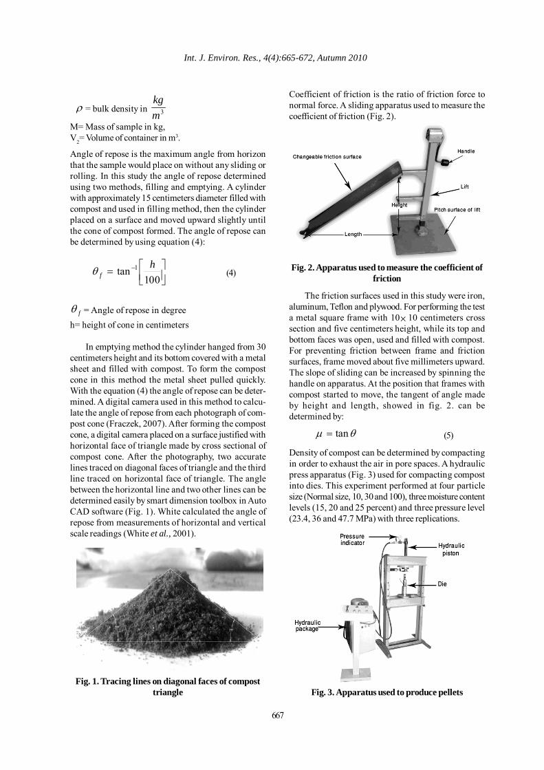
Int. J. Environ. Res., 4(4):665-672, Autumn 2010
667
Angle of repose is the maximum angle from horizonthat the sample would place on without any sliding orrolling. In this study the angle of repose determinedusing two methods, filling and emptying. A cylinderwith approximately 15 centimeters diameter filled withcompost and used in filling method, then the cylinderplaced on a surface and moved upward slightly untilthe cone of compost formed. The angle of repose canbe determined by using equation (4):
ρ = bulk density in 3mkg
M= Mass of sample in kg,V2= Volume of container in m3.
⎥⎦⎤
⎢⎣⎡= −
100tan 1 h
fθ (4)
fθ = Angle of repose in degreeh= height of cone in centimeters
In emptying method the cylinder hanged from 30centimeters height and its bottom covered with a metalsheet and filled with compost. To form the compostcone in this method the metal sheet pulled quickly.With the equation (4) the angle of repose can be deter-mined. A digital camera used in this method to calcu-late the angle of repose from each photograph of com-post cone (Fraczek, 2007). After forming the compostcone, a digital camera placed on a surface justified withhorizontal face of triangle made by cross sectional ofcompost cone. After the photography, two accuratelines traced on diagonal faces of triangle and the thirdline traced on horizontal face of triangle. The anglebetween the horizontal line and two other lines can bedetermined easily by smart dimension toolbox in AutoCAD software (Fig. 1). White calculated the angle ofrepose from measurements of horizontal and verticalscale readings (White et al., 2001).
Fig. 1. Tracing lines on diagonal faces of composttriangle
Coefficient of friction is the ratio of friction force tonormal force. A sliding apparatus used to measure thecoefficient of friction (Fig. 2).
Fig. 2. Apparatus used to measure the coefficient offriction
The friction surfaces used in this study were iron,aluminum, Teflon and plywood. For performing the testa metal square frame with 10×10 centimeters crosssection and five centimeters height, while its top andbottom faces was open, used and filled with compost.For preventing friction between frame and frictionsurfaces, frame moved about five millimeters upward.The slope of sliding can be increased by spinning thehandle on apparatus. At the position that frames withcompost started to move, the tangent of angle madeby height and length, showed in fig. 2. can bedetermined by:
Density of compost can be determined by compactingin order to exhaust the air in pore spaces. A hydraulicpress apparatus (Fig. 3) used for compacting compostinto dies. This experiment performed at four particlesize (Normal size, 10, 30 and 100), three moisture contentlevels (15, 20 and 25 percent) and three pressure level(23.4, 36 and 47.7 MPa) with three replications.
θµ tan= (5)
Fig. 3. Apparatus used to produce pellets
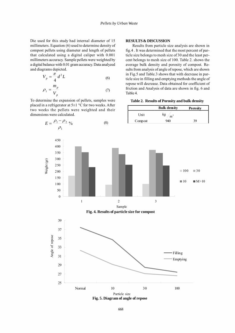
668
Die used for this study had internal diameter of 15millimeters. Equation (6) used to determine density ofcompost pellets using diameter and length of pelletsthat calculated using a digital caliper with 0.001millimeters accuracy. Sample pellets were weighted bya digital balance with 0.01 gram accuracy. Data analyzedand diagrams depicted.
LdV p2
4π
=
p
pt V
m=ρ (7)
(6)
To determine the expansion of pellets, samples wereplaced in a refrigerator at 5±1 °C for two weeks. Aftertwo weeks the pellets were weighted and theirdimensions were calculated.
RESULTS & DISCUSSIONResults from particle size analysis are shown in
fig.4 . It was determined that the most percent of par-ticle size belongs to mesh size of 30 and the least per-cent belongs to mesh size of 100. Table 2. shows theaverage bulk density and porosity of compost. Re-sults from analysis of angle of repose, which are shownin Fig.5 and Table.3 shows that with decrease in par-ticle size in filling and emptying methods the angle ofrepose will decrease. Data obtained for coefficient offriction and Analysis of data are shown in fig. 6 andTable 4.
Table 2. Results of Porosity and bulk density
Porosity Bulk density
3kg m Unit
39 940 Compost
0
50
100
150
200
250
300
350
400
450
1 2 3
100 30
10 M>10
Wei
ght (
gr)
Sample
25
27
29
31
33
35
37
39
Normal 10 30 100
Filling
Emptying
%1
21
ρρρ −
=E (8)
Fig. 4. Results of particle size for compost
Fig. 5. Diagram of angle of reposeParticle size
Ang
le o
f re
pose
Pellets by Urban Waste
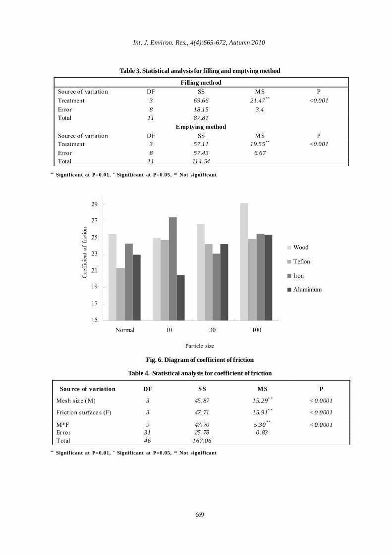
Int. J. Environ. Res., 4(4):665-672, Autumn 2010
669
Table 3. Statistical analysis for filling and emptying method
Filling method Source of varia tion DF SS MS P Treatment 3 69.66 21.47** <0.001 Error 8 18.15 3.4 Total 11 87.81
Emptying method Source of varia tion DF SS MS P Treatment 3 57.11 19.55** <0.001 Error 8 57.43 6.67 Total 11 114.54 ** Significant at P=0.01, * Significant at P=0.05, ns Not significant
15
17
19
21
23
25
27
29
Normal 10 30 100
Wood
Teflon
Iron
Aluminium
Particle size
Coe
ffici
ent o
f fri
ctio
n
Fig. 6. Diagram of coefficient of friction
Table 4. Statistical analysis for coefficient of friction
Sou rce of variation DF S S MS P
Mesh siz e ( M) 3 45.87 15.29* * < 0.0001
Friction surface s (F) 3 47.71 15.91* * < 0.0001
M*F 9 47.70 5.30** < 0.0001 Er ror 31 25.78 0.83 Total 46 167.06 ** Significant at P=0.01, * Significant at P=0.05, ns Not significant
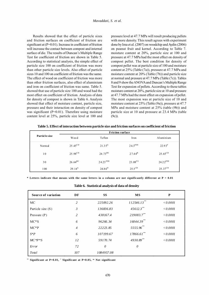
670
Results showed that the effect of particle sizesand friction surfaces on coefficient of friction aresignificant at (P=0.01). Increase in coefficient of frictionwill increase the contact between compost and internalsurface of die. The results of Duncan’s Multiple RangeTest for coefficient of friction are shown in Table 5.According to statistical analysis, the simple effect ofparticle size 100 on coefficient of friction was morethan other particle size levels. Also effect of particlesizes 10 and 100 on coefficient of friction was the same.The effect of wood on coefficient of friction was morethan other friction surfaces, also effect of aluminiumand iron on coefficient of friction was same. Table 5.showed that use of particle size 100 and wood had themost effect on coefficient of friction. Analysis of datafor density of compost is shown in Table 6. Analysisshowed that effect of moisture content, particle size,pressure and their interaction on density of compostwas significant (P=0.01). Therefore using moisturecontent level at 25%, particle size level at 100 and
pressure level at 47.7 MPa will result producing pelletswith more density. This result agrees with experimentdone by Ima et al. (2007) on woodchip and Aydin (2006)on peanut fruit and kernel. According to Table 7.moisture content at 20%, particle size at 100 andpressure at 47.7 MPa had the most effect on density ofcompost pellet. The best condition for density ofcompost pellet was at particle size of 100 and moisturecontent at 25% (Table (7a)), pressure at 47.7 MPa andmoisture content at 20% (Table (7b)) and particle sizeat normal and pressure at 47.7 MPa (Table (7c)). Tables8 and 9 show the ANOVA and Duncan’s Multiple RangeTest for expansion of pellets. According to these tablesmoisture content at 20%, particle size at 10 and pressureat 47.7 MPa had the most effect on expansion of pellet.The most expansion was at particle size of 10 andmoisture content at 25% (Table (9a)), pressure at 47.7MPa and moisture content at 25% (table (9b)) andparticle size at 10 and pressure at 23.4 MPa (table(9c)).
Table 5. Effect of interaction between particle size and friction surfaces on coefficient of friction
Friction surface Particle s ize
Wood Teflon Iron Aluminium
Normal 25 .45CD 21.3 5G 2 4.3FDE 22.93F
10 25 .98CD 24 .73DE 2 7.44B 25 .65CD
30 26 .64BC 24.23 FDE 23 .08F E 24.2 2FDE
100 29 .14A 24.8 6D 25.5 CD 25 .37CD
Table 6. Statistical analysis of data of density
Source of var iation DF SS MS P
MC 2 225092.26 112546.13** <0.0001
Particle size (S ) 3 136836.83 45612.3** <0.0001
Pressure (P ) 2 438167.4 219083.7** <0.0001
MC*S 6 96266.34 16044.39** <0.0001
MC*P 4 22223.85 5555.96** <0.0001
S*P 6 107199.67 17866.61** <0.0001
MC*P*S 12 59170.74 4930.89** <0.0001
Error 72 0 0
Total 107 1084957.08
* Letters indicate that means with the same letters in a column are not significantly different at P = 0.01
** Significant at P=0.01, * Significant at P=0.05, ns Not significant
Mavaddati, S. et al.
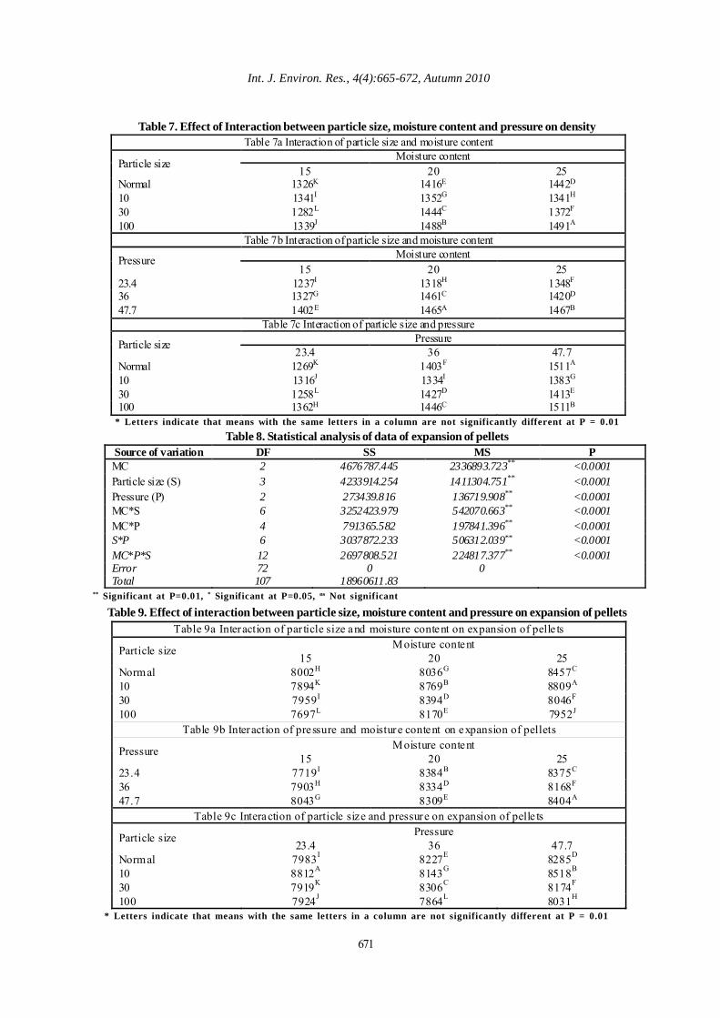
671
Int. J. Environ. Res., 4(4):665-672, Autumn 2010
Table 7. Effect of Interaction between particle size, moisture content and pressure on densityTable 7a Interaction of particle size and moisture content
Moisture content Particle size
15 20 25 Normal 1326K 1416E 1442D 10 1341I 1352G 1341H 30 1282L 1444C 1372F 100 1339J 1488B 1491A
Table 7b Interaction of particle size and moisture content Moisture content Pressure
15 20 25 23.4 1237I 1318H 1348F 36 1327G 1461C 1420D 47.7 1402E 1465A 1467B
Table 7c Interaction of particle size and pressure Pressure Particle size
23.4 36 47.7 Normal 1269K 1403F 1511A 10 1316J 1334I 1383G 30 1258L 1427D 1413E 100 1362H 1446C 1511B * Letters indicate that means with the same letters in a column are not significantly different at P = 0.01
Table 8. Statistical analysis of data of expansion of pelletsSource of variation DF SS MS P MC 2 4676787.445 2336893.723** <0.0001 Particle size (S) 3 4233914.254 1411304.751** <0.0001 Pressure (P) 2 273439.816 136719.908** <0.0001 MC*S 6 3252423.979 542070.663** <0.0001 MC*P 4 791365.582 197841.396** <0.0001 S*P 6 3037872.233 506312.039** <0.0001 MC*P*S 12 2697808.521 224817.377** <0.0001 Error 72 0 0 Total 107 18960611.83 ** Significant at P=0.01, * Significant at P=0.05, ns Not significant
Table 9. Effect of interaction between particle size, moisture content and pressure on expansion of pelletsTable 9a Interaction of par ticle size and moisture content on expansion of pelle ts
Moisture content Particle size 15 20 25
Normal 8002H 8036G 8457C 10 7894K 8769B 8809A 30 7959I 8394D 8046F 100 7697L 8170E 7952J
Table 9b Interaction of pressure and moisture content on expansion of pellets Moisture content Pressure
15 20 25 23.4 7719I 8384B 8375C 36 7903H 8334D 8168F 47.7 8043G 8309E 8404A
Table 9c Interaction of particle size and pressure on expansion of pelle ts Pressure Particle size
23.4 36 47.7 Normal 7983I 8227E 8285D 10 8812A 8143G 8518B 30 7919K 8306C 8174F 100 7924J 7864L 8031H * Letters indicate that means with the same letters in a column are not significantly different at P = 0.01
672
CONCLUSIONThe various properties measured will serve as a
useful tool in process and equipment design and thiswill go a long way in assisting to improve yield andquality of pellets. There are some major results in thisstudy. All the physical properties of compost pelletdepend on their moisture contents. Decrease in par-ticle size in filling and emptying methods causes de-crease in angle of repose. The effect of particle sizesand friction surfaces on coefficient of friction are sig-nificant at (P=0.01). The best condition for density ofcompost pellet was at particle size of 100 and moisturecontent at 25% and pressure at 47.7 MPa. Moisturecontent at 20%, particle size at 10 and pressure at 47.7MPa had the most effect on expansion of compost.
ACKNOWLEDGEMENTSThis research was supported by grants from INSF
(Iran National Science Foundation) and university ofTehran college of Abouraihan
REFERENCESASAE Standards, (1998). S269.4 Cubes. Pellets andCrumbles-Definitions and Methods for Determining Density,Durability and Moisture Content ASAE DEC96. StandardS358.2 Moisture Measurement-forages. ASAE, St. Joseph,MI.ASTM E-11-70 (Part 41) and U.S. National Bureau ofstandards official sieve designations.
Asoewgu, S., Ohanyere, S., Kanu, O. and Iwueke, C. (2006).Physical properties of African oil bean seed (Pentaclethramacrophylla). Agricultural Engineering International, theCIGR Ejournal, v.8.
Aydin, C. (2006). Some engineering properties of peanutand kernel. J. Food Engineering, 79, 810-816.
Bart-Plange, A. and Baryeh, E. A. (2002). The physicalproperties of Category B cocoa beans. J. Food Engineering,60, 219–227.
Barreira, L. P., Philippi Junior, A., Rodrigues, M. S. andTenorio c, J. A. S. (2008). Physical analyses of compostfrom composting plants in Brazil. Waste Management, 28(8), 1417-1422.
Bernhart, M. and Fasina, O. O. (2008). Moisture effect onthe storage, handling and flow properties of poultry litter.Waste Management, 29, 1392–1398.
Campitelli, P. and Ceppi, S. (2008). Chemical, physical andbiological compost and vermicompost characterization: Achemometric study. Chemometrics and Intelligent LaboratorySystems, 90 (1), 64-71.
Fraczek, J., Złobecki, A. and Zemanek, J. (2007). Assessmentof angle of repose of granular plant material using computerimage analysis. J. Food Engineering, 83, 17-22.
Fasina, O. O. (2007). Physical properties of peanut hullpellets. Bioresource Technology, 99, 1259-1266.
Hofsetz, K, Lopes, C. C., Hubingera, M. D., Mayo, L. andSereno, A. M. (2007). Changes in the physical properties ofbananas on applying HTST pulse during air-drying. J. FoodEngineering, 83, 531-540.
Ima, C. S. and Mann, D. D. (2007). Physical Properties ofWoodchip: Compost Mixtures used as biofilter media.Agricultural Engineering International: the CIGR Ejournal.Manuscript BC 07 005. v.9.
Kaptso, K. G., Njintang, Y. N., Komnek, A. E., Hounhouigan,J., Scher, J. and Mbofung, C. M. F. (2007). Physical propertiesand rehydration kinetics of two varieties of cowpea (Vignaunguiculata) and bambara roundnuts (Voandzeia subterranea)seeds. J. Food Engineering, 86, 91-99.
Kashaninejad, M., Mortazavi, A., Safekordi, A. and Tabil,L. G. (2006). Some physical properties of Pistachio (Pistaciavera L.) nut and its kernel. J. Food Engineering, 72, 30-38.
Mani, S., Tabil, L. G. and Sokhansanj, S. (2006). Effects ofcompressive force, particle size and moisture content onmechanical properties of biomass pellets from grasses.Biomass and Bioenergy, 30, 648-654.
Mohee, R. and Mudhoo, A. (2005). Analysis of the physicalproperties of an in-vessel composting matrix. PowderTechnology, 155, 92-99.
Olajide, J. O. and Igbeka, J. C. (2002). Some physicalproperties of groundnut kernels. J. Food Engineering, 58,201-204.
Pechon, R. R., Ito, N., Kito, K. and Jinyama, H. (2007).Effect of hand tractor implements on soil physical propertiesin upland conditions. Agricultural Engineering International:the CIGR Ejournal. Manuscript PM 07 005. v. 9.
Richard, T. L., Hamelers, H. V. L., Veeken, A. and Silva, T.(2002). Moisture Relationships in Composting Processes.Compost Science & Utilization, 10 (4), 286-302.
Sessiz, A., Esgici, R. and Kizil, S. (2006). Moisture-dependent physical properties of caper (Capparis ssp.)fruit. J. Food Engineering, 79, 1426-1431.
Shaw, M. D. and Tabil, L. G. (2007). Compression,Relaxation, and Adhesion Properties of Selected BiomassGrinds. Agricultural Engineering International: the CIGREjournal. Manuscript FP 07 006. v.9.
Tognetti, C., Mazzarino, M. J. and Laos, F. (2006).Improving the quality of municipal organic waste compost.Bioresource Technology, 98, 1067-1076.
Van Ginkel, J. T., Raats, P. A. C. and Van Haneghem, I. A.(1999). Bulk density and porosity distributions in a compostpile. Netherlands Journal of Agricultural Science, 47, 105-121.
White, N. D. G. and Jayas, D. S. (2001). Physical propertiesof canola and sunflower meal pellets. Canadian BiosystemsEngineering, 43, 49-52.
Pellets by Urban Waste
Int. J. Environ. Res., 4(4):673-680, Autumn 2010ISSN: 1735-6865
Received 7 March 2010; Revised 15 May 2010; Accepted 25 May 2010
*Corresponding author E-mail: [email protected]
673
Land Reclamation and Ecological Restoration in a Marine Area
Zagas, T.1*, Tsitsoni, T. 1, Ganatsas, P. 1, Tsakaldimi, M. 1, Skotidakis, T. 2 and Zagas D. 1
1 Laboratory of Silviculture, Faculty of Forestry and Natural Environment, Aristotle University ofThessaloniki, 54 124 Thessaloniki, Greece
2 ANKO Company, Kozani, Western Macedonia, Greece
ABSTRACT: This paper deals with the planning of rehabilitation of spoils of asbestos mine in NW Greecewith the name MABE in Prefecture of Kozani. For this purpose a detailed ecological research has taken placein the wider area in order to estimate the prevailing environmental (site) conditions. The spoils heaps arecharacterized by very steep slope inclination (80-90%). In order to improve the stability of the area, incooperation with civil engineers of our scientific team, a minimization of slope inclination to 39-43% had beendecided. For the avoidance of erosion hazard, broad terraces (8-12 m width) and small terraces (1.2 m width)must be constructed. After these works the whole surface of spoils will be covered by topsoil of 40 cm depth.On this topsoil the suitable trees and shrubs species will be planted. The list of these species is the result ofdetailed research in the mine and the surrounding area. The tree species Pinus nigra, Robinia pseudoacacia, andQuercus pubescens have proposed as dominant species and Acer campestre, Carpinus orientalis, Ostryacarpinifolia, Fraxinus ornus, Celtis austalis and Sorbus aucuparia as secondary tree species.
Key words: Inclination, Spoils depositions, Terraces, Topsoil, Plantings, Rehabilitation
INTRODUCTIONMinerals are significant economic resources worldwide,when they are used in rational way from financial andenvironmental point of view. The prevailing economicconjuncture determines if the exploitation on resourceis profitable or not. For this reason the exploitation ofthe minerals in a country should be decided after asystematical research of the prevailing economicparameters and the environmental problems connectedwith this activity, because the mining causes thedestruction of natural ecosystems through removal ofsoil and vegetation and burial beneath waste disposalsites (Saaty, 1990, Boyadziev and Boyadziev, 1997;Bradshaw, 1997). The restoration of mined land inpractice can largely be considered as ecosystemreconstruction. Unfortunately, in practice, the lack ofpost-restoration monitoring and research has meantfew opportunities to improve the theory and practiceof ecological restoration in mining. (Cooke and Johnson,2002). However, although the scale of human activities(overgrazing, deforestation, agriculture, overex-ploitation for fuel wood, and urban and industrial use)has become such that most of the ecosystems of theearth have been disturbed in some way (Ehrlich, 1993;Daily, 1995) the area of land directly altered by mining
industries is still relatively low in terms of the globalinventory of degradation, but can representconsiderable quantities on an individual countrybasis.
The mine area land reclamation and ecologicalrestoration research involves many research fieldssuch as mining, geology, geography, land use,environment, landscape, ecosystem, agriculture andforestry, biology, soil science, and social economy etc.and the amount of information is huge. Therefore,reasonable organization and management of researchdata is needed (Huading et al., 2005). The mostimportant problems faced in the procedure of mineareas rehabilitation is the choice of future land use(Cairney, 1995). Forestry is the most usual land usesof abandoned mine areas. For the establishment offorest on those areas the following particular problemsmust be solved: the formation of the slopes, the findingof the necessary quantities of good quality topsoil,the selection of the suitable plant species able tosurvive in such extreme site conditions, the possibleproblems of toxicity end environmental pollution andthe effective planning of rehabilitation. In thisstudy,the rehabilitation of spoils of asbestos mine
674
Zagas, T. et al.
MABE in Kozani prefecture (northern Greece) is theresearch object. Specifically, the aim of this studywas the land reclamation and ecological restorationof the spoils deposition in this asbestos mine area.In order to succeed this, we studied analytically theenvironment of the area (topography and spoils’slope, climate, soil and topsoil properties, vegetationand landscape), and based on the results obtained,we proposed the appropriate measures.
The asbestos mining area (M.A.B.E.) (in SW partof Kozani Prefecture, northern Greece) is situatedeastern of mountain Vourinos and north-western ofmountain Kambounia. It covers 414 ha and it islocated 1 km southern of the longest Greek river‘Aliakmon’. Geo-morphologically the wider area ischaracterized mountainous with a dense network ofstreams and the elevation ranges from 400 to 700 m,while in the northern part of the study area (in thevalley of Polyphyton artificial lake), the topographyis characterized as very smooth and the elevationreaches 295 m. Geologically the area is located to thewestern border of Pelagonic Zone, which is consistingfrom crystalline schist substrate (gneis, schist,amphibolites, granites, ophiolite rocks) (Rassios,2008). Phyto-sociologically the area belongs toQuercetalia pubescentis floristic zone (Athanasiadis,1986).
The mean annual rainfall is 563 mm and the meantemperature is 13.3 oC, (according to the 5-year dataobtained by the Meteorological station of Kozani).The bioclimatic of the area, according to Embergerdiagram (Mavromatis, 1981), is meso-mediterranean,sub humid with harsh winters, 40 days < Dry season<75 days. The landscape of the wider area is composedby the following characteristics: the artificial lake ofPolyphyton, intense hilly relief, dense network ofstreams, the asbestos mining area with the industrialinfrastructure, the excavation area and the depositionarea. The mine depositions have formed an artificialhilly area with very steep slopes. For this reason a lotof landslides have been occurred. Concerning thetopography and spoils depositions slope, in thenorth-eastern exposures the slope inclination was 80-90%, the bank’s height was 180 m and the depositionsmainly consisted of materials with particle size ofsand gravel and sludge-clay gravel. In the south-eastern exposures slope inclination was 70-90%, thebank’s height was 30-60 m and the depositions mainlyconsisted of asbestos spoils with coarse structure.
MATERIALS & METHODSWith the main target the land reclamation and
ecological restoration of the spoils deposition in the
asbestos mine, we studied analytically the topographyand spoils depositions’ slope, soil and topsoilproperties, vegetation and landscape of the studyarea. In restoration, emphasis was given first tominimize slope inclination, to build soil organic matter,by adding topsoil, and vegetation cover to acceleratenatural recovery process (Singh et al., 2002). Also, inorder to propose the more suitable planting materialfor the vegetation establishment, measurements inalready existed plantations were done. Finally weorganized and managed the initial data of the areaand proposed the most effective and economicrestoration techniques. The minimization of theslope inclination of the depositions was planned byterraces construction (bench plains) of differentwidth, in collaboration with the civil engineers ofthe same scientific work team, based on the mosteffective and economic solution. Physical andchemical properties of the soil and topsoil, whichare consider as the more basic factors together withtopography, for the vegetation establishment andfuture growth (Jafari et al., 2004; Tavilli and Jafari,2009), were estimated after detailed soil analysis. Thetopsoil (the productive soil) had been deposited intwo positions (covering surface area about 6 ha andhaving total volume 365.000 m3) at the beginning ofthe mining activities. We took 4-pooled samples fromtopsoil and we excavated two (2) soil profiles fromthe neighbour undisturbed area. However, additionaltopsoil that should be extracted from the wider areais needed for the spoils covering of the mine. Adetailed plant species inventory in the wider area(in a distance 2-3 Km around the mining area) andon the heaps of topsoil was made in order to studythe vegetation and to propose the most suitablespecies for the rehabilitation. We also recorded thespecies that had been planted by the MABECompany in the undisturbed and in the rehabilitatedsurfaces within the mining area. The change of thevisual absorptive capacity of the landscape beforeand after reclamation techniques was estimated. Thevisual absorption capacity of the landscape (VAC)is defined as the capacity of the landscape to absorbdevelopments wi thout it s character beingsignificantly changed or its scenic quality reduced(Amir and Gidalizon, 1990; Lucas, 1991; BCMoF,1995).
It was estimated according to the equation: VAC=S* (SE+RD+C+L), where: S= slope, SE= Soil Erosion,RD=Regeneration Dynamics, C= Color contrast, L=Landscape diversity (Anderson, et al. , 1979;Yeomans, 1979). For the selection of the suitableplan t ing stock, field survival and growthmeasurements were done in the existed plantationswithin the mine area.
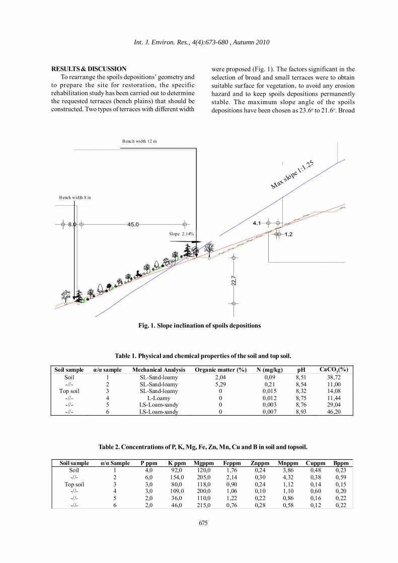
Int. J. Environ. Res., 4(4):673-680 , Autumn 2010
675
RESULTS & DISCUSSIONTo rearrange the spoils depositions’ geometry and
to prepare the site for restoration, the specificrehabilitation study has been carried out to determinethe requested terraces (bench plains) that should beconstructed. Two types of terraces with different width
were proposed (Fig. 1). The factors significant in theselection of broad and small terraces were to obtainsuitable surface for vegetation, to avoid any erosionhazard and to keep spoils depositions permanentlystable. The maximum slope angle of the spoilsdepositions have been chosen as 23.6o to 21.6o. Broad
Bench width 12 m
Bench width 8 m
Slope 2.14%
Max slope 1:1.25
Fig. 1. Slope inclination of spoils depositions
Table 1. Physical and chemical properties of the soil and top soil.
Soil sample α/α sample Mechanical Analysis Organic matter (%) N (mg/kg) pH CaCO3(%) Soil 1 SL-Sand-loamy 2,04 0,09 8,51 38,72 -//- 2 SL-Sand-loamy 5,29 0,21 8,54 11,00
Top soil 3 SL-Sand-loamy 0 0,015 8,32 14,08 -//- 4 L-Loamy 0 0,012 8,75 11,44 -//- 5 LS-Loam-sandy 0 0,003 8,76 29,04 -//- 6 LS-Loam-sandy 0 0,007 8,93 46,20
Table 2. Concentrations of P, K, Mg, Fe, Zn, Mn, Cu and B in soil and topsoil.
Soil sample α/α Sample P ppm K ppm Mgppm Feppm Znppm Mnppm Cuppm Bppm Soil 1 4,0 92,0 120,0 1,76 0,24 3,86 0,48 0,23 -//- 2 6,0 154,0 205,0 2,14 0,30 4,32 0,38 0,59
Top soil 3 3,0 80,0 118,0 0,90 0,24 1,12 0,14 0,15 -//- 4 3,0 109,0 200,0 1,06 0,10 1,10 0,60 0,20 -//- 5 2,0 36,0 110,0 1,22 0,22 0,86 0,16 0,22 -//- 6 2,0 46,0 215,0 0,76 0,28 0,58 0,12 0,22

676
Land Reclamation & Ecological Restoration
No Trees Shrubs 1 2 3 4 5 6 7 8 9 10 11 12 13 14 15
Platanus orientalis Quercus pubescens Quercus frainetto Carpinus orientalis Fraxinus ornus Cercis siliquastrum Pyrus amygdaliformis Populus nigra Ficus carica Celtis australis Morus nigra Salix alba Ulmus campestris Acer campestre Populus alba
Quercus coccifera Paliurus spina cristi Corinus coggygria Pistacia terebinuthus Phillyrea latifolia Juniperus oxycedrus Rubus canescens Sambucus ebulus Colutea arborescens Coronilla emeroides Clematis vitalba Rosa sp.
Table 3. Species composition of the naturalvegetation of the area
No Woody species Grasses 1 2 3 4 5 6 7 8 9 10 11 12
Colutea arborescens Ulmus campestris Rubus canescens Pistacia terebinthus Polulus alba Platanus orientalis Pinus nigra Cotinus coggygria Juglans regia Pyrus amygdaliformis Malus sylvestris Vitis vinifera
Ononis spinosa Cynodon dactylon Dactylis glomerata Tussilago farfara Hypericum perforatum Epilobium sp. Chamecytisus sp. Lotus corniculatus Trifolium campestre Trifolium arvense
Table 4. Naturally colonized species on the heapof topsoil
Table 5. Visual absorption capacity (VAC) of the landscape of the study area.
Factor Conditions Degree before restoration Degree after restoration
Slope Inclination
Slope 0-5 % 6-15 % 16-30 % 31-60 % >60 %
1
2.5- 3
Landscape diversity (vegetation, topography, water sources)
Low Medium
High
1
2
Soil erosion High
Medium Low
1
3
Regeneration dynamics Low
Medium High
1
3
Colour contrast of soil High
Medium Low
1
2
Table 6. Survival percentage of existed planted species in the mine area
Species Planting stock Survival (%) Pinus nigra Containerised 70 Pinus brutia Containerised 80 Robinia preudoacacia bareroot 95 Fraxinus ornus bareroot 80 Populus nigra bareroot 80
a/a Species Percentage (%) Planting stock 1 Pinus nigra 35 Container seedlings 2 Robinia pseudoacacia 35 Bareroot seedlings 3 Quercus pubescens 20 Container seedlings 4 Acer campestre 1.67 Bareroot seedlings 5 Carpinus orientalis 1.67 —//— 6 Ostrya carpinifolia 1.67 —//— 7 Fraxinus ornus 1.67 —//— 8 Celtis australis 1.67 —//— 9 Sorbus aucuparia 1.67 —//—
Table 7. Percentage contribution of the tree species, which are proposed for planting on the great andindividuals terraces
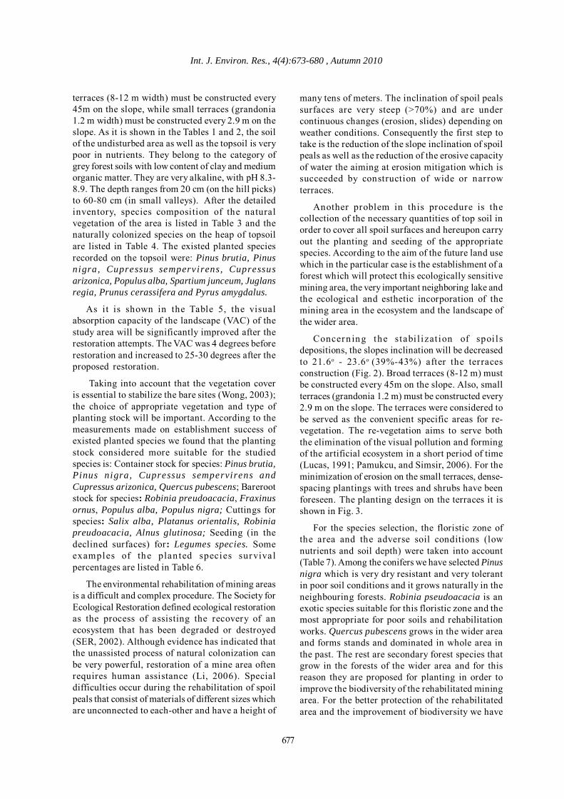
Int. J. Environ. Res., 4(4):673-680 , Autumn 2010
terraces (8-12 m width) must be constructed every45m on the slope, while small terraces (grandonia1.2 m width) must be constructed every 2.9 m on theslope. As it is shown in the Tables 1 and 2, the soilof the undisturbed area as well as the topsoil is verypoor in nutrients. They belong to the category ofgrey forest soils with low content of clay and mediumorganic matter. They are very alkaline, with pH 8.3-8.9. The depth ranges from 20 cm (on the hill picks)to 60-80 cm (in small valleys). After the detailedinventory, species composition of the naturalvegetation of the area is listed in Table 3 and thenaturally colonized species on the heap of topsoilare listed in Table 4. The existed planted speciesrecorded on the topsoil were: Pinus brutia, Pinusnigra, Cupressus sempervirens, Cupressusarizonica, Populus alba, Spartium junceum, Juglansregia, Prunus cerassifera and Pyrus amygdalus.
As it is shown in the Table 5, the visualabsorption capacity of the landscape (VAC) of thestudy area will be significantly improved after therestoration attempts. The VAC was 4 degrees beforerestoration and increased to 25-30 degrees after theproposed restoration.
Taking into account that the vegetation coveris essential to stabilize the bare sites (Wong, 2003);the choice of appropriate vegetation and type ofplanting stock will be important. According to themeasurements made on establishment success ofexisted planted species we found that the plantingstock considered more suitable for the studiedspecies is: Container stock for species: Pinus brutia,Pinus nigra, Cupressus sempervirens andCupressus arizonica, Quercus pubescens; Barerootstock for species: Robinia preudoacacia, Fraxinusornus, Populus alba, Populus nigra; Cuttings forspecies: Salix alba, Platanus orientalis, Robiniapreudoacacia, Alnus glutinosa; Seeding (in thedeclined surfaces) for: Legumes species. Someexamples of the plan ted species survivalpercentages are listed in Table 6.
The environmental rehabilitation of mining areasis a difficult and complex procedure. The Society forEcological Restoration defined ecological restorationas the process of assisting the recovery of anecosystem that has been degraded or destroyed(SER, 2002). Although evidence has indicated thatthe unassisted process of natural colonization canbe very powerful, restoration of a mine area oftenrequires human assistance (Li, 2006). Specialdifficulties occur during the rehabilitation of spoilpeals that consist of materials of different sizes whichare unconnected to each-other and have a height of
many tens of meters. The inclination of spoil pealssurfaces are very steep (>70%) and are undercontinuous changes (erosion, slides) depending onweather conditions. Consequently the first step totake is the reduction of the slope inclination of spoilpeals as well as the reduction of the erosive capacityof water the aiming at erosion mitigation which issucceeded by construction of wide or narrowterraces.
Another problem in this procedure is thecollection of the necessary quantities of top soil inorder to cover all spoil surfaces and hereupon carryout the planting and seeding of the appropriatespecies. According to the aim of the future land usewhich in the particular case is the establishment of aforest which will protect this ecologically sensitivemining area, the very important neighboring lake andthe ecological and esthetic incorporation of themining area in the ecosystem and the landscape ofthe wider area.
Concern ing the stabi l izat ion of spoi lsdepositions, the slopes inclination will be decreasedto 21.6o - 23.6o (39%-43%) after the terracesconstruction (Fig. 2). Broad terraces (8-12 m) mustbe constructed every 45m on the slope. Also, smallterraces (grandonia 1.2 m) must be constructed every2.9 m on the slope. The terraces were considered tobe served as the convenient specific areas for re-vegetation. The re-vegetation aims to serve boththe elimination of the visual pollution and formingof the artificial ecosystem in a short period of time(Lucas, 1991; Pamukcu, and Simsir, 2006). For theminimization of erosion on the small terraces, dense-spacing plantings with trees and shrubs have beenforeseen. The planting design on the terraces it isshown in Fig. 3.
For the species selection, the floristic zone ofthe area and the adverse soil conditions (lownutrients and soil depth) were taken into account(Table 7). Among the conifers we have selected Pinusnigra which is very dry resistant and very tolerantin poor soil conditions and it grows naturally in theneighbouring forests. Robinia pseudoacacia is anexotic species suitable for this floristic zone and themost appropriate for poor soils and rehabilitationworks. Quercus pubescens grows in the wider areaand forms stands and dominated in whole area inthe past. The rest are secondary forest species thatgrow in the forests of the wider area and for thisreason they are proposed for planting in order toimprove the biodiversity of the rehabilitated miningarea. For the better protection of the rehabilitatedarea and the improvement of biodiversity we have
677
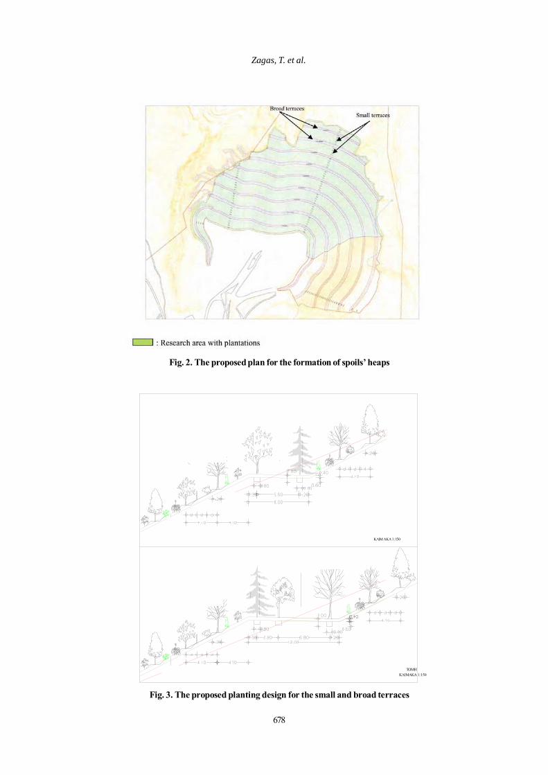
678
Zagas, T. et al.
ΚΛΙΜΑΚΑ 1:150
ΚΛΙΜΑΚΑ 1:150ΤΟΜΗ
Fig. 3. The proposed planting design for the small and broad terraces
Fig. 2. The proposed plan for the formation of spoils’ heaps
679
Int. J. Environ. Res., 4(4):673-680 , Autumn 2010
proposed also the followings: 1. Planting the shrubspecies: Spartium junceum, Cotinus coggygria, Rhuscoriaria, Colutea arborescens, Prunus spinosa,Quercus coccifera, Buxus sempervirens, Cercissiliquastrum, Ligustrum vulgare and Phillyrealatifolia, 2. Planting species as cuttings: Salix alba,Robinia pseudoacacia, Populus nigra, Alnusglutinosa, Platanus orientalis and 3. Seeding of thespecies: P. nigra, R. pseudoacacia, C. siliquastrum,Colutea arborescens, S. junceum, L. vulgare, C.coggygria, R. coriaria, Rosa canina, Rubuscanescens, Trifolium arvence, Vicia sp., Lathyrus sp.,Dactylis glomerata, Lolium multiflorum. For thesystematic irrigation of the established species on therehabilitated area, hydraulic engineers of the samescientific team have planned a modern irrigation system.
CONCLUSION
This study proposes the forestry as the future landuse of the mining area because this concentrates themost advantages and this was the previous land useof the area (degraded forest land, used for animalsgrazing and firewood production).
According to the results of the soil analysis, thesoil as well as the topsoil of the study area is very poorin nutrients, with low content of clay and mediumorganic matter and very alkaline. This study proposesthat the minimum depth of topsoil, which will be usedfor spoils covering, must be over 40 cm in order tosupport effectively the established species. Also, thetopsoil should be enriched with organic matter (2% atleast) and with the appropriate fertilizers in order toimprove soil fertility and reduce alkalinity. Since thedeposition peals are visible from a long distance dueto the relief change and the colour contrast, theprinciples of landscape architecture must be appliedfor the ecological restoration of the disturbed landaccording to the visual characteristics of the landscapeof the wider area.
After our restoration techniques the visualabsorption capacity of the landscape will be increasedfrom the very low class (4) to middle class (25-30).
REFERENCES
Anderson, L., Mosier, J. and Chandler, G. (1979). VisualAbsorption Capacity. In: Proc. of “Our National Landscape”,U.S.D.A. Forest Service, Berkeley, Cal.
Amir, S. and Gidalizon, E. (1990). Expert-based method forthe evaluation of the visual absorption capacity of thelandscape. J. Env. Manage., 30, 251-263.
Athanasiadis, N. (1986). Forest Phytosociology.(Thessaloniki :Giahoudis-Giapoulis Press), (in Greek).
Bojadziev, G. and Bojadziev, M. (1997). Fuzzy Logic forBusiness, Finance and Management. (Singapore :WorldScientific).
Bradshaw, A. (1997), Restoration of mine lands – usingnatural processes. Ecological Engineering, 8, 255-269.
British Columbia Ministry of Forests (BCMoF), (1995).Visual Landscape Design Training Manual, Vol. 2,Recreation Branch Publication, BCMoF, Victoria, BC.
Cairney, T. (1995). The Re-use of Contaminated Land, aHandbook of Risk Assessment, West Essex, UK.
Cooke, J. A. and Johnson, M. S. (2002). Ecologicalrestoration of land with particular reference to the miningof metals and industrial minerals: A review of theory andpractice. Environ. Rev., 10, 41-71.
Daily, G. C. (1995). Restoring value to the world’s degradedlands. Science, 269, 350–354.
Ehrlich, P.R. (1993). The scale of the human enterprise. (InD.A. Saunders, R.J. Hobbs and P.R. Ehrlich (Eds), Natureconservation 3: Reconstruction of fragmented ecosystems -global and regional perspectives. New South Wales: SurreyBeatty & Sons.
Huading, S., Su, L. and Zhongke, B. (2005). TheDevelopment of Land Reclamation and EcologicalRestoration Information System in mine area -A Case Studyof PingShuo opencast mine area. National ScienceFoundation of China (40071077).
Jafari, M., Zare Chahouki, M. A., Tavili, A., Azarnivand,H. and Zahedi Amiri. Gh. (2004). Effective environmentalfactors in the distribution of vegetation types in Poshtkouhrangelands of Yazd province (Iran). Journal of AridEnvironments, 56, 627-641.
Li, M. S. (2005). Ecological restoration of mineland withparticular reference to the metalliferous mine wasteland inChina: A review of research and practice. Science of theTotal Environment, 357, 38-53.
Lucas, O. W. R. (1991). The design of forest landscapes.(New York: Oxford University Press).
Mavromatis, G. (1981). The bioclima of Greece. Relationsof climate and natural vegetation, bioclimatic maps. (Athens:Forest Research Institute), (in Greek with English Abstract).
Pamukcu C., and Simsir, F. (2006). Example of reclamationattempts at a set of quarries located in Izmir, Turkey. J.Min.Sci., 42, 304-308.
Rassios, E.A. and students of the Aliakmon Valley Legacyproject, (2008). Rocks in the Wild. A Guide to theIdentification of IMPERFECT Rocks and Minerals.(Kozani-Greece: I.G.M.E. dot.print).
Saaty, T. L. (1990). Multicriteria decision-making. Theanalytic hierarchy process. Pittsburg P.A., Second Edition,USA: RWS Publications.

680
Land Reclamation & Ecological Restoration
Singh, A. N., Raghubanshi, A. S. and Singh J. S. (2002).Plantations as a tool for mine spoil restoration. CurrentScience, 82 (12), 1436-1441.
Tavili, A. and Jafari, M. (2009). Interrelations BetweenPlants and Environmental Variables. Int. J. Environ. Res., 3(2), 239-246
Wong, M. H. (2002). Ecological restoration of mine degradedsoils, with emphasis on metal contaminated soils.Chemosphere, 50, 775-780.
Yeomans, C. W. (1979). A proposed biophysical approachto Visual Absorption Capacity (VAC). In Proc. of “OurNational Landscape”, U.S.D.A. Forest Service, Berkeley,Cal.
Tehrani S. M., et al.
INTRODUCTIONTo date, rapid growth of population and high rate
of migrations along with the high number of shoppingtrips in metropolitan areas such as Tehran bringsenvironmental consequences like excessive amountsenergy use, a ir pollut ion and massive urbancongestions in all urban trips (Siikavirla et al., 2003;Pourahmad, et al., 2007; Shafie-Pour Motlagh, 2007;Panjeshahi and Ataei, 2008; Pijanowski, et al., 2009).Advantages of electronic shopping from economical,easiness, transparency, as well as environmentalpoints of view are clear and accepted, not only indeveloped countries with more than two decades of
ABSTRACT: Considering rapid growth and migration, higher accumulation of communities along with thehigh number of shopping trips in mega cities such as Tehran brings environmental consequences like excessiveamounts of energy use, air pollution and massive urban congestions in all urban trips ending to shopping areas.The present study has been performed in Tehran, capital of Iran in 2009-2010. With the advancement ofinformation, communication technology great access to the electronic devices such as internet, telephone andcell-phone had showed a remarkable increase. Moreover, as a result, the governmental support for eliminationor modification of trips through application of tele-presence in various activities has been also developed. Thestudy has investigated the willingness of people in changing their shopping habit from physical to electronicform. A comprehensive questionnaire was designed based on various demographical, geographical and techno-logical competences. For this purpose, final data were collected from 3580 respondents including customers,sellers and governmental sectors in order to achieve the present situation of e-shopping activity in Tehran.Furthermore, cluster analysis were performed and the results showed a significant relationship between e-shopping activities and demographic elements such as; income, education, occupation, marital status. Besides,e-shopping activities have a strong correlation with geographic distributions like distance and time to shop-ping areas as well as technological competence such as time spent, working, browsing on the net plus the modeof connection. Finally, in order to find out e-shopping management strategy in Tehran, the SWOT analysisalong with QSPM and SPACE matrices were performed. In this regard, internal and external factors weregained 3.03 and 2.99, respectively. Subsequently, 22 strategies were developed and the scores of each strategywere defined. Space matrix was also indicated that the e-shopping strategy grows to suggested competitivestrategy type.
Key words: Electronic shopping, Urban Environment, Municipal air pollution, Environmental management strategy
Received 10 May 2010; Revised 28 June 2010; Accepted 24 July 2010
*Corresponding author E-mail: [email protected]
681
Role of E-shopping Management Strategy in Urban Environment
1Department of Environmental Management, Graduate School of the Environment and Energy,Science and Research Branch, Islamic Azad University, Tehran, Iran
2Graduate Faculty of the Environment, University of Tehran, P.O.Box 14135-6135Tehran, Iran
3Department of Environmental Engineering, K. N. Toosi University, Tehran, Iran
experience, but also in developing countries (Tehraniand Karbassi, 2005; Chien and Shih, 2007; Tehrani etal., 2009). To purchase a product, the customers canof course visit a store or shopping centers andalternative way is to buy product through the internet(Browne and Allen, 2001; Farag, 2002; Weltevredenand van Rietbergen, 2009), but home shopping viaother electronic tools such as telephone, cell-phoneand TV are also practiced (Ferrell, 2004; Mokhtarian,2004; Ferrell, 2005). Several factors are of significantvalue in accepting and performing this activity. Thesefactors are; individual characteristics (Li et al., 1992);Shopping accessibility-time and distance (Ren and
Int. J. Environ. Res., 4(4):681-690 , Autumn 2010ISSN: 1735-6865
Tehrani, S. M. 1*, Karbassi, A. R. 2, Monavari, S. M. 1 and Mirbagheri S. A.3

Tehrani S. M., et al.
682
Kwan, 2006); products classification and delivery andpossession (Mokhtarian, 2004); Internet literacy,working, browsing and shopping experience (Brownet al., 2001; Liao and Cheung, 2001; O’cass and Tino2003; Cho, 2004). Environmental benefits counted forthe studied str ategy include el imination ormodification of shopping trips, air pollution control,minimization of energy consumption, land use savingand finally solution to urban congestions (Handy andYantis, 1997; Puanakivi and Holmstrom, 2001;Hjorthol, 2002; Rotem-Mindali and Salomon, 2007;Huang and Shih, 2009). Strategic planning is currentlyan extended tool for regional development, territorialstructuring and business management. Cities, regions,firms and business organization have carried out theirstrategic plans on the basis of participationprocesses, which have driven the later developmentof their own territories (Terrados, et al., 2005).Environmental analysis can also be used as a criticalpart of the strategic management planning process.SWOT framework (Strength; Weakness; Opportunityand Threat) along with QSPM strategy and SPACEmatrix are proposed by many as an analytical toolwhich should be used to categorize significantenvironmental factors both internal (strengths;weaknesses) and external (opportunities; Threats) to
the organization (Pickton and Wright, 1998; Mirkia,et al., 2008).
The present study on e-shopping has beenperformed in Tehran, capital of Iran in 2009-2010.
MATERIALS & METHODSIn order to test the five significant factors and
sub-factors amongst Tehran residents, aquestionnaire has been provided based on sociodemographic, daily and non daily in-store shoppingand e-shopping behavior. In addition, technologicalquestions such as Internet experience (time, intervaluse, method of access), geographical questions asdistance and time distance to the nearest shoppingcenter and local store and questions aboutenvironmental awareness and responsibilities weredesigned and distributed in two forms of Internetbased as well as through face to face interviews in 22Districts of Tehran using simple sample takingtechnique (Fig. 1). The total of 3580 completedquestionnaires was collected. Cluster analysis usingMVSP software performed. Furthermore, SWOTanalysis, QSPM and SPACE matrix for reaching tothe most important e-shopping management strategywere carried out.
Iran Map
Tehran Map
Fig. 1. Geographic location of the study area
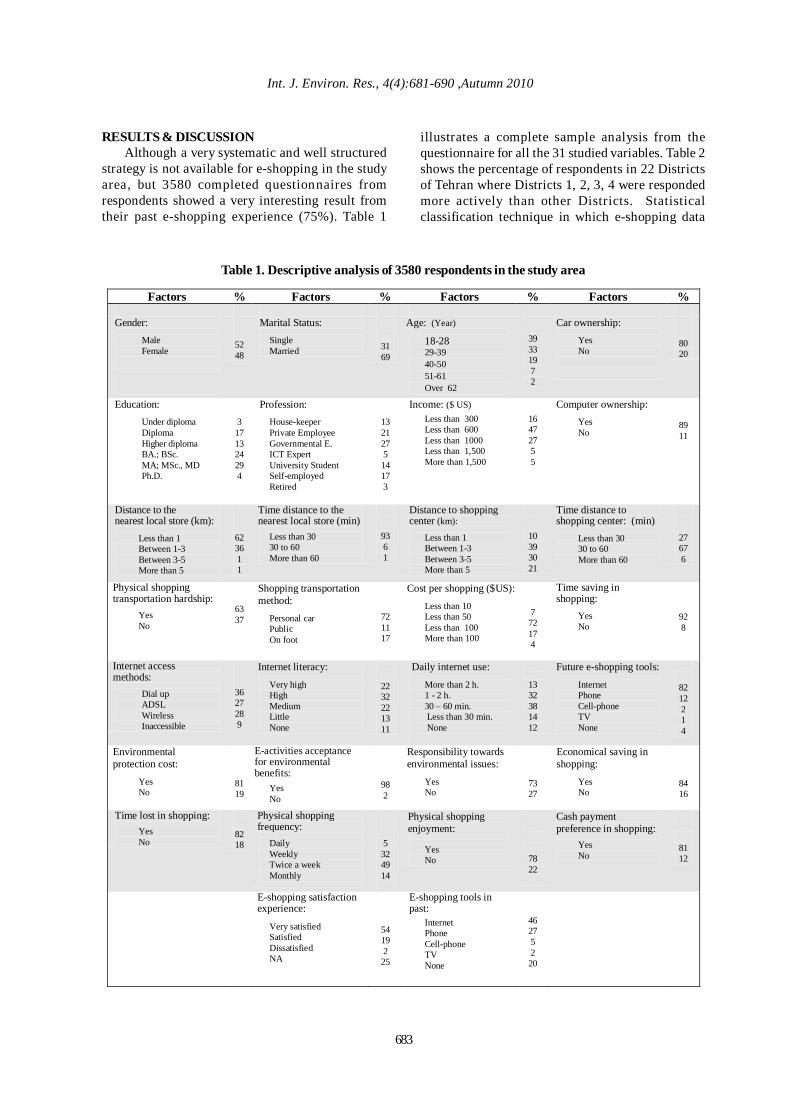
Tehrani S. M., et al.
Factors % Factors % Factors % Factors % Gender:
Male Female
52 48
Marital Status:
Single Married
31 69
Age: (Year)
18-28 29-39 40-50 51-61 Over 62
39 33 19 7 2
Car ownership:
Yes No
80 20
Education:
Under diploma Diploma Higher diploma BA.; BSc. MA; MSc., MD Ph.D.
3 17 13 24 29 4
Profession:
House-keeper Private Employee Governmental E. ICT Expert University Student Self-employed Retired
13 21 27 5 14 17 3
Income: ($ US)
Less than 300 Less than 600 Less than 1000 Less than 1,500 More than 1,500
16 47 27 5 5
Computer ownership:
Yes No
89 11
Distance to the nearest local store (km):
Less than 1 Between 1-3 Between 3-5 More than 5
62 36 1 1
Time distance to the nearest local store (min)
Less than 30 30 to 60 More than 60
93 6 1
Distance to shopping center (km):
Less than 1 Between 1-3 Between 3-5 More than 5
10 39 30 21
Time distance to shopping center: (min)
Less than 30 30 to 60 More than 60
27 67 6
Physical shopping transportation hardship:
Yes No
63 37
Shopping transportation method:
Personal car Public On foot
72 11 17
Cost per shopping ($US):
Less than 10 Less than 50 Less than 100 More than 100
7 72 17 4
Time saving in shopping:
Yes No
92 8
Internet access methods:
Dial up ADSL Wireless Inaccessible
36 27 28 9
Internet literacy:
Very high High Medium Little None
22 32 22 13 11
Daily internet use:
More than 2 h. 1 - 2 h. 30 – 60 min. Less than 30 min. None
13 32 38 14 12
Future e-shopping tools:
Internet Phone Cell-phone TV None
82 12 2 1 4
Environmental protection cost:
Yes No
81 19
E-activities acceptance for environmental benefits:
Yes No
98 2
Responsibility towards environmental issues:
Yes No
73 27
Economical saving in shopping:
Yes No
84 16
Time lost in shopping:
Yes No
82 18
Physical shopping frequency:
Daily Weekly Twice a week Monthly
5 32 49 14
Physical shopping enjoyment:
Yes No
78 22
Cash payment preference in shopping:
Yes No
81 12
E-shopping satisfaction experience:
Very satisfied Satisfied Dissatisfied NA
54 19 2 25
E-shopping tools in past:
Internet Phone Cell-phone TV None
46 27 5 2 20
683
RESULTS & DISCUSSIONAlthough a very systematic and well structured
strategy is not available for e-shopping in the studyarea, but 3580 completed questionnaires fromrespondents showed a very interesting result fromtheir past e-shopping experience (75%). Table 1
illustrates a complete sample analysis from thequestionnaire for all the 31 studied variables. Table 2shows the percentage of respondents in 22 Districtsof Tehran where Districts 1, 2, 3, 4 were respondedmore actively than other Districts. Statisticalclassification technique in which e-shopping data
Int. J. Environ. Res., 4(4):681-690 ,Autumn 2010
Table 1. Descriptive analysis of 3580 respondents in the study area
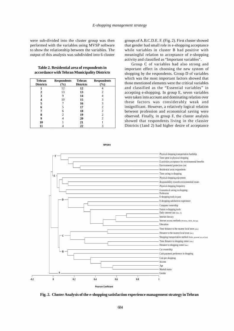
Tehrani S. M., et al.
Physical shopping transportation hardship Time spent in physical shopping E-activities acceptance for environmental benefits Environmental protection cost Residential areas respondents Time saving in shopping Physical shopping enjoyment Responsibility towards environmental issues Physical shopping frequency Economical saving in shopping Profession E-shopping tools in past E-shopping satisfaction experience Computer ownership Future e-shopping tools Daily internet use (min.; h.) Internet literacy Internet access methods (Wireless, ADSL, dial up) Education Time distance to the nearest local store (min.) Distance to the nearest local store (km.) Shopping transportation method (Public, personal car, on foot)
Time distance to shopping center (min.) Distance to shopping center (km.) Car ownership Cash payment preference in shopping Cost per shopping Income Age Marital status Gender
-0.2 0 0.2 0.4 0.6 0.8 1
B
C
A
D
E
WPGMA
Pearson Coefficient
F
684
Production of PHB from coir industrial wasteE-shopping management strategy
were sub-divided into the cluster group was thenperformed with the variables using MVSP softwareto show the relationship between the variables. Theoutput of this analysis was subdivided into 6 cluster
groups of A.B.C.D.E. F. (Fig. 2). First cluster showedthat gender had small role in e-shopping acceptancewhile variables in cluster B had positive withmeaningful relation to acceptance of e-shoppingactivity and classified as “Important variables”.
Group C of variables had also strong andimportant effect in choosing the new system ofshopping by the respondents. Group D of variableswhich was the most important factors showed thatthose mentioned elements were the critical variablesand classified as the “Essential variables” inaccepting e-shopping. In group E, seven variableswere taken into account and dominating relation overthese factors was considerably weak andinsignificant. However, a relatively logical relationbetween profession and economical saving wereobserved. Finally, in group F, the cluster analysisshowed that respondents living in the classierDistricts (1and 2) had higher desire of acceptance
Tehran Districts
Respondents (%)
Tehran Districts
Respondents (%)
1 12 12 4 2 13 13 2 3 9 14 4 4 10 15 3 5 7 16 3 6 5 17 2 7 6 18 2 8 2 19 2 9 4 20 2 10 1 21 1 11 4 22 3
Table 2. Residential area of respondents inaccordance with Tehran Municipality Districts
Fig. 2. Cluster Analysis of the e-shopping satisfaction experience management strategy in Tehran

Tehrani S. M., et al.Int. J. Environ. Res., 4(4):681-690 , Autumn 2010
685
Table 3. SWOT matrix: Derivation of the key strategies in the e-shopping management strategy3) Strengths (S) 4) Weaknesses (W)
Internal Factors External Factors
S1: More access to goods descriptions (According to the name, branch, color, weight and price) and ability of goods comparison from quality standard and price point of view in various stores S2: Interaction ability and exchanging views amongst the customers and close relations with the sellers due to system interaction S3: Ability of 24 hours shopping system from home or workplace S4: Buying and receiving simultaneously for some products electronically such as; music, books, software … S5: Lower offer prices of goods due to elimination of overhead in whole seller S6: Elimination of push system and absence of stress in comparison with physical shopping and ability of control in shopping process by the consumers S7: Easiness in payment transaction and price transparency due to standard coding system S8: Receiving goods and groceries without personal urban trip making S9: Less operational cost of e-shopping store versus brick and mortar stores S10: Possibility of customer classification according to their needs and styles for the sake of better goods selection S11: Earnest attention to the needs of customer due to customer orientation system S12: Elimination of third parties in goods distribution chain and transportations S13: Urban management close attention in development of application of e-commerce system
W1: Inadequate skills in ICT and computer usage W2: High cost and inadequate access to broad band internet W3: High cost of computer ownership W4: Lack of trust and confidence in the ordered goods quality W5: Lack of confidence in safe keeping of consumer and sellers personal information W6: Absence of trust in unacquainted e-shopping sites W7: Lack of tactile sense before shopping W8: Lack of competence in presence of goods return policy W9: No adequate and compiled laws and regulations specific for e-shopping system W10: Inadequate investment in establishment of technology related to e-commerce W11: In ability in forecasting environmental reactions W12: Lack of credit cards ownership
1) Opportunities (O) Strategies on the basis of strength
points and opportunities (SO) Strategies on the basis of the strength points and
opportunities (WO) O1: Trips reduction through e-shopping O2: Energy consumption reduction as the cause of trip elimination of consumers and utilization of efficient transportation by e-retailers O3: Air pollution and greenhouse gases reduction O4: Goods price reduction due to overhead elimination O5: Saving shopping time and its allocation to other activities O6: Less psychological tension through urban traffic jam diminishing O7: Groceries and goods elimination of truck delivery to the local supermarkets O8: providing a suitable business model based on new technology O9: Rapid and feasible interactions between government and business O10: Providing appropriate plans and policies along with constant monitoring and access to business state by government O11: Reduction of current bureaucracy amongst producers and sellers O12: Increasing of speed in shopping processes O13: Decreasing of unsold goods waste in wholesalers and their transportation to producers O14: Promoting culture of information and communication technology usage
1- To compel the producers and sellers to create their website in order to show the speciation, standards coding related to their products providing the case of company quality and prices before any commitment for shopping to the customer in direction of minimizing urban traffic and environmental pollution along with time saving and promoting speed of shopping process 2- Providing interactive facilities between customers and sellers through 24/ 7 shopping websites 3- Price reduction of goods and groceries bought online (Due to third parties and overhead elimination and competitive prices) to encourage customers to substitute physical shopping trips with e-shopping 4- Promoting and encouraging acceptance of e-shopping culture amongst the customers in order to eliminate stress factors coming from friction between customers and sellers and promoting environmental awareness culture 5- Creation of compelling circumstances for standardization and bar coding systems of products for price reduction purposes and application of a systematic model based on new technology in supply chain 6- Urban management attention and support in providing facilities for e-commerce system development 7- Providing applicable software's of e-shopping for establishment of better interaction between customers and e-sellers 8- Elimination of third parties and transparency of transactions in distribution, selling and buying of products chain as an encouragement sellers and customers and producers for e-commerce acceptance 9- Mass media advertising for magnifying the fact about elimination of urban shopping trips as the result of e-shopping
1- Providing awareness, education, transparency and persuasion of customers and sellers in understanding full dimensions of e-shopping in accordance with sustainable development and consumption patterns from policy makers 2- Compulsion to acquire IT skills through educational trainings in different school levels by government for benefiting from all opportunities of e-shopping in future 3- Economical savings through e-shopping activity 4- Providing a suitable business model based on new technology opportunities of goods and groceries by retailing government sector with monitoring and surveillance indirection of trust building amongst customers and sellers
2) Threats (T) Strategies basis of the strength points and threats (ST)
The strategies basis of the weak points and threats (WT)
T1: Elimination of physical shopping enjoyment T2: Elimination of social communication T3: Rapid variation in ICT industry and its cost T4: Over consumption due to lower prices and shopping accessibility T5: Excessive shopping orders due to easy delivery system T6: Solid waste growth resulting from packaging T7: Electricity consumption growth resulting from PC usage
1- Designing and implementing websites and e-catalogues in accordance with standards and high digital quality in order to attract customers and creation of enjoyment from using web environment 2- Updating and strengthening e-shopping sites along with ICT development 3- Providing multilateral interactive relation between sellers and customers in order to encourage them to achieve new experience in social relations 4- Encouragement and training of sellers to have better interaction with customers and accepting their point of views about packaging and delivering of goods 5- Providing education and awareness in choosing and buying products in regards with family consumption patterns by urban management
1- Providing complimentary education in the field of IT from beginner to advanced levels and putting into effect the notion of "E-citizen" 2- Providing necessary facilities for free or minimum price of access to internet with appropriate broad band 3- Constituting necessary facilities for sufficient investment for establishment of relating technology to e-commerce 4- Providing necessary facilities for allocating credit cards and internet access to bank accounts

Tehrani S. M., et al.
686
Table 4. Priorities of the executive strategies for e-shopping management strategy
No. S+T Strategy Rate %
1 ST22
Providing a suitable business model based on new technology opportunities of goods and groceries by retailing government sector with monitoring and surveillance indirection of trust building amongst customers and sellers
5.34 6.91
2 ST19
Providing awareness, education, transparency and persuasion of customers and sellers in understanding full dimensions of e-shopping in accordance with sustainable development and consumption patterns from policy makers
5.14 6.65
3 ST12Providing multilateral interactive relation between sellers and customers in order to encourage to achieve new experience in social relations
4.78 6.18
4
ST1
To compel the producers and sellers to create their website in order to show the speciation, standards coding related to their products providing the case of company quality and prices before any commitment for shopping to the customer in direction of minimizing urban traffic and environmental pollution along with time saving and promoting speed of shopping process
4.56 5.90
5 ST7 Providing applicable software's of e-shopping for establishment of better interaction between customers and e-sellers in order to promote e-shopping system amongst the customers
4.20 5.34
6 ST16
Providing necessary facilities for free or minimum price of access to internet with appropriate broad band
3.99 5.16
7 ST9Mass media advertising for magnifying the fact about elimination of urban shopping trips as the result of e-shopping
3.95 5.11
8 ST3Price reduction of goods and groceries bought online (Due to third parties and overhead elimination and competitive prices) to encourage customers to substitute physical shopping trips with e-shopping
3.89 5.03
9 ST6 Urban management close attention in development of application of e-commerce system 3.81 4.93
10 ST2Providing interactive facilities between customers and sellers through 24/ 7 shopping websites in order to minimizing urban traffic and environmental pollution along with time saving
3.79 4.90
11 ST13
Encouragement and training of sellers to have better interaction with customers and accepting their point of views about packaging and delivering of goods
3.46 4.47
12 ST17
Constituting necessary facilities for sufficient investment for establishment of relating technology to e-commerce
3.34 4.32
13 ST11 Updating and strengthening e-shopping sites in direction of ICT development 3.32 4.29 14
ST4
Promoting and encouraging acceptance of e-shopping culture amongst the customers in order to eliminate stress factors coming from friction between customers and sellers and promoting environmental awareness culture
3.19 4.12
15 ST21 Investment of all the economical savings resulting from e-shopping acceptance in relating ICT sector 3.01 3.89 16
ST10Designing and implementing websites and e-catalogues in accordance with standards and high digital quality in order to attract customers and creation of enjoyment from using web environment
2.94 3.80
17 ST14
Providing education and awareness in choosing and buying products in regards with family consumption patterns by urban management
2.86 3.70
18 ST18 Providing necessary facilities for allocating credit cards and internet access to bank accounts 2.79 3.61
19 ST8Elimination of third parties and transparency of transactions in distribution, selling and buying of products chain as an encouragement sellers and customers and producers for e-commerce acceptance
2.73 3.53
20
ST15Providing complimentary education in the field of IT from beginner to advanced levels and putting into effect the notion of "E-citizen"
2.58 3.33
21 ST5
Creation of compelling circumstances for standardization and bar coding systems of products for price reduction purposes and application of a systematic model based on new technology in supply chain
2.41 3.11
22 ST20
Compulsion to acquire IT skills through educational trainings in different school levels by government for benefiting from all opportunities of e-shopping in future
1.17 1.51
= 77.25
= 100
Σ Σ

Tehrani S. M., et al.Int. J. Environ. Res., 4(4):681-690 , Autumn 2010
and hardship of physical shopping with time loss forphysical shopping were two distinctive variablesrelated to shopping behavior changes. Finally it isbelieved that group D, which represents views of therespondents in regards with e-shopping had closerelation with the variables in group B and C while,group A, E, F had less significant value in overallperspectives of respondents in relation with e-shopping activity.
In the further investigation, environmentalanalysis was used as a critical part of the strategicmanagement planning process. SWOT frameworkcategorized the significant environmental factors both
internal (strengths; weaknesses) and external(opportunities; Threats) to the e- shoppingmanagement strategy. Many factors for strengths andweaknesses were determined. These factors wereweighted in a way that the sum of these weighs isequal to one. Then, a score was allocated to each factor,between 1 to 4 from severe weakness to importantstrengths. External factors consisted of opportunitiesand threats. In this regard, all the steps were similar toIFE matrix. According to Table 3, integration of thesetwo matrices indicated the key strategies in thee-shopping management.
Items
Score
Financial Status (FS)
1. Goods prices reduction +5 2. Cost of access to the e-shopping system through electronic tools, telephone, mobile-phone and TV +3 3. Cost of computer ownership +3 4. Lack of adequate investment in technology establishment related to e-commerce +5 5. Economical savings from energy consumption and social costs +4 20÷5 = 4 Industrial Status (IS)
1. Providing a suitable business model based on new technology and reviewing of existing regulations related to technology of e-shopping system
+5
2. Presence of e-shopping attractions (Speed, time, price, environmental attitude and belief) +3 3. Shopping 24/ 7 and Unnecessary handling and carrying cash +3 4. Buying and receiving some products simultaneously electronically +3 14÷4 = 3.5 Environmental Stability (ES)
1. Lack of proper access to electronic tools (Internet, Phone, Mobile, TV) -4 2. Rapid variations in ICT -2 3. Inadequate skills in IT and computer -4 4. Lack of credit cards and internet accounts ownership -3 5. Inadequate confidence in e-shopping sites (Quality of goods, safe keeping personal information, lack of tactile senses, goods return policy)
-5
-18÷5= -3.6 Competitive Advantage (CA)
1. Inadequate presence of force to oblige procedures for receiving standard products codes and establishing website
-5
2. Week interactions between government and business -4 3. Inadequate governmental support and investment in promoting e-shopping culture -3 4. Inadequate security in e-shopping systems -4 -16÷4= -4
X = ES + FS = 4 - 3.6 = + 0.4 Y = IS + CA = 3.5 - 4 = - 0.5
Table 5. SPACE matrix for evaluating situations and strategic measures
687
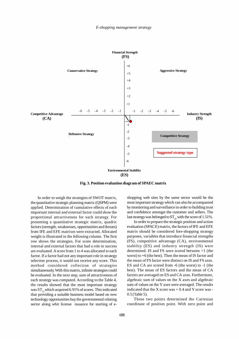
Tehrani S. M., et al.E-shopping management strategy
688
Fig. 3. Position evaluation diagram of SPAEC matrix
-1
1 - 2 - 3 - 4- 5 - 6-
Environmental Stability(ES)
Aggressive Strategy Conservative Strategy
Defensive Strategy
+1
+2
+3
+4
+5
+6
-6
-5
-4
-3
Competitive Strategy
Industry Strength(IS)
Competitive Advantage (CA)
Suggested strategy type
6- 5 - 4 - 3 - 2 - 1-
Financial Strength (FS)
-2
In order to weigh the strategies of SWOT matrix,the quantitative strategic planning matrix (QSPM) wereapplied. Determination of cumulative effects of eachimportant internal and external factor could show theproportional attractiveness for each strategy. Forpresenting a quantitative strategic matrix, quadricfactors (strength, weaknesses, opportunities and threats)from IFE and EFE matrixes were extracted. Allocatedweight is illustrated in the following column. The firstrow shows the strategies. For score determination,internal and external factors that had a role in successare evaluated. A score from 1 to 4 was allocated to eachfactor. If a factor had not any important role in strategyselection process, it would not receive any score. Thismethod considered collection of strategiessimultaneously. With this matrix, infinite strategies couldbe evaluated. In the next step, sum of attractiveness ofeach strategy was computed. According to the Table 4,the results showed that the most important strategywas ST22 which acquired 6.91% of scores. This indicatedthat providing a suitable business model based on newtechnology opportunities buy the governmental relatingsector along whit license issuance for starting of e-
shopping web sites by the same sector would be themost important strategy which can also be accompaniedby monitoring and surveillance in order to building trustand confidence amongst the customer and sellers. Thelast strategy was belonged to ST20 with the score of 1.51%.
In order to prepare the strategic position and actionevaluation (SPACE) matrix, the factors of IFE and EFEmatrix should be considered fore-shopping strategypurposes, variables that introduce financial strengths(FS), competitive advantage (CA), environmentalstability (ES) and industry strength (IS) weredetermined. IS and FS were scored between +1 (theworst) to +6 (the best). Then the mean of IS factor andthe mean of FS factor were distinct on IS and FS axes.ES and CA are scored from -6 (the worst) to -1 (thebest). The mean of ES factors and the mean of CAfactors are averaged on ES and CA axes. Furthermore,algebraic sum of values on the X axes and algebraicsum of values on the Y axes were averaged. The resultsindicated that the X score was + 0.4 and Y score was -0.5 (Table 5).
These two points determined the Cartesiancoordinate of position point. With zero point and
Tehrani S. M., et al.
position point, the diagram of position evaluation wasdrawn (Fig 3). Space matrix result indicated that the e-shopping strategy grown to be as suggestedcompetitive strategy type (Fig. 3).
CONCLUSIONA comprehensive questionnaire was designed
based on various demographical, geographical andtechnological competences. Data were collectedfrom 3580 respondents including customers, sellersand governmental sectors in order to achieve thepresent situation of e-shopping activity in Tehran.Furthermore, cluster analysis were performed andthe results showed a significant relationshipbetween e-shopping activities and demographicelements such as; income, education, occupation,marital status. Besides, e-shopping activities havea strong correlation with geographic distributionslike distance and time to shopping areas as well astechnological competence such as time lost,working, browsing on the net plus the mode ofconnection. The SWOT analysis along with QSPMand SPACE matrices were performed. Thus, internaland external factors were obtained. Subsequently,the total strategies were developed and the scoresof each strategy were defined. Space matrix indicatedthat the e-shopping strategy grows to competitivestrategy type.
ACKNOWLEDGEMENTSThe authors would like to express their sincere
appreciation for the scientific support of Dr. J.Goddossi for his generous help, also grateful to Dr. H.Nikoomaram for his scientific support. Moreover,sincere thanks are devoted to Dr. F. Gaffari for his greatassistance throughout the project statistical exercises.At last not at least, authors are most grateful to Mrs. S.Mirkia for her continuous advice.
REFERENCESBrowne, M., Allen, J., Anderson, S. and Jackson, M.(2001). Overview of delivery in UK. A study for DTI.University of Westminster, London, UK.
Chien, M. K. and Shih, L. H. (2007). An empirical studyof the implementation of green supply chain managementpractices in the electrical and electronic industry and theirrelation to organizational performances. Int. J. Environ.Sci. Tech. 4 (3), 383-394.
Cho, J . (2004). Likelihood to abort an onlinetransportation. Influences from cognitive evaluations,attitudes and behavioral variables. Information andManagement 41, 827-838.
Farag, S., Dijst, M. and Lazendorf, M., (2002). Exploringtesting of online store and shopper Research. Psycho.Market., 20(2), 139-150.
Ferrell, C. E. (2004). Tele-shoppers and shopping: Dotele-shoppers travel less? CD-Rom. The 83rd. AnnualTransportation Research Board Meeting. Washington,D.C.
Ferrell, C. E. (2005). Home-based teleshoppers andshopping travel: Do teleshoppers travel less?Transportation Research record No. 1926, 212-223.
Handy, S. L. and Yantis, T. (1997). The impact oftelecommunications technologies on nonwork travelbehavior. Southwest Region University TransportationCenter Research the University of Texas at Austin, 1-58.
Hjorthol, R. J. (2002). The relation between daily traveland use of the home computer. Transportation Research,36, 437-452.
Huang, P. and Shih, L. (2009). Effective environmentalmanagement through environmental knowledgemanagement. Int. J. Environ. Sci. Tech., 6 (1), 35-50
Liao, Z. and Cheung, M. T. (2001). Internet-based e-shopping and consumer attitudes: An empirical study.Information Manage. 38, 299-300.
Li, H., Kuo, C. and Russell, M. G. (1999). The impact ofperceived channel utilities, shopping orientation anddemographics on the consumers’ online buying behavior.J. Computer Mediated Communication. 5 (2).
Mokhtarian, P. L., (2004). A conceptual analysis of thetransportation impacts of B2C ecommerce.Transportation, 31, 257-284.
O’Cass; A. and Tino F. (2003). Web retailing adoption:Exploring the nature of internet users web relatingbehavior. J. Retailing Consumer Services, 10 (2), 81-94.
Pijanowski, B.C., Tayyebi, A., Delavar, M. R. andYazdanpanah, M. J. (2009). Urban Expansion SimulationUsing Geospatial Information System and ArtificialNeural Networks. Int. J. Environ. Res. 3 (4), 493-502
Pourahmad, A., Baghvand, A., Zangenehe Shahraki, S. andGivehchi, S. (2007). The Impact of Urban Sprawl up onAir Pollution Int. J. Environ. Res. 1 (3), 252-257.
Puanakivi, M. and Holmstrom, J. (2001). Environmentalperformance improvement potentials by food homedelivery. Paper presented at the NOFOMA Conference.
Ren, F. and Kwan, M., (2006). Does access to shoppingopportunities affect e-shopping? The second internationalspecial meeting on ICT, Everyday life and urban change.November 9-12. Bergen, the Netherlands.
Rotem-Mindali, O. and Salomon, L. (2007). The impactof E-retail on the choice of shopping trips and delivery:Some preliminary finding. Transportation Research PartA: Policy and Practice, 41(2), 176-189.
Tehrani, S. M. and Karbassi, A. R. (2005 ). Applicationof E-commerce in local home shopping and itsconsequences on energy consumption and air pollutionreduction. Iran J. Environ. Health Sci. Eng. 2 (4), 247-250.
Int. J. Environ. Res., 4(4): 681-690 , Autumn 2010
689

Tehrani S. M., et al.
Tehrani, S. M., Karbassi, A. R., Ghoddosi, J., Monavvari,S. M. and Mirbagheri, S. A. (2009). Prediction of energyconsumption and urban air pollution reduction in e-shoppingadoption. J. Food Agric. Environ. 7 (3&4), 8 9 8 - 9 0 3.
Shafie-Pour Motlagh, M. and Farsiabi, M. M. (2007). AnEnvironmental & Economic Analysis for Reducing EnergySubsidies. Int. J. Environ. Res. 1 (2), 150-162
Siikavirla, H., Punakivi, M., Karkkainen, M. and Linnanen,L.(2003). Effects of e-commerce on greenhouse gasemissions: A case study of grocery home delivery in Finland.Journal of International Ecology, 6 (2), 83-97.
Terrados, J., Almonacidand, G. and Hontoria, L. (2005).Regional energy planning through SWOT analysis andstrategic planning tools. Impact on renewable development.Renew. Sust. Energ. Rev., 11 (6), 1275-1287.
Weltevreden, J. W. J. and van Rietbergen, T. (2009). Theimplications of e-shopping for in-store shopping at variousshopping locations in the Netherlands, Environ. PlanningB: Planning and Design, Pion Ltd, London, 36 (2), 279-299.
690
Int. J. Environ. Res., 4(4):691-700 , Autumn 2010ISSN: 1735-6865
Received 6 March 2010; Revised 25 June 2010; Accepted 5 July 2010
*Corresponding author E-mail: [email protected]
691
Spatial Variability and Contamination of Heavy Metals in the Inter-tidalSystems of a Tropical Environment
Ratheesh Kumar, C. S.*, Joseph, M. M., Gireesh Kumar, T. R., Renjith, K.R., Manju, M. N. and Chandramohanakumar, N.
Department of Chemical Oceanography, School of Marine Sciences, Cochin University of Scienceand Technology, Kochi, Kerala, India
ABSTRACT: Heavy metals in the surface sediments of the two coastal ecosystems of Cochin, southwestIndia were assessed. The study intends to evaluate the degree of anthropogenic influence on heavy metalconcentration in the sediments of the mangrove and adjacent estuarine stations using enrichment factor andgeoaccumulation index. The inverse relationship of Cd and Zn with texture in the mangrove sediments suggestedthe anthropogenic enrichment of these metals in the mangrove systems. In the estuarine sediments, the absenceof any significant correlation of the heavy metals with other sedimentary parameters and their stronginterdependence revealed the possibility that the input is not through the natural weathering processes. Theanalysis of enrichment factor indicated a minor enrichment for Pb and Zn in mangrove sediments. While,extremely severe enrichment for Cd, moderate enrichment for Zn and minor enrichment of Pb were observedin estuarine system. The geo accumulation index exhibited very low values for all metals except Zn, indicatingthe sediments of the mangrove ecosystem are unpolluted to moderately polluted by anthropogenic activities.However, very strongly polluted condition for Cd and a moderately polluted condition for Zn were evident inestuarine sediments.
Key words: Geochemistry, Mangroves, Estuary, Metal pollution, Enrichment factor, Geoaccumulation index
INTRODUCTIONHigh degree of industrialization and urbanization
has led to a strong risk of heavy metal contamination inthe coastal ecosystems in tropical and subtropicalcountries. Mangrove ecosystems may act as a sink or asource of heavy metals in coastal environments,because of their variable physical and chemicalproperties (Harbison, 1986). Estuaries, which form thepart of coastal system are also a major reservoir of tracemetals, both of anthropogenic and natural origins(Bryan et al., 1980 and Langston, 1982).Spatial variationof metal concentration in surface sediments ofurbanized estuaries is often attributed to mixing ofsediments from different origins and to pollutionsources (Forstner, 1981). The measurement of traceelement concentrations and distribution in marineenvironment leads to better understanding of theirbehavior in aquatic environment and is important fordetecting the sources of pollution (Unnikrishnan andNair, 2004). The objective of the study was to determinethe total concentrations of some heavy metals in thesurface sediments of three mangrove and six adjacentestuarine stations in the Cochin estuary in order to
evaluate the degree of anthropogenic influence.Enrichment factor and geoaccumulation index weretaken as the tool for the study. An attempt to identifythe major factors controlling the distribution of heavymetals in these systems was also made by using theprincipal component analysis.
MATERIALS & METHODSCochin estuary, the largest estuarine system in the
southwest coast of India, is a part of the Vembanad-Kol wetlands, a Ramsar Site (No. 1214). This estuary(Lat.09°30'-10o10’N and Long.76o15’-76o25’E) istopographically divisible into two arms; a southernone extending south of bar mouth from Cochin toThanneermukkam and a northern one extending northfrom Cochin to Azhikode (Ramamirtham et al., 1986).This tropical aquatic system is under the profoundinfluence of monsoon, which contribute to about 71%of annual rainfall (Jayaprakash, 2002) and accordinglythere are three seasonal conditions prevailing-monsoon (June–September), post-monsoon(October–January) and pre-monsoon (February–May). The abundant mangrove vegetation along the

692
Ratheesh Kumar, C. S. et al.
Cochin estuarine system has been shrinking in areadue to land reclamation and developmental activitiesand pollution by industrial effluents as well as domesticsewage. Eloor, the major industrial belt of Kerala isnotorious for heavy pollution and is rated as one ofthe most toxic hotspots of the world by Green PeaceInternational.The major polluting industries in theregion include fertilizer plant, oil refinery, rare earthprocessing plant, minerals and rutiles plant, zinc smelterplant, insecticide factory and organic chemical plant.Three mangroves ecosystems M1, M2 and M3 and sixestuarine stations E1 to E6 along is the northern arm ofCochin estuary were selected for the present study(Fig. 1). Among the mangrove locations, Station 1,Puthuvyppu (M1), is a mangrove nursery maintainedby the fisheries research unit of Kerala AgriculturalUniversity, located about 100 m away from theestuarine front and is free from sewage inputs. Station2, Murikkumpadam (M2), is a densely populatedfishermen-settlement. The discharge of sewage anddisposal of garbage and solid waste add to the problemof pollution. Station 3, Manglavanam (M3), is a patchy
mangrove area in the heart of the city of Cochin. Thisis an almost closed system with a single narrow canallinking to the estuary, which is the only source fortidal propagation. The pressure of urban developmentis causing an adverse effect on this sanctuary. Theindiscriminate discharge of the untreated effluentscontaining heavy metals and pesticides from the Eloorindustrial belt is a common point source of pollutionto the estuary. Samplings of water and sediments weremade from these locations during December 2005, April2006 and July 2006 representing post-monsoon, pre-monsoon and monsoon respectively. Water sampleswere taken using a Niskin sampler. Van Veen grab (0.042m2) and a clean plastic spoon was used for sedimentsampling. After being collected, sediments were putinto a sealed polyethylene bag, placed in an ice boxand were brought back to the laboratory and keptrefrigerated at -20°C before analyses. pH in the watercolumn was measured in situ and temperature wasmeasured using a sensitive thermometer. Salinity ofthe water samples was estimated by Mohr-Knudsenmethod (Muller, 1999). Modified Winkler method was
Fig. 1. Location map of the sampling stations
Int. J. Environ. Res., 4(4):691-700 , Autumn 2010
693
used for the estimation of dissolved oxygen (Hansen,1999). Alkalinity of the water samples was estimatedby the method of Koroleff (Anderson et al., 1999).Phosphate, nitrite, nitrate and silicate were estimatedspectophotometrically (Grasshoff et al., 1999). Redoxpotential (Eh) of the sediment was measured withplatinum and standard calomel electrodes standardizedagainst Zobell’s solution (Brassard, 1997). Textureanalysis of the sediment was done based on Stoke’slaw using the method of Krumbein and Pettijohn(1938). Finely powdered air dried sediments were usedfor the further analyses and values are expressed ondry weight basis. Total Carbon, Hydrogen, Nitrogenand Sulphur were determined using a Vario EL III CHNSAnalyzer. Sediment organic carbon was estimated bythe procedure of El Wakeel and Riley modified byGaudette et al. (1974). Total phosphorous wasestimated spectrophotometrically after digestion usinga di-acid mixture (1:5 HClO4:HNO3).
For the heavy metal analysis (total), about 1 g ofthe dried and finely powdered sediments was digestedin Teflon vessels with a 1:5 mixture of HClO4-HNO3(Loring and Rantala, 1992). Complete digestion wasensured by repeating the acidification until a clearsolution was obtained and brought into solution in 0.5M HCl using Milli Q water. Samples were analyzed ona flame AAS (Perkin Elmer 3110) after calibration withsuitable elemental standards. The precision andaccuracy of the analytical procedure was checkedusing BCSS-1 (standard reference material for marineand estuarine sediments). Triplicate analysis of BCSS-1 showed a good accuracy and the recovery rate rangedbetween 90.7 % for Mn and 103.9 % for Zn. Theenrichment factor (EF) was calculated for each metal,using iron as normalizing element following theequation EF = (metal/Fe) sediment/ (metal/Fe) crust.EF values were interpreted as suggested by Birth(2003) for metals studied with respect to naturalbackground concentration. The GeoaccumulationIndex (Igeo), introduced by Muller (1979) was used toassess metal pollution in sediments according to theequation Igeo = log2 (Cn/1.5Bn), where Cn = measuredconcentration of heavy metal in the mangrovesediment, Bn =geochemical background value inaverage shale (Wedepohl, 1995) of element n, 1.5 is thebackground matrix correction in factor due to lithogeniceffects.
RESULTS & DISCUSSIONpH of mangroves ranged between 6.58 and 7.57.
Wide fluctuations in salinity were observed and itvaried from 1.3 to 34.03 ppt and the highest value wasrecorded at M2 during pre-monsoon. Dissolvedoxygen content in mangroves ranged between 1.44 mgO2 /L (M1, post-monsoon) to 10.24 mg O2 /L (M2, pre-
monsoon). Alkalinity varied from 68 mg CaCO3/L (M3,post-monsoon) to 216 mg CaCO3/L (M2, pre-monsoon). Total nitrogen, Inorganic phosphate, andsilicate varied from 6.24, 5.288, 3.55 µmol/L to 48.65,49.73, 63µmol/L respectively. Total nitrogen contentexhibited highest value at M3 during post-monsoon.Highest concentrations of inorganic phosphate andsilicate were reported from M2 during post-monsoonand M1 during monsoon respectively.
In the estuary, pH values varied from 6.08 to 8.15and 5.95 to 8.77 for the surface and bottom watersrespectively. As the distance from the bar mouthincreases the decreasing trend in pH was observed.The salinity of the samples varied from 0.01 to 34.92ppt and 0.03 to 36.02 ppt for surface and bottomsamples respectively with the highest values observedat E1. Dissolved oxygen concentrations were higherduring monsoon period ranging between 4.57 and 7.68mg O2/L for surface and 3.04 and 8 mg O2/L for bottomwaters respectively. Alkalinity varied from 12 to 317mg/l and 16 to 208 mg/L for surface and bottom samplesrespectively. Bottom waters of E4 exhibited the highesttotal nitrogen content during monsoon and it rangedbetween 6.24 and 48.65 µmol/L. Inorganic phosphatevaried from 5.29 to 49.73 µmol/L and the highestconcentration was recorded at bottom waters ofE1during post-monsoon. Silicate content displayed itshighest content at surface waters of E6 duringmonsoon and ranged between 3.55 and 63 µmol/L.
In the case of mangrove sediments, pH varied from5.85 to 7.10 (Table 1). Marked variation in Eh valueswas recorded in sediments (-398 to +12 mV) and highlynegative redox condition was observed at M3. Textureanalysis showed that sand content ranged between0.94 and 36.60%. M1 exhibited the highest silt contentduring pre-monsoon period and it varied from 28.51 to71.79%. Clay content ranged between 19.07 and 39.68%with the highest value at M2 during post-monsoon.Total carbon and organic carbon content varied from2.91 to 7.64% and 2.2 to 6.66 %, respectively. Totalnitrogen content ranged between 0.27 and 0.66 % andthe total sulphur varied from 0.22 to 1.96 % of thesediment. The variation in total P content was from0.22 to 2.80% of the sediment. The highest values forthe contents of total C, organic C, total P and total Nwas observed at M3 during post-monsoon but total Sconcentration exhibited its highest value at the samestation during pre-monsoon.
In the estuarine sediments (Table 2), pH rangedbetween 5.60 and 7.80 and was maximum at E2 duringpost- monsoon. The highest redox condition wasnoticed at E3 during pre-monsoon. The predominanceof the silty nature was observed up to E3 and higher

694
Heavy Metals in the Inter-tidal Systems
Table 1. Chemical parameters estimated for mangrove sediments
M 1 M 2 M 3 Parameters Pre Mon Post Pre Mon Post Pre Mon Post pH 6.2 5.85 7 6.46 6.48 7.1 6.65 - 6.6 Eh -98 -16 -10 12 -41 -53 -337 - -398 Sand % 6.73 36.6 8.87 4.34 2.32 0.94 23.59 - 10.46 Silt % 71.79 28.51 58.92 59.97 63.78 59.38 45.56 - 70.47 Clay % 21.45 34.89 32.2 35.69 33.9 39.68 21.97 - 19.07 Total C % 3.73 6.75 4.72 2.91 3.31 6.25 5.52 - 7.64 Organic C % 2.80 6.30 3.90 2.20 2.50 4.90 5.00 - 6.70 Total N % 0.34 0.5 0.32 0.27 0.29 0.46 0.47 - 0.66 Total P % 2308 2226 2249 2987 2387 2933 28000 - 28665 Total S % 0.32 0.25 0.62 0.35 0.22 0.63 1.96 - 1.14 Cd (µg/g) 0.07 0.064 0.089 0.098 0.059 0.062 0.223 - 0.223 Co (µg/g) 22.30 17.73 21.42 22.20 22.80 23.08 12.82 - 15.70 Cr (µg/g) 90.22 73.18 76.08 85.28 89.77 89.05 53.30 - 63.27 Cu (µg/g) 30.75 24.98 23.97 27.75 31.38 31.58 29.17 - 39.12 Fe % 5.83 4.26 4.56 5.76 5.74 5.71 5.62 - 5.74 Mg% 1.78 1.24 1.53 1.72 1.69 1.68 1.23 - 1.27 Mn (µg/g) 315.32 227.82 257.83 227.20 210.50 299.08 260.95 - 225.95 Ni (µg/g) 55.5 55.425 54.75 68.75 69.35 65.57 30.60 - 40.25 Pb (µg/g) 35.25 21.25 37.50 39.50 33.25 32.5 25.25 - 19.5 Zn (µg/g) 128.80 101.30 111.30 116.30 112.55 132.55 315.05 - 455.675
-The sample from M3 during monsoon was not able to collect due to technical reasons.
sand content was seen from E4 onwards. The silt andclay content was observed to be higher in E1 duringpre and post-monsoon seasons respectively. Adecreasing trend was observed for the concentrationsof the chemical parameters such as total N (0.02-0.3%),total S (0.01-1.7%) and total P (0.01-0.8%) from E1 toE6.Total nitrogen content was higher at E1 duringmonsoon. The higher contents of organic carbon, totalP and total S was also recorded at E1 during pre-monsoon.
The range of heavy metal concentrations in surfacesediments of mangrove ecosystems (Table 1) were 4.26-5.83% for Fe, 1.23-1.78% for Mg, 210.5-315.35 µg/g forMn, 101.3-455.68 µg/g for Zn, 53.30- 90.22 µg/g for Cr,30.60–69.35 µg/g for Ni, 19.5-39.50 µg/g for Pb, 23.97-39.12 µg/g for Cu, 12.82-23.08 µg/g for Co and 0.062-0.223 µg/g for Cd. The variation in the metal content inestuarine sediments (Table 2) was Fe (0.33-5.21%), Mg(0.01-1.76%), Zn (51.93-741.93 µg/g), Mn (14.73-252.93µg/g), Cr (0.15-89.38 µg/g), Ni (2.08-58.20 µg/g), Cu(0.28-41.80 µg/g), Pb (0-34.5 µg/g), Co (3.90-21.58 µg/g), Cd (0-11 µg/g). Mn exceeded Zn and Cu exceededPb in mangrove sediments, but reverse trend observedin the estuarine system. In mangrove sediments,ANOVA revealed that cadmium was significantly higher(p=0.004) at M3. But significant seasonal variationswere absent. Co and Cr also did not show any seasonaltrend, but were significantly lower (p=0.005 and p=0.016respectively) at M3. Copper, iron, magnesium andmanganese did not show any significant spatial and
seasonal variations. But nickel was significantly lower(p=0.001) at M3. Lead showed no significant seasonaland spatial variations. Zinc was significantly higher(p=0.002) at M3. In the case of estuarine sediments,ANOVA established significantly (p=0.047) high valuesfor Cd during pre-monsoon, with no spatial variations.Co and Cr also showed similar distributional trends(p=0.026 and p=0.013 respectively). No spatial andtemporal variations were exhibited by Cu, whereas Fewas significantly high (p=0.019) during pre-monsoon.Mn showed significant spatial (p=0.036) variations andwas lower at sandy stations E5 and E6. Concentrationsof manganese and magnesium were higher during pre-monsoon season (p=0.01 and p=0.007 respectively).Ni showed no spatial variations, but was high duringpre-monsoon (p=0.015). Zn content was significantlylower at sandy stations E5 and E6 (p=0.036) and washigh (p=0.01) during pre-monsoon. Pearson correlationmatrix of the sedimentary parameters of mangrove andestuarine systems revealed differences ininterrelationships existing among the geochemicalparameters in these systems. In mangrove systems,sand exhibited highly significant negative correlationwith Mg and silt was positively correlated with Fe.Clay fraction exhibited highly significant negativecorrelations with the metals such as Cd and Zn, butshowed significant positive correlation with Ni. Inestuarine sediments, no significant correlations werenoticed between the textural parameters and the heavymetals. Highly significant negative correlations of totalC, organic C and total N with Mg and Pb were recorded

Int. J. Environ. Res., 4(4):691-700 , Autumn 2010
Tabl
e 2. C
hem
ical
par
amet
ers e
stim
ated
for t
he es
tuar
ine s
edim
ents
E 1
E
2 E3
E
4 E
5 E
6 Pa
ram
eter
s Pr
e M
on
Post
Pr
e M
on
Post
Pr
e M
on
Post
Pr
e M
on
Post
Pr
e M
on
Post
Pr
e M
on
Post
pH
6.
60
7.61
7.
57
7.24
6.
53
7.80
7.
17
7.60
7.
60
7.31
6.
65
7.65
7.
26
5.60
7.
19
7.05
6.
96
6.86
Eh
(mV
) -2
09
-205
-2
08
-233
34
-1
65
-200
-2
13
-248
-2
37
-150
-2
60
-219
13
0 -2
35
-193
14
6 -1
25
sand
%
10.6
4 9.
65
13.5
0 73
.68
75.9
3 87
.69
61.4
4 70
.30
17.1
8 57
.12
70.3
2 78
.55
94.5
2 95
.48
86.7
5 96
.57
97.2
1 85
.39
Silt
%
61.4
7 57
.75
48.6
3 9.
90
16.5
6 4.
07
27.2
3 21
.40
45.5
5 30
.41
22.0
0 14
.89
3.06
3.
32
9.32
1.
69
1.56
8.
29
Clay
%
27.9
0 32
.59
37.8
7 16
.42
7.51
8.
24
11.3
4 8.
32
37.2
7 12
.47
7.68
6.
56
2.42
1.
20
3.93
1.
74
1.23
6.
32
Tota
l C %
2.
90
3.00
3.
04
0.47
1.
32
0.83
0.
98
0.54
2.
85
0.82
0.
58
2.10
0.
67
0.38
0.
64
0.38
0.
48
0.42
O
rg.C
%
2.76
1.
90
2.75
0.
22
0.96
0.
54
0.45
0.
24
2.30
0.
38
0.29
1.
80
0.28
0.
18
0.56
0.
23
0.52
0.
38
Tota
l N %
0.
26
0.30
0.
27
0.02
0.
13
0.04
0.
05
0.05
0.
27
0.02
0.
04
0.18
0.
03
0.02
0.
09
0.02
0.
03
0.08
To
tal S
%
1.70
1.
48
1.50
0.
18
0.57
0.
25
0.76
0.
29
1.41
0.
14
0.32
0.
78
0.18
0.
28
0.54
0.
09
0.16
0.
18
Tota
l P %
0.
80
0.10
0.
30
0.36
0.
04
0.16
0.
10
0.03
0.
18
0.12
0.
04
0.16
0.
10
0.02
0.
12
0.06
0.
01
0.08
Cd
(µg/
g)
9.
38
0.05
5.
10
11.0
0 3.
70
3.25
7.
88
3.40
10
.50
9.03
2.
45
1.83
1.
35
1.20
N
D
ND
0.
53
0.30
Co
(µg/
g)
19
.43
4.80
8.
68
19.0
0 8.
05
7.13
20
.75
5.35
17
.28
21.5
8 12
.45
7.65
5.
33
5.73
4.
63
3.90
4.
95
4.58
Cr
(µg/
g)
84
.18
4.38
23
.30
86.3
5 25
.35
16.7
3 70
.48
7.90
52
.55
89.3
8 27
.58
17.9
5 4.
85
6.00
0.
15
5.93
11
.38
0.58
Cu
(µg/
g)
41
.80
0.95
13
.03
38.0
8 11
.28
7.73
13
.03
3.53
28
.43
38.8
5 19
.70
10.8
8 1.
60
2.50
0.
28
1.20
2.
73
0.58
Fe
%
4.76
1.
34
1.54
4.
19
1.29
5.
01
4.03
5.
11
3.34
5.
21
1.62
1.
24
0.38
0.
37
0.33
0.
49
0.82
0.
38
Mg
%
1.
16
0.06
0.
29
1.76
0.
34
0.20
1.
58
0.09
0.
79
1.48
0.
26
0.16
0.
07
0.04
0.
01
0.02
0.
01
0.01
M
n (µ
g/g)
236.
05
22.0
3 58
.80
249.
18
56.9
5 11
2.30
24
1.68
31
.60
252.
93
190.
00
167.
30
142.
93
21.8
8 19
.10
20.7
5 23
.60
19.1
0 14
.73
Ni (
µg/g
)
54.2
3 5.
38
16.4
0 58
.20
18.6
0 11
.38
56.4
5 4.
40
38.0
3 54
.65
22.0
5 15
.60
4.15
5.
08
2.80
2.
08
5.05
2.
33
Pb (µ
g/g)
13.5
0 N
D
12.0
0 34
.50
7.50
6.
50
28.0
0 5.
75
22.2
5 22
.50
21.0
0 11
.25
4.50
9.
75
ND
0.
25
5.50
1.
75
Zn (µ
g/g)
741.
93
110.
68
331.
93
716.
93
246.
30
231.
93
645.
05
211.
93
630.
68
658.
18
227.
55
156.
30
146.
93
85.6
8 52
.55
82.5
5 58
.18
51.9
3
695
696
Ratheesh Kumar, C. S. et al.
in mangrove sediments. The absence of significantrelationships of the heavy metals with total C, organicC and total N was noticed in estuarine system. Inestuarine sediments total P exhibited significantpositive correlations with the heavy metals such asCd, Ni, Cu, Cr, Zn and Fe whereas in mangrovesystems total P exhibited highly significant positivecorrelations with Cd and Zn and highly significantnegative correlations with Co, Cr and Ni. Clays havehigh specific surface area and can directly trap heavymetals, but they also may act as a substrate fororganic matter flocculation (Kiel et al., 1994) that inturn adsorbs metals. Several investigationsrepeatedly advocate that the metal scavenging abilityof sediments increases as the particle size decreases(Unnikrishnan and Nair, 2004 and Casey et al. 2007).
The inverse relationship of the metals Cd and Znwith texture in the mangrove sediments pointedtoward the anthropogenic enrichment of these metalsin the mangrove systems. The absence of anysignificant correlation of the heavy metals withtexture, organic C, total N and total N in the estuarinesediments also reflects that the input is not throughthe natural weathering processes. The significantincreases in the concentration of most of the heavymetals in the estuarine sediments during pre-monsoon also testify the point source contamination.Normalization was attempted to differentiate betweenthe metals originating from human activity and thosefrom natural weathering processes. It is a powerfultool for the regional comparison of trace metalscontent in sediments and can be applied to determineenrichment factors for the studied metals withrespect to crustal average (Nolting et al., 1999).Since Al, Fe, and grain size all tend to co-vary, theuse of a single normalizer can often represent severalunderlying geochemical relationships. In this work,EFs were computed by normalizing with Fe(Blomqvist et al., 1992). Iron is conservative duringdiagenesis (Berner, 1980) and its geochemistry issimilar to that of many trace metals both in oxic andanoxic environments. Natural concentrations of Fein sediments are more uniform than Al and beyondthe influence of humans, justify its use as anormalizer (Daskalakis and O’Connor, 1995). An EFvalue less than 1.5 suggests that the trace metalsmay be entirely from crustal materials or naturalweathering processes (Zhang and Liu, 2002 and Fenget al., 2004).However, an EF value greater than 1.5suggests that a significant portion of the trace metalis delivered from non-crustal materials, or non-natural weathering processes and that the tracemetals are provided by other sources (Feng et al.,2004). In order to determine the extent of pollutionin sediment and better estimate anthropogenic
inputs using the heavy metals load in sediment, thegeoaccumulation index can also be employed(Ridgway and Shimmield, 2002). The values ofenrichment factor for mangrove sediments indicateda minor enrichment for Pb and Zn and no enrichmentfor other metals. The EF values for Pb in mangrovesystems ranged between 0.78 and 1.88 with itshighest value being recorded at M1 during post-monsoon. The highest EF value for Zn was reportedfrom M3 and the values for enrichment factor variedfrom 0.94 to 3.82 respectively. The analysis of theEF values of the estuary revealed that Pb exhibitedonly a minor enrichment in the surface sedimentswith a variation of 0 to 2.95 and the highest valuewas observed in E4 during pre-monsoon. Cadmiumexhibited extremely severe enrichment (up to 505.57)in al l estuarine sta tions. Moderately severeenrichment at the first five stations and a moderateenrichment at E6 were observed for Zn (EF range:1.90-10.39) with highest value at E1 during monsoonperiod. A minor enrichment of Cr at E2 and Cu at E4was also noticed in estuary, but no enrichment wasnoticed for any other heavy metals. The geoaccumulation index revealed similar trends as thatof EF and exhibited very low values (Igeo <0) for themangrove sediments in the case of all metals exceptZn (>1.0 at M3), indicating the sediments ofecosystem are unpolluted to moderately polluted asa result of anthropogenic activities. The Igeo valuesof estuarine sediments revealed that Cd exhibitedvery strongly polluted condition in all the stations.Zn exhibited moderately polluted condition upto E4and the highest value for Igeo was reported at E1during post monsoon season and all other metalswere in the unpolluted condition.
Zinc is a very mobile element under oxidizing andacidic conditions, while the mobility substantiallydecreases in alkaline and reducing environments,due to its affinity for S and the tendency to formsulphide phases (Thornton, 1983 and Alloway,1990a). Highly significant positive correlations ofZn with total S and highly significant negativecorrelation with Eh in mangroves support thisargument. Lead is the only chalcophile element thatis immobile under any pH- Eh conditions, althoughacidic conditions can trigger Pb desorption to agreater degree than alkaline environments. Theadverse effects of environmental lead pollution arewell recognized (Landrigan and Todd, 1994). Strongnegative correlation of cadmium with clay and Ehand its positive correlation with total S in mangrovesediments suggested the anthropogenic origin andits accumulation under anoxic condition. Adsorptionand desorption of Cd is highly variable dependingon the type of colloid and local pH-Eh conditions. It

697
Int. J. Environ. Res., 4(4):691-700 , Autumn 2010
a)
b)
Fig. 2. Factor loadings for the geochemical parameters in (a) mangrove and (b) estuarine sediments
can also form complexes with Cl or can be adsorbedin larger quantit ies by organic matter or Feoxyhydroxides than by smectitic clays, despite thelatter’s high cation exchange capacity (Alloway,1990b). Cadmium is released to pore waters duringorganic matter diagenesis and authigenicallyenriched in sediments where Mn has been depleted(Gobeil et al., 1997). The mangrove mud can beconsidered as a massive, sub-oxic bed reactor (Aller,1998), the repetitive redox cycling may inducedissolution of some forms of heavy metals andexplain their lower concentrations in mangrovesediments as compared to the estuarine system. Theredox state of the sediment controls the solubility,or bioavailability of heavy metals (Kehew, 2001). Thelack of a clear enrichment of other metals in themangrove sediments may be caused by their strongsoluble complexes with reduced sulphur (Emersonet al., 1983), which will increase the migration ofthese elements from sediments to the water column(Huerta-Diaz and Morse, 1992). In estuarine system,total S showed no significant correlations with the
heavy metals. Fe displayed highly significantpositive correlations with all other metals in estuary,except Mn. The poor association of Mn with othermetals suggests that Mn-oxide may be only a minorhost phase for these elements in both environments.Pollution of the natural environment by heavymetals is a worldwide problem as these metals areindestructible and have toxic effects on livingorganisms when they exceed a certain concentrationlimit (MacFarlane and Burchett, 2000). Sediment-associated metals pose a direct risk to detrital anddeposit-feeding benthic organisms and may alsorepresent long-term sources of contamination tohigher trophic level (Mendil and Uluözlü, 2007).Therefore, ecotoxicological sense of heavy metalcontamination in sediments was determined usingsediment quality guidelines developed for marineand estuarine ecosystem (Bakan and Ozkoc, 2007).The ecological effects identified were the effectrange low (ERL) and the effect range median (ERM).Zn content was found to be close to ERL value atM1 and M2 and exceeded ERM at M3, while Pb was
698
Heavy Metals in the Inter-tidal Systems
lower than ERL value at all the mangrove systems.In estuary, Cd concentrations exceeding ERM levelat E2 and E3 during pre and post-monsoon seasonsrespectively. Cadmium content in the estuarinesediments exhibited values close to ERL at the firstfour stations and exceeded ERM value occasionally.The concentration of Zn exceeded the ERM level atfirst four stations during pre-monsoon period. It wasobserved that Cr content in the sediments of estuaryexceeded ERL value at first four stations during pre-monsoon period. Stations E1, E2 and E4 showed Cuconcentration exceeding ERL value during pre-monsoon. Principal Component Analysis was employedto deduce the geochemical processes in theseecosystems. Varimax orthogonal rotation was appliedin order to identify the variables that are moresignificant for each factor based on the significance oftheir correlations that are expressed as factor loadings(Buckley et al., 1995 and Davis, 2002).
PCA analysis of mangrove sediments (Fig.2a)showed that five components account for a total of97.41% variance. First factor, which accounted for 39.86% of the total variance, is characterized by very highpositive loadings on clay, Eh, Co, Cr and Ni and strongnegative loadings on total P, total S, Cd and Zn. Thiscomponent reflects the redox process controlling theheavy metals distribution in mangrove sediments.Factor 2 accounted for 24.13% of total variance, hashigh loadings on carbon and nitrogen and negativeloadings on Pb. This could be attributed to theflocculation and sedimentation of the organic matter.19.18% of the total variance is explained by Factor 3,which exhibited high positive loadings on silt and Feand negative loadings on sand. This component likelyto be the granulometric factor. Fourth factor is the pHeffect, which seems to be negligible in the geochemicaldistribution as there is very less pH variation in thestudy region. In estuarine sediments, PCA revealedthat three factors ascribed almost 88.46 % of the totalvariance of the system (Fig. 2b). Factor 1 accountedfor 45.60 % of the total variance and had significantpositive loadings on all heavy metals analyzed andtotals P. It showed no loadings on the othersedimentary parameters and this could be attributedto anthropogenic factor. The factor 2 has significantpositive loadings on silt, clay, total C, Org C, total NTotal S, Fe, Mn and Mg and accounts for 34.12 % ofthe total variance. This seems to be the granulometricfactor and sorption/desorption on the fine-grainedminerals and organic matter. The influence of redoxpotential and pH changes on these metals in sedimentcould be deduced from factor 3 which scores 8.74 % ofthe total variance.
CONCLUSIONThe combined use of different approaches for
evaluating sediment metal contamination facilitates acomprehensive interpretation of the sedimentarycharacteristics in terms of the background influences.The observations suggest that the mangroveecosystems are relatively unpolluted but the estuarinestations are under the threat of severe accumulationof the toxic trace metals. Among the studied heavymetals only Pb, Cd and Zn are of major concern, whichoccasionally may be associated with adverse biologicaleffects based on the comparison with sediment qualityguidelines. The sediments are almost not polluted byother heavy metals and they seem to reflectbackground concentrations in the study area.
ACKNOWLEDGEMENTSThe authors gratefully acknowledge the facilities
and the support provided by the Dean and Director,School of Marine Sciences, CUSAT. We alsoacknowledge the help rendered by SAIF Lab, STIC,Cochin for CHN-S analyses.
REFERENCESAller, R. C. (1998). Mobile deltaic and continental shelfmuds as suboxic, fluidized bed reactors. Mar. Chem., 61,143-155.
Alloway, B. J. (1990 a). Soil processes and the behaviour ofmetals. (In: Alloway, B.J. (Ed.) Heavy Metals in Soils, NewYork, Blackie, J Wiley and Sons, Inc., pp.7-28.
Alloway, B. J. (1990 b). Cadmium. (In: Alloway, B. J. (Ed.)Heavy Metals in Soils, New York, Blackie, J Wiley andSons, Inc., pp. 100-124.
Anderson, L. G., Turner, D. R., Wedborg, M. and Dyrssen,D. (1999). Determination of alkalinity. (In: Grasshoff, K.,Ehrhardt, M., Kremling, K. (Eds.), Methods of Sea WaterAnalyses, Chemie, Weinheim, Verlag, pp. 127-147.
Bakan, G. and Ozkoc, H. B. (2007). An ecological riskassessment of the impact of heavy metals in surfacesediments on biota from the mid-Black Sea coast of Turkey.Int. J. Environ. Stud., 64, 45-57.
Berner, R. A. (1980). Early Diagenesis: a TheoreticalApproach. Princeton, Princeton University Press.
Birth, G. (2003). A scheme for assessing human impacts oncoastal aquatic environments using sediments. (In :Woodcofie, C. D., Furness, R. A. (Eds.) Coastal GIS 2003.Wollongong University Papers in Center for Maritime Policy,14, Australia.
Blomqvist, S., Larsson, U.and Borg, H. (1992). Heavy metaldecrease in the sediments of a Baltic Bay following tertiarysewage treatment. Marine Pollution Bulletin, 24, 258–266.
Brassard, P. (1997). Measurement of Eh and pH in aquaticsediments. (In: Mudroch, A., Azcue, J. M., Mudroch, P.
Int. J. Environ. Res., 4(4):691-700 , Autumn 2010
(Eds.) Mannual of Physico-chemical Analysis of Aquaticsediment, CRC Press, Inc.Lewis Publishers, pp 47-69.
Bryan, G. W., Langston, W. J.and Humberstone, L. G.(1980). The use of biological indicators of heavy metalcontamination in estuaries, with special reference to anassessment of the biological availability of metals in estuarinesediments from South-West Britain. Marine BiologicalAssociation of the United Kingdom, Occasional PublicationNo. 1, 73 pp.
Buckley, D., Smith, J. and Winters, G. (1995). Accumulationof contaminant metals in marine sediments of HalifaxHarbour, Nova Scotia: environmental factors and historicaltrends. Applied Geochemistry, 10, 175-195.
Casey, R. E., Simon, J. A., Atueyi. A., Snodgrass, J .W.,Karouna-Renier, N.and Sparling, D. W. (2007). Temporaltrends of trace metals in sediment and invertebrates fromstormwater management ponds. Water Air Soil Pollut., 178,69-77.
Daskalakis, D. K. and O’Connor, T. P. (1995). Normalizationand elemental sediment contamination in the coastal UnitedStates. Environmental Science and Technology, 29, 470-477.
Davis, J. C. (2002). Statistics and Data Analysis in Geologypp. 638. New York: Wiley.
Emerson, S., Jacobs, L. and Tebo, B. (1983). The behaviorof trace metals in marine anoxic waters: Solubilities at theoxygen-hydrogen sulfide interface. (In : Wong, C. S., Boyle,E., Bruland, K. W., Burton, J. D., Goldberg, E. D. (Eds.)Trace Metals in Sea Water Plenum, New York, pp. 579-608.
Feng, H., Han, X., Zhang, W. and Yu, L. (2004). Apreliminary study of heavy metal contamination in YangtzeRiver intertidal zone due to urbanization. Mar Pollut Bull.,49, 910-915.
Filgueiras, A. V., Lavilla, I., and Bendicho, C. (2004).Evaluation of distribution, mobility and binding behaviourof heavy metals in surficial sediments of Louro River (Galicia,Spain) using chemometric analysis: A case study. The Scienceof the Total Environment, 330, 115 129.
Forstner, U. (1981). Metal Transfer between Solid andAqueous Phases, In : Metal Pollution in the AquaticEnvironment, Springer, Berlin, pp. 197-269.
Gaudette, H. E., Flight ,W. R., Toner, L. and Folger, D. W.(1974). An inexpensive titration method for thedetermination of organic carbon in recent sediments. JSediment Petrol., 44, 249-253.
Gobeil, C., MacDonald, R. W. and Sundby. B. (1997).Diagenetic separation of cadmium and manganese in suboxiccontinental margin sediments. Geochim. et Cosmochim Acta,61, 4647-4654.
Grasshoff, K., Kremling, M. and Ehrhardt, M. (1999).Methods of Seawater Analysis, 3rd Ed., pp. 263-271, Wiley-VCH.
Hansen, H. P. (1999). Determination of oxygen, (In :Grasshoff, K., Ehrhardt M., Kremling K. (Eds.) Methodsof Sea Water Analyses. Verlag Chemie,Weinheim, pp. 75-90.
Harbison, P., (1986). Mangrove muds: a sink and a sourcefor trace metals. Mar. Pollut. Bull., 17, 246-250.
Huerta-Diaz, M. A. and Morse, J. W. (1992). Pyritizationof trace metals in anoxic marine sediments. Geochimica etCosmochimica Acta, 56, 2681-2702.
Jayaprakash, A. A. (2002). Long term trends in rainfall, sealevel and solar periodicity: A case study for forecast ofMalabar sole and Oil sardine fishery. J Mar Biol Ass India,44, 163-175.
Kehew, A. E. (2001). Applied Chemical Hydrogeology,Prentice Hall, New Jersey.
Keil, R. G., Montlucon, D. B., Prahl, F. R. and Hedges, J. I.(1994). Sorptive preservation of labile organic matter inmarine sediments. Nature, 370, 549-552.
Krumbein, W. C. and Pettijohn, F. J. (1938). (Eds.)Sedimentary petrography, Appleton Century Crofts, Inc.,NewYork, pp. 349.
Landrigan, P. J. and Todd, A. C. (1994). Lead poisoning.West J. Med., 161, 53-159.
Langston, W. J. (1982). The distribution of mercury inBritish estuarine sediments and its availability to deposit-feeding bivalves. Journal of the Marine Biological Associationof the United Kingdom, 62, 667-684.
Loring, D. H. and Rantala, R. T. T. (1992). Manual for thegeochemical analyses of marine sediments and suspendedmatter. Earth-Science Reviews, 32, 235-283.
Macfarlane, G. R. and Burchett, M. D. (2000). Cellulardistribution of Cu, Pb and Zn in the grey mangrove Avicenniamarina (Frorsk.) Vierh. Aquatic Botany, 68, 45-59.
Mendil, D. and Uluözlü, O. D. (2007). Determination oftrace metal levels in sediment and five fish species fromlakes in Tokat, Turkey. Food Chemistry, 101, 739-745.
Muller, G. (1979). Schwermetallen in den Redimen desrheins. Veranderrugen Seit. Umschau 79, 778-783.
Muller, T. J. (1999). Determination of salinity (In: Grasshoff,K., Ehrhardt, M., Kremling K. (Eds.) Methods of SeaWaterAnalyses . Chemie,Weinheim, Verlag, pp. 41-74.
Nolting, R. F., Ramkema, A. and Everaats, J. M. (1999).The geochemistry of Cu, Cd, Zn, Ni and Pb in sedimentcores from the continental slope of the Banc d’Arguin(Mauritania). Continental Shelf Research, 19, 665-691.
Ramamirtham, C. P., Muthusamy, S. and Khambadkar, L.R. (1986). Estuarine oceanography of the vembanad lake,part-I the region between Pallipuram (vaikom) and Thevara(Cochin). Ind. J. Fish., 33, 85-94.
699

Ratheesh Kumar, C. S. et al.
Ridgway, J. and Shimmield, G. (2002). Estuaries asrespositories of historical contamination and their impacton shelf seas. Estuarine, Coastal and Shelf Science, 55, 903-928.
Thornton, I. (1983). Applied Environmental Geochemistry.Academic Press, London.
Unnikrishnan, P. and Nair, S. M. (2004). Partitioning oftrace metals in dissolved and particulate faces in a tropicalbackwater system of Kerala, India. Int. J Environ Stud., 61,659–676.
Walkley, A. and Black, I. A. (1934). An examination of theDegtjareff method for determining soil organic matter andproposed modification of the chromic acid titration method.Soil Sci., 37, 29–38.
Wedepohl, K. H. (1995). The composition of the continentalcrust. Geochimica et Cosmochimica Acta 59, 217-239.
Zhang, J. and Liu , C. L. (2002). Riverine composition andestuarine geochemistry of particulate metals in China –Weathering features, anthropogenic impact and chemicalfluxes. Estuarine, Coastal and Shelf Science, 54, 1051–1070.
700

Int. J. Environ. Res., 4(4):701-712, Autumn 2010ISSN: 1735-6865
Received 12 March 2008; Revised 15 April 2010; Accepted 25 April 2010
*Corresponding author E-mail: [email protected]
701
A GIS Based Assessment Tool for Biodiversity Conservation
Monavari , S. M. and Momen Bellah Fard, S .*
Department of Environmental Science, Graduate School of the Environment and Energy,Science and Research Campus, Islamic Azad University, Tehran, Iran
ABSTRACT:Infrastructure development often leads to considerable changes in the land use. These changesare major causes of habitat fragmentation and ecosystem loss. Moreover, decrease of the environmentalimpacts on biodiversity is among the most important objectives of sustainable development. For this purpose,Environmental Impact Assessment (EIA) along with the other appropriate tools can be applied to identify andpredict the magnitude of such problems. Biodiversity Impact Assessment (BIA) as a specific disciplinary toolcould be useful to identify the actual impacts on biodiversity within Environmental Impact Assessment. Thistool with the assistance of Geographic Information system (GIS) techniques evaluates the data in a compre-hensible way. In this paper, a brief case study dealing with the assessment of road alternatives has been carriedout to demonstrate the efficiency of BIA. It is found that according to vegetation and wildlife maps, ecosystemloss and fragmentation score of proposed road are more than the existing one. On the basis of the assessmentresults, the authors also stated that application of BIA in Iran with an exclusive biodiversity is essentiallyneeded.
Key words: Infrastructures, Biodiversity Impact Assessment, Environmental Impact assessment, Fragmen tation, Habitat loss
INTRODUCTIONIn the recent years ample attention has been paid
to various environmental pollution in Iran (Mehrdadiet al., 2007a; Torkian et al., 2007; Mehrdadi et al.,2007b;); however the ecological studies are scanty.
One of the most significant anthropogenic modifi-cation of terrestrial habitats in the past century is thenetwork of roads that has become a pervasive compo-nent of landscape worldwide (Trombulack and Frissel,2000; Roe et al., 2006). In fact, biodiversity loss is dueto its potential impacts on ecosystem functioning (Bigget al., 2008; Irsen and Carpenter, 2007; Loreau et al.,2002). Thus, establishment of GIS- based (GeographicInformation System) ecological models as the predic-tion tool for biodiversity assessment has been consid-ered. Numerous studies have addressed the importanceof infrastructures development reduction in order toprotect the wildlife habitat (Forman and Alexander, 1998;Nellemann et al., 2003), but a few environmental impactstatements (EIS), take advantage of biodiversity mod-els. Furthermore, many planning decisions carried outin infrastructure and other development issues causesthe fragmentation of natural habitats which result in
both habitat loss and isolation, as well as habitat deg-radation (Opdam and Wein, 2002; Gontier et al., 2006).Petroleum development and hydroelectric power damsform are some of the energy extraction (Kakonen, 1993;Mahonay and Schaefer, 2002), which expand networkof roads, pipeline or power line. On the other hand,habitat loss and fragmentation are commonly associ-ated with linear projects which, in turn, lead to con-siderable impacts on biodiversity at genetic, speciesand ecosystem levels. At these levels, EnvironmentalImpact Assessment (EIA) should be essentially con-sidered (Slootweg and Koholf, 2003). Generally, in thisproceeding, there are often uncertainties and prob-lems during the assessment of ecological impact.While, in initial stages of EIA, such as planning, de-sign and construction phase of a new road way, themost important object is recognition of a wide rangeof ecological impacts. This has led to establishmentof a specific disciplinary field namely BiodiversityImpact Assessment (BIA). The most important objec-tive of BIA is development and application of strate-gies for performing the analysis of the impacts onbiodiversity within EIA (Geneletti, 2003). Hence, the
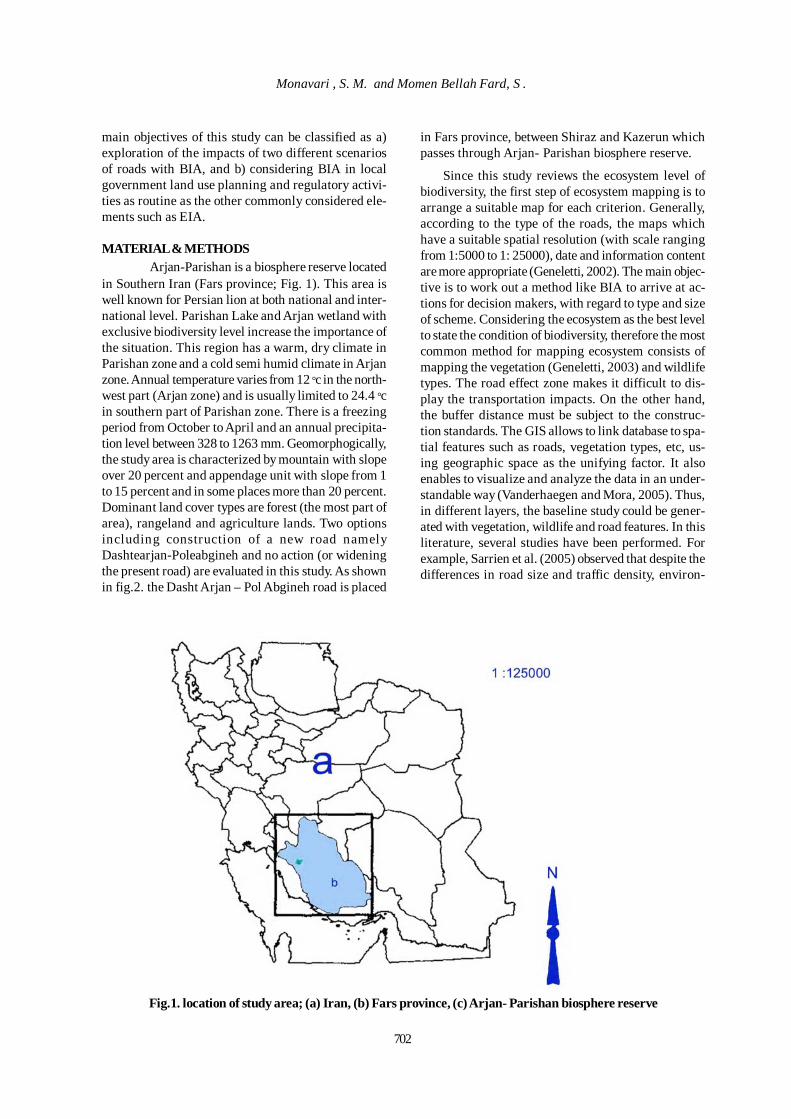
702
Monavari , S. M. and Momen Bellah Fard, S .
main objectives of this study can be classified as a)exploration of the impacts of two different scenariosof roads with BIA, and b) considering BIA in localgovernment land use planning and regulatory activi-ties as routine as the other commonly considered ele-ments such as EIA.
MATERIAL & METHODSArjan-Parishan is a biosphere reserve located
in Southern Iran (Fars province; Fig. 1). This area iswell known for Persian lion at both national and inter-national level. Parishan Lake and Arjan wetland withexclusive biodiversity level increase the importance ofthe situation. This region has a warm, dry climate inParishan zone and a cold semi humid climate in Arjanzone. Annual temperature varies from 12 °c in the north-west part (Arjan zone) and is usually limited to 24.4 °cin southern part of Parishan zone. There is a freezingperiod from October to April and an annual precipita-tion level between 328 to 1263 mm. Geomorphogically,the study area is characterized by mountain with slopeover 20 percent and appendage unit with slope from 1to 15 percent and in some places more than 20 percent.Dominant land cover types are forest (the most part ofarea), rangeland and agriculture lands. Two optionsincluding construction of a new road namelyDashtearjan-Poleabgineh and no action (or wideningthe present road) are evaluated in this study. As shownin fig.2. the Dasht Arjan – Pol Abgineh road is placed
in Fars province, between Shiraz and Kazerun whichpasses through Arjan- Parishan biosphere reserve.
Since this study reviews the ecosystem level ofbiodiversity, the first step of ecosystem mapping is toarrange a suitable map for each criterion. Generally,according to the type of the roads, the maps whichhave a suitable spatial resolution (with scale rangingfrom 1:5000 to 1: 25000), date and information contentare more appropriate (Geneletti, 2002). The main objec-tive is to work out a method like BIA to arrive at ac-tions for decision makers, with regard to type and sizeof scheme. Considering the ecosystem as the best levelto state the condition of biodiversity, therefore the mostcommon method for mapping ecosystem consists ofmapping the vegetation (Geneletti, 2003) and wildlifetypes. The road effect zone makes it difficult to dis-play the transportation impacts. On the other hand,the buffer distance must be subject to the construc-tion standards. The GIS allows to link database to spa-tial features such as roads, vegetation types, etc, us-ing geographic space as the unifying factor. It alsoenables to visualize and analyze the data in an under-standable way (Vanderhaegen and Mora, 2005). Thus,in different layers, the baseline study could be gener-ated with vegetation, wildlife and road features. In thisliterature, several studies have been performed. Forexample, Sarrien et al. (2005) observed that despite thedifferences in road size and traffic density, environ-
Fig.1. location of study area; (a) Iran, (b) Fars province, (c) Arjan- Parishan biosphere reserve
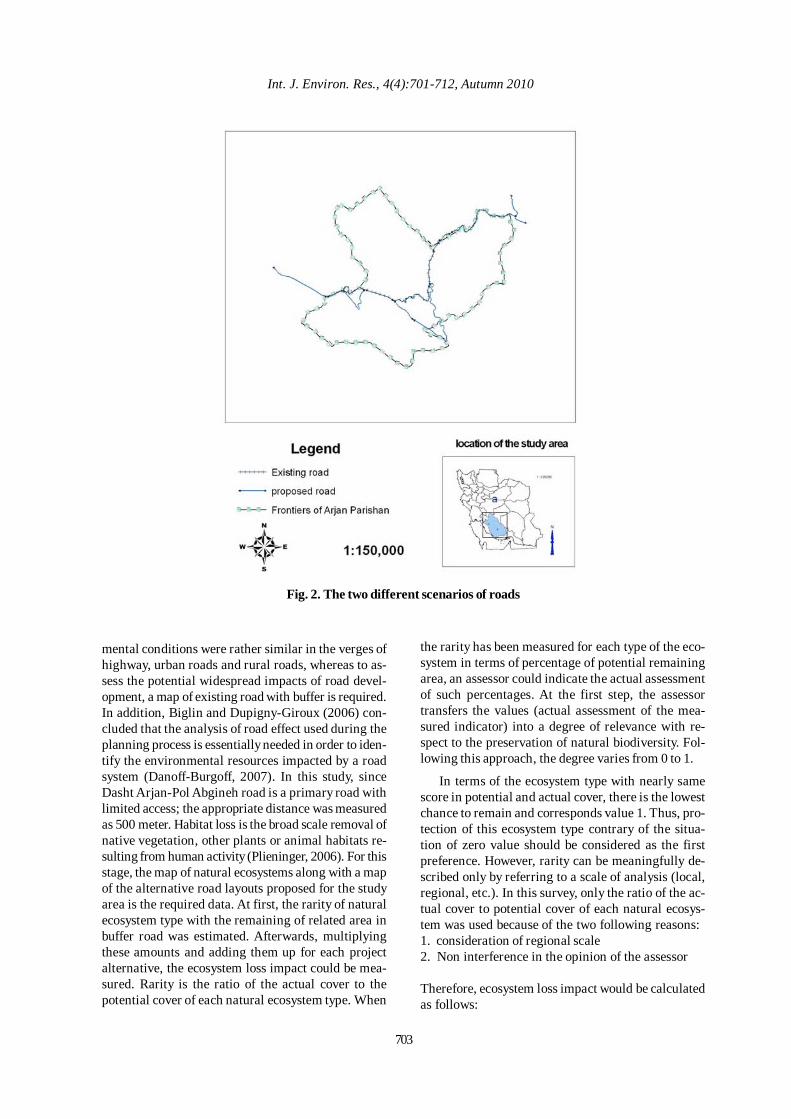
Int. J. Environ. Res., 4(4):701-712, Autumn 2010
703
mental conditions were rather similar in the verges ofhighway, urban roads and rural roads, whereas to as-sess the potential widespread impacts of road devel-opment, a map of existing road with buffer is required.In addition, Biglin and Dupigny-Giroux (2006) con-cluded that the analysis of road effect used during theplanning process is essentially needed in order to iden-tify the environmental resources impacted by a roadsystem (Danoff-Burgoff, 2007). In this study, sinceDasht Arjan-Pol Abgineh road is a primary road withlimited access; the appropriate distance was measuredas 500 meter. Habitat loss is the broad scale removal ofnative vegetation, other plants or animal habitats re-sulting from human activity (Plieninger, 2006). For thisstage, the map of natural ecosystems along with a mapof the alternative road layouts proposed for the studyarea is the required data. At first, the rarity of naturalecosystem type with the remaining of related area inbuffer road was estimated. Afterwards, multiplyingthese amounts and adding them up for each projectalternative, the ecosystem loss impact could be mea-sured. Rarity is the ratio of the actual cover to thepotential cover of each natural ecosystem type. When
the rarity has been measured for each type of the eco-system in terms of percentage of potential remainingarea, an assessor could indicate the actual assessmentof such percentages. At the first step, the assessortransfers the values (actual assessment of the mea-sured indicator) into a degree of relevance with re-spect to the preservation of natural biodiversity. Fol-lowing this approach, the degree varies from 0 to 1.
In terms of the ecosystem type with nearly samescore in potential and actual cover, there is the lowestchance to remain and corresponds value 1. Thus, pro-tection of this ecosystem type contrary of the situa-tion of zero value should be considered as the firstpreference. However, rarity can be meaningfully de-scribed only by referring to a scale of analysis (local,regional, etc.). In this survey, only the ratio of the ac-tual cover to potential cover of each natural ecosys-tem was used because of the two following reasons:1. consideration of regional scale2. Non interference in the opinion of the assessor
Therefore, ecosystem loss impact would be calculatedas follows:
Fig. 2. The two different scenarios of roads
704
∑=
n
ili
1 = ∑ ( Aj * Rj )
where
∑ li = ecosystem loss impact score of alternative j
Aj = predicted area loss for ecosystem type jRJ = assessed rarity value of ecosystem type jn = number of ecosystem types
The extent of habitat fragmentation is an impor-tant indicator of habitat quality because new road de-velopment may result in the reduction of habitat intosmaller and more scattered patches (Kuo et al., 2005).In order to predict the effects caused by fragmentationon each ecosystem patch, the ecosystem viability haveto be assigned. On this basis, as presented in Geneletti(2004), three patch indicators (core area, isolation anddisturbance) were described to predict the ecosystemviability through the above mentioned indicators. Thecore area was chosen because it simultaneously ac-counts for two fragmentation effects: the reduction inpatch size and the increase in edge area.Although this indicator can be computed with GIS but,the following equation which was carried out in Iran(Nejadi, 2008) is used. Core area= S – (P * 72)where
S: Spot areaP: spot perimeter72: considered radius which is affected by external
factors (this amount was taken inView of forest ecosystem and expert knowledge)
Thus, by estimating the core area, in both the pre andpost-project, the value of the region would be definedwith respect to the total area of patch and the differ-ence between the amounts. As shown in the followingequation, such a score of each project by multiplyingthe rarity and their remaining area were computed.
∑=
n
i
fi1
= ∑ (VIj * Sj * Rj)
where
∑ fi =ecosystem fragmentation impact score of al-
ternativeVIj = assessed loss in viability of ecosystem patch jSj = area of ecosystem patch jRj = rarity value of ecosystem patch jn = number of ecosystem patches affected by theproject
The aggregation of the impacts maps into syntheticimpact score is necessary for comparing the perfor-mance of the different alternatives. But, since thisstudy only surveys one alternative, comparison of frag-mentation impact score doesn’t perform.
RESULTS & DISCUSSIONSince biodiversity has been used to locate impor-
tant wildlife areas, transportation infrastructures andall above roads network are blamed for highly contrib-uting to the decrease in both the quality and quantityof natural habitat (Geneletti, 2002). Based on this ap-proach, the first survey was carried on vegetation andthe patches of natural vegetation types are shown inFig. 3. Different types of natural ecosystems of thestudy area can be seen in Tables 1 and 2. As it wasmentioned, the rarity value of each ecosystem type isto be expressed by the ratio of the actual cover to thepotential cover. Tables 3 and 4 express the rarity ofdifferent ecosystem types which are computed in dif-ferent phases (pre and post-project). Then the com-parison between the original ecosystem map and theother scenarios allowed the computation of the ex-pected loss for each ecosystem type. The ecosystemloss value for pre-project ecosystem map was calcu-lated as 318 while it was 594 for post-project. As it canbe seen, the comparison between these scenarios ex-presses that the direct loss after the construction ofthe project is more than the existing one. Thus, thepresent road is more appropriate than the other one.Table 5 indicates the fragmentation impact score pre-sented by aggregate of the impacts into a single score.This is particularly useful when the performance ofseveral alternatives need to be computed. But, as inthis study the value of different scenarios wasn’t con-sidered, the comparison of fragmentation has been notalso performed. Therefore, the comparison of ecosys-tem loss for construction option and no-action wasused. It is observed that for construction option theimpact score was measured as 18. The assessment ofthe ecological value of animal species in the same wayas vegetation type required BIA. The base line dataare represented by a set of habitat maps which showthe geographical range of distribution of the most sig-nificant animal species (Fig.5). The selected group ofspecies was based on ecological value, conservationvalue, economical value, etc. The results presented inTables 6, 7, 8 and 9 are similar to vegetation that showvarious condition of wildlife habitat.The ecosystem lossimpact assessment comparable with vegetation typesillustrated that impacts of road construction in this areaare more than widening the existing one (Table 10). Frag-mentation impact for wildlife was also evaluated, indi-cating that the post-project score is estimated as 11.The results of this process are shown in Table 11.
Assessment Tool for Biodiversity Conservation

Int. J. Environ. Res., 4(4):701-712, Autumn 2010
705
Fig. 3. Ecosystem map of the existing road (Vegetation)
Fig. 4. Ecosystem map of the proposed road (Vegetation)
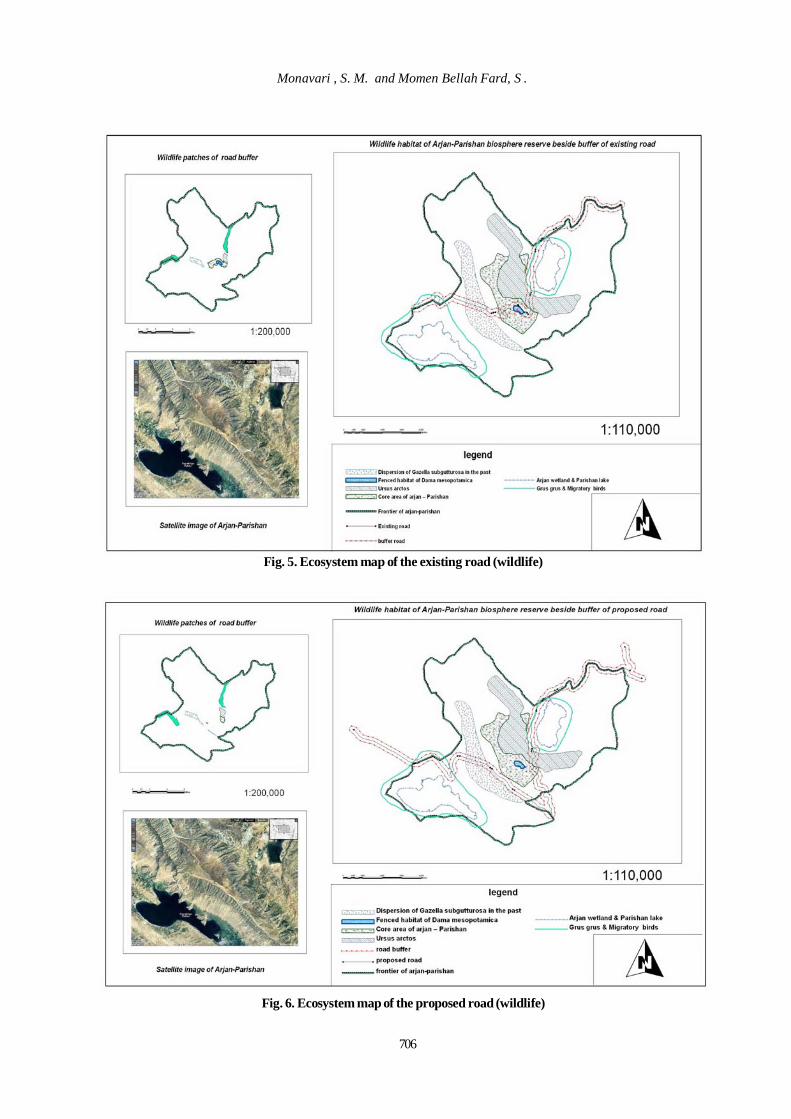
706
Fig. 5. Ecosystem map of the existing road (wildlife)
Fig. 6. Ecosystem map of the proposed road (wildlife)
Monavari , S. M. and Momen Bellah Fard, S .
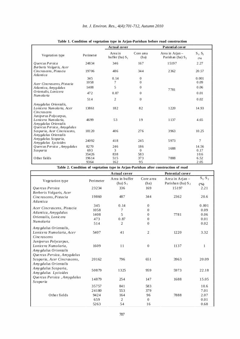
707
Int. J. Environ. Res., 4(4):701-712, Autumn 2010
Table 1. Condition of vegetation type in Arjan-Parishan before road construction Potential cover Actual cover
S1/ S2
(%) Area in Arjan –
Parishan (ha) S2 Core area
(ha) Area in
buffer (ha) S1 Perimeter Vegetation type
2 .27 15197 167 346 24834 Q uercus Persica
20.57 2362 344 486 19706 Berberis Volgaris, Acer Cincrascens, Pistacia A tlantica
0.001 0 0.14 345 0.09 0 7 1058 0.06 0 5 1408 0.01 0 0.87 472 0.02
7781
0 2 514
Acer Cincrascens, Pistacia A tlantica, Amygdalus O rientalis, Lonicera Num olaria
14.93 1220 82 182 13861 Amygdalus Orientalis, Lonicera Num olaria, Acer Cincrascens
4.65 1137 19 53 4699 Juniperus Polycarpus, Lonicera Num olaria, Amygdalus Orientalis
10.25 3963 276 406 18120 Q uercus Persica , Amygdalus Scoparia, Acer Cincrascens, Amygdalus Orientalis
7 5973 245 418 24092 Amygdalus Scoparia, Amygdalus Lycio ides
14.56 186 246 8270 0.17 1688 0 3 693
Q uercus Persica , Amygdalus Scoparia
10.6 583 838 35426 6.52 373 515 19614 2.05
7888 95 162 9364
O ther fields
Table 2. Condition of vegetation type in Arjan-Parishan after construction of road Pote ntial cove r Actual cover
S1/ S 2
(%) Are a in Arjan – Parisha n (ha) S 2
Core a rea (ha)
Area in buffer (ha) S 1 Perimeter Vege ta tion type
2.21 15197 169 336 23234 Que rcus Persica
20.6 2362 344 487 19860 Berberis Volgaris, Acer Cinc rascens, Pistacia Atlantica
0.001 0 0.14 345 0.09 0 7 1058 0.06 0 5 1408 0.01 0 0.87 473 0.02
7781
0 2 514
Acer Cincrascens, Pistacia Atlantica, Amygdalus Orientalis, Lonic era Numolaria
3.32 1220 2 41 5407 Amy gdalus Orientalis, Lonice ra N umolaria, Ace r Cinc rascens
1 1137 0 11 1609 Juniperus Polycarpus, Lonice ra N umolaria, Amy gdalus Orientalis
20.09 3963 651 796 20162 Que rcus Persica, Amygdalus Scoparia, Acer Cincrascens, Amy gdalus Orientalis
22.18 5973 959 1325 50879 Amy gdalus Scoparia, Amy gdalus Lycioides
15.05 1688 147 254 14879 Que rcus Persica , Amygdalus Scoparia
10.6 583 841 35757 7.01 379 553 24180 2.07 96 164 9424 0.01 0 2 659 0.68
7888
16 54 5263
Othe r fields
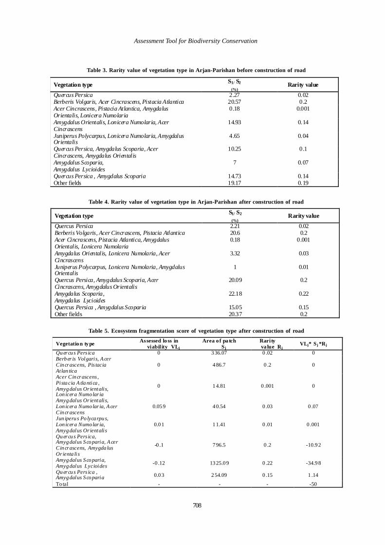
Table 3. Rarity value of vegetation type in Arjan-Parishan before construction of road
Rarity value S1/ S2
(%) Vegetation type 0.02 2.27 Quercus Persica 0.2 20.57 Berberis Volgaris, Acer Cincrascens, Pistacia Atlantica
0.001 0.18 Acer Cincrascens, Pistacia Atlantica, Amygdalus Orientalis, Lonicera Numolaria
0.14 14.93 Amygdalus Orientalis, Lonicera Numolaria, Acer Cincrascens
0.04 4.65 Juniperus Polycarpus, Lonicera Numolaria, Amygdalus Orientalis
0.1 10.25 Quercus Persica, Amygdalus Scoparia, Acer Cincrascens, Amygdalus Orientalis
0.07 7 Amygdalus Scoparia, Amygdalus Lycioides
0.14 14.73 Quercus Persica , Amygdalus Scoparia 0.19 19.17 Other fields
Table 4. Rarity value of vegetation type in Arjan-Parishan after construction of road
Rarity value S1/ S2
(%) Vegetation type 0.02 2.21 Quercus Persica 0.2 20.6 Berberis Volgaris, Acer Cincrascens, Pistacia Atlantica
0.001 0.18 Acer Cincrascens, Pistacia Atlantica, Amygdalus Orientalis, Lonicera Numolaria
0.03 3.32 Amygdalus Orientalis, Lonicera Numolaria, Acer Cincrascens
0.01 1 Juniperus Polycarpus, Lonicera Numolaria, Amygdalus Orientalis
0.2 20.09 Quercus Persica, Amygdalus Scoparia, Acer Cincrascens, Amygdalus Orientalis
0.22 22.18 Amygdalus Scoparia, Amygdalus Lycioides
0.15 15.05 Quercus Persica , Amygdalus Scoparia 0.2 20.37 Other fields
Table 5. Ecosystem fragmentation score of vegetation type after construction of road
VLj* Sj *Rj Rarity va lue Rj
Area o f pa tch Sj
Assessed lo ss in viabil ity VLj
Vegetatio n type 0 0 .02 3 36.07 0 Qu ercu s Pers ica
0 0 .2 4 86.7 0 Berb er is Volgaris, A cer Cin crascens, Pis tacia At lan tica
0 0 .001 1 4.81 0 Acer Cincrascens , Pistacia A tla ntica , Amygdalus Or ientalis, Lon icera Numo lar ia
0 .07 0 .03 4 0.54 0.05 9 Amygdalus Or ientalis, Lon icera Numo lar ia, A cer Cin crascens
0 .001 0 .01 1 1.41 0.0 1 Jun iperus Po lycarpu s, Lon icera Numo lar ia, Amygdalus Or ientalis
-10.9 2 0 .2 7 96.5 -0 .1 Qu ercu s Pers ica, Amygdalus S coparia, A cer Cin crascens, Amygda lus Or ienta lis
-34.9 8 0 .22 13 25.0 9 -0 .12 Amygdalus S coparia, Amygdalus Lycioides
1 .14 0 .15 2 54.09 0.0 3 Qu ercu s Pers ica , Amygdalus S coparia
-50 - - - To tal
Assessment Tool for Biodiversity Conservation
708
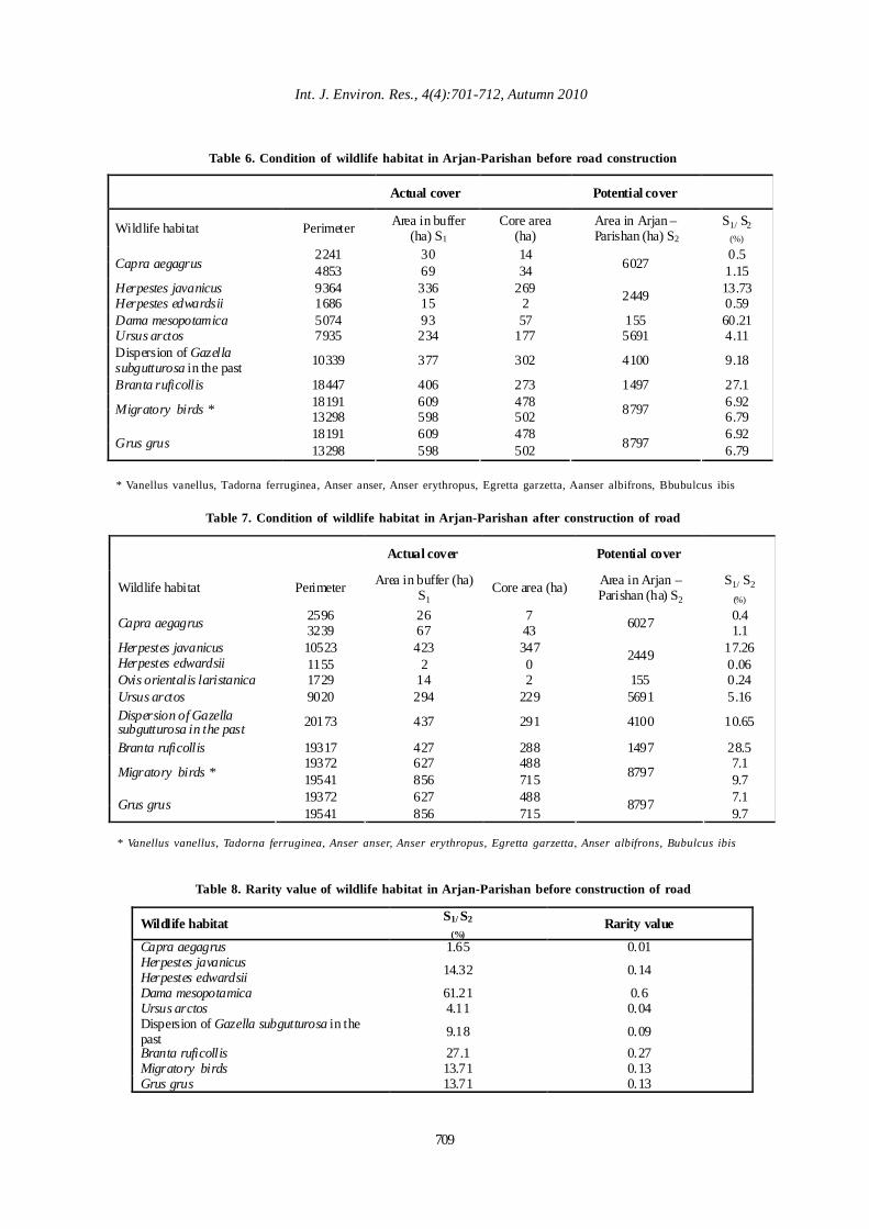
Table 6. Condition of wildlife habitat in Arjan-Parishan before road construction
Potential cover Actual cover
S1/ S2 (%)
Area in Arjan – Parishan (ha) S2
Core area (ha)
Area in buffer (ha) S1 Perimeter Wildlife habitat
0.5 14 30 2241 1.15 6027 34 69 4853 Capra aegagrus 13.73 269 336 9364 0.59 2449 2 15 1686
Herpestes javanicusHerpestes edwardsii
60.21 155 57 93 5074 Dama mesopotamica 4.11 5691 177 234 7935 Ursus arctos 9.18 4100 302 377 10339 Dispersion of Gazella
subgutturosa in the past 27.1 1497 273 406 18447 Branta ruficollis 6.92 478 609 18191 6.79 8797 502 598 13298 Migratory birds * 6.92 478 609 18191 6.79 8797 502 598 13298 Grus grus
* Vanellus vanellus, Tadorna ferruginea, Anser anser, Anser erythropus, Egretta garzetta, Aanser albifrons, Bbubulcus ibis
Table 7. Condition of wildlife habitat in Arjan-Parishan after construction of road
Potential cover Actual cover
S1/ S2 (%)
Area in Arjan – Parishan (ha) S2 Core area (ha)Area in buffer (ha)
S1 Perimeter Wildlife habitat
0.4 7 26 2596 1.1 6027 43 67 3239 Capra aegagrus
17.26 347 423 10523 0.06 2449
0 2 1155 Herpestes javanicusHerpestes edwardsii
0.24 155 2 14 1729 Ovis orientalis laristanica 5.16 5691 229 294 9020 Ursus arctos 10.65 4100 291 437 20173 Dispersion of Gazella
subgutturosa in the past 28.5 1497 288 427 19317 Branta ruficollis 7.1 488 627 19372 9.7 8797 715 856 19541 Migratory birds * 7.1 488 627 19372 9.7 8797
715 856 19541 Grus grus
* Vanellus vanellus, Tadorna ferruginea, Anser anser, Anser erythropus, Egretta garzetta, Anser albifrons, Bubulcus ibis
Table 8. Rarity value of wildlife habitat in Arjan-Parishan before construction of road
Rarity value S1/ S2
(%) Wildlife habitat 0.01 1.65 Capra aegagrus 0.14 14.32 Herpestes javanicus
Herpestes edwardsii 0.6 61.21 Dama mesopotamica 0.04 4.11 Ursus arctos 0.09 9.18 Dispersion of Gazella subgutturosa in the
past 0.27 27.1 Branta ruficollis 0.13 13.71 Migratory birds 0.13 13.71 Grus grus
Int. J. Environ. Res., 4(4):701-712, Autumn 2010
709
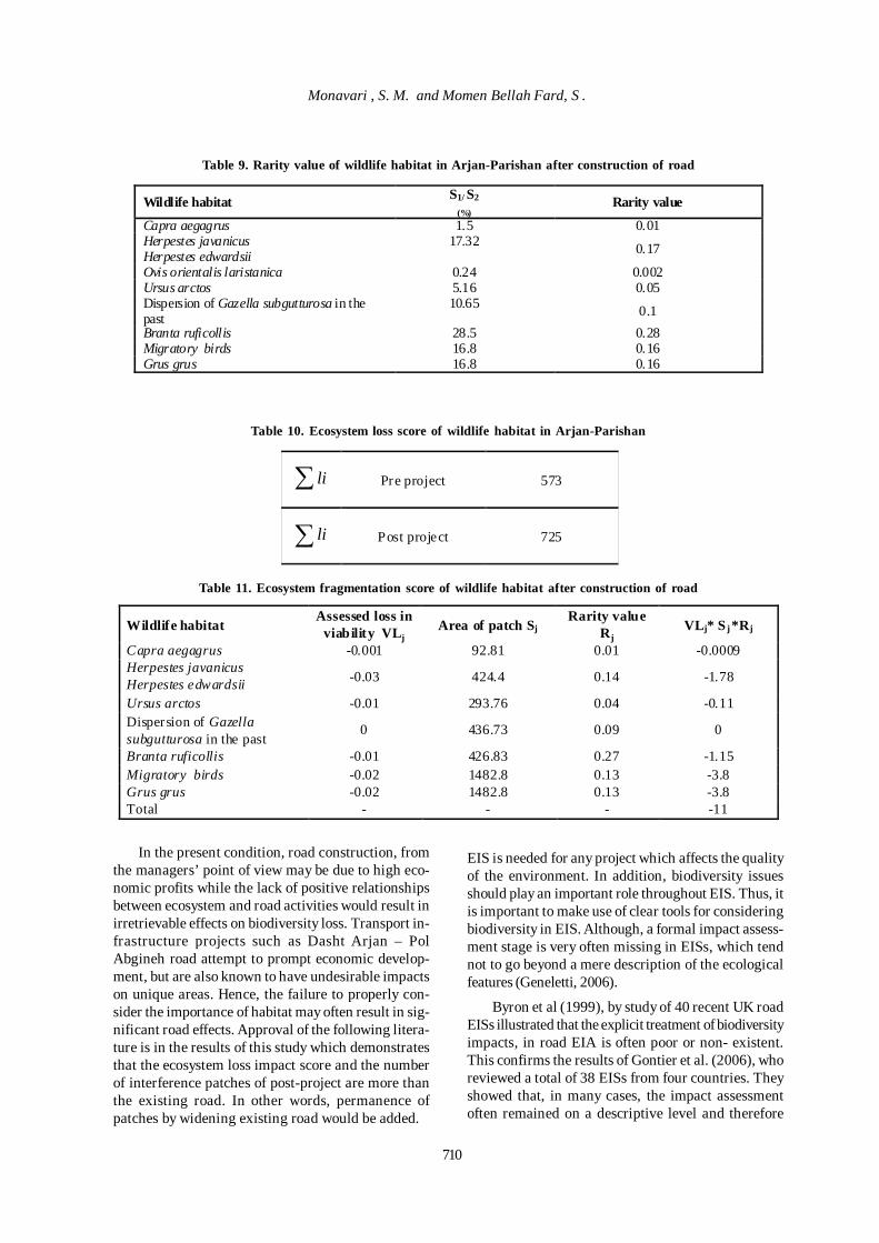
710
Table 9. Rarity value of wildlife habitat in Arjan-Parishan after construction of road
Rarity value S1/ S2
(%) Wildlife habitat 0.01 1.5 Capra aegagrus 0.17 17.32 Herpestes javanicus
Herpestes edwardsii 0.002 0.24 Ovis orientalis laristanica 0.05 5.16 Ursus arctos 0.1 10.65 Dispersion of Gazella subgutturosa in the
past 0.28 28.5 Branta ruficollis 0.16 16.8 Migratory birds 0.16 16.8 Grus grus
Table 10. Ecosystem loss score of wildlife habitat in Arjan-Parishan
∑ li Pre project 573
∑ li Post project 725
Table 11. Ecosystem fragmentation score of wildlife habitat after construction of road
VLj* Sj *Rj Rarity value Rj
Area of patch Sj Assessed loss in
viability VLj Wildlife habitat
-0.0009 0.01 92.81 -0.001 Capra aegagrus -1.78 0.14 424.4 -0.03 Herpestes javanicus
Herpestes edwardsii -0.11 0.04 293.76 -0.01 Ursus arctos
0 0.09 436.73 0 Dispersion of Gazella subgutturosa in the past
-1.15 0.27 426.83 -0.01 Branta ruficollis -3.8 0.13 1482.8 -0.02 Migratory birds -3.8 0.13 1482.8 -0.02 Grus grus -11 - - - Total
In the present condition, road construction, from
the managers’ point of view may be due to high eco-nomic profits while the lack of positive relationshipsbetween ecosystem and road activities would result inirretrievable effects on biodiversity loss. Transport in-frastructure projects such as Dasht Arjan – PolAbgineh road attempt to prompt economic develop-ment, but are also known to have undesirable impactson unique areas. Hence, the failure to properly con-sider the importance of habitat may often result in sig-nificant road effects. Approval of the following litera-ture is in the results of this study which demonstratesthat the ecosystem loss impact score and the numberof interference patches of post-project are more thanthe existing road. In other words, permanence ofpatches by widening existing road would be added.
EIS is needed for any project which affects the qualityof the environment. In addition, biodiversity issuesshould play an important role throughout EIS. Thus, itis important to make use of clear tools for consideringbiodiversity in EIS. Although, a formal impact assess-ment stage is very often missing in EISs, which tendnot to go beyond a mere description of the ecologicalfeatures (Geneletti, 2006).
Byron et al (1999), by study of 40 recent UK roadEISs illustrated that the explicit treatment of biodiversityimpacts, in road EIA is often poor or non- existent.This confirms the results of Gontier et al. (2006), whoreviewed a total of 38 EISs from four countries. Theyshowed that, in many cases, the impact assessmentoften remained on a descriptive level and therefore
Monavari , S. M. and Momen Bellah Fard, S .
considered only direct impacts, such as local habitatloss for some species, without considering indirectimpacts linked to the overall habitat fragmentation ona landscape level. These considerations should bemade during comprehensive habitat conservation plan-ning and development of land use regulations whichcan limit such impacts (Crist et al., 2000).However, us-ing the guidance presented in Byron (2000) beside BIAtool ensures that the potential impacts on biodiversityare thoroughly addressed in road EIA. In this studywith taking advantage of this guidance become clearthat impacts of road in post-project would not be com-pensated.
The fragmentation approach of BIA tool is basedon the results of landscape ecology. It also aims toassess the overall impact on ecosystem. This evalua-tion isn’t same as the other models (Sluis 2001; Dale etal., 1998; Foppen and Chardon 1998; White et al.,1997) that are based on species and area requirement.This is because no target species were selected(Genelletti, 2004). In fact, limiting the evaluation tospecies that are formally protected still represents arather common approach (Byron et al., 2000).
In this way, to improve the management ofbiodiversity as part of the EIA process, the approachproposed for impact assessment along with the men-tioned guidance could be applied for areas with a morevulnerable position. However, the use of BIA tool hascertain shortcomings which have to be considered.For instance, the accuracy of assessment processcould be affected (e.g. by the error in entered data anduncertainty analysis due to evaluation of the factors)(Nejadi, 2008). Thus, to enhance the clarity of thebiodiversity, future studies should be done in the im-pact assessment procedure.This study also indicatethat however, according to Noss and Cooperrider(1994) and Geneletti (2003), conservation, in many cases,is the most efficient when focuses directly on ecosys-tem but it is required to develop the studies of theimpact on landscape, species and genes.
CONCLUSIONThis study focuses on the assessment process
which explores the interaction between infrastructureand biodiversity. Hence, BIA has been considered toestimate the impacts of Dasht Arjan – Pol Abginehroad on vegetation and wildlife. In terms of ecosystempreservation, the quantified data shows that the exist-ing road is preferable to construction of a new road.The results also revealed that BIA could make the ap-plication of ecological assessment easier and more ef-fective. Although there are different limitations in suchtools, they could be used to eliminate the unclear as-
pects of current biodiversity assessment. Also appli-cation of BIA beside EIA in other linear infrastructuressuch as power lines, oil pipes, railway, monorail, etccan be considered of high importance.
REFERENCESBiggs, R., Simons, H., Bakkenes, M., Scholes, R. J., Eickhout,B., Vuuren, D. V. and Alkemade, R. (2008). Scenarios ofbiodiversity loss in southern Africa in the 21st century.Global Environmental Change, 18 (2), 296-309.
Biglin, K. and Dupigny-Giroux, L. A. (2007). Mapping theroad-effect zone to assess impacts of proposed road seg-ments. J. Conserv. Plann., 2, 1-16.
Byron, H. J., Treweek, J. R., Sheate, W. R. and Thompson,S. (2000). Road developments in the UK: an analysis ofecological assessment in environmental impact statements produced between 1993 and 1997. J. Environ. Plann. Man-age., 43, 71-95.
Byron, H. J. (1999). Biodiversity issues in road environ-mental impact assessments: guidance and Case studies. In:Evink, G. L., Garrett, P. and Zeigler, D. (Eds.), Proceedingsof the Third International Conference on Wildlife Ecologyand Transportation. Tallahassee, Florida Department ofTransportation. Florida, USA.
Crist, P. J., Kohley, T. W. and Oakleaf, J. (2000). Assessingland-use impacts on biodiversity using an expert systemstool. Landscape Ecol., 15, 47-62.
Dunn, R. R. and Danoff-Burg, J. A. (2007). Road size andcarrion beetle assemblages in a New York forest. J. insectconserv., 11 (4), 325-332.
Forman, R. T. T. and Alexander, L. E. (1998). Roads andtheir major ecological effects. Ann. Rev. Ecol. System., 29,207-231.
Geneletti, D. (2002). Ecological evaluation for environmen-tal impact assessment. Neth Geogr Stud (NGS 301). Utrecht7Knag. pp. 224.
Geneletti, D. (2003). Biodiversity Impact Assessment ofroads: an approach based on ecosystem rarity. Environ.Impact Assess. Rev., 23, 343-365.
Geneletti, D., Beinat, E., Chung, C. F., Fabbri, A. G. andScholten, H. J. (2003). Accounting for uncertainty factorsin biodiversity impact assessment: lessons from a case study.Environ Impact Assess Rev., 23, 47-87.
Geneletti, D. (2004). Using spatial indicators and value func-tions to assess ecosystem fragmentation caused by linearinfrastructures. Int. J. Appl. Earth Observ. Geoinform., 5,1-15.
Geneletti, D. (2006). Some common shortcomings in thetreatment of impacts of linear infrastructures on naturalhabitat. Environ. Impact Assess. Rev., 26, 257-267.
Int. J. Environ. Res., 4(4):701-712, Autumn 2010
711
Gontier, M., Balfors, B. and Mortberg, U. (2006).Biodiversity in environmental assessment—current prac-tice and tools for prediction. Environ. Impact Assess. Rev.,26, 268-286.
Ives, A. R. and Carpenter, S. R. (2007). Stability and diver-sity of ecosystems. Science., 317, 58-62.
Kakonen, J. (1993). Politics and Sustainable Growth in theArctic. Aldershot, Darthmouth.
Kuo, N. W., Hsiao, T. Y. and Yu, Y. H. (2005). A Delphi–matrix approach to SEA and its application within the tour-ism sector in Taiwan. Environ. Impact Assess. Rev., 25,259-280.
Loreau, M., Naeem, S. and Inchausti, P. (Eds.) (2002).Biodiversity and Ecosystem Functioning: A Synthesis. Ox-ford University Press, UK.
Mahoney, S.P. and Schaefer, J.A. (2002). Hydroelectric de-velopment and the disruption of migration in caribou. Biol.Conserv., 107, 147-153.
Mehrdadi, N., Daryabeigi Zand, A. and Matloubi, A. A.(2007a). Natural and human-induced impacts on coastalgroundwater. Int. J. Environ. Res., 1(2), 170-178.
Mehrdadi, N., Joshi, S. G., Nasrabadi, T. and Hoveidi, H.(2007b). Aplication of Solar Energy for Drying of Sludgefrom Pharmaceutical Industrial Waste Water and ProbableReuse. Int. J. Environ. Res., 1(1), 42-48.
Nellemanna, C., Vistnesb, I., Jordhøyc, P., Strandc, O. andNewtond, A. (2003). Progressive impact of piecemeal infra-structure development on wild reindeer. Biol. Conserv., 113,307-317.
Noss, R. F. and Cooperrider, A. (1994). Saving Nature’sLegacy:Protecting and Restoring Biodiversity. Washington:DC Defenders of Wildlife and Island Press, USA.
Opdam, P. and Wiens, J. A. (2002). Fragmentation, habitatloss and landscape management. (In: Norris, K. and Pain, D.J. (Eds.), Conserving bird biodiversity General principlesand their application. Cambridge University Cambridge.
Plieninger, T. (2006). Habitat loss, fragmentation, and alter-ation – Quantifying the impact of land-use changes on aSpanish dehesa landscape by use of aerial photography andGIS. Landscape Ecol., 21, 91-105.
Roe, J. H., Gibson, J. and Kingsbury, B. A. (2006). Beyondthe wetland border: Estimating the impact of roads for twospecies of water snakes. Biol. Conserve., 130, 161-168.
Saarinen, K., Valtonen, A., Jantunen, J. and Saarnio, S. (2005).Butterflies and diurnal moths along road verges: Does roadtype affect diversity and abundance? Biol. Conserv., 123,403-412.
Slootweg, R. and Kolhoff, A. (2003). A generic approach tointegrate biodiversity considerations in screening and scopingfor EIA. Environ. Impact Assess. Rev., 23, 657-681.
Torkian, A., Keshavarzi Shirazi, H. and Mehrdadi, N.(2007). Fate of intermediate biodegradation products of tri-ethyl amine in a compost-based biofiltration system. Int. J.Environ. Res., 1(2), 163-169.
Trombulack, S. C. and Frissell, C. A. (2000). Review ofecological effects of roads on terrestrial and aquatic commu-nities. Conserv. Biol., 14, 18-30.
Vanderhaegena, M. and Muro, E. (2005). Contribution of aEuropean spatial data infrastructure to the effectiveness ofEIA and SEA studies. Environ. Impact Assess. Rev., 25,123-142.
Assessment Tool for Biodiversity Conservation
712
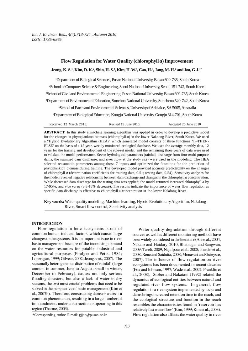
Int. J. Environ. Res., 4(4):713-724 , Autumn 2010ISSN: 1735-6865
Received 12 March 2010; Revised 15 June 2010; Accepted 25 June 2010
*Corresponding author E-mail: [email protected]
713
Flow Regulation for Water Quality (chlorophyll a) Improvement
Jeong, K. S.1, Kim, D. K.2, Shin, H. S.3, Kim, H. W.4, Cao, H.5, Jang, M. H.6 and Joo, G. J.1*
1Department of Biological Sciences, Pusan National University, Busan 609-735, South Korea2School of Computer Science & Engineering, Seoul National University, Seoul, 151-742, South Korea
3School of Civil and Environmental Engineering, Pusan National University, Busan 609-735, South Korea4Department of Environmental Education, Sunchon National University, Suncheon 540-742, South Korea
5School of Earth and Environmental Sciences, University of Adelaide, SA 5005, Australia6Department of Biological Education, Kongju National University, Gongju 314-701, South Korea
ABSTRACT: In this study a machine learning algorithm was applied in order to develop a predictive modelfor the changes in phytoplankton biomass (chlorophyll a) in the lower Nakdong River, South Korea. We useda “Hybrid Evolutionary Algorithm (HEA)” which generated model consists of three functions ‘IF-THEN-ELSE’ on the basis of a 15-year, weekly monitored ecological database. We used the average monthly data, 12years for the training and development of the rule-set model, and the remaining three years of data were usedto validate the model performance. Seven hydrological parameters (rainfall, discharge from four multi-purposedams, the summed dam discharge, and river flow at the study site) were used in the modeling. The HEAselected reasonable parameters among those 7 inputs and optimized the functions for the prediction ofphytoplankton biomass during training. The developed model provided accurate predictability on the changesof chlorophyll a (determination coefficients for training data, 0.51; testing data, 0.54). Sensitivity analyses forthe model revealed negative relationship between dam discharge and changes in the chlorophyll a concentration.While decreased dam discharge for the testing data was applied; the model returned increased chlorophyll a by17-95%, and vice versa (a 3-18% decrease). The results indicate the importance of water flow regulation asspecific dam discharge is effective to chlorophyll a concentration in the lower Nakdong River.
Key words: Water quality modeling, Machine learning, Hybrid Evolutionary Algorithm, Nakdong River, Smart flow control, Sensitivity analysis
INTRODUCTIONFlow regulation in lotic ecosystems is one of
common human-induced factors, which causes largechanges to the systems. It is an important issue in riverbasin management because of the increasing demandon the water resources for potable, industrial andagricultural purposes (Foulger and Petts, 1984;Loneragan, 1999; Gilvear, 2002; Jeong et al., 2007). Theseasonally heterogeneous distribution of rainfall (largeamount in summer, June to August; small in winter,December to February), causes not only seriousflooding disasters, but also a lack of water in dryseasons, the two most crucial problems that need to besolved in the perspective of basin management (Kim etal., 2007b). Therefore, constructing dams or weirs is acommon phenomenon, resulting in a large number ofimpoundments under construction or operating in thisregion (Tharme, 2003).
Water quality degradation through differentsources as well as different monitoring methods havebeen widely considered in the literature (Ali et al., 2004;Nakane and Haidary, 2010; Bhatnagar and Sangwan,2009; Taseli, 2009; Najafpour et al., 2008; Joarder et al.,2008; Rene and Saidutta, 2008; Monavari and Guieysse,2007). The influence of flow regulation on riverecosystems has been documented in recent decades(Fox and Johnson, 1997; Wade et al., 2002; Franklin etal., 2008). Stober and Nakatani (1992) related thedynamics of ecological entities between natural andregulated river flow systems. In general, flowregulation in a river system implemented by locks anddams brings increased retention time in the reach, andthe ecological structure and function in the reachresembles the characteristics found in ‘reservoir hasrelatively fast water flow’ (Kim, 1999; Kim et al., 2003).Flow regulation also affects the water quality in river
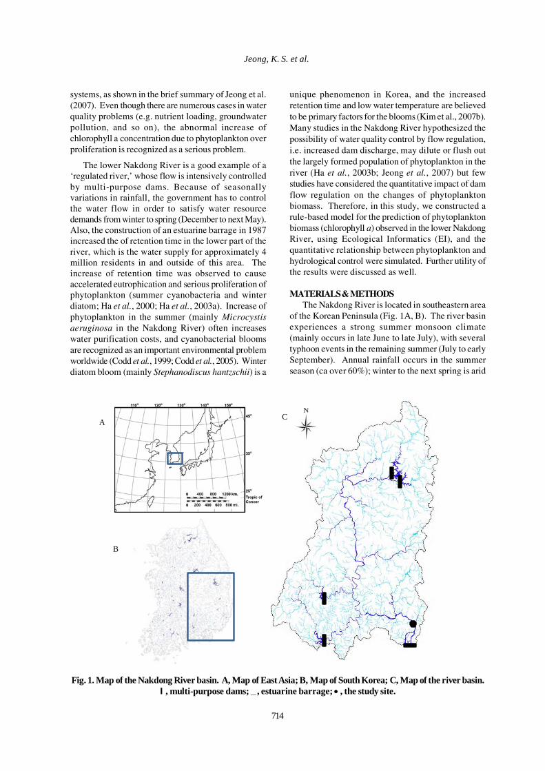
714
Jeong, K. S. et al.
systems, as shown in the brief summary of Jeong et al.(2007). Even though there are numerous cases in waterquality problems (e.g. nutrient loading, groundwaterpollution, and so on), the abnormal increase ofchlorophyll a concentration due to phytoplankton overproliferation is recognized as a serious problem.
The lower Nakdong River is a good example of a‘regulated river,’ whose flow is intensively controlledby multi-purpose dams. Because of seasonallyvariations in rainfall, the government has to controlthe water flow in order to satisfy water resourcedemands from winter to spring (December to next May).Also, the construction of an estuarine barrage in 1987increased the of retention time in the lower part of theriver, which is the water supply for approximately 4million residents in and outside of this area. Theincrease of retention time was observed to causeaccelerated eutrophication and serious proliferation ofphytoplankton (summer cyanobacteria and winterdiatom; Ha et al., 2000; Ha et al., 2003a). Increase ofphytoplankton in the summer (mainly Microcystisaeruginosa in the Nakdong River) often increaseswater purification costs, and cyanobacterial bloomsare recognized as an important environmental problemworldwide (Codd et al., 1999; Codd et al., 2005). Winterdiatom bloom (mainly Stephanodiscus hantzschii) is a
unique phenomenon in Korea, and the increasedretention time and low water temperature are believedto be primary factors for the blooms (Kim et al., 2007b).Many studies in the Nakdong River hypothesized thepossibility of water quality control by flow regulation,i.e. increased dam discharge, may dilute or flush outthe largely formed population of phytoplankton in theriver (Ha et al., 2003b; Jeong et al., 2007) but fewstudies have considered the quantitative impact of damflow regulation on the changes of phytoplanktonbiomass. Therefore, in this study, we constructed arule-based model for the prediction of phytoplanktonbiomass (chlorophyll a) observed in the lower NakdongRiver, using Ecological Informatics (EI), and thequantitative relationship between phytoplankton andhydrological control were simulated. Further utility ofthe results were discussed as well.
MATERIALS & METHODSThe Nakdong River is located in southeastern area
of the Korean Peninsula (Fig. 1A, B). The river basinexperiences a strong summer monsoon climate(mainly occurs in late June to late July), with severaltyphoon events in the remaining summer (July to earlySeptember). Annual rainfall occurs in the summerseason (ca over 60%); winter to the next spring is arid
Fig. 1. Map of the Nakdong River basin. A, Map of East Asia; B, Map of South Korea; C, Map of the river basin.I , multi-purpose dams; _ , estuarine barrage; • , the study site.
A
B
CA
B
C
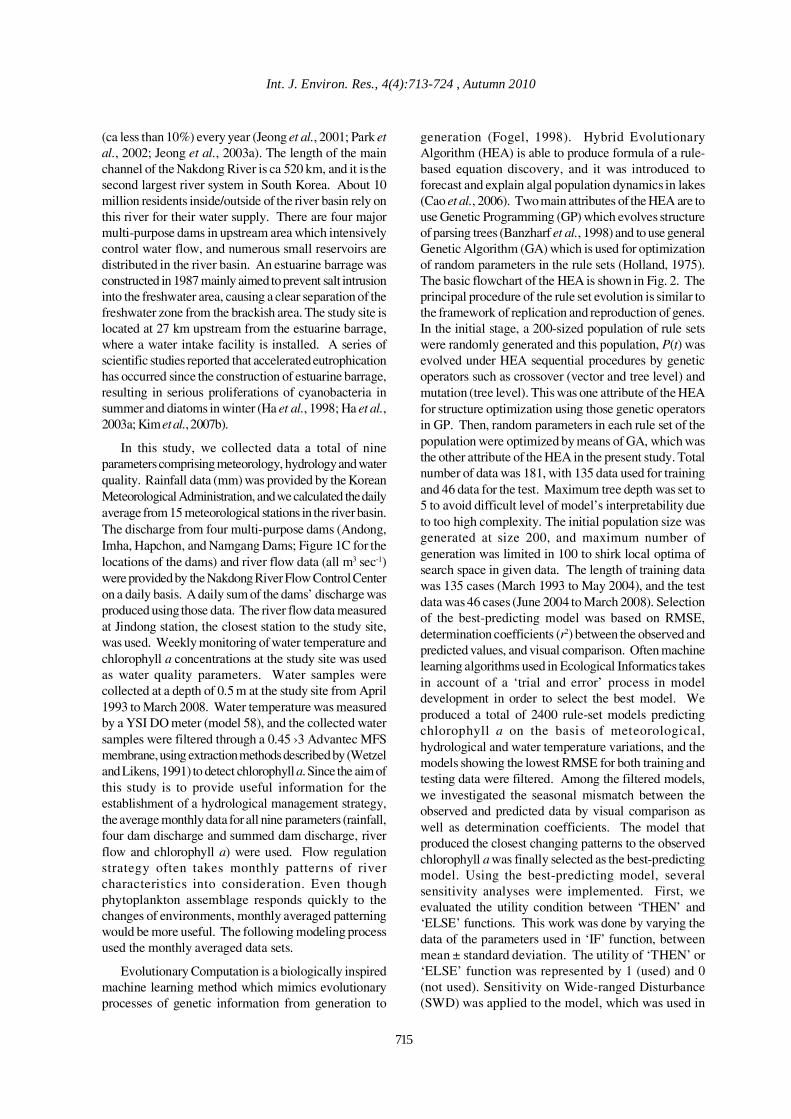
Int. J. Environ. Res., 4(4):713-724 , Autumn 2010
715
(ca less than 10%) every year (Jeong et al., 2001; Park etal., 2002; Jeong et al., 2003a). The length of the mainchannel of the Nakdong River is ca 520 km, and it is thesecond largest river system in South Korea. About 10million residents inside/outside of the river basin rely onthis river for their water supply. There are four majormulti-purpose dams in upstream area which intensivelycontrol water flow, and numerous small reservoirs aredistributed in the river basin. An estuarine barrage wasconstructed in 1987 mainly aimed to prevent salt intrusioninto the freshwater area, causing a clear separation of thefreshwater zone from the brackish area. The study site islocated at 27 km upstream from the estuarine barrage,where a water intake facility is installed. A series ofscientific studies reported that accelerated eutrophicationhas occurred since the construction of estuarine barrage,resulting in serious proliferations of cyanobacteria insummer and diatoms in winter (Ha et al., 1998; Ha et al.,2003a; Kim et al., 2007b).
In this study, we collected data a total of nineparameters comprising meteorology, hydrology and waterquality. Rainfall data (mm) was provided by the KoreanMeteorological Administration, and we calculated the dailyaverage from 15 meteorological stations in the river basin.The discharge from four multi-purpose dams (Andong,Imha, Hapchon, and Namgang Dams; Figure 1C for thelocations of the dams) and river flow data (all m3 sec-1)were provided by the Nakdong River Flow Control Centeron a daily basis. A daily sum of the dams’ discharge wasproduced using those data. The river flow data measuredat Jindong station, the closest station to the study site,was used. Weekly monitoring of water temperature andchlorophyll a concentrations at the study site was usedas water quality parameters. Water samples werecollected at a depth of 0.5 m at the study site from April1993 to March 2008. Water temperature was measuredby a YSI DO meter (model 58), and the collected watersamples were filtered through a 0.45 ›3 Advantec MFSmembrane, using extraction methods described by (Wetzeland Likens, 1991) to detect chlorophyll a. Since the aim ofthis study is to provide useful information for theestablishment of a hydrological management strategy,the average monthly data for all nine parameters (rainfall,four dam discharge and summed dam discharge, riverflow and chlorophyll a) were used. Flow regulationstrategy often takes monthly patterns of rivercharacteristics into consideration. Even thoughphytoplankton assemblage responds quickly to thechanges of environments, monthly averaged patterningwould be more useful. The following modeling processused the monthly averaged data sets.
Evolutionary Computation is a biologically inspiredmachine learning method which mimics evolutionaryprocesses of genetic information from generation to
generation (Fogel, 1998). Hybrid EvolutionaryAlgorithm (HEA) is able to produce formula of a rule-based equation discovery, and it was introduced toforecast and explain algal population dynamics in lakes(Cao et al., 2006). Two main attributes of the HEA are touse Genetic Programming (GP) which evolves structureof parsing trees (Banzharf et al., 1998) and to use generalGenetic Algorithm (GA) which is used for optimizationof random parameters in the rule sets (Holland, 1975).The basic flowchart of the HEA is shown in Fig. 2. Theprincipal procedure of the rule set evolution is similar tothe framework of replication and reproduction of genes.In the initial stage, a 200-sized population of rule setswere randomly generated and this population, P(t) wasevolved under HEA sequential procedures by geneticoperators such as crossover (vector and tree level) andmutation (tree level). This was one attribute of the HEAfor structure optimization using those genetic operatorsin GP. Then, random parameters in each rule set of thepopulation were optimized by means of GA, which wasthe other attribute of the HEA in the present study. Totalnumber of data was 181, with 135 data used for trainingand 46 data for the test. Maximum tree depth was set to5 to avoid difficult level of model’s interpretability dueto too high complexity. The initial population size wasgenerated at size 200, and maximum number ofgeneration was limited in 100 to shirk local optima ofsearch space in given data. The length of training datawas 135 cases (March 1993 to May 2004), and the testdata was 46 cases (June 2004 to March 2008). Selectionof the best-predicting model was based on RMSE,determination coefficients (r2) between the observed andpredicted values, and visual comparison. Often machinelearning algorithms used in Ecological Informatics takesin account of a ‘trial and error’ process in modeldevelopment in order to select the best model. Weproduced a total of 2400 rule-set models predictingchlorophyll a on the basis of meteorological,hydrological and water temperature variations, and themodels showing the lowest RMSE for both training andtesting data were filtered. Among the filtered models,we investigated the seasonal mismatch between theobserved and predicted data by visual comparison aswell as determination coefficients. The model thatproduced the closest changing patterns to the observedchlorophyll a was finally selected as the best-predictingmodel. Using the best-predicting model, severalsensitivity analyses were implemented. First, weevaluated the utility condition between ‘THEN’ and‘ELSE’ functions. This work was done by varying thedata of the parameters used in ‘IF’ function, betweenmean ± standard deviation. The utility of ‘THEN’ or‘ELSE’ function was represented by 1 (used) and 0(not used). Sensitivity on Wide-ranged Disturbance(SWD) was applied to the model, which was used in
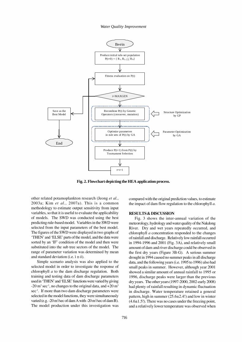
716
Water Quality Improvement
Begin
Produce initial rule-set population P(t=0) = { R1, R2, ¡¦¡¦ RN}
t=MAXGEN
Save as the Best Model
End
Fitness evaluation on P(t)
Recombine P(t) by Genetic Operators (crossover, mutation)
Optimize parameters in rule sets of P(t) by GA
Produce P(t+1) from P(t) by Tournament Selection
t=t+1
Structure Optimization by GP
Parameter Optimization by GA
Fig. 2. Flowchart depicting the HEA application process.
other related potamoplankton research (Jeong et al.,2003a; Kim et al., 2007a). This is a commonmethodology to estimate output sensitivity from inputvariables, so that it is useful to evaluate the applicabilityof models. The SWD was conducted using the bestpredicting rule-based model. Variables in the SWD wereselected from the input parameters of the best model.The figures of the SWD were displayed in two graphs of‘THEN’ and ‘ELSE’ parts of the model, and the data weresorted by an ‘IF’ condition of the model and then weresubstituted into the sub tree sectors of the model. Therange of parameter variation was determined by meanand standard deviation (i.e. ì ± ó).
Simple scenario analysis was also applied to theselected model in order to investigate the response ofchlorophyll a to the dam discharge regulation. Bothtraining and testing data of dam discharge parametersused in ‘THEN’ and ‘ELSE’ functions were varied by giving-20 m3 sec-1, no changes to the original data, and +20 m3
sec-1. If more than two dam discharge parameters wereselected in the model functions, they were simultaneouslyvaried (e.g. -20 m3/sec of dam A with -20 m3/sec of dam B).The model production under this investigation was
compared with the original prediction values, to estimatethe impact of dam flow regulation to the chlorophyll a.
RESULTS & DISCUSSIONFig. 3 shows the inter-annual variation of the
meteorology, hydrology and water quality of the NakdongRiver. Dry and wet years repeatedly occurred, andchlorophyll a concentration responded to the changesof rainfall and discharge. Relatively low rainfall occurredin 1994-1996 and 2001 (Fig. 3A), and relatively smallamount of dam and river discharge could be observed inthe first dry years (Figure 3B-G). A serious summerdrought in 1994 caused no summer peaks in all dischargedata, and the following years (i.e. 1995 to 1996) also hadsmall peaks in summer. However, although year 2001showed a similar amount of annual rainfall to 1995 or1996, discharge peaks were larger than the previousdry years. The other years (1997-2000, 2002-early 2008)had plenty of rainfall resulting in dynamic fluctuationin discharge. Water temperature retained a generalpattern, high in summer (25.6±2.4!) and low in winter(4.6±1.5!). There was no cases under the freezing point,and a relatively lower temperature was observed when
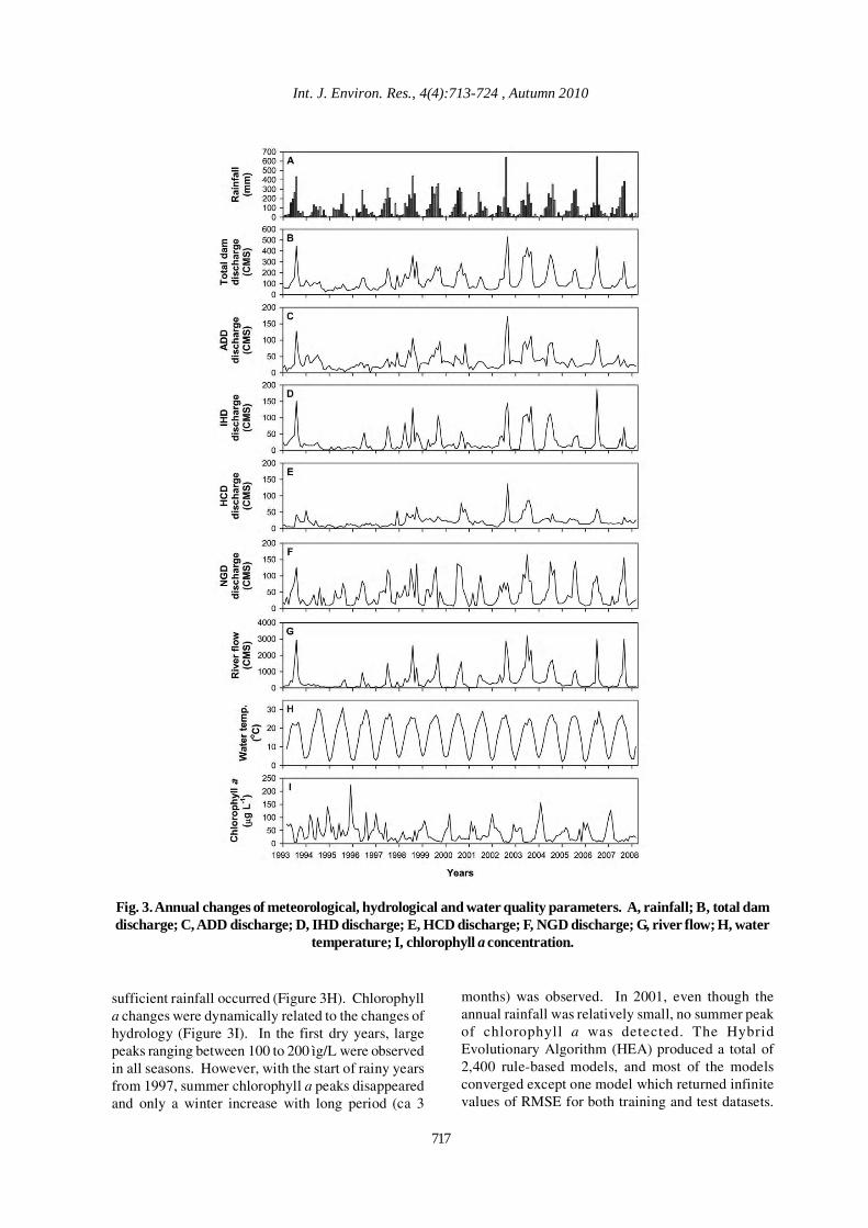
Int. J. Environ. Res., 4(4):713-724 , Autumn 2010
Fig. 3. Annual changes of meteorological, hydrological and water quality parameters. A, rainfall; B, total damdischarge; C, ADD discharge; D, IHD discharge; E, HCD discharge; F, NGD discharge; G, river flow; H, water
temperature; I, chlorophyll a concentration.
sufficient rainfall occurred (Figure 3H). Chlorophylla changes were dynamically related to the changes ofhydrology (Figure 3I). In the first dry years, largepeaks ranging between 100 to 200 ìg/L were observedin all seasons. However, with the start of rainy yearsfrom 1997, summer chlorophyll a peaks disappearedand only a winter increase with long period (ca 3
months) was observed. In 2001, even though theannual rainfall was relatively small, no summer peakof chlorophyll a was detected. The HybridEvolutionary Algorithm (HEA) produced a total of2,400 rule-based models, and most of the modelsconverged except one model which returned infinitevalues of RMSE for both training and test datasets.
717

718
Jeong, K. S. et al.
The average ± standard deviation of 2,399 models’RMSE, for the training data set, was 27.2±2.4, andthat for testing data set was 25.1±10.9. The minimum-maximum ranges of RMSE for both data sets were asthe following: 23.2-101.2 for the training data, 18.7-357.8 for the testing data set. Among the 2400 models,we selected one rule-set model as the best-predictingmodel, on the basis of RMSE, determination coefficient(i.e. r2), and visual comparison (Equation 1). In the ruleset model, five environmental parameters out of eightwere selected, and some of them were duplicated (rainfall,HCD discharge, NGD discharge, and water temperature).The ‘IF’ function consisted of two parameters (HCDdischarge and water temperature), and data samples withhigh temperature and large HCD discharge would havehigh probability to use ‘THEN’ function.
Fig. 4 illustrates the condition of water temperatureand HCD discharge by selectively using ‘THEN’ and‘ELSE’ functions. When the training data was rearrangedfrom the minimum to the maximum values of watertemperature and HCD discharge, respectively, a differentusage pattern of ‘THEN’ and ‘ELSE’ equations wereobserved (Figure 4A, B). In the case of water temperature,only the ‘ELSE’ equation was used when the temperaturewas below 5ºC, and complex usage between ‘THEN’ and‘ELSE’ equations above 5ºC. For HCD discharge, ‘THEN’equation was used when HCD discharge was less than20 m3 sec-1. Between ca 20 and 95 m3/sec of discharge,both ‘THEN’ and ‘ELSE’ tended to be used, but only‘ELSE’ was used when HCD discharge exceeded 100 CMS.There was a non-linear pattern in the use of ‘THEN’ or‘ELSE’ functions (Figure 4C). When water temperatureranges between 1~5ºC, ‘ELSE’ was used in chlorophyll acalculation. The model used the ‘THEN’ equation whentemperature is between 5~15ºC and HCD dischargeincreases. A gradual decrease in the use of the ‘THEN’
(1)
equation was observed when the temperature exceeded15ºC, and an increase of HCD discharge was also relatedwith using the ‘ELSE’ function in this temperature range.Fig. 5 illustrates the prediction accuracy of the bestpredicting rule set. The final rule-based model workedreasonably well with both training and test data sets(RMSE for training data, 24.9, test data, 20.6).Determination coefficients (r2) for both data sets werehigher than 0.50 (n=135 and 46 for training and testingdata respectively; p<0.01). For the training data, the timingof chlorophyll a peaks in summer and winter wererelatively well recognized, but a slight over-estimationoccurred, especially in spring and autumn. Similar patternof over-estimation was observed in the testing data set,and the end of 2007 to early of 2008 was relatively largelyover-estimated, but the winter peak of 2007 was under-estimated. Sensitivity analysis revealed that most of theinput parameters negatively affected the changes ofchlorophyll a concentration in the lower Nakdong River.Between two equations, the most influential parametersfor the changes of chlorophyll a were different; NGDdischarge for the ‘THEN’ function, and IHD for the ‘ELSE’.Two input parameters out of three were the same between‘THEN’ and ‘ELSE’ functions (i.e. rainfall and NGDdischarge), and the sensitivity of chlorophyll a to thesetwo parameters were different between the equations.Rainfall did not have a strong influence on the changesof chlorophyll a in the ‘THEN’ function, but a strongnegative impact could be observed in the ‘ELSE’ function(Fig. 6A, D). Especially, a sharp drop of chlorophyll aoccurred when rainfall ranged between 0 to 20 mm.Chlorophyll a was reduced when NGD dischargeincreased, and their relationship was in an exponentiallydecaying pattern (Figure 6B, E). The impact of NGDdischarge was stronger in the ‘THEN’ function than the‘ELSE’.
The remaining parameter was different in each of thefunctions. In the ‘THEN’ function, water temperaturewas used, but IHD discharge was selected instead ofwater temperature in the ‘ELSE’ (Fig. 6C, F). Both of theparameters negatively affected the chlorophyll a changes,similar to the other hydrological parameters. The impactof dam discharge regulation on the changes of chlorophylla can be found in the Fig. 7. Inputting varied dischargevalues for the two dam discharge parameters (-20 m3/secto +20 m3/sec; IHD and NGD discharge, respectively)resulted in the changes of predicted chlorophyll a. Whenthe discharge of both dams were decreased by 20 m3/secthroughout the study period, chlorophyll a concentrationdrastically increased compared with normally predictedvalues. In this case the changing rate of chlorophyll a(disturbed data vs. normal simulation) was 322%. WhenIHD and NGD dam discharge was decreased separately,the rates were 25% and 95%, respectively. Separateincrease of dam discharge resulted in the decrease of
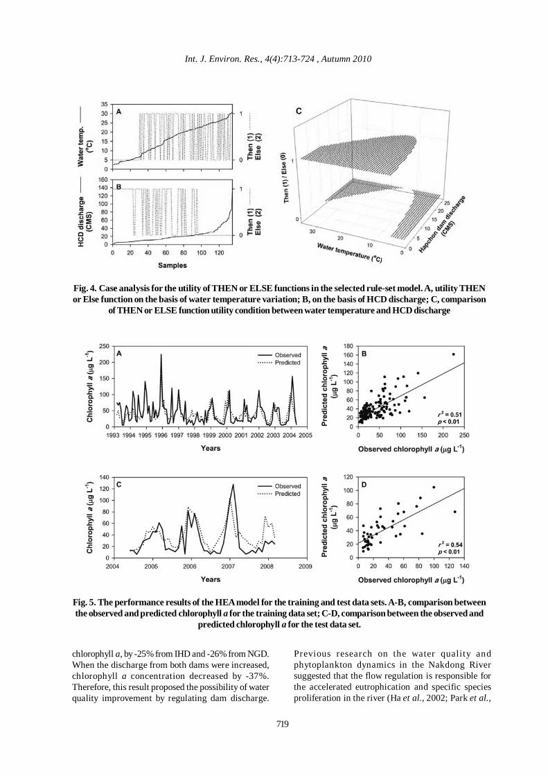
719
Int. J. Environ. Res., 4(4):713-724 , Autumn 2010
Fig. 4. Case analysis for the utility of THEN or ELSE functions in the selected rule-set model. A, utility THENor Else function on the basis of water temperature variation; B, on the basis of HCD discharge; C, comparison
of THEN or ELSE function utility condition between water temperature and HCD discharge
Fig. 5. The performance results of the HEA model for the training and test data sets. A-B, comparison betweenthe observed and predicted chlorophyll a for the training data set; C-D, comparison between the observed and
predicted chlorophyll a for the test data set.
chlorophyll a, by -25% from IHD and -26% from NGD.When the discharge from both dams were increased,chlorophyll a concentration decreased by -37%.Therefore, this result proposed the possibility of waterquality improvement by regulating dam discharge.
Previous research on the water quality andphytoplankton dynamics in the Nakdong Riversuggested that the flow regulation is responsible forthe accelerated eutrophication and specific speciesproliferation in the river (Ha et al., 2002; Park et al.,

720
Water Quality Improvement
Fig. 6. Results of sensitivity analysis for the selected model. A-C, parameters included in the THEN function;D-F, parameters included in the ELSE function. A, rainfall; B, NGD discharge; C, water temperature; D,
rainfall; E, NGD discharge; F IHD discharge.
2002; Ha et al., 2003a; Jeong et al., 2003b; Kim et al.,2003; Jeong et al., 2007). Development in the watershedand loss of numerous riparian wetlands in the recentdecades has been known to result in the continuousnutrient loading into the river (Joo et al., 1997).Sufficient nutrients in the water enabled phytoplanktonspecies to easily increase (Ha et al., 1998), and theyused to proliferate in the early summer just before thesummer concentrated rainfall due to monsoon climate(Park et al., 2002). The start of nutrient accumulationand phyto-plankton proliferation in the lower part ofthe river were caused by the construction of anestuarine barrage in 1987. Flow control by multi-purpose dams was on-going before the constructionof estuarine barrage, but scientific studies revealedthe drastic changes in ecological structures in termsof the barrage. Since the construction of the barrage,increase in nutrients such as phosphate and nitrogenwere observed (Kim, 1969; Choi and Park, 1986; Lee etal., 1993), which in turn brought out assemblagechanges of phytoplankton and proliferation of specificspecies (Cho, 1991; Kim and Lee, 1991; Moon and Choi,1991; Cho et al., 1993; Chung et al., 1994; Seo andChung, 1994; Ha et al., 1998). Currently, it is difficult toremove the estuarine barrage/ therefore, a wisemanagement strategy to eliminate the phytoplankton-causing water quality problems by adapting to thecurrent situation is needed. Adaptive flow regulation,so called ‘environmental flow,’ would be a solution forthis perspective. River flow in East Asia is mainlygoverned by the summer monsoon climate and typhoon
events. Monsoon is recognized as a primary factordetermining the characteristics of freshwaterecosystems (Silva and Davis, 1987; Brewin et al., 2000;Kim et al., 2000a; An and Park, 2002; Dudgeon, 2002;Azami et al., 2004; Yoshimura et al., 2005; Madhu etal., 2007). Also typhoon events bring enormousquantity of rain within short period, which is alsoknown as source for water resource in this region(Jeong et al., 2007). In consequence, reliance onsummer rainfall is relatively high in East-Asiancountries, and particularly in Korea it is very importanthow to manage and allocate water resources efficientlyby constructing dams in spite of deliberation forenvironmentally negative effects on ecosystem. Thechanges of meteorology, hydrology and water qualityparameters showed strong seasonality during the studyperiod and chlorophyll a changes responded well tothe changes in hydrological parameters. In the lowerNakdong River, previous research focused on theseasonal dynamics of phytoplankton distribution, andtwo bloom-forming periods were the most importantphenomena for water quality point of view, such assummer cyanobacteria and winter diatom. Ha et al.(2002) revealed that the lower part of the river showeddifferent patterns of phytoplankton successioncompared with the middle part of the river. Theysuggested that accumulated nutrients and increasedretention time would be the primary factor for thedifference. Modeling results from Jeong et al. (2001)and Jeong et al. (2003a) concluded that phytoplanktonwould react with chemical factors such as nutrient or
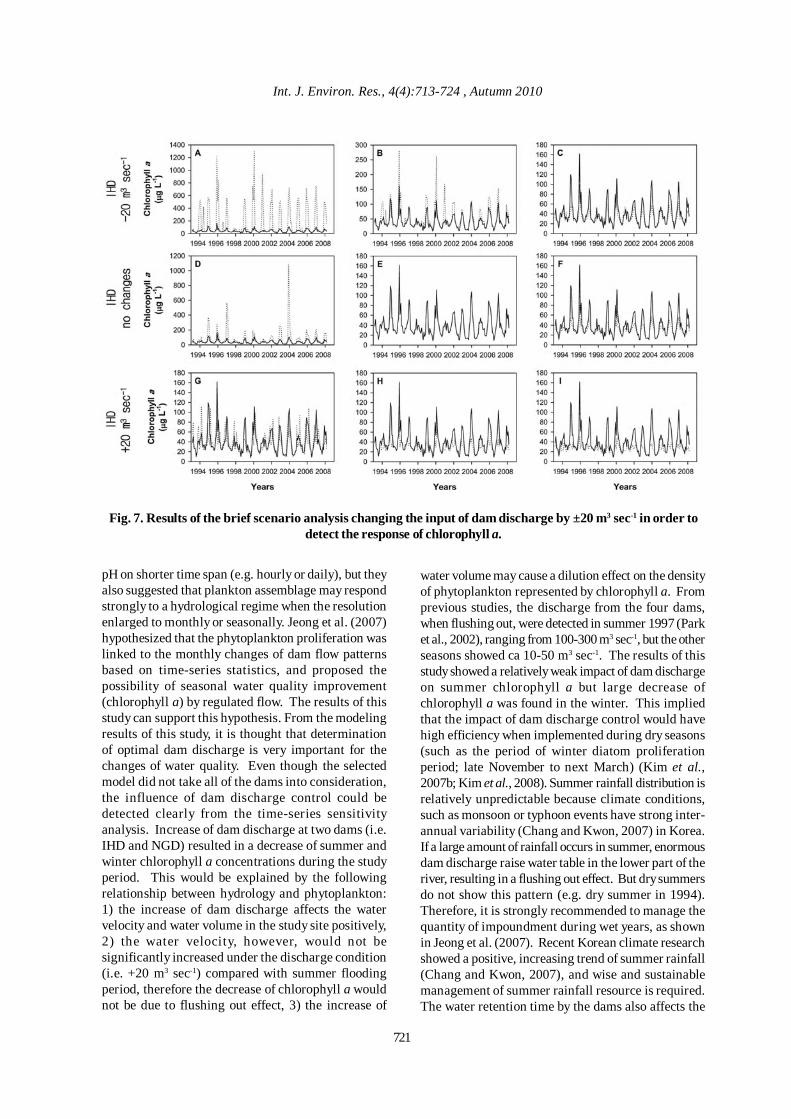
Int. J. Environ. Res., 4(4):713-724 , Autumn 2010
Fig. 7. Results of the brief scenario analysis changing the input of dam discharge by ±20 m3 sec-1 in order todetect the response of chlorophyll a.
pH on shorter time span (e.g. hourly or daily), but theyalso suggested that plankton assemblage may respondstrongly to a hydrological regime when the resolutionenlarged to monthly or seasonally. Jeong et al. (2007)hypothesized that the phytoplankton proliferation waslinked to the monthly changes of dam flow patternsbased on time-series statistics, and proposed thepossibility of seasonal water quality improvement(chlorophyll a) by regulated flow. The results of thisstudy can support this hypothesis. From the modelingresults of this study, it is thought that determinationof optimal dam discharge is very important for thechanges of water quality. Even though the selectedmodel did not take all of the dams into consideration,the influence of dam discharge control could bedetected clearly from the time-series sensitivityanalysis. Increase of dam discharge at two dams (i.e.IHD and NGD) resulted in a decrease of summer andwinter chlorophyll a concentrations during the studyperiod. This would be explained by the followingrelationship between hydrology and phytoplankton:1) the increase of dam discharge affects the watervelocity and water volume in the study site positively,2) the water velocity, however, would not besignificantly increased under the discharge condition(i.e. +20 m3 sec-1) compared with summer floodingperiod, therefore the decrease of chlorophyll a wouldnot be due to flushing out effect, 3) the increase of
water volume may cause a dilution effect on the densityof phytoplankton represented by chlorophyll a. Fromprevious studies, the discharge from the four dams,when flushing out, were detected in summer 1997 (Parket al., 2002), ranging from 100-300 m3 sec-1, but the otherseasons showed ca 10-50 m3 sec-1. The results of thisstudy showed a relatively weak impact of dam dischargeon summer chlorophyll a but large decrease ofchlorophyll a was found in the winter. This impliedthat the impact of dam discharge control would havehigh efficiency when implemented during dry seasons(such as the period of winter diatom proliferationperiod; late November to next March) (Kim et al.,2007b; Kim et al., 2008). Summer rainfall distribution isrelatively unpredictable because climate conditions,such as monsoon or typhoon events have strong inter-annual variability (Chang and Kwon, 2007) in Korea.If a large amount of rainfall occurs in summer, enormousdam discharge raise water table in the lower part of theriver, resulting in a flushing out effect. But dry summersdo not show this pattern (e.g. dry summer in 1994).Therefore, it is strongly recommended to manage thequantity of impoundment during wet years, as shownin Jeong et al. (2007). Recent Korean climate researchshowed a positive, increasing trend of summer rainfall(Chang and Kwon, 2007), and wise and sustainablemanagement of summer rainfall resource is required.The water retention time by the dams also affects the
721

Jeong, K. S. et al.
changes in zooplankton. They are grazers that cause adecrease in chlorophyll a concentrations by selectiveconsumption of phytoplankton, resulting in theincrease of water clarity (Kim, 1999; Kim et al., 2000b;Kim et al., 2003). Although this study only considereddam discharge as the forcing function, it was alsorequested to comprehend the relationship amonghydrology, phytoplankton and zooplankton. If adischarge condition that can facilitate or does notinhibit spring zooplankton growth can be defined, thewater quality during the dry seasons can behydrologically and biologically controlled. If optimaldischarge conditions from hydrological models areavailable in the future, more accurate and reliablehydro-ecological simulations would be possible.
Most river systems are regulated by dams and locks,and this phenomenon can be frequently observed inEast Asia, due to the seasonally biased distribution ofannual rainfall. Therefore the blockage of water flowresponsible for the deterioration of water quality canbe solved by prudent regulation of the water flow. Eventhough there were some cases showing flushing effectson the accumulated phytoplankton scum by the instantincrease in dam discharge (Webster et al., 2000; Maieret al., 2001; Maier et al., 2004), it is rare to find casesproviding quantitative evidence in the perspective oftotal basin management. Therefore, the results of thisstudy can provide useful information for rivermanagement in East Asia.
On the basis of this study’s results, the followingtwo water resource management strategies can bedetermined. First, flow regulation must be focused oncontrolling or improving river ‘quality’ on the viewpointof watershed or rivers. Regardless of the water resourcedemand from the basin, the current status of the riverand its basin need to be considered simultaneously.Ecosystem health, covering not only phytoplanktonproliferations, but also other ecological componentssuch as fish, benthic macro invertebrates andvegetation in the riparian zone, have to be intensivelydetermined in the river basin, and the structure andfunctions of those factors need to be related to basinwater resource management.
The second is ‘acute therapy’ for the water qualityproblems in the river. The model developed in this studywas used to simulate the current status ofphytoplankton biomass changes with relation tocurrent hydrological patterns. This information canhelp producing predictive ecological models to be usedin the ‘acute therapy.’ In other words, discharges ofdams from the upstream can be implemented whererapid prescription is required for controlling waterquality deterioration by flushing impact. For instance,a forecasting model based on hydrological and
ecological components’ relationship will be able tosupport early-warning systems for algal blooms (referto Jeong et al., 2008). For this purpose, data with moredetailed time resolution (less than monthly time-interval) has to be available. Once this type of modelcan be constructed, the government can utilize themodel for water environment management in a long-term strategy. The above two types of strategies, i.e.adaptive watershed management and acute therapy,can be taken into account other regulated river systemsin the countries where a rainfall pattern is biased anddependence on flow regulation by dams is relativelyhigh.
CONCLUSIONThis study focused on the simulation of a water
quality parameter (phytoplankton biomass representedby chlorophyll a concentration), using long-termecological monitoring data collected between March1993 to March 2008 (16 years) from the lower NakdongRiver. Hybrid Evolutionary Algorithm (HEA) known asefficient ecological informatics method was utilized andthe relationship between meteorological, hydrologicaland water quality parameters were investigated. Thispaper has proposed possibility to quantify the regulationimpact of dam discharge on chlorophyll a changestrough the developed rule-set model. In particular, itwas shown that increase of HCD and NGD damdischarge by +20 m3/sec respectively reduced algalbiomass up to 37% in terms of total average ofchlorophyll a. Therefore, it is strongly advised to wiselyregulate water flow in preparation of water resourcemanagement strategy implementation in the regulatedriver systems in East Asia.
ACKNOWLEDGEMENTThe authors would like to thank Mr. Maurice
Lineman for proof reading the manuscript during itspreparation. Also we appreciate members of theLimnology Lab., Pusan National University, for theirinvaluable efforts on river monitoring. This study wasfinancially supported by the Pusan National Universityprogram Post-Doc 2007 for Dr. Kwang-Seuk Jeong.
REFERENCESAli, Y., Aslam, Z., Ashraf, M. Y. and Tahir, G. R. (2004).Effect of salinity on chlorophyll concentration, leaf area,yield and yield components of rice genotypes grown undersaline environment. Int. J.. Environ. Sci. Tech., 1(3), 221-225.
An, K.-G. and Park, S. S. (2002). Indirect influence of thesummer monsoon on chlorophyll–total phosphorus modelsin reservoirs: a case. Ecol. Modelling, 152, 191-203.
Azami, K., Suzuki, H. and Toki, S. (2004). Changes inRiparian vegetation communities below a large dam in a
722
Int. J. Environ. Res., 4(4):713-724 , Autumn 2010
monsoonal region: Futase Dam, Japan. River Res. Applic.,20, 549-563.
Banzharf, W., Nortin, P., Keller, R. E. and Francone, F. D.(1998). Genetic Programming: On the Automatic Evolutionof Computer Programs and its Applications. California:Morgan Kaufmann Publishers Inc.
Bhatnagar, A. and Sangwan, P. (2009). Impact of Mass Bathingon Water Quality. Int. J. Environ. Res., 3(2), 247-252.
Brewin, P. A., Buckton, S. T. and Ormerod, S. J. (2000). Theseasonal dynamics and persistence of streammacroinvertebrates in Nepal: do monsoon floods representdisturbance? Freshwater Biol., 44, 581-594.
Cao, H., Recknagel, F., Kim, B. and Takamura, N. (2006).Hybrid Evolutionary Algorithm for Rule Set Discovery inTime-Seies Data to Forecast and Explain Algal PopulationDynamics in Two Lakes Different in Morphometry andEutrophication. (In F. Recknagel (Ed.), Ecological Informatics:Scope, Techniques and Applications (pp. 347-367). Berlin:Springer-Verlag.)
Chang, H. and Kwon, W.-T. (2007). Spatial variations ofsummer precipitation trends in South Korea, 1973-2005.Environ. Res. Lett., 2, 1-9.
Cho, K.-J. (1991). Spatial and temporal distribution ofphytoplanktonic and periphytic diatom assemblages ofNaktong River Estuary. Kor. J. Phycol., 6 (1), 47-53.
Cho, K.-J., Chung, I.-K. & Lee, J.-A. (1993). Seasonaldynamics of phytoplankton community in the Nakdong RiverEstuary, Korea. Kor. J. Phycol., 8(1), 15-28.
Choi, Y.-C. & Park, C.-K. (1986). Eutrophication in thedownstream of Nakdong River. J. Kor. Fish. Soc., 19(4), 339-346.
Chung, J., Kim, H.-S. & Kim, Y.-J. (1994). Structure ofphytoplankton community in the Nakdong River EstuaryDam. Kor. J. Limnol., 27(1), 33-46.
Codd, G.A., Bell, S.G., Kaya, K., Ward, C.J., Beattie, K.A. &Metcalf, J.S. (1999). Cyanobacterial toxins, exposure routesand human health. Eur. J. Phycol., 250, 339-350.
Codd, G.A., Morrison, L.F. & Metcalf, J.S. (2005).Cyanobaterial toxins: risk management for health protection.Toxicol. Appl. Pharm., 203, 264-272.
Dudgeon, D. (2002). An inventory of riverine biodiversity inmonsoonal Asia: present status and conservation challenges.Water Sci.Tech., 45, 11-19.
Fogel, D.B. (1998). Evolutionary computation: toward a newphilosophy of machine intelligence. New York: IEEE Press.
Foulger, T.R. and Petts, G.E. (1984). Water quality implicationsof artificial flow fluctuations in regulated rivers. Sci. TotalEnv., 37(3), 177-185.
Fox, I.A. & Johnson, R.C. (1997). The hydrology of the riverTweed. Sci. Total Env., 194&195, 163-172.
Franklin, P., Dunbar, M. and Whitehead, P. (2008). Flowcontrols on lowland river macrophytes: A review. Sci. TotalEvn., 400(1-3), 369-378.
Gilvear, D.J., K.V.Heal, and A. Stephen. (2002). Hydrology
and the ecological quality of Scottish river ecosystems. Sci.Total Env., 294(1-3), 131-159.
Ha, K., Jang, M.-H. and Joo, G.-J. (2002). Spatial andtemporal dynamics of phytoplankton communities along aregulated river system, the Nakdong River, Korea.Hydrobiologia, 470, 235-245.
Ha, K., Jang, M.-H. and Joo, G.-J. (2003a). WinterStephanodiscus bloom development in the lower NakdongRiver regulated by an estuary dam and tributaries.Hydrobiologia, 506(1), 221-227.
Ha, K., Jang, M.H. and Joo, G.J. (2003b). WinterStephanodiscus bloom development in the Nakdong Riverregulated by an estuary dam and tributaries. Hydrobiologia,506&509(1), 221-227.
Ha, K., Kim, H.-W., Jeong, K.-S. and Joo, G.-J. (2000). Verticaldistribution of Microcystis population in the regulatedNakdong River, Korea. Limnology, 1, 225-230.
Ha, K., Kim, H.-W. and Joo, G.-J. (1998). The phytoplanktonsuccession in the lower part of hypertrophic Nakdong River(Mulgum), South Korea. Hydrobiologia, .369&370, 217-227.
Holland, J.H. (1975). Adaptation in Natural and ArtificialSystem: An Introductory Analysis with Applications toBiology, Control, and Artificial Intelligence. Ann Arbor,Michigan: University of Michigan Press.
Jeong, K.-S., Joo, G.-J., Kim, H.-W., Ha, K. and Recknagel, F.(2001). Prediction and elucidation of phytoplankton dynamicsin the Nakdong River (Korea) by means of a recurrent artificialneural network. Ecol. Modelling, 146, 115-129.
Jeong, K.-S., Kim, D.-K. and Joo, G.-J. (2007). Delayedinfluence of dam storage and discharge on the determinationof seasonal proliferations of Microcystis aeruginosa andStephanodiscus hantzschii in a regulated river system of thelower Nakdong River (South Korea). Water Res., 41, 1269-1279.
Jeong, K.-S., Kim, D.-K., Whigham, P. and Joo, G.-J. (2003a).Modelling Microcystis aeruginosa bloom dynamics in theNakdong River by means of evolutionary computation andstatistical approach. Ecol. Modelling, 161, 67-78.
Jeong, K.-S., Recknagel, F. and Joo, G.-J. (2003b). Predictionand elucidation of population dynamics of a blue-green Alga(Microcystis aeruginosa) and diatom (Stephanodiscushantzschii) in the Nakdong River-Reservoir System (SouthKorea) by a recurrent artificial neural network. (In F. Recknagel(Ed.), Ecological Informatics (pp. 196-213). Berlin: Springer.
Jeong, K.S., Kim, D.K., Jung, J.M., Kim, M.C. and Joo, G.J.(2008). Non-linear autoregressive modelling by TemporalRecurrent Neural Networks for the prediction of freshwaterphytoplankton dynamics. Ecol. Modelling, 211(3-4), 292-300.
Joarder, M. A. M., Raihan, F., Alam, J. B. and Hasanuzzaman,S. (2008). Regression Analysis of Ground Water Quality Dataof Sunamganj District, Bangladesh. Int. J. Environ. Res., 2(3),291-296.
Joo, G.J., Kim, H.W., Ha, K. and Kim, J.K. (1997). Long-term trend of the eutrophication of the lower Nakdong River.Korean J. Limnol., 30, 472-480.
723

Water Quality Improvement
Kim, B., Choi, K., Kim, C., Lee, U.-H. and Kim, Y.-H. (2000a).Effects of the summer monsoon on the distribution and loadingof organic carbon in a deep reservoir, Lake Soyang, Korea.Water Res., 34(14), 3495-3504.
Kim, D.-K., Cao, H., Jeong, K.-S., Recknagel, F. and Joo, G.-J.(2007a). Predictive function and rules for population dynamicsof Microcystis aeruginosa in the regulated Nakdong River (SouthKorea), discovered by evolutionary algorithms. Ecol. Model.,203(1-2), 147-156.
Kim, D.-K., Jeong, K.-S., Whigham, P.A. and Joo, G.-J. (2007b).Winter diatom blooms in a regulated river in South Korea:explanations based on evolutionary computation. FreshwaterBiol., 52, 2021-2041.
Kim, H.-W. (1999). Water quality, plankton communitydynamics, and trophic regulation in the microbial food web byzooplankton in a hypertrophic river (Nakdong River, Korea).Dissertation, Pusan National University.
Kim, H.-W., Chang, K.-H., Jeong, K.-S. and Joo, G.-J. (2003).The spring metazooplankton dynamics in the river-reservoirhybrid system (Nakdong River, Korea): its role in controllingthe phytoplankton biomass. Kor. J. Limnol.,36(4), 420-426.
Kim, H.-W., Hwang, S.-J. and Joo, G.-J. (2000b). Zooplanktongrazing on bacteria and phytoplankton in a regulated large river(Nakdong River, Korea). J. Plankton Res., 22, 1559-1577.
Kim, I.-B. (1969). Fundamental studies of the lower part of theNaktong River for fisheries exploitation. J. Kor. Fish. Soc.,2(1), 25-32.
Kim, J.-W. and Lee, H.-Y. (1991). A study onn phytoplanktoncommunities in the reservoir of Nakdong River Estuary. Kor. J.Limnol., 24(3), 143-151.
Kim, M.-C., La, G.-H., Kim, H.-W., Jeong, K.-S., Kim, D.-K.and Joo, G.-J. (2008). The effect of water temperature onproliferation of Stephanodiscus sp. in vitro from the NakdongRiver, South Korea. Kor. J. Limnol., 41(1), 26-33.
Lee, J.-A., Cho, K.-J., Kwon, O.-S. and Chung, I.-K. (1993). Astudy on the environmental factors in Naktong Estuarineecosystem. Kor. J. Phycol., 8(1), 29-36.
Loneragan, N.R. (1999). River flows and estuarine ecosystems:Implications for coastal fisheries from a review and a casestudy of the Logan River, southeast Queensland. Austral. Ecol.,24(4), 431-440.
Madhu, N.V., Jyothibabu, R., Balachandran, K.K., Honey, U.K.,Martin, G.D., Vijay, J.G., Shiyas, C.A., Gupta, G.V.M. andAchuthankutty, C. T. (2007). Monsoonal impact on planktonicstanding stock and abundance in a tropical estuary (Cochinbackwaters - India). Estuar. Coast. Shelf Sci., 73(1-2), 54-64.
Maier, H.R., Burch, M.D. and Bormans, M. (2001). Flowmanagement strategies to control blooms of the cyanobacterium,Anabaena circinalis, in the River Murray at Morgan, SouthAustralia. Regul. Rivers: Res. Mgmt., 17, 637-650.
Maier, H.R., Kingston, G.B., Clark, T., Frazer, A. and Sanderson,A. (2004). Risk-based approach for assessing the effectivenessof flow management in controlling cyanobacterial blooms inrivers. River Res. Appl. v.20, No.4, pp. 459-471.
Monavari, S. and Guieysse, B. (2007). Development of WaterQuality Test Kit Based on Substrate Utilization and ToxicityResistance in River Microbial Communities. Int. J. Environ.Res., 1(2), 139-142.
Moon, C.-H. and Choi, H.-J. (1991). Studies on theenvironmental characteristics and phytoplankton communityin the Nakdong River Estuary. J. Oceanol. Soc. Kor., 26(2),144-154.
Najafpour, Sh., Alkarkhi, A. F. M., Kadir, M. O. A. andNajafpour, Gh. D. (2008). Evaluation of Spatial and TemporalVariation in River Water Quality. Int. J. Environ. Res., 2(4),349-358.
Nakane, K. and Haidary, A. (2010). Sensitivity Analysis ofStream Water Quality and Land Cover Linkage Models UsingMonte Carlo Method. Int. J. Environ. Res., 4(1), 121-130.
Park, S.-B., Lee, S.-K., Chang, K.-H., Jeong, K.-S. and Joo, G.-J. (2002). The impact of Jangma (monsoon rainfall) on thechanges of water quality in the lower Nakdong River (Mulgeum).Kor. J. Limnol., 35, 161-170.
Rene, E R. and Saidutta, M. B. (2008). Prediction of WaterQuality Indices by Regression Analysis and Artificial NeuralNetworks. Int. J. Environ. Res., 2(2), 183-188.
Seo, J.-K. and Chung, I.-K. (1994). The phytoplanktoncommunity structure in the Nakdong River Mouth. Kor. J.Limnol., 27(3), 227-250.
Silva, E.I.L. and Davis, R.W. (1987). The seasonality ofmonsoonal primary productivity in Sri Lanka. Hydrobiologia,150, 165-175.
Stober, Q.J. and Nakatani, R.E. (1992). Water quality and biotaof the Columbia River system. (In C.D. Becker & D.A. Neitzel(Ed.), Water Quality in North American River Systems (pp.51-83). Ohio: Battelle Press.
Taseli, B. K. (2009). Influence of Land-based Fish Farm Effluentson the Water Quality of Yanýklar Creek. Int. J. Environ. Res.,3(1), 45-56.
Tharme, R.E. (2003). A global perspective on environmentalflow assessment: emerging trends in the development andapplication of environmental flow methodologies for rivers.River Res. Appl., 19, 397-441.
Wade, A.J., Whitehead, P.G., Hornberger, G.M. and Snook,D.L. (2002). On modelling the flow controls on macrophyteand epiphyte dynamics in a lowland permeable catchment: theRiver Kennet, southern England. Sci. Total Env., 282&283,375-393.
Webster, I.T., Sherman, B.S., Bormans, M. and Jones, G. (2000).Management strategies for cyanobacterial blooms in animpounded lowland river. Regul. Rivers: Res. mgmt., 16, 513-525.
Wetzel, R.G. and Likens, G.E. (1991). Limnological Analyses.New York: Springer-Verlag.
Yoshimura, C., Omura, T., Furumai, H. and Tockner, K. (2005).Present state of rivers and streams in Japan. River Res.Applic., 21, 93-112.
724
Int. J. Environ. Res., 4(4):725-734 , Autumn 2010ISSN: 1735-6865
Received 17 Sep. 2008; Revised 15 March 2010; Accepted 27 May 2010
*Corresponding author E-mail: [email protected]
725
Ecological Impact Analysis on Mahshahr Petrochemical Industries UsingAnalytic Hierarchy Process Method
Malmasi, S. 1, Jozi, S . A.1 , Monavari, S .M. 2, Jafarian, M. E. 2*
1 Department of Natural Resources Engineering, Technical and engineering Faculty,IAU, Northern Branch of Tehran, Iran
2 Department of Environmental Science, Graduate School of Environment and nergy,Science and Research Campus, IAU, P.O.Box 1748743341, Tehran, Iran
ABSTRACT: Petrochemical Industries are potentially capable of impacts on environment due to the essenceof the activities and producing waste water, pollutant emissions and hazardous wastes. This case study hasconsidered the environmental adverse impacts of petrochemical industries on existing habitats in MahshahrEconomic Special Zone with respect to the regional significant biological diversity and ecological valuablespecies. When results from regional estuary sampling as well as impacts by petrochemical industries pollut-ants has been analyzed and studied. Then affected ecosystems have been prioritized using Analytic HierarchyProcess (AHP) method, Expert Choice software and Eigenvector technique. Studies outcomes show that, withregard to petrochemical industries pollutants, especially waste waters including heavy metals, oil and grease,Chemical Oxygen Demand (COD), Total Suspended Solids (TSS), along with criteria defined in AHP methodsuch as ecological and protecting value, estuaries are most affected ecosystems in the region. On the otherhand, types of fishes and benthic, such as Decapods, Gastropods and Tanaida have been highly affected by thepetrochemical industries activities consequents. It is concluded that, heavy metals, oil and grease, deposit intothe environment, are the most important pollutant sources for the regional estuaries which should be con-trolled
Key words: Petrochemical Industries, Impacts, Analytic Hierarchy Process, Expert Choice, Estuaries, Environment
INTRODUCTIONPetrochemical Industry refers to those industries
in which Hydro Carbon within the natural gas and oil istransformed into chemical products. “Petrochemical”,which implies chemical materials obtained from oil, iscompound of two words indeed; “petrol” and “chemis-try” (Monavari, 2001). Petrochemical industry is theindustry that produce our daily life needed chemicalmaterials from oil by processing and transforming Hy-dro Carbon into final products which have about 10 to15 times higher value added than its feed stock namelygas and crud oil. Other advantages of this base indus-try is it’s infinite possibility of producing thousandsof chemical products that many of them are used asfeed to other industries and agriculture. (Jafarzadeh,2008).
Petrochemical Industry has been established firstin America. The word “Petrochemicals” was used torefer to raw materials achieved from oil. Then after oil
material was used as primarily raw materials by Euro-pean and other countries. National Petrochemical Com-pany (NPC) subsidiary of National Iranian Oil Com-pany (NIOC) has been established in Iran since 1964and began its activities about half a century ago(Mostajabi, 2008).The first relatively cohesive orga-nization which has been established for the purposeof petrochemical activities was chemical institute af-filiated to ministry of economy and its major work wasfoundation of chemical fertilizer factory in Marvdasht-Fars in 1957. Later in 1964, all the activities entitledPetrochemical Industries Development by ministriesaffiliates and other governmental organizations, havebeen centralized in National Iranian Oil Company(NIOC) and subsequently established National Petro-chemical Company as a subsidiary in order to fulfillthe main objective which is producing chemical, pet-rochemical and side products from oil and gas deriva-tions and other organic and mineral materials. Thus,Hydro Carbon which are frequently found in Iran and

726
Malmasi, S. et al.
has been previously burnt as solid useless waste formany years, now are being used according to scien-tific and industrial standards (Rafeenejad, 2007).
Although petrochemical industries brought toomany benefits for our life, are considered as environ-mental pollutant source it could be said that controland mitigation of petrochemical industries pollutionhave been a cause for concern and today’s interna-tional major challenges to save the environmentagainst its impacts. The environmental impact of theseindustries, if the environmental standards and regula-tions are ignored, could cause hazardous impacts andmake great disturbance to the health of human com-munity as well as wildlife (Rooney, 2005). Petrochemi-cal industries potentially have environmental impactsdue to the essence of their activities and process, aswell as its producing waste water, emissions and haz-ardous wastes (Xiao-ping, et al., 2004). Moreover, in-dustrial waste water deposit to the environment bypetrochemical industries, regarding the nature of thewaste composition, is capable of destroying signifi-cant amount of biological elements of the water re-sources that receive these wastes and gradually elimi-nates aquatic types of fauna and flora directly or indi-rectly which follows by food network simplification asthe number of species and diversity decrease and fi-nally change the water resource to a dead one (Rajeshand Edwin Tam, 2006). These impacts not only affectthe biological factors of the ecosystem especially incase of heavy metals pollution, but also can affect thewater resource quality and threat the human health aswell (Esmaeli Sari, 2002). According to sustainable de-velopment and environmental standards, ignoring en-vironment and threatening environmental and biologi-cal factors is equal to ignoring human health whichfollows by health, social and economical impacts(Asian development bank, 1997).
With respect to this subject, discharging wasteby several petrochemical industries into the PersianGulf affects regional natural life of animals in the seawhich are considered as nutrition source to the resi-dence of the area and consequently threatens humanhealth. Persian Gulf is a semi open sea with 40000 m2
areas and between 400 and 450 types of fishes whichis very unique diversity indeed. Persian Gulf is locatedin a dry and warm climate. With respect to special en-vironmental condition, regional aquatic species arerather vulnerable against climate changes in one handand regional pollutants have doubled the harm on theother hand (Samadyar, 2005).
Studied area is located on Persian Gulf shore inMahshahr County which has a strategic positionamongst Iranian oil & gas area due to petrochemicalindustries plant operating there and makes the feed
stock oil and gas resources available to the plants(Jafarzadeh, 2008). Estuaries are the most importantregional aquatic ecosystems. Appropriate temperatureand food condition in these ecosystems make the situ-ation suitable for abundant types of fishes, benthicsuch as Tanaida, Polychaeta, molluscs. In addition,types of indigenous and peregrine birds, living in thestudy area, which are mostly regional native birds ormigrated to this place each year from cold regions tohibernate, prove the importance of estuary’s ecologynear the study area (Nabavi, 1999). Great amount ofdischarged waste water into these estuaries is the ma-jor water pollution factor. On the other hand frequenttide has considerably expanded the scope of pollu-tion. Pollution in Mousa estuary and its tributary origi-nates from the estuary (Mazaheri 2001). Therefore, re-garding estuaries as one of the most productive eco-systems on the world in one hand and several petro-chemical industries activities in the region on the otherhand, degradation factors exploration and defining thecharacteristic pollutants in the region to provide ap-propriate mitigation measures in order to remove ordecline the adverse impacts, become inevitable neces-sity.
In this study, adverse impact caused by petro-chemical industries activities located in Mahshahr eco-nomic special zone of, focusing on Tondguyan Petro-chemical Complex has been analyzed. This complex isconsidered as the only PET (Poly Ethylene Terephtha-late) bottle manufacturer in Iran, which possesses awaste treatment system independently. The main rea-son of constructing this treatment plant and not justsend the waste to Fajr plant, what other petrochemicalindustries just do, is the existence of heavy metal inthe complex waste (Mg and Co for instance), high CODand a large quantity of the produced waste byTondguyan Complex. (Shil Amayesh Consulting Engi-neers, 2006).
Now a days, environmental impact assessmentand analysis of petrochemical industries waste waterson biological communities particularly those factorswhich are more vulnerable against pollutions, is oneof the main measurements which is taken in to ac-count to protect natural resources. Assessment andanalysis of impacts must be done along with carryingout required sampling from affected water resources ina way that guarantees the protection of affected bio-logical factors. Therefore environmental managementwith the purpose of protecting these affected resourcesrequires impacts identification and analyzing (Jafarian,2008). Although obeying environmental requirementsdeals with mitigation or declining of the most signifi-cant incompatible environmental impacts involvescosts, it offers a more promising future in terms of en-
Int. J. Environ. Res., 4(4):725-734 , Autumn 2010
727
vironmental issues, and specially will bring the oppor-tunity to join the Kyoto Protocol for countries(Mostajabi, 2008).
In this study, Analytic Hierarchy Process (AHP)method has been used to rank the pollutants and envi-ronmental impact assessment of petrochemical indus-try. Since Analytic Hierarchy Process theory came toexist, many essays have been published focusing onthat and some magazines have specialized particularpublished number to those essays. European Journalof Operational research journal as specialized one,Socio- Economic planning magazine and Mathemati-cal Modeling journal has specialized two volumes sepa-rately to discuss the AHP and multiple criteria deci-sion making (Saaty, 1994). In addition about 20 vol-umes of books have been published and different con-ferences have been hold all around the world in re-lated to AHP method (Ghodsipur2006). Application ofAHP method in environmental projects and plans isbeing frequently discussed in many essays. Thismethod has also been used in environmental impactassessment of this case study, petrochemical indus-tries, and pollutants ranking. Objective and subjectiveevaluation of power plants and their non-radioactiveemissions, an essay by Athanasios, has evaluated in-compatible environmental impacts of 10 power plantsusing analytic hierarchy process method and it con-cluded that nuclear, water, geothermal and wind powerplants have less environmental impacts (Athanasios,et al., 2007).Moreover, Ramanathan, R used this methodin assessing socio-economical impacts of the construc-tion of a recycling factory in India. The assessmentwas done based on public participation from nearbycity and countryside in a plebiscite. Results showedthat water supply is a major problem among the peoplefrom both city and countryside (Ramanathan,2001).Another example of AHP application is an essaypublished by Solnes, J., in which, the environmentalquality of the development of the three industries,namely, aluminum factory, oil refinery and regional in-dustries has been determined and the result showedthat, the least environmental impacts go to regionalindustries development (Solnes, 2003).
MATERIALS & METHODSRegional major habitat and biological characteris-
tic have been studied and identified. At first, the mostimportant regional affected habitats by petrochemicalactivities have been identified by means of hierarchytree formation and outlined criteria and sub-criteria.Then, subsequent pollution of different process unitsat the state petrochemical complex as well as otherpetrochemical industries along with areas of environ-mental potential pollution have been studied at sec-ond step.
Water pollution and aquatic species diversity in con-fined and unconfined parts of estuaries has beenobserved through biological and physio-chemical fac-tors test results analyses , which have been sampledfrom different stations on nearby estuaries. Along withit, effluent treatment discharge of petrochemical com-plex has been measured in three periods of time, eachthree months alternatively, and their average has beencompared to those standards of department of envi-ronment.
Finally, according to test results and the amountof influence on the effect receiver environment towardsidentified pollutant factors, five major types of waterpollutants have been recognized, chosen and ranked,which include heavy metals, oil and grease, COD, TSSand H2S . Then, AHP methods with Expert Choice soft-ware were used to rank the water major environmentalpollutants and to study their impacts. In this method,relative weight of defined criteria and sub-criteria inrelation to each other and their immediate upper layershave been measured using Eigenvector technique,thereof, alternative’s final weight has been calculatedand studied, and pollutants ranked based on assignedcriteria. Having recognized the most important envi-ronmental pollutants, mitigation measures have beenprovided and advised consequently. Fig.1. shows thestages of this study.
With the purpose of identifying the most impor-tant affected ecosystem by petrochemical industries,the first step has been specialized to the formation ofhierarchy tree. In this formation, the second level ofhierarchy tree belongs to ecological value, protectingvalue and exposure of the regional state environmentwithin the study area as well as their vulnerability to-wards petrochemical pollution such as water, air, noisepollution and solid waste as main criteria. Habitats af-fected by petrochemical industries within the studyarea are considered as alternatives which are given onthe last level (Fig. 2).
As seen on step two, hierarchy tree has formedwith the purpose of ranking the environmental im-pacts on the most important ecosystem, which hasbeen identified on step one. In this structure, environ-mental degradation major criterion has been evaluated.Ecological value, vulnerability and pollutants densityare considered as three major criteria to determine theenvironmental impacts, and aquatic habitats as sub-criteria of this hierarchy tree, which has been classi-fied into four parts including Zangi estuary confinedand unconfined area, Mousa and Jafari estuaries. Thesefour parts have been through a pair wise comparisonwith each other relation to major criteria. The impactson all types of living parameters such as density anddiversity of aquatic vegetation, fishes, and peregrine
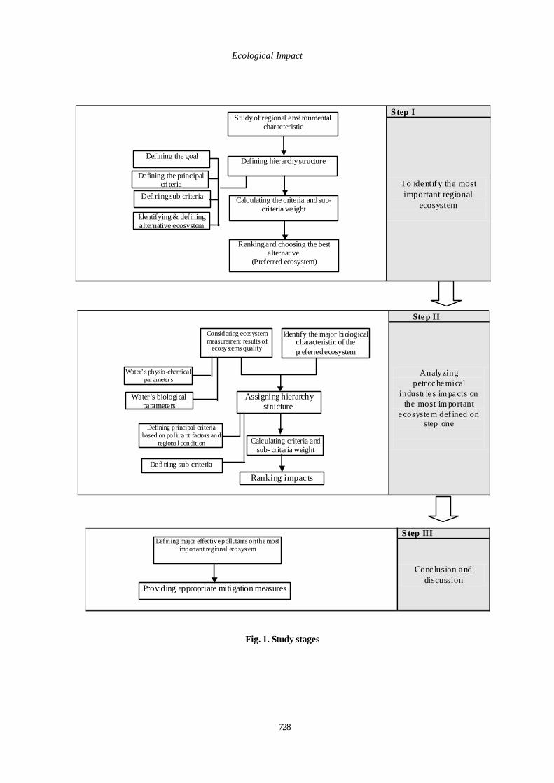
728
Study of regional environmentalcharacteristic
Defining hierarchy structure
Defining the principal cri teria
Defining sub criteria
Identifying & defining alternative ecosystem
Calculating the criteria and sub-cri teria weight
Ranking and choosing the best alternative
(Preferred ecosystem)
Identify the major biological characteristic of the preferred ecosystem
Considering ecosystem measurement results of
ecosystems quality
Water’s physio-chemical parameters
Water’s biological parameters
Assigning hierarchy structure
Calculating criteria and sub- criteria weight
Defining principal criteria based on polluta nt factors and
regiona l condition
Defining sub-criteria
Defining major effective pollutants on the most important regional ecosystem
Providing appropriate mitigation measures
Ranking impac ts
Defining the goal
Step I
To identify the most important regional
ecosystem
Ste p II
Analyzing petr oc he mical
industr ie s im pa cts on the most im portant
e cosyste m def ined on step one
Step III
Conc lusion and discussion
Fig. 1. Study stages
Ecological Impact

Int. J. Environ. Res., 4(4):725-734 , Autumn 2010
729
Determining most importantaffected environment bypetrochemical industries
Protectingvalue Ecological value Exposure
Vulnerabilitytowards petrochemi-
cal pollutants
Valuablespecies
Habitatdiversity
Speciesdiversity Intactness
Terrestrialec osystem Tidal zone Shade g an
wet landEstuaries
First level: objective
Second level: criteria
Third level: Sub criteria
Fourth level: alternatives(Ecosystems affected by petrochemical
industries)
Fig. 2. Hierarchy tree to identify most important affected ecosystem
Pollutants densityEcological value
COD Oil and grease
Determining the most important impacts on preferred ecosystem
Heavy metals
Impacts on bird diversity & density
Impacts on benthic diversity & density
Impacts on fish diversity & density
Impacts on aquatic vegetation diversity &
density
Jafari estuary Zangi estuary unconfined part
Impacts on living things
Impacts on non-living things
TSS
Level one: objective
Level two: criteria
Level three: sub- criteria
Level four: sub- criteria
Level five: alternatives, most important impacts
Most important water pollutants
Vulnerability
Za ngi estuary confined part Mousa estuary
Fig. 3. Hierarchy tree to identify most important impacts on preferred ecosystem
birds, benthic and aquatic bird’s likewise non-livingparameters (physio- chemical) such as salinity, sus-pended solid matters, temperature, and pH have beenweighted and measured (Fig. 3). In order to evaluatethe alternatives, different criteria should be ranked byconsidering weight for each criterion and sub- crite-rion, in this research to be able to distinguish moreimportant alternatives (environmental pollutants).These relative weights were only considered for the
purpose of ranking criterions using pair wise compari-son method. In this method more important criterion isbeing assigned between each couple and qualitativephrases. Pair wise comparison converts qualitativecomparison into quantitative weight for all factors(Asgharpur, 2006) (Table 1).Preference Matrix for eachlevel in relation to its upper level has been prepared inthis method. The first row and column contain param-eters of each level, then every parameter of each level

730
being compared to parameters of upper level throughpair wise comparison. If criteria in a row (i) are moreimportant than those of column (j), this importancewill be shown by integral number. On the other hand, ifcriteria of column (j) are more important than those ofrow (i) then this importance will be shown with frac-tional number (Villa and Mcleod, 2006) (Table 2).
Table 1. Preference qualitative for pair wisecomparison method (Ghodsipur, 2006)
Preferences Value )Extremely Preferred (9
)Very strongly Preferred (7 )Strongly Preferred( 5
)Moderately Preferred( 3 )Equally Preferred( 1
-2 ،4 ،6 ،8
Table 2. Preference matrix and pair wisecomparison of criteria in each level in relation to
upper level
jn j2 j1 1 i1
1 i2 1 in
In this method criteria weight (wi) are assigned in away to make hereunder relations accurate:a11 w1 + a12 w2 + … + a1n wn = λ.w1
a21 w1 + a22 w2 + … + a2n wn = λ.w2
an1 w1 + an2 w2 + … + ann wn = λ.wn
If an equation, in which, aij is criterion i preferenceto criterion j, and wi is criterion i weight and λ is invari-able figure. Then wi is calculated as below:
i= 1, 2,…, n Wi = 1/λn “ aij wj A. W = λ. WThis equation which is the same as pair wise compari-son matrix, it means, {A= [aij]}. W is weight vector andλ is a scalar figure (Roberts, et al., 2001; Ong, et al.,2001).
Determinant matrix (A- λ.I) is calculated for eachA matrix and been equaled to 0, thereof λ quantitiesresulted. The biggest λ applied to (A-λ max I) =0 andfinally, (Wi) has been computed for each criterion. Thewhole computing process done by Expert Choice soft-
ware. Final weight of each alternative is equal to totalproduct of criterion and alternative’s weight (Ghodsipur,2006).
Ecosystems prioritizing matrix in the study areaidentifies the biggest relative weight as the most im-portant affected ecosystem by petrochemical indus-tries activities and, petrochemical industries pollutantranking matrix each alternative with the biggest weightis considered having the most incompatible environ-mental impacts and requires more efficient mitigationmeasures.
RESULTS & DISCUSSIONAccording to the studies, pair wise comparison
on affected ecosystems in terms of ecological valueand protecting value, tidal zones and Shadegan wet-land, which both are protected and managed by de-partment of environment, acquired top grade.
It should be mentioned that, in ecosystems pairwise comparison matrix based on exposure and vul-nerability of the criteria towards petrochemical indus-tries pollutants, estuaries and their tidal zones arelocated not far from those industries. Therefore, ran-offs in site of petrochemical complex, especiallyTondguyan complex, and cooling towers blow downare discharged to the estuaries directly or through gath-ering channels in special zone. Moreover, waste wa-ters of all petrochemical industries are being dischargedto these aquatic ecosystems after being treated in thestudy area (Razavi, 2004). With respect to mentionedfactors, these areas are more affected by petrochemi-cal pollutants than other habitats in the study areaand they have bigger weight in the related matrix Ter-restrial ecosystems in the study area are restricted toplain habitats with a poor quality and have no signifi-cant fauna and flora diversity due to establishment ofpetrochemical industries in the region. Besides, thesoil is salty and alkaline and it’s not qualified to growtypes of vegetation. Thus, this habitat enjoys no pro-tecting value and considered as the last priority in ter-restrial ecosystem’s pair wise comparison matrixtowards other affected ecosystems, in terms of all ob-served criteria in hierarchy tree, it gained the lowestrelative weight.
In hierarchy tree, the most important environmen-tal impact on preferred ecosystem, ecologic value andvulnerability with same relative weight has been rankedas first priority and the most important ones amongthree considered principal criteria on second level. Thestate petrochemical complex is equipped with separatetreatment plant and measurement results show that,discharged materials from this waste treatment plantsto estuaries exceed standard limits in terms of dischargeto surface water (Table 3). Waste water produced by
Malmasi, S. et al.

731
Int. J. Environ. Res., 4(4):725-734 , Autumn 2010
other petrochemical complexes in Mahshahr is trans-ferred to Fajr utility complex to be treated; therefore,the criterion for amount of pollution caused by pollut-ant factors from this complex and the other ones in thestudy area, has the least portion of environment deg-radation in the region and gain lowest weight on pairwise comparison matrix.
Results from estuaries comparison in terms of eco-logical value, vulnerability and amount of pollutantfactors show that, Mousa estuary has highest eco-logical value and species density and diversity. Simi-larly, during investigation on Mousa estuary in 1999overall 12 groups of micro-benthos have been identi-fied and separated. Most frequently seen in percentare respectively 43.1% Amphipods, 41.6% Polychaeta,3.5% Copepods and 3.1% Tanaida. They are most fre-quently seen on April about 17707 and the least onOctober 2407 n/m2. 28 family of Polychaeta have beenidentified in this study (Nabavi 1999).
Natural water cycle and tide are partially disor-dered on Zangi and Jafari estuaries confined partsdue to being separated from nearby water. Addition-ally, results from these estuaries’s deposits and bedsampling indicate that, pollutants from petrochemi-cal industries discharged into them has impoverishedthe aquatic species into poor and very few number ofbenthic types.Density and diversity of micro benthosin Zangi estuary confined parts are intensely affectedby incoming pollutants, as biodiversity index is al-most 1 and average of micro benthos density is 254per m2 which mainly includes larva and insects on theedge of estuary. Confined estuary bed has almost noliving organism. Moreover results from researches
Table 3. Average of effluent treatment factors which are more than standards limits in studied complex(Shil Amayesh Consulting Engineers, 2006; Jafarzadeh, 2008; DOE, 1999) – mg/L
) mg/L( Density Physio- chemical
factors Speck No.2
Influent treatment Speck
Speck No.12
Speck No.13
Speck No.14
Standard limits of discharge to surface
waters
BOD 120 275 30
COD 486.23 537.06 406.86 192.26 60
Oil & Grease 32 10 TSS 856 760 290 40 NH4 3.3 4.4 2.5 Mg 132.48 100 pH 8.9 8.74 8.6 8.8 8.5-6.5 PO4 8.46 6 BOD: Biochemical Oxygen Demand, COD: Chemical Oxygen Demand, TSS: Total Suspended Solids
state that biodiversity and density of micro benthosincrease from confined towards unconfined areas inZangi estuary (Manuchehri, 2008). Thus, in relatedmatrix, confined parts of estuaries received lowestcredit in terms of ecological value. Pair wise compari-son based on vulnerability shows that Zangi estuaryas the closest one to the petrochemical complex, sub-ject to this study, is recognized as the most vulner-able one against petrochemical complex pollutants,while Mousa estuary’s main tributaries is less vul-nerable against petrochemical pollutants and is lessexposed to petrochemical pollutants in comparisonto other aquatic ecosystems.
Water quality measurements on confined and un-confined parts of Zangi and Jafari estuaries indicatethat the latter one is the most polluted estuary in thestudy area; moreover, confined parts are more pol-luted than unconfined waters (Table 4). Results fromwater quality sampling carried by Manuchehri, 2008on these estuaries showed that confined areas whichare closer to the Tondguyan petrochemical complexhas higher amount of COD and pH, therefore in estu-aries pollution comparative matrix, the biggest weightgoes to confined and unconfined parts of Jafari estu-ary and the lowest weight goes to Mousa estuary.
According to pair wise comparison matrix of aquat-ics density and biodiversity, major adverse impactscaused by water pollutants is on fishes and benthicand impacts on their density and diversity gained thefirst priority in this matrix. Impacts on aquatic bird andvegetation are considered as second priority. Final stepinvolves in comparing density average of water pol-lutants with standards of department of environment
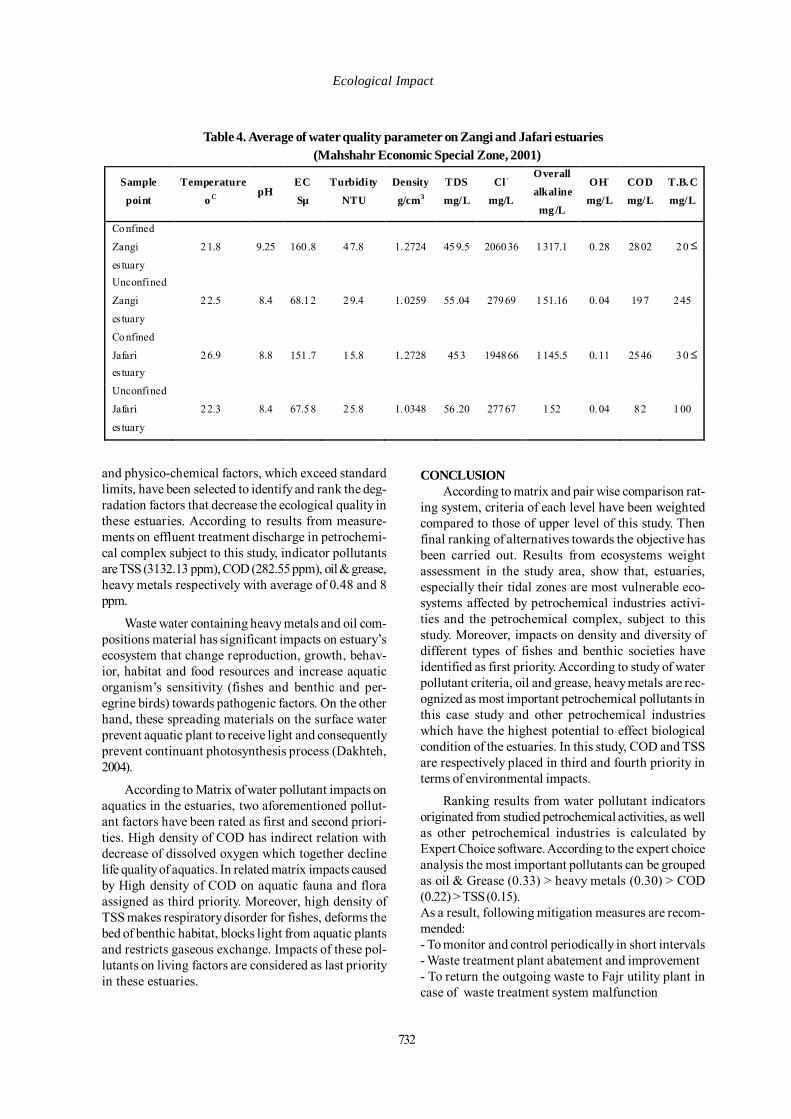
732
and physico-chemical factors, which exceed standardlimits, have been selected to identify and rank the deg-radation factors that decrease the ecological quality inthese estuaries. According to results from measure-ments on effluent treatment discharge in petrochemi-cal complex subject to this study, indicator pollutantsare TSS (3132.13 ppm), COD (282.55 ppm), oil & grease,heavy metals respectively with average of 0.48 and 8ppm.
Waste water containing heavy metals and oil com-positions material has significant impacts on estuary’secosystem that change reproduction, growth, behav-ior, habitat and food resources and increase aquaticorganism’s sensitivity (fishes and benthic and per-egrine birds) towards pathogenic factors. On the otherhand, these spreading materials on the surface waterprevent aquatic plant to receive light and consequentlyprevent continuant photosynthesis process (Dakhteh,2004).
According to Matrix of water pollutant impacts onaquatics in the estuaries, two aforementioned pollut-ant factors have been rated as first and second priori-ties. High density of COD has indirect relation withdecrease of dissolved oxygen which together declinelife quality of aquatics. In related matrix impacts causedby High density of COD on aquatic fauna and floraassigned as third priority. Moreover, high density ofTSS makes respiratory disorder for fishes, deforms thebed of benthic habitat, blocks light from aquatic plantsand restricts gaseous exchange. Impacts of these pol-lutants on living factors are considered as last priorityin these estuaries.
CONCLUSIONAccording to matrix and pair wise comparison rat-
ing system, criteria of each level have been weightedcompared to those of upper level of this study. Thenfinal ranking of alternatives towards the objective hasbeen carried out. Results from ecosystems weightassessment in the study area, show that, estuaries,especially their tidal zones are most vulnerable eco-systems affected by petrochemical industries activi-ties and the petrochemical complex, subject to thisstudy. Moreover, impacts on density and diversity ofdifferent types of fishes and benthic societies haveidentified as first priority. According to study of waterpollutant criteria, oil and grease, heavy metals are rec-ognized as most important petrochemical pollutants inthis case study and other petrochemical industrieswhich have the highest potential to effect biologicalcondition of the estuaries. In this study, COD and TSSare respectively placed in third and fourth priority interms of environmental impacts.
Ranking results from water pollutant indicatorsoriginated from studied petrochemical activities, as wellas other petrochemical industries is calculated byExpert Choice software. According to the expert choiceanalysis the most important pollutants can be groupedas oil & Grease (0.33) > heavy metals (0.30) > COD(0.22) > TSS (0.15).As a result, following mitigation measures are recom-mended:- To monitor and control periodically in short intervals- Waste treatment plant abatement and improvement- To return the outgoing waste to Fajr utility plant incase of waste treatment system malfunction
Table 4. Average of water quality parameter on Zangi and Jafari estuaries(Mahshahr Economic Special Zone, 2001)
Sample
point
Temperature
o C pH EC
Sµ Turbidity
NTU Density
g/cm3
TDS
mg/L Cl-
mg/L
Overall
alkaline
mg/L
OH-
mg/L COD
mg/L T.B.C
mg/L
Confined
Zangi
es tuary 21.8 9.25 160 .8 47.8 1.2724 459.5 206036 1317.1 0.28 2802 20
Unconfined
Zangi
es tuary 22.5 8.4 68.12 29.4 1.0259 55 .04 27969 151.16 0.04 197 245
Confined
Jafari es tuary
26.9 8.8 151 .7 15.8 1.2728 453 194866 1145.5 0.11 2546 30
Unconfined
Jafari
es tuary 22.3 8.4 67.58 25.8 1.0348 56 .20 27767 152 0.04 82 100
Ecological Impact
≤
≤

- To Predict pre-treatment system in petrochemicalcomplexes which produce waste with high load of pol-lution- Discharge no surface ran-offs, cooling towers blowdown in to the estuaries and direct them into the wastetreatment system.- To vacuum ran-offs effluent polluted by oily andgrease matters- To prevent disconnecting Zangi and Jafari confinedestuaries from nearby water
REFERENCESAsian development bank, (1997), Environmental im-pact assessment for developing countries in Asia.Asian development bank publications, 349-357.
Asgharpur, J. (2006). Multi-criteria decision making.Tehran University press, Tehran, Iran, 298-306.
Chatzimouratidis, A. I. and Pilavachi P. A. (2007). Ob-jective and subjective evaluation of power plants andtheir non-radioactive emissions using the analytic hi-erarchy process. Energy policy, 35 (8), 4027-4038.
Dakhteh, K. (2004). Heavy metals impacts on aquatics.Master’s Thesis, Faculty of Marine Sciences & andTechnology, IAU, Tehran, Iran, 105.
DOE, H. R. (1999). Environmental standards and regu-lations. Department of Environment, Tehran, Iran, 27.
Esmaeli Sari, A. (2002). Pollutants, Health and Stan-dard in environment, Tarbiat Modares University press,Tehran, Iran, 112-143.
Ghodsipur, S. H. (2006), Analytic Hierarchy Process,Amirkabir University press, Tehran, Iran, 14, 45-49, 152-172.
Ghodsipur, S. H. (2006). Multiple objective decisionmaking (MODM), Amirkabir University Press, Tehran,Iran, 16-18, 32-35.
Jafarzadeh, M. (2008). Petrochemical industries envi-ronmental portrait, NPC press, Tehran, Iran, pp.31, 125-144.
Jafarian, E. (2008). Survey on environmental impactsof PET- PTA petrochemical industries (Case Study:Mahshahr Economic Special Zone), Master’s Thesis,Graduate school of the environment and energy, Sci-ence and research campus, IAU, Tehran, Iran.
Mahshahr economic special zone. (2001). Study of eco-nomic special zone estuary improvement, Mahshahreconomic special zone press, Mahshahr, Iran, No.1,113-124.
Manuchehri, H. (2008). Mahshahr petrochemical ac-tivities ecological impact assessment on microbenthos density and diversity on Zangi estuary from
Mousa estuary tributaries located in Persian Gulf,fishery PHD Thesis, Graduate school of natural re-sources engineering, Science and research campus,IAU, Tehran, Iran.
Mazaheri, M. (2001). Correlation and focal study ofheavy metals in mousa estuary deposits and effectiveabsorbing and repelling factors, PHD thesis, Graduateschool of natural resources engineering, Science andresearch campus, IAU, Tehran, Iran, 57-61.
Monavari, S. M. (2001), Environmental impact assess-ment guidelines for petrochemical plants, DOE press,Tehran, Iran, pp. 6- 7.
Mostajabi, A. (2008). Analysis of environmental im-pact of petrochemical industries, From http://www.npc-rt.ir.
Nabavi, S. B. (2009). Study of Mahshahr estuary’smicro-benthos, Focusing on their role in terms of fish-ery aquatic nutrition, PHD thesis, Faculty of marinescience and technology, IAU, Tehran, Iran, pp.114-123.
Ong, S. K, Koh, T. H., Nee, A. Y. C. (2001). Assessingthe environmental impact of materials processing tech-niques using an analytical hierarchy process method.Journal of materials processing technology,113, 424-431.
Rafeenejad, E., (2007), Carelessness of petrochemicalindustries about mercury discharge to Persian Gulf,From http://www.farsnews.com.
Rajesh, S., Edwin, K. L. T. (2006). Toxic impact assess-ment of a manufacturing process: illustrative applica-tion to the automotive paint process. International Jour-nal of Environmental Studies, 63 (4), 453- 462.
Ramanathan, R. (2001). A note on the use of the ana-lytic hierarchy process for environmental impact, Int.J. environ. Manage., 63, 27-34.
Razavi, S. (2004). Tondguyan petrochemical complexprocesses, Tondguyan petrochemical complex publi-cation, 25-46.
Handfield, R., Walton, S. V., Sroufe, R., Melnyk, S. A.(2002). Applying environmental criteria to supplier as-sessment: A study in the application of the analytichierarchy process. European Journal of OperationalRes., 141, 71-81.
Rooney, P., (2005). Factors that influence the petro-chemical industry in the Middle East, From http://www.mees.com.
Saaty, T. L. (1994). Highlights and critical points in theapplication of the analytic hierarchy process, Euro. J.operational Res. 74, 426-447.
Int. J. Environ. Res., 4(4):725-734 , Autumn 2010
733
Samadyar, S. (2005). initiation of pollutants transmis-sion model of petrochemical plants in Persian Gulf,Master’s Thesis, Faculty of marine science and tech-nology, IAU, Tehran, Iran, 20, 114-127.
Shil Amayesh consulting engineers, (2006). Petrochemi-cal special economic zone, Environmental comprehen-sive plan, potential polluting areas report, Mahshahreconomic special zone press, No.2, 12-14, 23.
Solnes, J. (2003). Environmental quality of large indus-tries development alternatives using AHP. Environ.Impact Assess. Rev., 23, 283-303.
Villa, F., Mcleod, H. (2006). Environmental vulnerabil-ity indicators for environmental planning and decision-making guidelines and applications, Institute for eco-logical economics, University of Maryland press, USA,21-25.
Xiao-ping, J., Fang- yu, H., Xin-shun, T. (2004). Inte-grated environmental performance assessment ofchemical processes. Computers & chemical engineer-ing, 29, 243-247.
Malmasi, S. et al.
734

Int. J. Environ. Res., 4(4):735-740 , Autumn 2010ISSN: 1735-6865
Received 17 Aug. 2009; Revised 10 March 2010; Accepted 25 March 2010
*Corresponding author E-mail: [email protected]
735
Precipitation Chelation of Cyanide Complexes in ElectroplatingIndustry Wastewater
Naim, R. 1, 2*, Kisay , L .1, Park , J. 1, Qaisar, M .2, Zulfiqar, A . B. 2, Noshin, M . 2 and Jamil, K . 2
1 Department of Environmental Engineering and Biotechnology, Myongji University, Yongin,449-728, Korea
2 Department of Environmental Sciences, COMSATS Institute of Information TechnologyAbbottabad, Pakistan
ABSTRACT: Electroplating industry wastewater (EIW) characterized by high chemical oxygen demand(COD) is a big source of water and air contamination with heavy metals. The formation of cyanide complexwith heavy metals is responsible for its elevated COD. The concentration of heavy metals in EIW can beremoved by the use of different precipitating agents (sulfide and hydroxide). But the major bottleneck in theremoval of these metals is the presence of cyanide in EIW resulting in chelation with all the metals that aresoluble in water. The present work focused on, the treatment of EIW containing Cr, Ni, Zn and CN and theoptimization of dosage concentration which was reliable for the dissociation of cyanide complex for maximalremoval efficiency. We used hydroxide, sulfide and carbonate precipitation from different precipitating agents(NaOH, Ca (OH)2, CaCO3 Na2S5H2O, NaHS and NaHSO3). Sulfide precipitation was a viable option for thetreatment of EIW as compared to hydroxide and carbonate precipitation. Moreover, COD reduction capacityof sulfide precipitation was higher than others. It was also found that Ni and Cr made a complex with cyanidethat halted the removal efficiency while there was no evidence for Zn complexation; otherwise fragile complex-ation was evidenced.
Key words: Chelation precipitation, Cyanide complexes, Electroplating industry wastewater
INTRODUCTIONDischarges from electroplating industries are one
of the major concerns of the present world. The estab-lishment of electroplating industries is prohibited dueto their heavy metals and other toxic chemical emis-sions (Aziz et al., 2008). The effluent discharged fromthese industries can contaminate the water resulting intoxic effect to our health and ecosystem due to theirpotential of bioaccumulation (Yassi et al., 2001). Theeffluent waste water from the electroplating industriescontain chromium, cyanide, nickel, copper, zinc and lead(Aziz and Adlan,2008; XU and Ti-Xu, 2008; Jeon et al.,2001). In electrplating industry wastewater (EIW), cya-nide has a great affinity for heavy metals forming com-plexes with almost all the metals that are responsiblefor increase in COD of EIW. As cyanide causes breath-ing problems, neurotoxic effects, nerve damage evendeath (Dash et al., 2008). However, metal-cyanide com-plexes themselves are much less toxic than free cya-
nide. So, some preventive measures should be adoptedto get rid of its toxic and hazardous effects. Heavymetals can be removed from EIW by the process ofprecipitation and ion exchange resins (Mikhopadhyayand Sundquist., 2007; Jeon et al., 2001). But the majorproblem is again the removal or breakage of metal-cyanide complex as a function of solution pH (Dashand Balomajumder., 2008) agitation time, settling timeand precipitant dosage also (Feng et al., 2000). Themetal-cyanide complex can breakdown under alkalinepH.
The specific objective of the present study wasto test the suitability of precipitation chelation forheavy metals recovery from EIW using sulfide, hy-droxide and carbonate as precipitants.
MATERIAL & METHODSEIW was collected from an electroplating indus-
try named as “Myung-Sung 344-7 Wonchun-
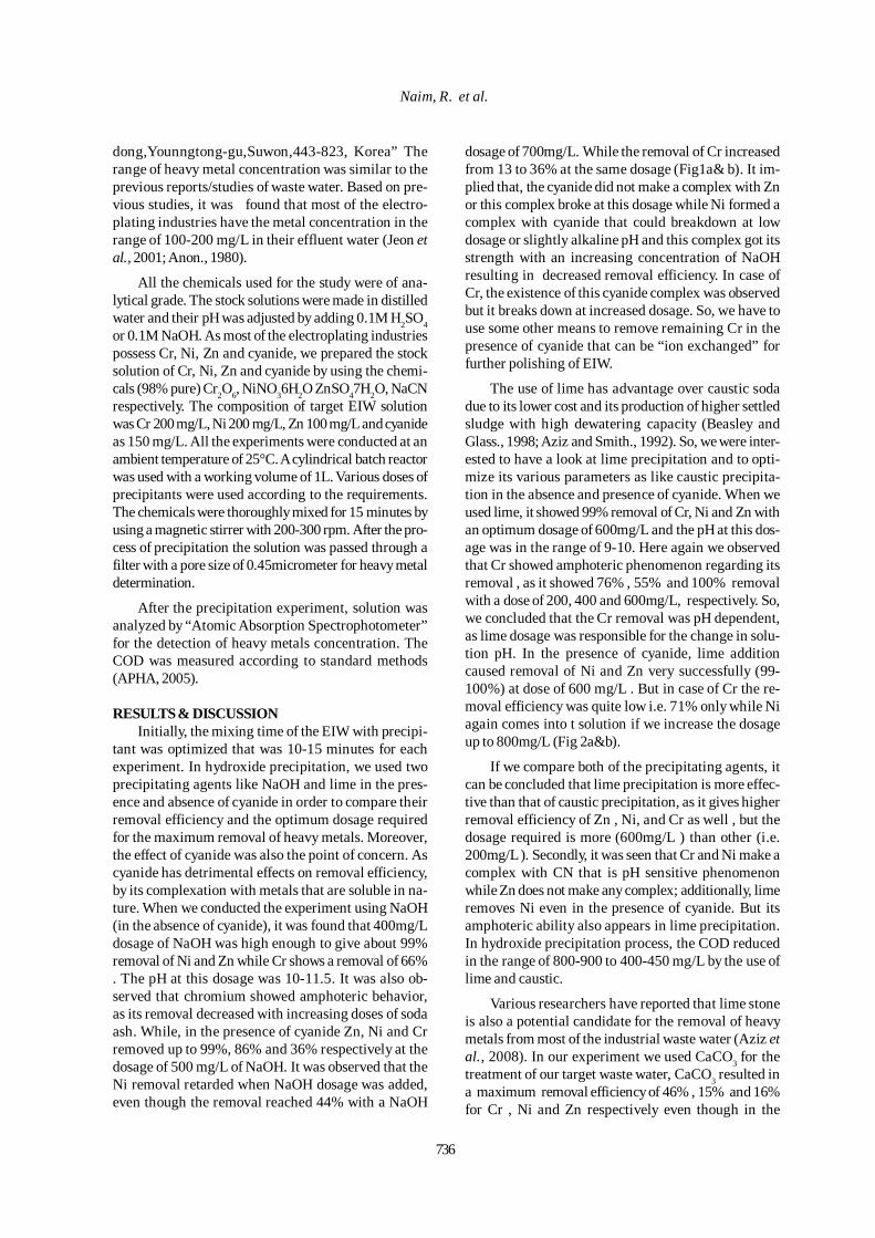
736
Naim, R. et al.
dong,Younngtong-gu,Suwon,443-823, Korea” Therange of heavy metal concentration was similar to theprevious reports/studies of waste water. Based on pre-vious studies, it was found that most of the electro-plating industries have the metal concentration in therange of 100-200 mg/L in their effluent water (Jeon etal., 2001; Anon., 1980).
All the chemicals used for the study were of ana-lytical grade. The stock solutions were made in distilledwater and their pH was adjusted by adding 0.1M H2SO4or 0.1M NaOH. As most of the electroplating industriespossess Cr, Ni, Zn and cyanide, we prepared the stocksolution of Cr, Ni, Zn and cyanide by using the chemi-cals (98% pure) Cr2O6, NiNO36H2O ZnSO47H2O, NaCNrespectively. The composition of target EIW solutionwas Cr 200 mg/L, Ni 200 mg/L, Zn 100 mg/L and cyanideas 150 mg/L. All the experiments were conducted at anambient temperature of 25°C. A cylindrical batch reactorwas used with a working volume of 1L. Various doses ofprecipitants were used according to the requirements.The chemicals were thoroughly mixed for 15 minutes byusing a magnetic stirrer with 200-300 rpm. After the pro-cess of precipitation the solution was passed through afilter with a pore size of 0.45micrometer for heavy metaldetermination.
After the precipitation experiment, solution wasanalyzed by “Atomic Absorption Spectrophotometer”for the detection of heavy metals concentration. TheCOD was measured according to standard methods(APHA, 2005).
RESULTS & DISCUSSIONInitially, the mixing time of the EIW with precipi-
tant was optimized that was 10-15 minutes for eachexperiment. In hydroxide precipitation, we used twoprecipitating agents like NaOH and lime in the pres-ence and absence of cyanide in order to compare theirremoval efficiency and the optimum dosage requiredfor the maximum removal of heavy metals. Moreover,the effect of cyanide was also the point of concern. Ascyanide has detrimental effects on removal efficiency,by its complexation with metals that are soluble in na-ture. When we conducted the experiment using NaOH(in the absence of cyanide), it was found that 400mg/Ldosage of NaOH was high enough to give about 99%removal of Ni and Zn while Cr shows a removal of 66%. The pH at this dosage was 10-11.5. It was also ob-served that chromium showed amphoteric behavior,as its removal decreased with increasing doses of sodaash. While, in the presence of cyanide Zn, Ni and Crremoved up to 99%, 86% and 36% respectively at thedosage of 500 mg/L of NaOH. It was observed that theNi removal retarded when NaOH dosage was added,even though the removal reached 44% with a NaOH
dosage of 700mg/L. While the removal of Cr increasedfrom 13 to 36% at the same dosage (Fig1a& b). It im-plied that, the cyanide did not make a complex with Znor this complex broke at this dosage while Ni formed acomplex with cyanide that could breakdown at lowdosage or slightly alkaline pH and this complex got itsstrength with an increasing concentration of NaOHresulting in decreased removal efficiency. In case ofCr, the existence of this cyanide complex was observedbut it breaks down at increased dosage. So, we have touse some other means to remove remaining Cr in thepresence of cyanide that can be “ion exchanged” forfurther polishing of EIW.
The use of lime has advantage over caustic sodadue to its lower cost and its production of higher settledsludge with high dewatering capacity (Beasley andGlass., 1998; Aziz and Smith., 1992). So, we were inter-ested to have a look at lime precipitation and to opti-mize its various parameters as like caustic precipita-tion in the absence and presence of cyanide. When weused lime, it showed 99% removal of Cr, Ni and Zn withan optimum dosage of 600mg/L and the pH at this dos-age was in the range of 9-10. Here again we observedthat Cr showed amphoteric phenomenon regarding itsremoval , as it showed 76% , 55% and 100% removalwith a dose of 200, 400 and 600mg/L, respectively. So,we concluded that the Cr removal was pH dependent,as lime dosage was responsible for the change in solu-tion pH. In the presence of cyanide, lime additioncaused removal of Ni and Zn very successfully (99-100%) at dose of 600 mg/L . But in case of Cr the re-moval efficiency was quite low i.e. 71% only while Niagain comes into t solution if we increase the dosageup to 800mg/L (Fig 2a&b).
If we compare both of the precipitating agents, itcan be concluded that lime precipitation is more effec-tive than that of caustic precipitation, as it gives higherremoval efficiency of Zn , Ni, and Cr as well , but thedosage required is more (600mg/L ) than other (i.e.200mg/L ). Secondly, it was seen that Cr and Ni make acomplex with CN that is pH sensitive phenomenonwhile Zn does not make any complex; additionally, limeremoves Ni even in the presence of cyanide. But itsamphoteric ability also appears in lime precipitation.In hydroxide precipitation process, the COD reducedin the range of 800-900 to 400-450 mg/L by the use oflime and caustic.
Various researchers have reported that lime stoneis also a potential candidate for the removal of heavymetals from most of the industrial waste water (Aziz etal., 2008). In our experiment we used CaCO3 for thetreatment of our target waste water, CaCO3 resulted ina maximum removal efficiency of 46% , 15% and 16%for Cr , Ni and Zn respectively even though in the
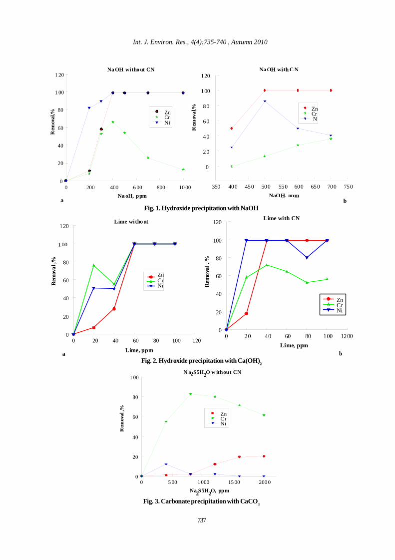
Int. J. Environ. Res., 4(4):735-740 , Autumn 2010
737
Na OH witho ut CN
Na oH, ppm 0 200 400 6 00 800 10 00
Rem
oval
,%
0
20
40
60
80
1 00
1 20
ZnCrNi
NaOH with C N
NaOH, ppm350 400 450 500 550 600 650 700 750
Rem
oval
,%
0
20
40
60
80
100
120
ZnCr N
a bFig. 1. Hydroxide precipitation with NaOH
Lime without
Lime, ppm
0 20 40 60 80 100 120
Rem
oval
,%
0
20
40
60
80
100
120
ZnCrNi
Lime with CN
Lime, ppm 0 20 40 60 80 100 1200
Rem
oval
, %
0
20
40
60
80
100
120
ZnCrNi
Fig. 2. Hydroxide precipitation with Ca(OH)2
a b
N a2S5H2O w ithout CN
Na2S5H2O, ppm0 5 00 1 000 15 00 200 0
Rem
oval
,%
0
20
40
60
80
1 00
ZnCrNi
Fig. 3. Carbonate precipitation with CaCO3
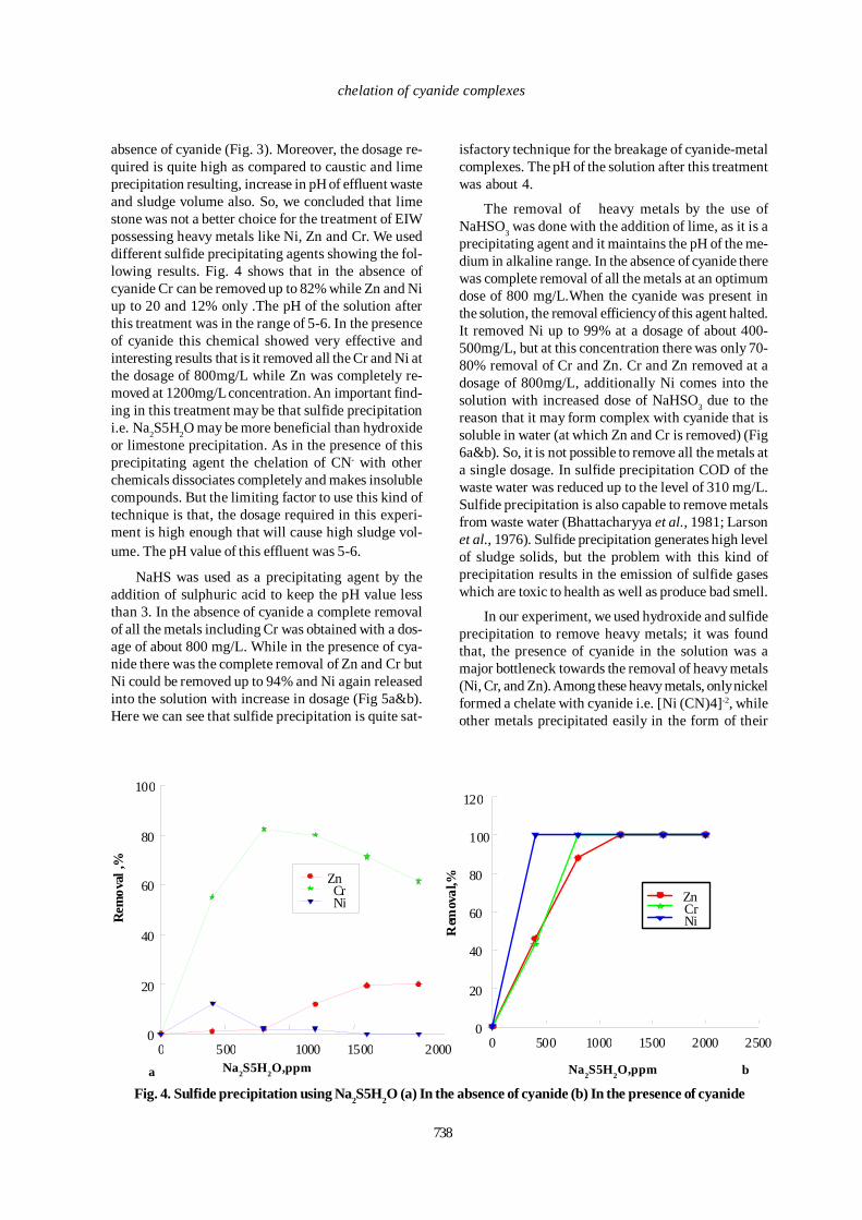
738
chelation of cyanide complexes
absence of cyanide (Fig. 3). Moreover, the dosage re-quired is quite high as compared to caustic and limeprecipitation resulting, increase in pH of effluent wasteand sludge volume also. So, we concluded that limestone was not a better choice for the treatment of EIWpossessing heavy metals like Ni, Zn and Cr. We useddifferent sulfide precipitating agents showing the fol-lowing results. Fig. 4 shows that in the absence ofcyanide Cr can be removed up to 82% while Zn and Niup to 20 and 12% only .The pH of the solution afterthis treatment was in the range of 5-6. In the presenceof cyanide this chemical showed very effective andinteresting results that is it removed all the Cr and Ni atthe dosage of 800mg/L while Zn was completely re-moved at 1200mg/L concentration. An important find-ing in this treatment may be that sulfide precipitationi.e. Na2S5H2O may be more beneficial than hydroxideor limestone precipitation. As in the presence of thisprecipitating agent the chelation of CN- with otherchemicals dissociates completely and makes insolublecompounds. But the limiting factor to use this kind oftechnique is that, the dosage required in this experi-ment is high enough that will cause high sludge vol-ume. The pH value of this effluent was 5-6.
NaHS was used as a precipitating agent by theaddition of sulphuric acid to keep the pH value lessthan 3. In the absence of cyanide a complete removalof all the metals including Cr was obtained with a dos-age of about 800 mg/L. While in the presence of cya-nide there was the complete removal of Zn and Cr butNi could be removed up to 94% and Ni again releasedinto the solution with increase in dosage (Fig 5a&b).Here we can see that sulfide precipitation is quite sat-
isfactory technique for the breakage of cyanide-metalcomplexes. The pH of the solution after this treatmentwas about 4.
The removal of heavy metals by the use ofNaHSO3 was done with the addition of lime, as it is aprecipitating agent and it maintains the pH of the me-dium in alkaline range. In the absence of cyanide therewas complete removal of all the metals at an optimumdose of 800 mg/L.When the cyanide was present inthe solution, the removal efficiency of this agent halted.It removed Ni up to 99% at a dosage of about 400-500mg/L, but at this concentration there was only 70-80% removal of Cr and Zn. Cr and Zn removed at adosage of 800mg/L, additionally Ni comes into thesolution with increased dose of NaHSO3 due to thereason that it may form complex with cyanide that issoluble in water (at which Zn and Cr is removed) (Fig6a&b). So, it is not possible to remove all the metals ata single dosage. In sulfide precipitation COD of thewaste water was reduced up to the level of 310 mg/L.Sulfide precipitation is also capable to remove metalsfrom waste water (Bhattacharyya et al., 1981; Larsonet al., 1976). Sulfide precipitation generates high levelof sludge solids, but the problem with this kind ofprecipitation results in the emission of sulfide gaseswhich are toxic to health as well as produce bad smell.
In our experiment, we used hydroxide and sulfideprecipitation to remove heavy metals; it was foundthat, the presence of cyanide in the solution was amajor bottleneck towards the removal of heavy metals(Ni, Cr, and Zn). Among these heavy metals, only nickelformed a chelate with cyanide i.e. [Ni (CN)4]-2, whileother metals precipitated easily in the form of their
0 500 1000 1500 2000
Rem
oval
,%
0
20
40
60
80
100
ZnCrNi
0 500 1000 1500 2000 2500
Rem
oval
,%
0
20
40
60
80
100
120
ZnCrNi
Fig. 4. Sulfide precipitation using Na2S5H2O (a) In the absence of cyanide (b) In the presence of cyanide
Na2S5H2O,ppm Na2S5H2O,ppma b

Int. J. Environ. Res., 4(4):735-740 , Autumn 2010
739
hydroxides or sulfides at certain pH value. Two mostcommon alkalis, caustic soda and lime were used forthe formation of insoluble hydroxides. Lime has ad-vantage over caustic soda of lower per unit cost forneutralizing capacity; further the settled sludge fromthe lime treatment was higher in solids content andmuch easy to dewater (Beasley et al., 1998). By the useof sulfide precipitation, a high level of metal insolubil-ity was achieved (Cheremisionoff, 1995) but it gener-ated large volume of sludge as compared to hydrox-ides. In our experiment, we optimized the conditions(dosage mg/L, pH, mixing time)for different precipitat-ing agent (hydroxide ,carbonate and sulfide) likeNaOH, Ca(OH)2 , Na2S , NaHS and NaHSO3.Calciumcarbonate is also an alternative and potential candi-
date for metal removal with low price and smaller sludgevolume but comparatively low removal efficiency (Fenget al., 2000; Anon., 1980). We compared the removalefficiency of each agent in the presence and absenceof cyanide with an optimal dosage value. It was found,that hydroxide precipitation was more convenient thansulfide precipitation, regarding its removal efficiencyand the effect of metal-cyanide complex as well.
CONCLUSIONThe EIW can be treated very efficiently by the use
of hydroxide and sulfide precipitation. In the absenceof cyanide there is no hurdle for the treatment, but inthe presence of cyanide there is the formation of metalchelate that is soluble in water. Ni and Cr are the metals
NaHS without CN
NaHS, ppm 0 50 1000 1500 2000
Rem
oval
,%
0
20
40
60
80
100
120
ZnNiCr
Fig. 5. Sulfide precipitation with NaHS
NaHS with CN
NaHS, ppm0 50 100 1500 2000
Rem
oval
,%0
20
40
60
80
100
120
ZnCrNi
0 500 1000 1500 2000
Rem
oval
,%
0
20
40
60
80
100
120
ZnCrNi
0 50 100 150 200
Rem
oval
,%
0
20
40
60
80
100
120
Zn CrNi
NaHSO3 ,ppm NaHSO3 ,ppm
Fig. 6. Sulfide precipitation with NaHSO3
a
a b
b
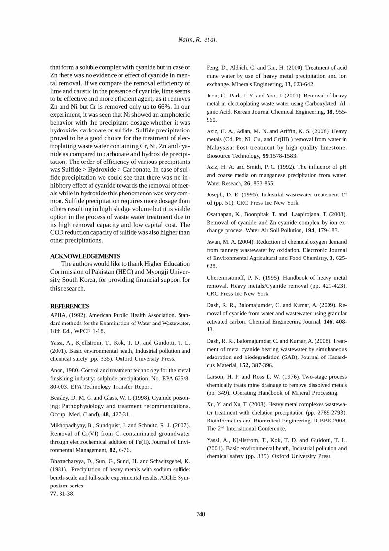
740
that form a soluble complex with cyanide but in case ofZn there was no evidence or effect of cyanide in men-tal removal. If we compare the removal efficiency oflime and caustic in the presence of cyanide, lime seemsto be effective and more efficient agent, as it removesZn and Ni but Cr is removed only up to 66%. In ourexperiment, it was seen that Ni showed an amphotericbehavior with the precipitant dosage whether it washydroxide, carbonate or sulfide. Sulfide precipitationproved to be a good choice for the treatment of elec-troplating waste water containing Cr, Ni, Zn and cya-nide as compared to carbonate and hydroxide precipi-tation. The order of efficiency of various precipitantswas Sulfide > Hydroxide > Carbonate. In case of sul-fide precipitation we could see that there was no in-hibitory effect of cyanide towards the removal of met-als while in hydroxide this phenomenon was very com-mon. Sulfide precipitation requires more dosage thanothers resulting in high sludge volume but it is viableoption in the process of waste water treatment due toits high removal capacity and low capital cost. TheCOD reduction capacity of sulfide was also higher thanother precipitations.
ACKNOWLEDGEMENTSThe authors would like to thank Higher Education
Commission of Pakistan (HEC) and Myongji Univer-sity, South Korea, for providing financial support forthis research.
REFERENCESAPHA, (1992). American Public Health Association. Stan-dard methods for the Examination of Water and Wastewater.18th Ed., WPCF, 1-18.
Yassi, A., Kjellstrom, T., Kok, T. D. and Guidotti, T. L.(2001). Basic environmental heath, Industrial pollution andchemical safety (pp. 335). Oxford University Press.
Anon, 1980. Control and treatment technology for the metalfinsishing industry: sulphide precipitation, No. EPA 625/8-80-003. EPA Technology Transfer Report.
Beasley, D. M. G. and Glass, W. I. (1998). Cyanide poison-ing; Pathophysiology and treatment recommendations.Occup. Med. (Lond), 48, 427-31.
Mikhopadhyay, B., Sundquist, J. and Schmitz, R. J. (2007).Removal of Cr(VI) from Cr-contaminated groundwaterthrough electrochemical addition of Fe(II). Journal of Envi-ronmental Management, 82, 6-76.
Bhattacharyya, D., Sun, G., Sund, H. and Schwitzgebel, K.(1981). Precipitation of heavy metals with sodium sulfide:bench-scale and full-scale experimental results. AIChE Sym-posium series,77, 31-38.
Feng, D., Aldrich, C. and Tan, H. (2000). Treatment of acidmine water by use of heavy metal precipitation and ionexchange. Minerals Engineering, 13, 623-642.
Jeon, C., Park, J. Y. and Yoo, J. (2001). Removal of heavymetal in electroplating waste water using Carboxylated Al-ginic Acid. Korean Journal Chemical Engineering, 18, 955-960.
Aziz, H. A., Adlan, M. N. and Ariffin, K. S. (2008). Heavymetals (Cd, Pb, Ni, Cu, and Cr(III) ) removal from water inMalaysisa: Post treatment by high quality limestone.Biosource Technology, 99.1578-1583.
Aziz, H. A. and Smith, P. G. (1992). The influence of pHand coarse media on manganese precipitation from water.Water Reseach, 26, 853-855.
Joseph, D. E. (1995). Industrial wastewater treatement 1st
ed (pp. 51). CRC Press Inc New York.
Osathapan, K., Boonpitak, T. and Laopirojana, T. (2008).Removal of cyanide and Zn-cyanide complex by ion-ex-change process. Water Air Soil Pollution, 194, 179-183.
Awan, M. A. (2004). Reduction of chemical oxygen demandfrom tannery wastewater by oxidation. Electronic Journalof Environmental Agricultural and Food Chemistry, 3, 625-628.
Cheremisionoff, P. N. (1995). Handbook of heavy metalremoval. Heavy metals/Cyanide removal (pp. 421-423).CRC Press Inc New York.
Dash, R. R., Balomajumder, C. and Kumar, A. (2009). Re-moval of cyanide from water and wastewater using granularactivated carbon. Chemical Engineering Journal, 146, 408-13.
Dash, R. R., Balomajumdar, C. and Kumar, A. (2008). Treat-ment of metal cyanide bearing wastewater by simultaneousadsorption and biodegradation (SAB), Journal of Hazard-ous Material, 152, 387-396.
Larson, H. P. and Ross L. W. (1976). Two-stage processchemically treats mine drainage to remove dissolved metals(pp. 349). Operating Handbook of Mineral Processing.
Xu, Y. and Xu, T. (2008). Heavy metal complexes wastewa-ter treatment with chelation precipitation (pp. 2789-2793).Bioinformatics and Biomedical Engineering. ICBBE 2008.The 2nd International Conference.
Yassi, A., Kjellstrom, T., Kok, T. D. and Guidotti, T. L.(2001). Basic environmental heath, Industrial pollution andchemical safety (pp. 335). Oxford University Press.
Naim, R. et al.

Int. J. Environ. Res., 4(4):741-750 , Autumn 2010ISSN: 1735-6865
Received 2 June 2009; Revised 10 March 2010; Accepted 25 July 2010
*Corresponding author E-mail:[email protected]
741
Efficiency of Landsat ETM+ Thermal Band for Land Cover Classification ofthe Biosphere Reserve “Eastern Carpathians” (Central Europe)
Using SMAP and ML Algorithms
Ehsani, A . H . 1* and Quiel, F. 2
1International Research Center for Living with Desert, University of Tehran, P.O. Box 14185-354Tehran, Iran
2Department of Civil and Architectural Engineering, Royal Institute of Technology (KTH), SE-100 44Stockholm, Sweden
ABSTRACT: Two different methods of Bayesian segmentation algorithm were used with different bandcombinations. Sequential Maximum a Posteriori (SMAP) is a Bayesian image segmentation algorithm whichunlike the traditional Maximum likelihood (ML) classification attempts to improve accuracy by taking contextualinformation into account, rather than classifying pixels separately. Landsat 7 ETM+ data with Path/Row 186-26, dated 30 September 2000 for a mountainous terrain at the Polish - Ukrainian border is acquired. In order tostudy the role of thermal band with these methods, two data sets with and without the thermal band were used.Nine band combinations including ETM+ and Principal Component (PC) data were selected based on thehighest value of Optimum Index Factor (OIF). Using visual and digital analysis, field observation data andauxiliary map data like CORINE land cover, 14 land cover classes are identified. Spectral signatures werederived for every land cover. Spectral signatures as well as feature space analysis were used for detailedanalysis of efficiency of the reflective and thermal bands. The result shows that SMAP as the superior methodcan improve Kappa values compared with ML algorithm for all band combinations with on average 17%.Using all 7 bands both SMAP and ML classifications algorithm achieved the highest Kappa accuracy of 80.37% and 64.36 % respectively. Eliminating the thermal band decreased the Kappa values by about 8% for bothalgorithms. The band combination including PC1, 2, 3, and 4 (PCA calculated for all 7 bands) produced thesame Kappa as bands 3, 4, 5 and 6. The Kappa value for band combination 3, 4, 5 and 6 was also about 4%higher than using 6 bands without the thermal band for both algorithms. Contextual classification algorithmlike SMAP can significantly improve classification results. The thermal band bears complementary informationto other spectral bands and despite the lower spatial resolution improves classification accuracy.
Key words: SMAP, Landsat ETM+, Thermal band, Maximum likelihood
INTRODUCTIONIn the recent years various remote sensing
techniques as well as geographical positioning systemshave been widely used (Alesheikh et al., 2007; Shobeiriet al., 2007; Cetin, 2009; Solaimani, et al., 2009;Pijanowski et al., 2009). Wide area coverage, timelydelivery, digital storage, low cost, repeatedlyinformation acquisition also in areas with limitedaccessibility is of the advantages of remote sensing.Land cover, i.e. the composition and characteristics ofland surface elements is a key information for manyscientific and policy purposes and for sustainablemanagement activities (Borak & Strahler, 1999; Chintanet al., 2004; Cihlar, 2001; Ouattara et al., 2004). Althoughland cove mapping is one of the earliest applications of
remote sensing but the effect of a thermal band onclassification accuracy and differentiation of landcover types still is not fully explored. The thermal bandLandsat 7, ETM+6 is measuring the reflected solarradiation of electromagnetic radiation from 10.40 to12.50 µm. Thermal sensors essentially measure thesurface temperature and emitted radiation of targetsbut reflective bands measures the spectral reflectanceof the surface at different wavelengths. Thus, TIRremote sensing data can significantly contribute tothe observation, measurement, and analysis of energybalance characteristics (i.e., the fluxes andredistribution of thermal energy within and across theland surface) as an implicit and important aspect oflandscape dynamics and landscape functioning (Dale

742
Ehsani A.H. and Quiel F.
& Jeffrey 1999). Thermal information is complementaryto visible and reflected infrared bands for theidentification of different land covers. For instanceDator et al. (1998) demonstrate the best way todifferentiate between gypsiferous and saline soils isto use the thermal band of Landsat TM in theclassification. Their result showed that using the TMthermal band, the gypsiferous soils can be mapped ina relatively fast and accurate way (Dator et al., 1998).Alavi panah et al. (2007) used remote sensing to studysoil salinity in the Ardakan area, Iran. They concludedthat the behavior of TM thermal and reflective TMbands is highly depended on the type of land cover. Inanother study they also showed that thermal band isunique in identification of surface materials andfeatures such as Yardangs in Lut desert (Alavi Panahet al., 2007). Since the source of thermal remote sensingis emitted energy from earth’s surface, the handlingand processing of thermal band is totally different fromreflective bands. The different processing steps dependon the application of thermal band. Using thermal andreflective information together in classificationalgorithms such as Maximum likelihood (ML) andSequential Maximum a Posteriori (SMAP) to increaseland cover classification accuracy is one of the aimsof this study. The other objective of this study iscomparing the accuracy of a contextual classifiers likeSequential Maximum a Posteriori (SMAP) with atraditional Maximum likelihood (ML) algorithm. Per-pixel ML classification is limited by only utilizingspectral information without considering texture andcontextual information (Dean & Smith, 2003; Gao et al.,2006; Pizzolato & Haertel, 2003; Zhou & Robson, 2001).Zhou and Robson (Zhou & Robson, 2001) claimed thattexture information is ultimately necessary to obtainaccurate image classification. Bouman and Shapiro(Bouman & Shapiro, 1994) also showed that withSMAP higher classification accuracy is achieved withML for SPOT images. McCauley and Engel (McCauley
et al., 1977) compared two spectral/spatial scenesegmentation algorithms (SMAP and ECHO, Extractionand Classification of homogenous Objects,) with ML.They found SMAP was better than ECHO and ML inall mean classification accuracies (McCauley et al.,1977). In this study increasing the Kappa accuracy bycombining the thermal and reflective information usingcontextual classifiers is the main purpose.
The study area is centered on the common borderpoint of Poland, Slovakia and Ukraine is locatedbetween 48° 52' N and 49° 25' N latitude, 21° 59' E and23° 1’ E longitude with a total area about 4543 Km2
(Fig. 1). It covers the biosphere reserve “EasternCarpathians” with the Bieszczady national park inPoland, Uzanski national park in Ukraine and Poloninynational park in Slovakia. Climatic conditions, differentpolitical and socioeconomic systems as well asecological conditions resulted in complex landscapeunits. Land covers include deciduous forest dominatedby beech (Fagus sylvatica) and sycamore (AcerPseudoplatanus) in the central part, mixed forestdominated by beech and fir (Abies Alba) in the centerand north eastern part, coniferous forest composed offir, Norway spruce (Picea abies) and Scots pin (pinusSylvestris) in Slovakia and Ukraine part (Kuemmerleet al., 2006) . Grassland is the dominant landscape inthe northwest, northeast and east. Arable lands aremostly found in the south west in Slovakia and in thenorth east in Ukraine.
MATERIALS & METHODSThe data set in this study consists of:
· Landsat ETM+ data path 186, row 26 dated 2000-09-30 (Fig.1) were acquired from the Global Land CoverFacility (GCLF) server at the University of Maryland,Institute for Advanced Computer Studies (UMIACS).GLCF provides free access to an integrated collectionof critical land cover and earth science data (http://glcf.umiacs.umd.edu).
Fig. 1. RGB color composite of Landsat 7, ETM+ bands 3, 2 and 1 of the study area at the border of Poland,Slovakia and Ukraine.
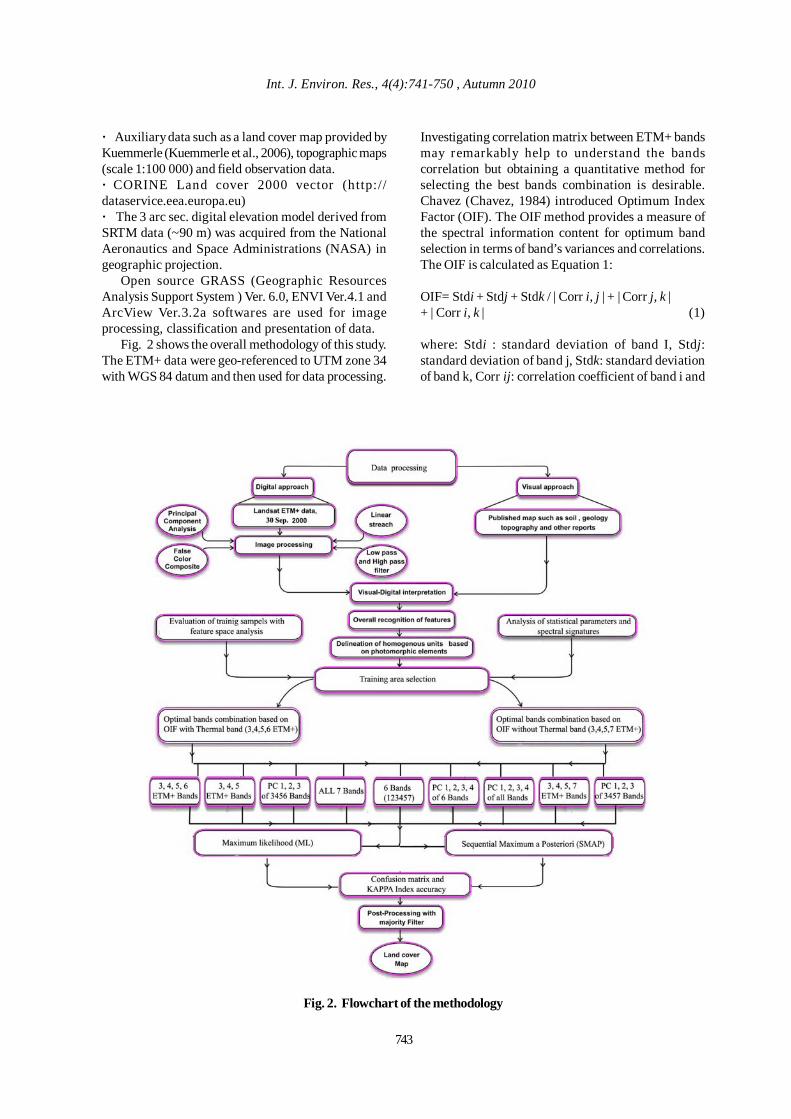
Int. J. Environ. Res., 4(4):741-750 , Autumn 2010
743
· Auxiliary data such as a land cover map provided byKuemmerle (Kuemmerle et al., 2006), topographic maps(scale 1:100 000) and field observation data.· CORINE Land cover 2000 vector (http://dataservice.eea.europa.eu)· The 3 arc sec. digital elevation model derived fromSRTM data (~90 m) was acquired from the NationalAeronautics and Space Administrations (NASA) ingeographic projection.
Open source GRASS (Geographic ResourcesAnalysis Support System ) Ver. 6.0, ENVI Ver.4.1 andArcView Ver.3.2a softwares are used for imageprocessing, classification and presentation of data.
Fig. 2 shows the overall methodology of this study.The ETM+ data were geo-referenced to UTM zone 34with WGS 84 datum and then used for data processing.
Fig. 2. Flowchart of the methodology
Investigating correlation matrix between ETM+ bandsmay remarkably help to understand the bandscorrelation but obtaining a quantitative method forselecting the best bands combination is desirable.Chavez (Chavez, 1984) introduced Optimum IndexFactor (OIF). The OIF method provides a measure ofthe spectral information content for optimum bandselection in terms of band’s variances and correlations.The OIF is calculated as Equation 1:
OIF= Stdi + Stdj + Stdk / | Corr i, j | + | Corr j, k |+ | Corr i, k | (1)
where: Stdi : standard deviation of band I, Stdj:standard deviation of band j, Stdk: standard deviationof band k, Corr ij: correlation coefficient of band i and
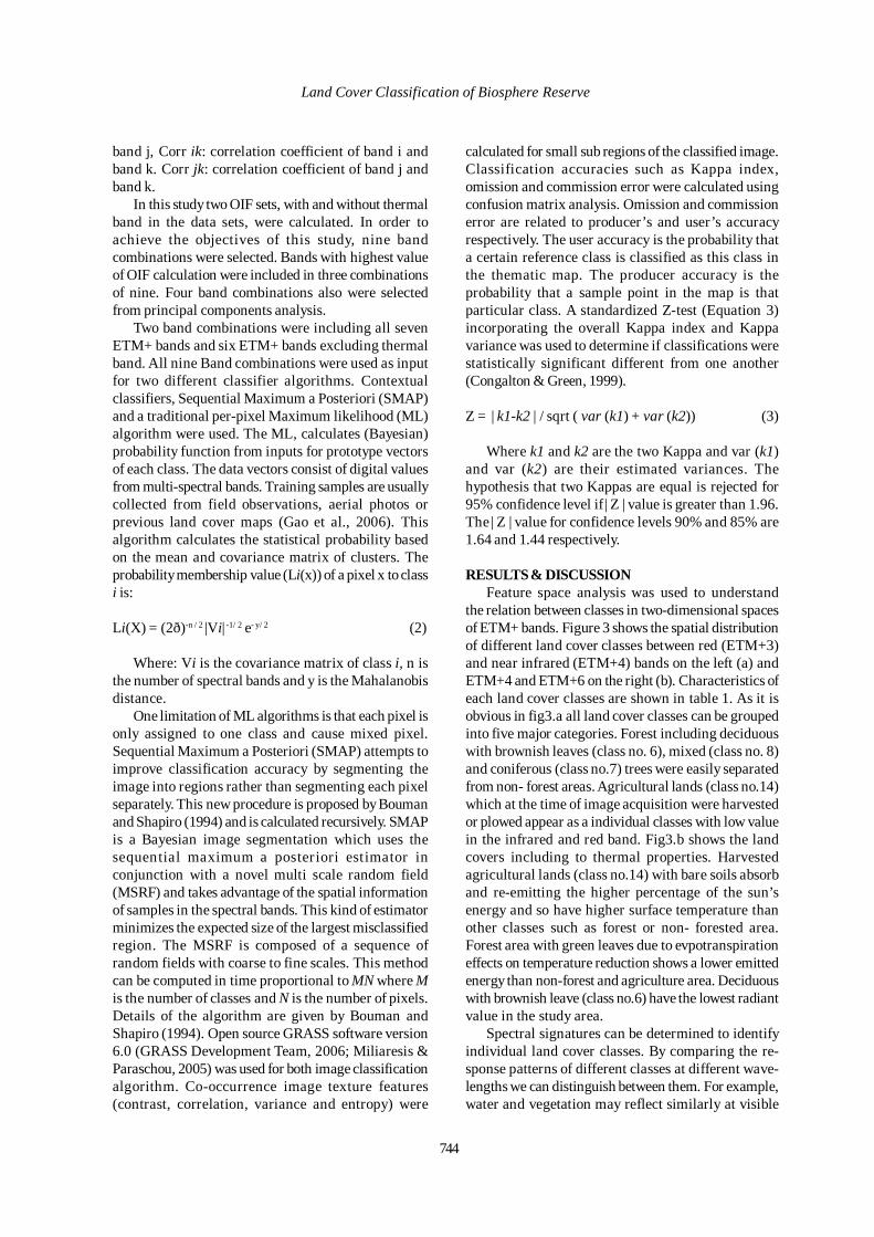
744
Land Cover Classification of Biosphere Reserve
band j, Corr ik: correlation coefficient of band i andband k. Corr jk: correlation coefficient of band j andband k.
In this study two OIF sets, with and without thermalband in the data sets, were calculated. In order toachieve the objectives of this study, nine bandcombinations were selected. Bands with highest valueof OIF calculation were included in three combinationsof nine. Four band combinations also were selectedfrom principal components analysis.
Two band combinations were including all sevenETM+ bands and six ETM+ bands excluding thermalband. All nine Band combinations were used as inputfor two different classifier algorithms. Contextualclassifiers, Sequential Maximum a Posteriori (SMAP)and a traditional per-pixel Maximum likelihood (ML)algorithm were used. The ML, calculates (Bayesian)probability function from inputs for prototype vectorsof each class. The data vectors consist of digital valuesfrom multi-spectral bands. Training samples are usuallycollected from field observations, aerial photos orprevious land cover maps (Gao et al., 2006). Thisalgorithm calculates the statistical probability basedon the mean and covariance matrix of clusters. Theprobability membership value (Li(x)) of a pixel x to classi is:
Li(X) = (2ð)-n / 2 |Vi| -1/ 2 e- y/ 2 (2)
Where: Vi is the covariance matrix of class i, n isthe number of spectral bands and y is the Mahalanobisdistance.
One limitation of ML algorithms is that each pixel isonly assigned to one class and cause mixed pixel.Sequential Maximum a Posteriori (SMAP) attempts toimprove classification accuracy by segmenting theimage into regions rather than segmenting each pixelseparately. This new procedure is proposed by Boumanand Shapiro (1994) and is calculated recursively. SMAPis a Bayesian image segmentation which uses thesequential maximum a posteriori estimator inconjunction with a novel multi scale random field(MSRF) and takes advantage of the spatial informationof samples in the spectral bands. This kind of estimatorminimizes the expected size of the largest misclassifiedregion. The MSRF is composed of a sequence ofrandom fields with coarse to fine scales. This methodcan be computed in time proportional to MN where Mis the number of classes and N is the number of pixels.Details of the algorithm are given by Bouman andShapiro (1994). Open source GRASS software version6.0 (GRASS Development Team, 2006; Miliaresis &Paraschou, 2005) was used for both image classificationalgorithm. Co-occurrence image texture features(contrast, correlation, variance and entropy) were
calculated for small sub regions of the classified image.Classification accuracies such as Kappa index,omission and commission error were calculated usingconfusion matrix analysis. Omission and commissionerror are related to producer’s and user’s accuracyrespectively. The user accuracy is the probability thata certain reference class is classified as this class inthe thematic map. The producer accuracy is theprobability that a sample point in the map is thatparticular class. A standardized Z-test (Equation 3)incorporating the overall Kappa index and Kappavariance was used to determine if classifications werestatistically significant different from one another(Congalton & Green, 1999).
Z = | k1-k2 | / sqrt ( var (k1) + var (k2)) (3)
Where k1 and k2 are the two Kappa and var (k1)and var (k2) are their estimated variances. Thehypothesis that two Kappas are equal is rejected for95% confidence level if | Z | value is greater than 1.96.The | Z | value for confidence levels 90% and 85% are1.64 and 1.44 respectively.
RESULTS & DISCUSSIONFeature space analysis was used to understand
the relation between classes in two-dimensional spacesof ETM+ bands. Figure 3 shows the spatial distributionof different land cover classes between red (ETM+3)and near infrared (ETM+4) bands on the left (a) andETM+4 and ETM+6 on the right (b). Characteristics ofeach land cover classes are shown in table 1. As it isobvious in fig3.a all land cover classes can be groupedinto five major categories. Forest including deciduouswith brownish leaves (class no. 6), mixed (class no. 8)and coniferous (class no.7) trees were easily separatedfrom non- forest areas. Agricultural lands (class no.14)which at the time of image acquisition were harvestedor plowed appear as a individual classes with low valuein the infrared and red band. Fig3.b shows the landcovers including to thermal properties. Harvestedagricultural lands (class no.14) with bare soils absorband re-emitting the higher percentage of the sun’senergy and so have higher surface temperature thanother classes such as forest or non- forested area.Forest area with green leaves due to evpotranspirationeffects on temperature reduction shows a lower emittedenergy than non-forest and agriculture area. Deciduouswith brownish leave (class no.6) have the lowest radiantvalue in the study area.
Spectral signatures can be determined to identifyindividual land cover classes. By comparing the re-sponse patterns of different classes at different wave-lengths we can distinguish between them. For example,water and vegetation may reflect similarly at visible

Int. J. Environ. Res., 4(4):741-750 , Autumn 2010
wavelengths but are almost always separable in theinfrared. Spectral response can be quite variable, evenfor the same target type, and can also vary with time(e.g. “green-ness” of leaves) and location. Knowingwhere to “look” spectrally and understanding the fac-tors which influence the spectral response of the fea-tures of interest are critical to correctly interpret theinteraction of electromagnetic radiation with the sur-face. Figure 4 shows the spectral signature of two wa-ter classes. Red and near infrared radiation is absorbedmore by water classes than shorter visible wavelengths.Class no. 12 includes the Solina reservoir in the Po-land and Starina reservoir in the Slovakia but class no.11 consist of streams, canals and rivers resulting inmixed pixels and higher values. Spectral signatures offour forest classes are shown in figure 5.
The internal structure of healthy leaves act asexcellent reflectors of near-infrared wavelengths. So
class no.13 (deciduous with green leaves) reflectsmore in all bands. Conversely, class no.7 (coniferousforest) which mainly covers the northeast of the studyarea has the lowest signature value in this group.Spectral signature of mixed forest (class no.8) is higherthan for coniferous forest but lower than deciduousforest.
Figure 6 indicates the spectral signatures of thenon-forest area. Class no.14 (agricultural lands)shows the different spectral response in all bands.This class tends to have reflection properties thatincrease approximately monotonically with wave-length. Due to factors such as the color, constituentsand especially the moisture content, this class tendsto have high reflectance in all bands. The class no.10which is transitional zone between shrubs and forestshows the spectral signatures similar to these twogroups.
Fig. 3. Distribution of the land covers classes in two-dimensional feature spaces.
0
20
40
60
80
100
120
ETM+1 ETM+2 ETM+3 ETM+4 ETM+5 ETM+6 ETM+7
Mea
n of
DN
val
ue
class 11class 12
Fig. 4. Spectral signatures of two water classes, class 11 (water courses) and, class 12 (water bodies).
745
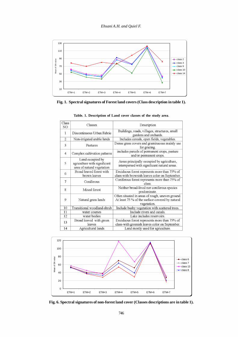
746
Ehsani A.H. and Quiel F.
10
30
50
70
90
110
130
ETM+1 ETM+2 ETM+3 ETM+4 ETM+5 ETM+6 ETM+7
Mea
n of
DN
val
ue class 2class 3class 9class 10class 14
Fig. 1. Spectral signatures of Forest land covers (Class description in table 1).
Table. 1. Description of Land cover classes of the study area.
0
20
40
60
80
100
120
ETM+1 ETM+2 ETM+3 ETM+4 ETM+5 ETM+6 ETM+7
Mea
n of
DN
valu
e
class 6class 7class 13class 8
Fig. 6. Spectral signatures of non-forest land cover (Classes descriptions are in table 1).
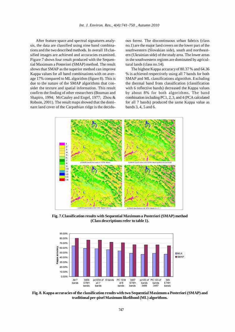
747
Int. J. Environ. Res., 4(4):741-750 , Autumn 2010
After feature space and spectral signatures analy-sis, the data are classified using nine band combina-tions and the two described methods. In overall 18 clas-sified images are achieved and accuracies examined.Figure 7 shows four result produced with the Sequen-tial Maximum a Posteriori (SMAP) method. The resultshows that SMAP as the superior method can improveKappa values for all band combinations with on aver-age 17% compared to ML algorithm (figure 8). This isdue to the nature of the SMAP algorithms that con-sider the texture and spatial information. This resultconfirm the finding of other researchers (Bouman andShapiro, 1994; McCauley and Engel, 1977; Zhou &Robson, 2001). The result maps showed that the domi-nant land cover of the Carpathian ridge is the decidu-
ous forest. The discontinuous urban fabrics (classno.1) are the major land covers on the lower part of thesouthwestern (Slovakian side), south and northeast-ern (Ukrainian side) of the study area. The lower areasin the southwestern regions are dominated by agricul-tural lands (class no.14).
The highest Kappa accuracy of 80.37 % and 64.36% is achieved respectively using all 7 bands for bothSMAP and ML classifications algorithm. Excludingthe thermal band from classification (classificationwith 6 reflective bands) decreased the Kappa valuesby about 8% for both algorithms. The bandcombination including PC1, 2, 3, and 4 (PCA calculatedfor all 7 bands) produced the same Kappa value asbands 3, 4, 5 and 6.
Fig. 7.Classification results with Sequential Maximum a Posteriori (SMAP) method(Class descriptions refer to table 1).
Fig. 8. Kappa accuracies of the classification results with two Sequential Maximum a Posteriori (SMAP) andtraditional per-pixel Maximum likelihood (ML) algorithms.
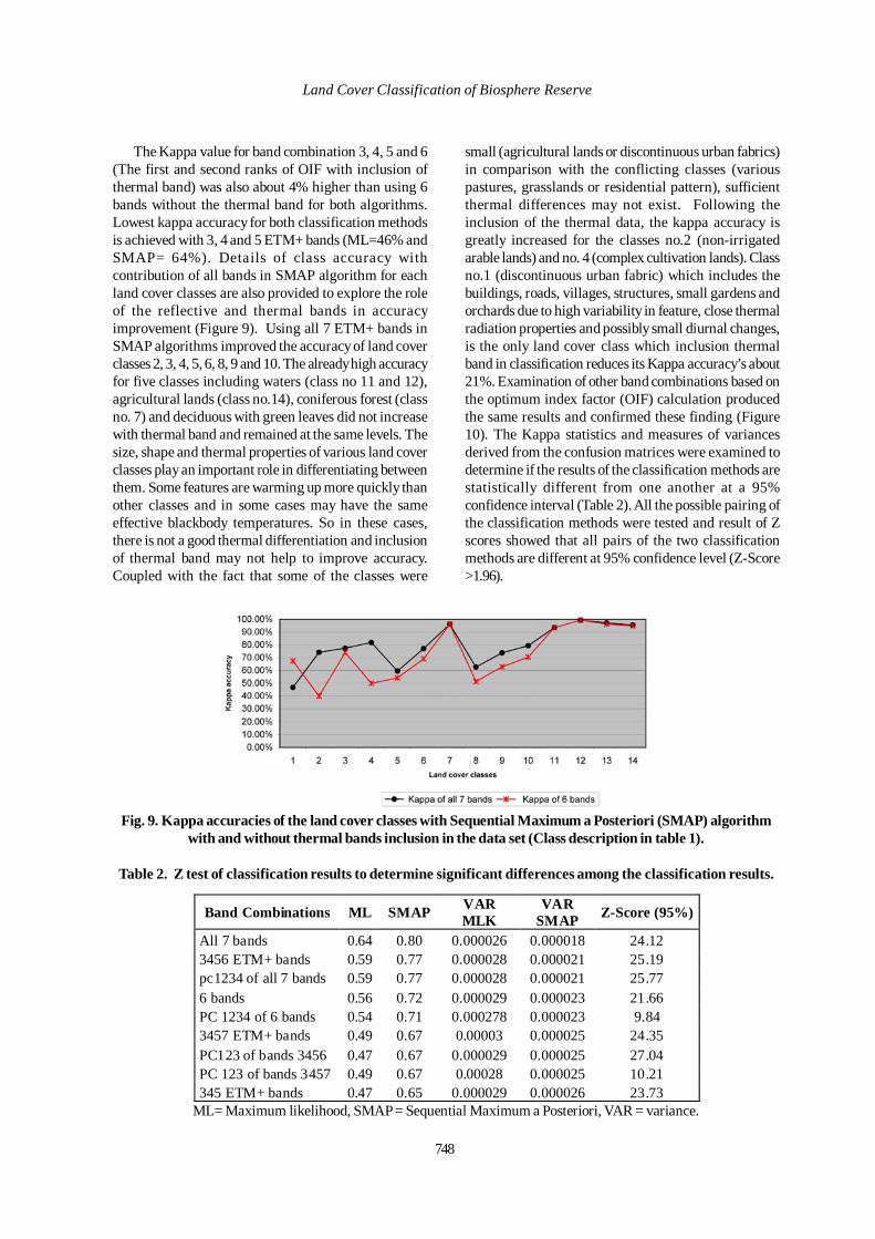
748
The Kappa value for band combination 3, 4, 5 and 6(The first and second ranks of OIF with inclusion ofthermal band) was also about 4% higher than using 6bands without the thermal band for both algorithms.Lowest kappa accuracy for both classification methodsis achieved with 3, 4 and 5 ETM+ bands (ML=46% andSMAP= 64%). Details of class accuracy withcontribution of all bands in SMAP algorithm for eachland cover classes are also provided to explore the roleof the reflective and thermal bands in accuracyimprovement (Figure 9). Using all 7 ETM+ bands inSMAP algorithms improved the accuracy of land coverclasses 2, 3, 4, 5, 6, 8, 9 and 10. The already high accuracyfor five classes including waters (class no 11 and 12),agricultural lands (class no.14), coniferous forest (classno. 7) and deciduous with green leaves did not increasewith thermal band and remained at the same levels. Thesize, shape and thermal properties of various land coverclasses play an important role in differentiating betweenthem. Some features are warming up more quickly thanother classes and in some cases may have the sameeffective blackbody temperatures. So in these cases,there is not a good thermal differentiation and inclusionof thermal band may not help to improve accuracy.Coupled with the fact that some of the classes were
small (agricultural lands or discontinuous urban fabrics)in comparison with the conflicting classes (variouspastures, grasslands or residential pattern), sufficientthermal differences may not exist. Following theinclusion of the thermal data, the kappa accuracy isgreatly increased for the classes no.2 (non-irrigatedarable lands) and no. 4 (complex cultivation lands). Classno.1 (discontinuous urban fabric) which includes thebuildings, roads, villages, structures, small gardens andorchards due to high variability in feature, close thermalradiation properties and possibly small diurnal changes,is the only land cover class which inclusion thermalband in classification reduces its Kappa accuracy’s about21%. Examination of other band combinations based onthe optimum index factor (OIF) calculation producedthe same results and confirmed these finding (Figure10). The Kappa statistics and measures of variancesderived from the confusion matrices were examined todetermine if the results of the classification methods arestatistically different from one another at a 95%confidence interval (Table 2). All the possible pairing ofthe classification methods were tested and result of Zscores showed that all pairs of the two classificationmethods are different at 95% confidence level (Z-Score>1.96).
Fig. 9. Kappa accuracies of the land cover classes with Sequential Maximum a Posteriori (SMAP) algorithmwith and without thermal bands inclusion in the data set (Class description in table 1).
Band Combinations ML SMAP VAR MLK
VAR SMAP Z-Score (95%)
All 7 bands 0.64 0.80 0.000026 0.000018 24.12 3456 ETM+ bands 0.59 0.77 0.000028 0.000021 25.19 pc1234 of all 7 bands 0.59 0.77 0.000028 0.000021 25.77 6 bands 0.56 0.72 0.000029 0.000023 21.66 PC 1234 of 6 bands 0.54 0.71 0.000278 0.000023 9.84 3457 ETM+ bands 0.49 0.67 0.00003 0.000025 24.35 PC123 of bands 3456 0.47 0.67 0.000029 0.000025 27.04 PC 123 of bands 3457 0.49 0.67 0.00028 0.000025 10.21 345 ETM+ bands 0.47 0.65 0.000029 0.000026 23.73
Table 2. Z test of classification results to determine significant differences among the classification results.
ML= Maximum likelihood, SMAP = Sequential Maximum a Posteriori, VAR = variance.
Land Cover Classification of Biosphere Reserve

Fig. 10. Kappa accuracies of the land cover classes with Sequential Maximum a Posteriori (SMAP) algorithmwith and without inclusion of the thermal band in the data set. These band combinations are selected based on
the OIF calculation with and without thermal bands inclusion. (Class description in table 1).
CONCLUSIONThe major obstacle for using remote sensing datafor land cover classification is the similarity some ofthe surface spectral characteristics under a widerange of environmental conditions. Combiningthermal and reflective information can help todifferentiate between similar classes. Thermal banddue to lower spatial resolution (60 meter in Landsat7) compared with reflective bands (30 meter) areexcluded from classification processing in moststudies. In this study we showed that the thermalband coupled with proper classification algorithmslike Sequential Maximum a Posteriori (SMAP)algorithm could significantly increase the kappaaccuracy for most of land cover classes. Thisindicates that the thermal data can aid in classifyingcertain land cover classes providing that there is agood thermal differentiation properties. Using firstand second ranks of the optimum index factor (OIF)calculation with inclusion of thermal band in dataset may provide the best bands combination forclassifications. Supplying thermal band in bandcombination in order to combine emitted andreflective information is necessary and may enhancethe accuracy. But some features are warming upmore quickly than other classes and in some casesmay reach the same effect ive blackbodytemperatures. Thus in these cases, due to closeradiation temperature, inclusion of thermal band maynot help to improve accuracy. Coupled with smallsize of some of the classes (agricultural lands ordiscontinues urban fabrics) in comparison with theconflicting classes (various pastures, grasslands orresidential pattern), sufficient thermal differencesmay not exist.
ACKNOWLEDGEMENTWe are grateful to Swedish Institute for funding alltravel expenses in the framework of the Visby program.We like to thank the University of Tehran, InternationalDesert Research Center and all our colleaguesespecially Docent Ivan Kruhlov, Department of PhysicalGeography, Ivan Franko University in Lvov, Ukraineand Dr. Mieczyslaw Sobik, Institute of Geography andRegional Development, University Wroclaw, Polandfor interesting discussions and for providing facilitiesand support.
REFERENCES
Alavi Panah, S. K., Komaki, C. B., Goorabi, A. and Matinfar,H. R. (2007). Characterizing Land Cover Types and SurfaceCondition of Yardang Region in Lut Desert (Iran) Basedupon Landsat Satellite Images. World Applied SciencesJournal, 2 (3), 212-228.
Alesheikh, A. A., Ghorbanali, A. and Nouri, N. (2007).Coastline change detection using remote sensing. Int. J.Environ. Sci. Tech., 4 (1), 61-66.
Borak, J. S. and Strahler, A. H. (1999). Feature selection andland cover classification of a MODIS-like data set for asemiarid environment. International Journal of RemoteSensing, 20, 919-938.
Bouman, C.A. and Shapiro, M. (1994). A MultiscaleRandom Field Model for Bayesian Image Segmentation. IEEETransaction on Image Processing, 3 (2), 162-177.
Cetin, M. (2009). A satellite based assessment of the impactof urban expansion around a lagoon. Int. J. Environ. Sci.Tech., 6 (4), 579-590.
Chavez, P. S., Guptill, S. C. and Bowell, J. A. (1984).Statistical method for selecting landsat MSS Ratios.Journal of Applied Photographic Engineering, 8, 23-30.
Int. J. Environ. Res., 4(4):741-750 , Autumn 2010
749

Chintan, A. S., Arora, M. K., and Pramod, K. V. (2004).Unsupervised classification of hyperspectral data: an ICAmixture model based approach International Journal ofRemote Sensing, 25, 481-487.
Cihlar, J. (2001). Land cover mapping of large areas fromsatellites: status and research priorities. International Journalof Remote Sensing, 21 (6,7), 1093-1114.
Congalton, R. G., and Green, K. (1999). Assessing theaccuracy of remotely sensed data: principles and practices.New York: Lewis publishers.
Dale, A.Q., and Jeffrey , C. L. (1999). Thermal infraredremote sensing for analysis of landscape ecological processes:methods and applications. Landscape Ecology., 14 (6), 577-598.
Dator, J., Goossens, R., and Van Ranst, E. (1998). The useof remote sensing to map gypsiferous soils in the IsmailiaProvince (Egypt). Geoderma, 87 (1), 47-56.
Dean, A. M., and Smith, G. M. (2003). An evaluation ofper-parcel land cover mapping using maximum likelihoodclass probabilities. International Journal of Remote Sensing,24, 2905-2920.
Gao, Y., Mas, J. F., Maathuis, B. H. P., Xiangmin, Z., andDijk, P. M. V. (2006). Comparison of pixel-based and object-oriented image classification approaches—a case study in acoal fire area, Wuda, Inner Mongolia, China. InternationalJournal of Remote Sensing, 27 (18), 4039-4055.
GRASS Development Team. (2006). Geographic ResourcesAnalysis Support System (GRASS), GNU General PublicLicense. Eletronic document. http://grass.itc.it.
Kuemmerle, T., Volker, C. R., Perzanowski, K., and Hostert,P. (2006). Cross-border comparison of land cover andlandscape pattern in Eastern Europe using a hybrid
classification technique. Remote Sensing of Environment,103, 449-464.
McCauley, J. F., Grolier, M. J., and Breed, C. S. (1977).Yardangs. In D.O. Doehring (Ed.), Geomorphology in AridRegions (pp. 233-269). London: Allen and Unwin.
Miliaresis, G. C., and Paraschou, C. V. E. (2005). Verticalaccuracy of the SRTM DTED level 1 of Crete. InternationalJournal of Applied Earth Observation and Geoinformation,7, 49-59.
Ouattara, T., Gwyn, Q. H. J., and Dubois, J. M. M. (2004).Evaluation of the runoff potential in high relief semi-aridregions using remote sensing data: application to Bolivia.International Journal of Remote Sensing, 25, 423-435.
Pijanowski, B.C., Tayyebi, A., Delavar, M. R. andYazdanpanah, M. J. (2009). Urban Expansion SimulationUsing Geospatial Information System and Artificial NeuralNetworks. Int. Journal. Environ. Res., 3 (4), 493-502.
Pizzolato, A. N., and Haertel, V. (2003). On the applicationof Gabor filtering in supervised image classification.International Journal of Remote Sensing, 24, 2167-2189.
Shobeiri, S. M. , Omidvar, B. and Prahallada, N. N. (2007).Digital Change Detection Using Remotely Sensed Data forMonitoring Green Space Destruction in Tabriz. Int. J.Environ. Res., 1 (1), 35-41.
Solaimani, K. and Modallaldoust, S. and Lotfi, S. (2009).Investigation of land use changes on soil erosion processusing geographical information system. Int. J. Environ. Sci.Tech., 6 (3), 415-424.
Zhou, Q., and Robson, M. (2001). Contextual informationis ultimately necessary if one is to obtain accurate imageclassifications. . International Journal of Remote Sensing,22, 3457-3470.
750

Int. J. Environ. Res., 4(4):751-758 , Autumn 2010ISSN: 1735-6865
Received 7 Sep. 2009; Revised 9 May 2010; Accepted 19 May 2010
*Corresponding author E-mail: [email protected]
751
Improving Competitive Advantage with Environmental Infrastructure Sharing:A Case Study of China-Singapore Suzhou Industrial Park
Yuan, Z., Zhang, L., Zhang, B., Huang, L., Bi, J.* and Liu, B.
State Key Laboratory of Pollution Control and Resource Reuse, School of the Environment, NanjingUniversity, Nanjing 210093, P. R. China
ABSTRACT: As one way to approach industrial symbiosis, environmental infrastructure sharing is principallyconcerned with providing an integrated environmental utility system for clustered firms. It is based on theassumption that environmental infrastructure sharing can improve the regional competitive advantage byreducing overall cost and improving environmental performance. In order to verify the assumption, theresearch examines the cost-effectiveness of wastewater treatment system of China-Singapore Suzhou IndustrialPark between the isolated model and sharing one. The results show that the sharing mode can greatly reduce theoverall cost and furthermore provide competitive advantage comparing to the isolated one. In addition, it alsoimproves the overall environmental performance and enforces the cooperation among clustered companies,which creates a good integrated image and attracts more and more excellent enterprises to join in.
Key words: industrial symbiosis, eco-industrial parks; cost-effectiveness, environmental management
INTRODUCTIONRecently, environmental management studies have
been taken into the consideration in lots of Asiancountries (Abbaspour et al., 2009; Khadka and Khanal,2008; Mohammadrezaie and Eskafi, 2007; Shobeiri etal., 2007; Chien and Shih, 2007). As one of the threeprincipal enterprise strategies, the overall costleadership plays an important role in the improvementof enterprise’s competitive advantage (Michael, 1980).Geographic proximity of different firms especially smalland medium-sized enterprises in a certain area, calledindustrial clusters (Heiner, 2005), will greatly reducethe costs of transaction, transportation, andcooperation with the conveniences of materialssourcing, service providing, pools of skilled labor hiring,and other similar advantages (Sturgeon, 2003; Masahisaand Paul, 2004). However, the clustering of manydifferent kinds of firms in a limited area inevitably bringsintensive pollutant emissions. It will be more seriousprovided inefficient environmental infrastructuresystem (Boland et al., 1997) and rather low resourceproductivity and eco-efficiency (Allenby, 2004).Conventionally, environmental engineeringtechnologies were used to decrease the pollutants withthe help of environmental infrastructure system.However, these end-of-pipe approaches alwaystransport pollutants from one place to another ortransform them from one kind to another. They do not
really clean or demolish the pollutants, and so are veryeasy to cause the pollution in a new form or placeagain. Furthermore, these approaches heavily rely onplentiful chemical materials inputs and huge energyconsumption, and so they are usually too costly tofunction continuously.
In order to improve resource productivity and preventpollutant discharges in a cheaper way, the concept ofutilizing one firm’s effluents as inputs of another cameinto being (Graedel and Allenby, 2004; Frosch andGallopoulos, 1989). It is called industrial symbiosis(IS) which principally concerned with the cyclical flowof resources through networks of business as a meansof cooperatively approaching ecologically sustainableindustrial activity (Chertow et al., 2005). IS has a moremeaningful definition comparing to industrial clusterbecause it includes not only the geographicalproximity but also the cooperative management ofresources and environment among the co-locatedfirms.
Based on empirical models, IS has three kinds oflinkages (symbiotic relationships) among differentfirms: a) products or service-related; b) by-productsexchanges; c) (environmental) infrastructure andservice sharing (YUAN and Bi, 2007). The a) addsenvironmental and resource utilization managementinto the concept of conventional supply chain (Adam
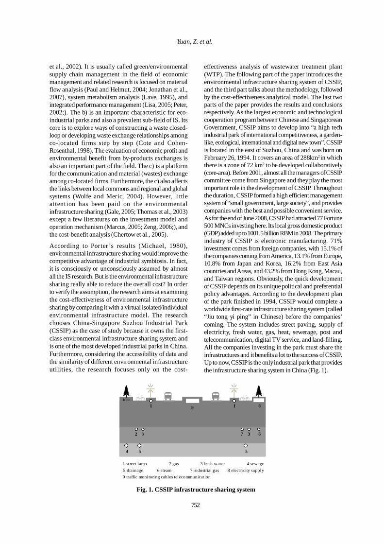
752
Yuan, Z. et al.
et al., 2002). It is usually called green/environmentalsupply chain management in the field of economicmanagement and related research is focused on materialflow analysis (Paul and Helmut, 2004; Jonathan et al.,2007), system metabolism analysis (Lave, 1995), andintegrated performance management (Lisa, 2005; Peter,2002;). The b) is an important characteristic for eco-industrial parks and also a prevalent sub-field of IS. Itscore is to explore ways of constructing a waste closed-loop or developing waste exchange relationships amongco-located firms step by step (Cote and Cohen-Rosenthal, 1998). The evaluation of economic profit andenvironmental benefit from by-products exchanges isalso an important part of the field. The c) is a platformfor the communication and material (wastes) exchangeamong co-located firms. Furthermore, the c) also affectsthe links between local commons and regional and globalsystems (Wolfe and Meric, 2004). However, littleattention has been paid on the environmentalinfrastructure sharing (Gale, 2005; Thomas et al., 2003)except a few literatures on the investment model andoperation mechanism (Marcus, 2005; Zeng, 2006;), andthe cost-benefit analysis (Chertow et al., 2005).
According to Porter ’s results (Michael, 1980),environmental infrastructure sharing would improve thecompetitive advantage of industrial symbiosis. In fact,it is consciously or unconsciously assumed by almostall the IS research. But is the environmental infrastructuresharing really able to reduce the overall cost? In orderto verify the assumption, the research aims at examiningthe cost-effectiveness of environmental infrastructuresharing by comparing it with a virtual isolated/individualenvironmental infrastructure model. The researchchooses China-Singapore Suzhou Industrial Park(CSSIP) as the case of study because it owns the first-class environmental infrastructure sharing system andis one of the most developed industrial parks in China.Furthermore, considering the accessibility of data andthe similarity of different environmental infrastructureutilities, the research focuses only on the cost-
effectiveness analysis of wastewater treatment plant(WTP). The following part of the paper introduces theenvironmental infrastructure sharing system of CSSIP,and the third part talks about the methodology, followedby the cost-effectiveness analytical model. The last twoparts of the paper provides the results and conclusionsrespectively. As the largest economic and technologicalcooperation program between Chinese and SingaporeanGovernment, CSSIP aims to develop into “a high techindustrial park of international competitiveness, a garden-like, ecological, international and digital new town”. CSSIPis located in the east of Suzhou, China and was born onFebruary 26, 1994. It covers an area of 288km2 in whichthere is a zone of 72 km2 to be developed collaboratively(core-area). Before 2001, almost all the managers of CSSIPcommittee come from Singapore and they play the mostimportant role in the development of CSSIP. Throughoutthe duration, CSSIP formed a high efficient managementsystem of “small government, large society”, and providescompanies with the best and possible convenient service.As for the end of June 2008, CSSIP had attracted 77 Fortune500 MNCs investing here. Its local gross domestic product(GDP) added up to 1001.5 billion RBM in 2008. The primaryindustry of CSSIP is electronic manufacturing. 71%investment comes from foreign companies, with 15.1% ofthe companies coming from America, 13.1% from Europe,10.8% from Japan and Korea, 16.2% from East Asiacountries and Areas, and 43.2% from Hong Kong, Macau,and Taiwan regions. Obviously, the quick developmentof CSSIP depends on its unique political and preferentialpolicy advantages. According to the development planof the park finished in 1994, CSSIP would complete aworldwide first-rate infrastructure sharing system (called“Jiu tong yi ping” in Chinese) before the companies’coming. The system includes street paving, supply ofelectricity, fresh water, gas, heat, sewerage, post andtelecommunication, digital TV service, and land-filling.All the companies investing in the park must share theinfrastructures and it benefits a lot to the success of CSSIP.Up to now, CSSIP is the only industrial park that providesthe infrastructure sharing system in China (Fig. 1).
1 street lamp 4 sewege5 drainage 8 electricity supply6 steam
1tree tree
19 8
2 3 7 3 6
54 5
2 gas 3 fresh water
9 traffic monitoring cables telecommunication7 industrial gas
Fig. 1. CSSIP infrastructure sharing system
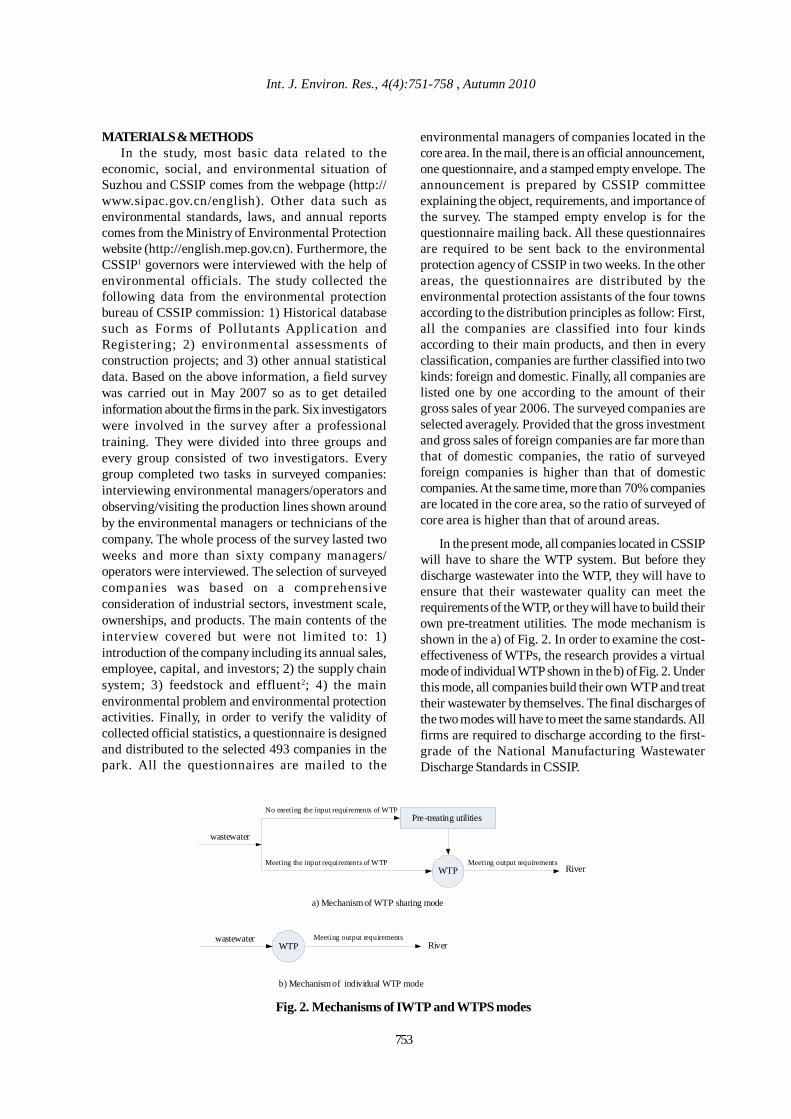
Int. J. Environ. Res., 4(4):751-758 , Autumn 2010
753
MATERIALS & METHODSIn the study, most basic data related to the
economic, social, and environmental situation ofSuzhou and CSSIP comes from the webpage (http://www.sipac.gov.cn/english). Other data such asenvironmental standards, laws, and annual reportscomes from the Ministry of Environmental Protectionwebsite (http://english.mep.gov.cn). Furthermore, theCSSIP1 governors were interviewed with the help ofenvironmental officials. The study collected thefollowing data from the environmental protectionbureau of CSSIP commission: 1) Historical databasesuch as Forms of Pollutants Application andRegistering; 2) environmental assessments ofconstruction projects; and 3) other annual statisticaldata. Based on the above information, a field surveywas carried out in May 2007 so as to get detailedinformation about the firms in the park. Six investigatorswere involved in the survey after a professionaltraining. They were divided into three groups andevery group consisted of two investigators. Everygroup completed two tasks in surveyed companies:interviewing environmental managers/operators andobserving/visiting the production lines shown aroundby the environmental managers or technicians of thecompany. The whole process of the survey lasted twoweeks and more than sixty company managers/operators were interviewed. The selection of surveyedcompanies was based on a comprehensiveconsideration of industrial sectors, investment scale,ownerships, and products. The main contents of theinterview covered but were not limited to: 1)introduction of the company including its annual sales,employee, capital, and investors; 2) the supply chainsystem; 3) feedstock and effluent2; 4) the mainenvironmental problem and environmental protectionactivities. Finally, in order to verify the validity ofcollected official statistics, a questionnaire is designedand distributed to the selected 493 companies in thepark. All the questionnaires are mailed to the
environmental managers of companies located in thecore area. In the mail, there is an official announcement,one questionnaire, and a stamped empty envelope. Theannouncement is prepared by CSSIP committeeexplaining the object, requirements, and importance ofthe survey. The stamped empty envelop is for thequestionnaire mailing back. All these questionnairesare required to be sent back to the environmentalprotection agency of CSSIP in two weeks. In the otherareas, the questionnaires are distributed by theenvironmental protection assistants of the four townsaccording to the distribution principles as follow: First,all the companies are classified into four kindsaccording to their main products, and then in everyclassification, companies are further classified into twokinds: foreign and domestic. Finally, all companies arelisted one by one according to the amount of theirgross sales of year 2006. The surveyed companies areselected averagely. Provided that the gross investmentand gross sales of foreign companies are far more thanthat of domestic companies, the ratio of surveyedforeign companies is higher than that of domesticcompanies. At the same time, more than 70% companiesare located in the core area, so the ratio of surveyed ofcore area is higher than that of around areas.
In the present mode, all companies located in CSSIPwill have to share the WTP system. But before theydischarge wastewater into the WTP, they will have toensure that their wastewater quality can meet therequirements of the WTP, or they will have to build theirown pre-treatment utilities. The mode mechanism isshown in the a) of Fig. 2. In order to examine the cost-effectiveness of WTPs, the research provides a virtualmode of individual WTP shown in the b) of Fig. 2. Underthis mode, all companies build their own WTP and treattheir wastewater by themselves. The final discharges ofthe two modes will have to meet the same standards. Allfirms are required to discharge according to the first-grade of the National Manufacturing WastewaterDischarge Standards in CSSIP.
WTP
Pre-treating utilities
wastewater
No meeting the input requirements of WTP
Meeting the input requirements of WTP Meeting output requirements
WTPwastewater
River
RiverMeeting output requirements
a) Mechanism of WTP sharing mode
b) Mechanism of individual WTP mode
Fig. 2. Mechanisms of IWTP and WTPS modes
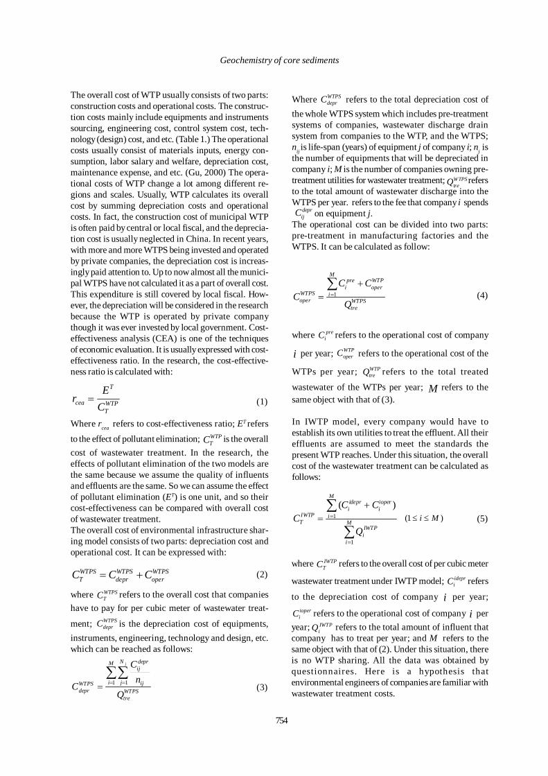
754
Geochemistry of core sediments
The overall cost of WTP usually consists of two parts:construction costs and operational costs. The construc-tion costs mainly include equipments and instrumentssourcing, engineering cost, control system cost, tech-nology (design) cost, and etc. (Table 1.) The operationalcosts usually consist of materials inputs, energy con-sumption, labor salary and welfare, depreciation cost,maintenance expense, and etc. (Gu, 2000) The opera-tional costs of WTP change a lot among different re-gions and scales. Usually, WTP calculates its overallcost by summing depreciation costs and operationalcosts. In fact, the construction cost of municipal WTPis often paid by central or local fiscal, and the deprecia-tion cost is usually neglected in China. In recent years,with more and more WTPS being invested and operatedby private companies, the depreciation cost is increas-ingly paid attention to. Up to now almost all the munici-pal WTPS have not calculated it as a part of overall cost.This expenditure is still covered by local fiscal. How-ever, the depreciation will be considered in the researchbecause the WTP is operated by private companythough it was ever invested by local government. Cost-effectiveness analysis (CEA) is one of the techniquesof economic evaluation. It is usually expressed with cost-effectiveness ratio. In the research, the cost-effective-ness ratio is calculated with:
WTPT
T
cea CE
r = (1)
Where rcea refers to cost-effectiveness ratio; ET refers
to the effect of pollutant elimination; WTPTC is the overall
cost of wastewater treatment. In the research, theeffects of pollutant elimination of the two models arethe same because we assume the quality of influentsand effluents are the same. So we can assume the effectof pollutant elimination (ET) is one unit, and so theircost-effectiveness can be compared with overall costof wastewater treatment.The overall cost of environmental infrastructure shar-ing model consists of two parts: depreciation cost andoperational cost. It can be expressed with:
(2)
where WTPSTC refers to the overall cost that companies
have to pay for per cubic meter of wastewater treat-
ment; WTPSdeprC is the depreciation cost of equipments,
instruments, engineering, technology and design, etc.which can be reached as follows:
(3)
WTPSoper
WTPSdepr
WTPST CCC +=
WTPStre
M
i
N
j ij
deprij
WTPSdepr Q
nC
C
j
∑∑= == 1 1
Where WTPSdeprC refers to the total depreciation cost of
the whole WTPS system which includes pre-treatmentsystems of companies, wastewater discharge drainsystem from companies to the WTP, and the WTPS;nij is life-span (years) of equipment j of company i; nj isthe number of equipments that will be depreciated incompany i; M is the number of companies owning pre-treatment utilities for wastewater treatment; refersto the total amount of wastewater discharge into theWTPS per year. refers to the fee that company i spends on equipment j.The operational cost can be divided into two parts:pre-treatment in manufacturing factories and theWTPS. It can be calculated as follow:
WTPStreQ
deprijC
WTPStre
WTPoper
M
i
prei
WTPSoper Q
CCC
+=∑=1 (4)
where preiC refers to the operational cost of company
i per year; WTPoperC refers to the operational cost of the
WTPs per year; WTPtreQ refers to the total treated
wastewater of the WTPs per year; M refers to thesame object with that of (3).
In IWTP model, every company would have toestablish its own utilities to treat the effluent. All theireffluents are assumed to meet the standards thepresent WTP reaches. Under this situation, the overallcost of the wastewater treatment can be calculated asfollows:
∑
∑
=
=
+= M
i
IWTPi
M
i
ioperi
idepri
IWTPT
Q
CCC
1
1
)( (5))1( Mi ≤≤
where IWTPTC refers to the overall cost of per cubic meter
wastewater treatment under IWTP model; idepriC refers
to the depreciation cost of company i per year;ioperiC refers to the operational cost of company i per
year; refers to the total amount of influent thatcompany has to treat per year; and M refers to thesame object with that of (2). Under this situation, thereis no WTP sharing. All the data was obtained byquestionnaires. Here is a hypothesis thatenvironmental engineers of companies are familiar withwastewater treatment costs.
IWTPiQ
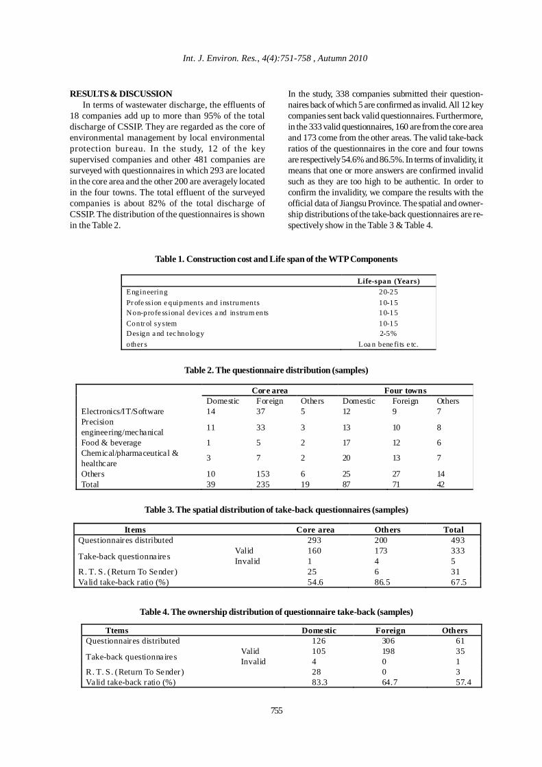
Int. J. Environ. Res., 4(4):751-758 , Autumn 2010
RESULTS & DISCUSSIONIn terms of wastewater discharge, the effluents of
18 companies add up to more than 95% of the totaldischarge of CSSIP. They are regarded as the core ofenvironmental management by local environmentalprotection bureau. In the study, 12 of the keysupervised companies and other 481 companies aresurveyed with questionnaires in which 293 are locatedin the core area and the other 200 are averagely locatedin the four towns. The total effluent of the surveyedcompanies is about 82% of the total discharge ofCSSIP. The distribution of the questionnaires is shownin the Table 2.
Life-span (Years) Engineering 20-25 Pr ofe ssion e quipments and instruments 10-15 Non-profe ssional devices a nd instrum ents 10-15 Contr ol system 10-15 Design a nd tec hnology 2-5% other s Loa n bene fits e tc.
Table 1. Construction cost and Life span of the WTP Components
Table 2. The questionnaire distribution (samples)
Core area Four towns Domestic Foreign Others Domestic Foreign Others
Electronics/IT/Software 14 37 5 12 9 7 Precision engineering/mechanical 11 33 3 13 10 8
Food & beverage 1 5 2 17 12 6 Chemical/pharmaceutical & healthcare
3 7 2 20 13 7
Others 10 153 6 25 27 14 Total 39 235 19 87 71 42
In the study, 338 companies submitted their question-naires back of which 5 are confirmed as invalid. All 12 keycompanies sent back valid questionnaires. Furthermore,in the 333 valid questionnaires, 160 are from the core areaand 173 come from the other areas. The valid take-backratios of the questionnaires in the core and four townsare respectively 54.6% and 86.5%. In terms of invalidity, itmeans that one or more answers are confirmed invalidsuch as they are too high to be authentic. In order toconfirm the invalidity, we compare the results with theofficial data of Jiangsu Province. The spatial and owner-ship distributions of the take-back questionnaires are re-spectively show in the Table 3 & Table 4.
Table 3. The spatial distribution of take-back questionnaires (samples)
Items Core area Others Total Questionnaires distributed 293 200 493
Valid 160 173 333 Take-back questionnaires Invalid 1 4 5 R. T. S. (Return To Sender) 25 6 31 Valid take-back ratio (%) 54.6 86.5 67.5
Table 4. The ownership distribution of questionnaire take-back (samples)
Ttems Domestic Foreign Others Questionnaires distributed 126 306 61
Valid 105 198 35 Take-back questionna ires Invalid 4 0 1 R. T. S . (Return To Sender) 28 0 3 Valid take-back ratio (%) 83.3 64.7 57.4
755
756
Yuan, Z. et al.
It is shown from table 3 that the take-back ratio ofquestionnaires in the core area is lower than that ofother areas. The results confirm the conclusions wegot from interviews that big foreign companies wereoften not inclined to cooperate with local governments.Usually, foreign companies have large-scaleinvestment and most of them are approved by highergovernments. So if they have no environmental issuesthey will decline the regular environmental monitoringor supervision by local EPB. Comparatively, small andmiddle foreign firms are more willing to cooperate withlocal government. Domestic companies usually have agood relationship with local government.
The table 3 also shows that ratio of invalidquestionnaires from domestic companies is higher thanthat of foreign companies. It may be because themanagers and engineers of foreign companies havemore professional knowledge than that of domesticcompanies. In addition, the environmental performanceof domestic companies is usually worse than that offoreign companies and so they are not willing todisclose their environmental information, especiallypollutant discharge information. Domestic companiesalways complain at their higher stress of environmentalprotection mainly caused by discriminate investmentpolicies between domestic and foreign companies(Wang et al., 2005).
In addition, other 31 mails are R. T. S. (Return ToSender) in the study. The return reasons can be dividedinto three kinds: (1) the enterprises had moved. In thelast few years, CSSIP began to force some heavypolluted companies move out of the park. For example,about 83 heavy polluted companies were forced toleave in 2002; (2) the enterprises registered in the parkare actually not located in the park. Some enterprisesestablished outside the park but enrolled in the parkso as to enjoy the preferential economic policies; (3)the enterprises had bankrupted. More and more fiercecompetitiveness force some enterprises bankrupt andmoved to invest in the Central and Western China,especially the small and middle ones.
According to the analysis, the overall wastewatertreatment cost under WTPS model varies between 0.0and 90.0 RMB per cubic meter wastewater. The averageoverall cost is 35.66 RMB per cubic meter wastewater.In the overall cost, the depreciation cost is 31.2% andthe operational cost is 68.8%. With regards todepreciation cost, equipments and instruments is 42%,engineering depreciation is 40%, technology/designis 6%, and the other is 12%. In terms of operationalcost, 45.4% is from power consumption, 32.4% is frommaterials inputs, 18.2% from salary and welfare, and4.2 from others.
Under IWTP model, the average overall cost ofwastewater treatment is 5,542 RMB per cubic meterwastewater. In the overall cost, the depreciation costis 33% and the operational cost counts 67%. In thedepreciation cost, 49% is from equipments andinstruments, 45% is from engineering, 2.8% is fromtechnology/design, and the left is 3.2%. In theoperational cost, power consumption is 43%, materialsinputs is 32%, salary and welfare is 21%, and others is4%.
The results show that the wastewater treatmentcost is 5,542 RMB per cubic meter wastewater underIWTP model. It is much higher than that under theWTPS model (35.66 RMB per cubic meter wastewater).The big difference is probably caused by: (1) underthe IWTP model, every company would have to buildits own WTP. It would greatly improves theconstruction cost and furthermore cause an increaseof depreciation expense. (2) Under the IWTP model,every company would have to employ its ownenvironmental engineers and operators to operatingits WTP. It would greatly increase the operation cost.(3) Under the IWTP model, more land would have tobe needed for WTPs and it would increasecontinuously if the number of companies keepsgrowing.
Considering the same environmental effects of thetwo models, the cost-effectiveness ratio (effect/cost)of the WTPS is about 167 times as that of IWTP. Thatis to say, in terms of wastewater treatment, WTPS modelis more cost-effectiveness than IWTP one. It can bothgreatly reduce the overall cost of wastewater treatmentand improve the environmental performance. Basedon the analysis of above, the governments should makepolicies to encourage the WTPS model rather than theIWTP one.
With economic development of CSSIP, more andmore companies will invest in the park which wouldreduce the overall cost due to the scale-enlarging.Furthermore, according to development plan, more andmore people will live in the park and manufacturingenterprises will be restricted. Consequently, thesewage will greatly increase and the overall cost oftreatment will subsequently decrease.
Of course, in terms of the methodology maybe somepeople will question the veracity of the model. Afterall, it comes from questionnaires rather than the factualexpenditures. At the same time, the overall cost ofvirtual model will increase the uncertainty. In fact, it isever questioned in ref (Rebecca et al, 2004; Matleena,2006; Qiu et al., 2003). However, the study aims tocompare the relative cost-effectiveness of the twomodels rather than calculate the absolute value. In order
757
Int. J. Environ. Res., 4(4):751-758 , Autumn 2010
to confirm the validity, we ever compared the result tothe statistics from six provinces of Eastern China andfound that it was very similar.
In fact, companies not only spend money onpretreatment and treatment service, but also paypollutant discharge fee (PDF) to the local governmentin China. Even if the discharge of companies meets therequirements of WTP, they will have to pay the PDF. Iftheir discharge cannot meet the requirements,companies will have to pay more PDF according tohow much pollutants they discharge. That is to say,the overall cost calculations of the two models arelower than that of the factual cost in practice. But it hassimilar effects on variations of overall cost of the twomodels. Of course, there are some problems in the WTPSmodel. For example, if the WTP stops or runs abnormallydue to some unexpected reasons, all the wastewaterwould have to be discharged directly. So in practice, allWTPS have to establish their own accident pools tostore the unexpected discharge. That would increasethe overall cost and plays a greater effect on the IWTPmodel than the WTPS model. However, it would beeasier to deal with the accidence under the IWTP modelbecause the amount of discharge under the IWTP modelis usually less than that of the WTPS model.
Anyway, it is at least an effective way for pollutioncontrol with regards to economic cost in China. Theresults also explains the fact that why China encouragesthe development of WTPS model.
All the analysis of above is based on an assumptionthat all companies abide by the environmental law. Thatis to say, all companies do not deliberately dischargetheir wastewater without any treatment. But at present,most industrial parks have not established their ownWTPS in China. So it is still a rather commonphenomenon for companies to illicitly dischargewastewater without any treatment in China, especiallyin Central and Western China. Under this situation, theoverall cost of the IWTP model maybe less than that ofthe WTPS model. But this decrease of overall cost isbased on the increase of pollutant discharge. It willinevitably cause the environmental pollution. Underthe WTPS model, the environmental violation will beavoided effectively because all companies are usuallyforbidden to discharge directly. Their limber holes areforce to connect with waste pipe system before theyput into production.
CONCLUSIONAs an effective and inexpensive way to approach
industrial symbiosis, environmental infrastructuresharing is becoming more and more popular all overthe world. The study carries out a case study in CSSIPto verify the cost-effectiveness of environmental
infrastructure sharing vs. conventional mode. Theresearch calculates the overall cost of wastewatertreatment paid by companies under WTPS model andIWTP model. The results show that under WTPSmodel, the overall cost in 2006 is 2.34 billion RMB interms of wastewater treatment. It would be 364.1billion RMB if it runs under IWTP model. The overallcost of wastewater treatment under WTPS model isonly about 0.6 percent of that under IWTP model.The resul ts show that the environmentalinfrastructure sharing can improve competitiveadvantage effectively.
ACKNOWLEGEMENTThe research was financially supported by Natural
Science Foundation of China (40971302 and 40501027),the Eleventh Five-year Key Technology R&D Program(2006BAC02A15), the China Ministry of Science andTechnology (MOST) National Research InitiativeGrants Program for State Key Laboratories. Thisresearch benefits a lot from the officials of CSSIPcommittee, especially the deans of environmentalprotection bureau: Xiaojun Jiang and Xuejun Wang.All of their work and support are highly appreciated.In addition, the author would like to thank theanonymous reviews for their comments andsuggestions.
REFERENCESAbbaspour, M., Lotfi, F. Hosseinzadeh, Karbassi, A.R.,Roayaei, E. and Nikoomaram, H. (2009). Development ofthe Group Malmquist Productivity Index on non-discretionary Factors. Int. J. Environ. Res., 3(1), 109-116.
Adam, C. F., Richard, C. L., Paul, D. C. and Frances, E. B.(2002). Analyzing, Mapping, and Managing EnvironmentalImpacts along Supply Chain. J. Industrial Ecology, 5(2),13-36.
Allenby, B. (2004). Clean Production in Context: AnInformation Infrastructure Perspective. J. CleanerProduction, 12, 833-839.
Boland, J . J ., Bell, M. E., Stakhiv, E. E. (1997).Environmental Infrastructure Management. Netherlands:the Kluwer Academic Publisher.
Chertow, M. R. and Rachel, D. (2005). Lombardi.Quantifying Economic and Environmental Benefits of Co-located Firms. Environmental Science & Technology, 39(17), 6535-6541.
Chien, M. K. and Shih, L. H. (2007). An empirical study ofthe implementation of green supply chain managementpractices in the electrical and electronic industry and theirrelation to organizational performances. Int. J. Environ. Sci.Tech., 4(3), 383-394.
Cote, R. and Cohen-Rosenthal, E. (1998). Designing Eco-industrial Parks: A Synthesis of Some Experiences. Journalof Cleaner Production, 6 (3-4), 181-188.
758
Geochemistry of core sediments
Frosch, R. A., Gallopoulos, N. (1989). Strategies forManufacturing. Scientific American, 261 (3), 144-152.
Gale, A. B. (2005). A Method for Measuring the EfficiencyGap between Average and Best Practice Energy Use. Journalof Industrial Ecology, 9 (3), 51-65.
Graedel, T. and Allenby, B. (2004). Industrial Ecology.Englewood Cliffs, NJ: Prentice Hall, USA.
Gu, X. C. (2000). The New Stage of Utilizing Foreign Fundsand Policy Adjustment. Business Economics andAdministration, 10, 6-9.
Heiner, D. (2005). Exporting the German Model: theEstablishment of a New Automobile Industry Cluster inShanghai. Economic Geography, 81 (1), 53-81.
Jonathan, N., Alex D. C. and Heather L. M. (2007). EconomicInput-output Life-cycle Assessment of Trade betweenCanada and United States. Environmental Science &Technology, 41 (5), 1523-1532.
Khadka, R. B. and Khanal, A. B. (2008). EnvironmentalManagement Plan (EMP) for Melamchi WaterSupplyProject, Nepal. Int. J. Environ. Res., 2(1), 87-96.
Lave, L., Cobas, E., Hendrickson, C. and McMichael, F. C.(1995). Using Input-Output Analysis to Estimate Economy-Wide Discharges. Environmental Science & Technology, 29(9), 420-426.
Lisa, H. (2005). Toward Sustainable Management ofNational Parks in Japan: Securing Local Community andStake Holder Participation. Environmental Management, 35(6), 753-764.
Marcus, C. R. (2005). Economic Assessment of MunicipalWaste Management Systems - Case Studies Using aCombination of Life Cycle Assessment and Life CycleCosting, Journal of Cleaner Production, 13, 253-263.
Masahisa, F., and Paul, K. (2004). The New EconomicGeography: Past, Present and the Future. Regional Science,83 (1), 139-164
Matleena, K. (2006). Users and Non-users of ConservationAreas: Are There Differences in WTP, Motives and theValidity of Responses in CVM Surveys? EcologicalEconomics, 59, 530-539.
Michael, E. P. (1980). Competitive Strategy. New York: theFree Press, USA.
Mohammadrezaie, Sh. and Eskafi, F. (2007). EnvironmentalPerformance Evaluation (EPE) of Iran Khodro Co. (IKCO).Int. J. Environ. Res., 1(1), 49-57.
Paul, H. B. (2004). Helmut R. Practical Handbook ofMaterial Flow Analysis. New York, CRC Press LLC.
Peter, L. D. (2002). Approaches for Quantifying theMetabolism of Physical Economies: A Comparative Survey.Journal of Industrial Ecology, 6 (1), 65-88.
Peter, S., Martha, P. and David, S. (2002). The Dynamics ofIndustrial Clustering: International Comparisons inComputing and Biotechnology. Oxford: Oxford UniversityPress, USA.
Ning, Q., Zhao, W., Yue, Y., Chunsheng, Z. and Yuqian, S.(2003). Overall costs Calculation of Wastewater TreatmentPlant. China Water & Wastewater, 19 (2), 97-98.
Rebecca, A. E., Joseph, P. N. and Glenn, W. S. (2004). AFramework for Net Environmental Benefit Analysis forRemediation or Restoration of Contaminated Sites.Environmental Management, 34 (3), 315-330.
Shobeiri, S. M. , Omidvar, B. and Prahallada, N. N. (2007).A Comperative Study of Environmental Awareness amongSecondary School Students in Iran and India. Int. J. Environ.Res., 1(1), 28-34.
Sturgeon, T. J. (2003). What Really Goes on in SiliconValley: Spatial Clustering and Dispersal in ModularProduction Networks? Economic Geography, 3 (3), 199-225.
Thomas, D., Elinor, O. and Paul, C. S. (2003). The Struggleto Govern the Commons. Science, 302 (12), 1907-1912.
Wang, C. M., Wang, L. P. and Li, Y. J. (2005). Study on theEnvironmental Infrastructure under market mechanism inChina: Case study of Sewage and Remains Utilities. JiangsuEnvironmental Science and Technology, 18 (4), 60-63.
Wolfe, D. and Meric, G. (2004). Clusters from the Insideand Out: Local Dynamics and Global Linkages. UrbanStudies, 41 (5/6), 1071-1093.
Yuan, Z. W. and Bi, J. (2007). Evolution Mechanism of Eco-Industrial Symbiosis Network and Its Analytical Framework.ACTA Ecological Sinica, 27 (8), 1-7.
Zeng, X. G. (2006). Governance under Market-basedMechanism of Environmental Infrastructure. ChinaEnvironmental Protection Industry, 4, 10-13.
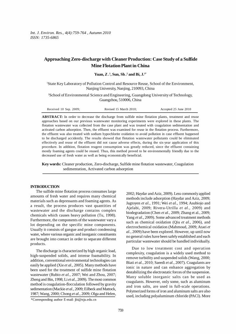
Int. J. Environ. Res., 4(4):759-764 , Autumn 2010ISSN: 1735-6865
Received 10 Sep. 2009; Revised 15 March 2010; Accepted 25 June 2010
*Corresponding author E-mail: [email protected]
759
Approaching Zero-discharge with Cleaner Production: Case Study of a SulfideMine Flotation Plant in China
Yuan, Z .1, Sun, Sh .2 and Bi, J.1*
1State Key Laboratory of Pollution Control and Resource Reuse, School of the Environment,Nanjing University, Nanjing, 210093, China
2School of Environmental Science and Engineering, Guangdong University of Technology,Guangzhou, 510006, China
ABSTRACT: In order to decrease the discharge from sulfide mine flotation plants, treatment and reuseapproaches based on our previous wastewater monitoring experiments were explored in these plants. Theflotation wastewater was collected from the case plant and was treated with coagulation sedimentation andactivated carbon adsorption. Then, the effluent was examined for reuse in the flotation process. Furthermore,the effluent was also treated with sodium hypochlorite oxidation to avoid pollution in case effluent happenedto be discharged accidently. The results showed that flotation wastewater pollutants could be eliminatedeffectively and reuse of the effluent did not cause adverse effects, during the six-year application of thisprocedure. In addition, flotation reagent consumption was greatly reduced, since the effluent containingmostly foaming agents could be reused. Thus, this method proved to be environmentally friendly due to thedecreased use of fresh water as well as being economically beneficial.
Key words: Cleaner production, Zero-discharge, Sulfide mine flotation wastewater, Coagulation sedimentation, Activated carbon adsorption
INTRODUCTIONThe sulfide mine flotation process consumes large
amounts of fresh water and requires many chemicalmaterials such as depressants and foaming agents. Asa result, the process produces vast quantities ofwastewater and the discharge contains complexchemicals which causes heavy pollution (Tu, 1998).Furthermore, the components of the wastewater vary alot depending on the specific mine components.Usually it consists of gangue and product condensingwater, where various organic and inorganic constituentsare brought into contact in order to separate differentproducts.
The discharge is characterized by high organic load,high-suspended solids, and intense foamability. Inaddition, conventional environmental technologies caneasily be applied (Xie et al., 2005). Many methods havebeen used for the treatment of sulfide mine flotationwastewater (Rubio et al., 2007; Wei and Zhou, 2007;Zheng and Bin, 1998; Li et al., 2009). The most commonmethod is coagulation-flocculation followed by gravitysedimentation (Mackie et al., 2009; Eilbeck and Mattock,1987; Wang, 2000; Chong et al., 2009; Olga and Helen,
2002; Haydar and Aziz, 2009). Less commonly appliedmethods include adsorption (Haydar and Aziz, 2009;Jagtoyen et al., 1991; Wei et al., 1994; Asubiojo andAjelabi, 2009; Rivera-Utrilla et al., 2009) andbiodegradation (Chen et al., 2009; Zhang et al., 2009;Yang et al., 2009). Some advanced treatment methodssuch as chemical oxidation (Qiu et al., 2006), andelectrochemical oxidation (Mahmoud, 2009; Ataei etal., 2009) have been explored. However, up until nowno general rules have been safely established and eachparticular wastewater should be handled individually.
Due to low treatment cost and operationcomplexity, coagulation is a widely used method toremove turbidity and suspended solids (Wang, 2000;Biati et al., 2010; Saeedi et al., 2007). Coagulants areionic in nature and can enhance aggregation bydestabilizing the electrostatic forces of the suspension.Many soluble inorganic salts can be used ascoagulants. However, only some, such as aluminumand iron salts, are used in full-scale operations.Polymerized forms of iron and aluminum salts are alsoused, including polyaluminum chloride (PACl). More
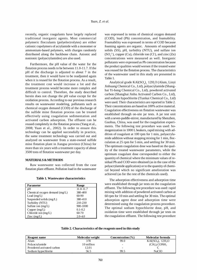
760
Yuan, Z. et al.
recently, organic coagulants have largely replacedtraditional inorganic agents. Most commercialpolymeric flocculants (polyelectrolytes) are eithercationic copolymers of acrylamide with a monomer orammonium-based polymers, with charges randomlydistributed along the backbone chain. Anionic andnonionic (polyacrylamides) are also used.
Furthermore, the pH value of the water for theflotation process needs to be between 11.0-11.7. If thepH of the discharge is adjusted to about 7 in thetreatment, then it would have to be readjusted againwhen it is reused for the flotation process. As a result,the treatment cost would increase a lot and thetreatment process would become more complex anddifficult to control. Therefore, the study describedherein does not change the pH value except for theoxidation process. According to our previous researchresults on wastewater modeling, pollutants such aschemical oxygen demand (COD) of the discharge ofthe sulfide mine flotation process can be treatedeffectively using coagulation sedimentation andactivated carbon adsorption. The effluent can bereused completely in the flotation process (Yang et al.,2008; Yuan et al., 2002). In order to ensure thistechnology can be applied successfully in practice,the same treatment technology was carried out andanalyzed on wastewater from a state-owned sulfidemine flotation plant in Jiangsu province (China) formore than six years with a treatment capacity of about3500 tons of flotation wastewater per day.
MATERIALS & METHODSRaw wastewater was collected from the case
flotation plant effluent. Pollution load in the wastewater
was expressed in terms of chemical oxygen demand(COD), lead (Pb) concentration, and foamability.Foamability was expressed in terms of COD becausefoaming agents are organic. Amounts of suspendedsolids (SS), pH, turbidity (NTU), and sulfate ion(SO4
2-), copper (Cu), chloride ion (Cl-), and zinc (Zn)concentrations were measured as well. Inorganicpollutants were expressed as Pb concentration becausethe product qualities would worsen if the treated waterwas reused for the flotation process. The characteristicsof the wastewater used in this study are presented inTable 1.
Analytical grade KAl(SO4)2 .12H2O (Alum, Linyi
Jinhuang Chemical Co., Ltd), polyacrylamide (Shang-hai Yi-heng Chemical Co., Ltd), powdered activatedcarbon (Shanghai Jinhu Activated Carbon Co., Ltd),and sodium hypochlorite (Tiankai Chemical Co., Ltd)were used. Their characteristics are reported in Table 2.Their concentrations are based on 100% active material.Coagulation effectiveness on flotation wastewater wasestablished through on-site jar tests. A jar test unitwith a seven-paddle-stirrer, manufactured by Shenzhen,Guohua, China, was used for the coagulation experi-ments. The following test procedure was used: ho-mogenization in 1000 L beakers, rapid mixing with ad-dition of coagulant at 100 rpm for 1 min, polyacryla-mide addition without stopping mixing for 1 min, floc-culation at 25 rpm for 5 min, and settling for 30 min.The optimum coagulation dose was based on the qual-ity of the treated wastewater parameters, while theoptimum coagulant dose corresponded to either thequantity of chemical where the minimum values of re-sidual Pb and COD were obtained (as in the case of thepolyacrylamide application) or to the quantity of chemi-cal beyond which no significant amelioration wasachieved (as for the rest of the chemicals used).
The adsorption effectiveness and adsorption timewere established through jar tests on the coagulationeffluent. The following test procedure was used: rapidmixing with addition of powdered activated carbon at60 rpm for 10 min and settling for 30 min. The optimaladsorption agent dose and adsorption time weredetermined using the coagulation process procedure.The optimal sodium hypochlorite dose, pH, andoxidation time were established through jar tests onthe coagulation effluent. The following test procedure
Table 1. Wastewater characteristics
Parameter Range pH 11.0-11.7 Chemical oxygen demand (mg/L) 380-400 Lead (mg/L) 60-90 Suspended solids (mg/L) 380-410 Turbidity (NTU) 210-230 Sulfate ion (mg/L) 900-1000 Copper (mg/L) 0.1-0.2 Chloride ion (mg/L) 60-70 Zinc (mg/L) 2.0-4.0
Table 2. Characteristics of the reagents used in this study
Reagent name Molecular weight Concentration (%) Molecular formula Alum 378 99.0 KAl(SO4)2 .12H2O Polyacrylamide 10 million - (CH2)2CONH2 Powdered activated carbon 12.01 - C Sodium hypochlorite 56.5 99.5 NaClO
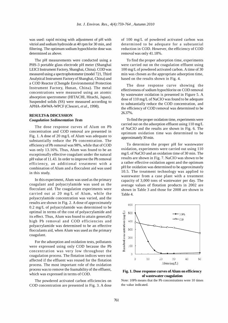
Int. J. Environ. Res., 4(4):759-764 , Autumn 2010
761
was used: rapid mixing with adjustment of pH withvitriol and sodium hydroxide at 40 rpm for 30 min, andfiltering. The optimum sodium hypochlorite dose wasdetermined as above.
The pH measurements were conducted using aPHS-3 portable glass electrode pH meter (ShanghaiLEICI Instrument Factory, Shanghai, China). COD wasmeasured using a spectrophotometer (model 721, ThirdAnalytical Instrument Factory of Shanghai, China) anda COD Reactor (Chengde Environmental ProtectionInstrument Factory, Hunan, China). The metalconcentrations were measured using an atomicabsorption spectrometer (HITACHI, Hitachi, Japan).Suspended solids (SS) were measured according toAPHA-AWWA-WPCF (Clesceri, et al., 1998).
RESULTS & DISCUSSIONCoagulation Sedimentation Tests
The dose response curves of Alum on Pbconcentration and COD removal are presented inFig. 1. A dose of 20 mg/L of Alum was adequate tosubstantially reduce the Pb concentration. Theefficiency of Pb removal was 98%, while that of CODwas only 13.16%. Thus, Alum was found to be anexceptionally effective coagulant under the naturalpH value of 11.43. In order to improve the Pb removalefficiency, an addi t ional t r ea tment wi th acombination of Alum and a flocculent aid was usedin this study.
In this experiment, Alum was used as the primarycoagulant and polyacrylamide was used as theflocculant aid. The coagulation experiments werecar ried out a t 20 mg/L of Alum, whi le thepolyacrylamide concentration was varied, and theresults are shown in Fig. 2. A dose of approximately0.2 mg/L of polyacrylamide was determined to beoptimal in terms of the cost of polyacrylamide andits effect. Thus, Alum was found to attain generallyhigh Pb r emoval and COD efficiencies andpolyacrylamide was determined to be an effectiveflocculants aid, when Alum was used as the primarycoagulant.
For the adsorption and oxidation tests, pollutantswere expressed using only COD because the Pbconcen trat ion was very low throughout thecoagulation process. The flotation indices were notaffected if the effluent was reused for the flotationprocess. The most important role of the oxidationprocess was to remove the foamability of the effluent,which was expressed in terms of COD.
The powdered activated carbon efficiencies onCOD concentration are presented in Fig. 3. A dose
Fig. 1. Dose response curves of Alum on efficiencyof wastewater coagulation
Note: 10Pb means that the Pb concentrations were 10 timesthe value indicated.
of 100 mg/L of powdered activated carbon wasdetermined to be adequate for a substant ialreduction in COD. However, the efficiency of CODremoval was only 41.18%.
To find the proper adsorption time, experimentswere carried out on the coagulation effluent using100 mg/L of powdered activated carbon. A time of 30min was chosen as the appropriate adsorption time,based on the results shown in Fig. 4.
The dose response curve showing theeffectiveness of sodium hypochlorite on COD removalby wastewater oxidation is presented in Figure 5. Adose of 110 mg/L of NaClO was found to be adequateto substantially reduce the COD concentration, andthe efficiency of COD removal was determined to be26.37%.
To find the proper oxidation time, experiments werecarried out on the adsorption effluent using 110 mg/Lof NaClO and the results are shown in Fig. 6. Theoptimum oxidation time was determined to beapproximately 30 min.
To determine the proper pH for wastewateroxidation, experiments were carried out using 110mg/L of NaClO and an oxidation time of 30 min. Theresults are shown in Fig. 7. NaClO was shown to bea rather effective oxidation agent and the optimumpH for oxidation was determined to be approximately10.5. The treatment technology was applied towastewater from a case plant with a treatmentcapacity of 3,000 tons of wastewater per day. Theaverage values of flotation products in 2002 areshown in Table 3 and those for 2008 are shown inTable 4.
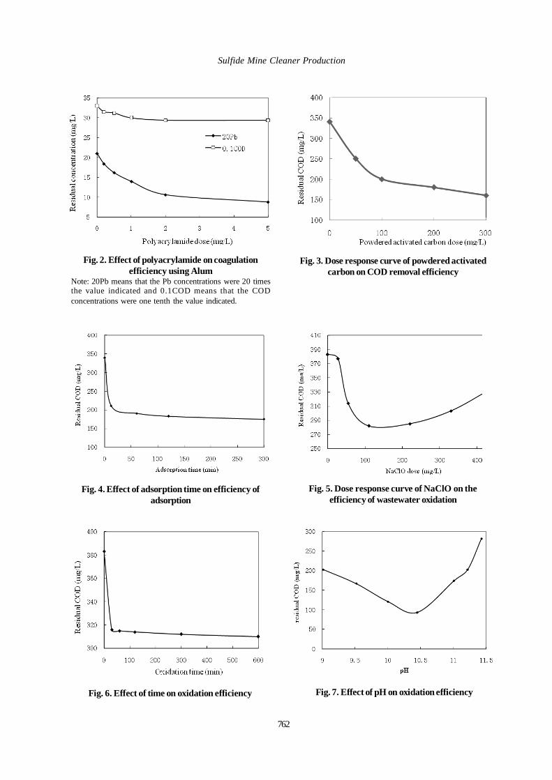
762
Sulfide Mine Cleaner Production
Fig. 2. Effect of polyacrylamide on coagulationefficiency using Alum
Note: 20Pb means that the Pb concentrations were 20 timesthe value indicated and 0.1COD means that the CODconcentrations were one tenth the value indicated.
Fig. 3. Dose response curve of powdered activatedcarbon on COD removal efficiency
Fig. 4. Effect of adsorption time on efficiency ofadsorption
Fig. 5. Dose response curve of NaClO on theefficiency of wastewater oxidation
Fig. 6. Effect of time on oxidation efficiency Fig. 7. Effect of pH on oxidation efficiency
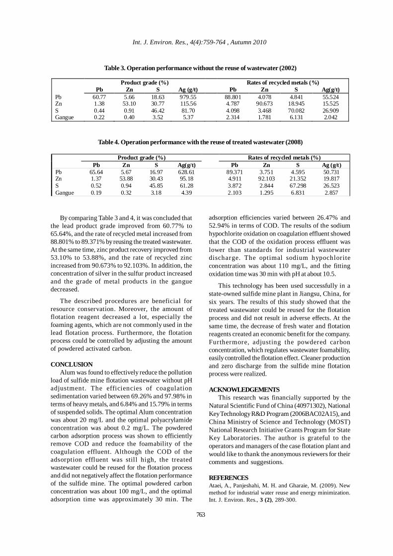
Int. J. Environ. Res., 4(4):759-764 , Autumn 2010
Table 3. Operation performance without the reuse of wastewater (2002)
Product grade (%) Rates of recycled metals (%) Pb Zn S Ag (g/t) Pb Zn S Ag(g/t) Pb 60.77 5.66 18.63 979.55 88.801 4.078 4.841 55.524 Zn 1.38 53.10 30.77 115.56 4.787 90.673 18.945 15.525 S 0.44 0.91 46.42 81.70 4.098 3.468 70.082 26.909 Gangue 0.22 0.40 3.52 5.37 2.314 1.781 6.131 2.042
Table 4. Operation performance with the reuse of treated wastewater (2008)
Product grade (%) Rates of recycled metals (%) Pb Zn S Ag(g/t) Pb Zn S Ag (g/t)
Pb 65.64 5.67 16.97 628.61 89.371 3.751 4.595 50.731 Zn 1.37 53.88 30.43 95.18 4.911 92.103 21.352 19.817 S 0.52 0.94 45.85 61.28 3.872 2.844 67.298 26.523 Gangue 0.19 0.32 3.18 4.39 2.103 1.295 6.831 2.857
By comparing Table 3 and 4, it was concluded thatthe lead product grade improved from 60.77% to65.64%, and the rate of recycled metal increased from88.801% to 89.371% by reusing the treated wastewater.At the same time, zinc product recovery improved from53.10% to 53.88%, and the rate of recycled zincincreased from 90.673% to 92.103%. In addition, theconcentration of silver in the sulfur product increasedand the grade of metal products in the ganguedecreased.
The described procedures are beneficial forresource conservation. Moreover, the amount offlotation reagent decreased a lot, especially thefoaming agents, which are not commonly used in thelead flotation process. Furthermore, the flotationprocess could be controlled by adjusting the amountof powdered activated carbon.
CONCLUSIONAlum was found to effectively reduce the pollution
load of sulfide mine flotation wastewater without pHadjustment. The efficiencies of coagulationsedimentation varied between 69.26% and 97.98% interms of heavy metals, and 6.84% and 15.79% in termsof suspended solids. The optimal Alum concentrationwas about 20 mg/L and the optimal polyacrylamideconcentration was about 0.2 mg/L. The powderedcarbon adsorption process was shown to efficientlyremove COD and reduce the foamability of thecoagulation effluent. Although the COD of theadsorption effluent was still high, the treatedwastewater could be reused for the flotation processand did not negatively affect the flotation performanceof the sulfide mine. The optimal powdered carbonconcentration was about 100 mg/L, and the optimaladsorption time was approximately 30 min. The
adsorption efficiencies varied between 26.47% and52.94% in terms of COD. The results of the sodiumhypochlorite oxidation on coagulation effluent showedthat the COD of the oxidation process effluent waslower than standards for industrial wastewaterdischarge. The optimal sodium hypochloriteconcentration was about 110 mg/L, and the fittingoxidation time was 30 min with pH at about 10.5.
This technology has been used successfully in astate-owned sulfide mine plant in Jiangsu, China, forsix years. The results of this study showed that thetreated wastewater could be reused for the flotationprocess and did not result in adverse effects. At thesame time, the decrease of fresh water and flotationreagents created an economic benefit for the company.Furthermore, adjusting the powdered carbonconcentration, which regulates wastewater foamability,easily controlled the flotation effect. Cleaner productionand zero discharge from the sulfide mine flotationprocess were realized.
ACKNOWLEDGEMENTSThis research was financially supported by the
Natural Scientific Fund of China (40971302), NationalKey Technology R&D Program (2006BAC02A15), andChina Ministry of Science and Technology (MOST)National Research Initiative Grants Program for StateKey Laboratories. The author is grateful to theoperators and managers of the case flotation plant andwould like to thank the anonymous reviewers for theircomments and suggestions.
REFERENCESAtaei, A., Panjeshahi, M. H. and Gharaie, M. (2009). Newmethod for industrial water reuse and energy minimization.Int. J. Environ. Res., 3 (2), 289-300.
763

764
Yuan, Z. et al.
Biati, A., Moattar, F., Karbassi, A. R. and Hassani, A. H.(2010). Role of saline water in removal of heavy elementsfrom industrial wastewaters. Int. J. Environ. Res., 4 (1),177-182.
Clesceri, L. S., Greenberg, A. E. and Eaton, A.D. (1998).APHA-AWWA-WPCF (1998a) Method 4500-NO3-I. In:Standard methods for the examination of water andwastewater, pp. 4-121. American Public Health Association,Washington, USA.
Asubiojo, O. I. and Ajelabi, O. B. (2009). Removal of heavymetals from industrial wastewaters using natural adsorbents.Toxicological and Environmental Chemistry, 91 (5), 883-890.
Chen, T., Huang, X., Pan, M., Song, J., Peng, S. and Fallgren,P. H. (2009). Treatment of coking wastewater by usingmanganese and magnesium ores. Journal of HazardousMaterials, 168 (2-3), 843-847.
Chong, M. F., Lee, K. P., Chieng, H. J. and Ramli, I. I. S. B.(2009). Removal of boron from ceramic industry wastewaterby adsorption-flocculation mechanism using palm oil millboiler (POMB) bottom ash and polymer. Water Research,43 (13), 3326-3334.
Eilbeck, W. J. and Mattock, G. (1987). Chemical processesin waste water treatment. (Chichester, UK: Ellis HorwoodLtd.)
Haydar, S. and Aziz, J. A. (2009). Coagulation-flocculationstudies of tannery wastewater using combination of alumwith cationic and anionic polymers. Journal of HazardousMaterials, 168 (2-3), 1035-1040.
Jagtoyen, M., Lafferty, C. and Kimber, G. (1991). Newactivated carbon material used in wastewater treatment.NEW Carbon Material, 12 (2), 37-38.
Li, Y., Liu, Y., Zuo, H., Du, G. and Zhang, F. (2009). Studyon the treatment of phosphorite floatation wastewater withcoagulation method. Industrial Safety and EnvironmentalProtection, 35 (4), 6-9.
Mackie, A., Woszczynski, M., Farmer, H., Walsh, M. E.and Gagnon, G. A. (2009). Water reclamation and reuse.Water Environment Research, 81 (10), 1406-1418.
Mahmoud, E. K. (2009). Chemically enhanced primarytreatment of textile industrial effluents. Polish Journal ofEnvironmental Studies, 18 (4), 651-655.
Olga, D. and Helen, G. (2002). Coagulation for treatment ofpaint industry wastewater. Journal of Environmental Scienceand Health (Part A), A37 (7), 1361-1377
Qiu, Y. P., Chen, J. L., Li, A. M., Chen, Y. L. and Zhang, Q.X. (2006). Treatment and reuse of wastewater in pesticide2,4-D production. International Journal of Environment andPollution, 27 (4), 347-358.
Rivera-Utrilla, J., Prados-Joya, G., Sanchez-Polo, M., Ferro-Garcia, M. A. and Bautista-Toledo, I. (2009). Removal ofnitroimidazole antibiotics from aqueous solution byadsorption/bioadsorption on activated carbon. Journal ofHazardous Materials, 170 (1), 298-305.
Rubio J., Carissimi, E. and Rosa, J. J. (2007). Flotation inwater and wastewater treatment and reuse: recent trends inBrazil. International Journal of Environmental and Pollution,30 (2), 197-212.
Saeedi, M. and Amini, H. R. (2007). Chemical, physical,mineralogical, morphology and leaching characteristics of athermal power plant air heater washing waste. Int. J. Environ.Res., 1 (1), 74-79.
Tu, J. Ch. (1998). Wastewater of millrun industry andtreatment. Yunnan Metallurgy, 1, pp. 5-8.
Wang J. Y. (2000). Treatment and utilization of miningwastewater. Comprehensive Utilization of ChineseResources,13, 4-7.
Wei, Ch. H., Sun, S. J. and She, J. (1994). A study ofmechanism of treating cyanide containing wastewater byactivated carbon. Journal of South China University ofTechnology (Natural Science), 22 (5), 1-9.
Wei, Y. H. and Zhou, G. Y. (2007). A new approach towastewater reuse in the flotation of Pb/Zn sulphide. Journalof Wuhan Institute of Technology, 29 (4), 21-24.
Xie, G. Y., Wang, X. W., Sun, Sh. Y. and Dai, W. C. (2005).Study on application of floatation wastewater reuse insulfide lead-zinc mines. Techniques and Equipment forEnvironmental Pollution Control, 6 (8), 14-17.
Yang, Q., Shang, H. T. and Wang, J. L. (2009). Dyewastewater treatment by using ceramic membrane bioreactor.International Journal of Environment and Pollution, 38 (3),267-279.
Yang, T. W., Zhang, Q. M. and Wu, H. Y. (2008). Wastewatertreatment pilot tests in a coking plant using HSB technology.Journal of Tsinghua University, 48 (3), 363-366.
Yuan, Z., Sun, Sh. Y., Zhao,Y. B., Dai, W. C. and Liu, R. Y.(2002). Purification of flotation wastewater and reuse.Technology of Water Treatment, 28 (4), 232-234.
Zhang, L. H., Wang, Q. H., Xue, N. T., Tian, Sh. L., Xie,W. M. and Shimaoka, T. (2009). Treatment of odourcontaining hydrogen sulphide released from pharmaceuticalwastewater treatment plant with SBR process by bio-trickling filter. International Journal of Environment andPollution, 38 (1/2), 140-150.
Zheng, Ch. N. and Bin, H. X. (1998). On the mechanism ofthe activated carbon biological treatment. Journal of HefeiUniversity of Technology, 21 (6), 32-35.

Int. J. Environ. Res., 4(4):765-776, Autumn 2010ISSN: 1735-6865
Received 2 Oct. 2009; Revised 19 April 2010; Accepted 10 May 2010
*Corresponding author E-mail: [email protected]
765
Simulating Multi-Objective Spatial Optimization Allocation of Land Use Basedon the Integration of Multi-Agent System and Genetic Algorithm
Zhang, H. H .1, Zeng, Y. N.1* and Bian, L. 2
1School of Info-Physics and Geomatics Engineering & Research Center of Space Info-Techniqueand Sustainable Development, Central South University, Changsha 410083, China
2Department of Geography, University at Buffalo, State University of New York, NY 14261, USA
ABSTRACT: In this study, under the constraint of resource-saving and environment-friendliness objective,based on multi-agent genetic algorithm, multi-objective spatial optimization (MOSO) model for land useallocation was developed from the view of simulating the biological autonomous adaptability to environmentand the competitive-cooperative relationship. The model was applied to solve the practical multi-objectivespatial optimization allocation problems of land use in the core region of Changsha, Zhuzhou, Xiangttan citycluster in China. The results has indicated that MOSO model has much better performance than GA for solvingcomplex multi-objective spatial optimization allocation problems and it is a promising method for generatingland use alternatives for further consideration in spatial decision-making.
Key words: Land use allocation, Multi-objective, spatial optimization, Multi-agent system, Genetic algorithm, Resource-saving, Environment-friendliness
INTRTODUCTIONNowadays, the rapid socio-economic development
has produced enormous material interests, however,the unreasonable land use allocation has also led to aseries of serious resource and environment problems,and affected seriously sustainable land use (Verburg,et al., 1999; Peng, et al., 2006; Li and Liu, 2008). Thus,developing a spatial optimization allocation model ofregional land use will have important significance toscientific planning and rational management of landuse. Owing to multifaceted nature of land use allocation,spatial optimization allocation model should aim atfinding a set of high-performing alternatives instead ofjust one solution (Duh and Brown, 2007; Xiao, et al.,2007; Zhang and Armstrong, 2008; Ligmann-Zielinska,et al., 2008). As a type of general global optimizationalgorithm, genetic algorithm (GA) has been widely usedfor numerical optimization, combinatorial optimizationand travelling salesman problems. And manyresearchers have been trying to apply this method tosolve the multi-objective land use allocation problemsquantitatively (Feng and Lin, 1999; Balling, et al., 1999;Matthews, 2001; Xiao, et al., 2002; Stewart, et al., 2004;Holzkamper and Seppelt, 2007; Janssen, et al., 2008).All the above studies indicate that GA is effective insolving multi-objective spatial optimization allocation
problems of land use. However, the main problem ofGA is that it may be trapped in the local optima ofobjective functions when the optimization problemsare too complicated. And it’s more possible to obtainlocal optimal solutions and increase convergence timewith increase of the complexity of problems and searchspace of algorithms. In the meantime, it is difficult toincorporate human and social factors in GA. Therefore,it’s necessary to develop more intelligent algorithmsfor the solution of multi-objective spatial optimizationallocation problems of land use.
Artificial life methods inspired by complexityscience has witnessed a significant development andbeen applied extensively (Chebeane and Echalier, 1999;Liu, et al., 1997). As one of these methods, multi-agentsystem has been successfully applied to build dynamicrepresentations of geographical systems (Parker, etal., 2003; Manson, 2005, 2006; Evans, et al., 2006;Evans and Kelley, 2008; Brown, et al., 2005, 2008; Brownand Xie, 2006; Xie and Batty, 2007), especially inrepresenting spatial allocation of land use (Benenson,1998; Arentze and Timmermans, 2003; Saarloos, et al.,2005; Li and Liu, 2007, 2008). The multi-agent systemhas a cell structure which can make each agent achieveoptimization in its neighborhood areas respectivelyinstead of in the whole system to ensure the population
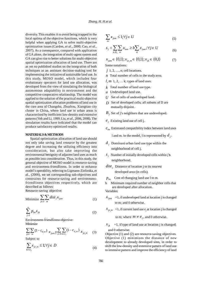
766
Zhang, H. H.et al.
diversity. This enables it to avoid being trapped in thelocal optima of the objective functions, which is veryhelpful when applying GA to solve multi-objectiveoptimization issues (Cardon, et al., 2000; Cao, et al.,2007). As a consequence, compared with applicationof GA alone, the integration of multi-agent system andGA can give rise to better solutions for multi-objectivespatial optimization allocation of land use. There areas yet no published studies on the integration of bothtechniques as an assistant decision-making tool forimplementing the initiative of sustainable land use. Inthis study, MOSO model, which includes fourevolutionary operators for land use allocation, wasdeveloped from the view of simulating the biologicalautonomous adaptability to environment and thecompetitive-cooperative relationship. The model wasapplied to the solution of the practical multi-objectivespatial optimization allocation problems of land use inthe core area of Changsha, Zhuzhou, Xiangttan citycluster in China, where land use in urban areas ischaracterized by inefficient low-density and extensivepatterns (Yeh and Li, 1999; Liu, et al., 2006, 2008). Thesimulation results have indicated that the model canproduce satisfactory optimized results.
MATERIALS & METHODSSpatial optimization allocation of land use should
not only take saving land resource by the greatestdegree and increasing the utilizing efficiency intoconsideration, but also take improving theenvironmental benignity of adjacent land uses as muchas possible into consideration. Thus, in this study, thegeneral objective of MOSO model is resource-savingand environment-friendliness. In order to enhancemodel’s operability, referring to Ligmann-Zielinska, etal., (2008), we set corresponding sub-objectives andconstraints for resource-saving and environment-friendliness objectives respectively, which aredescribed as follows:Resource-saving objective:
Minimize ∑∑∈Uj m
jumj xdist (1)
jk
n
jlmxp∑
=1 (2)
Environment-friendliness objective:Minimize
∑∑∈
−Uj m
md jc )1(
jumx ÿ∑∑∈ ≠
−Dj em
mdj
jc )1(
mje jx (3)
Subject to
∑≠
∈∀≤j
jem
mje Djx ;1 (4)
Ujxm
jum ∈∀≤∑ ;1 (5)
Ujxbxsm
jumBi m
iumjj
∈∀≥+ ∑∑∑∈
; (6)
}1,0{};1,0{};1,0{ ∈∈∈ jkmjejum xxxj
(7)
Some notations:j 1, 2, …, n; cell locations.n Total number of cells in the study area.
ml, 1, 2, … k; types of land uses.
k Total number of land use type.u Undeveloped land use.
U Set of cells of undeveloped land.
D Set of developed cells; all subsets of D are mutually disjoint.
jB Set of j’s neighbors that are undeveloped.
je Existing land use of cell j.
lmc Estimated compatibility index between land uses
l and m. in the model, l is represented by jd .
jd Dominant urban land use type within the neighborhood of cell j.
js Number of initially developed cells within j’ss neighborhood.
jdist Distance of location j to its nearest developed area (in cells).
lmp Cost of changing land use l to m.b Minimum required number of neighbor cells that are developed after allocation.Variables:
jumx =1, if undeveloped land at location j is changed to m; and 0 otherwise.
mje jx
=1, if current land use ej at location j is changed
to m; where jem ≠ , and 0 otherwise.
jkx =1, if type of land use at location j is changed;
and 0 otherwise.Objective (1) and (2) are resource-saving objectives.Objective (1) minimizes the distance of newdevelopment to already developed sites, in order toshift the low-density and extensive pattern of land useto intensive pattern and improve the efficiency of land
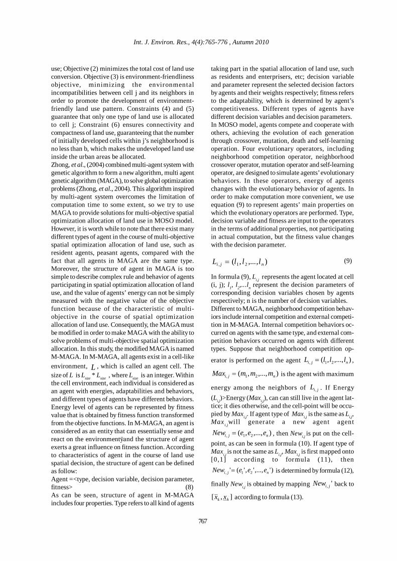
Int. J. Environ. Res., 4(4):765-776 , Autumn 2010
767
use; Objective (2) minimizes the total cost of land useconversion. Objective (3) is environment-friendlinessobjective, minimizing the environmentalincompatibilities between cell j and its neighbors inorder to promote the development of environment-friendly land use pattern. Constraints (4) and (5)guarantee that only one type of land use is allocatedto cell j; Constraint (6) ensures connectivity andcompactness of land use, guaranteeing that the numberof initially developed cells within j’s neighborhood isno less than b, which makes the undeveloped land useinside the urban areas be allocated.Zhong, et al., (2004) combined multi-agent system withgenetic algorithm to form a new algorithm, multi agentgenetic algorithm (MAGA), to solve global optimizationproblems (Zhong, et al., 2004). This algorithm inspiredby multi-agent system overcomes the limitation ofcomputation time to some extent, so we try to useMAGA to provide solutions for multi-objective spatialoptimization allocation of land use in MOSO model.However, it is worth while to note that there exist manydifferent types of agent in the course of multi-objectivespatial optimization allocation of land use, such asresident agents, peasant agents, compared with thefact that all agents in MAGA are the same type.Moreover, the structure of agent in MAGA is toosimple to describe complex rule and behavior of agentsparticipating in spatial optimization allocation of landuse, and the value of agents’ energy can not be simplymeasured with the negative value of the objectivefunction because of the characteristic of multi-objective in the course of spatial optimizationallocation of land use. Consequently, the MAGA mustbe modified in order to make MAGA with the ability tosolve problems of multi-objective spatial optimizationallocation. In this study, the modified MAGA is namedM-MAGA. In M-MAGA, all agents exist in a cell-likeenvironment, L , which is called an agent cell. Thesize of L is Lsize * Lsize , where Lsize is an integer. Withinthe cell environment, each individual is considered asan agent with energies, adaptabilities and behaviors,and different types of agents have different behaviors.Energy level of agents can be represented by fitnessvalue that is obtained by fitness function transformedfrom the objective functions. In M-MAGA, an agent isconsidered as an entity that can essentially sense andreact on the environmentÿand the structure of agentexerts a great influence on fitness function. Accordingto characteristics of agent in the course of land usespatial decision, the structure of agent can be definedas follow:Agent =<type, decision variable, decision parameter,fitness> (8)As can be seen, structure of agent in M-MAGAincludes four properties. Type refers to all kind of agents
taking part in the spatial allocation of land use, suchas residents and enterprisers, etc; decision variableand parameter represent the selected decision factorsby agents and their weights respectively; fitness refersto the adaptability, which is determined by agent’scompetitiveness. Different types of agents havedifferent decision variables and decision parameters.In MOSO model, agents compete and cooperate withothers, achieving the evolution of each generationthrough crossover, mutation, death and self-learningoperation. Four evolutionary operators, includingneighborhood competition operator, neighborhoodcrossover operator, mutation operator and self-learningoperator, are designed to simulate agents’ evolutionarybehaviors. In these operators, energy of agentschanges with the evolutionary behavior of agents. Inorder to make computation more convenient, we useequation (9) to represent agents’ main properties onwhich the evolutionary operators are performed. Type,decision variable and fitness are input to the operatorsin the terms of additional properties, not participatingin actual computation, but the fitness value changeswith the decision parameter.
(9)
In formula (9), Li,j represents the agent located at cell(i, j); l1, l2,...ln represent the decision parameters ofcorresponding decision variables chosen by agentsrespectively; n is the number of decision variables.Different to MAGA, neighborhood competition behav-iors include internal competition and external competi-tion in M-MAGA. Internal competition behaviors oc-curred on agents with the same type, and external com-petition behaviors occurred on agents with differenttypes. Suppose that neighborhood competition op-
erator is performed on the agent ),...,,( 21, nji lllL = ,
),...,,( 21, nji mmmMax = is the agent with maximum
energy among the neighbors of jiL , . If Energy(Li,j)>Energy (Maxi,j), can can still live in the agent lat-tice; it dies otherwise, and the cell-point will be occu-pied by Maxi,j. If agent type of Maxi,j is the same as Li,j,Maxi,jwill generate a new agent agent
),...,,( 21, nji eeeNew = , then Newi,j is put on the cell-point, as can be seen in formula (10). If agent type ofMaxi,j is not the same as Li,j, Maxi,j is first mapped onto[0,1] according to formula (11), then
)',...,','(' 21, nji eeeNew = is determined by formula (12),
finally Newi,j is obtained by mapping ', jiNew back to
],[ kk xx according to formula (13).
),...,,( 21, nji lllL =

768
Allocation of Land Use
othersxlmUmxlmUm
lmUmxx
e kkkk
kkkk
kkk
k
k
k ,))()1,1(())()1,1((
)()1,1(>−×−+<−×−+
⎪⎩
⎪⎨
⎧
−×−+=
nk ,...1= (10)
In formula (10), )1,1(−U is random number on (-1,1),
],[ kk xx is the search space.
nkxxxm kkkk ,...1),/()('mk =−−= (11)
2121 ,1,1),',...,1','
,1',...,1',',1',...,'('
iininimmm
mmmmmewN
n
1ji,
2i1i
1i2i2i1i
<<<<<+
+−−= (12)
nkxxexe kkkkk ,...,1),(' =−⋅+= (13)
Neighborhood crossover operator is used to simulatethe cooperation behavior of agents. Compared withneighborhood crossover operator in MAGA, the neigh-borhood crossover operator in M-MAGA takes ad-vantage of elitist strategy in order to make populationevolve to the best solutions more quickly and reducethe unnecessary random degradation. Although thisstrategy will cause the reduction of population diver-sity to some extent, it can be compensated by mutationoperator. In the neighborhood of Li,j, if agent type ofMaxi,j is the same as Li,j, this operator is performed onLi,j, and Maxi,j to achieve the purpose of cooperation.In this process, neighborhood crossover operator gen-erates two new agents, one of which with larger fit-ness survives. This kind of process takes place for m(m <5) times. Finally, the agent Max with maximum en-ergy is selected to replaceLi,j, if Energy(Max) >Energy(Li,j,); no replacement otherwise.As a result of some sudden factors, the decision pa-rameters of agent in the course of land use spatial op-timization decision may mutate. Therefore, we use mu-tation operator to express this situation. Different toMAGA, the interchange mutation operator is taken todescribe agents’ mutation behaviors in order to im-prove efficiency of algorithm in M-MAGA. In inter-change mutation operator, after randomly choosing two
positions in agent Li,j, new agent ),...,,(' 21, nji bbbL = is
generated from agent ),...,,( 21, nji lllL = through inter-changing corresponding parameters in these twopositions. The concrete operation is described as follow:
⎩⎨⎧
<≥
=−+ mpqpq
mkk PUllll
PUlb
)1,0(...),,,...,,(...,)1,0(,
11 (14)
Where n,...,1k = , )1,0(U is random number on (0,1),
mP is mutation probability.The self-learning operatorcan be considered as a small scale M-MAGA, beingperformed on the best agent in each generation tosimulate the behavior of self-learning to improve itsown energy. The operator in M-MAGA is the same asMAGA, and for more details, see Leung and Wang, etal., (2001). In M-MAGA, all agents of the populationare ranked with the priority method according to theirfitness to each objective function, and then gettingthe total fitness. ),...,2,1)(( niiZ = represents theobjective function and n is the number of objectives.
For each objective, agent jX ( Nj ,...,2,1= ) will forma collating sequence Y according to the magnitude of
the objective function values of )( ji XZ . For objective
i, fitness of agent jX is calculated according to,
⎪⎩
⎪⎨⎧
=>−
=;1)(;1)())((
)( 2
2
ji
jijiji XYkN
XYXYNXF
Njni ,...,2,1;,...,2,1 == (15)
In the formula, N is the total number of agents; jX is
the jth agent in the population; iY refers to jX ’s serial
number in the collating sequence Y( jX ); represents’ss
fitness for objective i. Total fitness of agent jX (j=1,2, ...,N) will be obtained according to,
∑=
=n
ijij XFXFit
1)()( (16)
Where n is the total number of the objective func-
tions; )( jXFit is jX ’s total fitness for all objectives.It’s self-evident that those agents with higher total fit-ness value can obtain lager fitness, which makes agentsenjoy more opportunities of evolution.In order to keep the diversity of the population andavoid genetic drift, the niche technology based onsharing mechanism is introduced to decrease thereplication of similar individuals. The radius of ecological
niche ( shareσ ) can be determined by formula (17).
share
n
i
n
ijishareji
nshare
XFXF
σ
σσ
∏ ∏= =−
−+− 1 11
)())((N = 0 (17)
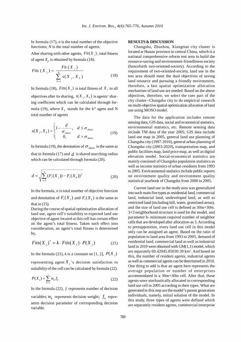
Int. J. Environ. Res., 4(4):765-776, Autumn 2010
In formula (17), n is the total number of the objectivefunctions; N is the total number of agents.
After sharing with other agents, )( jXFit , total fitnessof agent Xj, is obtained by formula (18).
∑=
= N
kkj
jj
XXs
XFitXFits
1),(
)()(
(18)
In formula (18), )( jXFits is total fitness of jX to all
objectives after its sharing, ),( kj XXs is agents’ shar-ing coefficient which can be calculated through for-mula (19), where kX stands for the kth agent and Ntotal number of agents
⎪⎩
⎪⎨⎧
>
≤−=
share
sharesharekj
d
ddXXs
σ
σσ
,0
,1),( (19)
In formula (19), the denotation of shareσ is the same as
that in formula (17) and d is shared searching radiuswhich can be calculated through formula (20).
∑=
−=n
ikiji XFXFd
1
2))())(( (20)
In the formula, n is total number of objective function
and denotation of )( ji XF and )( ki XF is the same asthat in (15).During the course of spatial optimization allocation ofland use, agent cell’s suitability to expected land useobjective of agent located at this cell has certain effecton the agent’s total fitness. Taken such effect intoconsideration, an agent’s total fitness is determinedby,
)()()( *jjj XPXFitskXFits ⋅⋅= (21)
In the formula (21), k is a constant on [1, 2], )( jXP
representing agent jX ’s decision satisfaction tosuitability of the cell can be calculated by formula (22).
k
l
kk fwXP ∑
=
=1
j)( (22)
In the formula (22), l represents number of decision
variables; kw represents decision weight; kf repre-sents decision parameter of corresponding decisionvariable.
RESULTS & DISCUSSIONChangsha, Zhuzhou, Xiangttan city cluster is
located at Hunan province in central China, which is anational comprehensive reform test area to build theresource-saving and environment-friendliness society(henceforth two-oriented-society). According to therequirement of two-oriented-society, land use in thetest area should meet the dual objectives of savingland resource and pursuing a friendly environment,therefore, a fast spatial optimization allocationmechanism of land use are needed. Based on the aboveobjectives, therefore, we select the core part of thecity cluster--Changsha city to do empirical researchon multi-objective spatial optimization allocation of landuse using MOSO model.
The data for the application includes remotesensing data, GIS data, social and economical statistics,environmental statistics, etc. Remote sensing datainclude TM data of the year 2005; GIS data includeland use map in 2005, general land use planning ofChangsha city (1997-2010), general urban planning ofChangsha city (2003-2020), transportation map, andpublic facilities map, land price map, as well as digitalelevation model. Social-economical statistics aremainly consisted of Changsha population statistics aswell as income statistics of urban residents from 1993to 2005. Environmental statistics include public reportson environment quality and environment qualitystatistical yearbook of Changsha from 2000 to 2005.
Current land use in the study area was generalizedinto such main five types as residential land, commercialland, industrial land, undeveloped land, as well asrestricted land (including hill, water, greenland areas),and the size of land use cell is defined as 30m×30m.3×3 neighborhood structure is used for the model, andparameter b- minimum required number of neighborcells that are developed after allocation-as 3. Accordingto presupposition, every land use cell in this modelonly can be assigned an agent. Based on the ratio ofpopulation to land area from 1993 to 2005, demand ofresidential land, commercial land as well as industrialland in 2010 were obtained with GM(1,1) model, whichare separately 69.42045.85030.39 km2. And based onthis, the number of resident agents, industrial agentsas well as commercial agents can be determined in 2010.One thing to add is that an agent here represents theaverage population or number of enterprisesaccommodated in a 30m×30m cell. After that, theseagents were stochastically allocated to correspondingland use cell in 2005 according to their types. What aregenerated in this step are the model’s parent generationindividuals, namely, initial solution of the model. Inthis study, three types of agents were defined whichare separately resident agents, commercial enterprise
769
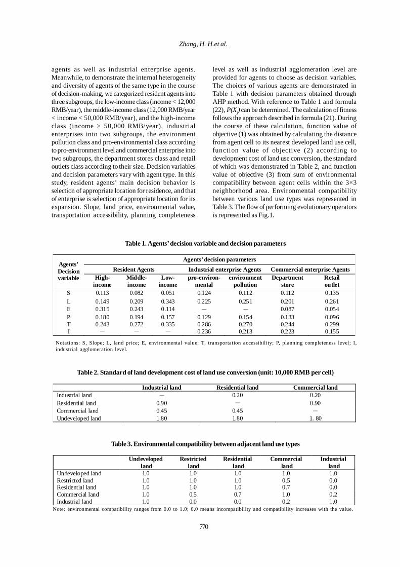
770
Zhang, H. H.et al.
agents as well as industrial enterprise agents.Meanwhile, to demonstrate the internal heterogeneityand diversity of agents of the same type in the courseof decision-making, we categorized resident agents intothree subgroups, the low-income class (income < 12,000RMB/year), the middle-income class (12,000 RMB/year< income < 50,000 RMB/year), and the high-incomeclass (income > 50,000 RMB/year), industrialenterprises into two subgroups, the environmentpollution class and pro-environmental class accordingto pro-environment level and commercial enterprise intotwo subgroups, the department stores class and retailoutlets class according to their size. Decision variablesand decision parameters vary with agent type. In thisstudy, resident agents’ main decision behavior isselection of appropriate location for residence, and thatof enterprise is selection of appropriate location for itsexpansion. Slope, land price, environmental value,transportation accessibility, planning completeness
Table 1. Agents’ decision variable and decision parameters
Agents’ decision parameters Resident Agents Industrial enterprise Agents Commercial enterprise Agents
Agents’ Decision variable High-
income Middle- income
Low- income
pro-environ- mental
environment pollution
Department store
Retail outlet
S 0.113 0.082 0.051 0.124 0.112 0.112 0.135 L 0.149 0.209 0.343 0.225 0.251 0.201 0.261 E 0.315 0.243 0.114 - - 0.087 0.054 P 0.180 0.194 0.157 0.129 0.154 0.133 0.096 T 0.243 0.272 0.335 0.286 0.270 0.244 0.299 I - - - 0.236 0.213 0.223 0.155
Notations: S, Slope; L, land price; E, environmental value; T, transportation accessibility; P, planning completeness level; I,industrial agglomeration level.
level as well as industrial agglomeration level areprovided for agents to choose as decision variables.The choices of various agents are demonstrated inTable 1 with decision parameters obtained throughAHP method. With reference to Table 1 and formula(22), P(Xj) can be determined. The calculation of fitnessfollows the approach described in formula (21). Duringthe course of these calculation, function value ofobjective (1) was obtained by calculating the distancefrom agent cell to its nearest developed land use cell,function value of objective (2) according todevelopment cost of land use conversion, the standardof which was demonstrated in Table 2, and functionvalue of objective (3) from sum of environmentalcompatibility between agent cells within the 3×3neighborhood area. Environmental compatibilitybetween various land use types was represented inTable 3. The flow of performing evolutionary operatorsis represented as Fig.1.
Industrial land Residential land Commercial land Industrial land - 0.20 0.20 Residential land 0.90 - 0.90 Commercial land 0.45 0.45 - Undeveloped land 1.80 1.80 1. 80
Table 2. Standard of land development cost of land use conversion (unit: 10,000 RMB per cell)
Table 3. Environmental compatibility between adjacent land use types
Undeveloped land
Restricted land
Residential land
Commercial land
Industrial land
Undeveloped land 1.0 1.0 1.0 1.0 1.0 Restricted land 1.0 1.0 1.0 0.5 0.0 Residential land 1.0 1.0 1.0 0.7 0.0 Commercial land 1.0 0.5 0.7 1.0 0.2 Industrial land 1.0 0.0 0.0 0.2 1.0
Note: environmental compatibility ranges from 0.0 to 1.0; 0.0 means incompatibility and compatibility increases with the value.
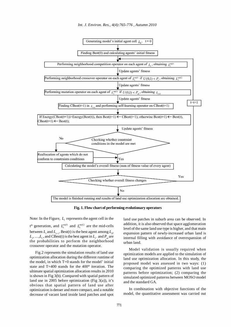
771
Int. J. Environ. Res., 4(4):765-776 , Autumn 2010
Fig. 1. Flow chart of performing evolutionary operators
Note: In the Figure, tL represents the agent cell in the
tth generation, and 1midtL and 2mid
tL are the mid-cellsbetween Lt and Lt+1. Best(t) is the best agent among L0,L1, …,Lt , and CBest(t) is the best agent in Lt. and Pm arethe probabilities to perform the neighborhoodcrossover operator and the mutation operator.
Fig.2 represents the simulation results of land useoptimization allocation during the different runtime ofthe model, in which T=0 stands for the model’ initialstate and T=400 stands for the 400th iteration. Theultimate spatial optimization allocation results in 2010is shown in Fig 3(b). Compared with spatial pattern ofland use in 2005 before optimization (Fig 3(a)), it’sobvious that spatial pattern of land use afteroptimization is denser and more compact, and a notabledecrease of vacant land inside land patches and spot
land use patches in suburb area can be observed. Inaddition, it is also observed that space agglomerationlevel of the same land use type is higher, and that mainexpansion pattern of newly-increased urban land isinternal filling with avoidance of overexpansion ofurban land.
Model validation is usually required whenoptimization models are applied to the simulation ofland use optimization allocation. In this study, theproposed model was assessed in two ways: (1)comparing the optimized patterns with land usepatterns before optimization; (2) comparing thesimulated optimized patterns between MOSO modeland the standard GA.
In combination with objective functions of themodel, the quantitative assessment was carried out
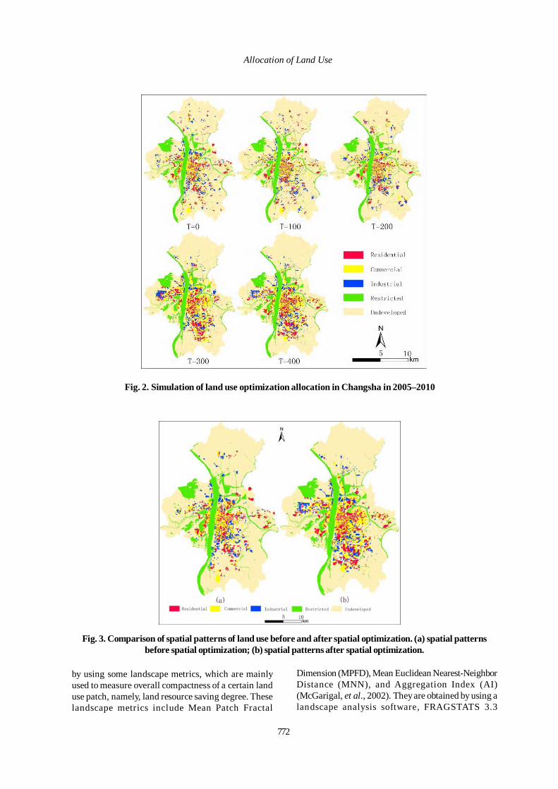
772
Allocation of Land Use
Fig. 2. Simulation of land use optimization allocation in Changsha in 2005–2010
Fig. 3. Comparison of spatial patterns of land use before and after spatial optimization. (a) spatial patternsbefore spatial optimization; (b) spatial patterns after spatial optimization.
by using some landscape metrics, which are mainlyused to measure overall compactness of a certain landuse patch, namely, land resource saving degree. Theselandscape metrics include Mean Patch Fractal
Dimension (MPFD), Mean Euclidean Nearest-NeighborDistance (MNN), and Aggregation Index (AI)(McGarigal, et al., 2002). They are obtained by using alandscape analysis software, FRAGSTATS 3.3
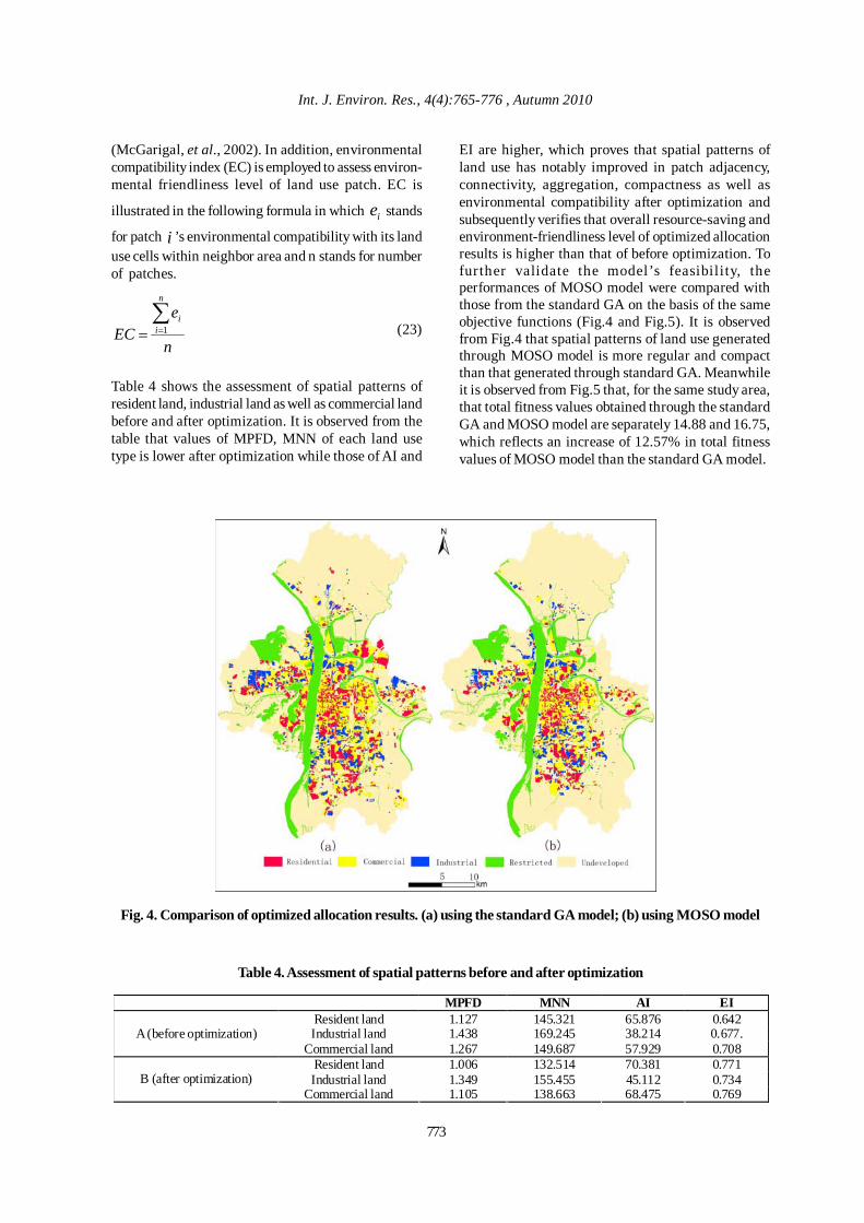
Int. J. Environ. Res., 4(4):765-776 , Autumn 2010
(McGarigal, et al., 2002). In addition, environmentalcompatibility index (EC) is employed to assess environ-mental friendliness level of land use patch. EC is
illustrated in the following formula in which ie stands
for patch i ’s environmental compatibility with its landuse cells within neighbor area and n stands for numberof patches.
n
eEC
n
ii∑
== 1 (23)
Table 4 shows the assessment of spatial patterns ofresident land, industrial land as well as commercial landbefore and after optimization. It is observed from thetable that values of MPFD, MNN of each land usetype is lower after optimization while those of AI and
EI are higher, which proves that spatial patterns ofland use has notably improved in patch adjacency,connectivity, aggregation, compactness as well asenvironmental compatibility after optimization andsubsequently verifies that overall resource-saving andenvironment-friendliness level of optimized allocationresults is higher than that of before optimization. Tofurther validate the model’s feasibility, theperformances of MOSO model were compared withthose from the standard GA on the basis of the sameobjective functions (Fig.4 and Fig.5). It is observedfrom Fig.4 that spatial patterns of land use generatedthrough MOSO model is more regular and compactthan that generated through standard GA. Meanwhileit is observed from Fig.5 that, for the same study area,that total fitness values obtained through the standardGA and MOSO model are separately 14.88 and 16.75,which reflects an increase of 12.57% in total fitnessvalues of MOSO model than the standard GA model.
Fig. 4. Comparison of optimized allocation results. (a) using the standard GA model; (b) using MOSO model
Table 4. Assessment of spatial patterns before and after optimization
MPFD MNN AI EI Resident land 1.127 145.321 65.876 0.642 Industrial land 1.438 169.245 38.214 0.677. A (before optimization)
Commercial land 1.267 149.687 57.929 0.708 Resident land 1.006 132.514 70.381 0.771 Industrial land 1.349 155.455 45.112 0.734 B (after optimization)
Commercial land 1.105 138.663 68.475 0.769
773
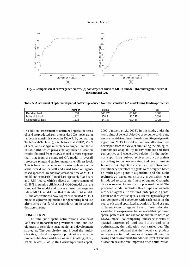
Zhang, H. H.et al.
Fig. 5. Comparison of convergence curves. (a) convergence curve of MOSO model; (b) convergence curve ofthe standard GA.
MPFD MNN AI EI Resident land 1.008 140.976 66.803 0.689 Industrial land 1.412 158.74 40.257 0.694 Commercial land 1.208 141.53 60.445 0.723
Table 5. Assessment of optimized spatial patterns produced from the standard GA model using landscape metrics
In addition, assessment of optimized spatial patternsof land use produced from the standard GA model usinglandscape metrics is shown in Table 5. By comparingTable 5 with Table 4(b), it is obvious that MPFD, MNNof each land use type in Table 5 are higher than thosein Table 4(b), which proves that optimized allocationresults obtained from MOSO model is more superiorthan that from the standard GA model in overallresource-saving and environmental-friendliness level.This is because the behavior of various players in theactual world can be well addressed based on agent-based approach. In additionÿiteration time of MOSOmodel and standard GA model are separately 3.31 hoursand 8.57 hours, which reflects an improvement of61.38% in running efficiency of MOSO model than thestandard GA model and proves a faster convergencerate of MOSO model than that of standard GA model.All the observations above together indicated MOSOmodel is a promising method for generating land usealternatives for further consideration in spatialdecision-making.
CONCLUSIONThe technique of spatial optimization allocation of
land use is important for government and land useplanners to formulate sustainable land developmentstrategies. The complexity, and indeed the multi-objective, of land use spatial optimization allocationproblems has been widely recognized (Balling, et al.,1999; Stewart, et al., 2004; Holzkamper and Seppelt,
2007; Janssen, et al., 2008). In this study, under theconstraints of general objective of resource-saving andenvironment-friendliness, based on multi-agent geneticalgorithm, MOSO model of land use allocation wasdeveloped from the view of simulating the biologicalautonomous adaptability to environment and theircompetitive and cooperative relation. In the model,corresponding sub-objectives and constraintsaccording to resource-saving and environment-friendliness objectives were set; structure andevolutionary operators of agents were designed basedon multi-agent genetic algorithm; and the nichetechnology based on sharing mechanism wasintroduced to calculate fitness of agents. Changshacity was selected for testing this proposed model. Theproposed model includes three types of agents-resident agents, industr ial enterprise agents,commercial enterprise agents. Different types of agentscan compete and cooperate with each other in thecourse of spatial optimized allocation of land use anddifferent types of agents have different decisionvariables. The experiment has indicated that optimizedspatial patterns of land use can be simulated based onMOSO model. By comparing landscape metrics ofspatial patterns of land use before and afteroptimization, the validation was carried out. Theanalysis has indicated that the model can producesatisfactory optimized results and the overall resource-saving and environment-friendliness level of land useallocation results were improved after optimization.
774
Int. J. Environ. Res., 4(4):765-776 , Autumn 2010
This model also performed better than the standardGA models in simulating spatial optimization allocationof land use in the study area. This is because thebehavior of various players in actual world can be welladdressed by the agent-based approach. Extensiveconversions and quick changes in urban land use tookplace in Chinese cities. Consequently, it is urgent toform sustainable land use pattern using techniques ofspatial optimization allocation. Spatial optimizationallocation of land use is an intricate process of multi-objective decision behavior. Although the objectiveof resource-saving and environmental friendliness hasbeen taken into consideration in this study, more andmore complex objectives such as policy and resourceconstraints are possible ones in need of considerationin the course of spatial optimization allocation.Therefore, in the actual application of the model,objective systems should vary with real situationsaccording the principle of adaptation to localconditions. In addition, uncertainties from models suchas scales and neighborhood structures will also affectthe application of these agent-based models, whichwill be explored in further studies.
ACKNOWLEDGEMENTSThis study was supported by the National Natural
Science Foundation of China (Grant no. 40771198), andthe Natural Science Foundation of Hunan province,China (Grant no. 08JJ6023).
REFERENCESArentze, T. and Timmermans, H. (2003). A multi agent modelof negotiation processes between multiple actors in urbandevelopments: a framework for and results of numericalexperiments. Environ. Plan. B., 30 (3), 391-410.
Balling, R. J., Taber, J. T., Brown, M. R. and Day, K. (1999).Multi objective urban planning using genetic algorithm. J.Urban Plan. Dev.-, 125 (2), 86-99.
Benenson, I. (1998). Multi-agent simulation of residentialdynamics in the city. Computers, Environ. Urban Sys., 22(1), 25-42.
Brown, D. G., Page, S.E., Riolo, R., Zellner, M. and Rand,W. (2005). Path dependence and the validation of agent-based spatial models of land use. Int. J. Geographic. Info.Sys., 19 (2), 153-174.
Brown, D. G., Robinson, D. T., An, L., Nassauer, J. I.,Zellner, M., Rand, W., Riolo, R., Page, S.E., and Low, B.(2008). Exurbia from the bottom-up: Confronting empiricalchallenges to characterizing complex systems. GeoForum,39 (2), 805-818.
Brown, D. G. and Xie, Y. (2006). Spatial Agent-basedModeling. Int. J. Geographic. Info. Sys., 20 (9), 941-943.
Cao, K., Feng, X. and Ma, H. (2007). Pinch multi-agentgenetic algorithm for optimizing water-using networks.
Comput. Chem. Eng., 31 (12), 1565-1575.
Cardon, A., Galinho, T. and Vacher, J-P. (2000). Geneticalgorithms using multi-objectives in a multi-agent system.Robot. Auton. Syst., 33 (2), 179-190.
Chebeane, H. and Echalier, F. (1999). Towards the use of amulti-agents event based design to improve reactivity ofproduction system. Comput. Ind. Eng., 37 (1), 9-13.
Duh, J-D. and Brown, D. G. (2007). Knowledge-informedPareto simulated annealing for multi-objective spatial allocation.Computers, Environ. Urban Sys., 31 (3), 253-281.
Evans, T. P. and Kelley, H. (2008). Exploring HistoricalDynamics of Reforestation with an Agent-Based Model forSouth-Central Indiana. Geoforum., 39 (2), 819-832.
Evans, T. P., Sun, W. and Kelley, H. (2006). Spatially ExplicitExperiments for the Exploration of Land Use Decision-Making Dynamics. Int. J. Geographic. Info. Sys., 20 (9),1013-1037.
Feng, C. M. and Lin, J. J. (1999). Using a genetic algorithmto generate alternative sketch maps for urban planning.Computers, Environ. Urban Sys., 23 (2), 91-108.
Holzkamper, A. and Seppelt, R. (2007). A generic tool foroptimising land-use patterns and landscape structures.Environ. Model. Softw., 22 (12),1801-1804.
Janssen, R., Herwijnen, M. V., Stewart, T. J. and Aerts, J.C. J. H. (2008). Multiobjective decision support for land-use planning. Environ. Plan. B., 35 (4), 740-756.
Leung, Y. W. and Wang, Y. (2001). An orthogonal geneticalgorithm with quantization for global numericaloptimization. IEEE. Trans. Evol. Comput., 5(1), 41-53.
Li, X. and Liu, X. P. (2007). Defining agents’ behaviors tosimulate complex residential development using multicriteriaevaluation. J. Environ. Manage., 85 (4), 1063-1075.
Li, X. and Liu, X. P. (2008). Embedding sustainabledevelopment strategies in agent-based models for use as aplanning tool. Int. J. Geographic. Info. Sys., 22 (1), 21-45.
Ligmann-Zielinska, A., Church, R.L. and Jankowski, P.(2008). Spatial optimization as a generative technique forsustainable multiobjective land-use allocation. Int. J.Geographic. Info. Sys., 22 (6), 601-622.
Liu, J. M., Tang, Y. Y. and Cao, Y. C. (1997). An evolutionaryautonomous agents approach to image feature extraction.IEEE Trans. Evol. Comp., 1 (2), 681-688.
Liu, X. P., Li, X. and Yeh, A. G. O. (2006). Multi-agentsystems for simulating spatial decision behaviors and landuse dynamics. Sci. China, Ser. D., 49 (11), 1184 -1194.
Liu, X. P., Li, X., Liu, L. and He, J. Q. (2008). A bottom-upapproach to discover transition rules of cellular automatausing ant intelligence. Int. J. Geographic. Info. Sys., 22 (11-12), 1247-1269.
Manson, S. M. (2005). Agent-based modeling and geneticprogramming for modeling land change in the Southern YucatanPeninsular Region of Mexico. AGR. ECOSYST. ENVIRON.,111 (1), 47-62.
775
Allocation of Land Use
Manson, S. M. (2006). Bounded rationality in agent-basedmodels: experiments with evolutionary programs. Int. J.Geographic. Info. Sys., 20 (9), 991-1012.
Matthews, K. (2001) Applying genetic algorithms to multiobjective land-use planning. Dissertation, The RobertGordon University, Aberdeen, UK.
McGarigal, K., Cushman, S. A., Neel, M. C. and Ene., E.(2002). FRAGSTATS: Spatial Pattern Analysis Programfor Categorical Maps. University of Massachusetts,Amherst, USA. Retrieved October 15, 2007, fromwww.umass.edu/landeco/research/fragstats/fragstats.html
Parker, D. C., Manson, S. M., Janssen, M. A., Hoffmann,M. J. and Deadman, P. (2003). Multi-agent systems for thesimulation of land-use and land-cover change: A review. Ann.Assoc. Am. Geogr., 93 (2), 314-337.
Peng, J., Wang, Y. L., Wu, J. S., Y, J., Z, Y. & Li, Y. F. (2006).Ecological effects associated with land-use change in China’ssouthwest agricultural landscape. Int. J . Sust. Dev.World.,13(4), 315-325.
Saarloos, D., Arentze, T., Borgers, A. and Timmermans, H.(2005). A multiagent model for alternative plan generation.Environ. Plan. B., 32 (4), 505-522.
Stewart, T. J., Janssen, R. and Herwijnen, M. V. (2004). Agenetic algorithm approach to multi objective land useplanning. Comput. Oper. Res.-, 31 (14), 2293-2313.
Verburg, P. H., Veldkamp, A. and Fresco, L. O. (1999).Simulation of changes in the spatial pattern of land use inChina. Appl. Geo., 19 (3), 211-233.
Xiao, N., Bennett, D. A., and Armstrong, M. P. (2002).Using evolutionary algorithms to generate alternatives formulti objective site search problems. Environ. Plan. A., 34(4), 639-656.
Xiao, N., Bennett, D. A. and Marc, P. A. (2007). Interactiveevolutionary approaches to multi objective spatial decisionmaking: A synthetic review. Computers, Environ. UrbanSys., 31 (3), 232-252.
Xie, Y., Batty, M. and Zhao, K. (2007). Simulating emergenturban form using agent-based modeling: desakota in theSuzhou-Wuxian region in China. Ann. Assoc. Am. Geogr.,97 (3), 477-495.
Yeh, A. G. O. and Li, X. (1999). Economic development andagricultural land loss in the Pearl River Delta, China. Habitat.Int., 23 (3), 373-390.
Zhang, X. and Armstrong, M. P. (2008). Genetic algorithmsand the corridor location problem: multiple objectives andalternative solutions. Environ. Plan. B., 35 (1),148-168.
Zhong, W. C., Liu, J., Xue M. Z. and Jiao, L. C. (2004). Amultiagent genetic algorithm for global numericaloptimization. IEEE. Trans. Syst. Man. Cybern. B., 34 (2),1128-1141.
776
Int. J. Environ. Res., 4(4):777-784, Autumn 2010ISSN: 1735-6865
Received 18 Nov. 2009; Revised 15 May 2010; Accepted 25 May 2010
*Corresponding author E-mail: [email protected]
777
Stormwater Quality from Gas Stations in Tijuana, Mexico
Mijangos-Montiel, J. L., Wakida F.T.* and Temores-Peña, J.
Facultad de Ciencias Químicas e Ingeniería, Universidad Autónoma de Baja California. CalzadaTecnológico 14418, Mesa de Otay, Tijuana, Baja California, México, CP. 22390
ABSTRACT: There are many potential sources of stormwater pollutants in urban areas; one of these sourcesis gas stations, which are numerous and spread city-wide. A study was conducted to evaluate the water qualityof runoff from gas stations in the city of Tijuana, Mexico. Pollutant loads in runoff from gas stations in thestudy area were higher than in other published studies. The estimated loads from gas stations of oil and grease(OG), total suspended solids (TSS) and chemical oxygen demand (COD) were 39.9, 265.3 and 168.6 Kg/ha,respectively. These values of OG, TSS and COD were 57, 41 and 18 times higher than the values reported inanother similar study conducted in the US. The possible reasons for these differences may lie in the differentcleaning processes utilized in gas stations, in the mechanical conditions of the cars that enter the sites and theurban characteristics surrounding the gas stations. The results from this study show that runoff from gasstations can be a main contributor of pollutants such as suspended solids, heavy metals, oil and grease tostormwater and water bodies.
Key words: Tijuana, Pollution, Gas station, Urban runoff, Oil, Grease
INTRODUCTIONOil pollution in water bodies through different
sources and the subsequent treatment methods havebeen widely considered by different researchers(Hassani et al., 2009; Abduli et al., 2007; Bagherzadeh-Namazi et al., 2008; Onwurah et al., 2007; Otitoloju,2010; Adekunle et al., 2010; Jafari and Ebrahimi, 2007;Nouri et al., 2010; Durán and González, 2009).Stormwater has become a significant contributor ofpollutants to water bodies. These pollutants can beinorganic (e.g. heavy metals and nutrients), or organicsuch as polycyclic aromatic hydrocarbons and phenolsfrom asphalt pavement degradation (Sansalone andBuchberger, 1995). Extensive research has beenconducted to evaluate heavy metals and otherpollutants in stormwater from urban sites (Makepeaceet al., 1995; Estebe et al., 1998; Gromaire-Metz et al.,1999), focusing mainly on diffuse pollution sourcesconstituted by impermeable surfaces such as parkinglots, roads and roofs. However, only a limited numberof studies related to stormwater quality from gasstations have been conducted. Stormwater runoff fromgas stations can be considered an important pointpollution source in urban areas (Khan et al., 2004);although individual gas stations tend to use small landresources they are, nevertheless, numerous and wide-spread in urban areas. Gas station runoff has also been
identified as one of the main sources of oil and greasein stormwater. Oil and grease in gas station stormwaterrunoff comes from engine oil, gasoline spills, fueladditives, lubricants, hydraulic fluids and drydeposition of automobile exhaust (Khan et al., 2004).Gnecco et al. (2006) measured the concentration ofpollutants from a gas station and an auto dismantlerfacility; they found that the pollutant loads from thesepoint pollution sources were higher than in urbanrunoff. The mean chemical oxygen demand (COD)concentration in the gas station runoff was 2.4 timeshigher than the concentration in runoff from thesampled urban site. Zinc and copper concentrationswere approximately 4 times higher. However, the meanlead concentration was approximately five times lowerin the gas station runoff than the mean concentrationfrom the sampled urban site.
Borden et al., (2002) analyzed methyl tert-butylether (MTBE) and aromatic hydrocarbons instormwater of different land uses and gas stationsand found median concentrations of MTBE (1.29 µg/L), benzene (0.09 µg/L) and toluene (0.15 µg/L).
Different studies have found that stormwaterquality is directly related to the anthropogenicactivities surrounding the sampling sites and thatpollutants in stormwater can be more concentrateddue to longer dry periods in these places. It is also
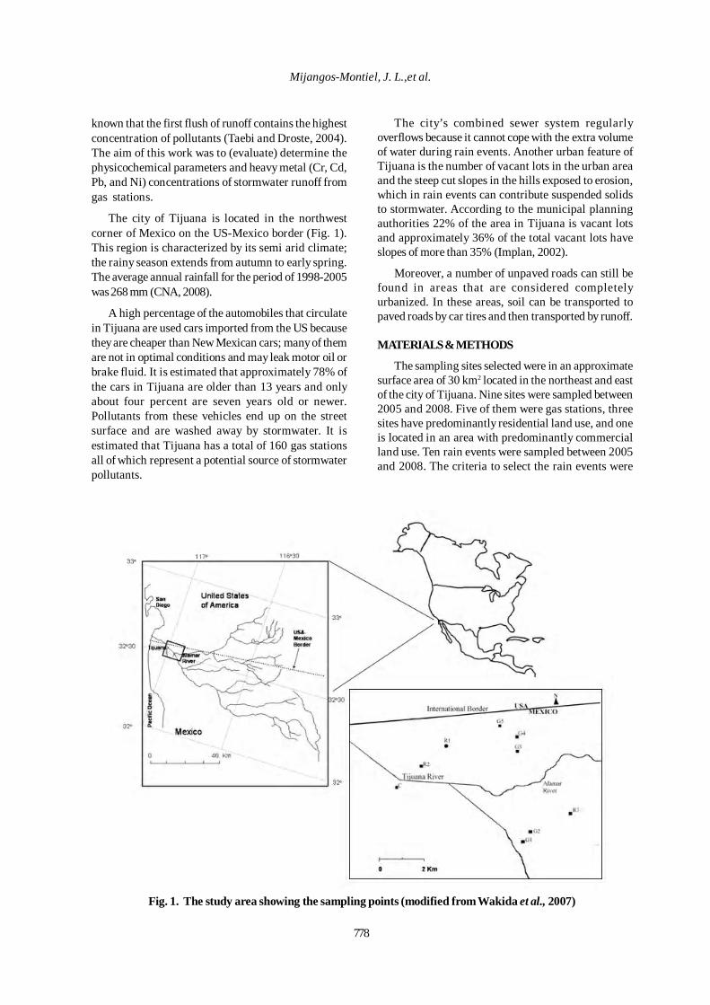
778
Mijangos-Montiel, J. L.,et al.
known that the first flush of runoff contains the highestconcentration of pollutants (Taebi and Droste, 2004).The aim of this work was to (evaluate) determine thephysicochemical parameters and heavy metal (Cr, Cd,Pb, and Ni) concentrations of stormwater runoff fromgas stations.
The city of Tijuana is located in the northwestcorner of Mexico on the US-Mexico border (Fig. 1).This region is characterized by its semi arid climate;the rainy season extends from autumn to early spring.The average annual rainfall for the period of 1998-2005was 268 mm (CNA, 2008).
A high percentage of the automobiles that circulatein Tijuana are used cars imported from the US becausethey are cheaper than New Mexican cars; many of themare not in optimal conditions and may leak motor oil orbrake fluid. It is estimated that approximately 78% ofthe cars in Tijuana are older than 13 years and onlyabout four percent are seven years old or newer.Pollutants from these vehicles end up on the streetsurface and are washed away by stormwater. It isestimated that Tijuana has a total of 160 gas stationsall of which represent a potential source of stormwaterpollutants.
The city’s combined sewer system regularlyoverflows because it cannot cope with the extra volumeof water during rain events. Another urban feature ofTijuana is the number of vacant lots in the urban areaand the steep cut slopes in the hills exposed to erosion,which in rain events can contribute suspended solidsto stormwater. According to the municipal planningauthorities 22% of the area in Tijuana is vacant lotsand approximately 36% of the total vacant lots haveslopes of more than 35% (Implan, 2002).
Moreover, a number of unpaved roads can still befound in areas that are considered completelyurbanized. In these areas, soil can be transported topaved roads by car tires and then transported by runoff.
MATERIALS & METHODS
The sampling sites selected were in an approximatesurface area of 30 km2 located in the northeast and eastof the city of Tijuana. Nine sites were sampled between2005 and 2008. Five of them were gas stations, threesites have predominantly residential land use, and oneis located in an area with predominantly commercialland use. Ten rain events were sampled between 2005and 2008. The criteria to select the rain events were
Fig. 1. The study area showing the sampling points (modified from Wakida et al., 2007)

Int. J. Environ. Res., 4(4):777-784 , Autumn 2010
779
that the storm was preceded by at least 72 hours of dryweather and a rainfall higher than 2.5 mm (USEPA,1990). Table 1 shows the rainfall data of the rain eventssampled in this study. Three duplicate grab sampleswere taken directly in the street pipes that conduct thestormwater out of the gas stations, except for site G4,where samples were taken in an area where water wasstagnant. In the other sites (R1, R2, R3 and C) thesamples were taken directly from road and drain runoff.The duplicate samples were collected in differentstages of the rain events.
The selection criteria for gas stations were that theyhave a conduit that carries stormwater to the street.Only one of the sites has a small area with a crevice inthe pavement where water accumulates (G4). Three ofthe gas stations also have diesel dispatchers (G1, G2and G5) and one has a car wash on the premises (G2).The drainage area of the gas stations was between1176 to 2772 m2, the largest being site G1. Thecommercial land use (C) site has a drain located in anarea close to a horse racing track and a golf coursewith an approximate drainage area of 113 ha. Site R1drains an area of approximately 13 ha with a lowerpopulation density (92 inhabitants/ha), populated byhigh-income families. The residential R2 site has anopen channel that drains an area with houses ownedby low-income families. The approximate populationdensity is 63 inhabitants/ha and the drainage area isabout 44.6 ha. A number of auto repair shops are foundin the area that drains site R2. The drainage area of siteR3 is 2 ha and is densely populated (> 200 inhabitants/ha). Samples were analyzed for chemical oxygen demand(COD), total phosphate (TP), nitrate, sulphate, totalsuspended solids (TSS), total dissolved solids (TDS),oil and grease (OG) and heavy metals (Cr, Cd, Ni andPb). These physicochemical parameters are commonlyanalyzed in stormwater studies. The heavy metalsanalyzed were selected for their toxicity.
Heavy metals were analyzed by atomic absorptionusing a spectrophotometer with a graphite furnace
(Perkin-Elmer 3100, graphite furnace HGA 600). TSSanalysis was performed according to the MexicanStandard NMX-AA-034-SFCI-2001. Oil and grease wereanalyzed under Mexican Standard NMX-AA-005-SFCI-2000, in which oil and grease are adsorbed in diatomsoil and then extracted with hexane, evaporated andlater weighed. Nitrate was measured using the cadmiumreduction method, COD by the reactor digestionmethod, sulphate by the turbidity method andphosphate by the acid persulphate digestion method.Unit loads for runoff in gas stations and residentialsites were calculated based on the equation
L=10000 SMC X P X RC where L is the unit load(Kg/ha), SMC is the site mean concentration (kg m-3),P is rainfall depth (m) and RC the runoff coefficient.For the gas stations an RC of 0.95 was used and for theresidential sites the RCs used were those estimated byWinckell and Le Page (2003) for these urban basins inTijuana. An RC value of 0.7 was utilized for sites R1and R2 and an RC value of 0.8 for R3.
RESULTS & DISCUSSIONSulphate, TDS, TP, Cr and Pb concentrations
showed a tendency to decrease concomitant with theadvance of the rainy season. This phenomenon is dueto the “washing” effect of the deposited material bystormwater runoff, which has been reported by anotherstudy conducted in Los Angeles, USA (McPherson etal., 2005). No clear tendency of concentration reductionwas observed for nitrate, OG, TSS, COD, Cd or Ni. Thismay be the result of different amounts of rainfall or ofa constant input of these pollutants in the study sites.For example, the frequent entrance of cars with oil leaksto the gas station sites can produce the accumulationof oil and grease on the surface.
The range and mean of the physicochemicalparameters analyzed in all the rain events are shown inTable 2. The highest mean concentration (1084 mg/L)of oil and grease (OG) was found in gas station G1 andthe maximum OG concentration was found in G1 (3436mg/L), where diesel spillages were observed in the load
Table 1. Rainfall characteristics of the sampling events
Rain event
Date (month-day-year)
Average rainfall intensity (mm/hr)
Maximum rainfall intensity (mm/hr)
Total rainfall (mm)
Dry days previous to rainfall event (days)
1 10-17-05 1.33 2.0 4.3 172 2 11-10-05 1.00 1.0 2.8 14 3 02-27-06 2.71 6.0 6.9 47 4 03-10-06 1.62 2.0 8.1 11 5 04-04-06 2.11 4.0 8.1 18 6 11-30-07 1.74 4.0 13.7 55 7 01-06-08 1.33 2.0 11.2 26 8 01-26-08 1.25 2.0 5.0 18 9 02-03-08 1.12 2.0 7.9 7 10 02-14-08 2.07 5.0 25.0 11
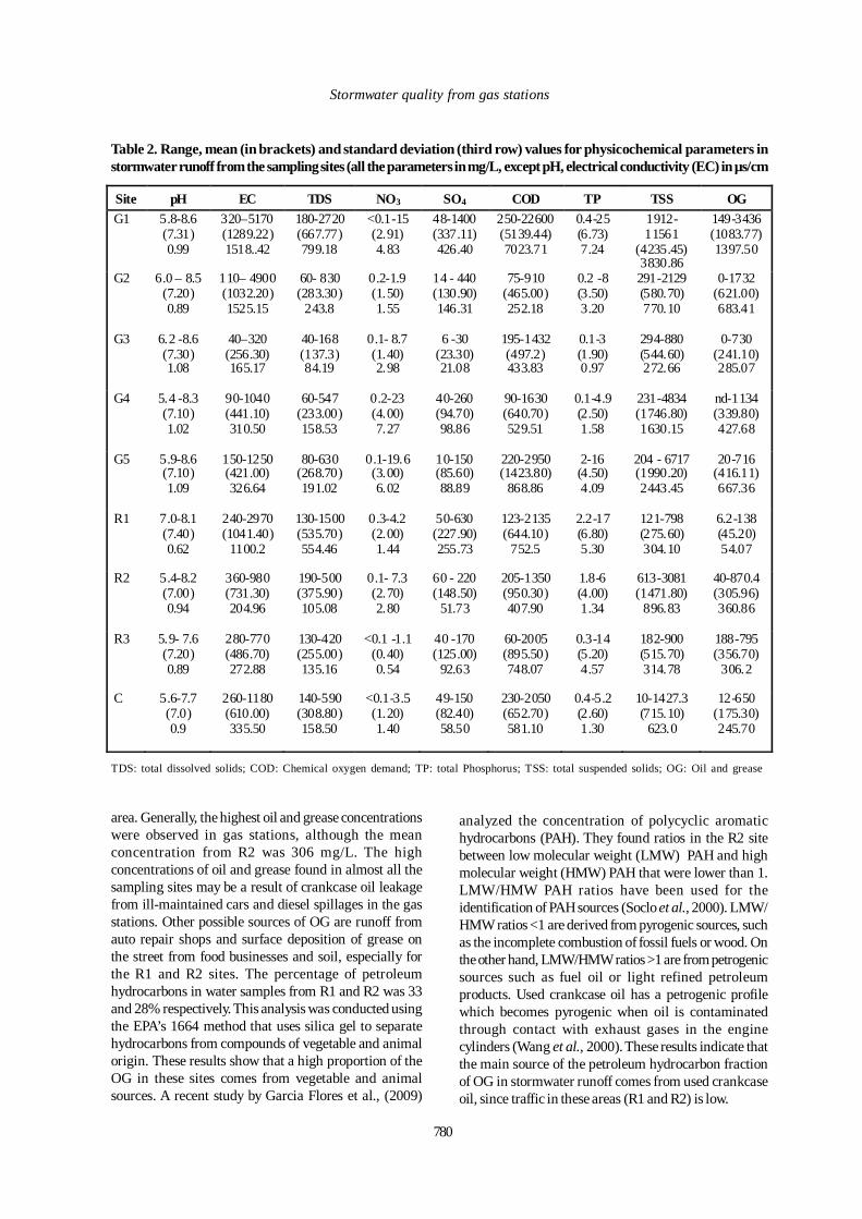
780
Stormwater quality from gas stations
Table 2. Range, mean (in brackets) and standard deviation (third row) values for physicochemical parameters instormwater runoff from the sampling sites (all the parameters in mg/L, except pH, electrical conductivity (EC) in µs/cm
Site pH EC TDS NO3 SO4 COD TP TSS OG G1 5.8-8.6
(7.31) 0.99
320–5170 (1289.22) 1518..42
180-2720 (667.77) 799.18
<0.1-15 (2.91) 4.83
48-1400 (337.11) 426.40
250-22600 (5139.44) 7023.71
0.4-25 (6.73) 7.24
1912-11561
(4235.45) 3830.86
149-3436 (1083.77) 1397.50
G2 6.0 – 8.5 (7.20) 0.89
110– 4900 (1032.20) 1525.15
60- 830 (283.30)
243.8
0.2-1.9 (1.50) 1.55
14 - 440 (130.90) 146.31
75-910 (465.00) 252.18
0.2 -8 (3.50) 3.20
291-2129 (580.70) 770.10
0-1732 (621.00) 683.41
G3 6.2 -8.6
(7.30) 1.08
40–320 (256.30) 165.17
40-168 (137.3) 84.19
0.1- 8.7 (1.40) 2.98
6 -30 (23.30) 21.08
195-1432 (497.2) 433.83
0.1-3 (1.90) 0.97
294-880 (544.60) 272.66
0-730 (241.10) 285.07
G4 5.4 -8.3
(7.10) 1.02
90-1040 (441.10) 310.50
60-547 (233.00) 158.53
0.2-23 (4.00) 7.27
40-260 (94.70) 98.86
90-1630 (640.70) 529.51
0.1-4.9 (2.50) 1.58
231-4834 (1746.80) 1630.15
nd-1134 (339.80) 427.68
G5 5.9-8.6
(7.10) 1.09
150-1250 (421.00) 326.64
80-630 (268.70) 191.02
0.1-19.6 (3.00) 6.02
10-150 (85.60) 88.89
220-2950 (1423.80)
868.86
2-16 (4.50) 4.09
204 - 6717 (1990.20) 2443.45
20-716 (416.11) 667.36
R1 7.0-8.1
(7.40) 0.62
240-2970 (1041.40)
1100.2
130-1500 (535.70) 554.46
0.3-4.2 (2.00) 1.44
50-630 (227.90) 255.73
123-2135 (644.10)
752.5
2.2-17 (6.80) 5.30
121-798 (275.60) 304.10
6.2-138 (45.20) 54.07
R2 5.4-8.2
(7.00) 0.94
360-980 (731.30) 204.96
190-500 (375.90) 105.08
0.1- 7.3 (2.70) 2.80
60 - 220 (148.50)
51.73
205-1350 (950.30) 407.90
1.8-6 (4.00) 1.34
613-3081 (1471.80)
896.83
40-870.4 (305.96) 360.86
R3 5.9- 7.6
(7.20) 0.89
280-770 (486.70) 272.88
130-420 (255.00) 135.16
<0.1 -1.1 (0.40) 0.54
40 -170 (125.00)
92.63
60-2005 (895.50) 748.07
0.3-14 (5.20) 4.57
182-900 (515.70) 314.78
188-795 (356.70)
306.2
C 5.6-7.7 (7.0) 0.9
260-1180 (610.00) 335.50
140-590 (308.80) 158.50
<0.1-3.5 (1.20) 1.40
49-150 (82.40) 58.50
230-2050 (652.70) 581.10
0.4-5.2 (2.60) 1.30
10-1427.3 (715.10)
623.0
12-650 (175.30) 245.70
TDS: total dissolved solids; COD: Chemical oxygen demand; TP: total Phosphorus; TSS: total suspended solids; OG: Oil and grease
area. Generally, the highest oil and grease concentrationswere observed in gas stations, although the meanconcentration from R2 was 306 mg/L. The highconcentrations of oil and grease found in almost all thesampling sites may be a result of crankcase oil leakagefrom ill-maintained cars and diesel spillages in the gasstations. Other possible sources of OG are runoff fromauto repair shops and surface deposition of grease onthe street from food businesses and soil, especially forthe R1 and R2 sites. The percentage of petroleumhydrocarbons in water samples from R1 and R2 was 33and 28% respectively. This analysis was conducted usingthe EPA’s 1664 method that uses silica gel to separatehydrocarbons from compounds of vegetable and animalorigin. These results show that a high proportion of theOG in these sites comes from vegetable and animalsources. A recent study by Garcia Flores et al., (2009)
analyzed the concentration of polycyclic aromatichydrocarbons (PAH). They found ratios in the R2 sitebetween low molecular weight (LMW) PAH and highmolecular weight (HMW) PAH that were lower than 1.LMW/HMW PAH ratios have been used for theidentification of PAH sources (Soclo et al., 2000). LMW/HMW ratios <1 are derived from pyrogenic sources, suchas the incomplete combustion of fossil fuels or wood. Onthe other hand, LMW/HMW ratios >1 are from petrogenicsources such as fuel oil or light refined petroleumproducts. Used crankcase oil has a petrogenic profilewhich becomes pyrogenic when oil is contaminatedthrough contact with exhaust gases in the enginecylinders (Wang et al., 2000). These results indicate thatthe main source of the petroleum hydrocarbon fractionof OG in stormwater runoff comes from used crankcaseoil, since traffic in these areas (R1 and R2) is low.
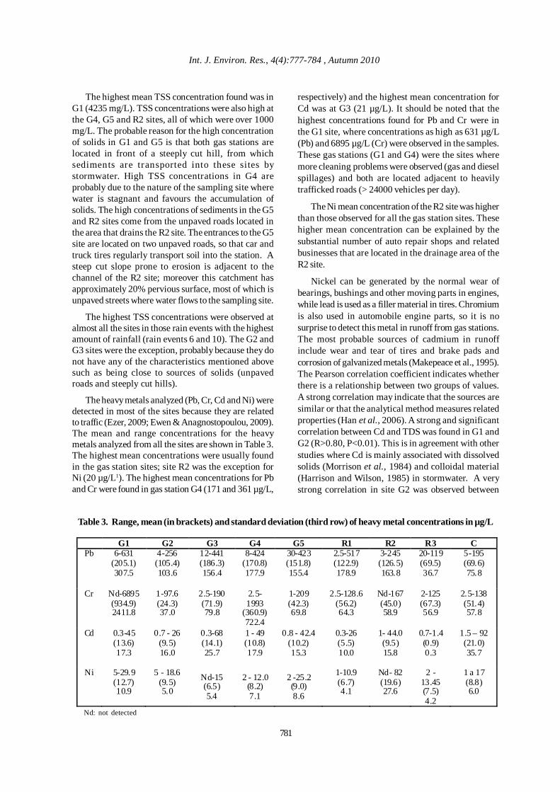
Int. J. Environ. Res., 4(4):777-784 , Autumn 2010
The highest mean TSS concentration found was inG1 (4235 mg/L). TSS concentrations were also high atthe G4, G5 and R2 sites, all of which were over 1000mg/L. The probable reason for the high concentrationof solids in G1 and G5 is that both gas stations arelocated in front of a steeply cut hill, from whichsediments are transported into these sites bystormwater. High TSS concentrations in G4 areprobably due to the nature of the sampling site wherewater is stagnant and favours the accumulation ofsolids. The high concentrations of sediments in the G5and R2 sites come from the unpaved roads located inthe area that drains the R2 site. The entrances to the G5site are located on two unpaved roads, so that car andtruck tires regularly transport soil into the station. Asteep cut slope prone to erosion is adjacent to thechannel of the R2 site; moreover this catchment hasapproximately 20% pervious surface, most of which isunpaved streets where water flows to the sampling site.
The highest TSS concentrations were observed atalmost all the sites in those rain events with the highestamount of rainfall (rain events 6 and 10). The G2 andG3 sites were the exception, probably because they donot have any of the characteristics mentioned abovesuch as being close to sources of solids (unpavedroads and steeply cut hills).
The heavy metals analyzed (Pb, Cr, Cd and Ni) weredetected in most of the sites because they are relatedto traffic (Ezer, 2009; Ewen & Anagnostopoulou, 2009).The mean and range concentrations for the heavymetals analyzed from all the sites are shown in Table 3.The highest mean concentrations were usually foundin the gas station sites; site R2 was the exception forNi (20 µg/L1). The highest mean concentrations for Pband Cr were found in gas station G4 (171 and 361 µg/L,
respectively) and the highest mean concentration forCd was at G3 (21 µg/L). It should be noted that thehighest concentrations found for Pb and Cr were inthe G1 site, where concentrations as high as 631 µg/L(Pb) and 6895 µg/L (Cr) were observed in the samples.These gas stations (G1 and G4) were the sites wheremore cleaning problems were observed (gas and dieselspillages) and both are located adjacent to heavilytrafficked roads (> 24000 vehicles per day).
The Ni mean concentration of the R2 site was higherthan those observed for all the gas station sites. Thesehigher mean concentration can be explained by thesubstantial number of auto repair shops and relatedbusinesses that are located in the drainage area of theR2 site.
Nickel can be generated by the normal wear ofbearings, bushings and other moving parts in engines,while lead is used as a filler material in tires. Chromiumis also used in automobile engine parts, so it is nosurprise to detect this metal in runoff from gas stations.The most probable sources of cadmium in runoffinclude wear and tear of tires and brake pads andcorrosion of galvanized metals (Makepeace et al., 1995).The Pearson correlation coefficient indicates whetherthere is a relationship between two groups of values.A strong correlation may indicate that the sources aresimilar or that the analytical method measures relatedproperties (Han et al., 2006). A strong and significantcorrelation between Cd and TDS was found in G1 andG2 (R>0.80, P<0.01). This is in agreement with otherstudies where Cd is mainly associated with dissolvedsolids (Morrison et al., 1984) and colloidal material(Harrison and Wilson, 1985) in stormwater. A verystrong correlation in site G2 was observed between
Table 3. Range, mean (in brackets) and standard deviation (third row) of heavy metal concentrations in µg/L
G1 G2 G3 G4 G5 R1 R2 R3 C Pb 6-631
(205.1) 307.5
4-256 (105.4) 103.6
12-441 (186.3) 156.4
8-424 (170.8) 177.9
30-423 (151.8) 155.4
2.5-517 (122.9) 178.9
3-245 (126.5) 163.8
20-119 (69.5) 36.7
5-195 (69.6) 75.8
Cr Nd-6895 (934.9) 2411.8
1-97.6 (24.3) 37.0
2.5-190 (71.9) 79.8
2.5-1993
(360.9) 722.4
1-209 (42.3) 69.8
2.5-128.6 (56.2) 64.3
Nd-167 (45.0) 58.9
2-125 (67.3) 56.9
2.5-138 (51.4) 57.8
Cd 0.3-45 (13.6) 17.3
0.7 - 26 (9.5) 16.0
0.3-68 (14.1) 25.7
1 - 49 (10.8) 17.9
0.8 - 42.4 (10.2) 15.3
0.3-26 (5.5) 10.0
1- 44.0 (9.5) 15.8
0.7-1.4 (0.9) 0.3
1.5 – 92 (21.0) 35.7
Ni 5-29.9 (12.7) 10.9
5 - 18.6 (9.5) 5.0
Nd-15 (6.5) 5.4
2 - 12.0 (8.2) 7.1
2 -25.2 (9.0) 8.6
1-10.9 (6.7) 4.1
Nd- 82 (19.6) 27.6
2 - 13.45 (7.5) 4.2
1 a 17 (8.8) 6.0
Nd: not detected
781
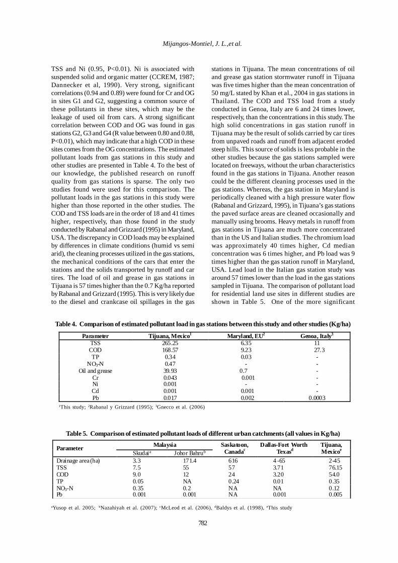
782
Mijangos-Montiel, J. L.,et al.
TSS and Ni (0.95, P<0.01). Ni is associated withsuspended solid and organic matter (CCREM, 1987;Dannecker et al, 1990). Very strong, significantcorrelations (0.94 and 0.89) were found for Cr and OGin sites G1 and G2, suggesting a common source ofthese pollutants in these sites, which may be theleakage of used oil from cars. A strong significantcorrelation between COD and OG was found in gasstations G2, G3 and G4 (R value between 0.80 and 0.88,P<0.01), which may indicate that a high COD in thesesites comes from the OG concentrations. The estimatedpollutant loads from gas stations in this study andother studies are presented in Table 4. To the best ofour knowledge, the published research on runoffquality from gas stations is sparse. The only twostudies found were used for this comparison. Thepollutant loads in the gas stations in this study werehigher than those reported in the other studies. TheCOD and TSS loads are in the order of 18 and 41 timeshigher, respectively, than those found in the studyconducted by Rabanal and Grizzard (1995) in Maryland,USA. The discrepancy in COD loads may be explainedby differences in climate conditions (humid vs semiarid), the cleaning processes utilized in the gas stations,the mechanical conditions of the cars that enter thestations and the solids transported by runoff and cartires. The load of oil and grease in gas stations inTijuana is 57 times higher than the 0.7 Kg/ha reportedby Rabanal and Grizzard (1995). This is very likely dueto the diesel and crankcase oil spillages in the gas
stations in Tijuana. The mean concentrations of oiland grease gas station stormwater runoff in Tijuanawas five times higher than the mean concentration of50 mg/L stated by Khan et al., 2004 in gas stations inThailand. The COD and TSS load from a studyconducted in Genoa, Italy are 6 and 24 times lower,respectively, than the concentrations in this study. Thehigh solid concentrations in gas station runoff inTijuana may be the result of solids carried by car tiresfrom unpaved roads and runoff from adjacent erodedsteep hills. This source of solids is less probable in theother studies because the gas stations sampled werelocated on freeways, without the urban characteristicsfound in the gas stations in Tijuana. Another reasoncould be the different cleaning processes used in thegas stations. Whereas, the gas station in Maryland isperiodically cleaned with a high pressure water flow(Rabanal and Grizzard, 1995), in Tijuana’s gas stationsthe paved surface areas are cleaned occasionally andmanually using brooms. Heavy metals in runoff fromgas stations in Tijuana are much more concentratedthan in the US and Italian studies. The chromium loadwas approximately 40 times higher, Cd medianconcentration was 6 times higher, and Pb load was 9times higher than the gas station runoff in Maryland,USA. Lead load in the Italian gas station study wasaround 57 times lower than the load in the gas stationssampled in Tijuana. The comparison of pollutant loadfor residential land use sites in different studies areshown in Table 5. One of the more significant
Table 4. Comparison of estimated pollutant load in gas stations between this study and other studies (Kg/ha)
Parameter Tijuana, Mexico1 Maryland, EU2 Genoa, Italy3 TSS 265.25 6.35 11 COD 168.57 9.23 27.3 TP 0.34 0.03 -
NO3-N 0.47 - - Oil and grease 39.93 0.7 -
Cr 0.043 0.001 - Ni 0.001 - - Cd 0.001 0.001 - Pb 0.017 0.002 0.0003
1This study; 2Rabanal y Grizzard (1995); 3Gnecco et al. (2006)
Malaysia Parameter Skudaia Johor Bahrub
Saskatoon, Canadac
Dallas-Fort Worth Texasd
Tijuana, Mexicoe
Drainage area (ha) 3.3 171.4 616 4 -65 2-45 TSS 7.5 55 57 3.71 76.15 COD 9.0 12 24 3.20 54.0 TP 0.05 NA 0.24 0.01 0.35 NO3-N 0.35 0.2 NA NA 0.12 Pb 0.001 0.001 NA 0.001 0.005
Table 5. Comparison of estimated pollutant loads of different urban catchments (all values in Kg/ha)
aYusop et al. 2005; bNazahiyah et al. (2007); cMcLeod et al. (2006), dBaldys et al. (1998), eThis study
783
Int. J. Environ. Res., 4(4):777-784, Autumn 2010
differences was found in the COD load. Mean CODload found in residential areas in Tijuana were 2 and 5times higher than the load values reported in the studiesfrom Canada (24 Kg/ha) and Indonesia (12 Kg/ha),respectively. This difference of COD concentrationscan be explained in terms of catchment size. TheCanadian and Indonesian studies used a much largerarea. Other probable reasons could be the differencesin climates and the high OG content found in stormwaterrunoff from residential areas in Tijuana. The maximumOG concentrations in R2 and R3 were 870 and 795 mg/L (Table 2).
The load of TSS in stormwater runoff fromresidential sites in Tijuana is higher than that reportedby other studies. This may be the result of a higher soilerosion rate as a result of the shanty settlements onland with high slopes (> 35%) and the percentage ofunpaved roads that reach 20% in site R2.
CONCLUSIONThe results from this study have shown that the
pollutant concentrations in runoff from gas stations inTijuana are higher than those reported by studiesconducted in other countries. The COD and TSS loadsin gas station runoff were in the order of 18 and 41times higher, respectively, than in a study carried outin Maryland, US. The high TSS and CODconcentrations observed in this study may be producedby poor cleaning conditions and crankcase oil leakagefrom cars.
A higher load of COD was observed in stormwaterfrom residential areas in Tijuana than in other publishedstudies. This may be the result of higher OGconcentrations in runoff due to crankcase oil leakagesobserved in many streets and parking lots in Tijuana.Our results show that stormwater runoff from gasstations can be a significant source of pollutants tourban runoff in a city of a developing country with asemi arid climate. The results presented here will behelpful in evaluating the contribution of pollutants tostormwater from gas stations, and may provide decisiontools for the implementation of pollution controlmeasures in these facilities.
ACKNOWLEDGEMENTThe authors gratefully acknowledge the Mexican
Council of Science and Technology (CONACYT) forawarding a doctoral scholarship to J.L Mijangos, theUniversidad Autónoma de Baja California for itsfinancial support, and professors Mario Del Valle andSamuel Meléndez-Lopez for proof-reading this andearlier versions of the manuscript of this article.
REFERENCESAbduli, M. A., Nabi Bidhendi, G. R , Nasrabadi, T. andHoveidi, H. (2007). Evaluating the Reduction of HazardousWaste Contact in Tabriz Petrochemical Complex, Focusingon Personal Protective Equipment Method. Int. Journal.Environ. Res., 1(1), 14-18.
Adekunle, I.M., Ajijo, M.R., Adeofun, C.O. and Omoniyi,I.T. (2010). Response of Four Phytoplankton Species Foundin Some Sectors of Nigerian Coastal Waters to Crude Oil inControlled Ecosystem. Int. Journal. Environ. Res., 4(1),65-74.
Bagherzadeh-Namazi, A., Shojaosadati, S. A. and Hashemi-Najafabadi, S. (2008). Biodegradation of Used Engine OilUsing Mixed and Isolated Cultures. Int. Journal. Environ.Res., 2(4), 431-440.
Baldys S., Raines, T. H., Mansfield B. L. and Sanding J. T.(1998). Urban stormwater quality, event-meanconcentrations and estimated of stormwater pollutant loadDallas-Forth Worth area, Texas, 1992-93. USGS Water-Resources Investigations Report, 98-4158.
Borden, R. C., Black D. C. and Mcblief K. V. (2002). MTBEand aromatic hydrocarbons in North Carolina stormwaterrunoff. Environ. Pollut., 118, 141-152.
Comisión Nacional del Agua (CNA) (2008). Datos inéditosde precipitación pluvial de la presa Abelardo L. Rodríguez(unpublished data of annual rainfall of the Abelardo L.Rodríguez Dam). CNA, Tijuana. México.
CCREM (Canadian Council of Resource and EnvironmentMinisters) (1987). Canadian Water Quality Guidelines,Health and Welfare, Canada.
Dannecker, W., Au, M. and Stechmann H. (1990). Substanceload in rainwater runoff from different streets in Hamburg.Sci. Total Environ., 93, 385-392.
Durán, A. C. and González, A. (2009). Determination oflead, naphthalene, phenanthrene, anthracene and pyrene instreet dust. Int. Journal. Environ. Sci. Tech., 6(4), 663-670.
Estebe, A., Boudries, H., Mouchel J. M. and Thevenot D.R. (1998). Urban runoff impacts on particulate metal andhydrocarbon concentrations in river Seine: suspended solidand sediment transport. Water Sci. Technol., 36 (8-9), 185-193.
Ewen, C. and Anagnostopoulou, M. (2009). Monitoring ofheavy metal levels in roadside dusts of Thessaloniki, Greecein relation to motor vehicle traffic density and flow. Environ.Monit. Assess., 157 (1-4), 483-498.
Ezer, M. (2009). Heavy metal content of roadside soil inKahramanmaras, Turkey. Fresenius environ. Bull., 18 (5a),704-708.
García-Flores E., Herrera-Castañón I., Vega-Cruz D. A.,López-Laureano E., Rodríguez-Ventura G., Espinoza-Gómez H. and Wakida F. T. (2009). Sources of oil andgrease in stormwater of Tijuana, Mexico. (Paper presentedat the 13th Conference on Diffuse Pollution. Seoul, SouthKorea, October 12-15, Mexico.
784
Stormwater quality from gas stations
Gnecco I., Berreta C., Lanza L. G. and La Barbera P. (2006).Quality of stormwater runoff from paved surface of twoproduction sites. Water Sci. Technol., 54 (6-7), 177-184.
Gromaire-Mertz M. C., Garnaud S., Gonzalez A. andChebbo G. (1999). Characterisation of urban runoff pollutionin Paris. Water Sci. Technol., 39 (2), 1-8.
Han Y., Lau S. L., Kayhanian M. and Stenstrom M. K.(2006). Characteristics of highway stormwater runoff. WaterEnviron. Res., 78 (12), 2377-2388.
Harrison, R. M. and Wilson S. J. (1985). The chemicalcomposition of highway drainage waters. III. Runoff watermetal speciation characteristics. Sci. Total Environ., 43 (1-2), 89-102.
Hassani, A. H., Otadi, N., Javid, A.H., Khiabani, F.F. andHoshyaripour, G. (2009). Improving the performance ofPars Oil Refinery Wastewater Treatment System. Int.Journal. Environ. Res., 3(4), 653-662.
IMPLAN. (2002). Programa de Desarrollo Urbano delCentro de Población Tijuana 2002-2025 (Program of urbandevelopment of the City of Tijuana). Periódico Oficial delEstado de Baja California, 13 de diciembre de, No. 54.
Jafari, H. R. and Ebrahimi, S. (2007). A Study on RiskAssessment of Benzene as one of the VOCs Air Pollution.Int. Journal. Environ. Res., 1(3), 214-217.
Khan, E., Virojnagud W. and Ratpudki T. (2004). Use ofbiomass sorbent for oil removal from gas station runoff.Chemosphere, 57, 681-689.
Makepeace D. K, Smith D. W. and Stanley S. J. (1995).Urban stormwater quality: Summary of Contaminant Data.,Crit. Rev. Environ. Sci. Technol., 25 (2), 93-139.
Mcleod, S. M., Kells J. A. and Putz G. J. (2006). Urbanrunoff quality characterization and load estimation inSaskaton, Canada. J. Environ. Engin. ASCE, 132 (11), 1470-1481.
McPherson, T. N., Burian, S. J., Stenstrom, M. K., Turin,H. J., Brown, M. J and Suffet, I. H. (2005). Trace metalpollutant load in urban runoff from a southern Californiawatershed. J. Environ. Engin. ASCE., 131, 1073-1080.
Morrison, G. M. P., Revitt, D. M., Ellis, J. B., Svensson.,G. and Balmer, P. (1984). Variations of dissolved andsuspended solid heavy metals through an urban hydrograph.Environ. Technol. Let., 7, 313.
Nazahiyah, R., Yusop, Z. and Abustan, L. (2007) Stormwaterquality and pollution loading from an urban residentialcatchment in Johor, Malaysia. Water Sci. Technol., 56 (7), 1-9.
Nouri, J., Omidvari, M. and Tehrani, S.M. (2010). RiskAssessment and Crisis Management in Gas Stations. Int.Journal. Environ. Res., 4(1), 143-152.
Onwurah, I. N. E., Ogugua, V. N., Onyike, N. B., Ochonogor,A. E. and Otitoju, O. F. (2007). Crude Oil Spills in theEnvironment, Effects and Some Innovative Clean-upBiotechnologies. Int. Journal. Environ. Res., 1(4),307-320.
Otitoloju, A. A. (2010). Evaluation of Crude Oil DegradationUnder a No-Control and Dispersant-Control Settings, Basedon Biological and Physical Techniques. Int. Journal. Environ.Res., 4(2), 353-360.
Rabanal F. I. and Grizzard T. (1995). Concentrations ofselected constituents in runoff from impervious surfaces infour urban catchments of different land use (Paper presentedin the Four Biennial Stormwater Research Conference,Florida) retrieved February 12, 2007, fromwww.owr.ehnr.state.nc.us/ref/41/40302.pdf.
Sansalone J. J. and Buchberger S. G. (1995). An infiltrationdevice as a best management practice for immobilizing heavymetals in urban highway runoff. Water Sci. Technol., 32 (1),119-125.
Soclo H. H., Garrigues P. and Ewald M. (2000). Origin ofpolycyclic aromatic hydrocarbons (PAHs) in coastal marinesediments: case studies in Cotonou (Benin) and Aquitaine(France) areas. Mar. Poll. Bull., 40, 387-96.
Taebi A. and Droste R. L. (2004). First flush pollution loadof urban stormwater runoff. J. Environ. Eng. Sci., 3, 301-309.
U.S. Environmental protection agency (1990). NationalPollutant Discharge Elimination System Permit ApplicationRegulations for stormwater discharges- Final rule: U.S.Federal Register. 55 (22), 47989-48091.
Yussop, Z., Tang, L. W., Ujang, Z, Mohamed, M. and Nasir,K. (2005). Runoff quality and pollution loadings from atropical urban catchment. Water Sci. Technol., 52 (9), 125-32.
Wang, J., Jia C. R., Wong C. K. and Wong P. K. (2000).Characterization of polycyclic aromatic hydrocarbonscreated in lubricating oils. Water air soil poll., 120, 381-396.
Wakida, F. T., Lara D., Temores-Peña J., Rodríguez-VenturaG., Díaz C., García-Flores E. (2007). Heavy metals insediments of the Tecate River. Environ. Geol., 54, 637-642.
Winckell, A. and Le Page, A. (2003). El Niño in the city:Vulnerability assessment in Tijuana during the winter of1997-98. Geof. Int., 42 (3), 553-565.
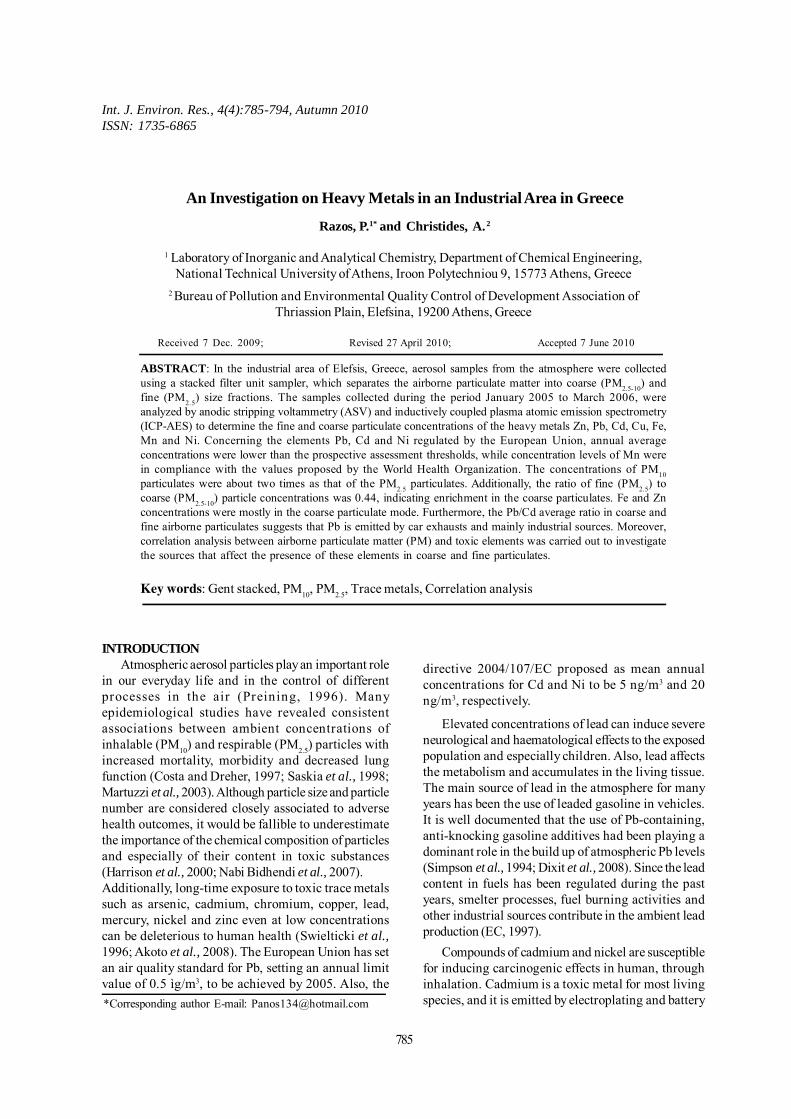
Int. J. Environ. Res., 4(4):785-794, Autumn 2010ISSN: 1735-6865
Received 7 Dec. 2009; Revised 27 April 2010; Accepted 7 June 2010
*Corresponding author E-mail: [email protected]
785
An Investigation on Heavy Metals in an Industrial Area in Greece
Razos, P.1* and Christides, A. 2
1 Laboratory of Inorganic and Analytical Chemistry, Department of Chemical Engineering,National Technical University of Athens, Iroon Polytechniou 9, 15773 Athens, Greece
2 Bureau of Pollution and Environmental Quality Control of Development Association ofThriassion Plain, Elefsina, 19200 Athens, Greece
ABSTRACT: In the industrial area of Elefsis, Greece, aerosol samples from the atmosphere were collectedusing a stacked filter unit sampler, which separates the airborne particulate matter into coarse (PM2.5-10) andfine (PM2.5) size fractions. The samples collected during the period January 2005 to March 2006, wereanalyzed by anodic stripping voltammetry (ASV) and inductively coupled plasma atomic emission spectrometry(ICP-AES) to determine the fine and coarse particulate concentrations of the heavy metals Zn, Pb, Cd, Cu, Fe,Mn and Ni. Concerning the elements Pb, Cd and Ni regulated by the European Union, annual averageconcentrations were lower than the prospective assessment thresholds, while concentration levels of Mn werein compliance with the values proposed by the World Health Organization. The concentrations of PM10particulates were about two times as that of the PM2.5 particulates. Additionally, the ratio of fine (PM2.5) tocoarse (PM2.5-10) particle concentrations was 0.44, indicating enrichment in the coarse particulates. Fe and Znconcentrations were mostly in the coarse particulate mode. Furthermore, the Pb/Cd average ratio in coarse andfine airborne particulates suggests that Pb is emitted by car exhausts and mainly industrial sources. Moreover,correlation analysis between airborne particulate matter (PM) and toxic elements was carried out to investigatethe sources that affect the presence of these elements in coarse and fine particulates.
Key words: Gent stacked, PM10, PM2.5, Trace metals, Correlation analysis
INTRODUCTIONAtmospheric aerosol particles play an important role
in our everyday life and in the control of differentprocesses in the air (Preining, 1996). Manyepidemiological studies have revealed consistentassociations between ambient concentrations ofinhalable (PM10) and respirable (PM2.5) particles withincreased mortality, morbidity and decreased lungfunction (Costa and Dreher, 1997; Saskia et al., 1998;Martuzzi et al., 2003). Although particle size and particlenumber are considered closely associated to adversehealth outcomes, it would be fallible to underestimatethe importance of the chemical composition of particlesand especially of their content in toxic substances(Harrison et al., 2000; Nabi Bidhendi et al., 2007).Additionally, long-time exposure to toxic trace metalssuch as arsenic, cadmium, chromium, copper, lead,mercury, nickel and zinc even at low concentrationscan be deleterious to human health (Swielticki et al.,1996; Akoto et al., 2008). The European Union has setan air quality standard for Pb, setting an annual limitvalue of 0.5 ìg/m3, to be achieved by 2005. Also, the
directive 2004/107/EC proposed as mean annualconcentrations for Cd and Ni to be 5 ng/m3 and 20ng/m3, respectively.
Elevated concentrations of lead can induce severeneurological and haematological effects to the exposedpopulation and especially children. Also, lead affectsthe metabolism and accumulates in the living tissue.The main source of lead in the atmosphere for manyyears has been the use of leaded gasoline in vehicles.It is well documented that the use of Pb-containing,anti-knocking gasoline additives had been playing adominant role in the build up of atmospheric Pb levels(Simpson et al., 1994; Dixit et al., 2008). Since the leadcontent in fuels has been regulated during the pastyears, smelter processes, fuel burning activities andother industrial sources contribute in the ambient leadproduction (EC, 1997).
Compounds of cadmium and nickel are susceptiblefor inducing carcinogenic effects in human, throughinhalation. Cadmium is a toxic metal for most livingspecies, and it is emitted by electroplating and battery
786
Razos, P. and Christides, A.
production industries. Furthermore, cadmium andnickel compounds in particulate matter mainly originatefrom coal and fuel oil combustion processes,metallurgical industry and road transport (EC, 2001;Mugica et al., 2002). Nickel is one of the metals used inthe electroplating industry. Continuous and prolongedexposure to nickel can produce dermatitis and disordersin the respiratory system. Ni-bearing particles occur inthe atmosphere as part of suspended particulate matterand, rarely, of mist aerosols. Ni is commonly associatedwith the fine particulate matter fraction of ambient airsamples with diameters ranging from 0.6 to 10 ìm. Ironand manganese are related to industrial processes.Manganese is a neurotoxic element that in continuousand prolonged exposure causes a neurological diseasecalled manganism. Concerning manganese, exposureto increased levels is known to lead to neurotoxicalimpairments. The suspension of crustal particles(Harrison et al., 2003) and industrial activities arepossibly responsible for the ejection of manganese inthe atmosphere. Iron is a potentially toxic element thatacts as a catalyst in the development of the highly freeoxygen radicals in living organisms (Hemminki et al.,1995). Moreover, elements such as Pb, Cu and Zn aremainly found in the particulate phase. These metalsare mostly emitted into the atmosphere by heavyindustry, coal burning, metallurgical smelters andautomobile traffic (Pacyna, 1986). Zinc is also used inthe lubricant additive zinc diethyldithiophosphate andis therefore likely to be incorporated into road duststhrough oil leakage, and exhaust particles through oilcombustion. A contribution from road traffic for Zn istherefore likely, but is not dominant. Additionally,emissions of atmospheric copper are primarily due tometal production and other industrial processes. Theever-increasing dispersion of heavy metals throughthe atmosphere, water and soil is a major concern dueto their hazardous effect on human health, the possiblechanges they initiate in natural biochemical processesin all ecosystems and their inevitable accumulation inthe food chain.
Up to these days, several studies, on thecomposition of particulate matter in metals, have beenreported for Athens (Scheff et al., 1990; Torfs et al.,1997; Protonotarios et al., 2002; Thomaidis et al., 2003;Manalis et al., 2005) and Thessaloniki, Greece (Samaraet al., 1990; Manoli et al., 2002; Voutsa et al., 2002;Samara et al., 2005). In the framework of anenvironmental study, an ambient particulate monitor(tapered oscillating microbalance - TEOM) (Rupprecht& Patashnick Co, Inc., TEOM Series 1400) was usedfor the industrial area of Elefsis in order to compare theresults found for the PM10 airborne particulates withthose using a Gent stacked filter unit. The findingsshowed for the period January 2005 to December 2005
that there was a very good agreement for the PM10concentrations, 67.0±55.4 ìg/m3 (TEOM) and 69.0±21.8ìg/m3 (Gent-stacked filter unit), respectively. Theobjectives of this investigation include characterizingfine (PM2.5), coarse (PM2.5-10) and inhalable (PM10)concentrations and atmospheric heavy metals, andstudying their temporal variations taking into accountthe meteorological parameters. Correlations betweencoarse (PM2.5-10), fine (PM2.5) particulates and heavymetals have been extracted to identify the major sourcetypes in the industrial area of Elefsis, Greece.
MATERIALS & METHODSSize fractionated airborne particulates were collected
by means of a Gent-type stacked filter unit (Maenhautet al., 1994; Hopke et al., 1997; Hien et al., 2002; Salmaet al., 2006, Kothai et al., 2009), during the period fromJanuary 2005 to March 2006, at an industrial area,Elefsis/Greece.
The sampling station belongs to the Bureau ofPollution and Environmental Quality Control of theDevelopment Association of Thriassion Plain, Elefsina,and is close to the old and narrow exit road from Athensto Corinth. The major industrial plants in the greaterindustrial zone that affect the sampling site includetwo oil refineries, two cement manufacturing plants,two shipyards and a steelworks factory (Fig. 1).
The sampler was installed at a height of 3 m aboveground level and the flow rate of sampling was 16.7 L/min. The operation time for sampling was midnight-to-midnight. The separation of the aerosol particles intotwo size fractions was achieved by the sequentialfiltration through two Nuclepore track-etchpolycarbonate filters (Whatman) of different pore size;each filter has a diameter of 47 mm. The first (coarse)and the second (fine) filters were placed in a stackedfilter cassette that is equipped with an upper-size inletcut-off.
Furthermore, the initial filter is an 8 µm pore 47 mmNuclepore filter and the second filter is an 0.4 µm poreNuclepore filter. The Gent sampler allows the collectionof coarse particles with Effective Cut off Diameter(EAD) between 10 and 2.5 µm (PM10) in the first stageand fine particles with EAD 2.5 µm (PM2.5) in the secondstage. As preliminary studies had shown that theamount of aerosol sampled within 24 h in that area wasoften less than 1 mg, the duration of each samplingperiod was prolonged to 48 h starting at midnight, tocollect enough airborne material for the analyses.
For the leaching process, HNO3 65% w/w(Suprapure, Merck), HCl 30% w/w (Suprapure, Merck)were used. High purity water (HP water) was obtainedfrom a Water Purification System (Barnstead, EasypureRF). Also, for the pH adjustment NH3 25% w/w
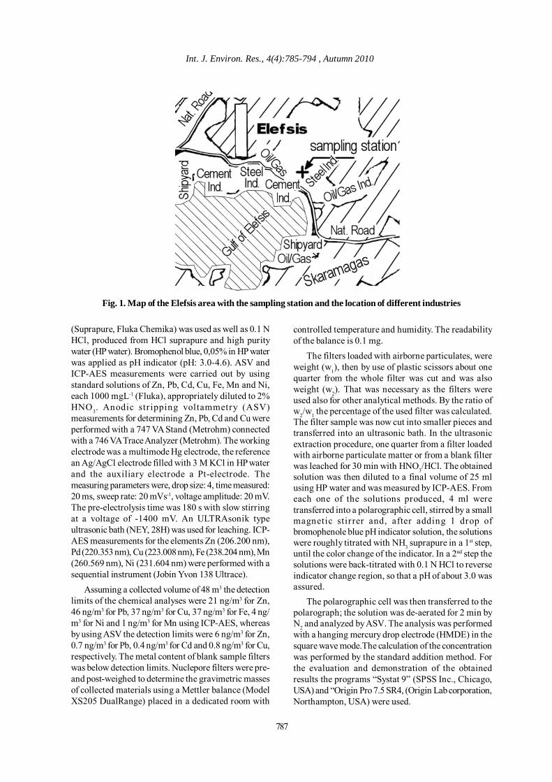
Int. J. Environ. Res., 4(4):785-794 , Autumn 2010
787
Fig. 1. Map of the Elefsis area with the sampling station and the location of different industries
(Suprapure, Fluka Chemika) was used as well as 0.1 NHCl, produced from HCl suprapure and high puritywater (HP water). Bromophenol blue, 0,05% in HP waterwas applied as pH indicator (pH: 3.0-4.6). ASV andICP-AES measurements were carried out by usingstandard solutions of Zn, Pb, Cd, Cu, Fe, Mn and Ni,each 1000 mgL-1 (Fluka), appropriately diluted to 2%HNO3. Anodic str ipping voltammetry (ASV)measurements for determining Zn, Pb, Cd and Cu wereperformed with a 747 VA Stand (Metrohm) connectedwith a 746 VA Trace Analyzer (Metrohm). The workingelectrode was a multimode Hg electrode, the referencean Ag/AgCl electrode filled with 3 M KCl in HP waterand the auxiliary electrode a Pt-electrode. Themeasuring parameters were, drop size: 4, time measured:20 ms, sweep rate: 20 mVs-1, voltage amplitude: 20 mV.The pre-electrolysis time was 180 s with slow stirringat a voltage of -1400 mV. An ULTRAsonik typeultrasonic bath (NEY, 28H) was used for leaching. ICP-AES measurements for the elements Zn (206.200 nm),Pd (220.353 nm), Cu (223.008 nm), Fe (238.204 nm), Mn(260.569 nm), Ni (231.604 nm) were performed with asequential instrument (Jobin Yvon 138 Ultrace).
Assuming a collected volume of 48 m3 the detectionlimits of the chemical analyses were 21 ng/m3 for Zn,46 ng/m3 for Pb, 37 ng/m3 for Cu, 37 ng/m3 for Fe, 4 ng/m3 for Ni and 1 ng/m3 for Mn using ICP-AES, whereasby using ASV the detection limits were 6 ng/m3 for Zn,0.7 ng/m3 for Pb, 0.4 ng/m3 for Cd and 0.8 ng/m3 for Cu,respectively. The metal content of blank sample filterswas below detection limits. Nuclepore filters were pre-and post-weighed to determine the gravimetric massesof collected materials using a Mettler balance (ModelXS205 DualRange) placed in a dedicated room with
controlled temperature and humidity. The readabilityof the balance is 0.1 mg.
The filters loaded with airborne particulates, wereweight (w1), then by use of plastic scissors about onequarter from the whole filter was cut and was alsoweight (w2). That was necessary as the filters wereused also for other analytical methods. By the ratio ofw2/w1 the percentage of the used filter was calculated.The filter sample was now cut into smaller pieces andtransferred into an ultrasonic bath. In the ultrasonicextraction procedure, one quarter from a filter loadedwith airborne particulate matter or from a blank filterwas leached for 30 min with HNO3/HCl. The obtainedsolution was then diluted to a final volume of 25 mlusing HP water and was measured by ICP-AES. Fromeach one of the solutions produced, 4 ml weretransferred into a polarographic cell, stirred by a smallmagnetic stirrer and, after adding 1 drop ofbromophenole blue pH indicator solution, the solutionswere roughly titrated with NH3 suprapure in a 1st step,until the color change of the indicator. In a 2nd step thesolutions were back-titrated with 0.1 N HCl to reverseindicator change region, so that a pH of about 3.0 wasassured.
The polarographic cell was then transferred to thepolarograph; the solution was de-aerated for 2 min byN2 and analyzed by ASV. The analysis was performedwith a hanging mercury drop electrode (HMDE) in thesquare wave mode.The calculation of the concentrationwas performed by the standard addition method. Forthe evaluation and demonstration of the obtainedresults the programs “Systat 9” (SPSS Inc., Chicago,USA) and “Origin Pro 7.5 SR4, (Origin Lab corporation,Northampton, USA) were used.
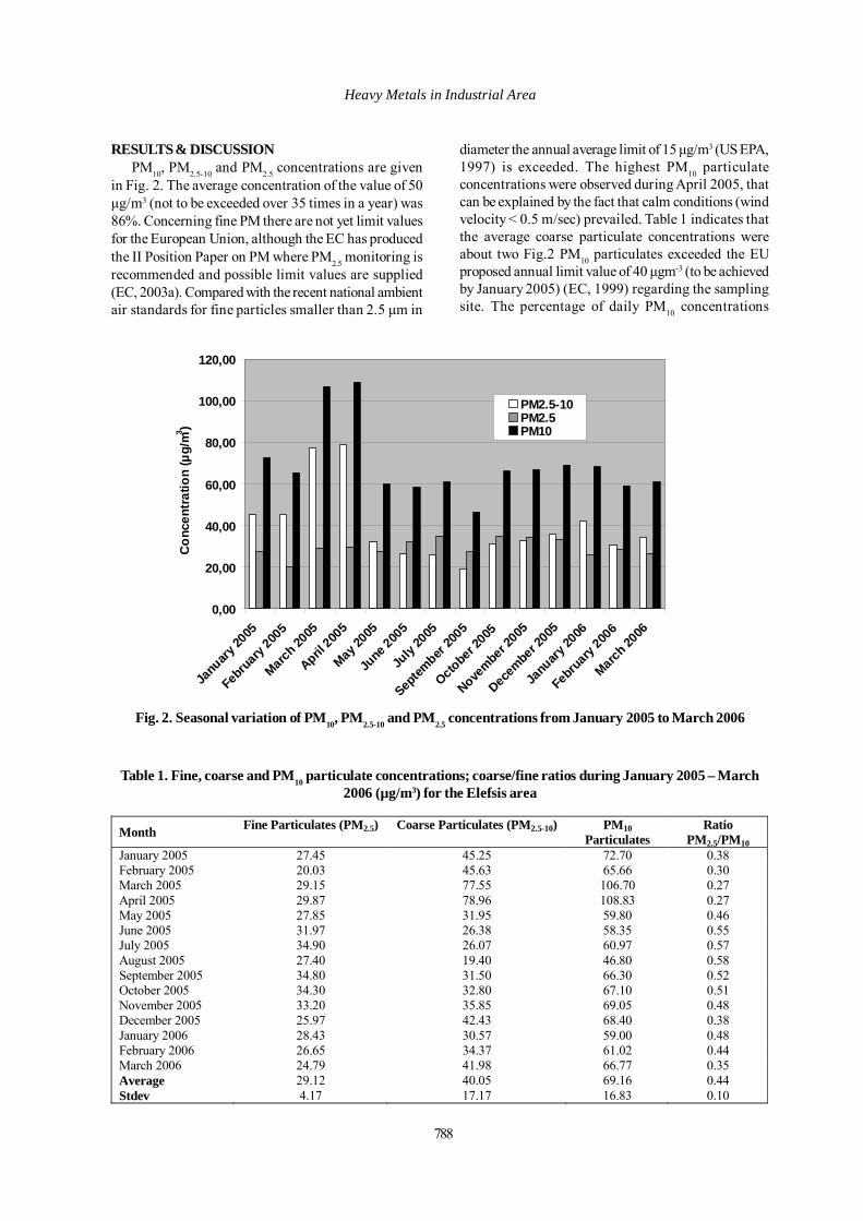
788
Heavy Metals in Industrial Area
Month Fine Particulates (PM2.5) Coarse Particulates (PM2.5-10) PM10 Particulates
Ratio PM2.5/PM10
January 2005 27.45 45.25 72.70 0.38 February 2005 20.03 45.63 65.66 0.30 March 2005 29.15 77.55 106.70 0.27 April 2005 29.87 78.96 108.83 0.27 May 2005 27.85 31.95 59.80 0.46 June 2005 31.97 26.38 58.35 0.55 July 2005 34.90 26.07 60.97 0.57 August 2005 27.40 19.40 46.80 0.58 September 2005 34.80 31.50 66.30 0.52 October 2005 34.30 32.80 67.10 0.51 November 2005 33.20 35.85 69.05 0.48 December 2005 25.97 42.43 68.40 0.38 January 2006 28.43 30.57 59.00 0.48 February 2006 26.65 34.37 61.02 0.44 March 2006 24.79 41.98 66.77 0.35 Average 29.12 40.05 69.16 0.44 Stdev 4.17 17.17 16.83 0.10
0,00
20,00
40,00
60,00
80,00
100,00
120,00
Janu
ary 20
05
Febr
uary
2005
March 2
005
April 200
5
May 20
05
June
2005
July
2005
Septem
ber 20
05
Octobe
r 200
5
Novembe
r 200
5
Decem
ber 2
005
Janu
ary 20
06
Febr
uary
2006
March 20
06
Con
cent
ratio
n (µ
g/m3 )
PM2.5-10PM2.5PM10
Fig. 2. Seasonal variation of PM10, PM2.5-10 and PM2.5 concentrations from January 2005 to March 2006
Table 1. Fine, coarse and PM10 particulate concentrations; coarse/fine ratios during January 2005 – March2006 (µg/m3) for the Elefsis area
RESULTS & DISCUSSIONPM10, PM2.5-10 and PM2.5 concentrations are given
in Fig. 2. Τhe average concentration of the value of 50µg/m3 (not to be exceeded over 35 times in a year) was86%. Concerning fine PM there are not yet limit valuesfor the European Union, although the EC has producedthe II Position Paper on PM where PM2.5 monitoring isrecommended and possible limit values are supplied(EC, 2003a). Compared with the recent national ambientair standards for fine particles smaller than 2.5 µm in
diameter the annual average limit of 15 µg/m3 (US EPA,1997) is exceeded. The highest PM10 particulateconcentrations were observed during April 2005, thatcan be explained by the fact that calm conditions (windvelocity < 0.5 m/sec) prevailed. Table 1 indicates thatthe average coarse particulate concentrations wereabout two Fig.2 PM10 particulates exceeded the EUproposed annual limit value of 40 µgm-3 (to be achievedby January 2005) (EC, 1999) regarding the samplingsite. The percentage of daily PM10 concentrations
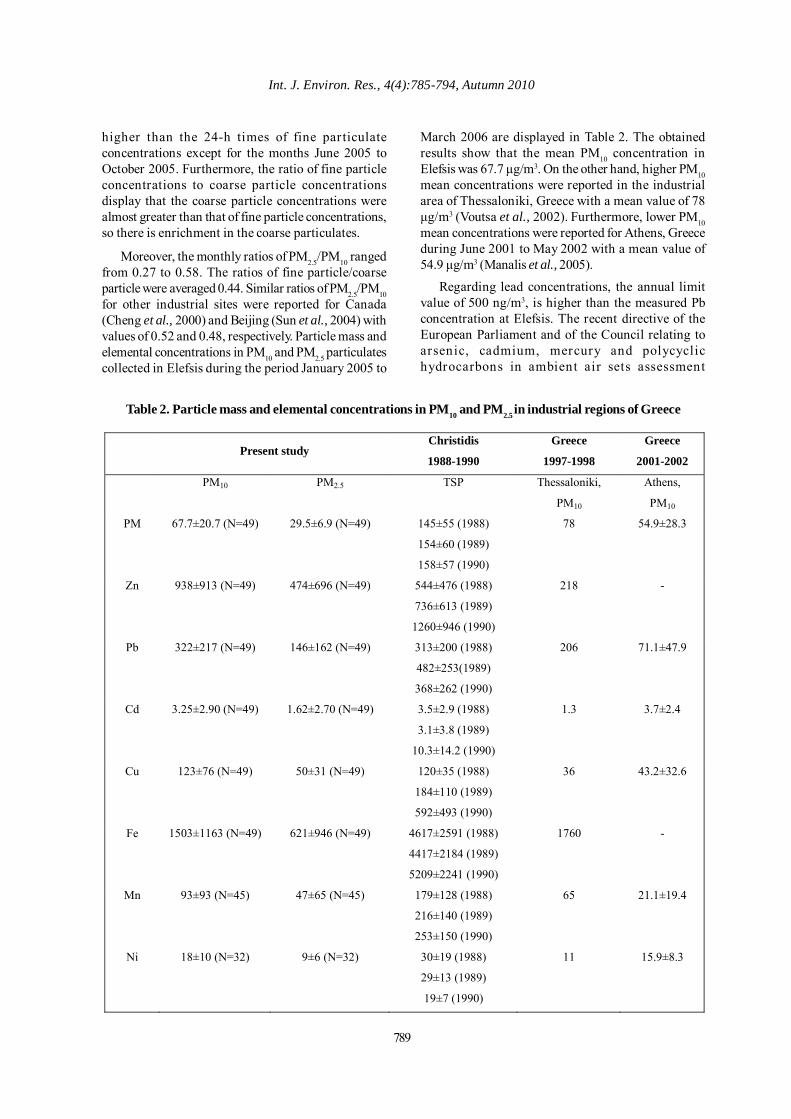
Int. J. Environ. Res., 4(4):785-794, Autumn 2010
Table 2. Particle mass and elemental concentrations in PM10 and PM2.5 in industrial regions of Greece
Present study
Christidis
1988-1990
Greece
1997-1998
Greece
2001-2002
PM10 PM2.5
TSP Thessaloniki,
PM10
Athens,
PM10
PM 67.7±20.7 (N=49) 29.5±6.9 (N=49) 145±55 (1988)
154±60 (1989)
158±57 (1990)
78 54.9±28.3
Zn 938±913 (N=49) 474±696 (N=49) 544±476 (1988)
736±613 (1989)
1260±946 (1990)
218 -
Pb 322±217 (N=49)
146±162 (N=49) 313±200 (1988)
482±253(1989)
368±262 (1990)
206 71.1±47.9
Cd 3.25±2.90 (N=49)
1.62±2.70 (N=49) 3.5±2.9 (1988)
3.1±3.8 (1989)
10.3±14.2 (1990)
1.3 3.7±2.4
Cu 123±76 (N=49)
50±31 (N=49) 120±35 (1988)
184±110 (1989)
592±493 (1990)
36 43.2±32.6
Fe 1503±1163 (N=49) 621±946 (N=49) 4617±2591 (1988)
4417±2184 (1989)
5209±2241 (1990)
1760 -
Mn 93±93 (N=45) 47±65 (N=45) 179±128 (1988)
216±140 (1989)
253±150 (1990)
65 21.1±19.4
Ni 18±10 (N=32) 9±6 (N=32) 30±19 (1988)
29±13 (1989)
19±7 (1990)
11 15.9±8.3
higher than the 24-h times of fine particulateconcentrations except for the months June 2005 toOctober 2005. Furthermore, the ratio of fine particleconcentrations to coarse particle concentrationsdisplay that the coarse particle concentrations werealmost greater than that of fine particle concentrations,so there is enrichment in the coarse particulates.
Moreover, the monthly ratios of PM2.5/PM10 rangedfrom 0.27 to 0.58. The ratios of fine particle/coarseparticle were averaged 0.44. Similar ratios of PM2.5/PM10for other industrial sites were reported for Canada(Cheng et al., 2000) and Beijing (Sun et al., 2004) withvalues of 0.52 and 0.48, respectively. Particle mass andelemental concentrations in PM10 and PM2.5 particulatescollected in Elefsis during the period January 2005 to
March 2006 are displayed in Table 2. The obtainedresults show that the mean PM10 concentration inElefsis was 67.7 µg/m3. On the other hand, higher PM10mean concentrations were reported in the industrialarea of Thessaloniki, Greece with a mean value of 78µg/m3 (Voutsa et al., 2002). Furthermore, lower PM10mean concentrations were reported for Athens, Greeceduring June 2001 to May 2002 with a mean value of54.9 µg/m3 (Manalis et al., 2005).
Regarding lead concentrations, the annual limitvalue of 500 ng/m3, is higher than the measured Pbconcentration at Elefsis. The recent directive of theEuropean Parliament and of the Council relating toarsenic, cadmium, mercury and polycyclichydrocarbons in ambient air sets assessment
789
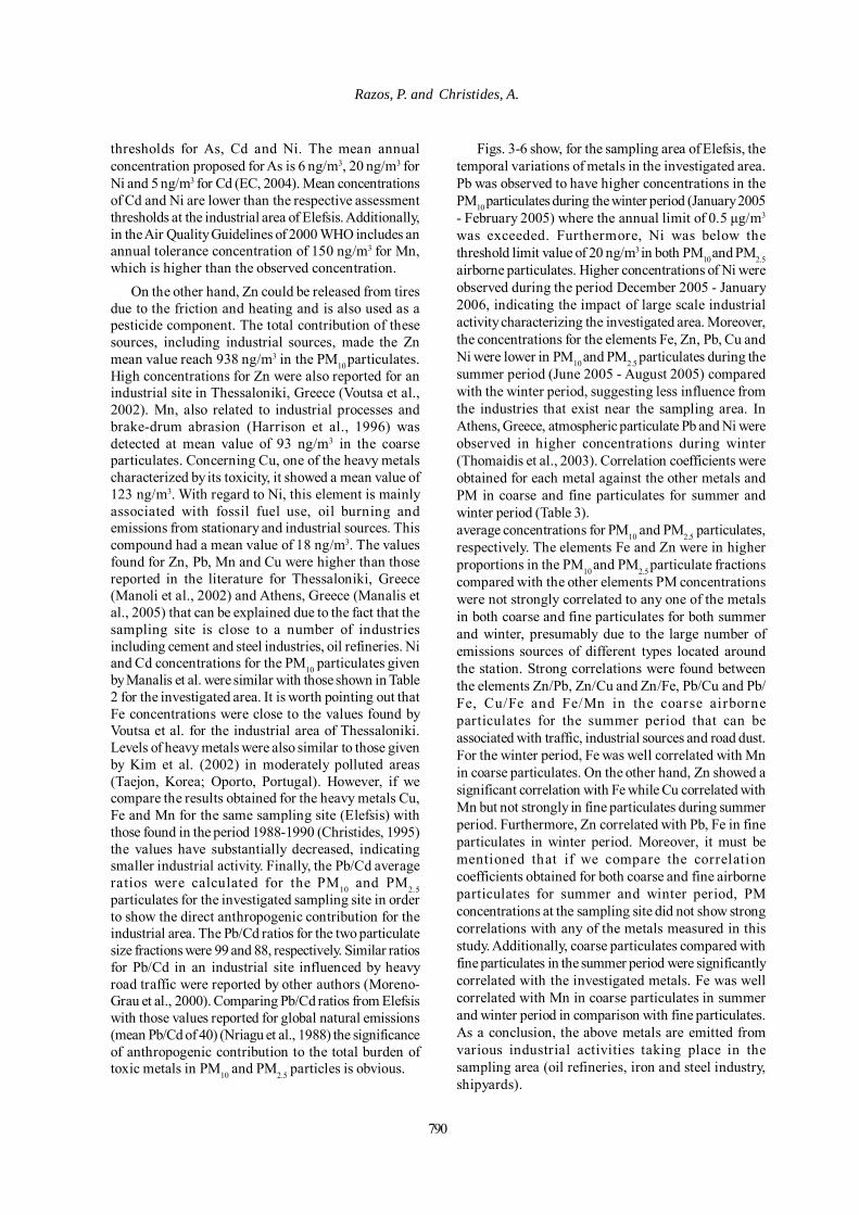
790
Razos, P. and Christides, A.
thresholds for As, Cd and Ni. The mean annualconcentration proposed for As is 6 ng/m3, 20 ng/m3 forNi and 5 ng/m3 for Cd (EC, 2004). Mean concentrationsof Cd and Ni are lower than the respective assessmentthresholds at the industrial area of Elefsis. Additionally,in the Air Quality Guidelines of 2000 WHO includes anannual tolerance concentration of 150 ng/m3 for Mn,which is higher than the observed concentration.
On the other hand, Zn could be released from tiresdue to the friction and heating and is also used as apesticide component. The total contribution of thesesources, including industrial sources, made the Znmean value reach 938 ng/m3 in the PM10 particulates.High concentrations for Zn were also reported for anindustrial site in Thessaloniki, Greece (Voutsa et al.,2002). Mn, also related to industrial processes andbrake-drum abrasion (Harrison et al., 1996) wasdetected at mean value of 93 ng/m3 in the coarseparticulates. Concerning Cu, one of the heavy metalscharacterized by its toxicity, it showed a mean value of123 ng/m3. With regard to Ni, this element is mainlyassociated with fossil fuel use, oil burning andemissions from stationary and industrial sources. Thiscompound had a mean value of 18 ng/m3. The valuesfound for Zn, Pb, Mn and Cu were higher than thosereported in the literature for Thessaloniki, Greece(Manoli et al., 2002) and Athens, Greece (Manalis etal., 2005) that can be explained due to the fact that thesampling site is close to a number of industriesincluding cement and steel industries, oil refineries. Niand Cd concentrations for the PM10 particulates givenby Manalis et al. were similar with those shown in Table2 for the investigated area. It is worth pointing out thatFe concentrations were close to the values found byVoutsa et al. for the industrial area of Thessaloniki.Levels of heavy metals were also similar to those givenby Kim et al. (2002) in moderately polluted areas(Taejon, Korea; Oporto, Portugal). However, if wecompare the results obtained for the heavy metals Cu,Fe and Mn for the same sampling site (Elefsis) withthose found in the period 1988-1990 (Christides, 1995)the values have substantially decreased, indicatingsmaller industrial activity. Finally, the Pb/Cd averageratios were calculated for the PM10 and PM2.5particulates for the investigated sampling site in orderto show the direct anthropogenic contribution for theindustrial area. The Pb/Cd ratios for the two particulatesize fractions were 99 and 88, respectively. Similar ratiosfor Pb/Cd in an industrial site influenced by heavyroad traffic were reported by other authors (Moreno-Grau et al., 2000). Comparing Pb/Cd ratios from Elefsiswith those values reported for global natural emissions(mean Pb/Cd of 40) (Nriagu et al., 1988) the significanceof anthropogenic contribution to the total burden oftoxic metals in PM10 and PM2.5 particles is obvious.
Figs. 3-6 show, for the sampling area of Elefsis, thetemporal variations of metals in the investigated area.Pb was observed to have higher concentrations in thePM10 particulates during the winter period (January 2005- February 2005) where the annual limit of 0.5 µg/m3
was exceeded. Furthermore, Ni was below thethreshold limit value of 20 ng/m3 in both PM10 and PM2.5airborne particulates. Higher concentrations of Ni wereobserved during the period December 2005 - January2006, indicating the impact of large scale industrialactivity characterizing the investigated area. Moreover,the concentrations for the elements Fe, Zn, Pb, Cu andNi were lower in PM10 and PM2.5 particulates during thesummer period (June 2005 - August 2005) comparedwith the winter period, suggesting less influence fromthe industries that exist near the sampling area. InAthens, Greece, atmospheric particulate Pb and Ni wereobserved in higher concentrations during winter(Thomaidis et al., 2003). Correlation coefficients wereobtained for each metal against the other metals andPM in coarse and fine particulates for summer andwinter period (Table 3).average concentrations for PM10 and PM2.5 particulates,respectively. The elements Fe and Zn were in higherproportions in the PM10 and PM2.5 particulate fractionscompared with the other elements PM concentrationswere not strongly correlated to any one of the metalsin both coarse and fine particulates for both summerand winter, presumably due to the large number ofemissions sources of different types located aroundthe station. Strong correlations were found betweenthe elements Zn/Pb, Zn/Cu and Zn/Fe, Pb/Cu and Pb/Fe, Cu/Fe and Fe/Mn in the coarse airborneparticulates for the summer period that can beassociated with traffic, industrial sources and road dust.For the winter period, Fe was well correlated with Mnin coarse particulates. On the other hand, Zn showed asignificant correlation with Fe while Cu correlated withMn but not strongly in fine particulates during summerperiod. Furthermore, Zn correlated with Pb, Fe in fineparticulates in winter period. Moreover, it must bementioned that if we compare the correlationcoefficients obtained for both coarse and fine airborneparticulates for summer and winter period, PMconcentrations at the sampling site did not show strongcorrelations with any of the metals measured in thisstudy. Additionally, coarse particulates compared withfine particulates in the summer period were significantlycorrelated with the investigated metals. Fe was wellcorrelated with Mn in coarse particulates in summerand winter period in comparison with fine particulates.As a conclusion, the above metals are emitted fromvarious industrial activities taking place in thesampling area (oil refineries, iron and steel industry,shipyards).
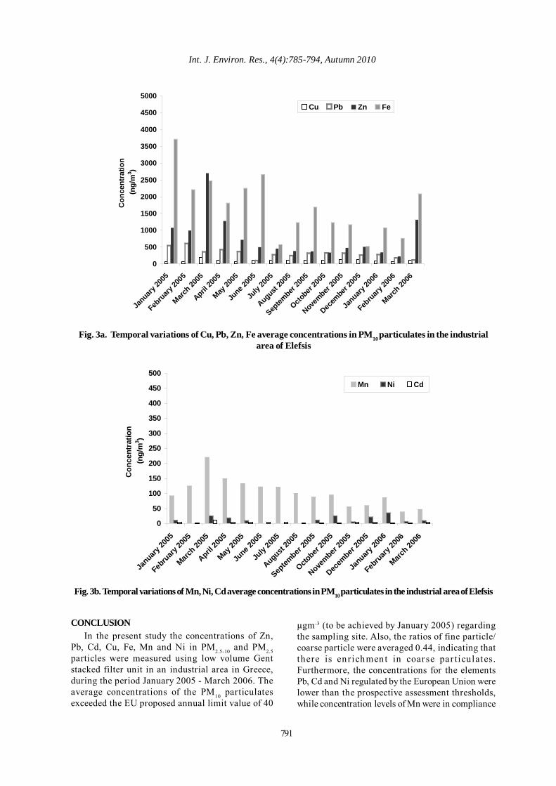
791
Int. J. Environ. Res., 4(4):785-794, Autumn 2010
0
500
1000
1500
2000
2500
3000
3500
4000
4500
5000
January
2005
Febru
ary 20
05
March 20
05
April 20
05
May 20
05
June 2
005
July
2005
August 20
05
Septem
ber 20
05
October
2005
November
2005
Decem
ber 2
005
January
2006
Febru
ary 20
06
March 20
06
Con
cent
ratio
n (n
g/m
3 )
Cu Pb Zn Fe
Fig. 3a. Temporal variations of Cu, Pb, Zn, Fe average concentrations in PM10 particulates in the industrialarea of Elefsis
0
50
100
150
200
250
300
350
400
450
500
January
2005
Febru
ary 20
05
March 20
05
April 20
05
May 20
05
June 2
005
July
2005
August 20
05
Septem
ber 20
05
October
2005
November
2005
Decem
ber 20
05
January
2006
Febru
ary 20
06
March 20
06
Con
cent
ratio
n (n
g/m
3 )
Mn Ni Cd
Fig. 3b. Temporal variations of Mn, Ni, Cd average concentrations in PM10 particulates in the industrial area of Elefsis
CONCLUSIONIn the present study the concentrations of Zn,
Pb, Cd, Cu, Fe, Mn and Ni in PM2.5-10 and PM2.5particles were measured using low volume Gentstacked filter unit in an industrial area in Greece,during the period January 2005 - March 2006. Theaverage concentrations of the PM10 particulatesexceeded the EU proposed annual limit value of 40
µgm-3 (to be achieved by January 2005) regardingthe sampling site. Also, the ratios of fine particle/coarse particle were averaged 0.44, indicating thatthere is en richmen t in coar se par ticulates.Furthermore, the concentrations for the elementsPb, Cd and Ni regulated by the European Union werelower than the prospective assessment thresholds,while concentration levels of Mn were in compliance
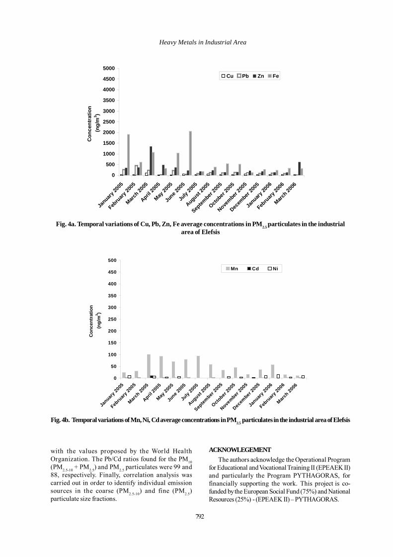
792
Heavy Metals in Industrial Area
0
500
1000
1500
2000
2500
3000
3500
4000
4500
5000
January
2005
Febru
ary 20
05
March 20
05
April 20
05
May 20
05
June 2
005
July
2005
August 20
05
Septem
ber 20
05
October
2005
November
2005
Decem
ber 20
05
January
2006
Febru
ary 20
06
March 20
06
Con
cent
ratio
n (n
g/m
3 )
Cu Pb Zn Fe
Fig. 4a. Temporal variations of Cu, Pb, Zn, Fe average concentrations in PM2.5 particulates in the industrialarea of Elefsis
0
50
100
150
200
250
300
350
400
450
500
Januar
y 2005
Febru
ary 20
05
March
2005
April 20
05
May 20
05
June 2
005
July
2005
August 20
05
Septem
ber 20
05
October 2
005
November
2005
December 2
005
January
2006
Febru
ary 20
06
March 20
06
Con
cent
ratio
n (n
g/m
3 )
Mn Cd Ni
Fig. 4b. Temporal variations of Mn, Ni, Cd average concentrations in PM2.5 particulates in the industrial area of Elefsis
with the values proposed by the World HealthOrganization. The Pb/Cd ratios found for the PM10(PM2.5-10 + PM2.5) and PM2.5 particulates were 99 and88, respectively. Finally, correlation analysis wascarried out in order to identify individual emissionsources in the coarse (PM2.5-10) and fine (PM2.5)particulate size fractions.
ACKNOWLEGEMENTThe authors acknowledge the Operational Program
for Educational and Vocational Training II (EPEAEK II)and particularly the Program PYTHAGORAS, forfinancially supporting the work. This project is co-funded by the European Social Fund (75%) and NationalResources (25%) - (EPEAEK II) – PYTHAGORAS.

Int. J. Environ. Res., 4(4):785-794, Autumn 2010
Table 3. Correlation analysis of metallic elements and PM in Elefsis, Greece: a) coarse particulates (summer period),b) coarse particulates (winter period), c) fine particulates (summer period) and d) fine particulates (winter period)
(a) PM Zn Pb Cu Fe Mn Ni PM 1.000 Zn -0.084 1.000 Pb -0.257 0.931 1.000 Cu 0.030 0.878 0.786 1.000 Fe -0.102 0.799 0.769 0.825 1.000 Mn -0.299 0.513 0.549 0.582 0.707 1.000 Ni 0.293 -0.064 -0.073 0.088 -0.050 0.026 1.000 (b) PM 1.000 Zn 0.388 1.000 Pb 0.021 0.261 1.000 Cu -0.193 -0.089 0.207 1.000 Fe 0.205 0.178 0.203 -0.150 1.000 Mn 0.093 0.195 0.278 -0.022 0.742 1.000 Ni 0.154 0.513 0.081 -0.246 0.192 0.197 1.000 (c) PM 1.000 Zn -0.000 1.000 Pb -0.022 0.010 1.000 Cu 0.056 0.338 0.086 1.000 Fe 0.079 0.838 -0.316 0.473 1.000 Mn 0.452 0.397 0.421 0.562 0.401 1.000 Ni 0.100 0.133 0.132 -0.017 0.136 0.438 1.000 (d) PM 1.000 Zn -0.428 1.000 Pb -0.031 0.570 1.000 Cu -0.036 0.087 0.081 1.000 Fe -0.275 0.526 0.115 0.110 1.000 Mn -0.075 0.305 0.187 0.399 0.431 1.000 Ni 0.383 -0.218 -0.105 -0.397 0.092 0.121 1.000
REFERENCESAkoto, O., Ephraim, J. H. and Darko, G. (2008). Heavymetals pollution in surface soils n the vicinity of abundantrailway servicing workshop in Kumasi, Ghana. Int. J.Environ. Res., 2 (4), 359-364.
Cheng, L., Sandhu, H. S., Angle, R. P., McDonald, K. M.and Myrick, R. H. (2000). Rural particulate matter in Alberta,Canada. Atmos. Environ., 34, 3365-3372.
Christides, A. (1995). Study of the distribution of airbornepollutants in Thriasio Pedio, Elevsis, Greece. PhD Thesis,NTUA Athens.
Costa, D. L. and Dreher, K. L. (1997). Bioavailable transitionmetals in particulate matter mediate cardiopulmonary injury inhealthy and compromised animal models. Environ. HealthPerspect, 105 (5), 1053-1060.
Dixit, S. and Tiwari, S. (2008). Impact Assessment of heavymetals pollution of Shahpura Lake, Bhopal, India. Int. J.Environ. Res., 2 (1), 37-42.
EC, European Commission, DG XI, Working Group on Lead(1997). Air Quality Daughter Directives-Position Paper on Lead.
EC (1999). Council Directive 83/399/ECC relating to limit valuesfor sulphur dioxide and oxides of nitrogen, particulate matter
and lead in ambient air. Official Journal of EuropeanCommunications L 163/99.
EC, European Commission, DG Environment, Working Groupon Arsenic, Cadmium and Nickel Compounds (2001). AmbientAir Pollution by As, Cd and Ni compounds-Position Paper.Office for Official Publications of the European Communities,Luxembourg.
EC (2003a). Commission decision of 16 January 2003 concerningguidance on a provisional reference method for sampling andmeasurement of PM2.5 under directive 199/30/EC.
EC (2004). Directive 2004/107/EC of the European Parliamentand of the Council of 15 December 2004 relating to arsenic,cadmium, mercury and polycyclic aromatic hydrocarbons inambient air.
Harrison, R., Smith, D. and Luhana, L. (1996). Sourceapportionment of atmospheric polycyclic aromatichydrocarbons collected from an urban location in Birmingham,UK. Environ. Sci. Technol., 30, 825-832.
Harrison, R.M. and Yin, J. (2000). Particulate matter in theatmosphere: which particle properties are important for itseffect on health. Sci. Total Environ., 249, 85-101.
Harrison, R. M., Tilling, R., Callen Romero, M. S., Harrad, S.and Jarvis, K. (2003). A study of trace metals and polycyclic
793

Razos, P. and Christides, A.
aromatic hydrocarbons in the roadside environment. Atmos.Environ., 37, 2391-2402.
Hemminki, E., Horvath, M. and Schuler, D. (1995). Impactof iron fortification of milk formulas on infants growth andhealth. Nutr. Res., 15, 491-503.
Hien, P. D., Bac, V. T., Tham, H. C., Nhan, D. D. and Vinh, L.D. (2002). Influence of meteorological conditions on PM2.5and PM2.5-10 concentrations during the monsoon season inHanoi, Vietnam. Atmos. Environ. 36, 3473-3484.
Hopke, P. K., Xie, Y., Raunemaa, T.,. Biegalski, S., Landsberger,S., Maenhaut, W., Artaxo, P. and Cohen, D. (1997).Characterization of the Gent Stacked Filter Unit PM10 Sampler.Aerosol Sci. Technol. 27, 726-735.
Kim, K. H., Lee, J. H. and Jang, M. S. (2002). Metals inairborne particulate matter from the first and secondindustrial complex area of Taejon City, Korea. Environ.Pollut. 118, 41-51.
Kothai, P., Prathibha, P., Saradhi, I.V., Pandit, G.G. and Puranik,V.D. (2009). Characterization of Atmospheric ParticulateMatter using PIXE Technique. Proc. Int. Conf. En. Environ.
Maenhaut, W., Francois, F. and Cafmeyer J. (1994). “The ‘gent’stacked filter unit (SFU) sampler for the collection ofatmospheric aerosols in two size fractions”, in NAHRES-19,IAEA, Vienna, 249-263.
Manalis, N., Grivas, G., Protonotarios, V., Moutsatsou, A.Samara, C. and Chaloulakou, A. (2005). Toxic metal content ofparticulate matter (PM10), within the Greater Area of Athens.Chemosphere, 60, 557-566.
Manoli, E., Voutsa, D. and Samara, C. (2002). Chemicalcharacterization and source identification/apportionment of fineand coarse air particles in Thessaloniki, Greece. Atmos.Environ., 36, 949-961.
Martuzzi, M., Krzyzanowski, M. and Bertollini, R. (2003).Health impact assessment of air pollution: providing furtherevidence for public health action. Eur. Respir. J., 21, 86s-91s.
Moreno-Grau, S., Pérez-Tornell, A., Bayo, J., Moreno, J.,Angosto, J. M. and Moreno-Clavel, J. (2000). Particulate matterand heavy metals in the atmospheric aerosol from Cartagena,Spain. Atmos. Environ., 34, 5161-5167.
Mugica, V., Maubert, M., Torres, M., Muñoz, J. and Rico, E.(2002). Temporal and spatial variations of metal content inTSP and PM10 in Mexico City during 1996-1998. J. AerosolSci., 3, 91-102.
Nabi Bidhendi, G. R. and Halek, F. (2007). Aerosol sizesegregated of Tehran’s Atmosphere in Iran. Int. J. Environ.Res., 1 (1), 58-65.
Nriagu, J. O. and Pacyna, J. M. (1988). Quantitative assessmentof worldwide contamination of air, water and soils by tracemetals. Nature, 333, 134-139.
Pacyna, J. M. (1986). Atmospheric trace elements from naturaland anthropogenic sources. In: Toxic Metals in the Atmosphere.(New York: Wiley, pp. 33-52).
Preining, O. (1996). The many facets of aerosol science. J.Aerosol Sci., 27, S1-S6.
Protonotarios, V., Petsas, N. and Moutsatsou, A. (2002). Levelsand composition of atmospheric particulates (PM10) in a mining-industrial site, at the city of Lavrion, Greece, J. Air & WasteManage. Assoc., 52, 1263-1273.
Salma, I. and Maenhaut, W. (2006). Changes in elementalcomposition and mass of atmospheric aerosol pollutionbetween 1996 and 2002 in a Central European city. Environ.Pollut., 143, 479-488.
Samara, C., Voutsa, D., Kouimtzis, T. H., Bournis, N. andTsani, E. (1990). Characterization of airborne particulate matterin Thessaloniki, Greece. Part 1: Source related heavy metalconcentration within TSP. Toxicol. Environ. Chem., 29, 107-119.
Samara, C. and Voutsa, D. (2005). Size distribution of airborneparticulate matter and associated heavy metals in the roadsideenvironment. Chemosphere, 59, 1197-1206.
Scheff, P. A. and Valiozis, C. (1990). Characterization and sourceidentification of respirable particulate matter in Athens, Greece.Atmos. Environ., 24A, 203-211.
Saskia, C., Van Der Zee, S. C., Hoek, G., Harrssema, H. andBrunekreef, B. (1998). Characterization of particulate airpollution in urban and non-urban areas in Netherlands. Atmos.Environ., 32, 3717-3729.
Simpson, R. W. and Xu, H. (1994). Atmospheric lead pollutionin an urban area-Brisbane, Australia. Atmos. Environ., 28, 3073-3082.
Sun, Y., Zhuang, G., Wang, Y., Han, L., Guo, J., Dan, M. Zhang,W., Wang, Z. and Hao, Z. (2004). The air-borne particulatepollution in Beijing-concentration, composition, distributionand sources. Atmos. Environ., 38, 5991-6004.
Swielticki, E., Puri, S. and Hanson, H. C. (1996). Urban airpollution source apportionment using a combination of aerosoland gas monitoring techniques. Atmos. Environ., 30, 2795-2809.
Thomaidis, N. S., Bakeas, E. B. and Siskos, P. A. (2003).Characterization of lead, cadmium, arsenic and nickel in PM2.5particles in the Athens atmosphere, Greece. Chemosphere, 52,959-966.
Torfs, K. and Van Grieken, R. (1997). Chemical relationsbetween atmospheric aerosols, deposition and stone decaylayers on historic buildings at the Mediterranean coast. Atmos.Environ., 31, 2179-2192.
US EPA (1997). National Ambient Air Quality Standards.
Voutsa, D. and Samara, C. (2002). Labile and bioaccessiblefractions of heavy metals in the airborne particulate matterfrom urban and industrial areas. Atmos. Environ., 36, 3583-3590.
Voutsa, D., Samara, C., Kouimtzis, T. H. and Ochsenkuhn, K.(2002). Elemental composition of airborne particulate matterin the multi-impacted urban area of Thessaloniki, Greece. Atmos.Environ., 36, 4453-4462.
794
Int. J. Environ. Res., 4(4):795-806, Autumn 2010ISSN: 1735-6865
Received 7 July 2009; Revised 2 April 2010; Accepted 25 May 2010
*Corresponding author E-mail: [email protected]
795
Management of Urban Solid Waste Pollution in Developing Countries
Firdaus, G .* and Ahmad , A .
Department of Geography, AM.U. Aligarh-202002, India
ABSTRACT: Solid waste pollution, like the other environmental problems, is assuming serious dimensions inDelhi. From the last few decades, the study area has been experiencing a significant increase in the generationof solid waste that is adversely affecting its physical environment and is creating aesthetic problems. Thecurrent study reviews the data on the quantity of municipal solid waste generation, its physico-chemicalcharacteristics, collection and disposal system. During the analysis it has been found that rapid populationgrowth in Delhi has enhanced the rate of generation of solid wastes manifolds. Consequently, the managementof waste has become Herculean work, and, piles of garbage and waste of all kinds littered everywhere havebecome a common site. The present analysis highlighted that the existing system of waste collection and itsdisposal within the municipal board is not only inadequate and insufficient but also unscientific. It has beentried to develop a strategy for mitigating and managing this problem in the sustainable urban developmentperspectives by involving Non-Government and Community-Based Organizations. Besides, the analysis alsoprovides a background for the discussion of strategic issues relating to how these organizations in Delhi canassist the local government in solving the waste management crisis.
Key words: Delhi, Solid Waste, Organization, Urbanization, NGOs
INTRODUCTIONSolid waste and by-products of production and
consumption are considered urban terr itorialphenomena and can be defined as an excess supply ofwaste materials resulting from a mismatch between thecosts and benefits of material use in general, andgenerating and managing waste material in particular.It includes the heterogeneous mass of garbage fromthe urban community as well as more homogenousaccumulations comprising of countless differentmaterials such as food wastes, construction wastes,industrial process wastes and pathological wastes etc(Turk and Turk, 1984; Joseph and Nagendran, 2004).Since the beginning human kind has been generatingwaste, be it is the bones or the wood they use to makefood. But the management of solid waste was hardly anissue for the old communities. The quantum andcomposition of wastes produced by them was suchthat it would easily decompose and revert to soil or bewashed away by rivers without creating any seriousenvironmental hazard. With the progress of civilization,the waste generated became of a more complex nature.It assumed serious proportion only after the humanconcentrations became engaged in non-agriculturalforms of production (Roy, 2003). The population isprojected to increase from 2.4 billion in 2007 to 5.3 billion
in 2050 (World Urbanization Prospects, 2007Revision).Recently, several studies have been orientedtowards implementation of an appropriate solid wastemanagement system in developing countries(Nwabanne et al., 2009; Monazzam and Park, 2009;Omran et al., 2009; Oshode et al., 2008; Jalili Ghazizadeand Noori, 2008; Ghiasinejad and Abduli, 2007; Abdoli,2009; Uemura, 2010; Abduli et al., 2008; Karamouz etal., 2006).
Unlike the other developing countries, India, beingthe world’s second highest populated country andone of the fastest urbanizing countries is facing theproblem of solid waste management. With industrialprogress, growing urban areas and resultant growthin urban solid wastes has become an emerging andengaging area of study. From the last few decadesIndia has witnessed a significant increase in solidwaste generation. It has been estimated that duringmid-seventies, the per capita solid waste generationranged from 150 - 350 gm/day for various Indian cities(CPCB, 2001); whereas presently, it ranges from 0.3 –0.6 Kg/day (CPCB, 1999). India produces approximately46 million tons of urban solid waste annually (Kumaret al., 2004) and is expected to increase to a mammothfigure of 300 million by 2047. The estimated landrequirement for disposal of such huge quantum of

796
Firdaus, G. and Ahmad, A.
waste would be 169.6 km2 as compared to 20.2 km2 in1997. The amount of waste generated per capita isestimated to increase at a rate of 1%–1.33% annually(Shekdar, 1999). Municipal Solid Waste (MSW) inIndian cities is collected by respective municipalitiesand transported to designated disposal sites, whichare normally low lying areas on the outskirts of thecity. The limited revenues earmarked for themunicipalities make them ill-equipped to provide forhigh costs involved in the collection, storage, treatment,and proper disposal. As a result, a substantial part ofthe MSW generated remains unattended and grows inthe heaps at poorly maintained collection centres.Typically one to two thirds of the solid waste generatedis not collected. As a result, the uncollected waste,which is often also mixed with human and animalexcreta, is dumped indiscriminately in the streets andin drains, so contributing to flooding, breeding of insectand rodent vectors and the spread of diseases. Inaddition, most of the municipal solid waste which iscollected is dumped on land in a more or lessuncontrolled manner. The average collection efficiencyfor MSW in Indian cities is about 72.5% and around70% of the cities lack adequate waste transportcapacities (Singhal and Pndey, 2001). This paperexamines types, sources and physico-chemicalcharacteristics of municipal solid waste in Delhi. Anattempt has also been made to evaluate the collectionand disposal management practices. Finally, we havetried to develop enforced and time-bound strategy for
collection efficiency and treatment/disposal practicesby involving Non-Government and Community-BasedOrganizations that will help in reducing the risks ofhealth damage and will ensure better environment fora growing Delhi.
MATERIALS & MEHTODSThe present analysis is theoretical based on
empirical observation and has an exploratory design.The methodological principle adopted for the presentanalysis is based on primary and secondary sourcesof data collected from field survey and official recordof various govt. agencies. The data are organized,classified and analyzed with the statistical techniquesas well as visual presentation in the form of graphs,diagrams and maps.
NCT of Delhi with 13.8 million populations (2001) isthe third largest urban centre of India. It is situatedbetween the latitude of 28º24´17”and 28Ú52”north, andof 76Ú50’26"and 77Ú20’37"east longitude at an altitudeof between 700 and 1000 feet. It covers an area of 1483sq. km. with maximum length and breath of 51900 km.and 4848 km respectively. Situated on the both side ofthe River Yamuna, Delhi is flanked by Uttar Pradesh inthe east and Haryana in the north, south and west(Fig.1). Delhi is governed by three administrative bodiesnamely Municipal Corporation of Delhi (MCD), NewDelhi Municipal Council (NDMC) and DelhiCantonment Board (DCB). MCD occupies an area of
Narela
Civil Line Shahdara (S)
Shahdara (N)
City S.P.
Rohini
Najafgarh
West Karol Bagh
Central
South
Fig. 1. Delhi: Location Map

Int. J. Environ. Res., 4(4):795-806, Autumn 2010
797
1397.29 sq. km., containing 96.96 per cent of the totalpopulation while the rest is shared by NDMC and DCB.MCD is next only to Tokyo Municipal Corporation interms of area. It has the dual responsibility of providingcivic services to its people in both rural and urbanareas.
RESULTS & DISCUSSIONThe urban population increased from 52.76% (1901)
to 93.01% in 2001 whereas the urban area has increasedfrom 43.3 km2 in 1921 to 924.68 km2 of the total area in2001 (Fig.2). Consequently, it has been experiencing asignificant increase in the generation of municipal solidwaste. In recent years not only solid waste has grownin quantity but it has increasingly acquired a hazardousdimension. The generation of solid waste has beenestimated to increase from 4,500 Metric Tones/day(MT/day), 6,500 MT/day to 12,000 MT/day in the year1981, 1991, and 2001 respectively (ADSORBS/37/ 2001-2002). It is expected that on the basis of growthassumption of 6-8 per cent, the quantity of waste willbe 17,000-25,000 MT/day by 2021 (Dhamija, 2006). Evenif it was possible to provide the maximum reduction ofwaste through composting and incineration therewould still be a minimum 20 per cent residue of 4,000-5,000 tones per day that would have to be land filledby 202113. Out of the total solid waste, municipal solidwaste accounts for 6000 -7000 metric tones, theindustrial waste weigh up to 4000 metric tones andbio-medical waste contribute 60 metric tones per day(LATS/17/2004-2005). The rest is contributed byconstruction debris, silt and other wastes. The averagedensity of the solid waste in Delhi is estimated to be500 kg /cubic meter (TERI 2001).
Due to growing prosperity and changing lifestyleof people, communities in Delhi are getting increasinglyoriented toward consumerism. From the last fewdecades, the rate of generation of solid waste hasincreased so much that the civic agencies responsiblefor the collection and disposal of wastes are unable todeal with the total quantity produced every day. As aresult, a major part of the waste remains uncollectedand accumulates in the form of heaps at variouslocations within the inhabited areas that soon beginsto rot and becomes an environmental hazard (TERIReport No. 1999 EE41). It is estimated that Delhigenerates about 6000- 7,000 metric tones of MSW perday (MCD 2001). Fig.3 indicates the increasing trendof domestic solid waste generation. The quantity ofdomestic waste has been found to increase from 2305MT/day, 4070 MT/day to 6188 MT/day in the year1981, 1993 and 2001 respectively. It recoded 168.17 percent growth rates over the period of twenty years(1981-2001).
As far as the sources of solid waste are concernedit has been observed that they are primarily arisingfrom anthropogenic activities. Table 1 reveals that themost prominent sources of solid waste generation inDelhi are residential areas, institutions, commercialestablishments, health-care facilities and slaughterhouses etc. It has been estimated that there are nearly1, 40,000 informal retail units, 24,000 wholesaleestablishments, 6,000 makeshift shopping spaces, 3000residential areas, and many other sources that aregenerating solid wastes of varied nature. In addition,the wholesale fruits and vegetable markets, truckterminals, slaughter houses and small scale industrieswith their filth, squatter and unsanitary conditions also
0100200300400500600700800900
1000
1901 1911 1921 1931 1941 1951 1961 1971 1981 1991 2001
Year
Are
a (s
q.km
)
0102030405060708090100
Pop
ulat
ion
(%)
Area Population
Fig. 2. Delhi: Changing Urban Area and Population
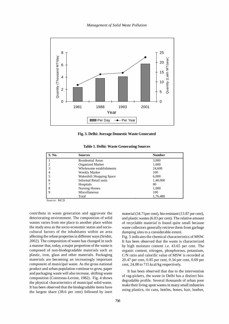
798
Management of Solid Waste Pollution
0
2
4
6
8
1981 1988 1993 2001Year
Qua
ntity
(Tho
usan
d M
T/da
y)
0
5
10
15
20
25
Qua
ntity
(Lak
h M
T/y
ear)
Per Day Per Year
Fig. 3. Delhi: Average Domestic Waste Generated
Table 1. Delhi: Waste Generating Sources
S. No. Sources Number 1 Residential Areas 3,000 2 Organized Market 1,600 3 Wholesome establishments 24,600 4 Weekly Market 100 5 Makeshift Shopping Space 6,000 6 Informal Retail units 1,40,000 7 Hospitals 80 8 Nursing Homes 1,000 9 Miscellaneous 100 Total 1,76,480
Source: MCD
contribute in waste generation and aggravate thedeteriorating environment. The composition of solidwastes varies from one place to another place withinthe study area as the socio-economic status and socio-cultural factors of the inhabitants within an areaaffecting the refuse properties in different ways (Srishti,2002). The composition of waste has changed in sucha manner that, today, a major proportion of the waste iscomposed of non-biodegradable materials such asplastic, iron, glass and other materials. Packagingmaterials are becoming an increasingly importantcomponent of municipal waste. As the gross nationalproduct and urban population continue to grow, paperand packaging waste will also increase, shifting wastecomposition (Cointreau-Levine, 1982). Fig. 4 showsthe physical characteristics of municipal solid waste.It has been observed that the biodegradable items havethe largest share (38.6 per cent) followed by inert
material (34.71per cent), bio-resistant (13.87 per cent),and plastic wastes (6.03 per cent). The relative amountof recyclable material is found quite small becausewaste collectors generally retrieve them from garbagedumping sites to a considerable extent.Fig. 5 indicates the chemical characteristics of MSW.It has been observed that the waste is characterizedby high moisture content i.e. 43.65 per cent. Theorganic content, nitrogen, phosphorous, potassium,C/N ratio and calorific value of MSW is recorded at20.47 per cent, 0.85 per cent, 0.34 per cent, 0.69 percent, 24.08 to 715 kcal/kg respectively.
It has been observed that due to the interventionof rag-pickers, the waste in Delhi has a distinct bio-degradable profile. Several thousands of urban poormake their living upon wastes in many small industriesusing plastics, tin cans, bottles, bones, hair, leather,
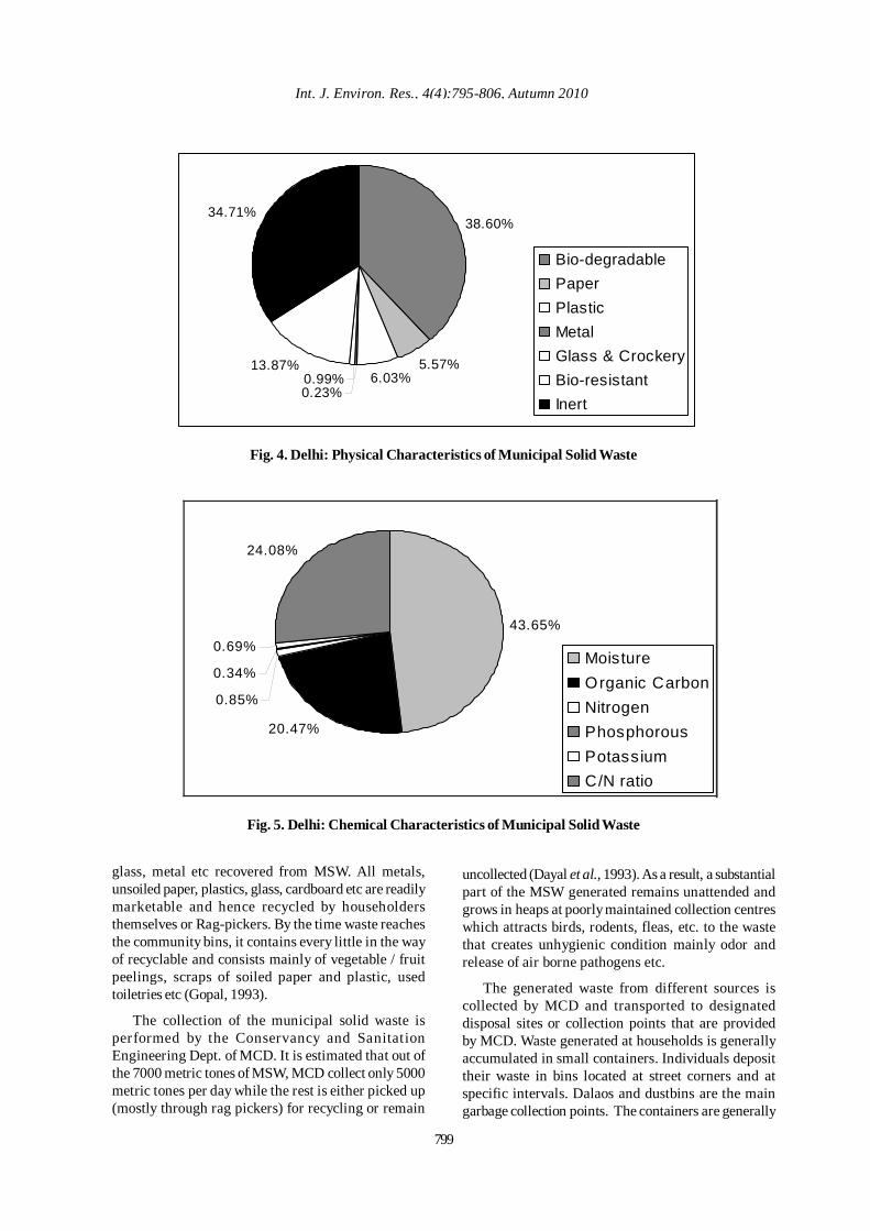
Int. J. Environ. Res., 4(4):795-806, Autumn 2010
38.60%
5.57%6.03%
13.87%
34.71%
0.23%0.99%
Bio-degradablePaperPlasticMetalGlass & CrockeryBio-resistantInert
Fig. 5. Delhi: Chemical Characteristics of Municipal Solid Waste
43.65%
20.47%
0.85%
0.34%
0.69%
24.08%
MoistureOrganic CarbonNitrogenPhosphorousPotassiumC/N ratio
Fig. 4. Delhi: Physical Characteristics of Municipal Solid Waste
glass, metal etc recovered from MSW. All metals,unsoiled paper, plastics, glass, cardboard etc are readilymarketable and hence recycled by householdersthemselves or Rag-pickers. By the time waste reachesthe community bins, it contains every little in the wayof recyclable and consists mainly of vegetable / fruitpeelings, scraps of soiled paper and plastic, usedtoiletries etc (Gopal, 1993).
The collection of the municipal solid waste isperformed by the Conservancy and SanitationEngineering Dept. of MCD. It is estimated that out ofthe 7000 metric tones of MSW, MCD collect only 5000metric tones per day while the rest is either picked up(mostly through rag pickers) for recycling or remain
uncollected (Dayal et al., 1993). As a result, a substantialpart of the MSW generated remains unattended andgrows in heaps at poorly maintained collection centreswhich attracts birds, rodents, fleas, etc. to the wastethat creates unhygienic condition mainly odor andrelease of air borne pathogens etc.
The generated waste from different sources iscollected by MCD and transported to designateddisposal sites or collection points that are providedby MCD. Waste generated at households is generallyaccumulated in small containers. Individuals deposittheir waste in bins located at street corners and atspecific intervals. Dalaos and dustbins are the maingarbage collection points. The containers are generally
799
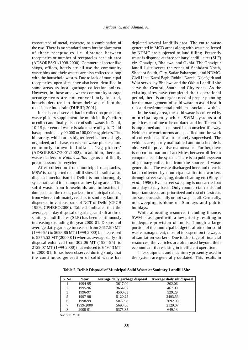
800
Firdaus, G. and Ahmad, A.
constructed of metal, concrete, or a combination ofthe two. There is no standard norm for the placementof these r eceptacles i .e. distance betweenreceptacles or number of receptacles per unit area(ADSORBS/31/1998-2000). Commercial sector likeshops, offices, hotels etc all use the communitywaste bins and their wastes are also collected alongwith the household wastes. Due to lack of municipalreceptacles, open sites have also been identified insome areas as local garbage collection points.However, in those areas where community storagearrangements are not conven ient ly located,householders tend to throw their wastes into theroadside or into drain (DUEIIP, 2001).
It has been observed that in collection procedurewaste pickers supplement the municipality’s effortto collect and finally dispose of solid waste. In Delhi,10-15 per cent of waste is taken care of by it. Delhihas approximately 90,000 to 100,000 rag pickers. Thehierarchy, which at its higher level is increasinglyorganized, at its base, consists of waste pickers morecommonly known in India as ‘r ag pickers’(ADSORBS/37/2001/2002). In addition, there arewaste dealers or Kabariwallas agents and finallypreprocessors or recyclers.
After collection from municipal receptacles,MSW is transported to landfill sites. The solid wastedisposal mechanism in Delhi is not thoroughlysystematic and it is dumped at low lying areas. Thesolid waste from households and industries isdumped near the roads, parks or in municipal dalaos,from where it ultimately reaches to sanitary landfillsdispersed in various parts of NCT of Delhi (CPCB1999; CPHEEO2000). Table 2 indicates that theaverage per day disposal of garbage and silt at threesanitary landfill sites (SLF) has been continuouslyincreasing excluding the year 2000-01. Disposal ofaverage daily garbage increased from 3617.90 MT(1994-95) to 5693.86 MT (1999-2000) but decreasedto 5375.53 MT (2000-01) whereas average daily siltdisposal enhanced from 302.06 MT (1994-95) to2129.07 MT (1999-2000) that reduced to 649.13 MTin 2000-01. It has been observed during study thatthe continuous generation of solid waste has
depleted several landfills area. The entire wastegenerated in MCD areas along with waste collectedby NDMC are subjected to land filling. Presentlywaste is disposed at three sanitary landfill sites (SLF)viz. Ghazipur, Bhalswa, and Okhla. The Ghazipurlandfill site serves the zones of Shahdara North,Shadara South, City, Sadar Pahargunj, and NDMC.Civil Line, Karol Bagh, Rohini, Narela, Najafgarh andWest served by Bhalswa and the Okhla Landfill siteserve the Central, South and City zones. As theexisting sites have completed their operationalperiod, there is an urgent need of proper planningfor the management of solid waste to avoid healthrisk and environmental problem associated with it.
In the study area, the solid waste is collected bymunicipal agency where SWM systems andpractices continue to be outdated and inefficient. Itis unplanned and is operated in an unscientific way.Neither the work norms are specified nor the workof collection staff appropriately supervised. Thevehicles are poorly maintained and no schedule isobserved for preventive maintenance. Further, thereis no co-ordination of activities between differentcomponents of the system. There is no public systemof primary collection from the source of wastegeneration. The waste discharged here and there islater collected by municipal sanitation workersthrough street sweeping, drain cleaning etc (Bhoyaret al., 1996). Even street sweeping is not carried outon a day-to-day basis. Only commercial roads andimportant streets are prioritized and rest of the streetsare swept occasionally or not swept at all. Generally,no sweeping is done on Sundays and publicholidays.
While allocating resources including finance,SWM is assigned with a low priority resulting ininadequate provision of funds. Though a largeportion of the municipal budget is allotted for solidwaste management, most of it is spent on the wagesof sanitation workers. Due to shortage of financialresources, the vehicles are often used beyond theireconomical life resulting in inefficient operation.
The equipment and machinery presently used inthe system are generally outdated. This results in
Table 2. Delhi: Disposal of Municipal Solid Waste at Sanitary Landfill Site
S. No. Year Average daily garbage disposal Average daily silt disposal 1 1994-95 3617.90 302.06 2 1995-96 3654.07 467.90 3 1996-97 4500.65 529.29 5 1997-98 5120.25 2493.53 6 1998-99 5077.98 2692.00 7 1999-2000 5693.86 2129.07 8 2000-01 5375.35 649.13
Source: MCD
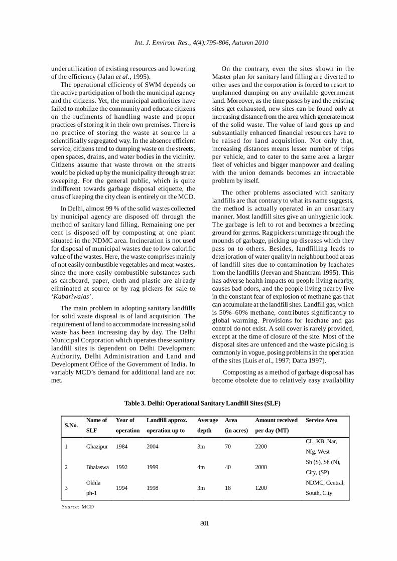
801
Int. J. Environ. Res., 4(4):795-806, Autumn 2010
underutilization of existing resources and loweringof the efficiency (Jalan et al., 1995).
The operational efficiency of SWM depends onthe active participation of both the municipal agencyand the citizens. Yet, the municipal authorities havefailed to mobilize the community and educate citizenson the rudiments of handling waste and properpractices of storing it in their own premises. There isno practice of storing the waste at source in ascientifically segregated way. In the absence efficientservice, citizens tend to dumping waste on the streets,open spaces, drains, and water bodies in the vicinity.Citizens assume that waste thrown on the streetswould be picked up by the municipality through streetsweeping. For the general public, which is quiteindifferent towards garbage disposal etiquette, theonus of keeping the city clean is entirely on the MCD.
In Delhi, almost 99 % of the solid wastes collectedby municipal agency are disposed off through themethod of sanitary land filling. Remaining one percent is disposed off by composting at one plantsituated in the NDMC area. Incineration is not usedfor disposal of municipal wastes due to low calorificvalue of the wastes. Here, the waste comprises mainlyof not easily combustible vegetables and meat wastes,since the more easily combustible substances suchas cardboard, paper, cloth and plastic are alreadyeliminated at source or by rag pickers for sale to‘Kabariwalas’.
The main problem in adopting sanitary landfillsfor solid waste disposal is of land acquisition. Therequirement of land to accommodate increasing solidwaste has been increasing day by day. The DelhiMunicipal Corporation which operates these sanitarylandfill sites is dependent on Delhi DevelopmentAuthority, Delhi Administration and Land andDevelopment Office of the Government of India. Invariably MCD’s demand for additional land are notmet.
On the contrary, even the sites shown in theMaster plan for sanitary land filling are diverted toother uses and the corporation is forced to resort tounplanned dumping on any available governmentland. Moreover, as the time passes by and the existingsites get exhausted, new sites can be found only atincreasing distance from the area which generate mostof the solid waste. The value of land goes up andsubstantially enhanced financial resources have tobe raised for land acquisition. Not only that,increasing distances means lesser number of tripsper vehicle, and to cater to the same area a largerfleet of vehicles and bigger manpower and dealingwith the union demands becomes an intractableproblem by itself.
The other problems associated with sanitarylandfills are that contrary to what its name suggests,the method is actually operated in an unsanitarymanner. Most landfill sites give an unhygienic look.The garbage is left to rot and becomes a breedingground for germs. Rag pickers rummage through themounds of garbage, picking up diseases which theypass on to others. Besides, landfilling leads todeterioration of water quality in neighbourhood areasof landfill sites due to contamination by leachatesfrom the landfills (Jeevan and Shantram 1995). Thishas adverse health impacts on people living nearby,causes bad odors, and the people living nearby livein the constant fear of explosion of methane gas thatcan accumulate at the landfill sites. Landfill gas, whichis 50%–60% methane, contributes significantly toglobal warming. Provisions for leachate and gascontrol do not exist. A soil cover is rarely provided,except at the time of closure of the site. Most of thedisposal sites are unfenced and the waste picking iscommonly in vogue, posing problems in the operationof the sites (Luis et al., 1997; Datta 1997).
Composting as a method of garbage disposal hasbecome obsolete due to relatively easy availability
Table 3. Delhi: Operational Sanitary Landfill Sites (SLF)
S.No. Name of
SLF
Year of
operation
Landfill approx.
operation up to
Average
depth
Area
(in acres)
Amount received
per day (MT)
Service Area
1 Ghazipur 1984 2004 3m 70 2200 CL, KB, Nar,
Nfg, West
2 Bhalaswa 1992 1999 4m 40 2000 Sh (S), Sh (N),
City, (SP)
3 Okhla
ph-1 1994 1998 3m 18 1200
NDMC, Central,
South, City
Source: MCD
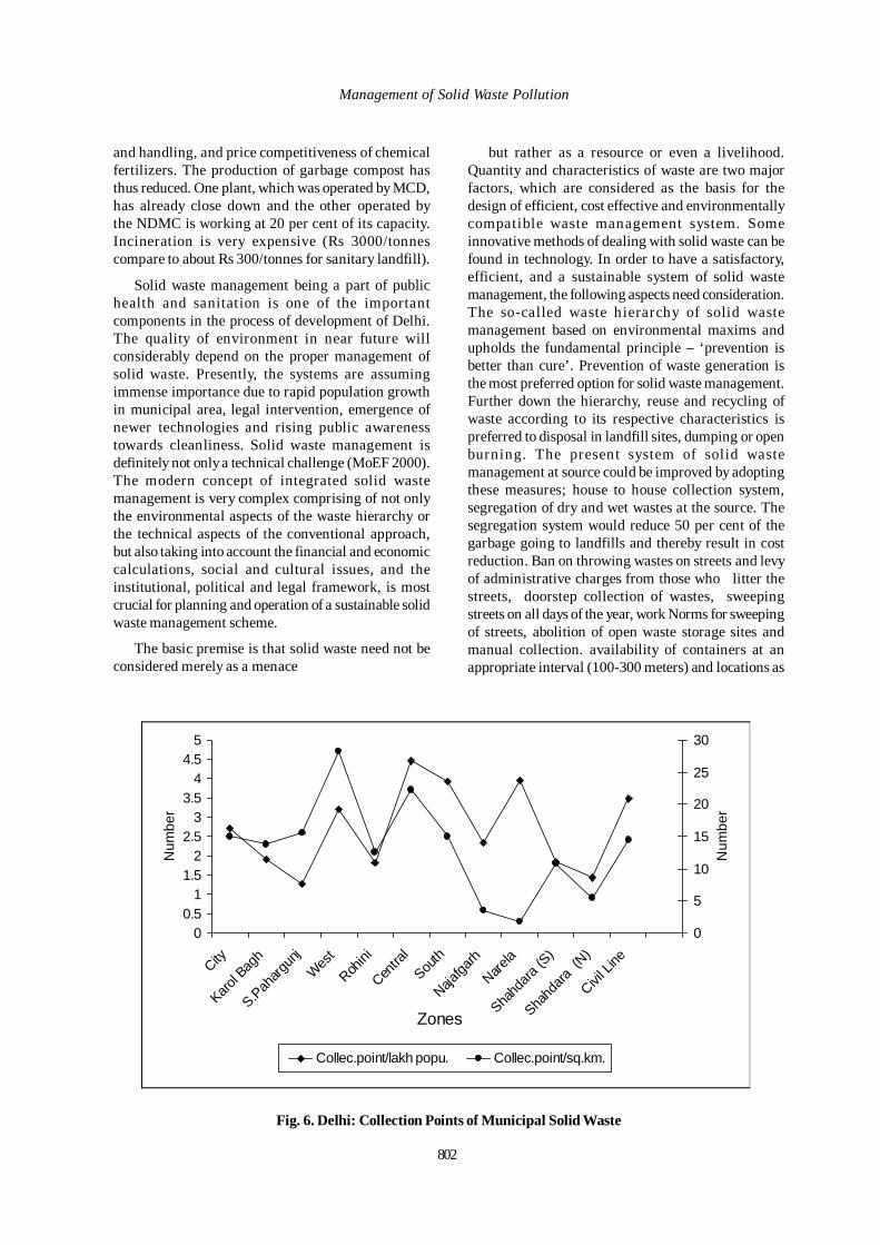
802
Management of Solid Waste Pollution
and handling, and price competitiveness of chemicalfertilizers. The production of garbage compost hasthus reduced. One plant, which was operated by MCD,has already close down and the other operated bythe NDMC is working at 20 per cent of its capacity.Incineration is very expensive (Rs 3000/tonnescompare to about Rs 300/tonnes for sanitary landfill).
Solid waste management being a part of publichealth and sanitation is one of the importantcomponents in the process of development of Delhi.The quality of environment in near future willconsiderably depend on the proper management ofsolid waste. Presently, the systems are assumingimmense importance due to rapid population growthin municipal area, legal intervention, emergence ofnewer technologies and rising public awarenesstowards cleanliness. Solid waste management isdefinitely not only a technical challenge (MoEF 2000).The modern concept of integrated solid wastemanagement is very complex comprising of not onlythe environmental aspects of the waste hierarchy orthe technical aspects of the conventional approach,but also taking into account the financial and economiccalculations, social and cultural issues, and theinstitutional, political and legal framework, is mostcrucial for planning and operation of a sustainable solidwaste management scheme.
The basic premise is that solid waste need not beconsidered merely as a menace
but rather as a resource or even a livelihood.Quantity and characteristics of waste are two majorfactors, which are considered as the basis for thedesign of efficient, cost effective and environmentallycompatible waste management system. Someinnovative methods of dealing with solid waste can befound in technology. In order to have a satisfactory,efficient, and a sustainable system of solid wastemanagement, the following aspects need consideration.The so-called waste hierarchy of solid wastemanagement based on environmental maxims andupholds the fundamental principle – ‘prevention isbetter than cure’. Prevention of waste generation isthe most preferred option for solid waste management.Further down the hierarchy, reuse and recycling ofwaste according to its respective characteristics ispreferred to disposal in landfill sites, dumping or openburning. The present system of solid wastemanagement at source could be improved by adoptingthese measures; house to house collection system,segregation of dry and wet wastes at the source. Thesegregation system would reduce 50 per cent of thegarbage going to landfills and thereby result in costreduction. Ban on throwing wastes on streets and levyof administrative charges from those who litter thestreets, doorstep collection of wastes, sweepingstreets on all days of the year, work Norms for sweepingof streets, abolition of open waste storage sites andmanual collection. availability of containers at anappropriate interval (100-300 meters) and locations as
00.5
11.5
22.5
33.5
44.5
5
City
Karol B
agh
S.Paharg
unj
West
Rohini
Centra
lSou
th
Najafga
rhNare
la
Shahd
ara (S
)
Shahd
ara (N
)
Civil Li
ne
Zones
Num
ber
0
5
10
15
20
25
30N
umbe
r
Collec.point/lakh popu. Collec.point/sq.km.
Fig. 6. Delhi: Collection Points of Municipal Solid Waste

Int. J. Environ. Res., 4(4):795-806, Autumn 2010
per MSW handling rules, 2000, installation of closedcontainer or dumper placer bins, use of separate colourcode as per MSW (Management & Handling) Rules,2000, separate collection system for slaughter house,horticulture, demolition, market and commercial wastes,removal of many open collection spots, selection oflandfill sites on the basis of geological and hydrologicalfactors of the site and the development of green beltaround the landfill sites to avoid soil erosion etc. Thethree R’s of waste management namely Reduce,Recycle and Recover are oft-repeated phrases in Indianpolicy circles. In addition, Private Sector Participation(PSP) must be used as an agent for change. There isenough evidence that PSP may achieve substantialcost saving with improved quality of service. PSP doesnot mean privatizing solid waste management. PSPmeans using “Third Sector”, organization such asNGOs as well as the commercial sector. Such initiativesas exist in Chennai, Banglore and other cities may serveas models. Public Private Partnerships (PPPs) areinternationally used to build and operate largedownstream reduction and disposal facilities.
In general, NGOs can be involved into twocategories: those with a more labour- market/sociallyoriented agenda, such as working with street childrenand women, and ones with a more environmentalfocus which are involved in education. They canestablish the house to house collect ion andtransport of waste to transfer points through theirown employees, as well as separation of waste fortheir own compost production or for sale. Recyclingand rag-picking of municipal solid waste is widelyprevalent in Delhi through the involvement of anextensive network of informal (rag-pickers and scrap-dealer s) and formal (r ecycl ing faci l i t ies)stakeholders. A wide range of materials and itemsare involved, such as, paper / cardboard, plastics,metals, glass, rubber, leather, textiles and clothingetc. As per a study the number of rag-pickers in Delhiis in the range of 80,000 to 100,000 (Srishti). It isestimated that about 1200-1500 TPD is removed fromthe municipal collection and disposal chain by theseactivities. However, these activities, carried out inunhygienic and unscient i fic manner, haveunfavourable environmental, occupational healthand community health implications. The ragpickercommunity is an important link in the SWM system.They can survive under Indian conditions as a resultof two basic situations - the extreme poverty of largesections of urban communities, and the relativelyhigh value of raw materials to be recycled. They areinstrumental in segregating the waste and thentaking away the non-biodegradable for selling to theKabariwalas. This ensures an income of about one
hundred rupees per day for an individual. Theincome not only provides employment but alsorecognises their important contribution to thesociety and prevents them from resorting to pettythefts and other anti-social activities. It is a laudablestep towards “dignity of labour”. Present dayactivities of ragpickers are not systematic and theyscavenge around from one locality to another. Theirmovements in the early hours of the morning lead tosuspicions and they are exploi ted by lawenforcement agencies. All ragpickers in a particularlocality should be brought together by the municipalauthorities, assigned areas of responsibilities andintroduced to the RWA. They could also be giventhe task of picking up segregated waste fromhouseholds for which they could be paid a fixedmonthly amount by residents. The ragpickers couldalso be trained to do composting and a certainamount from the proceeds of sale could be allottedto them.
By charging for the environmental and economiccosts of production and disposal of waste upfront,market forces can be employed to improve theefficiency of waste management. By incorporatingthe cost of disposal also in the production cost,tendency to use less packaging or adoption of therecyclable/reusable packaging material would bepromoted. Setting mandatory standards could makebusiness responsible for the waste it generates.
Waste-to-Energy (WTE) technologies includeincineration, pelletization, and bio-methanation. Thepresen t analysis indicates that the wastecharacteristics are expected to change due to rapidurban development, increased commercialization andchanging standard of living. The physical andchemical characteristics of waste show that the paperand plastics content will increase while the organiccontent will decrease in near future. The ash andearth content is also expected to increase mainlydue to an increase in the constructional activities.Although, the organic content is expected todecrease, the material will still be amenable tobiodegradation and the calorific value will continueto be unsuitable for incineration. The analysis bringsout the fact that a self-sustaining combustionreaction cannot be obtained and auxiliary fuel willbe required to aid waste combustion. That is why;an incineration plant at Timarpur (Delhi), set up in1987 using Danish technology, failed to operateproperly because the waste fed into the plant didnot have sufficient calorific value.
Biomethanation of municipal solid waste is oneoption. It involves bioconversion of organic matter
803
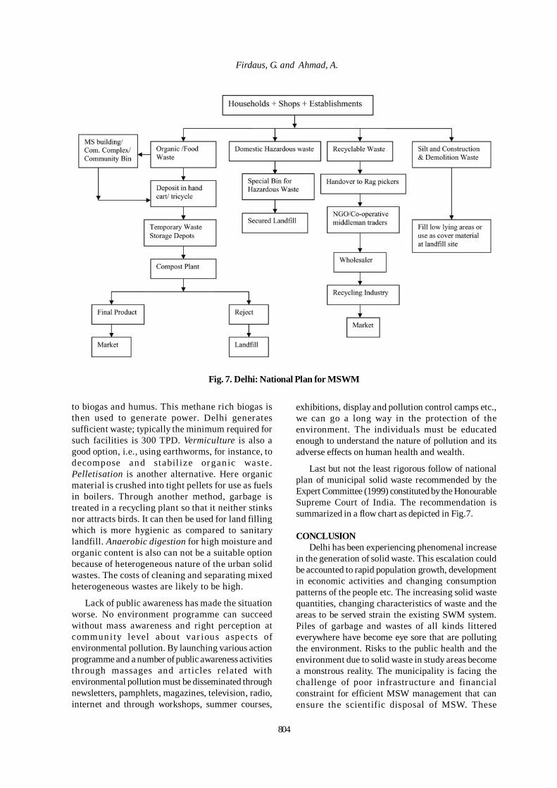
Firdaus, G. and Ahmad, A.
to biogas and humus. This methane rich biogas isthen used to generate power. Delhi generatessufficient waste; typically the minimum required forsuch facilities is 300 TPD. Vermiculture is also agood option, i.e., using earthworms, for instance, todecompose and stabil ize organ ic waste.Pelletisation is another alternative. Here organicmaterial is crushed into tight pellets for use as fuelsin boilers. Through another method, garbage istreated in a recycling plant so that it neither stinksnor attracts birds. It can then be used for land fillingwhich is more hygienic as compared to sanitarylandfill. Anaerobic digestion for high moisture andorganic content is also can not be a suitable optionbecause of heterogeneous nature of the urban solidwastes. The costs of cleaning and separating mixedheterogeneous wastes are likely to be high.
Lack of public awareness has made the situationworse. No environment programme can succeedwithout mass awareness and right perception atcommunity level about var ious aspects ofenvironmental pollution. By launching various actionprogramme and a number of public awareness activitiesthrough massages and articles related withenvironmental pollution must be disseminated throughnewsletters, pamphlets, magazines, television, radio,internet and through workshops, summer courses,
exhibitions, display and pollution control camps etc.,we can go a long way in the protection of theenvironment. The individuals must be educatedenough to understand the nature of pollution and itsadverse effects on human health and wealth.
Last but not the least rigorous follow of nationalplan of municipal solid waste recommended by theExpert Committee (1999) constituted by the HonourableSupreme Court of India. The recommendation issummarized in a flow chart as depicted in Fig.7.
CONCLUSIONDelhi has been experiencing phenomenal increase
in the generation of solid waste. This escalation couldbe accounted to rapid population growth, developmentin economic activities and changing consumptionpatterns of the people etc. The increasing solid wastequantities, changing characteristics of waste and theareas to be served strain the existing SWM system.Piles of garbage and wastes of all kinds litteredeverywhere have become eye sore that are pollutingthe environment. Risks to the public health and theenvironment due to solid waste in study areas becomea monstrous reality. The municipality is facing thechallenge of poor infrastructure and financialconstraint for efficient MSW management that canensure the scientific disposal of MSW. These
Fig. 7. Delhi: National Plan for MSWM
804
Int. J. Environ. Res., 4(4):795-806, Autumn 2010
requirements have generated demand for planning,administration, finance, technical expertise, equipment,material, and legal aspects of activities associated withgeneration, storage, collection, transportation,processing and disposal in an environmentallycompatible manner. It has been found that the wastemanagement system cannot be successful without theinvolvement of all stakeholders including people,NGOs and entrepreneur etc who have a vital role toplay in successful implementation of the scheme.Besides, community sensitization and publicawareness should develop for the successfulimplementation of the legal provisions of MSWM.
REFERENCES
Abdoli, S. (2009). RFID Application in Municipal SolidWaste Management System. Int. J. Environ. Res., 3(3), 447-454.
Abduli, M. A., Samieifard, R. and Jalili Ghazi Zade, M.(2008). Rural Solid Waste Management. Int. J. Environ. Res.,2(4), 425-430.
Bhoyar, R. V., Titus, S. K., Bhide, A. D. and Khanna, P.(1996). Municipal and Industrial Solid Waste Managementin India. Journal of IAEM, 23, 53-64.
CPCB, (2001). Management of municipal solid waste Delhi:Central Pollution Control Board, Delhi.
CPCB, (1999). Status of solid waste generation, collection,treatment and disposal in metro cities, Central PollutionControl Board, Delhi.
CPHEEO, (2000). Manual on Municipal Solid WasteManagement, Central Public Health and EnvironmentalEngineering Organisation, Ministry of UrbanDevelopment, New Delhi.
Cointreau-Levine, S. (1982). Environmental management ofurban solid waste in developing countries. A project guidefor the World Bank staff, 4p.
Datta, M. (1997). Waste Disposal in Engineered Landfills.Narosa Publishing House, New Delhi.
Dayal, G., Yadav, A., Singh, R. P. and Upadhyay, R. (1993).Impact of climatic conditions and socio-economic status onsolid waste characteristics: A case study. The Science of theTotal Environment, 136, 143-153.
Delhi urban environment and infrastructure improvementproject, 2001, pp. 49.
Dhamija, U. (2006). Sustainable solid water management,Academic Foundation, New Delhi, pp. 16.
Diaz, L. F., Savage, G. M. and Eggerth, L. L. (1997).Managing solid wastes in developing countries. journal ofwaste management, 43-45.
Ghiasinejad, H. and Abduli, S. (2007). Technical andEconomical Selection of Optimum Transfer-Transport
Method in Solid Waste Management in Metropolitan Cities.Int. J. Environ. Res., 1(2), 179-187.
Interim Report of the First Finance Commission for NCTof Delhi (1996), quoted in TERI Report No. 1999 EE41(March 2002), Urban Service Environmental Rating System,p.169.
Jalan, R. K., Sushil and Srivastava V. K. (1995). The emergingpriority for disposal use and recycling of MSW in India.Journal of Waste Management, 17-18.
Jalili Ghazizade, M. and Noori, R. (2008). Prediction ofMunicipal Solid Waste Generation by Use of ArtificialNeural Network: A Case Study of Mashhad. Int. J. Environ.Res., 2(1), 13-22.
Jeevan Rao, K. and Shantram, M. V. (1995). Ground waterpollution from Refuse Dumps at Hyderabad”Indian journalof Environmental Health, 37 (3), 197-204.
Joseph, K. and Nagendran, R. (2004). Essential ofenvironmental studies, Pearson Education, New Delhi, p.159.
Karamouz, M., Zahraie, B., Kerachian, R., Mahjouri, N.and Moridi, A. (2006). Development of a master plan forindustrial solid waste management. Int. J. Environ. Sci. Tech.,3(3), 229-242.
Kumar, S., Gaikwad, S. A., Shekdar, A. V., Kshirsagar, P. S.and Singh, R. N. (2004). “Estimation Method for NationalMethane Emission from Solid Waste Landfills. AtmosphericEnvironment, 38, 3481-3487.
MCD Background Note on Conservancy and SanitationEngeering Report, 2001, p.1.
MoEF. (2000). Municipal Solid Wastes ( Management andHandling ) Rules, Ministry of Environment and Forests,Government of India, New Delhi.
Monazzam, M. R. and Park, B. (2009). Prediction of MSWLong-term Settlement Induced by Mechanical andDecomposition-Based Compressions. Int. J. Environ. Res.,3(3), 335-348.
Nwabanne, J. T., Onukwuli, O. D. and Ifeakandu, C. M.(2009). Biokinetics of Anaerobic Digestion of MunicipalWaste. Int. J. Environ. Res., 3(4), 511-516.
Omran, A., Mahmood, A., Abdul Aziz, H. and Robinson,G .M. (2009). Investigating Households Attitude TowardRecycling of Solid Waste in Malaysia: A Case Study. Int. J.Environ. Res., 3(2), 275-288.
Oshode, O. A., Bakare, A. A., Adeogun, A. O., Efuntoye M.O. and Sowunmi, A. A. (2008). Ecotoxicological AssessmentUsing Clarias Gariepinus and Microbial Characterizationof Leachate from Municipal Solid Waste Landfill. Int. J.Environ. Res., 2(4), 391-400.
Ray, B. K. (2003). Policy Issue in Solid Waste Management,Environmental Science and Engineering. August 16.
Shekdar. (1999). Municipal solid waste management – theIndian Perspective, Journal of Indian Association forEnvironmental Management, 26 (2), 100-108.
805

Management of Solid Waste Pollution
Srishti report on recycling responsibility traditional systemsand new challenges of urban waste management in India,2002, pp. 14-15.
Singhal, S and Pandey, S. (2001). Solid waste managementin India: status and future
directions, TERI Information Monitor on EnvironmentalScience, 6 (1), 1-4.
The Energy Research Institute (TERI), State of EnvironmentReport for Delhi 2001, New Delhi, p. 65.
Turk, J. and Turk, A., (1984). Environmental Science, 3rd
Edition, Sounder College Publ., New York, 482-497.
Uemura, Sh. (2010). Mineral Requirements for Mesophilicand Thermophilic Anaerobic Digestion of Organic SolidWaste. Int. J. Environ. Res., 4(1), 33-40.
World Urbanization Prospects, (2007). (ExecutiveSummary), United Nation, New York, USA.
806
Int. J. Environ. Res., 4(4):807-816, Autumn 2010ISSN: 1735-6865
Received 17 Sep. 2009; Revised 15 March 2010; Accepted 25 April 2010
*Corresponding author E-mail:[email protected]
807
Model Simulation of Biodegradation of Polycyclic aromatic Hydrocarbon
in a Microcosm
Owabor, C. N . 1*, Ogbeide, S . E . 1 and Susu, A . A .2
1 Department of Chemical Engineering, University of Benin, P.M.B.1154, Benin City, Nigeria
2 Department of Chemical Engineering, University of Lagos, Akoka, Lagos 101017, Nigeria
ABSTRACT: The solutions of mathematical models for the estimation of the kinetic, and biokinetic parametersof naphthalene, anthracene and pyrene during degradation in surface and subsurface soils are presented in thiswork. The models were developed using the twin concepts of rate-determining step and steady-stateapproximation method. They described the biodegradation of single and a mixture of polycyclic aromatichydrocarbons. Prediction of the concentration of the reactive PAHs with time was aided by fitting the modelsto the experimental data obtained from a soil microcosm reactor. Given an initial concentration of 100mg/L,approximately 2.9%, 1.9% and 1.4% of naphthalene, pyrene and anthracene present in the microcosm reactorat zero time were found to be utilized in a minute when the velocity of the reaction remained constant for theperiod.The rate-determining step model gave a better fit as its reaction rate constant (k) closely fitted theexperimental values. Prediction by the steady state approximation model was not feasible as a comparativeanalysis of both single and multisubstrate results showed that the steady state approximation overestimatesthe biodegradation rates.Using the relative error method, results indicated that the rate-determining step modelshowed a deviation of 7.5%. The rate-determining step model was chosen because the differences in the modelfits were small and its prediction of mixture experiment was more enhanced.
Key words: PAH, Degradation, Mathematical models, Solution method, Twin concept
INTRODUCTIONLarge amounts of petroleum and petroleum prod-
ucts are discharged into the environments as a resultof exploration, production, transportation, refining andutilization. Despite careful handling and containment,some may spill into the soil through blowouts, acci-dents; rupture of oil pipelines and from domestic waste.In Nigeria, as a result of increasing daily activities withinthe petroleum industry, polycyclic aromatic hydrocar-bons input into the environment have increased greatly(Asuquo et al., 2004; Akpofure et al., 2007). It hastherefore become imperative and very desirable to de-contaminate locations that have had loading of petro-leum or petroleum products.
Concerted efforts have been made to understandthe reactions of these groups of compounds in aque-ous-solids/sediments matrix. Bioremediation has be-come a huge success in harnessing the natural activityof microorganisms for the performance of beneficial
functions that have greatly enhanced our standard ofliving (Bhatt, 2002; Oleszczuk and Baran, 2003;Janikowski et al., 2004; Xu and Obbard, 2004). Themicroorganisms exposed to these anthropogenic sub-stances have sometimes responded by acquiring newgenes for degradation of these compounds, either fordetoxification or to enable the microbe use the con-taminant as a source of energy to meet metabolic needs(Boochan et al, 2000; Chunga and King, 2001; Reardonet al; 2002; de Lucas et al., 2005). There are dearth ofreports on the rate and metabolism of this group ofcompounds in experimental systems developed tomodel natural degradation. The use of the microbesas catalysts in bioremediation, particularly in Nigeriahas been to essentially increase the rate of degrada-tion so as to eliminate as quickly as possible, bothlong and short-term effects of these contaminants thatcompromise the integrity of the environments(Nwachukwu, 2001; Ebuehi et al., 2005; Oboh et al.,2006; Ojo, 2006).
808
Owabor, C. N . et al.
In this study, the use of a microcosm reactor isadvanced. The microcosm was set up to provide ac-climated soil for the microbiota. The investigation wasto determine the rates of mineralization of the poly-cyclic aromatic hydrocarbons and assess the level ofmicrobial activity using oxygen uptake and carbondioxide evolution data as indicators. A mathematicalmodel was also developed. It incorporates interac-tion between molecular diffusion and kinetics of theprocess which will help to validate the data obtainedfrom experiments.
MATERIALS & METHODSThe polycyclic aromatic hydrocarbons used (naph-
thalene, anthracene and pyrene) were purchased fromHarrison and Harrison Laboratories Co. Ltd in Lagos.The culture media used were Potato Dextrose Agar andNutrient Agar. The Minimal salts medium consisted ofthe following K2HPO4, KH2PO4, MgSO4, NaCl, CaCl2 andNH4NO3. Trace elements solution was prepared usingMgO, CaCO3, FeSO4.7H2O, ZnSO4.7H2O, MgSO4.4H2O,CuSO4.5H2O, H3BO3, and HCl. Other chemicals usedwere: potassium hydroxide, calcium hydroxide, pyro-gallol, and mercuric chloride. All reagents used were ofanalytical grade. Distilled water was used for solution,sample preparation and dilution.
Soil sample collected from unimpacted zones atfield 17 in the Nigerian Institute For oil Palm Research(NIFOR), near Benin City, Edo State, Nigeria was used.The sampling was done around a sampling point to adepth of 0-15cm.The bulked composite soil sampleswere put in a sterile black polyethylene bag sealed andstored in a refrigerator prior to analysis.The contami-nant hydrocarbons used for the study include naph-thalene, anthracene and pyrene.1 kg unimpacted sur-face and subsurface soils were excavated and placedinside the microcosm. The soil was spiked with a mix-ture of the contaminant hydrocarbons (200mg each)dispersed in 2 liters of water containing a 0.02% sur-factant sodium hexametaphosphate, SHMP (Koeppelet al., 1997) and nutrients (straw, saw dust, and poul-try dung) as prescribed by the organization for eco-nomic cooperation and development (OECD). Anotherreactor was also set up and used as a control. A con-stant flow rate of oxygen was then sent into the tworeactors. The temperature and pressure of the micro-cosm reactors were monitored throughout the periodof experimentation using a digital multimeter and pres-sure gauge.
Thereafter, samples were taken on a weekly ba-sis and analyzed using solvent extraction and gaschromatography methods to determine the concen-tration of contaminants. The oxygen uptake and
carbon (iv) oxide evolution measurements were alsocarried out.
The absorbent (100mL) in the absorption bottleconsisted of one volume of a 1% (w/v) aqueous solu-tion of pyrogallol with three volumes of a 30% (w/v)aqueous solution of potassium hydroxide. Openingthe stopcock connecting the absorption bottle to themicrocosm absorbed oxygen, sample gas was drawninto the absorbent solution and the amount of oxygennot consumed was determined colorimetrically using aUV/V spectrophotometer (Spectronic 21D), at a wave-length of 605nm. Sampling was done every 5days.
Carbon dioxide evolved was carried out using orsatgas analyzer. The absorption vessel was charged with100mL calcium hydroxide as the absorbent. The level-ing bottle was filled with a confining liquid (5%sulphuric acid solution containing a few drops of me-thyl orange indicator). The leveling bottle was raisedto the top of the analyzer, with the 3-way cock at theend of the manifold opened. The burette was filledwith water up to the capillary tube and air was removedfrom the connecting tube using a rubber bellows pump.With the 3-way cock suitably set, sample gas was drawninto the burette by lowering the leveling bottle untilthe water meniscus reaches the lowest graduation markof the burette. The stopcock connecting the burette tothe absorption vessel containing calcium hydroxidewas opened and the level bottle rose. The level bottlewas lowered again and the gas brought into the bu-rette until the absorbent in the vessel reaches the markjust above the top of the vessel. The operation wasrepeated until absorption was complete as was evi-denced when the meniscus in the level bottle was atthe level with that in the burette. The burette readingwas recorded. Sampling was done every 10days.Kinetic models for the biodegradation of con-taminants at the gas-liquid and liquid-solid interfacefilm were developed using the concepts of rate-de-termining step (RDS) and steady state approximation(SSA), with molecular diffusion governed by Fick’slaw inclusive. The kinetic model equations for both asingle and multisubstrate catalyzed reactions, aregiven below using the equations described by Owaboret al., 2002.
a. RDS: (i) Single Substrate Reaction, n = 1
( )1
2 1 2 1
L xo o
oL L
C e C eC C
e e
⎡ ⎤⎡ ⎤⎢ ⎥= + −⎢ ⎥− −⎢ ⎥⎣ ⎦ ⎣ ⎦
(1)

Int. J. Environ. Res., 4(4):807-816, Autumn 2010
809
The initial condition:
C ( z, t) = f(z) at t = 0 and ze” 0 (5)
Boundary conditions:
C ( z, t ) = 1 at z = 0 and t d” 0 (6)
C (z, t ) = 0 at z = 1 and t e” 0 (7)
RESULTS & DISCUSSIONThe experiments conducted in this study provide
a deep understanding of the degradation kinetics ofboth single and a mixture of naphthalene, anthraceneand pyrene as model polycyclic aromatic hydrocar-bons (PAHs) in the surface and subsurface aqueous-soil matrix.The main objective of the microcosm studywas to provide an insight on the activity of the micro-organisms as well as a source of acclimated soils. Re-sults of the physicochemical properties of the soil areas shown in Table 1.
The salient characteristics of the uncontaminatedsoil used showed that the soil was highly porous witha particle size distribution in the ratio 85%: 14%: 1%for sand, clay and silt respectively. The microbial ac-tivities which would have been impeded as a result ofthe low moisture content (5%) of the soil were en-hanced by the addition of water which provided anaqueous environment suitable for the degradation pro-cess. The cation exchange capacity of the soil waswithin the recommended value of 5 cmol/kg for sandy
Table 1. Soil Characteristics
Soil moisture (%) 5.027
Bulk density 1.25
Total porosity 0.481
Particle size (%)
Sand Silt
Clay
85 1
14
pH (1:1) H2O 3.98
Organic Carbon (%) 2.44 Organic Matter (%) 4.19
Total Nitrogen (%) 0.114
Available Phosphorus (mg/Kg) 6.65 Exchangeable Bases (cmol/kg)
Ca++
Mg++
K+ Na+
0.65
0.14
0.12 0.08
Exchangeable Acidity (Al3+ + H+) 2.66
CEC (cmol/kg) 3.65
soil low in organic matter. This is especially significantbecause decaying organic matter shrinks and swellsand encourages micro fauna which create or widenopenings in the soil thus improving infiltration andaeration. The level of exchangeable acidity as reflectedby the pH implied that the soil was very acidic. This,therefore, portends a reducing environment. The re-dox condition necessary to enhance microbial activityand hence the degradation of the PAHs in the soil wasachieved through the use of oxygen which functionedas electron donor. The low nitrogen and low-to- mod-erate available phosphorus in the soil accounted forthe low nutrient level which was however, supple-mented with straw, sawdust and poultry dung as pre-scribed by the organization for economic cooperationand development (OECD).
As a means of assessing the level of microbialactivities in relation to biodegradation kinetics in thesoil, the soil samples in the microcosm reactor wasused as a source of acclimated micro biota for measur-ing oxygen uptake by respiration to determine biodeg-radation kinetics and carbon (iv) oxide evolution ki-netics. The objective was to ascertain the actual oxy-gen uptake and carbon (iv) oxide evolved as a result ofthe mineralization of the PAHs in the absence of soilorganic carbon. Fig. 1 showed the net cumulative car
(iv) Multi substrate Reaction, n >1
[ ][ ]
max o
m o
V C xCK C D
⎛ ⎞= ⎜ ⎟⎜ ⎟+⎝ ⎠
(3)
[ ][ ]
max i
m i
V C xCK C D
=+∑∑
(4)
b. SSA: (iii) Single substrate Reaction, n =1
(ii) Multi - Substrate Reaction, n > 1
( )1
1 2 1
L xo o
oL L
C e C e nC C
e xe
⎡ ⎤⎡ ⎤ −⎢ ⎥= + +⎢ ⎥− −⎢ ⎥⎣ ⎦ ⎣ ⎦
(2)

810
Biodegradation of Polycyclic aromatic Hydrocarbon
Fig. 1. Net Cumulative carbon dioxide evolution from the reactor spiked with a mixture of Naphthalene,Anthracene and Pyrene
0
0.5
1
1.5
2
2.5
0 10 20 30 40 50 60 70 80
'Experimental
"Control"
Time (Days)
Fig. 2. Oxygen uptake in Microcosm reactor
Oxy
gen
upta
ke (
mg/
L)
0
1
2
3
4
5
6
7
8
0 10 20 30 40 50 60 70 80
Cum
ulat
ive
CO
2 gen
erat
ion
(mol
) x 1
0-4
Time (Days)
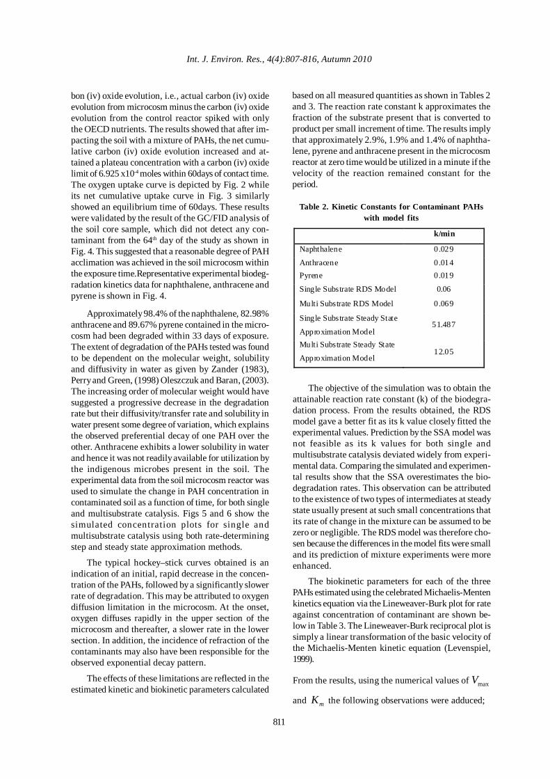
Approximately 98.4% of the naphthalene, 82.98%anthracene and 89.67% pyrene contained in the micro-cosm had been degraded within 33 days of exposure.The extent of degradation of the PAHs tested was foundto be dependent on the molecular weight, solubilityand diffusivity in water as given by Zander (1983),Perry and Green, (1998) Oleszczuk and Baran, (2003).The increasing order of molecular weight would havesuggested a progressive decrease in the degradationrate but their diffusivity/transfer rate and solubility inwater present some degree of variation, which explainsthe observed preferential decay of one PAH over theother. Anthracene exhibits a lower solubility in waterand hence it was not readily available for utilization bythe indigenous microbes present in the soil. Theexperimental data from the soil microcosm reactor wasused to simulate the change in PAH concentration incontaminated soil as a function of time, for both singleand multisubstrate catalysis. Figs 5 and 6 show thesimulated concentration plots for single andmultisubstrate catalysis using both rate-determiningstep and steady state approximation methods.
The typical hockey–stick curves obtained is anindication of an initial, rapid decrease in the concen-tration of the PAHs, followed by a significantly slowerrate of degradation. This may be attributed to oxygendiffusion limitation in the microcosm. At the onset,oxygen diffuses rapidly in the upper section of themicrocosm and thereafter, a slower rate in the lowersection. In addition, the incidence of refraction of thecontaminants may also have been responsible for theobserved exponential decay pattern.
The effects of these limitations are reflected in theestimated kinetic and biokinetic parameters calculated
Table 2. Kinetic Constants for Contaminant PAHswith model fits
k/min
Naphthalene 0.029
Anthracene 0.014 Pyrene 0.019
Single Substrate RDS Model 0.06
Multi Substrate RDS Model 0 .069
Single Substrate Steady State
Approximation Model 51.487
Multi Substrate Steady State
Approximation Model 12.05
The objective of the simulation was to obtain the
attainable reaction rate constant (k) of the biodegra-dation process. From the results obtained, the RDSmodel gave a better fit as its k value closely fitted theexperimental values. Prediction by the SSA model wasnot feasible as its k values for both single andmultisubstrate catalysis deviated widely from experi-mental data. Comparing the simulated and experimen-tal results show that the SSA overestimates the bio-degradation rates. This observation can be attributedto the existence of two types of intermediates at steadystate usually present at such small concentrations thatits rate of change in the mixture can be assumed to bezero or negligible. The RDS model was therefore cho-sen because the differences in the model fits were smalland its prediction of mixture experiments were moreenhanced.
The biokinetic parameters for each of the threePAHs estimated using the celebrated Michaelis-Mentenkinetics equation via the Lineweaver-Burk plot for rateagainst concentration of contaminant are shown be-low in Table 3. The Lineweaver-Burk reciprocal plot issimply a linear transformation of the basic velocity ofthe Michaelis-Menten kinetic equation (Levenspiel,1999).
From the results, using the numerical values of maxV
and mK the following observations were adduced;
bon (iv) oxide evolution, i.e., actual carbon (iv) oxideevolution from microcosm minus the carbon (iv) oxideevolution from the control reactor spiked with onlythe OECD nutrients. The results showed that after im-pacting the soil with a mixture of PAHs, the net cumu-lative carbon (iv) oxide evolution increased and at-tained a plateau concentration with a carbon (iv) oxidelimit of 6.925 x10⁻⁴ moles within 60days of contact time.The oxygen uptake curve is depicted by Fig. 2 whileits net cumulative uptake curve in Fig. 3 similarlyshowed an equilibrium time of 60days. These resultswere validated by the result of the GC/FID analysis ofthe soil core sample, which did not detect any con-taminant from the 64th day of the study as shown inFig. 4. This suggested that a reasonable degree of PAHacclimation was achieved in the soil microcosm withinthe exposure time.Representative experimental biodeg-radation kinetics data for naphthalene, anthracene andpyrene is shown in Fig. 4.
based on all measured quantities as shown in Tables 2and 3. The reaction rate constant k approximates thefraction of the substrate present that is converted toproduct per small increment of time. The results implythat approximately 2.9%, 1.9% and 1.4% of naphtha-lene, pyrene and anthracene present in the microcosmreactor at zero time would be utilized in a minute if thevelocity of the reaction remained constant for theperiod.
Int. J. Environ. Res., 4(4):807-816, Autumn 2010
811
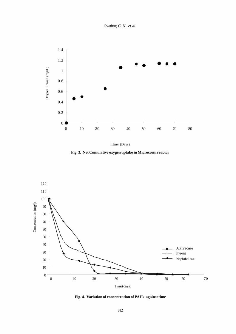
812
Con
cent
ratio
n (m
g/l)
Time(days)
0
10
20
30
40
50
60
70
80
90
100
110
120
0 10 20 30 40 50 60 70
PyreneAnthracene
Naphthalene
Fig. 4. Variation of concentration of PAHs against time
Fig. 3. Net Cumulative oxygen uptake in Microcosm reactor
Oxy
gen
upta
ke (
mg/
L)
Time (Days)
0
0.2
0.4
0.6
0.8
1
1.2
1.4
0 10 20 30 40 50 60 70 80
Owabor, C. N . et al.
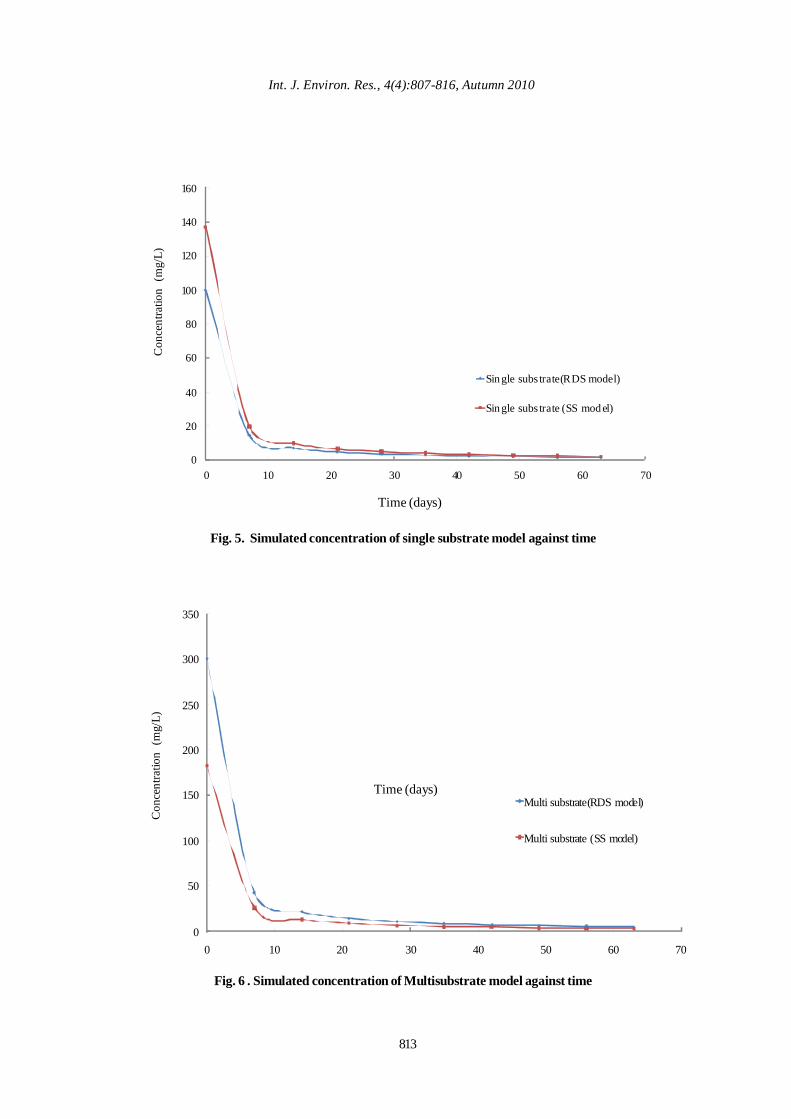
813
0
20
40
60
80
100
120
140
160
0 10 20 30 40 50 60 70
Sin gle subs trate(RDS model)
Sin gle subs trate (SS mod el)
Con
cent
ratio
n (m
g/L)
Time (days)
Fig. 6 . Simulated concentration of Multisubstrate model against time
0
50
100
150
200
250
300
350
0 10 20 30 40 50 60 70
Multi substrate(RDS model)
Multi substrate (SS model)
Fig. 5. Simulated concentration of single substrate model against time
Con
cent
ratio
n (m
g/L)
Time (days)
Int. J. Environ. Res., 4(4):807-816, Autumn 2010
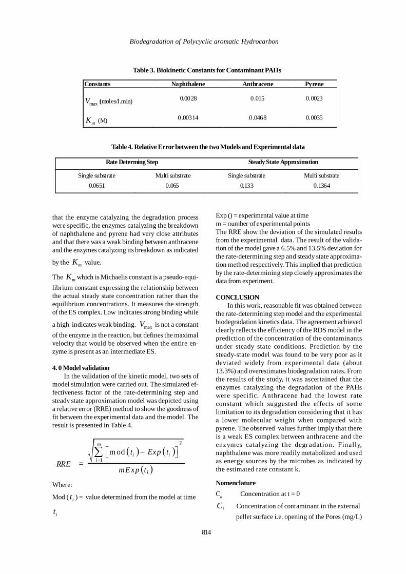
814
Table 3. Biokinetic Constants for Contaminant PAHs
Constants Naphthalene Anthracene Pyrene
maxV (moles/l.min)
0.0028
0.015
0.0023
mK (M)
0.00314
0.0468
0.0035
Table 4. Relative Error between the two Models and Experimental data
Rate Determing Step Steady State Approximation
Single substrate Multi substrate Single substrate Multi substrate 0.0651 0.065 0.133 0.1364
RRE =( ) ( )
( )
2
1m od
m
i ii
i
t Exp t
mExp t=
⎡ ⎤−⎣ ⎦∑
Where:
Mod ( it ) = value determined from the model at time
it
Exp () = experimental value at timem = number of experimental pointsThe RRE show the deviation of the simulated resultsfrom the experimental data. The result of the valida-tion of the model gave a 6.5% and 13.5% deviation forthe rate-determining step and steady state approxima-tion method respectively. This implied that predictionby the rate-determining step closely approximates thedata from experiment.
CONCLUSIONIn this work, reasonable fit was obtained between
the rate-determining step model and the experimentalbiodegradation kinetics data. The agreement achievedclearly reflects the efficiency of the RDS model in theprediction of the concentration of the contaminantsunder steady state conditions. Prediction by thesteady-state model was found to be very poor as itdeviated widely from experimental data (about13.3%) and overestimates biodegradation rates. Fromthe results of the study, it was ascertained that theenzymes catalyzing the degradation of the PAHswere specific. Anthracene had the lowest rateconstant which suggested the effects of somelimitation to its degradation considering that it hasa lower molecular weight when compared withpyrene. The observed values further imply that thereis a weak ES complex between anthracene and theenzymes catalyzing the degradation. Finally,naphthalene was more readily metabolized and usedas energy sources by the microbes as indicated bythe estimated rate constant k.
NomenclatureCo Concentration at t = 0
iC Concentration of contaminant in the external pellet surface i.e. opening of the Pores (mg/L)
that the enzyme catalyzing the degradation processwere specific, the enzymes catalyzing the breakdownof naphthalene and pyrene had very close attributesand that there was a weak binding between anthraceneand the enzymes catalyzing its breakdown as indicated
by the mK value.
The mK which is Michaelis constant is a pseudo-equi-librium constant expressing the relationship betweenthe actual steady state concentration rather than theequilibrium concentrations. It measures the strengthof the ES complex. Low indicates strong binding while
a high indicates weak binding. maxV is not a constantof the enzyme in the reaction, but defines the maximalvelocity that would be observed when the entire en-zyme is present as an intermediate ES.
4. 0 Model validationIn the validation of the kinetic model, two sets of
model simulation were carried out. The simulated ef-fectiveness factor of the rate-determining step andsteady state approximation model was depicted usinga relative error (RRE) method to show the goodness offit between the experimental data and the model. Theresult is presented in Table 4.
Biodegradation of Polycyclic aromatic Hydrocarbon
815
D Diffusivity of contaminant m2/sL Length of reactor (m)k Reaction rate constant (min-1)X Distance in the direction of flow (m)RRE Relative Error
REFERENCESAkpofure, E. A., Efere, M. L. and Ayawei, P. (2007). Inte-grated grass root post-impact assessment of acute damagingeffects of continuous oil spills in the Niger Delta January1998-January 2000" in: Oil spillage in Nigeria’s Niger Delta,Urhobo Historical Society.
Asuquo, F. E., Ewa-oboho, I., Asuquo, E. F. and Udo, P. J.(2004). Fish species used as biomarker for heavy metal andhydrocarbon contamination for Cross River, Nigeria. TheEnvironmentalist, 24, 1-2.
Bhatt, M. Cajthaml, T. and Šašek, V. (2002).Mycoremediation of PAH-contaminated soil. FoliaMicrobiologica, 47 (3), 255-258.
Boochan, M. L., Sudarat, B. and Grant, A. S. (2000). Degra-dation of high molecular weight polycyclic aromatic hydro-carbon by defined fungi- bacteria cocultures. Applied andEnvironmental Microbiology, 66 (3), 1007-1019.
Buchholz, F., Wick, L. Y., Harms, H. and Maskow, T. (2007).The kinetics of polycyclic aromatic hydrocarbon (PAH)biodegradation assessed by isothermal titration calorimetry(ITC). Thermochimica Acta, 458 (1-2), 47-53.
Chunga W. K. and King, G. M. (2001). Isolation, character-ization and polyaromatic hydrocarbon degradation poten-tial of aerobic bacteria from marine macrofaunal burrow sedi-ments. Appl. Environ Microbiol., 67, 5585-5592.
de Lucas, A., Rodriguez, L., Villasenor, J. and Fernandez, F.J. (2005). Biodegradation kinetics of stored wastewatersubstrate by a mixed microbial culture. Biochem. Eng. J.,26, 191-197.
Ebuehi, O. A.., Abibo, I. B., Shekwolo, P. D., Sigismund, K.I., Adoki, A. and Okoro, I. C. (2005). Remediation of crudeoil contaminated soil by enhanced natural attenuation tech-nique. Journal of Applied Science and Environmental Man-agement, 9, 103-106.
Janikowski, T., Velicogna, D., Punt, M. and Daugulis, A.(2004). Use of a two-phase partitioning bioreactor for de-grading polycyclic aromatic hydrocarbons by asphingonomonas spp. Appl. Microbiol. Biotechnol., 59,2-3.
Huckins, J. M., Petty, J. D., Orazio, C.E., Lebo, J. A., Clark,R. C., Gibson ,V. L., Gala, W. R.. and Echols, K. R. (1999).Determination of uptake kinetics (sampling rates) by liq-uid-containing semipermeable membrane devices (SPMDs)
for polycyclic aromatic hydrocarbons (PAHs) in water.Environ. Sci. Technol., 33 (21), 3918-3923.
Koeppel, C., Popovic, M. and Bajpai, R. K. (1997). Micro-bial migration in soil in: bioremediation of surface and sub-surface contamination in: bioremediation of surface and sub-surface contamination, Bajpai Sciences, the New York Acad-emy of Sciences, 829, 50-262, New York.
Levenspiel, O. (1999). Chemical Reaction Engineering, JohnWiley and Sons Inc., 3rd edition, 623-641.
Lotfabad, S. K. and Gray, M. R (2002) Kinetics of biodeg-radation of mixtures of polycyclic aromatic hydrocarbons.Appl. Microbiol. Biotechnol., 60 (3), 361-366.
Mohan, P. K., Nakhla, G. and Yanful, E. K. (2006) Bioki-netics of biodegradation of surfactants under aerobic, an-oxic and anaerobic conditions. Water Research, 40 (3), 533-540.
Nwachukwu, S. C. U. (2001). Bioremediation of sterile ag-ricultural soils polluted with crude petroleum by applica-tion of the soil bacterium, Pseudomonas putida, with inor-ganic nutrient supplementation. Current Microbiology, 42,231-236.
Oboh, B. O., Ilori, M. O., Akinyemi, J. O. and Adebusoye,S. A. (2006). Hydrocarbon degrading potentials of bacteriaisolated from a Nigerian bitumen (Tarsand) deposit. Na-ture and Science, 4 (3), 51-57.
Ojo, O. A. (2006). Petroleum hydrocarbon utilization bynative bacterial population from a wastewater canal South-west Nigeria. African Journal of Biotechnology, 5, 333-337.
Oleszczuk, P. and Baran, S. (2003), Degradation of indi-vidual polycyclic aromatic hydrocarbons (PAHs) in soilpolluted with aircraft fuel”, Polish Journal of Environmen-tal Studies, 12 (4), 431-437.
Owabor, C. N., Ogbeide, S. E. and Susu, A. A. (2002). Sub-strate bioavailability and biodegradation in contaminatedaqueous-soil matrix Model development for steady-statebiofilm kinetics. J. Sci. Tech. Environ., 2 (2), 40-46.
Perry, R. H. and Green, D. W. (1998). Perry’s ChemicalEngineers Handbook, 7th Edition. McGraw-Hill Inc.
Reardon, K. F., Mosteller , D. C., Rogers, J. B., Duteau, N.and Kim, K. (2002). Biodegradation kinetics of aromatichydrocarbon mixtures by Pure and mixed bacterial cultures.Environmental Health Perspectives, 110, 1005-1011.
Ramaswami, A. and Luthy, R. G. (1997). Mass transfer andbioavailability of PAH compounds in Coal Tar NAPL-slurrysystems. 1. Model Development. Environ. Sci. Technol. 31(8), 2260-2267.
Int. J. Environ. Res., 4(4):807-816, Autumn 2010

Ramaswami, A and Luthy, R. G. (1997). Mass transfer andbioavailabilty of PAH compounds in Coal Tar NAPL-slurrysystems. 2. Experimental Evaluations. Environs. Sci.Technol., 31 (8), 2268-2276.
Smith, K.., Cutright, T. and Qammar, H. (2000). Biokineticparameter estimation for ISB of PAH-contaminated soil.Journal of Environment Engineering, 126 (4), 369-374.
Wammer, K. H. and Peters, C. A. (2005). Polycyclic aro-matic hydrocarbon biodegradation rates: A Structure-basedstudy. Environ. Sci. Technol., 39 (8), 2571-2578.
Xu, R. and Obbard, J.P. (2004). “Biodegradation of polycy-clic aromatic hydrocarbons in oil-contaminated beach sedi-ments treated with nutrients amendments. J. Environ.Qual.,33, 861-867.
Zander, M. (1983). Physical and chemical properties ofpolycyclic aromatic aromatic hydrocarbons, pp1-20. In: A.Bjorseth (ed), Handbook of polycyclic aromatic hydrocar-bons. Marcel Dekker, Inc., New York.
Owabor, C. N . et al.
816
Int. J. Environ. Res., 4(4):817-824, Autumn 2010ISSN: 1735-6865
Received 3 April 2009; Revised 15 May 2010; Accepted 26 May 2010
*Corresponding author E-mail:[email protected]
817
Equilibrium and Kinetic Studies on Sorption of Malachite Green usingHydrilla Verticillata Biomass
Rajesh Kannan, R.1*, Rajasimman, M.1, Rajamohan, N.2 and Sivaprakash, B.1
1 Environmental Engineering Laboratory, Department of Chemical Engineering, AnnamalaiUniversity, Annamalai Nagar-608 002, Tamil Nadu, India
2 Department of Chemical Engineering, Sohar University, Sohar, Sultanate of Oman
ABSTRACT: In the present study, Hydrilla verticillata biomass was investigated as a novel biosorbent for theuptake of basic dye malachite green from its aqueous solution. Kinetic and equilibrium studies were carried out inbatch process. Batch adsorption experiments were conducted to study the effect of pH, temperature, sorbentdosage, initial dye concentration, and contact time for the removal malachite green dye. The dye uptake wasmaximum for the initial pH of 8, temperature of 30oC, sorbent dosage of 0.55g, initial dye concentration200mg/l and contact time – 150 min. The kinetic studies were well modeled using pseudo first order and secondorder with isotherm studies.
Key words: Malachite Green, Hydrilla verticillata, plant biomass, Equilibrium studies
INTRODUCTIONSynthetic dyes are extensively used in many
industries such as the textile, leather, paper production,food technology, hair colorings, etc. Wastewatersdischarged from these industries are usually pollutedby dyes. Malachite green (MG) is most com-monly usedfor the dyeing of cotton, silk, paper, leather and also inmanufacturing of paints and printing inks. Malachitegreen is widely used in distilleries for coloring purposes(Khattri et al., 1999). In the recent decade ampleattention has been paid to equilibrium and kineticstudies of various sorbents (Igwe et al., 2008; Gharbaniet al., 2008; Goyal et al., 2008; Shah et al., 2009;Zvinowanda et al., 2009). Mala-chite green hasproperties that make it difficult to remove from aqueoussolutions and also toxic to major microorganisms(Papinutti et al., 2006). Though the use of this dye hasbeen banned in several countries and not approved byUS Food and Drug Administration (Chang et al., 2001),it is still being used in many parts of the world due toits low-cost, ready availability and efficacy and to lackof a proper alternative(Schnick et al., 1988). Its use inthe aquaculture practice in many countries, includingIndia has not been regulated (Rahman et al., 2005).Malachite green when discharged into receivingstreams will affect the aquatic life and causesdetrimental effects in liver, gill, kidney, intes-tine,gonads and pituitary gonadotrophic cells (Srivastava
et al., 2004). Therefore, the treatment of effluentcontaining such dye is of interest due to its estheticimpacts on receiving waters.
Various techniques have been employed for theremoval of dyes from wastewaters. These methodsinclude adsorp-tion, nano-filtrtion, electro kineticcoagulation, coagulation and precipitation, advancedchemical oxidation, electrochemical oxidation,ozonation, supported liquid membrane, liquid-liquidextraction and biological process (Mahmoud et al.,2007). The adsorption process is one of the efficientmethods to remove dyes from effluent due to its lowinitial cost, simplicity of design, ease of operation andinsensitivity to toxic substances (Robinson et al.,2001). Activated carbon is the most widely usedadsorbent with great success due to its large surfacearea, micro-porous struc-ture, high adsorptioncapacity, etc. However, its use is limited because of itshigh cost. This has led to search for cheapersubsti-tutes (Allen et al., 2003). Various cheapadsorbents like wood and lignite have been used forthe removal of colour and metal ions in effluents. Othermaterials include fly ash, rice husk, tree bark and humanhair have been tested and reported to give encouragingresults in several areas of application (Malik et al.,2003). However the adsorption capacities of the aboveadsorbents are not very high. In order to improve the
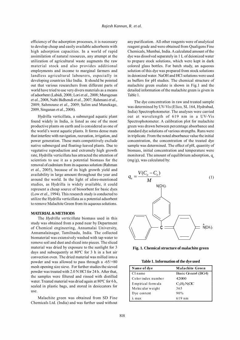
818
Rajesh Kannan, R. et al.
efficiency of the adsorption processes, it is necessaryto develop cheap and easily available adsorbents withhigh adsorption capacities. In a world of rapidassimilation of natural resources, any attempt at theutilization of agricultural waste augments the rawmaterial stock and also provides additionalemployments and income to marginal farmers andlandless agricultural labourers, especially indeveloping countries like India. It should be pointedout that various researchers from different parts ofworld have tried to use very divers materials as a meansof adsorbent (Labidi, 2008; Lori et al., 2008; Murugesanet al., 2008, Nabi Bidhendi et al., 2007; Rahmani et al.,2009; Sahmoune et al., 2009; Salim and Munekage,2009, Singanan et al., 2008).
Hydrilla verticillata, a submerged aquatic plantfound widely in India, is listed as one of the mostproductive plants on earth and is considered as one ofthe world’s worst aquatic plants. It forms dense matsthat interfere with navigation, recreation, irrigation, andpower generation. These mats competitively excludenative submerged and floating-leaved plants. Due tovegetative reproduction and extremely high growthrate, Hydrilla verticillata has attracted the attention ofscientists to use it as a potential biomass for theremoval of cadmium from its aqueous solution (Rahmanet al., 2005), because of its high growth yield andavailability in large amount throughout the year andaround the world. In the light of afore-mentionedstudies, as Hydrilla is widely available, it couldrepresent a cheap source of biosorbent for basic dyes(Low et al., 1994). This research study is conducted toutilize the Hydrilla verticillata as a potential adsorbentto remove Malachite Green from its aqueous solutions.
MATERIAL & METHODSThe Hydrilla verticillata biomass used in this
study was obtained from a pond near by Departmentof Chemical engineering, Annamalai University,Annamalainagar, Tamilnadu, India. The collectedbiomaterial was extensively washed with tap water toremove soil and dust and sliced into pieces. The slicedmaterial was dried by exposure to the sunlight for 3days and subsequently at 80ºC for 3 h in a hot airconvection oven. The dried material was milled into apowder and was allowed to pass through a -65/+80mesh opening size sieve. For further studies the sievedpowder was treated with 2.0 N HCl for 24 h. After that,the samples were filtered and rinsed with distilledwater. Treated material was dried again at 80ºC for 6 h,sealed in plastic bags, and stored in desiccators foruse.
Malachite green was obtained from SD FineChemicals Ltd. (India) and was further used without
any purification. All other reagents were of analyticalreagent grade and were obtained from Qualigens FineChemicals, Mumbai, India. A calculated amount of thedye was dissolved separately in 1 L of deionized waterto prepare stock solutions, which were kept in darkcolored glass bottles. For batch study, an aqueoussolution of this dye was prepared from stock solutionsin deionized water. NaOH and HCl solutions were usedas buffers for pH studies. The chemical structure ofmalachite green oxalate is shown in Fig.1 and thedetailed information of the malachite green is given inTable 1.
The dye concentration in raw and treated samplewas determined by UV-Vis (Elico, SL 164, Hydrabad,India) Spectrophotometer. The analyses were carriedout at wavelength of 619 nm in a UV-VisSpectrophotometer. A calibration plot for malachitegreen was drawn between percentage absorbance andstandard dye solutions of various strengths. Runs werein triplicate. From the noted absorbance value the initialconcentration, the concentration of the treated dyesample was determined. The effect of pH, quantity ofbiomass, initial concentration and temperature weremonitored. The amount of equilibrium adsorption, qe(mg/g), was calculated by:
MCCV
q eoe
)( −= (1)
C
N(CH3)2
N(CH3)2+
Fig. 1. Chemical structure of malachite green
Table 1. Information of the dye used
Nam e of dye M alachite Gree n CI name Basic Green4 (BG4) Color index numbe r 42000 Empirical form ula C23H25N2ClC Molec ular weight 365 Dye content 90% λ max 619 nm

Int. J. Environ. Res., 4(4):817-824, Autumn 2010
819
where C0 and Ce (mg/L) are the liquid-phaseconcentrations of dye at initial and equilibrium,respectively. V (L) is the volume of the solution and M(g) is the mass of dry sorbent used.
RESULTS & DISCUSSIONIn this work, the effect of pH on the MG adsorption
onto Hydrilla verticillata Biomass was studied whilethe initial dye concentration, shaking time, amount ofHydrilla verticillata biomass and temperature were fixedat 100 mg/L, 200 min, 0.30 g and 30 °C, respectively.Solution pH would affect both aqueous chemistry andsurface binding-sites of the adsorbent. The effect ofpH on the adsorption of MG by the Hydrilla verticillatabiomass is presented in Fig. 2. The equilibrium sorptioncapacity was minimum at pH 2 (11 mg/g) and increasesmonotonically up to pH 5, Further increase in pH leadsto appreciable increase in % adsorption. The absenceof sorption at low pH can be explained by the fact thatat this acidic pH, H+ may compete with dye ions for theadsorp-tion sites of adsorbent, thereby inhibiting theadsorption of dye. At higher solution pH, the Hydrillaverticillata biomass may get negatively charged, whichenhances the adsorption of positively charged dyecations through electrostatic forces of attraction. Alsoa change of solution pH affects the adsorptive processthrough dissociation of functional groups on theadsorbent surface. Such behavior leads to a shift inequilibrium characteristics of adsorption process. Asimilar result of pH effect was also reported for theadsorption of Malachite green onto rattan saw dust(Hameed et al., 2008).
The influence of temperature on the sorption ofmalachite green by the Hydrilla verticillata biomass wasstudied with a constant initial concentration of 100mg/L and with a temperature range of 20oC to 50 oC.
The Effect of temperature on adsorption capacity isdepicted in Fig. 3. The temperature profile indicatesthat as the temperature increases the sorption capacityincreases to a maximum value and then decreases. Thisis because at very high temperature the biosorbentlooses its property due to denaturation. The maximumsorption capacity was attained at 30oC. Similar resultof Temperature effect was also reported for theadsorption of Basic dye onto chitosan (Chellababu etal., 2008).The effect of quantity of Hydrilla verticillatabiomass dosage on the amount of color adsorbed wasstudied by agitating 200mL of 100mg/L dye solutionwith different amounts of sorbent addition such as0.25, 0.35, 0.45 and 0.55g. All these studies wereconducted at room temperature and at a constant speedof 200 rpm. Fig. 4 shows the effect of adsorbent dosage
on the amount of dye adsorbed eq (mg/g). It wasobserved that the amount of dye adsorbed varied withinitial adsorbent dosage. The amount adsorbeddecreased from 41.5 to 28.46 mg/g for an increase insorbent dosage from 0.25 to 0.55g. An increase in %colour removal was observed with an increase inadsorbent dosage. The decrease in may be due to thesolute transfer rate on to the adsorbent surface,i.e.,Theamount of solute adsorbed onto unit weight ofadsorbent get split with increasing adsorbent dosage.
The contact time between the dye molecules andthe sor-bent is of significant importance in the dyetreatment by sorption. The effect of contact time on thesorption of malachite green was studied for an initial dyeconcentration of 100 mg/l, a sorbent mass of 0.25 g, asolution volume of 100 mL, an agi-tation speed of 200rpm, and a temperature of 30 °C. The effect of contacttime on the removal of dye by the studied sorbent isshown in Fig. 5. The obtained results reveal that the uptake
0
10
20
30
40
50
0 2 4 6 8 10 12
pH
Dye
Upt
ake (
mg/
g)
Fig. 2. Effect of pH on equilibrium uptake of MG (M = 0.30 g; V = 0.2 L; Co = 100 mg/L)

820
Kinetic Studies on Sorption of Malachite Green
Fig. 3. Effect of temperature on equilibrium uptake of MG (M = 0.30g; V = 0.2 L; Co= 100 mg/L)
0
5
1 0
1 5
2 0
2 5
3 0
3 5
4 0
4 5
5 0
0 1 0 2 0 3 0 4 0 5 0 6 0
Te mpe ratur e (oC )
Dye
upt
ake
(mg/
0
10
20
30
40
50
0.2 0.25 0.3 0.35 0.4 0.45 0.5 0.55 0.6
Sorbent dos age(g)
Dye
Upt
ake
(mg/
g)
Fig. 4. Effect of sorbent dosage on equilibrium uptake of MG (V = 0.2; Co = 100 mg/L)
0
10
20
30
40
50
0 50 100 150 200 250 300 350
Time(min)
Dye
upta
ke (m
g/g)
Fig. 5. Effect of contact time on sorption of MG dyes by the Hydrilla Verticillata biomass - initial dyeconcentration: 100 mg/L, sorbent mass: 0.55 g; agitation speed: 200 rpm)
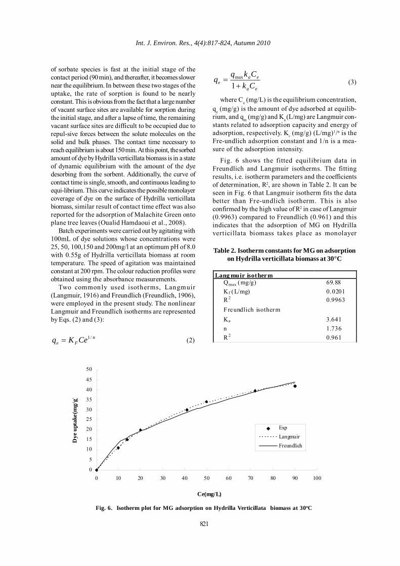
Int. J. Environ. Res., 4(4):817-824, Autumn 2010
of sorbate species is fast at the initial stage of thecontact period (90 min), and thereafter, it becomes slowernear the equilibrium. In between these two stages of theuptake, the rate of sorption is found to be nearlyconstant. This is obvious from the fact that a large numberof vacant surface sites are available for sorption duringthe initial stage, and after a lapse of time, the remainingvacant surface sites are difficult to be occupied due torepul-sive forces between the solute molecules on thesolid and bulk phases. The contact time necessary toreach equilibrium is about 150 min. At this point, the sorbedamount of dye by Hydrilla verticillata biomass is in a stateof dynamic equilibrium with the amount of the dyedesorbing from the sorbent. Additionally, the curve ofcontact time is single, smooth, and continuous leading toequi-librium. This curve indicates the possible monolayercoverage of dye on the surface of Hydrilla verticillatabiomass, similar result of contact time effect was alsoreported for the adsorption of Malachite Green ontoplane tree leaves (Oualid Hamdaoui et al., 2008).
Batch experiments were carried out by agitating with100mL of dye solutions whose concentrations were25, 50, 100,150 and 200mg/l at an optimum pH of 8.0with 0.55g of Hydrilla verticillata biomass at roomtemperature. The speed of agitation was maintainedconstant at 200 rpm. The colour reduction profiles wereobtained using the absorbance measurements.
Two commonly used isotherms, Langmuir(Langmuir, 1916) and Freundlich (Freundlich, 1906),were employed in the present study. The nonlinearLangmuir and Freundlich isotherms are representedby Eqs. (2) and (3):
nFe CeKq /1= (2)
ea
eae Ck
Ckqq
+=
1max
(3)
where Ce (mg/L) is the equilibrium concentration,qe (mg/g) is the amount of dye adsorbed at equilib-rium, and qm (mg/g) and Ka (L/mg) are Langmuir con-stants related to adsorption capacity and energy ofadsorption, respectively. K
F (mg/g) (L/mg)1/n is the
Fre-undlich adsorption constant and 1/n is a mea-sure of the adsorption intensity.
Fig. 6 shows the fitted equilibrium data inFreundlich and Langmuir isotherms. The fittingresults, i.e. isotherm parameters and the coefficientsof determination, R2, are shown in Table 2. It can beseen in Fig. 6 that Langmuir isotherm fits the databetter than Fre-undlich isotherm. This is alsoconfirmed by the high value of R2 in case of Langmuir(0.9963) compared to Freundlich (0.961) and thisindicates that the adsorption of MG on Hydrillaverticillata biomass takes place as monolayer
Fig. 6. Isotherm plot for MG adsorption on Hydrilla Verticillata biomass at 30oC
0
5
10
15
20
25
30
35
40
45
50
0 10 20 30 40 50 60 70 80 90 100
Ce(mg/L)
Dye
upt
ake(
mg/
g)
ExpLangmuirFreundlich
Table 2. Isotherm constants for MG on adsorptionon Hydrilla verticillata biomass at 30°C
Lang muir isothermQmax (mg/g) 69.88 Kf (L/mg) 0.0201 R 2 0.9963 Freundlich isotherm Ka 3.641 n 1.736 R 2 0.961
821
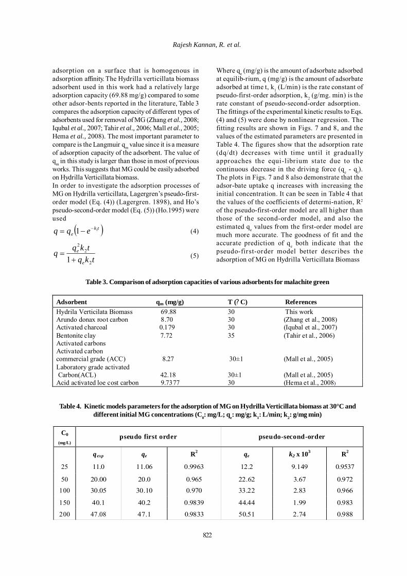
822
Rajesh Kannan, R. et al.
adsorption on a surface that is homogenous inadsorption affinity. The Hydrilla verticillata biomassadsorbent used in this work had a relatively largeadsorption capacity (69.88 mg/g) compared to someother adsor-bents reported in the literature, Table 3compares the adsorption capacity of different types ofadsorbents used for removal of MG (Zhang et al., 2008;Iqubal et al., 2007; Tahir et al., 2006; Mall et al., 2005;Hema et al., 2008). The most important parameter tocompare is the Langmuir qm value since it is a measureof adsorption capacity of the adsorbent. The value ofqm in this study is larger than those in most of previousworks. This suggests that MG could be easily adsorbedon Hydrilla Verticillata biomass.In order to investigate the adsorption processes ofMG on Hydrilla verticillata, Lagergren’s pseudo-first-order model (Eq. (4)) (Lagergren. 1898), and Ho’spseudo-second-order model (Eq. (5)) (Ho.1995) wereused
( )tke eqq 11 −−= (4)
tkqtkq
qe
e
2
22
1+= (5)
Where qe (mg/g) is the amount of adsorbate adsorbedat equilib-rium, q (mg/g) is the amount of adsorbateadsorbed at time t, k1 (L/min) is the rate constant ofpseudo-first-order adsorption, k2 (g/mg. min) is therate constant of pseudo-second-order adsorption.The fittings of the experimental kinetic results to Eqs.(4) and (5) were done by nonlinear regression. Thefitting results are shown in Figs. 7 and 8, and thevalues of the estimated parameters are presented inTable 4. The figures show that the adsorption rate(dq/dt) decreases with time until it graduallyapproaches the equi-librium state due to thecontinuous decrease in the driving force (qe - qt).The plots in Figs. 7 and 8 also demonstrate that theadsor-bate uptake q increases with increasing theinitial concentration. It can be seen in Table 4 thatthe values of the coefficients of determi-nation, R2
of the pseudo-first-order model are all higher thanthose of the second-order model, and also theestimated qe values from the first-order model aremuch more accurate. The goodness of fit and theaccurate prediction of qe both indicate that thepseudo-first-order model better describes theadsorption of MG on Hydrilla Verticillata Biomass
Table 3. Comparison of adsorption capacities of various adsorbents for malachite green
Adsorbent qm (mg/g) T (? C) References Hydrila Verticilata Biomass 69.88 30 This work Arundo donax root carbon 8.70 30 (Zhang et al., 2008) Activated charcoal 0.179 30 (Iqubal et al., 2007) Bentonite clay 7.72 35 (Tahir et al., 2006) Activated carbons Activated carbon commercial grade (ACC) 8.27 30±1 (Mall et al., 2005) Laboratory grade activated Carbon(ACL) 42.18 30±1 (Mall et al., 2005) Acid activated loe cost carbon 9.7377 30 (Hema et al., 2008)
Table 4. Kinetic models parameters for the adsorption of MG on Hydrilla Verticillata biomass at 30°C anddifferent initial MG concentrations (C0: mg/L; qe: mg/g; k1: L/min; k2: g/mg min)
C0
(mg/L) pseudo first order pseudo-second-order
qexp qe R2 qe k2 x 103 R2
25 11.0 11.06 0.9963 12.2 9.149 0.9537
50 20.00 20.0 0.965 22.62 3.67 0.972 100 30.05 30.10 0.970 33.22 2.83 0.966
150 40.1 40.2 0.9839 44.44 1.99 0.983
200 47.08 47.1 0.9833 50.51 2.74 0.988
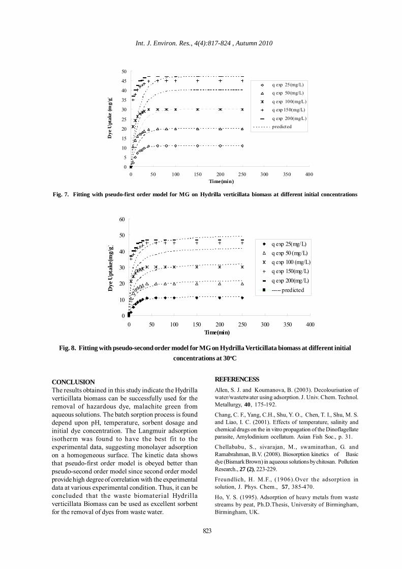
823
Int. J. Environ. Res., 4(4):817-824 , Autumn 2010
0
5
10
15
20
25
30
35
40
45
50
0 50 100 150 200 250 300 350 400Time(min)
Dye
Upt
ake
(mg/
g)
q exp 25(mg/L)
q exp 50(mg/L)
q exp 100(mg/L)
q exp 150(mg/L)
q exp 200(mg/L)
predict ed
Fig. 7. Fitting with pseudo-first order model for MG on Hydrilla verticillata biomass at different initial concentrations
0
10
20
30
40
50
60
0 50 100 150 200 250 300 350 400Time(min)
Dye
Upt
ake(
mg/
g)
q exp 25(mg/L)q exp 50 (mg/L)q exp 100 (mg/L)q exp 150(mg/L)q exp 200(mg/L)----- predicted
Fig. 8. Fitting with pseudo-second order model for MG on Hydrilla Verticillata biomass at different initialconcentrations at 30oC
CONCLUSIONThe results obtained in this study indicate the Hydrillaverticillata biomass can be successfully used for theremoval of hazardous dye, malachite green fromaqueous solutions. The batch sorption process is founddepend upon pH, temperature, sorbent dosage andinitial dye concentration. The Langmuir adsorptionisotherm was found to have the best fit to theexperimental data, suggesting monolayer adsorptionon a homogeneous surface. The kinetic data showsthat pseudo-first order model is obeyed better thanpseudo-second order model since second order modelprovide high degree of correlation with the experimentaldata at various experimental condition. Thus, it can beconcluded that the waste biomaterial Hydrillaverticillata Biomass can be used as excellent sorbentfor the removal of dyes from waste water.
REFERENCESSAllen, S. J. and Koumanova, B. (2003). Decolourisation ofwater/wastetwater using adsorption. J. Univ. Chem. Technol.Metallurgy, 40, 175-192.
Chang, C. F., Yang, C.H., Shu, Y. O., Chen, T. I., Shu, M. S.and Liao, I. C. (2001). Effects of temperature, salinity andchemical drugs on the in vitro propagation of the Dinoflagellateparasite, Amylodinium ocellatum. Asian Fish Soc., p. 31.
Chellababu, S., sivarajan, M., swaminathan, G. andRamabrahman, B.V. (2008). Biosorption kinetics of Basicdye (Bismark Brown) in aqueous solutions by chitosan. PollutionResearch., 27 (2), 223-229.
Freundlich, H. M.F., (1906).Over the adsorption insolution, J. Phys. Chem., 57, 385-470.
Ho, Y. S. (1995). Adsorption of heavy metals from wastestreams by peat, Ph.D.Thesis, University of Birmingham,Birmingham, UK.

824
Kinetic Studies on Sorption of Malachite Green
Gharbani, P., Tabatabaii, S. M. and Mehrizad, A. (2008).Removal of Congo red from textile wastewater by ozonation.Int. J. Environ. Sci. Tech., 5 (4), 495-500.
Goyal, P., Sharma, A., Srivastava, S., and Srivastava, M. M.(2008). Saraca indica leaf powder for decontamination of Pb:removal, recovery, adsorbent characterization and equilibriummodeling. Int. J. Environ. Sci. Tech., 5 (1), 27-34.
Hamdaoui, O., Saoudi, F., Chiha, M. and Naffrechoux, M.(2008). Sorption of malachite green by a novel sorbent, deadleaves of plane tree:Equilibrium and kinetic modeling, Chem.Eng. J., 14, 73-84.
Hameed, B. H. and El-Khaiary, M. I. (2008). Malachite greenadsorption by rattan sawdust: Isotherm, kinetic and mechanismmodeling. J. Hazard. Mater., 159, 574-579.
Hema, M. and Arivoli, S. (2008). Adsorption kinetics andthermodynamics of malachite green dye unto acid activatedlow cost carbon. J. Appl. Sci. Environ. Manage., 12 (1), 43-51.
Igwe, J. C., Abia, A. A. and Ibeh, C. A. (2008). Adsorptionkinetics and intrap articulate diffusivities of Hg, As and Pb ionson unmodified and thiolated coconut fiber. Int. J. Environ. Sci.Tech., 5 (1), 83-92.
Iqbal, M. J. and Ashiq, M. N. (2007). Adsorption of dyes fromaqueous solutions on activated charcoal. J. Hazard. Mater.,B139, 57-66.
Khattri, S. D. and Singh, M. K. (1999). Colour removal fromdyewastewater using sugar cane dust as an adsorbent. Adsorpt.Sci. Technol., 7 (4), 269-282 .
Labidi, N. S. (2008). Removal of Mercury from AqueousSolutions by Waste Brick. Int. J. Environ. Res., 2 (3), 275-278.
Lagergren, S., (1898). About the theory of so-called adsorptionof soluble substances. K.Sven. Vetenskapsakad. Handl., 24(4), 1-39.
Langmuir, I., (1916). The constitution and fundamentalproperties of solids and liquids. J. Am. Chem. Soc., 38 (11),2221-2295.
Lori, J. A., Lawal, A. O. and Ekanem, E. J. (2008). ActiveCarbons from Chemically Mediated Pyrolysis of AgriculturalWastes: Application in Simultaneous Removal of BinaryMixture of Benzene and Toluene from Water. Int. J. Environ.Res., 2 (4),411-418.
Low, K. S., Lee, CK. and Heng, L. L., (1994). Sorption of basicdyes by Hydrilla verticillata. Environ. Tech., 15, 115-124.
Malik, P. K. (2003). Use of activated carbons prepared fromsawdust and rice husk for adsorption of acid dyes: a case studyof acid yellow 36. Dyes Pigm., 56, 239-249.
Mall,I.D., Srivastava, V.C., Agarwal, N.K. and Mishra, I.M.(2005). Adsorptive removal of malachite green dye fromaqueous solution by bagasse fly ash and activated carbon-kineticstudy and equilibrium isotherm analyses. Colloids Surf. APhysicochem. Eng. Aspects., 264, 17-28.
Mahmoud, A. S., Ghaly, A. E. and Brooks, M. S. (2007).Removal of dye from textile wastewater using plant oils underdifferent pH and temperature conditions. Am. J. Environ. Sci.,3, 205-218.
Murugesan, A. G., Maheswari, S. and Bagirath, G. (2008).Biosorption of Cadmium by Live and Immobilized Cells ofSpirulina Platensis. Int. J. Environ. Res., 2 (3), 307-312.
Nabi Bidhendi, Gh. R., Torabian, A., Ehsani, H., Razmkhah,N. and Abbasi, M. (2007). Evaluation of Industrial DyeingWastewater Treatment with Coagulants. Int. J. Environ. Res.,1 (3), 242-247.
Papinutti, L., Mouso, N. and Forchiassin, F., (2006). Removaland degradation of the fungicide dye malachite green fromaqueous solution using the system wheat bran -Fomessclerodermeus. Enzyme Microb. Technol., 39, 848-853.
Robinson, T., McMullan, G., Marchant, R. and Nigam, P.(2001). Remediation of dyes in textile effluent: a critical reviewon current treatment technologies with a proposed alternative.Bioresour. Technol., 77, 247-255.
Rahman, I. A., Saad, B., Shaidan, S. and Sya Rizal, E. S. (2005).Adsorption characteristics of malachite green on activatedcarbon derived from rice husks produced by chemical–thermalprocess., Bioresour. Technol., 96, 1578-1583.
Rahmani, K., Mahvi, A. H., Vaezi, F., Mesdaghinia, A. R., Nabizade, R. and Nazmara, Sh. (2009). Bioremoval of Leadby Use of Waste Activated Sludge. Int. J. Environ. Res., 3 (3),471-476.
Sahmoune, M. N., Louhab, K. and Boukhiar, A. (2009).Biosorption of Cr (III) from Aqueous Solutions UsingBacterium Biomass Streptomyces rimosus. Int. J. Environ.Res., 3 (2), 229-238.
Salim, M. and Munekage, Y. (2009). Removal of Arsenic FromAqueous Solution Using Silica Ceramic: Adsorption Kineticsand Equilibrium Studies. Int. J. Environ. Res., 3 (1),13-22.
Schnick, R. A. (1988).The impetus to register newtherapeutants for aquaculture. Prog. Fish Cul., 50, 190-196.
Shah, B. A., Shah, A. V. and Singh, R. R. (2009). Sorptionisotherms and kinetics of chromium uptake from wastewaterusing natural sorbent material. Int. J. Environ. Sci. Tech., 6 (1),77-90.
Shetty, R. and Rajkumar, Sh. (2009). Biosorption of Cu (II) byMetal Resistant Pseudomonas sp. Int. J. Environ. Res., 3 (1),121-128.
Singanan, M., Singanan, V., and Abebaw, A. (2008). Biosorptionof Cr (III) from aqueous solutions using indigenous biomaterials.Int. J. Environ. Res., 2 (2),177-182.
Srivastava, S., Sinha, R. and Roy, D. (2004). Toxicological effectsof malachite green. Aquat. Toxico., 66 (3), 319-329.
Tahir, S. S., Rau, N. (2006). Removal of a cationic dye fromaqueous solutions by adsorp-tion onto bentonite clay.Chemosphere, 63, 1842-1848.
Zhang, J., Li, Y., Zhang, C. and Jing, Y. (2008)., Adsorption ofmalachite green from aqueous
Solution onto carbon prepared from Arundo donax root. J.Hazard. Mater., 150, 774-782.
Zvinowanda, C. M., Okonkwo, J. O., Shabalala, P. N. andAgyei, N. M. (2009). A novel adsorbent for heavy metalremediation in aqueous environments. Int. J. Environ. Sci. Tech.,6 (3), 425-434.
Int. J. Environ. Res., 4(4): 825-836, Autumn 2010ISSN: 1735-6865
Received 25 Sep. 2009; Revised 12 Feb. 2010; Accepted 15 May 2010
*Corresponding author E-mail:[email protected]
825
Effect of Sludge Initial Depth on the Fate of Pathogens in Sand Drying Beds inthe Eastern Province of Saudi Arabia
Al-Malack, M. H.
King Fahd University of Petroleum & Minerals, Dhahran, Saudi Arabia
ABSTRACT: In order to optimize sludge depth in sand drying beds under the climatic conditions of SaudiArabia, the effect of initial sludge depth on the fate of pathogens was investigated.The investigation wascarried out for one year in Al-Khobar Wastewater Treatment Plant, where initial sludge depths of 10, 15, 20,25, 30 and 35 cm were implemented. Sludge samples were collected on 0, 1, 2, 4, 7, 14, and 30 days andwere analyzed for various types of bacterial species and protozoan and helminthic pathogens.The studyshowed that the effect of the initial sludge depth in drying beds on the dye-off rate of pathogens underinvestigation was apparent.Total coliform, streptococci, shigella, salmonella and clostridium were found tosurvive longer as the sludge initial depth was increased. As an example, the streptococci count reachedvalues of 25, 37, 49, 59, 71, and 90 organisms per gram dry weight for sludge initial depths of 10, 15, 20, 25,30 and 35 cm, respectively.The same trend was also observed for protozoan and helminthic pathogens. Forexample, the number of ascaris lumbricoides after 2 days of drying was 3, 4, 6, 7, 7, and 10 in sludgesamples collected from drying beds with initial depths of 10, 15, 20, 25, 30 and 35 cm, respectively.Amathematical representation was formed to describe the pathogens dye-off with respect to time thatincluded the effect of the sludge initial depth. The results indicated that the mathematical representation ofthe drying beds for individual species was dramatically improved when average values of constants forindividual species were used in the model.
Key words: Domestic Sludge, Pathogens, Total Coliform, Fecal Coliform, Protozoa, Helminthes
INTRODUCTIONSludge dewatering is a physical unit process used
to remove as much water as possible from sludge toproduce a highly concentrated cake.Dewatering dif-fers from thickening, as the sludge should behave as asolid after it has been dewatered.Metcalf and Eddy(2003) reported more than one reason for the dewater-ing to be performed. Dewatering of the different typesof water from sludge was studied by several investiga-tors such as Robinson and Knocke (1994), Smith andVesilind (1995), Cantet et al. (1996), Chen et al. (1996),Wu and Huang (1997), and Lajoie et al. (2000). Sludgedrying beds are the oldest method of sludge dewater-ing and are still used extensively in small-to-mediumsized plants to dewater sludge.They are relatively inex-pensive and provide dry sludge cake.In the recentyears, much advancement has been made to the con-ventional drying beds, and new systems are used onmedium- and large-sized plants. Theses variations ofthe drying beds are (1) conventional sand, (2) paved,(3) wire-wedge, and (4) vacuum assisted.
Conventional sand beds consist of a layer of coarsesand 15-25 cm in depth and supported on a gravel bed(0.3-2.5 cm) that incorporates selected tiles or perfo-rated pipe under-drain. Sludge is placed on the bed in20-30 cm layers and allowed to dry. Sludge cake re-moval is manual by shoveling into wheelbarrows ortrucks or a scraper or front-end loader. The under-drained liquid is returned to the plant.The drying pe-riod is 10-15 days, and the moisture content of thecake is 60-70 percent. Sludge loading rate is 100-300kg dry solids per m2 per year for uncoveredbeds.Marklund (1993) studied the dewatering of aero-bically digested sludge using drying beds. He con-cluded that larger portions of the moisture could beremoved by drainage from thin sludge layers.Whenthe initial sludge layer depth was 350 mm, only onethird of the moisture was removed. Al-Muzaini (2003)assessed sludge produced by the Jahra treatmentplant.The assessment of the quality of the sludge pro-duced was based on the standards for land applica-tion of sewage sludge. Analyses were carried out for
826
trace heavy metals and bacteria. He reported that theresults of the analyses showed that the sludge pro-duced was high in organic matter and sand contentbut low in heavy metals. Al-Malack et al. (2007) con-ducted an extensive research in order to determine themicrobiological characteristics of municipal sludgesproduced at three major cities, namely, Qateef, Dammamand Khobar in the Eastern Province of Saudi Arabia.The results indicated that municipal sludge producedat the three cities was not suitable for utilization inagricultural activities due to the high levels of salmo-nella even after 14 days of drying at Qateef wastewa-ter treatment plant. Dried Sludge samples collectedfrom Qateef, Dammam and Khobar were found to con-tain salmonella species on the average of 22, 107 and127 MPN per gram of dried sludge, respectively.O’Shaughnessy et al. (2008) investigated the effectsof moisture and temperature on the inactivation rate offecal coliforms in biosolids and developed a mathemati-cal model to predict their level in biosolids in solardrying beds at any time during the drying process.They reported that temperature and moisture had sig-nificant main and interactive effects on the inactiva-tion rate of Escherichia coli in biosolids. The resultsalso showed that observed and predicted inactivationrates from the microcosm study correlated well (R2 =0.81). The use of different modifications of drying bedsin dewatering of municipal sludge was also investi-gated by Elariny and Miller (1984), Hossam and Saad(1990), Marklund (1990), Nishimura et al. (1994),Yamaoka and Hata (2003), Al-Muzaini (2004), Choi etal. (2005), Zaleski et al (2005), Alkan et al. (2007),Mehrdadi et al. (2007) Achon et al. (2008),O’Shaughnessy et al. (2008), and Yi et al. (2008).
With respect to the survival of pathogens in dry-ing beds, Cofie et al. (2006) investigated the use ofdrying beds with municipal sludge. They reported thatdrying beds were found to retain 80 per cent of solidsand 100 per cent of helminth eggs. Fars et al (2005)investigated the survival of fecal coliforms in activatedsludge after dewatering in drying beds. They reportedthat the treatment of sludge in drying beds appearedto be efficient in eliminating pathogenic micro-organ-isms such as fecal coliforms, protozoan cysts and hel-minth eggs. Plachy and Juris (1995) investigated thesurvival of eggs of A. suum in two sludge drying bedsof sewage treatment plants (STP) under different cli-matic-geographical conditions. They reported thatsludge drying beds of both sewage treatment plantsshowed different survival of eggs. In one of the STPs,a rapid reduction in viable eggs from was reported (from80.4 to 19.8 per cent). Later this decrease became lessrapid and at the end of the experiment, after 240 daysonly 5 per cent of eggs were viable. In the other STP,the viability of eggs was reduced rather gradually, and
after 320 days of exposure 36 per cent of viable A.suum eggs were still recorded.
With respect to the effect of initial sludge depth indrying beds on the fate of pathogens, and up to theknowledge of the author, there is no single work inthat direction. Based on that, the main objective of thestudy is to investigate the effect of initial sludge depthon the microbiological characteristics of the sludgeduring the drying period.
MATERIALS & METHODSAs proposed, the fieldwork was conducted at
Khobar wastewater treatment plant (WWTP) locatedin Azizia area. The experimental setup was designedby isolating and modifying two sludge drying beds tosuit the experimental objectives. The beds were dividedequally into six compartments (plots) of 8.3 × 15 meach with a numerical designation of 1 - 6. Plot numbersix was maintained as a control bed that is identical tothe present actual sludge loading practiced in the plant.The existing feed line was connected with individualinlets to be operated independently in order to main-tain the desired sludge thickness in each plot. Splashplates were installed in each bed to regulate the flow.For each experiment, six experimental plots were loadedwith 10, 15, 20, 25, 30, and 35-cm thickness of sludge.The drying period ranged from 0 to 30 days, whichconstituted one experimental run. Samples were col-lected from each plot at time intervals of 0, 1, 2, 4, 7, 14,and 30 days. At the end of each experiment, a five-dayperiod was allowed to prepare the beds for the next setof experiments by removing the residual dry sludgeand maintaining a constant sand depth. Two experi-mental runs were conducted during each season and,therefore, a total of eight experimental runs were car-ried out during the one-year experimental investiga-tion.
Standard methods were implemented in the sampleanalysis.It is worth to mention that collected sludgesamples were analyzed in triplicates.The following is abrief description of the techniques which were em-ployed in the determination of different microbiologi-cal parameters:
Total and Fecal Coliforms:Presumptive lauryl sulfateMPN test followed by BGB confirmed test; direct enu-meration by Membrane Filter technique using M-Endoagar.Presumptive positive samples were inoculated inEC medium to confirm quantitatively fecal coliformsfrom total coliforms.
Streptococcus sp.:Inoculate samples into azide dex-trose broth and incubate at 35°C to observe turbidityfor the presence of Streptococcus sp. Confirmationwas done by streaking PSE agar for brown positivecolonies.
Al-Malack, M . H.

Int. J. Environ. Res., 4(4): 825-836, Autumn 2010
827
Salmonella sp.:MPN method using dulcitol seleniteas enrichment media and streak from each tube to bril-liant green and xylose lysine desoaycholate agars.Reinoculate colony in triple sugar iron slant and lysineiron agars.Shigella sp. :Using xylose lysine desoxycholate(XLD) agar for primary isolation of Shigella sp. strainsand incubate at 35°C for 24 hrs for isolation of redpositive colonies.Clostridium perfringens: Samples were inoculated inclostridium basal media and incubated at 37°C to de-tect positive black Clostridium perfringens colonies.Helminthic ova: Using zinc sulfate floatation tech-nique all the helminthic types present were identified.Parasites :Both protozoan and helminthic parasitesare expected to be present in the sludge. The mainhelminthic parasites present as ova of human entericspecies are represented by Ascaris lumbricoides,Enterobious vermicularis, Ancylostoma doudenale,Trichuri trichura, Hymenolepis nana. The main en-teric protozoan parasite include Entamoeba histolytica.Two techniques were used for the detection and enu-meration of helminthic and protozoan parasites, theywere floatation and sedimentation. Sedgewick-Raftercell was used for quantitative analysis.Entamoeba histolytica:Suspension were strainedthrough 7-10 µm membrane and resuspended.Sedgewick-Rafter cell was used in enumeration (Con-centration Method).
RESULTS & DISCUSSIONDue to the similarity of the results obtained in all
sessions, only one set of data will be presented. Theeffect of initial sludge depth on the survival of totalcoliform in sludge samples collected during the firstsession is presented in Fig. 1. Generally, the figureshows that total coliform count was decreasing, insludge samples, with respect to drying period. More-over, the figure demonstrates a trend where totalcoliform was found to survive longer in higher sludgedepths.The reason for longer survival of coliform bac-teria in thicker sludge could be due to penetration ofsolar heat and radiation, which will be reduced in thickersludge depths. The results show that sludge samples,collected during that session, contain coliform densi-ties ranging between 8×10⁴ and 1.1×10⁵ organisms pergram dry weight, after 30 days of drying period. Re-garding the effect of initial sludge depth on the sur-vival of streptococci, Fig. 2 shows that as the initialsludge depth was increased, the streptococci wouldsurvive longer. By the end of the 30-day drying pe-riod, the streptococci count reached values of 25, 37,49, 59, 71, and 90 organisms per gram dry weight, forinitial depths of 10, 15, 20, 25, 30, and 35 cm, respec-tively. The effect of initial sludge depth on the sur-
vival of shigella in sludge samples is presented in Fig.3. Generally, the figure shows that shigella count wasdecreasing, in sludge samples, with respect to dryingperiod. Moreover, the results demonstrate a trendwhere shigella was found to survive longer in highersludge depths. The reason for longer survival of shi-gella bacteria in thicker sludge could be due to thesame reasons given above. The results show thatsludge samples contain shigella densities rangingbetween 50 and 200 organisms per gram dry weight,after 30 days of drying period. Regarding the effect ofinitial sludge depth on the survival of salmonella,Fig. 4 shows that as the initial sludge depth was in-creased, the salmonella would survive longer. At theend of the 30-day drying period, the salmonella countreached values of 15, 25, 35, 35, 50, and 60 organismsper gram dry weight, for initial depths of 10, 15, 20, 25,30, and 35 cm, respectively. The effect of initial sludgedepth on the survival of clostridium in sludge samplesis presented in Fig. 5. Generally, the figure shows thatclostridium count was decreasing, in sludge samples,with respect to drying period. Moreover, the resultsdemonstrate a trend where clostridium was found tosurvive longer in higher sludge depths. The reason forlonger survival of clostridium bacteria in thicker sludgecould be due to penetration of solar heat and radia-tion, which will be reduced in thicker sludges. Theresults show that sludge samples contain clostridiumdensities ranging between 7 and 45 organisms per gramdry weight, after 30 days of drying period.
Protozoan and helminthic pathogens are of greatconcern due to their probable effects on the publichealth. Sludge samples were examined for helminthicand protozoan pathogens such as Ascarislumbricoides, Enterobious vermicularis, Ancylostomadoudenale, Trichuris trichura, Hymenolepis nana, andEntamoeba histolytica. The results show that allsludge samples collected from the six different sludgedepths, were free from Enterobious vermicularis, Hy-menolepis nana, and Ancylostoma doudenale.
050000000
100000000150000000200000000250000000300000000350000000400000000450000000500000000
0 1 2 4 7 15 30
Time (days)
Colif
orm
s (ce
lls p
er g
ram
)
Depth = 10 cmDepth = 15 cmDepth = 20 cmDepth = 25 cmDepth = 30 cmDepth = 35 cm
Fig. 1. Coliform Die-off at Different Initial SludgeDepths
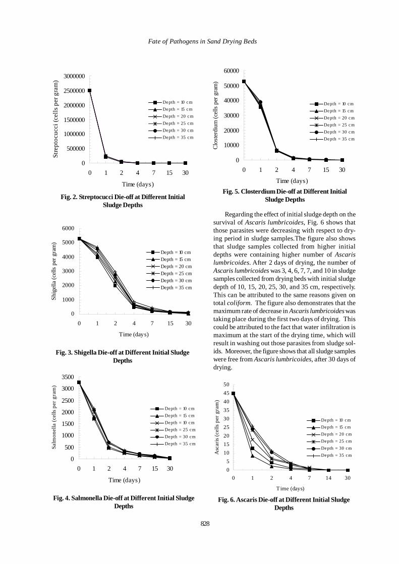
828
Regarding the effect of initial sludge depth on thesurvival of Ascaris lumbricoides, Fig. 6 shows thatthose parasites were decreasing with respect to dry-ing period in sludge samples.The figure also showsthat sludge samples collected from higher initialdepths were containing higher number of Ascarislumbricoides. After 2 days of drying, the number ofAscaris lumbricoides was 3, 4, 6, 7, 7, and 10 in sludgesamples collected from drying beds with initial sludgedepth of 10, 15, 20, 25, 30, and 35 cm, respectively.This can be attributed to the same reasons given ontotal coliform. The figure also demonstrates that themaximum rate of decrease in Ascaris lumbricoides wastaking place during the first two days of drying. Thiscould be attributed to the fact that water infiltration ismaximum at the start of the drying time, which willresult in washing out those parasites from sludge sol-ids. Moreover, the figure shows that all sludge sampleswere free from Ascaris lumbricoides, after 30 days ofdrying.
0
500
1000
1500
2000
2500
3000
3500
0 1 2 4 7 15 30
Time (days)
Salm
onel
la (c
ells
per g
ram
)
Depth = 10 cmDepth = 15 cmDepth = 10 cmDepth = 25 cmDepth = 30 cmDepth = 35 cm
0
1000
2000
3000
4000
5000
6000
0 1 2 4 7 15 30
Time (days)
Shig
ella
(cel
ls p
er g
ram
)
Depth = 10 cmDepth = 15 cmDepth = 20 cmDepth = 25 cmDepth = 30 cmDepth = 35 cm
0
500000
1000000
1500000
2000000
2500000
3000000
0 1 2 4 7 15 30
Time (days)
Stre
ptoc
ucci
(cel
ls p
er g
ram
)
Depth = 10 cmDepth = 15 cmDepth = 20 cmDepth = 25 cmDepth = 30 cmDepth = 35 cm
Fig. 2. Streptocucci Die-off at Different InitialSludge Depths
Fig. 3. Shigella Die-off at Different Initial SludgeDepths
Fig. 4. Salmonella Die-off at Different Initial SludgeDepths
0
10000
20000
30000
40000
50000
60000
0 1 2 4 7 15 30
Time (days)
Clo
ster
dium
(cel
ls p
er g
ram
)
Depth = 10 cmDepth = 15 cmDepth = 20 cmDepth = 25 cmDepth = 30 cmDepth = 35 cm
Fig. 5. Closterdium Die-off at Different InitialSludge Depths
05
101520253035404550
0 1 2 4 7 14 30
Time (days)
Asc
aris
(cel
ls pe
r gra
m)
Depth = 10 cmDepth = 15 cmDepth = 20 cmDepth = 25 cmDepth = 30 cmDepth = 35 cm
Fig. 6. Ascaris Die-off at Different Initial SludgeDepths
Fate of Pathogens in Sand Drying Beds

Int. J. Environ. Res., 4(4): 825-836, Autumn 2010
829
Fig. 7 shows the effect of initial sludge depth on thecontent of Trichuris trichura in sludge samples. Thefigure clearly demonstrates that as initial sludge depthwas increased, the count of surviving Trichuristrichura in sludge samples increases, during the firstdays of drying. Sludge samples collected after twodays of drying were found to contain Trichuris trichuracounts of 1, 2, 4, 4, 5, and 7 when collected from dryingbeds with initial sludge depth of 10, 15, 20, 25, 30, and35 cm, respectively. This is attributed to the same rea-sons given on Ascaris lumbricoides. The figure clearlydemonstrates that all sludge samples were free fromTrichuris trichura, after 30 days of drying.
The effect of initial sludge depth on the contentsof the protozoan parasite Entamoeba histolytica insludge samples is shown in Fig. 8. As in the case ofAscaris lumbricoides and Trichuris trichura, the countof surviving Entamoeba histolytica was found to beaffected by the initial sludge depth. After two days ofdrying, the Entamoeba histolytica counts were 1, 2, 2,3, 5, and 8 for samples collected from drying beds withinitial sludge depth of 10, 15, 20, 25, 30, and 35 cm,respectively. After 30 days of drying, the Entamoebahistolytica parasites were not detected in all sludgesamples.
In order to best describe the obtained results,statistical analysis was implemented.Table 1 showsmathematical representations of the effect of the initialsludge depth on the fate of microorganisms underinvestigation.The table clearly shows that there is ageneral mathematical representation of all depths. Thegeneral representation is in the form of:
0
5
10
15
20
25
30
0 1 2 4 7 14 30
Time (days)
Tric
huris
(cel
ls p
er g
ram
)
Depth = 10 cmDepth = 15 cmDepth = 20 cmDepth = 25 cmDepth = 30 cmDepth = 35 cm
Fig. 7. Trichuris Die-off at Different Initial SludgeDepths
( ) ( )timeBAy lnln ×−=
wherey = microorganism / gram of dry sludgeA and B = constants depend on initial sludge depth
The effect of the sludge initial depth on the valuesof constants A and B is clearly depicted in Table 2.which shows the different range of values and trendsof constants A and B for the microorganisms underinvestigation when increasing the initial depth of thesludge in the drying beds.Generally, the values ofconstants A and B were found to increase with theincrease in the initial sludge depth in the drying beds,except in two cases that are not explainable. In thecase of the total coliform, the constants A and B werefound to increase in the initial stage of increasing thesludge depth, but after that the values were almostconstant. In order to come up with one approximatedvalues of constants A and B, average values werefound to be 8.05 and 1.79, respectively.Based on theseresults, the general mathematical representation of theprocess is the following form:
The graphical representation of the approximatedmathematical representation is shown in Fig. 9 whichis represented by a solid line. The dashed line in Fig. 9.is the best fit of the data pertinent to all species. Thefigure clearly shows that the differences between thetwo attempts are insignificant. However, it is clear,from the figure, that the mathematical representationof the data was not satisfactory in both attempts. Inorder to improve the mathematical representation,average values of constants A and B for individualspecies were determine and presented in Table 3.
( ) ( )timey ln79.105.8ln ×−=
Fig. 8. Histolytica Die-off at Different Initial SludgeDepths
0
5
10
15
20
25
30
35
40
45
50
0 1 2 4 7 14 30Time (days)
Hist
olyt
ica
(cel
ls pe
r gra
m)
Depth = 10 cmDepth = 15 cmDepth = 20 cmDepth = 25 cmDepth = 30 cmDepth = 35 cm
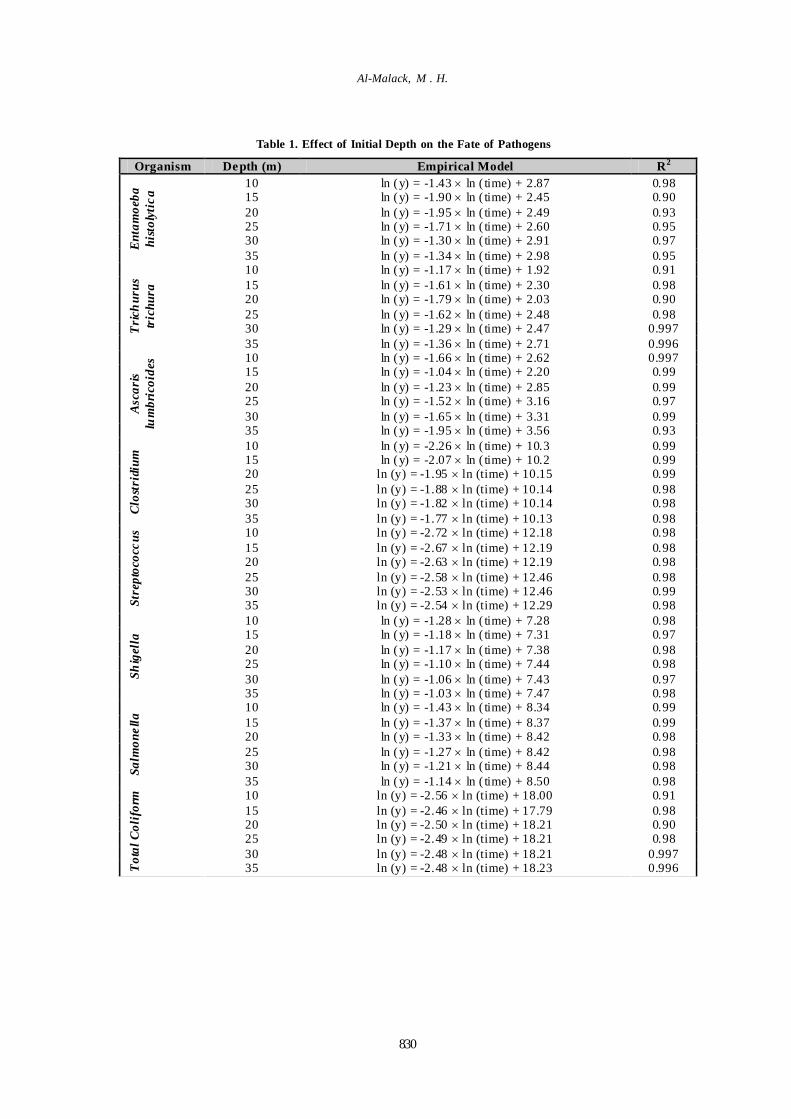
830
Table 1. Effect of Initial Depth on the Fate of Pathogens
Organism Depth (m) Empirical Model R2 10 ln (y) = -1.43 × ln ( time) + 2.87 0.98 15 ln (y) = -1.90 × ln ( time) + 2.45 0.90 20 ln (y) = -1.95 × ln ( time) + 2.49 0.93 25 ln (y) = -1.71 × ln ( time) + 2.60 0.95 30 ln (y) = -1.30 × ln ( time) + 2.91 0.97 E
ntam
oeba
hi
stol
ytic
a
35 ln (y) = -1.34 × ln ( time) + 2.98 0.95 10 ln (y) = -1.17 × ln ( time) + 1.92 0.91 15 ln (y) = -1.61 × ln ( time) + 2.30 0.98 20 ln (y) = -1.79 × ln ( time) + 2.03 0.90 25 ln (y) = -1.62 × ln ( time) + 2.48 0.98 30 ln (y) = -1.29 × ln ( time) + 2.47 0.997 T
rich
urus
tr
ichu
ra
35 ln (y) = -1.36 × ln ( time) + 2.71 0.996 10 ln (y) = -1.66 × ln ( time) + 2.62 0.997 15 ln (y) = -1.04 × ln ( time) + 2.20 0.99 20 ln (y) = -1.23 × ln ( time) + 2.85 0.99 25 ln (y) = -1.52 × ln ( time) + 3.16 0.97 30 ln (y) = -1.65 × ln ( time) + 3.31 0.99 A
scar
is
lum
bric
oide
s
35 ln (y) = -1.95 × ln ( time) + 3.56 0.93 10 ln (y) = -2.26 × ln ( time) + 10.3 0.99 15 ln (y) = -2.07 × ln ( time) + 10.2 0.99 20 ln (y) = -1.95 × ln (time) + 10.15 0.99 25 ln (y) = -1.88 × ln (time) + 10.14 0.98 30 ln (y) = -1.82 × ln (time) + 10.14 0.98 C
lost
ridi
um
35 ln (y) = -1.77 × ln (time) + 10.13 0.98 10 ln (y) = -2.72 × ln (time) + 12.18 0.98 15 ln (y) = -2.67 × ln (time) + 12.19 0.98 20 ln (y) = -2.63 × ln (time) + 12.19 0.98 25 ln (y) = -2.58 × ln (time) + 12.46 0.98 30 ln (y) = -2.53 × ln (time) + 12.46 0.99
Stre
ptoc
occu
s
35 ln (y) = -2.54 × ln (time) + 12.29 0.98 10 ln (y) = -1.28 × ln ( time) + 7.28 0.98 15 ln (y) = -1.18 × ln ( time) + 7.31 0.97 20 ln (y) = -1.17 × ln ( time) + 7.38 0.98 25 ln (y) = -1.10 × ln ( time) + 7.44 0.98 30 ln (y) = -1.06 × ln ( time) + 7.43 0.97 Sh
igel
la
35 ln (y) = -1.03 × ln ( time) + 7.47 0.98 10 ln (y) = -1.43 × ln ( time) + 8.34 0.99 15 ln (y) = -1.37 × ln ( time) + 8.37 0.99 20 ln (y) = -1.33 × ln ( time) + 8.42 0.98 25 ln (y) = -1.27 × ln ( time) + 8.42 0.98 30 ln (y) = -1.21 × ln ( time) + 8.44 0.98 Sa
lmon
ella
35 ln (y) = -1.14 × ln ( time) + 8.50 0.98 10 ln (y) = -2.56 × ln (time) + 18.00 0.91 15 ln (y) = -2.46 × ln (time) + 17.79 0.98 20 ln (y) = -2.50 × ln (time) + 18.21 0.90 25 ln (y) = -2.49 × ln (time) + 18.21 0.98 30 ln (y) = -2.48 × ln (time) + 18.21 0.997
Tot
al C
olif
orm
35 ln (y) = -2.48 × ln (time) + 18.23 0.996
Al-Malack, M . H.
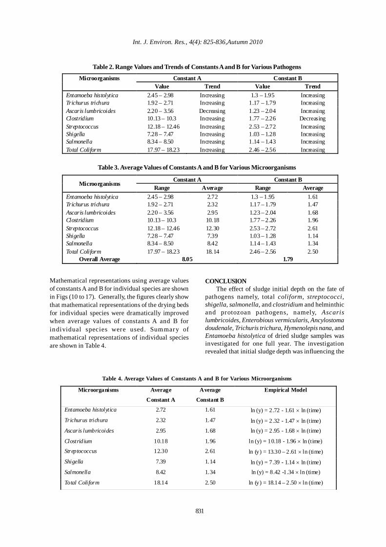
831
Int. J. Environ. Res., 4(4): 825-836,Autumn 2010
Table 2. Range Values and Trends of Constants A and B for Various Pathogens
Constant A Constant B Microorganisms Value Trend Value Trend
Entamoeba histolytica 2.45 – 2.98 Increasing 1.3 – 1.95 Increasing Trichurus trichura 1.92 – 2.71 Increasing 1.17 – 1.79 Increasing Ascaris lumbricoides 2.20 – 3.56 Decreasing 1.23 – 2.04 Increasing Clostridium 10.13 – 10.3 Increasing 1.77 – 2.26 Decreasing Streptococcus 12.18 – 12.46 Increasing 2.53 – 2.72 Increasing Shigella 7.28 – 7.47 Increasing 1.03 – 1.28 Increasing Salmonella 8.34 – 8.50 Increasing 1.14 – 1.43 Increasing Total Coliform 17.97 – 18.23 Increasing 2.46 – 2.56 Increasing
Table 3. Average Values of Constants A and B for Various Microorganisms
Constant A Constant B Microorganisms
Range Average Range Average Entamoeba histolytica 2.45 – 2.98 2.72 1.3 – 1.95 1.61 Trichurus trichura 1.92 – 2.71 2.32 1.17 – 1.79 1.47 Ascaris lumbricoides 2.20 – 3.56 2.95 1.23 – 2.04 1.68 Clostridium 10.13 – 10.3 10.18 1.77 – 2.26 1.96 Streptococcus 12.18 – 12.46 12.30 2.53 – 2.72 2.61 Shigella 7.28 – 7.47 7.39 1.03 – 1.28 1.14 Salmonella 8.34 – 8.50 8.42 1.14 – 1.43 1.34 Total Coliform 17.97 – 18.23 18.14 2.46 – 2.56 2.50
Overall Average 8.05 1.79
Table 4. Average Values of Constants A and B for Various Microorganisms
Microorganisms Average
Constant A
Average
Constant B
Empirical Model
Entamoeba histolytica 2.72 1.61 ln (y) = 2.72 - 1.61 × ln (time)
Trichurus trichura 2.32 1.47 ln (y) = 2.32 - 1.47 × ln (time)
Ascaris lumbricoides 2.95 1.68 ln (y) = 2.95 - 1.68 × ln (time)
Clostridium 10.18 1.96 ln (y) = 10.18 - 1.96 × ln (time)
Streptococcus 12.30 2.61 ln (y) = 13.30 – 2.61 × ln (time)
Shigella 7.39 1.14 ln (y) = 7.39 - 1.14 × ln (time)
Salmonella 8.42 1.34 ln (y) = 8.42 -1.34 × ln (time)
Total Coliform 18.14 2.50 ln (y) = 18.14 – 2.50 × ln (time)
Mathematical representations using average valuesof constants A and B for individual species are shownin Figs (10 to 17). Generally, the figures clearly showthat mathematical representations of the drying bedsfor individual species were dramatically improvedwhen average values of constants A and B forindividual species were used. Summary ofmathematical representations of individual speciesare shown in Table 4.
CONCLUSIONThe effect of sludge initial depth on the fate of
pathogens namely, total coliform, streptococci,shigella, salmonella, and clostridium and helminthicand protozoan pathogens, namely, Ascarislumbricoides, Enterobious vermicularis, Ancylostomadoudenale, Trichuris trichura, Hymenolepis nana, andEntamoeba histolytica of dried sludge samples wasinvestigated for one full year. The investigationrevealed that initial sludge depth was influencing the
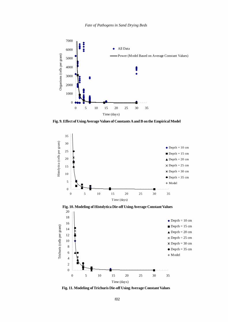
832
0
5
10
15
20
25
30
35
40
0 5 10 15 20 25 30 35
Time (days)
Hist
olyt
ica
(cel
ls pe
r gra
m)
Depth = 10 cm
Depth = 15 cm
Depth = 20 cm
Depth = 25 cm
Depth = 30 cm
Depth = 35 cm
Model
0
2
4
6
8
10
12
14
16
18
20
0 5 10 15 20 25 30 35
Time (days)
Tric
huris
(cel
ls p
er g
ram
)
Depth = 10 cm
Depth = 15 cm
Depth = 20 cm
Depth = 25 cm
Depth = 30 cm
Depth = 35 cm
Model
Fig. 11. Modeling of Trichuris Die-off Using Average Constant Values
Fig. 10. Modeling of Histolytica Die-off Using Average Constant Values
0
1000
2000
3000
4000
5000
6000
7000
0 5 10 15 20 25 30 35
Time (days)
Org
anis
ms
(cel
ls p
er g
ram
)
All Data
Power (Model Based on Average Constant Values)
Fig. 9. Effect of Using Average Values of Constants A and B on the Empirical Model
Fate of Pathogens in Sand Drying Beds
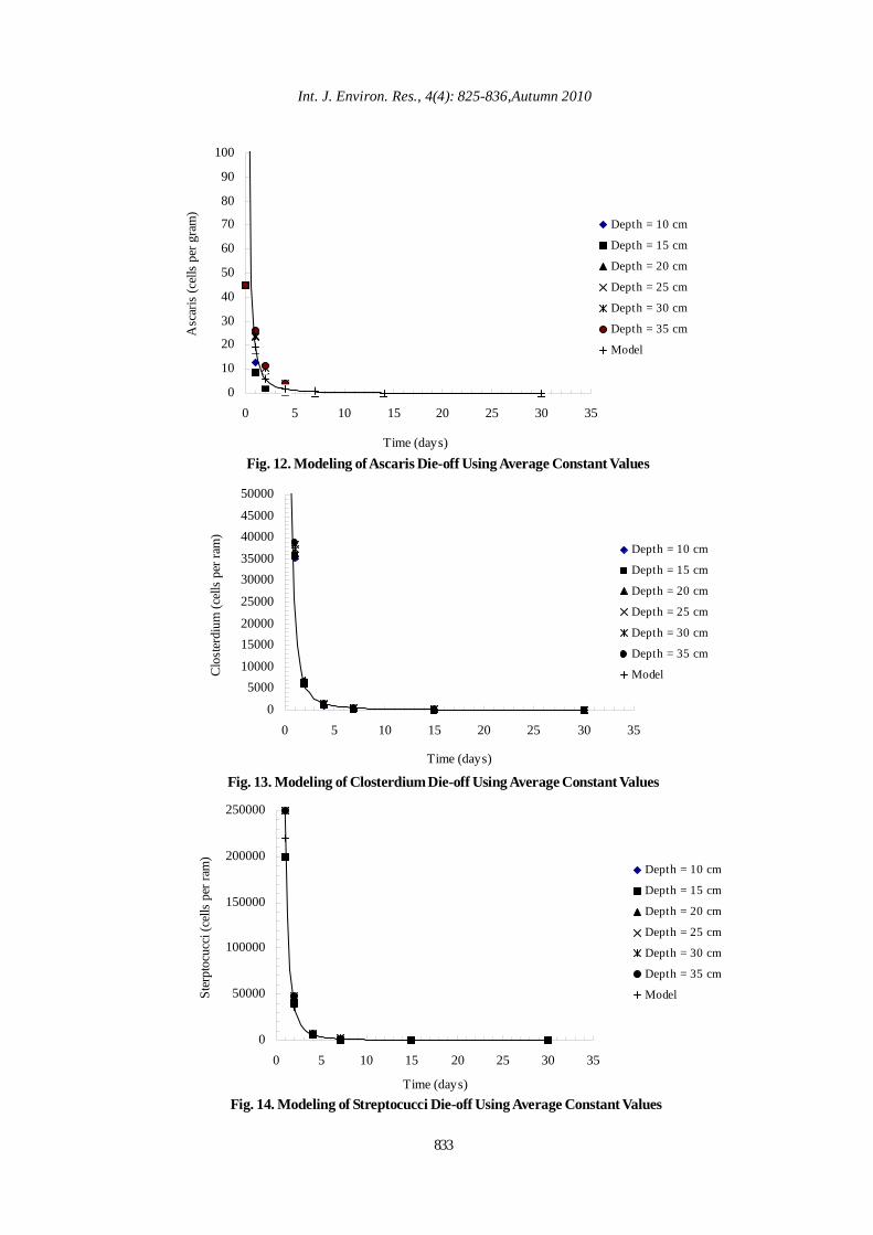
0
10
20
30
40
50
60
70
80
90
100
0 5 10 15 20 25 30 35
Time (days)
Asc
aris
(cel
ls p
er g
ram
)
Depth = 10 cm
Depth = 15 cm
Depth = 20 cm
Depth = 25 cm
Depth = 30 cm
Depth = 35 cm
Model
0
500010000
1500020000
25000
3000035000
4000045000
50000
0 5 10 15 20 25 30 35
Time (days)
Clo
ster
dium
(cel
ls p
er ra
m)
Depth = 10 cm
Depth = 15 cm
Depth = 20 cm
Depth = 25 cm
Depth = 30 cm
Depth = 35 cm
Model
Fig. 12. Modeling of Ascaris Die-off Using Average Constant Values
0
50000
100000
150000
200000
250000
0 5 10 15 20 25 30 35
Time (days)
Ster
ptoc
ucci
(cel
ls p
er ra
m)
Depth = 10 cm
Depth = 15 cm
Depth = 20 cm
Depth = 25 cm
Depth = 30 cm
Depth = 35 cm
Model
Fig. 14. Modeling of Streptocucci Die-off Using Average Constant Values
Fig. 13. Modeling of Closterdium Die-off Using Average Constant Values
Int. J. Environ. Res., 4(4): 825-836,Autumn 2010
833
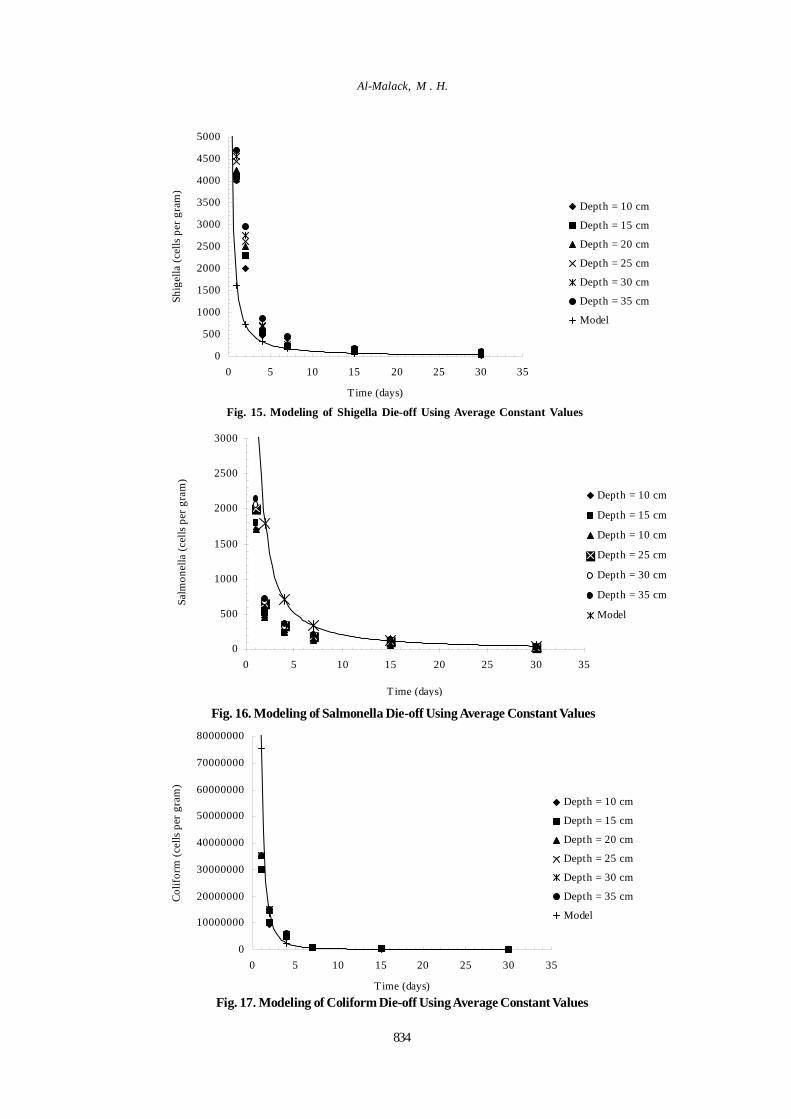
0
500
1000
1500
2000
2500
3000
3500
4000
4500
5000
0 5 10 15 20 25 30 35
Time (days)
Shig
ella
(cel
ls pe
r gra
m)
Depth = 10 cm
Depth = 15 cm
Depth = 20 cm
Depth = 25 cm
Depth = 30 cm
Depth = 35 cm
Model
0
500
1000
1500
2000
2500
3000
0 5 10 15 20 25 30 35
Time (days)
Salm
onel
la (c
ells
per g
ram
)
Depth = 10 cm
Depth = 15 cm
Depth = 10 cm
Depth = 25 cm
Depth = 30 cm
Depth = 35 cm
Model
0
10000000
20000000
30000000
40000000
50000000
60000000
70000000
80000000
0 5 10 15 20 25 30 35
Time (days)
Colif
orm
(cel
ls pe
r gra
m)
Depth = 10 cm
Depth = 15 cm
Depth = 20 cm
Depth = 25 cm
Depth = 30 cm
Depth = 35 cm
Model
Fig. 15. Modeling of Shigella Die-off Using Average Constant Values
Fig. 16. Modeling of Salmonella Die-off Using Average Constant Values
Fig. 17. Modeling of Coliform Die-off Using Average Constant Values
Al-Malack, M . H.
834
fate of pathogens under investigation. Mathematicalrepresentation of the drying beds revealed that thefate of pathogens, under investigation, with respectto drying time obeyed the following model:
Moreover, the investigation showed that the use ofconstants (A and B) that are pertinent to individualspecies, in the model, produced better results than theuse of overall average values of the constants.
REFERENCESAchon, C. L. Barroso, M. M. and Cordeiro, J. S. (2008).Draining Beds: Natural System For Sludge Volume Reduc-tion In The Water Treatment Plant. Engenharia Sanitaria EAmbiental 13 (1), 54-62.
Alkan, U., Topac, F. O., Birden, B. and Baskaya, H. S.(2007). Bacterial regrowth potential in alkaline sludges fromopen-sun and covered sludge drying beds. EnvironmentalTechnology, 28 (10), 1111-1118.
Al-Malack, M. H., Bukhari, A. A. and Abuzaid, N. S. (2007).Fate of pathogens in sludge sand drying beds at Qateef,Khobar and Dammam: A case study. Int. J. Environ. Res., 1(1), 19-27.
Al-Muzaini, S. (2003). Performance of sand drying beds forsludge dewatering. Arabian Journal For Science And Engi-neering 28 (2B), 161-169.
Al-Muzaini, S. (2004). A comparative study of sludge de-watering units for sludge management. Journal Of Environ-mental Science And Health Part A-Toxic/Hazardous Sub-stances & Environmental Engineering 39 (2), 473-482.
Cantet, J., Paul, E. and Clauss, F. (1996). Upgrading Perfor-mance of an Activated Sludge Process through Addition ofTalqueous Powders. Wat. Sci. and Technol. 34 (5-6), 75-83.
Chen, G. W.; Lin, W. W. and Lee, D. J. (1996). CapillarySuction Time (CST) as a Measure of Sludge Dewaterability.Wat. Sci. Technol., 34 (3-4), 443-448.
Choi, C.Y., Grabau, M. R., O’Shaughnessy, S. A. and Pep-per, I. L. (2005). Pathogen reduction in biosolids for landapplication. Journal of Residuals Science & Technology, 2(3), 159-171.
Cofie, O. O., Agbottah, S., Strauss, M., Esseku, H.,Montangero, A., Awuah, E. and Kone, D. (2006). Solid-liquid separation of faecl sludge using drying beds in Ghana:Implications for nutrient recycling in urban agriculture. WaterResearch, 40 (1), 75-82.
Elariny, A. and Miller, H. (1984). Utilization of Solar-En-ergy for Sludge Drying Beds. Journal of Solar Energy Engi-neering-Transactions of the ASME, 106 (3), 351-357.
Fars, S., Oufdou, K., Nejmedddine, A., Hassani, L., Melloul,A., Bousselhaj, K., Amahmid, O., Bouhoum, K., Lakmichi,H. and Mezrioui, N., (2005). Antibiotic resistance and sur-vival of fecal coliforms in activated sludge system in a semi-arid region (Beni Mellal, Morocco).World J. Microb. Biot.,21 (4), 493-500.
Hossam, A. and Saad, S. (1990). Solar Energy for SludgeDrying in Alexandria Metropolitan Area. Wat. Sci. Technol.22 (12), 193-204.
Lajoie, C. A., Layton, A. C., Gregory, I. R., Sayler, G. S.,Taylor, D. E. and Meyers, A. J. (2000). Zoogleal Clustersand Sludge Dewatering Potential in an Industrial Activated-Sludge Wastewater Treatment Plant. Water EnvironmentResearch, 72 (1), 56-64.
Marklund, S. (1990). Dewatering of Sludge by NaturalMethods. Wat. Sci. Technol. 22 (3-4), 239-246.
Marklund, S. (1993). Dewatering of Drying Beds – Com-bined Biological-Chemical Sludge Behaviour.Wat. Sci.Technol., 28 (10), 65-72.
Mehrdadi, N., Joshi, S. G., Nasrabadi, T. and Hoveidi, H.(2007). Aplication of solar energy for drying of sludge frompharmaceutical industrial waste water and probable reuse.Int. J. Environ. Res., 1 (1), 42-48.
Metcalf and Eddy. (2003). Wastewater Engineering: Treat-ment and Reuse. Fourth Edition, McGraw-Hill, Inc., NewYork, U.S.A.
Nishimura, O., Gotoh, K. and Sato, A. (1994). Gravity De-watering Mechanism – Application to High Speed SludgeDrying Beds. Proceedings of the Japan Society of CivilEngineers, no. 497 (2-2), 119-126.
O’Shaughnessy, S. A, Kim, M. Y. and Choi, C. Y. (2008).Mathematical model to predict pathogen die-off in biosolids.Journal Of Residuals Science & Technology, 5 (2), 87-93.
O’Shaughnessy, S. A, Song, I., Artiola, J. F. and Choi, C. Y.(2008). Nitrogen loss during solar drying of biosolids. Envi-ronmental Technology, 29 (1), 55-65.
Plachy, P. and Juris, P. (1995). Survival of the Model Helm-inth Ascaris-Suum Eggs in the Sludge Drying Beds of Sew-age-Treatment Plants. Veterinarni Medicina, 40 (1), 23-27.
Robinson, J. and Knocke, W. R. (1992). Use of Dilatomet-ric and Drying Techniques for Assessing Sludge DewateringCharacteristics. J. WPCF., 64 (1), 60-68.
Smith J. K. and Vesilind P. A. (1995). Dilatometric mea-surement of bound water in wastewater sludge. Wat. Res.,29 (12), 2621-2626.
Wu, C. C. and Huang, C. (1997). Effects of Recycling-Sludge Operation on the Structure and Moisture Content of
Int. J. Environ. Res., 4(4): 825-836, Autumn 2010
( ) ( )timeBAy lnln ×−=
835

Floc in Water Treatment Plant. Separation Science andtechnology. 32 (17), 2873-2882.
Yamaoka, M. and Hata, K. (2003). Improvements in dryingbeds for non-concentrated sludge. Advances In EnvironmentalResearch, 7 (3), 721-725.
Yi, S. M., Pagilla, S. R., Seo, Y.C., Mills, W. J. and Holsen,T. M. (2008). Emissions of polychlorinated biphenyls(PCBs) from sludge drying beds to the atmosphere in Chi-cago. Chemosphere, 71 (6), 1028-1034.
Zaleski, K. J., Josephson, K. L., Gerba, C. P. and Pepper, I.L. (2005). Potential regrowth and recolonization of salmo-nellae and indicators in biosolids and biosolid-amended soil.Applied And Environmental Microbiology, 71 (7), 3701-3708.
Fate of Pathogens in Sand Drying Beds
836
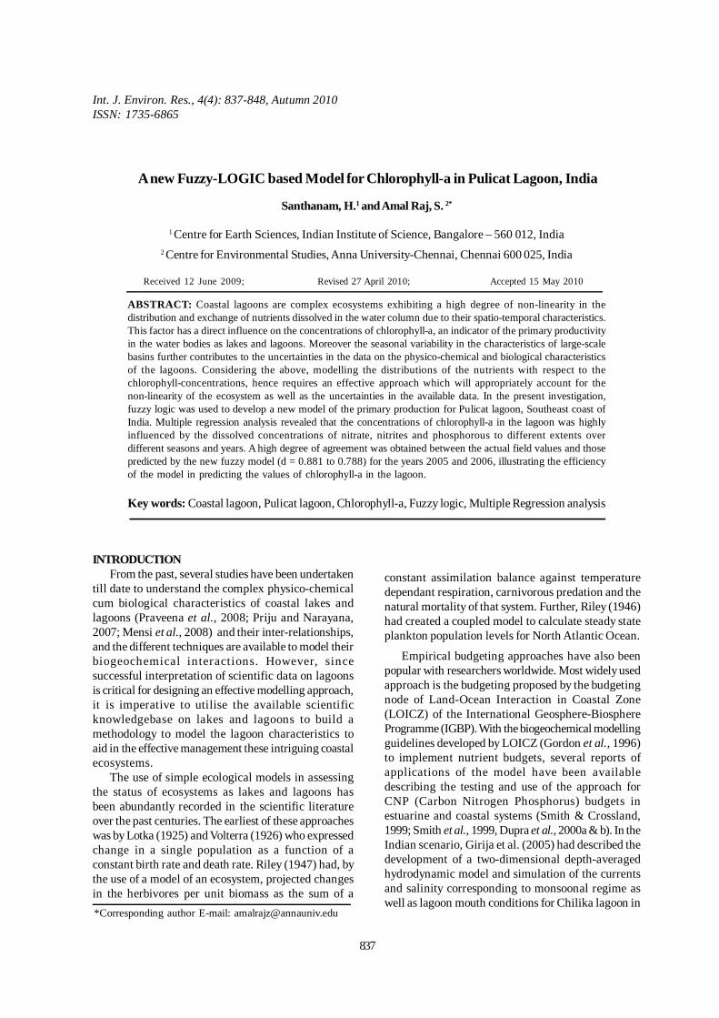
Int. J. Environ. Res., 4(4): 837-848, Autumn 2010ISSN: 1735-6865
Received 12 June 2009; Revised 27 April 2010; Accepted 15 May 2010
*Corresponding author E-mail: [email protected]
837
A new Fuzzy-LOGIC based Model for Chlorophyll-a in Pulicat Lagoon, India
Santhanam, H.1 and Amal Raj, S. 2*
1 Centre for Earth Sciences, Indian Institute of Science, Bangalore – 560 012, India2 Centre for Environmental Studies, Anna University-Chennai, Chennai 600 025, India
ABSTRACT: Coastal lagoons are complex ecosystems exhibiting a high degree of non-linearity in thedistribution and exchange of nutrients dissolved in the water column due to their spatio-temporal characteristics.This factor has a direct influence on the concentrations of chlorophyll-a, an indicator of the primary productivityin the water bodies as lakes and lagoons. Moreover the seasonal variability in the characteristics of large-scalebasins further contributes to the uncertainties in the data on the physico-chemical and biological characteristicsof the lagoons. Considering the above, modelling the distributions of the nutrients with respect to thechlorophyll-concentrations, hence requires an effective approach which will appropriately account for thenon-linearity of the ecosystem as well as the uncertainties in the available data. In the present investigation,fuzzy logic was used to develop a new model of the primary production for Pulicat lagoon, Southeast coast ofIndia. Multiple regression analysis revealed that the concentrations of chlorophyll-a in the lagoon was highlyinfluenced by the dissolved concentrations of nitrate, nitrites and phosphorous to different extents overdifferent seasons and years. A high degree of agreement was obtained between the actual field values and thosepredicted by the new fuzzy model (d = 0.881 to 0.788) for the years 2005 and 2006, illustrating the efficiencyof the model in predicting the values of chlorophyll-a in the lagoon.
Key words: Coastal lagoon, Pulicat lagoon, Chlorophyll-a, Fuzzy logic, Multiple Regression analysis
INTRODUCTIONFrom the past, several studies have been undertaken
till date to understand the complex physico-chemicalcum biological characteristics of coastal lakes andlagoons (Praveena et al., 2008; Priju and Narayana,2007; Mensi et al., 2008) and their inter-relationships,and the different techniques are available to model theirbiogeochemical interactions. However, sincesuccessful interpretation of scientific data on lagoonsis critical for designing an effective modelling approach,it is imperative to utilise the available scientificknowledgebase on lakes and lagoons to build amethodology to model the lagoon characteristics toaid in the effective management these intriguing coastalecosystems.
The use of simple ecological models in assessingthe status of ecosystems as lakes and lagoons hasbeen abundantly recorded in the scientific literatureover the past centuries. The earliest of these approacheswas by Lotka (1925) and Volterra (1926) who expressedchange in a single population as a function of aconstant birth rate and death rate. Riley (1947) had, bythe use of a model of an ecosystem, projected changesin the herbivores per unit biomass as the sum of a
constant assimilation balance against temperaturedependant respiration, carnivorous predation and thenatural mortality of that system. Further, Riley (1946)had created a coupled model to calculate steady stateplankton population levels for North Atlantic Ocean.
Empirical budgeting approaches have also beenpopular with researchers worldwide. Most widely usedapproach is the budgeting proposed by the budgetingnode of Land-Ocean Interaction in Coastal Zone(LOICZ) of the International Geosphere-BiosphereProgramme (IGBP). With the biogeochemical modellingguidelines developed by LOICZ (Gordon et al., 1996)to implement nutrient budgets, several reports ofapplications of the model have been availabledescribing the testing and use of the approach forCNP (Carbon Nitrogen Phosphorus) budgets inestuarine and coastal systems (Smith & Crossland,1999; Smith et al., 1999, Dupra et al., 2000a & b). In theIndian scenario, Girija et al. (2005) had described thedevelopment of a two-dimensional depth-averagedhydrodynamic model and simulation of the currentsand salinity corresponding to monsoonal regime aswell as lagoon mouth conditions for Chilika lagoon in
838
Santhanam, H. and Amal Raj. S
India. More recently, Gupta et al. (2006) provided thebudgets of nitrogen and phosphorus constructedusing LOICZ approach for Muthupet lagoon.
However, despite recounting the experiences ofmodelling coastal lagoons from various researchersworldwide, these studies have at the same time,indicated the need for realistic and simple models ofecosystem for unique coastal ecotones such aslagoons. For example, in their study of the role ofcarbonate dissolution in determining the complexdynamics of dissolved inorganic carbon in estuarineecosystems such as Gautami - Godavari estuary,Bouillon et al. (2003) had indicated that at least a simpleand reliable nutrient budgeting of the coastal zone wasnecessary for quantifying the changes in thebiogeochemistry and productivity of the coastalecosystems.
At present, a complete study of the various sourcesof external inputs and internal transformation in acoastal lagoon in connection with its productivity is,at large, a subject that requires greater introspectionin India. Given the multi-faceted role of a coastal lagoonas an socio-economic lifeline, an eco-cultural entity aswell as a environmental laboratory for research,modelling the biology and hydro-chemicalcharacteristics, albeit a necessary component forsustainable management of these resources, remainsan gargantuan scientific quest with little direction andlots of uncertainties.
However, modelling the ecosystem status andpredicting productivity within large basins of highspatio-temporal and seasonal variability is the greatestchallenge at present for the modellers. While differentmodelling techniques are available to represent theseecosystems, their applicability is often limited to thosesystems having similar conditions to the range of dataprescribed in these models (Soyupak and Chen, 2004).Further, these empirical or statistical models do notconsider the spatio-temporal aspects of the lagoons.Rast et al (1983) carried out an assessment of thepredictive power of the available simple empiricalmodels for primary productivity and found that thepredicted values of the chlorophyll-a were within afactor of ± 3 in all lakes.
Dynamic water quality modelling software such asCE-QUAL is more accurate, and includes the spatio-temporality of the lagoons as a factor in modelling.Using differential equations, they help to investigatethe relationships between the physico-chemical orbiological mechanisms. But these involve expensiveand time-consuming data collection as well asextensive numerical calculation (Soyupak and Chen,2004) in which the potential for error is greater with
increasing complexity in calculation. Hence, thecombination of uncertainty in data and complexity incalculation may give erroneous results.
In the past few years, soft computing techniques,such as fuzzy logic, neural networks and cellularautomata that are capable of handling the uncertaintyin data and analysis have been used in ecosystemmodelling (Rene and Saidutta, 2008; Nakane andHaidary, 2010; Tuzkaya and Gulsun, 2008). Fuzzy logicsystems can be used to model non-linear relationshipseasily and effectively even when only limited data isavailable (Silvert, 1997). Fuzzy rules provide a common-sense description of the action of the system and theinformation in a fuzzy-logic system are processed interms of fuzzy sets defined through an associatedmembership function. The ability of the fuzzy logicsystems, being universally approximators and also well–defined functions mapping real-value input to real-value output has made them powerful tools forexploring complex non-linear biological problems in thecontext of an ecosystem.
MATERIALS & METHODSThe study area for the present investigation is
situated near the village of Pulicat Town, located about60 km from Chennai city (Fig. 1). It is a coastal inlandwater embayment in the form of a lagoon, known asthe Pulicat lagoon, which is the second largestbrackish water lake in India. Geographically the coastallagoon is situated between latitudes 13° 25´– 13° 55´N and longitudes 80° 03 – 80°19 E with and an altitudeof 0-10 m (Azariah, 1988). The lagoon is a cross-boundary ecosystem extending between theneighbouring states of Andhra Pradesh (AP) and TamilNadu (TN). According to WWF report (1993), about84% of the Pulicat Lake ecosystem lies in AP. Itoccupies a total area 650 km2 with a high tide waterspread area of about 178 m2 (Rao and Rao, 1975). Theentire lake is a huge evaporating basin and hasbeen known to fall 3.9 feet below the mean sealevel during April – May and June. The lake isabout 60 km in length and 0.2 to 17.5 km in width.The total area of about 72,000 ha includes about 20,000ha (27.7%) of swamps to north of the lake. It has ahigh water spread area of 460 Km and low waterspread area of 250 Km. The seawater enters the lakethrough two bar mouths located at the north and southends of the lagoons (WWF, 1993). The lake is shallowwith an average depth of about 1.5 m; the maximumdepth being 9.0 m near the entrance to the sea. Thelake is separated from the Bay of Bengal by aninland spit called the Sriharikota Island, which iscurrently used as a launching pad of India’s spaceresearch programme. The main source of fresh water
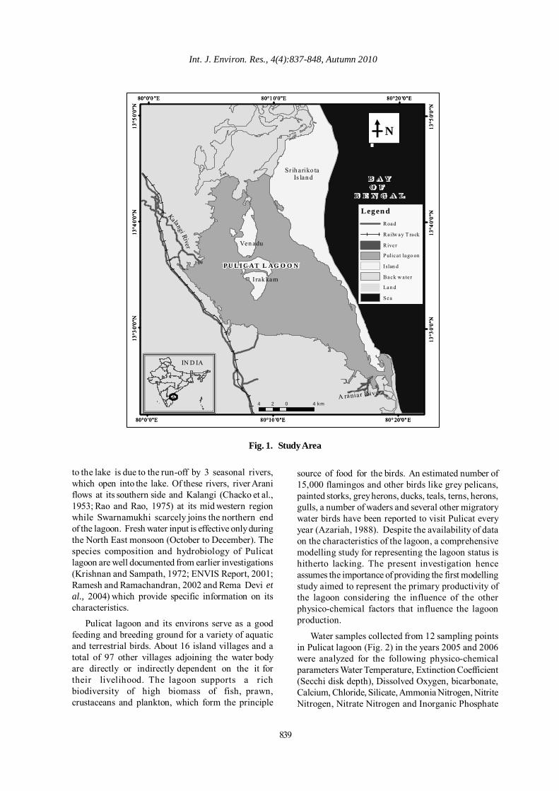
Int. J. Environ. Res., 4(4):837-848, Autumn 2010
839
80° 20'0" E
80°20 '0"E
80°10 '0"E
80°1 0'0"E
80°0 '0"E
80°0'0 "E
13°5
0'0"
N
13°5
0'0"
N
13°4
0'0"
N
13°4
0'0"
N
13°3
0'0"
N
13°3
0'0"
N
µ
4 0 42 km
B A YO F
B E N G A L
PU L I C AT L AG O O N
Ven adu
I rak kam
Sr ih ariko ta Is lan d
Ka lang i R ive r
A raniar R iver
IN D IA
Legen dRoad
Railw ay T rack
River
Pulica t lago on
Islan d
Back w ater
Lan d
Sea
N
80° 20'0" E
80°20 '0"E
80°10 '0"E
80°1 0'0"E
80°0 '0"E
80°0'0 "E
13°5
0'0"
N
13°5
0'0"
N
13°4
0'0"
N
13°4
0'0"
N
13°3
0'0"
N
13°3
0'0"
N
µ
4 0 42 km
B A YO F
B E N G A L
PU L I C AT L AG O O N
Ven adu
I rak kam
Sr ih ariko ta Is lan d
Ka lang i R ive r
A raniar R iver
IN D IA
Legen dRoad
Railw ay T rack
River
Pulica t lago on
Islan d
Back w ater
Lan d
Sea
NN
Fig. 1. Study Area
to the lake is due to the run-off by 3 seasonal rivers,which open into the lake. Of these rivers, river Araniflows at its southern side and Kalangi (Chacko et al.,1953; Rao and Rao, 1975) at its mid western regionwhile Swarnamukhi scarcely joins the northern endof the lagoon. Fresh water input is effective only duringthe North East monsoon (October to December). Thespecies composition and hydrobiology of Pulicatlagoon are well documented from earlier investigations(Krishnan and Sampath, 1972; ENVIS Report, 2001;Ramesh and Ramachandran, 2002 and Rema Devi etal., 2004) which provide specific information on itscharacteristics.
Pulicat lagoon and its environs serve as a goodfeeding and breeding ground for a variety of aquaticand terrestrial birds. About 16 island villages and atotal of 97 other villages adjoining the water bodyare directly or indirectly dependent on the it fortheir livelihood. The lagoon supports a richbiodiversity of high biomass of fish, prawn,crustaceans and plankton, which form the principle
source of food for the birds. An estimated number of15,000 flamingos and other birds like grey pelicans,painted storks, grey herons, ducks, teals, terns, herons,gulls, a number of waders and several other migratorywater birds have been reported to visit Pulicat everyyear (Azariah, 1988). Despite the availability of dataon the characteristics of the lagoon, a comprehensivemodelling study for representing the lagoon status ishitherto lacking. The present investigation henceassumes the importance of providing the first modellingstudy aimed to represent the primary productivity ofthe lagoon considering the influence of the otherphysico-chemical factors that influence the lagoonproduction.
Water samples collected from 12 sampling pointsin Pulicat lagoon (Fig. 2) in the years 2005 and 2006were analyzed for the following physico-chemicalparameters Water Temperature, Extinction Coefficient(Secchi disk depth), Dissolved Oxygen, bicarbonate,Calcium, Chloride, Silicate, Ammonia Nitrogen, NitriteNitrogen, Nitrate Nitrogen and Inorganic Phosphate
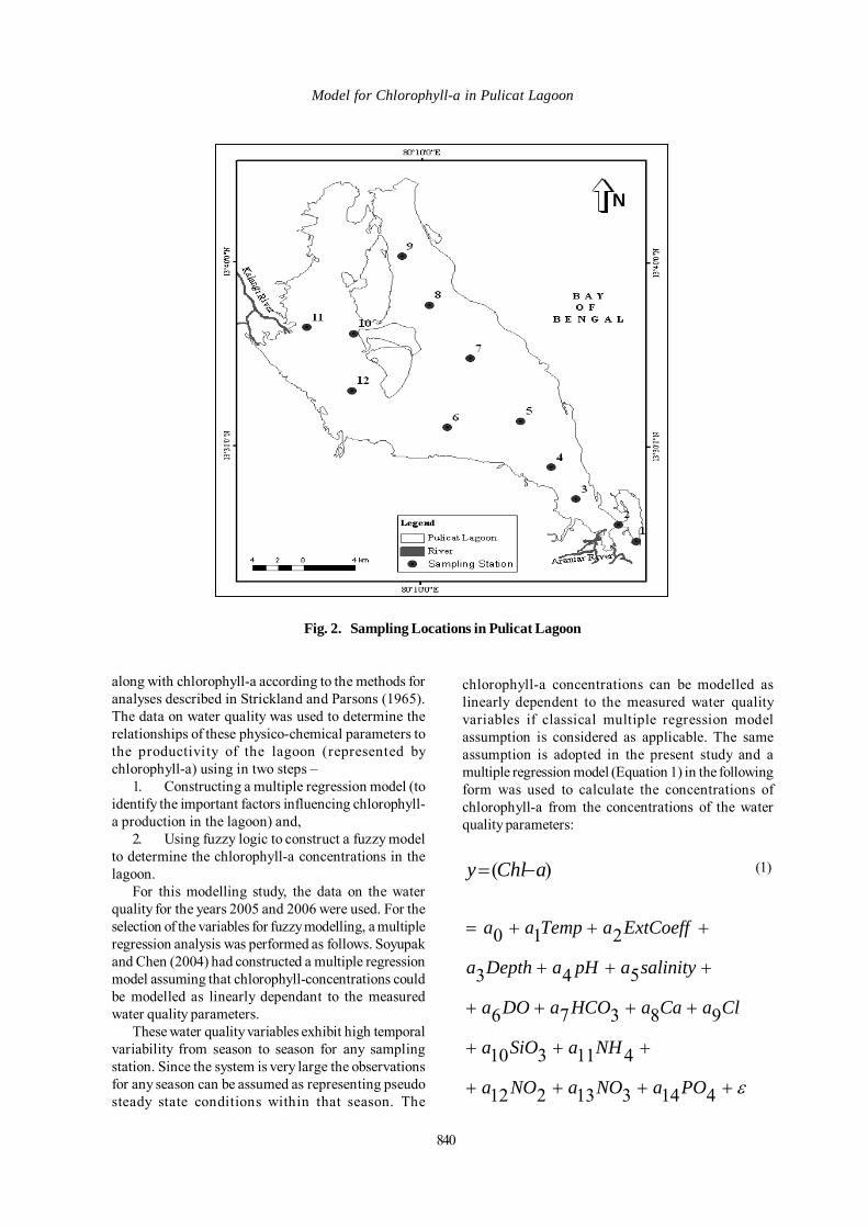
840
Model for Chlorophyll-a in Pulicat Lagoon
NN
along with chlorophyll-a according to the methods foranalyses described in Strickland and Parsons (1965).The data on water quality was used to determine therelationships of these physico-chemical parameters tothe productivity of the lagoon (represented bychlorophyll-a) using in two steps –
1. Constructing a multiple regression model (toidentify the important factors influencing chlorophyll-a production in the lagoon) and,
2. Using fuzzy logic to construct a fuzzy modelto determine the chlorophyll-a concentrations in thelagoon.
For this modelling study, the data on the waterquality for the years 2005 and 2006 were used. For theselection of the variables for fuzzy modelling, a multipleregression analysis was performed as follows. Soyupakand Chen (2004) had constructed a multiple regressionmodel assuming that chlorophyll-concentrations couldbe modelled as linearly dependant to the measuredwater quality parameters.
These water quality variables exhibit high temporalvariability from season to season for any samplingstation. Since the system is very large the observationsfor any season can be assumed as representing pseudosteady state conditions within that season. The
Fig. 2. Sampling Locations in Pulicat Lagoon
chlorophyll-a concentrations can be modelled aslinearly dependent to the measured water qualityvariables if classical multiple regression modelassumption is considered as applicable. The sameassumption is adopted in the present study and amultiple regression model (Equation 1) in the followingform was used to calculate the concentrations ofchlorophyll-a from the concentrations of the waterquality parameters:
)( aChly −=
ε++++
+++
++++
+++
+++=
414313212
411310
98376
543
210
POaNOaNOa
NHaSiOa
ClaCaaHCOaDOa
salinityapHaDeptha
ExtCoeffaTempaa
(1)

Int. J. Environ. Res., 4(4):837-848, Autumn 2010
Where, ai (i = 0-14) are the regression coefficients,ε is the error term which is normally distributed (ε ~N(0,σ2),Temp = Temperature (°C)ExtCoeff = Extinction Coefficient (m)DO = Dissolved Oxygen (mL/L)HCO3 = Bicarbonate (mg/L)Ca = Calcium (mg/L)Cl = Chloride (mg/L)SiO3= Silicate (mg/L)NH4 = Ammoniacal Nitrogen (µg/L)NO2 = Nitrite Nitrogen (µg/L)NO3 = Nitrate Nitrogen (µg/L)PO4 = Phosphate (µg/L)
For the regression equation to be valid to be usedfor predictions, it must reflect the regression model forthe population. The regression statistics including the
Multiple R (used to measure the strength of therelationship between the independent variables anddependent variable); the R Square, Adjusted R Squareand the Standard Error were obtained from the analysesand are summarized in Tables 1 to 4 along with theAnalysis of Variance (ANOVA) table. From the ANOVAtable, the F-statistic and the significance F are used totest the validity of the regression. In the present studyrelationships between the physico-chemical parametersof water quality derived from earlier analyses were usedto formulate the fuzzy rules which describe thesecomplex inter-relationships in logical statements. Theobserved values were normalised to a scale of 0 to 1for fuzzification using the Fuzzy Logic Toolbox ofMATLAB 7.0 software. This process yielded the fuzzymemberships functions (FMF) that defined how eachpoint in the input space was mapped to a membershipvalue (also called the ‘degree of membership’ denotedas‘d’ between 0 and 1.
Regression Statistics Multiple R 0.826621717 R Square 0.683303462 Adjusted R Square 0.190664404 Standard Error 0.009439559
ANOVA
df SS MS F Significance F Regression 14 0.001730279 0.000123591 1.387026567 0.316285563 Residual 9 0.000801947 8.91053E-05 Total 23 0.002532227
Coefficients Standard
Error t Stat P-value
Significance Intercept -0.010 0.257 -0.040 0.969 -
Temperature 0.003 0.007 0.419 0.685 N Extinction Coefficient -0.008 0.011 -0.728 0.485
N
Depth 0.003 0.019 0.146 0.887 N
pH 0.001 0.010 0.075 0.942 N
Salinity -0.001 0.002 -0.643 0.536 N
DO 0.003 0.008 0.404 0.696 N
Bicarbonate 0.000 0.000 0.751 0.472 N
Calcium 0.000 0.000 1.278 0.233 N
Chloride 0.000 0.000 -1.001 0.343 N
Silicate 0.000 0.000 0.796 0.447 N
Ammonia-N 0.000 0.000 0.731 0.483 N
Nitrite-N 0.001 0.001 0.605 0.560 N
Nitrate-N 0.000 0.000 -0.297 0.773 N
Phosphate-P 0.000 0.000 -0.913 0.385 N Significant / most influential variables: none
Table 1. Summary Of the Output for Multiple Regression Analysis For Post Monsoon Season
841
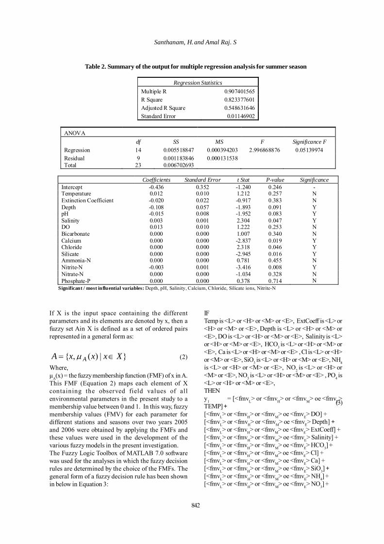
842
Santhanam, H. and Amal Raj. S
Table 2. Summary of the output for multiple regression analysis for summer season
Regression Statistics Multiple R 0.907401565 R Square 0.823377601 Adjusted R Square 0.548631646 Standard Error 0.01146902
ANOVA
df SS MS F Significance F Regression 14 0.005518847 0.000394203 2.996868876 0.05139974 Residual 9 0.001183846 0.000131538 Total 23 0.006702693
Coefficients Standard Error t Stat P-value Significance
Intercept -0.436 0.352 -1.240 0.246 - Temperature 0.012 0.010 1.212 0.257 N Extinction Coefficient -0.020 0.022 -0.917 0.383 N Depth -0.108 0.057 -1.893 0.091 Y pH -0.015 0.008 -1.952 0.083 Y Salinity 0.003 0.001 2.304 0.047 Y DO 0.013 0.010 1.222 0.253 N Bicarbonate 0.000 0.000 1.007 0.340 N Calcium 0.000 0.000 -2.837 0.019 Y Chloride 0.000 0.000 2.318 0.046 Y Silicate 0.000 0.000 -2.945 0.016 Y Ammonia-N 0.000 0.000 0.781 0.455 N Nitrite-N -0.003 0.001 -3.416 0.008 Y Nitrate-N 0.000 0.000 -1.034 0.328 N Phosphate-P 0.000 0.000 0.378 0.714 N
Significant / most influential variables: Depth, pH, Salinity, Calcium, Chloride, Silicate ions, Nitrite-N
If X is the input space containing the differentparameters and its elements are denoted by x, then afuzzy set Ain X is defined as a set of ordered pairsrepresented in a general form as:
}|)(,{ XxxxA A ∈= µ (2)
Where,µA(x) = the fuzzy membership function (FMF) of x in A.This FMF (Equation 2) maps each element of Xcontaining the observed field values of allenvironmental parameters in the present study to amembership value between 0 and 1. In this way, fuzzymembership values (FMV) for each parameter fordifferent stations and seasons over two years 2005and 2006 were obtained by applying the FMFs andthese values were used in the development of thevarious fuzzy models in the present investigation.The Fuzzy Logic Toolbox of MATLAB 7.0 softwarewas used for the analyses in which the fuzzy decisionrules are determined by the choice of the FMFs. Thegeneral form of a fuzzy decision rule has been shownin below in Equation 3:
IFTemp is <L> or <H> or <M> or <E>, ExtCoeff is <L> or<H> or <M> or <E>, Depth is <L> or <H> or <M> or<E>, DO is <L> or <H> or <M> or <E>, Salinity is <L>or <H> or <M> or <E>, HCO3 is <L> or <H> or <M> or<E>, Ca is <L> or <H> or <M> or <E> , Cl is <L> or <H>or <M> or <E>, SiO3 is <L> or <H> or <M> or <E>, NH4is <L> or <H> or <M> or <E>, NO2 is <L> or <H> or<M> or <E>, NO3 is <L> or <H> or <M> or <E> , PO4 is<L> or <H> or <M> or <E>,THENy1 = [<fmvL> or <fmvH> or <fmvM> oe <fmvE>TEMP] +[<fmvL> or <fmvH> or <fmvM> oe <fmvE> DO] +[<fmvL> or <fmvH> or <fmvM> oe <fmvE> Depth] +[<fmvL> or <fmvH> or <fmvM> oe <fmvE> ExtCoeff] +[<fmvL> or <fmvH> or <fmvM> oe <fmvE> Salinity] +[<fmvL> or <fmvH> or <fmvM> oe <fmvE> HCO3] +[<fmvL> or <fmvH> or <fmvM> oe <fmvE> Cl] +[<fmvL> or <fmvH> or <fmvM> oe <fmvE> Ca] +[<fmvL> or <fmvH> or <fmvM> oe <fmvE> SiO3] +[<fmvL> or <fmvH> or <fmvM> oe <fmvE> NH4] +[<fmvL> or <fmvH> or <fmvM> oe <fmvE> NO3] +
(3)
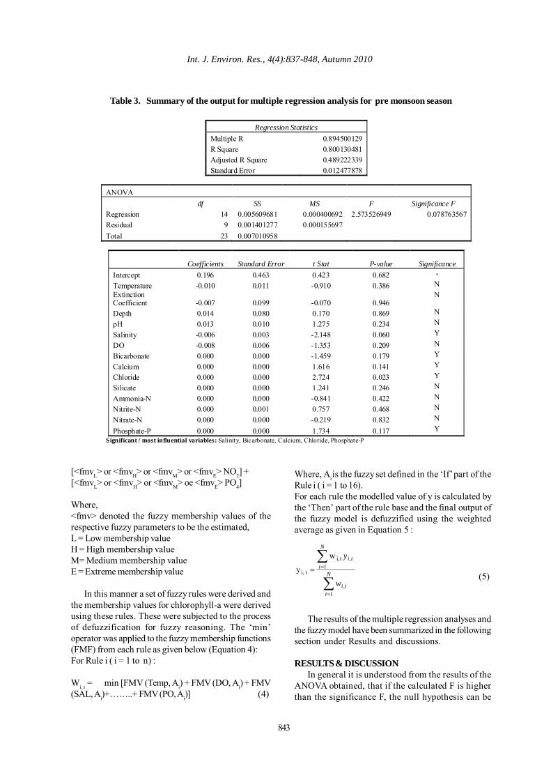
843
Int. J. Environ. Res., 4(4):837-848, Autumn 2010
Table 3. Summary of the output for multiple regression analysis for pre monsoon season
Regression Statistics Multiple R 0.894500129 R Square 0.800130481 Adjusted R Square 0.489222339 Standard Error 0.012477878
ANOVA
df SS MS F Significance F Regression 14 0.005609681 0.000400692 2.573526949 0.078763567 Residual 9 0.001401277 0.000155697 Total 23 0.007010958
Coefficients Standard Error t Stat P-value
Significance Intercept 0.196 0.463 0.423 0.682 - Temperature -0.010 0.011 -0.910 0.386 N Extinction Coefficient -0.007 0.099 -0.070 0.946
N
Depth 0.014 0.080 0.170 0.869 N pH 0.013 0.010 1.275 0.234 N Salinity -0.006 0.003 -2.148 0.060 Y DO -0.008 0.006 -1.353 0.209 N Bicarbonate 0.000 0.000 -1.459 0.179 Y Calcium 0.000 0.000 1.616 0.141 Y Chloride 0.000 0.000 2.724 0.023 Y Silicate 0.000 0.000 1.241 0.246 N Ammonia-N 0.000 0.000 -0.841 0.422 N Nitrite-N 0.000 0.001 0.757 0.468 N Nitrate-N 0.000 0.000 -0.219 0.832 N
Phosphate-P 0.000 0.000 1.734 0.117 Y Significant / most influential variables: Salinity, Bicarbonate, Calcium, Chloride, Phosphate-P
[<fmvL> or <fmvH> or <fmvM> or <fmvE> NO2] +[<fmvL> or <fmvH> or <fmvM> oe <fmvE> PO4]
Where,<fmv> denoted the fuzzy membership values of therespective fuzzy parameters to be the estimated,L = Low membership valueH = High membership valueM= Medium membership valueE = Extreme membership value
In this manner a set of fuzzy rules were derived andthe membership values for chlorophyll-a were derivedusing these rules. These were subjected to the processof defuzzification for fuzzy reasoning. The ‘min’operator was applied to the fuzzy membership functions(FMF) from each rule as given below (Equation 4):For Rule i ( i = 1 to n) :
Wi, t = min [FMV (Temp, Ai) + FMV (DO, Ai) + FMV(SAL, Ai)+……..+ FMV (PO, Ai)] (4)
Where, Ai is the fuzzy set defined in the ‘If’ part of theRule i ( i = 1 to 16).For each rule the modelled value of y is calculated bythe ‘Then’ part of the rule base and the final output ofthe fuzzy model is defuzzified using the weightedaverage as given in Equation 5 :
∑
∑
=
==N
iti
ti
N
i
w
y
1,
,1
ti,
ti,
w
y (5)
The results of the multiple regression analyses andthe fuzzy model have been summarized in the followingsection under Results and discussions.
RESULTS & DISCUSSIONIn general it is understood from the results of the
ANOVA obtained, that if the calculated F is higherthan the significance F, the null hypothesis can be
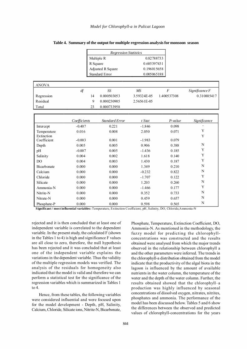
844
Model for Chlorophyll-a in Pulicat Lagoon
Table 4. Summary of the output for multiple regression analysis for monsoon season
Regression Statistics Multiple R 0.82788733 R Square 0.685397431 Adjusted R Square 0.196015658 Standard Error 0.005065188
ANOVA
df SS MS F Significance F Regression 14 0.000503053 3.59324E-05 1.400537308 0.310885417 Residual 9 0.000230905 2.56561E-05 Total 23 0.000733958
Coefficients Standard Error t Stat P-value
Significance Intercept -0.407 0.221 -1.846 0.098 - Temperature 0.016 0.008 2.050 0.071 Y Extinction Coefficient -0.003 0.001 -1.983 0.079
Y
Depth 0.005 0.005 0.906 0.388 N pH -0.007 0.005 -1.436 0.185 Y Salinity 0.004 0.002 1.618 0.140 Y DO 0.004 0.003 1.430 0.187 Y Bicarbonate 0.000 0.000 1.349 0.210 N Calcium 0.000 0.000 -0.232 0.822 N Chloride 0.000 0.000 -1.707 0.122 Y Silicate 0.000 0.000 1.203 0.260 N Ammonia-N 0.000 0.000 -1.466 0.177 Y Nitrite-N 0.000 0.000 0.352 0.733 N Nitrate-N 0.000 0.000 0.459 0.657 N
Phosphate-P 0.000 0.000 0.598 0.565 N Significant / most influential variables: Temperature, Extinction Coefficient, pH, Salinity, DO, Chloride,Ammonia-N
rejected and it is then concluded that at least one ofindependent variable is correlated to the dependentvariable. In the present study, the calculated F (shownin the Tables 1 to 4) is high and significance F valuesare all close to zero, therefore, the null hypothesishas been rejected and it was concluded that at leastone of the independent variable explains thevariations in the dependent variable. Thus the validityof the multiple regression models was verified. Theanalysis of the residuals for homogeneity alsoindicated that the model is valid and therefore we canperform a statistical test for the significance of theregression variables which is summarized in Tables 1to 4.
Hence, from these tables, the following variableswere considered influential and were focused uponfor the model development - Depth, pH, Salinity,Calcium, Chloride, Silicate ions, Nitrite-N, Bicarbonate,
Phosphate, Temperature, Extinction Coefficient, DO,Ammonia-N. As mentioned in the methodology, thefuzzy model for predicting the chlorophyll-concentrations was constructed and the resultsobtained were analysed from which the major trendsobserved in the relationship between chlorophyll aand the other parameters were inferred. The trends inthe chlorophyll-a distribution obtained from the modelindicate that the productivity of the algal biota in thelagoon is influenced by the amount of availablenutrients in the water column, the temperature of thewater and the depth of the water column. Further, theresults obtained showed that the chlorophyll–aproduction was highly influenced by seasonalconcentrations of dissolved oxygen, nitrates, nitrites,phosphates and ammonia. The performance of themodel has been discussed below. Tables 5 and 6 showthe differences between the observed and predictedvalues of chlorophyll-concentrations for the years
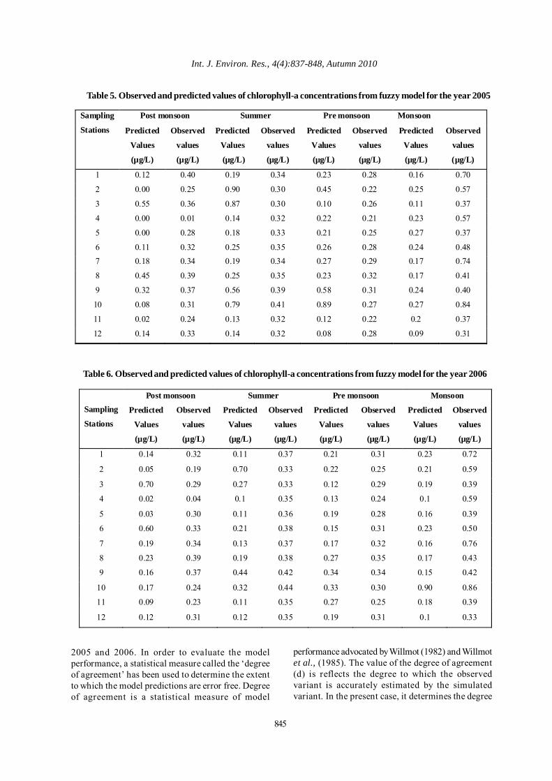
Int. J. Environ. Res., 4(4):837-848, Autumn 2010
Post monsoon Summer Pre monsoon Monsoon Sampling
Stations Predicted
Values
(µg/L)
Observed
values
(µg/L)
Predicted
Values
(µg/L)
Observed
values
(µg/L)
Predicted
Values
(µg/L)
Observed
values
(µg/L)
Predicted
Values
(µg/L)
Observed
values
(µg/L)
1 0.12 0.40 0.19 0.34 0.23 0.28 0.16 0.70
2 0.00 0.25 0.90 0.30 0.45 0.22 0.25 0.57
3 0.55 0.36 0.87 0.30 0.10 0.26 0.11 0.37
4 0.00 0.01 0.14 0.32 0.22 0.21 0.23 0.57
5 0.00 0.28 0.18 0.33 0.21 0.25 0.27 0.37
6 0.11 0.32 0.25 0.35 0.26 0.28 0.24 0.48 7 0.18 0.34 0.19 0.34 0.27 0.29 0.17 0.74
8 0.45 0.39 0.25 0.35 0.23 0.32 0.17 0.41
9 0.32 0.37 0.56 0.39 0.58 0.31 0.24 0.40
10 0.08 0.31 0.79 0.41 0.89 0.27 0.27 0.84
11 0.02 0.24 0.13 0.32 0.12 0.22 0.2 0.37
12 0.14 0.33 0.14 0.32 0.08 0.28 0.09 0.31
Table 5. Observed and predicted values of chlorophyll-a concentrations from fuzzy model for the year 2005
2005 and 2006. In order to evaluate the modelperformance, a statistical measure called the ‘degreeof agreement’ has been used to determine the extentto which the model predictions are error free. Degreeof agreement is a statistical measure of model
Table 6. Observed and predicted values of chlorophyll-a concentrations from fuzzy model for the year 2006
Post monsoon Summer Pre monsoon Monsoon Sampling
Stations Predicted
Values
(µg/L)
Observed
values
(µg/L)
Predicted
Values
(µg/L)
Observed
values
(µg/L)
Predicted
Values
(µg/L)
Observed
values
(µg/L)
Predicted
Values
(µg/L)
Observed
values
(µg/L)
1 0.14 0.32 0.11 0.37 0.21 0.31 0.23 0.72
2 0.05 0.19 0.70 0.33 0.22 0.25 0.21 0.59
3 0.70 0.29 0.27 0.33 0.12 0.29 0.19 0.39
4 0.02 0.04 0.1 0.35 0.13 0.24 0.1 0.59
5 0.03 0.30 0.11 0.36 0.19 0.28 0.16 0.39
6 0.60 0.33 0.21 0.38 0.15 0.31 0.23 0.50
7 0.19 0.34 0.13 0.37 0.17 0.32 0.16 0.76
8 0.23 0.39 0.19 0.38 0.27 0.35 0.17 0.43
9 0.16 0.37 0.44 0.42 0.34 0.34 0.15 0.42
10 0.17 0.24 0.32 0.44 0.33 0.30 0.90 0.86
11 0.09 0.23 0.11 0.35 0.27 0.25 0.18 0.39
12 0.12 0.31 0.12 0.35 0.19 0.31 0.1 0.33
performance advocated by Willmot (1982) and Willmotet al., (1985). The value of the degree of agreement(d) is reflects the degree to which the observedvariant is accurately estimated by the simulatedvariant. In the present case, it determines the degree
845
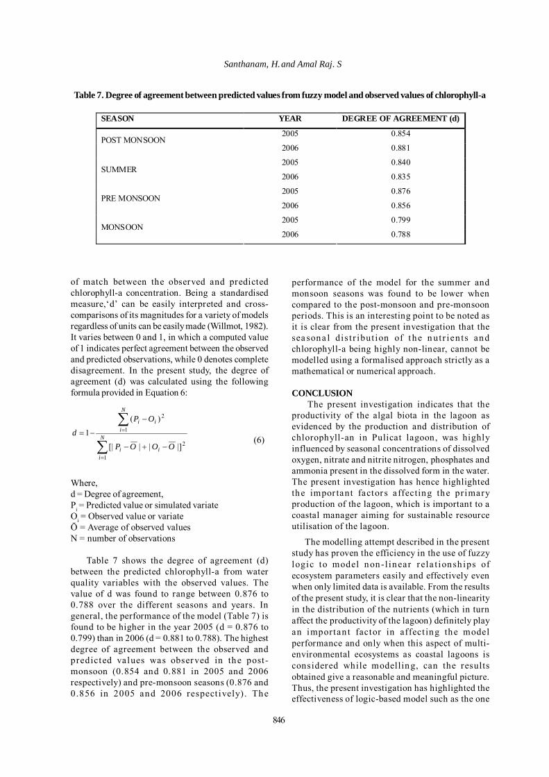
Santhanam, H. and Amal Raj. S
of match between the observed and predictedchlorophyll-a concentration. Being a standardisedmeasure,‘d’ can be easily interpreted and cross-comparisons of its magnitudes for a variety of modelsregardless of units can be easily made (Willmot, 1982).It varies between 0 and 1, in which a computed valueof 1 indicates perfect agreement between the observedand predicted observations, while 0 denotes completedisagreement. In the present study, the degree ofagreement (d) was calculated using the followingformula provided in Equation 6:
∑
∑
=
=
−+−
−
−=N
iii
N
iii
OOOP
OP
d
1
2
1
2
|]||[|
)(
1 (6)
Where,d = Degree of agreement,Pi = Predicted value or simulated variateOi = Observed value or variateŌ = Average of observed valuesN = number of observations
Table 7 shows the degree of agreement (d)between the predicted chlorophyll-a from waterquality variables with the observed values. Thevalue of d was found to range between 0.876 to0.788 over the different seasons and years. Ingeneral, the performance of the model (Table 7) isfound to be higher in the year 2005 (d = 0.876 to0.799) than in 2006 (d = 0.881 to 0.788). The highestdegree of agreement between the observed andpredicted values was observed in the post -monsoon (0.854 and 0.881 in 2005 and 2006respectively) and pre-monsoon seasons (0.876 and0.856 in 2005 and 2006 respect ively) . The
Table 7. Degree of agreement between predicted values from fuzzy model and observed values of chlorophyll-a
SEASON YEAR DEGREE OF AGREEMENT (d)
2005 0.854 POST MONSOON
2006 0.881
2005 0.840 SUMMER
2006 0.835
2005 0.876 PRE MONSOON
2006 0.856
2005 0.799 MONSOON
2006 0.788
performance of the model for the summer andmonsoon seasons was found to be lower whencompared to the post-monsoon and pre-monsoonperiods. This is an interesting point to be noted asit is clear from the present investigation that thesea sona l dis t r ibut ion of t he n utr ien ts andchlorophyll-a being highly non-linear, cannot bemodelled using a formalised approach strictly as amathematical or numerical approach.
CONCLUSIONThe present investigation indicates that the
productivity of the algal biota in the lagoon asevidenced by the production and distribution ofchlorophyll-an in Pulicat lagoon, was highlyinfluenced by seasonal concentrations of dissolvedoxygen, nitrate and nitrite nitrogen, phosphates andammonia present in the dissolved form in the water.The present investigation has hence highlightedthe impor tant factor s affecting the primaryproduction of the lagoon, which is important to acoastal manager aiming for sustainable resourceutilisation of the lagoon.
The modelling attempt described in the presentstudy has proven the efficiency in the use of fuzzylogic to model non-l inear r ela t ionsh ips ofecosystem parameters easily and effectively evenwhen only limited data is available. From the resultsof the present study, it is clear that the non-linearityin the distribution of the nutrients (which in turnaffect the productivity of the lagoon) definitely playan importan t factor in affect ing the modelperformance and only when this aspect of multi-environmental ecosystems as coastal lagoons isconsidered while modelling, can the resultsobtained give a reasonable and meaningful picture.Thus, the present investigation has highlighted theeffectiveness of logic-based model such as the one
846
Int. J. Environ. Res., 4(4):837-848, Autumn 2010
developed presently in modelling a complexenvironment as coastal lagoons.
ACKNOWLEDGEMENTThe authors are extremely grateful to Dr. A.
Navaneetha Gopalakr ishnan, Professor andDirector, Centre for Environmental Studies, AnnaUniversity, Chennai (CES), Dr. K. Thanasekaran,Professor, CES and Dr. K. Palanivelu, AssistantProfessor, CES, for their suggestions, support andencouragement. The authors express their thanksto All India Council for Technical Education(AICTE), New Delhi for the ‘National DoctoralFellowship’ (NDF) received by the first author forpursuing her Ph.D of which this study comprises apart.
REFERENCESAzariah. J, Banth, P., Azariah, H. and Selvam, V. (1988)Impact of urbanization in the status of mangroveswamps of Madras, In: The Ecology and Managementof Wetlands. Volume 2: Management, Use and Value ofWetlands, D.D Hook (Ed.), Timber Press, Portland,Oregon. USA, pp. 225 - 233. Reprinted in: Bulletin No. 4Madras. Fisheries Investigation of Madras, pp 1-24.
Bouillon, S, Frankignoulle, M., Dehairs, F., Velimirov, B,Eiler, A, Abril, G, Etcheber, H and Borges, A.V (2003)Inorganic and organic carbon biogeochemistry in theGautami Godavari estuary (Andhra Pradesh, India) duringpre-monsoon: The local impact of extensive mangroveforests. Global Biogeochem. Cycles, 17 (4), 25-1 to 12.
Chacko, P. I., Abraham, J. G. and Andal, R. (1953) Reporton a survey of the flora, fauna and fisheries of Pulicat lake,Madras, India’ Cent. Freshwater Fish Biol., 8, 1-20.
Dupra, V., Smith, S. V., Crossland, J. I. M. and Crossland,C. J. (2000a). Estuarine systems of the South China Searegion: carbon, nitrogen and phosphorus fluxes’ LOICZReports and Studies 14, LOICZ, Texel, The Netherlands,156 pp, from : http://www.loicz.org/products/publication/reports/index.html.en
Dupra, V., Smith, S. V., Marshall Crossland, J. I. andCrossland, C. J. (2000 b) ‘Estuarine systems of the SouthAmerican region: carbon, nitrogen and phosphorus fluxes’LOICZ Reports and Studies 15, LOICZ, Texel, TheNetherlands, 87 pp, from : http://www.loicz.org/products/publication/reports/index.html.en
Jayaraman, G., D. Rao, A., Dube, A. and Pratap K. andMohanty, P. K. (2000) Numerical Simulation of Circulationand Salinity Structure in Chilika Lagoon, J. of Coast.Research, 22,195-211.
Gordon, Jr., D. C., P. R. Boudreau, K. H. Mann, J. -E.Ong, W. L. Silvert, S. V. Smith, G. Wattayakorn, F. Wulff
and Yanagi, T. (1996) LOICZ Biogeochemical ModellingGuidelines. LOICZ Reports & Studies No 5, pp 1-96,from: http://www.loicz.org/products/publication/reports/index.html.en
Gupta , G. V. M., Natesan, U., Ramana Murthy, M. V.,Sravan Kumar, V. G., Viswanathan, S., Bhat, M. S., KumarRay, A. and Subramanian, B. R. (2006) ‘Nutrient budgetsfor Muthupet lagoon, Southeastern India’, Curr. Sci., 90(7), 967-972.
Krishnan , P. and Sampath, V. (1972). Report onDevelopment of Pulicat Lake and its Fisheries,Department of Fisheries, Government. of Tamil Nadu,1-60.
Lagoons of India State-of-the-art report, (2001) ENVISPublication Series: 3/2001 CAS in Marine Biology,Parangipettai.
Lotka, A. J . (1925). Elements of physical biology’ ,Williams and Wilkins, Baltimore, MD. Reprinted in 1956:Elements of mathematical biology. Dover Publications, Inc.,New York.
Mensi, Gh. S., Moukha, S., Creppy, E. E. and Maaroufi,K. (2008).Metals Accumulation in Marine Bivalves andSeawater from theLagoon of Boughrara in Tunisia (NorthAfrica). Int. J. Environ. Res., 2 (3), 279-284.
Nakane, K. and Haidary, A. (2010).Sensitivity Analysisof Stream Water Quality and Land Cover Linkage ModelsUsing Monte Carlo Method. Int. J. Environ. Res., 4 (1),121-130.
Praveena, S. M., Ahmed, A., Radojevic, M., Abdullah, M.H. and Aris, A. Z. (2008).Heavy Metals in MangroveSurface Sediment of Mengkabong Lagoon, Sabah:Multivariate and Geo-Accumulation Index Approaches.Int. J. Environ. Res., 2 (2), 139-148.
Priju, C. P. and Narayana, A. C. (2007). Heavy and TraceMetals in Vembanad Lake Sediments. Int. J. Environ. Res.,1 (4), 280-289.
Ramesh, R. and Ramachandran, S. (2002). CoastalEnvironment and Management – Anna UniversityPublication’, 389 pp.
Rao, N. V. N. D. and Rao, M. P. (1975). AqueousEnvironment’s in the Pulicat Lake, East coast of India.R. Natarajan (Eds), Resent Researches in EstuarineBiology, Hindustan Publishing Corporation (I) Delhi(India), pp.109-122.
Rast, W., Lee, G. F. and Jones, R. A. (1983). Predictivecapability of U.S. OECD phosphorus loading - lakeresponse models’ J. Wat. Pollut. Cont. Fed., 55, 990-1003.
Rema Devi, K., Indra, T. J. and Raghunathan, M. B.(2004). Fisheries of Pulicat Lake. Rec. Zool. Surv. India,102 (Part 3-4), 33-42.
Rene, E. R. and Saidutta, M. B. (2008). Prediction ofWater Quality Indices by Regression Analysis andArtificial Neural Networks. Int. J. Environ. Res., 2 (2),183-188.
847
Model for Chlorophyll-a in Pulicat Lagoon
Riley, G. A., and Bumpus, D. F. (1946). Phytoplankton –zooplankton relationships on Georges Bank’ J. of Mar.Res., 6 (1), 33-47.
Silvert, W. (1997). Ecological impact classification withfuzzy sets’, Ecol. Model., 96,1-10.
Smith, S. V. and Crossland, C. J. (Eds).(1999). AustralasianEstuarine Systems: Carbon, Nitrogen, and PhosphorusFluxes’ LOICZ reports and Studies No. 12. 182 pp. from: http://www.loicz.org/products/publication/reports/index.html.en
Smith, S. V., Marshall Crossland, J. I. and Crossland, C. J.(1999). Mexican and Central American coastal lagoonsystems: carbon, nitrogen and phosphorus fluxes’ LOICZReports and Studies 13, LOICZ, Texel, the Netherlands,115 pp. from : http://www.loicz.org/products/publication/reports/index.html.en
Soyupak, S. and Chen, D. (2004). Fuzzy logic model toestimate seasonal pseudo steady state chlorophyll-aconcentrations in reservoirs’. Env.Mod. and Ass., 9, 51-59.
Strickland, J. D. H and Parsons, T. R. (1965). A Manual ofseawater analyses, Fisheries Research Board of Canada,Ottawa, Bull., 2 (125), 117-124
Tuzkaya, G. and Gulsun, B. (2008). Evaluating centralizedreturn centers in a reverse logistics network: An integratedfuzzy multi-criteria decision approach . Int. J. Environ.Sci. Tech., 5 (3), 339-352.
Volterra, B. (1926). Fluctuations in the abundance of aspecies mathematically Nature, 118, 558-560.
Willmot, C. J. (1982). Some comments on the evaluationof model performance, Bull. Amer. Meteo. Soc., 63, 1309-1313.
Willmot, C. J., Ackleson, S. G., Davis, R. E., Feddema, J.J., Klink, K. M., Legates, D. R., O’Donnel, J. and Powe,C. M. (1985). Statistics for evaluation and comparison ofmodels’, J. Geophy. Res., 90, 8995-9005.
WWF, (1993). Directory of Indian Wetlands. Worldwide Fundof Nature, India. Asian Wetland Bureau. pp. 1 – 264, from,http://www.wwfindia.org.
848
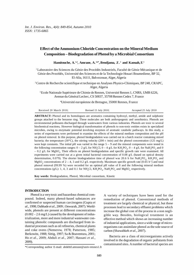
Int. J. Environ. Res., 4(4): 849-854, Autumn 2010ISSN: 1735-6865
Received 20 March 2010; Revised 15 July 2010; Accepted 25 July 2010
*Corresponding author E-mail: [email protected]
849
Effect of the Ammonium Chloride Concentration on the Mineral MediumComposition – Biodegradation of Phenol by a Microbial Consortium
Hamitouche, A. 1,2, Amrane, A. 3,4*, Bendjama, Z . 1 and Kaouah, F. 1
1 Laboratoire des Sciences du Génie des Procédés Industriels, Faculté de Génie Mécanique et deGénie des Procédés, Université des Sciences et de la Technologie Houari Boumediene, BP 32,
El-Alia, 16111, Bab ezzouar, Alger, Algeria2 Centre de Recherche scientifique et technique en Analyses Physico-Chimiques, BP 248, CRAPC,
Alger, Algeria3 Ecole Nationale Supérieure de Chimie de Rennes, Université Rennes 1, CNRS, UMR 6226,
Avenue du Général Leclerc, CS 50837, 35708 Rennes Cedex 7, France4Université européenne de Bretagne, 35000 Rennes, France
ABSTRACT: Phenol and its homologues are aromatics containing hydroxyl, methyl, amide and sulphonicgroups attached to the benzene ring. These molecules are both anthropogenic and xenobiotics. Phenols areenvironmental pollutants discharged through wastewaters from various industries. Phenols are toxic to severalbiochemical reactions. However biological transformation of phenols to non-toxic entities exists in specializedmicrobes, owing to enzymatic potential involving enzymes of aromatic catabolic pathways. In this study, aseries of experiments were performed to examine the effects of the mineral medium composition and the pHon phenol removal. In this purpose, phenol biodegradation was carried out in a batch reactor containing mixedbacteria; the temperature (30°C), the stirring velocity (200 r /min) and the phenol concentration (125 mg/L)were kept constants. The initial pH was varied in the range 5 – 9 and the mineral components were tested inthe following concentration ranges: 0 – 2 g/L for NH4Cl, 0 – 4 g/L for KH2PO4, 0 – 4 g/L for NaH2PO4 and 0– 0.2 g/L for MgSO4. Their effects on phenol biodegradation and specific growth rate were examined. Allexperiments were carried out at a given initial bacterial concentration of 0.08 g/L (based on optical densitydetermination, 0.079). The shorter biodegradation time of phenol was 20.6 h for NaH2PO4, KH2PO4 andMgSO4 concentrations of 2 – 4, 3 and 0.2 g/L respectively. Maximum specific growth rate (0.65 h-1) and totalphenol removal (99.99 %) were recorded for an optimal pH value of 8 and the following mineral mediumconcentrations (g/L): 1, 4, 3 and 0.1 for NH4Cl, KH2PO4, NaH2PO4 and MgSO4 respectively.
Key words: Biodegradation, Phenol, Microbial consortium, Kinetic
INTRODUCTIONPhenol is a very toxic and hazardous chemical com-
pound. Indeed, many phenol-based substances areconfirmed or suspected human carcinogens (Gupta etal., 1998; Dabhade et al., 2009 ; Onwurah, 2007). World-wide, phenols are present at different concentrations(0.002 – 2.6 mg/L) caused by the development of indus-trialization, more and more industrial wastewater con-taining phenolic compounds are discharged from in-dustrial processes such as oil refineries, chemical plantsand coke ovens (Nemerow, 1978; Patterson, 1985;Berkowitz, 1988; Sittig, 1997; Sa & Boaventura, 2001;Ho et al., 2009; Abduli et al., 2007; Hassani et al.,2009).
A variety of techniques have been used for theremediation of phenol. Conventional methods oftreatment are largely chemical or physical, but theseprocesses lead to secondary effluent problems whichincrease the global cost of the process in a non negli-gible way. Besides, biological treatment is aneffective method which shows an increasing numberof industrial applications, since a wide range of micro-organisms can assimilate phenol as the sole source ofcarbon (Shawabkeh et al., 2007).
Bacteria are a class of microorganisms activelyinvolved in the degradation of organic pollutants fromcontaminated sites. A number of bacterial species are

850
Hamitouche, A. et al.
known to degrade phenolic compounds. Most of them,showing high biodegradation efficiency, are isolatedfrom contaminated soil or sediments (Haritash et al.,2009). The identified organisms belonged to severalgenera, like Pseudomonas, as well as Agrobacterium,Bacillus (Gurujeyalakshmi & Oriel, 1989),Burkholderia, Sphingomonas (Berkowitz, 1988),Rhodococcus (Margesin et al., 2005) species and mixedculture.
The main goal of this paper was to investigate thebiodegradation of phenol by mixed bacteria; the effectof pH and the mineral medium composition were opti-mized to determine the best conditions for phenolremoval, especially the mineral salts supplementationand the optimal mineral nitrogen (ammonium chloride)concentration.
MATERIALS & METHODSThe mixed bacteria used in this work were
obtained from activated sludge from the hazardouswastewater plant of Boumerdès (Algeria). The stockcultures were stored at 4 °C. The mixed bacteria wereactivated for 24 h at 30 °C in the nutrient medium (NB)containing (g/ L): peptone, 15, yeast extract, 3, sodiumchloride, 6, and (D+)-glucose, 1.
After 24 h, when cells were grown, the biomasswas harvested by centrifugation. The microorganismscollected after centrifugation (3000 r/min) for 30 minwere suspended in NaCl 0.5 % and re-centrifuged. Af-ter the third washing, The microorganisms collectedafter centrifugation were re-suspended in NaCl 0.5 %to determine the concentration of the mixed bacteria.This solution (mixed bacteria and NaCl 0.5%) was ana-lyzed by measuring OD at 600 nm using a Vis spectro-photometer (HACH DR2800); the OD value was thenconverted to dry cell mass using a dry weight calibra-tion curve. The dry cell mass density (g/ L) was foundto follow the following regression equation x (g/L) =1.044 × OD600.
Specific growth rate was determined in the expo-nential growth phase (Dagley & Gibson, 1965; Stanieret al., 1966; Chiam & Harris, 1982; Worden &Donaldson, 1987). For each flask, the specific growthvalue was determined from linear semi logarithmic plotof cell concentration versus time during the exponen-tial growth phase, namely when specific growth ratebecame nearly constant (D’Adamo et al., 1984).
As the OD value of adapted cells reached 2.7 –2.9, an aliquot of the culture was centrifuged at 3000rpm for 30 min. To wash the biomass, it was re-sus-pended in NaCl 0.5% and centrifuged. The cells (1 ml)were then transferred and inoculated in Erlenmeyerflasks (250 mL) to yield an initial OD of 0.078, and con-
taining 100 mL of medium containing nitrogen source(NH4Cl) and the following mineral salt supplementa-tion (MSS), namely NaH2PO4, KH2PO4 and MgSO4 atthe required concentrations, and 125 mg/ L of phenol.The cells were cultivated at 30 °C and 200 rpm. Sampleswere withdrawn at suitable time-intervals and the con-centration of cells was deduced from optical densitymeasurement and phenol was measured as describedbelow.
Phenol was colorimetrically estimated using a Visspectrophotometer (HACH DR2800) according to themethod previously described by Yang & Humphrey(1975) and based on rapid condensation with 4-aminoantipyrine followed by oxidation with alkalinepotassium ferricyanide and absorbance read at 510 nm.
RESULTS & DISCUSSIONThe effect of mineral salt supplementation of cul-
ture medium on phenol degradation was shown forinstance for NaH2PO4 (Fig.1). The lag phase was atleast 10 h, and in the range of NaH2PO4 concentrationstested, total phenol removal (125 mg/L) was recordedin less than 22.5 h.
For NaH2PO4 concentrations in the range 2 – 4 g/ L,no really effect of this component was recorded andtotal phenol removal was observed in about 20.6 h.Thesimilar evolution of cell concentration and residualphenol concentration as function of time for the con-centration of KH2PO4, the concentration of MgSO4,the concentration of NH4Cl and initial pH solution wereobserved, complete phenol degradation (125 mg/L) bythe mixed cultures was achieved in a range of time of20.6 to 33.2 h.
Fig. 2 shows the effect of culture medium compo-nents on specific growth rate. Maximum specific growthrate was 0.34 h-1 recorded for 3 g/L NaH2PO4 (Fig.2a).This amount was in agreement with the mineral supple-mentation considered by other workers, since Luo etal. (2009) and Nakano et al. (1999) supplemented with2.544 and 1 g/L NaH2PO4 to biodegrade phenol, re-spectively; while 4 g/L was used by Zilouei et al. (2006)to biodegrade chlorophenols (2-chlorophenol, 4-chlo-rophenol, 2, 4-dichlorophenol and 2, 4, 6-trichlorophenol).
The highest maximum specific growth rate was 0.58h-1 recorded for 4 g/L KH2PO4 (Fig.2b) concentration,in agreement with other findings (dos Santos et al.,2009) used 4.3 g/L of KH2PO4 in mineral salt medium tobiodegrade phenol by Aureobasidium pullulans FE13isolated from industrial effluents.
At 30°C and pH 7, the evolution of specific growthrate versus MgSO4 concentration (Fig.2c) shows maxi-

Int. J. Environ. Res., 4(4):849-854, Autumn 2010
851
Fig. 1. Time-courses of the residual phenol and biomass concentrations for different initial NaH2PO4 concen-tration. Medium composition and physico-chemical parameter values were [NH4Cl] = 1 g/L, [KH2PO4] = 3 g/L,
[MgSO4] = 0.1 g/L, [Phenol] = 125 mg/L, Temperature = 30 °C, stirring velocity = 200 r/min and pH = 7
140
120
100
80
60
40
20
00 5 10 15 20 25
0.30
0.25
0.15
0.10
0.05
0.20
cell
conc
entra
tions
(g/L
)
0 g/L0.5 g/L1 g/L2 g/L3 g/L4 g/L
Res
idua
l phe
nol c
once
ntra
tions
(m
g/L)
Fig. 2. Specific growth rate as function of initial NaH2PO4 (a), KH2PO4 (b), MgSO4 (c), NH4Cl (d) concentra-tions and pH (e). Except the considered culture medium component or physico-chemical parameter, the othermedium parameter values were [Phenol] = 125 mg/L, [NH4Cl] = 1 g/L, [MgSO4] = 0.1 g/L, [NaH2PO4] = 3 g/L,
[KH2PO4] = 4 g/L, temperature = 30 °C, stirring velocity = 200 r/min and pH = 7 (Continues)
0.6
0.4
0.2
0.00 1 2 3 4
NaH2Po4 (g/L)
KH2Po4 (g/L)
0.6
0.4
0.2
0.01 2 3 40
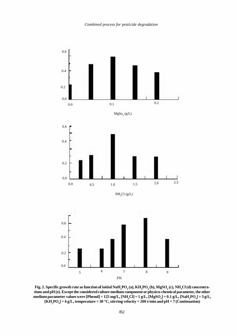
852
MgSo4 (g/L)
NH4Cl (g/L)
PH
0.6
0.4
0.2
0.00.1 0.20.0
0.6
0.4
0.2
0.0
0.5 1.00.0 1.5 2.0 2.5
0.6
0.4
0.2
0.0
5 6 7 8 9
Fig. 2. Specific growth rate as function of initial NaH2PO4 (a), KH2PO4 (b), MgSO4 (c), NH4Cl (d) concentra-tions and pH (e). Except the considered culture medium component or physico-chemical parameter, the othermedium parameter values were [Phenol] = 125 mg/L, [NH4Cl] = 1 g/L, [MgSO4] = 0.1 g/L, [NaH2PO4] = 3 g/L,
[KH2PO4] = 4 g/L, temperature = 30 °C, stirring velocity = 200 r/min and pH = 7 (Continuation)
Combined process for pesticide degradation
Int. J. Environ. Res., 4(4):849-854, Autumn 2010
853
mum value of 0.58 h-1 when MgSO4 for 0.1 g/L MgSO4,in agreement with Zhao et al. (2009) during their stud-ies on phenol biodegradation.
Fig.2d shows that the optimal value of specificgrowth rate was 0.58 h-1, recorded for 1 g/L NH4Clsupplementation. The effect of pH on µmax shows anoptimum (0.65 h-1) for pH 8 (Fig.2e). Other workers inthe field obtained the same optimal pH during phenoland p-nitrophenol degradation (Wang et al., 2007; Hoet al., 2009; Qiu et al., 2009).The optimal values of spe-cific growth rate are in the same order of magnitudethan the values reported by other authors for mixedcultures, namely in the range 0.13 to 0.6 h-1 (Pawlowsky& Howell, 1973; Hill & Robinson, 1975; Yang &Humphrey, 1975; D’Adamo et al., 1984; Rozich &Colvin, 1986; Sokol, 1987; Allsop et al., 1993; Goswamiet al., 2005).
CONCLUSIONGrowth kinetics of the used microbial consortium
and its potential for phenol assimilation were investi-gated leading to high biodegradation activity of theconsidered mixed culture, with an optimal maximumspecific growth rate of 0.65 h-1 for a total phenol bio-degradation time of 24.2 h. Irrespective of the cultureconditions, total phenol biodegradation (125 mg/L) wasachieved during times ranging from 20.6 to 33.2 h. Theoptimal mineral medium concentrations (g/L) were 1, 4,3 and 0.1 for NH4Cl, KH2PO4, NaH2PO4 and MgSO4respectively, and the optimal pH value were 8.
REFERENCESAbduli, M. A., Nabi Bidhendi, G. R., Nasrabadi, T. andHoveidi, H. (2007).Evaluating the Reduction of HazardousWaste Contact in Tabriz Petrochemical Complex, Focusingon Personal Protective Equipment Method. Int. J. Environ.Res., 1(1), 14-18.
D’Adamo, P. D., Rozich, A. F. and Gaudy, A. F. Jr. (1984).Analysis of growth data with inhibitory carbon sources.Biotechnol. Bioeng., 26 (4), 397-402.
Allsop, P. J., Chisti, Y., Moo-Young, M. and Sullivan, G. R.(1993). Dynamic of phenol degradation by Pseudomonasputida. Biotechnol. Bioeng., 41(5), 572-580.
Berkowitz, J. B. (1988). Standard Handbook of HazardousWater Treatment and Disposal – Hazardous waste recoveryprocesses. (New York: McGraw – Hill).
Chiam, H. F. and Harris, I. J . (1982). A model fornoninhibitory microbial growth. Biotechnol. Bioeng., 24 (1),37-55.
Dabhade, M. A., Saidutta, M.B. and Murthy, D.V.R. (2009).Adsorption of Phenol on Granular Activated Carbon from
Nutrient Medium:Equilibrium and kinetic Study. Int. J.Environ. Res., 3(4), 545-556.Dagley, S. and Gibson, D. T. (1965). The bacterial degrada-tion of catechol. Biochem. J., 95 (2), 466-474.
Goswami, M., Shivaraman, N. and Singh, R. P. (2005). Mi-crobial metabolism of 2-chlorophenol, phenol and p-cresolby Rhodococcus erythropolis M1 in co-culture withPseudomonas fluorecens P1. Microbiol. Res., 100, 101-109.
Gupta, V. K., Sharma, S., Yadav, I. S. and Mohan, D. (1998).Utilization of Bagasse Fly Ash Generated in the Sugar In-dustry for the Removal and Recovery of Phenol and p-Nitrophenol from Wastewater. J. Chem. Technol. Biotechnol,71 (2), 180-186.
Gurujeyalakshmi, G. and Oriel, P. (1989). Isolation of phe-nol degrading Bacillus stearothermophilus and partialcharacterisation of the phenol hydroxylase. Appl. Environ.Microbiol., 55 (2), 500-502.
Haritash, A. K. and Kaushik, C. P. (2009). Biodegradationaspects of Polycyclic Aromatic Hydrocarbons (PAHs): Areview. J. Hazard. Mater., 169 (1-3), 1-15.
Hassani, A. H., Otadi, N., Javid, A.H., Khiabani, F.F. andHoshyaripour, G. (2009). Improving the performance ofPars Oil Refinery Wastewater Treatment System. Int. J.Environ. Res., 3(4), 653-662.
Hill, G. A. and Robinson, C. W. (1975). Substrate inhibitionkinetics: phenol degradation by Pseudomonas putida.Biotechnol. Bioeng., 17 (11), 1599-1615.
Ho, K.-L. Lin, B., Chen, Y.-Y. and Lee, D.-J. (2009). Bio-degradation of phenol using Corynebacterium sp. DJ1 aero-bic granules. Bioresour. Technol., 100 (21), 5051-5055.
Luo, H., Liu, G., Zhang, R. and Jin, S. (2009). Phenol degra-dation in microbial fuel cells. Chem. Eng. J., 147 (2-3), 259-264.
Margesin, R., Fonteyne, P. A. and Redl, B. (2005). Low-temperature biodegradation of high amounts of phenol byRhodococcus spp and basidiomycetous yeasts. Res.Microbiol., v.156, No.1, pp.68-75.
Nakano, Y., Nishijima, W., Soto, E. and Okada, M. (1999).Relationship between growth rate of phenol utilizing bacte-ria and the toxic effect of metabolic intermediates of trichlo-roethylene (TCE). Water Res., 33 (4), 1085-1089.
Nemerow, N. L. (1978). Industrial Water Pollution, Origin,Characteristics and Treatment. (London: Addison-Wesley).
Onwurah, I. N. E.; Ogugua, V. N.; Onyike, N. B.; Ochonogor,A. E. & Otitoju, O. F. (2007).Crude Oil Spills in the Envi-ronment, Effects and Some Innovative Clean-up Biotech-nologies. Int. J. Environ. Res., 1(4), 307-320.

854
Patterson, J. W. (1985). Industrial Wastewater TreatmentTechnology. 2nd Edition. (New York: Butterworths).
Pawlowsky, U. and Howell, J. A. (1973). Mixed culturebiooxidation of phenol, Determination of kinetic parameters.Biotechnol. Bioeng., 15 (5), 889-896.
Qiu, X., Wu, P., Zhang, H., Li, M. and Yan, Z. (2009).Isolation and characterization of Arthrobacter sp. HY2 ca-pable of degrading a high concentration of p-nitrophenol.Bioresour. Technol., 100 (21), 5243-5248.
Rozich, A. F. and Colvin, R. J. (1986). Effects of glucose onphenol biodegradation by heterogeneous populations.Biotechnol Bioeng, 28 (7), 965-971.
Sa, C. S. A. and Boaventura, R. A. R. (2001). Biodegrada-tion of phenol by Pseudomonas putida DSM 548 in a trick-ling bed reactor. Biochem. Eng. J., 9 (3), 211-219.
Shawabkeh, R., Khleifat, K., Al-Majali, I. and Tarawneh, K.(2007). Rate of biodegradation pf phenol by Klebsiellaoxytoca in minimal medium and nutrient broth conditions.Bioremed. J., 11 (1), 13-19.
Sittig, M. (1997). How to Remove Pollutants and ToxicMaterials from Air and Water, A Pratical Guide. (Park Ridge,NJ: Noyes Data Corporation).
Sokol, W. (1987). Oxidation of an inhibitory substrate bywashed cells (oxidation of phenol by Pseudomonas putida).Biotechnol. Bioeng., 30 (8), 921-927.
Stanier, R. Y., Palleroni, N. J. and Doudoroff, M. (1966).The aerobic Pseudomonas taxonomic study. J . Gen.Microbiol., 43, 159-275.
dos Santos, V. L., de Souza Monteiro, A., Braga, D. T. andSantoro, M. M. (2009). Phenol degradation byAureobasidium pullulans FE13 isolated from industrial ef-fluents. J. Hazard. Mater., 161 (2-3), 1413-1420.
Wang, Y., Tian, Y., Han B., Zhao, H.-B., Bi, J.-N., Cai, B.-L.(2007). Biodegradation of phenol by free and immbilizedAcinetobacter sp. strain PD12. J. Environ. Sci., 19 (2), 222-225.
Worden, R. M. and Donaldson, T. L. (1987). Dynamics of abiological fixed film for phenol degradation in a fluidized-bed bioreactor. Biotechnol. Bioeng., 30 (3), 398-412.
Yang, P. D. and Humphrey, A. E. (1975). Dynamic andsteady state studies of phenol biodegradation in pure andmixed cultures. Biotechnol. Bioeng., 17 (8), 1211-1235.
Zhao, G., Zhou, L., Li, Y., Liu, X. ,Ren, X. and Liu, X.(2009). Enhancement of phenol degradation using immobi-lized microorganisms and organic modified montmorillonitein a two-phase partitioning bioreactor. J. Hazard. Mater.,16(1-3), 402-410.
Zilouei, H., Guieysse, B. and Mattiasson, B. (2006). Bio-logical degradation of chlorophenols in packed-bedbioreactors using mixed bacterial consortia. Process Biochem.41 (5), 1083-1089.
Hamitouche, A. et al.
Int. J. Environ. Res., 4(4):855-860 , Autumn 2010ISSN: 1735-6865
Received 3 June 2009; Revised 2 July 2010; Accepted 12 July 2010
*Corresponding author E-mail: [email protected]
855
Adsorption and Stabilization of Phenol by Modified Local Clay
Belarbi, H.1 and Al-Malack, M. H.2*
1Laboratoire Synthèse et Catalyse, Ibn Khaldoun University, Tiaret, Algeria2King Fahd University of Petroleum & Minerals, Box 1150, Dhahran 31261, Saudi Arabia
ABSTRACT: Phenol is a common pollutant that was listed by US Environmental Protection Agency (EPA)among the priority pollutants. Classical methods employed for phenol removal are either costly or limited tolarge-scale applications such as biological and thermal decomposition methods. In this study, adsorption ofphenol by a type of clay that is extracted from a local soil called Khoweldi was investigated. The X-Raydiffraction revealed that the studied clay is mainly muscovite. The study showed that the local clay could beused as matrix for long-term storage of organic pollutants. Phenol adsorption isotherms conducted on naturaland modified clay with Hexadecyltrimethylammonium (HDTMA) revealed that HDTMA enhanced theadsorption capacity of the clay for phenol.To prevent the migration of the adsorbed pollutants into theenvironment, encapsulation of the modified clay by organosilane was found to be very effective.
Key words: Phenol, Adsorption, Clay, Encapsulation, Solidification, Stabilization
INTRODUCTIONClay minerals are effective in adsorbing both organic
and inorganic pollutants. This is due to their largespecific surface area and high ion exchange capacity.Understanding of the interaction between pollutantsand the surface of the clay is essential for environmentalsolution design. The recent studies which wereconcerned with the development of new proceduresfor the immobilization of pollutants in aqueous mediaand soil showed that modified clays exhibit high affinityfor a specific class of pollutants (Srinivasan et al., 1989;Jaynes and Boyd, 1991; Wibulswas et al., 1999; Shen,2002;). Abuzaid et al., 2000 reported that the Khoweldisoil, which can be found in the city of Qatif, EasternProvince of Saudi Arabia, showed to have good sorptioncapabilities for phenol. Accordingly, an economic linerdesigns can be achieved by using this soil, particularly,when modified using hexadecytimethylammonium(HDTMA) to enhance its sorptive capacity forpollutants. The sorptive capacity of Khoweldi soil isexpected to be improved if the clay proportion isincreased by separating quartz (Abuzaid et al., 1989).
Phenols are considered as priority pollutants byUS EPA and European Union (EU). They can be foundin aquatic environments as biodegradation productsof humic substances, lignins and tannins or asderivatives of plastics, dye industries and pulpprocessing (Bruzzoniti et al., 2000). Their adsorption
by clays and soils has been studied extensively.Lawrence et al. (1998) studied the sorption of phenoland 2-,3- and 4-chlorophenol from water bytetramethylammonium (TMA)-clay andtetramethylphosphonium (TMP)-clay. They showedthat the (TMP)-clay was better sorbent than the(TMA)-clay. Furthermore, the TMP clay was selectivewithin the chlorinated phenols studied, where phenoland 4-chlorophenol were effectively sorbed, while 2-and 3-chlorophenol were not sorbed. Irene (1996)showed that the use of quaternary ammonium modifiedclays as presolidification adsorbent produced asuccessful solidification and stabilization process inthe treatment of soils contaminated with phenol. Shen(2002) reported that, under appropriate conditions, aremoval of more than 90 per cent of phenol from watercould be achieved by the use of dispersed bentoniteto the phenol contaminated water followed by theaddition of benzyltrimethylammonium bromide(BTMA) ions as a flocculant. The use of clay in phenoladsorption was also investigated by Wang and Lin(2003), Arellano-Cárdenas et al. (2005), Richards andBouazza (2007), Roperts et al. (2007), Boufatita et al.(2007) and Froehner et al. (2009.
Song et al. (2001) reported that encapsulation ofmontmorillonite with organosilanes resulted in ahydrophobic coating that acts like a “cage” aroundthe clay particles to limit diffusion of organic speciespreviously adsorbed. The molecules of organosilanes
856
Belarbi, H. and Al-Malack, M. H.
are probably adsorbed to the outer surfaces and boundto the edges of the clay via condensation with edge-OH groups. The carbon and oxygen K-edge NEXAFSspectroscopy of the modified montmorillonite surfacesspectroscopy of the modified montmorillonite surfacesshowed that surface coatings on the outside of theclay particles exist. This method was applied byWasserman et al. (1998) to isolate hazardous metalliccations and to reduce their leach ability from storagemedia and from substrates containing toxic cations.There are many other ways to remove phenol fromenvironment that will not be discussed in the presentwork (Dabhade et al., 2009; Agarry and Solomon, 2008;Samarghandi, et al., 2007).
Based on the above discussion, the main objectivesof this study are to investigate the adsorptive capacity,for phenol, of the local clay after being separated fromthe local soil called Khoweldi and to study the effectof encapsulation of the clay with organosilane on themigration of pollutants to the environment, after beingexposed to vigorous shaking.
MATERIALS & METHODSIn order to separate the clay part, 20 g of the
Khoweldi soil was dispersed for one hour by stirringin 1 liter of distilled water at pH 9. The obtainedsuspension was then left to settle for 24 hours. Theupper part of the liquid was filtrated with Whatmanno. 42 filter paper and the residue was dried in theoven at 105 °C and then grinded to fine powder. Themodification process consists of altering the surfacepolarity of the clay minerals via treatment with cationicsurfactants such as hexadecyltrimethylammoniumbromide (HDTMA)( Jaynes and Boyd, 1991; andWibulswas et al., 1999). Modified clay was preparedbased on the cationic exchange capacity (CEC), whichwas measured as 60 meq/100 g. Fourteen (14) grams ofthe separated clay were mixed with 4.6 grams ofHDTMA in 280 mL distilled water and were shacked at270 rpm for one day. The mixture was then filtered usingWhatman no. 44 filter paper. The residue was dried inan oven at 105° C and was then grinded.
X-Ray diffraction (Cu-Ka) was performed usingJEOL JDX 3530 X-Ray diffractometer. The sample wasin powder form and its diffraction was compared withthe standard diffraction pattern for different phasesestablished by the International Center for DiffractionData. The result showed that the separated clay wasmainly muscovite with less than 1per cent quartzimpurity. A small amount of the sample was spread onadhesive conductive aluminum tape attached to asample holder and examined with the scanning electronmicroscope JEOL 5800LV. The analysis was performedat a resolution of 40 Å, depth of penetration of electron
beam of 5 Å and detection limit of 0.2 per cent. EnergyDispersive Spectrometry (EDS) analysis was performedat different spots and the percentages of the elementspresent were semi-quantitatively determined andcorrected.
An amount of separated clay varying between 200and 1000 grams was added to 25 mL of phenol solutionhaving a concentration of 25 to 100 mg/L. The batchequilibration technique was used to determine theadsorption isotherms of phenol on modified and naturalclay samples. All samples were sealed in Erlenmeyerconical flasks (50 mL) and oscillated at 165 rpm at roomtemperature for a period of 42h. Phase separation wasthen performed using centrifugation and filtrationprocesses and separated samples were stored at 4 °Cfor further treatment before GC analysis. The adsorbedquantities of phenol were determined according to thebalance equation 1
( )m
CeCVq −= 0 (1)
Where q is the sorbed phenol concentration (mg/g), V is the volume of phenol solution (L), m is themass of adsorber (g) and C0 and Ce are initial andequilibrium phenol concentration (mg/L), respectively.The solid part that represents the polluted clay wasdried at 105°C and reserved for further investigation(encapsulation with organosilane). The stabilizationof pollutants is considered as an essential step in orderto prevent their migration from clay as a result ofleaching, evaporation or hydration. In the currentinvestigation, contaminated clay was dried andencapsulated by organosilane. The clay was thentreated by butyltrichlorosilane to make it hydrophobic.Samples of polluted clay with different amounts ofadsorbed phenol were well mixed together and thengrinded to obtain homogeneous polluted media withan average concentration of phenol of 1.63 and 1.5 mg/g in modified and natural clay samples, respectively.The encapsulation of the polluted clay was obtainedby reacting the clay with organosilane in methylenechloride solvent. The reaction was performed at aweight ratio of 1:1:30 for polluted clay: silane: solventin a closed system for 2-3 days. After that, theencapsulated clay samples were rinsed with a solventseveral times in order to remove free silanes, and thenair dried. Samples of 0.3g of modified and natural claywere dispersed in water at different environmentalstresses. Both encapsulated and non-encapsulatedsamples were dispersed for 42 hours in aqueoussolution with pH values of 3,5,7,9 and 11 to simulateextreme environmental conditions. After phaseseparation by centrifugation and filtration, the
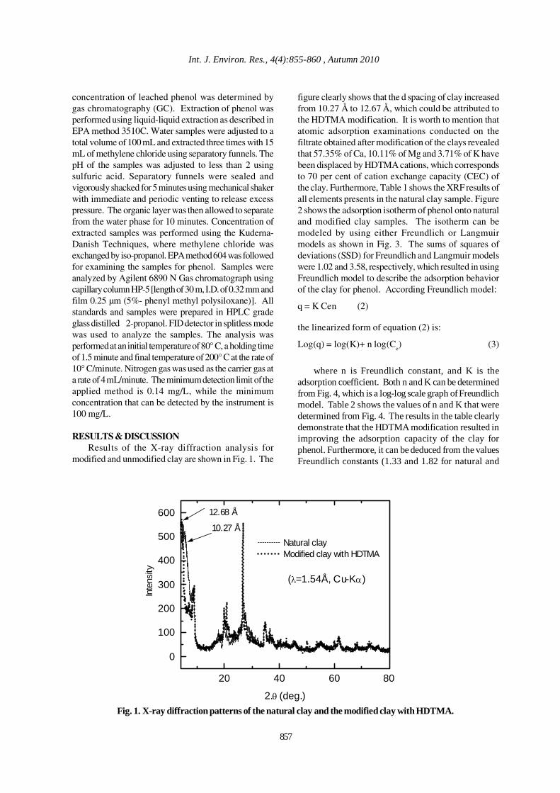
Int. J. Environ. Res., 4(4):855-860 , Autumn 2010
857
concentration of leached phenol was determined bygas chromatography (GC). Extraction of phenol wasperformed using liquid-liquid extraction as described inEPA method 3510C. Water samples were adjusted to atotal volume of 100 mL and extracted three times with 15mL of methylene chloride using separatory funnels. ThepH of the samples was adjusted to less than 2 usingsulfuric acid. Separatory funnels were sealed andvigorously shacked for 5 minutes using mechanical shakerwith immediate and periodic venting to release excesspressure. The organic layer was then allowed to separatefrom the water phase for 10 minutes. Concentration ofextracted samples was performed using the Kuderna-Danish Techniques, where methylene chloride wasexchanged by iso-propanol. EPA method 604 was followedfor examining the samples for phenol. Samples wereanalyzed by Agilent 6890 N Gas chromatograph usingcapillary column HP-5 [length of 30 m, I.D. of 0.32 mm andfilm 0.25 µm (5%- phenyl methyl polysiloxane)]. Allstandards and samples were prepared in HPLC gradeglass distilled 2-propanol. FID detector in splitless modewas used to analyze the samples. The analysis wasperformed at an initial temperature of 80° C, a holding timeof 1.5 minute and final temperature of 200° C at the rate of10° C/minute. Nitrogen gas was used as the carrier gas ata rate of 4 mL/minute. The minimum detection limit of theapplied method is 0.14 mg/L, while the minimumconcentration that can be detected by the instrument is100 mg/L.
RESULTS & DISCUSSIONResults of the X-ray diffraction analysis for
modified and unmodified clay are shown in Fig. 1. The
figure clearly shows that the d spacing of clay increasedfrom 10.27 Å to 12.67 Å, which could be attributed tothe HDTMA modification. It is worth to mention thatatomic adsorption examinations conducted on thefiltrate obtained after modification of the clays revealedthat 57.35% of Ca, 10.11% of Mg and 3.71% of K havebeen displaced by HDTMA cations, which correspondsto 70 per cent of cation exchange capacity (CEC) ofthe clay. Furthermore, Table 1 shows the XRF results ofall elements presents in the natural clay sample. Figure2 shows the adsorption isotherm of phenol onto naturaland modified clay samples. The isotherm can bemodeled by using either Freundlich or Langmuirmodels as shown in Fig. 3. The sums of squares ofdeviations (SSD) for Freundlich and Langmuir modelswere 1.02 and 3.58, respectively, which resulted in usingFreundlich model to describe the adsorption behaviorof the clay for phenol. According Freundlich model:
q = K Cen (2)
the linearized form of equation (2) is:
Log(q) = log(K)+ n log(Ce) (3)
where n is Freundlich constant, and K is theadsorption coefficient. Both n and K can be determinedfrom Fig. 4, which is a log-log scale graph of Freundlichmodel. Table 2 shows the values of n and K that weredetermined from Fig. 4. The results in the table clearlydemonstrate that the HDTMA modification resulted inimproving the adsorption capacity of the clay forphenol. Furthermore, it can be deduced from the valuesFreundlich constants (1.33 and 1.82 for natural and
20 40 60 80
0
100
200
300
400
500
600
(λ=1.54Å, Cu-Kα)
10.27 Å
12.68 Å
Natural clay Modified clay with HDTMA
Inte
nsity
2.θ (deg.)Fig. 1. X-ray diffraction patterns of the natural clay and the modified clay with HDTMA.
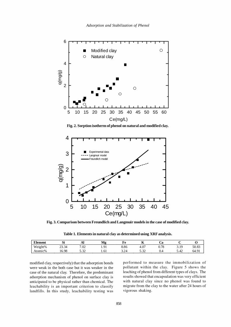
858
Adsorption and Stabilization of Phenol
5 10 15 20 25 30 35 40 45 50 55 600
2
4
6
Modified clay Natural clay
q(m
g/g)
Ce(mg/L)Fig. 2. Sorption isotherm of phenol on natural and modified clay.
5 10 15 20 25 30 35 40 450
1
2
3
4
Ce(mg/L)
Experimental data Langmuir model Freundlich model
q(m
g/g)
Fig. 3. Comparison between Freundlich and Langmuir models in the case of modified clay.
Table 1. Elements in natural clay as determined using XRF analysis.
Element Si Al Mg Fe K Ca C O Weight% 23.34 7.02 1.91 8.86 4.07 0.78 3.19 50.83 Atomic% 16.98 5.32 1.61 3.24 5.32 0.4 5.42 64.91
modified clay, respectively) that the adsorption bondswere weak in the both case but it was weaker in thecase of the natural clay. Therefore, the predominantadsorption mechanism of phenol on surface clay isanticipated to be physical rather than chemical. Theleachability is an important criterion to classifylandfills. In this study, leachability testing was
performed to measure the immobilization ofpollutant within the clay. Figure 5 shows theleaching of phenol from different types of clays. Theresults showed that encapsulation was very efficientwith natural clay since no phenol was found tomigrate from the clay to the water after 24 hours ofvigorous shaking.

Int. J. Environ. Res., 4(4):855-860 , Autumn 2010
0.8 1.0 1.2 1.4 1.6 1.8 2.0
-0.6
-0.4
-0.2
0.0
0.2
0.4
0.6
0.8 Modified clay Natural clay
log(
q(m
g/g)
)
log(Ce(mg/L))Fig. 4. Log(q) vs. log(Ce) adsorbing phenol by natural and modified clay.
0.0
0.2
0.4
0.6
0.8
1.0
Tota
l ads
orbe
d ph
enol
deso
rbed
phen
ol by
Non
enc
apsu
lated
poll
uted
clay
deso
rbed
phe
nol b
y en
caps
ulated
poll
uted
clay
phen
ol (m
g/g)
Fig. 5. The leachability data for phenol in encapsulated and non-encapsulated clay.
Table 2. Gas Chromatography conditions
Total flow 97.5 mL/min Head column pressure 117.41 kPa Injector temperature 280°C Oven program 80°C (1.5 min)+ 10°C/min, 200°C (1 min)
Table 3: Freundlich isotherm constant for the adsorption of phenol onto both clays.
Type of clay Freundlich Constant (n)
Adsorption Coefficient (K)
Correlation Coefficient (R2)
Natural Clay 1.82 2.28 10-3 0.97 Modified clay with HDTMA 1.33 0.024 0.97
859
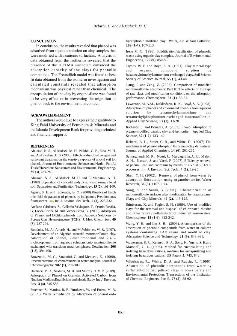
860
Belarbi, H. and Al-Malack, M. H.
CONCLUSIONIn conclusion, the results revealed that phenol was
adsorbed from aqueous solution on clay samples thatwere modified with a cationic surfactant. Analysis ofdata obtained from the isotherms revealed that thepresence of the HDTMA surfactant enhanced theadsorption capacity of the clays for phenoliccompounds. The Freundlich model was found to bestfit data obtained from the isotherm investigation andcalculated constatnts revealed that adsorptionmechanism was physical rather than chemical. Theencapsulation of the clay by organosilane was foundto be very effective in preventing the migration ofphenol back to the environment in contact.
ACKNOWLEDGEMENTThe authors would like to express their gratitude to
King Fahd University of Petroleum & Minerals andthe Islamic Development Bank for providing technicaland financial supports.
REFERENCESAbuzaid, N. S., Al-Malack, M. H., Nakhla, G. F., Essa, M. H.and Al-Tawabini, B. S. (2000). Effects of dissolved oxygen andsurfactant treatment on the sorptive capacity of a local soil forphenol. Journal of Environmental Science and Health, Part A:Toxic/Hazardous Substances and Environmental Engineering,35 (3), 263-280.
Abuzaid, N. S., Al-Malack, M. H. and El-Mubarak, A. H.(1989). Separation of colloidal polymeric waste using a localsoil. Separation and Purification Technology, 13 (2), 161-169.
Agarry, S. E. and Solomon, B. O. (2008).Kinetics of batchmicrobial degradation of phenols by indigenous Pseudomonasfluorescence . Int. J. Environ. Sci. Tech., 5 (2), 223-232.
Arellano-Cárdenas, S., Gallardo-Velázquez, T., Osorio-Revilla,G., López-Cortéz, M. and Gómez-Perea, B. (2005). Adsorptionof Phenol and Dichlorophenols from Aqueous Solutions byPorous Clay Heterostructure (PCH). J. Mex. Chem. Soc., 49(3), 287-291.
Boufatita, M., Ait-Amarb, H., and McWhinniec, W. R. (2007).Development of an Algerian material montmorillonite clay.Adsorption of phenol, 2-dichlorophenol and 2,4,6-trichlorophenol from aqueous solutions onto montmorilloniteexchanged with transition metal complexes. Desalination, 206(1-3), 394-406.
Bruzzoniti, M. C., Sarzanini, C. and Mentasti, E. (2000).Preconcentration of contaminants in water analysis. Journal ofChromatography, 902 (1), 289-309.
Dabhade, M. A., Saidutta, M. B. and Murthy, D. V. R. (2009).Adsorption of Phenol on Granular Activated Carbon fromNutrient Medium:Equilibrium and kinetic Study. Int. J. Environ.Res., 3 (4), 545-556.
Froehner, S., Martins, R. F., Furukawa, W. and Errera, M. R.(2009). Water remediation by adsorption of phenol onto
hydrophobic modified clay. Water, Air, & Soil Pollution,199 (1-4), 107-113.
Irene M. C. (1996). Solidification/stabilization of phenolicwaste using organic-clay complex. Journal of EnvironmentalEngineering, 122 (9), 850-855.
Jaynes, W. F. and Boyd, S. A. (1991). Clay mineral typeand organic compound sorption byhexadecyltrimethylammonium-exchanged clays. Soil ScienceSociety of America Journal, 55 (1), 43-48.
Jiang, J. and Zeng, Z. (2003). Comparison of modifiedmontmorillonite adsorbents: Part II: The effects of the typeof raw clays and modification conditions on the adsorptionperformance. Chemosphere, 53 (1), 53-62.
Lawrence, M. A.M., Kukkadapu, R. K., Boyd, S. A. (1998).Adsorption of phenol and chlorinated phenols from aqueoussolution by tetramethylammonium- andtetramethylphosphonium-exchanged montmorillonite.Applied Clay Science, 13 (1), 13-20.
Richards, S. and Bouazza, A. (2007). Phenol adsorption inorgano-modified basaltic clay and bentonite. Applied ClayScience, 37 (1-2), 133-142.
Roberts, A. L., Street, G. B., and White, D. (2007) Themechanism of phenol adsorption by organo-clay derivatives.Journal of Applied Chemistry, 14 (6), 261-265.
Samarghandi, M. R., Nouri, J., Mesdaghinia, A. R., Mahvi,A. H., Nasseri, S. and Vaezi, F. (2007). Efficiency removalof phenol, lead and cadmium by means of UV/TiO2/H2O2processes. Int. J. Environ. Sci. Tech., 4 (1), 19-25.
Shen, Y. H. (2002). Removal of phenol from water byadsorption-flocculation using organobentonite. WaterResearch, 36 (5), 1107-1114.
Song, K. and Sandi, G. (2001). Characterization ofmontmorillonite surfaces after modification by organosilane.Clays and Clay Minerals, 49 (2), 119-125.
Srinivasan, K. and Fogler, S. H. (1989). Use of modifiedclays for the removal and disposal of chlorinated dioxinsand other priority pollutants from industrial wastewaters.Chemosphere, 18 (1-6), 333-342.
Wang, Y. H. and Lin S. H. (2003). A comparison of theadsorption of phenolic compounds from water in columnsystems containing XAD resins and modified clay.Adsorption Science and Technology, 21 (9), 849-861.
Wasserman, S. R., Kenneth, B. A., Song, K., Yuchs, S. E.andMarshall, C. L. (1998). Method for encapsulating andisolating hazardous cations, medium for encapsulating andisolating hazardous cations. US Patent 5, 743, 842.
Wibulswas, R., White, D. A. and Rautiu, R. (1999).Adsorption of phenolic compounds from water bysurfactant-modified pillared clays. Process Safety andEnvironmental Protection: Transactions of the Institutionof Chemical Engineers, Part B, 77 (2), 88-92.
Int. J. Environ. Res., 4(4):861-876, Autumn 2010ISSN: 1735-6865
Received 10 June 2009; Revised 15 April 2010; Accepted 15 June 2010
*Corresponding author E-mail: [email protected]
861
Geochemistry of Core Sediments from Gulf of Mannar, India
Sundararajan, M.1* and Srinivasalu, S. 2
1 National Institute for Interdisciplinary science and Technology, Council of Scientific andIndustrial Research, Thiruvananthapuram – 695019, India
2 Department of Geology, Anna University, Chennai-600 025, India
ABSTRACT: The Gulf of Mannar, located between India and Sri Lanka, is a shallow embayment of the Bayof Bengal. The gulf, which has been declared a bio-reserve is a highly productive area endowed with rich marinefauna including corals. In order to study the origin and nature of the sediments and paleo-environment, 2.6 mlength core was collected with 5cm interval at 1320m water depths. Textural studies indicate that the sedimentshave been poorly sorted and most of the sub samples are silty clay and few top samples are sandy silty clay.The nature of organic matter also indicate high sedimentation rate. Based on the behaviors of CaCO3, Organicmatter (OM) and textural parameters the core was studied under the three units. The first unit representssurface to 65cm (unit-1), the second unit (unit-2) represents 65cm to 165cm and third unit represents 165 cmto the bottom of the core. The major oxide geochemistry shows higher concentration of detritus constituents.The trace element studies indicate ferruginous nature for all elements except Cu and Zn. The element/Al ratiosalso are computed. The geochemical analysis for trace elements like Mn, Cr, Cu, Ni, Co, Pb, and Zn has beencarried out for core sediments. Normalization with Al values for all the trace elements have been calculated.
Key words: Sediment texture, Calcium carbonate, organic matter, Major elements, Trace metals
INTRODUCTIONThe Bay of Bengal has attracted a fair share of
attention with regard to its sedimentation geology,notably the origin and history of the Bengal sediments(Stewart et al., 1965). Geochemical investigations ofthis vast expanse are, however, limited, and confinedto the deep (Ramesh and Ramasamy 1997). Thecontinental shelf off the east coast (Rao, 1978; Paropkari,1990) Visakhapatnam (Gogate et al., 1970; Rajamanickamand Setty, 1973), river Godavari (Rao and Rao, 1975)also has been studied. According to Pragatheeswaranet al. (1986), the sediments off Chennai are morecontaminated in heavy metals and organic carbon thanVisakhapatnam shelf sediments. The enhanced levelsof Cu, Hg and organic carbon were attributed to inputfrom industrial sources including organo-mercurial paintindustry and oil refineries. Ramanathan et al. (1988)analyzed major and minor element geochemistry of waterand suspended and bed sediments collected from theupper reaches of the Cauvery estuary to understandthe geochemical processes in tropical estuarinesystems. The investigation of the characteristics of thesediments from a core collected from the Gulf of Mannarrevealed high concentration of CaCO
3 (61.4%) and low
organic carbon values, distinctly different from theanoxic sediments of Bombay (Ray et al., 1990).Palanichamy et al. (1995) inferred that industrialeffluents pollute the waters of Arumuganeri region,Gulf of Mannar; they also recorded higher suspendedsolids due to discharge of effluents from the chlor-alkaline industries and land drainage. Vanmathi (1995),in her study of sediments of Tuticorin coast,concluded that heavy metals, especially cadmium, aresignificantly higher than in other coastal regions,affecting the biota in the region. Selvaraj et al. (2004),in his study on the Kalpakkam coastal waters andsediments, recorded high concentrations of Fe, Cu,Hg and Pb; he attributed the enriched levels of Pb,Cu, Cr, Cd and Zn in sediments to mainly anthropogenicinput along the coast and the river Palar.
Geochemical studies of surficial sediment as wellas sediment cores are helpful in the assessment ofpollution (Holm, 1988; Ahmad et al., 2010, Al-Juboury,2009; Chibunda, 2009; Chibunda et al., 2010; Geetha etal., 2008), changes in climatic conditions (Faganelli, etal., 1987; Karbassi and Amirnezhad, 2004; Karbassiand Shankar 2005) accumulation or mobilization oftrace elements in the sediments of aquatic environment(Al-Masri, 2002).Sediments act as sinks and sources
862
Sundararajan, M. and Srinivasalu, S.
of contaminants in aquatic systems because of theirvariable physical and chemical properties (Rainey, etal., 2003; Marchand, et al., 2006; Pekey, 2006; Prijiuand Narayan, 2007; Praveena, et al., 2008;Sundararajan, et al., 2009; Sundararajan, and UshaNatesan, 2010).During their transport, the trace metalsundergo numerous changes in their speciation due todissolution, precipitation, sorption and complexationphenomena (Akcay et al., 2003; Abdel-Ghani et al.,2007; Abdel- Ghani and Elchaghaby, 2007; Praveena,et al., 2008; Harikumar et al., 2009; Mohiuddin et al.,2010) which affect their behaviour and bioavailability.The review of geochemical research carried out so faron and off the east coast reveals that considerableamount of work still remains to be done with regard togeochemistry and metal pollution in sediments. It iswell understood that very few studies have been carriedout on these aspects, especially in the Gulf of Mannar.
MATERIALS & METHODSSediment core for the present study was collected
from Tuticorin offshore, (Lat. 8o19’06" and Long.78038’57" at a depth of 1320m Gulf of Mannar (Fig.1).The Gulf of Mannar is a transitional zone between theArabian Sea and Indian Ocean proper and is connectedwith the Bay of Bengal through a shallow sill, the PalkStrait. The area under investigation off Tuticorin in theGulf of Mannar presents great interest because it is anindustrial belt consisting of many major industriesinvolved in the production of chemicals, petrochemicalsand plastics. In addition, a major harbor, thermal powerplant, heavy water plant and human activities fromaround Tuticorin to Tiruchendur have altered the eco-system prominently. The area investigated forms thesouthern part of the South Indian Granulite facies terrain,which includes part of Madurai Block (MB) and theKerala Khondalite Belt (KKB). The southern part of MBis represented by charnockites in the western part andgneisses in the eastern part which are inter-banded withsupra-crustal mainly of meta-sedimentary sequencesmade up of quartzite, carbonate and metapelite with aminor metabolic component. KKB is bounded by theCardamon Hills in the north and the NagerkoilCharnockite Massif in the south, which consists of high-grade supra-crustal. The MB and KKB, which areseparated by the Achankoil Shear Zone (AKSZ), aremostly similar in geochronology characteristics(Santhosh and others 1992; Harris and others 1994).Core sampling was done at one particular location duringDecember 2000 for the present study. This location wasselected as it is very close to the mouth of the riverwhich can decipher the influence of coastal region.Collection of core samples was done under ACADEMIK
ALENKSANDR SIDORENKO cruise program organized byNational Center for Antarctic Ocean Research, Dona
Paula, Goa. The sub-samples were sliced at 5 cm depthinterval resulting in 52 numbers of samples. The waterdepth at the coring site were 1320 m and the sub-sampleswere tightly packed, transported to the laboratoryand stored at -4º C until further analysis. Thegeochemical data in the present study have not beencorrected for compaction, as it is likely to be uniformdown the length of the core (Clark et al., 1998). Duringthe first stage of work, sand and mud (silt + clay) wereestimated following the procedure of Ingram (1970).Carbonate content (CaCO
3) was measured following the
procedure of Loring and Rantala (1992) and organiccarbon (OC) was determined following the procedure ofGaudette et al., (1974). Major elements (Si, Al, Fe, Ca,Mg, Na, K, and P) and trace elements (Mn, Cr, Cu, Ni,Co, Pb, and Zn) were determined after preliminarytreatment and total decomposition of sedimentsfollowing the procedure of Loring and Rantala (1992).The final solution was analyzed using AAS (VarianSpectra AA220) which is equipped with a detritumbackground corrector. Further standard referencematerial MESS1 was used to ensure the quality controland accuracy of the analysis (Table 1). Thegeochemical elements delivered to the creek are notonly from anthropogenic sources but also by naturalflux of elements from the catchment areas. One of thepopular methods to distinguish the fraction ofmetals or enrichment is by normalization with respectto Al (Kemp et al., 1976; Van Metre and Callender,1997; Loring, 1991). Moreover, Al is successfullyand widely used as a normalizer and it alsocompensates for variations in the grain size andcomposition because it represents the quality ofalumina silicates which is the most important carrierfor adsorbed metals in the aquatic environments. Thevariability of the normalized concentrations isexpressed as enrichment factors (EFs), which is aratio of the content of the element in the analyzedlayer to the content corresponding to the pre-industrial period: EF = (Cx/CAl)s/(Cx/CAl)c where,(Cx/CAl)s ratio of concentration of element x andaluminum in the sample, (Cx/CAl)c ratio ofconcentration of element x and aluminum inunpolluted sediments Continental crustal values(Taylor and McLennan, 1985). An EF around 1.0indicates that the sediment originates predominantlyfrom lithogenous material, whereas an EF muchgreater than 1.0 indicates that the element is ofanthropogenic origin (Szefer et al., 1996).
RESULTS & DISCUSSIONThe relative abundance in Sand, Silt and clay
content with sediment types inferred for the subsamples of core are presented in Fig. 2. The sandpercentage ranges from 4.33% to 19.08% except for the

Int. J. Environ. Res., 4(4): 861-876, Autumn 2010
863
Fig. 1. Study area
Sand
Sand
Clay sand
Sandy clay
Silty clay sand
Silty sand Sandy silt
Sandy clay silit
Sandy silt clay
Silty clay
Clay silt
Silt
Silt
Clay
Clay
Fig. 2. Trilinear diagram showing the sediment type
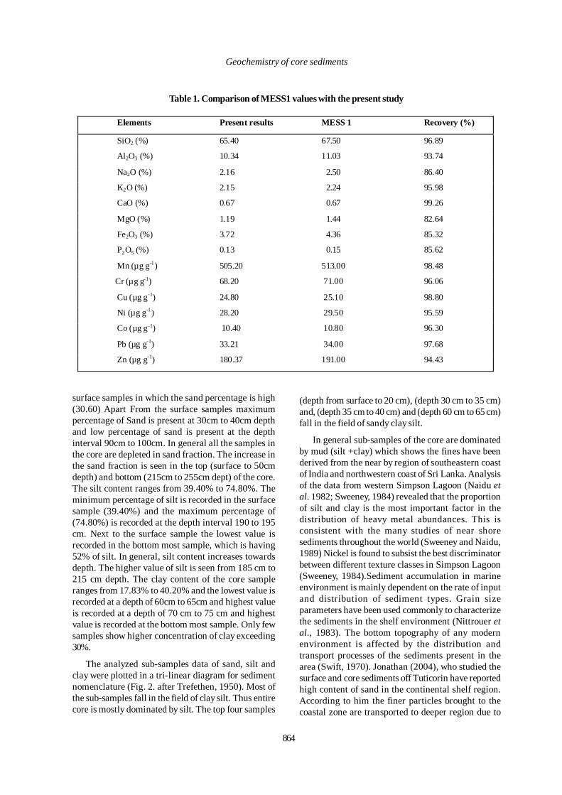
864
Geochemistry of core sediments
Table 1. Comparison of MESS1 values with the present study
Elements Present results MESS 1 Recovery (%)
SiO2 (%) 65.40 67.50 96.89
Al2O3 (%) 10.34 11.03 93.74
Na2O (%) 2.16 2.50 86.40
K2O (%) 2.15 2.24 95.98
CaO (%) 0.67 0.67 99.26
MgO (%) 1.19 1.44 82.64
Fe2O3 (%) 3.72 4.36 85.32
P2O5 (%) 0.13 0.15 85.62
Mn (µg g-1) 505.20 513.00 98.48
Cr (µg g-1) 68.20 71.00 96.06
Cu (µg g-1) 24.80 25.10 98.80
Ni (µg g-1) 28.20 29.50 95.59
Co (µg g-1) 10.40 10.80 96.30
Pb (µg g-1) 33.21 34.00 97.68
Zn (µg g-1) 180.37 191.00 94.43
surface samples in which the sand percentage is high(30.60) Apart From the surface samples maximumpercentage of Sand is present at 30cm to 40cm depthand low percentage of sand is present at the depthinterval 90cm to 100cm. In general all the samples inthe core are depleted in sand fraction. The increase inthe sand fraction is seen in the top (surface to 50cmdepth) and bottom (215cm to 255cm dept) of the core.The silt content ranges from 39.40% to 74.80%. Theminimum percentage of silt is recorded in the surfacesample (39.40%) and the maximum percentage of(74.80%) is recorded at the depth interval 190 to 195cm. Next to the surface sample the lowest value isrecorded in the bottom most sample, which is having52% of silt. In general, silt content increases towardsdepth. The higher value of silt is seen from 185 cm to215 cm depth. The clay content of the core sampleranges from 17.83% to 40.20% and the lowest value isrecorded at a depth of 60cm to 65cm and highest valueis recorded at a depth of 70 cm to 75 cm and highestvalue is recorded at the bottom most sample. Only fewsamples show higher concentration of clay exceeding30%.
The analyzed sub-samples data of sand, silt andclay were plotted in a tri-linear diagram for sedimentnomenclature (Fig. 2. after Trefethen, 1950). Most ofthe sub-samples fall in the field of clay silt. Thus entirecore is mostly dominated by silt. The top four samples
(depth from surface to 20 cm), (depth 30 cm to 35 cm)and, (depth 35 cm to 40 cm) and (depth 60 cm to 65 cm)fall in the field of sandy clay silt.
In general sub-samples of the core are dominatedby mud (silt +clay) which shows the fines have beenderived from the near by region of southeastern coastof India and northwestern coast of Sri Lanka. Analysisof the data from western Simpson Lagoon (Naidu etal. 1982; Sweeney, 1984) revealed that the proportionof silt and clay is the most important factor in thedistribution of heavy metal abundances. This isconsistent with the many studies of near shoresediments throughout the world (Sweeney and Naidu,1989) Nickel is found to subsist the best discriminatorbetween different texture classes in Simpson Lagoon(Sweeney, 1984).Sediment accumulation in marineenvironment is mainly dependent on the rate of inputand distribution of sediment types. Grain sizeparameters have been used commonly to characterizethe sediments in the shelf environment (Nittrouer etal., 1983). The bottom topography of any modernenvironment is affected by the distribution andtransport processes of the sediments present in thearea (Swift, 1970). Jonathan (2004), who studied thesurface and core sediments off Tuticorin have reportedhigh content of sand in the continental shelf region.According to him the finer particles brought to thecoastal zone are transported to deeper region due to
Int. J. Environ. Res., 4(4): 861-876, Autumn 2010
underwater currents. The average mud content of thecore samples is around 90% and sand is present onlyaround 10%. With in the mud fraction silt forms 64% ofthe total sediments. The grain size distribution is veryhomogenous and it does not show much down corevariation. This may be due to the absence of turbulenceduring the sedimentation in the region. The velocityof the water current is considered too slight to disturbsedimentary strata in the innermost part of Gulf ofManner.
Many natural chemical substances circulatethrough the environment and are important to thechemistry and biology of the earth .The circulation ofthese substances is defined by its reservoirs,processes affecting it fluxes, termed “biogeochemicalcycle”. Results of textural analyses indicate that thesediment core samples of Gulf of Mannar are dominatedby fine material. Silt and clay sized material (less than4f (63mm)) typically comprises >90% of the sedimentby weight and the sand fraction represents relatively aminor component within the mud; the silt fractiondominates the clay fraction. Thus, the sand-sizedparticles are relatively rare in the coarse sediments.The core is characterized by thin sandy silt clayoverlying fine clayey silt. The grain size distribution,which does not show much variation, indicateshomogenous nature. The muddy nature of thesediments also indicates calm sedimentation withoutany turbulence. The higher water content of the mud-dominated samples indicates that they were depositedrelatively recently. The mud accumulation indicates thatthese muddy sediments are deposited seasonally. Thesilt and clay fraction have been flushed out andtransported from the Indian coast and continental shelfregion especially from Tuticorin to Capecoumerin coastand were deposited in the deep sea of the Gulf ofManner. The North Equatorial Counter Current andIndian Counter Current, which are circulating south ofCapecoumerin in clock wise and anticlockwisedirections and having their influence in the study area.The North Equatorial Counter Current, which is alsopassing through the study area has transported thefine sediments from the continental region anddeposited in the continental slope region. Out of the52 samples analyzed, seven samples are sandy clayeysilt and all other samples are clayey silt. Even the sandyclayey silt is present between surfaces to 65cm only.
The depth wise concentrations of CaCO3, and
organic matter (OM) are given in Table 2. Calciumcarbonate
is generally known as a dilutor of trace metal
concentration and is contributed mainly by terrestrialrun off and organisms in water column. The CaCO
3
content in this core is generally high and it rangesfrom 1.60% to 13.01%. The lower concentration of 1.60%
was shown by the sample at a depth between 165 cmto170 cm. The higher concentration of 13.01% wasnoticed at the depth 230 cm to 235 cm. The CaCO
3
content shows a lot of variations towards depth. Upto 40 cm depth it does not show any variation. From 45cm depth it shows gradual depletion up to a depth of195 cm with some deviations. From 195 cm it increaseswith depth. Most of the organic matter in the sedimentsis derived from plant life of the sea or land or both. Theamount of sedimentary organic matter depends uponthe rate of deposition of organic and inorganic matterand rate of decomposition of organic matter followingits deposition. The sedimentation of organic matterthrough water removes organic pollutants from thewater column (Mackereth, 1965). In other words,organic matter plays a major role in concentrating tracemetals. The organic matter concentration in the sub-samples of the study area ranges from 0.12% to 2.52%.The higher value of 2.52% is recorded at depths 65 cmto 70 cm and 85 cm to 100 cm and lower value of 0.12%is recorded at a depth interval of 185 cm to 190 cm. Afluctuation in the organic matter through depth isnoticed. From the surface OM content graduallydecreases down the core. Even though the core isdominated by mud, the concentration of organic matteris generally low. Slightly higher concentrationsobserved in the surface samples may be due to theadsorption and incorporation of organic materials fromoverlying water column. Based on the behaviors ofcalcium carbonate, organic matter and texturalparameters, the core was analyzed under three units.The first unit represents surface to 65 cm (unit 1), thesecond unit represents 65 to 165 cm (unit 2) and thethird unit represents 165 cm to bottom of the core.Calcium carbonate gradually decreases towards depthand in bottom segment it shows slight increase. Thehigh value of calcium carbonate in the bottom segmentis mainly due to high sedimentation. The lowerconcentration in the middle part suggests that theactive detritus dilution has reduced the concentrationof calcium carbonate. Three sedimentary unitsdistinguished by the carbonate profile have beendemarcated in the present study. It holds good evenfor the other parameters. Unit one represents themodern sedimentary facies, which represents the depthfrom surface to 65cm. Unit two represents the sedimentsfrom 65 to 165cm and the third unit comprises ofsediments from 160 to 255cm. In the present study, theaverage concentration of organic matter is 1.55%,which is similar to the concentration recorded byParopkari (1979). In the sediments of northwesterncontinental shelf of India (Ramesh and Ramasamy, 1997)who has reported average values of 1.54, 1.14, 1.04and 1.7% of organic carbon from four sediment corestudies of lower Bengal Fan and Jonathan (2004) who
865
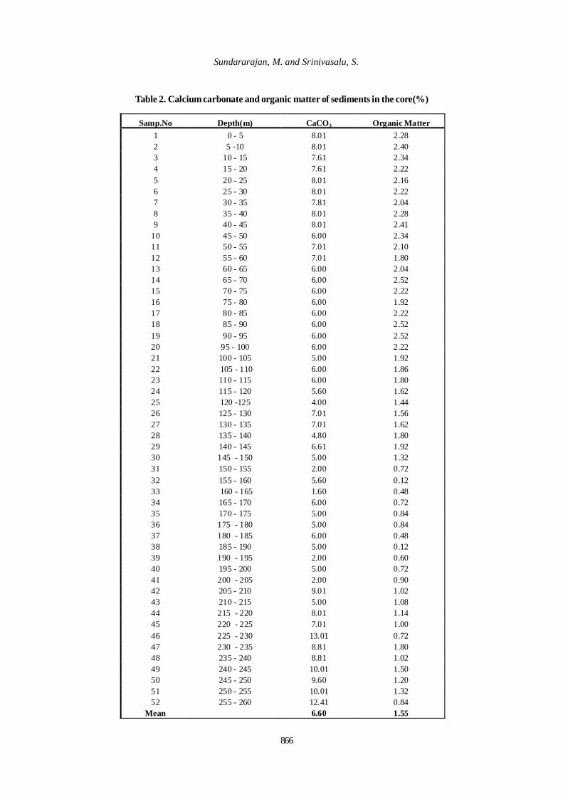
866
Sundararajan, M. and Srinivasalu, S.
Samp.No Depth(m) CaCO3 Organic Matter 1 0 - 5 8.01 2.28 2 5 -10 8.01 2.40 3 10 - 15 7.61 2.34 4 15 - 20 7.61 2.22 5 20 - 25 8.01 2.16 6 25 - 30 8.01 2.22 7 30 - 35 7.81 2.04 8 35 - 40 8.01 2.28 9 40 - 45 8.01 2.41
10 45 - 50 6.00 2.34 11 50 - 55 7.01 2.10 12 55 - 60 7.01 1.80 13 60 - 65 6.00 2.04 14 65 - 70 6.00 2.52 15 70 - 75 6.00 2.22 16 75 - 80 6.00 1.92 17 80 - 85 6.00 2.22 18 85 - 90 6.00 2.52 19 90 - 95 6.00 2.52 20 95 - 100 6.00 2.22 21 100 - 105 5.00 1.92 22 105 - 110 6.00 1.86 23 110 - 115 6.00 1.80 24 115 - 120 5.60 1.62 25 120 -125 4.00 1.44 26 125 - 130 7.01 1.56 27 130 - 135 7.01 1.62 28 135 - 140 4.80 1.80 29 140 - 145 6.61 1.92 30 145 - 150 5.00 1.32 31 150 - 155 2.00 0.72 32 155 - 160 5.60 0.12 33 160 - 165 1.60 0.48 34 165 - 170 6.00 0.72 35 170 - 175 5.00 0.84 36 175 - 180 5.00 0.84 37 180 - 185 6.00 0.48 38 185 - 190 5.00 0.12 39 190 - 195 2.00 0.60 40 195 - 200 5.00 0.72 41 200 - 205 2.00 0.90 42 205 - 210 9.01 1.02 43 210 - 215 5.00 1.08 44 215 - 220 8.01 1.14 45 220 - 225 7.01 1.00 46 225 - 230 13.01 0.72 47 230 - 235 8.81 1.80 48 235 - 240 8.81 1.02 49 240 - 245 10.01 1.50 50 245 - 250 9.60 1.20 51 250 - 255 10.01 1.32 52 255 - 260 12.41 0.84
Mean 6.60 1.55
Table 2. Calcium carbonate and organic matter of sediments in the core(%)

867
Int. J. Environ. Res., 4(4):861-876 , Autumn 2010
has reported 1.54, 1.79 and 1.15% of organic matterfrom the study of three sediment cores of the continentalshelf of Gulf of Mannar, near Tuticorin. In the downcore variation, the sediments show depletion towardsdepth. At a depth of 152 – 155 cm and 180 – 185cm thesediments have recorded very low percentage oforganic matter. The general decrease in organic carbonis due to the domination of decomposition overprotection. A distinct maximum supply of terrigenousorganic matter is obvious at 65-70cm and 85-95cm. Inthe lower part of the core (unit-3), the sediments arepoor in organic matter and rich in carbonate and havebeen deposited under a well mixed, oxygenated watercolumn (Pratt, 1984; Barlow and kauffman, 1985).The measured concentration of major oxides of thesediment core is given in Table 3. The silica contents ofthe core sample are generally moderate. The higherconcentration of silica (56.87%) is found at a depth of190 cm to 195 cm. The lowest concentration of silica(38.20%) is recorded at a depth of 245 cm to 250 cm.There is no much down core variation in the silicacontent. The mean silica concentration is 45.38%. Thealumina content ranges from 9.61% to 14.46%. Higherconcentration of alumina (14.46%) is present in the subsample at a depth of 130 cm to 135 cm and the bottomshows lowest value of 9.61%. The total Fe has beenestimated as Fe2O3. The Fe content is generally low.The higher concentration of Fe2O3 (6.47%) is noticedat a depth of 175 cm to 180 cm. and the lowest value(2.56%) is recorded at the depth interval of 5 cm to 10cm. There is no uniform depletion or enrichment in theiron content towards bottom of the core. However, theupper part of the core is having lower concentrationsof Fe content than the middle part. The mean value ofiron content of the core is 5.433%. CaO is very highwhen compared to other major oxides except silica. Theconcentration of MgO and Na2O are poor and K2O andP2O5 are very poor. CaO ranges from 8.60% to 31.20 %with a mean value of 17.57% and MgO varies from 1.26%to 3.89% with a mean concentration of 2.92%. However,Na2O varies from 1.68% to 7.84% and the concentrationof K2O falls between 0.72% and 4.72%. The meanconcentrations for Na2O and K2O are 4.29% and 2.62%,respectively. P2O5 shows concentrations ranging from0.52% to 0.97%. The mean values for CaO, MgO, Na2O,K2O and P2O5 for the core sample are 17.57%, 2.92%,4.29%, 2.62% and 0.72%, respectively. Na2O shows ageneral depletion towards depth. K2O shows a suddenenrichment from 85 cm depth and from this depth it showsa gradual slight downward depletion. CaO and Fe2O3show enrichment in the top and bottom of the core. MgOshows depletion in the top of the core. The concentrationof elements is in the order of SiO2 >CaO>Al2O3 >Fe2O3>Na2O> MgO >K2O>P2O5, which indicates that theanalyzed sediments are enriched in CaO.
Major element analysis effectively represents thecomposition of the solid fraction being eroded fromthe continent (Taylore and McLennan, 1985). Basedon mean as well as range of concentration of majoroxides, generally, the following decreasing order wasnoticed in the present study. SiO2>CaO>Al2O3>Fe2O3>Na2O>MgO>K2O>P2O5.This trend shows thatSi is the dominant element followed by CaO andAl2O3.The mean silica concentration (45.38) indicates thatthe silica is present in moderate amounts. The Alnormalized values of silica ranges from 3.99 to 5.60having an average value of 4.38. The Si/Al ratio of thecore does not show much variation towards depthand the average value (4.38) is just above the uppercrustal value (3.83). Hence, it indicates that most ofthe sediments have been derived from the continentalmargin. The higher Si/Al ratio is due to the variationsin quartz in the sediments (Calvert et al., 1993).CaOforms the second major oxide in the present studynext to silica; concentration of high CaO is due toboth biogenic and lithogenic material. The continentalmargin of the southeastern Indian coast, which isdominated by sedimentary limestones (Armstrong,1999) might have contributed more CaO to the Shelfand slope sediments (Jonathan et al., 2004). Hence thehigher concentration of CaO is attr ibuted toterrigenous input. Hence, it is possible to note thecontribution of biogenic organic and inorganic materialfor the CaO concentration. The mean concentration ofCaO in the core is 17.57%, which is higher than theconcentration of CaO in other parts of the Bengal fan(Ramesh and Ramasamy 1997). The behavior of Fe inthe core sediments is governed largely by thedistribution of Ferro magnesium minerals and dispersedoxy-hydroxides. The Fe/Al ratio does not show muchvariation towards depth. The mean Fe/Al ratio is 0.59,which is higher than the upper continental crustal value(0.44). It indicates the minor influence of oxy-hydroxides, other than terrigenous material.
Mg/Al ratio is also consistent with thisinterpretation. The mean Mg/Al ratio of the presentcore (0.27) is slightly higher than the value of uppercontinental crust (0.17). The down core variation ofMg/Al ratio shows increment towards depth, which issimilar to Fe/Al ratio. Hence the ferromagnesiumminerals are the main contributor for these elements,which have been derived from the continental margin.The behaviors of K and Na largely reflect thedistribution of K-and Plagioclase feldspar in thesediments. The Na/Al ratio decreases towards depth.The mean Na/Al ratio (0.48) is slightly higher than theupper continental crustal value (0.31), which indicatescontribution of Na2O to the sediments is not only fromthe feldspar. The P/Al ratios do not show much

868
Geochemistry of core sediments
Samp.No Depth(m) SiO2 Al2O3 Na2O K2O CaO MgO Fe2O3 P2O5 Total CIA 1 0 - 5 44.33 13.37 6.96 0.92 27.20 2.06 4.40 0.75 99.99 27.09 2 5 -10 43.56 12.50 7.20 0.96 26.40 1.26 2.56 0.87 95.31 25.88 3 10 - 15 45.57 12.27 7.84 0.96 27.60 1.86 2.83 0.85 99.78 25.96 4 15 - 20 43.87 11.50 7.76 0.88 29.20 1.98 2.78 0.75 98.72 23.82 5 20 - 25 40.03 11.88 6.96 0.88 31.20 2.47 4.83 0.80 99.05 25.58 6 25 - 30 40.56 11.27 7.52 0.80 28.60 2.37 2.84 0.77 94.73 25.79 7 30 - 35 43.03 13.07 6.72 0.96 24.60 2.92 5.20 0.77 97.27 28.40 8 35 - 40 43.03 13.46 6.56 0.96 23.00 2.76 4.85 0.71 95.33 30.56 9 40 - 45 48.19 13.26 5.68 0.96 18.00 3.36 5.69 0.71 95.85 35.84 10 45 - 50 41.79 11.95 5.84 0.96 18.20 1.46 5.57 0.80 86.57 31.50 11 50 - 55 45.03 11.23 5.52 0.96 17.80 2.56 5.42 0.67 89.19 31.20 12 55 - 60 43.79 11.40 4.24 0.72 18.20 2.75 5.87 0.76 87.73 32.82 13 60 - 65 48.87 11.95 4.56 0.72 18.60 2.74 5.66 0.69 93.79 32.66 14 65 - 70 47.57 10.87 4.96 0.80 19.80 2.96 5.63 0.67 93.26 28.55 15 70 - 75 45.36 13.07 4.64 0.80 17.40 2.87 5.72 0.67 90.53 36.24 16 75 - 80 41.36 13.86 4.16 0.80 18.40 2.82 5.89 0.67 87.96 37.23 17 80 - 85 40.17 12.88 4.16 0.72 17.40 3.20 5.94 0.92 85.39 36.51 18 85 - 90 45.03 13.46 3.68 0.96 8.60 2.55 6.36 0.79 84.15 47.64 19 90 - 95 43.79 13.46 4.72 1.12 15.20 3.10 6.13 0.65 91.77 35.01 20 95 - 100 41.36 14.05 4.64 1.04 16.00 3.23 6.27 0.67 90.86 35.48 21 100 - 105 50.19 13.86 3.68 0.80 15.60 3.51 5.88 0.75 97.15 37.04 22 105 - 110 41.36 13.07 4.56 0.88 19.20 3.31 6.01 0.65 92.72 30.73 23 110 - 115 41.36 14.05 3.84 0.80 16.20 3.12 5.86 0.62 88.89 37.00 24 115 - 120 41.36 11.40 4.16 0.88 16.60 3.49 6.02 0.67 87.86 30.15 25 120 -125 46.29 13.66 3.36 0.80 15.40 2.89 5.68 0.67 91.31 36.97 26 125 - 130 41.36 14.05 2.96 0.72 15.80 3.11 5.96 0.62 86.82 40.37 27 130 - 135 49.36 14.46 2.72 0.64 15.60 3.03 5.73 0.69 94.31 42.13 28 135 - 140 49.36 14.25 4.32 0.88 13.40 3.30 6.06 0.91 95.92 38.77 29 140 - 145 49.36 12.88 3.92 0.80 13.40 3.65 6.07 0.52 93.72 38.28 30 145 - 150 53.03 12.46 3.84 0.72 14.60 3.55 6.27 0.97 98.56 34.94 31 150 - 155 51.79 12.46 3.12 0.80 13.00 3.27 6.11 0.88 93.75 36.60 32 155 - 160 54.29 11.68 4.24 0.88 13.40 2.66 5.97 0.85 97.33 34.06 33 160 - 165 49.36 11.68 3.28 0.88 13.20 3.18 6.20 0.82 91.00 33.91 34 165 - 170 49.36 11.49 3.04 0.88 13.20 2.92 6.23 0.75 90.03 37.35 35 170 - 175 49.36 13.27 3.52 0.96 9.80 2.54 6.50 0.61 89.12 44.53 36 175 - 180 49.36 13.48 2.32 0.88 9.80 3.23 6.47 0.67 87.65 49.66 37 180 - 185 50.56 12.46 3.84 0.88 10.20 2.71 6.18 0.77 90.56 41.88 38 185 - 190 50.56 13.69 3.76 0.96 10.80 3.43 6.31 0.79 93.10 42.97 39 190 - 195 56.87 14.11 2.72 0.88 10.40 3.89 5.95 0.69 97.35 45.14 40 195 - 200 49.35 14.11 5.44 0.96 10.00 3.85 6.11 0.72 95.02 40.12 41 200 - 205 48.35 13.92 2.64 0.80 10.80 3.58 6.11 0.72 88.76 42.20 42 205 - 210 41.40 12.06 2.80 0.80 11.80 2.94 5.64 0.82 80.26 44.88 43 210 - 215 46.45 11.63 3.44 0.72 12.40 3.12 5.16 0.79 86.43 36.89 44 215 - 220 45.55 10.81 3.04 0.56 20.00 2.98 4.85 0.75 91.02 28.97 45 220 - 225 44.34 10.81 2.96 0.40 18.00 2.72 4.06 0.72 86.57 30.58 46 225 - 230 42.17 12.70 5.52 0.48 16.60 3.09 4.79 0.85 91.24 34.46 47 230 - 235 41.52 12.05 3.20 0.48 17.00 2.45 5.05 0.85 85.32 35.24 48 235 - 240 40.13 11.22 2.24 0.40 25.80 3.17 5.25 0.75 90.80 44.40 49 240 - 245 40.13 11.22 2.24 0.40 24.80 3.34 5.07 0.67 89.71 44.12 50 245 - 250 38.20 11.63 1.68 0.40 24.00 2.92 5.46 0.72 86.29 47.54 51 250 - 255 41.40 10.99 2.64 0.40 19.29 2.63 4.87 0.57 85.03 52.68 52 255 - 260 40.12 9.61 3.50 0.40 22.20 2.84 3.88 0.57 86.22 25.49
Mean 45.38 12.54 4.29 0.79 17.57 2.92 5.43 0.74 91.48 36.03
Table 3. Major elements in the core samples

Int. J. Environ. Res., 4(4):861-876 , Autumn 2010
variation towards depth. The mean P/Al ratio is 0.06.The relatively low P/al ratios and lack of relationshipwith P/Al and organic suggest that organiccontributions of P in these samples are of minorimportance and that detritus phases mainly control theirP contents. Even though the over all geochemistryshows detritus nature of the sediments, the differentunits of the core shows some variations in theirchemical signature.The Al normalized values of the major elements of thethree units are compared and it shows variations in Si/Al, Na/Al, K/Al and Ca/Al ratios (Table 5). The meanvalues of Si/Al ratio of the three units show high valuesfor Unit-3, followed by Unit-1 and Unit-2. This high Si/Al ratio for the core of Unit-3 reflects the higher quartzcontent than unit 2 and 1. The high Fe/Al and Mg/Alratios in unit 2 and 3 reflect the chlorite and smectite/illite ratios in this horizon. The Mg/Al ratio is higher inunit 3, than in 2 and Fe/Al ratio is higher in unit 2 thanin 3. These variations may be due to marked increasein chlorite in unit 2, Mg being a more sensitive reflectionof the presence of chlorite than Fe (Calvert, 1990).Thereis no much variation in P/Al concentration betweenthe two units in this study.The measured concentration of the trace elements ofthe core sediment is given in Table 4. Manganese inthe core ranges from 83 mg/kg to 151 mg/kg except atthe depth interval 160 cm to 165 cm where theconcentration of Mn suddenly increases to 379 mg/kg. The next highest concentration (151 mg/kg) isencountered at 85 cm to 90 cm depth of the core,whereas, the lowest concentration is recorded at thebottom most sample of the core. In general, upper partof the core shows slightly higher values whencompared to lower part.The down core variation of Cr shows wide range from49.6 mg/kg to 512 mg/kg. The mean concentration ofCr is 170 mg/kg.The mean value of cu is 38 mg/kg.Nickel ranges from 34 mg/kg to 149 mg/kg in the coreand there is not much variation in the concentration ofNi. The higher concentration of Ni (149 mg/kg) is seenin surface layer of the core. The mean concentration ofNi is 65.5 mg/kg. Slight increase in the concentrationof Ni is observed at a depth of 140 to 150cm and 205 –210cm. Thus, down core profile of Ni does not exhibita systematic variation.The lower concentration of Co ranging from 4 mg/kgto 11 mg/kg was observed in the present study. Themean concentration is very low (6.7 mg/kg) and it showsa higher value of Co (8 mg/kg) at a depth of 155 to160cm. The mean value of Pb is 10.9 mg/kg.Concentration of Zn ranges from 71 mg/kg to 128 mg/kg in the sub-samples. The mean concentration is 81mg/kg. The mean value of Cd is 0.2 mg/kg.Theassociation of the minor elements with the principal
sediment components of the core is summarized bythe results of the factor analysis. It can be seen thatthe trace elements are strongly fractionated betweenthe three components and can therefore be used torefine the chemical characterization of the differentsediment units already revealed by the distribution ofthe major elements. In addition, the conditions ofsedimentation and effects of digenesis will alsoinfluence the distribution of some of the trace elements.The distribution of trace elements shows the followingdecreasing order based on the mean of trace elementsin the core Cr>Mn>Zn>Ni>Cu>Pb>Co>Cd.Manganese concentrations with 83 mg/kg value is thelowest observed in the core and shows a ratherconstant down core distribution except a maximum of379 mg/kg at 160-165cm. Small fluctuations co-varywith aluminum concentrations suggesting ferruginoussource for the manganese. The mean Mn/Al ratio(20.70) is very much less than the upper continentalcrustal values (75) and average shale (85) (Taylor andMcLennan, 1985). The Mn peak at 160-165cm may bedue to the presence of Pleistocene/Holocene boundary.Similar observations have been described from thePleistocene/Holocene boundary by (Ramesh andRamasamy, 1997). The Al normalized values of the traceelements of the three units are given in Table 6 and fig.3.The distribution of Cr and Ni permits a more definedidentification of the mineralogical change in the core.The Cr/Al and Ni/Al ratios co-vary and are highest inunit 2. Both ratios decrease in unit 1, with a Cr/Ni > 1.In the Cr/Al and Ni/Al ratio there is no much variationamong the units, and the total core is markedly enrichedin chlorite and smectite in relation to illite. The ratiobetween Cr and Ni is constant and it indicatesterrigenous source for Cr and Ni. Cu and Zn appear tobehave coherently in the core sediments, althoughthere is difference in their detailed behaviors. Cu/Aland Zn/Al co-vary in all the units. Both the values arehighest in unit 3 and low in unit 2 and again high inunit 1. For Cu/Al and Zn/Al ratios the upper continentalcrustal value are 3.10 and 8.8, which are much lowerthan the values in the present study. Certain minorand trace elements are enriched (i.e. occur atconcentrations significantly above the crustalabundances) in many organic rich sediments (Calvert,1976). The mean Co/Al ratio of 1.02 is much lesser thanthe upper continental value (1.24). The mean Co/Alvalues of unit 1 (0.93) and unit 2 (0.95) remain similarand it shows slight enrichment in unit 3 (1.16). Themean Pb/Al ratios of the core sediments are much lesserthan the crustal value (2.48). The Pb/Al ratios are 1.75for unit 1, 1.39 for unit 2 and 1.90 for unit 3. Hence,these trace metals have been derived from ferruginousinput. Comparisons of trace metal concentration in the
869
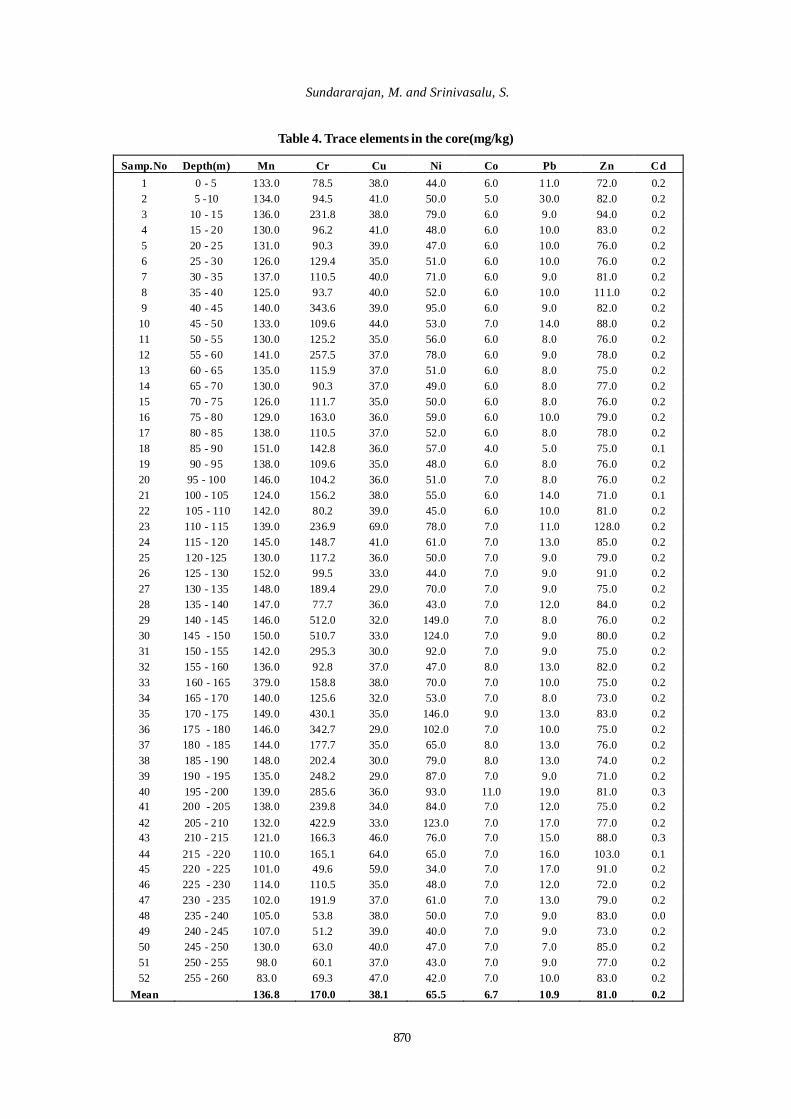
Sundararajan, M. and Srinivasalu, S.
Samp.No Depth(m) Mn Cr Cu Ni Co Pb Zn Cd 1 0 - 5 133.0 78.5 38.0 44.0 6.0 11.0 72.0 0.2 2 5 -10 134.0 94.5 41.0 50.0 5.0 30.0 82.0 0.2 3 10 - 15 136.0 231.8 38.0 79.0 6.0 9.0 94.0 0.2 4 15 - 20 130.0 96.2 41.0 48.0 6.0 10.0 83.0 0.2 5 20 - 25 131.0 90.3 39.0 47.0 6.0 10.0 76.0 0.2 6 25 - 30 126.0 129.4 35.0 51.0 6.0 10.0 76.0 0.2 7 30 - 35 137.0 110.5 40.0 71.0 6.0 9.0 81.0 0.2 8 35 - 40 125.0 93.7 40.0 52.0 6.0 10.0 111.0 0.2 9 40 - 45 140.0 343.6 39.0 95.0 6.0 9.0 82.0 0.2 10 45 - 50 133.0 109.6 44.0 53.0 7.0 14.0 88.0 0.2 11 50 - 55 130.0 125.2 35.0 56.0 6.0 8.0 76.0 0.2 12 55 - 60 141.0 257.5 37.0 78.0 6.0 9.0 78.0 0.2 13 60 - 65 135.0 115.9 37.0 51.0 6.0 8.0 75.0 0.2 14 65 - 70 130.0 90.3 37.0 49.0 6.0 8.0 77.0 0.2 15 70 - 75 126.0 111.7 35.0 50.0 6.0 8.0 76.0 0.2 16 75 - 80 129.0 163.0 36.0 59.0 6.0 10.0 79.0 0.2 17 80 - 85 138.0 110.5 37.0 52.0 6.0 8.0 78.0 0.2 18 85 - 90 151.0 142.8 36.0 57.0 4.0 5.0 75.0 0.1 19 90 - 95 138.0 109.6 35.0 48.0 6.0 8.0 76.0 0.2 20 95 - 100 146.0 104.2 36.0 51.0 7.0 8.0 76.0 0.2 21 100 - 105 124.0 156.2 38.0 55.0 6.0 14.0 71.0 0.1 22 105 - 110 142.0 80.2 39.0 45.0 6.0 10.0 81.0 0.2 23 110 - 115 139.0 236.9 69.0 78.0 7.0 11.0 128.0 0.2 24 115 - 120 145.0 148.7 41.0 61.0 7.0 13.0 85.0 0.2 25 120 -125 130.0 117.2 36.0 50.0 7.0 9.0 79.0 0.2 26 125 - 130 152.0 99.5 33.0 44.0 7.0 9.0 91.0 0.2 27 130 - 135 148.0 189.4 29.0 70.0 7.0 9.0 75.0 0.2 28 135 - 140 147.0 77.7 36.0 43.0 7.0 12.0 84.0 0.2 29 140 - 145 146.0 512.0 32.0 149.0 7.0 8.0 76.0 0.2 30 145 - 150 150.0 510.7 33.0 124.0 7.0 9.0 80.0 0.2 31 150 - 155 142.0 295.3 30.0 92.0 7.0 9.0 75.0 0.2 32 155 - 160 136.0 92.8 37.0 47.0 8.0 13.0 82.0 0.2 33 160 - 165 379.0 158.8 38.0 70.0 7.0 10.0 75.0 0.2 34 165 - 170 140.0 125.6 32.0 53.0 7.0 8.0 73.0 0.2 35 170 - 175 149.0 430.1 35.0 146.0 9.0 13.0 83.0 0.2 36 175 - 180 146.0 342.7 29.0 102.0 7.0 10.0 75.0 0.2 37 180 - 185 144.0 177.7 35.0 65.0 8.0 13.0 76.0 0.2 38 185 - 190 148.0 202.4 30.0 79.0 8.0 13.0 74.0 0.2 39 190 - 195 135.0 248.2 29.0 87.0 7.0 9.0 71.0 0.2 40 195 - 200 139.0 285.6 36.0 93.0 11.0 19.0 81.0 0.3 41 200 - 205 138.0 239.8 34.0 84.0 7.0 12.0 75.0 0.2 42 205 - 210 132.0 422.9 33.0 123.0 7.0 17.0 77.0 0.2 43 210 - 215 121.0 166.3 46.0 76.0 7.0 15.0 88.0 0.3 44 215 - 220 110.0 165.1 64.0 65.0 7.0 16.0 103.0 0.1 45 220 - 225 101.0 49.6 59.0 34.0 7.0 17.0 91.0 0.2 46 225 - 230 114.0 110.5 35.0 48.0 7.0 12.0 72.0 0.2 47 230 - 235 102.0 191.9 37.0 61.0 7.0 13.0 79.0 0.2 48 235 - 240 105.0 53.8 38.0 50.0 7.0 9.0 83.0 0.0 49 240 - 245 107.0 51.2 39.0 40.0 7.0 9.0 73.0 0.2 50 245 - 250 130.0 63.0 40.0 47.0 7.0 7.0 85.0 0.2 51 250 - 255 98.0 60.1 37.0 43.0 7.0 9.0 77.0 0.2 52 255 - 260 83.0 69.3 47.0 42.0 7.0 10.0 83.0 0.2
Mean 136.8 170.0 38.1 65.5 6.7 10.9 81.0 0.2
Table 4. Trace elements in the core(mg/kg)
870

Int. J. Environ. Res., 4(4):861-876 , Autumn 2010
Table 5. Al normalization for major elements in the core samples
Samp.No Depth(m) Si/Al Na/Al K/Al Ca/Al Mg/Al Fe/Al P/Al 1 0 - 5 3.99 0.73 0.11 2.75 0.18 0.44 0.06 2 5 -10 4.20 0.81 0.12 2.85 0.11 0.45 0.07 3 10 - 15 4.47 0.90 0.12 3.04 0.17 0.51 0.07 4 15 - 20 4.59 0.95 0.12 3.43 0.20 0.54 0.07 5 20 - 25 4.06 0.82 0.12 3.55 0.24 0.54 0.07 6 25 - 30 4.33 0.94 0.11 3.43 0.24 0.55 0.07 7 30 - 35 3.96 0.72 0.12 2.54 0.25 0.54 0.06 8 35 - 40 3.85 0.68 0.11 2.31 0.23 0.48 0.06 9 40 - 45 4.38 0.60 0.11 1.83 0.29 0.57 0.06
10 45 - 50 4.21 0.69 0.13 2.06 0.14 0.63 0.07 11 50 - 55 4.83 0.69 0.13 2.14 0.26 0.64 0.06 12 55 - 60 4.63 0.52 0.10 2.16 0.27 0.68 0.07 13 60 - 65 4.92 0.54 0.09 2.10 0.26 0.63 0.06 14 65 - 70 5.27 0.64 0.12 2.46 0.31 0.70 0.07 15 70 - 75 4.18 0.50 0.10 1.80 0.25 0.58 0.05 16 75 - 80 3.59 0.42 0.09 1.79 0.23 0.57 0.05 17 80 - 85 3.76 0.45 0.09 1.83 0.28 0.60 0.08 18 85 - 90 4.03 0.38 0.43 0.86 0.22 0.63 0.06 19 90 - 95 3.92 0.49 0.55 1.53 0.26 0.60 0.05 20 95 - 100 3.54 0.46 0.52 1.54 0.26 0.59 0.05 21 100 - 105 4.36 0.37 0.42 1.52 0.29 0.57 0.06 22 105 - 110 3.81 0.49 0.55 1.99 0.29 0.61 0.05 23 110 - 115 3.54 0.38 0.43 1.56 0.25 0.55 0.05 24 115 - 120 4.37 0.51 0.57 1.97 0.35 0.70 0.06 25 120 -125 4.08 0.35 0.39 1.52 0.24 0.55 0.05 26 125 - 130 3.54 0.30 0.33 1.52 0.25 0.57 0.05 27 130 - 135 4.11 0.26 0.30 1.46 0.24 0.52 0.05 28 135 - 140 4.17 0.43 0.48 1.27 0.26 0.56 0.07 29 140 - 145 4.61 0.43 0.48 1.41 0.32 0.63 0.04 30 145 - 150 5.12 0.43 0.48 1.58 0.32 0.67 0.08 31 150 - 155 5.01 0.35 0.39 1.41 0.30 0.65 0.08 32 155 - 160 5.60 0.51 0.57 1.55 0.26 0.68 0.08 33 160 - 165 5.09 0.39 0.44 1.53 0.31 0.71 0.07 34 165 - 170 5.17 0.37 0.42 1.55 0.29 0.72 0.07 35 170 - 175 4.48 0.37 0.42 1.00 0.22 0.66 0.05 36 175 - 180 4.41 0.24 0.27 0.98 0.27 0.65 0.05 37 180 - 185 4.89 0.43 0.48 1.11 0.25 0.67 0.07 38 185 - 190 4.45 0.39 0.43 1.07 0.29 0.62 0.06 39 190 - 195 4.85 0.27 0.30 1.00 0.31 0.56 0.05 40 195 - 200 4.21 0.54 0.60 0.96 0.31 0.58 0.05 41 200 - 205 4.18 0.27 0.30 1.05 0.29 0.58 0.06 42 205 - 210 4.13 0.33 0.36 1.32 0.28 0.63 0.07 43 210 - 215 4.81 0.41 0.46 1.44 0.31 0.59 0.07 44 215 - 220 5.07 0.39 0.44 2.50 0.31 0.59 0.07 45 220 - 225 4.94 0.38 0.43 2.25 0.29 0.51 0.07 46 225 - 230 4.00 0.61 0.68 1.77 0.28 0.51 0.07 47 230 - 235 4.15 0.37 0.42 1.91 0.23 0.56 0.08 48 235 - 240 4.31 0.28 0.31 3.11 0.32 0.62 0.07 49 240 - 245 4.31 0.28 0.31 2.99 0.34 0.61 0.06 50 245 - 250 3.96 0.20 0.23 2.79 0.29 0.63 0.07 51 250 - 255 4.54 0.34 0.38 2.37 0.27 0.58 0.06 52 255 - 260 5.03 0.51 0.57 3.12 0.34 0.53 0.06
Mean 4.38 0.48 0.33 1.93 0.27 0.59 0.06
871

Geochemistry of core sediments
Table 6. Al normalization for trace elements in the core samples
Samp.No Depth(m) M n/Al Cr/Al Cu/Al Ni/Al Co/Al Pb/Al Zn/Al 1 0 - 5 18.80 11.10 5.37 6.22 0.85 1.56 10.18 2 5 -10 20.26 14.29 6.20 7.56 0.76 4.54 12.40 3 10 - 15 20.95 35.71 5.85 12.17 0.92 1.39 14.48 4 15 - 20 21.37 15.81 6.74 7.89 0.99 1.64 13.64 5 20 - 25 20.84 14.37 6.21 7.48 0.95 1.59 12.09 6 25 - 30 21.13 21.70 5.87 8.55 1.01 1.68 12.75 7 30 - 35 19.81 15.98 5.79 10.27 0.87 1.30 11.72 8 35 - 40 17.56 13.16 5.62 7.30 0.84 1.40 15.59 9 40 - 45 19.96 48.98 5.56 13.54 0.86 1.28 11.69
10 45 - 50 21.04 17.34 6.96 8.38 1.11 2.21 13.92 11 50 - 55 21.88 21.08 5.89 9.43 1.01 1.35 12.79 12 55 - 60 23.38 42.70 6.14 12.93 0.99 1.49 12.93 13 60 - 65 21.36 18.33 5.85 8.07 0.95 1.27 11.86 14 65 - 70 22.61 15.70 6.43 8.52 1.04 1.39 13.39 15 70 - 75 18.22 16.16 5.06 7.23 0.87 1.16 10.99 16 75 - 80 17.59 22.23 4.91 8.05 0.82 1.36 10.77 17 80 - 85 20.25 16.22 5.43 7.63 0.88 1.17 11.45 18 85 - 90 21.21 20.06 5.06 8.01 0.56 0.70 10.53 19 90 - 95 19.38 15.39 4.92 6.74 0.84 1.12 10.67 20 95 - 100 19.64 14.02 4.84 6.86 0.94 1.08 10.23 21 100 - 105 16.91 21.30 5.18 7.50 0.82 1.91 9.68 22 105 - 110 20.54 11.60 5.64 6.51 0.87 1.45 11.72 23 110 - 115 18.70 31.87 9.28 10.49 0.94 1.48 17.22 24 115 - 120 24.04 24.66 6.80 10.12 1.16 2.16 14.09 25 120 -125 17.99 16.22 4.98 6.92 0.97 1.25 10.93 26 125 - 130 20.45 13.39 4.44 5.92 0.94 1.21 12.24 27 130 - 135 19.35 24.76 3.79 9.15 0.92 1.18 9.80 28 135 - 140 19.50 10.31 4.78 5.70 0.93 1.59 11.14 29 140 - 145 21.43 75.14 4.70 21.87 1.03 1.17 11.15 30 145 - 150 22.76 77.48 5.01 18.81 1.06 1.37 12.14 31 150 - 155 21.54 44.80 4.55 13.96 1.06 1.37 11.38 32 155 - 160 22.01 15.02 5.99 7.61 1.29 2.10 13.27 33 160 - 165 61.34 25.70 6.15 11.33 1.13 1.62 12.14 34 165 - 170 23.03 20.66 5.26 8.72 1.15 1.32 12.01 35 170 - 175 21.23 61.27 4.99 20.80 1.28 1.85 11.82 36 175 - 180 20.47 48.06 4.07 14.30 0.98 1.40 10.52 37 180 - 185 21.85 26.96 5.31 9.86 1.21 1.97 11.53 38 185 - 190 20.44 27.95 4.14 10.91 1.10 1.80 10.22 39 190 - 195 18.09 33.25 3.89 11.66 0.94 1.21 9.51 40 195 - 200 18.62 38.26 4.82 12.46 1.47 2.55 10.85 41 200 - 205 18.74 32.57 4.62 11.41 0.95 1.63 10.19 42 205 - 210 20.69 66.29 5.17 19.28 1.10 2.66 12.07 43 210 - 215 19.67 27.03 7.48 12.35 1.14 2.44 14.30 44 215 - 220 19.24 28.87 11.19 11.37 1.22 2.80 18.01 45 220 - 225 17.66 8.67 10.32 5.95 1.22 2.97 15.91 46 225 - 230 16.97 16.45 5.21 7.14 1.04 1.79 10.72 47 230 - 235 16.00 30.10 5.80 9.57 1.10 2.04 12.39 48 235 - 240 17.69 9.06 6.40 8.42 1.18 1.52 13.98 49 240 - 245 18.03 8.63 6.57 6.74 1.18 1.52 12.30 50 245 - 250 21.13 10.24 6.50 7.64 1.14 1.14 13.82 51 250 - 255 16.86 10.34 6.36 7.40 1.20 1.55 13.24 52 255 - 260 16.33 13.63 9.25 8.26 1.38 1.97 16.33
Mean 20.70 25.40 5.83 9.86 1.02 1.67 12.32
872

Int. J. Environ. Res., 4(4):861-876 , Autumn 2010
study area with various other coastal regions aroundthe world are indicated in Table 7.
CONCLUSIONThe sediments have been poorly sorted and most
of the sub samples are silty clay and few top samplesare sandy silty clay. The slightly higher values of thesand fraction when compared to the other sub samplesare due to shell fragments and undecomposed organicmatter and not due to sand grains. The nature of organic
Table 7. Comparison of trace metals in sediments with various coastal regions around the world and southeastcoast of India (mg/kg)
Location Mn Cr Cu Ni Co Pb Zn Present Study Core (Range) 83-379 49.6-512 29-69 34 -149 4 -11 5-30 71-128 Average 136.8 170 38.1 65.5 6.7 10.9 81 (1) Gulf of Aqaba (Red Sea) 53-655 15-186 7-27 19-76 21-56 83 -225 31-260 (2) Palos VerdesPeninsula, Southern California - 74-1,480 14-937 16-134 - 19-578 54-2,880 (3) HalifaxBay - - 7 12 7.6 17 33 (4) China Shelf Sea 530 61 15 24 12 20 65 (5) Tokyo Bay 1,098 77.3 53.47 32.63 - 50.68 322 (6) Narragansett Bay 410 155 190 28 8 140 250 (7) Boston Harbour - 231.5 112 34.7 - 135 176 (8) Gulf of St. Lawerence 700 87 25 36 14 21 84 (9) Bombay Coast 1192 103 100.9 52 38.2 16.4 96.2 (10) Tuticorin coast 305 177 57 24 15 16 73 (11) Kalpakkam, Bay of Bengal 356 57 20 30 9 16 71 (12) Shallow cores, Bay of Bengal 529 84 26 64 - - - (13) Surface sediments, Gulf of Mannar 296 167 - 24 7 16 73 1) Abu-Hilal (1987); 2) Hershelmen and others (1981); 3) Knauer (1977); 4) Yiyang and Ming-cai (1992); 5) Fukushima and others (1992); 6) Goldberg and others (1977); 7) Bothner and others (1998); 8)Loring (1978, 1979); 9) Dilli (1986); 10) Jonathan and others (2004).11) Selvaraj et al., (2004); 12) Sarin et al., (1979); 13) Jonathan and Ram-Mohan (2003).
matter also indicates high sedimentation rate. The majoroxide geochemistry shows higher concentrations ofdetrital constituents. Calcium carbonate and organicmatter concentration controlled the Calcium oxideconcentration of the sediments. Ferromagnesiumminerals controlled the concentration of Fe and Mg inthe sediments. The trace element study indicates exceptfor Cu and Zn, ferruginous nature. Aluminum silicatesand ferromagnesium mineral have greater contributionin the lower most part of the core. Calcium carbonate
873
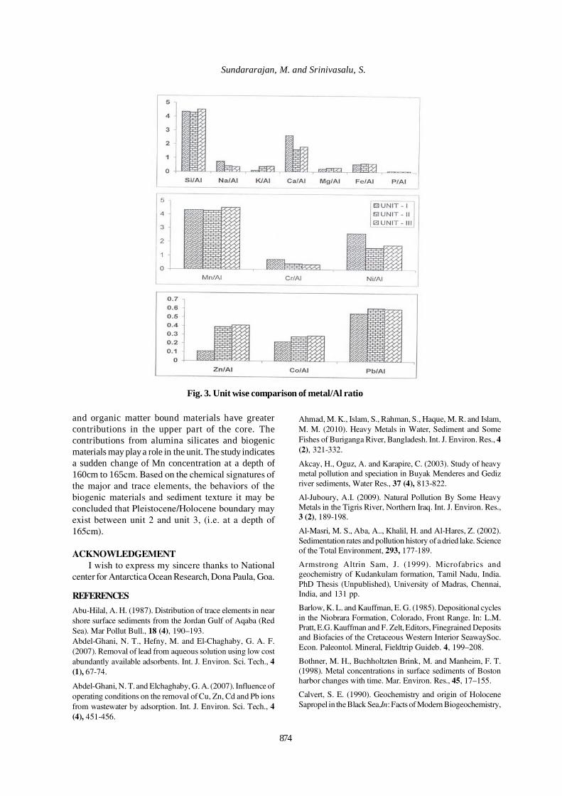
Sundararajan, M. and Srinivasalu, S.
Fig. 3. Unit wise comparison of metal/Al ratio
and organic matter bound materials have greatercontributions in the upper part of the core. Thecontributions from alumina silicates and biogenicmaterials may play a role in the unit. The study indicatesa sudden change of Mn concentration at a depth of160cm to 165cm. Based on the chemical signatures ofthe major and trace elements, the behaviors of thebiogenic materials and sediment texture it may beconcluded that Pleistocene/Holocene boundary mayexist between unit 2 and unit 3, (i.e. at a depth of165cm).
ACKNOWLEDGEMENTI wish to express my sincere thanks to National
center for Antarctica Ocean Research, Dona Paula, Goa.
REFERENCES
Abu-Hilal, A. H. (1987). Distribution of trace elements in nearshore surface sediments from the Jordan Gulf of Aqaba (RedSea). Mar Pollut Bull., 18 (4), 190–193.Abdel-Ghani, N. T., Hefny, M. and El-Chaghaby, G. A. F.(2007). Removal of lead from aqueous solution using low costabundantly available adsorbents. Int. J. Environ. Sci. Tech., 4(1), 67-74.
Abdel-Ghani, N. T. and Elchaghaby, G. A. (2007). Influence ofoperating conditions on the removal of Cu, Zn, Cd and Pb ionsfrom wastewater by adsorption. Int. J. Environ. Sci. Tech., 4(4), 451-456.
Ahmad, M. K., Islam, S., Rahman, S., Haque, M. R. and Islam,M. M. (2010). Heavy Metals in Water, Sediment and SomeFishes of Buriganga River, Bangladesh. Int. J. Environ. Res., 4(2), 321-332.
Akcay, H., Oguz, A. and Karapire, C. (2003). Study of heavymetal pollution and speciation in Buyak Menderes and Gedizriver sediments, Water Res., 37 (4), 813-822.
Al-Juboury, A.I. (2009). Natural Pollution By Some HeavyMetals in the Tigris River, Northern Iraq. Int. J. Environ. Res.,3 (2), 189-198.
Al-Masri, M. S., Aba, A.., Khalil, H. and Al-Hares, Z. (2002).Sedimentation rates and pollution history of a dried lake. Scienceof the Total Environment, 293, 177-189.
Armstrong Altrin Sam, J. (1999). Microfabrics andgeochemistry of Kudankulam formation, Tamil Nadu, India.PhD Thesis (Unpublished), University of Madras, Chennai,India, and 131 pp.
Barlow, K. L. and Kauffman, E. G. (1985). Depositional cyclesin the Niobrara Formation, Colorado, Front Range. In: L.M.Pratt, E.G. Kauffman and F. Zelt, Editors, Finegrained Depositsand Biofacies of the Cretaceous Western Interior SeawaySoc.Econ. Paleontol. Mineral, Fieldtrip Guideb. 4, 199–208.
Bothner, M. H., Buchholtzten Brink, M. and Manheim, F. T.(1998). Metal concentrations in surface sediments of Bostonharbor changes with time. Mar. Environ. Res., 45, 17–155.
Calvert, S. E. (1990). Geochemistry and origin of HoloceneSapropel in the Black Sea,In: Facts of Modern Biogeochemistry,
874
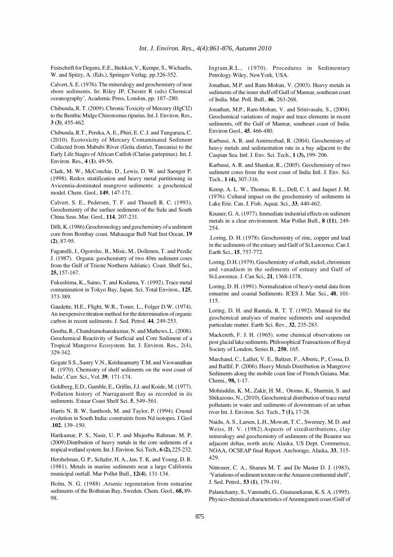
Int. J. Environ. Res., 4(4):861-876, Autumn 2010
Festschrift for Degens, E.E., Ittekkot, V., Kempe, S., Wichaelis,W. and Spitzy, A. (Eds.), Springer-Verlag, pp.326-352.
Calvert, S. E. (1976). The mineralogy and geochemistry of nearshore sediments. In: Riley JP, Chester R (eds) Chemicaloceanography’, Academic Press, London, pp. 187–280.
Chibunda, R. T. (2009). Chronic Toxicity of Mercury (HgCl2)to the Benthic Midge Chironomus riparius. Int. J. Environ. Res.,3 (3), 455-462.
Chibunda, R.T., Pereka, A. E., Phiri, E. C. J. and Tungaraza, C.(2010). Ecotoxicity of Mercury Contaminated SedimentCollected from Mabubi River (Geita district, Tanzania) to theEarly Life Stages of African Catfish (Clarias gariepinus). Int. J.Environ. Res., 4 (1), 49-56.
Clark, M. W., McConchie, D., Lewis, D. W. and Saenger P.(1998). Redox stratification and heavy metal partitioning inAvicennia-dominated mangrove sediments: a geochemicalmodel. Chem. Geol., 149, 147-171.
Calvert, S. E., Pedersen, T. F. and Thunell R. C. (1993).Geochemistry of the surface sediments of the Sulu and SouthChina Seas. Mar. Geol., 114, 207-231.
Dilli, K. (1986).Geochronology and geochemistry of a sedimentcore from Bombay coast. Mahasagar Bull Natl Inst Ocean, 19(2), 87-95.
Faganelli, J., Ogorolec, B., Misic, M., Dollenen, T. and PezdicJ. (1987). Organic geochemistry of two 40m sediment coresfrom the Gulf of Trieste Northern Adriatic). Coast. Shelf Sci.,25, 157-167.
Fukushima, K., Saino, T. and Kodama, Y. (1992). Trace metalcontamination in Tokyo Bay, Japan. Sci. Total Environ., 125,373-389.
Gaudette, H.E., Flight, W.R., Toner, L., Folger D.W. (1974).An inexpensive titration method for the determination of organiccarbon in recent sediments. J. Sed. Petrol. 44, 249-253.
Geetha, R., Chandramohanakumar, N. and Mathews, L. (2008).Geochemical Reactivity of Surficial and Core Sediment of aTropical Mangrove Ecosystem. Int. J. Environ. Res., 2(4),329-342.
Gogate S.S., Sastry V.N., Krishnamurty T.M. and ViswanathanR. (1970). Chemistry of shelf sediments on the west coast ofIndia’, Curr. Sci., Vol. 39, 171-174.
Goldberg, E.D., Gamble, E., Grifûn, J.J. and Koide, M. (1977).Pollution history of Narragansett Bay as recorded in itssediments. Estuar Coast Shelf Sci. 5, 549–561.
Harris N. B. W, Santhosh, M. and Taylor, P. (1994). Crustalevolution in South India: constraints from Nd isotopes. J Geol.102, 139–150.
Harikumar, P. S., Nasir, U. P. and Mujeebu Rahman, M. P.(2009).Distribution of heavy metals in the core sediments of atropical wetland system. Int. J. Environ. Sci. Tech., 6 (2), 225-232.
Hershelman, G. P., Schafer, H. A., Jan, T. K. and Young, D. R.(1981). Metals in marine sediments near a large Californiamunicipal outfall. Mar Pollut Bull., 12(4), 131-134.
Holm, N. G. (1988) .Arsenic regeneration from estuarinesediments of the Bothnian Bay, Sweden. Chem. Geol., 68, 89-98.
Ingram,R.L., (1970). Procedures in SedimentaryPetrology.Wiley, NewYork, USA.
Jonathan, M.P. and Ram-Mohan, V. (2003). Heavy metals insediments of the inner shelf off Gulf of Mannar, southeast coastof India. Mar. Poll. Bull., 46, 263-268.
Jonathan, M.P., Ram-Mohan, V. and Srinivasalu, S., (2004).Geochemical variations of major and trace elements in recentsediments, off the Gulf of Mannar, southeast coast of India.Environ Geol., 45, 466-480.
Karbassi, A. R. and Amirnezhad, R. (2004). Geochemistry ofheavy metals and sedimentation rate in a bay adjacent to theCaspian Sea. Intl. J. Env. Sci. Tech., 1 (3), 199- 206.
Karbassi, A. R. and Shankar, R., (2005). Geochemistry of twosediment cores from the west coast of India Intl. J. Env. Sci.Tech., 1 (4), 307-316.
Kemp, A. L. W., Thomas, R. L., Dell, C. I. and Jaquet J. M.(1976). Cultural impact on the geochemistry of sediments inLake Erie. Can. J. Fish. Aquat. Sci., 33, 440-462.
Knauer, G. A. (1977). Immediate industrial effects on sedimentmetals in a clear environment. Mar Pollut Bull., 8 (11), 249-254.
.Loring, D. H. (1978). Geochemistry of zinc, copper and leadin the sediments of the estuary and Gulf of St.Lawrence. Can J.Earth Sci., 15, 757-772.
Loring, D.H. (1979). Geochemistry of cobalt, nickel, chromiumand vanadium in the sediments of estuary and Gulf ofSt.Lawrence. J. Can Sci., 21, 1368-1378.
Loring, D. H. (1991). Normalization of heavy-metal data fromestuarine and coastal Sediments. ICES J. Mar. Sci., 48, 101-115.
Loring, D. H. and Rantala, R. T. T. (1992). Manual for thegeochemical analyses of marine sediments and suspendedparticulate matter. Earth Sci. Rev., 32, 235-283.
Mackereth, F. J. H. (1965). some chemical observations onpost glacial lake sediments. Philosophical Transactions of RoyalSociety of London, Series B., 250, 165.
Marchand, C., Lalliet, V. E., Baltzer, F., Alberic, P., Cossa, D.and Baillif, P. (2006). Heavy Metals Distribution in MangroveSediments along the mobile coast line of French Guiana. Mar.Chemi., 98, 1-17.
Mohiuddin, K. M., Zakir, H. M., Otomo, K., Sharmin, S. andShikazono, N., (2010). Geochemical distribution of trace metalpollutants in water and sediments of downstream of an urbanriver Int. J. Environ. Sci. Tech., 7 (1), 17-28.
Naidu, A. S., Larsen, L.H., Mowatt, T. C., Sweeney, M. D. andWeiss, H. V. (1982).Aspects of sizedistributions, claymineralogy and geochemistry of sediments of the Beautor seaadjacent deltas, north arctic Alaska. US Dept. Commerece,NOAA, OCSEAP final Report. Anchorage, Alaska, 33, 315-429.
Nittrouer, C. A., Sharara M. T. and De Master D. J. (1983),‘Variations of sediment texture on the Amazon continental shelf’,J. Sed. Petrol., 53 (1), 179-191.
Palanichamy, S., Vanmathi, G., Gnanasekaran, K. S. A. (1995).Physico-chemical characteristics of Arumuganeri coast (Gulf of
875
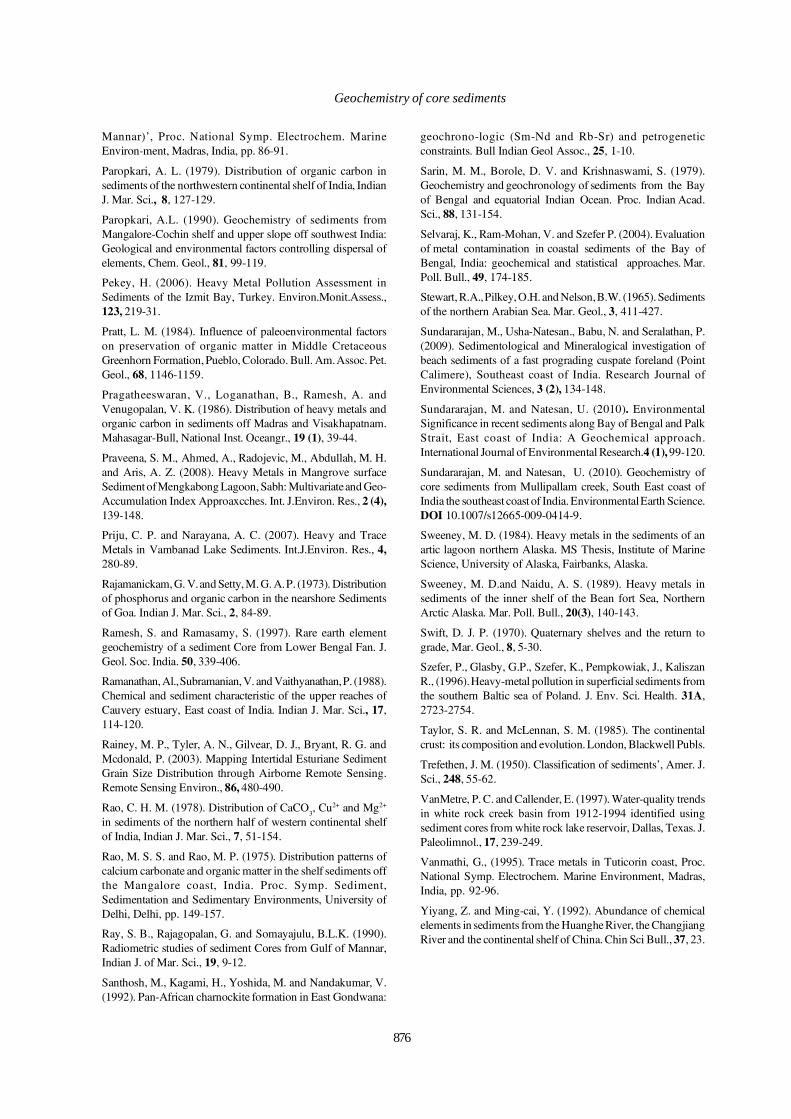
Geochemistry of core sediments
Mannar)’, Proc. National Symp. Electrochem. MarineEnvironment, Madras, India, pp. 86-91.
Paropkari, A. L. (1979). Distribution of organic carbon insediments of the northwestern continental shelf of India, IndianJ. Mar. Sci., 8, 127-129.
Paropkari, A.L. (1990). Geochemistry of sediments fromMangalore-Cochin shelf and upper slope off southwest India:Geological and environmental factors controlling dispersal ofelements, Chem. Geol., 81, 99-119.
Pekey, H. (2006). Heavy Metal Pollution Assessment inSediments of the Izmit Bay, Turkey. Environ.Monit.Assess.,123, 219-31.
Pratt, L. M. (1984). Influence of paleoenvironmental factorson preservation of organic matter in Middle CretaceousGreenhorn Formation, Pueblo, Colorado. Bull. Am. Assoc. Pet.Geol., 68, 1146-1159.
Pragatheeswaran, V., Loganathan, B., Ramesh, A. andVenugopalan, V. K. (1986). Distribution of heavy metals andorganic carbon in sediments off Madras and Visakhapatnam.Mahasagar-Bull, National Inst. Oceangr., 19 (1), 39-44.
Praveena, S. M., Ahmed, A., Radojevic, M., Abdullah, M. H.and Aris, A. Z. (2008). Heavy Metals in Mangrove surfaceSediment of Mengkabong Lagoon, Sabh: Multivariate and Geo-Accumulation Index Approaxcches. Int. J.Environ. Res., 2 (4),139-148.
Priju, C. P. and Narayana, A. C. (2007). Heavy and TraceMetals in Vambanad Lake Sediments. Int.J.Environ. Res., 4,280-89.
Rajamanickam, G. V. and Setty, M. G. A. P. (1973). Distributionof phosphorus and organic carbon in the nearshore Sedimentsof Goa. Indian J. Mar. Sci., 2, 84-89.
Ramesh, S. and Ramasamy, S. (1997). Rare earth elementgeochemistry of a sediment Core from Lower Bengal Fan. J.Geol. Soc. India. 50, 339-406.
Ramanathan, Al., Subramanian, V. and Vaithyanathan, P. (1988).Chemical and sediment characteristic of the upper reaches ofCauvery estuary, East coast of India. Indian J. Mar. Sci., 17,114-120.
Rainey, M. P., Tyler, A. N., Gilvear, D. J., Bryant, R. G. andMcdonald, P. (2003). Mapping Intertidal Esturiane SedimentGrain Size Distribution through Airborne Remote Sensing.Remote Sensing Environ., 86, 480-490.
Rao, C. H. M. (1978). Distribution of CaCO3, Cu2+ and Mg2+
in sediments of the northern half of western continental shelfof India, Indian J. Mar. Sci., 7, 51-154.
Rao, M. S. S. and Rao, M. P. (1975). Distribution patterns ofcalcium carbonate and organic matter in the shelf sediments offthe Mangalore coast, India. Proc. Symp. Sediment,Sedimentation and Sedimentary Environments, University ofDelhi, Delhi, pp. 149-157.
Ray, S. B., Rajagopalan, G. and Somayajulu, B.L.K. (1990).Radiometric studies of sediment Cores from Gulf of Mannar,Indian J. of Mar. Sci., 19, 9-12.
Santhosh, M., Kagami, H., Yoshida, M. and Nandakumar, V.(1992). Pan-African charnockite formation in East Gondwana:
geochrono-logic (Sm-Nd and Rb-Sr) and petrogeneticconstraints. Bull Indian Geol Assoc., 25, 1-10.
Sarin, M. M., Borole, D. V. and Krishnaswami, S. (1979).Geochemistry and geochronology of sediments from the Bayof Bengal and equatorial Indian Ocean. Proc. Indian Acad.Sci., 88, 131-154.
Selvaraj, K., Ram-Mohan, V. and Szefer P. (2004). Evaluationof metal contamination in coastal sediments of the Bay ofBengal, India: geochemical and statistical approaches. Mar.Poll. Bull., 49, 174-185.
Stewart, R.A., Pilkey, O.H. and Nelson, B.W. (1965). Sedimentsof the northern Arabian Sea. Mar. Geol., 3, 411-427.
Sundararajan, M., Usha-Natesan., Babu, N. and Seralathan, P.(2009). Sedimentological and Mineralogical investigation ofbeach sediments of a fast prograding cuspate foreland (PointCalimere), Southeast coast of India. Research Journal ofEnvironmental Sciences, 3 (2), 134-148.
Sundararajan, M. and Natesan, U. (2010). EnvironmentalSignificance in recent sediments along Bay of Bengal and PalkStrait, East coast of India: A Geochemical approach.International Journal of Environmental Research.4 (1), 99-120.
Sundararajan, M. and Natesan, U. (2010). Geochemistry ofcore sediments from Mullipallam creek, South East coast ofIndia the southeast coast of India. Environmental Earth Science.DOI 10.1007/s12665-009-0414-9.
Sweeney, M. D. (1984). Heavy metals in the sediments of anartic lagoon northern Alaska. MS Thesis, Institute of MarineScience, University of Alaska, Fairbanks, Alaska.
Sweeney, M. D.and Naidu, A. S. (1989). Heavy metals insediments of the inner shelf of the Bean fort Sea, NorthernArctic Alaska. Mar. Poll. Bull., 20(3), 140-143.
Swift, D. J. P. (1970). Quaternary shelves and the return tograde, Mar. Geol., 8, 5-30.
Szefer, P., Glasby, G.P., Szefer, K., Pempkowiak, J., KaliszanR., (1996). Heavy-metal pollution in superficial sediments fromthe southern Baltic sea of Poland. J. Env. Sci. Health. 31A,2723-2754.
Taylor, S. R. and McLennan, S. M. (1985). The continentalcrust: its composition and evolution. London, Blackwell Publs.
Trefethen, J. M. (1950). Classification of sediments’, Amer. J.Sci., 248, 55-62.
VanMetre, P. C. and Callender, E. (1997). Water-quality trendsin white rock creek basin from 1912-1994 identified usingsediment cores from white rock lake reservoir, Dallas, Texas. J.Paleolimnol., 17, 239-249.
Vanmathi, G., (1995). Trace metals in Tuticorin coast, Proc.National Symp. Electrochem. Marine Environment, Madras,India, pp. 92-96.
Yiyang, Z. and Ming-cai, Y. (1992). Abundance of chemicalelements in sediments from the Huanghe River, the ChangjiangRiver and the continental shelf of China. Chin Sci Bull., 37, 23.
876

Int. J. Environ. Res., 4(4):877-886, Autumn 2010ISSN: 1735-6865
Received 17 Nov. 2009; Revised 10 June 2010; Accepted 25 June 2010
*Corresponding author E-mail: [email protected]
877
Vertical Distribution of Heavy Metals and Enrichment in the South China SeaSediment Cores
Rezaee, Kh.1*, Saion, E. B. 2, Yap, C. K. 3, Abdi, M. R.4 and Riyahi Bakhtiari, A.5
1Department of Nuclear Engineering, Faculty of Modern Sciences and Technologies, University ofIsfahan, Isfahan 81747-73441, Iran
2 Universiti Putra Malaysia, Physics Department, 43400 UPM SERDANG, Selangor, Malaysia3Universiti Putra Malaysia, Biology Department, 43400 UPM SERDANG, Selangor, Malaysia4Department of physics, Faculty of Science, University of Isfahan, Isfahan 81747-73441, Iran
5Department of Environmental Science, Faculty of Natural Resources and Marine Sciences, TarbiatModares University, Noor, Mazandaran, Iran
ABSTRACT: Forty seven sediment cores recovered from the South China Sea coasts along the east coast ofPeninsular Malaysia were analysed for As, Cd, Cr, Cu, Hg, Ni, Pb and Zn using instrumental neutron activationanalysis. The results indicate a homogeneous distribution except for As and Pb in all stations. Assessment ofheavy metal pollution in marine sediments requires knowledge of pre-anthropogenic metal concentrations toact as a reference against which measured values can be compared. Primitive values for the cored sedimentswere determined from shale average metal. Various methods for calculating metal enrichment and contaminationfactors are reviewed in detail and a modified and more robust version of the procedure for calculating the degreeof contamination is proposed. The revised procedure allows the incorporation of a flexible range of pollutants,including various organic species, and the degree of contamination is expressed as an average ratio rather thanan absolute summation number. Comparative data for normalized enrichment factors and the modified degreeof contamination show that the South China Sea sediments are in uncontaminated to moderately contaminatedlevel of heavy metal contamination. Compared to obtained values the Kelantan and Pahang big rivers mouthshow higher enrichment averaged across other sites.
Key words: Heavy metals, Enrichment factor, Degree of contamination, Sediment cores pollution, South China Sea, Peninsular Malaysia
INTRODUCTIONThe pollution of aquatic ecosystems by heavy
metals has assumed serious proportions due to theirtoxicity and accumulative behavior (Milenkovic et al.,2005; Nirmal Kumar et al., 2005). Like soils in theterrestrial ecosystem, marine sediments in aquaticecosystem are the sources of substrate nutrients andbecome the basis of support to living aquatic organisms(Abdullah et al., 2007). Their origins may be classifiedinto various sources including terrigenous derived fromcontinents (weathering and erosion), biogenic derivedfrom organism decays (skeletal parts, carbonaceous orsiliceous), authigenic derived from seawater (chemicalor biochemical precipitation and Fe-Mn nodules),volcanogenic, extraterrestrial or cosmogonies, andanthropogenic derived from human activities.Industrialization, urbanization, agriculture (food
production), and natural resources exploitation(mining and energy exploration) are basic activitiesassociated with the modern living and vibrant society(Fçrstner, 1989; Fowler 1990; Tatasukawa et al., 1990;Leach et al., 1985; Enell and Wennberg, 1991; Gribble,1994). However, these anthropogenic activities cancontr ibute to the environmental impacts ofsedimentation such as loss of aquatic habitat, decreasein fishery and aquatic plant resources, fish migration,and human health concerns (Young et al., 2007).Anthropogenic sources of elemental contaminationand pollution released into the environment have beensummarized by many researchers (Harrison, 2001;Morrisey et al., 2003; Malin et al., 2003).
This paper is concerned with a study oncontamination and pollution of heavy metals in coastalmarine sediments off the South China Sea along the
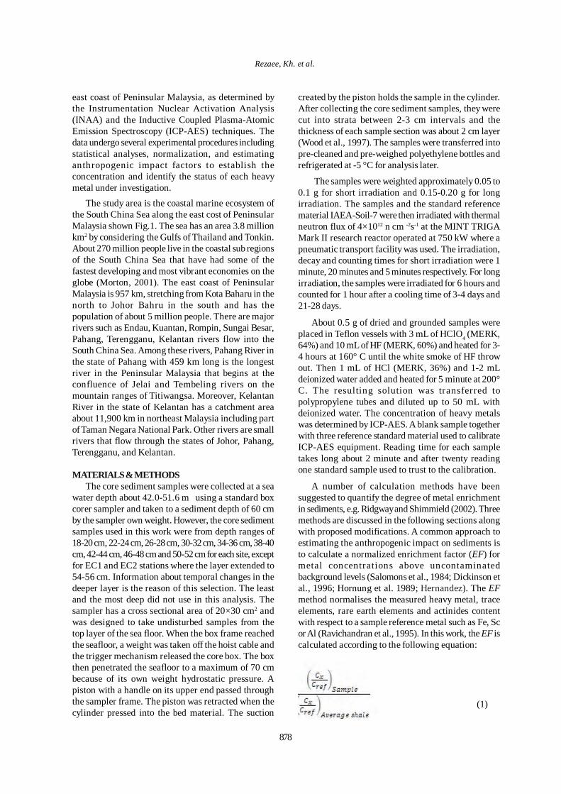
878
Rezaee, Kh. et al.
east coast of Peninsular Malaysia, as determined bythe Instrumentation Nuclear Activation Analysis(INAA) and the Inductive Coupled Plasma-AtomicEmission Spectroscopy (ICP-AES) techniques. Thedata undergo several experimental procedures includingstatistical analyses, normalization, and estimatinganthropogenic impact factors to establish theconcentration and identify the status of each heavymetal under investigation.
The study area is the coastal marine ecosystem ofthe South China Sea along the east cost of PeninsularMalaysia shown Fig.1. The sea has an area 3.8 millionkm2 by considering the Gulfs of Thailand and Tonkin.About 270 million people live in the coastal sub regionsof the South China Sea that have had some of thefastest developing and most vibrant economies on theglobe (Morton, 2001). The east coast of PeninsularMalaysia is 957 km, stretching from Kota Baharu in thenorth to Johor Bahru in the south and has thepopulation of about 5 million people. There are majorrivers such as Endau, Kuantan, Rompin, Sungai Besar,Pahang, Terengganu, Kelantan rivers flow into theSouth China Sea. Among these rivers, Pahang River inthe state of Pahang with 459 km long is the longestriver in the Peninsular Malaysia that begins at theconfluence of Jelai and Tembeling rivers on themountain ranges of Titiwangsa. Moreover, KelantanRiver in the state of Kelantan has a catchment areaabout 11,900 km in northeast Malaysia including partof Taman Negara National Park. Other rivers are smallrivers that flow through the states of Johor, Pahang,Terengganu, and Kelantan.
MATERIALS & METHODSThe core sediment samples were collected at a sea
water depth about 42.0-51.6 m using a standard boxcorer sampler and taken to a sediment depth of 60 cmby the sampler own weight. However, the core sedimentsamples used in this work were from depth ranges of18-20 cm, 22-24 cm, 26-28 cm, 30-32 cm, 34-36 cm, 38-40cm, 42-44 cm, 46-48 cm and 50-52 cm for each site, exceptfor EC1 and EC2 stations where the layer extended to54-56 cm. Information about temporal changes in thedeeper layer is the reason of this selection. The leastand the most deep did not use in this analysis. Thesampler has a cross sectional area of 20×30 cm2 andwas designed to take undisturbed samples from thetop layer of the sea floor. When the box frame reachedthe seafloor, a weight was taken off the hoist cable andthe trigger mechanism released the core box. The boxthen penetrated the seafloor to a maximum of 70 cmbecause of its own weight hydrostatic pressure. Apiston with a handle on its upper end passed throughthe sampler frame. The piston was retracted when thecylinder pressed into the bed material. The suction
created by the piston holds the sample in the cylinder.After collecting the core sediment samples, they werecut into strata between 2-3 cm intervals and thethickness of each sample section was about 2 cm layer(Wood et al., 1997). The samples were transferred intopre-cleaned and pre-weighed polyethylene bottles andrefrigerated at -5 °C for analysis later.
The samples were weighted approximately 0.05 to0.1 g for short irradiation and 0.15-0.20 g for longirradiation. The samples and the standard referencematerial IAEA-Soil-7 were then irradiated with thermalneutron flux of 4×10¹² n cm -2s-1 at the MINT TRIGAMark II research reactor operated at 750 kW where apneumatic transport facility was used. The irradiation,decay and counting times for short irradiation were 1minute, 20 minutes and 5 minutes respectively. For longirradiation, the samples were irradiated for 6 hours andcounted for 1 hour after a cooling time of 3-4 days and21-28 days.
About 0.5 g of dried and grounded samples wereplaced in Teflon vessels with 3 mL of HClO4 (MERK,64%) and 10 mL of HF (MERK, 60%) and heated for 3-4 hours at 160° C until the white smoke of HF throwout. Then 1 mL of HCl (MERK, 36%) and 1-2 mLdeionized water added and heated for 5 minute at 200°C. The resulting solution was transferred topolypropylene tubes and diluted up to 50 mL withdeionized water. The concentration of heavy metalswas determined by ICP-AES. A blank sample togetherwith three reference standard material used to calibrateICP-AES equipment. Reading time for each sampletakes long about 2 minute and after twenty readingone standard sample used to trust to the calibration.
A number of calculation methods have beensuggested to quantify the degree of metal enrichmentin sediments, e.g. Ridgway and Shimmield (2002). Threemethods are discussed in the following sections alongwith proposed modifications. A common approach toestimating the anthropogenic impact on sediments isto calculate a normalized enrichment factor (EF) formetal concentrations above uncontaminatedbackground levels (Salomons et al., 1984; Dickinson etal., 1996; Hornung et al. 1989; Hernandez). The EFmethod normalises the measured heavy metal, traceelements, rare earth elements and actinides contentwith respect to a sample reference metal such as Fe, Scor Al (Ravichandran et al., 1995). In this work, the EF iscalculated according to the following equation:
(1)
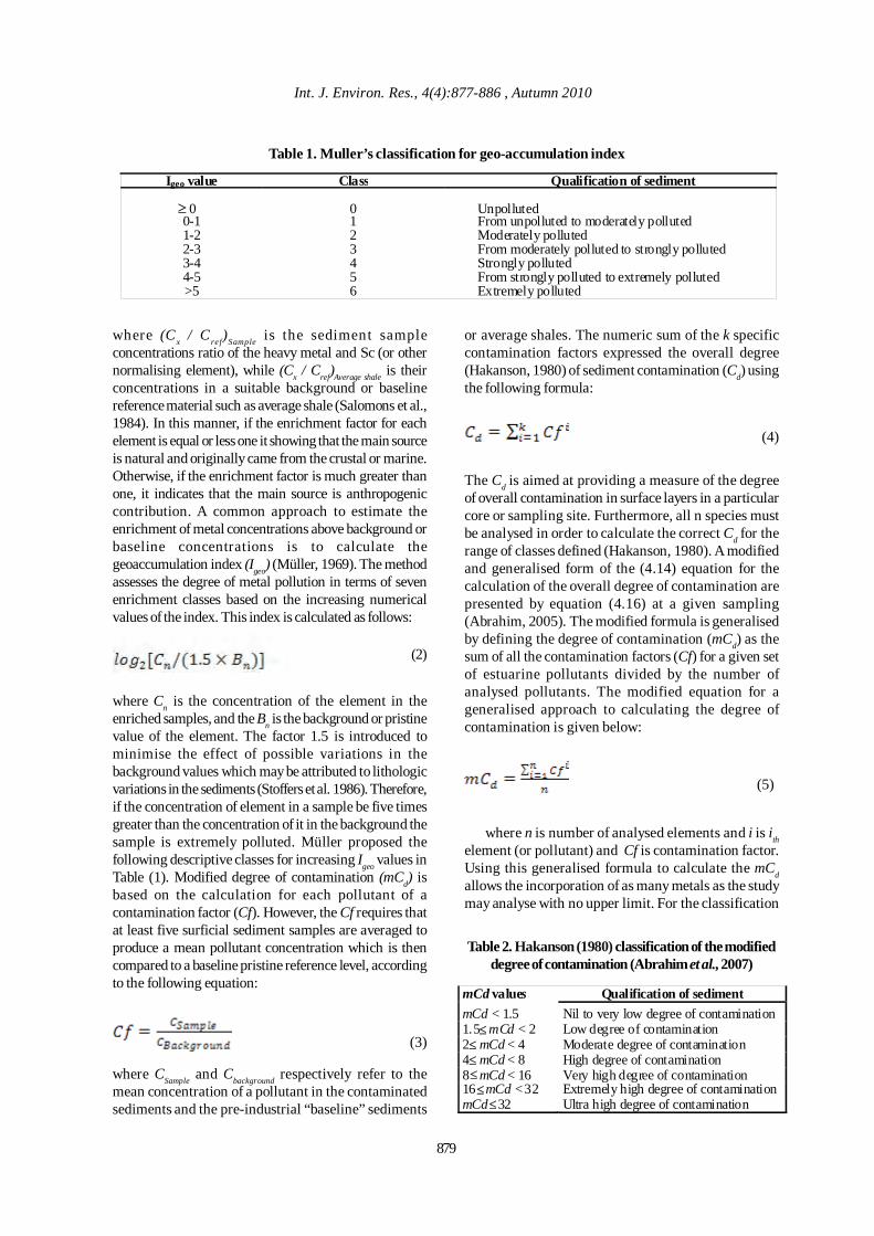
Int. J. Environ. Res., 4(4):877-886 , Autumn 2010
879
where (Cx / Cref)Sample is the sediment sampleconcentrations ratio of the heavy metal and Sc (or othernormalising element), while (Cx / Cref)Average shale is theirconcentrations in a suitable background or baselinereference material such as average shale (Salomons et al.,1984). In this manner, if the enrichment factor for eachelement is equal or less one it showing that the main sourceis natural and originally came from the crustal or marine.Otherwise, if the enrichment factor is much greater thanone, it indicates that the main source is anthropogeniccontribution. A common approach to estimate theenrichment of metal concentrations above background orbaseline concentrations is to calculate thegeoaccumulation index (Igeo) (Müller, 1969). The methodassesses the degree of metal pollution in terms of sevenenrichment classes based on the increasing numericalvalues of the index. This index is calculated as follows:
(2)
where Cn is the concentration of the element in theenriched samples, and the Bn is the background or pristinevalue of the element. The factor 1.5 is introduced tominimise the effect of possible variations in thebackground values which may be attributed to lithologicvariations in the sediments (Stoffers et al. 1986). Therefore,if the concentration of element in a sample be five timesgreater than the concentration of it in the background thesample is extremely polluted. Müller proposed thefollowing descriptive classes for increasing Igeo values inTable (1). Modified degree of contamination (mCd) isbased on the calculation for each pollutant of acontamination factor (Cf). However, the Cf requires thatat least five surficial sediment samples are averaged toproduce a mean pollutant concentration which is thencompared to a baseline pristine reference level, accordingto the following equation:
(3)
where CSample and Cbackground respectively refer to themean concentration of a pollutant in the contaminatedsediments and the pre-industrial “baseline” sediments
Table 1. Muller’s classification for geo-accumulation index
Igeo value Class Qualification of sediment
0 0 Unpolluted 0-1 1 From unpolluted to moderately polluted 1-2 2 Moderately polluted 2-3 3 From moderately polluted to strongly polluted 3-4 4 Strongly polluted 4-5 5 From strongly polluted to extremely polluted >5 6 Extremely polluted
or average shales. The numeric sum of the k specificcontamination factors expressed the overall degree(Hakanson, 1980) of sediment contamination (Cd) usingthe following formula:
(4)
The Cd is aimed at providing a measure of the degreeof overall contamination in surface layers in a particularcore or sampling site. Furthermore, all n species mustbe analysed in order to calculate the correct Cd for therange of classes defined (Hakanson, 1980). A modifiedand generalised form of the (4.14) equation for thecalculation of the overall degree of contamination arepresented by equation (4.16) at a given sampling(Abrahim, 2005). The modified formula is generalisedby defining the degree of contamination (mCd) as thesum of all the contamination factors (Cf) for a given setof estuarine pollutants divided by the number ofanalysed pollutants. The modified equation for ageneralised approach to calculating the degree ofcontamination is given below:
(5)
where n is number of analysed elements and i is ithelement (or pollutant) and Cf is contamination factor.Using this generalised formula to calculate the mCdallows the incorporation of as many metals as the studymay analyse with no upper limit. For the classification
mCd values Qualification of sedimentmCd < 1.5 Nil to very low degree of contamination 1.5 mCd < 2 Low degree of contamination 2 mCd < 4 Moderate degree of contamination 4 mCd < 8 High degree of contamination 8 mCd < 16 Very high degree of contamination 16 mCd < 32 Extremely high degree of contamination mCd 32 Ultra high degree of contamination
Table 2. Hakanson (1980) classification of the modifieddegree of contamination (Abrahim et al., 2007)
≥
≤≤≤≤≤≤
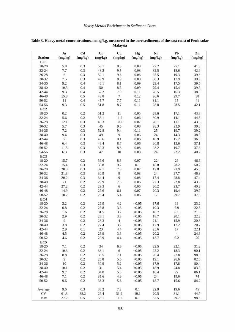
880
Heavy Metals Enrichment in Sediment Cores
Table 3. Heavy metal concentrations, in mg/kg, measured in the core sediments of the east coast of PeninsularMalaysia
Station As
(mg/kg) Cd
(mg/kg) Cr
(mg/kg) Cu
(mg/kg) Hg
(mg/kg) Ni
(mg/kg) Pb
(mg/kg) Zn
(mg/kg) EC1 18-20 5.8 0.3 53.1 9.3 0.08 27.2 25.1 41.3 22-24 7.7 0.3 48.2 9.5 0.08 32.5 18.6 42.9 26-28 6 0.3 52.1 9.8 0.06 25.5 19.3 39.8 30-32 7.5 0.3 49.9 8.9 0.08 30.3 17.9 39.9 34-36 9.2 0.4 48.1 8.1 0.09 29.4 17.5 39.5 38-40 10.5 0.4 50 8.6 0.09 29.4 15.4 39.5 42-44 9.3 0.4 52.2 7.9 0.11 28.5 16.3 38.9 46-48 15.8 0.5 49.8 7 0.12 26.6 29.7 38 50-52 11 0.4 45.7 7.7 0.11 31.1 15 41 54-56 9.3 0.5 51.8 8.7 0.11 28.8 28.5 42.1 EC2 18-20 0.2 0.2 51.2 11 0.05 28.6 17.1 43.3 22-24 5.6 0.2 53.1 11.2 0.06 30.9 14.1 44.8 26-28 12.1 0.3 49.3 10.2 0.07 28.1 11.1 43.6 30-32 5.7 0.3 45 9.5 0.08 28.3 23.9 39.8 34-36 7.2 0.3 52.8 9.4 0.11 25 19.7 39.2 38-40 9.4 0.3 49 9 0.06 24 14.3 38.3 42-44 7 0.3 43.6 9.1 0.06 18.9 15.2 36.3 46-48 6.4 0.3 46.4 8.7 0.06 20.8 12.6 37.1 50-52 11.5 0.3 39.3 8.8 0.08 28.2 19.7 37.6 54-56 6.3 0.3 47 10 0.08 24 22.2 40.2 EC3 18-20 15.7 0.2 36.6 8.8 0.07 22 29 46.6 22-24 15.4 0.3 33.8 9.2 0.1 18.8 28.2 50.2 26-28 20.3 0.3 37.1 7.9 0.07 17.8 21.9 45.8 30-32 21.3 0.3 30.9 9 0.08 24 27.7 46.3 34-36 20.2 0.3 34.4 9 0.08 17.4 28.8 47.4 38-40 21 0.2 29.9 7.3 0.06 22.3 22.8 43.9 42-44 27.2 0.2 29.3 6 0.06 20.2 23.7 40.2 46-48 14.9 0.2 27.6 6.1 0.07 20.3 19.4 39.7 50-52 18.7 0.2 23.4 5.4 0.06 17 29.7 37.5 EC4 18-20 2.2 0.2 29.9 4.2 <0.05 17.6 13 23.2 22-24 0.8 0.2 25.8 3.8 <0.05 19.3 7.9 22.5 26-28 1.6 0.2 31.5 3.2 <0.05 18.7 6.1 21.5 30-32 2.9 0.2 28.1 3.3 <0.05 18.7 20.1 22.2 34-36 9 0.2 23.3 4 <0.05 21.1 15.9 20.8 38-40 3.8 0.2 27.4 3.2 <0.05 17.9 17.2 20.7 42-44 2.9 0.1 23 4.4 <0.05 23.6 17 22.1 46-48 4.5 0.2 28.9 3.3 <0.05 20.2 - 24.3 50-52 4.6 0.2 23.9 4.4 <0.05 13.7 6.2 26 EC5 18-20 7.1 0.2 34 6.6 <0.05 22.5 22.1 31.2 22-24 10.3 0.2 33.1 6 <0.05 22.2 18.3 90.1 26-28 8.8 0.2 33.5 7.1 <0.05 20.4 27.8 98.3 30-32 9 0.2 25.8 5.6 <0.05 19.1 26.6 82.6 34-36 10 0.2 30.9 5.2 <0.05 17.9 17.8 80.4 38-40 10.1 0.2 31 5.4 <0.05 18.9 24.8 83.8 42-44 9.7 0.2 34.8 5.3 <0.05 18.4 22 86.1 46-48 7.1 0.2 35.6 4.9 <0.05 24 19.6 74 50-52 9.6 0.2 36.3 5.6 <0.05 18.7 15.6 84.2
Average 9.6 0.3 38.2 7.2 0.1 22.9 19.6 45
CV 61.3 38.2 26.4 31.9 19.1 20.5 31.1 44.7 Max 27.2 0.5 53.1 11.2 0.1 32.5 29.7 98.3
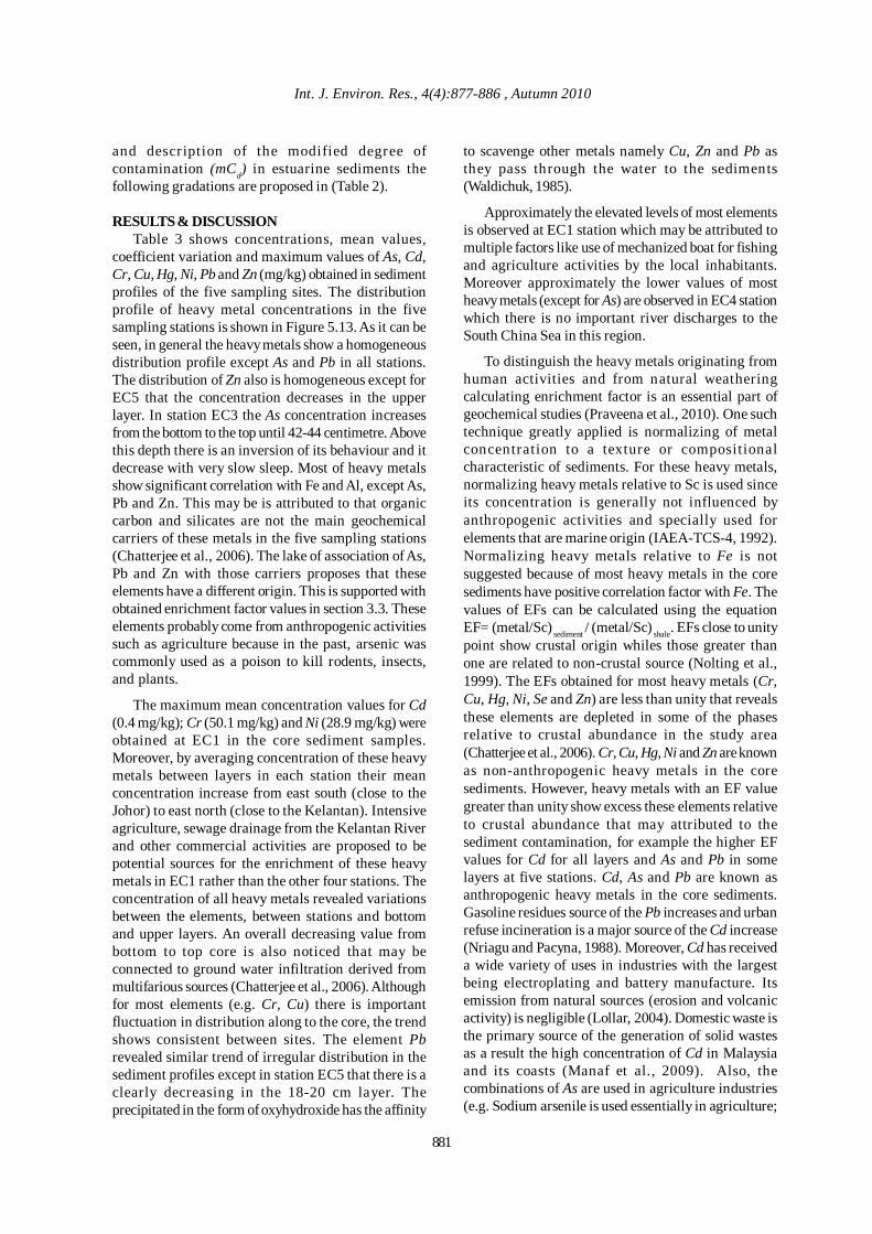
Int. J. Environ. Res., 4(4):877-886 , Autumn 2010
and description of the modified degree ofcontamination (mCd) in estuarine sediments thefollowing gradations are proposed in (Table 2).
RESULTS & DISCUSSIONTable 3 shows concentrations, mean values,
coefficient variation and maximum values of As, Cd,Cr, Cu, Hg, Ni, Pb and Zn (mg/kg) obtained in sedimentprofiles of the five sampling sites. The distributionprofile of heavy metal concentrations in the fivesampling stations is shown in Figure 5.13. As it can beseen, in general the heavy metals show a homogeneousdistribution profile except As and Pb in all stations.The distribution of Zn also is homogeneous except forEC5 that the concentration decreases in the upperlayer. In station EC3 the As concentration increasesfrom the bottom to the top until 42-44 centimetre. Abovethis depth there is an inversion of its behaviour and itdecrease with very slow sleep. Most of heavy metalsshow significant correlation with Fe and Al, except As,Pb and Zn. This may be is attributed to that organiccarbon and silicates are not the main geochemicalcarriers of these metals in the five sampling stations(Chatterjee et al., 2006). The lake of association of As,Pb and Zn with those carriers proposes that theseelements have a different origin. This is supported withobtained enrichment factor values in section 3.3. Theseelements probably come from anthropogenic activitiessuch as agriculture because in the past, arsenic wascommonly used as a poison to kill rodents, insects,and plants.
The maximum mean concentration values for Cd(0.4 mg/kg); Cr (50.1 mg/kg) and Ni (28.9 mg/kg) wereobtained at EC1 in the core sediment samples.Moreover, by averaging concentration of these heavymetals between layers in each station their meanconcentration increase from east south (close to theJohor) to east north (close to the Kelantan). Intensiveagriculture, sewage drainage from the Kelantan Riverand other commercial activities are proposed to bepotential sources for the enrichment of these heavymetals in EC1 rather than the other four stations. Theconcentration of all heavy metals revealed variationsbetween the elements, between stations and bottomand upper layers. An overall decreasing value frombottom to top core is also noticed that may beconnected to ground water infiltration derived frommultifarious sources (Chatterjee et al., 2006). Althoughfor most elements (e.g. Cr, Cu) there is importantfluctuation in distribution along to the core, the trendshows consistent between sites. The element Pbrevealed similar trend of irregular distribution in thesediment profiles except in station EC5 that there is aclearly decreasing in the 18-20 cm layer. Theprecipitated in the form of oxyhydroxide has the affinity
to scavenge other metals namely Cu, Zn and Pb asthey pass through the water to the sediments(Waldichuk, 1985).
Approximately the elevated levels of most elementsis observed at EC1 station which may be attributed tomultiple factors like use of mechanized boat for fishingand agriculture activities by the local inhabitants.Moreover approximately the lower values of mostheavy metals (except for As) are observed in EC4 stationwhich there is no important river discharges to theSouth China Sea in this region.
To distinguish the heavy metals originating fromhuman activities and from natural weatheringcalculating enrichment factor is an essential part ofgeochemical studies (Praveena et al., 2010). One suchtechnique greatly applied is normalizing of metalconcentration to a texture or compositionalcharacteristic of sediments. For these heavy metals,normalizing heavy metals relative to Sc is used sinceits concentration is generally not influenced byanthropogenic activities and specially used forelements that are marine origin (IAEA-TCS-4, 1992).Normalizing heavy metals relative to Fe is notsuggested because of most heavy metals in the coresediments have positive correlation factor with Fe. Thevalues of EFs can be calculated using the equationEF= (metal/Sc) sediment / (metal/Sc) shale. EFs close to unitypoint show crustal origin whiles those greater thanone are related to non-crustal source (Nolting et al.,1999). The EFs obtained for most heavy metals (Cr,Cu, Hg, Ni, Se and Zn) are less than unity that revealsthese elements are depleted in some of the phasesrelative to crustal abundance in the study area(Chatterjee et al., 2006). Cr, Cu, Hg, Ni and Zn are knownas non-anthropogenic heavy metals in the coresediments. However, heavy metals with an EF valuegreater than unity show excess these elements relativeto crustal abundance that may attributed to thesediment contamination, for example the higher EFvalues for Cd for all layers and As and Pb in somelayers at five stations. Cd, As and Pb are known asanthropogenic heavy metals in the core sediments.Gasoline residues source of the Pb increases and urbanrefuse incineration is a major source of the Cd increase(Nriagu and Pacyna, 1988). Moreover, Cd has receiveda wide variety of uses in industries with the largestbeing electroplating and battery manufacture. Itsemission from natural sources (erosion and volcanicactivity) is negligible (Lollar, 2004). Domestic waste isthe primary source of the generation of solid wastesas a result the high concentration of Cd in Malaysiaand its coasts (Manaf et al., 2009). Also, thecombinations of As are used in agriculture industries(e.g. Sodium arsenile is used essentially in agriculture;
881
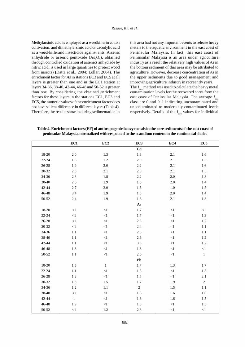
882
Rezaee, Kh. et al.
Methylarsinic acid is employed as a weedkillerin cottoncultivation, and dimethylarsinic acid or cacodylic acidas a weed-killerand insecticide against ants; Arsenicanhydride or arsenic pentoxide (As2O5), obtainedthrough controlled oxidation of arsenics anhydride bynitric acid, is used in large quantities to protect woodfrom insects) (Datta et al., 2004; Lollar, 2004). Theenrichment factor for As in stations EC3 and EC5 at alllayers is greater than one and in the EC1 station atlayers 34-36, 38-40, 42-44, 46-48 and 50-52 is greaterthan one. By considering the obtained enrichmentfactors for these layers in the stations EC1, EC3 andEC5, the numeric values of the enrichment factor doesnot have salient difference in different layers (Table 4).Therefore, the results show in during sedimentation in
Table 4. Enrichment factors (EF) of anthropogenic heavy metals in the core sediments of the east coast ofpeninsular Malaysia, normalized with respected to the scandium content in the continental shales
EC1 EC2 EC3 EC4 EC5 Cd
18-20 2.0 1.3 1.3 2.1 1.6 22-24 1.8 1.2 2.0 2.1 1.5 26-28 1.9 2.0 2.2 2.1 1.6 30-32 2.3 2.1 2.0 2.1 1.5 34-36 2.8 1.8 2.2 2.0 1.3 38-40 2.6 1.9 1.5 2.0 1.4 42-44 2.7 2.0 1.5 1.0 1.5 46-48 3.4 1.9 1.5 2.0 1.4 50-52 2.4 1.9 1.6 2.1 1.3
As 18-20 <1 <1 1.7 <1 <1 22-24 <1 <1 1.7 <1 1.3 26-28 <1 <1 2.5 <1 1.2 30-32 <1 <1 2.4 <1 1.1 34-36 1.1 <1 2.5 <1 1.1 38-40 1.1 <1 2.6 <1 1.2 42-44 1.1 <1 3.3 <1 1.2 46-48 1.8 <1 1.8 <1 <1 50-52 1.1 <1 2.6 <1 1
Pb 18-20 1.5 1 1.7 1.3 1.7 22-24 1.1 <1 1.8 <1 1.3 26-28 1.2 <1 1.5 <1 2.1 30-32 1.3 1.5 1.7 1.9 2 34-36 1.2 1.1 2 1.5 1.1 38-40 <1 <1 1.6 1.6 1.6 42-44 1 <1 1.6 1.6 1.5 46-48 1.9 <1 1.3 <1 1.3 50-52 <1 1.2 2.3 <1 <1
this area had not any important events to release heavymetals to the aquatic environment in the east coast ofPeninsular Malaysia. In fact, this east coast ofPeininsular Malaysia is an area under agricultureindustry as a result the relatively high values of As inthe bottom sediment of this area may be attributed toagriculture. However, decrease concentration of As inthe upper sediments due to good management andimproving agriculture industry in recreantly years.The Igeo method was used to calculate the heavy metalcontamination levels for the recovered cores from theeast coast of Peninsular Malaysia. The average Igeoclass are 0 and 0–1 indicating uncontaminated anduncontaminated to moderately contaminated levelsrespectively. Details of the Igeo values for individual
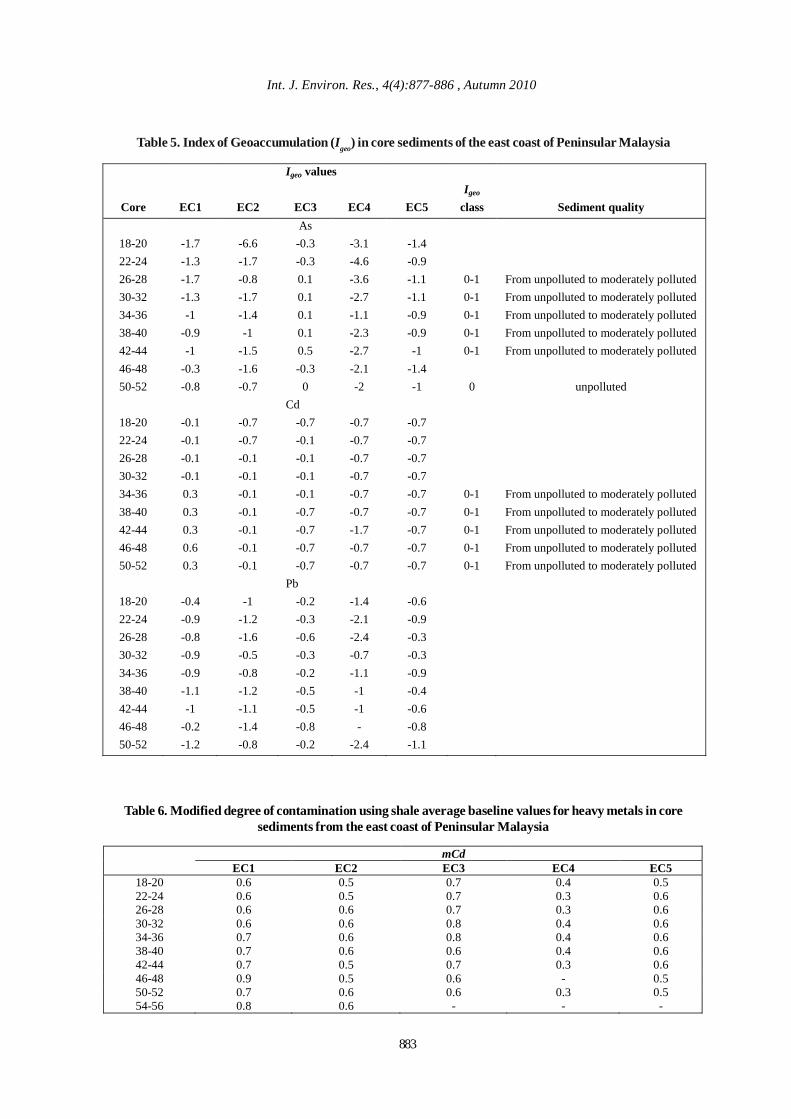
883
Int. J. Environ. Res., 4(4):877-886 , Autumn 2010
Table 5. Index of Geoaccumulation (Igeo) in core sediments of the east coast of Peninsular Malaysia
Igeo values
Core EC1 EC2 EC3 EC4 EC5 Igeo
class Sediment quality As
18-20 -1.7 -6.6 -0.3 -3.1 -1.4 22-24 -1.3 -1.7 -0.3 -4.6 -0.9 26-28 -1.7 -0.8 0.1 -3.6 -1.1 0-1 From unpolluted to moderately polluted 30-32 -1.3 -1.7 0.1 -2.7 -1.1 0-1 From unpolluted to moderately polluted 34-36 -1 -1.4 0.1 -1.1 -0.9 0-1 From unpolluted to moderately polluted 38-40 -0.9 -1 0.1 -2.3 -0.9 0-1 From unpolluted to moderately polluted 42-44 -1 -1.5 0.5 -2.7 -1 0-1 From unpolluted to moderately polluted 46-48 -0.3 -1.6 -0.3 -2.1 -1.4 50-52 -0.8 -0.7 0 -2 -1 0 unpolluted
Cd 18-20 -0.1 -0.7 -0.7 -0.7 -0.7 22-24 -0.1 -0.7 -0.1 -0.7 -0.7 26-28 -0.1 -0.1 -0.1 -0.7 -0.7 30-32 -0.1 -0.1 -0.1 -0.7 -0.7 34-36 0.3 -0.1 -0.1 -0.7 -0.7 0-1 From unpolluted to moderately polluted 38-40 0.3 -0.1 -0.7 -0.7 -0.7 0-1 From unpolluted to moderately polluted 42-44 0.3 -0.1 -0.7 -1.7 -0.7 0-1 From unpolluted to moderately polluted 46-48 0.6 -0.1 -0.7 -0.7 -0.7 0-1 From unpolluted to moderately polluted 50-52 0.3 -0.1 -0.7 -0.7 -0.7 0-1 From unpolluted to moderately polluted
Pb 18-20 -0.4 -1 -0.2 -1.4 -0.6 22-24 -0.9 -1.2 -0.3 -2.1 -0.9 26-28 -0.8 -1.6 -0.6 -2.4 -0.3 30-32 -0.9 -0.5 -0.3 -0.7 -0.3 34-36 -0.9 -0.8 -0.2 -1.1 -0.9 38-40 -1.1 -1.2 -0.5 -1 -0.4 42-44 -1 -1.1 -0.5 -1 -0.6 46-48 -0.2 -1.4 -0.8 - -0.8 50-52 -1.2 -0.8 -0.2 -2.4 -1.1
Table 6. Modified degree of contamination using shale average baseline values for heavy metals in coresediments from the east coast of Peninsular Malaysia
mCd EC1 EC2 EC3 EC4 EC5
18-20 0.6 0.5 0.7 0.4 0.5 22-24 0.6 0.5 0.7 0.3 0.6 26-28 0.6 0.6 0.7 0.3 0.6 30-32 0.6 0.6 0.8 0.4 0.6 34-36 0.7 0.6 0.8 0.4 0.6 38-40 0.7 0.6 0.6 0.4 0.6 42-44 0.7 0.5 0.7 0.3 0.6 46-48 0.9 0.5 0.6 - 0.5 50-52 0.7 0.6 0.6 0.3 0.5 54-56 0.8 0.6 - - -
884
Heavy Metals Enrichment in Sediment Cores
elements in the nine cores at five sampling are pre-sented in Table 5. The negative Igeo values found in thetable are the results of relatively low levels of contami-nation for some metals in some cores and the back-ground variability factor (1.5) in the Igeo equation.In the core sediments of the east coast of PeninsularMalaysia, the revised Hakanson equation (5) is usedto calculate the modified degree of contamination (mCd)for the all analysed trace elements. The results for eachcore are presented in Table 6. The mCd for the indi-vidual cores lie in the range 0.3-0.9 that is less than 1.5showing nit to very low degree of contamination in theeast coast of Peninsular Malaysia sediments. The mCddata indicate non-anthropogenic impact in all cores.
The results of the various methods for calculatingheavy metal enrichment in the east coast of PeninsularMalaysia sediments showed approximately sameobtained results in difference methods. Moreover, isused of the core deepest as a reference concentrationand averagely results demonstrate that, using thecontinental shale as a reference concentration theenrichment factor is relatively high. The results of allmethods enrichment factor, geoaccumulation index andmodified degree of contamination of this study showedthere is not any important pollutant in the east coastof Peninsula Malaysia.
Clearly, in any survey of marine, estuarine orfreshwater sediments, the best approach is to penetratebelow the present day surface contamination andsample the pristine or least contaminated sedimentsavailable at depth in cores from the target survey area.This will allow the determination of realistic baselinevalues for the target area. This approach will work bestin areas that have only suffered relatively recentcontamination such as in countries that have relativelyyoung industrial histories such as Malaysia where itis possible in most cases to get below the level of firstanthropogenic impact.
Moreover, the result was also compared to USNOAA’s sediments quality guidelines for estimatingthe possible environmental consequences of metalsanalyzed. In this study, just Effect Range-Low (ER-L)and Effect Range-Medium (ER-M) are considered. TheER-L shows chemical concentrations below whichhostile biological effects were rarely observed and theER-M shows concentrations above which effects weremore frequently observed (Long et al., 1995 and 1997).By considering the concentration values of the heavymetals at each layer in five stations, the majority of theelements revealed low values.
CONCLUSIONThe impact of anthropogenic heavy metal pollution
on the South China Sea along the east coast of
Peninsular Malaysia was evaluated using EnrichmentFactors (EF), geoaccumulation indices (Igeo) andmodified degrees of contamination (mCd) for As, Cd,Cr, Cu, Hg, Pb and Zn in marine sediments in nine coresat five sites.
The geoaccumulation indices (Igeo) are distinctlyvariable and suggest that marine sediments in thevarious the east coast of Peninsular Malaysia coresrange from uncontaminated to moderatelycontaminated with respect to the analysed heavymetals. The uncontaminated Igeo designation is clearlysupported by the other methods for calculating heavymetal pollution impact in the east coast of PeninsularMalaysia.
Normalised enrichment factor (EF) values for eightheavy metals were calculated for the east coast ofPeninsular Malaysia using the continental shaleabundance of Fe. The results show that using the Feconcentration in the continental shale as a normaliserproduces higher than two EF values for Cd for all coresamples and higher than one for As and Pb in somecore samples that indicate anthropogenic activity forthese heavy metals. The enrichment factor method ishowever the most relevant to the east coast ofPeninsular Malaysia. With regard to an overall measureof heavy metal contamination applicable to estuarineor coastal sediments, the present study proposes amodified and generalised form of the Hakanson (1980)pollution impact equation. A modified degree ofcontamination (mCd) is proposed in which the sum ofthe individual contamination factors is divided by thenumber of analysed pollutants. Overall, the range ofmCd values indicates nil to very low degree of marinesediment contamination in the east coast of PeninsularMalaysia cores.
ACKNOWLEDGEMENTSThe authors are thankful to the staff of TRIGA
Mark II research reactor especially to Dr. Abdul KhalikWood at Nuclear Institute in Malaysia for theirassistance during the execution of work.
REFERENCESAbdullah, M. H., Sidi, J. and Aris, A. Z. (2007). HeavyMetals (Cd, Cu, Cr, Pb and Zn) in Meretrix meretrix Roding,Water and Sediments from Estuaries in Sabah, North Borneo,International Journal of Environmental & Science Education,2 (3), 69- 74.
Abrahim, G. M. S., Parker, R. J. and Nichol, S. L. (2005).Distribution and Assessment of Sediment Toxicity in TamakiEstuary, Auckland, New Zealand. Environmental Geology,52, 1315-1323.
Abrahim, G. M. S. and Parker, R. J. (2007). Assessment ofHeavy Metal Enrichment Factors and the Degree ofContamination in Marine Sediments from Tamaki Estuary,
Int. J. Environ. Res., 4(4):877-886 , Autumn 2010
Auckland, New Zealand, Environ Monit Assess, 136, 227-238.
Chatterjee, M., Silva Filho, E. V., Sarkar, S. K., Sella, S. M.,Bhattacharya, A., Satpathy, K. K., Prasad, M. V. R.,Chakraborty, S. and Bhattacharya, B. D. (2006). Distributionand Possible Source of Trace Elements in the Sediment Coresof a Tropical Macrotidal Estuary and Their EcotoxicologicalSignificance, Environment International, 33, 346-356.
Dickinson, W. W., Dunbar, G. B. and McLeod, H. (1996).Heavy Metal History from Cores in Wellington Harbour,New Zealand. Environmental Geology, 27, 59–69.
Datta, P. K., Ray, A. K. Sharma, V. K. and Millero, F. J.(2004). Adsorption of Arsenate and Arsenic on TitaniumDioxide Suspensions. Journal Colloid Interface Sci., 278,270-275.
Enell, M. and Wennberg, L. (1991). Distribution ofHalogenated Organic Compounds (AOX)—SwedishTtransport to Surrounding Sea Areas and Mass BalanceStudies in Five Drainage Systems. Wat. Sci. Tech., 24,385-395.
Forstner, U. (1989). Contaminated Sediments: Lectureson Environmental Aspects of Part icle-AssociatedChemicals in Aquatic Systems (Lecture Notes in EarthSciences, 21. Springer, Berlin, Germany.
Fowler, V. M. (1990). Tropomodulin. A CytoskeletalProtein that Binds to the End of ErythrocyteTropomyosin and Inhibits Tropomyosin Bbinding toActin. J. Cell Biol, 111, 471-482.
Hakanson, L. (1980). Ecological Risk Index for AquaticPollution Control. A Sedimentological Approach. WaterResearch, 14, 975-1001.
Hernandez, L., Probst, A., Probst, J. L. and Ulrich, E.(2003). Heavy metal distribution in some French forestsoils: evidence for atmosphere contamination. The Scienceof Total Environment, 312, 195-210.
Hornung, H., Karm, M. D., and Cohen, Y. (1989). TraceMetal Distribution on Sediments and Benthic Fauna ofHaifa Bay, Israel. Estuarine, Coastal and Shelf Science,29, 43-56.
Leach, J. M., Howard, T. E. and Lanz, H. E. (1985).Chlorinated Organics in Shellfish from Coastal Waters.Pulp and Paper Canada, 86, 12, T398-T401.
Lollar, B. Sh. (2005). Environmental Geochemistry. FirstEdition. Elsevier Science: Amesterdam, Netherlands.
Long, E. R., MacDonald, D. D., Smith, S. L. and Calder,F. D. (1995). Incidence of Adverse Biological EffectsWithin Ranges of Chemical Concentrations in Marine andEstuarine Sediments, Environm. Manage., 19, 81-97.
Long, E. R. and Wilson, C. J. (1997). On the Identificationof Toxic Hot Spots Using Measures of the SedimentQuality Triad. Marine Pollution Bulletin, 34, 373-374.
Malin, E. K., Rauch, S., Morrison, G. M. and Andam, K.(2003). Impact of automobile emissions on the levels of
platinum and lead in Accra, Ghana. Journal ofEnvironmental Monitoring, 5, 91-95.
Manaf, L. A., Samah, M. A. A. and Zukki, N. I. M.(2009). Municipal Solid Waste Management in Malaysia:Practices and Challenges. Waste Management, 29, 2902–2906.
Morrisey, D. J., Turner, S. J., Mills, G. N., Williamson,R. B. and Wise, B. E. (2003). Factor affecting thedistr ibut ion of ben thic macrofauna in estuariescontaminated by urban runoff. Marine EnvironmentalResearch, 55 (2), 113-136.
Milenkovic, M., Damjanovic, M. and Ristic, M. (2005).Study of Heavy Metal Pollution in Sediments from theIron Gate (Danube River), Serbia and Montenegro. PolishJournal of Environmental Studies, 14 (6), 781-787.
Morton, B. and Blackmore, G. (2001). South China Sea,Journal of Marine Pollution Bulletin, 42, 1236-1263.
Müller, G. (1969). Index of Geoaccumulation in theSediments of the Rhine River. Eojournal, 2, 108-118.
Nirmal Kumar, J. I., Soni, H. and Kumar, R. N. (2007).Evalution of Biomonitoring Approach to Study LakeContamination by Accumulation of Trace Elements inSelected Aquatic Macrophytes: A Case Study of KanewalCommunity Reserve, Gujarat. India. Apploed Ecologyand Environmental Research, 6 (1), 65-76.
Nolting, R. F., Ramkema, A. and Everaarts, J. M. (1999).The Geochemistry of Cu, Cd, Zn, Ni and Pb in SedimentCores from the Continental Slope of the Banc d’ Arguin(Mauritania), Continental Shelf Research, 19, 665-691.
Nriagu, J. O. and Pacyna, J. M. (1988). QuantitativeAssessment of Worldwide Contamination of Air, Waterand Soils by Trace Metals. Nature, 333, 134-139.
Praveena, S. M., Aris, A. Z. and Radojevic, M. (2010).Heavy Metals Dyanamics and Source In IntertidalMangrove Sediment of Sabah, Borneo Island.EnvironmentAsia, 3, 79-83.
Ravichandran, M., Baskaran, M., Santschi, P. H. andBianchi, T. S. (1995). History of Trace Metal Pollutionin Sabine-Neches Estuary, Beaumont, Texas. Environ. Sci.Tech., 29, 1495–1503.
Ridgway, J., and Shimmield, G. (2002). Estuaries asRepositories of Historical Contamination and TheirImpact on Shelf Seas. Estuarine, Coastal and Shelf Science,55, 903-928.
Salomons, W., and Förstner, U. (1984). Metals in theHydrocycle. Springer, Berlin Heidelberg Tokyo.
Stoffers, P., Glasby, G. P., Wilson, C. J., Davis, K. R. andWatter. P. (1986). Heavy Metal Pollution in WellingtonHarbour. New Zealand Journal of Marine and FreshwaterResearch, 20, 495-512.
Tatasukawa, R. and Kurokawa, A. (1990). Distributionof Heavy Metals in Soils of Vellar River Estuary, South
885

Rezaee, Kh. et al.
India. In Proc. Ann . Symp. of the Society ofEnvironmental Science, Japan Tokyo: Toranomon, 152.
Gribble, G. W. (1994). The Natural Product ion ofChlorinated Compounds. Environ. Sci. Technol., 28 (7),310-319.
IAEA-TCS-4. (1992) . Sampling and AnalyticalMethodologies for Instrumental Neutron ActivationAnalysis of Airborne Particulate Matter. InternationalAtomic Energy Agency (IAEA), Vienna, Austria.
Waldichuk, M. (1985). Biological Availability of Metalsto Marine Organisms. Mar. Pollut. Bull., 16, 7-11.
Wood, A. K. H., Ahmed, Z., Shazili, N. A. MD., Yaakob,R. and Carpenter, R. (1997). Geochemistry of Sedimentsin Johor Straits between Malaysia and Singapore.Continental Shelf Research, 17 (10), 1207-1228.
Young, E. (2007). Can ‘Fertilizing’ the Ocean CombatClimate Change? Companies are Planning to Boost theOcean’s Plankton, Hoping they will Harvest more CO2from the Air. But will it work? New Scientist, 15, 42-45.
886

Int. J. Environ. Res., 4(4):887-892, Autumn 2010ISSN: 1735-6865
Received 10 Nov. 2009; Revised 27 April 2010; Accepted 25 June 2010
*Corresponding author E-mail: [email protected]
887
Trihalomethanes Concentration in Different Components of Water TreatmentPlant and Water Distribution System in the North of Iran
Hassani, A. H. 1, Jafari, M. A.2* and Torabifar, B.3
1 Department of Environmental Engineering, Graduate School of the Environment and Energy,Science and Research Branch, Islamic Azad University, Tehran, Iran
2 Environmental Engineering, Young Researchers Club Rasht Branch, Islamic Azad UniversityRasht Branch, Guilan, Iran
3 Department of Environmental Engineering, Graduate Faculty of Environment, University ofTehran, Tehran, Iran
ABSTRACT: Since the surface water is one of the main potable water resources, the usage of chlorine as adisinfectant has increased. Consequently the production rate of disinfection by-products (DBPs) such asTrihalomethane (THM) compounds has grown dramatically. In this paper the THMS concentration changes inthe Sangar Water Treatment Plant (SWTP) and Rasht Water Distribution System (RWDS) is presented. Theduration of these monitoring tasks were 6 months in 2007 and samples were collected every 2 weeks. Watersamples were collected from five locations at SWTP and RWDS. Some independent variables including TotalOrganic Carbon (TOC), pH, temperature, and residual chlorine were measured by Pearson method to find arelation between THMS formation and these variables. In the case of TOC, Pearson method showed a corre-lation of r = 0.8096 for SWTP and r = 0.3696 for RWDS between THM formation and TOC. Also therelationship for SWTP was r = 0.239 and r = 0.2336 for RWDS between THM formation and temperature.Correlation between THM formation and pH, Pearson method showed r = 0.4658 for SWTP and r = 0.3232for RWDS. In the case of residual chlorine, Pearson method showed a relationship of r = 0.7354 for SWTP andr = 0.5623 for RWDS. Results proved a direct relation between THMS concentration and distance of chlorina-tion injection points. The results showed that in SWTP, 42.7 percent of THM compounds were removed aftersedimentation and filtration.
Key words: Disinfection by-products, Water distribution system, Chlorination, Guilan province
INTRODUCTIONThere is a variety of disinfection methods being
utilized world wide for treatment but chlorination is themost common method among these methods. Waterdisinfection with chlorine improves the hygienic qual-ity of water by eliminating waterborne bacterial patho-gens such as dysentery and diarrhea diseases, chol-era, typhoid fever, hepatitis A, etc. Residual chlorinecan protect water from secondary pollution in the wa-ter network; also Chlorine application is simpler thanother disinfectants. The usage of chlorine conse-quences a wide range of organic compounds (DBPs),which occur due to the reaction between chlorine withnatural organic compounds, mainly humic substances(Nikolaou, et al., 2001). One of the main groups of DBPsis THMS compounds. According to Clark et al, morethan 500 DBPs have been identified in tap water (Clark,et al., 1996). Chloroform, a DBP was first identified inthe finished drinking water in 1974 in the Netherlands
by Rook (1974) and in the United States by Bellar et al.(1974). As a result of Rook and Bellar findings, a sur-vey was conducted in the United States in 1975 by thenational organic reconnaissance for the water sup-plies of 27 large cities by Symons et al. (1975). Thisstudy revealed that four THMS are widespread in chlo-rinated drinking waters at trace concentrations: chlo-roform, bromo-dichloromethane (BDCM),dibromochloro-methane (DBCM) and bromoform. To-tal THMs (TTHMs) refers to the sum of these foursubstances (Rodriguez, et al., 2004). InternationalAgency for Research on Cancer (IARC) and some re-searchers reported that most THMS are carcinogenicin rodentsand mutagenic in a variety of systems(IARC, 1991; Marimoto et al., 1983; Simpson et al.,1998; Dodds et al., 1999). The United States Environ-mental Protection Agency (USEPA) classifies THMscompounds into cancer groups including: chloroform(CHC13), BDCM (CHBrCI2) and bromoform (CHBr3)
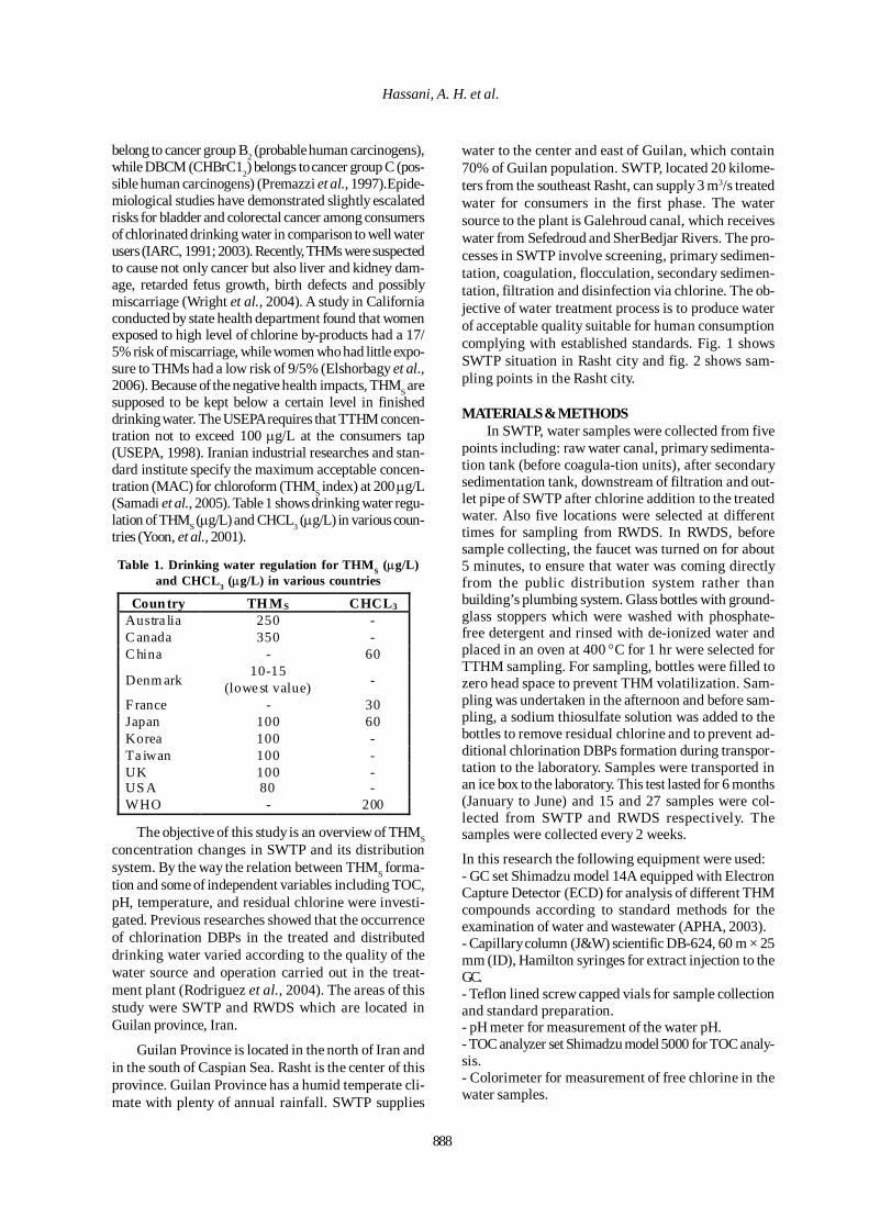
888
Hassani, A. H. et al.
belong to cancer group B2 (probable human carcinogens),while DBCM (CHBrC12) belongs to cancer group C (pos-sible human carcinogens) (Premazzi et al., 1997).Epide-miological studies have demonstrated slightly escalatedrisks for bladder and colorectal cancer among consumersof chlorinated drinking water in comparison to well waterusers (IARC, 1991; 2003). Recently, THMs were suspectedto cause not only cancer but also liver and kidney dam-age, retarded fetus growth, birth defects and possiblymiscarriage (Wright et al., 2004). A study in Californiaconducted by state health department found that womenexposed to high level of chlorine by-products had a 17/5% risk of miscarriage, while women who had little expo-sure to THMs had a low risk of 9/5% (Elshorbagy et al.,2006). Because of the negative health impacts, THMS aresupposed to be kept below a certain level in finisheddrinking water. The USEPA requires that TTHM concen-tration not to exceed 100 µg/L at the consumers tap(USEPA, 1998). Iranian industrial researches and stan-dard institute specify the maximum acceptable concen-tration (MAC) for chloroform (THMS index) at 200 µg/L(Samadi et al., 2005). Table 1 shows drinking water regu-lation of THMS (µg/L) and CHCL3 (µg/L) in various coun-tries (Yoon, et al., 2001).
Table 1. Drinking water regulation for THMS (µg/L)and CHCL3 (µg/L) in various countries
CHCL3 TH MS Coun try - 250 Austra lia - 350 C anada
60 - C hina
- 10-15
(lowe st value) Denm ark
30 - F rance 60 100 Japan - 100 Korea - 100 Ta iwan - 100 UK - 80 US A
200 - WHO
The objective of this study is an overview of THMSconcentration changes in SWTP and its distributionsystem. By the way the relation between THMS forma-tion and some of independent variables including TOC,pH, temperature, and residual chlorine were investi-gated. Previous researches showed that the occurrenceof chlorination DBPs in the treated and distributeddrinking water varied according to the quality of thewater source and operation carried out in the treat-ment plant (Rodriguez et al., 2004). The areas of thisstudy were SWTP and RWDS which are located inGuilan province, Iran.
Guilan Province is located in the north of Iran andin the south of Caspian Sea. Rasht is the center of thisprovince. Guilan Province has a humid temperate cli-mate with plenty of annual rainfall. SWTP supplies
water to the center and east of Guilan, which contain70% of Guilan population. SWTP, located 20 kilome-ters from the southeast Rasht, can supply 3 m3/s treatedwater for consumers in the first phase. The watersource to the plant is Galehroud canal, which receiveswater from Sefedroud and SherBedjar Rivers. The pro-cesses in SWTP involve screening, primary sedimen-tation, coagulation, flocculation, secondary sedimen-tation, filtration and disinfection via chlorine. The ob-jective of water treatment process is to produce waterof acceptable quality suitable for human consumptioncomplying with established standards. Fig. 1 showsSWTP situation in Rasht city and fig. 2 shows sam-pling points in the Rasht city.
MATERIALS & METHODSIn SWTP, water samples were collected from five
points including: raw water canal, primary sedimenta-tion tank (before coagula-tion units), after secondarysedimentation tank, downstream of filtration and out-let pipe of SWTP after chlorine addition to the treatedwater. Also five locations were selected at differenttimes for sampling from RWDS. In RWDS, beforesample collecting, the faucet was turned on for about5 minutes, to ensure that water was coming directlyfrom the public distribution system rather thanbuilding’s plumbing system. Glass bottles with ground-glass stoppers which were washed with phosphate-free detergent and rinsed with de-ionized water andplaced in an oven at 400 °C for 1 hr were selected forTTHM sampling. For sampling, bottles were filled tozero head space to prevent THM volatilization. Sam-pling was undertaken in the afternoon and before sam-pling, a sodium thiosulfate solution was added to thebottles to remove residual chlorine and to prevent ad-ditional chlorination DBPs formation during transpor-tation to the laboratory. Samples were transported inan ice box to the laboratory. This test lasted for 6 months(January to June) and 15 and 27 samples were col-lected from SWTP and RWDS respectively. Thesamples were collected every 2 weeks.
In this research the following equipment were used:- GC set Shimadzu model 14A equipped with ElectronCapture Detector (ECD) for analysis of different THMcompounds according to standard methods for theexamination of water and wastewater (APHA, 2003).- Capillary column (J&W) scientific DB-624, 60 m × 25mm (ID), Hamilton syringes for extract injection to theGC.- Teflon lined screw capped vials for sample collectionand standard preparation.- pH meter for measurement of the water pH.- TOC analyzer set Shimadzu model 5000 for TOC analy-sis.- Colorimeter for measurement of free chlorine in thewater samples.
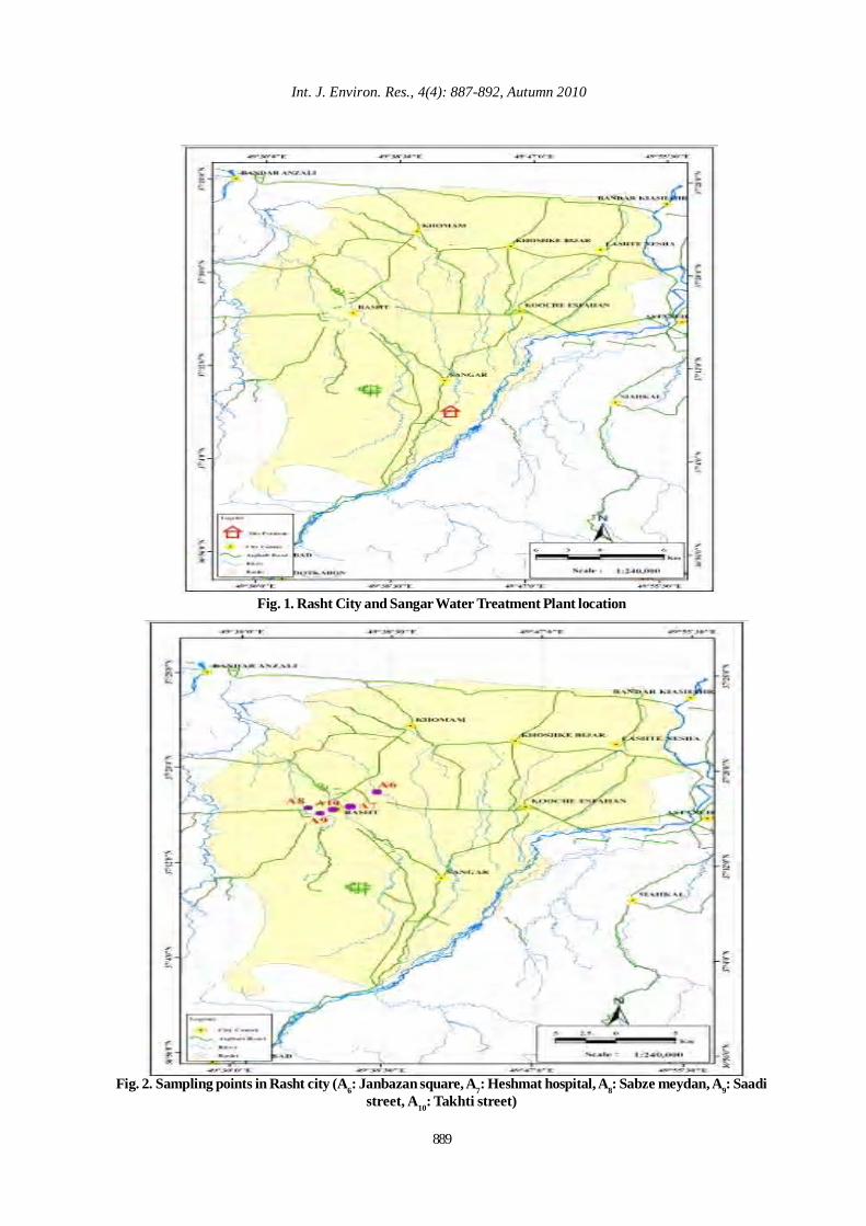
Int. J. Environ. Res., 4(4): 887-892, Autumn 2010
889
Fig. 1. Rasht City and Sangar Water Treatment Plant location
Fig. 2. Sampling points in Rasht city (A6: Janbazan square, A7: Heshmat hospital, A8: Sabze meydan, A9: Saadistreet, A10: Takhti street)
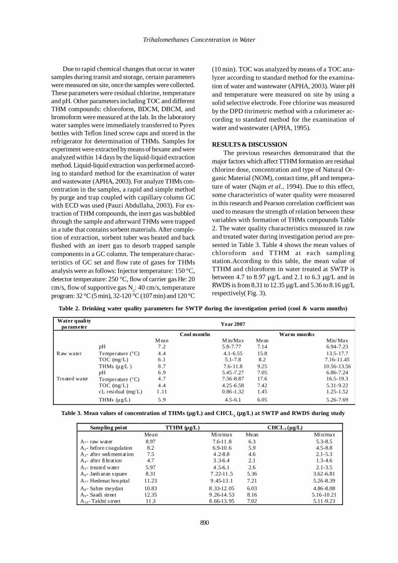
890
Trihalomethanes Concentration in Water
Due to rapid chemical changes that occur in watersamples during transit and storage, certain parameterswere measured on site, once the samples were collected.These parameters were residual chlorine, temperatureand pH. Other parameters including TOC and differentTHM compounds: chloroform, BDCM, DBCM, andbromoform were measured at the lab. In the laboratorywater samples were immediately transferred to Pyrexbottles with Teflon lined screw caps and stored in therefrigerator for determination of THMs. Samples forexperiment were extracted by means of hexane and wereanalyzed within 14 days by the liquid-liquid extractionmethod. Liquid-liquid extraction was performed accord-ing to standard method for the examination of waterand wastewater (APHA, 2003). For analyze THMs con-centration in the samples, a rapid and simple methodby purge and trap coupled with capillary column GCwith ECD was used (Pauzi Abdullaha, 2003). For ex-traction of THM compounds, the inert gas was bubbledthrough the sample and afterward THMs were trappedin a tube that contains sorbent materials. After comple-tion of extraction, sorbent tuber was heated and backflushed with an inert gas to desorb trapped samplecomponents in a GC column. The temperature charac-teristics of GC set and flow rate of gases for THMsanalysis were as follows: Injector temperature: 150 °C,detector temperature: 250 °C, flow of carrier gas He: 20cm/s, flow of supportive gas N2: 40 cm/s, temperatureprogram: 32 °C (5 min), 32-120 °C (107 min) and 120 °C
(10 min). TOC was analyzed by means of a TOC ana-lyzer according to standard method for the examina-tion of water and wastewater (APHA, 2003). Water pHand temperature were measured on site by using asolid selective electrode. Free chlorine was measuredby the DPD titrimetric method with a colorimeter ac-cording to standard method for the examination ofwater and wastewater (APHA, 1995).
RESULTS & DISCUSSIONThe previous researches demonstrated that the
major factors which affect TTHM formation are residualchlorine dose, concentration and type of Natural Or-ganic Material (NOM), contact time, pH and tempera-ture of water (Najm et al., 1994). Due to this effect,some characteristics of water quality were measuredin this research and Pearson correlation coefficient wasused to measure the strength of relation between thesevariables with formation of THMs compounds Table2. The water quality characteristics measured in rawand treated water during investigation period are pre-sented in Table 3. Table 4 shows the mean values ofchloroform and TTHM at each samplingstation.According to this table, the mean value ofTTHM and chloroform in water treated at SWTP isbetween 4.7 to 8.97 µg/L and 2.1 to 6.3 µg/L and inRWDS is from 8.31 to 12.35 µg/L and 5.36 to 8.16 µg/Lrespectively( Fig. 3).
Table 2. Drinking water quality parameters for SWTP during the investigation period (cool & warm months)
Year 2007 Water quali ty pa rameter
Warm months Cool months Min/Max Mean M in/Max M ean 6.94-7.23 7.14 5.8-7.77 7 .2 pH 13.5-17.7 15.8 4.1-6.55 4 .4 Temperature (°C) Raw water
7.16-11.45 8.2 5.1-7.8 6 .1 TOC (mg/L) 10.56-13.56 9.25 7.6-11.8 8 .7 THMs (µg/L )
6.86-7.24 7.05 5.45 -7.27 6 .9 pH 16.5-19.3 17.6 7.56 -8.87 4 .7 Temperature (°C) Treated water 5.31-9.22 7.42 4.25 -6.58 4 .4 TOC (mg/L) 1.25-1.52 1.45 0.86 -1.32 1 .11 cl2 residual (mg/L) 5.26-7.69 6.05 4.5-6.1 5 .9 THMs (µg/L)
Table 3. Mean values of concentration of THMs (µg/L) and CHCL3 (µg/L) at SWTP and RWDS during study
CHCL3 (µg/L) TTHM (µg/L) Sampling point Min/max Mean Min/max Mean 5.3-8.5 6.3 7.6-11 .8 8.97 raw water A1- 4.5-8.8 5.9 6.9-10 .6 8.2 A2- before coagulation 2.1-5.3 4.6 4 .2-8.8 7.5 A3- after sedimentat ion 1.3-4.6 2.1 3 .3-6.4 4.7 A4- after fi ltrat ion 2.1-3.5 2.6 4 .5-6.1 5.97 A5- treated water
3.62 -6.81 5.36 7 .22-11 .5 8.31 A6- Janb azan square 5.26 -8.39 7.21 9 .45-13 .1 11.23 A7- Heshmat hospital 4.86 -8.08 6.03 8 .33-12.05 10.83 A8- Sabze meydan
5.16 -10.21 8.16 9 .26-14.53 12.35 A9- Saadi street 5.11 -9.23 7.02 8 .66-13.95 11 .3 A10- Takhti s treet
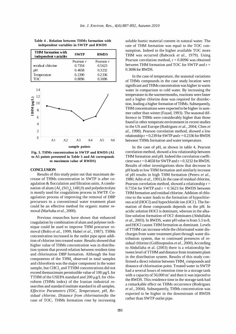
Int. J. Environ. Res., 4(4):887-892, Autumn 2010
891
Table 4 . Relation between THMs formation withindependent variables in SWTP and RWDS
RWDS SWTP THM formation with independent variable
Pearson r Pearson r 0.5623 0.7354 residual chlorine 0.3232 0.4658 pH 0.2336 0.2390 Temperature 0.3696 0.8096 TOC
CONCLUSIONResults of this study point out that maximum de-
crease of THMs concentration in SWTP is after co-agulation & flocculation and filtration units. A combi-nation of alum (Al2 (SO4)3,14H20) and polyelectrolyteis mostly used for coagulation process in SWTP. Co-agulation process of improving the removal of DBPprecursors in a conventional water treatment plantcould be an effective method for organic matter re-moval (Marhaba et al., 2000).
Previous researches have shown that enhancedcoagulation by combination of alum and polymer tech-nique could be used to improve THM precursor re-moval (Bolto et al., 1999; Hubel et al., 1987). THMsconcentration increased in the outlet pipe upon addi-tion of chlorine into treated water. Results showed thathigher value of THMs concentration was in distribu-tion system that proved relation between resident timeand chlorination DBP formation. Although the fourcomponents of the THMS observed in total samplesand chloroform was the major component in the watersample, but CHCl3 and TTHM concentrations did notexceed themaximum permissible value of 100 µg/L forTTHM of the USEPA standard and 200 µg/L for chlo-roform (THMs index) of the Iranian industrial re-searches and standard institute standard in all samples.Effective Parameters (TOC, Temperature, pH, Re-sidual chlorine, Distance from chlorination)In thecase of TOC, THMs formation rose by increasing
0
2
4
6
8
10
12
14
Fig. 3. THMs concentration in SWTP and RWDS (A1to A5 points presented in Table 3 and A6 corresponds
to maximum value of RWDS)
soluble humic material content in natural water. Therate of THM formation was equal to the TOC con-sumption. Indeed in the higher available TOC moreTHM was occurred (Babcock et al., 1979). UsingPearson correlation method, r = 0.8096 was obtainedbetween THM formation and TOC for SWTP and r =0.3696 for RWDS.
In the case of temperature, the seasonal variationsof THMs compounds in the case study location weresignificant and THMs concentration was higher in warmwater in comparison to cold water. By increasing thetemperature in the warmermonths, reactions were fasterand a higher chlorine dose was required for disinfec-tion, leading a higher formation of THMs. Subsequently,THM concentrations were expected to be higher in sum-mer rather than winter (Fayad, 1993). The seasonal dif-ference in THMs were considerably higher than thosefound in other temperate environment in recent studiesin the US and Europe (Rodriguez et al., 2004; Chen etal., 1998). Pearson correlation method, showed a lowrelationship r = 0.239 for SWTP and r = 0.2336 for RWDSbetween THMs formation and water temperature.
In the case of pH, as shown in table 4, Pearsoncorrelation method, showed a low relationship betweenTHM formation and pH. Indeed the correlation coeffi-cient was r = 0.4658 for SWTP and r = 0.3232 for RWDS.Results of other investigations show that decrease inpH leads to low THM formation and similarly increaseof pH results in high THM formation (Peters et al.,1980; Adin et al., 1991).In the case of residual chlorine,Pearson correlation method, showed a relationship r =0.7354 for SWTP and r = 0.5623 for RWDS betweenTHM formation and residual chlorine. Addition of chlo-rine to the water leads to the formation of hypochlor-ous acid (HOCl) and hypochloride ion (OCl-). The for-mation of these compounds depends on the pH. Inacidic solution HOCl is dominant, whereas in the alka-line solution formation of OCl- dominates (Abdullahaet al., 2003). In RWDS, water pH value is from 5.5 to 8,and HOCl causes THM formation as dominant. Levelsof TTHM can increase while the chlorinated water dis-charges from water treatment plant through water dis-tribution system, due to continued presences of re-sidual chlorine (Golfinopoulos et al., 2000).Accordingto Abdullaha et al. (2003) there is a relationship be-tween level of TTHM and distance from treatment plantin the distribution system. Results of this study con-firmed a direct relation between THMS compounds anddistance of chlorination point. Treated water in SWTPhad a several hours of retention time in a storage tankwith a capacity of 50,000 m3 and then it was injected tothe RWDS. This residence time in the storage tank hada remarkable effect on THMs occurrence (Rodriguezet al., 2004). Subsequently, THMs concentration wasexpected to be higher in the downstream of RWDSrather than SWTP outlet pipe.
I IH
M (µ
g/L
)
sample points
A1 A2 A3 A4 A5 A6
892
REFERENCESAbdullaha, Md.P., Yewa C.H., and bin Ramlib, M.S. (2003).Formation, modeling and validation of trihalometha nes inMalaysian drinking water: a case study in the districts ofTampin, Negeri Sembilan and Sabak Bernam, Selangor, Ma-laysia. Water Research, 37, 4637–4644.
Adin, A., Katzhendler, J., Alkaslassy, D. and Rav, A.C.(1991). Trihalomethanes formation in chlorinated drinkingwater: a kinetic model. Water Res., 25, 797–805.
Al Omrani, A., Fayyad, M. and Abdel Qader, A. (2004).Modeling trihalomethane formation for jabal amman watersupply in Jordan. Environment Modeling and Assessment,9, 245-252.
APHA, (2003). Standard Methods for the Examination ofWater and Wastewater Ed. American Public Health Associa-tion, Washington DC.
APHA, AWWA and WPCF., (1995). Standard Methods forthe Examination of Water and Wastewater, 19th ed. APHA,AWWA and WPCF, Washington, DC.
Babcock, D. and Singer, P. (1979). Chlorination and coagu-lation of humic and fulvic acids. AWWA, 71, 149–52.
Bellar, T., Lichtenberg, J. and Kroner, R. (1974). The Oc-currence of organohalides in chlorinated waters. AWWA.,66 (12), 703-706.
Bolto, B., Abbt-Braun, G., Dixon, D., Eldridge, R., Frimmel,F., Hesse, S., King, S. and Toifl, M. (1999). Experimentalevaluation of cationic polyelectrolytes for removing naturalorganic matter from Water. Water Science Technology, 40(9), 71-79.
Chen, W.J. and Weisel, C.P. (1998). Halogenated DBP concen-trations in a distribution system. AWWA., 90 (4), 151–163.
Clark, R., Pourmoghaddas, H., Wymer, L. and Dressman, R.(1996). Modeling the kinetics of chlorination by-productsformation: the effects of bromides. SRT-aqua., 45 (3), 112-119.
Dodds, L., King, W., Woolcott, C. and Pole, J. (1999).Trihalomethanes in public water supplies and adverse birthoutcomes. Epidemiology, 10 (3), 233-237.
Elshorbagy, W. (2006). Kinetics of THM species in fin-ished water. Water Resources Planning and Management.,126 (1), 21-28.
Fayad, N.M. (1993). Seasonal variations of THMs in SaudiArabian drinking water. AWWA, 85, 46-50.
Golfinopoulos, S. K. (2000). The occurrence oftrihalomethanes in the drinking water in Greece. Chemo-sphere., 41 (11), 1761-1767.
Garcia-Villanova, R.J., Garcia, C., Gomez, J.A., Garcia, M.P.and Ardanuy, R. (1997). Formation, evolution and modelingof trihalomethanes in the drinking water of a town: II, in thedistribution system. Water Res., 31 (6), 1405-1413.
Hubel, R.E. and Edzwald, J.K. (1987). Removing trihalomethane precursors by coagulation. AWWA., July, 98-106.
IARC (1991). Chlorinated drinking water chlorination by-product: some other halogenated compounds cobalt and
cobalt compounds, IARC Monographs on Evaluation ofCarcinogenic Risks in Humans, vol. 52.
IARC (2003). Some drinking water disinfectants and con-taminants, including arsenic, IARC Monographs on Evalu-ation of Carcinogenic Risks in Humans, vol. 84.
Marhaba, T.F. and Pipada, N.J. (2000). Coagulation: Effec-tiveness in Removing Dissolved Organic Matter Fractions.Environ. Eng. Sci., 17(2), 107-115.
Marimoto, K.. and Koizumi, A. (1983). Trihalomethanesinduce sister chromatid exchange in human lymphocytes invitro and mouse bone marrow cells in vivo. Environ. Res.,32, 72-79.
Najm, I., Patania, N.L., Jacangelo, J.G. and Krasner, S.W.(1994). Evaluating surrogates for disinfection by-products.AWWA., 86, 98-106.
Nikolaou, A. and Lekkas, T. (2001). The role of naturalorganic materials during formation of chlorination by-prod-ucts: a review. Acta Hydrochimica et Hydrobiologica 29,63-77.
Peters, C.J., Young, R.J. and Perry, R. (1980). Factors influ-encing the formation of Haloforms in the chlorination ofhumic materials. Environ. Sci. Technol., 14, 1391–1395.
Premazzi, G., Cardoso, C., Conio, O., Palumbo, F., Ziglio,G., Meucci, L. and Borgioli, A. (1997). Standards and strat-egies in the European Union to control trihalomethanes indrinking water; Environment Institute. European Commis-sion Joint Research Centre and Techware. Italy.
Rodriguez, M.J., Serodes, J.B. and Levallois, P. (2004).Behavior of trihalomethanes and haloacitic acids in a drink-ing water distribution system. Water Research, 38, 4367-4382.
Rook, J.J. (1974). Formation of haloforms during chlorinationof natural waters. Water Treat., Examiners 23 (2), 234-243.
Samadi, M.T., Nasseri, S., Mesdaghinia, A. and Alizadefard,M.R. (2006). A comparative study on THMS removal effi-ciencies from drinking water through nanofiltration and airstripping packed-column. Iranian Journal of Water andWastewater., 57, 14-21.
Simpson, K.L. and Hayes, K.P. (1998). Drinking water dis-infection by-products: An Australian perspective. WaterResour., 32 (5), 1522-1528.
Symons, J., Bellar, T., Carswell, J., DeMarco, J., Kropp,K., Robeck, G., Seeger, D., Slucom, C., Smith, B., andStevens,A. (1975). National organic reconnaissance surveyfor halogenated organics. AWWA., 67 (11), 634-648.
USEPA (1998). National primary drinking water regulations:disinfectants and disinfection by products; Final rule. Fed-eral Register 63 (241), 69390-69476.
Wright, J.M., Schwartz, J. and Dockery, D.W. (2004). Theeffect of disinfection by products and mutagenic activity onbirth weight and gestational duration. Environ. Health Persp.,112, 920-925.
Yoon, J., Choia, Y., Chob, S. and Lee, D. (2003). Lowtrihalomethane formation in Korean drinking water. TheScience of the Total Environment, 302,157-166.
Hassani, A. H. et al.
Int. J. Environ. Res., 4(4):893-900 , Autumn 2010ISSN: 1735-6865
Received 12 March 2009; Revised 15 May 2010; Accepted 25 May 2010
*Corresponding author E-mail: [email protected]
893
Dissolved Methane Fluctuations in Relation to Hydrochemical Parameters inTapi Estuary, Gulf of Cambay, India
Nirmal Kumar, J. I. 1*, Kumar, R. N. 2 and Viyol, S. 1
1 Post Graduate Department of Environmental Science and Technology, Institute of Science andTechnology for Advanced Studies and Research (ISTAR), Vallabh Vidyanagar -388 120,
Gujarat, India2 Department of Biosciences and Environmental Science, Natubhai V Patel College of Pure and
Applied Sciences (NVPAS), Vallabh Vidyanagar -388 120, Gujarat, India
ABSTRACT:Methane is one of the important greenhouse gases that contribute to a rise in global mean surfacetemperature. Aquatic environments are postulated to contribute > 50% of the total global methane (CH4) fluxto the atmosphere (de angelis and Lilley, 1987). Dissolved methane concentration in surface waters wasmeasured from January to December 2008 at two selected sites upper reaches (ONGC Bridge) and lowerreaches (Dumas) of Tapi estuary, Gulf of Cambay, Gujarat, India. Besides, the important hydrochemicalparameters like total organic carbon (TOC), dissolved oxygen (DO), salinity and nutrients (phosphate, nitrateand sulphate) were also analyzed. The mean dissolved CH4 concentration for all water samples at upperreaches was 1369.00 nmol/L and at lower reaches was 1082.04 nmol/L. The positive correlation was foundbetween dissolved methane content and total organic carbon. On the contrary, the negative correlation wasobserved between methane concentration and nutrients like dissolved oxygen, salinity, phosphate, nitrate andsulphate. The probable causes for varying dissolved methane concentration and saturation at different reacheswith hydrochemical parameters are discussed.
Key words: Dissolved CH4, Tropical estuary, Total organic carbon and nutrients
INTRODUCTIONMethane is an atmospheric trace gas that contrib-
utes significantly to the greenhouse effect. Despite itslower concentrations in the atmosphere, CH4 absorbsinfrared radiation much more intensely than CO2 andcontributes about 15% to the anthropogenic green-house effect (Ferron et al., 2007). Many investigationshave been carried out to control methane for variouspurposes but little attention is given to aquatic sys-tems (Banu et al., 2007; Zinatizadeh et al., 2007;Yoochatchaval et al., 2008; Uemura, 2010). Most inves-tigations on methane emissions from aquatic ecosys-tems have concentrated on salt marshes (Cicerone andShetter, 1981). Oceans play only a modest role in meth-ane global budget, accounting for 0.1% to 4% of thetotal atmospheric emissions (Crutzen, 1991). Theseoceanic emissions of CH4 are not homogeneously dis-tributed. Hence, biological productive regions, suchas estuaries and coastal areas contribute about 75% to
the global oceanic CH4 production (Bange et al., 1994).Due to the shallowness of the estuarine systems, alarge fraction of labile organic matter can be depos-ited in the sediments which generate favorable condi-tions for the microbial production of methane (Bangeet al., 1998). Biogenic methane is produced exclusivelyby a group of strict anaerobes (methanogens) duringmethanogenesis. This process occurs in the sedi-ments, in the interior of suspended particles and inthe guts of marine organisms (Wolfe, 1971). The ac-tual methane concentration at any point is a complexfunction of many factors including hydrology, drain-age basin morphology and vegetation, microbial oxi-dation, and reaeration. Hydro-geochemistry of thewetlands and paddy fields influences the methaneemission (Nirmal Kumar and Viyol, 2008 and 2009).Methane concentration of mangrove forest sedimentswere investigated with respect to organic matter con-tent, bacterial numbers and sulphide concentration
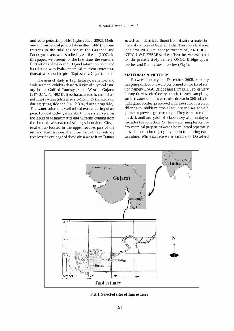
894
Nirmal Kumar, J. I. et al.
and redox potential profiles (Lyimo et al., 2002). Meth-ane and suspended particulate matter (SPM) concen-trations in the tidal regions of the Garonne andDordogne rivers were studied by Abril et al (2007). Inthis paper, we present for the first time, the seasonalfluctuations of dissolved CH4 and saturation point andits relation with hydro-chemical nutrient concentra-tions at two sites of tropical Tapi estuary, Gujarat, India.
The area of study is Tapi Estuary; a shallow andwide segment exhibits characteristics of a typical estu-ary in the Gulf of Cambay ,South West of Gujarat(21°402 N, 72° 402 E). It is characterized by semi-diur-nal tides (average tidal range 2.3–5.5 m, 25 km upstreamduring spring tide and 0.4 - 2.3 m, during neap tide).The water column is well mixed except during shortperiod of tidal cycle (Qasim, 2003). The system receivesthe inputs of organic matter and nutrients coming fromthe domestic wastewater discharges from Surat City, atextile hub located in the upper reaches part of theestuary. Furthermore, the lower part of Tapi estuaryreceives the drainage of domestic sewage from Dumas
as well as industrial effluent from Hazira, a major in-dustrial complex of Gujarat, India. This industrial areaincludes ONGC, Reliance petrochemical, KRIBHCO,NTPC, L & T, ESSAR steel etc. Two sites were selectedfor the present study namely ONGC Bridge upperreaches and Dumas lower reaches (Fig.1).
MATERIALS & METHODSBetween January and December, 2008, monthly
sampling collections were performed at two fixed sta-tion namely ONGC Bridge and Dumas in Tapi estuaryduring third week of every month. In each sampling,surface water samples were also drawn in 300 mL air-tight glass bottles, preserved with saturated mercuricchloride to inhibit microbial activity and sealed withgrease to prevent gas exchange. They were stored inthe dark until analysis in the laboratory within a day ortwo after the collection. Surface water samples for hy-dro-chemical properties were also collected separatelyin wide mouth inert polyethylene bottle during eachsampling. While surface water sample for Dissolved
Fig. 1. Selected sites of Tapi estuary
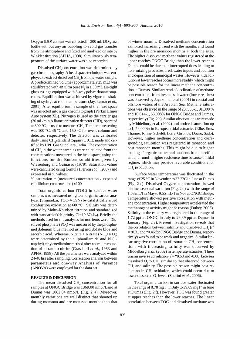
Int. J. Environ. Res., 4(4):893-900 , Autumn 2010
895
Oxygen (DO) content was collected in 300 mL DO glassbottle without any air bubbling to avoid gas transferfrom the atmosphere and fixed and analyzed on site byWinkler titration (APHA, 1998). Simultaneously tem-perature of the surface water was also recorded.
Dissolved CH4 concentration was determined bygas chromatography. A head space technique was em-ployed to extract dissolved CH4 from the water sample.A predetermined volume (approximately 25 mL) wasequilibrated with an ultra pure N2 in a 50 mL air-tightglass syringe equipped with 3-way polycarbonate stop-cocks. Equilibration was achieved by vigorous shak-ing of syringe at room temperature (Jayakumar et al.,2001). After equilibrium, a sample of the head spacewas injected into a gas chromatograph (Perkin ElmerAuto system XL). Nitrogen is used as the carrier gas(30 mL/min A flame ionization detector (FID), operatedat 300 °C, is used to measure CH4. Temperature settingwas 100 °C, 45 °C and 150 °C for oven, column anddetector, respectively. The detector was calibrateddaily using CH4 standard (5ppmv ± 0.1), made and cer-tified by UPL Gas Suppliers, India. The concentrationof CH4 in the water samples were calculated from theconcentrations measured in the head space, using thefunctions for the Bunsen solubilities given byWiesenburg and Guinasso (1979). Saturation valueswere calculated using formula (Ferron et al., 2007) andexpressed in % values:% saturation = (measured concentration / expectedequilibrium concentration) x100
Total organic carbon (TOC) in surface watersamples was measured using total organic carbon ana-lyzer (Shimadzu, TOC-VCSN) by catalytically aidedcombustion oxidation at 680°C. Salinity was deter-mined by Mohr–Knudsen titration and standardizedwith standard of (chlorinity, Cl=19.374‰). Briefly, themethods used for the analyses for nutrients were: Dis-solved phosphate (PO4) was measured by the phospho-molybdenum blue method using molybdate blue andascorbic acid. Whereas, Nitrite + Nitrate (NO2+NO3)were determined by the sulphanilamide and N (1-napthyl) ethylenediamine method after cadmium reduc-tion of nitrate to nitrite (Grasshoff et al., 1983 andAPHA, 1998). All the parameters were analyzed within24-48 hrs after sampling. Correlation analysis betweenparameters and one-way Analysis of Variance(ANOVA) were employed for the data set.
RESULTS & DISCUSSIONThe mean dissolved CH4 concentration for all
samples at ONGC Bridge was 1369.00 nmol/Land atDumas was 1082.04 nmol/L (Fig. 2 a). Moreover,monthly variations are well distinct that shooted upduring monsoon and pre-monsson months than that
of winter months. Dissolved methane concentrationexhibited increasing trend with the months and foundhigher in the pre monsoon months at both the sites.The higher dissolved methane values registered at theupper reaches ONGC Bridge than the lower reachesDumas could be due to uninterrupted tides leading tonon- mixing processes, freshwater inputs and additionand deposition of municipal wastes. However, tidal di-lution at lower reaches occurs more readily, which mightbe possible reason for the linear methane concentra-tion at Dumas. Similar trend of declination of methaneconcentrations from fresh to salt water (lower reaches)was observed by Jayakumar et al (2001) in coastal andoffshore waters of the Arabian Sea. Methane satura-tions was observed in the range of 23, 505-1, 91,308 %and 10,614-1, 65,008% for ONGC Bridge and Dumas,respectively (Fig. 2 b). Similar observations were madeby Middelburg et al. (2002) and noticed saturation upto 1, 58,000% in European tidal estuaries (Elbe, Ems,Thames, Rhine, Scheldt, Loire, Gironde, Douro, Sado).However, higher methane concentration and corre-sponding saturation was registered in monsoon andpost monsoon months. This might be due to higherloading of organic matter and nutrients from the efflu-ent and runoff, higher residence time because of tidalregime, which may provide favorable conditions forCH4 production.
Surface water temperature was fluctuated in therange of 25 %C in November to 32.2%C in June at Dumas(Fig. 2 c). Dissolved Oxygen concentration showeddistinct seasonal variation (Fig. 2 d) with the range of1.68 mL/l in May to 9.55 mL/ l in Nov at ONGC Bridge.Temperature showed positive correlation with meth-ane concentration. Higher temperature accelerated themethanogens activity might be reason (Dubey, 2005).Salinity in the estuary was registered in the range of1.72 ppt at ONGC in July to 26.89 ppt at Dumas inJanuary (Fig. 2 e). Present investigation reveals thatthe correlation between salinity and dissolved CH4 (r
2
= “0.31 and “0.46 for ONGC Bridge and Dumas, respec-tively) was found to be weak and negative. Similar lin-ear negative correlation of estuarine CH4 concentra-tions with increasing salinity was observed byMiddelburg et al. (2002) in temperate estuaries. Therewas an inverse correlation (r2= “0.68 and -0.06) betweendissolved O2 to CH4, similar to that observed betweenCH4 and salinity. The possible reason might be a re-duction in CH4 oxidation, which could occur due tolower dissolved O2 levels (Shalini et al., 2006).
Total organic carbon in surface water fluctuatedin the range of 8.78 mg l-1 in July to 39.09 mg l-1 in Juneat Dumas (Fig. 2 f). However, TOC was found greaterat upper reaches than the lower reaches. The linearcorrelation between TOC and dissolved methane was
896
found to be positive (r2=0.33 and 0.36 for ONGC Bridgeand Dumas, respectively). The high loading of organicmatter provides favorable conditions for the produc-tion of CH4 (Ferron et al., 2007).
Phosphate values varied in the range from 0.40µmol l-1at upper estuary (ONGC Bridge) in August to4.43 µmol l-1 at lower estuary (Dumas) in April. In con-trast to phosphate, nitrate was found greater in theupper estuary (ONGC Bridge) than in the lower estu-ary (Dumas) (Fig. 2.g and h). Both phosphate and ni-trate content showed weak or negative correlation withmethane content (Kang and Freeman, 2004). Dissolved
Fig. 2. showing (A) Dissolved methane (B) Methane saturation (C) Temperature and dissolved CH4 concentration(D) Dissolved oxygen and dissolved CH4 concentration (E) Salinity and dissolved CH4 concentration (F) Total
organic carbon and dissolved CH4 concentration at both the sites (G) Nutrients and dissolved CH4 concentration atONGC Bridge (H) Nutrients and Methane concentration at Dumas(Continues)
sulphate was observed in the range of 0.98 in Augustat ONGC Bridge to 3.23 mmol l-1 in April at Dumas.However, sulphate content was found higher at lowerreaches than in upper reaches. Dissolved CH4 showeda negative correlation with dissolved sulphate(r2=”0.13). High Sulphate content inhibits themethanogenesis which in turn reduces CH4 produc-tion in marine sediments (Dubey 2005) could be thereason in present study. Seasonally methane concen-tration was increased in monsoon months and postmonsoon months but declines with the onset of thewinter at both the sites. The greater input of organicmatter with fresh water and higher suspended solid
3500
3000
2500
2000
1500
1000
500
0
- 500
Diss
olve
d M
etha
ne(n
M)
Jan Feb Mar Apr May Jun Jul Aug Sep Oct Nov Dec
ONGC Bridge Dumas
(a)
Jan Feb Mar Apr May Jun Jul Aug Sep Oct Nov Dec
250000
200000
150000
100000
50000
0
-50000ONGC Bridge Dumas
Diss
olve
d M
etha
ne(n
M)
(b)
Dissolved Methane Fluctuations
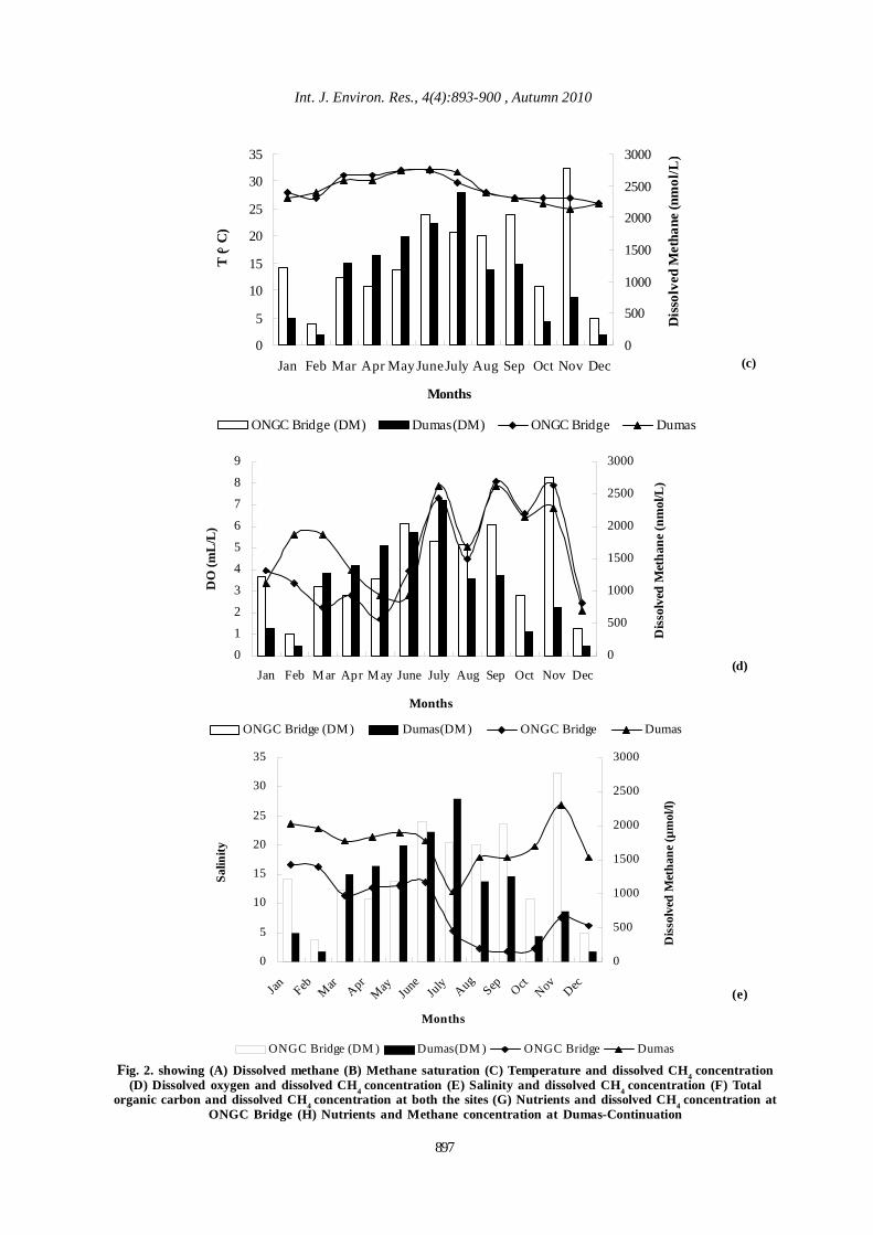
Int. J. Environ. Res., 4(4):893-900 , Autumn 2010
897
0
5
10
15
20
25
30
35
Jan Feb Mar Apr May JuneJuly Aug Sep Oct Nov Dec
Months
T (
C)
0
500
1000
1500
2000
2500
3000
Dis
solv
ed M
etha
ne (n
mol
/L)
ONGC Bridge (DM) Dumas(DM) ONGC Bridge Dumas
0
1
2
3
4
5
6
7
8
9
Jan Feb M ar Apr M ay June July Aug Sep Oct Nov Dec
Months
DO
(mL
/L)
0
500
1000
1500
2000
2500
3000
Dis
solv
ed M
etha
ne (n
mol
/L)
ONGC Bridge (DM ) Dumas(DM ) ONGC Bridge Dumas
0
5
10
15
20
25
30
35
Jan Feb Mar Apr
May Ju
ne July Aug Sep Oct
Nov Dec
Months
Salin
ity
0
500
1000
1500
2000
2500
3000
Dis
solv
ed M
etha
ne (µ
mol
/l)
ONGC Bridge (DM ) Dumas(DM ) ONGC Bridge Dumas
(c)
(d)
(e)
°
Fig. 2. showing (A) Dissolved methane (B) Methane saturation (C) Temperature and dissolved CH4 concentration(D) Dissolved oxygen and dissolved CH4 concentration (E) Salinity and dissolved CH4 concentration (F) Total
organic carbon and dissolved CH4 concentration at both the sites (G) Nutrients and dissolved CH4 concentration atONGC Bridge (H) Nutrients and Methane concentration at Dumas-Continuation
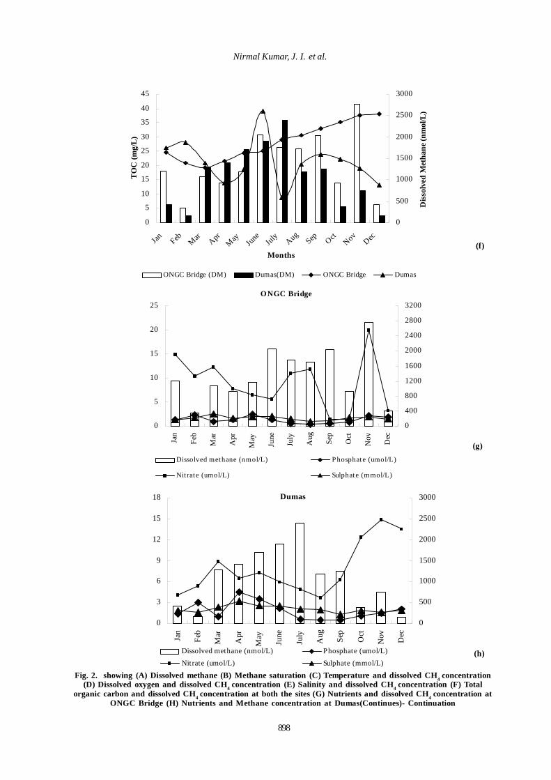
898
Nirmal Kumar, J. I. et al.
(f)
0
5
10
15
20
25
30
35
40
45
Jan Feb Mar Apr
May Ju
ne July Aug Sep Oct
Nov Dec
Months
TO
C (m
g/L
)
0
500
1000
1500
2000
2500
3000
Dis
solv
ed M
etha
ne (n
mol
/L)
ONGC Bridge (DM) Dumas(DM) ONGC Bridge Dumas
(g)
(h)
ONGC Bridge
0
5
10
15
20
25
Jan
Feb
Mar
Apr
May
June
July
Aug Sep
Oct
Nov Dec
0
400
800
1200
1600
2000
2400
2800
3200
Dissolved methane (nmol/L) P hosphate (umol/L)
Nit rate (umol/L) Sulphate (mmol/L)
Dumas
0
3
6
9
12
15
18
Jan
Feb
Mar
Apr
May
June
July
Aug Sep
Oct
Nov Dec
0
500
1000
1500
2000
2500
3000
Dissolved methane (nmol/L) Phosphate (umol/L)Nitrate (umol/L) Sulphate (mmol/L)
Fig. 2. showing (A) Dissolved methane (B) Methane saturation (C) Temperature and dissolved CH4 concentration(D) Dissolved oxygen and dissolved CH4 concentration (E) Salinity and dissolved CH4 concentration (F) Total
organic carbon and dissolved CH4 concentration at both the sites (G) Nutrients and dissolved CH4 concentration atONGC Bridge (H) Nutrients and Methane concentration at Dumas(Continues)- Continuation

899
Int. J. Environ. Res., 4(4):893-900 , Autumn 2010
due to turbulence run-off rain water flow may be theresponsible. In monsoon months methane concentra-tion and other parameters were higher at the lowerreaches than the higher reaches. This might be due togreater input of the organic load than the lower reachesfrom the Surat city (Lane 2002). One way ANOVAshowed slight variation (p = 0.15) in dissolved meth-ane concentration between ONGC Bridge and Dumas.
ACKNOWLEDGEMENTAuthors are highly thankful to Ocean and Atmo-
sphere Science and Technology Cell (OASTC),Bhavnagar University, Ministry of Earth Sciences(MoES), New Delhi India for financial assistance. Au-thors are also thankful to Sophisticated Instrumenta-tion Center for Advanced Research and Testing(SICART), Vallabh Vidyanagar, Gujarat for analysis ofmethane and total organic carbon by Gas Chromatog-raphy and Total Organic Carbon analyzer, respectively.
REFERENCESAbril, G., Commarie, M. V. and Guerin, F. (2007). En-hanced methane oxidation in an estuarine turbiditymaximum. Limnol. Oceanogr., 52 (1), 470-475.
APHA (1998). Standard methods for examination ofwater and waste water. Washington D.C., AmericanPublic Health Association, USA.
Bange, H. W., Bartel, U. H., Rapsomanikis, S. andAndreae, M. O. (1994). Methane in the Baltic and NorthSeas and reassessment of the marine emissions ofmethane. Glob. Biogeochem. Cycles., 8,465-480.
Bange, H. W., Dahlke, S., Ramesh, R., Meyer-Reil, L.A.,Rapsomanikis, S. and Andreae, M. O. (1998). Seasonalstudy of methane and nitrous oxide in the coastal wa-ters of the southern Baltic Sea. Estua. Coast. Shelf Sci.,47, 807–817.
Banu, J. R., Kaliappan, S. and Yeom, I. T. (2007). Treat-ment of domestic wastewater using upflow anaerobicsludge blanket reactor. Int. J. Environ. Sci. Tech., 4 (3),363-370.
Cicerone, R. J. and Shetter. J. D. (1981). Sources ofatmospheric methane: Measurements in rice paddiesand a discussion. J. Geophy. Res., 86, 7203-7209.
Crutzen, P.J., (1991). Methane’s sinks and sources.Nature. 350, 380-381.
de Angelis, M. A. and Lilley, M. D. (1987). Methane insurface waters of Oregon estuaries and rivers. Limnol.Oceanogr., 32 (3), 716-722.
Dubey, S. K. (2005). Microbial ecology of methaneemission in rice agroecosystem- A Review. App. Eco.& Environ. Rese., 3 (2), 1-27.
Ferron, S., Ortega, T., Gomez-Parra, A. and Forja, J. M.(2007). Seasonal study of dissolved CH4, CO2 and N2Oin a shallow tidal system of the bay of Cadiz (SW Spain).J. Mar. Sys., 66, 244-257.
Grasshoff, K., Ehrhardt, M. and Kremling, K. (1983).Methods of seawater analysis. Verlag Chemie, Berlin.Jayakumar, D. A., Naqvi, S. W. A., Narvekar, P. V. andGeorge, M. D. (2001). Methane in coastal and offshorewaters of the Arabian Sea. Mar. Chem., 74 (1), 1-13.
Lane, R., Day, W. J., Marx, B., Reyes, E. and Kemp, P.(2002). Seasonal and Spatial Water Quality Changes inthe Outflow Plume of the Atchafalaya River, Louisi-ana, USA. Estuaries, 25 (1), 30–42.
Lyimo, T. J., Arjan, P. and Opden Camp, H. J. M. (2002).Methane Emission, Sulphide Concentration and Re-dox Potential Profiles in Mtoni Mangrove Sediment,Tanzania Western Indian Ocean. J. Mar. Sci., 1 (1), 71–80.
Middelburg, J. J., Nieuwenhuize, J., Iversen, N., Hoegh,N., de Wilde, H., Helder, W., Seifert, R. and Christ, O.(2002). Methane distribution in European tidal estuar-ies. Biogeochemistry, 59, 95–119.
Nirmal Kumar, J. I. and Viyol, S. (2008). Short term as-sessment of influence of hydro-geochemistry on meth-ane emission from two contrasting tropical wetlandsof Central Gujarat, India. Int. J. Nat. Env. and Poll. Tech.,7 (1), 15-20.
Nirmal Kumar, J. I. and Viyol, S. (2009). Short term diur-nal and temporal measurement of methane emission inrelation to Organic carbon, Phosphate and sulphatecontent of two rice fields of central Gujarat, India. Paddyand Water Environment,7, 11-16.
Qasim, S. Z. (2003). Indian estuaries. Allied publish-ers, 356-357, India.
Shalini A, Ramesh, R. Purvaja R. and Barnes J. (2006).Spatial and temporal distribution of methane in an ex-tensive shallow estuary, south India. J. Earth Sys. andSci., 115 (4), 451-460.
Uemura, Sh. (2010). Mineral Requirements for Meso-philic and Thermophilic Anaerobic Digestion of Or-ganic Solid Waste. Int. J. Environ. Res., 4 (1), 33-40.
Wiesenburg, D. A. and Guinasso Jr., N. L. (1979). Equi-librium solubilities of methane, carbon monoxide, andhydrogen in water and sea water. J. Chem. Eng. Data,24, 356-360.

900
Wolfe, R.S. (1971). Microbial formation of methane.Adv. Micro. Phys., 6, 107–146.
Yoochatchaval, W., Ohashi, A., Harada, H.,Yamaguchi, T. and Syutsubo, K. (2008). IntermittentEffluent Recirculation for the Efficient Treatment ofLowStrength Wastewater by an EGSB Reactor. Int. J.Environ. Res., 2 (3), 231-238.
Zinatizadeh, A. A. L., Salamatinia, B., Zinatizadeh, S.L., Mohamed, A. R. and Hasnain Isa, M. (2007). Palmoil mill effluent digestion in an up-flow anaerobic sludgefixed film bioreactor. Int. J. Environ. Res., 1(3), 264-271.
Dissolved Methane Fluctuations
Int. J. Environ. Res., 4(4):901-912, Autumn 2010ISSN: 1735-6865
Received 22 Feb. 2010; Revised 15 May 2010; Accepted 25 May 2010
*Corresponding author E-mail: [email protected]
901
Municipal Waste Reduction Potential and Related Strategies in Tehran
Abduli, M . A . and Azimi, E .*
Graduate Faculty of Environment, University of Tehran P.O. Box 14155- 6135 , Tehran, Iran
ABSTRACT: The main problem of solid waste management system in Tehran is to handle a large amount ofwaste (7.641 ton/day in 2008). Therefore, source reduction can be introduced as one of the first priority forsolid waste management in Tehran. This research represents the first attempt to quantify the source reductionpotential in the city, and subsequently, outlines the principle guidelines, legislations and strategies regardingsource reduction application in Tehran metropolitan area.Based on the findings of current research sourcereduction strategies can be implemented in dealing with packaging material, paper, street waste, mixed householdwaste and hazardous household wastes. Also industrial wastes produced inside city boundaries can be reduceddrastically by implementing source reduction measures. It is also found that any recycling program can becombined effectively with source reduction strategies.The waste reduction potential for each component ofwaste stream is calculated as the result of the research source reduction potential were determined as:horticultural waste, 80%; food waste, 80; paper and cardboard, 50%; textiles, 20%; metals including ferrousand nonferrous, % 90; Glass, % 30; PET%, 70, and plastic 80%.Finally, overall potential for source reductionin Tehran city is estimated to be 66% for the waste stream as a whole.
Key words: Source reduction, Source reduction potential, Household hazardous waste,Recycling
INTRODUCTIONIn its Agenda for Action (1989), the U.S. Environmen-
tal Protection Agency gave source reduction the highestpriority as a method for addressing solid waste issues.Source reduction is the only practice that is preventative.This proactive approach also reduces material and en-ergy use.Recycling, composting, waste-to-energy, andlandfilling are reactive methods for recovering and man-aging materials after they are produced. The USEPA de-fines source reduction as the design, manufacture, pur-chase or use of materials to reduce their quantity or toxic-ity before they reach the waste stream. Several terms areoften used to mean source reduction. These include wastereduction, waste prevention, waste minimization, pollu-tion prevention, and precycling.
Waste reduction is a broader term encompassing allwaste management methods, i.e., source reduction, recy-cling, and composting that result in reduction of wastegoing to the combustion facility or landfill. Waste minimi-zation refers to activities specifically designed to reduceindustrial hazardous and toxic wastes as they affect landdisposal as well as contribute to air and water pollution.Pollution prevention includes input optimization, the re-duction of no product outputs, and production of low-
impact products. Precycling refers to the decision-making process that consumers use to judge a purchasebased on its waste implications; criteria used in the pro-cess include whether a product is reusable, durable, andrepairable; made from renewable or nonrenewable re-sources; over-packaged; or in a reusable container.
The basic elements of source reduction include the fol-lowing:• reduced material use in product manufacture• increased useful life of a product through durabilityand reparability• decreased toxicity• Material reuse• Reduced/more efficient consumer use of materials• Increased production efficiency resulting in less pro-duction of waste (R.O’Leary, 1995).
Area of study: Tehran, the capital of Iran, with thepopulation of 8.2 million people, occupies 730 km2 landexpanse, which is 4% of total area of country. Tehrangenerated 2,788,912 ton (7,641 ton/day) of waste inyear 2008. Hospital waste generation rate in Tehranreaches 83 ton/day. Almost 87% of total waste wasdisposed of by placing in a landfill located in Kahrizakregion. This large amount of waste causes a signifi-cant challenge for the city.
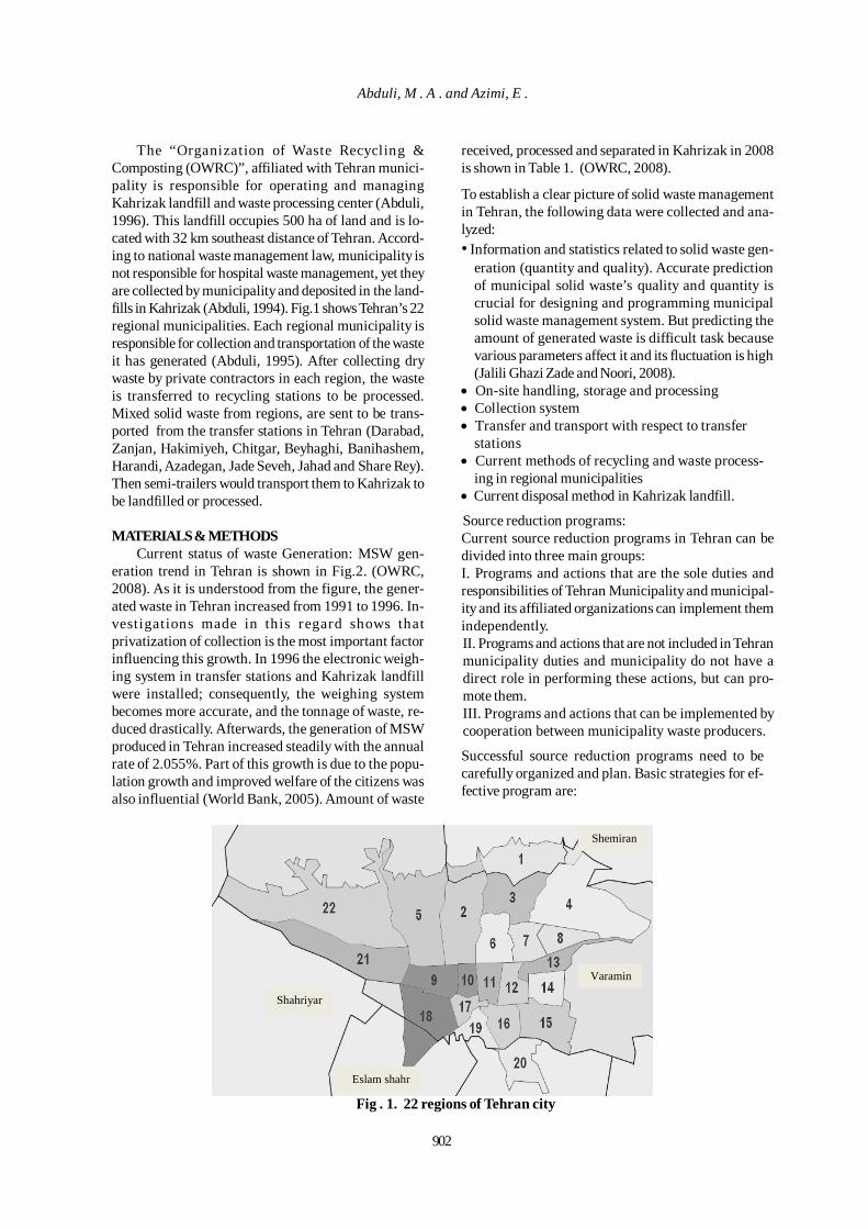
902
The “Organization of Waste Recycling &Composting (OWRC)”, affiliated with Tehran munici-pality is responsible for operating and managingKahrizak landfill and waste processing center (Abduli,1996). This landfill occupies 500 ha of land and is lo-cated with 32 km southeast distance of Tehran. Accord-ing to national waste management law, municipality isnot responsible for hospital waste management, yet theyare collected by municipality and deposited in the land-fills in Kahrizak (Abduli, 1994). Fig.1 shows Tehran’s 22regional municipalities. Each regional municipality isresponsible for collection and transportation of the wasteit has generated (Abduli, 1995). After collecting drywaste by private contractors in each region, the wasteis transferred to recycling stations to be processed.Mixed solid waste from regions, are sent to be trans-ported from the transfer stations in Tehran (Darabad,Zanjan, Hakimiyeh, Chitgar, Beyhaghi, Banihashem,Harandi, Azadegan, Jade Seveh, Jahad and Share Rey).Then semi-trailers would transport them to Kahrizak tobe landfilled or processed.
MATERIALS & METHODSCurrent status of waste Generation: MSW gen-
eration trend in Tehran is shown in Fig.2. (OWRC,2008). As it is understood from the figure, the gener-ated waste in Tehran increased from 1991 to 1996. In-vestigations made in this regard shows thatprivatization of collection is the most important factorinfluencing this growth. In 1996 the electronic weigh-ing system in transfer stations and Kahrizak landfillwere installed; consequently, the weighing systembecomes more accurate, and the tonnage of waste, re-duced drastically. Afterwards, the generation of MSWproduced in Tehran increased steadily with the annualrate of 2.055%. Part of this growth is due to the popu-lation growth and improved welfare of the citizens wasalso influential (World Bank, 2005). Amount of waste
Shahriyar
Eslam shahr
Varamin
Shemiran
Fig . 1. 22 regions of Tehran city
received, processed and separated in Kahrizak in 2008is shown in Table 1. (OWRC, 2008).
To establish a clear picture of solid waste managementin Tehran, the following data were collected and ana-lyzed:• Information and statistics related to solid waste gen-
eration (quantity and quality). Accurate predictionof municipal solid waste’s quality and quantity iscrucial for designing and programming municipalsolid waste management system. But predicting theamount of generated waste is difficult task becausevarious parameters affect it and its fluctuation is high(Jalili Ghazi Zade and Noori, 2008).
• On-site handling, storage and processing• Collection system• Transfer and transport with respect to transfer
stations• Current methods of recycling and waste process-
ing in regional municipalities• Current disposal method in Kahrizak landfill.
Source reduction programs:Current source reduction programs in Tehran can bedivided into three main groups:I. Programs and actions that are the sole duties andresponsibilities of Tehran Municipality and municipal-ity and its affiliated organizations can implement themindependently.II. Programs and actions that are not included in Tehranmunicipality duties and municipality do not have adirect role in performing these actions, but can pro-mote them.III. Programs and actions that can be implemented bycooperation between municipality waste producers.
Successful source reduction programs need to becarefully organized and plan. Basic strategies for ef-fective program are:
Abduli, M . A . and Azimi, E .
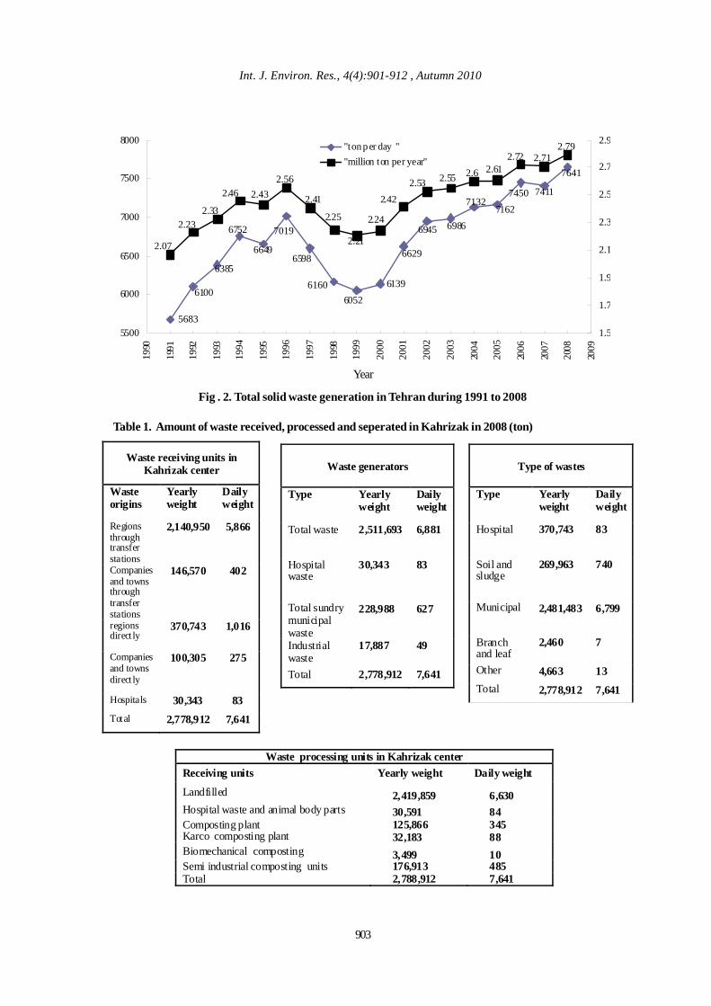
Int. J. Environ. Res., 4(4):901-912 , Autumn 2010
903
Fig . 2. Total solid waste generation in Tehran during 1991 to 2008
Table 1. Amount of waste received, processed and seperated in Kahrizak in 2008 (ton)
5683
7641
741174507162
7132
69866945
6629
61396052
6160
6598
7019
6649
6752
6385
6100
2.792.712.72
2.612.62.552.532.42
2.24
2.21
2.25
2.41
2.562.432.46
2.332.23
2.07
5500
6000
6500
7000
7500
800019
90
1991
1992
1993
1994
1995
1996
1997
1998
1999
2000
2001
2002
2003
2004
2005
2006
2007
2008
2009
1.5
1.7
1.9
2.1
2.3
2.5
2.7
2.9"ton p er day ""million ton per year"
Year
Type of wastes
Type Yearly weight
Daily weight
Hospital 370,743 83
Soil and sludge
269,963 740
Municipal 2,481,483 6,799
Branch and leaf
2,460 7
Other 4,663 13 Total 2,778,912 7,641
Waste generators
Type Yearly weight
Daily weight
Total waste 2,511,693 6,881
Hospital waste
30,343 83
Total sundry municipal waste
228,988 627
Industrial waste
17,887 49
Total 2,778,912 7,641
Waste receiving units in Kahrizak center
Waste origins
Yearly weight
Daily weight
Regions through transfer stations
2,140,950 5,866
Companies and towns through transfer stations
146,570 402
regions direct ly
370,743 1,016
Companies and towns direct ly
100,305 275
Hospitals 30,343 83 Total 2,778,912 7,641
Waste processing units in Kahrizak center Receiving units Yearly weight Daily weight
Landfilled 2,419,859 6,630 Hospital waste and animal body parts 30,591 84 Composting plant 125,866 345 Karco composting plant 32,183 88 Biomechanical composting 3,499 10 Semi industrial composting units 176,913 485 Total 2,788,912 7,641

904
Reduction of Municipal Waste
• The unique and consistent policy• Wise select of supervisor and workgroup creation• Efficient Collection required baseline data• Implementation of Waste audits conducted to
identify waste generation resources• Evaluating options and implementing a waste
reduction plan• Setting training program for all employees• Establishment of awards or incentive system for
participants• Designing a support system for sensing and
monitoring components of successful programs• Revising in the program if in case of need (U.S
Army Center, 1994)
Waste management organizations: Effective wastemanagement through MSW composition studies isimportant for numerous reasons, including the need toestimate material recovery potential, to identify sourcesof component generation and to facilitate design ofprocessing equipment (Gidarakos et al., 2006).The mostinfluential organizations to reduce process of wastefrom the sources in Tehran, is Tehran Municipality.The most influential organizations related to MSWsystem affiliated to the Tehran municipality are:Lawsand regulations Office, Studies and planning center ofTehran, Deputy for technical development, Coordina-tion and planning Department, Urban Service officesof Regional municipalities. These organizations canplay an important role in achieving the goals of sourcereduction in the city.
Also other waste reduction programs in industrialcountries such as experiences made in Japan, Chinaand South Korea in the field of source separation andrecycling, as well as in Germany, Switzerland, the Neth-erlands and the United States were considered in thisresearch.
Source reduction Potential: In order to calculatethe residual flow, before implementing a source reduc-tion program, managers can value a component of re-sidual flow by multiplication factor related to the pro-gram. It helps to determine whether a specific sourcereduction program makes sense for their community.The base of this decision is that whether the programsof source reductions can reduce considerable wasteflow by safe and cost saving methods (EPA530-F-99-006, 1999). According to this study and consideringthe possible factors such as applicability, feasibilityand technology, the following reduction potential fac-tors were determined for Tehran which can be appliedto reduce the waste:Food waste 80%, paper & cardboard 50%, textile 20%,metal 90%, PET 70%, glass 30% and plastic 80%. Theresults are shown in Table 2, Table 3 and Table 4.
In 2008, about 87% were landfilled; 2,419,859 ton, 4.5%composted, 1.15% processed in Karce, and 6.3% hadprocessed in Semi industrial units.
In “integrated waste management strategy andimplementation plan” of Tehran prepared (World Bank,2005), the separation strategy was emphasized. It wasexpressed that separation at source is one of the majortasks within the strategy of waste reduction. This strat-egy can also help to increase the rate of dry recyclingup to 20% and composting up to 50% by 2016.According to the presented statistics, in recent 3years, the amount of collected dry waste from the re-gions is growing. The rate of source separation in-creased from 3.3% in 2006 to 10.5% in 2008; neverthe-less, this study shows that there is appropriate tech-nology for increasing the rate of recovery to 66%.
Source reduction strategies in Tehran: Waste manage-ment strategies such as how to gather information,government outlook, longtime objectives, the role ofkey organizations, topics related to specific waste ma-terial flow (such as hazardous waste) and the basicrules used for the development of sustainable wastemanagement system put to action. This strategy con-siders our future outlook and tasks that each sectionrequire for the realization of conduct.
Source reduction legislation often focuses onestablishing the following:• specific goals (especially in domestic, commercialand industrial)• government services• purchases required• packaging and related guidelines• labeling and related guidelines• limiting yard and street waste• determine the type of chemicals and restrict theirproduction and usage (R.O’Leary, 1995)
It should be mentioned that not only economicincentives but also the economic disincentives canbe used to encourage source reduction strategies: Economic incentives include:• Funding for research and development of educationalprograms of source reduction• Funding for waste conversion• Funding for planning to use this material and sellthem.• assistance to industry reform• provide tax credits or exemptions for industries in thedrawings to attain goals to source reduction.Economic disincentives include:• Tax the situation is related to packaging wastedisposal.• Tax for raw materials if the materials can be usedrecycling.
Int. J. Environ. Res., 4(4):901-912 , Autumn 2010
905
• Tax for the disposal• Establishing fundamental programs for productsbased on volume collected
Source reduction programs proposed for Tehranmunicipality: According to this study, source reduc-tion programs in Tehran can be presented and per-formed as : source reduction in packaging, paper, streetwaste, household waste, industrial waste and house-hold hazardous waste.
Source reduction in packaging: The purpose of sourcereduction is to rehabilitate waste disposal problems.Two main techniques that they should be implementedregarding waste quantity and toxicity due to residualcontrol of packing products can be outlined as follow-ing:A– Controls before productionB– Controls after the production
Control methods of production, are focused on thetime that the products are made and the consumersuse them. Reduction of packaging waste in this situa-tion is the result of the following methods:• Recycling packaging materials consumed products• Reuse of packaging materials by consumer• separation of materials and reduce their size• Select the products by consumer due to packaging
Source reduction packaging goals before produc-tion include:• Reducing to the minimum required size for packag-
ing products• For increasing the attractiveness of products, many
companies, produce packages which is massive andunnecessary. By eliminating this material, minimumstandard packages can be achieved.
• Removing or minimizing toxic materials of coatingpackaging
• Eliminating an integral material and replacing themwith recyclable materials and avoiding usage
• Artificial replacement materials that not easily ab-sorb to environment with natural materials (Wasteonline, 2006)
Source reduction of paper: Paper source reductionexecutive options are as following:• support from management• prepare an assessment of paper consumption• identify program goals• specify the opportunities of the powers of paperconsumption for source reduction and• monitor work progress to achieve set goals (DukeUniversity, 1995)
Source reduction of street waste:• use as a coating material• used for filling holes and restore the earth• use in sand factories
• use for the production of prefabricated concrete,cement and asphalt• waste from horticultural and leaf of trees can beused to produce compost and fertilizer.• Use as a base under the road (Land Technologies,Inc, 1997)
Source reduction of household waste: Householdsource reduction strategies are as following:I. Source separation:
• Educating programs that are focused on thecustomers buying habits and also generationmethods on packaging factories.• Identified government programs, such aspreparation materials of recycled products.• Exchange of household and commercial waste• Commercial waste audit programs, that isperformed to evaluate the waste stream in a specialcareer and includes proposed strategies to reducewaste and increase recycling.
II. Home composting: composting in gardens andparks, can be use with the range of possibleactivities to reduce waste and produce compost,soil and plant food.• Aerobic treatment (with air) in the open bottombins (common method).• Using worms: Use of worms in a container in thepackage to improve the final product.• The use of microorganisms for fermentation,specifically for food residues.
III. Grass recycling: grass recycling includes leavingvery small cuts on the earth. Because of their fine,these small cuts influence the roots of grass quicklyand nutrients the soil and water. This work makesthe uniformity of lawn. This work is not practicaland suitable for all and some are rather to use spe-cial equipment. Municipal officials can give subsi-dies special washer machines, especially in theparks and help plan progress.
IV. Community compost: is complete home composting,in a way including preparation the material collectedfor a local composting. Composting interests in large-scale achieved by transport reduction and the dis-placement and will be with social benefits for soci-ety.
V. Centralized composting: includes; compost in largescale and size (inside the container for all organicwaste) using materials that are collected from alarge area and produce compost which carefullycontrolled for sale.
VI. Reuse of coordinated goodsVII. Education: Development and give subsidy to bins
is not enough. Raise awareness and give the neces-sary training during the program for successful pro-gram implementation is also necessary.
VIII. Home composting can support the following meth-ods:
906
- A brochure on how to start and be provided withpreparing compost bins.- Every four months or six months, a brochure con-taining information of seasonal and encouragingoptions be published.Families can be support by the following methods:- Help them to achieve and to resolve possibleproblems.- Hold meetings and workshops with the people forexchange of views about composting to raise theirknowledge in this field.- Set up phone and website (with professionals) tohelp solve the problems of people (NRWF, 2006).
Industr ial source reduction: Three mainapproaches in WM ((Waste Minimization) are consid-ered: source reduction, recycling and refining. OWRC(Organization for Waste Recycling and Composting)is responsible for these activities. This is also a wellknown statement that the incentive policies and eco-nomic disincentives in the industry can be feasible(Hyde, 2000).
Source reduction of household hazardous waste:Three main programs in source reduction of house-hold hazardous waste are:• Use of alternative products• Hazardous materials remaining gift to friend or
organization for use• Separately collected household hazardous waste and
their processing (Schnell, 2004).In this case, not considering the reduction programscould cause serious problem. Apart from the toxic ele-ments, leachate may contain microbes of which someare opportunistic pathogens. These microbes couldproduce toxins that may cause public health problem(Oshode, 2008). Although the effects of leachate areweakened with distance from the source of genera-tion, it can still cause pollution of surface and ground-water, organic carbon affecting odor and taste ofgroundwater, nitrogen compounds producingeutrophication in surface waters and high nitrates indrinking water, and toxic heavy metals in ground andsurface waters (Robinson, 1983).
Source reduction in recycling programs: recycling,perhaps the most positively received of all waste man-agement practices, is going to be an essential part ofcontemporary waste management strategies,composting can play an important role, while incinera-tion seems to be a conditionally feasiblesolution(Sadugh, 2009). This twelve-component planprovides an outline for successful program design:• Identify goals.• Characterize recyclable volume and accessibility.• Assess and generate political support.• Assess markets and market development strategies
for recyclables.
• Assess and choose technologies for collection andprocessing.
• Develop budget and organization plan.• Address legal and sitting issues.• Develop start-up approach.• Implement education and publicity program.• Commence program operation.• Supervise ongoing program and continue publicity/
education.• Review and adjust program (Walsh,1993)
RESULTS & DISCUSSIONRegional municipalities are required by law to in-
stitute specific source reduction practices. Regionalmunicipalities can model local policy to promote sourcereduction in their own institutions and in commercialand residential sectors, but all the targets which wereset by the regional municipalities, should have the fol-lowing strategies:• Targets must indicate that the source reduction has
the first priority, wherever practicable.• Targets must be supported with a practical program.• Local authorities should demonstrate to municipal-
ity of Tehran that the targets of the executive can beevaluated.
• Authorities must also report continuous improve-ment performance.
• Government, manufacturers, distributors and retail-ers assist in the maintenance of ecological pro-cesses and the biological diversity of the city, en-sure that the management of renewable resourcesis based on a sustained yield and make decisionsthat reflect wise and efficient use of renewable andnon-renewable resources.
According to this study, appropriate technologyand adequate economic conditions already exist to re-duce solid waste generation by 66 % (Reduction po-tential), in the next few years.Municipal and house-hold waste management, need to be emphasized onrecycling, composting, and energy recovery.Due to the present status, the following targets formunicipal management are proposed:• Recovery value from 50% of municipal waste by 2016• Recovery value from 60% of municipal waste by 2021• Recovery value from 66% of municipal waste by 2026
The term “recovery” refers to the bellow activities:• Recycling• Composting• Other forms of material recovery (anaerobic
digestion for instance)• Energy recovery (DETR, 2000)
The most important elements to achieve munici-pal and household waste targets are recycling andcomposting. Good quality compost requires separate
Abduli, M . A . and Azimi, E .

907
Int. J. Environ. Res., 4(4):901-912, Autumn 2010
collection of biowaste combined with plenty of infor-mation and guidance to households and potential us-ers of the compost. It also requires the setting up ofmonitoring systems and possibly quality standards orlabels (EEA, 2009).• Recycle or compost at least 25% of household waste
by 2016• Recycle or compost at least 30% of household waste
by 2021• Recycle or compost at least 33% of household waste
by 2026
Government, the Islamic assembly and the depart-ment of Tehran Municipality of laws and regulations,by laws should reduce the growth of household wastegeneration and can even stop or reverse. Such changesare competitive and in some regions are likely toachieve them than others.On the other hand, the gov-ernment and the Islamic assembly should set the fol-lowing target to encourage businesses to reduce waste,and to put any waste that is produced to better use:• By the year 2021, the amount of commercial and in-
dustrial waste sent to landfill should be 85% of thatlandfilled in 2006.
Standards must be primarily explains to municipalauthorities of active regions in waste disposal. Au-thorities will be required to meet statutory standardsfor 2016, 2021 and 2026.Different standards for differ-ent groups of authorities and different conditionsshould be set. Standards for 2016 should be defined inthe following levels:• In regional municipalities where the separation ratein 1998, is less than 10% reach at least to 10%.In countries with low material recovery and incinera-tion, the introduction of separate collection systemsfor packaging waste successfully decreased landfilledwaste in the first year (EEA, 2007).• In regional municipalities where the wastes is recycledor composted between 5 to 15% in 1998, achieve therecovery rate of 15% at least.
Potential of source reduction in Tehran: It is notpossible to recycle 100% of waste components. In therecycling systems, usually, 5 -% 20 of the materials aremixed together while they separated by the separatorunits. For Tehran the following coefficients can beapplied as recycled percentages: Real coefficients ofhorticultural waste reduction 80%, food waste 80%,paper and cardboard 50%, textile 20%, metals includ-ing ferrous and nonferrous% 90, Glass% 30, PET% 70,and plastic 80%.Ultimately 66% of overall reductionpotential can be achieved in Tehran which is446,516,586kg annually. Tables 2,3 &4 show the reduc-tion potential in 22 regions of Tehran in 2008. The po-tential of used bread collected is 94,201,811kg. Becausethe used bread is in the categories of food waste, they
can be reducing through composting and also throughthe reuse in livestock. About 143,443,667kg of paperand cardboard can be reduced. All types of metals in-cluding ferrous and non ferrous, such as aluminum,copper, brass and... can be reduced 55,878,802kg. Theglass 13,487,987kg and about 513,828,062kg textile canbe reduced in different ways, about 118,180,454Kg inplastics, and finally PET waste, 20,981,313Kg.
Summary of the principles of source reduction leg-islations in Tehran: Source reduction legislations arepervasive and should be developed and approved atnational level. However, due to regional, provincial,and municipal differences, laws and legislations ofsource reduction can be developed in regional, pro-vincial and municipal levels. According to the divi-sions of the country, it is suggested that the laws andguidelines of source reduction prepare and approve inthe following levels:• The national source reduction legislations approved
by The Islamic assembly government.• The source reduction provincial legislations approved
by The provincial council• The urban source reduction approved by Islamic City
Council
Support from management: One of the basic pil-lars of survival and the success of waste reductionprograms is support from management. At first to es-tablish the advisory committee of waste reduction, con-firmation of the management is necessary. Actually,the management with endorsing objectives and pro-gram would announce its support of the team and alsoby participation in meetings, encourage team membersand guide them, could benefit the team of the intellec-tual and psychological support.
Municipality powers: Municipality of Tehran es-tablishes a department of source reduction to performthe provisions of this law. This department is indepen-dent. It monitors tasks and measure other organiza-tions and regional municipalities for upgrading andstrengthening the multilateral approach of source re-duction programs and provides the necessary advice.The department director is appointed by the mayor.Mayors of regions establish departments of sourcereduction to implement source reduction programs andmission, in their regions.
Advisory committee of waste reduction (under mu-nicipality): Waste reduction team, consists of environ-mental engineers, industrial administer representative,education ministry representative, and a faculty mem-ber expert in the field of the source reduction. They areresponsible for implementation, planning, designing,and maintaining waste reduction programs in the or-ganization. Generally, members of a source reduction team are re-sponsible in the following factors:

Tabl
e 2. R
educ
tion
pote
ntia
l in
22 re
gion
s of T
ehra
n in
200
8(U
sed
brea
d, p
last
ic, P
aper
and
car
dboa
rd, F
erro
us m
etal
s)(K
g pe
r yea
r)
regi
on
Tota
l rec
eive
d so
lid w
aste
exc
ept
slim
e an
d br
anch
es
The
oret
ical
re
duct
ion
pote
ntia
l of u
sed
brea
d
Rea
l red
uctio
n po
tent
ial o
f us
ed b
read
(%
80)
The
oret
ical
re
duct
ion
pote
ntia
l of
Plas
tic
Rea
l red
uctio
n po
tent
ial o
f (%
80) P
last
ic
Theo
retic
al
redu
ctio
n po
tent
ial o
f Pap
er
and
card
boar
d
Rea
l red
uctio
n po
tent
ial o
f Pa
per a
nd
card
boar
d (5
0%)
The
oret
ical
re
duct
ion
pote
ntia
l of
Ferr
ous
met
als(
light
&
hea
vy)
Real
re
duct
ion
pote
ntia
l of
Ferr
ous
met
als
(%90
)
1 13
0,83
3,62
5 6,
018,
347
4,81
4,67
7 8,
504,
186
6,80
3,34
8 22
,110
,883
11
,055
,441
2,
224,
172
2,00
1,75
4 2
168,
800,
346
7,76
4,81
6 6,
211,
853
13,5
04,0
28
10,8
03,2
22
24,3
07,2
50
12,1
53,6
25
3,71
3,60
8 3,
342,
247
3 11
2,10
8,09
6 5,
605,
405
4,48
4,32
4 9,
304,
972
7,44
3,97
8 18
,722
,052
9,
361,
026
2,13
0,05
4 1,
917,
048
4 21
1,89
6,10
6 11
,442
,390
9,
153,
912
15,0
44,6
24
12,0
35,6
99
25,4
27,5
33
12,7
13,7
66
3,81
4,13
0 3,
432,
717
5 16
6,98
1,79
4 7,
848,
144
6,27
8,51
5 10
,352
,871
8,
282,
297
21,0
39,7
06
10,5
19,8
53
1,66
9,81
8 1,
502,
836
6 93
,851
,093
5,
537,
214
4,42
9,77
2 7,
038,
832
5,63
1,06
6 18
,770
,219
9,
385,
109
1,97
0,87
3 1,
773,
786
7 91
,937
,976
5,
700,
155
4,56
0,12
4 6,
067,
906
4,85
4,32
5 11
,216
,433
5,
608,
217
2,57
4,26
3 2,
316,
837
8 86
,229
,069
4,
915,
057
3,93
2,04
6 5,
863,
577
4,69
0,86
1 9,
485,
198
4,74
2,59
9 1,
552,
123
1,39
6,91
1
9 41
,340
,516
2,
232,
388
1,78
5,91
0 3,
431,
263
2,74
5,01
0 5,
002,
202
2,50
1,10
1 1,
240,
215
1,11
6,19
4 10
80
,595
,124
4,
029,
756
3,22
3,80
5 4,
835,
707
3,86
8,56
6 7,
656,
537
3,82
8,26
8 2,
498,
449
2,24
8,60
4
11
75,1
97,9
24
5,11
3,45
9 4,
090,
767
4,73
7,46
9 3,
789,
975
9,39
9,74
0 4,
699,
870
2,85
7,52
1 2,
571,
769
12
109,
368,
561
6,78
0,85
1 5,
424,
681
9,07
7,59
1 7,
262,
072
19,7
95,7
10
9,89
7,85
5 2,
624,
845
2,36
2,36
1 13
53
,281
,527
3,
196,
892
2,55
7,51
3 3,
889,
551
3,11
1,64
1 6,
500,
346
3,25
0,17
3 1,
385,
320
1,24
6,78
8
14
97,7
96,1
81
4,10
7,44
0 3,
285,
952
4,98
7,60
5 3,
990,
084
11,3
44,3
57
5,67
2,17
8 1,
955,
924
1,76
0,33
1
15
154,
314,
005
10,0
30,4
10
8,02
4,32
8 10
,801
,980
8,
641,
584
18,9
80,6
23
9,49
0,31
1 4,
475,
106
4,02
7,59
6 16
79
,468
,186
5,
403,
837
4,32
3,06
9 5,
483,
305
4,38
6,64
4 10
,569
,269
5,
284,
634
1,74
8,30
0 1,
573,
470
17
61,0
09,9
01
3,84
3,62
4 3,
074,
899
4,45
3,72
3 3,
562,
978
7,62
6,23
8 3,
813,
119
1,40
3,22
8 1,
262,
905
18
92,3
53,3
27
4,06
3,54
6 3,
250,
837
6,00
2,96
6 4,
802,
373
9,88
1,80
6 4,
940,
903
2,40
1,18
6 2,
161,
068
19
67,1
34,7
79
3,82
6,68
2 3,
061,
346
4,49
8,03
0 3,
598,
424
6,98
2,01
7 3,
491,
009
1,54
4,10
0 1,
389,
690
20
100,
600,
464
5,53
3,02
5 4,
426,
420
6,53
9,03
0 5,
231,
224
13,8
82,8
64
6,94
1,43
2 2,
313,
811
2,08
2,43
0 21
38
,290
,892
2,
412,
326
1,92
9,86
1 2,
642,
072
2,11
3,65
7 5,
322,
434
2,66
1,21
7 1,
225,
309
1,10
2,77
8
22
27,5
60,7
69
1,29
5,35
6 1,
036,
285
1,65
3,64
6 1,
322,
917
2,92
1,44
2 1,
460,
721
744,
141
669,
727
tota
l 2,
140,
950,
260
117,
752,
264
94,2
01,8
11
147,
725,
568
118,
180,
454
286,
887,
335
143,
443,
667
49,2
41,8
56
44,3
17,6
70
908
Reduction of Municipal Waste

Tabl
e 3 . R
educ
tion
pote
ntia
l in
22 re
gion
s of T
ehra
n in
200
8 (N
onfe
rrou
s met
als,
All
type
s of m
etal
, PET
and
text
iles)
(Kg
per y
ear)
regi
on
Theo
retic
al
redu
ctio
n po
tent
ial o
f N
onfe
rrou
s m
etal
s (c
oppe
r, al
umin
um,
bras
s)
Rea
l red
uctio
n po
tent
ial o
f N
onfe
rrou
s m
etal
s (co
pper
, al
umin
um,
bras
s)(%
90)
Theo
retic
al
redu
ctio
n po
tent
ial o
f All
type
s of m
etal
Rea
l red
uctio
n po
tent
ial o
f All
type
s of m
etal
(%
90)
Theo
retic
al
redu
ctio
n po
tent
ial o
f PET
Rea
l red
uctio
n po
tent
ial o
f PET
(7
0%)
Theo
retic
al
redu
ctio
n po
tent
ial
of te
xtile
s
Real
redu
ctio
n po
tent
ial o
f Te
xtile
s (%
20)
1 1,
439,
170
1,29
5,25
3 3,
663,
341
3,29
7,00
7 2,
224,
172
1,55
6,92
0 78
,500
,175
15
,700
,035
2 1,
181,
602
1,06
3,44
2 4,
895,
210
4,40
5,68
9 2,
363,
205
1,65
4,24
3 15
1,92
0,31
1 30
,384
,062
3 67
2,64
9 60
5,38
4 2,
802,
702
2,52
2,43
2 2,
130,
054
1,49
1,03
8 11
2,10
8,09
6 22
,421
,619
4 10
,594
,805
9,
535,
325
14,4
08,9
35
12,9
68,0
42
2,11
8,96
1 1,
483,
273
254,
275,
327
50,8
55,0
65
5 1,
502,
836
1,35
2,55
3 3,
172,
654
2,85
5,38
9 2,
337,
745
1,63
6,42
2 13
3,58
5,43
5 26
,717
,087
6 93
8,51
1 84
4,66
0 2,
909,
384
2,61
8,44
6 1,
220,
064
854,
045
122,
006,
421
24,4
01,2
84
7 73
5,50
4 66
1,95
3 3,
309,
767
2,97
8,79
0 1,
287,
132
900,
992
101,
131,
774
20,2
26,3
55
8 17
2,45
8 15
5,21
2 1,
724,
581
1,55
2,12
3 1,
379,
665
965,
766
232,
818,
486
46,5
63,6
97
9 20
6,70
3 18
6,03
2 1,
446,
918
1,30
2,22
6 57
8,76
7 40
5,13
7 74
,412
,929
14
,882
,586
10
1,04
7,73
7 94
2,96
3 3,
546,
185
3,19
1,56
7 80
5,95
1 56
4,16
6 19
3,42
8,29
7 38
,685
,659
11
225,
594
203,
034
3,08
3,11
5 2,
774,
803
1,20
3,16
7 84
2,21
7 90
,237
,509
18
,047
,502
12
656,
211
590,
590
3,28
1,05
7 2,
952,
951
1,96
8,63
4 1,
378,
044
153,
115,
985
30,6
23,1
97
13
3,19
6,89
2 2,
877,
202
4,58
2,21
1 4,
123,
990
639,
378
447,
565
58,6
09,6
79
11,7
21,9
36
14
293,
389
264,
050
2,24
9,31
2 2,
024,
381
880,
166
616,
116
127,
135,
035
25,4
27,0
07
15
462,
942
416,
648
4,93
8,04
8 4,
444,
243
1,85
1,76
8 1,
296,
238
216,
039,
607
43,2
07,9
21
16
238,
405
214,
564
1,98
6,70
5 1,
788,
034
1,03
3,08
6 72
3,16
0 63
,574
,548
12
,714
,910
17
244,
040
219,
636
1,64
7,26
7 1,
482,
541
732,
119
512,
483
54,9
08,9
11
10,9
81,7
82
18
277,
060
249,
354
2,67
8,24
6 2,
410,
422
1,29
2,94
7 90
5,06
3 83
,117
,994
16
,623
,599
19
201,
404
181,
264
1,74
5,50
4 1,
570,
954
1,14
1,29
1 79
8,90
4 11
4,12
9,12
4 22
,825
,825
20
603,
603
543,
243
2,91
7,41
3 2,
625,
672
1,20
7,20
6 84
5,04
4 12
0,72
0,55
6 24
,144
,111
21
22
9,74
5 20
6,77
1 1,
455,
054
1,30
9,54
9 68
9,23
6 48
2,46
5 49
,778
,160
9,
955,
632
22
82,6
82
74,4
14
826,
823
744,
141
275,
608
192,
925
44,0
97,2
31
8,81
9,44
6
tota
l 12
,845
,702
11
,561
,131
62
,087
,558
55
,878
,802
29
,973
,304
20
,981
,313
2,
569,
140,
311
513,
828,
062
Int. J. Environ. Res., 4(4):901-912, Autumn 2010
909
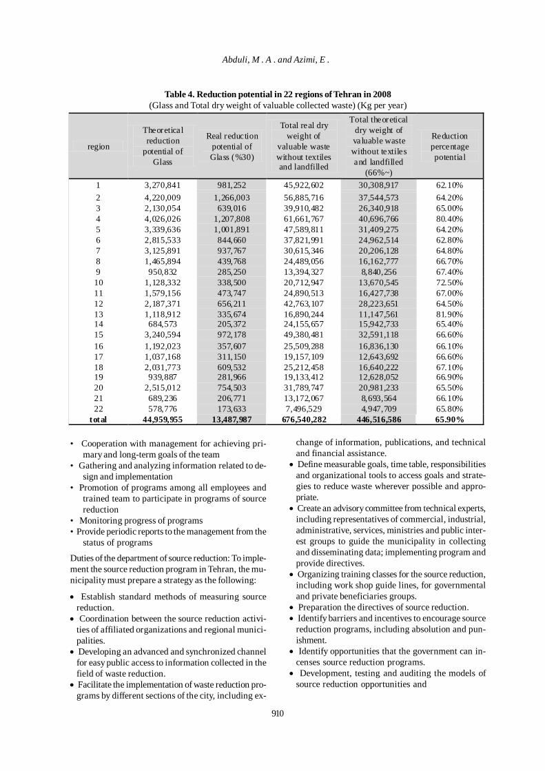
Table 4. Reduction potential in 22 regions of Tehran in 2008(Glass and Total dry weight of valuable collected waste) (Kg per year)
region
Theoretical reduction
potential of Glass
Real reduction potential of Glass (%30)
Total real dry weight of
valuable waste without textiles and landfilled
Total theoretical dry weight of valuable waste without textiles and landfilled
(66%~)
Reduction percentage potential
1 3,270,841 981,252 45,922,602 30,308,917 62.10% 2 4,220,009 1,266,003 56,885,716 37,544,573 64.20% 3 2,130,054 639,016 39,910,482 26,340,918 65.00% 4 4,026,026 1,207,808 61,661,767 40,696,766 80.40% 5 3,339,636 1,001,891 47,589,811 31,409,275 64.20% 6 2,815,533 844,660 37,821,991 24,962,514 62.80% 7 3,125,891 937,767 30,615,346 20,206,128 64.80% 8 1,465,894 439,768 24,489,056 16,162,777 66.70% 9 950,832 285,250 13,394,327 8,840,256 67.40% 10 1,128,332 338,500 20,712,947 13,670,545 72.50% 11 1,579,156 473,747 24,890,513 16,427,738 67.00% 12 2,187,371 656,211 42,763,107 28,223,651 64.50% 13 1,118,912 335,674 16,890,244 11,147,561 81.90% 14 684,573 205,372 24,155,657 15,942,733 65.40% 15 3,240,594 972,178 49,380,481 32,591,118 66.60% 16 1,192,023 357,607 25,509,288 16,836,130 66.10% 17 1,037,168 311,150 19,157,109 12,643,692 66.60% 18 2,031,773 609,532 25,212,458 16,640,222 67.10% 19 939,887 281,966 19,133,412 12,628,052 66.90% 20 2,515,012 754,503 31,789,747 20,981,233 65.50% 21 689,236 206,771 13,172,067 8,693,564 66.10% 22 578,776 173,633 7,496,529 4,947,709 65.80%
total 44,959,955 13,487,987 676,540,282 446,516,586 65.90%
• Cooperation with management for achieving pri-mary and long-term goals of the team
• Gathering and analyzing information related to de-sign and implementation
• Promotion of programs among all employees andtrained team to participate in programs of sourcereduction
• Monitoring progress of programs• Provide periodic reports to the management from the
status of programs
Duties of the department of source reduction: To imple-ment the source reduction program in Tehran, the mu-nicipality must prepare a strategy as the following:
• Establish standard methods of measuring sourcereduction.
• Coordination between the source reduction activi-ties of affiliated organizations and regional munici-palities.
• Developing an advanced and synchronized channelfor easy public access to information collected in thefield of waste reduction.
• Facilitate the implementation of waste reduction pro-grams by different sections of the city, including ex-
change of information, publications, and technicaland financial assistance.
• Define measurable goals, time table, responsibilitiesand organizational tools to access goals and strate-gies to reduce waste wherever possible and appro-priate.
• Create an advisory committee from technical experts,including representatives of commercial, industrial,administrative, services, ministries and public inter-est groups to guide the municipality in collectingand disseminating data; implementing program andprovide directives.
• Organizing training classes for the source reduction,including work shop guide lines, for governmentaland private beneficiaries groups.
• Preparation the directives of source reduction.• Identify barriers and incentives to encourage source
reduction programs, including absolution and pun-ishment.
• Identify opportunities that the government can in-censes source reduction programs.
• Development, testing and auditing the models ofsource reduction opportunities and
910
Abduli, M . A . and Azimi, E .
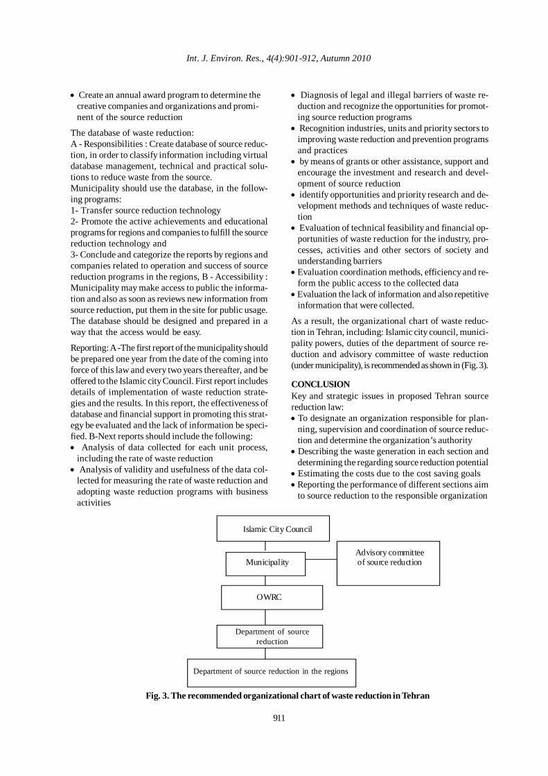
• Create an annual award program to determine thecreative companies and organizations and promi-nent of the source reduction
The database of waste reduction:A - Responsibilities : Create database of source reduc-tion, in order to classify information including virtualdatabase management, technical and practical solu-tions to reduce waste from the source.Municipality should use the database, in the follow-ing programs:1- Transfer source reduction technology2- Promote the active achievements and educationalprograms for regions and companies to fulfill the sourcereduction technology and3- Conclude and categorize the reports by regions andcompanies related to operation and success of sourcereduction programs in the regions, B - Accessibility :Municipality may make access to public the informa-tion and also as soon as reviews new information fromsource reduction, put them in the site for public usage.The database should be designed and prepared in away that the access would be easy.
Reporting: A -The first report of the municipality shouldbe prepared one year from the date of the coming intoforce of this law and every two years thereafter, and beoffered to the Islamic city Council. First report includesdetails of implementation of waste reduction strate-gies and the results. In this report, the effectiveness ofdatabase and financial support in promoting this strat-egy be evaluated and the lack of information be speci-fied. B-Next reports should include the following:• Analysis of data collected for each unit process,
including the rate of waste reduction• Analysis of validity and usefulness of the data col-
lected for measuring the rate of waste reduction andadopting waste reduction programs with businessactivities
• Diagnosis of legal and illegal barriers of waste re-duction and recognize the opportunities for promot-ing source reduction programs
• Recognition industries, units and priority sectors toimproving waste reduction and prevention programsand practices
• by means of grants or other assistance, support andencourage the investment and research and devel-opment of source reduction
• identify opportunities and priority research and de-velopment methods and techniques of waste reduc-tion
• Evaluation of technical feasibility and financial op-portunities of waste reduction for the industry, pro-cesses, activities and other sectors of society andunderstanding barriers
• Evaluation coordination methods, efficiency and re-form the public access to the collected data
• Evaluation the lack of information and also repetitiveinformation that were collected.
As a result, the organizational chart of waste reduc-tion in Tehran, including: Islamic city council, munici-pality powers, duties of the department of source re-duction and advisory committee of waste reduction(under municipality), is recommended as shown in (Fig. 3).
Islamic City Council
Municipality
OWRC
Advisory committeeof source reduction
Department of sourcereduction
Department of source reduction in the regions
Fig. 3. The recommended organizational chart of waste reduction in Tehran
CONCLUSIONKey and strategic issues in proposed Tehran sourcereduction law:• To designate an organization responsible for plan-
ning, supervision and coordination of source reduc-tion and determine the organization’s authority
• Describing the waste generation in each section anddetermining the regarding source reduction potential
• Estimating the costs due to the cost saving goals• Reporting the performance of different sections aim
to source reduction to the responsible organization
Int. J. Environ. Res., 4(4):901-912, Autumn 2010
911
912
• Working with different industries to modify theirproducts and set the strategies required
• Taxing disposal products• Providing tax credits or exemptions to industries that
meet set source reduction goals in design and produce• Set the source reduction database of in each part
(household, industrial, commercial)• Implementing scientific researches and technologies
regarding source reduction and preventing the nega-tive influence on environmental and economic
• Monitoring, supporting and modifying program withinternational strategies
The key elements of the proposed law are as following:• Incentivize efforts to reduce, re-use, recycle wasteand recover energy from waste;• Reform regulation to drive the reduction of wasteand diversion from landfill while reducing costs to com-pliant businesses and the regulator;• Target action on materials, products and sectors withthe greatest scope for improving environmental andeconomic outcomes;• Stimulate investment in collection, recycling and re-covery infrastructure, and markets for recovered mate-rials that will maximize the value of materials and en-ergy recovered; and• Improve national, regional and local governance, witha clearer performance and institutional framework todeliver better coordinated action and services on theground.(DEFRA, 2007).
REFERENCESAbduli,M.A.,(1996). Industrial Waste Management inTehran, J.Environ. Internatiaonal, 22(3), 335-341.
Abduli,M.A.,(1995). Solid Waste Management inTehran,J.Waste Management & Research,13,519-531.
Abduli,M.A.,(1994).Hospital Waste Management inTehran,J.Environ,Science and Health,29(3),477-492.
DEFRA, (2007). Waste Strategy for England 2007.De-partment for Environment, Food and Rural Affairs:Executive Summary, Key proposals for action,7-17.DETR (Department of the Environment, Transport and theRegions), (2000). Waste Strategy 2000 for England andWales: Our vision, 13-24. (London: Crown)
Duke University and Environmental Defense Fund (1995).Paper Task Force Recommendations for Purchasing and Us-ing Environmentally Preferable Paper: Recycling and BuyingRecycled Paper, 64-118. (New York: Recycled Paper).
EEA(European Environment Agency), (2007). The road fromlandfilling to recycling:common destination, different routes:Final reflections: success factors for effectiveness, 18-20(Luxembourg:Office for Official Publications of the Euro-pean Communities).
EEA(European Environment Agency), (2009). Divertingwaste from landfill, Effectiveness of wastemanagement poli-cies in the European Union: comparative assessment & con-
clusion, 50-60. (Luxembourg:Office for Official Publicationsof the European Communities).
EPA,(1999).ReduceIt Companion Software to Source Re-duction Program Potential Manual: Source Reduction andYour Community An Introduction to EPA’s PlanningPacket(EPA530-F-99-006).
Gidarakos, E., Havas, G. and Ntzamilis, P. (2006). Munici-pal solid waste composition determination supporting theintegrated solid waste management system in the island ofCrete. Waste Manage., 26, 668–679.
Hyde,K., Smith,A., Smith,M. And Henningson,S.,(2000).The Challenge of Waste Minimization in the Food and DrinkIndustry: a Demonstration Project in East Anglia, UK. J.Cleaner Production, 9,57-64.
Jalili Ghazi Zade,M., and Noori,R.,(2008). Prediction ofMunicipal Solid Waste Generation by Use of Artificial Neu-ral Network: A Case Study of Mashhad, Int. J. Environ.Res., 2(1), 13-22.
Land Technologies, Inc., Price-Moon Enterprises. andSnohomish County Road MaintenanceDivision,(1997).Reprocessing and Reuse of Street WasteSolids. IBP-97-5.
NRWF, (2006).Household Waste Prevention Toolkit, PARTA and PART B, National Resource & Waste Forum.
Oshode, O. A., Bakare, A. A., Adeogun, A. O., Efuntoye,M. O. and Sowunmi, A. A. (2008). Ecotoxicological Assess-ment Using Clarias Gariepinus and Microbial Characteriza-tion of Leachate from Municipal Solid Waste Landfill, Int.J. Environ. Res., 2(4), 391-400.
OWRC, (2008). Statistics report on (2008). Organizationfor Waste Recycling and Composting, Tehran Municipality,Iran.
Leary, R.O. Ph. and Walsh,W.P.,(1995). Decision-Makers’GuideTo Solid Waste Management, Volume II:Source Re-duction 5-1,5-22.
Robinson, H. D. (1983). Problems of leachate from domes-tic waste tips in analysis for environmental protection. Anal.Proc. 20.
Sadugh, M.B., Jalili Ghazizadeh, M., Pezeshk, H. and JaliliGhazizadeh, V.,(2009). Evaluating the Recovery Potentialof Solid Wastes, Int. J. Environ. Res., 3(4), 681-690.
Schnell,J.,Barwick,K., and Shah,A.,(2004).Hazardous WasteSource Reduction Assessment of Selected Sectors of TheCalifornia Chemical Industry:Report Overview,i-iii.
U.S Army Center, For Public Works, Source Reduction Plan-ning, (1994).
Walsh, P. (1993). University of Wisconsin–Extension, Solidand Hazardous Waste Education Center.
Waste Online,(2006). managed by Waste Watch and has beenfunded by the New Opportunities Fund Digitise project,from http://www.wasteonline.org.uk/resources/InformationSheets/Packaging.htm.
World Bank, final Report, Tehran Solid Wsate Management(Integrated Waste Management Strategy & ImplementationPlan), (2005).
Reduction of Municipal Waste

Aims & Scopes
International Journal of Environmental Research is a multidisciplinary peer review journal concerned with all aspects of environment. In pursuit of these, environmentalist disciplines are invited to contribute their knowledge and experience. International Journal of Environmental Research publishes original research papers, research notes and reviews across the broad field of environment. These include but are not limited to environmental science, environmental engineering, environmental management and planning and environmental design, urban and regional landscape design and natural disaster management. Thus high quality research papers or reviews dealing with any aspect of environment are welcomed. Papers may be theoretical, interpretative or experimental.
Instructions to Authors Manuscript Submission Authors are requested to download the Copyright form and Covering letter web site http://ijer.ut.ac.ir/ Please send a completed and signed form either by mail or fax to the International Journal of Environmental Research Office. Manuscripts should be emailed to: [email protected]. It should be noted that normal time for reviewing the submitted papers is about 12 weeks. Language The journal's language is English. British English or American English spelling and terminology may be used. We appreciate any efforts that you make to ensure that the language is corrected before submission. This will greatly improve the legibility of your paper if English is not your first language. Manuscript Presentation Manuscripts should be typewritten on A4 paper, with a font Times New Roman of 11 pt, one side only, leaving adequate margins on all sides to allow reviewers' remarks. Please double space all material. Number the pages consecutively with the first page containing: Running head (shortened title) Title Author(s) Affiliation(s) Full address for correspondence, including telephone number, fax number and e-mail address. Text The text should include: Title, author(s) name and address, an abstract, key words, introduction, materials and methods, results and discussions, conclusion, acknowledgement and references. Abstract Please provide a short abstract of 100 to 250 words. The abstract should not contain any undefined abbreviations or references. Key words Please provide 5 to 7 key words. Notes Please avoid notes, but if any, use footnotes rather than endnotes. Notes should be indicated by consecutive superscript numbers in the text. Acknowledgements Acknowledgements of people, grants, funds, etc. should be placed in a separate section before the References. References All publication cited in the text should be presented in the list of references following the text of the manuscript. In the text refer to the authors' name (without initials) and year of publication (e. g. Williams, 2004). For three or more autours use the first autour followed by "et al.," in the last. The list of references at the end of the manuscript should be arranged alphabetically authors' names and chronologically per author: The list of references should be given in the following style: 1. Journal article: Karbassi, A. R. and Amirnezhad, R. (2004). Geochemistry of heavy metals and sedimentation rate in a bay adjacent to the Caspian Sea. Int. J. Environ. Sci. Tech., 1(3), 199-206. 2. Book chapter: Cutrona, C. E. & Russell, D. (1990). Type of social support and specific stress: Towards a theory of optimum matching. (In I.G. Sarason, B. R. Sarason, & G. Pierce (Eds.), Social support: An interactional view (pp. 341-366). New York: Wiley.) 3. Book, authored: Capland, G. (1964). Principles of preventive psychiatry. (New York: Basic Books) 4. Book, edited: Felner, R. D., Jason, L. A., Moritsugu, J. N. and Farber, S. S. (Eds.) (1983). Preventive psychology: Theory, research and practice. (New York: Pergamon Press)

5. Paper presented at a conference: Phelan, J. C., Link, B. G., Stueve, A. and Pescosolido, B. A. (1996, November). Have public conceptions of mental health changed in the past half century? Does it matter? (Paper presented at the 124th. Annual Meeting of the American Public Health Association, New York) 6. Dissertation: Trent, J.W. (1975) Experimental acute renal failure. Dissertation, University of California 7. Internet publication/Online document 7.1. Internet articles based on a print source VandenBos, G., Knapp, S. and Doe, J. (2001). Role of reference elements in the selection of resources by psychology undergraduates [Electronic version]. J. Bibliog. Res., 5, 117-123. VandenBos, G., Knapp, S., and Doe, J. (2001). Role of reference elements in the selection of resources by psychology undergraduates. J. Bibliog. Res., 5, 117-123. Retrieved October 13, 2001, from http://jbr.org/articles.html 7.2. Article in an Internet-only journal Fredrickson, B. L. (2000, March 7). Cultivating positive emotions to optimize health and well-being. Prevention & Treatment, 3, Article 0001a. Retrieved November 20, 2000, from http://journals.apa.org/prevent/vol3/pre03.html. Figures All photographs, graphs and diagrams should be referred to as a 'Figure' and they should be numbered consecutively (1, 2, etc.). Multipart figures ought to be labeled with lower case letters (a, b, etc.). Please insert keys and scale bars directly in the figures. Provide a detailed legend (without abbreviations) to each figure, refer to the figure in the text and note its approximate location in the margin. Only black and white figures must be submitted. The resolution of figure must at least be 300 dpi. Figures that are prepared by excel should be send along with their source of data. Tables Each table should be numbered consecutively (1,2, etc.). In tables, footnotes are preferable to long explanatory material in either the heading or body of the table. Such explanatory footnotes, identified by superscript letters, should be placed immediately below the table. Please provide a caption (without abbreviations) to each table, refer to the table in the text and note its approximate location in the margin. The same data should not be presented simultaneously in tables and figures. Proofs Proofs will be sent to the corresponding author by e-mail (if no email address is available or appears to be out of order, proofs will be sent by regular mail). Your response, with or without corrections, should be sent within 72 hours. Copyright Authors will be asked, upon acceptance of an article, to transfer copyright of the article to the Publisher. This will ensure the widest possible dissemination of information under copyright laws. The submitted materials may be considered for inclusion but can not be returned. Note Editors of the Journal reserve the right to accept, reject and edit any article in any stage, if necessary. The sole responsibility for the whole contents of the article (views, statements and names) remains only with the author(s). Additional Information Additional information can be obtained from: International Journal of Environmental Research P.O. Box: 14155-6135 University of Tehran Graduate Faculty of Environment E-mail: [email protected] http://ijer.ut.ac.ir Tel: +9821 61113188 Fax: +9821 66407719
Magiran; Iran;http://www.magiran.com
MagIran.com is the one site for all Iranian magazines. Findyour favorite magazines and view published numbers, table ofcontents and papers.
World Health Organization Regional Office for the Eastern Mediterranean
INTERNATIONAL JOURNAL OF ENVIRONMENTAL RESERACH (IJER) is indexed and abstracted in the bibliographical databases including:
Index Copernicus (IC); Poland;http://www.indexcopernicus.com/index.php
IC Journals is a journal indexing, ranking and abstracting site.This service helps a journal to grow from a local level to aglobal one as well as providing complete web-based solutionfor small editorial teams.
Bioline international; Canada; http://www.bioline.org
Bioline International is a not-for-profit electronic publishingservice committed to providing open access to quality researchjournals published in developing countries. BI’s goal of reducingthe South to North knowledge gap is crucial to a globalunderstanding of health (tropical medicine, infectious diseases,epidemiology, emerging new diseases), biodiversity, theenvironment, conservation and international development.
Cambridge Scientific Abstracts (CSA); USA;http://www.csa.com
CSA is a worldwide information company, serving as a guide toresearchers to help them be more effective in their work byenabling and expediting discovery, aiding the management andorganization of quality information and providing tools to assistin its subsequent dissemination.
Scientific Information Database (SID); Iran; http://www.sid.ir
Regarding the every day enhancement of the requirements forresearch, the growth of scientific production at universities andresearch center of Iran, and the necessity of instant access toscientific source, it is tangible to develop scientific database inIran.
World Health Organization (Egypt);http://www.emro.who.int/
The Index Medicus for the WHO Eastern Mediterranean Region(IMEMR) has sustained its indexing policy, which has made itvital current awareness information tool, for technical staff ofthe Regional Office, health care staff and medical professionalswho are able now to access health literature published in theRegion as soon as it is published.
Geobase (Netherlands);http://www.elsevier.com/
GEOBASE is a unique multidisciplinary database supplyingbibliographic information and abstracts for development studies,the Earth sciences, ecology, geomechanics, human geography,and oceanography.
Geobase (Netherlands);http://www.elsevier.com/
EMBiology is a new Abstracts and Indexing database. Drawnfrom close to 3,000 international titles and extending back to1980, EMBiology indexes more than 4 million records from thebiological science literature.
Thomson Journal Master List; USA; http://scientific.thomsonreuters.com/cgi-bin/jrnlst/
jlresults.cgi?PC=MASTER&ISSN=1735-6865The combined authoritative information with innovativetechnologies to enhance researchers’ ability to achieve world-class research and business results.
CAB Abstract (UK);http://www.cabi.org/
CAB Abstracts is the most comprehensive database of its kind;giving researchers instant access to over 5 Million recordscovering the applied life sciences.
Scopus; The Netherlands; http://www.scopus.com
Scopus is the largest abstract and citation database of researchliterature and quality web sources. It’s designed to find theinformation scientists need. Quick, easy and comprehensive,Scopus provides superior support of the literature researchprocess. Updated daily, Scopus offers.
ISI/SCIEWeb of Science; USA;
http://www.thomsonscientific.com/cgi-bin/jrnlst/jlresults.cgi?PC=B7&ISSN=1735-6865
The Web of Science provides seamless access to current andretrospective multidisciplinary information from approximately8,700 of the most prestigious, high impact research journals inthe world. Web of Science also provides a unique searchmethod, cited reference searching.
Related Documents