From supernovae to galaxy clusters Observing the chemical enrichment in the hot intra-cluster medium François Mernier

Welcome message from author
This document is posted to help you gain knowledge. Please leave a comment to let me know what you think about it! Share it to your friends and learn new things together.
Transcript

From supernovae to galaxy clustersObserving the chemical enrichment in the hot
intra-cluster medium
François Mernier
ISBN: 978-94-6233-622-3
© 2017 François MernierFrom supernovae to galaxy clusters, Observing the chemical enrichment in thehot intra-cluster medium, Thesis, Universiteit LeidenThis work was supported by Leiden Observatory and SRON Netherlands Insti-tute for Space Research.
Cover: Composite image of the Phoenix cluster (Credit: NASA/CXC/MIT/STScI).The X-ray emission (blue) shows the hot intra-cluster medium, while the clus-ter galaxies and star-forming filaments can be seen in optical (yellow and red).The front image shows an artist impression of the XMM-Newton satellite (Credit:ESA), together with metal lines derived from EPIC X-ray spectra (see Chapter 3and summary).
From supernovae to galaxy clustersObserving the chemical enrichment in the hot
intra-cluster medium
Proefschrift
ter verkrijging vande graad van Doctor aan de Universiteit Leiden,
op gezag van Rector Magnificus prof.mr. C.J.J.M. Stolker,volgens besluit van het College voor Promoties
te verdedigen op woensdag 31 mei 2017klokke 13.45 uur
door
François Denis Marin Mernier
geboren te Ukkel (Brussel), Belgiëin 1989
Promotiecommissie
Promotor: Prof. dr. Jelle S. KaastraCo-promotor: Dr. Jelle de Plaa
Overige leden: Prof. dr. M. FranxProf. dr. H.J.A. RöttgeringProf. dr. J. SchayeDr. A. Simionescu (ISAS, JAXA, Sagamihara, Japan)Dr. J. Vink (Universiteit van Amsterdam)

À mes parents

Contents
1 Introduction 11.1 The stellar nucleosynthesis: a brief history... . . . . . . . . . . 21.2 The role of Type Ia and core-collapse supernovae . . . . . . . 3
1.2.1 Core-collapse supernovae (SNcc) . . . . . . . . . . . . 51.2.2 Type Ia supernova (SNIa) . . . . . . . . . . . . . . . . 6
1.3 Metals in clusters of galaxies . . . . . . . . . . . . . . . . . . . 81.3.1 The legacy of past X-ray missions . . . . . . . . . . . 101.3.2 The recent generation of X-ray missions . . . . . . . . 121.3.3 Constraining supernovae models by looking at the
intra-cluster medium . . . . . . . . . . . . . . . . . . . 131.3.4 Stellar and intra-cluster phases of metals . . . . . . . 161.3.5 Where and when was the ICM chemically enriched? 17
1.4 Spectral codes for a collisional ionisation equilibrium plasma 201.5 This thesis . . . . . . . . . . . . . . . . . . . . . . . . . . . . . 21
2 Abundance and temperature distributions in the hot intra-clustergas of Abell 4059 252.1 Introduction . . . . . . . . . . . . . . . . . . . . . . . . . . . . 262.2 Observations and data reduction . . . . . . . . . . . . . . . . 28
2.2.1 EPIC . . . . . . . . . . . . . . . . . . . . . . . . . . . . 282.2.2 RGS . . . . . . . . . . . . . . . . . . . . . . . . . . . . . 31
2.3 Spectral models . . . . . . . . . . . . . . . . . . . . . . . . . . 322.3.1 The cie model . . . . . . . . . . . . . . . . . . . . . . 322.3.2 The gdem model . . . . . . . . . . . . . . . . . . . . . . 332.3.3 Cluster emission and background modelling . . . . . 33
2.4 Cluster core . . . . . . . . . . . . . . . . . . . . . . . . . . . . 34
Contents
2.4.1 EPIC . . . . . . . . . . . . . . . . . . . . . . . . . . . . 342.4.2 RGS . . . . . . . . . . . . . . . . . . . . . . . . . . . . . 40
2.5 EPIC radial profiles . . . . . . . . . . . . . . . . . . . . . . . . 412.6 Temperature, σT , and Fe abundance maps . . . . . . . . . . . 482.7 Discussion . . . . . . . . . . . . . . . . . . . . . . . . . . . . . 52
2.7.1 Abundance uncertainties and SNe yields . . . . . . . 522.7.2 Abundance radial profiles . . . . . . . . . . . . . . . . 552.7.3 Temperature structures and asymmetries . . . . . . . 57
2.8 Conclusions . . . . . . . . . . . . . . . . . . . . . . . . . . . . 602.A Detailled data reduction . . . . . . . . . . . . . . . . . . . . . 63
2.A.1 GTI filtering . . . . . . . . . . . . . . . . . . . . . . . . 632.A.2 Resolved point sources excision . . . . . . . . . . . . 632.A.3 RGS spectral broadening correction fromMOS1 image 64
2.B EPIC background modelling . . . . . . . . . . . . . . . . . . . 652.B.1 Hard particle background . . . . . . . . . . . . . . . . 652.B.2 Unresolved point sources . . . . . . . . . . . . . . . . 672.B.3 Local Hot Bubble and Galactic thermal emission . . . 692.B.4 Residual soft-proton component . . . . . . . . . . . . 692.B.5 Application to our datasets . . . . . . . . . . . . . . . 69
2.C S/N requirement for the maps . . . . . . . . . . . . . . . . . 72
3 Origin of central abundances in the hot intra-cluster mediumI. Individual and average abundance ratios from XMM-Newton EPIC 753.1 Introduction . . . . . . . . . . . . . . . . . . . . . . . . . . . . 763.2 Observations and data preparation . . . . . . . . . . . . . . . 78
3.2.1 Data reduction . . . . . . . . . . . . . . . . . . . . . . 783.2.2 Spectra extraction . . . . . . . . . . . . . . . . . . . . . 80
3.3 EPIC spectral analysis . . . . . . . . . . . . . . . . . . . . . . 813.3.1 Background modelling . . . . . . . . . . . . . . . . . . 833.3.2 Global fits . . . . . . . . . . . . . . . . . . . . . . . . . 853.3.3 Local fits . . . . . . . . . . . . . . . . . . . . . . . . . . 85
3.4 Results . . . . . . . . . . . . . . . . . . . . . . . . . . . . . . . 863.4.1 Estimating reliable average abundances . . . . . . . . 893.4.2 EPIC stacked residuals . . . . . . . . . . . . . . . . . . 903.4.3 Systematic uncertainties . . . . . . . . . . . . . . . . . 92
3.5 Discussion . . . . . . . . . . . . . . . . . . . . . . . . . . . . . 963.5.1 Discrepancies in the S/Fe, Ar/Fe and Ni/Fe ratios . 1003.5.2 Comparison with the proto-solar abundance ratios . 101
Contents
3.5.3 Current limitations and future prospects . . . . . . . 1023.6 Conclusions . . . . . . . . . . . . . . . . . . . . . . . . . . . . 1043.A EPIC absorption column densities . . . . . . . . . . . . . . . 1073.B Radiative recombination corrections . . . . . . . . . . . . . . 1073.C Effects of the temperature distribution on the abundance ratios1103.D Best-fit temperature and abundances . . . . . . . . . . . . . . 113
4 Origin of central abundances in the hot intra-cluster mediumII. Chemical enrichment and supernova yield models 1194.1 Introduction . . . . . . . . . . . . . . . . . . . . . . . . . . . . 1204.2 Observations and spectral analysis . . . . . . . . . . . . . . . 1234.3 Chemical enrichment in the ICM . . . . . . . . . . . . . . . . 124
4.3.1 Abundance pattern of even-Z elements . . . . . . . . 1264.3.2 Mn/Fe ratio . . . . . . . . . . . . . . . . . . . . . . . . 1394.3.3 Fraction of low-mass stars that become SNIa . . . . . 1444.3.4 Clues on the metal budget conundrum in clusters . . 146
4.4 Enrichment in the solar neighbourhood . . . . . . . . . . . . 1494.5 Summary and conclusions . . . . . . . . . . . . . . . . . . . . 153
4.5.1 Future directions . . . . . . . . . . . . . . . . . . . . . 1554.A The effect of electron capture rates on the SNIa nucleosyn-
thesis yields . . . . . . . . . . . . . . . . . . . . . . . . . . . . 1584.B List of SN yield models used in this work . . . . . . . . . . . 159
5 Origin of central abundances in the hot intra-cluster mediumIII. The impact of spectral model improvements on the abundance ratios 1635.1 Introduction . . . . . . . . . . . . . . . . . . . . . . . . . . . . 1645.2 The sample and the reanalysis of our data . . . . . . . . . . . 166
5.2.1 The sample . . . . . . . . . . . . . . . . . . . . . . . . 1665.2.2 From SPEXACT v2 to SPEXACT v3 . . . . . . . . . . 167
5.3 Results . . . . . . . . . . . . . . . . . . . . . . . . . . . . . . . 1705.3.1 The Fe bias in cool plasmas . . . . . . . . . . . . . . . 1715.3.2 The Ni bias . . . . . . . . . . . . . . . . . . . . . . . . 1765.3.3 Updated average abundance ratios . . . . . . . . . . . 177
5.4 Discussion . . . . . . . . . . . . . . . . . . . . . . . . . . . . . 1795.4.1 Implications for the iron content in groups and clusters1795.4.2 Implications for supernovae yield models . . . . . . . 182
5.5 Conclusions . . . . . . . . . . . . . . . . . . . . . . . . . . . . 188
Contents
6 Radial metal abundance profiles in the intra-cluster medium ofcool-core galaxy clusters, groups, and ellipticals 1936.1 Introduction . . . . . . . . . . . . . . . . . . . . . . . . . . . . 1946.2 Observations and data preparation . . . . . . . . . . . . . . . 1986.3 Spectral modelling . . . . . . . . . . . . . . . . . . . . . . . . 199
6.3.1 Thermal emission modelling . . . . . . . . . . . . . . 1996.3.2 Background modelling . . . . . . . . . . . . . . . . . . 2016.3.3 Local fits . . . . . . . . . . . . . . . . . . . . . . . . . . 202
6.4 Building average radial profiles . . . . . . . . . . . . . . . . . 2036.4.1 Exclusion of fitting artefacts . . . . . . . . . . . . . . . 2036.4.2 Stacking method . . . . . . . . . . . . . . . . . . . . . 2036.4.3 MOS-pn uncertainties . . . . . . . . . . . . . . . . . . 205
6.5 Results . . . . . . . . . . . . . . . . . . . . . . . . . . . . . . . 2066.5.1 Fe abundance profile . . . . . . . . . . . . . . . . . . . 2066.5.2 Abundance profiles of other elements . . . . . . . . . 208
6.6 Systematic uncertainties . . . . . . . . . . . . . . . . . . . . . 2146.6.1 Projection effects . . . . . . . . . . . . . . . . . . . . . 2186.6.2 Thermal modelling . . . . . . . . . . . . . . . . . . . . 2186.6.3 Background uncertainties . . . . . . . . . . . . . . . . 2206.6.4 Weight of individual observations . . . . . . . . . . . 2236.6.5 Atomic code uncertainties . . . . . . . . . . . . . . . . 2256.6.6 Instrumental limitations for O and Mg abundances . 227
6.7 Discussion . . . . . . . . . . . . . . . . . . . . . . . . . . . . . 2286.7.1 Enrichment in clusters and groups . . . . . . . . . . . 2286.7.2 The central metallicity drop . . . . . . . . . . . . . . . 2306.7.3 The overall Fe profile . . . . . . . . . . . . . . . . . . . 2366.7.4 Radial contribution of SNIa and SNcc products . . . 242
6.8 Conclusions . . . . . . . . . . . . . . . . . . . . . . . . . . . . 2506.A Cluster properties and individual Fe profiles . . . . . . . . . 2556.B Average abundance profiles of O, Mg, Si, S, Ar, Ca, and Ni . 255
7 Future prospects for intra-cluster medium enrichment studies 2657.1 Current limitations of abundance measurements . . . . . . . 2657.2 The future ofXMM-Newton in intra-cluster enrichment studies267
7.2.1 Nearby clusters and supernova models . . . . . . . . 2677.2.2 High redshift clusters . . . . . . . . . . . . . . . . . . 269
7.3 Future work on atomic data and spectral modelling . . . . . 2697.4 X-ray micro-calorimeters . . . . . . . . . . . . . . . . . . . . . 270
Contents
7.5 The upcoming generation of X-ray missions . . . . . . . . . . 2737.5.1 Hitomi . . . . . . . . . . . . . . . . . . . . . . . . . . . 2737.5.2 XARM . . . . . . . . . . . . . . . . . . . . . . . . . . . 2757.5.3 Athena . . . . . . . . . . . . . . . . . . . . . . . . . . . 277
7.6 Concluding remarks . . . . . . . . . . . . . . . . . . . . . . . 279
Bibliography 281
Nederlandse samenvatting 293
English summary 301
Résumé en français 309
Curriculum Vitae 317
List of publications 319
Acknowledgements 321

Quand on me demande: «À quoi sert l’astronomie?»il m’arrive de répondre: «N’aurait-elle servi qu’à révéler tant de beauté,
elle aurait déjà amplement justifié son existence.»
When people ask me: ”What is the use of astronomy?”I sometimes answer: ”If its use was only to reveal such beauty,astronomy would have already amply justified its existence.”
– Hubert Reeves, Patience dans l’azur
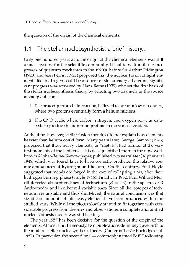
1| IntroductionAll along the 20th century, many discoveries have revolutionised our cur-rent view of the Universe. The success of the special and general relativitypredicted by Albert Einstein more than hundred years ago (Einstein 1905,1916) is probably one of the most famous examples. A second major resultis certainly the discovery of other ”island universes” by Edwin Hubble in1926, extending our conception of the entire cosmos from the only MilkyWay to a universe full of galaxies (Hubble 1926). Even more surprising isthat, as also found by Hubble, these galaxies escape away from each other(Hubble 1929). This provided a solid piece of evidence that the Universe isactually expanding. A third major discovery, which quickly became a ma-jor issue for physicists and astronomers, was the evidence for missing (or”dark”) matter, suggested independently in individual galaxies by VeraRubin (1970) and in galaxy clusters by Jacobus Kapteyn (1922) and FritzZwicky (1933). Fourth, the accidental discovery of the cosmic microwavebackground by Arno Penzias and Robert Woodrow Wilson (1965; see alsoDicke et al. 1965) provided a decisive proof of the Big Bang theory. Finally,the discovery of the acceleration of the expansion of the Universe by look-ing as distant Type Ia supernovae (Riess et al. 1998) suggests that the Uni-verse is dominated by a mysterious ”dark” energy, whose fundamentalnature remains unknown.
All these above discoveries are now fully part of the basic history ofsciences, as they have had an extraordinary impact on the current way weconceive the Universe. Nevertheless, some past discoveries are somewhatless known to a large public, although they have not contributed less tofundamentally revisit our relation to astronomy. One of them deals with
1
1.1 The stellar nucleosynthesis: a brief history...
the question of the origin of the chemical elements.
1.1 The stellar nucleosynthesis: a brief history...Only one hundred years ago, the origin of the chemical elements was stilla total mystery for the scientific community. It had to wait until the pro-gresses of quantum mechanics in the 1920’s, before Sir Arthur Eddington(1920) and Jean Perrin (1922) proposed that the nuclear fusion of light ele-ments like hydrogen could be a source of stellar energy. Later on, signifi-cant progress was achieved by Hans Bethe (1939) who set the first basis ofthe stellar nucleosynthesis theory by selecting two channels as the sourceof energy of stars:
1. The proton-proton chain reaction, believed to occur in lowmass stars,where two protons eventually form a helium nucleus;
2. The CNO cycle, where carbon, nitrogen, and oxygen serve as cata-lysts to produce helium from protons in more massive stars.
At the time, however, stellar fusion theories did not explain how elementsheavier than helium could form. Many years later, George Gamow (1946)proposed that these heavy elements, or ”metals”, had formed at the veryfirst moments of the Universe. This was quantified more in the now well-knownAlpher-Bethe-Gamowpaper, published twoyears later (Alpher et al.1948, which was found later to have correctly predicted the relative cos-mic abundances of hydrogen and helium). On the contrary, Fred Hoylesuggested that metals are forged in the core of collapsing stars, after theirhydrogen burning phase (Hoyle 1946). Finally, in 1952, Paul Willard Mer-rill detected absorption lines of technetium (Z = 43) in the spectra of RAndromedae and in other red variable stars. Since all the isotopes of tech-netium are unstable and thus short-lived, the natural conclusion was thatsignificant amounts of this heavy element have been produced within thestudied stars. While all the pieces slowly started to fit together with con-siderable progress from theories and observations, a complete and unifiednucleosynthesis theory was still lacking.
The year 1957 has been decisive for the question of the origin of theelements. Almost simultaneously, two publications definitely gave birth tothe modern stellar nucleosynthesis theory (Cameron 1957a; Burbidge et al.1957). In particular, the second one — commonly named B2FH following
2
Introduction
the authors (Margaret Burbidge, her husband Geoffrey Burbidge, WilliamFowler, and Fred Hoyle) — explicitly detailed all the processes responsiblefor the synthesis of all the heavy elements, from lithium to uranium. Twospectacular conclusions could be drawn from that paper.
1. Itwas definitely demonstrated thatmetals are synthesised in the coresof stars and, especially, in supernovae. On the contrary, the primor-dial nucleosynthesis is capable of creating hydrogen and helium only(as well as traces of lithium and berilium).
2. Perhaps evenmore importantly, the authors showed for the first timethat when a star explodes as a supernova, it enriches its surroundinginterstellarmediumwith its freshly createdmetals, thus participatingactively in the formation of a new generation of stars.
In summary, about sixty years ago, evidence was provided that inter-stellar dust, planets, the Earth, living and human beings are all made ofstars and supernovae, thereby revolutionising even further our conceptionof the Universe.
1.2 The role of Type Ia and core-collapse supernovaeSince 1957, stellar and supernova nucleosynthesis theories considerablyimproved (for an evolution of reviews, see e.g. Arnett 1973; Tinsley 1980;Arnett 1995; Nomoto et al. 2013). With the increase of computing perfor-mance (in synergy with the increasing number and quality of supernovaeobservations) from the end of the 1970’s, several research groups started tosimulate explosive nucleosynthesis in massive stars and supernovae whiletaking observational features into account (e.g. Arnett 1977; Weaver et al.1978; Weaver & Woosley 1980; Nomoto et al. 1984).
Nowadays, it is well established that the production of metals can bedistinguished as follows.
• Asymptotic giant branch stars synthesise carbon (C), nitrogen (N),as well as traces of neon (Ne) and magnesium (Mg) — e.g. Karakas(2010).
• Core-collapse supernovae (SNcc; Fig. 1.1 left panel) and theirmassivestar progenitors synthesise almost all the oxygen (O), Ne, and Mg ofthe Universe, as well as a non-negligible fraction (about one half) ofsilicon (Si) and sulfur (S) — e.g. Kobayashi et al. (2006).
3
1.2 The role of Type Ia and core-collapse supernovae
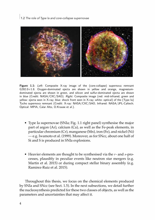
Figure 1.1: Left: Composite X-ray image of the (core-collapse) supernova remnantG292.0+1.8. Oxygen-dominated ejecta are shown in yellow and orange, magnesium-dominated ejecta are shown in green, and silicon and sulfur-dominated ejecta are shownin blue (Credit: NASA/CXC/SAO). Right: Composite image (red: mid-infrared; green andyellow: ejecta seen in X-ray; blue: shock front seen in X-ray; white: optical) of the (Type Ia)Tycho supernova remnant (Credit: X-ray: NASA/CXC/SAO, Infrared: NASA/JPL-Caltech;Optical: MPIA, Calar Alto, O.Krause et al.).
• Type Ia supernovae (SNIa; Fig. 1.1 right panel) synthesise the majorpart of argon (Ar), calcium (Ca), as well as the Fe-peak elements, inparticular chromium (Cr), manganese (Mn), iron (Fe), and nickel (Ni)— e.g. Iwamoto et al. (1999). Moreover, as for SNcc, about one half ofSi and S is produced in SNIa explosions.
• Heavier elements are thought to be synthesised via the r- and s-pro-cesses, plausibly in peculiar events like neutron star mergers (e.g.Martin et al. 2015) or during compact stellar binary assembly (e.g.Ramirez-Ruiz et al. 2015).
Throughout this thesis, we focus on the chemical elements producedby SNIa and SNcc (see Sect. 1.5). In the next subsections, we detail furtherthe nucleosynthesis predicted for these two classes of objects, as well as theparameters and uncertainties that may affect it.
4
Introduction
1.2.1 Core-collapse supernovae (SNcc)When a massive star (≳8–10 M⊙) has burned about 10% of its hydrogeninto helium, it reaches the end of its life on the main sequence (typicallywithin a fewmillion years). Heavier elements (C,Ne,O, Si) are successivelycreated, then burn in turn, building an onion-like structure in the core of thestar, where heavier elements are synthesised in deeper layers. This burn-ing process stops at 56Ni (which further decays into stable 56Fe), becausenuclear fusion becomes energetically inefficient for higher isotopes. Conse-quently, Fe accumulates in the core and increases its density up to the elec-tron degeneracy. When the core density reaches the Chandrasekhar limit(∼1.4 M⊙), the electron degenerate pressure is not sufficient anymore tocounter gravitational contraction, and the core quickly collapses. Neutronsand neutrinos are thenmassively created by electron capture. This collapsesuddenly stops when the core reaches the neutron degeneracy pressure,producing a powerful reverse shock from the core toward the upper layers.As the shock traverses the less dense external layers, its velocity increasesand can reach about 25% to 50% of the speed of light, heating the upperstellar material (which rapidly synthesises more elements) and violentlyejecting it into the interstellar medium. A core-collapse supernova is born.For recent reviews on the mechanisms driving SNcc explosions, see e.g.Janka (2012); Burrows (2013).
SNcc are commonly associated to Type II supernovae (i.e. supernovaeshowing hydrogen in their spectrum), but also to Type Ib (if the star has lostits hydrogen layer) and Type Ic supernovae (if the star has lost its hydro-gen and helium layers). As mentioned above, their main nucleosynthesisproducts are O, Ne, and Mg which are created almost exclusively in SNcc,as well as Si and S whose production originates from both SNcc and SNIa(see also Sect. 1.2.2). Heavier elements like Ca, Ar, Fe, and Ni may also besynthesised during SNcc explosions, but at much lower quantities.
How much mass of these elements are created by a SNcc or, in otherwords, what are the typical yields that a single SNcc produces? Accordingto the current SNcc models, the answer to this question depends on twomain parameters:
1. The mass of the stellar progenitor;
2. The initial metallicity of the progenitor or, in other words: was theprogenitor previously enriched by past supernovae?.
5
1.2 The role of Type Ia and core-collapse supernovae
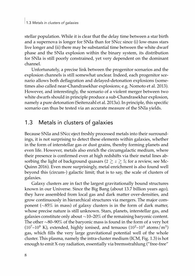
Of course, instead of considering only one SNcc, one can also address thesame question for a collection of SNcc resulting from a same single stel-lar population. In this case, one must integrate the above parameters overthe whole stellar population. Generally speaking, the integrated yields ofa population of SNcc will depend on the initial mass function (IMF) of theprogenitor population, and on its average initial metallicity, supposed tobe very similar for all the population members (Fig. 1.2 top).
1.2.2 Type Ia supernova (SNIa)Type Ia supernovae are different from SNcc in many aspects. In partic-ular, they are not the result of the end-of-life of a massive star. Instead,is it generally admitted that SNIa progenitors are binary systems includ-ing at least one carbon-oxygen white dwarf, i.e. the stellar remnant of alow-mass (≲8 M⊙) star, which suddenly gets (re-) ignited by mass accre-tion from the companion object. Unlike sometimes claimed, and becausethey do not result from a gravitational collapse, SNIa or their progenitorsapproach the Chandrasekhar limit, but never reach it. Although the pre-cise mechanism is still unknown, the ignition is thought to be triggeredby the explosive burning of carbon and newly synthesised nuclei. Becausethe electron degeneracy is independent of temperature, the white dwarf isunable to regulate its thermonuclear fusion, e.g. by expanding and coolingdown, as amain sequence star supported by thermal pressure would natu-rally do. This somehow triggers one or several ignition flames, resulting ina violent explosion entirely disrupting the object (contrary to SNcc, wherethe remaining stellar core collapses into either a neutron star or a blackhole), and ejecting its material into the interstellar medium. For reviews onthe mechanisms driving SNIa explosions, see e.g. Hillebrandt & Niemeyer(2000); Hillebrandt et al. (2013). Within a couple of seconds, many heavyelements are created from the multiple explosive burnings. In particular,SNIa are thought to synthesise most of the Ar, Ca, Cr, Mn, Fe, and Ni,and about half of the Si and S present in the Universe. On the contrary, be-cause lighter metals like C, O, Ne, andMg are actually the fuel that is beingburned during the explosion, not many of these elements remain after theexplosion.
Although SNIa are widely used as standard candles tomeasure cosmo-logical distances (and provide thus crucial help to estimate the accelerationof the expansion of the Universe, e.g. Riess et al. 1998), they are poorly un-derstood astrophysical objects.
6
Introduction
First, the physics of the explosion, or more precisely the precise propa-gation of the burning flame, is poorly known. Among the supernova com-munity, two (or three) models are currently competing:
• The deflagration model, in which the flame is assumed to propagatesubsonically through the exploding white dwarf;
• The delayed-detonationmodel, in which below a certain critical den-sity, the flame becomes supersonic before reaching the surface;
• A third model, the pure detonation, in which the flame propagatesalways supersonically, is less plausible, though sometimes evoked.
In parallel to the mass and initial metallicity of the SNcc progenitors (Sect.1.2.1), it is important to note that the nucleosynthesis yields of SNIa arevery sensitive to the explosion model considered. In particular, deflagra-tion explosions should produce significantly more Ni and less Si, S, Ar, Ca,and Cr with respect to delayed-detonation explosions (Fig. 1.2 bottom).This means that an accurate measure of SNIa yields may help to favourspecific models, and thus better constrain the explosion mechanism.
Second, and perhaps even more embarrassingly, the precise nature ofthe progenitor companion is still unclear. The reason is that the observedvariation in properties of SNIa is not well understood. In practice, it ap-pears to be difficult to derive the nature of the progenitor from the SNIalightcurve and spectrum (for recent reviews, see Howell 2011; Maoz &Mannucci 2012;Maoz et al. 2014). Currently, the twomain progenitor chan-nels proposed are:
• The single-degenerate channel, in which the companion is a non-degenerate star. Its material is progressively accreted by the whitedwarf via Roche lobe overflow until carbon ignition of the latter;
• The double-degenerate channel, in which the companion is an otherwhite dwarf. The ignition can then be triggered either by a violentmerger, or by slow accretion if one white dwarf gets disrupted beforereaching the other.
Whereas many observational constraints may be useful to favour/disfa-vour one particular channel, each of these two scenarios has its strengthsandweaknesses, and the situation is still far from being clear. Among theseconstraints, a promising one is the determination of the delay time distri-bution, i.e. when do SNIa explode after the formation of an initial single
7
1.3 Metals in clusters of galaxies
stellar population. While it is clear that the delay time between a star birthand a supernova is longer for SNIa than for SNcc since (i) low-mass starslive longer and (ii) there may be substantial time between the white dwarfphase and the SNIa explosion within the binary system, its distributionfor SNIa is still poorly constrained, yet very dependent on the dominantchannel.
Unfortunately, a precise link between the progenitor scenarios and theexplosion channels is still somewhat unclear. Indeed, each progenitor sce-nario allows both deflagration and delayed-detonation explosions (some-times also called near-Chandrasekhar explosions; e.g. Nomoto et al. 2013).However, and interestingly, the scenario of a violent merger between twowhite dwarfs should in principle produce a sub-Chandrasekhar explosion,namely a pure detonation (Seitenzahl et al. 2013a). In principle, this specificscenario can thus be tested via an accurate measure of the SNIa yields.
1.3 Metals in clusters of galaxiesBecause SNIa and SNcc eject freshly processed metals into their surround-ings, it is not surprising to detect these elements within galaxies, whetherin the form of interstellar gas or dust grains, thereby forming planets andeven life. However, metals also enrich the circumgalactic medium, wheretheir presence is confirmed even at high redshifts via their metal lines ab-sorbing the light of background quasars (2 ≳ z ≳ 5; for a review, see Mc-Quinn 2016). Even more surprisingly, metal enrichment is also found wellbeyond this (circum-) galactic limit; that is to say, the scale of clusters ofgalaxies.
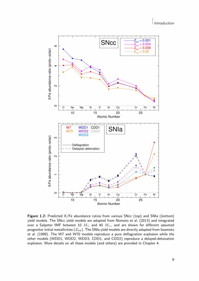
Galaxy clusters are in fact the largest gravitationally bound structuresknown in our Universe. Since the Big Bang (about 13.7 billion years ago),they have assembled from local gas and dark matter over-densities, andgrow continuously in hierarchical structures via mergers. The major com-ponent (∼85% in mass) of galaxy clusters is in the form of dark matter,whose precise nature is still unknown. Stars, planets, interstellar gas, andgalaxies constitute only about∼10–20% of the remaining baryonic content.The other ∼80–90% of the baryonic mass is found in the form of a very hot(107–108 K), extended, highly ionised, and tenuous (102–104 atoms/m3)gas, which fills the very large gravitational potential well of the wholecluster. This plasma, namely the intra-cluster medium (ICM, Fig. 1.3) is hotenough to emit X-ray radiation, essentially via bremsstrahlung (”free-free”
8
Introduction
10 15 20 25
02
46
X/F
e a
bundance
ratio
(pro
to−
sola
r)
Atomic Number
O Ne Mg Si S Ar Ca Cr Fe Ni
SNccZinit = 0.001Zinit = 0.004Zinit = 0.008Zinit = 0.02
10 15 20 25
01
23
X/F
e a
bundance
ratio
(pro
to−
sola
r)
Atomic Number
O Ne Mg Si S Ar Ca Cr Fe Ni
SNIaW7W70
WDD1WDD2WDD3
CDD1CDD2
DeflagrationDelayed−detonation
Figure 1.2: Predicted X/Fe abundance ratios from various SNcc (top) and SNIa (bottom)yield models. The SNcc yield models are adapted from Nomoto et al. (2013) and integratedover a Salpeter IMF between 10 M⊙ and 40 M⊙, and are shown for different assumedprogenitor initial metallicities (Zinit). The SNIa yield models are directly adapted from Iwamotoet al. (1999). The W7 and W70 models reproduce a pure deflagration explosion while theother models (WDD1, WDD2, WDD3, CDD1, and CDD2) reproduce a delayed-detonationexplosion. More details on all these models (and others) are provided in Chapter 4.
9
1.3 Metals in clusters of galaxies
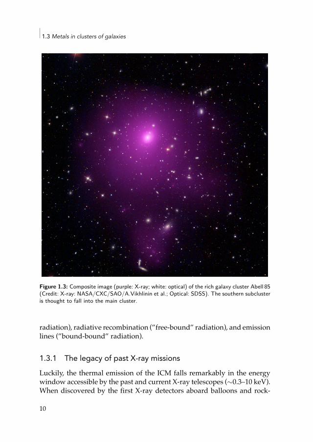
Figure 1.3: Composite image (purple: X-ray; white: optical) of the rich galaxy cluster Abell 85(Credit: X-ray: NASA/CXC/SAO/A.Vikhlinin et al.; Optical: SDSS). The southern subclusteris thought to fall into the main cluster.
radiation), radiative recombination (”free-bound” radiation), and emissionlines (”bound-bound” radiation).
1.3.1 The legacy of past X-ray missionsLuckily, the thermal emission of the ICM falls remarkably in the energywindow accessible by the past and current X-ray telescopes (∼0.3–10 keV).When discovered by the first X-ray detectors aboard balloons and rock-
10
Introduction
ets (Byram et al. 1966; Bradt et al. 1967), and eventually by the first X-raysatellite Uhuru (Cavaliere et al. 1971; Kellogg et al. 1972, 1973), whetherthis extended emission originated from thermal (e.g. bremsstrahlung) ornon-thermal (e.g. inverse-Compton) processes was still unclear. A break-through came in the late 1970’s, with theAriel V andOSO-8X-raymissions,whose improved spectral resolution allowed to detect for the first time anFe-K emission feature around ∼7 keV in the spectra of the Perseus, Virgo,and Coma clusters (Mitchell et al. 1976; Serlemitsos et al. 1977). This resultwas spectacular in two aspects: (i) it definitely confirmed the predominantthermal, collisional nature of the ICM; and (ii) it showed for the first timethat the ICM is polluted by metals, providing evidence that chemical en-richment plays a role even at the largest scales of the Universe.
Since these pioneering studies, and all along the succession of severalgenerations of X-ray observatories with improved technology and instru-ments, measurements of metals in the ICM (and their interpretation) con-siderably improved. Launched in 1978, the Einstein observatory allowedto detect line emission from other elements than Fe (Canizares et al. 1979;Mushotzky et al. 1981). Another valuable discovery made by the Einsteinmission was that about half of the observed clusters show a sharp peakin the X-ray surface brightness. Converting this brightness into gas den-sity1 and estimating their gas temperature, it was found that the coolingtime2 at the centre of these clusters is shorter than the Hubble time (∼ 14Gyr) (Jones & Forman 1984; Stewart et al. 1984). In fact, these ”cool-core”clusters (Molendi & Pizzolato 2001) are dynamically relaxed and usuallyexhibit a strong inverted temperature gradient in their cores. On the otherhand, ”non-cool-core” clusters show amore extended and disturbed X-raysurface brightness, and do not reveal a clear central ICM temperature drop.
Agreat step forward in chemical abundance studies of clusters occurredwith the launch of ASCA in 1993. This Japanese mission provided for thefirst time a reasonable estimate of the abundances of O, Ne, Mg, Si, S,Ar, Ca, Fe, and Ni in the ICM (e.g. Mushotzky et al. 1996; Baumgartneret al. 2005). Furthermore, ASCA also allowed to study for the first time thespatial distribution of Fe within the ICM, and showed a clear increase inthe abundance of this element toward the centre of the Centaurus clus-
1The X-ray surface brightness of the ICM is proportional to the square of the gas density.2In the case of an isobaric radiative cooling of a gas of density ne and temperature T ,
the cooling time, tcool, is calculated as tcool = 8.5×10¹⁰ yr(
ne
10−3 cm−3
)−1 ( T108 K
)1/2 (Sarazin1986).
11
1.3 Metals in clusters of galaxies
ter (Allen & Fabian 1994; Fukazawa et al. 1994). Later on, the Italian-Dutchmission BeppoSAX (launched in 1996) established a clearer picture of the Fedistribution in clusters. In particular, De Grandi &Molendi (2001) showedthat, while cool-core clusters host an excess of Fe in their core compared tothe outskirts, non-cool-core clusters have a systematically flatter Fe radialprofile.
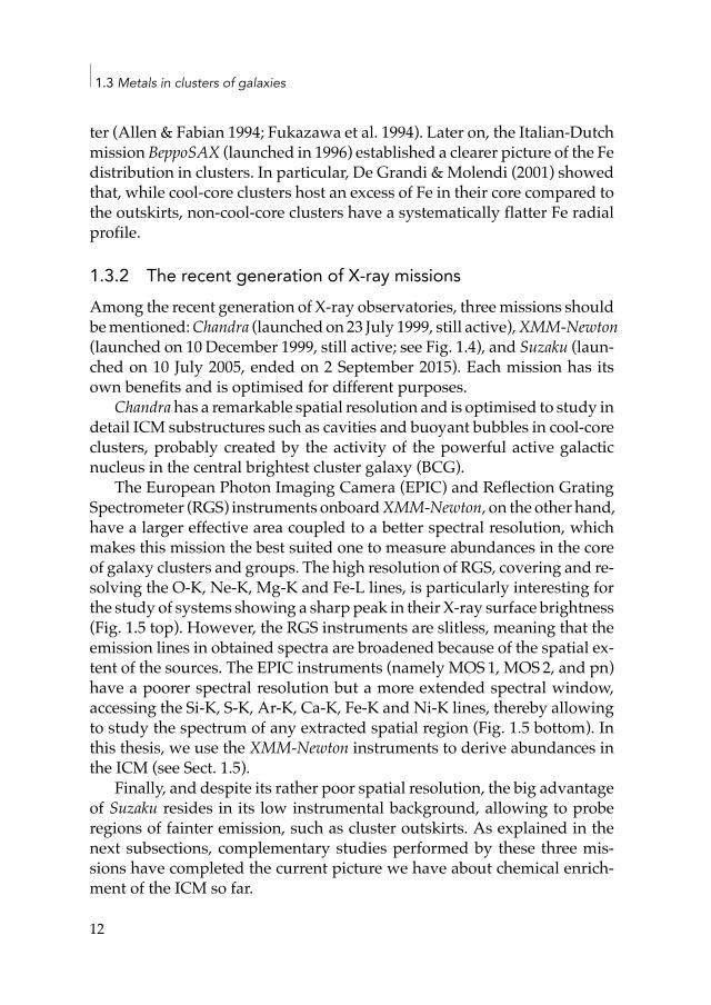
1.3.2 The recent generation of X-ray missionsAmong the recent generation of X-ray observatories, threemissions shouldbementioned:Chandra (launched on 23 July 1999, still active),XMM-Newton(launched on 10 December 1999, still active; see Fig. 1.4), and Suzaku (laun-ched on 10 July 2005, ended on 2 September 2015). Each mission has itsown benefits and is optimised for different purposes.
Chandra has a remarkable spatial resolution and is optimised to study indetail ICM substructures such as cavities and buoyant bubbles in cool-coreclusters, probably created by the activity of the powerful active galacticnucleus in the central brightest cluster galaxy (BCG).
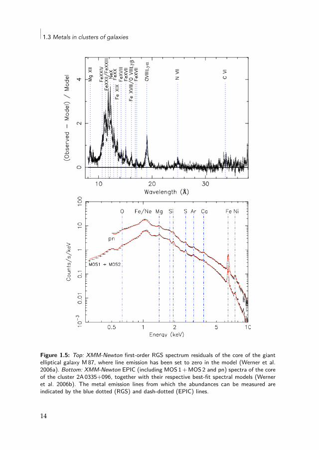
The European Photon Imaging Camera (EPIC) and Reflection GratingSpectrometer (RGS) instruments onboardXMM-Newton, on the other hand,have a larger effective area coupled to a better spectral resolution, whichmakes this mission the best suited one to measure abundances in the coreof galaxy clusters and groups. The high resolution of RGS, covering and re-solving the O-K, Ne-K, Mg-K and Fe-L lines, is particularly interesting forthe study of systems showing a sharp peak in their X-ray surface brightness(Fig. 1.5 top). However, the RGS instruments are slitless, meaning that theemission lines in obtained spectra are broadened because of the spatial ex-tent of the sources. The EPIC instruments (namely MOS1, MOS2, and pn)have a poorer spectral resolution but a more extended spectral window,accessing the Si-K, S-K, Ar-K, Ca-K, Fe-K and Ni-K lines, thereby allowingto study the spectrum of any extracted spatial region (Fig. 1.5 bottom). Inthis thesis, we use the XMM-Newton instruments to derive abundances inthe ICM (see Sect. 1.5).
Finally, and despite its rather poor spatial resolution, the big advantageof Suzaku resides in its low instrumental background, allowing to proberegions of fainter emission, such as cluster outskirts. As explained in thenext subsections, complementary studies performed by these three mis-sions have completed the current picture we have about chemical enrich-ment of the ICM so far.
12
Introduction
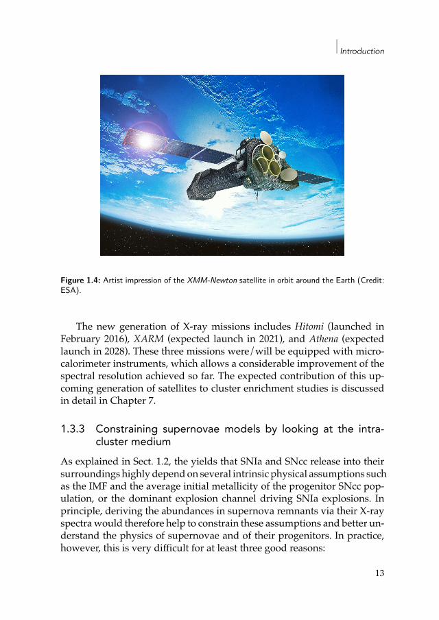
Figure 1.4: Artist impression of the XMM-Newton satellite in orbit around the Earth (Credit:ESA).
The new generation of X-ray missions includes Hitomi (launched inFebruary 2016), XARM (expected launch in 2021), and Athena (expectedlaunch in 2028). These three missions were/will be equipped with micro-calorimeter instruments, which allows a considerable improvement of thespectral resolution achieved so far. The expected contribution of this up-coming generation of satellites to cluster enrichment studies is discussedin detail in Chapter 7.
1.3.3 Constraining supernovae models by looking at the intra-cluster medium
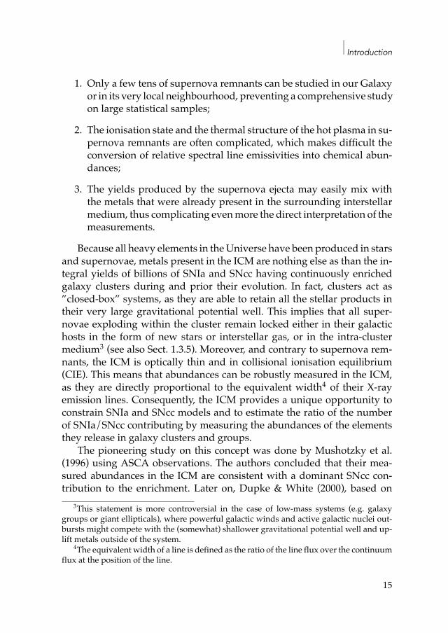
As explained in Sect. 1.2, the yields that SNIa and SNcc release into theirsurroundings highly dependon several intrinsic physical assumptions suchas the IMF and the average initial metallicity of the progenitor SNcc pop-ulation, or the dominant explosion channel driving SNIa explosions. Inprinciple, deriving the abundances in supernova remnants via their X-rayspectrawould therefore help to constrain these assumptions and better un-derstand the physics of supernovae and of their progenitors. In practice,however, this is very difficult for at least three good reasons:
13
1.3 Metals in clusters of galaxies
Figure 1.5: Top: XMM-Newton first-order RGS spectrum residuals of the core of the giantelliptical galaxy M 87, where line emission has been set to zero in the model (Werner et al.2006a). Bottom: XMM-Newton EPIC (including MOS 1 + MOS 2 and pn) spectra of the coreof the cluster 2A 0335+096, together with their respective best-fit spectral models (Werneret al. 2006b). The metal emission lines from which the abundances can be measured areindicated by the blue dotted (RGS) and dash-dotted (EPIC) lines.
14
Introduction
1. Only a few tens of supernova remnants can be studied in our Galaxyor in its very local neighbourhood, preventing a comprehensive studyon large statistical samples;
2. The ionisation state and the thermal structure of the hot plasma in su-pernova remnants are often complicated, which makes difficult theconversion of relative spectral line emissivities into chemical abun-dances;
3. The yields produced by the supernova ejecta may easily mix withthe metals that were already present in the surrounding interstellarmedium, thus complicating evenmore the direct interpretation of themeasurements.
Because all heavy elements in theUniverse have been produced in starsand supernovae, metals present in the ICM are nothing else as than the in-tegral yields of billions of SNIa and SNcc having continuously enrichedgalaxy clusters during and prior their evolution. In fact, clusters act as”closed-box” systems, as they are able to retain all the stellar products intheir very large gravitational potential well. This implies that all super-novae exploding within the cluster remain locked either in their galactichosts in the form of new stars or interstellar gas, or in the intra-clustermedium3 (see also Sect. 1.3.5). Moreover, and contrary to supernova rem-nants, the ICM is optically thin and in collisional ionisation equilibrium(CIE). This means that abundances can be robustly measured in the ICM,as they are directly proportional to the equivalent width4 of their X-rayemission lines. Consequently, the ICM provides a unique opportunity toconstrain SNIa and SNcc models and to estimate the ratio of the numberof SNIa/SNcc contributing by measuring the abundances of the elementsthey release in galaxy clusters and groups.
The pioneering study on this concept was done by Mushotzky et al.(1996) using ASCA observations. The authors concluded that their mea-sured abundances in the ICM are consistent with a dominant SNcc con-tribution to the enrichment. Later on, Dupke & White (2000), based on
3This statement is more controversial in the case of low-mass systems (e.g. galaxygroups or giant ellipticals), where powerful galactic winds and active galactic nuclei out-bursts might compete with the (somewhat) shallower gravitational potential well and up-lift metals outside of the system.
4The equivalent width of a line is defined as the ratio of the line flux over the continuumflux at the position of the line.
15
1.3 Metals in clusters of galaxies
ASCA observations of three clusters, favoured a dominant deflagrationexplosion channel for SNIa explosions. These two results, however, werechallenged by more recent studies using the current generation of X-raytelescopes (e.g. Finoguenov et al. 2002; Böhringer et al. 2005; Werner et al.2006b; de Plaa et al. 2006; Sato et al. 2007a). The most complete work hasbeen done by de Plaa et al. (2007), who compiled the abundance mea-surements of 22 cool-core clusters observed by XMM-Newton and fittedtheir average abundance ratios with a combination of SNIa+SNcc mod-els. They concluded that the measured abundance ratios: (i) favour thedelayed-detonation channel for SNIa explosions; (ii) suggest that SNcc pro-genitors were previously enriched (i.e. have a positive initial metallicity);and (iii) show that Ca is overproduced with respect to the most commonmodel predictions. Of course, such a study may now be further improvedby compiling the abundance ratios of more (high- and low-mass) systemsobservedwith deeper exposures, and by comparing these ratios withmorerecent supernova yield models, after carefully checking all the systematicuncertainties that may affect the results (see Chapters 3 and 4).
1.3.4 Stellar and intra-cluster phases of metalsAs explained earlier, the baryonic content of galaxy clusters consists of twoseparate components: (i) the ICM and (ii) the stellar mass in (and between)galaxies.Whereas a significant fraction of themetals is somehowdispersedinto the ICM (see also Sect. 1.3.5), the other part remains locked within thecluster galaxies, in particular in low- and intermediate-mass stars. In prin-ciple, such a fraction is simple to estimate on basis of the stellar luminosity(as a proxy of the stellar mass) and the assumed yields from SNIa and SNccmodels. Several analytical works (Loewenstein 2013; Renzini & Andreon2014, and references therein) estimate that there is at least as much Fe re-leased into the ICM as there is still locked into stars. In massive clusters(>1014 M⊙), this fraction seems to increase and may even pose a seriousproblem: there is 2 to 3 times too much Fe measured in the ICM comparedto what could have been produced by all the stars in the cluster galaxies.A recent study based on semi-analytic simulations better conciliates theexpected and measured Fe abundances in the ICM of the most massiveclusters (Yates et al. 2017). However, a mismatch is still found in clusters ofintermediate mass (too much metals compared to the predictions) and ingroups (too few metals compared to the predictions). Clearly, the relationbetween absolute supernova yields and the metal content in groups and
16
Introduction
clusters is far from being solved.Do the intra-cluster abundances really reflect the nucleosynthesis of all
the stars and supernovae in galaxy clusters? This question is not trivial atall, but the answer is probably no, essentially for two reasons. First, com-paring directly the ICM abundances with supernova yields implicitly as-sumes that all stars and supernovae create and disperse their products in-stantaneously after their formation5. In reality, SNcc and SNIa require sig-nificant and different delays before they could effectively enrich the ICM(Matteucci & Chiappini 2005). Second, it is likely that SNIa and SNcc arenot dispersed into the ICMwith the same efficiency. It is currently believedthat SNcc products are preferentially locked up in stars while SNIa prod-ucts are more easily released in the ICM (e.g. Loewenstein 2013). Ignoringthese enrichment delays may lead to some incorrect interpretations, for ex-ample about the true ratio of all supernovae having exploded in clusters.
Although the ICM abundances may not be fully representative of thechemical composition produced at first place, they can still be correctlyinterpreted in terms of SNIa and SNcc having actually contributed to theICMenrichment. Keeping this difference inmind, the ICMabundances canstill be used to constrain SNIa and SNcc models.
1.3.5 Where and when was the ICM chemically enriched?Whereas it is clear that metals present in the ICMultimately originate fromSNIa and SNcc having occurred within the cluster gravitational potentialwell, three major questions still arise:
• From which astrophysical sources does the bulk of the enrichmentoriginate? The central BCG, late-type satellite galaxies, or intra-clusterstars?
• By which dominant mechanism(s) does a fraction of the metals es-cape their galactic gravitational potential wells and pollute the intra-cluster gas?
• At which step(s) of the cosmic time and/or cluster evolution do met-als enrich the ICM?
Clearly, these questions are not trivial and require a deep synergy betweentheory, simulations, and observations in order to be solved.Generally speak-ing, the bulk of the enrichment has probably occurred around the peak of
5This assumption is also known as the ”instantaneous recycling approximation”.
17
1.3 Metals in clusters of galaxies
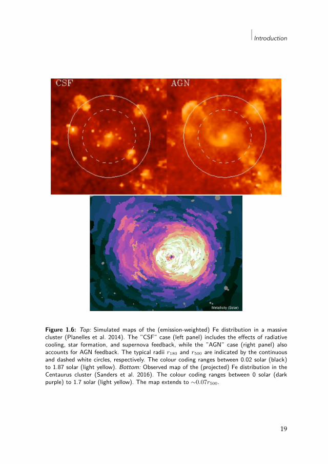
cosmic star formation z ∼ 2–3 (for a review, see Madau & Dickinson 2014),i.e. when the ICM started to form. More precisely, the observed spatialdistribution of metals in clusters (whether from real observations or fromsnapshots of chemo-dynamical simulations) may provide useful hints andfurther constraints (Fig. 1.6) to these three above questions.
Since the discovery of a systematic central Fe enhancement in cool-core clusters up to about one solar in the centre (Allen & Fabian 1994;Fukazawa et al. 1994; De Grandi & Molendi 2001, see also Sect. 1.3.1), sev-eral studies showed that the Femass of this excess has been likely producedby SNIa belonging to the central BCG (Böhringer et al. 2004a; De Grandiet al. 2004). On the other hand, recent observations by Suzaku showed a re-markably uniform level of Fe enrichment in the outskirts of the Perseuscluster (Werner et al. 2013). The latter result has also been extended toother elements as well. This includes SNcc-dominated products, like Mg,among other elements in the outskirts of theVirgo cluster (Simionescu et al.2015). Put together, these findings converge toward the picture of two ma-jor stages of enrichment (at least for cool-core clusters):
1. An early (z ≳ 2) enrichment which took place essentially before thecluster was well assembled, when metals created by both SNIa andSNcc had been released and efficientlymixed in the still forming ICMfrom star-forming galaxies via powerful galactic winds (see also be-low);
2. A later enrichment, presumably coming fromSNIa in the central BCG,responsible for the central Fe excess in cool-core clusters.
Observational hints toward this picture also seem to corroborate the mostrecent cosmological simulations that take the cluster enrichment aspectinto account (e.g. Planelles et al. 2014; Biffi et al. 2017).
In parallel, several chemo-dynamical simulations investigated the rela-tive role of the possiblemechanisms that could be responsible for the galac-tic escape of metals into the ICM (for a review, see Schindler & Diaferio2008). Among them, two dominant channels seem to be favoured: (i) ram-pressure stripping, occurring when an infalling galaxy gets its interstellargas stripped by the pressure of the ambient ICM (Gunn & Gott 1972) and(ii) galactic winds or outflows provided by the total kinetic energy of thesupernova explosions (De Young 1978). While ram-pressure stripping ismore efficient in cluster cores, where the ICM pressure is more importantand the gravitational potential more efficient to attract galaxies, galactic
18
Introduction
Figure 1.6: Top: Simulated maps of the (emission-weighted) Fe distribution in a massivecluster (Planelles et al. 2014). The ”CSF” case (left panel) includes the effects of radiativecooling, star formation, and supernova feedback, while the ”AGN” case (right panel) alsoaccounts for AGN feedback. The typical radii r180 and r500 are indicated by the continuousand dashed white circles, respectively. The colour coding ranges between 0.02 solar (black)to 1.87 solar (light yellow). Bottom: Observed map of the (projected) Fe distribution in theCentaurus cluster (Sanders et al. 2016). The colour coding ranges between 0 solar (darkpurple) to 1.7 solar (light yellow). The map extends to ∼0.07r500.
19
1.4 Spectral codes for a collisional ionisation equilibrium plasma
winds take a larger role in cluster outskirts (and presumably at earlier cos-mic times), where there is less resistance of the ambient ICM to spread outthe metals and when the star-forming activity in galaxies was more impor-tant than at present times (see also above). Note that other processes, suchas galaxy-galaxy interaction, outflows from active galactic nuclei (AGN),or enrichment by the intra-cluster stars may also contribute to the ICMenrichment, although probably to a less significant extent (Schindler & Di-aferio 2008).
Despite all these significant progresses, many uncertainties on the fullcluster enrichment picture still remain. For instance, due to their very lowsignal-to-noise obtained by the current generation of X-ray telescopes, clus-ter outskirts are left widely unexplored. For a recent review on cluster out-skirts, see Reiprich et al. (2013). Moreover, the current instrumental limita-tions also prevent us from studying in detail the amount and spatial distri-butions of metals in high-redshift clusters (z ≳ 0.5). Last but not least, evenin nearby clusters past and recent studies of individual objects or smallsamples did not converge toward a consistent radial distribution for SNccproducts (O, Mg, Si, etc.; e.g. Werner et al. 2006a; Simionescu et al. 2009b;Lovisari et al. 2011), leaving questions on the role of SNcc in enriching thecentral parts of clusters and groups.
1.4 Spectral codes for a collisional ionisation equilib-rium plasma
As mentioned in Sect. 1.3.3, the derivation of chemical abundances in theICM from the equivalent widths of their corresponding emission lines isin principle straight forward. However, it clearly requires a good knowl-edge of all the subsequent emission processes responsible for both the lineand the continuum spectral components. In other words, the use of properspectral models with up-to-date atomic databases is crucial to correctly de-rive and interpret the ICM abundances.
Historically, the first atomic code reproducing X-ray spectra of hot, op-tically thin plasmas in CIE was calculated by Cox & Tucker (1969). Afterthis pioneeringwork, and thanks to the increasing computing performancesince the 1970’s, essentially two atomic codes were built and then continu-ously updated up to now.
The first one was initially written by Mewe (1972), and after some up-dates (Mewe et al. 1985, 1986) became a reference for many years (abbrevi-
20
Introduction
ated as the ”Mewe-Gronenschild” code). The code was later updated firstas the meka code (following itmain contributors: RolfMewe and Jelle Kaas-tra), and then as the mekal code (Rolf Mewe, Jelle Kaastra, Duane Liedahl)in 1995. Itwas incorporated into theXSPEC fitting package6 (Arnaud 1996).Since 1995, the code (renamed cie) has been continuously updated as partof its own fitting package, SPEX7 (Kaastra et al. 1996), with two major up-dates, in 1996 and in 2016 (see Chapter 5). SPEX (and its available single-andmulti-temperature CIEmodels) is the code that is used throughout thisthesis.
The second one was initially written by Raymond & Smith (1977) andhad been widely used by the X-ray community, together with the Mewe-Gronenschild code. Later on, the codewasupdated (Smith et al. 2001; Brick-house & Smith 2005) and became part of the atomic database AtomDB8.This spectral model (and atomic database) is also known as the apecmodelas part of XSPEC, and is still regularly updated.
1.5 This thesis
As we have seen in the previous sections, despite considerable progressin the determination of abundances in the ICM and their interpretation asa chemical enrichment from SNIa and SNcc over the largest scales of theUniverse, many intriguing questions on supernovae or on the chemical en-richment itself remain to be solved. Obviously, tackling all the aspects ofthe ICM enrichment would probably take several decades of future efforts.Nevertheless, in this thesis I focus on two particular questions, closely re-lated to what has been discussed in Sect. 1.3.3 and 1.3.5:
1. What do the elemental abundances measured in the ICM cool corestell us about the intrinsic physics and environmental conditions of thebillions of supernovae that exploded and produced these elements?
2. What do the observed spatial distribution of elemental abundancesin the cool-core ICM tell us about the main epoch(s) and productionsites of the enrichment?
6http://heasarc.gsfc.nasa.gov/docs/xanadu/xspec7https://www.sron.nl/astrophysics-spex8http://www.atomdb.org/index.php
21
1.5 This thesis
This thesis is essentially based on a large sample ofXMM-Newton obser-vations of 44 cool-core galaxy clusters, groups, and ellipticals (the CHEmi-cal Enrichment Rgs Sample, or CHEERS), with a total net exposure of∼4.5Ms (de Plaa et al. 2017). This is the first time that the ICM enrichmentis studied over such a large sample and such a deep total exposure. TheCHEERS sample combines new very deep observations of 11 systems witharchival data of other clusters and groups. The selection of the objects ofthe sample are based on a >5σ significance of the detection of the OVIII1s–2p emission line at 19 Å with the RGS instrument. For further detailson the CHEERS project, see de Plaa et al. (2017). In addition to ensuringoptimal constraints on the SNcc enrichment, the instrumental detection ofthe OVIII line in the ICM is a good indicator or the reasonable detectabilityof the other main metal lines. Because line emissivities are larger in coolerplasmas and because cool-core clusters are more compact, hence producehigher resolution RGS spectra, all the objects in our sample are cool-core9.
The outline of this thesis is structured as follows.Chapter 2 is devoted to the full XMM-Newton analysis of Abell 4059, a
galaxy cluster which is part of the CHEERS sample. A careful treatment ofthe background is detailed, and is applied to the analysis of all the other ob-jects in the next chapters. Abell 4059 is a textbook example that clear asym-metries can be found in the metal distribution of galaxy clusters, and thatram-pressure stripping might sometimes play a significant role in enrich-ing the central regions of the ICM.
In Chapter 3, I present the individual abundances of all the CHEERSobjects within a consistent radius, 0.05r500
10, as well as within 0.2r500 whenpossible. I discuss extensively several systematic uncertainties that couldbe associated with our measurements. Then, I stack the individual mea-surements to build an average abundance pattern, representative of theenrichment in the ICM as a whole. Doing so, I also report constraints onthe average Cr/Fe ratio and, for the very first time, the presence of Mn inthe ICM.
Chapter 4 constitutes the immediate follow-up of Chapter 3, as wellas a central point of this thesis. I interpret the previously derived ICM
9A similar study could be done on non-cool-core systems, although this would probablyrequire even deeper exposures, and would be limited to less massive systems exhibitingreasonable central temperatures.
10Used as a commonway to define astrophysically consistent sizes in galaxy clusters andgroups, r500 defines the radius within which the cluster/group total density reaches 500times the critical density of the Universe.
22
Introduction
abundance pattern in terms of enrichment by SNIa and SNcc. By fittingthe CHEERS data to various supernova yield models, I attempt to provideindependent constraints on (i) the IMF and initial metallicity of the aver-age population of the SNcc progenitors; (ii) the favoured channels drivingSNIa explosions as well as the dominant nature of SNIa progenitors; and(iii) possible initial enrichment by metal poor (or Population III) stars, orhypernovae.
Chapter 5 is the updated version of Chapters 3 and 4, and corrects theprevious results from a major update in the spectral models and atomicdatabases used to fit the X-ray spectra (SPEX). From a more global per-spective, this chapter deals with the impact of atomic uncertainties on theinterpretations of the ICM enrichment.
While Chapters 3, 4, and 5 essentially focus on the integrated super-nova yields in the central cluster cool cores, inChapter 6 I use the CHEERSsample to establish radial abundance profiles in cool-core systems, and in-terpret them in term of enrichment sources and history.
Finally, Chapter 7 concludes this thesis by discussing the current limi-tations in this field and the bright (although still somewhat far) future thatthe next generation of X-ray missions will offer.
23

Toeval is logisch.
Coincidence is logical.
– Johan Cruijff
2|Abundance and temperaturedistributions in the hot intra-cluster gas of Abell 4059
F. Mernier, J. de Plaa, L. Lovisari, C. Pinto, Y.-Y. Zhang, J. S. Kaastra,N. Werner, and A. Simionescu
(Astronomy & Astrophysics, Volume 575, id.A37, 17 pp.)
Abstract
Using the EPIC and RGS data from a deep (200 ks) XMM-Newton observation, weinvestigate the temperature structure (kT and σT ) and the abundances of nine el-ements (O, Ne, Mg, Si, S, Ar, Ca, Fe, and Ni) of the intra-cluster medium (ICM) inthe nearby (z=0.046) cool-core galaxy cluster Abell 4059. Next to a deep analysisof the cluster core, a careful modelling of the EPIC background allows us to buildradial profiles up to 12′ (∼650 kpc) from the core. Probably because of projectioneffects, the ICM temperature is not found to be in single phase, even in the outerparts of the cluster. The abundances of Ne, Si, S, Ar, Ca, and Fe, but also O arepeaked towards the core. The elements Fe and O are still significantly detectedin the outermost annuli, which suggests that the enrichment by both Type Ia andcore-collapse SNe started in the early stages of the cluster formation. However, theparticularly high Ca/Fe ratio that we find in the core is not well reproduced bythe standard SNe yield models. Finally, 2-D maps of temperature and Fe abun-dance are presented and confirm the existence of a denser, colder, and Fe-richridge south-west of the core, previously observed by Chandra. The origin of thisasymmetry in the hot gas of the cluster core is still unclear, but it might be ex-plained by a past intense ram-pressure stripping event near the central cD galaxy.
25
2.1 Introduction
2.1 Introduction
Thedeep gravitational potential of clusters of galaxies retains large amountsof hot (∼107–108 K) gas,mainly visible in X-rays,which accounts for no lessthan 80% of the total baryonic mass. This so-called intra-cluster medium(ICM) contains not only H and He ions, but also heavier metals. Iron (Fe)was discovered in the ICMwith the first generation of X-ray satellites (Mit-chell et al. 1976); then neon (Ne), magnesium (Mg), silicon (Si), sulfur (S),argon (Ar), and calcium (Ca) were measured with ASCA (e.g. Mushotzkyet al. 1996). Precise abundance measurements of these elements have beenmade possible thanks to the good spectral resolution and the large effec-tive area of the XMM-Newton (Jansen et al. 2001) instruments (e.g. Tamuraet al. 2001). Nickel (Ni) abundance measurements and the detection of rareelements like chromium (Cr) have been reported as well (e.g. Werner et al.2006b; Tamura et al. 2009). Finally, thanks to its low and stable instrumentalbackground, Suzaku is capable of providing accurate abundance measure-ments in the cluster outskirts (e.g. Werner et al. 2013).
These metals clearly do not have a primordial origin; they are thoughtto be mostly produced by supernovae (SNe) within cluster galaxy mem-bers and have enriched the ICM mainly around z ∼ 2–3, i.e. during apeak of the star formation rate (Hopkins & Beacom 2006). However, therespective contributions of the different transport processes required to ex-plain this enrichment are still under debate. Among them, galactic winds(De Young 1978; Baumgartner & Breitschwerdt 2009) are thought to playthe most important role in the ICM enrichment itself. Ram-pressure strip-ping (Gunn & Gott 1972; Schindler et al. 2005), galaxy-galaxy interactions(Gnedin 1998; Kapferer et al. 2005), AGN outflows (Simionescu et al. 2008,2009b), and perhaps gas sloshing (Simionescu et al. 2010) can also con-tribute to the redistribution of elements. Studying the metal distributionin the ICM is a crucial step in order to understand and quantify the role ofthese mechanisms in the chemical enrichment of clusters.
Another open question is the relative contribution of SNe types pro-ducing each chemical element. While O, Ne, and Mg are thought to beproduced mainly by core-collapse SNe (SNcc, including types Ib, Ic, andII, e.g. Nomoto et al. 2006), heavier elements like Ar, Ca, Fe, and Ni areprobably producedmainly by Type Ia SNe (SNIa, e.g. Iwamoto et al. 1999).The elements Si and S are produced by both types (see de Plaa 2013, fora review). The abundances of high-mass elements highly depend on SNIa
26
Abundance and temperature distributions in the hot intra-cluster gas of Abell 4059
explosion mechanisms, while the abundances of the low-mass elements(e.g. nitrogen) are sensitive to the stellar initial mass function (IMF). There-fore, measuring accurate abundances in the ICM can help to constrain oreven rule out some models and scenarios. Moreover, significant discrep-ancies exist between recent measurements and expectations from currentfavoured theoretical yields (e.g. de Plaa et al. 2007), and thus require fur-ther investigation.
The temperature distribution in the ICM is often complicated and itsunderlying physics is not yet fully understood. For instance, many relaxedcluster cores are radiatively cooling on short cosmic timescales, which waspresumed to lead to so-called cooling flows (see Fabian 1994, for a review).However, the lack of cool gas (including the associated star formation)in the core revealed in particular by XMM-Newton (Peterson et al. 2001;Tamura et al. 2001; Kaastra et al. 2001) leads to the so-called cooling-flowproblem and argues for substantial heating mechanisms, yet to be foundand understood. For example, heating by AGN could explain the lack ofcool gas (see e.g. Cattaneo & Teyssier 2007). Studying the spatial structureof the ICM temperature in galaxy clusters may help to solve it.
Abell 4059 is a good example of a nearby (z=0.0460, Reiprich&Böhringer2002) cool-core cluster. Its central cD galaxy hosts the radio source PKS2354-35 which exhibits two radio lobes along the galaxy major axis (Tayloret al. 1994). In addition to ASCA and ROSAT observations (Ohashi 1995;Huang & Sarazin 1998), previous Chandra studies (Heinz et al. 2002; Choiet al. 2004; Reynolds et al. 2008) show a ridge of additional X-ray emissionlocated ∼20 kpc south-west of the core, as well as two X-ray ghost cavitiesthat only partly coincide with the radio lobes. Moreover, the south-westridge has been found to be colder, denser, and with a higher metallicitythan the rest of the ICM, suggesting a past merging history of the core priorto the triggering of the AGN activity.
In this paper we analyse in detail two deep XMM-Newton observations(∼200 ks in total) of A 4059, obtained through the CHEERS1 project (dePlaa et al., in prep.). The XMM-Newton European Photon Imaging Camera(EPIC) instruments allow us to derive the abundances of O, Ne, Mg, Si,S, Ar, Ca, Fe, and Ni not only in the core, but also up to ∼650 kpc in theouter parts of the ICM. TheXMM-Newton Reflection Grating Spectrometer(RGS) instruments are also used to measure N, O, Ne, Mg, Si, and Fe. Thispaper is structured as follows. The data reduction is described in Sect. 2.2.
1CHEmical Evolution Rgs cluster Sample
27
2.2 Observations and data reduction
We discuss our selected spectral models and our background estimation inSect. 2.3. We then present our temperature and abundance measurementsin the cluster core, as well as their systematic uncertainties (Sect. 2.4), mea-sured radial profiles (Sect. 2.5), and temperature and Fe abundance maps(Sect. 2.6). We discuss and interpret our results in Sect. 2.7 and concludein Sect. 2.8. Throughout this paper we assume H0 = 70 km s−1 Mpc−1,Ωm = 0.3, and ΩΛ = 0.7. At the redshift of 0.0460, 1 arcmin correspondsto ∼54 kpc. The whole EPIC field of view (FoV) covers R ≃ 0.81 Mpc≃ 0.51r200 (Reiprich & Böhringer 2002, where r200 is the radius withinwhich the density of cluster reaches 200 times the critical density of theUniverse). All the abundances are given relative to the proto-solar valuesfrom Lodders et al. (2009). The error bars indicate 1σ uncertainties at a 68%confidence level. Unless mentioned otherwise, all our spectral analyses aredone within 0.3–10 keV by using the Cash statistic (Cash 1979).
2.2 Observations and data reductionTwo deep observations (DO) of A 4059 were taken on 11 and 13 May 2013with a gross exposure time of 96 ks and 95 ks respectively (hereafter DO1and DO2). In addition to these deep observations, two shorter observa-tions (SO; see also Zhang et al. 2011) are available from the XMM-Newtonarchive. The observations are summarised in Table 2.1. Both DO and SOdatasets are used for the RGS analysis while for the EPIC analysis we onlyuse the DO datasets. In fact, the SO observations account for ∼20% of thetotal exposure time, and consequently the signal-to-noise ratio S/Nwouldincrease only by √
1.20 ≃ 1.10, while the risk of including extra systematicerrors and unstable fits due to the EPIC background components (Sect. 2.3and Appendix 2.B) is high. The RGS extraction region is small, has a highS/N, and its background modelling is simpler than using EPIC; therefore,combining the DO and SO remains safe.
The datasets are reduced using theXMM-Newton Science Analysis Sys-tem (SAS) v13 and partly with the SPEX spectral fitting package (Kaastraet al. 1996) v2.04.
2.2.1 EPICIn both DO datasets the MOS and pn instruments were operating in FullFramemode andExtendedFull Framemode respectively.We reduceMOS1,
28
Abundance and temperature distributions in the hot intra-cluster gas of Abell 4059
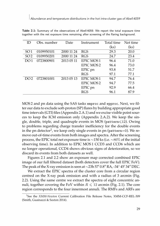
Table 2.1: Summary of the observations of Abell 4059. We report the total exposure timetogether with the net exposure time remaining after screening of the flaring background.
ID Obs. number Date Instrument Total time Net time(ks) (ks)
SO1 0109950101 2000 11 24 RGS 29.3 20.0SO2 0109950201 2000 11 24 RGS 24.7 23.4DO1 0723800901 2013 05 11 EPIC MOS1 96.4 71.0
EPIC MOS2 96.4 73.0EPIC pn 93.8 51.7RGS 97.1 77.1
DO2 0723801001 2013 05 13 EPIC MOS1 94.7 76.4EPIC MOS2 94.7 77.5EPIC pn 92.9 66.4RGS 96.1 87.9
MOS2 and pn data using the SAS tasks emproc and epproc. Next, we fil-ter our data to exclude soft-proton (SP) flares by building appropriate goodtime intervals (GTI) files (Appendix 2.A.1) andwe excise visible point sour-ces to keep the ICM emission only (Appendix 2.A.2). We keep the sin-gle, double, triple, and quadruple events in MOS (pattern⩽12). Owingto problems regarding charge transfer inefficiency for the double eventsin the pn detector2, we keep only single events in pn (pattern=0). We re-move out-of-time events from both images and spectra. After the screeningprocess, the EPIC total net exposure time is∼150 ks (i.e.∼80% of the initialobserving time). In addition to EPIC MOS1 CCD3 and CCD6 which areno longer operational, CCD4 shows obvious signs of deterioration, so wediscard its events from both datasets as well.
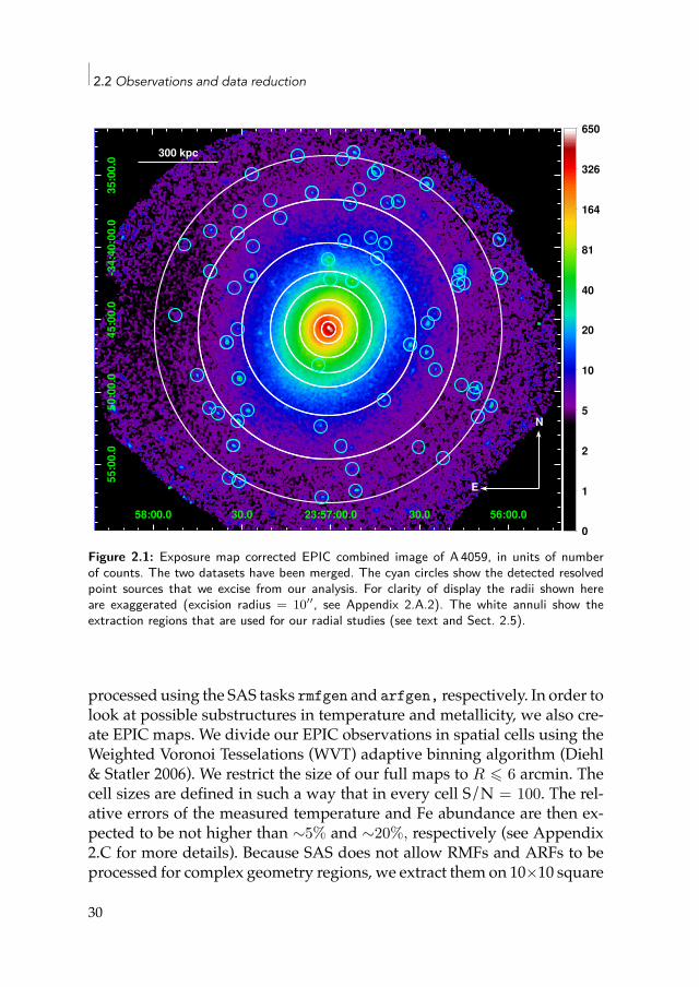
Figures 2.1 and 2.2 show an exposure map corrected combined EPICimage of our full filtered dataset (both detectors cover the full EPIC FoV).The peak of theX-ray emission is seen at∼23h 57′ 0.8′′ RA, -34 45′ 34′′ DEC.
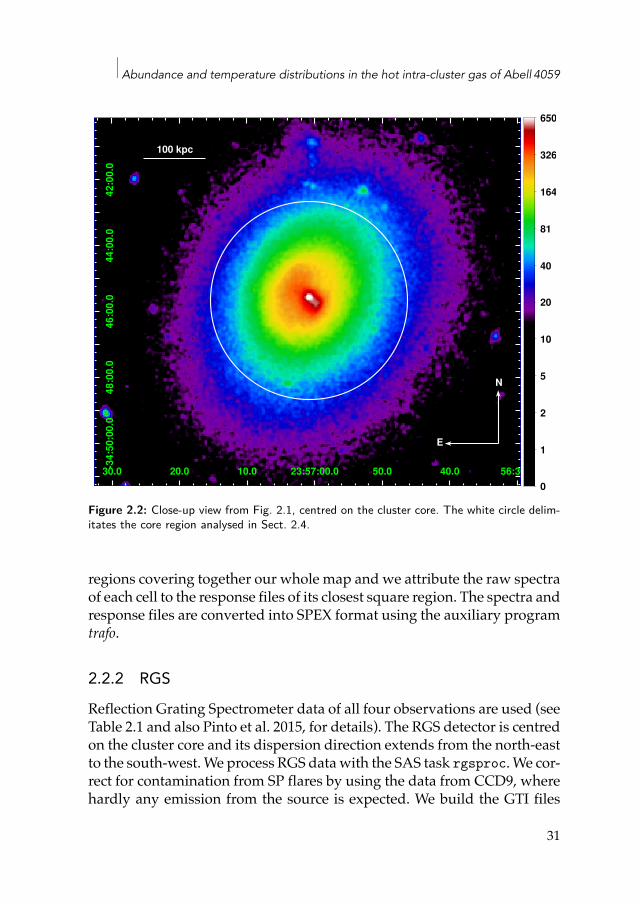
We extract the EPIC spectra of the cluster core from a circular regioncentred on the X-ray peak emission and with a radius of 3 arcmin (Fig.2.2). Using the same centre we extract the spectra of eight concentric an-nuli, together covering the FoV within R ⩽ 12 arcmin (Fig. 2.1). The coreregion corresponds to the four innermost annuli. The RMFs and ARFs are
2See the XMM-Newton Current Calibration File Release Notes, XMM-CCF-REL-309(Smith, Guainazzi & Saxton 2014).
29
2.2 Observations and data reduction
0
1
2
5
10
20
40
81
164
326
650
58:00.0 30.0 23:57:00.0 30.0 56:00.0
35
:00
.0-3
4:4
0:0
0.0
45
:00
.05
0:0
0.0
55
:00
.0
300 kpc
N
E
Figure 2.1: Exposure map corrected EPIC combined image of A 4059, in units of numberof counts. The two datasets have been merged. The cyan circles show the detected resolvedpoint sources that we excise from our analysis. For clarity of display the radii shown hereare exaggerated (excision radius = 10′′, see Appendix 2.A.2). The white annuli show theextraction regions that are used for our radial studies (see text and Sect. 2.5).
processed using the SAS tasks rmfgen and arfgen, respectively. In order tolook at possible substructures in temperature and metallicity, we also cre-ate EPIC maps. We divide our EPIC observations in spatial cells using theWeighted Voronoi Tesselations (WVT) adaptive binning algorithm (Diehl& Statler 2006). We restrict the size of our full maps to R ⩽ 6 arcmin. Thecell sizes are defined in such a way that in every cell S/N = 100. The rel-ative errors of the measured temperature and Fe abundance are then ex-pected to be not higher than ∼5% and ∼20%, respectively (see Appendix2.C for more details). Because SAS does not allow RMFs and ARFs to beprocessed for complex geometry regions, we extract them on 10×10 square
30
Abundance and temperature distributions in the hot intra-cluster gas of Abell 4059
0
1
2
5
10
20
40
81
164
326
650
30.0 20.0 10.0 23:57:00.0 50.0 40.0 56:30.0
42
:00
.04
4:0
0.0
46
:00
.04
8:0
0.0
-34
:50
:00
.0
100 kpc
N
E
Figure 2.2: Close-up view from Fig. 2.1, centred on the cluster core. The white circle delim-itates the core region analysed in Sect. 2.4.
regions covering together our whole map and we attribute the raw spectraof each cell to the response files of its closest square region. The spectra andresponse files are converted into SPEX format using the auxiliary programtrafo.
2.2.2 RGSReflection Grating Spectrometer data of all four observations are used (seeTable 2.1 and also Pinto et al. 2015, for details). The RGS detector is centredon the cluster core and its dispersion direction extends from the north-eastto the south-west.We process RGS datawith the SAS task rgsproc. We cor-rect for contamination from SP flares by using the data from CCD9, wherehardly any emission from the source is expected. We build the GTI files
31
2.3 Spectral models
similarly to the EPIC analysis (Appendix 2.A.1) and we process the dataagain with rgsproc by filtering the events with these GTI files. The totalRGS net exposure time is 208.4 ks. We extract response matrices and RGSspectra for the observations. The final net exposure times are given in Table2.1.
We subtract a model background spectrum created by the standardRGS pipeline from the total spectrum. This is a template background file,based on the count rate in CCD9 of RGS.
We combine the RGS 1 and RGS 2 spectra, responses and backgroundfiles of the four observations through the SAS task rgscombine obtainingone stacked spectrum for spectral order 1 and one for order 2. The two com-bined spectra are converted to SPEX format through trafo. Based on theMOS1 image, we correct the RGS spectra for instrumental broadening asdescribed in Appendix 2.A.3. We include 95% of the cross-dispersion di-rection in the spectrum.
2.3 Spectral modelsThe spectral analysis is done using SPEX. Since there is an important off-set in the pointing of the two observations, stacking the spectra and theresponse files of each of them may lead to bias in the fittings. Moreover,the remaining SP component is found to change from one observation toanother (see Appendix 2.B). Therefore, the better option is to fit simulta-neously the single spectra of every EPIC instrument and observation. Thishas been done using trafo.
2.3.1 The cie modelWe assume that the ICM is in collisional ionisation equilibrium (CIE) andwe use the cie model in our fits (see the SPEX manual3). Our emissionmodels are corrected from the cosmological redshift and are absorbed bythe interstellar medium of the Galaxy (for this pointing NH ≃ 1.26 × 10²⁰
cm−2 as obtained with the method of Willingale et al. 2013). The free pa-rameters in the fits are the emission measure Y =
∫nenHdV , the single-
temperature kT , and O, Ne, Mg, Si, S, Ar, Ca, Fe, and Ni abundances. Theother abundances with an atomic number Z ⩾ 6 are fixed to the Fe value.
3http://www.sron.nl/spex
32
Abundance and temperature distributions in the hot intra-cluster gas of Abell 4059
2.3.2 The gdem modelAlthough cie single-temperaturemodels (i.e. isothermal) fit theX-ray spec-tra from the ICM reasonably well, previous papers (see e.g. Peterson et al.2003; Kaastra et al. 2004;Werner et al. 2006b; de Plaa et al. 2006; Simionescuet al. 2009b) have shown that employing a distribution of temperatures inthe models provides significantly better fits, especially in the cluster cores.The strong temperature gradient in the case of cooling flows and the 2-D projection of the supposed spherical geometry of the ICM suggest thatusing multi-temperature models would be preferable. Apart from the ciemodel mentioned above, we also fit a Gaussian differential emission mea-sure (gdem) model to our spectra. This model assumes that the emissionmeasure Y follows a Gaussian temperature distribution centred on kTmeanand as defined by
Y (x) = Y0
σT
√2π
exp((x − xmean)2
2σ2T
), (2.1)
where x = log(kT ) and xmean = log(kTmean) (see de Plaa et al. 2006). Com-pared to the ciemodel, the additional free parameter from the gdemmodelis the width of the Gaussian emission measure profile σT . By definitionσT=0 is the isothermal case.
2.3.3 Cluster emission and background modellingWe fit the spectra of the cluster emission with a cie and a gdem model suc-cessively, except for the EPIC radial profiles and maps, where only a gdemmodel is considered.
Since the EPIC cameras are highly sensitive to the particle background,a precise estimate of the local background is crucial in order to estimateICMparameters beyond the core (i.e. where this background is comparableto the cluster emission). The emission of A 4059 entirely fills the EPIC FoV,making a direct measure of the local background impossible. Some effortshave been made in the past to deal with this problem (see e.g. Zhang et al.2009, 2011; Snowden & Kuntz 2013), but a customised procedure based onfull modelling is more convenient in our case. In fact, an incorrect subtrac-tion of instrumental fluorescence lines might lead to incorrect abundanceestimates.
For each extraction region, several background components are mod-elled in the EPIC spectra in addition to the cluster emission. Thismodelling
33
2.4 Cluster core
procedure and its application to our extracted regions are fully describedin Appendix 2.B. We note that we do not explicitly model the cosmic X-ray background in RGS (although we did in EPIC) because any diffuseemission feature would be smeared out into a broad continuum-like com-ponent.
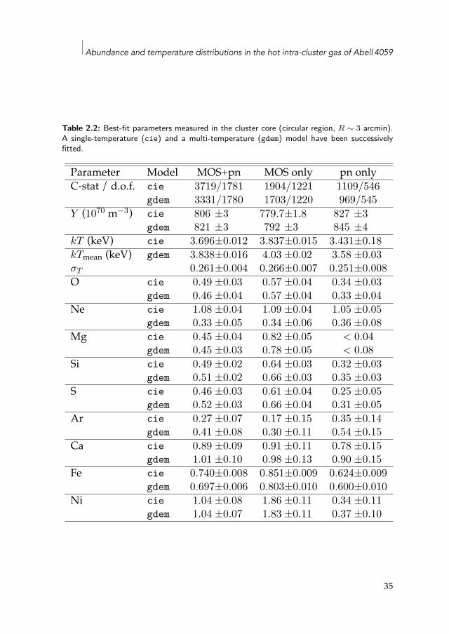
2.4 Cluster core2.4.1 EPICOur deep exposure time allows us to get precise abundancemeasurementsin the core, even using EPIC (Fig. 2.3 top). Moreover, the background isvery limited since the cluster emission clearly dominates. Table 2.2 showsour results, both for the combined fits (MOS+pn) and independent fits (ei-ther MOS or pn only).
Using a multi-temperature model clearly improves the combinedMOS+pn fit. Nevertheless, even by using a gdemmodel, the reducedC-stat valueis still high because the excellent statistics of our data reveal anti-correlatedresiduals betweenMOS and pn, especially below∼1 keV (Fig. 2.3 bottom).
When we fit the EPIC instruments independently, the reduced C-statnumber decreases from 1.87 to 1.40 and 1.78 in the MOS and pn fits, re-spectively. Visually, the models reproduce the spectra better as well. Wealso note that the temperature and abundances measurements in the coreare different between the instruments (Table 2.2). While temperature dis-crepancies between MOS and pn have been already reported and investi-gated (Schellenberger et al. 2015), herewe focus on theMOS-pn abundancediscrepancies. Figure 2.4 (top) illustrates these values and shows the abso-lute abundance measurements obtained from our gdem models. Except forNe, Ar, and Ca (all consistent within 2σ), we observe systematically highervalues in MOS than in pn. Assuming (for convenience) that the systematicerrors are roughly in a Gaussian distribution, we can estimate them fordifferent abundance measurements ZMOS and Zpn, having their respectivestatistical errors σMOS and σpn,
σsys =
√σ2tot −
σ2MOS + σ2pn
2, (2.2)
where σtot =√
((ZMOS − µ)2 + (Zpn − µ)2)/2 and µ = (ZMOS + Zpn)/2. Weobtain absolute O, Si, S, and Fe systematic errors of ±25%, ±30%, ±34%,
34
Abundance and temperature distributions in the hot intra-cluster gas of Abell 4059
Table 2.2: Best-fit parameters measured in the cluster core (circular region, R ∼ 3 arcmin).A single-temperature (cie) and a multi-temperature (gdem) model have been successivelyfitted.
Parameter Model MOS+pn MOS only pn onlyC-stat / d.o.f. cie 3719/1781 1904/1221 1109/546
gdem 3331/1780 1703/1220 969/545Y (1070 m−3) cie 806 ±3 779.7±1.8 827 ±3
gdem 821 ±3 792 ±3 845 ±4kT (keV) cie 3.696±0.012 3.837±0.015 3.431±0.18kTmean (keV) gdem 3.838±0.016 4.03 ±0.02 3.58 ±0.03σT 0.261±0.004 0.266±0.007 0.251±0.008O cie 0.49 ±0.03 0.57 ±0.04 0.34 ±0.03
gdem 0.46 ±0.04 0.57 ±0.04 0.33 ±0.04Ne cie 1.08 ±0.04 1.09 ±0.04 1.05 ±0.05
gdem 0.33 ±0.05 0.34 ±0.06 0.36 ±0.08Mg cie 0.45 ±0.04 0.82 ±0.05 < 0.04
gdem 0.45 ±0.03 0.78 ±0.05 < 0.08Si cie 0.49 ±0.02 0.64 ±0.03 0.32 ±0.03
gdem 0.51 ±0.02 0.66 ±0.03 0.35 ±0.03S cie 0.46 ±0.03 0.61 ±0.04 0.25 ±0.05
gdem 0.52 ±0.03 0.66 ±0.04 0.31 ±0.05Ar cie 0.27 ±0.07 0.17 ±0.15 0.35 ±0.14
gdem 0.41 ±0.08 0.30 ±0.11 0.54 ±0.15Ca cie 0.89 ±0.09 0.91 ±0.11 0.78 ±0.15
gdem 1.01 ±0.10 0.98 ±0.13 0.90 ±0.15Fe cie 0.740±0.008 0.851±0.009 0.624±0.009
gdem 0.697±0.006 0.803±0.010 0.600±0.010Ni cie 1.04 ±0.08 1.86 ±0.11 0.34 ±0.11
gdem 1.04 ±0.07 1.83 ±0.11 0.37 ±0.10
35
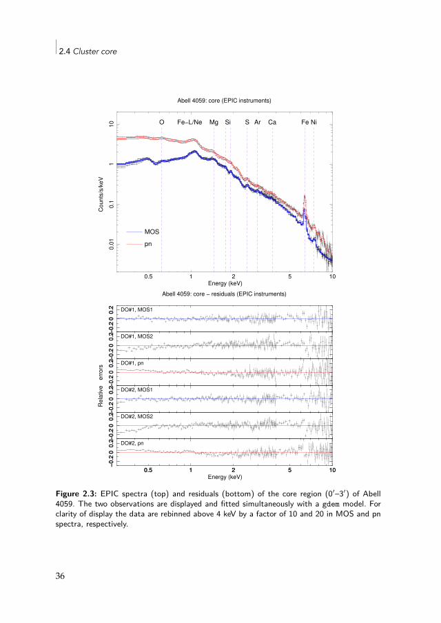
2.4 Cluster core
1 100.5 2 5
0.0
10
.11
10
Co
un
ts/s
/ke
V
Energy (keV)
Abell 4059: core (EPIC instruments)
O Fe!L/Ne Mg Si S Ar Ca Fe Ni
MOS
pn
!0
.20
0.2
Abell 4059: core ! residuals (EPIC instruments)
DO#1, MOS1
!0
.20
0.2
!0
.20
0.2 DO#1, MOS2
!0
.20
0.2
!0
.20
0.2 DO#1, pn
!0
.20
0.2
err
ors
!0
.20
0.2
R
ela
tive DO#2, MOS1
!0
.20
0.2
!0
.20
0.2 DO#2, MOS2
!0
.20
0.2
1 100.5 2 5
!0
.20
0.2 DO#2, pn
1 100.5 2 5
!0
.20
0.2
Energy (keV)
Figure 2.3: EPIC spectra (top) and residuals (bottom) of the core region (0′–3′) of Abell4059. The two observations are displayed and fitted simultaneously with a gdem model. Forclarity of display the data are rebinned above 4 keV by a factor of 10 and 20 in MOS and pnspectra, respectively.
36
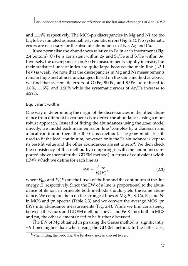
Abundance and temperature distributions in the hot intra-cluster gas of Abell 4059
and ±14% respectively. The MOS-pn discrepancies in Mg and Ni are toobig to be estimated as reasonable systematic errors (Fig. 2.4). No systematicerrors are necessary for the absolute abundances of Ne, Ar, and Ca.
If we normalise the abundances relative to Fe in each instrument (Fig.2.4 bottom), O/Fe is consistent within 2σ and Si/Fe and S/Fe within 3σ.Inversely, the discrepancies on Ar/Fe measurements slightly increase, buttheir statistical uncertainties are quite large because the main line (∼3.1keV) is weak. We note that the discrepancies in Mg and Ni measurementsremain huge and almost unchanged. Based on the same method as above,we find that systematic errors of O/Fe, Si/Fe, and S/Fe are reduced to±8%, ±15%, and ±20% while the systematic errors of Ar/Fe increase to±27%.
Equivalent widthsOne way of determining the origin of the discrepancies in the fitted abun-dance from different instruments is to derive the abundances using a morerobust approach. Instead of fitting the abundances using the gdem modeldirectly, we model each main emission line/complex by a Gaussian anda local continuum (hereafter the Gauss method). The gdem model is stillused to fit the local continuum; however, only the Fe abundance is kept toits best-fit value and the other abundances are set to zero4. We then checkthe consistency of this method by comparing it with the abundances re-ported above (hereafter the GDEM method) in terms of equivalent width(EW), which we define for each line as
EW = FlineFc(E)
, (2.3)
whereFline andFc(E) are the fluxes of the line and the continuumat the lineenergy E, respectively. Since the EW of a line is proportional to the abun-dance of its ion, in principle both methods should yield the same abun-dance. We compare them on the strongest lines of Mg, Si, S, Ca, Fe, and Niin MOS and pn spectra (Table 2.3) and we convert the average MOS+pnEWs into abundance measurements (Fig. 2.4). While we find consistencybetween the Gauss andGDEMmethods for Ca and Fe-K lines both inMOSand pn, the other elements need to be further discussed.
The EW of Mg obtained in pn using the Gauss method is, significantly,∼9 times higher than when using the GDEM method. In the latter case,
4When fitting the Fe-K line, the Fe abundance is also set to zero.
37
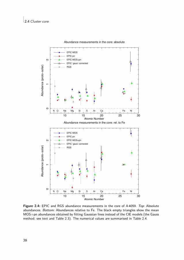
2.4 Cluster core
10 15 20 25 30
01
2
Ab
un
da
nce
(p
roto
!so
lar)
Atomic Number
Abundance measurements in the core: absolute
EPIC MOS
EPIC pn
EPIC MOS+pn
RGS
N O Ne Mg Si S Ar Ca Fe Ni
EPIC ’gaus’ corrected
10 15 20 25 30
01
2
Ab
un
da
nce
(p
roto
!so
lar)
Atomic Number
Abundance measurements in the core: rel. to Fe
EPIC MOS
EPIC pn
EPIC MOS+pn
RGS
N O Ne Mg Si S Ar Ca Fe Ni
EPIC ’gaus’ corrected
Figure 2.4: EPIC and RGS abundance measurements in the core of A 4059. Top: Absoluteabundances. Bottom: Abundances relative to Fe. The black empty triangles show the meanMOS+pn abundances obtained by fitting Gaussian lines instead of the CIE models (the Gaussmethod; see text and Table 2.3). The numerical values are summarised in Table 2.4.
38
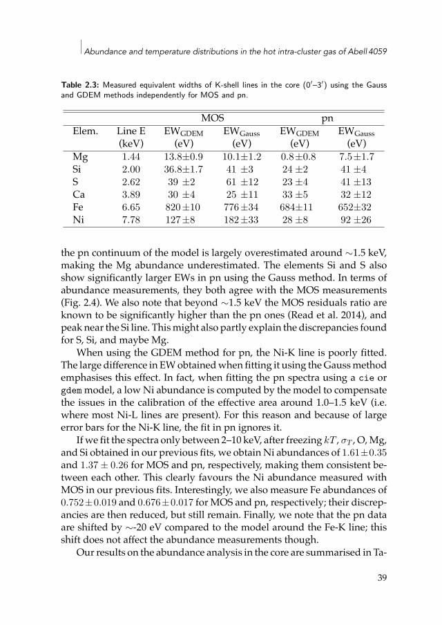
Abundance and temperature distributions in the hot intra-cluster gas of Abell 4059
Table 2.3: Measured equivalent widths of K-shell lines in the core (0′–3′) using the Gaussand GDEM methods independently for MOS and pn.
MOS pnElem. Line E EWGDEM EWGauss EWGDEM EWGauss
(keV) (eV) (eV) (eV) (eV)Mg 1.44 13.8±0.9 10.1±1.2 0.8±0.8 7.5±1.7Si 2.00 36.8±1.7 41 ±3 24 ±2 41 ±4S 2.62 39 ±2 61 ±12 23 ±4 41 ±13Ca 3.89 30 ±4 25 ±11 33 ±5 32 ±12Fe 6.65 820±10 776±34 684±11 652±32Ni 7.78 127±8 182±33 28 ±8 92 ±26
the pn continuum of the model is largely overestimated around ∼1.5 keV,making the Mg abundance underestimated. The elements Si and S alsoshow significantly larger EWs in pn using the Gauss method. In terms ofabundance measurements, they both agree with the MOS measurements(Fig. 2.4). We also note that beyond ∼1.5 keV the MOS residuals ratio areknown to be significantly higher than the pn ones (Read et al. 2014), andpeak near the Si line. Thismight also partly explain the discrepancies foundfor S, Si, and maybe Mg.
When using the GDEM method for pn, the Ni-K line is poorly fitted.The large difference in EWobtainedwhen fitting it using theGaussmethodemphasises this effect. In fact, when fitting the pn spectra using a cie orgdemmodel, a lowNi abundance is computed by the model to compensatethe issues in the calibration of the effective area around 1.0–1.5 keV (i.e.where most Ni-L lines are present). For this reason and because of largeerror bars for the Ni-K line, the fit in pn ignores it.
If we fit the spectra only between 2–10 keV, after freezing kT , σT , O,Mg,and Si obtained in our previous fits, we obtainNi abundances of 1.61±0.35and 1.37 ± 0.26 for MOS and pn, respectively, making them consistent be-tween each other. This clearly favours the Ni abundance measured withMOS in our previous fits. Interestingly, we also measure Fe abundances of0.752±0.019 and 0.676±0.017 for MOS and pn, respectively; their discrep-ancies are then reduced, but still remain. Finally, we note that the pn dataare shifted by ∼-20 eV compared to the model around the Fe-K line; thisshift does not affect the abundance measurements though.
Our results on the abundance analysis in the core are summarised in Ta-
39
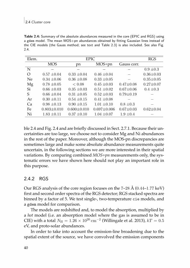
2.4 Cluster core
Table 2.4: Summary of the absolute abundances measured in the core (EPIC and RGS) usinga gdem model. The mean MOS+pn abundances obtained by fitting Gaussian lines instead ofthe CIE models (the Gauss method; see text and Table 2.3) is also included. See also Fig.2.4.
Elem. EPIC RGSMOS pn MOS+pn Gauss corr.
N − − − − 0.9 ±0.3O 0.57 ±0.04 0.33 ±0.04 0.46 ±0.04 − 0.36±0.03Ne 0.34 ±0.06 0.36 ±0.08 0.33 ±0.05 − 0.35±0.05Mg 0.78 ±0.05 < 0.08 0.45 ±0.03 0.47±0.08 0.27±0.07Si 0.66 ±0.03 0.35 ±0.03 0.51 ±0.02 0.67±0.06 0.4 ±0.3S 0.66 ±0.04 0.31 ±0.05 0.52 ±0.03 0.79±0.19 −Ar 0.30 ±0.11 0.54 ±0.15 0.41 ±0.08 − −Ca 0.98 ±0.13 0.90 ±0.15 1.01 ±0.10 0.8 ±0.3 −Fe 0.803±0.010 0.600±0.010 0.697±0.006 0.67±0.03 0.62±0.04Ni 1.83 ±0.11 0.37 ±0.10 1.04 ±0.07 1.9 ±0.4 −
ble 2.4 and Fig. 2.4 and are briefly discussed in Sect. 2.7.1. Because their un-certainties are too large, we choose not to consider Mg and Ni abundancesin the rest of the paper. Moreover, although the MOS-pn discrepancies aresometimes large and make some absolute abundance measurements quiteuncertain, in the following sections we are more interested in their spatialvariations. By comparing combinedMOS+pnmeasurements only, the sys-tematic errors we have shown here should not play an important role inthis purpose.
2.4.2 RGS
Our RGS analysis of the core region focuses on the 7–28 Å (0.44–1.77 keV)first and second order spectra of the RGS detector; RGS stacked spectra arebinned by a factor of 5. We test single-, two-temperature cie models, anda gdem model for comparison.
The models are redshifted and, to model the absorption, multiplied bya hot model (i.e. an absorption model where the gas is assumed to be inCIE) with a total NH = 1.26 × 1020 cm−2 (Willingale et al. 2013), kT = 0.5eV, and proto-solar abundances.
In order to take into account the emission-line broadening due to thespatial extent of the source, we have convolved the emission components
40
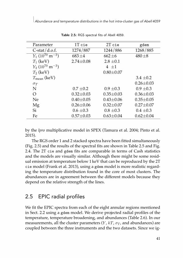
Abundance and temperature distributions in the hot intra-cluster gas of Abell 4059
Table 2.5: RGS spectral fits of Abell 4059.
Parameter 1T cie 2T cie gdemC-stat/d.o.f. 1274/887 1244/886 1268/885Y1 (1070 m−3) 683±4 662±6 480±8T1 (keV) 2.74±0.08 2.8 ±0.1Y2 (1070 m−3) 4 ±1T2 (keV) 0.80±0.07Tmean (keV) 3.4 ±0.2σT 0.26±0.03N 0.7 ±0.2 0.9 ±0.3 0.9 ±0.3O 0.32±0.03 0.35±0.03 0.36±0.03Ne 0.40±0.05 0.43±0.06 0.35±0.05Mg 0.26±0.06 0.32±0.07 0.27±0.07Si 0.6 ±0.3 0.8 ±0.3 0.4 ±0.3Fe 0.57±0.03 0.63±0.04 0.62±0.04
by the lpro multiplicative model in SPEX (Tamura et al. 2004; Pinto et al.2015).
The RGS order 1 and 2 stacked spectra have been fitted simultaneously(Fig. 2.5) and the results of the spectral fits are shown in Table 2.5 and Fig.2.4. The 2T cie and gdem fits are comparable in terms of Cash statisticsand the models are visually similar. Although there might be some resid-ual emission at temperature below 1keV that can be reproduced by the 2Tcie model (Frank et al. 2013), using a gdem model is more realistic regard-ing the temperature distribution found in the core of most clusters. Theabundances are in agreement between the different models because theydepend on the relative strength of the lines.
2.5 EPIC radial profilesWe fit the EPIC spectra from each of the eight annular regions mentionedin Sect. 2.2 using a gdem model. We derive projected radial profiles of thetemperature, temperature broadening, and abundances (Table 2.6). In ourmeasurements, all the cluster parameters (Y , kT , σT , and abundances) arecoupled between the three instruments and the two datasets. Since we ig-
41
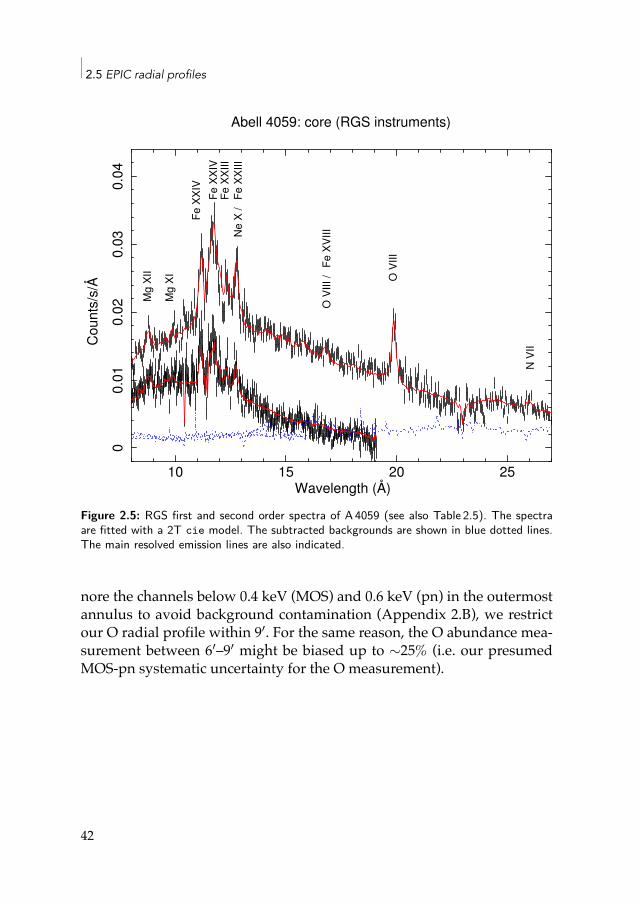
2.5 EPIC radial profiles
10 15 20 25
00.
010.
020.
030.
04
Cou
nts/
s/Å
Wavelength (Å)
Abell 4059: core (RGS instruments)
Mg
XII
Fe X
XIV
Fe X
XIV
Fe X
XIII
Fe X
XIII
Ne
X /
O V
III /
Fe X
VIII
O V
III
N V
II
Mg
XI
Figure 2.5: RGS first and second order spectra of A 4059 (see also Table 2.5). The spectraare fitted with a 2T cie model. The subtracted backgrounds are shown in blue dotted lines.The main resolved emission lines are also indicated.
nore the channels below 0.4 keV (MOS) and 0.6 keV (pn) in the outermostannulus to avoid background contamination (Appendix 2.B), we restrictour O radial profile within 9′. For the same reason, the O abundance mea-surement between 6′–9′ might be biased up to ∼25% (i.e. our presumedMOS-pn systematic uncertainty for the O measurement).
42
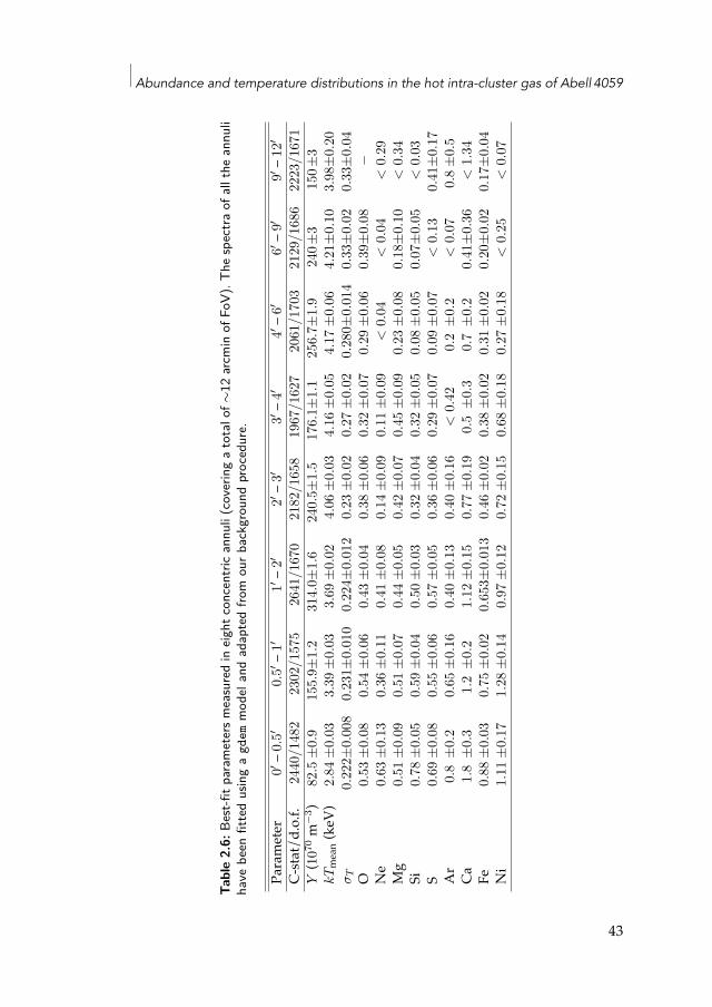
Abundance and temperature distributions in the hot intra-cluster gas of Abell 4059
Tabl
e2.
6:Be
st-fi
tpar
amet
ersm
easu
red
ineig
htco
ncen
tric
annu
li(c
over
ing
ato
talo
f∼12
arcm
inof
FoV)
.The
spec
traof
allt
hean
nuli
have
been
fitte
dus
ing
agd
emm
odel
and
adap
ted
from
ourb
ackg
roun
dpr
oced
ure.
Paramete
r0′–0
.5′
0.5′–1
′1′–2
′2′–3
′3′–4
′4′–6
′6′–9
′9′–1
2′
C-sta
t/d.o.f.
2440
/148
223
02/1
575
2641
/167
021
82/16
5819
67/1
627
2061
/17
0321
29/1
686
2223
/167
1Y(1
070m
−3 )
82.5
±0.
915
5.9±
1.2
314.
0±1.
624
0.5±
1.5
176.
1±1.
125
6.7±
1.9
240±
315
0±3
kTmean(keV)
2.84
±0.
033.
39±
0.03
3.69
±0.
024.
06±
0.03
4.16
±0.
054.
17±
0.06
4.21
±0.
103.
98±
0.20
σT
0.22
2±0.
008
0.23
1±0.
010
0.22
4±0.
012
0.23
±0.
020.
27±
0.02
0.28
0±0.
014
0.33
±0.
020.
33±
0.04
O0.
53±
0.08
0.54
±0.
060.
43±
0.04
0.38
±0.
060.
32±
0.07
0.29
±0.
060.
39±
0.08
−Ne
0.63
±0.
130.
36±
0.11
0.41
±0.
080.
14±
0.09
0.11
±0.
09<
0.04
<0.
04<
0.29
Mg
0.51
±0.
090.
51±
0.07
0.44
±0.
050.
42±
0.07
0.45
±0.
090.
23±
0.08
0.18
±0.
10<
0.34
Si0.
78±
0.05
0.59
±0.
040.
50±
0.03
0.32
±0.
040.
32±
0.05
0.08
±0.
050.
07±
0.05
<0.
03S
0.69
±0.
080.
55±
0.06
0.57
±0.
050.
36±
0.06
0.29
±0.
070.
09±
0.07
<0.
130.
41±
0.17
Ar0.
8±
0.2
0.65
±0.
160.
40±
0.13
0.40
±0.
16<
0.42
0.2
±0.
2<
0.07
0.8
±0.
5Ca
1.8
±0.
31.
2±
0.2
1.12
±0.
150.
77±
0.19
0.5
±0.
30.
7±
0.2
0.41
±0.
36<
1.34
Fe0.
88±
0.03
0.75
±0.
020.
653±
0.01
30.
46±
0.02
0.38
±0.
020.
31±
0.02
0.20
±0.
020.
17±
0.04
Ni
1.11
±0.
171.
28±
0.14
0.97
±0.
120.
72±
0.15
0.68
±0.
180.
27±
0.18
<0.
25<
0.07
43

2.5 EPIC radial profiles
1 100.2 0.5 2 5
23
45
Te
mp
era
ture
(ke
V)
Radius (arcmin)
kT
1 100.2 0.5 2 5
0.2
0.3
0.4
!T
Radius (arcmin)
!T
1 100.2 0.5 2 5
00
.20
.40
.60
.81
O a
bu
nd
an
ce (
pro
to!
sola
r)
Radius (arcmin)
O
1 100.2 0.5 2 5
00
.20
.40
.60
.81
Ne
ab
un
da
nce
(p
roto
!so
lar)
Radius (arcmin)
Ne
Figure 2.6: EPIC radial profiles of Abell 4059. The datapoints show our best-fit measurements(Table 2.6). The solid lines show our best-fit empirical distributions (Table 2.7). The spectraof all the annuli have been fitted using a gdem model and adapted from our backgroundmodelling. We note the change of abundance scale for Ar and Ca.
In order to quantify the trends that appear in our profiles, we fit themwith simple empirical distributions. For temperature and abundance pro-files,
kT (r) = D∞ + α exp(−r/r0) (2.4)Z(r) = D∞ + α exp(−r/r0) (2.5)
and for σT radial profile,
σT (r) = D∞ + αrγ . (2.6)
Table 2.7 shows the results of our fitted trends. Figure 2.6 shows the radialprofiles and their respective best-fit distributions.
The temperature profile reveals a significant drop from ∼2.5′ to the in-nermost annuli, confirming the presence of a cool-core. Beyond ∼2.5′, the
44
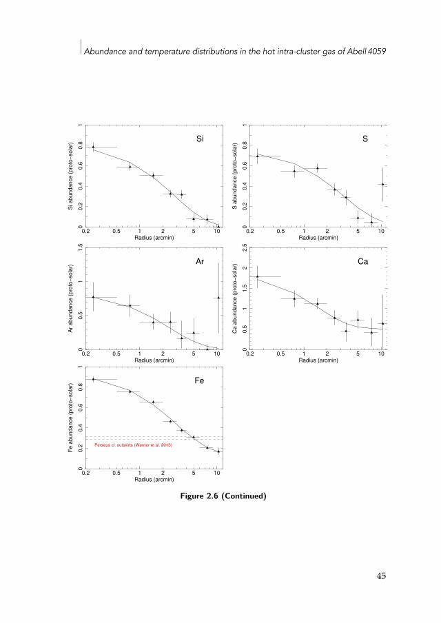
Abundance and temperature distributions in the hot intra-cluster gas of Abell 4059
1 100.2 0.5 2 5
00
.20
.40
.60
.81
Si a
bu
nd
an
ce (
pro
to!
sola
r)
Radius (arcmin)
Si
1 100.2 0.5 2 5
00
.20
.40
.60
.81
S a
bu
nd
an
ce (
pro
to!
sola
r)Radius (arcmin)
S
1 100.2 0.5 2 5
00
.51
1.5
Ar
ab
un
da
nce
(p
roto
!so
lar)
Radius (arcmin)
Ar
1 100.2 0.5 2 5
00
.51
1.5
22
.5
Ca
ab
un
da
nce
(p
roto
!so
lar)
Radius (arcmin)
Ca
1 100.2 0.5 2 5
00
.20
.40
.60
.81
Fe
ab
un
da
nce
(p
roto
!so
lar)
Radius (arcmin)
Perseus cl. outskirts (Werner et al. 2013)
Fe
Figure 2.6 (Continued)
45
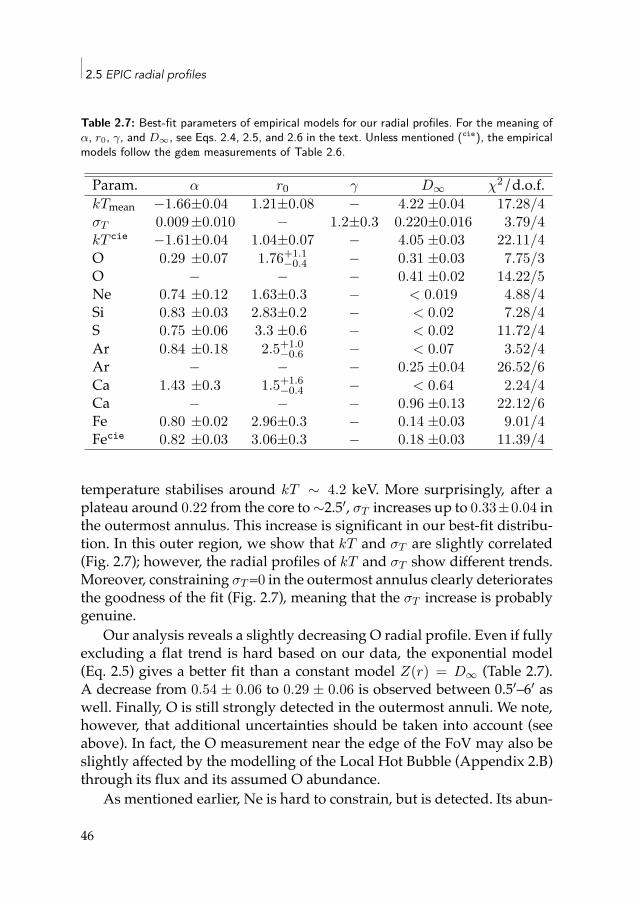
2.5 EPIC radial profiles
Table 2.7: Best-fit parameters of empirical models for our radial profiles. For the meaning ofα, r0, γ, and D∞, see Eqs. 2.4, 2.5, and 2.6 in the text. Unless mentioned (cie), the empiricalmodels follow the gdem measurements of Table 2.6.
Param. α r0 γ D∞ χ2/d.o.f.kTmean −1.66±0.04 1.21±0.08 − 4.22 ±0.04 17.28/4σT 0.009±0.010 − 1.2±0.3 0.220±0.016 3.79/4kT cie −1.61±0.04 1.04±0.07 − 4.05 ±0.03 22.11/4O 0.29 ±0.07 1.76+1.1
−0.4 − 0.31 ±0.03 7.75/3O − − − 0.41 ±0.02 14.22/5Ne 0.74 ±0.12 1.63±0.3 − < 0.019 4.88/4Si 0.83 ±0.03 2.83±0.2 − < 0.02 7.28/4S 0.75 ±0.06 3.3 ±0.6 − < 0.02 11.72/4Ar 0.84 ±0.18 2.5+1.0
−0.6 − < 0.07 3.52/4Ar − − − 0.25 ±0.04 26.52/6Ca 1.43 ±0.3 1.5+1.6
−0.4 − < 0.64 2.24/4Ca − − − 0.96 ±0.13 22.12/6Fe 0.80 ±0.02 2.96±0.3 − 0.14 ±0.03 9.01/4Fecie 0.82 ±0.03 3.06±0.3 − 0.18 ±0.03 11.39/4
temperature stabilises around kT ∼ 4.2 keV. More surprisingly, after aplateau around 0.22 from the core to∼2.5′, σT increases up to 0.33±0.04 inthe outermost annulus. This increase is significant in our best-fit distribu-tion. In this outer region, we show that kT and σT are slightly correlated(Fig. 2.7); however, the radial profiles of kT and σT show different trends.Moreover, constraining σT=0 in the outermost annulus clearly deterioratesthe goodness of the fit (Fig. 2.7), meaning that the σT increase is probablygenuine.
Our analysis reveals a slightly decreasing O radial profile. Even if fullyexcluding a flat trend is hard based on our data, the exponential model(Eq. 2.5) gives a better fit than a constant model Z(r) = D∞ (Table 2.7).A decrease from 0.54 ± 0.06 to 0.29 ± 0.06 is observed between 0.5′–6′ aswell. Finally, O is still strongly detected in the outermost annuli. We note,however, that additional uncertainties should be taken into account (seeabove). In fact, the O measurement near the edge of the FoV may also beslightly affected by the modelling of the Local Hot Bubble (Appendix 2.B)through its flux and its assumed O abundance.
As mentioned earlier, Ne is hard to constrain, but is detected. Its abun-
46
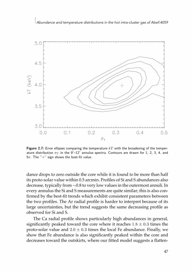
Abundance and temperature distributions in the hot intra-cluster gas of Abell 4059
Figure 2.7: Error ellipses comparing the temperature kT with the broadening of the temper-ature distribution σT in the 9′–12′ annulus spectra. Contours are drawn for 1, 2, 3, 4, and5σ. The ”+” sign shows the best-fit value.
dance drops to zero outside the core while it is found to be more than halfits proto-solar value within 0.5 arcmin. Profiles of Si and S abundances alsodecrease, typically from∼0.8 to very low values in the outermost annuli. Inevery annulus the Si and Smeasurements are quite similar; this is also con-firmed by the best-fit trends which exhibit consistent parameters betweenthe two profiles. The Ar radial profile is harder to interpret because of itslarge uncertainties, but the trend suggests the same decreasing profile asobserved for Si and S.
The Ca radial profile shows particularly high abundances in general,significantly peaked toward the core where it reaches 1.8 ± 0.3 times theproto-solar value and 2.0 ± 0.3 times the local Fe abundance. Finally, weshow that Fe abundance is also significantly peaked within the core anddecreases toward the outskirts, where our fitted model suggests a flatten-
47
2.6 Temperature, σT , and Fe abundance maps
ing to 0.14 ± 0.03.We note that our radial analysis focuses on the projected profiles only.
Although deprojection can give a rough idea about the 3-D behaviour ofthe radial profiles, they are based on the assumption of a spherical sym-metry, which is far from being the case in the innermost parts of A 4059(Sect. 2.6). Moreover, the deprojected abundance radial profiles are notthought to deviate significantly from the projected ones (see e.g. Werneret al. 2006b). Based on the analysis of Kaastra et al. (2004), we estimate thatthe contamination of photons into incorrect annuli as a result of the EPICpoint-spread function (PSF) changes our Fe abundance measurements by∼2% and∼4% in the first and second innermost annuli, respectively, whichis not significant regarding our 1σ error bars. The choice of a gdem modelshould take into account both the multi-temperature features due to pro-jection effects and the possible PSF contamination in the kT radial profile.
2.6 Temperature, σT , and Fe abundance mapsUsing a gdemmodel, we derive temperature and abundancemaps from theEPIC data of our two deep observations. The long net exposure time (∼140ks) for A 4059 allows the distribution of kT , σT , and Fe abundance to bemapped within 6′. As in the radial analysis, all the EPIC instruments andthe two datasets are fitted simultaneously.
In order to emphasise the impact of the statistical errors on the mapsand to possibly reveal substructures, we create so-called residuals mapsfollowing themethod of Lovisari et al. (2011). In each cell, we subtract fromeach measured parameter the respective value estimated from our mod-elled radial profile (Fig. 2.6) at the distance r of the geometric centre of thecell. The significance index is defined as being this difference divided bythe error on the measured parameter. The kT , σT , and Fe abundance mapsand their respective error and residuals maps are shown in Fig. 2.8.
The kT map reveals the cool core of the cluster in detail. It appearsto be asymmetric and to have a roughly conic shape extending from thenorth to the east and pointing toward the south-west. Along this axis, thetemperature gradient is steeper to the south-west than to the north-eastof the core. Most of the relative errors obtained with the cie model (notshown here) are within 2–5%, which is in agreement with our expectations(Appendix 2.C); however, they slightly increase with radius. This trend isstronger when using the gdem model, and the errors are somewhat larger.
48
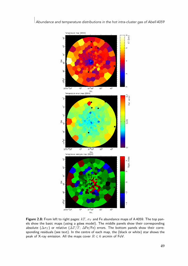
Abundance and temperature distributions in the hot intra-cluster gas of Abell 4059
Figure 2.8: From left to right pages: kT , σT and Fe abundance maps of A 4059. The top pan-els show the basic maps (using a gdem model). The middle panels show their correspondingabsolute (∆σT ) or relative (∆T/T ; ∆Fe/Fe) errors. The bottom panels show their corre-sponding residuals (see text). In the centre of each map, the (black or white) star shows thepeak of X-ray emission. All the maps cover R ⩽ 6 arcmin of FoV.
49
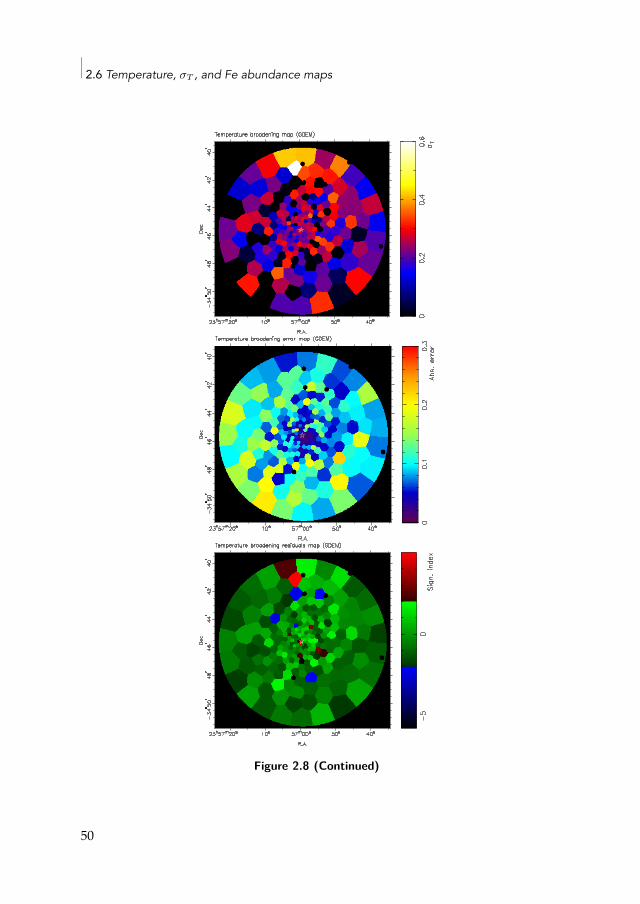
2.6 Temperature, σT , and Fe abundance maps
Figure 2.8 (Continued)
50
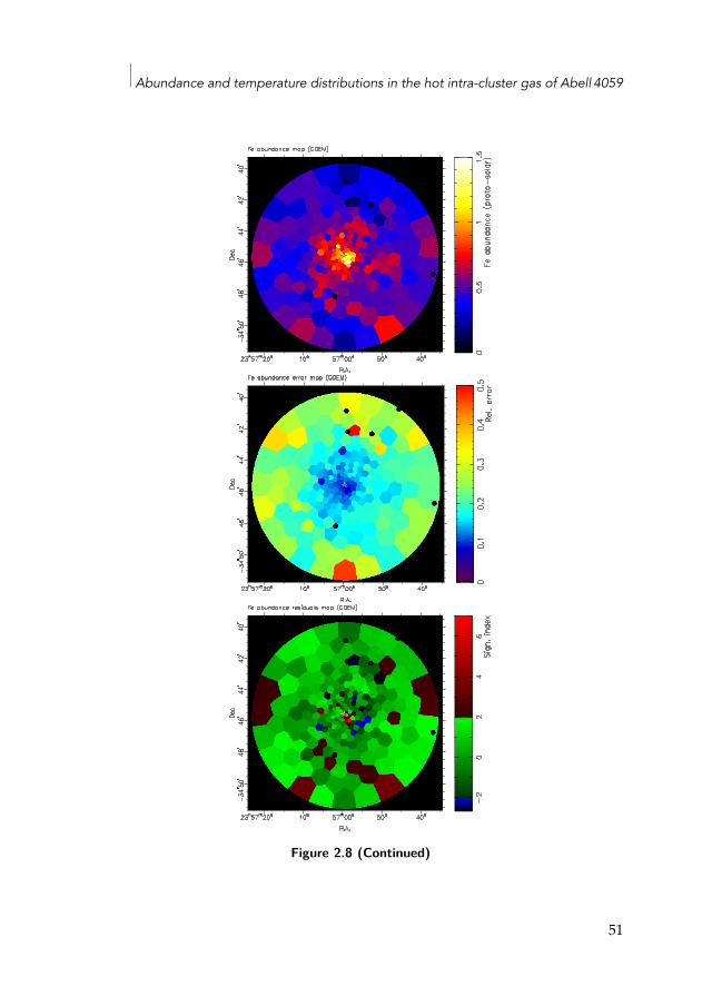
Abundance and temperature distributions in the hot intra-cluster gas of Abell 4059
Figure 2.8 (Continued)
51
2.7 Discussion
A very local part (∼5 cells) of the core is up to 8σ cooler than our modelledtemperature profile. This coldest part is offset∼25′′ SW from theX-ray peakemission. This contrasts with the western part of the core, which shows asignificantly hotter bow than the average ∼55′′ away from the X-ray peakemission. We also note that some outer cells are found significantly (>2σ)colder or hotter than the radial trend.
The σT map confirms the positive σT measurements in most of the cellsoutside the core, typically within 0.1–0.4. Globally, σT is consistent withthat measured from the σT radial profile. We note that outside the core theerrors are inhomogeneous and are sometimes hard to estimate precisely.
The Fe map also shows that the core is asymmetric. As it is in the kTmap, the abundance gradient from the core toward the south-west is steeperthan toward the north-east. The highest Fe emitting region is found to be∼25′′ SW offset from the X-ray peak emission and coincides with the cold-est region. In this offset SW region, Fe is measured to bemore than 7σ over-abundant.
We note that the smallest cells (∼12”) have a size comparable to theEPIC PSF (∼6” FWHM); a contamination from leaking photons betweenadjacent cells might thus slightly affect our mapping analysis. However,the PSF has a smoothing effect on the spatial distributions, and gradientsmay be only stronger than they actually show in the map. This does not af-fect our conclusion of important asymmetries of temperature and Fe abun-dance in the core of A 4059.
2.7 DiscussionWedetermined the temperature distribution and the elemental abundancesof O, Ne, Si, S, Ar, Ca, and Fe in the core region (⩽ 3′) of A 4059 and ineight concentric annuli centred on the core. In addition, we built 2-D mapsof the mean temperature (kT ), the temperature broadening (σT ), and theFe abundance. Because of the large cross-calibration uncertainties, Mg andNi abundances are not reliable in these datasets using EPIC, and we preferto measure the Mg abundance using RGS instead.
2.7.1 Abundance uncertainties and SNe yieldsAs shown in Table 2.2, the Ne abundance measured using EPIC dependsstrongly on the choice of the modelled temperature distribution. The main
52
Abundance and temperature distributions in the hot intra-cluster gas of Abell 4059
Ne lines are hidden in the Fe-L complex, around ∼1 keV. This complexcontains many strong Fe lines and is extremely sensitive to temperature. Aslight change in the temperature distribution will thus significantly affectthe Ne abundance measurement, making it not very reliable using EPIC(see alsoWerner et al. 2006b). For the same reason, Fe abundances of single-and multi-temperature models might change slightly but already cause asignificant difference between both models.
Most of the discrepancies in the abundance determination between theEPIC instruments come from an incorrect estimation of the lines and/orthe continuum in pn (Sect. 2.4.1). Cross-calibration issues between MOSand pn have been already reported (see e.g. de Plaa et al. 2007; Schellen-berger et al. 2015), but their deterioration has probably increased over timedespite current calibration efforts (Read et al. 2014). Our analysis usingthe Gauss method (Table 2.3 and Fig. 2.4) suggests that in general MOS ismore reliable than pn in our case, even thoughMOSmight slightly overes-timate some elements as well (e.g. Mg, S, or even Fe). In all cases, this latestmethod is the most robust one with which to estimate the abundances inthe core using EPIC.
Another interesting result is our detection of very high Ca/Fe abun-dances in the core. This trend has been already reported by de Plaa et al.(2006) in Sérsic 159-03 (see also de Plaa et al. 2007).Within 0.5′ the combinedEPICmeasurements give a Ca/Fe ratio of 2.0±0.3. This is even higher thanmeasured within 3′ (Ca/Fe = 1.45 ± 0.14). Following the approach of dePlaa et al. (2007) and assuming a Salpeter IMF (Salpeter 1955), we select dif-ferent SNIamodels (soft deflagration versus delayed-detonation, Iwamotoet al. 1999) as well as different initial metallicities affecting the yields fromSNcc population (Nomoto et al. 2006). We fit the constructed SNe mod-els to our measured abundances in the core (O, Ne, Mg, and Si from RGS;Ar and Ca from EPIC; Fe from the Gauss method). We find that a WDD2model, taken with Z=0.02 and a Salpeter IMF, reproduce our measure-ments best, with (χ2/d.o.f.)WDD2 = 4.28/6 (Fig. 2.9). Although the fit isreasonable in terms of reduced χ2, it is unable to explain the high Ca/Fevalue that we found. Based again on de Plaa et al. (2007), we also consid-ered a delayed-detonation model that fitted the Tycho SNIa remnant best(Badenes et al. 2006). The fit is improved ((χ2/d.o.f.)Tycho = 1.77/5), but themodel barely reaches the lower error bar of our measured Ca/Fe. Assum-ing that the problem is not fully solved even by using the latest model, wecan raise two further hypotheses that might explain it:
53
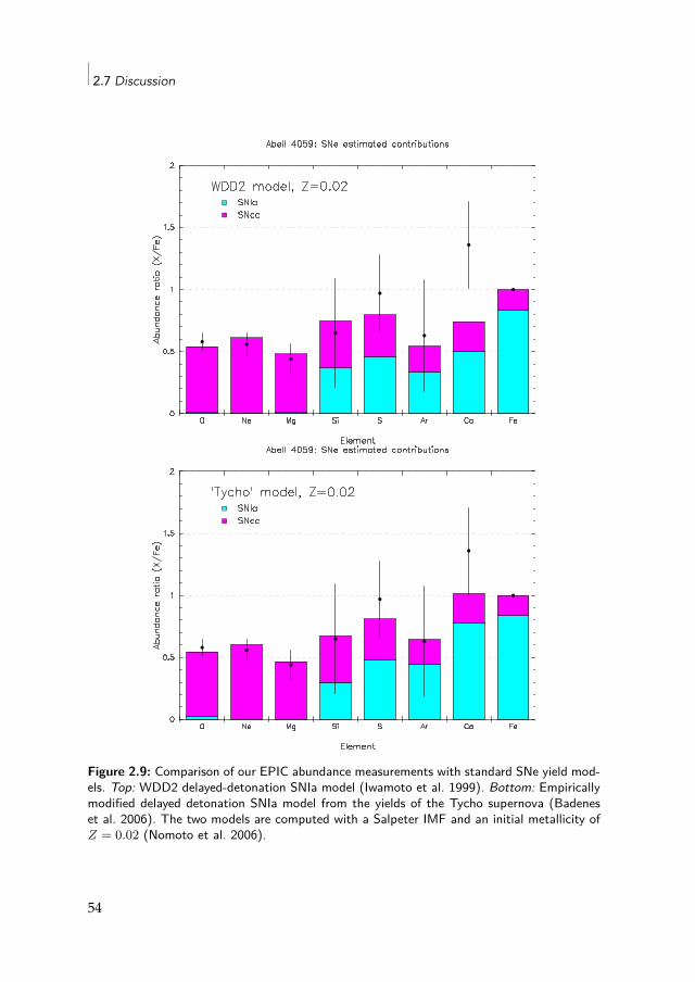
2.7 Discussion
Figure 2.9: Comparison of our EPIC abundance measurements with standard SNe yield mod-els. Top: WDD2 delayed-detonation SNIa model (Iwamoto et al. 1999). Bottom: Empiricallymodified delayed detonation SNIa model from the yields of the Tycho supernova (Badeneset al. 2006). The two models are computed with a Salpeter IMF and an initial metallicity ofZ = 0.02 (Nomoto et al. 2006).
54
Abundance and temperature distributions in the hot intra-cluster gas of Abell 4059
1. Calcium abundancemeasurements might suffer from additional sys-tematic uncertainties. Our analysis (Sects. 2.4.1 and 2.5) shows, how-ever, that MOS and pn Ca/Fe measurements are consistent withinthe entire core (3′). Moreover, the continuum and EW of Ca lines(∼3.9 keV) are correctly estimated by our cie models. Because ofcurrent efforts to limit them, uncertainties in the atomic database cancontribute only partly. Finally the effective area at the position of thisline is smooth andno instrumental-line feature is known around∼3.9keV.
2. Some SNe subclasses, so far ignored, might contribute to the metalenrichment in the ICM. For example, the so-called calcium-rich gaptransients as a possible subclass of SNIa, are expected to produce alarge amount of Ca even outside galaxies, making the transportationof Ca in the ICM much easier (Mulchaey et al. 2014).
2.7.2 Abundance radial profilesAll the abundance radial profiles decrease with radius. Interestingly, Oshows a slight decrease (confirmed by our empirical fitted distribution),even though a flat profile cannot be fully excluded. This decreasing trendhas been observed in other clusters, such as Hydra A (Simionescu et al.2009a), A2029, and Centaurus (Lovisari et al. 2011). However, the observa-tions of A 496 (Lovisari et al. 2011) and A1060 (Sato et al. 2007b) suggest aflatter profile. The O distribution is less clear in Sérsic 159-03 (de Plaa et al.2006; Lovisari et al. 2011).
Moreover, onlyO and Fe profiles show abundances significantly higherthan zero in the outermost annuli. The Fe profile is clearly peaked to thecore, and agrees with typical slopes found in many other clusters (e.g.Simionescu et al. 2009a; Lovisari et al. 2011).Moreover, its apparent plateauin the outer regions may suggest a constant Fe abundance in the ICM evenoutside r500, as recently observed by Suzaku in Perseus (Werner et al. 2013)and other clusters (e.g. Leccardi &Molendi 2008;Matsushita 2011). As seenin Fig. 2.6, the Fe abundance found in the outskirts of Perseus (0.303±0.012,in proto-solar abundance units) is higher than what we find for A 4059,even when accounting for the systematic uncertainties estimated from thecore in Sect. 2.4.1. This constant Fe abundance found in other cluster out-skirts and thiswork suggest that the bulk of the enrichment at least by SNIastarted in the early stages of the cluster formation.
55
2.7 Discussion
In the previous cluster analyses where O appeared to be flat, the in-crease of O/Fe with radius is usually justified by arguing a very early pop-ulation of SNIa and SNcc, starting after an intense star formation aroundz ∼ 2–3 (Hopkins & Beacom 2006) and undergoing a very efficient mix-ing all over the potential well, followed by a delayed population of SNIaresponsible for the Fe peaked profile, and produced preferably in the cen-tral galaxy members in which a strong ram-pressure stripping is assumed(see also discussion for Sérsic 159-03 from de Plaa et al. 2006). It has alsobeen suggested that ram-pressure stripping could shape the Fe peak pro-file between z = 1 and z = 0 (Schindler et al. 2005). However, De Grandiet al. (2014) suggest that the bulk of the Fe peakwas already in place beforez = 1 in most clusters, meaning that at least SNIa type products started toget a centrally peaked distribution early on in the cluster formation. In fact,Fe seems to follow the near-infrared light profile of the central cD galaxiesmuch better at z = 1 than at z = 0, suggesting that most of the currentmixing mechanisms tend to spread out the metals in the ICM.
The decreasing O radial profile measured in this work suggests that thesame kind of scenario is likely for SNcc type products. Although its best-fitslope of the profile appears to be flatter than the slope of the Fe radial pro-file (Table 2.7), the O/Fe radial values are still compatible with a constantdistribution (except possibly for the 6’-9’ annulus,where systematicsmightaffect the O measurements). Consequently, it is not necessary to invoke adelayed population of SNIa and/or SNcc occurring after z = 1, although itmight contribute to a minor part of the metals found in the core. At z ∼ 2–3 the central cD galaxy and its surrounding galaxy members were alreadyactively star-forming and could have produced the bulk of all metals ob-served in the core, probably injected into the ICM through galactic winds.More recently, ram-pressure stripping could have also played a minor rolein the enrichment of the core, for example to explain the asymmetry foundon the maps (see below).
Assuming a flat and positive distribution of Fe and O beyond the FoV,the mixing of the metals is likely very efficient in the outskirts, where theentropy is high. In the core however, the entropy was already very strati-fied early onwithout anymajormergers to disturb it, and themixingmech-anisms could be less efficient there.
While O and Fe are detected far from the core and this favours an earlyinitial enrichment from SNIa and SNcc types, puzzlingly we do not detectsignificant abundances of Ne and Si in the outermost annuli. This result
56
Abundance and temperature distributions in the hot intra-cluster gas of Abell 4059
is less striking in the S and Ar radial measurements, even though our fit-ted trends give small upper limits for D∞. Nevertheless, abundance mea-surements in the outer parts of the FoV can also suffer from additionalsystematic uncertainties related to the background contribution. These un-certainties may explain our lack of clear detection of Ne, Si, S, and Ar inthe outermost annuli. Finally, we note the similarity between the Si and Sprofiles, already reported in the cD galaxy M87 by Million et al. (2011).
In addition to these radial trends, ourmaps show local regions of anoma-lously rich Fe abundance in the core. This is particularly striking in thesouth-west ridge, where the Fe abundance is >7σ higher than the averagetrend from its corresponding radial profile. Since no galaxy can be associ-ated with this particular region, it is hard to explain its enrichment withgalactic winds. As previously reported and discussed by Reynolds et al.(2008), it is possible that an important part of the metals in the core comesfrom one early starburst galaxy that passed very close to the cD centralgalaxy before the onset of the central AGN. In this case ram-pressure strip-ping could probably have played a dominant role in the enrichment within∼0.5 arcmin after the initial enrichment seen through the radial profiles.This possible scenario is also discussed in the next section.
2.7.3 Temperature structures and asymmetriesAlthough the ICM appears homogeneous and symmetric at large scale, theinner part appears to be more asymmetric (Fig. 2.2). As already observedin the past by Chandra (Heinz et al. 2002; Reynolds et al. 2008), the south-west ridge is clearly visible as an additional peaked X-ray emission nearthe core, and a diffuse tail from the core toward the north-east can also bedetected.
Evidence of asymmetries are also found in our spectral analyses. Al-though our radial kT profile looks similar to other cool-core clusters, ourkT and Fe abundance maps show clear inhomogeneities in the ICM struc-ture ofA 4059. Compared to the 2-DmapspreviouslymeasuredusingChan-dra (Reynolds et al. 2008), the S/N of the cells in our EPIC maps are ∼3.3and∼2.5 times greater for kT and the Fe abundance, respectively, allowingus to confirm these substructures with a higher precision and over a largerFoV.
First, like the Fe abundance, the temperature gradient is steeper withinthe south-west ridge than north-east of the core. The central core (includingthe south-west ridge) is also significantly colder (∼2.3 keV) and the south-
57
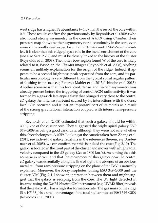
2.7 Discussion
west ridge has a higher Fe abundance (∼1.5) than the rest of the corewithin0.5′. These results confirm the previous study by Reynolds et al. (2008)whoalso found strong asymmetry in the core of A 4059 using Chandra. Theirpressuremap shows neither asymmetry nor discontinuity in the core, evenaround the south-west ridge. From both Chandra and XMM-Newton stud-ies, it is clear that this ridge plays a role in the metal enrichment of the core(see also Sect. 2.7.2) and must be closely linked to the history of the cluster(Reynolds et al. 2008). The hotter bow region found W of the core is likelyrelated to it. Based on the Chandra images (Reynolds et al. 2008), sloshingseems an unlikely explaination for the origin of the ridge. Indeed, it ap-pears to be a second brightness peak separated from the core, and its par-ticular morphology is very different from the typical spiral regular patternof sloshing fronts (see e.g. Paterno-Mahler et al. 2013; Ichinohe et al. 2015).Another scenario is that this local cool, dense, and Fe-rich asymmetry wasalready present before the triggering of central AGN radio-activity; it wasformed by a gas-rich late-type galaxy that plunged very close to the centralcD galaxy. An intense starburst caused by its interactions with the denselocal ICM occurred and it lost an important part of its metals as a resultof the strong gravitational interaction coupled with intense ram-pressurestripping.
Reynolds et al. (2008) estimated that such a galaxy should be within300v3 kpc of the cluster core. They suggested the bright spiral galaxy ESO349-G009 as being a good candidate, although they were not sure whetherthis object belongs to A4059. Looking at the caustic taken fromZhang et al.(2011, see individual galaxy redshifts in the references therein, e.g. Ander-nach et al. 2005), we can confirm that this is indeed the case (Fig. 2.10). Thegalaxy is located in the front part of the cluster andmoveswith a high radialvelocity compared to the cD galaxy (∆v ≃ 1800 km/s). Assuming that thisscenario is correct and that the movement of this galaxy near the centralcD galaxy was essentially along the line of sight, the absence of an obviousmetal tail from ram-pressure stripping on the plane of the FoV is naturallyexplained. Moreover, the X-ray isophotes joining ESO 349-G009 and thecluster ICM (Fig. 2.11) show an interaction between them and might sug-gest that the galaxy is escaping from the core. The UV light detected inits arms using the XMM-NewtonOM instrument (e.g. UVM2 filter) revealsthat the galaxy still has a high star formation rate. The gasmass of the ridge(5×10⁹ M⊙) is a small percentage of the total stellar mass of ESO 349-G009(Reynolds et al. 2008).
58
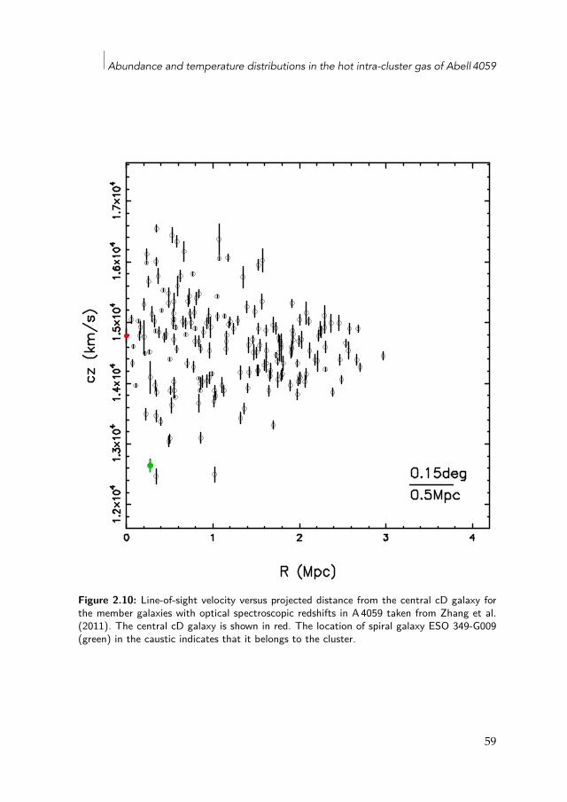
Abundance and temperature distributions in the hot intra-cluster gas of Abell 4059
Figure 2.10: Line-of-sight velocity versus projected distance from the central cD galaxy forthe member galaxies with optical spectroscopic redshifts in A 4059 taken from Zhang et al.(2011). The central cD galaxy is shown in red. The location of spiral galaxy ESO 349-G009(green) in the caustic indicates that it belongs to the cluster.
59
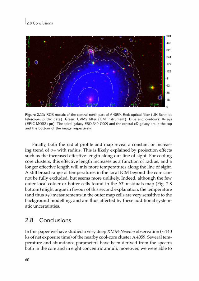
2.8 Conclusions
0
18
38
62
91
128
177
241
329
445
601
30.0 20.0 10.0 23:57:00.0 50.0 40.0 56:30.0
-34:4
0:0
0.0
42:0
0.0
44
:00
.0
Figure 2.11: RGB mosaic of the central-north part of A 4059. Red: optical filter (UK Schmidttelescope, public data). Green: UVM2 filter (OM instrument). Blue and contours: X-rays(EPIC MOS2+pn). The spiral galaxy ESO 349-G009 and the central cD galaxy are in the topand the bottom of the image respectively.
Finally, both the radial profile and map reveal a constant or increas-ing trend of σT with radius. This is likely explained by projection effectssuch as the increased effective length along our line of sight. For coolingcore clusters, this effective length increases as a function of radius, and alonger effective length will mix more temperatures along the line of sight.A still broad range of temperatures in the local ICM beyond the core can-not be fully excluded, but seems more unlikely. Indeed, although the fewouter local colder or hotter cells found in the kT residuals map (Fig. 2.8bottom) might argue in favour of this second explanation, the temperature(and thus σT ) measurements in the outer map cells are very sensitive to thebackground modelling, and are thus affected by these additional system-atic uncertainties.
2.8 ConclusionsIn this paperwe have studied a very deepXMM-Newton observation (∼140ks of net exposure time) of the nearby cool-core cluster A 4059. Several tem-perature and abundance parameters have been derived from the spectraboth in the core and in eight concentric annuli; moreover, we were able to
60
Abundance and temperature distributions in the hot intra-cluster gas of Abell 4059
derive kT , σT , and Fe abundance maps. We conclude the following:
• The temperature structure shows the cool-core and in addition in-creasing deviations from apparent isothermality in and out of thecore.
• The abundances of O, Ne, Si, S, Ar, Ca, and Fe all are peaked towardthe core, and we report the presence of Fe and O beyond ∼0.3 Mpcfrom the core. This suggests that the enrichment from SNIa and SNccstarted early on in the cluster formation, probably through galacticwinds in the young galaxy members.
• The EPIC image as well as the temperature and Fe abundance mapsreveal strong asymmetries in the cluster core. We confirm a colderand Fe-richer ridge south-west of the core, previously found byChan-dra, perhaps due to an intense ram-pressure stripping event. There-fore, in addition to an early enrichment through galactic winds, ram-pressure stripping might have greatly contributed to a more recentenrichment of the inner core.
• TheCa/Fe abundance ratio in the core is particularly high (1.45±0.14using a combined EPIC fit), even accounting for systematic uncer-tainties. If we assume the Ca/Fe abundance of the entire core to begenuine, it is unlikely explained by current standard SNe yield mod-els. Recently proposed calcium-rich gap transient SNIa might be aninteresting alternative with which to explain the high Ca abundancegenerally found in the ICM.
• Because of cross-calibration issues, the EPIC MOS and pn detectorsmeasure significantly different values of temperature andmost abun-dances. Although this leads to systematic uncertainties on their ab-solute values, the discrepancies are generally smaller when consid-ering abundances relative to Fe. Moreover, it should not affect rel-ative differences between spectra from different regions if the sameinstrument(s) are used. Fitting a Gaussian line and a local continuuminstead of CIE models is a robust method to measure more reliableabundances.
61
2.8 Conclusions
AcknowledgementsThis work is a part of the CHEERS (CHEmical Evolution Rgs cluster Sam-ple) collaboration.Wewould like to thank itsmembers and the anonymousreferee for their feedback and discussions. F.M. thanks Huub Röttgeringand Darko Donevski for useful discussions. L.L. acknowledges supportby the DFG through grant LO 2009/1-1. Y.Y.Z. acknowledges support bytheGermanBMWi through theVerbundforschung under grant 50OR1304.This work is based on observations obtained with XMM-Newton, an ESAsciencemissionwith instruments and contributions directly fundedbyESAmember states and the USA (NASA). The SRON Netherlands Institute forSpace Research is supported financially by NWO, the Netherlands Organ-isation for Scientific Research.
62
Abundance and temperature distributions in the hot intra-cluster gas of Abell 4059
2.A Detailled data reduction
2.A.1 GTI filteringIn order to reduce the soft-proton (SP) background, we build good time in-tervals (GTI) using the light curves in the 10–12 keV band for MOS and12–14 keV band for pn. We fit the count-rate histograms from the lightcurves of each instrument, binned in 100 s intervals, with a Poissonianfunction and we reject all time bins for which the number of counts liesoutside the interval µ ± 2σ (i.e. µ ± 2√
µ), where µ is the fitted averageof the distribution. We repeat the same screening procedure and threshold(so-called 2σ-clipping) for 10 s binned histograms in the 0.3–10 keV bandbecause De Luca & Molendi (2004) reported episodes of particularly softbackground flares. In order to get a qualitative estimation of the residual SPflare contamination, we use the Fin_over_Fout algorithmwhich comparesthe count rates in and out of the FoV of each detector (De Luca & Molendi2004). We found that in both observations MOS1 displays a Fin/Fout ratiohigher than 1.3, meaning that the observations have been significantly con-taminated by SP events. This value is still reasonable though, and a lookat the filtered light curve lead us to keep the MOS1 datasets. Furthermore,a careful modelling of convenient SP spectral components are used in ourspectral fittings as well (see Appendix 2.B).
2.A.2 Resolved point sources excisionThe point sources in our FoV contribute to the total flux and may biasthe astrophysical results that we aim to derive from the cluster emission.Therefore, they should bediscarded.Wedetect all the resolvedpoint sources(RPS) with the SAS task edetect_chain and we proceed with a secondcheck by eye in order to discard erroneous detections and possibly includea few missing candidates. It is common practice in extended source anal-ysis to excise bright point sources from the EPIC data. We note, however,that many sources have fluxes below the detection limit Scut and an unre-solved component might remain (Appendix 2.B.2).
A remaining problem is how to choose the excision radius in the bestway. A very small excision radius may leave residual flux from the excisedpoint sources while a very large radius may cut out a significant fractionof the cluster emission leading to decreased S/N. We define Aeff as theextraction region area for the cluster emission when the point sources are
63
2.A Detailled data reduction
excised with a radius rs,
Aeff = A
(1 − πr2
s
∫ ∞
Scut
(dN
dS
)dS
), (2.7)
where N is the number of sources, S is the flux, and A is the full detectionarea.
Since we are dealing with a Poissonian process, S/N can be estimatedas S/N = C√
C+B, where C and B are the number of counts of the cluster
emission and the total background, respectively. The value of C dependson the extraction area and can thus be written C = C∗Aeff, where C∗ isthe local surface brightness of the cluster (counts/′′), andB can be dividedinto the instrumental or hard particle (HP) background I , an unresolvedpoint sources (UPS) component, and the remaining excised point sourceflux outside the excision region. The total background can be thus writtenas
B = I +∫ Scut
0S
(dN
dS
)dS + (1 − EEF (rs))
∫ ∞
ScutS
(dN
dS
)dS, (2.8)
where EEF (rs) is the encircled energy fraction of the PSF as a function ofradius. We can finally write the total S/N as
S/N =C∗√
A(1 − πr2s
∫∞Scut
(dNdS
)dS)
√C∗ + I +
∫ Scut0 S
(dNdS
)dS + (1 − EEF (rs))
∫∞Scut S
(dNdS
)dS
.
(2.9)The optimum S/N can be then computed as a function of rs and Scut
(Eq. 2.9). In Appendix 2.B.2 we discuss the origin of dN/dS. We find andadopt an optimised radius for RPS excision in our dataset of ∼10′′.
2.A.3 RGS spectral broadening correction from MOS1 imageBecause the RGS spectrometers are slitless and the source is spatially ex-tended in the dispersion direction, the RGS spectra are broadened. The ef-fect of the broadening of a spectrum by the spatial extent of the source isgiven by
∆λ = 0.138m
∆θ, (2.10)
64
Abundance and temperature distributions in the hot intra-cluster gas of Abell 4059
where m is the spectral order and θ is the offset angle in arcmin (see theXMM-Newton Users Handbook).
The MOS1 DETY direction is parallel to the RGS dispersion direction.Therefore, we extract the brightness profile of the source in the dispersiondirection from theMOS1 image and use this to account for the broadeningfollowing the method described by Tamura et al. (2004). This method isimplemented through the Rgsvprof task in SPEX. As an input of this task,we choose a width of 10′ around the core and along the dispersion axis,in which the cumulative brightness profile is estimated. In order to correctfor continuum and background, we use a MOS1 image extracted within0.5–1.8 keV (i.e. the RGS energy band). This procedure is applied to bothobservations and we average the two spatial profiles obtaining a singleprofile that will be used for the stacked RGS spectrum.
2.B EPIC background modellingWe split the total EPIC background into two categories, divided furtherinto several components:
1. Astrophysical X-ray background (AXB), from the emission of astro-physical sources and thus folded by the response files. The AXB in-cludes the Local Hot Bubble (LHB), the galactic thermal emission(GTE), and the UPS.
2. Non-X-ray background (NXB), consisting of soft or hard particles hit-ting the CCD chips and considered as photon events. For this reason,they are not folded by the response files. The NXB contains the SPand the HP backgrounds.
In total, five components are thus carefully modelled.
2.B.1 Hard particle backgroundHigh energy particles are able to reach the EPIC detectors from every di-rection, even when the filter wheel is closed. Besides continuum emission,they also produce instrumental fluorescence lines which should be care-fully modelled. Moreover, for low S/N areas, we observe a soft tail in thespectra due to the intrinsic noise of the detector chips. A good estimate ofthe HP background can be obtained by using Filter Wheel Closed (FWC)
65
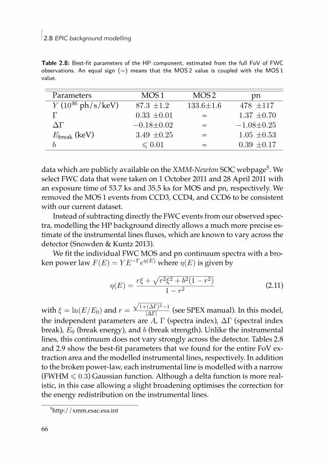
2.B EPIC background modelling
Table 2.8: Best-fit parameters of the HP component, estimated from the full FoV of FWCobservations. An equal sign (=) means that the MOS 2 value is coupled with the MOS 1value.
Parameters MOS1 MOS2 pnY (1046 ph/s/keV) 87.3 ±1.2 133.6±1.6 478 ±117Γ 0.33 ±0.01 = 1.37 ±0.70∆Γ −0.18±0.02 = −1.08±0.25Ebreak (keV) 3.49 ±0.25 = 1.05 ±0.53b ⩽ 0.01 = 0.39 ±0.17
data which are publicly available on theXMM-Newton SOCwebpage5. Weselect FWC data that were taken on 1 October 2011 and 28 April 2011 withan exposure time of 53.7 ks and 35.5 ks for MOS and pn, respectively. Weremoved the MOS1 events from CCD3, CCD4, and CCD6 to be consistentwith our current dataset.
Instead of subtracting directly the FWC events from our observed spec-tra, modelling the HP background directly allows a much more precise es-timate of the instrumental lines fluxes, which are known to vary across thedetector (Snowden & Kuntz 2013).
We fit the individual FWCMOS and pn continuum spectra with a bro-ken power law F (E) = Y E−Γeη(E) where η(E) is given by
η(E) = rξ +√
r2ξ2 + b2(1 − r2)1 − r2 (2.11)
with ξ = ln(E/E0) and r =√
1+(∆Γ)2−1|∆Γ| (see SPEX manual). In this model,
the independent parameters are A, Γ (spectra index), ∆Γ (spectral indexbreak), E0 (break energy), and b (break strength). Unlike the instrumentallines, this continuum does not vary strongly across the detector. Tables 2.8and 2.9 show the best-fit parameters that we found for the entire FoV ex-traction area and the modelled instrumental lines, respectively. In additionto the broken power-law, each instrumental line is modelled with a narrow(FWHM ⩽ 0.3) Gaussian function. Although a delta function is more real-istic, in this case allowing a slight broadening optimises the correction forthe energy redistribution on the instrumental lines.
5http://xmm.esac.esa.int
66
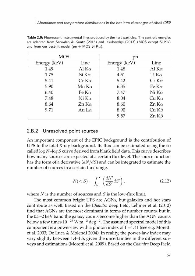
Abundance and temperature distributions in the hot intra-cluster gas of Abell 4059
Table 2.9: Fluorescent instrumental lines produced by the hard particles. The centroid energiesare adapted from Snowden & Kuntz (2013) and Iakubovskyi (2013) (MOS except Si Kα)and from our best-fit model (pn + MOS Si Kα).
MOS pnEnergy (keV) Line Energy (keV) Line
1.49 Al Kα 1.48 Al Kα1.75 Si Kα 4.51 Ti Kα5.41 Cr Kα 5.42 Cr Kα5.90 Mn Kα 6.35 Fe Kα6.40 Fe Kα 7.47 Ni Kα7.48 Ni Kα 8.04 Cu Kα8.64 Zn Kα 8.60 Zn Kα9.71 Au Lα 8.90 Cu Kβ
9.57 Zn Kβ
2.B.2 Unresolved point sourcesAn important component of the EPIC background is the contribution ofUPS to the total X-ray background. Its flux can be estimated using the socalled log N–log S curve derived fromblank field data. This curve describeshowmany sources are expected at a certain flux level. The source functionhas the form of a derivative (dN/dS) and can be integrated to estimate thenumber of sources in a certain flux range,
N(< S) =∫ ∞
S
(dN ′
dS′ dS′)
, (2.12)
where N is the number of sources and S is the low-flux limit.The most common bright UPS are AGNs, but galaxies and hot stars
contribute as well. Based on the Chandra deep field, Lehmer et al. (2012)find that AGNs are the most dominant in terms of number counts, but inthe 0.5–2 keV band the galaxy counts become higher than the AGN countsbelow a few times 10−28 Wm−2 deg−2. The assumed spectral model of thiscomponent is a power-law with a photon index of Γ=1.41 (see e.g. Morettiet al. 2003; De Luca & Molendi 2004). In reality, the power-law index mayvary slightly between 1.4–1.5, given the uncertainties in the different sur-veys and estimations (Moretti et al. 2009). Based on the ChandraDeep Field
67
2.B EPIC background modelling
South (CDF-S) data, Lehmer et al. (2012) define the (dN/dS) relations foreach source category as follows:
dN
dS
AGN=
KAGN(S/Sref)−βAGN1 (S ⩽ fAGNb )
KAGN(fb/Sref)βAGN2 −βAGN
1 (S/Sref)−βAGN2 (S > fAGNb )
, (2.13)
dN
dS
gal= Kgal(S/Sref)−βgal
, (2.14)dN
dS
star= Kstar(S/Sref)−βstar
. (2.15)Each relation describes a power law with a normalisation constant K
and a slope β. Since the (dN/dS) relation of AGNs shows a break, there isan additional β2 parameter and a break flux fb. The reference flux is definedas Sref ≡ 10−14 erg cm−2 s−1. The best-fit parameters for the studied energybands are listed in Table 1 of Lehmer et al. (2012).
The relations above can be used to estimate the flux from sources thatare not detected in our EPIC observations. The UPS component also holdsfor the deepest Chandra observations. Hickox &Markevitch (2006) found adetection limit of 1.4×10⁻¹⁶ in a 1MsCDF-S observation and estimated theunresolved flux to be (3.4±1.7)×10−12 erg cm−2 s−1 deg−2 in the 2–8 keVband. Since Chandra has a much lower confusion limit and a narrower PSF,we do not expect EPIC to reach this detection limit even in a deep clusterobservation. It is therefore not necessary to know the log N–log S curvebelow this flux limit to obtain a reasonable estimate for the unresolved flux.
In the flux range from 1.4 × 10⁻¹⁶ up to the EPIC flux limit, we cancalculate the flux using the log N–log S relation. The total unresolved fluxΩUPS for the 2–8 keV band is then calculated using
ΩUPS = 3.4 × 10⁻¹² +∫ Scut
1.4×10⁻¹⁶S′(
dN
dS′
)dS′ erg cm−2 s−1 deg−2. (2.16)
Using the Eqs. 2.13, 2.14, and 2.15 for dNdS in the integral above, the un-
resolved flux calculation is straightforward. Given the detection limit ofour observations Scut = 3.83 × 10⁻¹⁵ W m−2, we find a total UPS flux of8.07 × 10−15 W m−2 deg−2. This value can be used to constrain the nor-malisation of the power-law component describing the AXB backgroundin cluster spectral fits. We note that this method does not take the cosmicvariance into account (see e.g. Miyaji et al. 2003), which means that thenormalisation may still be slightly biased.
68
Abundance and temperature distributions in the hot intra-cluster gas of Abell 4059
2.B.3 Local Hot Bubble and Galactic thermal emissionThe LHB component is thought to originate from a shock region betweenthe solar wind and our local interstellar medium (Kuntz & Snowden 2008),while the GTE is the X-ray thermal emission from the Milky Way halo. Atsoft energies (below∼1 keV), the flux of these two foreground componentsis significant. They are both known to vary spatially across the sky, but weassume that they do not change significantly within the EPIC FoV. Bothcomponents are modelled with a cie component where we assume theabundances to be proto-solar. Both temperatures are left free, but are ex-pected to be within 0.1–0.7 keV. The GTE component is absorbed by a gaswith hydrogen column density (NH = 1.26 × 1020 cm−2), while the LHBcomponent is not.
2.B.4 Residual soft-proton componentEven after filtering soft flare events fromour rawdatasets, a quiescent levelof SP remains thatmight affect the spectra, especially at lowS/Nand above∼1 keV. It is extremely hard to precisely estimate the normalisation and theshape of its spectrum since SP quiescent events strongly varywith detectorposition and time (Snowden & Kuntz 2013). They may also depend on theattitude of the satellite. For these reasons, blank sky XMM-Newton obser-vations are not good enough for our deep exposures. The safest way to dealwith this issue is to model the spectrum by a single power law (Snowden& Kuntz 2013). Using a broken power law might be slightly more realistic,but the number of free parameters is then too high to make the fits stable.Although the spectral index Γ of the power law is unfortunately unpre-dictable and may be different for MOS and pn instruments and betweendifferent observations. Since Snowden&Kuntz (2013) reported spectral in-dices between∼0.1–1.4, we allow the Γ parameter in our fits to varywithinthis range.
2.B.5 Application to our datasetsWe apply the procedure described above for each component on our twoobservations of A 4059. We extract an annular region with inner and outerradii of 6′ and 12′, respectively, and centred on the cluster core (Fig. 2.1, theouter two annuli), assuming that all the background components describedabove contribute to the detected events covered by this area. In order to get
69
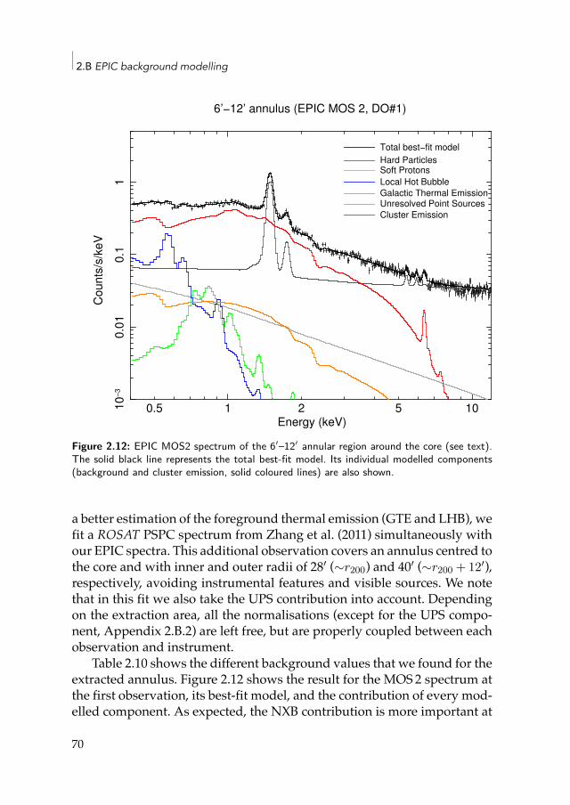
2.B EPIC background modelling
1 100.5 2 510
!3
0.0
10
.11
Co
un
ts/s
/ke
V
Energy (keV)
6’!12’ annulus (EPIC MOS 2, DO#1)
Total best!fit model
Hard ParticlesSoft Protons
Local Hot BubbleGalactic Thermal EmissionUnresolved Point SourcesCluster Emission
Figure 2.12: EPIC MOS2 spectrum of the 6′–12′ annular region around the core (see text).The solid black line represents the total best-fit model. Its individual modelled components(background and cluster emission, solid coloured lines) are also shown.
a better estimation of the foreground thermal emission (GTE and LHB), wefit a ROSAT PSPC spectrum from Zhang et al. (2011) simultaneously withour EPIC spectra. This additional observation covers an annulus centred tothe core and with inner and outer radii of 28′ (∼r200) and 40′ (∼r200 + 12′),respectively, avoiding instrumental features and visible sources. We notethat in this fit we also take the UPS contribution into account. Dependingon the extraction area, all the normalisations (except for the UPS compo-nent, Appendix 2.B.2) are left free, but are properly coupled between eachobservation and instrument.
Table 2.10 shows the different background values that we found for theextracted annulus. Figure 2.12 shows the result for the MOS2 spectrum atthe first observation, its best-fit model, and the contribution of every mod-elled component. As expected, the NXB contribution is more important at
70
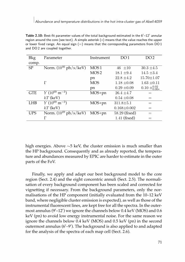
Abundance and temperature distributions in the hot intra-cluster gas of Abell 4059
Table 2.10: Best-fit parameter values of the total background estimated in the 6′–12′ annularregion around the core (see text). A simple asterisk (∗) means that the value reaches the upperor lower fixed range. An equal sign (=) means that the corresponding parameters from DO 1and DO 2 are coupled together.
Bkg Parameter Instrument DO1 DO2comp.SP Norm. (1046 ph/s/keV) MOS1 46 ±10 30.3 ±4.5
MOS2 18.1 ±9.4 14.5 ±3.4pn 22.8 ±4.2 15.70±1.07
Γ MOS 1.18 ±0.08 1.63 ±0.11pn 0.29 ±0.09 0.10 ±0.02
0.00∗GTE Y (1069 m−3) MOS+pn 26.4 ±4.7 =
kT (keV) 0.54 ±0.08 =LHB Y (1069 m−3) MOS+pn 311.8±5.1 =
kT (keV) 0.168±0.002 =UPS Norm. (1049 ph/s/keV) MOS+pn 58.29 (fixed) =
Γ 1.41 (fixed) =
high energies. Above ∼5 keV, the cluster emission is much smaller thanthe HP background. Consequently and as already reported, the tempera-ture and abundances measured by EPIC are harder to estimate in the outerparts of the FoV.
Finally, we apply and adapt our best background model to the coreregion (Sect. 2.4) and the eight concentric annuli (Sect. 2.5). The normali-sation of every background component has been scaled and corrected forvignetting if necessary. From the background parameters, only the nor-malisations of the HP component (initially evaluated from the 10–12 keVband, where negligible cluster emission is expected), as well as those of theinstrumental fluorescent lines, are kept free for all the spectra. In the outer-most annulus (9′–12′) we ignore the channels below 0.4 keV (MOS) and 0.6keV (pn) to avoid low energy instrumental noise. For the same reason weignore the channels below 0.4 keV (MOS) and 0.5 keV (pn) in the secondoutermost annulus (6′–9′). The background is also applied to and adaptedfor the analysis of the spectra of each map cell (Sect. 2.6).
71
2.C S/N requirement for the maps
2.C S/N requirement for the mapsDespite their good statistics, we want to optimise the use of our data andfind the best compromise between the required spatial resolution of ourmaps (Sect. 2.6) and S/N. The former is necessary when searching for in-homogeneities and kT/metal clumps (i.e. the smaller the better), the latterto ensure that the associate error bars are small enough to make our mea-surement significant. Clearly, these variables depend on the properties ofthe cluster and on the exposure time of our observations.
Weperforma set of simulations to determinewhat the best combinationof S/N and spatial resolution is for the case of A 4059. For every annulus(i.e. the ones determined in Sect. 2.5) we simulate a spectrum with inputparameters (i.e. kT , O, Ne, Mg, Si, S, Ca, Fe, Ni, and the normalisation)corresponding to the ones determined in the radial profiles analysis. TheAXB and the HP background are added to the total spectrum by using theproperties derived in Appendix 2.B. We allow their respective normalisa-tions to vary within ±3% in order to take into account spatial variationson the FoV. Starting from the value we derived for the radial profile, werescale the normalisation of the simulated spectrum to the particular spa-tial resolutions we are interested in (here we test 15′′, 20′′, 25′′, 30′′, 40′′, 50′′,and 60′′). We then fit the spectrum as done for the real data and for all theannuli and spatial resolutions we calculate the relative errors on the tem-perature and Fe abundance as a function of S/N. Themedian values of 300realisations are shown in Fig. 2.13 with their 1σ errors.
A S/N of 100 is required tomeasure the abundancewith a relative errorlower than∼20%. With this choice the temperaturewill be also determinedwith a very good accuracy, i.e. relative errors always lower than ∼5%.
72
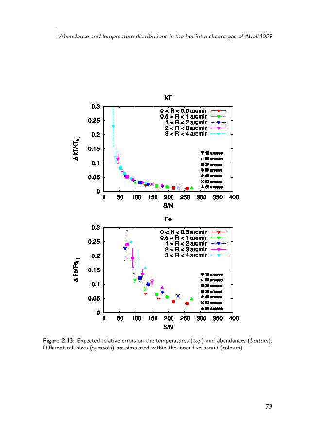
Abundance and temperature distributions in the hot intra-cluster gas of Abell 4059
0
0.05
0.1
0.15
0.2
0.25
0.3
0 50 100 150 200 250 300 350 400
∆ k
T/k
Tfit
S/N
kT
15 arcsec
+ 20 arcsec
25 arcsec
30 arcsec
40 arcsec
50 arcsec
60 arcsec
0 < R < 0.5 arcmin
0
0.05
0.1
0.15
0.2
0.25
0.3
0 50 100 150 200 250 300 350 400
∆ k
T/k
Tfit
S/N
kT
15 arcsec
+ 20 arcsec
25 arcsec
30 arcsec
40 arcsec
50 arcsec
60 arcsec
0 < R < 0.5 arcmin
0
0.05
0.1
0.15
0.2
0.25
0.3
0 50 100 150 200 250 300 350 400
∆ k
T/k
Tfit
S/N
kT
15 arcsec
+ 20 arcsec
25 arcsec
30 arcsec
40 arcsec
50 arcsec
60 arcsec
0 < R < 0.5 arcmin
0
0.05
0.1
0.15
0.2
0.25
0.3
0 50 100 150 200 250 300 350 400
∆ k
T/k
Tfit
S/N
kT
15 arcsec
+ 20 arcsec
25 arcsec
30 arcsec
40 arcsec
50 arcsec
60 arcsec
0 < R < 0.5 arcmin
0
0.05
0.1
0.15
0.2
0.25
0.3
0 50 100 150 200 250 300 350 400
∆ k
T/k
Tfit
S/N
kT
15 arcsec
+ 20 arcsec
25 arcsec
30 arcsec
40 arcsec
50 arcsec
60 arcsec
0 < R < 0.5 arcmin
0.5 < R < 1 arcmin
0
0.05
0.1
0.15
0.2
0.25
0.3
0 50 100 150 200 250 300 350 400
∆ k
T/k
Tfit
S/N
kT
15 arcsec
+ 20 arcsec
25 arcsec
30 arcsec
40 arcsec
50 arcsec
60 arcsec
0 < R < 0.5 arcmin
0.5 < R < 1 arcmin
0
0.05
0.1
0.15
0.2
0.25
0.3
0 50 100 150 200 250 300 350 400
∆ k
T/k
Tfit
S/N
kT
15 arcsec
+ 20 arcsec
25 arcsec
30 arcsec
40 arcsec
50 arcsec
60 arcsec
0 < R < 0.5 arcmin
0.5 < R < 1 arcmin
0
0.05
0.1
0.15
0.2
0.25
0.3
0 50 100 150 200 250 300 350 400
∆ k
T/k
Tfit
S/N
kT
15 arcsec
+ 20 arcsec
25 arcsec
30 arcsec
40 arcsec
50 arcsec
60 arcsec
0 < R < 0.5 arcmin
0.5 < R < 1 arcmin
0
0.05
0.1
0.15
0.2
0.25
0.3
0 50 100 150 200 250 300 350 400
∆ k
T/k
Tfit
S/N
kT
15 arcsec
+ 20 arcsec
25 arcsec
30 arcsec
40 arcsec
50 arcsec
60 arcsec
0 < R < 0.5 arcmin
0.5 < R < 1 arcmin
1 < R < 2 arcmin
0
0.05
0.1
0.15
0.2
0.25
0.3
0 50 100 150 200 250 300 350 400
∆ k
T/k
Tfit
S/N
kT
15 arcsec
+ 20 arcsec
25 arcsec
30 arcsec
40 arcsec
50 arcsec
60 arcsec
0 < R < 0.5 arcmin
0.5 < R < 1 arcmin
1 < R < 2 arcmin
0
0.05
0.1
0.15
0.2
0.25
0.3
0 50 100 150 200 250 300 350 400
∆ k
T/k
Tfit
S/N
kT
15 arcsec
+ 20 arcsec
25 arcsec
30 arcsec
40 arcsec
50 arcsec
60 arcsec
0 < R < 0.5 arcmin
0.5 < R < 1 arcmin
1 < R < 2 arcmin
0
0.05
0.1
0.15
0.2
0.25
0.3
0 50 100 150 200 250 300 350 400
∆ k
T/k
Tfit
S/N
kT
15 arcsec
+ 20 arcsec
25 arcsec
30 arcsec
40 arcsec
50 arcsec
60 arcsec
0 < R < 0.5 arcmin
0.5 < R < 1 arcmin
1 < R < 2 arcmin
0
0.05
0.1
0.15
0.2
0.25
0.3
0 50 100 150 200 250 300 350 400
∆ k
T/k
Tfit
S/N
kT
15 arcsec
+ 20 arcsec
25 arcsec
30 arcsec
40 arcsec
50 arcsec
60 arcsec
0 < R < 0.5 arcmin
0.5 < R < 1 arcmin
1 < R < 2 arcmin
0
0.05
0.1
0.15
0.2
0.25
0.3
0 50 100 150 200 250 300 350 400
∆ k
T/k
Tfit
S/N
kT
15 arcsec
+ 20 arcsec
25 arcsec
30 arcsec
40 arcsec
50 arcsec
60 arcsec
0 < R < 0.5 arcmin
0.5 < R < 1 arcmin
1 < R < 2 arcmin
0
0.05
0.1
0.15
0.2
0.25
0.3
0 50 100 150 200 250 300 350 400
∆ k
T/k
Tfit
S/N
kT
15 arcsec
+ 20 arcsec
25 arcsec
30 arcsec
40 arcsec
50 arcsec
60 arcsec
0 < R < 0.5 arcmin
0.5 < R < 1 arcmin
1 < R < 2 arcmin
0
0.05
0.1
0.15
0.2
0.25
0.3
0 50 100 150 200 250 300 350 400
∆ k
T/k
Tfit
S/N
kT
15 arcsec
+ 20 arcsec
25 arcsec
30 arcsec
40 arcsec
50 arcsec
60 arcsec
0 < R < 0.5 arcmin
0.5 < R < 1 arcmin
1 < R < 2 arcmin
2 < R < 3 arcmin
0
0.05
0.1
0.15
0.2
0.25
0.3
0 50 100 150 200 250 300 350 400
∆ k
T/k
Tfit
S/N
kT
15 arcsec
+ 20 arcsec
25 arcsec
30 arcsec
40 arcsec
50 arcsec
60 arcsec
0 < R < 0.5 arcmin
0.5 < R < 1 arcmin
1 < R < 2 arcmin
2 < R < 3 arcmin
0
0.05
0.1
0.15
0.2
0.25
0.3
0 50 100 150 200 250 300 350 400
∆ k
T/k
Tfit
S/N
kT
15 arcsec
+ 20 arcsec
25 arcsec
30 arcsec
40 arcsec
50 arcsec
60 arcsec
0 < R < 0.5 arcmin
0.5 < R < 1 arcmin
1 < R < 2 arcmin
2 < R < 3 arcmin
0
0.05
0.1
0.15
0.2
0.25
0.3
0 50 100 150 200 250 300 350 400
∆ k
T/k
Tfit
S/N
kT
15 arcsec
+ 20 arcsec
25 arcsec
30 arcsec
40 arcsec
50 arcsec
60 arcsec
0 < R < 0.5 arcmin
0.5 < R < 1 arcmin
1 < R < 2 arcmin
2 < R < 3 arcmin
0
0.05
0.1
0.15
0.2
0.25
0.3
0 50 100 150 200 250 300 350 400
∆ k
T/k
Tfit
S/N
kT
15 arcsec
+ 20 arcsec
25 arcsec
30 arcsec
40 arcsec
50 arcsec
60 arcsec
0 < R < 0.5 arcmin
0.5 < R < 1 arcmin
1 < R < 2 arcmin
2 < R < 3 arcmin
0
0.05
0.1
0.15
0.2
0.25
0.3
0 50 100 150 200 250 300 350 400
∆ k
T/k
Tfit
S/N
kT
15 arcsec
+ 20 arcsec
25 arcsec
30 arcsec
40 arcsec
50 arcsec
60 arcsec
0 < R < 0.5 arcmin
0.5 < R < 1 arcmin
1 < R < 2 arcmin
2 < R < 3 arcmin
0
0.05
0.1
0.15
0.2
0.25
0.3
0 50 100 150 200 250 300 350 400
∆ k
T/k
Tfit
S/N
kT
15 arcsec
+ 20 arcsec
25 arcsec
30 arcsec
40 arcsec
50 arcsec
60 arcsec
0 < R < 0.5 arcmin
0.5 < R < 1 arcmin
1 < R < 2 arcmin
2 < R < 3 arcmin
0
0.05
0.1
0.15
0.2
0.25
0.3
0 50 100 150 200 250 300 350 400
∆ k
T/k
Tfit
S/N
kT
15 arcsec
+ 20 arcsec
25 arcsec
30 arcsec
40 arcsec
50 arcsec
60 arcsec
0 < R < 0.5 arcmin
0.5 < R < 1 arcmin
1 < R < 2 arcmin
2 < R < 3 arcmin
3 < R < 4 arcmin
0
0.05
0.1
0.15
0.2
0.25
0.3
0 50 100 150 200 250 300 350 400
∆ k
T/k
Tfit
S/N
kT
15 arcsec
+ 20 arcsec
25 arcsec
30 arcsec
40 arcsec
50 arcsec
60 arcsec
0 < R < 0.5 arcmin
0.5 < R < 1 arcmin
1 < R < 2 arcmin
2 < R < 3 arcmin
3 < R < 4 arcmin
0
0.05
0.1
0.15
0.2
0.25
0.3
0 50 100 150 200 250 300 350 400
∆ k
T/k
Tfit
S/N
kT
15 arcsec
+ 20 arcsec
25 arcsec
30 arcsec
40 arcsec
50 arcsec
60 arcsec
0 < R < 0.5 arcmin
0.5 < R < 1 arcmin
1 < R < 2 arcmin
2 < R < 3 arcmin
3 < R < 4 arcmin
0
0.05
0.1
0.15
0.2
0.25
0.3
0 50 100 150 200 250 300 350 400
∆ k
T/k
Tfit
S/N
kT
15 arcsec
+ 20 arcsec
25 arcsec
30 arcsec
40 arcsec
50 arcsec
60 arcsec
0 < R < 0.5 arcmin
0.5 < R < 1 arcmin
1 < R < 2 arcmin
2 < R < 3 arcmin
3 < R < 4 arcmin
0
0.05
0.1
0.15
0.2
0.25
0.3
0 50 100 150 200 250 300 350 400
∆ k
T/k
Tfit
S/N
kT
15 arcsec
+ 20 arcsec
25 arcsec
30 arcsec
40 arcsec
50 arcsec
60 arcsec
0 < R < 0.5 arcmin
0.5 < R < 1 arcmin
1 < R < 2 arcmin
2 < R < 3 arcmin
3 < R < 4 arcmin
0
0.05
0.1
0.15
0.2
0.25
0.3
0 50 100 150 200 250 300 350 400
∆ k
T/k
Tfit
S/N
kT
15 arcsec
+ 20 arcsec
25 arcsec
30 arcsec
40 arcsec
50 arcsec
60 arcsec
0 < R < 0.5 arcmin
0.5 < R < 1 arcmin
1 < R < 2 arcmin
2 < R < 3 arcmin
3 < R < 4 arcmin
0
0.05
0.1
0.15
0.2
0.25
0.3
0 50 100 150 200 250 300 350 400
∆ k
T/k
Tfit
S/N
kT
15 arcsec
+ 20 arcsec
25 arcsec
30 arcsec
40 arcsec
50 arcsec
60 arcsec
0 < R < 0.5 arcmin
0.5 < R < 1 arcmin
1 < R < 2 arcmin
2 < R < 3 arcmin
3 < R < 4 arcmin
0
0.05
0.1
0.15
0.2
0.25
0.3
0 50 100 150 200 250 300 350 400
∆ F
e/F
efit
S/N
Fe
15 arcsec
+ 20 arcsec
25 arcsec
30 arcsec
40 arcsec
50 arcsec
60 arcsec
0 < R < 0.5 arcmin
0
0.05
0.1
0.15
0.2
0.25
0.3
0 50 100 150 200 250 300 350 400
∆ F
e/F
efit
S/N
Fe
15 arcsec
+ 20 arcsec
25 arcsec
30 arcsec
40 arcsec
50 arcsec
60 arcsec
0 < R < 0.5 arcmin
0
0.05
0.1
0.15
0.2
0.25
0.3
0 50 100 150 200 250 300 350 400
∆ F
e/F
efit
S/N
Fe
15 arcsec
+ 20 arcsec
25 arcsec
30 arcsec
40 arcsec
50 arcsec
60 arcsec
0 < R < 0.5 arcmin
0
0.05
0.1
0.15
0.2
0.25
0.3
0 50 100 150 200 250 300 350 400
∆ F
e/F
efit
S/N
Fe
15 arcsec
+ 20 arcsec
25 arcsec
30 arcsec
40 arcsec
50 arcsec
60 arcsec
0 < R < 0.5 arcmin
0
0.05
0.1
0.15
0.2
0.25
0.3
0 50 100 150 200 250 300 350 400
∆ F
e/F
efit
S/N
Fe
15 arcsec
+ 20 arcsec
25 arcsec
30 arcsec
40 arcsec
50 arcsec
60 arcsec
0 < R < 0.5 arcmin
0.5 < R < 1 arcmin
0
0.05
0.1
0.15
0.2
0.25
0.3
0 50 100 150 200 250 300 350 400
∆ F
e/F
efit
S/N
Fe
15 arcsec
+ 20 arcsec
25 arcsec
30 arcsec
40 arcsec
50 arcsec
60 arcsec
0 < R < 0.5 arcmin
0.5 < R < 1 arcmin
0
0.05
0.1
0.15
0.2
0.25
0.3
0 50 100 150 200 250 300 350 400
∆ F
e/F
efit
S/N
Fe
15 arcsec
+ 20 arcsec
25 arcsec
30 arcsec
40 arcsec
50 arcsec
60 arcsec
0 < R < 0.5 arcmin
0.5 < R < 1 arcmin
0
0.05
0.1
0.15
0.2
0.25
0.3
0 50 100 150 200 250 300 350 400
∆ F
e/F
efit
S/N
Fe
15 arcsec
+ 20 arcsec
25 arcsec
30 arcsec
40 arcsec
50 arcsec
60 arcsec
0 < R < 0.5 arcmin
0.5 < R < 1 arcmin
0
0.05
0.1
0.15
0.2
0.25
0.3
0 50 100 150 200 250 300 350 400
∆ F
e/F
efit
S/N
Fe
15 arcsec
+ 20 arcsec
25 arcsec
30 arcsec
40 arcsec
50 arcsec
60 arcsec
0 < R < 0.5 arcmin
0.5 < R < 1 arcmin
1 < R < 2 arcmin
0
0.05
0.1
0.15
0.2
0.25
0.3
0 50 100 150 200 250 300 350 400
∆ F
e/F
efit
S/N
Fe
15 arcsec
+ 20 arcsec
25 arcsec
30 arcsec
40 arcsec
50 arcsec
60 arcsec
0 < R < 0.5 arcmin
0.5 < R < 1 arcmin
1 < R < 2 arcmin
0
0.05
0.1
0.15
0.2
0.25
0.3
0 50 100 150 200 250 300 350 400
∆ F
e/F
efit
S/N
Fe
15 arcsec
+ 20 arcsec
25 arcsec
30 arcsec
40 arcsec
50 arcsec
60 arcsec
0 < R < 0.5 arcmin
0.5 < R < 1 arcmin
1 < R < 2 arcmin
0
0.05
0.1
0.15
0.2
0.25
0.3
0 50 100 150 200 250 300 350 400
∆ F
e/F
efit
S/N
Fe
15 arcsec
+ 20 arcsec
25 arcsec
30 arcsec
40 arcsec
50 arcsec
60 arcsec
0 < R < 0.5 arcmin
0.5 < R < 1 arcmin
1 < R < 2 arcmin
0
0.05
0.1
0.15
0.2
0.25
0.3
0 50 100 150 200 250 300 350 400
∆ F
e/F
efit
S/N
Fe
15 arcsec
+ 20 arcsec
25 arcsec
30 arcsec
40 arcsec
50 arcsec
60 arcsec
0 < R < 0.5 arcmin
0.5 < R < 1 arcmin
1 < R < 2 arcmin
0
0.05
0.1
0.15
0.2
0.25
0.3
0 50 100 150 200 250 300 350 400
∆ F
e/F
efit
S/N
Fe
15 arcsec
+ 20 arcsec
25 arcsec
30 arcsec
40 arcsec
50 arcsec
60 arcsec
0 < R < 0.5 arcmin
0.5 < R < 1 arcmin
1 < R < 2 arcmin
0
0.05
0.1
0.15
0.2
0.25
0.3
0 50 100 150 200 250 300 350 400
∆ F
e/F
efit
S/N
Fe
15 arcsec
+ 20 arcsec
25 arcsec
30 arcsec
40 arcsec
50 arcsec
60 arcsec
0 < R < 0.5 arcmin
0.5 < R < 1 arcmin
1 < R < 2 arcmin
0
0.05
0.1
0.15
0.2
0.25
0.3
0 50 100 150 200 250 300 350 400
∆ F
e/F
efit
S/N
Fe
15 arcsec
+ 20 arcsec
25 arcsec
30 arcsec
40 arcsec
50 arcsec
60 arcsec
0 < R < 0.5 arcmin
0.5 < R < 1 arcmin
1 < R < 2 arcmin
2 < R < 3 arcmin
0
0.05
0.1
0.15
0.2
0.25
0.3
0 50 100 150 200 250 300 350 400
∆ F
e/F
efit
S/N
Fe
15 arcsec
+ 20 arcsec
25 arcsec
30 arcsec
40 arcsec
50 arcsec
60 arcsec
0 < R < 0.5 arcmin
0.5 < R < 1 arcmin
1 < R < 2 arcmin
2 < R < 3 arcmin
0
0.05
0.1
0.15
0.2
0.25
0.3
0 50 100 150 200 250 300 350 400
∆ F
e/F
efit
S/N
Fe
15 arcsec
+ 20 arcsec
25 arcsec
30 arcsec
40 arcsec
50 arcsec
60 arcsec
0 < R < 0.5 arcmin
0.5 < R < 1 arcmin
1 < R < 2 arcmin
2 < R < 3 arcmin
0
0.05
0.1
0.15
0.2
0.25
0.3
0 50 100 150 200 250 300 350 400
∆ F
e/F
efit
S/N
Fe
15 arcsec
+ 20 arcsec
25 arcsec
30 arcsec
40 arcsec
50 arcsec
60 arcsec
0 < R < 0.5 arcmin
0.5 < R < 1 arcmin
1 < R < 2 arcmin
2 < R < 3 arcmin
0
0.05
0.1
0.15
0.2
0.25
0.3
0 50 100 150 200 250 300 350 400
∆ F
e/F
efit
S/N
Fe
15 arcsec
+ 20 arcsec
25 arcsec
30 arcsec
40 arcsec
50 arcsec
60 arcsec
0 < R < 0.5 arcmin
0.5 < R < 1 arcmin
1 < R < 2 arcmin
2 < R < 3 arcmin
0
0.05
0.1
0.15
0.2
0.25
0.3
0 50 100 150 200 250 300 350 400
∆ F
e/F
efit
S/N
Fe
15 arcsec
+ 20 arcsec
25 arcsec
30 arcsec
40 arcsec
50 arcsec
60 arcsec
0 < R < 0.5 arcmin
0.5 < R < 1 arcmin
1 < R < 2 arcmin
2 < R < 3 arcmin
0
0.05
0.1
0.15
0.2
0.25
0.3
0 50 100 150 200 250 300 350 400
∆ F
e/F
efit
S/N
Fe
15 arcsec
+ 20 arcsec
25 arcsec
30 arcsec
40 arcsec
50 arcsec
60 arcsec
0 < R < 0.5 arcmin
0.5 < R < 1 arcmin
1 < R < 2 arcmin
2 < R < 3 arcmin
0
0.05
0.1
0.15
0.2
0.25
0.3
0 50 100 150 200 250 300 350 400
∆ F
e/F
efit
S/N
Fe
15 arcsec
+ 20 arcsec
25 arcsec
30 arcsec
40 arcsec
50 arcsec
60 arcsec
0 < R < 0.5 arcmin
0.5 < R < 1 arcmin
1 < R < 2 arcmin
2 < R < 3 arcmin
3 < R < 4 arcmin
0
0.05
0.1
0.15
0.2
0.25
0.3
0 50 100 150 200 250 300 350 400
∆ F
e/F
efit
S/N
Fe
15 arcsec
+ 20 arcsec
25 arcsec
30 arcsec
40 arcsec
50 arcsec
60 arcsec
0 < R < 0.5 arcmin
0.5 < R < 1 arcmin
1 < R < 2 arcmin
2 < R < 3 arcmin
3 < R < 4 arcmin
0
0.05
0.1
0.15
0.2
0.25
0.3
0 50 100 150 200 250 300 350 400
∆ F
e/F
efit
S/N
Fe
15 arcsec
+ 20 arcsec
25 arcsec
30 arcsec
40 arcsec
50 arcsec
60 arcsec
0 < R < 0.5 arcmin
0.5 < R < 1 arcmin
1 < R < 2 arcmin
2 < R < 3 arcmin
3 < R < 4 arcmin
0
0.05
0.1
0.15
0.2
0.25
0.3
0 50 100 150 200 250 300 350 400
∆ F
e/F
efit
S/N
Fe
15 arcsec
+ 20 arcsec
25 arcsec
30 arcsec
40 arcsec
50 arcsec
60 arcsec
0 < R < 0.5 arcmin
0.5 < R < 1 arcmin
1 < R < 2 arcmin
2 < R < 3 arcmin
3 < R < 4 arcmin
0
0.05
0.1
0.15
0.2
0.25
0.3
0 50 100 150 200 250 300 350 400
∆ F
e/F
efit
S/N
Fe
15 arcsec
+ 20 arcsec
25 arcsec
30 arcsec
40 arcsec
50 arcsec
60 arcsec
0 < R < 0.5 arcmin
0.5 < R < 1 arcmin
1 < R < 2 arcmin
2 < R < 3 arcmin
3 < R < 4 arcmin
0
0.05
0.1
0.15
0.2
0.25
0.3
0 50 100 150 200 250 300 350 400
∆ F
e/F
efit
S/N
Fe
15 arcsec
+ 20 arcsec
25 arcsec
30 arcsec
40 arcsec
50 arcsec
60 arcsec
0 < R < 0.5 arcmin
0.5 < R < 1 arcmin
1 < R < 2 arcmin
2 < R < 3 arcmin
3 < R < 4 arcmin
0
0.05
0.1
0.15
0.2
0.25
0.3
0 50 100 150 200 250 300 350 400
∆ F
e/F
efit
S/N
Fe
15 arcsec
+ 20 arcsec
25 arcsec
30 arcsec
40 arcsec
50 arcsec
60 arcsec
0 < R < 0.5 arcmin
0.5 < R < 1 arcmin
1 < R < 2 arcmin
2 < R < 3 arcmin
3 < R < 4 arcmin
Figure 2.13: Expected relative errors on the temperatures (top) and abundances (bottom).Different cell sizes (symbols) are simulated within the inner five annuli (colours).
73

The world is noisy and messy.You need to deal with the noise and uncertainty.
– Daphne Koller
3|Origin of central abundances inthe hot intra-cluster mediumI. Individual and average abundance ratiosfrom XMM-Newton EPIC
F. Mernier, J. de Plaa, C. Pinto, J. S. Kaastra, P. Kosec, Y.-Y. Zhang, J. Mao,and N. Werner
(Astronomy & Astrophysics, Volume 592, id.A157, 18 pp.)
Abstract
The hot intra-clustermedium (ICM) is rich inmetals, which are synthesised by su-pernovae (SNe) explosions and accumulate over time into the deep gravitationalpotential well of clusters of galaxies. Since most of the elements visible in X-raysare formed by Type Ia (SNIa) and/or core-collapse (SNcc) supernovae, measuringtheir abundances gives us direct information on the nucleosynthesis products ofbillions of SNe since the epoch of the star formation peak (z ∼ 2–3). In this study,we use the EPIC and RGS instruments on board XMM-Newton to measure theabundances of nine elements (O, Ne, Mg, Si, S, Ar, Ca, Fe, and Ni) from a sampleof 44 nearby cool-core galaxy clusters, groups, and elliptical galaxies. We find thatthe Fe abundance shows a large scatter (∼20–40%) over the sample, within 0.2r500and especially 0.05r500. Unlike the absolute Fe abundance, the abundance ratios(X/Fe) are uniform over the considered temperature range (∼0.6–8 keV) andwitha limited scatter. In addition to an unprecedented treatment of systematic uncer-tainties, we provide the most accurate abundance ratios measured so far in theICM, including Cr/Fe and Mn/Fe which we firmly detected (>4σ with MOS andpn independently). We find that Cr/Fe, Mn/Fe, and Ni/Fe differ significantlyfrom the proto-solar values. However, the large uncertainties in the proto-solarabundances prevent us from making a robust comparison between the local and
75
3.1 Introduction
the intra-cluster chemical enrichments. We also note that, interestingly, and de-spite the large net exposure time (∼4.5Ms) of our dataset, no line emission featureis seen around ∼3.5 keV.
3.1 IntroductionAbout 80–90% of the baryonic matter in the Universe is in the form ofa hot and diffuse intergalactic gas, which has mostly a very low densityand, therefore, is hard to observe. However, in the largest gravitationallybound regions of the Universe, which are clusters of galaxies, the densityand temperature of this hot gas, or intra-cluster medium (ICM), becomeshigh enough for it to glow in X-rays. This ICM, which has been extensivelystudied by X-ray observatories over the past decades (for a review, seeBöhringer &Werner 2010), is particularly rich in metals (e.g. Mitchell et al.1976; Mushotzky et al. 1996). Since the baryonic content of the Universejust after the Big Bang consists exclusively of hydrogen and helium (andtraces of lithium), these heavy elements – typically from oxygen to nickel– must have been synthesised by stars and supernovae (SNe) in the galaxymembers and then ejected into the ICM (for a review, seeWerner et al. 2008;de Plaa 2013).
Although the general picture of this chemical enrichment is now wellestablished, many aspects are still poorly understood. In addition to thequestion of the transport mechanisms that drive the enrichment, a majoruncertainty resides in the metal yields produced by Type Ia (SNIa) andcore-collapse (SNcc) supernovae. In fact, the nature of the SNIa progenitorsand the SNIa explosionmechanisms are still under debate, while the globalnucleosynthesis of SNcc highly depends on the initial mass function (IMF)and the initial metallicity of the considered stellar population.Moreover, inaddition to SNe, AGB stars can also play a role in releasing lighter metals(e.g. nitrogen) or even heavy metals (via the s-process). Taken together,these unsolved questions lead to large uncertainties in predicting the globalabundance ratios that are finally released by the SNe and AGB stars intothe ICM.
In contrast to the remaining uncertainties in the theoretical yields fromthe SNe/AGB models, the current generation of X-ray observatories mea-sures the chemical abundances in the ICMwith remarkable accuracy sincemost transitions of H- and He-like elements from Z=7 to Z=28 fall within0.2–12 keV. Thanks to the large effective area and the good spectral reso-
76
Origin of central abundances in the hot intra-cluster medium I.
lution of its European Photon Imaging Camera (EPIC, Strüder et al. 2001;Turner et al. 2001) and Reflection Grating Spectrometer (RGS, den Herderet al. 2001),XMM-Newton is particularly suitable formeasuring abundancesof elements like oxygen (O), neon (Ne), magnesium (Mg), silicon (S), sulfur(S), argon (Ar), calcium (Ca), iron (Fe), and nickel (Ni), especially in cool-core objects1 which exhibit a high surface brightness in X-ray and wherethe most prominent K-shell emission lines of these elements are clearly de-tected. Consequently, the accuracy of these measurements can, in princi-ple, bring new constraints on the SNe (and AGB) models, and can leadto a deeper understanding of the chemical enrichment processes beyondgalactic scales.
Several authors have reported such analyses by measuring the abun-dances in the ICM of nearby clusters and groups. For instance, de Plaaet al. (2007) has compiled a sample of 22 cool-core clusters and found thatthe standard SNIa models fail to reproduce the Ar/Ca and Ca/Fe abun-dance ratios. They also show that the number of SNIa over the total numberof SNe highly depends on the considered models. De Grandi & Molendi(2009) have shown that Si/Fe abundance ratios are remarkably uniformover a sample of 26 cool-core clusters observed with XMM-Newton, argu-ing for a similar enrichment process within cluster cores. However theysuggest that systematic uncertainties are too large to precisely estimate therelative contribution of SNIa and SNcc. Finally, many abundance studieshave also been performed on individual objects (e.g. Werner et al. 2006b;de Plaa et al. 2006; Sato et al. 2007a; Simionescu et al. 2009b, Chapter 2).From these studies, and considering the actual instrumental performancesof current X-ray observatories, it appears that higher quality data (i.e. withlonger exposure time) spread over larger samples are needed to clarify theactual picture of the precise origin of metals in the ICM.
In this work, we use new and archival XMM-Newton EPIC observa-tions to measure the chemical abundances of nine elements (O, Ne, Mg, Si,S, Ar, Ca, Fe, and Ni) in the core of a sample of nearby cool-core galaxyclusters, groups, and elliptical galaxies. These EPIC observations are thencombined with the RGS abundance measurements adapted from de Plaaet al. (2017) in order to derive average X/Fe abundance ratios represen-tative of the nearby ICM. Taking into account as many systematic uncer-
1A cluster, or group, is defined as “cool-core” when the ICM in its core is sufficientlydense that its cooling time, typically of the order of ∼
√TX/ne, is shorter than the Hubble
time.
77
3.2 Observations and data preparation
tainties as possible, we discuss the robustness of these measurements andcompare them to the proto-solar abundances. In Chapter 4, we discuss indetail the astrophysical implications of our results, and compare our av-erage abundance pattern presented here with predictions from theoreticalSNIa and SNcc yield models.
This paper is structured as follows. In Sect. 3.2, we present the sam-ple and the data reduction pipeline. In Sect. 3.3 we describe the spectralanalysis procedure applied to our EPIC observations. Our results are pre-sented in Sect. 3.4, briefly discussed in Sect. 3.5, and summarised in Sect.3.6. Throughout this paperwe assume cosmological parameters ofH0 = 70km s−1 Mpc−1, Ωm = 0.3, and ΩΛ = 0.7. All the error bars are given at a68% confidence level.
3.2 Observations and data preparationOur sample consists of the CHEERS2 catalogue (de Plaa et al. 2017), andis detailed in Table 3.1 (see also Pinto et al. 2015; de Plaa et al. 2017). It in-cludes 44 nearby (z < 0.1) cool-core clusters, groups, and elliptical galax-ies for which the OVIII 1s–2p line at 19 is detected by the RGS instru-ment with >5σ. More information on the intrinsic properties of these ob-jects (e.g. fluxes) can be found in various available cluster catalogues, suchas the HIGFLUGCS (Reiprich & Böhringer 2002), the REFLEX (Böhringeret al. 2004b), and the ACCEPT (Cavagnolo et al. 2009) catalogues. In oursample, recent XMM-Newton observations (AO-12, PI: de Plaa) have beencombined with archival data. We only select the pointings for which thecombined EPIC observations (MOS1, MOS2, and pn) gather at least 15ks of net exposure time. The observations that suffer from high soft flareevents or calibration problems are also excluded.
3.2.1 Data reductionAll the data are reduced with the XMM-Newton Science Analysis System(SAS) v14.0.0 and by using the calibration files dated by March 2015. TheRGS data are the same as used in Pinto et al. (2015, see their Table 1),and are reduced the same way. We reduce the EPIC data by using thestandard pipeline command emproc and epproc, and, following the stan-dard recommendations, we keep the single to quadruple pixel MOS events
2CHEmical Enrichment Rgs Sample
78
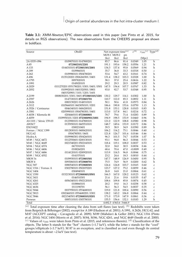
Origin of central abundances in the hot intra-cluster medium I.
Table 3.1: XMM-Newton/EPIC observations used in this paper (see Pinto et al. 2015, fordetails on RGS observations). The new observations from the CHEERS proposal are shownin boldface.
Source ObsID Net exposure time(a) z(b) r500(c) Type(d)
MOS1 MOS2 pn(ks) (ks) (ks) (Mpc)
2A 0335+096 0109870101 0147800201 85.7 86.6 81.4 0.0349 1.05 hA85 0723802101/2201 191.1 193.6 158.2 0.0556 1.21 hA133 0144310101 0723801301/2001 134.3 137.4 95.8 0.0569 0.94 hA189 0109860101 35.7 36.8 33.3 0.0318 0.50 cA262 0109980101 0504780201 53.4 54.7 43.2 0.0161 0.74 hA496 0135120201 0506260301/0401 131.4 138.2 103.3 0.0328 1.00 hA1795 0097820101 38.1 37.0 25.4 0.0616 1.22 hA1991 0145020101 29.2 29.3 20.5 0.0587 0.82 hA2029 0111270201 0551780201/0301/0401/0501 147.5 154.4 107.7 0.0767 1.33 hA2052 0109920101 0401520501/0801 93.0 92.7 53.7 0.0348 0.95 h
0401520901/1101/1201/1601A2199 0008030201/0301/0601 0723801101/1201 130.2 129.7 114.1 0.0302 1.00 hA2597 0147330101 0723801701 110.7 112.0 85.3 0.0852 1.11 hA2626 0083150201 0148310101 50.1 50.6 41.8 0.0573 0.84 hA3112 0105660101 0603050101/0201 186.6 190.8 153.6 0.0750 1.13 hA3526 / Centaurus 0046340101 0406200101 151.8 153.1 128.8 0.0103 0.83 hA3581 0205990101 0504780301/0401 113.0 117.8 84.1 0.0214 0.72 cA4038 / Klemola 44 0204460101 0723800801 78.7 79.6 71.4 0.0283 0.89 hA4059 0109950101/0201 0723800901/1001 194.9 198.5 153.9 0.0460 0.96 hAS 1101 / Sérsic 159-03 0123900101 0147800101 121.0 122.9 108.8 0.0580 0.98 hAWM7 0135950101 0605510101 148.7 149.6 153.9 0.0172 0.86 hEXO0422 0300210401 39.5 38.9 34.9 0.0390 0.89 hFornax / NGC1399 0012830101 0400620101 106.2 114.2 75.1 0.0046 0.40 cHCG62 0504780501/0601 121.8 126.7 101.6 0.0146 0.46 cHydraA 0109980301 0504260101 96.3 101.5 74.7 0.0538 1.07 hM49 / NGC4472 0112550601 0200130101 93.1 94.8 86.3 0.0044 0.53 cM60 / NGC4649 0021540201 0502160101 118.4 119.1 108.0 0.0037 0.53 cM84 / NGC4374 0673310101 32.0 34.0 30.5 0.0034 0.46 cM86 / NGC4406 0108260201 68.4 70.4 47.0 -0.0009 0.49 cM87 / NGC4486 0114120101 0200920101 113.9 114.5 96.8 0.0044 0.75 cM89 / NGC4552 0141570101 23.2 24.4 18.3 0.0010 0.44 cMKW3s 0109930101 0723801501 147.7 148.9 126.9 0.0450 0.95 hMKW4 0093060101 0723800701 75.5 74.9 56.9 0.0200 0.62 hNGC507 0080540101 0723800301 124.4 124.8 103.7 0.0165 0.60 cNGC1316 / Fornax A 0302780101 0502070201 123.7 127.2 75.2 0.0059 0.46 cNGC1404 0304940101 26.8 14.8 21.0 0.0064 0.61 cNGC1550 0152150101 0723800401/0501 166.3 167.0 128.2 0.0123 0.62 cNGC3411 0146510301 21.4 21.6 19.8 0.0155 0.47 cNGC4261 0056340101 0502120101 108.6 109.8 85.8 0.0074 0.45 cNGC4325 0108860101 20.2 19.0 16.3 0.0258 0.58 cNGC4636 0111190701 56.1 56.3 54.5 0.0037 0.35 cNGC5044 0037950101 0554680101 119.0 121.8 100.4 0.0090 0.56 cNGC5813 0302460101 0554680201/0301 138.2 143.2 106.8 0.0064 0.44 cNGC5846 0021540501 0723800101/0201 171.0 173.9 147.9 0.0061 0.36 cPerseus 0085110101 0305780101 155.5 156.6 132.1 0.0183 1.29 hTotal 4 492.3 4 563.6 3 666.9
(a) Total exposure time after cleaning the data from soft flares (see text). (b) Redshifts were takenfrom Reiprich & Böhringer (2002), except for A 189 (Hudson et al. 2001); A 1991, A 2626, HCG62, andM87 (ACCEPT catalog – Cavagnolo et al. 2009); M89 (Mahdavi & Geller 2001); NGC1316 (Pintoet al. 2014); NGC1404 (Morris et al. 2007); M84, M86, NGC4261, and NGC4649 (Smith et al. 2000).(c) Values of r500 were taken from Pinto et al. (2015, and references therein). (d) Classification of theobjects. The letter h stands for the “hot” clusters (>1.7 keV), while the letter c stands for the “cool”groups/ellipticals (<1.7 keV). M 87 is an exception, and is classified as cool even though its centraltemperature is about ∼2 keV (see text).
79
3.2 Observations and data preparation
(PATTERN⩽12), and only the single pixel pn events (PATTERN==0). More-over, only the highest quality MOS and pn events (FLAG==0) are takeninto account. We filter our observations from soft-proton flares by buildinggood time interval (GTI) files following themethod described in Chapter 2.We extract light curves within the 10–12 keV (MOS) and the 12–14 keV (pn)bands in 100 s bins, we calculate the mean count rate µ and the standarddeviation σ, and we apply a threshold of µ ± 2σ to the fitted distribution.For safety (Lumb et al. 2002), we repeat the procedure for the 0.3–10 keVband in 10 s bins. The average fraction of “good” time accepted after sucha filtering is ∼77%, ∼78%, and ∼66% for MOS1, MOS2, and pn, respec-tively, although this fraction varies widely from pointing to pointing. Foreach object, the net exposure times of the EPIC instruments are indicatedin Table 3.1. Combining our whole dataset, we obtain total EPIC and RGSnet exposure times of ∼4.5 Ms and ∼5.1 Ms, respectively.
Finally, point-like sourcesmight pollute our spectra; therefore, we needto discard all of them from the rest of our analysis. We first detect thepoint sources of every dataset within four spectral bands (0.3–2 keV, 2–4.5 keV, 4.5–7.5 keV, and 7.5–12 keV) using the SAS task edetect_chain.After a second check by eye, we excise circular regions with 10′′ of radiusaround the point sources (except in some specific situations where a largerexcision radius is required to remove scattered photons from bright fore-ground sources). This radius size is estimated to be a good compromisebetween discarding the polluting flux of the point sources and keeping amaximumof cluster emission in their neighbourhood (Chapter 2). Depend-ing on the target, the typical fraction of removed flux after discarding thepoint sources varies between ∼0.3% and ∼4%.
3.2.2 Spectra extractionThe sources of our sample span a wide range of sizes, masses, and tem-peratures, and studying their elemental abundances with EPIC over onecommon astrophysical scale rcore is difficult in practice. A definition of rcoreas 0.2r500
3 for the farther (and, by selection, hotter) clusters is commonlyfound in the literature (e.g. de Plaa et al. 2007); however, most of the near-est galaxy groups from our sample are seen at this radius with an angularsize θ > 15 arcmin, i.e. beyond the EPIC field of view (FoV). Moreover,
3r500 is defined as the radiuswithinwhich the gas density is 500 times the critical densityof the Universe.
80
Origin of central abundances in the hot intra-cluster medium I.
extracting spectra over a large θ for these cooler and more compact objectswill include a lot of background, which may dominate beyond ∼2–3 keVand entirely flood the K-shell lines of crucial elements such as S, Ar, Ca, orNi. Therefore, we choose to split our sample into two subsamples:
1. The “hot” galaxy clusters (kT ⩾ 1.7 keV, 23 objects),2. The “cool” galaxy groups and ellipticals (kT < 1.7 keV, 21 objects).
Using the SAS task evselect, we extract the EPIC spectra of every sourcewithin a circular region, centred on the peak of the cluster X-ray emissionand within a radius of 0.05r500. Since in the hot clusters a radius of 0.2r500can also be reached and provides better signal-to-noise ratio (S/N), we ex-tract these spectra as well.
Table 3.1 classifies each object in one of these two subsamples. OnlyM87 deviates from the rule. Indeed, although its main central temperatureis about ∼2 keV (and is thus considered a hot object), its 0.2r500 limit isbeyond the EPIC FoV, and only the spectra within 0.05r500 could be ex-tracted.
We extract the RGS spectra as described in Pinto et al. (2015) and inde Plaa et al. (2017). Since the dispersion direction of RGS extends alongthe whole EPIC FoV, its extraction region will be always different from ourcircular EPIC extraction regions. Therefore, we extract all the RGS spectrausing a cross-dispersionwidth of 0.8′ from theEPICFoV,which still focuseson the ICM core. In Sect. 3.4.3 we show that this choice does not affect ourresults.
The redistributionmatrix file (RMF), which gives the channel probabil-ity distribution for a photon of given energy, is built using the task rmfgen.The ancillary response file (ARF), which provides the effective area curveas a function of the energy and the position on the detectors, is built usingthe task arfgen. Both the RMF and the ARF contain all the information rel-ative to the response of the instruments, and need to be further applied foreach observation to the spectral modelling4.
3.3 EPIC spectral analysisWe use the SPEX fitting package (Kaastra et al. 1996) v2.05 to performthe spectral analysis of our sample. We fit all our spectra using the C-
4See the “Users Guide to the XMM-Newton Science Analysis System”, Issue 11.0, 2014(ESA: XMM-Newton SOC).
81
3.3 EPIC spectral analysis
statistics (i.e. a modified Cash statistics; Cash 1979), which is appropriatefor Poisson-noise dominated data (see the SPEX manual).
Making the reasonable assumption that the hot ICM is in a collisionalionisation equilibrium (CIE) state, throughout this paper we describe itsemission using a cie model (based on an updated version of the mekalplasma code, Mewe et al. 1985). This model includes processes such as col-lisional ionisation and excitation-autoionisation, as well as radiative anddielectronic recombination (for further details, we refer the reader to theSPEX manual5). We adopt the updated ionisation balance calculations ofBryans et al. (2009). The abundances are calculated from all the transitionsand ions of a given element, and are scaled to the proto-solar values6 ofLodders et al. (2009).
We fit the cluster emission component in EPICwith amulti-temperatureciemodel, theGaussianDifferential EmissionMeasure (gdem)model,whichreproduces a Gaussian temperature distribution in the form
Y (x) = Y0
σT
√2π
exp((x − xmean)2
2σ2T
), (3.1)
where x = log(kT ) and xmean = log(kTmean), kTmean is the peak temper-ature of the distribution, and σT is the full width at half maximum of thedistribution (see de Plaa et al. 2006). By definition, σT=0 provides a single-temperature cie model (1T).
The use of a multi-temperature model for such a study is crucial sincemost of the clusters and groups have a complicated thermal structure intheir cores where the cooling rate and temperature gradient are quite im-portant. Therefore, assuming the plasma to be isothermal in general maylead to the so-called Fe bias, i.e. an underestimate of the Fe abundance (seee.g. Buote & Canizares 1994; Buote & Fabian 1998; Buote 2000). The effectsof different thermal models on the abundances and a comparison betweenEPIC and RGS measurements are discussed below (Sect. 3.4.3).
For both EPIC and RGS abundances, we also correct the O and Ne esti-mates from updated calculations of the radiative recombination contribu-tion to the cluster emission as a function of its mean temperature. We do soby multiplying the O and Ne best-fit measurements of each object by the
5https://www.sron.nl/astrophysics-spex6The proto-solar abundances used in this paper (Lodders et al. 2009) are the most up-
to-date representative abundances of the solar system at its formation, as they are based onmeteoritic compositions.
82
Origin of central abundances in the hot intra-cluster medium I.
factors of the corrected OVIII and NeX Lyman α fluxes, as described inAppendix 3.B. On average, these corrections increase the O and Ne abun-dances by ∼20% and ∼6%, respectively.
The Galactic absorption that we apply to our fitted thermal models ismodelled by the transmission of a neutral plasma (hot model, for whichkT=0.5 eV). In EPIC, the hydrogen column density NH has been estimatedfrom a grid search of (fixed) values within
NHI − 5 × 1019 cm−2 ⩽ NH ⩽ NH,tot + 1 × 1020 cm−2, (3.2)
whereNHI andNH,tot are respectively the neutral (Kalberla et al. 2005) andtotal (neutral and molecular) hydrogen column densities estimated usingthe method of Willingale et al. (2013). More details on the reasons for thisapproach are given in Appendix 3.A.
Details on the RGS spectral analysis (including models, free parame-ters, and background treatment) can be found in de Plaa et al. (2017), andin Pinto et al. (2015).
3.3.1 Background modellingAlthough the clusters considered in this work are usually bright and dis-play a high S/N within their core, in most of them the EPIC backgroundcan still play a significant role, especially in the hard spectral bands (i.e.≳2 keV) where less thermal emission is expected. Because a slightly incor-rect scaling in the subtraction of background data (taken from either filterclosed wheel data or blank sky observations) can significantly affect thetemperature estimates and thus bias the spectral analyses (de Plaa et al.2006), we choose here to model the background directly in our spectra.The method we use is extensively described in Chapter 2. In summary, wemodel five separate background components:
• The local hot bubble, modelled by a non-absorbed isothermal ciecomponent, whose abundances are kept proto-solar;
• The galactic thermal emission, modelled by an absorbed isothermalcie component, whose abundances are also kept proto-solar;
• The unresolved point sources, modelled by an absorbed power lawwith a photon index fixed to 1.41 (De Luca & Molendi 2004);
83
3.3 EPIC spectral analysis
• The hard particle background, modelled by a broken power law (un-folded by the effective area) and several instrumental Gaussian pro-files. The parameters are taken from Chapter 2, except for all the nor-malisations, which are left free;
• The soft-proton background, modelled by a power law (unfolded bythe effective area). The parameters are estimated using EPIC spectracovering the total FoV (where the parameters of the gdem componentfrom the ICM are also left free; see Sect. 3.3.2). From such spectra, theICM emission can be easily constrained in the soft band (≲2 keV),while the particle backgrounds clearly dominate the harder bands,making the soft-proton background contribution easier to estimate.
The fluxes and the temperatures of the local hot bubble and galacticthermal emission components, as well as the flux of the unresolved pointsources, are estimated fromROSAT PSPC spectra extracted from the regionbeyond r200 of each object (Zhang et al. 2009).
Finally, all these background components are fixed and rescaled to thesky area of our EPIC core spectra (except the normalisation of the hardparticle background, which we always left free in order to avoid incorrectscalings and temperature biases, see above).
In addition to the background described above, M87, M89, NGC4261,NGC4636, and NGC5813 host a powerful active galactic nucleus (AGN),which can generate cavities in the hot gas (e.g. Russell et al. 2013), but canalso pollute the total X-ray emission. For each of these observations, westart by extracting a circular region of 30′′ centred on the AGN, and wefit its EPIC spectra with an absorbed power law (in addition to the clus-ter emission and the background components described above). We thenextrapolate this additional component to the EPIC core spectra, fixing itscolumn density and photon index values derived from the 30′′ apertureregion, and rescaling its normalisation to the area ratio of these two ex-tracted regions. We note that in the EPIC core spectra the 0.5–10 keV fluxof the AGN component is never larger than ∼15–20% of the cluster emis-sion. This justifies a posteriori our choice of fitting the AGN contributionrather than excising the AGN, i.e. where the peak of the cluster emissionis.
84
Origin of central abundances in the hot intra-cluster medium I.
3.3.2 Global fitsIn addition to the normalisation of the hard particle background, the onlyparameters that are left free when fitting our spectral components to theEPIC spectra of the core regions are the normalisation (or emission mea-sure, Y =
∫nenHdV ) of the gdem model; its mean temperature (kTmean);
σT ; and the abundances of O, Ne, Mg, Si, S, Ar, Ca, Fe, and Ni. The otherZ ⩾ 6 abundance parameters are coupled to the value of the Fe abun-dance parameter, and are thus not free. The MOS and pn spectra of everypointing are fitted simultaneously. Since the large number of total param-eters prevents us from fitting simultaneously three observations or more,for each object we form pairs of two pointings that we fit simultaneously.For objects including ⩾3 pointings, we then combine the results of the fit-ted pairs using a weighting factor of 1/σ2
i , where σi is the statistical erroron the considered parameter.
An important variable that might affect our EPIC results is the spectralranges of our fits. In particular, significant cross-calibration issues betweenMOS and pn have been reported in the soft bands (Read et al. 2014; Schel-lenberger et al. 2015). Similarly, we observe a sharp and extremely variablesoft tail in the EPIC filter wheel closed events7 that might considerably af-fect the spectra below 0.5 keV. On the other hand, we would like to keepour spectral range as large as possible, for instance to estimate the abun-dance measurements of O and the temperature structure in the Fe-L com-plex. A good compromise is found by using the 0.5–10 keV and 0.6–10 keVbands for MOS and pn, respectively.
3.3.3 Local fitsIn the case of a plasma in CIE, the abundances of a given element show-ing prominent and well-resolved emission lines are easy to derive as theyare proportional to the ratio between the line flux and the continuum flux,namely the equivalent width (EW). However, as a consequence of the im-perfections of the EPIC instruments effective areas, when fitting the EPICspectra over a large range (0.5/0.6–10 keV in the previous subsection, here-after the “global” fits), the modelled continuum emission may be slightlyover- or underestimated in some specific energy bands. Consequently, themodelled line fluxes tend to compensate the continuum discrepancies in
7See also the XMM-Newton Calibration Technical Note, XMM-SOC-CAL-TN-0018 (Ed:Guainazzi, 2014).
85
3.4 Results
the global fits, by, in turn, slightly under- or overestimating the value ofthe abundance parameters.
This effect, already discussed in Chapter 2, can be easily corrected byfitting the EPIC spectra locally, in order to allow the modelled continuumto be fitted to its correct (local) level. Therefore, we re-fit the EPIC spec-tra within local bands successively centred around the strongest K-shelllines of each element (except Ne, whose strongest lines reside in the Fe-Lcomplex and are not resolved by the EPIC instruments). The temperatureparameters kTmean and σT are frozen to their EPIC global best-fit values,in such a way that in every local fit, the free parameters are only the (local)normalisation Y and the abundance of the considered element. We com-pare these abundances estimated locally in MOS (MOS1 and MOS2 arefitted simultaneously) and in pn individually. If the MOS and pn abun-dances agree within 1σ, we combine the measurements using a weightingfactor of 1/σ2
i (see also Sect. 3.3.2). Otherwise, we compute the weightedaverage and artificially increase the combined uncertainties until they fullycover the extremeMOS and pn 1σ values. By applying such a conservativemethod to each object, we cover individual systematic uncertainties relatedto the EPIC cross-calibration issues (see also Sect. 3.4.3), and ensure gettingfully reliable abundance measurements.
Hereafter, all the EPIC abundances are locally corrected, unless other-wise stated. We note, however, that the EPIC Fe abundances reported inthis paper are obtained using global fits because they are more accuratelydetermined using both the Fe-K and Fe-L complexes. Except A 3526 (forwhich we estimate Fe using local fits), all the other objects show (<2σ) con-sistent EPIC Fe abundances when using successively local and global fits,so this choice does not affect our results.
3.4 ResultsThe final abundance estimates for EPIC (within 0.2r500 and 0.05r500) andRGS of all the objects in the sample are presented in Fig. 3.1 (Fe abundance)and Fig. 3.2 (other relative-to-Fe abundance ratios), spread over their EPICmean temperatures.
As can be seen in Fig. 3.1, some sources show a significant discrepancybetween their EPIC and RGS measured Fe abundances. This is not sur-prising, since the RGS extraction regions always have the same angularsize (∼30′×0.8′), while the radius of the circular EPIC extraction regions
86
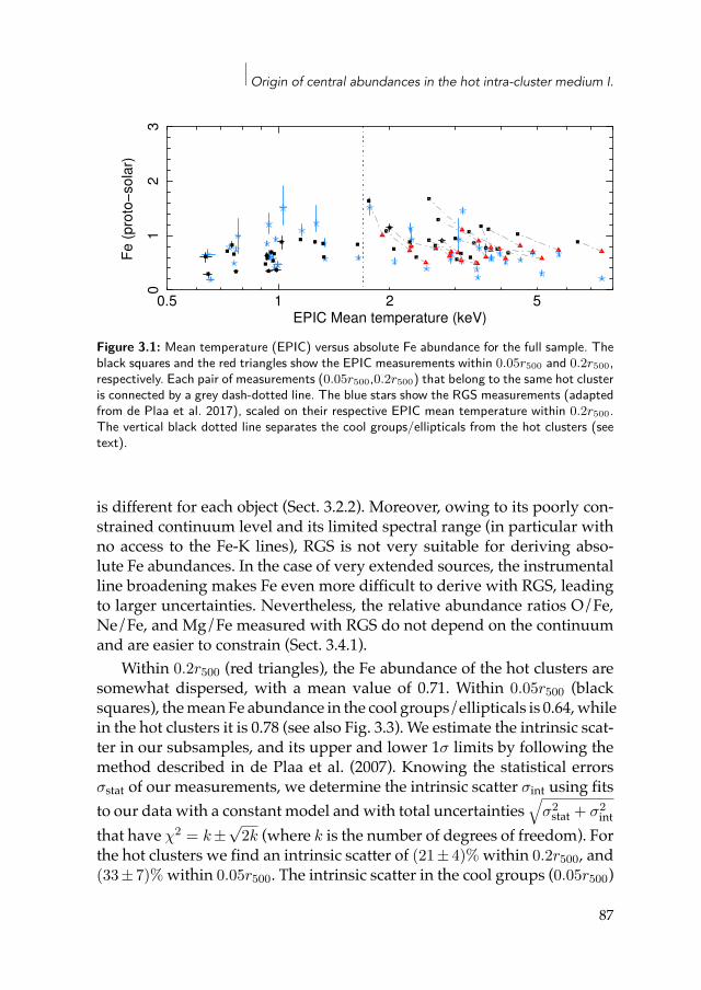
Origin of central abundances in the hot intra-cluster medium I.
10.5 2 5
01
23
Fe (
pro
to!
sola
r)
EPIC Mean temperature (keV)
Figure 3.1: Mean temperature (EPIC) versus absolute Fe abundance for the full sample. Theblack squares and the red triangles show the EPIC measurements within 0.05r500 and 0.2r500,respectively. Each pair of measurements (0.05r500,0.2r500) that belong to the same hot clusteris connected by a grey dash-dotted line. The blue stars show the RGS measurements (adaptedfrom de Plaa et al. 2017), scaled on their respective EPIC mean temperature within 0.2r500.The vertical black dotted line separates the cool groups/ellipticals from the hot clusters (seetext).
is different for each object (Sect. 3.2.2). Moreover, owing to its poorly con-strained continuum level and its limited spectral range (in particular withno access to the Fe-K lines), RGS is not very suitable for deriving abso-lute Fe abundances. In the case of very extended sources, the instrumentalline broadening makes Fe even more difficult to derive with RGS, leadingto larger uncertainties. Nevertheless, the relative abundance ratios O/Fe,Ne/Fe, and Mg/Fe measured with RGS do not depend on the continuumand are easier to constrain (Sect. 3.4.1).
Within 0.2r500 (red triangles), the Fe abundance of the hot clusters aresomewhat dispersed, with a mean value of 0.71. Within 0.05r500 (blacksquares), themeanFe abundance in the cool groups/ellipticals is 0.64,whilein the hot clusters it is 0.78 (see also Fig. 3.3). We estimate the intrinsic scat-ter in our subsamples, and its upper and lower 1σ limits by following themethod described in de Plaa et al. (2007). Knowing the statistical errorsσstat of our measurements, we determine the intrinsic scatter σint using fitsto our data with a constant model andwith total uncertainties
√σ2stat + σ2
intthat have χ2 = k ±
√2k (where k is the number of degrees of freedom). For
the hot clusters we find an intrinsic scatter of (21 ± 4)% within 0.2r500, and(33 ± 7)% within 0.05r500. The intrinsic scatter in the cool groups (0.05r500)
87
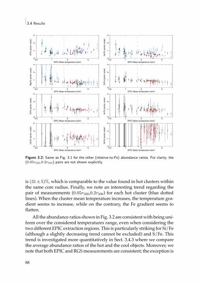
3.4 Results
10.5 2 5
01
23
O/F
e (
pro
to!
sola
r)
EPIC Mean temperature (keV)10.5 2 5
01
23
Ne/F
e (
pro
to!
sola
r)
EPIC Mean temperature (keV)
10.5 2 5
01
23
Mg/F
e (
pro
to!
sola
r)
EPIC Mean temperature (keV)10.5 2 5
01
23
Si/F
e (
pro
to!
sola
r)
EPIC Mean temperature (keV)
10.5 2 5
01
23
S/F
e (
pro
to!
sola
r)
EPIC Mean temperature (keV)10.5 2 5
01
23
Ar/
Fe (
pro
to!
sola
r)
EPIC Mean temperature (keV)
10.5 2 5
01
23
Ca/F
e (
pro
to!
sola
r)
EPIC Mean temperature (keV)10.5 2 5
01
23
Ni/F
e (
pro
to!
sola
r)
EPIC Mean temperature (keV)
Figure 3.2: Same as Fig. 3.1 for the other (relative-to-Fe) abundance ratios. For clarity, the(0.05r500,0.2r500) pairs are not shown explicitly.
is (31 ± 5)%, which is comparable to the value found in hot clusters withinthe same core radius. Finally, we note an interesting trend regarding thepair of measurements (0.05r500,0.2r500) for each hot cluster (blue dottedlines). When the cluster mean temperature increases, the temperature gra-dient seems to increase, while on the contrary, the Fe gradient seems toflatten.
All the abundance ratios shown in Fig. 3.2 are consistentwith being uni-form over the considered temperatures range, even when considering thetwo different EPIC extraction regions. This is particularly striking for Si/Fe(although a slightly decreasing trend cannot be excluded) and S/Fe. Thistrend is investigated more quantitatively in Sect. 3.4.3 where we comparethe average abundance ratios of the hot and the cool objects. Moreover, wenote that both EPIC and RGSmeasurements are consistent; the exception is
88
Origin of central abundances in the hot intra-cluster medium I.
Ne/Fe, for which the RGS measurements remain uniform while the EPICvalues suggest a decrease with temperature (see discussion in Sect. 3.4.1,and a further inspection in Sect. 3.4.3). Finally, although their uncertaintiesare large and deriving any trend is very difficult, we note that the Ni/Feabundance ratios are all consistent with being larger than the proto-solarvalue.
3.4.1 Estimating reliable average abundancesAssuming that all these relative-to-Fe abundance ratios are indeed uniformover clusters and do not depend (much) on their histories, we can combineour individual measurements and estimate for each element one averageabundance ratio representative of the nearby cool-core ICM as awhole.Weestimate the average relative-to-Fe abundance of a given element “X” byusing the weighting factors 1/σ(X/Fe)2
i , where σ(X/Fe)i is the uncertaintyon the X/Fe abundance in the ith observation. In the case of asymmet-ric X/Fe uncertainties in some observations, we systematically choose thelarger one (in absolute value).
In addition to studying the subsamples of the hot clusters (within ei-ther 0.2r500 or 0.05r500), we can also combine the hot subsample (within0.2r500) with the cool subsample (within 0.05r500), in order to get a “full”sample, named hereafter (0.05+0.2)r500, which contains the highest statis-tics. A complete comparison of this full sample with the three subsamplesmentioned above is discussed in Sect. 3.4.3.
As mentioned earlier, RGS measures the absolute Fe abundance with ahigh degree of uncertainty. However, it is quite reliable in measuring theabundance ratios of O/Fe, Ne/Fe, and sometimesMg/Fe (assuming a lowredshift and a high S/N, which is the case for our sample). Unlike RGS,EPIC is not very suitable for measuring O/Fe abundance ratios (whosemain emission lines reside at ∼0.6 keV near the O absorption edge andwhere the calibration is somewhat uncertain) and Ne/Fe abundance ra-tios (whoseK-shell transitions arewithin the Fe-L complex,which dependson the temperature structure and is not resolved by the EPIC instruments),but can in principlemake reliablemeasurements of all the other consideredones. Moreover, EPIC observes both the Fe-L and Fe-K complexes, as wellas the continuum emission, and thus provides more trustworthy absoluteFe abundances and temperatures.We note thatwe find large positive resid-uals around 1.2 keV in the EPIC spectra of NGC5813 andNGC5846, whichprevents us from estimating reasonable Mg abundances, even by perform-
89
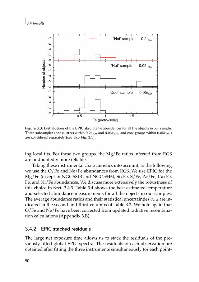
3.4 Results
02
46
80
24
68
Num
ber
of obje
cts
0 0.5 1 1.5 2
02
46
8
Fe (proto!solar)
’Hot’ sample !! 0.2r500
’Hot’ sample !! 0.05r500
’Cool’ sample !! 0.05r500
Figure 3.3: Distributions of the EPIC absolute Fe abundances for all the objects in our sample.Three subsamples (hot clusters within 0.2r500 and 0.05r500, and cool groups within 0.05r500)are considered separately (see also Fig. 3.1).
ing local fits. For these two groups, the Mg/Fe ratios inferred from RGSare undoubtedly more reliable.
Taking these instrumental characteristics into account, in the followingwe use the O/Fe and Ne/Fe abundances from RGS. We use EPIC for theMg/Fe (except in NGC5813 and NGC5846), Si/Fe, S/Fe, Ar/Fe, Ca/Fe,Fe, and Ni/Fe abundances. We discuss more extensively the robustness ofthis choice in Sect. 3.4.3. Table 3.4 shows the best estimated temperatureand selected abundance measurements for all the objects in our samples.The average abundance ratios and their statistical uncertainties σstat are in-dicated in the second and third columns of Table 3.2. We note again thatO/Fe and Ne/Fe have been corrected from updated radiative recombina-tion calculations (Appendix 3.B).
3.4.2 EPIC stacked residualsThe large net exposure time allows us to stack the residuals of the pre-viously fitted global EPIC spectra. The residuals of each observation areobtained after fitting the three instruments simultaneously for each point-
90
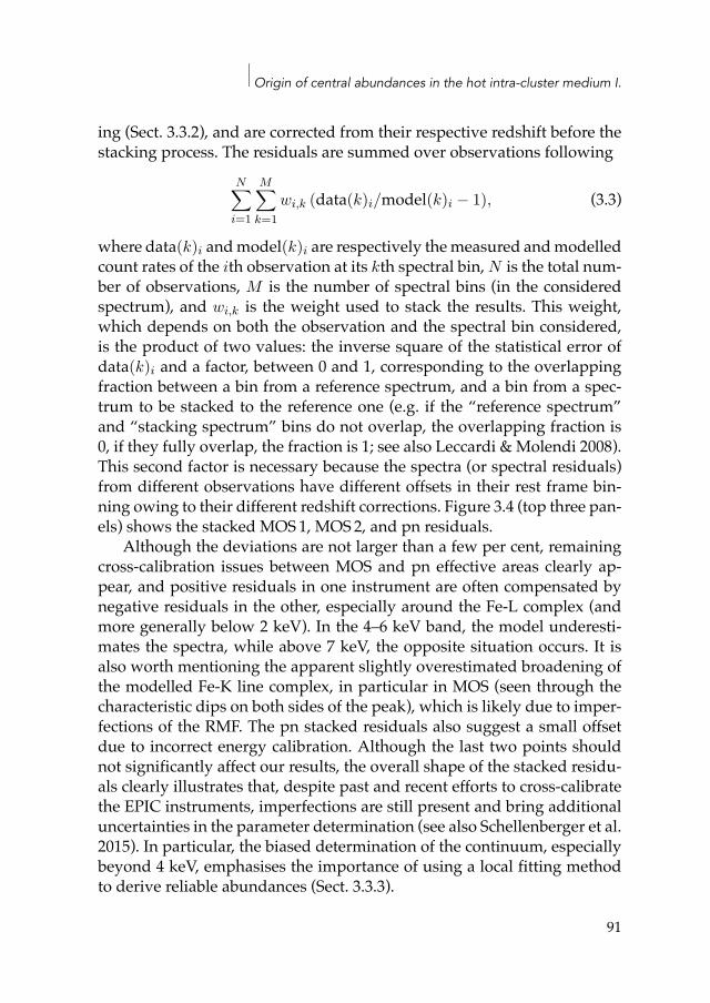
Origin of central abundances in the hot intra-cluster medium I.
ing (Sect. 3.3.2), and are corrected from their respective redshift before thestacking process. The residuals are summed over observations following
N∑i=1
M∑k=1
wi,k (data(k)i/model(k)i − 1), (3.3)
where data(k)i andmodel(k)i are respectively themeasured andmodelledcount rates of the ith observation at its kth spectral bin, N is the total num-ber of observations, M is the number of spectral bins (in the consideredspectrum), and wi,k is the weight used to stack the results. This weight,which depends on both the observation and the spectral bin considered,is the product of two values: the inverse square of the statistical error ofdata(k)i and a factor, between 0 and 1, corresponding to the overlappingfraction between a bin from a reference spectrum, and a bin from a spec-trum to be stacked to the reference one (e.g. if the “reference spectrum”and “stacking spectrum” bins do not overlap, the overlapping fraction is0, if they fully overlap, the fraction is 1; see also Leccardi & Molendi 2008).This second factor is necessary because the spectra (or spectral residuals)from different observations have different offsets in their rest frame bin-ning owing to their different redshift corrections. Figure 3.4 (top three pan-els) shows the stacked MOS1, MOS2, and pn residuals.
Although the deviations are not larger than a few per cent, remainingcross-calibration issues between MOS and pn effective areas clearly ap-pear, and positive residuals in one instrument are often compensated bynegative residuals in the other, especially around the Fe-L complex (andmore generally below 2 keV). In the 4–6 keV band, the model underesti-mates the spectra, while above 7 keV, the opposite situation occurs. It isalso worth mentioning the apparent slightly overestimated broadening ofthe modelled Fe-K line complex, in particular in MOS (seen through thecharacteristic dips on both sides of the peak), which is likely due to imper-fections of the RMF. The pn stacked residuals also suggest a small offsetdue to incorrect energy calibration. Although the last two points shouldnot significantly affect our results, the overall shape of the stacked residu-als clearly illustrates that, despite past and recent efforts to cross-calibratethe EPIC instruments, imperfections are still present and bring additionaluncertainties in the parameter determination (see also Schellenberger et al.2015). In particular, the biased determination of the continuum, especiallybeyond 4 keV, emphasises the importance of using a local fitting methodto derive reliable abundances (Sect. 3.3.3).
91
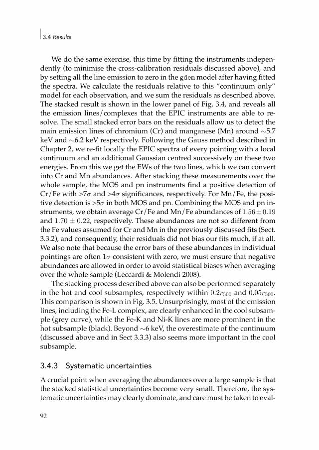
3.4 Results
We do the same exercise, this time by fitting the instruments indepen-dently (to minimise the cross-calibration residuals discussed above), andby setting all the line emission to zero in the gdemmodel after having fittedthe spectra. We calculate the residuals relative to this “continuum only”model for each observation, and we sum the residuals as described above.The stacked result is shown in the lower panel of Fig. 3.4, and reveals allthe emission lines/complexes that the EPIC instruments are able to re-solve. The small stacked error bars on the residuals allow us to detect themain emission lines of chromium (Cr) and manganese (Mn) around ∼5.7keV and ∼6.2 keV respectively. Following the Gauss method described inChapter 2, we re-fit locally the EPIC spectra of every pointing with a localcontinuum and an additional Gaussian centred successively on these twoenergies. From this we get the EWs of the two lines, which we can convertinto Cr and Mn abundances. After stacking these measurements over thewhole sample, the MOS and pn instruments find a positive detection ofCr/Fe with >7σ and >4σ significances, respectively. For Mn/Fe, the posi-tive detection is >5σ in both MOS and pn. Combining the MOS and pn in-struments, we obtain average Cr/Fe andMn/Fe abundances of 1.56±0.19and 1.70 ± 0.22, respectively. These abundances are not so different fromthe Fe values assumed for Cr andMn in the previously discussed fits (Sect.3.3.2), and consequently, their residuals did not bias our fits much, if at all.We also note that because the error bars of these abundances in individualpointings are often 1σ consistent with zero, we must ensure that negativeabundances are allowed in order to avoid statistical biases when averagingover the whole sample (Leccardi & Molendi 2008).
The stacking process described above can also be performed separatelyin the hot and cool subsamples, respectively within 0.2r500 and 0.05r500.This comparison is shown in Fig. 3.5. Unsurprisingly, most of the emissionlines, including the Fe-L complex, are clearly enhanced in the cool subsam-ple (grey curve), while the Fe-K and Ni-K lines are more prominent in thehot subsample (black). Beyond ∼6 keV, the overestimate of the continuum(discussed above and in Sect 3.3.3) also seems more important in the coolsubsample.
3.4.3 Systematic uncertaintiesA crucial point when averaging the abundances over a large sample is thatthe stacked statistical uncertainties become very small. Therefore, the sys-tematic uncertaintiesmay clearly dominate, and caremust be taken to eval-
92
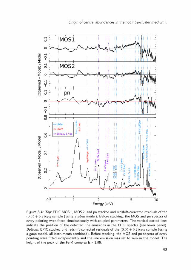
Origin of central abundances in the hot intra-cluster medium I.
0.1
00.
10
.10
0.1
(Obs
erve
d
Mod
el) /
Mod
el
1 100.5 2 5
0.1
00.
1
Energy (keV)
MOS1
MOS2
pn
1 100.5 2 5
00.
20.
40.
60.
8(O
bser
ved
Mod
el) /
Mod
el
Energy (keV)
O V
III (L
y)
FeL
com
plex
(incl.
Ne)
Mg
XII (
Ly)
Si X
III (H
e) Si
XIV
(Ly
)
S XV
(He
)S
XVI (
Ly)
Ar X
VII (
He)
Ar X
VIII
(Ly
)
Ca X
IX (H
e)
Ca X
X (L
y)
Ca X
IX /
Ca X
X
Cr X
XIII
(He
)M
n XX
IV (H
e)
FeK
com
plex
Fe X
XVI (
Ly)
Fe X
XV (H
e)
(/ Fe
XXI
V)
Ni X
XVII
/ Ni X
XVIII
/ Fe
XXV
(He
)
> SNIa> SNcc> SNIa & SNcc
Figure 3.4: Top: EPIC MOS 1, MOS 2, and pn stacked and redshift-corrected residuals of the(0.05 + 0.2)r500 sample (using a gdem model). Before stacking, the MOS and pn spectra ofevery pointing were fitted simultaneously with coupled parameters. The vertical dotted linesindicate the position of the detected line emissions in the EPIC spectra (see lower panel).Bottom: EPIC stacked and redshift-corrected residuals of the (0.05 + 0.2)r500 sample (usinga gdem model, all instruments combined). Before stacking, the MOS and pn spectra of everypointing were fitted independently and the line emission was set to zero in the model. Theheight of the peak of the Fe-K complex is ∼1.95.
93
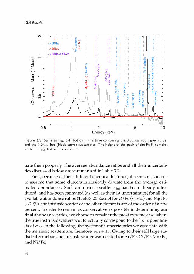
3.4 Results
1 100.5 2 5
00
.51
1.5
2
(Ob
serv
ed
! M
od
el) /
Mo
de
l
Energy (keV)
O V
III
(Ly!
)
Fe!
L c
om
ple
x
(in
cl.
Ne
)
Mg
XII
(L
y!)
Si X
III
(He
!) S
i XIV
(L
y!)
S X
V (
He
!)
S X
VI
(Ly!
)
Ar
XV
II (
He
!)
Ar
XV
III
(Ly!
)
Ca
XIX
(H
e!
)C
a X
X (
Ly!
)
Ca
XIX
/ C
a X
X
Cr
XX
III
(He
!)
Mn
XX
IV (
He
!)
Fe
!K
co
mp
lex
Fe
XX
VI
(Ly!
)
Fe
XX
V (
He
")
(/ F
e X
XIV
)
Ni X
XV
II /
Ni X
XV
III
/ F
e X
XV
(H
e#)
!> SNIa
!> SNcc
!> SNIa & SNcc
Figure 3.5: Same as Fig. 3.4 (bottom), this time comparing the 0.05r500 cool (grey curve)and the 0.2r500 hot (black curve) subsamples. The height of the peak of the Fe-K complexin the 0.2r500 hot sample is ∼2.23.
uate them properly. The average abundance ratios and all their uncertain-ties discussed below are summarised in Table 3.2.
First, because of their different chemical histories, it seems reasonableto assume that some clusters intrinsically deviate from the average esti-mated abundances. Such an intrinsic scatter σint has been already intro-duced, and has been estimated (as well as their 1σ uncertainties) for all theavailable abundance ratios (Table 3.2). Except for O/Fe (∼16%) andMg/Fe(∼29%), the intrinsic scatter of the other elements are of the order of a fewpercent. In order to remain as conservative as possible in determining ourfinal abundance ratios, we choose to consider the most extreme case wherethe true instrinsic scatters would actually correspond to the (1σ) upper lim-its of σint. In the following, the systematic uncertainties we associate withthe instrinsic scatters are, therefore, σint + 1σ. Owing to their still large sta-tistical error bars, no intrinsic scatterwas needed forAr/Fe, Cr/Fe,Mn/Fe,and Ni/Fe.
94
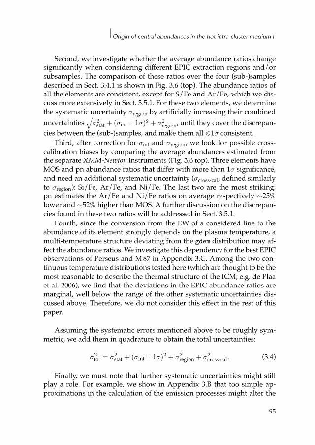
Origin of central abundances in the hot intra-cluster medium I.
Second, we investigate whether the average abundance ratios changesignificantly when considering different EPIC extraction regions and/orsubsamples. The comparison of these ratios over the four (sub-)samplesdescribed in Sect. 3.4.1 is shown in Fig. 3.6 (top). The abundance ratios ofall the elements are consistent, except for S/Fe and Ar/Fe, which we dis-cuss more extensively in Sect. 3.5.1. For these two elements, we determinethe systematic uncertainty σregion by artificially increasing their combineduncertainties
√σ2stat + (σint + 1σ)2 + σ2
region, until they cover the discrepan-cies between the (sub-)samples, and make them all ⩽1σ consistent.
Third, after correction for σint and σregion, we look for possible cross-calibration biases by comparing the average abundances estimated fromthe separate XMM-Newton instruments (Fig. 3.6 top). Three elements haveMOS and pn abundance ratios that differ with more than 1σ significance,and need an additional systematic uncertainty (σcross-cal, defined similarlyto σregion): Si/Fe, Ar/Fe, and Ni/Fe. The last two are the most striking:pn estimates the Ar/Fe and Ni/Fe ratios on average respectively ∼25%lower and ∼52% higher than MOS. A further discussion on the discrepan-cies found in these two ratios will be addressed in Sect. 3.5.1.
Fourth, since the conversion from the EW of a considered line to theabundance of its element strongly depends on the plasma temperature, amulti-temperature structure deviating from the gdem distribution may af-fect the abundance ratios.We investigate this dependency for the best EPICobservations of Perseus and M87 in Appendix 3.C. Among the two con-tinuous temperature distributions tested here (which are thought to be themost reasonable to describe the thermal structure of the ICM; e.g. de Plaaet al. 2006), we find that the deviations in the EPIC abundance ratios aremarginal, well below the range of the other systematic uncertainties dis-cussed above. Therefore, we do not consider this effect in the rest of thispaper.
Assuming the systematic errors mentioned above to be roughly sym-metric, we add them in quadrature to obtain the total uncertainties:
σ2tot = σ2
stat + (σint + 1σ)2 + σ2region + σ2
cross-cal. (3.4)
Finally, we must note that further systematic uncertainties might stillplay a role. For example, we show in Appendix 3.B that too simple ap-proximations in the calculation of the emission processes might alter the
95
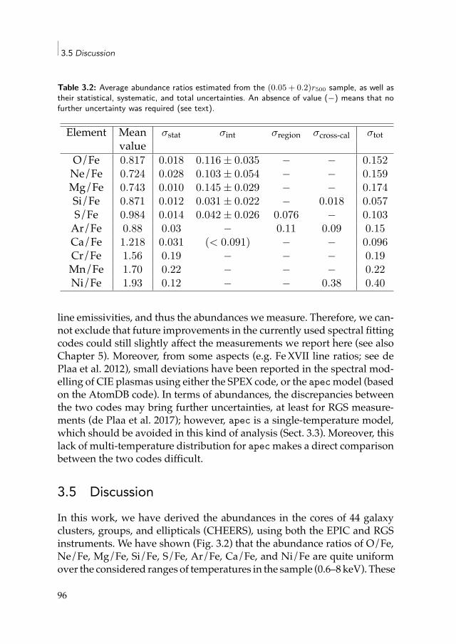
3.5 Discussion
Table 3.2: Average abundance ratios estimated from the (0.05 + 0.2)r500 sample, as well astheir statistical, systematic, and total uncertainties. An absence of value (−) means that nofurther uncertainty was required (see text).
Element Mean σstat σint σregion σcross-cal σtotvalue
O/Fe 0.817 0.018 0.116 ± 0.035 − − 0.152Ne/Fe 0.724 0.028 0.103 ± 0.054 − − 0.159Mg/Fe 0.743 0.010 0.145 ± 0.029 − − 0.174Si/Fe 0.871 0.012 0.031 ± 0.022 − 0.018 0.057S/Fe 0.984 0.014 0.042 ± 0.026 0.076 − 0.103Ar/Fe 0.88 0.03 − 0.11 0.09 0.15Ca/Fe 1.218 0.031 (< 0.091) − − 0.096Cr/Fe 1.56 0.19 − − − 0.19Mn/Fe 1.70 0.22 − − − 0.22Ni/Fe 1.93 0.12 − − 0.38 0.40
line emissivities, and thus the abundances we measure. Therefore, we can-not exclude that future improvements in the currently used spectral fittingcodes could still slightly affect the measurements we report here (see alsoChapter 5). Moreover, from some aspects (e.g. FeXVII line ratios; see dePlaa et al. 2012), small deviations have been reported in the spectral mod-elling of CIE plasmas using either the SPEX code, or the apecmodel (basedon the AtomDB code). In terms of abundances, the discrepancies betweenthe two codes may bring further uncertainties, at least for RGS measure-ments (de Plaa et al. 2017); however, apec is a single-temperature model,which should be avoided in this kind of analysis (Sect. 3.3). Moreover, thislack of multi-temperature distribution for apecmakes a direct comparisonbetween the two codes difficult.
3.5 DiscussionIn this work, we have derived the abundances in the cores of 44 galaxyclusters, groups, and ellipticals (CHEERS), using both the EPIC and RGSinstruments. We have shown (Fig. 3.2) that the abundance ratios of O/Fe,Ne/Fe, Mg/Fe, Si/Fe, S/Fe, Ar/Fe, Ca/Fe, and Ni/Fe are quite uniformover the considered ranges of temperatures in the sample (0.6–8 keV). These
96
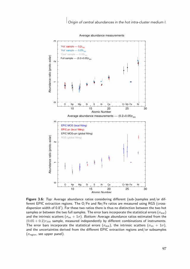
Origin of central abundances in the hot intra-cluster medium I.
10 15 20 25 30
01
23
Ab
un
da
nce
ra
tio (
pro
to!
sola
r)
Atomic Number
Average abundance measurements
O Ne Mg Si S Ar Ca Cr Mn Fe Ni
’Hot’ sample !! 0.2r500
’Hot’ sample !! 0.05r500
’Cool’ sample !! 0.05r500
Full sample !! (0.2+0.05)r500
10 15 20 25 30
01
23
Ab
un
da
nce
ra
tio (
pro
to!
sola
r)
Atomic Number
Average abundance measurements !! (0.2+0.05)r500
O Ne Mg Si S Ar Ca Cr Mn Fe Ni
EPIC MOS (local fitting)
EPIC pn (local fitting)
EPIC MOS+pn (global fitting)
RGS (global fitting)
Figure 3.6: Top: Average abundance ratios considering different (sub-)samples and/or dif-ferent EPIC extraction regions. The O/Fe and Ne/Fe ratios are measured using RGS (cross-dispersion width of 0.8′). For these two ratios there is thus no distinction between the two hotsamples or between the two full samples. The error bars incorporate the statistical errors (σstat)and the intrinsic scatters (σint + 1σ). Bottom: Average abundance ratios estimated from the(0.05 + 0.2)r500 sample, measured independently by different combinations of instruments.The error bars incorporate the statistical errors (σstat), the intrinsic scatters (σint + 1σ),and the uncertainties derived from the different EPIC extraction regions and/or subsamples(σregion, see upper panel).
97
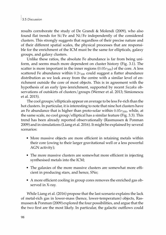
3.5 Discussion
results corroborate the study of De Grandi & Molendi (2009), who alsofound flat trends for Si/Fe and Ni/Fe independently of the consideredclusters. This strongly suggests that regardless of their precise nature andof their different spatial scales, the physical processes that are responsi-ble for the enrichment of the ICM must be the same for ellipticals, galaxygroups, and galaxy clusters.
Unlike these ratios, the absolute Fe abundance is far from being uni-form, and seems much more dependent on cluster history (Fig. 3.1). Thescatter is more important in the inner regions (0.05r500) of the core. A lessscattered Fe abundance within 0.2r500 could suggest a flatter abundancedistribution as we look away from the centre with a similar level of en-richment outside the core of most objects. This is in agreement with thehypothesis of an early (pre-)enrichment, supported by recent Suzaku ob-servations of outskirts of clusters/groups (Werner et al. 2013; Simionescuet al. 2015).
The cool groups/ellipticals appear on average to be less Fe-rich than thehot clusters. In particular, it is interesting to note that nine hot clusters havean Fe abundance that is higher than proto-solar within 0.05r500, while, atthe same scale, no cool group/elliptical has a similar feature (Fig. 3.3). Thistrend has been already reported observationally (Rasmussen & Ponman2009) and in simulations (Liang et al. 2016). Itmight be explained by severalscenarios:
• More massive objects are more efficient in retaining metals withintheir core (owing to their larger gravitational well or a less powerfulAGN activity);
• The more massive clusters are somewhat more efficient in injectingsynthesised metals into the ICM;
• The galaxies of the more massive clusters are somewhat more effi-cient in producing stars, and hence, SNe;
• Amore efficient cooling in group cores removes the enriched gas ob-served in X-ray.
While Liang et al. (2016) propose that the last scenario explains the lackof metal-rich gas in lower-mass (hence, lower-temperature) objects, Ras-mussen&Ponman (2009) explored the four possibilities, and argue that thethe two first are the most likely. In particular, the galactic outflows could
98
Origin of central abundances in the hot intra-cluster medium I.
be less efficient in releasing metals in the ICM of cooler groups or, alterna-tively, the AGN activity of the BCG could have helped to remove metalsfrom their core (see also Yates et al. 2017). However, we must emphasisethat several of these mechanisms might co-exist, and that the list aboveis not necessarily exhaustive. For instance, Elkholy et al. (2015) recentlyfound a hint of a positive correlation between the metallicity in low-massclusters, and the morphological disturbance of their ICM (likely related tothe dynamical activity of their galaxy members). Alternatively, cooler ICMmight be more efficient in depleting ionic Fe (and probably other metals)into grains close to the brightest central galaxy, although Panagoulia et al.(2015) found hints of Fe depletion in the cores of more massive clusters aswell.
We must warn, however, that the large intrinsic scatters mentionedabove prevent us from claiming any clear and significant trend on the ab-solute Fe abundances. Moreover, a more complicated thermal structure ingroups/ellipticals than in more massive clusters cannot be excluded, andcould lead to a slight but significant Fe bias, which would affect in prioritythe cooler objects in our sample.
We have also found an apparent variation in the Fe abundance and tem-perature gradients (i.e. between 0.05r500 and 0.2r500) in the hot clusters.These differences could be related to the individual cluster enrichment his-tories or to other parameters, such as the cooling rate. Linking the historyof each cluster/group to its Fe budget requires a more careful spatial studyof the Fe distribution. Establishing radial profiles for the entire sample isbeyond the scope of this work, but are addressed in Chapter 6.
From the stacked results of our (0.05 + 0.2)r500 sample, we have esti-mated the average abundance ratios and their respective total uncertainties(statistical and systematic). This also includes Cr/Fe andMn/Fe,whichwehave detected within >4σ significance with MOS and pn independently.To our knowledge, this is the first time that Mn has been firmly detectedin the ICM. For comparison, Werner et al. (2006b) already detected Cr in2A0335+096 within 2σ (but were unable to detect Mn), while Cr and Mnhave been detected in Perseuswithin 5σ and 1σ, respectively (Tamura et al.2009). It is also striking to note that we do not see any emission line featurearound∼3.5 keV in the stacked EPIC spectra (Fig. 3.4 bottom, Fig. 3.5) con-trary to several claims from recent studies, in particular Bulbul et al. (2014)and Boyarsky et al. (2014), whose total EPIC net exposure times are ∼3 Msand ∼1.5 Ms, respectively (i.e. less than in this work). Such an apparent
99
3.5 Discussion
non-detection is thus very interesting to report, since it might challengethe hypothesis of decaying sterile neutrinos, known as a dark matter can-didate, being observed in the ICM. We note that the dark matter interpre-tation is far from being the only possible explanation of an emission line at∼3.5 keV (e.g. Gu et al. 2015), and our non-detection could also be exploredin the context of these other possibilities. However, this question is not theinitial purpose of this present study, and a more detailed investigation ofour stacked spectra around ∼3.5 keV, and consequent discussions, are leftto a future paper.
3.5.1 Discrepancies in the S/Fe, Ar/Fe and Ni/Fe ratiosThe average S/Fe ratio shows a slight but significant enhancement in thecool objects within 0.05r500 compared to the hot objects within 0.2r500 (Fig.3.6). From Fig. 3.2 (left, third panel), it is clear that M49 (kTmean ∼ 1.148keV) and A3581 (kTmean ∼ 1.637 keV) largely contribute to this higherS/Fe ratio measured in the cool subsample because their statistical errorsare small compared to the other cool objects. Moreover, the >1σ discrep-ancy between the cool and hotmeasured S/Fe ratios disappears when con-sidering the same radius (0.05r500) for all the objects.
The Ar/Fe discrepancy observed in Fig. 3.6 (top) is more intriguing,since a larger aperture seems to lower its measurement. This trend is diffi-cult to interpret. A change in the relative Ar to Fe radial distribution in theICM cannot be excluded, although we would then expect it for other ele-ments as well. A full study of the abundance radial profiles of the sampleare performed in Chapter 6. Furthermore, it also appears from Fig. 3.6 (bot-tom) that MOS and pn measure significantly different Ar/Fe values, evenafter taking account of the uncertainty described above (i.e. σregion). Thereason for this second Ar/Fe discrepancy is again challenging to clearlyidentify, but it is very likely due to imperfections in the calibration of theEPIC instruments.
As seen in Fig. 3.6 (bottom), the largeMOS-pn discrepancy in theNi/Feabundance ratio prevents us from deriving a precise measurement. Thisdiscrepancy isworrying, but can be explained by imperfections in the cross-calibration of the two instruments. Alternatively, and perhaps more likely,the high energy band around the Ni-K transitions is significanly affectedby the instrumental background (as the flux of the cluster emission sharplydecreases at high energies). This hard particle background (already men-tioned in Sect. 3.3.1) has a different spectral shape in MOS and pn, which
100
Origin of central abundances in the hot intra-cluster medium I.
might even vary with time, thus between observations. In particular, an in-strumental line (Cu Kα) is known to affect pn at a rest-frame energy of ∼8keV (Chapter 2). Despite our efforts to carefully estimate the background,that line might interfere with the Ni-K line in several observations, mak-ing a propermodelling of theNi-K line impossible, and hence, boosting theNi absolute abundance in pn. In this context, it can be instructive to com-pare our Ni/Fe measurements with those of Suzaku, which has a lowerrelative hard particle background. Sato et al. (2007b) (A 1060) and Tamuraet al. (2009) (Perseus) reported ratios of ∼1.3±0.4 and ∼1.11±0.19, respec-tively (after rescaling to the proto-solar values). Although these measure-ments might be also be affected by further uncertainties (e.g. the choiceof the spectral modelling, Sect. 3.4.3), they appear to be consistent with theNi/Fe average ratiomeasuredwithMOS is this work, favouring our abovesupposition that MOS is more trustworthy than pn for measuring Ni/Fe.However, in order to be conservative, we prefer to retain the pn value asa possible result and, therefore, we keep large systematic uncertainties forNi/Fe. We finally note that, unsurprisingly, Ni/Fe cannot be constrainedin the cool objects (Fig. 3.6 top) because the gas temperature is too low toexcite Ni-K transitions.
3.5.2 Comparison with the proto-solar abundance ratiosIn Fig. 3.7 (black squares), we report our final X/Fe abundance patternmeasured in the (0.05 + 0.2)r500 sample, accounting for all the systematicuncertainties discussed earlier in this paper. At first glance, most of theabundance ratiosmeasured in the ICM look significantly different from theproto-solar abundance ratios. Indeed, if we fit a constant to our abundancepattern (dashed grey line), we obtain a χ2 of 43.1 for 10 degrees of free-dom, in poor agreement with the abundance ratios in the ICM. However,as shown by the red dash-dotted lines (adapted from Lodders et al. 2009),the solar abundance ratios also suffer from large uncertainties, typicallyabout 20–25%. When comparing the two sets of abundance ratios takenwith their respective uncertainties, we find that the O/Fe, Ne/Fe, Mg/Fe,Si/Fe S/Fe, Ar/Fe, and Ca/Fe ratios measured in the ICM are consistentwithin 1σ with the proto-solar values (±1σ). The Cr/Fe abundance ratiosmeasured in the ICM are consistent within 2σ with the proto-solar values(±1σ), and the Mn/Fe and Ni/Fe abundance ratios are consistent within3σ.
Given these considerations, whether the chemical enrichment in the
101
3.5 Discussion
ICM is similar to the chemical enrichment of the solar neighbourhood isnot a trivial question to solve. As mentioned above, while most of the rel-ative abundances appear to be consistent with being proto-solar, Ni/Fe,Mn/Fe, and perhaps Cr/Fe seem to be significantly enhanced. This resultmight be of interest since significant different abundance ratios in the ICMmeans that the fraction of SNIa (or conversely SNcc) responsible for theICM enrichment differs from that of the Galactic enrichment. We will ad-dress this discussion in greater detail in Chapter 4. We recall, however,that the abundances of interest in this context (Cr, Mn, and Ni) are not wellconstrained in X-ray, given the current instrument capabilities. Moreover,as specified in Sect. 3.4.3, we do not exclude that differences in currentatomic codes might bring further systematic uncertainties to the measure-ments reported in this work. Therefore, whether our abundance ratios aresignificantly more accurate than the proto-solar estimates should still beconsidered an open question.
3.5.3 Current limitations and future prospectsAs we have shown throughout this paper, our excellent data quality (∼4.5Ms and ∼3.7 Ms of total net exposure time for EPIC MOS and pn, re-spectively) provides very accurate abundance measurements in the ICMof cool-core galaxy clusters and groups. Therefore, these data should bea legacy for any future work directly or indirectly related to the chemicalenrichment in the ICM. However, our study clearly reveals that the abun-dance ratios of some elements of interest are still poorly constrained. Inparticular, the Cr/Fe, Mn/Fe, and Ni/Fe ratios in our study appear higherthan the solar neighbourhood and are thus crucial to study in detail, whichis currently challenging given the limited spectral resolution of CCDs andthe large cross-calibration uncertainties (at least for Ni/Fe) that we empha-sise here.
In this work we probably reach the instrumental limitations of XMM-Newton in terms of abundance determination, and thus stacking more datawill have very little impact on the current accuracy of our already exist-ing measurements. Indeed, in our sample, the statistical uncertainties arealready marginal compared to the systematic ones. In addition to furtherefforts in calibrating the instruments and improving the atomic databases,it is clear that a sensibly higher X-ray spectral resolution is now needed.
Such an improvement can be reachedwithmicro-calorimeter spectrom-eters, which should be on board the next generation of X-ray observato-
102
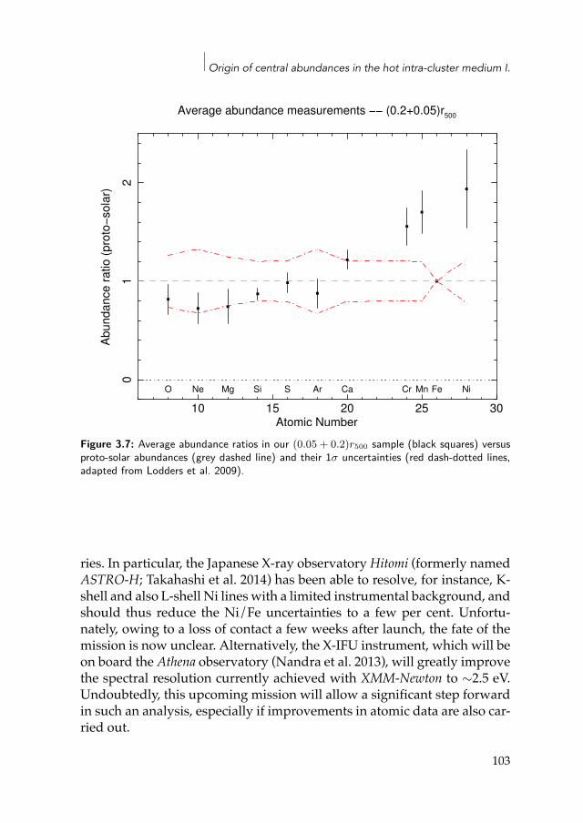
Origin of central abundances in the hot intra-cluster medium I.
10 15 20 25 30
01
2
Ab
un
da
nce
ra
tio (
pro
to!
sola
r)
Atomic Number
Average abundance measurements !! (0.2+0.05)r500
O Ne Mg Si S Ar Ca Cr Mn Fe Ni
Figure 3.7: Average abundance ratios in our (0.05 + 0.2)r500 sample (black squares) versusproto-solar abundances (grey dashed line) and their 1σ uncertainties (red dash-dotted lines,adapted from Lodders et al. 2009).
ries. In particular, the Japanese X-ray observatoryHitomi (formerly namedASTRO-H; Takahashi et al. 2014) has been able to resolve, for instance, K-shell and also L-shell Ni lines with a limited instrumental background, andshould thus reduce the Ni/Fe uncertainties to a few per cent. Unfortu-nately, owing to a loss of contact a few weeks after launch, the fate of themission is now unclear. Alternatively, the X-IFU instrument, which will beon board the Athena observatory (Nandra et al. 2013), will greatly improvethe spectral resolution currently achieved with XMM-Newton to ∼2.5 eV.Undoubtedly, this upcoming mission will allow a significant step forwardin such an analysis, especially if improvements in atomic data are also car-ried out.
103
3.6 Conclusions
3.6 ConclusionsIn this paper, we have used the XMM-Newton EPIC and RGS instrumentsto investigate the Fe abundance and abundance ratios of O/Fe, Ne/Fe,Mg/Fe, Si/Fe, S/Fe, Ar/Fe, Ca/Fe, Cr/Fe, Mn/Fe, and Ni/Fe in the cen-tral regions of 44 cool-core galaxy clusters, groups, and elliptical galaxies(CHEERS). Our main results can be summarised as follows.
• The X/Fe abundance ratios appear quite uniform over themean tem-perature range of our sample. This confirms previous results, and in-dicates that no matter what the physical mechanisms responsible forthe enrichment are, they must be very similar in enriching the ICMof ellipticals, groups, and clusters of galaxies.
• By stacking all the EPIC spectra of our sample (within 0.2r500 whenpossible, within 0.05r500 otherwise), we were able to derive abun-dances of Cr/Fe and Mn/Fe independently with MOS and pn, with>4σ significance. While Cr had been already detected in the past, thisis the first time that a firm detection of Mn in the hot ICM has beenreported.
• Contrary to recent claims, and despite the large net exposure time(∼4.5 Ms) of our combined data, we do not see any emission lineat ∼3.5 keV. Although a deeper investigation will be addressed in afuture paper, this might challenge the possibility of decaying sterileneutrinos, a dark matter candidate, being observed in the ICM.
• The Fe abundance varies between 0.2–2 times the proto-solar values,and shows an important scatter, especially within a radius of 0.05r500(∼30–40%). Looking at smaller (0.05r500) and larger (0.2r500) centralregions in a subsample of hot clusters, it appears that the Fe peaksharpens and the temperature drop flattens as the mean cluster tem-perature decreases. Clearly, these various Fe abundances must de-pend on individual clusters histories, and complete abundance radialprofiles are investigated in greater detail in Chapter 6.
• Having benefited from a large total net exposure time (∼4.5 Ms) andhaving processed a very careful estimation of the systematic effectsthat could affect our measurements, we have shown that the system-atic uncertainties clearly dominate over the statistical ones. Taking
104
Origin of central abundances in the hot intra-cluster medium I.
these systematic uncertainties into account, most of the ICM abun-dance ratios measured in this work are consistent with the proto-solar abundance ratios. Notable exceptions are Mn/Fe, Ni/Fe, andperhaps Cr/Fe, which are found to be significantly higher in the ICMthan in the solar neighbourhood.
• Overall, our careful analysis demonstrates that stacking more obser-vations would not further improve the accuracy of our results, and,more generally, that we have probably reached the limits of the cur-rent X-ray capabilities (in particular XMM-Newton) for this sciencecase. Therefore, our data constitute the most accurate abundance ra-tios ever measured in the ICM, and should be a legacy for futurework. Using the results presented in this paper, a full discussion onthe role of the SNIa and SNcc in the context of both the proto-solarand the ICMenrichments is addressed inChapter 4.However, amoreaccurate comparison between the local Galactic enrichment and theICM enrichment in the local Universe will require improvements inatomic data, as well as better calibration of the instruments. In paral-lel to these needs for improvements, the upcoming X-ray observato-ries should further improve the accuracy of the abundance measure-ments, and thus help to solve the puzzle of the chemical enrichmentin the hot ICM.
AcknowledgementsThe authors would like to thank the referee Marten van Kerkwijk for hishelpful comments and suggestions. Thiswork is partly based on theXMM-Newton AO-12 proposal “The XMM-Newton view of chemical enrichment inbright galaxy clusters and groups” (PI: de Plaa), and is a part of the CHEERS(CHEmical EvolutionRgs cluster Sample) collaboration. The authors thankits members, as well as Liyi Gu and Craig Sarazin for helpful discussions.P.K. thanks Steve Allen and Ondrej Urban for support and hospitality atStanford University. Y.Y.Z. acknowledges support by the German BMWIthrough the Verbundforschung under grant 50OR1506. Thiswork is basedon observations obtainedwithXMM-Newton, an ESA sciencemission withinstruments and contributions directly funded by ESA member states andthe USA (NASA). The SRON Netherlands Institute for Space Research issupported financially byNWO, theNetherlandsOrganisation for Scientific
105

3.6 Conclusions
Research.
106
Origin of central abundances in the hot intra-cluster medium I.
3.A EPIC absorption column densitiesIn the hot model used in this work to mimic absorption of X-rays throughinterstellarmaterial (Sect. 3.3), we initially fixed the hydrogen column den-sityNH to theweighted valueNH,tot of both the neutral (NHI, Kalberla et al.2005) and themolecular (NH2 , Schlegel et al. 1998) materials, calculated us-ing the method of Willingale et al. (2013)8. However, this approach oftengives poor fits in the soft band of our EPIC spectral modelling, by signifi-cantly under- or overestimating the flux of its continuum. In order to com-pensate this effect, the O abundance is often biased consequently by thefits. Fig. 3.8 (red data points) clearly illustrates that some objects have theirEPIC O/Fe ratio significantly offset from the corresponding RGS values.
The EPIC-RGS correlation for the O/Fe ratio is clearly improved if wefree the NH (Fig. 3.8, black data points). Similarly, most of the fits are im-proved in terms of C-stat/d.o.f. However, keeping NH as a free parame-ter without any further constraint is quite dangerous, and might lead tounphysical results. In order to remain reasonably consistent with the es-timated values of NHI and NH,tot mentioned above, we allow NH to takevalues within the following arbitrary limits:
NHI − 5 × 1019 cm−2 ⩽ NH ⩽ NH,tot + 1 × 1020 cm−2. (3.5)These upper and lower ranges allow limited deviations also around
NHI and NH,tot. Since constraining a free parameter within a narrow rangecan lead to problems in evaluating the statistical errors, we perform a gridsearch of fixed NH values (taken within the limits mentioned above), andselect the one that gives the lowest C-stat/d.o.f. to the fits. Despite all theseprecautions, it should also be kept inmind that the O abundancemeasuredin clusters with EPIC is also affected by the oxygen absorption in the in-terstellar medium, which in turn depends on NH (e.g. de Plaa et al. 2004).Similarly, the measured O abundance in the ICM may be also affected bythe foreground thermal X-ray emission.
3.B Radiative recombination correctionsThe version of SPEX that is used in thiswork calculates the line emissivitiesassuming that the radiative recombination (RR) rates of the cluster emis-sion can be expressed as a power law of the electron temperature (Mewe
8http://www.swift.ac.uk/analysis/nhtot/index.php
107
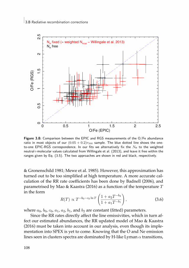
3.B Radiative recombination corrections
0 0.5 1 1.5 2 2.5
00
.51
1.5
22
.5
O/F
e (
RG
S)
O/Fe (EPIC)
NH fixed (= weighted NH,tot ! Willingale et al. 2013)NH free
Figure 3.8: Comparison between the EPIC and RGS measurements of the O/Fe abundanceratio in most objects of our (0.05 + 0.2)r500 sample. The blue dotted line shows the one-to-one EPIC-RGS correspondence. In our fits we alternatively fix the NH to the weightedneutral+molecular values calculated from Willingale et al. (2013), and leave it free within theranges given by Eq. (3.5). The two approaches are shown in red and black, respectively.
& Gronenschild 1981; Mewe et al. 1985). However, this approximation hasturned out to be too simplified at high temperature. A more accurate cal-culation of the RR rate coefficients has been done by Badnell (2006), andparametrised by Mao & Kaastra (2016) as a function of the temperature Tin the form
R(T ) ∝ T −b0−c0 ln T
(1 + a2T −b2
1 + a1T −b1
), (3.6)
where a0, b0, c0, a1, a2, b1, and b2 are constant (fitted) parameters.Since the RR rates directly affect the line emissivities, which in turn af-
fect our estimated abundances, the RR updated model of Mao & Kaastra(2016) must be taken into account in our analysis, even though its imple-mentation into SPEX is yet to come. Knowing that the O and Ne emissionlines seen in clusters spectra are dominated by H-like Lyman α transitions,
108
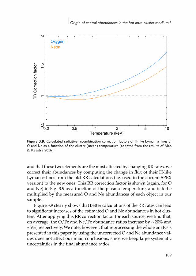
Origin of central abundances in the hot intra-cluster medium I.
1 100.2 0.5 2 50.5
11
.52
RR
Co
rre
ctio
n f
act
or
Temperature (keV)
Oxygen
Neon
Figure 3.9: Calculated radiative recombination correction factors of H-like Lyman α lines ofO and Ne as a function of the cluster (mean) temperature (adapted from the results of Mao& Kaastra 2016).
and that these two elements are themost affected by changing RR rates, wecorrect their abundances by computing the change in flux of their H-likeLyman α lines from the old RR calculations (i.e. used in the current SPEXversion) to the new ones. This RR correction factor is shown (again, for Oand Ne) in Fig. 3.9 as a function of the plasma temperature, and is to bemultiplied by the measured O and Ne abundances of each object in oursample.
Figure 3.9 clearly shows that better calculations of the RR rates can leadto significant increases of the estimated O and Ne abundances in hot clus-ters. After applying this RR correction factor for each source, we find that,on average, the O/Fe and Ne/Fe abundance ratios increase by ∼20% and∼9%, respectively. We note, however, that reprocessing the whole analysispresented in this paper by using the uncorrected O andNe abundance val-ues does not affect our main conclusions, since we keep large systematicuncertainties in the final abundance ratios.
109
3.C Effects of the temperature distribution on the abundance ratios
3.C Effects of the temperature distribution on the abun-dance ratios
As already specified in Sect. 3.3, the measured absolute abundances (inparticular Fe) are in principle sensitive to the choice of the thermal modelused in the fits (single- vs. multi-temperature). Among multi-temperaturemodels, the assumed temperature distribution might also affect the mea-sured (X/Fe) abundances. We explore this possibility by successively fit-ting the best-quality observations of Perseus and M87 (which both haveexcellent statistics but rather different mean temperatures) with a 1T (i.e.cie), a 2T (i.e. cie+cie), and a power-law differential emission measuremodel9 (wdem; see e.g. Kaastra et al. 2004). The results are shown in Fig. 3.10and Table 3.3. From Fig. 3.10, it clearly appears that the abundance patterndepends on the considered thermal model. In particular, Ne/Fe varies alot (i.e. by more than a factor of 6 for Perseus and by almost a factor of 3for M87) because the Ne abundance parameter from the models is usedby the fits to compensate the EPIC residuals in the Fe-L complex (e.g. dePlaa et al. 2006). This illustrates that the EPIC estimate of Ne/Fe cannot beinterpreted as a reliable Ne abundance (Sect. 3.4.1). Striking differences inthe Ca/Fe and Ni/Fe ratios considering the four different models shouldalso be noted; for instance, a considerably high Ca/Fe ratio is measured bythe 1T and/or 2T model(s).
9This model is thought to reproduce quite well the temperature structure in the ICM ofmost cool-core objects, but has not been used in this work owing to computing time.
110
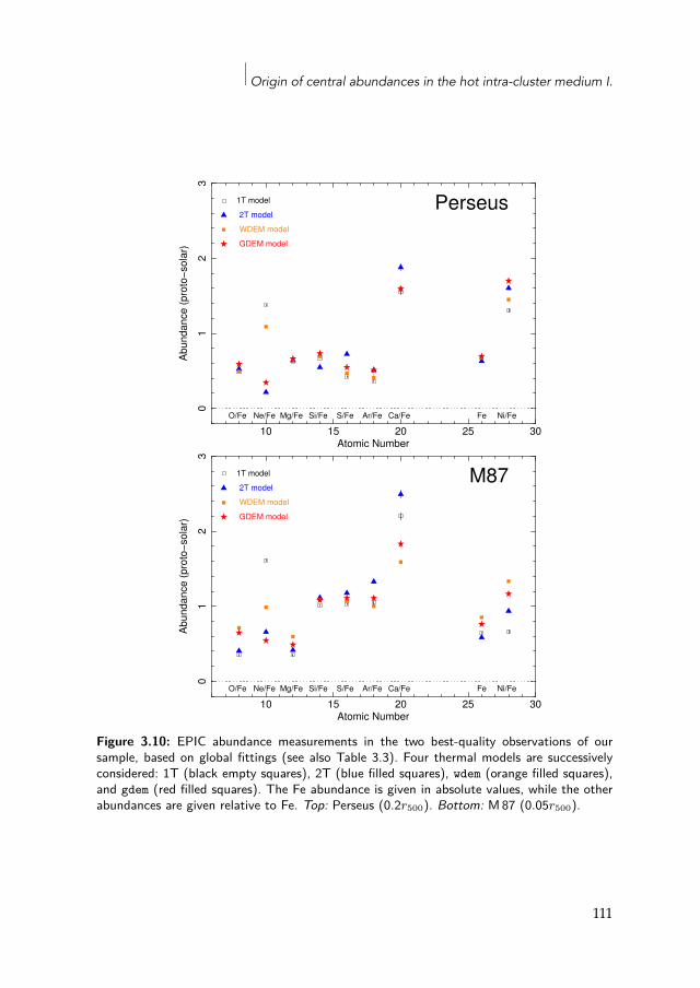
Origin of central abundances in the hot intra-cluster medium I.
10 15 20 25 30
01
23
Ab
un
da
nce
(p
roto
!so
lar)
Atomic Number
O/Fe Ne/Fe Mg/Fe Si/Fe S/Fe Ar/Fe Ca/Fe Fe Ni/Fe
1T model
2T model
WDEM model
GDEM model
Perseus
10 15 20 25 30
01
23
Ab
un
da
nce
(p
roto
!so
lar)
Atomic Number
O/Fe Ne/Fe Mg/Fe Si/Fe S/Fe Ar/Fe Ca/Fe Fe Ni/Fe
1T model
2T model
WDEM model
GDEM model
M87
Figure 3.10: EPIC abundance measurements in the two best-quality observations of oursample, based on global fittings (see also Table 3.3). Four thermal models are successivelyconsidered: 1T (black empty squares), 2T (blue filled squares), wdem (orange filled squares),and gdem (red filled squares). The Fe abundance is given in absolute values, while the otherabundances are given relative to Fe. Top: Perseus (0.2r500). Bottom: M 87 (0.05r500).
111
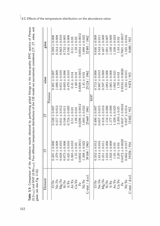
3.C Effects of the temperature distribution on the abundance ratios
Tabl
e3.
3:Co
mpa
rison
ofth
eab
unda
nce
resu
ltsob
tain
edby
perfo
rmin
ggl
obal
fittin
gsto
the
best
-qua
lity
EPIC
spec
traof
Pers
eus
(0.2
r 500
)and
M87
(0.0
5r50
0).
Four
diffe
rent
tem
pera
ture
dist
ribut
ions
ofth
eCI
Em
odel
are
succ
essiv
elyco
nsid
ered
(1T,
2T,w
dem,
and
gdem
;see
also
Fig.
3.10
).
Elem
ent
1T2T
wdem
gdem
Perse
usO/
Fe0.
491
±0.
006
0.52
6±
0.00
70.
491
±0.
007
0.58
9±
0.00
6Ne/Fe
1.37
9±
0.00
80.
217
±0.
012
1.09
0±
0.00
90.
344
±0.
008
Mg/Fe
0.62
8±
0.01
00.
641
±0.
012
0.65
1±
0.01
00.
663
±0.
010
Si/Fe
0.67
3±
0.00
60.
548
±0.
011
0.69
3±
0.00
60.
732
±0.
005
S/Fe
0.42
5±
0.01
60.
724
±0.
005
0.47
0±
0.01
00.
546
±0.
008
Ar/Fe
0.36
5±
0.01
00.
51±
0.03
0.41
±0.
040.
51±
0.03
Ca/Fe
1.55
±0.
031.
88±
0.04
1.60
±0.
031.
59±
0.03
Fe0.
6802
±0.
0011
0.62
96±
0.00
120.
6808
±0.
0015
0.69
34±
0.00
12Ni/Fe
1.30
8±
0.02
21.
603
±0.
024
1.45
±0.
031.
698
±0.
022
C-sta
t/d.o.f.
39168/
1963
25669/
1961
25124/
1962
32481/
1962
M87
O/Fe
0.35
2±
0.01
20.
406
±0.
007
0.71
3±
0.00
80.
646
±0.
009
Ne/Fe
1.61
4±
0.01
60.
657
±0.
015
0.98
7±
0.01
30.
543
±0.
011
Mg/Fe
0.35
1±
0.01
10.
416
±0.
010
0.59
7±
0.00
90.
487
±0.
009
Si/Fe
1.01
6±
0.00
61.
116
±0.
006
1.08
4±
0.00
61.
081
±0.
007
S/Fe
1.03
2±
0.00
91.
177
±0.
009
1.06
5±
0.00
81.
109
±0.
009
Ar/Fe
1.05
±0.
031.
329
±0.
025
1.00
2±
0.02
11.
108
±0.
023
Ca/Fe
2.20
±0.
042.
493
±0.
051.
59±
0.03
1.83
±0.
04Fe
0.64
72±
0.00
200.
5847
±0.
0016
0.85
32±
0.00
200.
7601
±0.
0017
Ni/Fe
0.66
2±
0.01
70.
937
±0.
014
1.33
4±
0.01
51.
165
±0.
016
C-sta
t/d.o.f.
19034/
914
13602/
912
9474
/913
8680
/913
112
Origin of central abundances in the hot intra-cluster medium I.
Despite these considerations, and the fact that the real temperature dis-tributions in the ICM is unknown, considering a continuous distribution isclearly more realistic than only one or two unique temperatures. By com-paring only the gdem and wdem models, we note that they give very similarabundance ratios for both Perseus and M87. Except for Ne/Fe, the largestdifference is found for Ni/Fe, and is clearly smaller than the range of sys-tematic uncertainties affecting the measurements. Therefore, using a wdemmodel instead of a gdem model should have a limited impact on our EPICfinal results. For comparison, de Plaa et al. (2017) find that such an effecton the O/Fe ratio derived from RGS is always smaller than 20%. There-fore, considering further uncertainties related to the thermal models is notnecessary for the purpose of this work.
3.D Best-fit temperature and abundancesIn Table 3.4we present the full results of our best-fit parameters (kT , σT , theabsolute Fe abundance, and the abundance ratios of O/Fe, Ne/Fe, Mg/Fe,Si/Fe, S/Fe, Ar/Fe, Ca/Fe, andNi/Fe) for each object of the CHEERS sam-ple, within a radius of 0.05r500. When possible (hot clusters), we indicatethe parameters extracted from 0.2r500 as well. The O/Fe and Ne/Fe abun-dances have been corrected from updated RR calculations, as described inAppendix 3.B.
113
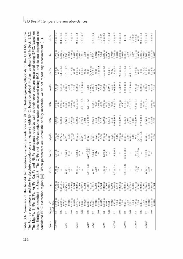
3.D Best-fit temperature and abundancesTa
ble
3.4:
Sum
mar
yof
the
best
-fit
tem
pera
ture
s,σ
Tan
dab
unda
nces
for
allt
heclu
ster
s/gr
oups
/elli
ptica
lsof
the
CHEE
RSsa
mpl
e.Th
ek
T,σ
Tpa
ram
eter
san
dth
eFe
abso
lute
abun
danc
ear
em
easu
red
with
EPIC
,bas
edon
glob
alfit
tings
,as
desc
ribed
inSe
ct.3
.3.2
.Th
eM
g/Fe
,Si/
Fe,S
/Fe,
Ar/F
e,Ca
/Fe
and
Ni/F
eab
unda
nce
ratio
sas
well
asth
eirer
ror
bars
are
mea
sure
dus
ing
EPIC
,bas
edon
loca
lfitt
ings
,as
desc
ribed
inSe
ct.3
.3.3
.The
O/F
ean
dNe
/Fe
abun
danc
era
tios
are
mea
sure
dus
ing
RGS,
and
dono
tde
pend
onth
eco
nsid
ered
EPIC
extra
ctio
nre
gion
(=).
Whe
npa
ram
eter
sar
eun
real
istic
orfu
llyun
certa
in,w
edo
notr
epor
tany
mea
sure
men
t(−
).
Source
Region
kT
σT
O/Fe
Ne/Fe
Mg/Fe
Si/Fe
S/Fe
Ar/Fe
Ca/Fe
FeNi/Fe
(r50
0)(keV)
2A0335
0.22.
661
±0.
004
0.24
33±
0.00
130.
88±
0.09
0.97
±0.
140.
69±
0.15
0.82
±0.
100.
83±
0.14
0.87
±0.
271.
04±
0.25
0.76
5±
0.00
42.
0±
1.0
0.05
2.26
5±
0.00
50.
2116
±0.
0014
==
0.72
±0.
200.
83±
0.10
0.96
±0.
151.
01±
0.26
1.1
±0.
30.
882
±0.
007
3.4
±1.
6
A85
0.25.
715
±0.
018
0.35
4±
0.00
30.
80±
0.11
0.80
±0.
160.
76±
0.06
0.76
±0.
180.
92±
0.06
0.98
±0.
131.
0±
0.6
0.73
3±
0.00
61.
7±
1.2
0.05
4.43
2±
0.02
00.
300
±0.
004
==
0.74
±0.
070.
84±
0.20
0.98
±0.
061.
01±
0.15
1.10
±0.
171.
028
±0.
011
1.7
±1.
1
A133
0.23.
476
±0.
021
0.26
9±
0.00
40.
86±
0.13
0.83
±0.
180.
57±
0.07
0.82
±0.
120.
8±
0.4
0.90
±0.
161.
25±
0.19
0.90
1±
0.01
32.
1±
1.4
0.05
2.70
4±
0.02
00.
227
±0.
004
==
0.65
±0.
080.
89±
0.04
0.9
±0.
31.
1±
0.5
1.21
±0.
221.
29±
0.03
1.8
±0.
8
A189
0.05
1.02
0±
0.02
10.
178
±0.
016
0.7
±0.
30.
27+
0.44
−0.
210.
42±
0.23
1.4
±0.
70.
7±
0.4
0.08
(<0.
62)
0.14
(<1.
44)
0.88
±0.
13−
A262
0.22.
264
±0.
013
0.19
2±
0.00
30.
76±
0.10
0.93
±0.
220.
94±
0.21
0.93
±0.
110.
95±
0.07
0.85
±0.
131.
27±
0.18
0.72
6±
0.01
22.
6±
2.4
0.05
1.95
7±
0.01
50.
188
±0.
004
==
0.59
±0.
080.
95±
0.15
1.01
±0.
090.
87±
0.16
1.2
±0.
81.
08±
0.03
0.9
(<2.
8)A496
0.23.
754
±0.
012
0.27
3±
0.00
31.
03±
0.12
1.16
±0.
200.
86±
0.20
0.90
±0.
130.
96±
0.05
0.90
±0.
101.
0±
0.4
0.72
9±
0.00
61.
3±
0.3
0.05
3.00
7±
0.01
20.
229
±0.
003
==
0.82
±0.
250.
94±
0.13
1.03
±0.
050.
97±
0.11
1.04
±0.
120.
947
±0.
010
1.6
±0.
4
A1795
0.25.
15±
0.04
0.31
8±
0.01
31.
7±
0.4
1.5
±0.
40.
63±
0.15
0.6
±0.
41.
1±
0.6
1.0
±0.
31.
4±
0.4
0.58
1±
0.01
02.
1±
0.6
0.05
4.18
±0.
040.
298
±0.
013
==
0.65
±0.
180.
8±
0.5
0.99
±0.
171.
4±
0.4
0.7
±0.
50.
683
±0.
018
3.5
±1.
1
A1991
0.22.
28±
0.03
0.20
2±
0.00
70.
9±
0.3
0.5
±0.
30.
66±
0.15
0.85
±0.
071.
18±
0.20
1.2
±0.
31.
6±
0.4
0.80
±0.
034
±3
0.05
2.00
±0.
040.
205
±0.
009
==
0.68
±0.
190.
81±
0.09
1.3
±0.
31.
2±
0.4
0.7
±0.
51.
14±
0.07
0.6
(<2.
9)A2029
0.27.
48±
0.04
0.30
1±
0.00
61.
70±
0.25
0.17
(<0.
59)
0.5
(<0.
9)0.
5±
0.3
0.8
±0.
30.
41±
0.16
0.96
±0.
200.
710
±0.
006
1.58
±0.
220.0
56.
44±
0 .04
0.29
2±
0 .00
9=
=0.
7±
0.5
0.7
±0.
30.
67±
0 .09
0.39
±0 .
200.
8( <
1 .5)
0.88
5±
0 .01
22.
1±
1.1
A2052
0.22.
931
±0.
012
0.24
4±
0.00
30.
84±
0.09
0.82
±0.
160.
57±
0.06
0.86
±0.
110.
8±
0.4
0.75
±0.
131.
15±
0.16
0.70
2±
0.00
82.
6±
0.7
0.05
2.55
4±
0.01
60.
234
±0.
004
==
0.57
±0.
080.
92±
0.22
0.95
±0.
090.
91±
0.18
1.28
±0.
240.
917
±0.
017
1.1
±0.
9
114
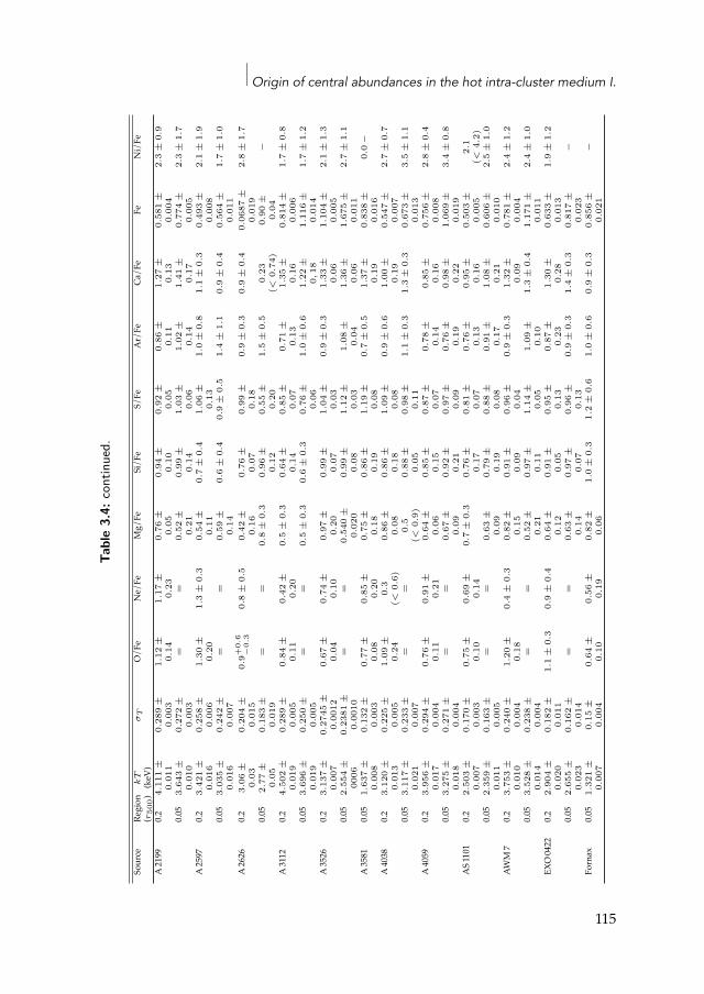
Origin of central abundances in the hot intra-cluster medium I.
Tabl
e3.
4:co
ntin
ued.
Source
Region
kT
σT
O/Fe
Ne/Fe
Mg/Fe
Si/Fe
S/Fe
Ar/Fe
Ca/Fe
FeNi/Fe
(r50
0)(keV)
A2199
0.24.
111
±0.
011
0.28
9±
0.00
31.
12±
0.14
1.17
±0.
230.
76±
0.05
0.94
±0.
100.
92±
0.05
0.86
±0.
111.
27±
0.13
0.58
1±
0.00
42.
3±
0.9
0.05
3.64
3±
0.01
00.
272
±0.
003
==
0.52
±0.
210.
99±
0.14
1.03
±0.
061.
02±
0.14
1.41
±0.
170.
774
±0.
005
2.3
±1.
7
A2597
0.23.
421
±0.
016
0.25
8±
0.00
61.
30±
0.20
1.3
±0.
30.
54±
0.11
0.7
±0.
41.
06±
0.13
1.0
±0.
81.
1±
0.3
0.49
3±
0.00
82.
1±
1.9
0.05
3.03
5±
0.01
60.
242
±0.
007
==
0.59
±0.
140.
6±
0.4
0.9
±0.
51.
4±
1.1
0.9
±0.
40.
564
±0.
011
1.7
±1.
0
A2626
0.23.
06±
0.03
0.20
4±
0.01
50.
9+0.
6−
0.3
0.8
±0.
50.
42±
0.16
0.76
±0.
070.
99±
0.18
0.9
±0.
30.
9±
0.4
0.06
87±
0.01
92.
8±
1.7
0.05
2.77
±0.
050.
183
±0.
019
==
0.8
±0.
30.
96±
0.12
0.55
±0.
201.
5±
0.5
0.23
(<0.
74)
0.90
±0.
04−
A3112
0.24.
502
±0.
019
0.28
9±
0.00
50.
84±
0.11
0.42
±0.
200.
5±
0.3
0.64
±0.
140.
85±
0.07
0.71
±0.
131.
35±
0.16
0.81
4±
0.00
61.
7±
0.8
0.05
3.69
6±
0.01
90.
250
±0.
005
==
0.5
±0.
30.
6±
0.3
0.76
±0.
061.
0±
0.6
1.22
±0,
181.
116
±0.
014
1.7
±1.
2
A3526
0.23.
137
±0.
007
0.27
45±
0.00
120.
67±
0.04
0.74
±0.
100.
97±
0.20
0.99
±0.
071.
04±
0.03
0.9
±0.
31.
33±
0.06
1.10
4±
0.00
52.
1±
1.3
0.05
2.55
4±
0006
0.23
81±
0.00
10=
=0.
540
±0.
020
0.99
±0.
081.
12±
0.03
1.08
±0.
041.
36±
0.06
1.67
5±
0.01
12.
7±
1.1
A3581
0.05
1.63
7±
0.00
80.
132
±0.
003
0.77
±0.
080.
85±
0.20
0.75
±0.
180.
86±
0.19
1.19
±0.
080.
7±
0.5
1.37
±0.
190.
838
±0.
016
0.0
−
A4038
0.23.
120
±0.
013
0.22
5±
0.00
51.
09±
0.24
0.3
(<0.
6)0.
86±
0.08
0.86
±0.
181.
09±
0.08
0.9
±0.
61.
00±
0.19
0.54
7±
0.00
72.
7±
0.7
0.05
3.11
7±
0.02
10.
233
±0.
007
==
0.5
(<0.
9)0.
88±
0.05
0.98
±0.
111.
1±
0.3
1.3
±0.
30.
673
±0.
013
3.5
±1.
1
A4059
0.23.
956
±0.
017
0.29
4±
0.00
40.
76±
0.11
0.91
±0.
210.
64±
0.06
0.85
±0.
150.
87±
0.07
0.78
±0.
140.
85±
0.16
0.75
6±
0.00
82.
8±
0.4
0.05
3.27
5±
0.01
80.
271
±0.
004
==
0.67
±0.
090.
92±
0.21
0.97
±0.
090.
76±
0.19
0.98
±0.
221.
069
±0.
019
3.4
±0.
8
AS1101
0.22.
503
±0.
007
0.17
0±
0.00
30.
75±
0.10
0.69
±0.
140.
7±
0.3
0.76
±0.
170.
81±
0.07
0.76
±0.
130.
95±
0.16
0.50
3±
0.00
52.
1(<
4.2)
0.05
2.35
9±
0.01
10.
163
±0.
005
==
0.63
±0.
090.
79±
0.19
0.88
±0.
080.
91±
0.17
1.08
±0.
210.
606
±0.
010
2.5
±1.
0
AWM7
0.23.
753
±0.
010
0.24
0±
0.00
41.
20±
0.18
0.4
±0.
30.
82±
0.15
0.91
±0.
090.
96±
0.04
0.9
±0.
31.
32±
0.09
0.78
1±
0.00
42.
4±
1.2
0.05
3.52
8±
0.01
40.
238
±0.
004
==
0.52
±0.
210.
97±
0.11
1.14
±0.
051.
09±
0.10
1.3
±0.
41.
171
±0.
011
2.4
±1.
0
EXO0422
0.22.
904
±0.
020
0.18
2±
0.01
11.
1±
0.3
0.9
±0.
40.
64±
0.12
0.91
±0.
050.
95±
0.13
0.87
±0.
231.
30±
0.28
0.63
3±
0.01
31.
9±
1.2
0.05
2.65
5±
0.02
30.
162
±0.
014
==
0.63
±0.
140.
97±
0.07
0.96
±0.
130.
9±
0.3
1.4
±0.
30.
817
±0.
023
−
Fornax
0.05
1.32
1±
0.00
70.
15±
0.00
40.
64±
0.10
0.56
±0.
190.
82±
0.06
1.0
±0.
31.
2±
0.6
1.0
±0.
60.
9±
0.3
0.85
6±
0.02
1−
115
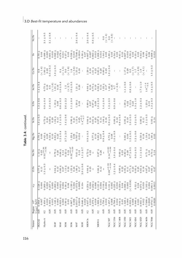
3.D Best-fit temperature and abundancesTa
ble
3.4:
cont
inue
d.
Source
Region
kT
σT
O/Fe
Ne/Fe
Mg/Fe
Si/Fe
S/Fe
Ar/Fe
Ca/Fe
FeNi/Fe
(r50
0)(keV)
HCG
620.0
50.
958
±0.
007
0.12
8±
0.00
40.
77±
0.11
1.14
±0.
230.
79±
0.09
1.0
±0.
31.
3±
0.6
1.4
±0.
40.
8(<
1.6)
0.70
±0.
04−
HydraA
0.23.
450
±0.
010
0.26
9±
0.00
31.
3±
0.3
0.53
+0.
26−
0.06
0.42
±0.
090.
72±
0.24
0.9
±0.
40.
75±
0.18
1.00
±0.
220.
488
±0.
005
2.1
±0.
5
0.05
3.30
3±
0.01
50.
257
±0.
005
==
0.33
±0.
100.
69±
0.29
1.0
±0.
30.
9(<
1.6)
0.5
±0.
30.
601
±0.
010
3.1
±0.
8
M49
0.05
1.14
8±
0.00
40.
269
±0.
003
0.64
±0.
100.
78±
0.20
0.83
±0.
231.
04±
0.13
1.18
±0.
091.
01±
0.16
1.0
±0.
30.
928
±0.
022
−
M60
0.05
0.92
3±
0.00
30.
042
±0.
004
0.66
±0.
070.
66±
0.13
1.2
±0.
41.
1±
0.3
0.8
±0.
31.
0±
0.4
0.4
(<1.
5)0.
478
±0.
011
−
M84
0.05
0.99
±0.
030.
36±
0.06
1.13
±0.
240.
22±
0.18
2.7
±2.
01.
4±
0.6
2.6
±2.
21.
3(<
2.7)
0.0
(<1.
8)0.
37±
0.03
−
M86
0.05
0.96
7±
0.00
60.
120
±0.
004
1.23
±0.
240.
32+
0.47
−0.
091.
22±
0.08
0.96
±0.
211.
1±
0.4
1.0
±0.
31.
8(<
3.6)
0.53
8±
0.01
9−
M87
0.05
2.05
17±
0.00
180.
1572
±0.
0005
1.06
±0.
170.
61±
0.12
0.70
7±
0.01
41.
13±
0.05
1.30
±0.
161.
21±
0.20
1.55
±0.
160.
7546
±0.
0014
2.6
±0.
4
M89
0.05
0.64
6±
0.01
80.
10∗
2.0
±0.
61.
1±
0.7
−1.
4+5.
3−
0.7
−−
−0.
30±
0.07
−
MKW
3s0.2
3.63
7±
0.01
30.
254
±0.
004
0.84
±0.
230.
72±
0.22
0.9
±0.
30.
84±
0.18
0.89
±0.
070.
84±
0.16
1.29
±0.
180.
607
±0.
007
2.0
±0.
4
0.05
3.37
9±
0.01
80.
232
±0.
006
==
0.77
±0.
100.
81±
0.25
0.97
±0.
090.
75±
0.19
1.01
±0.
230.
863
±0.
013
0.9
±0.
5
MKW
40.2
1.90
9±
0.01
10.
121
±0.
004
0.66
±0.
120.
87±
0.26
0.69
±0.
070.
97±
0.14
1.0
±0.
30.
92±
0.14
0.85
±0.
201.
008
±0.
013
−
0.05
1.75
6±
0.01
20.
116
±0.
004
==
0.9
±0.
41.
04±
0.16
1.4
±0.
41.
22±
0.17
0.89
±0.
231.
64±
0.03
0.0
(<1.
4)NGC
507
0.05
1.25
7±
0.00
80.
131
±0.
005
0.69
+0.
39−
0.18
0.14
+0.
60−
0.06
0.73
±0.
080.
9±
0.3
1.3
±0.
51.
46±
0.25
1.0
±0.
40.
89±
0.03
0.0
(<3.
0)NGC
1316
0.05
0.76
8±
0.01
20.
235
±0.
016
1.2
±0.
41.
0±
0.4
1.0
±0.
90.
66±
0.12
0.9
±0.
60.
7(<
2.3)
−0.
34±
0.03
−
NGC
1404
0.05
0.64
±0.
030.
359
±0.
040.
89±
0.22
0.60
±0.
23−
0.8
±0.
4−
−−
0.61
±0.
10−
NGC
1550
0.05
1.32
8±
0.00
40.
088
±0.
003
0.95
±0.
110.
80±
0.20
0.68
±0.
040.
95±
0.19
1.09
±0.
221.
1±
0.6
1.17
±0.
200.
607
±0.
010
−
NGC
3411
0.05
0.93
3±
0.00
6(<
0.01
8)0.
71±
0.23
0.7
±0.
51.
3±
0.5
1.0
±0.
31.
13±
0.23
0.8
±0.
60.
0(<
1.7)
0.59
±0.
03−
NGC
4261
0.05
0.94
0±
0.02
10.
32±
0.04
0.95
±0.
250.
9±
0.3
1.2
±0.
61.
2±
0.5
1.3
±1.
0−
1.7
(<4.
9)0.
35±
0.03
−
NGC
4325
0.05
0.93
1±
0.01
20.
071
±0.
010
0.65
±0.
181.
1±
0.4
0.50
±0.
160.
80±
0.11
1.2
±0.
41.
7±
1.0
1.9
(<4.
1)0.
64±
0.06
−
NGC
4636
0.05
0.74
98±
0.00
250.
103
±0.
004
0.87
±0.
070.
71±
0.10
1.19
±0.
101.
1±
0.3
1.23
±0.
151.
6+1.
6−
0.6
−0.
82±
0.06
−
NGC
5044
0.05
0.97
41±
0.00
200.
0811
±0.
0011
0.85
±0.
070.
74±
0.14
1.00
±0.
030.
93±
0.14
1.3
±0.
31.
4±
0.5
1.5
±0.
30.
668
±0.
010
−
116
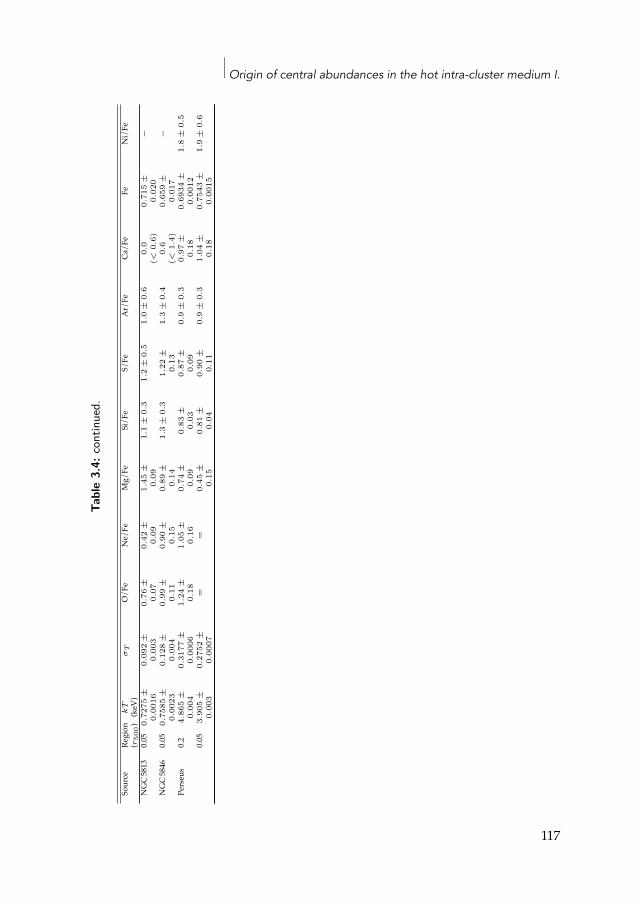
Origin of central abundances in the hot intra-cluster medium I.
Tabl
e3.
4:co
ntin
ued.
Source
Region
kT
σT
O/Fe
Ne/Fe
Mg/Fe
Si/Fe
S/Fe
Ar/Fe
Ca/Fe
FeNi/Fe
(r50
0)(keV)
NGC
5813
0.05
0.72
75±
0.00
160.
092
±0.
003
0.76
±0.
070.
42±
0.09
1.45
±0.
091.
1±
0.3
1.2
±0.
51.
0±
0.6
0.0
(<0.
6)0.
715
±0.
020
−
NGC
5846
0.05
0.75
85±
0.00
230.
128
±0.
004
0.99
±0.
110.
90±
0.15
0.89
±0.
141.
3±
0.3
1.22
±0.
131.
3±
0.4
0.6
(<1.
4)0.
659
±0.
017
−
Perse
us0.2
4.86
5±
0.00
40.
3177
±0.
0006
1.24
±0.
181.
05±
0.16
0.74
±0.
090.
83±
0.03
0.87
±0.
090.
9±
0.3
0.97
±0.
180.
6934
±0.
0012
1.8
±0.
5
0.05
3.90
5±
0.00
30.
2752
±0.
0007
==
0.45
±0.
150.
81±
0.04
0.90
±0.
110.
9±
0.3
1.04
±0.
180.
7543
±0.
0015
1.9
±0.
6
117

L’Univers est ce qu’il est. Il n’a que faire de nos préjugés.
The Universe is what it is. It does not care about our preconceptions.
– Hubert Reeves, Patience dans l’azur
4|Origin of central abundances inthe hot intra-cluster mediumII. Chemical enrichment and supernova yieldmodels
F. Mernier, J. de Plaa, C. Pinto, J. S. Kaastra, P. Kosec, Y.-Y. Zhang, J. Mao,N. Werner, O. R. Pols, and J. Vink
(Astronomy & Astrophysics, Volume 595, id.A126, 19 pp.)
Abstract
The hot intra-cluster medium (ICM) is rich in metals, which are synthesised bysupernovae (SNe) and accumulate over time into the deep gravitational potentialwell of clusters of galaxies. Sincemost of the elements visible in X-rays are formedby type Ia (SNIa) and/or core-collapse (SNcc) supernovae, measuring their abun-dances gives us direct information on the nucleosynthesis products of billions ofSNe since the epoch of the star formation peak (z ∼ 2–3). In this study,we comparethe most accurate average X/Fe abundance ratios (compiled in a previous workfromXMM-Newton EPIC and RGS observations of 44 galaxy clusters, groups, andellipticals), representative of the chemical enrichment in the nearby ICM, to var-ious SNIa and SNcc nucleosynthesis models found in the literature. The use ofa SNcc model combined to any favoured standard SNIa model (deflagration ordelayed-detonation) fails to reproduce our abundance pattern. In particular, theCa/Fe andNi/Fe ratios are significantly underestimated by the models. We showthat the Ca/Fe ratio can be reproduced better, either by taking a SNIa delayed-detonationmodel that matches the observations of the Tycho supernova remnant,or by adding a contribution from the “Ca-rich gap transient” SNe, whose mate-rial should easily mix into the hot ICM. On the other hand, the Ni/Fe ratio canbe reproduced better by assuming that both deflagration and delayed-detonationSNIa contribute in similar proportions to the ICM enrichment. In either case, the
119
4.1 Introduction
fraction of SNIa over the total number of SNe (SNIa+SNcc) contributing to theICM enrichment ranges within 29–45%. This fraction is found to be systemati-cally higher than the corresponding SNIa/(SNIa+SNcc) fraction contributing tothe enrichment of the proto-solar environnement (15–25%). We also discuss andquantify two useful constraints on both SNIa (i.e. the initial metallicity on SNIaprogenitors and the fraction of low-mass stars that result in SNIa) and SNcc (i.e.the effect of the IMF and the possible contribution of pair-instability SNe to theenrichment) that can be inferred from the ICM abundance ratios. Finally, we showthat detonative sub-Chandrasekhar WD explosions (resulting, for example, fromviolentWDmergers) cannot be a dominant channel for SNIa progenitors in galaxyclusters.
4.1 IntroductionSince the emergence and progress of stellar nucleosynthesis models overthe past century, it is now well known that all the heavy elements in theUniverse (i.e. except H, He, and traces of Li and Be, which were producedshortly after the Big Bang) have been produced by stars and stellar rem-nants (Cameron 1957b; Burbidge et al. 1957). In particular, α- and Fe-peakelements (8 ⩽ Z ⩽ 28) are mostly synthesised by nuclear fusion reactionsduring stellar lifetimes and supernova (SN) explosions, and are then re-leased into and beyond the interstellar medium (e.g. Arnett 1973; Tinsley1980). On the one hand, oxygen (O), neon (Ne), magnesium (Mg), silicon(Si), and sulfur (S), are thought to be mostly produced by core-collapse su-pernovae (SNcc). On the other hand, Type Ia supernovae (SNIa) producepredominantly argon (Ar), calcium (Ca), chromium (Cr), manganese (Mn),iron (Fe), and nickel (Ni). Finally, when low-mass stars (<6 M⊙) leave themain sequence and enter into their asymptotic giant branch (AGB) phase,they are efficient in releasing lighter metals, such as carbon (C) or nitrogen(N), via powerful winds. Although this general picture of synthesis (andrecycling) of metals through cosmic ages is now well established, manyissues are still unsolved and still bring a great deal of uncertainty whenidentifying the specific origins of each element.
First, it is well known that SNcc result from the end-of-life explosionof massive stars (∼10–140 M⊙). However, several parameters, such as themass cut that separates the collapsing core from the supernova remnant(SNR) or the final kinetic energy of the explosion, are poorly constrained.Consequently, some differences in the predicted abundance pattern fromproposed SNcc models proposed by different groups still remain (for a re-
120
Origin of central abundances in the hot intra-cluster medium II.
view, see Nomoto et al. 2013). Moreover, the relative amount of unburnedelements depends on the initial mass and metallicity of the progenitor star(e.g. Woosley & Weaver 1995). These two parameters are not always easyto constrain, especially when considering a whole population of (massive)stars, whereas the universality of the initial mass function (IMF) is still un-der debate (e.g. Treu et al. 2010; Dutton et al. 2012).
Second, despite their fundamental role both in the Galactic chemicalevolution (e.g. Timmes et al. 1995; Kobayashi & Nomoto 2009) and as stan-dard candles for cosmological distances (Riess et al. 1998; Schmidt et al.1998), the nature of SNIa progenitors is still elusive (for reviews, see How-ell 2011; Maoz & Mannucci 2012; Hillebrandt et al. 2013; Maoz et al. 2014).It seems likely that the explosion results from an accreting carbon-oxygenwhite dwarf (WD),which ignites shortly before reaching its Chandrasekharmass. However, it is not clear whether the mass transfer is due to a normalstellar companion (single degenerate scenario; Whelan & Iben 1973) or asecondwhite dwarf (double degenerate scenario;Webbink 1984; Iben&Tu-tukov 1984). Furthermore, the physics of the SNIa explosion itself is poorlyconstrained (for a review, see Hillebrandt &Niemeyer 2000). In most mod-els, the explosion starts with a deflagration (i.e. the burning front propa-gates subsonically). The currently favoured explosion models suggest thatwhen the burning front reaches a certain critical density, it propagates su-personically, and the deflagration becomes a detonation. These so-calleddelayed-detonation models (Khokhlov 1989), in particular their variant ofdeflagration-to-detonation transition (DDT), have been studied in detail(Khokhlov 1991; Niemeyer & Woosley 1997; Gamezo et al. 2005; Seiten-zahl et al. 2013b, e.g.), but not yet fully understood. Moreover, some pecu-liar SNIa (e.g. the 2002cx supernovae, Kromer et al. 2013) seem to be betterexplained by invoking a pure deflagration explosion (Branch et al. 2004;Jha et al. 2006; Phillips et al. 2007). What is clear, however, is that the abun-dance pattern of the elements synthesised by SNIa is very sensitive to theirexplosion mechanism.
Many attempts to constrain all these SNcc and SNIa uncertainties havebeenmade by studying the optical and X-ray spectra of SNRs and, particu-larly, their abundance pattern (e.g. Badenes et al. 2006; Yasumi et al. 2014).However, such an approach is difficult in practice, mostly because only afewGalactic SNRs are suitable for studying the composition of their ejecta,preventing any statistical study over large samples; the emitting plasmaof the SNRs is far from being in ionisation equilibrium, making its spec-
121
4.1 Introduction
troscopy complicated and not yet fully understood; and the ejected ma-terial from the SNR easily mixes with the surrounding ISM, making it achallenge to correctly estimate the metal abundances from the SN itself.
An interesting alternative approach to investigating nucleosynthesisproducts from supernovae (SNe) is to consider the chemical enrichmentat the scale of galaxy clusters. In fact, the hot intra-cluster medium (ICM)pervading the volume of galaxy clusters and groups, and accounting forno less than ∼80% of their total baryonic matter, is rich in α- and Fe peakelements (for reviews, see Werner et al. 2008; Böhringer & Werner 2010).These metals, which can be observed via their emission lines from X-rayspectroscopy, must have been synthesised by SNIa and SNcc inside thecluster galaxies, and have enriched the ICM, especially around z ≃ 2–3,during the major cosmic epoch of star formation (Hopkins & Beacom 2006;Madau & Dickinson 2014). Assuming that the large gravitational potentialwell of clusters/groups make them behave like a closed-box system, themetal abundances of the ICM are a remarkable signature of the yields ofbillions of SNIa and SNcc over time. Moreover, the ICM is well known tobe in (or very close to) collisional ionisation equilibrium state, making itsspectroscopy less complex than SN spectra and its abundances relativelyeasy to derive.
Several previous studies have already attempted to use abundancemea-surements in the ICM in order to constrain SNIa and SNcc yield mod-els. For instance, de Plaa et al. (2007) compiled a sample of 22 cool-coreclusters, and found that the standard SNIa models fail to reproduce theAr/Ca and Ca/Fe abundance ratios. They also showed that the fractionof SNIa over the total number of SNe highly depends of the consideredmodels. De Grandi & Molendi (2009) showed that Si/Fe abundance ratiosare remarkably uniform over a sample of 26 cool-core clusters observedwith XMM-Newton, arguing for a similar enrichment process within clus-ter cores. However, they concluded that systematic uncertainties betweenthe SN models are too large to precisely estimate the relative contributionof SNIa and SNcc. Finally, many abundance studies have been performedon individual objects as well (e.g. Werner et al. 2006b; de Plaa et al. 2006;Sato et al. 2007a; Simionescu et al. 2009b, Chapter 2). From these studies,and considering the instrumental performance of current X-ray observa-tories, it appears that higher quality data (i.e. with longer exposure time),collected over larger samples, are needed to clarify the picture of the pre-
122
Origin of central abundances in the hot intra-cluster medium II.
cise origin of metals in the ICM.In this paper, we make use of ICM abundances measured in two previ-
ous works (Chapter 3; de Plaa et al. 2017) and compare them with predic-tions from theoretical SNIa and SNcc yield models. These measurementsconsist of the averageX/Fe abundance ratios of ten elements (O/Fe,Ne/Fe,Mg/Fe, Si/Fe, S/Fe, Ar/Fe, Ca/Fe, Cr/Fe, Mn/Fe, and Ni/Fe) in the ICMof 44 cool-core clusters, groups, and ellipticals, using the XMM-NewtonEPIC and RGS instruments. To our knowledge, this is the most completeand robust abundance pattern measured in the ICM available to date.
This paper is structured as follows. In Sect. 4.2 we present the sampleand briefly recall the data reduction, as well as the spectral analysis usedto derive the abundance ratios. We then discuss the comparison betweenvarious SNIa and SNcc models and our average ICM abundance pattern(Sect. 4.3) on the one hand, and the proto-solar abundances (Sect. 4.4) onthe other hand. Section 4.5 summarises our discussion and addresses fu-ture prospects. Throughout this paperwe assume cosmological parametersof H0 = 70 km s−1 Mpc−1, Ωm = 0.3, and ΩΛ = 0.7. The abundances pre-sented in this paper are taken relative to the proto-solar values of Lodderset al. (2009). All the error bars are given at a 68% confidence level.
4.2 Observations and spectral analysisWe start by briefly summarising the main steps of the data reduction andthe spectral analysis thatwere necessary to provide the averageX/Fe abun-dance pattern (Fig. 4.1), representative of the ICM of cool-core objects. Thedetailed presentation, reduction, and spectral analysis of our observationscan be found in Chapter 3 and in de Plaa et al. (2017).
Our sample consists of the CHEERS1 catalogue (de Plaa et al. 2017), andis detailed in Table 3.1 (see also Pinto et al. 2015; de Plaa et al. 2017). It in-cludes 44 nearby (z < 0.1) cool-core clusters, groups, and elliptical galaxiesfor which the OVIII 1s–2p line at 19 is detected by the RGS instrumentwith >5σ. Recent XMM-Newton observations (AO-12, PI: de Plaa) havebeen combined with archival data. We reduced the EPIC and RGS datausing the XMM-Newton Science Analysis System (SAS) software v14.0.0.After having filtered them from solar-flare events, we obtain cleaned EPICMOS1, MOS2, and pn data of ∼4.5, ∼4.6, and ∼3.7 Ms, respectively.
1CHEmical Enrichment Rgs Sample
123
4.3 Chemical enrichment in the ICM
The EPIC spectra were extracted within a circle of a radius of either0.2r500 (for kTmean > 1.7 keV, i.e. the farther clusters) or 0.05R500 (for kTmean< 1.7 keV, i.e. the nearer groups/ellipticals). The RGS spectra were ex-tracted with a cross-dispersion width of 0.8′. We carefully checked that thedifference in these EPIC and RGS extraction regions did not affect our finalresults (Chapter 3).
We used the SPEX fitting package (Kaastra et al. 1996) v2.05 to performour spectral fits. The EPIC and RGS spectra were fitted with a gdem and a2T (i.e. cie+cie) thermalmodel, respectively. The EPIC (X-ray andparticle)background components were carefully modelled following the methoddetailed in Chapter 2. The free parameters in our fits were the emissionmeasure (or normalisation), the temperature parameters (kTmean and σT
for a gdem model; kTup and kTlow for a 2T model), and the abundances ofO, Ne, Mg, Si, S, Ar, Ca, Fe, and Ni for EPIC, and O, Ne, Mg, and Fe forRGS.Wewere also able to constrain the EPIC sample-averaged abundancesof Cr and Mn by converting the equivalent width of their line fluxes (atrest-frame energies of∼5.7 keV and∼6.2 keV, respectively) as described inChapter 2.
We finally computed a weighted average of all the considered X/Feabundance ratios (taking O/Fe and Ne/Fe from RGS, and Mg/Fe, Si/Fe,S/Fe, Ar/Fe, Ca/Fe, Cr/Fe, Mn/Fe, and Ni/Fe from EPIC), carefully tak-ing account of all the possible systematic uncertainties that could affect ourmeasurements. This final abundance pattern, reasonably representative ofthe ICM enrichment in the cool cores of clusters, groups, and ellipticals, isshown in Fig. 4.1 (see also Fig. 3.7). The Cr/Fe, Mn/Fe, and Ni/Fe abun-dance ratios are found to differ significantly from the proto-solar values.The ICM average abundance pattern, as well as the proto-solar estimates2and their uncertainties (Lodders et al. 2009), can now be directly comparedto various sets of SN yield models.
4.3 Chemical enrichment in the ICMSince the metals present in the ICM are the product of billions of SNe thatexplodedmostly in the cluster galaxies, the average abundance ratiosmea-sured in the ICM bear witness to the contribution of both SNIa and SNcc
2The proto-solar abundances used in this paper (Lodders et al. 2009) are currently themost representative abundances of the solar system at its formation as they are based onmeteoritic compositions.
124
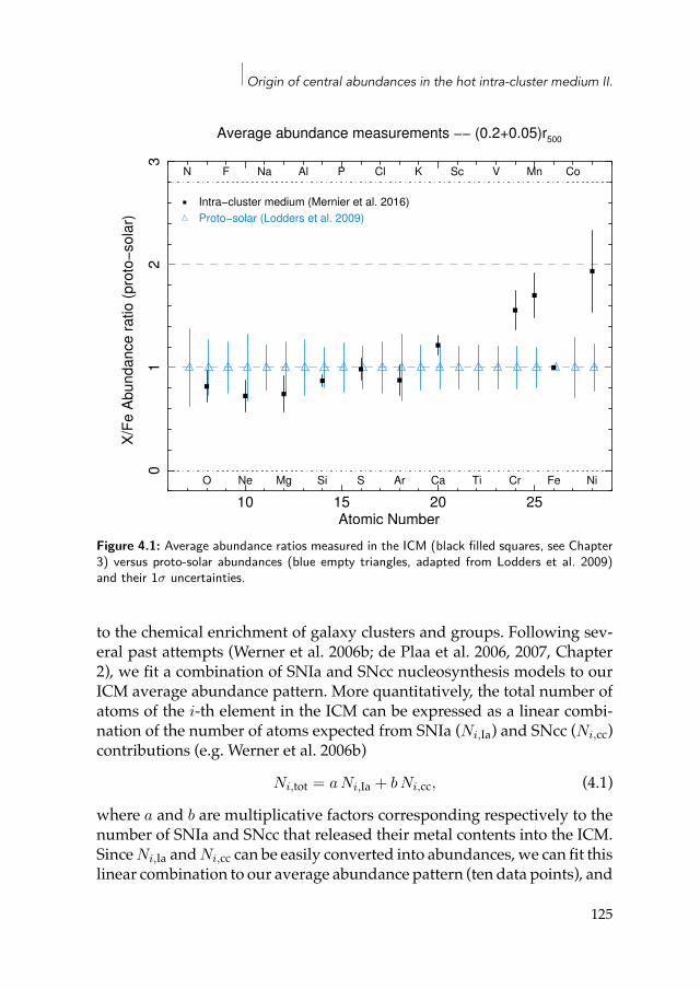
Origin of central abundances in the hot intra-cluster medium II.
10 15 20 25
01
23
X/F
e A
bundance
ratio
(pro
to!
sola
r)
Atomic Number
Average abundance measurements !! (0.2+0.05)r500
O Ne Mg Si S Ar Ca Ti Cr Fe Ni
N F Na Al P Cl K Sc V Mn Co
Intra!cluster medium (Mernier et al. 2016)
Proto!solar (Lodders et al. 2009)
Figure 4.1: Average abundance ratios measured in the ICM (black filled squares, see Chapter3) versus proto-solar abundances (blue empty triangles, adapted from Lodders et al. 2009)and their 1σ uncertainties.
to the chemical enrichment of galaxy clusters and groups. Following sev-eral past attempts (Werner et al. 2006b; de Plaa et al. 2006, 2007, Chapter2), we fit a combination of SNIa and SNcc nucleosynthesis models to ourICM average abundance pattern. More quantitatively, the total number ofatoms of the i-th element in the ICM can be expressed as a linear combi-nation of the number of atoms expected from SNIa (Ni,Ia) and SNcc (Ni,cc)contributions (e.g. Werner et al. 2006b)
Ni,tot = a Ni,Ia + b Ni,cc, (4.1)where a and b are multiplicative factors corresponding respectively to thenumber of SNIa and SNcc that released their metal contents into the ICM.SinceNi,Ia andNi,cc can be easily converted into abundances, we can fit thislinear combination to our average abundance pattern (ten data points), and
125
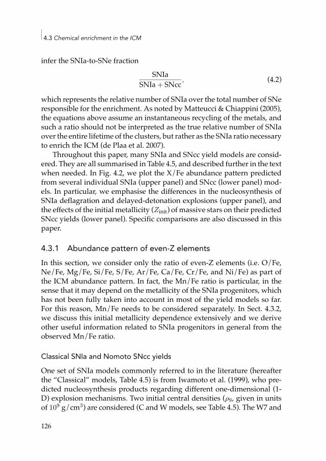
4.3 Chemical enrichment in the ICM
infer the SNIa-to-SNe fractionSNIa
SNIa + SNcc , (4.2)
which represents the relative number of SNIa over the total number of SNeresponsible for the enrichment. As noted byMatteucci & Chiappini (2005),the equations above assume an instantaneous recycling of the metals, andsuch a ratio should not be interpreted as the true relative number of SNIaover the entire lifetime of the clusters, but rather as the SNIa ratio necessaryto enrich the ICM (de Plaa et al. 2007).
Throughout this paper, many SNIa and SNcc yield models are consid-ered. They are all summarised in Table 4.5, and described further in the textwhen needed. In Fig. 4.2, we plot the X/Fe abundance pattern predictedfrom several individual SNIa (upper panel) and SNcc (lower panel) mod-els. In particular, we emphasise the differences in the nucleosynthesis ofSNIa deflagration and delayed-detonation explosions (upper panel), andthe effects of the initial metallicity (Zinit) of massive stars on their predictedSNcc yields (lower panel). Specific comparisons are also discussed in thispaper.
4.3.1 Abundance pattern of even-Z elementsIn this section, we consider only the ratio of even-Z elements (i.e. O/Fe,Ne/Fe, Mg/Fe, Si/Fe, S/Fe, Ar/Fe, Ca/Fe, Cr/Fe, and Ni/Fe) as part ofthe ICM abundance pattern. In fact, the Mn/Fe ratio is particular, in thesense that it may depend on the metallicity of the SNIa progenitors, whichhas not been fully taken into account in most of the yield models so far.For this reason, Mn/Fe needs to be considered separately. In Sect. 4.3.2,we discuss this initial metallicity dependence extensively and we deriveother useful information related to SNIa progenitors in general from theobserved Mn/Fe ratio.
Classical SNIa and Nomoto SNcc yieldsOne set of SNIa models commonly referred to in the literature (hereafterthe “Classical” models, Table 4.5) is from Iwamoto et al. (1999), who pre-dicted nucleosynthesis products regarding different one-dimensional (1-D) explosion mechanisms. Two initial central densities (ρ9, given in unitsof 109 g/cm3) are considered (C andWmodels, see Table 4.5). TheW7 and
126
Origin of central abundances in the hot intra-cluster medium II.
10 15 20 25
01
23
X/F
e a
bu
nd
an
ce r
atio
(p
roto
!so
lar)
Atomic Number
O Ne Mg Si S Ar Ca Cr Fe Ni
SNIa1!D models (Iwamoto et al. 1999)
2!D models (Maeda et al. 2010)
3!D models (Seitenzahl et al. 2013; Fink et al. 2014)
Deflagration
Delayed!detonation
Delayed!detonation (O!DDT)
10 15 20 25
05
10
X/F
e a
bu
nd
an
ce r
atio
(p
roto
!so
lar)
Atomic Number
O Ne Mg Si S Ar Ca Cr Mn Fe Ni
SNcc Zinit = 0
Zinit = 0.001
Zinit = 0.004
Zinit = 0.008
Zinit = 0.02
Zinit = 0 (cut)
Figure 4.2: Predicted X/Fe abundances from various SNIa and SNcc yield models. For com-parison, the ICM average abundance ratios (inferred from Chapter 3) are also plotted. Top:SNIa yield models: 1-D (W7 and WDD2 from Iwamoto et al. 1999), 2-D (C-DEF, C-DDT, andO-DDT from Maeda et al. 2010), and 3-D (N100def and N100 from Fink et al. (2014) andSeitenzahl et al. (2013b), respectively) models are indicated in back, red, and blue, respec-tively. A distinction is also made between the explosion models: deflagration (W7, C-DEF,and N100def; solid lines) and delayed-detonation (dashed lines for WDD2, C-DDT, and N100;dash-dotted lines for O-DDT). The Mn/Fe ratio is not shown here because it highly dependson the initial metallicity of SNIa progenitors (Sect. 4.3.2). Bottom: SNcc models, all takenfrom Nomoto et al. (2013), assuming a Salpeter IMF. Various initial metallicities (Zinit) forSNcc progenitors are compared. The dashed line corresponds to the Z0_cut model (see text).
127
4.3 Chemical enrichment in the ICM
W70 models assume a pure deflagration during the SNIa event, while theWDD and CDD models assume a delayed-detonation, with three possibletransition densities (ρT,7, given in units of 107 g/cm3). The models cur-rently favoured by the supernova community are the delayed-detonationmodels, and among these,WDD2 is usually preferred (Iwamoto et al. 1999).
Awell-referenced set of SNccmodelswas given byNomoto et al. (2006)andhas been recently updated byNomoto et al. (2013, hereafter the “Nomo-to” models), who estimated nucleosynthesis products of a SNcc as a func-tion of the mass and the initial metallicity (Zinit = 0, 0.001, 0.004, 0.008, or0.02) of its progenitor. In order to estimate the total yield mass Mi,SNcc ofthe i-th element coming from SNcc explosions, we integrate these models(following Tsujimoto et al. 1995) over a power-law IMF between 10–40M⊙(or 10–140 M⊙ when Zinit = 0; Nomoto et al. 2013), as
Mi,SNcc =∫ (1)40M⊙
10M⊙Mi(m) m−(1+x) dm∫ (1)40M⊙
10M⊙m−(1+x) dm
, (4.3)
where Mi(m) is the mass yield of the i-th element at a given mass m ofthe main sequence progenitor and x is the power index of the IMF. Herewe assume that the fraction of metals resulting from the SNcc enrichmenthave been generated by a population of massive stars having a SalpeterIMF (x = 1.35; Salpeter 1955) and sharing a common Zinit. We note thatin the case Zinit = 0, the stellar yields beyond 40 M⊙ are available for 100M⊙ and 140 M⊙ only. Consequently, a precise integration over the IMF(Eq. 4.3) within the 40–140 M⊙ range is not trivial, and the IMF-weightedabundance ratios of the Z0model might be somewhat altered by the choiceof the mass binning. For this reason, in the following we also consider theZ0_cut model, similar to the Z0 model, but restricted to ⩽40 M⊙ (Table 4.5and Fig. 4.2 top; see also Nomoto et al. 2006).
Considering all the possible combinations of a Classical SNIa modelplus a Nomoto SNcc model, our best fit (Fig. 4.3) is reached for a WDD2model and a SNcc initial metallicity Zinit = 0.008. With a reduced χ2 of∼2.8, this fit is quite poor. In particular, the Ar/Fe, Ca/Fe, and Ni/Fe ra-tios are underestimated with >1σ, >3σ, and >2σ respectively, while Si/Feis overestimated with >2σ. In Table 4.1 (top panel) we indicate the fivebest fits (including this one) that we find with this Classical combinationof models, as well as their respective estimated SN fractions. The errorson the SN fractions are typically about ±5–6%. Although all these fits arepoor, the delayed-detonation models are always favoured. The SNIa rates
128
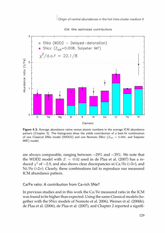
Origin of central abundances in the hot intra-cluster medium II.
Figure 4.3: Average abundance ratios versus atomic numbers in the average ICM abundancepattern (Chapter 3). The histograms show the yields contribution of a best-fit combinationof one Classical SNIa model (WDD2) and one Nomoto SNcc (Zinit = 0.008, and SalpeterIMF) model.
are always comparable, ranging between ∼29% and ∼35%. We note thatthe WDD2 model with Z = 0.02 used in de Plaa et al. (2007) has a re-duced χ2 of ∼2.9, and also shows clear discrepancies in Ca/Fe (>3σ), andNi/Fe (>2σ). Clearly, these combinations fail to reproduce our measuredICM abundance pattern.
Ca/Fe ratio: A contribution from Ca-rich SNe?
In previous studies and in this work the Ca/Fe measured ratio in the ICMwas found to be higher than expected. Using the sameClassicalmodels (to-gether with the SNcc models of Nomoto et al. 2006), Werner et al. (2006b),de Plaa et al. (2006), de Plaa et al. (2007), and Chapter 2 reported a signifi-
129
4.3 Chemical enrichment in the ICM
cant underestimate of the Ca/Fe expected yields compared to themeasure-ments. Also in stellar populations, chemical evolutionmodels fromCrosbyet al. (2016) (whomade use of the Classical SNIa yields predictions as well)failed to reproduce observations of Ca/Fe. Although residual systematicbiases in the Ca abundance measurements cannot be excluded, this possi-bility is quite unlikely. Indeed, atomic databases have been considerablyimproved during the past decades, the continuum and line fluxes in thiswork have been fitted carefully, the EPIC MOS and pn instruments agreeverywell in their Ca/Femeasurements, and no line feature around∼4 keVhas been reported so far in the EPIC effective areas or in the particle back-ground (for more details, see Chapter 3).
As one possibility of solving this conundrum, de Plaa et al. (2007) madeuse of an alternative delayed-detonation SNIa model, which provides thebest description of the spectra of the Tycho SNR (Badenes et al. 2006). Morespecifically, de Plaa et al. (2007) showed that the DDTcmodel of Bravo et al.(1996) better fits the measured Ar/Fe and Ca/Fe ratios. In this paper, wetest three models (DDTa, DDTc, and DDTe; hereafter the ”Bravo” models)introduced in Badenes et al. (2003) and Badenes et al. (2006) that are basedon the calculations of Bravo et al. (1996) and that reasonably reproduce thespectral features of Tycho. The best fit using these models is shown in Fig.4.4 (top left) and Table 4.1 (second panel).
Similarly to de Plaa et al. (2007), we obtain the best fit to our abundancepattern when using the DDTc model. The fits are significantly better thanin the Classical models (for the best fit, χ2/d.o.f. ≃ 1.3), essentially be-cause this alternative successfully reproduces the observed Si/Fe, Ar/Fe,and (above all) Ca/Fe ratios. However, the Ni/Fe ratio is still clearly un-derestimated (>2σ). The SNIa-to-SNe fraction ranges from ∼29% to ∼35%,which is similar to what was found for the Nomoto+Classical case.
Another possibility has been recently proposed byMulchaey et al. (2014),and suggests a significant additional contribution from Ca-rich gap tran-sients to the ICM enrichment. Although spectroscopically defined as TypeIb/Ic, this recently discovered subclass of SNe (Filippenko et al. 2003; Peretset al. 2010, 2011) is thought to originate from aHe-accretingWD (Waldmanet al. 2011; Foley 2015) rather than a core-collapse object, andwill be furtherconsidered as being part of the SNIa contribution. Their nebular spectrumis dominated byCa, they show large photospheric velocities (Kasliwal et al.2012), and they preferentially explode far from galaxies (Yuan et al. 2013),likely making their nucleosynthesis products easily mixed into the ICM
130
Origin of central abundances in the hot intra-cluster medium II.
(see below). We explore this possibility by adding one ”Ca-rich gap” yieldmodel to the Classical SNIa and Nomoto SNcc models. We base this addi-tional contribution on a set of yield models calculated by Waldman et al.(2011), who considered various masses of the CO core and the He upperlayer of the accreting WD (as well as, for instance, a 2% mass fraction ofN in the He layer, or a mixing of 30% between the CO core and the Helayer). The decimal numbers in the model acronyms refer to the mass ofeach considered layer (in M⊙; see Waldman et al. 2011, and Table 4.5).
The best fit is obtained for a Z0.008+W70+CO.5HE.2N.02 combination,with a reduced χ2 of ∼0.7. Compared to the Nomoto+Classical models,the fit is thus significantly improved and fully acceptable. The enrichingfraction of SNIa over the total number of SNe is estimated to be ∼40%,thus similar to (although somewhat higher than) what was found in theprevious cases.
However, based on this best fit, we estimate that the relative fractionof Ca-rich gap transients over the total number of SNIa contributing to theenrichment, SNIa(Ca)/SNIa, is ∼34%. This is much larger than recent esti-mates of the Ca-rich SNe rate over the total SNIa rate from the literature;i.e. 7 ± 5% (Perets et al. 2010), <20% (Li et al. 2011), and ∼16% (Mulchaeyet al. 2014). Since Ca-rich gap transients occur preferably in the outskirtsof galaxies (or even in the intra-cluster light) and have large photosphericvelocities (see above), one interesting possibility is that they may be sig-nificantly more efficient in enriching the ICM than classical SNIa (whosemetals may be more easily locked in the gravitational well of galaxy mem-bers). The fraction SNIa(Ca)/SNIa contributing to the enrichment mightthus naturally be higher than the absolute Ca-rich/SNIa rate (for compar-ison with the solar neighbourhood enrichment, see also Sect. 4.4). On theother hand, the amount of produced Ca highly depends on the models.In particular, assuming 30% of mixing between the CO core and the Helayer in the accretingWDproduces significantlymore Ca during the explo-sion (Waldman et al. 2011), and thus requires a smaller contribution fromCa-rich gap transients to the total enrichment. Considering this particularcase (i.e. taking the CO.5HE.2C.3 model only; see Table 4.1, third panel),the best fit is achieved for the combination Z0.001+WDD2+CO.5HE.2C.3(with a reduced χ2 of∼1.1, thus formally acceptable as well), which is plot-ted in Fig. 4.4 (top right). We then obtain SNIa(Ca)/SNIa ≃ 9%, which isin agreement with the estimated rates from the literature. The enrichingSNIa-to-SNe fraction is ∼35–40%. It is important to note, in this case, the
131
4.3 Chemical enrichment in the ICM
need for a SNIa delayed-detonation model (WDD2) instead of a deflagra-tion model, in order to predict a consistent Cr/Fe ratio3. However, the useof a delayed-detonation model again underestimates the Ni/Fe ratio, asnoted previously (Fig. 4.3 and 4.4 top left). This shows that the choice ofa specific Ca-rich gap contribution has a significant impact on favouringone of the two possible SNIa explosion mechanisms. A further discussionof the Ni/Fe ratio and the choice of a SNIa explosion model can be foundin Sect. 4.3.1.
At this stage, we must point out that the assumption of a significantfraction of the ICM enrichment coming from Ca-rich gap transient SNe ispurely speculative. However, as demonstrated in this section, this may bea realistic possibility, as it successfully reproduces the high Ca/Fe abun-dance ratio measured in the ICM. Whereas in the rest of our analysis wechoose to constrain the most realistic Ca-rich gapmodel regarding the cur-rent estimates of the Ca-rich/SNIa rate (i.e. allowing the CO.5HE.2C.3 mo-del only), we must note that such rates are not well constrained yet by theobservations. Alternatively,more precisemeasurements of the abundancesin the ICM using the next generation of X-ray satellites could potentiallyhelp to constrain this rate as well (see also Sect. 4.5.1).
Ni/Fe ratio: Diversity in SNIa explosions?
During SNcc explosions most of the Ni remains locked in the collapsingcore, while in SNIa explosions the Ni production depends on the electroncapture efficiency in the core. In particular, delayed-detonationmodels (i.e.the models currently favoured by the supernova community) should pro-duce limited amounts of Ni. Dupke &White (2000) usedASCA to measurea large Ni/Fe abundance ratio of ∼4 in the central region of three clus-ters. They deduced that this ratio is more consistent with SNIa deflagra-tion models and inconsistent with delayed-detonation models. Böhringeret al. (2005) measured the abundances of O, Si, and Fe in four clusters, andfavour predictions from WDD models. Other papers based on the abun-dance ratios of more Si-group elements (de Plaa et al. 2007, Chapter 2)also show a better consistency with the delayed-detonation models. How-
3In addition to Ca, the CO.5HE.2N.02 model produces a significant fraction of Cr. Thefits then favour SNIa deflagration models because in compensation they predict a limitedCr/Fe ratio and match the high observed Ni/Fe ratio. On the contrary, the CO.5HE.2C.3model does not produce Cr, and the Cr/Fe ratio can only be successfully reproduced byusing a delayed-detonation model for the SNIa contribution.
132
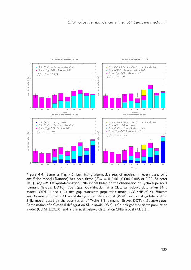
Origin of central abundances in the hot intra-cluster medium II.
Figure 4.4: Same as Fig. 4.3, but fitting alternative sets of models. In every case, onlyone SNcc model (Nomoto) has been fitted (Zinit = 0, 0.001, 0.004, 0.008 or 0.02; SalpeterIMF). Top left: Delayed-detonation SNIa model based on the observation of Tycho supernovaremnant (Bravo, DDTc). Top right: Combination of a Classical delayed-detonation SNIamodel (WDD2) and a Ca-rich gap transients population model (CO.5HE.2C.3). Bottomleft: Combination of a Classical deflagration SNIa model (W70) and a delayed-detonationSNIa model based on the observation of Tycho SN remnant (Bravo, DDTe). Bottom right:Combination of a Classical deflagration SNIa model (W7), a Ca-rich gap transients populationmodel (CO.5HE.2C.3), and a Classical delayed-detonation SNIa model (CDD1).
133
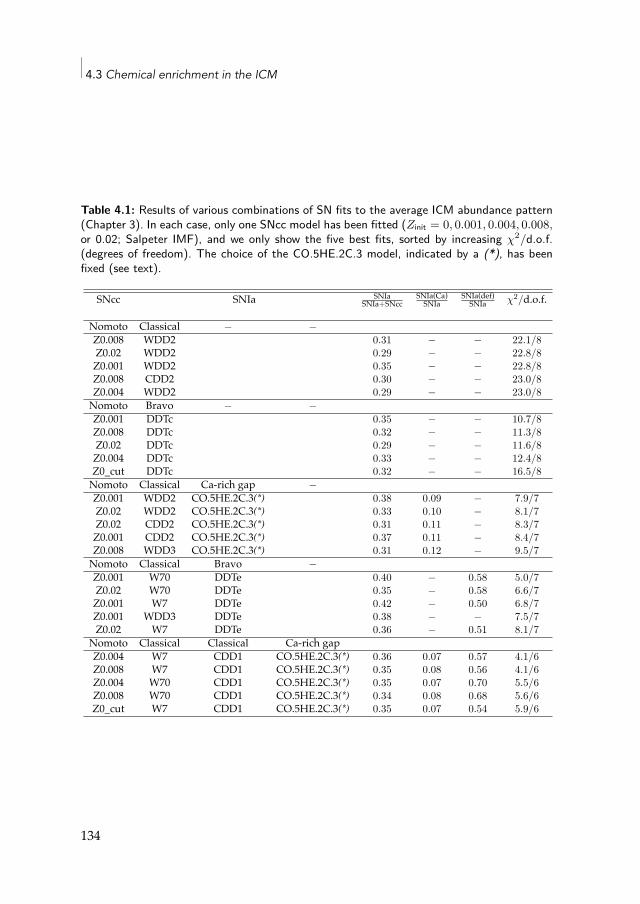
4.3 Chemical enrichment in the ICM
Table 4.1: Results of various combinations of SN fits to the average ICM abundance pattern(Chapter 3). In each case, only one SNcc model has been fitted (Zinit = 0, 0.001, 0.004, 0.008,or 0.02; Salpeter IMF), and we only show the five best fits, sorted by increasing χ2/d.o.f.(degrees of freedom). The choice of the CO.5HE.2C.3 model, indicated by a (*), has beenfixed (see text).
SNcc SNIa SNIaSNIa+SNcc
SNIa(Ca)SNIa
SNIa(def)SNIa χ2/d.o.f.
Nomoto Classical − −Z0.008 WDD2 0.31 − − 22.1/8Z0.02 WDD2 0.29 − − 22.8/8Z0.001 WDD2 0.35 − − 22.8/8Z0.008 CDD2 0.30 − − 23.0/8Z0.004 WDD2 0.29 − − 23.0/8Nomoto Bravo − −Z0.001 DDTc 0.35 − − 10.7/8Z0.008 DDTc 0.32 − − 11.3/8Z0.02 DDTc 0.29 − − 11.6/8Z0.004 DDTc 0.33 − − 12.4/8Z0_cut DDTc 0.32 − − 16.5/8Nomoto Classical Ca-rich gap −Z0.001 WDD2 CO.5HE.2C.3(*) 0.38 0.09 − 7.9/7Z0.02 WDD2 CO.5HE.2C.3(*) 0.33 0.10 − 8.1/7Z0.02 CDD2 CO.5HE.2C.3(*) 0.31 0.11 − 8.3/7Z0.001 CDD2 CO.5HE.2C.3(*) 0.37 0.11 − 8.4/7Z0.008 WDD3 CO.5HE.2C.3(*) 0.31 0.12 − 9.5/7Nomoto Classical Bravo −Z0.001 W70 DDTe 0.40 − 0.58 5.0/7Z0.02 W70 DDTe 0.35 − 0.58 6.6/7Z0.001 W7 DDTe 0.42 − 0.50 6.8/7Z0.001 WDD3 DDTe 0.38 − − 7.5/7Z0.02 W7 DDTe 0.36 − 0.51 8.1/7
Nomoto Classical Classical Ca-rich gapZ0.004 W7 CDD1 CO.5HE.2C.3(*) 0.36 0.07 0.57 4.1/6Z0.008 W7 CDD1 CO.5HE.2C.3(*) 0.35 0.08 0.56 4.1/6Z0.004 W70 CDD1 CO.5HE.2C.3(*) 0.35 0.07 0.70 5.5/6Z0.008 W70 CDD1 CO.5HE.2C.3(*) 0.34 0.08 0.68 5.6/6Z0_cut W7 CDD1 CO.5HE.2C.3(*) 0.35 0.07 0.54 5.9/6
134
Origin of central abundances in the hot intra-cluster medium II.
ever, when measured, the Ni/Fe ratio is very often found to be super-solar(e.g. Tamura et al. 2009; De Grandi & Molendi 2009, Chapter 3). Compar-ing their Ni/Fe value of 1.5 ± 0.3 solar with the ones found by Dupke &White (2000), Finoguenov et al. (2002) suggested that both deflagration anddelayed-detonation SNIa could participate in the enrichment of the ICM.
We explore this compromise bymodelling one additional Classical con-tribution of SNIa to our two combinations already described in Sect. 4.3.1.Again, we choose to use the CO.5HE.2C.3 model as the most reasonablepossibility for the Ca-rich gap contribution (Sect. 4.3.1). The five best fitsof theNomoto+Classical+Bravo andNomoto+Classical+Classical+Ca-richgapmodels are presented in Table 4.1 (last twopanels). The best fits of thesetwo cases are shown in Fig. 4.4 (bottom left and bottom right, respectively).These two combinations of models are now fully consistent (≲1σ) with allour average abundance ratios. With a reduced χ2 of ∼0.7 in both cases, thefits are better than all our previous attempts discussed above. From Table4.1 (last two panels), it also appears that at least four out of the five best fitsof these combinations include a contribution of one deflagration and onedelayed-detonation model. The relative number of deflagration SNIa overthe total number of SNIa contributing to the enrichment, SNIa(def)/SNIa,is typically in the range of 50–70%. It is, however, very difficult to discrim-inate between the best fits of each case. Similarly, we cannot clearly favoureither of the two cases above since their respective best fits reproduce theaverage abundance pattern equally well within the uncertainties (Fig. 4.4lower panels). However, no matter which case we select, again the SNIa-to-SNe fraction (34–42%) is comparable with the estimates in the cases dis-cussed earlier.
Such a possibility for a SNIa bimodality in the enrichment processesof the ICM is interesting. In many respects, the bimodal nature of SNIahas already been clearly established. For instance, it seems that ∼50% ofSNIa explode promptly (∼108 years after the starburst), while the other halfexplode much later, following an exponential decrease with a time scale of∼3Gy (Mannucci et al. 2006). Furthermore,while a population of luminousSNIa with a slow magnitude decline is mostly found in late-type galaxies,another population of subluminous SNIa has a steeper decline, and seemsto explode preferentially in old elliptical galaxies (Hamuy et al. 2000). It islikely that the bright, slowly declining SNIa correspond to the ”prompt”population, while the subluminous and fast declining SNIa correspond tothe ”delayed” population. Similarly, while the supernova community is
135
4.3 Chemical enrichment in the ICM
still debating the nature of the SNIa progenitors (see also Sect. 4.3.2), recentresults suggest that both the single-degenerate and the double-degeneratescenarios might co-exist in nature (e.g. Li et al. 2001; Scalzo et al. 2014; Caoet al. 2015; Olling et al. 2015) (see however Branch 2001). Considering allthese indications of diversity in SNIa, a bimodal population of deflagrationand delayed-detonation SNIa responsible for the enrichment of the ICMremains possible. Moreover, it should be noted that such a diversity in theexplosion mechanisms of SNIa has already been proposed, from results ofan optical study (Hatano et al. 2000). This might bring one more piece tothe complex puzzle of SNIa and their progenitors.
Some alternative scenarios to explain the high Ni/Fe ratio can be alsoconsidered. There is compelling evidence that some SNIa produce largefractions of Ni (e.g. Yamaguchi et al. 2015). On the other hand, some SNccmay overproduce Ni as well, sometimes at a super-solar level (Jerkstrandet al. 2015), and it is possible that the current yield models actually under-estimate the Ni production within SNcc. Finally, the Ni/Fe ratio from SNIacontribution may be sensitive to the initial metallicity of the SNIa progen-itors (see further discussion in Sect. 4.3.2).
Despite these intriguing possibilities, it is important to note that mea-suring the Ni abundance is a challenge using the current X-ray capabili-ties. In the abundance pattern derived in Chapter 3 and used for this work,substantial systematic uncertainties have been taken into account to over-come the large disagreement between MOS and pn. Moreover, the hardband (7–9 keV) in which the main Ni-K lines reside is often significantlycontaminated by the instrumental background. Despite the very carefulbackground modelling performed in Chapter 3, we cannot fully excludethat the background still affects our Ni/Fe measurements in both MOSand pn detectors (see also discussion in Chapter 3). Finally, the SN mod-els themselves have uncertainties in their yield predictions (e.g. related tothe electron capture rates adopted in SNIa models, see Appendix 4.A), andprevent us from firmly favouring one specific combination of models (DeGrandi &Molendi 2009). A better future constraint on theNi/Fe ratio, cou-pled to updated SNIa and SNcc yield models, will help us to favour oneparticular SNIa explosion model, and perhaps to confirm (or rule out) theco-existence of two explosion mechanisms (Sect. 4.5.1).
136
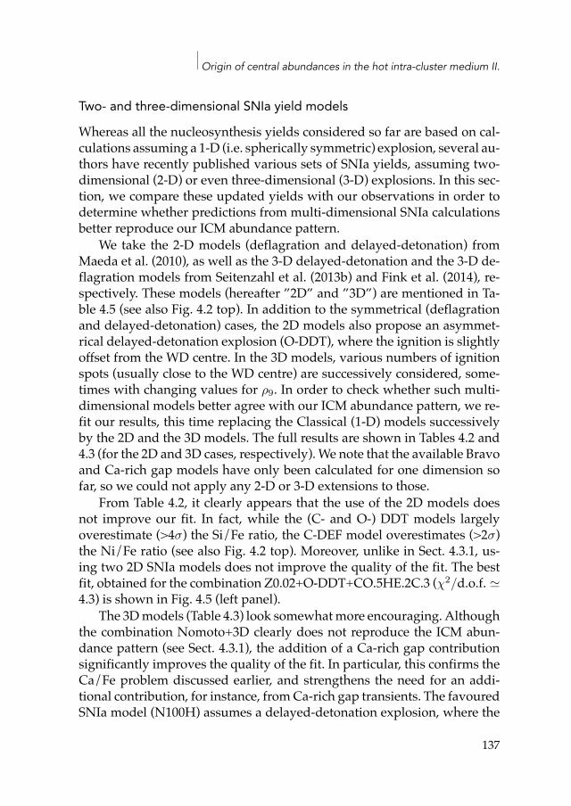
Origin of central abundances in the hot intra-cluster medium II.
Two- and three-dimensional SNIa yield models
Whereas all the nucleosynthesis yields considered so far are based on cal-culations assuming a 1-D (i.e. spherically symmetric) explosion, several au-thors have recently published various sets of SNIa yields, assuming two-dimensional (2-D) or even three-dimensional (3-D) explosions. In this sec-tion, we compare these updated yields with our observations in order todetermine whether predictions from multi-dimensional SNIa calculationsbetter reproduce our ICM abundance pattern.
We take the 2-D models (deflagration and delayed-detonation) fromMaeda et al. (2010), as well as the 3-D delayed-detonation and the 3-D de-flagration models from Seitenzahl et al. (2013b) and Fink et al. (2014), re-spectively. These models (hereafter ”2D” and ”3D”) are mentioned in Ta-ble 4.5 (see also Fig. 4.2 top). In addition to the symmetrical (deflagrationand delayed-detonation) cases, the 2D models also propose an asymmet-rical delayed-detonation explosion (O-DDT), where the ignition is slightlyoffset from the WD centre. In the 3D models, various numbers of ignitionspots (usually close to the WD centre) are successively considered, some-times with changing values for ρ9. In order to check whether such multi-dimensional models better agree with our ICM abundance pattern, we re-fit our results, this time replacing the Classical (1-D) models successivelyby the 2D and the 3D models. The full results are shown in Tables 4.2 and4.3 (for the 2D and 3D cases, respectively). We note that the available Bravoand Ca-rich gap models have only been calculated for one dimension sofar, so we could not apply any 2-D or 3-D extensions to those.
From Table 4.2, it clearly appears that the use of the 2D models doesnot improve our fit. In fact, while the (C- and O-) DDT models largelyoverestimate (>4σ) the Si/Fe ratio, the C-DEF model overestimates (>2σ)the Ni/Fe ratio (see also Fig. 4.2 top). Moreover, unlike in Sect. 4.3.1, us-ing two 2D SNIa models does not improve the quality of the fit. The bestfit, obtained for the combination Z0.02+O-DDT+CO.5HE.2C.3 (χ2/d.o.f. ≃4.3) is shown in Fig. 4.5 (left panel).
The 3Dmodels (Table 4.3) look somewhatmore encouraging. Althoughthe combination Nomoto+3D clearly does not reproduce the ICM abun-dance pattern (see Sect. 4.3.1), the addition of a Ca-rich gap contributionsignificantly improves the quality of the fit. In particular, this confirms theCa/Fe problem discussed earlier, and strengthens the need for an addi-tional contribution, for instance, fromCa-rich gap transients. The favouredSNIa model (N100H) assumes a delayed-detonation explosion, where the
137
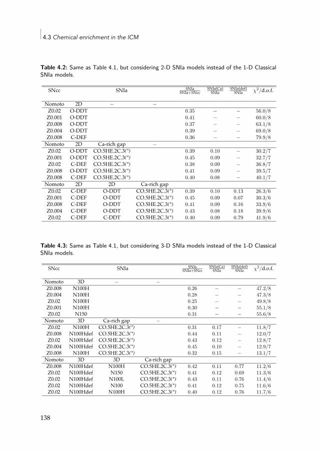
4.3 Chemical enrichment in the ICM
Table 4.2: Same as Table 4.1, but considering 2-D SNIa models instead of the 1-D ClassicalSNIa models.
SNcc SNIa SNIaSNIa+SNcc
SNIa(Ca)SNIa
SNIa(def)SNIa χ2/d.o.f.
Nomoto 2D − −Z0.02 O-DDT 0.35 − − 56.0/8Z0.001 O-DDT 0.41 − − 60.0/8Z0.008 O-DDT 0.37 − − 63.1/8Z0.004 O-DDT 0.39 − − 69.0/8Z0.008 C-DEF 0.36 − − 79.9/8Nomoto 2D Ca-rich gap −Z0.02 O-DDT CO.5HE.2C.3(*) 0.39 0.10 − 30.2/7Z0.001 O-DDT CO.5HE.2C.3(*) 0.45 0.09 − 32.7/7Z0.02 C-DEF CO.5HE.2C.3(*) 0.38 0.09 − 36.8/7Z0.008 O-DDT CO.5HE.2C.3(*) 0.41 0.09 − 39.5/7Z0.008 C-DEF CO.5HE.2C.3(*) 0.40 0.08 − 40.1/7Nomoto 2D 2D Ca-rich gapZ0.02 C-DEF O-DDT CO.5HE.2C.3(*) 0.39 0.10 0.13 26.3/6Z0.001 C-DEF O-DDT CO.5HE.2C.3(*) 0.45 0.09 0.07 30.3/6Z0.008 C-DEF O-DDT CO.5HE.2C.3(*) 0.41 0.09 0.16 33.9/6Z0.004 C-DEF O-DDT CO.5HE.2C.3(*) 0.43 0.08 0.18 39.9/6Z0.02 C-DEF C-DDT CO.5HE.2C.3(*) 0.40 0.09 0.79 41.9/6
Table 4.3: Same as Table 4.1, but considering 3-D SNIa models instead of the 1-D ClassicalSNIa models.
SNcc SNIa SNIaSNIa+SNcc
SNIa(Ca)SNIa
SNIa(def)SNIa χ2/d.o.f.
Nomoto 3D − −Z0.008 N100H 0.26 − − 47.2/8Z0.004 N100H 0.28 − − 47.3/8Z0.02 N100H 0.25 − − 49.8/8Z0.001 N100H 0.30 − − 55.1/8Z0.02 N150 0.31 − − 55.6/8
Nomoto 3D Ca-rich gap −Z0.02 N100H CO.5HE.2C.3(*) 0.31 0.17 − 11.8/7Z0.008 N100Hdef CO.5HE.2C.3(*) 0.44 0.11 − 12.0/7Z0.02 N100Hdef CO.5HE.2C.3(*) 0.43 0.12 − 12.8/7Z0.004 N100Hdef CO.5HE.2C.3(*) 0.45 0.10 − 12.9/7Z0.008 N100H CO.5HE.2C.3(*) 0.32 0.15 − 13.1/7Nomoto 3D 3D Ca-rich gapZ0.008 N100Hdef N100H CO.5HE.2C.3(*) 0.42 0.11 0.77 11.2/6Z0.02 N100Hdef N150 CO.5HE.2C.3(*) 0.41 0.12 0.69 11.3/6Z0.02 N100Hdef N100L CO.5HE.2C.3(*) 0.43 0.11 0.76 11.4/6Z0.02 N100Hdef N100 CO.5HE.2C.3(*) 0.41 0.12 0.75 11.6/6Z0.02 N100Hdef N100H CO.5HE.2C.3(*) 0.40 0.12 0.76 11.7/6
138
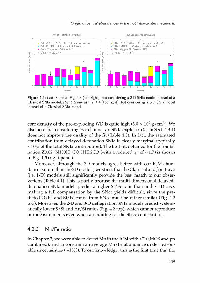
Origin of central abundances in the hot intra-cluster medium II.
Figure 4.5: Left: Same as Fig. 4.4 (top right), but considering a 2-D SNIa model instead of aClassical SNIa model. Right: Same as Fig. 4.4 (top right), but considering a 3-D SNIa modelinstead of a Classical SNIa model.
core density of the pre-exploding WD is quite high (5.5 × 10⁹ g/cm3). Wealso note that considering two channels of SNIa explosion (as in Sect. 4.3.1)does not improve the quality of the fit (Table 4.3). In fact, the estimatedcontribution from delayed-detonation SNIa is clearly marginal (typically∼10% of the total SNIa contribution). The best fit, obtained for the combi-nation Z0.02+N100H+CO.5HE.2C.3 (with a reduced χ2 of ∼1.7) is shownin Fig. 4.5 (right panel).
Moreover, although the 3D models agree better with our ICM abun-dance pattern than the 2Dmodels,we stress that theClassical and/or Bravo(i.e. 1-D) models still significantly provide the best match to our obser-vations (Table 4.1). This is partly because the multi-dimensional delayed-detonation SNIa models predict a higher Si/Fe ratio than in the 1-D case,making a full compensation by the SNcc yields difficult, since the pre-dicted O/Fe and Si/Fe ratios from SNcc must be rather similar (Fig. 4.2top). Moreover, the 2-D and 3-D deflagration SNIa models predict system-atically lower S/Si and Ar/Si ratios (Fig. 4.2 top), which cannot reproduceour measurements even when accounting for the SNcc contribution.
4.3.2 Mn/Fe ratioIn Chapter 3, we were able to detect Mn in the ICMwith >7σ (MOS and pncombined), and to constrain an average Mn/Fe abundance under reason-able uncertainties (∼13%). To our knowledge, this is the first time that the
139
4.3 Chemical enrichment in the ICM
abundance of an odd-Z element has been measured in the ICM. It is com-monly known that the bulk of Mn comes from SNIa explosions as SNccare very inefficient in producing Mn (Fig. 4.2 bottom). In this section, wediscuss two interesting consequences that the observed ICM Mn/Fe ratio(again, witnessing the explosion of billions of SNIa) can have on the SNIaprogenitors.
Metallicity of the SNIa progenitorsSeitenzahl et al. (2013b) calculated the yields from their N100 (3-D delayed-detonation) model, assuming four different initial metallicities (0.01Z⊙,0.1Z⊙, 0.5Z⊙, and 1Z⊙) of SNIa progenitors, Zinit(SNIa). Interestingly, theresult (Fig. 4.6) shows a slight, but clear dependence of the Mn/Fe abun-dance ratio with Zinit(SNIa) (see also Seitenzahl et al. 2015). Since the bulkof the Mn observed in the ICM is produced by SNIa, we can use our ob-servedMn/Fe abundance ratio to derive constraints on the average metal-licity of the progenitors of SNIa responsible for the enrichment. Followingthe 1-D yieldmodels best reproducing our abundance pattern, we estimatethat respectively∼95% and∼82% of the Mn and Fe are produced by SNIa.Taking these factors into account, the average Mn/Fe abundance ratio inthe ICM coming from SNIa is 1.97 ± 0.25. Again assuming the N100 modelfor the SNIa contribution, the interpolation of the yields from Seitenzahlet al. (2013b) involves a lower limit of Zinit(SNIa) ≳ Z⊙ (Fig. 4.7).
The lack of yield models with Z > 1Z⊙ combined with the uncer-tainties in our Mn/Fe ICM measurement prevents us from inferring fur-ther constraints such as an upper limit to Zinit(SNIa). We also recall thatour inferred lower limit depends on the assumed limited Mn productionby SNcc. If, for some reason, the Mn production is revised upwards inupcoming SNcc yield models, it would have a strong impact on the in-ferred limits of the initial metallicities of SNIa progenitors. Moreover, amore complete understanding of the precise relation between Zinit(SNIa)and the Mn yields could only be achieved by comparing this Zinit(SNIa)dependence in various SNIa yield models. Except N100, no other avail-able deflagration/delayed-detonation model has been calculated for sev-eral successive values of Zinit(SNIa). For this reason, we prefer to treat Mnas a peculiar element, and therefore, Mn/Fe was not included in the pre-vious fits (Sect. 4.3.1).
Finally, it is worth noting (see Fig. 4.6) that the Ni/Fe ratio from SNIacontributions may also vary with Zinit(SNIa) (at least for metallicities be-
140
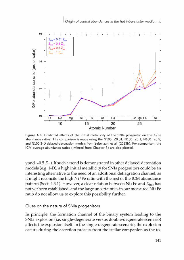
Origin of central abundances in the hot intra-cluster medium II.
10 15 20 25
01
23
X/F
e a
bundance
ratio
(pro
to!
sola
r)
Atomic Number
O Ne Mg Si S Ar Ca Cr Mn Fe Ni
Zinit = 0.01 Zsol
Zinit = 0.1 Zsol
Zinit = 0.5 Zsol
Zinit = 1 Zsol
Figure 4.6: Predicted effects of the initial metallicity of the SNIa progenitor on the X/Feabundance ratios. The comparison is made using the N100_Z0.01, N100_Z0.1, N100_Z0.5,and N100 3-D delayed-detonation models from Seitenzahl et al. (2013b). For comparison, theICM average abundance ratios (inferred from Chapter 3) are also plotted.
yond∼0.5Z⊙). If such a trend is demonstrated in other delayed-detonationmodels (e.g. 1-D), a high initial metallicity for SNIa progenitors could be aninteresting alternative to the need of an additional deflagration channel, asit might reconcile the high Ni/Fe ratio with the rest of the ICM abundancepattern (Sect. 4.3.1). However, a clear relation between Ni/Fe and Zinit hasnot yet been established, and the large uncertainties in ourmeasuredNi/Feratio do not allow us to explore this possibility further.
Clues on the nature of SNIa progenitors
In principle, the formation channel of the binary system leading to theSNIa explosion (i.e. single-degenerate versus double-degenerate scenario)affects the explosion itself. In the single-degenerate scenario, the explosionoccurs during the accretion process from the stellar companion as the to-
141
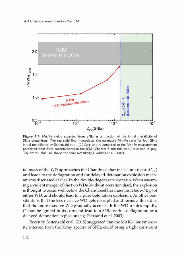
4.3 Chemical enrichment in the ICM
10-4 10-3 10-2 10-1
Zinit(SNIa)
0.5
1.0
1.5
2.0
(Mn/
Fe) S
NIa
N100
(3-D delayed-detonation)
ICM(Mernier et al. 2016)
Z sun
0.01
41(L
odde
rs e
t al.
2009
)
Figure 4.7: Mn/Fe yields expected from SNIa as a function of the initial metallicity ofSNIa progenitors. The red solid line interpolates the estimated Mn/Fe ratio for four SNIainitial metallicites by Seitenzahl et al. (2013b), and is compared to the Mn/Fe measurement(expected from SNIa contributions) in the ICM (Chapter 3 and this work) is shown in grey.The dotted blue line shows the solar metallicity (Lodders et al. 2009).
tal mass of the WD approaches the Chandrasekhar mass limit (near-MCh)and leads to the deflagration and/or delayed-detonation explosion mech-anisms discussed earlier. In the double-degenerate scenario, when assum-ing a violent merger of the twoWDs (without accretion disc), the explosionis thought to occur well below the Chandrasekhar mass limit (sub-MCh) ofeither WD, and should lead to a pure detonation explosion. Another pos-sibility is that the less massive WD gets disrupted and forms a thick discthat the more massive WD gradually accretes. If the WD rotates rapidly,C may be ignited in its core and lead to a SNIa with a deflagration or adelayed-detonation explosion (e.g. Piersanti et al. 2003).
Recently, Seitenzahl et al. (2015) suggested that theMnKα line emissiv-ity inferred from the X-ray spectra of SNIa could bring a tight constraint
142
Origin of central abundances in the hot intra-cluster medium II.
on the scenarios mentioned above as the near-MCh models produce sig-nificantly more 55Fe (later decaying into stable 55Mn) than the sub-MChmodels. On the other hand, Seitenzahl et al. (2013a) showed that sub-MChexplosion models from Pakmor et al. (2012, ; violent WD merger with re-spective masses of 1.1 M⊙ and 0.9 M⊙) and Ruiter et al. (2013, ; violentWD merger with masses of 0.6 M⊙ each) systematically predict sub-solarMn/Fe abundance ratios, and can hardly explain the proto-solar value ofMn. Although Mn yields from SNIa may be metallicity-dependent (Sect.4.3.2), Seitenzahl et al. (2015) noted that even the highest-Zinit (i.e. 1 Z⊙)sub-MCh model produces two times less Mn than the lowest-Zinit (i.e. 0.01Z⊙) near-MCh model.
Again assuming that ∼95% of the Mn/Fe ratio measured in the ICMoriginates from SNIa explosions, our super-proto-solar ICM Mn/Fe ratioconstrains this result even more, and suggests that the WD violent mergerscenario should be excluded as a dominant SNIa progenitor channel (atleast assuming that such a merger produces a pure detonation).
To confirm this claim in a larger context, we re-fit our ICM abundancepattern, this time by including the publicly available yields from the WDviolent merger model of Pakmor et al. (2010). This sub-MCh yield is onlyavailable for the violent merger of two WDs with equal masses (MWD1 =MWD2 = 0.9 M⊙; see also Table 4.5). We consider two specific cases:
1. All SNIa (excluding Ca-rich gap transients) originate from violentWDmergers (both of equalmassMWD1 = MWD2 = 0.9 M⊙), and theyoccur as sub-MCh explosions (i.e. the Nomoto+sub-MCh+Ca-rich gapcombination);
2. One part of the SNIa originate from violent WD mergers, the otherpart originate from another channel, occurring as near-MCh explo-sions, either deflagration or delayed-detonation (i.e. theNomoto+sub-MCh+3D+Ca-rich gap combination).
In the first case, the fit fails to find any positive contribution for thesub-MCh model. In the second case, the contribution of the sub-MCh SNIato the enrichment is limited to ∼1.3% of the total number of SNIa, withsimilar best fits to those we reported in Sect. 4.3.1 (Nomoto+Classical+Ca-rich combination). This occurs because the Si/Fe ratio predicted by the0.9_0.9 model is dramatically higher (∼8) than the observed ratio in theICM. Again, this favours near-MCh explosions, and discards the violent
143
4.3 Chemical enrichment in the ICM
WDmergers scenario (leading to sub-MCh explosions) as a significant con-tributor to SNIa nucleosynthesis, at least for the two specific combinationsof initial masses discussed above (1.1 M⊙+0.9 M⊙ and 0.9 M⊙+0.9 M⊙).We must note, however, that this result does not necessarily discard all thesubchannels of the double-degenerate scenario. For instance, asmentionedabove, a disruption of the least massive WD, followed by the creation of athick torus that could feed the most massive WD, may lead to a near-MChexplosion, and to similar yields as used in the Classical, 2D and 3D mod-els. Moreover, we recall that our discussion is entirely based on the cur-rent yield predictions. Any substantial change in upcoming yield modelsof sub-MCh explosions (for instance in the initial masses that are assumed)may potentially challenge our interpretation.
4.3.3 Fraction of low-mass stars that become SNIaSince SNcc explosions are the result of the end-of-life of massive stars (⩾10M⊙), the bulk of SNcc events occur very rapidly (≲40 Myr) after its associ-ated episode of star formation. On the contrary, SNIa events require a con-siderable time delay (up to several Gyr), from their zero age low-mass starprogenitors to the end of the binary evolution of the correspondingWD(s).In our Galaxy, multiple episodes of star formation continuously generatelow-mass stars, and make it difficult to directly compare the number ofSNIa events and the corresponding number of low-mass stars that havegenerated them.
In galaxy clusters, however, the situation is different. In fact, since thebulk of the star formation occurred at the epoch of cluster formation (z ≃2–3), and has now dramatically quenched, clusters are an interesting lab-oratory which allow us to relate the estimated number of low-mass starsto the number of SNIa, and thus estimate the SNIa efficiency, ηIa (i.e. thefraction of low-mass stars that eventually result in SNIa). Following theapproach of de Plaa et al. (2007), in this section we attempt to estimate ηIafrom the ICMabundancemeasurements and their best-fit SN yieldmodels.
Quantitatively, assuming a power-law IMF, we can write (de Plaa et al.2007)
SNIaSNIa+SNcc =
ηIa∫Mcc
Mlow m−(1+x) dm
ηIa∫Mcc
Mlow m−(1+x) dm +∫Mup
Mcc m−(1+x) dm, (4.4)
where Mlow and Mcc are respectively the lower and upper mass limit of
144
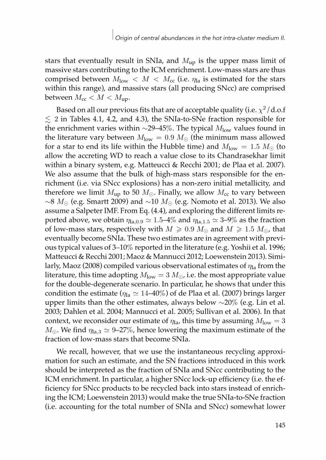
Origin of central abundances in the hot intra-cluster medium II.
stars that eventually result in SNIa, and Mup is the upper mass limit ofmassive stars contributing to the ICM enrichment. Low-mass stars are thuscomprised between Mlow < M < Mcc (i.e. ηIa is estimated for the starswithin this range), and massive stars (all producing SNcc) are comprisedbetween Mcc < M < Mup.
Based on all our previous fits that are of acceptable quality (i.e. χ2/d.o.f≲ 2 in Tables 4.1, 4.2, and 4.3), the SNIa-to-SNe fraction responsible forthe enrichment varies within ∼29–45%. The typical Mlow values found inthe literature vary between Mlow = 0.9 M⊙ (the minimum mass allowedfor a star to end its life within the Hubble time) and Mlow = 1.5 M⊙ (toallow the accreting WD to reach a value close to its Chandrasekhar limitwithin a binary system, e.g. Matteucci & Recchi 2001; de Plaa et al. 2007).We also assume that the bulk of high-mass stars responsible for the en-richment (i.e. via SNcc explosions) has a non-zero initial metallicity, andtherefore we limit Mup to 50 M⊙. Finally, we allow Mcc to vary between∼8 M⊙ (e.g. Smartt 2009) and ∼10 M⊙ (e.g. Nomoto et al. 2013). We alsoassume a Salpeter IMF. FromEq. (4.4), and exploring the different limits re-ported above, we obtain ηIa,0.9 ≃ 1.5–4% and ηIa,1.5 ≃ 3–9% as the fractionof low-mass stars, respectively with M ⩾ 0.9 M⊙ and M ⩾ 1.5 M⊙, thateventually become SNIa. These two estimates are in agreement with previ-ous typical values of 3–10% reported in the literature (e.g. Yoshii et al. 1996;Matteucci &Recchi 2001;Maoz&Mannucci 2012; Loewenstein 2013). Simi-larly, Maoz (2008) compiled various observational estimates of ηIa from theliterature, this time adoptingMlow = 3 M⊙, i.e. the most appropriate valuefor the double-degenerate scenario. In particular, he shows that under thiscondition the estimate (ηIa ≃ 14–40%) of de Plaa et al. (2007) brings largerupper limits than the other estimates, always below ∼20% (e.g. Lin et al.2003; Dahlen et al. 2004; Mannucci et al. 2005; Sullivan et al. 2006). In thatcontext, we reconsider our estimate of ηIa, this time by assuming Mlow = 3M⊙. We find ηIa,3 ≃ 9–27%, hence lowering the maximum estimate of thefraction of low-mass stars that become SNIa.
We recall, however, that we use the instantaneous recycling approxi-mation for such an estimate, and the SN fractions introduced in this workshould be interpreted as the fraction of SNIa and SNcc contributing to theICM enrichment. In particular, a higher SNcc lock-up efficiency (i.e. the ef-ficiency for SNcc products to be recycled back into stars instead of enrich-ing the ICM; Loewenstein 2013) wouldmake the true SNIa-to-SNe fraction(i.e. accounting for the total number of SNIa and SNcc) somewhat lower
145
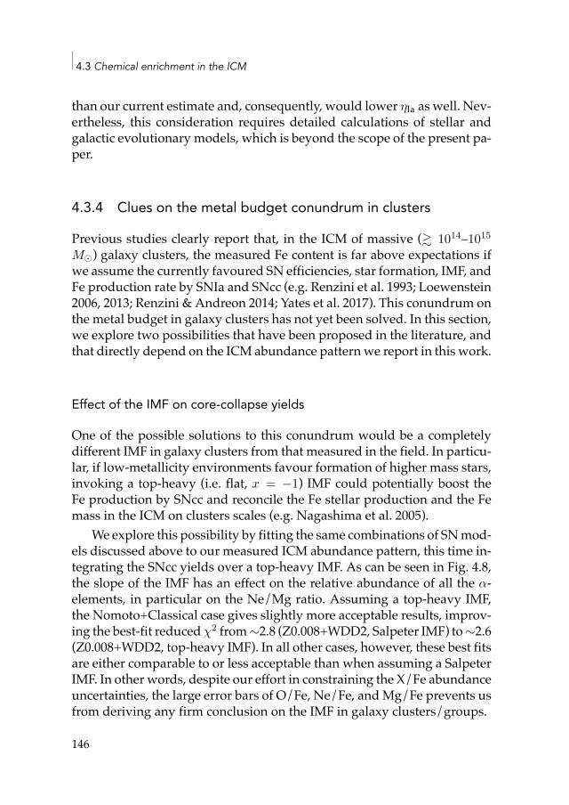
4.3 Chemical enrichment in the ICM
than our current estimate and, consequently, would lower ηIa as well. Nev-ertheless, this consideration requires detailed calculations of stellar andgalactic evolutionary models, which is beyond the scope of the present pa-per.
4.3.4 Clues on the metal budget conundrum in clusters
Previous studies clearly report that, in the ICM of massive (≳ 1014–1015
M⊙) galaxy clusters, the measured Fe content is far above expectations ifwe assume the currently favoured SN efficiencies, star formation, IMF, andFe production rate by SNIa and SNcc (e.g. Renzini et al. 1993; Loewenstein2006, 2013; Renzini & Andreon 2014; Yates et al. 2017). This conundrum onthe metal budget in galaxy clusters has not yet been solved. In this section,we explore two possibilities that have been proposed in the literature, andthat directly depend on the ICM abundance patternwe report in this work.
Effect of the IMF on core-collapse yields
One of the possible solutions to this conundrum would be a completelydifferent IMF in galaxy clusters from that measured in the field. In particu-lar, if low-metallicity environments favour formation of higher mass stars,invoking a top-heavy (i.e. flat, x = −1) IMF could potentially boost theFe production by SNcc and reconcile the Fe stellar production and the Femass in the ICM on clusters scales (e.g. Nagashima et al. 2005).
We explore this possibility by fitting the same combinations of SNmod-els discussed above to our measured ICM abundance pattern, this time in-tegrating the SNcc yields over a top-heavy IMF. As can be seen in Fig. 4.8,the slope of the IMF has an effect on the relative abundance of all the α-elements, in particular on the Ne/Mg ratio. Assuming a top-heavy IMF,the Nomoto+Classical case gives slightly more acceptable results, improv-ing the best-fit reducedχ2 from∼2.8 (Z0.008+WDD2, Salpeter IMF) to∼2.6(Z0.008+WDD2, top-heavy IMF). In all other cases, however, these best fitsare either comparable to or less acceptable than when assuming a SalpeterIMF. In other words, despite our effort in constraining the X/Fe abundanceuncertainties, the large error bars of O/Fe, Ne/Fe, andMg/Fe prevents usfrom deriving any firm conclusion on the IMF in galaxy clusters/groups.
146
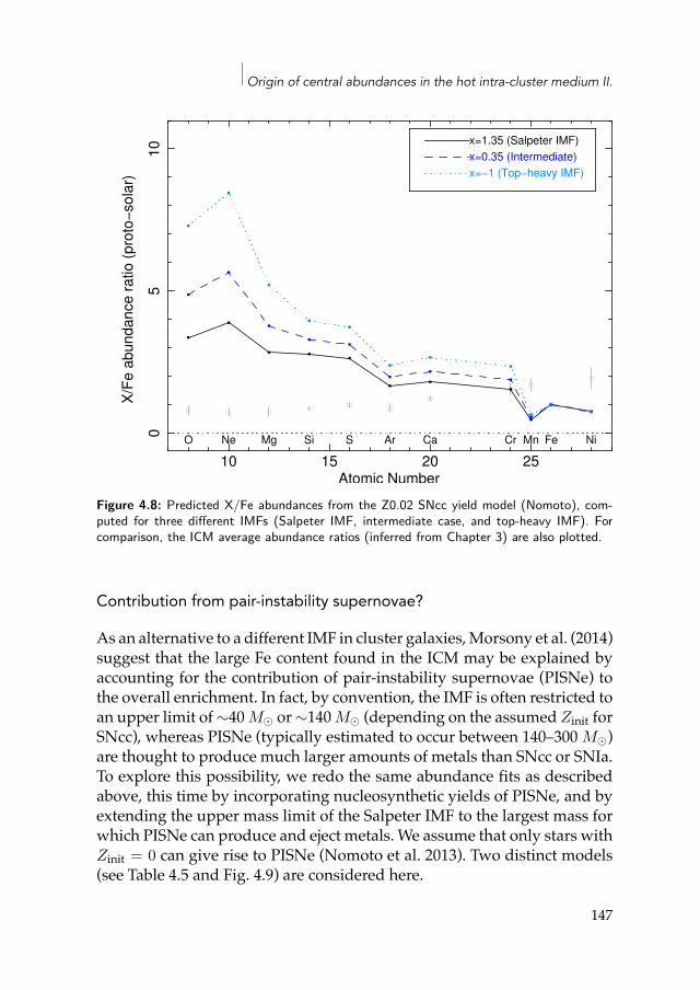
Origin of central abundances in the hot intra-cluster medium II.
10 15 20 25
05
10
X/F
e a
bundance
ratio
(pro
to!
sola
r)
Atomic Number
O Ne Mg Si S Ar Ca Cr Mn Fe Ni
x=1.35 (Salpeter IMF)
x=0.35 (Intermediate)
x=!1 (Top!heavy IMF)
Figure 4.8: Predicted X/Fe abundances from the Z0.02 SNcc yield model (Nomoto), com-puted for three different IMFs (Salpeter IMF, intermediate case, and top-heavy IMF). Forcomparison, the ICM average abundance ratios (inferred from Chapter 3) are also plotted.
Contribution from pair-instability supernovae?
As an alternative to a different IMF in cluster galaxies,Morsony et al. (2014)suggest that the large Fe content found in the ICM may be explained byaccounting for the contribution of pair-instability supernovae (PISNe) tothe overall enrichment. In fact, by convention, the IMF is often restricted toan upper limit of∼40M⊙ or∼140M⊙ (depending on the assumed Zinit forSNcc), whereas PISNe (typically estimated to occur between 140–300 M⊙)are thought to produce much larger amounts of metals than SNcc or SNIa.To explore this possibility, we redo the same abundance fits as describedabove, this time by incorporating nucleosynthetic yields of PISNe, and byextending the upper mass limit of the Salpeter IMF to the largest mass forwhich PISNe can produce and eject metals. We assume that only stars withZinit = 0 can give rise to PISNe (Nomoto et al. 2013). Two distinct models(see Table 4.5 and Fig. 4.9) are considered here.
147
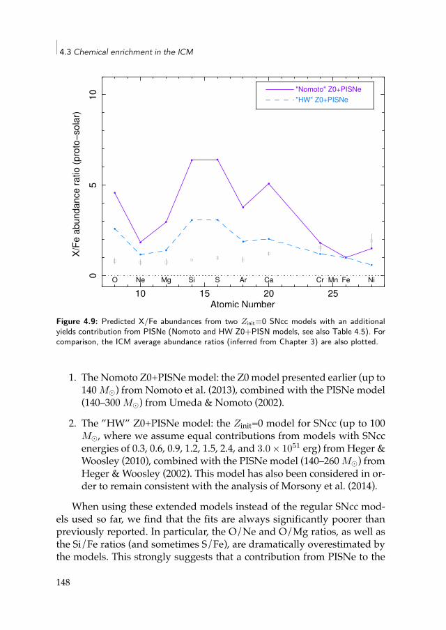
4.3 Chemical enrichment in the ICM
10 15 20 25
05
10
X/F
e a
bundance
ratio
(pro
to!
sola
r)
Atomic Number
O Ne Mg Si S Ar Ca Cr Mn Fe Ni
"Nomoto" Z0+PISNe
"HW" Z0+PISNe
Figure 4.9: Predicted X/Fe abundances from two Zinit=0 SNcc models with an additionalyields contribution from PISNe (Nomoto and HW Z0+PISN models, see also Table 4.5). Forcomparison, the ICM average abundance ratios (inferred from Chapter 3) are also plotted.
1. The Nomoto Z0+PISNemodel: the Z0model presented earlier (up to140 M⊙) from Nomoto et al. (2013), combined with the PISNe model(140–300 M⊙) from Umeda & Nomoto (2002).
2. The ”HW” Z0+PISNe model: the Zinit=0 model for SNcc (up to 100M⊙, where we assume equal contributions from models with SNccenergies of 0.3, 0.6, 0.9, 1.2, 1.5, 2.4, and 3.0 × 1051 erg) from Heger &Woosley (2010), combined with the PISNe model (140–260 M⊙) fromHeger & Woosley (2002). This model has also been considered in or-der to remain consistent with the analysis of Morsony et al. (2014).
When using these extended models instead of the regular SNcc mod-els used so far, we find that the fits are always significantly poorer thanpreviously reported. In particular, the O/Ne and O/Mg ratios, as well asthe Si/Fe ratios (and sometimes S/Fe), are dramatically overestimated bythe models. This strongly suggests that a contribution from PISNe to the
148
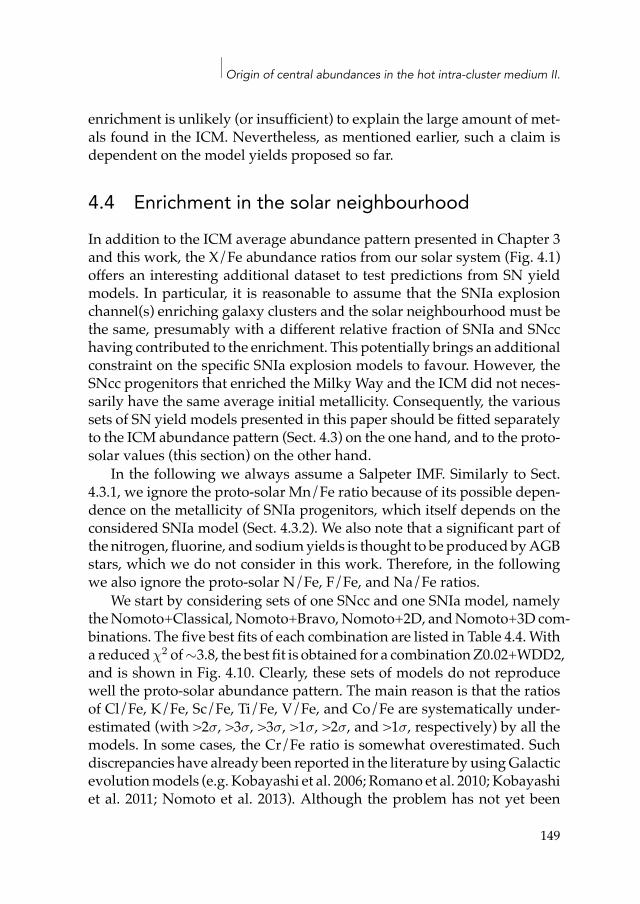
Origin of central abundances in the hot intra-cluster medium II.
enrichment is unlikely (or insufficient) to explain the large amount of met-als found in the ICM. Nevertheless, as mentioned earlier, such a claim isdependent on the model yields proposed so far.
4.4 Enrichment in the solar neighbourhoodIn addition to the ICM average abundance pattern presented in Chapter 3and this work, the X/Fe abundance ratios from our solar system (Fig. 4.1)offers an interesting additional dataset to test predictions from SN yieldmodels. In particular, it is reasonable to assume that the SNIa explosionchannel(s) enriching galaxy clusters and the solar neighbourhood must bethe same, presumably with a different relative fraction of SNIa and SNcchaving contributed to the enrichment. This potentially brings an additionalconstraint on the specific SNIa explosion models to favour. However, theSNcc progenitors that enriched the Milky Way and the ICM did not neces-sarily have the same average initial metallicity. Consequently, the varioussets of SN yield models presented in this paper should be fitted separatelyto the ICM abundance pattern (Sect. 4.3) on the one hand, and to the proto-solar values (this section) on the other hand.
In the following we always assume a Salpeter IMF. Similarly to Sect.4.3.1, we ignore the proto-solar Mn/Fe ratio because of its possible depen-dence on the metallicity of SNIa progenitors, which itself depends on theconsidered SNIa model (Sect. 4.3.2). We also note that a significant part ofthe nitrogen, fluorine, and sodiumyields is thought to be produced byAGBstars, which we do not consider in this work. Therefore, in the followingwe also ignore the proto-solar N/Fe, F/Fe, and Na/Fe ratios.
We start by considering sets of one SNcc and one SNIa model, namelytheNomoto+Classical,Nomoto+Bravo,Nomoto+2D, andNomoto+3D com-binations. The five best fits of each combination are listed in Table 4.4.Witha reducedχ2 of∼3.8, the best fit is obtained for a combinationZ0.02+WDD2,and is shown in Fig. 4.10. Clearly, these sets of models do not reproducewell the proto-solar abundance pattern. The main reason is that the ratiosof Cl/Fe, K/Fe, Sc/Fe, Ti/Fe, V/Fe, and Co/Fe are systematically under-estimated (with >2σ, >3σ, >3σ, >1σ, >2σ, and >1σ, respectively) by all themodels. In some cases, the Cr/Fe ratio is somewhat overestimated. Suchdiscrepancies have already been reported in the literature by usingGalacticevolutionmodels (e.g. Kobayashi et al. 2006; Romano et al. 2010; Kobayashiet al. 2011; Nomoto et al. 2013). Although the problem has not yet been
149
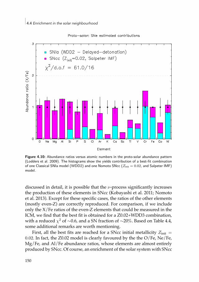
4.4 Enrichment in the solar neighbourhood
Figure 4.10: Abundance ratios versus atomic numbers in the proto-solar abundance pattern(Lodders et al. 2009). The histograms show the yields contribution of a best-fit combinationof one Classical SNIa model (WDD2) and one Nomoto SNcc (Zinit = 0.02, and Salpeter IMF)model.
discussed in detail, it is possible that the ν-process significantly increasesthe production of these elements in SNcc (Kobayashi et al. 2011; Nomotoet al. 2013). Except for these specific cases, the ratios of the other elements(mostly even-Z) are correctly reproduced. For comparison, if we includeonly the X/Fe ratios of the even-Z elements that could be measured in theICM, we find that the best fit is obtained for a Z0.02+WDD3 combination,with a reduced χ2 of ∼0.6, and a SN fraction of ∼20%. Based on Table 4.4,some additional remarks are worth mentioning.
First, all the best fits are reached for a SNcc initial metallicity Zinit =0.02. In fact, the Z0.02 model is clearly favoured by the the O/Fe, Ne/Fe,Mg/Fe, and Al/Fe abundance ratios, whose elements are almost entirelyproduced by SNcc. Of course, an enrichment of the solar systemwith SNcc
150
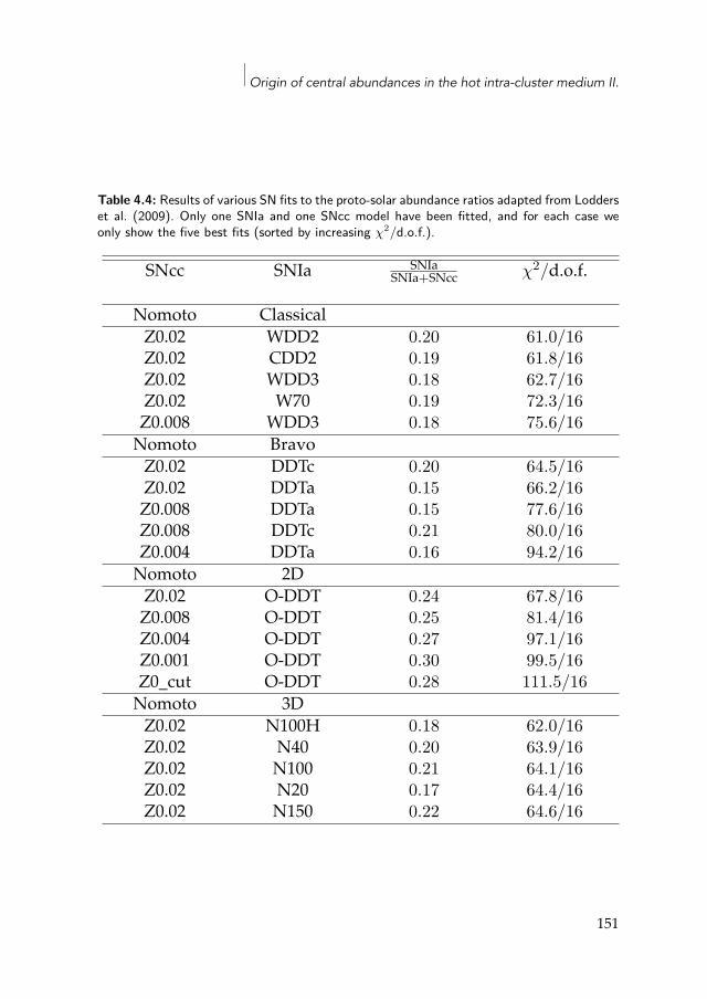
Origin of central abundances in the hot intra-cluster medium II.
Table 4.4: Results of various SN fits to the proto-solar abundance ratios adapted from Lodderset al. (2009). Only one SNIa and one SNcc model have been fitted, and for each case weonly show the five best fits (sorted by increasing χ2/d.o.f.).
SNcc SNIa SNIaSNIa+SNcc χ2/d.o.f.
Nomoto ClassicalZ0.02 WDD2 0.20 61.0/16Z0.02 CDD2 0.19 61.8/16Z0.02 WDD3 0.18 62.7/16Z0.02 W70 0.19 72.3/16Z0.008 WDD3 0.18 75.6/16Nomoto BravoZ0.02 DDTc 0.20 64.5/16Z0.02 DDTa 0.15 66.2/16Z0.008 DDTa 0.15 77.6/16Z0.008 DDTc 0.21 80.0/16Z0.004 DDTa 0.16 94.2/16Nomoto 2DZ0.02 O-DDT 0.24 67.8/16Z0.008 O-DDT 0.25 81.4/16Z0.004 O-DDT 0.27 97.1/16Z0.001 O-DDT 0.30 99.5/16Z0_cut O-DDT 0.28 111.5/16Nomoto 3DZ0.02 N100H 0.18 62.0/16Z0.02 N40 0.20 63.9/16Z0.02 N100 0.21 64.1/16Z0.02 N20 0.17 64.4/16Z0.02 N150 0.22 64.6/16
151
4.4 Enrichment in the solar neighbourhood
already having solar initial metallicities is not possible. On the other hand,Zinit = 0.008 may be on the low side for the average contributing SNcc,and no model assuming intermediate values of Zinit is available so far.Therefore, Z0.02 is themost suitable model, but this statement must be car-feully interpreted. Because of the poor quality of the fits, it is more difficultto favour one specific SNIa model. However, it appears that the delayed-detonationmodels are systematically preferred to the deflagrationmodels.The preference of the WDD2, DDTc, O-DDT, and N100H models, respec-tively in the Classical, Bravo, 2D, and 3D categories, is also consistent withthe best fits of the ICM abundance pattern (Tables 4.1, 4.2, and 4.3).
Second, the proto-solar abundance pattern does not need an additionalcontribution from Ca-rich gap transients as the Ca/Fe ratio is already suc-cessfully reproduced. Such a result may not be surprising if, as alreadydiscussed in Sect. 4.3.1, Ca-rich gap SNe explode preferably in the galaxyoutskirts, hence easily enriching the ICM, while their contribution in en-riching the solar neighbourhood should be quite limited.
Similarly, an additional SNIa component (to account for the possiblediversity of SNIa explosions, Sect. 4.3.1) does not improve the quality ofthe fits. Quantitatively, when fitting an additional SNIamodel to the proto-solar abundance pattern, the contribution of delayed-detonation SNIa tothe local enrichment is systematically ≳10 times more important than anyadditional contribution of deflagration SNIa.
Finally, the estimated enriching SNIa-to-SNe fraction is systematicallylower for the enrichment of the solar neighbourhood (∼15–30%) than forthe ICM enrichment. Here again, this is not surprising. If the bulk of lo-cal SNIa progenitors result from a recent star formation, most of them hadnot yet exploded at the epoch of the formation of the Sun, and could nothave contributed to the enrichment of the solar neighbourhood (on the con-trary of SNcc progenitors, which explode shortly after their formation). Onthe other hand, in galaxy clusters, almost all potential SNIa have exploded(except perhaps those with extremely long delay times) giving rise to asubstantial fraction of SNIa yields. We cannot exclude, however, that othereffects (e.g. different lock-up efficiencies) may also play a role to explainthe difference between local and cluster SNIa-to-SNe fractions.
Wemust emphasise that our approach in comparing the SN yieldmod-els to the proto-solar abundance ratios is purely empirical as we are justinterested in a direct comparison between local and ICM enrichments. Ide-ally, a full Galactic enrichment study would require a complete evolution-
152
Origin of central abundances in the hot intra-cluster medium II.
ary model (taking account of star formation, infall, outflows, Galactic age,binary populations, etc.) to be compared to the abundances in stars in thesolar neighbourhood (e.g. Kobayashi et al. 2006; Kobayashi&Nomoto 2009;Romano et al. 2010; Kobayashi et al. 2011). However, such a detailed studyis beyond the scope of this present work.
4.5 Summary and conclusionsIn this paper, we have made use of the most precise and complete averageX/Fe abundance ratios measured in the ICM so far (derived in Chapter 3),in order to constrain properties of SNIa, SNcc, and their relative contribu-tion to the enrichment at the scale of galaxy clusters. Our main results canbe summarised as follows.
• Whereas a simple combination of oneClassical SNIa andoneNomotoSNcc model is sufficient to explain most of the X/Fe abundance ra-tios in the solar neighbourhood, this is clearly not the case in the ICM.In particular, this set of models cannot explain the high Ca/Fe andNi/Fe ratios found in the ICM. In other words, the ICM seems to beparticularly Ca- and Ni-rich.
• The Ca/Fe ratio can be successfully reproduced if we assume a sig-nificant contribution to the enrichment from Ca-rich gap transients,a recently discovered class of SNe which explode as WDs and aresurprisingly rich in Ca. Based on the available models, a significantmixing (∼30% in mass) between the C-O core and the He layer ofthe pre-explodingWD is necessary to reconcile the enriching fractionof Ca-rich gap transients to the rates inferred from optical observa-tions (less than ∼10% of the total number of SNIa events). However,a higher Ca-rich SNe contribution to the enrichment (this time as-suming no mixing of the WD material) cannot be excluded as theseobjects preferentially explode far away from the galactic centres, andtheir yields could thus be easily mixed into the ICM, as compared tothe Galaxy or solar neighbourhood. This could also explain why nosignificant Ca-rich SNe contribution is necessary in the enrichmentof the solar neighbourhood.Alternatively to this scenario, the Ca/Fe predicted ratio can be rec-onciled with our measurement by using a SNIa delayed-detonation
153
4.5 Summary and conclusions
model based on the Tycho supernova remnant (Badenes et al. 2006).Unfortunately, the uncertainties in our measurements do not allowus to favour one of these two scenarios.
• The best way to successfully reproduce the Ni/Fe ratio in the ICM(simultaneously with the other X/Fe ratios) is to invoke a diversityin SNIa explosions, with ∼50–77% of deflagration SNIa, and the re-maining fraction of delayed-detonation SNIa. On the other hand, theproto-solar abundance pattern does not require such a diversity inSNIa, and clearly favours the delayed-detonation explosion as thedominant channel (≳90% of SNIa).
• The Mn/Fe ratio — measured in the ICM for the first time — canin principle bring useful constraints on the initial metallicity of SNIaprogenitors. Assuming a limited (∼5%) Mn production from SNcc,we find that Zinit(SNIa) ≳ 1Z⊙. This result is, of course, very de-pendent on the assumed yields, and more SNIa models (with vary-ing values of Zinit(SNIa)) are clearly needed to extend the discussionfurther. The initial metallicity of SNIa progenitors also affects the Niproduction, and could be considered as a possible alternative to theco-existence of both delayed-detonation and deflagration SNIa ex-plosions.In addition to this consideration, the high Mn/Fe ratio suggests anegligible contribution from a hypothetical sub-MCh SNIa channel(associatedwith a detonative explosion). Considering themodels av-ailable so far, this could imply that the majority of SNIa contributingto the ICM (and Galactic) enrichment were not produced by violentWD mergers.
• Interestingly, the recent 2-D (Maeda et al. 2010) and 3-D (Seitenzahlet al. 2013b; Fink et al. 2014) SNIa models are less efficient in repro-ducing the ICM (and proto-solar) abundance pattern than the basic1-D (Iwamoto et al. 1999; Badenes et al. 2006) SNIa models. In partic-ular, the multi-dimensional models tend to overproduce Si, whereasthe Si/Fe ratio in the ICM is very well constrained by our observa-tions.
• Based on all the models that reasonably reproduce our ICM abun-dance pattern, we estimate that ∼29–45% of the SNe contributingto the enrichment are SNIa, the remaining part coming from SNcc.
154
Origin of central abundances in the hot intra-cluster medium II.
This fraction is systematically higher than in the solar neighbour-hood (∼15–25%), and could be explained by the rapid quenching ofstar formation in galaxy clusters shortly after their assembling. Such aSNIa fraction in the ICM also implies, under rough assumptions, thatthe fraction of low-mass stars that become SNIa ranges between 1.5%and 27% (depending on the assumed lowermass limit), in agreementwith most of the observations.
• Theuncertainties in the ICMabundance ratios prevent us fromputtingtight constraints on the IMF, the initial parameters of the deflagra-tion/delayed-detonationWDexplosion leading to SNIa, or the initialmetallicity of SNcc progenitors. For the latter, however, ourmeasure-ments can reasonably exclude a SNcc enrichment with a zero initialmetallicity, meaning that the SNcc progenitors that enriched the ICMmust have been previously pre-enriched. Similarly, a significant en-richment of the ICM by PISNe (in addition to SNcc) can reasonablybe excluded.
4.5.1 Future directionsAs we have seen throughout this paper, the determination of several SNIaand SNcc properties (as well as their relative contribution to the ICM en-richment) can, in principle, be constrained from the ICM (and proto-solar)abundance pattern. Althoughwe showed that some combinations of mod-els and hypotheses can be ruled out with a high degree of certainty, it isstill impossible to clearly favour one specific combination of SN models.For instance, as we have shown in Sect. 4.3.1, if one wants to confirm (orrule out) the bimodality in SNIa explosions that enrich the ICM, a very pre-cise determination of theNi/Fe ratio is essential, but currently not possible.Similarly, although the amount of metals released by SNcc is in principlesensitive to the the shape of the IMF, we cannot clearly favour one specificIMF with our current results and the available models (Sect. 4.3.4). Finally,despite our detailed discussion on the possible contribution of Ca-rich gaptransients to the enrichment, the high Ca/Fe ratio measured in the ICMremains an open issue. In order to better constrain the stellar origins ofthe ICM enrichment, further improvements on many aspects are clearlyneeded.
First, both SNIa and SNcc yield models still suffer from uncertainties(e.g. see discussion in Appendix 4.A). Major improvements of these mod-
155
4.5 Summary and conclusions
els (in particular, better agreements in the yields of physically comparablemodels) are thus crucial for the purpose of this study. Second, an ongoingeffort should be made to reduce the systematic uncertainties in the solarand meteoritic abundances, as, together with ICM abundances, they mayprovide further constraints to SNIa and SNcc yield models. Third, futuredirect studies of SNe will be complementary to this work. In particular,improvements in estimating the relative fraction of SNIa, and particularlyof Ca-rich gap transients, exploding in the Galaxy and in galaxy clusterscould bring additional valuable constraints on the SN models to favour.Conversely, the estimates from our study may be useful to complementfuture direct observations of SNe.
Finally, the uncertainties in the ICM abundances must be reduced aswell. For instance, the discrepancies between atomic data have been greatlyreduced over the past decades, but the atomic codes should be continu-ously updated (see also Chapter 5). Similarly, calibration issues in the cur-rent X-ray instruments have been improved, but still largely contribute tothe current uncertainties (e.g. Schellenberger et al. 2015, Chapter 2; Chap-ter 3). In Chapter 3 we showed that adding more cluster data would notreduce the current uncertainties in the ICM abundance pattern. Therefore,next-generation X-ray missions (in particular using micro-calorimeter ar-rays, which should significantly improve the spectral resolution currentlyachievedwith CCDs) are crucial to provide a better general understandingof the ICM enrichment and the origin of metals in the Universe.
AcknowledgementsWe thank the anonymous referee for useful comments which helped to im-prove the paper. Thiswork is partly based on theXMM-NewtonAO-12 pro-posal “The XMM-Newton view of chemical enrichment in bright galaxy clustersand groups” (PI: de Plaa), and is a part of the CHEERS (CHEmical Evo-lution Rgs cluster Sample) collaboration. The authors thank its members,as well as Liyi Gu and Craig Sarazin for helpful discussions. P.K. thanksSteve Allen and Ondrej Urban for support and hospitality at Stanford Uni-versity. Y.Y.Z. acknowledges support from the German BMWI through theVerbundforschung under grant 50OR1506. This work is based on obser-vations obtained with XMM-Newton, an ESA science mission with instru-ments and contributions directly funded by ESA member states and theUSA (NASA). The SRON Netherlands Institute for Space Research is sup-
156

Origin of central abundances in the hot intra-cluster medium II.
ported financially by NWO, the Netherlands Organisation for ScientificResearch.
157
4.A The effect of electron capture rates on the SNIa nucleosynthesis yields
4.A The effect of electron capture rates on the SNIanucleosynthesis yields
Because the electron gas in the core of WDs is highly degenerate, the elec-tron capture process can play an important role during the SNIa explosion,and has a significant impact on the nucleosynthesis of intermediate-massand Fe-group elements. The Classical SNIa yield models referred to in thispaper are taken from Iwamoto et al. (1999), who used the electron capturerates of Fuller et al. (1982). These rates were tabulated for light (i.e. sd-shell) nuclei only. Later on, Brachwitz et al. (2000) showed that updatedcalculations of heavier (pf -shell) nuclei (e.g. Langanke &Martinez-Pinedo1998; Langanke &Martínez-Pinedo 2001) lead to a significant reduction inthe electron capture rates compared to the previous estimates. In princi-ple, these lowered rates affect the overall nucleosynthesis predicted by theSNIa models.
In Fig. 4.11, we compare the X/Fe ratios predicted by the Classical W7model, using first the older and then themore recent electron capture rates.These twoW7 models are directly adopted from Iwamoto et al. (1999) andMaeda et al. (2010), respectively. The largest difference in the X/Fe ratiosfrom the more recent calculations is found for Cr/Fe, with a decrease of39% compared to the older electron capture rates. The other abundanceratios, however, show less pronounced differences (∼20% at most).
Except W7, no other Classical (or Bravo) model incorporating theseupdated electron capture rates is explicitly available in the literature. Al-though we do not expect this issue to alter the conclusions of this paper,this illustrates well that SN yield models may suffer from uncertainties,and that care must be taken when interpreting the ability of the models tostrictly reproduce the measured abundance ratios in the ICM.
158
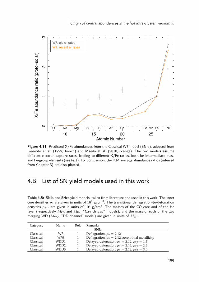
Origin of central abundances in the hot intra-cluster medium II.
10 15 20 25
01
23
X/F
e a
bundance
ratio
(pro
to!
sola
r)
Atomic Number
O Ne Mg Si S Ar Ca Cr Mn Fe Ni
W7, old e! rates
W7, recent e! rates
Figure 4.11: Predicted X/Fe abundances from the Classical W7 model (SNIa), adopted fromIwamoto et al. (1999, brown) and Maeda et al. (2010, orange). The two models assumedifferent electron capture rates, leading to different X/Fe ratios, both for intermediate-massand Fe-group elements (see text). For comparison, the ICM average abundance ratios (inferredfrom Chapter 3) are also plotted.
4.B List of SN yield models used in this work
Table 4.5: SNIa and SNcc yield models, taken from literature and used in this work. The innercore densities ρ9 are given in units of 109 g/cm3. The transitional deflagration-to-detonationdensities ρT,7 are given in units of 107 g/cm3. The masses of the CO core and of the Helayer (respectively MCO and MHe, ”Ca-rich gap” models), and the mass of each of the twomerging WD (MWD, ”DD channel” model) are given in units of M⊙.
Category Name Ref. RemarksSNIa
Classical W7 1 Deflagration, ρ9 = 2.12Classical W70 1 Deflagration, ρ9 = 2.12, zero initial metallicityClassical WDD1 1 Delayed-detonation, ρ9 = 2.12, ρT,7 = 1.7Classical WDD2 1 Delayed-detonation, ρ9 = 2.12, ρT,7 = 2.2Classical WDD3 1 Delayed-detonation, ρ9 = 2.12, ρT,7 = 3.0
159
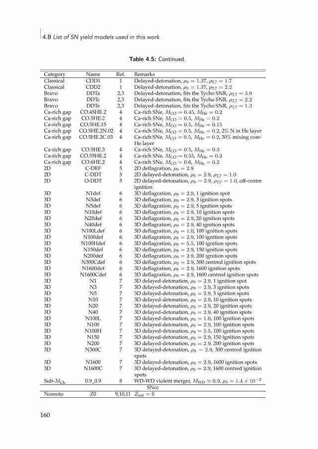
4.B List of SN yield models used in this work
Table 4.5: Continued.
Category Name Ref. RemarksClassical CDD1 1 Delayed-detonation, ρ9 = 1.37, ρT,7 = 1.7Classical CDD2 1 Delayed-detonation, ρ9 = 1.37, ρT,7 = 2.2Bravo DDTa 2,3 Delayed-detonation, fits the Tycho SNR, ρT,7 = 3.9Bravo DDTc 2,3 Delayed-detonation, fits the Tycho SNR, ρT,7 = 2.2Bravo DDTe 2,3 Delayed-detonation, fits the Tycho SNR, ρT,7 = 1.3Ca-rich gap CO.45HE.2 4 Ca-rich SNe, MCO = 0.45, MHe = 0.2Ca-rich gap CO.5HE.2 4 Ca-rich SNe, MCO = 0.5, MHe = 0.2Ca-rich gap CO.5HE.15 4 Ca-rich SNe, MCO = 0.5, MHe = 0.15Ca-rich gap CO.5HE.2N.02 4 Ca-rich SNe, MCO = 0.5, MHe = 0.2, 2% N in He layerCa-rich gap CO.5HE.2C.03 4 Ca-rich SNe, MCO = 0.5, MHe = 0.2, 30% mixing core-
He layerCa-rich gap CO.5HE.3 4 Ca-rich SNe, MCO = 0.5, MHe = 0.3Ca-rich gap CO.55HE.2 4 Ca-rich SNe, MCO = 0.55, MHe = 0.2Ca-rich gap CO.6HE.2 4 Ca-rich SNe, MCO = 0.6, MHe = 0.22D C-DEF 5 2D deflagration, ρ9 = 2.92D C-DDT 5 2D delayed-detonation, ρ9 = 2.9, ρT,7 = 1.02D O-DDT 5 2D delayed-detonation, ρ9 = 2.9, ρT,7 = 1.0, off-centre
ignition3D N1def 6 3D deflagration, ρ9 = 2.9, 1 ignition spot3D N3def 6 3D deflagration, ρ9 = 2.9, 3 ignition spots3D N5def 6 3D deflagration, ρ9 = 2.9, 5 ignition spots3D N10def 6 3D deflagration, ρ9 = 2.9, 10 ignition spots3D N20def 6 3D deflagration, ρ9 = 2.9, 20 ignition spots3D N40def 6 3D deflagration, ρ9 = 2.9, 40 ignition spots3D N100Ldef 6 3D deflagration, ρ9 = 1.0, 100 ignition spots3D N100def 6 3D deflagration, ρ9 = 2.9, 100 ignition spots3D N100Hdef 6 3D deflagration, ρ9 = 5.5, 100 ignition spots3D N150def 6 3D deflagration, ρ9 = 2.9, 150 ignition spots3D N200def 6 3D deflagration, ρ9 = 2.9, 200 ignition spots3D N300Cdef 6 3D deflagration, ρ9 = 2.9, 300 centred ignition spots3D N1600def 6 3D deflagration, ρ9 = 2.9, 1600 ignition spots3D N1600Cdef 6 3D deflagration, ρ9 = 2.9, 1600 centred ignition spots3D N1 7 3D delayed-detonation, ρ9 = 2.9, 1 ignition spot3D N3 7 3D delayed-detonation, ρ9 = 2.9, 3 ignition spots3D N5 7 3D delayed-detonation, ρ9 = 2.9, 5 ignition spots3D N10 7 3D delayed-detonation, ρ9 = 2.9, 10 ignition spots3D N20 7 3D delayed-detonation, ρ9 = 2.9, 20 ignition spots3D N40 7 3D delayed-detonation, ρ9 = 2.9, 40 ignition spots3D N100L 7 3D delayed-detonation, ρ9 = 1.0, 100 ignition spots3D N100 7 3D delayed-detonation, ρ9 = 2.9, 100 ignition spots3D N100H 7 3D delayed-detonation, ρ9 = 5.5, 100 ignition spots3D N150 7 3D delayed-detonation, ρ9 = 2.9, 150 ignition spots3D N200 7 3D delayed-detonation, ρ9 = 2.9, 200 ignition spots3D N300C 7 3D delayed-detonation, ρ9 = 2.9, 300 centred ignition
spots3D N1600 7 3D delayed-detonation, ρ9 = 2.9, 1600 ignition spots3D N1600C 7 3D delayed-detonation, ρ9 = 2.9, 1600 centred ignition
spotsSub-MCh 0.9_0.9 8 WD-WD violent merger, MWD ≃ 0.9, ρ9 = 1.4 × 10⁻²
SNccNomoto Z0 9,10,11 Zinit = 0
160
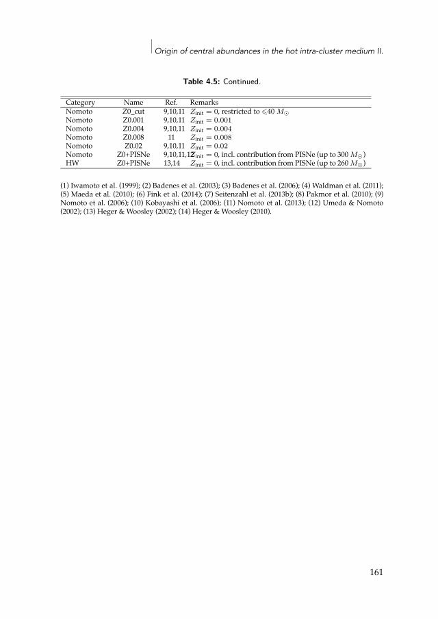
Origin of central abundances in the hot intra-cluster medium II.
Table 4.5: Continued.
Category Name Ref. RemarksNomoto Z0_cut 9,10,11 Zinit = 0, restricted to ⩽40 M⊙Nomoto Z0.001 9,10,11 Zinit = 0.001Nomoto Z0.004 9,10,11 Zinit = 0.004Nomoto Z0.008 11 Zinit = 0.008Nomoto Z0.02 9,10,11 Zinit = 0.02Nomoto Z0+PISNe 9,10,11,12Zinit = 0, incl. contribution from PISNe (up to 300 M⊙)HW Z0+PISNe 13,14 Zinit = 0, incl. contribution from PISNe (up to 260 M⊙)
(1) Iwamoto et al. (1999); (2) Badenes et al. (2003); (3) Badenes et al. (2006); (4) Waldman et al. (2011);(5) Maeda et al. (2010); (6) Fink et al. (2014); (7) Seitenzahl et al. (2013b); (8) Pakmor et al. (2010); (9)Nomoto et al. (2006); (10) Kobayashi et al. (2006); (11) Nomoto et al. (2013); (12) Umeda & Nomoto(2002); (13) Heger & Woosley (2002); (14) Heger & Woosley (2010).
161

Don’t fear mistakes. There are none.
– Miles Davis
5|Origin of central abundances inthe hot intra-cluster mediumIII. The impact of spectral model improve-ments on the abundance ratios
F. Mernier, J. de Plaa, J. S. Kaastra, A. J. J. Raassen, L. Gu, J. Mao, andI. Urdampilleta
(submitted to Astronomy & Astrophysics)
Abstract
The hot intra-clustermedium (ICM) permeating galaxy clusters and groups is richin metals, which were synthesised by billions of supernovae and have accumu-lated in cluster gravitational wells for several Gyrs. Since Type Ia (SNIa) and core-collapse supernovae (SNcc) produce different elements in quantities that dependon their explosions and/or progenitors, measuring accurately the abundances inthe ICM can help to bring further constraints on the SNIa and SNcc models tofavour. In a series of previous papers (Chapters 3 and 4), we compiled XMM-Newton observations of 44 cool-core clusters, groups, and massive ellipticals (theCHEERS catalogue) in order to establish an average abundance pattern repre-sentative of the nearby ICM, and to compare it to SNIa and SNcc yield modelstaken from the literature. In this paper, we revisit our previous abundance mea-surements by using an updated version of the spectral code and atomic database(SPEXACT) to fit the XMM-Newton EPIC spectra. We find that the Fe abundancein the lessmassive groups (kT < 1.7 keV) has been systematically underestimatedin our previous results, up to a factor of 2 for the coolest systems. Because smallmodel-to-data discrepancies in the unresolved Fe-L complex may lead to a largeFe bias, and because even the up-to-date spectral models do not well reproducethe shape of this complex below kT ≃ 1 keV, we conclude that the Fe content ofthese cool systems is still very uncertain. Moreover, the updated average Ni/Fe
163
5.1 Introduction
ratio is found to be ∼28% lower than our previous estimate. This implies that theICM abundance pattern can be reasonably reproduced when assuming delayed-detonation as the sole explosion mechanism in SNIa.
5.1 IntroductionBecause galaxy clusters host the largest gravitational potentialwells knownin ourUniverse, they act as ”closed-box” systems and retain all the baryonsthey have accreted during their formation. This is particularly interest-ing, because the hot gas — or intra-cluster medium (ICM) — permeatinggalaxy clusters is rich in heavy elements, which are thought to have beenproduced by stars and supernovae mostly during the peak of cosmic starformation (Madau & Dickinson 2014). After a significant fraction of thesemetals escape from their stellar and galactic hosts, they easily mix with theICM, and become observable through X-ray observatories via the emissionlines of their highly ionised ions (for recent reviews, see Werner et al. 2008;de Plaa 2013; de Plaa &Mernier 2017). Consequently, metals in the ICM area valuable imprint of the integral yields of billions of supernovae havingexploded within galaxy clusters over cosmic time.
Different supernova (SN) types produce elements in different amounts.Core-collapse supernovae (SNcc) are thought to produce large quantitiesof oxygen (O), neon (Ne), and magnesium (Mg), and negligible amountsof chromium (Cr), manganese (Mn), iron (Fe), and nickel (Ni). On the con-trary, Type Ia supernovae (SNIa) are thought to produce Cr, Mn, Fe, andNi in large amounts, but almost no O, Ne, nor Mg. Intermediate elements,like silicon (Si), sulfur (S), argon (Ar), and calcium (Ca) are thought to beproduced by both types of supernovae in comparable quantities. On theother hand, the exact yields produced by SNIa and SNcc depend on severalfactors. First, the relative yields produced by SNIa are sensitive to the prop-agation of the burning flame triggering the explosion (e.g. Iwamoto et al.1999). Deflagrationmodels predict that the flame propagates sub-sonically,which produces larger amounts of Ni and moderate amounts of interme-diate elements. Delayed-detonation models, on the contrary, predict thatthe flame becomes super-sonic below a specific density, which producesless Ni and more intermediate elements. Second, the relative yields pro-duced by a population of SNcc depend on the initial mass function (IMF)and the average initial metallicity of their stellar progenitors (e.g. Nomotoet al. 2013).
164
Origin of central abundances in the hot intra-cluster medium III.
Because the ICM is in collisional ionisation equilibrium (CIE) and opti-cal depth effects are negligible, abundances of O, Ne, Mg, Si, S, Ar, Ca, Fe,and Ni (and, to some extent, Cr andMn) can be robustly constrained in theICM. Therefore, the abundances of various elements X (or their ratio rela-tive to Fe, X/Fe) can be directly compared to predictions of SNIa and SNccyieldmodels, in order to bring further constraints on SNIa explosions, stel-lar populations, and the relative fraction of SNIa and SNcc to enrich galaxyclusters. Several studies were devoted to this aspect over the last decades(e.g. Mushotzky et al. 1996; Finoguenov et al. 2002; de Plaa et al. 2007; Satoet al. 2007a).
Recently, we compiled deepXMM-Newton EPIC and RGS observationsof 44 nearby cool-core ellipticals, galaxy groups, and clusters (theCHEERS1catalogue, see Sect. 5.2.1) in order to measure accurately the X/Fe abun-dance ratios of the 10 elements mentioned above, and to derive a completeabundance pattern, representative of the nearby ICM as a whole (Chapter3).We then compared this abundance patternwith commonly used and/orrecent SNIa and SNcc yield models, in order to provide reliable constraintson SNIa/SNcc explosions and/or progenitors (Chapter 4). Among the re-sults presented in Chapter 4, we could note that, interestingly, a diversityin SNIa explosions (with both deflagration and delayed-detonation mod-els) was required to reproduce successfully all the average estimated X/Feratios.
Of course, for such a study, it is crucial to fully understand (and, pos-sibly, reduce) the systematic uncertainties affecting the measurements ofthe X/Fe abundance ratios in the ICM. In Chapter 3, we showed that theseuncertainties were actually largely dominating over the statistical uncer-tainties. While many sources of systematic uncertainties were taken intoaccount in that study (including local continuumbiases in the instrumentalresponse, EPIC cross-calibration uncertainties, intrinsic scatter, assumedthermal structure of the ICM, differences in the studied spatial regions, aswell as a careful modelling of the background), our results relied on theup-to-date version (2.06) of the plasmamodels from the SPEX fitting pack-age (Kaastra et al. 1996) at that time. Recently, however, a major updateof SPEX has been performed (see Sect. 5.2.2 for more details). Since, byessence, the estimated abundances of a CIE plasma depend on the inputatomic calculations in the spectral model that is used, studying the effectsof these improvements on our previous measurements is essential for set-
1CHEmical Enrichment Rgs Sample
165
5.2 The sample and the reanalysis of our data
ting correct constraints on supernova yield models.In this work, we explore the effects of such spectral model improve-
ments on our previously measured average abundance pattern in the cool-core ICM, in particular with XMM-Newton EPIC (Chapter 3). As a secondstep, we discuss the implications of these effects on our previous interpre-tation of the ICM enrichment by SNIa and SNcc (Chapter 4). This paperis organised as follows. Section 5.2 is devoted to the reanalysis of the datapresented in Chapter 3. Our updated results are presented in Sect. 5.3, andtheir implications regarding to previous studies are discussed in Sect. 5.4.We sum up our findings in Sect. 5.5. Throughout this paper, we assumeH0= 70 km s−1 Mpc−1, Ωm = 0.3, and ΩΛ= 0.7. Unless otherwise stated, theerror bars are given within a 68% confidence interval. All the abundancesmentioned in this work are given with respect to their proto-solar valuesderived from Lodders et al. (2009).
5.2 The sample and the reanalysis of our data5.2.1 The sampleThe sample, the data reduction, and the spectral analysis and strategies areall described in detail in Chapter 3. Like our present work, that previousstudy focused on the XMM-Newton observations of 44 nearby cool-coreclusters, groups, and ellipticals, all being part of the CHEERS sample (seealso Pinto et al. 2015; de Plaa et al. 2017). In addition to their limited redshift(z < 0.2), the main criterion of the sample is that the oxygen abundance(mainly traced by its OVIII emission line) measured by the RGS instru-ment must be detected with >5σ of significance. In this way, we ensureselecting clusters with prominent metal lines in their cores. This allows arobust determination of most of the metal abundances also with the EPICinstruments.
Starting from the same filtered data and spectra as in Chapter 3, weadopt the same definitions and we split our sample into two subsamples.
1. The hot ”clusters” (23 objects), which exhibit a central mean temper-ature of kT > 1.7 keV. They can be investigated within 0.2r500 (andsometimes beyond).
2. The cool ”groups” (21 objects, also including ellipticals), which ex-hibit a central mean temperature of kT < 1.7 keV. By selection, their
166
Origin of central abundances in the hot intra-cluster medium III.
0.2r500 limit often falls outside the EPIC field of view, but they canbe investigated within 0.05r500.
The elliptical galaxyM87 is an exception. As the brightest central galaxy ofa large cluster (Virgo), itsmean temperature is about∼2 keV, but the galaxyis too nearby to allow the ICM for being investigated within 0.2r500. Fol-lowing Chapter 3, we choose to consider it as part of the group subsample.
In order to maximise our statistics, and unless mentioned otherwise, inthe rest of the paper we focus on the (0.2+0.05)r500 sample, i.e. where theabundances in our clusters and our groups are investigated within 0.2r500and 0.05r500, respectively. A complete discussion of the effects of adoptingdifferent extraction radii on our abundance measurements can be found inChapter 3.
5.2.2 From SPEXACT v2 to SPEXACT v3Since 1996, the original mekal code, used tomodel thermal plasmas (Mewe1972; Mewe et al. 1985, 1986), has been developed independently withinthe SPEX spectral fitting package (Kaastra et al. 1996) and gradually im-proved. Up to the version 2.06, the code made use of an atomic databaseand a collection of routines that are all referred to SPEXACT2 v2. Since 2016,however, a major update has been performed on both the atomic databaseand the corresponding routines, leading to SPEXACT v3. For example, theatomic database contains nowhundreds of thousands of energy transitions(from hydrogen to zinc) whose updated collisional excitation and desexci-tation rates, radiative transition probabilities and auto-ionisation and di-electronic recombination rates have been obtained from the literature orconsistently calculated using the FAC3 code (Gu 2008). All these transi-tions, much more numerous than in SPEXACT v2, cover now atomic lev-els with principle quantum number up to 20 for H-like, and up to 16 forHe-like ions. On the other hand, significant improved calculations of theradiative recombination (Badnell 2006;Mao&Kaastra 2016) and collisionalionisation coefficients (Urdampilleta et al. 2017) have been achieved. Theupdated version of the fitting package, namely SPEX v3, allows to use ei-ther SPEXACT v2 or SPEXACT v3, depending on the user’s requirements.
After the release of SPEXACT v3, we noted in Chapter 6 (see also dePlaa et al. 2017) that the choice of the SPEXACT version could lead to sig-
2SPEX Atomic Code and Tables; see also the SPEX manual.3https://www-amdis.iaea.org/FAC
167
5.2 The sample and the reanalysis of our data
nificant changes in the abundances measured with RGS and EPIC, respec-tively. Since all the spectral analysis in Chapter 3 has been done usingSPEXACT v2, in this paper we aim to quantify the changes on the aver-age ICM abundance ratios when using SPEXACT v3. A straight forwardway to do so would be to re-process entirely the spectral analysis for allour observations before re-stacking the results in a similar way as in Chap-ter 3. However, the very large number of new lines in the updated atomicdatabase considerably expands the computing time required for each sin-gle fit, making this approach technically unrealistic. Instead, we choose asimilar alternative already presented in de Plaa et al. (2017) and Chapter 6.
In Chapter 3, the abundances of O, Ne, Cr, and Mn were either mea-sured with SPEXACT v3 or already corrected to their SPEXACT v3 esti-mates. Therefore, there is no need to include them in our simulations. Toestimate the impact of spectral model improvements on the Mg, Si, S, Ar,Ca, Fe, andNi abundances, we first use SPEXACT v3 to simulate 24 spectraof an absorbed multi-temperature CIE plasma, namely gdem, which mim-ics a plasma with a Gaussian temperature distribution4. Each spectrum issimulated at a fixedmean temperature (kTmean) between 0.6 and 6 keV (i.e.the typical range of temperatures that are measured in the core of our sys-tems), assuming the recent ionisation balance of Urdampilleta et al. (2017),and each model is convolved with the EPIC MOS and pn instrumental re-sponses. The abundances of all the elements are fixed to the proto-solarunity. The redshift (z), hydrogen column density (NH), the emission mea-sure (Y =
∫nenHdV ) and the width of the Gaussian temperature distri-
bution (σT ) are set to 0.039 (corresponding to a distance of ∼172 Mpc),1.14 × 1025 m−2, 7.17 × 1072 m−3, and 0.18, respectively. These param-eters are adapted from the best-fit results of EXO0422, a typical clusterof intermediate redshift, temperature, and abundances (see Chapter 3). Tominimise the statistical biases, all the spectra are simulated for a 100 ks ex-posure (which is comparable to the typical net exposure of each object).Furthermore, we keep the Poisson noise to zero to obtain the exact meannumber of counts that is expected in each bin (see de Plaa et al. 2017). Thisapproach is clearly faster than the Monte Carlo method since we do notneed to simulate a large number of spectra with Poisson noise.
As a second step, we fit all these spectra, this time using SPEXACT v2,leaving free the emission measure, the mean temperature, and the afore-mentioned abundances thatwe could reasonablymeasurewith EPIC. These
4For more details, see Chapter 3 and the SPEX manual.
168
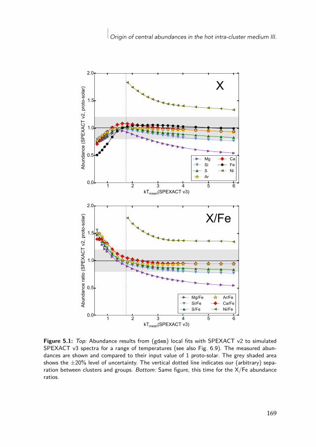
Origin of central abundances in the hot intra-cluster medium III.
1 2 3 4 5 6kTmean(SPEXACT v3)
0.0
0.5
1.0
1.5
2.0
Abun
danc
e (S
PEXA
CT
v2, p
roto
-sol
ar) X
MgSiSAr
CaFeNi
1 2 3 4 5 6kTmean(SPEXACT v3)
0.0
0.5
1.0
1.5
2.0
Abun
danc
e ra
tio (S
PEXA
CT
v2, p
roto
-sol
ar) X/Fe
Mg/FeSi/FeS/Fe
Ar/FeCa/FeNi/Fe
Figure 5.1: Top: Abundance results from (gdem) local fits with SPEXACT v2 to simulatedSPEXACT v3 spectra for a range of temperatures (see also Fig. 6.9). The measured abun-dances are shown and compared to their input value of 1 proto-solar. The grey shaded areashows the ±20% level of uncertainty. The vertical dotted line indicates our (arbitrary) sepa-ration between clusters and groups. Bottom: Same figure, this time for the X/Fe abundanceratios.
169
5.3 Results
fits are done assuming the ionisation balance of Bryans et al. (2009), as as-sumed in Chapter 3. To be consistent with our previous analysis (Chapter3), after having fixed the temperature parameter, the abundance parame-ters are re-estimated through a local fit (i.e. within a band encompassingtheir corresponding K-shell lines).
The result of this exercise, illustrating the differences between the twolatest SPEXACTversions inmeasuring the absolute abundances (X), is shownin the upper panel of Fig. 5.1 (see also Fig. 6.9). The lower panel providesthe same quantities, this time reported relative to the Fe abundance (X/Fe).
Finally, based on these simulated estimates, we correct the estimatedabsolute/relative abundances of each observed spectrum by applying acorresponding SPEXACT v2–v3 correction factor. These factors obviouslydepend on themeasuredmean temperature, and are simply taken as the in-verse of the values reported in Fig. 5.1. The individual corrections appliedhere are further commented in the next sections.
5.3 Results
Before applying the correction method described in Sect. 5.2.2 to our pre-vious data (Chapter 3), we discuss the ratios in Fig. 5.1. In the upper panel,Fe appears to be well recovered in the cluster regime (kTmean > 1.7 keV),in which the Fe abundance is essentially measured via its K-shell complex(∼6.4 keV). However, for cooler systems (kTmean < 1.7 keV), in which theFe L-shell lines become clearly dominant, the Fe abundance is systemat-ically underestimated by SPEXACT v2, up to a factor of 2 for the coolestplasmas (kTmean ≃ 0.6 keV). This underestimate has an effect on the X/Feratios, which are measured ∼50% higher using SPEXACT v2 than usingSPEXACT v3 (Fig. 5.1 bottom). Besides Fe, two other elements (and theircorresponding X/Fe ratios) deserve some attention, in particular at clus-ter temperatures. When measured with SPEXACT v2, the Ni abundance isclearly overestimated, from∼30% in the hottest plamas to∼80%when ap-proaching the group regime (where the Ni K-shell lines become difficult todetectwith the current instruments). On the other hand, theMg abundancecan be biased low to ∼50%.
170
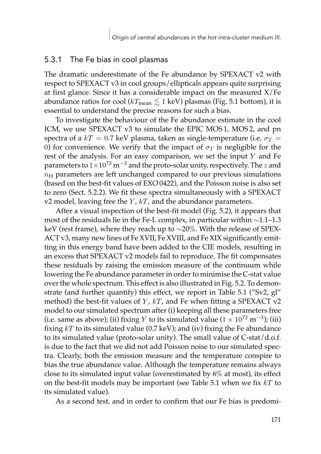
Origin of central abundances in the hot intra-cluster medium III.
5.3.1 The Fe bias in cool plasmasThe dramatic underestimate of the Fe abundance by SPEXACT v2 withrespect to SPEXACT v3 in cool groups/ellipticals appears quite surprisingat first glance. Since it has a considerable impact on the measured X/Feabundance ratios for cool (kTmean ≲ 1 keV) plasmas (Fig. 5.1 bottom), it isessential to understand the precise reasons for such a bias.
To investigate the behaviour of the Fe abundance estimate in the coolICM, we use SPEXACT v3 to simulate the EPIC MOS1, MOS2, and pnspectra of a kT = 0.7 keV plasma, taken as single-temperature (i.e. σT =0) for convenience. We verify that the impact of σT is negligible for therest of the analysis. For an easy comparison, we set the input Y and Feparameters to 1×1072 m−3 and the proto-solar unity, respectively. The z andnH parameters are left unchanged compared to our previous simulations(based on the best-fit values of EXO0422), and the Poisson noise is also setto zero (Sect. 5.2.2). We fit these spectra simultaneously with a SPEXACTv2 model, leaving free the Y , kT , and the abundance parameters.
After a visual inspection of the best-fit model (Fig. 5.2), it appears thatmost of the residuals lie in the Fe-L complex, in particular within ∼1.1–1.3keV (rest frame), where they reach up to ∼20%. With the release of SPEX-ACT v3,many new lines of FeXVII, FeXVIII, and FeXIX significantly emit-ting in this energy band have been added to the CIE models, resulting inan excess that SPEXACT v2 models fail to reproduce. The fit compensatesthese residuals by raising the emission measure of the continuum whilelowering the Fe abundance parameter in order tominimise the C-stat valueover thewhole spectrum. This effect is also illustrated in Fig. 5.2. Todemon-strate (and further quantify) this effect, we report in Table 5.1 (”Sv2, gl”method) the best-fit values of Y , kT , and Fe when fitting a SPEXACT v2model to our simulated spectrum after (i) keeping all these parameters free(i.e. same as above); (ii) fixing Y to its simulated value (1 × 1072 m−3); (iii)fixing kT to its simulated value (0.7 keV); and (iv) fixing the Fe abundanceto its simulated value (proto-solar unity). The small value of C-stat/d.o.f.is due to the fact that we did not add Poisson noise to our simulated spec-tra. Clearly, both the emission measure and the temperature conspire tobias the true abundance value. Although the temperature remains alwaysclose to its simulated input value (overestimated by 6% at most), its effecton the best-fit models may be important (see Table 5.1 when we fix kT toits simulated value).
As a second test, and in order to confirm that our Fe bias is predomi-
171
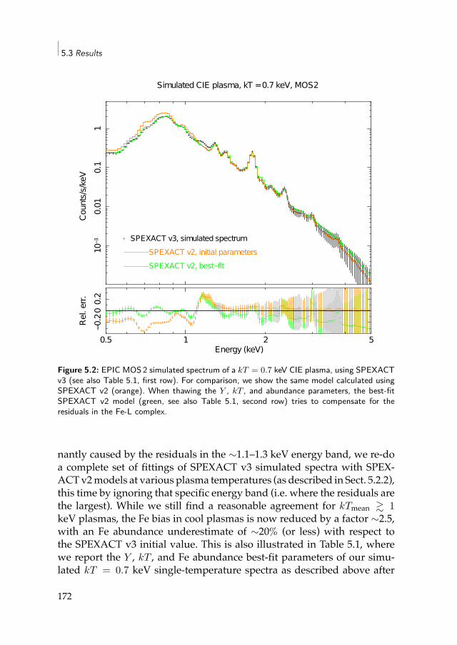
5.3 Results
10.5 2 5
−0.2
00.
2Re
l. err.
Energy (keV)
10.5 2 5
10−3
0.01
0.1
1Co
unts/
s/keV
Simulated CIE plasma, kT = 0.7 keV, MOS2
SPEXACT v3, simulated spectrumSPEXACT v2, initial parametersSPEXACT v2, best−fit
Figure 5.2: EPIC MOS 2 simulated spectrum of a kT = 0.7 keV CIE plasma, using SPEXACTv3 (see also Table 5.1, first row). For comparison, we show the same model calculated usingSPEXACT v2 (orange). When thawing the Y , kT , and abundance parameters, the best-fitSPEXACT v2 model (green, see also Table 5.1, second row) tries to compensate for theresiduals in the Fe-L complex.
nantly caused by the residuals in the ∼1.1–1.3 keV energy band, we re-doa complete set of fittings of SPEXACT v3 simulated spectra with SPEX-ACTv2models at various plasma temperatures (as described in Sect. 5.2.2),this time by ignoring that specific energy band (i.e. where the residuals arethe largest). While we still find a reasonable agreement for kTmean ≳ 1keV plasmas, the Fe bias in cool plasmas is now reduced by a factor ∼2.5,with an Fe abundance underestimate of ∼20% (or less) with respect tothe SPEXACT v3 initial value. This is also illustrated in Table 5.1, wherewe report the Y , kT , and Fe abundance best-fit parameters of our simu-lated kT = 0.7 keV single-temperature spectra as described above after
172
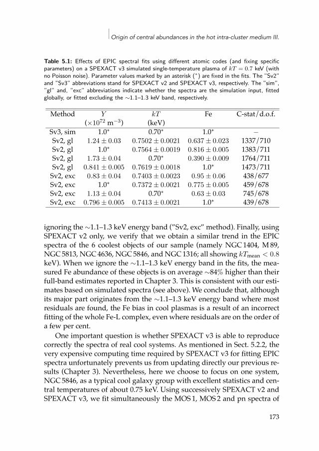
Origin of central abundances in the hot intra-cluster medium III.
Table 5.1: Effects of EPIC spectral fits using different atomic codes (and fixing specificparameters) on a SPEXACT v3 simulated single-temperature plasma of kT = 0.7 keV (withno Poisson noise). Parameter values marked by an asterisk (∗) are fixed in the fits. The ”Sv2”and ”Sv3” abbreviations stand for SPEXACT v2 and SPEXACT v3, respectively. The ”sim”,”gl” and, ”exc” abbreviations indicate whether the spectra are the simulation input, fittedglobally, or fitted excluding the ∼1.1–1.3 keV band, respectively.
Method Y kT Fe C-stat/d.o.f.(×1072 m−3) (keV)
Sv3, sim 1.0∗ 0.70∗ 1.0∗ −Sv2, gl 1.24 ± 0.03 0.7502 ± 0.0021 0.637 ± 0.023 1337/710Sv2, gl 1.0∗ 0.7564 ± 0.0019 0.816 ± 0.005 1383/711Sv2, gl 1.73 ± 0.04 0.70∗ 0.390 ± 0.009 1764/711Sv2, gl 0.841 ± 0.005 0.7619 ± 0.0018 1.0∗ 1473/711Sv2, exc 0.83 ± 0.04 0.7403 ± 0.0023 0.95 ± 0.06 438/677Sv2, exc 1.0∗ 0.7372 ± 0.0021 0.775 ± 0.005 459/678Sv2, exc 1.13 ± 0.04 0.70∗ 0.63 ± 0.03 745/678Sv2, exc 0.796 ± 0.005 0.7413 ± 0.0021 1.0∗ 439/678
ignoring the ∼1.1–1.3 keV energy band (”Sv2, exc” method). Finally, usingSPEXACT v2 only, we verify that we obtain a similar trend in the EPICspectra of the 6 coolest objects of our sample (namely NGC1404, M89,NGC5813, NGC4636, NGC5846, and NGC1316; all showing kTmean < 0.8keV). When we ignore the ∼1.1–1.3 keV energy band in the fits, the mea-sured Fe abundance of these objects is on average ∼84% higher than theirfull-band estimates reported in Chapter 3. This is consistent with our esti-mates based on simulated spectra (see above). We conclude that, althoughits major part originates from the ∼1.1–1.3 keV energy band where mostresiduals are found, the Fe bias in cool plasmas is a result of an incorrectfitting of the whole Fe-L complex, even where residuals are on the order ofa few per cent.
One important question is whether SPEXACT v3 is able to reproducecorrectly the spectra of real cool systems. As mentioned in Sect. 5.2.2, thevery expensive computing time required by SPEXACT v3 for fitting EPICspectra unfortunately prevents us from updating directly our previous re-sults (Chapter 3). Nevertheless, here we choose to focus on one system,NGC5846, as a typical cool galaxy group with excellent statistics and cen-tral temperatures of about 0.75 keV. Using successively SPEXACT v2 andSPEXACT v3, we fit simultaneously the MOS1, MOS2 and pn spectra of
173
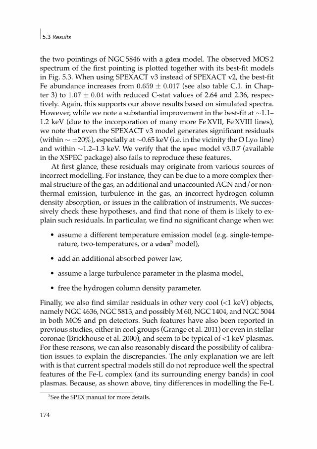
5.3 Results
the two pointings of NGC5846 with a gdem model. The observed MOS2spectrum of the first pointing is plotted together with its best-fit modelsin Fig. 5.3. When using SPEXACT v3 instead of SPEXACT v2, the best-fitFe abundance increases from 0.659 ± 0.017 (see also table C.1. in Chap-ter 3) to 1.07 ± 0.04 with reduced C-stat values of 2.64 and 2.36, respec-tively. Again, this supports our above results based on simulated spectra.However, while we note a substantial improvement in the best-fit at ∼1.1–1.2 keV (due to the incorporation of many more FeXVII, FeXVIII lines),we note that even the SPEXACT v3 model generates significant residuals(within∼ ±20%), especially at∼0.65 keV (i.e. in the vicinity theO Lyα line)and within ∼1.2–1.3 keV. We verify that the apec model v3.0.7 (availablein the XSPEC package) also fails to reproduce these features.
At first glance, these residuals may originate from various sources ofincorrect modelling. For instance, they can be due to a more complex ther-mal structure of the gas, an additional and unaccounted AGN and/or non-thermal emission, turbulence in the gas, an incorrect hydrogen columndensity absorption, or issues in the calibration of instruments. We succes-sively check these hypotheses, and find that none of them is likely to ex-plain such residuals. In particular, we find no significant change when we:
• assume a different temperature emission model (e.g. single-tempe-rature, two-temperatures, or a wdem5 model),
• add an additional absorbed power law,• assume a large turbulence parameter in the plasma model,• free the hydrogen column density parameter.
Finally, we also find similar residuals in other very cool (<1 keV) objects,namelyNGC4636,NGC5813, andpossiblyM60,NGC1404, andNGC5044in both MOS and pn detectors. Such features have also been reported inprevious studies, either in cool groups (Grange et al. 2011) or even in stellarcoronae (Brickhouse et al. 2000), and seem to be typical of <1 keV plasmas.For these reasons, we can also reasonably discard the possibility of calibra-tion issues to explain the discrepancies. The only explanation we are leftwith is that current spectral models still do not reproduce well the spectralfeatures of the Fe-L complex (and its surrounding energy bands) in coolplasmas. Because, as shown above, tiny differences in modelling the Fe-L
5See the SPEX manual for more details.
174
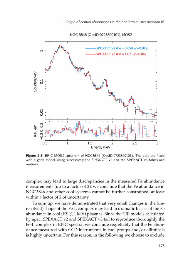
Origin of central abundances in the hot intra-cluster medium III.
0.5 1 1.5 2 2.5 3
0.01
0.1
1Co
unts/
s/keV
NGC 5846 (ObsID:0723800101), MOS2
SPEXACT v2 (Fe = 0.659 +/− 0.017)SPEXACT v3 (Fe = 1.07 +/− 0.04)
0.5 1 1.5 2 2.5 3
−0.2
00.
2Re
l. err.
Energy (keV)
Figure 5.3: EPIC MOS 2 spectrum of NGC 5846 (ObsID:0723800101). The data are fittedwith a gdem model, using successively the SPEXACT v2 and the SPEXACT v3 tables androutines.
complex may lead to large discrepancies in the measured Fe abundancemeasurements (up to a factor of 2), we conclude that the Fe abundance inNGC5846 and other cool systems cannot be further constrained, at leastwithin a factor of 2 of uncertainty.
To sum up, we have demonstrated that very small changes in the (un-resolved) shape of the Fe-L complex may lead to dramatic biases of the Feabundance in cool (kT ≲ 1 keV) plasmas. Since the CIE models calculatedby apec, SPEXACT v2 and SPEXACT v3 fail to reproduce thoroughly theFe-L complex in EPIC spectra, we conclude regrettably that the Fe abun-dance measured with CCD instruments in cool groups and/or ellipticalsis highly uncertain. For this reason, in the following we choose to exclude
175
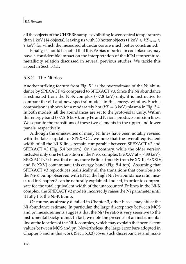
5.3 Results
all the objects of theCHEERS sample exhibiting lower central temperaturesthan 1 keV (14 objects), leaving uswith 30 hotter objects (1 keV ⩽ kTmean ⩽7 keV) for which the measured abundances are much better constrained.
Finally, it should be noted that this Fe bias reported in cool plasmasmayhave a considerable impact on the interpretation of the ICM temperature-metallicity relation discussed in several previous studies. We tackle thisaspect in Sect. 5.4.1.
5.3.2 The Ni biasAnother striking feature from Fig. 5.1 is the overestimate of the Ni abun-dance by SPEXACT v2 compared to SPEXACT v3. Since the Ni abundanceis estimated from the Ni-K complex (∼7.8 keV) only, it is instructive tocompare the old and new spectral models in this energy window. Such acomparison is shown for a moderately hot (kT = 3 keV) plasma in Fig. 5.4.In both models, all the abundances are set to the proto-solar unity. Withinthis energy band (∼7.5–8 keV), only Fe andNi ions produce emission lines.We separate the transitions of these two elements in the upper and lowerpanels, respectively.
Although the emissivities of many Ni lines have been notably revisedwith the latest update of SPEXACT, we note that the overall equivalentwidth of all the Ni-K lines remain comparable between SPEXACT v2 andSPEXACT v3 (Fig. 5.4 bottom). On the contrary, while the older versionincludes only one Fe transition in the Ni-K complex (FeXXV at∼7.88 keV),SPEXACTv3 shows thatmanymore Fe lines (mostly fromFeXXIII, FeXXIV,and FeXXV) contaminate this energy band (Fig. 5.4 top). Assuming thatSPEXACT v3 reproduces realistically all the transitions that contribute tothe Ni-K bump observed with EPIC, the high Ni/Fe abundance ratio mea-sured in Chapter 3 can be naturally explained. Indeed, in order to compen-sate for the total equivalent width of the unaccounted Fe lines in the Ni-Kcomplex, the SPEXACT v2models incorrectly raises theNi parameter untilit fully fits the Ni-K bump.
Of course, as already detailed in Chapter 3, other biases may affect theNi abundance estimate. In particular, the large discrepancy between MOSand pn measurements suggests that the Ni/Fe ratio is very sensitive to theinstrumental background. In fact, we note the presence of an instrumentalline at the location of theNi-K complex,whichmay explain the inconsistentvalues betweenMOS and pn. Nevertheless, the large error bars adopted inChapter 3 and in this work (Sect. 5.3.3) cover such discrepancies and make
176
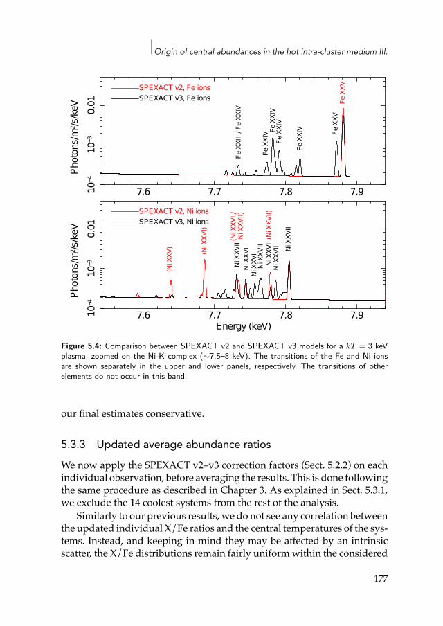
Origin of central abundances in the hot intra-cluster medium III.
7.6 7.7 7.8 7.910−4
10−3
0.01
Phot
ons/m
2 /s/ke
V
Energy (keV)
Ni X
XVII
Ni X
XVII
Ni X
XVI
(Ni X
XVII)
Ni X
XVII
Ni X
XVI
Ni X
XVI
Ni X
XVII
(Ni X
XVI /
Ni X
XVII)
(Ni X
XVI)
(Ni X
XV)
SPEXACT v2, Ni ionsSPEXACT v3, Ni ions
7.6 7.7 7.8 7.910−4
10−3
0.01
Phot
ons/m
2 /s/ke
V
Energy (keV)
Fe X
XVFe
XXV
Fe X
XIV
Fe X
XIV
Fe X
XIV
Fe X
XIV
Fe X
XIII
/ Fe
XXIV
SPEXACT v2, Fe ionsSPEXACT v3, Fe ions
Figure 5.4: Comparison between SPEXACT v2 and SPEXACT v3 models for a kT = 3 keVplasma, zoomed on the Ni-K complex (∼7.5–8 keV). The transitions of the Fe and Ni ionsare shown separately in the upper and lower panels, respectively. The transitions of otherelements do not occur in this band.
our final estimates conservative.
5.3.3 Updated average abundance ratiosWe now apply the SPEXACT v2–v3 correction factors (Sect. 5.2.2) on eachindividual observation, before averaging the results. This is done followingthe same procedure as described in Chapter 3. As explained in Sect. 5.3.1,we exclude the 14 coolest systems from the rest of the analysis.
Similarly to our previous results, we do not see any correlation betweenthe updated individual X/Fe ratios and the central temperatures of the sys-tems. Instead, and keeping in mind they may be affected by an intrinsicscatter, the X/Fe distributions remain fairly uniformwithin the considered
177
5.3 Results
temperature range (∼1–7 keV). This agrees with our previous conclusionsthat the relative SNIa to SNcc enrichment do not (or very poorly) dependon the temperature (and, by extension, the mass) of the systems, and thatthe enrichment mechanisms at play in ellipticals, galaxy groups and clus-ters must be quite similar (Chapter 3, see also De Grandi &Molendi 2009).This also means that our attempt to average the X/Fe abundance ratios inthe ICM is fully relevant.
The updated average X/Fe abundance ratios and their respective sta-tistical (σstat) and systematic uncertainties are listed in Table 5.2. This tablecan thus be directly compared with Table 3.2 of Chapter 3, to which werefer the reader for an extensive description of the estimated systematicuncertainties — σint (the intrinsic scatter), σregion (the uncertainty relatedto the different size of the extraction regions), and σcross-cal (the uncertaintyin the cross-calibration of the different instruments). All the uncertaintiesare added in quadrature to obtain σtot, our total estimated uncertainties.Evidently, improvements in the spectral models have no impact on the dis-crepancies in the measurements made by the different instruments. There-fore, the Ar/Fe and Ni/Fe abundance ratios still suffer from consequentadditional cross-calibration uncertainties, which we take into account inour final estimates.
The updated average ICM abundance pattern is also shown in Fig. 5.5,together with the comparison of our previous estimates from Chapter 3(i.e. the full sample, fitted with SPEXACT v2). It clearly appears that, formost ratios, the changes are quite small. In particular, although the Mgbias appears to be quite important in Fig. 5.1, we note that Mg is more ac-curately determined in cooler gas. Therefore, and because the individualMg/Fe ratios are affected by a non-negligible scatter, the updated averageMg/Fe ratio remains fully consistent with its old estimate. Some attention,however, should be devoted to Si/Fe and S/Fe, as these ratios are slightlyrevised upwards (of∼21% and∼12%, respectively). Contrary toMg, the Siand S abundances are easier to constrain in hot plasmas, and their averagerespective X/Fe ratios are thus weighted toward hot systems, where theSPEX v2–v3 corrections are themost important. Another noticeable changeis seen on the Ni/Fe ratio, for which our new value is∼28% lower than theold one. Although the (large) total uncertainties of our two Ni/Fe mea-surements are formally consistent with each other, we will see in Sect. 5.4that such a change has a substantial impact in the selection of specific SNIayield models to explain the ICM enrichment.
178
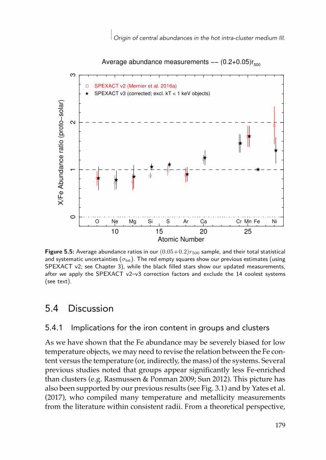
Origin of central abundances in the hot intra-cluster medium III.
10 15 20 25
01
23
X/F
e A
bu
nd
an
ce r
atio
(p
roto
−so
lar)
Atomic Number
Average abundance measurements −− (0.2+0.05)r500
O Ne Mg Si S Ar Ca Cr Mn Fe Ni
SPEXACT v3 (corrected; excl. kT < 1 keV objects)
SPEXACT v2 (Mernier et al. 2016a)
Figure 5.5: Average abundance ratios in our (0.05+0.2)r500 sample, and their total statisticaland systematic uncertainties (σtot). The red empty squares show our previous estimates (usingSPEXACT v2; see Chapter 3), while the black filled stars show our updated measurements,after we apply the SPEXACT v2–v3 correction factors and exclude the 14 coolest systems(see text).
5.4 Discussion5.4.1 Implications for the iron content in groups and clustersAs we have shown that the Fe abundance may be severely biased for lowtemperature objects, wemayneed to revise the relation between the Fe con-tent versus the temperature (or, indirectly, themass) of the systems. Severalprevious studies noted that groups appear significantly less Fe-enrichedthan clusters (e.g. Rasmussen & Ponman 2009; Sun 2012). This picture hasalso been supported by our previous results (see Fig. 3.1) and by Yates et al.(2017), who compiled many temperature and metallicity measurementsfrom the literature within consistent radii. From a theoretical perspective,
179
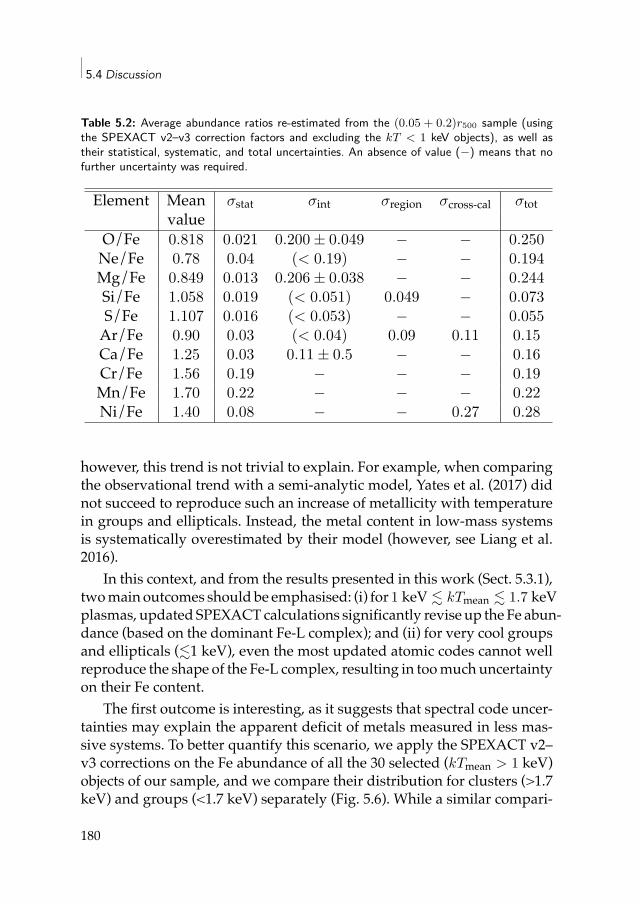
5.4 Discussion
Table 5.2: Average abundance ratios re-estimated from the (0.05 + 0.2)r500 sample (usingthe SPEXACT v2–v3 correction factors and excluding the kT < 1 keV objects), as well astheir statistical, systematic, and total uncertainties. An absence of value (−) means that nofurther uncertainty was required.
Element Mean σstat σint σregion σcross-cal σtotvalue
O/Fe 0.818 0.021 0.200 ± 0.049 − − 0.250Ne/Fe 0.78 0.04 (< 0.19) − − 0.194Mg/Fe 0.849 0.013 0.206 ± 0.038 − − 0.244Si/Fe 1.058 0.019 (< 0.051) 0.049 − 0.073S/Fe 1.107 0.016 (< 0.053) − − 0.055Ar/Fe 0.90 0.03 (< 0.04) 0.09 0.11 0.15Ca/Fe 1.25 0.03 0.11 ± 0.5 − − 0.16Cr/Fe 1.56 0.19 − − − 0.19Mn/Fe 1.70 0.22 − − − 0.22Ni/Fe 1.40 0.08 − − 0.27 0.28
however, this trend is not trivial to explain. For example, when comparingthe observational trend with a semi-analytic model, Yates et al. (2017) didnot succeed to reproduce such an increase of metallicity with temperaturein groups and ellipticals. Instead, the metal content in low-mass systemsis systematically overestimated by their model (however, see Liang et al.2016).
In this context, and from the results presented in this work (Sect. 5.3.1),twomain outcomes should be emphasised: (i) for 1 keV ≲ kTmean ≲ 1.7 keVplasmas, updated SPEXACT calculations significantly revise up the Fe abun-dance (based on the dominant Fe-L complex); and (ii) for very cool groupsand ellipticals (≲1 keV), even the most updated atomic codes cannot wellreproduce the shape of the Fe-L complex, resulting in toomuch uncertaintyon their Fe content.
The first outcome is interesting, as it suggests that spectral code uncer-tainties may explain the apparent deficit of metals measured in less mas-sive systems. To better quantify this scenario, we apply the SPEXACT v2–v3 corrections on the Fe abundance of all the 30 selected (kTmean > 1 keV)objects of our sample, and we compare their distribution for clusters (>1.7keV) and groups (<1.7 keV) separately (Fig. 5.6). While a similar compari-
180
Origin of central abundances in the hot intra-cluster medium III.
son from Chapter 3 (Fig. 3.3) argued in favour of a deficit of metals in thecooler groups, our present results suggest that cluster and group coresmaybe equally enriched.
This updated trend appears to better match (at least qualitatively) themodel predictions of Yates et al. (2017). If further confirmed, this resultis potentially important, as it suggests that significant metal removal ingroup cores (by either stellar or AGN feedback), as usually invoked so far(e.g. Rasmussen & Ponman 2009), may not be necessary. Unfortunately,the situation is still unclear and prevents us to draw any firm conclusion,mainly for three reasons:
1. In the updated comparison between cluster and group metallicitiespresentedhere, only 7 groups are comprisedwithin 1 keV< kTmean <1.7 keV, preventing us from establishing a robust study over a reason-able number of nearby groups;
2. As shown in Sect. 5.3.1, the Fe abundance of the systemswith kTmean <1 keV cannot be robustly constrained evenwith current spectralmod-els;
3. The measurements on group metallicities made in previous studiesare from various versions of SPEX and/or apecmodels, and can thushardly be compiled and compared in a consistent way.
In conclusion, although we propose the intriguing possibility that thelack of metals observed in less massive systems might be entirely due toa bias in the spectral models, we stress that this astrophysical question isnot yet solved. Synergy between further observations of galaxy groups (forwhich the Fe abundance is measured consistently) and improvements inCIE plasma models and atomic codes will help to clarify the picture of themetal content in clusters and groups.
In addition to the Fe bias discussed in this work, we also note from Ta-ble 5.1 that fitting the spectra of cool systems with outdated plasma codesmay also bias high the emissionmeasure and the temperature by∼24%and∼7%, respectively. In turn, these biases may have consequences on the es-timates of further interesting quantities. For instance, based on our test de-scribed in Sect. 5.3.1, we estimated that the ICM pressure, usually definedas P = nekT can be biased high by ∼19% in the case of a ∼0.7 keV plasma.Unlike the pressure, the ICM entropy, usually defined as K = kT/n
2/3e , re-
mains very close to its true value, with a underestimate of less than ∼1%.
181
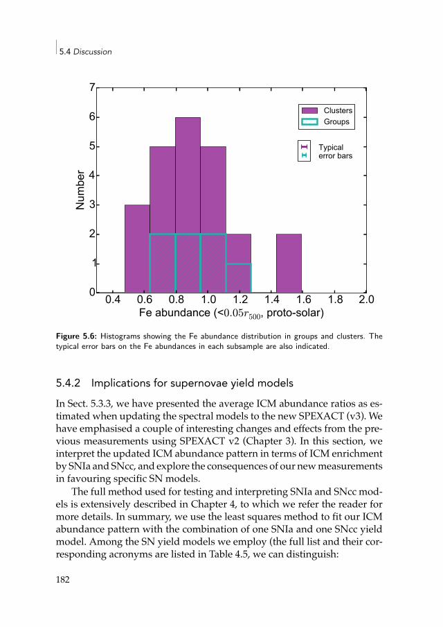
5.4 Discussion
0.4 0.6 0.8 1.0 1.2 1.4 1.6 1.8 2.0Fe abundance (<0.05r500, proto-solar)
0
1
2
3
4
5
6
7N
umbe
r
Typical error bars
ClustersGroups
Figure 5.6: Histograms showing the Fe abundance distribution in groups and clusters. Thetypical error bars on the Fe abundances in each subsample are also indicated.
5.4.2 Implications for supernovae yield modelsIn Sect. 5.3.3, we have presented the average ICM abundance ratios as es-timated when updating the spectral models to the new SPEXACT (v3). Wehave emphasised a couple of interesting changes and effects from the pre-vious measurements using SPEXACT v2 (Chapter 3). In this section, weinterpret the updated ICM abundance pattern in terms of ICM enrichmentby SNIa and SNcc, and explore the consequences of our newmeasurementsin favouring specific SN models.
The full method used for testing and interpreting SNIa and SNcc mod-els is extensively described in Chapter 4, to which we refer the reader formore details. In summary, we use the least squares method to fit our ICMabundance pattern with the combination of one SNIa and one SNcc yieldmodel. Among the SN yield models we employ (the full list and their cor-responding acronyms are listed in Table 4.5, we can distinguish:
182
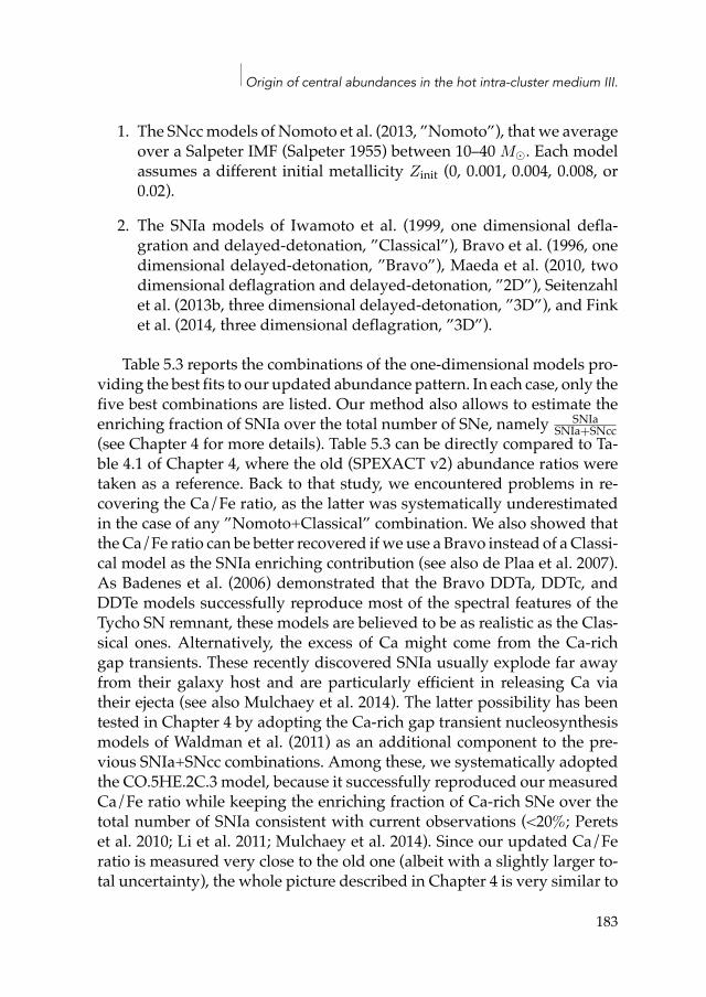
Origin of central abundances in the hot intra-cluster medium III.
1. The SNccmodels of Nomoto et al. (2013, ”Nomoto”), that we averageover a Salpeter IMF (Salpeter 1955) between 10–40 M⊙. Each modelassumes a different initial metallicity Zinit (0, 0.001, 0.004, 0.008, or0.02).
2. The SNIa models of Iwamoto et al. (1999, one dimensional defla-gration and delayed-detonation, ”Classical”), Bravo et al. (1996, onedimensional delayed-detonation, ”Bravo”), Maeda et al. (2010, twodimensional deflagration and delayed-detonation, ”2D”), Seitenzahlet al. (2013b, three dimensional delayed-detonation, ”3D”), and Finket al. (2014, three dimensional deflagration, ”3D”).
Table 5.3 reports the combinations of the one-dimensional models pro-viding the best fits to our updated abundance pattern. In each case, only thefive best combinations are listed. Our method also allows to estimate theenriching fraction of SNIa over the total number of SNe, namely SNIa
SNIa+SNcc(see Chapter 4 for more details). Table 5.3 can be directly compared to Ta-ble 4.1 of Chapter 4, where the old (SPEXACT v2) abundance ratios weretaken as a reference. Back to that study, we encountered problems in re-covering the Ca/Fe ratio, as the latter was systematically underestimatedin the case of any ”Nomoto+Classical” combination. We also showed thattheCa/Fe ratio can be better recovered ifwe use a Bravo instead of aClassi-cal model as the SNIa enriching contribution (see also de Plaa et al. 2007).As Badenes et al. (2006) demonstrated that the Bravo DDTa, DDTc, andDDTe models successfully reproduce most of the spectral features of theTycho SN remnant, these models are believed to be as realistic as the Clas-sical ones. Alternatively, the excess of Ca might come from the Ca-richgap transients. These recently discovered SNIa usually explode far awayfrom their galaxy host and are particularly efficient in releasing Ca viatheir ejecta (see also Mulchaey et al. 2014). The latter possibility has beentested in Chapter 4 by adopting the Ca-rich gap transient nucleosynthesismodels of Waldman et al. (2011) as an additional component to the pre-vious SNIa+SNcc combinations. Among these, we systematically adoptedthe CO.5HE.2C.3 model, because it successfully reproduced our measuredCa/Fe ratio while keeping the enriching fraction of Ca-rich SNe over thetotal number of SNIa consistent with current observations (<20%; Peretset al. 2010; Li et al. 2011; Mulchaey et al. 2014). Since our updated Ca/Feratio is measured very close to the old one (albeit with a slightly larger to-tal uncertainty), the whole picture described in Chapter 4 is very similar to
183
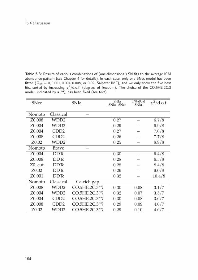
5.4 Discussion
Table 5.3: Results of various combinations of (one-dimensional) SN fits to the average ICMabundance pattern (see Chapter 4 for details). In each case, only one SNcc model has beenfitted (Zinit = 0, 0.001, 0.004, 0.008, or 0.02; Salpeter IMF), and we only show the five bestfits, sorted by increasing χ2/d.o.f. (degrees of freedom). The choice of the CO.5HE.2C.3model, indicated by a (*), has been fixed (see text).
SNcc SNIa SNIaSNIa+SNcc
SNIa(Ca)SNIa χ2/d.o.f.
Nomoto Classical −Z0.008 WDD2 0.27 − 6.7/8Z0.004 WDD2 0.29 − 6.9/8Z0.004 CDD2 0.27 − 7.0/8Z0.008 CDD2 0.26 − 7.7/8Z0.02 WDD2 0.25 − 8.9/8
Nomoto Bravo −Z0.004 DDTc 0.30 − 6.4/8Z0.008 DDTc 0.28 − 6.5/8Z0_cut DDTc 0.28 − 8.4/8Z0.02 DDTc 0.26 − 9.0/8Z0.001 DDTc 0.32 − 10.4/8Nomoto Classical Ca-rich gapZ0.008 WDD2 CO.5HE.2C.3(*) 0.30 0.08 3.1/7Z0.004 WDD2 CO.5HE.2C.3(*) 0.32 0.07 3.5/7Z0.004 CDD2 CO.5HE.2C.3(*) 0.30 0.08 3.6/7Z0.008 CDD2 CO.5HE.2C.3(*) 0.29 0.09 4.0/7Z0.02 WDD2 CO.5HE.2C.3(*) 0.29 0.10 4.6/7
184
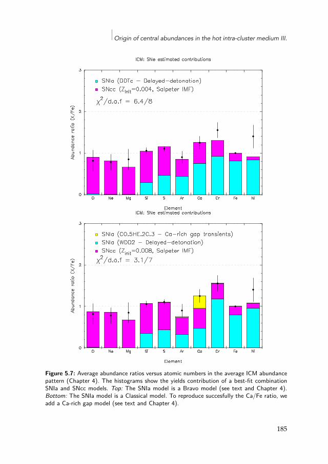
Origin of central abundances in the hot intra-cluster medium III.
Figure 5.7: Average abundance ratios versus atomic numbers in the average ICM abundancepattern (Chapter 4). The histograms show the yields contribution of a best-fit combinationSNIa and SNcc models. Top: The SNIa model is a Bravo model (see text and Chapter 4).Bottom: The SNIa model is a Classical model. To reproduce succesfully the Ca/Fe ratio, weadd a Ca-rich gap model (see text and Chapter 4).
185
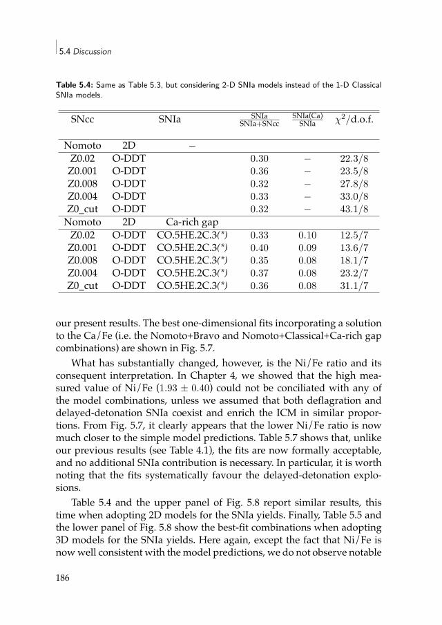
5.4 Discussion
Table 5.4: Same as Table 5.3, but considering 2-D SNIa models instead of the 1-D ClassicalSNIa models.
SNcc SNIa SNIaSNIa+SNcc
SNIa(Ca)SNIa χ2/d.o.f.
Nomoto 2D −Z0.02 O-DDT 0.30 − 22.3/8Z0.001 O-DDT 0.36 − 23.5/8Z0.008 O-DDT 0.32 − 27.8/8Z0.004 O-DDT 0.33 − 33.0/8Z0_cut O-DDT 0.32 − 43.1/8Nomoto 2D Ca-rich gapZ0.02 O-DDT CO.5HE.2C.3(*) 0.33 0.10 12.5/7Z0.001 O-DDT CO.5HE.2C.3(*) 0.40 0.09 13.6/7Z0.008 O-DDT CO.5HE.2C.3(*) 0.35 0.08 18.1/7Z0.004 O-DDT CO.5HE.2C.3(*) 0.37 0.08 23.2/7Z0_cut O-DDT CO.5HE.2C.3(*) 0.36 0.08 31.1/7
our present results. The best one-dimensional fits incorporating a solutionto the Ca/Fe (i.e. the Nomoto+Bravo and Nomoto+Classical+Ca-rich gapcombinations) are shown in Fig. 5.7.
What has substantially changed, however, is the Ni/Fe ratio and itsconsequent interpretation. In Chapter 4, we showed that the high mea-sured value of Ni/Fe (1.93 ± 0.40) could not be conciliated with any ofthe model combinations, unless we assumed that both deflagration anddelayed-detonation SNIa coexist and enrich the ICM in similar propor-tions. From Fig. 5.7, it clearly appears that the lower Ni/Fe ratio is nowmuch closer to the simple model predictions. Table 5.7 shows that, unlikeour previous results (see Table 4.1), the fits are now formally acceptable,and no additional SNIa contribution is necessary. In particular, it is worthnoting that the fits systematically favour the delayed-detonation explo-sions.
Table 5.4 and the upper panel of Fig. 5.8 report similar results, thistime when adopting 2D models for the SNIa yields. Finally, Table 5.5 andthe lower panel of Fig. 5.8 show the best-fit combinations when adopting3D models for the SNIa yields. Here again, except the fact that Ni/Fe isnowwell consistent with themodel predictions, we do not observe notable
186
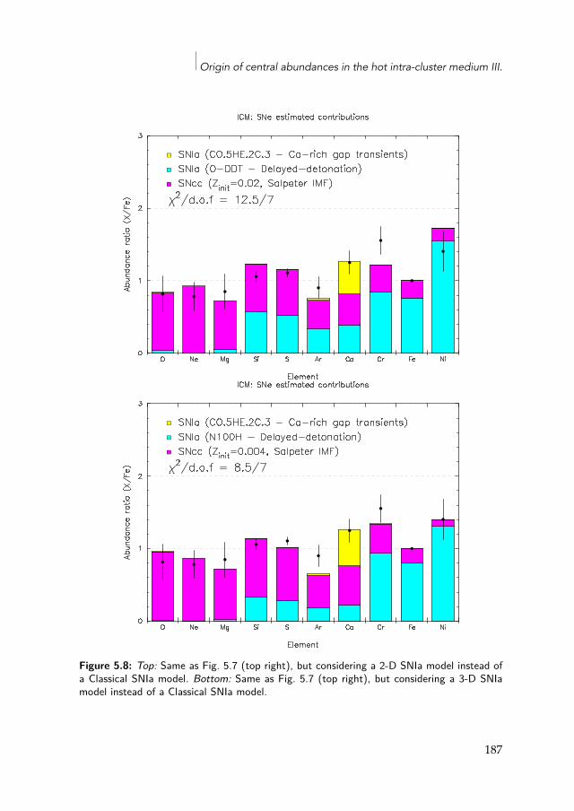
Origin of central abundances in the hot intra-cluster medium III.
Figure 5.8: Top: Same as Fig. 5.7 (top right), but considering a 2-D SNIa model instead ofa Classical SNIa model. Bottom: Same as Fig. 5.7 (top right), but considering a 3-D SNIamodel instead of a Classical SNIa model.
187
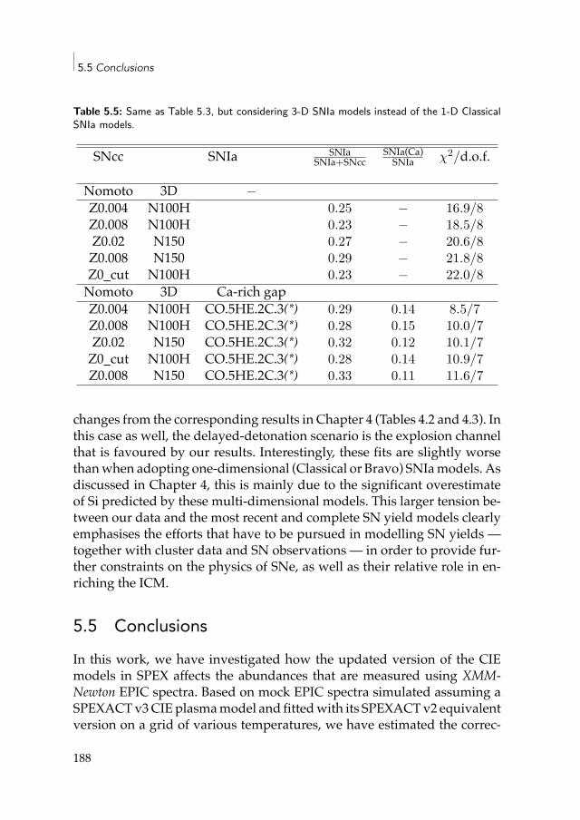
5.5 Conclusions
Table 5.5: Same as Table 5.3, but considering 3-D SNIa models instead of the 1-D ClassicalSNIa models.
SNcc SNIa SNIaSNIa+SNcc
SNIa(Ca)SNIa χ2/d.o.f.
Nomoto 3D −Z0.004 N100H 0.25 − 16.9/8Z0.008 N100H 0.23 − 18.5/8Z0.02 N150 0.27 − 20.6/8Z0.008 N150 0.29 − 21.8/8Z0_cut N100H 0.23 − 22.0/8Nomoto 3D Ca-rich gapZ0.004 N100H CO.5HE.2C.3(*) 0.29 0.14 8.5/7Z0.008 N100H CO.5HE.2C.3(*) 0.28 0.15 10.0/7Z0.02 N150 CO.5HE.2C.3(*) 0.32 0.12 10.1/7Z0_cut N100H CO.5HE.2C.3(*) 0.28 0.14 10.9/7Z0.008 N150 CO.5HE.2C.3(*) 0.33 0.11 11.6/7
changes from the corresponding results in Chapter 4 (Tables 4.2 and 4.3). Inthis case as well, the delayed-detonation scenario is the explosion channelthat is favoured by our results. Interestingly, these fits are slightly worsethanwhen adopting one-dimensional (Classical or Bravo) SNIamodels. Asdiscussed in Chapter 4, this is mainly due to the significant overestimateof Si predicted by these multi-dimensional models. This larger tension be-tween our data and the most recent and complete SN yield models clearlyemphasises the efforts that have to be pursued in modelling SN yields —together with cluster data and SN observations — in order to provide fur-ther constraints on the physics of SNe, as well as their relative role in en-riching the ICM.
5.5 ConclusionsIn this work, we have investigated how the updated version of the CIEmodels in SPEX affects the abundances that are measured using XMM-Newton EPIC spectra. Based on mock EPIC spectra simulated assuming aSPEXACTv3CIE plasmamodel and fittedwith its SPEXACTv2 equivalentversion on a grid of various temperatures, we have estimated the correc-
188
Origin of central abundances in the hot intra-cluster medium III.
tion factors that should be applied to the EPIC abundances initially mea-sured using the old SPEX versions. After having corrected accordingly theabundance estimates fromChapter 3, we have obtained updated estimatesof the average X/Fe ratios in the ICM, which we have compared to nucle-osynthesis models following Chapter 4. Our results can be summarised asfollows.
• For hot (>1.7 keV) plasmas, the Fe abundance measured with SPEX-ACT v3 is in excellent agreement with the previous estimates ob-tained using SPEXACT v2. For cool plasmas, in which the Fe abun-dance is mostly determined by fitting the Fe-L complex (unresolvedwith CCD-like instruments), we observe a substantial discrepancybetween the old (SPEXACT v2) and the new (SPEXACT v3) mea-surements. This bias can reach up to a factor of 2 for kT ≃ 0.6 keV.After a careful investigation on real EPIC spectra from the coolest ob-jects of the CHEERS sample, we confirm that the combined effect ofthe emission measure and the Fe abundance parameters used to fitthe Fe-L complex leads to a large Fe bias, even though SPEXACT v2and SPEXACT v3 eventually provide similar best-fit qualities. Sinceeven the up-to-date plasma codes do not well reproduce the shapeof the Fe-L complex in the coolest (≲1 keV) systems, we concludethat their Fe abundances are still highly uncertain. Besides, we pro-pose that this newly discovered Fe bias might explain the lower gas-phase metallicity previously observed in groups and ellipticals, andwhich has been difficult to conciliate with predictions so far (e.g. Ras-mussen & Ponman 2009; Yates et al. 2017). Similarly, spectral modelimprovements may also slightly affect the gas density, temperature,and pressure measurements of low-mass systems. The impact on theentropy measurement, however, is more limited.
• If we restrict our results to ⩾1 keV systems (see above), we find thatthe spectral model uncertainties on the Si, S, Ar, and Ca abundancesare always less than ∼20%. Consequently, their respective X/Fe ra-tios averaged over the 30 hottest objects sample are very close to theprevious estimates from Chapter 3, with a >1σ discrepancy observedonly in Si/Fe (because of the very limited total uncertainties affect-ing this ratio). While there is a large difference in the Mg abundanceestimate between SPEXACT v2 and SPEXACT v3 for high tempera-ture plasmas, the Mg/Fe ratio is better constrained in cooler objects.
189
5.5 Conclusions
This, together with the large intrinsic scatter affecting the individualMg/Fe measurements, explains why the Mg/Fe ratio averaged overthe sample does not change significantly.
• Unlike the other elements, spectral model improvements have a con-siderable impact on the individual and average Ni/Fe ratios, as wellas on its interpretation in terms of ICM enrichment by SNIa. BecausetheNi-K complex at∼7.8 keV contains several FeXXIII, FeXXIV, andFeXXV transitions that were not included in SPEXACT v2, previousfits of cluster spectra overestimated the Ni/Fe ratio by ∼40% on av-erage. Whereas the previous average Ni/Fe estimate could only bereproduced by SN yield models when invoking a diversity in theexplosion channels of SNIa (Chapter 4), such an assumption is notnecessary anymore. The whole ICM abundance pattern now highlyfavours delayed-detonation as the dominant (and perhaps exclusive)explosion channel of SNIa.
• Except SNIa explosion model(s), we do not observe other noticeablechanges from the conclusions made in Chapter 4. Our results stillsuggest that the enriching ratio of SNIa over the total number ofSNe rangeswithin∼0.23–0.40, and that the SNcc having enriched theICMhad been previously enriched by a former generation ofmassivestars. Finally, we highlight the fact that compared to outdated one-dimensional calculations (Iwamoto et al. 1999), updated two- andthree-dimensional SNIa yield models (Seitenzahl et al. 2013b; Finket al. 2014; Maeda et al. 2010) are less successful in reproducing ouraverage ICM abundance pattern. This should be a source of motiva-tion to keep improving both spectral plasma models and predictionsfor SNIa and SNcc yields in the upcoming years.
AcknowledgementsThiswork is partly based on theXMM-NewtonAO-12 proposal “TheXMM-Newton view of chemical enrichment in bright galaxy clusters and groups” (PI:de Plaa), and is a part of the CHEERS (CHEmical Evolution Rgs clusterSample) collaboration. This work is based on observations obtained withXMM-Newton, an ESA sciencemissionwith instruments and contributionsdirectly funded by ESA member states and the USA (NASA). The SRON
190

Origin of central abundances in the hot intra-cluster medium III.
Netherlands Institute for Space Research is supported financially byNWO,the Netherlands Organisation for Scientific Research.
191

You don’t have to see the whole staircase, just take the first step.
– Martin Luther King Jr.
6|Radial metal abundanceprofiles in the intra-clustermedium of cool-core galaxyclusters, groups, and ellipticals
F. Mernier, J. de Plaa, J. S. Kaastra, Y.-Y. Zhang1, H. Akamatsu, L. Gu,P. Kosec, J. Mao, C. Pinto, T. H. Reiprich, J. S. Sanders, A. Simionescu, and
N. Werner(Astronomy & Astrophysics, in press, arXiv:1703.01183)
Abstract
The hot intra-cluster medium (ICM) permeating galaxy clusters and groups is notpristine, as it has been continuously enriched by metals synthesised in Type Ia(SNIa) and core-collapse (SNcc) supernovae since the major epoch of star forma-tion (z ≃ 2–3). The cluster/group enrichment history and mechanisms responsi-ble for releasing and mixing the metals can be probed via the radial distributionof SNIa and SNcc products within the ICM. In this paper, we use deep XMM-Newton/EPIC observations from a sample of 44 nearby cool-core galaxy clusters,groups, and ellipticals (CHEERS) to constrain the average radial O, Mg, Si, S, Ar,Ca, Fe, and Ni abundance profiles. The radial distributions of all these elements,averaged over a large sample for the first time, represent the best constrained pro-files available currently. Specific attention is devoted to a proper modelling of theEPIC spectral components, and to other systematic uncertainties that may affectour results. We find an overall decrease of the Fe abundance with radius out to∼0.9r500 and ∼0.6r500 for clusters and groups, respectively, in good agreementwith predictions from the most recent hydrodynamical simulations. The average
1This paper is dedicated to the memory of our wonderful colleague Yu-Ying Zhang,who passed away on December 11, 2016.
193
6.1 Introduction
radial profiles of all the other elements (X) are also centrally peaked and, whenrescaled to their average central X/Fe ratios, follow well the Fe profile out to atleast∼0.5r500. As predicted by recent simulations, we find that the relative contri-bution of SNIa (SNcc) to the total ICMenrichment is consistentwith beinguniformat all radii, both for clusters and groups using two sets of SNIa and SNcc yieldmodels that reproduce the X/Fe abundance pattern in the core well. In additionto implying that the central metal peak is balanced between SNIa and SNcc, ourresults suggest that the enriching SNIa and SNcc products must share the sameorigin and that the delay between the bulk of the SNIa and SNcc explosions mustbe shorter than the timescale necessary to diffuse out themetals. Finally, we reportan apparent abundance drop in the very core of 14 systems (∼32% of the sample).Possible origins of these drops are discussed.
6.1 IntroductionGalaxy clusters and groups are more than a simple collection of galaxies(and dark matter haloes), as they are permeated by large amounts of veryhot gas. This intra-cluster medium (ICM) was heated up to 107–108 K dur-ing the gravitational assembly of these systems, and is glowing in the X-ray band, mainly via bremsstrahlung emission, radiative recombination,and line radiation (for a review, see Böhringer & Werner 2010). Since thefirst detection of a Fe-K emission feature at ∼7 keV in its X-ray spectra(Mitchell et al. 1976; Serlemitsos et al. 1977), it is well established that theICM does not have a primordial origin, but has been enriched with heavyelements, or metals, up to typical values of∼0.5–1 times solar (for reviews,see Werner et al. 2008; de Plaa 2013). Since the ICM represents about∼80%of the total baryonic matter in clusters, this means that there is more massin metals in the ICM than locked in all the cluster galaxies (e.g. Renzini &Andreon 2014).
Despite the first detection of several K-shell metal lines with the Ein-stein observatory in the early 1980s (e.g. Canizares et al. 1979; Mushotzkyet al. 1981), before 1993 only the iron (Fe) abundance could be accuratelymeasured in the ICM.After the launch ofASCA, abundance studies in clus-ters could extend (although with a limited accuracy) to oxygen (O), neon(Ne), magnesium (Mg), silicon (Si), sulfur (S), argon (Ar), calcium (Ca),and nickel (Ni), thus opening a new window on the ICM enrichment (e.g.Mushotzky et al. 1996; Baumgartner et al. 2005). However, the most spec-tacular step forward in the field has been achieved by the latest generationof X-ray observatories, i.e. Chandra, XMM-Newton, and Suzaku, which al-
194
Radial abundance profiles in the ICM of cool-core clusters, groups, and ellipticals
lowed much more accurate abundance measurements of these elementsthanks to the significantly improved effective area and spectral resolutionof their instruments (e.g. Tamura et al. 2001; de Plaa et al. 2006; Werneret al. 2006a). With excellent Suzaku andXMM-Newton exposures, the abun-dance of other elements, such as carbon, nitrogen (e.g. Werner et al. 2006a;Sanders& Fabian 2011,Mao et al. 2017, to be submitted), or even chromiumand manganese (Tamura et al. 2009, see also Chapter 3), could be reason-ably constrained as well.
Metals present in the ICM must have been synthesised by stars andsupernovae (SNe) explosions, mainly within cluster galaxies. While O, Ne,and Mg are produced almost entirely by core-collapse supernovae (SNcc),the Fe-peak elements mostly originate from Type Ia supernovae (SNIa).Intermediate elements (e.g. Si, S, and Ar) are synthesised by both SNIa andSNcc (for a review, seeNomoto et al. 2013). Since the current X-raymissionsallow the measurement of the abundance of all these elements with a goodlevel of accuracy in the core of the ICM (i.e. where the overall flux and themetal line emissivities are the highest), several attempts have been madeto use these abundances to provide constraints on SNIa and SNcc yieldmodels in individual objects (e.g. Werner et al. 2006b; de Plaa et al. 2006;Bulbul et al. 2012a) or in samples (e.g. de Plaa et al. 2007; Sato et al. 2007a,and Chapter 4). From these studies, it appears that the typical fraction ofSNIa (SNcc) contributing to the enrichment lies within∼20–45% (55–80%),depending (mainly) on the selected yield models.
Beyond the overall elemental abundances, witnessing the time-integra-ted enrichment history in galaxy clusters and groups since themajor epochof star formation (z ≃ 2–3; for a review, see Madau & Dickinson 2014) de-termining the distribution of metals within the ICM is also of crucial im-portance. Indeed, this metal distribution constitutes a direct signature of,first, the locations and epoch(s) of the enrichment and, second, the domi-nant mechanisms transporting the metals into and across the ICM. In turn,these transport mechanisms must also play a fundamental role in govern-ing the thermodynamics of the hot gas. Since the ASCA discovery of astrong metallicity gradient in Centaurus (Allen & Fabian 1994; Fukazawaet al. 1994), a systematically peaked Fe distribution in cool-core clustersand groups (i.e. showing a strong ICM temperature decrease towards thecentre) has been confirmed bymany studies (e.g. Matsushita et al. 1997; DeGrandi & Molendi 2001; Gastaldello & Molendi 2002; Thölken et al. 2016).On the contrary, non-cool-core clusters and groups (i.e. with no central
195
6.1 Introduction
ICM temperature gradient) do not exhibit any clear Fe abundance gradientin their cores (De Grandi &Molendi 2001). It is likely that the Fe central ex-cess in cool-core clusters has been produced predominantly by the stellarpopulation of the brightest cluster galaxy (BCG) residing in the centre ofthe gravitational potential well of the cluster during or after the cluster as-sembly (Böhringer et al. 2004a; De Grandi et al. 2004). However, this excessis often significantly broader than the light profile of the BCG, suggestingthat one or several mechanisms, such as turbulent diffusion (Rebusco et al.2005, 2006) or active galactic nucleus (AGN) outbursts (e.g. Guo & Math-ews 2010), may efficiently diffuse metals out of the cluster core. Alterna-tively, the higher concentration of Fe in the core of the ICMmay be causedby the release of metals from infalling galaxies via ram-pressure stripping(Domainko et al. 2006) together with galactic winds (Kapferer et al. 2007,2009). Other processes, such as galaxy-galaxy interactions, AGN outflows,or an efficient enrichment by intra-cluster stars, may also play a role (fora review, see Schindler & Diaferio 2008). In addition to this central excess,there is increasing evidence of a uniform Fe enrichment floor extending outto r200
2 and probably beyond (Fujita et al. 2008;Werner et al. 2013; Thölkenet al. 2016). This suggests an additional early enrichment by promptly ex-ploding SNIa, i.e. having occurred and efficiently diffused before the clus-ter formation. However, a precise quantification of this uniform level isdifficult, since clusters outskirts are very dim and yet poorly understood(Molendi et al. 2016).
Whereas the ICM radial distribution of the Fe abundance (rather wellconstrained thanks to its Fe-K and Fe-L emission complexes, accessible tocurrent X-ray telescopes) has been extensively studied in recent decades,the situation is much less clear for the other elements. Several studies re-port a rather flat O (and/or Mg) profile, or similarly, an increasing O/Fe(and/or Mg/Fe) ratio towards the outer regions of the cool-core ICM (e.g.Tamura et al. 2001; Matsushita et al. 2003; Tamura et al. 2004; Werner et al.2006a). As for Fe, there are also indications of a positive and uniform Mg(and other SNcc products) enrichment out to r200 (Simionescu et al. 2015;Ezer et al. 2017). This apparent flat distribution of SNcc products, con-trasting with the enhanced central enrichment from SNIa products, hasled to the picture of an early ICM enrichment by SNcc (and prompt SNIa,see above), when galaxies underwent important episodes of star forma-
2r∆ is defined as the radius within which the gas density corresponds to ∆ times thecritical density of the Universe.
196
Radial abundance profiles in the ICM of cool-core clusters, groups, and ellipticals
tion. These metals would have mixed efficiently before the cluster assem-bled, contrary to delayed SNIa enrichment originating from the red anddead BCG. This picture, however, has been questioned by recent obser-vations, suggesting centrally peaked O (and/or Mg) profiles instead (e.g.Matsushita et al. 2007; Sato et al. 2009; Simionescu et al. 2009b; Lovisariet al. 2011, and Chapter 2). The radial distribution of Si, produced by bothSNIa and SNcc, is also unclear, as the Si/Fe profile has been reported to besometimes flat, sometimes increasing with radius (e.g. Rasmussen & Pon-man 2007; Lovisari et al. 2011; Million et al. 2011; Sasaki et al. 2014).
In all the studies referred to above, theO,Mg, Si, S, Ar, Ca, andNi radialabundance profiles have beenmeasured either for individual (mostly cool-core) objects or for very restricted samples (⩽15 objects). Consequently, inmost cases, these profiles suffer from large statistical uncertainties. In par-allel, little attention has been drawn to systematic effects that could po-tentially bias some results. Building average abundance profiles (not onlyfor Fe, but for all the other possible elements mentioned above) over alarge sample of cool-core (and, if possible, non-cool-core) systems is clearlyneeded to clarify the picture of the SNIa and SNcc enrichment history ingalaxy clusters and groups.
In this paper, we use deep XMM-Newton/EPIC observations from asample of 44 nearby cool-core galaxy clusters, groups, and ellipticals to de-rive the average O, Mg, Si, S, Ar, Ca, Fe, and Ni abundance profiles in theICM. In order to make our results as robust as possible, specific attentionis devoted to understanding all the possible systematic biases and reduc-ing them when possible. This paper is structured as follows. We describethe observations and our data reduction in Sect. 6.2, the adopted spectralmodelling in Sect. 6.3, and the averaging of the individual profiles overthe sample in Sect. 6.4. Our results, and an extensive discussion on the re-maining systematic uncertainties, are presented in Sect. 6.5 and Sect. 6.6,respectively. We discuss the possible implications of our findings in Sect.6.7 and conclude in Sect. 6.8. Throughout this paper, we adopt the cos-mological parameters H0 = 70 km s−1 Mpc−1, Ωm = 0.3, and ΩΛ = 0.7.Unless otherwise stated, the error bars are given at 68% confidence level,and the abundances are given with respect to the proto-solar abundancesof Lodders et al. (2009).
197
6.2 Observations and data preparation
6.2 Observations and data preparation
All the observations considered here are taken from the CHEERS3 cata-logue (de Plaa et al. 2017, Chapter 3). This sample, optimised to studychemical enrichment in the ICM, consists of 44 nearby cool-core galaxyclusters, groups, and ellipticals forwhich theOVIII 1s–2p line at∼19 is de-tected with >5σ in theirXMM-Newton/RGS spectra. This includes archivalXMM-Newton data and several recent deep observations that were per-formed to complete the sample in a consistent way (de Plaa et al. 2017).
We reduce the EPIC MOS1, MOS2, and pn data using the XMM Sci-ence Analysis System (SAS) v14.0 and the calibration files dated by March2015. The standard pipeline commands emproc and epproc are used toextract the event files from the EPIC MOS and pn data, respectively. Wefilter each observation from soft-flare events by applying the appropriategood time interval (GTI) files following the 2σ-clipping criterion (Chap-ter 2). After filtering, the MOS1, MOS2, and pn exposure times of thefull sample are ∼4.5 Ms, ∼4.6 Ms, and ∼3.7 Ms, respectively (see Table3.1). Following the usual recommendations, we keep the single-, double-and quadruple-pixel events (pattern⩽12) in MOS, and we only keep thesingle-pixel events in pn (pattern=0), since the pn double events may suf-fer from charge transfer inefficiency4. In bothMOS andpn, only the highestquality events are selected (flag=0). The point sources are detected in fourdistinct energy bands (0.3–2 keV, 2–4.5 keV, 4.5–7.5 keV, and 7.5–12 keV)using the task edetect_chain and further rechecked by eye. We discardthese point sources from the rest of the analysis, by excising a circular re-gion of 10′′ of radius around their surface brightness peak. This radius isfound to be the best compromise between minimising the fraction of con-taminating photons from point sources and maximising the fraction of theICM photons considered in our spectra (Chapter 2). In some specific cases,however, photons from very bright point sources may leak beyond 10′′,and consequently we adopt a larger excision radius.
In each dataset, we extract the MOS1, MOS2, and pn spectra of eightconcentric annuli of fixed angular size (0′–0.5′, 0.5′–1′, 1′–2′, 2′–3′, 3′–4′, 4′–6′, 6′–9′, and 9′–12′), all centred on the X-ray peak emission seen on theEPIC surface brightness images. The redistribution matrix file (RMF) and
3CHEmical Enrichment Rgs Sample4See the XMM-Newton Current Calibration File Release Notes, XMM-CCF-REL-309
(Smith, Guainazzi & Saxton 2014).
198
Radial abundance profiles in the ICM of cool-core clusters, groups, and ellipticals
the ancillary response file (ARF) of each spectrum are produced via thermfgen and arfgen SAS tasks, respectively.
6.3 Spectral modellingThe spectral analysis is performed using the SPEX5 package (Kaastra et al.1996), version 2.05. Following the method described in Chapter 3, we startby simultaneously fitting the MOS1, MOS2, and pn spectra of each point-ing. When a target includes two separate observations, we fit their spectrasimultaneously. Since the large number of fitting parameters does not al-low us to fit more than two observations simultaneously, we form pairsof simultaneous fits when an object contains three (or more) observations.We then combine the results of the fitted pairs using a factor of 1/σ2
i , whereσi is the error on the considered parameter i. We also note that the secondEPIC observation of M87 (ObsID:0200920101) is strongly affected by pile-up in its core, owing to a sudden activity of the central AGN (Werner et al.2006a). Therefore, the radial profiles within 3′ are only estimated with thefirst observation (ObsID:0114120101).
Because of calibration issues in the soft X-ray band of the CCDs (≲0.5keV) and beyond ∼10 keV, we limit our MOS and pn spectral fittings tothe 0.5–10 keV and 0.6–10 keV energy bands, respectively. We rearrangethe data bins in each spectrum via the optimal binning method of Kaastra& Bleeker (2016) to maximise the amount of information provided by thespectra while keeping reasonable constraints on the model parameters.
6.3.1 Thermal emission modellingIn principle, we can model the ICM emission in SPEX with the (redshiftedand absorbed) cie thermalmodel. This single-temperaturemodel assumesthat the plasma is in (or close to) collisional ionisation equilibrium (CIE),which is a reasonable assumption (e.g. Sarazin 1986).
Although the cie model may be a good approximation of the emit-ting ICM in some specific cases (i.e. when the gas is nearly isothermal),the temperature structure within the core of clusters and groups is oftencomplicated and a multi-temperature model is clearly required. In partic-ular, fitting the spectra of a multi-phase plasma with a single-temperaturemodel can dramatically affect the measured Fe abundance, leading to the
5https://www.sron.nl/astrophysics-spex
199
6.3 Spectral modelling
”Fe-bias” (Buote & Canizares 1994; Buote & Fabian 1998; Buote 2000) or tothe ”inverse Fe-bias” (Rasia et al. 2008; Simionescu et al. 2009b; Gastaldelloet al. 2010). Taking this caveat into account, we model the ICM emissionwith a gdemmodel (e.g. de Plaa et al. 2006), which is also available in SPEX.Thismulti-temperature componentmodels aCIEplasma following aGaus-sian-shaped temperature distribution,
Y (x) = Y0
σT
√2π
exp(
(x − xmean)2
2σ2T
), (6.1)
where x = log(kT ), xmean = log(kTmean), kTmean is the mean temperatureof the distribution, σT is the width of the distribution, and Y0 is the totalintegrated emission measure. The other parameters are similar as in thecie model. By definition, a gdem model with σT = 0 reproduces a cie (i.e.single-temperature) model. The free parameters of the gdem model are thenormalisation (or emission measure) Y0 =
∫nenH dV , the temperature pa-
rameters kTmean and σT , and the abundances of O, Ne, Mg, Si, S, Ar, Ca,Fe, and Ni (given with respect to the proto-solar table of Lodders et al.2009, see Sect. 6.1). Because these analyses are out of the scope of this pa-per, we devote the radial analyses of the temperatures, emissionmeasures,and subsequent densities and entropies for a future work. The abundancesof the Z⩽7 elements are fixed to the proto-solar unity, while the remainingabundances are fixed to the Fe value. Asmentioned by Leccardi &Molendi(2008), constraining the free abundance parameters to positive values only(for obvious physical reasons) may result in a statistical bias when aver-aging out the profiles. Therefore, we allow all the best-fit abundances totake positive and negative values. Following Chapter 3, the measured Oabundances have been corrected from updated parametrisation of the ra-diative recombination rates (see also de Plaa et al. 2017). Since Ne abun-dances measured with EPIC are highly unreliable (because the main Neemission feature is entirely blended with the Fe-L complex at EPIC spec-tral resolution), we do not consider them in the rest of the paper.
The absorption of the ICM photons by neutral interstellar matter is re-produced by a hot model, where the temperature parameter is fixed to0.5 eV (see the SPEX manual). Because adopting the column densities ofWillingale et al. (2013) — taking both atomic and molecular hydrogen intoaccount — sometimes leads to poor spectral fits, we perform a grid searchof the best-fit NH parameter within the limits
NHI − 5 × 1019 cm−2 ⩽ NH ⩽ NH,tot + 1 × 1020 cm−2, (6.2)
200
Radial abundance profiles in the ICM of cool-core clusters, groups, and ellipticals
where NHI and NH,tot are the atomic and total (atomic and molecular) hy-drogen column densities, respectively (for further details, see Chapter 3).
6.3.2 Background modellingWhereas in the core of bright clusters the ICM emission is largely domi-nant, in cluster outskirts the backgroundplays an important role and some-times may even dominate. For extended objects, a background subtractionapplied to the raw spectra is clearly not advised because a slightly incorrectscaling may lead to dramatic changes in the derived temperatures (de Plaaet al. 2006). In turn, since themetal line emissivities depend on the assumedplasma temperature, this approachmay lead to erroneous abundancemea-surements outside the cluster cores. Moreover, the observed backgrounddata (usually obtained from blank-field observations) may significantlyvary with time and position on the sky.
Instead, we choose to model the background directly in the spectralfits by adopting the method extensively described in Chapter 2. The totalbackground emission is decomposed into five components as follows:
1. The Galactic thermal emission (GTE) is modelled by an absorbed ciecomponent with proto-solar abundances.
2. The local hot bubble (LHB) is modelled by a (unabsorbed) cie com-ponent with proto-solar abundances.
3. The unresolved point sources (UPS), whose accumulated flux can ac-count for a significant fraction of the background emission, are mod-elled by a power law of index ΓUPS = 1.41 (De Luca &Molendi 2004).
4. The hard particle background (HP, or instrumental background) con-sists of a continuum and fluorescence lines. The continuum is mod-elled by a (broken) power law, whose parameters can be constrainedusing filter wheel closed observations, and the lines are modelled byGaussian functions. Because this is a particle background, we leavethis modelled component unfolded by the effective area of the CCDs.
5. The quiescent soft-protons (SP) may contribute to the total emission,even after filtering of the flaring events. This component is modelledby a power law with an index varying typically within 0.7 ≲ ΓSP ≲1.4. Similarly to the HP background, this component is not folded bythe effective area.
201
6.3 Spectral modelling
The background components have been first derived from spectra cov-ering the total EPIC field of view to obtain good constraints on their pa-rameters. In particular, this approach allows us to determine both themeantemperature of the ICM (which is the dominant emission below ∼2 keV)and the slope of the SP component (better visible beyond ∼2 keV), whilethese twoparameters are usually degeneratewhen only analysing one outerannulus. In addition to the gdem component, the free parameters of thebackground components in the fitted annuli are the normalisations of theHP continuum, HP Gaussian lines (because their emissivities vary withtime and across the detector), and quiescent SP (beyond 6′ only).
6.3.3 Local fits
As discussed extensively in Chapters 2 and 3, the abundances measuredfrom a fit covering the full EPIC energy band may be significantly biased,especially for deep exposure datasets. In fact, a slightly incorrect calibra-tion in the effective area may result in an incorrect prediction of the localcontinuum close to an emission line. Since the abundance of an ion is di-rectly related to the measured equivalent width of its corresponding emis-sion lines, a correct estimate of the local continuum level is crucial to deriveaccurate abundances.
Therefore, in the rest of the analysis, we measure the O, Mg, Si, S, Ca,Ar, and Ni abundances by fitting the EPIC spectra within several narrowenergy ranges centred around their K-shell emission lines (hereafter the”local” fits; Chapter 3). The temperature parameters (kTmean and σT ) arefixed to their values derived from initial fits performed within the broadenergy band (hereafter the ”global” fits). In order to assess the systematicuncertainties related to remaining cross-calibration issues between the dif-ferent EPIC detectors (Sect. 6.4.3), we perform our local fits in MOS (i.e.the combined MOS1+MOS2) and pn spectra independently. Finally, theFe abundance can be measured in EPIC using both the K-shell lines (∼6.4keV) and the L-shell line complex (∼0.9–1.2 keV, although not resolvedwith CCD instruments). For this reason, in the rest of the paper we use theglobal fits to derive the Fe abundances.
202
Radial abundance profiles in the ICM of cool-core clusters, groups, and ellipticals
6.4 Building average radial profilesFollowing the approach of Chapter 3, in addition to the full sample weconsider further in this paper, we also split the sample into two subsam-ples, namely the ”clusters” (23 objects) and the ”groups” (21 objects), forwhich the mean temperature within 0.05r500 is greater or lower than 1.7keV, respectively (see also Table 6.4). One exception is M87, an ellipticalgalaxy with kTmean(0.05r500) = (2.052 ± 0.002) keV, which we treat in thefollowing as part of the ”groups” subsample.
6.4.1 Exclusion of fitting artefactsSince little ICM emission is expected at large radii, one may reasonably ex-pect large statistical uncertainties on our derived fitting parameters in theoutermost annuli of every observation. In a few specific cases, however,suspiciously small error bars are reported at large radii, often togetherwithunphysical best-fit values. These peculiar measurements are often due toissues in the fitting process, consequently to bad spectral quality togetherwith a number of fitted parameters that is too large. Since these artefactmeasurements may significantly pollute our average profiles, we prefer todiscard them from the analysis and select outer measurements with rea-sonably large error bars on their parameters only. To be conservative, wechoose to exclude systematically the Fe abundance measurements show-ing error bars smaller than 0.01, 0.02, and 0.03 in their 4′–6′, 6′–9′, and 9′–12′ annuli, respectively. A similar filtering is applied to the other abun-dances, this time when their measurements show error bars smaller than0.01, 0.02, 0.05, and 0.07 in their 3′–4′, 4′–6′, 6′–9′, and 9′–12′ annuli, respec-tively. These discarded artefacts represent a marginal fraction (∼4%) of allour data. We list the maximum radial extend for each cluster and all the el-ements considered (rout,X) in Table 6.4. Finally, we exclude further specificmeasurements either because their spectral quality could simply not pro-vide reliable estimates or because of possible contamination by the AGNemission. These unaccounted annuli are specified in Table 6.1.
6.4.2 Stacking methodSince spectral analysis was performed within annuli of fixed angular sizesregardless of the distances or the cosmological redshifts of the sources,care must be taken to build average radial profiles within consistent spa-
203
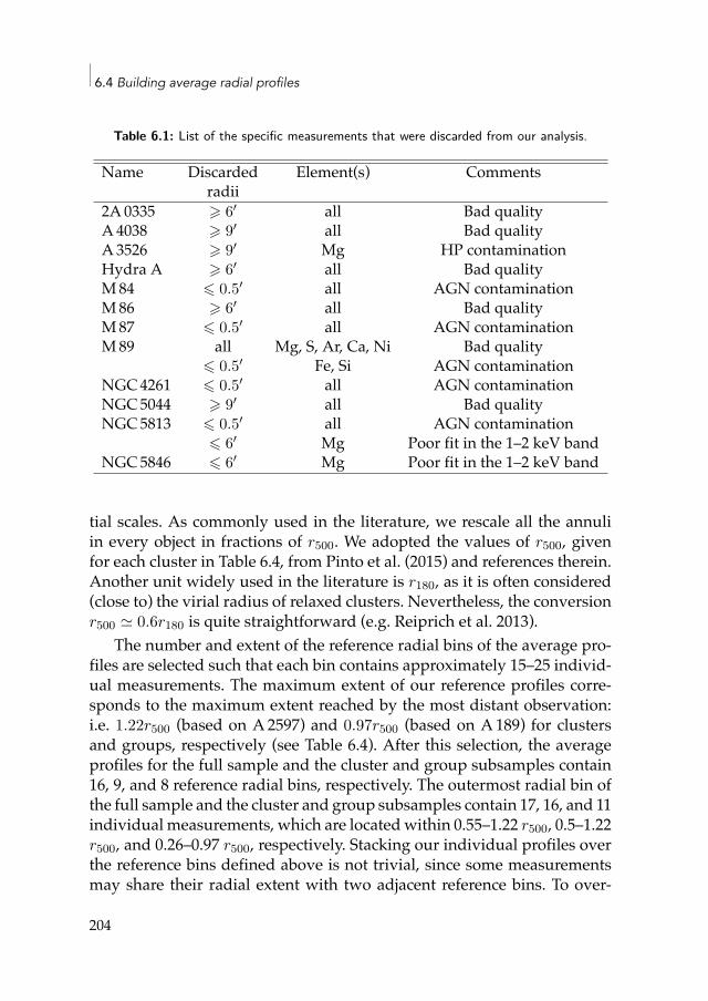
6.4 Building average radial profiles
Table 6.1: List of the specific measurements that were discarded from our analysis.
Name Discarded Element(s) Commentsradii
2A 0335 ⩾ 6′ all Bad qualityA4038 ⩾ 9′ all Bad qualityA3526 ⩾ 9′ Mg HP contaminationHydra A ⩾ 6′ all Bad qualityM84 ⩽ 0.5′ all AGN contaminationM86 ⩾ 6′ all Bad qualityM87 ⩽ 0.5′ all AGN contaminationM89 all Mg, S, Ar, Ca, Ni Bad quality
⩽ 0.5′ Fe, Si AGN contaminationNGC4261 ⩽ 0.5′ all AGN contaminationNGC5044 ⩾ 9′ all Bad qualityNGC5813 ⩽ 0.5′ all AGN contamination
⩽ 6′ Mg Poor fit in the 1–2 keV bandNGC5846 ⩽ 6′ Mg Poor fit in the 1–2 keV band
tial scales. As commonly used in the literature, we rescale all the annuliin every object in fractions of r500. We adopted the values of r500, givenfor each cluster in Table 6.4, from Pinto et al. (2015) and references therein.Another unit widely used in the literature is r180, as it is often considered(close to) the virial radius of relaxed clusters. Nevertheless, the conversionr500 ≃ 0.6r180 is quite straightforward (e.g. Reiprich et al. 2013).
The number and extent of the reference radial bins of the average pro-files are selected such that each bin contains approximately 15–25 individ-ual measurements. The maximum extent of our reference profiles corre-sponds to the maximum extent reached by the most distant observation:i.e. 1.22r500 (based on A2597) and 0.97r500 (based on A189) for clustersand groups, respectively (see Table 6.4). After this selection, the averageprofiles for the full sample and the cluster and group subsamples contain16, 9, and 8 reference radial bins, respectively. The outermost radial bin ofthe full sample and the cluster and group subsamples contain 17, 16, and 11individual measurements, which are locatedwithin 0.55–1.22 r500, 0.5–1.22r500, and 0.26–0.97 r500, respectively. Stacking our individual profiles overthe reference bins defined above is not trivial, since some measurementsmay share their radial extent with two adjacent reference bins. To over-
204
Radial abundance profiles in the ICM of cool-core clusters, groups, and ellipticals
come this issue, we employ the method proposed by Leccardi & Molendi(2008). The average abundance profileXref(k), as a function of the k-th ref-erence radial bin (defined above), is obtained as
Xref(k) =( N∑
j=1
8∑i=1
wi,j,kX(i)j
σ2X(i)j
)/( N∑j=1
8∑i=1
wi,j,k1
σ2X(i)j
), (6.3)
where X(i)j is the individual abundance measurement of the j-th observa-tion at its i-th annulus (as defined in Sect. 6.2), σX(i)j
is its statistical error(and thus 1/σ2
X(i)jweights each annulus with respect to its emission mea-
sure),N is the number of observations, depending of the (sub)sample con-sidered, and wi,j,k a weighting factor. This factor, taking values between 0and 1, represents the linear overlapping geometric area fraction of the k-threference radial bin on the i-th annulus (belonging to the j-th observation).
6.4.3 MOS-pn uncertaintiesAfter stacking the measurements as described above, for each element weare left with Xref, MOS(k) and Xref, pn(k); i.e. an average MOS and pn abun-dance profile, respectively, except O, which could only be measured withthe MOS instruments, and Fe, which we measured in simultaneous EPICglobal fits (see Sect. 6.3.3). The average EPIC (i.e. combinedMOS+pn) pro-files are then computed as follows:
Xref, EPIC(k) =(
Xref, MOS(k)σ2ref, MOS(k)
+Xref, pn(k)σ2ref, pn(k)
)/( 1
σ2ref, MOS(k)
+ 1σ2ref, pn(k)
), (6.4)
where σref, MOS(k) and σref, pn(k) are the statistical errors ofXref, MOS(k) andXref, pn(k), respectively. As shown in Chapter 3, abundance estimates us-ing MOS and pn may sometimes be significantly discrepant. Unsurpris-ingly, we also find MOS-pn discrepancies in some radial bins of our aver-age abundance profiles. We take this systematic effect into account whencombining theMOS andpn profiles by increasing the error bars of the EPICcombined measurements until they cover both their MOS and pn counter-parts.
205
6.5 Results
6.5 Results6.5.1 Fe abundance profileThe average Fe abundance radial profile, measured for the full sample,is shown in Fig. 6.1, and the numerical values are detailed in Table 6.2.The profile shows a clear decreasing trend with radius with a maximumat 0.014–0.02r500, and a slight drop below ∼0.01r500. Such a drop is alsoobserved in the Fe profile of several individual objects (Figs. 6.18 and 6.19)and is discussed in Sect. 6.7.2. The very large total exposure time of thesample (∼4.5Ms)makes the combined statistical uncertainties σstat(k) verysmall — less than 1% in the core, up to ∼7% in the outermost radial bin.The scatter of the measurements (grey shaded area in Fig. 6.1), expressedas
σscatter(k) =
√√√√ N∑j=1
8∑i=1
wi,j,k
(X(i)j − Xref(k)
σX(i)j
)2
/√√√√ N∑j=1
8∑i=1
wi,j,k1
σ2X(i)j
(6.5)
for each k-th reference bin, is much larger (up to ∼36% in the innermostbin).
We parametrise this profile by fitting the empirical function
Fe(r) = A(r − B)C − D exp(
−(r − E)2
F
), (6.6)
where r is given in units of r500, and A, B, C, D, E, and F are constants todetermine. The first term on the right hand side of Eq. (6.6) is a power lawthat is used to model the decrease beyond ≳0.02r500. To model the innermetal drop, we subtract a Gaussian (second term) from the power law. Thebest fit of our empirical distribution is shown in Fig. 6.1 (red dashed curve)and can be expressed as
Fe(r) = 0.21(r + 0.021)−0.48 − 6.54 exp(
−(r + 0.0816)2
0.0027
), (6.7)
which provides a reasonable fit to the data (χ2/d.o.f. = 10.3/9). We alsolook for possible hints towards a flattening at the outskirts.When assuming
206
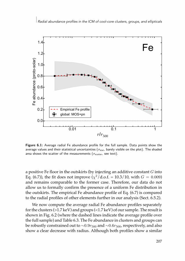
Radial abundance profiles in the ICM of cool-core clusters, groups, and ellipticals
0.01 0.1 1r/r500
0.0
0.2
0.4
0.6
0.8
1.0
1.2
1.4
Fe a
bund
ance
(pro
to-s
olar
)
Fe
Empirical Fe profileglobal: MOS+pn
Figure 6.1: Average radial Fe abundance profile for the full sample. Data points show theaverage values and their statistical uncertainties (σstat, barely visible on the plot). The shadedarea shows the scatter of the measurements (σscatter, see text).
a positive Fe floor in the outskirts (by injecting an additive constant G intoEq. (6.7)), the fit does not improve (χ2/d.o.f. = 10.3/10, with G = 0.009)and remains comparable to the former case. Therefore, our data do notallow us to formally confirm the presence of a uniform Fe distribution inthe outskirts. The empirical Fe abundance profile of Eq. (6.7) is comparedto the radial profiles of other elements further in our analysis (Sect. 6.5.2).
We now compute the average radial Fe abundance profiles separatelyfor the clusters (>1.7 keV) and groups (<1.7 keV) of our sample. The result isshown in Fig. 6.2 (where the dashed lines indicate the average profile overthe full sample) and Table 6.3. The Fe abundance in clusters and groups canbe robustly constrained out to∼0.9r500 and∼0.6r500, respectively, and alsoshow a clear decrease with radius. Although both profiles show a similar
207
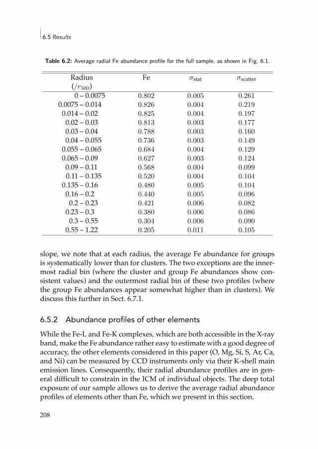
6.5 Results
Table 6.2: Average radial Fe abundance profile for the full sample, as shown in Fig. 6.1.
Radius Fe σstat σscatter(/r500)0 – 0.0075 0.802 0.005 0.261
0.0075 – 0.014 0.826 0.004 0.2190.014 – 0.02 0.825 0.004 0.1970.02 – 0.03 0.813 0.003 0.1770.03 – 0.04 0.788 0.003 0.1600.04 – 0.055 0.736 0.003 0.1490.055 – 0.065 0.684 0.004 0.1290.065 – 0.09 0.627 0.003 0.1240.09 – 0.11 0.568 0.004 0.0990.11 – 0.135 0.520 0.004 0.1040.135 – 0.16 0.480 0.005 0.1040.16 – 0.2 0.440 0.005 0.0960.2 – 0.23 0.421 0.006 0.0820.23 – 0.3 0.380 0.006 0.0860.3 – 0.55 0.304 0.006 0.0900.55 – 1.22 0.205 0.011 0.105
slope, we note that at each radius, the average Fe abundance for groupsis systematically lower than for clusters. The two exceptions are the inner-most radial bin (where the cluster and group Fe abundances show con-sistent values) and the outermost radial bin of these two profiles (wherethe group Fe abundances appear somewhat higher than in clusters). Wediscuss this further in Sect. 6.7.1.
6.5.2 Abundance profiles of other elementsWhile the Fe-L and Fe-K complexes, which are both accessible in the X-rayband,make the Fe abundance rather easy to estimatewith a good degree ofaccuracy, the other elements considered in this paper (O, Mg, Si, S, Ar, Ca,and Ni) can be measured by CCD instruments only via their K-shell mainemission lines. Consequently, their radial abundance profiles are in gen-eral difficult to constrain in the ICM of individual objects. The deep totalexposure of our sample allows us to derive the average radial abundanceprofiles of elements other than Fe, which we present in this section.
208
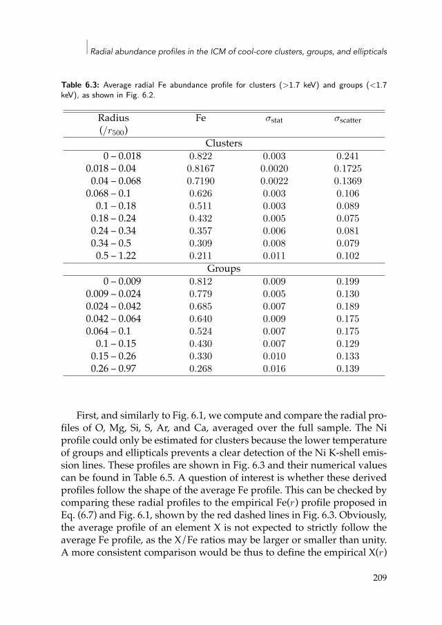
Radial abundance profiles in the ICM of cool-core clusters, groups, and ellipticals
Table 6.3: Average radial Fe abundance profile for clusters (>1.7 keV) and groups (<1.7keV), as shown in Fig. 6.2.
Radius Fe σstat σscatter(/r500)
Clusters0 – 0.018 0.822 0.003 0.241
0.018 – 0.04 0.8167 0.0020 0.17250.04 – 0.068 0.7190 0.0022 0.13690.068 – 0.1 0.626 0.003 0.1060.1 – 0.18 0.511 0.003 0.0890.18 – 0.24 0.432 0.005 0.0750.24 – 0.34 0.357 0.006 0.0810.34 – 0.5 0.309 0.008 0.0790.5 – 1.22 0.211 0.011 0.102
Groups0 – 0.009 0.812 0.009 0.199
0.009 – 0.024 0.779 0.005 0.1300.024 – 0.042 0.685 0.007 0.1890.042 – 0.064 0.640 0.009 0.1750.064 – 0.1 0.524 0.007 0.1750.1 – 0.15 0.430 0.007 0.1290.15 – 0.26 0.330 0.010 0.1330.26 – 0.97 0.268 0.016 0.139
First, and similarly to Fig. 6.1, we compute and compare the radial pro-files of O, Mg, Si, S, Ar, and Ca, averaged over the full sample. The Niprofile could only be estimated for clusters because the lower temperatureof groups and ellipticals prevents a clear detection of the Ni K-shell emis-sion lines. These profiles are shown in Fig. 6.3 and their numerical valuescan be found in Table 6.5. A question of interest is whether these derivedprofiles follow the shape of the average Fe profile. This can be checked bycomparing these radial profiles to the empirical Fe(r) profile proposed inEq. (6.7) and Fig. 6.1, shown by the red dashed lines in Fig. 6.3. Obviously,the average profile of an element X is not expected to strictly follow theaverage Fe profile, as the X/Fe ratios may be larger or smaller than unity.A more consistent comparison would be thus to define the empirical X(r)
209
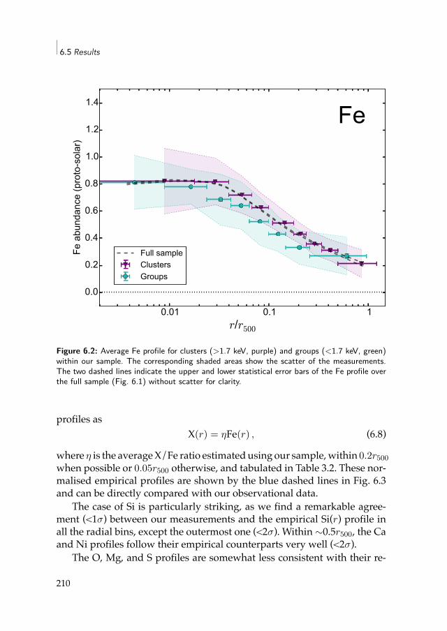
6.5 Results
0.01 0.1 1r/r500
0.0
0.2
0.4
0.6
0.8
1.0
1.2
1.4
Fe a
bund
ance
(pro
to-s
olar
)
Fe
Full sampleClustersGroups
Figure 6.2: Average Fe profile for clusters (>1.7 keV, purple) and groups (<1.7 keV, green)within our sample. The corresponding shaded areas show the scatter of the measurements.The two dashed lines indicate the upper and lower statistical error bars of the Fe profile overthe full sample (Fig. 6.1) without scatter for clarity.
profiles asX(r) = ηFe(r) , (6.8)
where η is the averageX/Fe ratio estimatedusing our sample,within 0.2r500when possible or 0.05r500 otherwise, and tabulated in Table 3.2. These nor-malised empirical profiles are shown by the blue dashed lines in Fig. 6.3and can be directly compared with our observational data.
The case of Si is particularly striking, as we find a remarkable agree-ment (<1σ) between our measurements and the empirical Si(r) profile inall the radial bins, except the outermost one (<2σ). Within ∼0.5r500, the Caand Ni profiles follow their empirical counterparts very well (<2σ).
The O, Mg, and S profiles are somewhat less consistent with their re-
210
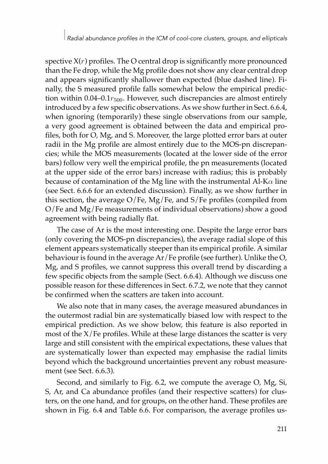
Radial abundance profiles in the ICM of cool-core clusters, groups, and ellipticals
spective X(r) profiles. The O central drop is significantly more pronouncedthan the Fe drop, while theMg profile does not show any clear central dropand appears significantly shallower than expected (blue dashed line). Fi-nally, the S measured profile falls somewhat below the empirical predic-tion within 0.04–0.1r500. However, such discrepancies are almost entirelyintroduced by a few specific observations. Aswe show further in Sect. 6.6.4,when ignoring (temporarily) these single observations from our sample,a very good agreement is obtained between the data and empirical pro-files, both for O, Mg, and S. Moreover, the large plotted error bars at outerradii in the Mg profile are almost entirely due to the MOS-pn discrepan-cies; while the MOS measurements (located at the lower side of the errorbars) follow very well the empirical profile, the pn measurements (locatedat the upper side of the error bars) increase with radius; this is probablybecause of contamination of the Mg line with the instrumental Al-Kα line(see Sect. 6.6.6 for an extended discussion). Finally, as we show further inthis section, the average O/Fe, Mg/Fe, and S/Fe profiles (compiled fromO/Fe and Mg/Fe measurements of individual observations) show a goodagreement with being radially flat.
The case of Ar is the most interesting one. Despite the large error bars(only covering the MOS-pn discrepancies), the average radial slope of thiselement appears systematically steeper than its empirical profile. A similarbehaviour is found in the average Ar/Fe profile (see further). Unlike the O,Mg, and S profiles, we cannot suppress this overall trend by discarding afew specific objects from the sample (Sect. 6.6.4). Although we discuss onepossible reason for these differences in Sect. 6.7.2, we note that they cannotbe confirmed when the scatters are taken into account.
We also note that in many cases, the average measured abundances inthe outermost radial bin are systematically biased low with respect to theempirical prediction. As we show below, this feature is also reported inmost of the X/Fe profiles. While at these large distances the scatter is verylarge and still consistent with the empirical expectations, these values thatare systematically lower than expected may emphasise the radial limitsbeyond which the background uncertainties prevent any robust measure-ment (see Sect. 6.6.3).
Second, and similarly to Fig. 6.2, we compute the average O, Mg, Si,S, Ar, and Ca abundance profiles (and their respective scatters) for clus-ters, on the one hand, and for groups, on the other hand. These profiles areshown in Fig. 6.4 and Table 6.6. For comparison, the average profiles us-
211
6.5 Results
0.01 0.1 1r/r500
0.0
0.2
0.4
0.6
0.8
1.0
1.2
1.4
O a
bund
ance
(pro
to-s
olar
)
OEmpirical Fe profile(Empirical Fe profile) * 0.817local: MOS
0.01 0.1 1r/r500
0.0
0.2
0.4
0.6
0.8
1.0
1.2
1.4
Mg
abun
danc
e (p
roto
-sol
ar)
MgEmpirical Fe profile(Empirical Fe profile) * 0.743local: MOS+pn
0.01 0.1 1r/r500
0.0
0.2
0.4
0.6
0.8
1.0
1.2
1.4
Si a
bund
ance
(pro
to-s
olar
)
Si
Empirical Fe profile(Empirical Fe profile) * 0.871local: MOS+pn
0.01 0.1 1r/r500
0.0
0.2
0.4
0.6
0.8
1.0
1.2
1.4
S ab
unda
nce
(pro
to-s
olar
)
S
Empirical Fe profile(Empirical Fe profile) * 0.984local: MOS+pn
Figure 6.3: Average radial abundance profiles of all the objects in our sample. The error barscontain the statistical uncertainties and MOS-pn uncertainties (Sect. 6.4.3) except for theO abundance profiles, which are only measured with MOS. The corresponding shaded areasshow the scatter of the measurements. The Ni profile has only been averaged for clusters(>1.7 keV).
212
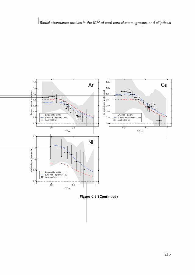
Radial abundance profiles in the ICM of cool-core clusters, groups, and ellipticals
0.01 0.1 1r/r500
0.0
0.2
0.4
0.6
0.8
1.0
1.2
1.4
Ar a
bund
ance
(pro
to-s
olar
)
Ar
Empirical Fe profile(Empirical Fe profile) * 0.88local: MOS+pn
0.01 0.1 1r/r500
0.0
0.2
0.4
0.6
0.8
1.0
1.2
1.4
Ca
abun
danc
e (p
roto
-sol
ar)
Ca
Empirical Fe profile(Empirical Fe profile) * 1.218local: MOS+pn
0.01 0.1 1r/r500
0.0
0.5
1.0
1.5
2.0
Ni a
bund
ance
(pro
to-s
olar
)
Ni
Empirical Fe profile(Empirical Fe profile) * 1.93local: MOS+pn
Figure 6.3 (Continued)
213
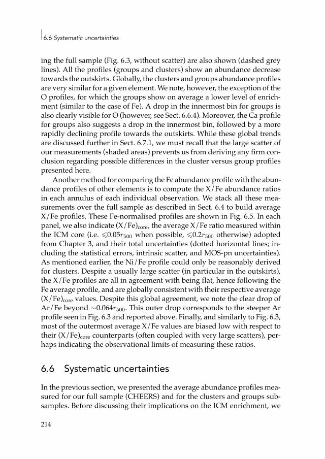
6.6 Systematic uncertainties
ing the full sample (Fig. 6.3, without scatter) are also shown (dashed greylines). All the profiles (groups and clusters) show an abundance decreasetowards the outskirts. Globally, the clusters and groups abundance profilesare very similar for a given element.We note, however, the exception of theO profiles, for which the groups show on average a lower level of enrich-ment (similar to the case of Fe). A drop in the innermost bin for groups isalso clearly visible for O (however, see Sect. 6.6.4). Moreover, the Ca profilefor groups also suggests a drop in the innermost bin, followed by a morerapidly declining profile towards the outskirts. While these global trendsare discussed further in Sect. 6.7.1, we must recall that the large scatter ofour measurements (shaded areas) prevents us from deriving any firm con-clusion regarding possible differences in the cluster versus group profilespresented here.
Anothermethod for comparing the Fe abundance profilewith the abun-dance profiles of other elements is to compute the X/Fe abundance ratiosin each annulus of each individual observation. We stack all these mea-surements over the full sample as described in Sect. 6.4 to build averageX/Fe profiles. These Fe-normalised profiles are shown in Fig. 6.5. In eachpanel, we also indicate (X/Fe)core, the average X/Fe ratio measured withinthe ICM core (i.e. ⩽0.05r500 when possible, ⩽0.2r500 otherwise) adoptedfrom Chapter 3, and their total uncertainties (dotted horizontal lines; in-cluding the statistical errors, intrinsic scatter, and MOS-pn uncertainties).As mentioned earlier, the Ni/Fe profile could only be reasonably derivedfor clusters. Despite a usually large scatter (in particular in the outskirts),the X/Fe profiles are all in agreement with being flat, hence following theFe average profile, and are globally consistentwith their respective average(X/Fe)core values. Despite this global agreement, we note the clear drop ofAr/Fe beyond ∼0.064r500. This outer drop corresponds to the steeper Arprofile seen in Fig. 6.3 and reported above. Finally, and similarly to Fig. 6.3,most of the outermost average X/Fe values are biased low with respect totheir (X/Fe)core counterparts (often coupled with very large scatters), per-haps indicating the observational limits of measuring these ratios.
6.6 Systematic uncertaintiesIn the previous section, we presented the average abundance profiles mea-sured for our full sample (CHEERS) and for the clusters and groups sub-samples. Before discussing their implications on the ICM enrichment, we
214
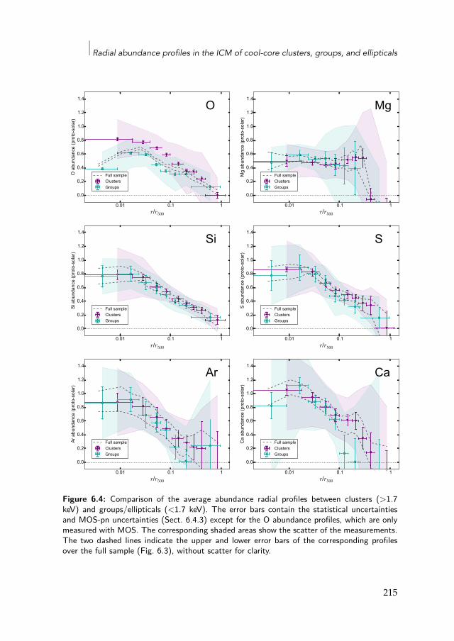
Radial abundance profiles in the ICM of cool-core clusters, groups, and ellipticals
0.01 0.1 1r/r500
0.0
0.2
0.4
0.6
0.8
1.0
1.2
1.4
O a
bund
ance
(pro
to-s
olar
)
O
Full sampleClustersGroups
0.01 0.1 1r/r500
0.0
0.2
0.4
0.6
0.8
1.0
1.2
1.4
Mg
abun
danc
e (p
roto
-sol
ar)
Mg
Full sampleClustersGroups
0.01 0.1 1r/r500
0.0
0.2
0.4
0.6
0.8
1.0
1.2
1.4
Si a
bund
ance
(pro
to-s
olar
)
Si
Full sampleClustersGroups
0.01 0.1 1r/r500
0.0
0.2
0.4
0.6
0.8
1.0
1.2
1.4
S ab
unda
nce
(pro
to-s
olar
)S
Full sampleClustersGroups
0.01 0.1 1r/r500
0.0
0.2
0.4
0.6
0.8
1.0
1.2
1.4
Ar a
bund
ance
(pro
to-s
olar
)
Ar
Full sampleClustersGroups
0.01 0.1 1r/r500
0.0
0.2
0.4
0.6
0.8
1.0
1.2
1.4
Ca
abun
danc
e (p
roto
-sol
ar)
Ca
Full sampleClustersGroups
Figure 6.4: Comparison of the average abundance radial profiles between clusters (>1.7keV) and groups/ellipticals (<1.7 keV). The error bars contain the statistical uncertaintiesand MOS-pn uncertainties (Sect. 6.4.3) except for the O abundance profiles, which are onlymeasured with MOS. The corresponding shaded areas show the scatter of the measurements.The two dashed lines indicate the upper and lower error bars of the corresponding profilesover the full sample (Fig. 6.3), without scatter for clarity.
215
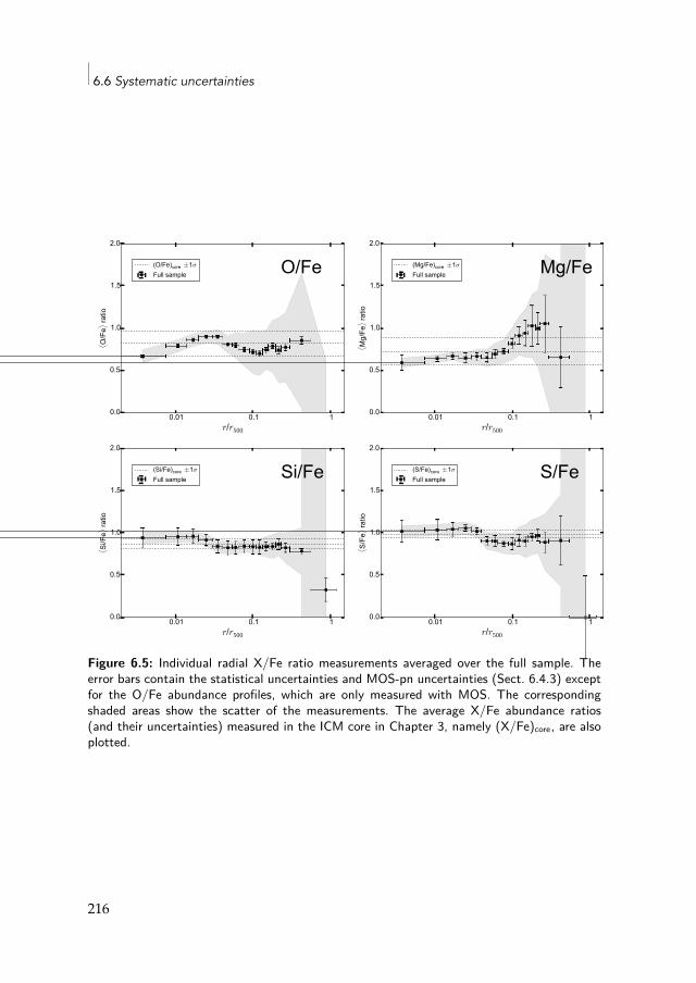
6.6 Systematic uncertainties
0.01 0.1 1r/r500
0.0
0.5
1.0
1.5
2.0
⟨ O/F
e⟩ ratio
O/Fe(O/Fe)core ±1σFull sample
0.01 0.1 1r/r500
0.0
0.5
1.0
1.5
2.0
⟨ Mg/
Fe⟩ ra
tio
Mg/Fe(Mg/Fe)core ±1σFull sample
0.01 0.1 1r/r500
0.0
0.5
1.0
1.5
2.0
⟨ Si/F
e⟩ ratio
Si/Fe(Si/Fe)core ±1σFull sample
0.01 0.1 1r/r500
0.0
0.5
1.0
1.5
2.0
⟨ S/Fe⟩ ra
tio
S/Fe(S/Fe)core ±1σFull sample
Figure 6.5: Individual radial X/Fe ratio measurements averaged over the full sample. Theerror bars contain the statistical uncertainties and MOS-pn uncertainties (Sect. 6.4.3) exceptfor the O/Fe abundance profiles, which are only measured with MOS. The correspondingshaded areas show the scatter of the measurements. The average X/Fe abundance ratios(and their uncertainties) measured in the ICM core in Chapter 3, namely (X/Fe)core, are alsoplotted.
216
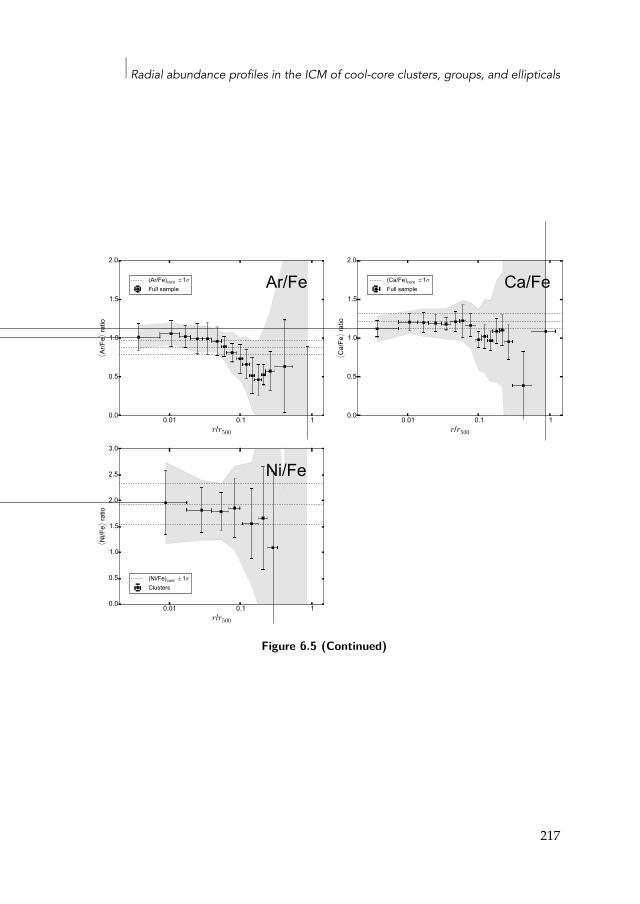
Radial abundance profiles in the ICM of cool-core clusters, groups, and ellipticals
0.01 0.1 1r/r500
0.0
0.5
1.0
1.5
2.0
⟨ Ar/F
e⟩ ratio
Ar/Fe(Ar/Fe)core ±1σFull sample
0.01 0.1 1r/r500
0.0
0.5
1.0
1.5
2.0
⟨ Ca/
Fe⟩ ra
tio
Ca/Fe(Ca/Fe)core ±1σFull sample
0.01 0.1 1r/r500
0.0
0.5
1.0
1.5
2.0
2.5
3.0
⟨ Ni/F
e⟩ ratio
Ni/Fe
(Ni/Fe)core ±1σClusters
Figure 6.5 (Continued)
217
6.6 Systematic uncertainties
must ensure that our results are robust and do not (strongly) depend onthe assumptions we invoke throughout this paper. In this section, we ex-plore the systematic uncertainties that could potentially affect our results.They can arise from: (i) the intrinsic scatter in the radial profiles of the dif-ferent objects of our sample; (ii) MOS-pn discrepancies in the abundancemeasurements due to residual EPIC cross-calibration issues; (iii) projectioneffects on the plane of the sky; (iv) uncertainties in the thermal structure ofthe ICM; (v) uncertainties in the backgroundmodelling; and (vi) theweightof a few individual highest quality observations, which might dominatethe average measurements.
We already took items (i) and (ii) into account in our analysis (Sect. 6.5.1and 6.4.3, respectively), and here we focus on items (iii), (iv), (v), and (vi).
6.6.1 Projection effectsThroughout this paper, we report the average abundance profiles of theICM as observed by XMM-Newton/EPIC, i.e. projected on the plane of thesky. Several models are currently available to deproject cluster data and es-timate the radial metal distribution contained in concentric spherical shells(e.g. Churazov et al. 2003; Kaastra et al. 2004; Johnstone et al. 2005; Rus-sell et al. 2008). However, all of them assume a spherical symmetry in theICM distribution, which may not always be true. Moreover, some meth-ods are known for introducing artefacts in the deprojected measurements(for a comparison, see Russell et al. 2008), as deprojection methods assumea dependency between all the fitted annuli. We thus prefer to work withprojected results to keep a statistical independence in the radial bins.
Several past works investigated the effects of deprojection on the abun-dance estimates at different radii. The general outcome is that these ef-fects have a very limited impact on the abundancemeasurements (e.g. Ras-mussen & Ponman 2007; Russell et al. 2008). Therefore, we do not expectthem to be a source of significant systematic uncertainty for the purpose ofthis work.
6.6.2 Thermal modellingAs explained in Sect. 6.3.1, the abundance determination is very sensitive tothe assumed thermal structure of the cluster/group. Therefore, it is crucialto fit our spectra with a thermal model that reproduces the projected tem-perature structure as realistically as possible. In particular, a cie (single-
218
Radial abundance profiles in the ICM of cool-core clusters, groups, and ellipticals
temperature) model is clearly not optimal for our analysis. The thermalmodel used in this work (gdem) has been used in many previous studiesand is thought to be rather successful at reproducing the true temperaturestructure of some clusters (e.g. Simionescu et al. 2009b; Frank et al. 2013),as it represents one of the simplest way of accounting for a continuousmix-ing of temperatures in the ICM (coming from either projection effects or alocally intrinsic multi-phase plasma). The precise temperature distributionis however difficult to determine with the current spectrometers and maysomewhat differ from the gdem assumption. Alternatively, some previousworks suggest that the temperature distribution in cool-core clusters maybe reasonably approximated by a truncated power law (typically between0.2 keV ≲ kT ≲ 3 keV, with more emission towards higher temperatures;see e.g. Kaastra et al. 2004; Sanders et al. 2008). Such a distribution can bemodelled in SPEX via the wdem model (for more details, see e.g. Kaastraet al. 2004).
Using a wdemmodel instead of a gdemmodel can potentially lead to dif-ferences in the measured abundances, hence contributing to add furthersystematic uncertainties to the derived profiles (for a RGS comparison, seede Plaa et al. 2017). Unfortunately, the large computing time required bythe wdem model in the fits does not allow us to perform a full comparisonbetween the twomodels over the whole sample.We thus select one cluster,MKW3s, and we explore how the use of a wdemmodel affects its Fe profile.MKW3s has the advantage of emitting a moderate ICM temperature (∼3.4keV) inside 0.05r500, which is very close to the mean temperature of theclusters in the sample (∼3.2 keV) within this radius. Moreover, the Fe ra-dial profile of MKW3s (Fig. 6.18) is rather similar to the average Fe profilepresented in Fig. 6.1. The gdem-wdem comparison on the Fe radial profile ofMKW3s is presented in Fig. 6.6. The use of a wdem model in MKW3s sys-tematically predicts higher Fe abundances than using a gdem model, wherethe increase may vary from +6% (core) up to +20% (outskirts). Since thereis a difference of temperature between the core (kTmean ≃ 3.5 keV) and theoutskirts (kTmean ≃ 1 keV), this may suggest a temperature dependence(see also de Plaa et al. 2017). However, there is no substantial change in theslope of the overall profile. The same trend is also found for the abundanceprofiles of the other elements. For comparison, we also check that we ob-tain similar results for NGC507, i.e. a cooler group. In conclusion, we donot expect any variation in the shape of the average abundance profilesowing to the use of another temperature distribution in ourmodelling. The
219
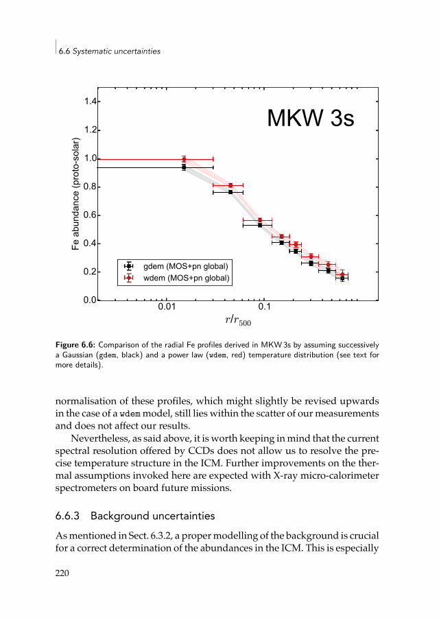
6.6 Systematic uncertainties
0.01 0.1r/r500
0.0
0.2
0.4
0.6
0.8
1.0
1.2
1.4
Fe a
bund
ance
(pro
to-s
olar
)
MKW 3s
gdem (MOS+pn global)wdem (MOS+pn global)
Figure 6.6: Comparison of the radial Fe profiles derived in MKW 3s by assuming successivelya Gaussian (gdem, black) and a power law (wdem, red) temperature distribution (see text formore details).
normalisation of these profiles, which might slightly be revised upwardsin the case of a wdemmodel, still lies within the scatter of ourmeasurementsand does not affect our results.
Nevertheless, as said above, it is worth keeping inmind that the currentspectral resolution offered by CCDs does not allow us to resolve the pre-cise temperature structure in the ICM. Further improvements on the ther-mal assumptions invoked here are expected with X-ray micro-calorimeterspectrometers on board future missions.
6.6.3 Background uncertaintiesAsmentioned in Sect. 6.3.2, a propermodelling of the background is crucialfor a correct determination of the abundances in the ICM. This is especially
220
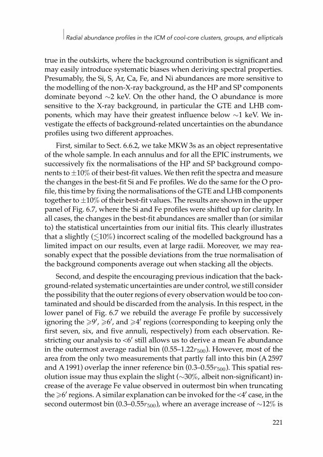
Radial abundance profiles in the ICM of cool-core clusters, groups, and ellipticals
true in the outskirts, where the background contribution is significant andmay easily introduce systematic biases when deriving spectral properties.Presumably, the Si, S, Ar, Ca, Fe, and Ni abundances are more sensitive tothe modelling of the non-X-ray background, as the HP and SP componentsdominate beyond ∼2 keV. On the other hand, the O abundance is moresensitive to the X-ray background, in particular the GTE and LHB com-ponents, which may have their greatest influence below ∼1 keV. We in-vestigate the effects of background-related uncertainties on the abundanceprofiles using two different approaches.
First, similar to Sect. 6.6.2, we take MKW3s as an object representativeof the whole sample. In each annulus and for all the EPIC instruments, wesuccessively fix the normalisations of the HP and SP background compo-nents to±10%of their best-fit values.We then refit the spectra andmeasurethe changes in the best-fit Si and Fe profiles. We do the same for the O pro-file, this time by fixing the normalisations of theGTE and LHB componentstogether to±10%of their best-fit values. The results are shown in the upperpanel of Fig. 6.7, where the Si and Fe profiles were shifted up for clarity. Inall cases, the changes in the best-fit abundances are smaller than (or similarto) the statistical uncertainties from our initial fits. This clearly illustratesthat a slightly (≲10%) incorrect scaling of the modelled background has alimited impact on our results, even at large radii. Moreover, we may rea-sonably expect that the possible deviations from the true normalisation ofthe background components average out when stacking all the objects.
Second, and despite the encouraging previous indication that the back-ground-related systematic uncertainties are under control, we still considerthe possibility that the outer regions of every observationwould be too con-taminated and should be discarded from the analysis. In this respect, in thelower panel of Fig. 6.7 we rebuild the average Fe profile by successivelyignoring the ⩾9′, ⩾6′, and ⩾4′ regions (corresponding to keeping only thefirst seven, six, and five annuli, respectively) from each observation. Re-stricting our analysis to <6′ still allows us to derive a mean Fe abundancein the outermost average radial bin (0.55–1.22r500). However, most of thearea from the only two measurements that partly fall into this bin (A 2597and A1991) overlap the inner reference bin (0.3–0.55r500). This spatial res-olution issue may thus explain the slight (∼30%, albeit non-significant) in-crease of the average Fe value observed in outermost bin when truncatingthe⩾6′ regions. A similar explanation can be invoked for the <4′ case, in thesecond outermost bin (0.3–0.55r500), where an average increase of ∼12% is
221
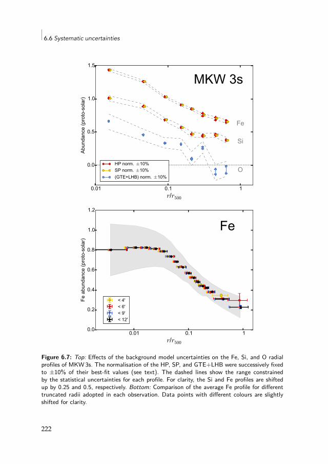
6.6 Systematic uncertainties
0.01 0.1 1r/r500
0.0
0.5
1.0
1.5
Abun
danc
e (p
roto
-sol
ar)
MKW 3s
Fe
Si
OHP norm. ±10%SP norm. ±10%(GTE+LHB) norm. ±10%
0.01 0.1 1r/r500
0.0
0.2
0.4
0.6
0.8
1.0
1.2
Fe a
bund
ance
(pro
to-s
olar
)
Fe
< 4'< 6'< 9'< 12'
Figure 6.7: Top: Effects of the background model uncertainties on the Fe, Si, and O radialprofiles of MKW 3s. The normalisation of the HP, SP, and GTE+LHB were successively fixedto ±10% of their best-fit values (see text). The dashed lines show the range constrainedby the statistical uncertainties for each profile. For clarity, the Si and Fe profiles are shiftedup by 0.25 and 0.5, respectively. Bottom: Comparison of the average Fe profile for differenttruncated radii adopted in each observation. Data points with different colours are slightlyshifted for clarity.
222
Radial abundance profiles in the ICM of cool-core clusters, groups, and ellipticals
observed (though less than 2σ significant). In any case, the changes relatedto the truncation of the profiles at different radii are always smaller thanthe scatter (grey area) even in the outskirts. Therefore, this scatter can rea-sonably be seen as a conservative limit encompassing all the backgrounduncertainties mentioned here.
In summary, our results clearly suggest that our careful modelling ofthe background allows us to keep all its related systematic uncertaintieson the abundances under control, even at larger radii. However, it is notimpossible that the background dominates in the outermost radial bin (⩾0.55r500) too much, thereby biasing low the average abundances of someelements (Sect. 6.5.2).
6.6.4 Weight of individual observationsAmong the 44 objects of our sample, the three brightest objects (A 3526a.k.a. Centaurus, M87, and Perseus) benefit from excellent data quality,leading to very small statistical uncertainties (σ2
X(i)j) of theirmeasured abun-
dances. Consequently, these observations may have an important contri-bution in shaping the average abundance profiles (as 1/σ2
X(i)j≫ 1). The
consequences of this weighting selection effect is explored in this section.In Fig. 6.8 (top left panel), we show how the average Fe profile changes
whenwe excludeA3526,M87, and Perseus from the sample. Compared tothe initial Fe profile (blue empty boxes; see also Fig. 6.1), the largest effect isan increase of ∼8% in the innermost average radial bin (⩽ 7.5 × 10⁻³r500),while the rest of the radial profile varies a few per cent at most.
Similarly, this weighting effect may affect the other abundance profiles.In Fig. 6.3, we showed that the average Si, Ca, and Ni radial profiles followvery well the fitted average Fe radial profile normalised by the averageX/Fe ratio found in the core. However, the innermost region (⩽0.01r500)shows an O drop about ∼20% lower than predicted by our empirical pro-file, while theMgprofile looks significantly flatter than expected. Similarly,some deviations from the expected S profile are also observed within 0.04–0.1r500. In this section, we show that these profiles are more affected by theweight of a few individual observations, and that the empirical O/Mg/Sprofiles can be very well reproduced when temporarily ignoring these pe-culiar measurements.
Whenwe excludeM49, M60, andNGC4636 from the analysis, we finda much better agreement between the O abundance and its correspond-
223
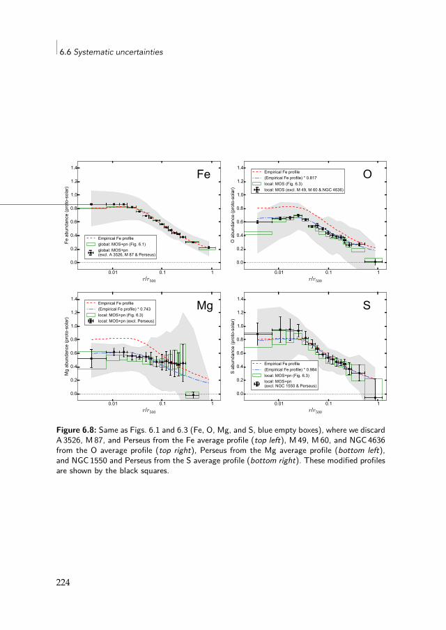
6.6 Systematic uncertainties
0.01 0.1 1r/r500
0.0
0.2
0.4
0.6
0.8
1.0
1.2
1.4
Fe a
bund
ance
(pro
to-s
olar
)
Fe
Empirical Fe profileglobal: MOS+pn (Fig. 6.1)global: MOS+pn (excl. A 3526, M 87 & Perseus)
0.01 0.1 1r/r500
0.0
0.2
0.4
0.6
0.8
1.0
1.2
1.4
O a
bund
ance
(pro
to-s
olar
)
OEmpirical Fe profile(Empirical Fe profile) * 0.817local: MOS (Fig. 6.3)local: MOS (excl. M 49, M 60 & NGC 4636)
0.01 0.1 1r/r500
0.0
0.2
0.4
0.6
0.8
1.0
1.2
1.4
Mg
abun
danc
e (p
roto
-sol
ar)
MgEmpirical Fe profile(Empirical Fe profile) * 0.743local: MOS+pn (Fig. 6.3)local: MOS+pn (excl. Perseus)
0.01 0.1 1r/r500
0.0
0.2
0.4
0.6
0.8
1.0
1.2
1.4
S ab
unda
nce
(pro
to-s
olar
)
S
Empirical Fe profile(Empirical Fe profile) * 0.984local: MOS+pn (Fig. 6.3)local: MOS+pn (excl. NGC 1550 & Perseus)
Figure 6.8: Same as Figs. 6.1 and 6.3 (Fe, O, Mg, and S, blue empty boxes), where we discardA 3526, M 87, and Perseus from the Fe average profile (top left), M 49, M 60, and NGC 4636from the O average profile (top right), Perseus from the Mg average profile (bottom left),and NGC 1550 and Perseus from the S average profile (bottom right). These modified profilesare shown by the black squares.
224
Radial abundance profiles in the ICM of cool-core clusters, groups, and ellipticals
ing empirical prediction in the innermost bin (Fig. 6.8 top right). Indeed,these three ellipticals/groups are characterised by a suspiciously low Oabundance within their respective <0.5′ annuli (inconsistent with the val-ues found within 0.8′ with RGS by de Plaa et al. 2017), which, togetherwith very small errors bars, contribute to substantially lower the averageO abundance in the ⩽ 7.5 × 10⁻³r500 region.
When we exclude Perseus from the analysis, the average Mg measure-ments agree much better with the expected empirical profile, especiallywithin ∼0.01–0.05r500 (Fig. 6.8 bottom left panel). The significant MOS-pndiscrepancies measured in the Perseus spectra make the Mg abundancesomewhat uncertain over the region considered above. However, and co-incidentally, combining these (discrepant) MOS/pn measurements fromPerseus with those from the rest of the sample brings the average MOSand pn estimates of Mg at very similar levels, thereby dramatically reduc-ing the total MOS-pn uncertainties that we consider in Sect. 6.4.3. This caseis thus a good illustration that care must be taken when combining indi-vidual systematic uncertainties over a large data sample. Finally, the ex-clusion of NGC1550 and Perseus from the sample contributes to a betteragreement of themeasured S profile with its empirical expectation (Fig. 6.8bottom right).
To sum up, in addition to showing that the average measured radialabundance profiles for all elements can reproduce verywell their empiricalcounterparts, this section illustrates that care must be taken when strictlyinterpreting the error bars shown in the figures of this paper, as only one ortwo individual observations may slightly (usually, within a few per cent)but significantly raise or lower our measurements. That said, in the restof the paper we consider our full sample, including the peculiar measure-ments discussed here.
6.6.5 Atomic code uncertaintiesThe CIE model employed to fit our EPIC spectra is based on the mekalmodel (Mewe et al. 1985, 1986, also present in XSPEC), with important up-dates up to now. The atomic database and routines on which this modelrelies is called SPEXACT6. Whereas the initial version of SPEXACT can besimply attributed to the original mekalmodel, the version used in thiswork(corresponding to the atomic code that was regularly updated between
6SPEX Atomic Code and Tables
225
6.6 Systematic uncertainties
1996 and 2016) is referred to SPEXACT v2. In recent months, substantial ef-forts have beendevoted towards amajor update of the code (SPEXACTv3),followed by a newly released version of SPEX (de Plaa et al. 2017). For ex-ample, this new version includes a more precise parametrisation of the ra-diative recombination rates (Mao & Kaastra 2016), updated collisional ion-isation coefficients (Urdampilleta et al. 2017), and the calculation of manymore transitions. Following Chapter 3, we included the correction of thislatest update on ourO abundancemeasurements (Sect. 6.3.1). However theabundances of the other elements may also be affected by such improvedcalculations.
Unfortunately, fitting all our EPIC spectra using SPEXACT v3 wouldrequire unrealistic amounts of computing time and resources. Therefore,we evaluate the impact of these atomic code differences on the EPIC abun-dances by following a similar approach as carried out by de Plaa et al.(2017) for RGS (see also Chapter 5). Here, we simulate EPIC spectra assum-ing a gdem distribution calculated from SPEXACT v3, for a range of meantemperatures from 0.6 keV to 6.0 keV and by setting all the abundancesto 1. We then fit these mock spectra locally with a gdem model calculatedfrom SPEXACT v2 (i.e. the version used in this work), and we measure thechanges in the best-fit abundances. The result is shown in Fig. 6.9.
For temperatures hotter than ∼1.5 keV, most of the abundances do notchange by more than ∼20%. The two exceptions are Mg and Ni, which canchange by almost a factor of 2 at high and low temperatures, respectively.For temperatures cooler than ∼1.5 keV, we see a dramatic decrease (bymore than a factor of 2) of themeasured Fe abundance. Themain differencebetween the spectral models generated by SPEXACT v2 and SPEXACT v3resides in the Fe-L complex, which is foremost used by the fits to determinethe Fe abundance in cool (kT ≲ 2 keV) plasmas.
Since most of the computed abundances remain fairly constant withinthe typical temperature range (∼1–5 keV) of all the spectra of our sam-ple, such atomic code uncertainties are not expected to affect our results.Nevertheless, we note that these changes between SPEXACT v2 and SPEX-ACT v3 may have a non-negligible impact on the integrated abundances(and X/Fe abundance ratios) reported in previous works. For instance, ifupdated atomic calculations indeed revise the average Ni/Fe abundancedownwards (so far measured to be surprisingly high; e.g. Chapters 3 and4), a more simple agreement than previously assumed between the ICMabundance pattern and SN yield models may be expected. This issue (and
226
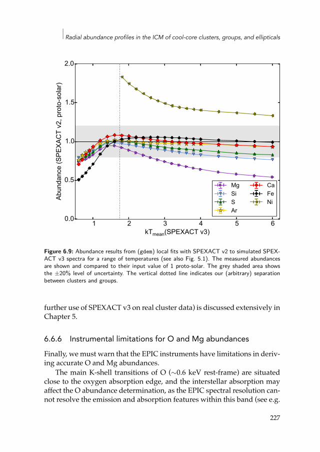
Radial abundance profiles in the ICM of cool-core clusters, groups, and ellipticals
1 2 3 4 5 6kTmean(SPEXACT v3)
0.0
0.5
1.0
1.5
2.0Ab
unda
nce
(SPE
XAC
T v2
, pro
to-s
olar
)
MgSiSAr
CaFeNi
Figure 6.9: Abundance results from (gdem) local fits with SPEXACT v2 to simulated SPEX-ACT v3 spectra for a range of temperatures (see also Fig. 5.1). The measured abundancesare shown and compared to their input value of 1 proto-solar. The grey shaded area showsthe ±20% level of uncertainty. The vertical dotted line indicates our (arbitrary) separationbetween clusters and groups.
further use of SPEXACT v3 on real cluster data) is discussed extensively inChapter 5.
6.6.6 Instrumental limitations for O and Mg abundancesFinally, we must warn that the EPIC instruments have limitations in deriv-ing accurate O and Mg abundances.
The main K-shell transitions of O (∼0.6 keV rest-frame) are situatedclose to the oxygen absorption edge, and the interstellar absorption mayaffect the O abundance determination, as the EPIC spectral resolution can-not resolve the emission and absorption features within this band (see e.g.
227
6.7 Discussion
de Plaa et al. 2004). Moreover, and despite our considerations from Sect.6.6.3, the Galactic foreground may play a more important role than ex-pected, which can potentially bias the O abundance, especially when thebackground dominates. Although affecting on average 3–4% of the XMM-Newton observations, solar wind charge exchange might also be a sourceof (limited) bias for the O abundance, at it may affect the OVII and OVIIIlines in the contaminated spectra (e.g. Snowden et al. 2004; Carter et al.2011).
On the other hand, themain K-shell emission line ofMg (∼1.5 keV rest-frame) falls partly into the Fe-L complex, which is unresolved by the EPICinstruments. Moreover, measuring the Mg abundance in clusters outskirtsis challenging because the EPIC hard particle background is contaminatedby the Al Kα fluorescence line, which is also situated at ∼1.5 keV both inMOS and pn instruments (Chapter 2), and thus impossible to disentanglefrom the Mg K-shell ICM emission lines using the EPIC spectrometers.
Despite all these limitations, the good agreement of our average O andMg profiles with their respective empirical predictions (at least out to∼0.3r500, and after discarding specific observations from the sample, see Sect.6.6.4) is very encouraging, and makes us confident about the results pre-sented in this work.
6.7 DiscussionWe derived the average radial abundance profiles of 44 galaxy clusters,groups, and elliptical galaxies. In Sect. 6.5, we were able to provide con-straints on the radial ICM distributions of Fe, but also O, Mg, Si, S, Ar,Ca, and Ni, comparing them within clusters (>1.7 keV) and groups (<1.7keV). In the previous section, we also showed that the major systematicuncertainties are kept under control. We now discuss our results and wecompare them with measurements and predictions from previous studies.
6.7.1 Enrichment in clusters and groupsIn Fig. 6.2, we compared the radial Fe abundance profile averaged overclusters, on the one hand, and groups, on the other hand. Although thescatter in each profile is large, the average enrichment level in clusters isslightly higher than in groups. This result is not surprising, as an increaseof the ICM metallicity with the cluster/group temperature (at least up to
228
Radial abundance profiles in the ICM of cool-core clusters, groups, and ellipticals
kT ≃ 3 keV) has been commonly observed in previous studies (e.g. Ras-mussen & Ponman 2009; Yates et al. 2017). This trend is also consistentwith the results of Chapter 3, where we analysed the same sample withthe same data and same definition for clusters versus groups/ellipticals.They found that, within 0.05r500, the Fe abundance in clusters is on average∼22% higher than in groups. We find a similar Fe enhancement (on aver-age∼21%) in our profiles for clusters and groups at all radii, except in theirrespective innermost and outermost radial bins (see also Sect. 6.5.1). Theabsence of difference of Fe abundance in the innermost bin of clusters andgroups can be explained by the important weight of a few individual clus-ters, as already discussed in Sect. 6.6.4. In particular, the cores of Perseusand A3526 show deep and significant Fe drops (see also Sect. 6.7.2), whichtend to lower the innermost average Fe abundance for clusters. Removingthese two objects from the sample increases this innermost Fe abundance(Fig. 6.8 top left), and, therefore, should contribute towards keeping a sim-ilar enhancement between clusters and groups within ∼0.01r500. On theother hand, among the 11 measurements in the outermost radial bin of thegroups profile, only 2 (∼18%) are located beyond 0.5r500, i.e. covering theoutermost bin of the clusters profile. The Fe abundance averaged over thisoutermost bin of the groups profile is thus weighted towards the measure-ments at smaller radii, roughly at the location of the third (<0.34r500) andsecond (0.34–0.5r500) outermost bins of the clusters profile. This explainsthe illusion of a Fe enhancement in the outskirts of groups with respect tothose of clusters.
In summary, the average Fe profile of clusters is consistent with beingmore enhanced in a similar way not only in the core, but also at all radialdistances at least out to 0.5r500. The origin of such a difference of ICM en-richment between cooler and hotter objects is still unclear, and has beenalready debated in the literature (e.g. Rasmussen & Ponman 2009; Lianget al. 2016; Yates et al. 2017). For example, in contrast to clusters, galaxygroups may not be closed boxes (e.g. McCarthy et al. 2011) and AGN feed-back may contribute to remove enrichedmaterial out of the groups. It mayeven be possible that part of this apparent difference of enrichment couldbe due to underestimated Fe abundances in low temperature plasmas, asmentioned in Sect. 6.6.5. A thorough discussion of these aspects is some-what beyond the scope of this paper. However, our radial profiles mayprovide useful constraints on the dominant mechanisms that are responsi-ble for such a difference.
229
6.7 Discussion
Interestingly, the same trend between clusters and groups is not clearlyobserved in the average profiles of other elements. Instead, these abun-dance profiles are consistent within clusters and groups (Fig. 6.4). In fact,we report a slight (but not significant) enhancement in the X/Fe ratio pro-files of groups compared to those of clusters, up to 0.03r500, whose effect isvisible in the Si/Fe and S/Fe profiles of the full sample (Fig. 6.5). However,the large error bars (including systematic uncertainties from the MOS-pncross-calibration) prevent us from firmly confirming this trend. We alsonote the exception of the O profiles, which clearly show an enhancementin the case of clusters with respect to that of groups. However, we mustrecall that O measurements using EPIC may be still uncertain (Sect. 6.6.6).Moreover, the measured O abundance in hotter systems may be biasedhigh compared to its true value, essentially owing to issues in determiningthe correct continuum coupled to the weak emissivity of the OVIII line atthese temperatures (Rasia et al. 2008).
6.7.2 The central metallicity dropAs seen in Figs. 6.18 and 6.19, some clusters and groups clearly exhibit acentral drop in their Fe abundances. The presence of drops in these systemsalso appear in Fig. 6.1, where a slight central decrease is observed in theaverage Fe abundance profile. Figures 6.3 and 6.5 suggest that these dropsare not exclusive to Fe, as the other metals seem to be concerned. In thissection, we attempt to quantify these abundance drops (focussing mainlyon Fe) and then discuss their possible origins.
One way of quantifying the Fe drops is to measure their ”depths”. Wechoose arbitrarily the quantity Fe(rmax)/Fedrop: we divide the Fe abun-dance at its off-centre peak (or the Fe abundance at its second innermostbin, if the profile is monotonically decreasing) by the Fe abundance at thefirst innermost bin.With this definition, all the objects with Fe(rmax)/Fedropsignificantly greater than 1 are considered to host a significant drop. Wefind that 14 objects (∼32%) of our sample show a decrease of Fe abundancein their very core. Three of these objects (2A 0335+096, A 3526, and Perseus)are classified as clusters (i.e. ∼13% of the subsample), while the remain-ing 11 (A 189, A 3581, Fornax, HCG62, M49, M86, NGC4325, NGC4636,NGC5044, NGC5813, andNGC5846) are classified as groups (i.e.∼52% ofthe subsample). This apparent larger proportion of groups hosting a centralmetallicity drop should be treated with caution because the larger distanceof many clusters does not allow us to investigate their very core with the
230
Radial abundance profiles in the ICM of cool-core clusters, groups, and ellipticals
same spatial resolution as for nearer groups and ellipticals. Similarly, thedrop seen in the average Fe profile (Fig. 6.1) is smoothed by the lower spa-tial resolution of more distant systems, and thus appears less pronouncedthan in individual nearby objects.
In most cases, the Fe drop is only seen in the innermost bin. However,some objects (e.g. Perseus, Fornax, M49, and NGC5044) clearly exhibit adrop extending within several radial bins. Therefore, for each object wealso evaluate rmax/r500, i.e. the location of the (off-centre) Fe peak, in unitsof r500. For objects not showing any apparent drop, we adopt the extent ofthe innermost bin, which only provides an upper limit. Figure 6.10 showsa diagram of Fe(rmax)/Fedrop versus rmax/r500 (i.e. the depth of the dropsversus the location of the Fe off-centre peaks). The grey shaded area corre-sponds to the objects with no apparent drop (Fe(rmax)/Fedrop ⩽ 1), whereonly an upper limit of rmax/r500 could be constrained. When restrictingourselves to the objects exhibiting a drop (white area), we do not find ev-idence for a clear correlation (ρ ≃ 0.19) between the depth and radial ex-tent of the drops. In fact, the error bars and scatter of the measurementsare quite large and prevent us from deriving any firm conclusion on thisassessment. The ACIS instrument on board Chandra could help to reducethe error bars and to confirm (or rule out) this correlation. Such a detailedstudy, however, is beyond the scope of this present paper, and we leave itfor future work.
This is not the first time that central metallicity drops have been foundin the core of the ICM (e.g. Sanders & Fabian 2002; Johnstone et al. 2002;Sanders & Fabian 2007; Rafferty et al. 2013). However, their interpretationis not yet established. Below we discuss several possibilities that could ex-plain the metallicity drops found in this work.
First, these apparent drops in metallicity could be the result of an arte-fact when fitting the spectra of the central regions. For example, an in-appropriate modelling of the X-ray emission of the central AGN (or cu-mulated X-ray binaries in the BCG) could potentially introduce an incor-rect estimate of the continuum of the ICM emission and underestimatethe abundances in the very core. However, the abundance decrease ex-tends sometimes outside the innermost region (Fig. 6.19, see e.g. Fornax,M49, and NGC5044), where no contamination from AGN emission is ex-pected. Similarly (and perhaps more interestingly), the presence of non-thermal electrons in X-ray cavities could produce an additional power lawcomponent, which would underestimate the abundances if not properly
231
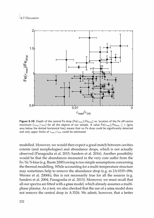
6.7 Discussion
0.01 0.1rmax/r500
0.6
1
1.5
2Fe
(rm
ax)/F
e dro
p
Figure 6.10: Depth of the central Fe drop (Fe(rmax)/Fedrop) vs. location of the Fe off-centremaximum (rmax/r500) for all the objects of our sample. A value Fe(rmax)/Fedrop ≲ 1 (greyarea below the dotted horizontal line) means that no Fe drop could be significantly detectedand only upper limits of rmax/r500 could be estimated.
modelled. However, we would then expect a good match between cavitiesextents (and morphologies) and abundance drops, which is not actuallyobserved (Panagoulia et al. 2015; Sanders et al. 2016). Another possibilitywould be that the abundances measured in the very core suffer from theFe/Si/S-bias (e.g. Buote 2000) owing to too simple assumptions concerningthe thermalmodelling.While accounting for amulti-temperature structuremay sometimes help to remove the abundance drop (e.g. in 2A0335+096;Werner et al. 2006b), this is not necessarily true for all the sources (e.g.Sanders et al. 2004; Panagoulia et al. 2013). Moreover, we must recall thatall our spectra are fittedwith a gdemmodel, which already assumes amulti-phase plasma. As a test, we also checked that the use of a wdem model doesnot remove the central drop in A3526. We admit, however, that a better
232
Radial abundance profiles in the ICM of cool-core clusters, groups, and ellipticals
knowledge of the true temperature distribution in cooling cores would berequired to investigate in detail its impact on the very central abundancemeasurements. We can also discard other artificial effects such as projec-tion on the plane of the sky (Sanders & Fabian 2007) or resonant scattering(Sanders & Fabian 2006b), since they are not efficient enough to fully re-move the drops. Finally, the underestimate of the Fe abundance at CCDresolution for low temperatures (Sect. 6.6.5) could be an alternative fittingbias to explain the abundance drops. Although this could explain someabundance drops found in very cool group cores (e.g. NGC5813), this biascan hardly be invoked in the case of core temperatures above ∼1 keV stillexhibiting a drop (e.g. A 3526).
Second, assuming that the drops are real, it may be reasonable to spec-ulate that a fraction of the central metal mass has been redistributed fromthe core, by either AGN feedback, or sloshing motions. Whereas it is nowwell established that AGN feedbackmay play a key role in transporting themetals outside of the very core via jets and/or buoyant bubbles, as alreadyobserved inM87 (Simionescu et al. 2008) and inHydraA (Simionescu et al.2009b), simulations do not favour any clear formation of inner drops (e.g.Guo & Mathews 2010). Furthermore, we do not find any correlation be-tween AGN radio luminosities (L1.4 GHz) reported in the literature (e.g.Bîrzan et al. 2012) and the depths (Fe(rmax)/Fedrop) or the radial extent(rmax/r500) of the drops in our sample. Similarly, while the extended dropseen in NGC5044 might be partly explained by its peculiar metal distribu-tion in the sloshed gas (O’Sullivan et al. 2014), sloshing process can proba-bly not explain the (narrower) drops seen in other objects (Roediger et al.2011, 2012).
Third, and alternatively, the drops could be the result of the depletionof a part of the ICM-phasemetals into dust grains. In the scenario proposedby Panagoulia et al. (2013, 2015), a significant part of the metals releasedby SNewithin the BCG remain in the form of cold dust grains (Voit & Don-ahue 2011) and become incorporated into the central dusty filaments. Thesedust grains are then dragged out by buoyant bubbles caused by the AGNactivity and are released back in the hot ICM phase out of the very core,thereby forming the off-centre Fe peak. This idea is supported by the pres-ence of dust in most of the objects studied by Panagoulia et al. (2015) andshowing a metallicity drop. The authors emphasise that such a scenariocan be tested by the behaviour of the Ne and Ar radial profile in the verycore of clusters and groups. Indeed, while elements like Fe, Si, and S are
233
6.7 Discussion
known to be easily embedded in dust grains, Ne and Ar are noble gasesand are not expected to be incorporated into dust7. Consequently, theirradial abundance profiles should not show any sign of drop or flatteningin the innermost regions. As mentioned in Sect. 6.3.1, the EPIC spectralresolution does not allow us to investigate the Ne radial distribution. In-terestingly, the radial Ar distribution does not follow well the (rescaled)Fe distribution as it shows a sharper gradient than expected by the empir-ical Fe profile (Figs. 6.3 and 6.5). This sharper gradient is consistent withthe different average Ar/Fe ratios measured in Chapter 4 in the ⩽0.05r500and the ⩽0.2r500 regions. Similarly, the central (≲ 0.02r500) measured Arabundances lie somewhat higher than expected. As an (speculative) expla-nation for this particular feature seen only in the Ar profile, dust depletionin the cool-core ICM (presumably affecting all the considered elements,except Ar) might play a substantial role in shaping the abundance profilesof depleted elements, in particular within ∼0.1r500. However, our averageAr profile points towards the presence of a flattening (if not a drop) in theinnermost bin (Fig. 6.3), suggesting that dust depletion only may not besufficient to explain the innermost metal drops. That said, the very largescatter of the Ar abundance prevents us from claiming any firm evidencefor/against this scenario. When investigating the individual abundanceprofiles of Perseus and A3526 (i.e. the two objects hosting an abundancedrop and providing the best statistics), as shown in Fig. 6.11, we find thatthe MOS measurements in A3526 suggest a monotonic increase of Ar to-wards the centre. The other measurements (pn in A3526, and MOS andpn in Perseus) instead suggest that Ar follows the Fe drop. To summarise,although we are not able to firmly favour or rule out this dust depletionscenario, our results might suggest a non-negligible effect of dust deple-tion of gas-phase metals in clusters, but do not confirm that metals that areembedded in dust in the very core of clusters/groups would be the uniqueorigin of the abundance drops.
Fourth, the apparent drops may be the result of an underestimate ofthe helium content in the very core of such objects. Because He transitionsdo not occur at X-ray energies, it is impossible to provide any direct con-straint on the He abundance in the ICM. In all our fits (as in the major-ity of the similar studies found in the literature), we assume that He fol-lows the primordial abundance (∼25% of mass fraction; e.g. Peimbert et al.
7Dusty Ar might appear in the form of cold molecular gas 36ArH+ (Barlow et al. 2013),but the presence of such a gas in cluster cores still remains highly uncertain.
234
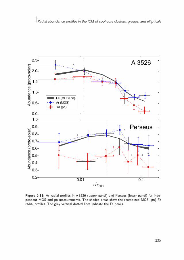
Radial abundance profiles in the ICM of cool-core clusters, groups, and ellipticals
0.0
0.5
1.0
1.5
2.0
2.5
Abun
danc
e (p
roto
-sol
ar) A 3526
Fe (MOS+pn)Ar (MOS) Ar (pn)
0.01 0.1r/r500
0.2
0.3
0.4
0.5
0.6
0.7
0.8
0.9
1.0
Abun
danc
e (p
roto
-sol
ar) Perseus
Figure 6.11: Ar radial profiles in A 3526 (upper panel) and Perseus (lower panel) for inde-pendent MOS and pn measurements. The shaded areas show the (combined MOS+pn) Feradial profiles. The grey vertical dotted lines indicate the Fe peaks.
235
6.7 Discussion
2016). However, the large gravitational potential in the core of clusters andgroups may be efficient in retaining He, which could be more centrallypeaked than H (Fabian & Pringle 1977; Abramopoulos et al. 1981). If we ef-fectively underestimate the He abundance in our fits of the core region, thenet continuumwould be overestimated, resulting in a bias of all our metalabundances towards lower values (e.g. Ettori & Fabian 2006). We illustratethis effect in Fig. 6.12, where we assume the He abundance in our fits ofthe innermost bin of A 3526 to be successively 1.25, 1.5, 1.75, 2, 2.25, and2.50 times the primordial value. As can be seen, a He abundance that is 1.5higher than previously assumed in the ICM core is sufficient to remove theinner Fe drop significantly. However, recent models point towards a lessimportant He sedimentation in the very centre of cool-core clusters thanin their surroundings (∼0.4–0.8r500; Peng & Nagai 2009). Moreover, as al-ready noted by Panagoulia et al. (2015), thermal diffusionmay also play animportant role in counteractingHe sedimentation and in removingHe andothermetals (including Fe) out of the very core of clusters (Medvedev et al.2014). Nevertheless, the relative importance of thermal diffusion is also ex-pected to be significantly weaker than the importance of AGN feedbacks,especially in galaxy groups, where most of the Fe drops are found.
Finally, and interestingly, somehydrodynamical simulations (Schindleret al. 2005; Kapferer et al. 2009) predict a drop of central abundances whenassuming galacticwinds as the dominantmechanism transporting themet-als from galaxies to the ICM. However, the typical extent of such a drop is∼400 kpc, which is always much larger than the typical extents derivedfrom our observations (a few tens of kpc at most). Moreover, this suppres-sion ofmetal enrichment by galactic winds should preferentially happen inhot and massive clusters, where the ICM pressure is high enough. Instead,we find metal drops for a large portion of less massive objects.
6.7.3 The overall Fe profileComparison with previous measurements
The average Fe radial profile of our full sample (Fig. 6.1) can be comparedto other average profiles reported in the literature. Leccardi & Molendi(2008)measured radialmetallicity profiles for a sample of 48 hot (≳3.3 keV)intermediate redshift (0.1 ≲ z ≲ 0.3) clusters using XMM-Newton. Simi-lar studies for nearby cool-core clusters have been carried out by Sander-son et al. (2009, Chandra, z < 0.1) and Matsushita (2011, XMM-Newton,
236
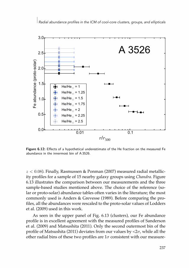
Radial abundance profiles in the ICM of cool-core clusters, groups, and ellipticals
0.01 0.1r/r500
0.0
0.5
1.0
1.5
2.0
2.5
3.0Fe
abu
ndan
ce (p
roto
-sol
ar)
A 3526
He/He¯ = 1He/He¯ = 1.25He/He¯ = 1.5He/He¯ = 1.75He/He¯ = 2He/He¯ = 2.25He/He¯ = 2.5
Figure 6.12: Effects of a hypothetical underestimate of the He fraction on the measured Feabundance in the innermost bin of A 3526.
z < 0.08). Finally, Rasmussen & Ponman (2007) measured radial metallic-ity profiles for a sample of 15 nearby galaxy groups using Chandra. Figure6.13 illustrates the comparison between our measurements and the threesample-based studies mentioned above. The choice of the reference (so-lar or proto-solar) abundance tables often varies in the literature; the mostcommonly used is Anders & Grevesse (1989). Before comparing the pro-files, all the abundances were rescaled to the proto-solar values of Lodderset al. (2009) used in this work.
As seen in the upper panel of Fig. 6.13 (clusters), our Fe abundanceprofile is in excellent agreement with the measured profiles of Sandersonet al. (2009) and Matsushita (2011). Only the second outermost bin of theprofile of Matsushita (2011) deviates from our values by <2σ, while all theother radial bins of these two profiles are 1σ consistent with our measure-
237
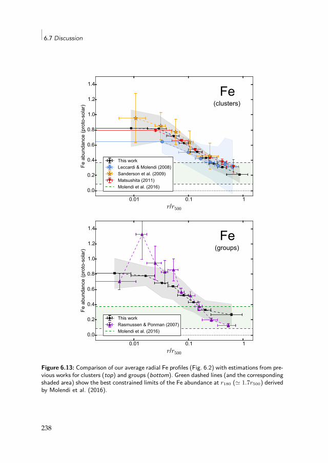
6.7 Discussion
0.01 0.1 1r/r500
0.0
0.2
0.4
0.6
0.8
1.0
1.2
1.4Fe
abu
ndan
ce (p
roto
-sol
ar)
Fe(clusters)
This workLeccardi & Molendi (2008)Sanderson et al. (2009)Matsushita (2011)Molendi et al. (2016)
0.01 0.1 1r/r500
0.0
0.2
0.4
0.6
0.8
1.0
1.2
1.4
Fe a
bund
ance
(pro
to-s
olar
)
Fe(groups)
This workRasmussen & Ponman (2007)Molendi et al. (2016)
Figure 6.13: Comparison of our average radial Fe profiles (Fig. 6.2) with estimations from pre-vious works for clusters (top) and groups (bottom). Green dashed lines (and the correspondingshaded area) show the best constrained limits of the Fe abundance at r180 (≃ 1.7r500) derivedby Molendi et al. (2016).
238
Radial abundance profiles in the ICM of cool-core clusters, groups, and ellipticals
ments. The two innermost bins of the average profile of Leccardi&Molendi(2008), however, have significantly lower Fe abundances than this study.This can be easily explained, as the sample of Leccardi & Molendi (2008)contains both cool-core and non-cool-core clusters. Because of their sub-stantially less steep abundance decrease (Sect. 6.1), including non-cool-coreclusters in a sample naturally flattens its average metallicity profile. Inter-estingly (and encouragingly), the four compared profiles agree very wellbeyond∼0.15r500 up to their respective outermost bins. This, togetherwiththe limited Fe scatter in the outermost radial bins of this work, may sug-gest a universal metallicity distribution outside cluster cores. We note that,however, from the 17 cool-core objects of the sample of Matsushita (2011),13 are present in our sample as well (including M87). Very similar abun-dance profiles were thus expected, even at the cluster outskirts. Neverthe-less, none of the clusters from the sample of Leccardi &Molendi (2008) arealso present in our sample, and the very similar average abundance (∼0.2–0.3) found beyond∼0.5r500 for both nearby and intermediate redshift clus-ters is clearly an interesting result. Finally, the average Fe abundance mea-sured in thiswork is fully consistentwith the (large but conservative) limitsat r180 (≃ 1.7r500) established by Molendi et al. (2016).
The lower panel of Fig. 6.13 (groups) shows a comparison between ouraverage Fe abundance profile for groups and the average profile derivedby Rasmussen & Ponman (2007). There is an overlap of six groups be-tween the two samples. While the results agree below 0.01r500 and within0.07–0.2r500, disagreements can be seen elsewhere. Within 0.01–0.07r500,the Rasmussen & Ponman (2007) abundances are <2σ consistent with ouraverage groups profile. However, the authors detect a deep average centralabundance drop, which does not appear in our stacked profile. This differ-ence may be explained by the large variety of metallicity profiles withinthe very core of groups, as seen in Fig. 6.19 and in Rasmussen & Ponman(2007, see their fig. 3), and by the different groups selected in each respec-tive sample. In particular, Rasmussen & Ponman (2007) consider MKW4part of their group sample, and using the ACIS instrument, they detectan off-centre Fe peak reaching ∼5–10 times the proto-solar value, which ismore than two times the Fe abundance in its centre. This extrememeasuredmetallicity should partly explain the high value of their second innermostaverage bin (Fig. 6.13 bottom). On the other hand, mismatch is also foundbeyond ∼0.2r500, where the average metallicity of Rasmussen & Ponman(2007) in the outskirts is measured ∼2 times lower than in this work (al-
239
6.7 Discussion
though still within our inferred scatter). This issue is important to pointout since Rasmussen & Ponman (2007) interpret the lower enrichment inthe group outskirts as a different groups enrichment history compared tomore massive clusters. While uncertainties in the respective backgroundtreatments of the studies might explain the disagreement with our results,wemust point out that an updatedChandra calibrationmay revise upwardsthe Fe abundance in the outermost bins (e.g. ∼+25% for NGC4325 Ras-mussen & Ponman 2009). Moreover (and perhaps more importantly), Ras-mussen & Ponman (2007) measured the Fe abundances via only the Fe-Lcomplex, and they assumed a single-temperature model in the spectra ofeach of their outermost bins. This may significantly underestimate the Feabundance in case of a multi-phase plasma in the group outskirts.
Comparison with simulationsThe average Fe radial profile derived in this work (Fig. 6.1) can also becompared with the average Fe profile predicted by hydrodynamical simu-lations. Two of the most recent simulation sets of the ICM including metalenrichmentwere performed by Planelles et al. (2014) andRasia et al. (2015).Both sets use the smooth particle hydrodynamics codeGADGET-3, assumea Chabrier initial mass function (IMF; Chabrier 2003), and incorporate thechemical evolutionmodel (includingmetal production by SNIa, SNcc, andAGB stars) of Tornatore et al. (2007), taking SN-powered galactic windsand AGN feedback into account. The comparison of our average Fe profilewith these two simulation sets is shown in Fig. 6.14.
Themean emission-weighted Feprofile from the ”AGNset” of Planelleset al. (2014, derived from a sample of 36 hot nearby systems within 29 sim-ulated regions), shown in solid red lines (with its scatter in the shaded redarea) in Fig. 6.14, does not agree with our observations. In fact, a similarresult was already discussed by the authors when comparing their pre-dictions with the observations of Leccardi & Molendi (2008). However, asexplained by Planelles et al. (2014), this significantly higher normalisationcan be easily explained by outdated assumptions on the SN yields, the as-sumed IMF, the fraction of binary systems (eventually resulting in SNIa),and/or the SN efficiency to release metals into the ICM. The overall shapeof the AGN set profile, however, is more crucial to confront with observa-tional data, since AGN feedbacks presumably have a strong influence on(i) displacing metals from star-forming regions, (ii) suppressing star for-mation, and (iii) preventing cooling of the hot gas to temperatures emitting
240
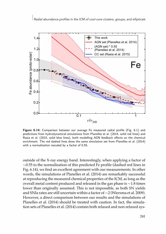
Radial abundance profiles in the ICM of cool-core clusters, groups, and ellipticals
0.1 1r/r500
0.0
0.2
0.4
0.6
0.8
1.0
1.2
1.4
Fe a
bund
ance
(pro
to-s
olar
)
Fe
This workAGN set (Planelles et al. 2014)(AGN set) * 0.55(Planelles et al. 2014)CC set (Rasia et al. 2015)
Figure 6.14: Comparison between our average Fe measured radial profile (Fig. 6.1) andpredictions from hydrodynamical simulations from Planelles et al. (2014, solid red lines) andRasia et al. (2015, solid blue lines), both modelling AGN feedback effects on the chemicalenrichment. The red dashed lines show the same simulation set from Planelles et al. (2014)with a normalisation rescaled by a factor of 0.55.
outside of the X-ray energy band. Interestingly, when applying a factor of∼0.55 to the normalisation of this predicted Fe profile (dashed red lines inFig. 6.14), we find an excellent agreement with our measurements. In otherwords, the simulations of Planelles et al. (2014) are remarkably successfulat reproducing themeasured chemical properties of the ICM, as long as theoverall metal content produced and released in the gas phase is∼1.8 timeslower than originally assumed. This is not impossible, as both SN yieldsand SNIa rates are still uncertainwithin a factor of∼2 (Wiersma et al. 2009).However, a direct comparison between our results and the simulations ofPlanelles et al. (2014) should be treated with caution. In fact, the simula-tion sets of Planelles et al. (2014) contain both relaxed and non-relaxed sys-
241
6.7 Discussion
tems (and fail to recover the cool-core versus non-cool-core dichotomy),while our observation are only based on cool-core clusters. Moreover, thesimulated profiles are extracted from three-dimensional spherical shells,whereas our results are projected on the plane of the sky. This latter differ-ence, however, is not expected to strongly affect the present comparison(Sect. 6.6.1).
A significant improvement of the simulation sets of Planelles et al. (2014)has been achieved by Rasia et al. (2015), shown by the solid blue lines (withits scatter in the shaded blue area) in Fig. 6.14. This more recent set of simu-lations, also includingAGN feedback effects, constitutes the first success ofdisentangling cool-core (shown in Fig. 6.14) and non-cool-core clusters.Wefind a reasonable agreement between the simulated profile of Rasia et al.(2015) and our observed profile within∼0.05–0.2r500. Beyond∼0.2r500, thesimulated profile slightly underestimates our observations (∼20–25%), butstill lies within the scatter, which also includes possible systematic uncer-tainties (see Sect. 6.6). Here as well, care must be taken when directly com-paring observations and simulations. Similar to Planelles et al. (2014), thesimulated profile of Rasia et al. (2015) is also unprojected. Moreover, thisprofile is alsomassweighted, while ourmeasurements are directly derivedfrom spectroscopy and are thus emissionweighted. The conversion ofmassweighted to emission weighted Fe profiles may result in a ∼30% increaseof the normalisation within r500 (Planelles et al. 2014). Such a change inthe profile normalisation would lead to an excellent agreement with ourresults outside ∼0.2r500, but to predictions that are slightly too high belowthis radius.
Furthermore, fromanumerical point of view, simulations of the chemo-dynamical state of the very core (≲0.05r500) of the ICM are extremely chal-lenging.Nevertheless, the goodoverall agreement between theoreticalmod-els and observations presented in this paper must emphasise the remark-able progress achieved by simulation groups in recent years. Future andmore complete simulations will surely help to further improve the currentpicture of metal distributions in the ICM (e.g. Biffi et al. 2017).
6.7.4 Radial contribution of SNIa and SNcc productsFrom Figs. 6.3 and 6.5 and the discussion above (e.g. Sect. 6.6.4), it clearlyappears that the radial abundance profiles of O, Mg, Si, S, Ar, Ca, and Nidecrease with radius. Except Ar (see Sect. 6.7.2), all these profiles also scalequite remarkably with the Fe radial distribution, keeping a constant X/Fe
242
Radial abundance profiles in the ICM of cool-core clusters, groups, and ellipticals
ratio out to (and sometimes even beyond) 0.5r500. In particular, the uniformradial O/Fe ratio is an important result. It is in contradictionwith the flat Oprofiles found in, for example A496 (Tamura et al. 2001), M87 (Böhringeret al. 2001; Matsushita et al. 2003; Werner et al. 2006a), NGC5044 (Buoteet al. 2003), AWM7 (Sato et al. 2008), and a sample of 19 clusters (Tamuraet al. 2004). On the contrary, this trend is consistent with the peaked O pro-files found in, for example AS1101 (de Plaa et al. 2006), A 3526 (Sanders& Fabian 2006a), Hydra A (Simionescu et al. 2009b), A 3112 (Bulbul et al.2012b), A 4059 (Chapter 2), and 5 cool-core clusters Lovisari et al. (2011).
In Fig. 6.15, we show a comparison of ourmeasured Si/Fe profile (fromFig. 6.5) with two equivalent profiles reported from the literature. In theirsample of 15 nearby galaxy groups, Rasmussen & Ponman (2007, purpletriangles) measured a flat Si/Fe profile up to 0.2r500, followed by a dra-matic increase in the outskirts (although observed with rather large errorbars in two radial bins only). In a companion paper (Rasmussen& Ponman2009), the same authors interpret this increase as a dominant enriching frac-tion of SNcc products in group outskirts, in agreement with the increasingO/Fe and/orMg/Fe profiles observed in other studies (see above). Takingadvantage of the low instrumental background of Suzaku XIS, Simionescuet al. (2015, four outermost green circles) reported a flat Si/Fe radial distri-bution in the outskirts of the Virgo cluster, in agreement with the Si/Feratios measured at smaller radii (Simionescu et al. 2010, two innermostgreen circles). Our flat Si/Fe profile is in agreement with the results ofSimionescu et al. (2010, 2015) and contradicts the results of Rasmussen &Ponman (2007). Furthermore, our results are consistent with the Si/Fe pre-dictions from the simulation sets of Planelles et al. (2014, solid red line),but we do not observe the slight predicted increase of Si relative to Fe to-wards the core below 0.1r500, expected from the suppression of cooling(predominantly processed by SNcc products) due to the AGN feedback(see also Fabjan et al. 2010). This issue was already discussed by Planelleset al. (2014), and could be due to efficient diffusion or transport mecha-nisms that were not yet implemented in the simulations.
In order to better quantify the radial contribution of SNIa and SNccproducts, we fit the X/Fe abundance ratios in each radial bin with a com-bination of SNIa and SNcc yield models as described in Chapter 4. Basedon their results, and because the large uncertainties of the measured abun-dances in individual bins do not allow us to favour any yield model inparticular, we select the following two combinations of one SNIa and one
243
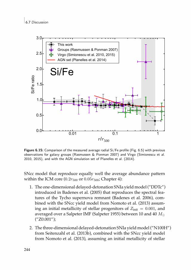
6.7 Discussion
0.01 0.1 1r/r500
0.0
0.5
1.0
1.5
2.0
2.5
3.0Si
/Fe
ratio
Si/Fe
This workGroups (Rasmussen & Ponman 2007)Virgo (Simionescu et al. 2010, 2015)AGN set (Planelles et al. 2014)
Figure 6.15: Comparison of the measured average radial Si/Fe profile (Fig. 6.5) with previousobservations for galaxy groups (Rasmussen & Ponman 2007) and Virgo (Simionescu et al.2010, 2015), and with the AGN simulation set of Planelles et al. (2014).
SNcc model that reproduce equally well the average abundance patternwithin the ICM core (0.2r500 or 0.05r500; Chapter 4):
1. The one-dimensional delayed-detonation SNIa yieldmodel (”DDTc”)introduced in Badenes et al. (2005) that reproduces the spectral fea-tures of the Tycho supernova remnant (Badenes et al. 2006), com-bined with the SNcc yield model from Nomoto et al. (2013) assum-ing an initial metallicity of stellar progenitors of Zinit = 0.001, andaveraged over a Salpeter IMF (Salpeter 1955) between 10 and 40 M⊙(”Z0.001”);
2. The three-dimensional delayed-detonation SNIa yieldmodel (”N100H”)from Seitenzahl et al. (2013b), combined with the SNcc yield modelfrom Nomoto et al. (2013), assuming an initial metallicity of stellar
244
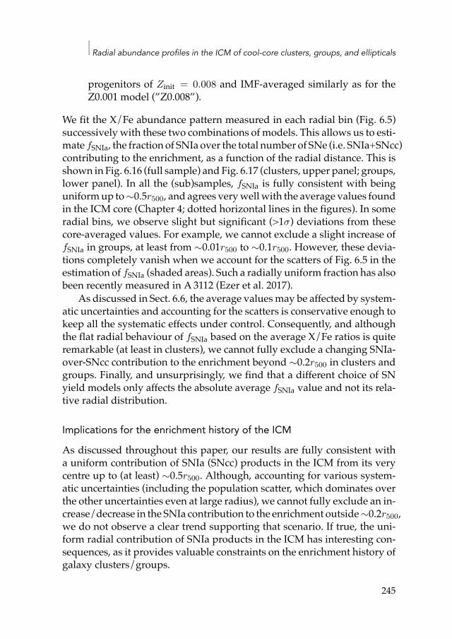
Radial abundance profiles in the ICM of cool-core clusters, groups, and ellipticals
progenitors of Zinit = 0.008 and IMF-averaged similarly as for theZ0.001 model (”Z0.008”).
We fit the X/Fe abundance pattern measured in each radial bin (Fig. 6.5)successively with these two combinations of models. This allows us to esti-mate fSNIa, the fraction of SNIa over the total number of SNe (i.e. SNIa+SNcc)contributing to the enrichment, as a function of the radial distance. This isshown in Fig. 6.16 (full sample) and Fig. 6.17 (clusters, upper panel; groups,lower panel). In all the (sub)samples, fSNIa is fully consistent with beinguniformup to∼0.5r500, and agrees verywellwith the average values foundin the ICM core (Chapter 4; dotted horizontal lines in the figures). In someradial bins, we observe slight but significant (>1σ) deviations from thesecore-averaged values. For example, we cannot exclude a slight increase offSNIa in groups, at least from ∼0.01r500 to ∼0.1r500. However, these devia-tions completely vanish when we account for the scatters of Fig. 6.5 in theestimation of fSNIa (shaded areas). Such a radially uniform fraction has alsobeen recently measured in A3112 (Ezer et al. 2017).
As discussed in Sect. 6.6, the average valuesmay be affected by system-atic uncertainties and accounting for the scatters is conservative enough tokeep all the systematic effects under control. Consequently, and althoughthe flat radial behaviour of fSNIa based on the average X/Fe ratios is quiteremarkable (at least in clusters), we cannot fully exclude a changing SNIa-over-SNcc contribution to the enrichment beyond ∼0.2r500 in clusters andgroups. Finally, and unsurprisingly, we find that a different choice of SNyield models only affects the absolute average fSNIa value and not its rela-tive radial distribution.
Implications for the enrichment history of the ICM
As discussed throughout this paper, our results are fully consistent witha uniform contribution of SNIa (SNcc) products in the ICM from its verycentre up to (at least) ∼0.5r500. Although, accounting for various system-atic uncertainties (including the population scatter, which dominates overthe other uncertainties even at large radius), we cannot fully exclude an in-crease/decrease in the SNIa contribution to the enrichment outside∼0.2r500,we do not observe a clear trend supporting that scenario. If true, the uni-form radial contribution of SNIa products in the ICM has interesting con-sequences, as it provides valuable constraints on the enrichment history ofgalaxy clusters/groups.
245
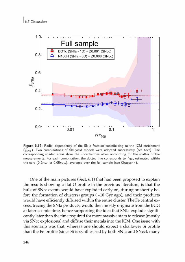
6.7 Discussion
0.01 0.1 1r/r500
0.0
0.2
0.4
0.6
0.8
1.0f S
NIa
Full sampleDDTc (SNIa - 1D) + Z0.001 (SNcc)N100H (SNIa - 3D) + Z0.008 (SNcc)
Figure 6.16: Radial dependency of the SNIa fraction contributing to the ICM enrichment(fSNIa). Two combinations of SN yield models were adopted successively (see text). Thecorresponding shaded areas show the uncertainties when accounting for the scatter of themeasurements. For each combination, the dotted line corresponds to fSNIa estimated withinthe core (0.2r500 or 0.05r500), averaged over the full sample (see Chapter 4).
One of the main pictures (Sect. 6.1) that had been proposed to explainthe results showing a flat O profile in the previous literature, is that thebulk of SNcc events would have exploded early on, during or shortly be-fore the formation of clusters/groups (∼10 Gyr ago), and their productswould have efficiently diffused within the entire cluster. The Fe central ex-cess, tracing the SNIa products, would thenmostly originate from the BCGat later cosmic time, hence supporting the idea that SNIa explode signifi-cantly later than the time required formoremassive stars to release (mostlyvia SNcc explosions) and diffuse their metals into the ICM. One issue withthis scenario was that, whereas one should expect a shallower Si profilethan the Fe profile (since Si is synthesised by both SNIa and SNcc), many
246
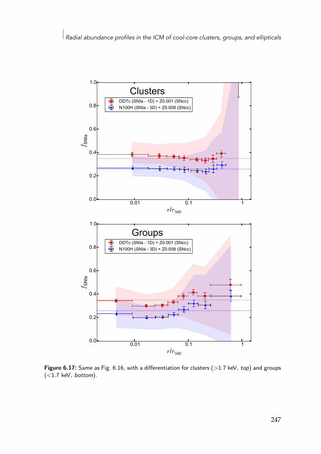
Radial abundance profiles in the ICM of cool-core clusters, groups, and ellipticals
0.01 0.1 1r/r500
0.0
0.2
0.4
0.6
0.8
1.0f S
NIa
ClustersDDTc (SNIa - 1D) + Z0.001 (SNcc)N100H (SNIa - 3D) + Z0.008 (SNcc)
0.01 0.1 1r/r500
0.0
0.2
0.4
0.6
0.8
1.0
f SN
Ia
GroupsDDTc (SNIa - 1D) + Z0.001 (SNcc)N100H (SNIa - 3D) + Z0.008 (SNcc)
Figure 6.17: Same as Fig. 6.16, with a differentiation for clusters (>1.7 keV, top) and groups(<1.7 keV, bottom).
247
6.7 Discussion
previous studies reported a constant (e.g. Sanders & Fabian 2006a; Satoet al. 2008) or sometimes even decreasing (Million et al. 2011) Si/Fe ratioacross radius. To solve this paradox, Finoguenov et al. (2002) propose a di-versity of SNIa to contribute to the ICM enrichment: promptly explodingSNIa (whose products are supposed to be efficiently mixed over the wholecluster) produce less Si than SNIa with longer delay times (mostly enrich-ing the cluster core). Since our results suggest a uniform contribution ofSNIa (SNcc) products in the core and in the outskirts, invoking a diver-sity in SNIa (as well as in their delay times) is not required anymore, andalternative scenarii should be considered.
In their study of the chemical enrichment in Hydra A, Simionescu et al.(2009b) found that the central O excess can be explained either if stellarwinds are 3 to 8 times more efficient in releasing metals than previouslypredicted, or if 3–8×10⁸ SNcc had exploded in the cluster core over the last∼10 Gyr. Alternatively, ram-pressure stripping may help to build a centralpeak of SNcc (and SNIa) products from infalling cluster galaxy members(Domainko et al. 2006); however such a process should also occur at ratherlarge distances (∼1 Mpc), while the O excess is only observed in HydraA within ∼120 kpc. Similarly, Million et al. (2011) found centrally peakedprofiles for eight elements in the core of M87. In addition to the peakedMg profile, they measured a steeper gradient for Si and S than for Fe, andinterpret their findings as the result of efficient enriching winds from acentral pre-enriched stellar population and/or intermittent formation ofmassive stars in the BCG.
If the centralO (and/orMg) excess is indeeddue to a significant amountof concentrated SNcc explosions in the cluster core, one relevant questionis whether this SNcc peakwas produced prior to the formation of the BCG,or by the BCG itself at a later stage of the cluster assembly. Recent simula-tions (Tornatore et al. 2007; Fabjan et al. 2010) suggest that the enrichmenttime of both O and Fe in the inner∼0.4r500 is significantly shorter than out-side this radius, which may imply that the BCG is indeed responsible forthe central excess in the ICM observed for both SNIa and SNcc products.Moreover, the recent analysis of WARPJ1415.1+3612 (z ≃ 1) by De Grandiet al. (2014) shows that the bulk of the central Fe excesswas already present∼8 Gyr ago and that its slope is steeper than at present times. This suggestsin turn that the BCG is the dominant source responsible for the enrichmentin the ICM core, and that the metals released by the BCG spread out of thecore with time via diffusive/mixing processes.
248
Radial abundance profiles in the ICM of cool-core clusters, groups, and ellipticals
If the Fe peak indeed comes from the BCG (as the Fe mass in the ICMcould suggest; Böhringer et al. 2004a; De Grandi et al. 2004) and has a simi-lar (scaled) radial distribution as SNcc products, as our results suggest, thiscentral SNcc enrichment may also originate from the BCG. Although mostBCGs appear red and dead at present times (with typical star formationrates of a few M⊙/yr at most; e.g. McDonald et al. 2011), their star forma-tion was dramatically higher over the last ∼9 Gyr (McDonald et al. 2016),and in some cases, can still reach a few tens to hundreds M⊙/yr at z ≃ 0(O’Dea et al. 2008). This past (and, sometimes, present) high star formationin BCGs could thus be responsible for the central excess of SNcc productsseen in the ICM. In this case, and assuming that some mechanisms diffuseout the metals from the cluster core (see above), the consistency betweenthe slopes of the radial SNIa and SNcc distributions suggests that the bulkof SNIa exploded quite shortly after the period of star formation in theBCG. More precisely, the typical delay time of SNIa should not be largerthan the timescale of metal mixing/diffusing processes in the ICM.
More generally, and regardless of whether the central excess of SNccproducts reported in this study originates from the BCG or not, the (lackof) radial dependence translates into a time dependence of the chemicalenrichment patterns that we can infer. Specifically, the consistent radialprofiles for all the measured abundances may suggest that the SNIa andSNcc components of the enrichment originate from the same astrophysi-cal source(s) and have been occurring at similar epochs. Such a reasoningcan be applied to the case of the intra-cluster stellar population. Both ob-servations (e.g. Krick et al. 2006; Krick & Bernstein 2007) and simulations(Willman et al. 2004) provide increasing evidence for a significant frac-tion (10–50%) of stars that are unbound to any cluster galaxy and couldpotentially contribute to the ICM enrichment (Domainko et al. 2004). Asit takes a substantial time for these stars to be ejected and travel awayfrom their galaxy hosts, the intra-cluster population should essentially con-tain low-mass stars, and thus enrich the ICM predominantly with SNIa,likely providing a different radial distribution of SNIa products than thatof SNcc products (coming from other sources). This picture disagrees withour present results. Therefore, under these assumptions, intra-cluster starsmay not be the dominant source of the ICM enrichment. A similar conclu-sion is reached by Kapferer et al. (2010) on the basis of hydrodynamicalsimulations and SNIa expected rates.
In summary, while it was commonly thought from previous studies
249
6.8 Conclusions
that the bulk of the SNcc (SNIa) enrichment would contribute only at early(late) times, recent works— including our present study— have providedincreasing evidence that the SNIa versus SNcc dichotomy is not pronouncedsince the chemical composition does not evolve dramatically with radius.
The astrophysical implications discussed here hold only if further anddefinitive confirmation of the uniformdistribution of fSNIa is achievedwithmore accurate instruments on board futuremissions. In particular, the highspectral resolution and effective area of Athena will be required to investi-gate the distribution of key elements, like O or Mg, with unprecedentedaccuracy from the core to the outskirts. Moreover, a complete discussionwould be required to fully quantify the speculative arguments used here,and therefore, to pursue the extensive use of realistic hydrodynamical sim-ulations, preferably including all the potential sources of (SNIa and SNcc)enrichment and all the mixing and diffusion mechanisms known so far.
6.8 ConclusionsIn this work, we used deep XMM-Newton/EPIC observations of 44 nearbycool-core galaxy clusters, groups, and ellipticals (all taken from theCHEERScatalogue, i.e.∼4.5Ms of total net exposure) to derive the average projectedradial abundance profiles of eight elements in the ICM. Whereas averageFe and Si abundance profiles had been previously reported in the literature(though over limited samples only), theO,Mg, S, Ar, Ca, andNi profiles aremeasured and averaged over a large sample for the first time. This allowsan unprecedented estimation of the average radial contribution of SNIaand SNcc products in the ICM. Our results can be summarised as follows.
• The Fe abundance can be robustly constrained out to ∼ 0.9r500 and∼ 0.6r500 in clusters and groups, respectively, while most of the otherabundances are uncertain beyond ∼0.5r500. Owing to a robust andconservativemodelling of the EPIC background, the systematic back-ground uncertainties are limited typically to a fewper cent, which areusually smaller than (or comparable to) the statistical uncertaintiesfor each object. The other systematic uncertainties (related to MOS-pn discrepancies, projection effects, an uncertain temperature distri-bution, or selection effects) are always smaller than the populationscatter derived in each average profile. Therefore, the latter can beconsidered as a conservative limit for our measurements.
250
Radial abundance profiles in the ICM of cool-core clusters, groups, and ellipticals
• The average radial profiles of all the considered elements exhibit acentrally peaked distribution, and seem to converge at large radiiconsistently towards the limits (0.09–0.37 times proto-solar) assessedat r180 by Molendi et al. (2016). When rescaled by the X/Fe ratiosmeasured previously in the ICM core (Chapter 3), the average pro-files of all the elements (except perhaps Ar) follow the average Feprofile very well out to at least ∼0.5r500. Similarly, the average radialX/Fe profiles (again, with the possible exception of Ar) are remark-ably uniform out to this radius.
• Subdividing our sample into clusters (>1.7 keV) and groups (<1.7keV) subsamples, we find that groups are on average ∼21% less en-riched in Fe than clusters. From 0.01r500 to 0.5r500, this fraction israther constant and no significant change is observed in the slopes ofthe two subsamples. Below and beyond this radial range, the similarenrichment level found in clusters and groups can be explained byselection and binning effects. Interestingly, no sign of metal enhance-ment towardsmoremassive objects could be significantly detected inthe other profiles (with the possible exception of the O profile).
• The average Fe profile for clusters reported here agrees remarkablywell with previous observations (Leccardi & Molendi 2008; Sander-son et al. 2009; Matsushita 2011). The agreement of our average Feprofile for groups with the previous observations of Rasmussen &Ponman (2007) is less good, but still comparable within uncertain-ties. Although it should be treated with caution, the comparison ofour measured Fe profile with predictions from recent hydrodynami-cal simulations, taking AGN feedback and galactic winds effects intoaccount (Planelles et al. 2014; Rasia et al. 2015), is also very encour-aging. Future cluster simulations will be interesting to compare withour measurements.
• In 14 systems (∼32% of our sample), we detect a significant centraldrop of the Fe abundance. This can also be observed in the averageabundance profiles (both for Fe and the other elements) by an ap-parent flattening below ∼0.01r500. We do not see a clear correlationbetween the depth of such metal drops and their radial extent. Thesedrops are probably real and could be related to dust depletion ofmet-als in the very core of the ICM, before they are dragged out by AGNfeedback and released back in the hot gas phase. The slightly steeper
251
6.8 Conclusions
profile of Ar (expected not to be incorporated in dust grains), com-pared to that of Fe, could (at least partly) witness dust depletion ofthe other elements within∼0.1 r500. However, the (statistical and sys-tematic) uncertainties prevent us from firmly confirming or rulingout the presence of a central Ar drop.
• Using the approach described in Chapter 4, we estimate the radialcontribution of SNIa products to the ICMenrichment (fSNIa). Althoughthe scatter (and, by extension, the other systematic uncertainties) pre-vents us from excluding sudden changes in the outskirts, our obser-vations suggest, on average, a remarkably uniform fSNIa distributionout to, at least, 0.5r500. This result contrasts with the dramatic in-crease of SNcc contribution in the outskirts inferred by Rasmussen& Ponman (2009), but is consistent with more recent measurements(Simionescu et al. 2015; Ezer et al. 2017) and simulations (Fabjan et al.2010; Planelles et al. 2014; Biffi et al. 2017). This suggests that the ma-jor fraction of the SNIa and SNcc enriching the ICM may share thesame origins and may have both exploded before mixing and diffu-sion processes played a significant role in spreading out the metals.In particular, since there is increasing evidence that the central Fe ex-cess originates from the BCG, it is likely that a past intense periodof star formation in the BCG had released SNcc products in the ICMcore in a similar way.
• Finally,we emphasise that, although the systematic uncertainties con-sidered here are under control, the Ni abundance may be systemati-cally overestimated when using SPEXACT v2. Whereas it should nothave a significant impact on the shape of the Ni profile presentedhere, such a bias might affect the average Ni/Fe ratio (see also Chap-ter 3) and the subsequent constraints inferred on the SNIa yieldmod-els (see also Chapter 4). We devote Chapter 5 to that specific issue.
While the abundance profiles of some elements (such as Fe or Si) couldbe remarkably constrained thanks to the large statistics of our sample, thispaper clearly shows that, apart from the apparent scatter of the measure-ments, themost important limitations encountered so far are the systematicuncertainties, in particular related to MOS-pn cross-calibration imperfec-tions (see also Schellenberger et al. 2015, and Chapter 3). Using the currentX-ray facilities, a significant improvement of the accuracy of our results
252
Radial abundance profiles in the ICM of cool-core clusters, groups, and ellipticals
may only be achieved by improving the EPIC cross-calibration and bet-ter understanding all the systematic biases that could affect the EPIC in-struments. Nevertheless, further improvement in interpreting these resultscould also come from studying a more representative sample, for exampleincluding non-cool-core systems as well.
Despite our current efforts and achievements, we must stress the con-siderable breakthrough that the next X-ray missions (e.g. Athena; Barretet al. 2013) will be able to achieve. On the one hand, the very large effec-tive area of future instruments will allow us to probe a detailed view ofthe chemical state of cluster outskirts, which is still challenging for XMM-Newton, as demonstrated in this paper. On the other hand, the remarkablespectral resolution of micro-calorimeters on board these future missionswill considerably reduce the uncertainties on both the thermal structureand the distribution of various metals within and outside cluster cores.Therefore, there is no doubt that the next generation of X-ray observatorieswill bring further light on this study and provide a valuable understandingof the full history of the ICM enrichment.
AcknowledgementsThe authors are very thankful to the referee for valuable comments thathelped to improve the paper. The authors would also like to thank Jes-per Rasmussen and Alastair Sanderson for kindly providing their obser-vational data, as well as Susana Planelles and Elena Rasia for kindly pro-viding their simulation outputs and for useful discussions. This work ispartly based on theXMM-NewtonAO-12 proposal ”The XMM-Newton viewof chemical enrichment in bright galaxy clusters and groups” (PI: de Plaa), andis a part of the CHEERS (CHEmical Evolution Rgs cluster Sample) collab-oration. H.A. acknowledges the support of NWO via a Veni grant. P.K.acknowledges financial support from STFC. C.P. acknowledges supportfrom ERC Advanced Grant Feedback 340442. T.H.R. acknowledges sup-port from theDFG through grant RE 1462/6 and through the TransregionalCollaborative Research Centre TRR33 The Dark Universe, project B18. Thisproject has been supported by the Lendület LP2016-11 grant awarded bythe Hungarian Academy of Sciences. This work is based on observationsobtainedwithXMM-Newton, an ESA sciencemissionwith instruments andcontributions directly funded by ESAmember states and theUSA (NASA).The SRON Netherlands Institute for Space Research is supported finan-
253

6.8 Conclusions
cially by NWO, the Netherlands Organisation for Scientific Research.
254
Radial abundance profiles in the ICM of cool-core clusters, groups, and ellipticals
6.A Cluster properties and individual Fe profilesThis section enumerates the objects of our sample (CHEERS) and providessupplementary information on their individual Fe profiles and radial ex-tents. Table 6.4 lists all the sources considered in this paper and their r500values (adapted from Pinto et al. 2015, and references therein). For each el-ement X, we also provide rout,X, the maximum radius at which we evaluatethe corresponding abundance (see Sect. 6.4.1 for further details). The Fe ra-dial profiles of each source of our sample are shown in Figs. 6.18 (clusters)and 6.19 (groups).
6.B Average abundance profiles of O,Mg, Si, S, Ar, Ca,and Ni
In Sect. 6.5.1 we provided numerical values of the radial Fe profile in thefull sample (Table 6.2) and after subdividing it into clusters and groups(Table 6.3). In this Appendix we extend these numbers to the average O,Mg, Si, Ar, Ca, and Ni profiles that are shown in Figs. 6.3 and 6.4 (see Sect.6.5.2 for further details). These values are listed in Table 6.5 (full sample)and Table 6.6 (comparison between clusters and groups).
255
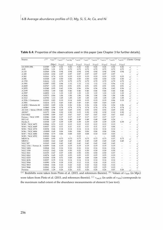
6.B Average abundance profiles of O, Mg, Si, S, Ar, Ca, and Ni
Table 6.4: Properties of the observations used in this paper (see Chapter 3 for further details).
Source z(a) r500(b) rout,O(c) rout,Mg(c) rout,Si(c) rout,S(c) rout,Ar(c) rout,Ca(c) rout,Fe(c) rout,Ni(c) Cluster Group
(Mpc) (r500) (r500) (r500) (r500) (r500) (r500) (r500) (r500)2A 0335+096 0.0349 1.05 0.26 0.26 0.26 0.26 0.26 0.26 0.26 0.26 √
−A85 0.0556 1.21 0.72 0.72 0.72 0.72 0.72 0.72 0.72 0.72 √
−A133 0.0569 0.94 0.94 0.94 0.94 0.94 0.94 0.94 0.94 0.94 √
−A189 0.0318 0.50 0.97 0.97 0.97 0.97 0.97 0.97 0.97 − −
√
A262 0.0161 0.74 0.33 0.33 0.33 0.33 0.33 0.33 0.25 0.33 √−
A496 0.0328 1.00 0.50 0.50 0.50 0.50 0.50 0.50 0.50 0.50 √−
A1795 0.0616 1.22 0.79 0.79 0.79 0.79 0.79 0.79 0.79 0.79 √−
A1991 0.0587 0.82 0.84 1.12 1.12 1.12 1.12 1.12 0.56 1.12 √−
A2029 0.0767 1.33 0.91 0.91 0.91 0.91 0.91 0.91 0.91 0.91 √−
A2052 0.0348 0.95 0.42 0.56 0.56 0.56 0.56 0.56 0.42 0.56 √−
A2199 0.0302 1.00 0.46 0.46 0.46 0.46 0.46 0.46 0.46 0.46 √−
A2597 0.0852 1.11 1.22 1.22 1.22 1.22 1.22 1.22 1.22 1.22 √−
A2626 0.0573 0.84 1.06 1.06 1.06 1.06 1.06 1.06 1.06 1.06 √−
A3112 0.0750 1.13 1.05 1.05 1.05 1.05 1.05 1.05 1.05 1.05 √−
A3526 / Centaurus 0.0103 0.83 0.19 0.14 0.09 0.19 0.19 0.19 0.06 0.19 √−
A3581 0.0214 0.72 0.45 0.45 0.45 0.45 0.45 0.45 0.45 − −√
A4038 / Klemola 44 0.0283 0.89 0.36 0.36 0.36 0.36 0.36 0.36 0.36 0.36 √−
A4059 0.0460 0.96 0.74 0.74 0.74 0.74 0.74 0.74 0.74 0.74 √−
AS1101 / Sérsic 159-03 0.0580 0.98 0.69 0.69 0.92 0.92 0.92 0.92 0.69 0.92 √−
AWM7 0.0172 0.86 0.30 0.30 0.15 0.30 0.30 0.30 0.10 0.30 √−
EXO0422 0.0390 0.89 0.67 0.67 0.67 0.67 0.67 0.67 0.67 0.67 √−
Fornax / NGC1399 0.0046 0.40 0.17 0.17 0.17 0.17 0.17 0.17 0.17 − −√
HCG62 0.0146 0.46 0.36 0.48 0.48 0.48 0.48 0.48 0.24 − −√
HydraA 0.0538 1.07 0.39 0.39 0.39 0.39 0.39 0.39 0.39 0.39 √−
M49 / NGC4472 0.0044 0.53 0.12 0.12 0.12 0.12 0.12 0.12 0.12 − −√
M60 / NGC4649 0.0037 0.53 0.11 0.11 0.11 0.11 0.11 0.11 0.06 − −√
M84 / NGC4374 0.0034 0.46 0.14 0.14 0.14 0.14 0.14 0.14 0.14 − −√
M86 / NGC4406 -0.0009 0.49 0.06 0.06 0.06 0.06 0.06 0.06 0.06 − −√
M87 / NGC4486 0.0044 0.75 0.06 0.08 0.03 0.08 0.10 0.10 0.03 − −√
M89 / NGC4552 0.0010 0.44 − − 0.12 − − − 0.09 − −√
MKW3s 0.0450 0.95 0.73 0.73 0.73 0.73 0.73 0.73 0.37 0.73 √−
MKW4 0.0200 0.62 0.49 0.49 0.49 0.49 0.49 0.49 0.49 0.49 √−
NGC507 0.0165 0.60 0.42 0.42 0.42 0.42 0.42 0.42 0.42 − −√
NGC1316 / Fornax A 0.0059 0.46 0.19 0.19 0.19 0.19 0.19 0.19 0.19 − −√
NGC1404 0.0064 0.61 0.16 0.16 0.16 0.16 0.16 0.16 0.16 − −√
NGC1550 0.0123 0.62 0.30 0.30 0.22 0.30 0.30 0.30 0.30 − −√
NGC3411 0.0155 0.47 0.37 0.50 0.50 0.50 0.50 0.50 0.37 − −√
NGC4261 0.0074 0.45 0.25 0.25 0.25 0.25 0.25 0.25 0.19 − −√
NGC4325 0.0258 0.58 0.51 0.68 0.68 0.68 0.68 0.68 0.51 − −√
NGC4636 0.0037 0.35 0.14 0.14 0.14 0.14 0.14 0.14 0.14 − −√
NGC5044 0.0090 0.56 0.18 0.18 0.12 0.18 0.18 0.18 0.12 − −√
NGC5813 0.0064 0.44 0.16 0.22 0.22 0.22 0.22 0.22 0.16 − −√
NGC5846 0.0061 0.36 0.19 0.25 0.25 0.25 0.25 0.25 0.19 − −√
Perseus 0.0183 1.29 0.26 0.26 0.11 0.26 0.26 0.26 0.07 0.26 √−
(a) Redshifts were taken from Pinto et al. (2015, and references therein). (b) Values of r500 (in Mpc)were taken from Pinto et al. (2015, and references therein). (c) rout,X (in units of r500) corresponds tothe maximum radial extent of the abundance measurements of element X (see text).
256
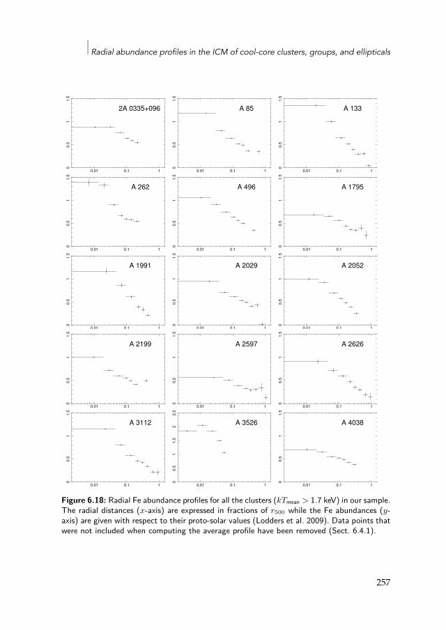
Radial abundance profiles in the ICM of cool-core clusters, groups, and ellipticals
0.01 0.1 1
00
.51
1.5
2A 0335+096
0.01 0.1 10
0.5
11
.5
A 85
0.01 0.1 1
00
.51
1.5
A 133
0.01 0.1 1
00
.51
1.5
A 262
0.01 0.1 1
00
.51
1.5
A 496
0.01 0.1 1
00
.51
1.5
A 1795
0.01 0.1 1
00
.51
1.5
A 1991
0.01 0.1 1
00
.51
1.5
A 2029
0.01 0.1 1
00
.51
1.5
A 2052
0.01 0.1 1
00
.51
1.5
A 2199
0.01 0.1 1
00
.51
1.5
A 2597
0.01 0.1 1
00
.51
1.5
A 2626
0.01 0.1 1
00
.51
1.5
A 3112
0.01 0.1 1
00
.51
1.5
22
.5
A 3526
0.01 0.1 1
00
.51
1.5
A 4038
Figure 6.18: Radial Fe abundance profiles for all the clusters (kTmean > 1.7 keV) in our sample.The radial distances (x-axis) are expressed in fractions of r500 while the Fe abundances (y-axis) are given with respect to their proto-solar values (Lodders et al. 2009). Data points thatwere not included when computing the average profile have been removed (Sect. 6.4.1).
257
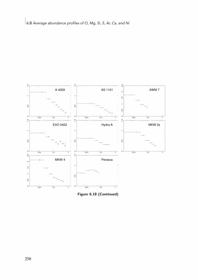
6.B Average abundance profiles of O, Mg, Si, S, Ar, Ca, and Ni
0.01 0.1 1
00
.51
1.5
A 4059
0.01 0.1 1
00
.51
1.5
AS 1101
0.01 0.1 1
00
.51
1.5
22
.5
AWM 7
0.01 0.1 1
00
.51
1.5
EXO 0422
0.01 0.1 1
00
.51
1.5
Hydra A
0.01 0.1 1
00
.51
1.5
MKW 3s
0.01 0.1 1
00
.51
1.5
22
.5
MKW 4
0.01 0.1 1
00
.51
1.5
Perseus
Figure 6.18 (Continued)
258
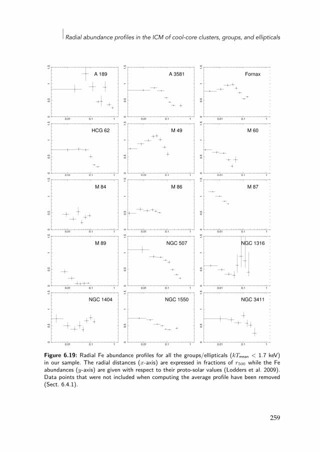
Radial abundance profiles in the ICM of cool-core clusters, groups, and ellipticals
0.01 0.1 1
00
.51
1.5
A 189
0.01 0.1 1
00
.51
1.5
A 3581
0.01 0.1 1
00
.51
1.5
Fornax
0.01 0.1 1
00
.51
1.5
HCG 62
0.01 0.1 1
00
.51
1.5
M 49
0.01 0.1 1
00
.51
1.5
M 60
0.01 0.1 1
00
.51
1.5
M 84
0.01 0.1 1
00
.51
1.5
M 86
0.01 0.1 1
00
.51
1.5
M 87
0.01 0.1 1
00
.51
1.5
M 89
0.01 0.1 1
00
.51
1.5
NGC 507
0.01 0.1 1
00
.51
1.5
NGC 1316
0.01 0.1 1
00
.51
1.5
NGC 1404
0.01 0.1 1
00
.51
1.5
NGC 1550
0.01 0.1 1
00
.51
1.5
NGC 3411
Figure 6.19: Radial Fe abundance profiles for all the groups/ellipticals (kTmean < 1.7 keV)in our sample. The radial distances (x-axis) are expressed in fractions of r500 while the Feabundances (y-axis) are given with respect to their proto-solar values (Lodders et al. 2009).Data points that were not included when computing the average profile have been removed(Sect. 6.4.1).
259
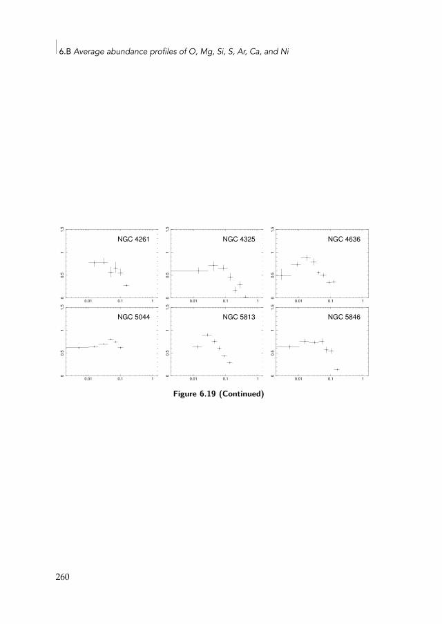
6.B Average abundance profiles of O, Mg, Si, S, Ar, Ca, and Ni
0.01 0.1 1
00
.51
1.5
NGC 4261
0.01 0.1 1
00
.51
1.5
NGC 4325
0.01 0.1 1
00
.51
1.5
NGC 4636
0.01 0.1 1
00
.51
1.5
NGC 5044
0.01 0.1 1
00
.51
1.5
NGC 5813
0.01 0.1 1
00
.51
1.5
NGC 5846
Figure 6.19 (Continued)
260
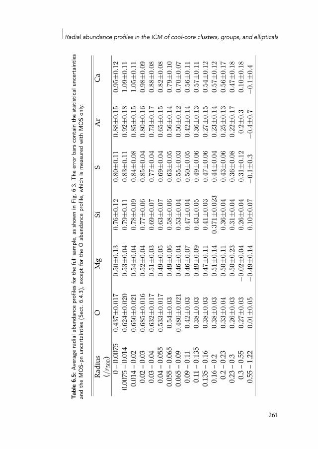
Radial abundance profiles in the ICM of cool-core clusters, groups, and ellipticals
Tabl
e6.
5:Av
erag
era
dial
abun
danc
epr
ofiles
fort
hefu
llsa
mpl
e,as
show
nin
Fig.
6.3.
The
erro
rbar
scon
tain
the
stat
istica
lunc
erta
intie
san
dth
eM
OS-
pnun
certa
intie
s(S
ect.
6.4.
3),e
xcep
tfor
the
Oab
unda
nce
profi
le,wh
ichis
mea
sure
dwi
thM
OS
only.
Radius
OMg
SiS
ArCa
(/r 5
00)
0–0.0
075
0.43
7±0.
017
0.50
±0.
130.
76±
0.12
0.80
±0.
110.
88±
0.15
0.95
±0.
120.0
075–
0.014
0 .62
4 ±0 .
020
0 .53
±0 .
040 .
79±
0 .11
0 .83
±0 .
110 .
92±
0 .18
1 .09
±0 .
110.0
14–0
.020.
650±
0.02
10.
54±
0.04
0.78
±0.
090.
84±
0.08
0.85
±0.
151.
05±
0.11
0.02–
0.03
0.68
5±0.
016
0.52
±0.
040.
77±
0.06
0.85
±0.
040.
80±
0.16
0.98
±0.
090.0
3–0.0
40.
632±
0.01
70.
51±
0.03
0.69
±0.
070.
77±
0.04
0.73
±0.
170.
88±
0.08
0.04–
0.055
0.53
3±0.
017
0.49
±0.
050.
63±
0.07
0.69
±0.
040.
65±
0.15
0.82
±0.
080.0
55–0
.065
0.54
±0.
030.
49±
0.06
0.58
±0.
060.
63±
0.05
0.56
±0.
140.
79±
0.10
0.065
–0.09
0.48
0±0.
021
0.46
±0.
040.
53±
0.04
0.55
±0.
030.
50±
0.12
0.70
±0.
070.0
9–0.11
0.42
±0.
030.
46±
0.07
0.47
±0.
040.
50±
0.05
0.42
±0.
140.
56±
0.11
0.11–
0.135
0.38
±0.
030.
49±
0.09
0.43
±0.
050.
49±
0.06
0.36
±0.
130.
57±
0.11
0.135
–0.16
0.38
±0.
030.
47±
0.11
0.41
±0.
030.
47±
0.06
0.27
±0.
150.
54±
0.12
0.16–
0.20.
38±
0.03
0.51
±0.
140.
371±
0.02
30.
44±
0.04
0.23
±0.
140.
57±
0.12
0.2–0
.230 .
33±
0 .04
0 .50
±0 .
110 .
36±
0 .04
0 .43
±0 .
060 .
25±
0 .13
0 .56
±0 .
170.2
3–0.3
0.26
±0.
030.
50±
0.23
0.31
±0.
040.
36±
0.08
0.22
±0.
170.
47±
0.18
0.3–0
.550.
27±
0.03
−0.
02±
0.04
0.26
±0.
040.
31±
0.12
0.2±
0.3
0.10
±0.
180.5
5–1.2
20.
01±
0.05
−0.
49±
0.14
0.10
±0.
07−
0.1±
0.3
−0.
4±0.
7−
0.1±
0.4
261
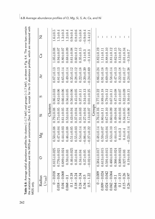
6.B Average abundance profiles of O, Mg, Si, S, Ar, Ca, and Ni
Tabl
e6.
6:Av
erag
era
dial
abun
danc
epr
ofiles
forc
lust
ers(
>1.
7ke
V)an
dgr
oups
(<1.
7ke
V),a
ssho
wnin
Fig.
6.4.
The
erro
rbar
scon
tain
the
stat
istica
lunc
erta
intie
san
dth
eM
OS-
pnun
certa
intie
s(S
ect.
6.4.
3),e
xcep
tfo
rthe
Oab
unda
nce
profi
les,w
hich
are
mea
sure
dwi
thM
OS
only. Radius
OMg
SiS
ArCa
Ni
(/r 5
00)
Clusters
0–0.0
180.
815±
0.02
50.
50±
0.08
0.79
±0.
080.
86±
0.03
0.87
±0.
131.
05±
0.08
1.6±
0.5
0.018
–0.04
0.77
6±0.
021
0.47
±0.
040.
75±
0.05
0.82
±0.
060.
81±
0.13
0.94
±0.
071.
5±0.
40.0
4–0.0
680.
689±
0.02
40.
44±
0.03
0.61
±0.
050.
66±
0.06
0.65
±0.
140.
80±
0.07
1.3±
0.3
0.068
–0.1
0.59
±0.
030.
46±
0.08
0.53
±0.
040.
56±
0.05
0.49
±0.
140.
68±
0.09
1.2±
0.4
0.1–0
.180.
46±
0.02
50.
51±
0.05
0.43
±0.
040.
50±
0.06
0.35
±0.
120.
61±
0.08
0.9±
0.4
0.18–
0.24
0.35
±0.
040.
55±
0.03
0.37
±0.
040.
45±
0.05
0.28
±0.
120.
60±
0.12
0.8±
0.6
0.24–
0.34
0.34
±0.
040.
54±
0.14
0.31
±0.
030.
37±
0.11
0.22
±0.
180.
35±
0.15
0.5±
0.8
0.34–
0.50.
37±
0.05
−0.
06±
0.16
0.27
±0.
040.
34±
0.13
0.20
±0.
390.
1±0.
3−
0.9±
0.4
0.5–1
.22−
0.02
±0.
05−
0.27
±0.
220.
13±
0.07
0.01
±0.
25−
0.24
±0.
69−
0.1±
0.3
−3.
4±2.
1Groups
0–0.0
090.
384±
0.01
70.
48±
0.14
0.76
±0.
160.
77±
0.22
0.86
±0.
240.
82±
0.19
–0.0
09–0
.024
0.61
3±0.
015
0.59
±0.
070.
80±
0.11
0.89
±0.
180.
91±
0.18
1.11
±0.
11–
0.024
–0.04
20.
591±
0.01
50.
53±
0.04
0.67
±0.
100.
79±
0.12
0.69
±0.
190.
88±
0.10
–0.0
42–0
.064
0.46
0±0.
018
0.53
±0.
100.
60±
0.09
0.67
±0.
110.
58±
0.14
0.81
±0.
12–
0.064
–0.1
0.36
6±0.
024
0.44
±0.
150.
49±
0.04
0.47
±0.
080.
47±
0.13
0.62
±0.
15–
0.1–0
.150.
309±
0.02
30.
4±0.
30.
40±
0.03
0.41
±0.
070.
22±
0.18
0.13
±0.
27–
0.15–
0.26
0.32
7±0.
030.
4±0.
40.
34±
0.05
0.32
±0.
090.
01±
0.17
0.01
±0.
34–
0.26–
0.97
0.19
±0.
04−
0.23
±0.
140.
17±
0.06
0.16
±0.
150.
24±
0.38
−0.
3±0.
7–
262


The consequences of every act are included in the act itself.
– George Orwell, 1984
7|Future prospects for intra-cluster medium enrichmentstudies
7.1 Current limitations of abundance measurementsThroughout this thesis, we have seen repeatedly that systematic uncertain-ties dominate over statistical uncertainties for large samples of deep clusterobservations. It would be difficult (if not impossible) to make an exhaus-tive list of all the limitations that could potentially affect the average X/Feabundance ratios measured in the ICM by the XMM-Newton instruments.In this thesis (and based on additional work on RGS measurements of theO/Fe ratio by de Plaa et al. 2017) we have discussed and quantified:
• the intrinsic scatter of the measurements1 (up to ∼25%);• uncertainties in the spectral models and plasma codes (mostly below
∼20%, up to∼40–50% for Mg/Fe and Ni/Fe at a few specific plasmatemperatures);
• uncertainties in the thermal structure of the ICM (up to ∼20%);• uncertainties in the Galactic absorption, potentially affecting the Oand N abundance measurements, when available (up to ∼40% in afew specific cases);
• the difference in the extracted regions between different instruments,e.g. RGS vs. EPIC, or within the same instrument, e.g. EPIC 0.05r500
1Although the intrinsic scatter is partly natural and should not be considered as a sys-tematic uncertainty, it clearly affects the total dispersion of ourmeasurements and deservesto be well understood.
265
7.1 Current limitations of abundance measurements
vs. EPIC 0.2r500 (up to ∼10%);• uncertainties related to the cross-calibration between the instruments(up to ∼20%, depending on the energy band considered);
• uncertainties in the background and foreground modelling (difficultto quantify, as it depends on the data quality, the plasma tempera-ture, the studied region, and the method used to deal with the back-ground).
Apart from these limitations on the abundance ratios, we can also listadditional systematic uncertainties (usually difficult to quantify) that mayaffect the abundance measurements in general:
• projection effects ;• possible unaccounted radiative effects (charge exchange, resonant scat-tering, etc.);
• uncertainties related to possible spatially unresolved substructureswith possibly different enrichment levels.
Some items can be identified as systematic effects from spectral fitting(e.g. atomic uncertainties, uncertainties in the Galactic absorption), whilesome others are clearly due to the limitations of the current instrumenta-tion (e.g. cross-calibration uncertainties, non-X-ray background). In somecases, however, the distinction is less easy to do. For instance, the uncer-tainties in the ICM thermal structure are related to both the choice of thethermal model in the fits (single-temperature, gdem, etc.) and to the lim-ited spectral resolution of the instruments, which prevents to favour anyparticular thermal model.
One more complication is that some uncertainties might depend onothers. For instance, if the studied region of the ICM contains unresolvedsubstructures (for example small clumps of cold, enriched gas), this willhave a simultaneous impact on (i) the derived average abundances directlyand (ii) the derived average temperature and/or the assumptionsmade onthe temperature structure. In turn, this incorrectly modelled temperaturestructure may play a role in bringing further uncertainties on the (alreadybiased) average abundances.
What needs to be done to further improve our measurements? The an-swer to this question is not trivial, as it depends onwhich uncertainties one
266
Future prospects for intra-cluster medium enrichment studies
wants to reduce. While deeper individual exposures with current missionsmay help to better understand some limitations (Sect. 7.2), it is clear thatsubstantial efforts should be pursued on other aspects. In particular, thetwo most crucial improvements that are needed are
1. improvements on the spectral codes and atomic calculations (Sect.7.3);
2. more advanced X-ray instruments, including better spectral resolu-tion, spatial resolution, and effective area (Sect. 7.4 and 7.5).
Finally, further comprehensive studies on Galactic absorption effects, onthe X-ray background and foreground, and on how to interpret the pro-jected spectra (e.g. using mock datasets from 3-D chemodynamical simu-lations) would also help to better understand an correct some of the sys-tematic biases mentioned above.
7.2 The future of XMM-Newton in intra-cluster enrich-ment studies
7.2.1 Nearby clusters and supernova modelsSince, for large nearby samples like the CHEERS sample, systematic uncer-tainties of the abundancemeasurements dominate over the statistical ones,collecting more photons will not help to improve significantly the resultsthat were obtained in this analysis. Therefore, one of the most importanttake-home messages of this thesis is that we have probably reached thelimits of what can be possibly achieved with XMM-Newton.
This conclusion, however, should be somewhat nuanced. First, as dis-cussed by de Plaa et al. (2017), the high quality of the data may be used toreveal unexpected systematic biases. In turn, this may lead to a better un-derstanding of some systematic uncertainties, and contribute to substan-tially improve the global accuracy of the results. Second, deep observationsof each object of the sample are very useful to constrain and eventually bet-ter understand the intrinsic scatter. Outliers can be then isolated and stud-ied in more detail. Finally, increasing the exposure of each source of theCHEERS sample would allow to build detailed 2-D metal maps and studythe possible azimuthal asymmetries in a more comprehensive way.
In addition to the systematic uncertainties discussed above, the inter-pretation of our measured abundances is limited by the accuracy of the
267
7.2 The future of XMM-Newton in intra-cluster enrichment studies
current SN models. Indeed, when one wants to constrain SN models fromthe ICM abundance ratios, additional uncertainties affecting the yield pre-dictions should be also considered. They may be due to the input physics,the initial conditions and assumptions, or the computational methods thatwere used. For example, similar SNcc yield models proposed in the lit-erature by different groups do not perfectly agree (see e.g. De Grandi &Molendi 2009; Nomoto et al. 2013). Such discrepancies are also found inSNIa yieldmodels, for examplewhen comparing one- andmulti-dimensio-nal approaches, orwhen using updated electron capture rates (Maeda et al.2010, see also Chapter 4). In that respect, it will be crucial to improve theconvergence between the SN yield predictions obtained by the differentgroups over the next few years.
Regardless of the future convergence between the nucleosynthesis yieldmodels for SNIa explosions, another possible improvement that may beachieved by the SNIa theoretical community is on the yields predictedby the different SNIa progenitor channels. As explained in Chapter 1, themain unsolved question regarding SNIa is whether they occur in a single-degenerate (SD) or double-degenerate (DD) system. Since we have shownthat ICM observations can easily favour and/or rule out some explosionmechanisms, a clear differentiation of the yields predicted by SD and DDscenarios would also allow us to bring substantial clues on the dominantSNIa progenitor channel. If the white dwarf (WD) density is high, elec-tron captures are quite efficient and produce large amounts of neutronisedspecies, such as 58Ni and 55Co, further decaying into 55Mn. If we assumethe SD channel to result from a slow accretion by the WD (thus approach-ing the Chandrasekhar mass, MCh) and the DD channel to result from thedirect merger between two WDs (whose masses remain well below MCh),the SD scenario should produce significantly more Mn and Ni than theDD scenario (e.g. Seitenzahl et al. 2013a; Yamaguchi et al. 2015). Unfor-tunately, the total uncertainties of these two elements in the ICM are stilllarge.Moreover,Mn is also affected by the initial metallicity of theWDpro-genitor, while Ni is also sensitive to the SNIa explosion mechanism itself.Therefore, the accurate predicted yields of more elements are also needed.
In Chapter 4, we have shown that our measured ICM abundance pat-tern does notmatch the yield predictions of a violent collision between twoWDs of similar masses (∼0.9 M⊙ each, Pakmor et al. 2010). This does notnecessarily mean that all violent WD-WD collisions are to be discardedas SNIa progenitors, because at this stage the dependency of the relative
268
Future prospects for intra-cluster medium enrichment studies
yields on the different parameters of the merger (e.g. the WD-WD massratio) is still unclear. Moreover, the DD scenario could even be possible ina sub-MCh case, where the most massiveWD slowly accretes the disruptedmaterial of the less massive WD (e.g. Piersanti et al. 2003). In that context,if efforts are pursued by the SNIa community to predict the differences be-tween the yields of all the SD and DD scenarios, our ICM abundances willbe a valuable legacy that may help to solve the SNIa progenitor problem.
7.2.2 High redshift clustersAnother question that arises is whether XMM-Newton can be useful forstudying the enrichment at higher redshifts. Historically, after a firstASCAstudy showing no evidence of evolution in the ICM metallicity up to z ∼0.4 (Mushotzky & Loewenstein 1997), XMM-Newton and Chandra allowedto investigate clusters up to z ∼ 1.3, andmore recentwork suggests a slightdecrease of Fe abundance with redshift (Balestra et al. 2007; Maughan et al.2008; Anderson et al. 2009; Baldi et al. 2012). These results, however, arenot always confirmed (e.g. Tozzi et al. 2003). In fact, if the core-excised re-gions only are considered, a flat trend even beyond z ≃ 1 would not besurprising, as the early enrichment in the outskirts is expected to have oc-curred already before that epoch (Chapters 1 and 6). That being said, a clearredshift-metallicity trend is difficult to confirm, because of possible intrin-sic dispersion in the measurements. Moreover, the statistical errors on themetallicities of higher-z clusters are often large (≳ 30%).
Recently, de Plaa & Mernier (2017) estimated that, to clearly separate aflat from a decreasing trend with 90% of probability, observations of about150 clusters within 0.3 < z < 1.0 would be needed, with a total net ex-posure time of ∼13.7 Ms. Although technically feasible, the chances to ob-tain such a large total exposure in the upcomingXMM-Newton observationrounds are low.
7.3 Future work on atomic data and spectral modellingIn Chapter 5, we showed that updates in atomic codes may provide signif-icant effects on the abundance determination. This clearly illustrates theimportance of such improvements if one wants to further constrain theabundances and better interpret the ICM enrichment.
Despite the remarkable improvements of SPEXACT v3 compared to its
269
7.4 X-ray micro-calorimeters
previous version, current models hardly reproduce specific spectral fea-tures in cool (kT ≲ 1 keV) plasmas, in particular in the Fe-L complex(Chapter 5). This clearly shows that further efforts toward more completespectral modelling is desirable. These efforts can be led on different as-pects: better calculations of the ionisation processes and the overall ioni-sation balance (e.g. Urdampilleta et al. 2017), better parametrisation of theradiative recombination rate coefficients (e.g. Mao & Kaastra 2016), imple-menting more spectral transitions into plasma codes (not only for H-likeand He-like ions, but also for more complex electronic sequences), and/ora continuous and self-consistent update of the atomic data.
The optimal way to test our current knowledge of the radiation pro-cesses in CIE plasmas is to compare the current models with the most de-tailed data available. While laboratory experiments may be useful in somespecific cases (e.g. Beiersdorfer et al. 2004; Shah et al. 2016), it is not possibleto recreate the exact ICM conditions in laboratories (for instance, forbiddentransitions observed in astrophysical plasmas require very low densitiesthat cannot be currently achieved on Earth). Instead, the very first spectraof the ICM made by the new generation of X-ray satellites (Sect. 7.5) willbe extremely useful to confrontwith the up-to-datemodels from SPEXACT(cie or gdem) and AtomDB (apec).
Above all, it is essential to understand the origin of the current discrep-ancies between the different spectral codes. Parallel ongoing improvementof SPEXACT andAtomDBwill certainly improve the convergence betweenthe predictionmade by these two codes, andwill clearly help to reduce theatomic uncertainties of our abundance measurements.
7.4 X-ray micro-calorimetersIn addition to atomic data, the most constraining limitation of the cur-rent X-ray instruments (i.e. CCDs and grating spectrometers) in the abun-dance measurements is their spectral resolution. In fact, many of the sys-tematic uncertainties listed in Sect. 7.1 will be better understood with abetter resolution of the emission lines in X-ray cluster spectra. More gen-erally, improved spectral resolution will bring our understanding of thespectroscopy in the ICM (and hot plasmas in general) to another level.This will, in turn, considerably enlarge our current knowledge of metalenrichment in the ICM. Currently, the next step toward a better spectralresolution is the use of X-ray micro-calorimeters in future missions.
270
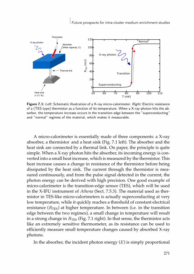
Future prospects for intra-cluster medium enrichment studies
X-ray photon
Heat sink(< 0.1 K)
Thermistor
Thermal link
Absorber(Heat capacity, C)
50 60 70 80 90 100 110T (mK)
0
20
40
60
80
100
120
RTES (
mΩ
)Superconducting
Normal
Transition
X-ray photon
Figure 7.1: Left: Schematic illustration of a X-ray micro-calorimeter. Right: Electric resistanceof a (TES type) thermistor as a function of its temperature. When a X-ray photon hits the ab-sorber, the temperature increase occurs in the transition edge between the ”superconducting”and ”normal” regimes of the material, which makes it measurable.
A micro-calorimeter is essentially made of three components: a X-rayabsorber, a thermistor and a heat sink (Fig. 7.1 left). The absorber and theheat sink are connected by a thermal link. On paper, the principle is quitesimple. When a X-ray photon hits the absorber, its incoming energy is con-verted into a small heat increase, which ismeasured by the thermistor. Thisheat increase causes a change in resistance of the thermistor before beingdissipated by the heat sink. The current through the thermistor is mea-sured continuously, and from the pulse signal detected in the current, thephoton energy can be derived with high precision. One good example ofmicro-calorimeter is the transition-edge sensor (TES), which will be usedin the X-IFU instrument of Athena (Sect. 7.5.3). The material used as ther-mistor in TES-like micro-calorimeters is actually superconducting at verylow temperature, while it quickly reaches a threshold of constant electricalresistance (RTES) at higher temperature. In between (i.e. in the transitionedge between the two regimes), a small change in temperature will resultin a strong change in RTES (Fig. 7.1 right). In that sense, the thermistor actslike an extremely sensitive thermometer, as its resistance can be used toefficiently measure small temperature changes caused by absorbed X-rayphotons.
In the absorber, the incident photon energy (E) is simply proportional
271
7.4 X-ray micro-calorimeters
to the heat variation (∆T ):∆T ∝ E
C, (7.1)
where C is the heat capacity of the absorber. Since ∆T/T is typically of theorder of 0.01%, the heat sink must keep the absorber as close as possibleto the absolute zero in order to minimise the thermal noise. This impliesthe need for a complex unit efficiently cooling the detector. Moreover, theabsorbing material should have its heat capacity as low as possible, andshould be efficient in absorbing X-rays.
Compared toCCD (or proportional counter) detectors, themain advan-tage of micro-calorimeters resides in their remarkable energy resolution(∆E). For CCDs, ∆E depends on both the photon energy and the numberof the subsequent collected electrons (N ), as
∆E ∝ E
√N
N. (7.2)
On the other hand, it can be shown that for micro-calorimeters,
∆E ∝
√kT 2C
α, (7.3)
where α is the sensitivity of the thermistor. In other words, ∆E does notdepend on E and can potentially reach very low values (a few eV at most)if the detector is kept at very low temperatures. One limitation to the en-ergy resolution iswhen twophotons hit the absorberwithin a short intervalimplying that their subsequent temperature jumps cannot be clearly sep-arated. In most clusters, however, the count rate of the ICM emission isweak enough to limit such a pile-up effect.
One of themain challenges for the next X-ray detectors is to build an ar-ray of independentmicro-calorimeter units, thereby recreating a full grid ofpixels and allowing to perform spatially-resolved spectroscopy. So far (i.e.in the SXS instrument, Sect. 7.5.1 and 7.5.2), each pixel is wired indepen-dently to the read-out electronics, which limits the number of pixels on thedetector (to 36 in the case of SXS). In future instruments (e.g. X-IFU, Sect.7.5.3), multiple pixels will be connected to one read-out chain, althoughthey can still be read-out independently using a multiplexing technique.This will allow to create more pixels per detector (∼3500 approximately),and to reach a good spatial resolution while keeping an exquisite spectralresolution.
272
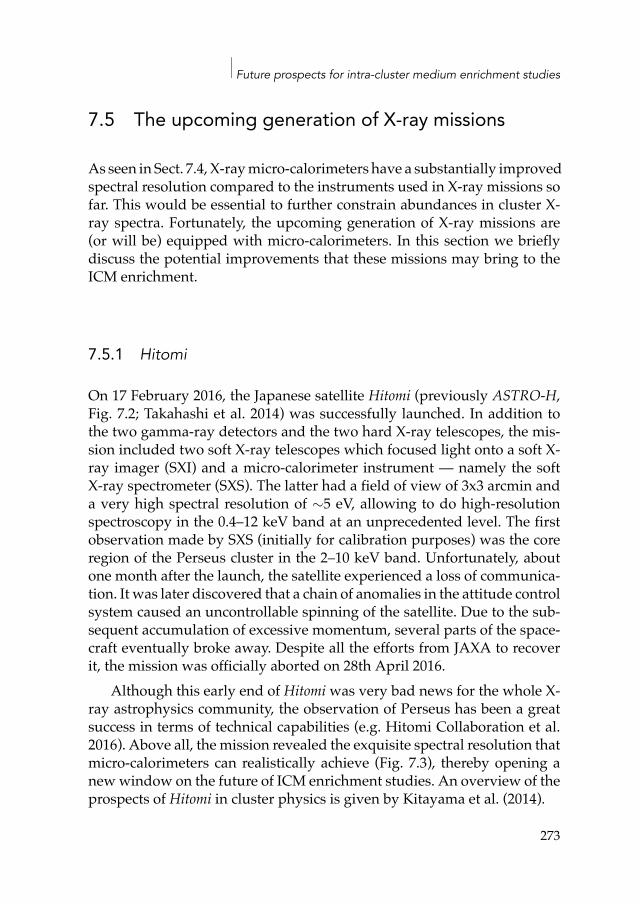
Future prospects for intra-cluster medium enrichment studies
7.5 The upcoming generation of X-ray missions
As seen in Sect. 7.4, X-raymicro-calorimeters have a substantially improvedspectral resolution compared to the instruments used in X-ray missions sofar. This would be essential to further constrain abundances in cluster X-ray spectra. Fortunately, the upcoming generation of X-ray missions are(or will be) equipped with micro-calorimeters. In this section we brieflydiscuss the potential improvements that these missions may bring to theICM enrichment.
7.5.1 Hitomi
On 17 February 2016, the Japanese satellite Hitomi (previously ASTRO-H,Fig. 7.2; Takahashi et al. 2014) was successfully launched. In addition tothe two gamma-ray detectors and the two hard X-ray telescopes, the mis-sion included two soft X-ray telescopes which focused light onto a soft X-ray imager (SXI) and a micro-calorimeter instrument — namely the softX-ray spectrometer (SXS). The latter had a field of view of 3x3 arcmin anda very high spectral resolution of ∼5 eV, allowing to do high-resolutionspectroscopy in the 0.4–12 keV band at an unprecedented level. The firstobservation made by SXS (initially for calibration purposes) was the coreregion of the Perseus cluster in the 2–10 keV band. Unfortunately, aboutone month after the launch, the satellite experienced a loss of communica-tion. It was later discovered that a chain of anomalies in the attitude controlsystem caused an uncontrollable spinning of the satellite. Due to the sub-sequent accumulation of excessive momentum, several parts of the space-craft eventually broke away. Despite all the efforts from JAXA to recoverit, the mission was officially aborted on 28th April 2016.
Although this early end of Hitomi was very bad news for the whole X-ray astrophysics community, the observation of Perseus has been a greatsuccess in terms of technical capabilities (e.g. Hitomi Collaboration et al.2016). Above all, the mission revealed the exquisite spectral resolution thatmicro-calorimeters can realistically achieve (Fig. 7.3), thereby opening anewwindow on the future of ICM enrichment studies. An overview of theprospects of Hitomi in cluster physics is given by Kitayama et al. (2014).
273
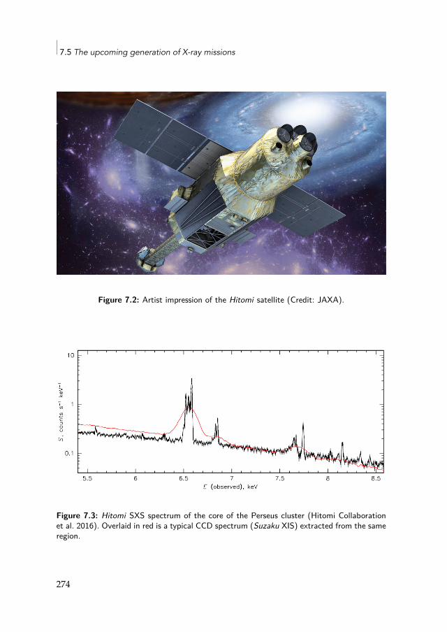
7.5 The upcoming generation of X-ray missions
Figure 7.2: Artist impression of the Hitomi satellite (Credit: JAXA).
Figure 7.3: Hitomi SXS spectrum of the core of the Perseus cluster (Hitomi Collaborationet al. 2016). Overlaid in red is a typical CCD spectrum (Suzaku XIS) extracted from the sameregion.
274
Future prospects for intra-cluster medium enrichment studies
7.5.2 XARM
The success of the SXS instrument onboard Hitomi to resolve metal linesin the spectrum of Perseus has been a strong motivation to recover themission. On 14 July 2016, JAXA announced that a successor of Hitomi isactually planned for the year 2021. Named the X-ray Astronomy RecoveryMission (XARM), this satellite would be essentially centred on the SXS in-strument.
If this mission is indeed confirmed, its SXS instrument will be highlyvaluable to future ICM enrichment studies. In Fig. 7.4, we simulate a SXSobservation of 100 ks of cleaned exposure of the core region of Abell 4059(see also Chapter 2). Here again, the simulated data illustrate the unprece-dented spectral resolution we can achieve with a micro-calorimeter instru-ment.
One interestingdirect application of the SXS capabilities is the improvedmeasurement of the Ni/Fe ratio. As seen in Chapters 1, 4, and 5, the Ni/Feratio provides valuable constraints on the dominant SNIa explosion chan-nel. Unfortunately, when measured with the EPIC instruments, this ratiosuffers from large cross-calibration and background uncertainties (Chap-ter 3), and is very sensitive to the used spectral codes and atomic databases(Chapter 5). Moreover, at CCD spectral resolution, Ni-K lines are blendedwith FeXXV (He-like) lines, thereby limiting the robustness of theNi abun-dance measurement. In addition to be weakly affected by the instrumentalbackground even at high energies2, the SXS instrument is able to fully dis-entangle all the Ni and Fe lines, and will thus dramatically improve ourmeasurement of the Ni/Fe ratio. Based on the simulation presented in Fig.7.4, and assuming ongoing efforts are pursued toward an improvement ofthe plasma atomic codes, we estimate that the statistical errors on Ni/Feshould not be larger than ∼8%. At that level of accuracy, it will be easy todetermine which of the deflagration or the delayed-detonation explosionmechanism is the dominant one in SNIa.
Another significant progress that SXS will be able to achieve is a betterquantification of the radial variation in the relative number of SNIa (SNcc)enriching galaxy clusters. As shown in Chapter 6, we have provided in-teresting hints that SNIa and SNcc enrich the ICM at the same level in thecentre and in the outer parts (∼0.5r500). This could be further confirmed
2The main reason of the low background level of the SXS instrument is related to thechoice of the low-Earth orbit of theHitomi/XARMmissions. This choice, however, also hasdrawbacks, like a shorter lifetime of the mission.
275
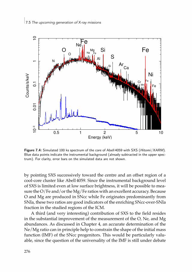
7.5 The upcoming generation of X-ray missions
1 100.5 2 510
−3
0.0
10.1
110
Counts
/s/k
eV
Energy (keV)
A4059: core (3 arcmin, 100 ks SXS simulation)
N
OO
NeFe
NaMg
Fe
Al
Si
Si
S
ArCa
CrMn
Fe
Fe
Ni
Fe
Figure 7.4: Simulated 100 ks spectrum of the core of Abell 4059 with SXS (Hitomi/XARM).Blue data points indicate the instrumental background (already subtracted in the upper spec-trum). For clarity, error bars on the simulated data are not shown.
by pointing SXS successively toward the centre and an offset region of acool-core cluster like Abell 4059. Since the instrumental background levelof SXS is limited even at low surface brightness, it will be possible to mea-sure theO/Fe and/or theMg/Fe ratioswith an excellent accuracy. BecauseO and Mg are produced in SNcc while Fe originates predominantly fromSNIa, these two ratios are good indicators of the enriching SNcc-over-SNIafraction in the studied regions of the ICM.
A third (and very interesting) contribution of SXS to the field residesin the substantial improvement of the measurement of the O, Ne, and Mgabundances. As discussed in Chapter 4, an accurate determination of theNe/Mg ratio can in principle help to constrain the shape of the initial massfunction (IMF) of the SNcc progenitors. This would be particularly valu-able, since the question of the universality of the IMF is still under debate
276
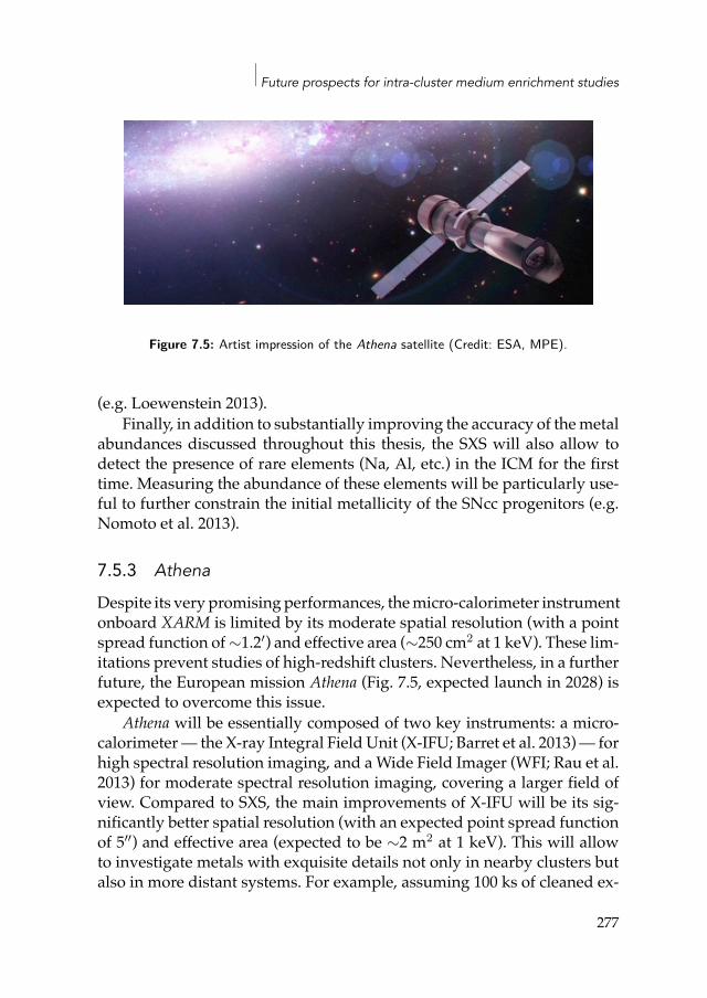
Future prospects for intra-cluster medium enrichment studies
Figure 7.5: Artist impression of the Athena satellite (Credit: ESA, MPE).
(e.g. Loewenstein 2013).Finally, in addition to substantially improving the accuracy of themetal
abundances discussed throughout this thesis, the SXS will also allow todetect the presence of rare elements (Na, Al, etc.) in the ICM for the firsttime. Measuring the abundance of these elements will be particularly use-ful to further constrain the initial metallicity of the SNcc progenitors (e.g.Nomoto et al. 2013).
7.5.3 Athena
Despite its very promisingperformances, themicro-calorimeter instrumentonboard XARM is limited by its moderate spatial resolution (with a pointspread function of∼1.2′) and effective area (∼250 cm2 at 1 keV). These lim-itations prevent studies of high-redshift clusters. Nevertheless, in a furtherfuture, the European mission Athena (Fig. 7.5, expected launch in 2028) isexpected to overcome this issue.
Athena will be essentially composed of two key instruments: a micro-calorimeter— the X-ray Integral Field Unit (X-IFU; Barret et al. 2013)— forhigh spectral resolution imaging, and aWide Field Imager (WFI; Rau et al.2013) for moderate spectral resolution imaging, covering a larger field ofview. Compared to SXS, the main improvements of X-IFU will be its sig-nificantly better spatial resolution (with an expected point spread functionof 5′′) and effective area (expected to be ∼2 m2 at 1 keV). This will allowto investigate metals with exquisite details not only in nearby clusters butalso in more distant systems. For example, assuming 100 ks of cleaned ex-
277
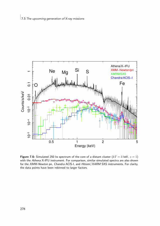
7.5 The upcoming generation of X-ray missions
10.5 2 5
10
−5
10
−4
10
−3
0.0
10
.11
Co
un
ts/s
/ke
V
Energy (keV)
O
Ne Mg Si S
Fe
Athena/X−IFU
XMM−Newton/pn
XARM/SXS
Chandra/ACIS−I
Figure 7.6: Simulated 250 ks spectrum of the core of a distant cluster (kT = 3 keV, z = 1)with the Athena X-IFU instrument. For comparison, similar simulated spectra are also shownfor the XMM-Newton pn, Chandra ACIS-I, and Hitomi/XARM SXS instruments. For clarity,the data points have been rebinned to larger factors.
278
Future prospects for intra-cluster medium enrichment studies
posure, X-IFUwill be able to detect O, Si, and Fe in clusters up to z = 1 andto measure their abundances with at least 10% of accuracy (Pointecouteauet al. 2013). We illustrate this by simulating 250 ks of cleaned exposure ofa bright distant (z = 1) cluster (kT = 3 keV) with X-IFU, and by com-paring its simulated spectrum with that of other instruments (Fig. 7.6). Anoverview of the prospects of Athena in cluster physics is given by Ettoriet al. (2013).
7.6 Concluding remarksSince the launch ofAthena is expected for 2028, patiencewill be required be-fore entering into this completely new era. Nevertheless, there is no doubtthat this mission— together withXARM and the possible other X-ray mis-sions that may be planned in a near future—will considerably expand ourknowledge on the origin and distribution of metals in the ICM. While sys-tematic uncertainties should always be borne in mind (as discussed aboveand throughout this thesis), we can reasonably hope that simultaneous andcontinuous improvements in ICM observations, ICM simulations, super-novamodels, instrument calibration, and atomic calculations will substan-tially reduce them.
Clearly, the future of chemical enrichment studies at the largest scales ofthe Universe looks promising and full of surprising upcoming discoveries.
279

Bibliography
Abramopoulos, F., Chanan, G. A., & Ku, W. H.-M. 1981, ApJ, 248, 429Allen, S. W. & Fabian, A. C. 1994, MNRAS, 269, 409Alpher, R. A., Bethe, H., & Gamow, G. 1948, Physical Review, 73, 803Andernach, H., Tago, E., Einasto, M., Einasto, J., & Jaaniste, J. 2005, in Astronomi-cal Society of the Pacific Conference Series, Vol. 329, Nearby Large-Scale Struc-tures and the Zone of Avoidance, ed. A. P. Fairall & P. A. Woudt, 283–287
Anders, E. & Grevesse, N. 1989, Geochim. Cosmochim. Acta, 53, 197Anderson, M. E., Bregman, J. N., Butler, S. C., & Mullis, C. R. 2009, ApJ, 698, 317Arnaud, K. A. 1996, in Astronomical Society of the Pacific Conference Series, Vol.101, Astronomical Data Analysis Software and Systems V, ed. G. H. Jacoby &J. Barnes, 17
Arnett, D. 1995, ARA&A, 33, 115Arnett, W. D. 1973, ARA&A, 11, 73Arnett, W. D. 1977, ApJS, 35, 145Badenes, C., Borkowski, K. J., & Bravo, E. 2005, ApJ, 624, 198Badenes, C., Borkowski, K. J., Hughes, J. P., Hwang, U., & Bravo, E. 2006, ApJ, 645,1373
Badenes, C., Bravo, E., Borkowski, K. J., & Domínguez, I. 2003, ApJ, 593, 358Badnell, N. R. 2006, ApJS, 167, 334Baldi, A., Ettori, S., Molendi, S., & Gastaldello, F. 2012, A&A, 545, A41Balestra, I., Tozzi, P., Ettori, S., et al. 2007, A&A, 462, 429Barlow, M. J., Swinyard, B. M., Owen, P. J., et al. 2013, Science, 342, 1343Barret, D., den Herder, J. W., Piro, L., et al. 2013, ArXiv e-prints [arXiv:1308.6784]Baumgartner, V. & Breitschwerdt, D. 2009, Astronomische Nachrichten, 330, 898Baumgartner, W. H., Loewenstein, M., Horner, D. J., &Mushotzky, R. F. 2005, ApJ,620, 680
Beiersdorfer, P., Bitter, M., von Goeler, S., & Hill, K. W. 2004, ApJ, 610, 616Bethe, H. A. 1939, Physical Review, 55, 434
281
Bibliography
Biffi, V., Planelles, S., Borgani, S., et al. 2017, MNRAS, 468, 531Bîrzan, L., Rafferty, D. A., Nulsen, P. E. J., et al. 2012, MNRAS, 427, 3468Böhringer, H., Belsole, E., Kennea, J., et al. 2001, A&A, 365, L181Böhringer, H., Matsushita, K., Churazov, E., Finoguenov, A., & Ikebe, Y. 2004a,A&A, 416, L21
Böhringer, H., Matsushita, K., Finoguenov, A., Xue, Y., & Churazov, E. 2005, Ad-vances in Space Research, 36, 677
Böhringer, H., Schuecker, P., Guzzo, L., et al. 2004b, A&A, 425, 367Böhringer, H. & Werner, N. 2010, A&A Rev., 18, 127Boyarsky, A., Ruchayskiy, O., Iakubovskyi, D., & Franse, J. 2014, Physical ReviewLetters, 113, 251301
Brachwitz, F., Dean, D. J., Hix, W. R., et al. 2000, ApJ, 536, 934Bradt, H., Mayer, W., Naranan, S., Rappaport, S., & Spada, G. 1967, ApJ, 150, L199Branch, D. 2001, PASP, 113, 169Branch, D., Thomas, R. C., Baron, E., et al. 2004, ApJ, 606, 413Bravo, E., Tornambe, A., Dominguez, I., & Isern, J. 1996, A&A, 306, 811Brickhouse, N. S., Dupree, A. K., Edgar, R. J., et al. 2000, ApJ, 530, 387Brickhouse, N. S. & Smith, R. K. 2005, Highlights of Astronomy, 13, 651Bryans, P., Landi, E., & Savin, D. W. 2009, ApJ, 691, 1540Bulbul, E., Markevitch, M., Foster, A., et al. 2014, ApJ, 789, 13Bulbul, E., Smith, R. K., & Loewenstein, M. 2012a, ApJ, 753, 54Bulbul, G. E., Smith, R. K., Foster, A., et al. 2012b, ApJ, 747, 32Buote, D. A. 2000, MNRAS, 311, 176Buote, D. A. & Canizares, C. R. 1994, ApJ, 427, 86Buote, D. A. & Fabian, A. C. 1998, MNRAS, 296, 977Buote, D. A., Lewis, A. D., Brighenti, F., & Mathews, W. G. 2003, ApJ, 595, 151Burbidge, E. M., Burbidge, G. R., Fowler, W. A., & Hoyle, F. 1957, Reviews ofModern Physics, 29, 547
Burrows, A. 2013, Reviews of Modern Physics, 85, 245Byram, E. T., Chubb, T. A., & Friedman, H. 1966, Science, 152, 66Cameron, A. G. W. 1957a, PASP, 69, 201Cameron, A. G. W. 1957b, AJ, 62, 9Canizares, C. R., Clark, G. W., Markert, T. H., et al. 1979, ApJ, 234, L33Cao, Y., Kulkarni, S. R., Howell, D. A., et al. 2015, Nature, 521, 328Carter, J. A., Sembay, S., & Read, A. M. 2011, A&A, 527, A115Cash, W. 1979, ApJ, 228, 939Cattaneo, A. & Teyssier, R. 2007, MNRAS, 376, 1547Cavagnolo, K. W., Donahue, M., Voit, G. M., & Sun, M. 2009, ApJS, 182, 12Cavaliere, A. G., Gursky, H., & Tucker, W. H. 1971, Nature, 231, 437Chabrier, G. 2003, PASP, 115, 763
282
Bibliography
Choi, Y.-Y., Reynolds, C. S., Heinz, S., et al. 2004, ApJ, 606, 185Churazov, E., Forman, W., Jones, C., & Böhringer, H. 2003, ApJ, 590, 225Cox, D. P. & Tucker, W. H. 1969, ApJ, 157, 1157Crosby, B. D., O’Shea, B. W., Beers, T. C., & Tumlinson, J. 2016, ApJ, 820, 71Dahlen, T., Strolger, L.-G., Riess, A. G., et al. 2004, ApJ, 613, 189De Grandi, S., Ettori, S., Longhetti, M., & Molendi, S. 2004, A&A, 419, 7De Grandi, S. & Molendi, S. 2001, ApJ, 551, 153De Grandi, S. & Molendi, S. 2009, A&A, 508, 565De Grandi, S., Santos, J. S., Nonino, M., et al. 2014, A&A, 567, A102De Luca, A. & Molendi, S. 2004, A&A, 419, 837de Plaa, J. 2013, Astronomische Nachrichten, 334, 416de Plaa, J., Kaastra, J. S., Tamura, T., et al. 2004, A&A, 423, 49de Plaa, J., Kaastra, J. S., Werner, N., et al. 2017, A&A, submittedde Plaa, J. & Mernier, F. 2017, Astronomische Nachrichten, in press[arXiv:1611.03723]
de Plaa, J., Werner, N., Bleeker, J. A. M., et al. 2007, A&A, 465, 345de Plaa, J., Werner, N., Bykov, A. M., et al. 2006, A&A, 452, 397de Plaa, J., Zhuravleva, I., Werner, N., et al. 2012, A&A, 539, A34De Young, D. S. 1978, ApJ, 223, 47den Herder, J. W., Brinkman, A. C., Kahn, S. M., et al. 2001, A&A, 365, L7Dicke, R. H., Peebles, P. J. E., Roll, P. G., & Wilkinson, D. T. 1965, ApJ, 142, 414Diehl, S. & Statler, T. S. 2006, MNRAS, 368, 497Domainko, W., Gitti, M., Schindler, S., & Kapferer, W. 2004, A&A, 425, L21Domainko, W., Mair, M., Kapferer, W., et al. 2006, A&A, 452, 795Dupke, R. A. & White, III, R. E. 2000, ApJ, 528, 139Dutton, A. A., Mendel, J. T., & Simard, L. 2012, MNRAS, 422, 33Eddington, A. S. 1920, The Observatory, 43, 341Einstein, A. 1905, Annalen der Physik, 322, 891Einstein, A. 1916, Annalen der Physik, 354, 769Elkholy, T. Y., Bautz, M. W., & Canizares, C. R. 2015, ApJ, 805, 3Ettori, S. & Fabian, A. C. 2006, MNRAS, 369, L42Ettori, S., Pratt, G. W., de Plaa, J., et al. 2013, ArXiv e-prints [arXiv:1306.2322]Ezer, C., Bulbul, E., Nihal Ercan, E., et al. 2017, ApJ, 836, 110Fabian, A. C. 1994, ARA&A, 32, 277Fabian, A. C. & Pringle, J. E. 1977, MNRAS, 181, 5PFabjan, D., Borgani, S., Tornatore, L., et al. 2010, MNRAS, 401, 1670Filippenko, A. V., Chornock, R., Swift, B., et al. 2003, IAU Circ., 8159, 2Fink, M., Kromer, M., Seitenzahl, I. R., et al. 2014, MNRAS, 438, 1762Finoguenov, A., Matsushita, K., Böhringer, H., Ikebe, Y., &Arnaud,M. 2002, A&A,381, 21
283
Bibliography
Foley, R. J. 2015, MNRAS, 452, 2463Frank, K. A., Peterson, J. R., Andersson, K., Fabian, A. C., & Sanders, J. S. 2013,ApJ, 764, 46
Fujita, Y., Tawa, N., Hayashida, K., et al. 2008, PASJ, 60, S343Fukazawa, Y., Ohashi, T., Fabian, A. C., et al. 1994, PASJ, 46, L55Fuller, G. M., Fowler, W. A., & Newman, M. J. 1982, ApJS, 48, 279Gamezo, V. N., Khokhlov, A. M., & Oran, E. S. 2005, ApJ, 623, 337Gamow, G. 1946, Physical Review, 70, 572Gastaldello, F., Ettori, S., Balestra, I., et al. 2010, A&A, 522, A34Gastaldello, F. & Molendi, S. 2002, ApJ, 572, 160Gnedin, N. Y. 1998, MNRAS, 294, 407Grange, Y. G., de Plaa, J., Kaastra, J. S., et al. 2011, A&A, 531, A15Gu, L., Kaastra, J., Raassen, A. J. J., et al. 2015, A&A, 584, L11Gu, M. F. 2008, Canadian Journal of Physics, 86, 675Gunn, J. E. & Gott, III, J. R. 1972, ApJ, 176, 1Guo, F. & Mathews, W. G. 2010, ApJ, 717, 937Hamuy, M., Trager, S. C., Pinto, P. A., et al. 2000, AJ, 120, 1479Hatano, K., Branch, D., Lentz, E. J., et al. 2000, ApJ, 543, L49Heger, A. & Woosley, S. E. 2002, ApJ, 567, 532Heger, A. & Woosley, S. E. 2010, ApJ, 724, 341Heinz, S., Choi, Y.-Y., Reynolds, C. S., & Begelman, M. C. 2002, ApJ, 569, L79Hickox, R. C. & Markevitch, M. 2006, ApJ, 645, 95Hillebrandt,W., Kromer,M., Röpke, F. K., & Ruiter, A. J. 2013, Frontiers of Physics,8, 116
Hillebrandt, W. & Niemeyer, J. C. 2000, ARA&A, 38, 191Hitomi Collaboration, Aharonian, F., Akamatsu, H., et al. 2016, Nature, 535, 117Hopkins, A. M. & Beacom, J. F. 2006, ApJ, 651, 142Howell, D. A. 2011, Nature Communications, 2, 350Hoyle, F. 1946, MNRAS, 106, 343Huang, Z. & Sarazin, C. L. 1998, ApJ, 496, 728Hubble, E. 1929, Proceedings of the National Academy of Science, 15, 168Hubble, E. P. 1926, ApJ, 64Hudson, M. J., Lucey, J. R., Smith, R. J., Schlegel, D. J., & Davies, R. L. 2001, MN-RAS, 327, 265
Iakubovskyi, D. 2013, PhD thesisIben, Jr., I. & Tutukov, A. V. 1984, ApJS, 54, 335Ichinohe, Y., Werner, N., Simionescu, A., et al. 2015, MNRAS, 448, 2971Iwamoto, K., Brachwitz, F., Nomoto, K., et al. 1999, ApJS, 125, 439Janka, H.-T. 2012, Annual Review of Nuclear and Particle Science, 62, 407Jansen, F., Lumb, D., Altieri, B., et al. 2001, A&A, 365, L1
284
Bibliography
Jerkstrand, A., Timmes, F. X., Magkotsios, G., et al. 2015, ApJ, 807, 110Jha, S., Branch, D., Chornock, R., et al. 2006, AJ, 132, 189Johnstone, R. M., Allen, S. W., Fabian, A. C., & Sanders, J. S. 2002, MNRAS, 336,299
Johnstone, R. M., Fabian, A. C., Morris, R. G., & Taylor, G. B. 2005, MNRAS, 356,237
Jones, C. & Forman, W. 1984, ApJ, 276, 38Kaastra, J. S. & Bleeker, J. A. M. 2016, A&A, 587, A151Kaastra, J. S., Ferrigno, C., Tamura, T., et al. 2001, A&A, 365, L99Kaastra, J. S., Mewe, R., & Nieuwenhuijzen, H. 1996, in UV and X-ray Spec-troscopy of Astrophysical and Laboratory Plasmas, ed. K. Yamashita &T. Watanabe, 411–414
Kaastra, J. S., Tamura, T., Peterson, J. R., et al. 2004, A&A, 413, 415Kalberla, P. M. W., Burton, W. B., Hartmann, D., et al. 2005, A&A, 440, 775Kapferer, W., Knapp, A., Schindler, S., Kimeswenger, S., & van Kampen, E. 2005,A&A, 438, 87
Kapferer, W., Kronberger, T., Breitschwerdt, D., et al. 2009, A&A, 504, 719Kapferer, W., Kronberger, T., Weratschnig, J., et al. 2007, A&A, 466, 813Kapferer, W., Schindler, S., Knollmann, S. R., & van Kampen, E. 2010, A&A, 516,A41
Kapteyn, J. C. 1922, ApJ, 55, 302Karakas, A. I. 2010, MNRAS, 403, 1413Kasliwal, M. M., Kulkarni, S. R., Gal-Yam, A., et al. 2012, ApJ, 755, 161Kellogg, E., Murray, S., Giacconi, R., Tananbaum, T., & Gursky, H. 1973, ApJ, 185,L13
Kellogg, E., Schreier, E., Tananbaum,H., Gursky, H., &Giacconi, R. 1972, in BAAS,Vol. 4, Bulletin of the American Astronomical Society, 336
Khokhlov, A. M. 1989, MNRAS, 239, 785Khokhlov, A. M. 1991, A&A, 245, L25Kitayama, T., Bautz, M., Markevitch, M., et al. 2014, ArXiv e-prints[arXiv:1412.1176]
Kobayashi, C., Karakas, A. I., & Umeda, H. 2011, MNRAS, 414, 3231Kobayashi, C. & Nomoto, K. 2009, ApJ, 707, 1466Kobayashi, C., Umeda, H., Nomoto, K., Tominaga, N., & Ohkubo, T. 2006, ApJ,653, 1145
Krick, J. E. & Bernstein, R. A. 2007, AJ, 134, 466Krick, J. E., Bernstein, R. A., & Pimbblet, K. A. 2006, AJ, 131, 168Kromer, M., Fink, M., Stanishev, V., et al. 2013, MNRAS, 429, 2287Kuntz, K. D. & Snowden, S. L. 2008, ApJ, 674, 209Langanke, K. & Martinez-Pinedo, G. 1998, Physics Letters B, 436, 19Langanke, K. & Martínez-Pinedo, G. 2001, Atomic Data and Nuclear Data Tables,
285
Bibliography
79, 1Leccardi, A. & Molendi, S. 2008, A&A, 487, 461Lehmer, B. D., Xue, Y. Q., Brandt, W. N., et al. 2012, ApJ, 752, 46Li, W., Chornock, R., Leaman, J., et al. 2011, MNRAS, 412, 1473Li, W., Filippenko, A. V., Treffers, R. R., et al. 2001, ApJ, 546, 734Liang, L., Durier, F., Babul, A., et al. 2016, MNRAS, 456, 4266Lin, Y.-T., Mohr, J. J., & Stanford, S. A. 2003, ApJ, 591, 749Lodders, K., Palme, H., & Gail, H.-P. 2009, Landolt Börnstein, 44Loewenstein, M. 2006, ApJ, 648, 230Loewenstein, M. 2013, ApJ, 773, 52Lovisari, L., Schindler, S., & Kapferer, W. 2011, A&A, 528, A60Lumb, D. H., Warwick, R. S., Page, M., & De Luca, A. 2002, A&A, 389, 93Madau, P. & Dickinson, M. 2014, ARA&A, 52, 415Maeda, K., Röpke, F. K., Fink, M., et al. 2010, ApJ, 712, 624Mahdavi, A. & Geller, M. J. 2001, ApJ, 554, L129Mannucci, F., Della Valle, M., & Panagia, N. 2006, MNRAS, 370, 773Mannucci, F., Della Valle, M., Panagia, N., et al. 2005, A&A, 433, 807Mao, J. & Kaastra, J. 2016, A&A, 587, A84Maoz, D. 2008, MNRAS, 384, 267Maoz, D. & Mannucci, F. 2012, PASA, 29, 447Maoz, D., Mannucci, F., & Nelemans, G. 2014, ARA&A, 52, 107Martin, D., Perego, A., Arcones, A., et al. 2015, ApJ, 813, 2Matsushita, K. 2011, A&A, 527, A134Matsushita, K., Finoguenov, A., & Böhringer, H. 2003, A&A, 401, 443Matsushita, K., Fukazawa, Y., Hughes, J. P., et al. 2007, PASJ, 59, 327Matsushita, K., Makishima, K., Rokutanda, E., Yamasaki, N. Y., & Ohashi, T. 1997,ApJ, 488, L125
Matteucci, F. & Chiappini, C. 2005, PASA, 22, 49Matteucci, F. & Recchi, S. 2001, ApJ, 558, 351Maughan, B. J., Jones, C., Forman, W., & Van Speybroeck, L. 2008, ApJS, 174, 117McCarthy, I. G., Schaye, J., Bower, R. G., et al. 2011, MNRAS, 412, 1965McDonald, M., Stalder, B., Bayliss, M., et al. 2016, ApJ, 817, 86McDonald, M., Veilleux, S., Rupke, D. S. N., Mushotzky, R., & Reynolds, C. 2011,ApJ, 734, 95
McQuinn, M. 2016, ARA&A, 54, 313Medvedev, P., Gilfanov,M., Sazonov, S., & Shtykovskiy, P. 2014,MNRAS, 440, 2464Merrill, P. W. 1952, in The National Academy of Sciences: Abstracts of Papers Pre-sented at the Annual Meeting April 28-30, Science, Vol. 115, 479–489
Mewe, R. 1972, A&A, 20, 215Mewe, R. & Gronenschild, E. H. B. M. 1981, A&AS, 45, 11
286
Bibliography
Mewe, R., Gronenschild, E. H. B. M., & van den Oord, G. H. J. 1985, A&AS, 62, 197Mewe, R., Lemen, J. R., & van den Oord, G. H. J. 1986, A&AS, 65, 511Million, E. T., Werner, N., Simionescu, A., & Allen, S. W. 2011, MNRAS, 418, 2744Mitchell, R. J., Culhane, J. L., Davison, P. J. N., & Ives, J. C. 1976, MNRAS, 175, 29PMiyaji, T., Griffiths, R. E., Lumb, D., Sarajedini, V., & Siddiqui, H. 2003, As-tronomische Nachrichten, 324, 24
Molendi, S., Eckert, D., De Grandi, S., et al. 2016, A&A, 586, A32Molendi, S. & Pizzolato, F. 2001, ApJ, 560, 194Moretti, A., Pagani, C., Cusumano, G., et al. 2009, A&A, 493, 501Moretti, A., Portinari, L., & Chiosi, C. 2003, A&A, 408, 431Morris, R. A. H., Phillipps, S., Jones, J. B., et al. 2007, A&A, 476, 59Morsony, B. J., Heath, C., & Workman, J. C. 2014, MNRAS, 441, 2134Mulchaey, J. S., Kasliwal, M. M., & Kollmeier, J. A. 2014, ApJ, 780, L34Mushotzky, R., Loewenstein, M., Arnaud, K. A., et al. 1996, ApJ, 466, 686Mushotzky, R. F., Holt, S. S., Boldt, E. A., Serlemitsos, P. J., & Smith, B. W. 1981,ApJ, 244, L47
Mushotzky, R. F. & Loewenstein, M. 1997, ApJ, 481, L63Nagashima, M., Lacey, C. G., Baugh, C. M., Frenk, C. S., & Cole, S. 2005, MNRAS,358, 1247
Nandra, K., Barret, D., Barcons, X., et al. 2013, ArXiv e-prints [arXiv:1306.2307]Niemeyer, J. C. & Woosley, S. E. 1997, ApJ, 475, 740Nomoto, K., Kobayashi, C., & Tominaga, N. 2013, ARA&A, 51, 457Nomoto, K., Thielemann, F.-K., & Wheeler, J. C. 1984, ApJ, 279, L23Nomoto, K., Tominaga, N., Umeda, H., Kobayashi, C., & Maeda, K. 2006, NuclearPhysics A, 777, 424
O’Dea, C. P., Baum, S. A., Privon, G., et al. 2008, ApJ, 681, 1035Ohashi, T. 1995, in American Institute of Physics Conference Series, Vol. 336, DarkMatter, ed. S. S. Holt & C. L. Bennett, 255–263
Olling, R. P., Mushotzky, R., Shaya, E. J., et al. 2015, Nature, 521, 332O’Sullivan, E., David, L. P., & Vrtilek, J. M. 2014, MNRAS, 437, 730Pakmor, R., Kromer, M., Röpke, F. K., et al. 2010, Nature, 463, 61Pakmor, R., Kromer, M., Taubenberger, S., et al. 2012, ApJ, 747, L10Panagoulia, E. K., Fabian, A. C., & Sanders, J. S. 2013, MNRAS, 433, 3290Panagoulia, E. K., Sanders, J. S., & Fabian, A. C. 2015, MNRAS, 447, 417Paterno-Mahler, R., Blanton, E. L., Randall, S. W., & Clarke, T. E. 2013, ApJ, 773,114
Peimbert, A., Peimbert, M., & Luridiana, V. 2016, Rev. Mexicana Astron. Astrofis.,52, 419
Peng, F. & Nagai, D. 2009, ApJ, 693, 839Penzias, A. A. & Wilson, R. W. 1965, ApJ, 142, 419
287
Bibliography
Perets, H. B., Gal-yam, A., Crockett, R. M., et al. 2011, ApJ, 728, L36Perets, H. B., Gal-Yam, A., Mazzali, P. A., et al. 2010, Nature, 465, 322Perrin, J. 1922, L’Astronomie, 36, 49Peterson, J. R., Kahn, S. M., Paerels, F. B. S., et al. 2003, ApJ, 590, 207Peterson, J. R., Paerels, F. B. S., Kaastra, J. S., et al. 2001, A&A, 365, L104Phillips, M. M., Li, W., Frieman, J. A., et al. 2007, PASP, 119, 360Piersanti, L., Gagliardi, S., Iben, Jr., I., & Tornambé, A. 2003, ApJ, 598, 1229Pinto, C., Fabian, A. C., Werner, N., et al. 2014, A&A, 572, L8Pinto, C., Sanders, J. S., Werner, N., et al. 2015, A&A, 575, A38Planelles, S., Borgani, S., Fabjan, D., et al. 2014, MNRAS, 438, 195Pointecouteau, E., Reiprich, T. H., Adami, C., et al. 2013, ArXiv e-prints[arXiv:1306.2319]
Rafferty, D. A., Bîrzan, L., Nulsen, P. E. J., et al. 2013, MNRAS, 428, 58Ramirez-Ruiz, E., Trenti, M., MacLeod, M., et al. 2015, ApJ, 802, L22Rasia, E., Borgani, S., Murante, G., et al. 2015, ApJ, 813, L17Rasia, E., Mazzotta, P., Bourdin, H., et al. 2008, ApJ, 674, 728Rasmussen, J. & Ponman, T. J. 2007, MNRAS, 380, 1554Rasmussen, J. & Ponman, T. J. 2009, MNRAS, 399, 239Rau, A., Meidinger, N., Nandra, K., et al. 2013, ArXiv e-prints [arXiv:1308.6785]Raymond, J. C. & Smith, B. W. 1977, ApJS, 35, 419Read, A. M., Guainazzi, M., & Sembay, S. 2014, A&A, 564, A75Rebusco, P., Churazov, E., Böhringer, H., & Forman, W. 2005, MNRAS, 359, 1041Rebusco, P., Churazov, E., Böhringer, H., & Forman, W. 2006, MNRAS, 372, 1840Reiprich, T. H., Basu, K., Ettori, S., et al. 2013, Space Sci. Rev., 177, 195Reiprich, T. H. & Böhringer, H. 2002, ApJ, 567, 716Renzini, A. & Andreon, S. 2014, MNRAS, 444, 3581Renzini, A., Ciotti, L., D’Ercole, A., & Pellegrini, S. 1993, ApJ, 419, 52Reynolds, C. S., Casper, E. A., & Heinz, S. 2008, ApJ, 679, 1181Riess, A. G., Filippenko, A. V., Challis, P., et al. 1998, AJ, 116, 1009Roediger, E., Brüggen, M., Simionescu, A., et al. 2011, MNRAS, 413, 2057Roediger, E., Lovisari, L., Dupke, R., et al. 2012, MNRAS, 420, 3632Romano, D., Karakas, A. I., Tosi, M., & Matteucci, F. 2010, A&A, 522, A32Rubin, V. C. & Ford, Jr., W. K. 1970, ApJ, 159, 379Ruiter, A. J., Sim, S. A., Pakmor, R., et al. 2013, MNRAS, 429, 1425Russell, H. R., McNamara, B. R., Edge, A. C., et al. 2013, MNRAS, 432, 530Russell, H. R., Sanders, J. S., & Fabian, A. C. 2008, MNRAS, 390, 1207Salpeter, E. E. 1955, ApJ, 121, 161Sanders, J. S. & Fabian, A. C. 2002, MNRAS, 331, 273Sanders, J. S. & Fabian, A. C. 2006a, MNRAS, 371, 1483Sanders, J. S. & Fabian, A. C. 2006b, MNRAS, 370, 63
288
Bibliography
Sanders, J. S. & Fabian, A. C. 2007, MNRAS, 381, 1381Sanders, J. S. & Fabian, A. C. 2011, MNRAS, 412, L35Sanders, J. S., Fabian, A. C., Allen, S. W., et al. 2008, MNRAS, 385, 1186Sanders, J. S., Fabian, A. C., Allen, S. W., & Schmidt, R. W. 2004, MNRAS, 349, 952Sanders, J. S., Fabian, A. C., Taylor, G. B., et al. 2016, MNRAS, 457, 82Sanderson, A. J. R., O’Sullivan, E., & Ponman, T. J. 2009, MNRAS, 395, 764Sarazin, C. L. 1986, Reviews of Modern Physics, 58, 1Sasaki, T., Matsushita, K., & Sato, K. 2014, ApJ, 781, 36Sato, K., Matsushita, K., Ishisaki, Y., et al. 2009, PASJ, 61, S353Sato, K., Matsushita, K., Ishisaki, Y., et al. 2008, PASJ, 60, S333Sato, K., Tokoi, K., Matsushita, K., et al. 2007a, ApJ, 667, L41Sato, K., Yamasaki, N. Y., Ishida, M., et al. 2007b, PASJ, 59, 299Scalzo, R. A., Ruiter, A. J., & Sim, S. A. 2014, MNRAS, 445, 2535Schellenberger, G., Reiprich, T. H., Lovisari, L., Nevalainen, J., & David, L. 2015,A&A, 575, A30
Schindler, S. & Diaferio, A. 2008, Space Sci. Rev., 134, 363Schindler, S., Kapferer, W., Domainko, W., et al. 2005, A&A, 435, L25Schlegel, D. J., Finkbeiner, D. P., & Davis, M. 1998, ApJ, 500, 525Schmidt, B. P., Suntzeff, N. B., Phillips, M. M., et al. 1998, ApJ, 507, 46Seitenzahl, I. R., Cescutti, G., Röpke, F. K., Ruiter, A. J., & Pakmor, R. 2013a, A&A,559, L5
Seitenzahl, I. R., Ciaraldi-Schoolmann, F., Röpke, F. K., et al. 2013b, MNRAS, 429,1156
Seitenzahl, I. R., Summa, A., Krauß, F., et al. 2015, MNRAS, 447, 1484Serlemitsos, P. J., Smith, B. W., Boldt, E. A., Holt, S. S., & Swank, J. H. 1977, ApJ,211, L63
Shah, C., Dobrodey, S., Bernitt, S., et al. 2016, ApJ, 833, 52Simionescu, A., Roediger, E., Nulsen, P. E. J., et al. 2009a, A&A, 495, 721Simionescu, A., Werner, N., Böhringer, H., et al. 2009b, A&A, 493, 409Simionescu, A., Werner, N., Finoguenov, A., Böhringer, H., & Brüggen, M. 2008,A&A, 482, 97
Simionescu, A., Werner, N., Forman, W. R., et al. 2010, MNRAS, 405, 91Simionescu, A., Werner, N., Urban, O., et al. 2015, ApJ, 811, L25Smartt, S. J. 2009, ARA&A, 47, 63Smith, R. J., Lucey, J. R., Hudson, M. J., Schlegel, D. J., & Davies, R. L. 2000, MN-RAS, 313, 469
Smith, R. K., Brickhouse, N. S., Liedahl, D. A., & Raymond, J. C. 2001, ApJ, 556,L91
Snowden, S. L., Collier, M. R., & Kuntz, K. D. 2004, ApJ, 610, 1182Snowden, S. L. & Kuntz, K. D. 2013, XMM ESAS cookbook
289
Bibliography
Stewart, G. C., Fabian, A. C., Jones, C., & Forman, W. 1984, ApJ, 285, 1Strüder, L., Briel, U., Dennerl, K., et al. 2001, A&A, 365, L18Sullivan, M., Le Borgne, D., Pritchet, C. J., et al. 2006, ApJ, 648, 868Sun, M. 2012, New Journal of Physics, 14, 045004Takahashi, T., Mitsuda, K., Kelley, R., et al. 2014, ArXiv e-prints [arXiv:1412.2351]Tamura, T., Bleeker, J. A. M., Kaastra, J. S., Ferrigno, C., & Molendi, S. 2001, A&A,379, 107
Tamura, T., Kaastra, J. S., den Herder, J. W. A., Bleeker, J. A. M., & Peterson, J. R.2004, A&A, 420, 135
Tamura, T., Maeda, Y., Mitsuda, K., et al. 2009, ApJ, 705, L62Taylor, G. B., Barton, E. J., & Ge, J. 1994, AJ, 107, 1942Thölken, S., Lovisari, L., Reiprich, T. H., & Hasenbusch, J. 2016, A&A, 592, A37Timmes, F. X., Woosley, S. E., & Weaver, T. A. 1995, ApJS, 98, 617Tinsley, B. M. 1980, Fund. Cosmic Phys., 5, 287Tornatore, L., Borgani, S., Dolag, K., & Matteucci, F. 2007, MNRAS, 382, 1050Tozzi, P., Rosati, P., Ettori, S., et al. 2003, ApJ, 593, 705Treu, T., Auger, M. W., Koopmans, L. V. E., et al. 2010, ApJ, 709, 1195Tsujimoto, T., Nomoto, K., Yoshii, Y., et al. 1995, MNRAS, 277, 945Turner, M. J. L., Abbey, A., Arnaud, M., et al. 2001, A&A, 365, L27Umeda, H. & Nomoto, K. 2002, ApJ, 565, 385Urdampilleta, I., Kaastra, J. S., & Mehdipour, M. 2017, A&A, in press[arXiv:1702.06007]
Voit, G. M. & Donahue, M. 2011, ApJ, 738, L24Waldman, R., Sauer, D., Livne, E., et al. 2011, ApJ, 738, 21Weaver, T. A. & Woosley, S. E. 1980, in Annals of the New York Academy ofSciences, Vol. 336, Ninth Texas Symposium on Relativistic Astrophysics, ed.J. Ehlers, J. J. Perry, & M. Walker, 335–357
Weaver, T. A., Zimmerman, G. B., & Woosley, S. E. 1978, ApJ, 225, 1021Webbink, R. F. 1984, ApJ, 277, 355Werner, N., Böhringer, H., Kaastra, J. S., et al. 2006a, A&A, 459, 353Werner, N., de Plaa, J., Kaastra, J. S., et al. 2006b, A&A, 449, 475Werner, N., Durret, F., Ohashi, T., Schindler, S., & Wiersma, R. P. C. 2008,Space Sci. Rev., 134, 337
Werner, N., Urban, O., Simionescu, A., & Allen, S. W. 2013, Nature, 502, 656Whelan, J. & Iben, Jr., I. 1973, ApJ, 186, 1007Wiersma, R. P. C., Schaye, J., Theuns, T., Dalla Vecchia, C., & Tornatore, L. 2009,MNRAS, 399, 574
Willingale, R., Starling, R. L. C., Beardmore, A. P., Tanvir, N. R., & O’Brien, P. T.2013, MNRAS, 431, 394
Willman, B., Governato, F., Wadsley, J., & Quinn, T. 2004, MNRAS, 355, 159
290
Bibliography
Woosley, S. E. & Weaver, T. A. 1995, ApJS, 101, 181Yamaguchi, H., Badenes, C., Foster, A. R., et al. 2015, ApJ, 801, L31Yasumi, M., Nobukawa, M., Nakashima, S., et al. 2014, PASJ, 66, 68Yates, R. M., Thomas, P. A., & Henriques, B. M. B. 2017, MNRAS, 464, 3169Yoshii, Y., Tsujimoto, T., & Nomoto, K. 1996, ApJ, 462, 266Yuan, F., Kobayashi, C., Schmidt, B. P., et al. 2013, MNRAS, 432, 1680Zhang, Y.-Y., Andernach, H., Caretta, C. A., et al. 2011, A&A, 526, A105Zhang, Y.-Y., Reiprich, T. H., Finoguenov, A., Hudson, D. S., & Sarazin, C. L. 2009,ApJ, 699, 1178
Zwicky, F. 1933, Helvetica Physica Acta, 6, 110
291

Nederlandse samenvatting
Waar komen we vandaan? Deze vraag is natuurlijk heel breed omdat hijveel verschillende disciplines omvat (natuurkunde, biologie, sterrenkun-de, filosofie, etc.). Het is moeilijk (of zelfs onmogelijk) om daar één duide-lijk antwoord op te geven. Echter, één van de meest buitengewone ontdek-kingen van de 20ste eeuw heeft voor een revolutie gezorgd in onze kennisover onze oorsprong. Zestig jaar geleden hebben we ontdekt dat de bouw-stenen van planeten en het leven gevormd worden in de kern van sterrenen wanneer die als supernova ontploffen. We zijn, met andere woorden,niets anders dan ”sterrenstof”.
De oorsprong van chemische elementenDe elementaire bouwstenen van alle stoffen die we kennen worden che-mische elementen genoemd. Ze groeperen zich vaak in moleculen om zoplaneten, rotsen, water, ijs, cellen, dieren etc. te vormen. Ze zijn de basisvan de chemie en van het leven. Dankzij het werk van verschillende gene-raties van astronomen kennen we nu het verhaal over de oorsprong vanchemische elementen in het Heelal. Zo’n 13.7 miljard jaar geleden hebbende extreme condities tijdens de eerste minuten na de Big Bang gezorgdvoor de vorming van het waterstof en een groot deel van het heliumdatwein ons Universum vinden. Zwaardere elementen, oftewel ”metalen”, zoalskoolstof, stikstof, zuurstof, silicum en ijzer, konden in deze eerste minutenniet worden geproduceerd. Zij werden pas honderden miljoenen jaren nade Big Bang in de eerste sterren gevormd toen die ontploften als superno-vae. Sindsdien hebben vele generaties van sterren mede door supernovaexplosies het Heelal verrijkt met zwaardere elementen.
293
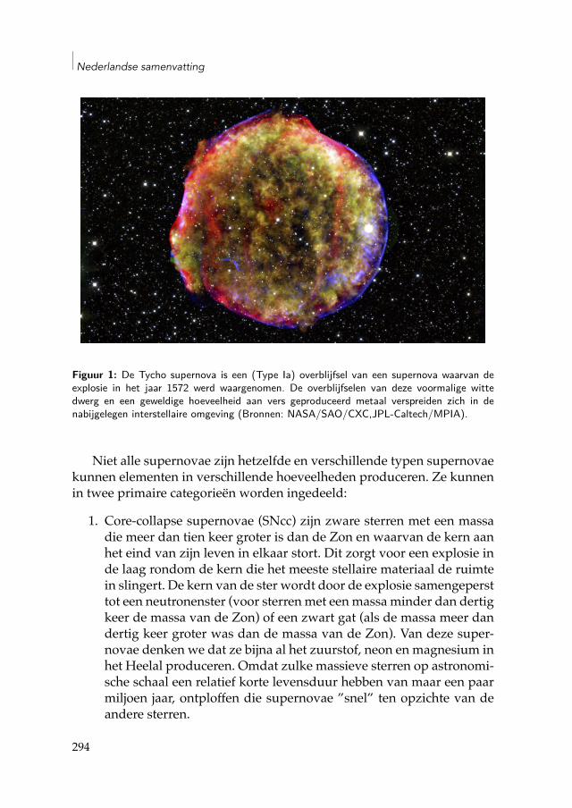
Nederlandse samenvatting
Figuur 1: De Tycho supernova is een (Type Ia) overblijfsel van een supernova waarvan deexplosie in het jaar 1572 werd waargenomen. De overblijfselen van deze voormalige wittedwerg en een geweldige hoeveelheid aan vers geproduceerd metaal verspreiden zich in denabijgelegen interstellaire omgeving (Bronnen: NASA/SAO/CXC,JPL-Caltech/MPIA).
Niet alle supernovae zijn hetzelfde en verschillende typen supernovaekunnen elementen in verschillende hoeveelheden produceren. Ze kunnenin twee primaire categorieën worden ingedeeld:
1. Core-collapse supernovae (SNcc) zijn zware sterren met een massadie meer dan tien keer groter is dan de Zon en waarvan de kern aanhet eind van zijn leven in elkaar stort. Dit zorgt voor een explosie inde laag rondom de kern die het meeste stellaire materiaal de ruimtein slingert. De kern van de ster wordt door de explosie samengepersttot een neutronenster (voor sterren met eenmassa minder dan dertigkeer de massa van de Zon) of een zwart gat (als de massa meer dandertig keer groter was dan de massa van de Zon). Van deze super-novae denken we dat ze bijna al het zuurstof, neon en magnesium inhet Heelal produceren. Omdat zulke massieve sterren op astronomi-sche schaal een relatief korte levensduur hebben van maar een paarmiljoen jaar, ontploffen die supernovae ”snel” ten opzichte van deandere sterren.
294
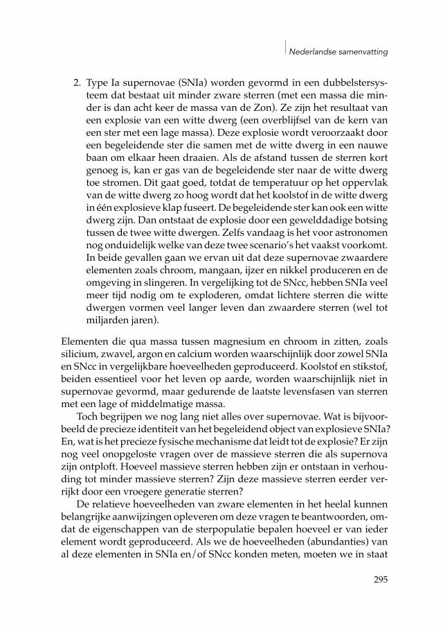
Nederlandse samenvatting
2. Type Ia supernovae (SNIa) worden gevormd in een dubbelstersys-teem dat bestaat uit minder zware sterren (met een massa die min-der is dan acht keer de massa van de Zon). Ze zijn het resultaat vaneen explosie van een witte dwerg (een overblijfsel van de kern vaneen ster met een lage massa). Deze explosie wordt veroorzaakt dooreen begeleidende ster die samen met de witte dwerg in een nauwebaan om elkaar heen draaien. Als de afstand tussen de sterren kortgenoeg is, kan er gas van de begeleidende ster naar de witte dwergtoe stromen. Dit gaat goed, totdat de temperatuur op het oppervlakvan de witte dwerg zo hoog wordt dat het koolstof in de witte dwergin één explosieve klap fuseert. De begeleidende ster kan ook eenwittedwerg zijn. Dan ontstaat de explosie door een gewelddadige botsingtussen de twee witte dwergen. Zelfs vandaag is het voor astronomennog onduidelijkwelke vandeze twee scenario’s het vaakst voorkomt.In beide gevallen gaan we ervan uit dat deze supernovae zwaardereelementen zoals chroom, mangaan, ijzer en nikkel produceren en deomgeving in slingeren. In vergelijking tot de SNcc, hebben SNIa veelmeer tijd nodig om te exploderen, omdat lichtere sterren die wittedwergen vormen veel langer leven dan zwaardere sterren (wel totmiljarden jaren).
Elementen die qua massa tussen magnesium en chroom in zitten, zoalssilicium, zwavel, argon en calciumwordenwaarschijnlijk door zowel SNIaen SNcc in vergelijkbare hoeveelheden geproduceerd. Koolstof en stikstof,beiden essentieel voor het leven op aarde, worden waarschijnlijk niet insupernovae gevormd, maar gedurende de laatste levensfasen van sterrenmet een lage of middelmatige massa.
Toch begrijpen we nog lang niet alles over supernovae. Wat is bijvoor-beelddeprecieze identiteit vanhet begeleidendobject van explosieve SNIa?En,wat is het precieze fysischemechanismedat leidt tot de explosie? Er zijnnog veel onopgeloste vragen over de massieve sterren die als supernovazijn ontploft. Hoeveel massieve sterren hebben zijn er ontstaan in verhou-ding tot minder massieve sterren? Zijn deze massieve sterren eerder ver-rijkt door een vroegere generatie sterren?
De relatieve hoeveelheden van zware elementen in het heelal kunnenbelangrijke aanwijzingen opleveren omdeze vragen te beantwoorden, om-dat de eigenschappen van de sterpopulatie bepalen hoeveel er van iederelement wordt geproduceerd. Als we de hoeveelheden (abundanties) vanal deze elementen in SNIa en/of SNcc konden meten, moeten we in staat
295
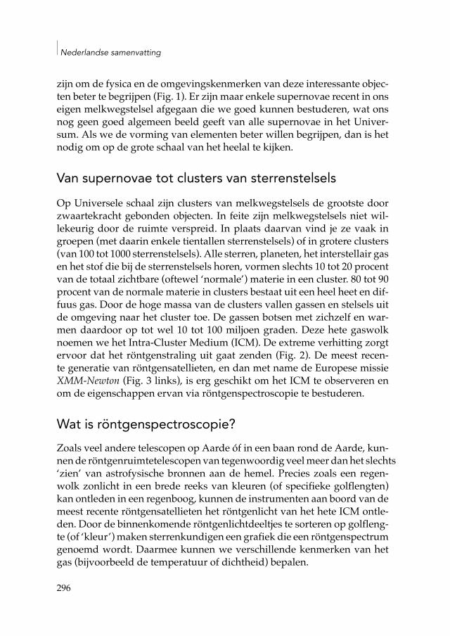
Nederlandse samenvatting
zijn om de fysica en de omgevingskenmerken van deze interessante objec-ten beter te begrijpen (Fig. 1). Er zijn maar enkele supernovae recent in onseigen melkwegstelsel afgegaan die we goed kunnen bestuderen, wat onsnog geen goed algemeen beeld geeft van alle supernovae in het Univer-sum. Als we de vorming van elementen beter willen begrijpen, dan is hetnodig om op de grote schaal van het heelal te kijken.
Van supernovae tot clusters van sterrenstelselsOp Universele schaal zijn clusters van melkwegstelsels de grootste doorzwaartekracht gebonden objecten. In feite zijn melkwegstelsels niet wil-lekeurig door de ruimte verspreid. In plaats daarvan vind je ze vaak ingroepen (met daarin enkele tientallen sterrenstelsels) of in grotere clusters(van 100 tot 1000 sterrenstelsels). Alle sterren, planeten, het interstellair gasen het stof die bij de sterrenstelsels horen, vormen slechts 10 tot 20 procentvan de totaal zichtbare (oftewel ‘normale’) materie in een cluster. 80 tot 90procent van de normale materie in clusters bestaat uit een heel heet en dif-fuus gas. Door de hoge massa van de clusters vallen gassen en stelsels uitde omgeving naar het cluster toe. De gassen botsen met zichzelf en war-men daardoor op tot wel 10 tot 100 miljoen graden. Deze hete gaswolknoemen we het Intra-Cluster Medium (ICM). De extreme verhitting zorgtervoor dat het röntgenstraling uit gaat zenden (Fig. 2). De meest recen-te generatie van röntgensatellieten, en dan met name de Europese missieXMM-Newton (Fig. 3 links), is erg geschikt om het ICM te observeren enom de eigenschappen ervan via röntgenspectroscopie te bestuderen.
Wat is röntgenspectroscopie?Zoals veel andere telescopen op Aarde óf in een baan rond de Aarde, kun-nende röntgenruimtetelescopenvan tegenwoordig veelmeer danhet slechts‘zien’ van astrofysische bronnen aan de hemel. Precies zoals een regen-wolk zonlicht in een brede reeks van kleuren (of specifieke golflengten)kan ontleden in een regenboog, kunnen de instrumenten aan boord van demeest recente röntgensatellieten het röntgenlicht van het hete ICM ontle-den. Door de binnenkomende röntgenlichtdeeltjes te sorteren op golfleng-te (of ‘kleur’) maken sterrenkundigen een grafiek die een röntgenspectrumgenoemd wordt. Daarmee kunnen we verschillende kenmerken van hetgas (bijvoorbeeld de temperatuur of dichtheid) bepalen.
296
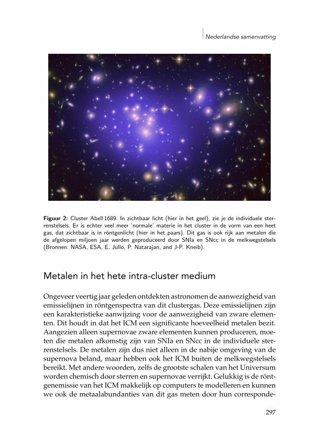
Nederlandse samenvatting
Figuur 2: Cluster Abell 1689. In zichtbaar licht (hier in het geel), zie je de individuele ster-renstelsels. Er is echter veel meer ’normale’ materie in het cluster in de vorm van een heetgas, dat zichtbaar is in röntgenlicht (hier in het paars). Dit gas is ook rijk aan metalen diede afgelopen miljoen jaar werden geproduceerd door SNIa en SNcc in de melkwegstelsels(Bronnen: NASA, ESA, E. Jullo, P. Natarajan, and J-P. Kneib).
Metalen in het hete intra-cluster medium
Ongeveer veertig jaar geleden ontdekten astronomende aanwezigheid vanemissielijnen in röntgenspectra van dit clustergas. Deze emissielijnen zijneen karakteristieke aanwijzing voor de aanwezigheid van zware elemen-ten. Dit houdt in dat het ICM een significante hoeveelheid metalen bezit.Aangezien alleen supernovae zware elementen kunnen produceren, moe-ten die metalen afkomstig zijn van SNIa en SNcc in de individuele ster-renstelsels. De metalen zijn dus niet alleen in de nabije omgeving van desupernova beland, maar hebben ook het ICM buiten de melkwegstelselsbereikt. Met andere woorden, zelfs de grootste schalen van het Universumworden chemisch door sterren en supernovae verrijkt. Gelukkig is de rönt-genemissie van het ICMmakkelijk op computers te modelleren en kunnenwe ook de metaalabundanties van dit gas meten door hun corresponde-
297
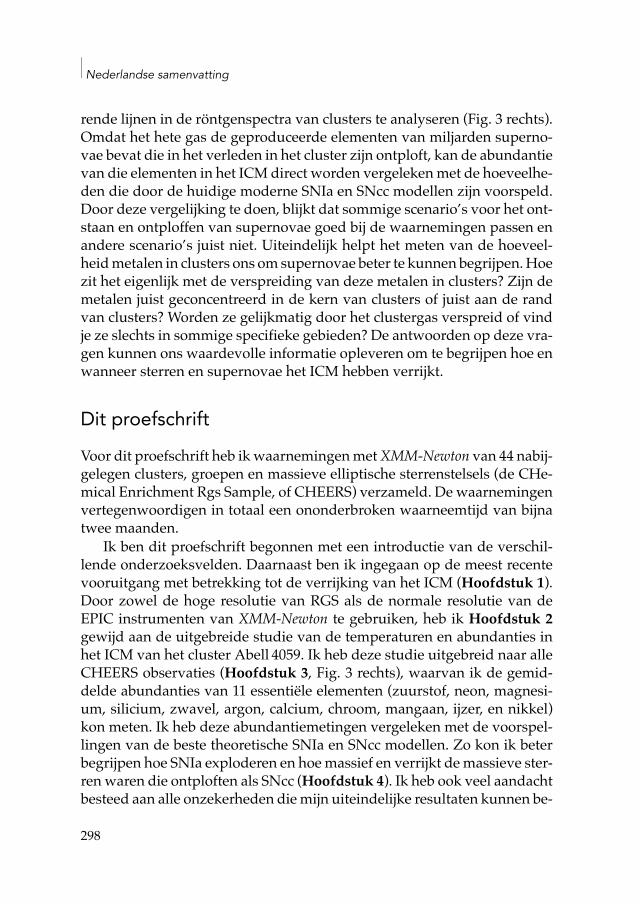
Nederlandse samenvatting
rende lijnen in de röntgenspectra van clusters te analyseren (Fig. 3 rechts).Omdat het hete gas de geproduceerde elementen van miljarden superno-vae bevat die in het verleden in het cluster zijn ontploft, kan de abundantievan die elementen in het ICM direct worden vergelekenmet de hoeveelhe-den die door de huidige moderne SNIa en SNcc modellen zijn voorspeld.Door deze vergelijking te doen, blijkt dat sommige scenario’s voor het ont-staan en ontploffen van supernovae goed bij de waarnemingen passen enandere scenario’s juist niet. Uiteindelijk helpt het meten van de hoeveel-heidmetalen in clusters ons om supernovae beter te kunnen begrijpen.Hoezit het eigenlijk met de verspreiding van deze metalen in clusters? Zijn demetalen juist geconcentreerd in de kern van clusters of juist aan de randvan clusters? Worden ze gelijkmatig door het clustergas verspreid of vindje ze slechts in sommige specifieke gebieden? De antwoorden op deze vra-gen kunnen ons waardevolle informatie opleveren om te begrijpen hoe enwanneer sterren en supernovae het ICM hebben verrijkt.
Dit proefschriftVoor dit proefschrift heb ikwaarnemingenmetXMM-Newton van 44 nabij-gelegen clusters, groepen en massieve elliptische sterrenstelsels (de CHe-mical Enrichment Rgs Sample, of CHEERS) verzameld. De waarnemingenvertegenwoordigen in totaal een ononderbroken waarneemtijd van bijnatwee maanden.
Ik ben dit proefschrift begonnen met een introductie van de verschil-lende onderzoeksvelden. Daarnaast ben ik ingegaan op de meest recentevooruitgang met betrekking tot de verrijking van het ICM (Hoofdstuk 1).Door zowel de hoge resolutie van RGS als de normale resolutie van deEPIC instrumenten van XMM-Newton te gebruiken, heb ik Hoofdstuk 2gewijd aan de uitgebreide studie van de temperaturen en abundanties inhet ICM van het cluster Abell 4059. Ik heb deze studie uitgebreid naar alleCHEERS observaties (Hoofdstuk 3, Fig. 3 rechts), waarvan ik de gemid-delde abundanties van 11 essentiële elementen (zuurstof, neon, magnesi-um, silicium, zwavel, argon, calcium, chroom, mangaan, ijzer, en nikkel)kon meten. Ik heb deze abundantiemetingen vergeleken met de voorspel-lingen van de beste theoretische SNIa en SNcc modellen. Zo kon ik beterbegrijpen hoe SNIa exploderen en hoemassief en verrijkt demassieve ster-ren waren die ontploften als SNcc (Hoofdstuk 4). Ik heb ook veel aandachtbesteed aan alle onzekerheden diemijn uiteindelijke resultaten kunnen be-
298
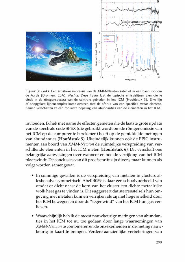
Nederlandse samenvatting
0.1
00.
10
.10
0.1
(Obs
erve
d
Mod
el) /
Mod
el
1 100.5 2 5
0.1
00.
1
Energy (keV)
MOS1
MOS2
pn
1 100.5 2 5
00.
20.
40.
60.
8(O
bser
ved
Mod
el) /
Mod
el
Energy (keV)
O VI
II (L
y)
FeL
com
plex
(incl.
Ne)
Mg
XII (
Ly)
Si X
III (H
e) Si
XIV
(Ly
)
S XV
(He
)S
XVI (
Ly)
Ar X
VII (
He)
Ar X
VIII
(Ly
)
Ca X
IX (H
e)
Ca X
X (L
y)
Ca X
IX /
Ca X
X
Cr X
XIII
(He
)M
n XX
IV (H
e)
FeK
com
plex
Fe X
XVI (
Ly)
Fe X
XV (H
e)
(/ Fe
XXI
V)
Ni X
XVII
/ Ni X
XVIII
/ Fe
XXV
(He
)
> SNIa> SNcc> SNIa & SNcc
Figuur 3: Links: Een artistieke impressie van de XMM-Newton satelliet in een baan rondomde Aarde (Bronnen: ESA). Rechts: Deze figuur laat de typische emissielijnen zien die jevindt in de röntgenspectra van de centrale gebieden in het ICM (Hoofdstuk 3). Elke lijnof onopgelost lijnencomplex komt overeen met de afdruk van een specifiek zwaar element.Samen verschaffen ze een robuuste bepaling van abundanties van de elementen in het ICM.
ïnvloeden. Ik hebmet name de effecten gemeten die de laatste grote updatevan de spectrale code SPEX (die gebruikt wordt om de röntgenemissie vanhet ICM op de computer te berekenen) heeft op de gemiddelde metingenvan abundanties (Hoofdstuk 5). Uiteindelijk kunnen ook de EPIC instru-menten aan boord van XMM-Newton de ruimtelijke verspreiding van ver-schillende elementen in het ICM meten (Hoofdstuk 6). Dit verschaft onsbelangrijke aanwijzingen over wanneer en hoe de verrijking van het ICMplaatsvindt. De conclusies van dit proefschrift zijn divers, maar kunnen alsvolgt worden samengevat.
• In sommige gevallen is de verspreiding van metalen in clusters al-lesbehalve symmetrisch. Abell 4059 is daar een schoolvoorbeeld vanomdat er dicht naast de kern van het cluster een dichte metaalrijkewolk heet gas te vinden is. Dit suggereert dat sterrenstelsels hun om-geving met metalen kunnen verrijken als zij met hoge snelheid doorhet ICM bewegen en door de ”tegenwind” van het ICM hun gas ver-liezen.
• Waarschijnlijk heb ik de meest nauwkeurige metingen van abundan-ties in het ICM tot nu toe gedaan door lange waarnemingen vanXMM-Newton te combineren ende onzekerheiden indemeting nauw-keurig in kaart te brengen. Verdere aanzienlijke verbeteringen van
299
Nederlandse samenvatting
dezemetingen kunnen niet worden bereikt zonder betere instrumen-ten aan boord van toekomstige röntgenmissies, zoals XARM of Athe-na (Hoofdstuk 7), of zonder een wezenlijke vermindering van syste-matische onzekerheden (bijvoorbeeld door een betere ijking van deXMM-Newton instrumenten).
• Demetingen van de gemiddelde ICM abundanties die ik heb gedaanzijn waardevol als het gaat om het beter begrijpen van supernovae.Ze suggereren dat de schokgolf die SNIa explosies aandrijft zich eerstmet een snelheid lager dan de geluidssnelheid uitbreidt en later in deontploffing een supersonische snelheid bereikt. Hierna wordt al hetmateriaal de ruimte in geslingerd. De metingen suggereren ook datde meeste SNcc die clusters verrijken, voortkomen uit massieve ster-ren die al waren verrijkt door eerdere generaties sterren. Daarnaastis het ook mogelijk dat een specifieke subgroep van SNIa (namelijkde Ca-rich gap transients, die calcium in grote hoeveelheden produ-ceren en vrijgeven) een belangrijke rol spelen in de verrijking vanclusters.In het hete gas van clusters en groepen van sterrenstelsels die in deafgelopen honderden miljoenen jaren geen grote samensmelting meteen ander cluster hebben ondervonden, is de concentratie van zuur-stof, magnesium, silicium, zwavel, argon, calcium, ijzer, en nikkel opzijn hoogst in de kern van het cluster. Gemiddeld genomen lijkt deverspreiding van de metalen als functie van straal allemaal erg opelkaar. Dit suggereert dat zowel SNIa èn SNcc clusters min of meertegelijk hebben verrijkt. Het feit dat het in vergelijking tot SNcc bijSNIa langer duurt voordat ze exploderen, betekentwaarschijnlijk dathet grootste deel van het ICM verrijking plaatsvond op vroegere tijd-stippen, nog voordat het het ICM bestond en het heelal nogmaar eenleeftijd had van enkele miljarden jaren.
300
English summary
Where do we come from? This question is of course very broad, as it con-cerns many disciplines (physics, biology, astronomy, philosophy, etc.), andit is difficult (if not impossible) to provide one clear and trivial answer.One of the most extraordinary astronomical discoveries of the 20th cen-tury, however, has revolutionised our view of the Universe regarding thisquestion. Sixty years ago, we understood that the building blocks of plan-ets and life have been formed in the core of stars and in their powerfulend-of-life explosions, namely supernovae. In other words, we are noth-ing else than ”stardust”.
The origin of chemical elementsThese elemental building blocks are named chemical elements. They as-semble into molecules to form stars, planets, rock, water, ice, cells, plants,animals, etc. They are the essence of matter and life. Thanks to the remark-able work of several generations of astrophysicists, we know the basic his-tory of the production of chemical elements in theUniverse. About 13.7 bil-lion years ago, the extreme conditions following the first minutes of the BigBang created all the hydrogen, and almost all the helium that are present intoday’s Universe. However, heavier elements (or ”metals”, including forexample carbon, nitrogen, oxygen, silicon, iron, etc.) could not have beensynthesised during these first minutes. Instead, they formed in the veryhot and dense core of stars and, especially when these stars explode as su-pernovae.
Not all supernovae are the same, and different supernovae may pro-duce elements in different amounts. In fact, supernovae can be broadly
301
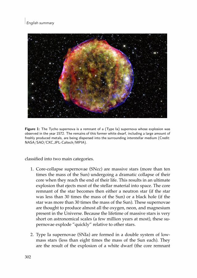
English summary
Figure 1: The Tycho supernova is a remnant of a (Type Ia) supernova whose explosion wasobserved in the year 1572. The remains of this former white dwarf, including a large amount offreshly produced metals, are being dispersed into the surrounding interstellar medium (Credit:NASA/SAO/CXC,JPL-Caltech/MPIA).
classified into two main categories.
1. Core-collapse supernovae (SNcc) are massive stars (more than tentimes the mass of the Sun) undergoing a dramatic collapse of theircore when they reach the end of their life. This results in an ultimateexplosion that ejects most of the stellar material into space. The coreremnant of the star becomes then either a neutron star (if the starwas less than 30 times the mass of the Sun) or a black hole (if thestar was more than 30 times the mass of the Sun). These supernovaeare thought to produce almost all the oxygen, neon, and magnesiumpresent in the Universe. Because the lifetime of massive stars is veryshort on astronomical scales (a few million years at most), these su-pernovae explode ”quickly” relative to other stars.
2. Type Ia supernovae (SNIa) are formed in a double system of low-mass stars (less than eight times the mass of the Sun each). Theyare the result of the explosion of a white dwarf (the core remnant
302
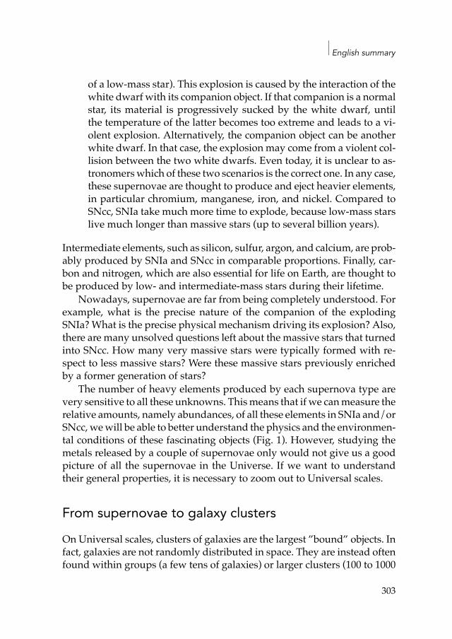
English summary
of a low-mass star). This explosion is caused by the interaction of thewhite dwarf with its companion object. If that companion is a normalstar, its material is progressively sucked by the white dwarf, untilthe temperature of the latter becomes too extreme and leads to a vi-olent explosion. Alternatively, the companion object can be anotherwhite dwarf. In that case, the explosion may come from a violent col-lision between the two white dwarfs. Even today, it is unclear to as-tronomerswhich of these two scenarios is the correct one. In any case,these supernovae are thought to produce and eject heavier elements,in particular chromium, manganese, iron, and nickel. Compared toSNcc, SNIa take much more time to explode, because low-mass starslive much longer than massive stars (up to several billion years).
Intermediate elements, such as silicon, sulfur, argon, and calcium, are prob-ably produced by SNIa and SNcc in comparable proportions. Finally, car-bon and nitrogen, which are also essential for life on Earth, are thought tobe produced by low- and intermediate-mass stars during their lifetime.
Nowadays, supernovae are far from being completely understood. Forexample, what is the precise nature of the companion of the explodingSNIa?What is the precise physical mechanism driving its explosion? Also,there are many unsolved questions left about the massive stars that turnedinto SNcc. How many very massive stars were typically formed with re-spect to less massive stars? Were these massive stars previously enrichedby a former generation of stars?
The number of heavy elements produced by each supernova type arevery sensitive to all these unknowns. Thismeans that if we canmeasure therelative amounts, namely abundances, of all these elements in SNIa and/orSNcc,wewill be able to better understand the physics and the environmen-tal conditions of these fascinating objects (Fig. 1). However, studying themetals released by a couple of supernovae only would not give us a goodpicture of all the supernovae in the Universe. If we want to understandtheir general properties, it is necessary to zoom out to Universal scales.
From supernovae to galaxy clustersOn Universal scales, clusters of galaxies are the largest ”bound” objects. Infact, galaxies are not randomly distributed in space. They are instead oftenfound within groups (a few tens of galaxies) or larger clusters (100 to 1000
303
English summary
Figure 2: The galaxy cluster Abell 1689. At optical wavelengths (here in yellow), the individualgalaxies can be seen. However, most of the ”normal” matter of the cluster is present in theform of a hot gas, visible in X-ray (here in purple). This gas is also rich in metals, whichare produced by SNIa and SNcc over the last billion years (Credit: NASA, ESA, E. Jullo, P.Natarajan, and J-P. Kneib).
galaxies). All the stars, planets, and the interstellar gas and dust belongingto the galaxies accounts for only 10 to 20 percent of the total visible (or”normal”) matter in a galaxy cluster. The major ”normal” component ofgalaxy clusters is, in fact, in the form of a very hot, diffuse gas. Becauseof the very large gravity in clusters, this intra-cluster medium (ICM) fallsrapidly towards the centre, interacts and collides with itself, and is thusheated up to 10 to 100million degrees. This extreme heatingmakes that gasvisible in X-ray light (Fig. 2). The most recent generation of X-ray satellites,in particular the EuropeanmissionXMM-Newton (Fig. 3 left), is well suitedto observe the ICM and study its properties via X-ray spectroscopy.
304
English summary
What is X-ray spectroscopy?Like many other telescopes on Earth or in orbit around the Earth, the cur-rent X-ray space telescopes can do much more than simply ”see” astro-physical sources in the sky. Exactly like a rainy cloud is able to decomposesunlight into a wide range of colours (or more specifically, wavelengths),the instruments onboard themost recent X-ray satellites are able to decom-pose the X-ray light coming from the hot ICM. By analysing the relativeamounts of all these X-ray ”colours” we get (in other words, what its X-rayspectrum looks like), we can determine various features of that gas, suchas its temperature or its density.
Metals in the hot intra-cluster mediumAbout forty years ago, astronomers discovered the presence of emissionlines in the X-ray spectra of this intra-cluster gas. These emission lines area characteristic imprint of the presence of heavy elements. This means thatthe ICM contains a significant fraction of metals. Since only supernovaecan produce heavy elements, these metals must originate from SNIa andSNcc within the individual galaxies. Metals are thus not only located inthe vicinity of supernovae, but also in the ICM, beyond galaxies. In otherwords, even the largest scales of the Universe are chemically enriched bystars and supernovae.
Luckily, the X-ray emission of the ICM is easy to model with comput-ers, and the metal abundances of this gas can be accurately measured, byanalysing their corresponding lines in the X-ray spectra of galaxy clusters(Fig. 3 right). In turn, because they trace the total yields of billions of su-pernovae over cosmic times, the abundances of these elements measuredin the ICM can be directly compared to the yields predicted by the cur-rently competing SNIa and SNcc theoretical models. This helps to favoursome specific scenarios for supernovae, and to rule out some others. Even-tually, measuring the amount of metals in galaxy clusters enables us tobetter understand supernovae.
How about the spatial distribution of these metals in galaxy clusters?Are they concentrated rather in the core of clusters, or rather in the out-skirts? Are they distributed uniformly through the intra-cluster gas, or arethey present in some specific regions only?Answering these questionsmayprovide valuable information to understand how and when stars and su-
305
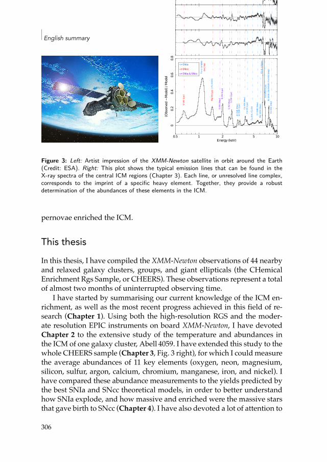
English summary
0.1
00.
10
.10
0.1
(Obs
erve
d
Mod
el) /
Mod
el
1 100.5 2 5
0.1
00.
1
Energy (keV)
MOS1
MOS2
pn
1 100.5 2 5
00.
20.
40.
60.
8(O
bser
ved
Mod
el) /
Mod
el
Energy (keV)
O VI
II (L
y)
FeL
com
plex
(incl.
Ne)
Mg
XII (
Ly)
Si X
III (H
e) Si
XIV
(Ly
)
S XV
(He
)S
XVI (
Ly)
Ar X
VII (
He)
Ar X
VIII
(Ly
)
Ca X
IX (H
e)
Ca X
X (L
y)
Ca X
IX /
Ca X
X
Cr X
XIII
(He
)M
n XX
IV (H
e)
FeK
com
plex
Fe X
XVI (
Ly)
Fe X
XV (H
e)
(/ Fe
XXI
V)
Ni X
XVII
/ Ni X
XVIII
/ Fe
XXV
(He
)
> SNIa> SNcc> SNIa & SNcc
Figure 3: Left: Artist impression of the XMM-Newton satellite in orbit around the Earth(Credit: ESA). Right: This plot shows the typical emission lines that can be found in theX-ray spectra of the central ICM regions (Chapter 3). Each line, or unresolved line complex,corresponds to the imprint of a specific heavy element. Together, they provide a robustdetermination of the abundances of these elements in the ICM.
pernovae enriched the ICM.
This thesisIn this thesis, I have compiled the XMM-Newton observations of 44 nearbyand relaxed galaxy clusters, groups, and giant ellipticals (the CHemicalEnrichment Rgs Sample, or CHEERS). These observations represent a totalof almost two months of uninterrupted observing time.
I have started by summarising our current knowledge of the ICM en-richment, as well as the most recent progress achieved in this field of re-search (Chapter 1). Using both the high-resolution RGS and the moder-ate resolution EPIC instruments on board XMM-Newton, I have devotedChapter 2 to the extensive study of the temperature and abundances inthe ICM of one galaxy cluster, Abell 4059. I have extended this study to thewhole CHEERS sample (Chapter 3, Fig. 3 right), for which I couldmeasurethe average abundances of 11 key elements (oxygen, neon, magnesium,silicon, sulfur, argon, calcium, chromium, manganese, iron, and nickel). Ihave compared these abundance measurements to the yields predicted bythe best SNIa and SNcc theoretical models, in order to better understandhow SNIa explode, and how massive and enriched were the massive starsthat gave birth to SNcc (Chapter 4). I have also devoted a lot of attention to
306
English summary
all the uncertainties that may affect the final results. In particular, I have in-vestigated the effects that the latestmajor update of the spectral code SPEX,which is used to model the X-ray emission of the ICM, has on the averageabundance measurements (Chapter 5). Finally, the EPIC instruments onboard XMM-Newton also allow for a study of the radial distribution of thedifferent elements in the ICM (Chapter 6). In turn, this provides importantclues on the main epoch and the dynamics driving the ICM enrichment.The conclusions of this thesis are various, but can be summarised as fol-lows.
• In some cases, the metal distribution in galaxy clusters is far frombeing symmetric. Abell 4059 is a textbook example, where a dense,metal-rich region of the hot gas is found outside of the cluster centre.This suggests that galaxies can enrich their surroundingswithmetalswhen they travel so fast that their gas gets stripped by the ambientICM pressure.
• I have probably obtained themost accurate ICMabundancemeasure-ments that are ever possible to obtain with XMM-Newton. Furthersignificant improvements of thesemeasurements cannot be achievedwithout better instruments on board future X-ray missions, such asXARM or Athena (Chapter 7), or without a substantial reduction ofthe systematic uncertainties (for example a better calibration of theXMM-Newton instruments).
• The average ICMabundancemeasurements I have obtained are valu-able to better understand supernovae. In particular, they suggest thatthe burning flame driving SNIa explosions propagates first below thespeed of sound, then reaches a supersonic speed before ejecting thestellar material into space. They also suggest that most of the SNcchaving enriched galaxy clusters come from massive stars that hadbeen already enriched by a former generation of stars. Finally, it ispossible that a specific sub-class of SNIa, namely theCa-rich gap tran-sients, which produce and release calcium in very large quantities,play an important role in enriching galaxy clusters.
• In the hot gas of relaxed galaxy clusters and groups, the radial dis-tribution of oxygen, magnesium, silicon, sulfur, argon, calcium, iron,and nickel are all peaked: there is more of these metals in the centrethan in the outskirts of clusters. On average, these profiles are all very
307

English summary
similar to each other. This strongly suggests that both SNIa and SNccenrich clusters in a very similar way. Given that SNIa take longer toexplode than SNcc, this probably means that the bulk of the ICM en-richment occurred at early times, before the Universe was half of itscurrent age.
308
Résumé en français
D’où venous-nous? Cette question est bien-sûr très vaste puisqu’elle con-cerne de nombreuses disciplines (physique, biologie, astronomie, philoso-phie, etc.), et il est difficile (sinon impossible) d’y apporter une seule etmême réponse. Une des plus extraordinaires découvertes astronomiquesdu XXe siècle a pourtant révolutionné notre conception de l’Univers parrapport à cette question. Il y a soixante ans, on a compris que les briquesélémentaires essentielles à la formation des planètes et de la vie ont étéforgées au coeur même des étoiles, et dans la puissante explosion qu’ellesgénèrent à la fin de leur vie: les supernovae. Finalement, nous ne sommesrien d’autre que des ”poussières d’étoiles”.
L'origine des éléments chimiquesCes briques élémentaires sont appelées les éléments chimiques. Elles s’as-semblent enmolécules pour ensuite former les étoiles, les planètes, la roche,l’eau, les cellules, les plantes, les animaux, etc. Elles sont l’essencemême dela matière et de la vie. Grâce au travail remarquable de plusieurs généra-tions d’astrophysiciens au cours des dernières décennies, nous connais-sons l’histoire de la production des éléments chimiques dans l’Univers. Ily a environ 13.7 milliards d’années, les conditions extrêmes qui suivirentles premières minutes du Big Bang ont créé tout l’hydrogène et presquetout l’hélium que l’on retrouve aujourd’hui dans le Cosmos. Par contre,les éléments plus lourds (ou ”métaux”, par exemple le carbone, l’azote,l’oxygène, le silicium, le fer, etc.) n’ont pas pu se former lors de ces pre-mières minutes. Ces métaux sont en fait fabriqués dans la dense et bouil-lonnante fournaise du coeur des étoiles, et en particulier lorsque ces étoiles
309
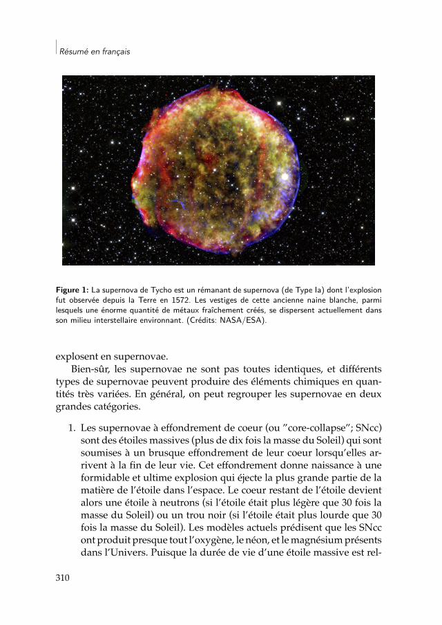
Résumé en français
Figure 1: La supernova de Tycho est un rémanant de supernova (de Type Ia) dont l’explosionfut observée depuis la Terre en 1572. Les vestiges de cette ancienne naine blanche, parmilesquels une énorme quantité de métaux fraîchement créés, se dispersent actuellement dansson milieu interstellaire environnant. (Crédits: NASA/ESA).
explosent en supernovae.Bien-sûr, les supernovae ne sont pas toutes identiques, et différents
types de supernovae peuvent produire des éléments chimiques en quan-tités très variées. En général, on peut regrouper les supernovae en deuxgrandes catégories.
1. Les supernovae à effondrement de coeur (ou ”core-collapse”; SNcc)sont des étoiles massives (plus de dix fois la masse du Soleil) qui sontsoumises à un brusque effondrement de leur coeur lorsqu’elles ar-rivent à la fin de leur vie. Cet effondrement donne naissance à uneformidable et ultime explosion qui éjecte la plus grande partie de lamatière de l’étoile dans l’espace. Le coeur restant de l’étoile devientalors une étoile à neutrons (si l’étoile était plus légère que 30 fois lamasse du Soleil) ou un trou noir (si l’étoile était plus lourde que 30fois la masse du Soleil). Les modèles actuels prédisent que les SNccont produit presque tout l’oxygène, le néon, et lemagnésiumprésentsdans l’Univers. Puisque la durée de vie d’une étoile massive est rel-
310
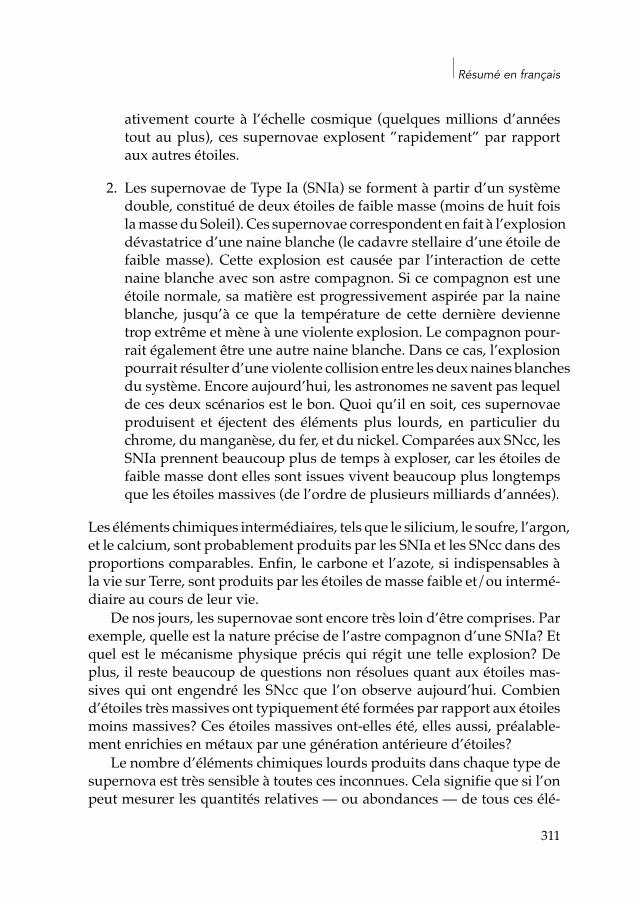
Résumé en français
ativement courte à l’échelle cosmique (quelques millions d’annéestout au plus), ces supernovae explosent ”rapidement” par rapportaux autres étoiles.
2. Les supernovae de Type Ia (SNIa) se forment à partir d’un systèmedouble, constitué de deux étoiles de faible masse (moins de huit foislamasse du Soleil). Ces supernovae correspondent en fait à l’explosiondévastatrice d’une naine blanche (le cadavre stellaire d’une étoile defaible masse). Cette explosion est causée par l’interaction de cettenaine blanche avec son astre compagnon. Si ce compagnon est uneétoile normale, sa matière est progressivement aspirée par la naineblanche, jusqu’à ce que la température de cette dernière deviennetrop extrême et mène à une violente explosion. Le compagnon pour-rait également être une autre naine blanche. Dans ce cas, l’explosionpourrait résulter d’une violente collision entre les deuxnaines blanchesdu système. Encore aujourd’hui, les astronomes ne savent pas lequelde ces deux scénarios est le bon. Quoi qu’il en soit, ces supernovaeproduisent et éjectent des éléments plus lourds, en particulier duchrome, dumanganèse, du fer, et du nickel. Comparées aux SNcc, lesSNIa prennent beaucoup plus de temps à exploser, car les étoiles defaible masse dont elles sont issues vivent beaucoup plus longtempsque les étoiles massives (de l’ordre de plusieurs milliards d’années).
Les éléments chimiques intermédiaires, tels que le silicium, le soufre, l’argon,et le calcium, sont probablement produits par les SNIa et les SNcc dans desproportions comparables. Enfin, le carbone et l’azote, si indispensables àla vie sur Terre, sont produits par les étoiles de masse faible et/ou intermé-diaire au cours de leur vie.
De nos jours, les supernovae sont encore très loin d’être comprises. Parexemple, quelle est la nature précise de l’astre compagnon d’une SNIa? Etquel est le mécanisme physique précis qui régit une telle explosion? Deplus, il reste beaucoup de questions non résolues quant aux étoiles mas-sives qui ont engendré les SNcc que l’on observe aujourd’hui. Combiend’étoiles trèsmassives ont typiquement été formées par rapport aux étoilesmoins massives? Ces étoiles massives ont-elles été, elles aussi, préalable-ment enrichies en métaux par une génération antérieure d’étoiles?
Le nombre d’éléments chimiques lourds produits dans chaque type desupernova est très sensible à toutes ces inconnues. Cela signifie que si l’onpeut mesurer les quantités relatives — ou abondances — de tous ces élé-
311
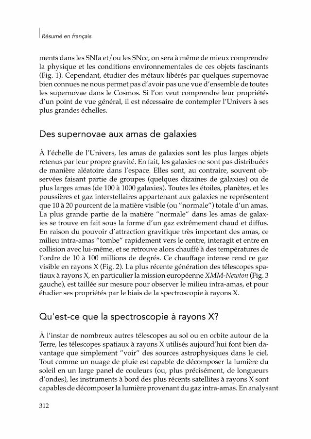
Résumé en français
ments dans les SNIa et/ou les SNcc, on sera à même demieux comprendrela physique et les conditions environnementales de ces objets fascinants(Fig. 1). Cependant, étudier des métaux libérés par quelques supernovaebien connues ne nous permet pas d’avoir pas une vue d’ensemble de toutesles supernovae dans le Cosmos. Si l’on veut comprendre leur propriétésd’un point de vue général, il est nécessaire de contempler l’Univers à sesplus grandes échelles.
Des supernovae aux amas de galaxies
À l’échelle de l’Univers, les amas de galaxies sont les plus larges objetsretenus par leur propre gravité. En fait, les galaxies ne sont pas distribuéesde manière aléatoire dans l’espace. Elles sont, au contraire, souvent ob-servées faisant partie de groupes (quelques dizaines de galaxies) ou deplus larges amas (de 100 à 1000 galaxies). Toutes les étoiles, planètes, et lespoussières et gaz interstellaires appartenant aux galaxies ne représententque 10 à 20 pourcent de la matière visible (ou ”normale”) totale d’un amas.La plus grande partie de la matière ”normale” dans les amas de galax-ies se trouve en fait sous la forme d’un gaz extrêmement chaud et diffus.En raison du pouvoir d’attraction gravifique très important des amas, cemilieu intra-amas ”tombe” rapidement vers le centre, interagit et entre encollision avec lui-même, et se retrouve alors chauffé à des températures del’ordre de 10 à 100 millions de degrés. Ce chauffage intense rend ce gazvisible en rayons X (Fig. 2). La plus récente génération des télescopes spa-tiaux à rayons X, en particulier lamission européenneXMM-Newton (Fig. 3gauche), est taillée sur mesure pour observer le milieu intra-amas, et pourétudier ses propriétés par le biais de la spectroscopie à rayons X.
Qu'est-ce que la spectroscopie à rayons X?
À l’instar de nombreux autres télescopes au sol ou en orbite autour de laTerre, les télescopes spatiaux à rayons X utilisés aujourd’hui font bien da-vantage que simplement ”voir” des sources astrophysiques dans le ciel.Tout comme un nuage de pluie est capable de décomposer la lumière dusoleil en un large panel de couleurs (ou, plus précisément, de longueursd’ondes), les instruments à bord des plus récents satellites à rayons X sontcapables de décomposer la lumière provenant dugaz intra-amas. En analysant
312
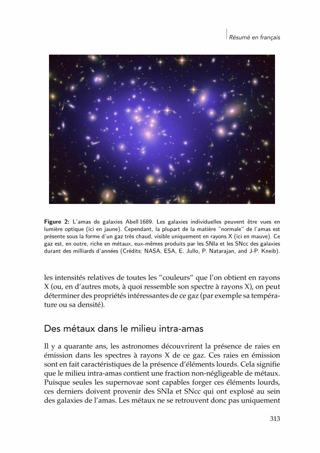
Résumé en français
Figure 2: L’amas de galaxies Abell 1689. Les galaxies individuelles peuvent être vues enlumière optique (ici en jaune). Cependant, la plupart de la matière ”normale” de l’amas estprésente sous la forme d’un gaz très chaud, visible uniquement en rayons X (ici en mauve). Cegaz est, en outre, riche en métaux, eux-mêmes produits par les SNIa et les SNcc des galaxiesdurant des milliards d’années (Crédits: NASA, ESA, E. Jullo, P. Natarajan, and J-P. Kneib).
les intensités relatives de toutes les ”couleurs” que l’on obtient en rayonsX (ou, en d’autres mots, à quoi ressemble son spectre à rayons X), on peutdéterminer des propriétés intéressantes de ce gaz (par exemple sa tempéra-ture ou sa densité).
Des métaux dans le milieu intra-amasIl y a quarante ans, les astronomes découvrirent la présence de raies enémission dans les spectres à rayons X de ce gaz. Ces raies en émissionsont en fait caractéristiques de la présence d’éléments lourds. Cela signifieque le milieu intra-amas contient une fraction non-négligeable de métaux.Puisque seules les supernovae sont capables forger ces éléments lourds,ces derniers doivent provenir des SNIa et SNcc qui ont explosé au seindes galaxies de l’amas. Les métaux ne se retrouvent donc pas uniquement
313
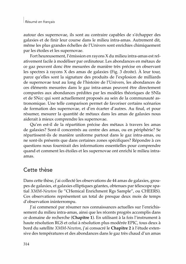
Résumé en français
autour des supernovae, ils sont au contraire capables de s’échapper desgalaxies et de finir leur course dans le milieu intra-amas. Autrement dit,même les plus grandes échelles de l’Univers sont enrichies chimiquementpar les étoiles et les supernovae.
Fort heureusement, l’émission en rayons X dumilieu intra-amas est rel-ativement facile à modéliser par ordinateur. Les abondances en métaux dece gaz peuvent donc être mesurées de manière très précise en observantles spectres à rayons X des amas de galaxies (Fig. 3 droite). À leur tour,parce qu’elles sont la signature des produits de l’explosion de milliardsde supernovae tout au long de l’histoire de l’Univers, les abondances deces éléments mesurées dans le gaz intra-amas peuvent être directementcomparées aux abondances prédites par les modèles théoriques de SNIaet de SNcc qui sont actuellement proposés au sein de la communauté as-tronomique. Une telle comparison permet de favoriser certains scénariosde formation des supernovae, et d’en écarter d’autres. Au final, et pourrésumer, mesurer la quantité de métaux dans les amas de galaxies nousaiderait à mieux comprendre les supernovae.
Qu’en est-il de la répartition précise des métaux à travers les amasde galaxies? Sont-il concentrés au centre des amas, ou en périphérie? Serépartissent-ils de manière uniforme partout dans le gaz intra-amas, oune sont-ils présents que dans certaines zones spécifiques? Répondre à cesquestions nous fournirait des informations essentielles pour comprendrequand et comment les étoiles et les supernovae ont enrichi le milieu intra-amas.
Cette thèseDans cette thèse, j’ai collecté les observations de 44 amas de galaxies, grou-pes de galaxies, et galaxies elliptiques géantes, obtenues par télescope spa-tial XMM-Newton (le ”CHemical Enrichment Rgs Sample”, ou CHEERS).Ces observations représentent un total de presque deux mois de tempsd’observation ininterrompu.
J’ai commencé par résumer nos connaissances actuelles sur l’enrichis-sement du milieu intra-amas, ainsi que les récents progrès accomplis dansce domaine de recherche (Chapitre 1). En utilisant à la fois l’instrument àhaute résolution RGS et celui à résolution plus modérée EPIC, tous deux àbord du satellite XMM-Newton, j’ai consacré le Chapitre 2 à l’étude exten-sive des températures et des abondances dans le gaz très chaud d’un amas
314
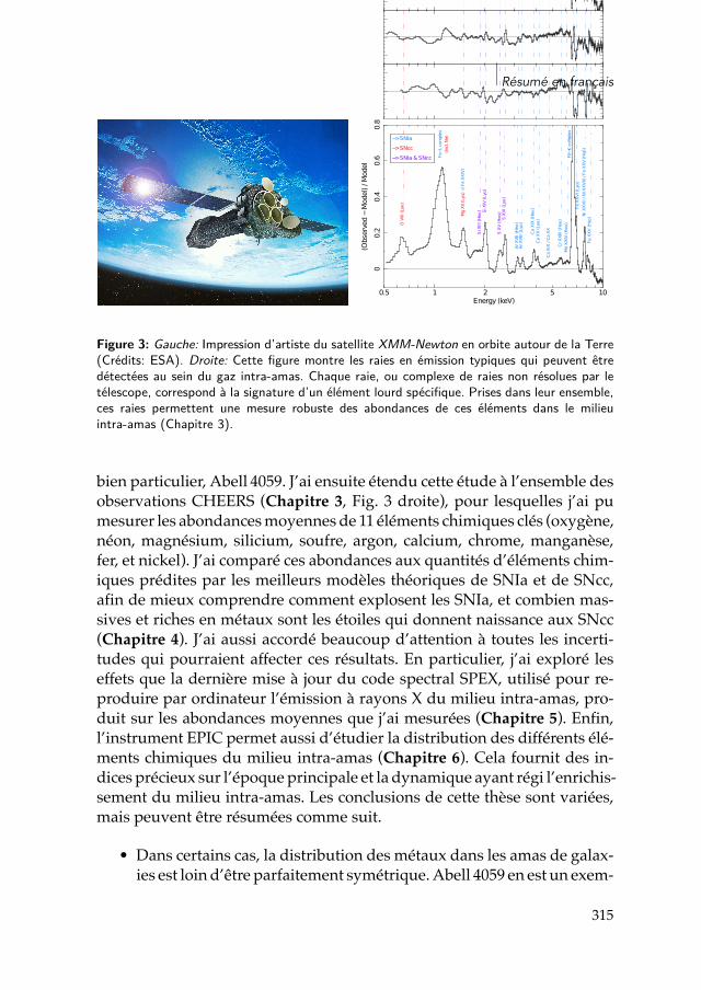
Résumé en français
0.1
00.
10
.10
0.1
(Obs
erve
d
Mod
el) /
Mod
el
1 100.5 2 5
0.1
00.
1
Energy (keV)
MOS1
MOS2
pn
1 100.5 2 5
00.
20.
40.
60.
8(O
bser
ved
Mod
el) /
Mod
el
Energy (keV)
O VI
II (L
y)
FeL
com
plex
(incl.
Ne)
Mg
XII (
Ly)
Si X
III (H
e) Si
XIV
(Ly
)
S XV
(He
)S
XVI (
Ly)
Ar X
VII (
He)
Ar X
VIII
(Ly
)
Ca X
IX (H
e)
Ca X
X (L
y)
Ca X
IX /
Ca X
X
Cr X
XIII
(He
)M
n XX
IV (H
e)
FeK
com
plex
Fe X
XVI (
Ly)
Fe X
XV (H
e)
(/ Fe
XXI
V)
Ni X
XVII
/ Ni X
XVIII
/ Fe
XXV
(He
)
> SNIa> SNcc> SNIa & SNcc
Figure 3: Gauche: Impression d’artiste du satellite XMM-Newton en orbite autour de la Terre(Crédits: ESA). Droite: Cette figure montre les raies en émission typiques qui peuvent êtredétectées au sein du gaz intra-amas. Chaque raie, ou complexe de raies non résolues par letélescope, correspond à la signature d’un élément lourd spécifique. Prises dans leur ensemble,ces raies permettent une mesure robuste des abondances de ces éléments dans le milieuintra-amas (Chapitre 3).
bien particulier, Abell 4059. J’ai ensuite étendu cette étude à l’ensemble desobservations CHEERS (Chapitre 3, Fig. 3 droite), pour lesquelles j’ai pumesurer les abondancesmoyennes de 11 éléments chimiques clés (oxygène,néon, magnésium, silicium, soufre, argon, calcium, chrome, manganèse,fer, et nickel). J’ai comparé ces abondances aux quantités d’éléments chim-iques prédites par les meilleurs modèles théoriques de SNIa et de SNcc,afin de mieux comprendre comment explosent les SNIa, et combien mas-sives et riches en métaux sont les étoiles qui donnent naissance aux SNcc(Chapitre 4). J’ai aussi accordé beaucoup d’attention à toutes les incerti-tudes qui pourraient affecter ces résultats. En particulier, j’ai exploré leseffets que la dernière mise à jour du code spectral SPEX, utilisé pour re-produire par ordinateur l’émission à rayons X du milieu intra-amas, pro-duit sur les abondances moyennes que j’ai mesurées (Chapitre 5). Enfin,l’instrument EPIC permet aussi d’étudier la distribution des différents élé-ments chimiques du milieu intra-amas (Chapitre 6). Cela fournit des in-dices précieux sur l’époqueprincipale et la dynamique ayant régi l’enrichis-sement du milieu intra-amas. Les conclusions de cette thèse sont variées,mais peuvent être résumées comme suit.
• Dans certains cas, la distribution des métaux dans les amas de galax-ies est loin d’être parfaitement symétrique.Abell 4059 en est un exem-
315
Résumé en français
ple typique, où une région dense et riche en métaux est observée endehors du centre de l’amas. Cela suggère que les galaxies peuvent en-richir leurs environs en métaux lorsqu’elles voyagent tellement viteque leur gaz s’arrache sous l’effet de la pression dumilieu intra-amasenvironnant.
• J’ai probablement obtenu les mesures d’abondances du milieu intra-amas les plus précises qu’il soit jamais possible d’obtenir avec les téle-scopes spatiaux actuels. Des améliorations de cesmesures ne peuventêtre atteintes sans de meilleurs instruments à bord de futures mis-sions à rayons X, telles que XARM ou Athena (Chapitre 7), ou sansune réduction drastique des incertitudes systématiques (par exem-ple via une meilleure calibration des instruments de XMM-Newton).
• Lesmesuresmoyennes d’abondances du gaz intra-amas que j’ai obte-nues sont précieuses pourmieux comprendre les supernovae. Enpar-ticulier, elles suggèrent que la déflagration qui se propage lorsqu’uneSNIa explose se déplace d’abord à une vitesse raisonnable — en des-sous de la vitesse du son, ensuite s’accélère et atteint des vitesses su-personiques avant d’éjecter sa matière dans l’espace. Mes résultatssuggèrent aussi que la plupart des SNcc qui ont enrichi les amas degalaxies proviennent d’étoiles massives qui avaient déjà été aupar-avant enrichies par une précédente génération d’étoiles. Pour finir,il est possible qu’une sous-classe spécifique de SNIa, les ”Ca-richgap transients”, qui fabriquent et éjectent du calcium en très grandesquantités, jouent un rôle important dans l’enrichissement des amasde galaxies.
• Dans le gaz chaud des amas et groupes de galaxies, les distributionsradiales de l’oxygène, du magnésium, du silicium, du soufre, de l’ar-gon, du calcium, du fer, et du nickel sont toutes piquées: il y a bienplus demétauxdans le centre des amas qu’enpériphérie. Enmoyenne,ces profils sont très semblables les uns par rapport aux autres. Celasuggère fortement que les SNIa et les SNcc enrichissent toutes deuxle milieu intra-amas de manière très similaire. Étant donné que lesSNIa mettent plus de temps à exploser que les SNcc, cela impliqueprobablement que la majeure partie de cet enrichissement a eu lieuen des temps très lointains, avant même que l’Univers n’atteigne lamoitié de son âge actuel.
316
Curriculum Vitae
I was born on June 27, 1989, in Uccle (in Dutch, ”Ukkel”), one of the 19 mu-nicipalities of Brussels, in Belgium. Except for a period of two or three years(which I barely remember), in which we moved to a small town namedHannut, I spent almost the 20 first years ofmy life in Brussels. It was duringmy primary school (Le Jardin des Écoliers), after a class on the Solar Sys-tem (and on the mysteries of Pluto, which was still a planet at that time,and for which we had no picture yet) that I naively decided to becomean astronomer. I did my secondary studies at the Lycée Émile Jacqmain,where I graduated in ”Latin-mathematics” in 2007 (cum laude). Duringthose years, I regularly attended astronomy camps in Modave, where myinterest for astronomy and astrophysics kept growing.
I didmyBachelor degree in physics at theUniversité Libre de Bruxelles,where I graduated in 2010 (cum laude). My Bachelor project was focusedon the observation of variable stars using the telescope of the university,and was supervised by Sophie Van Eck. I finally left my home town in2010, when I started my Master degree in space sciences at the Universityof Liège. On that time, I developed a strong interest for high-energy astro-physics on one hand, and extragalactic astrophysics on the other hand. Idid my Master thesis with Gregor Rauw on the X-ray emission of massivestars in theM17 nebula as observed byXMM-Newton. Aftermy graduationin 2012 (magna cum laude), I stayed four more months at the University ofLiège to work with Thierry Morel on optical observations of the massivestar ζ Puppis. I devoted the next few months to tutor high school studentsin mathematics, physics, and chemistry before I moved to the Netherlandsin June 2013 to start my PhD.
This thesis summarises the results of my PhD project, and on which I
317
worked both at SRON (Utrecht) and Leiden Observatory with Jelle Kaas-tra and Jelle de Plaa. During these four years, I had the opportunity topresent my work at several conferences and workshops, in Dublin (Ire-land), Tokyo (Japan), Sexten (Italy), Madrid (Spain), Paris (France), andBeijing (China). I was also the lucky laureate of the ”poster prize” of the71st Dutch Astronomy Conference in Nunspeet (The Netherlands) in 2016.I spent a few weeks of my PhD to visit colleagues in other institutes: Yu-YingZhang, Lorenzo Lovisari, Thomas Reiprich, andGerrit Schellenberger(Argelander-Institut für Astronomie, Bonn, Germany), as well as NorbertWerner (MTA-Eötvös University Lendület Hot Universe Research Group,Budapest, Hungary), with whom I will work as a postdoc from September2017. From the first years of my academic studies up to now, I occasion-ally go back to Modave, this time as a ”teacher”, to share my knowledgeof astronomy with younger students (with the secret hope they will wantto become astronomer, too).
318
List of publications
First author publications• Mernier, F., de Plaa, J., Kaastra, Raassen, A. J. J., Gu, L., Mao, andUrdampil-leta, I.Origin of central abundances in the hot intra-cluster medium -III. The impact of spectral model improvements on the abundance ratios2017, A&A, submitted (this thesis, Chapter 5)
• Mernier, F., de Plaa, J., Kaastra, J. S., Zhang, Y.-Y., Akamatsu, H., Gu, L.,Kosec, P., Mao, J., Pinto, C., Reiprich, T. H., Sanders J. S., Simionescu, A.,and Werner, N.Radial metal abundance profiles in the intra-cluster medium of cool-core galaxyclusters, groups,and ellipticals2017, A&A, in press (this thesis, Chapter 6)
• Mernier, F., de Plaa, J., Pinto, C., Kaastra, J. S., Kosec, P., Zhang, Y.-Y., Mao,J., Werner, N., Pols, O. R., and Vink, J.Origin of central abundances in the hot intra-cluster medium -II. Chemical enrichment and supernova yield models2016b, A&A, 595, A126 (this thesis, Chapter 4)
• Mernier, F., de Plaa, J., Pinto, C., Kaastra, J. S., Kosec, P., Zhang, Y.-Y., Mao,J., and Werner, N.Origin of central abundances in the hot intra-cluster medium -I. Individual and average abundance ratios from XMM-Newton EPIC2016a, A&A, 592, A157 (this thesis, Chapter 3)
• Mernier, F., de Plaa, J., Lovisari, L., Pinto, C., Zhang, Y.-Y., Kaastra, J. S.,Werner, N., and Simionescu, A.
319
Abundance and temperature distributions in the hot intra-cluster gas of Abell 40592015, A&A, 575, A37 (this thesis, Chapter 2)
Co-author publications• Mao, J., de Plaa, J., Kaastra, J. S., Pinto, C., Gu, L.,Mernier, F., Hong-Liang,Y., Zhang, Y.-Y., and Akamatsu, H.Nitrogen abundance in X-ray halos of clusters and groups of galaxies2017, A&A, submitted
• Albert, J. G., Sifón, C., Stroe, A.,Mernier, F., Intema, H. T., Röttgering, H. J.A., Brunetti, G.Complex Diffuse Emission in the z=0.52 Cluster PLCK G004.5-19.52017, A&A, submitted
• de Plaa, J., Kaastra, J. S., Werner, N., Pinto, C., Kosec, P., Mernier, F., Lo-visari, L., Akamatsu, H., Schellenberger, G., Hofmann, F., Reiprich, T. H.,Finoguenov,A., Ahoranta, J., Sanders, J. S., Fabian,A.C., Pols,O. R., Simionescu,A., Vink, J., and Böhringer, H.CHEERS: The chemical evolution RGS sample2017, A&A, submitted
• Akamatsu, H., Fujita, Y., Akahori, T., Ishisaki, Y., Hayashida, K., Hoshino,A.,Mernier, F., Yoshikawa, K., Sato, K., and Kaastra, J. S.Properties of the cosmological filament between two clusters: A possible detectionof a large-scale accretion shock by Suzaku2017, A&A, in press
• de Plaa, J., andMernier, F.CHEERS: Future perspectives for abundancemeasurements in clusters withXMM-Newton2017, Astron. Nachr., in press
• Akamatsu, H., Gu, L., Shimwell, T.,Mernier, F., Mao, J., Urdampilleta, I., dePlaa, J., Röttgering, H. J. A., and Kaastra, J. S.Suzaku andXMM-Newton observations of the newly discovered early-stage clustermerger 1E2216.0-0401 and 1E2215.7-04042016, A&A, 593, L7
• Ichinohe, Y., Werner, N., Simionescu, A., Allen, S. W., Canning, R. E. A.,Elhert, S.,Mernier, F., and Takahashi, T.The growth of the galaxy cluster Abell 85: mergers, shocks, stripping and seedingof clumping2015, MNRAS, 448, 2971
320
Acknowledgements
Herewe are: the end of four rich and exciting years spent at both Leiden ob-servatory and SRON, but also full of great moments outside work. Writingthe ”acknowledgements” part of this manuscript is rather easy (becausethis thesis would not have been possible without the valuable help of somany people), and at the same time rather difficult (because I must takecare of not forgetting anyone to thank).
First of all, this thesis was made possible thanks to Jelle de Plaa, whosuccessfully obtained most of the very deep XMM-Newton data analysedhere, and who built the entire CHEERS project. But far beyond that, Jellewas always available and ready to help me, from the very first days tothe very last steps of my PhD thesis. I will never be grateful enough forall the expertise I have learned from him. Thank you Jelle! One Jelle mayhide another, and I’m also very grateful to Jelle Kaastra for all his usefulscientific and non-scientific advice, as well as for his constant optimismand support throughout these four years.
To become a doctor, you first need to get a PhD position. This requirestwo ingredients: (i) a deeppassion for astronomyand (ii) peoplewhogreatlysupport you and recommend you. This is why I deeply thank: (i) my highschool physics teacher Albert Friadt and all the members of the association”Jeunesse et Science” for having made me an astro-addict, and (ii) GregorRauw, Yaël Nazé, Thierry Morel, and Michaël De Becker for all their helpand support during my Master thesis and during my search for a PhD po-sition.
A PhD thesis is nothing either without excellent collaborators. It was apleasure for me to work with Hiroki, Junjie, Igone, Liyi, and Ton as greatcolleagues within the cluster group at SRON. I also enjoyed working with
321
the whole CHEERS collaboration, in particular Yu-Ying (to the memory ofwhom I would like to dedicate most of the chapters of this thesis), Ciro,Norbert (I’m looking forward to starting my postdoc in your group!), Au-rora, Lorenzo, Yuto, Thomas, Jeremy, Florian, Onno, Jacco, Peter, and Ger-rit. All these friendly colleagues (and many more I may have forgotten)helped me to learn about chemical enrichment in clusters, but also aboutother fascinating aspects of cluster physics in general. I also had very nicediscussions with cluster people from Leiden, and I would like to thankHuub, Jit, Huib, Josh, Tim, Duy, Francesco, Andra, Jeroen, and Raymond.Igone, let me thank you once more for having helped me to organise thecluster meetings. You brought awesome ideas to make these meetings at-tractive and convivial! Finally, I really appreciated the availability and ami-ability of the supporting staff in Leiden: thanks a lot to Evelijn, Els, Erik,Eric, Alexandra, Marjan, Caroline, Anita, and Liesbeth for your assistance!
A nice advantage of doing a PhD in two different places is that the num-ber of awesome colleagues and friends increases by a factor of 2. Thanksto the ”followers of evolutionism” (they will recognise themselves), andto Marianne, Tullio, Laura, Zuzanna, Missagh, Lucien, Wim, Jean, Cor, Es-ther, Elisa, Theo, Jan-Willem, and all the other Astro-U members for thegreat and dynamical atmosphere you bring every day to SRON. Besides,I’ve been very lucky to be part of one of the weakest indoor football teamsthat have ever existed. However, nothing is impossible. From ”Village BikeFC” to ”The Supermassive BlackGoals” (via ”WTFITDMYT FC”), weman-aged to greatly improve our level, and to win two trophies (including onethat was not just to eat)! For all those great moments, thanks a lot to allof you, teammates: Emanuele, Clément, Jit (again!), Sasha, Ahmad, Chris-tos, Pedro, Santiago, Duy (again!), Zanjar, Fabian, Iulian, and Andrea. Clé-ment: le foot, les débats politiques, les discussions sur l’émission radiodes galaxies elliptiques géantes, les pauses café, et les borrels auraient étébien fades sans toi. Merci pour tout, et bonne suite pour ton futur postdoc!Also thanks to Darko, Edwin, David, Aayush, Mieke, Andrej, Ricardo, Va-leriya, Andrew, Tomasso,Nico, and Eleonora for the friendlymoments youbrought in the Kaiser Lounge and outside of the observatory.
Finally, the huge amount of work that a PhD thesis represents wouldbe impossible to achieve without a strong support from friends and fam-ily. A huge thanks to all my friends, who are disseminated between Brus-sels, Liège, and the Netherlands! Lieselot, if these last four years have beenthe happiest ones in my life, it’s thanks to you. Thank you for having ac-
322
companied me and supported me during this great adventure! Whateverwill happen in the months/years to come, remember that I will be alwaysthere for you. Also, my ”Nederlandse samenvatting” would have lookedso ridiculouswithout your valuable help to translate it. Thank you somuchfor this as well! Le dernier mot de remerciement sera pourma famille. Lise,il n’est jamais trop tard pour arrêter ton cinéma et faire de l’astronomie!Paul, un doctorat, ça vaut pas un fifa! Enfin, je termine cette thèse commeje l’ai commencée, en la dédiant à mes parents. On dit souvent qu’on nechoisit pas sa famille, mais qu’est-ce que je suis chanceux de vous avoir! Jene vous remercierai jamais assez pour votre soutien inconditionnel depuistoujours, en particulier durant ces quatre dernières années... et pour toutescelles à venir.
323

Related Documents