REPORT DOCUMENTATION PAGE AFRL-SR-BL-TR-98- 38 Public reporting burden for this collection of information Is estimated to average 1 hour per response, in and maintaining the data needed, and completing and reviewing the collection of information. Send information, including suggestions for reducing this burden, to Washington Headquarters Services, Direi 1204, Artington, VA 22202-4302, and to the Office of management and Budget, Paperwork Reduction Pre 1. AGENCY USE ONLY (Leave Blank) 2. REPORT DATE November, 1994 fr&O irees, gathering lis collection of Highway, Suite 3. F Final 4. TITLE AND SUBTITLE USAF Summer Research Program -1993 Summer Research Extension Program Final Reports, Volume 4B, Wright Laboratory 6. AUTHORS Gary Moore 7. PERFORMING ORGANIZATION NAME(S) AND ADDRESS(ES) Research and Development Labs, Culver City, CA 9. SPONSORING/MONITORING AGENCY NAME(S) AND ADDRESS(ES) AFOSR/NI 4040 Fairfax Dr, Suite 500 Arlington, VA 22203-1613 5. FUNDING NUMBERS 8. PERFORMING ORGANIZATION REPORT NUMBER 10. SPONSORING/MONITORING AGENCY REPORT NUMBER 11. SUPPLEMENTARY NOTES Contract Number: F4962-90-C-0076 12a. DISTRIBUTION AVAILABILITY STATEMENT Approved for Public Release 12b. DISTRIBUTION CODE 13. ABSTRACT (Maximum 200 words) The purpose of this program is to develop the basis for continuing research of interest to the Air Force at the institution of the faculty member; to stimulate continuing relations among faculty members and professional peers in the Air Force to enhance the research interests and capabilities of scientific and engineering educators; and to provide follow-on funding for research of particular promise that was started at an Air Force laboratory under the Summer Faculty Research Program. Each participant provided a report of their research, and these reports are consolidated into this annual report. 14. SUBJECT TERMS AIR FORCE RESEARCH, AIR FORCE, ENGINEERING, LABORATORIES, REPORTS, UNIVERSITIES 15. NUMBER OF PAGES 16. PRICE CODE 17. SECURITY CLASSIFICATION OF REPORT Unclassified 18. SECURITY CLASSIFICATION OF THIS PAGE Unclassified 19. SECURITY CLASSIFICATION OF ABSTRACT Unclassified 20. LIMITATION OF ABSTRACT UL Standard Form 298 (Rev. 2-89) Prescribed by ANSI Std. 239.18 Designed using WordPerfect 6.1, AFOSR/XPP, Oct 96

Welcome message from author
This document is posted to help you gain knowledge. Please leave a comment to let me know what you think about it! Share it to your friends and learn new things together.
Transcript

REPORT DOCUMENTATION PAGE AFRL-SR-BL-TR-98- 38
Public reporting burden for this collection of information Is estimated to average 1 hour per response, in and maintaining the data needed, and completing and reviewing the collection of information. Send information, including suggestions for reducing this burden, to Washington Headquarters Services, Direi 1204, Artington, VA 22202-4302, and to the Office of management and Budget, Paperwork Reduction Pre
1. AGENCY USE ONLY (Leave Blank) 2. REPORT DATE
November, 1994
fr&O irees, gathering lis collection of Highway, Suite
3. F
Final
4. TITLE AND SUBTITLE USAF Summer Research Program -1993 Summer Research Extension Program Final Reports, Volume 4B, Wright Laboratory 6. AUTHORS Gary Moore
7. PERFORMING ORGANIZATION NAME(S) AND ADDRESS(ES)
Research and Development Labs, Culver City, CA
9. SPONSORING/MONITORING AGENCY NAME(S) AND ADDRESS(ES)
AFOSR/NI 4040 Fairfax Dr, Suite 500 Arlington, VA 22203-1613
5. FUNDING NUMBERS
8. PERFORMING ORGANIZATION REPORT NUMBER
10. SPONSORING/MONITORING AGENCY REPORT NUMBER
11. SUPPLEMENTARY NOTES Contract Number: F4962-90-C-0076
12a. DISTRIBUTION AVAILABILITY STATEMENT
Approved for Public Release 12b. DISTRIBUTION CODE
13. ABSTRACT (Maximum 200 words) The purpose of this program is to develop the basis for continuing research of interest to the Air Force at the institution of the faculty member; to stimulate continuing relations among faculty members and professional peers in the Air Force to enhance the research interests and capabilities of scientific and engineering educators; and to provide follow-on funding for research of particular promise that was started at an Air Force laboratory under the Summer Faculty Research Program. Each participant provided a report of their research, and these reports are consolidated into this annual report.
14. SUBJECT TERMS AIR FORCE RESEARCH, AIR FORCE, ENGINEERING, LABORATORIES, REPORTS, UNIVERSITIES
15. NUMBER OF PAGES
16. PRICE CODE
17. SECURITY CLASSIFICATION OF REPORT
Unclassified
18. SECURITY CLASSIFICATION OF THIS PAGE
Unclassified
19. SECURITY CLASSIFICATION OF ABSTRACT
Unclassified
20. LIMITATION OF ABSTRACT
UL
Standard Form 298 (Rev. 2-89) Prescribed by ANSI Std. 239.18 Designed using WordPerfect 6.1, AFOSR/XPP, Oct 96
UNITED STATES AIR FORCE
SUMMER RESEARCH PROGRAM - 1993
SUMMER RESEARCH EXTENSION PROGRAM FINAL REPORTS
VOLUME 4B
WRIGHT LABORATORY
RESEARCH & DEVELOPMENT LABORATORIES
5800 Upiander Way
Culver City, CA 90230-6608
n. artnr Rni Program Manager, AFOSR Program Director, RDL £ Davjd ^ Gary Moore J
*« ~n*r Rni Program Administrator, RDL Program Manager, RDL r 9 ^ Scott Licoscos ow '
Program Administrator, RDL Johnetta Thompson
Submitted to:
AIR FORCE OFFICE OF SCIENTIFIC RESEARCH
Boiling Air Force Base
Washington, D.C.
November 1994
BTIG QUALITY INSPECTED 4
PREFACE
This volume is part of a five-volume set that summarizes ^^^^^ 1993 AFOSR Summer Research Extension Program (SREP). The current volume, Volume4B of 5, presents the final reports of SREP participants at Wnght Laborarory.
Reoorts presented in this volume are arranged alphabetically by author and are numbered Reports presentea in 2-3, with each series of reports preceded by
r^l^en.1^. Reports in'the five— se, are crazed as fefiows:
VOLUME
1A
IB
5
TITLE
Armstrong Laboratory (part one)
Armstrong Laboratory (part two)
2 Phillips Laboratory
3 Rome Laboratory
4A Wright Laboratory (part one)
4B Wright Laboratory (part two)
Arnold Engineering Development Center Frank J. Seiler Research Laboratory Wilford Hall Medical Center

1993 SREP FINAL REPORTS
Armstrong Laboratory
VOLUME 1A
Report Title ReP0rt # Author's university
10
11
12
13
Three-Dimensional Calculation of Blood Flow in a Thick -Walled Vessel Using the University of Missouri, Rolla, MO
Wright State University, Dayton, OH
An Approach to On-Line Assessment and Diagnosis of Student Troubleshooting Knowl New Mexico State University, Las Cruces, NM
An Experimental Investigation of Hand Torque Strength for Tightening Small Fast g
Tennessee Technological University, Cookeville, TN
Determination of Total Peripheral Resistance, Arterial Compliance and Venous Com North Dakota State University, Fargo, ND
A Computational Thermal Model and Theoretical Thermodynamic Model of Laser Indue Florida International University, Miami, FL
A Comparison of Various Estimators of Half-Life in the Air Force Health Study University of Maine, Orono, ME
The Effects of Exogenous Melatonin on Fatigue, Performance and Daytime Sleep Bowling Green State University, Bowling Green, OH
Report Author Dr. Xavier Avula
Mechanical & Aerospace AL/AO Engineering
Dr. Jer-sen Chen Computer Science &
AL/CF Engineering
Dr. Nancy Cooke Psychology
AL/HR
Dr. Subramaniam Deivanayagam Industrial Engineering
A1V-UR
Dr. Dan Ewert
Electrical Engineering AL/AO
Dr. Bernard Gerstman Physics
AL/OE
Dr. Pushpa Gupta Mathematics
AL/AO
Mr. Rod Hughes Psychology
AL/CF
A New Protocol for Studying Carotid Baroreceptor Function
Georgia Institute of Technology, Atlanta, GA
Adaptive Control Architecture for Teleoperated Freflex System
Purdue University, West Lafayette, IN
University of Tennessee, Memphis, TN
MuÄw!°"mM*C»»P»"»» »'A«en,a,ive
Arizona State University, Tempe, AZ
5l*Sr Red"C,i»" »f E—'» * Air FM,C University of Georgia Research, Athens, GA
Dr. Arthur Koblasz Civil Engineering
AL/AO B
Dr. A. Koivo
Electrical Engineering AJL/C..F
Dr. Robert Kundich Biomedical Engineering
Dr. William Moor InduStrial & Management
AL/HR Engineering
Dr. B. Mulligan Psychology
AL/OE
1993 SREP FINAL REPORTS
Armstrong Laboratory
VOLUME IB
Report Title Report # A..?hnr's University
Report Author
14
15
16
17
18
19
20
21
22
23
Simulation of the Motion of Single and Linked Ellipsiods
Representing Human Body Wright State University, Dayton, OH
Bioeffects of Microwave Radiation on Mammalian Cells and
Cell Cultures Xavier University of Louisiana, New Orleans, LA
Analysis of Isocyanate Monomers and Oligomers in Spray Paint
Formulations rrv Southwest Texas State University, San Marcos, TX
Development of the "Next Generation" of the Activities Interest
Inventory for Se Wayne State University, Detroit, MI
Investigations on the Seasonal Bionomics of the Asian Tiger
Mosquito, Aedes Albo Macon College, Macon, GA
Difficulty Facets Underlying Cognitive Ability Test Items
Ohio State University, Columbus, OH
A Simplified Model for Predicting Jet Impingement Heat
North Carolina A & T State University, Greensboro, NC
Geostatistical Techniques for Understanding Hydraulic Conductivity Variability Washington State University, Pullman, WA
An Immobilized Cell Fluidized Bed Bioreactor for 2,4-Dinitrotoluene Degradation Colorado State University, Fort Collins, CO
Applications of Superconductive Devices in Air Force
Alfred University, Alfred, NY
Dr. David Reynolds Biomedical & Human
ALICE Factors
Dr. Donald Robinson Chemistry
AL/OE
Dr. Walter Rudzinski Chemistry
AL/OE
Dr. Lois Tetrick Industrial Relations Prog
AL/HR
Dr. Michael Womack Natural Science and
AL/OE Mathematics
Dr. Mary Roznowski Psychology
AL/HR
Mr. Mark Kitchart Mechanical Engineering
AL/EQ
Dr. Valipuram Manoranjan Pure and Applied
AL/EQ Mathematics
Dr. Kenneth Reardon Agricultural and Chemical
AL/EQ Engineering
Dr. Xingwu Wang Electrical Engineering
AL/EQ
in
1993 SREP FINAL REPORTS
Phillips Laboratory
VOLUME 2
Report Title Report # Author's TTniw^jty
10
11
12
13
14
°ptimal Passive Damping of a Complex Strut-Built Structure "
Iowa State University, Ames, IA
Theoretical and Experimental Studies on the Effects of Low-Energy X-Rays on Elec University of Arizona, Tucson, AZ
Uttrawideband Antennas with Low Dispersion for Impulse
University of Alabama, Huntsville, AL
Experimental Neutron Scattering Investigations of Liquid-Crystal Polymers Arkansas Technology University, Russellville, AR
SrlTrratU^SpeCtrOSCOPy °f Alka,i Metal VaP°™ for solar to Thermal Energy University of Iowa, Iowa City, IA
Vefcc-r^ University of Southern California, Los Angeles, CA
Measurements of Ion-Molecule Reactions at High Temperatures
University of Puerto Rico, Mayaguez, PR
OpnticaIIeRS,gend C°nStrUCti°n °f Lidar Receiver *>r the Starfire
Georgia Institute of Technology, Atlanta, GA
Dynamics of Gas-Phase Ion-Molecule Reactions
Carnegie Mellon University, Pittsburgh, PA
A Numerical Approach to Evaluating Phase Change Material Performance in Infrared University of Texas, San Antonio, TX
An Analysis of ISAR Imaging and Image Simulation lechnologies and Related Post University of Nevada, Reno, NV
Optical and Clear Air Turbulence
Worcester Polytechnic Institut, Worcester, MA
Rotational Dynamics of Lageos Satellite
North Carolina State University, Raleigh, NC
Study of Instabilities Excited by Powerful HF Waves for Efficient Generation of Polytechnic University, Farmingdale, NY
Report Author Dr. Joseph Baumgarten
Mechanical Engineering
Dr. Raymond Beliem Electrical & Computer
PL/VT Engineering
Dr. Albert Biggs
Electrical Engineering PL/WS
Dr. David Elliott Engineering
PL/RK
Mr. Paul Erdman Physics and Astronomy
PL/RK
Dr. Daniel Erwin
Aerospace Engineering x LARK
Dr. Jeffrey Friedman Physics
PL/GP
Dr. Gary Gimmestad Research Institute
PL/LI
Dr. Susan Graul Chemistry
PL/WS
Mr. Steven Griffin Engineering
PL/VT
Dr. James Henson
Electrical Engineering PL/WS 8
Dr. Mayer Humi Mathematics
PL/LI
Dr. Arkady Kheyfets Mathematics
PL/LI
Dr. Spencer Kuo Electrical Engineering
IV
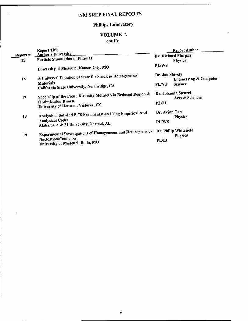
1993 SREP FINAL REPORTS
Phillips Laboratory
VOLUME 2 cont'd
Report Title Report # A.ithnr's University
15 Particle Stimulation of Plasmas
Report Author
University of Missouri, Kansas City, MO
16 A Universal Equation of State for Shock in Homogeneous Materials California State University, Northndge, CA
17 Speed-Up of the Phase Diversity Method Via Reduced Region & Optimization Dimen. University of Houston, Victoria, TX
18 Analysis of Solwind P-78 Fragmentation Using Empirical And Analytical Codes Alabama A & M University, Normal, AL
19 Experimental Investigations of Homogeneous and Heterogeneous Nucleation/Condensa University of Missouri, Rolla, MO
Dr. Richard Murphy Physics
PL/WS
Dr. Jon Shively Engineering & Computer
PL/VT Science
Dr. Johanna Stenzel Arts & Sciences
PL/LI
Dr. Arjun Tan Physics
PL/WS
Dr. Philip Whitefield Physics
PL/LI
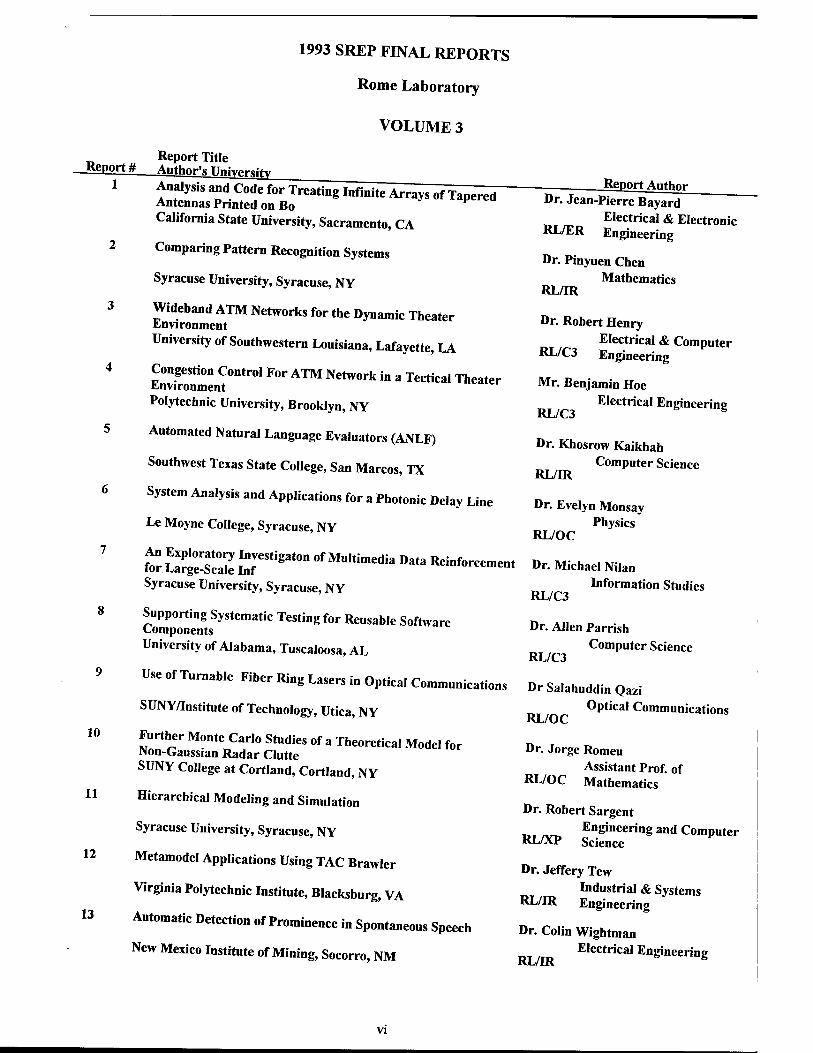
1993 SREP FINAL REPORTS
Rome Laboratory
VOLUME 3
Report Title Report # Author's Trn.w«.-^,
10
11
12
13
Analysis and Code for Treating Infinite Arrays of Tapered Antennas Printed on Bo California State University, Sacramento, CA
Comparing Pattern Recognition Systems
Syracuse University, Syracuse, NY
Wideband ATM Networks for the Dynamic Theater .Environment University of Southwestern Louisiana, Lafayette, LA
Congestion Control For ATM Network in a Tectical Theater Environment Polytechnic University, Brooklyn, NY
Automated Natural Language Evaluators (ANLF)
Southwest Texas State College, San Marcos, TX
System Analysis and Applications for a Photonic Delay Line
Le Moyne College, Syracuse, NY
Z 5££2 Jr"'83""1 of M""'m"d>'Da,a ■*•—— Syracuse University, Syracuse, NY
Supporting Systematic Testing for Reusable Software Components University of Alabama, Tuscaloosa, AL
Use of Turnable Fiber Ring Lasers in Optical Communications
SUNY/Institute of Technology, Utica, NY
Further Monte Carlo Studies of a Theoretical Model for INon-Gaussian Radar Clutte SUNY College at Cortland, Cortland, NY
Hierarchical Modeling and Simulation
Syracuse University, Syracuse, NY
Metamodel Applications Using TAC Brawler
Virginia Polytechnic Institute, Blacksburg, VA
Automatic Detection of Prominence in Spontaneous Speech
New Mexico Institute of Mining, Socorro, NM
Report Author Dr. Jean-Pierre Bayard
Electrical & Electronic RL/ER Engineering
Dr. Pinyuen Chen Mathematics
RLTR
Dr. Robert Henry Electrical & Computer
RL/C3 Engineering
Mr. Benjamin Hoe
Electrical Engineering RL/C3
Dr. Khosrow Kaikhah Computer Science
RL/IR
Dr. Evelyn Monsay Physics
RL/OC
Dr. Michael Nilan Information Studies
RL/C3
Dr. Allen Parrish Computer Science
RL/C3
Dr Salahuddin Qazi
Optical Communications RL/OC
Dr. Jorge Romeu Assistant Prof, of
RL/OC Mathematics
Dr. Robert Sargent Engineering and Computer
RL/XP Science
Dr. Jeffery Tew
Industrial & Systems RL/IR Engineering
Dr. Colin Wightman Electrical Engineering
VI
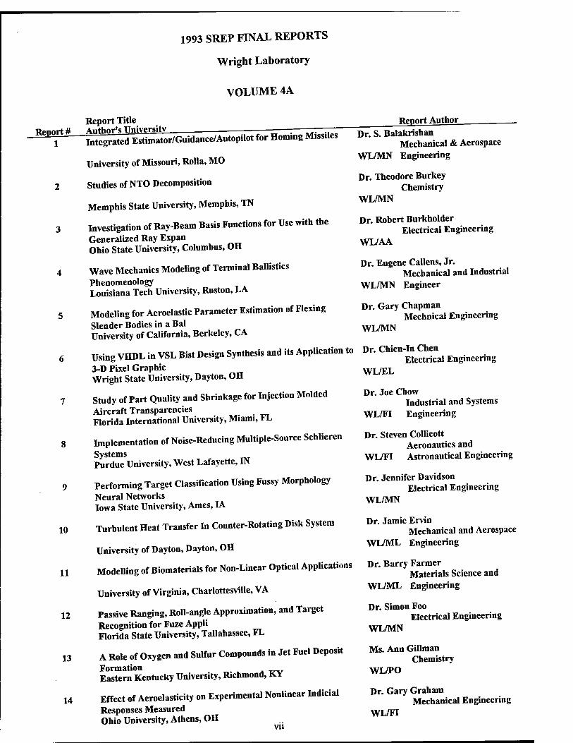
1993 SREP FINAL REPORTS
Wright Laboratory
VOLUME 4A
Report Title Report # Author's University
10
11
12
13
14
Author's University . —:—- ~ Integrated Estimator/Guidance/Autopilot for Homing Missiles
University of Missouri, Rolla, MO
Studies of NTO Decomposition
Memphis State University, Memphis, TN
Investigation of Ray-Beam Basis Functions for Use with the Generalized Ray Expan Ohio State University, Columbus, OH
Wave Mechanics Modeling of Terminal Ballistics Phenomenology Louisiana Tech University, Ruston, LA
Modeling for Aeroelastic Parameter Estimation of Flexing
Slender Bodies in a Bal University of California, Berkeley, CA
Using VHDL in VSL Bist Design Synthesis and its Application to
3-D Pixel Graphic Wright State University, Dayton, OH
Study of Part Quality and Shrinkage for Injection Molded Aircraft Transparencies Florida International University, Miami, FL
Implementation of Noise-Reducing Multiple-Source Schlieren
Systems Purdue University, West Lafayette, IN
Performing Target Classification Using Fussy Morphology
Neural Networks Iowa State University, Ames, IA
Turbulent Heat Transfer In Counter-Rotating Disk System
University of Dayton, Dayton, OH
Modelling of Biomaterials for Non-Linear Optical Applications
University of Virginia, Charlottesville, VA
Passive Ranging, Roll-angle Approximation, and Target Recognition for Fuze Appli Florida State University, Tallahassee, FL
A Role of Oxygen and Sulfur Compounds in Jet Fuel Deposit
Formation # Eastern Kentucky University, Richmond, KY
Effect of Aeroelasticity on Experimental Nonlinear Indicial Responses Measured Ohio University, Athens, OH
vu
Report Author Dr. S. Balakrishan
Mechanical & Aerospace WL/MN Engineering
Dr. Theodore Burkey Chemistry
WL/MN
Dr. Robert Burkholder Electrical Engineering
WL/AA
Dr. Eugene Callens, Jr. Mechanical and Industrial
WL/MN Engineer
Dr. Gary Chapman Mechnical Engineering
WL/MN
Dr. Chien-In Chen Electrical Engineering
WL/EL
Dr. Joe Chow Industrial and Systems
WL/FI Engineering
Dr. Steven Collicott Aeronautics and
WL/FI Astronautical Engineering
Dr. Jennifer Davidson Electrical Engineering
WL/MN
Dr. Jamie Ervin Mechanical and Aerospace
WL/ML Engineering
Dr. Barry Farmer Materials Science and
WL/ML Engineering
Dr. Simon Foo Electrical Engineering
WL/MN
Ms. Ann Gillman Chemistry
WL/PO
Dr. Gary Graham Mechanical Engineering
WL/FI
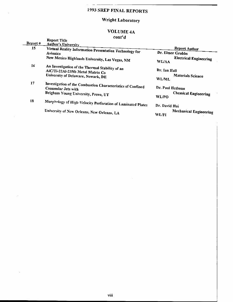
Report Title Report # Author'« TTniv»r«;«y
15
16
17
18
1993 SREP FINAL REPORTS
Wright Laboratory
VOLUME 4A cont'd
AiioUnkSRea,ity Llfor^tion Presentation Technology for
New Mexico Highlands University, Las Vegas, NM
An Investigation of the Thermal Stability of an AiC/Ti-22Al-23Nb Metal Matrix Co University of Delaware, Newark, DE
Investigation of the Combustion Characteristics of Confined Coannular Jets with Brigham Young University, Provo, UT
Morphology of High-Velocity Perforation of Laminated Plates
University of New Orleans, New Orleans, LA
Report Author Dr. Elmer Grubbs
WL/AA Electrical Engineering
Dr. Ian Hall
Materials Science WL/ML
Dr. Paul Hedman
Chemical Engineering
Dr. David Hui
Mechanical Engineering
vui
1993 SREP FINAL REPORTS
Wright Laboratory
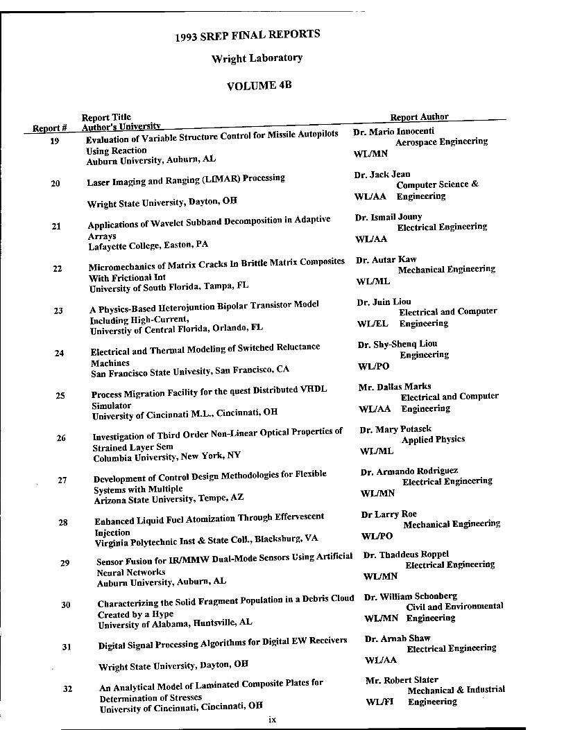
VOLUME 4B
Report Title F^pnr* ü Aiithnr's University . ——
~~"I9" Equation of Variable Structure Control for Miss.le Autop.lots
Using Reaction Auburn University, Auburn, AL
Report Author
20 Laser Imaging and Ranging (LEMAR) Processing
Wright State University, Dayton, OH
21 Applications of Wavelet Subband Decomposition in Adaptive
Arrays Lafayette College, Easton, PA
22 Micromechanics of Matrix Cracks In Brittle Matrix Composites
With Frictional Int University of South Florida, Tampa, FL
23 A Physics-Based Heterojuntion Bipolar Transistor Model Including High-Current, Universtiy of Central Florida, Orlando, FL
24 Electrical and Thermal Modeling of Switched Reluctance
Machines San Francisco State Univesity, San Francisco, CA
25 Process Migration Facility for the quest Distributed VHDL
Simulator . University of Cincinnati M.L., Cincinnati, (Jtt
26 Investigation of Third Order Non-Linear Optical Properties of
Strained Layer Sem Columbia University, New York, NY
27 Development of Control Design Methodologies for Flexible Systems with Multiple Arizona State University, Tempe, AZ
28 Enhanced Liquid Fuel Atomization Through Effervescent
Injection , . ... Virginia Polytechnic Inst & State Coll., Blacksburg, VA
29 Sensor Fusion for ER/MMW Dual-Mode Sensors Using Artificial
Neural Networks Auburn University, Auburn, AL
30 Characterizing the Solid Fragment Population in a Debris Cloud
Created by a Hype University of Alabama, Huntsville, AL
31 Digital Signal Processing Algorithms for Digital EW Receivers
Wright State University, Dayton, OH
32 An Analytical Model of Laminated Composite Plates for Determination of Stresses University of Cincinnati, Cincinnati, OH
ix
Dr. Mario Innocenti Aerospace Engineering
WL/MN
Dr. Jack Jean Computer Science &
WL/AA Engineering
Dr. Ismail Jouny Electrical Engineering
WL/AA
Dr. Autar Kaw Mechanical Engineering
WL/ML
Dr. Juin Liou Electrical and Computer
WL/EL Engineering
Dr. Shy-Shenq Liou Engineering
WL/PO
Mr. Dallas Marks Electrical and Computer
WL/AA Engineering
Dr. Mary Potasek Applied Physics
WL/ML
Dr. Armando Rodriguez Electrical Engineering
WL/MN
Dr Larry Roe Mechanical Engineering
WL/PO
Dr. Thaddeus Roppel Electrical Engineering
WL/MN
Dr. William Schonberg Civil and Environmental
WL/MN Engineering
Dr. Arnab Shaw Electrical Engineering
WL/AA
Mr. Robert Slater Mechanical & Industrial
WL/FI Engineering
34
35
36
37
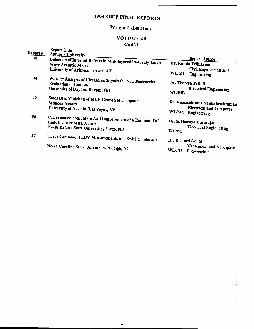
1993 SREP FINAL REPORTS
Wright Laboratory
VOLUME 4B cont'd
Report Title ReP<»t# Author's University
33 Detection of Internal Defects in Multilayered Plates By Lamb Wave Acoustic Micro Universtiy of Arizona, Tucson, AZ
Wavelet Analysis of Ultrasonic Signals for Non-Destructive Evaluation of Composi University of Dayton, Dayton, OH
Stochastic Modeling of MBE Growth of Compoud Semiconductors University of Nevada, Las Vegas, NV
Performance Evaluation And Improvement of a Resonant DC Link Inverter With A Lim North Dakota State University, Fargo, ND
Three Component LDV Measurements in a Swirl Combustor
North Carolina State University, Raleigh, NC
Report Author Dr. Kundu Tribikram
Civil Engineering and WL/ML Engineering
Dr. Theresa Tuthill Electrical Engineering
WL/ML
Dr. Ramasubrama Venkatasubraman «rr «„ Electrical and Computer WL/ML Engineering
Dr. Subbaraya Yuvarajan Electrical Engineering
WL/PO
Dr. Richard Gould Mechanical and Aerospace
WL/PO Engineering
8
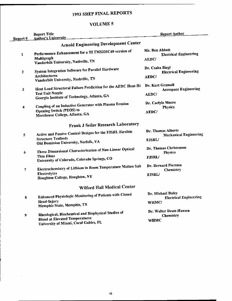
1993 SREP FINAL REPORTS
VOLUME 5
Report Title Report # Author's University
Report Author
Arnold Engineering Development Center
Performance Enhancement for a TITMS320C40 version of
Multigraph Vanderbilt University, Nashville, TN
System Integration Software for Parallel Hardware Architectures Vanderbilt University, Nashville, TN
Heat Load Structural Failure Predicition for the AEDC Heat-Hi Test Unit Nozzle Georgia Institute of Technology, Atlanta, GA
Coupling of an Inductive Generator with Plasma Erosion Opening Switch (PEOS) to Morehouse College, Atlanta, GA
Frank J Seiler Research Laboratory
Active and Passive Control Designs for the FJSRL Flexible Structure Testbeds Old Dominion University, Norfolk, VA
Three Dimensional Characterization of Non-Linear Optical
Thin Films . University of Colorado, Colorado Springs, tu
Electrochemistry of Lithium in Room Temperature Molten Salt
Electrolytes Houghton College, Houghton, NY
Wilford Hall Medical Center
Enhanced Physiologic Monitoring of Patients with Closed Head-Injury Memphis State, Memphis, TN
Rheological, Biochemical and Biophysical Studies of Blood at Elevated Temperatures University of Miami, Coral Gables, FL
Mr. Ben Abbott Electrical Engineering
AEDC/
Dr. Csaba Biegl Electrical Engineering
AEDC/
Dr. Kurt Gramoll Aerospace Engineering
AEDC/
Dr. Carlyle Moore Physics
AEDC/
Dr. Thomas Alberts Mechanical Engineering
FJSRL/
Dr. Thomas Christensen Physics
FJSRL/
Dr. Bernard Piersma Chemistry
FJSRL/
Dr. Michael Daley Electrical Engineering
WHMC/
Dr. Walter Drost-Hansen Chemistry
WHMC
xi
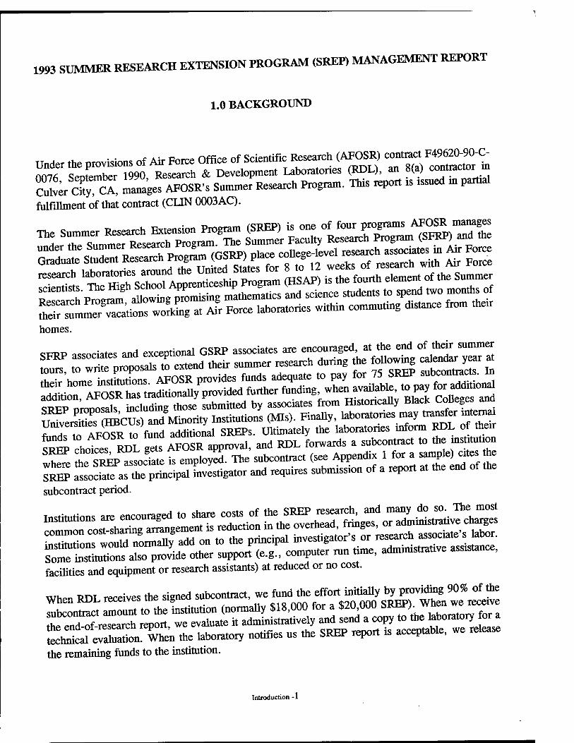
1993 SUMMER RESEARCH EXTENSION PROGRAM (SREP) MANAGEMENT REPORT
1.0 BACKGROUND
Under the provisions of Air Force Offlee of Scientific Rese^h (AFOSR) contract:««W omf. Smiember 1990 Research & Development Laboratones (RDL), an 8(a) contractor m SLÄX manages AFOSR's Summer Research Pregram. This report is «sued m partral
fulfillment of that contract (CLIN 0003AC).
homes.
Umversities (W3C- ) addiüo„al SREPs. Ultimately the laboratories inform RDL of their funds to AFOSR to "™ »™" rf ^ j^ foIwards a subcontract to the institution
s£S SSIÄ -eys,igator and reuuires submission of a report a, the end of the
subcontract period.
facilities and equipment or research assistants) at reduced or no cost.
When RDL receives the signed subcontract, we fund the effort initially by providing 90% of the
KSlUta (normally $18,000 for a W^^JJ^o^T. L «,H of research report we evaluate it administratively and send a copy to the laboratory ior a SSSSS^ die laboratory notifies us the SREP report is acceptable, we release
the remaining funds to the institution.
Introduction -1
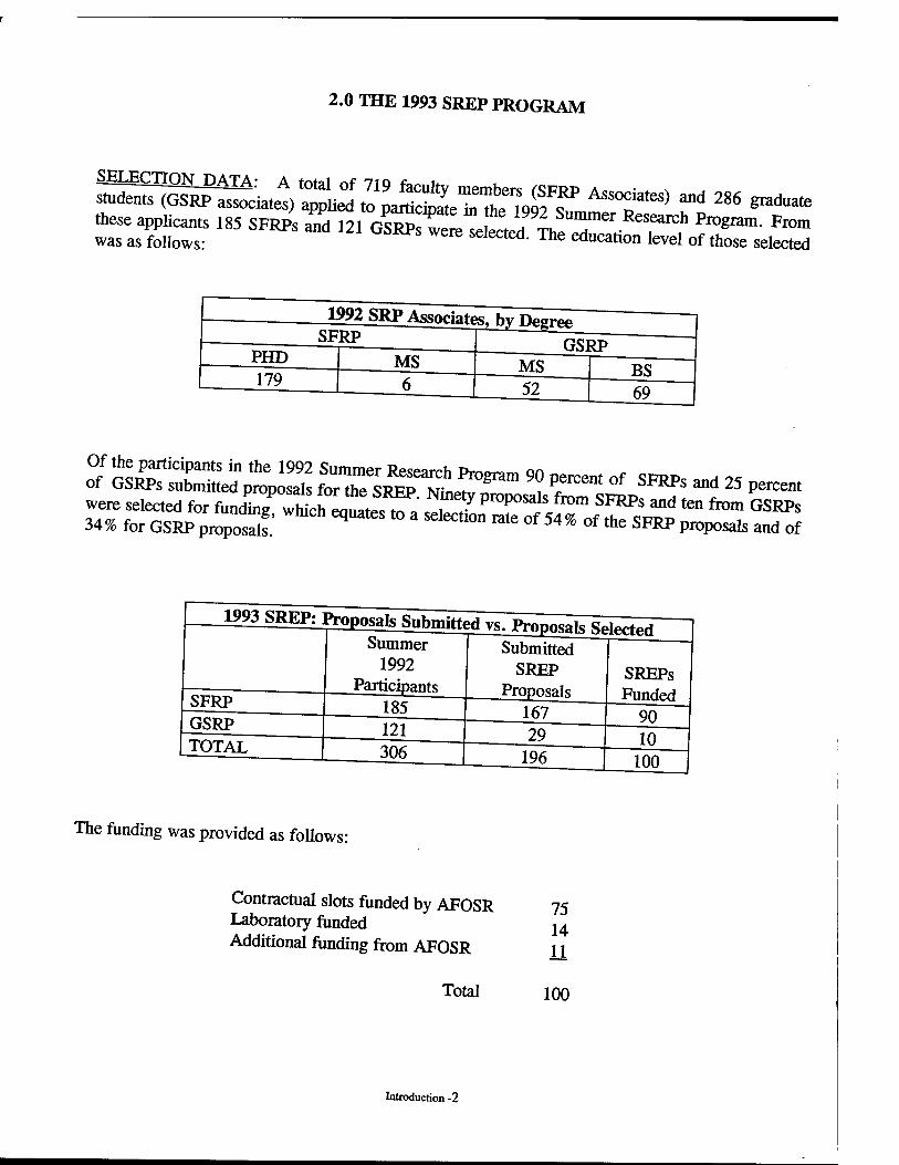
2.0 THE 1993 SREP PROGRAM
rjsr185 SFEPS -i21 «-«""aaa
1992 SRP Associate by Degree SFRP ' &—
PHD 179
MS GSRP
MS 52
BS 69
o7 äSj^s srssrsrgrara 9? rof SFRPS -d 25»-«
SFRP GSRP TOTAL
185 121 306
167 29
196
1993 SREP: Proposals Submitted v.. Proposes frto^i Summer 1 Submitted 1
1992 SREP Participants | Proposals
SREPs Funded
90 10
100
The funding was provided as follows:
Contractual slots funded by AFOSR Laboratory funded Additional funding from AFOSR
75 14 11
Total 100
Introduction -2
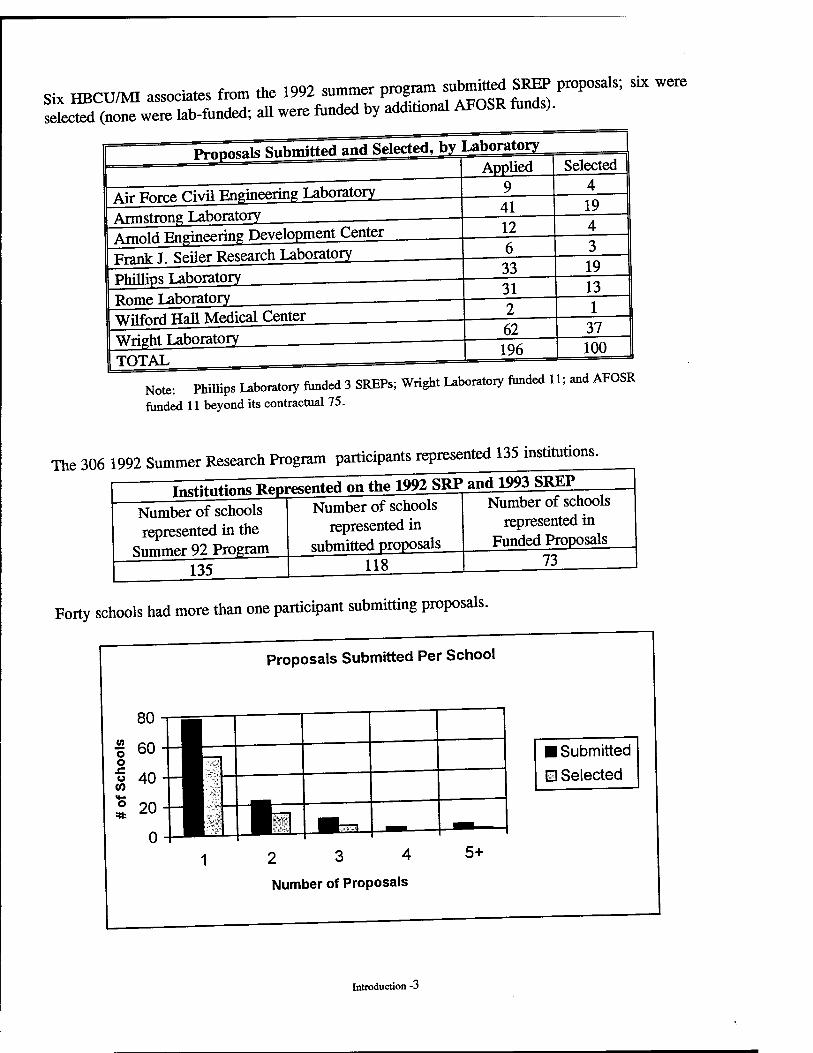
c tho 1QQ? «,mmer program submitted SREP proposals; six were Six HBCU/MI associates from the 1992 summer Prog™» SRfo d) selected (none were lab-funded; all were funded by additional AFOSR funds).
Proposals Submitted and Selected, bv Laboratory
Air Force Civil Engineering Laboratory Armstrong Laboratory
Rome Laboratory Wilford Hall Medical Center Wright Laboratory TOTAL
Arnold Engineering Development Center Frank J. Seiler Research Laboratory Phillips Laboratory
Note: Phillips Laboratory funded 3 SREPs; Wright Laboratory funded 11; and AFOSR
funded 11 beyond its contractual 75.
The 306 1992 Summer Research Program participants represented 135 institutions.
Tl^:win™ ^presented on the 1992 SRP and 1993 SREP
Number of schools represented in the
Summer 92 Program 135
Number of schools represented in
submitted proposals 118
Number of schools represented in
Funded Proposals 73
Forty schools had more than one participant submitting proposals.
Proposals Submitted Per School
■ Submitted
m Selected
2 3 4
Number of Proposals
Introduction -3
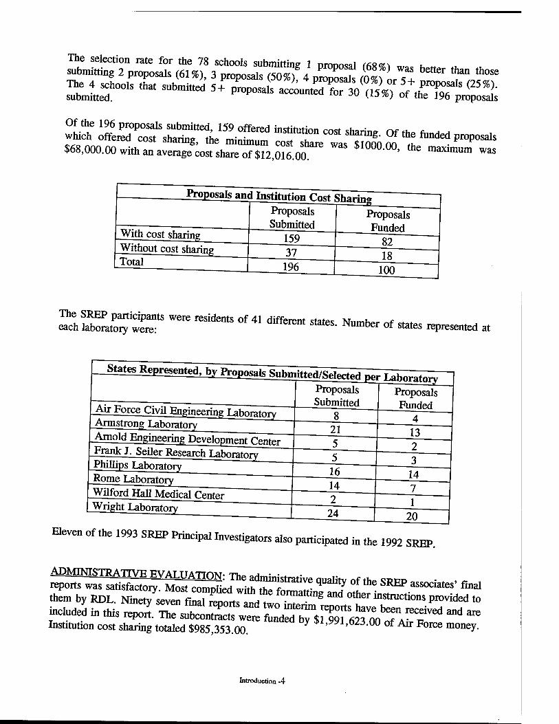
$68,000.00 with an average cost share of $12,016.00 ' ' maXUnUm Was
Proposals and Institution Cost Sharing
With cost sharing Without cost sharing Total
Proposals Submitted
159 37 196
Proposals Funded
82 18
100
The SREP participants were residents of 41 different state«: M„mh«. t . . each laboratory were: arnerent states. Number of states represented at
Proposals | Proposals
Air Force Civil Engineering Laboratory Armstrong Laboratory Arnold Engineering Development Center Frank J. Seiler Research Laboratory Phillips Laboratory
Submitted 8
21
Rome Laboratory Wilford Hall Medical Center Wright Laboratory
16
Funded
13
14
24
14
20
Eleven of the 1993 SREP Principal Investigators also participated in the 1992 SREP.
them by RDL. Nine*^vTfÄ^T ti t ^ 8 *** °ther inrt™^»» Prided to included in this repoS. TsÄ^re *^^^fc^ «* ™ Institutron cost sharing totaled $985,353.00. *i,wi,ö^.U0 of Arr Force money.
Introduction -4
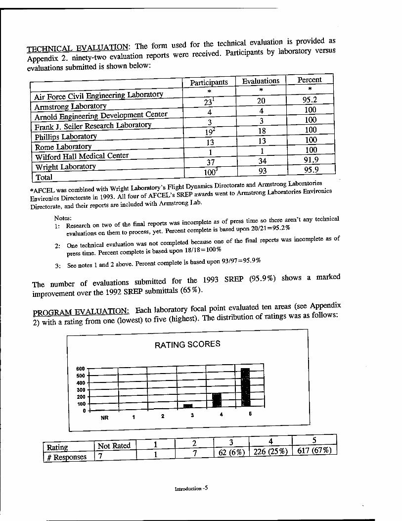
TFrHNTCAL EVALUATION: The fern used for the technical evaluation is provided as 5™SfÄÄita. rope* were received. Participants by laboratory versus
evaluations submitted is shown below:
Air Force Civil Engineering Laboratory Armstrong Laboratory Arnold Engineering Development Center Frank J. Seiler Research Laboratory Phillips Laboratory Rome Laboratory
Participants
231
1*
Evaluations
20
13
Wilfnrd Hall Medical Center Wright Laboratory Total
37 100'
18 13
Percent *
95.2 100 100 100
34 93
100 100 91.9 95.9
,_• A •«. w««*t T aWatorv's Flight Dynamics Directorate and Armstrong Laboratories
'£Z:»~:"i^^™^ -»*—.—™ Directorate, and their reports are included with Armstrong Lab.
Hesearch on two of the final reports was incomplete »« V"^^?» "* **** evaluations on them to process, yet. Percent complete ,s based upon 20/21-95.2%
2- One technical evaluation was not completed because one of the final reports was incomplete as of
press time. Percent complete is based upon 18/18-100%
3: See notes 1 and 2 above. Percent complete is based upon 93/97=95.9%
The number of evaluations submitted for the 1993 SREP (95.9%) shows a marked improvement over the 1992 SREP submittals (65%).
PROGRAM EVALUATION: Each laboratory focal point evaluated ten areas (see Appendix ^Snff^nT^west) to five (highest). The distribution of ratmgs was as follows.
Introduction -5

The 8 low ratings (one 1 and seven 2's ) were for question 5 rone K «Th. TTCAT, U ,,
— (20p„f 62) jrxrc^Äover 30% of -
Question Average 4.6 4.6 4.7 4.7 4.6 4.7
7 4.8 4.5 4.6
10 4.0
The distribution of the averages was:
4
AREA AVERAGES
3.5-
3-
2.5-
2-
1.5-
1 ■
0.5-
0-
|
1 II
1 II 1 1 II 1 1 II « 1 II II 1 1 II
1 II II II 1 —\ 4 4.1 4.2 4.3 4.4 4.5 4.6 4.7 4.8 4.9 5
■ .
aXt ratog7 m?o^ aTPlete SREP,r-h * — right" had to .owest
standL dSion of ^ ST^STT- "T" ff" WaS 46 With a smaU "«*> lower than to oveSl ™ «^SS?* ??"*■ " (4li) " «"■"»««fr <*« •*»
Introduction -6

A frnm <* A tn 5 0 The overall average for those reports that were
higher. The distribution of the average report ratings is as shown:
AVERAGE RATINGS
18-r — 16-
14-
12-
10-
8-
6-
4-
2-
0- 5.C
-1 — —
4.8 [
_
3.0 3.8 4.C _ 4.4 3.2 3.4 3.6 1 4.2 4.6
1
It is clear Research 1
fro Ext«
tnt ;nsi
he Lon
hig] Pre
[in
»gra itin uns
gsl .hat the >la1 jor
Into
atoi
xiuct
ies
ion-
pla
7
ice ah igh val ue on AFOSR's Summer
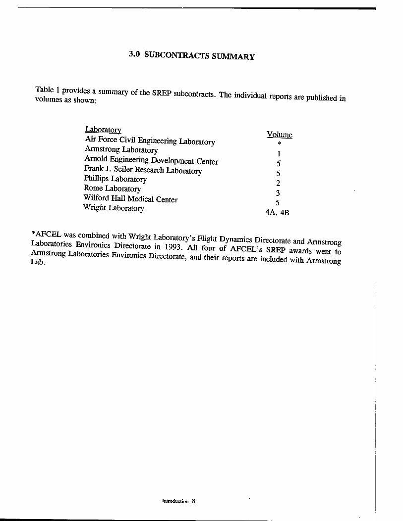
3.0 SUBCONTRACTS SUMMARY
ÄÄ SUmmaiy °f "" SREP SUbC°ntraCtS- *» ^"^ ^ - pubHshed in
Laboratory Air Force Civil Engineering Laboratory Armstrong Laboratory Arnold Engineering Development Center Frank J. Seiler Research Laboratory Phillips Laboratory Rome Laboratory Wilford Hall Medical Center Wright Laboratory 4A%B
£-», Ubon^ies Envies Directorate, and Z^t LS 7^
Volume *
1 5 5 2 3 5
Introduction -8
Report Author Author's University
Abbott, Ben Electrical Engineering Vanderbilt University, Nashville, TN
Alberts, Thomas Mechanical Engineering Old Dominion University, Norfolk, VA
Avula, Xavier Mechanical & Aerospace Engineering University of Missouri, Rolla, MO
Balakrishan, S. Mechanical & Aerospace Engineering University of Missouri, Rolla, MO
Baumgarten, Joseph Mechanical Engineering Iowa State University, Ames, IA
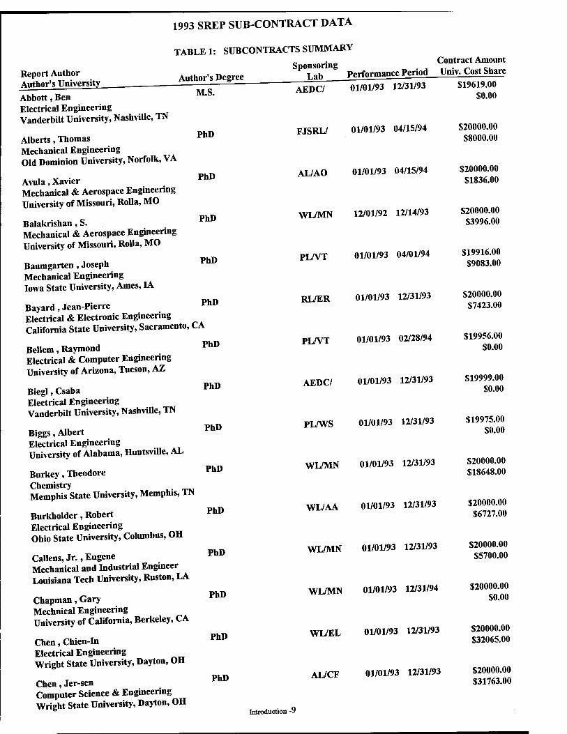
1993 SREP SUB-CONTRACT DATA
TABLE 1: SUBCONTRACTS SUMMARY
Sponsoring Author's Degree
M.S.
y nh Performance Period Contract Amount Univ. Cost Share
PhD
PhD
PhD
PhD
Bayard, Jean-Pierre Electrical & Electronic Engineering California State University, Sacramento, CA
PhD
Bellem, Raymond Electrical & Computer Engineering University of Arizona, Tucson, AZ
Biegl, Csaba Electrical Engineering Vanderbilt University, Nashville, TN
Biggs, Albert Electrical Engineering University of Alabama, Huntsville, AL
Burkey, Theodore Chemistry Memphis State University, Memphis, TN
Burkholder, Robert Electrical Engineering Ohio State University, Columbus, OH
Callens, Jr., Eugene Mechanical and Industrial Engineer Louisiana Tech University, Ruston, LA
Chapman, Gary Mechnical Engineering University of California, Berkeley, CA
Chen, Chien-In Electrical Engineering Wright State University, Dayton, OH
Chen, Jer-sen Computer Science & Engineering Wright State University, Dayton, OH
PhD
PhD
PhD
PhD
PhD
PhD
PhD
PhD
PhD
AEDC/ 01/01/93 12/31/93
FJSRL/ 01/01/93 04/15/94
AL/AO 01/01/93 04/15/94
WL/MN 12/01/92 12/14/93
PL/VT 01/01/93 04/01/94
RL/ER 01/01/93 12/31/93
PL/VT 01/01/93 02/28/94
AEDC/ 01/01/93 12/31/93
PLAVS 01/01/93 12/31/93
WL/MN 01/01/93 12/31/93
WL/AA 01/01/93 12/31/93
WL/MN 01/01/93 12/31/93
WL/MN 01/01/93 12/31/94
WL/EL 01/01/93 12/31/93
AL/CF 01/01/93 12/31/93
$19619.00 $0.00
$20000.00 $8000.00
$20000.00 $1836.00
$20000.00 $3996.00
$19916.00 $9083.00
$20000.00 $7423.00
$19956.00 $0.00
$19999.00 $0.00
$19975.00 $0.00
$20000.00 $18648.00
$20000.00 $6727.00
$20000.00 $5700.00
$20000.00 $0.00
$20000.00 $32065.00
$20000.00 $31763.00
Introduction -9

1993 SREP SUB-CONTRACT DATA
Author's Degree
PhD
Report Author Author's University Chen, Pinyuen Mathematics Syracuse University, Syracuse, NY
Chow, Joe Industrial and Systems Engineering Florida International University, Miami, FL
Christensen, Thomas Physics
University of Colorado, Colorado Springs, CO
Collicott, Steven phD
Aeronautics and Astronautical Engineering Purdue University, West Lafayette, IN
PhD
PhD
PhD
PhD
PhD
Cooke, Nancy Psychology
New Mexico State University, Las Cruces, NM
Daley, Michael Electrical Engineering Memphis State, Memphis, TN
Davidson, Jennifer Electrical Engineering Iowa State University, Ames, IA
Deivanayagam, Subramaniam pj,D Industrial Engineering Tennessee Technological University, Cookeville, TN
Elliott, David Engineering
Arkansas Technology University, Russellville, AR
PhD
M.S. Erdman, Paul Physics and Astronomy University of Iowa, Iowa City, IA
Ervin , Jamie «LQ
Mechanical and Aerospace Engineering University of Dayton, Dayton, OH
Erwin, Daniel Aerospace Engineering University of Southern California, Los Angeles, CA
Ewert, Dan Electrical Engineering North Dakota State University, Fargo, ND
PhD
PhD
Farmer, Barry Materials Science and Engineering University of Virginia, Chariottesville, VA
Foo, Simon Electrical Engineering Florida State University, Tallahassee, FL
PhD
PhD
Sponsoring Contract Amou. Lab Performance Period Univ. Cost si,».
RL/IR 01/01/93 12/31/93 S20000.00
$0.00
WL/FI 01/01/93 01/14/94
FJSRL/ 01/01/93 12/31/93
WL/FI 01/01/93 12/31/93
AL/HR 01/01/93 12/31/93
WHMC/ 01/01/93 12/31/93
WL/MN 01/01/93 02/28/94
AL/HR 02/01/93 12/31/93
PL/RK 10/01/92 08/15/93
PL/RK 01/01/93 12/31/93
WL/ML 01/01/93 12/31/93
PL/RK 01/01/93 12/31/93
AL/AO 01/01/93 12/31/93
WL/ML 01/01/93 02/28/94
WL/MN 01/01/93 12/31/93
Introduction -10
$20000.00 $2500.00
$20000.00 $5390.00
$20000.00 $13307.00
$20000.00 $6178.00
$20000.00 $18260.00
$19999.00 $0.00
$20000.00 $12491.00
$20000.00 $50271.00
$20000.00 $26408.00
$18632.00 $3000.00
$19962.00 $12696.00
$20000.00 $2100.00
$20000.00 $2000.00
$19977.00 $0.00
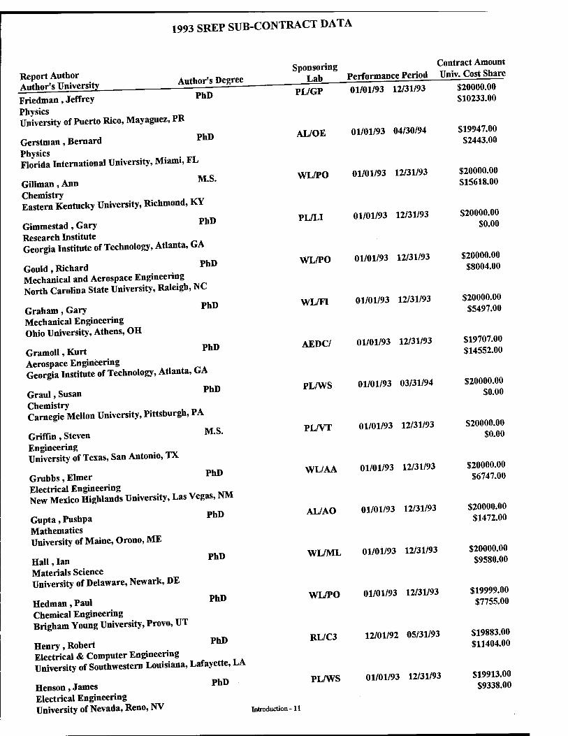
1993 SREP SUB-CONTRACT DATA
Report Author Author's University
Friedman, Jeffrey Physics University of Puerto Rico, Mayaguez, PR
Gerstman, Bernard Physics Florida International University, Miami, *L
Author's Degree
PhD
PhD
M.S. Gillman, Ann Chemistry Eastern Kentucky University, Richmond, K*
Gimmestad, Gary PhD
Research Institute Georgia Institute of Technology, Atlanta, GA
Gould, Richard PhD
Mechanical and Aerospace Engineering North Carolina State University, Raleigh, NC
Graham, Gary PhD
Mechanical Engineering Ohio University, Athens, OH
Gramoll, Kurt Aerospace Engineering Georgia Institute of Technology, Atlanta, GA
PhD
PhD
M.S.
Graul, Susan Chemistry Carnegie Mellon University, Pittsburgh, PA
Griffin, Steven Engineering University of Texas, San Antonio, TX
Grubbs, Elmer PhD
Electrical Engineering New Mexico Highlands University, Las Vegas, NM
Gupta, Pushpa Mathematics University of Maine, Orono, ME
PhD
Hall, Ian Materials Science University of Delaware, Newark, DE
Hedman, Paul Chemical Engineering Brigham Young University, Provo, UT
PhD
PhD
PhD Henry, Robert Electrical & Computer Engineering University of Southwestern Louisiana, Lafayette, LA
Henson, James Electrical Engineering University of Nevada, Reno, NV
Sponsoring Lab
PL/GP
Contract Amount Performance Period Univ. Cost Share 01/01/93 12/31/93 $20000.00
$10233.00
AL/OE 01/01/93 04/30/94 $19947.00 $2443.00
WL/PO 01/01/93 12/31/93 $20000.00 $15618.00
PL/LI 01/01/93 12/31/93 $20000.00 $0.00
WL/PO 01/01/93 12/31/93 $20000.00 $8004.00
WL/FI 01/01/93 12/31/93 $20000.00 $5497.00
AEDC/ 01/01/93 12/31/93 $19707.00 $14552.00
PLAVS 01/01/93 03/31/94 $20000.00 $0.00
PL/VT 01/01/93 12/31/93 $20000.00 $0.00
WL/AA 01/01/93 12/31/93 $20000.00 $6747.00
AL/AO 01/01/93 12/31/93 $20000.00 $1472.00
WL/ML 01/01/93 12/31/93 $20000.00 $9580.00
WL/PO 01/01/93 12/31/93 $19999.00 $7755.00
RL/C3 12/01/92 05/31/93 $19883.00 $11404.00
PLAVS 01/01/93 12/31/93 $19913.00 $9338.00
Introduction-11

1993 SREP SUB-CONTRACT DATA
Author's Degree
Report Author Author's University Hoe , Benjamin jyj § Electrical Engineering Polytechnic University, Brooklyn, NY
Hughes, Rod M s
Psychology
Bowling Green State University, Bowling Green, OH
Hui, David Mechanical Engineering University of New Orleans, New Orleans, LA
Humi, Mayer phD
Mathematics Worcester Polytechnic Institut, Worcester, MA
PhD
PhD
PhD
PhD
Innocenti, Mario Aerospace Engineering Auburn University, Auburn, AL
Jean, Jack Computer Science & Engineering Wright State University, Dayton, OH
Jouny, Ismail Electrical Engineering Lafayette College, Easton, PA
Kaikhah, Khosrow pnD
Computer Science Southwest Texas State College, San Marcos, TX
Kaw, Autar pnD
Mechanical Engineering University of South Florida, Tampa, FL
Kheyfets, Arkady phD
Mathematics North Carolina State University, Raleigh, NC
M.S. Kitchart, Mark Mechanical Engineering North Carolina A & T State University, Greensboro, NC
Koblasz, Arthur Civil Engineering Georgia Institute of Technology, Atlanta, GA
PhD
Koivo, A. Electrical Engineering Purdue University, West Lafayette, IN
Kundich, Robert Biomedical Engineering University of Tennessee, Memphis, TN
Kuo, Spencer Electrical Engineering Polytechnic University, Farmingdale, NY
PhD
PhD
PhD
Sponsoring Contract Amou, Lab Performance Period Univ. Cost Sh».
RL/C3 09/01/92 05/31/93 $19988.00
$7150.00
AL/CF 01/01/93 04/15/94
WL/FI 01/01/93 12/31/93
PL/LI 01/01/93 12/31/93
WL/MN 01/01/93 02/28/94
WL/AA 01/01/93 12/31/93
WL/AA 01/01/93 12/31/93
RL/m 01/01/93 12/31/93
WIVML 01/01/93 12/31/93
PL/LI 01/01/93 12/31/93
AL/EQ 01/01/93 12/31/93
AL/AO 01/01/93 12/31/93
AL/CF 01/01/93 06/30/94
AL/CF 01/01/93 12/31/94
PL/GP 01/01/93 04/30/94
Introduction -12
$20000.00 $20846.00
$20000.00 $0.00
$20000.00 $5000.00
$20000.00 $12536.00
$20000.00 $34036.00
$19381.00 $4500.00
$20000.00 $0.00
$20000.00 $22556.00
$20000.00 $2500.00
$20000.00 $0.00
$19826.00 $0.00
$20000.00 $0.00
$20000.00 $23045.00
$20000.00 $9731.00
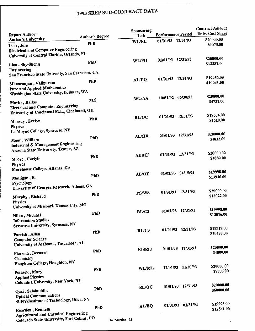
1993 SREP SUB-CONTRACT DATA
Report Author Author's University
Liou, Juin
Author's Degree
PhD
Electrical and Computer Engineering Universtiy of Central Florida, Orlando, FL
Liou, Shy-Shenq PhD
Engineering San Francisco State Univesity, San Francisco, CA
Manoranjan, Valipuram Pure and Applied Mathematics Washington State University, Pullman, WA
PhD
M.S. Marks, Dallas Electrical and Computer Engineering University of Cincinnati M.L., Cincinnati, OH
Monsay, Evelyn Physics Le Moyne College, Syracuse, NY
Moor, William Industrial & Management Engineering Arizona State University, Tempe, AZ
Moore, Carlyle Physics Morehouse College, Atlanta, GA
PhD
PhD
PhD
Mulligan, B. Psychology University of Georgia Research, Athens, l*A
PhD
Murphy, Richard Physics University of Missouri, Kansas City, MO
Nilan, Michael Information Studies Syracuse University, Syracuse, NY
Parrish, Allen Computer Science University of Alabama, Tuscaloosa, AL
Piersma, Bernard Chemistry Houghton College, Houghton, NY
Potasek, Mary Applied Physics Columbia University, New York, NY
Qazi, Salahuddin Optical Communications SUNY/Institute of Technology, Utica, NY
Reardon, Kenneth Agricultural and Chemical Engineering Colorado State University, Fort Collins, CO
PhD
PhD
PhD
PhD
PhD
PhD
PhD
Sponsoring ^^^T* Lab Performance Period Univ. Cost Share
$20000.00 $9073.00
WL/EL 01/01/93 12/31/93
WL/PO
AL/EQ
WL/AA
RL/OC
AL/HR
AEDC/
AL/OE
PL/WS
RL/C3
RL/C3
FJSRL/
WL/ML
01/01/93 12/31/93 $20000.00 $13387.00
01/01/93 12/31/93 $19956.00 $10041.00
10/01/92 06/30/93 $20000.00 $4731.00
01/01/93 12/31/93 $19634.00 $1510.00
01/01/93 12/31/93 $20000.00 $4833.00
01/01/93 12/31/93 $20000.00 $4880.00
01/01/93 04/15/94 $19998.00 $13936.00
01/01/93 12/31/93 $20000.00 $13022.00
01/01/93 12/31/93 $19998.00 $13016.00
01/01/93 12/31/93 $19919.00 $20599.00
01/01/93 12/31/93 $20000.00 $4000.00
12/01/93 11/30/93 $20000.00 $7806.00
01/01/93 12/31/93 $20000.00 $68000.00
01/01/93 01/31/94 $19996.00 $12561.00
Introduction- 13

1993 SREP SUB-CONTRACT DATA
Report Author Author's University Author's Degree
PhD
Reynolds, David PhD
Biomedical & Human Factors Wright State University, Dayton, OH
Robinson, Donald Chemistry Xavier University of Louisiana, New Orleans, LA
Rodriguez, Armando PhD Electrical Engineering Arizona State University, Tempe, AZ
Roe, Larry PhD
Mechanical Engineering Virginia Polytechnic Inst & State Coll., Blacksburg, VA
Romeu, Jorge PhU Assistant Prof, of Mathematics SUNY College at Cortland, Cortland, NY
Roppel, Thaddeus phD
Electrical Engineering Auburn University, Auburn, AL
Roznowski, Mary pnD
Psychology Ohio State University, Columbus, OH
Rudzinski, Walter phD
Chemistry
Southwest Texas State University, San Marcos, TX
Sargent,Robert Engineering and Computer Science Syracuse University, Syracuse, NY
Schonberg, William Civil and Environmental Engineering University of Alabama, Huntsville, AL
Shaw, Arnab Electrical Engineering Wright State University, Dayton, OH
Shively, Jon Engineering & Computer Science California State University, Northridge, CA
Slater, Robert Mechanical & Industrial Engineering University of Cincinnati, Cincinnati, OH
PhD
PhD
PhD
PhD
M.S.
Stenzel, Johanna Arts & Sciences University of Houston, Victoria, TX
Tan, Arjun Physics Alabama A & M University, Normal, AL
PhD
PhD
Sponsoring Contract Amoun Lab Performance Period Univ. Cost Shar AL/CF 01/01/93 06/30/94 $20000.00
$14063.00
AL/OE 01/01/93 06/30/94
WL/MN 01/01/93 12/31/93
WL/PO 01/01/93 12/31/93
RL/OC 01/01/93 12/31/93
WL/MN 01/01/93 12/31/93
AL/HR 01/01/93 03/31/94
AL/OE 01/01/93 12/31/93
RL/XP 01/01/93 12/31/93
WL/MN 01/01/93 12/31/93
WL/AA 01/01/93 12/31/93
PL/VT 01/01/93 12/31/93
WL/FI 01/01/93 12/31/93
$20000.00 $12935.00
$20000.00 $0.00
$20000.00 $11421.00
$19997.00 $7129.00
$20000.00 $21133.00
$19953.00 $6086.00
$20000.00 $10120.00
$20000.00 $11931.00
$19991.00 $5083.00
$20000.00 $4766.00
$20000.00 $9782.00
$20000.00 $8257.00
Introduction -14
PL/LI 01/01/93 12/31/93 $20000.00 $9056.00
PL/WS 01/01/93 12/31/93 $20000.00 $1000.00
1993 SREP SUB-CONTRACT DATA
Report Author Author's University .—
Tetrick, Lois Industrial Relations Prog Wayne State University, Detroit, MI
Author's Degree
PhD
PhD Tew, Jeffery Industrial & Systems Engineering Virginia Polytechnic Institute, Blacksburg, VA
Tribikram, Kundu Civil Engineering and Engineering Universtiy of Arizona, Tucson, AZ
Tuthill, Theresa Electrical Engineering University of Dayton, Dayton, OH
Venkatasubraman, Ramasubrama Electrical and Computer Engineering University of Nevada, Las Vegas, NV
Wang, Xingwu Electrical Engineering Alfred University, Alfred, NY
Whitefield, Philip Physics University of Missouri, Rolla, MO
PhD
PhD
PhD
PhD
PhD
Wightman, Colin Electrical Engineering New Mexico Institute of Mining, Socorro, NM
PhD
Womack, Michael Natural Science and Mathematics Macon College, Macon, GA
Yuvarajan, Subbaraya Electrical Engineering North Dakota State University, Fargo, ND
PhD
PhD
0rins Contract Amount P°Lab Performance Period Univ. Cost Share AL/HR 01/01/93 12/31/93 $20000.00 ^ $17872.00
RL/m
WL/ML
WL/ML
AL/EQ
PL/LI
RL/IR
AL/OE
WL/PO
05/31/93 12/31/93 $16489.00 $4546.00
01/01/93 12/31/93 $20000.00 $9685.00
01/01/93 12/31/93 $20000.00 $24002.00
01/01/93 12/31/93 $20000.00 $18776.00
01/01/93 12/31/93 $20000.00 $10000.00
01/01/93 03/01/94 $20000.00 $11040.00
01/01/93 12/31/93 $20000.00 $1850.00
01/01/93 06/30/94 $19028.00 $6066.00
01/01/93 12/31/93 $19985.00 $22974.00
Introduction- 15

APPENDIX 1:
SAMPLE SREP SUBCONTRACT
Introduction-16
ATR FORCE OFFICE OF SCIENTIFIC RESEARCH 1993 SUMMERTSE^CH EXTENSION PROGRAM SUBCONTRACT 93-133
BETWEEN
Research & Development Laboratories 5800 Uplander Way
Culver City, CA 90230-6608
AND
San Francisco State University University Comptroller
San Francisco, CA 94132
REFERENCE: Summer Research Extension Program Proposal 93-133 ^ Start Date: 01/01/93 End Date: 12/31/93
Proposal Amount: $20,000.00
m PRINCIPAL INVESTIGATOR: Dr. Shy Shenq P. Liou v ' Engineering
San Francisco State University San Francisco, CA 94132
(2) UNITED STATES AFOSR CONTRACT NUMBER: F49620-90-C-09076
„N r AT AT or OF FEDERAL DOMESTIC ASSISTANCE NUMBER (CFDA): 12.800 (3) PRomcT^^
(4) ATTACHMENTS 1 AND 2: SREP REPORT INSTRUCTIONS
>* *TrTN SREP STmr.ONTRACT AND KFTURN TO RDL*
Introduction -17

1. BACKGROUND- Research & Development Laboratories (RDL) is under contract
(F49620-90-C-0076) to the United States Air Force to administer the Summer Research
Programs (SRP), sponsored by the Air Force Office of Scientific Research (AFOSR),
Boiling Air Force Base, D.C. Under the SRP, a selected number of college faculty
members and graduate students spend part of the summer conducting research in Air Force
laboratories. After completion of the summer tour participants may submit, through their
home institutions, proposals for follow-on research. The follow-on research is known as
the Summer Research Extension Program (SREP). Approximately 75 SREP proposals
annually will be selected by the Air Force for funding of up to $20,000; shared funding
by the academic institution is encouraged. SREP efforts selected for funding are
administered by RDL through subcontracts with the institutions. This subcontract
represents such an agreement between RDL and the institution designated in Section 5 below.
2- RDL PAYMENTS- RDL will provide the following payments to SREP institutions:
• 90 percent of the negotiated SREP dollar amount at the start of the SREP Research period.
• the remainder of the funds within 30 days after receipt at RDL of the acceptable
written final report for the SREP research.
3- INSTITUTION'S RESPONSIBILITIES- As a subcontractor to RDL, the institution
designated on the title page will:
Assure that the research performed and the resources utilized adhere to those defined in the SREP proposal.
Provide the level and amounts of institutional support specified in the RIP proposal.
Notify RDL as soon as possible, but not later than 30 days, of any changes in 3a or
3b above, or any change to the assignment or amount of participation of the Principal
Investigator designated on the title page.
a.
b.
c.
Introduction- 18

d.
4.
e.
f.
Assure that the research is completed and the final report is delivered to RDL no.
la,er than tweWe months from «he effective date of this subconttact, but no later man
December 31 1993. The effective date of the subcontract is one week after the date
that the institution's contracting representative signs this subcontract, but no later than
January 15, 1993. Assure that the final report is submitted in accordance with Attachment 1.
Agree that any «lease of information relating to this subcontract (news releases,
arttc.es, manuscripts, brochures, advertisements, still and motion pictures, speeches,
«de association meetings, symposia, etc.) will include a statement that the project
or effort depicted was or is sponsored by: Air Force Office of Scientific Research,
Boiling AFB, D.C. g. Notify RDL of inventions or patents claimed as the result of this research as spectfied
in Attachment 1. . n RDL is required by the prime contract to flow down patent rights and techno data
requirements in this subcontract. Attachment 2 to this subcontract contains a hst of
contract clauses incorporated by reference in the prime contract.
All notices to RDL shall be addressed to:
RDL Summer Research Program Office 5800 Uplander Way Culver City, CA 90230-6608
u i th^ nsrties aeree to the provisions of this subcontract. By their signatures below, the parties agree TO mc v
Abe S. Sopher RDL Contracts Manager
Signature of Institution Contracting Official
Typed/Printed Name
Date Title
Institution
(Date/Phone)
Introduction-19

52.203-5
52.304-6
ATTACHMENT -> CONTRACT CT A TT.CT.S
This contract incorporates by reference the following clauses of the Federal Acqu1S1 ,on Regulaüons (FAR), with the same force and effect !s if they were gin L M
^5^2°5n2-2)UeSt' mraCting °ffiCer °r ^ Wlü ^ thGir Ml te^*
FAR CLAUSES TITLE AND DATF 52.202-1 DEFINITIONS (SEP 1991)
52.203-1 OFFICIALS NOT TO BENEFIT (APR 1984)
52.203-3 GRATUITIES (APR 1984)
COVENANT AGAINST CONTINGENT FEES (APR 1984)
RESTRICTIONS ON SUBCONTRACTOR SALES TO THE GOVERNMENT (JUL 1985)
52.203-7 ANTI-KICKBACK PROCEDURES (OCT 1988)
LIMITATION ON PAYMENTS TO INFLUENCE CERTAIN FEDERAL TRANSACTIONS (JAN 1990)
52.204-2 SECURITY REQUIREMENTS (APR 1984)
PROTECTING THE GOVERNMENT'S INTEREST WHEN SUBCONTRACTING WITH CONTRACTORS DEBARRED SUSPENDED, OR PROPOSED FOR DEB ARMENT (NO V 1992)
SEPEIT90)
PRIORITY ^ ALL0CATI0^ REQUIREMENTS
EXAMINATION OF RECORDS BY COMPTROLLER GENERAL (APR 1984)
52.215-2 AUDIT - NEGOTIATION (DEC 1989)
52.222-26 EQUAL OPPORTUNITY (APR 1984)
52.203-12
52.209-6
52.212-8
52.215-1
52.222-28 EQUAL OPPORTUNITY PREAWARD CLEARANCE OF SUBCONTRACTS (APR 1984)
Introduction - 20

52.222-35
52.222-36
52.223-2
52.232-6
52.224-1
52.225-13
52.227-1
52.227-2
52.227-10
52.227-11
52.228-6
52.228-7
52.230-5
52.232-23
52.237-3
AFFIRMATIVE ACTION FOR SPECIAL DISABLED AND VIETNAM ERA VETERANS (APR 1984)
AFFIRMATIVE ACTION FOR HANDICAPPED WORKERS
(APR 1984)
„ ,n 37 EMPLOYMENT REPORTS ON SPECIAL DISABLED 52222 VETERAN AND VETERANS OF THE VIETNAM ERA
(JAN 1988)
CLEAN AIR AND WATER (APR 1984)
DRUG-FREE WORKPLACE (JUL 1990)
PRIVACY ACT NOTIFICATION (APR 1984)
52.224-2 PRIVACY ACT (APR 1984)
RESTRICTIONS ON CONTRACTING WITH SANCTIONED
PERSONS (MAY 1989)
AUTHORIZATION AND CONSENT (APR 1984)
NOTICE AND ASSISTANCE REGARDING PATENT AND COPYRIGHT INFRINGEMENT (APR 1984)
FILING OF PATENT APPLICATIONS - CLASSIFIED SUBJECT MATTER (APR 1984)
PATENT RIGHTS - RETENTION BY THE CONTRACTOR
(SHORT FORM) (JUN 1989)
INSURANCE - IMMUNITY FROM TORT LIABILITY
(APR 1984)
INSURANCE - LIABILITY TO THIRD PERSONS (APR 1984)
DISCLOSURE AND CONSISTENCY OF COST ACCOUNTING
PRACTICES (AUG 1992)
ASSIGNMENT OF CLAIMS (JAN 1986)
CONTINUITY OF SERVICES (JAN 1991)
Introduction-21

52.246-25 LIMITATION OF LIABILITY - SERVICES (APR 1984)
52.249-6 TERMINATION (COST-REIMBURSEMENT) (MAY 1986)
52.249-14 EXCUSABLE DELAYS (APR 1984)
52.251-1 GOVERNMENT SUPPLY SOURCES (APR 1984)
Introduction - 22

APPENDIX 2:
SAMPLE TECHNICAL EVALUATION FORM
Introduction - 23

1993 SUMMER RESEARCH EXTENSION PROGRAM
RIP NO.: 93-0092 RIP ASSOCIATE: Dr. Gary T. Chapman
aTJKu^csr^^s^s^ir^Tr111?foiiowed by »«»»■ °* highest. Circle the rat£L Lilt " ^ l0WSSt and (5) is the
evaluation form.
Mail or fax the completed form to
RDL Attn: 1993 SREP TECH EVALS 5800 Uplander Way- Culver City, CA 90230-6608 (FAX: 310 216-5940)
l.
2.
3.
4.
5. 12 3 4 5
12 3 4 5
7.
8.
9.
10
This SREP report has a high level of technical merit. i 2 3 4 5
missfSP Pr09ram iS imP°rtant to -—P^hing the labs<s 12 3 4 5
posa^LiXr aCCOn*>lished «** the associate's pro-
This SREP report addresses area(s) important to the ÜSAF
säpüre?oS°Uld C°ntinUe t0 PUrSUS the —ch - this
S^aJsoSat^ maintain ^^^ relationships with this 12 3 4 5
The money spent on this SREP effort was well worth it
This SREP report is well organized and well written
associated ^future^ ^ * ~ "—* — SREP
Throne-year period for complete SREP research is about
12 3 4 5
12 3 4 5
12 3 4 5
—USE THE BACK OF THIS FORM FOR ADDITIONAL COMMENTS****
LAB FOCAL POINT'S NAME (PRINT):
OFFICE SYMBOL: PHONE:
Introduction - 24
JSSSSSSSSSS^SSSSSSSSSL
FINAL REPORT
by Ajay Thukral, John E. Cochran, Jr.
Department of Aerospace Engineering, Auburn Universny, Alabama 36849-5338
and Mario Innocenti
Department of Electrical Systems and Automation University of Pisa, 56126 Pisa, Italy
submitted to Research Development Laboratories
5800 Upiander Way, Culver City, California 90230-6608
under Contract: RDL-93-132
Auburn University, Alabama 15 May 1994
19-1
Preface
This report documents the results obtained under the grant RDL-93-132 from February 1993 until February 1994. The work was performed at Auburn University, Alabama, in the Department of Aerospace Engineering. The principal investigator of record for the project was Dr. John E. Cochran, Jr., however, the work was initiated by Dr. Mario Innocenti whole he was at Auburn. Furthermore, most of the work was done by Dr. Mario Innocenti as a consultant, and Mr. Ajay Thukral, a Ph.D. candidate. Mr. Gregory D. Strawn, graduate student, also contributed to the preparation of the report.
John E. Cochran, Jr.
Principal Investigator
19-2

Table of Contents
ii Preface - Table of Contents .y
List of Figures vü
List of Tables viii
List of Important Symbols 1 iduction 1
1.1. Motivation 3
1.2. Maneuver Description
1.3. Summary of Results
2. Variable Structure Control
3. Missile Dynamics 3.1. System Characteristics
3.2. Missile Aerodynamics 3.3. Low Angle of Attack Model 3.4. High Angle of Attack Model
3.5. Acquisition of Steady State
4. Autopilot Design 4.1. Objectives 4.2. Phase I Autopilot
3o 4.3. Phase II Autopilot 4.4 Phase III Autopilot
45 5. Simulation . _
5.1. Description
5.2. Results 4?
5.2.1. Nominal Case 5.2.2. Sensitivity Analysis
64 5.3. Simulation Software
6 Conclusions and Recommendations Do
7. References
Appendices _Q
Al. Gains A2. Software Description
A3. Parametric Analysis
19-3
List of Figures
Figure 1. Generic Control Configuration
Figure 2. Selected Midcourse Trajectory Figure 3. Missile Configuration
Figure 4. Control Panel Deflections (from rear) Figure 5. RCS Model 17
Figure 6. Elliptical Cylinder and Dimensions Figure 7. Vortex Street 21
Figure 8. Effective Velocity
Figure 9. Lift and Drag Coefficients Curves ""
Figure 10. Angles Relationship during Maneuver
Figure 11. Adjusted versus Actual Angle of Attack 26
Figure 12. Phase I Autopilot
Figure 13. G-Command Response
Figure 14. Performance during Phase I
Figure 15. Performance during Phase II
Figure 16. Control Effort during Phase E
Figure 17. Phase II Autopilot Block Diagram
Figure 18. Phase m Autopilot Block Diagram (method 1) '"~ 44
Figure 19. Phase m Autopilot Block Diagram (method 2) 44 Figure 20. Complete Autopilot Schematic
Figure 21. Angular Behavior below Stall
Figure 22. Load Factor Response below Stall
Figure 23. Control Activity during Phase I
Figure 24. Reaction Jet Activity (On-Off) and Sliding Surface during Phase I 49 Figure 25. Attitude and Pitch Rate during Phase E
Figure 26. Missile Angular Behavior during Phase E
Figure 27. Control Activity and Sliding during Phase JJ 51 Figure 28. Trajectory during Phase U a 52 Figure 29. Angular Diplacement during Phase IE
Figure 30. Control Activity during Phase IE ••* • ••♦ • ^A
Figure 31. Sliding Surfaces during Phase El
Figure 32. Motion Behavior during Phase IE (Model Following of Attitude only) 55
Figure 33. Pitch Rate and Sliding Surface (Model Following of Attitude only) 56
Figure 34. Control Activity during Phase IE (Model Following of Attitude only) 56
Figure 35. Trajectory Comparison for Phase El
19-4
List of Figures (contd.)
_ 58 Figure 36. Angles Comparison for Phase m ^ Figure 37. Angular Behavior during the Entire Maneuver ^
Figure 38. Vehicle's Trajectory during the Entire Maneuver Figure 39. Trajectory Comparison at different Mach Number
(Model Following of 6,q, and Y) Figure 40. Trajectory Comparison at different Mach Number (Model Following of 6, q) 61
Figure 4L Trajectory Comparison at different Main Engine firing
(Model Following of 6, q, and Y) ^ Figure 42. Trajectory Comparison at different Main Engine firing
(Model Following of 6, q) Figure 43. Trajectory Comparison at different RCS Thrust
(Model Following of 6,q, and Y) Figure 44. Trajectory Comparison a. differe« RCS Thrust (Model Following of 6,,) 63
Figure 45. Simulation Code Flowchart ^ Figure A-l Normal Acceleration and Pitch Rate, Phase I Figure A-2 Pitch Angle, Angle of Attack and Flight Path Angle, Phase I «^
Figure A-3 Elevator and Reaction Jet Deflections, Phase I ^
Figure A-4 Trajectory, Phase I 83
Figure A-5 Normal Acceleration and Pitch Rate, Phase II Figure A-6 Pitch Angle, Angle of Attack and Flight Path Angle, Phase Ü
Figure A-7 Elevator and Reaction Jet Deflections, Phase H
Figure A-8 Trajectory, Phase H Figure A-9 Normal Acceleration and Pitch Rate, Phase m (Approach I) « Figure A-10 Pitch Angle, Angle of Attack and Flight Path Angle, Phase JH (Approach I) 88
Figure A-l 1 Elevator and Reaction Jet Deflections, Phase IE (Approach I) ^
Figure A-12 Trajectory, Phase JH (Approach I) •••• •"" Figure A-13 Normal Acceleration and Pitch Rate, Complete Maneuver (Approach I)
Figure A-14 Pitch Angle, Angle of Attack, Flight Path Angle, Complete Maneuver ^
(Approach I) "" _ Figure A-15 Elevator and Reaction Jet Deflections, Complete Maneuver (Approach I) 93
Figure A-16 Trajectory, Complete Maneuver (Approach I) ^
85 86
Figure A-17 Speed, Complete Maneuver (Approach I) ™ qfi Figure A-18 Normal Acceleration and Pitch Rate, Phase HI (Approach II) J
Figure A-19 Pitch Angle, Angle of Attack and Flight Path Angle, Phase HI (Approach II) 97 98
Figure A-20 Elevator and Reaction Jet Deflections, Phase m (Approach II) ^
Figure A-21 Trajectory, Phase ffl (Approach II) 19-5
List of Figures (contd.)
Figure A-22 Normal Acceleration and Pitch Rate, Complete Maneuver (Approach II) 100 Figure A-23 Pitch Angle, Angle of Attack, Flight Path Angle, Complete Maneuver
(Approach II)
Figure A-24 Elevator and Reaction Jet Deflections, Complete Maneuver (Approach II) 102 Figure A-25 Trajectory, Complete Maneuver (Approach II) 103 Figure A-26 Speed, Complete Maneuver (Approach II) 104
Figure A-27 CL-CD curves, Mach 0.6
Figure A-28 CL-CD curves, Mach 1.2 ~
19-6
List of Tables
16 Table 1. Physical and Geometric Characteristics ^
Table 2. Moments and Panel Deflections " TableB.MissileandHightConditionDataancludingactuatortimeconstants) 1»
Table 4. Aerodynamic Stability Derivatives ^ Table 5. Aerodynamic Coefficients from DATCOM ^
Table A-l 7g Table A-2
19-7
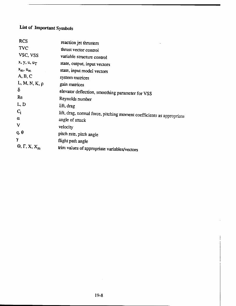
List of Important Symbols
Rcs reaction jet thrusters
** C thrust vector control VSC, VSS variable structure control x, y, u, uT state, output, input vectors xm' um state, input model vectors A'B' c system matrices L, M, N, K, p gain matrices
elevator deflection, smoothing parameter for VSS Re Reynolds number L' D lift, drag
Q lift, drag, normal force, pitching moment coefficients as appropriate 06 angle of attack v velocity q' e pitch rate, pitch angle y flight path angle
0, T, X, Xm trim values of appropriate variables/vectors
5
19-8

1. Introduction
The feasibility of eombining traditional aerodynamie eontrol with teaetion jets,
in me framework of missile aotopilo, design, was addressed in Ms work. The pnrpose
„f propulsive actuation is mainly to increase the angle of attack envelope for improved
turn rate capabilities and maneuverability. Due to nonlinear characteristics of both
controller and airframe dynamics, aerodynamic and geometric model uncertainty a
control strategy based on variable structure systems was adopted. A control law was
then synthesized for a simplified pitch channel autopilot and used in a high angle of
attack midcourse maneuver. Results of the nonlinear situation show the capability of
the autopilot to satisfy the control objectives for a variety of flight conditions.
1.1. Motivation
Future missile systems will be required to possess higher turn rates and larger
„aneuverabiliry envelopes, whale simultaneously meeting the requirement of reduced
storage and signature. In mis respect, efforts are under way to evaluate alternate
methods of missile control as opposed to purely aerodynamic control [1], [2], [3].
Several technology payoffs can be envisioned if alternate conttol strategies are
implemented, among which there arc:
. decreased stowage volume for internal carriage, especially important for the type of
fighters currently being developed,
. increased maneuverability and off-boresigh. capability for improved aU-aspect
defensive shield,
. high angle of attack launch capability to take advantage of improved aircraft agility,
and better end-game accuracy.
19-9
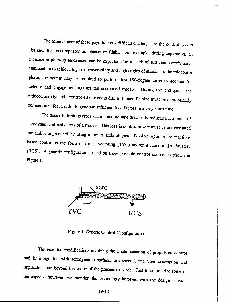
The achievement of these payoffs poses difficult challenges to the control system
designer that encompasses all phases of flight For example, during separation, an
increase in pitch-up tendencies can be expected due to lack of sufficient aerodynamic
stabilization to achieve high maneuverability and high angles of attack. In the midcourse
phase, the system may be required to perform fast 180-degree turns to account for
defense and engagement against tail-positioned threats. During the end-game, the
reduced aerodynamic control effectiveness due to limited fin size must be appropriately
compensated for in order to generate sufficient load factors in a very short time.
The desire to limit its cross section and volume drastically reduces the amount of
aerodynamic effectiveness of a missile. This loss in control power must be compensated
for and/or augmented by using alternate technologies. Possible options are reaction-
based control in the form of thrust vectoring (TVC) and/or a reaction jet thrusters
(RCS). A generic configuration based on three possible control sources is shown in
Figure 1.
TVC
aero
ED
RCS
Figure 1. Generic Control Cconfiguration
The potential modifications involving the implementation of propulsion control
and its integration with aerodynamic surfaces are several, and their description and
implications are beyond the scope of the present research. Just to summarize some of
the aspects, however, we mention the technology involved with the design of each
19-10

component, as well as the integration of elements leading to variable degree of effort:
from the mere addition of aetuator on existing airframe, all the way to a new missde
design Tta wo* done under mis grant was concentrated on one of the propulstve
solutions, speedily the use of reaction jets. TTte apptication of thrus, vector control .
addressed in reference [4].
1.2. Maneuver Description
b order to gain appreciation for some of the problems involving reaction jet
conmol and its blending with traditional aerodynamic control, a high angle of attack
midcourse maneuver was chosen as test scenario. In particular, a two-dimensional,
heading reversal trajectoty in the longitudinal plane was selected as a typical defense
maneuver against tail and fly-by threats as shown schematically in Figure 2.
_^ Inertial X-axis
Inertial Z-axis
« '-T - 'S
^
Figure 2. Selected Midcourse Trajectory
19-11

Many challenges to guidance and control systems are posed by the above
selection. To completely overcome them will require much greater effort than that
available during the present research. However, some of the critical issues are addressed
here leading to a preliminary design of the autopilot
The maneuver is a 180-degree off-boresight trajectory with turn rates of the
order of 80 deg/sec, capable of pointing as well as flying the missile roughly in the
opposite direction as quickly as possible along a minimum radius turn path and in a time
frame of the order of two seconds.
TTie specifications involve both guidance and autopilot requirements. The
guidance aspects deal with the generation of an appropriate flight path along which the
missile turns in minimum time changing its heading and an attitude of up to 180 degrees.
TTie selection of this path could depend on agility issues and/or tactical ones. The
autopilot aspects deal with the creation offerees and moments on the missile capable of
generating accelerations and attitude rates required by the guidance system. Appropriate
blending of aerodynamic and reaction jet controls may be required since, during parts of
the trajectory, the missile may experience loss of lifting capabilities due to angles of
attack much higher than stall.
In this report we do not address the question of guidance law design, rather we
present the development of a nonlinear autopilot logic capable of implementing the
maneuver, and a blending strategy which uses aerodynamic control at low angles of
attack and RCS control when the missile angle of attack is higher stall.
13. Summary of Results
The results provided in this report are in terms of autopilot structure, gains and
simulation data. The theory of variable structure control is briefly reviewed first, then a
19-12

description of the model dynamics derivation at low and high angle of attack is presented
to set the analytical framework for the autopilot design.
The design of the autopilot is the central part of the report. The design includes:
control structure, conffoller gain matrices, and block diagrams. The performance of the
closed loop system is evaluated using a nonlinear simulation code that contains attitude
as well as point mass dynamics of the missile. The simulation code was written using
Matlab® and the software is included with this report as part of the deliverables.
2. Variable Structure Control
Variable structure control has been described in the former Soviet literature since
the early sixties, see, for example, Emel'yanov [5], Utkin [6] and Itkis [7], among others.
Invariance of VSC to a class of disturbances and parameter variations was first
developed by Drazenovic in 1969 [8]. In the past two decades, a large amount of
research has been performed in the area by the international community. This research
has linked VSC to adaptive control and model reference adaptive control, using
Lyapunov control techniques. Also, investigators have derived connections of VSC with
hyperstability theory, and solved VSC tracking problems (see references [9] and [10] for
a survey on the subject).
Most of the applications of VSC have been in the areas of industrial control and
robotics. Only recendy some work has been done in the aerospace field. Applications to
aircraft control have been presented by Calise and Kramer [11] where robnsmess with
respect to nonlineariües is addressed, and by Innocend and Thukral [20]. Mudge and
Patton [12], solved the sensitivity to parameter variations by incorporating
eigenstructure assignment in the structure of tine control law, Hedrick e. al. [13] nsed
Slotine's concept of bonndary layer to eliminate chattering. Lyapnnov stability theory
19-13

and VSC were used by Vadali in designing large-angle maneuvers controllers for a
spacecraft [14]. Applications to missiles appear to have been confined mainly to
guidance schemes [15], [16].
The essential feature of a variable structure controller is that it uses nonlinear
feedback control with discontinuities on one or more manifolds (sliding hyperplanes) in
the state space, or error space, in the case of model following control. This type of
methodology is attractive in the design of controls for nonlinear, uncertain, dynamic
systems with uncertainties and nonlinearities of unknown structure as long as they are
bounded and occurring within a subspace of the state space [9]. Ryan and Corless [17]
have also shown that VSC could be used to establish 'almost certain' convergence to
vicinity of the origin for a class of uncertain systems. A brief description of the
principles of variable structure systems is now presented, and essentially follows those of
references [6] and [9].
The basic feature of VSC is sliding motion. This occurs when the system state
continuously crosses a switching manifold because all motion in its vicinity is directed
towards the sliding surface. When the motion occurs on all the switching surfaces at
once, the system is said to be in the "sliding mode" and then the original system is
equivalent to an unforced, completely controllable system of lower order.
The design of a variable structure controller consists of several steps: the choice
of switching surfaces, the determination of the control law and the switching logic
associated with the discontinuity surfaces (usually fixed hyperplanes that pass through
the origin of the state space). To ensure that the state reaches the origin along the sliding
surfaces, the equivalent system must be asymptotically stable. This requirement defines
the selection of the switching hyperplanes (sometimes called the "existence" problem),
which is completely independent of the choice of control laws. The selection of the
19-14

control iaw is *. so-called "reachability" problem. It requires .ha. the system be capabie
of reaching die sliding hypersurtaee from any initial state.
Daring operation in .he shding mode, the discondnuons control chatters about
the switching surface a. high frequency. Chatter is the major probiem associated wrth
„us type of control. Execution of control commands may require high energy effort
from the actuators, thus leading to continuous saturation. I. can also excite neg.ec.ed
high order dynamic, TWs is perhaps .he reason «by VSC has no. ye. found wider
acceptance in tine flight conttol community, where smoothness of actuation is desirable
t„ avoid saturation and, possibly, instability. The introduction of discontinuous
actuators such as reaction je* and active flow controi is however changing tins
perspective and variaMe structure systems are Wng viewed as a viable al.ernat.ve to
traditional relay control strategies.
There are several ways to mitiga* the effects of chattering, with li.de loss in
performance. These include the definition of a boundary !ayer near the sliding surface as
introduced by Slotine, and/or the introduction of a smoothing parameter in a unit vector-
type conttol law as shown by Ambrosino e. ai [18], Burton and Zinober [9), Balestrino
[191. and Thukral and Innocenti [20], The latter approach was used in the present work.
As noted in [21], the smoothing factors do not guarantee full robustness,
however such relaxation is the price paid for avoiding actuator sanction. Of course,
smoothing is no, necessary when on-off actuators such as thrusters are being used.
The general control problem is based on the following nonlinear, uncertain, and
controllable dynamic system
x = (A + AA)x + {B + M)u + Cv
y = X + W
where the state and input vectors have dimensions n and m respectively, vW is a one-
dimensional disturbance vector also representing nominees and MO is a vector of
19-15

output (measurement) uncertainties. The parameter variation matrices A4 and Aß can be
uncertain and time varying. Matching conditions are assumed to be satisfied by the
matrices AA, AB and C, thus satisfying Drazenovic invariance conditions as well as
perfect model following [8]. Since matching requires AA, AB and C to be in the range
space of B (assumed to be full rank), the following relations are necessary for perfect
invariance
AA=BD,
AB = BE, (2)
C = BF
where D, E, and F have dimension nxn, mxm and mxl respectively. The purpose of a
VSC design is then to determine the control law u of the form
Ui(x)J«tforSi(x)>0 [ujforsi(x)<0 (3)
with the switching hyperplanes denoted in matrix form by
s = Gx (4)
where s is m-dimensional and G is an mxn constant matrix. For a stable sliding motion
to occur on all surfaces, the following conditions, based on LyapunoVs stability theory,
must be satisfied:
stsi<0 near^O s = Gx = s = Gx = O in the sliding mode. (5)
Since the sliding mode belongs to the null space of G, if the product GB is
nonsingular, the sliding motion is independent of the control law. During sliding, from
Eqs. (1) and (5) we can determine an equivalent control law
ueq = -(GB)-lG[Ax + h] (6)
h = AAx + ABu + Cv
19-16

Since the matching conditions (2) are assumed to be valid, the system dynamics during
sliding arc then governed by
X = [I-B(GB)'1G]AX
shoving the sliding motion to be insensitive to unknown, but bounded, parameter
variations and disturbances. The selection of the switching surfaces, i. e. G, depends on
the desired system behavior during sliding and given by Eq. (7).
To select the switching surfaces, we consider first a nominal system extracted
from (1) and given by
x = Ax + Bu
y = x s =Gx In order to simplify the design scheme, we transform Eq. (8) into a controllable
canonical form using the transformation a = Tx, where T is an orthogonal matrix. This
yields, [with An square of dimensions (n-m)]
q = An Al2
Q + 0
L*2j
s = GTTq = [G1 G2]q
(9)
Note that, since GB is nonsingular, so are G2B2 and G2. During sliding, we have from
s = 0
qi=[AU-Al2K]qi (10)
q2 = -Kqx
with K = G2 G\.
The sliding motion occurs, therefore, in the n-m dimensional subspace of the
state space. The choice of K, and consequently of G, is free for the designer to choose
19-17

and several methods have been used in the literature such as pole placement,
eigenstructure assignment [12], and optimal control [20]. Using the latter method to
find K, we can set up an LQR synthesis that minimizes
J = -l[xTQx] dt withß>ö
subject to the constraints given by Eq. (10). The above index of performance can be
reduced to the transformed state space q by using T. We can write
TQTT =
If we let
Oil Ö12
Ö21 Ö22.
ß* = Öll-<2l2ßl2Ö21 A* = An-Al2Q22Q2i (11)
S = <72 +Ö22Ö21<7l
then the LQR problem has now the standard form
J=^l[QiQ*gi+(;TQ22<;h . .' (12) q\=A qi+Al2<;.
After solving for the appropriate Riccati matrix P associated with Eq. (12), we obtain
K = Q22l{Q2l + Al2P\ ' (13)
A simple method for deriving the switching matrix G in (10) from Eq. (13) is given in [9]
and[20]. Ifwe let G2=/m, then [G, G2] = GTT =[K /m],thus
G<K ^T- (14)
Having specified the sliding surfaces, we now turn our attention to the
computation of the control law u, that will drive the state vector x into the null space of
19-18

G and rnain^ it there. The choice of con.ro. is oniy limited by the discontinuity .on one
or more subspaces containing the null space of C as stated in Eq. (3).
In general, the VSC control la« u consists of a liner component * and a
nonpar one * combined together .0 produce the feedback, with the nonlinear
component incorporating Ute discontinuous element, >n the present work, the Mowing
iratial structure for the control law is chosen to be
, „ NX d«
The linear component is typically a Ml state feedback, while the nonlinear element has a
■ft vector font. [9], [19] that is easier .0 implement than other structures. The
parameter matiix p is fee to be chosen and the matrices N, M, and G [see Eq. (14)]
belong to the same null space. To compute the gain mamces L, M, and W in Eq. (15), we follow the procedure
described in [17] and [20], or we use a simple sign function depending on the phase of
flight as described in section 4.
Let us define a new nonsingular transformation matrix T2 as
?2 = Vm °
Using the above matrix the state vector q is changed into z = T2q, with zj = gj and
z2 = Kqj+ q2- The dynamics of z are then given by
jzi = AiZ\ + Ai2z2 (16) \i2 = A2zl + A3z2+ß2M
where
h\ = &\\-A\2K (17) A2=/<:A1 + A2i-A22^-
19-19

To attain a sliding mode it is required from (10) and (16) that z = i = 0,
therefore we can define
u(z) = «£ + uN Where
uHz) = -B2l[A2 (A3-A*)]Z = -02 (lg)
where A3 is a stability matrix whose eigenvalues determine the speed and transient
characteristics with which the state vector asymptotically attains a sliding motion. The
nonlinear component allows the state z2 to reach the sliding mode infinite time. By
defining Pj > 0 to be the solution of the Lyapunov equation />lA*3+(A*3)
r/'1+/OT=0
we can set
UN=B2%2 fell * (19)
Finally, returning to the original state vector x we have the control law given by
Eq. (15), with gain matrices
L = -6 T2T
N = -B21[0 P{\T2T.
M = [0 Pi]T2T UU;
When there are disturbances and parameter variations included in the system
dynamics as in Eq. (1), the control law (15) and gain matrices (20) still hold, the output
vectory however appears in the control structure in place of x and p becomes a function
of the off-nominal components M, Aß, etcetera. Details on the computation of p can be
found in [10] and [17]. Briefly, recalling the uncertain system model (1), and using Eqs.
(2) and (15), we obtain the form
19-20

3. Select the speed with which sliding is to be attained by choosing A* in Eq. (18)
4. Compute the control gain matrices using Eq. (20)
5. Select p according to the perturbations included in the model, else choose it to be
a constant
6. Implement a smoothed control law by proper choice of 8 in Eq. (23)
The general procedure described above will be specialized and applied to the
autopilot design in section 4.
3. Missile Dynamics
This section describes the derivation of governing equations of motion for the
system's dynamics and reviews the underlying theory behind the modelling of the
aerodynamic characteristics.
3.1. System Characteristics
Before we can design an autopilot, a model of the system to be controlled must
be available. Since the flight envelope of interest here includes both low and high angle
of attack conditions, two dynamic models were established, the first is based on the
standard short period mode approximation. The second is a combination of pure
pitching motion and point mass dynamics. From the viewpoint of aerodynamics, the
system dynamic models are based on a generic air-to-air configuration corresponding to
a standard cruciform axial-symmetric shape shown in Figure 3. Preliminary analyses [2],
[4], indicated that structure flexibility was not a crucial issue for such geometry. The
estimated first bending mode natural frequency is of the order of 30 Hertz and outside
the projected autopilot bandwidth. For this reason, the system was modelled as a rigid
19-21
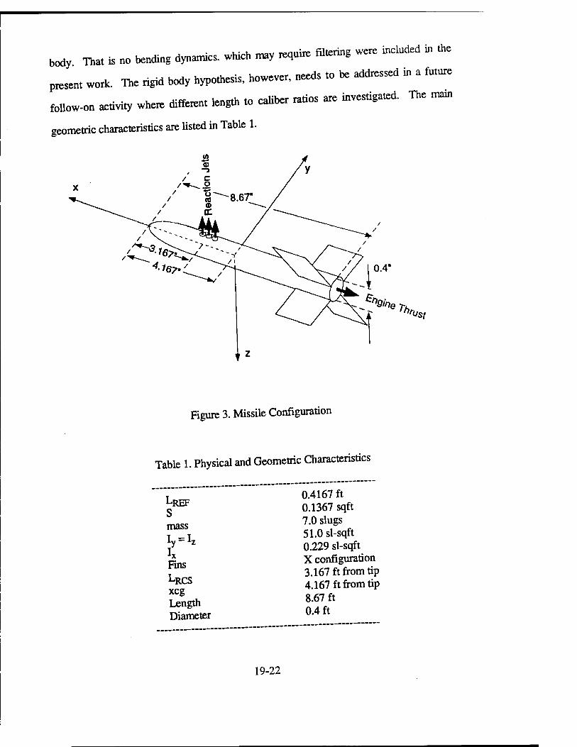
body That is no bending dynamic, which may .quire filtering were included m the
present work. The rigid body hypothesis, however, needs to be addressed in a future
follow-on activity where different length to caliber ratios are investigated. The ma*
geometric characteristics are listed in Table 1.
ihn list
Figure 3. Missile Configuration
Table 1. Physical and Geometric Characteristics
LREF s mass Iy = IZ
*x Fins LRCS xcg Length Diameter
0.4167 ft 0.1367 sqft 7.0 slugs 51.0 sl-sqft 0.229 sl-sqft X configuration 3.167 ft from tip 4.167 ft from tip 8.67 ft 0.4 ft
19-22
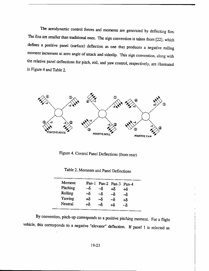
The aerodynamic control forces and moments are generated by deflecting fins.
The fins are smaller than traditional ones. The sign convention is taken from [22], which
defines a positive panel (surface) deflection as one that produces a negative rolling
moment increment at zero angle of attack and sideslip. This sign convention, along with
the relative panel deflections for pitch, roll, and yaw control, respectively, are illustrated
in Figure 4 and Table 2.
POSITIVE ROLL POSITIVE YAW
Figure 4. Control Panel Deflections (from rear)
Table 2. Moments and Panel Deflections
Moment Pan-1 Pan-2 Pan-3 Pan-4 Pitching -5-5+8+6 Rolling -5-5-5-5 Yawing +5-5-5+5 Neutral +5-5+5-5
By convention, pitch-up corresponds to a positive pitching moment. For a flight
vehicle, this corresponds to a negative "elevator" deflection. If panel 1 is selected as
19-23
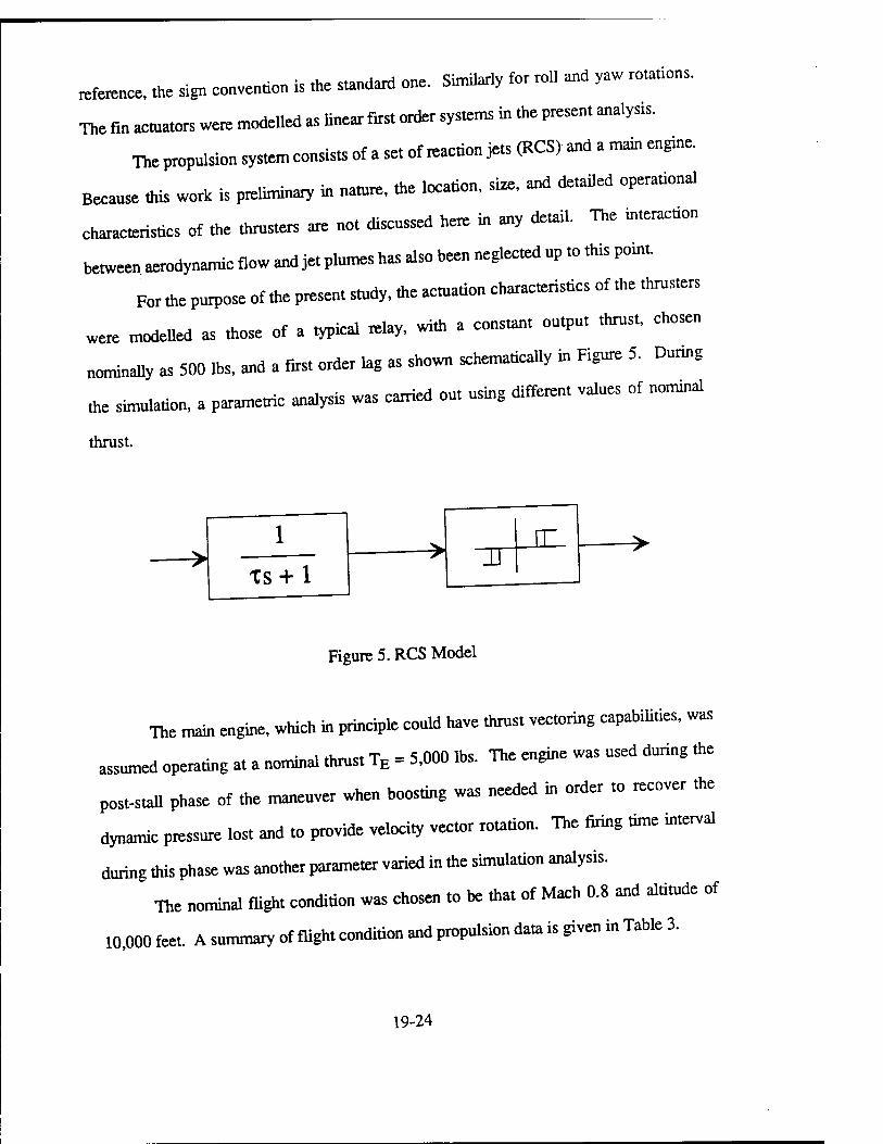
mfemnce, .he sign convention is the s«andard one. Singly (or roll and yaw rotations.
The fin actuators were modelled as linear firs, order systems in the present analysts.
^propulsion system consists of a set of reaction jets (RCS) and a main engine.
Because titis work is pre» in nan«, tine location, size, and dcailed operational
characKristics of .he thrusters are no. discussed here in any deuail. 11« infraction
between aerodynamic flow and je, plumes has also been neglected up to .his point
For fte purpose of me present study, the achtation characteristics of the thrusters
were modelled as those of a typical telay, wi«h a consutt. ou.pn. mrns., chosen
nominally as 500 lbs, and a first order lag as shown schematically in Figure 5. Dunng
the simulation, a paramedic analysis was carried ou. using differen. values of nomrnaJ
thrust.
TS+ 1
Figure 5. RCS Model
The main engine, which in principle could have thrust vectoring capabilities, was
assumed operating at a nominal thrust TE = 5,000 lbs. The engine was used during the
post-stall phase of the maneuver when boosting was needed in order to recover the
dynamic pressure lost and to provide velocity vector rotation. The firing time interval
during this phase was another parameter varied in the simulation analysis.
The nominal flight condition was chosen to be that of Mach 0.8 and altitude of
10,000 feet. A summary of flight condition and propulsion data is given in Table 3.
19-24

Table 3. Missile and Flight Condition Data
Main Engine Nominal T = 5,ooo lbs Reaction Jets Nominal TRCS = 5001bs RCS Time Constant Tu = 1/500 ^ Elevator Time Constant Tg = i/180 sec
RCSDeadband variable by design Reference Mach Number M = 0 8 Trim Altitude h = 10"0(K) ft Trim Angle of Attack 10 degrees Trim Attitude 10 degrees
3.2. Missile Aerodynamics
The aerodynamic forces and moments are usually obtained from wind tunnel data
of the vehicle and then "tuned" using flight testing. In the present work, neither type
data was available and analytical and numerical prediction methods were used. The
uncertainty and parameter variations introduced this way were then used as robustness
test for the variable structure controller.
In the maneuver chosen as the test scenario for autopilot validation, the vehicle
experiences a wide range of variations in angle of attack . Due to the absence of data,
the computation of aerodynamic coefficients was carried out by considering two
different flight regimes. First, the missile DATCOM code [22] was used for low angles
of attack (predefined by being below an assumed stall value between 35 and 40 degrees).
Second, classical fluid dynamics prediction methods [23], [24] were used for high angles
of attack (up to 90 degrees).
For bluff bodies, including streamline bodies at high angles of attack, the flow
separates causing a large wake behind the body. The predominant component of the
drag force is therefore pressure drag. The estimation of the aerodynamic forces was
done assuming the missile as a cylinder and neglecting the interference effect between
19-25

wings and main body as a firs, approximation. For the present work it was aiso assumed
tot to center of pressure was coincident with to geometric center of to missde.
The main aerodynamic force at high angles of attack is to normal force N. The
«:„;.„. r - NIOS where Q is to dynamic pressure and S to normal force coefficient CN - m» . «"■<="= ^
reference area, is a function of (1) angle of attack, (2) Reynolds number, and, (3) Mach
„umber. The coefficient CN was first computed as a function of Re, a, zero angle of
attack and constant Mach number, ton mtxüned accordingly. Based on the above
assumptions, a code was written » obtain aerodata for high angle of attack values.
Reynolds NflmhRr <T*e) For very low Re, the flow, described as - creeping flow ". creates pressure
differentials equivalent to skin friction. For symmetric, elliptical cylinders, the drag
coefficient based on the frontal area is given by
CI)o=87t/^/[c/(c + /I) + 1.5-2.31n(/?*)] (24)
wherehis the heightandcis the length of the axis of the cylinder in the flow direction as
shown in Figure 6. The Reynolds number R* is defined as
R*=V{h + c)/2/v
For a cylinder, Rd = Vdlv, since * = c and d = (h + c),2. Thus, for a cylinder
with Rd < 1, the drag coefficient at zero angle of attack is
CD0=10.9//?d/(0.87-ln/?d)
If Rd > 1, dynamic forces of the fluid cannot be neglected since they influence the
CD0 Dynamic forces are predominant over the viscous forces to such an extent that
they cause periodic shedding of vortices behind blunt bodies at a non-dimensional
fluency, which increases steadily with the Reynolds number. Tltis type of vortex
pattern is found in the wake of 2-D bodies, such as cylinders, plates or bluff rods.
19-26

Figure 6. Elliptical Cylinder and Dimensions
This comparatively stable system is called "double-row vortex trau" or "vortex-
street". Straight vortices are periodically released from the two sides of the body. If the
cylinder is moving with respect to fluid at a velocity w, the vortex street follows the
cylinder at velocity w. The distance between two vortices is x, as shown in Figure 7.
Both w and x are difficult to predict theoretically. Below the critical Reynolds number,
*V = 1/6 and xld - 4.5(based on tests), and CD0 = 4.5CDx, where
CDX=DI (gbx) = 1.6(w / V) - 0.64(w / V)2
where, b is the span of the cylinder. It has been shown that the drag equivalent for a
bluff body, such as a cylinder is entirely contained in the vortex system. It is emphasized
that the vortex street is a mechanism which leads to a realistic drag coefficient, without
introducing any qualitative viscosity values. The frequency indicating the "Strouhal
number," reaches a constant level in the vicinity of Rd = 103. For regions from 1 to 103
a curve fit is a good enough approximation. Accurate calculation of CD0 requires
however the knowledge of pressure coefficient, C .
19-27

\ /
Figure 7. Vortex Street
Vnrfpy frequency
The number of vortices formed at one side of the street in a unit time is given by
(27) /= (V-w)lx
where w = VI6, and x = 4 S d. The Strouhal number S, is defined as (28)
5 = Strouhal number -fhlV
where » = d for cylinder. For a flat plate, h is A. heigh, of the plate. The drag
coefficient Q)0, is given by
c|/04 =0.21/S=>CD0=(0.21/5)3/4. (29)
Equation (27) can be rewritten as
fx = V(l - w/V )= V (1 -1/6) = V(5/6). (30)
The S*ouhal number 5 - (Vlx) (5/6) (W = (5/6)W =(5/6) (1/4.5) . and therefore,
CDO is
C?/n4 = 0.21/5 = 1.134
(3D W)0 -"•-"'" •
Thus for Reynolds number, ^ e(l03,106), the above equation gives
CD0= U82. Transition from laminar to turbulent flow causes an appreciable change in CD0
value. Since this depends on factors like turbulence in wind, surface type, mechanical
19-28

vibrations, it will be assumed that the transition occurs when Recr = 3*105 is reached.
The value of CD0 then falls to 0.3. The value of CD0 increases for higher Reynolds
number but was assumed to be constant and equal to 0.3. For Reynolds number Rd* e
(1,1000), CD0 was linearly interpolated and approximated by :
CD0 =- 0.113581/^ + 12.5401 (3
Mach Number F.ffcrt
For bluff bodies, like a cylinder lying across the flow, as the Mach number
increases, there is an appreciable change in stagnation pressure, while the base pressure
remains unchanged. The drag due to the nose pressure is adjusted by a factor (1 + 0.25
M2) whereas the drag due to the base pressure remains unchanged. For a plate it has
been shown that 50% of the drag is from base and 50% from nose. For the cylinder we
do not have such numbers and the estimate used are based on the flat plate. Thus
Q>0 =CZ?o[o.5 + 0.5(l + 0.25M2)] = CZ)o[l.04-0.125M2] (32)
which is valid up to the transonic region.
Cross Flnw PrinHpV
The cross flow principle, states that the fluid dynamic pressure forces on a bluff
body corresponds to the velocity component normal to cylindrical axes, which is
Vsin(a), as shown in Figure 8.
The following is then valid up to the critical Reynolds number 3*105, if the
cross-sectional area S = d bis the frontal area for which CDbasic is defined. Then
CN = N/QS = CDbasicsin2a
and
\cD=CDbasicsin3a
Q. = CDbasic s^ OC COS a
19-29

Figure 8. Effective Velocity
These equations are valid for sub-critical Reynolds number Recr = 3*1()5.
Adding A CD - nCf to CDbasic improves the above prediction. The cross-flow
principle is not valid for super-critical conditions,
flpfrmmy. Arf-f Correction
The reference area for a missile is defined in terms of its cross-sectional area
S'=nd2l4. Therefore,
CN =CN(S/S') = CDbasic(S/Z)sM2* (33) CD=CDbasic(S/^)sin3a CL=CDbasic(S/^)sm2acosa
are the correct aerodynamic coefficients for the missile.
In summary, CD0 calculation involves :
(a) Finding CD0 based on Reynolds number
(b) Adjusting for compressibility
(c) Using cross-flow correction to get final CD0
(d) Correcting the reference area.
19-30
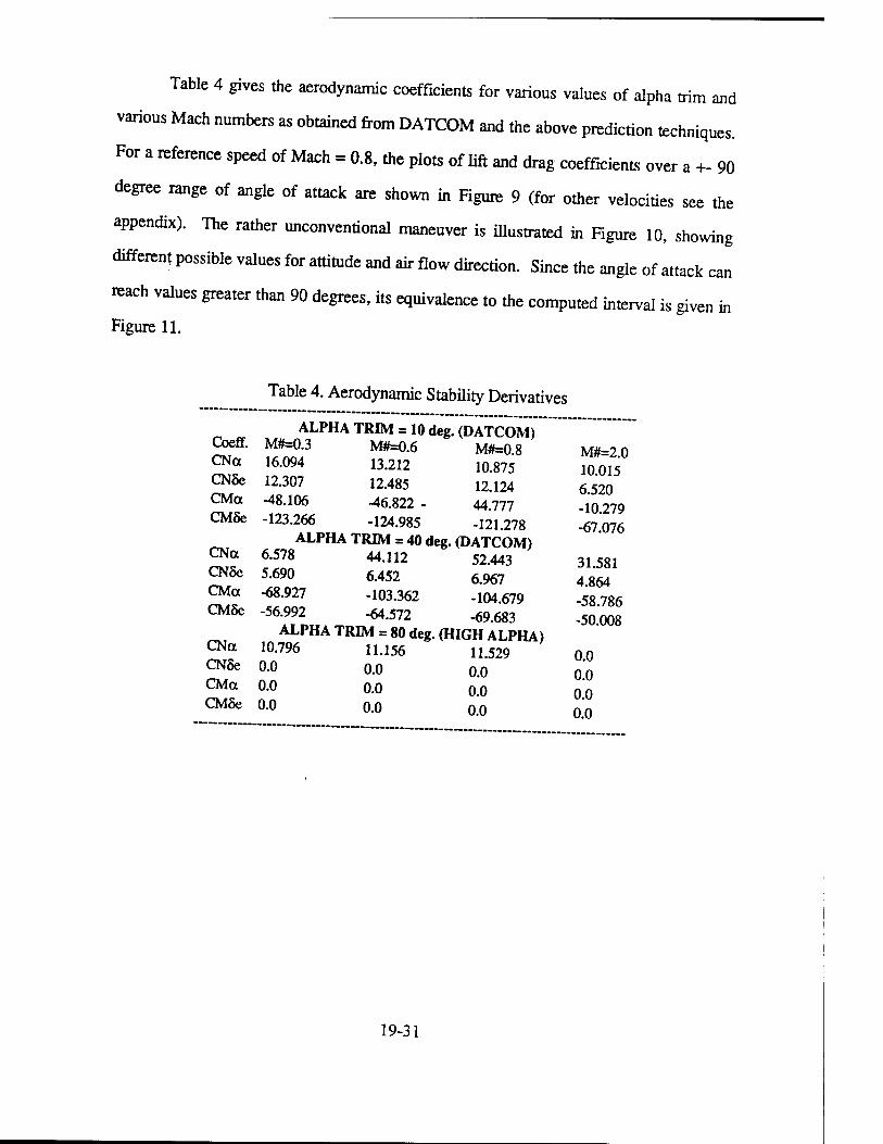
Table 4 gives the aerodynamic coefficients for various values of alpha trim and
various Mach numbers as obtained from DATCOM and the above prediction techniques.
For a reference speed of Mach = 0.8, the plots of lift and drag coefficients over a +. 90
degree range of angle of attack are shown in Figure 9 (for other velocities see the
appendix). The rather unconventional maneuver is illustrated in Figure 10, showing
different possible values for attitude and air flow direction. Since the angle of attack can
reach values greater than 90 degrees, its equivalence to the computed interval is given in
Figure 11.
Table 4. Aerodynamic Stability Derivatives
Coeff. CNa CN6e CMa CM5e
CNa CN5e CMa CM5e
CNa CN5e CMa CMSe
M#=0.3 16.094 12.307 -48.106 -123.266
ALPHA TRIM = 10 deg. (DATCOM) M#=0.6 13.212 12.485 -46.822 - -124.985
M#=0.8 10.875 12.124 44.777 -121.278
ALPHA TRIM = 40 deg. (DATCOM) 6.578 44.112 52.443 5.690 6.452 6.967 -68-927 -103.362 -104 679 -56.992 -64.572 -69.683
ALPHA TRIM = 80 deg. (HIGH ALPHA) 10.796 H.156 n.529 °-° 0.0 o.O °-° 0.0 o.O 00 0.0 o.O
M#=2.0 10.015 6.520 -10.279 -67.076
31.581 4.864 -58.786 -50.008
0.0 0.0 0.0 0.0
19-31
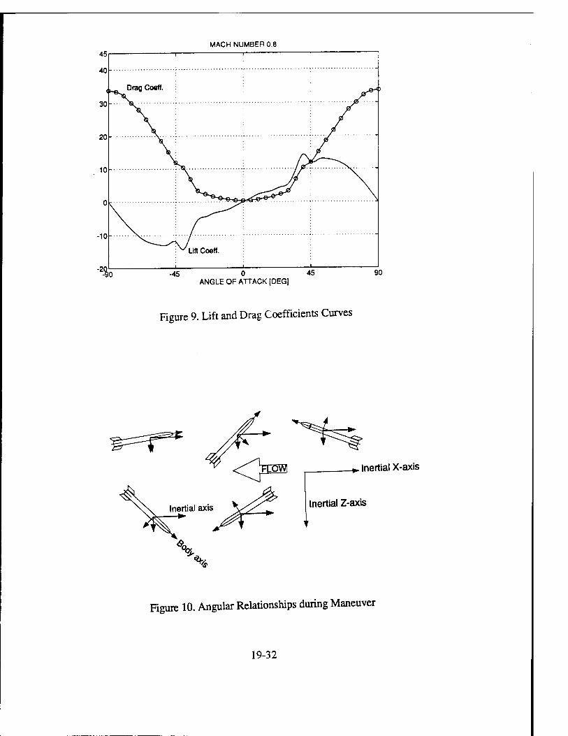
MACH NUMBER 0.8
-45 0 45 ANGLE OF ATTACK [DEG]
90
Figure 9. Lift and Drag Coefficients Curves
^^r* #. Inertial X-axis
Inertial Z-axis
Figure 10. Angular Relationships during Maneuver
19-32
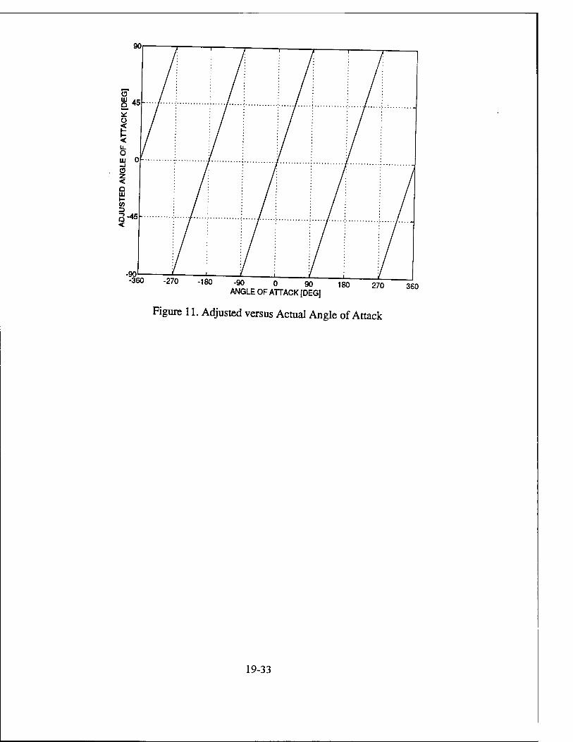
-360 -270 -180 -90 0 90 ANGLE OF ATTACK [DEG]
180 270 360
Figure 11. Adjusted versus Actual Angle of Attack
19-33

3.3. Low Angle of Attack Model
to the induction, toe M maneuver and toe autopilot design were confined to
toe longitudina! plane. Due to toe wide range of dynamic pressure experienced by toe
vehicle, toe modelling was divided into two pa«, A simpüfied rigid body linearized
motion a, angles of attack below stall, and a combined pitch rotation and point mass
translation above stall. In the low angle of attack region, the speed was assumed constant and a typical
short period approximation was used [1], [26]. In equation form we have
mVT Na ™VT mVT (34)
? = cmaa+ I ly ly y J
which becomes, in dimensional form
ä = Zaa + q + Z5b + ZTuT (341)
q = Maa + M88 + MTuj
TRCS is the thrust provided by reaction jet and LRCS is the jets moment arm. The
actuators are modelled by linear first order systems with time constants xd and xu for the
elevator and RCS respectively. In equation form
x55 = 8 + 5c (35)
Since standard measurements and commands in missile autopilots include
accelerometers and rate gyros, Eqs. (34') and (35) can be rewritten in state space form
19-34

by introducing the normal load factor N, z as a state variable replacing the angle of attack.
From kinematics we have
(36)
By defining xT =[NZ q 8 uT]anduT=[8c uTc] weobtain
8 Üj
vTza
0
0
S. VrZ6
^ S*8
0
0
M„Z
VrZr
M6-i^±i Mr-
^8
ja W^r "^Z~
za <7 8
Uj
+
J
#T8 gtu o j_
0
0
0 c
luTc.
(37)
or, in standard form
x = Ax + Bu
with the output vector being equal to the state vector.
The time rate of change of the flight path angle is computed from the normal
acceleration, provided the angle of attack is small, as
" -_ az (38)
and the inertial velocity components are
X = Vy-cosy
Z = Vj sin y (39)
19-35

3.4. High Angle of Attack Model
The model tor the post stall region must accouo. tor «he dynamic pressure
variation, which is characterized by large excursions in angle of attack, attitude, flight
path angle, and velocity. In this region, aerodynamic control becomes negligible and the
only effective actuators are the reaction jets. Such control must rotate .he vehicle
counteractingthepMingmomentproduced by the normal force, which tends to oppose
the motion. Considering a pure rotational attitude motion, we have
I ft = QSCNLcp + LRCSTRCS"T
where Lcp is the distance between enter of press», (as computed from the assumed
cylindrical conflguration of section 3.2.) and the center of mass. The value of Lcp will be
a design parameter for future studies, when a more detailed aerodynamic model will be
available. The velocity variation is taken into account by adding a two-dimensional point
mass model, which in the inertial reference is given by
mX = -LsinY-öcosY + rEcose-r/?cssine mZ = -Lcosy + Dsmy-TEsine-TRCscosQ + mg.
Y = 6-a
The flight path angle is also related to the inertial velocity components from
_JZ] (42) 7 = -tan \jj
differentiating Eq. (42) with respect to time yields
Y~X2+Z2
zx-zx x2+z2
therefore the normal acceleration is
19-36
az=XsmQ + ZcosQ (43)
In Eq. (41), one of the force components is the main engine thrust TE. In this
phase, the main engine is fired to recover the speed loss experienced by the vehicle
during the rotation. The main engine thrust is set to be a function of the attitude angle in
an open loop fashion, and it is operational within preset values of the overall speed.
3.5. Acquisition of Steady State
At the end of the maneuver, the vehicle enters the low angle of attack regime
with full dynamic pressure recovery. The reaching of the desired steady state requires
specific values for the attitude, flight path angle, and consequently the angle of attack
itself. The point mass equations are still valid and the rotational motion equation must
now include the flight path angle. This model for the final phase of the trajectory is
used, instead of simple short period, to account for flight path and velocity variations
still present in this phase. Keeping Eq. (41), we now use
q = Maa + Md8 + MTuT
in place of Eq. (40). Replacing a with 6-yin Eq. (44) yields
q = Mae-May + Ms8 + MTuT (
where the flight path angle can now considered as an additional input or state depending
on the approach used for the autopilot design.
Since during this phase of the maneuver the vehicle is flying at an attitude and
flight path angles close to 180 degrees, the small perturbation Eq. (45) leads to a
mathematical singularity in that the controller does not distinguish between 180 and zero
degrees. To eliminate the problem, a simple 180-degree roll maneuver would be
sufficient, however because our work was limited to the longitudinal plane, an alternate
19-37

approach was taken consisting of ft. introduction of the desired steady state (mm)
values in Eq. (45). Drifting fte desired set of trim point values as [90 Yo »0 «roj. '"=
perturbation variables can be written as e = 0-6o, 1=T-y0, 8 = A-50, and
T .Or -uT0, (note that zero steady state pitch rate is assumed). Therefore Eq. (45)
becomes
X =
0 1 0 "0-6o" "0 o rA-80 1 Ma 0 -M0 Q + M5 Mj UT-uT0
-z„ o za . J-Yo. L-Z5 ZT\
(46)
where X = [0,q,nT and X=x .
K the flight path angle is considered as input rather than state, we have
[e ro r re-Gol + "0 0
A. M„ 0. ß M5 Mr_
A-8r 0 (r-Yo)- (46')
_UT-uT0\ L"Ma.
In summary, Eqs. (41) and (46) or Eqs. (41) and (46') represent the missile
model in the final phase of steady state acquisition.
4. Autopilot Design
This section describes the design of the pitch channel autopilot using variable
structure control. The control logic is broken down according to the phase of flight,
resulting in a structure that includes the low alpha component, the post stall rotation, and
the final steady state acquisition.
19-38

4.1. Objectives
The main objective of the present work was the synthesis of a pitch autopilot that
uses a combination of aerodynamic and reaction jet control to achieve a 180-degree
longitudinal heading maneuver in the vertical plane. As described in the previous
sections, the chosen maneuver consists of a full turn reversal, which requires for being
successful, high angles of attack, loss of dynamic pressure, and the acquisition of a final
state characterized by a straight level flight with speed equal to the initial velocity. Our
concentration has been on the pitch autopilot, assuming no interaction among the three
channels. Additional effort is suggested and has been proposed [25], to study the full
spatial implications of post stall maneuvering.
The flight condition chosen for the point design corresponds to Mach 0.8 and
altitude of 10,000 feet. The design goal was a controller structure, insensitive to the
uncertainty of the values of the aerodynamic coefficients and different values of reaction
jets thrust, because this will limit gain scheduling.
The autopilot design was found by using the VSC technique described in section
2. The control structure was changed as function of the angle of attack. The result was
a three-phase design. The first phase, (Phase I) begins after the initial command and
ends when stall is reached. The second phase, (Phase II) is flown at angles of attack
above stall. This phase encompasses the main part of the trajectory and involves a model
following of the attitude, as well as the open loop boost section for the rotation of the
velocity vector and its magnitude recovery. The final phase, (Phase HI) is again below
stall and it is implemented as tracking of attitude and flight path set points.
In addition to having a different control logic, the three phases differ in their
implementation. While the first and third use both reaction jet and elevator; the second
phase control relies on the use of reaction jet and main engine thrust
19-39
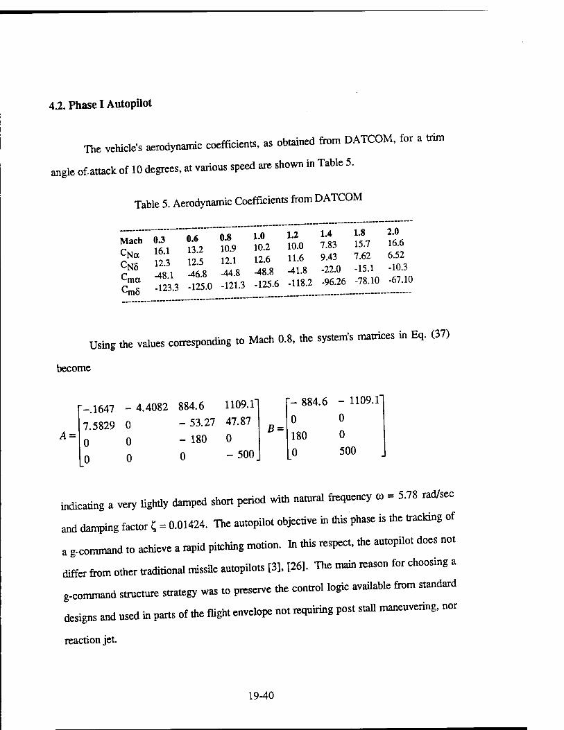
4.2. Phase I Autopilot
The vehicle's aerodynamic coefficients, as obtained from DATCOM, for a trim
angle of.attack of 10 degrees, at various speed are shown in Table 5.
Table 5. Aerodynamic Coefficients from DATCOM
0.6 13.2 12.5
0.8 10.9 12.1
1.0 10.2 12.6
1.2 10.0 11.6
1.4 7.83 9.43
Mach 0.3 CNa 16.1
~N5 Sfl ^8 -44.8 -48.8 -41.8 -22.0 -15.1 nL 4250 -121.3 -125.6 -118.2 -96.26 -78.10 -67.10
1.8 2.0 15.7 16.6 7.62 6.52
-10.3
Cm8
Using the values corres; ponding to Mach 0.8, the system's matrices in Eq. (37)
become
A =
_1647 -4.4082 884.6 1109.1'
7.5829 0 -53.27 47.87 0 0 - 180 0 0 0 0 -500
B =
- 884.6 - 1109.1'
0 0 180 0 0 500
indicating a very lightly damped short period with natural frequency co = 5.78 rad/sec
and damping factor C = 0.01424. The autopilot objective in this phase is the tracking of
a g-command to achieve a rapid pitching motion. In this respect, the autopilot does not
differ from other traditional missile autopilots [3], [26]. The main reason for choosing a
g-command structure strategy was to preserve the control logic available from standard
designs and used in parts of the flight envelope not requiring post stall maneuvering, nor
reaction jet.
19-40

In order to achieve perfect tracking of the load factor, an integrator was added to
the state vector, which then becomes xTaug=[^zdt Nz q 5 uT] leading to a
VSC-PI control structure. The augmented system dynamics are xaug ~ Aaugxaug + Baugu- (47)
From (15), the controller structure is
Nx
- ^-Pji^i- (48)
TTie values of the gain matrices can be found in the Appendix Al and were
obtained using the Mowing values for the design parameters, with 8 = 0.01
I
Q = diag[45 .1 .1 .1 40l
A3
P =
A3 =diag[- 10 -10] . (49)
P8=l 0 0 P«r=10
The selection of weightings in Eq. (49) was based on obtaining a fast load factor
response and at the same time on keeping the control efforts within their limitations.
The matrix G which defines the sliding surface , = Gxaug is also found in the Appendix
Al. Figure 12 shows the block diagram implementation of the autopilot
19-41
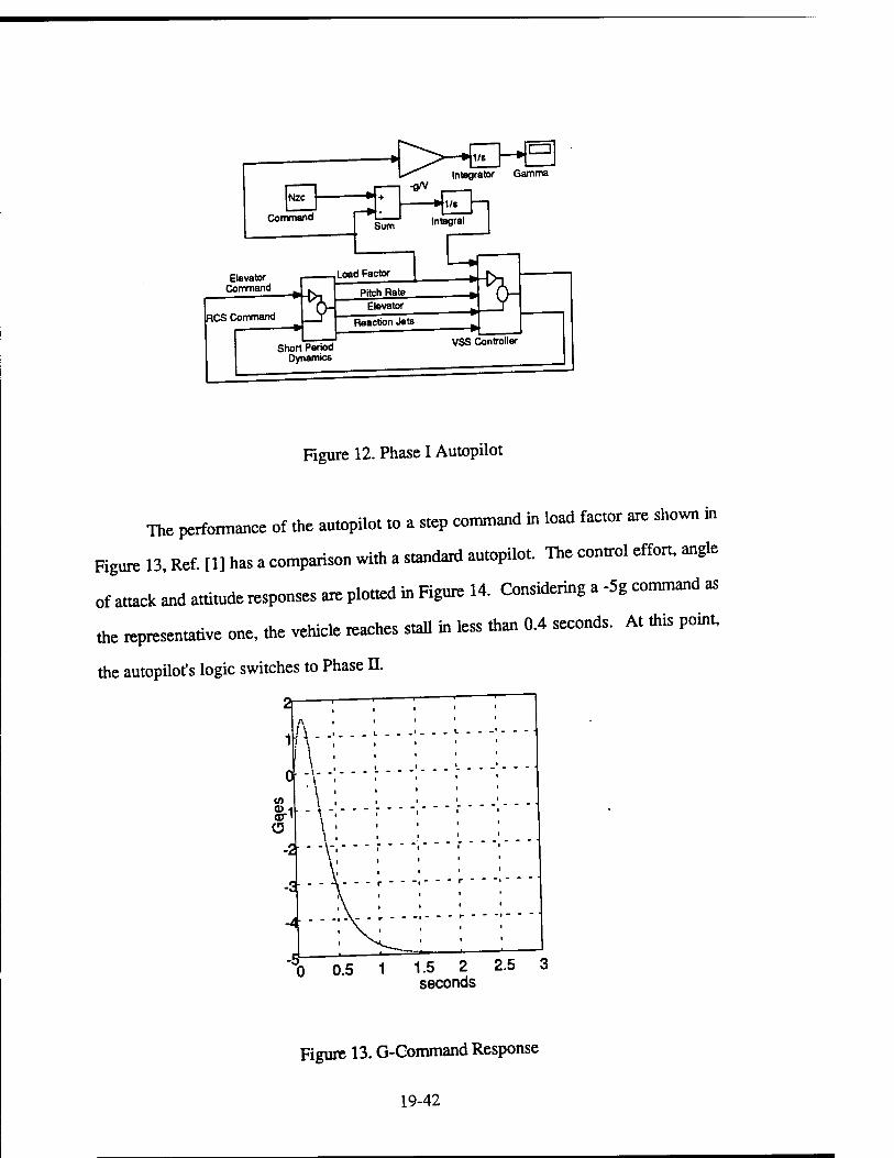
Figure 12. Phase I Autopilot
The performance of the autopilot «o a step command in load factor are shown in
Figure 13, Ref. [1] has a comparison with a standard autopilot. The control effort, angle
of attack and attitude responses are plotted in Figure 14. Considering a -5g command as
the representative one, the vehicle reaches stall in less than 0.4 seconds. A. mis point,
the autopilot's logic switches to Phase II.
0.5 1 1.5 2 2.5 3 seconds
Figure 13. G-Command Response
19-42
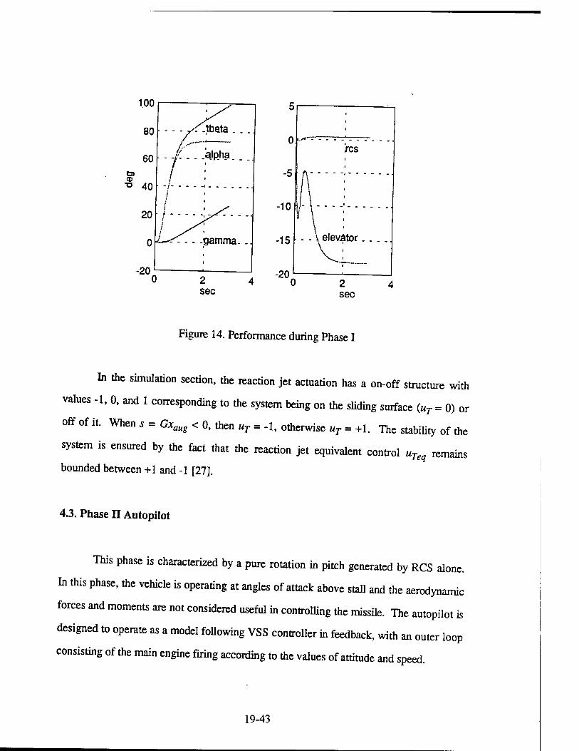
Figure 14. Performance during Phase I
In the simulation section, the reaction jet actuation has a on-off structure with
values -1, 0, and 1 corresponding to the system being on the sliding surface (uT = 0) or
off of it. When s = Gxaug < 0, then uT = -1, otherwise uT = +1. The stability of the
system is ensured by the fact that the reaction jet equivalent control uTeq remains
bounded between +1 and -1 [27].
4.3. Phase II Autopilot
This phase is characterized by a pure rotation in pitch generated by RCS alone.
In this phase, the vehicle is operating at angles of attack above stall and the aerodynamic
forces and moments are not considered useful in controlling the missile. The autopilot is
designed to operate as a model following VSS controller in feedback, with an outer loop
consisting of the main engine firing according to the values of attitude and speed.
19-43
The main objective of tine autopilot in this phase is the rotation of the vehicle and
compensation of dynamic pressure, which drops considerably due to speed reduction
associated with drag increase at high angles of attack. To recover dynamic pressure, the
« engine is fired in an open .oop fashion a. a predetermined attitude chosen,
nominally, 6 = 120 degrees. Tne engine remains in a boost phase mode until the final
desired speed (here assumed equal to the initial one) is achieved as well as the
appropriate direction of flight Tne equations of motion used for the conu-oller synthesis
are E,s. (40) and (41). VSC is applied to Eq. (40), that can be written in state space
form as
x =
*
"e" ro li
:= n o
x + • -
</ L -
- "
0 0
LRCST
RCS
Uj + Nd
h L J -1 h .
= AX + BUT + D (50)
Here N is the normal force acting on the vehicle and d is the moment arm (the
contribution of the axial force was considered negligible at post stall angles of attack).
Globally, the torque due to normal force produces a resisting effect that can be treated as
a disturbance D. To perform a point design of the autopilot, a worst case approach was
used and D was bounded by the value corresponding to a cylinder set perpendicular to
the flow, where the drag assumes its maximum value. With this, the B and D terms in
Eq. (50) become
B =
0
31.049.
,D =
0
- 10
19-44

Next, VSC was applied using a model following approach [9], [12], by
specifying a desired model for the pitch rotational dynamics. The model was chosen
based on the +1, -1 limitations of the reaction jet, and it is given by
xm ~ AmXm + Bmum = ("o i - ro - 178 - 24 xm +
178 u, vm (51)
from (50) and (51), the error dynamics e = xm - x are given by
e = Ame + [Am - A]x + Bmum -D-BuT (52)
a general form for the control law, for perfect model following, can be written as
uT=uNL+Klx + K2um + K3=uNL+uL (53)
with
\Kl=B>m-A] K2=B'Bi
K-i=B*D m (54)
and B* - (BTB)-lBTis the appropriate pseudoinverse of B.
In the present case, the implementation of the control law Eq. (53) is limited
the nonlinear component, which is given by to
\uT=uNL=sgn(s)
(55) s = Ge = [7 l]e.
TTie linear component of the control law is nothing but ueq, the controller
structure during sliding. The choice of G was made to ensure a desirable response
during sliding.
Phase n starts with initial conditions corresponding to the state variables final
conditions from Phase I. This phase lasts about 0.5 seconds and shows excellent
19-45
perforce. The «suits in tetms of model foUowing and control effon are presented in
Figures 15 and 16, and the structure of the autopilot is shown in Figure 17.
The attitude angle goes from 40 degrees to 180 degrees. A, 120 degrees, the
main engine is turned on and its effect is evident from the speed and flight path angle
„me histories included in the Simulation section. The engine is shut down when the
speed equivalent to Mach 0.8 is recovered, although other choices can he made to
decrease/increase the hoos, phase. A, the end of Phase II, the angle of attack is below
stall and Phase III autopilot becomes active. The above procedure will be shown in tine
simulation section.
200
150
CO
■o-ioO
50
1—■ >
, i '
/^
/: /:
\J¥" C 0 0.2 0.4 0.6 0.8
sec
Figure 15. Performance during Phase II
19^46
1
Figure 16. Control Effort during Phase II
ii Speed
Main Engine fired if: pitch angle > 120 deg. 4 speed < reference speed
^Speed
, Pitch Angle
Main Engine Thrust
Aerodynamic Model Aerodynamic Forces
Gravity
Reaction Jet Deflection
Point Mass Dynamics Motion of center of mass Forces acting : gravity aerodynamic reaction jets main engine
Speed Inertial x. z coordinator T' Inertiai x, z speed components Inertial Accieration Might Path Angle ~*~
J
Actuator Dynamics
Elevator Deflection Command
M Reaction Jet
Perfect Model Following Gain
Error Vector
Deflection Command Reaction Jet Deflection G e > 0 6rcs-1 G e - 0 6rcs-0 G e < 0 6rcs=-1
Flight Path Angle
Elevator Deflection
Reaction Jet Deflectiori
G «*
Rotational Dynamics
Pitch Angle
Pitch Rate
Reference Pitch Angle Model Following Model
Model Pitch Angle
Model Pitch Rate
* £ c n < IE o 0.
I 0.
Figure 17. Phase II Autopilot Block Diagram
19-47

4.4. Phase HI Autopilot
TOs phase involves the task of acquiring and maintaining a set of steady state
values for the attitude and flight path of the missile. In our work we established the
objective of reaching 180 of flight path and attitude angles, although different values can
be set if desired. The pertinent model for the system is given by Eqs. (41) and (46). Since the
flight path angle is required to reach 180 degrees, the rotational equation now contains y
as an additional state variable. Using the numerical values from Table 5, and defining the
trim conditions x0 = [90, q«> 7olT and u0 = [«o. uT0lT. Bq. (46) now becomes
X = x = A{X-x0) + B{U-Uo)
where
(56)
A =
0 1 o - 33.4266 0 33.4266 0.1647 0 -0.1647
B =
0 0 - 90.5355 31.049
0.1836 0.0829
using the VSC model following approach, we define the model dynamics as
Xm = xm = Am{Xm -xm0) + Bm{Um - um0)
where
(57)
Am —
"0 10 u u _[ec=180° -16 -8 0 Bm= 16 0 andtfm-Mm0-|^=lg0Oj
0 0 -0.5J L° °-5J The model following controller again operates on the error state, difference
between X and Xm and whose dynamics are given by
19-48

e = Ame + [Am-A]x + Bmum+AxQ-Bu
the control law has the form
u =uNL+K1(X-x0) + K2x0+K3Um=uNL+uL
with
(58)
(59)
K7=B*A K?=B B
(60) m
if the value of Um and x0 are the same, as in our case, then the controller becomes
u = uNL+Kl(X-x0) (61)
with the gain Kj given in Appendix Al. From Eq. (61) into (58) we obtain the error
dynamics as
e = Ame-BuNL
(62)
the structure of the nonlinear component in Eq. (62) is based on the Eq. (48) and given by
u = -Le-p Ne \\Me\\ + 8 (63)
with the matrix gains above computed similarly to those in Eq. (48) using the following
parameters
I
Q = diag[l 100 10] A*3 = diag[- 3-3]
"P6 =-01 0 0 P«r = 01
(64) P =
19-49
In the implementation, the elevator deflection operates Mowing Eq. (63), while
the reaction je, operates in an on-off fashion according to the sign of the sliding sorface
erros s = Ge [27]. A control strategy for the Phase III autopilot based on model following of the
attitude oriy was also derived In this case, the appropriate equations of motion for the
vehicle become (41) and (46'). TTte flight path angle is then considered as a disturbance
to the system, leading to the following rotational equations for tine vehicle and «he model
0
ß
4m
0 1
- 33.4266 0JL<7
e-e0 + j u
o o -90.536 31.049
8 + 0 - 33.4266
(65)
0 1 - 36.4 - 12
6m
ßm.
0 36.4 "m-
The procedure is similar to the previous one leading to a controller of the form
d = Kx{X-x0) + Ky{T-yo) + Kum{Um-um0)
1 {s>0)
uT=\ 0 (s = 0)
(66)
- 1 (s<0)
with s = Ge = 7(6m - 6) + <*, - ,), where the gains in Eq. (66) are reported in Appencüx
Al Note that, with this second approach, the elevator is responsible for providing
model following, while the reaction jet control gives robustness to parameter vanaüons
and disturbances. The block diagrams of Phase HI autopilots are shown in Figures 18
and 19.
19-50
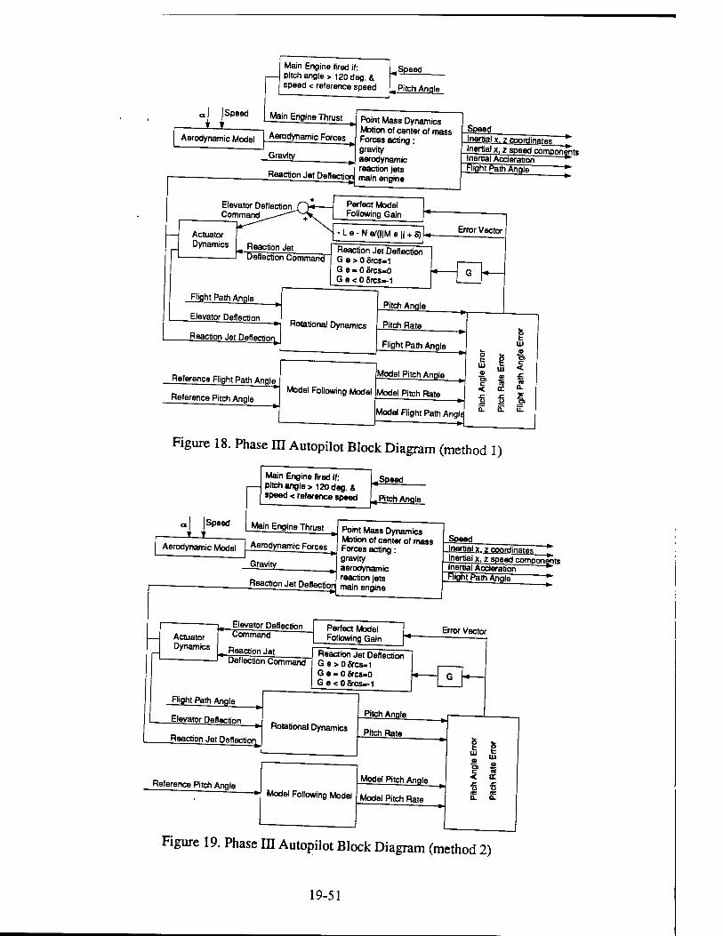
Main Engine fired if: pitch angle > 120 deg. & speed < reference speed
, Spaed
., Pitch Angle
«I |sPeec( | Main Engine Thrust
Aerodynamic Mnriol I Aerodynamic Forces
Reaction Jet Deflection
Point Mass Dynamics Motion of center of mass Forces acting: gravity aerodynamic reaction jets main engine
Elevator Deflection^ Command
Actuator Dynamics , Reaction Jet
Perfect Model Following Gain
-Le-Ne/(||Me|| + 8)
Deflection Command
Error Vector
Reaction Jet Deflection G e > 0 8rcs«1 G e - 0 Srcs«0 G e < 0 8rcs—1
Flight Path Angle
Elevator Deflection
Reaction Jet Deflection
Rotational Dynamics Pitch Rate
Pitch Angle
Flight Path Angle
Reference Flight Path Angle
Reference Pitch Angle Model Following Model
Model Pitch Angle
Model Pitch Rate
Model Flight Path Angli
fc t w
fc § w a c <
n < CC •6 ■5 £ a. a. u.
_
Figure 18. Phase m Autopilot Block Diagram (method 1)
±J Speed
Main Engine fired if: pitch angle > 120 deg. & speed < reference speed
.«Speed
% Pitch Angle
Aerodynamic Model
Main Engine Thrust
Aerodynamic Forces ■—»
r» _^ iwatuon jeis Reaction Jet Deflection majn engine
Point Mass Dynamics Motion of center of mass Forces acting: gravity aerodynamic reaction jets
Speed Inertial x. j coordinat««: Inertial x, z speed components Inernal Accleration Plight Path Angle *"
Actuator Dynamics
Elevator Deflection Command
Reaction Jet Deflection Command
Perfect Model Following Gain
Error Vector
Reaction Jet Deflection G e > o 5rcs-1 G e - 0 fircs-0 Ge<05rcs_-1
Flight Path Angle
Elevator Deflection
Reaction Jet Deftartinn Rotational Dynamics
Pitch Angle
Pitch Rate
Reference Pitch Angle Model Following Model
Model Pitch Angle
Model Pitch Rate
fc k.
t
o UJ
n < CC r. fi .« ä; 0. CL
Figure 19. Phase in Autopilot Block Diagram (method 2) _
19-51

5. Simulation This section presents the simulation results relative to the entire maneuver for the
nominal case as well as sensitivity analysis in terms of some of the vehicle's parameters
such as reaction jefs thrust, initial speed, and attitude angle at main engine firing time.
5.1. Description
The autopilot logic described in section 4, and whose diagram is summarized in
Figure 20, was tested with a nonlinear simulation code developed in the Matlab®-
Simulink™ environment, and enclosed in this report as deliverables. The main
objectives of the simulation were:
1. To validate the autopilot performance in the chosen scenario.
2. To test the robustness of the methodology by using fixed controller gains
instead of gains scheduled with angle of attack and Mach number variation.
3. To test the robustness of the methodology with respect to parameter variations
such as reference speed, initial time of main engine firing, and reaction jet
reference thrust.
It is important to note that, during the simulation, the aerodynamic forces and
moments are not constant, but vary according to Figure 9, as functions of the angle of
attack. One of the problems encountered in the development of the simulation was the
choice of integration routine, since the results were found to be quite sensitive to the
integration technique and step size selection. The most satisfactory results were
obtained using a third order Runge-Kutta method with minimum step size AT = 0.001.
19-52
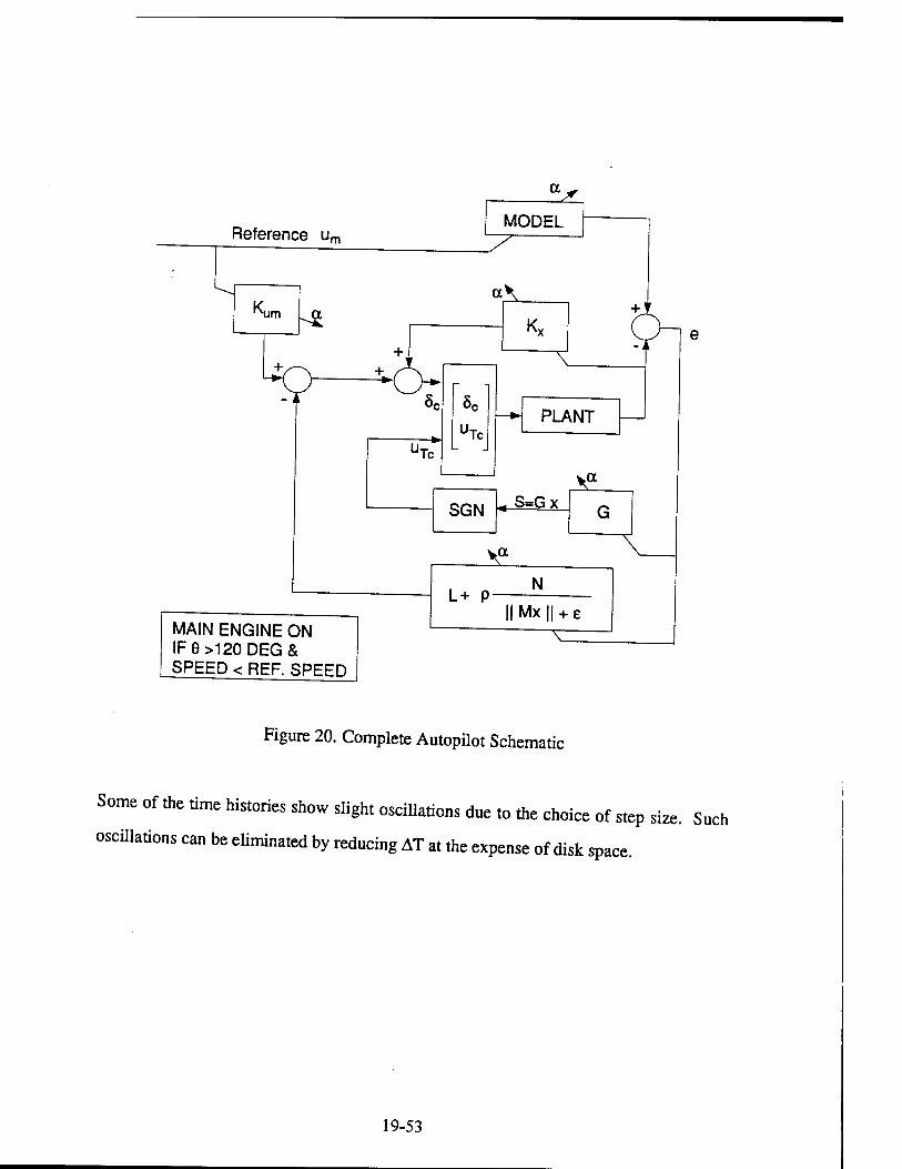
Reference u m
Ku m a
O
MAIN ENGINE ON IF8>120DEG& SPEED < REF. SPEED
a ̂ L MODEL
a\
Kv
+ T
^
4Tc
JTc PLANT
SGN S=Gx ^
a
_*5L L+ P-
N
IIMXJI + E
Figure 20. Complete Autopilot Schematic
Some of the time histories show slight oscillations due to the choice of step size. Such
osculations can be eliminated by reducing AT at the expense of disk space.
19-53

5.2. Results
*2,], ^nminal Case
Nominal values for the geometric and aerodynamic characteristics of the system
are found in Tables 1 and 3. The autopilot gains are given in Appendix Al.
The maneuver begins with a negative 5g Nzc command. The missile pitches up
reaching stall withing 0.278 seconds from the beginning of the maneuver. The motion
is essentially in pitch with no appreciable change in flight path angle as seen from
Figure 21 where pitch, flight path, and angle of attack are plotted. The load factor at
stall has basically reached the commanded value of five times the gravity acceleration
as shown in Figure 22, where the top curve corresponds to an integration using a step
size of 0.001 seconds and the bottom curve to a step size of 0.00005 seconds. The
control activity are shown in Figures 23 and 24.
0.2781 .3 TIME [SEC]
Figure 21. Angular Behavior below Stall
19-54
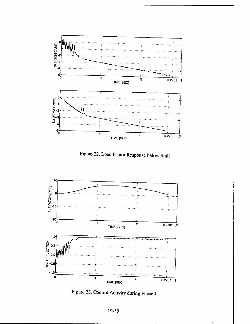
TIME [SEC] 0.2781 .3
TIME [SEC] 0.27 .3
Figure 22. Load Factor Response below Stall
TIME [SEC] 0.2781 .3
TIME [SEC]
Figure 23. Control Activity during Phase I
0.2781 .3
19-55
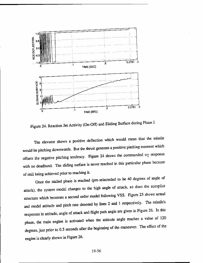
1.0
1 oJil Ü lUllUIIllllll ui ü! o.o ... UJ D 8-0.5 c - -1.0 llllllü
TIME [SECl
0.2781 .3
TIME [SEC]
Figur, 24. Reaction Jet Activity (On-Off) and Sliding Surface during Phase I
The elevator shows a positive deflection which would mean that «he missile
would be pitching downwards. But fine thrust generats a positive pitching moment which
offsets the negative pitching tendency. Ftgnre 24 shows the commanded uT response
with no deadband. The sUding surface is never reached in «his particular phase because
of stall being achieved prior to reaching it
Once the stalled phase is reached (pre-selecteded «o be 40 degrees of angle of
attack), the system mode! changes to the high angle of attack, so does the autopilot
structure which becomes a second order mode! Mowing VSS. Hgure 25 shows actual
and model attitude and pitch rate denoted by lines 2 and 1 respectively. The missile's
responses in attitude, angle of attack and flight path angle are given in Figure 26. In Una
phase, the main engine is activated when «he attitude angie reaches a value of 120
degrees, jus. prior to 0.5 seconds after the beginning of the maneuver. The effect of the
engine is clearly shown in Figure 26.
19-56
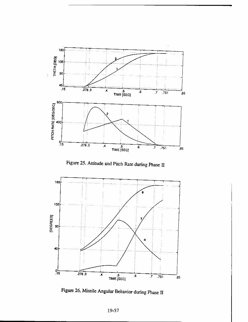
800 O LU M
o UJ o tfJ 400 < a: x o
.278.3 •4 .5 TIME [SEC]
4 -5 .6 TIME [SEC]
•7 .751 .85
■7 .751 .85
Figure 25. Attitude and Pitch Rate during Phase H
.278.3 ■« -5 .6 TIME [SEC]
.7 .751 .85
Figure 26. Missile Angular Behavior during Phase II
19-57
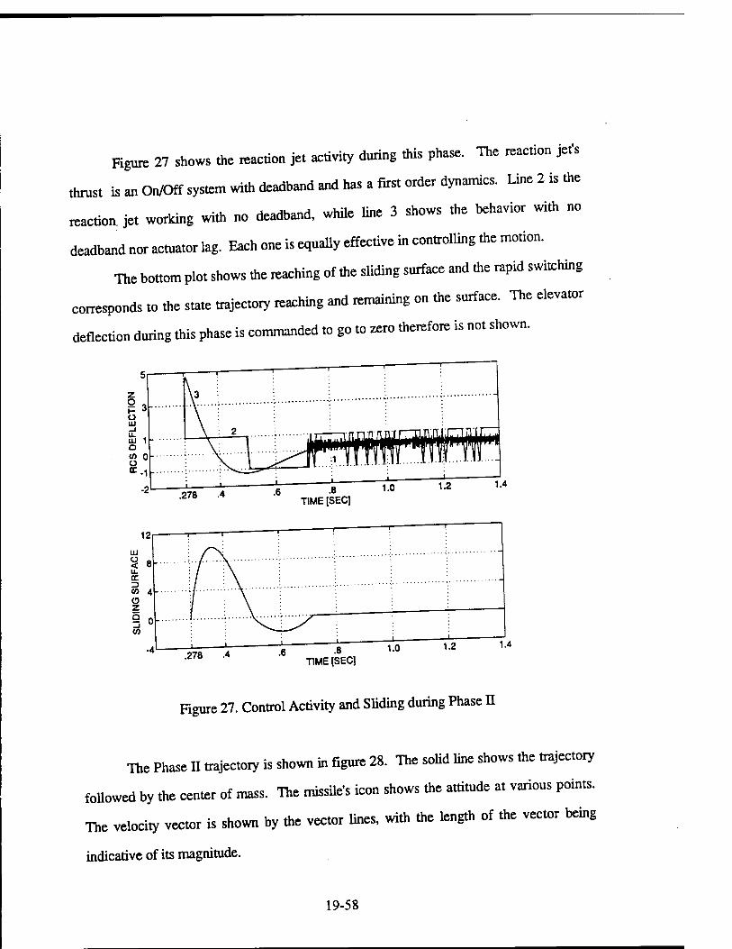
Figure 27 shows the reaction jet activity during this phase. The reaction jef s
thrust is an On/Off system with deadband and has a first order dynamics. Line 2 is the
reaction, jet working with no deadband, while line 3 shows the behavior with no
deadband nor actuator lag. Each one is equally effective in controlling the motion.
The bottom plot shows the reaching of the sliding surface and the rapid switching
corresponds to the state trajectory reaching and remaining on the surface. The elevator
deflection during this phase is commanded to go to zero therefore is not shown.
.278 TIME [SEC]
.6 -8 TIME [SEC]
Figure 27. Control Activity and Sliding during Phase II
The Phase II trajectory is shown in figure 28. The solid line shows the trajectory
followed by the center of mass. The missile's icon shows the attitude at various points.
The velocity vector is shown by the vector lines, with the length of the vector being
indicative of its magnitude.
19-58
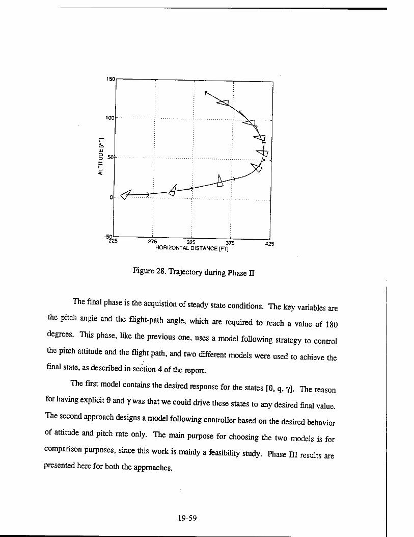
225 275 325 375 HORIZONTAL DISTANCE [FT]
425
Figure 28. Trajectory during Phase II
The final phase is the acquistion of steady state conditions. The key variables are
the pitch angle and the flight-path angle, which are required to reach a value of 180
degrees. This phase, like the previous one, uses a model following strategy to control
the pitch attitude and the flight path, and two different models were used to achieve the
final state, as described in section 4 of the report.
The first model contains the desired response for the states [0, q, y]. The reason
for having explicit 6 and y was that we could drive these states to any desired final value.
The second approach designs a model following controller based on the desired behavior
of attitude and pitch rate only. The main purpose for choosing the two models is for
comparison purposes, since this work is mainly a feasibility study. Phase HI results are
presented here for both the approaches.
19-59
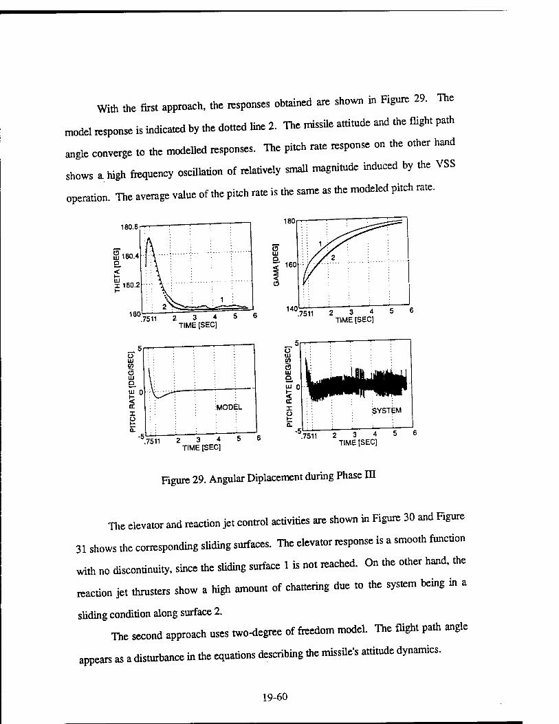
With the first approach, the responses obtained are shown in Figure 29. The
model response is indicated by fine dotted line 2. Tne missile attitude and the flight path
angle converge to the modelled responses. The pitch rate response on the other hand
shows a high frequency oscillation of relatively small magnitude induced by the VSS
operation. The average value of the pitch rate is the same as the modeled pitch rate.
180.6
S 180.4
< tu I 180.2
°7511 2 3 4 5 6 TIME [SEC]
.7511 2 3 4 TIME (SEC]
Ui
UJ 0
.7511 2 3 4 TIME [SEC]
.7511 2 3 4 5 TIME [SEC]
Figure 29. Angular Diplacement during Phase ffl
The elevator and reaction jet control activities are shown in Figure 30 and Figure
31 shows the corresponding sliding surfaces. The elevator response is a smooth function
with no discontinuity, since the sliding surface 1 is not reached. On the other hand, the
reaction jet thrusters show a high amount of chattering due to the system being in a
sliding condition along surface 2.
The second approach uses two-degree of freedom model. The flight path angle
appears as a disturbance in the equations describing the missile's attitude dynamics.
19-60
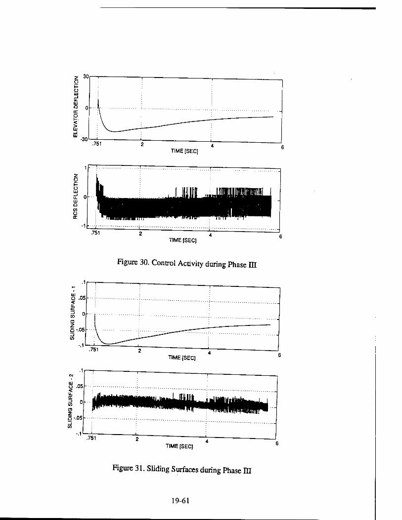
TIME [SEC]
TIME [SEC]
Figure 30. Control Activity during Phase m
TIME [SEC]
Figure 31. Sliding Surfaces during Phase m
19-61
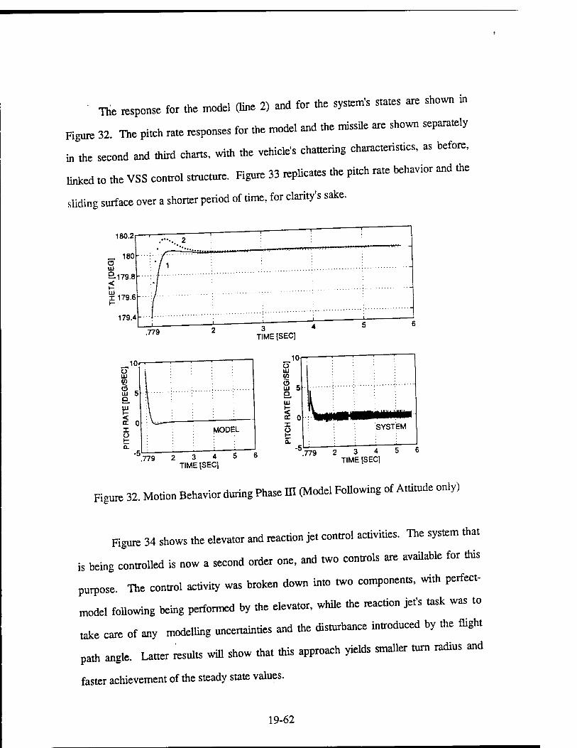
rte response for «he mode. (line 2) and for the system's states axe shown to
Hgure 32. Th. piteh rate responses for the model and the missile are shown separate*
in the second and third eharts, with the vehide's chattering characterisdcs, as before,
Unked to the VSS control structure. Hgure 33 replicates the pitch rate behavior and the
sliding surface over a shorter period of time, for clarity's sake.
.779 2 3 4 5 6 TIME [SEC]
.779 2 3 4 5 6 TIME [SEC]
Figure 32. Motion Behavior during Phase ffl (Model Following of Attitude only)
Figure 34 shows the elevator and reaction jet control activities. The system that
is being controlled is now a second order one, and two controls are available for this
purpose. The control activity was broken down into two components, with perfect-
model following being performed by the elevator, while the reaction jefs task was to
take care of any modelling uncertainties and the disturbance introduced by the flight
path angle. Latter results will show that this approach yields smaller turn radius and
faster achievement of the steady state values.
19-62
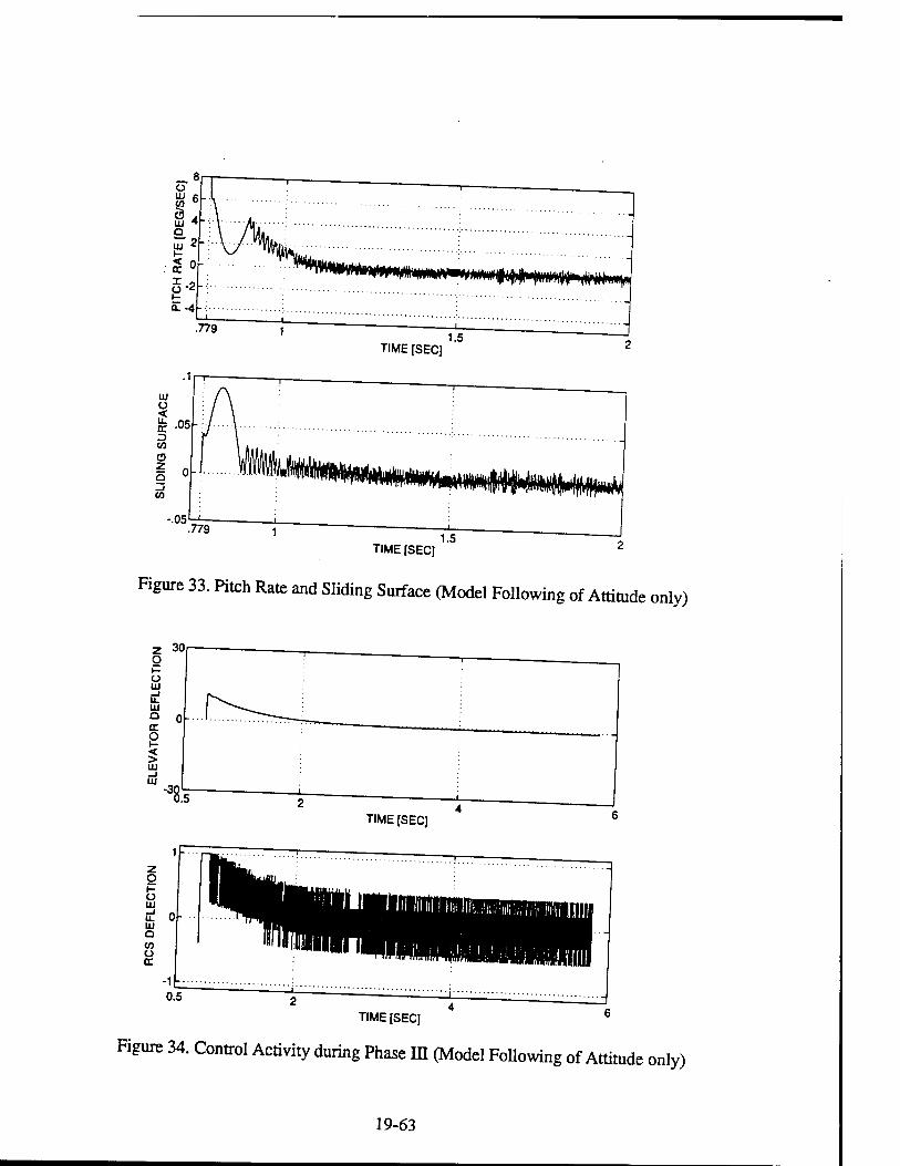
TIME [SEC]
Figure 33. Pitch Rate and Sliding Surface (Model Following of Attitude only)
TIME [SEC]
Figure 34. Control Activity during Phase IE (Model Following of Attitude only)
19-63
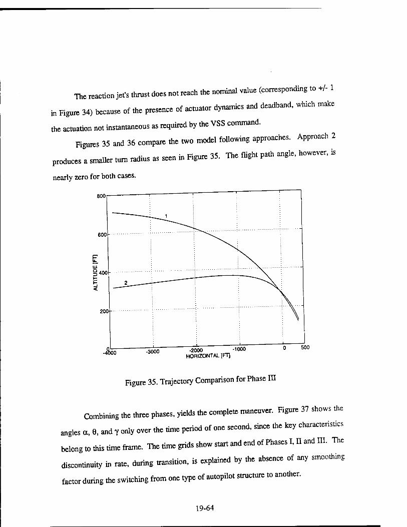
The reaction jefs thrust does no. reach the nominal valne (corresponding ,o +/-1
in Figure 34) because of the presence of actuator dynamics and deadhand, which make
the actuation not instantaneous as required by the VSS command.
Kgures 35 and 36 compare the two model following approaches. Approach 2
produces a smaller mm radius as seen in Hgnre 35. The flight path angle, however, is
nearly zero for both cases.
800
600
400
200
-401 00 -3000 -2000 -1000 HORIZONTAL [FT]
500
Figure 35. Trajectory Comparison for Phase in
Combining the three phases, yields the complete maneuver. Figure 37 shows the
angles a, 6, and y only over the time period of one second, since the key characteristics
belong to this time frame. The time grids show start and end of Phases I, n and III. The
discontinuity in rate, during transition, is explained by the absence of any smoothing
factor during the switching from one type of autopilot structure to another.
19-64
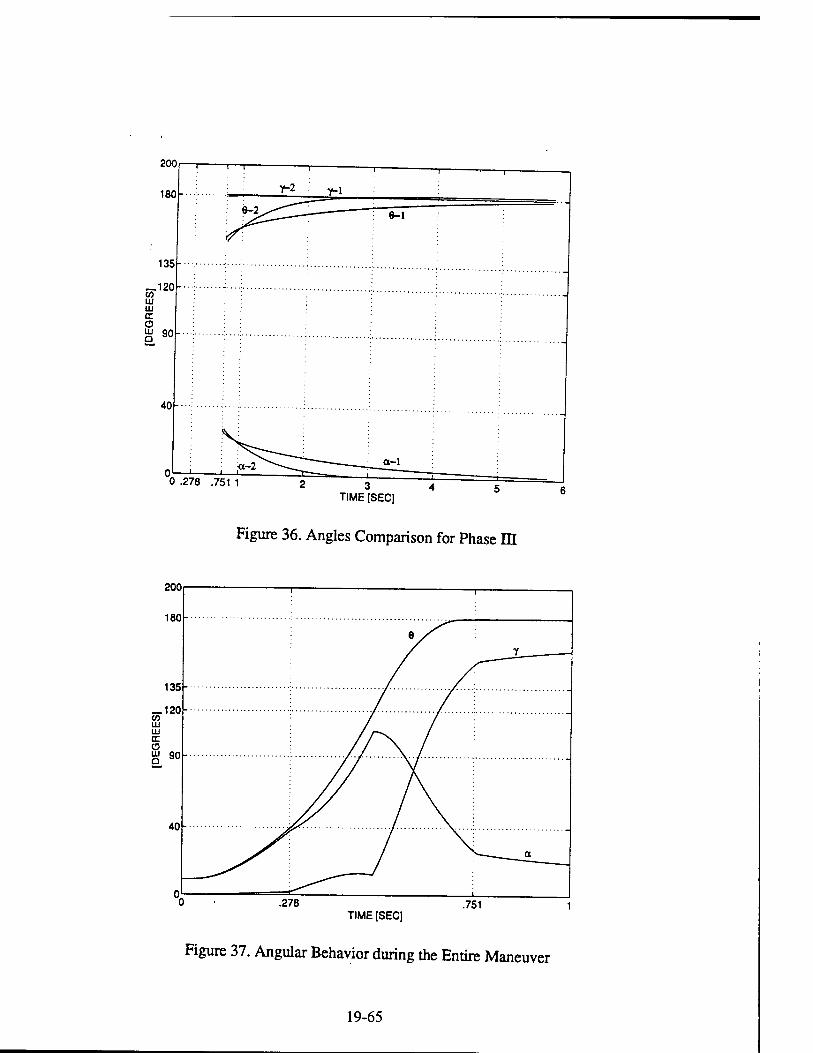
0 .278 .751 1 TIME [SEC]
Figure 36. Angles Comparison for Phase m
TIME [SEC]
Figure 37. Angular Behavior during the Entire Maneuver
19-65
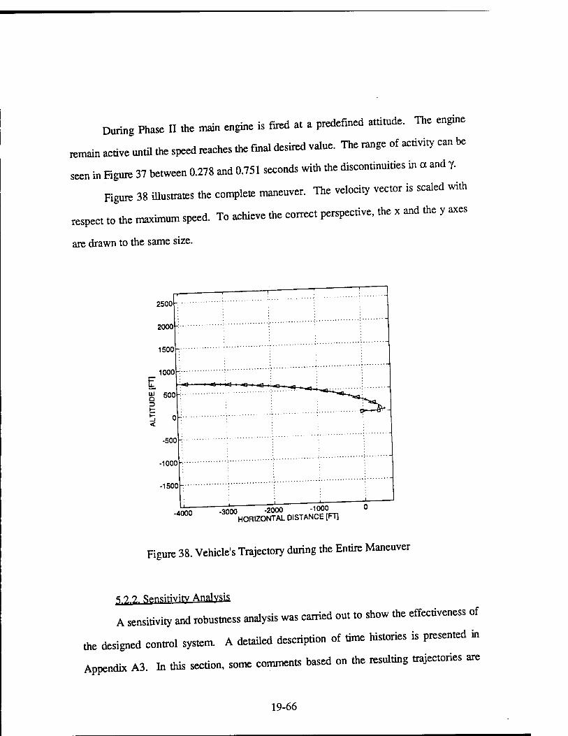
During Phase II the main engine is fired at a predefined attitude. The engine
rcmain active until the speed .aches the finai desired vaine. The range of activity can he
seen in Figure 37 between 0.278 and 0.751 second, with the discontinuities in a and T
Figure 38 illustrates the complete maneuver. The velocity vector is scaled with
respect to Ute maximum speed. To achieve the correct perspective, the x and the y axes
are drawn to the same size.
r 2500-
. ——-f——
r— " ' " ; 1—
2000-
1500 j '. r •
"I 1000 -:
ALT
ITU
DE
I
o
o
o
i : \ ; "■; -500 -. : ; ';""
-1000 -: : •
-150C - ; f ";
; I —i
*nnn -3000 -2000 -1000 4000 300°HORIZONTAL DISTANCE [FT]
0
Figure 38. Vehicle's Trajectory during the Entire Maneuver
?,?,,?„ frrn^fwitv Analvsis
A sensitivity and robustness analysis was carried out to show the effectiveness of
the designed control system. A detailed description of time histories is presented in
Appendix A3. In this section, some comments based on the resulting trajectories are
19-66
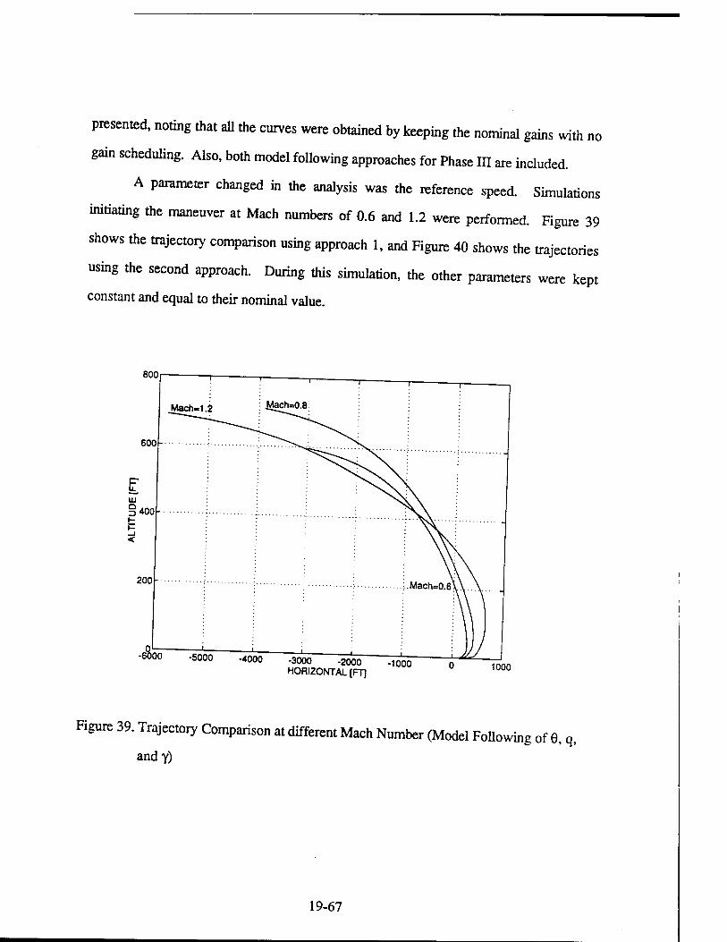
presented, noting that all the curves were obtained by keeping the nominal gains with no
gain scheduling. Also, both model following approaches for Phase in are included.
A parameter changed in the analysis was the reference speed. Simulations
initiating the maneuver at Mach numbers of 0.6 and 1.2 were performed. Figure 39
shows the trajectory comparison using approach 1, and Figure 40 shows the trajectories
using the second approach. During this simulation, the other parameters were kept
constant and equal to their nominal value.
800
Mach-1.2
600
UJ
§400
200
Mach=0.8
6000 -5000 -4000 -3000 -2000 -1000 HORIZONTAL [FT] 1000
Figure 39. Trajectory Comparison at different Mach Number (Model Following of 0, q,
and y)
19-67
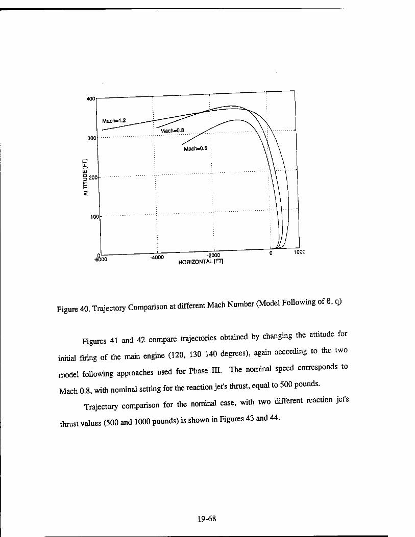
-60 lOO -♦ooo -2000
HORIZONTAL [FT]
1000
Figure 40. Trajectory Comparison at different Mach Number (Model Following of 6, q)
Figures 41 and 42 compare trajectories obtained by changing the attitude for
initial firing of the main engine (120, 130 140 degrees), again according to the two
model following approaches used for Phase III. The nominal speed corresponds to
Mach 0.8, with nominal setting for the reaction jet's thrust, equal to 500 pounds.
Trajectory comparison for the nominal case, with two different reaction jet's
thrust values (500 and 1000 pounds) is shown in Figures 43 and 44.
19-68
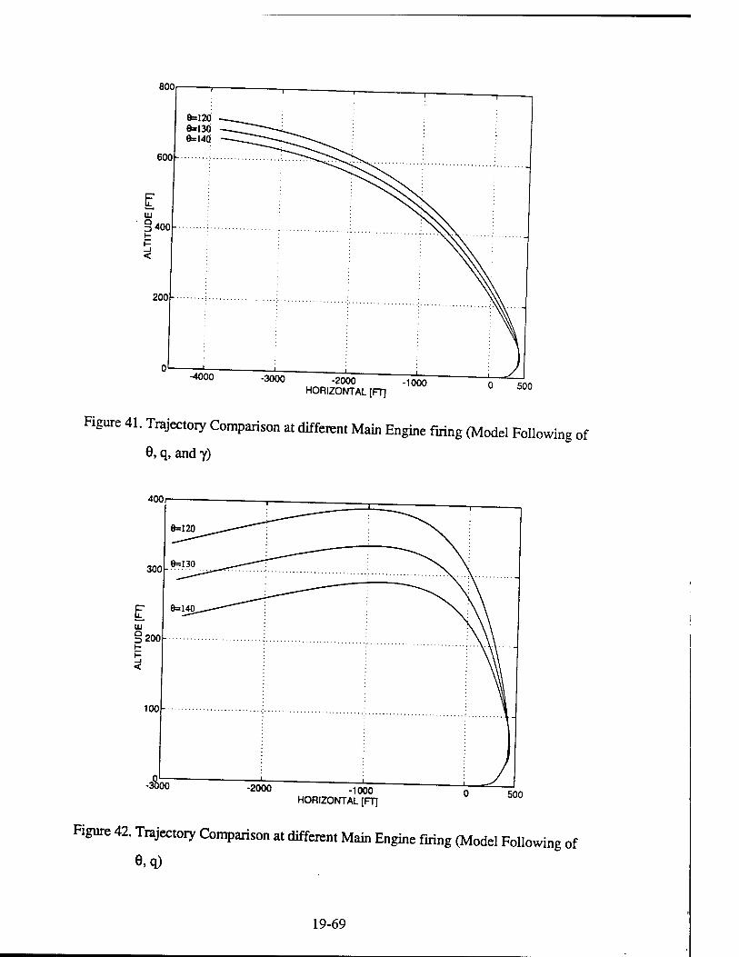
800
-4000 -3000 -2000 -1000 HORIZONTAL [FT]
0 500
Figure 41. Trajectory Comparison at different Main Engine firing (Model Following of
6, q, and y)
400
-3%i i00 -2000 -1000 HORIZONTAL [FT]
500
Figure 42. Trajectory Comparison at different Main Engine firing (Model Following of
6,q)
19-69
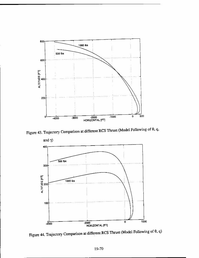
-4000 -3000 -2000 "1000 HORIZONTAL [FT]
0 500
Figure 43. Trajectory Comparison at different RCS Thrust (Model Following of 0, q,
andy)
-2000 HORIZONTAL [FT]
1000
Figure 44. Trajectory Comparison at different RCS Thrust (Model Following of 6, q)
19-70
Finally a frequency response analysis was carried out. The problem being
nonlinear in nature following approach was followed to obtain the systems frequency
response. Phase I of the system was excited by an impulse input and system response
was obtained. From the equally spaced time response of the system discrete frequency
response was obtained by using Fast Fourier Transform. This was then interpreted into
analog frequency, the key concern being the possibility of exciting the missile's bending
modes. The first bending mode frequency depends on the diameter and weight
(assuming no change in stiffness and material properties). For a 5 inch diameter and a
225 pound vehicle, the first bending mode frequency was found to be of the order of 30
hertz. Since the computed closed loop bandwidth is around 2 hertz, with large
magnitude attenuation beyond this value, we concluded that flexibility of the structure is
not an issue at this point.
Another aspect that was investigated, is the potential frequency aliasing due to
sampling rates used for the digital implementation of the autopilot. A step size of 0.001
seconds was used in the simulations, leading to a Nyquist sampling frequency of about
100 hertz. Again, this is well over the bandwidth of the system.
5.3. Simulation Software
The computational aspects of the work, autopilot design and simulation were
carried out using Matlab® version 4.1. The simulation code ACTMS (Alternate Control
Technology Missile Simulation) was developed making extensive use of the block
diagram capabilities of the available toolboxes and SIMULINK™. The computer used
for the work was a SUN workstation, however the code will run on other platforms,
provided version compatibility is satisfied. A description of the input/output properties
19-71

„f fte mffles developed for fte simmation can be found in Appendix A2. A diskette with
the source code is included in the report.
The input of physical parameters, state initialization are entered using an input
ffle (init M4 which defines missile parameters,speed, range of main engine
operation, angle of attack range helow stall, load factor command value, model desired
values for attitude and flight path angles, and integration characteristics.
The simulation drivers are file» actms-m and SimAlLm. They have two different
versions according to the implementation of the model following relative to Phase DL
The three phases are defined by files phasel.ro, phaselLm, and phaseULm,
with the results of the simulation being written on dam files Part4.mat, partS.mat,
part6.mat, and partT.mat (relative to the entire maneuver).
The models necessary to the simulation, inclusive of gain computation, are
determined by the file actdyn-n, System matrices and gains are stored into datafiles
wr.tsp.mat, gain.mat. Mffles for plotting the results are also available (mploUn and
mplotl.m). The file aero.m contains the lift and drag profiles in a matrix format, as functions
of Mach number and angle of attack, as computed by DATCOM and/or derived
analytically for «he region above stall. Linear interpolation is used to extract values in-
between Of course different vehicles require appropriate aerodynamic data. TT-e files
responsible for adjusting the angle of attack value in order to read data beyond 90
degrees are adjustalp.m and clauscm.
The flowchart relative to the code is shown in Figure 45.
19-72
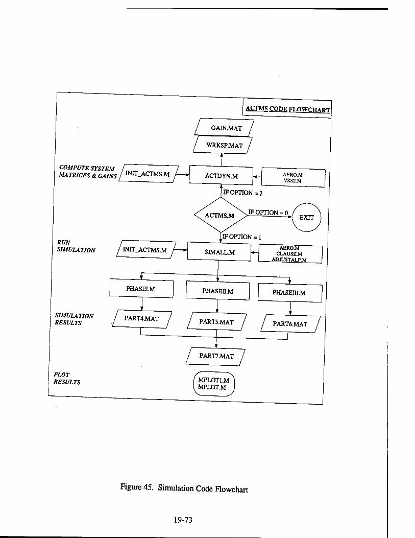
COMPUTE SYSTEM /Tvr_ MATRICES & GAINS / INIT-ACTMS.M
RUN SIMULATION
SIMULATION RESULTS
PLOT RESULTS
PART4.MAT /
ICTMS cnnv FLOWCHART
GAIN.MAT
WRKSP.MAT
ACTDYN.M
OPTION = 2
AERO.M VSS2.M
IF OPTION = 0 ( \ — *\ EXIT ]
PART5.MAT
PART7.MAT
f MPLOT1.M I MPLOT.M
AERO.M CLAUSE.M
ADJUSTAUM
1 PHASEm.M
PART6.MAT
Figure 45. Simulation Code Flowchart
19-73

6. Conclusions and Recommendations
Conclusions
The following conclusions were reached at the end of work done under the
present grant:
(1) Variable stucture control methods were applied with success to the feasibility design
of a pitch autopilot, using a reduced size elevator and reaction jets as controllers.
Different control structures were used during the chosen test maneuver.
(2) The autopilot did not require gain scheduling for a wide range of parameter
variations.
(3) A simpler autopilot structure could be achieved by changing the control logic for
Phase I, from a load factor command to one similar to that of the Phase n and Phase ffl.
Recommendations
The encouraging results of the present research warrant further work in several
areas, in order to achieve a point design. These are:
(1) The study of optimal nonlinear trajectories, that will take full advantage of
the added propulsive control capabilities. This study would definitely involve the
definition of missile agility metrics, similar to those available for aircraft
(2) The analysis of guidance laws capable of implementing acceleration and/or
rate command required to achieve point (1).
(3) Autopilot design and control authority selection using output feedback VSS,
since not all the states are used by the autopilot. This design would include analytical
contributions in variable structure theory, as well as classical channel integration due to
the three-dimensional aspects of the problem
(4) Study of optimal reaction jet characteristics, such as amplitude and frequency
modulated actuators to be used for pitch and yaw commands, as well as roll stabilization.
19-74
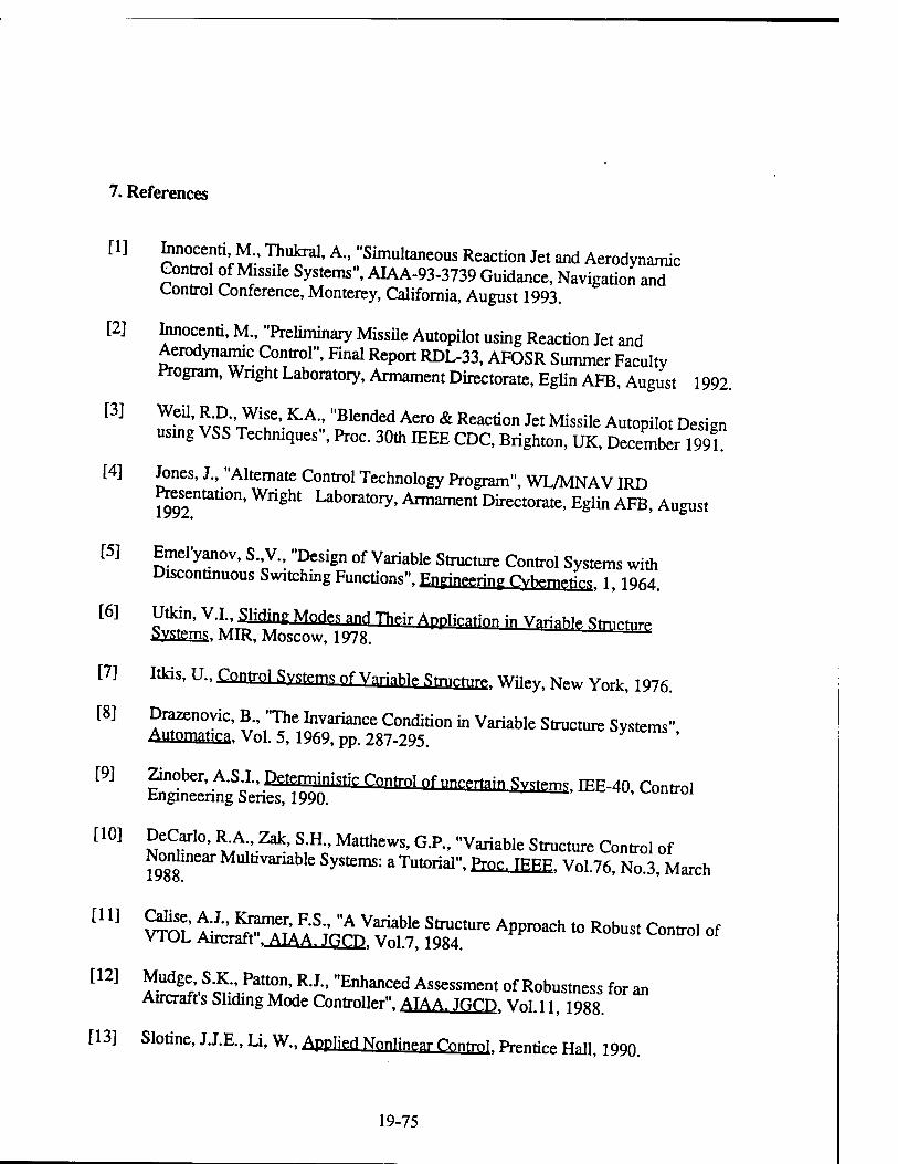
7. References
[1] Innocent! M Thukral, A., "Simultaneous Reaction Jet and Aerodynamic Gontro of Missile Systems", AIAA-93-3739 Guidance, Navigation and Control Conference, Monterey, California, August 1993.
[2] Wenti, M., "Preliminary Missile Autopilot using Reaction Jet and Aerodynamic Control", Final Report RDL-33, AFOSR Summer Faculty Program, Wright Laboratory, Armament Directorate, Eglin AFB, August 1992.
[3J S v£'TWif'KA-.: "£lended Aer° & Reacti0n Jet Missile Aut°P^t Design using VSS Techniques", Proc. 30th IEEE CDC, Brighton, UK, December 199L
[4] Jones, J., "Alternate Control Technology Program", WL/MNAVIRD Presentation, Wright Laboratory, Armament Directorate, Eglin AFB, August
[5] Emel-yanov, S.,V., "Design of Variable Structure Control Systems with Discontinuous Switching Functions". Engineering Cv^m,,^ h 1964
[6] Utkin, V.I Sliding Modes and Their Apnlintion jn Varishi. <^n.,~ SYStems, MIR, Moscow, 1978. —
[7] Itkis, U., Control Systems of Variahi,» fimTrt1TT Wiley, New York, 1976.
[8] Drazenovic, B., "The Invariance Condition in Variable Structure Systems" Automata, Vol. 5, 1969, pp. 287-295. '
[9] g5^st£Slwir Cowo] nfmr^n ^» IEE-40>Co"^ [10] DeCarlo, R A Zak, S.H., Matthews, G.P., "Variable Structure Control of
No^rJinear Multivanable Systems: a Tutorial", PTQC, IRRF, Vol.76, No.3, March
[11] Sä ASK srrc Approach to Robust c°^ °f [12] Mudge S.K Patton, R.J., "Enhanced Assessment of Robustness for an
Aircrafts Sliding Mode Controller". AIAA. JOCH Vol.11, 1988.
[13] Slotine, U.E., Li, W., Annlied Mnnlin>.nr rnrt?1 prentice H^ im
19-75
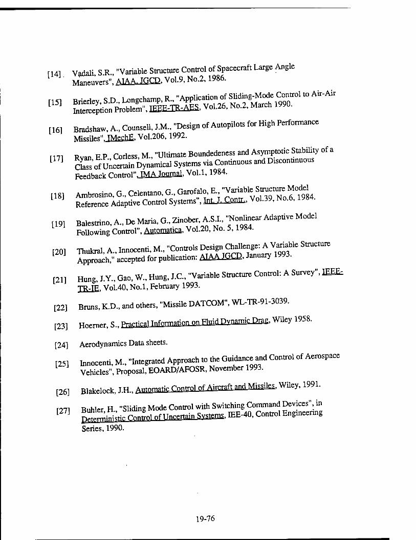
[16] Bradshaw, A., Counsell, J.M., "Design of Autopilots for High Performance Missiles" JMscllE, Vol.206, 1992.
T171 RvanEP Corless, M., "Ultimate Boundedeness and Asymptotic Stability of a [ ] S'of u'Sn Dynamical Systems via Continuous and Discontinuous
Feedback Control",J^AJojimai, Vol.1,1984.
[18] Ambrosino, G., Celentano, G Garofalo, E "^Xl^ZTtm. Reference Adaptive Control Systems", Tnt, I Contr,, Vol.39, No.6, iw.
[19] Balestrino, A., De Maria, G., Zinober, A.Si., "Nonlinear Adaptive Model Following Control", AuJomaTica, Vol.20, No. 5,1984.
[20] Thukral, A., Innocenti, M., "Controls W*?^™ *"*"" Approach," accepted for publication: ATAA JOCD, January 1W*.
[21] Hung, J.Y., Gao, W., Hung, J.C., "Variable Structure Control: A Survey", IEEE, TR-IE. Vol.40, No.l, February 1993.
[22] Bruns, K.D., and others, "Missile DATCOM", WL-TR-91-3039.
[23] Hoerner, S., W»1 information on Fluid Dynamic Drag, Wiley 1958.
[24] Aerodynamics Data sheets.
[25] Innocenti, M., "Integrated Approach to the Guidance and Control of Aerospace Vehicles", Proposal, EOARD/AFOSR, November 1993.
[26] Blakelock, J.H., /iffiomnfic Control pf Aircraft and Missiles, Wüey, 1991.
T271 Buhler H "Sliding Mode Control with Switching Command Devices", in [2?] fff — H ""^" ^ems. IEE-40, Control Engineering
Series, 1990.
19-76

Appendices
Al. Gains
This Appendix contains the gain matrices used for the autopilot described in the
report.
Phase T Ai^opilnf
The gain matrices used in Eq. (48) are:
L_l=[-5.3517e-03 -1.1120e-02 -1.2727e-03 -9.5270e-01 -3.6759e-02
-4.9005e-03 -2.6377e-03 -2.6132e-03 -2.1420e-02 -9.8215e-01]
M_l =[-1.3396e+00 -1.4005e-01 9.7002e-02 -6.8826e-01 2.3606e-01
5.0787e+00 2.2726e-01 1.5613e-01 -1.3907e+00 -5.8274e-01]
N_l=[-2.6758e-03 5.6661e-05 -3.8657e-04 3.0562e-03 1.2569e-04
-2.4502e-03 -2.5616e-04 1.7742e-04 -1.2589e-03 4.3177e-04]
The gain matrix G defining the sliding surface as defined on page 35 is given by:
G_l =[-2.6792e+00 -2.8010e-01 1.9400e-01 -1.3765e+00 4.7212e-01
1.0157e+01 4.5452e-01 3.1226e-01 -2.7815e+00 -1.1655e+00]
Phase TT Aufnpilnf
The gain matrices in Eq. (54) are:
Kj_2 = [-2.8664e+00 -3.8649e-01]
K2_2 = 2.8664e+00
K3_2 = -1.6104e-01
The gain matrix G defining the sliding surface from Eq. (55) is:
G_2 = [7 1]
19-77

Ph^c. TTT AmiriM frpftthod v> The model to be followed has a thud order dynamics. The gain matrix K, in Eq.
(61) is:
Ki_3 =[-4.9665e-01 5.0213e-02 -5.7851e-01
-4.4346e-01 -5.5621e-02 -1.3817e+00]
The gain matrices in Eq. (63) are:
L_3 =[ 8.7872e-02 3.1383e-02 -5.8779e+00
-9.7337e-02 -3.4763e-02 -8.5697e+00]
M_3 =[ 3.3804e-03 3.3804e-04 1.6667e-01
-1.6667e+00 -1.6667e-01 3.3804e-04]
N_3 =[ 1.0461e-02 1.0461e-03 -3.9186e-01
-1.1588e-02 -1.1588e-03 -5.7131e-01]
The gain matrix G defining the sliding surface is:
G_3 =[ 2.0283e-02 2.0283e-03 1.0000e+00
-1.0000e+01 -1.0000e+00 2.0283e-03]
The model to be followed has a second order dynamics. The gains in Eq. (66)
are given by:
Kx_3 = [ 3.2843e-02 1.3254e-01]
Kum_3 = -4.0205e-01
KY_3 = -3.6921e-01
The gain G defining the sliding surface is in this case:
G_3 = [7 1]
19-78

A2. Software Description
A short description of some of the more important mfiles is listed below. The file
names and the function names are in italics.
actms
Mfile Function Input files
Output files Functions
actms.m actms Inputlwrksp.mat Input/gain.mat None SimAll.m actdyn.m
System parameters are loaded Model matrices and gain matrices for controls
Messages
Function simulates all the phases Computes system matrices, model system matrices and gains
ACTMS Options: (0) Exit (1) Run Simulation (2) Compute System Models/Gains Selected Option => ... SIMULATION OVER... ... SYSTEM/MODELS/GAINS COMPUTED
fcrror Messages .. Incorrect entry..
Description
i, th, iJT" (ALTERNATE CONTROL TECHNOLOGY MISSILE SIMULATION) is he driver routine making calls to SimAll and actdyn functions, actdylauction fa
computed80"16 SyStem Parameter ^ *" ChangCd °r new sets °f tZ «Tte There is an error message if option number selected is an incorrect one.
19-79
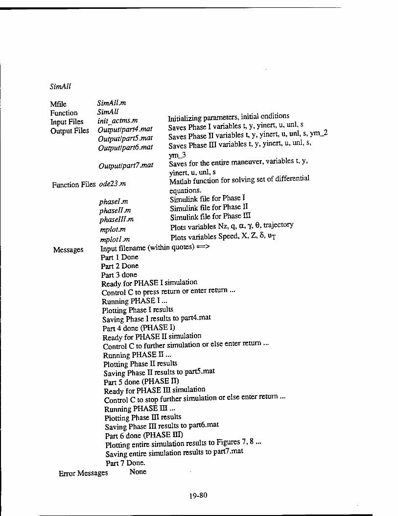
SimAll
Mfile SimAlLm
tautra« ItOcmsm Mtializtag parameters, initial onditions cXafiL 0uW«r/P<-rt4.mar Saves Phase I variables t, y, yinert, u, unl s Output Fües Ojmm^5mai SavM phase n variables t, y, yinert, u, unl s, ymj
Outputlpart6.rmt Saves Phase HI variables t, y, yinert, u, unl, s, ym_3
Outputlpart7.mat Saves for the entire maneuver, variables t, y, yinert, u, unl, s
Function Files ode23.m Matlab function for solving set of differential equations.
phaselm Simulink file for Phase I phasellm Simulink file for Phase H phasellLm Simulink file for Phase m mplotm Plots variables Nz, q, a, y, 6, trajectory mplotl .m Plots variables Speed, X, Z, 5, uT
Messages Input filename (within quotes) => Part 1 Done Part 2 Done Part 3 done Ready for PHASE I simulation Control C to press return or enter return ... Running PHASE I... Plotting Phase I results Saving Phase I results to part4.mat Part 4 done (PHASE I) Ready for PHASE II simulation Control C to further simulation or else enter return ... Running PHASE H... Plotting Phase II results Saving Phase II results to part5.mat Part 5 done (PHASE II) Ready for PHASE HI simulation Control C to stop further simulation or else enter return ... Running PHASE in... Plotting Phase HI results Saving Phase m results to part6.mat Part 6 done (PHASE HI) Plotting entire simulation results to Figures 7,8... Saving entire simulation results to part7.mat Part 7 Done.
Error Messages None
19-80

Description Simulation of all the phases is carried out by this function. The three phases are
formulated in terms of simple blocks. These blocks are then simulated us£g one o £ MATLABs rouünes for integrating or solving differential equations. Fuction 0^23 is called for simulating the phases.
the rnnlrTr5 ^^ * ""S* Commcntary on ** simulation status. Key message is the Control C .. message. The message tells the user that the MATLAB is ready for
StVoSuÄ6 ^ ^ ** POim thC US6r haS - °Pti0" ^Stfrom uSs imer^ ^ Capablhty t0 ™ the particular Phase- ™s is helPful if the bbckXSn^lT 7™* PaTetriC StUdiCS °r °ptimizinSthe **»• ^e simulink block diapm for the phases can be simply called by typing in the corresponding rnfile
ÄSSS" T° **" thC bl°Ck «**«» — «**» k frLte6
t time y [Y6aAzq8uT] yinert [UXWZVdy/dt] ym_2 [em qm] ym_3 [em qm rm] unl [5nl uxnll ulin f^in "TlinJ s [S8 SuT]
I L^l ™' fleS ^ SaVCd aS ' r°W °f ^ ""* «W** »it, are in degrees. The state vector, X=[JAZ Az q 8 uT ] is not saved but is in the MATLAB's workspace area. The state vector has angular units in radians
19-81
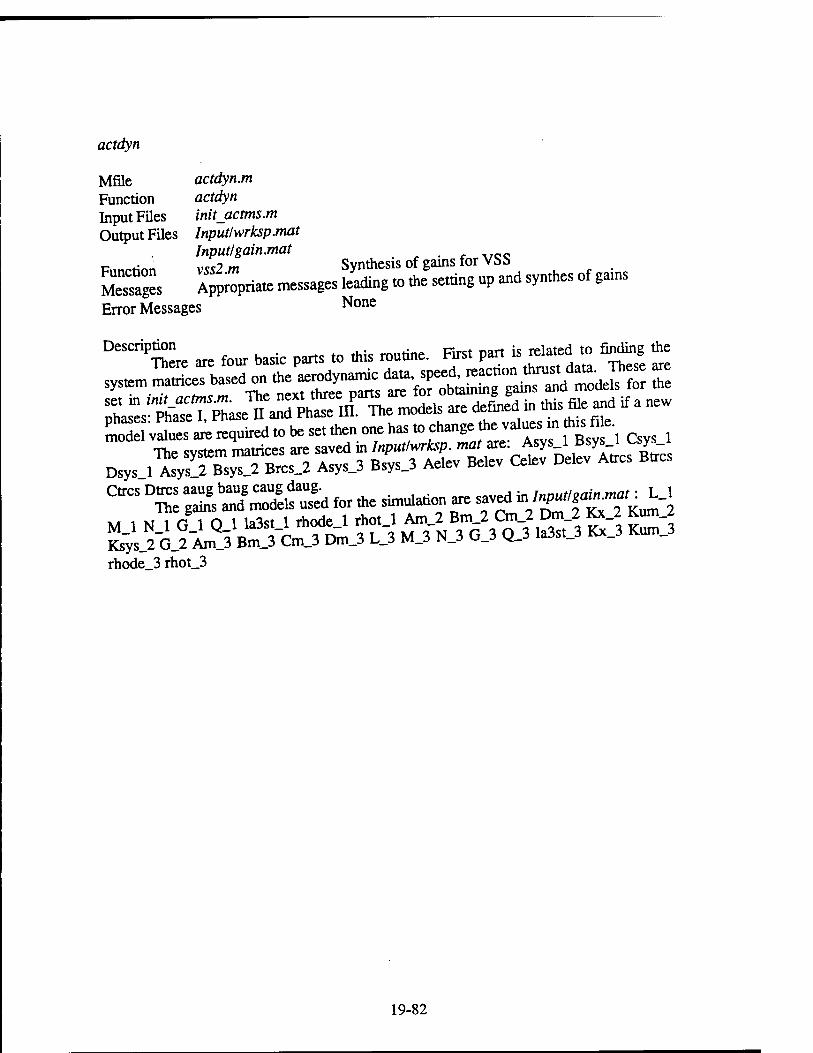
actdyn
Mffle actdyn.m Function actdyn Input Files init_actms.m Output Files Input/wrksp.mat
Input!ga.in.mat # ,cc c „^™ v«2 m Synthesis of gains for Vbb
S. Ä»«—«- ***t0 te ""* up ^syn,hes of 8ains Error Messages None
^^ere are four basic parts to this routine. Fist part is related to finding the
^^TiL^^Sir^^^^ >" this file and if a uew ÄÄÄl - * - to °"e haS ro t
ChangC *e ^ A?'" 1 BSV C1 Csys 1 The svstem matrices are saved in lnputlwrksp. mat are: Asys 1 Bsys 1 Lsys 1 Dsys lÄ BsyT^Brcs J Asys_3 Bsys.3 Aeiev Belev Celev Deiev Ames Btrcs
CmS DS ^nÄd for the sinken „ -«. in, Ig*£«^
rhode_3 rhot_3
19-82
phasel, phasell, phaselll
Mfile phasel.m, phasell.m, phaselll.m (SIMULINK files) Input files None Output files None Functions clause.m Checks the range condition
adjustalp.m Aero data for a beyond 90 degree is obtained by adjusting the value of a.
Messages None Error Messages None
Description
These are block diagrams for Phase I, Phase n and Phase III respectively Once all the variables are loaded into Matlab's workspace a phase can be simulated by clicking on fianutatum option. This pops up a pull down menu. Select Sjart option from this and the simulation starts. If some variable is not defined an error message saying variable The simulation results are stored into workspace. The variables are:
t time y [yeaAzq6uT] yinert [UXWZVdy/dt] y"1-2 [emqm] >™-3 [0mqmYm] ^ [8nl uTnl] ^ [Sün UTiin] s [Sg suT]
For each time instant, t, the variables are saved as a row of data. The angular units are in degrees. The state vector, X=[JAZ Az q 8 uT ] is not saved but is in the MATLAFs workspace area. The state vector has angular units in radians
19-83

A3. Parametric Analysis
Station results for various flight conditions and parameter vaiues are included
here for purposes of reference and vatidatio, The axes plots were all made using the
same scale so .ha, the results may be easüy compared. Results relative to Phases I, .1,
aM m are shown in figures A-l through A-26. Phase I and Phase I. simulations are
presented in Ftgures A-l through A-8. The toe histories shown in Rgures A-9 through
A-17 were generared using the 3-DOF model for Phase HI control. Those presented tn
Figures A-18 through A-26 were obtained using the 2-DOF model for the final phase.
The paramedic analysts values are described in Table A-l. Table A-2 shows a
summary relationship between figure number, variables presented, and appropriate
maneuver phase. Finally, Figures A-27 and A-28 show the CL, CD versus angle of attack curves at
Mach numbers 0.6 and 1.2 respectively.
Table A-l
RUN Inital Final RCS e
Nos Mach Mach Thrust Engine ON
1 0.6 0.6 500 120
2 0.6 0.6 1000 120
3* 0.8 0.8 500 120
4 0.8 0.8 500 130
5 0.8 0.8 500 140
6 0.8 0.8 1000 120
7 1.2 1.2 500 120
8 1.2 1.2 1000 120
19-84

Table A-2
Figure Nos. Output Plotted Corresponding Phase
Figure A-l Nz,q Phase I Figure A-2 6, a,y Phase I Figure A-3 5, uT Phase I Figure A-4 -ZvsX Phase I
Figure A-5 Nz,q Phase II Figure A-6 e,a,y Phase II Figure A-7 8, uT Phase II Figure A-8 -ZvsX Phase II
Figure A-9 NZ)q Phase m Figure A-10 0, a,y Phase in Figure A-11 8, uT Phase in Figure A-12 -ZvsX Phase m
Figure A-13 Nz,q Complete Maneuver Figure A-14 6,a,y Complete Maneuver Figure A-15 8, uT Complete Maneuver Figure A-16 -ZvsX Complete Maneuver Figure A-17 Speed Complete Maneuver
p^is^ÄrcontroL phase j "d Phase n -identicai»~ Figure A-18 Nz,q Phase m Figure A-19 6,a,y Phase m Figure A-20 8, uT Phase m Figure A-21 -ZvsX Phase m
Figure A-22 Nz,q Complete Maneuver Figure A-23 6, a, y Complete Maneuver Figure A-24 6, uT Complete Maneuver Figure A-25 -ZvsX Complete Maneuver Figure A-26 Speed Complete Maneuver
19-85
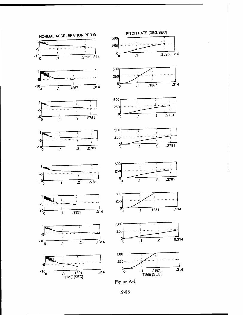
NORMAL ACCELERATION PER Q
-5
-10 .2595 .314
PITCH RATE [DEG/SEC]
.2595 .314
-5
-10
'r^n .1 .1867 .314
500
314
-10. .1 .2 .2781
500
250
0
1
-5
-10. .1 .2 .2781
1
-5
-10
500
250
0 .2 .2781
^p^-X n .1 -2 -2781
.314
500
250
314
1
-5
-10 0.314
500
250
0.314
1
-5
-10 .1 .1821 TIME [SEC]
.314 .1 .1821 TIME [SEC]
Figure A-l
19-86
314
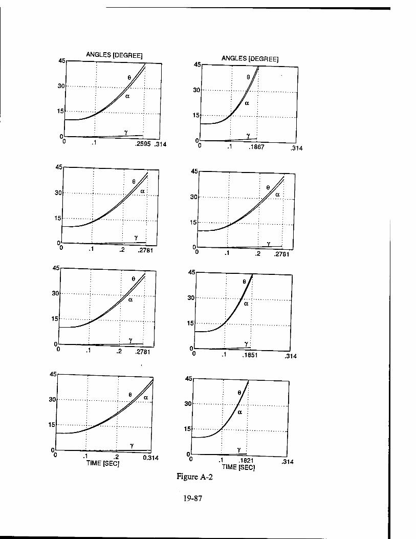
ANGLES [DEGREE]
2595 .314
ANGLES [DEGREE]
1 .1867 .314
2 .2781 2 .2781
2 .2781 1 .1851 .314
• 1 .2 TIME [SEC]
0.314
Figure A-2
.1 .1821 TIME [SEC]
19-87
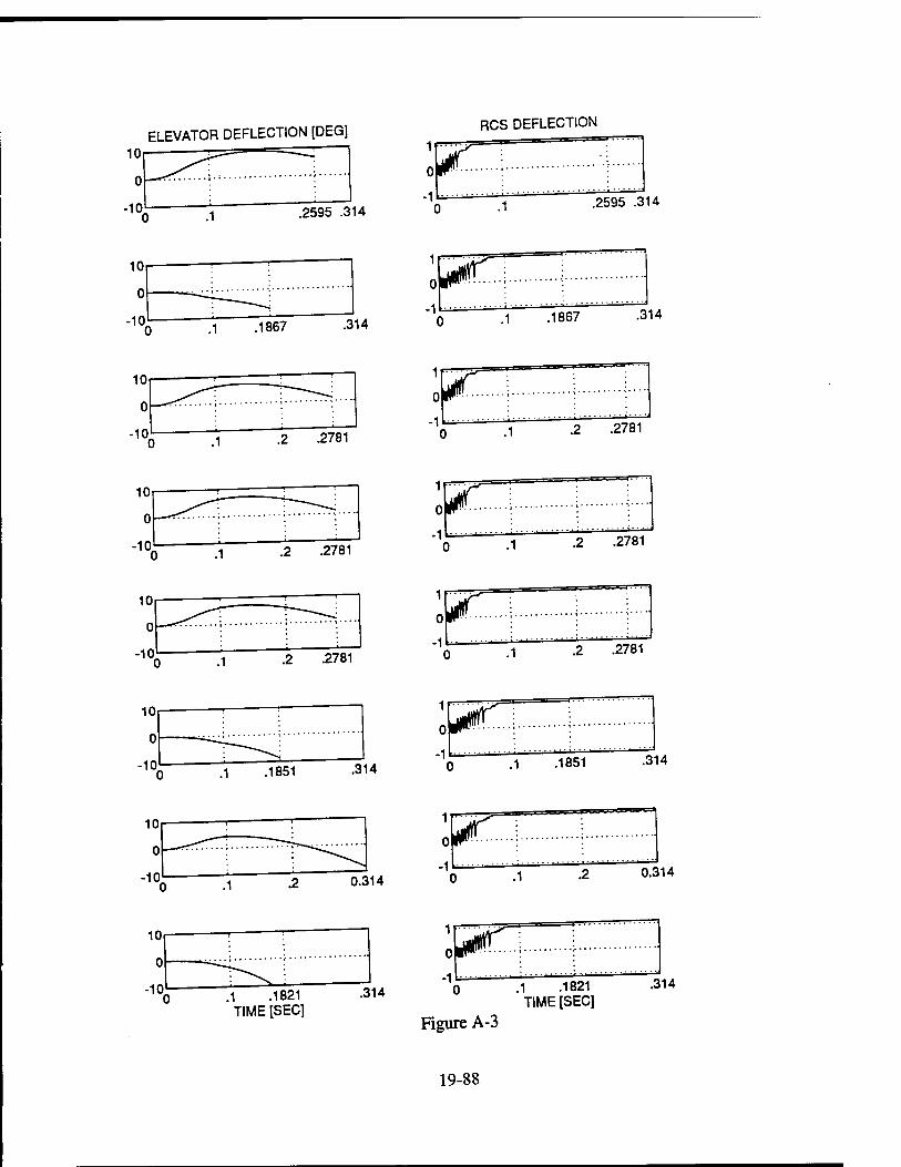
ELEVATOR DEFLECTION [DEG]
2595 .314
RCS DEFLECTION
.2595 .314
314 -1
IW .1 .1867 .314
.2 .2781
10
0
-10 .2 .2781
ir^ o
.2 .2781
314 .1 .1851 .314
0.314 .2 0.314
.1 .1821 TIME [SEC]
314
Figure A-3
.1 .1821 .314 TIME [SEC]
19-88
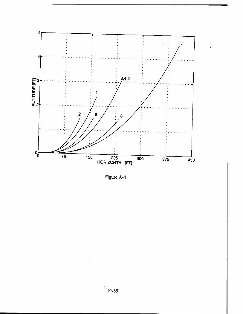
75 150 225 300 HORIZONTAL [FT]
375 450
Figure A-4
19-89
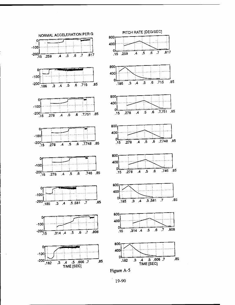
NORMAL ACCELERATION PER G
Of '■■■■■'■'
-100
-200, 15 .259 .4 .5 .6 .7 .817
PITCH RATE [DEG/SEC]
15 .259 .4 .5 .6 .7 .817
or
-100
-200 186 .3 .4 .5 .6 .715 .85
186 .3 .4 .5 .6 .715 .85
15 .278 .4 .5 .6 .7.751 .85
800
400
0 15 .278 .4 .5 .6 .7.751 .85
0
-100
-200.
=^r
15 .278 .4 .5 .6 .7.748 .85 15 .278 .4 .5 .6 .7.748 .85
>' '■ : ^—^ ^TiK 15 278 .4 .5 .6 .746 .85 15 .278 .4 .5 .6 .746 .85 -is -*'°
85 .3 .4 .5.581 .7 .85 .185 .3 .4 .5.581 .7 85
5 .314 .4 .5 .6 .7 .808 15 .314 .4 .5 .6 .7 .808
182 .3 .4 .5 .606 .7 .85 TIME [SEC]
182 3 .4 .5 .606 .7 .85 TIME [SEC]
Figure A-5
19-90
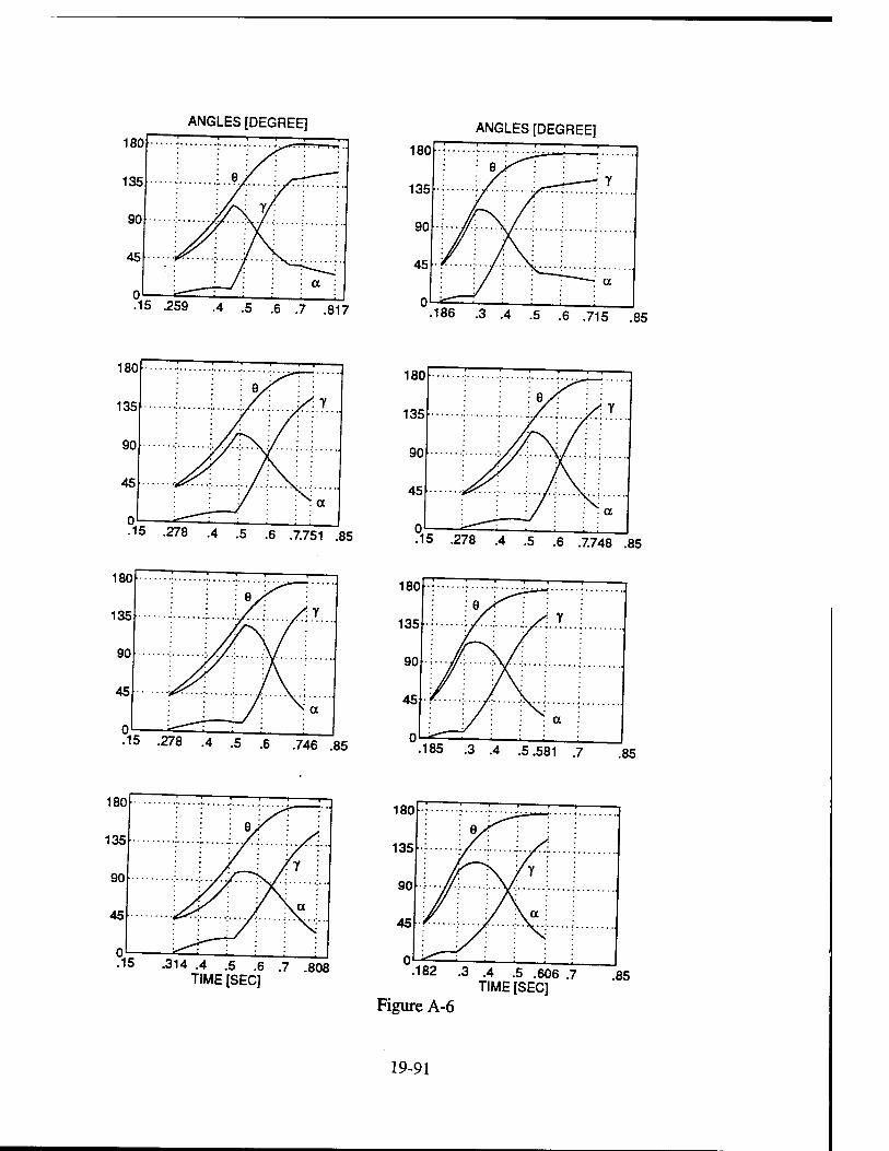
ANGLES [DEGREE]
15 .259 .4 .5 .6 .7 .817
ANGLES [DEGREE]
•186 .3 .4 .5 .6 .715 .85
15 .278 .4 .5 .6 .7.751 .85 .15 .278 .4 .5 .6 .7.748 .85
15 .278 .4 .5 .6 .746 .85 185 .3 .4 .5.581 .7 .85
.15 .314 .4 .5 .6 .7 .808 TIME [SEC]
.182 .3 .4 .5 .606 .7 TIME [SEC]
Figure A-6
.85
19-91
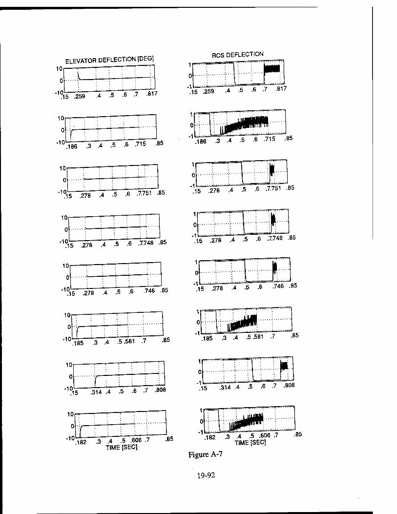
ELEVATOR DEFLECTION [DEG]
10
0
-10.
L
.15 .259 .4 .5 .6 .7 .817
10
0
-10
10
0
-10
186 .3 .4 .5 .6 .715 .85
'l5 .278 .4 .5 .6 .7.751 .85
RCS DEFLECTION -•t *.■ •"
115 .259 .4 .5 .6 •/ ■*"
186 .3 .4 .5 .6 .715 .85
1 ■
0 t !l5 .278 .4 .5 .6 .7.751 .85
10
0
-10 Y5 .278 .4 .5 .6 .7.748 .85
10
0
-10 °15 .278 .4 .5 .6 .746 .85
10
0
-10 rr. _ . .185 .3 .4 .5.581 .7 .85
1| ! !
o ; :• t ST1« * 15 -278 .4 .5 .6 .7.748 .85
1 '
0
-1 fc
15 .278 .4 .5 .6 .746 .85
185 .3 .4 .5.581 .7 .85
10
0
-10. r
15 .314 .4 .5 .6 .7 .808
10
-10 o 182 .3 .4 .5 .606 .7
TIME [SEC] .85
ft
.15 .314 .4 .5 .6 .7 .808
182 .3 .4 .5 .606 .7 TIME [SEC]
85
Figure A-7
19-92
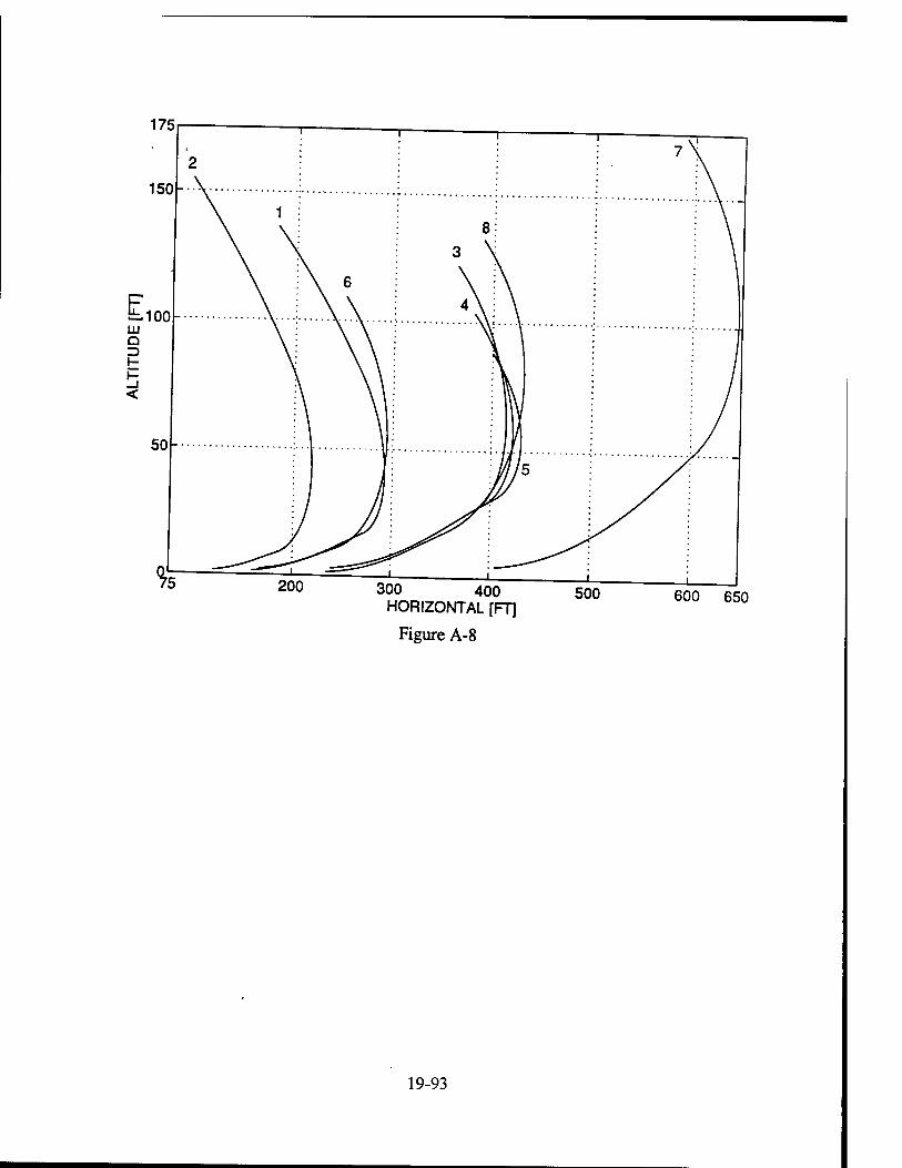
175
200 300 400 HORIZONTAL [FT]
Figure A-8
500 600 650
19-93
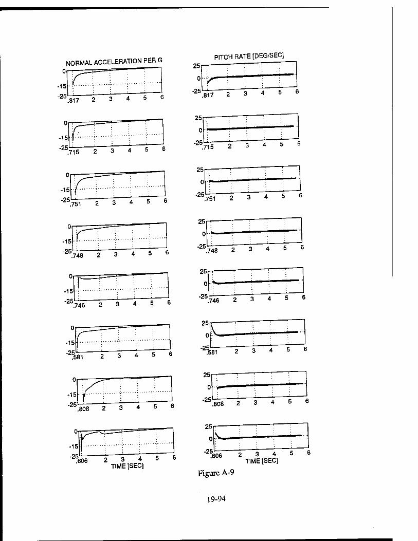
NORMAL ACCELERATION PER G
-15
-25 .817 2 3 4 5 6
-15
-25 .715 2 3 4 5 J
6
PITCH RATE [DEG/SEC]
25
0
-25 ,817
2 3 4 5 6
25
0
-25 715 2 3 4 5 6
2 3 4 5 6
25
0
-25 751
2 3 4 5 6
!.748 2 3 4 5
.746 2 3 4 5
25 n-
0
-25 748 2 3 4 5 6
25
0
-25 746 2 3 4 5 6
.581 2 3 4 5 6
25
0
-25. ;H1 2 3 4 5 6
.808 2 3 4 5 6
25
0
-25 .808 2 3 4 5 6
-15
-25
25
0
-25. '606 2 3 4 5 6
TIME [SEC]
;606 2 3 4 5 6 TIME [SEC]
Figure A-9
19-94
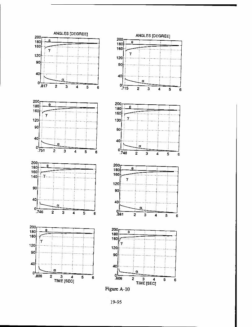
ANGLES [DEGREE]
200 180 160k
120
90
ANGLES [DEGREE]
200 200
200 180 160
120
90
: Y
200
.808 2 3 4 5 6 TIME [SEC]
200 180h 160
120
90
y
.606
Figure A-10
9 *} A
TIME [SEC]
19-95
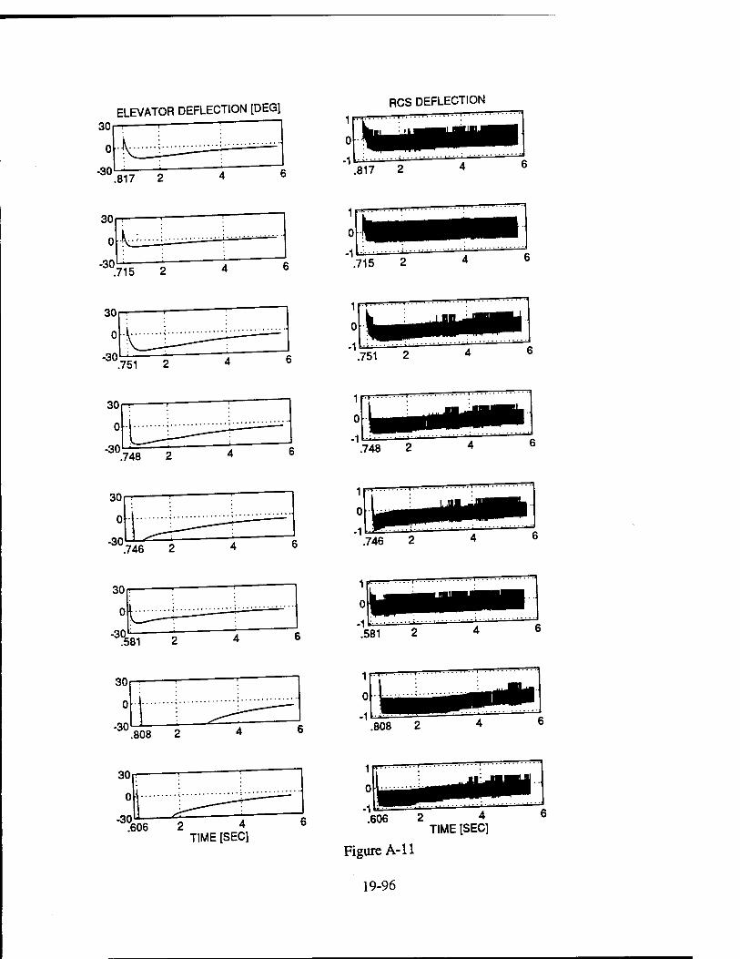
ELEVATOR DEFLECTION [DEG]
.817 2
.715 2
.751 2
.748 2
.746 2
.581 2
.808 2
7606 2 4 TIME [SEC]
RCS DEFLECTION
0
-1 .817 2
.715 2
.751 2
.748 2
.746 2
.606 2 4 TIME [SEC]
Figure A-11
19-96
808 2 4 6
, JLjUU
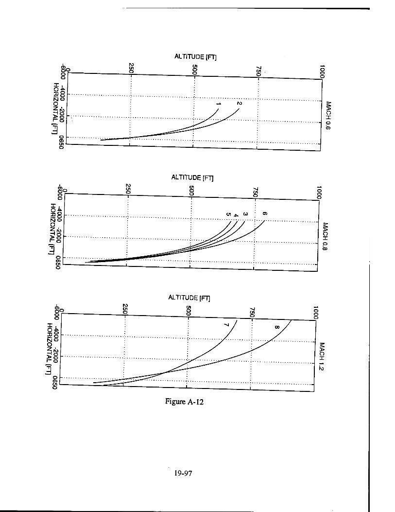
ALTITUDE [FT]
ALTITUDE [FT]
ALTITUDE [FT]
Figure A-12
19-97
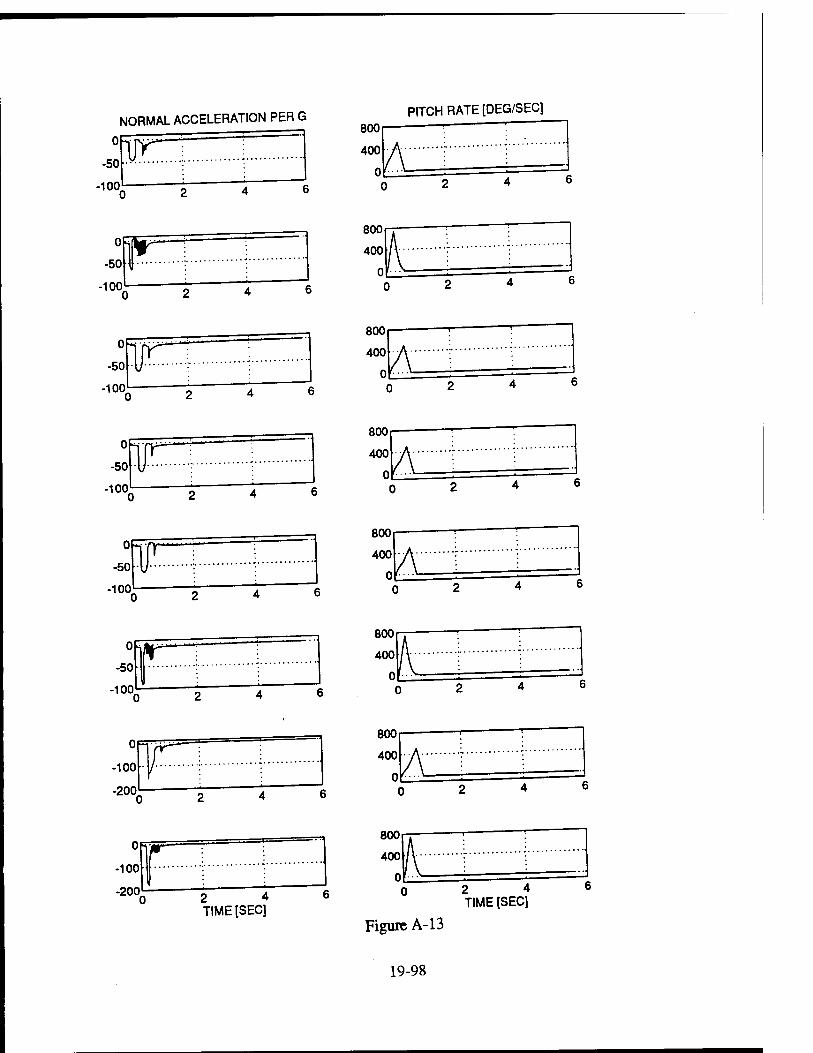
NORMAL ACCELERATION PER G
-50
-100.
PITCH RATE [DEG/SEC]
800
400
0 Al
-100
800
400 It
-50
-100
DO 800
400
8001—
400
-50
-100
t- 800
400
0
0
-50
-100.
800
400
0
Op
-100
-200
800
400
0
OF
-100
-200 2 4 TIME [SEC]
800 r
40ol
2 4 TIME [SEC]
Figure A-13
19-98
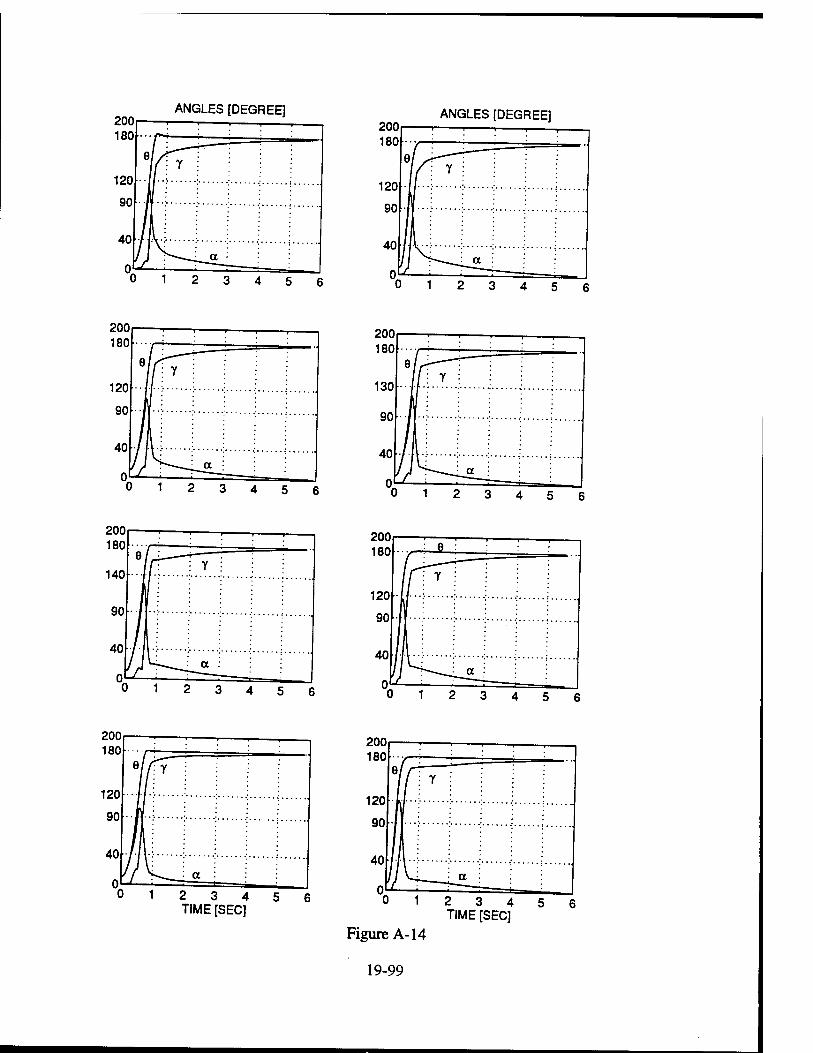
ANGLES [DEGREE]
0 12 3 4 5 6
ANGLES [DEGREE] ' i i -r-
12 3 4 5
200
ei
130 \\ y : i : :
90 i ; [ i
40 i [__ot :
0 J 0 12 3 4 5 6
2 3 4 5 6 TIME [SEC] 12 3 4
TIME [SEC]
Figure A-14
5 6
19-99
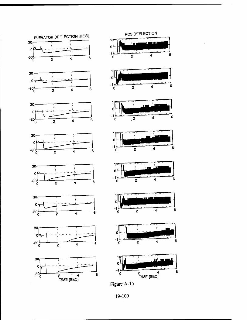
ELEVATOR DEFLECTION [DEG1 RCS DEFLECTION
2 4 TIME [SEC]
2 4 TIME [SEC]
Figure A-15
19-100
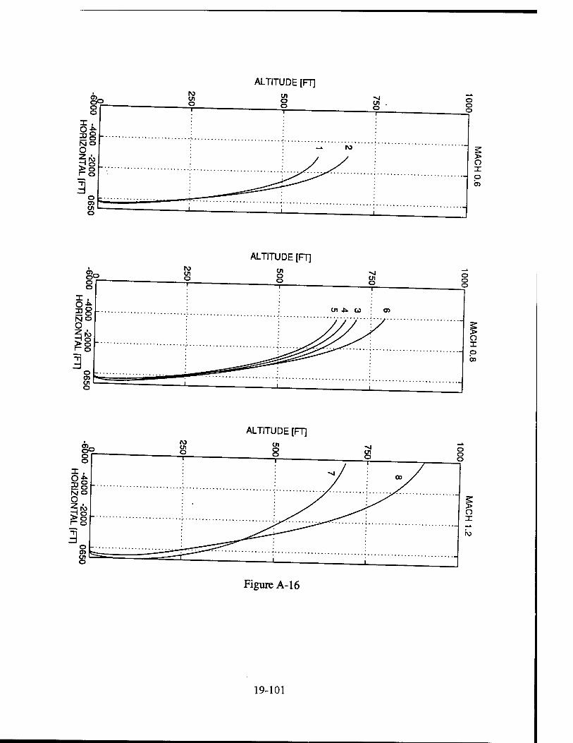
ALTITUDE [FT]
ALTITUDE [FT]
ALTITUDE [FT]
Figure A-16
19-101
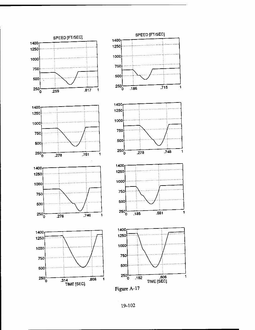
SPEED [FT/SEC] SPEED [FT/SEC]
817 1
314 .808 1 TIME [SEC]
"0 .182 .606 TIME [SEC]
Figure A-17
19-102
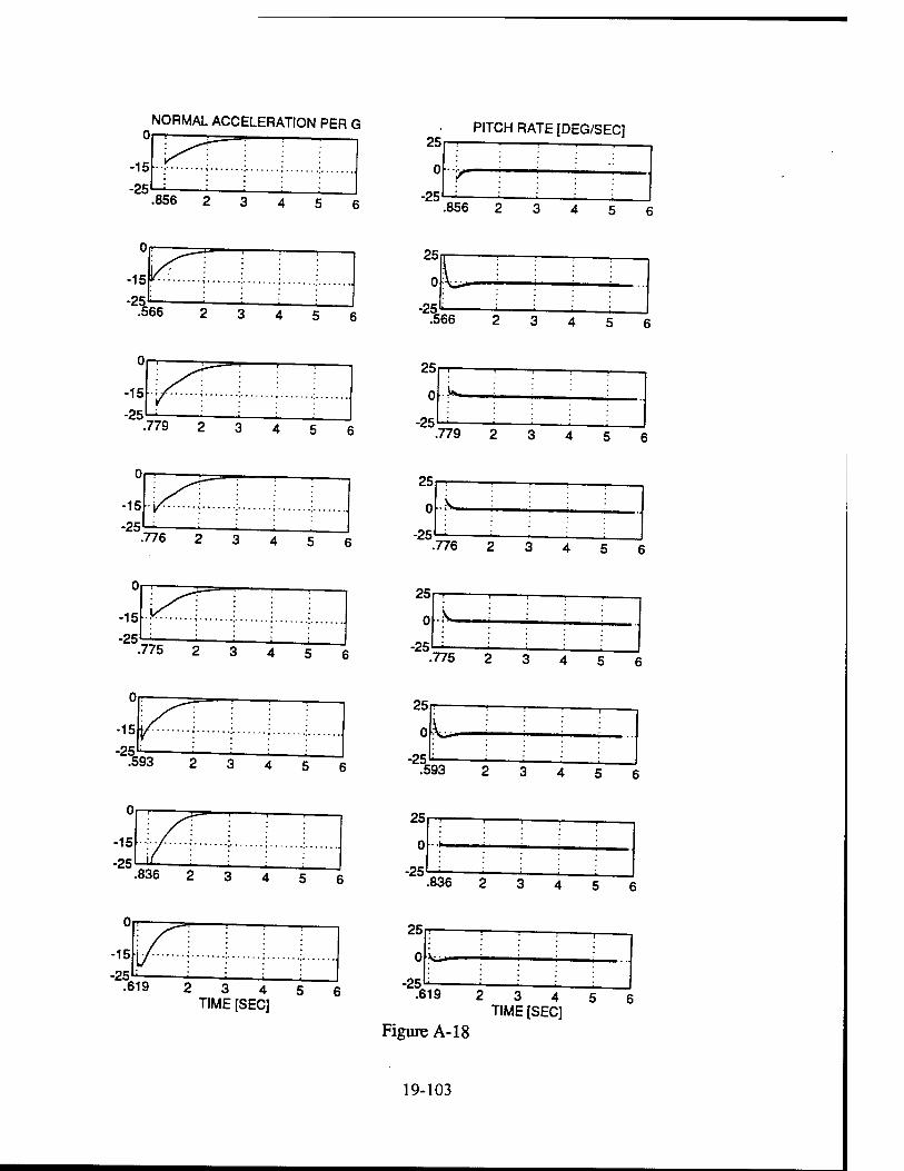
NORMAL ACCELERATION PER G
-1
°n !_
5 ••.""■•...;.
-2
(
5 —'■ .856 2 3 4 5 6
-1i -K~i -?'
566 2 3 4 5 6
r >|-!— ,
-15
-25 .779 2 3 4 5 6
n
-15 ,. i/T.
-25 : 776 2 3 4 5 6
n
-15 .kl.. -25 :
775 2 3 4 « i 6
n_
-15
-2^ i : .55 }3 2 3 * 5 6
Or
-15
•25 - if .£ I36 2 3 A 5 6
Or-
15 L
.619 2 3 4 5 6 TIME [SEC]
25
0
-25
PITCH RATE [DEG/SEC]
••/-
.856 2 3 4 5 6
25
-25.
SL .566 2 3 4 5 6
25
0
-25
i i
•779 2 3 4 5 6
25
0
-25
25
0
-25
•776 2 3 4 5 6
.V.
•775 2 3 4 5 6
25
.U -25 ^
•593 2 3 4 5 6
25
0-+-
-25 •836 2 3 4 5 6
25
-25
O'Vü*
•619 2 3 4 5 6 TIME [SEC]
Figure A-18
19-103
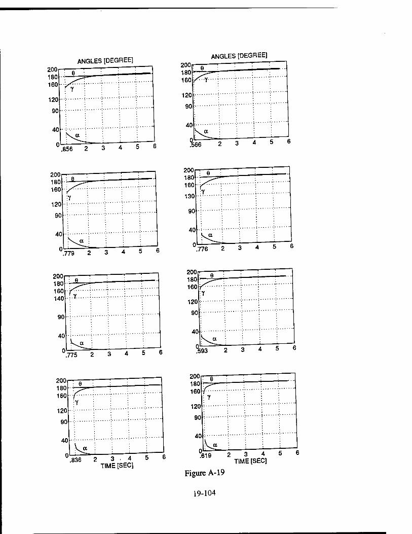
ANGLES [DEGREE]
200 180 160
120
90
40
0
9
r T
a :
.856
ANGLES [DEGREE]
200 180^ 160
120
90
40 a
% 66
200 180 160
120
90
40
0
■ < i—
J : I—
a
,779 .776
200 180 160
120
90
40
0. a
.775 593
.836 2 3 4 TIME [SEC]
.619
Figure A-19
2 3 4 5 6 TIME [SEC]
19-104
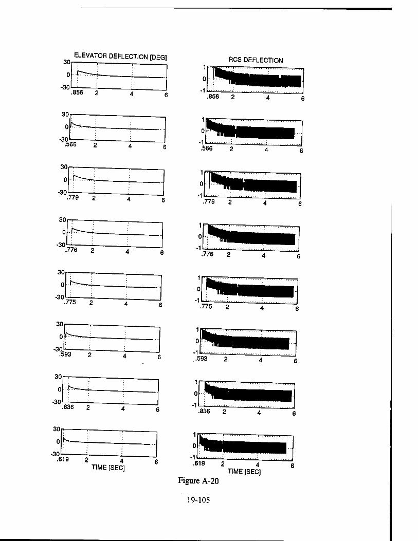
30
0
-30
ELEVATOR DEFLECTION [DEG]
.856 2
30
0
-30 .779 2
30
0
-30 .775 2
30r
0
-30 .836 2
30
0
-30 .619
TIME [SEC]
RCS DEFLECTION
.566
.775 2
593
836 2
.619
Figure A-20
19-105
TIME [SEC]
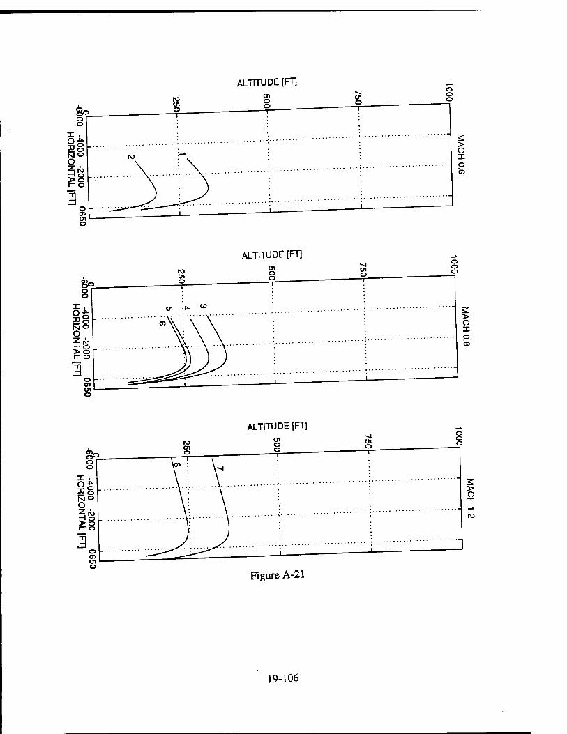
ALTITUDE [FT]
ALTITUDE [FT]
ALTITUDE [FT]
Figure A-21
19-106
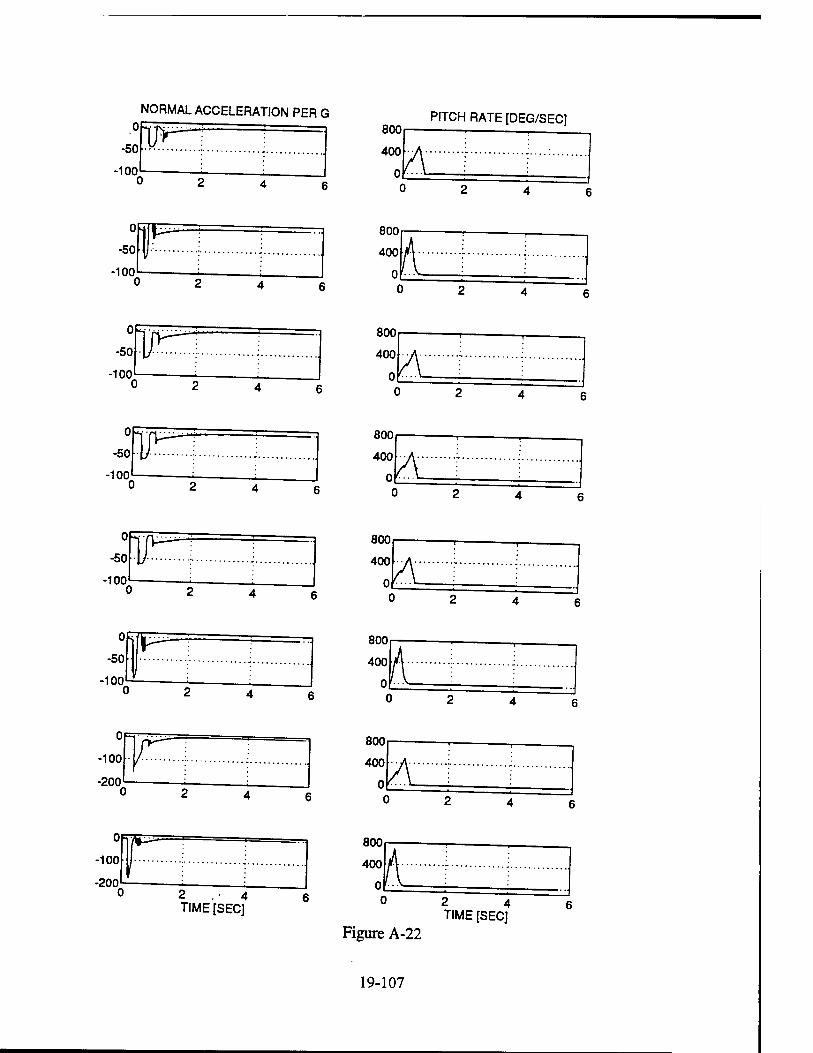
NORMAL ACCELERATION PER G
-50
-100
800
400
0
PITCH RATE [DEG/SEC]
0
-50
-100 I P=
-100
800
800
400
0
0
-50
-W
800
400 :t -100
-200
0
-100
-200 F
2 .-4 TIME [SEC]
800
400
in ; i
Figure A-22
2 4 TIME [SEC]
19-107
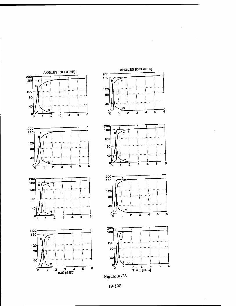
ANGLES [DEGREE] ANGLES [DEGREE]
12 3 4 5
200 ■ i —'
180
iny
120
90
40 ../.
°0 1 2 3 4 5
°0 1 2 3 4 5 6
200 180
120
90
40
e/ i
200 180
120
90
40
0 6
Figur
19-
A : :
0 0 12 3 4
TIME [SEC] 5
0 12 3 4 TIME [SEC]
eA-23
108
b
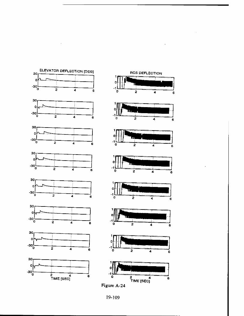
30
0
-30 (
30
0
-30 (
30
0
-30
ELEVATOR DEFLECTION [DEG]
-30
30
0
-30 2 4 TIME [SEC]
B
e e
RCS DEFLECTION
J-'" ' i r i - ■ i i
2 4
Q
i Figure A-24
2 4 TIME [SEC]
19-109
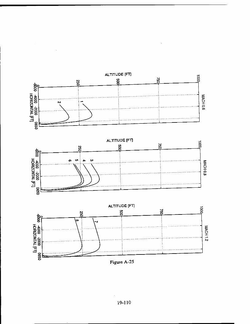
ALTITUDE [FT]
ALTITUDE [FT]
ALTITUDE [FT]
Figure A-25
19-110
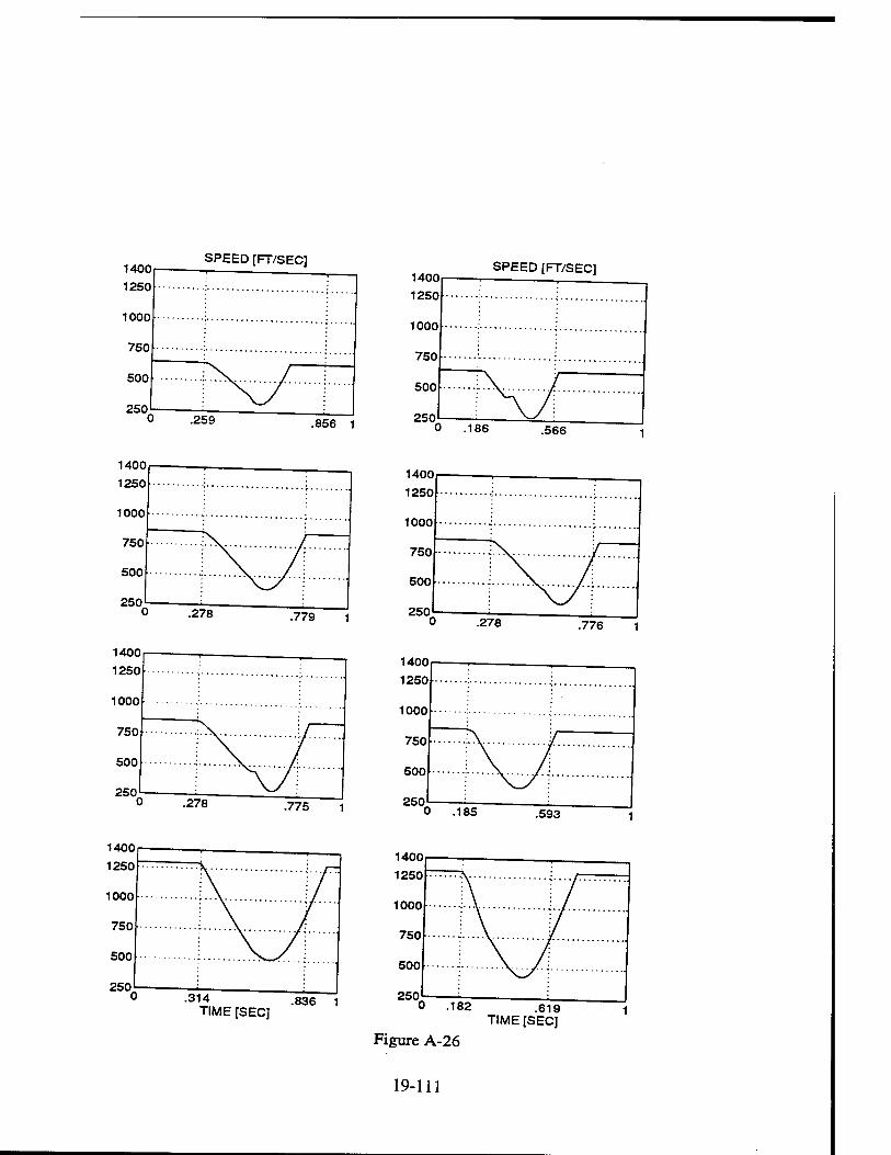
1400
1250
1000
750
500
250
SPEED [FT/SEC]
.259 .856 1
1400 SPEED [FT/SEC]
•314 .836 TIME [SEC] 0 .182 .619
TIME [SEC]
Figure A-26
19-111
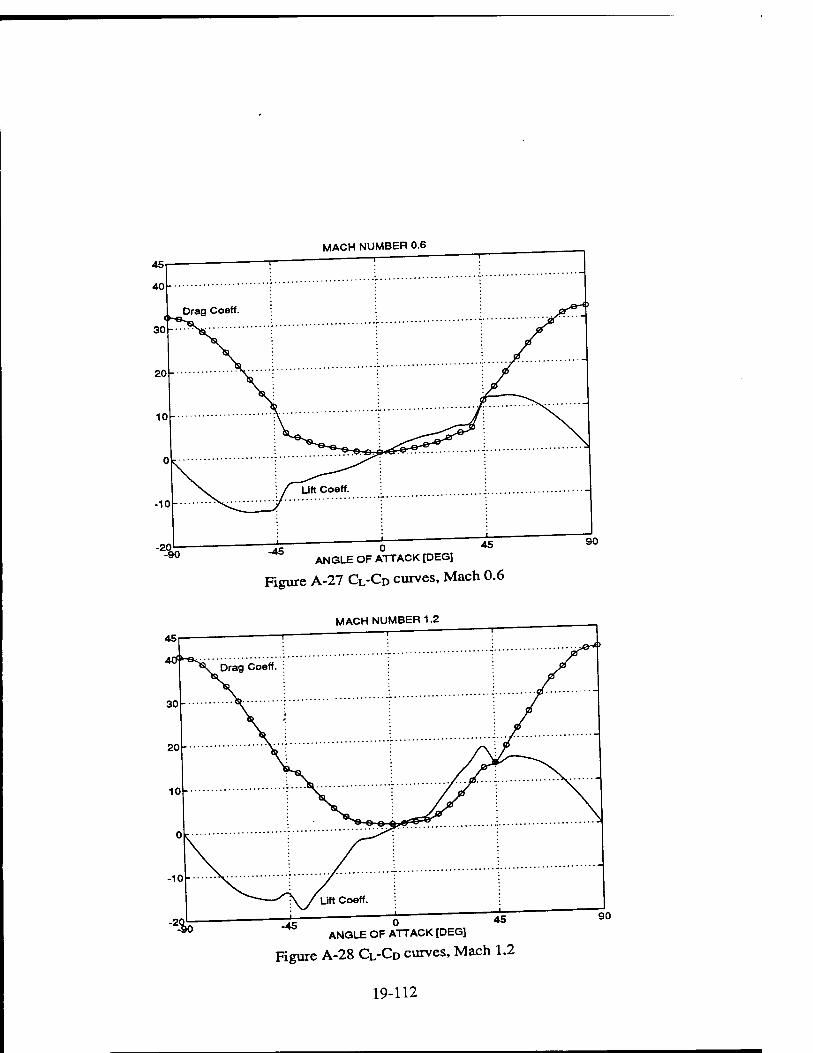
MACH NUMBER 0.6
-90 -45 ° ANGLE OF ATTACK [DEG]
Figure A-27 CL-CD curves, Mach 0.6
MACH NUMBER 1.2
ANGLE OF ATTACK [DEG]
Figure A-28 CL-CD curves, Mach 1.2
19-112
LASER IMAGING AND RANGING (LIMAR) PROCESSING
Jack S.N. Jean Assistant Professor
Department of Computer Science and Engineering
Wright State University Dayton, Ohio 45435
Louis A. Tamburino Avionics Directorate Wright Laboratory
Wright-Patterson AFB, Ohio 45433
Final Report for: Summer Research Extension Program
Wright Laboratory
Sponsored by: Air Force Office of Scientific Research
Boiling Air Force Base, Washington, D.C.
and
Wright State University
December 1993
20- 1
LASER IMAGING AND RANGING (LIMAR) PROCESSING
Jack S.N. Jean Assistant Professor
Department of Computer Science and Engineering Wright State University
Louis A. Tamburino Avionics Directorate Wright Laboratory
Abstract
The LIMAR (Laser IMaging and Ranging) project is a Wright Laboratory effort to de-
velop an advanced imaging and ranging system for robotics and computer vision applications
LIMAR embodies a concept for the fastest possible three-dimensional camera. It eliminates
the conventional scanning processes by producing a registered pair of range and intensity im-
ages w*h data collected from two video cameras. The initial prototype system was assembled
and successfully tested at Wright Laboratory's Avionics Directorate in 1992. This prototype
LIMAR system used several frame grabbers to capture the demodulated LIMAR image signals
from winch the range and intensity images were subsequently computed on a general purpose
computer. The prototype software did not address the errors which are introduced by differ-
ent.! camera gain, misalignment, and distortion. In last summer, the principal investigator
developed algorithms to correct the distortion introduced by using two cameras and designed
a special purpose hardware to convert, in real-time, the outputs from the two cameras into a
fully registered range and intensity image. During the project period, the detailed design of
the processing system has been finished and three hardware boards have been implemented and tested.
20-2
LASER IMAGING AND RANGING (LIMAR) PROCESSING
Jack S.N. Jean and Louis A. Tamburino
1 Introduction
The LIMAR (Laser IMaging and Ranging) project is a Wright Laboratory effort to develop an
advanced imaging and ranging system for robotics and computer vision applications. LIMAR,
the invention of Dr. Louis A. Tamburino of Wright Laboratory and Dr. John Taboada of the
USAF School of Aerospace Medicine, embodies a concept for the fastest possible three-dxmensxonal
camera It eliminates the conventional scanning processes by producing a registered pair of range
and intensity images with data collected from two video cameras. The initial prototype system
was assembled and successfully tested at Wright Laboratory's Avionics Directorate m 1992. The
prototype LIMAR system used several frame grabbers to capture the demodulated LIMAR image
signals from which the range and intensity images were subsequently computed on a general
purpose computer. The intent of this research effort is to design and implement a customized LIMAR processing
system to generate both the range and intensity images in real time. This new ability is needed to
facilitate future robotic and automatic vision applications. The processor design also takes mto
consideration error correction for camera distortions and misalignments. Error corrects was
not explored in the original LIMAR prototype and was investigated in the summer of 1992. The
result was the development of an alignment algorithm. This report first describes the computes
required for the processing and an algorithm used to reduce computations. It then descnbes a
LIMAR processing system and several hardware boards implemented.
LIMAR Device Overview As shown in Figure 1, the LIMAR device contains a laser, a
polarization modulator, a beam splitter, and a processing unit. The laser shines light on the
object which reflects the light back to the modulator. The modulator changes the polanzat.on of
the returned light. The polarization change depends on when the light reaches the modulator, or
equivalents depends on the distance between the object and the LIMAR device. Note that the
20-3
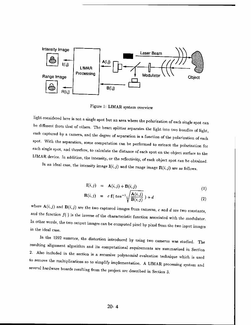
Intensity Image
l(ij)
Range Image
R(iJ)
LIMAR Processing
Figure 1: LIMAR system overview
light considered here is „ot a single spot but an area where the polarization of each single spot can
be dlfferent from that of others. The beam splitter separates the light into two bundles of light
each captured by a camera, and the degree of separation is a function of the polarization of each
spot. With the separation, some computation can be performed to extract the polarization for
each smgle spot, and therefore, to calculate the distance of each spot on the object surface to the
LIMAR device. In addition, the intensity, or the reflectivity, of each object spot can be obtained
In an .deal case, the intensity image I(i|i) and the range image R0,,-) are as follows
l(i,j) = A(i,j) + B(i,j)
K(iJ) = cf(tan-\lA<M)+d
(1)
(2) . B(i,j)
where A(i,J) and B(iJ) are the two captured images from cameras, c and d are two constants
and the function /(•) is the inverse of the characteristic function associated with the modulator'
In other words, the two output images can be computed pixel by pixel from the two input images in the ideal case.
In the 1992 summer, the distortion introduced by using two cameras was studied The
resultmg alignment algorithm and its computational requirements are summarized in Section
2- Also „eluded in the section is a recursive polynomial evaluation technique which is used
to remove the multiplications so to simplify implementation. A LIMAR processing system and
several hardware boards resulting from the project are described in Section 3
20-4
2 Computational Requirements
2.1 Image Alignment
Because the two input images are grabbed with two cameras, they may not be aligned well with
«pact to each other. Furthermore, the two cameras may introduce different distortions. So there
is a need to first align each of them to an "ideal" image before the pixel by pixel operation, as
indicated in equations 1 and 2 can be performed.
The alignment process contains two operations, position mapprng and interpolation. The
position mapping transforms a pixel location <«,,) to a new location (,,y) after alignment. It
was modeled as a bi-variate polynomials as follows.
x = a0 + a1u + a2v + a3u* + a4uv + a5v* + aeu3 + a7u->v + asuv> + a9v> + --- (3)
y = b0 + blu + b2v + b3u* + b<uv + b5v* + b6u3 + b7u*v + bsuv> + b9v* + .-- (4)
Since the new location (*,y) may not be a meaningful pixel location, e.g., « or y may
not be integer, bilinear interpolation is used. In the summer of 1992, it was found that tlnrd-
degree polynomials are good enough for alignment purposes and the polynomial coefficients can
be computed with a least square estimation algorithm.
2.2 Polynomial Evaluation
The evaluation of two third-degree bi-variate polynomials for each pixel is pretty expensive in
terms of computation. For images of size M (rows) by N (columns), the polynomials x(u,v) and
y(u v) in equations 3 and 4 are to be evaluated for all the (u,v)'s in {(u,v) | u 6 {0, 1, 2, ..., N-l)
and v G {0, 1, 2, .... M-l». In our case, M=480 and N=640. Since there are 30 frames of nnages
per second' the computation requires 18,432,000 (=2x480x640x30) polynomial evaluations per
second As a result, a fast way to evaluate the polynomials is necessary. The technique, recursive
evaluation, takes only three additions per pixel for the evaluation of a third-degree bi-vanate
polynomial. Numerical stability issues are also taken into consideration in the technique.
To illustrate the approach, the evaluation of a third-degree single-variable polynonual » first
presented. The result is then applied to the bi-variate case.
20-5

Smgle-variable Polynomial Evaluation Let »(,) = c0 + Cl* + C2, W> where x is in ^
range, 0, 1, 2, ..., N-l. Instead of performing the N evaluations separately, which takes at least
3N multiplications and 3N additions, a recursive formulation can be used to reduce the number
of computations. That is,
2/3(2 + 1) = y3(x) + y2(x)
J/s(0) = c0
where y2(x) is a second-degree polynomial which is equal to (Cl + c2 + C3) + (2c, + 3^ + 3^
Since the evaluation of a second-degree polynomial takes at least two multiplications and two
add-ons, the required computations are reduced to 2N multiplications and 3N additions (plus
the three multiplications and three additions in obtaining the coefficients of »(,)). For large N,
the 6N computations have been reduced to 5N.
Similarly, recursive formulation can be applied to y2(x), or
y2(x + 1) = y2(x) + yi(x)
J/2(0) = Cl + c2 + c3
and then be applied to Vl [= (2c2 + 6c3) + 6cax] such that
yi(x + l) = yi(x) + 6c3
tfi(0) = 2c2 + 6c3
In summ„y, the following rec„„ive formnls c„ fce nsed to evaluate ^ the ^
tially.
y3(x + l) = y3(x) + y2(x)
!&(* + l) = y2(x) + yi(x)
Vi(x + 1) = yi(x) + 6c3
20-6
given the initial values
2/(0) = co
yi(0) = 2C2 + 6C3
y2(0) = C1+C2 + C3
It is clear from the formulation that only 3iV additions are needed (in addition to the com-
putations of several constants). It is also clear that the polynomial evaluation can be implemented
with a pipelined three-adder hardware so to produce one y3(*) per clock cycle.
Bi-Variate Polynomial Evaluation For any specific image row, the bi-variate polynomial can
be reduced to a single-variable polynomial since the variable v has a given value. More specially,
= (a„ + a2v + a5„2 + a9,
3) + («n + a4v + a.,8)« + («3 + alv)u" + a6u3
Therefore, glven a specific value of v, the coefficients of ,(«,,) as a polynomial in u can be
computed. It then takes 3N additions for the evaluation of the single-variable polynormal.
Numerical Stability Considerations The coefficients of the bi-variate polynomials have very
different dynamic ranges. For example, the a0 value may be from -5 to 5 while the a9 value may
be from -0 0000001 to 0.0000001. This is because the value of ,(«, v) (or y(u, v)) is bounded for
image alignment and one of the contributing factor for ,(«,„) is from the multiplication of a9
with ,3 which can be very large. From implementation point of view, the different dynamic ranges
cause numerical problem due to finite precision. One way to ease the problem is to normahze the
coefficients as follows. The technique is illustrated below with a single-variable polynonual.
Let *,) = Co + ex, + c2*2 + ^ where , is in the range, 0, 1, 2, ..., N-l. The value of c3
may be too small because (N-lf is pretty large. To balance the ranges, y(x) can be reformulated
as
2/(x) = C0 + (ci5)f+(c252)(|)2 + (c3S
3)(|)3
20-7
Let xn = x/S and g(xn) = y(x), then
g(xn) = c0 + (ClS)xn+(c2S2)x2
n+(c3S3)x3
n
= cn0 + cn!Xn + cn2xl + c^x3
where S is a constant whose value is chosen to be close to N and ,(,„) becomes a polyno-
nnal whose coefficients are normalized to similar dynamic ranges. Note that ,„ is in the range
0,1/5,2/S,..., (N - 1)/S. This requires a simple change to the recursive formulation. It can be
shown that the previous evaluation formula become as follows.
»(* + !) = ys(x) + ^p.
*(« + !> = y2(x) + ^P- Vi(x+g) = yi(x) + c
where c is a constant and the initial values can be computed from the normalized coefficients
Therefore the cost of normalization to the polynomial evaluation is simply some data shifting
when S „ chosen to be as a power of two number. In the project, 512 is used for S.
2.3 Timing Requirements
The video input of the project has 30 frames a second and the frame resolution is 480 x 640
(helght, width). As a result, there are 9.216 MegaBytes (= 640 x 480 x 30) of pixels per second
for each channel of video signal. Since a video signal contains some horizontal/vertical blanking
periods, the actual pixel rate is even higher. In fact, a clock rate of 12.5 MHz is necessary for the
LIMAR hardware system for real time processing. This translates into 80 nsec of clock period
during which time, for each channel, two third-degree bi-variate polynomials need to be evaluated
and a bilinear interpolation needs to be calculated.
20-8
3 LIMAR Processing System
The current design of the LIMAR processing system is shown in Figure 2. The system processes
and combines two channels of camera signals. The system contains two camera,, two momtors,
two video I/O boards, a LIMAR processing board, two image alignment boards, a microcontroller
board, and a personal computer (PC). Each video I/O board processes one channel of analog
camera signal and converts it to a digital data string. The data buffering and video signal syn-
chronization are also performed by the video I/O boards. Each channel of digital data is then
sent to a corresponding image alignment board which, in real-time, aligns an image frame w,th an
"ideal" image frame, or equivalent*, removes some image spatial distortions. The aligned images
are fed to the LIMAR processing board for further processing. The results are sent to vxdeo
I/O boards and displayed on the monitors. A microcontroller board serves as the PC command
interpreter and controls the whole LIMAR system. An application program with graph, user
interface (under Windows 3.1 environment) runs on a PC and talks to the system through a PC
parallel port. The usage of the PC parallel port increases the portability of the whole system.
In this project the system has been fully defined and several hardware boards have been
implemented and tested so to verify the feasibility. Accomplished include (1) the definition of the
LIMAR system bus, (2) the design, implementation, and testing of a video I/O board, (3) the
design, implementation, and testing of an image alignment board, (4) the design, implements,
and testing of the microcontroller board, and (5) the implementation of the LIMAR control
program.
3.1 LIMAR System Bus Definition
Since the LIMAR system bus is used by all the boards involved, a clear definition of its signals helps
to decouple the designs of individual boards. The 16-bit PC/AT-bus is adopted and modmed to
serve as the system bus because of its low cost and popularity. By doing so, any AT-bus prototype
board can be used for the LIMAR development. In fact, each of the board in Figure 2 uses a full
size (13" x 4 5") AT-bus daughter board. The AT-bus connector is a 62-pin edge connector with a
secondary 36-pin edge connector. The bus pinouts were re-defined for LIMAR system so that all
the real-time signals are embedded in the system bus while some slower signals are implemented
20-9
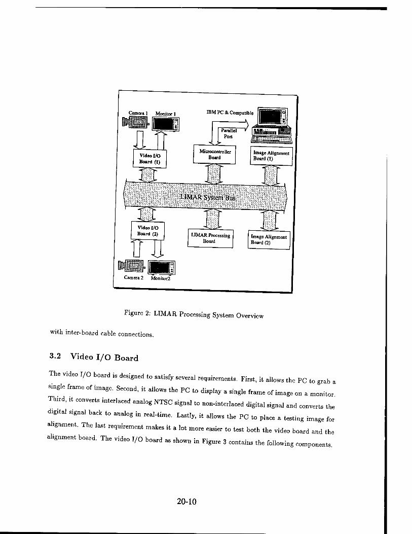
Figure 2: LIMAR Processing System Overview
with inter-board cable connections.
3.2 Video I/O Board
The video I/O board is designed to satisfy several requirements. First, it allows the PC to grab a
single frame of image. Second, it allows the PC to display a single frame of image on a monitor
Third, lt converts interlaced analog NTSC signal to non-interlaced digital signal and converts the
chgxtal S1gnal back to analog in real-time. Lastly, it allows the PC to p,ace a testing image for
alignment. The last requirement makes it a lot more easier to test both the video board and the
ahgnment board. The video I/O board as shown in Figure 3 contains the following components
20-10
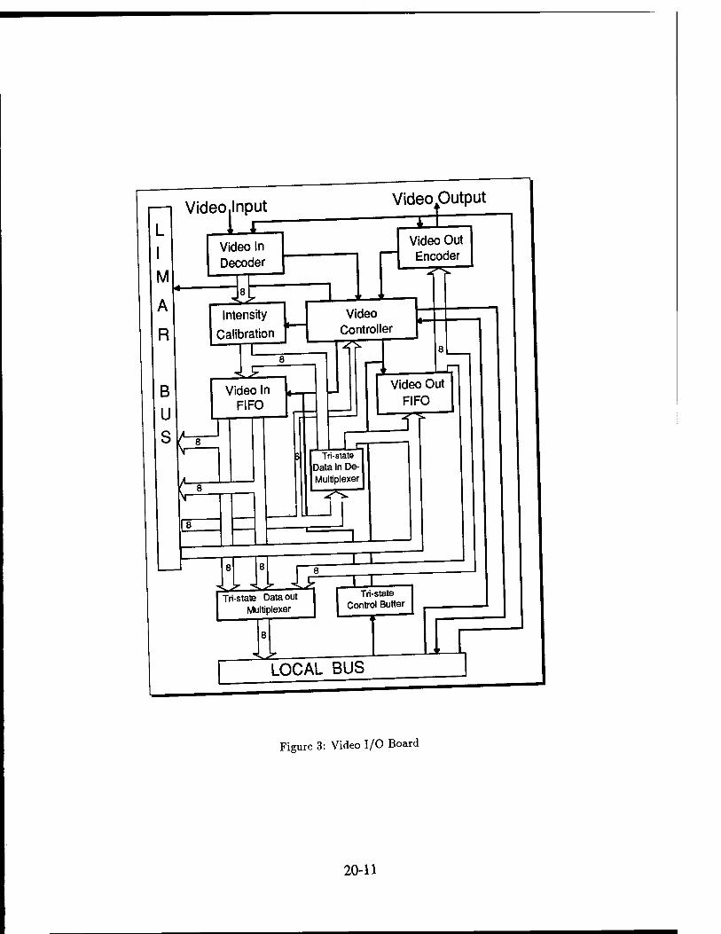
I M
A
R
B U S
Video .Input .1 n
t A-
Video In Decoder
S^ , Intensity
Calibration
I £. Video In
FIFO
Video Output
xt:
ZL
Video Out I Encoder
_* ■
Video Controller
1 Video Out
FIFO
Tri-stata Data In De- Multiplexer
Tri-state Data out Multiplexer
8
8 HE TX
Tri-state Control Buffer r ]
LOCAL BUS i Figure 3: Video I/O Board
20-11
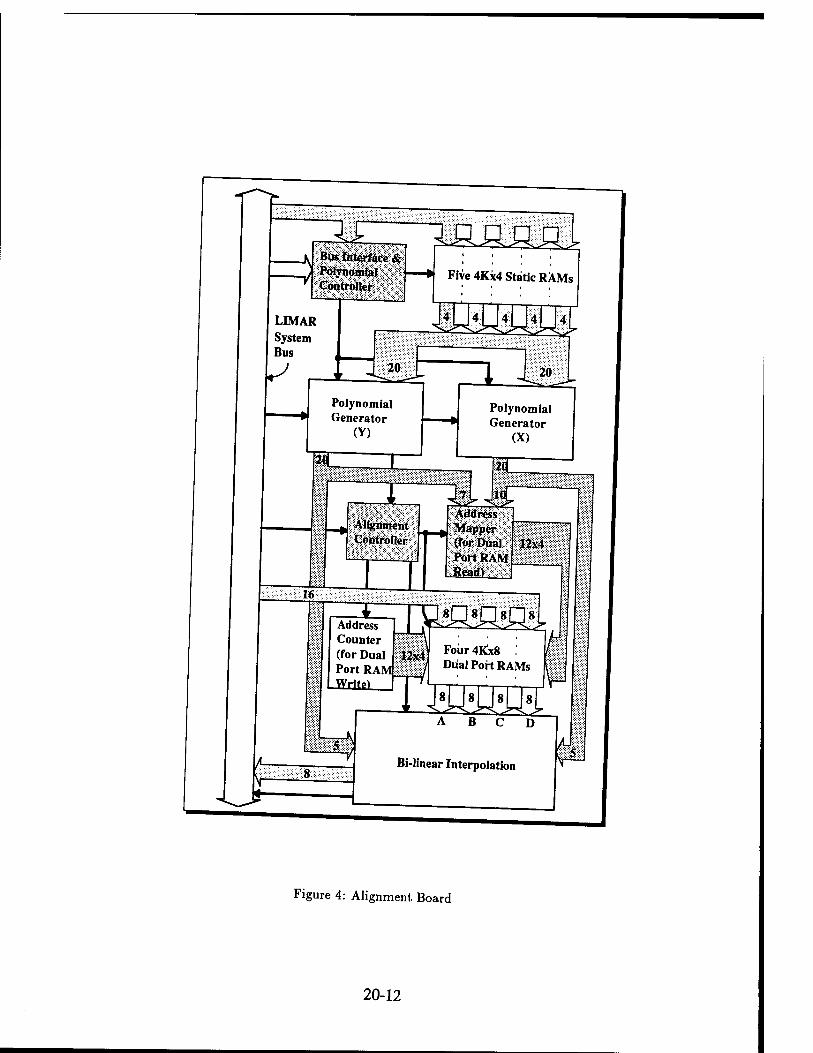
ii Bits Interface & Polynomial o\j Controller -\
LIMAR System Bus
20
Polynomial Generator
(Y)
mz I I
Alignment Controller
16
Address Counter (for Dual Port RAM
Mnool Five 4Kx4 Static RAMs
1 20
Polynomial Generator
(X)
it
t—» Address Mapper \ (Tor Dual Port RAM Head) -
All
A Bi-linear Interpolation
Figure 4: Alignment Board
20-12

1 Video In Decoder and Video In FIFO (First-In-First-Out): The decoder unit converts an
analog interlaced NTSC video signal into a frame of digital non-interlaced data which is then
stored into the inpnt FIFO unit. The problem of synchronizing two independent cameras
is solved with suitable timing control. The intensity calibration unit is currently bypassed
since it is useful only when both channels are in place.
2 Video Out FIFO: The image data in the input FIFO is sent to the dual-port memory on the
alignment board. For a complete system, the output of the alignment board is sent to the
LIMAR board which collects and processes two channels of data. The output FIFO «nit
receives data from the LIMAR board. All the inter-board data transfers here are in real-time
and go through the LIMAR system bus. Currently, the LIMAR board is not available yet.
So an extra board is used to relay the output of the alignment board to the video out FIFO
unit on the video board. The input to the FIFO is non-interlaced while the output of the
FIFO is interlaced.
3. Video Out Encoder: The encoder unit converts the digital images from the output FIFO
unit into NTSC signals which can be displayed on a monitor.
4 Video Controller: The controller unit is used to generate timing signals for the two FIFO
units and the intensity calibration unit. It solves the camera synchronization problem and
the interlaced image conversion problem. The controller is designed and implemented with
an Altera Erasable Programmable Logic Device (EPLD) EMP5128 EPLD chip.
5 Tri-state Data Multiplexer, Demultiplexer, and Buffers: They are used to select and buffer
desired data or control signals from/to bus. Note that a local bus is used between the V1deo
board and the microcontroller board to accommodate non-real-time signals.
3.3 Image Alignment Board
The image alignment is to convert an input image to another image according to two bi-variate
polynomials, x(u,v) and y(u,v). An input pixel at location (u, v) is mapped to location (x, y) on
an output image. If (x, y) is not a valid image location and falls among several pixels, a bx-lmear
interpolation is performed. The design of the image alignment board is sketched m Flgure 4.
20-13

The design contains dual-port memory components to buffer data, polynomial generators
to compute x(u,v) and y(u,v), a circuit to perform bi-linear interpolation, and two controllers
The polynomial generators and the circuit for the bi-linear interpolation are implemented with
XILINX Field Programmable Gate Array (FPGA) XC4003 and XC4005, respectively. The two
controllers are implemented with ALTERA EPLD EPM5000 series chips. The usage of these
advanced programmable logic devices reduces chip counts and facilitates rapid implementation.
3.4 The Microcontroller Board
An MC6811 microcontroller receives commands from a PC program through the standard PC
parallel port and controls the board accordingly. Since the standard PC parallel port is usually
used as an output printer port, some effort was spent in converting it to a bi-directional port The
m1Crocontroller sends t»C signals through local bus to control the video in decoder and video out
encoder on the video I/O board. In addition, the microcontroller controls various data buffers
(74244s) to select system working modes such as grabbing image, displaying image, or real-time processing.
3.5 The LIM AR Control Program
The LIMAR control program is an IBM-PC/Microsoft Windows-based program that serves to
m.tialize and control the activities of the various components of the LIMAR system. Due to the
speed required to process thirty 640x480 pixel images every second, the LIMAR control program
does not take part in the real time operation of the system. Rather, the program will load startup
parameters to various modules of the system and then send control signals to enable and disable
those modules. The program has very friendly user interface.
4 Conclusion
cameras The LIMAR device, which is conceptually the fastest image ranging device, utilizes two
to grab images which are required to be in full registration. In this project, camera registration
algorithms were refined and incorporated into a customized processor design which can convert the
mage pair into range and intensity images in real-time. The detailed design of the processing unit
20-14

and the control unit have been completed. Several hardware boards were implemented and tested
to verify the design. Compared to the prototype LIMAR system which was assembled m 1992
and could not perform real-time computations due to the usage of a general purpose computer,
the proposed processor represents a significant enhancement to the future LIMAR development
program at the Avionic Directorate of Wright Laboratory.
20-15
APPLICATIONS OF WAVELET SUBBAND DECOMPOSITION IN ADAPTIVE ARRAYS
Ismail Jouny Assistant Professor
Department of Electrical Engineering
Lafayette College Markle Hall, High Street
Easton, PA, 18042
Final Report for: Research Initiation Program
Wright Patterson Air Force Base
Sponsored by: Air Force Office of Scientific Research Boiling Air Force Base, Washington, D.C.
and
Lafayette College
December 1993
21-1
APPLICATIONS OF WAVELET SUBBAND DECOMPOSITION IN ADAPTIVE ARRAYS
Ismail Jouny Assistant Professor
Department of Electrical Engineering Lafayette College
Abstract
Pre-processing radar signals incident on an adaptive array by applying an invert-
■ble transformation snch as wavelets is the focus of this stndy. The effect of wavelet
subband decomposition of radar signals prior to adaptation nsing an LMS algorithm
or an Applebanm processor on the adaptation rate of these processors is examined
The mrpact of wavelet transform on the bandwidth performance of adaptive arrays
- also investigated. The performance of wavelet transform based array processors is
compared with that of the FFT, and Cosine transform. The dynamic range of the
array weights before and after wavelet transformation is also being examined. Sim-
ulates .nvolving experimental radar data and different types of wavelets are aJso presented.
21-2
APPLICATIONS OF WAVELET SUBBAND DECOMPOSITION IN
ADAPTIVE ARRAYS
Ismail Jouny
Introduction
Wavelet subband decomposition is a recently developed and rapidly evolving sig-
nal processing technology with emerging applications in speech compression, image
coding, geophysics, radar and sonar signal processing.
The author, in a study conducted at Wright Patterson Air Force Base during
the summer of 1992, used wavelet based target scattering features in radar target
recognition. The results indicated that wavelet decomposition of radar cross section
measurements (RCS) of unknown radar targets may be reliably used for target identi-
fication under different noise scenarios and without complete knowledge of the target
azimuth position.
The following study is the result of a research effort supported by AFOSR research
initiation program which followed the author's Summer Faculty Fellowship at Wright
Patterson AFB.
This study focuses on the application of wavelet decomposition in adaptive an-
tenna arrays, an idea that was developed during the summer of 1992 through conver-
sations with WPAFB fellow researchers and senior scientists. The following summary
of results shows that wavelets present a unique opportunity for improving the perfor-
mance of adaptive antenna arrays.
Two specific points are addressed in this study, first the effect of wavelet decompo-
sition on adaptation speed and convergence rate of adaptive systems including changes
in the eigen structure of the covariance matrix. A connection between wavelet domain
21-3

adaptation and other transform-domain adaptive processing techniques. Secondly
this study examines the effect of wavelet transform on the bandwidth performance J
adaptive arrays. Scenarios of wideband jamming are simulated and the array signal-
to- (noise+interference) ratio is examined. The study shows that improvement can be
achieved regarding the adaptation and convergence speed of adaptive arrays as well
as computational speed, but wavelet subband decomposition has little effect on the
bandwidth performance of an array.
This research focuses on incorporating wavelet subband decomposition into adap-
tive array processing of both narrowband and wideband radar signals. Radar signals
can be decomposed using wavelets into orthogonal and almost decorrelated subband,
Such a decomposition is usually performed using Fast Fourier Transform (which is
equivalent to using a bank of non-orthogonal bandpass filters) or using tapped delay line cancellers.
Because the concept of wavelet analysis was just recently developed, a brief review
of wavelet subband decomposition inc.uding definitions and properties is presented in
the following section. Sections III and IV detail the work done and present new results
concerning the performance of adaptive antennas. Section V presents conclusions and
suggestions for future work.
II. Wavelet Subband Signal Decomposition
Wavelet signal approximation is a powerful signal processing technique based
on subband decomposition using orthogonal Finite Impulse Response (FIR) filters
These filters are generated from the so-called wavelet functions. This framework
of signal processing, often called "multi-resolution analysis", provides the means for
signal decomposition into orthogonal octave bands so that every subband can be pro-
21-4

cessed separately. An exact replica of the original signal can be reconstructed using
a set of orthogonal octave band filters.
The wavelet transform of a signal x(t) is by definition a convolution of /(*) with
a wavelet */>(i) dilated by a factor a
which can be expressed in the frequency domain as
w,(o, b) = 4= f °° ^(«)*H^ ** (2) Va J-oo
Thus, the wavelet transform of z(t) is equivalent to filtering x(t) using the bandpass
filter *(aw) whose bandwidth varies as a function of scale a. For a = 2', j € Z
these filters represent octave band filters. Clearly, large scales correspond to narrow
smoothing filters that present a global view of the signal x(t) and small scales corre-
spond to wideband filters that extract the details of x(t) (high frequency components).
The signal x(t) can be recovered from its wavelet transform using
^=^Ubw)^)dadh (3)
assuming that
|#(u>)|2 , (4) 1 A-^- du < oo / U
or Jt m dt = 0. Fourier transform and Fourier series approximations of x{t) require
many expansion coefficients associated with high frequency components to model
transient signals and perform the necessary cancellation, thereby permitting the in-
clusion of high frequency noise. In contrast to that, wavelet analysis permits a se-
lective mode representation of the signal due to the compact nature of the analyzing
wavelet (limited duration of VW), and is therefore particularly suited for analyzing
transient signals and singularities. When using Fourier transform, we expand the
21-5
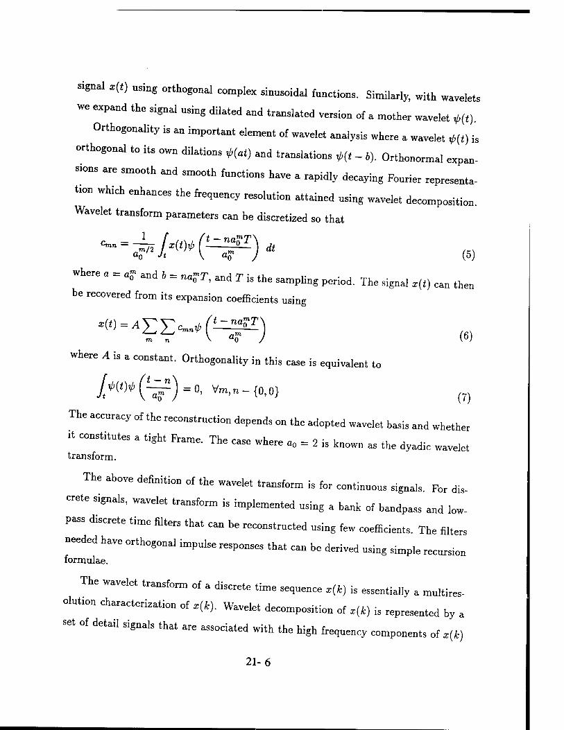
s.gnal X(t) using orthogonal complex sinusoidal functions. Similarly, with wavelets
we expand the signal using dilated and translated version of a mother wavelet *(«).
Orthogonality is an important element of wavelet analysis where a wavelet W is
orthogonal to its own dilations *«,) and translations «, - b). Orthonormal expan-
ses are smooth and smooth functions have a rapidly decaying Fourier represent.
t.on wh,ch enhances the frequency resolution attained using wavelet decomposition.
Wavelet transform parameters can be discretized so that
*- = -h /*W* ('-^) at ao Jt \ < J (5)
where a = < and b = n<T, and T is the sampling period. The signal ,(,) can then
be recovered from its expansion coefficients using
r? fl < ) (6) where A is a constant. Orthogonality in this case is equivalent to
/^W(^)=0, Vm,n-{0,0} (7)
The accuracy of the reconstruction depends on the adopted wavelet basis and whether
it constitutes a tight Frame. The case where a0 = 2 is known as the dyadic wavelet transform.
The above definition of the wavelet transform is for continuous signals. For dis-
crete signals, wavelet transform is implemented using a bank of bandpass and low-
pass d,screte time filters that can be reconstructed using few coefficients. The filters
needed have orthogonal impulse responses that can be derived using simple recursion formulae.
The wavelet transform of a discrete time sequence ,(*) is essentially a multires-
olut,on characterization of ,(*). Wavelet decomposition of x(i) is represented by a
set of detail signal that are associated with the high frequency components of ,(t)
21-6
and a final coarse approximation. Mallat [17] has developed a very efficient multires-
olution wavelet decomposition algorithm that limits the number of wavelet expansion
parameters to N where N is the length of the data sequence *(*). As the signal *(*)
propagates through the filter bank tree of lowpass and highpass filters, the output of
the highpass filter G(z) at stage m is a sampled version of the wavelet transform of
x(Jfc) at scale 2». At each stage, the bandwidth of both filters is halved with the high
halfband associated with the highpass filter and the low halfband associated with the
lowpass filter. The dyadic discrete wavelet transform is essentially a decomposition
of the spectrum of x(k), X(e^) into orthogonal subbands defined by
11-17 (8)
where T is the sampling period associated with *(*). Therefore, wavelets are unique
in offering a framework for examining radar signals at different resolutions (different
frequency bands) and processing each component separately.
III. Wavelets and Adaptive Arrays
Adaptive array processing with applications in radar and communications is a
discipline that has received considerable attention in the last few decades. There are
numerous studies addressing almost every aspect of the problem of adaptive signal
processing. Rejection of intentional jamming and scattered interference is one of the
many applications of adaptive array processing. Decorrelation of signal components,
for the purpose of simplifying the adaptation procedures, by means of subband de-
composition either using the FFT or using tapped delay-line cancellers has also been
a subject of great significance in adaptive processing.
The bandwidth performance (or nulling bandwidth) is an important factor in
designing adaptive arrays. To address this problem, researchers have proposed FFT
21-7
processing as a tool for band partitioning the frequency response of the received signal
and adapting each band separately. Others have shown that a transversal filter con-
structed as a tapped delay-line does improve the bandwidth performance of adaptive
arrays. L. E. Brennan compared the performance of both FFT based processing and
transversal filters in improving the cancellation ratio of sidelobe cancellers assuming
unmatched receiver characteristics. Mismatch between receivers in different chan-
nels could be simulated as random pole placement, or shift in the center frequency
and a difference in the bandwidth of the receive, Different receiver mismatch scenar-
ios were considered in Brennan's study and the transversal filter method constantly
outperformed the FFT approach. Later, Compton showed that both methods have
eqmvalent bandwidth performance (improving nulling bandwidth) provided that the
delay between taps is identical to the delay between samples of the FFT. He also
showed that no invertible transformation can be inserted between the delay-line taps
and the weights that may improve the nulling bandwidth of the array. However using
the FFT technique reduces the correlation between samples in disjoint frequency sub-
bands which leads to a block diagonal „variance matrix. Thus with FFT processing
the weights are computed and adapted separately in each band. Although, samples in
afferent frequency bands are usually not completely decorrelated and the covariance
matnx is not absolutely block diagonal, frequency domain adaptive filtering reduces
the eigenvalue spread of the data autocorrelation matrix.
1. Array Structure
The adaptive arrays examined in this report are known as the Applebaum array
and the LMS array. Although, we focus on the LMS adaptation algorithm, the results
can be readily generalized to include the Applebaum array.
21-8
An N elements array is shown in Figure 1 where X denotes the input vector
X =
xxl
X\2
X\K
Xi\
X-iK
w =
WXK
W21
W2K
(9)
XNK J L Wm
The array includes K tap delay elements with NK weights, henceforth the weight vec-
tor W. The weights are controlled using either the LMS algorithm (where a reference
signal is required) or the Howell-Applebaum algorithm where both algorithms yield
the same optimal solution. The output signal is denoted by sx where sx = XTW (T
denoting transpose). The optimal weight solution for both algorithms is
Wopt = K1Sx (10)
where Sx is the steering vector (Sx = E{Xr(t)}, r(t) being the reference signal) .
The matrix $x is the covariance matrix of the input vector X, and defined as
E{XnXn) ••• E{X^XlK E{XUXNK}
$ = E {X21X11} E{X21XlK} E{X21XNK] (11)
E{XNkX n ... E{XNkXiK} E{XNKXNK}\
21-9
at:
Xlk(t)
Figure 1: Adaptive antenna array of N elements each with K tap-delays
21-10

where E{.} denotes the expected value. Each weight vector is adjusted according to
the rule
dW = -kWwE{[r(t)-s(t)?} <12> at
where r(t) is the reference signal (correlated with the desired signal d(t)). If the input
is discrete then the above adaptation rule at time n reduces to
Wf1 = W$ + 2fiX^ [r(n) - s(n)) (13)
To ensure stability of the LMS algorithm, /z can be chosen as
2 (14) 0 < ß < NKE{X*}
In fact for the weights to converge, the adaptation parameter ß should be chosen such
that
2 (15) 0</i<MÜ)
Notice that by taking the expected value of both sides of the adaptation equation
(written in vector form hereafter)
E{Wn+1} = Wn + 2fiE{X [r(n) - XTW}} (16)
which can be rewritten as
E{Wn+1} = {I-2fi$)W + 2fiE{Xr{n)} (1T)
where $ = E{XXT}. The above equation can be further simplified to yield
E{W^ _ Wopt} = (/ - 2M*)B E{W° - Wopt] (18)
By properly choosing /x, the above equation leads to (10).
21-11
2- Transform-Domain Adaptation
The convergence of the above adaptation algorithm is dependent on the eigen-
spread (aiming stationary input) WA-> which is known as a the condition
number which is an indicator of the rate of convergence of the adaptive algorithm and
provmes diagnostic description of the ill-conditioning of the matrix *. Therefore, in
order to achieve high convergence rates (which is a crncial factor in radar technology)
the adaptation mnst be performed in an orthogonal domain obtained by transforming
the input vector X. The Karhunen-Loeve transform would be the ideal transform
wmch produces completely orthogonal signal components but computing the KLT
» very dependent on the exact estimate of * which is complicated and impractical
Two other possible options which are not based on transformation but can improve
the adaptation speed are; the recursive least square algorithm (RLS) and the Gram-
Schmidt orthgonalization method. These options are tedious and computationally demanding.
Alternatively we may use the following transforms:
1) Discrete Fourier transform (implemented with the FFT) where the input signal X
is transformed into
,e N Yit = ^£*" " («) j K-l
A,n ~ 77f Z^*e N
k=0
2) the Cosine transform
z« = ££*. n=0
K-\
(20)
* - ±±*„(*%m n=0
which can be implemented using a bank of bandpass filters.
21-12
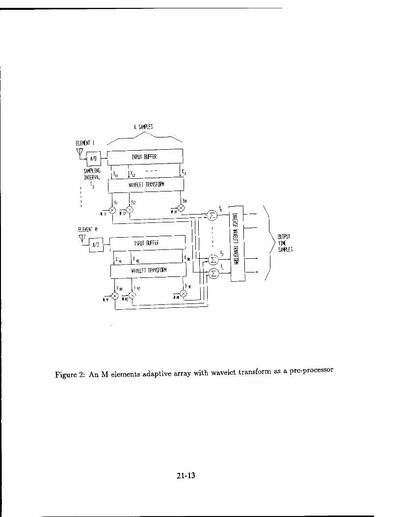
K SAMPLES
OUTPUT TIME SAMPLES
Figure 2: An M elements adaptive array with wavelet transform as a pre-processor
21-13

3)Wavelet transform (defined in Section II and implemented using a cascade of low
pass and high pass filters) a, shown in Fignre 2. The wavelet transform at resolution
M [3] of the discrete signal X, (where * is of length K and entering the i - th array
element) can be expressed as
V = Qio3MK{...{Q2{Q1Xi))...)
Qi = IK-M
1°9M
K-J+I 0
o Dj
(22)
(23)
where Dj is the wavelet analysis matrix at stage j, and / is the identity matrix.
The transform domain adaptive antenna array is shown in Figure 2 where the
input vector X is transformed into an output vector Y. Notice that in all of the
above transforms, the output could be written as Y = TX, where T represents the
transformation matrix of rank N. The new weight vector U is adapted using
Un+1=U» + 2,Y[r(n)-sY} (24)
where sY = YTU and ß is normalized with respect to E{YTY}. If ß is properly
chosen, then the optimal weight solution is
Uopt = $ZXSY (25)
where *y = E{YyT} = E{TXXTTr} and ^ = ^^ ^^
(26)
thus Uopt = ^SY = iGamma-r^^EiTXrin)} can expressed as and the state-
ment SY = Y?U = TX^W = IT?* is thus equivalent to
u0Pt = r-^r^rsv = r-Twopt
(27)
21-14
It is shown in [1] that the condition number of $y is always less than that of $x
which implies that adaptation in the transform domain will proceed faster than that
in the time domain.
The performance of wavelet based LMS filters depends on the convergence param-
eter and the type of mother wavelet used. In [5], the wavelet packet approach is used
to improve the rate of convergence of adaptive arrays. The method used in [5] is based
on maximizing the cross-correlation between received signals, and the decomposition
scheme is chosen so that wavelet processed signals are maximally correlated in each
of the subbands. This approach may produce better convergence rates than direct
wavelet subband decomposition, but requires a nontrivial additional computational
burden which makes the proposed method even more demanding than the recursive
least square approach or the Gram-Schmidt method.
The question that arises immediately after employing wavelet transform in adap-
tive antenna arrays is whether the covariance matrix of the transformed signal is
totally diagonal (i.e. its condition number is one). Neither the FFT, nor the Cosine
transform produce totally decollated signal components or a diagonal covariance
matrix because of limitations concerning the implementation of these transforms. The
wavelet transform, which is also an orthogonal subband decomposition scheme, does
not produce completely decollated signals either. In fact it is shown in [3] that, for
a large class of random processes, off the diagonal elements of the covariance matrix
can be generally expressed in the following form
*,(*, j) = ia(i)t~im MO + o(l)) + ai(i) (28)
and are, despite decreasing at a fast rate as a function of time, not identically zero.
The correlation between signal components that belong to different subbands decays
even faster than what is indicated in the above equation. Therefore the covariance
matrix of wavelet transformed radar signal is near diagonal.
21-15
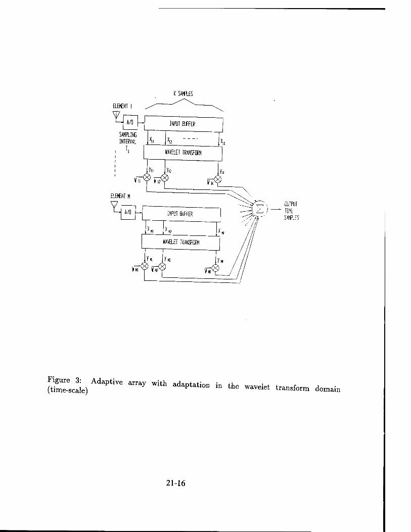
K SAHKES
EBENT I
OUTPUT TIME SAMPLES
&L) AdaP'iVe Mray W!th adaPtati°n » the ™»fet t~*™ dcnain
21-16

Erdol and Basbug [2] proposed an alternative incorporation of wavelet decom-
position into adaptive arrays through sampling the direct wavelet transform of the
incoming radar signal and truncating the dyadic wavelet series both in scale and
in translation. This approach requires computational complexity in the order of the
number of samples NK but no truncation criterion is available and improper sampling
of the wavelet transform may not yield the necessary improvement in adaptation rate.
Alternatively, we propose to use the regular subband decomposition scheme which re-
quires arithmetic operations directly proportional to the number of data samples NK
and thus compares favorably with that of the FFT or the Cosine transform from a
computational standpoint.
3. Error Analysis
The minimum asymptotic error (Wiener solution) achieved with adaptation in the
wavelet domain e« is related to that of the time domain et as follows (using similar
argument to [2])
e-^c-sfCr^Vr-*;1)** (29)
thus the asymptotic error obtained in the transform domain could be lower than its
counterpart in the time domain when 5? (I*Vr - *?) Sx is positive semi-definite.
The steady state mean square error is defined as
(30) e« = e + eA
where eA is the excess mean square error and e is the minimum error obtained by
Weiner solution. The excess mean square error of the time domain [4] and transform
domain LMS are
21-17

«s = ^«L. (32)
where 7Y() denotes the trace of a matrix. Note that Tr(ty) is upper bounded by the
energy of Y which is upper bounded by the energy of X (wavelet transform reserves
energy). Therefore, the excess mean square error of the wavelet transform LMS is
upper bounded by that of the time domain LMS.
4- The Adaptation Parameter ,,
The performance of the wavelet based adaptation scheme also depends on the
choice of adaptation parameter „. Stability requires that
" XTy* (33)
where A?~ is the largest eigenvalue of the «.variance matrix *,,. Alternatively, „
could be chosen as a function of time „ where „„ = ^. This approach ^„^
the convergence rate of the array but depends on the fluctuations of signal power
mcludmg steady state. A better convergence rate can be achieved if, is dependent
on the inverse of the covariance matrix.
£/-« = U" + 2ll*-r'lr(„)-Sy] (35)
This approach [1, 2, 4) is known as self-orthogonalization LMS and results in faster
convergence rate when applied in the time domain. The parameter „ in this case en be chosen as
o</,<JL NK (36)
The eigenvalues of the self-orthgonaliZation matrix are all one, which results in signifi-
cant movement in adaptation speed. An alternative wavelet adaptation parameter
21-18
that is exponentially weighted according to the subband of interest could also improve
the adaptation rate but requires careful adjustment of the parameter M. Cholesky de-
composition can also be employed to enhance the adaptation speed [3] of antenna
arrays where the adaptation parameter /z is pre-conditioned by a non-diagonal ma-
trix A (obtained by solving the equation A2/ = Sy) where / is a constraint vector and
the weights are then updated using W^ = W» + 2(,/A*)f. This can be attempted
with a modest increase in computational cost but is not included in the experimental
phase of this study. To this end, our approach is based on computing the wavelet
transform using a cascade of orthogonal low pass and band pass filters and using ei-
ther a fixed ft or an adaptation parameter which is normalized with respect to signal
energy.
5. Adaptation Rate of Wavelet Domain LMS ARRAYS
Radar cross section measurements of a DC10 aircraft model were used to examine
the impact of transformation on the adaptation speed of an antenna array. The data
is recorded in the frequency range 1-12 GHz with increments of 50 MHz and represent
scattering in the resonance region. The eigenvalues of a ninth order covariance matrix
are shown in Table 1. A lag of 9 was arbitrarily chosen for convenience, and Table
1 also shows the covariance elements of the DC10 RCS signal for lags 0 to 9. The
condition number Xmax/Xmin of the covariance matrix before and after transformation
of the DC10 data is shown in Table 2 (in addition to Amin and \max). Clearly, the
condition number of the wavelet transformed data is less than that of time domain,
FFT, and cosine transform. Therefore, the covariance matrix of the wavelet trans-
formed signal is less ill-conditioned than that of the FFTed or the Cosine transformed
data.
The adaptation rate of the arrays shown in Figures 4 and 5 was examined using
three types of signals; two sinusoids in noise, colored noise, and noisy radar data. The
21-19
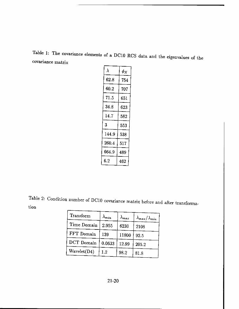
Table 1: The covariance elements of a DC10 RCS dat
covariance matrix a and the eigenvalues of the
A <f>x
62.8 754
60.2 707
71.5 651
34.8 623
14.7 582
3 553
144.9 538
260.4 517
664.9 489
6.2 462
Table 2: Condition number of DC10
tion covariance matrix before and after transforma-
Transform "min "max "max/^min \
Time Domain 2.955 6230 2108
FFT Domain 139 11800 92.5
DCT Domain 0.0633 12.99 205.2
Wavelet (D4) 1.2 98.2 81.8
21-20
first two examples are commonly used in the literature to demonstrate new adaptive
arrays algorithms, and the third example is associated with real radar data. The
sinusoidal signal is given as
,<*) = 0.1 cos g)+ cos (£)+ noise. <«)
Figure 6 shows a comparison between the LMS errors of time domain, Cosine trans-
formed, and wavelet transformed data. The wavelet used to generate Figure 6 is the
Daubechies 4-tap wavelet (D4). Figure 6 shows that the rate of convergence of the
wavelet transformed signal is higher than that of the DCT, FFT, or time-domain
data. Wavelets such as the Daubechies 8 and 19 tap filters produced similar results
to Figure 6. Figure 7 shows a comparison between the convergence rates of two
transforms using a non-smooth signal (generated using colored noise and determinis-
tic components) as input. The wavelet used to generate Figure 7 is the Daubechies
D4 wavelet. The error is averaged over 50 iterations and /x = 0.005. Figure 8 shows
similar convergence curves when the input signal represents the RCS measurements
of a DC10 model aircraft. Again, the adaptation of wavelet transformed data is faster
than other forms of transformation. Figure 9 shows a comparison between the adap-
tation rate of FFTed data and that of wavelet transformed data using a wavelet of
filter order 19 (D19) and the results are relatively similar to those shown in figures
6,7 and 8.
6. Wavelet Transform and Weight Dynamic Range
The weights dynamic range is another important issue of practical hardware sig-
nificance in adaptive arrays. To examine the impact of wavelet transformation on the
weight dynamic range let e,T be the eigenvectors of the transformation matrix T then
[39] the weight vector W can be expressed as a linear sum of ejr
21-21
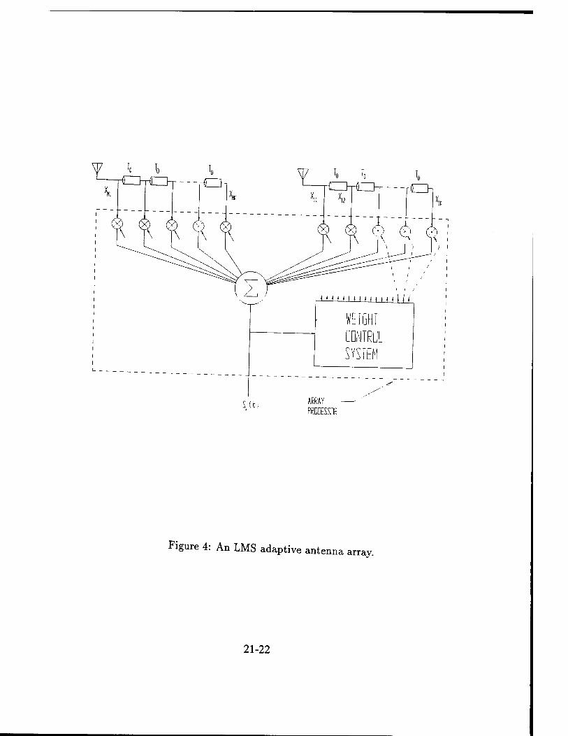
lllmiHHIIlH
WEIGHT CONTROL
S.(t) ARRAY PROCESSOR
Figure 4: An LMS adaptive antenna array.
21-22
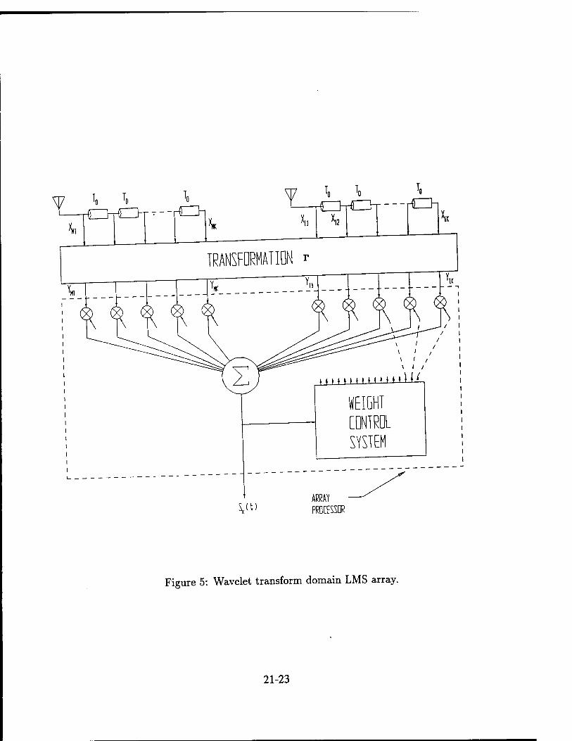
W To OTOT-PI
ARRAY PRDCESSDR
Figure 5: Wavelet transform domain LMS array.
21-23

NK
3=1
hence, given that
(38)
T~1 = 1
Xjj-ejr (39)
where Xjr are the eigenvalues of T, the new weight vector U = T^W can be expressed as
NK
U = E^r X X* (40)
Therefore, the elements of the new weight vector W can be smaller than their coun-
terparts in W when all the eigenvalues of T are greater than one (A,r > 1). Thus,
the dynamic range of weight vector elements can be improved if \jr > 1 Vj. This is
the case with wavelet transform. For example, consider the Haar wavelet transform
of 4 data points. The transformation matrix is
r = 1 -i 0 2 2 U
0 0
(41)
the eigenvalues of T are 2.576, 2.576, 2.4 and 2.0 (all > 1). Therefore, the wavelet
transform (see Figure 3) improves the weight dynamic range of an adaptive array.
7- Wayelet Transform and The Aoolebaum array
The above discussion about employing the wavelet transform applies to LMS based
adaptive antenna arrays. Similar arguments apply to the Applebaum array. To prove
this claim, we use arguments similar to those presented in [39]. Let G be the steering
vector and u be a constant. Then, the optimum weight vector of the Applebaum
array is given as
21-24
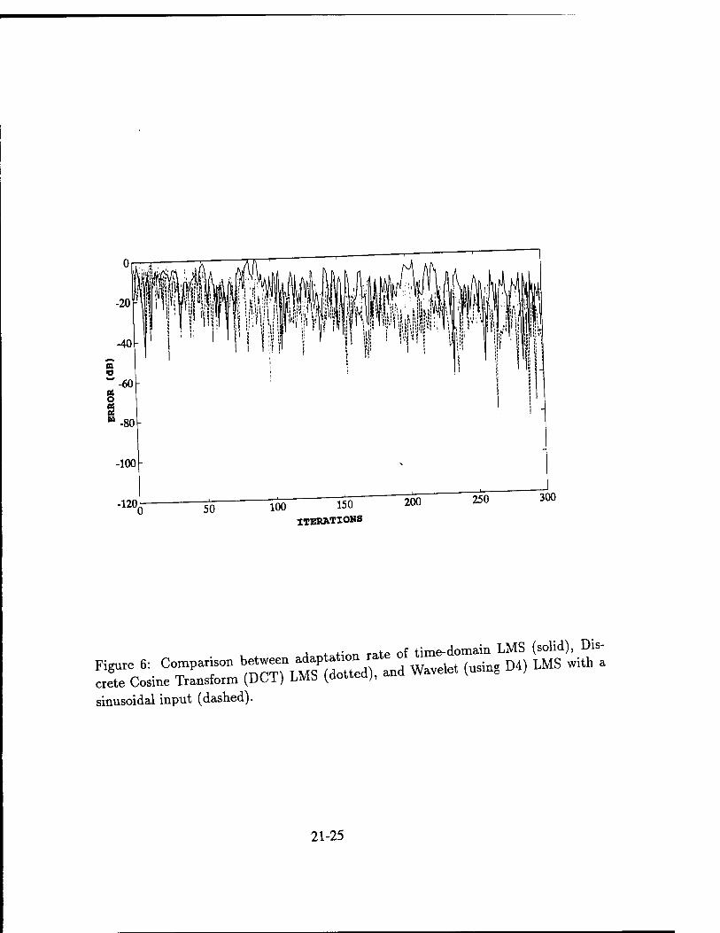
-120, 50 100 150 ITERATIONS
200 300
sinusoidal input (dashed).
21-25
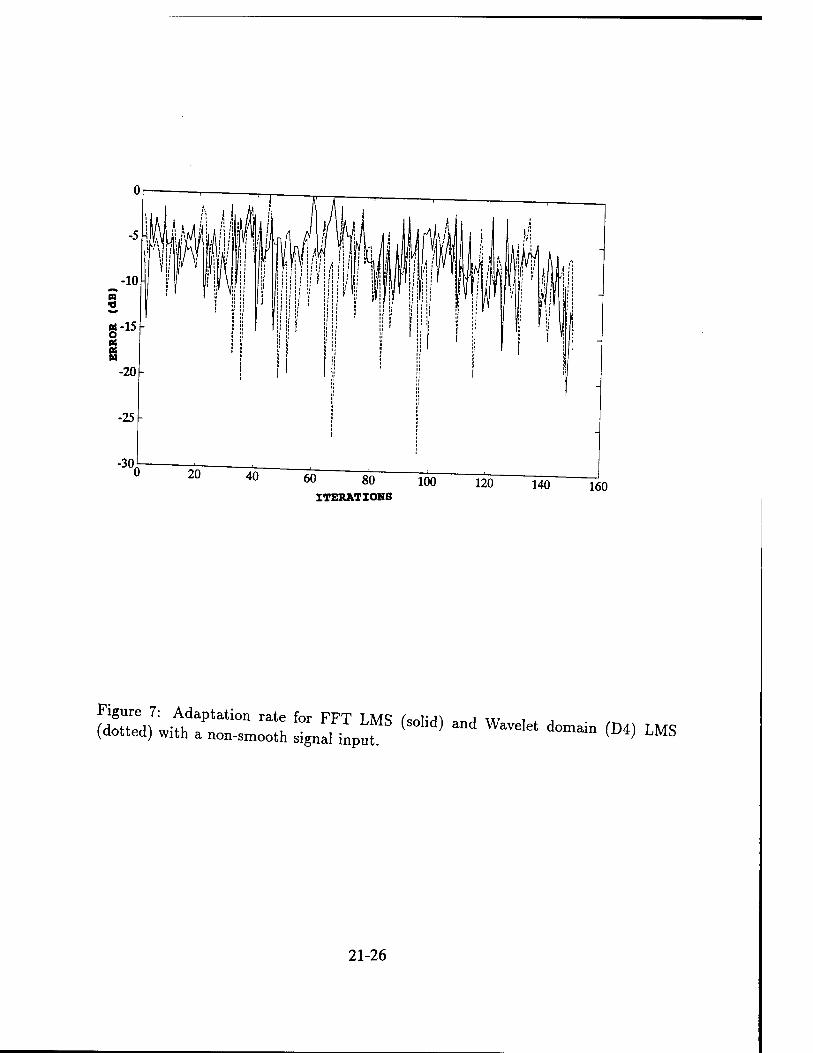
40 60 80 ITERATIONS
100 120 140 160
S*r::™s (solid) Md ~ *— <~> ™
21-26
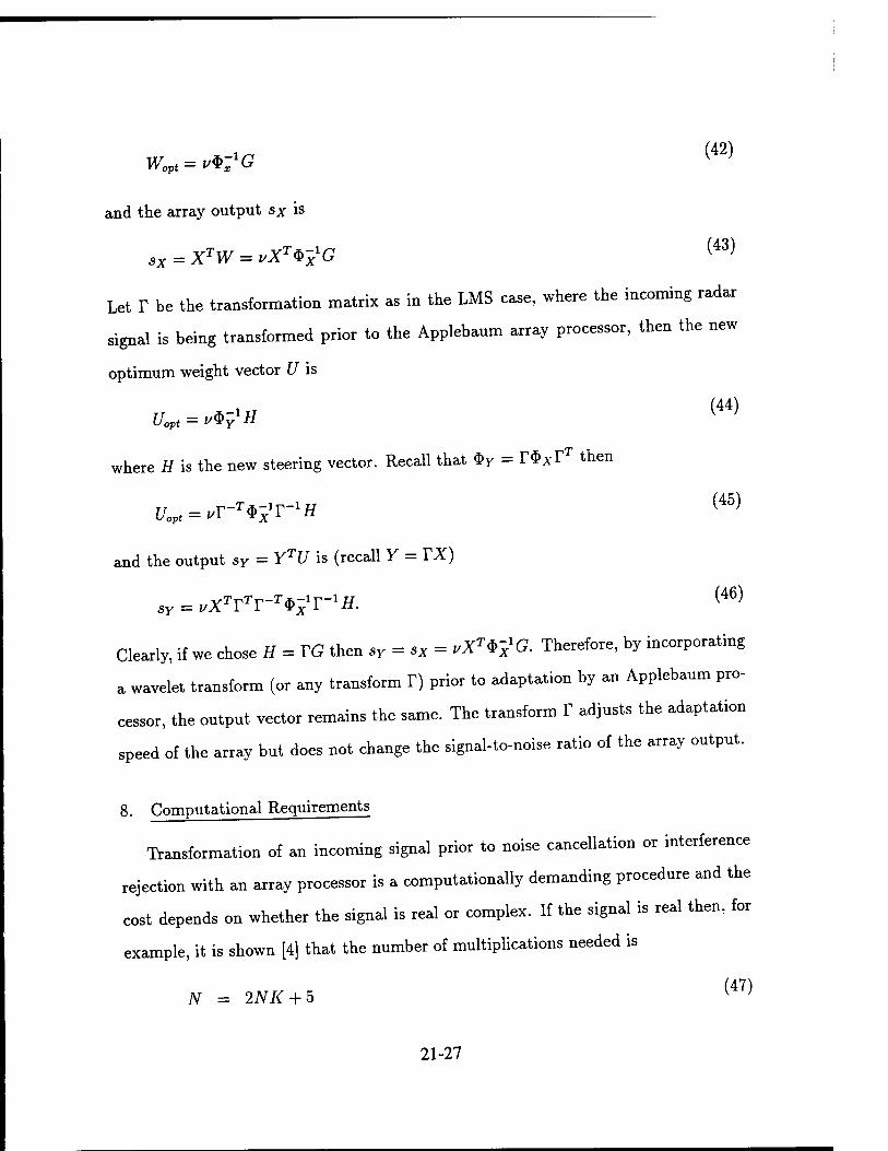
^ „ (42)
and the array output sx is
sx = XTW = vXTnlG (43)
Let r be the transformation matrix as in the LMS case, where the incoming radar
signal is being transformed prior to the Applebaum array processor, then the new
optimum weight vector U is
Uopt = u*?H (44)
where H is the new steering vector. Recall that $y = T$XTT then
Uvt = „T-T*?T-*H (45)
and the output sy = YTU is (recall Y = TX)
sy = VX?YTY-T*?T-XH. (46)
Clearly, if we chose H = TG then sy = sx = uX^G. Therefore, by incorporating
a wavelet transform (or any transform T) prior to adaptation by an Applebaum pro-
cessor, the output vector remains the same. The transform T adjusts the adaptation
speed of the array but does not change the signal-to-noise ratio of the array output.
8. Computational Requirements
Transformation of an incoming signal prior to noise cancellation or interference
rejection with an array processor is a computationally demanding procedure and the
cost depends on whether the signal is real or complex. If the signal is real then, for
example, it is shown [4] that the number of multiplications needed is
N = 2NK + 5 ^
21-27
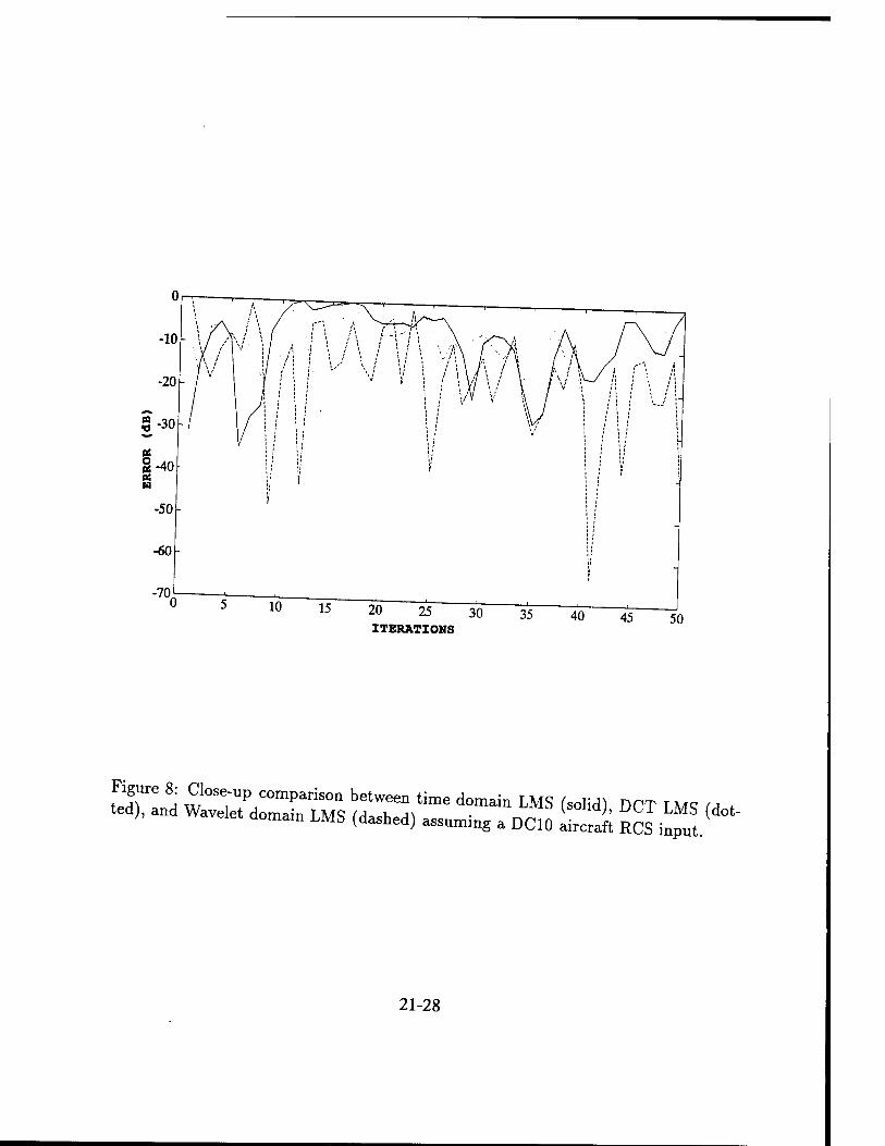
10 15 20 25 30 ITERATIONS
35 40 45 50
wT6 8A wOSTUP COmparison betwee^ time domain LMS (solid) DCT TMq M ♦
ted), and Wavelet domain LMS (dashed) assuming a DC10 Zl RCS inpUt.( '"
21-28
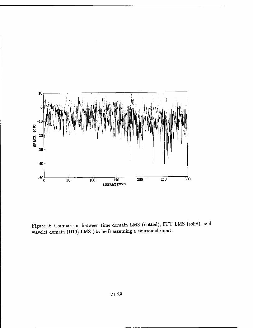
150 ITERATIONS
300
Figure 9: Comparison between time domain LMS (dotted), FFT LMS (solid), and wavelet domain (D19) LMS (dashed) assuming a sinusoidal input.
21-29
No = NK (3 + log2 NK) + 4 (4g)
N« = NK\og2(NK)-1.5NK + 4 + (6NK + l) (49)
N"* = NK\og2(NK) + (6NK + l) (50)
where iV, N0, A- N'» represent the number of multiplications needed for time
domain LMS, self-orthogonalizing LMS, Cosine transform based LMS, and FFT based
LMS. Accordingly the number of multiplications required by wavelet based LMS is
Nw = cNK + l (51)
where 6 < c < 7. Clearly, the number of multiplications required by the wavelet
transform LMS algorithm compares favorably with those of other transforms. The
computational complexity of the above algorithms when the incoming signal is com-
plex (with both quadrature and in-phase components which is the case in radar) is
about seven to nine times that of real data but the computational burden of each of
the above LMS techniques remains relatively the same.
IV. Bandwidth Performance of Transform Domain Arrays
The bandwidth performance of an adaptive array algorithm is an important mea-
sure of its nulling power in the presence of wideband interference. Tapped delay line
cancellers are usually introduced in an array to improve its bandwidth performance
and studies suggest that the tapped delay line technique, though costly, does improve
the nulling power of an array when wideband interference is present. Two studies [41]
and [38] indicated that nulling using the tapped delay line approach is superior to
employing an FFT prior to adaptation. In this section, we examine the significance
of the wavelet subband decomposition in improving the nulling performance of an
adaptive array when wideband interference is present. Our approach is similar to
21-30

that of [41] which begins with a narrowband signal, interference, and noise model.
The bandwidth of the interference signal is then increased and the nulling capability
of the array is examined. Let the signal incident on the ** tap of the m* element of
the array be
Arofc = AmJfe + Amfc -t- Wmfc
Note that, if d(t) is the desired signal then
Xdmk = d(t-[k-l)To-[m-l}Td) <53)
with
L . n (54) c
where L denotes the separation between array elements, and c is the sped of light. The
sampling period of the incoming signal is denoted by T0. Similarly, the interference
component is defined as
^mfc = i(t-[Jb-l]To-[m-l]rO ^
where i(t) is the interference signal arriving at an angle 0t, and
T L • A (56) T{ = — sin V{
c
Let Pd and Pi denote the power of both the desired signal and the interference given
by
n = E{\d(t)f} (57)
Pi = E{\i{t)\>) (58)
similarly
Xmk = nm(t -[k- l]To) (59)
21-31

where nm is the noise component arriving at the m* array element. The covariance
matrix $x is then defined as $d + $ • + $n
**i + *iu + *„u *, + $ ■ni2
$<rf21 + $ «21 ^22 + $,•„ + $ "22 ' »2N
^, + *i *N1 ®dNN + $iNN + $
where ■ nNN
(60)
(61)
(62)
(63)
*dm, = E{XdmXf}
*iml = EiXlX?}
*»- = E{XlXf
where ^ denotes the transpose of the desired signal vector received by the /" array
element and so on. The output of the array S is defined as [39]
s = WTX = Sd + Si + Sn'
where
(64)
sd = WTXd
Si = WTXi
sn = WTXn
where the vector Xd is a cascade of the vectors Xd
m
desired signal power is then
(65)
(66)
(67)
> m= l,...,N and soon. The
Pi = E{\s(t)\a} = E{WTXdXdTW] = WT$dW
similarly
(68)
Pi = W'QiW (69)
21-32
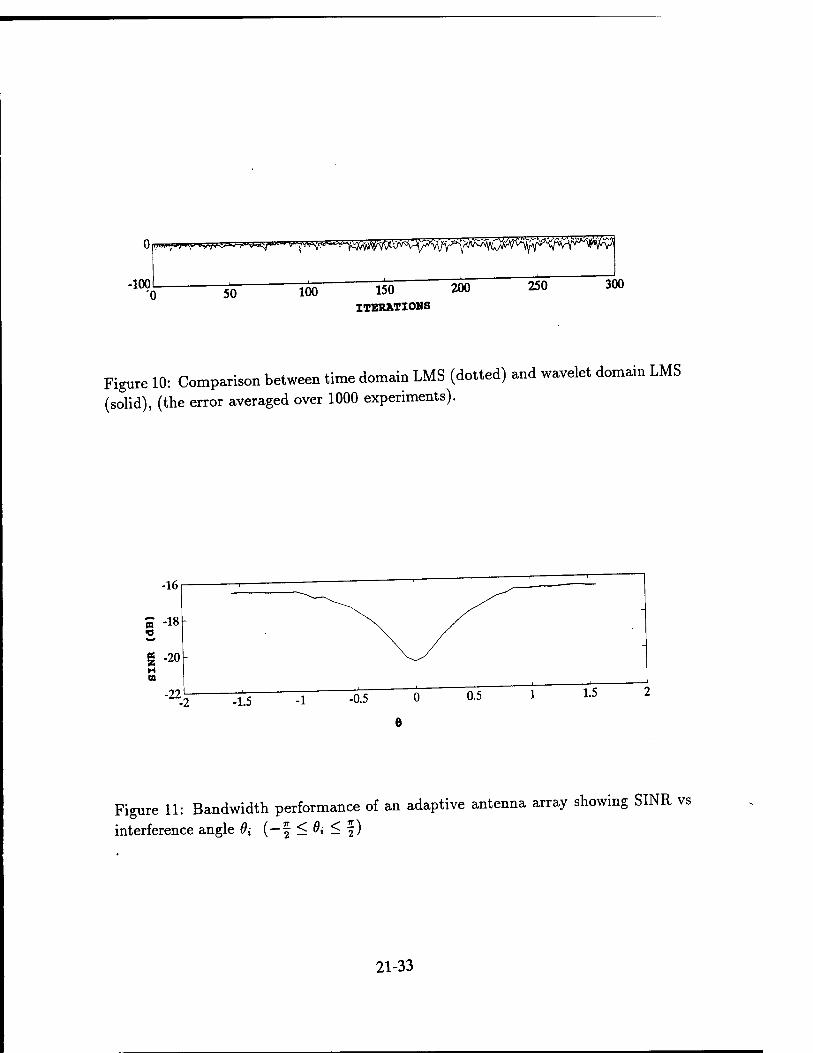
-100
r<>y*y*-*ry!$$^^
50 100 150 ITERATIONS
200 250 300
Figure 10: Comparison between time domain LMS (dotted) and wavelet domain LMS
(solid), (the error averaged over 1000 experiments).
Figure 11: Bandwidth performance of an adaptive antenna array showing SINR vs
interference angle 9{ (—f < 0; < §)
21-33
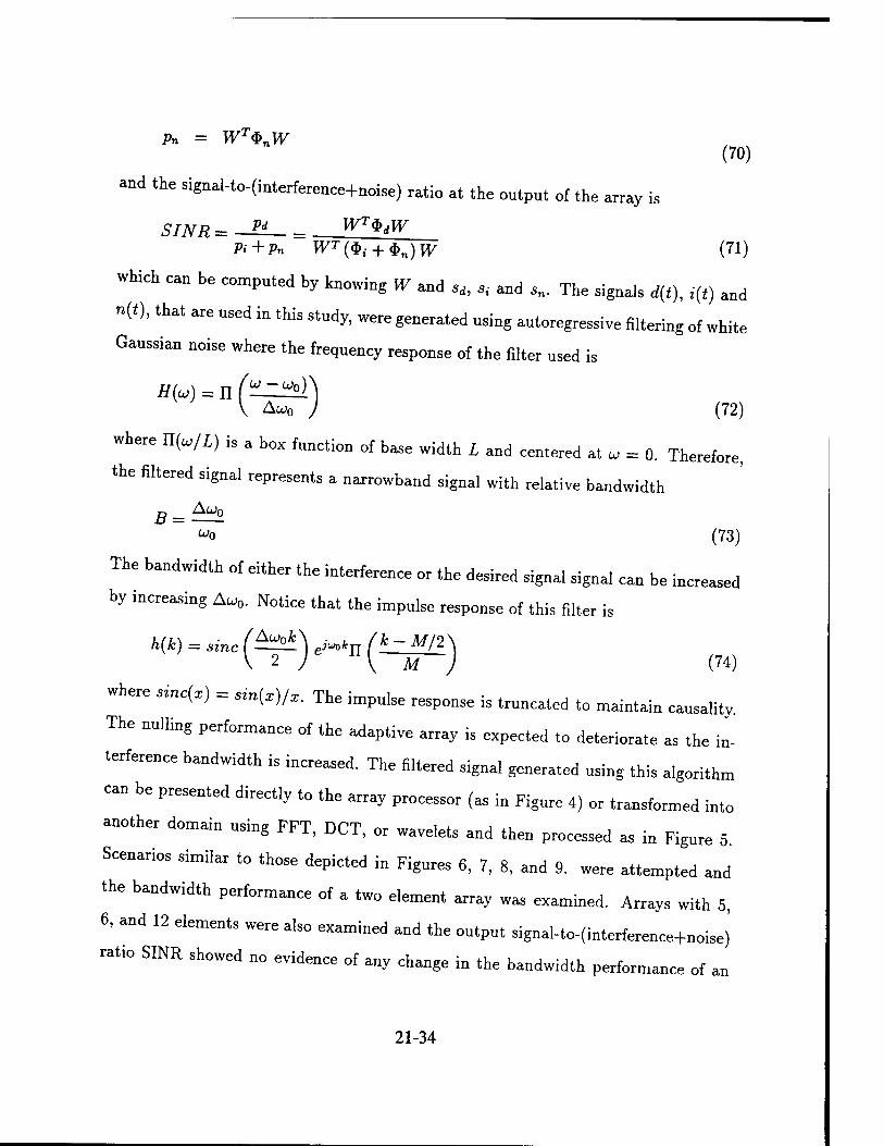
Pn = WT$nW (70)
and the signal-to-(interference+noise) ratio at the output of the array is
SINR = Pd = WT$dW Pi+Pn WT($i + $n)W (71)
which can be computed by knowing W and sd, « and sn. The signals d(t), i{t) and
»(<), that are used in this study, were generated using autoregressive filtering of white
Gaussian noise where the frequency response of the filter used is
H(U) = n f^^l) V Aw0 ) (72)
where U(u/L) is a box function of base width L and centered at u = 0. Therefore,
the filtered signal represents a narrowband signal with relative bandwidth
wo (73)
The bandwidth of either the interference or the desired signal signal can be increased
by mcreasing Au,„. Notice that the impulse response of this filter is
W-«(^)^-n(^) (74)
where a.„c(x) = sin{x),x. The impulse response is truncated to maintain causality.
The nulling performance of the adaptive array is expected to deteriorate as the in-
terference bandwidth is increased. The filtered signal generated „sing this algorithm
can be presented directly to the array processor (as in Figure 4) or transformed into
another domain using FFT, DCT, or wavelets and then processed as in Figure 5
Scenarios similar to those depicted in Figures 6, 7, 8, and 9. were attempted and
the bandwidth performance of a two element array was examined. Arrays with 5,
6, and 12 elements were also examined and the output signal-to-(interference+noise)
rat.o SINR showed no evidence of any change in the bandwidth performance of an
21-34
adaptive array despite the additional computational cost. Figure 10 shows the band-
width performance (SINR versus the interference arrival angle ft which is directly
related to frequency) of a two elements array with 64 tap delays. The incorpora-
tion of the wavelet transform, DCT, or the FFT did not improve the bandwidth
performance of the array, and in fact the nulling capability of the array was slightly
diminished upon transforming the input signal. This result agrees with Compton's
work [39] which claims that no invertible transformation placed between the incom-
ing signal and the array processor would improve the bandwidth performance of the
array. Therefore, wavelet decomposition, being an invertible transformation, did not
improve the nulling power of an array as the interference bandwidth was increased.
V. Conclusions and Future Work
Faster adaptation rates can be achieved by inserting a wavelet transformer be-
tween the incoming signal and the LMS or Applebaum array processors. The trans-
formation improves the condition number of the covariance matrix and thus improves
the convergence rate of an array. The weights dynamic range, which is of practical
interest, is also improved because of wavelet transformation by a factor directly pro-
portional to the eigenvalues of the wavelet transformation matrix. The learning rate
(or adaptation speed) of the LMS or Applebaum arrays can be further improved by
using time dependent adaptation parameter ^ or by using the self orthogonalization
adaptation approach. Preliminary studies suggest that the weight convergence rate
can be significantly improved using self orthogonalization with moderate increase in
computational cost.
The incorporation of wavelet transformation in an adaptive antenna array does
not enhance the array's capability of nulling wideband jamming beyond what can be
21-35

achieved using tap delay line elements. This effect of wavelet transform on the nulling
power of an array in the presence of wideband jamming requires further investigation
assuming different signal plus interference scenarios and different wavelets.
The computational cost of employing wavelet transformation in adaptive arrays
is modest and compares favorably with that of the FFT or the Cosine transform.
The success of the wavelet transform in improving the convergence rate or adapta-
tion speed of an array is remarkable and deserves much further attention. An optimal
wavelet suited for radar signals with wideband interference and multipath jamming
is yet to be developed. A theoretical assessment of the underlying reasons for such
an improvement in the convergence rate of adaptive arrays is yet to developed.
Acknowledgements: The author wishes to thank the Air Force Office of Naval Re-
search for supporting this project. The author acknowledges and appreciates the
support of fellow researchers at Wright Patterson Air Force Base, OH.
21-36
References
[11 S S Narayan, A. M. peterson, and M. J. Narasimha, «Transform Domain LMS 11 AkoritWIEEE Transactions on Acoustics, Speech, and Signal Processing, Vol.
3i;No. 3, pp 609-615, June 1983.
f9l N erdol and F Basbug, "Wavelet Transform Based Adaptive Filters: Analysis 11 L New Results Submitted to Applied and Computational Harmonic Analysis,
1993. Kl S Hosur and A H tewfik, "Wavelet Transform Domain LMS Algorithm," -Inter- 131 latZl Conftnce on Acoustics, Speech, and Signal Processing, ICASSP '93, PP
III-508-510, 1993.
[41 J C Lee and C. K. Un, "Performance of Transform Domain LMS AdaptiveTMgital 11 Filter™ WEE Transactions on Acoustics, Speech, and Signal Processing, Vol. 34,
No.3, pp. 499-510, June 1986.
[51 C Van den Branden Lamrecht and M. Karrakchou, "Subband Adaptive Filtering: [5] SutTal Wavelet Packets A^,"/«*"^ ^^93 ^ '
Speech, and Signal Processing, ICASSP '93, pp. HI-316 - 111-319, MM-
[6] M. B. Ruskai, G. Beylkin, R. Coif man I. Daubechies, S^ MaUatY. Meyer and L. Raphael eds., Wavelets and their applications, Jones and Bartlett, Boston, lyyz.
[7] LJouny, "Target Description Using Wavelet Transform", International Conference on Signal Processing, San Francisco, CA, March 1992.
[81 S G MaUat " A Theory for Multiresolution Signal Decomposition: The wavelet 11 Transform -IEEE Transactions on Pattern Analysis and Machine Intelligence,
Vol. 11, No. 7, pp 674-693, July 1989.
[91 P Flandrin F Magand, and M. Zakharia, "Generalized Target Description and 11 Wave'S^De'composftion,'" IEEE Transactions on Signal Processing, Vol. 38, No.
2, pp 350-352, February 1990.
[10] I. Daubechies, "Orthonormal Basis of Compactly Supported Wavelets " Com- 1 munications on Pure and Applied Mathematics, Vol. XLI, PP 909-996, 1988.
[11] G. Strang, "Wavelets and Dilation Equations: A Brief Introduction," SI AM, Vol. 31, No. 4, pp 614-627, December 1989.
[12] O. Rioul and M. Vitterli, "Wavelets and Signal Processing," IEEE Signal Pro- cessing Magazine, pp 14-38, October 1991.
mi R Kronland-Martinet J. Morlet, and A. Grossman, "Analysis of Sound Patterns MÄÄ^' Mernational^urnä of Pattern Recognition and
Artificial Intelligence, Vol. 1, No. 2, pp 273-302, 1987.
21-37
lU]FLi^y^^of^^' W«**J., Time-Frequency Methods and 14-18, 1987/j M SL et al lfe™atwnalC°?fe™^ Marsielle, France, Dec. Springer, PP 315, 1989 ' ^ Problems and Theoretical Imaging,
[^:ÄÖÄ AW Wnfc" ^ ^ *""** New York, 1990 * y' L Auslander et ^ eds., IMA, Vol. 22, Springe*
[16] 0. Rioul and M. Vitterli, "Wavelets and Signal Processing " TFFF c- i D cea«^ Magazine, pp 14-38, October, 1991 Processing, /£££ ^raa/ Pro.
[17]MSodd^/F^''r UltifreTenCy <?annel Dispositions of Images and Wavelet DTembe/flf. 2Ww*«^" - ^«> Processing, Vol. 37, No. if, ÄmJ
[191voi. ?rt1; Ä5d jffiKSisnaI p—S'" <**" **-*»
[23]foJr SAROoSfÖÄS'J^pW^ Coherent Frames May 1992. S mg' Proceedm^ IGARSS 92, pp 1318-1320, Houston,
N1^1S^BÄ £ MathieU' and } Daubechies' "I-age Coding Using 1992. Iranstorm' IEEE Transactions on Image Processing, Vol. 1, No. 2, April
125 wavelftf'' 'lEEF F' L" HwanS>/'Singularity Detection and Processing with wavelets, IEEE Transactions on Information Theory, Vol. 38, No. 2, March 1992
[26]/F>F T*4 &niS- Zh0n.S' "Characterization of Signals from Multiscale Ed«., " Ju§Eim nSaCtWnS °n Pattern Analy™ *»* Machfne InteTge^X^UN^,
[27] S. Mallat, "Zero-Crossing and Wavelet Transform," IEEE
Transactions on Information Theory, Vol. 37, No. 4, July 1991.
IM WÄ^ Backscattering Area Using July 1992. Ceeam9s °J1EEE AP/URSI Joint Symposium , Vol. 4, pp 1877-1881,
21-38
[29] I. Jouny, «Description and Recognition of Radar Targets Using Wavelets," Final Report, AFOSR Summer Faculty Program, August 1992.
[301 W D. White, "Wideband Interference Cancellation in Adaptive Sidelobe, Can- 1 cellers," IEEE Transactions on Aerospace and Electronic Systems, Vol. 19, No. 6,
pp 915-924, November, 1993.
[311 F W Vook, R. T. Compton, «Bandwidth Performance of Linear Adaptive Ar-^ 13 Jr;ys with Tapped Delay-Line Processing" IEEE Transactions on Aerospace and
Electronic Systems, Vol. 28, No. 3, pp 901-908, July 1992.
[32] H. H. Szu, B. Telfer, and S. Kadambe, "Neural network adaptive wavelets for signal representation and classification," Optical Engineering, Vol 31, No. 9, pp 1907-1916, September, 1992.
[331 W F Gabriel, "Adaptive digital processing investigation of DFT subbanding 1 ^transversal filter canceler," Naval Research Laboratory technical report, NRL
report 8981, July 1986.
[34] W. F. Gabriel, "Adaptive Processing Array Systems," Proceedings of The IEEE, Vol. 80, No. 1, pp 152-162, January 1992.
[35] S. S. Narayan and A. M. Peterson, «Frequency Domain^Least-Mean SqUar Al- 1 gorithm," Proceedings of The IEEE, Vol. 69, No. 1, pp 124-126, January 1981.
[361 J. T. Mayhan, A. J. Simmons, and W. C. Cummings, "Wide-Band Adaptive Nulling Using Tapped Delay Lines," IEEE Transactions on Antennas and Propagation, Vol. 29, No. 6, pp 923-936, November 1981.
[37] S. Mann and S. Haykin, "Adaptive Chirplet transform: an adaptive gen^hza- tion of the wavelet transform," Optical Engineering, Vol. 31, No. 6, pp 12« i2bt>, June 1992.
[38] L. E. Brennan and I. S. Reed, "Adaptive Cancellation of Scattered Interference," Adaptive Sensors, Inc., final report, December 1982.
[391 R T Compton, "The bandwidth performance of a two-element adaptive array 1 tapped deky-line processing," IEEE Transactions on Antennas and Propagation,
Vol. 36, No. 1, pp 5-13, January 1988.
[40] D. R. Morgan and A. Aridgides, "Adaptive Sidelobe Cancellation of Wide-Band Multipath Interference," IEEE transactions on Antennas and Propagation, Vol. 33, No. 8, pp 908-917, August 1985.
[411 R T. Compton, «The Relationship Between Tapped Delay-Line and FFT Pro- 1 cessing in Adaptive Arrays," IEEE Transactions on Antennas and Propagation,
Vol. 36, No. 1, pp 15-26, January 1988.
21-39
MICROMECHANICS OF MATRIX CRACKING IN BRITTLE MATRIX COMPOSITES
Autar K. Kaw Associate Professor
Mechanical Engineering Department
University of South Florida ENG 118, 4202 E. Fowler Avenue,
Tampa, FL 33620-5350
Final Report for: Research Initiation Program
Wright-Patterson Air Force Base
Sponsored by: Air Force Office of Scientific Research Boiling Air Force Base, Washington, D.C.
and
University of South Florida
December 1993
22- 1
MICROMECHANICS OF MATRIX CRACKING IN BRITTLE MATRIX COMPOSITES
Autar K. Kaw Associate Professor
Mechanical Engineering Department University of South Florida
Abstract:
tions, °£ a friCtl°Ml I-"»'**« on the respond of , unidirec- tional ceramic matrix composite ^ „ remote ™ "™re change i3 atudied. The ge o£ -n nd
a^aiT , a COnCen"i= Cyllnd6r "G*1 "lth « ™"1« «^ ^ tL UPonTa; ; matrf - "" fib—»iX in— 'olio- the Couio*
condi Ions the 0n
i^lyinS the »°"»<^ ~» th, interface continuity
oonaltlons, the solution is obtained in terms of coupled inteoral „J Unear equations, and inequality conditions. * °°*
fiber ?ndSthent f ."" '"'"^^ d»^ and the stress fields in the fiber and the matrix along the interface are studied for , Sic/CAS
composite system for varying coefficient of friction, temperature Lng
shear lag analysis model for identical geometry and loading.
22-2

MICROMECHANICS OF MATRIX CRACKING IN BRITTLE MATRIX COMPOSITES
Autar K. Kaw
TNTRODUCTION ^mlc matrix composites are becoming attractive as load bearing
structures for high temperature and corrosive atmosphere applications.
Although these composites have higher ultimate strength and strain than
monolithic ceramics, matrix cracking followed by interfacial failure
still a critical issue in their use.
Consider a unidirectional ceramic composite subjected to an axial
strain along the fiber direction. The cracks will first develop in the
matrix due to its lower failure strain than that of the fiber When a
matrix crack reaches the interface of the fiber and the matrix the
interface may open or slip. This opening/slipping of the interface blunts
the crack, and slows and arrests the propagation of the crack. Although
this blunting of the crack increases the fracture toughness of the
composite, the damage in the interface reduces the axial compress.ve and
transverse strength of the composite (Steif, 1984). Because of these con-
flicting effects of interfacial damage, it becomes important to fully ■u •„„ „-F mat-r-iv fracture in ceramic matrix composites understand the mechanics of matrix traccure
as a function of material, geometrical and loading parameters.
Axisymmetric three dimensional failure mechanics models, which
account for all equations of elasticity as well as assume an imperfect
interface, for the fracture in ceramic matrix composites are -ported-
the literature. These include the work of Wi^yewickrema.and Keer
(1993), Kaw and Pagano (1993), and Schweitert and Steif (1991). The
interface in all the above three studies is modeled differently.
Wijeyewickrema and Keer (1993) solved the problem of a composite
cylinder made of a solid cylinder (fiber) bonded to a surrounding hollow
cylinder (matrix) of finite outer radius. An annular crack was assumed in ^yj.±nuc , . _,_äJ 4-« a romnt.fi uniform the matrix. The composite cylinder was subjected to a remote uniform
tensile strain. The interface included a slip zone and was assumed to
have a constant shear stress equal to the ^^-^^ This is a fairly valid assumption when the interfacial friction
coefficient is small (Aksel, Hui and Lagoudas, 1991).
Kaw and Pagano (1993) solved for the same composite geometry as
Wijeyewickrema and Keer (1993). Kaw and Pagano (1993) included an
22-3
imperfect interface in the composite cylinder model but by approximate
the xnterface by distributed shear springs of constant stLrnLs Thel! model also included the effects of temperature change.
Schweitert and Steif fioon ,,^.=J _ • ■-, at-„H.M „ ] USSd a sxmila* geometry as the above two
in: nr, ;:r/er;:rnd pirst'tha outar -dius °£ -—~ f.*,« . . •/ ln£lnite- Se^ond, a penny shaped crack was assumed in the
y IdT ^;der) inStSad °f thS a— "«* - «- «trix (hollow cylxnder). They approxxmated the interface by the Coulomb friction law The composite geometry was subjected to a pressure on the crac1 ale
and a constant remote compressive radial stress. The pressure on the
:r:: esrr indireriy represented the — — -— - - remote unxform axxal strain. The remote radial stress represented
resxdual stresses due fcQ ^ mismatch Qf ^ coeffic7ents Qf
thermal expansion coefficient and the Poisson. ratio of the fiber^I
Steif-s^^TT StUdy' SeVeral aSSU^tions «* ^ Schweitert and fatexf s (1991) model are relaxed as follows_
The dilute fiber volume fraction assumption is replaced
by a nondilute fiber volume fraction.
The fiber crack is replaced by an annular matrix crack.
Also, the annular crack does not necessarily have to be
a through crack, it can be internal, edge and/or touching the interface.
The stresses due to the thermal expansion mismatch of
the fiber and the matrix can be directly accounted in the model.
of mater^l T*ed aSSUn,Pti0nS aU°» """« "-ay of the combined effect
se="o„s to'f ,r°me al l0adln3 "* —«— Peters. X» the
coe flLe't ° r. ". ^ £°-»1"i- °f th. »d.i. The effect of the coefLcLnt, « tr,1Ctl0n " thS £lb«-"" **•"—. — the linear L." ,"al d mal SXPaMi0" °* th« fib«/™trix c„ the extent of thl T • 9S' S"'SS dis"">»tion at the interface, under a thermomechanrcal load are studied. These results are compared „ith an
zi™: T1 £or -identiaai 9aomatry a-d ioa— ^ — »« ordrLt f °n " 3t"SSeS beln3 -^^»t of the radial co- lder " tC GU a°d M"90n°"'S (1"2» «dially constrained «trlx model.
22-4

METHOD OF ANALYSIS
Geometry . The geometry of the composite cylinder consists of an infinitely
long fiber bonded to an annular matrix of finite outer radius (Figure 1).
This geometry approximates a representative volume element (RVE) of a
composite in a double hexagonal array. The cylindrical coordinates are
denoted by r, 6 and z, and ur and uz are the radial and axxal
displacements, respectively. The normal and shear stresses are denoted by
ffrr, a„, *ee, and arz. The indices 0 and 1 stand for the fiber and the
matrix, respectively.
The fiber is approximated by a linearly elastic, isotropic,
homogeneous and infinitely long solid cylinder of radius a, shear modulus
u0 Poisson's ratio «0. Young's modulus E„=2(i+„0) ,0, and linear coeffxcxent of thermal expansion «0. The matrix is approximated by a linearly elastxc,
isotropic, homogeneous and infinitely long annular cylinder of inner
radius a and outer radius c, shear modulus Ml, Poisson's ratio „lf Young's
modulus, E, - 2(1 +Wl)Mx and linear coefficient of thermal expansxon, «,.
An annular crack of length 'e-d' (aSd<eSc) in the z=0 plane, at a dxstance
of 'd-a' from the interface is assumed in the matrix. The fxber volume
fraction is V£=a2/c2.
Boundary and Continuity Conditions The composite cylinder is subjected to a monotonically increasxng
axial remote strain, ,0 on the ends plus a constant temperature change, AT.
The imperfect interface between the fiber and the matrix follows the
Coulomb friction law and may have open, slip and stick zones.
The length of the open zone is 'Zl', while the length of the slip
zone is 'z2-Zl'. The kinetic and static friction coefficients are
considered to be equal. The friction coefficient •p> is assumed to be
constant in the slip zone. The superscripts '0' and '1' denote the fxber
and the matrix, respectively. The continuity conditions at the xnterface
between the fiber and the matrix at r=a are, hence, gxven by
o°IZ{a.z) =alr(a,z) , 0*|z|<~,
o°IZ(a,z) =oi,(a,z), 0s|z|<~.
Also, at the interface (r=a) between the fiber and the matrix, the zones
are governed by
22-5
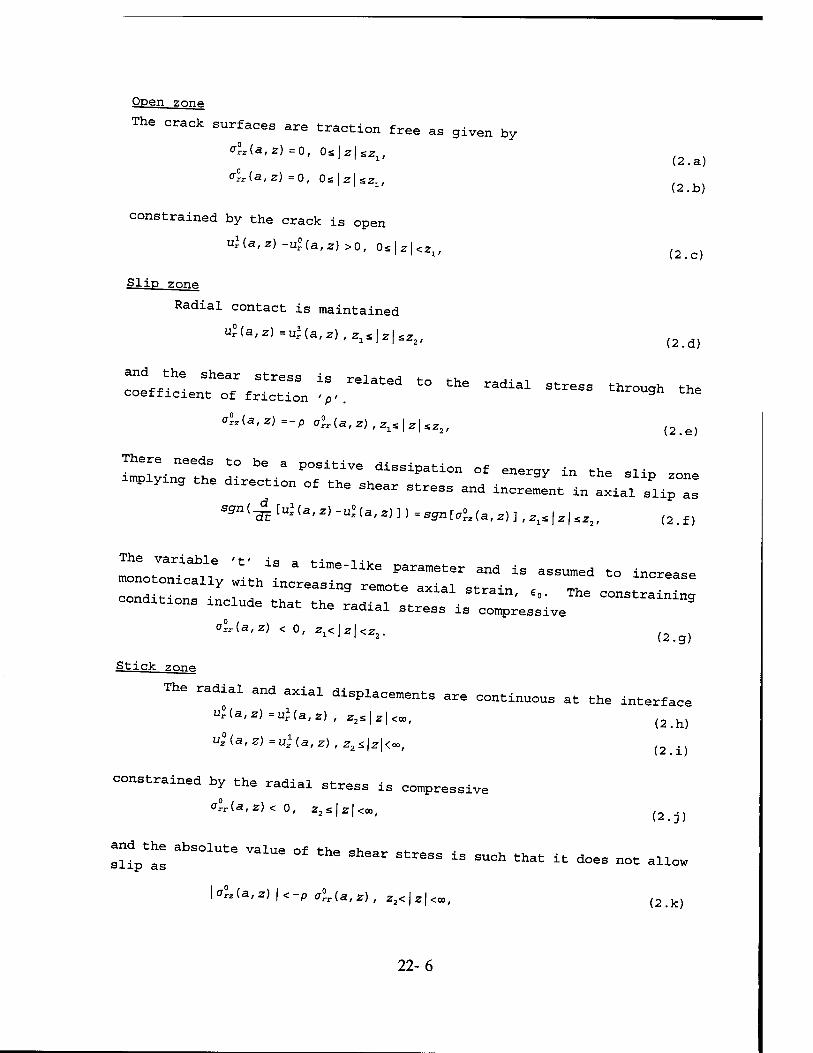
(2.a)
(2.b)
(2.c)
Open zonp
The crack surfaces are traction free as given by
ff°2(a,z) =o, 0s|z|s2i,
c°rr(a,z) =0, 0s\ z\Szir
constrained by the crack is open
uUa,z) -u°(a,z) >0, 0s|z|<2l,
Slip zonp
Radial contact is maintained
u°(a,z)=^(a,z)/ZlS|2|Sz2,
::^rr,;:-1™1^ - - — — — - olAa,z)=-P oUa,z),zx*\z\zz2, (2e)
There needs to be a positive dissipation of energy in the slip zone
implying the direction of the shear ^r««, * ■ or cne shear stress and increment in axial slip as
Sgn(^[^(a,z)-u°(a,z)])=sgnr^(a,z)],zlS|z|Sz2, (2.f)
(2.d)
increase The variable 't' i« a n™. -i-i m , . time-like parameter and is assumed to ii^icaBts
zzy rrincreasing remote axiai strai- ■•■ -e — , conditions include that the radial stress is compressive
°Ua,z) < o, z^lz^z,. (2g)
Stick 7nriP
The radial and axial displacements are continuous at the interface
nl(a,z)=ul{a,z) , z2S\z\<m, (2>h)
constrained by the rari-iai „f,..^ ■ i-\y ine raaiai stress is compressive
°°rAa,z)< o, z2S|z|<oo, (2j)
and^the absolute value of the shear stress is such that it does not alle
(2.k)
slip as "*-M -LO toucn cnac it does not allow
\°lAa,z) \<-p a°rAa,z), z2<|z|<oo,
22-6

The boundary conditions at the matrix edge r=c are given by
uUcz) = ulT[c,z) * u?ic,z), 0*|z|<«, (3)
(4)
a\z{c,z) = 0, 0s|z|»,
where uf is the radial displacement in the uncracked composite due to
a temperature change, AT; u» is the radial displacement in the uncracked
composite due to a remote axial strain, e0 (Kaw and Pagano, 1993; see their
Appendix A and B).
The boundary condition (3) results in the slope of the crack
surface Bui <r. 0) /6rU equal to zero for the edge crack problem
(e=c). Also at the edge r-c, far away from the crack plane, the radial
stress becomes zero.
The shear stress in the composite cylinder at the crack plane z=0 is (5.a)
o°z(r,0) = 0,rsa,
(5.b) a*z(r,0) = 0.a<.z<,c.
The other boundary conditions at the crack plane z=0 are
u°(r,0) = 0,r<;a,
uz(r,0) = 0,a*r<d, e<r<LC,
azz(r,0) = 0,d<r<e,
constrained by the transverse crack is open as
uUr,0) > 0, d<r<e.
(6.a)
(6.b)
(6.c)
(7)
Formulation
The solution for the above problem is obtained by a related boundary
element method. The composite cylinder geometry of Figure 1 can be viewed
as two auxiliary bodies as shown in Figure 2.
22-7
surface tT ^ ^ ^^ ±S ^ °f * S°lid C^lind- »^h unknown hi of ^ °?.the b°Undary r=a- ThS —d '"• body diagram "
ad us r_b b I tX; Wlth UnknOWn SUrfaCS traCti°nS °n the i- radxus r b, (b=a xn the composite cylinder) unknown slope of the crack
:i;i;;gr::
spiacement at z=o'and known —- —- - -:;;;:
(fiber) hceanCrret%diSP,laCement "" ^^ ^^ °f thS S°lid ****** For the hell ^ " ^ °£ ^ ^^ ^^ '»«ian. - r=a. For the hollow cylxnder (matrix), the complete displacement and stress
fields can also be found in terms of the unknown tractions at r-b and tne
unknown slope of the crack opening displacement at 2=0. Once these fill
equatxons are obtained, the continuity and boundary conditions !7 n
be applxed to find the solution in terms of coupled integral and 1 near
equations These coupled equations can then be solved numerically toUd the stress/dxsplacement field in the entire composite geometry.
Field equations fnr j-he soliH n,n^„.
radius^^diTaCement/StreSS fiSld f°r an -Metric «>lid cylinder of radxus a , shear modulus „„, Poisson,s ratio VQ and ^ ^
about the z=0 plane with boundary stresses
<7rrU,z) = S0(Z) ,0<Z<00, (8.a)
ff°z(a,z) = T0(Z) ,0<z<oo, (8 .b)
where s0(z, and T0(z) are absolutely integrable in (0,*), is given by
MUr'Z) =¥/o"[^(r's) ~ k?<^'s" CossinUs) dsrTo(t) Sin(st) dt Jo
ds (9) 2 r°° /•<»
+ ¥i0 T°{t)dtJ0
k?i(*>s) Cossin(zs) Sin(st)
2 f °° + ¥Jo lk2i(r>s) - k^U.s)] Cossin(zs) dsf~s0(t) Cos(st) dt
JO
2 /*°° /»» + ¥Jo S°U) dt\0
k2i(r,s) Cossin(zs) Cos(st) ds, i = l, . . ./6,
where
Mx = Radial displacement, ur(r,z),
22-8
M2 = Axial displacement, uz(r,z),
M3 = Radial stress, arr(r,z),
M4 = Axial stress, ffzz(r,z),
M5 = Shear stress, urz(r,z),
M6 = Hoop stress, a„(r,z),
and Cossin (zs) = Cos (zs), if i = 1, 3, 4, 6, = Sin (zs), if i = 2, 5.
The expressions for k1± and k2i are given by
kti= I E^r.e) fjt[s), 1=1,2 and 1 = 1,2,3,4,5,
fit = [a]^ [T]2X2 .J=1'2 and £=1,2.
an = Ji(as>
oia = as I0(as) + 2(l-v0) A (as)
«2i = -xo(as) + J!(as)/(as)
a,, = (2v0-l)X0(as) - (as)Ii(as)
(10)
(11)
(12)
1 Y = —
s3
1 0 0 1J
* = -_i_s* Ätrsje-«-"'.^ = -^-s» rs I.(rs)e-">s, 11 2/i0 ^o
E. 21 XM _Ls*Io(rs)e-<"'", E22 = _Ls2 [4 (l-v0) I0 (rs) ^s^ (rs) ] e
(a-r)s 22 ^
E31 = s3[-X„(rs)+i1(rs)/rs]e—, E32 - s'[ (2,0-l) I0 (rs) - rsXl(rs)]e
-(a-r)s (13)
(a-r)s
E41 = e- -o I0(rs)e-^'s, E42 = ss[2(2-v0)I0(rs) + rslx (rs) le-
xers) e-<a-'s, E52 = s3[rsl0(rs) + 2 (l-v0) ^(rs) ] e (a-r)s
EC1 = S3
I^x) = e-'I^x)
where I^x), i=0,l is the hyperbolic Bessel's function.
(14)
22-9
utole integrals to sxngle integrals with a judicious choice of the unknown traction functions S0 and T0, and also by reducing the k » as a
^z::::^T:polm±alsof (s) <~^--^t. faster TonJergence) " ^ "* ^ P°lyn°mial ^ <~
usina It k'r tSrS arS eValUatSd by findin^ k^ - closed form as s^ by 721 , aSymPt°tlC SXpansion f- liW for large values of 'x< as (Abramowitz and Stegun, 1970; Page 3 77)
*i (x) = (l - 111 + (S-l) (5-9) _ \ \ 8x 2(8x)2 /
e*
/2TTX :,i = 0, 1,2, 6=41 (15)
Field equations for the hollow cylinder
inner ^T^'"'"" ^ ** » «*-V«:r±c hollow cylinder of
stZt- K rad±US 'C'' ShSar m°duluS "" Essen's ratio „ symmetry about the z=0 plane with boundary conditions
_i
(16.a) *£r (b,Z) = S1(z) , 0S2<CO,
°«U>,«) = ^(z) , 0<IZ<=o,
Ur (C, Z) = 0, 0£Z<co,
olzic.z) = 0, O^Z<oo,
"z(r,0) = o, b<r<d, e<r<c,
(16.b)
(16.c)
(16.d)
(16.e)
(16.f)
^^^iz.r:^ int—e - «•■•> - *<*> -
22-10
MHT.Z) = ('[i^lT.B) - pTi(r.s)] Cassinis) daf'^it) Sin(st) dt 1 Jo
+ /"^(t) dtf~p?i(r,s) Cossin(zs) Sin(st) ds
+ ^(t) dtf'&iU.s) Cossin(zs) Cos(st) ds
+ r[p2i(r,s) - pZ^x.s)] Cossinizs) dsj's^t) Cos(st) dt Jo
(17)
+ | e(J) (t) dfc/o" [p3i (r, s, t) - P3i (r, s, t) d ° - p£(r.s, t)] Cossin(zs) ds
+ fiKtXJtf'dftTtr.s.t) +p3cr(r,s,t)]CoSSin(zS)dS
Jd ° + ^(r, t,z)}, i=l,...,6
where,
p„ = I F±j(r,s) gjt{s), 1=1,2,3 and 1 = 1,2,3,4,5,6,
g,, = IßV^ [r]4x3 ,j=l,2,3,4 and £=1,2,3.
(18)
(11)
r = -Ar
1 0 hx{s, t)
0 1 h2(s,t)
0 0 i23(S, t)
0 0 h4(s, t)
(20)
ßii = Ji(^s) e (c - b)s
P12 = [to J^bs) + 2(1 - vx) lidJs)] -(c - b)s
Pl3 = "*1 <*S> '
ß14 = -Jbs^(2>s) + 2(1 - vx) K^bs)
(21.a)
(21.b)
(21.c)
(21.d)
22-11
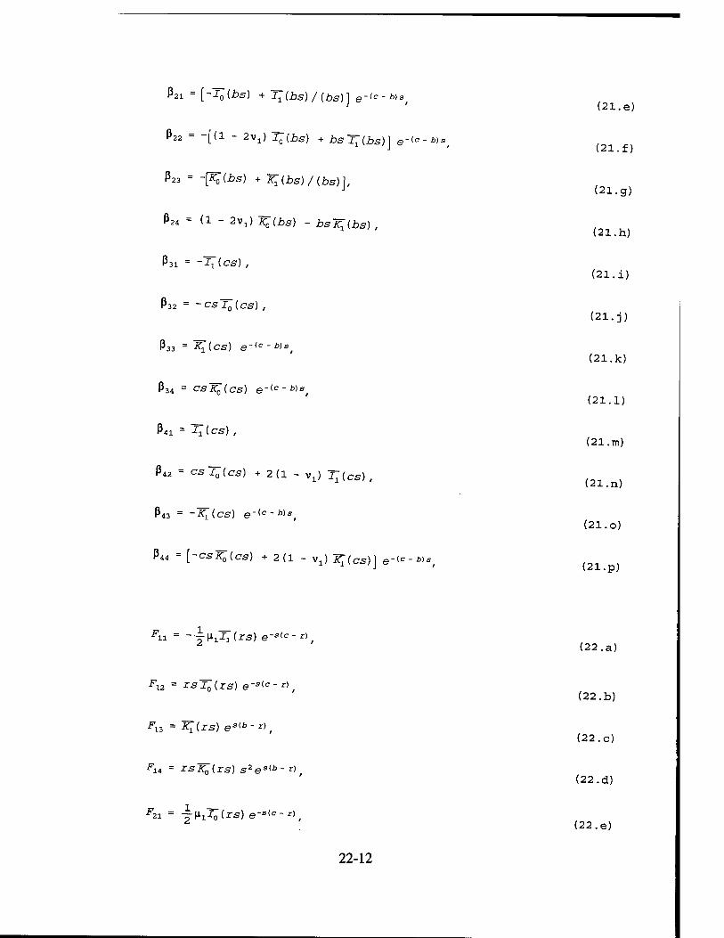
ß2i - [-I0(bs) + I1(bs)/(bs)] e-lc-»s,
ß22 = -[(1 - 2Vl) i0{bs) + is 27
ß23 = -[^(is) + K[(bs) / {bs)],
lbs)] -(c - b)s
ß24 = (1 - 2Vl) ^(2,S) _ bslqibs) ,
P31 = -^(cs).
ß32 = - es J0 ( es) ,
ß33 = Kj_i.cs) e-ic-»'
ß34 = csK0(cs) e-(c-•*»*,
ß4i = -Ti (es) ,
csl0(cs) + 2(1 - Vl) J^(cs),
ß43 = -^i(cs) e-<c-»s,
ß44 - [-csif0(cs) + 2(1 - Vl) Tq(cs)] ■(c - b)s
(21.e)
(21.f)
(21.g)
(21.h)
(21.i)
(21.j)
(21.k)
(21.1)
(21.m)
(21.n)
(21.0)
(21.p)
Fn = --jUi-TiUs) e-s(c-^>,
^12 = rs J0(rs) e-s(c-'),
^i3 = iq(rs) es^-r),
Fn = rsir0(rs) s2es(i.-r)
2 ^21 = -j^Jo (rs) e"s<c-■*->,
(22.a)
(22.b)
(22.c)
(22.d)
(22.e)
22-12

F22 = [4(1 - v^Jotrs) + rsl1(rs)]e
-JT I T-O\ oS(fc - -r)
-s(c - r)
F23 = J^(rs)e
F24 = [rsKlizs) - 4(1 - v^Us)] e s(i> - r)
F31 = [-J^(rs) + I1(zs)/rs]e -sic - I)
F32 = [(2|i0 - l)IÖ(rs) - rsl.trs)] e -s(c - r)
F33 = [J^(rs) iq(rs) / (rs)] e sib - r)
F34 = [(1 - 2v1)^ö(rs) - rsiq(rs)] e ;(i> - r)
F41 = X0(rs) e -s(e - r)
F42 = [2(2-vx) T0(rs) + rsl^rs)] e" ?(c - r)
sib - r) F43 = K0(xs) e
F,. = [-2(2-y>1)TT0(xs) + rsK^rs)] e sib - r)
F51 = liCrs) e" ?(c - r)
F52 = [rsT0(rs) + 2(1 - vjl^rs)] e" 3<c - r)
F53 = Kt(rs) e sib - r)
F„ = [2(1-11!) lq(rs) - rsKo(rs)] e s(£> - Jr>
(22.f)
(22.g)
(22.h)
(22.i)
(22.j)
(22.k)
(22.1)
(22.m)
(22.n)
(22.o)
(22.p)
(22.q)
(22.r)
(22.s)
(22.t)
■6J = 2^(1 ~ Vi) F + {F + F ), j = l,2,3,4.
Ü + v1^3j T ''«J'
(22.u)
jcT(x) = e^U) , (23)
22-13
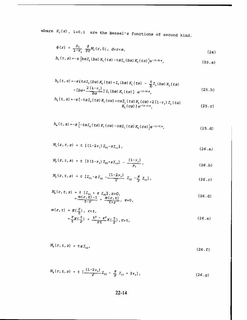
where K± (x) , i=0,i are the Bessel,s funcfc ions of second kind.
0(r) = T^T ^{r'0)' d<r<*'
hx (t, s) = -s [bsl0 (bs) Kl (ts) - tsl, (bs) Ka (ts) ]e-<*-«.#
A4 (t, s) =-s [-tsJ0 (ts) jq (cs) -csJ, (ts) K0 (cs)]e-<-«-#
^(r, t,z) = t [(1-2,/JJ^-zJ^],
^(r,t,z) = t [2(l-„l)Joo+ZJio] _ d-Vx) Mi
(r,t,z) = t [J01-zJ02 - (1-2"!> x _£ >- 10 ~ 11J '
*3
m(r,t) = E(*) , r<t,
N5(r, t,z) = tzl12,
10
(24)
(25.a)
h2^,s)-sUsIn(bs)K0(ts)+lo{bs)Kl{ts) - ^.(^^(ts)
'[J?g+-(Lflyi)-]Ji(jbg)^(tg)J e"(t"WS' (25'b)
^t-^"^-tsI0(tB)K1(aa)+caIx(ts)K0laB)+2(l.y1)TUa) iq(cs)]e-(c-«s, (25. c)
(25.d)
(26.a)
(26.b)
(26.c)
*«(r,t,,) = t [X01 + zx02],2>o, sffl(r,t)-l ai(r,t) (26-d)
t^F— + -tTF-' z=0'
-£*<■£> *^^.K^),r>t, (26-e)
(26.f)
*Ur, t,z) = t r (1-2yi> r _ z ~ ln ^Xn + 2l/i]/ (26. g)
22-14
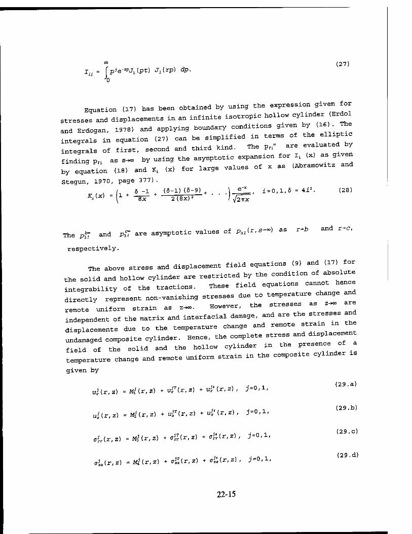
00 (27) I.. = [p^e-zPJx{pt) Ji(rp) dp.
Equation (17) has been obtained by using the expression given for
stresses and displacements in an infinite isotropic hollow cylinder-(Erdöl
and Erdogan, 1978) and applying boundary conditions given by (16). The
integrals in equation (27) can be simplified in terms of the elUptic
integrals of first, second and third kind. The pfl- are evaluated by
finding Pll as B~ by using the asymptotic expansion for I, (x) as gxven
by equation (18) and Ki (x, for large values of x as (Abramowitz and
Stegun, 1970, page 377). , x /, 5-1, (5-1) (5-9) + \ e* , 1 = 0,1,5 =4i2. (28)
*i<*> = \X + "SIT + 2(8x)' ' * ) AT
The p£ and p3T are asymptotic values of p3i(r,s-) as r~b and r-c,
respectively.
The above stress and displacement field equations (9) and (17) for
the solid and hollow cylinder are restricted by the condition of absolute
integrability of the tractions. These field equations cannot hence
directly represent non-vanishing stresses due to temperature change and
remote uniform strain as z~. However, the stresses as z- are
independent of the matrix and interfacial damage, and are the stresses and
displacements due to the temperature change and remote straxn i.the
undamaged composite cylinder. Hence, the complete stress and displacement
field of the solid and the hollow cylinder in the presence of a
temperature change and remote uniform strain in the composite cylinder is
given by
uHr.z) =Ml(r,z) + ujT(r,z) + u* (r, z) , j = 0,l,
uHr.z) =Ml(r,z) +uf(r,z) + u? (r, z) , j=0,l,
c4(r,z) =Mi(r,z) + c#(r,z) +4r(r,Z), j=0,l,
oiAr.z) =Miir,z) +ffS(r,z) + ffji(r,z), j=0,l,
22-15
(29.a)
(29.b)
(29.c)
(29.d)

otAr.z) = Mi(r,z) , j = o,l, (29.e)
*i.lr,z) =Mi(r,Z) *aiUr,z) + oft (r, z) , >0(1, (29.f)
In the above equations (29) , the second and third terms on the rio^
Appendices x ana B, . The superscript ,T, «.^«d. " «L ^^1 te„re change, „, che superscript ... ^
the axial remote tensile strain 6 errecc ot
give i«"^ tn"rt£a0e a"d bOUndary COndlti°'13 <1-" «» >* «»"- t.
unctions. Those equations oan be solved simultaneously to find the fH,™
r:r„r:;::L.The —^—- -—-«- --:: NUMERICAL SCHEME
edge cr^Tt'cTuch'TH **• """"^ ""' '~ ^ "** °' " i°'«-1 ae cracK not touching the interface M-*= ~ „\ for H,. , Iace (d>a' e=c> • The changes required
Lotion "Cal SChe™' t0r °th« — *>"~ » th. end oTtJ
Internal edas r-T-ack (d>a r Q-^
This is d ,? SlOP° °' thS ""* °Peni"3 d"Pi»d—t function, # inis is done as follows. ' 9-
Assu„. cat the range of 0<z<„ is divided into „
■f0(2) = A, + siZ, c».<z<w.ti/ i=1/2 _ _ _ .n-li
- Bn/z3, 6jJ,<z<oo, ' (30.a)
S0(z) = Ci + D.z, a1<z<altl, i=i,2 . . . .a - i - Da/z
3, ü)n<z<oo. ' (30.b)
Tl(z) =_Pi + QiZl ai<z<Uitll i=i,2 . . . #fl_1#
- Q„/z3, Ü) <Z<co (30.c)
22-16

Sx(z) = R± + S^, wi<z<o)itI, 1 = 1,2 . . . -n 1, (30.d) = Sn/z
3, wn<z<oo.
Further assume that the range (d,e) of the crack is divided into m
unequal segments such that r1=d and rm+1=e, and • -, o m (31.a) cj>(r) = {U^V^) w(r) , ri<z<ritl, 2 = 1,2 ,m,
where ! (31.b)
w(r) = v/r^a
is the weight function denoting the singularity of the slope of the crack
opening displacement at the crack tip (r=d). The problem, hence, reduces
to finding the values of the constants Ait Blf Clf Dlf Plf Qi, Ri, Slf Ulf an
V± in equations (30) and (31) .
Substituting the expressions for the tractions and slope given by
equations (30) and (31) in equations (9) and (17), the radial and axial
displacement at the interface (r-a) in the two bodies 0 and 1, and the
axial stress in body 1 on the z=0 plane can be written as
ulta.z) = S^Xi5(z) + J^U) +n^C±Xi7(z) *iDtXlalz).
(32.a)
(32.b)
i = 1 2 = 1 2-J-
m m
+ S U.Y^iz) + S V±Yi6(z) ,
ul(b,z) - fj^z) + UtY^z) + f^Y^z) +JUW*> (32 d)
+ S U.Y^z) + E V±Yil2(z) ,
22-17

(32.e)
°"(r'0) 'I*'*»™ \ioiZi2U)+VRiZi3(r) + £s (r) m ~X 1 = 1 2=1 2 24
»here xlf and YtJ ,r. functions of 2, ^ ^ ±g . ^.^ o£ ^
into .raintrr£*Ce ZO"e ,0<2<"' and th« c»=* *— «*«.> ie divided
n erfL ;llSe9mTS' reSPe0ti^ly- »"" "*-■* points along the interlace and the crack surface are chosen as
Ui = -cosl^i jEl n0n J 2 ' i = l, . . .,n0,
-coslü) i5C£i>_ + ifi+fi) • n»*J 2 2 ' I_fl"+1 no+ns, (33.a)
** = *i» i=i 277 (33.b)
where
zx = length of the open zone,
Z2-Zx = length of the slip zone,
z3 = maximum [n*+z2, n* (c-b)+z2] ,
n* = a number chosen large enough to account for most of the stress changes along the interface,
*i = ith root of the mth order Legendre polynomial.
cTohLenatr0aVteionCho0fiCe *' "*"*' ^^ * ^^ ^ ^™ • concentration of segments near the transition points, such as, at the end
of the open and slip zones, and at the transverse crack tip. The «s
of the interf """"* °' "*"*" * ^ <*«' ^ ™* Stick ««•■ llerLTe Girl's ^^ ^' *» "t.1 ™*~ of segments at the
n = n0 + ns + 73t. (34)
aTre'mirdirr.r3 aiong the interface and the «** ie^th «• «».« at the middle of the segment points as
22-18
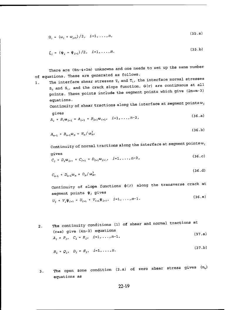
■ , (35.a) Q. = (oji + coi+1)/2, 2=1,...,n,
. , (35.b)
There are (8n-4+2m) unknowns and one needs to set up the same number
of equations. These are generated as follows. 1 The interface shear stresses T0 and Tlf the interface normal stresses
S0 and Sl, and the crack slope function, 0(r) are continuous at all
points. These points include the segment points which give (2n+m-3)
equations.
Continuity-
gives
of shear tractions along the interface at segment points co,
r, i (36.a) A± + BiWi+1 = AU1 + Si+1ui+1, 1 = 1.....n-2,
3 (36.b) A„-i + Bn-lWn = Bn/Un.
Continuity of normal tractions along the interface at segment points co,
gives ,-^ \ ■ , r, 1 (36.c)
Ci + r>i<oi+i = CU1 + Ci+1witl, 2 = 1 >n-2.
3 (36.d)
Continuity of slope functions <t>U) along the transverse crack at
segment points $i gives m 1 (36.e)
Ui + M^i = t/i+1 + Vitli|ritl, i = l...-.m-1.
2. The continuity conditions (1) of shear and normal tractions at
(r=a) qive (4n-2) equations a „ (37.a)
A± = Pt, C± = R±, 1=1/ n-1,
(37.b) B± = Qi. Dt = Sif 1 = 1.....n.
3. The open zone
equations as
condition (2.a) of zero shear stress gives (n0)
22-19

Ai + Bi&i = 0, i = i, n . (38)
4- The open zone condition (2.b) of zero normal tractions gives (n0) equations as
(39) * + DiQi = - [oor(a# Q±) + aoUai Qi)]ilml n
5- The Coulomb friction law in the slip zone condition (2 e) gives (ns) equations as
*i+B± Qi + p (Ci+Z,i0i, =-p [ooj(flf Qj) +aoe (a/ Qi) } t .=7io+i ^_ (4o)
6- The radial displacement continuity conditions (2.d) and (2.h) in the slip and stick zone aive«? In J. n \ -^,„4. • e ylves (ns + nt) equations from equations (32.a) ana (32.c), as
-!P'Y'W - SOMQ,) - £W^> - Ss^fQ,, {41)
-gUtY^Qj) -VViY^Q,) -0,>flo+i n.
7. The axial displacement continuity condition (2.1) in the stick
zone gives (nt) equations from equations (32.b) and (32.d) as
-1P'Y'W ~ lo^iü,) - E^r^) - Is, WQ,> (42)
-g^YmlOj) - gViY^lQj) =0lj=no+ns+l n.
22-20

The traction free crack surface condition (7) gives («) equatxons
from equation (32.e) as
'S P^tC,) ♦ fQiZulW + fji^^) + ?JiZ*W (43)
AüiZi5^) *%zu^) =-[a-(C,,o) +o»(C,,o)],;M. «.
9. Since uz(c,z) is a constant as given by equation (3), the slope of
the crack opening displacement -£u.(r.0> at the outer edge (r-e) of
the hollow cylinder is zero. From equations (24) and (31.a) this
gives
(44) um + C Vm = 0 .
The stress intensity factor (SIF) of the crack tip (r-d) is given by
K= Iim^2(d-r)oir(r,0) (45'a)
According to Gupta (1973), the SIF can be written as
K= 2(l\) UmJTTz^ar-jfcuUr.O) = -j= (U^V.d) r-*d+
(45.b)
The total number of equations (36) - (44) is (8n - 4 + 2m). These are
solved simultaneously to calculate the unknown functions. One can then
substitute these values in equation (29) to find the displacements and
stresses at any point in the composite cylinder.
T^qP crack i-nnrmna the «Upping or open interface (d=a, e=c).
The following steps are different for this case than given by
equation (30-44).
22-21
1. since the crac* goes through the ^
XT"^en£orced in the axlal "«"- - - ~- <-ynnaer. This is given by
-\°Ua,z) 2nb dz + [„»u.-) + oS(rf-)] Mc2-^) = 0 (46.a)
Substituting equation (30.c) in equation (46.a), we get
1 n 2<ol " (46.b) J=l J -. 2 a
- (^J(r, oo) +a1;|(z/ ~) ^(c2-^2)
The n- equation of equation (42) is replaced by equation (46.b).
The weight function of equation (31.b) is «(r> = , since the shear
stress is symmetric and zero at (r=b, z=0) . The absence of any
angularities for relevant values of elastic moduli and frictiol
ZtllTT' ?A f°r CeramiC matr±X C°mP0SiteS iS di—d by Schweitert and Steif (1991). If the interface ±a J
singularities again do not exist in (-*<=, el c , _ b exist in the slope function $(r) (Lu and Erdogan, 1984). a
in
are
3 ■ Since the hollow cylinder can now have a rigid body displacement the z direction, the first (n-1) equations of equation (42
replaced by the continuity of the axial displacement differences at cne interface as
«.°(".Q,, - u.'<a.Q,tl> . ulia.ll,) - ulia.Q^). i = 1 n.x
which gives
V^i5(Qj.) +i|ifl^(Qj.) +^cA7(Q,, + Sz,A,(Q.,
"^(^ "A'WW -SC^(QW -^.(Q^)
22-22
(47)
+ sVi7(Qirt> + SM8(ßi+1) + 2^^,(0^) + E^WQW i=l 1_1
+ E^^IOM) + S^FiI2(Qj+1) =0, j=n0+ns+l n-l. i=i i-i
„ =*- * * -i=! exactly zero and is enforced by 4. The shear stress at z=zx is exactly replacing the nth equation of equation (41) as x„(2>,*i> = 0,
Ano+1 + Bn^ co,o+1 = -P toS(a,v) + «"(a. «,„«)] {48)
For the above case, there are (8n - 4 + 2m) equations and equal
number of unknowns. This system of linear equations is solved to get the
unknowns.
The input remote strain e0 may not satisfy all the inequality and
sign conditions (2.c), <2.f), (2.g), (2.W and (7). Hence, the strain ,„ is changed iteratively till it satisfies all the inequality _ condition^
It is quite possible that a small range of strain e0 may satisfy all the
equations including the inequality conditions. The correct e0 is selected b^the unique value where the shear stress at the slip-stick transition
(z=z2) is smooth, that is
(49) Bn0*ns ~ Bna*ns*l-
This smoothness of the shear stress at the slip-stick transition is
implied by the asymptotic analysis of Dundurs and Comninou (1979) at the
slip-stick transition in a frictional interface between two dissimilar
elastic half-planes.
Closed crack in the matrix (d > a, e < cj.
The following steps are different for this case than given by
equations (30) - (44) .
22-23
Equation (44) is replaced by the closed crack condition
fe<J)(r) dr = o, J a
which gives
lu>LTwU) dr + iHTrwU) dz - °>i=i *. where
(50.a)
(50.b)
wU) = (50.c)
solveT SySte™ °f Sl"Ul«— l»««r equations can be
in aauaFt°L°72hS,°'t
the;br ""^ ""'' th" S°lu"°" ="" "» substituted the^trix 9 "MSS Md diSP1«™™" «•« - th. fiber and
intensive. TtlTs Z!tT5 h'" T "*** " ~"°"*^ ~* calculation of PH , "' "" t±me °n " IBM 3090 oomputer for ca cüiation , "! "llP le"9thS" "* « «" » *>™ °* <=» tl» for gaol" Hen ?•
CrltlCal ""—displacements in tba opposite geometry. Hence, lasted results a„ bei„g presented in ^ ^^
nan. ? haV<i' "°"eVer' "^ *d™tage of tba method described in this
I"""1'" thS inte™edi«a ««If to solve the problem fo different remote strain. cQ, the temperature change, Ar, friction
coefficient, P, the coefficients of therm*! expansion, „0 and .,. Tbis
as done as follow.. The most computationally intensive part of the computer program are calculation of the elements of agnations ,„.-.,«
setup, the remote strain, e0, the temperature change, Ar, friction
coefficient, P, the coefficients of tbennal expansion, „„ and a, can be
oCoeffLdient T* e9U"iOTS- "-" "™"»*« * "Of change the eoefftcaent „atrtx elements corresponding to equations (32).
Other
22-24
elements of the coefficient matrix and the right hand sides, which do need
to be changed, require only a few seconds of computational tune.
RESULTS AND DISCUSSION The numerical scheme presented in this study was tested as follows.
Extensive convergence studies were done to find the number of collocation
points to be used. In addition to numerical tests such as recovering
applied stresses on the two bodies, comparisons with some exact models
were also made. These tests included comparing the stress intensity
factor for a small edge crack under uniform pressure, p which is p /2(e-d)
(Sneddon, 1951). For edge cracks comparable to the thickness, (c-b) of
the hollow cylinder inside the matrix, the results for the stresses and
the stress intensity factors matched within 5% with an independent
computer program written for the problem solved by Wijeyewickrema and Keer
(1991) using numerical methods enumerated by Kaw and Pagano (1993).
The SiC/CAS material system with the following elastic properties
are used to discuss the results.
Silicon Carbide Fiber:
E0 = 207 MPa
V0 = 0.25
Calcium Alumino Silicate Glass Matrix:
E1 = 9 8 MPa
Vl = 0.25
Vf = 0.4.
Only cases with slip and no open zone are considered in this study.
This is because for cases where both types of zones are possible there
are two variables, the length of the open zone and the length of the slip
zone, which need to be found iteratively. Finding these two variables
is computationally tractable with the current computer program but would
require prohibitive amount of computational time.
Figure 3 shows the normalized slip length, Ls/a as a function of the
ratio of the matrix axial stress to interfacial radial pressure (ARS),
ARS= [ollix,-) +o£(r. ~) ] / [Orr (a, -) + o£ (a, -> 1 (51)
for constant coefficient of friction. The reason for choosing the
abscissa as the ratio of the stresses, ARS is because any combination of
22-25
2* sliP le:3th same stress rati° <AES) "ni«-" *» tb.
in Figure 3, the slip length increases linMrl „lth
that the slip iength was also found (not shown) to fce , ^^ ^ °£
«- «mote axial strain since the stress „»,.,„.„ for egual Pcisscn's ratio of the fiber and the matrix.
strain1" ItT^' T "^ °' MS=1-618 =°""^"d= - «~> «-*. axial l°' . " " lr»P°"ant to note that at this value of Ms, ths interface damage „ assumed to have already taxen place only due to the resloual tensile stresses in the matrix. residual
oht • ^V1^ lM9thS °btaiMd f™> ™r model are compared with those
rr(?u3ing a e^iraunt GU
- -— <»»> tje model, c:: aZ l: Tr °£ th6 SliP 1Sn9thS ***~ £™ *• «* MangonL.a U9«) type model and the present model as a function of the stress ratio
A*s for constant coefficients of friction. The ratio of slip length
approaches one as MS increases, which „ay be an indication that for large SUP lengths, the predictions from the two models are same.
follow^ «suits"9 Pr°PertleS arC aSSU"ed "««~»Uy * discuss tb,
«o = 3.5 xio-05 m/m/°c
<*i = 6.5X10-"5 m/m/°c
Ar=-iooo°c.
The main assumptions in the On and Mangonon-s (1992) model are that axial stresses ( „„, are independant of ^ ^.^ co.ordlnate
cLTp'ane 7o^ " "^ = ' «*" *" fJ*~ «" «=»»- ■* the IrTLt J' "S P °tted " ' £Un0tiOn °£ the -«-""- «dial co- ordinate, r/a, one can see that this assumption is not valid The
r ::;:'£ T'remain fa±riy —^ ^ »■»- *«- *- ^« s a"pTen«»0" ""* PlSne- *" -*' h°— ^ <« "« as the
defined by the 3treSS e0~-tn'"- f»«°r * «* fiber, SCP
SCP.«f(a-,0)/«S(r,-) (52)
22-26

decreases and may be an indication that for large slip lengths, Gu and
Mangonon's (1992) model and the present model give similar results.
in Figure 6, the interfacial radial and shear stresses are plotted
as a function of the normalized axial location, z/a for constant slxp
lengths (or constant remote axial strain). The radial stress increases
rapidly to the remote radial stress at the interface. Note the small
effect of the increasing slip length (increasing remote straxn) on the
interfacial radial stresses.
The interfacial shear stress in the slip zone follow the same
pattern as the radial stresses, since they are linearly related xn the
slip zone. At the end of the slip zone, the shear stress decays rapxdly
to zero. Note that the maximum interfacial shear stress does not change
with increasing slip length (increasing remote strain).
The conclusions from Figure 6 show that the assumption of constant
shear stress for a low friction coefficient used in other models
(Wijeyewickrama and Keer, 1993) may be valid. However, one should note
that a constant shear stress assumption gives logarithmically sxngular
fiber axial stresses at the crack tip, (r=a-,z=0), while the Coulomb
friction law gives large but finite fiber axial stresses at the crack txp.
CONCLUSIONS
The main conclusions of this study made for a typical SiC/CAS system
under a negative temperature change and a remote axial straxn are
1 The length of the slip zone increases linearly with increasing
remote axial strain and decreases linearly with low
coefficients of friction.
2. The stress concentration factor in the fiber at the crack tip
decreases with an increase in the remote axial strain.
The interfacial radial and shear stresses for low coefficients
of friction are nearly independent of the remote axial straxn.
Moreover, these stresses are fairly constant in the slip zone.
22-27
REFERENCES
-:i::::^.a::„::r ia ,i97o)' —■ ■* — Aksel, B., Hui, c. and Lagoudas, D.C. (1991). Effects of . . . h . 1
zzrj; th\ioad di£f-io" <™ - *—■ "^ij^rrr: elastxc medxum. jnt. j. SoIids structures_ 2?/ 833.847_
Dundurs, j. and comninou, M. (1979). Some consequences of ^ ineQualitv
condxtxons in contact and crack problems. ,. Elasticity ^j^*"*"*
Erdol, R. and Erdogan, F d97R} a i-v, ■ , -, ■, , , ■ U978) . A thick-walled cylinder wit-h =m axxsymmetric internal of edqe crack «m r » , an
eage crack. ASME J. Appl. Mech. 45, 281-286.
rainf' "a ra"90n0n' "• L- <1992' ■ "-»»"-»1 oharaot.ristios of fibar- «fnforoed tattl. «trix oolite, caae n, non.zero radial J£"
Sda I'' '1S73' • A layer6d COmP°Site "ith ■ ■«*- 1-l-t.. X«. , Solids Structures. 9, 1141-1154.
Ka». A.K ana pagano, „.j. ,„„, ^ ÄxlayOT,etric thermoelastlo .«£.*. oylindar =ontalnl„3 „ annular Mtrix ^ ^ ^ ~» of
iLu'o 'it Erd°3an' F- <1984' ■ S"eSS inteMlty £*«°« - t» bonded
wllttlr- and.Steif' P-S- <19S1»- *^^ of a broxen fib« in« weajcxy ponded composite Int ,T Q^7,-W^. C*. f 11.C. -mc. j\ Solids Structures. 28, 283-297.
^T*""' A'C- a"d K"'' «■■«• (»»> ■ »««ix „ackin3 in a £lbar
ZuTsl TP°SitB "ith S1±P " the ">™ix intarfaoa. x„ solids Structures. 30, 91-113.
«tSnST'.A;c-and Keer' L-M- (1993)-Matrix f™ ** britti. matrxx fxber-rexnforced composites. Xnt. ,. SoIids Structures. „, 43.65_
22-28
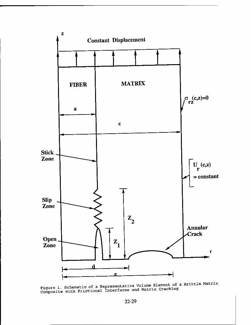
A Constant Displacement
H_ FIBER
Stick Zone
Open Zone
MATRIX
/
a (c,z)=0 rz
U (c,z) r
= constant
Annular 'rack
Fiaure 1 Schematic of a Representative Volume Element of a Brittle Matrix Composite wfth Frictional Interfaces and Matrix Cracking
22-29
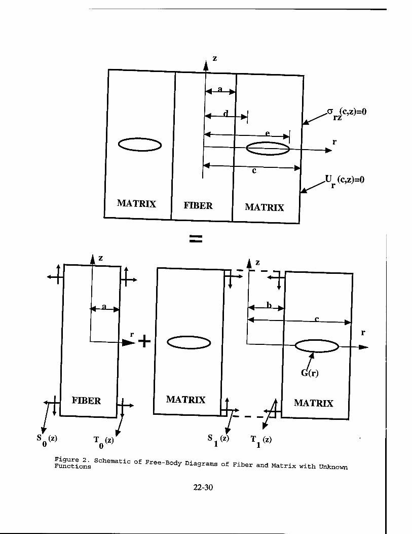
0 (c,z)=0 rz
U (c,z)=0 r
4 ~>
^+
f FIBER
Sn(z) T (z) r MATRIX
0 0 VZ) T!^ Fun'eMo™ Schematic of Free-Body Diagrams of Fiber Functions and Matrix with Unknown
22-30
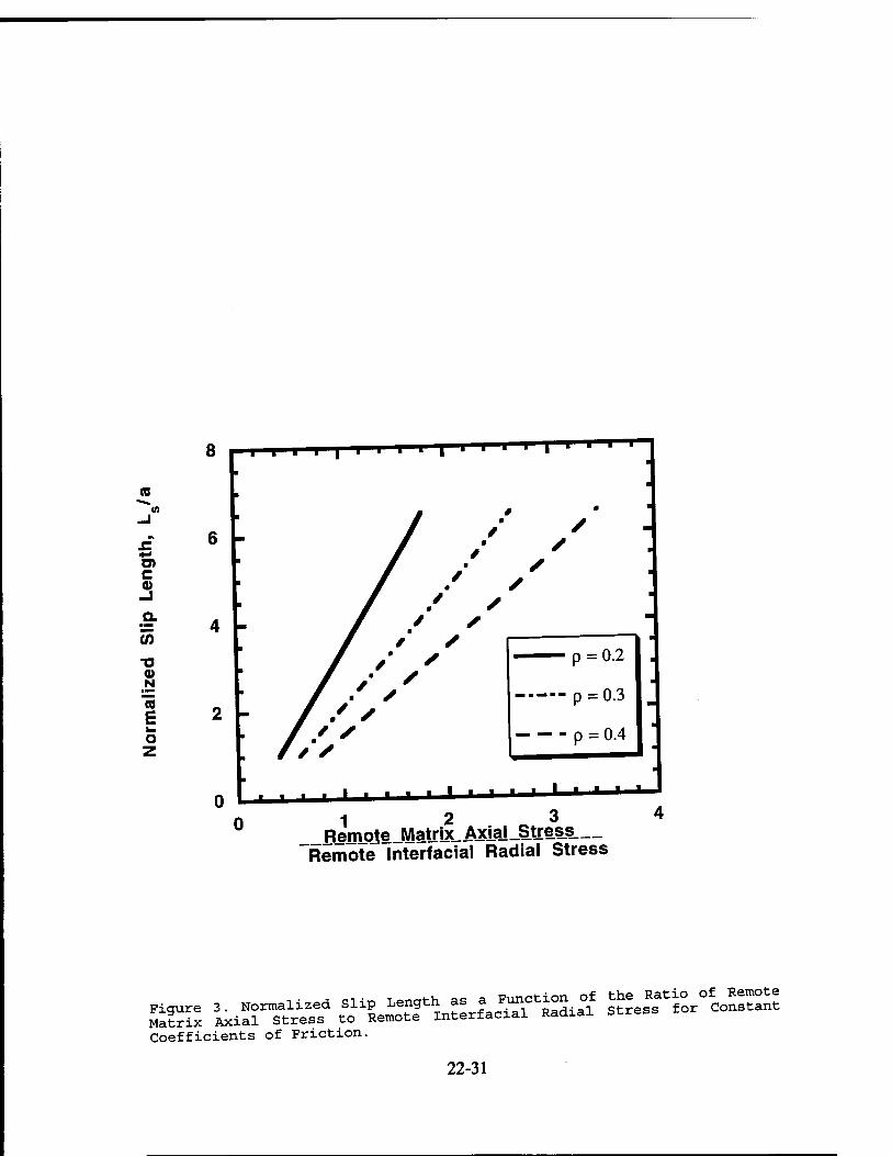
(0
ö) c o
a (35 ■o a> N
£
1 2 3 __Remj)Jejy!atiix_Axial_Stress.__ Remote Interfacial Radial Stress
Coefficients of Friction.
22-31
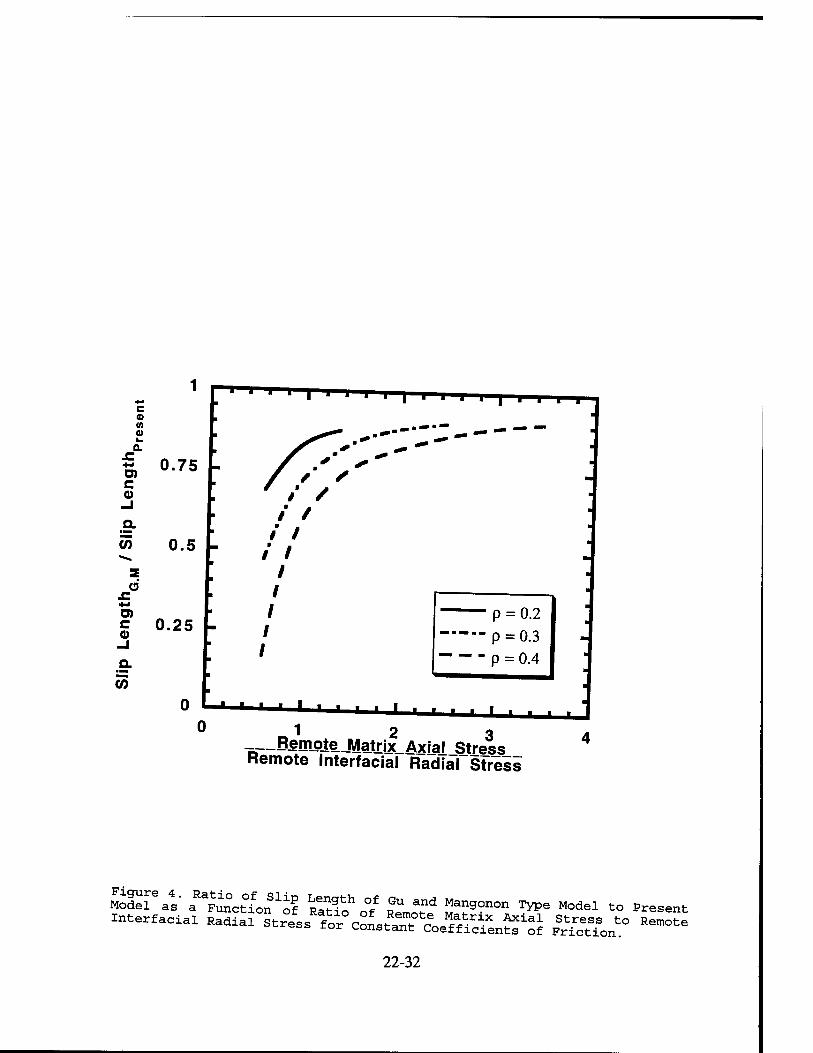
c 0) w <u
' ' I I | I I | | | I !■
*= 0.75 CD C Q)
a w *»»
s d
£ 4-1
c 0) -I
a. 55
0.5
0.25
:
i i i
1 2 3 -__BempIeJ\/latxix_AxlaI_Stress Remote Interfacial Radial Stress
Moieiea4s- a^ctfon'o? Sg? o°/ SnoT* M^
0^
TyPS M°del t0
22-32
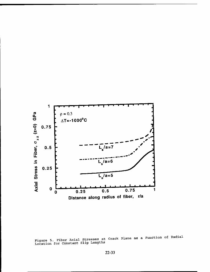
CO Q. O
o II N
0.75
N N
*-" 0.5 n il
(0 (0 0)
CO
« X <
0.25
i i i i I i ■ ''
p = 0.3
AT=-1000°C
i i i i
0
■
/. *u+
L/a=5 j ...
0.25 0.5 0.75 Distance along radius of fiber, r/a
Figure 5. Fiber Axial Stresses at Crack Plane as a Function of Radial Location for Constant Slip Lengths
22-33
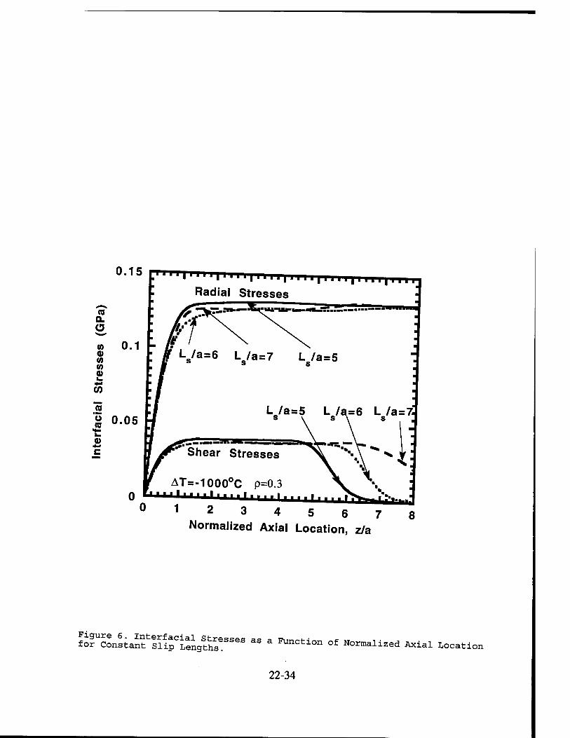
0.15
Radial Stresses
Ls/a=6 L/a=7 L /a=5
■' 111111111 ■ ■ ■ 11 ■ 11 j
Shear Stresses
AT=-1000°C p=0.3 0 f" 'Hilf ■ , , ,
0 12 3 4 5 6 7 8 Normalized Axial Location, z/a
fofJLstanf ifirtfngtS3868 " * FUnCti°n °f Normalized Axial Location
22-34
COMBINED EFFECTS OF GRADED ™ ^JBACK IMRS ON THE AlGaAs/GaAs HBT CURRENT-VOLTAGE CHARACTERISTICS
j. J. Liou Associate Professor
Electrical & Computer Engineering Dept. University of Central Florida, Orlando, FL 32816
Final Report for: Summer Research Extension Program
Wright Laboratory
Sponsored by: Air Force Office of Scientific Research Boiling Air Force Base, Washington, D.C.
and
University of Central Florida
December 1993
23-1

ON THTTlIGN,EAIl/ErFFB
ECTtfD0F GRADED AND SETBACK LASERS ON THE AlGaAs/GaAs HBT CURRENT-VOLTAGE CHARACTERISTICS
J. J. Liou Associate Professor
Electrical & Computer Engineering DeDt University of Central Florida, Orlando, FL 32816
Abstract
The combined effects of graded and setback layers (WG and Wx> on the
AlGaAs/GaAs heterojunction bipolar transistor (HBT) d.c. performance are
investigated, and an analytical model which can describe the behavior of such
HBTs is presented. The HBT base and collector currents accounting for the
vacation of the conduction and valence bands due to the presence of WG and W
are also calculated, it is shown that including WG and Wx actually degrades tj
HBT current gain at low current levels. The current gain at high current levels
on the other hand, can be enhanced if wx - 150 Ä and 0 , WG s 300 Ä or Wx - 0 and
150 Ä * wG s 300 Ä are used. The model predictions compare favorably with
results calculated from a numerical model.
23-2
« ^SSJ^^S=-^^Z^S?s^ j. j. Liou
1. INTRODUCTION The superior performance ef the AlGaAs/GaAs heter.junction bipolar
transistor (HBT, results directly from the valence band discontinuity AEV et the
heter.-interface, which .rises fro, the wider bandg.p in the fitter then base
U, The benefit of having U. is two-fold. First, it allows a high be», doprng
concentration, which reduces the base series resistance and thus the ..... .....
and transient emitter cr.wding, while maintaining a» a..eptable .urrent gain.
se=.nd, beo.use of the high base doping o.n.entrati.n. the base region can be
made very thin, thus redu.ing the base transit time and increasing the cutoff
frequency [2]. The conduction band discontinuity iEc (spike) at the hetero-interfa.e, on
the .tber hand, is not as desirable as AEV. This is because the spike
ne.essit.tes the free .arriers in the heter.junetion to transport by „cans of
thermionic and tunneling mechanisms [3-4,. This impedes the free-c.rrrer
inaction fron, the emitter to b.se and decreases the collector current. The
problem is often overcome by inserting , thin l.y.r (gr.ded l.yer, before the
hetero-interf.ce in the which the Al mole fraction is gr.ded linearly and/or a
thin .„doped oaAs layer (setback layer or spacer, after the
The junction grading will lower or even remove the spike, and thus reducing the
importance of thermionic and tunneling and making the injection more efferent
[SI. on the other hand, inserting a setback layer does not alter the spike, but
rather decreases the barrier potential before the spike. This also makes the
thermionic and tunneling less prominent and improves the injection efficiency
„,. Another advantage of the setback l.yer is th.t it c.n prevent purity out-
diffusion from the he.vily doped b.se to emitter.
Most BBT models reported in the literature focus on the gr.ded HBTs.
Boundary conditions for the excess carrier concentrations at the sp.oe-oh.rge
region edges of the graded »BT „ere derived by Lundstrom [71. These boundary
23-3
condxtions have been used to develop the thermionic-field-diffusion model
-eluding both thermionic and tunneling mechanisms [8]. A detailed analytic
study on the space-charge region recombination current derived from the charge-
control approach was presented [9]. Numerical solutions to the current transport
in the graded junction are also available [10-11],
Studies on the effect of setback layer on the HBT current transport have
been limited in the past. Such an effect was studied analytically in [6] by
solving the Poisson equation accounting for the boundary conditions associated
with the setback layer. A numerical model reported in [12] is also applicable
m which the Poisson and continuity equations are calculated accounting for the
nonuniform spatial band distribution as well as carrier degeneracy. To the best
of our knowledge, an analytical HBT model which treats comprehensively the graded
and setback layers is yet absent.
This paper develops an analytical HBT model including the combined effects
of graded and setback layers. The variation of the conduction and valence bands
as well as the base and collector currents, as functions of the graded and
setback layer thicknesses will be studied in detail. Results will be presented
for several graded- and setback-layer thickness combinations, and compared with
those calculated from a numerical model.
2. MODEL DEVELOPMENT
2.1 Barrier Potentials and Space-Charge-Region Thicknesses
Consider an N/p7n AlGaAs/GaAs HBT shown in Fig. 1. The position-dependent
d.electric permittivity eg(x) in the linearly graded layer (-WG s x . 0) i. given by
eg(x) = -(eE - eB)x/WG + E_ (1)
where eE and eB are the dielectric permittivities in the emitter and base
respectively, and WG is the graded layer thickness. The one-dimensional Poisson
equation in the graded layer is
23-4
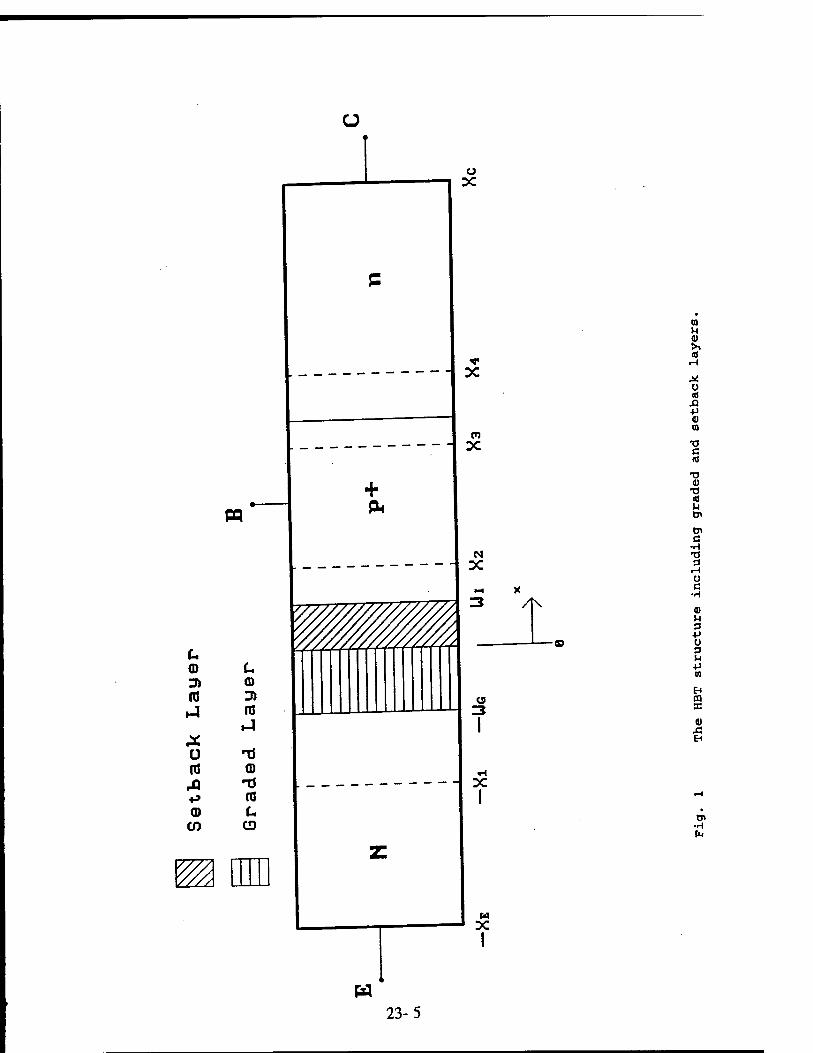
©
HJ
x u
<D en
(D
IB H4
-d (D
L CD
^
3 /T\
(9 3
I
n o I«
o <s sx ■p <0 01
T> c
<u TI <0 U W
D» c
•H •O D •-I Ü C
•H
0)
3 +J U 0 n +J (0
& m s 4)
03 frt
pa
W 23-5

d'v/dx^ = -{p/sg(x) _ (dv/dx)(sE - eB)/{WGEg(x)]} (2)
where V is the electrostatic potential, and p is the charge density, B^^
the conventional depletion approximation and integrating the eguation once we
obtarn the electric field §g(x) in the graded layer as
?g(x) = -dV/dx = (qNEx - C')/e0(x) 9 (3)
Here KE is the emitter doping concentration and c< is a constant which needs to
be determined from the boundary condition. Similarly, we can derive the electric
f«ld. §l(*> in the space charge region (SCR) on the emitter side, |8(X) in the
setback layer, and §a(x> in the SCR on the base side:
!i(x) = (qNE/eE)(x + x:) for -X, < x < -w G (4)
l.(x) = (qNB/eB)(x2 - Wj) for 0 < x <W 1 (5)
?2(x) = (gNB/eB)(x2 - x) for WT < x < x 1 2 (6)
where NB is the base doping concentration, wt is the thickness of the setback
layer, and X, and X2 are the thicknesses of the SCR on emitter and base sides
respectively (see Fig. 1}. since the flux density ^ ^ _ ^ ±> ^^
constant C in (3) can be obtained by using the boundary condition 1 (-w , -
§g(x) = [qNE/e (x)](x + x,) (7)
By choosing x - _Xj as the reference (zero point), the corresponding
electrostatic potential V(x) can be calculated by integrating |(Jt) over its boundary. Thus
23-6
Vx(x) = 0.5(qNE/eE)(x + Xi)2
Vg(x) = V^-Wc) + qNEWG(x + WG)/(eB - eE) +
qiWX! - WGBE)/(£B " BE)2ln{[(eB - eE)x + WGeB]/(WGeE)}
V.(x) = Vg(0) + (qNB/6B)(X2 - Wj)x
V2(X) = V.W + (qNB/£B)(X2x - X2/2 - X2WX + Wx2/2)
where
Vl(-WG) = O.S(qHE/eE){^i - WG)2
Vg(0) = 0.5(qNE/eE)(x + XJ2 +
[qNEWG/(eB - eE)]{x + WG + [X, - WGeE/(eB - eE) ] ln( EB/eE)}
V.(W!) = V,(0) + (qNB/eB)(X2 - WZ)VZ
(8)
(9)
(10)
(ID
(12)
(13)
(14)
Also, the total electrostatic potential V2(X2) across the SCR should be equal to
Vbi,BE - VBE, where VBE is the applied base-emitter voltage and Vbi,BE is the
junction built-in potential [13]. Thus
Vbi/BE " VBE = V.W + 0.5(qNB/eB)(X2 - Wx)2 (
The SCR thickness X, can be found from (15) and X2 - (H./B.JX, + *x (derived
from charge neutrality in the entire SCR):
(16) Xx = -0.5B/A - 0.5(B
2 - 4AC)°-5/A
23-7
where:
A = 0.5gNE/£E + 0.5qNEV(eENB) (i?
B = -qNEWG/eE - [qNEWG/(eB - eE) ] ln( EB/eE) + qN^/e, (18)
C = -qNEWGV(eB - e.) + [qNEW^eB/(£B _ es)2]ln( ^^ + Q.SqN^/e, (19)
The barrier potentials for the conduction band edge Ec in the SCR are
defined as
VBl ~ V^-W«.); VBGC = _AEc/q + Vg(0) - V^-W«.);
VBS = v.(Wl) - Vg(0); VB2 = V2(X2) - v.(Wl) (20)
where AEC is the conduction band discontinuity, since the valence band edge Ev
is in parallel with Ec except for that in the graded layer, the barrieJ
potentials for the valance band are the same as that given in (20) provided VBGC is changed to
VBGV = AEv/q + V (0) - V,(-Wr) g i\ G) (21)
AEV is the valence band discontinuity. Note that all barrier potentials have
positive values except for VBGC, the value of which can be positive or negative
depending on the applied voltage and thickness of the graded layer. A positive
value indicates that Ec have a positive slope in the graded layer, and vice versa
if the value is negative.
2.2 Collector and Base Currents
Following the thermionic-field-diffusion approach [7-8], the electron
current density Jn across the spike (located at x - -WG, is the difference
23-8
between two opposing fluxes:
(22) Jn(-WG) = qvnY[n(-WG-) - n(-WG )]
wnere v is the electron thermal velocity, Y is the tunneling coefficient [8],
and n is the electron concentration. It should be mentioned that Y depends
<-,„~ =r,H that v = 1 (no tunneling) and the TT ~~A \r if v is negative ana inat y ■»■ vw~ strongly on VB1 and V^ ir v^c is> "=y
conventional drift-diffusion model applies if VBGC is positive. In (22),
n(.WG-) = NEexp(-VB1/VT) and n(-V> = n(X2)exp[ (VB2 + VBS + V«)/^] (23)
At this point, the only unknown parameter is n(X2), which can be found using the
relation:
(24) Jn(-WG) = JSCRG + JSCRS + JSCR2 + Jn(X2)
where »„. J„. - J„ « the reeo„bination current densities in the graded
Uyer, setbach layer, end space-charge l.y.r in the bane region, respectively
«th. «.odels for Jsc«, .„. end ,„ will be developed in the next section,, and
,.<*,, is the diffusion-only current in the guasi-neutral base ,QKB,. For a very
thin base,
(25) Jc « Jn(X2) = qDnn(X2)/(WB + Dn/vsat)
where Jc is the collector current density, Dn is the electron diffusion
coefficient in the QNB, WB = X3 - X2 (Fig. 1) is the Q«B thickness, and vMt ( =
10' cm/sec) is the saturation drift velocity caused by the high field in the
base-collector junction. An empirical expression can be used to describe Dn
[14]:
(26) Dn = VT[7200/(1 + 5.5xl0-
17NB)°-233]
23-9
Combining (22)-(25) and solving for n(X2), we obt
n(X2) = [qvnyNEexp(-vB1/vT, - JSCR2 _ JgcRs _ ^^
am
(27)
where „ - gDn/(wB + Dn/v8at) + qVnYexp[^ + ^ + ^^
The components of the base current density j. of the HBT include 1)
section of hole current density JRE from the base to emitter; 2) electron-hole
recombination current density JRB ln the guasi.neutral base; 3) electron_hole
recombination current density JSCR in the emitter-base space-charge layer- and
4) electron-hole recombination current density JRS at the emitter and base surfaces.
The hole injection current can be modeled using the conventional diffusion-
current only approximation:
JRE = qDpNBexPf-(vB1 + VB2 + vBS + v^/v,]/», (28)
XE - Xj is the where Dp is the hole diffusion coefficient in the emitter and WE =
thickness of the guasi-neutral emitter. The doping-concentration dependent o
is given by [14] P
Dp = VT[380/(1 + 3.2xl0-17N„i°-2666i
1 (29)
The recombination current density in the guasi-neutral base is
JRB = J„(X2)(1 - aB)
(30)
where aB is the base transport factor:
aB = l/cosh[WB/(DnTn)0-5]
(31)
xn is the electron lifetime in the base (xn = 1 nsec is used in calculations,,
23-10
Kote that a, approaches unity for a very thin base.
Jsc, consists of four recombination current densities occurred in the
es.itter.side of the space-charge layer <Js„,>. in the graded layer (W " the
setback Xayer „„,. and in the base-side of the space-charge layer ,»„>.
Based on the assumption that the Shockley-Read-H.ll statistics is the dominant
«combination process, then these current densities are proportional to the
intrinsic free-carrier concentration and eKp(V„/2V,):
where nL is the intrinsic carrier concentration and B* is an empirical parameter
that relates to the trapping density in the space-charge region.
The surface current density is influenced strongly by the fabrication
process. It includes electron-hole recombination talcing place at the emitter as
well as base surfaces and can be empirically modeled as [15]
(33) JJS = J*exp(VBE/nVT)
„ere the ideality factor n is close to unity, and * is the empirical parameter
that characterized the recombination current at the emitter and base surfaces,
which is a function of the surface recombination velocity s, the value of which
depends strongly on the surface states and the location of the re„i level pinned
at the surface (S - 10« cm/sec is used in our calculations!.
3 BPSIIT.TS AND DISCUSSIONS
For illustrations, we consider a typical HBT makeup having 5x10». 10". and
10" cm- emitter, base, and collector doping concentrations, and 1700. 1000. and
5000 A emitter, base, and collector layer thicknesses, resp.otiv.ly. Also, the
„BT has graded and setback layer thicknesses ranging from 0 to 300 A. Since the
results for HBTs having only the graded layer and only the setback layer have
been reported previously [3-U,, our emphasis here „ill be placed o„ the combined
23-11

effects of the two layers on the HBT performance.
Fig. 2 illustrates the spatial variation of conduction and valence band edges of an HBT havina W = w - icn « f 9 x WG
" 15° Ä for three different VBE. it is shown that
while EV in the junction increases monotonically versus the position for all
voltages, the slope of Ec in the graded layer actually becomes ^.^ ^ ^
xs increased. Associated with such a negative slope is an "alloy« junction
barrier which is formed at the vicinity of x - -WG. The same results were also
obtalned in numerical simulation by Prank and Tiwari [16]. As wili be shown
later, the formation of alloy junction barrier increases the importance of the
thermionic and tunneling mechanisms and subseguently reduces the collector
current at large VBE. Flg. 3 compares the conduction band edges of the same HBT
calculated from the present model and obtained from a numerical model [12]. Good
agreement is found between the two models.
We next study the collector and base currents, and their voltage
dependencies are plotted in Pigs. 4 and 5 respectively. The results suggest
that, except for very large VBE at which the alloy junction barrier exists, both
Jc and JB increase considerably when Wz and WG increase from 0 to 150 Ä but change
only slightly when Wr and WG increase from !50 to 300 Ä. The Jc increase results
from the removal of AEV which reduces the importance of thermionic and tunneling
mechanisms. On the other hand, the Jß increase is due to the fact that the
presence of w, and WG widens the space-charge layer and thus enhances electron-
hole recombination in the region. Again the results calculated from the present
model compare favorably with those obtained from the numerical model [12,. Note
that when „x and WG are present, Jc saturates at a smaller VBE (Fig. 4). This
stems from the fact that the free-carrier transport in such HBTs is hinder by the
alloy junction barrier formed at large VBE (see Fig. 3).
To better compare the currents in HBTs with Wj and WG and without W, and
WG (abrupt HBT), the currents in HBTs with „x and WG are normalized by those in
abrupt HBTs. These normalized ac and Jß are shown in Pigs. S and 7
respectively. The results in Pig. 6 indicate that the HBT ^ ^ = ^ = ^ ^
has the highest Jc at relatively low VBE, but all four HBTs have similar JC at
23-12
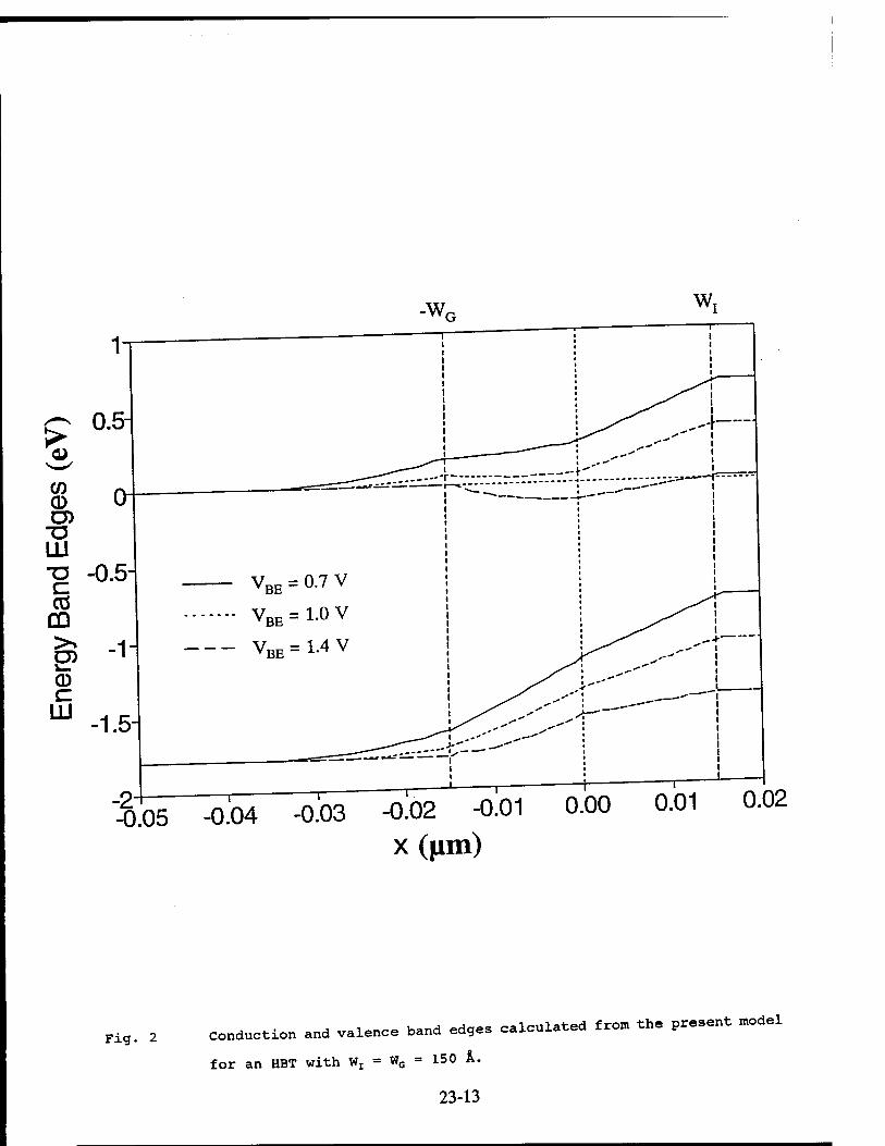
-0.05 -0.04 -0.03 0.02 -0.01 x(iLim)
0.00 0.01 0.02
Fig. 2 Conduction and valence band edges calculated from the present model
for an HBT with Wx = WG = 150 k.
23-13
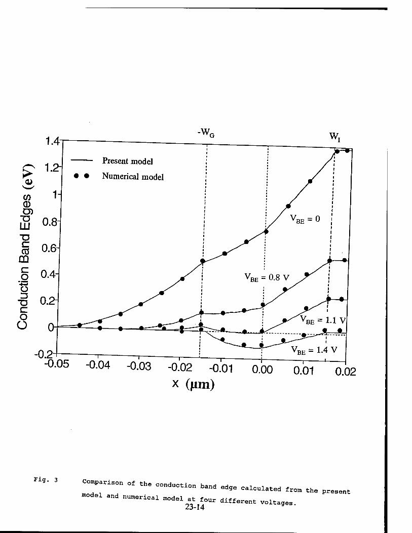
w.
o CO 0 D)
"O LU "Ö c CO
GQ c o
Present model
• • Numerical model
-0.05 -0.04 -0.03 -0.02 -0.01
x (Jim) 0.00 0.01 0.02
Fig. 3 0-P.rl« 0( the conduotiM band edge caicuuted from the preseM
-del and „u„«ical „deI tf different w
23-14
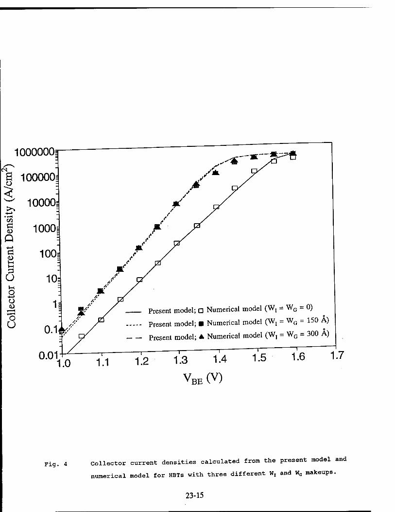
lOOOOOOi
ol
a 100000= o -
3? -
10000= >% - +-» . C/3 -
1000i Q - +-» ~
100= *-( - «-t - 53 - u 10-
V-i ; o : Ü 1}
T—(
o :
U 0M
Present model; D Numerical model (Wt = WG - 0)
Present model; ■ Numerical model (W, = WG = 150 A) o
— Present model; A Numerical model (Wj = WG = 300 A)
1.6 1.7
VBE (V)
Fig. 4 Collector current densities calculated from the present model and
numerical model for HBTs with three different Wx and WG makeups.
23-15
"lOOOOr
I a Q -4—>
e u c/3
0.001
Present model; a Numerical model (W{ = W = 0)
Present model; ■ Numerical model (W, = WG = 150 Ä)
- Present model; A Numerical model (Wr =.WG = 300 A)
~12 1-3 1.4 1.5
VBE(V)
1.6 1.7
Fig. 5 Base current densities calculated from the present model and
numerical model for HBTs with three different Wx and WG makeups. 23-16
50T-
ö
tl ö t-l
O ■*->
o »—■«
O U
<L> N
13
o
0
Wl = 300 A, WG = 300 A
100 1.10 1.20 1.30 1.40
vBE (V)
1.50 1.60 1.70
Fig. Collector current densities of HBTs having four different Wx and WG
normalized by that of the abrupt HBT (Wx = Wfi = 0).
23-17
45-
1.70 VBE (V)
«■• 7 Base current densities of HBTs having four different ., and W
normalized by that of the abrupt HBT (Wx = wG = 0) 23-18
*. un-p T in the HBTs with Wx and WG is high VBE. in comparison with the abrupt HBT, Jc in
r »t V = 1 V increases to a maximum of about 45 times about 5-10 times larger at VBE - 1 v, incte
l.rg.r at v., - 1.. V, and — comparable «"> that in the abrupt »BT at hrgh
volt.g.s. The presence of W, and «, also increases ,.. as shown i„ Fig- 7.
«- rt,t w = W = 300 k results in the widest space- Intuitively, one would expect that Vz - wG
charge layer and thus the highest ,.. This is indeed the case i» Pi,. 7, which
shews that the „BT with «,-«,- 300 A has the highest 0. at relatively -.11
v„ -on, th. four »BTs. At high V„, .11 four HBT, h.ve similar ,.. Thrs rs
because the sp.oe-ch.rge region h.s bee» greatly reduced by the high v„. .hd the
sp.ce-oh.rge region recombination is not important. Conversely, the hole current
, injected fro. the base to either beocn.es the dominant component for J..
Since »„ is not affected by W, and W0 at high voltages (the valence barrier as
aimost fl.t .t such bias conditions,, all four HBTs have comparable J..
Fig 8 shows the do current g.ins ., a low current level „c - 0.01 A/=m
is considered, c.lcul.ted as a function of W, .nd „.. The results suggest that
th. current gain ß decre.s.s lih.arly with inor.asin, W0 if w, - 0, and P rs
4-K,„ mn & Also, at this current relatively insensitive to WG if W, is greater than 150 A. Also,
level, ß decreases with increasing Wr for all WG.
Th. tr.„ds .r. guit. diff.r.nt for th. HBT op.r.t.d at a high ourr.nt l.v.l
(J . 10' A/-> is considered,, how.v.r. as shown in Fig. 9. First, comparable
current gains .r. found for .11 «, and w0 > 1=0 4. Furth.rmore, when «s
approaches zero, h.vin, . non-s.ro „, is beneficial, but increasing «, beyond 1S.
i does not provide any ourr.nt gain .nh.nc.ment.
4. CONCLUSIONS The spihe .t th. hetero-i„terf.=. oft.n lilt, the fre.-c.rri.r inj.ctron
from th. emitter to b.s., .nd th. gr.d.d .nd s.tbach layers are fre,u.„tly »^
to ov.rcom. such a probl.m. In this study, th. combined .ff.cts of th. 9r.d.d
and s.tbach l.y.rs on the curr.nt-voltag. oh.r.ct.ristics of AloaWOaAS HBTs are
inv.stigatad. and ah an.lytic.l mod.l which accounts for such effects rs
developed.
23-19
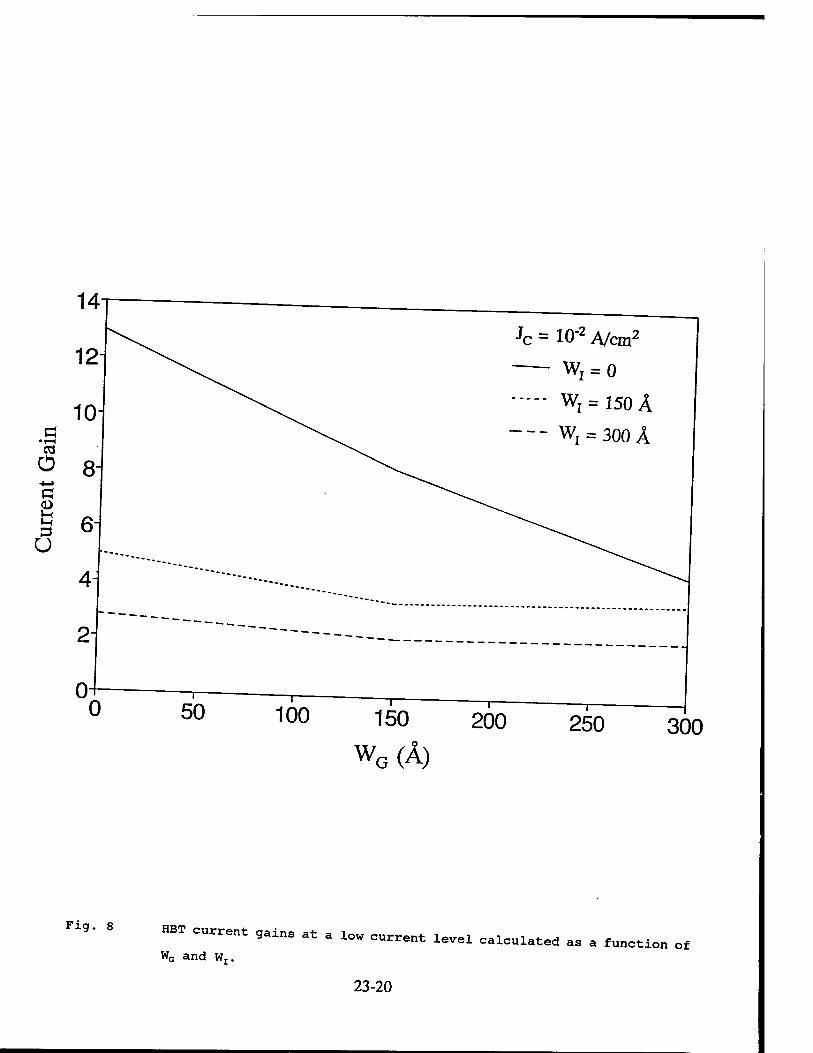
= 10-2 A/cm2
- WI = o - WI=150Ä
" Wx = 300 Ä
300
Fig. 8 HBT current gains
WG and wz. at a low current level calculated as a function of
23-20
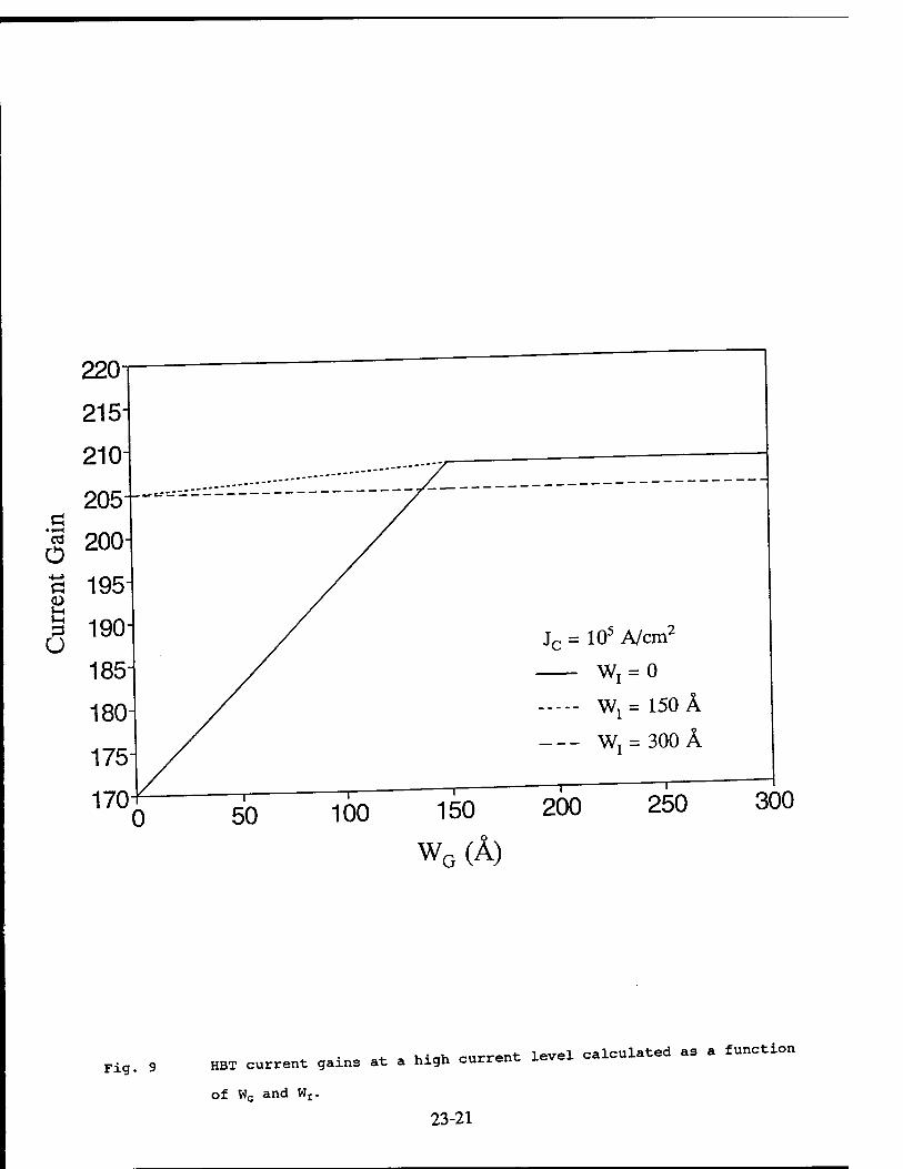
220
215
210
205t-
§ 200
u
150
WG(Ä)
Jc = 105 A/cnT
W! = 0
Wx= 150 Ä
Wj = 300Ä
200 250 300
Fig. 9 HBT current gains at a high current level calculated as a function
of WG and Wx.
23-21

The following conclusions can be drawn from the present study.
1. At low current levels, the presence of wx and WG actually degrades the current gain.
2. At high current levels, using W, = 150 Ä and any WG or wz = 0 and 150 Ä * WG
* 300 Ä yields the optimal current gain.
3. Among the HBTs considered (with or without Wx and/or WG), the abrupt HBT (Wj
= WG = 0) possesses the best current gain at low current levels and the worst
current gain at high current levels.
The model developed permits a degree of insight into the influence of the
graded and setback layers on the HBT performance and should have practical
applications for use in HBT design and circuit simulation.
23-22
REFERENCES
m H. Kroemer, "Theory of a Uide-gap emitter for transistors," Proo. IRE, vol.
45, pp. 1535, 1957.
[2] P. M. AsbecK at al., "Heterojunction bipolar transistors for ultra high
speed digital and analog applications," in IEDM Tech. Dig., 1988.
„H T p Bailbe, "Electrical behavior of an Npn [3] A. Marty, G. E. Rey, and J. P. BaiiDe,
• —t-~T- " cjolid-St. Electron., vol. 22, pp. GaAlAs/GaAs heterojunction transistor, Solid
549, 1979.
[4) A. A. Grinber, and s. Luryi. "on the thermiohio-diffusion theory of
minority «.»sport in heterojunotion bipolar transistors.- IEEE Trans.
Electron Devices, vol. 40, pp. 859, 1993.
[5] B. R. Ryu, and X. M. Abdel-Motaleb, "A Gummel-Poon model for abrupt and
graded heterojunction bipolar transistors," Solid-St. Electron., vol. 33,
pp. 869, 1990.
„1 ». ,. Lion, C. S. Ho, L. L. Lion, and C. I. Hu.„„ "An analytio.l model for
current transport in AlG.As/GaAs abrupt HBTs with a setback layer." Solid-
St. Electron., vol. 36, pp. 819, 1993.
[7] M. S. Lundstrom, »Boundary conditions for Pn heterojunctions,- Solid-St.
Electron., vol. 27, pp. 491, 1984.
[8] A. A. Grinberg, M. S. Shur, R. J. Fischer, and H. MorKoc, »An investigation
of the effect of graded layers and tunneling on the performance of
AlGaAs/GaAs heterojunction bipolar transistors," IEEE Trans. Electron
Devices, vol. ED-31, pp. 1758, 1984.
[9] c. D. PariXh and F. A. Lindholm, "Space-charge region recombination in
• 4.^,.«, » TFTTF Trans Electron Devices, vol. 39, heterojunction bipolar transistors, IEEE Trans.
pp. 2197, 1992.
HO, A. Das and M. S. Lundstrom, "Numerical study of emitter-base junction
design for AlGaAs/GaAs heterojunction bipolar transistors," IEEE Trans.
Electron Devices, vol. 35, pp. 863, 1988.
AT 7 Tee "A study of current transport on [11] S. -C. Chen, Y. -K. Su, and C. -Z. Lee, A stuay
23-23
P-Nheterojunctions," solid-st. Electron., vol. 35, pp. 1311, 1982.
[12] L. L. Liou and c. I. Huang, "Using constant base current as a boundary
condition for one-dimensional AlGaAs/GaAs net exjunction bipolar transistor
simulation," Electron. Lett., vol. 26, pp. 1501, 1990.
[13] A. Chatterjee and A. H. Marsha*, "Theory of abrupt heterojunctions in
equilibrium," Solid-st. Electron., vol. 24, pp. mi, 1981.
[14] D. A. Sunderland and P. L. Dapkus, »Optimizing N-p-n and P-n-P
heterojunction bipolar transistors for speed," iEEE Trans. Electron
Devices, vol. ED-34, pp. 367, 1987.
[15] W. Liu and j. s. Harris, Jr., "Diode ideality factor for surface
recombination current in AlGaAs/GaAs heterojunction bipolar transistors,"
IEEE Trans. Electron Devices, vol. 39, pp. 2726, 1992.
[16] S. Tiwari and D. j. Frank, "Analysis of the operation of GaAlAs/GaAs
HBT's," IEEE Trans. Electron Devices, vol. 36, pp. 2105, 1989.
23-24
EXPERIMENTAL STUDY OF A SWITCHED RELUCTANCE MOTOR
Shy-Shenq P. Lieu Assistant Professor
Division of Engineering San Francisco State University
1600 Holloway Avenue San Francisco, CA 94132
Final Report for: Summer Research Extension Program
The author would like to thank the sponsorship of Air Force Office of Scientific Research
Boiling AFB, Washington DC and
San Francisco State University
June, 1994
24-1
EXPERIMENTAL STUDY OF A SWITCHED RELUCTANCE MOTOR
Shy-Shenq p. Lioit- Assistant Professor
Division of Engineering San Francisco state University
Abstract
vo.ce S7eral.SearCh c°ils' "»or 'or phase windings and one for yoke, wer lnstalled .nto a prototype sv reluctan~
sear „ \* *"* iM»*™* <* P-e windings and ye*!
star I J rSSPeCt t0 the relatlVe P°siti°" o* «tor and Stator teeth. The induoed voltage waveforms for these search
cc:; tsa::ensDthrasted switched reiuctanc* «*«*« -- -
telerature se "^ ~* "^ "-"^ "* "P°"^ ^~
Ltor Dua to t7eTre Pr°file °f thE SWitChSd stance
Couture^ p^ofUe TsCti°n °* """ t^"t°" ""«•' ~ reiuotance JT «" £^/ ^ --' . —hed
«It. The driver circult for9th^TTs% oSU:Srtr "*
24-2

EXPERIMENTAL STUDY OF A SWITCHED RELUCTANCE MOTOR
Shy-Shenq P. Liou
INTRODUCTION Switched reluctance motor is a relative new member of the
family of rotating machines. Although conceptually the
switched reluctance motor is a simple electromechanical energy
conversion device, the popularity of it nowadays is not
possible without the pioneering work of Professor P.J.
Lawrenson of University of Leeds [1] almost 20 years ago and
the advance of semiconductor switching devices. Basically, switched reluctance motor is an electric motor
in which torque is produced by the tendency of its movable
part, the rotor, to move to a position where the inductance of
the excited winding is maximized. In energy conversion
terminology, torque is produced because of its tendency to
maximize the coenergy [2]. Figure 1 shows a typical switched reluctance motor xn a
8-6 design in which there are eight stator teeth and 6 rotor
teeth. There are also four phase windings wrapped around those
eight stator teeth; one winding for each two stator teeth.
Only one phase winding with one turn each on the stator teeth
is shown in Figure 1. Also shown in the Figure 1 are two
positions, aligned and unaligned positions. It can be expected
that the inductance for the phase winding shown xn Figure 1
will assume a maximum value whereas the second phase winding
to the right of the shown winding will assume a minimum
inductance. If a DC current is supplied to the first phase
winding to the right of the winding shown in Figure 1, the switched reluctance motor's rotor will rotate counterclockwise
24-3
because of the tendency of maximizing the inductance of the
energized phase winding. Usually, only one phase winding is
energ1Zed at any given time. Also it should be noted that only DC current is needed to produce torque. —
To produce a continuous rotation, current should be
supplied to successive phase winding one at a time based on
the position of the rotor with respect to the stator.
Therefore, some kind of switching mechanism must be there to
TURN ON and TURN OFF the current to each phase winding with
reasonable efficiency and power handling capability. The
advance made by the semiconductor industry on power switching
devaces make the control of switched reluctance motor
possible. Also, it is important to note that there is no need
to put any coil on the rotor poles to create the energy
conversion. This turns out to be another salient feature of switched reluctance motor.
Two typical power electronic phase switching circuits for
switched reluctance motor are shown in Figure 2. Mos-
Controlled Thyristor (MCT) are used in this instance just for
representation purpose only. Usually, either MOSFETs or IGBTs
are used m the commercial products. Two switches must be
turned on by gating from the control circuit simultaneously in
order to establish the current flow in the phase winding. When
the switches are turned off, the stored energy in the phase
winding is returned to the DC source via the two freewheel
dxodes as shown in Figure 2. The control circuitry must get
the rotor position through either encoder or resolver before it can decide which phase winding to be turned on.
The uniqueness of switched reluctance motor can be summarized as the following:
1. There is no winding on the rotor poles.
24-4
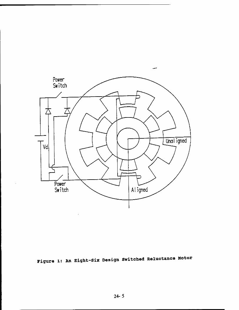
Power Switch
Power Switch
Figure l: An Eight-Six Design Switched Reluctance Motor
24-5
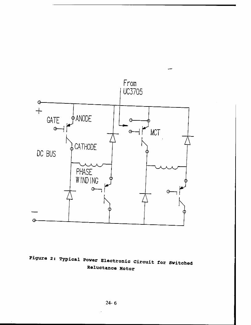
From UC3705
+ GATE JANODE
DC BUS
S 6)
-*- <M r MCT
PfttSE WINDING .
a—il
K 5 o—i
K
Figure 2: TWic,l Power Electronic circuit for Switched
Reluctance Motor
24-6

2. Both stator and rotor have salient poles.
3. The stator winding comprises a set of coils, each
of which is wound on the pole. 4. Excitation is a sequence of current pulses applied
to each phase in turn. 5. As the rotor rotates, the phase flux linkage should
have a triangular or sawtooth waveform [3] but not
vary with current.
POTENTIAL PROBLEMS with SWITCHED RELUCTANCE MOTORS
The switched reluctance motor has many advantages such as
simple geometry, easy to manufacture, high temperature
capability, and inherent fault tolerant operation, etc. On the
other hand, it does have many undesired features too. First of
all, it requires a rotor position sensor (either encoder or
resolver). Second, it definitely requires a dedicated power
electronic controller. Last but not least, the simple yet
complicated magnetic geometry poses a serious engineering
challenge for design engineer to design and optimize a
switched reluctance motor for specific application. Therefore,
the potential problems associated with the switched reluctance
motor are summarized in the following: 1. Needs a rotor position sensor in the form of either
encoder or resolver. (No dedicated sensor operation
should be ideal). 2. How to model the switched reluctance motor
electrically and magnetically due to complicated
magnetic geometry and severe local saturation when
rotor teeth approach those of stator. 3. How to model the switched reluctance motor
thermally so design engineer can optimize the
24-7
design for given specific applicatlon_
Some of the potential prob!« mentioned above „in be discussed in this report. Attests „ere made t„ 1 »any problems as possible Due L 3ddreSS as
every problem area is attaCL d "^ UnitSti°n' «<* research. But the effort 1 "* ^ °°Ur" °f this
research „or*. ^ 3 9°°d (°Undatio" '« ^ure
PROTOTYPE SWITCHED RELUCTANCE MOTOR
Physics Pir„0tHmPh SWltChed rSlUCtanCe **» ™*° "* «■*»
used in au the r°: °hi°' "^ *" S""9° ~ PUrCh"ed ^ reiuctl. motr T" "" ^"^ «« *"- -it—
No. of Phases 4
PM^oStau* 1S0 volts DC Raetaed
0Upeea '"oÄ Maximum speed 15 OI^M Rated Torque 100 0z-in
S2ic5E9?™nt 30*°**"
Ration So"?8-5!00 Weight =6° Llnes/Revolution 5.5 Lbs
also n COntr0ller fr°m s^""sion company, Santa Clara, CA „as
Tsr:r:i:° rrthe switchad —«-^« velocitv „ Vari°US °Perati"9 "Ode, position,
«^ very'u:;rr^enadni T m°dSS- ^ ^ *' »"i™
reauired f ^^^ A IBM compatible personal computer is
TZTzT T tSrfaCe betWeen thS — — controller
pa" r TL!" r1 is rd in this re9ara- A 4°-pin— HCTL lloo general purpose motion control chip is used
24-8
in the controller to take care of the number crunching task.
For example, read the rotor position from the position encoder
and output the proper commutating sequence to individualjphase
winding based on the desired command operating mode: This
setup turns out to be extremely useful for initial testing of
the switched reluctance motor. A simple friction type dynamometer from Hampton Inc. is
used to load the switched reluctance motor during the tests.
There is no constant torque load from this dynamometer.
Therefore, only constant speed command operating mode is
reported. In the future, if a decent dynamometer is available,
more tests on the constant torque operating mode can be
tested.
INDUCTANCE MEASUREMENT THROUGH SEARCH COILS Five search coils were put inside of the switched
reluctance motor in order to identify various parameters
associated with the motor. One aim is to see whether the
inductances of these search coils change when the rotor
position varies. If there is a unique pattern or certain
fingerprint associated with the rotor position, this might
provide an easy way to locate the position of the rotor
without either the encoder or resolver. Four one-turn search
coils were put into the same locations with the phase
windings. Another search coil enclose the yoke or back iron
portion of the motor. A handhold digital inductance meter was
used to measure the inductances of these search coils. Because the air gap of the switched reluctance motor is
small and localized saturation is very severe, it is important
to fix the relative position between stator and rotor while
inductance measurement was conducted to avoid any inaccuracy.
24-9
Atte.pt was „ade to run the switched reluctance Mtor
controner rn position operating »ode to fix the iocation or
the rotor. There are two probier with this approach. First
the resolution is about 2.5 degrees even although useMan
specify a resolution or about o.2S degree in the Lnu-driven
PC program Second, the 00 current flowing in one or the phase
IwitcH Pr7lde 3 DC °"Set f°r thE ma9netic "'Id ^side the switched reluctance notor. This »axes the inductance „eter
reading extremely unstable and hence render it useless
set UP TZ table Wlth a reSOlUtlon <* -mi— »• "egree is !earT " "*"" 3 t0 —»« «» ihductances of search coils „ore accurately. A c-clanp is used to fix the
rotor position at standstill whereas the stator part is
adhered to the rotary table. For every degree adjustment fro»
coil r7 table' ——ts «« — *or each search coils. The rotary table has a 96 degrees adjustable range. For
rangTfoTth "* ^ "***" r*lu°t"" **«• ■**«» range for the angle is 360/6-60 degrees. Thus it provides enough d points for a cOTpiete cycie_ The
each search coil versus the rotor angle for phase winding one
^s^r-yoke ■— °°" -—-—«*-. of ZT Fi9"reS 4 t0 '' Lt °an be Seen that the inductances of phase winding search coils do vary cyclically with the
rotor position with a distinct difference when the rotor teeth is alrgned wxth the stator teeth (minimun inductance). whe„
the rotor rs at aligned position (maxi™» inductance, , and in
induct Sta9e betWeSn the maxi»um and Mini™», inductance. Al<?n i+- , x. decrees I' * P r°UglUy eVery S0 "«hanical degrees. Based on the shape of these inductance curves it
see»s promising that »aybe there is some uniqueness in these
24-10
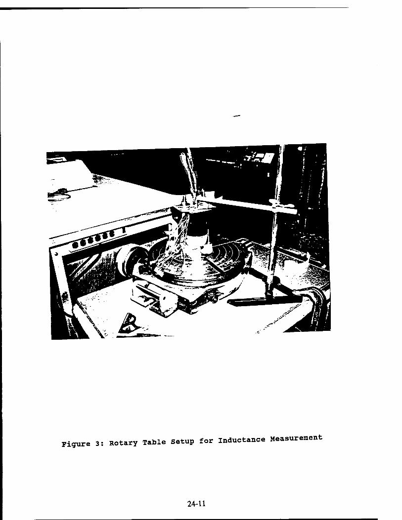
Figure 3: Rotary Table Setup for Inductance Measurement
24-11
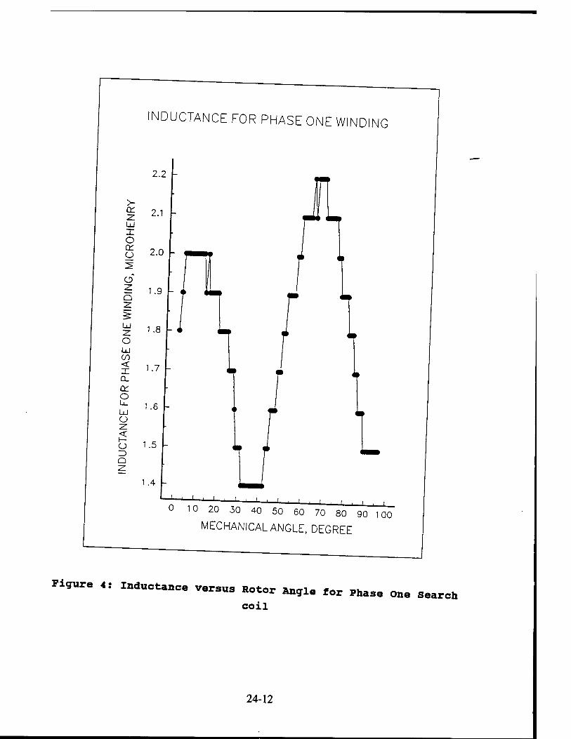
INDUCTANCE FOR PHASE ONE WINDING
>- on z: LU X o on o
o X Q X ^ Lü X o ÜJ CO < X a. on o b_ LU O
o X a
10 20 30 40 50 60 70 80 90 100
MECHANICAL ANGLE, DEGREE
Figure 4: Inductance versus Rotor Angle for Phase One Search coil
24-12
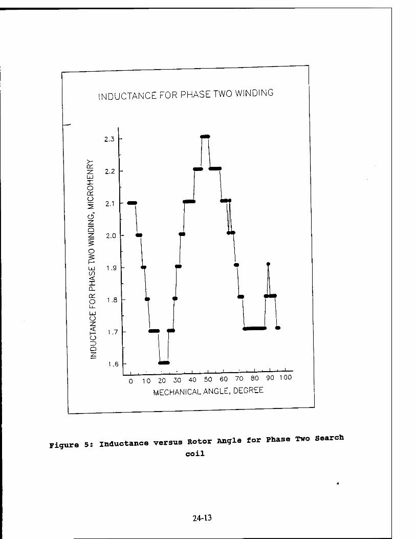
IN DUCTANCE FOR PHASE TWO WINDING
2.3
>
Z 2.2 UJ X o on
I 2-1 o z Q
2.0
UJ 1 .9 CO < X Q_ (T O 1 .8
UJ O
o Z) Q
1.7
1.6
ft
i ■ ' ■ ' I.I. I L.
0 10 20 30 40 50 60 70 80 90 100
MECHANICAL ANGLE, DEGREE
Figure 5: Inductance versus Rotor Angle for Phase Two Search coil
24-13
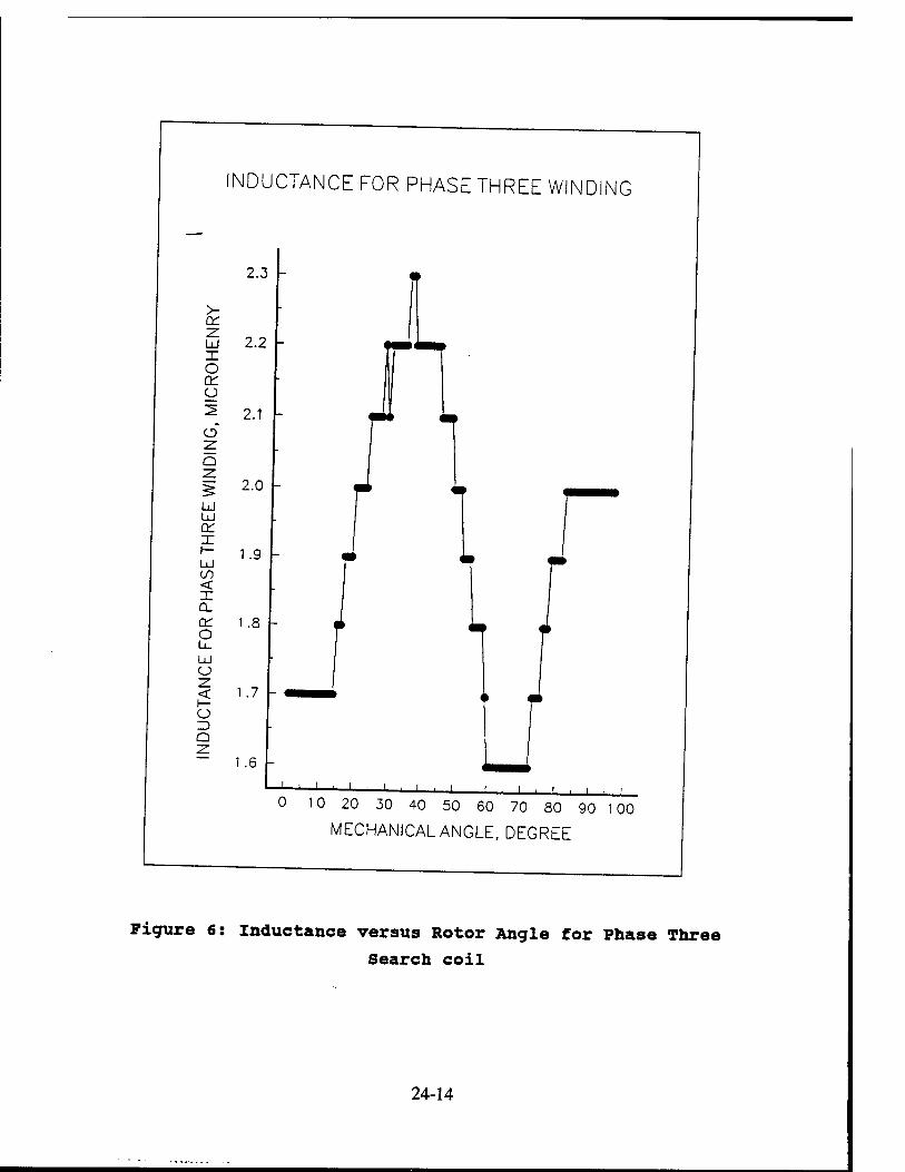
INDUCTANCE FOR PHASE THREE WINDING
>- on -z. ÜJ X o cr o
o
UJ ÜJ en X I— ÜJ CO < X Q_
on o L_ UJ o
o 3 Q
2.3
2.2
2.1
2.0
1.9
1.8
1.7
1.6
J I r
J ■ i ■ ' J—i_JL J i L
0 10 20 30 40 50 60 70 80 90 100
MECHANICAL ANGLE, DEGREE
Figure 6: Inductance versus Rotor Angle for Phase Three Search coil
24-14
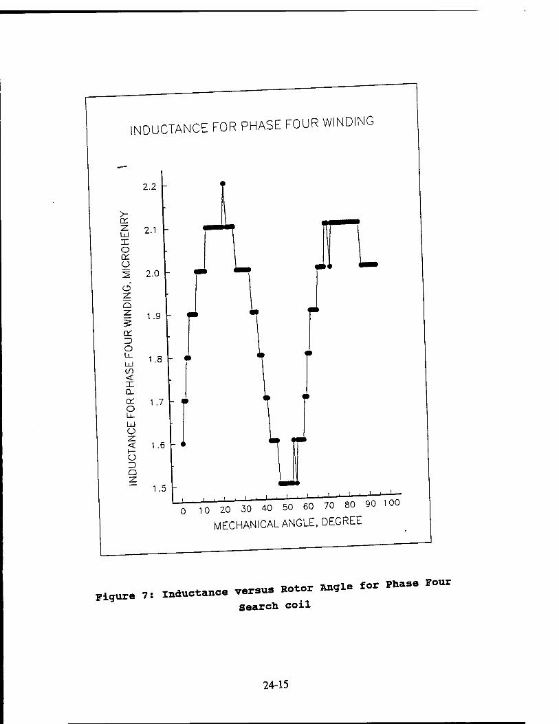
INDUCTANCE FOR PHASE FOUR WINDING
z: LU X o on o
o
2.2
2.1
2.0
? 1.9
O 1.8
1.7
CD < X Q. 0Ü o u_ UJ Ü
< 1 .6 o Q
1.5
0 10 20 30 40 50
MECHANICAL ANGLE, DEGREE
Figur. 7: inductance v«su, Rotcr «ale for mas. *our
Search coil
24-15
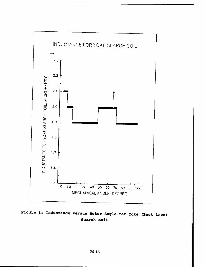
>- er X ÜJ X o ?,1 DC O 2
_J
o 2.0 o X a DC < 1 .9 Lü CO Lü ^ o >- 1.8
DC O U. Lü O I ./ X < f— ü 3 a 1.6
10 20 30 40 50 60 70 80 90 100
MECHANICAL ANGLE, DEGREE
Figure 8: Inductance versus Rotor Angle for Yoke (Back iron) Search coil
24-16
inductance patterns. It is also worthwhile noticing that the
inductance value is quite small, in the range of 1.3 to 2.3
microHenry only. This is because there is only one turn in
each search-coil. If a dedicated search coils were to be
installed inside the motor to serve as the position detector,
the number of turns shall not be too big. Thus, the absolute
inductance value probably is inherently small to begin with.
Consequently, emphasis shall not be to boost the magnitude of
the measured inductance through the search coils. Instead, the
focus shall be placed on the slope of these inductance values
since it provides a distinct and unique characteristic.
If a digital circuitry is designed to filter these
inductance values to produce a rotor position by assigning 1
to a rising inductance and 0 to a decreasing inductance, the
maximum resolution this can be achieved will be
360/(2N) = 360/(24) = 22 degrees (1)
where N is the number of search coils. It is hoped that the inductance measurement of the search
coil on the yoke can provide additional insight into the rotor
position identification. By examining the Figure 8, it is
determined that the inductance of the yoke search coil does
not vary sufficient to make any impact on the position sensing
at all.
FLUX WAVEFORMS A digital oscilloscope is used to measure the induced
voltage waveforms for each search coil for the stator poles
and yoke at various operating conditions and RPM. A 2000 RPM
24-17
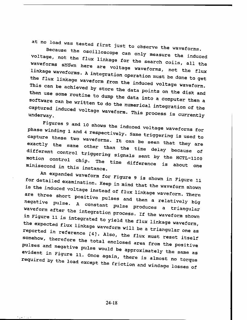
at no load was tested first 1«.»t *„ » Beoause the oscill" ^ *"* Wavef°™s.
voltage, not the ""1, "" ^ "'™r* the indu«d
wavers s^n hr llTZT ^ "^ ""^ «" «» linkage waveforms , J I '* WaVef°ras' "ot the flux
the f iux unk™:Lr^iT°per*tion must be aone to ** This can he achieved ^Tto«"^ ~ "^ "^^ -en use some routine I dtp 2 ^ JT " °" ^ ^ ^ software oan be written <- - computer then a
captured induced voita ""^ inte*rati°" <* the underway. ^ "V",~- This P— i- currently
capture these two waveforms itcan L '.T *' "*** *° exactly the same other than th , ^ they *" different control trio™ ^ delay because °*
■notion control ch!p";hr?tS19na/S "* * ^ "^"o
»inisecond in this iL^e. '" dl"— * •»«* one
for tl^elZ:10r" '°r Fi9UrS 9 iS Sh°™ in Fi^- » is the induced ^t"10"' ^ " "^ "* "» "»*•*»» ^own
- three shorT^t^Zl "2 T" "^ "~ negative pulse. A constant , * relat"ely big
waveform after the int!"" ""**"" * trian9ul- in Figure 11 is i^t'dt^" ^^' " ^ "aVef°™ Sh°™ the expected flux 1^! w l ^ ""* ^^ ™**°™'
-ported in r^T^T 1"? * ^"^ ~ " somehow, therefore the total , ""^ r""t ltSelf
Pulses and negative^ „ulTLT "" *"" ^ """^ evident in Figure ,/ " °Uld "* aPProxfmately the same as
«guired by the load exce" theT'• ^ '" ^"^ "° *»*» except the friction and windage losses of
24-18
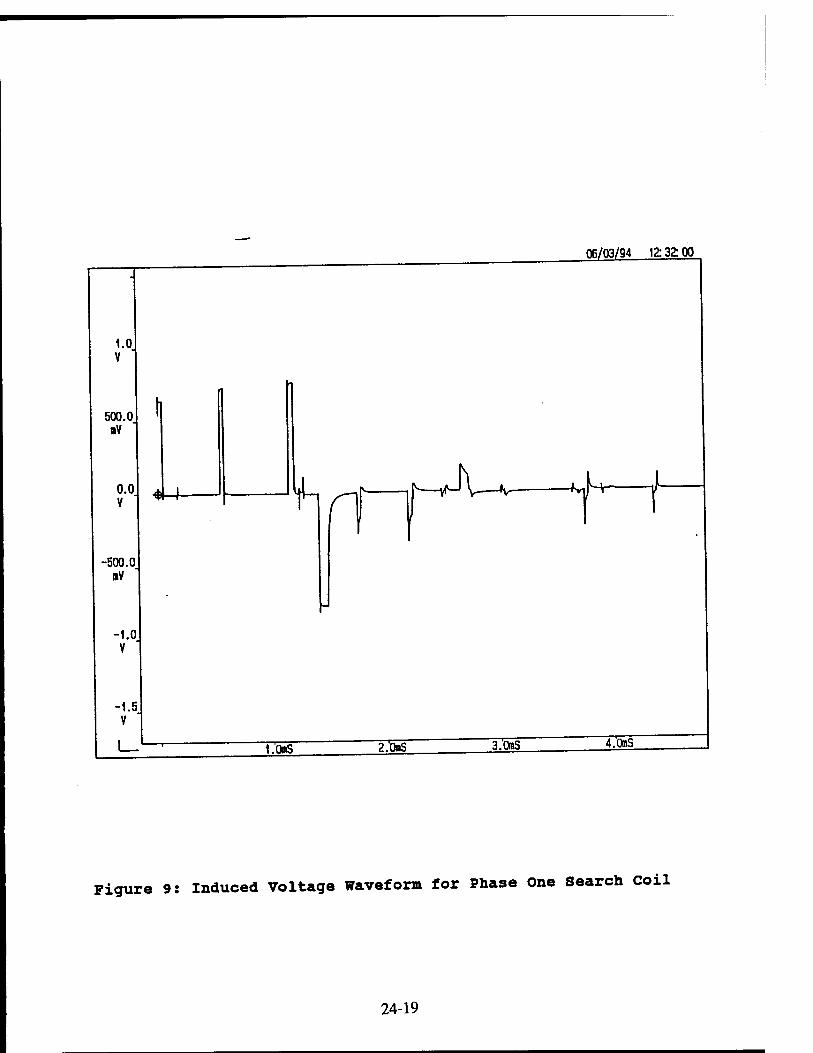
06/03/94 12:32 00
Figure 9: Induced Voltage Waveform for Phase One Search Coil
24-19
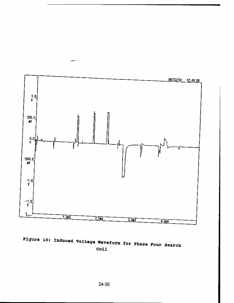
n 06/03/94 17- id- re
Figure 10, lnducad Voltige „^^ ^ ^ ^
Coil
24-20
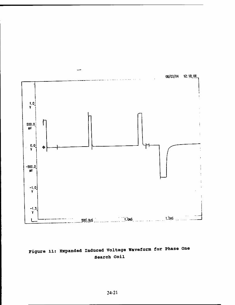
06/03/94 12:16:_44
1.0j V i
500.0' ■V 1
0.0 V
-500.0J nV
-1.0 V
-1.5 V
n
sod.ous Tons 1.5mS
Figure 11: Expanded Induced Voltage Waveform for Phase One Search Coil
24-21
the motor. Thus, very small current is reguired acceIerate the motor to the des.red speed_ Theref *
established in the air gap is relatively snail.
voke T t"dUCed V°ltage WaVef0rm £r0m the Search «" °" the yoke (back iron, is shown i„ Figure la. Basically/ *£
absolutely no distinct pattern for this wavefora xt ls
corn? dthfiCUlt t0 ima9ine how the "u* «— -
One sure "tn • ^^ """' "" ^«'i« P—s.
consists T " th" SinCE the indUCSd TOltagS •»«««- consists of many constant voltage pulses, the flux linkage
ZLT«11 be sawtooth like-"is also ^ite -"«^ - Mavbe thS =°mPleta CyCle «* th" indeed voltage waveform. Maybe once the flux Unkage waveform u Qb distinguishable pattern oan be found.
at abouT^" m°t0r iS l0aded " ab°Ut 40% °f the »*«» l°ad
were taken f "" **"* (S0°° "'" ' ^^ ^^ "«"«-- one H . Sa SearCh C°ilS and toe »aveforms for phase one and yoke searoh ooil are shown in Figures 13 and 14
ZITTT ?can be seen from these tw° "*>>*- «- - serLsof TT °Peratin9 in thS CUrrent ChOPPi"' ™°de- Ä neaatL T P°" * PUl*SS f°ll0Wed * a «Ltlvly long wave orm H .fniSh °na firi"' - *— »in^ng. Also, the waveform ls guite noisy. Onoe the integration is oonduoted the waveform win look much nicer.
0nce a*ain' "° ci^tinot pattern oan be found from Figure
linkage waveform. Based on the observations from Figures 12
section of th"UX Unkage WaVef0rm at thS **« <»*°* ~°"> section of the motor probably is highly dependent on the
location of the search coil and „hat is the operating mode of the motor. It might not be easy to predict the flux linkage
24-22
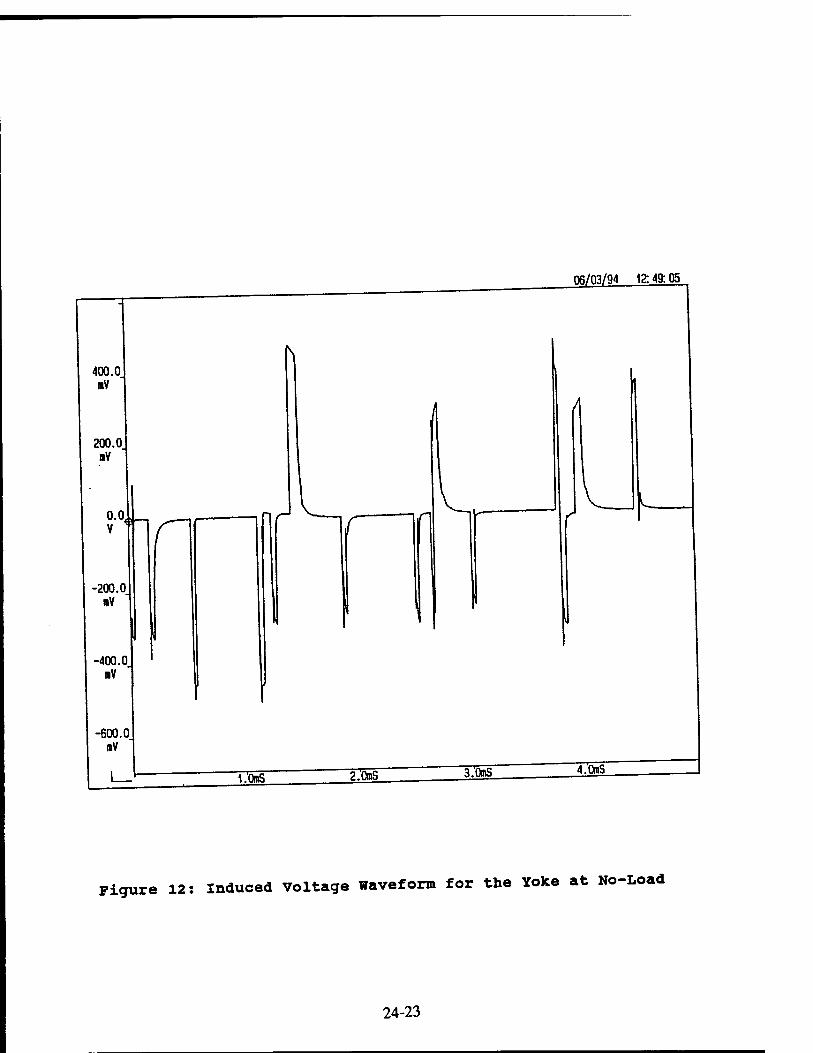
OR/03/94 12:49:05
Figure 12: Induced Voltage Waveform for the Yoke at No-Load
24-23
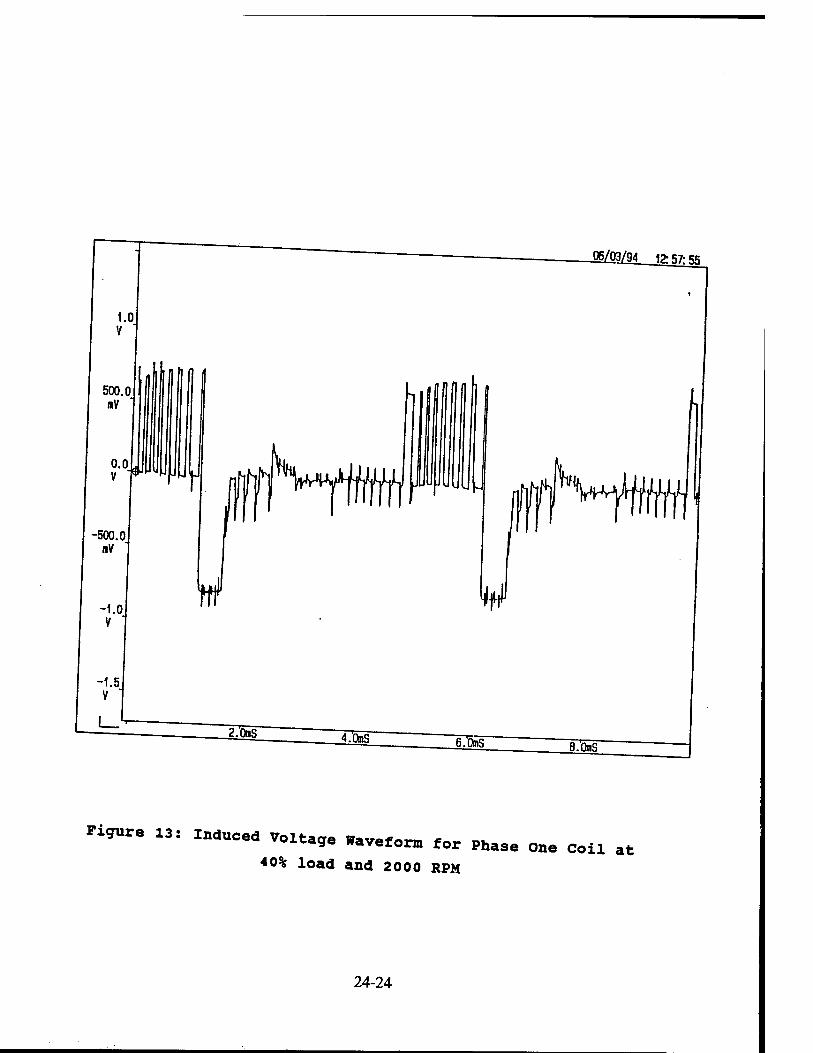
Figure 13: inaueed Voltage „„^ ^ ^ ^ ^ ^
40% load and 2000 RPM
24-24
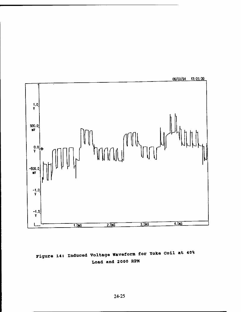
06/03/94 13:01:00
Figure 14: Induced Voltage Waveform for Yoke Coil at 40%
Load and 2000 RPM
24-25
waveform for the yo>ce section. Consequents to theoretically
calculate the core losses of the switched reluctance Motor is a very challenging task.
LOW SPEED OPERATION
The induced voltage waveforms for phase one and yoke
Flures 15 and 16 respectively, it is still in the current chopping mode. The yoke .nduced voitage wavefora
better compared to those of earlier cases as far as the distinct pattern is concerned.
OK GOING RESEARCH ARE* AND CONCENTRATION
(1) Temperature Profile and Thermal Modeling
SemicIT, temPeratUre S—- "<335Z *rom the National semiconductor, were instaHed inside the motor „hen the motor
«as bUilt. The locations chosen are the phase winding, pole,
and yoke section, „„fortunately, the pinout for these three
am™?- SSnSOrS "e "0t idSntified " -1- «**«-»* amount of time was spent in determining the pinout in order to
design a circuit to read the voltage which in turn will yield
the temperature at the winding, pole and yoke section of the
switched reluctance motor, so far, the pinout for two out of
the three temperature sensors are identified. The last one
durin „r n0t bE deternined -lately or it is damaged during the manufacturing process. Therefore, it is an on going
process to obtain the temperature profile at different locations of the switched reluctance motor.
24-26
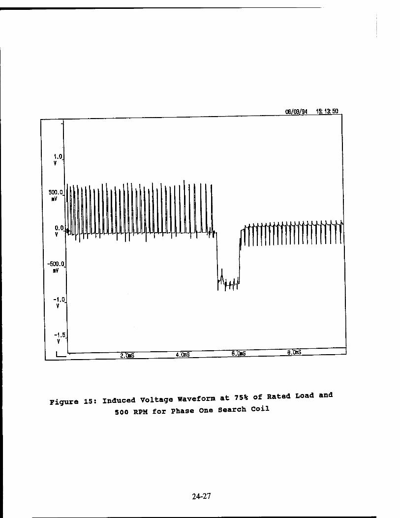
1.0 V
-500.0 »V
-1.0 V
-1.5 V
2 .OraS
W W 1
VH
4.0BS 6.0ms
06/03/94 15:13:50
^fWHffiN'
a.oms
Figure 15: Induced Voltage Waveform at 75% of Rated Load and
500 RPM for Phase One Search Coil
24-27
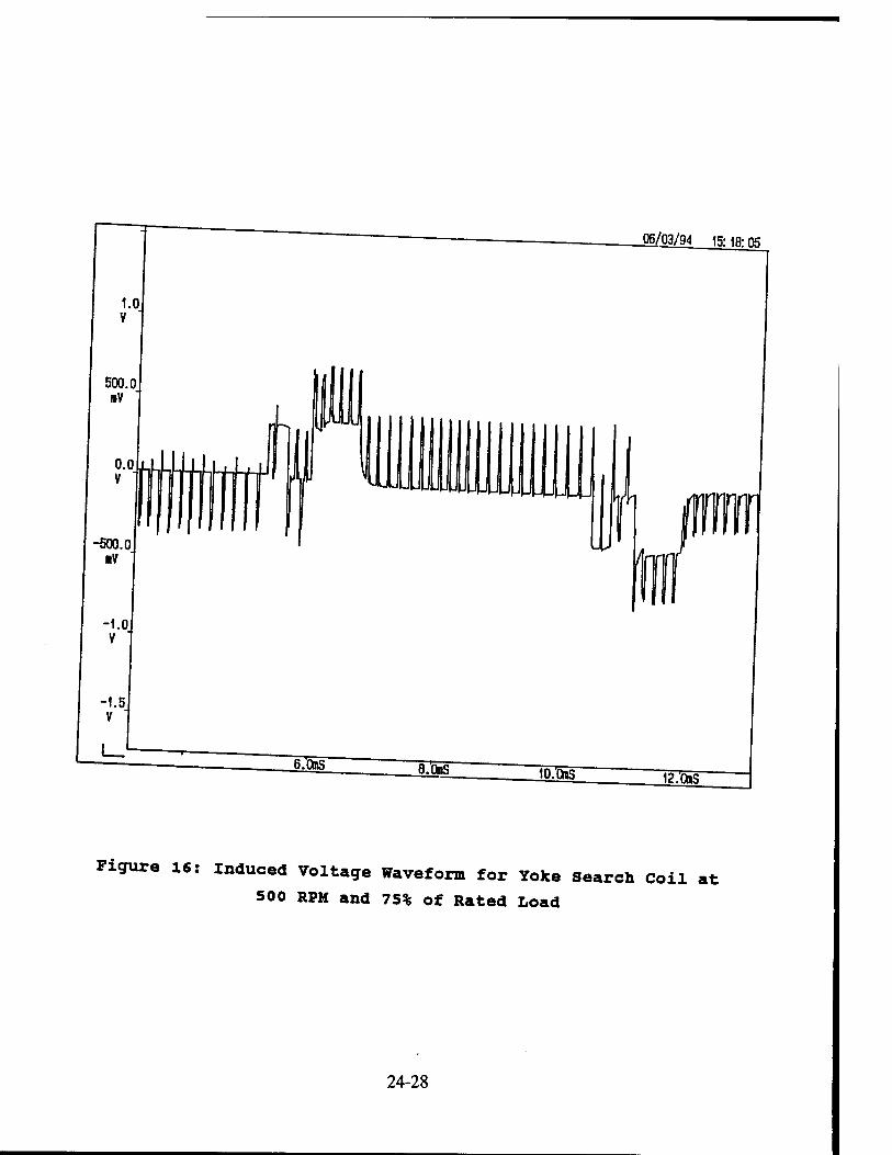
06/03/94 15:1fr ns
Figure 16: Induced Voltage Waveform for Yoke Search Coil at
500 RPM and 75% of Rated Load
24-28

(2) core Losses calculation end Prediction in order to calculate the core losses, accurate flux
„aveform at different location of the switched reluctance
motor is essential. Presently, effort is spento,.getting lu, ■FV.™ the induced voltage waveforms. Once
"Is IZ^, core losses calculation can proceed with
ease as shown in reference [5).
,3, Thermal Modeling of switched Reluctance «*« After accurate core losses data are obtained, effort will
he spent to get a decent and simple thermal model using
Tesistance and capacitor elements as shown in reference [6].
CONCLUSION
(1) The inductance measurement for the search coil wounded on
' ' Z yoke section does not have significant changes.when
^e rotor position varies. Thus it is not useful m
identifying the rotor position.
;/e inductance measurement from the search -- —
on each pole faces do vary cyclically when therotor
poles change position. It will be better to utilise»the
elope of those inductances instead of absolute values in
order to identify the rotor position.
With the limited no. of stator poles, the r-ol£«m
which can be achieved through the search coil might be
very course or limited. <,„,—«- W The induced voltage and deduced flu, linage waveforms
for the yoke section is guite irregular in nature. This
makes the core losses calculation very difficult.
(S) Tee induced voltage and deduced flu* linkage waveforms
(2)
(3)
24-29
for the stator poles are very predictable and hence pose less problem.
REFERENCES
[1] Lawrenson, P.j., stephenson, j.M., Blenkinsop, P.T
Corda, j., Fulton/ NeN## »variable Speed Switched
Reluctance Motors, IEE Proceedings, Vol. 127, Pt. B, No 4, July, 1980.
[2] Electrical Machinery, Fitegerald, A.E., Kingsley, c. Jr Umans, S.D., McGraw Hill, Fifth Edition, 1990
[3] Krishnan, R., Bharadwaj, A.S., Materu, P.N., »Computer-
Aided Design of Electrical Machines for Variable Speed
Applications," IEEE Transactions on Industrial Electronics, V. 35, No. 4, Nov. 1988, pp. 560-571.
[5] Lavers, J.D., Biringer, P.P., »Prediction of Core Losses
for High Flux Densities and Distorted Flux Waveforms •• IEEE Transactions on Magnetics, Vol. Mag-12, No. 6 November, 1976, pp. 1053-1055.
[6] Switched Reluctance Motors and Their Control, Miller,
T.J.E., Oxford Science Publications, 1993. [7] Vo, Lawrence, »Single-Phase PWM Inverter Using Mos-
Controlled Thyristor," Master Thesis, San Francisco State University, 1993.
24-30
Process Migration over a Network of Workstations
Dallas J. Marks and David A. Charley Graduate Students
Department of Electrical k Computer Engineering
University of Cincinnati Cincinnati, Oh. 45221-0030
Final Report for: Summer Research Extension Program
Wright Laboratory
Sponsored by: Air Force Office of Scientific Research
Boiling Air Force Base, Washington, D.C.
March, 1994
25-1
Process Migration over a Network of Workstations
Dallas J. Marks and David A. Charley Graduate Students
Department of Electrical k Computer Engineering University of Cincinnati
Abstract
computing jobs. maChmeS make Weal candidates to run additional
^Ä^ÄWf1 !!a graphical utiHty that *™intensive users to run processesonfdl 2? «f*™*™*** °n their network. DCM allows as evenings ZTeZZ vet 2£ -Ueagues during non-peak usage periods such periods Thi, k It ^ 1 retur\these machines to their original users during peak usage
L uspended on t K- T °f a pr°CeSS miSration mechanism that aUows programs 1o of suZnlt °* T T 'r! ^ *—P^ntly restarted on another machine from L "o^
ä: u?a e^rr ^^t^?^rmt—4ing to them LrU power otherwise unavailable
JÄ^T^uSzrsuch as mata—*°d ~* *«■£ worV nf «ülirr,r, n^„ i,- ^ , ^ vvlwii-ratrerson Al'iJ. DCM runs on a net-
^tn^^^T^D^?^-^ VerSi°n 4-°-5 °f IRIX' the SiHc0n Gr*s eratingTystem BStware DCM h T 7™ 'T** ™ modifications to the hardware or op- in the C++wir Thf K ^ ??*"* ^ obJ"*-°ri™ted techniques and coded enha«n^ load balancing. en™onment. Such enhancements might include fault tolerance or
25-2
Process Migration over a Network of Workstations Dallas J. Marks and David A. Charley
1 Introduction Despite the tact that hardware performance continues to rapidly ^^Ztl 72 use's a clL of users that are always unhappy with the state of cur«m^™ £££ such ^ ean be labeled as intensive users. Intense users tend to «^ 'ngrum, g p , simulations, around the clock and they are eager to And «Ultra.V°^fJe^ and weekend working environment, much of a facility's computmg «*»«=r»f«, tociorsTring these idle
not complete in a reasonable amount of time. Normally, a long-running process would
terminated without yielding any results. configuration utility that allows the dis- The Distributed Configuration Manager (DCM) is a connguration uu y
tributed processing resources of a network to be managed by both c^ua ^£^™ ^
Such a mechanism allows computation-intensive jobs to be started on mie y ,
m0ved when these systems become loaded by the, intended gusers ^^J^J£ of an
the machines become idle again. The ultimate achievement »that the^er r cannot
organization can be fully utilized, providing intensive users with additional pow
normally be found in their hardware budgets.
1.1 Motivation for Research
Process migration is not a new idea It has ^ — advanced features such as resource sharing, fault tolerance and load balancing unio *
plcTss migration mechanisms are built into custom °^fjf™^ Charlotte [2], and Sprite [7]. Using a custom operating ^^^^^„^ system that are available to run jobs; most users m an organization rely on »jta*d«d^ g y such as UNIX to run commercial productivity applications and are not ™^
operating system. However, if process migrat on can be ^^J^^Zers can system such as UNIX, average users may continue to run their applications use process migration to "borrow" their workstations
ordinary users will not choose to use such an operatmg y stem The3ondor D*
System [11, 9, 10, 3, 12, 14] is unique because .t ^^"^Z^steL is very f lUo TWTY Wnel i e on top of an unmodified operating system, ine ^« J AS £ -tain restrictions that prevent it from being useful m apphcatmn areas
25-3
by s^Ärräs^L,rd1,".be™to extend the types °f p— *—« with any process or set of p_ our font? " * T T^ migrati°a System «* «*. a Process migration ^'*«^S%£SZ^%&%^ —
1.2 The QUEST Distributed VHDL Simulator
pZnt cte telTa-lÄ ™gT t'1* C°tf Avionics Office at Wrigh, hardware for cockpit display generaZ This! ™ kT^ 1 '" M<1 ™ the ^ °f «««rf-H-ad generation transports and fi4Z MZ', n A f f'^ Y Stators ™« be nsed in next- The QUEST VHDL Simulator s a hi 1 Z " "A'^,"
tb* ^^ Tactiral FiS«<* M- execution on an Es-Kit ^^Ä" d-stobuted simulator originally written for
research [6]. Distribution and the Z tfo ' ^M * CmChmilti UndeI DARPA-supported performance than can Ä"ÄÄB °f « <"** Prides greater simulator has recently been ported to I Z l, f ?, ' " °n a Bmgle Proressor. The QUEST features of this port fnclude shied hb-f ?i'C°n GraphicS 4D »Nations [15]. The main interface that trLp^fc<^^l^fa
Il0?e s'zeRuction, and a unique message-passing
of local shared memory, ^ÄsS^T^ f* * ""* delivery!ystem [5]. * and b^RAMNet, a h,gh-speed shared memory networking system
Prodis :r:l:^:0r^:Lt ns orr;n hrreds °f S™M°» •>*<*. (ümx VHDL design lab has only ^Ä^ÄlS^^<!*^,," n"^' "" C°CkpH Avi™icS 0ffi« However, many other worksite UNK
tw?rk.st»"<»« «»» are capable of running QUEST.
used for real-time flight s!mu£^^ion stnmes bm 7 * "'T,' TheSe ^"^ m^ are A process migratio/system ttlHuppo QUE7Ttn oT^ ^ ""** ^ "^ Ws' during these non-peak usage periods vet !lsn„ 7 PfT max,mum use °f -""work resources fewer machines are »«,T*Sr?? 'hat emulations run until completion when capability to migrate QUEST simulator ohif f T, D'Stnbu'ed Configuration Manager is the uration Manage, supporte mim«™ !? J ""^ VerSio11 °f the ^«buted Conflg- supports migration SWKET 7*. ^V^^ ^ CUrrelU ™n «^
processes that interface to the hierarchical communication system.
1.3 Terminology
Several terms found throughout this report are defined here
execuTn w S£2 of^The nA*' "^ * !TSf™ °™ ™^ '° another during or host machine. A" oce ^»0^7 'f T™ mCOt« is k"°™ ** «» «^
Migration is performed by The D1butedS ■ T " "" ""S"1' process suspension, d^Apc^^^0^"^ MMa»er !" a three-step sequence of ing a process to halt its executfon ChSnni7' susP^'ou refers to the act of command-
state for later execution On, vsem ^ 6 " " P™^1116 that SaVeS the susPend<*> P™*» Restarting refers to the acTof starTn^ heT r?7£*" " & ^ k"°,ni " the checkP°« **■ process begins execution from Ät'of ^ t™ ^ ^ ^ "*"• '
On-demand process migration refers to manually-controlled process migration that occurs only
25-4

j- * i o A^r,aA Kv +>IP user These rules constitute what is known at the user's request or according to rules defined by the user, inese rm Distributed as a nolicv specifying which processes to migrate and where to restart them The Dwtnbutefl Zn^lLTuXi uses an" on-demand mechanism that is user-initiated with a graph«! user
inteWhl(tGheDistributed Configuration Manager uses a user-driven policy, it is possible»to ^tourf automated policies for controlling the process migration mechanism. Two examples of automated policies are fault tolerance and load balancing. Fault tolerance »a ch aracteri K of a system m dicating that it is immune to failure. A fault tolerance policy would be ™^h^.^^ machines that are about to shut down due to a fault, checkpointing ^V^^^^TEL inff these processes to new hosts or restarting them on the same machine after it is restored. Load bluÄtaE dividing processing requests equally over a set of machines usually machine
c^:Zt1ZioL on! network. \ load balancing policy would be «^^."^J whTmachines in a set were either too heavily loaded with processes <^^^^ policy would use process migration to redistribute processes on heavily loaded machines to lightly loaded machines to insure that each machine in the set was equally loaded.
1.4 Report Objectives
Manager to be easily extended.
1.5 Report Organization
stsftAj ssssss äI--ää
jectives. Finally, Section 5 outlines several directions for continuing research.
2 Background and Related Work
Process migration is defined as "the transfer of a sufficient amount of a £^^£^ machine to another for the process to execute on the target ma hne 20] It has
mfc atomechanism, provide a brief history of existing systems, give an overaew of the Condor Zributed Baton System, and analyze how the UNIX operating system stores process state.
25-5

2.1 Design Considerations
^^Z^^^^!^^^fOUr desisn COnsiderations for »* to satisfy these considerations for ounrnr
7 T"8 ""S^""1 SyStem and °Ur §oal has b^n Manager. ld^at10ns for our process migration system in the Distributed Configuration
• Transparency
strictious. Achiev ItanspaCcv m """l*«"? mÄ in «» network without re- that uses a spec«haa3TvL?Y m deSlgn trade°ffs- F°r ^'-<*. a process
because the ^tr^^^ÄÄ""* '° -~ • Minimal Interference with the System
ÄÄ^r*Ä ™e intefrence with either the i—^ 7 a Wh°le- The migration mechanism should operate atomically. • Residual Dependencies
B, the process shouid ^Z'Z^^t™ "" *» ^^ A '° *»*»
• Complexity
2Ä1^" Xf^Ä; a CUSt0m.0perfnS SySt6m SUCh - S^e- im- migration mechanism tends to hi 7 maJ°r T* °f ^ °Perating S^stem kernel [71- The kernel. meChamSm tends to be comPle* «ven when migration is implemented outside of the
is ^ol^^^^J^^^ ^/our ^gn considerations. In practice, it
goals of a particular process mk aül vl t V^ ^^ mUSt be made aCCOrdinS to the migration L**J^ZZZ^1^ t ^ ^ imPlementati™ requires that all Manager's migration mechanlm s trar, n 7 jf "^ kemeL The Distrib^d Configuration of increased complexity ^ansparent and free of residual dependencies, but at the expense
ion 2.2 Other Implementations of Process Migrat
ÄE^f ££^rr migriTEach of these — has its ™ ^ r, process migration mechanisms fall into two broad categories. These
• process migration inside the operating system kernel
• process migration outside the operating system kernel
This is
a.teruatives are autcLt^S Mu" re^r«. W'th Unm°dined ^ °« **■
25-6

This section presents the Charlotte [2] and Sprite [7] operating systems a* examples of process migr^n mplementations inside the operating system kerne. The Condor D ,«* Svstem 131 is presented as an example of a process migration implementation onts.de the opera mg
y'stm irnehBoth Smith [20] and Ankola [1] offer more ^V^su^^Z^Z svstems- the purpose here is to show the differences in design approach when kernel data, »teuctees S Sable to The migration mechanism (Charterte and Sprite) and when they are not (Condor).
2.2.1 Sprite Sprite is an operating system for a collection of personal workstations and file servers on a local !re" ne worM^Typical Sprite applications inclnde parallel compilation and^ simulation. The moÜvatn for adding" process migration capability to Sprite was the existence of .die machines on the network that could be freely used for additional computational power. T in
Sprite's overriding design objective was to provide transparency to the user, lransparencyin Sprftemelns hat a process's behavior is not affected by migration. Its execution «™™"* appeLTdentical on any machine on the Sprite network; processes have globa access to resource lh as files and devices An additional benefit of transparency is that a process's appearance to he est of the world is not affected by migration. Unlike process identifiers m systems such as UNIX
Sprite oroclses use global identifiers The system and its users always see processes running on theh »S host even if such processes are executing remotely. For instance, a user need not „hg ;^1 femote malhL to halt a process. Because the process appears to be executing on the
user's desktop workstation, the process may be killed directly on the ^J°™°^ daemon
A database of idle processors is maintained by a central migration server Load^^Toe processes on each machine notify a central migration server when "»f^"**^ ^ [die When a user requests that a process run remotely, this central migration server selects
"^^r^SlTXtS is automatic, the migration policy is determined by the nser Ptt^:tuiated from a home machine, typically on a user's desktop A home machi
execute until a new idle host is found. „w;™ ^r+v na^es of The Sprite migration mechanism operates by terminating a process and storing ^P^ °
the process virtual address space in a special file. When the process is ^^^^£*£ will^etrieve these dirty pages as the process executes using a form of ^^eZZ 3mues systems transfer the entire virtual address space to the new processor before ^* execution. Because Sprite delays the loading of the virtual address space, it can achieve
^hTTpTi'te operating system has minimized residual dependencies but not eliminated them AÄW»£ leave no residual dependencies on remote hosts, all processes have a residua tendency on their home machine. Some kernel calls achieve transparency by forwarding requests tThetme machine, such as gettimeofday(). Because of the residual ^cy ^ fj™ machine, users are unable to migrate processes to a new home machine m case of failures. However the Sprile system designers felt that achieving transparency was more important than providing
reliability.
25-7
2.2.2 Charlotte
^J^^^^ZZzr^TTdes!gned for —«™ with „i,
has bTS^ÄÄ Chf °tte USeS T/PeCifiC POlky for <"**>«■ *■—4 it The migration ««J^^^ÄT^ " "* """"^ migrati°n mech™^ premature cancellation o" migrat on PoH ' SUpP0rts,.concurrent ™Wpl«> migrations and modified to snpport research fdeaT *" "* " U"lltieS Md CM be ea^ <"*«• -"
taÄÄ^'^'Ä^IS.T^t0 tranSfe itS ^ «"»- *•»• Charlotte is easy to implement, howet! H r^^Ä" ^ ^ ™* "^
to ^n^e^Z^il^T and ,'he migrati0n meChMliSm haS ">~ <"*«• Therefore failure of he source St ? ffT '" "° ^^ ^«dencies on the host, process on that host ^ ** "^ the pr°Cess unkss « is communicating with a
2.2.3 The Condor Distributed Batch System
^^^t^^ti^z!:a proT m;gration facility **■* -d ***** - H/750 minicLput oTer ÄZff ? T ^ " '" ^ & "^ * VAX
platforms includL Sun3 Sun W HP PA ™n r^ ^ POrted t0 ten different hardware
Graphics 4D UNIX sys"ems As of hif w r °* ^ n^™0' °EC DecStation' and Sili<™ version of Condor tha" 2^.tZ o^PVM^U * ^ ^ DE° AIpha madlineS and a
are under development [13] P aM ProSramming environment, Condor-PVM,
n^^l^^ Zfh^; us"6' r baSiC.Cat^eS * ~ users: casual quently do large numblrs 51 ti^ i- f^' " mtenSiVe' US6rS are "PeoPle who fr^ happy with jJt a workstation WT ^V"',0"' 8eMche8- TheSe Pe°Ple are alm<^ never Unhke the w^dcZ^J^™ ^ ^ P
°WGTM
^^ to meet their -eds" [3]. hours a day. occasi™ally heavy users, mtensive users often keep their machines busy 24
to saS fy^i TJs^t^z:^ s:lfe rer from casuai and °"iiy h™y «• workstations in the locTnl^oX M! f™ T^" ^ aCtlvity °n a11 Participating resource pool, or processor banThJ^ t , "? determined to be idl* *» Placed into a they become idle STve when busy " & dynamiC "** ""**•*»■ ^ the bank whan
Features of Condor
Condor has been designed with the following seven design characteristics [3]:
1 ^^t^rs^tumx ^ ™s ■"«■—* *•>** <° 2 JäJSä&ä :K^Iä-ä
UNIX
25-8
1 The local execution environment is preserved for remotely executing processes using a shadow 3' prt tchan'm A shadow process runs on the local machine and^executes^ug
system calls on behalf of a remotely executing process. Shadow processes are necessary t he remote environment is not identical to the host environment. For example, machmes m Cerent time zones or with different flle systems require the shadow process mechamsm.
4. The Condor central manager is responsible for locating and f™^*™^™^ dor users do not have to search for idle machines, nor are they restarted to usmg machmes
only during a static portion of the day.
5 Owners of workstations have complete priority over their own machines Condorremot^y executes processes only when an idle machine is found. When an workstatron s owner et- to reclaim his or her workstation, Condor will automat.cally move all remote processes bacK to TZtlZmlo: to another idle machine. Condor's operation is transparent to other
system users.
6 Users of Condor may be assured that their jobs will eventually complete. If a user submits a fob to Condor which runs remotely but is not finished when the workstationowner returns, the job will be checkpointed and restarted as soon as possible on another machine.
7. File systems of remote execution sites are untouched *™^.^^^£!^ Condor from cluttering up private disk space. This problem can be eliminated if a transpar
ently distributed file system, such as NFS, is used.
Limitations of Condor
Although Condor is a powerful environment, it does possess limitations [3, 14]. These include:
1. Migration is limited to single-process jobs; programs that use the fork(2), exec(2), and similar
calls cannot be migrated.
2. Signals and signal handlers are not supported; programs that use the signal(3), sigvec(2), and
kill(2) calls cannot be migrated.
3. Processes using interprocess communication (IPC) cannot be migrated; the socket(2), send(2),
recv(2), and similar calls cannot be used.
4 All file operations most be idempotent. IW-only and write-only ^ ™ wo A «£*• but programs which both read and write the same file may not work. In addtfon, memory
mapped files are not supported.
5 Each Condor job has an associated checkpoint file that is approximately the size of the process fddressTpace. Enough space to store the checkpoint file must be available both on the host
and remote machines.
6. Processes that use shared libraries cannot be migrated.
Many programs do not require these advanced operating system features; however 1J^ Matures should be supported by a process migration mechanism if it is to be considered universal. The SutT^iguratL Manager demonstrates that the Condor migration mechanism can be extended to support shared libraries. It is conceivable that extensions could be made for better hie
and multi-process support.
25-9

2.2.4 Discussion
Manage, migration ^3Ä^^»Ä t , * "" DiS'ribUted Confi^« because kernel data strnctures^hat stot nZ , k<™el Presents some challenges, particularly modification also limits "otn7^ZT0t be ^—d or modified. Lack of kernel
is apparent from the an Z isTspriteJd ChaM? "" "T I*fann»»- H—. » not solve all performance problems """ eVm m'«rat'™ V»terns in the kernel do
2.3 Basic Components of Process State
In general, process migration ^^^[1]^^ ^^ " ™ * ^^
1. Suspension of a process on its original (source) machine.
2. Transfer of process state to a new (target) machine.
3. Resumption of execution on the new host.
of the!0«'TrecesT CSÄt ■ """ft 7* ""*■** «* «- the Distributed Configuration MaT^rT n " USed by Condor md modi^d for Because the migration2hai^tfno bnT't T" " ^'^ °n '°P °f the UNIX k—'■ obtained without illegaUcceTto!teZ £ to, . """"""S SyS'em' process state must be be determined *^£Z£CZ£?? data structures When the process state may not
forward the state to the tar«f or T-T m '^ the S'ate °n the source °^i« «rd
computer process: g y (7] 'den"fy flve «™P°n«*s of the state of an abstract
Virtual memory
Process execution state
• Open files
• Interprocess communication
• Other kernel states
These five states are examined in detail below.
2.3.1 Virtual Memory
2äÄ^£ ra trzz'iTr(text) and data that a ~ «■ ^ text is stored in an a.out o, exe u abl file Most UM? ""f' * ™K ^^ the ~ System V COFF file format In action tn\ M"' UNK ^Fomentations use a variation of the
Prior to system «xacutioT^ "T^ ^ ^ C°ntainS initialized dat* is stored by the UNIX ^J^^^^901 ^ * *?T
P°int °f ^™ «"**** in Section 2.5. VlftUal memory under UNIX will be discussed further
25-10
2 3.2 Process Execution State
p ogram count5the condition codes. This information is needed when a process » saved TdrSored during a context switch. Although this information is hardware specific and the Distributed "configuration Manager, migration mechanism permits noffiega access^o kerne data TTNTX orovides a set of user-level routines for preserving context: setjmpU and longmipu- i Sn system cal preserves the process execution state and longjmpQ system call restor s a rPÄVa pLo«. call toLjmpO. The benefit to the process "*^*£*%^£
a though these system calls deal with system-specific data, they must be ported by the OS vendo as parf of the UNIX standard. The use of these functions may be found in any UNIX systems
programming guide and are not discussed here.
2.3.3 Open Files ,5.0.0 wpcu * «vu
According to Ankola, "information about open files is one of the most difficult l*' <^"H Piece conformation to transfer" [1]. A process must store state information for each.open^ The sta e of an open file includes the file identifier, file access pointers, and any cached blocks of
ä: 'se—riutr noV^pÄ z^zzz it mtdX m^nUmpementation of the Distributed Configuration Manager a so *«-<*» «ItuPPort Supporting open files increases the complexity of the process rmgratron and^ reduces LTperformTce of the migration system. However, the open file mechamsm could be added to the basic system at a later date if such support is considered mandatory.
2.3.4 Interprocess Communication
Tb, «Ute of communicating processes is difficult to define. At any given time, a process may be
SdfficolumcTon datf, «'^^«•^^^^^^T'^^M Z ,„rnProcesses is difficult because most of the communication state is known only to the operatmg Item toSffi addition, a process that is migrated while sending or receivmg messages may no TZZZ properly because the entire message cannot be retrieved. Because the state of the .irffication system is difficult to obtain from outside the kernel, m.gration systems such as C "do not support, communication. However, many research operating systems have been constructed with process migration as a goal; however, designers of such systems have the luxury of rlpqiffnine and maintaining kernel data structures to aid in this task.
MkSn of communicating processes outside the kernel can be achieved through he use of a u^Tcomminication package. Unlike gating system coning as sockets and shared memory, a user-level communication package provides the migration system Srner wiTh access to its own internal states. In addition, the user-level package can be* unlike the operating system. Migration of communicating processes outside of the kernel has been
25-11
*. Co siPLrapuL ^^;^^^:^^^^^^^ * 2.3.5 Other Kernel States
SÄSä^äTSS' witVrh prrs such -the p— id-tifi«. - source usage informat on In the S« T ™ ' ^ "^ amJ handIers- ™d re- kernel, this state dataTs' iSTiT'Ä ^ <hat functi°°s »«* of the create a new correspond hHIteo. r'hf T '"t"" ^T' iSn0re tWs kernel sUte data «>d
For example, a migrated VNutoc^Jnu T' ™S reSU"S ia S°me loss °f '^sparency.
is different fa» tKSST I ""T, * T Pr°CeSS identifier °y "S MW host that
process that needs o accesshe nWdJZT t h 117M' " '°St b— «* °"» Her. In contrast to UNIX taspZcv for „ TV/ "^ "^ °f the "eW pr0cess iden«- system becanse v°cJ\£Z^JZ^£T? " uT' " "" Spr"e °^ti<* consistent process identifier dnringZ eTuttön "* ^^ " ^^ m^™ a
2.4 Process State in the UNIX Operating System
Configuration Man^rmtgraLn»S,ZLTT'^ ""■*? ",PP<,rted ta "* DiS'ribPted
space. This ^dÄ^C^/ÄS"'! Pr0CeSS ViltUal addKSS
format for storing program debuwin, d.t» A i Uu ,' for storm« Programs, the core COFF and core formal"ITS i'"' ^ h°W. b°'b formats suPPOTt *^ed libraries. The
2.4.1 The COFF File Format
^FW v ÄÄSf ÄF^T dtitim for the slracture °f aU that represents object files executibVfil j Jefcution describes a complex data structure
M^ÄÄS^ä Siiicon Graphics caIls their UOTx of the basic COFF file format of UNIX S^stemt." ^""S """* " M enh»~men*
The Basic Elements of COFF
execntlowSC^Ä"soff ? ^ " ^^ ^ "> """ ™WP* system to protect uHLTfi^L^ ^ 'he ""T" da'a *" a"°WS the °Perati»« contains vaLs tta»rtZÄ|" " f^*"? (-ri'e-P-^ctio„). Initialized data
is not write protected fike the texttl K, 7 t T"" °f " Pr°gram- The !nitWized d^ of the program. UAi S 2'""Z " ^ TT ^ "^ d™"« the e~™«°» to specific values. UninitwtdTatJTs not * T ' ^ ^ If""011 SUCh data is not in!tiaIi^ operating system must ^X^Ä-ÄJ W '~' *«
25-12
The COFF format organizes all three information types into individual areas called sections.
They are named as follows:
• The text section contains machine instructions
• The data section contains initialized data
• The bss section contains uninitialized data
The text section contain executable machine code and the °*^*£^^^ protected The data section contains initialized program data and is readable and writable The Csection does not actually store data (because this data has no initial^^^^ the size of uninitialized data. It tells the operating system how much ^.»^^0^^ for the executing process. The bss section is generally made contiguous with the data section wnen hetoXbloaded into virtual memory. All UNIX systems initialize the bss section to zeros "^teTm virtual memory. The bss acronym comes from IBM mam frame terminology; bss means memory Block Started by Symbol, a block of memory that is not -t-liz^
The COFF definition also specifies a symbol table and a string table. The symbol table s
used by high-level languages, such as C or C++, to store symbols ^ " ^™^^£ names These symbols are invaluable during the debugging process. The string table is used m coTnction with The symbol table. It defines symbols that exceed the eight-character limit of the ÄSSetLt. Because the symbol and string tables are only useful *^£^£ UNIX implementations provide utilities to strip the tables from an executable file to reduce the program file size. This operation is generally performed after program development.
The Benefits of COFF
The COFF definition provides the UNIX system with two major benefits: enhanced portability,
and system extens^ ^ ^ ^^ ^^ b ,h
specifics of a hardware platform and the basic fundamentals of a software program. Machine SI vary from machine to machine and even data can be stored m dufe^t formes (such as Uttle-endian and big-endian). COFF minimizes and localizes the, amoun. o machine dependent code in different ports of the UNIX operating system. Most of the porting work ot the U1NIA ope a^g syLm Lolves changes to the C compiler code generator assembler, *f^£* few localized areas in the kernel such as the program entry/exit, system cal service, and mte rupt tables [8]. Enhanced portability also aids process migration, as will be «*^^j^ all UNIX variants follow the basic COFF format to varying degrees, much of the code needed to perform migration can be reused when porting the process migration mechanism to different UNIX
PlatThremCOFF definition also provides a framework that allows for system extensibility. Additional sections may be added to the basic COFF definition to implement features exclusive to a particular versZ rf UNK or to take advantage of the underlying hardware architecture. For example the
SÜ on Graphics IRIX object format [17] stores initialized data in ^^*^^j£ one. These are the read only data section (rdata), large data section (data) ^amaU^tase^ (sdata). The IRIX object format also stores the bss data in two sec ions These a****** tarted by storage section (bss) and small block started by storage section (sbss) This additional suasion of sections allows the linker to localize data by its type to enhance system performance. A diagram of the IRIX extended COFF format is shown in Figure 2.2.
25-13
Unfortunately, while^^iTanced nortb^v ^ "£*** f m-hi-»dependent data formats. of process migration the ab 1 tCfhttThtcOFP Tf^% "■ *"/*>***•>** ^chanism pointing mechanism'and rJL°^^^^^^^^^ ^ <^
2.4.2 The core File Format
S: "ü % nZ^z 1-a tern inrprocess when ^ °f""- «« quit signals. The PvoZZ2^L° ' ^ mstmcti<™' ^ «™«. «d user-generated early mainframes Tat^4^^?^ ""* 'n^"™ " * CMe dump' a hoIdow *»» to- state of a process when tIrXt'd inZ fiT A ' """T °f 'he CMe imaSe is »° *™ ^ examine both the origTn ä Zit'f- A pr°S"W a «""»"« «ngger can then wrong. * P S ™d 'he COre ma«e and *» 'be user to determine what went
ÄÄÄ: dmage istdted by <coreouu>-The «• fo™at *»
»ay, Ä^^^JZ^SyU,e ^ ^ ^ "" »" «^ «*<**
and length d.'«torfS p oceL aUhe t me^h ?' f ^ 'S? <Wa- the VirW address
core image at the file location S„ 1 ° * f"6 dump- The map data is Pres^t in the The procL J*2n£ZSZ,^Z «escnptor only if the VDUMPED flag is set in the map.
the COFF file such as tawZ^!,^ m "* "** ^ wMe data availabk'» possible map types that may be stolt I^ore ^ "* " ^ ^ "*** *" *»*»'
• VTEXT text map (not normally present in core)
VDATA data/bss map
VSTACK stack map
VSHMEM shared memory map
• VLIBTXT shared library text map (not normally present in core)
• VLIBDATA shared library data map
• VGRAPHICS graphics hardware map
• VMAPFILE memory mapped file map
maPMc:i;L?;df:At\Ttl^adTe8serd is *?£in the corc imase-For insta^ "* **•/■>-
execution state T^^Ubl^T ^"^ P™«*8' The sta<* map contains the process to restore the staeotyÄ Configuration Manager do ,T~2^f * """^ Alth°Ugh C°nd°r Md the touted data is available in the core taaT Mech^ V*^^ mem°ry mapped fiIes'the ^ way that «^«d^^^^^*^ da'a> «- - -
25-14
•
•
2 4 3 UNIX System V Shared Libraries
iD In ftTuMXsystem, common code libraries are typically stored in archive. An archive is a
examples of archived libraries on Silicon Graphics systems mclude the GL gr»P^» ^ " Font Manager library. Again, these are libraries that are used by a slgn,ncant number of progjam.
Improved system performance can be achieved by storing common hbrar.es suche. the C hbrary
in a manner such that only one copy exists on disk and in P^ "T^^tT^ A shared library is »a file containing object code that several a.out [executable] hi«>™* simultaneously while executing.» [18] The current shared library unplementatron ,n IRIX ,s based
on System V Release 3 specifications.
Advantages of Shared Libraries
A shared library offers several advantages over simple archives by not copying code into individual
executable files. It can:
• save disk storage space Because shared library code is not copied into all the executaMe «- ft- « *• «£ programs built with shared libraries are smaller and use less d.sk sp^e Jto not ^ly saves TpaL but requires less I/O activity, a major performance penalty m any computer system.
• save memory By sharing library code at run time, the dynamic memory needs of processes are reduced. Again, I/O activity is reduced by reducing both paging and swapping activity.
• make executable files using library code easier to maintain Because shared library code is loaded into a process' address space at ™ tim* a shared library may be updated without requiring updates to all of the processes that use the shared library. Such updates are not possible with standard archives; updating a standard archive
will require all programs using the archive to be relinked.
Organization and Operation of Shared Libraries
into the executable. The target library closely resembles an executable file. This file by operating system if an executing process needs a shared library.
An executable linked with a shared library will contain a special section ca led lib that defines whii shTredÄs are needed. When the program is executed, the operatmg system will use
25-15
™ Private ^^(SZ^^^J^T**" "^ ""* ^ "" B1»^lu» ita
the target library). Processes Tat s W 7 I A t" SpaCe that mirrors the d*"> section of not interfere with one Toother Thettl ^ * ^ ^ Stack *"» s° that "><* d° can share its text bot noTtdafA ? ' ^ ^Ä t & ^ "^ <* "
the symbols in he ioA^J^^T"^ , M .T^ " leVd °f indirection betKe» with absolute addresses thaHo Zchant? "XeC^- A b™<* ^ble associates text symbols
a jump instruction toflÄÄTl^«^ ! " ^^ ^ ,dd~ laWs
aUows the shared library toTZatedL ht« T VJ^"1 The USe °f the brancb <*>* recompfimg applications tLt"e the itdl^ " add,"°n °f ^"^ ^^ «^
Ä Stnrnthin1 tÄ Ind^t ^ "^ ^'^ l"° ^"^ ««»• *° information: the addresses oT'theJ .! T"0113; The Ub SeCti°n COntains ^ rel°^tion tail section is alway^HS routmes Unlike the standard COFF definition, the
the only part of ^ZJ^J^^^™™££ Z^nt" ^ "
ou the initilation coTjÄrÄÄ^ ^ SeCtiM ^ ^ '^ "^
Building Shared Libraries
-A Ä2S rs KSÄrjsr- sr^ • Choose region addresses
• Choose the pathname for the shared library target file
• Select the library contents
• Rewrite existing library code to be included in the shared library
• Write the library specification file
• Use the mkshlib tool to build the host and target libraries.
theÜVntary design- " "" ^ d™tati»' S^ -—nts « placed upon
1. Fixed virtual addresses must be specified that do not conflict with existing shared libraries
2' SVSem teSt:ttaiy ^ ^ ^^ ^ ^ <""* ^ ™^ 25-16
3 The most difficult step, from practical experience, is writing the library specification file The proceTof building a shared library is very tedious and, not snrprismgly,» the source of most
of the limitations of using shared libraries.
Limitations of Shared Libraries
Although shared libraries provide many advantages, the current ^pteneatato b- a nurnbex-of disadvantages The first limitation is the requirement that shared library text and data reg on i^Äound to a specific virtual address. These addresses are statica ly £^£*£ references to shared library procedures and data may be resolved at link time However, conflicts ^Tifltftw« developer chooses to use two or more shared libranes ^-^ that require the same virtual address space. In this case, one or more of the shared libraries must
be rebuilt to exist at an unused address range. i:uralw tW are This problem is alleviated somewhat by the second limitation of shared libraries, they are
between a library reference in an application and the actual lo^ira;f1,t
b^^^^d for lihrarv The branch table is provided as a convenience, as a shared library can be modinea xor !^ttagfc» wUhout requiring programs that reference the shared§ ^ary to be "compiled. However! the creation of the branch table is tedious given he current state of shared librarv tools The tedium of shared libraries can be eliminated with better tools. 11 Se h d Umitation is that the location of the shared library is ^««"^^chm that use it. This requires any user shared libraries to be stored m a fixed location. A much more flexible svstem would allow shared libraries to be physically relocated. ,...
The fourth iLitation is the difficulty of using imported symbols. If a unction ,n a shared lib ary uses the printf() function In the standard C library, the prmtf ) symbol must be redefined wtth a rlummv svmbol to avoid symbol resolution until the final link step.
FffijfyThe most significant limitation is the inability to create shared libraries usmg he C++
this utility was obtained from John Wilkinson, its author during devel°Pm^^^^^
»„„ r UKrarv svmbols it finds in the shared library objects. C++ library symuuis Sefin3Tb7thet ed ifbrary builder; however, mkCCshlib displays an error message for any unddmed C++ library symbols with explicit directions on how to perform redefin tiom
MaTy of these deficiencies have also been resolved in the newest «-^™2b system/System V Release 4 (SVE4). SVR4 and its shared library implementafron are
section 4.
3 The DCM Process Migration System The process migration system in the Distributed Configuration Manager consists of two components: le Migration Policy Manager and the Migration Server. The Migration Policy Manager uses user
25-17

X^^P^^^Sä011 Trgi G
MUI
(Graphical user interface)> ™*s policy used by the Ug aITm^uT ^ t* ^S^™ SerV6r- This Section outlines thf the Migration Server. * ^ "* ^ °PemÜ°n °f the checkpointing mechanism of
3.1 The Migration Policy Manager
Network CO^MTZZ^JT . * r f"" SUCh M "' Each miÄ »^in «* such as the nuler 7proe ^and 'Zl T" f ^ ^^ "S PerfOTm— characteristics processes. H^J^ZtZ^gggg' *?. ™^™'^ to run DCM Configuration Database needs to h!T J-fij , c SraPh,cal USM interface. The Network
network and tJeZZ^tchasten " ^ ""^ ™ ^ °r "B""i ^ ^
Thi Jn^&est kntna:lMtPD] ""^T *•" °f P™ *" « Capabk °f ^ra'™- as a migratL PoTdl^e ^ ^MPD ^TS^ ^ " TÜ^ ^ pool entry is known as a migration candtiate Tjh JpnPT represented bV a S1™« ™gration of the process, its name fte fu „„t W t f . c ^ C°ntainS the UNIX Process id (pW) on. Like the lÄÄL1,t T .7 "* ^ SyS'em' Md the procesSOT » »**■ however, its existence nf "ranZrent f r ^ ^H™ P°°' DataW is stored as a «** «^ Network CmBg»^ ^3^^™^ ^ I^i1»*«»1 Configuration Manager. Unlike th
ent.es ^SÄ^«'!-^ d"'» "* "~
1 S&Tä: Lt"for migration and initiat-the p°^ M-i- «*« the
-ckpointfiie ca^^^^^
5. Once Slayer has completed its checkpointing procedure, the Policy Manager uses the NCD
Ä'-l^X-a target-Tte"the MigratL s™wil1 ™ 25-18

6. The Policy Manager returns to step 3 until all processes are removed from the invalid source
machine.
7. The Policy Manager returns to step 2 until all machines listed in the NCD have been checked
for availability.
The Migration Server is currently a single-client server and is part of the Distributed Config- uratln MalTg r cetral process. Future versions of the Distributed Configurate Manager wffi
cTuin "Sple-client Migration Server This will allow »^*^^ ™ Mgr t o „. roDV 0f the DCM graphical user interface, to request migration. A multiple client migrau S^eTÄ aSow the connection of other types of policy managers that may provi^ different oofides such as fault tolerance and load balancing policies. A proposed design for the multiple- dtrmigration server is presented in section 4. Fault tolerance and load balancing are discussed
in section 5.
3.2 The DCM Migration Mechanism - Overview The checkpointing and restart mechanism in the Distributed Configuration Manager is an en- l^nt7llgone found in the Condor Distributed Batch System but :t offers a number of
improvements. These include:
• Migration of processes that use shared libraries
• Migration of processes programmed in C++
• Upgrades to support the IRIX 4.0.5 operating system
. Increased performance by using NFS to eliminate need for file transfers
. Direct, rather than shadow, execution of system calls to reduce residual dependencies
. Object-oriented software construction in C++ to support the addition of extra capabilities
The heart of our migration mechanism is a procedure known as checkpointing As defined by
rlS™—ffleTd Hs'teLage1 ™^^M^*» «***£& th ouTthe use of portable UNIX system calls. This section will descnbe the operation of the DCM ÄÄ», which is an enhancement of the Condor checkpointing mechanism. Ch "Toned earlier/the state of a UNIX proems includes the contents of memorthe te*
data, and stack segments), processor registers, and the status rfJ^^-J^uTfiTto is easy to retrieve because it does not change and it can be found in the executable «'»•>-<> files aLin ended to aid in the program debugging process; however the >?*°?£»*** aebuTa Process and the information needed to restart it are nearly identical. Dati fc°m the cor file is copied into the new checkpoint file according to the semantics of the COFF formari Ihe sUck is dso retrieved from the core file, appended to the checkpoint file, and restored dunng h^re art Process The restart process is explained below. Restoration of the process execufon
tat T isTssed in section 2, i! difficult because recovery of ^^^^J^ registers and program counter varies among hardware platforms. Fortunately, UNIX provides ;:gneric pairoSmes called seri.mP() and longjmp(). These routines allow system programmers
25-19'

EÄr Iää'ä sf r r rIIy us:d <° jump <°«-» -«'«• internal hardware registers aid the „™ f«k frame with a current stack pointer, the
^t the checkpointing „Ä^^^JT ^ ^Ä ^
tbelooMrÄ™^
second component ÄSÄLÄlirrm t^T * "^'i011 C"dM*** Th* the migration candidate beginsTxecutbn The ho7"' Mlfatlon oc™rs - "«ee steps. First, handlers for checkpointing. Second^ the SWx ,,tT, ^ ^f eXeCUteS *"*' Se"in8 »P ^al begin the checkpoint sequence3 cZj. T ,lhty
4Sends the miSrati« «»didate a signal to
source machine^hirdTcanLa fwU^hetSd onTe'n 7^ T ^^ ™ «• migration algorithm. Once asain the h,w ♦ reStar;ed on the new tarS<* machine selected by the on the new machine. A^Sa^^^ «" ~
3.3 The DCM Migration Mechanism - Detailed Description
SSÄ^^^^^ °f the DCM ***» Mechanism. In general, process
1. Suspension of a process on its original (source) machine.
2. Transfer of process state to a new (target) machine.
3. Resumption of execution on the new host.
These steps are presented in the order of their operation.
3.3.1 Process Suspension
program startup, remov^hemkratoL^T^I^?0 "" Migrati°n P°o1 Databas« »P« termination, and set u" £Ä? ?T,?" ^""'O"
P°o1 DataW uP°n «*=«*1 ™e bootstrap module requT^^^ program must be linked withThe bootslln J 7 m°d>fi«t'°ns to his or her code; however, the
the Migration Pool Diabasis Mv£ £? ,? TT* a migrati°n Candidate- M°dify™S here. tllVla1' Se"mg UP the sl«nal •"""<"«* is not trivial and is explained
*Ä"ffaS" rimttelylinkedwithaflkcaIkd-»-«««-. contains initialization codeTXextlbk'r ^ri" T'.T "" ""^ The "' °bJec' fil* linker to use the symbol main », ZT♦ ? ? T °"e °f 'tS funCtions is to inform «* P™«ram that they must alwa" wrUefuncta in the ' T?™- ° ^ °++ W»J» know To build a migration clndTdate the b„k "T^ "^ main() tha* is ^^ ««»'«I «**. Ale, which is clued 4^S t^ ^V T?* ** f "' ^ crtl.o whose only difference is tW tfeT lmPlemf ta«on- The file mycrtl.o is a modified copy of
name is arbitrary; however h D s ribu^Tr^1 *? ^ ^^ The rePlaCement s^ol ever, tne Distributed Configuration Manager (and Condor) use MAIN for
25-20
simplicity When a migration candidate program is executed, it will execute the procedure MAIN() Sad of the usual main(). The MAIN() function is included in the bootst^p moduk-; which a migration candidate links with. In addition to performing it. mitiahzation d^?J^0^^ the user's main() with the correct environment (arge, argv, and envp) and return the correct return
value from main() upon process completion. h The initialization performed by MAIN() creates a slgnal handler for the TSTP^signal Ihe
TSTP signal is the terminal stop signal. Its original purpose is to recognize the proces, su spend key from the keyboard (usually Control-Z) that stops an executing process Because migration £ a snmiar purpose, a custom TSTP signal handler is used to inform the migrate candxda to suspend itselfVche'ckpointing. The TSTP handler saves the current process execu -i .Wem the process virtual address space using setjmp(). It also sets a global variable res ar >TRUE Then the TSTP handler sends the process the QUIT signal, which dumps the core ( equired tor ctckpoting) and terminates the program. Once the process has termmated, the Slayer utihty
may be invoked to produce a new checkpoint file.
3.3.2 The Checkpointing Process
The DCM checkpointing mechanism is a separate process, called Slayer. Because Slayer » Beparate I can b!finvoS directly from the command line or from inside another process using the remote
shell (rsh) command, as we do. Slayer is invoked as follows:
• slayer <process pid> <source file> checkpoint file> [core file]
The process pid parameter is the UNIX pid value that defines the specific P^ess. The, source file paramete^^s the name of the file which contains the text to be used in the checkpoint file. It is tZZeZ^ the original executable file, although textcan *^*£g^ checkpoint file as well. The checkpoint file parameter » the desired ^.f*^^^^^ alway! name a checkpoint file <original_name>.ckpt for consistency. Finally, the core file paramete specifies the name of the core file to be used. UNIX core files are always named core ™Z™^S
K!Ät created them. However, all of Slayer's file name arguments must be specified
WXtUfiPrf sends the TSTP signal to the migration candidate, t^P^-P^^ process pid. The migration candidate is also known as the victim. ^™TP^^^ the checkpointing mechanism in the bootstrap code of the migration candidate The TblF sgnal
Wtr will calUhe setjmpO function preserving the ^^^^^^^ frame contents) in the process virtual address space. Then, the TSTP signalj^r ^ KILL signal to the process, suspending its execution on the source ^^^^^J^
After the process has been terminated, Slayer will build a checkpoint file using the source me and c re fit specified. Slayer retrieves the text section and symbol tables from£~^ and combines them with data from the core to create a new executable file the cte d^ffl^Tto
original source file sto,d j^^^
ZtäZ^E^^ —dig to the location of the P-—^ -
the process was terminated. Unlike ^°ffj^^^ £ £ Tecton has ten save space, a checkpoint file has no uninitialized data. Alter execution, tne sectionin
initialled in virtual memory to values that must be preserved for f^^^ a Teckpoint a checkpoint file will contain a data in addition to its section header. For this reason, a checkpoint
file is substantially larger than its original executable file.
25-21
core file Ip^t llZl"^^ ^T "'^ "" ""* ^ ™p <™ *> The stack data map section Inot n^ottento'£,^T^-"" ^ * "** ""* ^ module contains code to retrieve the sta'ck data Conresterf ^ h°WeVer' "" ^'^
3.3.3 Process Restart
^SrX* Indtatt fik 1S reStarted The b— d-- Pool Database. Beeanse the J^T^S^ti^ ^Tt ^ ^ 'he Mi«ration
bootstrap code recognizes that it t 1? .• , It Previously by the TSTP handler), the that causes a custom ZJhandler to *"™tm« *» "* flrst tima -d ^nds the process a signal
the slayer applicatio" ifato ™tt' tfiTt ?f """"V?" ^ ^ map ttat ™ —d by of data have been res o ed l„ne " JTi, tl fr™\Saved from **J*P()- Once these two pieces
will begin executing wTh 'its oHstEkZt d U J .^V'T *"* "«""'O- The ~ successfully restarted on its new ho^ ^ A* "* P°in'' the process h- been
3.4 Migration of Processes Using Shared Libraries
s«Wte^ 'he migration ofexecutab.es that use
performance. Extending the IZoS T" T" SyS'em reS°UrCeS Md increas<! ^em important class oi,^^^^^"^ "* *™ ^ ' " ^
-t^^^S^LtS P-formance by saving dish space, saving memory,
on dish and in memory for Teh pro"«' thä t & ^ t™^ ""^ that is duplkatad h°^ shared library. Although the text ofasW^K u
arch/re''here is ™'y a single copy of the
copy of data associated wth he stred ll ' 7 "" ^ "* Pr°CeSS mUS'We a p™te
the text and data section of ashtld I'K ^ TvT miSIat'°n mech™^ ■>»"* recover both standard text and data ^ mUCh hke the m«**™™ ^eady used to retrieve
The other section M ™n ^rT r """T?" ? "" Shared Hbraries used * "* P">S™n execute, the system loLderu^ ™ " - v ' ^ '^ ^ a pr°<*SS ^ * them inio memorTandtS.Ä* T,, * SeCti°nS 4° ** "" sWd "• load
begins execution. Vefoe^PecSa;!?' ThlS.pr?C,eSS °ccurs automatically when a process
When a process executes' shared ibra^y tex Twill! 7^ "t ^t **"" '^ text; it merely exists at a HiffjT. •i fj Ute m an ldentical manner to standard
variables in the shared librfwfielt T™ " '^ "^ addreSS S^ G1°W (*«ic) the shared library) whilautoma ic ™ H T^ I"00" (spedfled durin« the «"*« o regular process stl^T^Z^» U » ? ""' ^ '^ ""' be Created « «« mechanism. However the Iba Tt > u c* reS'°red udn« the current ^ "trieval data is placed in 0^^^^^^*°™^ ^r^' FOr deb^ purpo-s, this
To recover this daU the booteträn res 7* °f ^ V"BDATA a1«« ™th its virtual address.
vU.„™ „, „, .'^ssÄSteKSÄ 25-22
For instance, a program that uses three shared libraries will have three ^^£*£». £. file. If no VLIBDATA maps are found in the core file, rt can be safely assumedthat ^P^ not use shared libraries and the restoration process is performed normally. If VLIBDA1A mapJ are founlthenip1 header is searched for the virtual address of the data section . *kng»^ and its location in the core file. The data section is read from the core an1 copied nt ts correct virtual address location in the process virtual address space. Once all of tteshared library sections have been restored, the normal bootstrap mechanism continues as before.
3.5 Migration of Processes Interfaced to a Communication System
As mentioned in section 1.1 our long-term research goals are focused toward migrating QUEST
DiTurre;tlyTc!; SÄÄ- Vantage of a hierarchical communication subsystem to transferWormattn The communication subsystem uses shared memory for intramacmne commu-
na "Cited shared memory (SCRAMNet) «^?™%*ZZZ%2% Each simulation object maps local shared memory into the,r virtual address space and does
kTntde: t^^r Q^EST'communicating objects mentioned in ^ ~ —'
This task requires support from the communication subsystem, lhe lollowmg su the steps taken to migrate a communicating process.
3.5.1 Process Suspension
The TSTP signal handler (described in section 3.3.1) was modified to call a migrate() routine prior
to saving the process execution state with the setjmp() call. ^«.tina messages The migrate!) routine is a communication primitive that places a hold on any «a ting.me sage
en route to the process to be migrated. After the delivery process has been put on hold, the process de refers it df as a participant in the shared memory communication system and unmaps the tZTZr^y Once'the communication space is unmapped, the process can proceed to the
CheS"o°nmilar to the process of a person who is moving. Before: moving maU^ on hold (actually forwarded to somewhere new). The living space is eventually relinquished (house
sold) and the person leaves the local neighborhood.
3.5.2 The Checkpointing Process
There is no special action required to checkpoint a communicating object.
3.5.3 Process Restart
When the Distributed Configuration Manager chooses a target machine the object identifier is supplied to the communication system manager on the target machine. This allows the manager to allocate a spot in the target machines registration area for the migrating object.
25-23

muSon syS™rind mlTth' "" ?*"? ^T """ W"h "" ^ mÄ —
(aiio^rf;: mii7LTegtÄThrtion ^fis is simiirto fiadin* a *» *> **
(issue the longjmpO call) commumcafon system), and continuing with life
3.5.4 Dealing with Communication System Managers
X^ÄÄÄI.40 wcrmunication system'the abili* <° ■>*- «» In other word , i rmacLlne wZ' , r' • u, comn»nk<"i°n s^ "«if« important, nnnst he migrated ^^l!^^^-^^^ - - ohjects
on the source machine rtSZIT£^3i" " "" ^'^'° ^ C—-«°-
—~ut:™Syu::L™^ rernet) and scRAMNet <° enabk -<—- he left in «****JZ^*Z%£&%£~ * "» <*"« ^ * «* «"**• would
—icatnt" °f ™ ™th «**•. ">e becomes available agafronLXuLt„)
PO,d "Vf,'° & migrati°n State mtil the "»*- [1] allows for the Säüon of Z- f' Ankolas work at'^ University of Cincinnati
original socket co3fons InsteTZ "^ T^t' Ho"W' US WOrk d°eS n0t ™taW» *e take their place. ' °nglMl S°Ckets Me closed and »ew *>"*<*> «e opened to
»Ät"Ä*f? W,hiCh T' be addreSSed if "» Distrib«ted Config- been developed but not fu^mpkml^ed SÜlUt'0,1 ** ^"^ "" EUtt™t S°*'S d°™ ^
3.6 Summary
processes that use ÜNK ^XZ"^^ ^ ^ ™* <° aU°W "» miSrat™ <* nism in DCM requires™ modificaü^"„ ^ V T T^l migrati°n mechMis™. «» mecha- network of Silicon Graphi« 4D TlXlv P ""* haS been sraMIy demonstrated on a
cesses interfaced to £VHDLslu ^7 7 ^S1"^ ™ltk™ -«hines. Pro-
4 Results / Evaluation of Work
ur2 Ä^r^ÄS^S^ TT migratT meChanlSm °f the DiStribut6d C-%- finished system. Ths^ST^Tf^tTJTJ'™'* ^ ^^ the <*Ualities of the
25-24

interference, residual dependencies and complexity. Performance ^f^^^J^ considered. Some enhancements to the system are also proposed. Finally, the ^tvwat™ system are addressed. The chief weakness of the DCM process migration mechanism is its vulnera oC^open^ ng system upgrades. A minor upgrade to the operating system during development po ed a substantial challenged future upgrades to the operating system will pose an even grease challenge. However, our modularized version is much less complex than original Condor. Some strategies for dealing with this weakness are presented shortly.
4.1 Achievement of Design Goals In designing the process migration mechanism, four main design considerations were addressed defineXsLionl These goals were transparency, minimal interference -^^^^ dependencies, and complexity. In this section, the implementation of migration in the Distributed Configuration Manager is analyzed with respect to these design considerations.
4.1.1 Transparency
A process migration system should have a network-transparent execution environment^.DCM system achieves transparency through the use of the Network F, e System, «»»^2 each workstation on the network with an identical view of the file ^^™'!*J£» naming scheme. It is possible to migrate a DCM pool process to any workstafon on the network
without restriction.
4.1.2 System Interference
Process migration should not introduce excess interference with either the process being migrated or the system as a whole. The migration mechanism should operate m « «^J*^ respect to the system. This consideration becomes especially important in cases such as ^process cormunLatfon where a time-out failure may result if the time between process suspension and ™ too great. Our present system does not interfere with the processes b«Bg^£ « the migration system. Processes can be halted, checkpoint«* and restarted at will. A^P™^ process is not required to restart immediately after checkpointing; it may reside on the file system
and be restarted at will.
4.1.3 Residual Dependencies
The process migration mechanism should be designed to minimize residual ^»^^f^ locations For instance, once a process has been migrated from Machine A to Machine B, the
^Tiould no longe; require Machine A. This is an ^v^^^^tf^ fmplementing a fault tolerance mechanism. If a process is moved from Machine A to Mach ne B buUhe process still has residual dependencies on Machine A, the process will crash if Machine A
fails. We seek to avoid such limitations. TTnlil«. thp Condor Residual dependencies have been minimized but not completely eliminated Unlike the Condor
system a shado'w call mechanism has not been implemented. Such a ^T^^^ Condo because not all systems on which Condor must run have a network-transparent file sys tern such as NFS. The shadow call mechanism imposed a residual dependency on the host where hTdow calls were executed. While we have eliminated the shadow call dependency, each pro
the Distributed Configuration Manager migration pool has a residual dependency on the cess m
25-25
^^t^y^™^- chfrnted files are restarted *»«» ™» mand, a parent-child relalioXn i! f ' i ™m BeCMSe °f the semaJltics of the rsh com- a restarted ^SS^i",*' Distributed Configuration Manager and the execution of checknoint file. It» ^P™1'™ Manager abnormally terminates during
nation of all checSfifesThiAIZT TT T" "' reSU"ing » the P"™*» te™ unavoidable. dependency is due to the semantics of the rsh command and is
4.1.4 Complexity
mimm?rmpr:rt!gSLTxhtM stprin'compiexity is an ^^ **«'° *>-<•« «^
A maintainab e rl ^aS1™ cn^taCsf r 77 ?"** ^ °f ", ^^ S^m kemd- though migration feLb"pfemLd out 'fiT ofVT* T * ,°P-"a,g ^ ^ E™ a.«%^Jri^uriSÄ'ä,ii71' crplexity T*stin be reduced- of code. Each feature of the UNIX „If Configuration Manager is a large, complex piece
communication rourean ZMZ "^.T u"" " SUPP°rted' SUch aS shued lib™« « Tk. ™- 7- re1m'e8 an additional subsystem to the standard migration mechanism
sssrjsS^^^^-—»Asa changes in the S '. 7* » »P«atmg system are completely beyond our control. Minor
thTmjation^IZ^SslT^^T^ ^'"^ **>W°** time spent on patchmg
therefore incZZZlIt TZT "t ° ttT """^ <he **"**» of °» <**■». «d ncreases complexity. The issue of portability is further discussed in section 4.4.
4.1.5 Performance Measurements and Verification
design of our'tJtlTc Perf0rmanCeiS imP°rt-'. « 1» -ver been an overriding issue in the tor The Di, rihTrf °onlemm(* <"<• «source management have been the key motivating fac
sleepO command t. t^pS^^T^Ä^^^T; ^ ""* "" UNK
a value and the display of its result Th! T 7 test programs between computation of which we invoked ffllt! rt t? command P1™« <" with a time window within
new holt Tere thiXolird "T?* ^ "" reSU"tog CUeckp°int flle ™ restart«l « * also cons ructed erngt^tnatZf^ '^ C°U'd be C°mpared <° Hs intended «"*• We built our recovery mfchTnsm for* ArT™ memMy aU°Cati°n ta a similar m— °nce we and used tCZTm^TnttT T' 7 T.8'™"*1 * sh^ ^rary using mkCCshlib contained routin"7ur «ilTi! ^ addHional test programs. Our shared library data, providing te t cTs fo tH P™8rams- We "^ *° assortment of local and globd
J^z^^^^r^r^ crdo;(io] Md apE w —• ™*«« process. The time Lu red to cTeckn , ? P.erf°™>»<* "* occurs during the checkpointing
virtual address ÄIÄT "' * c°"* "T" faShi°D W'th "» Äe °f the
shadow mechanism and the n^T u exOTt<™ «te aUows us to eliminate the Condor
n overhead and makes our system sensitive to the network traffic of other users.
25-26
Process startup and shut down occurs in a few mil— ■ «^Ä"^. ten seconds depending upon the size of the file,. mvolved and^^^'„„x A typical restart occurs in a few milliseconds; however, An™^C0'™ ' mecha„ism. Process
communication paths added up to an ^^^^f^^^. simu.atio„, migration is an expensive process, feasible only lor long running p S
Short jobs do not benefit from using a process migration system.
4.2 Migrating C++ Programs One of the limitations of Condor is that it supports ^^^SS^^^ TRAN. Our experience has shown that the migration of processes created additionalsteps. These steps are outlined here ^ to recompile
routines necessary for the migration sequence. replacing the system crtl.o As we explained in the previous section, ^P1^8^^ Stains initialization code
file with a modified version, in our case, mycrtl.o. T>^^° first bol to
that gets executed upon the startup of a program. It contains thedem dure entitied be «Luted after startup. The C language requires the p^ ^^^ define
main() that defines the starting point of the ^^^^^^ we can select a main as the starting symbol. By replacing M'° ^ ^^^tart ng symbol. The new symbol name for startup. For simplify, we chos^»^0 »^ calJMAIN(). This bootstrap code, linked into all migration candidates beg^ with»» F«£** the^riginal
function is responsible for setting up m gration ^J^ ^tL routines for the application. In this manner, we have transparently set up startup ana migration candidate without modifying code. game format for
This system works well for C programs; however, when we tried o u
C++ programs, it failed. After much trial and error, we ^^^^^Z^ why. It the location of the first C++ library function m our P^'J^^^™ we compiled a was obvious that the error was occurring due to our speaa1 1 nkin£° ^^ flation. test program with the C++ using its verbose option to hst al of th^tep ^ Q++
While we had used the verbose (-v) option of the C compiler tc, v additional
preprocessor contains an additional option (+v) for verbose outpu^ When ^ option, we discovered a little-known step of building; a ■°++^^ ^ + then Pcompüed by of a front end, often called cfront, that converts C++^^ a program called c++patch the standard C compiler. However, when the C OT^ " 7^'^^^^ in the system is executed, using the name of our program as an argument Mo^tLtiou of u-er code. The C++ library contain global constructors that must execute^pno «thee^t constructors.
We discovered that calling c++Patch was not the onlyprob ^ attec S ^
grams using C++ code. The global constructors are 7*^ »^^^ library functions
25-27

on the content of bootstrap code XnId be „K H f7. '" mUCh ^^ This const™1" Configuration Manager ^ti\^j;U" '° "* ^'^
4.3 Suggested Enhancements to DCM
£1Ä^T£ ntS^«? thh CUrrent ?CM imp1"- **» research o--se-of.use, bett^^^^
4.3.1 Suggested Enhancement, to the Distributed Configuration Manager GUI
S£^E£ SäT^Zü: cirst"W^ an,d migrati™ windowing environment orovide« 1h ,! r T , pull-down menus and dialog boxes. A good ofeventssuchas wM^^ritidTh? .^7*** fd *» P«*™. automatic detection main loop that d-dS^Zf^ÄT P°m'«bl'tt»s- °» ^ -'erface contained a
unnecessary in a true windowing enrironment 1 T'T" T" T™' Su°h C°de WOuM We been
GUI with a MOTIF-based GUI MOTl£T ^ l^T ' enhanremeIlt ™»W be «placing the It provides libraries for user inter£K , lV ** ^^ Standard for UNIX workstation., maintains a cons Ztlook-and ^witt ot.h ™,? "t ^"^ «* pretfe «—• «d portabiHtv of our user interface', ^SÄ^f * ^ ^ ^ "*
«ÄÄSS ÄfSof add;,ional menus to ■"- *« -**- or groups to the drtd^K^AAT^'p7 T" ^ * ^ '° *<" machtaes
standing their file format. % S 'W°rk Confi«ura«on Datable files or under-
4.3.2 Suggested Enhancements to the DCM Policy Manager
X^ÄTtt!^^.DataW (NCD> -d «* Mi- single client (the DCM Configma ion PdL M " ™plemented ln » ma™<* that allows only a separate the location ofXALA.^T,' •T" "" A '"*" ™«*™»*»ö« would This would permit r«nulU^3^t^Ä^^^^m^ ^"^ ^"^ databases are modified to permit mult pfe DCM „^ iü Ma"ager '° eXeCute- If the
by other kinds of policy mauaSrs Ourt Pokey managers, they will easily support access
for network confi^ratfon Zlt dfon da ah/ " °^n ?** """ ^ pr0CeSS "Ration managers that implemenUaXole'n t , u°, a"°W the «^«on of additional policy lems, such as COSZ^ST ^ ^^ P°lideS- AItho"Sb the database prob
-w« the »ÄÄSZutTtwith TItipIe clients Me "di k°°™. - problems and minimize iJ^Z^^ ^ " ^'^ SyS'em to add«« »ese
25-28
4 3 3 Suggested Enhancements to the DCM Migration Server
The current migration server is only capable o£ migrating one process at a tim. Some p«toa
by the increased NFS traffic generated during checkpointing.
4 4 Portability Issues and OS Upgrades Software maintenance is becoming an increasingly i-portant issue in the sofl^—* world [24]. Software maintenance is required when bugs are discovered m a, eastmg system
when Software is ported from one platform to another. A piece o ^^^^^^ can be moved from one platform to another, ideally with little or no modincauoi j
P:°te between differing'hardware platforms, such as from Silicon «^^t Urns, or it may be ported between f^^^fT^ * ^ an IBM PC from
S™ whenXa hardware vendor releases an upgrade ^^^t^Me.
and software.
4 4 1 Portability of the DCM Graphical User Interface
The DCM Graphical User Interface has been designed ^^^1^ graphics description language developed by Silicon Graphic GL has ^™Xare marketplace only on Silicon Graphics systems, mainly as a marketing feature. However the soltwar P
l abhole is embracing an idea known as open systems. ^™^°^ZSTyL,
Graphics has developed a version of the GL language known as OpenGL. OpenGL can be installed on a wide variety of operating systems, including SunOS.
Although the GL language is becoming a more open standard, there «^^££™
^Xa^^^
25-29
atlicar,m0daed' rather thM re™tten' *» «- «*** M-ribuied Configuration Manager
interface for UNIX workstations MOTTP I, L c 6 de"fact° Standard ™dowing abandoning its proprietaryÖnenLook JL T, " r*^ by S"n ^»systems, which is Distributed Co^^ltttZtT ' 7' *"** a,M0TIF-b^ ■«*«*« for the required to the code S'mP'e aS recomPiIfa«; n° modifications wonld be
good exLp e oTu ^ctlt tSÄI "^ f^'^ C°°%-«on Manager GUI is a
system should be ^^Z^^^^r1^^^"1 "' " °bJeCt » a S°ftware
We ha. achieved this oegre^maÄ^ *—•
4.4.2 Portability of Process Migration Mechanism
^S^S^^^^ " theRDistribtd C0nfi^i0n M-S- should be quite
and C library fuLrnssu!h a^ tt T , T^ ^ mechanism relies °* the COFF format
of the porting wot fo h IDSt Ä^fi T*P( ir" ^ ," ^ *" °Perati°nS' most
the designers of the oLvzLz sv^el T£ r^ ^^ hM &he^ been Performed by .echanL is based, MpÄ o^^^ ~ — °**«~
JlZT^ZJl SÄ port0!! ^tfTTd; th6re arG Stm enOUSh V™ be" code reveal, tL 7 w ? ^ P large J°b' A close lamination of the Condor source support!! Fro " T* *■ dlfferent checkpointing mechanism exists for each UNIX variant
m^^^ZS^^ poiob °f ;iew'we feel that object-orien tation £*£ developed and maTJLZ 1 Object-onentation allows a single class hierarchy to be
of tUs roblern^if^lT011?11 ""'* "" USe °f obi«'-°ri«tation will not reduce the complexity
let intg toour polbS^uTr: ^ ^ ^'^ ^'^'^ «« "Ä world seek! to eitel! manvofthe A S™™.« m<™ <°™* standardization in the UNIX time will tell whXr be t^ \ T d',fferences betw«> various implementations. Only
standard A tUs wing' *7th M ^ ""'If "" ma'eriali2e "*> " ^ UN« operating systems based« th f^n VÄTÄA"" fT'"*™™ 7*°" °f ** [22]. Although the goal is enhancedTortembtv Svifn ' AppllCa"°!;: B™ry ^^ (ABI> Configuration Manage, These pJ^TÄÄdTÄ Ä™* " "" ^"^
25-30
4 4 » Porting the Process Migration Mechanism from IRIX 4.0.1 to IRIX 4.0.5
sections in the bGl extended wr r luiu Pm, jftl^ and IRIX 4 0.1, which was the current
file <a.out.h>: , raTT,_.>,-«,:,, addedl to have the raw data »Coff ffles produced by the mips loader are »™f^«£™Sl the sum of the sizes
for the sections follow the headers in this order .text, .rdata, .data ana
of last three is the value in dsise in the optional h<*«r- . vd- m the system docu- Of course, we brought the upgrade problem upon ourselves by^ r y g A
mentation. Relying on system documentation is ^'^jl^ZZor went to all the comment in a system header ffle is not necessarily correct 1™J£*™%™ IRK iM ted
trouble of placing it there. When ™^T ^TofZ Sa and data sections had" been to be a minor bug fix, we discovered that the ordring* he rdaU an ^ ^
reversed. Once this reversal was discovered our ^P°^«^^ss space of the data area. proper section names and rely instead on ^^ZZ^esX^ address space. Our new The sections in the data area are ^.^ZZZlA andIZversions of the operating system,
^rpe^re^utt Ä^r £sr—- ** («.—*- * the next section). , , wpeks to diagnose and correct. Three
to be a minor bug fix.
4 4 4 Porting to Future Versions of IRIX
The current version of the Distributed ^^^^J^lZt^e^LZ „Meant changes will be introduced ^'^'^^Ind existi„g systems will support 5.0.1 is currently shipping on the new Onyx/Challenge familyj and ex g y ,. ^
miX 5 with release 5.1, tentatively scheduled for =«*£ ^aüngTystem were based on a System V Release 4 implementation; previous versions o the °P«^* * System V Release 3. While a majority of these « W'U be '^^ tion Manager, user, they have dire consequences for applications such asthe E,stnbated t, g Dis
that'rel/on underlying UNIX mechanism. *^*S^£Äo.l to IRIX 4.0.5 tributed Configuration Manager to support IRIX 5.. Ita, upgr underlying SVR4 required only minor change, to existing code; ^^'ZZtoie^tely rewritten, implementation »ill require the proems ^^KlmT^oiZl^L^ Configuration
Problems with operating system changes is the Achilles Heel^o developers do Manager and the Condor Distributed Batch System. «*Jg' P
We do
not care how the UNIX system builds and executes program , we areur^irna y „ot access internal kernel structures; however, we make full ^i^™^ UNI
gx 0S whose
such as COFF and the operation of the program loader; these are parts
^ttJ I. softtarVmSenance is high for a system such as DCM, it is a price that must be p!id tothTeve our design goals. This topic is further discussed in the next section.
25-31
4.5 UNIX System V Release 4
ofhteheeoTerleg Ät^ÄÄ"/ **T* ** ™" <™ ~ visions Objects (DSO^d Position-^^^^"l1^ Fmmt (ELF>> Dy"a™ Shared used in previous versions of th. pen°fM °°de (PIC)- The ELF format replaces the COFF format
s.atic sLirzz™i:^:zz7Tm and D.ynam.ic Shared objects repiace the c= them to those found in S^ÄÄT SeCt'°nS ""^ '^ "" **»- a"d «
4.5.1 COFF vs. ELF
ohXTÄ^^^^ format specified by the Svstem V MA T58',. • (Executable and Linking Format) is a new
ABD. ALough ^Ä^Ä^^™^^ <*<• fr r«- s™ versions of the operating svstem the WnJ , M16S created under Previous
ELF objects «dW.K'™^ COmP^r SySt6m Pu°dUCeS ELF °bject fiks i"*»i application program are recom' leaTnde W„T»' meanmS 'ha' * my m°dules of an ™rti°« well. Additionally, l^ffi^^T' "f ef ^T*™ will have to be recompiled a!
the shared 'Wimplementatn Ä
' Äl^ :teacnutadbt 'l ta foT;UitK Me tM linkiDg ^ °fe <**<* «- examples of these exeratabk- Intermediate object files created by the compiler are
' ^Ä°XÄ£t d.at:suitable for dynamk ■**■* *">* the runtime linkedcrlnX^*0 CTeate a dynamk mutable. At runtime, image. he executabk a"d dynamic shared objects to produce a process
' HnW "S "" Pr0gramS ready fM ™Cati«- Th- -y « »ay not use the dynamic
»XS«tSÄIirs-0^,iBix s-°wiu execute au binari- *•* Revised Edition and the System V ABI MIPSIP '* ^ V A»licati°- B--y Interface- under IRK o.O may not ^Zly^^JFZ^^.1^'^ —d
of IRIX may waver from the eenenV TOi l . * ABL Thls means that the designers
mechanism that may be Ä^ÄT^ "" "^ " "* '"
4.5.2 Static vs. Dynamic Shared Libraries
^r^^l^Ä^b^SVM uses what Me kno™ -sta& ■"«* address of a static sharediWy^in* ^,,t°.at *»£ proCess ""«' ™ «-, the virtual the compilation and linking p™Xe ^ ^ SpaCe is StatkalIy b°™d d»™S
l-^T^Ä1^^^^^^ *■«« shared hbraries and offer additiona!
with ffXed load addLes, ^^^^«2
25-32
under programmatic control. Both o£ these feature,.arepossible^e ^^^
4.6 Summary This report has demonstrated that migration of processes that use shared^hbrarie^is possible-We Ze additionally built a system that provides an on-demandImigraJon pohcyhat c»^be sdy
extended to support additional policies, .^-^££» ^Ä many UNIX system is extremely sensrfve to changes ,.theUNIX^opertmg syst P ^
platforms wi.l be supporting the.£«*iV ^^S^ldy of the System V Release 4 is present in the current version (System V Release o j. w nue ru> , d Configuration — weareab,^^^^ Manager to support SVK4 is mgn. me nur IUü changes in ELF have been
Ä i^^-ÄJ^^ÄE Ä tm th/current static shared
library implementation.
5 Conclusions/Future Research Opportunities
5.1 Results This report has demonstrated the successful ^jgn and implementation of a proce, migration system that provides network configuration capabilities to users of ; ™K netw
contribution was extending an existing process migration m^'^™r^nshared librarieS
Batch System to support the migration of processes '^™£J»*£££ Extending the have been demonstrated to reduce code size and improvesystem pert i<Jeri thatthe
Condor migration mechanism to migrate such processes is beneficial, e P^ly c 8
typical user of a process migration system is runmng large, comput.^"'^^^L.oriented In addition to extending the process migration mechanism, we have ereated an o 0,
framework designed to support additional research m ^^f^ZTSZ^ i. drive version of the Distributed Configuration Manager uses a policy of ^°rk con g the migration system. However, future research can bei aimd' ^£« '£ «J; a
to support policies o^ baling.«d ^^^^X^^^«^^ rue rdTtottprildrentmachine is to be removed from the available list.
5.2 Conclusions While a process migration system may be constructed, « areunsu. of Us true benejrt. Such benefits can not be realized until our application is m gene al use. Becauseour sy P
outside of an existing operating system kernel, it is very ™^°™™™^S™°Le this
because the distributed simulation objects considered for migration are sufficiently large. Theretore,
migration will consist of only a small fraction of total execution time.
25-33
ÄwÄSZrT *? frf; hOWeVer' SOftwMe Perf<™ re- trend to continue. SyXTs " ZlS, tJr °f bard™e Prance and we expect this high-performance computer users D,Stnbuted Configurafon Manager will always be useful to
5.3 Future Research Opportunities
°ZeZ"riz:CT's curtly controiied by a simpk °*™* -««-«- p.*«* structed S^S^^^r* WUch m°re -PW^icated policfes may be con-'
and dynamic load binlT C°mmUm'y "" SySt6mS Uu* Pr°m°te Mt **"«»
"otTn^^^ may construct policies that allow „om.c + veioPe'1 in tüe distributed Configuration Manager, we
other's Ultf ot pLCmt:^meT8 in the SyStenl ate USUaUy m°re ^ '-« *an from heavily loadedraZeTtoU«Mvr^ISm' Z" "" ^ * SyS'em """ miSrates P««— even system perform^ 7^0^^ ?t0eVeIlly distributed WOrkload Mld P'™<le to detLine^atZdrofTÄtZ8':: p^ble^' " "^ ^ «"-^ »d *"«
25-34
References [1] M. Ankola, Implementation of Process Migration in apE Master's Thesis, University of Cinein-
nati, 1992.
[2] Y. Artsy and R. Finkel, Designing a Process Migration FacMty: The Charlotte Experience
IEEE Computer, pp. 47-56, September 1989.
[3] A. Brickner, M. Litzkow, M. Livney, Condor Technical Summary, Version 4.1b University of
Wisconsin, October 1991.
[41 Grady Booch, OWt-Oriented Design with Applications, The Benjamin/Cummings Publish-
ing Company, Inc., ISBN 0-8053-0091-0, 1991.
T> tr PA Wilepv M Ankola, Distributed Simulation on a [51 D Charley, T. McBrayer, D. Hensgen, P. A. Wilsey, M. AnKoia, u [5] Iconfigu^able NetJk Usin9 Non-Uniform Message *^^^^£^
Parallel and Distributed Computing Systems C«^ f^^^te
ternational Users Forum Fall 1992 Conference and Exhibition, October 1992.
r«n> m, 1 TT W Carter P A Wilsey, An Investigation of the Performance of a Distributed 161 5Ä D^ib^S^Mor\Jk^ Symposium on Circuits and Systems, pp. 470-
473, 1989.
[7] F. Douglis and J. Ousterhout, Transparent Process Migration: ^A^^™" 11 Sprite Implementation, Software- Practice and Experience, 21(8), pp. 757-785, August
[8] Gintaras R. Gircys, Understanding and Using CO_FF, O'Reilly and Associates, Inc.,ISBN 0-
937175-31-5, 1988.
[91 M Litzkow, M. Livny and M. W. Mutka, Condor- Hunter of Idle Workstations Proceedings of 11 the Eighth international Conference on Distributed Computing Systems, 1988.
[10] M. Litzkow and M. Livny, Experience With the Condor Distributed Batch System Proceedings of the IEEE Workshop on Experimental Distributed Systems, 1988.
[11] M. Litzkow, Remote Unix Turing Idle Workstations Into Cycle Servers Proceedings of the
Summer 1987 USENIX Conference, 1987.
[12] M. Litzkow, Condor Installation Guide University of Wisconsin, Madison, WI, September 1991.
[13] M. Litzkow, Response to electronic mail correspondance, July 20, 19 93.
[14] M. Litzkow and M. Solomon, Supporting Checking and Process Migration Outside the 11 Unix Kernel Proceedings of the 1992 Winter USENIX Conference, 1992.
T-V nL , PA wilQPv D A Henseen A Parallel Optimistically Synchronized 1161 TviÄ&,Ät ÄlSi. VHDL inter— users Fornm
Fall 1992 Conference and Exhibition, October 1992.
[16] J. Myers, Project Update: Design of an Airborne Graphics Generator VHDL International Users Forum Fall 1992 Conference and Exhibition, October 1992.
25-35
[1?1 O^Ägl"'InC" ASSemUy LanKn^e P"*-™* Q"^ SGI Document Number 007-
[18] Silicon Graphics, Inc., IRK PrcTOmmme g,^ Vn,,_ IT sffl Document Number 007.144Q.
1191 oioT9MraPHCS' InC" IRK S^em IW«nn,in, M. SGI Document Number 007-1794-
(20) lfM2^Ttymry °fPrOCeSS MiaraUOn MeCkaniSmS °PeratiD« S^te™ «•*». 22(3),
[21] M. Tbeimer, K. Lantz, and D. Cheriton, Preempt Remote Execution FacUUies for the
ceÄr gS 10'h SympOSium™ °P-'-« System Princip^pp tllot
(23) llÄJÄT V AM MIPS P™ ***«»*> ™* P-ss/Prentice-
1241 20d36?0d3YO99r2On' Dedi°° a"d ^1 of the American ProgrammOT Prentice-Hali, ISBN 0-13-
25-36
INVESTIGATION OF THIRD ORDER NONLINEAR OPTICAL AND
ELECTRO-OPTIC PROPERTIES OF STRAINED LAYER SEMICONDUCTORS WITH APPLICATION
TO OPTICAL WAVEGUIDES
M. J. POTASEK Research Professor
Department of Applied Physics
Columbia University New York, New York 10027
Final Report For: Summer Research Extension Program
Wright-Patterson
Sponsored by: Air Force Office of Scientific Research Boiling Air Force Base, WashingtonDC
and Columbia University
New York, New York
December 1993
26-1

INVESTIGATION OF THIRD ORDER NONEINEAR OPTICAE AND
EEEGTRO-OPTIG PRGPERTIES OE STRAINED LAV^R SEMIGONDUCTORS WITH NATION
TO OPTICAL WAVEGUIDES
M. J. Potasek Research Professor
Department of Applied Physics Columbia University
Abstract
This research investigated the propert.es of strained layer III-V semiconductors with particular
emphas, on nonlmear opt.cal apphcat.ons. m order to broaden the scope of the research both
thrrd order nonlineant.es and electro-opt.c effects were consumed.
26-2

TMVFSTTGATION OF THIRD ORDER NONLINEAR OPTICAL AND ELECTRO-OFr^OPERlSfoF STRAmBD LAYER SEM.CONDUCTORS WITH APPEICAT.ON
TO OPTICAL WAVEGUIDES
M. J. Potasek
Introduction
The prospect of integral of several components such as detectors, lasers and modulators make
semiconductor materials advantageous for applications. In particular, the ffl-V sermconductors are of
constable mterest for applications m the v.s.ble and near mfrared spectral region, In order to guide the light
waveguides are often used. Semiconductor waveguides are of interest for applications ranging from
communications to computing.
Recent research efforts have focussed on the quantum confined Stark effect. However because of the
electron hole recombination dynamics, devices based on this concept are rather slow. As a result, all optical
processes are being actively pursued. These advances use the thud order nonlinear susceptibility which
encompasses the intensity dependent change in the refractive index (n2 is the coefficient of this nonlinear
index). In intensity dependent media, the phase of the wave changes as a function of distance givmg nse to
phenomena which are used for diverse applications. These have included the two channel nonlinear directional
coupler (1-3), nonlinear Mach-Zehnder interferometer (4-5), polarization switches in birefringent fibers (6-7),
two core fiber nonlinear directional couplers (8-9), and semiconductor multiple quantum well (MQW)
waveguides (10-11).
However, the study of third order nonlineanties often require fast pulsed lasers. Therefore in order to
broaden this investigation and incorporate features which make use of more near term laser sources, we have
a.so mvestigated the use of coupled semiconductor travelling-wave amplifiers. This system i. significant
because it does not involve the Quantum confined Stark effect and yet is electro optic in nature which blends
the applications with other electro optic devices. In this case, a single semiconductor amplifier ,s fabricated
much like a semiconductor laser with the exception of cleaved ends on the waveguide.
h, the beginning sections we will describe research on the third order nonlinearity and in the later sections we
26-3
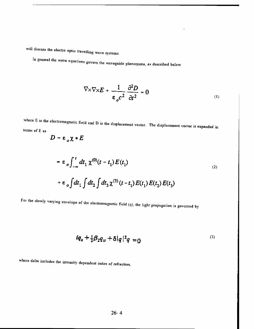
will discuss the electro optic travelling H iraveüuig wave systems.
In general the wave equations govern the waveguide phenomena, as described below
Vx VxE + —L &R . 0 EC2 dt2 (1>
where E is the electromagnetic field and D ,s the displacement vector. The displacement vector is expanded ir
terms of E as
+ eofdti fdtzfdt^Ht-tJEitJEitJEitJ
For the slowly varying envelope of the electromagnet, field (q)> the Hght propagation is governed by
(2)
'^+702?« +5|?|2<7=0 (3)
where delta includes the intensity dependent index of refraction.
26-4

Material Properties
As stated previously, the materials of interest are the III-V semiconductors; in particular, matenals such as
InGaAs/GaAs and InGaAs/AlGaAs. These are strained layer materials which offer band gap engineering
flexibility often not attainable in lattice matched material, Significant parameters including the well/bamer
combination, the level of strain and the material concentration in layers can be vaned to modify the physical
parameters such as the band-gap, electro optic and optical properties. Additionally these materials have band
gaps in the technologically important regions of 0.85 urn to 1.5 urn. Furthermore, recent computations indicate
that these compounds may have large optical nonlinearities.
In the case of thin layers, the layer mismatch induces internal strain rather than dislocations (12,13). The
presence of the built in strain affects the structural aspects of the materials and influences their electronic
properties through strain induced changes of the band structure. Enhanced optical properties are predicted (14-
15). As an example of the stramed superlattice, we cite the InGaAs/GaAs materials in which the InGaAs is the
well material and the GaAs is the barrier material. In this case, the smaller bandgap material i. under
compression and the larger bandgap material i. unstrained. For small amounts of Indium in the material, the
barrier heights are relatively low which can make the supperlattice effects more prominent (16-18).
For stramed layer superlattices with [111] growth axis, the onentation of the lattice constant mismatch
lnduced strains result in polarization fields directed along the growth ax.s. Group III-V semiconductors are
piezoelectric and strains can lead to electnc polarization fields. Because one of the materials ,s in b.axial
tension and the other is m biaxial compression, the electric polarization vectors are of opposite sign. The
internally generated electric fields modify the electronic properties of the superlattice.while the internal fields are
screened by photogenerated carriers which leads to large optical nonlinearities. The optical matrix elements are
altered because both the electronic energy levels and wavefunctions are altered by the internal field, In
InGaAs/GaAs the fields shift the conduction band state to lower energy and the valence band to higher energy.
This effect reduces the band gap. Since this is a type 1 superlattice the smaller band gap Ga alloy is in biaxial
compression and the light hole bands are split away from the heavy bands by stram. Therefore the band edge
26-5

»p..oa, p„perties ^ be domim(e<i „y hMvy Me K cmduo ,oa b>od ^^
Semiconductor WavPfn,;H0c-nnilrJoL1IüiL^
For ^m,„on processlag, coupM wayeguides are oftm ^ 0m ^^ |s ^ ^^
-»—. cou„w CM.OC, Tbjs w,s d,v,sed fa opfaiiy activated swiKtog ^ ^ ^ ^ ^
-«-A, ls ,chieved by „smg ,n mtensity depmden] 6Mor for ^ ^^ ^ ^ s ^ ^^
couple. Hi. ,„»,,, ,lKrs „. w.„ TO0,or wlmuA betwem (he ^ ^ ^ a ^ _h>t ^ ^^
«^ *»sf„ „a couplin6 ,mgth . bc ,dj„,ed by ^ ih< mput power Dtaotai ^ ^
w.th op,,«! gam h.ve been ü,ves.ig„ed ü, ,„e I™,, regime.
I. tb. case o, ^^ dePende„, .„ „„,«„ switchillg m senicMductor wlveguides fc ^ ^.^
are given below
il i^+^1u,+^\qx\
1 + a\q^)qx+kq2
= iyo9l-jr2qU!-iß(\qi\2 + CTlqil2)qi t
'?2Z+T02?2H + 5(\q2\2 + a\ql\2)q2+kql (4)
wbere k ,epresenK «be ^ o„ss eoupl„8 „d „. Um 0o ,he ^ „,„, „de ,, ^ „ ^ ^ ^^
effects.
I» B* (4) .he iMe™* dePer,„e», ^H, 1S , „__„, „„^ ^ ^^ ^ fc
eIte,el* lMge' ""' T "- « *" —>- ** - —1— by «*, reoombm„,on. H.weve,,
—_ —H—«- « have „pid ^ time8 because fcy „, „„, .^.^ ^ ^ .^
«nsfe. „9). Me.„ene„K of ttes, no^e.Hfe e» be Affic»,, bee,™ ,eve„, pr„cesses „.eludu.g virtu.,
e
26-6
and real earners and thermal effects can contribute. Several experimental techniques can be used to measure the
intentisny dependent nonlinear mdex changes mcluding four-wave rmxmg (20), nonlinear Fabry-Perot (21),
and fringe shift interferometry (22).
The third order susceptibility i. complex with the intensity dependent effects determined by the real part of
,*. complex function. The imaginary part is compnsed of two photon absorption (TPA) where two photons
are absorbed. This effect causes significant problems in semiconductor waveguides because it is essentially a
nonlinear loss mechanisms. Its effects on coupled waveguides are considered.
In order to investigate the effects of TPA on semiconductor properties we used the numerical beam
propagation method. Figure 1 shows the input power required to achieve the maximum transmission as a
function of TPA for various coupling parameters; k=0.25 (solid line); k=0.5 ( dashed line); and k= 1.0 (dot-
dashed line). The figure shows that for all values of the coupling parameter, the required input power increases
as the value of TPA increases. Tins represents a damaging effect because ,t indicates the extent of the input
power lost to TPA. As a result, greater and greater input power is required to achieve the same output. Since
the input power must be held to a minimum, the TPA presents a challenging problem.
Flgure 2 shows the maximum transmission at the input channel as a function of TPA for vanous coupling
parameters; lc= 0.25 (solid Ime); k=0, (dashed line); and k= 1.0 (dot-dashed line). The figure shows that the
amount of power transmitted declines rapidly as TPA increases.
26-7
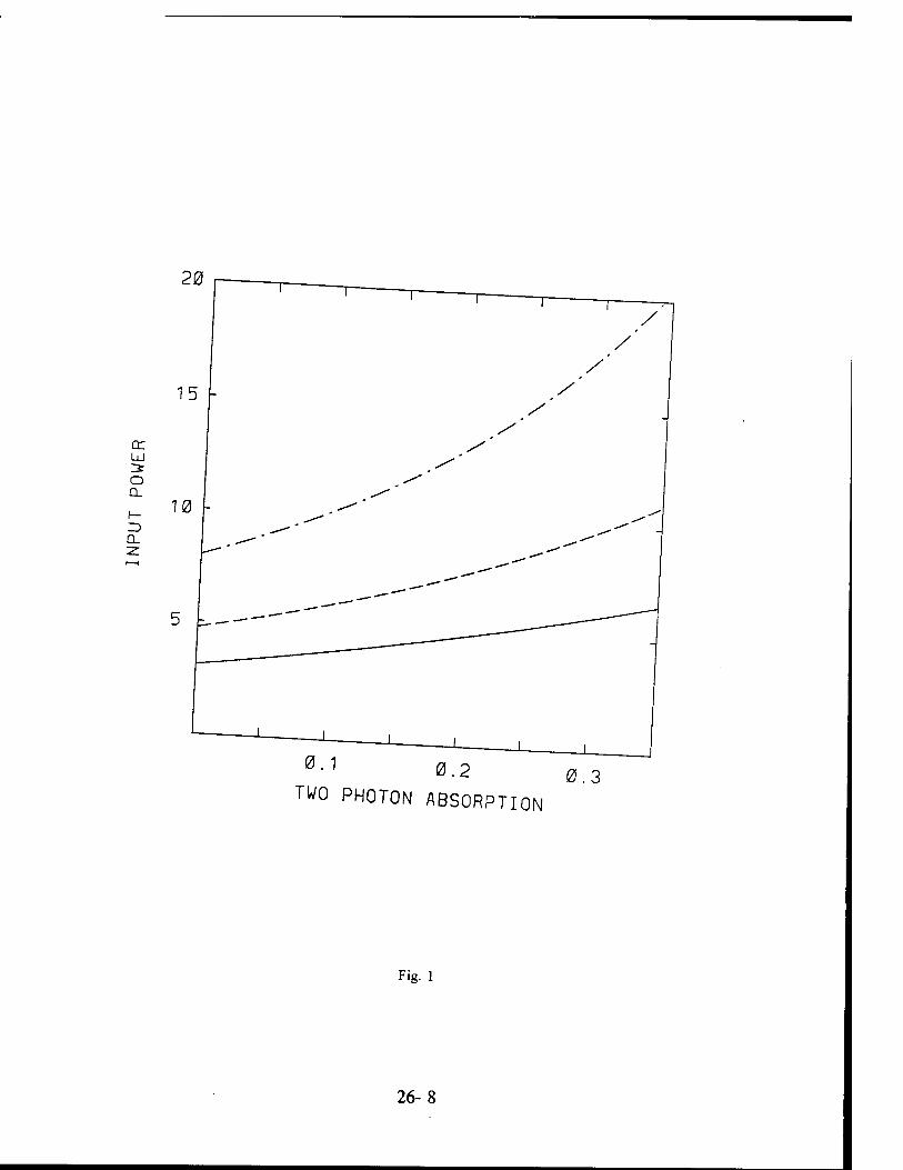
a:
o Q.
Q_
0-2 0.3 TWO PHOTON ABSORPTION
Fig. 1
26-8
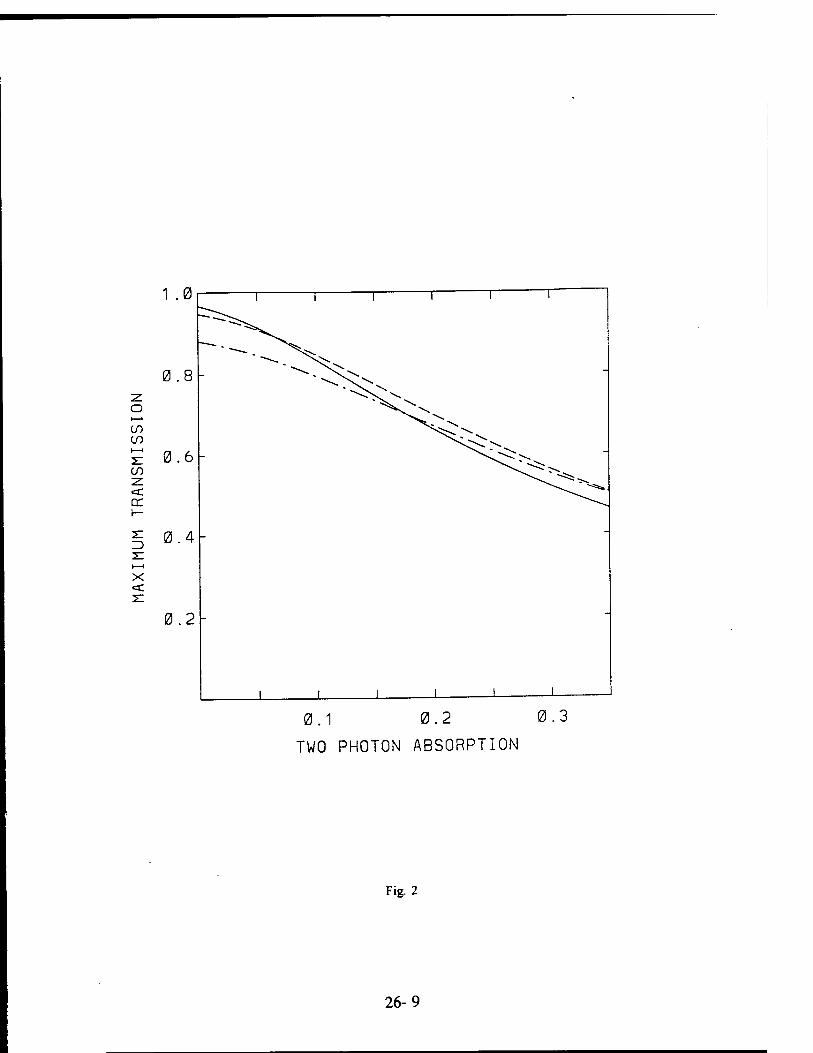
1.0
0.8
co CO
CO
cr
x
0.6 -
0.4
0.2
0.1 0.2 0.3
TWO PHOTON ABSORPTION
Fig. 2
26-9
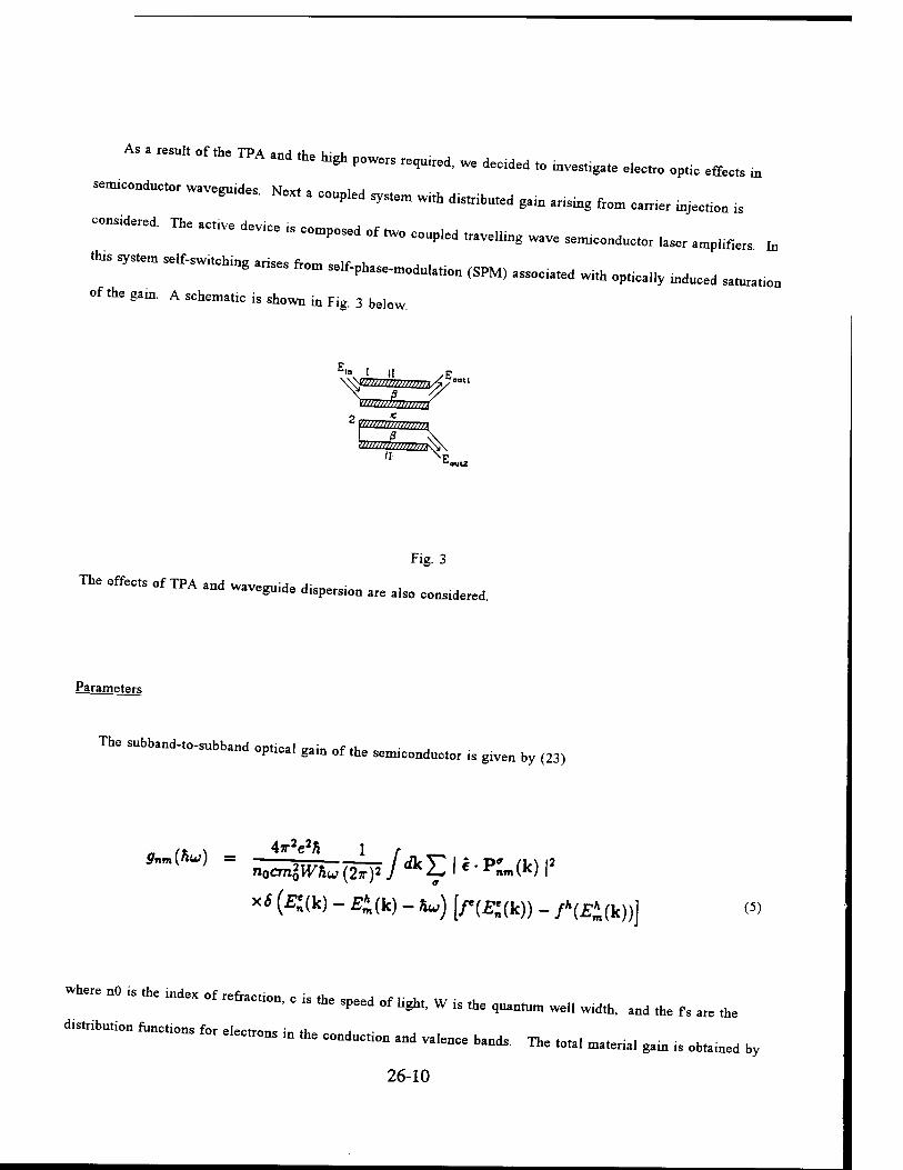
~ TB. „*. d„ice is composed „f mo coupW t_umg _ ^^ ^ ^ ^
- ^- -^*, „,scs from se,.pha_dulatiM (spM) _ wi(h op(rea|]y ^ ^ of the gain. A schemat.c is shown in Fig. 3 below.
mzmmmmn^\
Fig. 3
The effects of TPA and wavegu.de d.spers.on are also considered.
Parameters
The subband-to-subband optical gam of the semiconductor i. glven by (23)
„ /* ^ 4r2e2h 1 r
xS (£;(k) - Bi(k) - Hu,) [/-(^(k)) _ /*(j£(k))] (5)
— no ,s *. „dBX of re&„„011, c |s ,he ^ rf |ight w fc th= ^ ^ ^ ^ ^ f s ^ ^
26-10

summin; ing over all subbands n,m and integrating against a Lorentzian function (24)
g(E)= fdE"Zgnm(E')A(E-E'). (6)
The rad.at.ve current denshy i. evaluated from the dipole transnron rate (25) for the quantum confined earner
states
x6 (£.(k). £* (k) - hu) [riPMW- - fh(rtm •• (7)
At low concentrates the earners obey the Boltzman staüstics wrth the current being proposal to the square
of the mjected earner densrty n. However at higher earner denies the ermssmn rate falls off from the n2
curve (23). The hght only experiences optical gam in the well regum, as a result it is convenient to characters
the gain by a confinement factor given by
(8) r = NiW.
where N i. the number of quantum wells used in the multiquantum well structure, W is the w.dth of each well
26-11
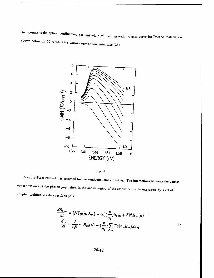
and gamma is the optical confinement
shown below for 50 A wells for
per unit width of quantum well. A gain curve for InGaAs materials is
various carrier concentrations (23).
W1 U6 1.51 1.56 1.61
ENERGY (eV)
Fig. 4
A F.hy-IW, «„„,„ 1S ,SMMd for ^ sem,condllctor aapMm ^ ^^ betweeo ^ ^
™"*" ""' "" Ph0""' *"*** " *■ «*■ ■*- -* .mpiffie, c„ b. expressed by . set of
coupled multimode rate equations (23)
dSi, ~- = [NTg(n,Em) - ae](^)S£,m + ßNR^n
(")
(9)
e,m
26-12

Mode Equations
An active system is composed of two parallel travelling wave semiconductor amplifiers with distributed gam
arising from carrier injection by pumping current into twin stripe contacts. The input beam is injected into
channel 1 and the gain of each amplifier is adjusted by varying the pumping current, I. The electromagnetic
field is a superposition of the modes of the isolated single-mode waveguides given by
E{x,y,i,t) = i S lfj(x.y)Aj(z,t) y'-i
• exp {i(ßz - ox,:)} + cx-l (10)
where A is the slowly varying envelope of the electromagnetic field. Linear coupling between the two modes is
provided by the evanescent overlap of the two waveguide modes. The coupled equations are
and
3 i_ a ] oz v, atJ i.
(ID
a i a 1 . i/t T" + 17 T \A* = IKA
< + -(! _
dz Vtot\ i - 2(1 ~ ia)*^N^A^
where alpha is the linewidth enhancement factor and the g,s are the intensity gains (dependent on the carrier
densities, N). The linewidth enhancement factor is a constant independent of density. When k=0 the
expressions reduce to an uncoupled semiconductor amplifier (26-28). For a one coupling length device light
will transfer from guide 1 to guide 2 without distortion in the linear limit. When the optical pulse duration
26-13

exceeds the intraband relaxation time th. ■ A J , • me, tue induced polarization can be eliminated and the field matter interaction
is given by a set of coupled equations Th. ■ A ■■ * H ions, ine carrier densities for the semiconductors obeys the equations (27-28)
dt qV TC fio>0 ' ''
(12)
where I , the injection current, q is the electron charge, and V is the cavity volume. A hnear dependence of
the gam on the carrier density is given as
W) - Ta{Nj - Nn) j = ,?: (13)
where No is the transparency carrier density.
A cross section averaged gam relaxation equation i. used smce the waveguide dimensions are smaller than
the carrier diffusion length (29)
d8f (8j ~ 8/o) gj , ,.
(14)
one where Es,, i, ,he miim Mergy> fc „ „, ^^ ^ ^ ^ ._ ^ ^ ^ ^ A
coupling ^ device is consldered so tto al |ow ^ mtensuies ihe ||ght ^ ^ ^ ^ ^^
.. , ««* ,,», fc „d* „f ,he P„Ise „ „uob u- lhln fc c,_ ,&tme_ As , _„ ,„, „^ ^
dete^ed by *. »,„ slgoll g3m and ,„, lmewidtb ^„„^ ^ ^ ^.^ ^ ^
li=ew,d,h «I.««« f,c,„t i, >bout 6. „ the ^^ >bson)t|oii Md ^^ u8 n=gucted (hm tte
optical
26-14
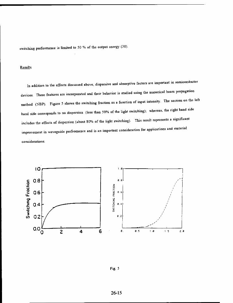
switching performance is limited to 50 % of the output energy (30).
Results
In addition to the effects discussed above, dispersive and absorptive factors are important in semiconductor
devices. These features are incorporated and their behavior ,s studied using the numerical beam propagation
method (NBP). Figure 5 shows the switching fraction as a function of input intensity. The section on the left
hand side corresponds to no dispersion (less than 50o/o of the light switching); whereas, the right hand side
includes the effects of dispersion (about SO'/o of the light switching). This result represents a significant
improvement in waveguide perfromance and is an important consideration for applications and material
considerations.
I.U
c 0.8 o o 2 0.6
UL o» c « /I £ 0.4 ■ ^^ ~~
u
3 (/> 0.2
1 1 !_..
0.8
0.4
0.2
Fig. 5
26-15
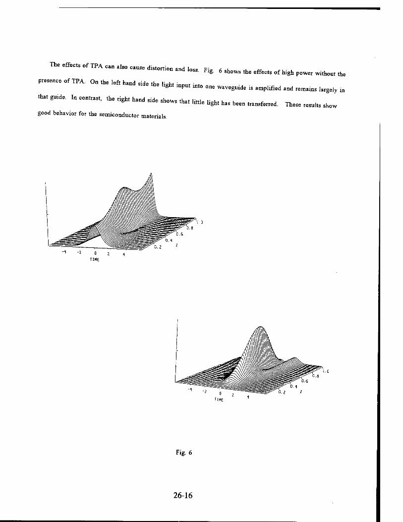
The effects of TPA can also cause d.stort.n and ,os, Fig. 6 shows the effects of h,gh power without the
Presence of TPA. On the left hand s.de the hght .put .to one wavegu.de ,s ampltfed and remams largely m
that guide. In contrast, the right hand side shows that li little light has been transferred. These results show
good behavior for the semiconductor materials.
Fig. 6
26-16
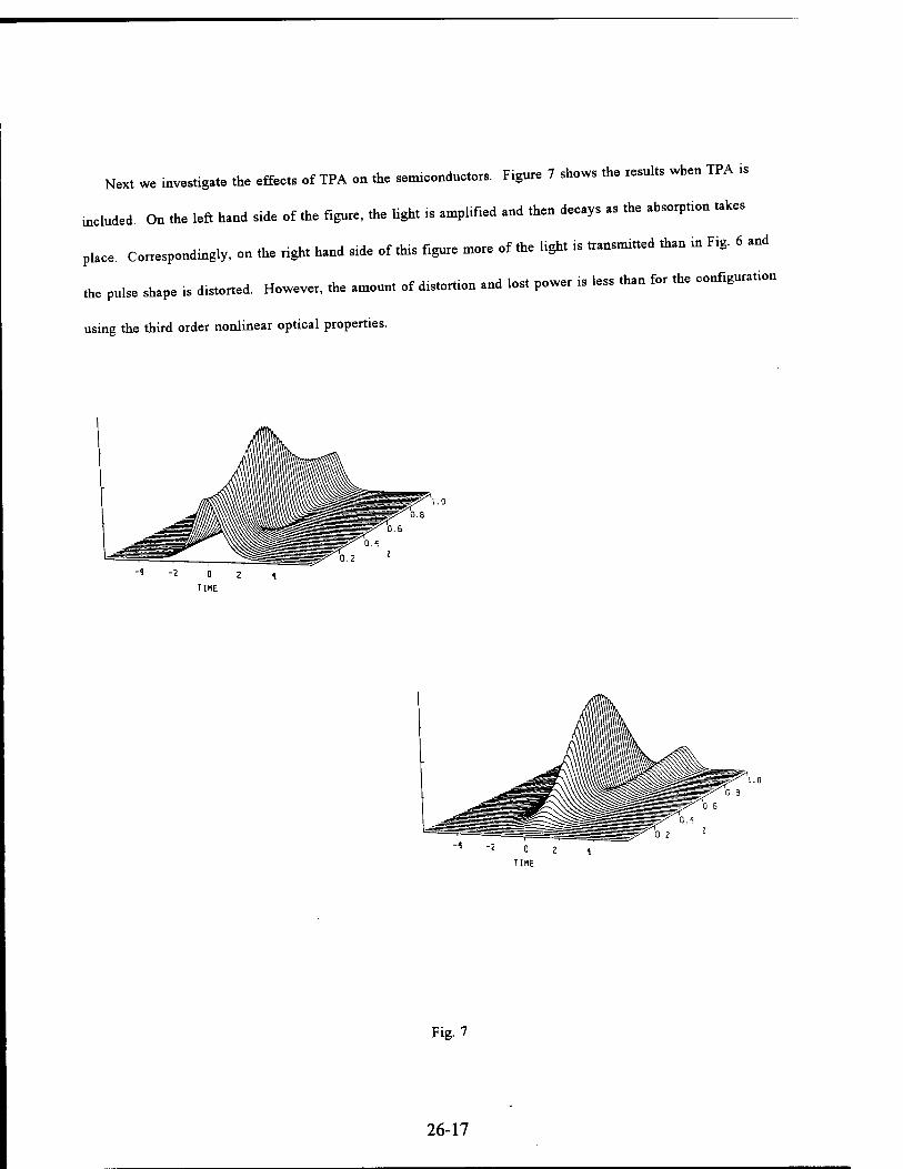
Next we üwestigate the effects of TPA on the semiconductors. Figure 7 shows the results when TPA i.
mcluded. On the left hand side of the figure, the light i. amplified and then decays as the absorpt.on takes
place. Correspondmgly, on the nght hand s.de of this figure more of the Hght is transmrtted than in Fig. 6 and
the pulse shape , d.storted. However, the amount of d.stort.on and lost power i. less than for the configurat.n
using the third order nonlinear optical properties.
Fig. 7
26-17

We have „,V8sl,g,ted lhe propert,es otthiid ode[ ^^ op ,M| ^ e|rotioopt|cai ^ fa
.e»co„d«,„t SMuled hy„ m„eri„s ^ maBm|s ^ ^^ fof ^ ^^ ^
c.™«,™ „d oompwmg. ^ ej[hibit b,nd gip Mgineermg ^ the v|s|bk ^ ^ ^ ^
reg,o.s for use m laset, „,„„„„,„, swl,ches and deteetors ^ mmMs ^ ^ ^ fo[ ^^ rf
»r.uu, dev.c. c„mp„„enl, desc„bed aboTO. ^ exbJb„mg ^ ^ ^ ^^ ^ ^^
•he effec, „f «. photen ,bsorp„on „^ ^ ^^ ^ ^ ^^ ^ ^ ^ ^
tod o,de, ■,« properties requm f>„ kser ^ for ^ mvea|ga .oii ^^ ^ ^ _^
.W.puceffee,^^,,^ „ord„10,vold,heslow timeconsuMsotlhech„ge „con,bin„io|i
effee* due ,. „,<„„„ hole r«orabmslloa „^ we ^^ ^^ ^ ^^ ^ ^ ^
•he adv,„„ge „f „htiv.ly low pow„ aad p=rhaps cisin ^^ w|ih other semconducter dev|ces smh >s
l.sers ,„d de.eco,* u, . !mgle packagmg „ was fo ^ ^ ^ ^ ^.^ ^ ^ ^ ^^^
were ,akeu „,,„ effec, „,a,,vely g„„d vma perforalM„ was ,cfcved. Thorefo„ ^ „^ ^
»mplifie« my «,«., , m„« advantage»«« «>, Brm application
26-18

Bibliography
1. S. Wabnitz, E.M. Wright, C.T. Seaton, and G.I. Stegeman, Appl. Phys. Lett. 49, 11 (1986).
2. S. M. Jensen, IEEE J. Quant. Electron., QE18, 1580 (1982).
3. Y. Silberberg and G. I. Stegeman, Appl. Phys. Lett. 50, 801 (1987).
4. M. N. Islam, S. P. Dijaili, and J. Gordon, Opt. Lett. 13, 518 (1988).
5. L. Thylen, N. Finlayson, C.T. Seaton, and G.I. Stegeman, Appl. Phys. Lett. 51, 1304 (1987).
6. B. Daino, G.Gregori, and S. Wabnitz, Opt. Lett. 11, 42 (1986).
7. A. Mecozzi. S. Trillo, S. Wabnitz and B. Diano, Opt. Lett. 12, 275 (1987).
8. S. R. Friberg, Y. Silberberg, M.K. Oliver, M.J. Andrejco, M.A.Satfi, and P.W. Smhh, Appl. Phys. Lett. 51,
1135 (1987).
9. D.D. Gusovskü. B. DUno, A.A. Ma.er. V.B. Neustruev, E.I. Shkloskn and I.A. Sheherbakov, Sov. J. Quant.
Electron. 15, 1523 (1985).
10. P. LiKam Wa, A. Miller, J.S. Roberts, and P.N. Robson, Integ. Phot. Mtg., 1990, paper WH7.
11. P. Li Kam Wa, P. N. Robson, J. S. Roberts, M.A. Pate, and J. P. David, Appl. Phys. Lett. 52, 2013 (1988).
12. G. Bastard, C. Delalande, Y. Guldner, and P. Voisin, Advances in Electromcs and Electron Physrcs, P.W.
Hawkes, ed. (Academic Press, NY, 1988).
13. J. W. Matthews and A.E. Blakeslee, J. Cry. Growth 27, 118 (1974).
14. D.L. Smith and C. Mailhoit, Phys. Rev. Lett. 58, 1264 (1987).
15. C. Mailhoit and D.L. Smith, Phys. Rev. B33, 8360 (1968).
16. S. T. Picraux, L.R. Dawson, G.C. Osbourne an W.K. Chu, Appl. Phys. Lett. 43, 930 (1983).
17. G.C. Osbourne, J. Vacuum Sei. Tech. 21, 459 (1982).
18. K. J. Moore, G. Duggan, K. Woodbridge, and C. Roberts, Phys. Rev. B41, 1090 (1990).
19. M. Yamanisbi and M. Kurosaki, IEEE J. Quantum Electron. 24, 325 (1988).
20. W.K. Burns and N. Bloembergen, Phys. Rev. B4, 3437 (1971).
21. Y. H. Lee, A. Chavez-Pirson, S.W. Koch, H. M. Gibbs, S.H. Park, J. Morhange, A. Jeffery, N.
Peyghambanan, L. Banya,, A:C. Gossard and W. Wiegmann, Phys. Rev. Lett. 57, 2446 (1986).
26-19
21- G. R. Olbrigh, ,0d R Pe,ghamb»riao, Appl. Phys. Let 48, „84 (1986).
23- , U*. Th,„„„,, Studles of Pseudomorphic Qmomm wej] ^^ ^ phD ^ ^ ^
Michigan, Technical Report N. SSEL-202, 1991.
24. G. D. Sanders and Y. C. Chang, Phys. Rev. B35, 1300 (1987).
25. J. J. Sakura,, Advanced Quantum Mechamcs (Addison-Wesley, New York, 1967).
26. G.P. Agrawal and N.A Olsson, Opt. Lett. 14, 500 (1989).
27. G. P. Agrawal and N.A. Olsson, IEEE J. Quantum. Electron. 25, 2297 (1989).
28. N.A. Olsson and G.P. Agrawal, Appl. Phys. Lett. 55, 13 (1989).
29. G P. Agrawal and N.K. Dutta, Long Wavelength Semiconductor Lasers (Van Nostrand, New York. 1986).
30S.TrilIo,SWabmtz JM Soto-CrespoandEM-Wnght, IEEE J. Quantum Electron, 27,410 (1991,
26-20
DEVELOPMENT OF CONTROL DESIGN METHODOLOGIES FOR FLEXIBLE SYSTEMS
WITH MULTIPLE HARD NONLINEARITIES
Final Report 1993 Summer Research Extension Program
RIP # 93-195
Armando Antonio Rodriguez Assistant Professor
Department of Electrical Engineering
Arizona State University
Tempe, AZ 85287-7606
(W) (602) 965-3712
Air Force Office of Scientific Research
Boiling AFB Washington, DC
December 31, 1993
27- 1
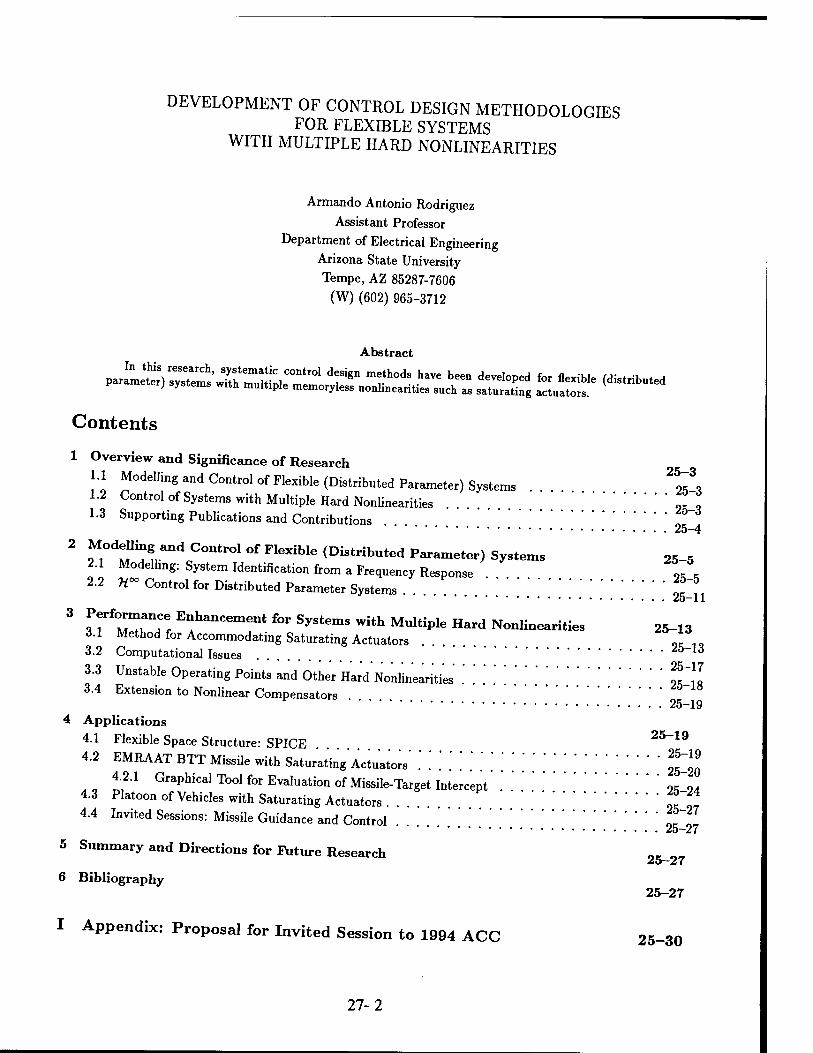
DEVELOPMENT OF CONTROL DESIGN METHODOLOGIES FOR FLEXIBLE SYSTEMS
WITH MULTIPLE HARD NONLINEARITIES
Armando Antonio Rodriguez
Assistant Professor
Department of Electrical Engineering Arizona State University
Tempe, AZ 85287-7606
(W) (602) 965-3712
Abstract
Contents
1 Overview and Significance of Research
U Modelling and Control of Flexible (Distributed Parameter) Systems ^o 1.2 Control of Systems with Multiple Hard Nonlinearities . . ~_ , 1.3 Supporting Publications and Contributions „ 25-4
2 ,M,0dM»M,?,ltrol °f FleXiWe <Distribute<* Parameter) Systems 25_5 2.1 Modellmg: System Identification from a Frequency Response ,A 2.2 H°° Control for Distributed Parameter Systems
3 f rf°JT!n EfanCemen* f°r SyStemS With MultiPle Hard Nonlinearities 25-13 3.1 Method for Accommodating Saturating Actuators " 3.2 Computational Issues 6
3.3 Unstable Operating Points and Other Hard Nonlinearities It'll 3.4 Extension to Nonlinear Compensators 25-19
4 Applications
4.1 Flexible Space Structure: SPICE 25_19
4.2 EMRAAT BTT Missile with Saturating Actuators' .'.'.'.'.'.'.'.'.'.'.' 25_20
4-21 Graphical Tool for Evaluation of Missile-Target Intercept ... o. 94
4.3 Platoon of Vehicles with Saturating Actuators . ZZ
4.4 Invited Sessions: Missile Guidance and Control .' 1, 11 2to~~Z\
5 Summary and Directions for Future Research 25—27
6 Bibliography 25-27
I Appendix: Proposal for Invited Session to 1994 ACC 25-30
27-2
DEVELOPMENT OF CONTROL DESIGN METHODOLOGIES FOR FLEXIBLE SYSTEMS
WITH MULTIPLE HARD NONLINEARITIES
Armando Antonio Rodriguez
Assistant Professor
Department of Electrical Engineering
Arizona State University
Tempe, AZ 85287-7606
1 Overview and Significance of Research
This report summarizes research conducted under Research Initiation Proposal *^^^^
focussed on two area,: (1) modelling and control of flexible (distributed parameter) system^Q~
trol of systems with multiple hard nonlinearities. The major contributes to each area are now summanzed.
1.1 Modelling and Control of Flexible (Distributed Parameter) Systems
Practically speaking, fletiUe systems are systems for which the structural modes overlap in frequency with
Le dI bandwidlh requirements. Such systems, in general, are modelled by partial d.fferen.a equates
and h nee are said to be äistrrtuteä ^meter or tnfinU, äimens.onal systems. Untn th. work me h d
Th c pTLt the design of controllers to deliver a pre-specifled level of performance for a genera <aStnbu,
pa1ter (i.e. complex) system did not exist. Throughout the course of this research, met odswh.h
rmTt the design of near-optimal nnite-dimensional controllers for such systems have been developed. Th,
haTTeen done for the so-called H~ sensitivity and mixed-sensitivity design paradigms wh.ch have rece. d
^L*a* for nnite-dimensional systems. The methods have been applied to the problem of controlhng
a flexible space structure.
1 2 Control of Systems with Multiple Hard Nonlinearities
Fo, physical reasons, system deaigners often »an, to ensure thai certab, variable, do not exceed^-specMed
Umi.s m ,h« case of M systems, such variables may inc.ude, for example, fin pcs.fons, « rates, angl
1ttach, sideslip angle, etc. Typically, adhoc modifications are employed and extend am* „ .-£
performed to jnstify the modfflcations. A procednre for systematizing this process has been dev lop«i dururg
"arch We previous methods, ,h. method developed here is accompanied by nomma. performan«
ril More spelifically, the completed research has shown ho» an initial ^f*£Z~£ !ystema,ically modified to accommodate memoryless hard „onlinearifea (e.g. saturafng actuators)
were initially not modelled.
27-3
1-3 Supporting Publications and Contributions
The following publication, «knowledge the support of the Research Initiation Proposal:
Modelling and Control of Flexible (Distributed Parameter) System»
'' !flMITr "7AA' ^risuez' "Sys,em Iden'mcation from a ""-* H^»-." "«-A* of (Ac Sind Conference .. S«™,, ... Cairo/, San Antonio, TX, December 15-17, 1993.
2. M. Mahlocb and A.A. Rodrigne,, "System M.„,i„c„io„ from a Fluency Response: A Sequen-
Ua Algorithm.» submitted lor pnblication in the ?roceei,n,e of tke American Control Conference Baltimore, MD, June 29-July 1, 1994. oon/erome,
1 ^ pgUeZ;nd 3f\a0M"' "n" °~*M» Mini™*ti0" *" "—* '««e-Dimensiona, 21^2151T AmeriCm C"""' C""mC'- Sa° «-*»> CA- '« «■ «93, pp.
4. A.A. Rodriguez and M.A. Dahleb, -«- Control of Stable „nnite-Dimensional Systems using Finite-
D.m.ns.ona, Techniques, submitted for pnblication in ,EEE TraneacUone o„ AutomnUc ConL, 1993
5' SylL°d.t„mittDdSfgn °Z 0P"mal IUt^~*^ C°**" *• «—* Infinite-Dimensional Systems, submitted for publication to AUTOMATIC A, 1993.
6. AA Rodriguez and Delano Carter, "Hierarchic,, HAC„./LAC Vibration Suppression for , Fl.xi-
* Space Taescope: SPICE, submitted for pnblication in the Proceed,* o, tne American Cont„, Conference, Baltimore, MD, June 29-July 1, 1994.
T' ^ 27T-8nd DeIano Ca"er' "*"Con"01 of SPICE: A F,exibk L»"Be™ E^I«," -*- mitted fo, pubhcation in the Journa, of Dynamic System,, Meae.KmenU, ani Control
Control of Systems with Multiple Hard Nonlinearities
'' %J£T K 'f~ Cl0Uti"' "COn"°' °ta BMl-^'"-M^ ""■ S—iM Actuators," submitted fo, publication „ ,h. Proeeeäiny, of tke ,99< American Contro, Conference, Mtai
2. A.A. Rodriguez and J.R. Cloutier, -Control of a Bank-tc-Turn-Missile with Multiple Saturating Ac- tuators, ,» preparation, to be submitted to AIAA Jo.m., of GuUnnce, Control, .nä Dynam.cl
3. M. Rodriguez and S.N. Balakrishnan, «Performance Enhancement for Missile Guidance and Control
Systems, proposal submitted fo, invited session to m4 American Control Conference, Baltimore,
4. "-»««P--air. Balakrishnan, -Perform»» Enhancement of Missile Guidance Systems in he Presence of Mu,t,p,e Saturating Actuators," in preparation, Invited session, »„ AUA Guidance
and Control Conference, Phoenix, AZ.
27-4
5. M. Sonne and A.A. Rodriguez, «PC's in the Design and Evaluation of Guidance and Control System
for Missiles," to appear in the Process of ike 1994 InUrnaUond Conference on Slmulatton ,n
Engineering Education, Tempe, AZ, January 24-26 1994.
6. M. Sonne and A.A. Rodrigue,, "A PC-based Graphics System * «he Evamation of Missile Guidance
and Control Laws," submitted for publication in the Procuo,»,, ./». An,«,«» (M <W«ren«,
Baltimore, MD, June 29-July 1, 1994.
7 S C Warnick and A.A. Rodriguez, "Longitudinal Control of a Platoon of Vehicles with Saturating
' Nonlinearities,» submitted fo, publication in the IEEE TV.,.««.« »» Control Tecknolo„.
The completed research provide, two significant contributions to control system designers. First, it
provides . systematic procedure for controlling flexible (distributed parameter) systems. In so domg,
provide, a s mple method for ascertaining «he optimal performance for varrous «- cn.enon. Second
ovides a method for modifying an eating compensator to —date initially —< ^n^ hard nonlinearitie, (e.g. saturating actuators, etc.) and maintain, to «he extent Po,„ble, the d,r,cfonah«y
properties of the original design.
2 Modelling and Control of Flexible (Distributed Parameter)
Systems ft, «bis section, «he portion of the research results rei.ted «o modelling and con.rol of flexible (dis«,ihu.ed
parameter) systems are described.
2 1 Modelling: System Identification from a Frequency Response
Often, an an*, mode, fo, the system under consideration i, not available. Instead „ engine«,may ha«
.cess only «o f,equency response data. In [1], [2], i. i, shown how such da«a can be exploded «o develop
models which are suitable for control design.
Iterative Approxinratio. Scheme. In [1], «he author, Pc. a nonlinear ? model-ntting problem which
addles „die and mamphc«»,« med.H.n, errurs. The p»blem can he ,«.«ed ma.hemaftcafty - follow,
du inf / tr{EH(ju)E(ju;)} ii.nM Jo
where,
E(s)^{^) ) - P(s) additive; (s)[P(s) - P(s)] multiplicative
P(jw) is a given frequency response (possibly MIMO),
«•>*$
27-5

is the approximant to be constructed, and
def N(s) ^
nu(s) n12(s) ••• nlr(s) "21 (s) n22(s) ■■■ n2r(s)
nn(s) nr2(s) ••• nrr(s)
def
Since the above optimization is nonlinear in the parameters, the problem was reformulated to yield simpler optimization: '
where now the error E is given by
def E(s) a=? W{s)[N{s) - d{s)P(s)]
zzz':"simpler prob,em iook iiie the °*si -M- - -«■*• -—«■» -** W(s) =f / 5W additive;
l^_1(s) multiplicative
*"•».«•> -* HW » unknown „„„„„-. Proceeding with „^ manipu|ationS] „,„ ^ optimization y.elds the following quadratic optimist
. er ion:
inf -xTAx -xTb + c
whose solution can be found by solving a system of linear algeb
Ax = b
and c depend on the frequency resp< approximant
raic equations:
HIiand C dCPend °n thC freqU6nCy reSP°nSe ^ and « COnta- the -known parameters of the
Iterative Procedure for Weighting. Since d(s) and N(s) are unknown apnori, the following iterative procedure suggests how to select the weighting W.
Choose Wi = l
Solve for JV"i and dx dJf f 1717) additive;
(s) multiplicative Let W2(s) dä ( dfc)
27-6
Solve for JV<_i and d;_i , , f i , additive;
Let W,-(«) - ^^(s) multiplicative
Solve for JVj and dt
Let Pi = * di
Consequently, «he initial nonlinear optimisation is addressed by solving a sequence of quadrafc op n
nation problems. I» [1], the above Iterative method - applied to a variety of *£££££ infinite-dimension,, and finite-dimension... The method i, shown to be eomp.ft.ve w, h earing methods,
those whieh rely on analytic models and those whieh rely on frequency response data alone.
Sequential Algorithn. for Large Apprcochnants. A limitation of the previous method is see. when
Zol approximauts „e sough, .„ such a case it requires that one be able to solve a large system
oibly ill-conditioned algebraic equations. Sucb a method is, of course, limited by the —« ™ availabL .n [2], a sequential method is presented fo, constructing the .pproxrm.nts - at each ,t p one only
^"solv .mal" system of «quatiens. The sequential algorithm presented iu [2 consequently permU
Z coustructien of high-order mod.,, whieh can approbate the original data a. closely as des.r.d. The
algorithm can be described as follows.
Suppose that an appro— P which approximates P over the frequency range [fi0, 0*] Q Ä i. desirecL
Partition [ß0,M as follows: [üoM = u£?[*M where fi. < ft+i for all . = 0, 1, .... N 1-
obtain the approximant P, one proceeds as follows:
Step 1: Obtain approximant of G(jw), denoted P^jw), on [Ov-i, QN].
Step 2: Obtain approximant of (P(JW) - P(jwj), denoted P2(jw), on [QN-M.
Step i: Obtain approximant of (P{jw) -££(»), denoted Pi(jw), on [UN-M-
This process is continued up to and including i = N. The final approximant is then given by
P{S) dä £A(S)
Damped Euler-BernoulU Beam. The above methods were applied in [2] to a model for a Damped Euler-
Bernoulli Beam. The model for a Damped Euler-Bernoulli Beam is given by the following partxal differential
equation:
27-7
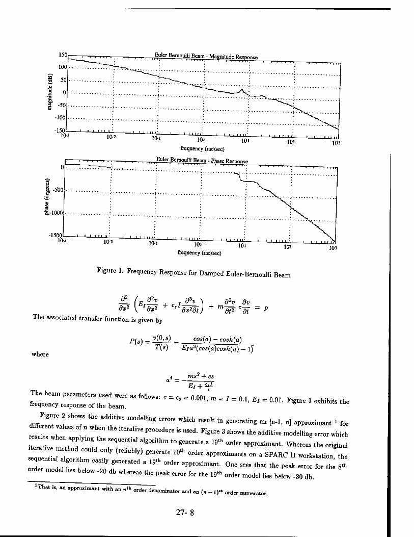
150
100
9 50
60 -500
&.-1000
-1500 10-3
Euler Bernoulli Beam - Magnitude. Rp.Tnno .' ' * ■ i i i iTr, ,
-1 1—■■■■■■' t i |
frequency (rad/sec)
"■—■ ■ Elder Bernoulli Beam -Phase Response * ' "^ 'iiii" i—i i i n 111»—
-j ■ ' ' i' n
10-2 -J—
10-1 -I L I I I I I
100
frequency (rad/sec)
Figure 1: Frequency Response for Damped Euler-Bernoulli Beam
Ü- (F ^ dx* y^'a*
The associated transfer function is given by
+ cld3v\ + &v dv = p
where
P(s) = V(°'S) = cos(a) ~ c°sh(a) T(s) Eia2(cos(a)cosh(a) - 1)
4 _ ms' + cs
The beam parameter, used „er, a, follow»: „ = c. = 0.001, m = 1 = 0.1, E, = 0.01. Figure 1 exhibit, the frequency response of the beam.
dJr'eT ! ST "". aTVe m0de"i"8 ert0rS "hiCh "*"" '" •—*« - I-1' »1 ■»-— ' for *T a'U6S ° " *n ,he ""at™ "°»d™ - -<• Raure 3 shows the additive modeUing error which
■W JTI SeqUe"tia' ilSOrilhm l° «—" " 19'K "«« ■""*—■ Whereas the orig J
ent.a, ^gor.thm «,„ gellemte(, . 19,h „„„ „^^ ^ ^
order mode. Ues below -20 db whereas the peak error for the 19- order mode, lie, b.!ow -30 db
'Tit i., „ „pp™™ wilh „ „,,. orf<r „„,„„„ „d „ („ _,,., order ^^
27-8
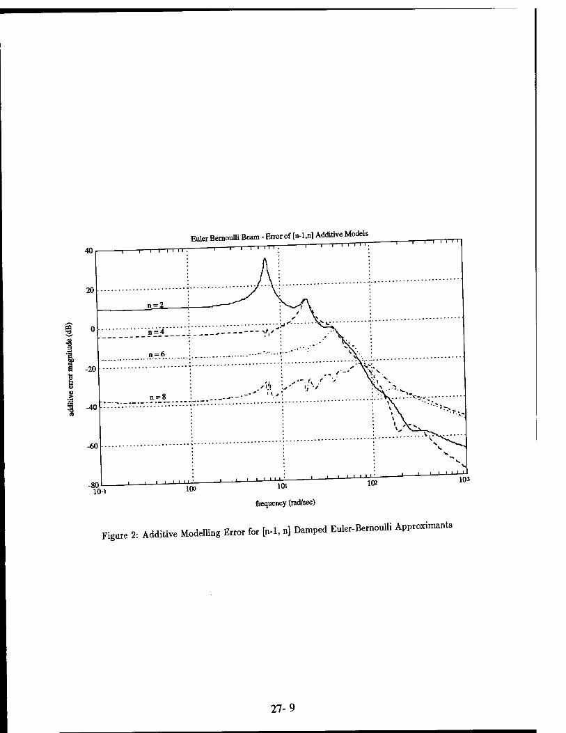
40 -i—i—i—i i 11
Euler Bernoulli Beam - Error of [n-l,n] Additive Models —i 1—i—i i i i i. T 1 1 I M I
-i——i 1—rr
20
M 0
•8 s •a SP e -20
-40
-60
-80 L- 10-1
I II1111
100 101 1UZ
I 103
Figure 2
frequency (rad/sec)
: Additive Modelling Error for [n-1, n] Damped Euler-Bernoulli Approximants
27-9
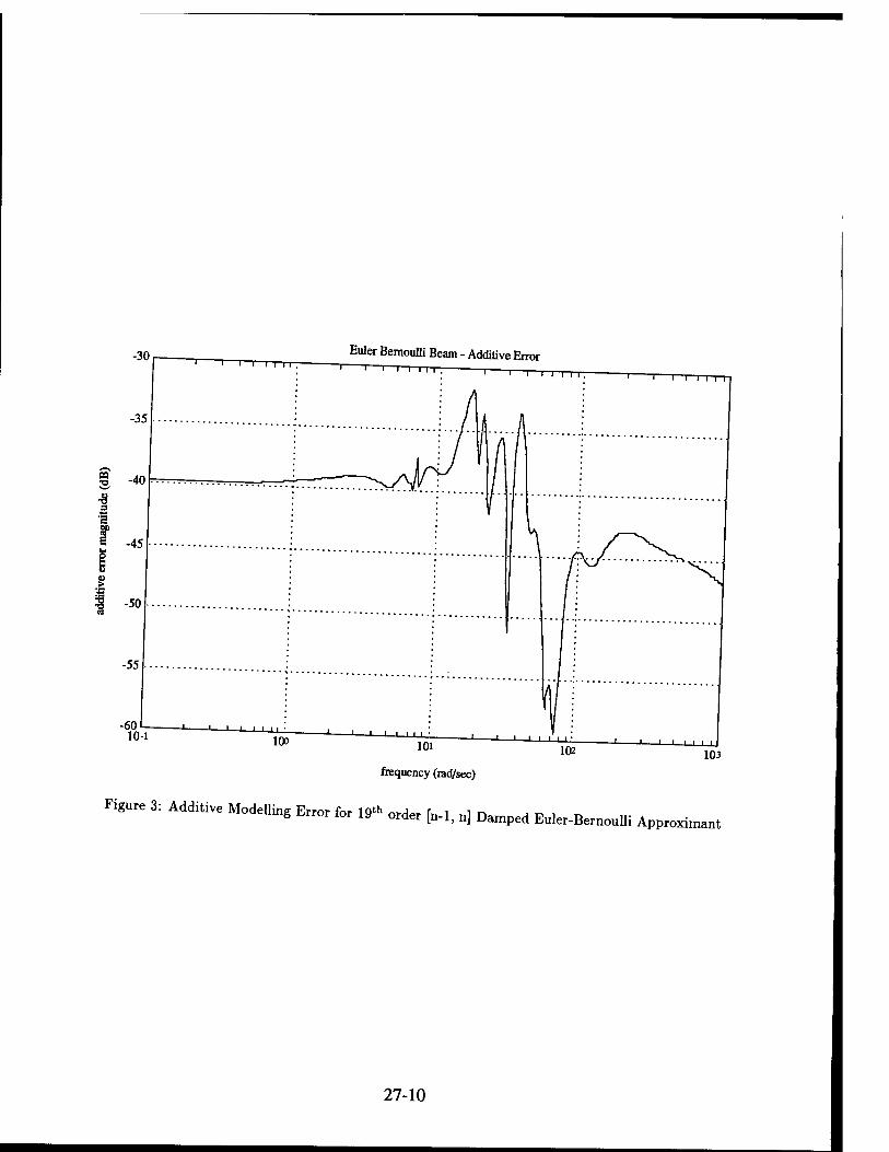
Euler BemouUi Beam - Additive Error
n
-8 s ■a
a -45
frequency (rad/sec)
Figure 3: Additive Modelling Error for 19* order [n-1, n] Damped Euler-Bernoulli Approximant
27-10
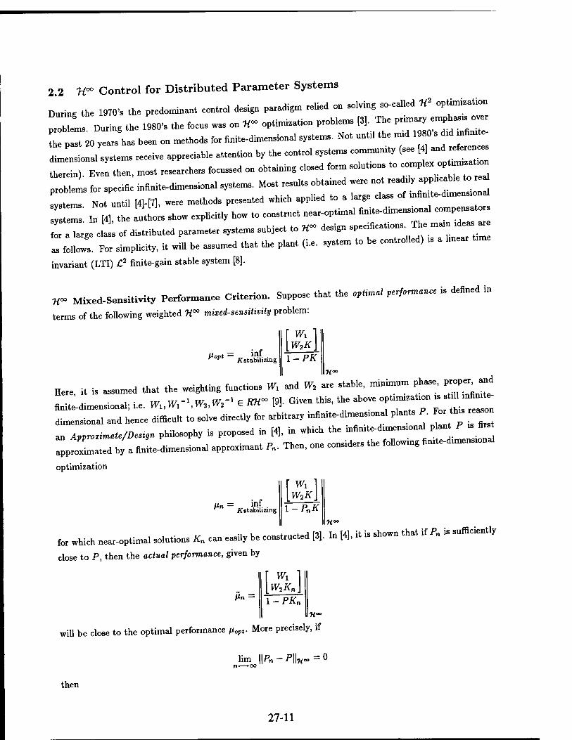
22 r Control for Distributed Parameter Systems
During the 1970, «he pcedominan« co„«,o, design pa,adigm — on solving ec-caUed *> option
p,oblem, During «he 1,80, «he focus was on «- option p,ob..ms [3 T e *-"£^Z L p-, 20 yea» „as been on ...hod, to, fini.e-dhnensiona! sys.ems. No. nntd «he m,d 1 80 s ^ »^
dimension,, sys«ems ,eceive appceciabl« a««.n«io» hy «he «to* sysfems ~«y (see [ ] and efere en
Cein). Eve «hen, mos« researches foenssed on ob.aming cl«ed f„,m solu«ions «o ^ <*™£
p,„blei far specific i„h„i«e-dime„sio„a> syS.ema. Most cesuUs „Mained we,« no. readdy apphcable «o , J
1ms No. un«il [4H71, we,e methods p,ese».ed which applied «o a large class of mta«e-d,m«ns,ond
n l! M, «he u« »s show exp.ici.iy how .0 consttuc« nea,-op«ima, fmUe-dimens-onal c„mpeM.«o,
o alg. 11 of dis«,ibu«ed p«,am.«e, sys.ems subjec« «o H~ design specinc.«ioM. The »-
I«:«: Fo, simp>ici«y, * wi» he assumed «h«. «he pi.n. (i.e. sys.em «o be c„n.,oll.d) ,s a hnea, «.me
invariant (LTI) C2 finite-gain stable system [8].
H~ Mixed-Sensitivity Performance Criterion. Suppose that the opümal performance is defined in
terms of the following weighted H°° mixed-sensitivHy problem:
^0pi Kstabilizing
f Wl 1 l-PK
Hc
He,, i« is corned «ha« «he weighting functions W, and W, >,« stable, minimum phase, p,op«,_ and
a «dimensional; i.e. WUW^W,.W,^ , ™~ M- <*- «his, «he above op«i— „ s«* dimension., and hence diffieu.« «o so,ve di,ec«,y fo, a,hi.,a,y mSni^mensmna, p„n.s P Fo «h,s e^n
an A^^U/D«* phdosophy is proposed in [4], in which «he ,„f,m.e.d,me„s,onJ P an« P » ««'
^ola«ed by a «„.««-dimension,, spptoxim.n« ft. Then, one considers «he followmg fin,e-d,mens,on„
optimization
u„ = inf Kstabilizing
\Wl 1 i-p„tf
«°
,o, which ne.,-op«ima. so.n.ions K. can easi.y be eo„s«,uc«ed ft). In [4), i. is shown «ha« if P. is sumeienf.y
close to P, then the actual performance, given by
^n =
f Wl 1 \-PKn
H°
will be close to the optimal performance n„pt. More precisely, if
lim ||P„ - P||„~ = 0
then
27-11
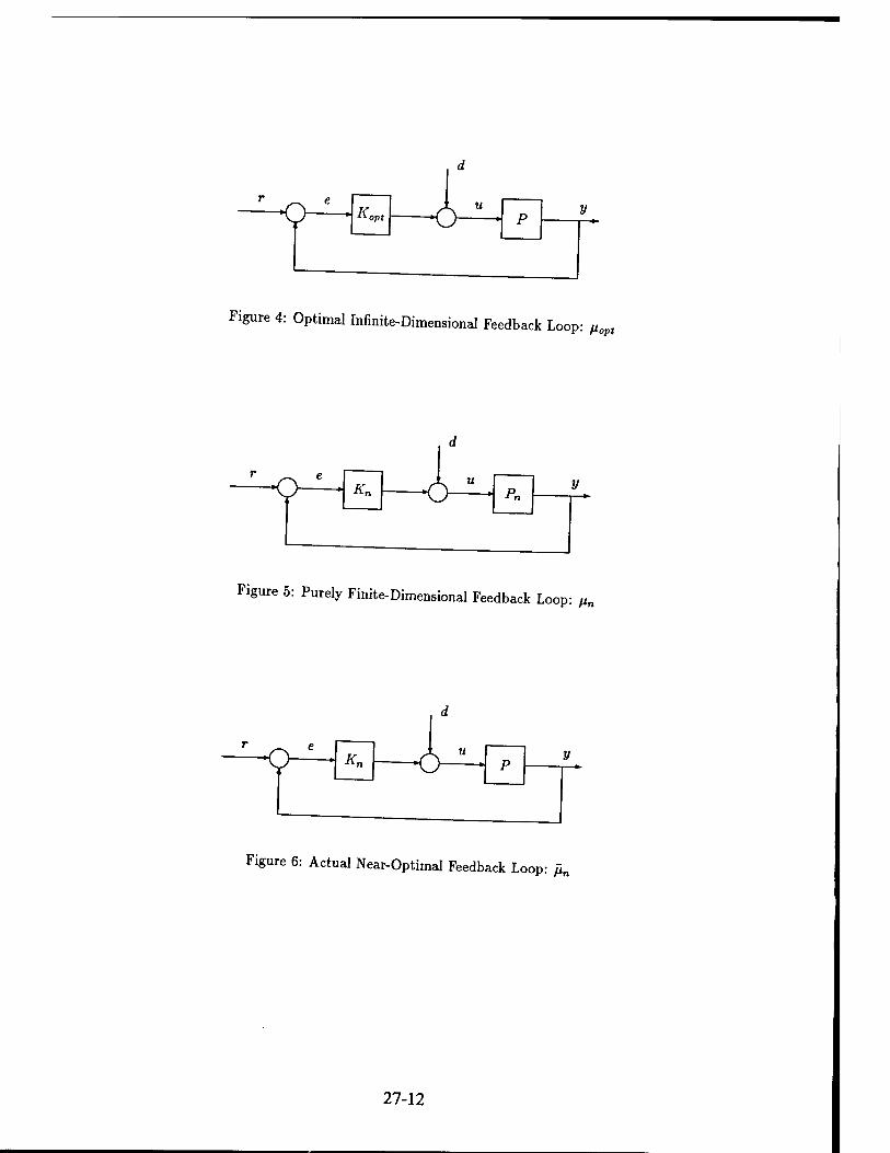
r ^ e o K, opt
Figure 4: Optimal Infinite-Dimensional Feedback Loop: Hopt
o Kn Pn
Figure 5: Purely Finite-Dimensional Feedback Loop: //„
r ^ e o— *„
Figure 6: Actual Near-Optimal Feedback Loop: fxn
27-12

lim fin — f*opt n—>oo
Given this, the .hove AtP^U/Des„« procedure provide, con.ro. enters with a sy^atic«oolfor
designing finite-dimensional controllers fo, complex Stahle disputed parameter systems (.ee F.gures 4£
2 i, I interesting to note that the .pproxim.nts P. can he constmcted directly from fluency response
data P(jw). The unstable case is treated in [5], [6].
U~ Sensitivity Performance Criterion. Also treated in [4] is the so-called weighted H~ sens^Uy
problem. For this problem, the optimal performance is denned as follows:
fiopt = inf W
^stabilizing || 1 — PK ||%oo
„here W 6 RH~. Fo, this prohl.m, the constrnction of . near-optimal compensator b more complex.
t this prohlem, the app— A mnst he such th.t the inner .nd outer parts P P; .ppropr..«e.y
.pp,„xim..e the inner and outer parts of the pl.nt P„ P.. The nnst.hle case „ treated ,n [5], [6].
3 Performance Enhancement for Systems with Multiple Hard
Nonlinearities
,. this section a method is presented for enhancing «he „erform.nce of . control system in «he presence of
multiple „emoryless „online.rities. For simplicity, the discussion i, limited to control sa.ura.ton.
3.1 Method for Accommodating Saturating Actuators
While an AFOSR Research Assoei.«e .« Egli» Air Force Bane and throughout the course of this research, the
Zincip.1 inves«ig.to, has foenssed on the prohlem of enh.ncing performance in the presence of memoryl,
Ld LlinearUies and, in particular, multiple s.tnr.ting actuators [10H13]. The me hods ev lop^d»
hased on «he work of [14] .nd «he more recent work of [15]. Other approaches are descnhed -M«^
suffer from performance and st.hili.y p.ohlems. To descrih. the procedure, some no.atton and assumpfons
will be needed.
Let P denote a linear time invariant (LTI), multiple-input multiple-output (MIMO) plant. Let K denote
a LTI MIMO compensator with state x(t) and state space triple [A,B,C]; i.e.
n (!) x = Ax + Be u = Cx
The pair (P, K) can be visualized as shown in Figure 7. The following assumptions will be made on P and K.
27-13
Assumption 3.1 (Assumptions on P and K)
It will be assumed that
(1) P is stable.
(2) K has been designed so that the closed loop system in Figure 7 has desirable properties >.
(3) K is neutrally stable3.
(4) The pair (A, C) is observable.
The case where P is unstable will be discussed subsequently. The compensator K may be designed usin! any linear design methodology (e.g. W~ ft» ri LOr/TTR „♦ ^ m « , method H -u J ,- , r , ' ' LQ<J/LTR' etc) PJ- If a complex model is available, the methods described earlier (see [4]-[7]) may prove useful.
It is implicitly assumed that the feedback loop in Figure 7 has «nice« properties. Now let .<) denote
:::ra7*g asaturation in each contro1 "• A,S°-
without i™ *-« ^ be sTopeTs Now 7t TTeS ^ ^ and tHat CaCh SatUrati°n ^ a tranSfer *«*-** With -ity
P [8]. Now consider the feedback loop in Figure 8. It is also implicitly assumed that the performance of
this loop is undesirable because of the presence of the saturations. The goal then is to modify K to improve
performance. Toward this end, the structure in Figure 9 is proposed. In this figure,
«,(*) = sat(n(t)) u(t) = k(t), [X{x> e)e(t)] (2)
where k(t) is the impulse response matrix of the compensator K, * denotes convolution, and A = A(* e) €
0 ] is a nonlinear scalar gain which depends on the compensator state <t) and the error signal eW=
f a^yLri rePreSentS a n0nlinear SyStem- ThlS 1S ^ —- * *™ * — *W = «0 - not^l'VlTTZ f COmPUtinS A ' SiVen- ThC idGa behiDd the >r°Cedure is s™Ple- If the system is no saturate it should be allowed to operate linearly as intended with A = 1. If the system is on the «verge
h T: r, r ;;gain A-since x is a sc^such gain reduction >— ^ »^ ^ajn ^s^T m ^ Pr°PertieS °f thC °riginal deSign)- ThC *™*™ »**- * — «Pace representation of the compensator and guarantees £°° finite-gain stability [8].
e.g. robust performance, etc
restrictive for missile autopilots. geometnc deficency are not pennitted here. This assumption is not
27-14
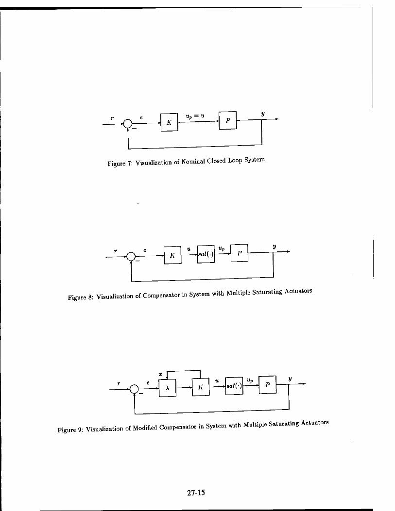
r ^ e uD = «
-Q A'
Figure 7: Visualization of Nominal Closed Loop System
r „-. e Or- K sat(-) p f—"
Figure 8 : Visualization of Compensator in System with Multiple Saturating Actuators
x I ,....,.. ... e
A K u
sat(-) Up
p » ¥•
t ' ►
Figure 9: Visualization of Modified Compensator in System with Multiple Saturating Actuators
27-15

To present the procedure, the following definition is necessary.
Definition 3.1 Suppose A 6 *»*". Given this, define the function g : R* _ R+ as follows:
*(.) d=f ||Ce^||£oo
Notice that.his function depends entirely on the homogeneous (unforced) response of the compensator'
* - [A, B, q. Given this, it ,s also useful to define the following set:
Definition 3.2
#AC =f {x€Rn: g(x) < 1}
7 ^ T ""* initiSl C°mP™S8,°' -- «» '"* "thi" « - *. bounds of " " se'to ze'°',he"lhe «-»* «<* - ^<*(0)«. row in magnita(1. ^ unily
The followmg propos,,™ conlains many usrfu| propertie8 rf ^ ^^ ^ ^ ^ ^ 'AC-
Proposition 3.1 (Properties of«; and BAC)
(1) </ is finite-valued, positive homogeneous, radially non-decreasing.
(2) g is subadditive, convex, continuous, and defines a cone.
(3) BAC is compact and convex.
A consequence of g being positive homogeneous is that p(x) - 11*11 af * \ Th« ;m r *u * • , ' determined from its values on the unit sphe ~ " ^ ? ^ ' " C°mP,etely
lere.
A continuous-time algorithm for constructing A can now be given.
Algorithm 3.1 ( Construction of A )
«IVmI«' State °?e ('°^M^ »->—« * - «- , Let . denote the e„„t signal at tun. <. The f„H„wmg -,,„tim ,lgOTithm k propo8ed fop con,tractin(, A „ ^ ^ (
(i) If x lies within B^c, then A = 1.
(Ü) If x lies on the boundary of BAC, then maximize A 6 [0,1] such that
lim ~r9(* + Wx + B\e}-g(x) e-o+ '7 < 0 (3)
(iii) If x lies outside BAC, choose A € [0,1] such that above expression is minimized.
27-16

„ should be noted that «he expression in elation (3) is essentially «he time derivative of , along the
trajectories of the modified compensator:
n (4)
given in Figure 9. More precisely, since , in general is not differentiate, the limit in equation (3) denotes
the uvver right Dini derivative - a quantity which is well defined for g. To tapllt «he algorithm, one must he ahle to determine where the compensator s«a«e . „es w.h
JtTthe boundjof ,M. To do this, one men« he able to evaluate , °"«—
wi,h this »ill be diseussed in the following seetion. However, given «hat A » computed . accordance
Algorithm 3.1, one obtains the following closed loop performance guarantees.
Theorem 3.1 (Guaranteed Closed Loop Properties)
Suppose that A is constructed in accordance with Algorithm 3.1. Let « = x(0). Given this, each of the
following holds.
(1) If xo lies within BAc, then \\u{t)\\c- < l for a11 e'
(2) If xo does not lie within BAC, then \\u{t)\\c- < ff(*o) for all e.
(3) The closed loop system in Figure 9 will be £°° finite-gain stable.
It should be noted that finite-gain stability can be proved because for sufficiently small exogenous signals
the system in Figure 9 exhibits linear behavior.
3.2 Computational Issues
As pointed out in «he previous section, «he fu„e«ion , mus« he evalurted on-line. This issue i, «"***>**
fhefac« «ha« «he dennHion for , given in dehnition 3.1, no, imm.dia«* -able^— ^ What i, needed is a useful characterisation, o, approximation, for «he funCon ,. Also, because Algonlh
T,tin lm.«ely he n»p.emen«.d on a digital compute,, a «ortX version of «he algordhm - needed.
These points are now addressed. Suppose that K has a discrete-time realization [Ä,B,C] as follows:
*n+l = Äxn + Ben Un = Cxn
where Ä is also at least neutrally stable. Given this, , may be approximated as follows.
27-17
(5)

Proposition 3.2 (Approximation for g.)
Given that Ä is at least neutrally stable, it follows that „ may be approximated as follows:
9{x) « g(x) 1?
C~ 1 4 Ci4 CÄ2
CÄ3
Lei*. where k is some sufficiently large integer which can be determined
£oo
off-line.
L" ET °Ut tha' S°me °f'he 'ermS " 'he ab°™ ■"»*-«- -* ■>• ™—*• To identify
Algorithm 3.2 ( Discrete Performance Enhancement Algorithm )
The f°"OWm6 d"—"™ ^orithm is proposed for constructing A. a. each „.
0) If 9(*n) < 1, then An = 1.
(ii) If g{xn) = 1, then maximize A„ € [0,1] such that
g(Äxn + BXnen) - g(xn) < 0
(üi) Ug(*n) > 1, choose A„ € [0,1] such that above expression is minimized.
(6)
^^;~th" aIgo;:thmrequires that an on-,ine optimization be "■*— « - «-te" Consequently, effiaent optlmizat10n routines must be sought. Because A controls the "amount" of error entenng the compensator, it is referred to as an error governor.
3.3 Unstable Operating Points and Other Hard Nonlinearities
hotvlr;!"::"; bbeen: rtems with dynamks that -,ocai*st^ ^ •*- —<>
unsTaMe^Tan has fi I * "" ^^ "" ^ "^ ^-ntally, this is because an
Isi^ commanH , . KV " * "**"" ^°—which «mi*- the rate of growth of the reference ;rrt:^^^ at Eglin Air Force Base the n, ' " ^ * ^^ ^P^ Conse<^> »hue
cJg-J^^r r? ;n;estisator worked on the probiem °f designing «-*■** -hi* 6 aPproPrlate estunates of the plant states to be used by the „/ere„ce governor. The ideas in
27-18

[171 and [18] were very helpful because they provided insight into the design of a suitable C es«,ma«o. Of
m o,«.nce here Is really the ,„.« »e— which occurs in the design <*--•.— "^
estimation theory, one expects that as the sensor nolse decreases, the •^^^T" proves. However, it may be that certain state estimation errors may grow »gruncantly before they d cay
rapidly to zero. This peaking phenomenon is discussed in [17] for Linear Quadr.«,c «"^."-M-
i.Lows that conditions can be obtained to prevent such peaking from occurr.ng. The cond,«,on, loosely
speaking requires that the transfer function matrix from the process noise to the measurements possesses
Italnl number of transmission «~ This will be guaranteed if «bis transfer funcrion matnx has
(normal) rank equal to the rank of its associated first Markov parameter.
ft should be noted that an CT estimator, i.e. one which is accompamedw.«., bounds on the pe
estimation errors, i. perhaps more appropriate to address the technical issues dtscussed abov. Th* «mr
I. still in progress. Other hard nonlinear,«!«,, such as rate limiters and o-hrmters, cm, easdy be addres.d
using the estimation methods ideas proposed here.
3.4 Extension to Nonlinear Compensators
It should also be noted that the above method extends directly to bilinear compensators [19]; i.e. nonlinear
compensators with state space descriptions as follows:
(7) x = Ax + B(x)e u = Cx
„here A and O are constant matrices and „(■) is a matrix function of the compensator state * ThiaTs
particularly interesting because nonlinear systems with fading memory can be »pproxmtated by brhnea,
systems. , , More generally, the ideas also seem to directly extend to compensators having the form
x = Ax + B(x,e) u = C{x)
where B(x,0) = 0 and C(-) is «sufficiently well-behaved". These ideas are currently being examined by the
principal investigator.
4 Applications
4.1 Flexible Space Structure: SPICE
,n [20] [21], the idea, discussed in section 2 were applied to the problem of controlling a flexible structure
which may operate an a space telescope o, - a laser beam expander. A, , flexible laaer beam expander, th
structure chemically generates , „arrow laser beam and expands it via Cassegrain primary secondary rmrro
system. Generation of the high intensity beam and coolant flow through ,h. mirror, result ,n exc.a.mn
,h, s«rnc.ural modes. The problem here is to perform rapid/accurate slewing^«nting maneuvers w,hout
excitation of «he flexible modes. Having been developed by the Air Force, w,h Lockheed and HoneyweU -
snhco„«,.c«o,s, «his sys«em physically resides a« «he Phillip. L.bo,a«o,y on KnUand A.r Force Base. Th»
system has been assigned the acronym SPICE for Space Integrated Control Expenmen«.
27-19
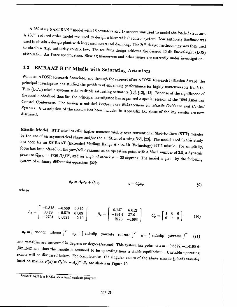
A ,tr rr f mode'wi,h is actua,o,s and is •—~ ^ «• -«<* *—-~*~ Id 'h
e,dUCed;"ier ■""*' "- "Sed «° **■ » W-«U-I -».el system. Low authority feedback „a,
";*: ***"> P'Mt ™'h '"«^l "™""<" <"«"*.* The W» design methodology was th.n used to ob,™ a H.gh authority contro! law. The resulting design achieves ,h. desired 40 db li„e-of-sigh. (LOS)
a,,.nua„o„ Alt Force speculation. Slewing maneuvers and other issue, are currently under investigation.
4.2 EMRAAT BTT Missile with Saturating Actuators
While w AFOSR Research Associate, and through the support of an AFOSR Research Initiation Award the
ZTB^TT'T haS 8'U<"ed ,he Pr0b'em °tenhanCi"8 "*"— *" ** —>»'« Baok-to-
the es Us o tamed thus far, «he principal investigator has organic a special session a. the 1994 American Contro, C„nfe,.nce The K^m is entitled ^„^„^ ^.„„„^
dtusld C"Pt,°" °f the SeSSi0" "" be" ^ '" AP-"diX IX' S°™ * ">« ^ «*. « -
Missus Modal. BTT issues offer higher maneuver.biUty over convention,! Skid-.o-Turn (STT) missiles
by the use of ,„ asymmetrical shape and/o, the addition of a wing [22], [23], The model „sed in this study
„T r °' ", " <EXtended Medi™ Ran6e A"^Ail T-h"*^> BTT —»* **J focus ha, been placed „„ the yaw/roll dynamics at an operating point with a Mach „umber of 2.5, a dynami
ZTrf*7=Tw'mi m an8le of attack ■=20 *•«-Th« ~"is *» * * «'°™ system of ordinary differential equations [22]:
ip = Apxp + B„u, pup y = Cpx, p*p (9) where
Ap = -0.818 -0.999 0.349 80.29 -0.579 0.009 -2734 0.5621 -2.10
0.147 0.012 Bp = -194.4 37.61
-2176 -1093
ri o o] [o i oj (10)
up-[ rudder aileron f ,rp = [ sideslip yawrate rollrate f ^[sideslip yawrate f (11)
and vanaHe, are measured in degrees or degrees/second. This system has poles at . = -0.6579, -1.4195 ±
HI TK T ,miSSÜe 1S ■"Umed t0 bC °Perating ^ a Stable e^uiIibrium- stable operating points wlI1 e d d below For compIetenesSj the s.nguIar yaiues Qf the aboye J function matrix P(s) = Cp(sl - Ap)^Bp are shown in Figure 10
4NASTRAN is a NASA structural analysis program.
27-20
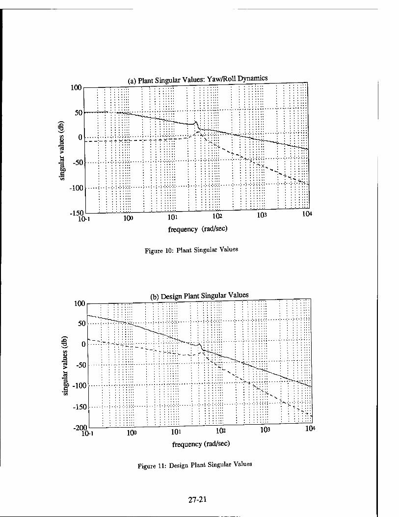
100 (a) Plant Singular Values: Yaw/Roll Dynamics
1 >
1 .a
-150 10-1 100 101 102
frequency (rad/sec)
103 104
Figure 10: Plant Singular Values
100
50
(b) Design Plant Singular Values
X> 0 N^
CA U 3 cd > -50 a
.s 09
-100
-150
-200 10-1 101 102
frequency (rad/sec)
Figure 11: Design Plant Singular Values
27-21

Nominal Autopilot Design. For purposes of demonstrating the performance enhancement concept, the
LQG/LTR design methodology [24] was used to obtain a nominal linear autopilot design. The procedure for obtaining the nominal autopilot design is now described.
Step 1: Form Design Plant. To guarantee zero steady state error to step commands, the plant P =
[AP,BP,CP], given above, was augmented with integrators; one in each control channel. The resulting system
is called the design plant and has a state space triple [Ade,, Bdes, Cdes] given by
AdeS=[BP I] B'" = [o] Cde, = [0 Cp] (12) The design plant singular values have been plotted in Figure 11.
Step 2: Design Target Loop. The next step in the process is to design the target (desired) open loop
transfer function matrix. The target loop was selected to have a state space triple [Ade„H,Cde,] where the Jitter gam matrix H was selected to be
tf=10 [,4 - ^1 f -0-0003 0.0912 I"1, 5J [ -1.6482 -1.7159 J ~
-0.1036 -0.0055 -4.8067 0.0009 2.0003 0.0000 0.0003 2.0000 4.8980 5.7272
(13)
where ,4=[ 0.0009 0 -0.0001 -0.3296 -0.9441 f and v5 =[ 0 0.0440 -0.0182 0.3432 0 9381 V
are right eignenvectors of Ades corresponding to the eigenvalue A = 0. This makes the pair (Adea>H) uncon-
trollable because the left eigenvectors of Ade, associated with the missile modes lie in the left null space of H
[25]. By so doing, one obtains a target loop which looks like an «integrator" with gain crossover frequency
near 2 rad/sec. For convenience, the target loop singular values have been plotted in Figure 12.
Step 3: Recover Target Loop. The next step in the process is to recover the target loop by solving
an appropriately formulated cheap control problem. This amounts to solving the Control Algebraic Riccati Equation (CARE)
0 = KcAde, + Al,Kc + Cl,Cdea - KeBde^Bl,K, (14)
for the unique symmetric positive definite solution Ke. This was done with a recovery parameter p = 10~« Doing this yields the control gain matrix
Gp = -Bl,Ke = f 612-444° -88.1472 -410.4327 -965.3118 -1.7612 1 P [ -88.1472 164.2489 -564.4860 254.7471 -7.1359 j (15)
The final (i.e. nominal) compensator, K, is then given by
x = Ax + Be u = Cx (16)
where e = r — y and
A = Ades - BdesGp - HCde, B = H C = GP (17)
27-22
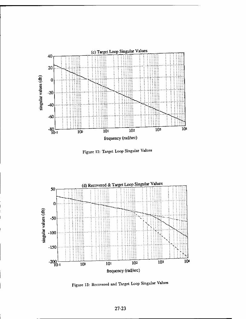
(c) Target Loop Singular Values
101 102
frequency (rad/sec)
10»
Figure 12: Target Loop Singular Values
-200, 10-1
(d) Recovered & Target Loop Singular Values
101 102
frequency (rad/sec)
Figure 13: Recovered and Target Loop Singular Values
27-23
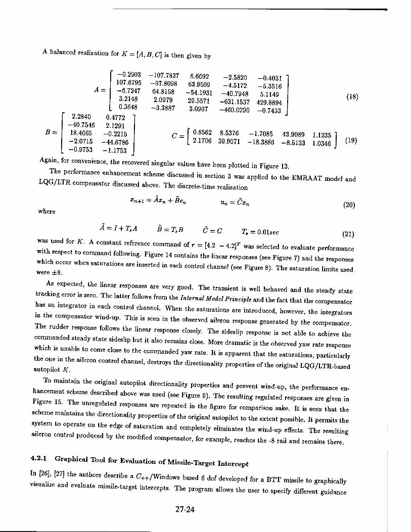
A balanced realization for K = [A,B,C] is then given by
B =
2.2840 -40.7546 18.4665 -2.0715 -0.9753
6.6692 63.9509
-54.1931 29.5571 3.0907
-2.5820 -4.5172 -40.7948
-631.1537 -460.0290
-0.4031 -5.3516 5.1149
429.8894 -0.7433
(18)
-0.2903 -107.7837 107.6795 -97.8098
A = -6.7247 64.8158 3.2148 2.0979 0.3648 -3.3887
0.4772 " 2.1291
-0.2215 c = \ °8562
-44.6786 I 21706 -1.1753
Again, for convenience, the recovered singular values have been plotted in Figure 13
rOP/rTperf0rmanCe enhanCement SCheme di8CUSSed in sect- 3 was applied to the EMRAAT model and i^G/LTR compensator discussed above. The discrete-time realization
8.5376 -1.7085 43.9089 1.1235 , 39.9071 -18.3886 -8.5133 1.0346 I (19) ]
xn+1 = Axn + Ben un = Cxn
where (20)
Ä = I + T,A C = C T,= O.Olsec B - T,B o = o T, = O.Olsec (21)
was used for K. A constant reference command of r = [4.2 - 4.2]- was selected to evaluate performance
w^h respect to command following. Figure 14 contains the linear responses (see Figure 7) and the responses wh ch when saturationg ^ inserted ^ each controi channej (see Figure 8) The gaturation ^ P ^
were ito.
As expected, the linear responses are very good. The transient is well behaved and the steady state
rackmg error ls zero. The latter follows from the Internal Model Principle and the fact that the compensator
has an mtegrator in each control channel. When the saturations are introduced, however, the integrators
m the compensator wind-up. This is seen in the observed aileron response generated by the compensator.
The rudder response follows the linear response closely. The sideslip response is not able to achieve the
commanded steady state sideslip but it also remains Cose. More dramatic is the observed yaw rate response
which .unable o come close to the commanded yaw rate. It is apparent that the saturations, particularly
the one m the aderon control channel, destroys the directionality properties of the original LQG/LTR-based autopilot J\.
To maintain the original autopilot directionality properties and prevent wind-up, the performance en-
hancement scheme described above was used (see Figure 9). The resulting regulated responses are given in
Figure 15. The unregulated responses are repeated in the figure for comparison sake. It is seen that the
scheme maintains the directionality properties of the original autopilot to the extent possible. It permits the
system to operate on the edge of saturation and completely eliminates the wind-up effects. The resulting
aderon control produced by the modified compensator, for example, reaches the -8 rail and remains there.
4.2.1 Graphical Tool for Evaluation of Missile-Target Intercept
In [26], [27] the authors describe a C++/Windows based 6 dof developed for a BTT missile to graphically
visualize and evaluate missile-target intercepts. The program allows the user to specify different guidand
27-24
(a) Linear and Unregulated Outputs
6
1 o U
0 0.5 1 1.5 2 25 3 3.5
time (seconds)
(b) Linear and Unregulated Controls
0 S
-2
•4
-6
-8
-10
-12
-14
V-
-V
V
L 0 0.5 1.5 2 2.5 3
time (seconds)
3.5 4.5
Figure 14: Linear and Unregulated Responses
27-25
10 (a) Regulated and Unregulated Outputs
0.5 1 1.5
0
-2
-4
-6
I -8
2 2.5 3 3.5 4 4.5
time (seconds)
(b) Regulated and Unregulated Controls
-10
-12
-i4 : : ; ;.'.*......
0 0.5 1 1.5
1.2
1
0.8
0.6
0.4 ....
0.2 ....
0 -V • -)
-0.2 j- : -'
(c) Lambda
Figure 15: Regulated and Unregulated Responses
2 2.5 3 3.5 4 4.5 5 time (seconds)
27-26
,aws autopilots, engagement geometries, and target maneuvers. The program aiso permrts • «-1 evalu. o„
tfThe effects rfwL-* o„ the guidance and control systems. The prop,™ - currently bemg
used to visualize the performance of the saturatiou algorithm described earher.
4 3 Platoon of Vehicles with Saturating Actuators
In[28,,,h,satu,ation method described b^*~^**^"^.™£££ dy amics of a platoou of vehicles with saturating actuators. Each vehicle ,n the platoon .■»«**■ £L nonllar dinerential equatio„. One degree of freedom is »sed to capture the vehtcle dy«
another to capture the engine dynamics. The nomina, contro, law i, designed usmg ^«™ techniques. The throttl. on each vehicle is assumed to he limited and vartous verstons of «h. algonthm
discussed earlier is applied.
4 4 Invited Sessions: Missile Guidance and Control
The completed research on memcyless hard „»„linearities and, in -~ —J^I [101 [11] has led to the organization of two invited sess.ons: one at the It» Arabern Lo I
llhe held in Baltimore, MD and one at the ,9» 0-*«* **»-, -< C°»"" **~" *° "J"" ta Phoenix, AZ [12], [13], Both address performance enhancement and integrated des,g„ to, mtssfie gurdance
and control systems.
5 Summary and Directions for Future Research
,„ summary, two significant contributions have bee» made in this research. The first is a systematic design
methodology fo, general distributed parameter systems. The second, is a procedure wh.ch „etnas con
Queers to dire tly ..he into account memory.es, hard nonlinearities such - ..«ura.mg actuators, r ZZ etc The procedure enhances performs in the presence of such „„„lineant.es, sys em.t.es the
'Z: process, „„„is computationally feasible with the Computing _ — or, e=*£-
The research is continuing as follows. New performance cnterton (other than « ) are g for distributed parameter systems. Also, the performance enhancement scheme . hemg extended to more
general nonlinear compensators.
6 Bibliography
References
M S H. Mahloeh »d A.A. Bodrigue,, «System .deu.iflca.ion from a Frequency Response" Proceed of
the Sind Coherence 0« Decision and Control, San Antonio, TX, December 15-17, 1993.
M S.H. Mahloeh and A.A. Rodriguez, -System Identification from a Frequency Response: A Seq^t.al
A.gori.hm,.submi«..d fo, publication in the PtWm,, of,„e Amene.» M. Conferee, B.l.nnore,
MD, June 29-July 1, 1994.
27-27

[3] i^T; p ^T'RR Khargonekar and BA- ^ancis' "State-Space s°iutions to stand-d * -* H Control Problems," IEEE Trans AC, Vol 34, No 8, August 1989.
[4] A.A. Rodriguez and M.A. Dahleh, «W~ Control of Stable Infinite-Dimensional Systems using Finite-
Dimensiona, Technos," submitted for publication in IEEE Transactions on Automatic Control 1993
[5] A.A. Rodriguez, "Design of H~ Optimal Finite-Dimensional Controllers for Unstable Infinite- Dimensional Systems," submitted for publication to AUTOMATICA, 1993.
[6] AA Rodriguez and J.R. Cloutier, «*~ Sensitivity Minimization for Unstable Infinite-Dimensional
Plants, Proceedings of the American Control Conference, San Francisco, CA, June 2-4, 1993, pp. 2155-
[7] A.A. Rodriguez and M.A. Dahleh, «On the Computation of Induced Norms for Non-Compact Hankel
Operators Arising Fromfor Distributed Control Problems," Sterns & Control Letters, December 1992
[8] CA. Desoer and M. Vidyasagar, Feedback Systems: InPut-OutPut Properties, Academic Press, Inc, NY,
[9] B.A. Francis, A Course in Hoo Control Theory, Springer-Verlag, 1987.
[10] sit' ^7UeZ Mnd J'R' C,0Utier' "C°ntr01 °f E Bank-^-Missile with Saturating Actuators", subrrutted for publication in the Proceedings of the 1994 American Control Conference, Baltimore MD
[11] A.A. Rodriguez and J.R. Cloutier, «Control of a Bank-to-Turn-Missile with Multiple Saturating Actu-
ators, m preparation, to be submitted to AIAA Journal of Guidance, Control, and Dynamics
[12] A^Rodriguez and S^N. Balakrishnan, «Performance Enhancement for Missile Guidance and Control
Systems , proposal submitted for invited session to 1994 American Control Conference, Baltimore MD
[13] S.N. Balakrishnan and A.A. Rodriguez, «Performance Enhancement for Integrated Missile Guidance
Control Systems", Invited Session, 1994 AIAA Guidance and Control Conference, Phoenix AZ
[14] P. Kapasouris, «Design for Performance Enhancement in Feedback Control Systems with Multiple Sat-
urating Nonhneanties," LIDS MIT, PhD Thesis, LIDS-TH-1757, March 1988.
[15] E.G Gilbert, and K.T. Tan, «Linear Systems with State and Control Constraints: The Theory and
Application of Maximal Output Admissible Sets," IEEE Trans Automatic Control, Vol AC-36 No 9 September 1991, pp. 1008-1020.
[16] M. Mo„,i -s™ Co„„„, Pt„blems in ehe Ptocess Industries . progresg .n SystenB and Contro
»„Control: Pe„p,ct,vea in the Theory and Us Application,, Bh-kh.user, Editor.: H.L. TY.ntehnan ,„d J.C. Willems, 1993, pp. 55-77.
[17] BIFt
FtTS and K' G1°Ver' "B°Unded Peaking iD thG °Ptimal Linear ***** with Cheap Control," IEEE Transactions on Automatic Control, Vol. AC-23, No. 4, August 1978, pp. 608-617
[18] sHyLiTm~RV' K;kotovic' ;The peakins phenomenon and the Gi°bai stabiiizati°n systems, IEEE Transactions on Automatic Control, Vol. AC-36, No. 4, August 1991, pp. 424-440
[19] A. Isidori, «Nonlinear Control Systems," 2nd Edition, Springer-Verlag, New York, 1989
27-28

.201 A A Rodriguez and Delano Carter, «Hierarchical HAC./XAC Vibration Suppression fo, a Flexi-
" uf Space -Loop.: SPICE," subndtted Tor pub.ication ia .be Proceed a/ Ü. A~n~ C~»>
Conference, Baltimore, MD, June 29-July 1, 1994.
J n i r»rt»r <"W°° Control of SPICE: A Flexible Laser Beam Expander," sub- mi A.A. Rodriguez and Delano Carter, Ji Control oi an^ mitted for publication in the Journal of Dynarmc Systems, Measurements, and Control.
L „ A T u „wi Rnssi et al "Advanced Robust Autopilot," Air Force Armament [22] I A. Hirsch, M.A. Langehough, J.A. Bossi, et ai. , Auvam,
Laboratory, Eglin AFB, Florida, AFATL-TR-89-64, November 1989.
[23] J H Blakelock, AutomaUc Control of Aircraft and Heiles, 2nd Edition, John Wiley & Sons, Inc., 1991.
[24] G. Stein and M. Athans, 'The LQG/LTR Procedure for Multivariable Feedback Control Design," IEEE
Transactions on Automatic Control, Vol. AC-32, No. 2, February 1987, pp. 105-114.
[25] T Kailath, "Linear Systems," Prentice-Hall, 1980.
r26l M Sonne and A.A. Rodriguez, "PC's in the Design and Evaluation of Guidance and Control Sys- [] LZ Missiles," to appear in the Proceed^ of the 1W I^aUonal Conference on S.mulaUon »
Engineering Education, Tempe, AZ, January 24-26 1994.
M M. Sonae aad A.A. Rodrigue,, «A PC-baaad Graphics System fo, the Eva>n,ti„n «™**£
aad Control Laws," submitted fo, publication in the Pm«.a,n9, ./ <*. Amencan Contra, Can/.rca«,
Baltimore, MD, June 29-July 1, 1994.
m S C. Warnick and A.A. Rodriguez, «Longitudinal Control of a Platoon of Vehicles with Saturating
Nonlinearities," submitted for publication in the IEEE Transacts on Control Technology.
27-29
Part I
Appendix: Proposal for Invited Session to 1994 ACC
A.A. Rodriguez, Chair S.N. Balakrishnan, Co-chair Arizona State University University of Missouri-Rolla Tempe, AZ 85287-7606 RoUa, M0 65401
Overview of Proposed Session
unstarr8 °f 'he g'eal T^* WhiC" a° e™i,e *"get PreSentS' "» '""»«' »*-» «I W-K, ^ Ienon-rrnn phase dynamics ^^ ^ ^ fc J
nussle systems ,„„ represent, „ne of the tichest „, ^
OT;;"! Tilhe pri drde raany ■*— have bea° made - ,h« - - ■** - -*- and aHow engmeer, to bet,., address nonlinear design issues. Thi, session is an effort to bring researcher
,tZcTurp;cl; "^suidance ™d con,to1 *-- -—- «- -»-« some of the „sues wh.ch researchers in the missile guidance aud control community are now addressing.
Motivation and Summary
The title of the proposed session is
Performance Enhancement for MiasUe Guidance «nd Control Systems.
«ePJZ'LadTr thiS SUbJeCf
t',it 'S imPO"ant that ■" ™PeC,S -*« "'"> ■*» ^»id— - «—' Z m * 0r8amZe'S ' eXamP'e' 'hat " ~ M~y fa "»— '° »»'- -*«l. for 7277*' °P r°8' a"d e"ha°CinS the "'*""*"* °f '°day'S »Uto-il* '»'1 «"M""» >J*™- This «a oi: ;T ? s * the auiopiiot i° accommoda'e "-"^hMd—-«- -* - -»*•. 8u d.rioot tr ;T 7doins' au">pi'o, pertormance ™"id be Mta»d -■-*—««», e r: ZdT r t such adi,c~must'*--■ inv*e•*—«"■—-* ZZT;«, ■ ,he ,ateat op"miza,ion tech"i<»'es-The -«*- - ««**- tTf: cl TK*
0 rd" MW ™'h0dS *» *-"- «■"— - -- state tracking. This,
*» f« t coui properiy be addressed by researchers working on -approximate!/' analytical guidance law
i^z,z::zr^ —-■ -* -« -—- - -~ - - - To accommodate the above requirements, ,h. organize. solicited paper, from researchers in academia
mdustry, and the rruhtary. Six (6) paper, „ere selected to address the following topic
27-30
1. Performance Enhancement for a Missile with Multiple Hard Nonlinearities.
A.A. Rodriguez, Arizona State University; Session Organizer.
James R. Cloutier, Armament Directorate, Eglin Air Force Base,
title: Control of a Bank-to-Turn (BTT) Missile with Saturating Actuators
2 Improved Guidance Laws for Missiles: An Analytic Approach.
S.N. Balakrishnan, University of Missouri-Rolla; Session Co-organizer,
title: Improved Guidance Laws for Missiles: An Analytic Approach
3. Autopilot Design using H°° Design Methods. Kevin A. Wise, McDonnell Douglas Missile Systems Co.
Eric S. Hamby, McDonnell Douglas Missile Systems Co.
title: n°° Missile Autopilot Design With and Without Imaginary Axis Zeros
4. Methods for Improved Target State Estimation.
Chris D'Souza, Armament Directorate, Eglin Air Force Base.
James R. Cloutier, Armament Directorate, Eglin Air Force Base,
title: Spherical-based Target State Estimation
5. Autopilot Optimization using Genetic Algorithms.
Richard Hull, University of Central Florida.
Roeer W Johnson, University of Central Florida. . 2pTrformance Enhancement of a Missile Autopilot via Genetic Algorithm Optmnza.on Technos
6. Missile Eigenstructure Assignment via Dynamic Compensation.
Robert Wilson, Armament Directorate, Eglin Air Force Base.
James R. Cloutier, Armament Directorate, Eglin Air Force Base,
title: Eigenstructure Assignment via Dynamic Compensation
27-31
ENHANCED LIQUID FUEL ATOMIZATION THROUGH EFFERVESCENT INJECTION
Larry A. Roe Assistant Professor
Mechanical Engineering Department
Virginia Polytechnic Institute and State University Blacksburg, VA 24061-0238
Final Report for: Research Initiation Program
Advanced Propulsion Division Aeropropulsion and Power Directorate
Wright Laboratories
Sponsored by: Air Force Office of Scientific Research
Boiling Air Force Base, Washington, D.C.
December 1993
28- 1

ENHANCED LIQUID FUEL ATOMIZATION THROUGH EFFERVESCENT INJECTION
Larry A. Roe Assistant Professor
Mechanical Engineering Department Virginia Polytechnic Institute and State University
Abstract
A snrgie-componen,, ptas.Dop^ mkk Maly2er mK) m ^^ modified for tabMe ^
rceasurem«, and appiied t0 ^ ^ „„^ rf ^^ ^ ^ ^ ^ ^
system, A wide range of ins*™« hardware and ^ ^ _ ^ ^ ^^ ^
■nances of ins«™« sedings „, gas ioading were evaluated. „ was „^ ^ fc pDpA ^
produces reiiabie bubble size informalion fa „^ ^^ ^ ^^ ^ ^ ^ ^ ^
"^ VO,,,me ra'i0S " * " 10 '«» <f» 1— - app,o*iMe,y 20 psia>. Tbese dinners are
— -be range of bneres, for efferent atoraizaoor, «benaes, «ongb ibe gas .„adings „ somewnal |ow
There drd „o, seem ,o be a strong correMon between b„bb,e size and ,be size ebameterisdcs of .be cubing
sprcy.M^aiidanonof^easn«^^^
pnovidedbyaJB1berco„me,„,lbeteslsys,emwas1Ur„edoverloUSAPa„dconttac„rp=rsonne,forcontinued
evaluation of injector designs.
28-2

ENHANCED LIQUID FUEL ATOMIZATION THROUGH EFFERVESCENT INJECTION
Larry A. Roe
INTRODUCTION
Effervescentinjection offers the potentM for signfficant performance improvements in all Hqdd-^^
systems, with advantages particularly suited to ramjet engines. This fuel injection scheme would typically
introduce small bubbles of air or another gas into the liquid fuel stream prior to injection into the combustion
chamber. The bursting of these bubbles leads to rapid breakup of the liquid fuel and dramatically improved
atomization at low fuel-supply pressures. A major drawback to the successful implementation of this technique
in actual combustion systems is the total lack of numerical data relating bubble size in the two-phase fuel stream
to the diameter of the resultant fuel spray droplets. A primary reason for this shortcoming has been the
unavailability of appropriate instrumentation capable of measuring the bubble size distributions.
One difficulty typically encountered when evaluating the performance of liquid fuel injectors is associated with
the acquisition of reliable droplet and bubble statistics. Parameters crucial to the characterization of the injection
scheme include average droplet diameter, droplet size distribution, droplet velocity, and diameter-velocity
correlations. In addition, any attempt to correlate droplet statistics with bubble statistics in 2-phase injectors
requires a reliable technique for bubble sizing. The focus of this program was to provide the instrumentation and
analysis capability required for such evaluations. The instrumentation system, a phase-Doppler particle analyzer
(PDPA), provides an analysis capability for effervescent injection studies which has not been previously utilized
by researchers in this field.
REVIEW: TWO-PHASE INJECTION
One of the earliest investigations of the atomization of a gas-liquid mixture was reported by Chawla (1985). It
was determined that small droplets were produced, largely independent of the size of the fuel delivery orifice.
In addition, small droplets were produced at relatively low fuel velocities when compared to pressure atomizers.
28-3

The concepts associated „id, effervescent injection have „. develope(1 h papers by Waj)g M ^ ^ ^
and Lefebvre (,987), Lefebvre e, a,. 0988), Avrasldcov e. a,. (1990), and Aral and Scherz (1992).
Wang e, a, (1987, studied efferent injection „f „aKr/„toge„ mixtures int0 quiescenl air . normal
atmospheric pressure and temperature. The nitrogen „as «« ^ , large chimber ^^ ^^ ^
.he injection orifice. Two gas injection designs (differing primarily in the diameter of me holes through which
the ps „asbubb,efli„,„Mq„id, and d™e oriflce diameters „ere evaiuated. Gas pressure and gas/fiquid mass
fraction were each varied over abon, an order of magnitude. DroP,e, size was determined with a Malvem
analyzer, which provides a spatially averaged mean drop,« size. Bubble sizing was no, attempted. I, „as
concluded that the atomizafion varied primarily „id, injecdon pressure and mass rafio, with less sensitive „
orifice diameter and injection geometry.
Roesler and Lefebvre (1987, extended me previous stud, to a wide, range of gasfliquid mass ratios. Air was
mfioduccdthroughaporouscyfinderinto me water stream, and „«influence of ai, supply pressure, aemto, tube
porosity, orifice diameter, aud 8asniqmd mass rafio were evaiuated. Again, orifice size and aerator polity
(which was assumed to con.ro, bubble size, „ere found to have lime influence on me mean droplet size. Bubble
sizes „ere no, measured. Good atomizafion occurred for ga*,„id mass mfios as ,o„ as 0.02. Tue air pressures
mquired were only tfiose sufficient to cause flow through ,he po^ cylWer at ,he mass mts ^
A continuation study by Lefebvre e, al. ,1988, conflrmed these conclusions over a different range
Good atomizafion „as again obiained „sing small amounts of injeced air. a. injection pressures as low as 5 psi
Avrashtov ., al. „990, used bod, hydrogen and helium bubb,es in kerosene, with 8a^iquid mass raflos from
0 an .0 percent The mixhrre was injMed a. high pressure (- 20 ahn, into a supersonic combustion chaml*r at
. aunosphere and me self-ignifion and stability characteristics evaiuated. The gas addiflon was found no increase
the dispersion of fine spray cone, provide better flquid penetrafion into the free siream and improve mixing, bu,
did no, significanfly affect mean drop size a, the high injection pressures utilized.
28-4

Aral and Schetz (1992) injected helium/water flows at high pressure (-20 aim) into a supersonic tunnel through
an array of 0.8 mm diameter orifices. The production of the small bubbles required to maintain bubbly flow
through such small passages required the addition of a surfactant to the liquid prior to gas injection. Photographic
analysis of the resulting sprays showed that the gas injection increased the plume dispersion angle and increased
penetration for single-orifice injection. Changes in surfactant concentration were found to affect the spray
characteristics, apparently due to changes in bubble size, although this was not a measured parameter.
In addition to the published information summarized above, more recent, but as yet unpublished, research efforts
are in process to evaluate the application of effervescent injection to scramjet engines (Northam 1992). As with
the prior studies, the porosity of the air injection cylinder was found to have little effect on the resulting spray
characteristics.
DESCRIPTION OF PHASE-DOPPLER PARTTCLE ANALYZER
The PDPA system as manufactured by Aerometrics is based on a development by Bachalo and Houser (1984).
A more thorough description of the application of this technique is provided by Bachalo et al. (1991). A complete
description of the operational principles is well beyond the scope of this report, but a brief summary is
appropriate.
A PDPA is essentially a single-component laser Doppler anemometer (LDA) with multiple photodetectors and
additional signal processing capability. As an LDA system, it is of the standard dual-beam type. Two laser beams
intersect at a small angle in the region where measurements are to be obtained. The crossing of these two beams
defines a probe volume; droplets or bubbles passing through this zone scatter light simultaneously from the two
beams. When this scattered light reaches the receiving optics (lens or photodetector), it forms an interference
pattern, which moves in space due to the droplet motion. Tne temporal frequency at which the interference
fringes sweep across the surface of the detector is related to the transmitting optics (laser wavelength and beam
28-5

tan*. ang,e> and ,h. pariiCe ve,ocity component in ». pIane of „, inKrsecling ^ ^ fc ^
configuration is known, the velocity component can be determined.
Additional informarion is required for sizing. This is frmjM by ^^ ^^ ^^ ^
photodetectors image differ« re8i„ns ot me inlerference ^ „ ., ^ ^ fa ^ ^ ^
photodetectors aU observe me same temporal frequency (me DoPpler fKqüency relaled 10 velocity) „„, obse„e
different spada, frequencies since the interfere pattern fringes are no, pan*,. This .*, l0 , phase
differ between detectors, mis phase differe„ee is rekated to the en™«* of me fringe patten, „hieh is
«dated ,„ droplet or babble diameter (and a long Us, of other parameters, which are generally known). Wim
sophistic«, signal processing and dan, anabysis, the diameter (assumed spheriea,) can be determined.
An earner version of the PDPA system had been fu,,y characterized by ,he Principal Lavesdgator during ,he ,992
Summer Factdty Research Prognun and udta, for drop,e, measurements (Roe 1992). The primary instntmem
operadng parameters which „ere found ,o Muence the resuhs were, me incident beam intersection ang,e,
frequency shifting of ,„e *»* ^ by . „^ ^.^ ^ ^ ^ ^^
photomuhip.ier (PMT) vohage, and fihering of the ourpu, signal Several modifications to the system hartwar,
and software occurred in the tune period between the Summer ,992 effort and the beginning of this research
program. ,„ addition, further modifications to the operadon of the system were required for appficadon to bubbte
sizing.
EXPERIMENTAL PROGRAM AND RRSTTT.TS
The experimental program was conducted on-site at the laboratories of the Advanced Propulsion Division,
Aeropropulsion and Power Directorate, Wright Laboratories, Wnght-PattersonAF^, Ohio. The program
aspects. Primarily, the PDPA system was modified to provide reliable operation for bubble sizing measurements,
debugged, characterized, and made operational. Secondarily, experimental apparatus designed and constructed
in conjunction with another on-site contractor was evaluated, using the PDPA as the primary analysis tool.
28-6

Bubble Generators
Personnel from CFD Research provided support for the design and construction of several bubble generating
systems which produced two-phase flows suitable for effervescent atomization. Main operational criteria included
the ability to reliably produce bubbles with specific size distribution characteristics, optical access for the PDPA
system, controllability, and repeatability. This task proved more difficult than originally anticipated.
The bubble generation was accomplished by bubbling air into a flowing stream of water. Three different
configurations were tested. The first utilized an existing 1-inch square test section, with a two-dimensional,
variable area, converging-diverging section to control bubble generation. Maximum use of pre-existing hardware
was made to minimize long lead times in the laboratory machine shops. Water flowed through the duct, and a
tube with small holes was inserted such that the air bubbled through the holes into the water. The position of the
tube could be varied throughout the variable area section of the assembly, so that the local water velocity at the
injection point would vary. It was hoped that this would alter the shearing action of the water on the bubble ports
and change bubble size controllably. Bubble size could, in fact, be varied, but repeatability was not acceptable.
Additionally, optical access required for good PDPA measurements was not sufficient.
The second bubble generator utilized a 1-inch diameter glass tube for maximum optical access, and two types
of air injection schemes. The water flowed through an axisymmetric converging-diverging nozzle, with air
injection either through a centerline tube, as with the first configuration, or directly through the wall at the nozzle
throat. The majority of the PDPA evaluation was conducted with this generator. Controllability of the bubble
generation process was still deficient, but, as the primary goal of the program was the establishment of the PDPA
measurement technique, this generator proved sufficient to achieve that end. as ai
A third configuration was assembled by CFD personnel, and some preliminary testing was done. This design
featured a porous plate bubble generator, multiple water inlets, swirling flow, accumulator tanks, and surge
eliminators. Continued modification and testing of this device is still in progress.
28-7

PDPA Evaluation
The primal goal „f the program was to establish ,he capabilily „f „tUiring phascDoppler paaricle analysis as
the Priory evaluadon ,00, for 2-phase, liquid-gas injection schemes. Although the mstrumentadcr, had been
previously utifized for „»p.e. measurements »» ,992, several modifications ,„ insftnmen, setup md operatic
were required for bubble sizing.
initial testing of the instntmen, was condneted with a conventional optical alignment, SMegnee forward scatter
"*»'«»• MajorAfficulu^^^
incorrect siring data, and non-repearable resute. The insolent configuradon „as modified ,„ collect scanned
light in the 63-degree off-axis back scatter dftecdon, b„, difficulties continued. An exuded assesstnen, followed,
stariing withthe system „pdcs, electronics, and processors, f, was eventoaliy discovered tha, a fac.oysnpp.ied
system software upgrade ,oad=d prior ,„ me stari of mis research progmm was faulty. ,„ this system, the Soffware
controls the entire data acquisftion arnd reducdon, including varying the spacing between transmitted beams,
controlling frequency shift settings, setdng filter cutoffs in the eleetronies, and calculating dhnneters and ve.oci.ies
from the measured fmquency data. The parameters .oaded wi,h the software upgrade were, in fact, no, completely
consistent wid, the hardware. This lead ,o a wide mnge „f peeing ^„fe wMh ^ sysKm Evefflually
pordons of me previous version soffwar. were .ccated and loaded, leading to acceptable system operation.
The system was validated and exercised on the second-configuradon CFD bubble generator. The system was
concluded to provide acceptable operadon for bubble diameters between approximately 2 to 800 microns, for gas-
to-liquid volume mfios as high as 10 percent This corresponds to a mass «in of approximately 0.5 percent a,
a pressure of 20 psia. Effervesce« injection was demons,** a, this gas loading, but typical applications are
andcipatcd ,„ have higher gasdo-liquid ra,io, The limitadon on gas .oading is primarily the obscuration of the
measurement region by hubbies «ween ftte measurement region and the opfic, ft may prove feasible to obtain
good PDPA dan, a, higher loadings by passing the flow, or some portion of it. through an opdcally thin secdon
between two glass plates, so that an essemially 2-dimensiona! slice of the flow can be examined.
28-8
ACKNOWLEDGMENTS
The author wishes to express his appreciation to all Advanced Propulsion Division personnel who contributed
to this research effort. Special appreciation goes to Kevin Kirkendall of CFD Research for continued and valiant
engineering support in the design, fabrication, assembly, and testing of the bubble generation systems, and to Alan
Spring of CFD for guidance in the conceptual design and application of effervescent injection systems. The
technical guidance and support of Abdi Nejad are especially appreciated.
REFERENCES
Arai, T., and J. A. Schetz, "Penetration and Mixing of Bubbling Liquid Jets From Multiple Injectors Normal to
a Supersonic Air Stream," submitted for publication to AIAA, Oct. 1992.
Avrashkov, V., S. Baranovsky, and V. Levin, "Gasdynamic Features of Supersonic Kerosene Combustion in a
Model Combustion Chamber," AIAA paper 90-5268, AIAA Second International Aerospace Planes Conference,
Orlando, Oct. 29-31, 1990.
Bachalo, W. D., and M. J. Houser, "Phase/Doppler Spray Analyzer for Simultaneous Measurements of Drop Size
and Velocity Distributions," Ontical Engineering, vol 23, no 6, pp. 583-590, Sept/Oct 1984.
Bachalo, W. D., A. Brena de la Rosa, and R. V. Sankar, "Diagnostics for Fuel Spray Characterization,"
rnmWion Measurements, N. Chigier, ed., pp. 229-278, Hemisphere, 1991.
Chawla, J. B.." Atomization of Liquids Employing the Low Sonic Velocity of Liquid/Gas Mixtures," Proceedings
of the 3rd International Conference on Liquid Atomisation and Spray Systems, London, 1985.
Lefebvre, A. H., X. F. Wang, and C. A. Martin, "Spray Characteristics of Aerated-Liquid Pressure Atomizers,"
Tnnrnal of Propulsion, vol. 4, no. 4, pp. 293-298, July-Aug. 1988.
28-9
Northam, G. B., personal communication, Oct. 1992.
Roe, L. A., -fttahta of ,he Operaaona, Changes of a Ptase-Doppier D^e, Maiyzer ^
App.ica.ion t0 a Ramje, FaeHnjecta Research Tu„„e,, final repon for APOSR Summer ReKarch ^^
Sept. 1992.
Roesler, T. C, and A. H. Lefebvre, "Studies on Aerated-Liquid Atomization," ASME paper 87-WA/HT-17,
Winter Annual Meeting, 1987.
Wang, X. F., J. S. Chin, and A. H. Lefebvre, "Influence of Gas-Injector Geometry on Atomization Performance
of Aerated-Liquid Nozzles," 24th National Heat Transfer Conference, ASME HTD vol. 74, pp. ll-i8( 1987.
28-10
Sensor Data Clustering and Fusion for IR/MMW Dual-Mode Sensors Using Artificial Neural Networks
Thaddeus A. Roppel Associate Professor
Department of Electrical Engineering
Auburn University 200 Broun Hall
Auburn, AL 36849-5201
Final Report for: Summer Research Extension Program
Wright Laboratory
Sponsored by: Air Force Office of Scientific Research
Boiling Air Force Base, Washington, D.C. and
Auburn University
December 1993
29-1
Sensor Data Clustering and Fusion for IR/MMW Dual-Mode Sensors Using Artificial Neural Networks
Thaddeus A. Roppel Associate Professor
Department of Electrical Engineering Auburn University
Abstract
ooT-77 Tar,ificia'neuraI ne,work processi"s ol in,rared ta^ — — «- irt "<e improvemen'can be obtained",he arai,abie da,a - «*»— »*» 7, ^ da,a are C'UStered into «™ dories: „orma, and outher. These categories are
.«erected by lhe average and standard deviation o, the HMS error that resu,(s J, „^
d" ,ra,nr;rs ,he leav~'method app,ied ,o a ^ -»****«- *—« gonthmreported Here, we fi„d ,Ka, performance is improved foom 30% to 80% correct classification
ZZ „ "' ,mageS' WMe "" 'nCOnM C'aSSifiCa,i0n »* —"-«--7 *»p. from 30% ,„ 0%. or 20 x 20 pxel .mages, correct Cassification improves from 29% to 62%, while incorrect Cassification
tz r to ,I2%- ^resu,,s for fusion °f ,o x ,o -—""" 2°»»^ «-* -— tor 20 x 20 images alone.
29-2

Sensor Data Clustering and Fusion for IR/MMW Dual-Mode Sensors Using Artificial Neural Networks
Thaddeus A. Roppel
INTRODUCTION This report includes work done from 1 January to 31 December 1993 under the Air Force Summer Research
Extension Program. The laboratory focal point for this work was Mr. Ellis Boudreaux, WL/MNG-X.
This work would not have been accomplished without the key contributions made by Mrs. Mary Lou
Padgett, Auburn University Research Associate, by Mr. Mark Townsley, and by Graduate Researchers
Mr. Camille Raad and Mr. Tobias Graf von Haslingen.
Sensor fusion has the potential for improving detection and identification of targets. According to
recent studies, both theoretical and experimental, the amount of improvement can range from almost
zero dB to well over 3 dB, depending on the signal-to-noise ratio (SNR) of each sensor, and the sensor
noise correlation. The improvement can be effectively infinite in the case where one sensor fails
completely. Neural networks have been under consideration for raw data fusion due to the lugh speed
of response needed and the complexity of the problem. This study addressed certain specific questions
regarding the training of a neural network to accomplish raw data fusion under conditions where sparse
data are available. The objective is to obtain generalizable results from a small data set with
unequally sampled categories. An algorithm is suggested by which a neural network can be trained to
take maximum advantage of existing data, as well as incorporating new data to maximum advantage.
METHODOLOGY In this work, artificial neural networks (ANNs) are trained on IR images of three types of ground
targets T-62 tanks, M-113 APCs, and Lance missile launchers. The available data set contains 10 tank
images 8 APCs, and 4 launchers. Each image is a 40 x 40 pixel image with 8-bit gray-scale pixels and *
averaged down to 10 x 10 pixels using a neighborhood averaging technique. The neural networks were
simulated using the Aspirin/MIGRAINES (A/M) package developed by Mitre [Leighton, 93]. The
architecture / training is feedforward with classical backpropagation of errors with the number of
input nodes equal to the number of pixels, 12 hidden layer nodes, and two or three output nodes (one per
target category).
29-3

A set of analysis tools developed by M, Mark Townsley and enhanced by Mr. Camille Raad, both
Auburn University Research Assistants, forms the basis for the results generated. These tools
supplement the neural network to assist in determining clusters within target type which have similar
average RMS error per image. The interactions of the images of different categories are observed from
graphs of successful identification rate versus the decision threshold [Masters, 93; Padgett et al 93]
Much of the work illustrated is an extension of the techniques described in [Webster et al.84; Padgett et
al.85; Padgett, Roppel 92 ; and Padgett, Karplus 84] and using the NASA Nets multilayer perceptron simulator described in [Savely et al. 90].
The motivation for the curren, approach came from several source,. Exp.ora.ion of the A/M simulator
capabthttes led to investigation of its "rocks and mines" example, which is similar in principle to our
fcnk/launcher/ APC problem, and to conversadons with T. Sejnowski [Gorman and Sejnowski 88], Alexis
Wetland, of UCLA, also discussed the use of the Principal Components Analysis (PCA, and Canonical
Dtscnmtnan. Analysis (CDA) tools in MIGRAINES. Further insight was provided by [Dai 92 and Gluck et al. 92].
In the example using sonar data to classify objects as rocks or mines, a large training set was available
and many angles of incidence were included in this set. Being able to control the samp,e data the'
environment and replications allowed the researchers to control the variance and sample size
However, as in many real-world situations, the project reported here is expected to use hard-to-obtain
expensive »nages with unequal sample sizes, faulty sensors, and few target rotations. The results of
nKhvxdua, flight tests are unequally represented in the training images, and the range of flight
conditions is limited compared to those expected in actual combat. It is also a condition of this study
that the „nage data be presented to the neural network with as little pre-processing as possible. Any
information generated about the images is considered to be valuable for the design of future data
collection experiments and for comparing data fusion techniques.
Future enhancements of the neural network strategy are targeted toward principles discussed by
Sepowski as extensions of his earlier work. Colleagues of M. Arbib are also investigating the fusion of
multisensory input using feedforward neural networks with backpropagation training and limited
connectivity [Fagg and Arbib 92]. Essentially, if two banks of sensors are providing input, the hidden
layer nodes may be divided into region, There maybe regions accepting input from only one sensor bank
type and a region accepting input from both types to illustrate their interaction. The degree of overlap
is controllable and an excellent experimental tool. The separation needed for identification of different
29-4

features found in the input sets might require the addition of another hidden layer. Such arch.tectural
modifications to the current single hidden layer, fully connected neural network are potentially useful,
but will not be employed unless deemed necessary with the addition of more image types and sensor
types in the future.
For the current set of IR images, experts cannot routinely visually detect the target category (tank, AFC
or launcher). Some clustering of images can be visually detected, but before analysis it is difficult to
decide the significance of this clustering. The methodology presented below extends that described ,n
[Padgett et al 93].
First the average RMS error per image is computed using the entire set of images and jackknifing using
the ieave-one-out method [Masters, 93 p. 12]. All but one example from each pattern category
(categories in this case include tanks, APCs, and missile launchers) is included in the training set, and
the left-out examples from each category are used for testing. This procedure is repeated until each
image has been used as a test image for an artificial neural network. Ideally, if the training sets for
each category are homogeneous in some sense detected by the neural network, the RMS error of each
image in a category will be close to the average RMS error for that category [Savely, et al. 1990]. In a
well-trained neural network, the average and maximum RMS errors should be low for the images in the
training set and for the image(s) in the testing set.
For a second determining factor, including the interactions among images, the confusion matrix results
versus threshold are diagrammed. The RMS error generated by each test set of images (one from each
pattern category) is graphically illustrated by grouping the results into correct, incorrect and amb.guous
responses based on a threshold. This threshold is intended to be varied by the user according to the
penalties associated with incorrect results (e.g. hitting a manned vehicle), versus setting a flag
indicating an "uncertain" condition to be dealt with in an increasingly vigilant manner in the next set of
images in the series.
The leave-one-out results and the confusion matrix results are used to cluster the available data into
"normal data" and "outlier data." The normal data are the images which are self-consistent and
mutually reinforcing. They will lead to good neural network performance in the sense that the network
will correctly classify them with a high probability regardless of which images are used for traxnmg
or testing. The outlier data are those images which tend not to be recognized by the network tramed on
the normal images. In other words, the network has trouble generalizing from the normal images to the
29-5

oudier image, This can occur due ,o a number of conditions. For example, an outlier image may have
been collected under extreme iUummauon conditions, or perhaps i, contains excessive noise or obstruction.
We are presently in the process of generating an objective, computer-based fuzzy logic algorithm to
perform the clustering discussed above, but presently it is done manually. For this analysis the
magnitude of the standard deviation is considered along with the average RMS error. These results are
used to separate the images of each target type into two clusters, "normal" and "outlier."
RESULTS
The results are presented graphically, accompanied by discussion. There are two types of graphs, each
of which requires some explanation before it can be usefully read.
Explanation of Graph Vnr™*^
Graph Type , «* Em)r Resul(s ^ ^ fc & ^ ^ ^ ^ ^ ^ ^
pom, on the hori2on,ai axis represents an individual image from the available data set. The images
are grouped by type <ta„k, APC, or launcher), and „itbin each type the images are „umbered starting
from zero. The numbering is consistent from graph to graph, so tha, "Launcher <T always refers ,„ the
same tmage, etc. The vertical axis scale is the percent RMS error. This is the neural network error as
measured by the RMS deviation o, the output from the idea, values of ,.0 or 0.0. Associated with each
™age are three data point symbols; two open circle, and an asterisk (•). The asterisk marks the value
of me average RMS error, as accumulated over a„ the ,eave-one-ou, runs where this image was ,ef, ou,
and then trained on. The open cirCes mark the average pius and minus twice the standard deviation of
the error. Inclusion of both open circles is intentionally redundant, bu, leads ,„ the disconcerting
appearance o, a negative RMS error, which is an artifact. On this typ, of graph, „ntlier images tend to
appear as having high average RMS error and/or large standard deviation of error.
Graph Type 2: Confusion Matrix Results versus Threshold (e.g., Figure 1, bottom,. On this graph type
«he .mages are no. individually represented. The vertical axis measures the percent o, the «a!
number of leave-one-ou, ,ria„ The tota, number of trials for a par,ic„,ar graph depends on which
■mages are tncluded in the experiment, For examp.e, i, launchers and tanks are included, then the
tota, „umber „f trials „i„ be „„ tanks, x (4 .auncbers, = 40 triais. The horizonta, axis, labeled
Threshold, ,s the decision threshold for the confusion matrix. Each time an image is tested the
29-6

neural network outputs take on values from zero to one (actually, 0.05 to 0.95 due to simulator
convergence requirements). If a particular threshold value is chosen, then the outputs can interpreted
thus: target correctly identified, target incorrectly identified, or indeterminate / unclassified. The
latter case occurs when the outputs are between 0.05 + threshold and 0.95 - threshold. The higher the
threshold value, the less likely an indeterminate value will be obtained, since more results are forced
to be considered either correct or incorrect. A perfectly performing neural network would show 00
percent correct classification at the lowest value of threshold. Each data point (value of threshold)
has three data markers associated with it. An asterisk is used to indicate the percentage of correct
classifications, an open circle indicates the percentage of indeterminate classifications, and an X *
used to indicate the percentage of incorrect classifications.
Graphical Results and Discussion Figure 1 shows the results of using all the available data to train the neural network, without trying to
identify outliers. Only about 30% of the targets are correctly identified at the maximum threshold
level while 30% are incorrectly identified and 40% are indeterminate. Figure 2 shows the substantial
improvement that results from identifying the outliers and forcing them into the training set at all
times. In this case the correct identification is made about 80% of the time, and no incorrect
identifications are made. The improved performance is also evident from the graph of RMS error
results, which shows reduced average RMS error and standard deviations. The numerical results from
these two figures are summarized in Table 1. Also shown in Table 1 are the confusion matrix results for
the two-target experiments. Figure 3 shows the graphical results for tanks and APCs, Figure 4 shows
APCs and launchers, and Figure 5 shows tanks and launchers. In each figure, the outliers are identified
from the RMS error graphs as those images having the largest average RMS error and/or the largest
standard deviations. After identifying all of the outliers, the outliers are forced into the training set,
with the results as described above, in Figure 2, and in the last row of Table 1.
29-7
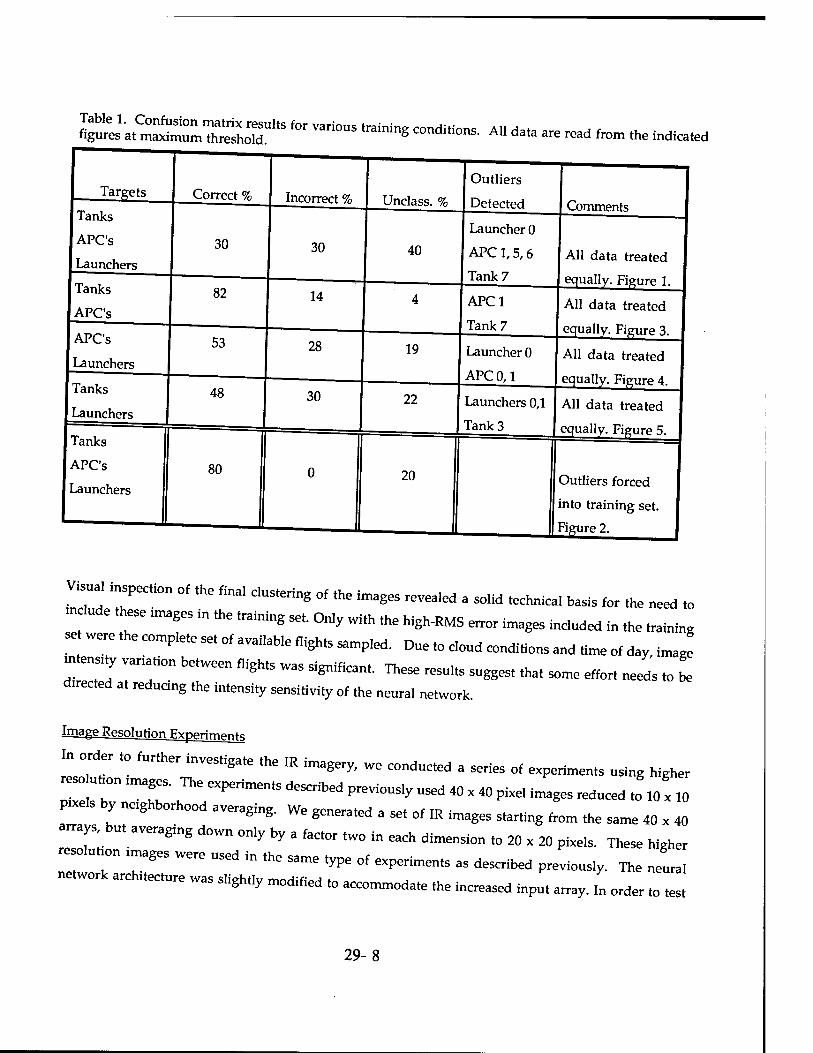
fl^a,Cr'S™XTho7dU,'S f0r Vari°US *«** ««"•*»- All data are read fron, the indicated
Targets
Tanks
APC's
Launchers
Tanks
APC's
APC's
Launchers
Tanks
Launchers
Tanks
APC's
Launchers
Correct %
30
82
53
48
80
Incorrect %
30
14
28
30
0
Unclass. %
40
19
22
20
Outliers
Detected
Launcher 0
APC1,5,6
Tank 7
APC1
Tank 7
Launcher 0
APC 0,1
Launchers 0,1
Tank 3
Comments
All data treated
equally. Figure 1.
All data treated
equally. Figure 3.
All data treated
equally. Figure 4.
All data treated
equally. Figure 5.
Outliers forced
into training set.
Figure 2.
V,S„a, tnspection „( ,he final clustering of (he images reyealed a so|jd technjcai basis for (he
«fade these tmages in the training set. Only wi,h the high-RMS error images included in the training
set were the compiete set of avaiiable flights samp,ed. Due to cloud conditions and „me o, day, image
mtensuy variation between flights was significant. These resuits suggest tha, some effort neel to I
directed at reducing the intensity sensidvity of the neural network.
Image Resolution FvperimpnK
In order ,„ further investigate the IR imagery, we conducted a series of experiments using higher
reso uh„n tmages. The experiments described previously nseo 40 x 40 pixe, images «duced to 10, ,0
pixels by netghborhood averaging. We generated a se, of IR images starting from the same 40 x 40
arrays bu, averagmg down only by a factor two in each dimension to 20 x 20 pixels. These higher
resolution images were used in the same type o, experiments as described previously. The neural
network architecture was slight.y modified ,„ accommodate the increased input array. In order to tes,
29-8

the effect of resolution on identification, a series of experiments was conducted with the 20 x 20 images.
We hypothesized that increased resolution would provide better target discrimination smce more
information was available to the neural network. We were somewhat surprised, therefore, to find that
the performance was considerably worsened. The results are shown in Figure 6, and may be compared
with those shown in Figure 1. Notable improvement was achieved, as in the 10 x 10 case, by forcing the
outliers into the training set. These results are shown in Figure 7, which may be compared with
Figure 2 These comparisons are summarized in Table 2. These results suggest that further work is
required to optimize the neural network architecture in order to accommodate the increased resolunon
images.
Table 2. Comparison of 10 x 10 performance with 20 x 20 ^^T^^^^, LEGEND: "*" = percentage correct, "X" = percentage mcorrect, O = percentage unciassmeu
Image Resolution
Tanks, APC's, Launchers
10 x 10 pixels
All images tested
Tanks, APC's, Launchers
20 x 20 pixels
* = 30%
X = 30%
O = 40%
* = 29%
X = 54%
O = 17%
Outliers forced into training set
* = 80%
X= 0%
O = 20%
* = 62%
X = 12%
O = 26%
Sensor Fusion Experiments Our original objective in this project was to investigate IR / MMW radar sensor fusion. However, there
has been an extensive delay in obtaining valid radar data. As of this writing, we have just been able to
extract radar data from a data set that should prove useful in future experiments. Nevertheless, we put
considerable effort into designing the fusion experiments with the goal of being ready to conduct the
experiments as quickly and efficiently as possible when the data are ready. In order to test our
algorithms, and to further investigate the high resolution results reported above, we conducted a sen»
of experiments on fusion of the low resolution images (10 x 10) with the higher resolution images (20 x
20) Our hypothesis was that some improvement should result, since the low resolution data would
provide coarse feature information, while the higher resolution would provide differentiating details.
The results are shown graphically in Figure 8 (all images treated equally) and in Figure 9 (outhers
forced into training set). The results at maximum threshold are summarized in Table 3. From this data,
it is evident that fusion enhancement is not significant for the experimental conditions shown here. The
29-9

fusion results are almost identical to the results for 20 x 20 alone, which seems to support the idea that
the neural network is not optimized for the higher resolution images.
Table 3. Low resolution, higher resolution,, and fusion performance at maximum threshold.
All mages tested Outliers forced into training set
Image
Resolution Correct % Incorrect % Unclass. % Correct % Incorrect % 10x10 30 30 40 80 0 20 20x20 29 54 17 62 12 Jfx
1 FUSION 24 53 23 1 61 11 28
Dual Mode Data Kvtraction from T DQA
The goal of this subtask is to use existing software and data to establish a dual mode image set for
sensor fusum experiments at Auburn. This subtask was begun during the author's 1993 summer research
program at Wright Laboratory, and continued upon returning to Auburn. The data set consists of co-
boreslghted MMW / IR data taken on a low-observable subsonic aircraft (LOSA). The packed raw data
together with a large ground-processing software (GPS) package was made available to us The
ongmal GPS was written for a specific VMS-based computer system A considerable amount of time has
beenspentmodifyingthe GPS codeto run under UNIX in a more flexible and portable environment, since
Auburn no longer has a supported VMS system. As of this writing, we have been able to view IR still
frames from the packed data, and also we have been able to view coarse-range gate MTI maps that are
tune-tagged to the IR images. We will begin fusion experiments immediately with this data
however, time will not permit the results to be included in this report. We intend to report the results in a briefing to WL/MN during January 1994.
CONCLIJSTDM«;
The most significant result of the experiments conducted under this contract is the development of an
algonthmic method to separate the available data into distinct categories for training purpose, For
best performance, it is essential to know which data will enhance performance and which will be
confusmg to a particular neural network architecture. Principal components analysis (PCA) and
canonical discriminant analysis (CDA) are conventional techniques which have the same objective It
29-10
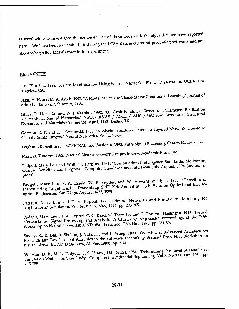
is worthwhile to investigate the combined use of these tools with the algorithm we have reported
here. We have been successful in installing the LOSA data and ground processing software, and are
about to begin IR / MMW sensor fusion experiments.
KF.FFRENCES
Dai, Han-Sen. 1992. System Identification Using Neural Networks. Ph. D. Dissertation. UCLA. Los
Angeles., CA.
Fagg, A. H. and M. A. Arbib. 1992. "A Model of Primate Visual-Motor Conditional Learning." Journal of
Adaptive Behavior, Summer, 1992.
Dynamics and Materials Conference. April, 1992. Dallas, TX.
Gorman, R. P. and T. J. Sejnowski. 1988. "Analysis o< Hidden Units in a Uyered Ne.wo* Trained .0 Classify Sonar Targets." Neural Networks. Vol. 1, 75-89.
Leighton, Russell, Aspirin/MIGRAINES, Version 6,1993, Mitre Signal Processing Center, McLean, VA.
Masters, Timothy. 1993. Practical Neural Network Recipes in C++. Academic Press, Inc.
press).
optical Engineering. San Diego, August 18-23,1985.
Padgett Mary Lou and T. A. Roppel. 1992. "Neural Networks and Simulation: Modeling for AppHca;ions."ySimulation. Vol. 58: No. 5, May, 1992. pp. 295-305.
Padgett, Mary Lou , T. A. Roppel, C. C. Raad, M Townsley£™^gZ^T£^ Networks for Signal Processing and Analysis: A Clustering Af^™J???ea S
Workshop on Neural Networks: AIND. (San Francisco, CA), Nov. 1993. pp. 384-89.
Savely, R., R. Lea, R. Shelton, J. Villareal, and L *>^™£%™«£?££ Wo^opo" Research and Development Activities in the Software Technology Branch, i roc. v Neural Networks: AIND (Auburn, AL Feb. 1990). pp. 3-14.
Webster, D. B., M. L. Padgett, G. S. Hines , D.L. Sirois. 1984. "Determining the Level «£^* Simulation Model - A Case Study." Computers in Industrial Engineering. Vol 8. No 3/4. Dec. PP
215-255
29-11
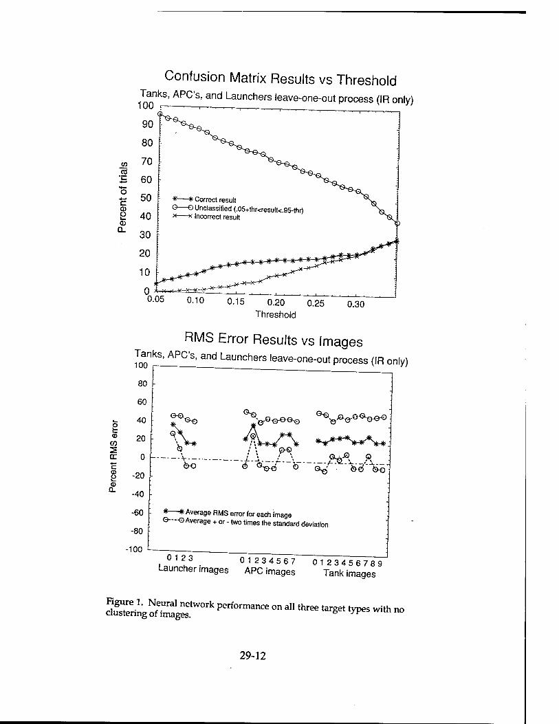
Confusion Matrix Results vs Threshold
1QQnkS' APC'S' 3nd Launchers 'eave-one-out process (IR only)
CO
c CD Ü l_ CD
<D CO
C CD
CD Q.
90
80
70
60
50
40
30
20
10
* *■ Correct result Q—O Unclassified (.05+thr<result<.95-thr) x x Incorrect result
iMHlHlHNHHHH!^
0.05 0.10 0.15 0.20 0.25 0.30 Threshold
RMS Error Results vs Images Tanks^APC^ana^Launchers leave-one-out process (IR only)
80
60
40
20
0
-20
-40
-60
-80
-100
... es*"*
G-,
o-o
O-O
ö " o-^4~ b " -Q^f- ■ %g-%Q-
* * Average RMS error for each image Q-~-O Average + or - two times the standard deviation
,°12u3. 01234567 0123456789
Launcher images APC images Tank images
«SZinSN
0^r0rk Perf0rmanCe °n a11 three *** ^eS With no
29-12
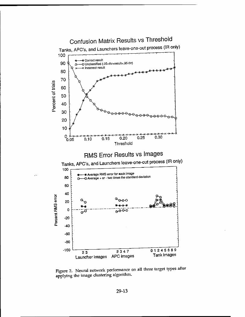
Confusion Matrix Results vs Threshold Tanks, APC's, and Launchers leave-one-out process (1R only)
100 r-" *—* Correct result G—O Unclassified (.05+thr<result<.95-thr)
: Incorrect result
* * * fr-*-*""^
j, vl/ di ^ ^^^ "f*
^^^^^^e^^^j,
0 %----r^---^r"^cS^"oS 0.05 0.10 -x-x.x x x-x-x-x-x
0.30
Threshold
RMS Error Results vs Images Tanks, APC's, and Launchers leave-one-out process (IR only)
100
80
60
40 o a 20
CO :> cc 0 *-» c CD U -20 (D Q. -40
-60
-80
-100
j Average RMS error for each image 0-—0 Average + or - two times the standard deviation
23 2347 Launcher images APC images
0 1245 689 Tank images
Figure 2. Neural network performance on all three target types after applying the image clustering algorithm.
29-13
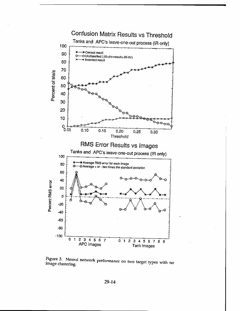
Confusion Matrix Results vs Threshold Tanks and APC's leave-one-out process (IR only)
90
80
*—* Correct result O—O Unclassified (.05+thr<result<.95-thr) *—x Incorrect result
0.10 0.15 0.20 0.25 Threshold
0.30
100
80
RMS Error Results vs Images Tanks and APC's leave-one-out process (IR only)
*—* Average RMS error for each image ©---•©Average + or - two times the standard deviation
03
CO
rr c 0) 2 (D
Q.
A.
o A
-100 c—
G-d Ö Ö--C %v .o
0 12 3 4 5 6 7 APC images
01 23456789 Tank images
taEiJST1 netW°rk »^™~ « «™ '«8« «yPes wi image clustering. with no
29-14
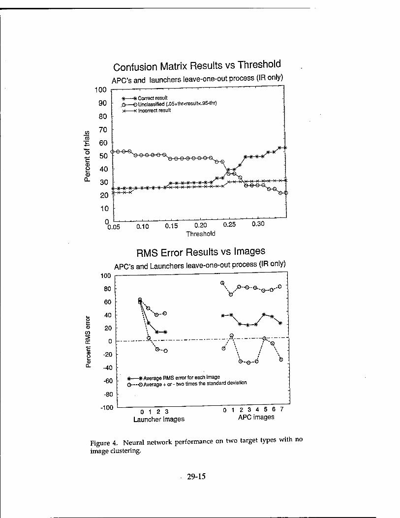
Confusion Matrix Results vs Threshold APC's and launchers leave-one-out process (IR only)
J2 co
c
© 0.
100 F
90
80
70
60
50
40
30
20
10
*—* Correct result .O—O Unclassified (.05+thr<resu1t<.95-thr) x—x Incorrect result
:t x x x
X\)( X )C )( K X X V.
"0.05 0.10 0.15 0.20 0.25 0.30 Threshold
RMS Error Results vs Images APC's and Launchers leave-one-out process (IR only)
^-o-0-o..Q-0
CO
c 2 CL
-20
-40
-60
-80
-100
*—* Average RMS error for each image G—-O Average + or- two times the standard deviation
0 12 3 Launcher images
0 1 2 3 4 5 6 7 APC images
Figure 4. Neural network performance on two target types with no image clustering.
29-15
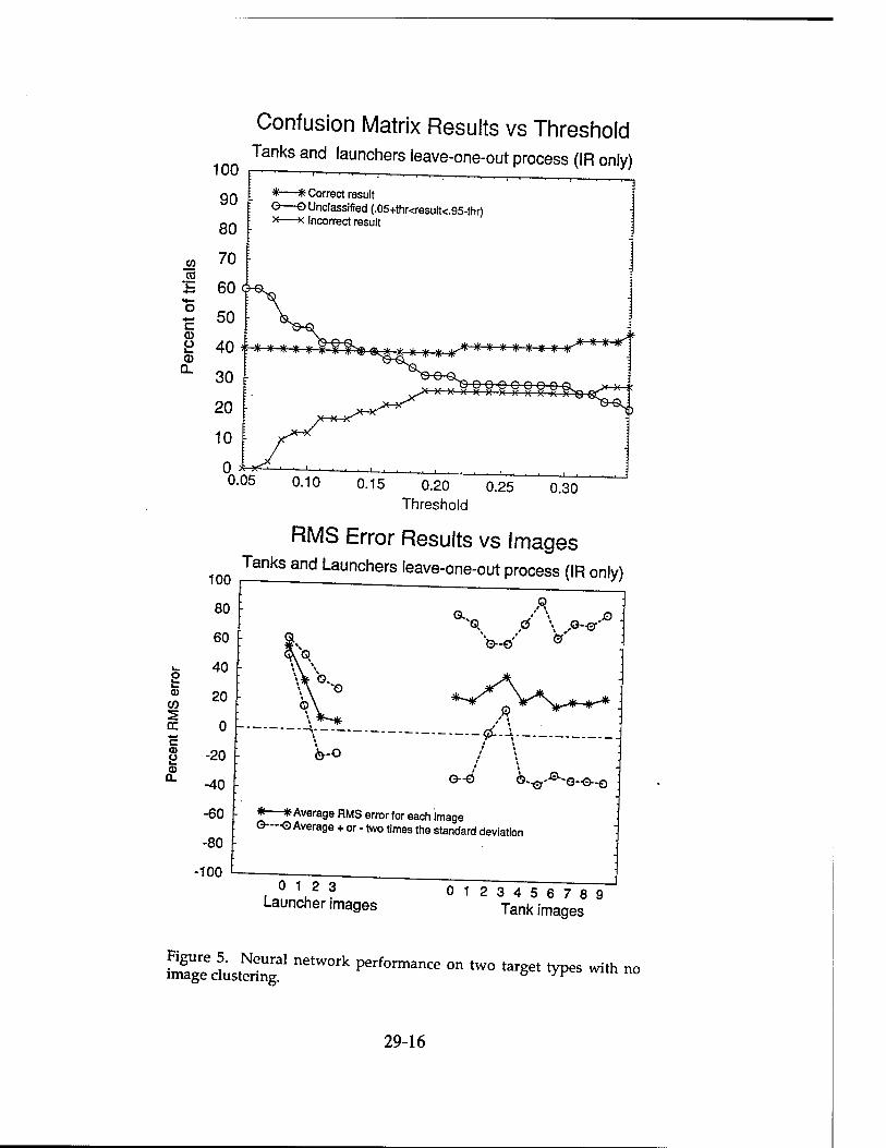
Confusion Matrix Results vs Threshold 100 Tanksand launchers leave-one-out process (IR only)
*—* Correct result O—O Unclassified (.05+thr<result<.95-thr) x—x Incorrect result
(A CO
c o
o 0-
0.10 0.15 0.20 0.25 Threshold
J 0.30
RMS Error Results vs Images 100 Tanks and Launchers leave-one-out process (IR only)
JO :
-60
-80
-100
•Or 0-©-0
*—* Average RMS error for each image ©—■©Average + or - two times the standard deviation
0 12 3 Launcher images
01 23456789 Tank images
iTg'cLenT ne,WOTk Perf°rmanCe °n ,W° 'arSe' 'ypS Wi'h no
29-16
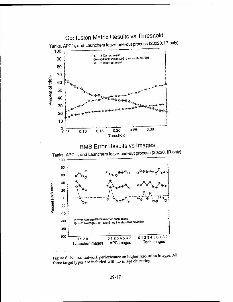
Confusion Matrix Results vs Threshold Tanks, APC's, and Launchers leave-one-out process (20x20, IR only)
100 r— ■ ■ | *—* Correct result
90 *—* Correct result G—© Unclassified (.05+thr<result<.95-tnr) x—x Incorrect result
0.05 0.10 0.15 0.20 0.25 Threshold
0.30
RMS Error Results vs Images Tanks, APC's, and Launchers leave-one-out process (20x20, IR only)
100
CO
rr *-» c a> u <D Q.
80
60
40
20
0
-20
-40
-60
-80
-100
a0iE>o,&oao erG^o^o^j' v°:
i \
"*"S£\
..t Average RMS error for each image Q—-o Average + or - two times the standard deviation
0123 01234567 0123 4 5 6789
Launcher images APC images Tank images
Figure 6. Neural network performance on higher resolution images. All three target types are included with no image clustering.
29-17
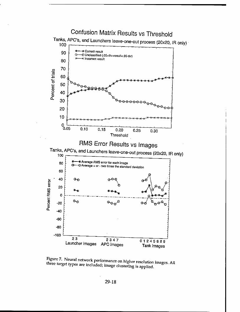
Confusion Matrix Results vs Threshold Tanks APC's, and Launchers leave-one-out process (20x20, IR only)
• UU L ■ . i i i ■ I | —,—___
90
80
w 70 CO
*—• 60 H— o ■*-» bO l_ a> o 40 a a. 30
20
*—* Correct result O—O Unclassified (.05+thr<result<.95-thr) *—x Incorrect result
«HHNHHHNT*^
10
eo o o o oi
_^ u v n if K ^ ^ ^ ^^^-K-X-^-X-X^^-^ » )( 1( xxx ,:
0.05 0.10 0.15 0.20 0.25 Threshold
0.30
RMS Error Results vs Images Tanks, APC's, and Launchers leave-one-out process (20x20, IR only)
80
60
t— " 40 o ^ <D 20
CO 2 DC 0 ** c C) -20 0) a. -40
-60
-80
-100 I
* * Average RMS error for each image O—O Average + or - two times the standard deviation
23 2347 Launcher images APC images
0 1245 6 89 Tank images
J
S taree^S1 ^^ Pf?™*"* on hiS^ resolution images. All three target types are included; image clustering is applied.
29-18
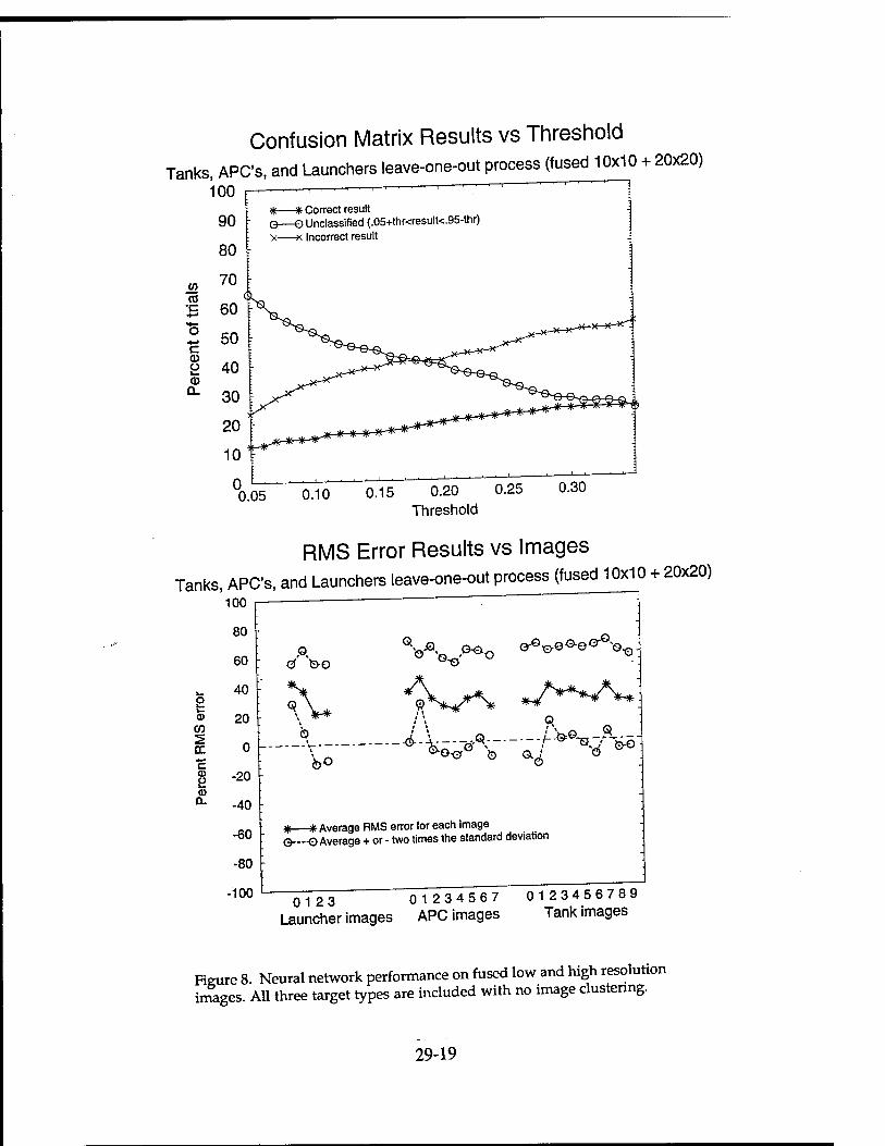
Confusion Matrix Results vs Threshold Tanks, APC's, and Launchers leave-one-out process (fused 10x10 + 20x20)
100
90
80
70
* * Correct result G—0 Unclassified (.05+thr<result<.95-thr) x x Incorrect result
0.05 0.10 0.15 0.20 0.25 Threshold
0.30
RMS Error Results vs Images Tanks, APC's, and Launchers leave-one-out process (fused 10x10 + 20x20)
100
80
60
40 S w 20
CO 2 rx *-* c
CD
Ü Q.
0
-20
-40
-60
-80
-100
P. Q O.
o iÄ-« P<>o o^^o^oo- TQ^
*-©
Q
--Ö-
b°
„ ^ Average RMS error for each image ©~--O Average + or - two times the standard deviation
0123 01234567 0123456789 Launcher images APC images Tank images
Fieure 8. Neural network performance on fused low and high resolution images. All three target types are included with no image clustering.
29-19
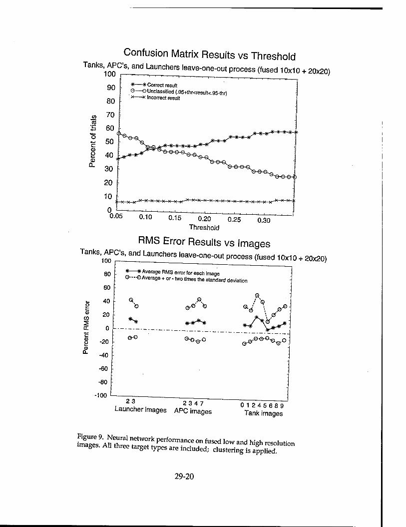
Confusion Matrix Results vs Threshold Tanks^APC's, and Launchers leave-one-out process (fused 10x10 + 20x20)
J2 CO
90
80
70
60
50
*—#■ Correct result Q—O Unclassified (.05+thr<resu!t<.95-thr) * * Incorrect result
JNMHHHM^
x^-^r"v x K " " "■' X-K-V v '( " ■•" x n JI v K )c K K x ^ ■x x i
0.05 0.10 0.15 0.20 0.25 Threshold
0.30
RMS Error Results vs Images Tanks, APC's, and Launchers leave-one-out process (fused 10x10 + 20x20)
80
60
* * Average RMS G—-O Average + or
error for each image - two times the standard deviation :
2 u <U
CO
rr
40
20
0
-20
to
2 G-O ^©o ^o-o^Q^^o;
Q. -40 .
-60 ■
-80 - .
-100 - 23
Launcher images 2347 01245689
APC images Tank images
2S£9i5?Xee T^knrri0rmanCe °n fUSed l0W and hi§h «***» images. All three target types are included; clustering is applied.
29-20
CHARACTERIZING THE SOLID FRAGMENT POPULATION IN A DEBRIS
CLOUD CREATED BY A HYPERVELOCITY IMPACT
William P. Schonberg Associate Professor
Civil & Environmental Engineering Department
University of Alabama in Huntsville Huntsville, Alabama 35899
Final Report for:
Research Initiation Program Wright Laboratory
Sponsored by: Air Force Office of Scientific Research
Boiling Air Force Base, Washington, D.C.
and
The University of Alabama in Huntsville
April 1994
30- 1

CIURACTERIZING THE SOLID FRAGMENT POPULATION IN A DEBRIS CLOUD CREATED BY A HYPERVELOCITY IMPACT
William P. Schonberg Associate Professor
Civil & Environmental Engineering Department University of Alabama in Huntsville
Abstract
■O. key to conducing an accurate lethality assessment is the use of a rob« assessment
memodology. To be applicable in a wide e,ass of engagement seenanos, a .etbality assessment memodo-
logy shonid incorporate aU the stgrufican, response ^ „^ mechanisms ^ ^ ^ ^
loctty krnetic energy weapon (KEW) tmpacts. One of me cntica, eomponents of a .ethmity assessment is
me ctaractonaation of the debris clond creatod by the mitial KEW impact. Withon, a proper
characteruafion of.be debris cloud matena,., is impos,h,e to obtain an accurate prediction of the
response of an anterior target eompoueu. to subset^, debris cloud uupac, loadings. The fast-nmning
codes FATEPEN2, KAPP-n, and PEN4 eoutam fiagtnentarion mode,s „at chamctoriae one debris Coud
frasnent popuiadon resultmg from a bigb speed impact. The objectives of me work described in this
report was firs, to compare the predictions of tbe fragmentation models wtfitir. dtese three codes agatns.
-* omer, aud, second, to document similanties aud differences between me predictive capabihties of me
mree fragment models over toe entire 2-,6 kmVs tmpac, veiccity regrme. These objectives were
aehteved through a parametne smdy of debns eioud material charactenaafion „smg «he fiagmentafion
schemes m me FATEPEN2, KAPP-,,, and PEN4 semt-empirica, ,etha,ity assessment schemes over toe 2-
16 km/s tmpac, velocity regime for a vanety of projectiles Urge, matenals and configurations
30-2

CHARACTERIZING THE SOLID FRAGMENT POPULATION IN A DEBRIS CLOUD CREATED BY A HYPERVELOCITY IMPACT
William P. Schonberg
1.0 INTRODUCTION
The key to conducting an accurate lethality assessment is the use of a robust assessment
methodology. The desire to understand the damage mechanisms that produce warhead kills in missile sys-
tems has increased the need for more accuracy in both response characterization and in lethality
assessment. To be applicable in a wide class of engagement scenarios, a lethality assessment methodology
should incorporate all the significant response and damage mechanisms which result from hvpervelocity
weapon-target mteracrions. For kinetic energy weapon (KEW) impacts, which can occur at speeds ranging
from 2 to 16 km/s, target response and damage mechanisms can be divided into distinct categories: 'local
phenomena' and 'global phenomena.'
Local response and damage phenomena are primarily due to the intense initial loading associated
with a hypervelocity impact: material damage occurs very quickly (on the order of microseconds) and is
limited to an area near the impact site. At sufficiently high impact velocities, shatter, melting, and/or
vaporization of the materials can occur. Global response and damage phenomena occur over a longer
penod of time (on the order of milliseconds), under less mtense loads, and over a larger area of the target
structure. In KEW impacts, one or more debris clouds are created during the initial impact on the outer
wall of a target. These debris clouds spread out as they move through target voids and eventually impact
an inner wall or interior component of the target structure. Depending on the impact velocity and the
relative matenal properties of the projectile and target, these debris clouds can contain solid, melted, and/or
vaporized projectile and target materials.
One of the critical components of a lethality assessment is the characterization of the debris cloud
created by the initial KEW impact. Without a proper characterization of the debris cloud material it is
impossible to obtain an accurate prediction of the response of an interior target component to subsequent
debris cloud impact loadings. Unfortunately, because very little impact test is available at speeds above
30-3

apprcxamately , loWs, characteristics of ^ debds doud fragmen(s creattd by tapacte a( ve|ocjfe ^
8 km/s have ye, ,„ be well defined. TOs h „„, ^ ^ ^^ ^ ^^ ^
currently used ,o determme the lethal effectiveness of KEW systems are sigrnficantly Umited in fteir
charactenzation of fte _U h, fte debris douds crea(ed by ve[y ^ ^ ^^ ^ ^ ^
leftaltiy assessment „f KEW impacs a, speeds i„ excess of the mnxamum velocities for which currently
avaiiahie leftahty assessment schemes are valid mas creates a dUemma for «he iethality assessment
community.
Most obviously, the results of lethality assessments using semi^mpirical codes may be
ques.iom.ble a, impact velocities greater man those for which me codes were designed. However, the
results of hydrocode damage assessment, may also be suspect in scenarios mvolving impact velocities
greater than the highest impact velocity for which the equation-of-state used by the hydrocode is valid.
Thus, the results obtained using hydrocodes may be just as correct or incorrect as those obtained using
to-running sem«mpirical codes. While hydrocodes may eventually reach a level of sophistication „here
their equations-of-sftte are valid for impact velocities greater than , lom/s, i, appears that m the immediate
future the most cost-effective means of performmg a lethality assessment is with fast-running semi-
empirical codes. The imporiance of performing an accurate debris cloud characterization in a lethality
assessment arm me availability „f. variety of lethality assessment codes naturally begs the question as to
whether or not me avadable codes are consisten. in their debris cloud maternal charac.eriza.ions. This
question applies not only ,0 the impact velocity regimes within „h,ch the codes have been experimentally
verified (typically between 2 and 8 km/s,, b„, also for speeds beyond due testable regime (i.e., in excess of 8
km/s).
Tie semi-empirical codes FATEPEN2 [1-4], KAPP-n [5-7], and PEN4 [8,9] conum fingmen-
tation models that characterize tine debris cloud fragment population resulting from a high speed impact
Tta equation, in these computer codes have been designed to provide estimates for the number and sizes of
the solid fragments resulting from such an impact as well as ft* speeds and angular distributions about
tie original projectile trajecto^, Each of these cedes has been benchmarked ™«h experimental test result,
aod designated for use within a specific impact velocity regime and for specific materials and target
30-4

configurations based on those tests. The objectives of the work descnbed in this report were first, to
compare the predictions of the fragmentation models within these three codes against each other, and,
second, to document similarities and differences between the predictive capabilities of the three
fragmentation models over the entire 2-16 km/s impact velocity regime.
A parametric study of debris cloud material characterization was performed using the
fragmentation schemes in the FATEPEN2, KAPP-II (version 1.1), and PEN4.vlO semi-empirical lethality
assessment schemes over the 2-16 km/s impact velocity regime for a variety of projectile and target mater-
ials and configurations. The analysis focused on the characterization of the solid fragment population in a
debris cloud created by a hypervelocity impact. This included calculating the number of projectile and
target material fragments, as well as their S1zes, speeds, and trajectories. In addition to comparing the
predictions of the various fragmentation models against one another, the three fragmentation schemes were
evaluated for their completeness, their ease of implementation and use, and the availability of material
properties required for their operation.
2.0 FRAGMENTATION SCHEMES: SYNOPSIS AND QUALITATIVE EVALUATION
The following sections contain a brief description of the three fast-running semi-empirical lethality
codes and their fragmentation schemes. In each case, a brief summary of the codes and their histories is
presented, followed by a summary of their respective fragmentation schemes. It is noted that no attempt is
made to critique the entire lethality assessment capability of any of the three fast-runrung codes selected for
study. The focus of this investigation and the comments made is strictly the manner in which each code
treats the fragmentation of the impacting projectile and the target material in the immediate vicinity of the
impact site. The comments made are also those of a first-time user of the three codes, and as such, can be
especially useful to those users experimenting with these three codes for the first time.
2.1 FATEPEN7 - An Introduction
The FATE family of codes [1-4] was developed for the Naval Surface Weapons Center (NSWC)
for analyzing the impacts of warhead fragments against aircraft structures over an impact velocity range of
1.0 to 5.0 km/s. The present version of FATEPEN2 is actually an improvement of FATEPEN, which itself
30-5

was created by combining two independently developed projectile penetration programs called FATE and
PENBAM. The code FATE was developed to sunulate very high velocity projectüe impacts of aluminum
and steel plates and focuses on the transformation of a smgle projectile into a debris cloud and the resulting
damage to a target plate array. PENBAM was developed to sunulate high velocity of multiple space plates
by steel, tungsten, and DU projectiles. While PENBAM considers a variety of projectile shapes, it is
concerned only with subsequent penetrations by the primary residual projectile fragment subsequent to
impact. Thus, the original FATEPEN code, and, subsequently FATEPEN2, incorporates the debris cloud
formation, penetration, and plate damage algorithms of FATE as well as the generality of the PENBAM
program with regard to projectile shape and projectile and plate materials. The FATEPEN code has been
modified over the years to include projectile tip eros.on even at impact velocities below shatter velocity.
TT* equations witbin the current vers.on of FATEPEN2 predict the number of plates perforated in multi-
plate target arrays as well as the diameters of the holes in the perforated plates. In addition, FATEPEN2
predicts the number, size, trajectories, and velocities of the fragments in the debris clouds created as the
projectile first unpacts the outermost plate and then as its remains move through the multi-plate target
array.
2.2 FATEPEN2 - Frsomqritation srhpmf>
The fragmentation scheme of FATEPEN2 consist, of a series of equations that calculate:
1) the ballistic limit velocity of the selected projectile/target material and geometric
configuration;
2) a threshold velocity for projectile fracture, i.e., fragmentation;
3) the largest residual projectile mass in the event of fragmentation;
4) the velocity of the largest residual projectile mass;
5) two additional mean projectile fragment masses and the number of such
fragments;
6) a mean target fragment mass and the number of target fragments; and,
7) a spread angle for the projectile fragments.
The expression for the ballistic limit velocity is a semi-empirical equation while the expression for
30-6

the resuiual velocity is based on the work of Recht and Ipson [10]. The expression for projectile fracture
threshold velocity is again purely empirical, and is based on NSWC test data. In calculating the largest
residual projectile fragment mass, a distinction is made between impacts that result only in projectile
erosion (i.e., no projectile fragmentation) and those which cause the projectile to fracture (i.e., to fragment).
Unlike KAPP-II and PEN4, FATEPEN2 does not distribute the projectile fragment masses. Rather, it
computes the largest residual projectile mass and average mass values for two sub-classes of projectile
fragments. The equation for calculating debris cloud spread is also a semi-empirical equation and is a
function of impact conditions, material properties, etc. However, the spread of the target material
fragments is taken to be independent of material properties and only a function of impact angle.
The equations within the FATEPEN2 code are valid for a wide variety of metallic spherical,
cylindrical, and parallelepiped projectiles impacting steel and aluminum target plates. It is stated in the
FATEPEN2 documentation that the highest applicable impact velocity is 5 km/s, and that the code should
not be used when the target thickness-to-projectile diameter ratio exceeds approximately 2.5. With such a
limited regime of applicability, the question naturally arises as to just how well (or poorly) the code
performs when it used outside its prescribed regimes of applicability.
, , c^„ r Pnt« ». Observation on the FATEPEN? FraFomentation Scheme
The documentation for the FATEPEN2 code is fairly complete, but very difficult to understand.
There are no sub- or super-scripts in any of the equations. This renders the equations practically
unreadable and almost impossible to implement without resorting to the code itself. In addition, the
equations are almost never self-contained, and rely heavily on tabular information and input from other
(similarly cumbersome equations). Fortunately, the actual code was available during the course of this
study so that it was possible to obtain quantitative information using the equations within FATEPEN2.
The fragmentation scheme of FATEPEN2 is not nearly as sophisticated as that of KAPP-II or
PEN4. While KAPP-II and PEN4 provide an actual mass distribution for the projectile and target
fragments, FATEPEN2 provides the mass of the largest residual projectile fragment and the average
masses of two 'sub-classes' of projectile fragments. For the target fragments, FATEPEN2 merely presents
an average fragment mass. In addition, while the spread of the projectile fragments is actually calculated,
30-7

the spread of the target fragments is taken to be a ftmction of impact „^ on,y, regardless rf „^
properties, impact velocity, etc.
On a more positive „ore, the FATEPEN2 algorithm for calculating the langes, restdual projectile
mass is very sophisticated, including such phenomena as shock erosion, shear extrusion, and late-sage
erosion. In addition, the FATCPEN2 documentation does an excellent^ describing «he limitations of tine
code with respect te materials, geometry, etc., and tine code itself is applicable over a reiatively wide range
of projectile material/targe, material combination, However, as noted previously, its rauge of applicability
in terms of impact velocity is rather limited.
2.4 KAPP-II (verrinn 1 I).. ^ |nfmri„rt:„n
KAPMI was developed for the Defense Nuclear Agency to predict damage to complex three-
dimensional targets impacted by multiple hypervelocity projectiles, including chunky fragments, rods, and
hollow cylinders [5). I, is the fusion of me previously developed KAPP and KNAPP computer cedes ([6J
and [7,, respectively). KAPP-I, has been calibrated for specific projectiles against specific targe, types
wim an extensive experimental database covering an impact velocity regime of approximately 1 to 9 km/,
Tie code contains mgorithms that have been modularized and arranged to allow a user to address a wide
range of impact problems.
T*e algonthms within KAPP-II can be placed in one of two categones: projectile algorithms,
which characters the state of the projectile as it passes through a target; and, target algonthms, which
characterize the response of target components. Projectile state characterization includes effects such as
eros10n and fragmentation. Target response charactenzation includes cratering, component
dismemberment, penetration, and perforation. The semi-empirical relationships within KAPP-II allow the
user to characterize the state of the projectile as it passes through the target as well as the response of the
target system to the impact loading of the initial projectile and the debris created by the initial impact. In
an effort to be a powerful and flexible tool, KAPP-II allows the user to select algorithms believed to be
appropriate for the impact scenarios of interest.
2.5 KAPP-II (version li)„ Pnpmentatinn W™
KAPP-II consist, of a series of algorithms with equations that can be used to calculate:
30-8

1) the largest residual projectile mass with and without projectile erosion;
2) the velocity of the residual projectile mass;
3) the number of projectile fragments;
4) the number of target fragments;
5) the mean projectile fragment mass;
6) the mean target fragment mass;
7) a distribution of the projectile fragment masses;
8) a distribution of the target fragment masses; and,
9) the spread angle of the debris cloud containing projectile and target fragments.
Upon review of the KAPP-II documentation, it becomes immediately apparent that there is no
explicit expression for the ballistic limit of the configuration and conditions under consideration. Such a
determination is made based on a comparison of the results of a penetration depth equation and the
thickness of the target plate, which is a highly subjective process. Thus, when using the equations within
KAPP-II to determine a residual velocity, the user must first determine whether or not perforation has
occurred. For long rods, the expression for residual velocity is based on the distance from the projectile
impact face at which the rarefaction wave overtakes the impact shock in the projectile. It reflects the
average of the initial front end and the initial rear end velocity at impact. The expression for short rods is a
semi-empirical expression.
The largest residual projectile fragment mass can be calculated in one of two ways. First, the user
can assume that the entire projectile w,ll be fragmented. While this may be a reasonable assumption for
disk-like and 'chunky' projectiles, it is generally not appropriate for long rod projectiles. Nonetheless, under
such an assumption, the largest residual projectile fragment is then simply the largest fragment mass in the
Weibull distribution of the projectile mass fragments. Second, the user can first calculate the length of the
impacting projectile that is eroded by the initial phase of the impact event. By subtracting the eroded
projectile mass, the largest residual projectile mass is immediately obtained. The eroded projectile mass
can then be fragmented using the standard KAPP-II approach. If the entire projectile length is eroded, then
the entire projectile can assumed to be fragmented, which is, in effect, the first option just discussed.
30-9

Although there appear to be four different expressions available for calculating debris cloud
spread angle, three of them are calibrated to calculated spaced penetration depth and not impact angle. Tue
expression that actually does predict a spread angle is also based on the distance from the leading edge of
the projectile at which the rarefaction wave overtakes the impact-induced shock wave in the projectile.
2.6 Some Comments » Observation- on thr- V WV-ll Fragmentation S.W
The equations within the KAPP-II fragmentation scheme are easy to understand, implement, and
use, fairly self-contained in that their reliance on tabular data is minimal, and applicable over a wide
variety of target and projectile materials, projectile shapes (long and short rods, solid and hollow rods,
spheres, etc.), and target configurations (flat plates, re-entry vehicles, etc.). The user is presented with a
wide choice of algorithms to use and is also provided with information regarding appropriate algorithm
groupings. This is a very useful piece of information for the first-tune user.
One of the most serious drawbacks of the equations within KAPP-II is the lack of any information
regarding their limitations. While some general statements are possible, specific statements concerning
individual equations are not possible because not all of the equations were calibrated over the same
dataset. In addition, while equations are provided for 'long' and 'short' rods, the user is left to wonder as to
the value of the length-to-diameter ratio that corresponds to the long rod/short rod boundary.
Unfortunately, no guidance is offered in the KAPP-II documentation as to this matter.
While the applicability of the equations within KAPP-II extends to a wide variety of metallic and
non-metallic materials, the use of the equation that calculates the number of fragments is complicated by
the fact that it requires as input the 'ultimate failure strain' of the material. This is a non-standard material
property and is not readily found in standard materials properties' handbook. To make matters worse, no
definition of this property is provided in the documentation regarding its origin or definition. Hence, while
this property is given for the materials in the properties table provided at the end of the KAPP-II
documentation, adding additional materials to this table for use with the fragmentation equation is
impossible. In addition, the manner in which the 'ultimate failure strain' parameter is used in the equation
to calculate the number of fragments created is also misleading. The user must actually divide the
parameter value by 100 prior to its substitution into the equation. No where is this stated in the KAPP-II
30-10

documentation: this fact becomes apparent only after consulting the KAPP-II source code, which
fortunately was available for this investigation.
1 7 PFN4 vlO -- An Introduction
The PEN4 lethality assessment code was developed for the NSWC in attempt to model the impact
of high density metal projectiles against multi-plate target arrays consisting of thin aluminum plates over a
wider range of impact velocities [9]. It is a collection of equations describing the projectile state and target
impact response. PEN4 is a modular code, constructed around the various physical phenomena that occur
during a high sped impact event. Tims, any improvement in the understanding of a particular aspect of the
impact process requires replacing only one module and does not require any extensive rewriting of the
entire code. This model is similar to the FATEPEN2 model in that the equations within PEN4 were derived
using a number of simplifying assumptions and experimentally derived constants.
By restricting the lower limit of the impact velocity to approximately 3.5 km/s, PEN4 neglects
shear failure in the projectile material; by restricting its upper limit of applicability to 7.6 km/s, PEN4
neglects material melting and vaporization. In the most recent version [9], PEN4 has been updated to
include more advanced fragmentation schemes (see, e.g., [11]). These fragmentation models are a
considerable improvement over the models used in the earlier versions of the code (see, e.g., [8]).
Additional recent improvements in PEN4 include new relations for hole diameter, crater depth and
diameter, and largest residual projectile fragment mass.
7 K PHN4.vlO -- Fragmentation Scheme
The fragmentation scheme of PEN4 consists of a series of equations that calculate:
1) the ballistic limit velocity of the selected projectile/target material and geometric
configuration;
2) a threshold velocity for projectile fragmentation;
3) the largest residual projectile mass;
4) the velocity of the largest residual projectile mass;
5) the mean mass of the projectile fragments;
6) a distribution of the projectile fragments; and,
30-11
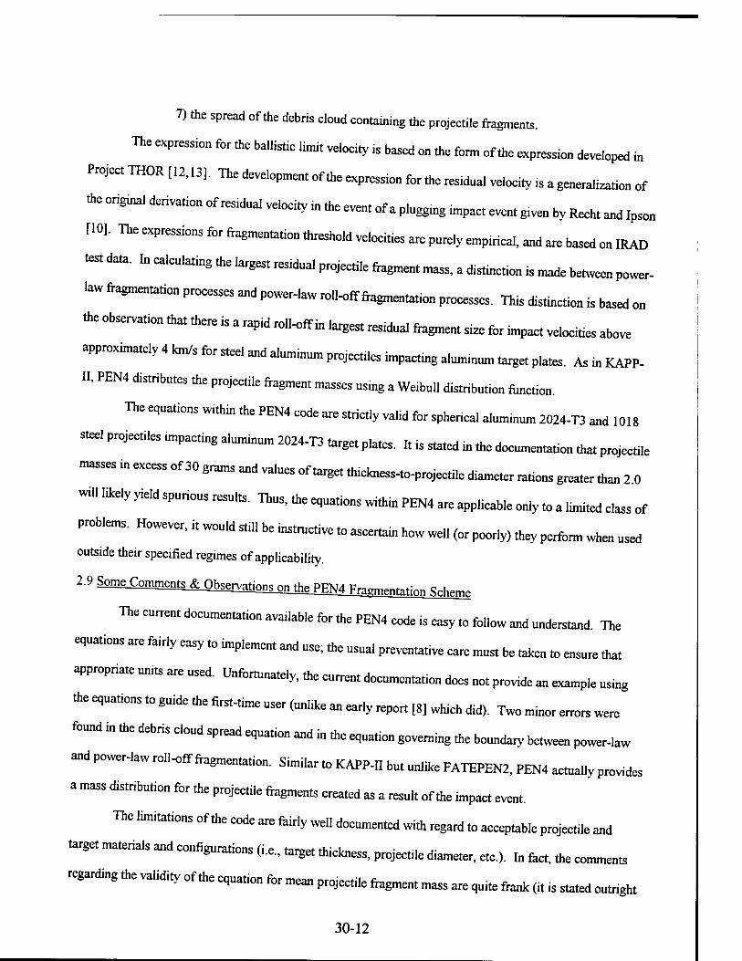
7) the spread of the debris cloud containing the projectile fragments.
The expression for the baUistic limit velocity ,s based on the form of the expression developed in
Project THOR [12,13], The development of the expression for the residual velocity is a generalization of
the original derivation of residual velocity m foe even, of a plugging impact event g,ve„ by Rech, and Ipson
[10]. The expressions for fragmentation threshold velocities are purely empirical, and are based on IRAD
test dato. In calculating the largest residual projectile fragment mass, a distinction is made between power-
law fragmentation processes and power-law rolLfffiagmentafion processes. This distinction is based on
the observation «ha« there is a rapid roU-offin largest residual fragen, stze for impac« velocities above
approximately 4 km,s for steel and aluminum projectiles impacting aluminum «arge, plate,. As in KAPP-
n, PEN4 distributes the projectile flagmen, masses using a Werbnll distribution function.
The equations within the PEN4 code are stnctiy valid for sphencal aluminum 2024-T3 and 1018
— Projectiles impacting aluminum 2024-T3 target plates. ,. is steted in me documentation ma. projee.de
masses in excess of 30 grams and values of .arge, ntickness-o-projectile diameter rations greater man 2.0
will likely yield spurious resul«, Thus, tine «.nations vrifoin PEN4 are applicable only to a limited class of
problems. However, i. would stil, be ins.ruc.ive fo ascertain how we,, (or poorly) they perform „hen used
outside their specified regimes of applicability.
2.9 Some Commenls f> Ohsenntinn- nn the PFN4 V„^,^ cu-.
The current documentation available for the PEN4 node is easy to follow and understand. The
et.na.ions are fairly easy «o implemen, and use; me usual preventive care runs, be taken fo ensure that
appropriate runts are used. Unfortunately, foe enrren. documentation does no. provide an example using
the equations to guide the first-time user (unlike an early „port [8, whieh did). Two minor errors were
found in the debris cloud spread equation nnd in foe equation govermng foe boundary between po„e,law
and power-law ro„-offftagme„,ation. Similar to KAPP-n but unlike FATEPEN2, PEN4 acfoally provides
a mass dis.rtbn.ion for foe projectile fragmenls created as a result of foe impact even,.
The limitations of the code are fairly well documented with regard to acceplable projectile and
forge, materials and configorations (i.e., «arge, thickness, projectile diameter, eto). In fac, «he concerns
regarding foe validity of «he equation for mean projectile flagmen, mass are quite fnmk (i, is stated outright
30-12

that the results it proves are dubious at best). However, while most likely an error of omission, the latest
documentation of PEN4 does not provide an expression for calculating the total number of projectile and
target fragments. In addition, no information is provided to explicitly address the fragmentation of the
material ejected from the target plate. Thus, because the actual PEN4 code was not avaUable for this
uwestigation, it was later not possible to compare these two predictive aspect, of the PEN4 fragmentation
scheme against the predictions of the corresponding algorithms within KAPP-II and FATEPEN2.
Finally, the equation for residual velocity is based on a plugging event; its usefulness in predicting
debris cloud motion is therefore rather dubious. While vanous forms of the equation are given in the
documentation (e.g.: projectile and target plug travel together or travel separately; the projectile is sharp or
blunt; the projectile is deformable or rigid), no guidance is provided to the user as to which options are
likely to be most valid in a particular impact scenario of interest. On a more pos.tive note, the expression
for residual velocity does contain the ballistic limit velocity, as well as impact velocity, as input variables.
If the impact velocity is less than the ballistic limit velocity, the residual velocity will be an imaginary
number, a clear indicator to the user that there is no need to proceed any further in the calculations. As
noted previously, this characteristic is shared by the corresponding equation in FATEPEN2, but not by
KAPP-II.
3.0 FRAGMENTATION SCHEMES: QUANTITATIVE COMPARISONS
3.1 Introductory Comments
The predictions of the fragmentation schemes of the three semi-empirical codes were compared
with each other by obtaining projectile and target material fragment characteristics for impact velocities
ranging from 1 to 15 km/s with right circular cylinder projectiles normally impacting flat target plates
without any projectile yaw. For each impact velocity, three projectile diameter-to-target plate thicknesses
(DA") ratios were considered: DH-0.1, DA-1.0, and D/IW0.0; and, for each DA ratio, thre, projectile
length-to-diameter ratios were considered: L/D=0.1, L/D=l .0, L/D=10.0. In this manner, the codes were
used to generate information for disk, compact, and long rod projectiles whose diameters were much
smaller than, the same size as, and much larger than the thickness of the target plate. In order to be able to
30-13

use the PEN4 equations, pr0J„ile „^ cons,dered m , high ^ ^ ^ ^ ^ ^^
while the target material considered was a generic alnminnm.
Tie following general observations „ere made after examining the outputs obtained fk,m
FATEPEN2 and the program written to implement the PEN4 equations;
1) Bom PEN4 and FATEPEN2 agreed to, „one of the aluminum projectiles would perforate tine
alnminnm targe, plate when IVW». 1; both also agreed mat the sfcel projectile with L/D=10.0 wonld
perforate to ataminnm targ,, plate whe„ mi b„( only „ ^ ^.^ Q(S ^ ^ ^
However, unlto FATEPEN2, PEN4 also predicfod to, to sfoel projectile wifo MM 0 wonid perforafod
the target plate when D/T=0.1, bnt only at speeds above 7 km/s.
2) While both FATEPEN2 and PEN4 predicted tot bom steel and ataminnm projectiles wtth
L/D-,0.0 wonld perforate to atannnm» mrge, plate when D/T=l 0, tore were nnmerons dWerences
between to predictions of FATEPEN2 srt PEN4 wid, regard to whether or no, bom to sfoei and to
atamhmm projectiies wtth L/D=0.1 and L/D-, .0 wonld perfbra* to ataminnm forget plates when
D/T=1.0
3) Both FATEPEN2 and PEN4 agreed that a„ three types of the steel and alummum projectiles
would perforate the aluminum target plates when D/T=10.0
Based on this information, it would appear that with regard to perforation or no perforation of the
target plates, there was more agreement than disagreement between PEN4 and FATEPEN2 for the
materials considered.
3.2 Largest Residual pmj„,n. Frapmmf Ma„
Fignres 1 toongh 4 show plots of non-dimensional largest residnal ptojectile mass as a function of
impact velocity for to al-on-al impacts (Fibres 1 and 2) and to st-on-al impacts (Figures 3 and 4, A
cursory exammation of these four figures that, with to exception of KAPP-U (with eroston) when
L/D-10.0, all three codes predict very small maximum residual projectile fragments above impact
vetoities of 3 tan/s for a,-o„-a, impacts arm 5 « for st-on-a, impacts. For PEN4, tos is no donb, due to
to fact tot to power-law/poweMaw rou-off botmdaries are approximately 3 km/s for al„„-al impacts
and approximately 4.5 lon/s for st-on-al impact, „ B +. „oted „,„ ^ „^ ^ ^^
30-14
mass as predicted by FATEPEN2 when L/D=10.0 decreases at a slower rate than the other projectile/target
combinations, but eventually does drop to a very small value.
The predictions of KAPP-II are interesting in that if projectile erosion is considered when
L/D=10.0 and DAWO.O, then KAPP-II predicts that the (relatively massive) projectile passes through the
(relatively thin) target plate relatively unscathed. This also appears to be true when L/EN10.0 and
Drr=l .0, although to a somewhat lesser degree. However, if projectile erosion is ignored, then the
predictions of KAPP-II are of the same order as those of PEN4. Unfortunately, knowing the amount of
erosion a priori is impossible, and the user is given no guidance by the KAPP-II documentation as to when
to conskler projectile erosion and when to ignore it. Common sense would appear to dictate that when a
long rod (i.e., L/D=10.0) impacts a relatively thin (i.e., D/T-10.0) target plate, it should pass through
relatively unscathed, especially at very high impact velocities (i.e., in excess of 10 km/s).
Closer examination of the data generated by the three codes does reveal some more significant
discrepancies in the predictions of largest residual projectile mass. The most serious of these is that while
the smallest maximum residual fragment masses predicted by KAPP-II are on the order of 0.1% to 2% of
the initial projectile mass, FATEPEN2 and PEN4 predict maximum residual projectile masses for similar
impact conditions that are on the order of 10-5 times ±e origi„al projectile mass. Thus, FATEPEN2 and
PEN4 in effect predict a more 'thorough or 'complete' fragmentation of the projectile than does KAPP-II-
T, 1 Projectile Residual Velocity
Figures 5 through 8 and 9 through 14 show plots of non-dimensional residual velocity for al-on-al
and st-on-al impacts, respectively. In calculating residual velocity using KAPP-II, only the short rod and
long rod equations were used for L/D=0.1 and L/D=10.0 projectiles, respectively. However, the
predictions of both the long rod and the short rod equations in KAPP-II were obtained and plotted for
L/D=1.0 projectiles (see, e.g., Figure 6). It is anticipated that the actual residual velocity when L/D=1.0
according to KAPP-II would lie somewhere between the predictions of the short rod and long rod equations.
In addition, data from two extreme cases were obtained and plotted using PEN4: elastic impact (e=l) and
inelastic impact (e=0). Again, it is anticipated that the actual residual velocity according to PEN4 would
lie somewhere between the two values.
30-15

As can be seen in Figures 5 and 6 (i.e., al-on-al when DrtM.O), the predictions of KAPP-II and
FATEPEN2 when L/D=1.0 and 10.0 are within approximately 20% to 25% of each other while the
predicted values of res.dual ve.odty accordmg to PEN4 when L/D=l .0 and 10.0 are approxnnately 50% of
those predicted by KAPP-II and FATEPEN2. When DAW.O and L/D=0.1, the predictions of KAPP-II
are of the same order as those of PEN4 for al-on-al impacts. In Figures 7 and 8 (i.e., al-on-al when
IVIM0.0) the predictions of residual velocity are significantly more uniform for the three L/D ratios
considered, but especially for L/D=10.0 (Figure 7, top set of curves). In addition, the values predicted by
PEN4 when e=0 and when e=l differ significantly except when D/IWO.O and L/D=10.0. Analogously, the
predictions of the KAPP-II long rod and short rod equations for L/D=1.0 are nearly identical when
D/T=10.0.
Figures 9 through 14 (i.e., st-on-al impacts) show the same trends in the data as those which were
observed in the al-on-al impacts: fairly close agreement between KAPP-II and FATEPEN2 when L/D=1.0
and 10.0 for DflW.O (and 0.1 as well); a wide gap between the predictions of PEN4 and those of
FATEPEN2 and KAPP-II when L/D=1.0and 10.0 for DHM.O (and 0, as well); and, general agreement
among all three codes when DAT=10.0, and especially when L/D-10.0. Additionally, significant
differences between long and short rod predictions were found for L/EM1.0; the differences were relatively
mxnor when D^l .0, and all but appeared when DAr=10.0. Fmally, in a manner agam snnilar to the al-
on-al impacts, the differences between the predictions of the e=0 and e=l options in PEN4 were fairly
significant except when L/D=10.0 and L/D=10.0
3.4 Materials Fragments«-;,™
Figures 15,16 and 17,18 show plots of the number of the number of projectile and target fragments
generated, respectively, by al-on-al impacts. Several features evident in these four plots highlight some of
the key differences in the way KAPP-II and FATEPEN2 fragment the projectile and target matenals. As
noted previously, the available PEN4 documentation does not provide for a means of calculating the
number of fragments generated; hence, no comparisons with PEN4 were possible.
One characteristic of the KAPP-II predictions is immediately apparent: the equation for number of
fragments generated does not distinguish between projectile and target material for like-on-like impacts.
30-16

However, it should be noted that the individual fragment masses created will in fact be different for the
projectile and target materials because of the difference between the initial projectile mass and the mass of
the target material ejected by the impact. Another feature immediately apparent from the four sets of
curves is that the number of fragments generated according to the KAPP-II equation is independent of the
value of the DfT and L/D ratios; FATEPEN2, however, does allow for a distinction in geometry in
calculating the number of fragments generated. Naturally, even though the number of fragments may be
the same according to KAPP-II for two different values of L/D or DAT, the actual masses of the fragments
formed in the two cases will still be different due to differences in to total initial mass values.
With the exception of Figure 16, in which the thickness of the target plate is much smaller than the
diameter of the impacting projectile, KAPP-II predict, that a far greater number of projectile and target
fragments will be created as compared to the predictions of FATEPEN2. In Figure 16, the FATEPEN2
plots are terminated at impact velocities of 7 km/s and 9 km/s for L/D ratios of 1.0 and 10.0, respectively.
This is not to say that projectile fragmentation no longer occurred at impact speeds above 7 and 9 km/s.
Rather, at speeds in excess of 7 and 9 km/s, FATEPEN2 predicted that the number of projectile fragments
would be on the order of 10* for L/D=1.0 and 10* for L/D=10.0. While these are astronomically high
numbers, perhaps some credence may be lent to them if one considers that, with the exception of the single
largest residual projectile fragment, the other projectile fragments are likely to be melted at impact
velocities above 7 km/s and possibly even vaporized at speed in excess of 10 km/s. In light of this
consideration, the high number of'fragments' (droplets?) predicted by FATEPEN2 no longer seems
unreasonable.
Figures 19-21 and 22-24 show plots of the number of the number of projectile and target fragments
generated, respectively, by st-on-al impacts. These figures show some of the same trends in the data as
those which were observed in the al-on-al impacts: KAPP-II predicts a far larger number of projectile and
target fragments than does FATEPEN2 (except when DflMO.0), and that when DAT=10.0, the number of
fragments predicted by FATEPEN2 become astronomically high. A major difference between these plots
and the al-on-al plots is that when the projectile and target materials are not the same, KAPP-II will in fact
predict a different number of fragments created for the projectile and for the target materials.
30-17
3.5 Debris ClnnH Spread An^R
Figures 25 and 26 show plots of the debns cloud half angles for the al-on-al impacts. For the two
IVT values shown, the predictions of the three codes are generally within 10° to 15° of each other. The
predictions of PEN4 approach their asymptotic limit of 26° at impact speed of approximately 9 and 15
km/s for D/T=1.0 and 10.0, respectively; in both cases, the predictions of FATEPEN2 appear to approach
an asymptotic limit of approximately 32° at an impact spa* of approximately 7 km/s. In complete
contrast to the asymptotic behavior exhibited by both the FATEPEN2 and the PEN4 predictions, the
predictions of KAPP-II appear to increase without bound for DfT=l .0 and actually begin to decrease
slightly for D/T=10.0 beyond a speed of approximately 12 km/s.
While an asymptotic value of debris cloud spread may be desirable in a lethality assessment code
from the standet of predicting a maximum damage area in subsequent target components, the behavior
exhibited by the KAPP-II predictor equation is probably more realistic. The reason for this, especially in
the case of very thin target plates (e.g., DAW0.0), is as follows. As the impact velocity is increased
beyond the incipient fragmentation velocity of the projectile, the debris created will naturally spread out
more and more. However, at very high .mpact speeds, it is logical to presume that a projectile impacting a
very thin target plate will pass through the plate relatively unscathed, which in effect constitutes a minimal
spread in the debris created. Hence, if a function is to describe the spread of the fragmented material in
terms of impact speed, it must be monotonically increasing from a value near zero for low impact speeds
and it must be near zero for very high impact speeds. The only way for this to happen is if it was to peak
at some impact velocity in between. Naturally, the velocity at which the peak occurs, as well as the
velocity at which the debris cloud spread finally settles on a near-zero value, is a function of projectile and
target material properties and the geometric parameters of the system under consideration.
Figures 27 through 29 show plots of the debris cloud half angles for the st-on-al impacts. For the
three DfT values consumed, the predictions of the three codes in this case are generally more widespread
than in the case of aluminum projectiles. The predictions of PEN4 approach their asymptotic limit of 26°
at impact speed of approximately 11, 13, and 15 km/s for D/T-0.1, 1.0, and 10.0, respectively; in both
cases, the predictions of FATEPEN2 appear to approach an asymptotic limit of approximately 15° at an
30-18

impact speed of approximately 7 km/s. Once again, in contrast to the asymptotic behavior exhibited by
both the FATEPEN2 and the PEN4 predictions, the predictions of KAPP-II appear to increase without
bound for D/T-0.1 and 1.0. For DAT= 10.0, there is a marked decrease in debris could spread beyond an
impact velocity of approximately 11 km/s.
4.0 SUMMARY
4.1 General Comments
A parametric study of debris cloud material characterization was performed using the
fragmentation schemes in the FATEPEN2, KAPP-II (version 1.1), and PEN4.vlO senu-empirical lethality
assessment schemes over the 2-16 km/s impact velocity regune for a variety of projectile and target mater-
ials and configurations. The analysis focused on the characterization of the solid fragment population in a
debris cloud created by a hypervelocity impact. This included calculating the number of projectile and
target material fragments, as well as their sizes, speeds, and trajectories. In addition to companng the
predictions of the various fragmentation models were compared with one another, the three fragmentation
schemes were evaluated for their completeness, their ease of implementation and use, and the availability of
material properties required for their operation.
4. 7 Qualitative Analysis Summary
The following is a summary of the results of the qualitative analyses performed as part of this
investigation:
1) The FATEPEN2 documentation is difficult to understand; the fragmentation equations are
almost impossible to implement and use without the actual source code. The PEN4 and KAPP-II
documentations are easy to follow and the equations are relatively easy to implement, although some errors
and omissions were observed in the PEN4 documentation.
2) The FATEPEN2 and PEN4 documentations are diligent about stating the limitations of the
respective codes and the equations contained therein; the KAPP-II documentation is often negligent in this
obligation to its users.
3) Both KAPP-II and PEN4 provide actual distributions of the fragment masses created while
30-19

FATEPEN2 does not. While this is not a cnrical flaw on the part of FATEPEN2, the other two codes do
present a more complete picture of the fragmentation process.
4) While the equations within FATEPEN2 take into account the effects of the D/T and L/D ratios
in determining the number of resulting fragments, those in KAPP-II do not. Ultimately, a few well-
instrumented tests will be needed to decide whether or not this a problem with KAPP-II or just a bonus
provided by FATEPEN2. In addition, one of the material parameters reared by KAPP-II is a non-
standard property. Hence, applying the KAPP-II fragmentation equation to materials not presently in its
material library is impossible.
5) The FATEPEN2 algorithm for calculating the largest residual projectile mass is very
sophisticated, while the KAPP-II algorithm is nunmentary m nature. Since the corresponding PEN4
algorithm is purely empirical, it may be argued that it is simplistic.
6) While both KAPP-II and FATEPEN2 prov.de sample problems as part of their documentation,
PEN4 does not. This makes it difficult for first-rime users of PEN4 to know whether or not they are
interpreting the subtleties of the code properly and using it correctly.
7) No guidance is given in the KAPP-II and PEN4 documentations regarding some of the subtleties
in their equations, such as whether to use the long rod or short rod equations in KAPP-II when L/D=l .0
and when to assume an elastic impact and when to assume a plastic unpact in PEN4. This makes it
difficult to use to equations in which these subtleties occur as predictive tools w.thout several iterative runs.
4.3 Quantitative Analvcfe Summary
The following is a summary of the results of the quantitative analyses performed as part of this
investigation:
1) Perforation Resistance - There was general agreement between PEN4 and FATEPEN2 with
regard to whether or no. the aluminum target plate was perforated by the impaeting steel and alummum
projectiles.
2) UrgesiRej^^ .. Wim ^ ^.^ ofKApp_n ^ ^^ for
WT-10.0 and when projectile erosion was included, there was general agreement between the three codes
in predicting the mass of the largest residual projectile fragment relative to the mass of the original
30-20

projectile. Except as noted, all three codes predicted very small maximum residual fragments for impact
velocities greater than approximately 5 km/s. For the conditions noted, the KAPP-II equations predicted
that the projectile would pass through the target plate relatively unscathed.
3) P.<idnal Projectile Velocity - KAPP-II and FATEPEN2 agreed within 20%-25% for compact
and long rod projectiles impacting moderately thick plates; all three codes were in close agreement (i.e., less
than 10%) for very thin target plates.
4) Materials Fragmentation - Except for the impact of very thin plates, KAPP-II predicted that
significantly more fragments would be generated than did FATEPEN2 (i.e., by several orders of
magnitude). For very thin plates, the opposite occurred: FATEPEN2 predicted that a tremendously high
number of fragments would be generated. The numbers predicted by FATEPEN2 in such cases exceeded
those predicted by KAPP-II by several tens of orders of magnitude.
5) TV.r,ris Cloud Spread - All three codes agreed in their prediction of debris cloud spread within
10O to 150 for ^ ai_on-al impacts. However, the differences grew to 20<> to 25° for the st-on-al impacts.
5.0 REFERENCES
1. Yatteau, J.D., High Velocity Multiple Plnte Penetration Model. NSWC-TR- 82-123, Dahlgren, Virginia,
February, 1982.
2. Yatteau, J.D., Modifications to Pm^m FATE - Fragment Residual Mass Calculations, Final Report,
Denver Research Institute, University of Denver, Denver, Colorado, May, 1983.
3. Yatteau, J.D., Zernow, R.H., and Recht, R.F., Compact Fragment Multiple Pint* Penetration Model,
Volnme I: Model Description, NSWC-TR-91-399, Dahlgren, Virginia, January, 1991.
4. Yatteau, J.D., Zernow, R.H., and Recht, R.F., Compact Fragment Multiple Plate Penetration Model,
Vn1„m. TT- Computer Code User's Manual. NSWC-TR-91- 399, Dahlgren, Virginia, January, 1991.
5. Greer, R, and Hatz, M., KAPP-TI User's Manual. Version 1.1, Kaman Sciences Corporation, K92-
17U(R), Colorado Springs, Colorado, April, 1992.
6. Snow, P., KAPP - Kaman Analytical Penetration Program, Kaman Sciences Corporation, K85-7U(R),
Colorado Springs, Colorado, 1985.
30-21

7- C°hen' L- Kaman New Anal>tical Penetration Program (KNAPP^ Sp^fiased Inter^r M^u;^
Effort, AFATL-TR-90-02, Eglin AFB, Florida, February, 1990.
8. Henderson, B.J., and Zimmerschied, A.B., Very High Velocity Penetration Mnriri NSWC-TR-83-189,
Dahlgren, Virginia, May, 1983.
9. Bjorkman, M.D., Geiger, J.D., and Wilhelm, E.E., Space Station Integrated Wall n^ion ,nH
Penetration Damage Control. Task 3- Theoretical Analv.i, nfPm^n *,^„ Boeing AerQSpace
Corporation, Final Report, Contract NAS8-36426, Seattle, Washington, July, 1987.
10. Recht, R.F. and Ipson, T.W., »Ballistic Perforation Dynamics», Journal of Applied Mechanics, Vol. 30,
No. 3, pp. 284-290, 1963.
11. Grady, D.E., "Local Inertial Effects in Dynamic Fragmentation", Journal of Applied Physics, Vol. 53,
No. 1, pp. 322-325, 1982.
12. THOR 41: A Comparison of the Perforation of Fragments of Four Mat«™!, Impacting V»™„ PI^.
Ballistics Analysis Laboratory, The Johns Hopkins University, Baltimore, Maryland, May, 1959.
13. THOR 47: The Resistance of Various Metallic Materials to Perforation hv St^l Fragments- F.mpir^l
Relations for Fragment Residual Velocity and Residual Weight, Ballistics Analysis Laboratory, The Johns
Hopkins University, Baltimore, Maryland, May, 1959.
30-22
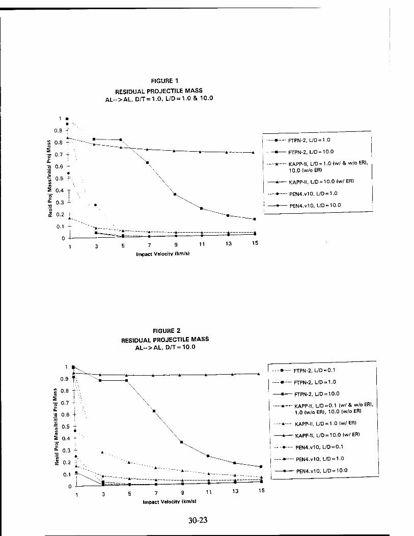
FIGURE 1
RESIDUAL PROJECTILE MASS AL-->AL, D/T=1.0, L/D = 1.0 & 10.0
0.9 -
S 0.8 —-m-— FTPN-2, UD = 1.0
■ FTPN-2, L/D = 10.0
—•-*•— KAPP-II, L/D = 1.0 (w/ & w/o ER), 10.0 (w/o ER)
* KAPP-II, L/D = 10.0 (w/ ER)
—♦— PEN4.v10, L/D = 1.0
• PEN4.v10, L/D = 10.0
FIGURE 2 RESIDUAL PROJECTILE MASS
AL-->AL, D/T=10.0
0.9 f\ S-
X 0.8 f'.' S ■ Ö 0-7 T £ i •5 0.6 +
=5 0.5 -
S 0.4 - 'o £ 0.3 - ? S. 0.2 ^
0.1 %-
^* 5 7 9 11
Impact Velocity (km/s)
—A-
13
---■■ FTPN-2, L/D=0.1
-—♦— FTPN-2, L/D = 1.0
■ FTPN-2, L/D = 10.0
—-*-— KAPP-II, L/D=0.1 (w/ & w/o ER), 1.0 (w/o ER), 10.0 (w/o ER)
I ---*-— KAPP-II, L/D = 1.0 (w/ ER)
' * KAPP-II, L/D = 10.0 (w/ ER)
I ..-•..-... PEN4.V10, L/D = 0.1
—•-— PEN4.V10, L/D = 1.0
—• PEN4.v10, L/D = 10.0 —A ^4
15
30-23
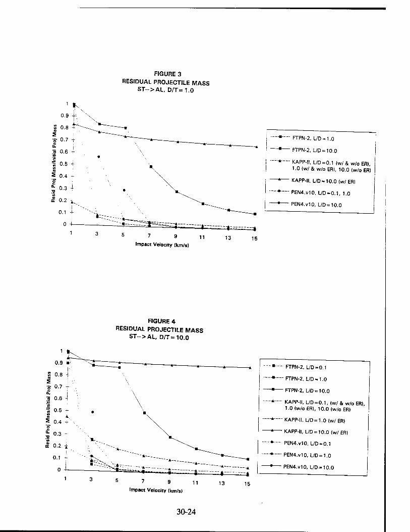
FIGURE 3
RESIDUAL PROJECTILE MASS ST-->AL, D/T=1.0
7 9
Impact Velocity (km/s) 11 13 15
--■—- FTPN-2, L/D=1.0
—■ FTPN-2, L/D = 10.0
-*"— KAPP-II, L/D = 0.1 (w/ & w/o ER), 1.0 (w/ & w/o ER), 10.0 (w/o ER)
-* KAPP-II, L/D = 10.0 (w/ ER)
"•"— PEN4.v10, L/D = 0.1, 1.0
-• PEN4.V10, L/D = 10.0
1!^
FIGURE 4 RESIDUAL PROJECTILE MASS
ST-->AL, D/T=10.0
7 9 11
Impact Velocity (km/s) 13 15
FTPN-2, L/D=0.1
■ FTPN-2, L/D = 1.0
FTPN-2, L/D = 10.0
* KAPP-II, L/D=0.1, (w/ & w/o ER), 1.0 (w/o ER), 10.0 (w/o ER)
-*■— KAPP-II, L/D = 1.0 (w/ ER)
-* KAPP-II, L/D = 10.0 (w/ ER)
••--- PEN4.v10, L/D = 0.1
♦— PEN4.v10, L/D = 1.0
* PEN4.v10, L/D = 10.0
30-24
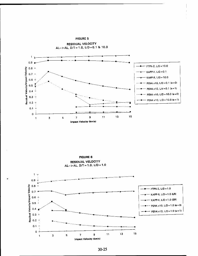
FIGURE 5
RESIDUAL VELOCITY AL-->AL, D/T=1.0, L/D = 0.1 & 10.0
0.1 +
0 -i- 1 7 9
Impact Velocity tkm/sl
11 13 15
-■ FTPN-2, L/D = 10.0
-*-— KAPP-II, L/D = 0.1
-* KAPP-II, L/D = 10.0
...»— PEN4.v10, L/D=0.1 (e=0)
♦— PEN4.V10, L/d = 0.1 (e = 1)
-••- PEN4.V10, L/D = 10.0 (e=0)
-• PEN4.V10, L/D = 10.0 (e=1)
FIGURE 6
RESIDUAL VELOCITY AL-- > AL, D/T = 1.0, L/D = 1.0
1 T i
0.9 +
7 9 11
Impact Velocity (km/s)
FTPN-2, L/D = 1.0
—-*-— KAPP-II, L/D = 1.0 (LR)
* KAPP-II, L/D = 1.0 (SR)
—♦— PEN4.v10, L/D = 1.0 (e=0)
• PEN4.V10, L/D = 1.0 (e = 1)
13
30-25
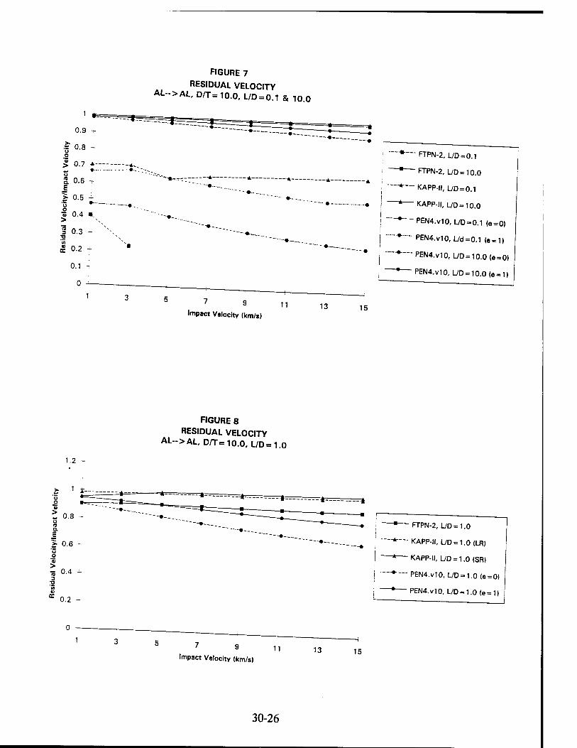
FIGURE 7
RESIDUAL VELOCITY AL-->AL, D/T=10.0, L/D = 0.1 & 10.0
1
0.9 -
| 0.8 -
| 0.7 * * — • • u £ 0.6 T s >■ 0.5 -i-
■3 *- —. 0 „ ü 0.4 ■ > 1 0.3 - X. 2 in N
£ 0.2 - "
0.1 -r
0
1 3 7 9 11
Impact Velocity (km/s)
*—" FTPN-2, L/D = 0.1
1 FTPN-2, L/D = 10.0
r— KAPP-ll, L/D = 0.1
KAPP-ll, L/D = 10.0
PEN4.V10, L/D = 0.1 (e = 0)
PEN4.v10, L/d=0.1 <e = 1|
— PEN4.V10, L/D = 10.0 (e=0)
— PEN4.v10,L/D = 10.0<e = 1)
13 15
1.2 -r
FIGURE 8 RESIDUAL VELOCITY
AL->AL, D/T=10.0r L/D=1.0
> 0.6
> s 0.4 -
0.2
— FTPN-2, L/D = 1.0
KAPP-ll, L/D = 1.0(LR)
— KAPP-ll, L/D = 1.0 (SR)
— PEN4.v10, L/D = 1.0 (e=0)
— PEN4.v10, L/D = 1.0 (e = 1)
7 9 11 Impact Velocity (km/s)
13 15
30-26
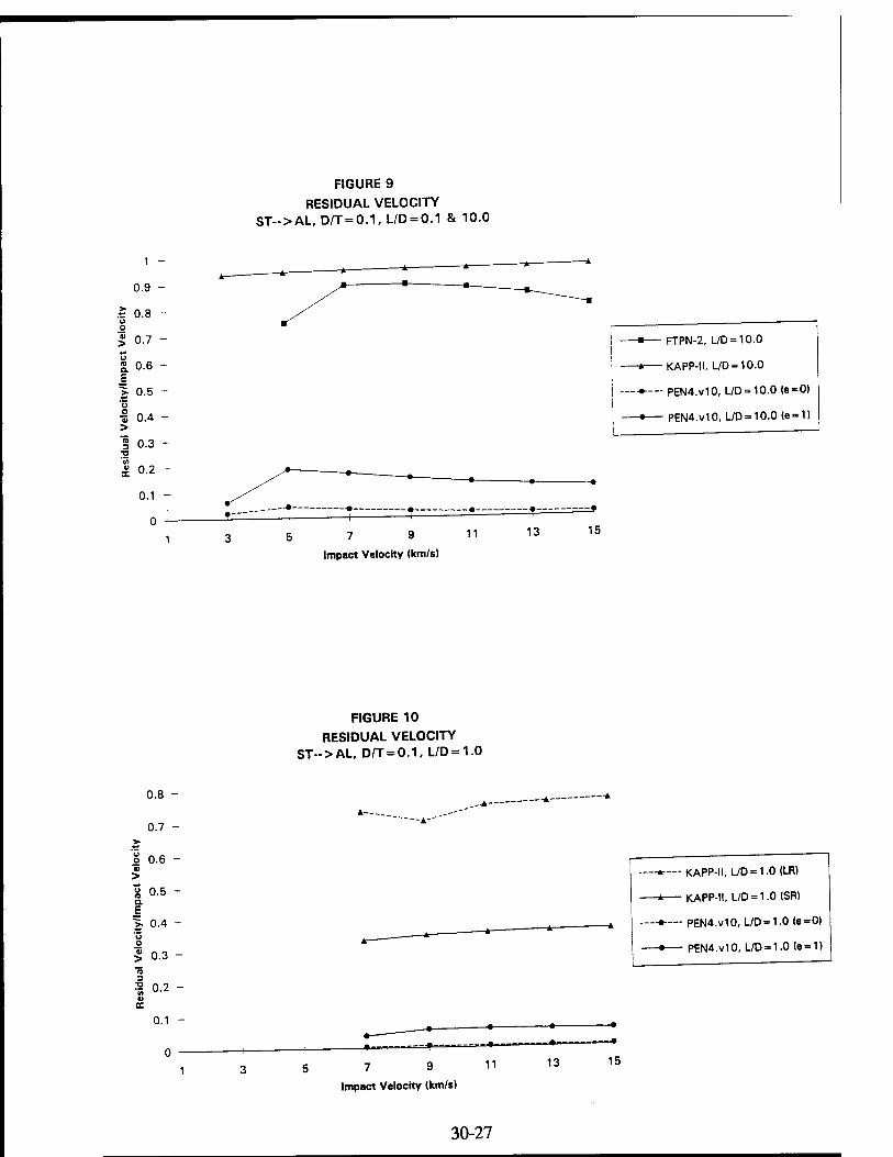
FIGURE 9 RESIDUAL VELOCITY
ST-->AL, D/T = 0.1, L/D = 0.1 & 10.0
1 -
0.9 -
.* 0.8 - o o £ 0.7 -
| 0.6 - £ > 0.5 -
■5 0.4 > I 0.3 ;a
& 0.2
0.1
0 7 9
Impact Velocity (km/s)
— FTPN-2, L/D = 10.0
-* KAPP-II, L/D = 10.0
—♦— PEN4.v10, L/D = 10.0 (e=0)
—• PEN4.v10, UD = 10.0(e = 1)
11 13 15
FIGURE 10 RESIDUAL VELOCITY
ST-->AL, D/T = 0.1, L/D=1.0
0.8 -
0.7 - > I 0.6 - > \ 0.5 - CL
E | 0.4 - 'G
£ 0.3 -
I 0.2 -
,,*-
KAPP-II. UD = 1.0(LR)
KAPP-II, L/D = 1.0 (SR)
-♦— PEN4.V10, UD = 1.0 (e=0)
-• PEN4.V10, L/D = 1.0(e = 1)
0.1
7 9
Impact Velocity (km/s)
11 13 15
30-27
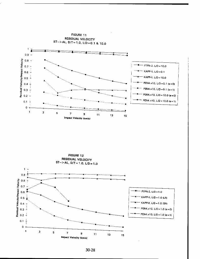
FIGURE 11
RESIDUAL VELOCITY ST~>AL, D/T=1.0, L/D = 0.1 & 10 0
9 11 Impact Velocity (km/s)
■ FTPN-2, L/D = 10.0
*~-- KAPP-II, L/D = 0.1
* KAPP-II, L/D = 10.0
» PEN4.V10, L/D=0.1 (e=OI
*■-- PEN4.V10, L/D = 0.1 (e = 1)
*—- PEN4.V10, L/D = 10.0 (e = 0)
1 PEN4.v10, L/D = 10.0 (e = 1)
13 15
FIGURE 12
RESIDUAL VELOCITY
ST-- > AL, D/T = 1.0, L/D = 1.0
7 9 11 Impact Velocity (km/s)
13
■ FTPN-2, L/D = 1.0
—-*•—KAPP-II, L/D = 1.0 (LR)
* KAPP-II, L/D = 1.0 (SR)
-"•—- PEN4.V10, L/D = 1.0 (e = 0)
PEN4.v10, L/D = 1.0(e = 1)
15
30-28
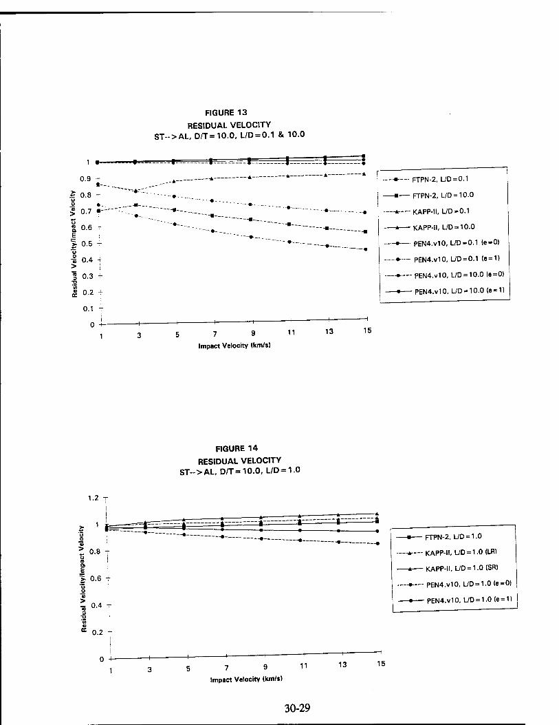
FIGURE 13
RESIDUAL VELOCITY ST-->AL, D/T=10.0, L/D = 0.1 & 10.0
1 •—
0.9 - •— Ä 0.8 -r u o •- £ 0.7 •-
| 0.6 4- E >. 0.5 -
■i 0.4 + > I 0.3 -
^ ^
0.1
0 7 9
Impact Velocity (km/s)
-*— FTPN-2, L/D = 0.1
-■ FTPN-2, L/D = 10.0
11
--*-— KAPP-II, L/D=0.1
-* KAPP-II, L/D = 10.0
--*■— PEN4.v10, L/D=0.1 (e = 0)
-■•- PEN4.v10, L/D=0.1 (e = 1)
-♦— PEN4.v10, L/D = 10.0 |e=0)
-• PEN4.v10, L/D = 10.0 (e = 1)
13 15
0.2 ^
FIGURE 14
RESIDUAL VELOCITY ST«>AL, D/T=10.0, L/D = 1.0
^0.4
-m FTPN-2, L/D = 1.0
--*-— KAPP-II, L/D = 1.0 (LR)
-* KAPP-II, UD = 1.0 (SR)
._-♦— PEN4.V10, L/D = 1.0 (e = 0)
• PEN4.v10, UD = 1.0 (e = D
7 9
Impact Velocity (km/s)
11 13 15
30-29
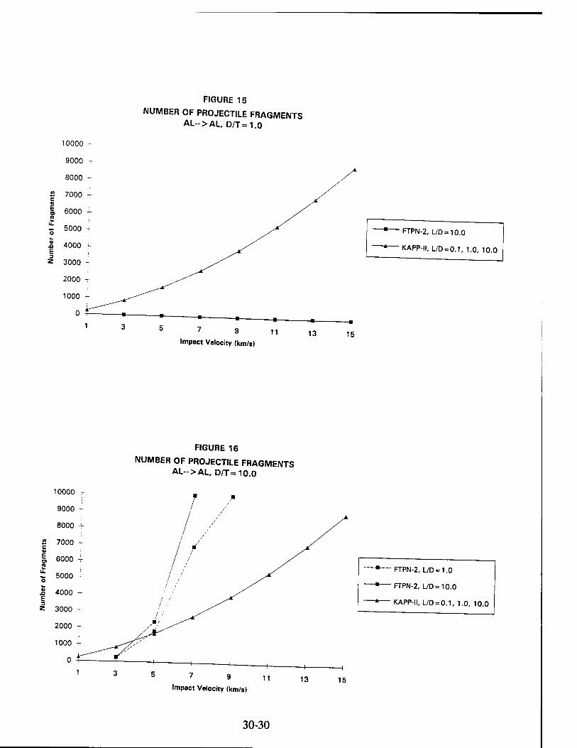
£ 7000 -
E 3 Z
FIGURE 15
NUMBER OF PROJECTILE FRAGMENTS AL-->AL, D/T=1.0
FTPN-2, L/D=10.0
KAPP-II, L/D = 0.1, 1.0, 10.0
7 9
Impact Velocity (km/s) 11 13 15
FIGURE 16
NUMBER OF PROJECTILE FRAGMENTS AL-->AL, D/T=10.0
E 3 Z
7 9 11 Impact Velocity (km/sl
13
H
15
•*— FTPN-2, L/D = 1.0
-■ FTPN-2, UD = 10.0
"* KAPP-II, L/D = 0.1, 1.0, 10.0
30-30
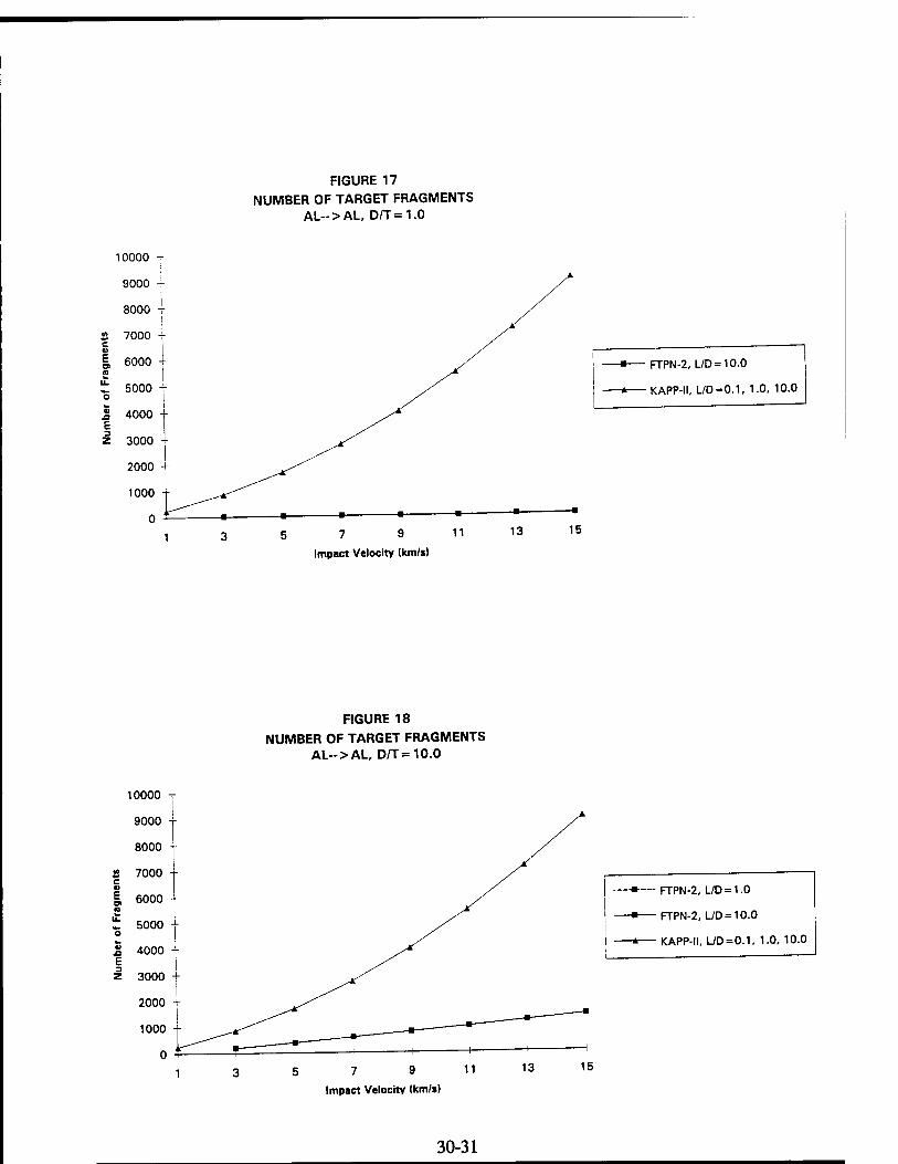
FIGURE 17
NUMBER OF TARGET FRAGMENTS AL-->AL, D/T=1.0
FTPN-2, L/D = 10.0
-* KAPP-II, L/D = 0.1, 1.0, 10.0
7 9
Impact Velocity (km/s)
FIGURE 18
NUMBER OF TARGET FRAGMENTS AL-->AL, D/T=10.0
7 9
Impact Velocity (km/s)
11 13
-*— FTPN-2, L/D = 1.0
-■ FTPN-2, L/D = 10.0
-* KAPP-II, L/D=0.1, 1.0, 10.0
30-31
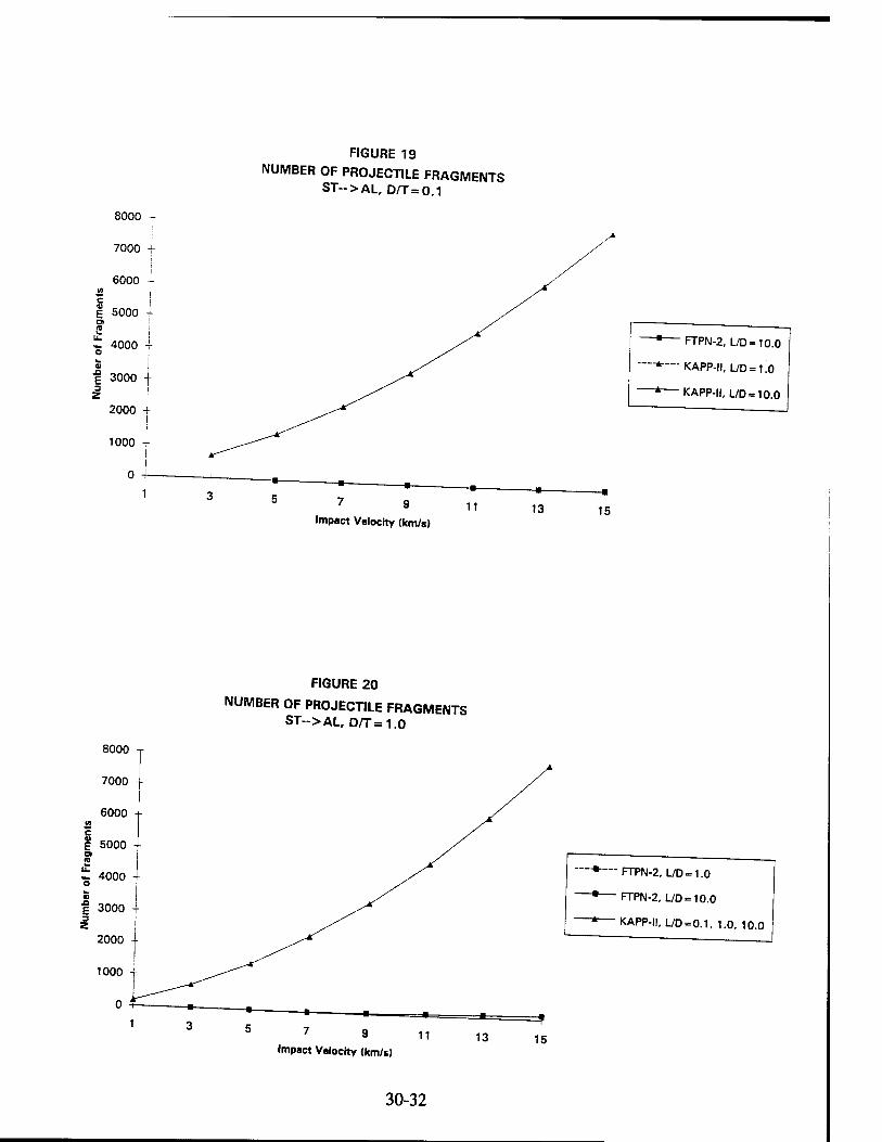
FIGURE 19
NUMBER OF PROJECTILE FRAGMENTS ST->AL, D/T = 0.1
FTPN-2, L/D = 10.0
A-— ■ KAPP-II, L/D = 1.0
-KAPP-II, L/D = 10.0
7 9
Impact Velocity (km/s) 11 13 15
8000
FIGURE 20
NUMBER OF PROJECTILE FRAGMENTS ST-->ALf D/T=1.0
h— FTPN-2, L/D = 1.0
1 FTPN-2, L/D = 10.0
KAPP-II, L/D = 0.1, 1.0, 10.0
7 9
Impact Velocity (km/s) 11 13 15
30-32
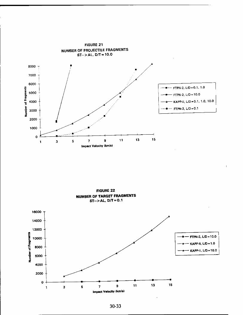
FIGURE 21
NUMBER OF PROJECTILE FRAGMENTS ST-->AL, D/T=10.0
5 7 9
Impact Velocity (km/t)
-»— FTPN-2, L/D = 0.1, 1.0
-■ FTPN-2, L/D = 10.0
-* KAPP-II, L/D = 0.1, 1.0, 10.0
......... FTPN-2, L/D = 0.1
15
FIGURE 22
NUMBER OF TARGET FRAGMENTS ST->AL, D/T = 0.1
16000
14000
12000 -
10000 --
" 8000 • o
6000 --
4000 ■
2000 -
0 ■ ■
7 9
Impact Velocity (km/t)
11
FTPN-2, UD = 10.0
-•*-— KAPP-II, L/D = 1.0
-* KAPP-II, UD = 10.0
13 15
30-33
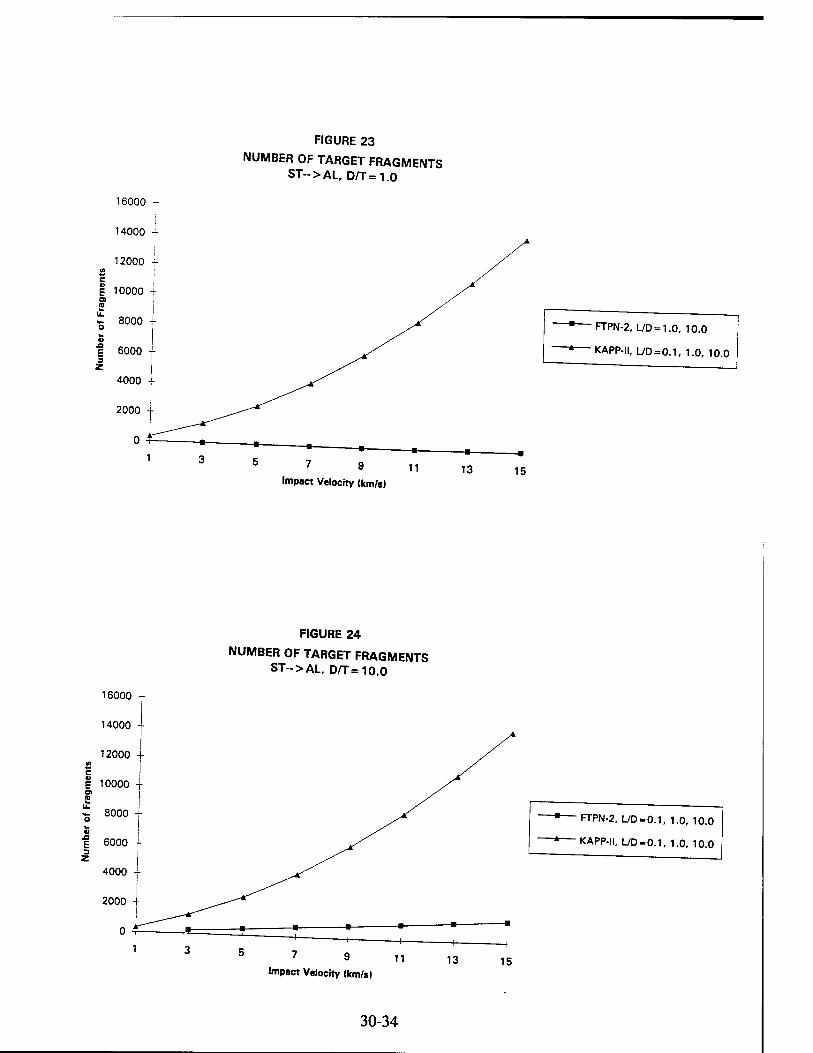
16000 -
FIGURE 23
NUMBER OF TARGET FRAGMENTS ST»>AL, D/T=1.0
14000 4-
12000 -
E 10000 a a w
£ 8000 -f o -FTPN-2, L/D = 1.0, 10.0
-KAPP-II, L/D = 0.1, 1.0, 10.0
7 9
Impact Velocity (km/sl 11 13 15
FIGURE 24
NUMBER OF TARGET FRAGMENTS ST-->AL, D/T=10.0
-FTPN-2, L/D = 0.1, 1.0, 10.0
KAPP-II, L/D = 0.1, 1.0, 10.0
7 9
Impact Velocity <km/s) 11 13 15
30-34
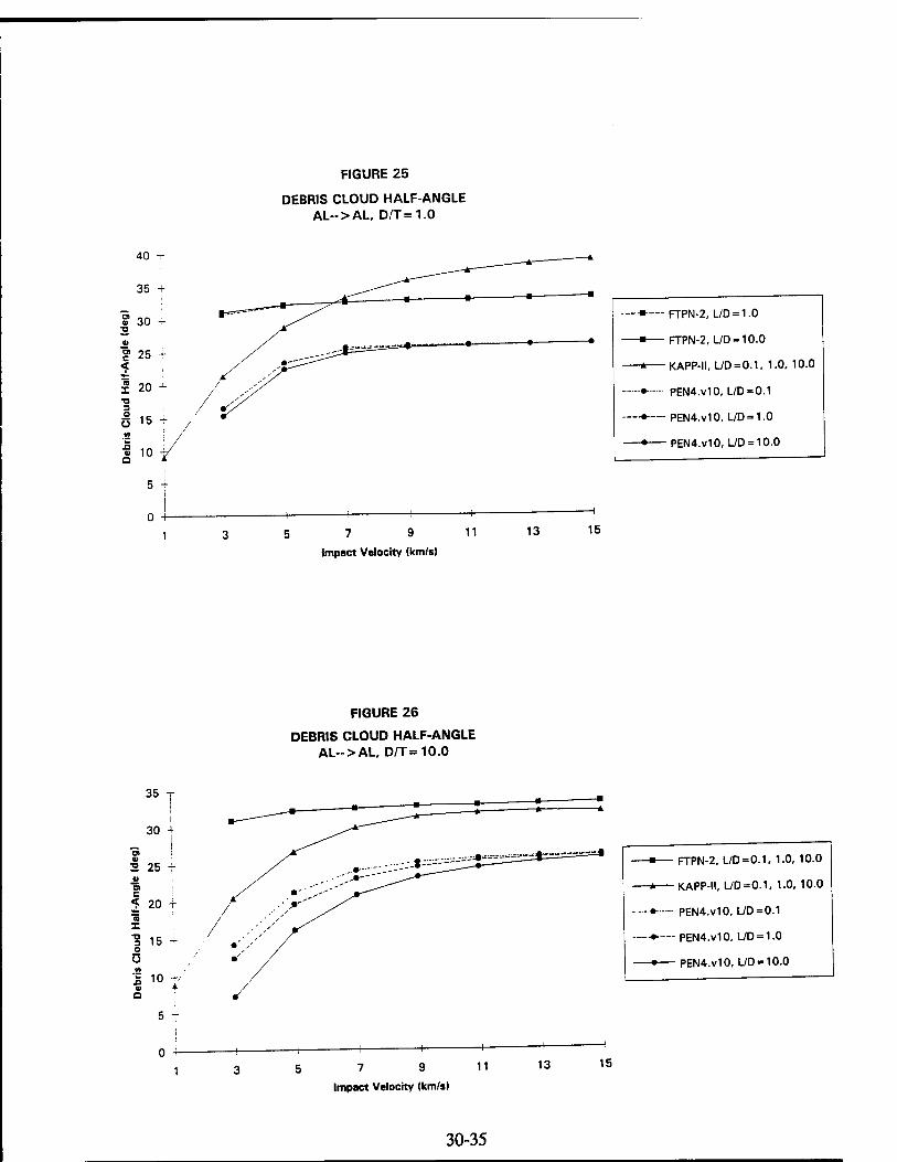
FIGURE 25
DEBRIS CLOUD HALF-ANGLE AL-->AL, D/T=1.0
—•»— FTPN-2, L/D = 1.0
■ FTPN-2, L/D = 10.0
* KAPP-II, L/D = 0.1, 1.0, 10.0
---•• PEN4.v10, L/D=0.1
—♦— PEN4.v10, L/D = 1.0
• PEN4.V10, L/D = 10.0
5 +
7 9
Impact Velocity (km/s)
11 13 15
35 j I
30 +
"a v S 25 T
< 20
1 15 o
10 4-/
5 i
FIGURE 26
DEBRIS CLOUD HALF-ANGLE AL-->AL, D/T=10.0
-■ FTPN-2, L/D = 0.1, 1.0, 10.0
-*— KAPP-II, L/D = 0.1, 1.0, 10.0
-•-■ PEN4.v10, L/D=0.1
-♦— PEN4.v10, UD = 1.0
-• PEN4.v10, L/D = 10.0
0 4-
1 7 9 11
Impact Velocity (km/s)
13 15
30-35
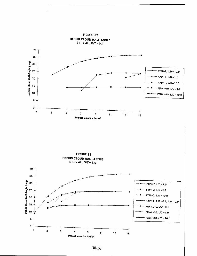
40
35
£ 30 H-
I 25 I
I 20 -f ■o 3 O ü 15 -L
« 10
5 -
FIGURE 27
DEBRIS CLOUD HALF-ANGLE ST-->AL, D/T = 0.1
FTPN-2, L/D = 10.0
—*■— KAPP-II, L/D = 1.0
—* KAPP-II, L/D = 10.0
—• PEN4.v10, L/D = 1.0
—• PEN4.v10, L/D = 10.0
7 9
Impact Velocity (km/s) 11 13 15
FIGURE 28
DEBRIS CLOUD HALF-ANGLE ST-->AL, D/T=1.0
7 9 11 Impact Velocity (km/s)
13 15
""-— FTPN-2, L/D = 1.0
"• FTPN-2, L/D=0.1
-" FTPN-2, L/D= 10.0
-* KAPP-II, L/D=0.1, 1.0, 10.0
..#...... pEN4 vl0 L/D = 0j
"♦— PEN4.v10, L/D = 1.0
-• PEN4.v10, L/D = 10.0
30-36
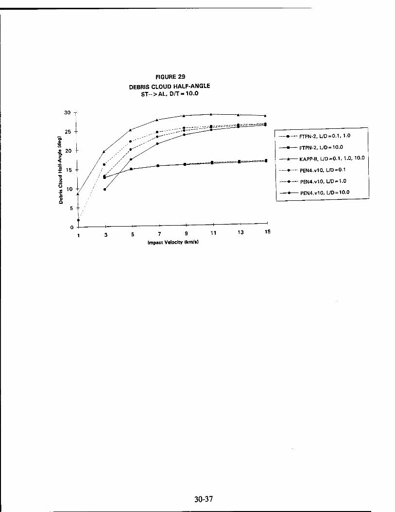
FIGURE 29
DEBRIS CLOUD HALF-ANGLE ST-->AL, D/T=10.0
-t-
5 7 9
Impact Velocity (km/*)
1 -*— FTPN-2, L/D = 0.1, 1.0
-* FTPN-2, UD = 10.0
—* KAPP-II, L/D = 0.1, 1.0, 10.0
.......... PEN4.V10, L/D=0.1
-♦— PEN4.v10, L/D = 1.0
-• PEN4.V10, L/D = 10.0
15
30-37
DIGITAL SIGNAL PROCESSING ALGORITHMS FOR DIGITAL EW RECEIVERS
Faculty Associate : Arnab K. Shaw Assistant Professor
Electrical Engineering Department Wright State University
Dayton, OHIO-45435
Final Report for : Research Initiation Program
Wright Laboratory, Avionics Directorate
Sponsored By : Air Force Office of Scientific Research
Boiling Air Force Base, Washington, D. C.
December 1993
31- 1
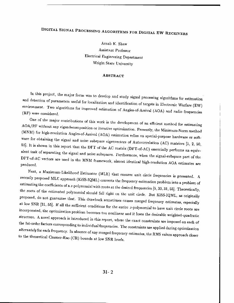
DIGITAL SIGNAL PROCESSING ALGORITHMS FOR DIGITAL EW RECEIVERS
Arnab K. Shaw
Assistant Professor
Electrical Engineering Department
Wright State University
ABSTRACT
a„d l^zT-the rjor f;rwas to deve,op md sMy sig-ai —^ •***- «* •—*- and detect,»» of parameters useful for ,ocafeation an<J .^.^ rf
envronment. T„„ algorithms fot improved estimation of A„gIes-„f-Arrival (AOAi and ,• (RF) were considered. ( ' "d rS<l'° f'«»»™
AOA/Rp!i!e 7M COnTU,'0nS °f 'hiS "°rk 'S 'he deVd01>"mt * ™ effid»' ■»-»■ *» —-ta.
I"!! 1 T ^,M-0f-A"i™1 'A0A» «^» -«- - sp.ci„-p„tp„8e hardware „ sof, w ,e o, oht.m.„g the s,e„al ,nd „oise subspace eiganvec[0K of Autocorre|atio]]
l:; r°m: :rrt ihat ,he DFT otthe AC m^ (Drx-°f-Ac>— -*- - - priced "e U '" ,he MNM ftameW"k' a,mOS' id»,i»1 ■*«**» AOA estimates are
Next, a Maximum-Likelihood Estimate, (MLE) tha, ensures n„i, circie frequencies is presented A
iry T r ™ (Kiss",QML) ronve"s the f—-*»*»■ *■*- *• • x - roots of the est.mated p„ly„omi„ should faU right on the „„„ ^
il rpo .I' th '■ " "e ,UffiCien' COndi'i0"S *" "» "*• -P*-"- - >- nm, circle roots ar
ZT A nov7 T Preb'em beC°meS '°° n0nline" "* " - "" **•"■ weighted-qn,dr.tic
7 , ord ,S m"°dUCed '" 'hiS 'ePOrt' *re "" ™< "*— » *■*— - «* of
to ZT • T, e"Cy- ' °f a"y merSed ''^ eS'—' «» ™S -h- aPP-ch deer to the theorefcal Camer-Rao (CR) hounds at low SNR level,.
31-2

DIGITAL SIGNAL PROCESSING ALGORITHMS FOR DIGITAL EW RECEIVERS
Arnab K. Shaw
I : INTRODUCTION
Digital processing of microwave signals in Electronic Warfare (EW) environment poses a great challenge
to researchers in Signal Processing. EW receivers are used for passive localization and identification of
target radars. All microwave receivers used in practice utilize analog signal processing techniques [49, 65-68].
The frequency-band of the EW signals are in the GHz range and the signals have wide bandwidth, which
necessitate sampling and processing of a massive amount of data at or near real-time. No presently existing
EW receiver process microwave radar signals entirely in the digital domain. But it is expected that with the
emergence of increasingly faster and inexpensive digital computers and high-speed A/D converters, digital
processing of microwave signals would most certainly be the way of the future.
The Electronic Support Measures (ESM) group at the Avionics Directorate, WPAFB, Ohio, has been
engaged in researching the digital microwave receiver design problem for the past few years. Their work
has resulted in many patents and important publications [37, 49, 65-68]. The proposal author had the
opportunity to collaborate with the researchers of the ESM group as a summer research faculty m June-
August, 1992 and also during the period covered by the present Research Initiation Project. The major
goals of the summer research were to develop and implement Digital Signal processing algorithms in order to
study their effectiveness and usefulness to the existing Digital Receiver Program. The following algorithms
have been studied :
• Time-Domain Detection of targets in the presence of noise : The time-domain detection problem has
been considered for single and multiple samples. Detection thresholds and Probability of Detection
based on Neyman-Pearson Criterion have been derived and coded.
. Adaptive Frequency/'AOA estimation : The effectiveness of the Direct-Adaptive-Freqnency-Estimation
(DAFE) algorithm [5] has been studied for realistic signal/noise conditions. Some modifications of
DAFE have also been incorporated for improving its performance.
. Prony's Algorithm : This well-known algorithm's effectiveness was studied with signals obtained after
passing through a hard-limiter (to avoid A/D saturation) and quantizer.
. Minimum Norm Method Without Eigendecomposition : One of the major contributions of this work
is the development of an efficient method for estimating AOA/RF without any eigendecomposition or
iterative optimization. It is shown in this report that the DFT of the AC matrix (DFT-of-AC) essentially
performs the task of separating the signal and noise subspaces. Furthermore, when the signal-subspace
31-3
'itr DFT"of"Ac vectors are uKd in MNM'
a,most ,d»,i»11*™**- *0* -m- »
h?rr r M"hoi wm E"ct cm,rmu: A «-* >»»— *- of M™um litel, hood algonthms (MLE), refetred to ^ Kiss/IQML] estima(e the s ^ W*
- -Pol— fc 30, „. „,. But the est.mated roots are Mt guitantMd to M 0„ (he uni( c °*
here that will ensure unit circle roots.
Details of the „rs, three ,opics „ inc|ude(J ,n (he toal report mbmjtM
es rch wer« m October 199, In this report] the detafls m the |ata P "—
urther w,tk M aII these topics has bMn conducM Md (he P 8■ -• ^n to,
ha. been briefed periodically „„ the progteK of our Ie8earch "' ^ '""" "' Y' Ts"'
SomeT„hrT'P05I °f 'f f0"0W"UP reSe"Ch ^ '° C°mPkmMt ""' «""»« th« «* "■*■■*. in summer
LThm T "I f" "" Pr°JeCt eXte"d °"' I""fa" "* "* « "- - «-loped new ab
mtermed at gos, of the proposed „^ which fa (o ^
oZT °n °Ut U"im,te *"" °f »*** * ^ mi— -*« P^.ype is presently being conducted with support from the AFOSR.
1.1 : The Digital Microwave Receiver Design Problem
rada^rZd"" T ""^ " * ^ ^ f°' -*« --*- - *. identifying the de t f , °° ' 'i0°' iammi°S' We,PO" de"Very " °'h" teisi»S « <" m rder to perform ^ tasks, the receiver m„s[ ^ ^ ^ ^ ^
ollowmg „ Parsmelers : Angle.0,A„iv!l| RaQio -'-* he
Amplitude (PA), Pulse Width (PW) and Polarization (PI Th ' '' «,„„„. , ■ ana formation (P). These parameters may be useful in more than one stages of receiver operation. For example AOA BF TO» PW j „ , • . more man one
::r:r; t r r ™ -' - - ^^=r:«™t: these::ir:::::;i~^^^^^^^^
Unlike most conventional radars the EW receiver rf«,lt™ „,. M
knowledge about t^ i . ■ . • g P m 1S comP,lcated by the fact that no
meit it a p T rai,able to the receiver-The nature °f the -obiem ais° »**- «»*
^65 a7Lh : " lmmediatdy °r Withm a fGW SCCOndS ^ - -^ P^e mode [49 65 68 . Furthermore, m order to reduce search time and the consequent response time the processing
:;:t zitb;"wid;as possible-h is aiso desirabie to w ^s— - >-~ range such that a broad range of slgnalS) including weak ones, can be detected.
31-4

1.2 : Background and Motivation
In the past two decades, many classes of radar and sonar receivers have been converted from conventional
analog technology to purely digital or hybrid systems [24], but EW receivers are yet to make such a transition.
The primary technological factors that have been holding back possible fabrication of any digital EW receiver
are probably twofold. Firstly, if Analog-to-Digital (A/D) converters are to be used at the operating frequency
range then the Nyquist rate would necessitate sampling at the GHZ range and secondly, the digital hardware
or firmware must have the capacity to process such high data rate and produce effective results at or near
real-time. But even though the carrier frequencies are in the GHz range, the bandwidths of the useful
signals are only in the 10s of MHz. Hence, an obvious compromise in such a situation would be to down-
convert the original signal to an intermediate frequency (IF) band before sampling. Down-conversion or
superheterodyning is also quite common in analog microwave receivers because it is much easier to design
accurate IF amplifiers and filters having fixed and predetermined bandwidths [49, 65-67], Frequency down-
conversion may cause image signals at the IF band and standard cures used in analog superheterodyne
receivers such as the use of I and Q channels and image suppression filters can be utilized to reduce these
effects. Furthermore, multirate sampling/processing or sub-band coding may also be useful to avoid high
sampling rate. Digital EW receivers can be expected to offer some major advantages over their analog counterparts.
Foremost among these is the almost lossless storage capability of digital memories which can eliminate the
dependence on lossy analog delay lines. Digital processors and memory chips are relatively inexpensive,
compact in size and low in weight and the trends are towards even further reductions. Digital signal
processing algorithms and digital computing technology have matured tremendously and offer a wide range of
capabilities. Parallel processing, pipelining, RISC, VLSI design, systolic architecture, vectorization and array
processing, fault tolerant computing and etc., are only some of the well-known aspects of digital computing
that the last few decades of research have produced. As our research progresses, we intend to study if some
of these ideas can be incorporated in the digital receiver in order to improve the efficiency and accuracy of
its performance. A broad range of digital signal processing algorithms are already available for detection as well as for
parametric and non-parametric estimation from observed data [13, 17, 24, 48]. These techniques are based
on well-established theory on random processes and applied linear algebra. Among the six parameters noted
above the AOA and frequency information are probably the most important ones for sorting, identification
and jamming and a rich body of literature is available for high-resolution AOA and frequency estimation
[1-13, 15-35, 37-48, 50-65, 69-79]. Much of the results on AOA/frequency estimation appearing in signal processing literature have been
developed for sonar and low-frequency radar applications. These mathematical and statistical theories are
mostly valid for the EW scenario. But considering the high data-rate in the present application, computation-
ally simpler algorithms must be developed. One of the major contributions of this work is the development
31-5
of» efficient „„hod for estimating A0A/RF without „y eiee»decomposit,o„ „ ^ ^^
1.3 = H.s.orica! Perspective „„ the Research on AOA/Frec,„e„cy E8timati„»
hne^ZlTf I! anelr0f-riV"! a°d -d'° *•"»*■ - «- .«— difficulty hec.use of the non- nature ef the option prob,era. An adaptive ^^ scheme de
eca„s. of ,,s computation., simp„city .. w.„ a. its rC-t.n,. .d.pt.ve „«As pat 0 J^ Perform« tins sumn,.,, ,. has been deraonslrated lhM ,he use rf J ol Z"
2" ,mTT;he bias and var,ance °f th< -ta~ - 'he - *— c" ih r M p" ptoject' ™efflc,ent approach fo"ni"g ^»"-»«>■ «-*- ^ -« method f„, Mnxnmun. L.kelihood estimation of &e,»«„cies is presented
has bTee»Aa°ltma,i0nr;b'em " ^^«^ * »« ^»-y Est.mation p,„b,em „hich
0. «c fo, h.dd.n penod.ct.es. from observed dat. has .ppeated i„ varied forms i„ sever., seeming,
«ring disciplines of science To appreciate the sustained appea, of this ptob,m to research™ P- «we cent™, consider that as f„ back «s in 17M, Ptonv proposed , „^ ^
the parameters of a mnltipfe sinusoids „odeI ot .„ obse™«i„n record flu «1 B„t ■ A
P»o eg, was computationally a very «pensive procednre. Bn, „i,H the advent of d^itatm^l after the discovery of the Fast Fourier Transform ,FF-n ,!„• -*u u r, , computers and
has hecome the standard choice fo, ^ST" ^ ^ ^ ^V"" trmltinl. ■ n j,, ,or lr«li"mey/ AOA estimation in a variety of important applications The
«eleacepe to ,„oh, the locat.ons of c.esely spaced stars [,]. ,t a,s„ ha, wide .„„„cations in geophysics radar
I.3.a : The Resolution Limitation of the Periodogram
Ever since its discovery in ,*,, th« FFT bas been lhe primMy ^ for
AOA, or fancies of far-ne.d sources from „o,sy ohserv.tion dat.. The software or hi™. J^
d me Ld 7"M-'^'-f™^ To date, the periodog,am continues to he the most Jqnent,y nsed method for freouency/AOA estimation [40, «1 In fact i, 1« „i, i .u . , , t».„^ f.L - . . aoj. in tact, it is well known that for localizing a sinde
which »™ * J x. , mumpie targets, the periodogram cannot resolve two frequencies
»1*1!' P" 08ram fai'S '° diS""eUiSh tW° dOSe" S"«d <^-*- - »ly P-ides * fre0UenCy eS,'mate mSfead °f - The '« —t truly portrays the prehlem one Z while
31-6

resolving two closely spaced sinusoids when a relatively short data record is available. Clearly, if any amount
of data is available for processing, the periodogram of sufficiently zero-padded data will provide reasonably
good estimates. But in many problems of practxcal interest only short data record is available and one has
to overcome the program's resolution limitation by resorting to what are commonly known m the signal
processing literature as 'High-Resolution' or 'Superresolution' techniques. The major contributes m the
higher resolution approaches are highlighted next.
I.3.b : High-Resolution Methods
A multitude of AOA/Frequency Estimation algorithms, their variations and analysis are available in the
literature [1-13, 15-35, 37-48, 50-65, 69-79]. In the following paragraphs only some of the major developments
are briefly discussed.
Minimum Variance Method : In order to improve upon Program's resolution limit, Capon had proposed
this linear estimator which minimizes the interference at frequencies outside the band of interest [9]. Its
performance has been shown to be better than the periodogram estimator but worse than the modeling
based estimators [34].
Model-Based Methods : A major motivation for many modern high-resolution frequency estimation methods
has come from the desire to achieve more exact models for the sinusoids-in-noise data. In the Parameter
Estimation area in the theory of Statistics, it had been well established that Auto-Regressive (AR) modehng
is very appropriate for modeling data with peaky spectra. But in the frequency estimation field also,
it had been a common knowledge that data composed of sinusoids in noise tend to have peaky spectra.
Consequently, frequency estimation based on AR-modeling has received considerable attention [7, 8, 18, 23,
35, 38, 44, 48, 72, 73]. Depending on how the autocorrelation values are estimated, there are three types of AR parameter
estimation methods, namely, Autocorrelation method [35], Covariance method [35], and Modified Covanance
method (also known as the Forward-Backward method) [38, 73]. The later two cases are more approbate
for sinusoidal processes because of their implicit relationship with Prony's method which provides perfect
frequency estimates when no noise is present. Incidentally, the Maximum Entropy method proposed by Burg
[7, 8] and the Linear Prediction based spectral estimator [35], both produce essentially identical frequency
estimates as the Covariance method. When p sinusoids are present and a p* order AR model is used, the frequency estimates are found to be
poor at low SNR (< 30d5). To circumvent this hurdle, larger order (L > p) AR model has been proposed
[28 72] The larger model order tends to accommodate a major part of the interfering noise and thereby
reduces the effect of noise in the estimates. The larger-order approach performs poorly below 20dB SNR
[28].
Eigen-Analysis of the Auto-Correlation Matri* of Sinusoid-in-Noise Data : Since the mid-to-late seventies,
31-7

;° MW ,daSS °f ,ISOri"""S « b™t *«*»« by effective expiation of the special propert.es of
« « „,,hzed by P,s,re„ko [42J wh0 showed ,häl the 2.polynomia, formed ' J -
co„esPon mg to the Sma„e„ eige„value has pMts ai (he ks —
by K_ M „here, for „ , p __ aU the noise eigenvectes had bem ^
approach, „ TO shown in [28, 29] tha[ (he sigMl subspace eigenvectoK CM ako ^ J« -
«b pace vector „hlch sho„,d have !ePOS at the 5igna, frequmcy loca[ions This _ -
;:rng * M~™ «**» '** > *• »»-* *sl „ill be used in the J^
and Kop ff' ^"""""T °" PiSMent°'S aPPr0"" W,S PreKnted ^ SChmdt (5°- 51) ^ Bi~
: i: ::;;°^tirion i°obtam the—-— * - -— -— It may be pertinent to emphasise here that the approach proposed in «Ms wort f„r extracting sign,,
r no« snbspace .„„hont eige„oecomposlti„„. „,y be combmed „,th either the MNM o, the M7s C
rae"* ™e MNM f"meWMt"- "- »'^ '» -lopin, the BrT-ba«ed MNM (D-MNM, b!Z
«Id be t„,c. thl, of MNM ' " ^ "Sed bU' '" ** "" "" °'dW °f'he ***-"
*, feamng to option of a „„„-linear crite„o„ „Hich can „my be performed itera.ively sZ different approaches are available in the literatnr. [5, 30-32 46 47 54 56 61 781 H \
Conned MlE approneh described in this report appears in 1^^11.11^" ^
oTtr "',!? T 'm,",ma °f"" Pr°*°"d UM°d' ■ AS ,iS'ed in "»■*■—• "»e are , Wse „„mber
rd h re"the h,sh"esoiutiM F—/AOA -— -—■'»»d« - it: op« m zaho», both of wh.eh are eompntationallv intensive for real-time appUeations. Among the ,wo high
z::: r :described in this repoti'the fitst mM - - ^ 'h»«- -4 «£££ methods whereas the second provdes the m„s. accurate frequency estimates.
31-8
II : HIGH-RESOLUTION ANGLE OF ARRIVAL (AOA) ESTIMATION WITHOUT
ElGENDECOMPOSITION
II. 1 : Introduction
The Fast Fourier Transform (FFT) is an efficient technique for calculating Discrete Fourier Transform
(DFT) at uniformly spaced bins. In many important practical applications, such as radar, sonar and as-
tronomy etc., the resolution capability of FFT is inadequate. Overcoming the resolution limitation of DFT
has been a vigorously researched topic in Signal Processing in the past three decades. The modem methods
attain the desired 'High-Resolution' or 'Superresolution' at the cost of steep computational burden. The
existing well-known methods utilize Eigen-Decomposition (ED), Singular Value Decomposition (SVD) or
Maximum Likelihood (ML) computation or nonlinear optimization. These algorithms can only be imple-
mented iteratively which limits their real-time capabilities.
The primary objective for this part of the project is to study whether the computational simplicity
of DFT can be effectively combined with the underlying mathematical framework of high-resolution meth-
ods The desired goal is to achieve high-resolution without any iterative optimization. Specifically, some
well-known existing approaches, such as the Minimum-Norm method (MNM), extract the signal and no1Se
subspace information from the eigenvectors of the Autocorrelation (AC) matrices. It is shown that the DFT
of the AC-matrix (DFT-of-AC) essentially performs an equivalent task of extracting and decoupling the
signal and noise subspace information. Hence, it is proposed that the signal eigenvectors be replaced by the
largest-norm DFT-of-AC vectors. It is demonstrated that when the DFT-of-AC vectors with larger norms
are used in the MNM framework, mostly better or almost equivalent high-resolution AOA estimates are pro-
duced. The bias, mean-squared error and the root locations of the proposed DFT-based-MNM (D-MNM)
compare well with the Eigendecomposition-based MNM (E-MNM). The simulations further show that the
performance of the D-MNM is more robust at low SNR and it has superior dynamic range. The major signif-
icance of the proposed work is that, no complicated iterative optimization is needed and the signal-subspace
information is extracted only by a single matrix multiplication. Hence, hardware implementation of D-MNM
for real-time high-resolution AOA/Frequency estimation may be feasible with currently available technology.
II.2 : Problem Definition
This part of the project addresses the problem of estimating of the Angles of Arrival (AOA) of densely
spaced narrowband targets. Suppose that p plane waves originating from far-field point sources at distinct
directions impinge on a linear array of N equally spaced sensors. The signal sampled simultaneously at m*
instant of time at N equally spaced sensors form a 'snapshot' vector defined as,
xm A [*m(0) xm(l) • • - xm(N - l)f. (/L1)
In the presence of noise, the observation samples can be written as,
xm(n) = xm(n) + zm(n) (7L2)
31-9

Ix:'!™ T T: obserTOtio°noise ,nd/ot the mode,ins — -d *-<»>*«-*• signal part of the observation, which is given by
p
xm(n) = J2Am(^if±ln - ^)sin". + ^m(i) t'=l n = 0,1,...,#-1 (77.3)
where,
P
d
X
Number of narrowband sources present
Spacing between sensor elements
Wavelength of radiation of the received signals
Angles-of-Arrival (AOA) of the ith source
Amplitude of the f* source at the mth snapshot
Phase angle of the i« source at the m"> snapshot,
Uniformly distributed between -x and TT
r: "ix(:i,:r,med rbe—a°d —^ -*■<*—*-.- ■. ta. «*.,. «V Ihe sjgnal model can be written in a more succinct form as,
Am(i)
<t>m{i)
p
xm(n) = J2A-imejü''n
where, «,• and yl!m are defined as
1=1
w«' A -y-sin^- and
(77.4)
(77.5)
(77.6)
Further details about the above model may be found in ri31 With th* K f , • observation matrix can be written as, f°rmUlatl°n ^ ""^ *» the
^TA (77,) where,
Am A ^m(i)e--''2x1(^i)sm«i + ;<M0.
T A
1 1 1 ejwp
_eJ*i(N-l) ej u>a(N- ■^ eJ"r(N-
^ [*1 *2 • • • tp],
A A [ ai a2 ... ajvf ] and
am A
'Aim
A2m
LA pm J
form = 1,2,...,M.
(77.8)
(77.9)
(77.10)
(77.11)
31-10
For half wavelength spacing between two successive sensors of the line array, «,- = * sin ft. With M
snapshot vectors defined in (77.2), the N x M observation matrix X is formed as,
(77.12)
(77.13a)
(77.136)
X A [xi x2 ... XM]-
Using the observation matrix, the spatial covariance matrix can be estimated as,
C A i(XXff) = M
1 M
ATS XmX, H
■m*-rn' m=l
The description of the observation and the model is now complete. Given the noisy observation matrix X, the
problem under consideration in this proposal is to estimate „,'• and Aim's. Note that the complex amplitudes
can be estimated linearly once the w,'s are known but the estimation of poses the greatest difficulty because
it is a highly nonlinear optimization problem. The primary objective for this part is to study whether the computational simplicity of DFT can be
effectively combined with the underlying mathematical framework of some of the existing high-resolution
methods. The final goal is to achieve high-resolution without any iterative optimization such that real-time
implementation may be feasible with existing hardware. The proposed method makes use of the special
properties of correlation matrices which are outlined next.
II.3 : Some Properties of the Autocorrelation Matrix
Since the data described by (77.3) is uncorrelated, zero mean WSS process, the N x N (N > p)
covariance matrix C will have the following matrix decomposition when there is no observation noise,
C = TST >H (77.14)
where, S A diag (<r? a\ ... o*) and cr? denotes the power of the the z-th signal. Note that this ideal C
has rank p. In this case, the eigen-decomposition of C can be written as,
CV = [Aivi
Ai
0
ApVp 0 0] = AV
0 A2
0 0 0 0
0 0 0 0
XP 0 0
Vi v2 Vp+l
T 1 VJV
(77.15a)
(77.156)
0 0 0 ... 0.
For observations with noise as defined in (77.3),
C = TSTH + <r2zI. (77.16)
31-11
No., ,„„ this theot(!ticaI c has rank „ though (he signa| par TsjH
«gen-decomposition of C CM be written as,
cv = [(A1+<rj)vi ... (AP + „|)V(, ^Vf+i ... ^j (//i7)
httbtlrf8 ind/? T6"' 'he SigDaI "d n0'Se eige°VdUeS' BUt '" »"** "» ^-»positton !r, IT: on samp covar,ince mate c - defi-ed'" <"'13> -* <- *• "*• *™b- -II „o, be .,„,, but will be absorbed with the signal e,6e„va,ues also. in ,h„ case,
cV-[AlVl ... Apvp Ap+lVp+1 ... \NVN] (/L18)
.triar« f-maW eiSenV,IUeS "e OTdered "• A' ~ ^ - V ^ -™*» —*■* - arges« e.genva.ues are caiied the 'signal electors' which constitute the 'signa.-subspace'. AHthe
her (AT -p) eigenvectors are known „ the W eigenvectors'. No,, also tha, the p 'signal eigenvectors' of C span the subspace denned by the column, of T a„H ,1 , ,u , eigenvectors eigenvectors. ^ "* °"h»S<'"!'' '» "■« 'noise subspace'
II.4 : The Proposed DFT-Based Minimum-Norm Method (D-MNM)
As , significant departure from the eigen-based approach,» discussed in the previous section, this work
vocates that the s.gnal-subsp.ce informatron be extracted from the DFT-of-AC mat™ which can be
rr; ra sinsie matrix muitipika"°n-Th,s «* ^° ^ -f»■*-» «***.» ^„vectors wh.ch ,s computational,, .»tensive. The centra, tdea beh.nd ,h, DFT-of-AC matrix is a„,ly2ed
Il.d.a : Signal and Noise Subspace Extraction from the DrT-of-AC Matrix
Let the DFT matrix be denoted as,
DA [er e2 ... e„], („ 19)
where, the Cements of the *-,„ DFT-vector e, is defined as, „<„ . .,*.. for kJ = „,,, % .. „_, ,f
the finances „,. are a„ on the DFT bins and if there ,s no observation noise, then in gene,,, '
ft A Cek = (//.20a)
1 M
= M X,(x£e*)x" m=l
M 2_/(xme*)xm, using (7.136) (//.206)
1 M
= lE(^T%x-n, using (//.8) m=l
1 '" = -Lx^aH M ^ m
m=l
tfe*
tfet
31-12
(//.20c)
(//.20(f)
If the fc-th DFT vector ek corresponds to one of the w,- frequencies,
1 M 1 A 1V1 ™=i m=l
kmam
T7l = l
= T
■" JÖ7 Em=l ^ibm^l'"
lEm=l \Akm\
1 ^M 4* 4 „
<Tkl
&kp
(77.21)
where, *H. denote the covariance of the complex amplitudes. Assuming the number of samples M to be
large and since Akms are independent random variables, aAkm,Alm A H\ = «*»**• Hence,
fk^a2ktk - &2
kek. (77.22)
Note that the norm off, is directly proportional to the signal power, S\, i.e., this norm will be large if the
signal power is significant. On the other hand, if a DFT-vector ek does not correspond to any of the u,
frequencies then due to orthogonality, t?ek = 0, Vi. For such cases,
h = 0.
For this ideal case then, the DFT-of-AC has the following decomposition,
F A CD
A [fi f2
-* [Aiui
fiv]
ApUp 0 0]
(77.23)
(77.24a)
(77.246)
(77.24c)
where the A,s and Uis are the lengths and unit vectors of each ft, respectively. Note that the unit vectors
in the matrix in (77.24c) have been rearranged so that the zero/nonzero components are clustered together.
Interestingly, this decomposition appears to be very similar to the usual Eigendecomposition of noiseless
and ideal C, as given by (77.15). For this ideal signal scenario again, if the DFT-of-AC is formed usmg the
theoretical and noisy Covariance matrix of (77.16), then the decomposition has the form,
F = CD
— [(Ai + (7,2)ui ••• (Ap + <r2)up <r2up+1 ••• <T?UJV]
(77.25a)
(77.256)
(77.25c)
where the u,'. have been arranged in decreasing order of lengths. Note again that this decomposition is
analogous to the one in (77.17). In this case also, the p largest-norm vectors of the DFT-of-AC matnx
contain the signal subspace information.
31-13
In practice the w, will „ot be on the DFT bins and the observes may also be noisy and hence
h decomposi on in (Z,24) or (Z,25) W1„ not hold. But the Deponents ft.) closer o the Slg i
: r::: :ha: lars;r norms (this is further anaiyzed * s-ti- **>■—- - scena 0> .hen the observation data is nolsy and the angular frequencies UfB are arbitrarily spaced the signal/noise subspace decomposition can be formed as :
F- [AlUl ... ApUp | Ap+lUp+1 ... A^u^] (IL26a)
A A[US | UJV] = J (11.26b)
> AN are the norms of the f, vectors and the matrices A, Us and U„ are formed as, where, Ai > A2 >
"A!
A A
APJ
Us A Ul u2 u„ and, UJV A UP+I UJV
(//.«). U m,y be noted he,, that in ce of the idea, signa, c!_ of (1IM) M(J ( ,„ ^ J^
corresponds to one of the DFT-vector „ l„, i„ .1 , , ' the DFT mm . , S **" °f ("'26)' they aK IiM» combination«, of
DFT-compo»e„,s Cose ,0 the sign,, fancies (the gene,,, „ ls f„rt„er analyzed in Secüon „ „
U.4.b : Incorporation of DFT-Ba.ed Signal Subsp.ee in Minhnnm-Norn, rWwork
d wh^rT idT T thC Mi"taUra*™ ™*°° * '° *™ - appropriate Wsnhspace' vector d which ,s orthogonal to the 'signal-snbspace' denned by Vs. Let,
°« £ £'*•-' (,,.27) fc=0
be an (N - l)-th order z-polynomial with p zeros at, zk = e^ for k - 1 ADA* Th0moffi • 4. . • , ' ' * ~ *' •••>*>> corresponding to the AUAs. lhe coefficient vector is denoted as,
(//.28) d A [d0 d, ... dJv-1]
T,
^^^r rderdetermined - °f ~ "** *» ***• —er of solution,
an it;^:sr ut:::h^mmimizes the -,,di12'—-——- rCle- ThlS mmimUm-norm,sol^nofdf0rsolving(//.29)Canbeexpressed
1
- G"(GG")~~g ' (//-30a)
d =
31-14

where, Uf is partitioned as, Uf A [g | G]. (/L306)
Once d is estimated, the p roots of D(z) closest to the unit circle are used to find the AOAs. It may be recalled
that in E-MNM the signal-subspace eigenvectors Vl> v2, ..., vp, as defined in (77.18) are used to form Us
[28, 29, 45]. But in case of the proposed approach, no eigendecomposition is necessary. Post-multiplication
of C by the DFT-matrix D is all that is required to extract the signal subspace in (77.26).
II.4.C : Summary of the Proposed D-MNM Algorithm
The key steps and some alternative possibilities are summarized in this Section.
II.4.C.1 : Algorithm Steps
1. Form the Covariance Matrix estimate using forward-backward method [28, 29] :
1 M
c &wiYl XmX" + x™Xm m = l
.H , „» x» H (77.31)
The 'backward' vector is defined as x», A Jx^, where, J denotes the permutation matrix with 1's at
the cross-diagonal entries and * denotes the complex-conjugate operation.
2. Post-multiply C by the DFT matrix D to form the DFT-OF-AC matrix, F A CD.
3. Form U as in (77.26c) using the p unit vectors corresponding to the largest norms. Partition Us as in
(77.306).
4. Estimate the d vector using (77.30a) and form the D{z) polynomial using the elements of d.
5. Find the roots of D{z). Pick the p roots closest to the unit circle to find the desired frequencies/AOAs.
II.4.C.2 : Alternate Possibilities
Steps 2 and 3: Post-multiplication of the AC-matrix by a DFT-matrix has been used here because the
decompositions as described in Section II.4.a appear analogous to eigendecomposition. But it is easy show
that identical results can be obtained if the AC-matrix is pre-multiplied by a DFT matrix, ,,, the DFT-of-
AC matrix can also be formed alternately as, F, A DC. In that case, the largest norm row vectors of the
DFT-of-AC matrix Fi must be used to form Uf defined in (77.31).
Step 4 • This step requires inversion of a matrix of dimension (N - I) x (N - 1). This can be avoided by
orthogonalizing the p largest norm vectors in Us. Let, UJ be the new 'signal-subspace' matrix with the
orthonormal set of vectors which can be written in partitioned form as,
U's" A [g„ | G,]. (JI-32)
With these partitioned matrices, d can again be found in Step-4 as [28, 29],
1 (77.33)
- Gfg0/(1 - gfg0).
31-15
d
U5 ts formed b, orthogonahsmg the p largest norm vectors of the DFT.„f-AO matrix.
Step 5 : This step requires rooting of the (N - IWh ™^ i • , ^, s
also be found from the peaks of the fo ^ ^ ^^ ^ *"*"*"*» ""* om tue peaks of the following minimum-norm pseudo-spectrum [28, 29, 64] :
PMNM(ejw) A = |D(e^)|2 (77.34)
II.5 : Simulation Results
In this Section the performance of D-MNM is compared with « of the existing welMmown algortthms
i::—:::,^s" FM tha ■——*» -——zz II.5.a : AOA Estimation
Simulation 1 : Two Densely.Spaced Targets of Eaual Powers [62, 63]
Planewaves from p = 2 sources with 0, = 18» and », - 99» • M * „ n
r29 so sol Th* K , ~ Cldent °n N=8 Sensors were modeled as in L^y, JU, d2J. I he number of snapshots M-m p;„ 1 u ^ SNR The ,„„ I , . , 8' S 'he "0rmS °f 'he f' vectesf°<2» "W- * 20dB SNR. The two largest A,s always appear „, be „„, ^.^ ^
o. e root, of D„ fo, 5„ mdependent „^ ^ ^ ^ ^^
I; 1 rts;bolh cases are at awt *ame "-^ T^—«™ ^ »« terms of the bias and RMS value«! with 9nn • J _. . ivimvi in
indicate that the performlT fD MNM H ""^ " ^ " ^ ^ ^ ""*
~ m,n,r.d in ,h s case. „ ^DTM T f 7t7 ^ """■' '^ "°
.nals) at 1- SNR ranges. " """^ """ "*" <ta ««- °f —«
Si»ul.,ioB 2 : 0™^,„ „/;,,„„„,, ^ „,, ^ ^ ^ ^^ ^ ^ ^
r^ ::::;~ ^;riocated - ha,f"-y*— ■———* trials a, each SNR fo, D-MNM and E MNM , 1 "^ "*"' i"deP»d«*
dynamic range than E-MNM "'^ '" F'S' * ^ ^ <" "*—
II.5.b : Frequency Estimation
^r^ ~ - ~;:~rihe -*- ~—->— Simu,»,io„ 3 : C„mp„r,sra „ Blgh.Rl,ckt,m „^^ and ThnMi ^^
31-16
The simulation data is generated using the formula [28, 69] :
y{n) = ai^2'(°-B)B+'« + a2e^{0-52)n + w(n), for, n = 0, 1, .... Af-1 (^-35)
where w(n) is complex white Gaussian noise with variance <*. The number of data samples used is, M=25.
This data set has been widely used in the literature for studying the performance of various methods. For
this data set, it has been shown in [28, 69] that the TK method performs best when high-order (L x L)
covariance matrix with L = 18 is used with forward-backward covariance matrix [19, 64]. Five hundred
independent noise realizations were used to compare the performance of the proposed method with that of
TK method and MUSIC. The mean values for three cases at different SNR values are displayed in Fig. 4.
The RMSE results are shown in Fig. 5 along with CR Bound for the frequency at h = 0MHz. The bias
and RMSE at different SNR values are also tabulated in Table 2. Clearly, the proposed method extends the
performance threshold closer to the CR bound. Hence the performance of the proposed method approaches
that of the Maximum-Likelihood method more closely.
II.6 : Analysis, Discussion and Directions on Further Research
The results presented so far are quite intriguing and can be expected to have far-reaching consequences
on simplifying the present practice of frequency/AOA estimation. The proposed approach of forming signal-
subspace using DFT without any eigendecomposition also opens up whole new avenues for further research
and at the same time, poses some unanswered questions. Furthermore, it may be possible to extend
and'incorporate similar ideas in other closely related problems or to develop more simplified algorithms.
The theoretical performance of the method needs to be thoroughly analyzed. The major advantage of the
proposed approach is that all the signal-subspaces are obtained with a single matrix multiplication. This step
may be performed using FFT which is very efficient for hardware and software implementation. Preliminary
analysis of the proposed work and some directions for further research are briefly outlined in this section.
1. Reduced Computational Complexity and Usefulness in High Sampling-Rate Problems : The
major significance of D-MNM is that its high-resolution capability does not rely on any iterative method
or eigendecomposition which is also computed iteratively. The lower computational complexity of D-
MNM should be attractive in any general frequency/AOA estimation scenario. But the usefulness of the
proposed method should be specially significant in those applications where traditional high-resolution
methods are yet to make much inroads due mainly to extremely high sampling rate requirements.
Specifically, in Electronic Warfare (EW) applications, the signals usually operate in the GHz range
but real-time, high-resolution capability is a necessity [65]. Currently no EW receiver processes signals
entirely in digital. The proposed DFT-based MNM with its low computational complexity, is expected
to provide the desired high-resolution capability to future digital EW receivers.
2. Signal-Subspace Information from the Autocorrelation Matrix Only : The strength of the
Minimum-Norm framework as a high-resolution method really comes from its ability to form the 'noise-
31-17
subsp.ce. vector d by expioiting the orthogonslity ^^ fa ft
r ™' DFT'°f-AC 'S M ■»^»ri- ~<M- *> P^e US became it is a h„e.r combination of th, s,g„,l-vect,rs ,„ T. Thl6 ca„ be seen by rewnling the DFTofAc ^
F = CD = T • 1 M
M E Mx£D) m = l
(//.36)
In facMhe AC matrix i« is also a possible candidate ,„t ob.ai„,„g ,h. .signabsnbspace' U„ because
,. can be expressed as a line« combination of the signal-vectors in T,
C = T ~M ^ amXra
m=l (JJ.37)
No, s„[pri»ng,y, hen Us is formed wM (he p |apgest nom vectors rf (he ^^
K because the DFT operafon accentuates the signal-subspace, as discussed next
I. Analysis of the DFT-b.sed Sign., Subspace for Arbitrary AOA/Frequency : For idea, noise
free observe if the frequenci« are not on the DFT bi„s, lhe DFT-of-AC ope,Jn CM be ^Z
F = CD
= TST^D
tfD tfD
= TS
LtfDj
(//.38a)
(//.386)
(//.38c)
Consider the matrix at rieht Each nf tv,^ +i?r» ngnt. bach of the tfD vectors are complex valued DFT of a sequence of a
:T:: The magmiude °f each - ^- << ° *-«*~—«* > ^»:: - «^mn dl„g to the biu location Cos., to the freque„cy „,. For Mmte äperlure J
appro! TT """" °f SenS°'S' eaC" KW ,eCk" ^ " "" Md "» <""« *»«* =f «bat row
b. r;T ofTc rwi"be the case fot each °fthe °th« ™—-■*■-■ —*. the DFT-„f-AC „p.r„,on agaln produces p ,„gest norm vec[ors a( *
vectors .„ the T. ft« those components a,so con,.™ signal-subsp.ee information which i, or,hogon,l to d and hence nseful fo, obtaining the mi„imum.„orm vector „. ^"^
31-18
4 Performance and Accuracy Analysis : The results presented here indicate that the DFT-of-AC
operation retains significant signal information comparable to signal eigenvectors produced by ^de-
composition. This phenomenon needs to be quantified analytically. A possibility would be to analyze
and compare the respective Frobenius norms of the Projections onto the true signal basis-space as
produced by the signal-subspaces due to the eigen-based as well as DFT-based methods. Most of the
existing eigen-based methods have been analyzed to study their performance and accuracy [22, 25,
43, 76, 77]. Following this trend we plan to perform statistical analysis of the bias, variance and the
resolution threshold of the estimates produced by the present method.
5 Estimation of the Parameters of Damped Sinnsoids in Noise : Many eigen-based methods
have been successfully utilized in estimating the unknown parameters of damped sinusoxds from noisy
observations [27, 28]. It appears that with some simple modifications the proposed DFT-based approach
could also be used for the same purpose. The advantage would again be that no eigendecomposition
but the performance will be comparable.
6 Largest Norms vs. Peaks : In all the simulations presented here, the signal subspaces have been
formed by selecting the p unit-vectors having largest norms. But the ideal solution may be to pick the
unit vectors corresponding to the p largest peaks (having smaller norm vectors on both adjacent bms).
This may eliminate any possibility of picking multiple vectors from the vicinity of strong signals. It
should be emphasized though that largest norm criteria has worked quite well so far, as demonstrated
by a large number of simulations. But this aspect certainly needs further analysis.
7 Zero padding : In classical spectral estimation, Periodogram relies on DFT/FFT, but it is often
necessary to extend (or, pad) the available data with zeros so that interpolated values between available
bins can be calculated. Zero-padding is also used to extend data-lengths to powers of two such that
the computational efficiency of the FFT can be taken advantage of. In the simulation stupes, no zero-
padding had been incorporated so far. It is not quite apparent whether the zero-padding should be done
directly to the data or to the covariance estimates and this aspect needs further study. It would also
be necessary to study the possible effects on the signal-subspace produced by the DFT-of-AC operaüon
after zero-padding is introduced.
8 Windowing : In classical spectral estimation, in order to avoid sudden discontinuities, the observed
data is often weighted (or tapered at both ends) by non-rectangular window which tends to enhance the
'dynamic range' at the cost of 'resolution' [19]. In the simulation results presented here, no windowing
has been used. But windowing is known to be highly effective in locating weak frequency components
which tend to get submerged by the sidelobes of strong components. Though it is believed that that
orthogonality property in (77.29) is the main contributing factor for the high-resolution capabihty of D-
MNM, it would certainly be interesting to study what effects windowing might have on the performance
of D-MNM.
31-19
No™ Method covered ,n thrs proposal, thete „ . ^ body rf ^
Ä i: i! :::2 r ;z™: r mst:[50' ^ SVD **■ « a°d ES- some of these .v-,- • a Pt°POSedDrT-ba«dslS»''l-™bsp,ce may be incorporated with »me of these .xrst,„g e,ge„decomp„si,io» based methods, i„ order to impiem.nt those methods without
e,S,»decc.mpos,.o„. Clearly, the proposed approach . he used to impiement MUSIC except t„at h noise subspace U« defined in rrro«„i TJ , ' excePl tüat tne
of the SVD of a da '° ** "^ M^ "" '«" Md *' ««.„vectors of the SVD of a data ma,„x are actually the eigenvectors of correlation matrices. Hence it appears
that some of the SVD-hased aPP,„aches may aisc he modified to i„c„,Po,ate DFT-based , »ZI
snW C„e should he take„ ahon, the choice of e.ther the left o, right Spaces, ,^Z
may not contam s,g„al .„formation. The case is not so apparept for those methods which „se generated
o.Se„decomPos,ti„„ [„, 57, 76]. Some of these poasibihties need to he farther ,nvestisa,ed
10. Model Order Section : ,„ its current form, the proPosed approach assumes that the „umber of
„orm of the DFT-of-AC vectors. This possibility „eeds to be explored farther.
11. DFT-Prcny : There „„ ^ ^ ^ .^ .__
Frequency-Domain f48, Pl^rlv +h ■ i algorithm m the form a („+ 1) x f„! ' »<^-v««o,s ,„ Us ca„ be treated as mu.tip.e time-series to
PZI e.v , raPmnCe ma'rb[ (USi°S fo™"d-^™d •"«*) »« «- the p-,h order Pre„y s Polynom,,, can he estimated. Based on preliminary simulations („ot included), this approach
hied u " K m"Ch be'to than "•" °f the StMd«d P»^ -W because the DFT-
fX r„llbSPaCe " CWd"UI> "^ —' - *—• These idea, „eeds to be
12 rioirz::rdarequency"waTO,i'imbe,"Esti"atio^ ——p-c^^^en^o,, bo.h
::„" it rD^;—::!": ,hrer '-^ ^ i°b- —*■ «■ **»• that the DFT of AC , 7 """^ '° ^ '° a<Wre,S this PMbk°>' " »PP«»>
t ol tZZhe, " ^ f°r™d '" b°th d"mai™ »d - *« P»'-«^can he be formed o «„mate the the frequences and AOAs separate*, rncorporation of the DFT-hased signal-spaces for
2D frequency eshmatio„ „eeds to be farther instigated.
frp ... hardWare imPIementation for high-resolution Angles-of-Arrival or
X:::;etrf"' ;he n,y ^M-—-»■—^ ^-—— 5 29 3n «:r:,ve op"m,zation °r iterative c°mpM*" *-*«-*- p-* •.«, 2o.22 25-29, 33, 39, ,1-43, 45, 50, 5,, 53, 57, 60, 70, 74-77, 70], I„ ce„„ast, all that the proposed approach
31-20

requires to form the 'signal-subspace' is a single matrix multiplication. Furthermore, the matnx to
be multiplied is a DFT matrix and it has special structures so that FFT based processing may be
utilized to further reduce the computational burden. Hence, one of the major goals in future work
would be to devise appropriate strategies to design, develop and, if possible, fabricate VLSI hardware
for high-resolution AOA/Frequency estimation.
31-21
ClO^TXlmU LlKEIIHOOD ES™«ION O, MDlT,P1E FREQUENCIES m EXACT CONSTRAINTS TO GUARANTEE UNIT CIRCIE ROOTS
ULI : Introduction
Estimating a. un«ying parameters of muWple comp|ex exponMtia]
of« e vlgorous,y researched top. s in 5i6na, piocessing iiteratnre ■
»ell. But ,f ,he fre,„anclas ate closely ^ ^ ^ ^ ^ J aperture ,s too sm.,1, the Petiodogram ^, ^ fte ^ and ^ J
1 th V l "* 'W0 *"*" [M3' 1M5' 37"48' 50-65' 6M* '» ™— - •*"**» the» method, make efe.,ve u5a of _ „„^ ^^ rf ^ ^ ^^ ^ ^ -».
m-^ZÜT KiS,inS(hieh-'eS*"°" fa^ -*»-*. —, «he MLE appears to provide the
most accurate frequency est.mates and has the lowest SNR threshold [5, 31 32 46 47 55 61 7», M ,
high-resolution methods rely on the rank and si,n.l • . ' '' .,,,.;„ j .. ntner.nk,„ds,g„,lor no.se subspace information which are extracted from
he «act Ltkehhood f„„c.,o» to «„mate the unknowns. F„, . single sinusold| th, peak of ^
.tseir corresponds to the ML estimate, hut for mnlt.p.e exponent,., the MLE turns „nt to be , no„C opt,m,zat,on problem (5, 31, 32, 46, 47, 55, 61, 78],
A recently proposed Max.mum-Likelmood Estimator (MLE) of multiple exponentials, developed in
«fmattng the co.fflc.ents of a c.polynolrual with ^ „ ^ ^ >
mui-t ih7rton probiem ,urns °ut to be •»«-"*- • »«.^...niati critei;:: imized iteratively. Theoretirallv tl,» m„tc fl. a. ««mm Thn, i. ff *■ iale0retlCa11^ ther0otsofthe estimated polynomial should fall right on the unit circle Though effective to a arge extent KW THMI • • „ drawback • the f ■ ! ^"QML, as originally proposed, is known to possess one fundamental drawback . the optimization procedure in f. 311 ,Wo ™ nnivn • , « . l ' j d°eS n0t impose sufficient theoretical constraints on the
work is to address this unresolved problem in KiSS-IQML.
Two conditions must be sat.sfied for , ge„er,l p-,h order .polynomial to have , n„it circle roots
=„g, a m try <C1, and a deHvativ, constraint (C2), the details of which are gL ,ater. ^
could „ , be mcorporated m the weighted-quadratic framework of KiSS. B„, „hen , > 1, Cl alone is no,
umctent f„, u»„ cirde roots, rur.hermore, from the theory of Linear-Phas, m fflterl it i w.„- I , h roo«s „f , Sym„etllc 2.polynomial m,y M ei(her on the un.t „ciproca, p.i j
falling inside and outside of the unit circle In f,,t •* ' reciprocal pairs unit circle. In fact, ,t was demonstrated in [1] and [3] that, if SNR < IQdB
31-22
and the frequencies are spaced closely, the roots produced by KiSS-IQML were sometimes in reciprocal pairs.
In such cases, two frequencies merge to produce only a single frequency estimate. The alternate approach
proposed in this paper attempts to alleviate this limitation in KiSS.
There is one particular exception to the two conditions stated above : for p = 1, the conjugate symmetry
constraint (Cl) alone is suffictent for the single root to fall on the unit circle. This is the main idea which
will be utilized in developing the proposed Constrained-KiSS (C-KiSS) algorithm. Specifically, Cl will be
imposed on each of the Ist-order factors of the p-th order z-polynomial, such that each individual root falls
on the unit circle. This process need not be applied to all the frequencies at all SNRs. The constraints
are imposed only on those lst-order factors which produce merged frequency estimates at convergence of
KiSS-IQML. The factors for which the roots are already on the unit circle, are held fixed. The proposed
algorithm may be considered to be a polynomial-domain counterpart of the 'Alternating Projection' approach
[66] where the ML criterion was minimized w.r.t. one frequency at a time while the other frequencies were
held at the previously estimated values. To the best knowledge of the author, this work appears to be the
first attempt to guarantee unit circle roots on the polynomial coefficients for Maximum-Likelihood frequency
estimation. The constraints are primarily effective at low SNR levels when there is a higher possibility
for KiSS-IQML to produce merged frequency estimates. In simulations, the RMS values of the frequency
estimates using C-KiSS were found to be closer to the theoretical CR bounds than those of the original KiSS
algorithm.
III.2 : The Maximum Likelihood Problem and a Brief Overview of KiSS-IQML
The observation samples of a complex multiple exponential signal can be represented as,
x(n) A J2 akeJiUkn + *° + Z{n) U = M' ,N-1 (III.l)
k = l
where wk, ak and <f>k are the unknown angular frequency, amplitude and phase, respectively, of the ktk
sinusoid; p is the assumed number of sinusoids and z(n) represents i.i.d. JV(0,<r>) Gaussian noise samples.
For this signal model, the MLE corresponds to optimization of the following error criterion [5, 31, 32, 46,
47, 55, 61, 78]. 112 A min . ||x - T»||! min
a>i,...,ujp,j4i,.
(77J.2) = wlv..,W],,Ai,.
where,
x A
*(0) \ x(l) *
\x(N-l)/
A Ta A »J<"I
1 1
^e;wi(N-i) eiui3(JV-i) ej»r(N-i))
At
\Aj
(III.3)
Ak A ate»'**, for Jfc = 1,2,.. .,p, respectively, are the complex amplitudes. The MLE problem stated in
(III.2) is a nonlinear optimization problem with respect to the angular frequencies. Instead, KiSS-IQML
31-23
ta» an ta«. but eq„ivale„. m ctilerion in the polynomial „^ ^
hn», s toCnre .„ich „ „eU-s„i,.d fo, Ue„„v, opt,mi«ion. A brief sumnMry of [he ^^ J^
Let, B(z) A b0 + b^z~l 4- _i_ k -D U ** , J = . + ••• + bpz P, be a p* degree .-polynomial with p roots at e*-»
folesum:jg~t°db=[6° ^ - S^—— — K,S,IQ„Lctiterim
{mm^(b) = b^Xff(BB^)-1Xb where, (/JL4)
(Jp ••• l»i io 0 \ / X(P) ■ ■ ■ *(0) \
"• -• -• ■ x* X(P+1) - x(1) a//5)
. . \*(tf-l) ... x{N-p-\)J The cntenon in (III.4) appears to be quadratic in b, except that the weight matrix itself depends on the
unknown coefficients. Hence, this criterion is minima iterative*. At the (* - 1>th iteration
min h»[X»(B(^)BH^)rix]h (///6)
is optimized where the weight matrix (BB») is formed using the estimate of b found at the previous
rat«m At convergence of these iterations, the frequencies are found from the roots of the estimated
: r°f7 ft, TrtUnately' ^ °PtimiZati0n °f - — * <*"> *~ - grantee" z:z : Trthe unit circie and * - —* - ^ * * ^ - «■**»». M stated next, must be satisfied to guarantee unit circle roots.
III.3 : Two Conditions for Guaranteeing Unit Circle Roots
Cl : The coefficients should obey conjugate symmetry constraints, t.e,
h = b*p_k, for,* = 0,1,...,p, and, (///7)
C2 : For p > 1, the derivative of B(z), i.e.,
B'(z) A dB^ 15 {Z) t ~dPT (7/7.8)
must have zeros either inside or on the unit circle. KiSS-IQML, as originally proposed [5, 31], imposes the
™ symmetry constraint only. C2 makes the optimization problem highly nonlinear nd he we^
^tTTm\ °1 ^:lost if C2 is mcorporated in the aisorithm-—-«~«- ^ [b, 60-62, 49] to include C2 in the algorithm But if D -> 1 Pi « w. ♦ * • . T, ,.t.
8 «ut it p > 1, Cl is not a sufficient condition for unit circle roots 1 he same condition mav in fact lparl t^ ,. * • ma,, m lact, lead to tools in reciprocal pairs which can «nd does occnr in KiSS-IQML
"XnC In such caä"two cMy sp,ced fre,ue"cie* -estimated - • **fc--" ■: 31-24
Ill 3 1 • Important Observation : Interestingly, for p = 1, the conjugate symmetry alone is a suffictent
condition to ensure unit-circle root. Hence, we propose to impose Cl sequentially on each Ist-order factor
of B(z) during optimization of (III.4). In that case, the optimization at each step will be with respect to
only a lst-order factor of B(z) and hence, there is no need for satisfying C2.
III.4 : Constrained KiSS (C-KiSS)
The p-th order polynomial B(z) can be expressed in factored form as :
B(z) = B^-i\z)B^i\z), V1™)
where B^\z) A #"'> + 6?"V' + ... + A^V"1 and *<<>(*) ^" + 6«z"\ are (P-l)-
th order and lst-order factors, respectively. If conjugate symmetry is imposed on the 1st order factor, then,
B(i){z) = 6(0 + bf)2-K Note that in (III.9) the coefficients of the polynomial B(z) is formed as the
convolution of the coefficients of B<*~%z) and B«(z). Hence, in matrix-vector notation :
MP-° 0 \
b =
uo b(p-i) b(P-i)
bp-l °p-2
|,)äB-(U)(|)ääB—• <«»•)
where, Bp_; denotes the matrix-factor with the i-th 1-st order factor removed and 6<*> A b$ + jb0\ . Using
(111.10) in (III.6), each lst-order factor of B(z) is estimated at the fc-th iteration by optimizing,
min bi[J*Bf_/*-1)X*(B<'-1)B*(*-1))-1XB^1)Jlbi, «"• * = ^-...P- (7JL11)
This is a weighted-quadratic criterion of the form :
bfwj.7% where, V"***)
w(*-l) A jHBH (^XH{B(k-l)BH(^)rlXB(^)3 (IJ/.126)
is the weight matrix formed with the estimates found at the previous iteration step. The criterion in
(III.ll) can be optimized sequentially or concurrently for each i-th first order factor. At each iteration, b, is
estimated as the eigenvector corresponding to the minimum eigenvalue of w£"1} G IR2*2. The advantage
of using (III.12a) instead of (III.6) is that, since each flW(r) is a first-order ^-polynomial, only the conjugate
symmetry constraint is sufficient to guarantee the root of *«>(,) to fall on the unit circle. In pracüce, the
alternate optimization procedure in (III.ll) need not be carried out for all the p factors of 5(z). It needs to
be invoked only in those cases for which KiSS-IQML produces merged frequency estimates. The roots which
are already on the unit circle need not be optimized further. This sequential process guarantees that all the
roots of B(z) will indeed fall on the unit circle while the exact ML criterion is also optimized at the same
time.
31-25
III.5 : Simulation Results
691 ThI fal,f thm
f deSCr;bed ab°Ve haS be- tested «* the same simulated data set used in [28, 29, 31 69]. The following formula was used to generate the data,
x{n) = aie?"*" + a2eJ^n + g(n) ^
n = 0, 1, ...,24
where «, = 2,/„ „, = 2,A, A and ^ being ^ ^ Q ^ =
compute, generated white ,.ro-mea„, complex „, ^^ ^ ^ ^ ^ « «
7,7 va"ance of the real and the imag,nary parts °f 2'»»-SNR - «-J -. io ioglo(mi) Tw„ hundred data sets with independent noise epochs „ere used. W'
and H" and(6b,Sh°W 'he eS"maled ™0tS fOT 20° indePmdml <™'S °f KiSS-'Q»l ** SNR = MB
6n r«;:;;:':" r :d and 6e show ,he —e -«■ * «^ «* *■ ^«, r t"Tu F g 6f I T me'ged C"eS b*te aft" •»** <>« «~ <~ The unit circle
F,g 6f do, show w,de, «pread than the corresponding merged fluency estimates in Fig 6c Fig
7 compares the performance of KiSS-IOML and rKSO -.1. tu o. that C Kilo <■ u rtl1 'he th»re""l CR bound. The results verify that C-K.SS performs better than original KiSS at low SNR range
31-26
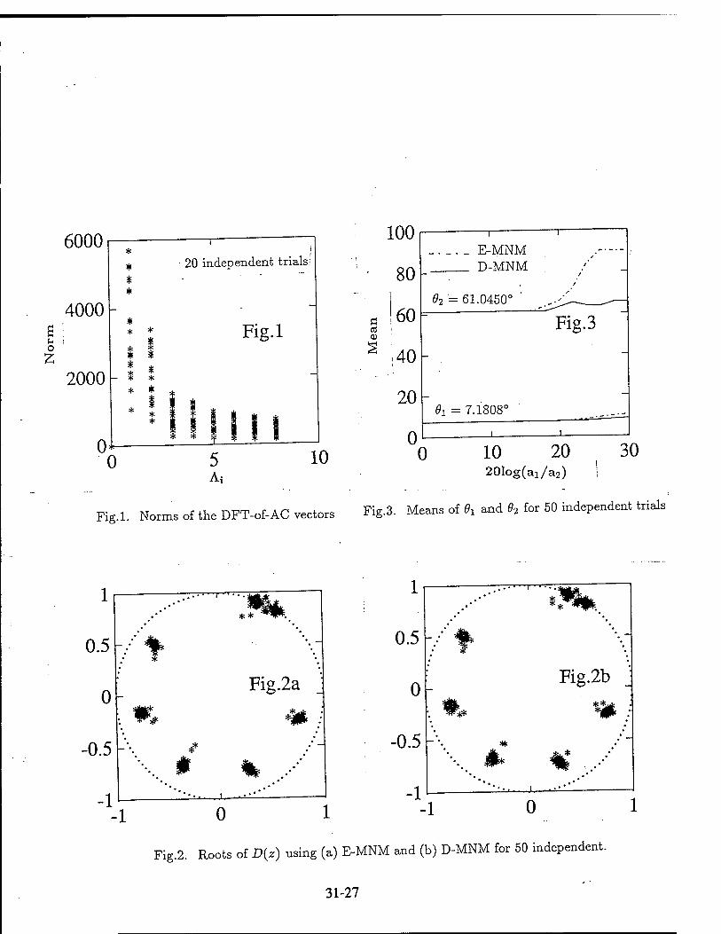
o
6000
4000
2000
Ö
0)
100
80
60
40
20
0
E-MNM D-MNM
02 = 61.0450c
Fig.3
0i = 7.1808°
0 10 20 20log(ai/a2)
30
Fig.l. Norms of the DFT-of-AC vectors Fig.3. Means of 9, and 02 for 50 independent trials
■1 o
Fig.2. Roots of D(z) using (a) E-MNM and (b) D-MNM for 50 independent.
31-27
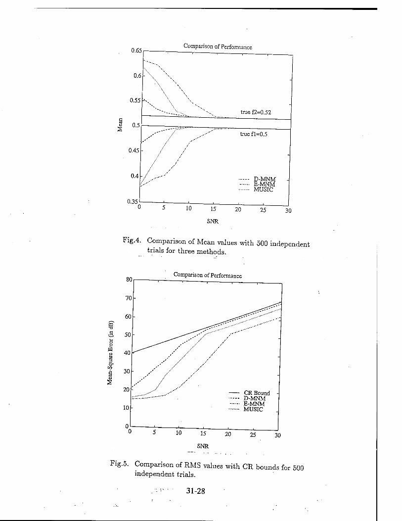
0.65
0.4
0.35
Comparison of Performance
"■-■,
0.6
0.55 L-VN
s u 0.5 a y'
0.45 -
10 15
SNR
true f2=0.52
true f 1=0.5
D-MNM E-MNM MUSIC
20 25 30
Fig.4. Comparison of Mean values with 500 independent trials for three methods.
Comparison of Performance
•a a
o t: «
3 cr CO
Ü o
20-
10-
CR Bound D-MNM E-MNM MUSIC
10 15 20 25 30
SNR
Fig.5. Comparison of RMS values with CR bounds for 500 independent trials.
31-28
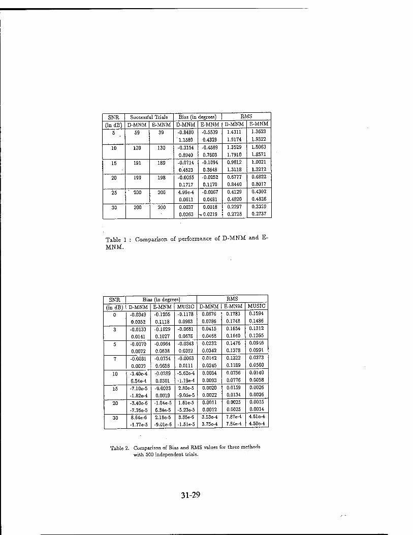
SNR Successful Trials Bia3 (in degrees) RMS
(in dB) D-MNM E-MNM D-MNM E-MNM D-MNM E-MNM
5 59 39 -0.8480
1.1589
-0.5539
0.4329
1.4311 1.9174
1.3623 1.9322
10 139 130 -0.3154 0.8940
-0.4589 0.7603
1.3529
1.7910
1.5063 1.8571
15 191 189 -0.0714 0.4623
-0.1094 0.3648
0.9812 1.3118
1.0021 1.3212
20 199 198 -0.0055 0.1717
-0.0252 0.1170
0.6777 0.8440
0.6822 0.8017
25 ' 200 200 4.99e-4 0.0611
-0.0067 0.0481
0.4129 0.4820
0.4302 0.4826
30 200 200 0.0037 0.0263
0.0018 -.-0.0219
0.2297 0.2728
0.2329 0.2737
Table 1 : Comparison of performance of D-MNM and E-
MNM.
SNR Bias (in degrees) RMS
(in dB) D-MNM E-MNM MUSIC D-MNM E-MNM MUSIC
0 -0.0349 0.0352
-0.1205 0.1118
-0.1178 0.0983
0.0876 0.0786
0.1783 0.1748
0.1594 0.1486
3 -0.0133 0.0141
-0.1029 0.1027
-0.0681 0.0678
0.0415 0.0468
0.1654 0.1640
0.1312 0.1265
5 -0.0070 0.0072
-0.0964 0.0838
-0.0343 0.0392
0.0232 0.0342
0.1476 0.1378
0.0946 0.0991
7 -0.0031 0.0039
-0.0754 0.0658
-0.0063 . 0.0111
0.0142 0.0245
0.1322 0.1189
0.0373 0.0560
10 -3.40e-4 6.54e-4
-.0.0289 0.0301
-5.62e-4 -1.19e-4
0.0054 0.0093
0.0756 0.0776
0.0140 0.0058
15 -7.10e-5 -1.82e-4
-0.0023 0.0019
2.80e-5 -9.05e-5
0.0020 0.0022
0.0159 0.0134
0.0026 0.0026
20 -3.40e-6 -7.76e-5
-1.04e-5 6.34e-5
1.61e-5 -5.23e-5
0.0011 0.0012
0.0025 0.0025
0.0015 0.0014
30 8.64e-6 -1.77e-5
2.18e-5 -9.01e-6
3.35e-6 -1.51e-5
3.53e-4 3.75e-4
7.87e-4 7.84e-4
4.61e-4 4.50e-4
Table 2. Comparison of Bias and RMS values for three methods with 500 independent trials.
31-29
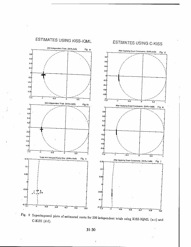
ESTIMATES USING KiSS-IQML
200 Independent Trials (SNR.5dB) Fig.
200 Independent Trials (SNR-iQdB) Fig.1b
0 0.5
Trials Wiih Merged Roots Only (SNR-tOdB) Hg.
-0.05
-0.6 -0.5
ESTIMATES USING C-KiSS
Alter Applying Exact Constraints (SNR-SdB) Fig. d
0.5 ,
Alter Applying Exact Constraints (SNR-iQdB) Fig. e
-0-5 . 0 0.5 ,
^ After Applying Exact Constraints (SNR-lodB) Fig. f
-0.8 -0.7 -0-6 -0.5
«* . s„p^p„3ed plotsofestimatedrootsfm200indepMdm[ triais^KssiQMi ^^
31-30
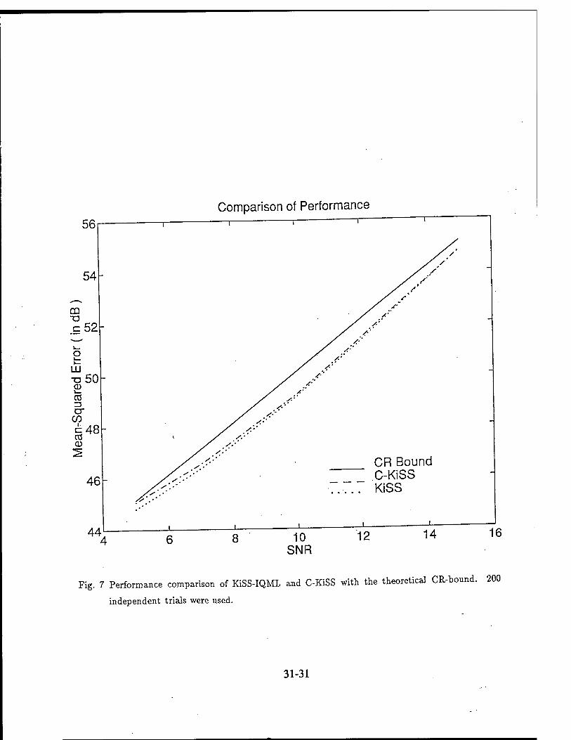
Comparison of Performance
Fig. 7 Performance comparison of KiSS-IQML and C-KiSS with the theoretical CR-bound. 200
independent trials were used.
31-31
REFERENCES
P™„„, Denver, CoIoTX ™1»" **""" " """** *~* ^ *■"
131 ^r;::PuLtin
Lr
K;p:„^7T;,High Resolut,on Me,h°d wi** c—»> *«- <«»»,, PP 33^4 1984 ' " '""""•'"'' C"f"""' 'I "»»«», Speecn W S,W E„.
W LNI9
BrWeI1' "Rad'° ,n'erfe'0me"y °f DiKret« S—" "««^ •/«* vo>. «, pp. 97-105, 151 «irttrit1'.. ir rMax,mr LMh~d p—Est— «---
ASSP-34,„o. .0,pp "OBITo89Z! ST ' " """""■ S""h "d SiS"" >"<"»*>• «*■ [6) ^Ä s:^:: Spectr7 ^mat,o° in a wi°»s—•• «** ^—~ 171 1 P p !.T ^»«»»9, vol. ASSP-38, no. 11, pp. 1842-1852, Nov., !990 1 J J' r- BurS' Mram»m Entropy Spectral Analysis " presented „t th. «M j
««(>»», Oklahoma City, OK, 1967. Presented at the SM Anm.l I.Urmhon.l SEG
181 «Ä "°*"""" ^ *•*»"■•»* "■•»• ^rtatiop, S,„ford Univetsity, StMfotd| CA
P1 Ä ;r1^^°^Wto™"b« S— «" "— •/»• /M* vo,. [10) 'a^ÄÄT ES"ma"°n TeChnique" *' *""" *~ ~ pl] Moli A" ;" ^iir :;r ,rplexi,y °f p~ *"•— f»— ri21 J W Too, d , w ' ' P"«».»,. vol. 40, po. 7, pp. 1811-1813, July, 1992. 11 <£«:::, ^."äAlsorithm *-the -^ c^ia"» -—**■••*-•». [13] S. Haykip e. al, Editors, Army fi«,„, *,«„,•„,, P«„,ice.Hall, ,985
» £' Ma'rch itr ' ReSl Tin" PiSaK"k0 Spert'»m *»'""* " »-«M. ./-. /04SSE-
356, Apr., IS?? ' ' *"C4 "nJ *»"' ft—»"»», Washington, DC, pp. 352.
[19] L.B. Jackson, D,s„.l F,l„„ W Stg„al Pnass,n ^^ ^^ ^
31-32
[20] D. H. Johnson et al, "Improving the Resolution of Bearing in Passive Sonar Arrays by Eigenvalue Analysis," Technical Report EE-8102, Department of Electrical Engineering, Rice University, Houston,
Texas 1980 [21] D. H.'johnson, "The Application of Spectral Methods to Bearing Estimation Problems," Proceedings
of the IEEE, Vol. 70, pp. 1018-1028, Sept., 1982.
[22] M. Kaveh and A. J. Barbell, "The Statistical Performance of the MUSIC and the Minimum-Norm Algorithms in Resolving Plane Waves in Noise," IEEE Transaction on Acoustics, Speech and Signal
Processing, vol. ASSP-34, pp. 331-341, April, 1986.
f23l S M Kay and A. K. Shaw, "Frequency Estimation by Principal Component Autoregressive Spectral Es- timator Without Eigendecomposition," IEEE Transactions on Acoustics, Speech and Signal Processing,
1988. [24] W. C. Knight, R. G. Pridham and S. M. Kay, "Digital Signal Processing of Sonar," Proceedings of the
IEEE, vol. 69, no. 11, Nov. 1981. [251 A C Kot, S. Parthasarathy, D. W. Tufts and R. J. Vaccaro, "Statistical Performance of Single Sinusoid
Frequency Estimation in White Noise Using State-Variable Balancing and Linear Prediction, to be
published in IEEE Transactions on Acoustics, Speech and Signal Processing, 1988.
[26] R. Kumaresan and D. W. Tufts, "A Two-Dimensional Technique for Frequency-Wavenumber Estima-
tion " Proceedings of the IEEE, vol. 69, no. 11, pp. 1515-1517, Nov., 1981.
[27] R. Kumaresan and D. W. Tufts, "Estimating the Parameters of Exponentially Damped Sinusoids and Pole-Zero Modeling in Noise," IEEE Transactions on Acoustics Speech and Signal Processing, vol.ASSP-
30, no. 6, pp. 833-840, Dec, 1982. [28] R. Kumaresan, Estimating the Parameters of Exponentially Damped and Undamped Sinusoidal Signals,
Ph D Dissertation, University of Rhode Island, 1982.
[29] R. Kumaresan and D. W. Tufts, "Estimating the Angles of Arrival of Multiple PUnewa«-/» IEEE
Transactions on Aerospace and Electronic Systems, vol. AES-19, no .1, pp. 134-139, Jan., 1983.
[30] R. Kumaresan and A. K. Shaw, "High Resolution Bearing Estimation Without Eigendecomposition" Proceedings of IEEE International Conference on Acoustics Speech and Signal Processing, Florida, April,
1985. [31] R. Kumaresan, L. L. Scharf and A. K. Shaw, "An Algorithm for Pole-Zero Modeling and pectral
Estimation," IEEE Transactions on Acoustics Speech and Signal Processing, vol.ASSP-34, pp. 637-64U,
June, 1986. [32] R. Kumaresan and A.K. Shaw, "Superresolution by Structured Matrix Approximation", IEEE Trans-
actions on Antennas and Propagation, Vol. AP-36, pp. 34-44, 1988.
r33l S Y Kung K S. Arun and D. V. Bhaskar Rao, "State-Space and Singular-Value Decomposition-
Based Approximation Methods for the Harmonic Retrieval Problem," Journal of the Optical Society of
America, vol. 73, pp. 1799-1811, Dec, 1983.
[34] R. T. Lacoss, "Data Adaptive Spectral Analysis Methods," Geophysics, vol. 36, pp. 661-675, Aug.,
1971. [35] J. Makhoul, "Linear Prediction : A Tutorial Review," Proceedings of the IEEE, vol. 63, pp. 561-580,
April, 1975. [36] M. Marden, Geometry of Polynomials, Math Surveys, No. 3, American Mathematical Society, Provi-
31-33
dence, RI, pp. 206, 1966.
[37] ™L^^2^tTtl0a' N7 Real"Time FreqUenCy EStimat°r for Sub-Micsecond [381 A H Nuttai S T 1 ™ ^ En**"™'> D^on> OH, pp.33-38, Aug., 1989. m u"^J:^z^^T- Prrwith Bad Data points"via Maxi—E
—«* New London, CT, Mar 1976. ^ TR"53°3' ^ ^^ ^™ C^>
[39] N. L. Owsley, "Adaptive Data Orthogonalization," Proceedinos of the TFFF r . r , n * on Acoustics, Speech and Sinnnl P™ ■ <MO ™ceedm^ 0-/ *Ae ^^ International Conference <-•>, o^eec« ara<r ^wa/ Processing 1978, pp 109-112 1978
[41! nAiq:::ispR^ tzzts.zsz? °/sign" pr*-via ^"^ ■—M
- Grove, CA, Oct 1985 Z*l ,1 \ F ''"*" °" S'm"- S'!"m' "d ^puters, Pacific
Pn.c^^pp 83-89 1986 ' """"" ^t'""" " """* *~* «* *">«<
ASSP-35, no. 2 Feb PMlen,'al8' 'EEE T™°<"«°»° »» Aa,»5fe, Speed „«• S^„, ,.„«„,„,,, vol
M t llVZ Er™"'UI" Analy,iqUe "C"" ™*«"»^. **, 1 Cahier 2, Pp. 2«6 1795 [45] S. S. Redd!, »Multiple Source Location- A Digital Approach » rFPF T .■ . EUctron.c S,„em,, vol. AES-15, „„.!, pp. 95-105 1979 *>»»..<*.». e„ X«™,.« „,,
[46' WEE ^r^' " Br;'y°' "Sing'e TOM P"*met« Es""»"°" f'<»» Discete-Time Observations ' ,a„ n f JT °" /,,m°"°" ^ Voh IT-20' ""• 591-598. Sept, 1974 °bSerVat"""'
[49] D. Curtis Schleher, /„,„,<,«*,„ ,„ £,«,„„,■< „,„„„„, Ar[ech ^ ^
[50) ^t::z^;r;r. ££ SäST—-■ —* -«"*
31-34
[55] A.K. Shaw, Structured Matrix Problems in Signal Processing, Ph.D. Dissertation, Univ. of Rhode Island,
RI, 1987. [56] A.K. Shaw and R. Kumaresan, "Some Structured Matrix Approximation P-blemsVPro, of the IEEE
International Conference on Acoustics, Speech and Signal Processing, New York, NY, pp. 2324-2327,
April, 1988. [57] A. K. Shaw and R. Kumaresan, "Estimation of Angles of Arrivals of Broadband Sources," Proceedings
of the IEEE International Conference on Acoustics, Speech and Signal Processing, Dallas, Texas, pp.
2296-2299, April, 1987. [58] A. K. Shaw, "A Novel Cyclic Algorithm for Maximum-Likelihood Frequency Estimation," IEEE Inter-
national Conference on Systems Engineering, Dayton, OH, Aug., 1991.
[59] A. K. Shaw, New Algorithms for Broad-band and Narrow-band Source Localization and A Separable 2-D
IIR Filter Realization, Technical Report, AFOSR-Bolling AFB, Sept., 1991.
[60] A. K. Shaw and S. Nunes, "Detection and Adaptive Frequency Estimation for Digital Microwave Re-
ceivers," Final Report, AFOSR Summer Research Program, Oct., 1992.
[61] A K Shaw, 'Approximate Maximum Likelihood Estimation of Multiple Frequencies with Constraints
to Guarantee Unit Circle Roots," IEEE Transactions on Signal Processing, to be published, 1994.
[62] A K. Shaw and W. Xia, "High-Resolution Angles of Arrival Estimation using Minimum-Norm Method Without Eigendecomposition," IEEE International Conference on Acoustics, Speech and Signal Pro-
cessing, Adelaide, Australia, April, 1994. [63] A. K. Shaw and W. Xia, "Minimum-Norm Method Without Eigendecomposition," IEEE Signal Pro-
cessing Letters, in press, 1994.
[64] C. W. Therrien, Discrete Random Signals and Statistical Signal Processing, Prentice-Hall, NJ, 1992.
[65] J. B. Y. Tsui, Digital Microwave Receivers : Theory and Applications, Artech House, MA, 1989.
[66] J. B. Y. Tsui, Microwave receivers with Related Components, National Technical Information Center,
1982, Peninsula, Los Altos, CA, 1985. [67] J. B. Y. Tsui, Microwave Receivers with Electronic Warfare Applications, John Wiley and Sons., New
York, 1986. [68] J. B. Y. Tsui and D. Sharpin, Unpublished Report on Time-Domain Detection for Digital Receivers,
June, 1992. [69] D W. Tufts and R. Kumaresan, "Frequency Estimation of Multiple Sinusoids: Making Linear Pred1Ction
Perform Like Maximum Likelihood," Proceedings of the IEEE, vol. 70, pp. 975-989. Sept., 1982.
[701 D W Tufts and C. D. Melissinos, "Simple, Effective Computation of Principal Eigenvectors and their Eigenvalues and Application to High-Resolution Estimation of Frequencies," IEEE Transactions on
Acoustics, Speech and Signal Processing, vol. ASSP-34, no. 10, pp. 1046-1053, Oct., 1986.
[71] D W. Tufts and S. Parthasarathy, "Statistical Analysis of the Effects of Matrix Perturbation in Some Least Squares Problems," 2nd SIAM Conference on Applied Linear Algebra, Raleigh, NC, 1985.
[72] T. J. Ulrych and T. N. Bishop, "Maximum Entropy Spectral Analysis and Autoregressive Decomposi-
tion," Rev. Geophysics and Space Physics, vol. 13, pp. 183-200, Feb., 1975.
[73] T.J. Ulrych and R. W.Clayton, "Time Series Modeling and Maximum Entropy," Phys. Earth Planetary
Int., vol. 12, 1976.
31-35
1741 ?/ Ä£ ÄST"mentations of Pi" H™K Re"-»' M"M" —- [75J H_ Wang and M. Kav.h "EsfmaLon of Angles „f Ar„»al f„, Wd.band So«,«,," in ?„miin,s «/ ,4«
120M209, of!^6 " '"' St"C" "d %"" ""■"**■ TOl- ASS™. »»■ 5, PP.
[77) ™ si™.°, P" K' M' T** "BiSS A°alyS,S °f the MUS,C L~ati»» E"i"»'»" ™ Ih,«.c«». o» Ssjnaf Processing, vol. 40, no. 10, Oct., 1992 J ransüenon»
[78] !elt" r WaX'/Ma™ ^^ Realization of Multiple Wees by Alternating Pro-
iS^UZ^T on S! Speech and Smal p—voL ASSP-36< - 'o. pp- [79] M. D. Zoltowski, G. M. Kautz and S. D. Silverstein, «Beamspaee Root-MUSIC - TFFF T
on Signal Processing, vol. 41, no. 1, Jan., 1993. ' Transactions
31-36
CONTACT LAW AND NUMERICAL MODELING FOR LOW-VELOCITY
IMPACT OF COMPOSITE MATERIALS
Rob Slater Graduate Research Assistant _
Department of Mechanical, Industrial, and Nuclear Engineerxng
University of Cincinnati Cincinnati, OH 45221-0072
Final Report for: Summer Research Extension Program
Wright Laboratory
Sponsored by: Air Force Office Of Scientific Research Boiling Air Force Base, Washington, D.C.
and University of Cincinnati
Cincinnati Ohio
December 1993
32- 1
CONTACT LAW AND NUMERICAL MODELING FOR LOW-VELOCITY
IMPACT OF COMPOSITE MATERIALS
Rob Slater Department of Mechanical, Industrial, and Nuclear Engineering
University of Cincinnati 9 lng
ABSTRACT
design o^J^Jt^S^SE!*" ! critical consideration in the materials offer high stiSSew anri Jl it* structu^s. Composite savings over metals. Low-veioci?v Imn^fn at a s^nificant weight insidious problem becauslit is SS*° ^f"?8 iS a Particularly inspection. These impart! occur luring 1^ t0 detect b^ visual and maintenance operations and «?£ ^ °°Urse of normal fli9ht dent on the impact Surface But thtt- t 0nl.y a Sma11' fallow and backface damage to tSe'laminat. T™* 5
S s^nificant interior
materials for impact tolerance u' In °rder to desi^n composite to model composite st^ctur^and^Jf J^VJ"* t0 develoP methods describes the relationshipblt-w*Jf1»"1**« the loads. A contact law object into the tarjet Pand ?h! ^ lndentation of an impacting Hertzian theory is Sonlv uSe^transmitted force. A modified data and only predTctsthetat? T**1 re<^ires experimental indentation. For more accuraT- HJ;1- i°.rce as a function of cause impact damage a contact w^'f 10Vf the Besses which of force in the contact area f« Z Predicts the distribution such as finite elements ar6
X* necessarv- N™erical techniques analyses of low-veTocitv iiJ£f 1Clent methods for performing computer technology continues to%n?* c??P.osit* structures. AI and evaluate new tedinS« V evolve, it is necessary to develop integration sShemeJ areTow h/, solvin<? these problems. Explicit recognized for their suoerLrfS™*"9 /lde-y available. They are explosions, very Lrge aeflectio^ LW" Problems involving also handle contact »robi^n^and. hl9n-sPeed collisions. They investigation of tneir useful« «gently and accurately, so is essential. usefulness on low-velocity impact problems
32-2

CONTACT LAW AND NUMERICAL MODELING FOR LOW-VELOCITY
MODELING OF COMPOSITE MATERIALS
ROB SLATER
INTRODUCTION
Composite materials are frequently considered in the design of
aircraft structures. They offer high stiffness and strength at a
significant weight savings over metals. There are distinct
differences in the design criteria for metal and composite
structures. Fracture and fatigue are the key concerns in the
service life of metal structures. Design of composites is driven by
concerns such as delaminations at the discontinuities, voids,
wrinkles, and low-velocity impact by foreign objects. Laminated
composites are particularly susceptible to low-velocity impact
damage. These impacts occur during normal operations due to hail or
stones blown around a runway by jet engines or during maintenance
operations due to tool drop of footsteps. The damage mechanisms
associated with low-velocity impacts include matrix cracking, ply
delamination, and fiber breakage. Delamination is particularly
troublesome because serious internal and back-face damage may be
present even though the damage on the impact face appears to be
quite minor. It is often not detected during routine visual
inspection because the visible damage is slight. Significant
reductions in strength and stiffness may result. The design
criteria for composites generally require tolerance of a certain
level of impact, defined either as an impact energy or a maximum
32-3

surface indentation, which must be tolerated without significant
degradation of service life. The simplest measure of impact is the
kinetic energy of the impactor; i.e. an object of Known „ass
impacting at a known velocity. Establishing rational design
criteria for low-velocity impacts is the subject of numerous
investigations. Characterization of initial damage and its
propensity to propagate under service loading are important
considerations in the development of the design criteria. In
addition, impact may occur at any point of a structure, so a panel
must be designed to resist impact at any location. There are
numerous local stress raisers in actua! aircraft panels such as
cutouts, ply dr0ps, and stiffeners which must be considered in
designing for impact damage tolerance. It is prohibitively
expensive to perfcrm laboratory tests on every composite panel
configuration in an aircraft and difficult to correlate results
from coupon tests to built-up structures. A more prudent course is
to develop analytical criteria and validate them with experiments.
In order to design for impact tolerance, it is necessary to
develop methods to model composite structures and simulate the
loads. Numerous researchers have attempted to determine a
methodology for predicting damage in a composite laminate subject
to impact U-5]. There are a number of variables which must be
considered in the analysis of such events. Sensitivity to changes
in materials, stacking sequence and panel thickness are
significant. Boundary conditions in numerical models and
experimental setups are difficult to match except by trial and
32-4

error. Various failure theories have been offered to predict the
size, shape, and location of damage for a given state of stress,
but there is little consensus about what mechanisms are at work. In
short, no general method exists to predict damage in an arbitrary
composite laminate due to an arbitrary impact.
The objective of this research is to develop a simple
analytical method for determining the relationship between
distribution of contact pressure and indentation of a composite
laminate struck by a spherical impactor. Along with such a contact
law, methods of modeling the behavior of composite laminates under
impact loading, using finite elements and other numerical analysis
tools are to be investigated.
32-5
SUMMARY OF RESFAPrw
The research conducted this summer was under the supervision
of Dr. Ronald Huston, Professor of Mechanics at the University of
Cincinnati. Dr. V.B. Venkayya, WL/FIBR, was the focal point for the
research at Wright-Patterson Air Force Base. Dr. Greg Schoeppner,
WL/FIBC, was also a major contributor of technical advice and
direction. The work explored several issues concerning low-velocity
impact of composites. First, a comprehensive review of existing
literature was performed, focusing on the following topics:
1) Analytic Models
2) Numerical Models
3) Contact Law
4) Damage Prediction
5) Residual Strength
Analytic models concern mainly plate theories which are
suitable for modeling laminated composites, it is generally
accepted that transverse shear stresses are a key concern for
impact problems. The simpler plate theories do not accurately
predict these stresses and thus have limited usefulness in solving
impact problems, it is normally necessary to use more complex
theories. Noor and Burton published a survey article »Assessment of
Shear Deformation Theories for Multilayered Composite Plates« [6]
which lists and compares numerous methods. Several of the plate
theories were reviewed more closely in order to determine which are
most appropriate for solution of low-velocity impact problems.
32-6
A suitable model for the laminate must be determined. The
complexity of this model depends strongly on the type of
information desired. If the gross response of the panel is all that
is required, a smeared plate theory may be sufficient. But if
damage is to be predicted, a discrete laminate theory is necessary
to evaluate the stresses layer-by-layer through the thickness. The
commonly used first-order shear deformation plate theories lead to
discontinuities in the stresses at the interfaces, so a more
computationally intense formulation is required.
Finite element methods were the focus of research on numerical
methods. Some simple analyses were performed using NASTRAN at
Wright-Patterson AFB in 1992. These demonstrated the general
feasibility of performing impact analyses using general-purpose
finite element programs but revealed that modeling techniques would
require further development to provide highly accurate simulations.
The ANSYS finite element package has better non-linear capabilities
than NASTRAN and includes some elements specifically designed for
contact problems, including non-linear springs, gap elements, and
contact surfaces.
Finite element methods have frequently been used to evaluate
the stress field in an impacted laminate and correlate levels of
stress components to experimentally observed damage [7-9]. The
stress gradients are very high in the region where the impactor
strikes the target and the immediate vicinity, so in order to find
the stresses accurately, a refined element mesh is required. The
contact force should be distributed over the numerous nodes of this
32-7
region. As „ith all analyses involving contactj ^^ ^ ^
predicting the size of the oontaot area beoause .fc ^.^ ^
linearly with transmitted force.
The two codes previously mentioned use implicit schemes to
integrate the equations of motion for dynamic analyses. These
methods, such as the Newmar* method, are unconditionally stable so
the user may select the time step according to the desired accuracy
of the solution. Stiffness and mass matrices must be assembled and
a system of simultaneous equations are solved for each time step.
For models with a moderate number of deqrees of freedom or
solutions in which a very small time step is not required, these
methods work „ell. But for large, complex models and high-speed
dynamics problems, the solutions become expensive due to issues of
temporary storage for the large matrices and the CPU time needed to
perform the matrix operations.
For such problems, explicit integration schemes present an
alternative. These methods, including the Central Difference
Method, are very efficient for analyses involving high-speed
dynamics, contact and separation of bodies or surfaces, and large
deformations of impacting bodies. Explicit methods have a minimum
time step associated „ith them to insure stability, it is often one
or two orders of magnitude smeller than might be chosen for an
implicit scheme, but explicit methods do not require assembly and
inversion for each time step. Lumped mass matrices are also
employed. The equations corresponding to each degree of freedom are
uncoupled, so only vector operations ere necessary.
32-8
Explicit finite element codes for commercial use have only
recently become available, for example in the forms of MSC/DYTRAN
and ABAQUS/Explicit, and no research is known which compares the
efficiency of these schemes to the more established implicit codes
for solution of low-velocity impact problems. It is established
that explicit schemes are preferable for high-speed collisions such
as bird strikes on airplanes or ballistic impacts, and implicit
methods are more efficient for low-speed and quasi-static events.
Low-velocity impacts on laminated composites fall into a gray area
between these two extremes. The low impact velocities suggest the
use of implicit methods. However, it is necessary to use a refined
element mesh in the contact area for impact problems, because the
magnitude of the stress gradients with respect to the spatial
coordinates is large. A large number of degrees of freedom, and the
fact that the explicit packages often include more sophisticated
modeling options specifically designed for impact problems, suggest
that explicit codes may be preferable.
Contact law refers to the relationship between the indentation
of the impacting body into the target and the transmitted force.
The distribution of the contact force on the surface of the target
is difficult to calculate. It is theoretically infinite for the
initial point impact, but then spreads out over a growing finite
area. Strain rate effects and plastic or brittle behavior of both
the impactor and the target materials are important, as there have
been instances observed in which multiple contacts occur during a
single impact event [10]. The force-indentation relationship
32-9
changes during unloading and reloading.
Analysis of contact between two bodies dates back to the work
of Hertz in the late 19th century [ii]. Today many of these same
solutions form the basis of contact laws for composites. The basic
form of the results are:
F=kan
F = contact force
k = contact stiffness
a = indentation
n = constant
Unfortunately, composite materials have characteristics which
often invalidate the assumptions necessary to solve the equations
analytically. A composite lamina is highly orthotropic, and
exhibits strain-rate-dependent effects. For most impacts the
stresses will be large enough to cause the target material to fail
locally like a brittle material so this behavior must be included
in the model. Friction between the impactor and target on the
surface adds tangential forces.
For these reasons experimental force-indentation data do not
agree well with the classic Hertzian law. Researchers have thus
turned to experimentally determined contact laws for purposes of
modeling, A relationship developed by Tan and Sun [12] has become
widely accepted as accurate and is frequently cited in publications
by other authors, it is assumed that during the initial loading of
32-10
an undamaged laminate force versus indentation obeys the Hertzian
relationship with a nonlinear (3/2) power. The stiffness of the
laminate is unique to each material and stacking sequence and is
determined by fitting a curve to experimental data. Upon unloading,
the relationship is different. The force is a function of the
maximum force during the loading phase, indentation depth and the
critical indentation. Critical indentation defines the depth at
which permanent deformation begins and must be determined by
experiment for each material and stacking sequence.
For certain ratios of impactor mass/velocity and target
stiffness, multiple contacts occur. The impactor transfers the
majority of its momentum to the laminate, which then breaks contact
with the now relatively slow-moving impactor. As the target
rebounds from its maximum displacement (it essentially vibrates
freely), it re-contacts the impactor before the impactor bounces
clear of the target. The contact law has yet a third relationship
for this reloading phase. It was found that the 3/2 power
relationship no longer holds. Again the exponent must be found
experimentally, and often 2 or 5/2 fits the data better. Results
from tests such as these are frequently used by other investigators
as the contact law of choice in their models. The obvious
disadvantage of this method is that the tests require expensive
equipment, expertise, and large amounts of time to perform. For
every combination of impactor and target material (including
stacking sequence) and geometry, a separate test is required,
investigators who do not have the facilities available to perform
32-11
their own tests are limited to scarce pubiished data.
Somprakit and Huston have developed a numerical method for
determining displacements, stresses, and distribution of contact
force between contacting cylinders [13]. it is an iterative
numerical procedure based upon fundamental solutions from the
theory of elasticity, m this technigue the cylinders are of
infinite length; it is a 2-D analysis. The contact surface is
discretized in the x (transverse, direction, and the stresses are
found in the x and z (depth) directions. The problem of a spherical
impactor en a flat plate can be solved in an analogous manner. The
contact area, rather than being defined by its width, is defined by
its radius. For now, oblique impacts are net considered. In the
Somprakit and Huston's analysis, the infinite length of the
cylinders allows the problem to be simplified to one of two
dimensions, in the impact problem, axisy^netry is assumed to
simplify the equations.
Knowledge of the relationship between the indentation of the
impacting body in the target and the magnitude and distribution of
the contact force is essential for accurate modeling and
determination of the stresses which cause damage. A contact law
which predicts total force without the details of its distribution
may be sufficient to model the gross deformations of the target
under impact loading, but will not allow a model to be as accurate
in predicting the stresses which cause the matrix cracking and
delaminations representative of low-velocity impact.
Damage prediction is an area which many researchers have made
32-12
considerable efforts. For a given state of stress in a laminate, a
model must be capable of predicting the onset and propagation of
damage. Matrix cracking, ply delamination, and fiber breakage are
the normal sequence in which damage takes place during a low-
velocity impact event. Properties of the laminate will change as
damage occurs, so the model must be continually updated (in a
temporal sense) as the analysis proceeds. Knowledge of the
material's behavior beyond the elastic range and its fracture
characteristics are needed. The damage modeling must deal with
failed material (cracked matrix and broken fibers) by either
removing it or treating it with revised properties, and also with
changing laminate properties.
A recent paper by Choi and Chang of Stanford [3] proposes two
mechanisms by which delaminations occurs. Both are the result of
matrix cracking. In the inner layers a »shear matrix crack-
generates delamination which propagate unstably. A small stable
delamination occurs at the interface above the cracked layer, and
the larger unstable delamination occurs at the interface below. The
delamination is governed by the interlaminar shear stress in the
fiber direction of the layer below <*„) and the interlaminar shear
stress in the direction normal to the fibers (ayz) in the layer
above the delaminated interface. The critical matrix crack is in
this upper layer.
in the layers toward the bottom »bending matrix cracks» occur
and stable delamination at the interface is seen. Again the
delamination is governed by the transverse shear stress in the
32-13
fiber direction („„, i„ the layer below the interface but it in the
upper layer it is the transverse in-plane stress normal to the
fibers (c„) which contributes.
For either type of delamination, matrix cracking is the event
which triggers delamination. So, failure criteria incorporating the
stresses named above are presented to predict matrix cracking and
subsequently the positions and si.es of the delaminations.
Experimental data is presented to verify the model.
An interesting analytical theory has been developed by Liu [4]
which predicts the oft-seen lemniscular or "peanut" shaped
delaminations associated with low velocity impact. This is based on
the quantity known as the mismatch angle, which is the difference
in fiber orientation between adjacent lamina in a laid-up composite
structure. A mismatch coefficient is derived from the difference in
bending stiffnesses of the upper and lower lamina at an interface
which predicts the relative area and orientation of the
delamination. For an interface „here the adjoining layers are
oriented in the same direction, no delamination is predicted, which
is consistent with experimental evidence that delamination only
exists where the fibers change orientation. The effects of material
properties, laminate thickness, and impact energy are discussed.
A great amount of test data has been gathered and published by
researchers but there is yet to be an accepted measure of impact
performance that is independent of the test method details fS). The
variations in impactor mass amd size, impaotor velocity, test
specimen size and boundary, et cetera are so wide that no
32-14

coordinating theory has been derived to predict the behavior for
any given set of impact parameters.
The purpose of damage prediction is to be able to design
composite structures which are tolerant to foreseeable impact
events. Low velocity impacts an aircraft might experience include
tool drop, hail, footsteps, and runway debris. If damage can be
predicted, then the properties of the composite structure post-
impact can be characterized also in order to estimate the residual
strength and stiffness. Laminates may suffer a significant
degradation of their properties due to low velocity impact, and to
design structures that can survive such impacts, one must be able
to predict the damage which is likely to occur.
The determination of residual properties has been undertaken
by many investigators. The strength of damaged laminates,
particularly in compression, is an important field of study. Since
low velocity impact damage can extend such a relatively long
distance from the impact site, strength can be reduced much more
than for the case of a penetrating impact. Similarly stiffness can
be change significantly due to back-ply damage.
Frequently there is a loss of symmetry in a laminate due to
impact damage. This introduces bending-stretching coupling. The
vast majority of composite laminates are laid up symmetrically
about the mid-plane in order to eliminate coupling of the bending
and extensional strains. This greatly simplifies the analysis of
such laminates. But when damage occurs the symmetry is lost and the
behavior of the laminate may change drastically.
32-15

The effects of impact damage on tensile strength has been
investigated by El-Zein and Reif snider [14]. They hypothesized that
residual strength is controlled by stress concentration effects in
the immediate vicinity of the damaged region. A complex variable
solution based on Lekhnitskii's problem of an anisotropic plate
with an elliptical inclusion is derived, and the results agree
fairly well with experiment.
The change in compression strength after impact is a more
widely reported phenomenon. Dost, Ilcewicz, and Gosse presented a
sublaminate stability based approach to predict damage tolerance
(i.e. post-impact strength) [15]. This approach does require an
accurate description of the state of the damage inside the plate.
Further it was noted that there were significant differences in
residual strength between experimental coupons and actual composite
structures due to finite width effects in the test specimens..
Buckling of delaminated composites is a third failure mode.
Global buckling is the same mode as occurs in undamaged panels, but
may occur at markedly smaller load levels when damage is present
due to loss of stiffness and the previously mentioned bending-
stretching coupling. The phenomenon of local or delamination
buckling is strictly related to delaminations near the free surface
of the laminate. Under load the delaminated region may buckle while
the rest of the laminate remains stable, chai and Babcock [16]
modeled an anisotropic layer separated from a thick Isotropie base
laminate. The delamination is elliptic in shape and the material
axes coincide with the ellipse's axes. The buckling for the damaged
32-16
region by the Rayleigh-Ritz method and propagation of the
delamination area is predicted via a fracture mechanics approach.
Results show stable, unstable, or unstable growth with crack arrest
depending on material properties and orientation, loading, and
fracture energy.
Davidson [17] considered failure of a damaged laminate by all
three failure modes: compression, global buckling, and delamination
buckling. Buckling loads are calculated by applying the Trefftz
criterion to governing equations found from the Rayleigh-Ritz
method and compression failure by a modified maximum strain
criterion. If the initial failure is delamination buckling, that
layer is removed (it carries no load), the laminate properties are
recalculated, and the loading sequence is continued until
catastrophic failure (compressive or global buckling) is reached.
Davidson compared five analyses (two performed by himself and
three reported by other researchers including Chai and Babcock) to
experimental results. He found only one gave conservative
predictions of buckling loads. The remaining four over-estimated
the failure loads. The model which gave conservative results
employed the reduced bending stiffness approximation. The [D]
matrix is replaced by a matrix [D*] defined as [D'] = [D]-[B] [A]'1^]
for cases where the coupling matrix [B] is non-zero. The analysis
is then performed as though the laminate was symmetric.
It was discovered that under certain conditions delamination
buckling can occur under tensile loading. The fibers in a lamina
normally have a small Poisson's ratio, approximately one order of
32-17
magnitude smaller than the matrix material or a quasi-isotropic
laminate, when the fibers in a delaminated layer are oriented
normal to a tensile load, both the delamination and the base
undergo lateral contraction. Due to the mismatching of the
Poisson's ratios, the delaminated region experiences compression
and the base tension. Thus buckling may occur under loading cases
when it is not expected.
Of these five areas that were reviewed, those concerning the
dynamic response of laminated plates and residual strength of
damaged composites seem to be the furthest developed. Plate theory
was a topic of great interest even before the development of
composites. The extension of research on these materials has
paralleled their increasing use in engineered structures. Residual
strength models have not received the same volume of attention, but
researchers have been able to demonstrate the capability to predict
post-impact characteristics for composite laminates with known,
although admittedly simplistic, damage states. Damage prediction
has recently been the focus of several researchers, unfortunately
the state of the art is not as advanced as for the first two
topics, several different theories have been proposed to predict
the onset of damage at a specified level of stress in a laminate.
The focus of this effort has been in the two remaining categories,
contact law and numerical modeling of impact events.
Contact law appears to be an area which has not received as
32-18

much attention from researchers as the other aspects of impact
analysis, but there are still questions which remain. New numerical
techniques, particularly from the finite element community, need to
be investigated to determine their applicability to impact
analysis. A new method for analytically developing a contact law
has been the major thrust of the work. The advantage this new
technique will bring is that it will predict the distribution of
contact pressure between an impactor and a target, not just the
total force. Current relationships only calculate the total force
versus indentation. When incorporated into models in which the
contact region is discretized into numerous sub-regions, such
methods cannot be used without subsequent assumptions concerning
the allocation of the force.
The advancement of numerical analysis techniques which will
take full advantage of such a contact law naturally follows. As
computing speeds and capabilities grow in a general sense,
development of specific methods for solving impact problems
deserves attention.
The contact law under development is based upon the theory of
elasticity. For cases involving torsionless axisymmetry, solutions
can be found for a host of loading and boundary conditions [18]. By
a series of derivations the problem of a constant distributed load
over a finite radius acting on an Isotropie half space can be
solved. This pressure-displacement relationship is the basis for
the contact law. The solutions show that stresses diminish rapidly
at distances a few contact radii from the original contact point,
32-19
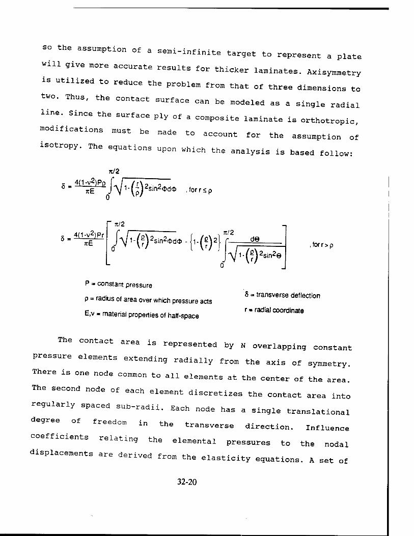
« the assumption of a semi-infinite target to represent a plate
will give „ore aoourate results for thicker laminates. Axisymmetry
« utilized to reduce the problem from that of three dimensions to
two. Thus, the contact surface can be modeled as a single radia!
line. Since the surface ply of a composite laminate is orthotropic
modifications must be made tc account for the assumption of
isotropy. The equations upon which the analysis is based follow:
A/2
S'^/VKP) 2cin2 sirred«!) , for r < p
g = 4(1-y2)Pr TIE
re/2
/\R5 2sin2<&d<& - jl-/ß\2 (?): 7T/2
de
V'-(?)2s» sin2e
P ■ constant pressure
p = radius of area over which pressure acts
E,v - material properties of half-space
,forr>p
5 = transverse deflection
r - radial coordinate
The contact area is represented by N overlapping constant
pressure elements extending radially from the axis of sy^etry.
There is one node common to all elements at the center of the area.
The second node of each element discretizes the contact area into
regularly spaced sub-radii. Each node has a single translational
degree of freedom in the transverse direction. Influence
coefficients renting the elemental pressures to the nodal
displacements are derived from the elasticity equations. A set of
32-20

initial displacements is determined based on the user-specified
parameters of the problem.
At the end of each iteration, the validity of the solution xs
checked based on three criteria:
1) Equilibrium
The sum of the elemental pressures multiplied by their
corresponding areas must equal the applied force.
2) Edge Pressure
The pressure in the outermost element must approach zero
at the edge of the contact zone. Since the contact area
is divided into discrete areas, the pressure in this
element cannot equal zero, or else there would be no
contact.
32-21
3) Contact/Separation
There must be continuous contact between the target and
impactor in the assumed contact region and separation
outside the contact region. For the geometry chosen, a
spherical impactor on a flat target, contact cannot be
broken at a given radius and re-established at a greater
radius.
When these three conditions are satisfied a solution has been
found and iteration stops, it was found that satisfying all three
conditions simultaneously is difficult due to the non-linearity of
the problem. Specifically, the size of the contact area varies
rapidly with changing load.
The original solution method relied on a heuristic approach to
solving the equations. But the rate of convergence depended very
strongly on the initial estimate of the displacements. In an effort
to find more accurate solutions, optimization methods were
investigated.
Optimization refers to any of a number of algorithms which
seek to minimize a mathematical function, called the objective
function, in addition, extra requirements to be satisfied, known as
constraints, may be placed on the solution. The parameters from
which the objective function and constraints are constructed are
the design variables. Although mathematical in theory, optimization
techniques have been of great interest to engineers as a means of
solving difficult systems of non-linear equations which frequently
32-22
arise, or for finding the "best" solution to a problem of many
variables which has no exact solution. If the important physical
phenomena in an engineering system can be accurately described by
an objective function and constraints, a numerical method can often
be found which will provide satisfactory solutions when analytical
methods do not.
For the contact problem, several equations have been derived
relating surface pressure and displacement. It is desirable to use
these equations as the basis for the objective function and
constraints, since they are known to govern the physical system.
For a similar contact problem, optimization techniques were applied
to the Rayleigh-Ritz method [19]. Rayleigh-Ritz is an energy method
which requires a mathematical function to describe the internal
strain energy of the elastic body. It was noted that it is
difficult to find a function which satisfies the kinematic boundary
conditions for a contact problem and gives reasonable solution
accuracy.
The first approach is to make the objective function by
rearranging the equilibrium equation. The optimization routine
would seek to minimize the absolute value of the difference between
the sum of the pressures multiplied by their respective areas and
the applied force. The conditions of the edge pressure approaching
zero and the contact/separation condition would be imposed as
constraints. A second approach would be to use the edge pressure
criterion as an objective function, and the other two as
constraints.
32-23
The computer modeling research focused on using a finite
element employing an explicit time integration scheme for solution
of the equations of motion. Specifically, the DYNA3D code developed
at Lawrence Livermore National Laboratories „as used. The Ohio
supercomputer Center made available its Cray Y-MP 8/264 computer
for this phase of the research. Dr. David Lemmon of the University
of Cincinnati „as instrumental in this effort, both in obtaining
the grant of the resources and his technical expertise.
DYNA3D has considerable capabilities for solving engineering
problems, but it lacks a pre-processor for building finite element
models. The I-DEAS package developed by Structural Dynamics
Research Corporation „as used for pre-processing. Dr. Lemmon
provided a translator „hich converts data stored in an I-DEAS
universal file to a DYNA3D input deck.The case that „as chosen to
be modeled „as a spherical impactor dropped on a composite plate.
This event has been analyzed by many researchers and can be most
easily recreated in a laboratory experiment. Although the geometry
of the model is uncomplicated, it incorporates several features
„hich are necessary in order for DYNA3D to be able to solve the
problem, such as compatibility of element size on the contact
surfaces of the impactor and target, without this precaution, a
valid input deck „in be „ittm but fatal errors wm ^
encountered during the solution, „asting computer time and
necessitating correction of the model, it is also necessary to
specify entities in the I-DEAS model „hich „ill be used to define
sliding interfaces, initial velocities, and material models in
32-24

DYNA3D. The translator writes the vast majority of the input cards
for the analysis. It transfers all the geometry, nodes, and
elements directly and allows the user to easily create the sliding
interfaces, initial conditions, and material models if the
appropriate groups of nodes and elements are contained in the
universal file.
The DYNA3D input deck must be edited to alter the job control
cards at the beginning of the deck and to edit the material cards
to include the composite. The translator does not handle composite
materials. Individual ply properties and stacking sequence must be
input, and a user-defined integration rule defining the number of
through-the-thickness integration points must be specified. Damage
is included in the material model. For solid elements, one of a
number of widely-recognized composite failure theories can be
chosen. For shell elements, which were used for this analysis,
individual failure theories detecting matrix cracking, matrix
crushing, ply delamination, and fiber breakage are checked at each
time step. If failure by any mode is predicted, the material
properties associated with that failure in the particular elements
are reduced to zero over the next one hundred time steps in order
to reduce numerical difficulties stemming from the sudden release
of strain energy. At this stage of the research however, damage was
not to be considered so the strengths of the material were made
artificially high to prevent failure.
The work using DYNA3D was undertaken only recently and is
ongoing. At present, there has been success in the modeling phase
32-25
and in performing analyses for isotropio materials, suoh as a steel
impactor striking a steel plate. The companion post-prooessor to
DYHA3D, oalied TAURUS, can be used to display results, and it is
also possible to import the results into a more sophisticated post-
processing program such as I-DEAS. But „hen a composite plate is
analyzed, the solution encounters numerical difficulties during the
analysis and aborts, it is believed that this is due to problems
with the sliding interfaces.
Sliding interfaces are specified in DYNA3d to define contact
surfaces on bodies which cannot penetrate one another. There are
several assorted types of interfaces available which use different
mathematical formulations to enforce the contact conditions. In
general groups of nodes and/or elements are chosen to define master
and slave surfaces which describe the contact surfaces.
Two type of interfaces are considered for this problem, both
penalty formulations. The »sliding with separation and friction-
option is most general, it includes friction and allows the two
specified surfaces (shell elements of the target plate, surface
faces of the solid elements of the impactor, to contact and
separate arbitrarily, it does not matter which of the two surfaces
is selected as the master and slave. For the »discrete nodes
impacting surface» option, the slave group is „ot a surface, but
rather a set of nodes [20].
Each of the available types of sliding interfaces has its own
idiosyncrasies. some are more robust than others so some
experimentation is necessary to determine which are compatible with
32-26

the composite materials.
32-27
CONCLUSTDMg
During the summer Research Extension Program a thorough review
of existing research in several areas oonoerning low-velocity
impact of composite materials was performed. Based on this review
the focus of the new research „as chosen to be the topics of
contact law and numerical modeling. A new technique for determining
the contact force-indentation relationship for low-velocity impact
of composite materials has been under development. This contact law
is critical for modeling of impact events. Present methods require
experimental results to determine several parameters. Different
combinations o, impactor and target materials require separate
tests. Due to the non-linearity of the contact phenomenon, it is
very difficult to extrapolate results or predict behavior when no
experimental results are available.
The new method also gives information about the distribution
of the contact pressure underneath the impactor. This is
particularly useful for performing finite element analyses where
the contact forces must be applied at several discrete points. The
stress gradients are extremely high in the contact zone, so in
order to accurately model impact and be able to track the stresses
which initiate damage, this type of precision is necessary. The
oontact laws which are currently used do not provide such
information. A computer program is under development which seeks to
reduce the amount of experimental data necessary for modeling of
«pact events. The method is based upon equations derived from the
32-28
theory of elasticity. An experimental plan for validating the
theoretical aspects of this method will be proposed.
Numerical methods were investigated to study impact and
contact problems. These include modeling for commercially available
codes such as ANSYS, which solves transient dynamics problems with
a conventional implicit solution scheme, and DYNA3D, which uses an
explicit scheme to solve the system of equations. The explicit
solution method is advantageous for problems involving high-
velocities and/or large deformation. For a low-velocity impact
problem, it is not clear which method will have the advantage in
computation cost.
32-29
REFERENTS
11.
12.
Structures, 23 (1993) 177-190 model, composite
Plates unRoeratra„SsPverns9eers'tatic- iJE""'?*"0?" in «*»!»•". composite Structures La«!) ili!2 Ö4 Perimental results-
U99^ Il34-2169 PaCt- J°Urnal °f c™P°"te Materials 26
Stress ^«1ÄC^J^iSinaJi,? " *■ Vi6W °f Bendi"9 (1988) 674-692 9' Journal of Composite Materials, 22
Robinson, p. and navip«; ran T ^ Geometry Effects Tn'r u/' .Impactor Mass and Specimen Composites InternatL^"Vel0<;lty Impact of Laminated (1992? iSS:2o? Ml Journal of ImPact Engineering, 12
Sods'For iSÄi8^ assessment of Computational 43 (1990) 67-97 Layered shells• Applied Mechanics Reviews,
Finite Element and'Dvna.^f0^-' H'' Three-Dimensional Subjected to InSct Sf aly81.f °f ComPosite Laminate 807-813 In>Pact. Computers and Structures, 19 (1984)
8* Stressed"' composite"' ifam'in'ate? *? ^^ °f Initially
Materials, 22(1988) 490*^ J°Urnal °f ComP°si^
9' Strain^'.nH^n nSPr.in9er' G.S., Impact Induced Stresses
SSSSi.^tÄ1.?.r3V^9.i? 5C3O3mP5°l0ite Pl3teS- J™"' 10' Stressed co^posTt^' &&L*"°? **? lBpact °* Initially
Materials, vtT^oÄS'.V, ppJ.OU4r9noa-15040f C°mP°Sit£
"ournal HReineUb
Aenr
gldeiMatB
he,hr9U2r71
988£irtlII ^^ *>**«-
Se'lmpaotanna?vnisC;f-r' "" °'statioal Indentation Laws in
Applied Mechanics? 52 \lsll) La?Jnated C°-P°site Plates. Journal 6
32-30

13. Somprakit, P., Huston, R.L., and Wade, J.E.II, Monitoring of Contact Stresses In Advanced Propulsion Systems. University of Cincinnati, Cincinnati, Ohio, 1990
14. El-Zein, M.S., and Reifsnider, K.L., "On the Prediction of Tensile Strength after Impact of Composite Laminates , Journal of Composites Technology and Research, Vol. 12, No.3, 1990, pp. 147-154
15. Dost, E.F., Ilcewicz, L.B., and Gosse, J.H., "Sublaminate Stability Based Modeling of Impact-Damaged Composite Laminates", Proceedings of the American Society for Composites, 3rd Technical Conference, Seattle, WA, 1988, pp. 354-363
16. Chai, H., and Babcock, CD., "Two-Dimensional Modeling of Compressive Failure in Delaminated Laminates", Journal ot Composite Materials, Vol. 19, January 1985, pp. 67-98
17. Davidson, B.D, "A Determination of the Strength and Mode of Failure of Compression Loaded Laminates Containing Multiple Delaminations", JPL Document D6447, September 1989
18. Timoshenko, S.P. and Goodier, J.N., Tneory of Elasticity, 3rd Edition, McGraw-Hill, 1970
19. McDonald, E.S., Optimization Technigues For Contact Stress Analysis, M.S. Thesis, Naval Postgraduate School, Monterey, California, 1992
20. Whirley, R.G., DYNA3D User's Manual, University of California, Lawrence Livermore National Laboratory, 1991
32-31
DETECTION OF INTERNAL DEFECTS IN MULTILAYERED PLATES BY LAMB WAVE ACOUSTIC MICROSCOPY
Tribikram Kundu Associate Professor
Department of Civil Engineering and Engineering Mechanics
University of Arizona Tucson, Arizona 85721
Final Report for: Summer Research Extension Program Wright-Patterson Material Laboratory
Sponsored by: Air Force Office of Scientific Research
Boiling Air Force Base, Washington, D.C.
and
University of Arizona
December 1993
33- 1
DETECTION OF INTERNAL DEFECTS IN MULTILAYERED PLATES BY LAMB WAVE ACOUSTIC MICROSCOPY
Tribikram Kundu Associate Professor
Department of Civil Engineering and Engineering Mechanics University-of Arizona
Abstract
Under this research contract a theoretical study has been carried out that shows
an excellent potential of detecting small internal defects in multilayered plates by Lamb
Wave Acoustic Microscopy (LAM) technique. Unlike conventional scanning acoustic
microscope (SAM) which are commercially available, the Lamb wave acoustic microscope
is still a concept. SAM generates Rayleigh waves to produce the acoustic image of the
near surface defects in a specimen. The Rayleigh wave has a poor penetration property
specially at high frequencies since it penetrates only about one wave length deep into a
material. Hence, at high frequencies, although its resolution is high, SAM cannot detect
relatively deeper cracks in a material. Lamb waves (also known as the »plate waves») on
the other hand propagate through the entire plate. For a multilayered plate various Lamb
wave modes excite different levels of energy in different layers. A number of Lamb wave
modes in multilayered plates have been studied from which it is concluded that different
Lamb wave modes can be used to detect defects in different layers.
33-2

DETECTION OF INTERNAL DEFECTS IN MULTILAYERED PLATES BY LAMB WAVE ACOUSTIC MICROSCOPY
Tribikram Kundu
INTRODUCTION
Increasing use of multilayered materials in engineering applications warrants
accurate detection of small cracks inside a layer for safe operations. Ultrasound is often
used for this purpose because of its ability to penetrate into the material. However,
detecting small material defects inside a multilayered or multiply composite plate is often
not an easy task. In such multilayered specimens surface and near-surface-defects can
be easily detected by conventional optical techniques or scanning acoustic microscopes
(SAM). In SAM, interference between near surface defects and surface skimming
Rayleigh waves produces the image of the defects. Thus very small near surface defects
can be detected by SAM. The only shortcoming of SAM is that it cannot detect deeper
defects, because Rayleigh waves do not penetrate deep into the material.
Deeper defects are generally detected by conventional ultrasonic techniques
analyzing the signals which are reflected by the defects (cracks and delaminations). For
multilayered specimens this is not an easy task because reflected signals also arrive from
material interfaces. Even if these signals can be identified and separated, real difficulties
arise when defects in the deeper layers lie in the shadow of other defects as shown in
Figure 1, crack 2. Ultrasonic technique also fails to detect defects which are located
parallel to the wave propagation direction, crack 4 in Figure 1, since they do not reflect
the signal back to the transducer. Because cracks 2 and 4 are located deep inside the
material SAM also fails to detect them. These types of difficult-to-detect-defects can be
33-3

T
/Z
Figure 1: A multilayered plate specimen with internal cracks of different orientations.
33-4

detected by Lamb waves as discussed in this report.
For this purpose, first, different Lamb wave modes are to be generated in a layered
plate. From the mechanics of elastic wave propagation in multilayered plates one can get
the frequencies and angles of incidence for producing different Lamb wave modes.
These modes are then studied carefully to see which mode produces strong excitation
in which layer.
PROBLEM FORMULATION
As mentioned above one needs to study the mechanics of elastic wave
propagation in multilayered elastic plates to decide which Lamb wave mode is
appropriate for generating strong excitation in a specific layer. The fundamental problem
of elastic wave propagation in a multilayered solid has been studied by a number of
investigators [1-11]. Here, a brief description of the transfer matrix formulation is given
and the modifications necessary for avoiding numerical difficulties are pointed out.
The geometry of the multilayered plate is shown in Figure 2. The plate contains
N homogeneous layers with perfect bonding at the interfaces. The thickness, P and S
wave speeds, and the density of a general m-th layer which lies between the interfaces
z^ and zm are denoted by hm, «m. ßm and pm, respectively. The corresponding
properties of the fluid are denoted by the subscript f. A time harmonic plane acoustic
wave of unit amplitude and circular frequency co is incident on the fluid-solid interface at
an angle e. We are interested in computing the reflected field (R), the transmitted field
(T) and the wave amplitudes am, bm, cm and dm in the m-th layer.
33-5
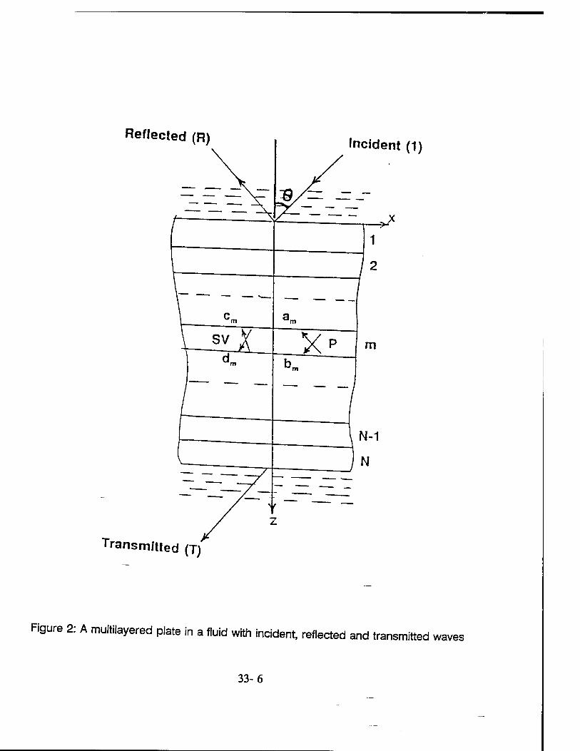
Reflected (R) Incident (1)
Transmitted (T)
Figure 2: A multilayered plate in a fluid with incident, reflected and transmitted waves
33-6

The wave potentials in the m-th layer are given by 0m(z)exp(-ikx-iot) and i|rm(z)exp(-
ikx-itot), where
tm^n? +Dme (1)
and the wave potentials in the fluid are 0o(z)exp(-ikx-iot) at the top fluid half space and
^.(zJexpt-ikx-icDt) at the bottom fluid half space, where
iqtz _ -/qjz 00=0 +Re (2) ^=Te/qf(z-zN)
in equations (1) and (2), am. bm, cm, dm, R and T are unknown constants to be
determined from the interface and boundary conditions. These conditions can be
satisfied using Thomson-Haskell matrix method [1,2]. By this technique the stress-
displacement vector at the top interface is related to the stress-displacement vector at the
bottom interface in the following manner
(3)
where
and A is the 4x4 layer matrix, also known as the propagator matrix, transfer matrix or *m
T matrix [1,2,4,8,10,11]. _
The stress-displacement vectors S0 and SN at the top and bottom surfaces of the
plate are given by
33-7

So=fuo tyO-fl) -p^O+fl) of
SN<UN 'V -Pf<*2T of (5)
Inserting these expressions in equation (3) reduces it to a system of four algebraic
equations for the four unknowns R, T, u0 and uN. After obtaining R and T the wave
amplitudes am> bm, cm and dm at any general m-th layer can be obtained by carrying out
the Thomson-Haskell matrix product between the m-th layer and top or bottom surface
of the plate [8].
Numerical Difficulties
Thomson-Haskell matrix method has inherent numerical problem of loss of
precision. The problem was first noticed by Dunkin [3]. He indicated that one can avoid
this numerical difficulty to a great extent by working with the subdeterminants of the
transfer matrix. This procedure is called the delta-matrix method. Since then, other
schemes have been described, all of them leading to formulations that do not really
ensure numerical stability [5-7]. Later Kundu and Mai [8] identified a second precision
problem that occurs when computing the amplitude of the transmitted signal and
suggested some alternatives to the conventional delta matrix technique to improve the
precision problem. Finally, Levesque and Piche [10] made more improvements to the
delta matrix method to get rid of all precision problems associated with the elastic wave
propagation analysis in multilayered solids.
NUMERICAL RESULTS
To illustrate the feasibility of using different Lamb wave modes to detect defects
33-8

in different layers in a multilayered solid two different types of specimens with four
different geometries are considered. The first type specimen is a two layered plate made
of copper and aluminum. The second type is a three layered plate specimen made of
two aluminum plates glued together by a thin epoxy layer. These specimens are shown
in Figure 3. Each type of specimen has two different geometries. For the two layered
plate the thickness of the layers is taken as 2 mm (specimen 1a) and 3 mm (specimen
1b). Aluminum plates in the three layered specimen have thickness 3.96 mm and 2.54
mm but the epoxy layer thickness is varied. Specimen 2a has epoxy thickness 0.5 mm
and 2b has this thickness equal to 0.1 mm. Table 1 shows the material properties used
in the following analyses.
The Lamb wave dispersion curves for the four different specimens (1 a, 1 b, 2a and
2b) are first computed and shown in Figure 4. From these dispersion curves one can
obtain the Lamb wave phase velocities at any frequency. For example, at 1 MHz
frequency the four specimens have 5, 6,7 and 7 different phase velocities between 0 and
10 km/sec. These are shown in Table 2. Three more phase velocities, which are greater
than 10 km/sec can be obtained by extrapolating the dispersion curves for three
specimens 1b, 2a and 2b. These are shown in parentheses in table 2. For every phase
velocity the corresponding critical angles can be computed from SnelPs law. These
angles are shown next to the phase velocities in Table 2.
Reflection and transmission coefficients are then computed for these specimens
as a function of the incident angle e. These plots are shown in Figure 5, for 1 MHz signal
frequency. The continuous and broken curves in each plot represent reflection and
33-9
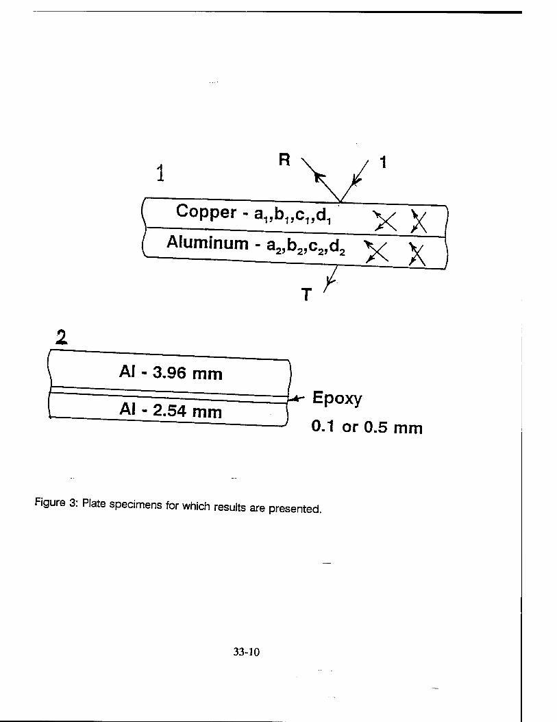
1 V' Copper - a^.c^d, ^ V
Aluminum - a2,b2,c2,d2
T? XX
AI - 3.96 mm
Al - 2.54 mm Epoxy
0.1 or 0.5 mm
Figure 3: Plate specimens for which results are presented.
33-10
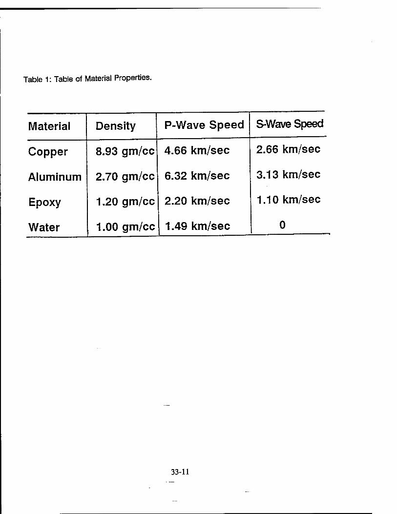
Table 1: Table of Material Properties.
Material Density P-Wave Speed S-Wave Speed
Copper
Aluminum
Epoxy
Water
8.93 gm/cc
2.70 gm/cc
1.20 gm/cc
1.00 gm/cc
4.66 km/sec
6.32 km/sec
2.20 km/sec
1.49 km/sec
2.66 km/sec
3.13 km/sec
1.10 km/sec
0
33-11
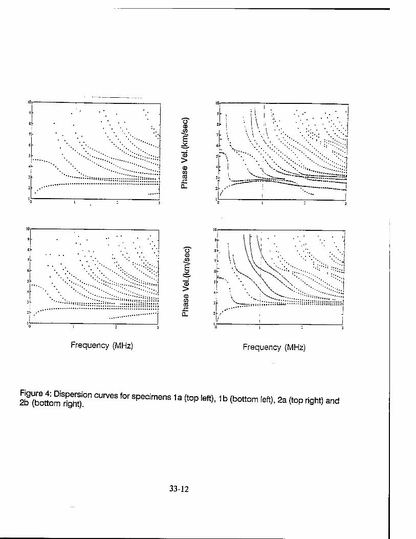
i
o CD CO
£
"05 > CD CO CD JZ QL
10 p 10 r-
I 1«— 0
siit::: •••i::: ::11111
i
o CD CO
£
"CD > CD CO CD
-C Q_
Frequency (MHz) Frequency (MHz)
SS"curves for specimens 1a (top left)'1 b (bottom Iett)'2a <top *«and
33-12
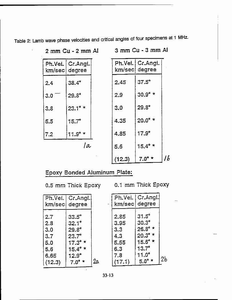
Table 2: Lamb wave phase velocities and critical angles of four specimens at 1 MHz.
2 mm Cu - 2 mm AI 3 mm Cu - 3 mm Ai
Ph.Vei. km/sec
Ci\Ang(. degree
2.4 38.4°
3.0 ~~~ 29.8°
3.8 23.1°*
5.5 15.7°
7.2 11.9°*
/fl.
Ph.Vei. km/sec
Cr.Angi. degree
2.45 37.5°
2.9 30.9° *
3.0 29.8°
4.35 20.0° *
4.85 17.9°
5.6 15.4° *
(12.3) 7.0°* IB
Epoxy Bonded Aluminum Plate:
0.5 mm Thick Epoxy 0.1 mm Thick Epoxy
Ph.Vei. Cr.Angi. km/sec degree
2.7 33.5° 2.8 32.1° 3.0 29.8° 3.7 23.7° 5.0 17.3° * 5.6 15.4°* 6.65 12.9° (12.3) 7.0°* 2a
Ph.Vei. Cr.Angi km/sec degree
2.85 31.5° 3.95 30.3° 3.3 26.8° * 4.3 20.3° * 5.55 15.6° * 6.3 13.7° 7.8 11.0° (17.1) 5.0°* 2b
33-13
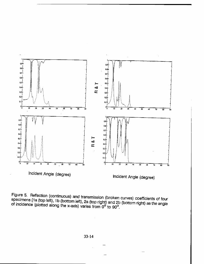
flTT 0.8 h
I 0.7h I
0.6
OJ
0.4
0-3
0.2
Qi
cc
SO 90
o3
Incident Angle (degree)
SO 90
30 40 30 «o 70
Incident Angle (degree)
Än^Ä1!1 ^transmission (broken curves) coefficients of four
33-14

transmission coefficients respectively. It should be noted here that the number of dips
in the reflection coefficient plots (or peaks in the transmission coefficient plots) are equal
or less than the number of phase velocities (or critical angles) at that frequency.
Theoretically the reflection coefficient plot should have a dip at every critical angle. If one
carefully computes and plots the reflection coefficients against the angle of incidence then
one should observe it. One can see from Figure 5 that for specimen 1a there are five
critical angles at 1 MHz and there are five dips in the reflection coefficient plot. However,
only two of those five dips are strong. The remaining three are weak. Very weak dips
can be too weak to observe and be missed. In table 2, the critical angles which show
strong dips in the reflection coefficient plots are marked by "*". Strong dips in the
reflection coefficient probably indicate relatively strong leaky Lamb wave modes at those
critical angles. All four specimens show some strong and some weak dips in their
reflection coefficient plots.
Finally the wave amplitudes a,, b,, c, and d, (i = 1 and 2 for top and bottom layers
respectively, see Figure 3) are computed as a function of the incident angle for all four
specimens. The results are plotted in Figures 6 and 7. Solid, dashed, dotted and
dashed-dotted curves are used to show the variations of a,, bif Cj and ds respectively. For
specimens 1a and 1b the wave amplitudes at the bottom layer are relatively stronger for
12° and 7° incidence respectively. At larger angles 40° or greater the wave amplitudes
at the top layer are relatively stronger. Hence, one can logically conclude that for
detecting cracks and defects at the bottom layer in specimens 1 a and 1 b the transducers
(transmitter and receiver) in a pitch-catch arrangement should be positioned at 12° and
33-15
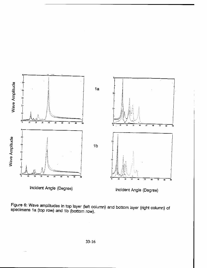
CD ■a
CD > cn
(D ■o 3
Q. E < CD >
I A / ^ 0' r^
o 10 a JO •O -0 60 70 30 90
Incident Angle (Degree)
1a
1b
;o :o :-3 JO <O ao ;o a 90
^ >>VY-', l 0 ;o a ;o 40 ;o 60 "1 30 90
Incident Angle (Degree)
Figure 6: Wave amplitudes in top layer (left column) and bottom layer (right column) of specimens 1a (top row) and 1b (bottom row). j
33-16
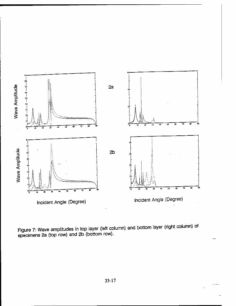
CD T3
Q. £ < CD > co
1: i
3j-
7-
H- I
J. i
al- ii 5 s».
\ m r 10 10 20 00 50 «0 70 80 90
2a
<S W'wA 0 .0 ;0 3 JO 50 60 70
10 3) X) *0
Incident Angle (Degree)
2b
Incident Angle (Degree)
Figure 7: Wave amplitudes in top layer (left column) and bottom layer (right column) of specimens 2a (top row) and 2b (bottom row).
33-17
7° inclinations respectively. On the other hand if this angle is set at 40° or greater then
defects at the top layer are detected and the bottom layer defects do not have any
influence on it. Similar plots for specimen 2a show that for 30° incidence the top
aluminum plate carries stronger waves and at an angle near 15° the bottom aluminum
plate has stronger wave amplitudes. Similar plots for specimen 2b failed to show any
angle that generates relatively stronger waves at the bottom layer at 1 MHz. However,
at another frequency it may be possible to generate relatively stronger waves in the
bottom layer of this specimen.
CONCLUDING REMARKS
The calculations presented in this paper show that it is possible to detect and
image defects at individual layers minimizing the influence of other layers on the image.
It can be done by generating Lamb waves of appropriate mode which produces strong
excitation in a specific layer of the plate. The theoretical analysis is carried out using the
Thomson-Haskell matrix method with delta matrix modification.
REFERENCES
1. W. T. Thomson, J. Appl. Phys. 21, 89 (1950).
2. N. A. Haskell, Bull. Seism. Soc. Am. 43, 17 (1953).
3. J. W. Dunkin, Bull. Seism. Soc. Am. 55, 335 (1965).
4. B. L N. Kennett and N. J. Kerry, Geophys. 57, 557 (1979).
5. D. L Folds and C. D. Loggins, J. Acoust. Soc. Am. 62, 1102 (1977).
33-18
6. D. B. Bogy and S. M. Gracewski, Int. J. Solids Struct. 20, 747 (1984).
7. A. H. Nayfeh and T. W. Taylor, in Review of Progress in QNDE, Vol.7B (1988).
8. T. Kundu and A. K. Mai, Wave Motion 7, 459 (1985).
9. T. Kundu, J. Acoust. Soc. Am. 83, 18 (1988).
10. D. Levesque and L Piche, J. Acoust. Soc. Am. 92 (1992).
11. B. Hosten and M. Castaings, in Review of Progress in QNDE (1993).
PUBLICATIONS
The following papers have been published/prepared by T. Kundu from his research
works sponsored by the AFOSR office.
1. T. Kundu and M. Blodgett, "Detection of Material Defects in Layered Solids Using
Lamb Waves", Review of Progress in Quantitative Nondestructive Evaluation, Vol.13, Eds.
D. O. Thompson and D. E. Chimenti, Pub. Plenum Publishing Co., QNDE Conference in
Brunswick, Maine, Aug.1-6, 1993.
2. T. Kundu and B. Maxfield, "A New Technique for Measuring Rayleigh and Lamb
Wave Speeds", Journal of the Acoustical Society of America, Vol.93(6), p.3066-3073,
1993.
3. M. A. Awal and T. Kundu, 'V(z) Curve Synthesis Using Two Ultrasonic
Transducers", ASME Journal of Applied Mechanics, submitted, 1994.
33-19
WAVELET ANALYSIS OF ULTRASONIC SIGNALS FOR NON-DESTRUCTIVE EVALUATION OF COMPOSITES
Theresa A. Tuthill Assistant Professor
Electrical Engineering Dept.
University of Dayton 300 College Park Dr.
Dayton, OH 45469-0226
Final Report for: Summer Research Extension Program
Wright Laboratories
Sponsored by: Air Force Office of Scientific Research
Boiling Air Force Base, Washington, D.C.
and
The University of Dayton
December 1993
34-1
WAVELET ANALYSIS OF ULTRASONIC SIGNALS FOR NON-DESTRUCTIVE EVALUATION OF COMPOSITES
Theresa A. Tuthill Assistant Professor
Electrical Engineering Dept. University of Dayton
Abstract
Wavelets are an innovative, computationally efficient method for the time-frequency anal-
ysis of nltrasound signals. This stndy looked at some fnndamemal traits associated with the
wavelet transform coefficients as applied to the non-destenctive evaluation of composite materials.
A software package utilizing the discrete wavelet transform was developed to facilitate the study
of many of these features.
Based on die Danbechies family of wavelets, an »optimum» wavelet kernel was determined
for use wim ultrasound scan lines. Application of this wavelet with a thresholding algorithm
provided an efficient data compression technique. For use in flaw detection, the time-frequency
scaJogram image was enhanced using adaptive histogram equalization. However, characterization
of materials based on patterns in the wavelet transform wem hampered by a shift variance. And,
finally, the frequency-dependent attenuation coefficient was extracted from the transform coeffi-
cients, though a large error in accuracy remained. The wavelet transform shows promise in
non-destmctive evaluation of materials, though further work is needed.
34-2
WAVELET ANALYSIS OF ULTRASONIC SIGNALS FOR NON-DESTRUCTIVE EVALUATION OF COMPOSITES
Theresa A. Tuthill
L INTRODUCTION
The characterization and detection of defects in composite materials is integral to the eval-
uation of structures. Ultrasound provides an efficient, inexpensive tool for examining material
composition without direct observation and is commonly used in non-destructive evaluation
(NDE) applications. However, the resolution provided by such techniques often precludes detec-
tion of localized anomalies.
As an ultrasound pulse propagates through a medium, it is refracted, scattered, and atten-
uated, depending on the material's internal structure and properties (specifically, variations in
sound speed and density). Information characterizing the material is thus included in the time
signal amplitude as weU as derived acoustic parameters such as the backscatter and attenuation
coefficients. These acoustic parameters, however, are often dependent on frequency, and a spec-
tral analysis is necessary.
Detection of flaws and microcracks is highly dependent on the resolution of the resulting
scans which is limited by the insonifying pulse width and frequency. Flaws smaller than a wave-
length will not be detected using standard amplitude intensity display techniques. Incorporation
of phase information, while retaining localized spatial resolution, will improve detection.
This study examines an innovative signal processing technique for combining time-
frequency analysis - the discrete wavelet transform. The motivation for examining wavelets is
based on a phenomenological approach to ultrasound echoes : echo pulses look like wavelets.
34-3

n. DISCUSSION OF THE PROBLEM
The evaluation of a material's strength and structural integrity is often difficult because
damage below the surface cannot be reso!ved. Delaminations, microcracking, and debonding are
common flaws which when left undetected can propagate with catastrophic results.
For a flawed material or inhomogeneous medium, the ultrasound signals are non-
stationary, and localized changes to frequency dependent parameters would be undetectable in a
spatially smeared windowed spectrum. Thus a time-frequency representation is more applicable.
An inherent problem of a time-varying spectrum, however, is founded in the uncertainty
principle. The product of the time resolution and frequency resolution remains a constant. In
creasing frequency resolution reduces time (or spatial) resolution and vice versa. Wavelet analysis
can optimize bom resolutions and offers an accurate and efficient approach for characterizing
materials.
Though wavelet theory has been a burgeoning research topic in the past few years, its
application to ultrasound signals warrants specific attention. An appropriate wavelet must be de-
termined to optimize efficiency in flaw detection and characterization. Additionally, a
fundamental understanding of the resulting wavelet transform patterns must be gained for evalu-
ation purposes.
HL THEORY
1) Wavelet Theory
As an alternative to windowed Fourier analysis techniques, the wavelet analysis [1] was
chosen for its ability to locate time discontinuities and its invertible transform. A wavelet family
34-4

is comprised of translations and scale variations of a single wavelet and can be described [ 2] by
ha,b(t)= ^h(4*) W
where a represents the time scale parameter and b is the time shift. For a<l, the the waveform is
compressed, and the frequency is correspondingly increased. The resulting family of wavelets
forms a set of basis functions for the decomposition of a given time signal. That is, a one-
dimensional signal can be expressed as a linear combination of the members in a given wavelet
family. The contribution of each wavelet is given by it's wavelet transform coefficient. The
wavelet transform of signal f (t) is just the correlation of the wavelets with the signal and is defined
as Wf(a,b) = -Jj _? f(t) h* (^) d t = (f, hajb) (2)
The signal can be reconstructed from its wavelet transform coefficients using the following
equation
f (t) = i / / Wf(a,b) ä^db (3)
where C is a constant dependent on the wavelet.
The choice of a specific "mother" wavelet (the original h(t)) is dependent on the
application. For an exact reconstruction, the wavelet must meet the following criteria:
1) admissibility (the wavelet has zero mean)
2) orthonormal
and 3) finite energy.
Ingrid Daubechies, a reknowned mathematician, has done extensive work in determining
orthonormal basis wavelets that are compactly supported [3]. Figure 1 shows a Daubechies wave-
34-5
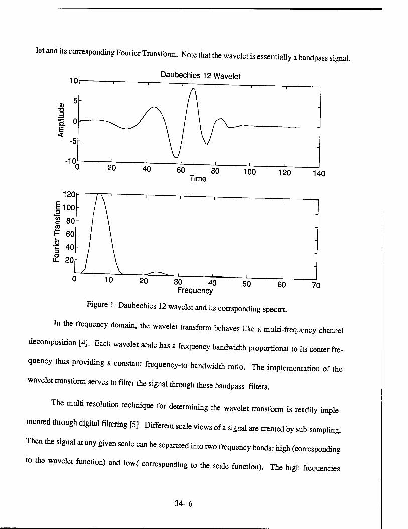
let and its corresponding Fourier Transform. Note that the wavelet is essentially a bandpass signal.
Daubechies 12 Wavelet
20 40 60 80 Time
100 120 140
10 20 30 40 Frequency
50 60 70
Figure 1: Daubechies 12 wavelet and its corrsponding spectra.
In the frequency domain, the wavelet transform behaves like a multi-frequency channel
decomposition [4]. Each wavelet scale has a frequency bandwidth proportional to its center fre-
quency thus providing a constant frequency-to-bandwidth ratio. The implementation of the
wavelet transform serves to filter the signal through these bandpass filters.
The multi-resolution technique for determining the wavelet transform is readily imple-
mented through digital filtering [5]. Different scale views of a signal are created by sub-sampling.
Then the signal at any given scale can be separated into two frequency bands: high (corresponding
to the wavelet function) and low( corresponding to the scale function). The high frequencies
34-6
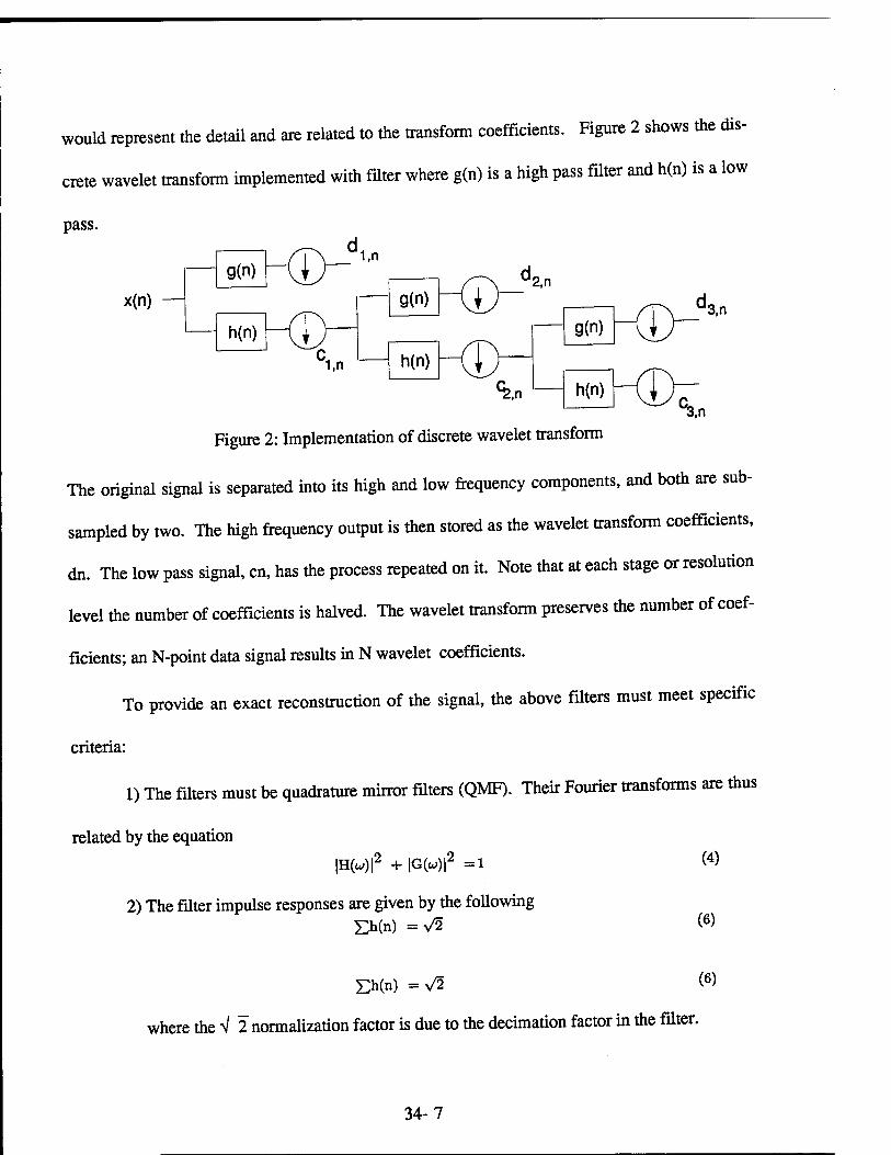
would represent the detail and are related to the transform coefficients. Figure 2 shows the dis-
crete wavelet transform implemented with filter where g(n) is a high pass filter and h(n) is a low
pass.
x(n)
9(n) 1,n
h(n)
1.n
g(n) '2,n
h(n)
<*>n
g(n) '3,n
h(n) T 3,n
Figure 2: Implementation of discrete wavelet transform
The original signal is separated into its high and low frequency components, and both are sub-
sampled by two. The high frequency output is then stored as the wavelet transform coefficients,
dn. The low pass signal, en, has the process repeated on it. Note that at each stage or resolution
level the number of coefficients is halved. The wavelet transform preserves the number of coef-
ficients; an N-point data signal results in N wavelet coefficients.
To provide an exact reconstruction of the signal, the above filters must meet specific
criteria:
1) The filters must be quadrature mirror filters (QMF). Their Fourier transforms are thus
related by the equation
|H(W)|2 +|G(W)|2 =1
2) The filter impulse responses are given by the following £h(n) =v/2
(4)
(6)
£h(n) = V2 («)
where the V 2 normalization factor is due to the decimation factor in the filter.
34-7

3) The filters must be "regular such that the filtering iterations converge.
Extensive research has been done in the area of determining filters that meet the above
criteria. Using maximally-flat low pass filters, Daubechies computed wavelet filter coefficients
for various filter lengths. Because the corresponding wavelets have continuous derivatives and are
compacdy supported, they have become the "standard" in many wavelet applications.
Displaying the wavelet transform requires a two-dimensional, rime-frequency plot. By
»tag the squared modulus of the transform coefficients, the energy of the signal can be «pre-
sented on a gray scale plot called a scalogram. Time or distance is shown on the horizontal axis
and increasing frequency is shown on the vertical axis going fa. bottom to top. Because the
number of wavelet coefficients decreases with decreasing frequency, the htteral resolution de-
creases at each successive level, and more pixels tue assigned to a single coefficient. The highest
resolution occurs for the highes, frequency and is displayed on the top row. Any localized or
transient phenomena should appear in this row.
2) Acoustic Parameters
The loss of energy as an acoustic pulse propagates throngh a medium is referred to as
attenuation. Attenuation encompasses longitudinal and shear scattering form »homogeneities and
conversion of acoustic energy to heat by absorption mechanisms. The resulting decay in signal
strength can be fitted to an exponential of the form
S(x)=soe-2Ax (7)
where x is depth, A is tine frequency-dependent attenuation coefficient, and s0 is a constant repre-
senting the backscattered signal strength. A standard procedure for estimating the attenuation
coefficient a, the center frequency of the pulse is to curve fie tire decay of the envelope of a
scanline. However, this technique doe not provide frequency information.
34-8
IV. METHODOLOGY
1) Facilities
The research was performed in the University of Dayton's Ultrasound Lab which was
established in 1991. The lab was designed for the implementation of research in the areas of both
biomedical tissue characterization and non-destructive evaluation of materials. A single ultra-
sound scanning station is used for data collection, signal processing, and data analysis. Samples
are placed in a gallon water tank and can be scanned at various frequencies ranging from 1 to 10
MHz using Panametrics transducers. A computer controlled, X-Z positioner, with high precision
stepper motors (with 1/100" increments), is used to move the transducer across the scanning plane.
The output from a Panametrics pulser/receiver is digitized via an HP45402 digitizing oscilloscope
(400 Msamples/sec, 2K sample storage). The data is transmitted over the IEEE bus to the SUN-
IPC SPARCstation (16" color monitor, 24Mbytes RAM, 2.2Gbyte hard drive) for storage and
processing.
The MATLAB software package (Mathworks, Inc., Natick, MA) with the Signal Process-
ing Toolbox is the primary programming environment. MATLAB allows users to incorporate
their own C-code for analysis and then display results using a variety of visualization techniques.
An Ethernet local area network also provides communication and file sharing with other comput-
ers for remote processing.
2) Implementation of Wavelet Transform
A fast discrete wavelet transform was implemented within the MATLAB environment. A
suitable algorithm, found in Numerical Recipes in C (Second edition), was coded and interfaced
34-9
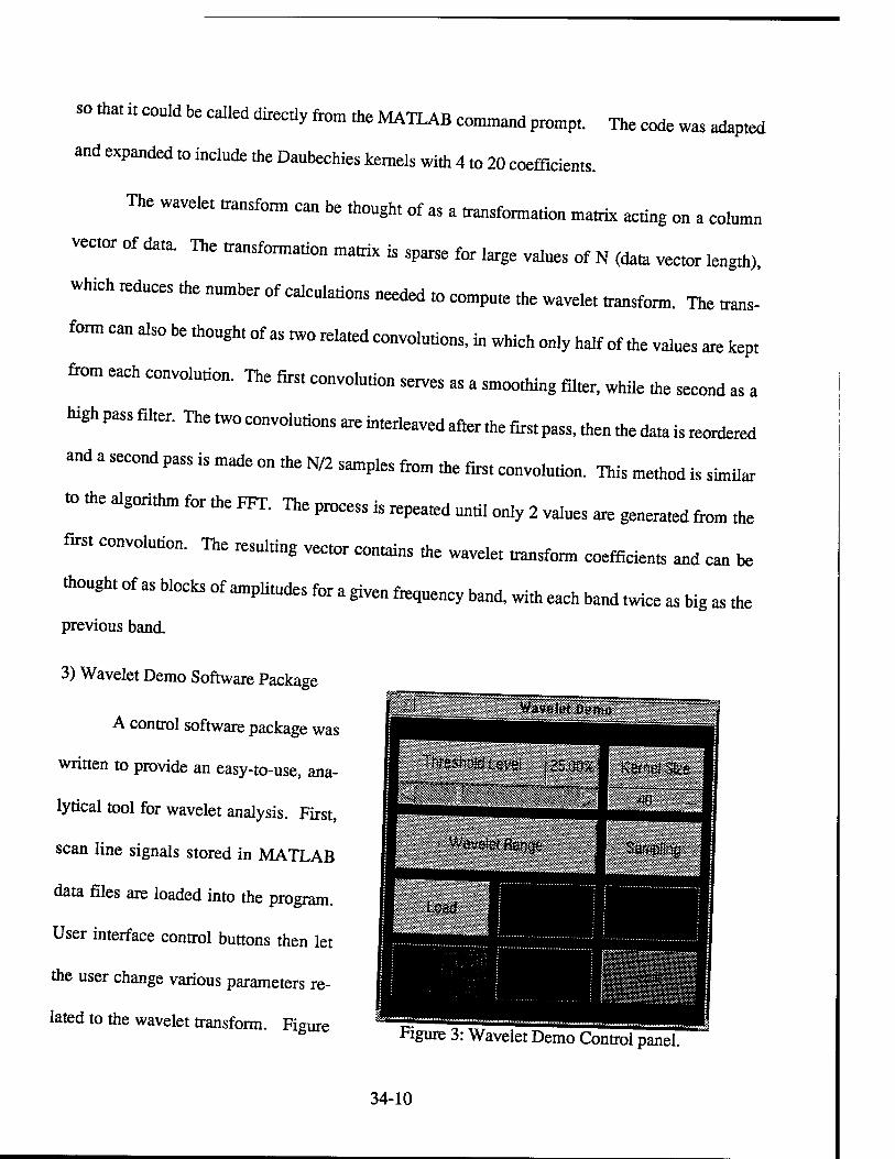
so that it could be called direcdy from tine MATLAB command prompt The code was adapted
and expanded to include the Daubechies kernels with 4 to 20 coefficients.
The wavelet transform can be thought of as a transformadon matrix acting on a column
vector of data. The transformadon matrix is sparse for large values of N (data vector length),
which reduces the number of calculations needed to compute the wavelet transform. The trans-
form can also be thought of as two related convomtions, in which only half of the values are kept
tan each convolution. The first convoludon serves as a smoothing filter, while the second as a
highpass filter. The two convolutions are interleaved after the firs, pass, Aen me data is reordered
and a second pass is made on the N/2 samples from the first convolution. This method is similar
«. me algorithm for the FFT. The process is repeated until only 2 values are generated from the
firs, convolution. The resulting vector contains the wavelet transform coefficients and can be
thought of as blocks of amplitudes for a given frequency band, with each band twice as big as the
previous band.
3) Wavelet Demo Software Package
A control software package was
written to provide an easy-to-use, ana-
lytical tool for wavelet analysis. First,
scan line signals stored in MATLAB
data files are loaded into the program.
User interface control buttons then let
the user change various parameters re-
lated to the wavelet transform. Figure Figure 3: Wavelet Demo Control panel,
34-10

3 shows the interface display with controls for the threshold level (for truncating coefficients),
kernel size (number of coefficients for the filters), wavelet range (for zooming in on a specific
range), and the number of points desired for downsampling. The program then computes and
displays four basic graphs: the original waveform, the wavelet transform, the reconstructed wave-
form, and the two-dimensional scalogram. The wavelets transform is displayed by combining the
coefficients from each band into a single vector. The highest frequency band is to the left using
points N/2 to N, the second highest band is in points N/4 to N/2, and so on down to the lowest
frequency band contained in the first two points.
Through the course of this research project, the scalogram was analyzed for patterns relat-
ing to the material. The original display mapped the coefficient values to the full 255 gray levels.
However, because the high frequency coefficients were much lower in magnitude, they were often
"washed out," precluding any identification of high frequency transient effects. As a result, a
histogram equalization was performed within each frequency band. Figure 4 shows a scalogram
from a typical waveform before and after the equalization process.
4) Composite Materials
Ultrasound scans were taken of a variety of composite materials. To analyze a "damaged"
composite, scans were made of a graphite-epoxy, quasi-isotropic, 3/32" thick sample with a 4.05
ft-lb impact. A scan of a non-damaged region is referred to as "QND010," and a scan of the
damaged region is "QND150."
34-11
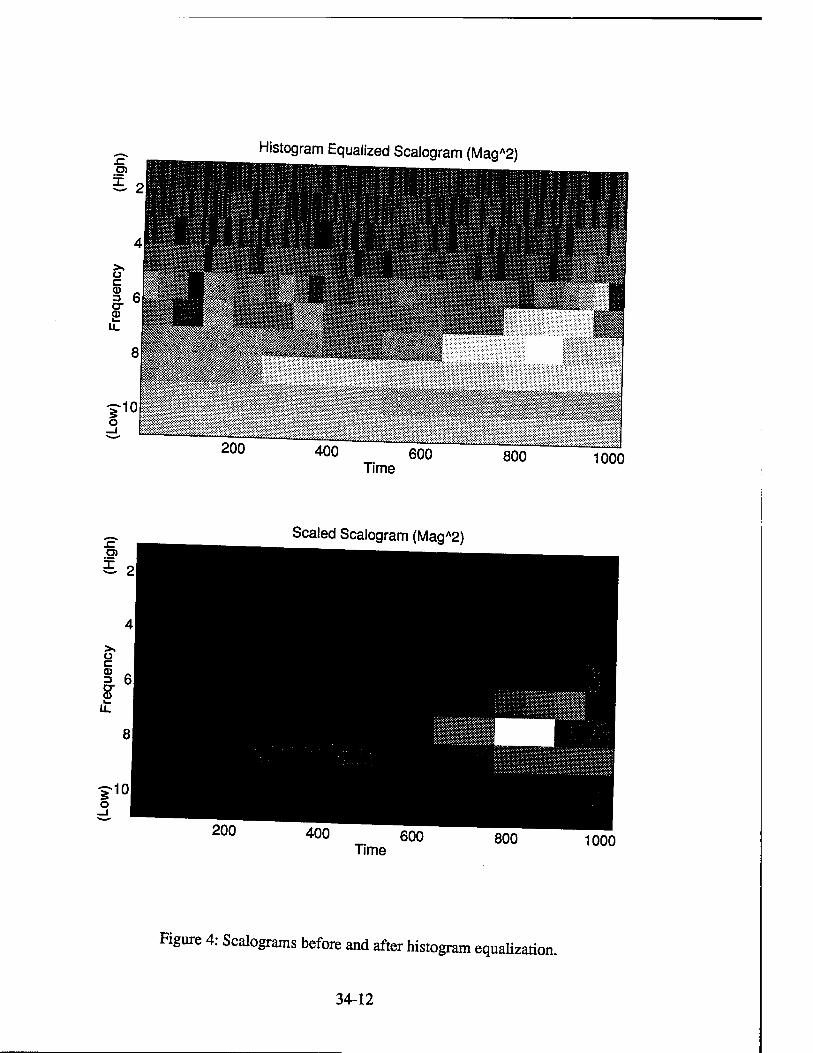
Histogram Equalized Scalogram (MagA2)
200 400 600 Time
800 1000
Scaled Scalogram (MagA2)
400 600 Time
800 1000
Figure 4: Scalograms before and after histogram equalization.
34-12

V. RESULTS
Ultrasound scan lines from the QND010, QND150, and a 32 ply uni-weave composite
sample were formed using a 3.5 MHz, 2" focused transducer and then processed for the following
analyses.
1) Optimum Wavelet
Throughout this study, various Daubechies wavelets were employed. The different wave-
lets are denoted by their kernel size (or length when considering filter coefficients) ranging from 4
to 40. Inspection of the corresponding waveforms shows that the size 20 kernel most resembled
the insonifying pulse in smoothness and in length. This observation was confirmed in the data
compression analysis discussed below. To illustrate, Figure 5 shows the 4-point kernel wavelet
transform for a scanline (1000 points using a 5 MHz transducer and sampling at 200 MHz) taken
of the 32 ply composite sample. In the reconstructed signal, only a portion of the coefficients are
used, and the result is a jagged waveform. Figure 6 shows the wavelet transform of the exact same
signal, but now using the 20-point kernel. Again, only a portion of the coefficients were used to
reconstruct the signal, though here the resulting waveform is much smoother and resembles the
original. Despite the vast difference in the resulting waveforms, the mean-square-errors (MSE)
between the original and the reconstruction are close.
It should be noted that despite the jaggedness of the 4-point kernel wavelet, when all the
coefficients are employed, an exact reconstruction is formed. This was tested with all the kernel
sizes and confirms the assertion that the Daubechies wavelets are invertible.
34-13
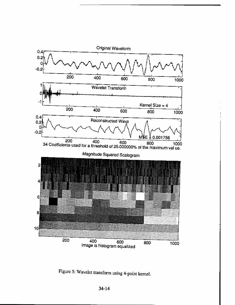
Original Waveform
200 400 34 Coefficients used for a threshold of 25.000000% of the
Magnitude Squared Scalogram
maximum val ue.
200 . 400 600 800 image is histogram equalized
1000
Figure 5: Wavelet transform using 4-point kernel.
34-14
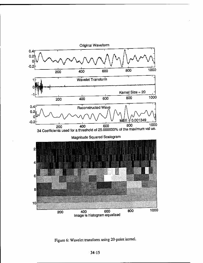
Original Waveform
Kernel Size = 20 , ,
0.4F 0.2
0 -0.2
200
—i—
400 600 800 1000
Reconstructed Wave
E ¥0.001349 1000 200 400 600 800
34 Coefficients used for a threshold of 25.000000% of the maximum val ue
Magnitude Squared Scalogram
200 400 600 800 Image is histogram equalized
1000
Figure 6: Wavelet transform using 20-point kernel.
34-15
2) Data Compression
The wavelet transform is suitable for data compression because it is orthogonal and has a
finite number of basis functions. Since me original signal's energy is compressed into a fewer
number of coefficients in the transform space, some of die coefficients can be eliminated from the
reconstruction without loss of information. The analysis of data compression focused on two
techniques: i) truncation of tnmsform coefficients to a given number of points and ii) thresholding
the transform values and keeping only those coefficients that were above a specified level. The
metric for evaluating the compression techniques is the mean square error between the recon-
structed signal and the original input signal.
i) Truncation - Since the wavelet transform orders the coefficients into frequency bands
going from lowest to highes, frequency, truncation is similar to downsampling the data. When
transform coefficients are zeroed, the high frequencies are removed and a smoother or low pass
filtered signal will be reconstructed Large errors occur if the signal is originally no. smooth or
contains high frequencies. A range of truncations were performed on the 512-poin, wavelet
transform of the scanlines from the QND composite sampled at 100 MHz . Figure 7 shows the
results for truncating the „umber of coefficients down to 64 or a compression of 8 to 1. The cor-
responding mean-square-error (MSE) of 8.5 provides a reasonable reconstruction. Further
analyses showed that a MSE value of 10 is a reasonable cut off point for detennining a good
compression scheme. However, further truncation down to 32 coefficients (a compression ratio
of 16 to 1) produced an MSE of 253 (Figure 8) and a poor reconstruction.
34-16
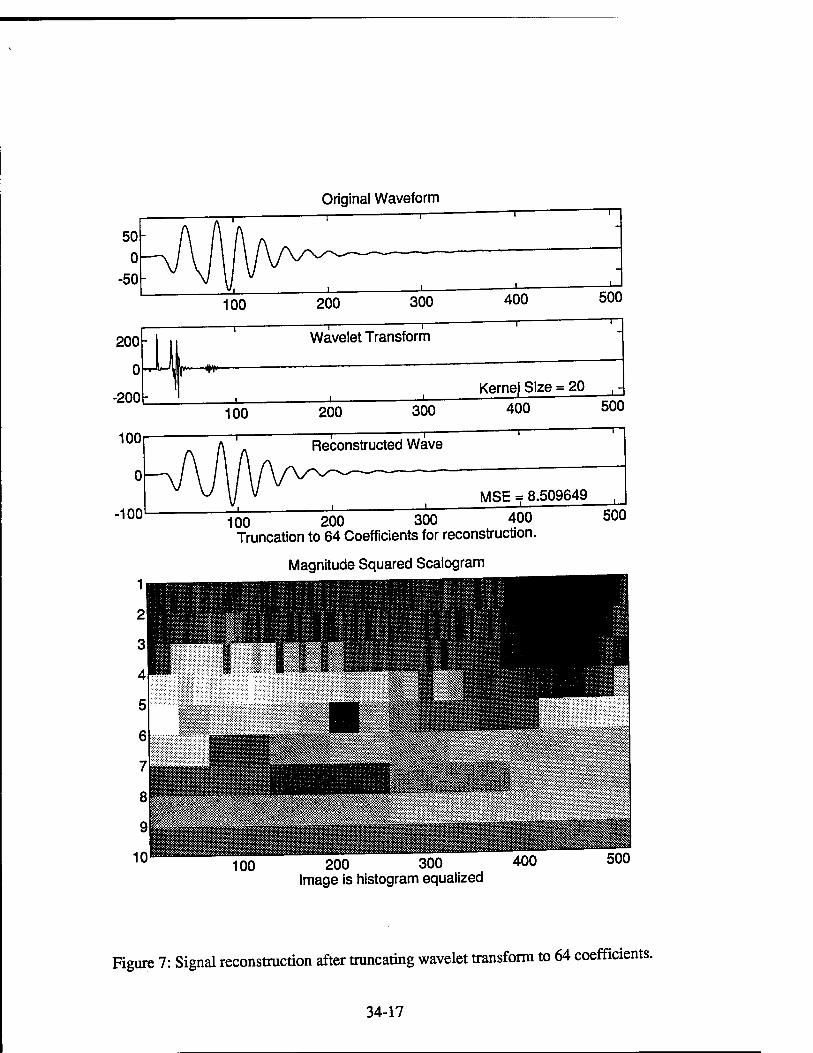
200H
0
-200
100
0
-100
Original Waveform
Kerne) Size = 20
100 200 300 400 500
—r Reconstructed Wave
MSE = 8.509649
100 200 300 400 Truncation to 64 Coefficients for reconstruction.
Magnitude Squared Scalogram
500
100 200 300 400 Image is histogram equalized
500
Figure 7: Signal reconstruction after truncating wavelet transform to 64 coefficients.
34-17

50
0
-50
Original Waveform
100 200 300 400 500
Wavelet Transform
-**»-
100 200 300 Kerne) Size = 20
400 500
Reconstructed Wave
100 MSE = 253.320851
T , ^00 300 400 Truncation to 32 Coefficients for reconstruction.
Magnitude Squared Scalogram
500
100 , 20? 300 400 image is histogram equalized
500
Figure 8: Signal reconstruction after truncating wavelet transform to 32 coefficients.
34-18

This technique did lead to interesting application for removing high frequency spikes from
an input signal. Since the wavelet transform has both frequency and time information a spike in
the input signal could be removed by attenuating or zeroing out the proper coefficients in the
transform that are near the time period of the spike. This could be thought of as a notch filter
localized in time around the spike.
Ü) Thresholding - Data compression can also be obtained by storing only those coefficients
with values above a certain threshold level. With this technique, however, it is necessary to also
store the corresponding position of the coefficient in the resulting transform vector. A program
was written in C which performs the
thresholding of the data. The program
searches for the absolute maximum value
then computes the threshold level and ze-
ros all transform coefficients below that
threshold. This does add some overhead,
since the value of the transform and the
location must be saved. However, this
method still provides better compression
of the signal and lower MSE for the re-
constructed signal.
The size of the kernel or wavelet
does effect the efficiency of the
thresholding. Table 1 shows that for the
Table 1 - Thresholding errors for constant threshold levels
Kernel Size
# Coeffs
Threshold level
Error (MSE)
4 11 33% 58.5
12 8 33% 41.9
16 9 33% 82.7
20 6 33% 43.2
24 4 33% 76.4
34 9 33% 32.2
40 6 33% 64.4
Table 2 - Thresholding errors for constant number of coefficients.
Kernel Size
# Coeffs
Threshold level
Error (MSE)
4 6 46% 139.5
12 6 42% 83.4
16 6 25% 50.3
20 6 33% 43.2
24 6 27% 32.2
34 6 49% 84.5
40 6 33% 64.4
34-19

wavelet transform coefficients of a scanline from the QND sample nsing a constant threshold
level, the number of resulting coefficients first decreases as the kernel size increases, but then
starts to increase again. As expected, the MSE varies inversely with the number of coefficients. It
does appear, however, that an "optimum" wavelet kernel size exists around 20 to 30. In support
of this theory, the errors were computed for the various kernel sizes nsing a set number of
coefficients. Table 2 shows that there is a minima for the MSE in the 20 to 30 range. For an
ultrasound scan line it is expected mat Ute optimum kernel size would be comparable eo the wave-
length, and for the preceding example of a 3.5 MHz pulse sampled at 100 MHz, the number of
sample points for a wavelength is in fact 28.
A direct comparison between the truncation and thresholding techniques was done on the
QND sample nsing tine 20-poin, kernel and varying the threshold until the desired number of
coefficients „as achieved. Figure 9 shows a threshold level of 0.8 percent of the maximum value
induded) or a compression ratio of 4 to 1 The error was only 0.20 in reconstructing tine signal. By
increasing the threshold until only 32 coefficients are used (Figure !0), the MSE increases to only
1.19. Examination of the reconstructed waveforms shows that the signal can be represented by
very few coefficients and still provide a good reconstruction of the signal. Higher threshold error
levels could achieve compression ratios of 50 to 1 with tolerable MSE values. This techniqne
provides better results and higher mtios than the truncation method, however mere is a higher
amount of overhead in determining, which valnes to keep .
34-20
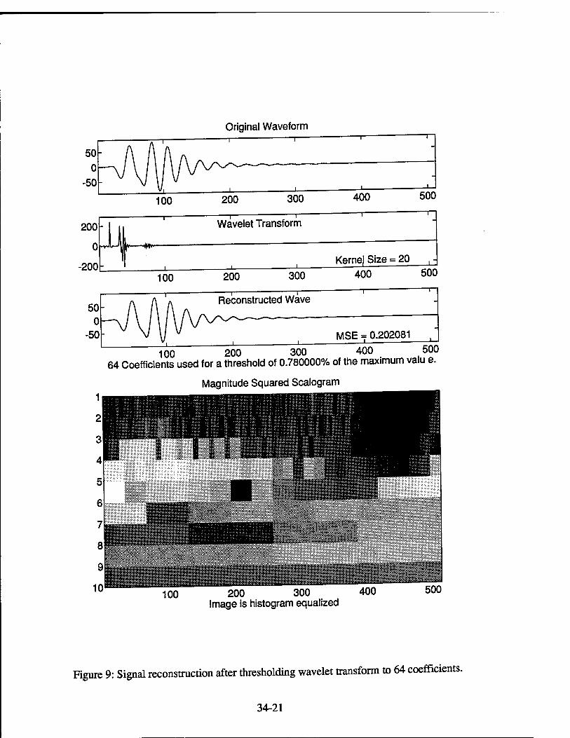
Original Waveform
200
0
-200
-i r Wavelet Transform
HW»~
_L
50 0
-50
100 -i—
200 300
Kerne) Size = 20 400 500
Reconstructed Wave
MSE = 0.202081
100 200 300 400 500 64 Coefficients used for a threshold of 0.780000% of the maximum valu e.
Magnitude Squared Scalogram
100 200 300 400 Image is histogram equalized
500
Figure 9: Signal reconstruction after thresholding wavelet transform to 64 coefficients.
34-21
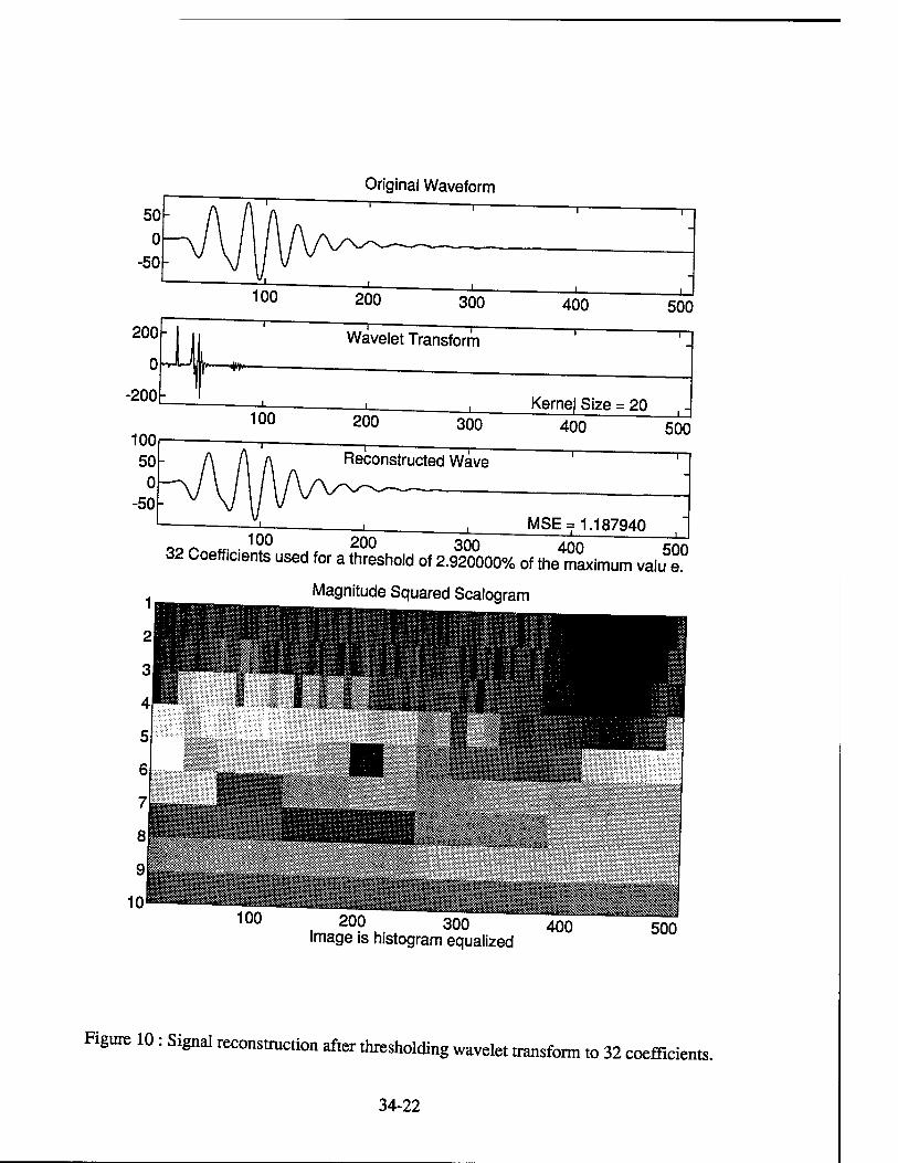
Original Waveform
200 300 400 500
Wavelet Transform -*!*■
100 200 100 50
0 -50
300 Kernej Size = 20
_i_ 400
Reconstructed Wave
500 —r
100 200 32 Coefficients used for a threshold of 2.920000% of the
MSE = 1.187940 300 400 500
maximum valu e.
Magnitude Squared Scalogram
100 200 300 400 Image is histogram equalized
500
Figure 10 : Signal reconstruction after thresholding wavelet transform to 32 coefficients.
34-22

3) Effect of Sampling Rate on Data Compression
The data analyzed in the previous section was over-sampled, so the effect of the sampling
rate on the compression ratios was examined. The input signals were down-sampled by various
factors of 2, and then reprocessed to determine new compression statistics. Only the thresholding
method was evaluated in this section since it had the best performance. Figure 11 shows a 512-
point, 3.5 center frequency scanline sampled at 100MHz. A threshold level of 33% produces a
reasonable reconstruction with a MSE of 43. Figures 12 and 13 show this same waveform down-
sampled by a factor of 2 and 4, respectively. In both cases, the number of coefficients needed for
a reconstruction error near 40 was approximately the same as for the original signal. Note that for
each decimation by two, the highest frequency band in the scalogram is eliminated. And, while
the resulting scalograms are not identical for the lower frequency bands, the patterns are similar.
This study showed that the sampling rate will not effect compression rations, as long as the signal
is sampled well above the Nyquist..
4) Shift Variance
The most significant problem with applying wavelet analysis to ultrasound signals is that
the wavelet transform is shift-variant. The resulting transform coefficients depend on the position
of the input signal in the time domain. Even small shifts in the time domain can lead to significant
changes in the wavelet domain. Figures 14 and 15 show the wavelet transform coefficients for
shifted versions of a 128 point sequence of the QND sample. Even for this narrow range of shifts
(-3 to +4), there is a noticeable difference in the transform, especially in the lower frequency
bands. The coefficients with the largest magnitude are fairly similar between 1-point shifts,
though the amplitude goes from positive to negative through the entire sequence of shifts.
34-23
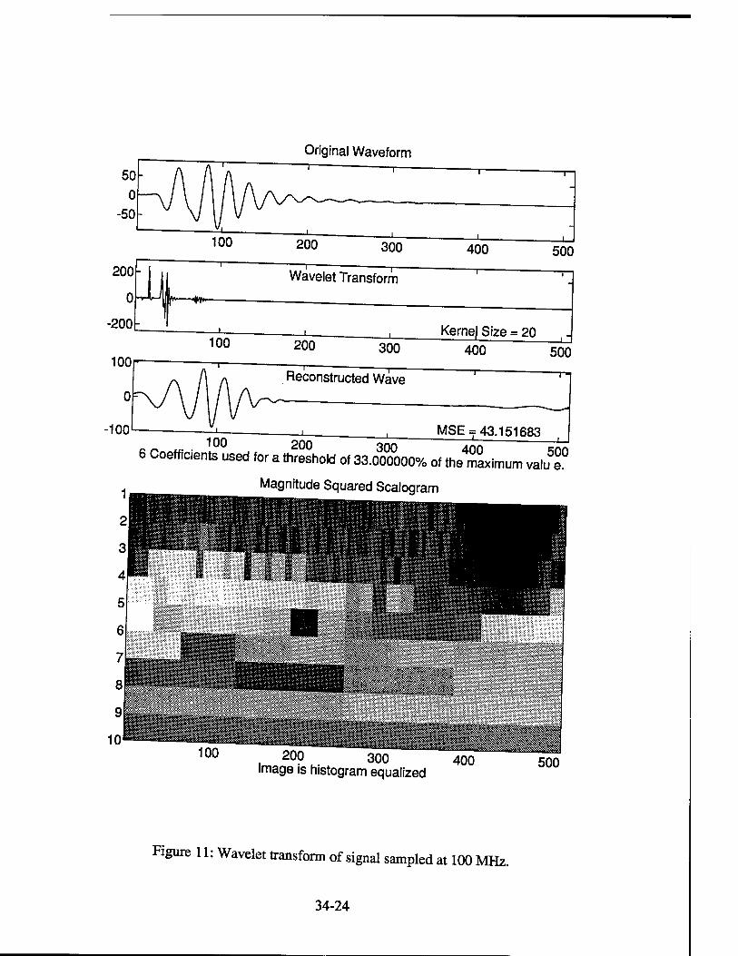
Original Waveform
6 Coefficients used for a threshold of 33.000000% of the
Magnitude Squared Scalogram
maximum valu e.
100 200 300 400 image is histogram equalized
500
Figure 11: Wavelet transform of signal sampled at 100 MHz.
34-24
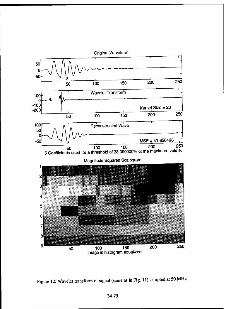
Original Waveform
50
0 -50 _L
100h 0
-100 -200
'^X-J
50
—i—
100 150
Wavelet Transform
200
—i—
250 —r
l^^—v*^v—
Kernel Size = 20
50 100 150 200
100F 50
0 -50
250
—ra Reconstructed Wave
MSE = 41.650496
50 100 150 200 250 5 Coefficients used for a threshold of 33.000000% of the maximum valu e.
Magnitude Squared Scalogram
50 100 150 Image is histogram equalized
200 250
Figure 12: Wavelet transform of signal (same as in Fig. 11) sampled at 50 MHz.
34-25
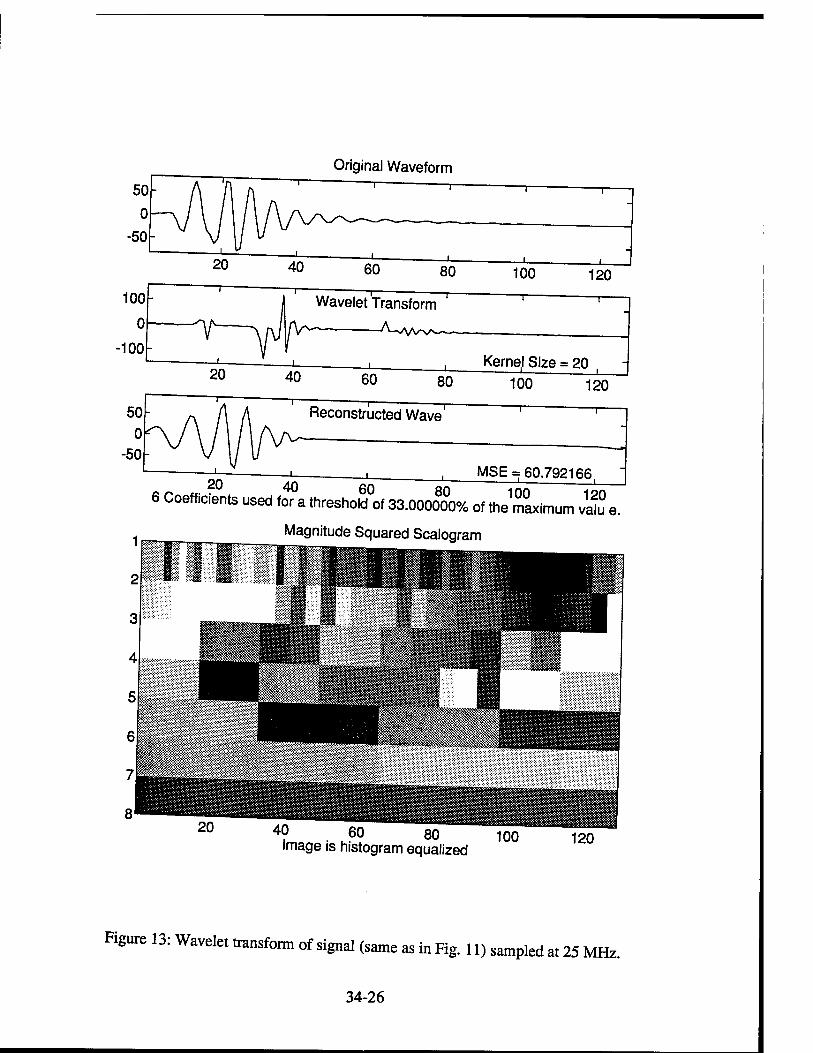
Original Waveform
100 120
Wavelet Transform
60 80 Kerne,! Size = 20
100 120
Reconstructed Wave
MSE = 60.792166
6 Coefficients used for~a threshold* 33.000000% of the maximum vllS e.
1 _ Magnitude Squared Scalogram
20 40 60 80 Image is histogram equalized
100 120
Figure 13: Wavelet transform of signal (same as in Fig. 11) sampled at 25 MHz.
34-26
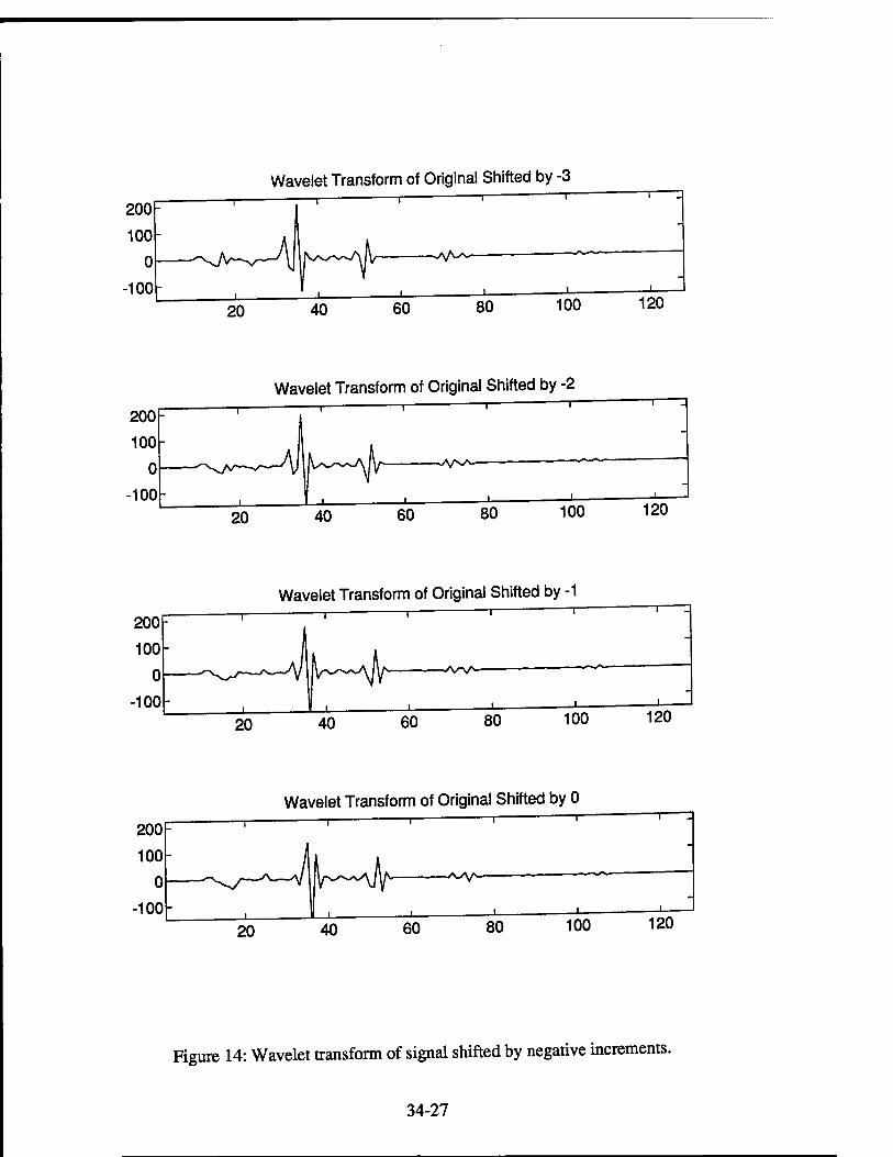
Wavelet Transform of Original Shifted by -3
Wavelet Transform of Original Shifted by -2
Wavelet Transform of Original Shifted by -1
Wavelet Transform of Original Shifted by 0
Figure 14: Wavelet transform of signal shifted by negative increments.
34-27
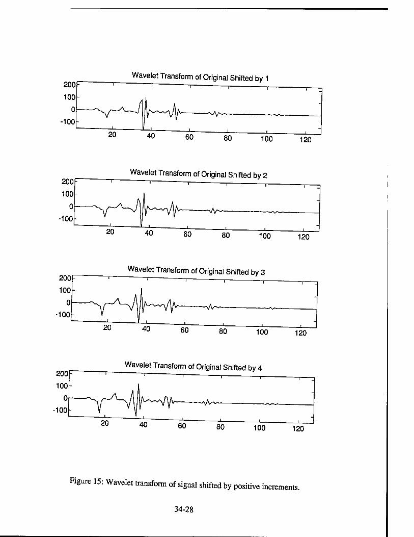
Wavelet Transform of Original Shifted by 1
120
Wavelet Transform of Original Shifted by 2
Wavelet Transform of Original Shifted by 3
Wavelet Transform of Original Shifted by 4
Figure 15: Wavelet transform of signal shifted by positive increments.
34-28

In computing the discrete wavelet transform, a decimation by two is performed after each
filtering stage. It is expected then, that within a specific frequency band, shifts by a corresponding
multiple of two would produce a simple shift within that band. For example, a shift by 4 would
correspond to a shift by 2 in the second highest frequency band (points 32 through 63 in a 128
point transform) and a shift by 1 in the highest band (points 32 through 63). The wavelet trans-
forms of a 128-point sequence (using a 20 point kernel size) are shown for shifts of various powers
of two in Figures 16 and 17. Close examination of the higher frequency bands shows that the
coefficients are shifted, but still show a small variation. It is concluded that the high pass filter
applied before decimation in determining the wavelet coefficients is the main cause of this minor
variation. The coefficients in the lower bands, however, appear uncorrelated.
Shifts in the time domain are an inherent problem with ultrasound scans since jitter in the
pulser/receiver can cause delay shifts for adjacent scan lines.. The vastly different wavelet trans-
form coefficients can preclude a reliable characterization based on wavelets.. To try and correct
this problem the signals were cross correlated and then shifted so that they had maximum
correlation.
The cross-correlation was computed for adjacent signals in the QND B-scan, then the
maximum value was found and a shift computed from how far the maximum value was from the
center of the correlation vector. This proved to be effective if the signals were similar, however if
the signals were repetitive (i.e. a strong back echo), the cross-correlation would correlate different
peaks and the shifted signals would be even worse than the original signals. Improvements were
made by correlating a small section of the signal, but the amount of signal used is dependent on
knowledge of what the signals look like and how much shift is in the signals.
34-29
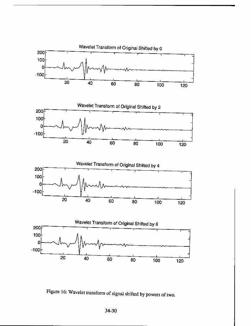
Wavelet Transform of Original Shifted by 0
Wavelet Transform of Original Shifted by 2
Wavelet Transform of Original Shifted by 4
120
Wavelet Transform of Original Shifted by 6
Figure 16: Wavelet transform of signal shifted by powers of two.
34-30
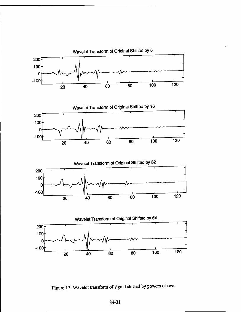
Wavelet Transform of Original Shifted by 8
Wavelet Transform of Original Shifted by 16
Wavelet Transform of Original Shifted by 32
Wavelet Transform of Original Shifted by 64
Figure 17: Wavelet transform of signal shifted by powers of two.
34-31

5) Signal Attenuation
The integrity of a composite material can often determined by the attenuation of the ultra-
sound signal as i, passes through the material. The attenuation coefficient, however, is frequency
dependent, and a frequency domain analysis is required. Eimer FFTs are used to compare atten-
uated power spectra, or the power outputs from a bank of filters are compared. This latter
technique was adapted for the wavelet transform frequency bands. To test the accuracy of mis
technique, a metal stepper block with uniform step sizes was scanned, and the wavelet analysis
was applied to the fron, and back echoes. The average front and back scan power was found for
each step and each individual frequency band. The log of the "back echo power» to the »front echo
power» was men computed and plotted versus the depth of the material for each frequency band.
The slope, which is direcdy related to the attenuation, was determined by applying a bnear curve
fit. To insure zero attenuation for zero depth, the curve was forced through the origin. Figure 18
shows the resuits using a 5 MHz transducer for filter bank 5 (corresponding to a low frequency
band near 5 MHz). The curve fits for bauds much higher or lower were not as accurate due to the
low amplitude strength of the transform coefficients in these band (Figure 19). This experiment
was repeated using a 10MHz transducer. Again, the best curve fits were found for those filter
banks nearest the 10MHz center frequency (in mis exampfc banks 3, 4, and 5). The slope for the
three most accurate banks is shown in Figure 20 plotted versus frequency. Note that for both
transducer data sets, as the frequency increases (corresponding to smaller filter bank numbers), the
attenuation increases. The accuracy (or lack thereof) of employing wavelet coefficients for ex-
tracting attenuation values is demonstrated by the difference in slope values for a given filter bank.
34-32
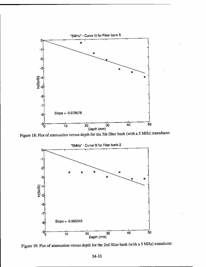
"5MHz" - Curve fit for Filter bank 5
20 30 Depth (mm)
50
Figure 18: Plot of attenuation versus depth for the 5th filter bank (with a 5 MHz) transducer.
"5MHz" - Curve fit for Filter bank 2
10 20 30 Depth (mm)
40 50
Figure 19: Plot of attenuation versus depth for the 2nd filter bank (with a 5 MHz) transducer.
34-33
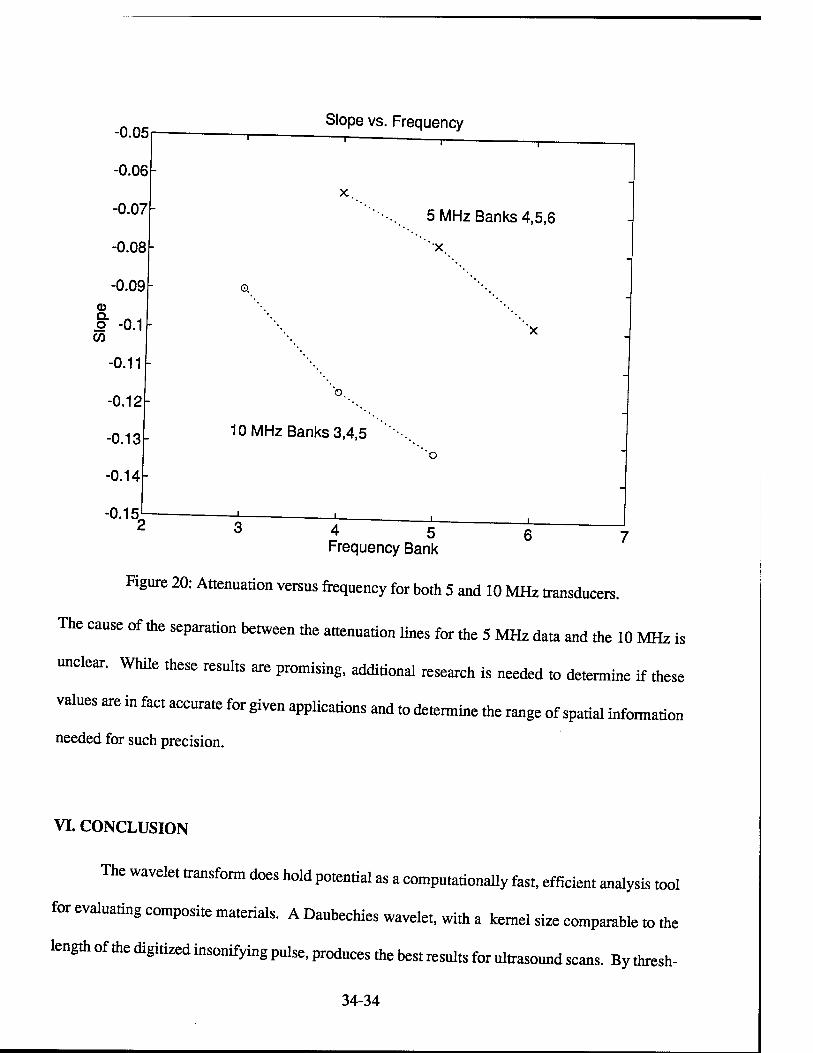
-0.05 i— —i i
-0.06
1 i i 1 _.
X-. -0.07 5 MHz Banks 4,5,6
-0.08 "x.
-0.09 Q
a>
o" -0.1 CO
X
-0.11
-0.12 b
10 MHz Banks 3,4,5 -0.13- 'o
-0.14-
-0.15- — 1 _
2 ° p Q 5 6 7 Frequency Bank
Figure 20: Attenuation versus frequency for both 5 and 10 MHz transducers.
The cause of the separation between the attenuation lines for the 5 MHz data and the 10 MHz is
unclear. While these results are promising, additional research is needed to determine if these
values are in fact accurate for given applications and to determine the range of spatial information
needed for such precision.
VI. CONCLUSION
The wavelet transform does hold potential as a computationally fast, efficient analysis tool
for evaluating composite materials. A Daubechies wavelet, with a kernel size comparable to the
length of the digitized insonifying pulse, produces the best results for ultrasound scans. By thresh-
34-34

olding the resulting wavelet transform coefficients, the scan lines can be compressed with minimal
error in the reconstruction. Depending on the application and corresponding resolution, compres-
sion ratios of 50 to 1 can be achieved.
Wavelet transform scalograms can depict transient flaws providing a histogram equaliza-
tion is applied. Characterization of debondings and cracks based on the scalogram patterns still
requires more research. Part of the problem in material characterization based on wavelet coeffi-
cients is the inherent non-linear shift variance of the wavelet transform. Techniques must still be
devised to account for unknown shift variations. Finally, the localized attenuation coefficient can
be obtained form the wavelet coefficients, but the error associated may preclude accurate
assessment-
While none of the analysis results demonstrate a remarkable breakthrough, the discrete
wavelet transform has provided a unified basis for a combined analysis. This research has shown
that wavelets can be useful in the non-destructive evaluation of composites and may be instru-
mental in the future automation of such processes.
ACKNOWLEDGMENTS
The author is indebted to Edward Meyer, a Ph.D. candidate in the Electrical Engineering
Dept., who developed and coded the Wavelet Demo Software Package and performed most of the
analysis simulations for this project. The author would also like to thank Dr. Tom Moran, Dr.
Prasanna Karpur, and Brian Frock from Wright Labs for their suggestions and insights.
34-35

VIZ REFERENCES
[1] Chui, CK. An Introduction to Wavelets (Academic Press, San Diego, 1992).
[2] Rioul, 0. and Vetterli, M., "Wavelets and signal processing," IEEE Signal Processing Maga-
zine.Oct. 1991, pp. 14-38.
[3] Daubechies, I., »Orthonormal bases of compactly supported wavelets," Comm. Pure Appl.
Math., V. 41, pp. 909-996,1988.
[4] Mallat, S.G., "Multifrequency channel decompositions of images and wavelet models," IEEE
Trans. Acoust., Speech, Signal Processing, V. 37, pp. 2091-2110, 1989.
[5] Press, W.H., Teukolshy, S.A., Vettering, W.T., and Flannery, B.P., Numerical Recipes in C
(Cambridge University Press: New York, NY, 1992)
34-30
STOCHASTIC MODELING OF MBE GROWTH OF COMPOUND SEMICONDUCTORS
Ramasubramanian Venkatasubramanian, Assistant Professor
Department of Electrical & Computer Engineering
University of Nevada, Las Vegas
Las Vegas, NV 89154
Final Report for:
Research Initiation Program
Wright Laboratory, (WL/MLPO)
Sponsored by:
Air Force Office of Scientific Research
Boiling Air Force Base, Washington, D.C.
and
University of Nevada, Las Vegas
December 1993
35- 1
STOCHASTIC MODELING OF MBE GROWTH OF
COMPOUND SEMICONDUCTORS
Ramasubramanian Venkatasubramanian, Assistant Professor
Department of Electrical & Computer Engineering
University of Nevada, Las Vegas
Las Vegas, NV 89154
Abstract
MBE Brow,h orco„p„und Kmicmdactm, ,„d ,„.,„„ dopl|ig mrestiidied m.ng lhejtocliut.c nodd
i.B appro«,, Th„e ,peci6c prob,em „„.,„ to MBE ,,„„„ „, compo„„d „„.^„^ „.„ ^
G*A, g„„„ ««„«, ,„„« ordering „ CaMAt ind JopLng ot_icondiiet<>r< The rauiis ^ rf
*- p-ojec.» «„ „^ „Hh «p,H„,„U „,„,„ „d lhe ,6r„men, _ ^ Thu> ihe p_M
study validates the use of stochastic modeling for the MRF or tu v .■ >ng lor the MBE growth kinetic studies. Details of results of
each project and its comparison with experiments are presented under the discussion of each project.
35-2
STOCHASTIC MODELING OF MBE GROWTH OF COMPOUND SEMICONDUCTORS
Ramasubramanian Venkatasubramanian, Assistant Professor
Department of Electrical &: Computer Engineering
University of Nevada, Las Vegas
Las Vegas, NV 89154
1 Introduction
High speed, high frequency and low noise electronic device are currently being fabricated by molecular
beam epitaxy (MBE) and studied for potential applications in information processing, signal processing
and communication. Reproducible and controlled growth of these devices by MBE is possible only if the
growth and doping mechanisms and their relation to growth parameters and their influence on the elecrtonic,
optical and transport properties are well understood. The theme of this project is to study the MBE growth
mechanisms of compound semiconductor and in-situ doping using the theoretical tool developed by the
author called "Stochastic Modeling".
This project addresses theoretically three issues of growth: GaAs growth kinetics, surface ordering ki-
netics of GaAlAs and in-situ doping of semiconductors. This report is organized as follows. The GaAs
growth kinetic study and its results and discussion are presented in section 2. The surface ordering kinetics
study of GaAlAs and its results and discussion are presented in section 3. The doping kinetics study of
semiconductors and its results and discussion are presented in section 4. Finally, conclusions are presented
in section 5.
35-3

2 GaAs Growth Kinetics
2.1 Background
The performance of op,«lect,omc de_ ,s degraded by interfacki roughness ^ ^^^ fabrkMed
wtth n,-V s.m.confiucto, compounds. The origin of the interfacisl rooghness b t^ surface iMjta_ rf
the layer on which another hetero-layer is grown There h,™ k Srown. There have been many experimental [1-9] and theoretical
[«51 „,empts lo underetMd the ongin of (he surface kiMtic _ ^ (he MBE ^ ^ ^
COO,. Specifically, the surface ro„gr.e„i„s kin.tics duting MBE ^ rf ^ ^ ^ ^ ^ ^
mo„ito,i„g the refiect.on high e„erg, electron «action <R„EED) intenslty (I, s^ ^ _ ^
heen carr.ed on, for Ce „00, M. ,„ lhe case of Ce study [16), a ti„,„c surface ,o„gr.e„,„g temper.tnr.
above which a smooth surface remains smooth, „ „hserv.fi. U „ conclufiefi that the surface ro„gh.„ir,g is
a result of compete h.tweeu surface r„„ghe„i„g _ such as afisorption .„„ the surface smooth^
process such „ surface migration to stable sites. In the case of r.A , A „, in tn« ease of GaA, study (1], a transition temperature
was observed above and below which the surface is ro„g„.r. This transition tempera,™ „as ohserved to
be fin, ratio and temperatnre d.pe„de„, The k^ „^ ^^ fa ^ _ ^ ^ __
terms of competition between the surface romrhenin„ „„ ro„ghe„mg processes such as adsorption and evaporation and the
surface sm„„the„,ng process such as the mig,,.io„ of atoms to e„e,g,„cally stahl, sites
- -is „o,k, the stochastic mode, of „BE grow.h developed hy the author [„.,,, is employed ,„ stndy
«he surface ,ooghe„i„g kinetics i„ GaAs (I„„, ,„ seclion ,, . ^^ _ ^ ^^ ^ ^
P-nted. ,» section ,3, results of the study of surface ,o„ghe„i„g lin.tics „ (IOO) GaM „ „
and compared with that of the experimental work of Refm Th. nh ■ , L orK oi Ket.[lj. The physical mechanism which describes the
theoretical and experimental observations is also presented q„mm p ,u- , presented. Summary of this study is presented in section
2.4.
35-4

2.2 The Stochastic Model
In the hierarchy of growth simulation models, the stochastic model belongs in the category of macroscopic
models. This model assumes a rigid lattice gas with nearest neighbor pair interactions. The stochastic model
describes the time evolution kinetic equations of MBE growth in terms of the primary macrovariables, the
concentration of atoms in the n<" layer, C(n), and the atom-vacancy bond density in the n'h layer, Q(n) and
is given by Eqs 8a and 8b of Ref.[17]. For details of the model, the reader is directed to Ref.[17-19]. The main
assumptions of the model are: (i) solid-on-solid (SOS) restriction (ii) random distribution approximation
of the surface atomic configurations weighted by the energy of the configuration (iii)Arrhenius type rate
equations for the surface kinetic processes (iv) exclusion of anti-site defects (v) exclusion of effects of surface
reconstruction on the surface kinetic processes.
The time evolution of the macrovariables is described in terms of the rates of such kinetic processes as
adsorption, evaporation and intra- and inter-layer migrations of Ga and As atoms. The adsorption process
is allowed at all sites where the SOS restriction holds, (i.e.), the surface covalent bonds corresponding to the
site from the layer below are satisfied. If the atoms arrive at non-SOS sites, then the atoms are allowed to
migrate rapidly in their weakly bound physisorbed state until they find a proper site.
For the adsorption process of As, the species in the molecular beam is assumed to be diatomic As7
which is equivalent to cracked arsenic. The stochastic model reported in Ref.[17] is suitable for monoatomic
molecular species. As diatomic As2 is used in this model, the terms corresponding to the adsorption process
in Eqs 8a and 8b in Ref.[17] need to be modified as follows. The incorporation of two As atoms in the nearest
neighboring sites satisfying the SOS condition in the In + Ith layer requires four Ga atoms be available as
nearest neighbors in the 2n<* layer as shown in Figure 1. The probability that there exists a surface Ga
35-5

adatom pair in the 2nth layer, Pu is given by:
p _ NGaGa(2n) 1 2CGa(2n) (1)
»here Ha^.) is the 0u - Cu second nearest neighbor bond density. Thtee „^ ^ ^ ^
quired to form the sutface Ga ^ Krangemenl shom in FiguK L TWore| (he ^^ ^
the« exists surface atomic arrangements as shown in Figure I, P„ w.
The concentration of C„ atoms which have nearest neighbor „,a„g,m,nt „ show„ „, ^ ,_ ^ .
given by:
C,(2») = ce.(in) P.
Thus, the concentration of sites avaiiabie for ^ incorporation in the 2„+ !■» layer, given bv Eq 4 of Ref.,17]
modifies to:
WuO-l) 1 j C0(2n) _ [C,(2n)-C4,(2n + 1)] (4)
Since ,h. As atom, ,„ mcorporating on the nearest neighbor sit. as pairs, the time evoiution of the
atom-bond macrovariab,., «,.(2„ + ,), Meds _ be modified _ ^ ^ ^ ^ _^ ^ ^^
the coordination „umber for ,„y surface site is 4 „hen considering ,he incorporation process „ono.tomic
mo.ecuiar beam specie,. Whereas, for the present study, the effective coordination number for a site i, o„y
3 - one of the „ea,Kt neighbor site „i„ be sim„,ta„eous,y occupied by the acc„mpa„yi„g As ,lom. This
change needs to be made in Eas 8a ar>A «K T* • a . , fcq.. 8a and 8b. It » noted that the terms corresponding to the intra- and
interlayer surface migrations need not be modified as the changes in .... A . , u cu, me cnanges in the As molecular species do not influence
35-6

rates of these processes directly.
The evaporation and surface migration processes are described by Arrhenius type rate equations such as:
R = R0e-^rr (5)
where R is the rate and R0 is the frequency factor of the process in sec"1. Eaci is the activation energy of
the process for an isolated terrace adatom, Kaa is the second nearest neighbor pair interaction energy in the
(100) plane and n is the number of nearest neighbors of the atom under consideration. Thus, the activation
energy term appearing in the argument of the exponential is coverage dependent with n equal to zero and
four for low and high coverages, respectively. In general, the Eact for surface migration is smaller than that
of evaporation. In this study, the Eact for interlayer and intralayer migrations are assumed to be equal. The
surface migration of an atom to non-SOS site is not allowed.
The model parameters for the present study of the MBE growth of GaAs were obtained from the literature
and the MBE growth parameters of Ref.[l]. The atom pair interaction energies for the second nearest
neighbors Ga - Ga and As - As were obtained as 0.25 eV and 0.325 eV, respectively, based on the data
reported in Ref.[20]. The frequency factors for the evaporation and migration processes were chosen as 1.0
x 1013/sec. The activation energy for surface migration of isolated Ga and As atoms was chosen as 1.3 eV
based on Ref.[7]. Based on Ref.[6], the activation energy for evaporation of an isolated As was chosen as
1.675 eV.
The MBE growth parameters for this study were obtained from the experimental data given in Ref.[l].
The growth temperature was chosen in the range 723 - 873°K and the flux rate was set at 2 A/sec. The
cation to anion flux ratio employed for the study was in the range 1 : 10 to 1 : 20. It is noted that the (100)
substrate surface employed in this study is flat without any steps.
The material and growth data discussed above were employed to calculate the model parameters according
35-7
to the procedure detailed ln sect.on IVB of ^.[17,. The mode, parameters were obtained as a function of
growth temperature. The t.me eVolution Rations given by Eqs 8a and 8b ^ modifications ^ ^
E, 4, and the boundary conditions corresponding a flat substrate descnbed by Eq 14 of Re,[17] _ soIved
numerically on a CRAY YMP 2/216 at NSCEE, UNLV Nevada The CPTT f f , u Lv, IN evada. 1 he CPU time for a typical growth of 20
A of GaAs was about 4 hours.
2.3 Results and Discussion
Concentration p,o«les _ obtai„ed .. , funciim of tjme for various growth ^^ ^ ^ ^
for «-K. 84,K and WK in Fig„re ^ rMpectjve|y] for „„ Mio l:1^m F. ure ^ c for ta ^
I : ». Be,ow 823-K, the concentrate profiles look ,„,„„ fe ^ ^ rf ^ ^ ^ ^ ^
-M^d. From Figurea 2 Md 3, it , observed that at and below 823„K, t„e growing ^ is ^^
» * expected when the cation to anion flux ratio is 1 : 10 or hi.he, But „ ,k , to or nigner. But, aa the temperature increasea
■he gro„h surface becomes less ,s.slabifaed, „ , ^ ^ ^ ^ ^ % ^ ^ ^
of the G, and subdue», ,s ,aye,s „ CMM th,ougW ^ ^ rf ^ ^ ^ ^ ^^
»motion of the ,ay,, The t,me May „,,„,„ „,. grow(h „ . „^ rf ^ ^ ^ ^ ^
effect ,s ptomme„t ,„„ larg„ fot higher temperatura and lQwer flux raiios
The above observes about the time evo>uti„„ „f the concentration promes can be exp.amed . fol.
lows. The gro„,h „f an As ,ay.r ,s co„,rolled hy ,„„ surfac. process»; adsorption and „„„ A[
temperatures We, than 82„. the evaporation of surfac. „ is nagligib,a _„, ^ fte ^ ^
- e^a. «o the adsorpt.ou rate which is constant duri„g the urowth of a ,ayer. Thus, the time de.av durin,
the growth of the layer is constant with time If th» t with time. If the temperature is above 823«% the temperature is high
enough that the evaporation of surface As be«nn, TV, lU , ■ As begins. The growth of an As layer is now controlled by the
competition between the adsorption and evannratinn P and evaporaüon processes. The growth rate is the difference between
35-8

the adsorption rate and evaporation rate. The adsorption rate is independent of the coverage, whereas, the
evaporation rate critically depends on the coverage through the activation energy for evaporation which is
the binding energy of the atom as discussed under Eq 5. The binding energy of a surface As pair increases
with coverage. Therefore, at the start of the growth of an As layer, the binding energy of the As pair is the
smallest possible and therefore, the evaporation rate is the largest as given by Eq 5. The growth rate given
by the difference between the constant adsorption rate and the large evaporation rate is small. Therefore,
there is a large time delay at the start of the growth. As the coverage increases, (i.e.), n increases, the As
atoms attain more nearest neighbors, and hence their binding energy increases which results in a decrease of
the evaporation rate as given by Eq 5. Then, the growth rate increases with the coverage which results in a
continuous decrease of the the time delay. The time delay is more at higher temperature, due to an increase
in the evaporation rate and at lower flux ratio due to smaller adsorption rate. Thus, at lower temperatures
and higher flux ratios, the surface appears more ^-stabilized. The description of the surface processes is in
complete agreement with the mechanisms proposed in Ref.[l] based on the experimental observations.
The intensity of a specular spot (1° off Bragg) of reflection high energy electron diffraction system with
10 kV electron beam was calculated using kinematical theory of electron diffraction as a function of growth
time. The time averaged RHEED intensities, TRI(T) were calculated for various growth temperatures. A
plot of TRI(T) versus growth temperature is shown in Figure 4 for flux ratios 1 : 10 and 1 : 20. The
TRI(T) decreases below and above a certain called the transition temperature, and is identified as 770°K
and 800°K, respectively, for flux ratios 1 : 10 and 1 : 20. The lower TRI(T) above and below the transition
temperature is directly related to rougher surface. Below the transition temperature, the thermal activation
for surface migration is low and therefore, the Ga and As atoms randomly adsorb on the surface at sites of
their arrival resulting in a rough surface. As temperature increases towards the transition temperature, the
thermal activation and hence surface migration increases, resulting in adatoms finding energetically more
stable sites. This surface process decreases the surface roughness. Above the transition temperature, the
35-9

w,.h decreased RBEED inMnsUv due lo destpuctive interference onhe eiectfM TOve> ^ ^ ^
surface layers. Thu, the RHEEO i„t,„s,ty peaks at the lransitio„ lempe„ture ^ fc ^ ^^
of WTO ea„ he eipl^ed - follows. Lowe, ta rat,o re8ults in long„ ^ fc ^ ^^ rf ^
atom cluater, with more tha„ two „ a[oms This impUes ihat the ^ ^^ ^ ^ ^
gro».h or monomer „t * , latger due ,_ ^ dependMt ^^ eMtgy fe ^^ ^
hence lower transition temperature This is in <r™,4 a • , P raiure. ihis is m good agreement with the work of Chen et al. [1]
The experiments otervalions of steady state RHEED intensity TO ^^ ^ ^ ^ ^ ^
the competition hetween »ari„us surfice „ ^ ., ^^ ^ ^^ ^ ^ ^ ^
"*" rOUghmin5 "^ *"d ,he — ""o'»«"o - .». -, edges which is a surface smoo.hh* proce, Th,s explanat.ou „ similar lo tha Me givM m this pspep M ^ ^ ^ _^ ^
- -1 ^.» due to „ndom incorpomion of atoms At |ow temperaure8 (he sutfM ^^ ^
- -d heue, the su,fac, smoo,h,ng etet „ _ Bu[, at high ^^ (he ^ ^ ^
surface mig,a„o„ ald in atoms reachjng m„y „ ^ ^ ^ ^ ^^
evaporation of ,s !rom the sutface ,5 rapoMible for the rMgher sutfsce Md w RHEED ^ ^
» m M~— with the proposed mechaui™ in «.„. Thus ^ ^^ ^ ^^ ^ ^^
and used iu this s,dy for the MBE grow.h studies of Go,s (100), accMa(ely ^ ^ ^ rf^
»Pahen,», of CaAs and also aid, „ apde.Updip, ,he details of the „echap.p,, under,ying the ^
roughening phenomenon.
The p,oe of ™ rasus tempetatute oblamed ^ ^ ^ _ ^^ ^ ^ ^ ^ ^^^
-«, of Chen e, a, W and Serai.qMnl,tative agteement ,,_ fte ^ ^ ^ ^ ^ ^
mam reasons fo, the quMiutive difference between the results- til Th. m I , me results, (i) The molecular species is employed for
«he experiments ,*,, Md our work ^ „ ,„_ ^ ^ ^ ^ ^^ ^ ^ _^_^ ^
ou, wo,k may he different as experiment, fc ratios are always reported in e^a,e„, heam pre^nre ,a.ios
35-10
not in terms of rates of arrival of anion to cation as done in our work. Both of this can influence the result
of transition temperature quantitatively.
2.4 Summary
The stochastic model of MBE growth based on the master equation approach with solid-on-solid restriction
and quasi-chemical approximation employed for the study of surface processes in (100) GaAs growth. The
growth rate, the time averaged surface roughness and the time averaged RHEED intensity were obtained for
various growth temperatures. The kinetic surface roughening transition temperature for the MBE growth of
GaAs is identified as 770°K and 800°K for flux ratios 1 : 10 and 1 : 20, respectively, from the temperature
dependence of the time averaged RHEED intensity. The results of this study compare favorably with that of
the experiments obtained under similar growth conditions[l]. The phenomenon of kinetic surface roughening
transition in the MBE growth of GaAs (100) is explained in terms of the competition among various surface
processes such as the incorporation and evaporation of atoms which roughen the surface and the surface
migration of atoms to energetically favorable sites which smoothens the process.
3 Surface Ordering Kinetics of GaAlAs
3.1 Background
The presence of long range ordering in as-grown epilayers reduces the band gap of the material and thus has
implications for opto-electronic device applications. Long range order has been observed in many compound
semiconductors grown by MBE and MOCVD [21-22]. A few of the compound semiconductors which exhibit
such order in as grown samples are: GaAlAs, GaAsSb, InAsSb, GalnAs and GalnP. The presence of
ordering in the epilayers is usually observed using transmission electron microscopy (TEM). The ordering
observed in these compounds has been shown to be affected by growth and surface conditions and to be
35-11
pendent o„ orientation. Eor example, ,» „BE grown ^.^^ „ _ „^ ^ ^ ^ rf
ordering „ observed ,n term, of th. inlens,ly of ^„„^ ^^ ^ ^ ^^ ^ _
the substrate orientation, growth temperature and the Al content [22].
In this work, the stochastic mode, approach developed fo, the study of the MBE growth of compound
semiconductors M is emp,oyed to sl„dy the MBE surface ordering kinetics of C^.ALA, ,n section
3.2, a h„ef discussion of the stochastic mode, for the MBE a.loying studies i. presented. The result, of the
surface ordering kinetic s,udy of Oa^As „. discussed and compared with the experiments w„,k „f
Ref.[21J in section 3.3. Summary is stated in section 3.4.
3.2 Stochastic Model for Alloy Kinetic Studies
The details of the development of the stochastic mode, for the MBE growth of .Hoy compound semiconductors
has heen presented elsewhere [„,18]. Du. lo llmited sp„e, 0„y ^ ^ ^ rf ^ ^^ ^
are discussed in the following section.
3.2.1 Time Evolution Equations for MBE Kinet 1CS
rates The stochastic mode, describes the time evolution of the macovariahle, of growth In terms of the
of the surface kinetic processes. The development of the model is hased on ,h. „aste, Ration scheme
and the random distribution aDDroximaHnn TV^ „ approximatton. The assumptions necessary fo, the derivation are: (i) a rigid
zinc blende lattice oriented along the 001 direct;™ t::\ i - g direction (u) excluston of the effects of surface reconstruction and
strain „ii, exclusion of ,h. creation of anti-site defects The kinetic procesa considered in the description of
•he time evolution ^nations are: adsorption and surface migration of Ca, M and A, AU of the „riving
«ions (C and ,„ are allowed to adsorb at o, the „ear the sites of their arrival depending on whether
neighbor site, the sticking coefficient nf th* ,.,*• g coefficient of the cations is maintained at unity as experimentally observed. In
35-12

the range of temperature of this study, the evaporation of atoms is assumed to be negligible. The rate of
surface migration of atoms, R (sec~l), is given by:
(£.c+rK..)/lT (6) R = R0e
where R0 is the frequency factor and the Eact the activation energy for an isolated atom on the terrace, x
the number of in-plane atom-atom bonds and Kaa the interaction energy of such a bond. Both the intralayer
and interlayer surface migrations rates are assumed equal.
3.2.2 Macrovariables
Two sets of macrovariables - one for each sublattice can be denned. For the purpose of this study, it is
assumed that the cations belong to the even sublattice and the anion, As, belongs to the odd sublattice. The
macrovariables for the 2nth layer are: concentration variables, CGa(2n) and CAi(2n), atom-vacancy bond
densities, QGa(2n) and QAi(2n) and atom-atom bond densities, ArGaA/(2n), JVGaGo(2n) and NAIA,(2n).
All the bonds referred to in this manuscript are second nearest neighbor bonds, where the whole crystal
is considered. They are also the first nearest neighbor inplane bonds in the (001) plane. Of the seven
macrovariables, only five are independent because of the following relations:
NGaGa(2n) = 2CGa(2n) - ^QGo(2n) - -iVGaA,(2n)
for Ga - Ga bond density,
NAiAi(2n) = 2CAl(2n) - ^QAi(2n) - -#GaA/(2n)
35-13
for Al - Al bond density and
Nvv(2n) = 2(C„(2n)) - lg(2n)
where
C„(2n) = (1.0-C(2n))
and
C(2n) = CGa(2n) + CA/(2n)
and
0(2n) = <J0.(2n) + <J^,(2„)
whe,e C„(2») is the vacnnc, dens.ty, and C(2n) i, lhe total alom concent,ilioI| jn ^ ^ ^ ^ ^ 2
U is as,„med tha, the i„plane coordinat,on „„„^ , ^ ^ ^ ^ ^^ ^ ^ ^ ^ ^'
anion lattice. For the study G,asAlo^ on|y the ^ ^^ ^ ^ ^ ^ ^ ^
■UblSlfc The" Wi" bC '" '"d^d"' * * *• cation sob,.«,» and tTO depend.», v.riables
for .he anion lattice. Thns, there is a tota, o, seven i„depe„dent mactovariab,M „_ „.^
needs to he mod.i.d fot a complete tecription Qf the MBE growth kiMia in (his study [he ^^
vanables for the cation sublattice are chosen as: C„„(2n) C.,(2nl n n , n ,„ > , - °°(z°' °-<«2n), <3o.(2n), 0j,(2n) and /Vo„,(2n). For
the anion sublattice, the independent variables are: C,.(2n+1) and Q„(2n+1).
3.2.3 The Ga^A^As Alloy System and Model Parameters
The Ga - <?«, Al - ^ and Ga - Al second nearest neighbor pair interaction energies were obtained from
the first principle calculations and found to be [6]:
35-14

Vaa-Ga = O.OOOeV,
VM-M = O.OOOeK
VGa-A, = O.UAeV (8)
It is noted that the VGa-Ga, VM-AI, and VGa-Ai are different for sigma and pi bonds (i.e.), if they are
along the covalent bond or perpendicular to it. Since, the present model is unable to differentiate between
the sigma and pi bonds in a layer, the energy values are averaged and used for both types of bonds. This
assumption is one of the possible reasons that the present study may show the correct kinetics, but may
not show the correct type of ordering in the grown crystal. The activation energy of surface migration for
Ga and Al are assumed to be 1.3 eV and the frequency factor is assumed to be 1.0 x 10¹³/sec. The growth
conditions considered for this study are: flux rate of cations is 2 A/sec; cation to anion flux ratios 1 : 10, 1
: 20 and 1 : 30; and substrate temperatures in the range of 760 - 880°K.
Since the equations governing the time evolution of the macrovariables are coupled, nonlinear, first-
order differential equations, they are not analytically integrable. They were numerically integrated using a
numerical integration scheme on a CRAY YMP 2/216. The average computational time for a typical growth
of 7 monolayers was 3-4 CPU hours.
3.3 Results and Discussion
The macrovariables, CGa(2n), CA,(2n), CAs(2n+l), QG«(2n), QAl(2n), QA,(2n+l), and NGaAi(n) were
obtained as a function of time for various temperatures in the range of 760-880°K which is the typical range
35-15
of growth f», lb« co„,po„„d». The shott Knge or(Jet (SR0) parameto ^ ^
ETV C(2n) J (9)
~ evaluated . v„iou3 flux „^ tempetatures Md arsen.c spe£ies The SRO ^ ^ ^ ^ ^ ^ ^ o
and 2.0 fo, „mp„,5ly wvtad> complae|y random Md ^^ orfered ^ ^^
A Plo, of SRO palate, rasus temperalure „ shora „ pignre 1 fot lhe _ rf fte dutomjc motaiat
»peci« *, („acfced -^ „Uh ta ratios of ! : 10, X : 20 and ! = 30. The kinetic otdat-d^de,
temper «. trom Figure , lo „, „„ m ^ ^ ^ te ^ ^ j ^^ ^ ^ ^ ^
: 30, respectively. The temperature dependence of th* SRO „ penaence ot the SRO parameter can be explained as follows In
•he >o. .empe„ture reg,me, the effective migtatio„ ^ Q{ Qa ^ M ^ ^ ^ ^ ^^ ^
chances of s^iin, many differenl „^ ^ ^^ ^ ^ ^ ^ ^ ^^
™domIy a, lheit „rival 8itK ,eading ,o a sma||K SRO parameter A> ^ ^^ ^^ ^
effect raigtati0„ „te inere^ re5ulting in _ 8ampling ^ ^ ^ ^^ ^ ^ ^ ^
,f atotns ^ enable8 them [0 flnd eMrgeiica|,y Wib|e atomi£ sta M ^^ AI ^ ^
•he W.tion temp.,a,n„, the ^ e„ergy becotnea comparable l0 the eMrgy ^^ ^ ^
energetically most and least favorable surfarp „♦„„,■ * surface atormc configuration. Thus, the thermal randomization of
surface atomic configurations sets in and lead«! to a ™ J leads to a more random arrangement of Ga and Al atoms, resulting
in a decrease of the SRO parameter with temperature Th. * •*• . w temperature. The transition temperature and the maximum value
of the SRO parameter are lower for lower flux rati„0 u .. «. . lower ttux ratios because the effective migration rate for lower flux ratios
are higher.
A plot of the temperature dependence of the UnU^A T ~ .- ~ nee oi tne Isolated Terrace Cation Parameter (ITCP) (ITCP is the
««ion of i^ted te™. cation which ca„ be obUmed ftom (he c_ntrat_ oic^ Mom
-aca„cy hond de„sity „d a^-a.on, bond d„sity usl„s randon d,stributio„ ^^^ _ ^ ^
35-16
Ref. 19) is shown in Figure 2. The ITCP increases with temperature for flux ratios 1 : 10, 1 : 20 and
1 : 30. This behavior indicates that the transition temperature is close to 760°K which is consistent with
the results of Figure 1. The physical explanation of thermal randomization increasing the concentration of
isolated terrace adatoms correlates well with decreasing degree of ordering.
Similar trends in the temperature dependence were observed for the case of monatomic As. It is not
reported here due to limited space. These results were compared with the experimental work reported in
Ref. [21]. The qualitative agreement between the results in terms of the temperature dependence of the SRO
parameter is excellent. One of the major differences between the results is that the type of ordering reported
in Ref.[21] for the MBE growth of (100) Gao.5Alo.5As Experimentally, L\0 type ordering is observed. Our
results show the ordered structure in which Ga atoms are surrounded by Al atoms and vice versa. The above
described structure is not an L\0 type ordered structure. The reasons for this discrepancy in the type of
ordering are as follows. Firstly, the L\0 type ordering results from the difference between the bulk-surface
and surface-surface pair interaction energies of atoms which the stochastic model does not take into account.
Secondly, the atom pair interaction energies for sigma and pi bonds were averaged out and both bonds
were treated equal for simplicity. At present, the authors are working on incorporating this detail into the
stochastic model.
3.3.1 Summary
The surface kinetics of MBE growth of (100) Gao.5Alo.5As was studied theoretically using the stochastic
model for various growth conditions. The degree of ordering was obtained in terms of the short range order
(SRO) parameter. The order-disorder temperature was obtained for flux ratios of 1 : 10, 1 : 20 and 1 :
30. Both As and As2 species were considered. For the As? soource, the order-disorder temperature was
found to be 780°K with a maximum degree of ordering of 85 % for a flux ratio of 1 : 10; 800°K with a
maximum degree of ordering of 84 % for a flux ratio of 1 : 20; and 810°K with a maximum degree of ordering
35-17

of 83 % for a flux ratio of 1 : 30. The results are i» good qualitative agreement with experiments. The
surface ordering kinetic, observed can be described in terms of the effective surface migration rate of cations
as follows. The qualitative agreement between experiments and theory is excellent. The key difference
between the experiments and theory is in the type of ordering observed. This difference is attributed to the
indistinguishability of various types of second nearest neighbor bonds, (i.e.), sigma, pi, surface-surface and
surface-bulk, in the present stochastic model. Presently, work is in progress to incorporate these differences
in the bonds in to the stochastic model.
4 Doping Kinetics in Semiconductors
4.1 Background
Doping an epilayer during its growth by coevaporating the dopant has been the standard practice in molecular
beam epitaxy (MBE) of semiconductors. Due to low growth rates (1 ,m/hr.) and low temperature of
growth (i.e., limited or negligib.e bulk diffusion), abrupt dopant profiles should be achievable in MBE grown
epilayers. However, for many dopants in Si MBE growth, either a smearing of the dopant profile and/or
surface enrichment of the dopant have been observed experimentally [24]. In addition, it has been observed
that some dopants incorporate inefficiently in some semiconductors due to excessive evaporation dictated by
low binding energy of these dopants to the growing surface.
Many theoretical models, both thermodynamic and kinetics based, have been proposed to explain these
experimental observations. Iver et al mil nr™ i i • .- ryer et al [25] proposed a kinetic model which described the time evolution of
surface concentration of dopant i„ terms of incorporation aud evaporation. Their model »as good enough
to expiam many experimental observations in th. doping of Si and GaAs [25]. However, it did no, expUcitd,
inc.ude th. surface segregation phenomenon. Barnett et a. [26] proposed a mode! including the segregation
Phenomenon in which they turned that dopants from several nanometers of subsurface diffits. to the
35-18
surface. Rockett et al [27] proposed a kinetic model to describe the surface segregation phenomenon of
Sn in GaAs. In their approach, a relationship between the bulk diffusion coefficient and surface diffusion
coefficient was assumed. This relationship does not include effects of surface conditions such as the roughness
or coverage. From the analysis and comparison of the results of their model with the experiments, they
concluded that their model was sufficient to explain the experimental observations. Andrieu et al [24]
proposed new physical mechanism of dopants climbing to the surface and developed a rate equation model
based on this assumption. Their model was able to explain the surface segregation phenomenon satisfactorily.
However, the pre-exponential factor for their rate processes was 10-ns_1 which is not physically justifiable.
Even though each of these model is suitable for one or more dopant-semiconductor systems, none of them
is, however, completely satisfactory for all systems, incorporate all observed effects. The model developed
by Andrieu et al [24] appears to be the best available model, it employs physically unjustifiable exponential
prefactors and therefore is questionable. This manuscript proposes a general rate equation model which cap-
tures most aspects of the in-situ doping kinetics and employs physically reasonable and justifiable parameters.
Thus, it overcomes most of the limitations of the earlier proposed models.
The phenomenological rate equation model is presented in section 4.2. A discussion of the model param-
eters is presented in section 4.3. The results of the application of this model to In doping of Si are presented
and compared with available experimental data in section 4.4. A discussion of the results is also presented
in section 4.4. Summary is presented in section 4.5.
4.2 Rate Equation Model for Doping
The elementary surface kinetic processes that control the doping kinetics are: adsorption, evaporation and
interlayer migration of the the host atom, Si, and the dopant, In, (In is chosen for this study, but the model
is general and can be applied to any system). The rate of change of concentration of Si in the n* layer
35-19
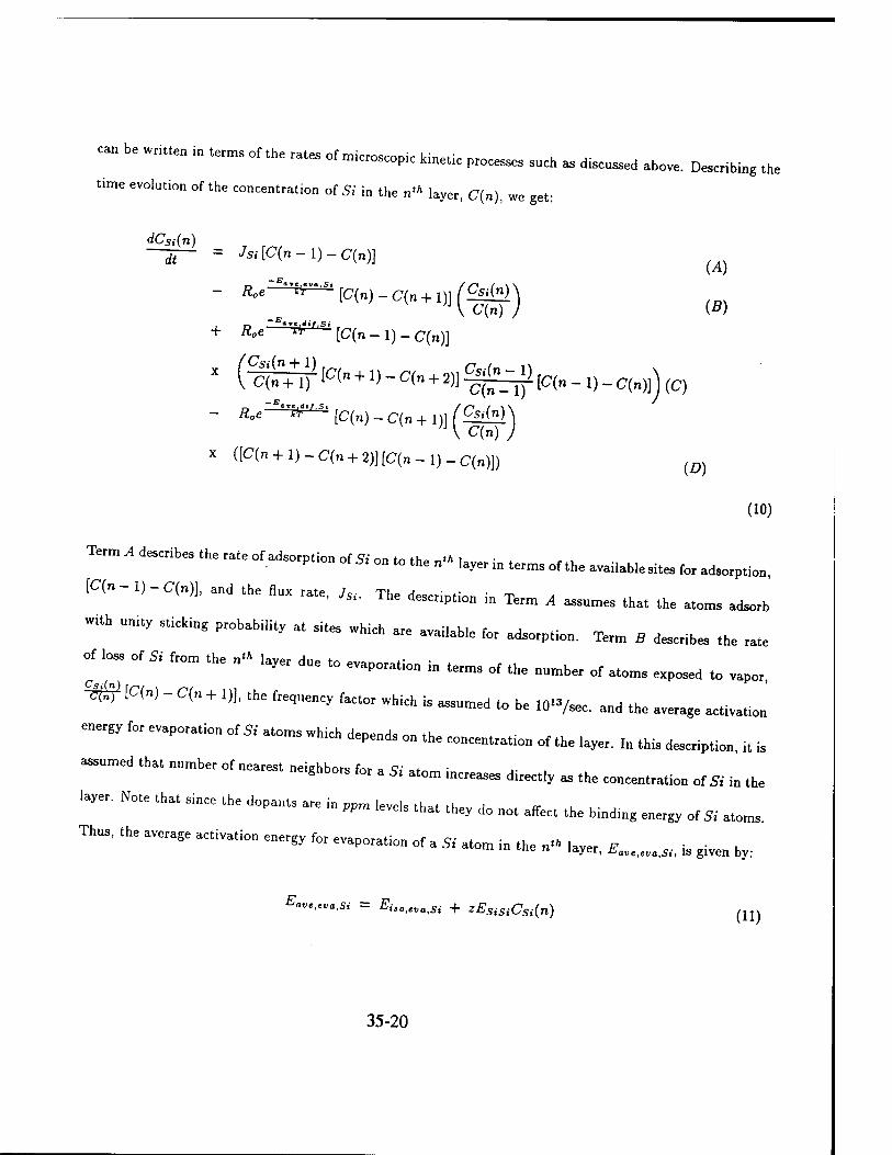
can be wnUen in terms of the rates of microscoP1c Hnet.c processes such as cüscussed above. Describing the
time evolution of the concentration of Si in the n<* layer, C(n), we get:
dCSi(n) " dt = JSi[C(n-l)-C(n)]
- R0e fc'J-
+ R.e "-"-[Cfii-lJ-cOO]
(C(„,-C,„ + l,,(!gg>) (fl)
1 (TOT W"+•> - <*•+»)] ^Lijl (c(„ - „ _ c(„)]) (c) - Ä,e-i!Wia[C(„)_C(„+1)]/'^iW'
V C(») , x (P(» + l)-C-(n + 2)JtC(n-l)-C(n)])
(O)
(10)
Term X desert the rate of adsorpt.on of 5,' on to the .» iaye, in terms of .h. avaiiah,. site, for a^.,
ic<.-1)-<*.)]. Md the Bux rale, ,si The descript.on .n Term A ^ ^ ^ ^ ^
-h nn.ty string p,ob,bility al sltes wUch „e availab|e fot adsorption Term fl ^ ^ ^
-I- of tf from the „, ,sy„ due to evapo„tion jn terms rf (he number rf stom ^ ^ ^
%# [CW - <*. + 1)1, the fluency f,c,„t which is ^^ „, „e ^ and ^ ^ ^.^
energy for evaporation of Si atoma which d»™^* ~„ .L depends on the concentration of the layer. In thia description, it is
•ssom.d tnat nnmher of nearest „eighbors fo, a « atom increases directiy as ,h. concenlPalioo otSi „ ^
Thus, the average actuation energy for evaporat.on of a Si atom in th, „» ,ayeP, £.„,.„. „, „ give„ by.
^««.,««.,5, = Eis0:evaSi + zESiSiCSi(n) (11)
35-20

where z is the inplane coordination number which is 4 for (001) plane and 6 for (111) plane and EsiSi and
Ei.„,.va,si are the second nearest neighbor interaction energy and the activation energy for the evaporation
of an isolated Si, respectively. (Note that in the (001) and (111) planes, the nearest neighbor atoms are
actually the second nearest neighbor atoms when the whole crystal is considered.) Term C in Equation 1
is the rate of gain of Si atoms in the nih layer due to interlayer migration of Si to the nth layer from the
adjacent layers, n - 1 and n + 1. Term D in Equation 1 is the rate of loss of Si atoms in the nth layer due to
interlayer migration of Si from the n"> layer to the adjacent layers, n - 1 and n + 1. The average activation
energy for the migration of Si, Eave,dij,Si is given by:
Eave,diJ,si = Eii0,dif,si + zEsiSiCsi(n) (12)
where Ei,0<<iif,si is the activation energy for interlayer migration of an isolated Si atom.
Similar equation for the rate of change of dopant concentration in the nih layer can be written by simply
replacing Si with In where In stands for the dopant. In the rate equation for the dopant, the activation
energy for evaporation and migration should be redefined as:
Eave,eva,ln = Eucevajn + zESUnCSi(n) (13)
and
Eave,dif,[n = Ei,0,dif,In + zESHnCSi(n) (14)
respectively. In the description of Equations 4 and 5, the fact that the second nearest neighbors of dopant
atoms are essentially Si atoms due to the ppm level concentrations of dopant utilized.
35-21

4.3 Model Parameters and Growth Parameters
The activation energy for the evaporation of an isolated <Ji F u L an isolated bi, Ei,0,evatSi, can be obtained for (100) and (111)
growths as 2.6 eV and 3.2 eV, respectively TOfll Tk. J spect.vely [20]. The second nearest neighbor interaction energy, Esisi for
(100) and (111) growths are estimated to be 0 25 eV and (iw?,v .• , , u.*> eV and 0.325 eV, respectively from Ref.[20]. The activation
-* «, evaporation „, ,. „ „ot ,epmM in the ,tmtm Ttas a trui ^ _ app_h _ ^ ^
« - of .he oata points on the concentation of ,n rasus , p|ot reported t w [28j ^ ^ ^ ^
value of 1.6 eV and -0.25 eV for F- o A V *....«,,„ and ESila, respectively. The activation energy for migration of
an isolated ft, 4.,^, was chosen as 0 8 eV based on avail ki ev based on available experimental data for activation energy
*» Si [7]. 2*..,Ä/,/n, was assumed to be equal to that of Si for lack of available data.
The growth parameters were chosen exartlv ac „c^ r t, exactly as used for the experimental work reported in Ref.[24] and
are presented below. The flux ratp nf Q; T . rate of ft, JSi, was kept at l^m/hr. The flux ratio between ft and /„,
Jsi/Jfn, was maintained at 2 Y in-4 TU„ at 2 x 10 . The evaporation of ft was negligible in the temperature range rf
this study and therefore the growth rate of th« „„l growth rate of the ep.layer was approximately equal to the Jsi. The substrate
temperature was in the range 500 - 750°C.
The nifcent,,, equatlons give„ by Equation : Md a simi|at OM for ^ a[e ^ ^ ^ ^ ^
d.ne,e„„a, equa„o„s „h.ch ate no, anilytically integrab|e. ^^ ^ ^^ _ ^ ^
icah, on the CRAY YMP2/245 located at Natio„a, Super£omputer cMto for Enew ^ MOM
(NSCEE, a, „n,versily ot Nevada, Las Vegas The boundKy condHion is te ^ ^ 3 ^ ^ M ^
5, an. ,est of the ,aye,s a™ empty at the ,latt of lhe gto„lh ^ ^^ fa ^^ ^ ^ ^^
A tvptcal run fo, a growth of 20 seconds took about 1 CRAY CPU hour.
35-22

4.4 Results and Discussion
Plots of dopant sticking coefficient, S/„, versus time (sec.) for various growth temperatures of the study
were obtained and analyzed. (The growths were simulated only for about 20 seconds due to computer
time limitations.) Analysis of the data indicated that 5/„ is an exponentially decaying function of time.
Exponentials of the form, A(T)e~?lW, were fitted for each temperature. Note that A(T) and r(T) are
functions of temperature. Using A(T) and T(T), 5/„ was obtained for the case of 3000 seconds of growth by
extrapolation. Such an extrapolation is justified because the growth rate is constant and the layer-by-layer
growth mode is maintained for all growth conditions of in this study.
A plot of the extrapolated SIn versus £ is shown in Figure 1 along with the experimental data. The
agreement between the theoretical values and the experimental values from Ref.[28] is excellent for the entire
temperature range. The mechanism which results in the temperature dependence of 5/„ is as follows. At
low temperatures, the surface segregation aided evaporation of In (due to its repulsive interaction with the
host sublattice) is not dominant as the thermal energy is not enough to allow this activated process. As
temperature increases, the interlayer migration rate of In to the surface increases and the In concentration
increases in the surface layer. More In in the top surface layer, results in more opportunities for evaporation.
Thus, a larger evaporation of In results at higher temperature. The evaporation rate of In aided by the
surface segregation process is much larger than the typical evaporation rate of atoms from the surface.
Plots of the dopant concentration, C/„, versus distance from the surface are shown in Figure 2 for various
growth times for a growth at 660°C. It is observed that the In concentration in the bulk is about the same
and is independent of the time of growth. The surface concentration of In, however, is increasing with time
as expected. Note that there is a dip in C/„ for all the profiles just below the surface layer. The concentration
of In in this zone is an order of magnitude less than that in the bulk and many orders of magnitude less
than that at the surface. We call this region the dopant depleted zone (DDZ). The physical reason for this
phenomenon is as follows. The dopant, In, segregates from the layers below upwards due to the repulsive
35-23

«om,c interact™ „,th the host |altice ,n o[her _ds considering the nih ^ /n ^ ^ ^
*» » - 1" layer to the .« iayer wh.ch increases C,„(„> Md to the „ + ,,4 Isyer from the „, ,ayer rti£h
leases ChW. The rates „, ,_ ptoc_ depe„d on lhe ava,Iability of/n atoms m the rMpectiye UyMs
wh.ch „. exposed to vapo, „ that they _ migra[e Md the avaiMi[y rf site ^ (he Mpective ^
For .he m.grat.ons ,„ the .a ,ayeP compared l0 lhe migralions from the ^ boih ^ ^ ^ ^ ^
Thus, the rat. of migrat.on to the surface |ayer ftom (he submface uyer js iM5et tta ^ rf ^^
on, „ lh.,ubsurf«e layer fromone Iayer beW Thig d_fference ta the ^ ^ ^ ^^^ ^
atoms ,„ u» subsutface ,ay„. This resembles the pheMmenon of a precip.tat.on depted aoM (pDz) ^
«I. near .he grain boundaries i„ many aiioys. This „» _ „„^ ^ ^ ^^ ^ ^
. «*! observation of .he segregation p,onl. data show„ („ ^ , rf ^ ^ ^ ^ ^ . ^
d,p ,„ .he prohie. ,„ our tesult the dip ,s much more pronoupced compare(i to that ^ ^^ ^
may be due to stronger repulsive interaction energies used in „u, model.
Plots of ,h, ,. segregation prohies for 853'K, 89rK, a„d o33'K a,e shown „ Figu,e 3. „ ^ ^
.he segregation promes are sim.iar for va,ious temperatures «cep, ,ha, the buIk ,. concentration. m lowe,
for h.gher temperature which co,re,ate „e„ with Figure , Thb lype of . dopa ^ _ ^ ^
..ways Be present even if the d„pa„t interactions with the host hattiee i, revive. ,t depends „„ . varie.v
of factors snch as the growth rate, the strength of the repuis.ve .nteraction (£si,„), the ratio, ,„,„> and
others.
4.5 Summary
The mode, is apphed to stndy th. surface segregation phenomenon during ,. doping of S, The doping
andres were performed for various growth conditions. The res* of the predicted sticking coefficient of ,.
35-24
versus j, and the dopant depth profile obtained shows excellent agreement with experiments. The sticking
coefficient decreases with T due to surface segregation aided evaporation of In at higher temperatures. The
surface segregation of In occurs due to strong repulsive interaction between In and the host lattice which
results in upward migration of In. A dopant depleted zone where the In concentration is lower than that in
the bulk and at the surface is observed and agrees well with experiments.
5 Conclusion
The stochastic modeling of MBE growth was employed to study three growth kinetics problems: surface
roughening kinetics of GaAs, surface ordering of GaAlAs and doping kinetics of semiconductors. The
results obtained were compared with that reported in the literature and the agreement obtainmed was good.
This study validates the use of the stochastic modeling as a viable and effective tool for MBE growth kinetic
studies. Many spin off projects from this project are underway at present. Acknowledgement
The authors would like to acknowledge the partial financial support provided by AFOSR under contract
# F 49620-90-C-09076 and CRAY Research Co. The author like to gratefully acknowledge the contributions
of Dr. Srinivasan Krishnamurthy to this work.
REFERENCES
1. P.Chen, J.Y.Kim and A.Madhukar, ''Optimal surface and growth front of III-V semiconductors in
molecular beam epitaxy: A study of kinetic processes via reflection high energy electron diffraction
specular beam intensity measurements on GaAs (100/' J. Vac. Sei. Tech., vol B 4, (1986), p890.
2. C.T.Foxon, M.R.Boudry and B.A.Joyce, Surface Sei., vol 44, (1974), p69.
3. C.T.Foxon, and B.A.Joyce, Surface Sei., vol. 50, (1975) p434.
4. C.T.Foxon, and B.A.Joyce, Surface Sei., vol. 64, (1977), p293.
35-25

5. J.R.Arthur, J. Appl. Phys., vol. 39, (1968), p4032.
6. J.R.Arthur, Surface Sei., vol. 43, (1974), p449.
7- J.H.Neave, P.J.Dobson and B.A.Joyce, Appl. Phy, Lett., vol. 47, (1985), plOO.
8. Seiichi Nagata and Tsuneo Tanaka, J. Appl. Phys., vol. 48, (1977), p940.
9. A.Madhukar and S.V.Ghaisas PBP r,;* o o ,-J <, v.^na.sas, CRC Cnt. Rev. Sohds State Mater. Sei., vol. 14, (1988), pi. (and
references therein).
10. J.Singh and A.Madhukar, J. Vac. Sei. Tech., vol. 1, (1983), P385.
11. A.Madhukar and S.V.Ghaisas, Appl. Phys. Lett., vol. 47, (1983), P247.
12. J.Singh and K.K.Bajaj, J. Vac. Sei. Tech., vol. 3, (1986), P520.
13. J.Singh and K.K.Bajaj, Appl. Phy. lett., vol. 47, (1985), P594.
14. S.Clarke and D.D.Vvedensky, Phys. Rev. Lett., vol. 58, (1987), P2235.
15. D.D.Vvedensky and S.C.arke, Surface Sei., vol. 225, (1990), P373. (and references therein).
16- E.Chason, J.Y.Tsao, K.M.Horn and S.T.Picraux, J. Vac. Sei. Tech., „7(2), 332, (1989).
17. R.Venkatasubramanian, J. Matl. Research., 7, 1222, (1992).
18. R.Venkatasubramanian, J. Matl. Research., 7, 1236, (1992).
19. R.Venkatasubramanian and D.L.Dorsey J Vac Sei T~4, n orsey, j. vac. Sei. Tech., (to appear in Mar/Apr issue 1993.).
20. Srinivasan Krishnamurthy, M.A.Berding, A.Sher and A B Ch.n T A , ou 6> oner ana A.-B.Lhen, J. Appl. Phys., vol. 68, (1990)
p4020.
21. T.S.KUM, T.F.Kuech, W ,.Wa„ga„d W.L.WÜ.ie, Phy, R„. ^ 54, I985, p20,
35-26

22. G.B.Stringfellow, J. Vac. Sei. Tech., B9, 1991, p2182 (and all the references therein).
23. S.Krishnamurthy, (private communication). (These values were obtained from first principle quantum
mechanical calculations. Related article is in preparation for Phys. Rev. Lett.).
24. A. Andrieu, F. Arnaud d'Avitaya and J.C. Pfister, J. Appl. Phys., 65, 2681, (1989).
25. S.S. Iyer, R.A. Metzger, and F.G. Allen, J. Appl. Phys., 52, 5608, (1981)
26. S.A. Barnett and J.E. Greene, Surf. Sei., 151, 67, (1985).
27. A. Rockett, S.A. Barnett, J.E. Greene, J. Knall, and J.E. Sundgren, J. Vac. Sei. Technol., A 3, 855,
(1985).
28. J. Knall, J.E. Sundgren, J.E. Greene, A. Rockett and S.A. Barnett., Appl. Phys. Lett., 45, 689,
(1984).
35-27
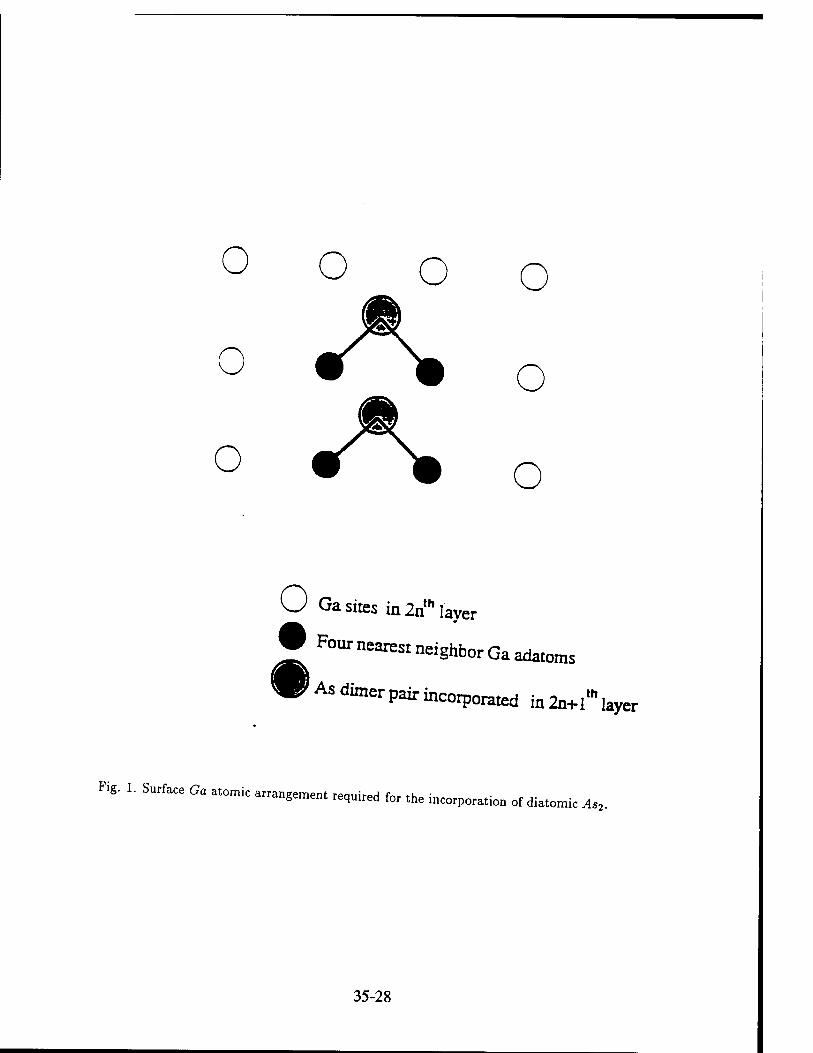
° o O o
o - - o
° - - o
U Ga sites in 2nth layer
• Four nearest neighbor Ga adatoms
• Asdimerpairincorporated inWlayer
Fig. 1. Surface Ga atomic arrangement required for the incorporation of diatomic As2.
35-28
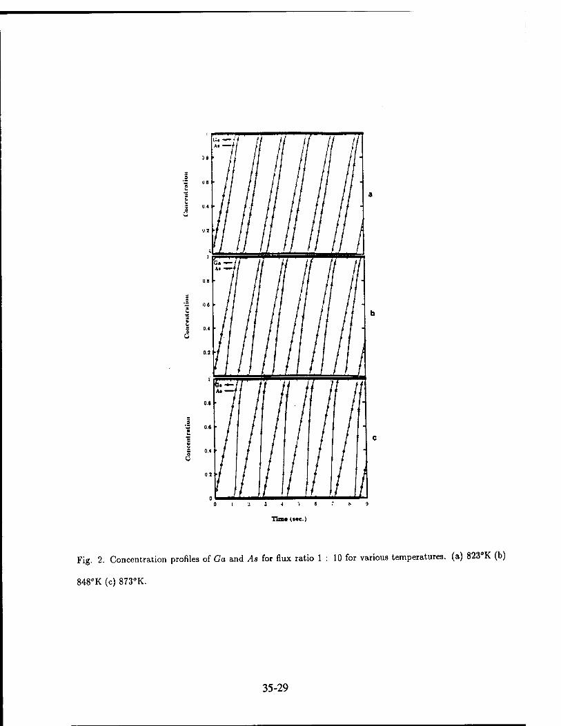
a U
- 0.6
Fig. 2. Concentration profiles of Ga and As for flux ratio 1 : 10 for various temperatures, (a) 823°K (b)
848°K (c) 873°K.
35-29
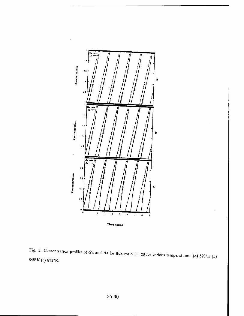
* 9
Tim* dec.)
Fig. 3. Concentration profiles of Ga and As for flux ratio 1 :
848°K (c) 873°K. 20 for various temperatures, (a) 823°K (b)
35-30
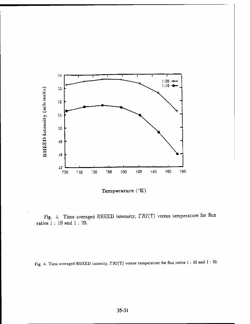
54
71 53
=
*s 52 i» X
>> 51 ■•*
en ^ 50
r* ÜÜ 49 a pmm W* P* 48
47 720 740 750 780 S00 S20 >40 S60 880
Temperature (°K)
Fig. 4. Time averaged RHEED intensity, TRI{T) versus temperature for flux ratios 1 : 10 and 1 : 20.
Fig. 4. Time averaged RHEED intensity, TRI(T) versus temperature for flux ratios 1 : 10 and 1 : 20.
35-31
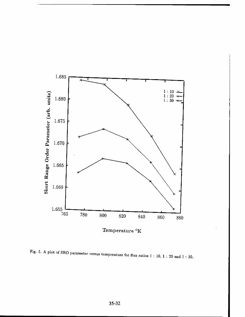
1.685
760 780 800 820 840 860 880
Temperature °K
Fig. 5. A p,ot of SEO p„,m.,er v„ms ,empePMuK for te ritios , ; ^ , ; 2„ ^ , ;
35-32
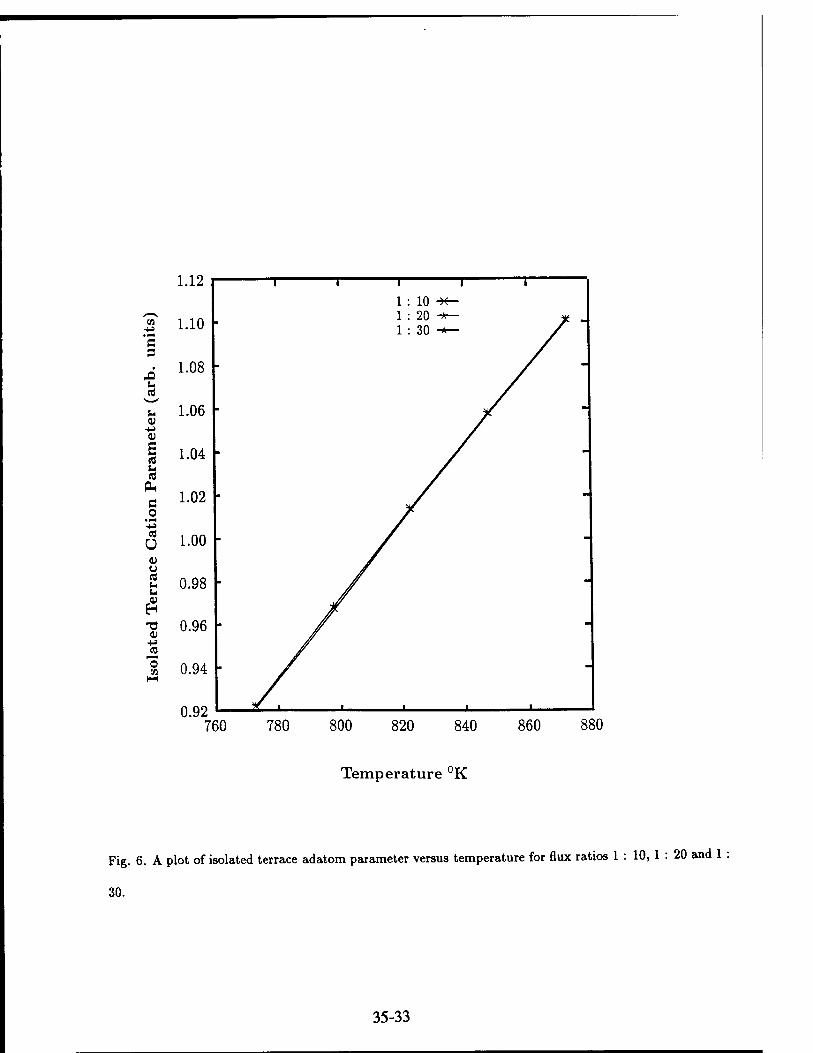
CO -(-9
'S 3
ji u CO
CD
4)
ca
ca OH
c o
Cfl
Ü V u cS t- u
0)
J2 "o
ca
1.12
1.10 ■
1.08 ■
1.06 -
1.04 ■
1.02 -
1.00 -
0.98 ■
0.96 ■
0.94 ■
0.92 760 780 800 820 840
Temperature °K
Fig. 6. A plot of isolated terrace adatom parameter versus temperature for flux ratios 1 : 10, 1 : 20 and 1
30.
35-33
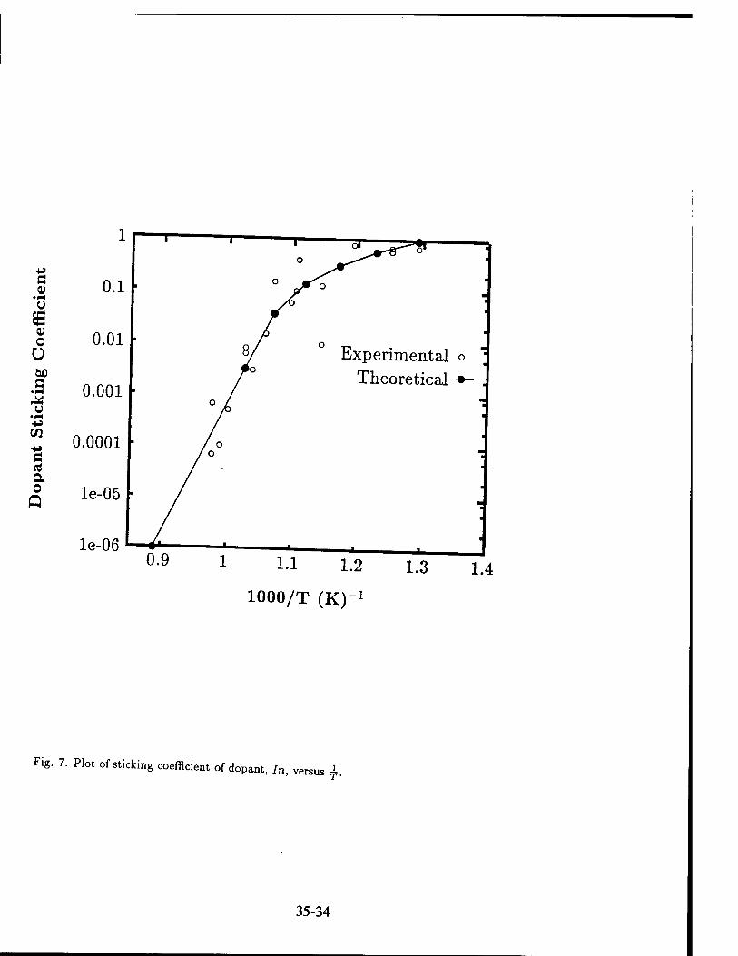
Ö 0) u e o Ü hO Ö
y • PN
Ö
a o
Q
1
0.1
0.01
0.001
0.0001
le-05
le-06 ■—**
Experimental o Theoretical -•-
1 1.1 1.2 1.3
1000/T (K)-1
1.4
Fig. 7. Plot of sticking coefficient of dopant, /„, versus ±.
35-34
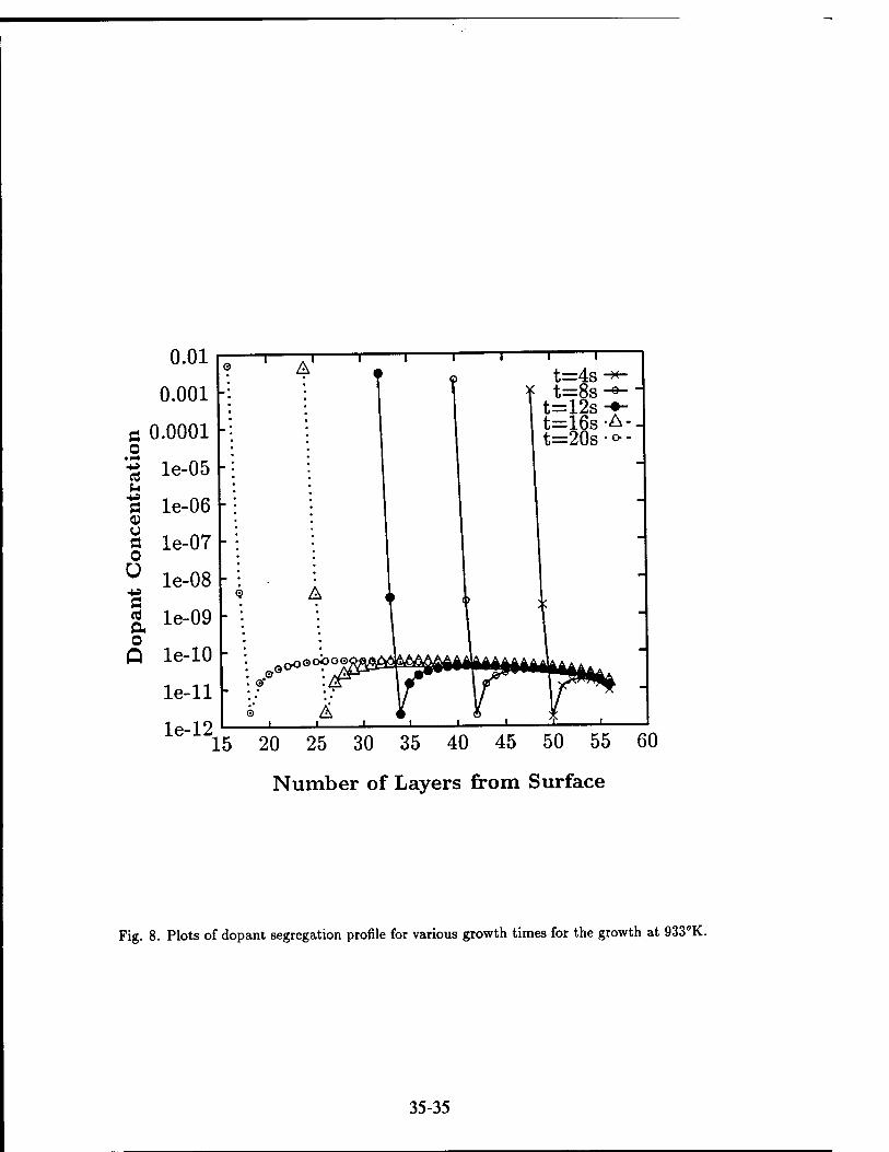
a o a u a U a o Ü a CO
o Q
0.01
0.001
0.0001
le-05
le-06
le-07
le-08
le-09 •
le-10
le-11
le-12
Äoo® ©■
15 20 25 30 35 40 45 50 55 60
Number of Layers from Surface
Fig. 8. Plots of dopant segregation profile for various growth times for the growth at 933°K.
35-35
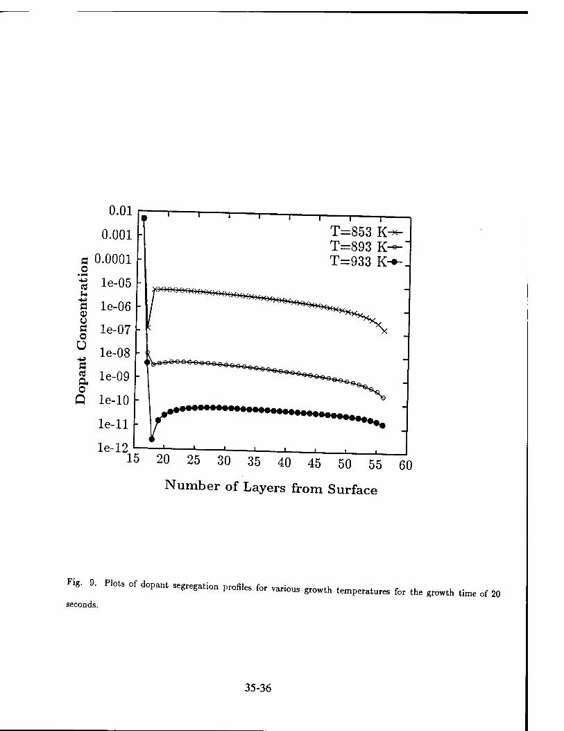
a o -4J CO
-4-9 a u d o
Ü
d a o
Q
0.01
0.001
0.0001
le-05
le-06
le-07
le-08
le-09
le-10
le-11 -
< i^eo'oooooo
le-12
"i 1 r- T=853 K- T=893 K- T=933 K-
15 20 25 30 35 40 45 50 55
Number of Layers from Surface
J 60
Fig. 9. Plots of dopant segregation profiles for various growth temperatures for the growth time of 20
seconds.
35-36
PERFORMANCE EVALUATION AND IMPROVEMENT OF A RESONANT DC LINK INVERTER
WITH A LIMITED Q-FACTOR
Subbaraya Yuvarajan Associate Professor
Department of Electrical Engineering
North Dakota State University North University Drive
Fargo, ND 58105
Final Report for: Research Initiation Program
Wright Laboratory
Sponsored by: Air Force Office of Scientific Research
Boiling Air Force Base, Washington, D.C.
and North Dakota State University
December 1993
36- 1

PERFORMANCE EVALUATION AND IMPROVEMENT OF A RESONANT DC LINK INVERTER
WITH A LIMITED Q-FACTOR
Subbaraya Yuvarajan Associate Professor
Department of Electrical Engineering North Dakota State University
Abstract
Resonant DC Link (RDCL) inverters have several advantages compared to conventional dc link
inverter, Some of the problems associated with an RDCL inverter with a limited Q-factor are studied.
An experimental inverter was built mainly to make quantitative measurements and analyze problems like
zero-crossing failure. The losses occurring in the resonant link were obtained for different link-circuit
parameters. A digital storage oscilloscope and digital data processing software were used in the
computation of the losses. The complete control circuit of the inverter system incorporating Sine PWM
control for the inverter switches was developed. The control circuit which was developed for a single-
phase inverter was extended to a three-phase inverter.
The zero-crossing failure in an RDCL inverter is a serious problem which reduces the efficiency of
the inverter system and increases the power rating of the link-shorting switch. First the effect of load on
the minimum link voltage was studied. A simple method of using current-feedback for eliminating the
zero-voltage crossing problem was first established using computer simulation. The method was
implemented on an experimental inverter system by incorporating current-feedback by using current-
sensing Power MOSFETs as inverter-switches. The details of the complete control circuit incorporating
current feedback and the experimental waveforms are presented.
36-2

PERFORMANCE EVALUATION AND IMPROVEMENT OF A RESONANT DC LINK INVERTER
WITH A LIMITED Q-FACTOR
Subbaraya Yuvarajan
1. INTRODUCTION
High-efficiency power converters are very useful in aircraft and space applications. Resonant DC
Link (RDCL) inverters introduced recently help to keep the switching loss negligibly small even at high
switching frequencies [1] - [4]. The addition of an L-C resonant section in a conventional inverter results
in an oscillating link with periodic zero-crossing points. If the inverter switches are turned-on and off at
the zero-voltage points, there will not be any power loss in the switches. The only condition is that the
operation of the inverter switches is to be synchronized to the oscillatory voltage waveform of the resonant
link. If the frequency of the resonant link is very high, the control signal of the inverter derived from
considerations like PWM remains unaltered.
While the concept of RDCL is very attractive, there are some basic difficulties in maintaining a
stable link with definite zero-crossings. The problem is mainly due to a low Q-factor of the L-C section.
The link voltage of an RDCL with an ideal inductor and a capacitor goes through zero voltage at the end
of each resonant cycle. When the inductor has a parasitic series-resistance, the link voltage gets damped
out. A switch connected across the capacitor is closed for a short time at the end of the resonant cycle so
as to supply some energy to the inductor to offset the damping effect. Fig. 1 shows the power circuit of
an RDCL feeding a single-phase inverter and the block diagram of the control circuit. The link inductor
Lc, the capacitor Cc, and the link-shorting MOSFET QL constitute the link section. The link-shorting
Power MOSFET is driven by a clock signal whose frequency is adjusted to be equal to the resonant
frequency of the link. It is enough if the duty cycle of the waveform is very small.
The project is to study the performance of an RDCL inverter with a resonant link having a limited
Q-factor. Fig. 2 shows the parasitic elements in the link section and the shape of the capacitor voltage in
a typical RDCL. The minimum capacitor voltage Vmin is a critical parameter which decides the
efficiency of the inverter. The effect of varying the values of the link elements on the shape of the link
36-3
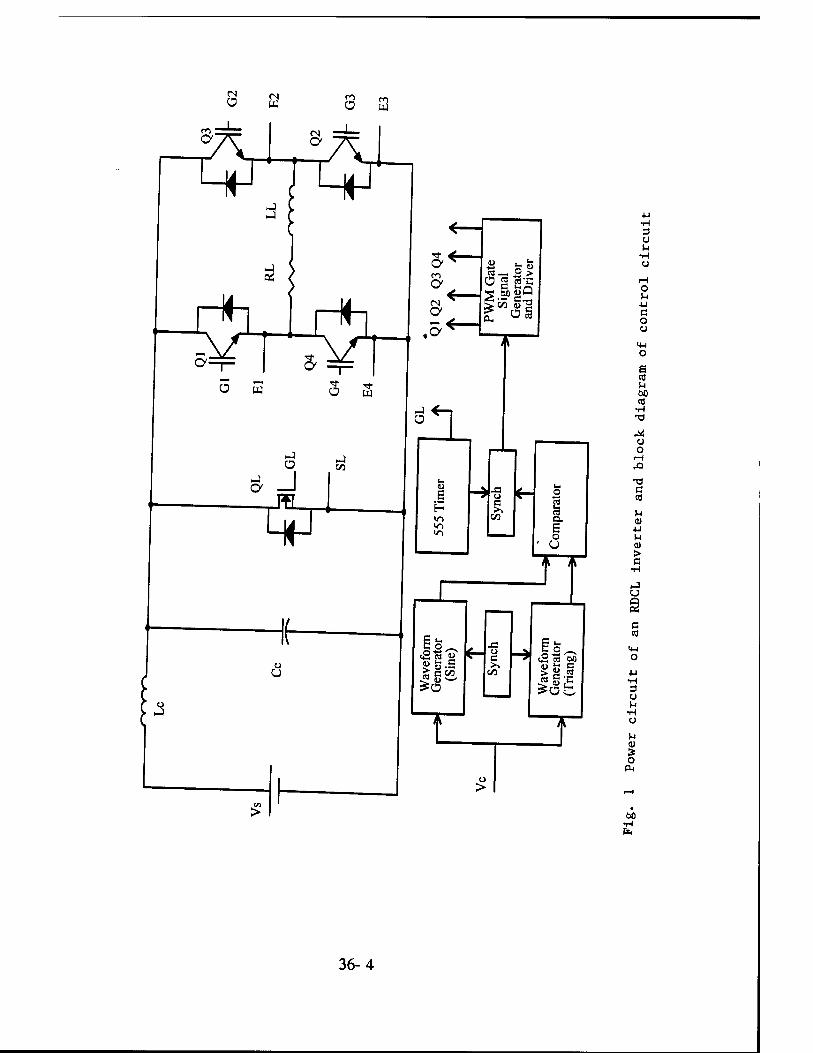
(N o o
3 U u
•H y
o
a o u
s to u M CO
•H •a
u o
c to
u 01
4J M
> C
i-3 U
c CO
3 cj u
u S o
M •H pH
36-4

voltage and the power loss in the link will be studied. In particular, the variation of V^ with the values
ofL andC will be studied. The project also proposes a method to reduce the value of V,^ and to
ensure zero-voltage crossing. Current Sensing MOSFETs will be used to provide current-feedback which
will be used to adjust the frequency and duty cycle of the gate signal to QL. The method will be first
verified by simulating the proposed control scheme using PSPICE [5]. It will be implemented on a single
phase RDCL inverter.
2. THE RESONANT DC LINK
In analyzing the operation of the RDCL, the inverter is modeled as a constant current source [6].
Fig. 3 shows the resulting circuit diagram. If the elements are ideal, R = 0. With the switch S open, the
capacitor voltage vc(t) is given by
vc(t)=Vs(l-Cos(Ort) 0)
where cor=^.
If the parasitic resistance of the inductor is included, the voltage across the capacitor is damped out. The
minimum voltage across the capacitor V^n is given by [6]
It is seen from (2) that zero-voltage crossing is lost if V^X). The value of V^ depends essentially on
the value of (Im-Id) and the values of L and C.
In the experimental inverter built, a Power MOSFET is used to realize the link-shorting switch.
The block diagram of the link-switch signal generator is shown in Fig. 4. The width and frequency of
the gate pulse to QL is varied by varying the potentiometers Rw and Rf respectively. The TTL output
from the 555 Timer is converted into a 15 V signal using a high-speed driver SG3626. The frequency of
the gate signal to QL is around 48 kHz.
36-5
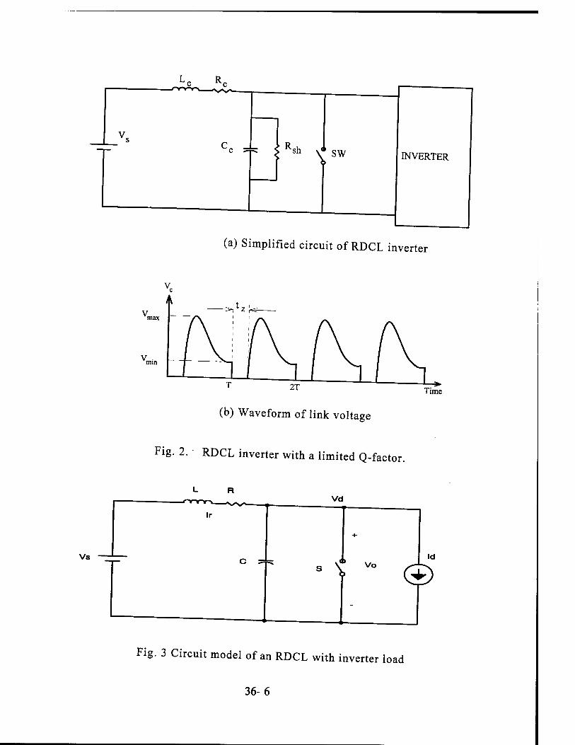
Lc Rc
v_:. _
R sh v* \
SW INVERTER
(a) Simplified circuit of RDCL inverter
(b) Waveform of link voltage
Fig. 2. RDCL inverter with a limited Q-factor.
L R
Vs
Fig. 3 Circuit model of an RDCL with inverter load
36-6

Several designs of the link inductor were tried. In one design, the inductor was built using a well-
insulated flat-copper conductor. In another design, a multi-strand litz wire was used [7]. In both the
designs, only air-cored inductors were built. The inductance-value was varied by changing the number of
turns. The coil resistance was reduced by using parallel construction. The waveforms of the capacitor
voltage and the inductor current under no load were recorded for several LCCC combinations. The power
loss in the link section was computed by recording the waveforms of the current and voltage associated
with all the link elements. It was found that the value of V^ was negligibly small and the power loss in
the link section was less than 3 W for a dc input voltage Vs = 30 V and for different LCCC combinations.
3. SINE PWM CONTROL FOR RDCL INVERTER
There are different type control schemes available for controlling the magnitude of the inverter
output voltage and reducing the harmonics in the output. The most common one is the Sine Pulse Width
Modulation (SPWM) [8]. The main advantages of this scheme are: reduced harmonics and the ability to
control the voltage and frequency in the same power circuit. If P is the number pulses per half cycle of the
reference sine wave, then all harmonics below (2P -1) will be eliminated from the output. With the lower
order harmonics eliminated, one needs to use a smaller filter inductance in the load circuit. The
synchronization between the gate signal of the link switch and the SPWM control signal should be
considered in the design of the RDCL inverter to ensure zero-voltage switching. To achieve this, a TTL
monostable multivibrator and a flip-flop can be used.
In the hardware realization of SPWM one has to generate a variable-frequency sine wave and a
synchronized triangular wave while maintaining the ratio ft/fs between the two frequencies (or the value
of P) constant. Generation of a distortion-free sine wave and the synchronization between the sine and
triangular waves are the main problems to be solved in the implementation. In the proposed control
circuit, both the sine and triangular waveforms are generated using high-precision waveform generating
ICs like ICL 8038 [9]. Fig. 5 shows the block diagram of the synchronized sine and triangular waveform
36-7
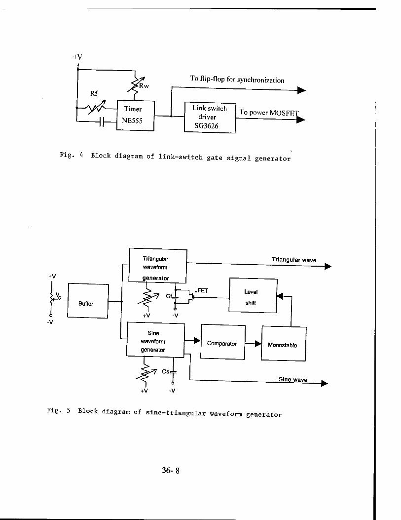
To flip-flop for synchronization
To power MOSFE' 2^
Fig. 4 Block diagram of link-switch gate signal generat or
JFET
Sine waveform generator
r T L-
Triangular wave
Level
shift
Comparator Monostable
Sine wave
+V
Fig. 5 Block diagram of sine-triangular waveform generator
36-8
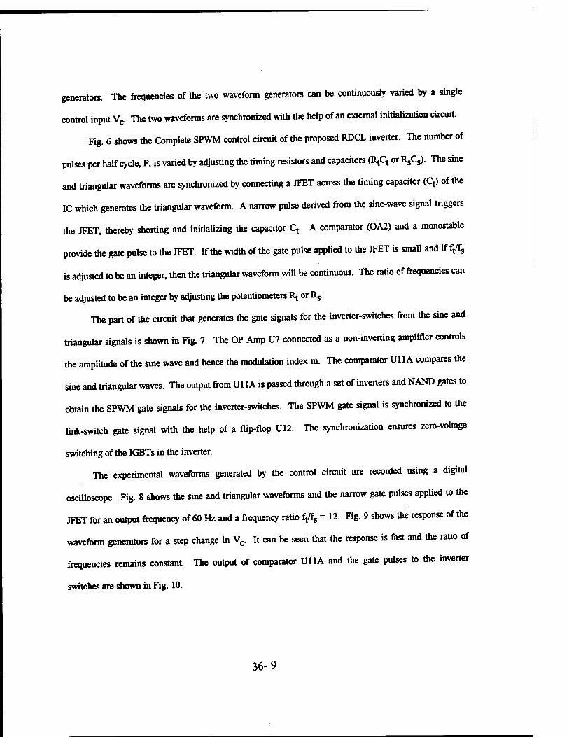
generators. The frequencies of the two waveform generators can be continuously varied by a single
control input Vc. The two waveforms are synchronized with the help of an external initialization circuit.
Fig. 6 shows the Complete SPWM control circuit of the proposed RDCL inverter. The number of
pulses per half cycle, P, is varied by adjusting the timing resistors and capacitors (R^ or P^Cs). The sine
and triangular waveforms are synchronized by connecting a JFET across the timing capacitor (q) of the
IC which generates the triangular waveform. A narrow pulse derived from the sine-wave signal triggers
the JFET, thereby shorting and initializing the capacitor q. A comparator (OA2) and a monostable
provide the gate pulse to the JFET. If the width of the gate pulse applied to the JFET is small and if ft/fs
is adjusted to be an integer, then the triangular waveform will be continuous. The ratio of frequencies can
be adjusted to be an integer by adjusting the potentiometers Rt or Rj.
The part of the circuit that generates the gate signals for the inverter-switches from the sine and
triangular signals is shown in Fig. 7. The OP Amp U7 connected as a non-inverting amplifier controls
the amplitude of the sine wave and hence the modulation index m. The comparator Uli A compares the
sine and triangular waves. The output from Ul 1A is passed through a set of inverters and NAND gates to
obtain the SPWM gate signals for the inverter-switches. The SPWM gate signal is synchronized to the
link-switch gate signal with the help of a flip-flop U12. The synchronization ensures zero-voltage
switching of the IGBTs in the inverter.
The experimental waveforms generated by the control circuit are recorded using a digital
oscilloscope. Fig. 8 shows the sine and triangular waveforms and the narrow gate pulses applied to the
JFET for an output frequency of 60 Hz and a frequency ratio ft/fs = 12. Fig. 9 shows the response of the
waveform generators for a step change in Vc. It can be seen that the response is fast and the ratio of
frequencies remains constant. The output of comparator Uli A and the gate pulses to the inverter
switches are shown in Fig. 10.
36-9
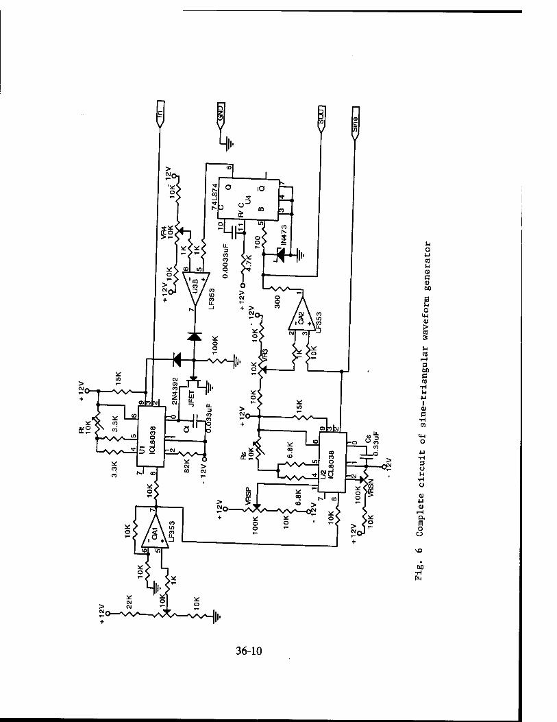
u o u as U <U a <u 00
e u o
4-1
>
M ca
t-i 3
e CO
I
c
o
3 o u
0) 4J (1)
a S o u
M •H
36-10
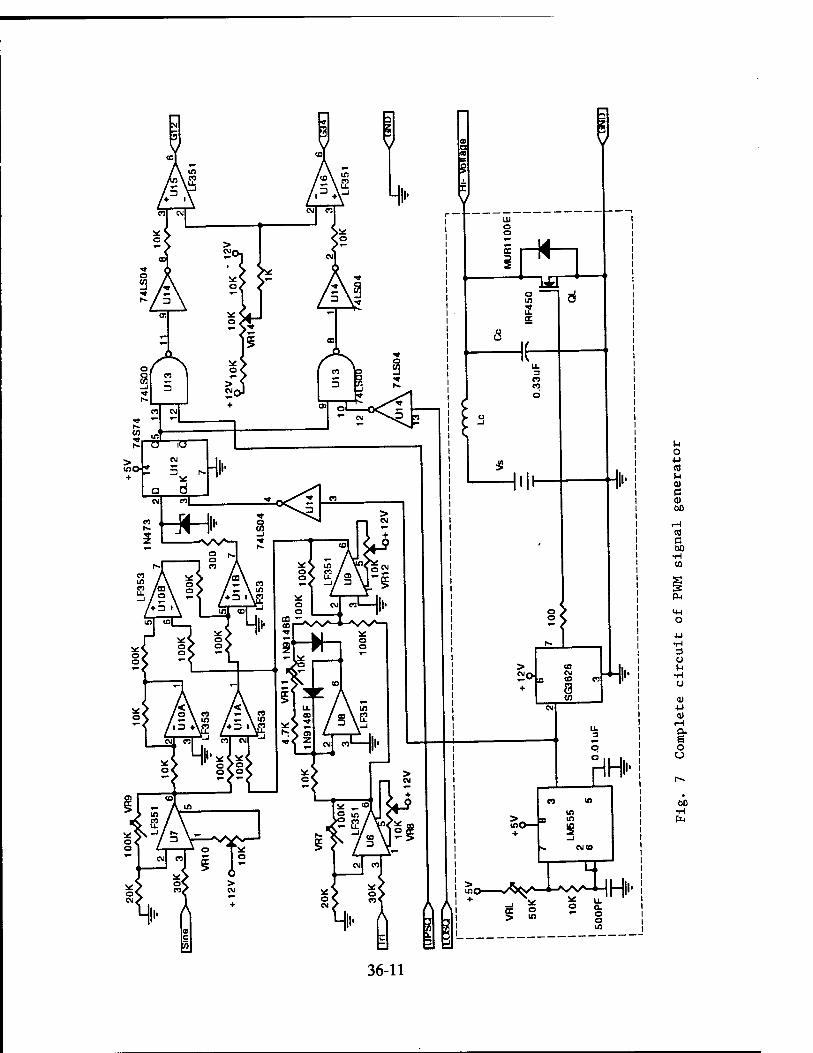
A
H>
"Tod
A
o o
>
+ CO
o <o m a en
CM
+
HHi"
in
> «> § in
M o 4-1 ca u <u c 0) 00
cd a 00
o. M-l o
3 u M
4J <U
rH (X 6 o u
t>0 •H
36-11
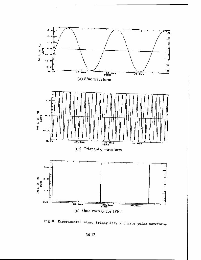
(a) Sine waveform
(b) Triangular waveform
- —' ' '—-i—-i 1—-I— i
a. a
1 l , , } , ' ': -
— _ _
a* 2. e EL -
«= £3 •H o -
e CO
—i 1 ■ , ■-+ , 1 __
—
le.Bk. za.am» riME 3a.en» 1 1 J
(c) Gate voltage for JFET
Fig.8 Experimental sine, triangular, and gate pulse waveforms
36-12
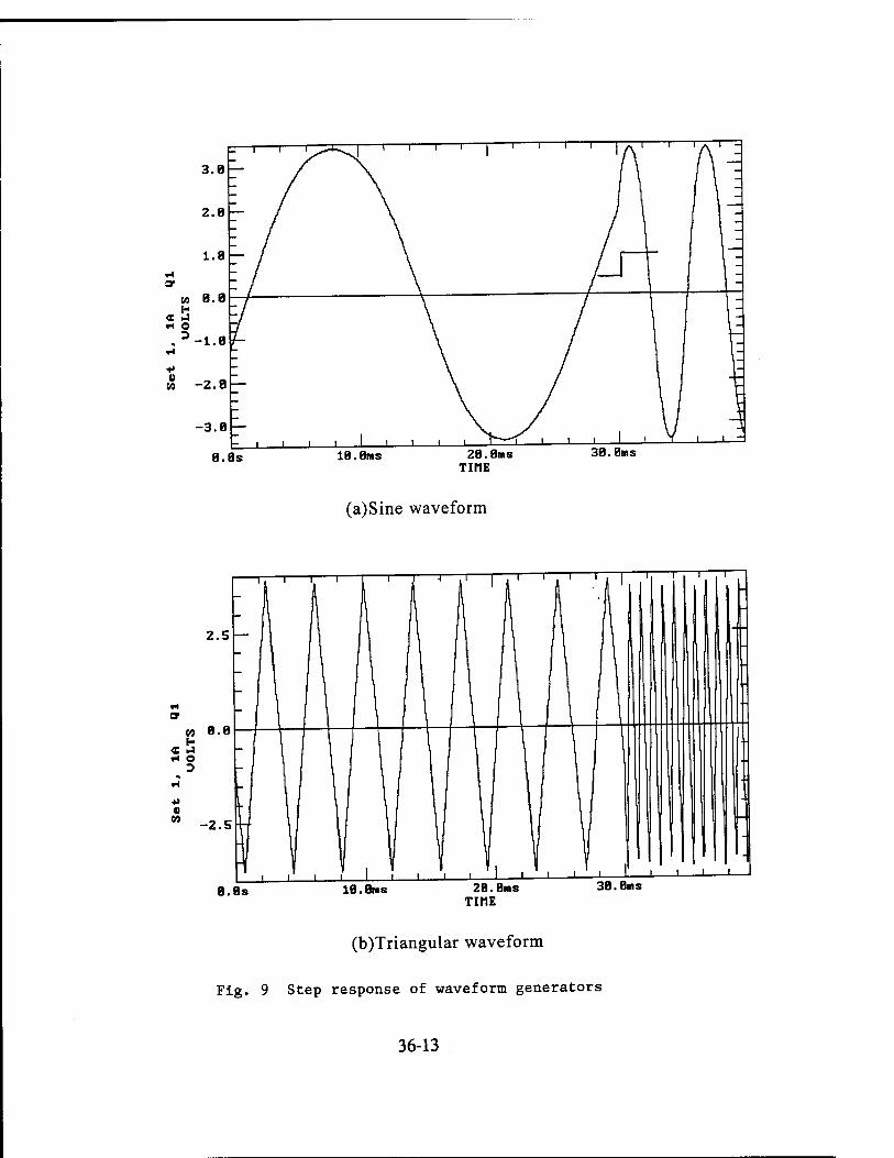
8.8s 18.8ms 28.8ms TIME
38.0ms
(a)Sine waveform
28.Bms TIME
38.BMS
(b)Triangular waveform
Fig. 9 Step response of waveform generators
36-13
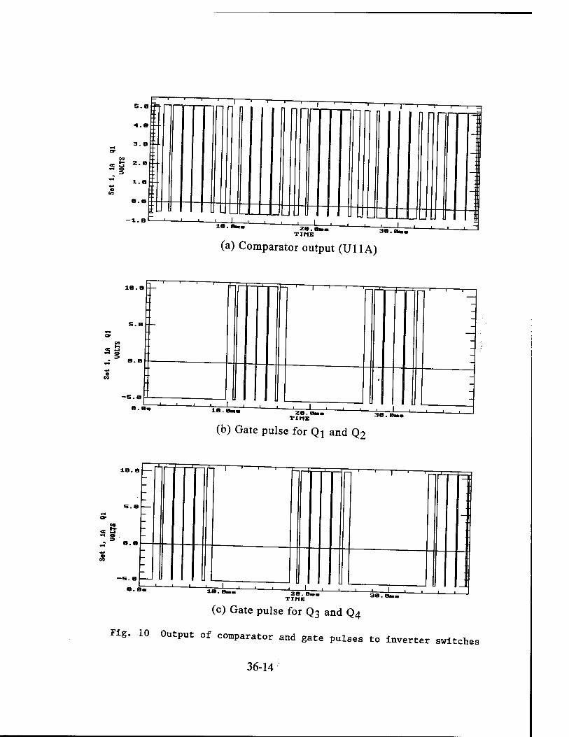
s.a f=- 1 T ■ ■ | --,— 1 ' 'I ' 1 1 1
1IHTTM I 1 —1 1 1 =
4.a '■'-■ :
s.a :--
V» J- 2.B ■-. o
1.8 :--
"■'m ■W-H-:-:-:+- . __ ] -l.B t J i _i_ , 1 . ,
la.em — «"■■■ u , _JI. i i L 1
i ill., j 2B . BM j, J__ ' ' 1 1 TIME 38.B«.
(a) Comparator output (Ul 1 A)
IB. B "I 1 1 1-
Ö o 3
"i—■—'—n=r
a. a« IB.a». -J 1 1 L
I ii 'lr,i 1 r-
28. Bai TIME
(b) Gate pulse for Qj and Q2
ft" S
8.8
I u _ 1 L
"I 1 1- 1 ' r
\
1
2B. e TIME
-I I J
(c) Gate pulse for Q3 and Q4
Fig. 10 Output of comparator and gate pulses to inverter switches
36-14

4. POWER CIRCUIT OF RDCL INVERTER
The power circuit of a single phase RDCL inverter is shown in Fig. 11. That gate signals for the
IGBTs are obtained using dedicated driver EXB 851 supplied Fuji Electric [10]. Two EXB 851 drivers
supply the gates of the high-side IGBTs Ql and Q3. Two push-pull drivers supply the gates of the two
low-side IGBTs Q2 and Q4. The driver EXB 851 provides the isolation necessary for the high-side
switches. It also protects the IGBT against over-current by feeding back the collector voltage through a
fast-recovery diode MUR1100E. The driver circuit and the power circuit are shown in Fig. 11.
The waveforms of voltages and currents in the RDCL inverter were recorded using a digital storage
oscilloscope. Fig. 12 shows the waveforms of the gate signal to the link-switching Power MOSFET and
the link capacitor voltage. With inductive load, there are definite zero-crossings. However, with resistive
load, the capacitor voltage fails to go to zero and the MOSFET QL is forced to switch at a finite voltage,
Vnün. The minimum voltage could be as high as 15 V. A possible solution to the above problem is
described in Section 8.
The load voltage and load current waveforms obtained on the RDCL inverter for an inductive load
are shown in Fig. 13. The Sine PWM scheme uses a reference frequency of 60 Hz, P = 6, and a
modulation index of 0.9. The harmonic content in the output is obtained by using a digital data
processing software. A Fast Fourier Transform (FFT) performed on the experimental waveform of voltage
(or current) yields the frequency spectrum a shown in Fig. 14. It is seen that the output is free from
several lower order harmonics below (2P - 1). The spectrum shows a harmonic component around the
resonant frequency of the link which can be easily filtered.
5. THREE-PHASE RDCL INVERTER
Three-phase RDCL inverter is suitable for driving induction motors. It uses the resonant dc link
described in Section 2. The Sine PWM control first developed for a single-phase inverter is extended to a
three-phase system. The block diagram of the three-phase sine wave generator is shown in Fig. 15. The
sine wave signal of Phase-A and a synchronized triangular wave are generated using two ICL 8038
waveform generators as described in Section 3. In order to get a balanced set of waveforms, the value of P
36-15
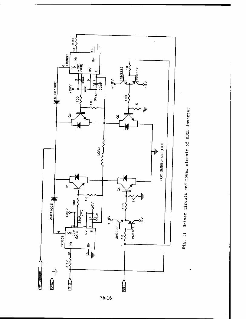
u ♦J M
> c
s o
3 o
■H CJ
M <D
o a. X) c CO
•H 3 u
> •rl
Q
60
36-16
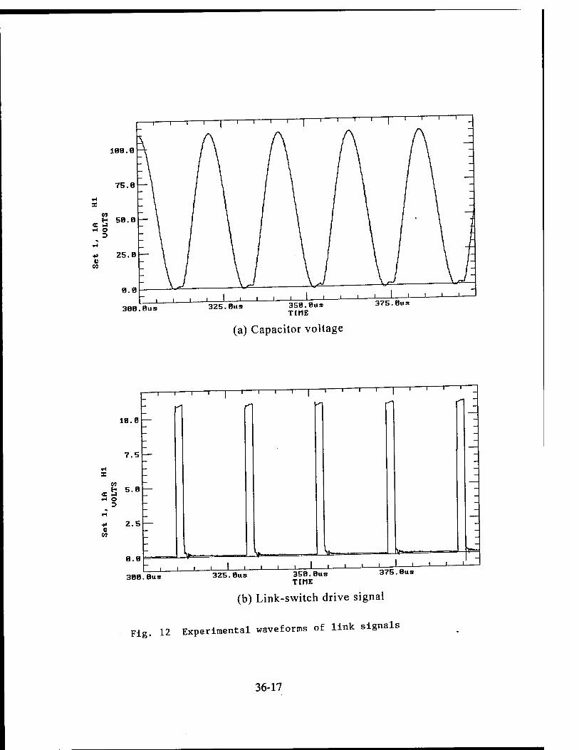
J I L ■ I I L.
30B.0US 325.Bus 358.Bus TIME
375.Bus
(a) Capacitor voltage
10.B
7.5
CO H 5.0
w o
* 2.5 w
0.B
-l 1 1 1 1 f"
n -I 1 T 1 T T I ' ~
1 3BB.0US
I I , , I l 1 I 1 1 " 1 > L- 375.Bus 358.Bus
TIME 325.Bus
(b) Link-switch drive signal
Fig. 12 Experimental waveforms of link signals
36-17
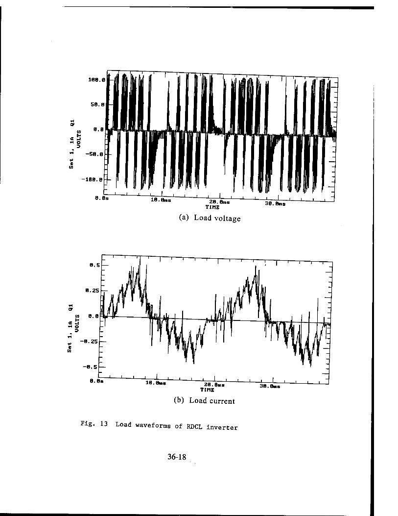
188.8
58.8
8.8 CO
«a it o 3
* -58.8
0 63
-188.8 -
28.8ms TIME
38.8ms
(a) Load voltage
a. 8s 18.8ms 28.8ms TIME
38.8ms
(b) Load current
Fig. 13 Load waveforms of RDCL inverter
36-18
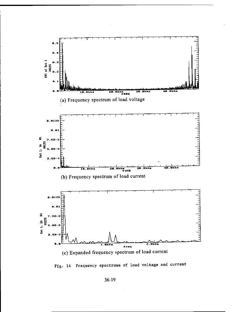
z=—i 1 1 r-
a.s
M B3 U 09
-1 1 1 r- -i 1 r- -i 1—=
fflhiWHhlii!«^-"-' k«^Mfe>^MMtta4kJl^ulhilJ<iBJ >MlM^J«u 18.Bkhz za.Bkhz
FREQ 38.Bkhz 48.Bkhz
(a) Frequency spectrum of load voltage
-—\—i—i—i—|—i—i—i—i—r
2.5E-3
-i 1 1 1 1 1 1 I r
■ * ' i I • • ' i I i_ J i i_ IB.Bkhz ZB.Bkhz 38.Bkha
TIME 4a.Bkhz
(b) Frequency spectrum of load current
B.8125
S.BE-3
Z.SE—3
-i 1 1 r-
a.e PU AA-AA_yv^ AL 9 peq
(c) Expanded frequency spectrum of load current
Fig. 14 Frequency spectrums of load voltage and current
36-19

should be a multiple of three. The Phase-B sine wave is generated using a third waveform generator and
is synchronized to the Phase-A sine wave. The synchronizing pulse is derived from the Phase-A
triangular wave as shown in Fig. 15. The phase shift of 120 deg is obtained by comparing the Phase-A
triangular wave and a reference Vx. The sine wave for Phase-C is generated from the sine waves of
Phase-A and Phase-B using the relation SinC - -<SinA+SinB). Fig. ,6 shows the triangular wave and the
sine waves of Phases A and B.
The power circuit of the inverter was built using six IGBTs available as a six-pack module. The
control circuit uses three EXB 851 drivers for the three high-side switches and three push-pull drivers for
the low-side switches. A three-phase induction motor was supplied by the RDCL inverter. Fig. 17 shows
the load voltage and load current waveforms of the induction motor.
6. PERFORMANCE OF AN RDCL INVERTER
While the concept of RDCL inverter is very attractive, there are some basic problems caused by the
low value of Q-factor of the resonant circuit. The link voltage of an RDCL inverter with an ideal
inductor and capacitor goes through zero at the end of each resonant cycle. The IA1 section in a practical
inverter has a finite Q-factor whose value is limited by the parasitic series resistance of the inductor and
the leakage resistance of the capacitor shown in Fig. 2. Consequently, the link voltage does not go to zero
and the link-shorting Power MOSFET is to be turned™ at a non-zero voltage, resulting in additional
power loss. The minimum link voltage (V^) and the power loss in the link elements are found to vary
with the power factor of the load, the resonant frequency, and the zero-voltage interval (y. The above
observations were made on the experimental inverter described in Section 4.
This section investigates some of the problems associated with an inverter having a limited Q-
factor. The performance of the inverter was studied by recording all the waveforms of voltage and current
associated with the link and measuring the power loss using a storage oscilloscope and a digital data
processing software. Certain modifications in the link operation that will improve the overall
performance of the inverter are being proposed in a later section.
36-20
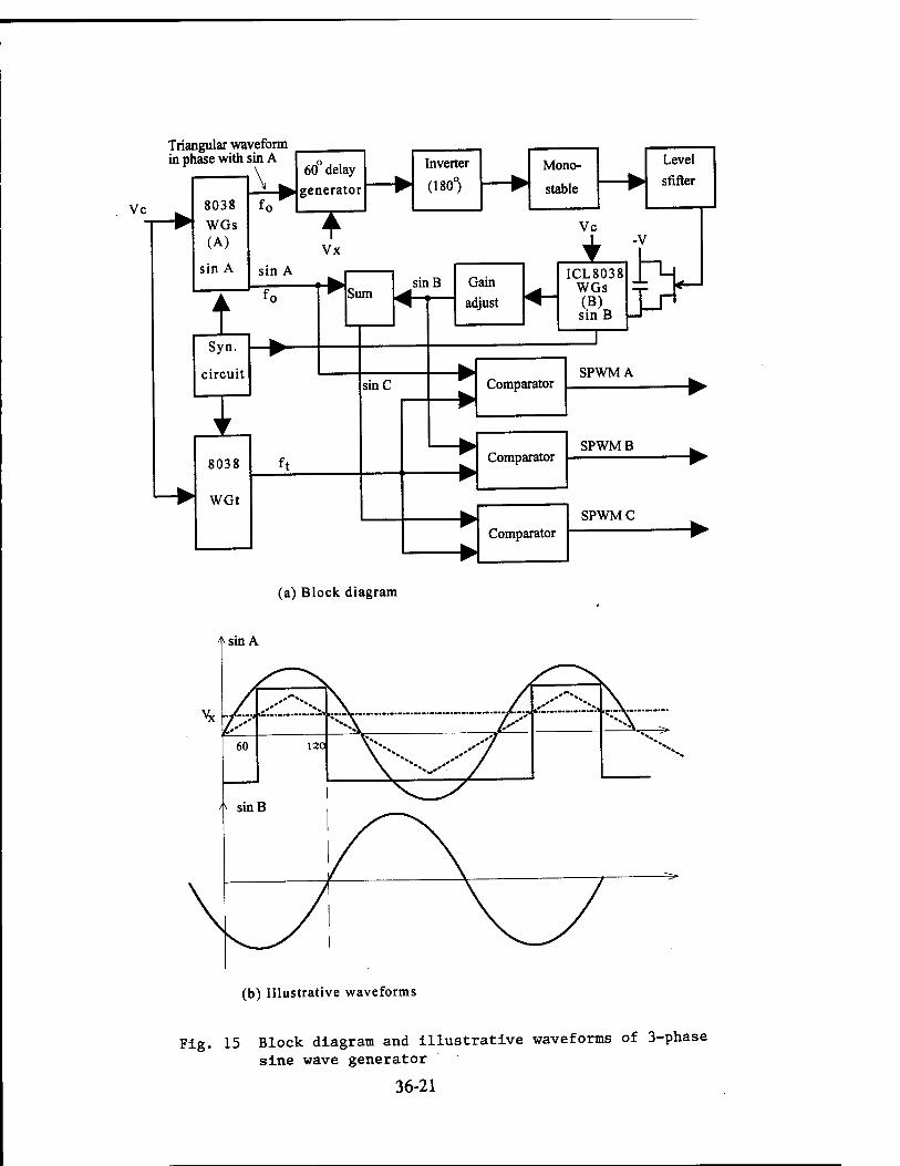
Triangular waveform in phase with sin A
Vc 8038 f0
WGs (A)
sin A
60 delay generator
Inverter
(180")
Mono-
stable
Level
softer
Vc
Vx
sin A
1 Syn.
circuit
I
Sum
8038
WGt
sinB
sinC
Gain
adjust
ICL8038 WGs
sin B
J CH
Comparator SPWMA
Comparator SPWMB
Comparator SPWMC
(a) Block diagram
4* sin A
(b) Illustrative waveforms
Fig. 15 Block diagram and illustrative waveforms of 3-phase sine wave generator
36-21
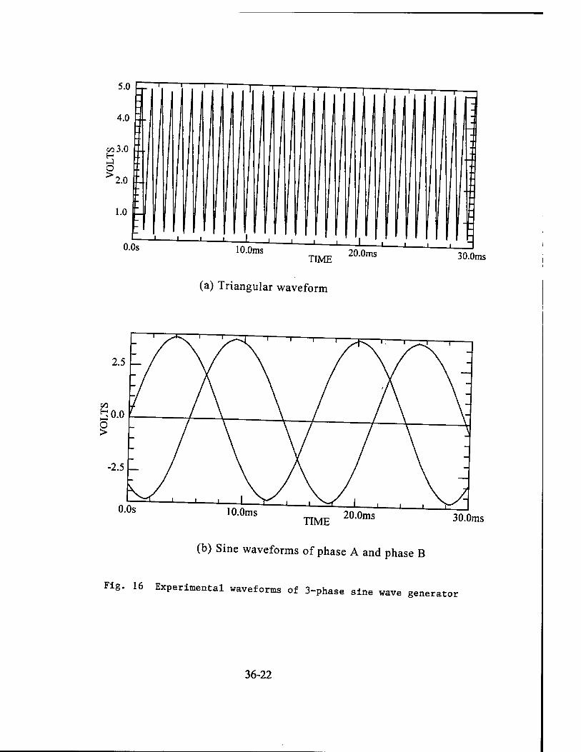
0.0s 10.0ms TIME
20.0ms i 1 1 3
30.0ms
(a) Triangular waveform
0.0s 10.0ms TIME 20.0ms 30.0ms
(b) Sine waveforms of phase A and phase B
Fig. 16 Experimental waveforms of 3-phase sine wave generator
36-22
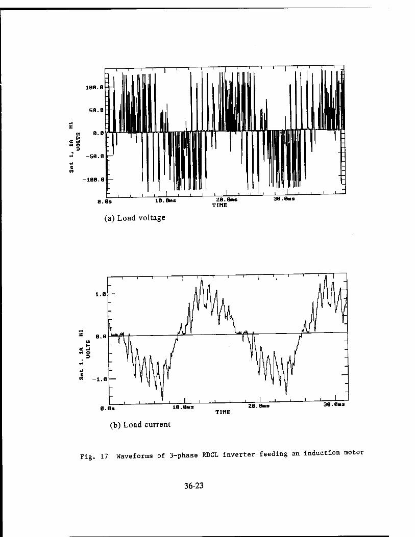
188.8 - -
8.8s 18.8ms
(a) Load voltage
28.8ns TIME
38.8MS
1.8
8.8 CO H
»* o
« -1.8
8.8s
(b) Load current
18.8MS 28.8MS 38.8MS
TIME
Fig . 17 Waveforms of 3-phase RDCL inverter feeding an induction motor
36-23

a) Effect Of low Q-fa/fnr
A resonant dc link with a high value of Q-factor is difficult to design. The RDCL built in the
laboratory has Q of 45 at the link frequency of 48 kHz. The resonant frequency is chosen high so that the
pulse density modulation used in the inverter does not introduce any appreciable error. A high resonant
frequency means a higher power loss due to the frequent closing and opening of the link-switch at a non-
zero voltage. A non-zero link voltage requires the use of a separate link-switch instead of the inverter
switches serving the purpose. In addition, the link-shorting MOSFET has to be rated for a high current
and protected by a proper snubber and a heat sink. An estimation of the power loss in the switch will
enable the choice of the link-shorting Power MOSFET and the design of the snubber.
The resonant frequency of the link is determined by the product LCCC. The maximum current
through Lc is determined by the ratio Cc/Lc. Since the link current determines the loss in the link section,
a careful choice of the values of Lc and Cc has to be made in order to minimize the loss at a given
resonant frequency. Since the inverter constitutes a nonlinear current source, computer simulation will be
useful in analyzing its performance,
b) Measurement power loss in an RDCL inverter
The power loss in an RDCL inverter with a reasonably high value of Q will be very small. An
accurate measurement of the power loss will enable the estimation of the efficiency of the inverter system
and will also enable one to investigate methods of improving its efficiency. Power loss in the RDCL
occurs in the link inductor, capacitor, and the link switch. An accurate measurement of the power lost in
any circuit element can be done by first recording the waveforms of voltage and current associated with
that element and then processing waveforms. The digital data processing software VU-POINT [11] was
used to multiply the two waveforms and compute the average power loss. This method of computing the
power loss can be used to identify the regions of voltage/current waveforms where considerable power loss
occurs and to eliminate the source to the extent possible.
The voltage and current waveforms of the elements in the link contain high frequency transitions.
The waveforms also include ac and dc components. Most of the loads are operated at 60 Hz which
36-24

corresponds to a period of 16.667 ms. The resonant frequency of the link is 48 kHz which corresponds to
a period of 20.8 jis. Since the digital oscilloscope uses an analog-to-digital (A/D) converter to acquire the
waveform data, the sampling rate has to be high enough to catch the high frequency transitions. At the
same time, the sweep time (record length) has to be long enough to cover at least one cycle of the output
waveform. To sample the data at the rate of 10 Mega samples/second (sampling interval = 100 ns) and
store one cycle of output at 60 Hz in memory, the minimum size of memory required is
16.667m =l6661kBtes (3) ' 100/w
The Nicolet Oscilloscope Model Pro 42 has a sampling rate of 20 Mega samples/second and a channel
memory of 1 MBytes, which are more than sufficient to store the data.
The power loss in the copper-foil or litz-wire type inductor is relatively small due to the absence of
skin effect. The power loss in the inductor is mainly due to the resistive effect of the copper itself. The
resistance of a coil made of 99.99% pure copper is given by
_ 1.724 x1p-6 xlength(cm) (4) thickness(cm) X width (cm)
The parasitic resistance of the copper-foil type inductor used in the experiment was calculated to be
10.344 mfl.
The losses in the link capacitor is due its leakage (shunt) resistance. A polypropylene capacitor is
used to keep the losses small. The typical value of leakage resistance provided by the manufacturer is
42500 MQ. The capacitor also has a series resistance of O.llmfl.
7. SIMULATION OF AN RDCL INVERTER WITH CURRENT FEEDBACK
The problem of zero-crossing failure is linked to the nature of the load current. The capacitor
current that is responsible for the zero-crossing failure is equal to the difference between the inductor
current and the load current. It is possible to adjust the frequency and duty cycle of the gate signal to QL,
36-25

through a feedback of the load current, in order to overcome zeroising fai,ure. The feasibility of the
method was first tested through computer simulation. In the simulation, the inverter switches were
modeled as ideal voltage controlled switches. The program used a resistive load as an example. Fig. 18
shows the simulated waveforms of capacitor voltage and the gate pulses to QL. The simulation was
started at t = 0 with no load. The link-voltage waveform shows periodic zero-crossings. At t = 100 w a
resistive load was added. With a fixed-frequency, and fixed-duty-cycle gate signal to QL, it is seen that
the addition of the load results in zero-crossing failure.
The waveform of Fig. 19 corresponds to the situation where the frequency and duty cycle are varied
as a function of the load current. It is seen that the link voltage exhibits definite zero-crossings. With a
careful choice of the frequency and duty cycle, the link voltage was forced to go through zero at the end
of each resonant cycle. Fig. 19 also shows the fast decay of the link voltage if there are no puhes applied
to the link-shorting MOSFET (after 200 ^ The gate voltage to QL has to be modified based on the
value of the load current and the instant of application of the load. Thus, one has to design the 555 Timer
with a nominal value of frequency and duty cycle and vary them suitably whenever the load changes (in
other words, the gate signals to the inverter switches change). The practical implementation of the
current feedback is described in the next section.
8. RDCL WITH CURRENT FEEDBACK
One has to sense the load current before providing a feedback. Current sensing MOSFETs have
been developed to meet the need of current monitoring in the power device [12]. The power circuit of the
inverter was built using current sensing Power MOSFETs. Fig. 20 shows the power circuit of the single-
phase inverter, the driver circuit, and the current sensing circuit. The dedicated driver for the Power
MOSFET, » 2110 was used in the circuit. A single driver supplies the gate signals for both »he low and
high-side switches in one arm. The sum of the drain currents of Q2 and Q4 gives the total load current.
The sense outputs of the low-side MOSFETs Q2 and Q4 are converted into proportional voltages and
added together to give the total signal V^.
36-26
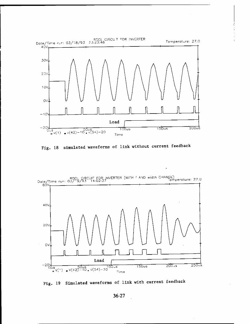
RDCL CIRCUIT FOR INVERTER Date/Time run: 03/18/93 23:23:48
40V4
30V..
20 V.
10V..
OV..
■10\i
-20V Ous
Load
~5o"ul
Temperature: 27.0
(1) . v(42)-10. v(54)-20 100us 15bus
n n n n n n n n IL.
200us
Fig. 18 simulated waveforms of link without current feedback
RDCL CIRCUIT FOR INVERTER (WITH f AND width CHANGE) 97 „ Date/Time run: 03/19/93 14:02:37 Temperature. 27.0
60V+
40V..
20V..
OV..
n__n_Ji n. -2o4
Load
~50"Üs Ous 50us , v 100us V(1) ,V(42)-10.V(54)-20
150us 200us 250us
Time
Fig. 19 Simulated waveforms of link with current feedback
36-27
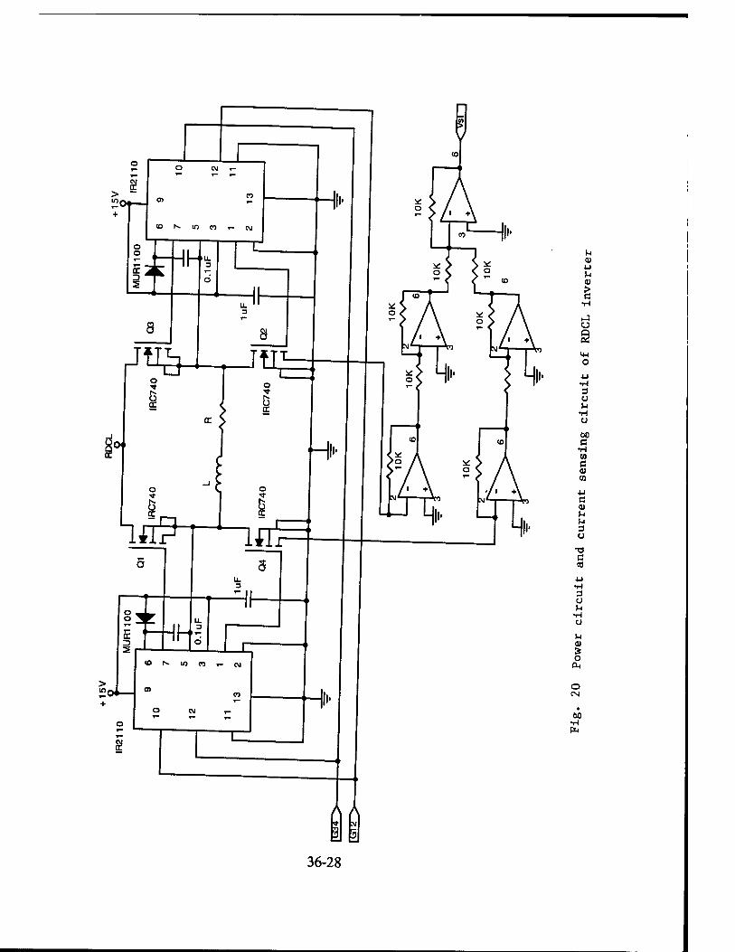
8! >
+ <0 N IT) CO T- c\l
&U O
j°ol—
2
4^
CU 4J M (U
o
3 U
Ö0 C
•H CO Ö CU CO
e CU u u 3 u
c cd
3 O
CU
o
o CN
M •H
36-28
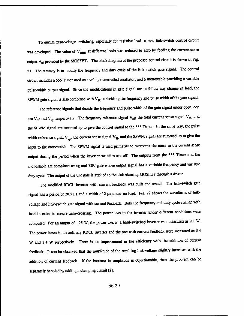
To ensure zero-voltage switching, especially for resistive load, a new link-switch control circuit
was developed. The value of V^ at different loads was reduced to zero by feeding the current-sense
output Va provided by the MOSFETs. The block diagram of the proposed control circuit is shown in Fig.
21. The strategy is to modify the frequency and duty cycle of the link-switch gate signal. The control
circuit includes a 555 Timer used as a voltage-controlled oscillator, and a monostable providing a variable
pulse-width output signal. Since the modifications in gate signal are to follow any change in load, the
SPWM gate signal is also combined with V^ in deciding the frequency and pulse width of the gate signal.
The reference signals that decide the frequency and pulse width of the gate signal under open loop
are V^ and V™ respectively. The frequency reference signal Vgf, the total current sense signal V^, and
the SPWM signal are summed up to give the control signal to the 555 Timer. In the same way, the pulse
width reference signal Vq,, the current sense signal V^, and the SPWM signal are summed up to give the
input to the monostable. The SPWM signal is used primarily to overcome the noise in the current sense
output during the period when the inverter switches are off. The outputs from the 555 Timer and the
monostable are combined using and 'OR' gate whose output signal has a variable frequency and variable
duty cycle. The output of the OR gate is applied to the link-shorting MOSFET through a driver.
The modified RDCL inverter with current feedback was built and tested. The link-switch gate
signal has a period of 20.5 ^ and a width of 2 us under no load. Fig. 22 shows the waveforms of link-
voltage and link-switch gate signal with current feedback. Both the frequency and duty cycle change with
load in order to ensure zero-crossing. The power loss in the inverter under different conditions were
computed. For an output of 95 W, the power loss in a hard-switched inverter was measured as 9.1 W.
The power losses in an ordinary RDCL inverter and the one with current feedback were measured as 5.4
W and 3.4 W respectively. There is an improvement in the efficiency with the addition of current
feedback. It can be observed that the amplitude of the resulting link-voltage slightly increases with the
addition of current feedback. If the increase in amplitude is objectionable, then the problem can be
separately handled by adding a clamping circuit [2].
36-29
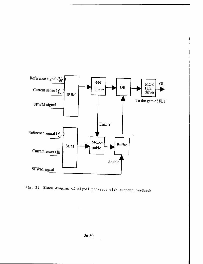
Reference signal (Yf
Current sense (V
SPWM signal
Reference signal (V
Current sense (Yt
SPWM signal
To the gate of FET
Fig. 21 Block diagram of signal prcessor with current feedback
36-30
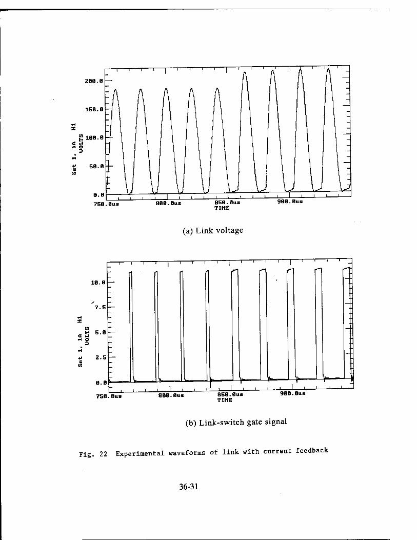
-i 1—-i 1 1 1 i r
288.8
758.Bus 888.Bus 858.Bus TIME
988.Bus
(a) Link voltage
18.8
7.5
«5 5-8
v 2.5 o CO
a.8
-i 1 1 r
n -i 1 r -i 1 1 1 1 r
n n
■ i l I l ' ' ' I 1 1 1—L ' i '
758.Bus 888.Bus 858.Bus TIME
988.Bus
(b) Link-switch gate signal
Fig. 22 Experimental waveforms of link with current feedback
36-31

9. CONCLUSIONS
A single-phase and a three-phase resonant dc link inverters were developed and built primarily to
study the performance and to investigate methods of improving it. The units developed consist of a
resonant link section and an inverter section. The performance studies carried out include the
measurement of power loss in the different sections. It was observed that a failure in zero-crossing results
in additional power loss in the link-shorting Power MOSFET. A method of ensuring definite zero-
crossings through the use of current feedback is described in the project. The possibility of providing load
current feedback to ensure zero-voltage crossing was studied with the help of computer simulation. An
RDCL inverter with current feedback was built using current sensing Power MOSFETs. The details of
obtaining the current sense signal and generating the variable-frequency variable-duty^ycle gate signal
for the link-shorting MOSFET are presented in the report. Several experimental waveforms obtained on
the RDCL inverter are also presented.
ACKNOWLEDGMENT
The author wishes to express his sincere thanks to the Air Force Office'of Scientific Research,
Boiling Air Force Base, Washington, DC for awarding the research initiation grant, and the authorities of
North Dakota State University and the Electrical Engineering Department for providing the matching
funds and the facilities. He is thankful to Mr. Joseph Weimer, Technical Area Manager, Electrical
Technology Laboratory, Wright Patterson Air Force Base for providing the necessary facilities and
encouragement during the initial investigations and the continued support thorough out the completion of
the project. The author also wishes to thank Mr. Greg Fronista, Project Engineer, Wright Patterson Air
Force, for providing the author with several useful informations during the execution of the project.
REFERENCES
[1] D.M. Divan, «The resonant dc link converters - A new concept in static power
conversion," IEEE Trans. Industry Applications, Vol. 25, No. 2, pp. 317-325, March/April 1989.
36-32
[2] D.M. Divan and G. Skibinski, "Zero-switching-loss inverters for high-power
applications," IEEE Trans. Industry Applications, Vol. 25, No. 4, pp. 634-643,
July/August 1989.
[3] K.S. Rajasekhara et al., "Resonant dc link inverter-fed ac machines control," Proc.
of Power Electronics Specialists Conference, pp. 491-4%, 1987.
[4] D.M. Divan et al., "Design methodologies for soft-switched inverters," Conf.
Record of IEEE IAS Annual Meeting, pp. 758-766,1987.
[5] PSPICE User's Manual, MicroSim Corporation, 1991
[6] J. Lai and B.K. Bose, "An induction motor drive using an improved high efficiency
resonant dc link inverter," IEEE Trans. Power Electronics, Vol. 6, No. 3, pp. 504-
513, July 1991.
[7] I. Smit et al., "Investigation of limitations in large converters with resonant input
link above 30 kHz using GTOs," Proc. of Power Electronics Specialists
Conference, pp. 1003-1009, 1989.
[8] MH. Rashid, Power Electronics, 2nd Ed., Prentice Hall, Englewood Cliffs, NJ,
1993.
[9] D.A. Bell, Solid State Pulse Circuits, 4th Ed., Prentice Hall , Englewood Ctiffs, NJ,
1992.
[10] MBT (IGBT) Driver, Fuji Electric, 1990.
[11] VU-POINT: A digital data processing system, Maxwell Laboratories, 1991.
[12] Power Field Effect Transistor with current sensing capability, Technical Data, AD
11419, Motorola Semiconductors Inc., 1987.
36-33
Related Documents