A Thesis entitled Friction-Stir Riveting: Characteristics of Friction-Stir Riveted Joints by Genze Ma Submitted to the Graduate Faculty as partial fulfillment of the requirements for the Masters of Science Degree in Mechanical Engineering __________________________________________ Dr. Hongyan Zhang (advisor), Committee Chair __________________________________________ Dr. Ahalapitiya Jayatissa (co-advisor), Committee Member __________________________________________ Dr. Sarit Bhaduri, Committee Member __________________________________________ Dr. Patricia R. Komuniecki, Dean College of Graduate Studies The University of Toledo May 2012

Welcome message from author
This document is posted to help you gain knowledge. Please leave a comment to let me know what you think about it! Share it to your friends and learn new things together.
Transcript
A Thesis
entitled
Friction-Stir Riveting:
Characteristics of Friction-Stir Riveted Joints
by
Genze Ma
Submitted to the Graduate Faculty as partial fulfillment of the requirements for the
Masters of Science Degree in Mechanical Engineering
__________________________________________
Dr. Hongyan Zhang (advisor), Committee Chair
__________________________________________
Dr. Ahalapitiya Jayatissa (co-advisor), Committee Member
__________________________________________
Dr. Sarit Bhaduri, Committee Member
__________________________________________
Dr. Patricia R. Komuniecki, Dean
College of Graduate Studies
The University of Toledo
May 2012

Copyright 2012, Genze Ma
This document is copyrighted material. Under copyright law, no parts of this document
may be reproduced without the expressed permission of the author.

iii
An Abstract of
Friction-Stir Riveting:
Characteristics of Friction-Stir Riveted Joints
by
Genze Ma
Submitted to the Graduate Faculty as partial fulfillment of the
requirements for the Masters of Science Degree in Mechanical
Engineering
The University of Toledo
May 2012
Driven by the needs of weight reduction for automobiles, light-metals such as
aluminum and magnesium alloys are increasingly used in the automobile industry.
However, there are significant barriers in welding these metals in large-scale
applications, and the difficulties lead to the development of alternative joining methods,
such as friction-stir welding and self-piercing riveting.
Hybrid friction-stir riveting is a new joining method developed at the University of
Toledo which can be used to join both similar and dissimilar materials. In this process a
joint is formed by spinning and pressing a solid rivet into layers of sheet medals. It has
the advantages of both friction-stir welding and self-piercing riveting processes.
In this process the sheet metals are jointed together by a rivet and a cohesion zone
around the rivet through the stirring action. The strength comes from the mechanical
interlocking, mixing/adhesion, and solid bonding. The geometry of the rivet, tooling, and
joining process all affect the joint quality. For instance, the rivet should provide as much
interlocking to the sheet metals as possible, and at the same time its concave area should
iv
be filled with the mixed materials. Experiments also proved that the process parameters
such as spindle speed and feed rate have significant effects on the joint quality. These
effects are discussed in this research through both experimental and numerical studies.
FEA method was used to analyze the effect of the geometry of the joint on strength, such
as the location of the end of the faying interface. An optimization of the joint geometry
was performed and experimentally verified.

v
Acknowledgements
I would like to thank Dr. Zhang for his guidance through my study at the University
of Toledo. His attitude towards working and his encouragement inspire me to reach a
new academic level. He taught me how to solve problems and analyze them in an
effective way. The experience of being his student will have profound influence in my
life. I am also grateful for the opportunity of working with other professors at the MIME
Department of UT, such as Dr. Jayatissa, and their help in both my course work and
research.
I would also like to show my gratitudes to the MIME machine shop staff members
Mr. John Jaegly, Mr. Tim GrIvanos and Mr. Randall Reihing. We would not have gone
this far in this research without their help.
I would also like to thank my fellow students who helped me to in this project,
especially Samuel Durbin and Weiling Wang, my cooperative partners.
Finally I would like to express my gratefulness and respect to my parents.

vi
Table of Contents
Acknowledgements ..............................................................................................................v
Table of Contents ............................................................................................................... vi
List of Tables ...................................................................................................................... ix
List of Figures ......................................................................................................................x
List of Symbols .............................................................................................................. xxiii
1. Introduction ..................................................................................................................1
1.1.Background Introduction ...................................................................................... 1
1.1.1.Self-piercing Riveting ................................................................................. 2
1.1.2.Friction-stir Welding ................................................................................... 3
1.1.3.Hybrid Friction-stir Riveting ...................................................................... 4
1.2.Objects of the Thesis ............................................................................................. 5
2. Friction-stir Riveting ....................................................................................................6
2.1. Process Introduction............................................................................................. 6
2.1.Joint Characterization ........................................................................................... 8
2.2.1. Characteristics of Riveted Joints ................................................................ 8
2.2.2. Effect of Riveting Die .............................................................................. 10
2.2.3. Process Parameters................................................................................... 16
2.2.4. Effect of Process Parameters on Joint Formation .................................... 16
3. Finite Element Modeling of Friction-stir Riveted Joints ...........................................19
vii
3.1. FE Modeling of Material Testing ....................................................................... 19
3.1.1. Theoretical Background of Tensile Testing ............................................. 19
3.1.2. Material Property Definition in ABAQUS .............................................. 24
3.1.3. Material Properties Used in Simulation ................................................... 25
3.1.4. FE Modeling of Uniaxial Testing ............................................................. 30
3.2. Modeling of Friction-stir Riveted Joints ............................................................ 32
3.2.1. Model Development................................................................................. 33
3.2.1.1. Geometry of the Model ................................................................ 33
3.2.1.2. Meshing........................................................................................ 36
3.2.1.3. Boundary Conditions and Loading .............................................. 38
3.2.2. Job Submission ........................................................................................ 39
3.2.3. Numerical Analysis of FSR Joints under Loading ................................... 40
3.2.3.1. Progressive deformation and fracture of joints with a 6-mm mixed
zone ............................................................................................. 41
3.2.3.2. Progressive damage and fracture of joints with a 7-mm mixed
zone ............................................................................................. 52
4. Experiments ...............................................................................................................57
4.1. Comparison between Simulation and Experiment ............................................. 59
4.2. Failure Mode Analysis ....................................................................................... 62
5. Summary and Future Work ........................................................................................69
5.1.Summary ............................................................................................................. 69
5.2.Future Work ........................................................................................................ 69
References ..........................................................................................................................70

viii
List of Publications ............................................................................................................73
ix
List of Tables
Table 2.1 CNC processing code ......................................................................................... 7
Table 3.1 Units used in ABAQUS ................................................................................... 28
Table 3.2 Material property definition in ABAQUS ........................................................ 29
Table 3.3 Batch script for job submitting ......................................................................... 40
Table 3.4 Figure number assignment ............................................................................... 41
Table 3.5 Progressive view of the deformation of a joint with 6-mm mixed zone and a
two-third curl up interface ................................................................................ 48
x
List of Figures
Figure 1-1 Self-piercing riveting joint .............................................................................. 2
Figure 1-2 Friction stir weld seem (a) and friction-stir spot weld joint (b) ...................... 3
Figure 1-3 Hybrid friction-stir riveting joint .................................................................... 4
Figure 2-1 Friction-stir riveting setup ............................................................................... 7
Figure 2-2 Metallographic sections of a friction-stir riveted joint, and dimensions and
various zones for characterizing the joint ..................................................... 10
Figure 2-3 Dies of different cavity volumes ................................................................... 12
Figure 2-4 FSR joint without using die........................................................................... 13
Figure 2-5 FSR joint with small die ................................................................................ 14
Figure 2-6 FSR joint with large die volume ................................................................... 15
Figure 2-7 Spindle_speed/Feed_rate versus width of mixed zone curve (a) .................. 18
Figure 3-1 Engineering stress-strain curves versus true stress-strain curve ................... 22
Figure 3-2 Stress and strain curves with increasing strain rate ....................................... 23
Figure 3-3 Typical specimen responses under tensile test .............................................. 24
Figure 3-4 ASTM E8 test specimen ................................................................................ 25
Figure 3-5 Specimen before testing ................................................................................ 26
Figure 3-6 Specimen after testing ................................................................................... 26
Figure 3-7 Experimental true stress - true strain plot ..................................................... 27

xi
Figure 3-8 Power law fitting ........................................................................................... 28
Figure 3-9 FE model for uniaxial tensile test .................................................................. 30
Figure 3-10 Simulation of the uniaxial testing 2-mm aluminum 5754 alloy .................... 31
Figure 3-11 Comparison of experimental and simulation results ..................................... 32
Figure 3-12 Model geometry of a riveted joint for tensile test ......................................... 33
Figure 3-13 Geometries of the riveted joints with different faying interface ends for
simulation ..................................................................................................... 34
Figure 3-14 Dimensions of the tensile testing specimens ............................................... 35
Figure 3-15 C3D8R element ........................................................................................... 36
Figure 3-16 Zero-energy mode ........................................................................................ 37
Figure 3-17 Mesh of the testing specimen ....................................................................... 37
Figure 3-18 Datum line for model rotation ...................................................................... 38
Figure 3-19 Effect of rotational force .............................................................................. 39
Figure 3-20 Deformation of a riveted joint with a flat faying interface end and a 6-mm
mixed zone .................................................................................................... 42
Figure 3-21 Maximum stress before fracture.................................................................... 43
Figure 3-22 Stress distribution after fracture .................................................................... 44
Figure 3-23 Deformation of a joint with one-third curling up faying interface end and 6-
mm mixed zone ............................................................................................ 46
Figure 3-24 Deformation of a joint with a two-third curling up faying interface end and 6-
mm mixed zone ............................................................................................ 47
Figure 3-25 Force versus displacement curves for joints with 6-mm mixed zone ........... 48
Figure 3-26 Deformation of a joint with a flat faying interface end and a 7-mm mixed
xii
zone ............................................................................................................... 53
Figure 3-27 Deformation of a joint with one-third curl up faying interface end and a 7-
mm mixed zone ............................................................................................ 54
Figure 3-28 Deformation of a joint with a two-third curl up faying interface end and a 7-
mm mixed zone ............................................................................................ 55
Figure 3-29 Simulation results of joints with a 7-mm mixed zone................................... 56
Figure 3-30 Force vs. displacement of joints with different sizes of the mixed zone ...... 56
Figure 4-1 Joints with flat (a) and one-third curl up (b) faying interface ends ............... 58
Figure 4-2 A joint with too much curl up of the faying interface end ............................ 58
Figure 4-3 A joint with a through interface ..................................................................... 59
Figure 4-4 Simulated (a) and tested (b) fractured specimens with flat interface ends ... 60
Figure 4-5 Simulated and experimentally measured force vs. displacement curves of
joints with flat interface ends ....................................................................... 60
Figure 4-6 Simulated (a) and tested (b) fractured specimens with interface ends of two-
third curl up .................................................................................................. 60
Figure 4-7 Simulated and experimentally measured force vs. displacement curves of
joints with two-third interface curl up ends .................................................. 61
Figure 4-8 Tested specimen (a) and the corresponding mechanical response (b) for a
joint with 2.794-mm penetration .................................................................. 63
Figure 4-9 Cross-section of the specimen in Figure 4-8(a) ............................................ 63
Figure 4-10 Tested specimen (a) and the corresponding mechanical response (b) for a
joint with 3.556-mm penetration .................................................................. 64
Figure 4-11 Cross-section of the specimen in Figure 4-10(a) .......................................... 64

xiii
Figure 4-12 Tested specimen with a flat interface and a 3.81-mm rivet penetration ........ 65
Figure 4-13 Tested specimen with a curl up interface and a 3.81-mm rivet penetration .. 65
Figure 4-14 Tested specimen with a curl up interface and a 4.318-mm rivet penetration 66
Figure 4-15 Comparison of load vs. displacement curves generated on specimens with
different failure modes.................................................................................. 67

xxiii
List of Symbols
dt vertical distance between the faying interface end and the rivet head
db vertical distance between the faying interface end and the rivet bottom flange
s separation between the tip of the rivet end and the top of the mixed zone
w the distance between the end of the interface and the trunk
W the distance between the ends of the interfaces
Є engineering strain
єtrue true strain
б engineering stress
бtrue true stress
A0 original cross sectional area of specimen
A instantaneous cross section area
L0 original length of specimen
Lf length of the deformed specimen
L instantaneous length of the specimen
dL small increment of the length
E Young’s modulus
P applied load
V volume of specimen

1
1. Introduction
1.1. Background Introduction
There are different ways of joining metals depending on the applications and
materials. Welding and riveting are two different methods of joining metals with totally
different principles. Welding basically includes; arc welding, gas welding, resistance
welding, and friction stir welding. Chemical reactions generally occur between
workpieces to form a joint in the welding processes mentioned above. Mechanical
fastening such as riveting, on the other hand, is a way to form an interlock between
workpieces. Each means has its pros and cons. They are chosen mostly based on an
overall consideration of the application and cost. Friction-stir welding and self-piercing
riveting (SPR) are common ways to form a mechanical joint between sheet metals. As
aforementioned light-metals such as aluminum and magnesium alloys are used in
industry, and joining these metals requires new advanced techniques because of their
unique chemical and mechanical properties. Resistance spot welding, one of the most
popular joining methods in the past years, has difficulties in joining light-metals because
of the volatile physical properties [1] of aluminum and magnesium alloys. For instance,
high thermal expansion in both solid and liquid states, and large volume expansion due to
melting make aluminum welding difficult [2], and the high chemical affinity of
aluminum for copper results in short electrode life in welding aluminum [3]. In the
following sections the characteristics of alternative mechanical joining means, i.e., self-
2
piercing riveting and friction-stir welding are reviewed. Then the new innovative friction-
stir riveting process is introduced.
1.1.1. Self-piercing Riveting
Self-piercing riveting has proven to be an effective way to join aluminum. It
overcomes the difficulties that appeared in common welding processes. Unlike spot
welding which involves metallurgical reactions [4-6], self-piercing riveting forms a
mechanical interlock. In the process of self-piercing riveting a semi-tubular rivet is
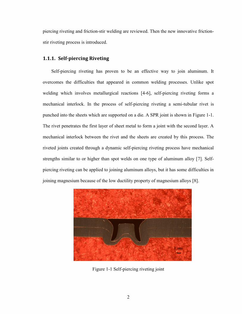
punched into the sheets which are supported on a die. A SPR joint is shown in Figure 1-1.
The rivet penetrates the first layer of sheet metal to form a joint with the second layer. A
mechanical interlock between the rivet and the sheets are created by this process. The
riveted joints created through a dynamic self-piercing riveting process have mechanical
strengths similar to or higher than spot welds on one type of aluminum alloy [7]. Self-
piercing riveting can be applied to joining aluminum alloys, but it has some difficulties in
joining magnesium because of the low ductility property of magnesium alloys [8].
Figure 1-1 Self-piercing riveting joint
1 mm
3
1.1.2. Friction-stir Welding
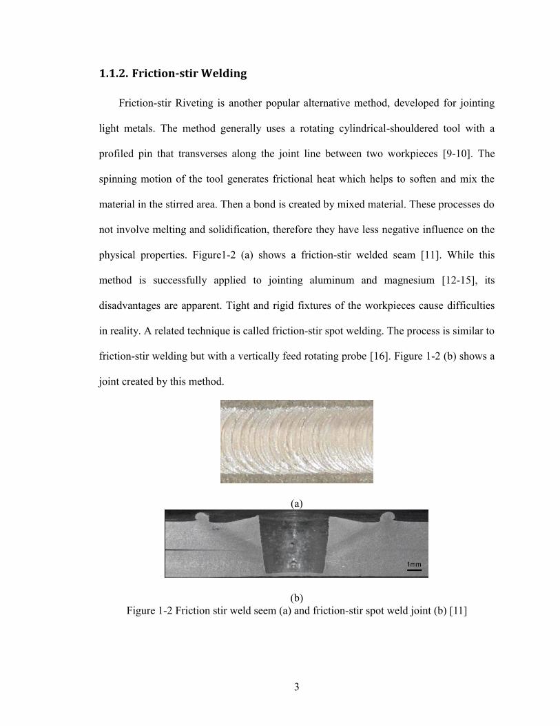
Friction-stir Riveting is another popular alternative method, developed for jointing
light metals. The method generally uses a rotating cylindrical-shouldered tool with a
profiled pin that transverses along the joint line between two workpieces [9-10]. The
spinning motion of the tool generates frictional heat which helps to soften and mix the
material in the stirred area. Then a bond is created by mixed material. These processes do
not involve melting and solidification, therefore they have less negative influence on the
physical properties. Figure1-2 (a) shows a friction-stir welded seam [11]. While this
method is successfully applied to jointing aluminum and magnesium [12-15], its
disadvantages are apparent. Tight and rigid fixtures of the workpieces cause difficulties
in reality. A related technique is called friction-stir spot welding. The process is similar to
friction-stir welding but with a vertically feed rotating probe [16]. Figure 1-2 (b) shows a
joint created by this method.
(a)
(b)
Figure 1-2 Friction stir weld seem (a) and friction-stir spot weld joint (b) [11]
4
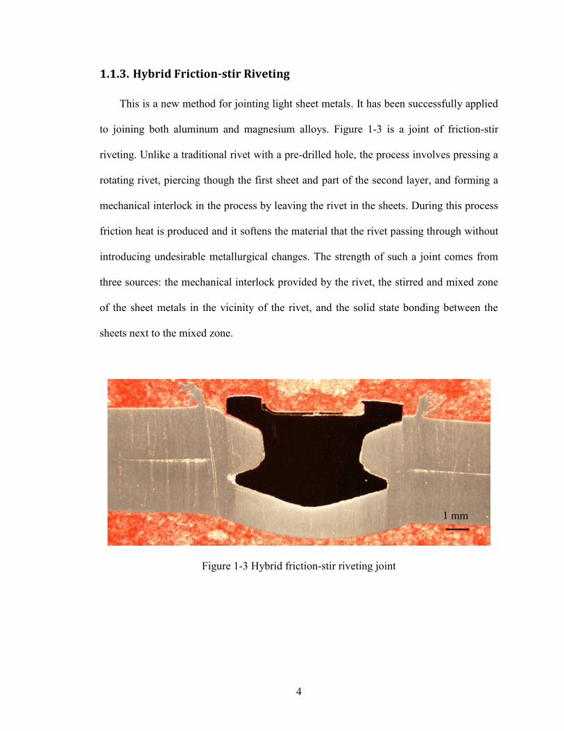
1.1.3. Hybrid Friction-stir Riveting
This is a new method for jointing light sheet metals. It has been successfully applied
to joining both aluminum and magnesium alloys. Figure 1-3 is a joint of friction-stir
riveting. Unlike a traditional rivet with a pre-drilled hole, the process involves pressing a
rotating rivet, piercing though the first sheet and part of the second layer, and forming a
mechanical interlock in the process by leaving the rivet in the sheets. During this process
friction heat is produced and it softens the material that the rivet passing through without
introducing undesirable metallurgical changes. The strength of such a joint comes from
three sources: the mechanical interlock provided by the rivet, the stirred and mixed zone
of the sheet metals in the vicinity of the rivet, and the solid state bonding between the
sheets next to the mixed zone.
Figure 1-3 Hybrid friction-stir riveting joint
1 mm

5
1.2. Objects of the Thesis
1. Characterize the friction-stir riveted joints which affect the performance of the rivet
joint.
2. Determine and optimize which affect the characterizations mentioned above.
6
2. Friction-stir Riveting
2.1. Process Introduction
The feasibility of the hybrid friction-stir riveting has proven to be viable by the
Materials Joining Laboratory at the University of Toledo. Rivet geometry, details of the
driver and clamping etc. were determined after large amount of experimental efforts and
theoretical analysis. A CNC mill was used for the riveting process. The driver, clamp,
rivet, die are assembled as shown in Figure 2-1. Before the process starts, the rivet is held
by the squeezing force between the driver and top sheet metal. This step is necessary to
ensure that the joint is made at the designated location. Then the driver starts rotating
without feeding. Rotation of the driver forces the rivet to spin at the same rate. Spindling
without feeding preheats material around the rivet bottom flange which helps material
soften and prepare for the subsequent penetration. After a moment of preheating, the
driver pushes the rivet while rotating with preset speed until the desired depth is reached.
Then the driver releases the rivet and the whole process is completed. Table 2.1 shows
the code to control the CNC mill.

7
Figure 2-1 Friction-stir riveting setup
Table 2.1 CNC processing code
RIVET#
G99#
G66#
G00Z-0.5#
X -0.3284 Y -3.546#
Z -0.5#
F10.#
G01 Z -2.0#
M01#
M03S2000#
F0.1#
Z -2.100#
G04F0.#
G00Z -0.5#
S100#
Y-4.712X-7.356#
M02#

8
2.1. Joint Characterization
The quality of a riveted joint relies on the rivet, the mixed zone around rivet trunk,
and the solid bonding between two sheets. Hence, the characterization of a joint produced
by friction-stir riveting should be investigated from these three aspects. Due to the easily
damaged nature of the solid bonding area, by the etchant for metallographic analysis, it
was neglected in the current study. Therefore, characterization of the solid bonding part is
omitted from discussion. With the chosen rivet and sheet materials, the riveting process
becomes the most important factor in influencing the characteristics of a joint, and hence
the joint strength. In the hybrid friction-stir riveting process, the spindle speed, feed rate,
feed depth and the preheating time are the parameters that can be controlled. Experiment
data proved that the effect of preheating time is not significant. The rotation speed ranges
from 500 rpm to 3000 rpm and the feed rate starts from 0.05 inch per minute and rises by
an increment of 0.05 inch per minute. For the depth it must be less than 4 mm which is
the total thickness of the 2-mm aluminum sheet stack-up.
2.2.1. Characteristics of Riveted Joints
Shown in Figure 2-2 is the microscopic cross section view of a riveted joint formed
without using a die. This close-up graphs of the structure shows the mixed area in the
vicinity of the rivet trunk where materials from different sheets become ‘one’. This area
is created by the rotating rivet which stirs and mixes the sheet metals around it. This
stirring motion generates heat and softens the sheet material around the rivet, and finally
‘welds’ these two sheets together. It is reasonable to assume the behavior the mixed zone
performs like on piece of metal if this zone is highly compacted by the riveting process.
Consequently, the junction where the faying surfaces meet at the end of interface
9
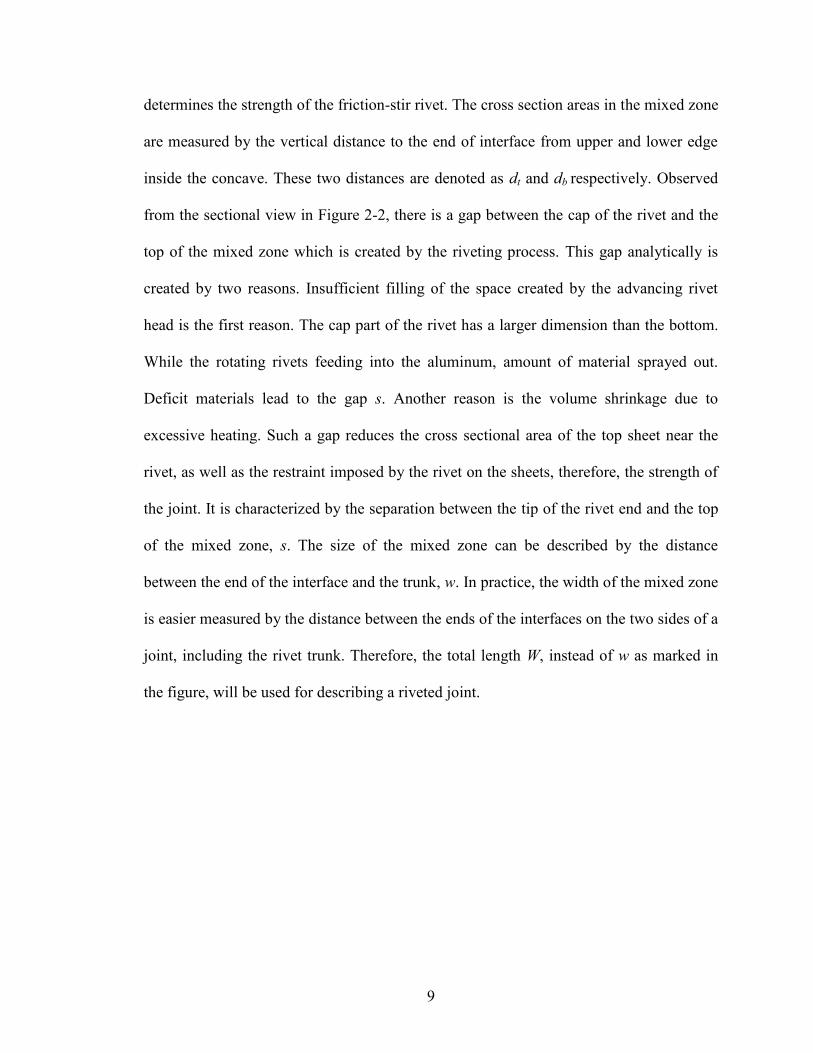
determines the strength of the friction-stir rivet. The cross section areas in the mixed zone
are measured by the vertical distance to the end of interface from upper and lower edge
inside the concave. These two distances are denoted as dt and db respectively. Observed
from the sectional view in Figure 2-2, there is a gap between the cap of the rivet and the
top of the mixed zone which is created by the riveting process. This gap analytically is
created by two reasons. Insufficient filling of the space created by the advancing rivet
head is the first reason. The cap part of the rivet has a larger dimension than the bottom.
While the rotating rivets feeding into the aluminum, amount of material sprayed out.
Deficit materials lead to the gap s. Another reason is the volume shrinkage due to
excessive heating. Such a gap reduces the cross sectional area of the top sheet near the
rivet, as well as the restraint imposed by the rivet on the sheets, therefore, the strength of
the joint. It is characterized by the separation between the tip of the rivet end and the top
of the mixed zone, s. The size of the mixed zone can be described by the distance
between the end of the interface and the trunk, w. In practice, the width of the mixed zone
is easier measured by the distance between the ends of the interfaces on the two sides of a
joint, including the rivet trunk. Therefore, the total length W, instead of w as marked in
the figure, will be used for describing a riveted joint.

10
Figure 2-2 Metallographic sections of a friction-stir riveted joint, and dimensions and
various zones for characterizing the joint
2.2.2. Effect of Riveting Die
As we mentioned before the strength of a joint mainly comes from two different
sources: mechanical interlocking and the mixed zone close to the rivet. A quality joint
should have a large interlock, a wide mixed zone, and an appropriate location where the
open faying interface ends. The location where the open faying interface ends, which is
mainly determined by the penetration process, influences the deformation and fracture
behavior of the sheet material significantly. It is assumed that the closer the end of the
interface is to the boundary of the rivet head, the easier the fracture will happen. This
assumption will be proven in the simulation part.
The vertical feeding process softens the material around the rivet and squeezes it in
an off-rivet direction. A separation between the two sheets is eliminated due to the
application of the clamp [2]. However, there is still surplus of material has nowhere to go
1 mm

11
but flow upwards. The end of the interface is pushed upwards by the mixed material, if
the process is not controlled.
A large amount of experiment was conducted to find out the method to control the
shape of the interface of the open faying area. It was realized that the easiest way to
control material flow is add a die with certain cavity. The concave will hold part of the
material extruded out by the rivet, therefore, change the material flow. Three processes
were tested to find out the effects of using different dies. The first one is using a flat piece
of steel, effectively without a die, underneath the aluminum sheets. This sample serves as
a benchmark. Two other specimens were made using dies of different cavity volumes
underneath the sheet metals. Figure 2-3 shows two different die cavity volumes. The one
with a small cavity has a cavity volume of 7.33 mm3, and the larger one of 21.2 mm
3.
With all other parameters such as spindle speed, feed rate, pre-heating time, etc. fixed, it
was concluded that a larger cavity volume produces a lower end of the half-mixed area.

12
7.89mm
0.85mm
0.50mm
6.90mm
V = 21.2 mm^3
V = 7.33 mm^3
Figure 2-3 Dies of different cavity volumes [2]
By using a die in the process, a flat interface can be formed. A flat end of the
interface provides a better strength of the joint. Because of the size of the mixed area, w,
is partly determined by the bottom of the rivet, it is assumed that the use of a die will not
alter w significantly.
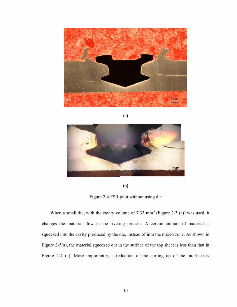
Figure 2-4 shows a joint without the usage of the die. As shown in Figure 2-4 (a) ,
the bottom sheet is flat and a large amount of metal is squeezed out the surface as burrs.
The end of the interface curled up obviously, as shown in Figure 2-4 (b).
(a)
(b)
13
(a)
(b)
Figure 2-4 FSR joint without using die
When a small die, with the cavity volume of 7.33 mm3 (Figure 2-3 (a)) was used, it
changes the material flow in the riveting process. A certain amount of material is
squeezed into the cavity produced by the die, instead of into the mixed zone. As shown in
Figure 2-5(a), the material squeezed out in the surface of the top sheet is less than that in
Figure 2-4 (a). More importantly, a reduction of the curling up of the interface is
1 mm
1 mm

14
observed in Figure 2-5(b). Comparing Figure 2-5(b) and Figure 2-4(b), no obvious
decrease in the mixed area size is observed.
(a)
(b)
Figure 2-5 FSR joint with small die
A further reduction of the curling up of the interface is observed by using the die
with a large cavity. Shown in Figure 2-3, a 21.2 mm3 cavity volume die (Figure 2-3(b)) is
used. The amount of metal squeezed out of the top surface also decreases as observed in
the previous figure. Instead of curving up, it forms a flat interface in this situation shown
in Figure 2-6. All these joints had the same amount of feed depth for the reason of
1 mm
1 mm
15
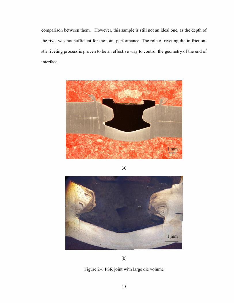
comparison between them. However, this sample is still not an ideal one, as the depth of
the rivet was not sufficient for the joint performance. The role of riveting die in friction-
stir riveting process is proven to be an effective way to control the geometry of the end of
interface.
(a)
(b)
Figure 2-6 FSR joint with large die volume
1 mm
1 mm

16
2.2.3. Process Parameters
Through a large amount of experiments it was found that reasonable joints can be
produced when spindle speed, feed rate and feed depth were controlled. Three different
spindle speeds, 1500, 2000, and 2500 rpm were used. The feed rates used in the process
were 0.1 inch per minute and 0.05 inch per minute.
2.2.4. Effect of Process Parameters on Joint Formation
It was found that the depth of a rivet was a significant measure of the mechanical
interlock of a joint. The rivet shape also affects the quality of the mechanical interlock.
The rotating motion of the rivet aims to generate heat, through the friction between the
rivet and the sheet metal. Generally, a high spindle speed generates more heat than a low
spindle speed. Therefore, the amount of heat produced during friction-stir riveting
process is proportional to the spindle speed. Also, a fast feed rate of the process reduces
the dwell time of the rivet at each depth, consequently less heat is generated under this
situation. In general, the amount of heat generated is proportional to the reciprocal of the
feed rate. Consider the combined effect of spindle speed and feed rate on the heat
generation, it is possible to use the ratio of spindle speed to feed rate, or
spindle_speed/feed_rate, as an indicator of heat input rate (referred to as “heating ratio”
hereafter), as in the conventional friction-stir seam welding. As mentioned in the
characterization of riveted joints, the quality of a joint can be described by the width of
the mixed zone W, the thicknesses of the sheets near the rivet dt and db, and the gap
between the rivet and top sheet surface s. In order to figure out the relationship between
these parameters and the heating ratio, numerous experiments were conducted. With the
17
same depth of feed, various friction-stir riveted joints were created using different
combinations of spindle speed and feed rate. Based on experiment data, relations between
the heating ratio and parameters affecting rivet joints are plotted in Figure 2-7. The
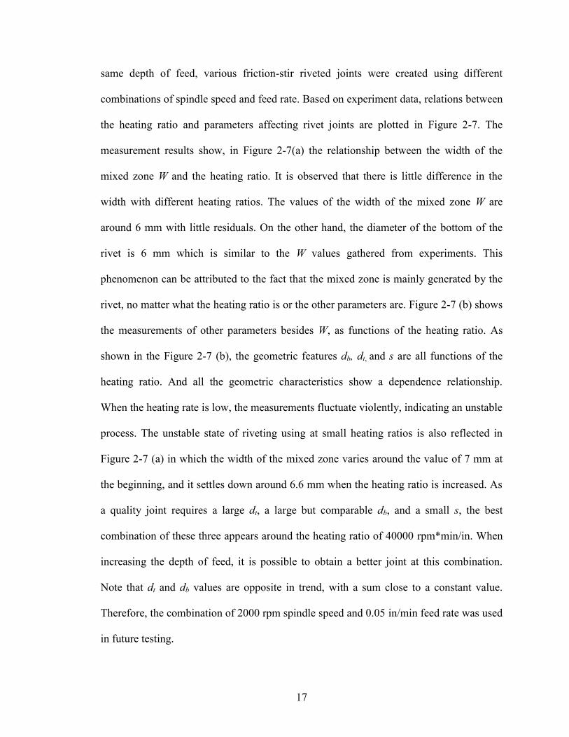
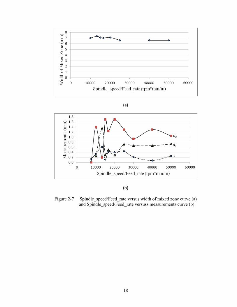
measurement results show, in Figure 2-7(a) the relationship between the width of the
mixed zone W and the heating ratio. It is observed that there is little difference in the
width with different heating ratios. The values of the width of the mixed zone W are
around 6 mm with little residuals. On the other hand, the diameter of the bottom of the
rivet is 6 mm which is similar to the W values gathered from experiments. This
phenomenon can be attributed to the fact that the mixed zone is mainly generated by the
rivet, no matter what the heating ratio is or the other parameters are. Figure 2-7 (b) shows
the measurements of other parameters besides W, as functions of the heating ratio. As
shown in the Figure 2-7 (b), the geometric features db, dt, and s are all functions of the
heating ratio. And all the geometric characteristics show a dependence relationship.
When the heating rate is low, the measurements fluctuate violently, indicating an unstable
process. The unstable state of riveting using at small heating ratios is also reflected in
Figure 2-7 (a) in which the width of the mixed zone varies around the value of 7 mm at
the beginning, and it settles down around 6.6 mm when the heating ratio is increased. As
a quality joint requires a large dt, a large but comparable db, and a small s, the best
combination of these three appears around the heating ratio of 40000 rpm*min/in. When
increasing the depth of feed, it is possible to obtain a better joint at this combination.
Note that dt and db values are opposite in trend, with a sum close to a constant value.
Therefore, the combination of 2000 rpm spindle speed and 0.05 in/min feed rate was used
in future testing.
18
(a)
(b)
Figure 2-7 Spindle_speed/Feed_rate versus width of mixed zone curve (a)
and Spindle_speed/Feed_rate versuss measurements curve (b)

19
3. Finite Element Modeling of Friction-stir Riveted
Joints
3.1. FE Modeling of Material Testing
Finite element modeling was employed to simulate the behavior of friction-stir
riveted joints under tensile-shear loading. A material model was developed first, based on
experimental results obtained from testing a uniform aluminum sheet which was used in
making most of the riveted joints in experiments. Then the verified material model was
used in finite element simulation of the riveted joints under tensile shear loading, and the
simulation was then compared with physical experiments. And the simulation was used
to gain an in-depth understanding of the deformation process, quantify the effects of
various geometric factors, and optimize the structure of a riveted joint.
All sample sheets made for testing were AA 5754 and rivets were made of Ol tool
steel.
3.1.1. Theoretical Background of Tensile Testing
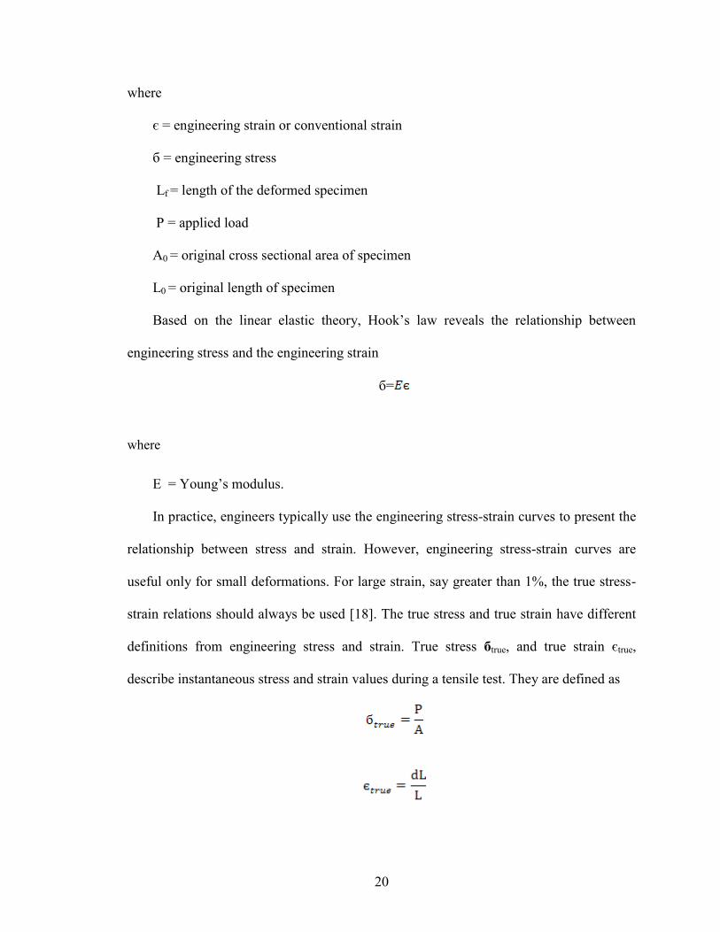
In an uniaxial tensile test, strain and stress are the terms to present mechanical
behavior. For such a test, the engineering strain and engineering stress can be expressed
as
є =
б =
20
where
є = engineering strain or conventional strain
б = engineering stress
Lf = length of the deformed specimen
P = applied load
A0 = original cross sectional area of specimen
L0 = original length of specimen
Based on the linear elastic theory, Hook’s law reveals the relationship between
engineering stress and the engineering strain
б=
where
E = Young’s modulus.
In practice, engineers typically use the engineering stress-strain curves to present the
relationship between stress and strain. However, engineering stress-strain curves are
useful only for small deformations. For large strain, say greater than 1%, the true stress-
strain relations should always be used [18]. The true stress and true strain have different
definitions from engineering stress and strain. True stress бtrue, and true strain єtrue,
describe instantaneous stress and strain values during a tensile test. They are defined as

21
where
L = instantaneous length of the specimen
A = instantaneous cross sectional area
dL = small increments of the length
By the definition of true stain, for each small change in length, the corresponding
strain increment can be described as
and by integrating dєtrue from 0 to є the results are
.
In this expression L also can be expressed as L = L0 + ΔL, when ΔL << L0, and єtrue
turns to become
Due to the difficulty in measuring the instantaneous cross section area during testing,
it can be calculated under the assumption of volume conservation
By using the equation above, one can express the relationship between true stress
and engineering stress
=
22
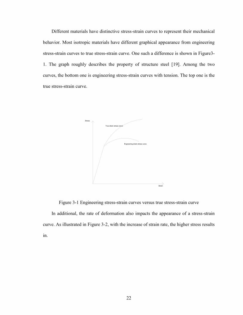
Different materials have distinctive stress-strain curves to represent their mechanical
behavior. Most isotropic materials have different graphical appearance from engineering
stress-strain curves to true stress-strain curve. One such a difference is shown in Figure3-
1. The graph roughly describes the property of structure steel [19]. Among the two
curves, the bottom one is engineering stress-strain curves with tension. The top one is the
true stress-strain curve.
Engneering strain stress curve
True strain stress curve
Strain
Stress
Figure 3-1 Engineering stress-strain curves versus true stress-strain curve
In additional, the rate of deformation also impacts the appearance of a stress-strain
curve. As illustrated in Figure 3-2, with the increase of strain rate, the higher stress results
in.

23
Figure 3-2 Stress and strain curves with increasing strain rate [20]
Figure 3-3 describes the true stress-strain response of a typical metal specimen in a
tensile test. The response, as shown in Figure 3-3, exhibits distinct stages. The first phase,
a—b, is linear elastic response. In the elastic region, the relationship between stress and
strain follows Hook’s Law as mentioned before. In addition, when the load is removed
the material recovers to its original shape without damage in this range. That means the
deformation is fully reversible. Then, plastic yielding with strain hardening happens in
b—c, when the load applied exceeds the elastic load limit of this material, and the
deformation is no longer fully reversible. Part of the deformation remains after unloading.
A remarkable drop occurs beyond c which is also identified as the onset of damage, and
the reduction of the stiffness of this material means a decrease of the load-carrying
capability of this metal. This extends until rupture happens at d.

24
Figure 3-3 Typical specimen responses under tensile test
3.1.2. Material Property Definition in ABAQUS
True stress (Cauchy stress) and logarithmic strain are used in the definition of the
material property in the commercial software package ABAQUSTM
[21], which was used
in the simulation of friction-stir riveted joints under tensile shear loading. Usually
nominal stress-strain data (engineering stress-strain data) is used for a uniaxial tensile
test. Under the assumption of isotropic material, the stress strain curve is separated into
four different stages corresponding to the Figure 3-3, elastic, plastic, damage initiation,
and damage evolution. Two variables are needed, Young’s modulus and Poisson’s ratio.
The conversional equation is exhibited below,
.
25
These two equations illuminate the relationship between nominal (engineering) stress-
strain data and true stress-strain data. The term represents the strain caused by elastic
deformation. Subtracting the elastic deformation term from the converted true stain data,
solves for plastic strain, which is needed for FEA modeling. Corresponding to point c in
Figure 3-3, fracture strain, stress triaxiality, and strain rate together describe a damage
initiation criterion. The parameter for damage evolution determines stiffness degradation.
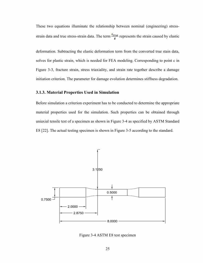
3.1.3. Material Properties Used in Simulation
Before simulation a criterion experiment has to be conducted to determine the appropriate
material properties used for the simulation. Such properties can be obtained through
uniaxial tensile test of a specimen as shown in Figure 3-4 as specified by ASTM Standard
E8 [22]. The actual testing specimen is shown in Figure 3-5 according to the standard.
Figure 3-4 ASTM E8 test specimen

26
This specimen was made of 2-mm aluminum 5754 alloy, which was used for most of the
friction-stir riveting in this study. A tensile test was conducted using a standard InstronTM
testing machine. The testing results are plotted in Figure 3-6.
Figure 3-5 Specimen before testing
Figure 3-6 Specimen after testing
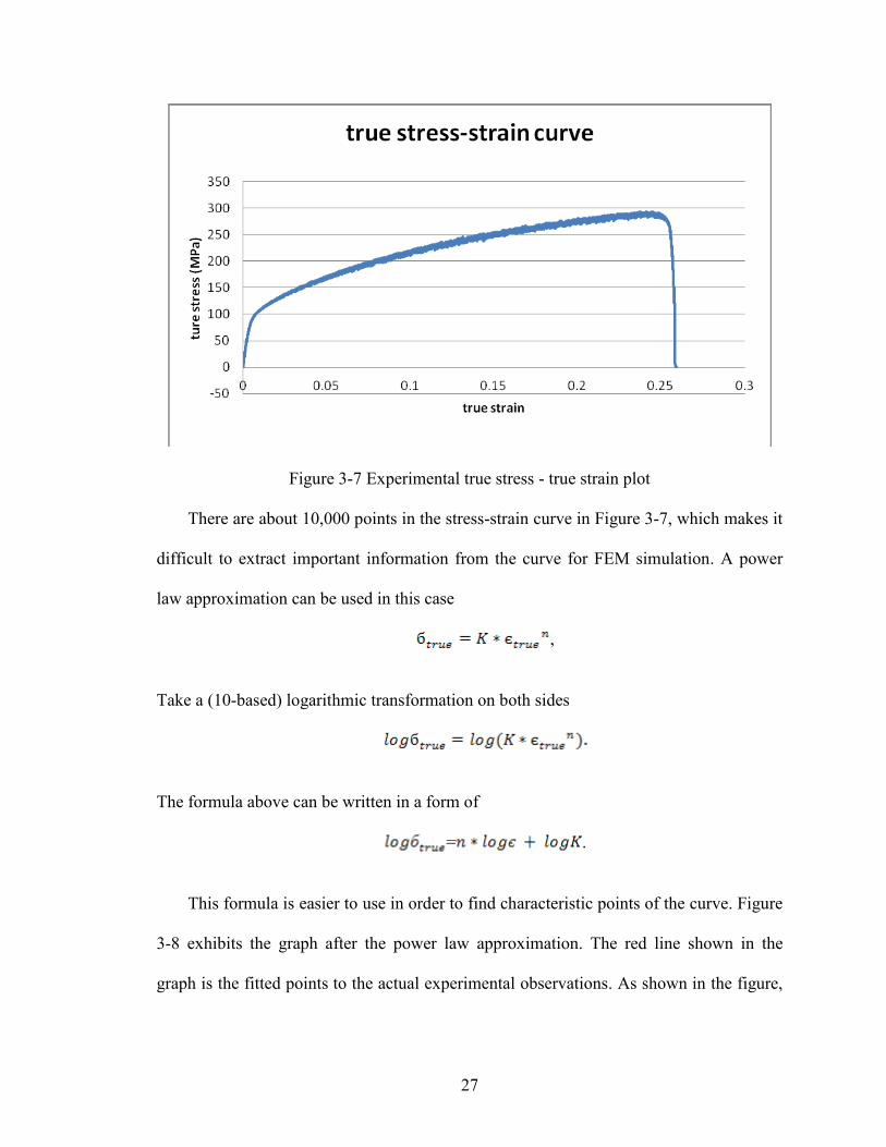
After testing the engineering stress-stain data was collected, while a conversion was
necessary to obtain the true stress-stain responses using the formulas derived in the
previous sections, and they are displayed in Figure 3-7.
1 mm
1 mm
27
Figure 3-7 Experimental true stress - true strain plot
There are about 10,000 points in the stress-strain curve in Figure 3-7, which makes it
difficult to extract important information from the curve for FEM simulation. A power
law approximation can be used in this case
,
Take a (10-based) logarithmic transformation on both sides
The formula above can be written in a form of
= .
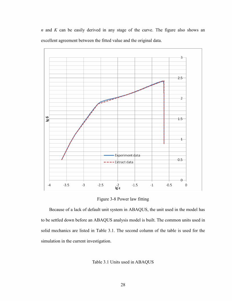
This formula is easier to use in order to find characteristic points of the curve. Figure
3-8 exhibits the graph after the power law approximation. The red line shown in the
graph is the fitted points to the actual experimental observations. As shown in the figure,
28
n and K can be easily derived in any stage of the curve. The figure also shows an
excellent agreement between the fitted value and the original data.
Figure 3-8 Power law fitting
Because of a lack of default unit system in ABAQUS, the unit used in the model has
to be settled down before an ABAQUS analysis model is built. The common units used in
solid mechanics are listed in Table 3.1. The second column of the table is used for the
simulation in the current investigation.
Table 3.1 Units used in ABAQUS

29
SI SI (mm) US (ft) US (inch)
length m mm ft in
load N N lbf lbf
mass kg tonne (10^3 kg) slug lbf s^2/in
time s s s s
stress Pa (N/m^2) MPa (N/mm^2) lbf/ft^2 psi (lbf/in^2)
energy J mJ (10^-3 J) ft lbf in lbf
density Kg/m^3 tonne/mm^3 slug/ft^3 lbf s^2/in^4
The following table (Table 3.2) shows the specific material properties gathered from
experimental data and then used in the simulation.
Table 3.2 Material property definition in ABAQUS
AA 5754 (aluminum sheets) O1 tool steel (rivet)
Rivet
Elastic: Density: Elastic:
Young’s Modulus: 27897 2.26*10^-6 Young’s Modulus: 200000
Passion’s Radio: 0.3 Passion’s Radio: 0.3
Plastic: Ductile Damage:
Yield stress Plastic strain Fracture Strain 0.24 Density: 7.9*10^-6
89.954 0 Stress Triaxiality 0
104.897 0.01 Strain Rate 0
122.323 0.018 Damage Evolution
127.002 0.021 Type Energy
146.06 0.032 Fracture Energy 0
175.749 0.056
211.472 0.1
262.378 0.196
274.041 0.224
30
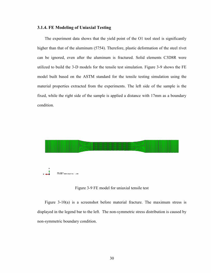
3.1.4. FE Modeling of Uniaxial Testing
The experiment data shows that the yield point of the O1 tool steel is significantly
higher than that of the aluminum (5754). Therefore, plastic deformation of the steel rivet
can be ignored, even after the aluminum is fractured. Solid elements C3D8R were
utilized to build the 3-D models for the tensile test simulation. Figure 3-9 shows the FE
model built based on the ASTM standard for the tensile testing simulation using the
material properties extracted from the experiments. The left side of the sample is the
fixed, while the right side of the sample is applied a distance with 17mm as a boundary
condition.
Figure 3-9 FE model for uniaxial tensile test
Figure 3-10(a) is a screenshot before material fracture. The maximum stress is
displayed in the legend bar to the left. The non-symmetric stress distribution is caused by
non-symmetric boundary condition.

31
(a)
(b)
Figure 3-10 Simulation of the uniaxial testing 2-mm aluminum 5754 alloy
Figure3-10 (b) illustrates the fractured specimen. As clearly visible from the figure,
element elimination method was used in the modeling.
It is assumed that a good agreement between experimental results and finite element
simulation of the uniaxial tensile testing is essential to qualify the use of finite element
simulation for the behavior of the friction-stir riveted joints under loading. A comparison
of the load-displacement curves between experiments and simulation is shown in Figure

32
3-11. They are very similar in most of the parts except at the necking and fracture. This is
because fracture of a solid in the FE modeling is simulated by element elimination, i.e.,
when the stresses on an element exceed the set value the element is removed. This
explains the rapid drop at the end of the simulated curve. Nonetheless, the FE model
captures most of the important features of the material under loading using the extract
material properties.
Figure 3-11 Comparison of experimental and simulation results
3.2. Modeling of Friction-stir Riveted Joints
Using the verified material properties as derived in the previous section, finite
element models were built to simulate the behavior of friction-stir riveted joints. Six
models were constructed to illustrate the different behaviors of friction-stir riveted joints
with different mixed zone area and various interface geometries. As discussed in Chapter
2, the geometry of a friction-stir riveted joint can be controlled by using dies. Especially,
33
the usage of die changes the shape of the end of the interface. The main purpose of the
simulation is to understand how the different interface shape influences the ultimate
force-carrying ability of a riveted joint. A numeric analysis has a number of advantages
over an experiment. For instance, the progressive deformation process can only be
revealed by a simulation, and the joint geometry can be easily altered and its effect
understood.
3.2.1. Model Development
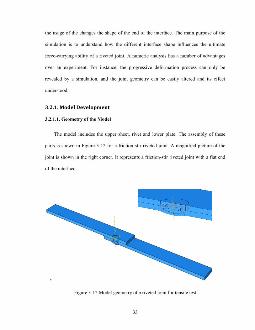
3.2.1.1. Geometry of the Model
The model includes the upper sheet, rivet and lower plate. The assembly of these
parts is shown in Figure 3-12 for a friction-stir riveted joint. A magnified picture of the
joint is shown in the right corner. It represents a friction-stir riveted joint with a flat end
of the interface.
Figure 3-12 Model geometry of a riveted joint for tensile test

34
(a) Flat faying interface end (b) One-third faying interface end
(c) Two-thirds faying interface end
Figure 3-13 Geometries of the riveted joints with different faying interface ends for
simulation
Other two magnified views with the different curvatures of the end of the interface
are shown in Figure 3-13. The geometry of the faying interface can be sorted by the
curvature. Flat faying interface end has a completely horizontal interface without
curvature. One-third faying interface end has interface that curls upward, reaching one
third of the way towards the rivet head. While a two-thirds faying interface end has an
interface that curls upward two thirds of the way towards the rivet head.
The red profile in the magnified images represents the ‘welded’ faying interface, or
the mixed part. The area under the rivet head is assumed to be ‘one’ piece to represent the
mixed zone. To simulate the mixed zone, a ‘tie’ interaction property of ABAQUS was
assigned to the red profiled parts. A surface-based tie constraint was applied to the
translational and rotational motions as well as all other active degrees of freedom, to

35
make them equal for the pair of surfaces. The surface to surface formulation reverts to the
node-to-surface formulation if a node-based or edge-based surface is used [23]. The
diameter of the red area was set as 7 mm in the simulation, even though the diameter of
the bottom of the rivet, 6 mm, is the main factor determining mixed zone, W, as discussed
in 3.4.4. According to Figure 2-2, the width of the mixed zone, W, finally settles down
around 6.6 mm. Therefore 7 mm is a reasonable value for simulation.
The dimensions of the sheets used for tensile test were 100x25x2 mm. Same
geometry was used in the simulation. An overlap is jointed by the rivet in the middle part
as shown in Figure 3-14. Half of the joint geometry was used in the simulation because of
the symmetric configuration. This simplification of geometry also improved the
computing efficiency.
Figure 3-14 Dimensions of the tensile testing specimens [7]

36
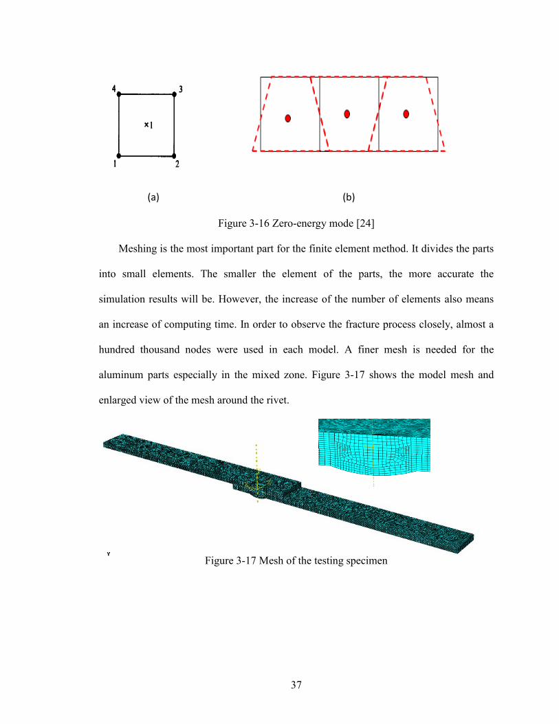
3.2.1.2. Meshing
Figure 3-15 A C3D8R element [21]
Solid element type C3D8R is used in the simulation as shown in Figure 3-15. This is
a linear element or first-order element with a node at each corner. The usage of reduced
integration numerical techniques for C3D8 element type reduces the running time,
especially for three dimensional problems. Reduced integration means an integration
scheme of lower order than full integration. One side of the brick can be considered as a 4
node element shown in Figure 3-16(a). Only one integral point exists at the center of the
square. This may result in zero-energy mode which means the integration point will have
no stain, shown in Figure 3-17(b). Zero-energy mode will soften the stiffness of the
nodes. Consequently, it will reduce the accuracy of calculation. Relax stiffness hourglass
control technique is used for the modeling.
37
(a) (b)
Figure 3-16 Zero-energy mode [24]
Meshing is the most important part for the finite element method. It divides the parts
into small elements. The smaller the element of the parts, the more accurate the
simulation results will be. However, the increase of the number of elements also means
an increase of computing time. In order to observe the fracture process closely, almost a
hundred thousand nodes were used in each model. A finer mesh is needed for the
aluminum parts especially in the mixed zone. Figure 3-17 shows the model mesh and
enlarged view of the mesh around the rivet.
Figure 3-17 Mesh of the testing specimen

38
3.2.1.3. Boundary Conditions and Loading
As the loading conditions of various specimens in this study were identical, the
boundary conditions were the same. The right side of the specimen was fixed and the left
side was pulled to a displacement of 10 mm along x-direction. As shown in Figure 3-18,
the dotted line is the path of the loading application, because of the off-set of the overlap
of the testing specimen. Therefore, in addition to the horizontal load to stretch the
specimen, a rotational force or bending moment is also needed to be applied on the
specimen to simulate the testing procedure in actual physical testing of such a specimen.
Figure 3-19 shows the influence of the rotational force. The rotational force provides a
clamping effect on the joint, and makes the specimen last longer before final fracture.
Because of the geometry a symmetric boundary condition was applied on the mid-plane.
Figure 3-18 Datum line for model rotation

39
(a) With a rotational force (b) Without a rotational force
Figure 3-19 Effect of rotational force
ABAQUS/Explicit was chosen as the solver for this problem. Even though the
ABAQUS/Standard is more accurate in solving stress and strain problems, it is not
effective when fracture or large deformation is involved.
The stretching motion applied through the boundary condition can be treated as a
quasi static process, because the motion happens infinitely slow, and no rate-dependent
material properties were used. Using the ‘smooth step’ improves the accuracy of the
force-displacement measurement. Simulation result shows that without the use of
‘smooth step’, a smaller Young’s Modulus can be resulted in than the actual value.
3.2.2. Job Submission
Due to the relatively large computing resource required, Ohio Super Computer
Center was contacted which agreed to allocate the needed computation time for the
simulations. To gain access to the 4000+ processors, an execution command written as a
batch program is required. Before submitting the ABAQUS jobs, input files of the model
to be calculated have to be uploaded to the OSC user space. The following code is an
example of the batch script used for submitting jobs

40
Table 3.3 Batch script for job submitting
#PBS -N Ma_GZ
#PBS -l walltime=72:00:00
#PBS -l nodes=1:ppn=8
#PBS -l software=abaqus+5
#PBS -j oe
#PBS -m ae
# The following lines set up the ABAQUS environment
module load abaqus
# Move to the directory where the job was submitted
cd /nfs/15/utl0324/MyWork
cp *.inp /nfs/15/utl0324/GMA_Tmp/Job.inp
cd /nfs/15/utl0324/GMA_Tmp
# Run ABAQUS
abaqus job=Job.inp cpus=8 interactive
#
# Now, copy data back once the simulation has completed
cp * /nfs/15/utl0324/MyWork
Eight C.P.U.’s were requested and provided in this program to reduce computing
time. After the simulation finishes, results in the form of odb files can be fetched from the
OSC user space.
3.2.3. Numerical Analysis of FSR Joints under Loading
As discussed in previous chapters the mixed zone size (W) and the location of the
end of the faying interface near the rivet trunk determine the mechanical strength of a
friction-stir riveted joint. Therefore, two series of simulations with different sizes of the
mixed zone were conducted. For each mixed zone three models with different faying
interfaces were built. Table 3.4 shows the figure numbers of the models with various
combinations of the mixed zone size and location of interface end.

41
Table 3.4 Figure number assignment
Interface
Mixed zone
flat
One-third curling up
Two-third curling up
6mm Figure 3-20 Figure 3-23 Figure 3-24
7mm Figure 3-26 Figure 3-27 Figure 3-28
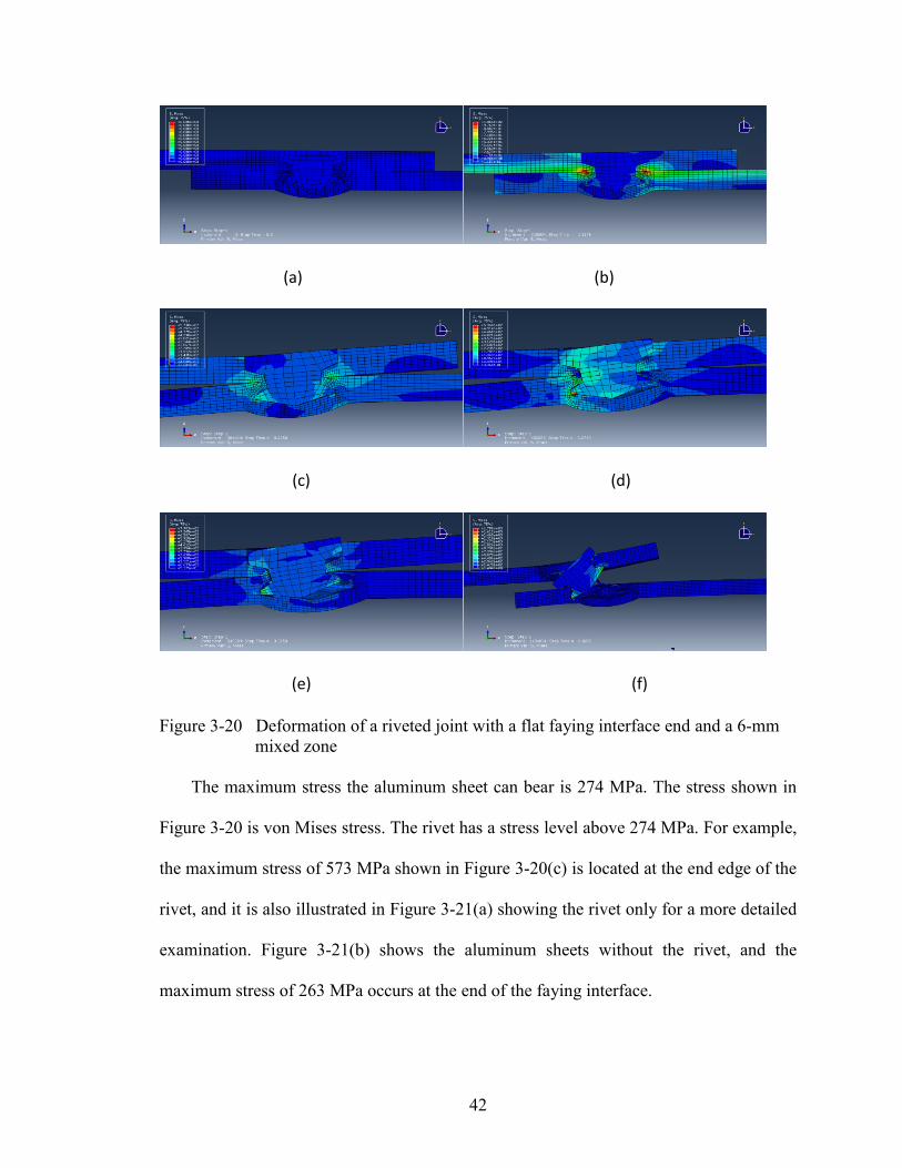
3.2.3.1. Progressive deformation and fracture of joints with a 6-mm mixed zone
Under a tensile load exerted on the ends of the specimen, the rivet is stressed and it
resists such loading as the sheets are deformed. As the loading increases, the sheets start
to separate from the rivet, and there is a stress concentration at the end of the open
interface (Figure 3-20(b)). Along with the sheet deformation the joint rotates with the
rivet (Figure 3-20(c)). When the material is stretched to a certain extent, i.e., a strain of
0.24 is reached in any element, the element is deemed as fractured and it loses load
bearing ability. During loading fracture initiates at the mixed zone where the faying
surfaces meet, and the weak parts of the mixed zone near the rivet head, with the smallest
thickness of attachment of the top sheet to the joint, get thinner and the top sheet starts to
separate from the joint. The start of the joint breaking is shown in Figure 3-20(d). The
final fracture with detailed morphology of the fractured joint is shown in Figure 3-20(f).
42
(a) (b)
(c) (d)
(e) (f)
Figure 3-20 Deformation of a riveted joint with a flat faying interface end and a 6-mm
mixed zone
The maximum stress the aluminum sheet can bear is 274 MPa. The stress shown in
Figure 3-20 is von Mises stress. The rivet has a stress level above 274 MPa. For example,
the maximum stress of 573 MPa shown in Figure 3-20(c) is located at the end edge of the
rivet, and it is also illustrated in Figure 3-21(a) showing the rivet only for a more detailed
examination. Figure 3-21(b) shows the aluminum sheets without the rivet, and the
maximum stress of 263 MPa occurs at the end of the faying interface.

43
(a)
(b)
Figure 3-21 Maximum stress before fracture
In the next stage of loading, the maximum stress reaches 274 MPa, as shown in
Figure 3-22. Progressive damage and fracture of the aluminum sheets occur in this stage.
Every element that reaches 274 MPa would be removed.
44
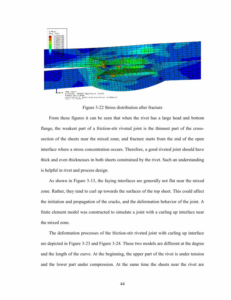
Figure 3-22 Stress distribution after fracture
From these figures it can be seen that when the rivet has a large head and bottom
flange, the weakest part of a friction-stir riveted joint is the thinnest part of the cross-
section of the sheets near the mixed zone, and fracture starts from the end of the open
interface where a stress concentration occurs. Therefore, a good riveted joint should have
thick and even thicknesses in both sheets constrained by the rivet. Such an understanding
is helpful in rivet and process design.
As shown in Figure 3-13, the faying interfaces are generally not flat near the mixed
zone. Rather, they tend to curl up towards the surfaces of the top sheet. This could affect
the initiation and propagation of the cracks, and the deformation behavior of the joint. A
finite element model was constructed to simulate a joint with a curling up interface near
the mixed zone.
The deformation processes of the friction-stir riveted joint with curling up interface
are depicted in Figure 3-23 and Figure 3-24. These two models are different at the degree
and the length of the curve. At the beginning, the upper part of the rivet is under tension
and the lower part under compression. At the same time the sheets near the rivet are
45
mostly under compression (Figure 3-23(b), Figure 3-24(b)). Stress is concentrated at the
interface of the two sheets. Under the increasing applied load, the tension and
compression stresses increase. In fact, if the rivet trunk is not thick enough, the rivet may
be chopped off at the trunk, as observed in some of the rivet designs. In addition to the
dimension of the rivet, the behavior of a rivet also depends on the strength of the rivet,
and it was observed in this study that fracture of the rivet at its trunk happens when
inappropriate materials were used for the rivets. Actually, inappropriate material or
design of rivet may lead to failure during the penetrating processing. As shown in Figure
3-23(d) and Figure 3-24(c), aluminum sheets fracture at the end of the faying interface
when the stress reaches its limit. Fracture happened on the left side first due to the tension
of the sheet bearing and the separation effect produced by the joint rotation. The crack
propagates until it reaches the rivet and is companied with the rivet rotation. These
processes can be described as the first stage of the joint damage. After the fracture of the
mixed zone, the interlock between the rivet and the aluminum sheet bears most of the
load as shown in Figure 3-23(d) and Figure 3-24(e). Underling the separating load, the
rivet keeps rotating and fracture propagates. After such a fracture, the rivet rotates to
align with the loading, and the load bearing capability of the joint increases. New stress
concentration appears and cracks propagate more into the sheets, resulting in a reduction
of load level again. This cyclic loading-unloading repeats at lowering levels until final
rupture of the specimen. Figure 3-23(f) and Figure 3-24(f) illustrate the final fractures.
As can be seen from Figure 3-20 and Figure 3-21, different deformation behaviors
and failures were caused by different kinds of interface geometry. Actually, when the
interface ends closer to the rivet, it is easier to break in the first stage of damage, and the

46
length of the crack propagation is directly related to the load bearing capability. Figure 3-
25 illustrates the response to tensile loading of the joints with 6-mm mixed zone. The 6-
mm mixed zone can be produced in actual joints by a rivet with a smaller bottom flange
diameter.
(a) (b)
(c) (d)
(e) (f)
Figure 3-23 Deformation of a joint with one-third curling up faying interface end and 6-
mm mixed zone

47
(a) (b)
(c) (d)
(e) (f)
Figure 3-24 Deformation of a joint with a two-third curling up faying interface end and
6mm mixed zone

48
Figure 3-25 Force versus displacement curves for joints with 6-mm mixed zone
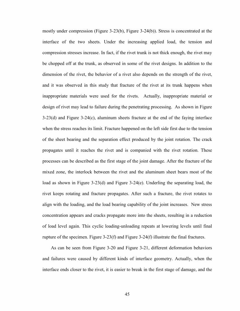
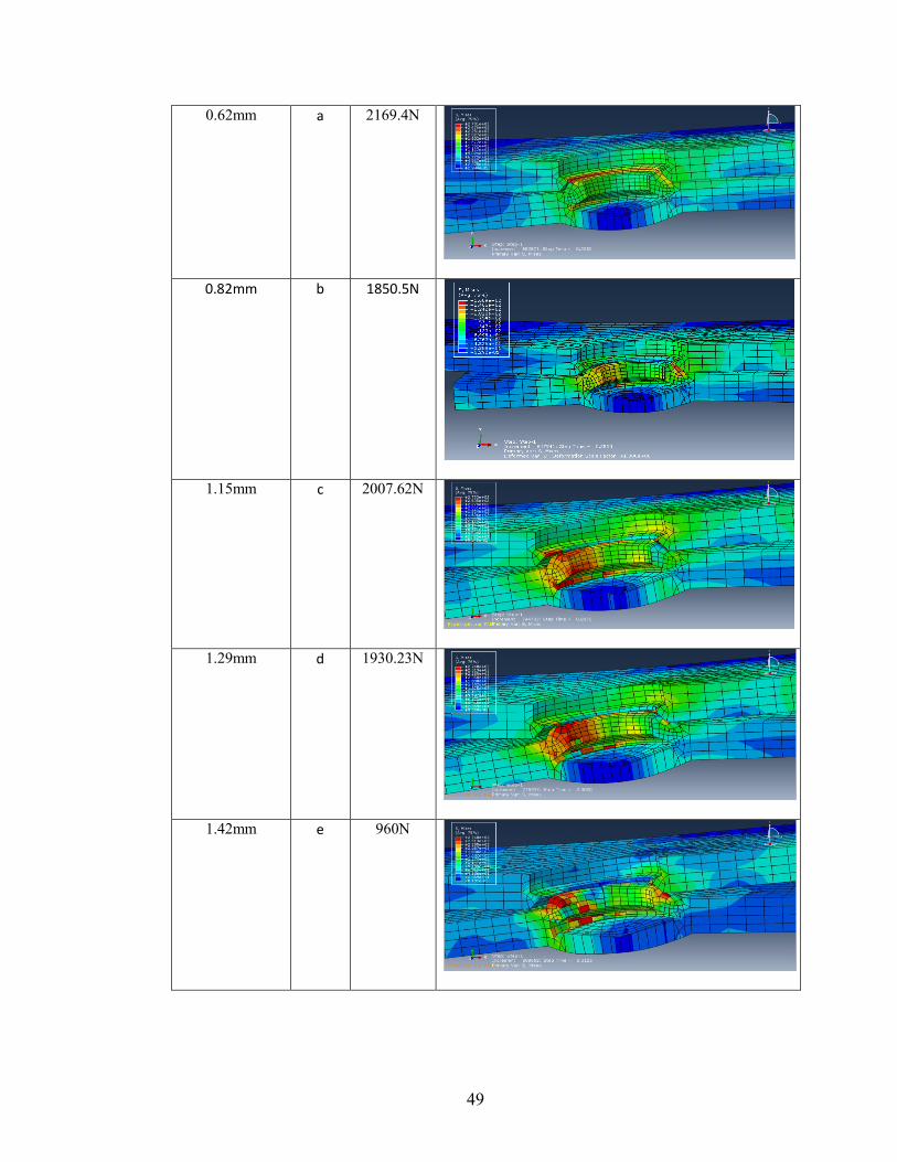
Table 3.5 Progressive view of the deformation of a joint with 6-mm mixed zone and a
two-third curl up interface
Displacement Label Force Graph
a
d
j
49
0.62mm
a 2169.4N
0.82mm b 1850.5N
1.15mm
c 2007.62N
1.29mm d 1930.23N
1.42mm e 960N

50
1.87mm f 1939.11N
2.2mm g 1103.53N
2.37mm h 922.246N
2.54mm i 1198.73N
2.72mm j 170.42N
51
The force-displacement curve for the one-third curl up model is not shown in Figure
3-25, as it has no significant difference from that of the flat interface end. This is the
result of a relatively small distance between the interfaces of the two sheets to the rivet
head boundary. One-third of the distance is very small compare to the element size used
in the simulation. As can be seen from the graph, a deformation process mainly consists
of two stages. In the first stage force increases before any fracture occurs. When it
reaches the maximum limit of bearing capability, fracture happens and load bearing
capabilities drop. In the second stage, the rivet continues rotating which results in the
tearing of the aluminum sheets. The force continues to fluctuate (drop and rise) after the
initial fracture with an overall decreasing trend.
Joints with a two-third curl up curved faying interface end have a better performance
than the flat interface end in the second stage according to the simulation. Shown in
Figure 3-24 (b) and Figure 3-24(c), the crack propagates into the top sheet easily.
Therefore the load bearing capability in the first stage is low for such a joint. However, a
joint with a two-third curl up faying interface end has a better performance than that of a
flat interface end in the second stage according to the simulation.
In order to understand the deformation mechanisms a progressive view of the
structures of the riveted joint was produced, as shown in Table 3.5 for the deformed
geometry at various deformation steps. Before 0.62mm, the force grows with the
displacement. This continues until the maximum load carried by the specimen is reached
at 2169 N. As can be seen from the graph, no fracture happens up to this point. A slightly
drop to 1850.5N due to element removal at 0.82mm. Afterwards continuing loading
generates initial fracture and the load carrying ability begins to drop at 1.15mm. Cracks
52
propagate along the faying interface end. Consequently, the load bearing capacity keeps
dropping. At 1.29mm all elements connecting the two sheets are fractured, then a
significant slump occurs. Only 960 N can be carried by the specimen at 1.42mm. The
first stage of damage ends at the total fracture of the mixed zone. Afterwards the force
starts to rise up at 1.42mm. The rotation of the rivet keeps deforming and tearing the
aluminum sheets, as a result the top sheet squeezes the bump up part of the bottom layer.
At 1.87mm, the rivet starts to destroy the mechanical interlocked near the left corner of
the rivet end, as shown in the graph. Load carrying ability drops again. The load is
922.246N at 2.37mm, and at this moment both the mixed zone and the mechanic
interlock are damaged. However, the rivet is still attached to the sheets and it resists the
separation motion. However, as most of the material around the rivet is damaged at this
moment, the load level is fairly low and the joint totally fails after a slight grow in force
at 2.54mm.
This simulation shows that the maximum load can be taken by a friction-stir riveted
joint with 6-mm mixed zone is around 2500 N. The fluctuation in load after the peak is
reached is the result of numerical simulation of the fracture process by element removal
in the simulation.
3.2.3.2. Progressive damage and fracture of joints with a 7-mm mixed zone
Compared to the simulation of joints with a 6-mm mixed zone, a simulation with a 7-
mm mixed zone is more consistent with the actual riveted joints produced in the
experiments. As discussed in Chapter 2, W is affected by the diameter of the rivet bottom
flange. The rivet bottom flange is 6 mm wide, and created by the rotating movement, the
width of the mixed zone W will likely be wider than 6 mm. Figure 2-7 illustrates that the

53
W value is stabilized at 6.5 mm when the spindle_speed/feed_rate ratio is over 40000.
Because etching of the specimens may destroy the solid bonding, the actual bonded area
is likely larger than the measurements obtained from the metallographic sections. In order
to understand the effect of mixed zone size a W of 7 mm was used in the simulation,
which is more comparable to the actual physical specimens and the load vs. displacement
response can be directly compared with the experimental observations.
Three different faying interface ends have been used in the simulation as in the case
of a 6-mm mixed zone. Figure 3-26 through Figure 3-28 show the deformation process of
such a joint under a tensile load. The basic deformation is very similar to what has been
seen in that of 6-mm mixed zone.
Figure 3-26 Deformation of a joint with a flat faying interface end and a 7-mm mixed
zone

54
Figure 3-27 Deformation of a joint with one-third curl up faying interface end and a 7-
mm mixed zone
55
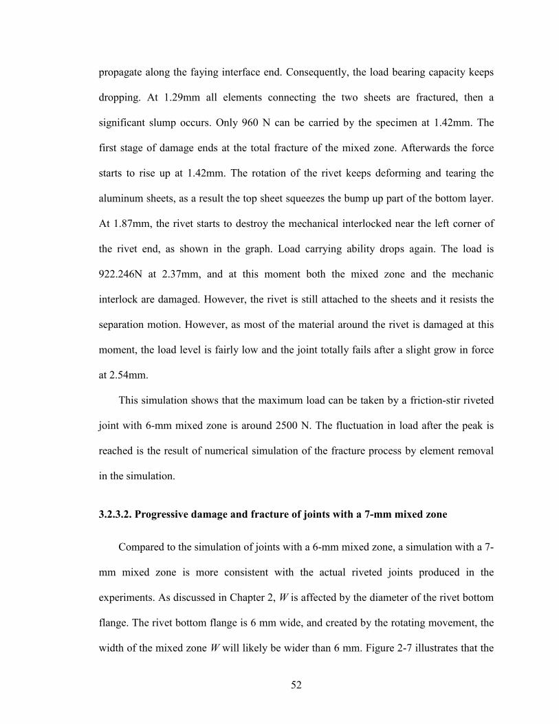
Figure 3-28 Deformation of a joint with a two-third curl up faying interface end and a 7-
mm mixed zone
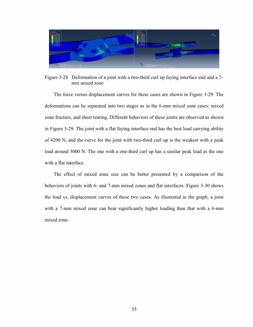
The force versus displacement curves for these cases are shown in Figure 3-29. The
deformations can be separated into two stages as in the 6-mm mixed zone cases: mixed
zone fracture, and sheet tearing. Different behaviors of these joints are observed as shown
in Figure 3-29. The joint with a flat faying interface end has the best load carrying ability
of 4200 N, and the curve for the joint with two-third curl up is the weakest with a peak
load around 3000 N. The one with a one-third curl up has a similar peak load as the one
with a flat interface.
The effect of mixed zone size can be better presented by a comparison of the
behaviors of joints with 6- and 7-mm mixed zones and flat interfaces. Figure 3-30 shows
the load vs. displacement curves of these two cases. As illustrated in the graph, a joint
with a 7-mm mixed zone can bear significantly higher loading than that with a 6-mm
mixed zone.
56
Figure 3-29 Simulation results of joints with a 7-mm mixed zone
Figure 3-30 Force vs. displacement of joints with different sizes of the mixed zone
57
4. Experiments
A series of experiments were carried out to identify an optimal friction-stir riveted
joint and to compare with simulation results. As revealed in Chapter 3 the shape of the
faying interface especially the location of the interface end has a significant influence on
the performance of a riveted joint. In riveting the faying interface end is controlled
mainly by two parameters: depth of the rivet and die volume. The deeper the rivet
penetrates into the sheets, the more the material is squeezed up, which pushes the
squeezed material upward and forms a curved interface. The possibility of changing the
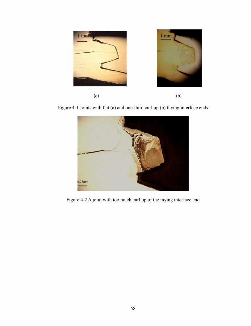
geometry of the joint is as discussed in Chapter 3. Figure 4-1 depicts interfaces of
different shapes formed by adjusting relevant parameters. The figure shows a flat faying
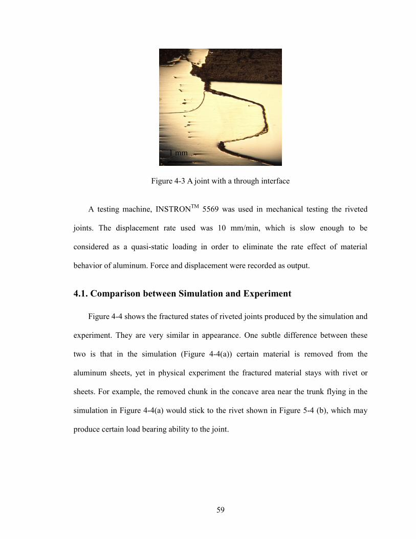
interface end and an approximately one-third curl up interface end. Figure 4-2 and Figure
4-3 illustrate a two-third curl up interface end and an effectively zero-strength joint
respectively, because of the junction of the interface with the surface of the top layer. The
finite element simulations in Chapter 3 correspond to the actual experimental
observations as shown in these figures.
58
(a) (b)
Figure 4-1 Joints with flat (a) and one-third curl up (b) faying interface ends
Figure 4-2 A joint with too much curl up of the faying interface end
1 mm 1 mm
0.25mm
59
Figure 4-3 A joint with a through interface
A testing machine, INSTRONTM
5569 was used in mechanical testing the riveted
joints. The displacement rate used was 10 mm/min, which is slow enough to be
considered as a quasi-static loading in order to eliminate the rate effect of material
behavior of aluminum. Force and displacement were recorded as output.
4.1. Comparison between Simulation and Experiment
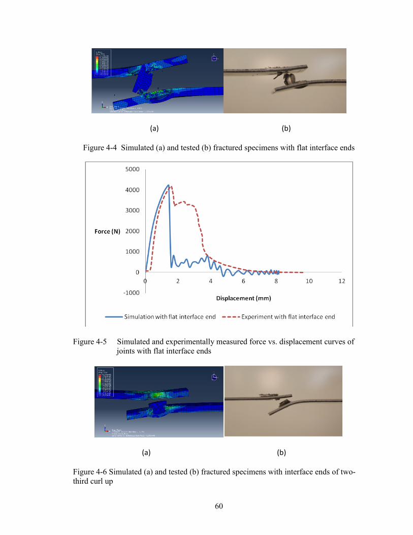
Figure 4-4 shows the fractured states of riveted joints produced by the simulation and
experiment. They are very similar in appearance. One subtle difference between these
two is that in the simulation (Figure 4-4(a)) certain material is removed from the
aluminum sheets, yet in physical experiment the fractured material stays with rivet or
sheets. For example, the removed chunk in the concave area near the trunk flying in the
simulation in Figure 4-4(a) would stick to the rivet shown in Figure 5-4 (b), which may
produce certain load bearing ability to the joint.
1 mm
60
(a) (b)
Figure 4-4 Simulated (a) and tested (b) fractured specimens with flat interface ends
Figure 4-5 Simulated and experimentally measured force vs. displacement curves of
joints with flat interface ends
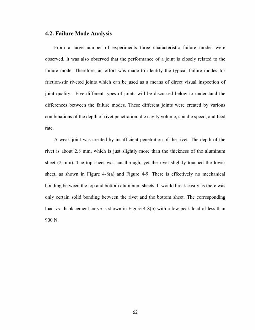
(a) (b)
Figure 4-6 Simulated (a) and tested (b) fractured specimens with interface ends of two-
third curl up

61
Figure 4-7 Simulated and experimentally measured force vs. displacement curves of
joints with two-third interface curl up ends
Comparing the load vs. displacement curves measured in the simulation and physical
experiments, as seen in Figure 4-5 and Figure 4-7, it appears that the simulation results
match reasonably with the experimental data in the first stage of loading before the peak
load is reached. However, the load bearing capability of the simulated specimen is
significantly lower than that of the physical specimen in the second stage loading. This
could be the result of the lacking of the shearing property definition in ABAQUS, and the
element removal in the simulation once an element is stressed to a limit, which does not
happen in a physical specimen. The fractured specimens shown in Figure 4-6 for joints
with two-third interface curl up are similar for the simulation and experiment, as both
have little deformation of the top sheet, and the rivet is left on the bottom sheet with large
rotation of the low sheet.
62
4.2. Failure Mode Analysis
From a large number of experiments three characteristic failure modes were
observed. It was also observed that the performance of a joint is closely related to the
failure mode. Therefore, an effort was made to identify the typical failure modes for
friction-stir riveted joints which can be used as a means of direct visual inspection of
joint quality. Five different types of joints will be discussed below to understand the
differences between the failure modes. These different joints were created by various
combinations of the depth of rivet penetration, die cavity volume, spindle speed, and feed
rate.
A weak joint was created by insufficient penetration of the rivet. The depth of the
rivet is about 2.8 mm, which is just slightly more than the thickness of the aluminum
sheet (2 mm). The top sheet was cut through, yet the rivet slightly touched the lower
sheet, as shown in Figure 4-8(a) and Figure 4-9. There is effectively no mechanical
bonding between the top and bottom aluminum sheets. It would break easily as there was
only certain solid bonding between the rivet and the bottom sheet. The corresponding
load vs. displacement curve is shown in Figure 4-8(b) with a low peak load of less than
900 N.

63
(a) (b)
Figure 4-8 Tested specimen (a) and the corresponding mechanical response (b) for a
joint with 2.794-mm penetration
Figure 4-9 Cross-section of the specimen in Figure 4-8(a)
Increasing rivet penetration produces stronger riveted joints. Figure 4-10(a) shows a
specimen with 3.556-mm penetration, and its section view is shown in Figure 4-11.
Although the depth is still not enough, there is a significant improvement in the load
bearing capacity. It has a fairly flat faying interface end which is desirable. The rivet
stays on the bottom sheet after fracture, unlike the previous case.
1 mm
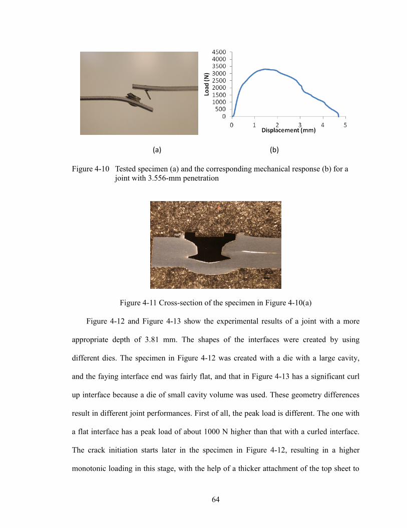
64
(a) (b)
Figure 4-10 Tested specimen (a) and the corresponding mechanical response (b) for a
joint with 3.556-mm penetration
Figure 4-11 Cross-section of the specimen in Figure 4-10(a)
Figure 4-12 and Figure 4-13 show the experimental results of a joint with a more
appropriate depth of 3.81 mm. The shapes of the interfaces were created by using
different dies. The specimen in Figure 4-12 was created with a die with a large cavity,
and the faying interface end was fairly flat, and that in Figure 4-13 has a significant curl
up interface because a die of small cavity volume was used. These geometry differences
result in different joint performances. First of all, the peak load is different. The one with
a flat interface has a peak load of about 1000 N higher than that with a curled interface.
The crack initiation starts later in the specimen in Figure 4-12, resulting in a higher
monotonic loading in this stage, with the help of a thicker attachment of the top sheet to
1 mm
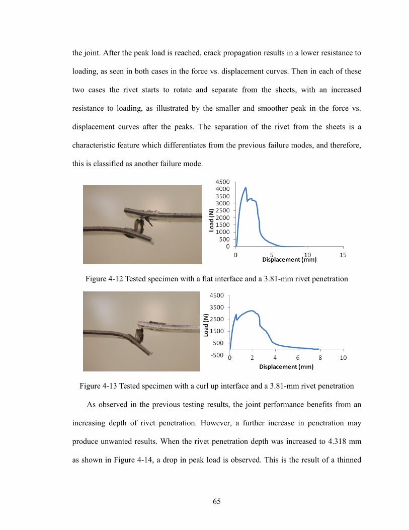
65
the joint. After the peak load is reached, crack propagation results in a lower resistance to
loading, as seen in both cases in the force vs. displacement curves. Then in each of these
two cases the rivet starts to rotate and separate from the sheets, with an increased
resistance to loading, as illustrated by the smaller and smoother peak in the force vs.
displacement curves after the peaks. The separation of the rivet from the sheets is a
characteristic feature which differentiates from the previous failure modes, and therefore,
this is classified as another failure mode.
Figure 4-12 Tested specimen with a flat interface and a 3.81-mm rivet penetration
Figure 4-13 Tested specimen with a curl up interface and a 3.81-mm rivet penetration
As observed in the previous testing results, the joint performance benefits from an
increasing depth of rivet penetration. However, a further increase in penetration may
produce unwanted results. When the rivet penetration depth was increased to 4.318 mm
as shown in Figure 4-14, a drop in peak load is observed. This is the result of a thinned
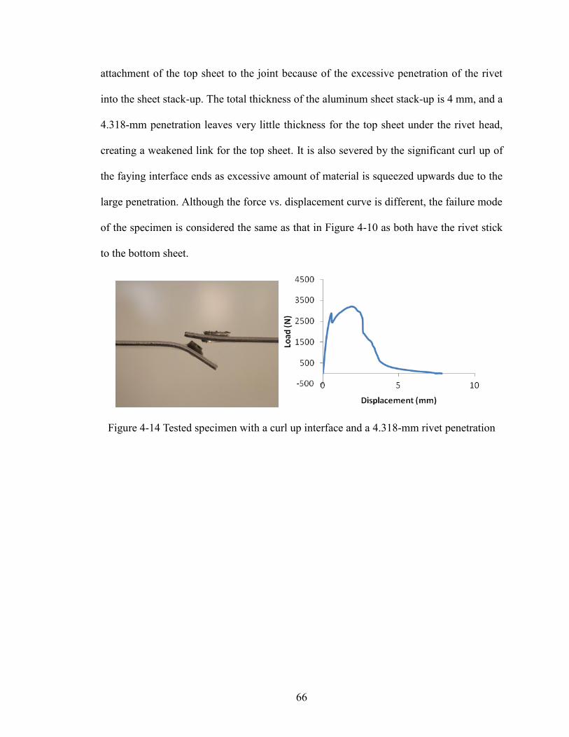
66
attachment of the top sheet to the joint because of the excessive penetration of the rivet
into the sheet stack-up. The total thickness of the aluminum sheet stack-up is 4 mm, and a
4.318-mm penetration leaves very little thickness for the top sheet under the rivet head,
creating a weakened link for the top sheet. It is also severed by the significant curl up of
the faying interface ends as excessive amount of material is squeezed upwards due to the
large penetration. Although the force vs. displacement curve is different, the failure mode
of the specimen is considered the same as that in Figure 4-10 as both have the rivet stick
to the bottom sheet.
Figure 4-14 Tested specimen with a curl up interface and a 4.318-mm rivet penetration

67
Figure 4-15 Comparison of load vs. displacement curves generated on specimens with
different failure modes
The force vs. displacement curves of the specimens with various failure modes are
plotted in Figure 4-15. The major observations of the deformation behavior and failure
modes observed in these friction-stir riveted joints can be summarized in the following:
1. Except for the one with excessive penetration, all the other joints have similar slopes
at the beginning of deformation. The one with a too large penetration has a smaller
slope as a result of the less constrained deformation of the top sheet.
2. For most of the specimens there are two stages of deformation before final rupture, as
observed in both numerical simulation and physical tests. In the first stage the sheet
material surrounding the rivet is stretched, and at the same time cracks start to initiate
mainly from the interface end where stress concentration exists, and propagate. The
second stage contains tearing and debonding caused by the rotation of rivet. As seen
from Figure 4-15: each of force vs. displacement curves has a sudden drop after the

68
peak load is reached, which is the end of the first stage; after that there is plateau or
slight increase in load bearing ability, which is the second stage.
3. A good joint should have an adequate penetration and small interface curl up. The
using of a die and clamping can significantly improve a rivet joint in this regard.
4. There are three major failure modes observed in this study:
(1) The first failure mode is when the rivet stays on the top sheet at final rupture,
often caused by insufficient penetration of the rivet. It has a very low ultimate
strength because of the weak attachment of the top sheet to the bottom sheet.
(2) The second failure mode is when the top sheet is separated from the joint and the
rivet stays on the bottom sheet at final rupture. The peak load observed in this
type of failure mode is higher than that in the first failure mode.
(3) The third failure mode is when the rivet is virtually separated from both the top
and bottom sheets with significant rotation. A large joint strength is usually
associated with the joint when this type of failure is observed.

69
5. Summary and Future Work
5.1. Summary
1. Through the study of characterizing the friction-stir riveted joint, mixed zone, dt and
db, and the depth of rivet penetration are considered to be most important factor that
may influence the riveted joint significantly.
2. By comparing simulation results shown in Figure 3-30, relatively wide rivet bottom
flange is recommended.
3. Both the simulation and experimental results give a good quality performance for flat
faying interface end joint.
4. The depth of rivet penetration should between 3.8mm and 4mm.
5.2. Future Work
1. Spindle speed and feed rate may influence the mixed zone quality by heat generation.
Efforts should be made to improve the mechanic strength of the mixed zone in order
to increase the load carrying ability.
2. In this thesis, the simulation agrees well with the experiments only in the first stage of
loading. This is caused by a lack of material definition for the shearing fracture of the
metal in the joint, especially the mixed zone. Realistic material properties can be
obtained from simulating a riveting process, and the resulted riveted joint is then used
for testing.
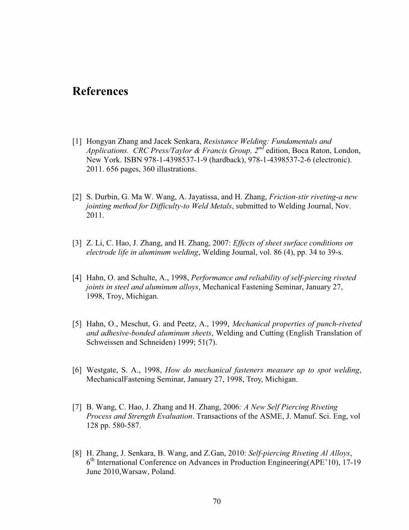
70
References
[1] Hongyan Zhang and Jacek Senkara, Resistance Welding: Fundamentals and
Applications. CRC Press/Taylor & Francis Group, 2nd
edition, Boca Raton, London,
New York. ISBN 978-1-4398537-1-9 (hardback), 978-1-4398537-2-6 (electronic).
2011. 656 pages, 360 illustrations.
[2] S. Durbin, G. Ma W. Wang, A. Jayatissa, and H. Zhang, Friction-stir riveting-a new
jointing method for Difficulty-to Weld Metals, submitted to Welding Journal, Nov.
2011.
[3] Z. Li, C. Hao, J. Zhang, and H. Zhang, 2007: Effects of sheet surface conditions on
electrode life in aluminum welding, Welding Journal, vol. 86 (4), pp. 34 to 39-s.
[4] Hahn, O. and Schulte, A., 1998, Performance and reliability of self-piercing riveted
joints in steel and aluminum alloys, Mechanical Fastening Seminar, January 27,
1998, Troy, Michigan.
[5] Hahn, O., Meschut, G. and Peetz, A., 1999, Mechanical properties of punch-riveted
and adhesive-bonded aluminum sheets, Welding and Cutting (English Translation of
Schweissen and Schneiden) 1999; 51(7).
[6] Westgate, S. A., 1998, How do mechanical fasteners measure up to spot welding,
MechanicalFastening Seminar, January 27, 1998, Troy, Michigan.
[7] B. Wang, C. Hao, J. Zhang and H. Zhang, 2006: A New Self Piercing Riveting
Process and Strength Evaluation. Transactions of the ASME, J. Manuf. Sci. Eng, vol
128 pp. 580-587.
[8] H. Zhang, J. Senkara, B. Wang, and Z.Gan, 2010: Self-piercing Riveting Al Alloys,
6th
International Conference on Advances in Production Engineering(APE’10), 17-19
June 2010,Warsaw, Poland.

71
[9] Thomas, WM; Nicholas, ED; Needham, JC; Murch, MG;Temple-Smith, P;Dawes,
CJ.Frictionstir butt welding, GB Patent No. 9125978.8, International patent
application No.PCT/GB92/02203, 1991.
[10] R. Mishra, Z. Ma. Friction stir welding and processing. Materials Science and
Engineering, 2005,R50:1-78.
[11] H. Luo, New joining techniques for magnesium alloy sheets, MS Thesis, Institute of
Metal Research, Chinese Academy of Sciences, May 2008.
[12] J. Esparza, W. Davis, E. Trillo, L. Murr. Friction-stir welding of magnesium alloy
AZ31B.Materials Science, 2002, 21(12):917-920.
[13] W. Lee, Y. Yeon, S. Jung. Joint properties of friction stir welded AZ31B-H24
magnesium alloy.Materials Science and Technology, 2003, 19(6):785-790.
[14] W. Lee, J. Kim, Y. Yeon, S. Jung. The joint characteristics of friction stir welded
AZ91D magnesium alloy. Materials Transactions, 2003, 44(5):917-923.
[15] S. Lathabai, M. Painter, G. Cantin, and V. Tyagi. Friction spot joining of an extruded
Al–Mg–Si alloy, Scripta Materialia, 2006, 55:899–902.
[16] A. Gerlich, P. Su, and T. North. Friction stir spot welding of Mg-alloys for
automotive applications. Magnesium Technology 2005. TMS, 2005, pp383-388.
[17] IEEE 5th
International symposium on Micro Machine and Human Science
Proceeding,Nagoya, Oct 1994
[18] Y. Ling, 1996: Uniaxial True Stress-Strain after Necking, AMP Journal of
Technology Vol. 5 pp.37-48.
[19] P. Boresi, Advanced Mechanics of Materials, 6th
Edition, October 2002, ©2003. page
14
72
[20] O. Chukwuemeka, I. Kingsley, 2008: Analysis of Strength of Self-Pierce Riveted
Alumiium Plate Using Finite Element Method, MS thesis. Blekinge Institute of
Technology, Karlskrona, Sweden.
[21] ABAQUS Analysis User’s Manual for version 6.10,2010, DS SIMULIA.
[22] American Society for Testing and Material Standard Tension Testing of Metallic of
Metallic Materials
[23] Zhuo Zhuang, ABAQUS nonlinear Finite Element Analysis and Example Manual,
2005, P70.
73
List of Publications
1. H. Zhang, A. H. Jayatissa, S. Durbin, and G. Ma: What if They Are Not Weld-able?
Management and Production Engineering Review" (MPER), a quarterly journal
published by the Polish Academy of Sciences, submitted Oct. 2011.
2. S. Durbin, G. Ma, A. Jayatissa, and H. Zhang, 2011: Characterization of Friction Stir
Riveting Process, submitted to Welding Journal, Nov. 2011.
3. G. Ma, S. Durbin, W. Wang, A. Jayatissa, and H. Zhang, 2012: Performance of
Friction Stir Riveted Joints, to be submitted to Welding Science and Technology.
4. G. Ma, S. Durbin, W. Wang, A. Jayatissa, and H. Zhang, 2012: Characteristics of
Friction-Stir Riveted Joints, 15th
Sheet Metal Welding Conference, Oct., 2012,
Livonia, MI.
5. S. Durbin, G. Ma, A. Jayatissa, H. Zhang, and J. Bohr, 2012: Friction-Stir Riveting,
15th
Sheet Metal Welding Conference, Oct., 2012, Livonia, MI.
6. Poster: Feasibility Study of Hybrid Friction-Stir Riveting, A.H. Jayatissa, G. Ma, S.
Durbin, and H. Zhang, 2011 National Science Foundation (NSF) Civil, Mechanical
and Manufacturing Innovation (CMMI) Conference, held January 4-7, 2011 in
Atlanta, Georgia.
Related Documents