Version 19.1 Frew

Welcome message from author
This document is posted to help you gain knowledge. Please leave a comment to let me know what you think about it! Share it to your friends and learn new things together.
Transcript

Version 19.1
Frew

Oasys Ltd
13 Fitzroy StreetLondon
W1T 4BQ
Central SquareForth Street
Newcastle Upon TyneNE1 3PL
Telephone: +44 (0) 191 238 7559Facsimile: +44 (0) 191 238 7555
e-mail: [email protected]: http://www.oasys-software.com/
© Oasys Ltd. 2012

All rights reserved. No parts of this work may be reproduced in any form or by any means - graphic, electronic, ormechanical, including photocopying, recording, taping, or information storage and retrieval systems - without thewritten permission of the publisher.
Products that are referred to in this document may be either trademarks and/or registered trademarks of therespective owners. The publisher and the author make no claim to these trademarks.
While every precaution has been taken in the preparation of this document, the publisher and the author assume noresponsibility for errors or omissions, or for damages resulting from the use of information contained in thisdocument or from the use of programs and source code that may accompany it. In no event shall the publisher andthe author be liable for any loss of profit or any other commercial damage caused or alleged to have been causeddirectly or indirectly by this document.
This document has been created to provide a guide for the use of the software. It does not provide engineeringadvice, nor is it a substitute for the use of standard references. The user is deemed to be conversant with standardengineering terms and codes of practice. It is the users responsibility to validate the program for the proposeddesign use and to select suitable input data.
Printed: May 2012
Frew Oasys GEO Suite for Windows
© Oasys Ltd. 2012
Frew Oasys GEO Suite for WindowsI
© Oasys Ltd. 2012
Table of Contents
1 About Frew 1................................................................................................................................... 11.1 General Program Description
................................................................................................................................... 11.2 Program Features
................................................................................................................................... 31.3 Components of the User Interface ......................................................................................................................................................... 3Working with the Gateway 1.3.1
2 Methods of Analysis 4................................................................................................................................... 42.1 Stability Check
......................................................................................................................................................... 4Fixed Earth Mechanisms 2.1.1
......................................................................................................................................................... 5Free Earth Mechanisms 2.1.2
.................................................................................................................................................. 5Multi-propped w alls2.1.2.1
......................................................................................................................................................... 8Active and Passive Limits 2.1.3
......................................................................................................................................................... 10Groundwater Flow 2.1.4
................................................................................................................................... 112.2 Full Analysis
................................................................................................................................... 122.3 Soil Models ......................................................................................................................................................... 13Safe Method 2.3.1
......................................................................................................................................................... 13Mindlin Method 2.3.2
......................................................................................................................................................... 14Method of Sub-grade Reaction 2.3.3
................................................................................................................................... 152.4 Active and Passive Pressures ......................................................................................................................................................... 16Effects of Excavation and Backfill 2.4.1
......................................................................................................................................................... 16Calculation of Earth Pressure Coefficients 2.4.2
................................................................................................................................... 182.5 Total and Effective Stress ......................................................................................................................................................... 19Drained Materials 2.5.1
......................................................................................................................................................... 19Undrained Materials and Calculated Pore Pressures 2.5.2
......................................................................................................................................................... 21Undrained Materials and User-defined Pore Pressure 2.5.3
......................................................................................................................................................... 23Undrained to Drained Example 2.5.4
3 Input Data 23................................................................................................................................... 243.1 Assembling Data
................................................................................................................................... 293.2 Preferences
................................................................................................................................... 303.3 New Model Wizard ......................................................................................................................................................... 30New Model Wizard: Titles and Units 3.3.1
......................................................................................................................................................... 30New Model Wizard: Basic Data 3.3.2
......................................................................................................................................................... 32New Model Wizard: Stage Defaults 3.3.3
......................................................................................................................................................... 32New Model Wizard: Soil Interfaces 3.3.4
................................................................................................................................... 333.4 Global Data ......................................................................................................................................................... 34Titles 3.4.1
.................................................................................................................................................. 35Titles w indow - Bitmaps3.4.1.1
......................................................................................................................................................... 35Units 3.4.2
......................................................................................................................................................... 36Specification 3.4.3
......................................................................................................................................................... 37Material Properties 3.4.4
......................................................................................................................................................... 39Stage Data 3.4.5
.................................................................................................................................................. 40Stage 0 - Initial Conditions3.4.5.1
IIContents
© Oasys Ltd. 2012
.................................................................................................................................................. 41New Stages3.4.5.2
.................................................................................................................................................. 41Inserting Stages3.4.5.3
.................................................................................................................................................. 42Deleting a Stage3.4.5.4
.................................................................................................................................................. 42Editing Stage Data3.4.5.5
.................................................................................................................................................. 43Editing Stage Titles3.4.5.6
.................................................................................................................................................. 44Apply/Remove Surcharges3.4.5.7
.................................................................................................................................................. 44Insert/Remove Struts3.4.5.8
.................................................................................................................................................. 45Soil Zones3.4.5.9
........................................................................................................................................... 48Dig/Fill Operations3.4.5.9.1
.................................................................................................................................................. 49Wall Data3.4.5.10
.................................................................................................................................................. 51Groundw ater3.4.5.11
.................................................................................................................................................. 54Analysis Data3.4.5.12
........................................................................................................................................... 55Model Type3.4.5.12.1
........................................................................................................................................... 56Boundary Distances3.4.5.12.2
........................................................................................................................................... 57Wall Relaxation3.4.5.12.3
........................................................................................................................................... 57Fixed or Free Solution3.4.5.12.4
........................................................................................................................................... 57Young’s Modulus (E)3.4.5.12.5
........................................................................................................................................... 58Redistribution of Pressures3.4.5.12.6
........................................................................................................................................... 58Minimum Equivalent Fluid Pressure3.4.5.12.7
........................................................................................................................................... 60Passive Softening3.4.5.12.8
.................................................................................................................................................. 61Convergence Control3.4.5.13
........................................................................................................................................... 62Maximum number of Iterations3.4.5.13.1
........................................................................................................................................... 62Tolerance for Displacement3.4.5.13.2
........................................................................................................................................... 62Tolerance for Pressure3.4.5.13.3
........................................................................................................................................... 62Damping Coeff icient3.4.5.13.4
........................................................................................................................................... 63Maximum Incremental Displacement3.4.5.13.5
......................................................................................................................................................... 63Nodes 3.4.6
......................................................................................................................................................... 66Strut Properties 3.4.7
.................................................................................................................................................. 68Modelling of Anchors3.4.7.1
......................................................................................................................................................... 69Surcharges 3.4.8
.................................................................................................................................................. 70Application of Uniformly Distributed Loads3.4.8.1
.................................................................................................................................................. 70Application of Strip Loads3.4.8.2
4 Partial Factors 72
5 Frew-Safe Link 75................................................................................................................................... 755.1 Data Entry
................................................................................................................................... 805.2 Data Conversion ......................................................................................................................................................... 80Stages/Runs 5.2.1
......................................................................................................................................................... 82Geometry 5.2.2
......................................................................................................................................................... 82Restraints 5.2.3
......................................................................................................................................................... 83Surcharges 5.2.4
......................................................................................................................................................... 83Struts 5.2.5
......................................................................................................................................................... 84Materials 5.2.6
.................................................................................................................................................. 86First Stage Material5.2.6.1
......................................................................................................................................................... 88Groundwater 5.2.7
......................................................................................................................................................... 89Unsupported Features 5.2.8
6 Integral Bridge Analysis 89................................................................................................................................... 906.1 Data Entry
................................................................................................................................... 946.2 Algorithms

Frew Oasys GEO Suite for WindowsIII
© Oasys Ltd. 2012
7 Output 94................................................................................................................................... 947.1 Analysis and Data Checking
................................................................................................................................... 977.2 Tabulated Output ......................................................................................................................................................... 99Stability Check Results 7.2.1
......................................................................................................................................................... 100Detailed Results 7.2.2
.................................................................................................................................................. 101Results Annotations and Error Messages7.2.2.1
................................................................................................................................... 1027.3 Graphical Output
................................................................................................................................... 1057.4 Batch Plotting
8 Detailed Processes in Frew 106................................................................................................................................... 1068.1 General
................................................................................................................................... 1068.2 Approximations Used in the Safe Method ......................................................................................................................................................... 106The Basic Safe Model 8.2.1
......................................................................................................................................................... 107Application of the Model in Frew 8.2.2
......................................................................................................................................................... 109Accuracy w ith Respect to Young's Modulus (E) 8.2.3
.................................................................................................................................................. 109Linear Profile of E With Non-Zero Value at the Surface8.2.3.1
.................................................................................................................................................. 109Irregular Variation of E8.2.3.2
......................................................................................................................................................... 111Effect of the Distance to Vertical Rigid Boundaries 8.2.4
.................................................................................................................................................. 112Accuracy of Modelling Boundaries in Frew8.2.4.1
......................................................................................................................................................... 115Friction at the Soil/Wall Interface 8.2.5
.................................................................................................................................................. 116Accuracy of the 'Fixed' Solution8.2.5.1
................................................................................................................................... 1168.3 Approximations Used in the Mindlin Method ......................................................................................................................................................... 116The Basic Mindlin Model 8.3.1
......................................................................................................................................................... 117Application of the Model in Frew 8.3.2
.................................................................................................................................................. 117Accuracy of the Mindlin Solution in Frew8.3.2.1
................................................................................................................................... 1198.4 Calculation of Active and Passive Limits and Application of Redistribution ......................................................................................................................................................... 120General 8.4.1
......................................................................................................................................................... 121Application in Frew 8.4.2
......................................................................................................................................................... 125Iterative Technique Adopted in Frew 8.4.3
................................................................................................................................... 1268.5 Active Pressures Due to Strip Load Surcharges ......................................................................................................................................................... 126Application in Frew 8.5.1
......................................................................................................................................................... 128Passive Pressures Due to Strip Load Surcharges 8.5.2
.................................................................................................................................................. 129Requirement 18.5.2.1
.................................................................................................................................................. 130Requirement 28.5.2.2
.................................................................................................................................................. 130Requirement 38.5.2.3
.................................................................................................................................................. 131Requirement 48.5.2.4
................................................................................................................................... 1328.6 Wall and Strut Stiffness Matrices ......................................................................................................................................................... 132Wall Stiffness Matrices 8.6.1
......................................................................................................................................................... 134Strut or Anchor Matrices 8.6.2
................................................................................................................................... 1358.7 Modelling Axi-symmetric Problems Using Frew ......................................................................................................................................................... 136Soil Inside the Excavation 8.7.1
......................................................................................................................................................... 137Soil Outside the Excavation 8.7.2
......................................................................................................................................................... 138Stiffness Varying with Depth 8.7.3
................................................................................................................................... 1388.8 Modelling Berms ......................................................................................................................................................... 139Rigorous Method 8.8.1
......................................................................................................................................................... 141Simplified Procedure 8.8.2
................................................................................................................................... 1428.9 Creep and Relaxation ......................................................................................................................................................... 142Changing From Short Term to Long Term Stiffness 8.9.1

IVContents
© Oasys Ltd. 2012
................................................................................................................................... 1448.10 Undrained to drained behaviour - Manual Process ......................................................................................................................................................... 145Undrained to Drained Examples 8.10.1
9 List of References 151................................................................................................................................... 1519.1 References
10Brief Technical Description 152................................................................................................................................... 15210.1 Suggested Description for Use in Memos/Letters, etc
................................................................................................................................... 15210.2 Brief Description for Inclusion in Reports
11Manual Example 153................................................................................................................................... 15311.1 General
Index 154

1 Frew Oasys GEO Suite for Windows
© Oasys Ltd. 2012
1 About Frew
1.1 General Program Description
Frew (Flexible REtaining Walls) is a program that analyses flexible earth retaining structures suchas sheet pile and diaphragm walls. The program enables the user to study the deformations of, andstresses within, the structure through a specified sequence of construction. This sequence usually involves the initial installation of the wall followed by a series of activities suchas variations of soil levels and water pressures, the insertion or removal of struts or ground anchorsand the application of surcharges. The program calculates displacements, earth pressures, bending moments, shear forces and strut(or anchor) forces occurring during each stage in construction. It is important to realise that Frew is an advanced program analysing a complex problem and theuser must be fully aware of the various methods of analysis, requirements and limitations discussedin this help file before use. The program input is fully interactive and allows both experienced and inexperienced users to controlthe program operation.
1.2 Program Features
The main features of Frew are summarised below:
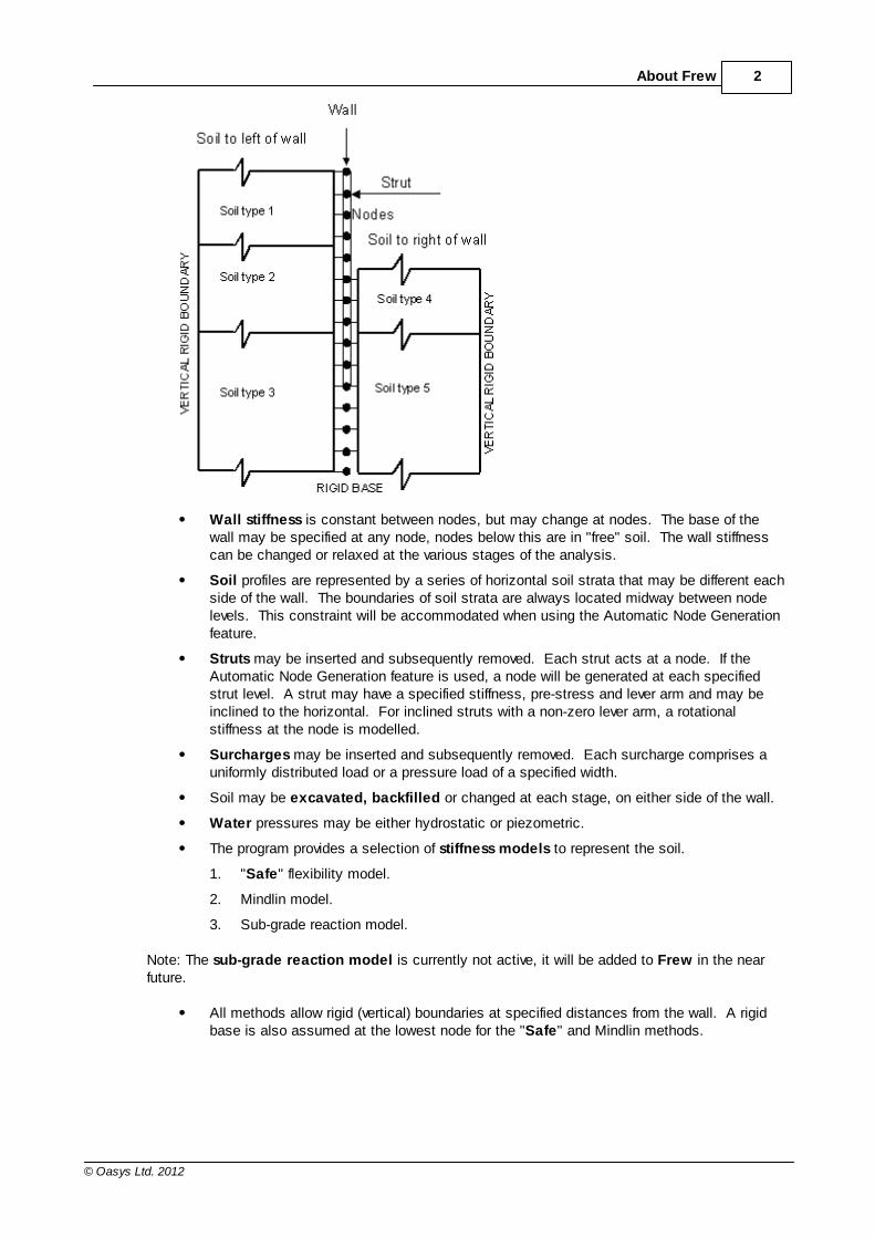
The geometry of the wall is specified by a number of nodes. The positions of these nodesare expressed by reduced levels. The nodes can be generated from the other data (soilinterface levels etc.) using the Automatic Node Generation feature.
2About Frew
© Oasys Ltd. 2012
Wall stiffness is constant between nodes, but may change at nodes. The base of thewall may be specified at any node, nodes below this are in "free" soil. The wall stiffnesscan be changed or relaxed at the various stages of the analysis.
Soil profiles are represented by a series of horizontal soil strata that may be different eachside of the wall. The boundaries of soil strata are always located midway between nodelevels. This constraint will be accommodated when using the Automatic Node Generationfeature.
Struts may be inserted and subsequently removed. Each strut acts at a node. If theAutomatic Node Generation feature is used, a node will be generated at each specifiedstrut level. A strut may have a specified stiffness, pre-stress and lever arm and may beinclined to the horizontal. For inclined struts with a non-zero lever arm, a rotationalstiffness at the node is modelled.
Surcharges may be inserted and subsequently removed. Each surcharge comprises auniformly distributed load or a pressure load of a specified width.
Soil may be excavated, backfilled or changed at each stage, on either side of the wall.
Water pressures may be either hydrostatic or piezometric.
The program provides a selection of stiffness models to represent the soil.
1. "Safe" flexibility model.
2. Mindlin model.
3. Sub-grade reaction model.
Note: The sub-grade reaction model is currently not active, it will be added to Frew in the nearfuture.
All methods allow rigid (vertical) boundaries at specified distances from the wall. A rigidbase is also assumed at the lowest node for the "Safe" and Mindlin methods.
3 Frew Oasys GEO Suite for Windows
© Oasys Ltd. 2012
Soil pressure limits, active and passive, may be redistributed to allow for arching effects.
Any vertical distribution of Young's modulus may be specified, and each model provides anapproximate representation of this distribution. Alternatively the user may specify Young'smodulus as either constant for the Mindlin model or linearly variable for the "Safe" methodif desired.
1.3 Components of the User Interface
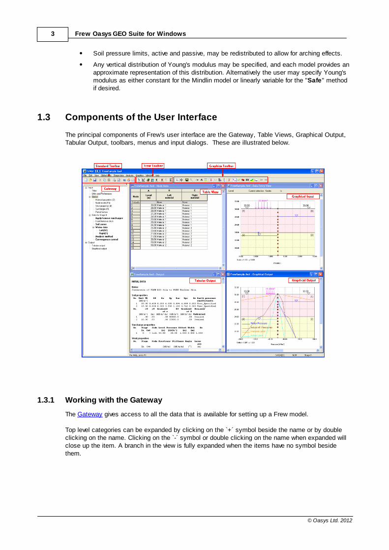
The principal components of Frew's user interface are the Gateway, Table Views, Graphical Output,Tabular Output, toolbars, menus and input dialogs. These are illustrated below.
1.3.1 Working with the Gateway
The Gateway gives access to all the data that is available for setting up a Frew model.
Top level categories can be expanded by clicking on the `+´ symbol beside the name or by doubleclicking on the name. Clicking on the `-´ symbol or double clicking on the name when expanded willclose up the item. A branch in the view is fully expanded when the items have no symbol besidethem.
4About Frew
© Oasys Ltd. 2012
Double clicking on an item will open the appropriate table view or dialog for data input. The gatewaydisplays data from the current stage under "Data for Stage ..." node. The data items which havechanged from the previous stage are indicated by bold font.
2 Methods of Analysis
Frew is used to compute the behaviour of a retaining wall through a series of constructionsequences. A limit equilibrium stability check is also available, either for a single stage (with finalexcavation levels) or for a complete construction sequence. Displacement calculations in the full analysis are complex and involve considerable approximations.It is essential therefore, that the user understands these approximations and considers theirlimitations before deciding which type of analysis is appropriate to the problem. The main features ofthe computations are summarised here. Further details are presented in the section on "DetailedProcesses in Frew". A summary of the Frew analysis, for inclusion with the program results and project reports, isincluded in Brief technical description.
2.1 Stability Check
The stability check calculations assume limit equilibrium, i.e. limiting active and passive stateseither side of the wall.
These pressures are used to calculate the required penetration of the wall to achieve rotationalstability.
Support for partial factor analysis is now available in the program.The user may specify this in "Partial Factors" dialog.
Two statically determinate mechanisms in the form of "Fixed earth" cantilever and "Free earth"propped retaining walls can be solved. For either problem several struts with specified forces can beapplied.
Note : The user should be aware that other mechanisms of collapse may exist for the problem whichare not considered by the stability check. These include rotation of the soil mass, failure of theprops/anchors or failure of the wall in bending.
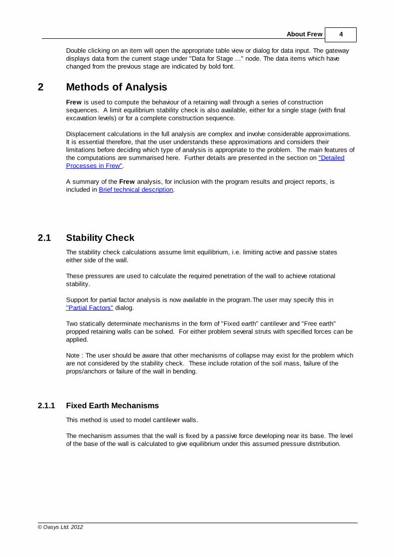
2.1.1 Fixed Earth Mechanisms
This method is used to model cantilever walls.
The mechanism assumes that the wall is fixed by a passive force developing near its base. The levelof the base of the wall is calculated to give equilibrium under this assumed pressure distribution.
5 Frew Oasys GEO Suite for Windows
© Oasys Ltd. 2012
Pressure diagram for Fixed Earth mechanism
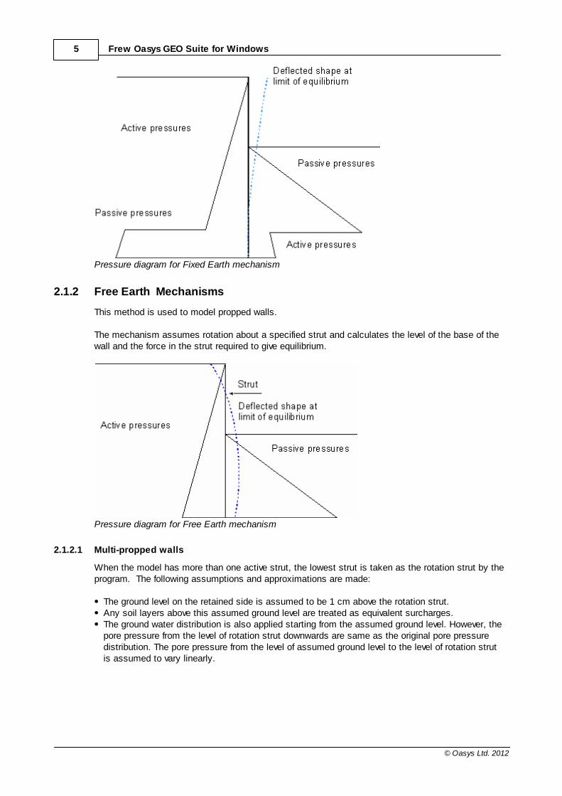
2.1.2 Free Earth Mechanisms
This method is used to model propped walls.
The mechanism assumes rotation about a specified strut and calculates the level of the base of thewall and the force in the strut required to give equilibrium.
Pressure diagram for Free Earth mechanism
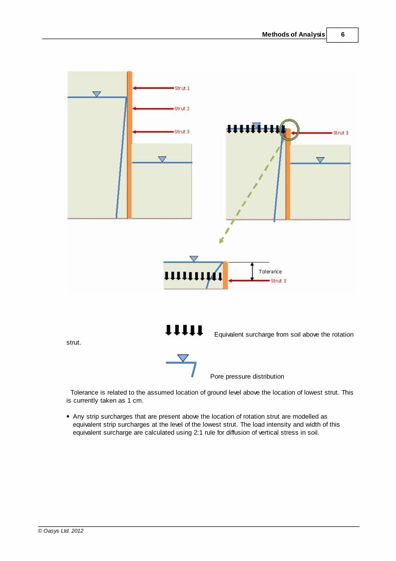
2.1.2.1 Multi-propped walls
When the model has more than one active strut, the lowest strut is taken as the rotation strut by theprogram. The following assumptions and approximations are made:
The ground level on the retained side is assumed to be 1 cm above the rotation strut. Any soil layers above this assumed ground level are treated as equivalent surcharges. The ground water distribution is also applied starting from the assumed ground level. However, thepore pressure from the level of rotation strut downwards are same as the original pore pressuredistribution. The pore pressure from the level of assumed ground level to the level of rotation strutis assumed to vary linearly.
6Methods of Analysis
© Oasys Ltd. 2012
Equivalent surcharge from soil above the rotationstrut.
Pore pressure distribution
Tolerance is related to the assumed location of ground level above the location of lowest strut. Thisis currently taken as 1 cm.
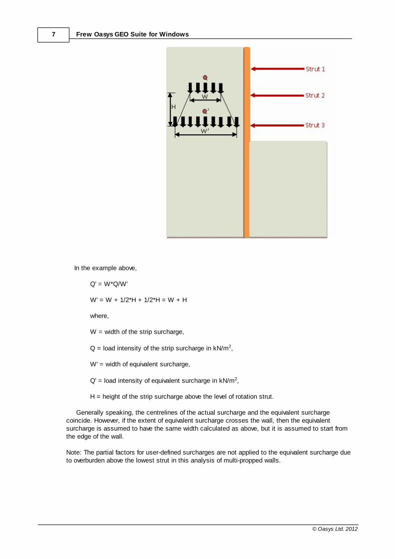
Any strip surcharges that are present above the location of rotation strut are modelled asequivalent strip surcharges at the level of the lowest strut. The load intensity and width of thisequivalent surcharge are calculated using 2:1 rule for diffusion of vertical stress in soil.
7 Frew Oasys GEO Suite for Windows
© Oasys Ltd. 2012
In the example above,
Q' = W*Q/W'
W' = W + 1/2*H + 1/2*H = W + H
where,
W = width of the strip surcharge,
Q = load intensity of the strip surcharge in kN/m2,
W' = width of equivalent surcharge,
Q' = load intensity of equivalent surcharge in kN/m2,
H = height of the strip surcharge above the level of rotation strut.
Generally speaking, the centrelines of the actual surcharge and the equivalent surchargecoincide. However, if the extent of equivalent surcharge crosses the wall, then the equivalentsurcharge is assumed to have the same width calculated as above, but it is assumed to start fromthe edge of the wall.
Note: The partial factors for user-defined surcharges are not applied to the equivalent surcharge dueto overburden above the lowest strut in this analysis of multi-propped walls.
8Methods of Analysis
© Oasys Ltd. 2012
2.1.3 Active and Passive Limits
Active and passive pressures are calculated at the top and base level of each stratum and atintermediate levels. These are placed where there is a change in linear profile of pressure with depth.
The generation of intermediate levels ensures the accuracy of the calculation of bending momentsand shear forces. Intermediate levels will be generated where there is a change in the linear profileof pressure with depth e.g.
at water table levels/piezometric points
at surcharge levels
at intervals of 0.5 units within a stratum with a cohesion strength component
The effective active and passive pressures are denoted by p'a and p'
p respectively. These are
calculated from the following equations:-
p'a = k
a '
v - k
acc'
p'p = k
p '
v + k
pcc'
wherec' = effective cohesion or undrained
strength as appropriate'v
= vertical effective overburden pressure
Note : Modification of the vertical effective stress due to wall friction should be made by takingappropriate values of k
a and k
p.
ka and k
p= horizontal coefficients of active and
passive pressurek
ac and k
pc = cohesive coefficients of active and
passive pressure
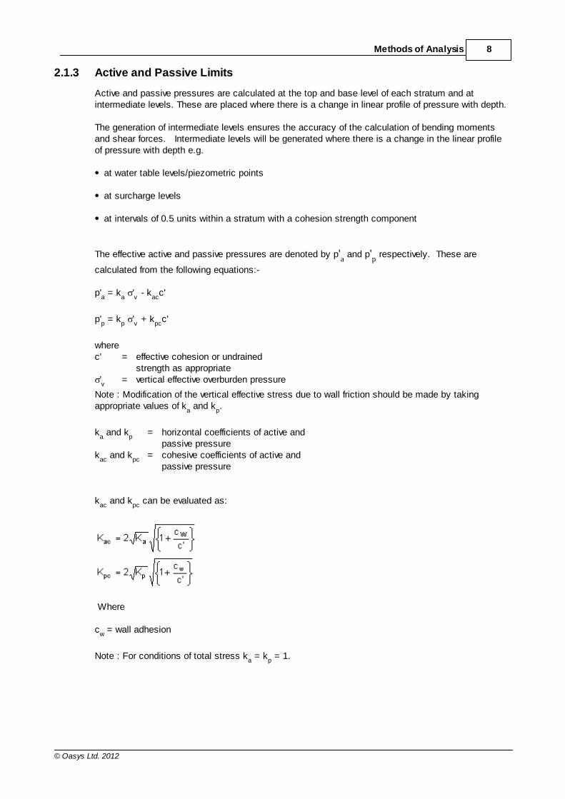
kac
and kpc
can be evaluated as:
Where c
w = wall adhesion
Note : For conditions of total stress ka = k
p = 1.
9 Frew Oasys GEO Suite for Windows
© Oasys Ltd. 2012
For a given depth z
where
s= unit weight of soil
u = pore water pressure
zudl= vertical sum of pressures of all
uniformly distributed loads (udl's) above depth z.
A minimum value of zero is assumed for the value of (ka
'v - k
acc').
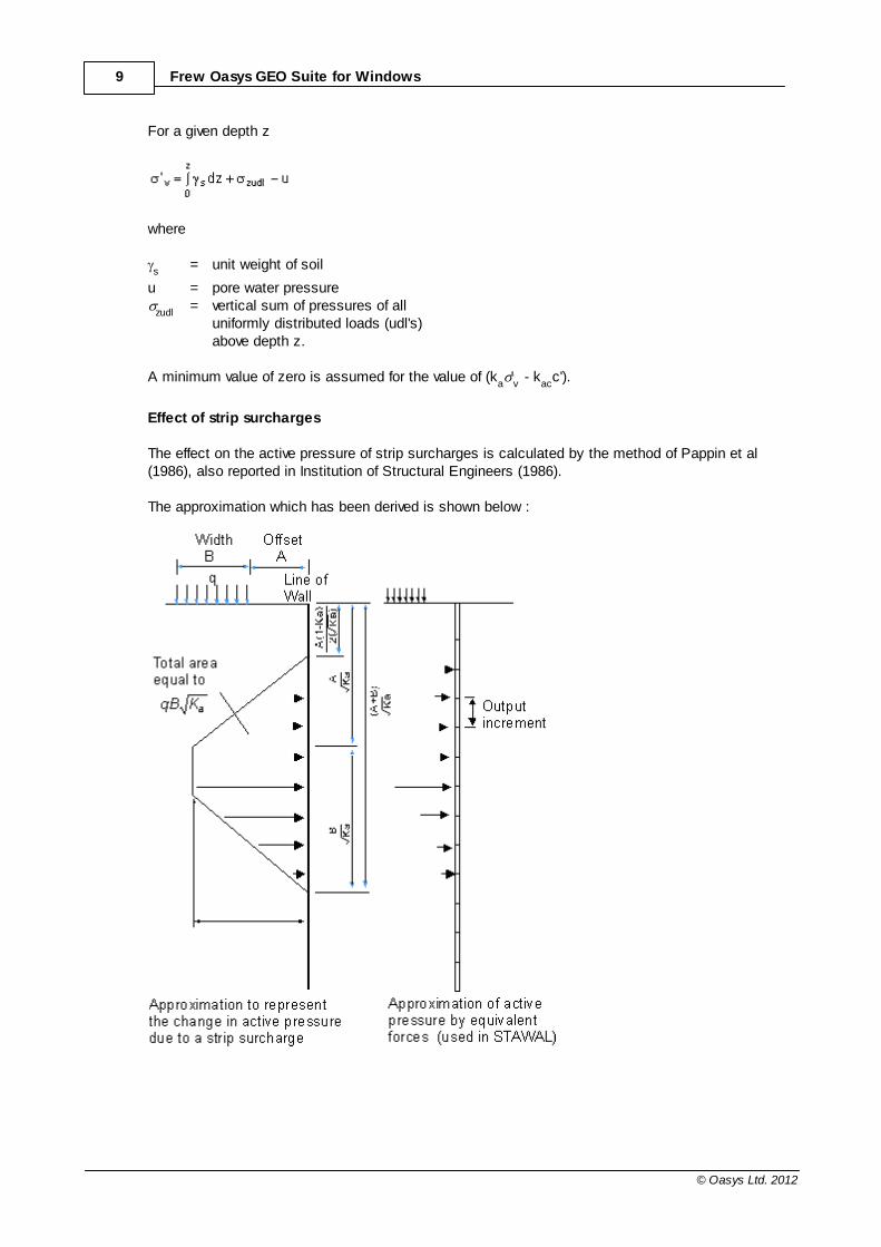
Effect of strip surcharges
The effect on the active pressure of strip surcharges is calculated by the method of Pappin et al(1986), also reported in Institution of Structural Engineers (1986).
The approximation which has been derived is shown below :
10Methods of Analysis
© Oasys Ltd. 2012
Note : If the width of the load (B) is small, the diagram will become triangular.
The additional active pressure due to the surcharge is replaced by a series of equivalent forces.These act at the same spacing of the output increment down the wall. Thus a smaller outputincrement will increase the accuracy of the calculation.
Varying values of ka
If the active pressure coefficient ka varies with depth, the program chooses a mean value of k
a
between any depth z and the level of the surcharge. Stawal then imposes the criterion that theactive force due to the surcharge down to depth z be equal to the force derived from the diagram inabove.
This is then subjected to the further limitation that the pressure does not exceed qkaz.
where
q = surcharge pressure.
kaz
= active pressure coefficient to depth z.
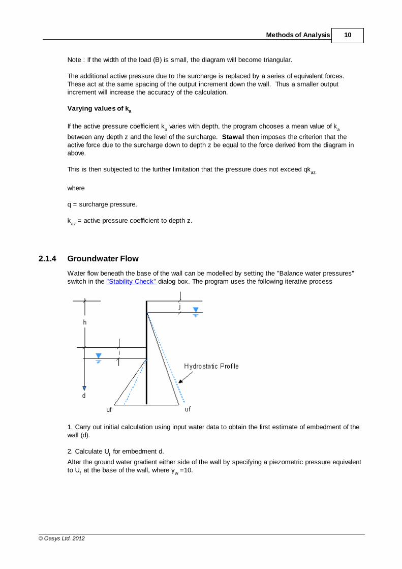
2.1.4 Groundwater Flow
Water flow beneath the base of the wall can be modelled by setting the "Balance water pressures"switch in the "Stability Check" dialog box. The program uses the following iterative process
1. Carry out initial calculation using input water data to obtain the first estimate of embedment of thewall (d).
2. Calculate Uf for embedment d.
Alter the ground water gradient either side of the wall by specifying a piezometric pressure equivalentto U
f at the base of the wall, where γ
w =10.
11 Frew Oasys GEO Suite for Windows
© Oasys Ltd. 2012
3. Re-run the Stability analysis.
4. Check calculated value of d.
5. Repeat steps 2 to 4 until d is consistent with the groundwater profile and Uf is balanced at thebase.
Note: This modification to water profile is only for stability calculations. It is NOT carried over to theactual Frew analysis.
2.2 Full Analysis
The analysis is carried out in steps corresponding to the proposed stages of excavation andconstruction. An example, showing typical stages of construction that can be modelled, is given in Assembling Data.
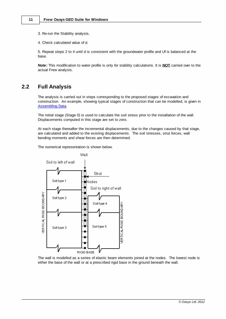
The initial stage (Stage 0) is used to calculate the soil stress prior to the installation of the wall. Displacements computed in this stage are set to zero. At each stage thereafter the incremental displacements, due to the changes caused by that stage,are calculated and added to the existing displacements. The soil stresses, strut forces, wallbending moments and shear forces are then determined. The numerical representation is shown below.
The wall is modelled as a series of elastic beam elements joined at the nodes. The lowest node iseither the base of the wall or at a prescribed rigid base in the ground beneath the wall.

12Methods of Analysis
© Oasys Ltd. 2012
The soil at each side of the wall is connected at the nodes as shown on the figure.
At each stage of construction the analysis comprises the following steps:
a) The initial earth pressures and the out of balance nodal forces are calculated assuming nomovement of the nodes.
b) The stiffness matrices representing the soil on either side of the wall and the wall itself are
assembled. c) These matrices are combined, together with any stiffness' representing the actions of
struts or anchors, to form an overall stiffness matrix. d) The incremental nodal displacements are calculated from the nodal forces acting on the
overall stiffness matrix assuming linear elastic behaviour. e) The earth pressures at each node are calculated by adding the changes in earth pressure,
due to the current stage, to the initial earth pressures. The derivation of the changes inearth pressure involves multiplying the incremental nodal displacements by the soilstiffness matrices.
f) The earth pressures are compared with soil strength limitation criteria; conventionally
taken as either the active or passive limits. If any strength criterion is infringed a set ofnodal correction forces is calculated. These forces are used to restore earth pressures,which are consistent with the strength criteria and also model the consequent plasticdeformation within the soil.
g) A new set of nodal forces is calculated by adding the nodal correction forces to those
calculated in step (a). h) Steps (d) to (g) are repeated until convergence is achieved. i) Total nodal displacements, earth pressures, strut forces and wall shear stresses and
bending moments are calculated.
2.3 Soil Models
The soil, on both sides of the wall, is represented as a linear elastic material which is subject toactive and passive limits. Three linear elastic soil models are available in Frew.
1. Safe Method.2. Mindlin Method.3. Sub-grade Reaction Model.
Note: The sub-grade reaction model is not currently active, it will be added to Frew in the nearfuture.
All use different methods to represent the reaction of the soil in the elastic phase.

13 Frew Oasys GEO Suite for Windows
© Oasys Ltd. 2012
2.3.1 Safe Method
This method uses a pre-calculated soil stiffness matrix developed from the Oasys Safe program.
The soil is represented as an elastic continuum. It can be 'fixed' to the wall, thereby representingfull friction between the soil and wall. Alternatively the soil can be 'free', assuming no soil/wallfriction, see Fixed or Free solution.
Accuracy of the Safe solution
This method interpolates from previously calculated and saved results, using finite element analysisfrom the Safe program.
The method gives good approximations for plane strain situations where Young's modulus isconstant or increases linearly from zero at the free surface.
For a linear increase in Young's modulus from non-zero at the free surface the results are also good,but for more complicated variations in layered materials the approximations become less reliable. In many situations when props or struts are being used, "fixed" and "free" give similar results. Anexception is a cantilever situation where the "fixed" method will give less displacements because itmodels greater fixity between the soil and wall. It must be noted that the case with interface friction ("fixed") is somewhat approximate becausePoisson's ratio effects are not well modelled. For example, these effects in a complete elasticsolution can cause outward movement of the wall when there is a shallow soil excavation.
For detailed information on the approximations and thereby the accuracy of the Safe method see Approximations used in the Safe Method.
2.3.2 Mindlin Method
The Mindlin method represents the soil as an elastic continuum modelled by integrated forms ofMindlin's elasticity equations (Vaziri et al 1982). The advantage of this method is that a wall of finitelength in the third (horizontal) dimension may be approximately modelled. It also assumes that thesoil/wall interface has no friction.
14Methods of Analysis
© Oasys Ltd. 2012
Accuracy of the Mindlin Solution
The method is only strictly accurate for a soil with a constant Young's modulus. Approximations areadopted for variable modulus with depth and as with the "Safe" method the user can override this bysetting a constant modulus value.
For further information, see Approximations used in the Mindlin method.
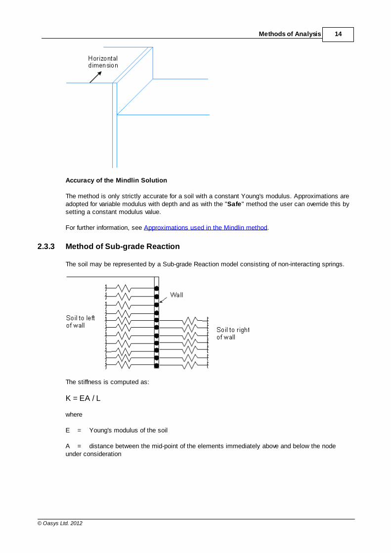
2.3.3 Method of Sub-grade Reaction
The soil may be represented by a Sub-grade Reaction model consisting of non-interacting springs.
The stiffness is computed as:
K = EA / L
where E = Young's modulus of the soil A = distance between the mid-point of the elements immediately above and below the nodeunder consideration
15 Frew Oasys GEO Suite for Windows
© Oasys Ltd. 2012
L = spring length (input by the user)
It is considered that this model is not realistic for most retaining walls, and no assistance can begiven here for the choice of spring length, which affects the spring stiffness.
Note: The sub-grade reaction model is not currently active, it will be added to Frew in the nearfuture.
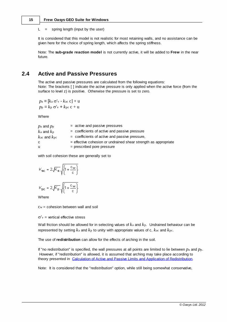
2.4 Active and Passive Pressures
The active and passive pressures are calculated from the following equations:Note: The brackets [ ] indicate the active pressure is only applied when the active force (from thesurface to level z) is positive. Otherwise the pressure is set to zero.
pa = [ka 'v - kac c] + u pp = kp 'v + kpc c + u
Where
pa and pp = active and passive pressures
ka and kp = coefficients of active and passive pressure
kac and kpc = coefficients of active and passive pressure,
c = effective cohesion or undrained shear strength as appropriateu = prescribed pore pressure
with soil cohesion these are generally set to
Where
cw = cohesion between wall and soil
'v = vertical effective stress
Wall friction should be allowed for in selecting values of ka and kp. Undrained behaviour can be
represented by setting ka and kp to unity with appropriate values of c, kac and kpc.
The use of redistribution can allow for the effects of arching in the soil.
If "no redistribution" is specified, the wall pressures at all points are limited to lie between pa and pp.
However, if "redistribution" is allowed, it is assumed that arching may take place according totheory presented in Calculation of Active and Passive Limits and Application of Redistribution. Note: It is considered that the "redistribution" option, while still being somewhat conservative,
16Methods of Analysis
© Oasys Ltd. 2012
represents the "real" behaviour much more accurately.
If surcharges of limited extent are specified above the level in question the active pressure isincreased in accordance with the theory presented in Active Pressures due to Strip LoadSurcharges.
However, strip surcharges are not included in calculating passive pressure (see Passive Pressuresdue to Strip Load Surcharges).
2.4.1 Effects of Excavation and Backfill
Excavation, backfill or changes of pore pressure cause a change in vertical effective stress 'v. Itis assumed that, in the absence of wall movement, the change in horizontal effective stress 'h will be given by
'h = Kr 'v
For an isotropic elastic material:
Kr = / (1 - )
where
= Poisson's ratio for drained behaviour
For drained behaviour, the typical range of Kr would be 0.1 to 0.5. For undrained behaviour, the same approach is applied to total stress. In this case, the undrained
Poisson's ratio would normally be taken to be 0.5, where Kr = 1.0When filling, the horizontal effective stresses in the fill material are initially set to K0 times thevertical effective stress.
i.e. 'h = K0 'v
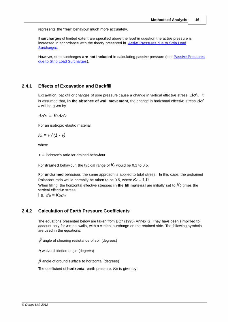
2.4.2 Calculation of Earth Pressure Coefficients
The equations presented below are taken from EC7 (1995) Annex G. They have been simplified toaccount only for vertical walls, with a vertical surcharge on the retained side. The following symbolsare used in the equations:
' angle of shearing resistance of soil (degrees)
wall/soil friction angle (degrees)
angle of ground surface to horizontal (degrees)
The coefficient of horizontal earth pressure, Kh is given by:
17 Frew Oasys GEO Suite for Windows
© Oasys Ltd. 2012
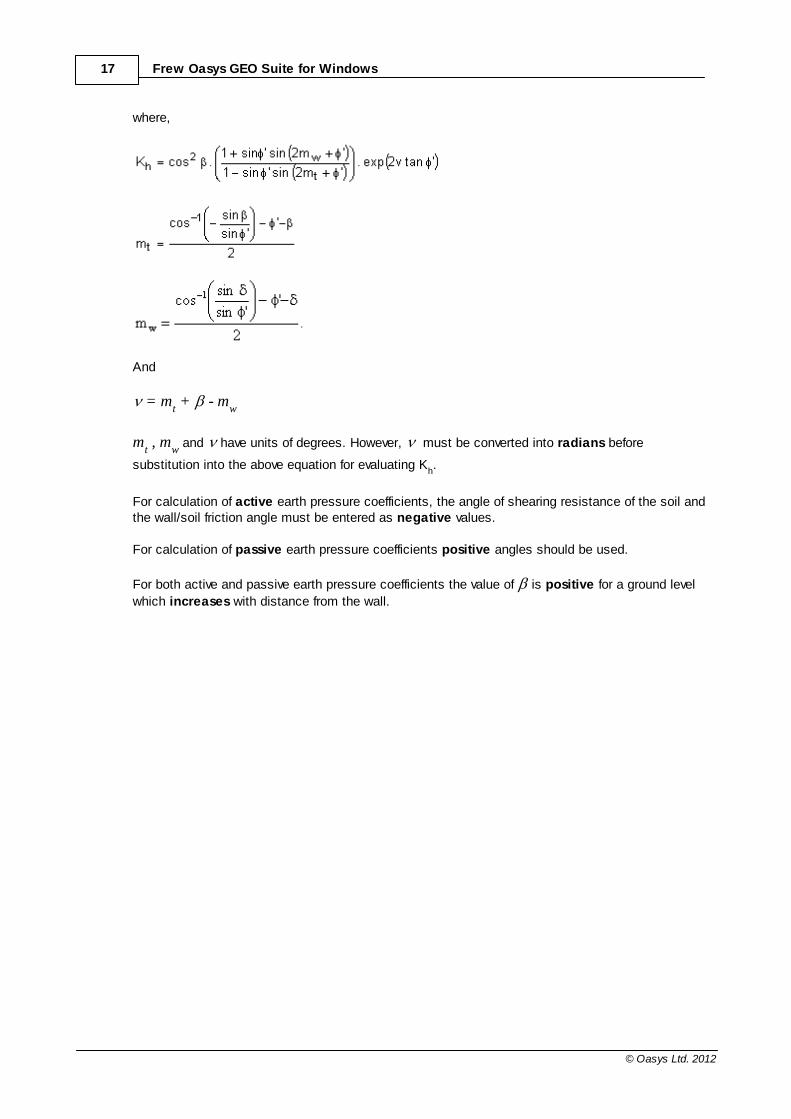
where,
And
= mt + - m
w
mt , m
w and have units of degrees. However, must be converted into radians before
substitution into the above equation for evaluating Kh.
For calculation of active earth pressure coefficients, the angle of shearing resistance of the soil andthe wall/soil friction angle must be entered as negative values. For calculation of passive earth pressure coefficients positive angles should be used.
For both active and passive earth pressure coefficients the value of is positive for a ground level
which increases with distance from the wall.

18Methods of Analysis
© Oasys Ltd. 2012
2.5 Total and Effective Stress
Frew recognises two components of pressure acting on each side of the wall. 1. Pore pressure (u). This is prescribed by the user and is independent of movement.2. Effective stress (Pe). This has initial values determined by multiplying the vertical effective
stress by the coefficient of earth pressure at rest (K0).
Thereafter its values change in response to excavation, filling and wall movement. The vertical effective stress is calculated as:
sz
z
zudlv udz'
where:u = Prescribed pore pressureg = unit weightz = level
zs = surface level
zudl = vertical stress due to all uniformly distributed surcharges above level z.

19 Frew Oasys GEO Suite for Windows
© Oasys Ltd. 2012
2.5.1 Drained Materials
Effective stress and pore pressure are used directly to represent drained behaviour.
Note: The pore pressure is profile defined by the user and is independent of movement.
2.5.2 Undrained Materials and Calculated Pore Pressures
Frew can be requested to calculate undrained pore pressures at each stage.
The feature is available in the Material Properties table, and is activated by specifying for anundrained material another material zone from which effective stress parameters are to be taken. A "shape factor" is also required, which controls the shape of the permitted effective stress path forundrained behaviour. The default value for the shape factor is 1, which prevents occurrence of anyeffective stress state outside the Mohr-Coulomb failure envelope, but it can optionally be revised to 0,representing a Modified Cam-Clay envelope, or any value in between. [NB: values less than 1 havenot been validated and use of a value less than 1 is not recommended. The option is retained in theprogram for experimental purposes. A spreadsheet 'undr_dr_calc.xls' is provided in the 'Samples'sub-folder of the program installation folder. This allows the user to experiment with values for thevarious parameters and with the shape factor, if wished.]
If reasonable values of pore pressure are not used during undrained behaviour, then on transition todrained behaviour, the program may not calculate displacements with satisfactory accuracy. Thecalculation in Frew aims to provide a reasonable set of undrained pore pressures. Given the relativesimplicity of Frew and the present state of knowledge of soil behaviour, they cannot be accurate(although should be better than a user-defined pore pressure profile) and the user should check thatthey appear reasonable. Guidance on warning messages is given below.
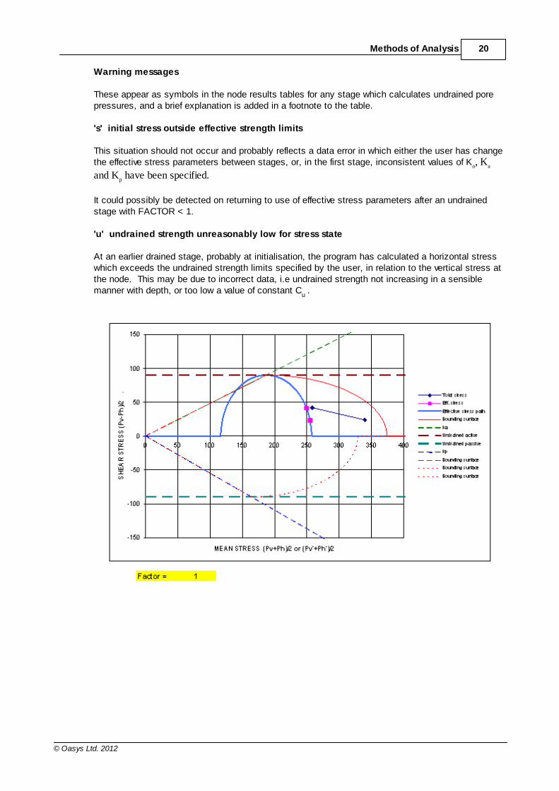
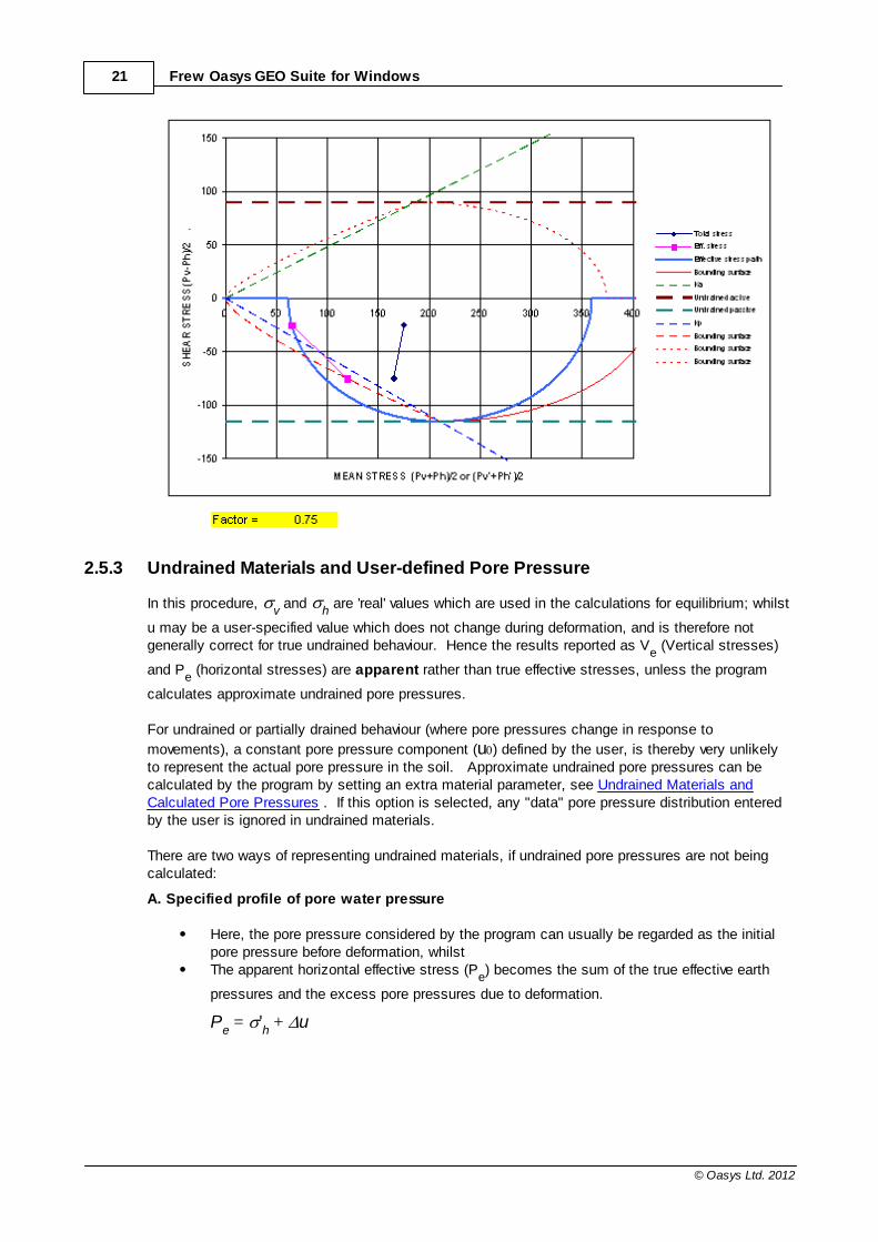
The process used in the program can be understood by studying the stress path plot below. Failurein an undrained material occurs at the intersection of the ' and C
u lines. This point is derived from
the effective stress parameters of the "material number for effective stress parameters" specified bythe user for each undrained material. The envelope of possible total stress values is shown in red(examples for shape factors of 1 and 0.75 are shown); this is taken to be elliptical except wherereduced by shape factors > 0. The calculated undrained effective stress path is shown in blue.
For each iteration in an undrained stage, the program calculates the total stress and the effectivestress, using the value on the blue effective stress path unless limited by the red envelope. Theundrained pore pressure is then the difference between the total and effective stresses.
The diagram shows that, if the shape factor is less than 1, it is possible for the effective stresscalculated to lie outside the limits of the effective stress parameters; this would lead to somechanges in total stress, and hence displacement, in the transition from undrained to effective stressbehaviour. This problem is avoided by following the recommendation to use the default shape factorof 1.0.
Advice on "data" pore pressures when using this feature
Any pore pressures entered by the user will be ignored in an undrained material for which automaticcalculation of pore pressures has been requested (i.e. by setting a valid "material for effective stressparameters" in the Materials table).
20Methods of Analysis
© Oasys Ltd. 2012
Warning messages
These appear as symbols in the node results tables for any stage which calculates undrained porepressures, and a brief explanation is added in a footnote to the table.
's' initial stress outside effective strength limits
This situation should not occur and probably reflects a data error in which either the user has changethe effective stress parameters between stages, or, in the first stage, inconsistent values of Ko, Ka
and Kp have been specified.
It could possibly be detected on returning to use of effective stress parameters after an undrainedstage with FACTOR < 1.
'u' undrained strength unreasonably low for stress state
At an earlier drained stage, probably at initialisation, the program has calculated a horizontal stresswhich exceeds the undrained strength limits specified by the user, in relation to the vertical stress atthe node. This may be due to incorrect data, i.e undrained strength not increasing in a sensiblemanner with depth, or too low a value of constant C
u .
21 Frew Oasys GEO Suite for Windows
© Oasys Ltd. 2012
2.5.3 Undrained Materials and User-defined Pore Pressure
In this procedure, v and
h are 'real' values which are used in the calculations for equilibrium; whilst
u may be a user-specified value which does not change during deformation, and is therefore notgenerally correct for true undrained behaviour. Hence the results reported as V
e (Vertical stresses)
and Pe (horizontal stresses) are apparent rather than true effective stresses, unless the program
calculates approximate undrained pore pressures. For undrained or partially drained behaviour (where pore pressures change in response to
movements), a constant pore pressure component (u0) defined by the user, is thereby very unlikelyto represent the actual pore pressure in the soil. Approximate undrained pore pressures can becalculated by the program by setting an extra material parameter, see Undrained Materials andCalculated Pore Pressures . If this option is selected, any "data" pore pressure distribution enteredby the user is ignored in undrained materials. There are two ways of representing undrained materials, if undrained pore pressures are not beingcalculated:
A. Specified profile of pore water pressure
Here, the pore pressure considered by the program can usually be regarded as the initialpore pressure before deformation, whilst The apparent horizontal effective stress (P
e) becomes the sum of the true effective earth
pressures and the excess pore pressures due to deformation.
Pe = '
h + u

22Methods of Analysis
© Oasys Ltd. 2012
B. Zero pore water pressure profile
Here, the value of apparent horizontal effective stress (Pe) can then be equated to the true
total stress.
Pe = '
h + u
In both these cases the values of Ka, K
p and K
r should be set to unity (1.0), but with non-zero
undrained strengths (c) and coefficients Kac
and Kpc
.
Calculation procedure
Frew executes the following calculation procedure. This includes for a profile of pore pressures, ifspecified, as indicated.
1. Calculation of the total vertical stress v.
2. Calculation of the effective vertical stress where:
'v =
v - u
3. Checks to make sure that v 0. The program stops and provides an error message if
this is not so.4. Calculation of the minimum active effective stress:
'a = K
a'v - K
acc
5. Checks to make sure that 'a 0 (i.e. Ka
'v K
acc). If the value is less than zero then
the program resets to 0. So generally:
'a = K
a(
v - u) - K
acc 0
23 Frew Oasys GEO Suite for Windows
© Oasys Ltd. 2012
Note: Frew uses 'a as a lower limit on the horizontal effective stress '
h. '
h is used in the
equilibrium equations, for determination of the wall deflection, where 'h =
h + u
Effect of specified pore pressure
Specified pore pressure, (u) takes effect in steps 2 and 5.Step 2 - Specified pore water pressure reduces the effective vertical stress.
Step 5 - Limits the apparent horizontal effective stresses to 0.
In earlier versions of Frew, this could be used to advantage because the specified 'pore pressure' ucould become equivalent to a 'minimum fluid pressure'. There is now a completely separate featurein which a minimum equivalent fluid pressure (MEFP) can be specified, see Minimum EquivalentFluid Pressure .
2.5.4 Undrained to Drained Example
An example file (Undr-PP-Example.fwd) is available in the Samples sub-folder of the programinstallation folder. The user can see from this the way that the feature for automatic calculation ofundrained pore pressures has been used.
3 Input Data
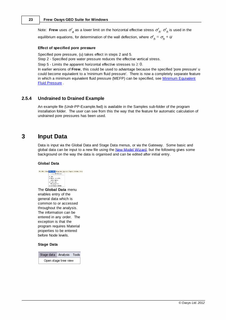
Data is input via the Global Data and Stage Data menus, or via the Gateway. Some basic andglobal data can be input to a new file using the New Model Wizard, but the following gives somebackground on the way the data is organised and can be edited after initial entry.
Global Data
The Global Data menuenables entry of thegeneral data which iscommon to or accessedthroughout the analysis. The information can beentered in any order. Theexception is that theprogram requires Materialproperties to be enteredbefore Node levels.
Stage Data
24Input Data
© Oasys Ltd. 2012
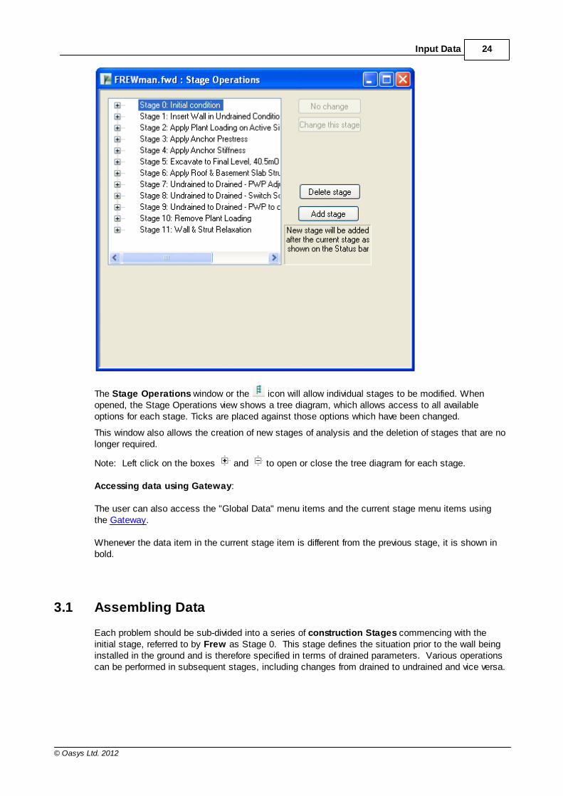
The Stage Operations window or the icon will allow individual stages to be modified. Whenopened, the Stage Operations view shows a tree diagram, which allows access to all availableoptions for each stage. Ticks are placed against those options which have been changed.
This window also allows the creation of new stages of analysis and the deletion of stages that are nolonger required.
Note: Left click on the boxes and to open or close the tree diagram for each stage.
Accessing data using Gateway:
The user can also access the "Global Data" menu items and the current stage menu items usingthe Gateway.
Whenever the data item in the current stage item is different from the previous stage, it is shown inbold.
3.1 Assembling Data
Each problem should be sub-divided into a series of construction Stages commencing with theinitial stage, referred to by Frew as Stage 0. This stage defines the situation prior to the wall beinginstalled in the ground and is therefore specified in terms of drained parameters. Various operationscan be performed in subsequent stages, including changes from drained to undrained and vice versa.
25 Frew Oasys GEO Suite for Windows
© Oasys Ltd. 2012
Sketches showing the wall, soil strata, surcharges, water pressure, strut and excavation levelsshould be prepared for each Stage.
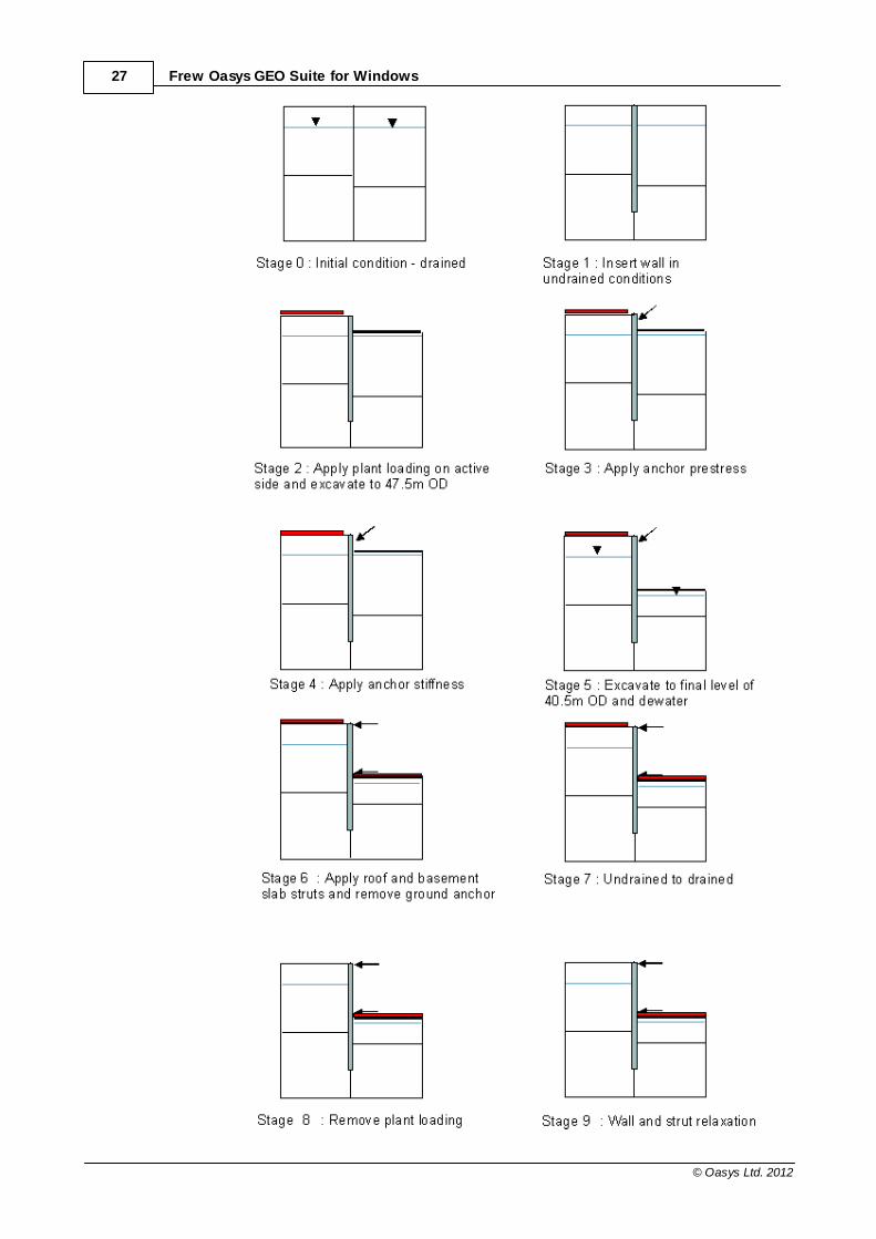
Examples of potential changes that can be applied during the construction stages are:
Stage 0 Set up initial stresses in the soil by adding the material types, groundwaterconditions and applying any surcharges required prior to installing the wall. Allmaterials should be set to drained parameters for this stage.
Stage 1 Install wall.
Change to undrained materials (if required). In this example, undrained porepressures are calculated by the program, see Undrained Materials andCalculated Pore Pressures.
Subsequentstages ofconstruction
Excavate / backfill.
Insert / Remove struts.
Insert / Remove surcharges.
Long termeffects
Return to drained parameters.
Change groundwater conditions.
Use the relaxation option to model the long term stiffness of the wall.
To illustrate these operations a manual example is given below.
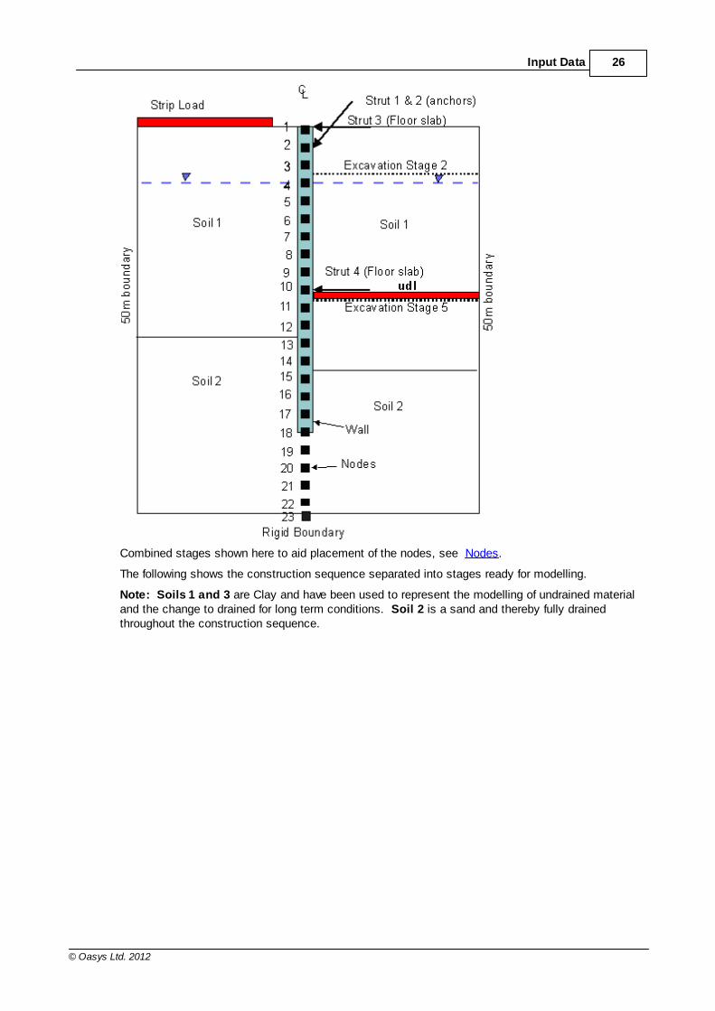
General layout of manual example
26Input Data
© Oasys Ltd. 2012
Combined stages shown here to aid placement of the nodes, see Nodes.
The following shows the construction sequence separated into stages ready for modelling.
Note: Soils 1 and 3 are Clay and have been used to represent the modelling of undrained materialand the change to drained for long term conditions. Soil 2 is a sand and thereby fully drainedthroughout the construction sequence.
27 Frew Oasys GEO Suite for Windows
© Oasys Ltd. 2012

28Input Data
© Oasys Ltd. 2012
The program recalculates the displacements and forces within the system at each stage.
Several activities can be included within a single stage provided their effects are cumulative. Forexample it is appropriate to insert a strut and then excavate below the level of the strut in one stage,but it is not correct to excavate and then insert a strut at the base of the excavation in one stage. Ifin doubt the user should incorporate extra stages.
The computer model of the program geometry should be drawn with the wall node locations carefullyselected in accordance with the guidance given in inserting Nodes.
The nature of each problem will vary considerably and thereby the amount of data changes requiredfor each construction stage. Some information is compulsory for the initial stages. Thereafter fullflexibility is allowed in order to build up the correct progression of construction stages and long termeffects.
Stage 0 & Globaldata
Stage 1 Constructionstages
Long term
Compulsory Material properties (All materials)
Node levels
Soil zones (drainedmaterials)
Analysis Method
Convergence controlparameters
Wall properties
Optional Surcharges
Struts
Water
Analysis Method
Convergence controlparameters
Soil zones(undrained or drainedmaterials)
Excavation or filling
Surcharges
Struts
Water
Analysis Method
Wall properties
Convergence controlparameters
Soil zones (undrained or drainedmaterials)
Excavation or filling
Surcharges
Struts
Water
Wall relaxation
Analysis Method
Convergence controlparameters
Soil zones (drainedmaterials)
Surcharges
Struts
Water
29 Frew Oasys GEO Suite for Windows
© Oasys Ltd. 2012
3.2 Preferences
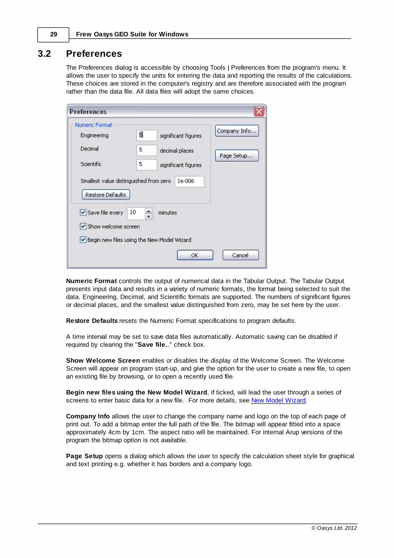
The Preferences dialog is accessible by choosing Tools | Preferences from the program's menu. Itallows the user to specify the units for entering the data and reporting the results of the calculations.These choices are stored in the computer's registry and are therefore associated with the programrather than the data file. All data files will adopt the same choices.
Numeric Format controls the output of numerical data in the Tabular Output. The Tabular Outputpresents input data and results in a variety of numeric formats, the format being selected to suit thedata. Engineering, Decimal, and Scientific formats are supported. The numbers of significant figuresor decimal places, and the smallest value distinguished from zero, may be set here by the user.
Restore Defaults resets the Numeric Format specifications to program defaults.
A time interval may be set to save data files automatically. Automatic saving can be disabled ifrequired by clearing the "Save file.." check box.
Show Welcome Screen enables or disables the display of the Welcome Screen. The WelcomeScreen will appear on program start-up, and give the option for the user to create a new file, to openan existing file by browsing, or to open a recently used file.
Begin new files using the New Model Wizard, if ticked, will lead the user through a series ofscreens to enter basic data for a new file. For more details, see New Model Wizard.
Company Info allows the user to change the company name and logo on the top of each page ofprint out. To add a bitmap enter the full path of the file. The bitmap will appear fitted into a spaceapproximately 4cm by 1cm. The aspect ratio will be maintained. For internal Arup versions of theprogram the bitmap option is not available.
Page Setup opens a dialog which allows the user to specify the calculation sheet style for graphicaland text printing e.g. whether it has borders and a company logo.

30Input Data
© Oasys Ltd. 2012
3.3 New Model Wizard
The New Model Wizard is accessed by selecting the `File | New´(Ctrl+N) option from the main menu,or by clicking the 'New' button on the Frew toolbar.
The New Model Wizard is designed to ensure that some basic settings and global data can beeasily entered. It does not create an entire data file, and strut, surcharge and stage data should beentered once the wizard is complete.
Cancelling at any time will result in an empty document.
Note! The New Model Wizard can only be accessed if the "Begin new files using New ModelWizard" check box in Tools | Preferences is checked.
3.3.1 New Model Wizard: Titles and Units
The first property page of the New Model Wizard is the Titles and Units window. The following fieldsare available:
Job Number allows entry of an identifying job number. The user can view previouslyused job numbers by clicking the drop-down button.
Initials for entry of the users initials.Date this field is set by the program at the date the file is saved.Job Title allows a single line for entry of the job title.Subtitle allows a single line of additional job or calculation information.Calculation Heading allows a single line for the main calculation heading.
The titles are reproduced in the title block at the head of all printed information for the calculations. The fields should therefore be used to provide as many details as possible to identify the individualcalculation runs.
An additional field for notes has also been included to allow the entry of a detailed description of thecalculation. This can be reproduced at the start of the data output by selection of notes using File |Print Selection.
Clicking the Units button opens the standard units dialog.
3.3.2 New Model Wizard: Basic Data
The second wizard page contains the following options:
Problem geometry Enter the levels of the top node and the lower rigid boundary. This will set
the correct view range in subsequent graphical display.
Materials Add or delete materials. Clicking "Add material" opens a further dialogallowing input of basic material data.

31 Frew Oasys GEO Suite for Windows
© Oasys Ltd. 2012
This data entry method will be sufficient in many cases, but some othersettings (for example, undrained pore pressure calculation parameters)need to be set later in the normal Materials table.
Problem type Select "Stability check only" if you wish to carry out a single stagestability check. Select "Staged construction" to allow specification of anumber of stages for either stability check or full analysis.
(If "Stability check only" is selected, the remaining options on this dialogwill be greyed out. )
Node generation "Automatic" will allow all data input to be specified by level and nodepositions are generated by Frew. "Manual" means that node positions must be entered by the user andmost other data must be specified by node number rather than level.
Wall toe level Selecting "Obtain from stability check" will enable the user to run astability check before full analysis, to estimate the required toe level. Thiscan be manually overridden if required.
To enter a known required toe level, select "Enter manually" and enter thelevel.
Clicking the Next button moves on to either the Stage Defaults page (for Staged Constructionmodels) or the Soil Interfaces page (for Stability Check models).

32Input Data
© Oasys Ltd. 2012
3.3.3 New Model Wizard: Stage Defaults
This page will only be shown if "Staged construction" was selected in the Basic Data page. Thiswizard page reproduces most of the Analysis Data dialog, and the values entered for analysismethod, wall/soil interface, lateral boundary distances and Young's modulus specification will beused in generation of all new stages.
Clicking "Finish" completes the wizard and creates Stage 0 with the input data. The graphical inputview will open to allow entry of node levels (if these are being created manually). If automatic nodegeneration was selected, the graphical input view will show a single soil zone extending the fulldepth of the problem. More soil zones can be added as required to set up the initial ground profilefor Stage 0.
Strut and surcharge data is added separately, and additional stages created with the required stagechanges, before proceeding to run a stability check and full analysis.
3.3.4 New Model Wizard: Soil Interfaces
Initial soil layers are entered on this page. For stability check problems, enter the geometry youwish to analyse, with the ground levels differing on each side of the wall. For staged constructionproblems, the initial ground level will usually be the same on each side of the wall.

33 Frew Oasys GEO Suite for Windows
© Oasys Ltd. 2012
Clicking 'Finish' exits the wizard and opens the graphical input view.
3.4 Global Data
Global data can be accessed from the Global data menu or the Gateway. The global data describesthe problem as a whole. All the material properties, struts and surcharges which will be required forall subsequent stages must be defined here. If using the Automatic Node Generation feature, nodelevels are not required. If using manual node entry, the nodes must be placed in the correctlocations to allow all subsequent construction stages to take place.
Note: The location of the nodes can not be changed in a later stage.
It is useful to sketch out the problem from beginning to end to ensure that the correct parameters areentered as global data, see Assembling Data.
Note: Tables are locked for editing in the program when results are available. To edit the data in the
34Input Data
© Oasys Ltd. 2012
tables, the user has to explicitly delete the results.
3.4.1 Titles
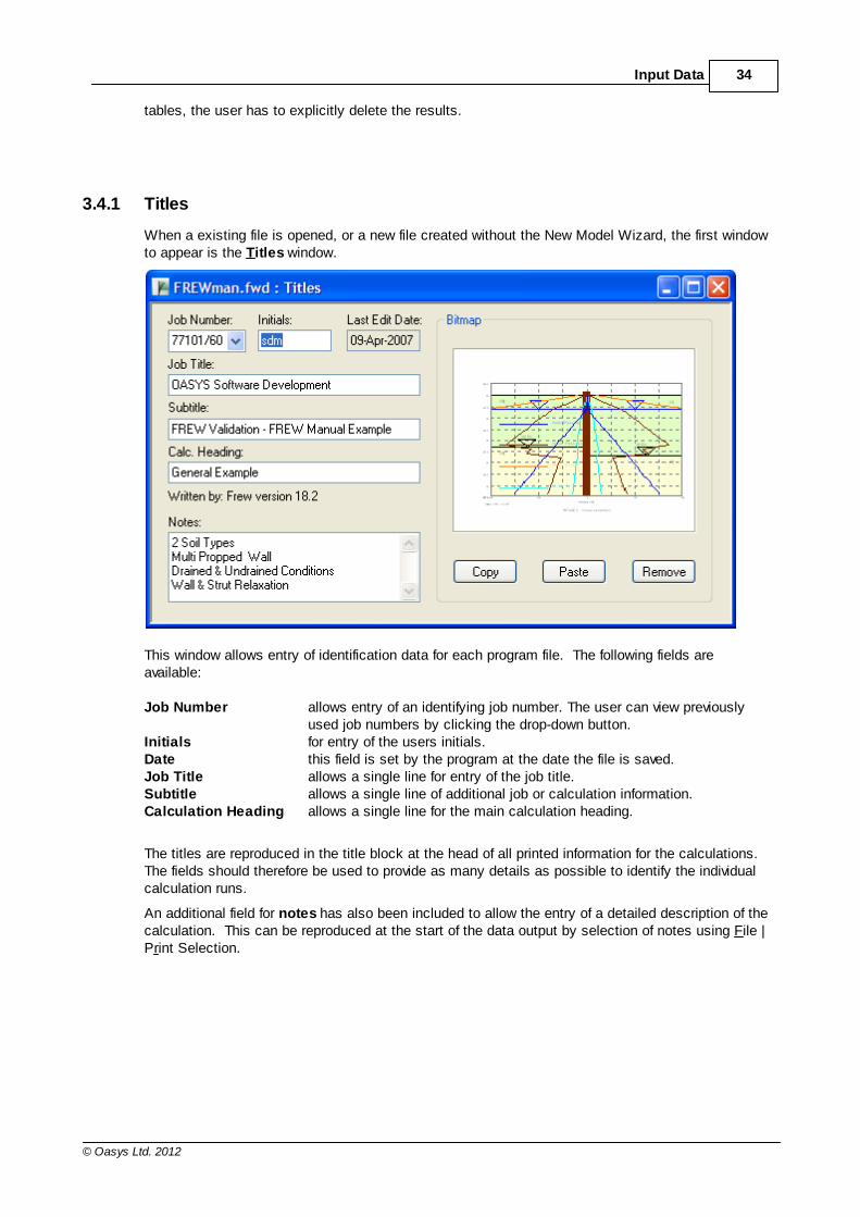
When a existing file is opened, or a new file created without the New Model Wizard, the first windowto appear is the Titles window.
This window allows entry of identification data for each program file. The following fields areavailable:
Job Number allows entry of an identifying job number. The user can view previouslyused job numbers by clicking the drop-down button.
Initials for entry of the users initials.Date this field is set by the program at the date the file is saved.Job Title allows a single line for entry of the job title.Subtitle allows a single line of additional job or calculation information.Calculation Heading allows a single line for the main calculation heading.
The titles are reproduced in the title block at the head of all printed information for the calculations. The fields should therefore be used to provide as many details as possible to identify the individualcalculation runs.
An additional field for notes has also been included to allow the entry of a detailed description of thecalculation. This can be reproduced at the start of the data output by selection of notes using File |Print Selection.

35 Frew Oasys GEO Suite for Windows
© Oasys Ltd. 2012
3.4.1.1 Titles window - Bitmaps
The box to the left of the Titles window can be used to display a picture beside the file titles.
To add a picture place an image on to the clipboard. This must be in a RGB (Red / Green / Blue)Bitmap format.
Select the button to place the image in the box.
The image is purely for use as a prompt on the screen and can not be copied into the output data.Care should be taken not to copy large bitmaps, which can dramatically increase the size of the file.
To remove a bitmap select the button.
3.4.2 Units
This option allows the user to specify the units for entering the data and reporting the results of thecalculations.
Default options are the Système Internationale (SI) units - kN and m. The drop down menus providealternative units with their respective conversion factors to metric.
Standard sets of units may be set by selecting any of the buttons: SI, kN-m, kip-ft or kip-in.
Once the correct units have been selected then click 'OK' to continue.
36Input Data
© Oasys Ltd. 2012
SI units have been used as the default standard throughout this document.
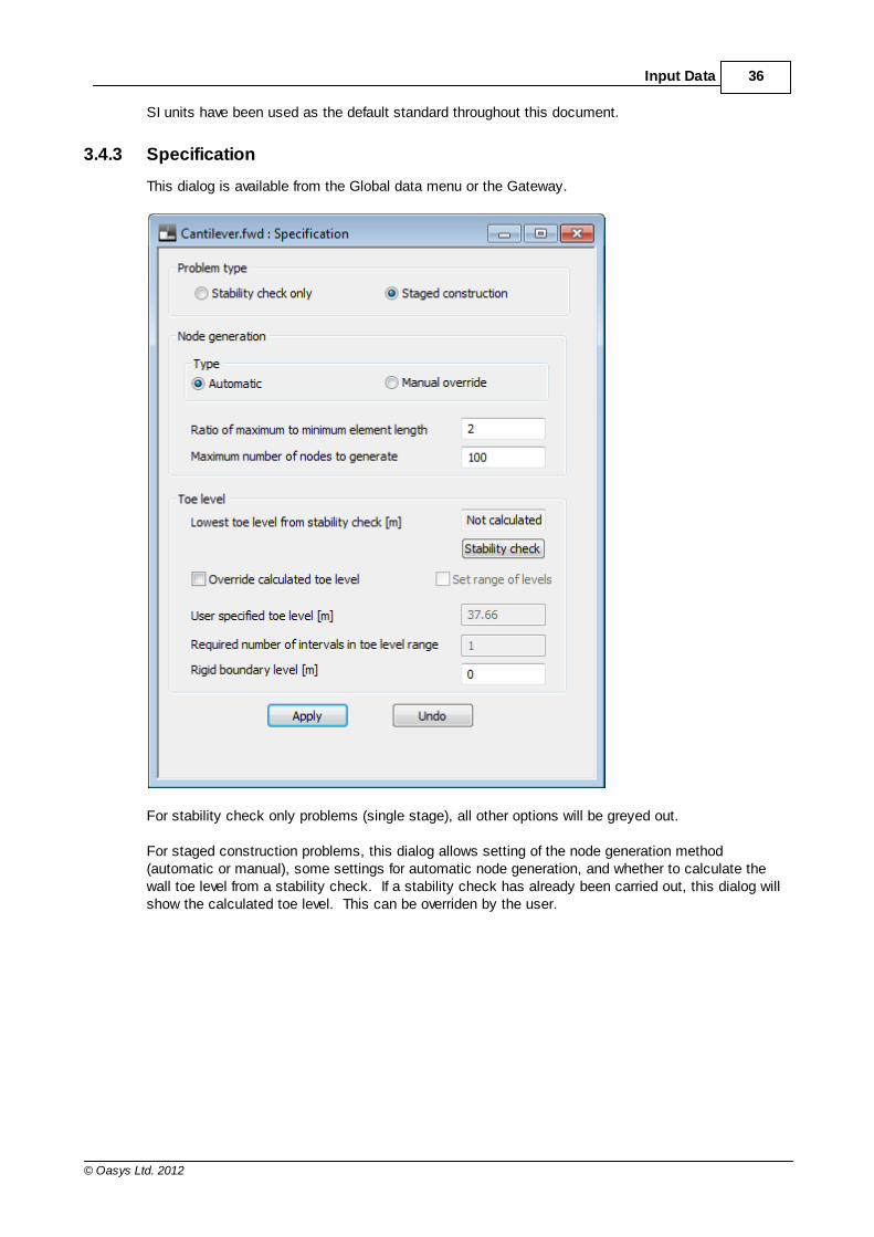
3.4.3 Specification
This dialog is available from the Global data menu or the Gateway.
For stability check only problems (single stage), all other options will be greyed out.
For staged construction problems, this dialog allows setting of the node generation method(automatic or manual), some settings for automatic node generation, and whether to calculate thewall toe level from a stability check. If a stability check has already been carried out, this dialog willshow the calculated toe level. This can be overriden by the user.
37 Frew Oasys GEO Suite for Windows
© Oasys Ltd. 2012
3.4.4 Material Properties
The properties for the different layers of materials, either side of the wall, are entered in tabular form.
Properties must be entered for all the materials which will be required for all construction stages. Ifdrained and undrained parameters of the same material type are to be used then each set ofparameters must be entered on a separate line.
Note: The user should understand the way Frew models undrained and drained behaviour and thetransition between the two. For further information see the section on Total and Effective Stress.
Brief descriptions for each of the material types can be entered here. This description is used whenassigning material types to either side of the wall, thereby creating the soil zones (see entering SoilZones).
Note: Material type 0 represents air or water - no additional input data is required by the user.
MaterialProperty
Description
E0 Young's modulus given as1. A general constant parameter for the layer as a whole, or2. A specific value for a given reference level y0.
Unit weight, defined as the bulk unit weight .
K0 Coefficient of earth pressure at rest, i.e. horizontal effective stress / verticaleffective stress.
Earth Press. Coef.
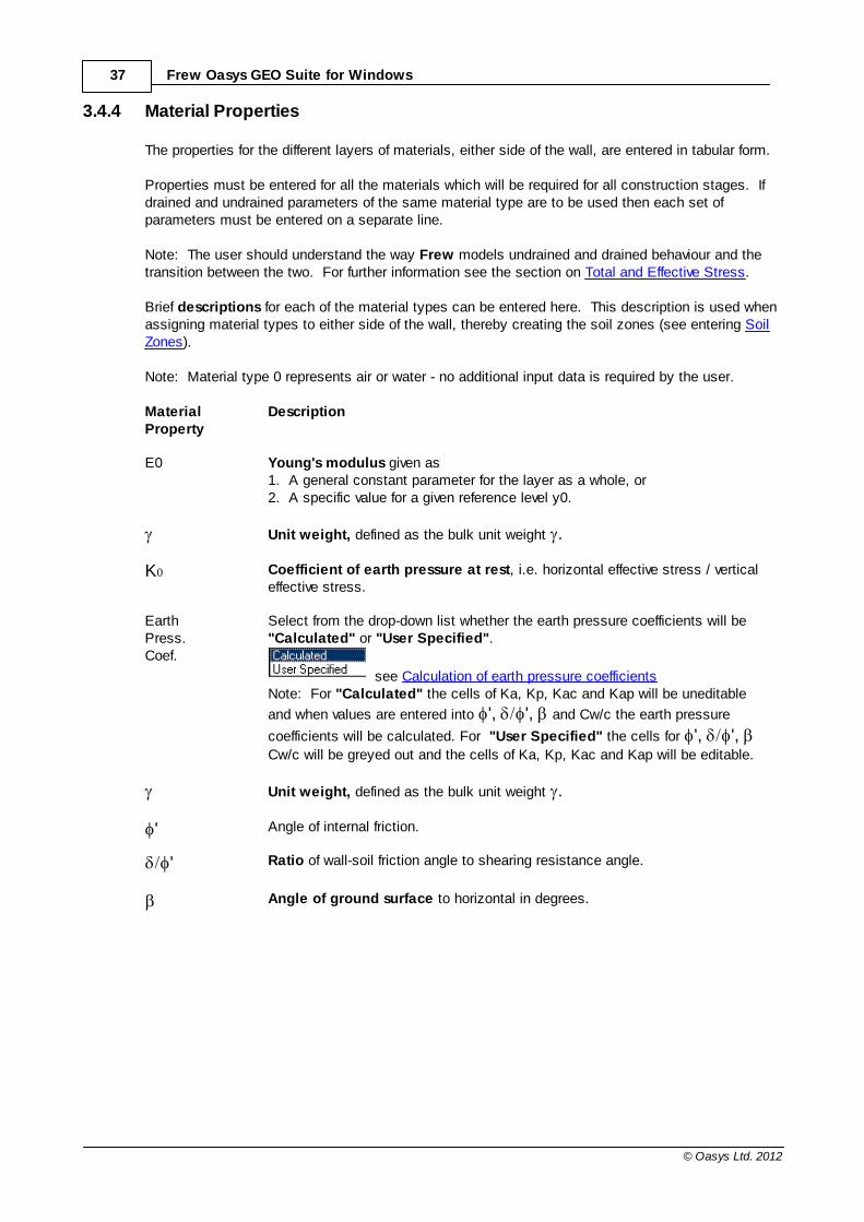
Select from the drop-down list whether the earth pressure coefficients will be "Calculated" or "User Specified".
see Calculation of earth pressure coefficients Note: For "Calculated" the cells of Ka, Kp, Kac and Kap will be uneditable
and when values are entered into ', ', and Cw/c the earth pressure
coefficients will be calculated. For "User Specified" the cells for ', ', Cw/c will be greyed out and the cells of Ka, Kp, Kac and Kap will be editable.
Unit weight, defined as the bulk unit weight .
' Angle of internal friction.
' Ratio of wall-soil friction angle to shearing resistance angle.
Angle of ground surface to horizontal in degrees.
38Input Data
© Oasys Ltd. 2012
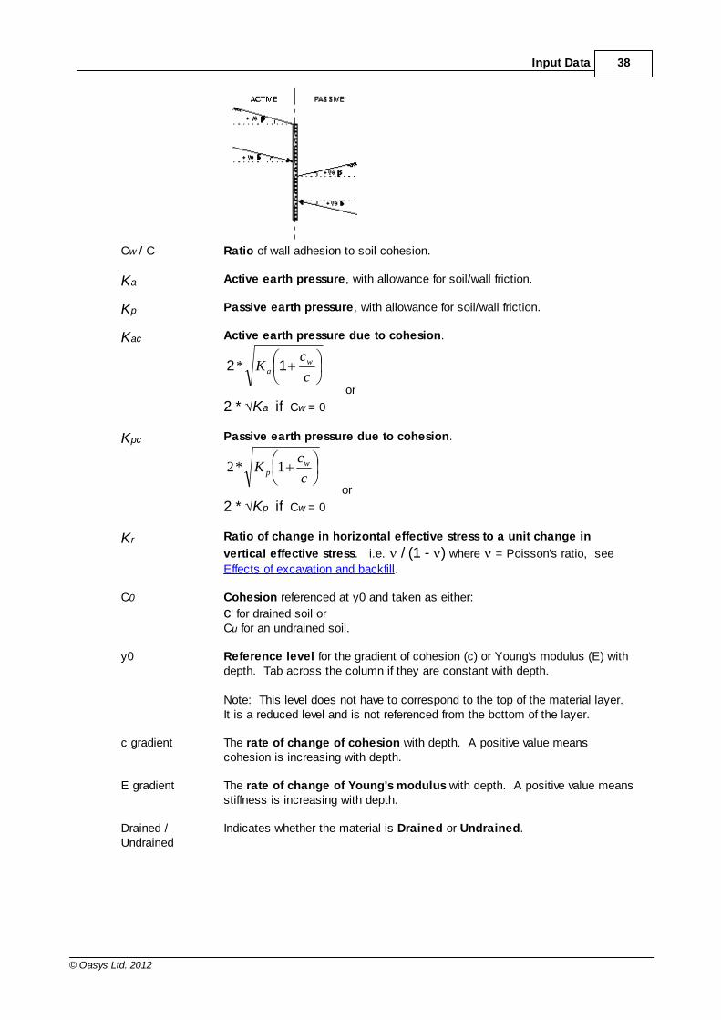
Cw / C Ratio of wall adhesion to soil cohesion.
Ka Active earth pressure, with allowance for soil/wall friction.
Kp Passive earth pressure, with allowance for soil/wall friction.
Kac Active earth pressure due to cohesion.
c
cK w
a 12*
or
2 * Ka if Cw = 0
Kpc Passive earth pressure due to cohesion.
c
cK w
p 1*2
or
2 * Kp if Cw = 0
Kr Ratio of change in horizontal effective stress to a unit change in
vertical effective stress. i.e. / (1 - ) where = Poisson's ratio, see
Effects of excavation and backfill.
C0 Cohesion referenced at y0 and taken as either:
c' for drained soil orCu for an undrained soil.
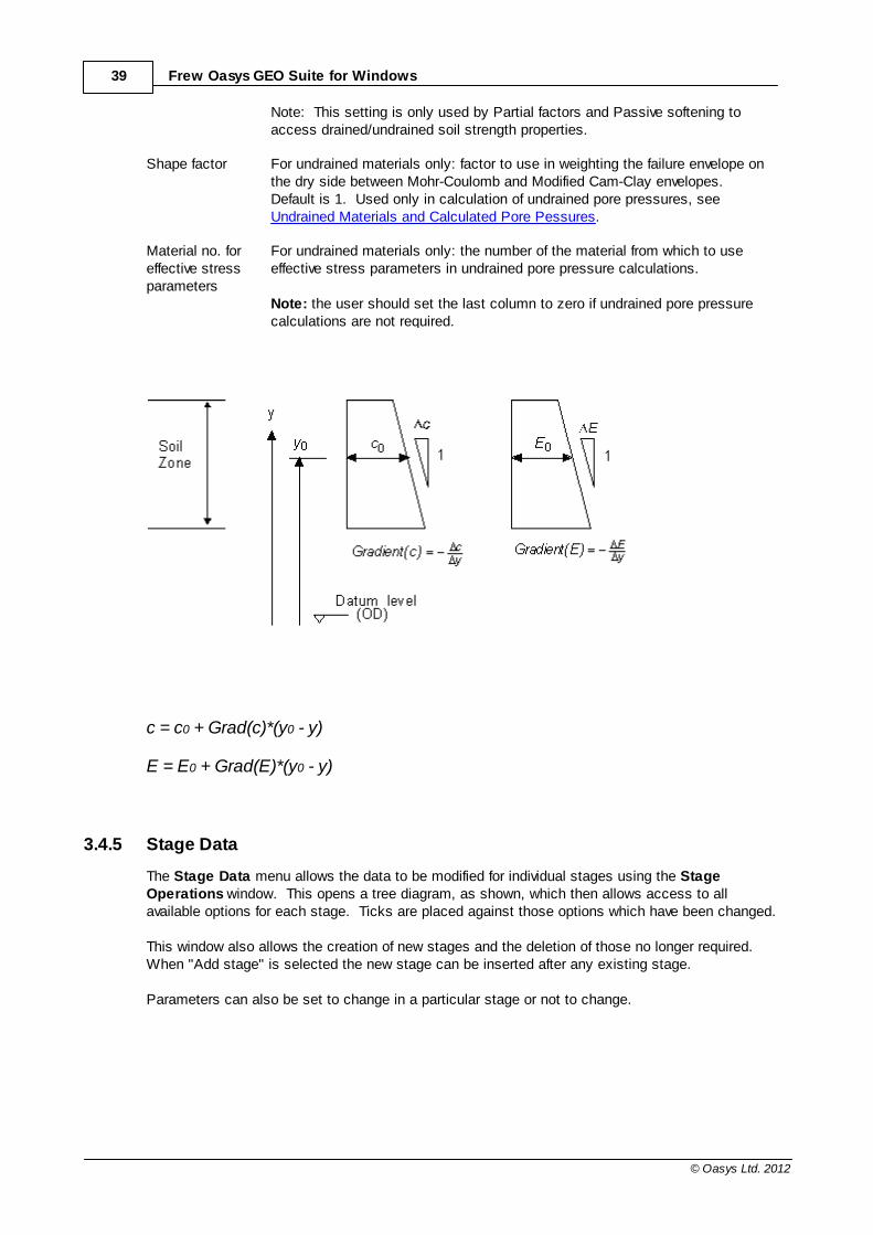
y0 Reference level for the gradient of cohesion (c) or Young's modulus (E) withdepth. Tab across the column if they are constant with depth.
Note: This level does not have to correspond to the top of the material layer. It is a reduced level and is not referenced from the bottom of the layer.
c gradient The rate of change of cohesion with depth. A positive value meanscohesion is increasing with depth.
E gradient The rate of change of Young's modulus with depth. A positive value meansstiffness is increasing with depth.
Drained /Undrained
Indicates whether the material is Drained or Undrained.
39 Frew Oasys GEO Suite for Windows
© Oasys Ltd. 2012
Note: This setting is only used by Partial factors and Passive softening toaccess drained/undrained soil strength properties.
Shape factor For undrained materials only: factor to use in weighting the failure envelope onthe dry side between Mohr-Coulomb and Modified Cam-Clay envelopes. Default is 1. Used only in calculation of undrained pore pressures, see Undrained Materials and Calculated Pore Pessures.
Material no. foreffective stressparameters
For undrained materials only: the number of the material from which to useeffective stress parameters in undrained pore pressure calculations.
Note: the user should set the last column to zero if undrained pore pressurecalculations are not required.
c = c0 + Grad(c)*(y0 - y)
E = E0 + Grad(E)*(y0 - y)
3.4.5 Stage Data
The Stage Data menu allows the data to be modified for individual stages using the StageOperations window. This opens a tree diagram, as shown, which then allows access to allavailable options for each stage. Ticks are placed against those options which have been changed.
This window also allows the creation of new stages and the deletion of those no longer required.When "Add stage" is selected the new stage can be inserted after any existing stage.
Parameters can also be set to change in a particular stage or not to change.
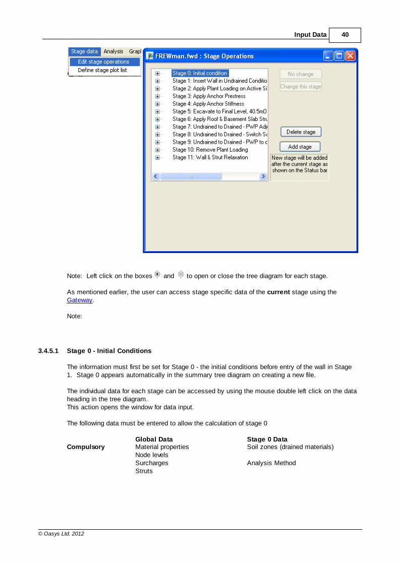
40Input Data
© Oasys Ltd. 2012
Note: Left click on the boxes and to open or close the tree diagram for each stage.
As mentioned earlier, the user can access stage specific data of the current stage using theGateway.
Note:
3.4.5.1 Stage 0 - Initial Conditions
The information must first be set for Stage 0 - the initial conditions before entry of the wall in Stage1. Stage 0 appears automatically in the summary tree diagram on creating a new file.
The individual data for each stage can be accessed by using the mouse double left click on the dataheading in the tree diagram.This action opens the window for data input.
The following data must be entered to allow the calculation of stage 0
Global Data Stage 0 DataCompulsory Material properties
Node levelsSurchargesStruts
Soil zones (drained materials)
Analysis Method

41 Frew Oasys GEO Suite for Windows
© Oasys Ltd. 2012
Convergence control parametersOptional Water data
Note: The properties set in Stage 0 will be carried forward into subsequent stages unless otherwiseamended.
On completion of Stage 0 new stages can be added or inserted to the list.
The number of the current stage is always displayed in the status line at the base of the mainwindow.
3.4.5.2 New Stages
New stages can be added to the list by selecting Add Stage on the Stage Operations window. Thisactivates a 'New Stage Title' box.
The stage title is then entered and the number of the stage before the new stage. Once the OKbutton is selected the new stage is added.
Note : The number that first appears in the Inserting after Stage window is the number of the stagecurrently highlighted by the cursor.
3.4.5.3 Inserting Stages
Select the "Add stage" button on the stage operations tree diagram and follow the instructions asfor new stages.

42Input Data
© Oasys Ltd. 2012
3.4.5.4 Deleting a Stage
Stages can be deleted by highlighting the stage title in the Stage Operation window and selectingDelete stage. A check box will appear before the stage is deleted.
3.4.5.5 Editing Stage Data
It is possible to step through the stages in order to access and edit the same data window for eachstage. Use the buttons on the tool bar to move up and down between the various stages.
The number of each stage is displayed on the status line at the base main window.
Once the correct stage has been reached. edit the data as normal. To reach specific windows go to the Stage Operations tree diagram, highlight the required operationat the required stage and then either
double click on the highlighted operation orselect the "Change this stage" button
to open the window.
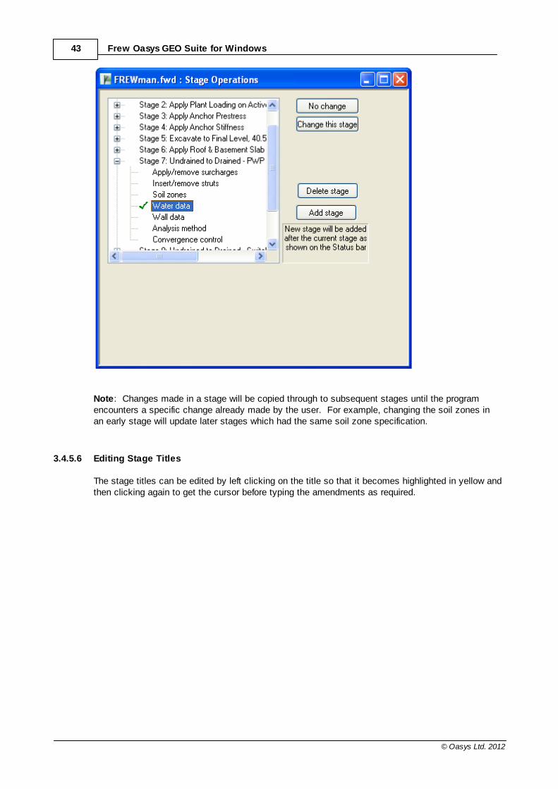
43 Frew Oasys GEO Suite for Windows
© Oasys Ltd. 2012
Note: Changes made in a stage will be copied through to subsequent stages until the programencounters a specific change already made by the user. For example, changing the soil zones inan early stage will update later stages which had the same soil zone specification.
3.4.5.6 Editing Stage Titles
The stage titles can be edited by left clicking on the title so that it becomes highlighted in yellow andthen clicking again to get the cursor before typing the amendments as required.
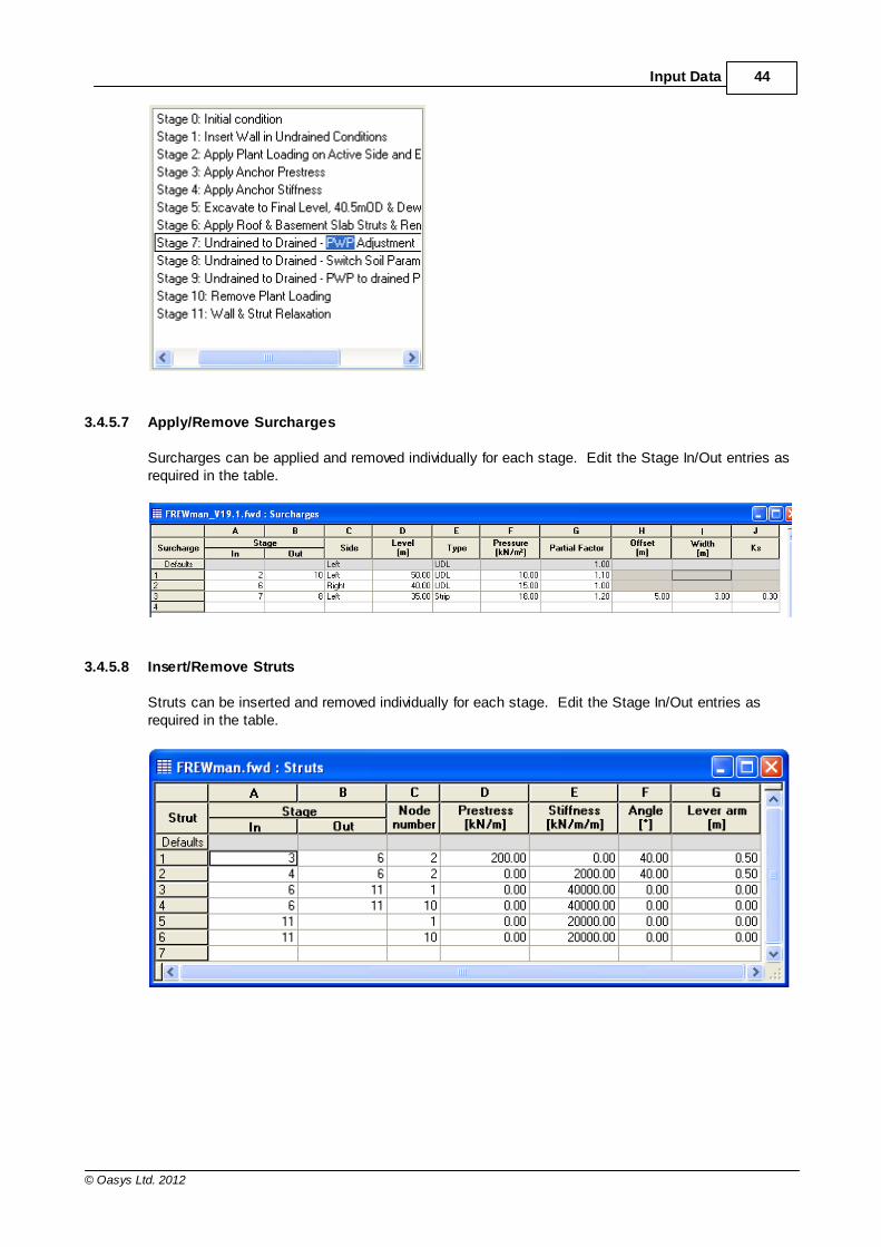
44Input Data
© Oasys Ltd. 2012
3.4.5.7 Apply/Remove Surcharges
Surcharges can be applied and removed individually for each stage. Edit the Stage In/Out entries asrequired in the table.
3.4.5.8 Insert/Remove Struts
Struts can be inserted and removed individually for each stage. Edit the Stage In/Out entries asrequired in the table.
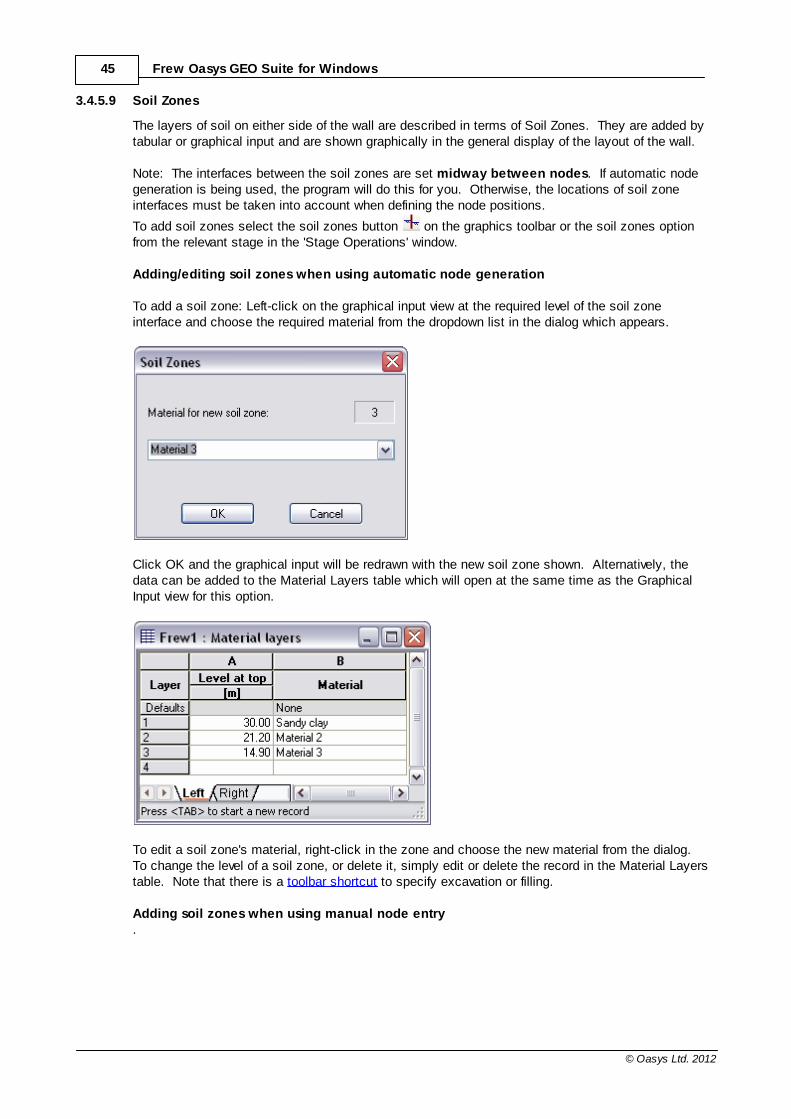
45 Frew Oasys GEO Suite for Windows
© Oasys Ltd. 2012
3.4.5.9 Soil Zones
The layers of soil on either side of the wall are described in terms of Soil Zones. They are added bytabular or graphical input and are shown graphically in the general display of the layout of the wall.
Note: The interfaces between the soil zones are set midway between nodes. If automatic nodegeneration is being used, the program will do this for you. Otherwise, the locations of soil zoneinterfaces must be taken into account when defining the node positions.
To add soil zones select the soil zones button on the graphics toolbar or the soil zones optionfrom the relevant stage in the 'Stage Operations' window.
Adding/editing soil zones when using automatic node generation
To add a soil zone: Left-click on the graphical input view at the required level of the soil zoneinterface and choose the required material from the dropdown list in the dialog which appears.
Click OK and the graphical input will be redrawn with the new soil zone shown. Alternatively, thedata can be added to the Material Layers table which will open at the same time as the GraphicalInput view for this option.
To edit a soil zone's material, right-click in the zone and choose the new material from the dialog. To change the level of a soil zone, or delete it, simply edit or delete the record in the Material Layerstable. Note that there is a toolbar shortcut to specify excavation or filling.
Adding soil zones when using manual node entry.
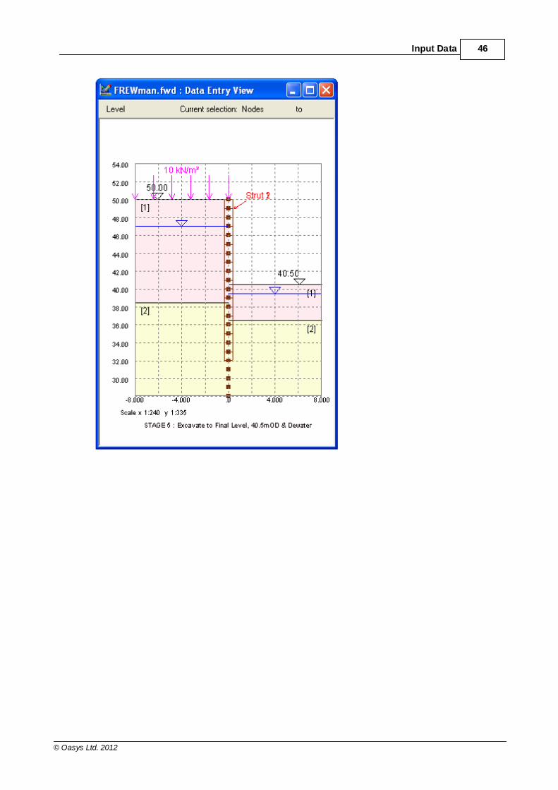
46Input Data
© Oasys Ltd. 2012
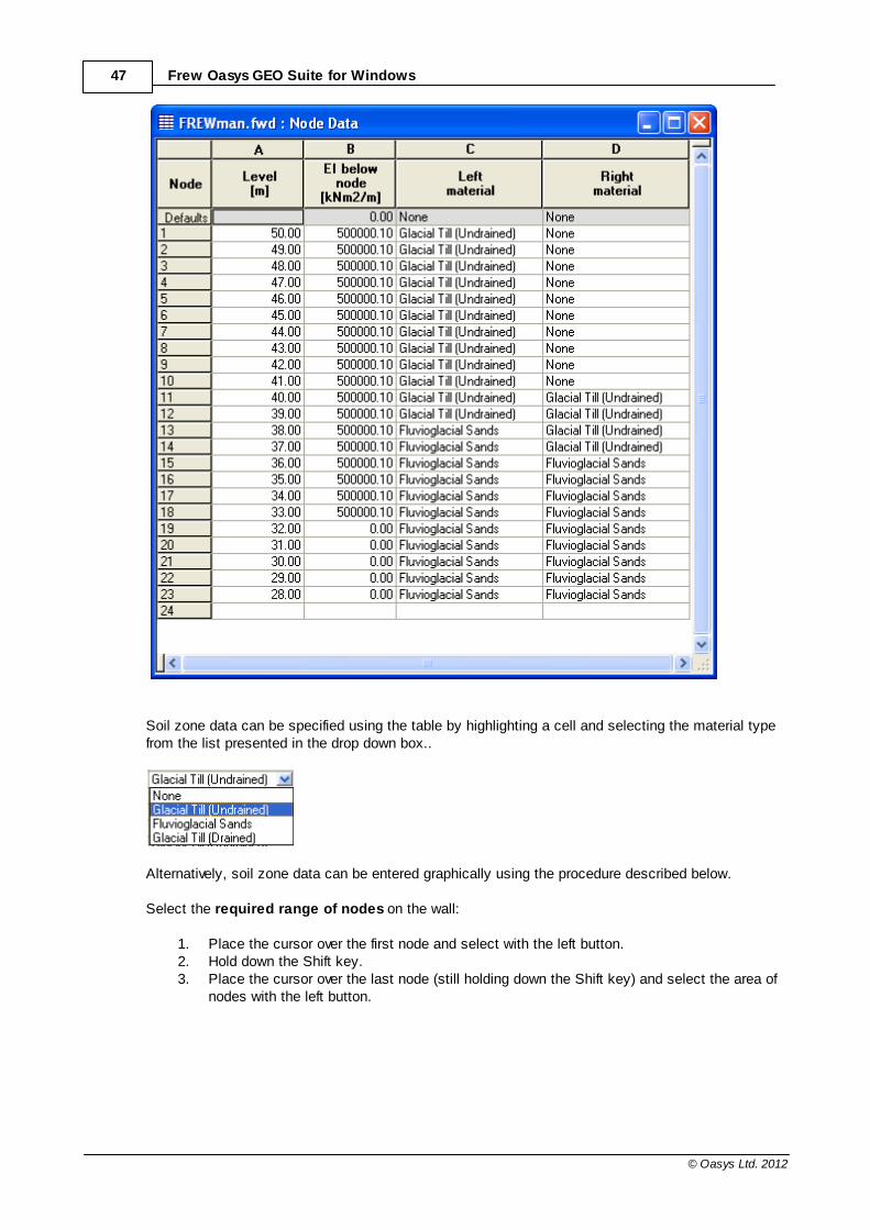
47 Frew Oasys GEO Suite for Windows
© Oasys Ltd. 2012
Soil zone data can be specified using the table by highlighting a cell and selecting the material typefrom the list presented in the drop down box..
Alternatively, soil zone data can be entered graphically using the procedure described below.
Select the required range of nodes on the wall:
1. Place the cursor over the first node and select with the left button.2. Hold down the Shift key.3. Place the cursor over the last node (still holding down the Shift key) and select the area of
nodes with the left button.
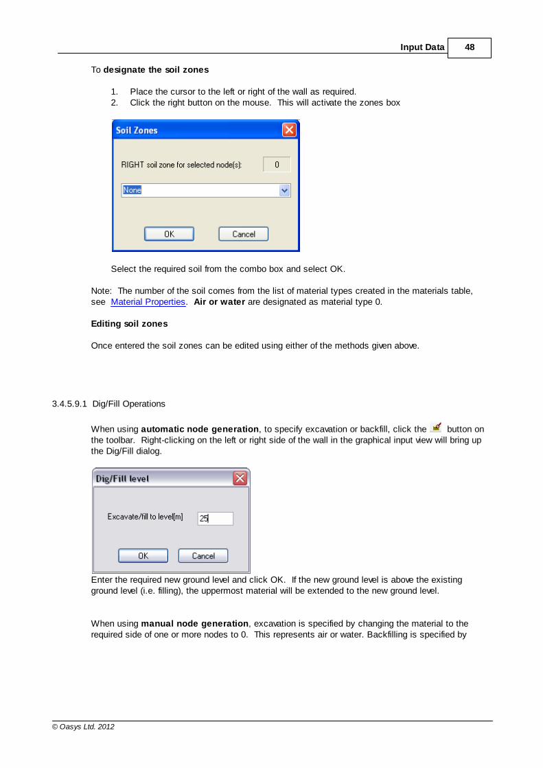
48Input Data
© Oasys Ltd. 2012
To designate the soil zones
1. Place the cursor to the left or right of the wall as required.2. Click the right button on the mouse. This will activate the zones box
Select the required soil from the combo box and select OK.
Note: The number of the soil comes from the list of material types created in the materials table,see Material Properties. Air or water are designated as material type 0.
Editing soil zones
Once entered the soil zones can be edited using either of the methods given above.
3.4.5.9.1 Dig/Fill Operations
When using automatic node generation, to specify excavation or backfill, click the button onthe toolbar. Right-clicking on the left or right side of the wall in the graphical input view will bring upthe Dig/Fill dialog.
Enter the required new ground level and click OK. If the new ground level is above the existingground level (i.e. filling), the uppermost material will be extended to the new ground level.
When using manual node generation, excavation is specified by changing the material to therequired side of one or more nodes to 0. This represents air or water. Backfilling is specified by
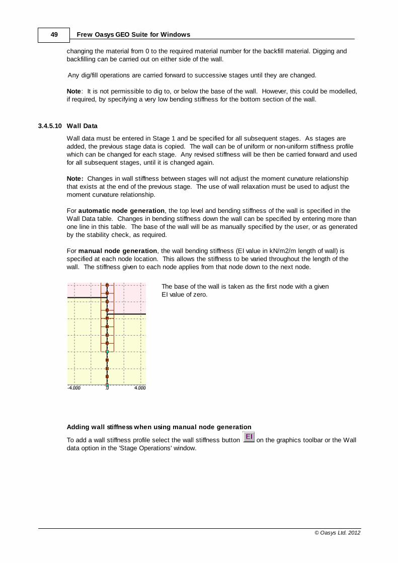
49 Frew Oasys GEO Suite for Windows
© Oasys Ltd. 2012
changing the material from 0 to the required material number for the backfill material. Digging andbackfilling can be carried out on either side of the wall.
Any dig/fill operations are carried forward to successive stages until they are changed.
Note: It is not permissible to dig to, or below the base of the wall. However, this could be modelled,if required, by specifying a very low bending stiffness for the bottom section of the wall.
3.4.5.10 Wall Data
Wall data must be entered in Stage 1 and be specified for all subsequent stages. As stages areadded, the previous stage data is copied. The wall can be of uniform or non-uniform stiffness profilewhich can be changed for each stage. Any revised stiffness will be then be carried forward and usedfor all subsequent stages, until it is changed again.
Note: Changes in wall stiffness between stages will not adjust the moment curvature relationshipthat exists at the end of the previous stage. The use of wall relaxation must be used to adjust themoment curvature relationship.
For automatic node generation, the top level and bending stiffness of the wall is specified in theWall Data table. Changes in bending stiffness down the wall can be specified by entering more thanone line in this table. The base of the wall will be as manually specified by the user, or as generatedby the stability check, as required.
For manual node generation, the wall bending stiffness (EI value in kN/m2/m length of wall) isspecified at each node location. This allows the stiffness to be varied throughout the length of thewall. The stiffness given to each node applies from that node down to the next node.
The base of the wall is taken as the first node with a givenEI value of zero.
Adding wall stiffness when using manual node generation
To add a wall stiffness profile select the wall stiffness button on the graphics toolbar or the Walldata option in the 'Stage Operations' window.
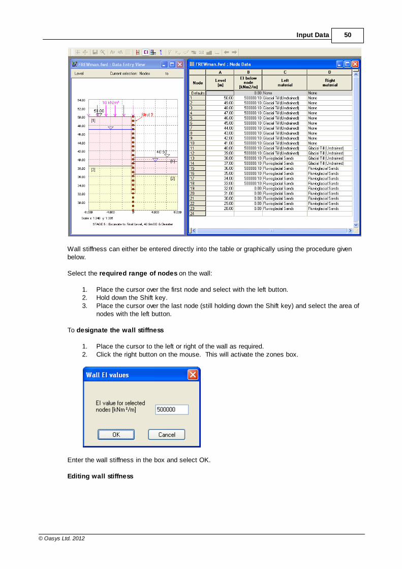
50Input Data
© Oasys Ltd. 2012
Wall stiffness can either be entered directly into the table or graphically using the procedure givenbelow.
Select the required range of nodes on the wall:
1. Place the cursor over the first node and select with the left button.2. Hold down the Shift key.3. Place the cursor over the last node (still holding down the Shift key) and select the area of
nodes with the left button.
To designate the wall stiffness
1. Place the cursor to the left or right of the wall as required.2. Click the right button on the mouse. This will activate the zones box.
Enter the wall stiffness in the box and select OK.
Editing wall stiffness

51 Frew Oasys GEO Suite for Windows
© Oasys Ltd. 2012
The wall stiffness can be changed, either
1. by repeating the procedure above to overwrite the entered data or 2. by selecting the required node in the table using the cursor and typing in a new number.
Note : The Wall stiffness extends to the top of the node below. The last node in the added list istherefore not available in the wall window to prevent the wall being extended below the base of thedefined problem.
3.4.5.11 Groundwater
The profile of groundwater can be either hydrostatic or piezometric. These can be different on eitherside of the wall.
For a hydrostatic distribution enter a single piezometer, with zero pressure, at the phreaticsurface. The profile of pressure with depth will be linear beneath this level and have a gradientdependent on the specified unit weight of water.
Note: The specified unit weight of water is a single global value which is applied to all piezometerson the same side of the wall.
The piezometric distribution is specified using a series of pressure heads. The water pressure atany point is computed by interpolating vertically between two adjacent points.
Note: The highest specified point must have zero water pressure. Negative pore pressures canbe specified below the highest point to describe soil suction. The water pressure is assumed toincrease hydrostatically below the lowest specified point.
The water pressures are also assumed to be constant laterally from either side of the wall.
Adding piezometers
Piezometer data is entered by selecting the piezometer button on the graphics toolbar or the inthe 'Stage Operations' window. Water data on the left or right side of the wall can be viewed byselecting the appropriate page tab at the bottom of the table.
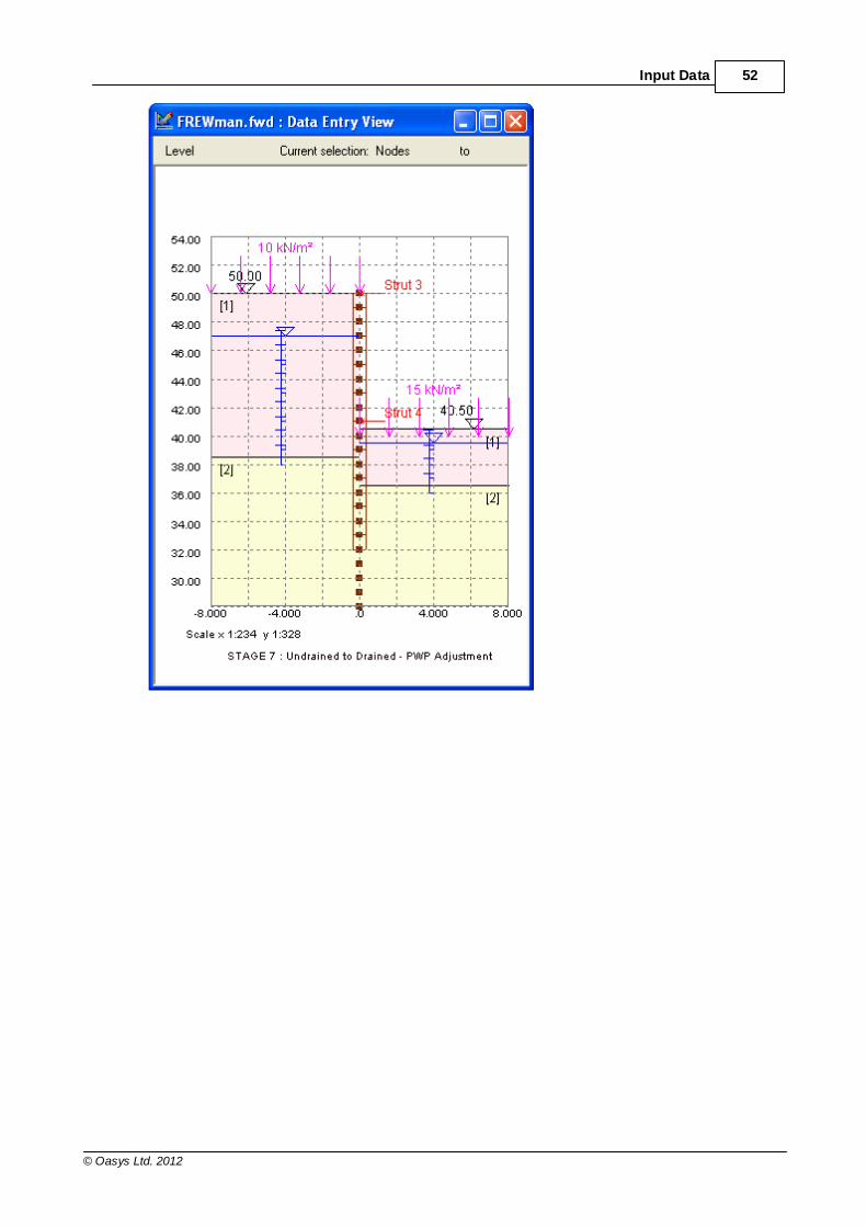
52Input Data
© Oasys Ltd. 2012
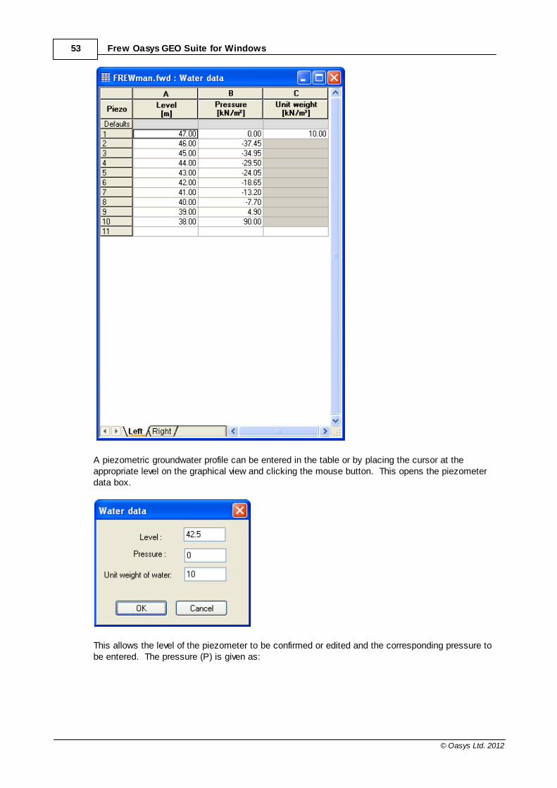
53 Frew Oasys GEO Suite for Windows
© Oasys Ltd. 2012
A piezometric groundwater profile can be entered in the table or by placing the cursor at theappropriate level on the graphical view and clicking the mouse button. This opens the piezometerdata box.
This allows the level of the piezometer to be confirmed or edited and the corresponding pressure tobe entered. The pressure (P) is given as:

54Input Data
© Oasys Ltd. 2012
P = (hp – h
w)
w
where:
hp
= The level of the piezometer
hw
= The level of the piezometric head at the piezometer
w= Global unit weight of water.
Note: Any amendments to the global weight of water will automatically be applied to all piezometerson the same side of the wall. Editing
Once the information for a piezometer has been entered then the data can be edited or deleted usingthe tabulated information beside the graphical view.
The piezometers can also be deleted by placing the cursor over the location and clicking the leftbutton whilst holding down the Shift key.
3.4.5.12 Analysis Data
The analysis data dialog allows specification of the following overall parameters required to define theproblem.
Note: These parameters can be changed for each stage.

55 Frew Oasys GEO Suite for Windows
© Oasys Ltd. 2012
3.4.5.12.1 Model Type
The type of soil model to be used must be selected here. Further data is then requested dependingwhich model is selected.
Safe method Wall/Soil interface must be selected as 'fixed' or 'free'.
Mindlin method The Global Poisson's ratio and wall plan length must bespecified.
Method of Sub-grade Reaction ***Not available yet in windows version***
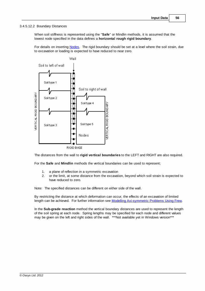
56Input Data
© Oasys Ltd. 2012
3.4.5.12.2 Boundary Distances
When soil stiffness is represented using the "Safe" or Mindlin methods, it is assumed that thelowest node specified in the data defines a horizontal rough rigid boundary.
For details on inserting Nodes. The rigid boundary should be set at a level where the soil strain, dueto excavation or loading is expected to have reduced to near zero.
The distances from the wall to rigid vertical boundaries to the LEFT and RIGHT are also required.
For the Safe and Mindlin methods the vertical boundaries can be used to represent;
1. a plane of reflection in a symmetric excavation 2. or the limit, at some distance from the excavation, beyond which soil strain is expected to
have reduced to zero.
Note: The specified distances can be different on either side of the wall.
By restricting the distance at which deformation can occur, the effects of an excavation of limitedlength can be achieved. For further information see Modelling Axi-symmetric Problems Using Frew.
In the Sub-grade reaction method the vertical boundary distances are used to represent the lengthof the soil spring at each node. Spring lengths may be specified for each node and different valuesmay be given on the left and right sides of the wall. ***Not available yet in Windows version***
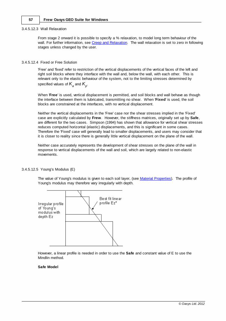
57 Frew Oasys GEO Suite for Windows
© Oasys Ltd. 2012
3.4.5.12.3 Wall Relaxation
From stage 2 onward it is possible to specify a % relaxation, to model long term behaviour of thewall. For further information, see Creep and Relaxation. The wall relaxation is set to zero in followingstages unless changed by the user.
3.4.5.12.4 Fixed or Free Solution
'Free' and 'fixed' refer to restriction of the vertical displacements of the vertical faces of the left andright soil blocks where they interface with the wall and, below the wall, with each other. This isrelevant only to the elastic behaviour of the system, not to the limiting stresses determined by
specified values of Ka and K
p.
When 'Free ' is used, vertical displacement is permitted, and soil blocks and wall behave as thoughthe interface between them is lubricated, transmitting no shear. When 'Fixed' is used, the soilblocks are constrained at the interfaces, with no vertical displacement.
Neither the vertical displacements in the 'Free' case nor the shear stresses implied in the 'Fixed'case are explicitly calculated by Frew. However, the stiffness matrices, originally set up by Safe,are different for the two cases. Simpson (1994) has shown that allowance for vertical shear stressesreduces computed horizontal (elastic) displacements, and this is significant in some cases. Therefore the 'Fixed' case will generally lead to smaller displacements, and users may consider thatit is closer to reality since there is generally little vertical displacement on the plane of the wall.
Neither case accurately represents the development of shear stresses on the plane of the wall inresponse to vertical displacements of the wall and soil, which are largely related to non-elasticmovements.
3.4.5.12.5 Young’s Modulus (E)
The value of Young's modulus is given to each soil layer, (see Material Properties). The profile ofYoung's modulus may therefore vary irregularly with depth.
However, a linear profile is needed in order to use the Safe and constant value of E to use theMindlin method.
Safe Model
58Input Data
© Oasys Ltd. 2012
When using the Safe Model Frew can generate a "best fit" linear profile through the stepped profilecreated by the individual soil layers on either side of the wall. Alternatively, the user can specify aprofile by giving the value of Young's modulus at the lowest node and then a gradient of the line. Apositive gradient creates an increasing profile with depth.
When Frew generates the best fit line, it then makes further modifications to the stiffness matrix.This attempts to fit the irregular profile of Young's modulus better.For details on the Accuracy with respect to Young's modulus (E).
Mindlin Model
The Mindlin Model requires a constant value of E. The method can either generate a best fit valueor use a user specified value.
For details on the use of E in the Mindlin method see Approximations used in the Mindlin method.
For both methods, if the "Generate" option is used, an approximate modification is made to allow forthe irregular variation of E value with depth. If the "Specified" option is selected then the user mustdefine the required profile.
3.4.5.12.6 Redistribution of Pressures
The use of redistribution can allow for the effects of arching in the soil.
If "no redistribution" is specified, the wall pressures at all points are limited to lie between pa and pp. However, if "redistribution" is allowed, it is assumed that arching may take place according totheory presented in Calculation of Active and Passive Limits and Application of Redistribution.
Note: It is considered that the "redistribution" option, while being less conservative is more realistic.
3.4.5.12.7 Minimum Equivalent Fluid Pressure
If it is required that the total active pressure on the wall at any depth below the ground surfaceshould not drop below a specified value, a Minimum Equivalent Fluid Pressure (MEFP) can beautomatically calculated by Frew. To use this feature, check the minimum equivalent fluid pressurebox on the Analysis Data dialog.
This will add an option to the Stage Operations which allows entry of MEFP parameters.
The MEFP option is available on the Analysis option dialog box.
Note: These parameters can be changed for each stage.
If the MEFP is checked then another option is added to the Stage Operations tree view for thatstage,called "Minimum Equivalent Fluid Pressure ".
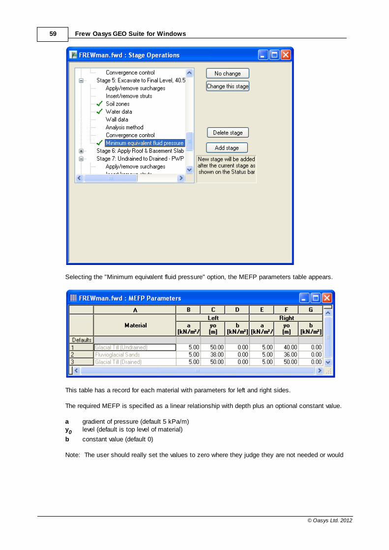
59 Frew Oasys GEO Suite for Windows
© Oasys Ltd. 2012
Selecting the "Minimum equivalent fluid pressure" option, the MEFP parameters table appears.
This table has a record for each material with parameters for left and right sides.
The required MEFP is specified as a linear relationship with depth plus an optional constant value.
a gradient of pressure (default 5 kPa/m)y0 level (default is top level of material)
b constant value (default 0)
Note: The user should really set the values to zero where they judge they are not needed or would

60Input Data
© Oasys Ltd. 2012
incorrectly affect the results, e.g. on the passive side of the wall.
During analysis, the active pressure is set to a minimum of a*(y0-y)+b, where y is the level of the
node. If this is the governing criterion on active pressure, an 'm' symbol is shown in the tabularoutput. In the graphical output, the MEFP-derived pressure is just plotted as part of the normalactive pressure line.
3.4.5.12.8 Passive Softening
This analysis option can be specified for individual stages. If passive softening is used, then theundrained shear strength of the material is assumed to increase linearly from zero to the globalsoftening value (%) over the passive softening depth entered.
To use this option enter:The depth to which surface softening occurs, (distance units)The magnitude of original strength/stiffness to be used for global softening, (%)
The strength of all undrained material below a softening depth will be reduced to global softening (%)of the value in the Material Properties table.
Note: Since either (or both) sides of the wall can be excavated, the user can specify separateparameters for both sides of the wall.
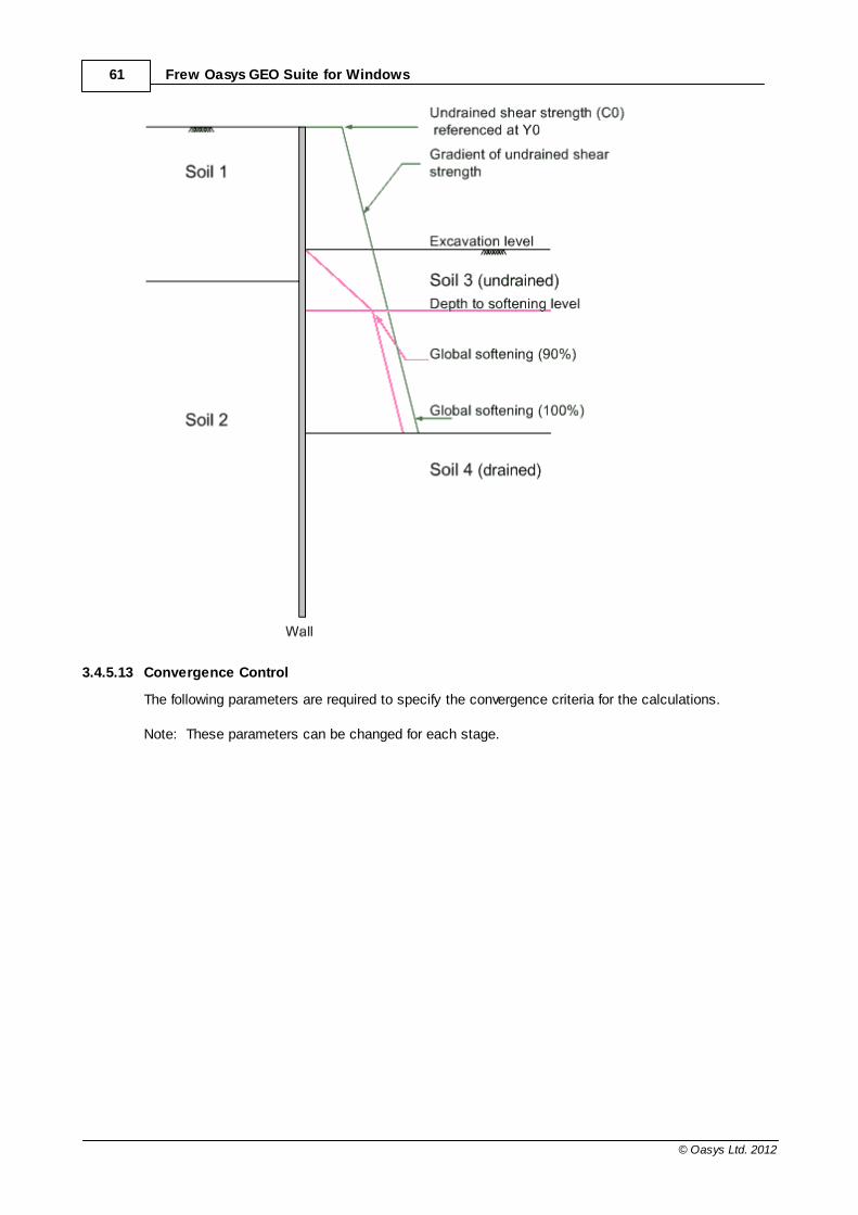
61 Frew Oasys GEO Suite for Windows
© Oasys Ltd. 2012
3.4.5.13 Convergence Control
The following parameters are required to specify the convergence criteria for the calculations.
Note: These parameters can be changed for each stage.
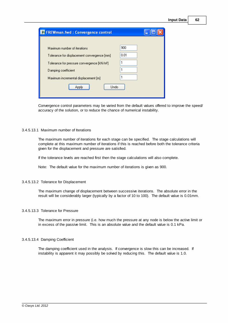
62Input Data
© Oasys Ltd. 2012
Convergence control parameters may be varied from the default values offered to improve the speed/accuracy of the solution, or to reduce the chance of numerical instability.
3.4.5.13.1 Maximum number of Iterations
The maximum number of iterations for each stage can be specified. The stage calculations willcomplete at this maximum number of iterations if this is reached before both the tolerance criteriagiven for the displacement and pressure are satisfied.
If the tolerance levels are reached first then the stage calculations will also complete.
Note: The default value for the maximum number of iterations is given as 900.
3.4.5.13.2 Tolerance for Displacement
The maximum change of displacement between successive iterations. The absolute error in theresult will be considerably larger (typically by a factor of 10 to 100). The default value is 0.01mm.
3.4.5.13.3 Tolerance for Pressure
The maximum error in pressure (i.e. how much the pressure at any node is below the active limit orin excess of the passive limit. This is an absolute value and the default value is 0.1 kPa.
3.4.5.13.4 Damping Coefficient
The damping coefficient used in the analysis. If convergence is slow this can be increased. Ifinstability is apparent it may possibly be solved by reducing this. The default value is 1.0.
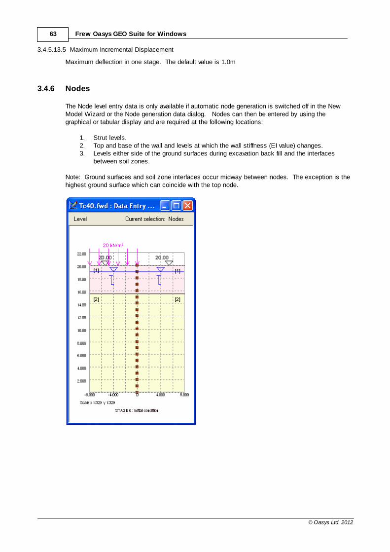
63 Frew Oasys GEO Suite for Windows
© Oasys Ltd. 2012
3.4.5.13.5 Maximum Incremental Displacement
Maximum deflection in one stage. The default value is 1.0m
3.4.6 Nodes
The Node level entry data is only available if automatic node generation is switched off in the NewModel Wizard or the Node generation data dialog. Nodes can then be entered by using thegraphical or tabular display and are required at the following locations:
1. Strut levels.2. Top and base of the wall and levels at which the wall stiffness (EI value) changes.3. Levels either side of the ground surfaces during excavation back fill and the interfaces
between soil zones.
Note: Ground surfaces and soil zone interfaces occur midway between nodes. The exception is thehighest ground surface which can coincide with the top node.
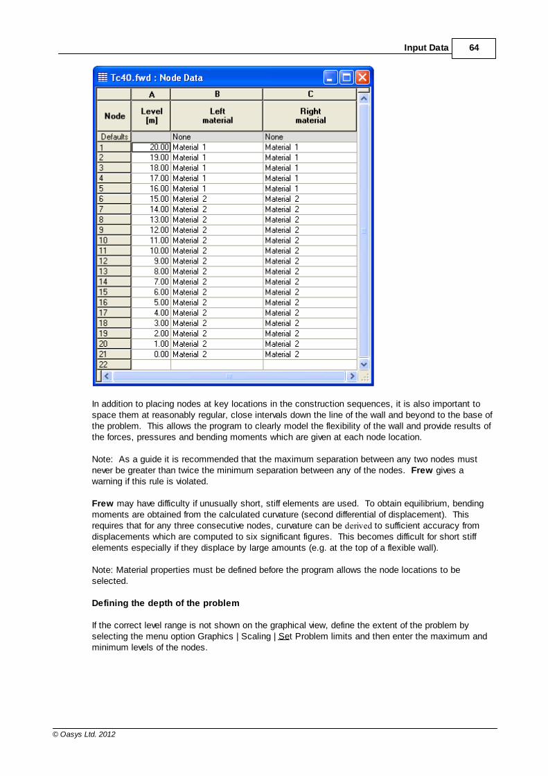
64Input Data
© Oasys Ltd. 2012
In addition to placing nodes at key locations in the construction sequences, it is also important tospace them at reasonably regular, close intervals down the line of the wall and beyond to the base ofthe problem. This allows the program to clearly model the flexibility of the wall and provide results ofthe forces, pressures and bending moments which are given at each node location.
Note: As a guide it is recommended that the maximum separation between any two nodes mustnever be greater than twice the minimum separation between any of the nodes. Frew gives awarning if this rule is violated.
Frew may have difficulty if unusually short, stiff elements are used. To obtain equilibrium, bendingmoments are obtained from the calculated curvature (second differential of displacement). Thisrequires that for any three consecutive nodes, curvature can be derived to sufficient accuracy fromdisplacements which are computed to six significant figures. This becomes difficult for short stiffelements especially if they displace by large amounts (e.g. at the top of a flexible wall).
Note: Material properties must be defined before the program allows the node locations to beselected.
Defining the depth of the problem
If the correct level range is not shown on the graphical view, define the extent of the problem byselecting the menu option Graphics | Scaling | Set Problem limits and then enter the maximum andminimum levels of the nodes.

65 Frew Oasys GEO Suite for Windows
© Oasys Ltd. 2012
Problem Range & Snap Interval
Note: When soil stiffness is represented using the "Safe" or Mindlin methods, it is assumed thatthe lowest node specified in the data defines a horizontal rough rigid boundary.
The snap interval is also entered here. This provides the closest point onto which the cursor will lockto mark a point. The snap interval is taken as the nearest interval in metres.
Adding nodes.
To add nodes select the Global data | Node levels menu option or select the nodes button onthe graphics toolbar. Nodes can then be added by entering their level directly in the table orgraphically by the following procedure;
1. Use the mouse to place the cursor over the location of the top node.2. Click with left button on the location.
This will place the node on the line of the wall. Note: If the scale of the diagram is too small to locate the nodes accurately, then maximise themain and graphics windows to increase the size of the image.
Editing the location of the node.
If the location of the node requires editing then this can be done in one of two ways:
1. Place the cursor over the node and click the right mouse button. This will bring up anamendment box.
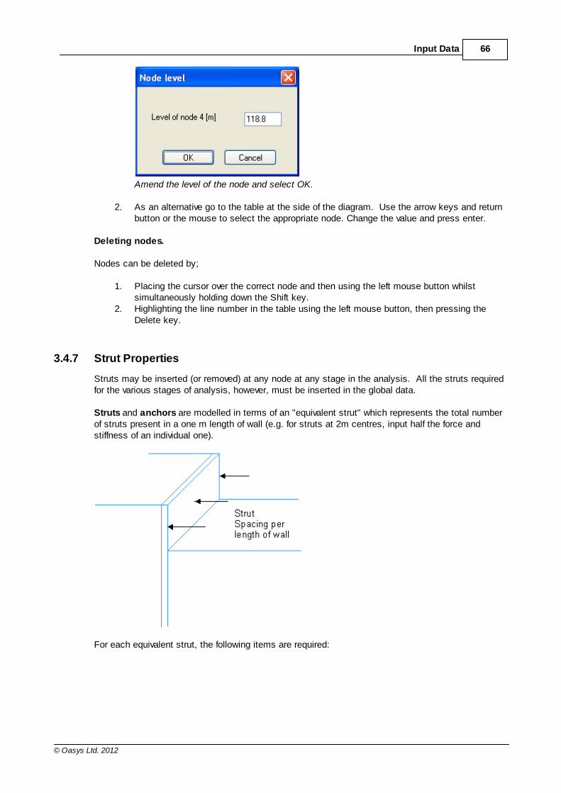
66Input Data
© Oasys Ltd. 2012
Amend the level of the node and select OK.
2. As an alternative go to the table at the side of the diagram. Use the arrow keys and returnbutton or the mouse to select the appropriate node. Change the value and press enter.
Deleting nodes.
Nodes can be deleted by;
1. Placing the cursor over the correct node and then using the left mouse button whilstsimultaneously holding down the Shift key.
2. Highlighting the line number in the table using the left mouse button, then pressing theDelete key.
3.4.7 Strut Properties
Struts may be inserted (or removed) at any node at any stage in the analysis. All the struts requiredfor the various stages of analysis, however, must be inserted in the global data.
Struts and anchors are modelled in terms of an "equivalent strut" which represents the total numberof struts present in a one m length of wall (e.g. for struts at 2m centres, input half the force andstiffness of an individual one).
For each equivalent strut, the following items are required:
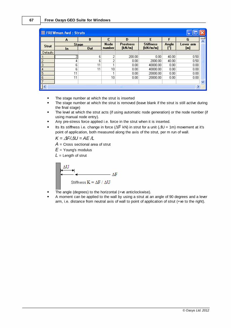
67 Frew Oasys GEO Suite for Windows
© Oasys Ltd. 2012
The stage number at which the strut is insertedThe stage number at which the strut is removed (leave blank if the strut is still active duringthe final stage)The level at which the strut acts (if using automatic node generation) or the node number (ifusing manual node entry).Any pre-stress force applied i.e. force in the strut when it is inserted.
Its Its stiffness i.e. change in force ( F kN) in strut for a unit ( U = 1m) movement at it's
point of application, both measured along the axis of the strut, per m run of wall.
K = F/ U = AE /LA = Cross sectional area of strut
E = Young's modulus
L = Length of strut
The angle (degrees) to the horizontal (+ve anticlockwise).A moment can be applied to the wall by using a strut at an angle of 90 degrees and a leverarm, i.e. distance from neutral axis of wall to point of application of strut (+ve to the right).
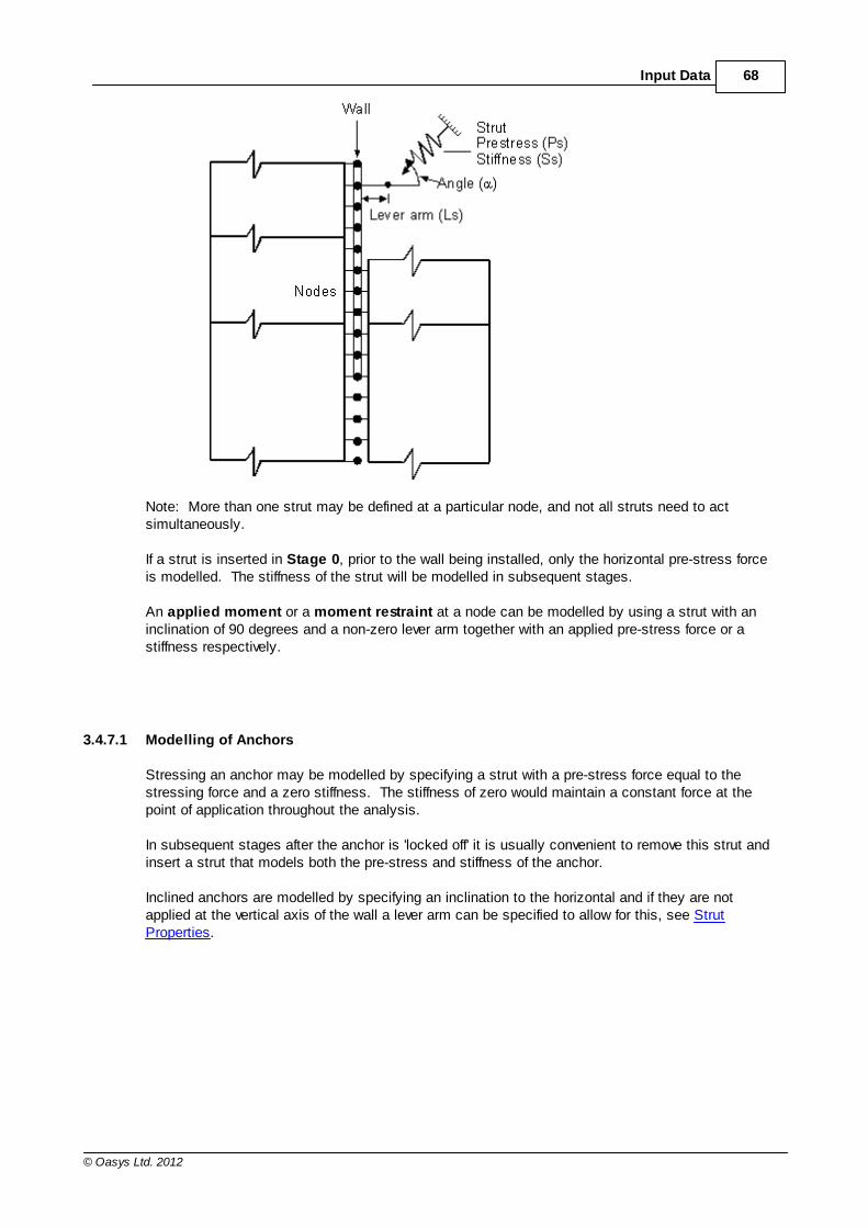
68Input Data
© Oasys Ltd. 2012
Note: More than one strut may be defined at a particular node, and not all struts need to actsimultaneously.
If a strut is inserted in Stage 0, prior to the wall being installed, only the horizontal pre-stress forceis modelled. The stiffness of the strut will be modelled in subsequent stages.
An applied moment or a moment restraint at a node can be modelled by using a strut with aninclination of 90 degrees and a non-zero lever arm together with an applied pre-stress force or astiffness respectively.
3.4.7.1 Modelling of Anchors
Stressing an anchor may be modelled by specifying a strut with a pre-stress force equal to thestressing force and a zero stiffness. The stiffness of zero would maintain a constant force at thepoint of application throughout the analysis.
In subsequent stages after the anchor is 'locked off' it is usually convenient to remove this strut andinsert a strut that models both the pre-stress and stiffness of the anchor.
Inclined anchors are modelled by specifying an inclination to the horizontal and if they are notapplied at the vertical axis of the wall a lever arm can be specified to allow for this, see StrutProperties.
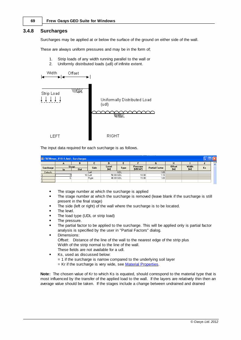
69 Frew Oasys GEO Suite for Windows
© Oasys Ltd. 2012
3.4.8 Surcharges
Surcharges may be applied at or below the surface of the ground on either side of the wall.
These are always uniform pressures and may be in the form of;
1. Strip loads of any width running parallel to the wall or 2. Uniformly distributed loads (udl) of infinite extent.
The input data required for each surcharge is as follows.
The stage number at which the surcharge is appliedThe stage number at which the surcharge is removed (leave blank if the surcharge is stillpresent in the final stage)The side (left or right) of the wall where the surcharge is to be located.The level. The load type (UDL or strip load)The pressure.The partial factor to be applied to the surcharge. This will be applied only is partial factoranalysis is specified by the user in "Partial Factors" dialog.Dimensions:Offset: Distance of the line of the wall to the nearest edge of the strip plusWidth of the strip normal to the line of the wall.These fields are not available for a udl.Ks, used as discussed below:= 1 if the surcharge is narrow compared to the underlying soil layer = Kr if the surcharge is very wide, see Material Properties.
Note: The chosen value of Kr to which Ks is equated, should correspond to the material type that ismost influenced by the transfer of the applied load to the wall. If the layers are relatively thin then anaverage value should be taken. If the stages include a change between undrained and drained

70Input Data
© Oasys Ltd. 2012
materials then multiple surcharges should be entered to take the change of Kr (at the relevant stage)into account.
The surcharge can be applied before the wall is inserted (Stage 0). If this is the case the programcomputes the effects of the surcharge on the soil stresses before installation of the wall.
3.4.8.1 Application of Uniformly Distributed Loads
To determine the elastic effect on the horizontal effective stress, udl surcharges are multiplied by K0
in Stage 0, whereas in later stages they are multiplied by Kr.
They are therefore treated in the same way as the weight of soil, both in the initial state (Stage 0)and in later stages as excavation and filling takes place, see Effects of excavation and backfill. In allstages, including Stage 0, strip surcharges are multiplied by the factor Ks described above.
Active and passive limit pressures are also modified using the values of Ka and K
p for each layer
beneath the udl.
3.4.8.2 Application of Strip Loads
For strip loads the change in stress in elastic conditions is difficult to determine because thehorizontal stress is extremely sensitive to the variation with depth of the soil stiffness and toanisotropy of the soil stiffness. Two extremes have therefore been considered.
1. For the case where the Young's modulus (E) for the soil is constant for a depth severaltimes greater than the width of the surcharge the Boussinesq equations may be used toderive horizontal stresses in the ground.
The pressures therefore on a rigid (ideally frictionless) vertical boundary would be doublethe Boussinesq values.
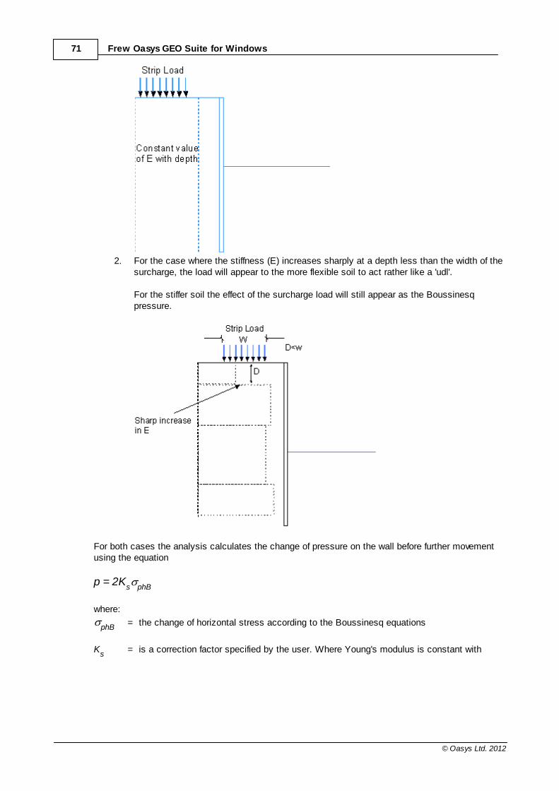
71 Frew Oasys GEO Suite for Windows
© Oasys Ltd. 2012
2. For the case where the stiffness (E) increases sharply at a depth less than the width of thesurcharge, the load will appear to the more flexible soil to act rather like a 'udl'. For the stiffer soil the effect of the surcharge load will still appear as the Boussinesqpressure.
For both cases the analysis calculates the change of pressure on the wall before further movementusing the equation
p = 2Ks phB
where:
phB= the change of horizontal stress according to the Boussinesq equations
Ks
= is a correction factor specified by the user. Where Young's modulus is constant with
72Input Data
© Oasys Ltd. 2012
depth, Ks should be taken as 1.0.
For the case where stiffness increases sharply Ks can have a large range of values, the evaluation of
which is beyond the scope of this text. However if the strip load is wide compared with its distance
from the wall and the depth of the deforming soil, a value of Ks = /(1 - ) will give results equivalent
to loading with a udl with Kr = /(1 - ).
Active and Passive PressuresThe values of active and passive pressures due to strip loads parallel to the wall are discussed in Active Pressures due to Strip Load Surcharges and Passive Pressures due to Strip LoadSurcharges.
The method described for the active pressure is automatically applied by the program, but themethod described for the passive pressure is not applied. The user must therefore manually
enhance the passive pressure coefficient Kp or the soil cohesion c, if this effect is to be incorporatedinto the analysis, see Passive Pressures due to Strip Load Surcharges.
The user is recommended to study the graphical output and check whether the pressures adoptedby the program are acceptable.
4 Partial Factors
The purpose of factors is to allow for uncertainty in material properties, loading and calculationmodels and to ensure safety and acceptable performance.
These are global factors that are applied to material properties or surcharges input parameters. Thenew material parameters affected by these factors will then be used in the calculations. A single setof factors shall be selected and these will apply to all materials in all stages.
WARNING: Frew has had new features added to simplify application of partial factors in line withEC7. However, there are alternative ways of complying with EC7 including manual adjustment ofcertain values. The features in the program do not automatically make a design EC7 compliant andthe user must continue to check the output carefully to ensure the assumptions and adjustments tocharacteristic values are as they require. Note that pore pressures and strut pre-stress are notfactored. If a strut pre-stress is used to model a structural force, and other effects of actions arebeing factored, the user may wish to factor the input value of strut pre-stress.
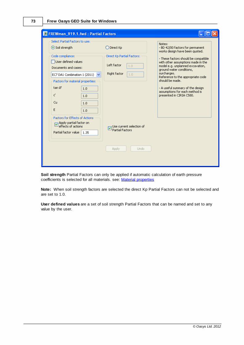
73 Frew Oasys GEO Suite for Windows
© Oasys Ltd. 2012
Soil strength Partial Factors can only be applied if automatic calculation of earth pressurecoefficients is selected for all materials. see: Material properties
Note: When soil strength factors are selected the direct Kp Partial Factors can not be selected andare set to 1.0.
User defined values are a set of soil strength Partial Factors that can be named and set to anyvalue by the user.

74Partial Factors
© Oasys Ltd. 2012
Document and cases is a pre defined list of code compliance Partial Factors:
Direct Kp Partial Factors can be applied even if earth pressure coefficients are User Specified.
Note: When this set of Partial Factors is selected the Soil strength factors can not be selected andare set to "Unfactored" and to 1.0.
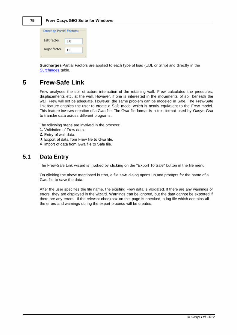
75 Frew Oasys GEO Suite for Windows
© Oasys Ltd. 2012
Surcharges Partial Factors are applied to each type of load (UDL or Strip) and directly in theSurcharges table.
5 Frew-Safe Link
Frew analyses the soil structure interaction of the retaining wall. Frew calculates the pressures,displacements etc. at the wall. However, if one is interested in the movements of soil beneath thewall, Frew will not be adequate. However, the same problem can be modeled in Safe. The Frew-Safelink feature enables the user to create a Safe model which is nearly equivalent to the Frew model.This feature involves creation of a Gwa file. The Gwa file format is a text format used by Oasys Gsato transfer data across different programs.
The following steps are involved in the process:1. Validation of Frew data.2. Entry of wall data.3. Export of data from Frew file to Gwa file.4. Import of data from Gwa file to Safe file.
5.1 Data Entry
The Frew-Safe Link wizard is invoked by clicking on the "Export To Safe" button in the file menu.
On clicking the above mentioned button, a file save dialog opens up and prompts for the name of aGwa file to save the data.
After the user specifies the file name, the existing Frew data is validated. If there are any warnings orerrors, they are displayed in the wizard. Warnings can be ignored, but the data cannot be exported ifthere are any errors. If the relevant checkbox on this page is checked, a log file which contains allthe errors and warnings during the export process will be created.
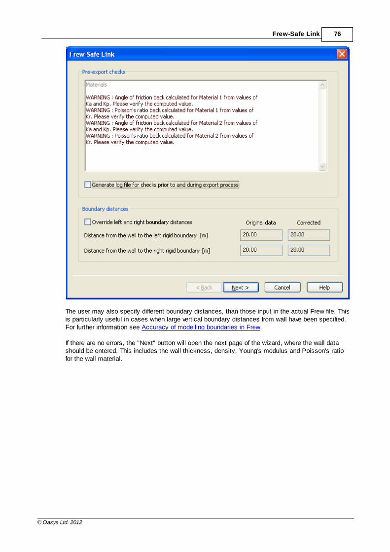
76Frew-Safe Link
© Oasys Ltd. 2012
The user may also specify different boundary distances, than those input in the actual Frew file. Thisis particularly useful in cases when large vertical boundary distances from wall have been specified.For further information see Accuracy of modelling boundaries in Frew.
If there are no errors, the "Next" button will open the next page of the wizard, where the wall datashould be entered. This includes the wall thickness, density, Young's modulus and Poisson's ratiofor the wall material.
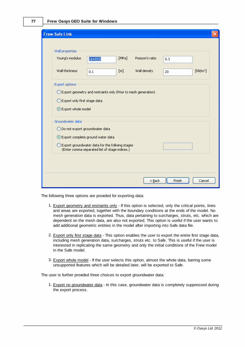
77 Frew Oasys GEO Suite for Windows
© Oasys Ltd. 2012
The following three options are provided for exporting data:
1. Export geometry and restraints only - If this option is selected, only the critical points, linesand areas are exported, together with the boundary conditions at the ends of the model. Nomesh generation data is exported. Thus, data pertaining to surcharges, struts, etc. which aredependent on the mesh data, are also not exported. This option is useful if the user wants toadd additional geometric entities in the model after importing into Safe data file.
2. Export only first stage data - This option enables the user to export the entire first stage data,including mesh generation data, surcharges, struts etc. to Safe. This is useful if the user isinterested in replicating the same geometry and only the initial conditions of the Frew modelin the Safe model.
3. Export whole model - If the user selects this option, almost the whole data, barring someunsupported features which will be detailed later, will be exported to Safe.
The user is further provided three choices to export groundwater data:
1. Export no groundwater data - In this case, groundwater data is completely suppressed duringthe export process.
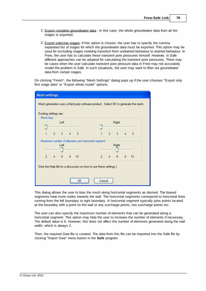
78Frew-Safe Link
© Oasys Ltd. 2012
2. Export complete groundwater data - In this case, the whole groundwater data from all thestages is exported.
3. Export selective stages- If this option is chosen, the user has to specify the commaseparated list of stages for which the groundwater data must be exported. This option may beused for excluding stages involving transition from undrained behaviour to drained behaviour. InFrew, the user has to calculate these transient pore pressures himself. However, in Safedifferent approaches can be adopted for calculating the transient pore pressures. There maybe cases when the user calculate transient pore pressure data in Frew may not accuratelymodel the problem in Safe. In such situations, the user may want to filter out groundwaterdata from certain stages.
On clicking "Finish", the following "Mesh Settings" dialog pops up if the user chooses "Export onlyfirst stage data" or "Export whole model" options:
This dialog allows the user to bias the mesh along horizontal segments as desired. The biasedsegments have more nodes towards the wall. The horizontal segments correspond to horizontal linesrunning from the left boundary to right boundary. A horizontal segment typically joins points locatedat the boundary with a point on the wall or any surcharge points, two surcharge points etc.
The user can also specify the maximum number of elements that can be generated along ahorizontal segment. This option may help the user to increase the number of elements if necessary.The default value is 6. However, this does not affect the number of elements generated along the wallwidth, which is always 2.
Then, the required Gwa file is created. The data from this file can be imported into the Safe file byclicking "Import Gwa" menu button in the Safe program.
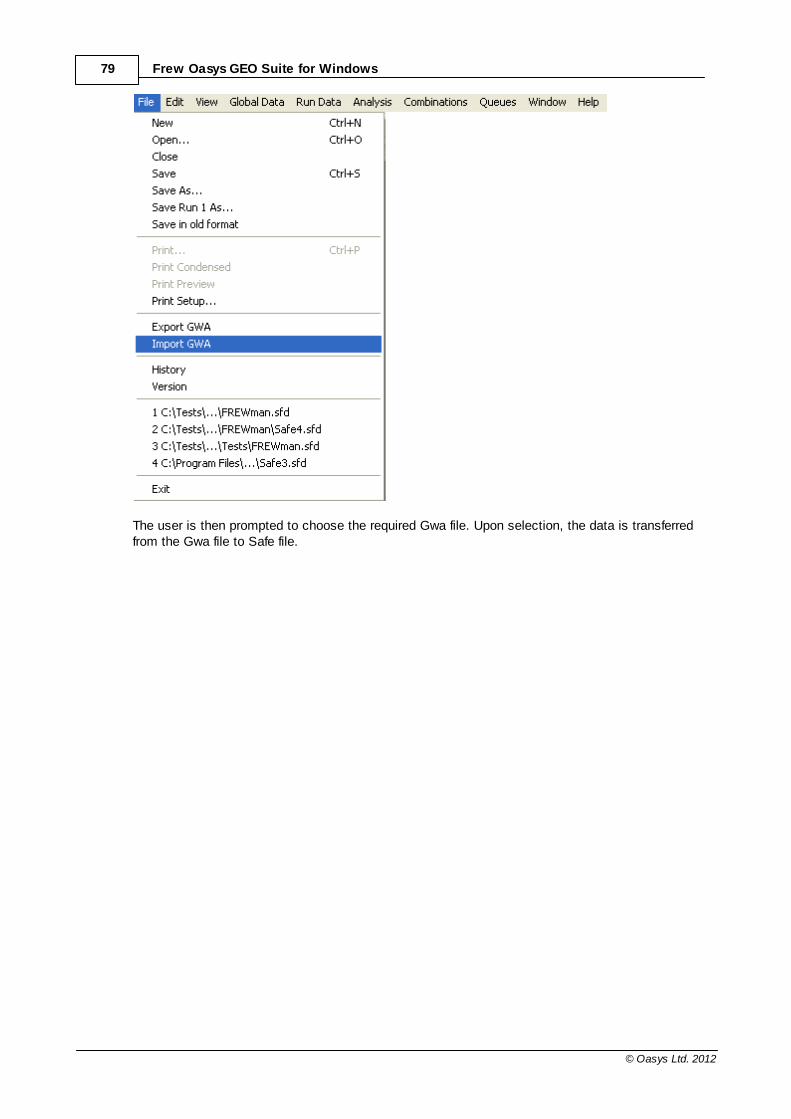
79 Frew Oasys GEO Suite for Windows
© Oasys Ltd. 2012
The user is then prompted to choose the required Gwa file. Upon selection, the data is transferredfrom the Gwa file to Safe file.
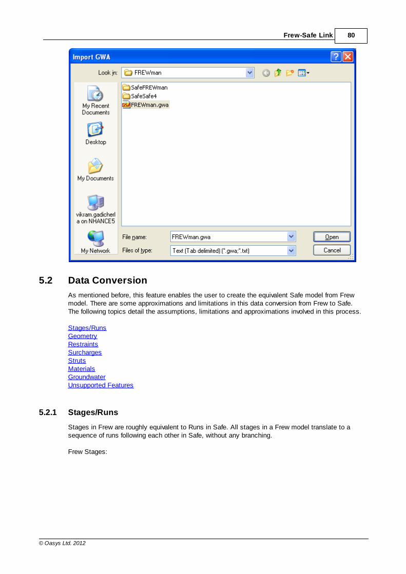
80Frew-Safe Link
© Oasys Ltd. 2012
5.2 Data Conversion
As mentioned before, this feature enables the user to create the equivalent Safe model from Frewmodel. There are some approximations and limitations in this data conversion from Frew to Safe.The following topics detail the assumptions, limitations and approximations involved in this process.
Stages/RunsGeometryRestraintsSurchargesStrutsMaterialsGroundwaterUnsupported Features
5.2.1 Stages/Runs
Stages in Frew are roughly equivalent to Runs in Safe. All stages in a Frew model translate to asequence of runs following each other in Safe, without any branching.
Frew Stages:

81 Frew Oasys GEO Suite for Windows
© Oasys Ltd. 2012
Safe Runs:
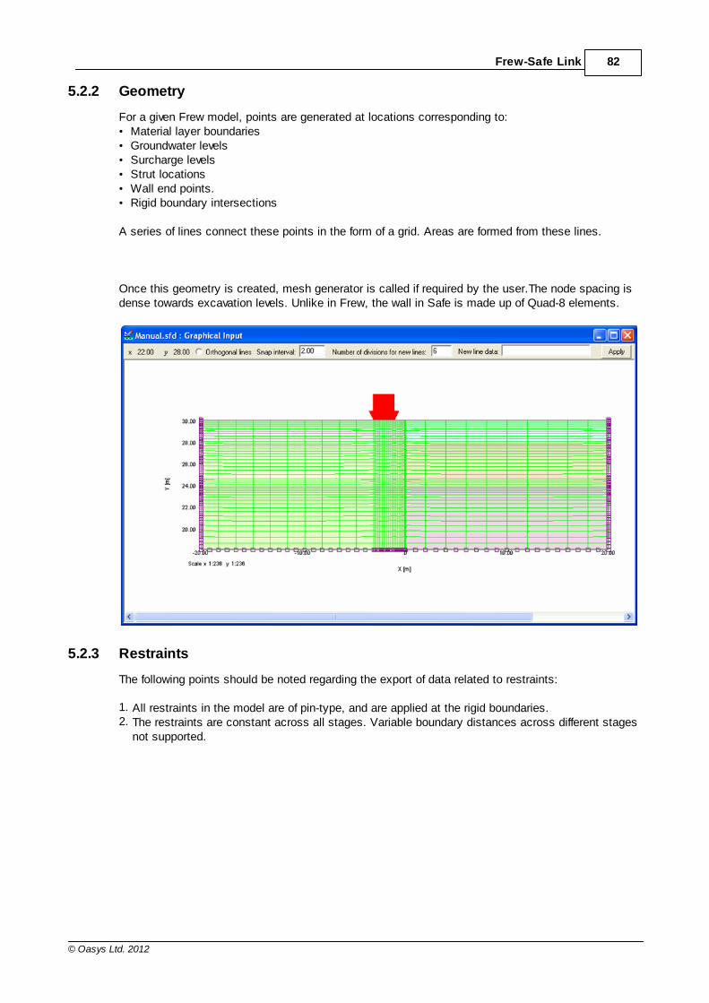
82Frew-Safe Link
© Oasys Ltd. 2012
5.2.2 Geometry
For a given Frew model, points are generated at locations corresponding to:• Material layer boundaries• Groundwater levels• Surcharge levels• Strut locations• Wall end points.• Rigid boundary intersections
A series of lines connect these points in the form of a grid. Areas are formed from these lines.
Once this geometry is created, mesh generator is called if required by the user.The node spacing isdense towards excavation levels. Unlike in Frew, the wall in Safe is made up of Quad-8 elements.
5.2.3 Restraints
The following points should be noted regarding the export of data related to restraints:
1. All restraints in the model are of pin-type, and are applied at the rigid boundaries.2. The restraints are constant across all stages. Variable boundary distances across different stages
not supported.

83 Frew Oasys GEO Suite for Windows
© Oasys Ltd. 2012
5.2.4 Surcharges
The surcharges are applied as element edge loads in the corresponding stages.
Frew surcharge data:
Equivalent Safe element load data:
5.2.5 Struts
Struts in Frew modeled as springs in Safe, and act at nodes located on the wall axis.
Lever arm information is not exported from Frew to Safe.
Pre-stress is applied as a node load in Safe. The prestress along the spring axis direction isresolved into components along the X and Y axes, and applied as a pair of node loads in Safe.
Frew strut data:
Equivalent Safe strut data:
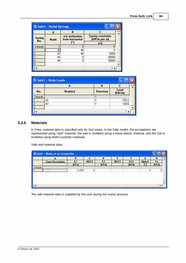
84Frew-Safe Link
© Oasys Ltd. 2012
5.2.6 Materials
In Frew, material data is specified only for Soil strata. In the Safe model, the excavations arerepresented using "void" material, the wall is modeled using a linear elastic material, and the soil ismodeled using Mohr-Coulomb materials.
Safe void material data:
The wall material data is supplied by the user during the export process.
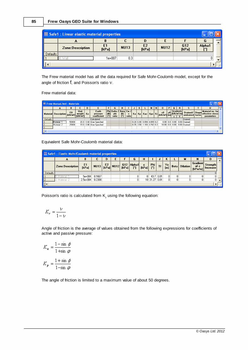
85 Frew Oasys GEO Suite for Windows
© Oasys Ltd. 2012
The Frew material model has all the data required for Safe Mohr-Coulomb model, except for the
angle of friction f, and Poisson's ratio
Frew material data:
Equivalent Safe Mohr-Coulomb material data:
Poisson's ratio is calculated from Kr using the following equation:
Angle of friction is the average of values obtained from the following expressions for coefficients ofactive and passive pressure:
The angle of friction is limited to a maximum value of about 50 degrees.
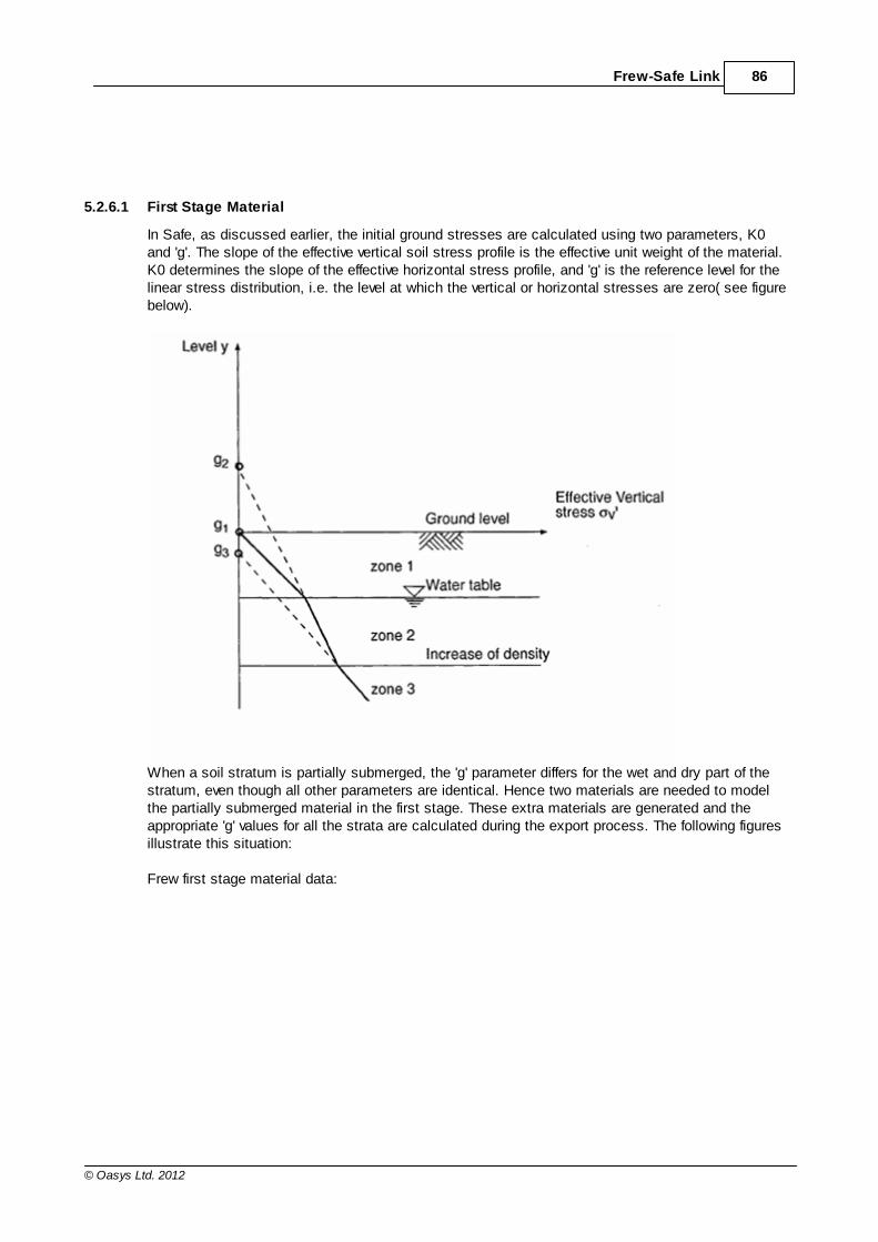
86Frew-Safe Link
© Oasys Ltd. 2012
5.2.6.1 First Stage Material
In Safe, as discussed earlier, the initial ground stresses are calculated using two parameters, K0and 'g'. The slope of the effective vertical soil stress profile is the effective unit weight of the material.K0 determines the slope of the effective horizontal stress profile, and 'g' is the reference level for thelinear stress distribution, i.e. the level at which the vertical or horizontal stresses are zero( see figurebelow).
When a soil stratum is partially submerged, the 'g' parameter differs for the wet and dry part of thestratum, even though all other parameters are identical. Hence two materials are needed to modelthe partially submerged material in the first stage. These extra materials are generated and theappropriate 'g' values for all the strata are calculated during the export process. The following figuresillustrate this situation:
Frew first stage material data:
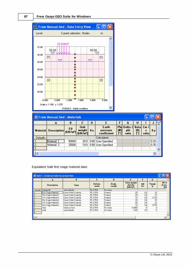
87 Frew Oasys GEO Suite for Windows
© Oasys Ltd. 2012
Equivalent Safe first stage material data:

88Frew-Safe Link
© Oasys Ltd. 2012
5.2.7 Groundwater
Frew and Safe use different approaches for modeling pore pressure distribution. Following are acouple of important differences.
Frew Safe
Piecewise linear interpolation of pore pressure.
Radius of influence approach.
All soil zone materials share the same pore pressure distribution data.
Each material has its own pore pressure distribution
In Safe, each data point is characterized by pore pressure value, its gradient, and a radius ofinfluence. The net pore pressure at a given point is the weighted average of the pore pressurescalculated at the given point using the existing pore pressure data points.
The weights for points which lie within a square defined by this radius of influence, the weights aretypically much higher compared to the weights for the points located outside the square.
In Frew, we can have different pore pressure gradients above and below a particular pore pressuredata point. However, this situation is not possible in Safe for a given data point, as only a single porepressure gradient is specified.
In order to generate a roughly equivalent pore pressure distribution in Safe, the pore pressures arecalculated at locations midway between the Frew pore pressure data points.
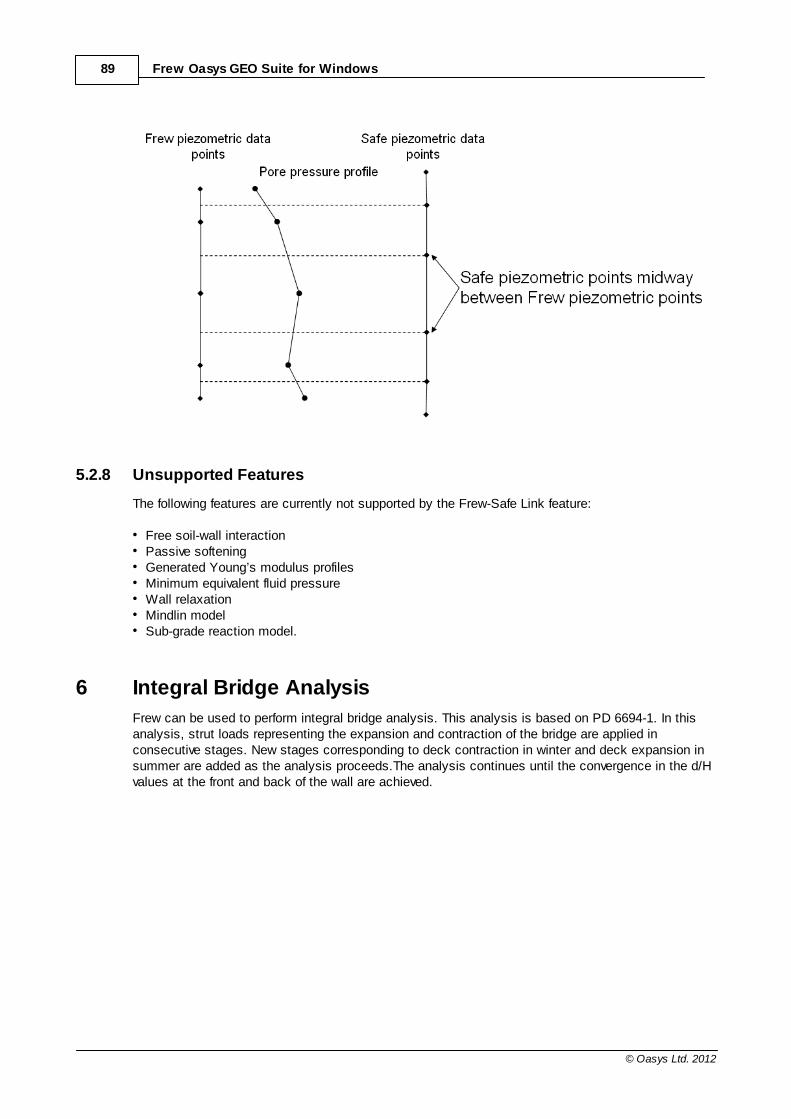
89 Frew Oasys GEO Suite for Windows
© Oasys Ltd. 2012
5.2.8 Unsupported Features
The following features are currently not supported by the Frew-Safe Link feature:
• Free soil-wall interaction• Passive softening• Generated Young’s modulus profiles• Minimum equivalent fluid pressure• Wall relaxation• Mindlin model• Sub-grade reaction model.
6 Integral Bridge Analysis
Frew can be used to perform integral bridge analysis. This analysis is based on PD 6694-1. In thisanalysis, strut loads representing the expansion and contraction of the bridge are applied inconsecutive stages. New stages corresponding to deck contraction in winter and deck expansion insummer are added as the analysis proceeds.The analysis continues until the convergence in the d/Hvalues at the front and back of the wall are achieved.
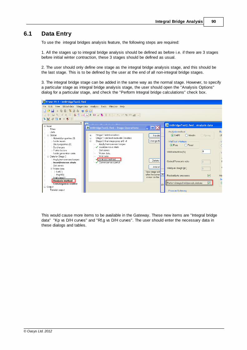
90Integral Bridge Analysis
© Oasys Ltd. 2012
6.1 Data Entry
To use the integral bridges analysis feature, the following steps are required:
1. All the stages up to integral bridge analysis should be defined as before i.e. if there are 3 stagesbefore initial winter contraction, these 3 stages should be defined as usual.
2. The user should only define one stage as the integral bridge analysis stage, and this should bethe last stage. This is to be defined by the user at the end of all non-integral bridge stages.
3. The integral bridge stage can be added in the same way as the normal stage. However, to specifya particular stage as integral bridge analysis stage, the user should open the "Analysis Options"dialog for a particular stage, and check the "Perform Integral bridge calculations" check box.
This would cause more items to be available in the Gateway. These new items are "Integral bridgedata" "Kp vs D/H curves" and "Rf,g vs D/H curves". The user should enter the necessary data inthese dialogs and tables.

91 Frew Oasys GEO Suite for Windows
© Oasys Ltd. 2012
4. The user has to specify whether the integral bridge analysis needs to be done at the front/back ofwall. The user needs to specify the strut index which models deck contraction and expansion.Preferably, this strut should have only prestress, and no stiffness. During the integral bridgeanalysis cycles of contraction and expansion, it will apply the prestress in this strut with appropriatesign.
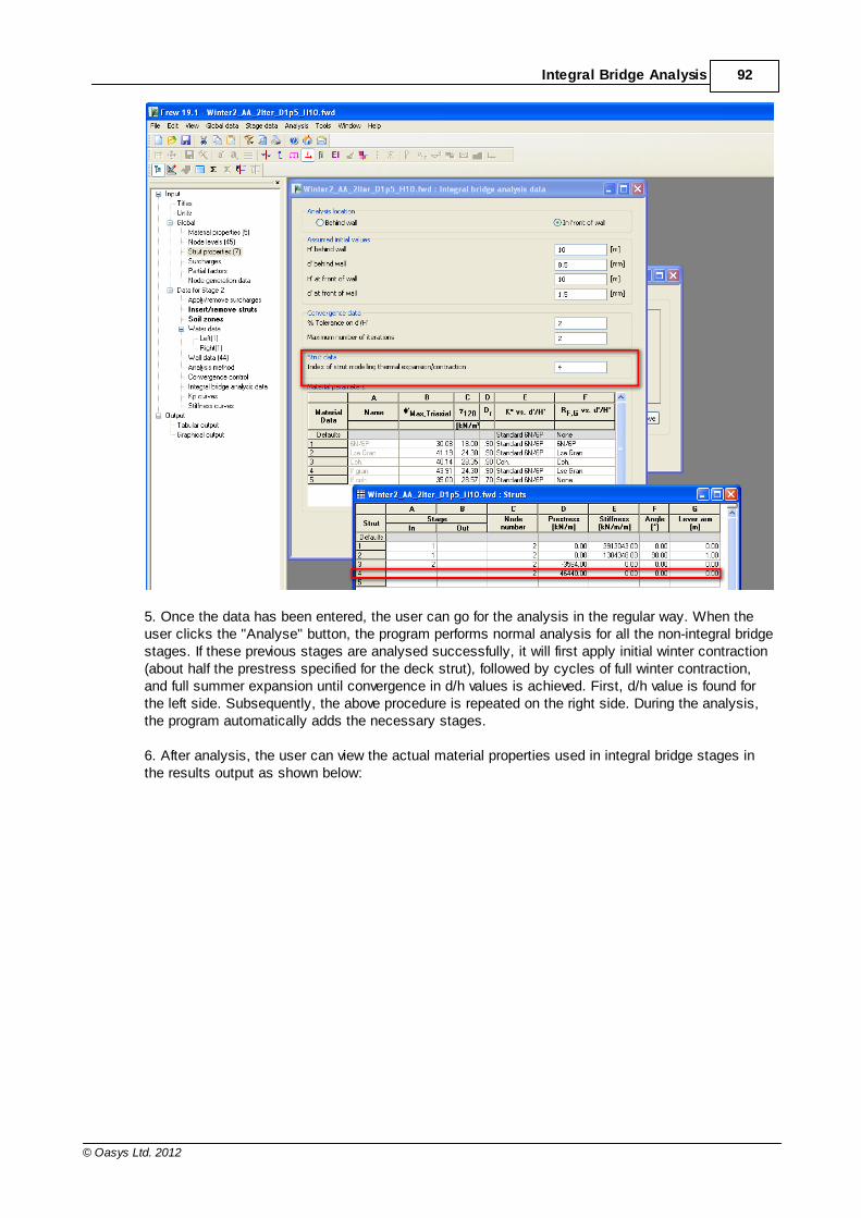
92Integral Bridge Analysis
© Oasys Ltd. 2012
5. Once the data has been entered, the user can go for the analysis in the regular way. When theuser clicks the "Analyse" button, the program performs normal analysis for all the non-integral bridgestages. If these previous stages are analysed successfully, it will first apply initial winter contraction(about half the prestress specified for the deck strut), followed by cycles of full winter contraction,and full summer expansion until convergence in d/h values is achieved. First, d/h value is found forthe left side. Subsequently, the above procedure is repeated on the right side. During the analysis,the program automatically adds the necessary stages.
6. After analysis, the user can view the actual material properties used in integral bridge stages inthe results output as shown below:
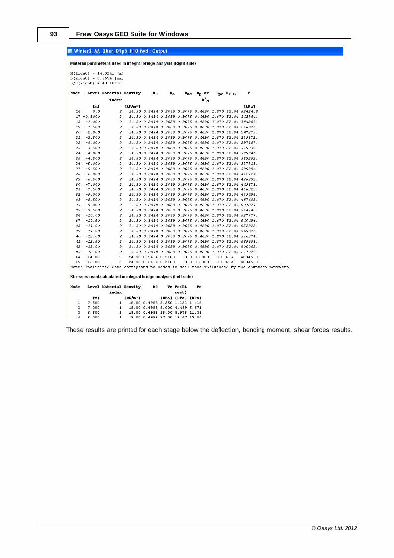
93 Frew Oasys GEO Suite for Windows
© Oasys Ltd. 2012
These results are printed for each stage below the deflection, bending moment, shear forces results.
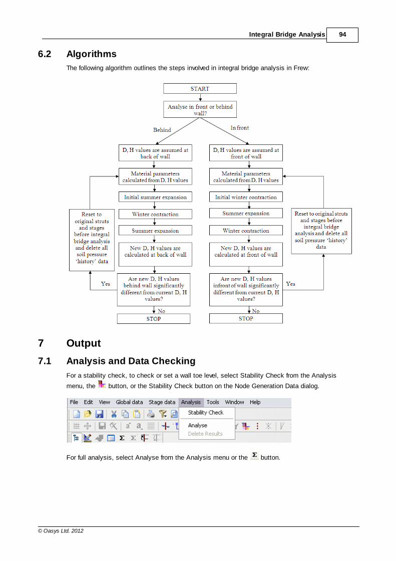
94Integral Bridge Analysis
© Oasys Ltd. 2012
6.2 Algorithms
The following algorithm outlines the steps involved in integral bridge analysis in Frew:
7 Output
7.1 Analysis and Data Checking
For a stability check, to check or set a wall toe level, select Stability Check from the Analysis
menu, the button, or the Stability Check button on the Node Generation Data dialog.
For full analysis, select Analyse from the Analysis menu or the button.
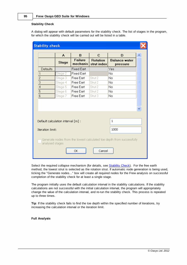
95 Frew Oasys GEO Suite for Windows
© Oasys Ltd. 2012
Stability Check
A dialog will appear with default parameters for the stability check. The list of stages in the program,for which the stability check will be carried out will be listed in a table.
Select the required collapse mechanism (for details, see Stability Check). For the free earthmethod, the lowest strut is selected as the rotation strut. If automatic node generation is being used,ticking the "Generate nodes..." box will create all required nodes for the Frew analysis on successfulcompletion of the stability check for at least a single stage.
The program initially uses the default calculation interval in the stability calculations. If the stabilitycalculations are not successful with the initial calculation interval, the program will appropriatelychange the value of the calculation interval, and re-run the stability check. This process is repeatedup to three times.
Tip: If the stability check fails to find the toe depth within the specified number of iterations, tryincreasing the calculation interval or the iteration limit.
Full Analysis
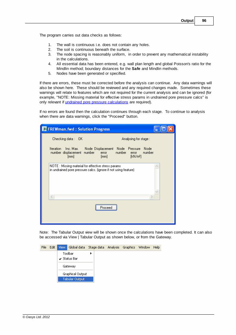
96Output
© Oasys Ltd. 2012
The program carries out data checks as follows:
1. The wall is continuous i.e. does not contain any holes.2. The soil is continuous beneath the surface.3. The node spacing is reasonably uniform, in order to prevent any mathematical instability
in the calculations. 4. All essential data has been entered, e.g. wall plan length and global Poisson's ratio for the
Mindlin method; boundary distances for the Safe and Mindlin methods.5. Nodes have been generated or specified.
If there are errors, these must be corrected before the analysis can continue. Any data warnings willalso be shown here. These should be reviewed and any required changes made. Sometimes thesewarnings will relate to features which are not required for the current analysis and can be ignored (forexample, "NOTE: Missing material for effective stress params in undrained pore pressure calcs" isonly relevant if undrained pore pressure calculations are required).
If no errors are found then the calculation continues through each stage. To continue to analysiswhen there are data warnings, click the "Proceed" button.
Note: The Tabular Output view will be shown once the calculations have been completed. It can alsobe accessed via View | Tabular Output as shown below, or from the Gateway.
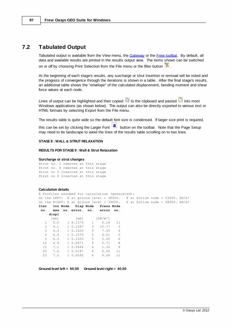
97 Frew Oasys GEO Suite for Windows
© Oasys Ltd. 2012
7.2 Tabulated Output
Tabulated output is available from the View menu, the Gateway or the Frew toolbar. By default, alldata and available results are printed in the results output view. The items shown can be switched
on or off by choosing Print Selection from the File menu or the filter button .
At the beginning of each stage's results, any surcharge or strut insertion or removal will be noted andthe progress of convergence through the iterations is shown in a table. After the final stage's results,an additional table shows the "envelope" of the calculated displacement, bending moment and shearforce values at each node.
Lines of output can be highlighted and then copied to the clipboard and pasted into mostWindows applications (as shown below). The output can also be directly exported to various text orHTML formats by selecting Export from the File menu.
The results table is quite wide so the default font size is condensed. If larger size print is required,
this can be set by clicking the Larger Font button on the toolbar. Note that the Page Setupmay need to be landscape to avoid the lines of the results table scrolling on to two lines.
STAGE 9 : WALL & STRUT RELAXATION
RESULTS FOR STAGE 9 : Wall & Strut Relaxation
Surcharge or strut changesStrut no. 3 removed at this stage
Strut no. 4 removed at this stage
Strut no 5 inserted at this stage
Strut no 6 inserted at this stage
Calculation detailsE Profiles assumed for calculation (generated):
On the LEFT: E at ground level = 38000. E at bottom node = 53000. kN/m²
On the RIGHT: E at ground level = 39000. E at bottom node = 58000. kN/m²
Iter Inc Node Disp Node Press Node
no. max no. error. no. error no.
displ
[mm] [mm] [kN/m²]
1 0.0 1 6.1375 1 0.14 11
2 6.1 1 0.1587 3 10.77 3
3 6.3 1 0.1620 4 7.65 4
4 6.4 1 0.1570 5 6.01 5
5 6.5 1 0.1503 5 5.00 6
10 6.9 1 0.0971 5 2.71 8
15 7.1 1 0.0484 6 1.32 9
20 7.2 1 0.0187 6 0.55 11
23 7.2 1 0.0092 6 0.26 11
Ground level left = 50.00 Ground level right = 40.50
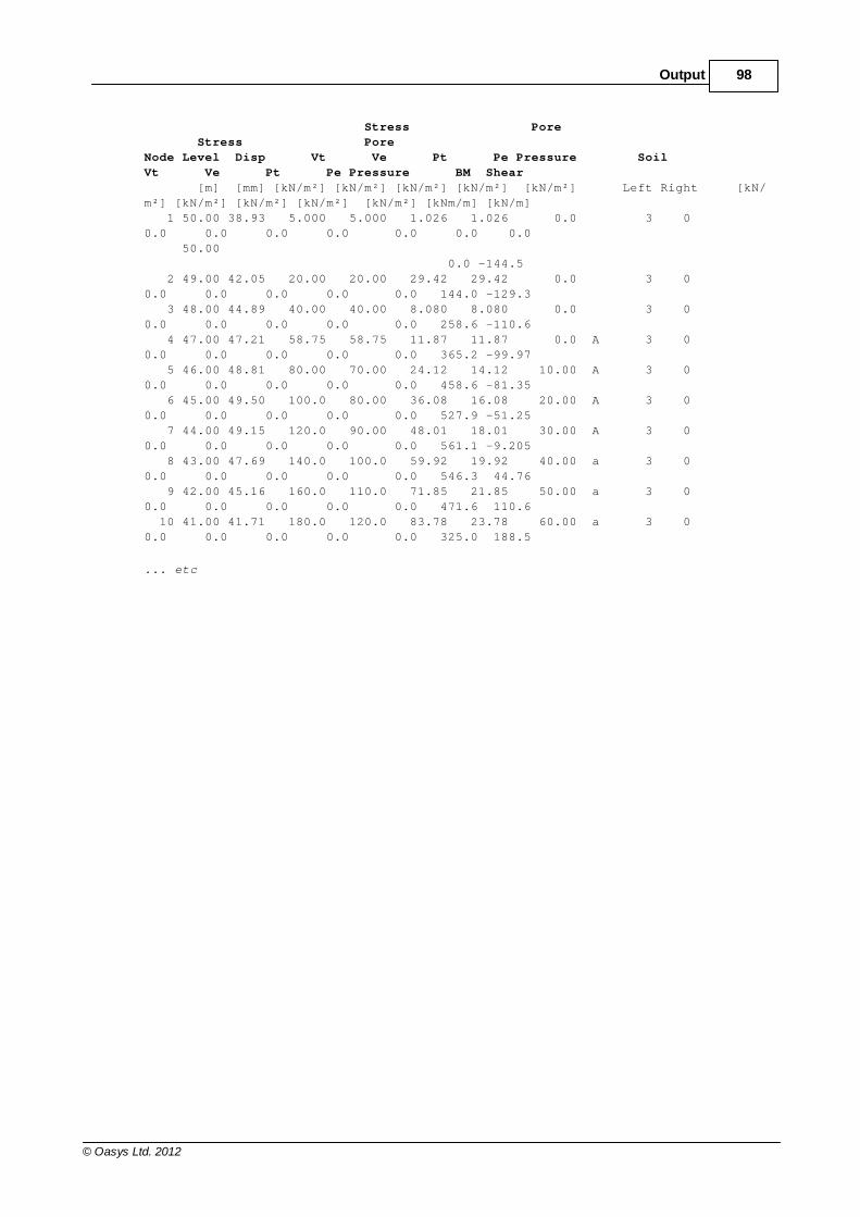
98Output
© Oasys Ltd. 2012
Stress Pore
Stress Pore
Node Level Disp Vt Ve Pt Pe Pressure Soil
Vt Ve Pt Pe Pressure BM Shear
[m] [mm] [kN/m²] [kN/m²] [kN/m²] [kN/m²] [kN/m²] Left Right [kN/
m²] [kN/m²] [kN/m²] [kN/m²] [kN/m²] [kNm/m] [kN/m]
1 50.00 38.93 5.000 5.000 1.026 1.026 0.0 3 0
0.0 0.0 0.0 0.0 0.0 0.0 0.0
50.00
0.0 -144.5
2 49.00 42.05 20.00 20.00 29.42 29.42 0.0 3 0
0.0 0.0 0.0 0.0 0.0 144.0 -129.3
3 48.00 44.89 40.00 40.00 8.080 8.080 0.0 3 0
0.0 0.0 0.0 0.0 0.0 258.6 -110.6
4 47.00 47.21 58.75 58.75 11.87 11.87 0.0 A 3 0
0.0 0.0 0.0 0.0 0.0 365.2 -99.97
5 46.00 48.81 80.00 70.00 24.12 14.12 10.00 A 3 0
0.0 0.0 0.0 0.0 0.0 458.6 -81.35
6 45.00 49.50 100.0 80.00 36.08 16.08 20.00 A 3 0
0.0 0.0 0.0 0.0 0.0 527.9 -51.25
7 44.00 49.15 120.0 90.00 48.01 18.01 30.00 A 3 0
0.0 0.0 0.0 0.0 0.0 561.1 -9.205
8 43.00 47.69 140.0 100.0 59.92 19.92 40.00 a 3 0
0.0 0.0 0.0 0.0 0.0 546.3 44.76
9 42.00 45.16 160.0 110.0 71.85 21.85 50.00 a 3 0
0.0 0.0 0.0 0.0 0.0 471.6 110.6
10 41.00 41.71 180.0 120.0 83.78 23.78 60.00 a 3 0
0.0 0.0 0.0 0.0 0.0 325.0 188.5
... etc
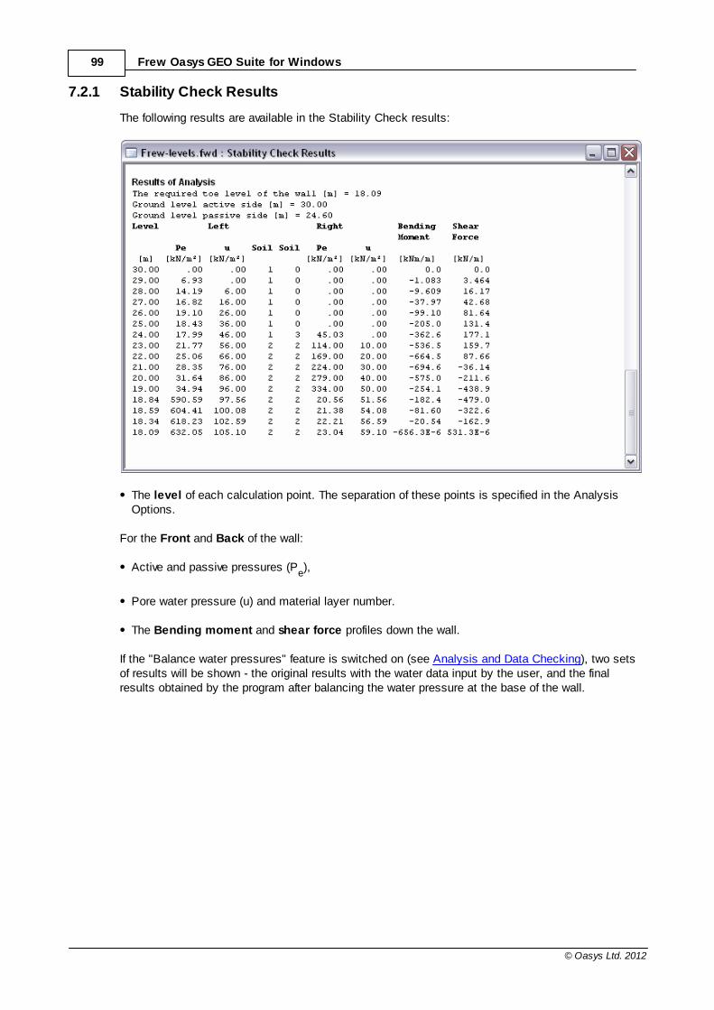
99 Frew Oasys GEO Suite for Windows
© Oasys Ltd. 2012
7.2.1 Stability Check Results
The following results are available in the Stability Check results:
The level of each calculation point. The separation of these points is specified in the AnalysisOptions.
For the Front and Back of the wall:
Active and passive pressures (Pe),
Pore water pressure (u) and material layer number.
The Bending moment and shear force profiles down the wall.
If the "Balance water pressures" feature is switched on (see Analysis and Data Checking), two setsof results will be shown - the original results with the water data input by the user, and the finalresults obtained by the program after balancing the water pressure at the base of the wall.
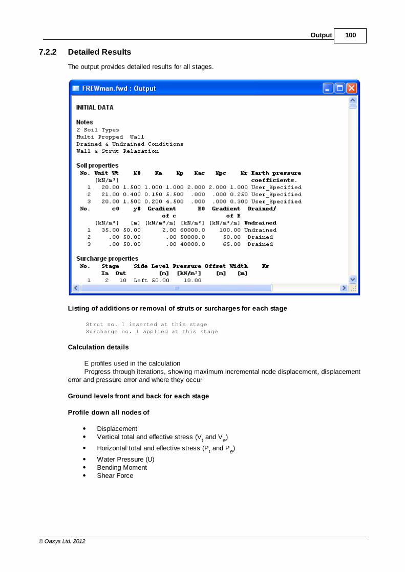
100Output
© Oasys Ltd. 2012
7.2.2 Detailed Results
The output provides detailed results for all stages.
Listing of additions or removal of struts or surcharges for each stage
Strut no. 1 inserted at this stage
Surcharge no. 1 applied at this stage
Calculation details
E profiles used in the calculation Progress through iterations, showing maximum incremental node displacement, displacementerror and pressure error and where they occur
Ground levels front and back for each stage
Profile down all nodes of
DisplacementVertical total and effective stress (V
t and V
e)
Horizontal total and effective stress (Pt and P
e)
Water Pressure (U)Bending Moment Shear Force
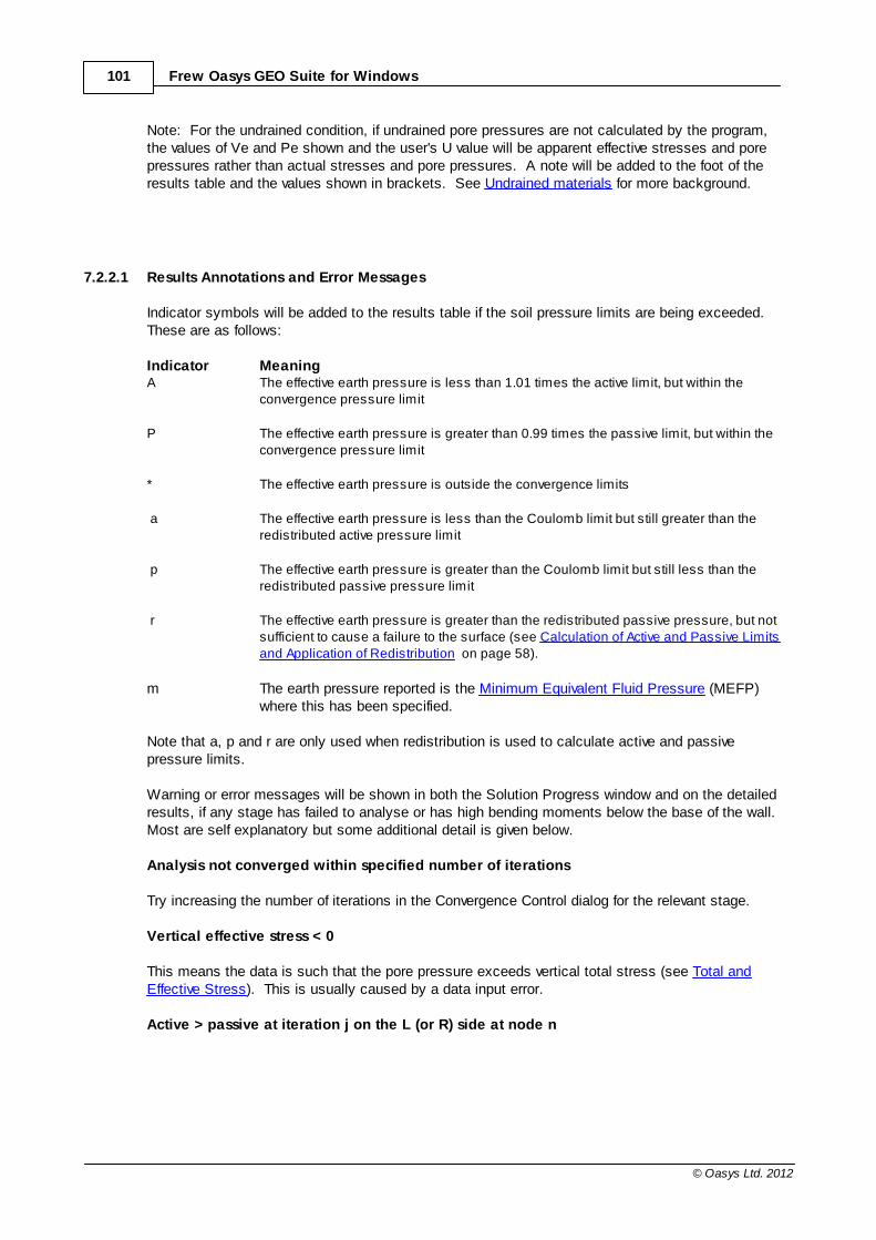
101 Frew Oasys GEO Suite for Windows
© Oasys Ltd. 2012
Note: For the undrained condition, if undrained pore pressures are not calculated by the program,the values of Ve and Pe shown and the user's U value will be apparent effective stresses and porepressures rather than actual stresses and pore pressures. A note will be added to the foot of theresults table and the values shown in brackets. See Undrained materials for more background.
7.2.2.1 Results Annotations and Error Messages
Indicator symbols will be added to the results table if the soil pressure limits are being exceeded. These are as follows:
Indicator MeaningA The effective earth pressure is less than 1.01 times the active limit, but within the
convergence pressure limit
P The effective earth pressure is greater than 0.99 times the passive limit, but within theconvergence pressure limit
* The effective earth pressure is outside the convergence limits
a The effective earth pressure is less than the Coulomb limit but still greater than theredistributed active pressure limit
p The effective earth pressure is greater than the Coulomb limit but still less than theredistributed passive pressure limit
r The effective earth pressure is greater than the redistributed passive pressure, but notsufficient to cause a failure to the surface (see Calculation of Active and Passive Limitsand Application of Redistribution on page 58).
m The earth pressure reported is the Minimum Equivalent Fluid Pressure (MEFP)where this has been specified.
Note that a, p and r are only used when redistribution is used to calculate active and passivepressure limits.
Warning or error messages will be shown in both the Solution Progress window and on the detailedresults, if any stage has failed to analyse or has high bending moments below the base of the wall. Most are self explanatory but some additional detail is given below.
Analysis not converged within specified number of iterations
Try increasing the number of iterations in the Convergence Control dialog for the relevant stage.
Vertical effective stress < 0
This means the data is such that the pore pressure exceeds vertical total stress (see Total andEffective Stress). This is usually caused by a data input error.
Active > passive at iteration j on the L (or R) side at node n
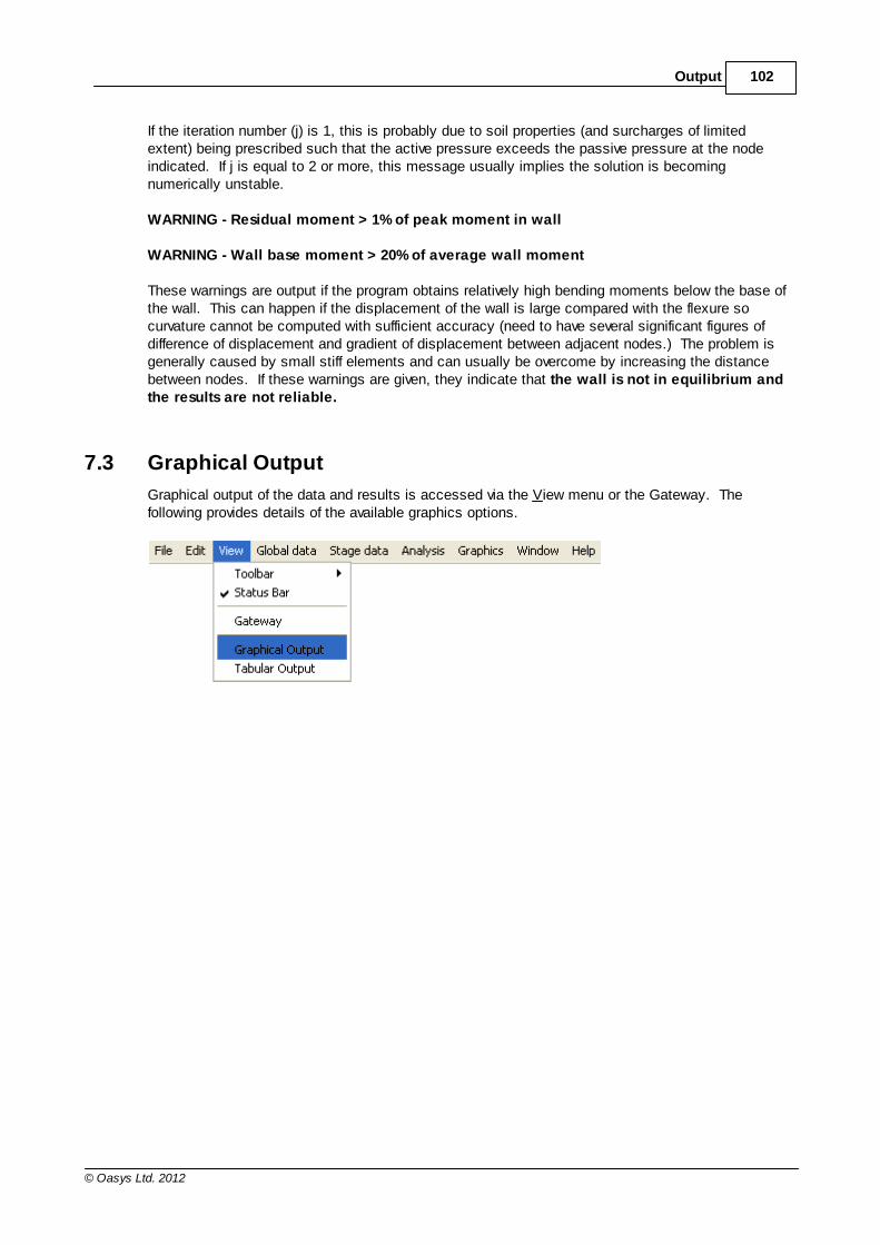
102Output
© Oasys Ltd. 2012
If the iteration number (j) is 1, this is probably due to soil properties (and surcharges of limitedextent) being prescribed such that the active pressure exceeds the passive pressure at the nodeindicated. If j is equal to 2 or more, this message usually implies the solution is becomingnumerically unstable.
WARNING - Residual moment > 1% of peak moment in wall
WARNING - Wall base moment > 20% of average wall moment
These warnings are output if the program obtains relatively high bending moments below the base ofthe wall. This can happen if the displacement of the wall is large compared with the flexure socurvature cannot be computed with sufficient accuracy (need to have several significant figures ofdifference of displacement and gradient of displacement between adjacent nodes.) The problem isgenerally caused by small stiff elements and can usually be overcome by increasing the distancebetween nodes. If these warnings are given, they indicate that the wall is not in equilibrium andthe results are not reliable.
7.3 Graphical Output
Graphical output of the data and results is accessed via the View menu or the Gateway. Thefollowing provides details of the available graphics options.
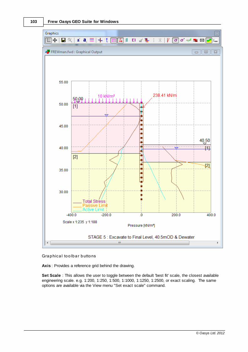
103 Frew Oasys GEO Suite for Windows
© Oasys Ltd. 2012
Gra p hica l to o lb a r b utto ns
Axis : Provides a reference grid behind the drawing.
Set Scale : This allows the user to toggle between the default 'best fit' scale, the closest availableengineering scale. e.g. 1:200, 1:250, 1:500, 1:1000, 1:1250, 1:2500, or exact scaling. The sameoptions are available via the View menu "Set exact scale" command.
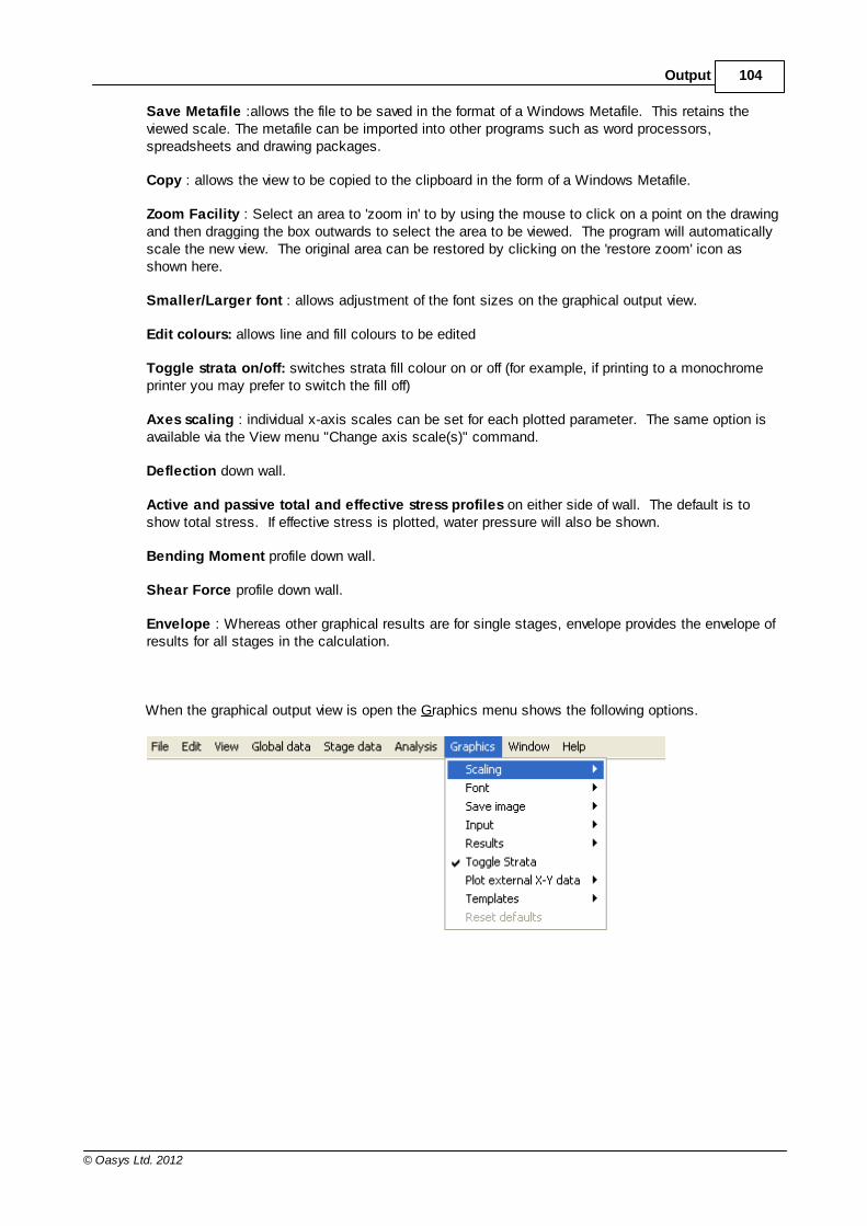
104Output
© Oasys Ltd. 2012
Save Metafile :allows the file to be saved in the format of a Windows Metafile. This retains theviewed scale. The metafile can be imported into other programs such as word processors,spreadsheets and drawing packages.
Copy : allows the view to be copied to the clipboard in the form of a Windows Metafile.
Zoom Facility : Select an area to 'zoom in' to by using the mouse to click on a point on the drawingand then dragging the box outwards to select the area to be viewed. The program will automaticallyscale the new view. The original area can be restored by clicking on the 'restore zoom' icon asshown here.
Smaller/Larger font : allows adjustment of the font sizes on the graphical output view.
Edit colours: allows line and fill colours to be edited
Toggle strata on/off: switches strata fill colour on or off (for example, if printing to a monochromeprinter you may prefer to switch the fill off)
Axes scaling : individual x-axis scales can be set for each plotted parameter. The same option isavailable via the View menu "Change axis scale(s)" command.
Deflection down wall.
Active and passive total and effective stress profiles on either side of wall. The default is toshow total stress. If effective stress is plotted, water pressure will also be shown.
Bending Moment profile down wall.
Shear Force profile down wall.
Envelope : Whereas other graphical results are for single stages, envelope provides the envelope ofresults for all stages in the calculation.
When the graphical output view is open the Graphics menu shows the following options.
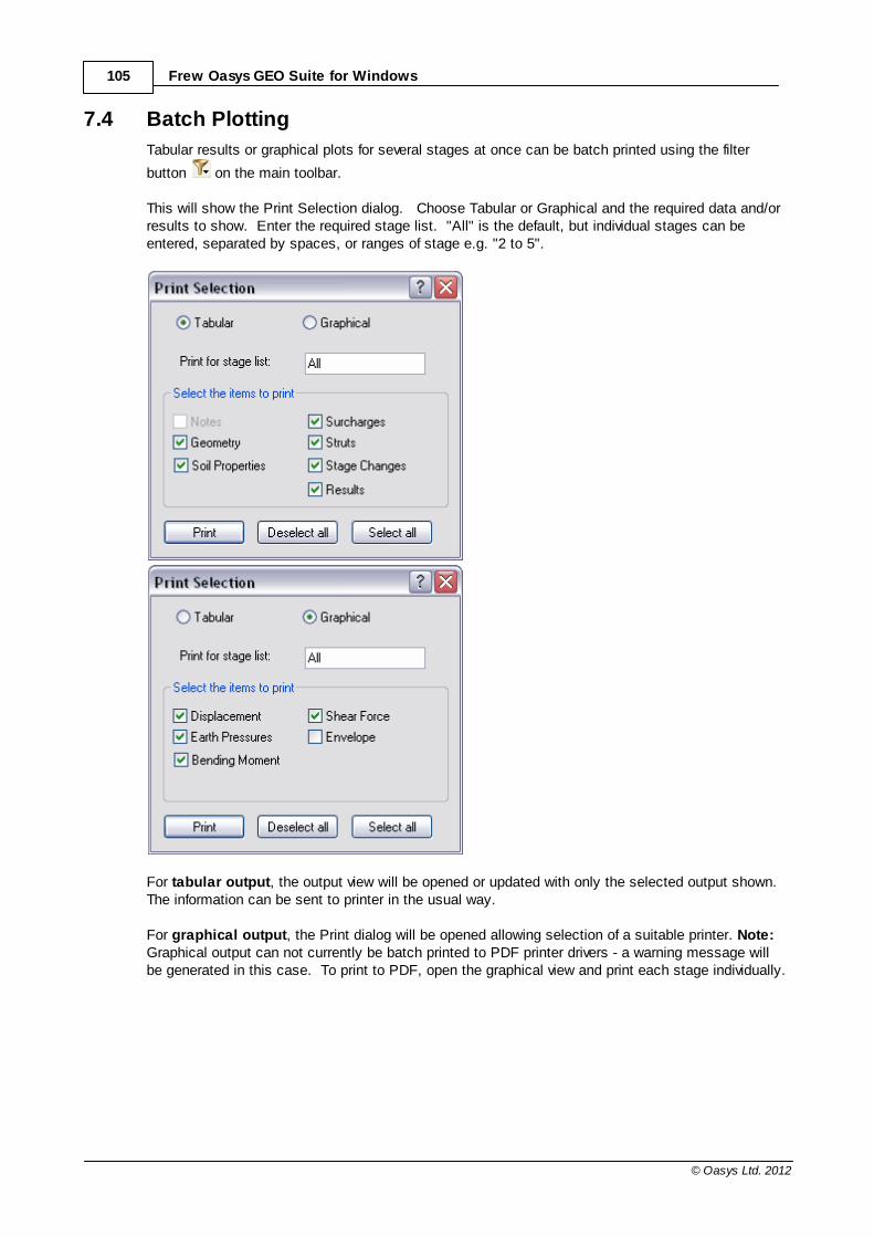
105 Frew Oasys GEO Suite for Windows
© Oasys Ltd. 2012
7.4 Batch Plotting
Tabular results or graphical plots for several stages at once can be batch printed using the filter
button on the main toolbar.
This will show the Print Selection dialog. Choose Tabular or Graphical and the required data and/orresults to show. Enter the required stage list. "All" is the default, but individual stages can beentered, separated by spaces, or ranges of stage e.g. "2 to 5".
For tabular output, the output view will be opened or updated with only the selected output shown.The information can be sent to printer in the usual way.
For graphical output, the Print dialog will be opened allowing selection of a suitable printer. Note:Graphical output can not currently be batch printed to PDF printer drivers - a warning message willbe generated in this case. To print to PDF, open the graphical view and print each stage individually.
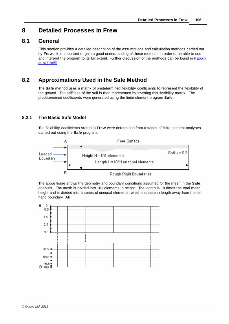
106Detailed Processes in Frew
© Oasys Ltd. 2012
8 Detailed Processes in Frew
8.1 General
This section provides a detailed description of the assumptions and calculation methods carried outby Frew. It is important to gain a good understanding of these methods in order to be able to useand interpret the program to its full extent. Further discussion of the methods can be found in Pappinet al (1985).
8.2 Approximations Used in the Safe Method
The Safe method uses a matrix of predetermined flexibility coefficients to represent the flexibility ofthe ground. The stiffness of the soil is then represented by inverting this flexibility matrix. Thepredetermined coefficients were generated using the finite element program Safe.
8.2.1 The Basic Safe Model
The flexibility coefficients stored in Frew were determined from a series of finite element analysescarried out using the Safe program.
The above figure shows the geometry and boundary conditions assumed for the mesh in the Safeanalysis. The mesh is divided into 101 elements in height. The length is 10 times the total meshheight and is divided into a series of unequal elements, which increase in length away from the lefthand boundary AB.

107 Frew Oasys GEO Suite for Windows
© Oasys Ltd. 2012
The model acts in plane strain and the vertical free face AB represents the location of the retainingwall in Frew.
The boundary AB is divided into 101 elements as shown. A unit force was applied to each elementin turn, distributed as a uniform pressure over the length of the element.
The horizontal displacement at all nodes in the middle of the side of each element was thencalculated, down the vertical free face AB. These displacements represent the flexibility coefficientsand were stored as the flexibility matrix.
Using the principle of superposition, the total horizontal displacement at all nodes due to any loadcombination, can be estimated.
Two cases are considered - one with the nodes on the line AB free to move vertically and the otherwith the nodes fixed vertically. These are referred to as the "Fixed" and "Free" cases respectively.For each case there are two sets of flexibility coefficients stored within Frew. These apply to soilshaving either:
a constant Young's modulus (E)or a Young's modulus which increases linearly with depth from zero at the surface.
For varying profiles of E the user can specify their best estimate of a linear profile to best describethe variation with level. The program will combine and modify the matrices to accommodate this,see Accuracy with respect to Young's modulus (E).
Alternatively, the program will select a linear profile of Young's modulus, based on the specified non-linear profile; the program then applies further corrections as described in Irregular variation of E.
8.2.2 Application of the Model in Frew
Scaling factors are used to map the flexibility matrices from the Safe model onto the user definedmodel in Frew.
To carry out this 'mapping' the boundary AB is divided into "Frew elements".
Each Frew node, below the current ground level position, isassigned a Frew element. Boundaries occur mid-way betweenadjacent Frew nodes.
Note : Since the node spacing in Frew does not have to beuniform the node position is not necessarily at the mid-point ofthe Frew element.
The boundaries of the Frew elements are mapped onto the Safe model. The flexibility for a unitpressure over the Frew element length can then be determined.
This is achieved by summing the contributions, at the Frew node position, from all Safe elements
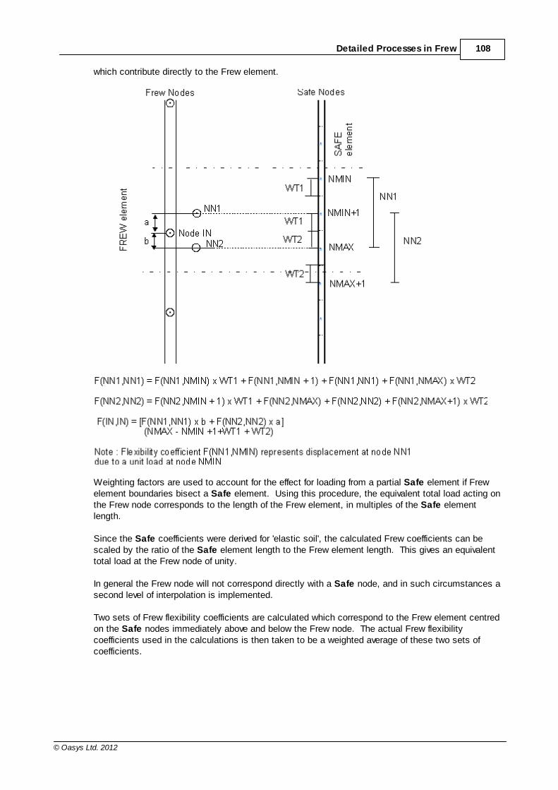
108Detailed Processes in Frew
© Oasys Ltd. 2012
which contribute directly to the Frew element.
Weighting factors are used to account for the effect for loading from a partial Safe element if Frewelement boundaries bisect a Safe element. Using this procedure, the equivalent total load acting onthe Frew node corresponds to the length of the Frew element, in multiples of the Safe elementlength.
Since the Safe coefficients were derived for 'elastic soil', the calculated Frew coefficients can bescaled by the ratio of the Safe element length to the Frew element length. This gives an equivalenttotal load at the Frew node of unity.
In general the Frew node will not correspond directly with a Safe node, and in such circumstances asecond level of interpolation is implemented.
Two sets of Frew flexibility coefficients are calculated which correspond to the Frew element centredon the Safe nodes immediately above and below the Frew node. The actual Frew flexibilitycoefficients used in the calculations is then taken to be a weighted average of these two sets ofcoefficients.
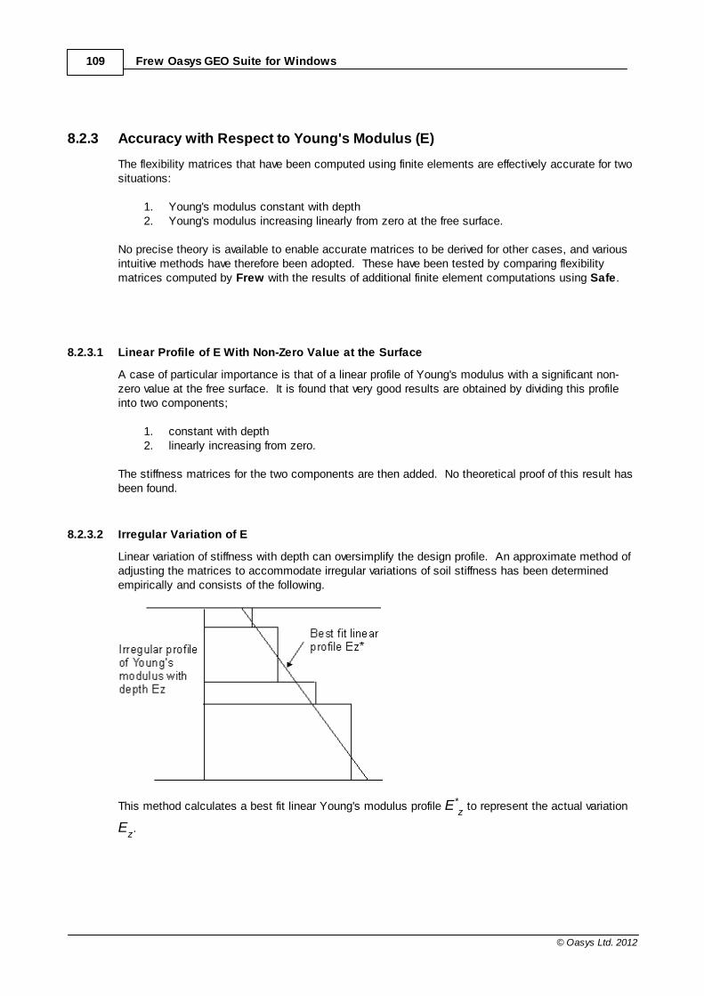
109 Frew Oasys GEO Suite for Windows
© Oasys Ltd. 2012
8.2.3 Accuracy with Respect to Young's Modulus (E)
The flexibility matrices that have been computed using finite elements are effectively accurate for twosituations:
1. Young's modulus constant with depth2. Young's modulus increasing linearly from zero at the free surface.
No precise theory is available to enable accurate matrices to be derived for other cases, and variousintuitive methods have therefore been adopted. These have been tested by comparing flexibilitymatrices computed by Frew with the results of additional finite element computations using Safe.
8.2.3.1 Linear Profile of E With Non-Zero Value at the Surface
A case of particular importance is that of a linear profile of Young's modulus with a significant non-zero value at the free surface. It is found that very good results are obtained by dividing this profileinto two components;
1. constant with depth 2. linearly increasing from zero.
The stiffness matrices for the two components are then added. No theoretical proof of this result hasbeen found.
8.2.3.2 Irregular Variation of E
Linear variation of stiffness with depth can oversimplify the design profile. An approximate method ofadjusting the matrices to accommodate irregular variations of soil stiffness has been determinedempirically and consists of the following.
This method calculates a best fit linear Young's modulus profile E*z to represent the actual variation
Ez.
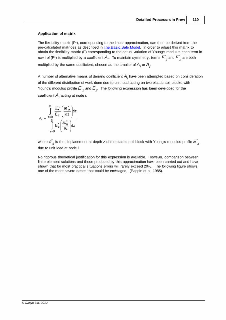
110Detailed Processes in Frew
© Oasys Ltd. 2012
Application of matrix
The flexibility matrix (F*), corresponding to the linear approximation, can then be derived from thepre-calculated matrices as described in The Basic Safe Model. In order to adjust this matrix toobtain the flexibility matrix (F) corresponding to the actual variation of Young's modulus each term in
row i of (F*) is multiplied by a coefficient Ai. To maintain symmetry, terms F*
ij and F*
ji are both
multiplied by the same coefficient, chosen as the smaller of Ai or A
j.
A number of alternative means of deriving coefficient Ai have been attempted based on consideration
of the different distribution of work done due to unit load acting on two elastic soil blocks with
Young's modulus profile E*z and E
z. The following expression has been developed for the
coefficient Ai acting at node i.
where *ij is the displacement at depth z of the elastic soil block with Young's modulus profile E*
z
due to unit load at node i.
No rigorous theoretical justification for this expression is available. However, comparison betweenfinite element solutions and those produced by this approximation have been carried out and haveshown that for most practical situations errors will rarely exceed 20%. The following figure showsone of the more severe cases that could be envisaged, (Pappin et al, 1985).

111 Frew Oasys GEO Suite for Windows
© Oasys Ltd. 2012
Comparison of Safe and Mindlin flexibility approximations with FEA, at three depths
Here the displacement of the elastic soil block, with Young's modulus profile Ez, due to unit load at
three different levels, is shown compared against rigorous finite element solutions.
8.2.4 Effect of the Distance to Vertical Rigid Boundaries
Vertical rigid boundaries may occur in the ground near a retaining wall due to unusual geological orman-made features. More often, the effect of a vertical boundary is required to model a plane ofsymmetry such as the centre line of the excavation.
The flexibility coefficients in the Safe model were derived for one specific geometric casewhich represented a ratio of L/D of 10, where L is the distance to the remote boundary and D thedepth of soil in front of the wall.
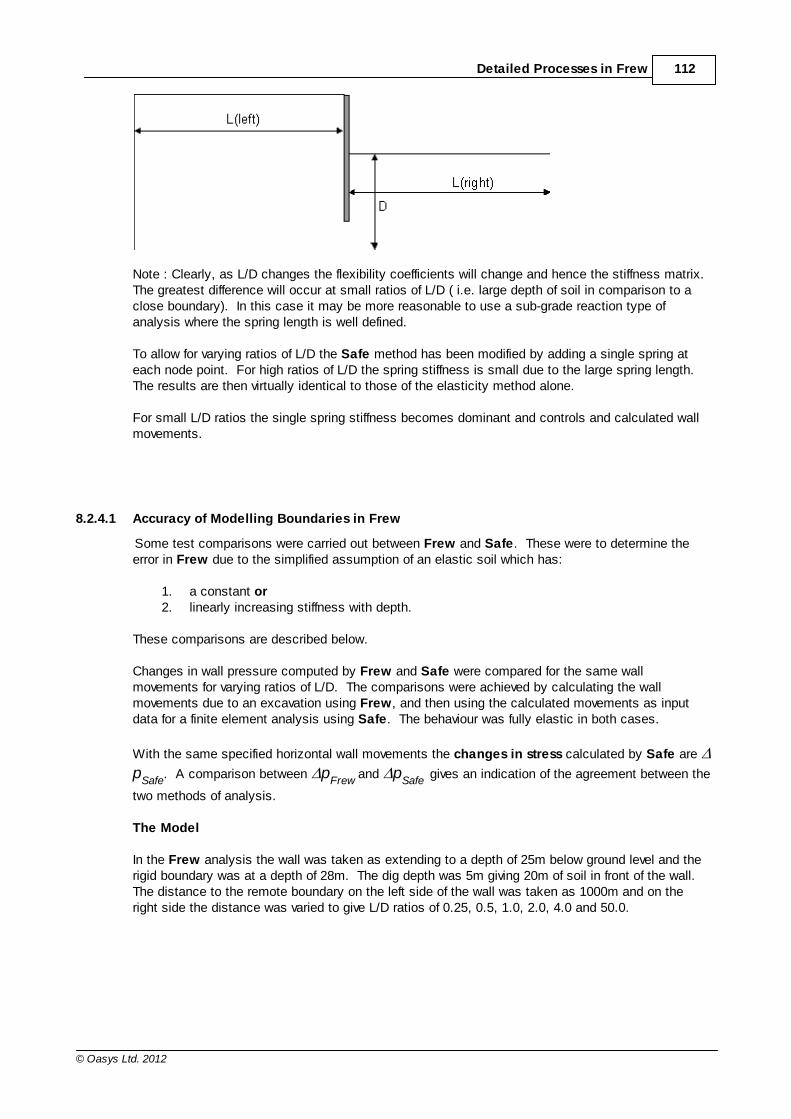
112Detailed Processes in Frew
© Oasys Ltd. 2012
Note : Clearly, as L/D changes the flexibility coefficients will change and hence the stiffness matrix.The greatest difference will occur at small ratios of L/D ( i.e. large depth of soil in comparison to aclose boundary). In this case it may be more reasonable to use a sub-grade reaction type ofanalysis where the spring length is well defined.
To allow for varying ratios of L/D the Safe method has been modified by adding a single spring ateach node point. For high ratios of L/D the spring stiffness is small due to the large spring length. The results are then virtually identical to those of the elasticity method alone.
For small L/D ratios the single spring stiffness becomes dominant and controls and calculated wallmovements.
8.2.4.1 Accuracy of Modelling Boundaries in Frew
Some test comparisons were carried out between Frew and Safe. These were to determine theerror in Frew due to the simplified assumption of an elastic soil which has:
1. a constant or 2. linearly increasing stiffness with depth.
These comparisons are described below.
Changes in wall pressure computed by Frew and Safe were compared for the same wallmovements for varying ratios of L/D. The comparisons were achieved by calculating the wallmovements due to an excavation using Frew, and then using the calculated movements as inputdata for a finite element analysis using Safe. The behaviour was fully elastic in both cases.
With the same specified horizontal wall movements the changes in stress calculated by Safe are
pSafe
. A comparison between pFrew
and pSafe
gives an indication of the agreement between the
two methods of analysis.
The Model
In the Frew analysis the wall was taken as extending to a depth of 25m below ground level and therigid boundary was at a depth of 28m. The dig depth was 5m giving 20m of soil in front of the wall. The distance to the remote boundary on the left side of the wall was taken as 1000m and on theright side the distance was varied to give L/D ratios of 0.25, 0.5, 1.0, 2.0, 4.0 and 50.0.
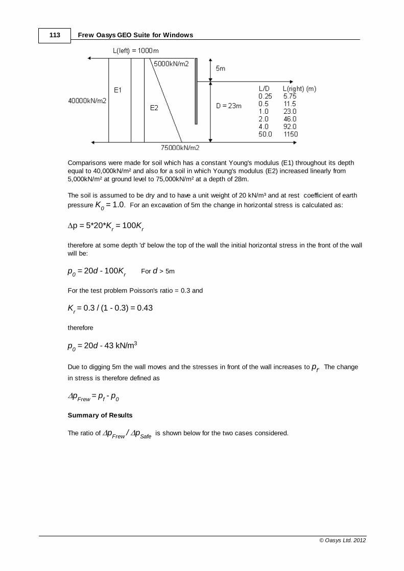
113 Frew Oasys GEO Suite for Windows
© Oasys Ltd. 2012
Comparisons were made for soil which has a constant Young's modulus (E1) throughout its depthequal to 40,000kN/m² and also for a soil in which Young's modulus (E2) increased linearly from5,000kN/m² at ground level to 75,000kN/m² at a depth of 28m.
The soil is assumed to be dry and to have a unit weight of 20 kN/m³ and at rest coefficient of earth
pressure K0 = 1.0. For an excavation of 5m the change in horizontal stress is calculated as:
p = 5*20*Kr = 100K
r
therefore at some depth 'd' below the top of the wall the initial horizontal stress in the front of the wallwill be:
p0 = 20d - 100K
r For d > 5m
For the test problem Poisson's ratio = 0.3 and
Kr = 0.3 / (1 - 0.3) = 0.43
therefore
p0 = 20d - 43 kN/m3
Due to digging 5m the wall moves and the stresses in front of the wall increases to pf. The change
in stress is therefore defined as
pFrew
= pf - p
0
Summary of Results
The ratio of pFrew
/ pSafe
is shown below for the two cases considered.
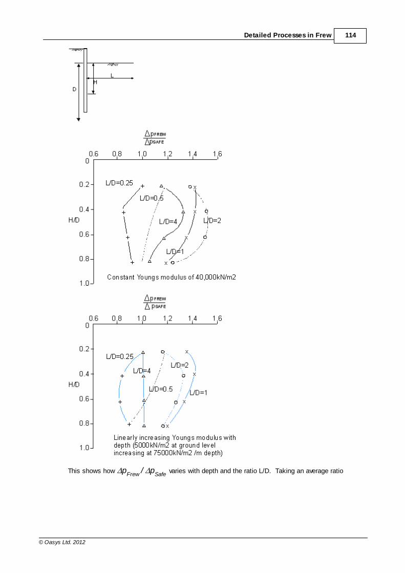
114Detailed Processes in Frew
© Oasys Ltd. 2012
This shows how pFrew
/ pSafe
varies with depth and the ratio L/D. Taking an average ratio
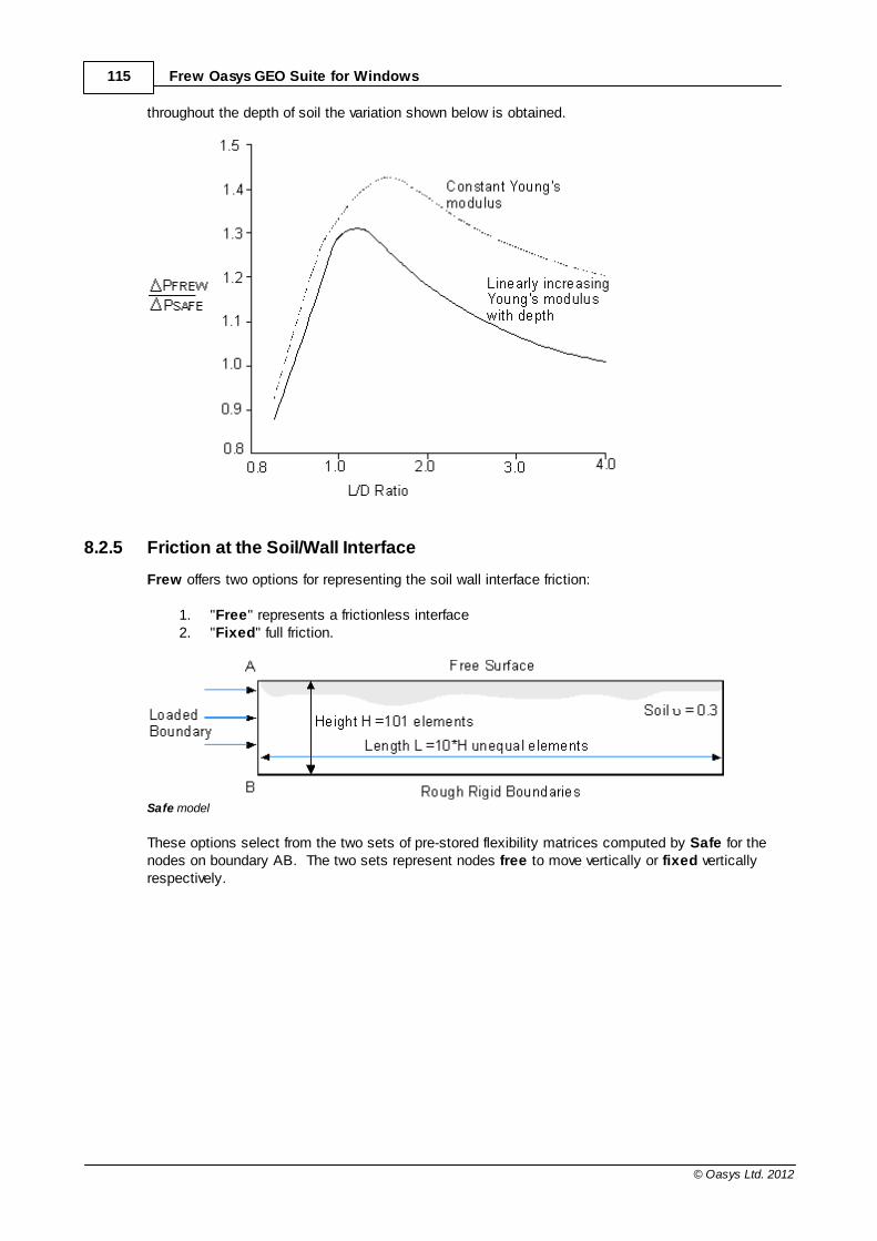
115 Frew Oasys GEO Suite for Windows
© Oasys Ltd. 2012
throughout the depth of soil the variation shown below is obtained.
8.2.5 Friction at the Soil/Wall Interface
Frew offers two options for representing the soil wall interface friction:
1. "Free" represents a frictionless interface 2. "Fixed" full friction.
Safe model
These options select from the two sets of pre-stored flexibility matrices computed by Safe for thenodes on boundary AB. The two sets represent nodes free to move vertically or fixed verticallyrespectively.
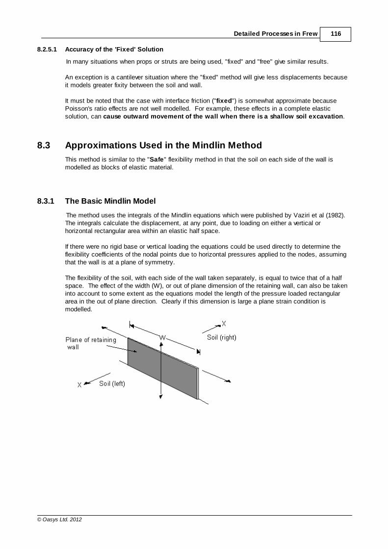
116Detailed Processes in Frew
© Oasys Ltd. 2012
8.2.5.1 Accuracy of the 'Fixed' Solution
In many situations when props or struts are being used, "fixed" and "free" give similar results.
An exception is a cantilever situation where the "fixed" method will give less displacements becauseit models greater fixity between the soil and wall.
It must be noted that the case with interface friction ("fixed") is somewhat approximate becausePoisson's ratio effects are not well modelled. For example, these effects in a complete elasticsolution, can cause outward movement of the wall when there is a shallow soil excavation.
8.3 Approximations Used in the Mindlin Method
This method is similar to the "Safe" flexibility method in that the soil on each side of the wall ismodelled as blocks of elastic material.
8.3.1 The Basic Mindlin Model
The method uses the integrals of the Mindlin equations which were published by Vaziri et al (1982).The integrals calculate the displacement, at any point, due to loading on either a vertical orhorizontal rectangular area within an elastic half space.
If there were no rigid base or vertical loading the equations could be used directly to determine theflexibility coefficients of the nodal points due to horizontal pressures applied to the nodes, assumingthat the wall is at a plane of symmetry.
The flexibility of the soil, with each side of the wall taken separately, is equal to twice that of a halfspace. The effect of the width (W), or out of plane dimension of the retaining wall, can also be takeninto account to some extent as the equations model the length of the pressure loaded rectangulararea in the out of plane direction. Clearly if this dimension is large a plane strain condition ismodelled.
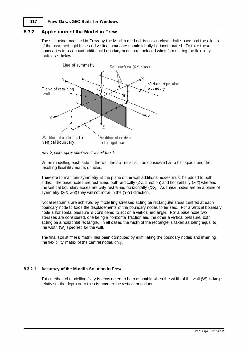
117 Frew Oasys GEO Suite for Windows
© Oasys Ltd. 2012
8.3.2 Application of the Model in Frew
The soil being modelled in Frew by the Mindlin method, is not an elastic half space and the effectsof the assumed rigid base and vertical boundary should ideally be incorporated. To take theseboundaries into account additional boundary nodes are included when formulating the flexibilitymatrix, as below.
Half Space representation of a soil block
When modelling each side of the wall the soil must still be considered as a half space and theresulting flexibility matrix doubled.
Therefore to maintain symmetry at the plane of the wall additional nodes must be added to bothsides. The base nodes are restrained both vertically (Z-Z direction) and horizontally (X-X) whereasthe vertical boundary nodes are only restrained horizontally (X-X). As these nodes are on a plane ofsymmetry (X-X, Z-Z) they will not move in the (Y-Y) direction.
Nodal restraints are achieved by modelling stresses acting on rectangular areas centred at eachboundary node to force the displacements of the boundary nodes to be zero. For a vertical boundarynode a horizontal pressure is considered to act on a vertical rectangle. For a base node twostresses are considered, one being a horizontal traction and the other a vertical pressure, bothacting on a horizontal rectangle. In all cases the width of the rectangle is taken as being equal tothe width (W) specified for the wall.
The final soil stiffness matrix has been computed by eliminating the boundary nodes and invertingthe flexibility matrix of the central nodes only.
8.3.2.1 Accuracy of the Mindlin Solution in Frew
This method of modelling fixity is considered to be reasonable when the width of the wall (W) is largerelative to the depth or to the distance to the vertical boundary.

118Detailed Processes in Frew
© Oasys Ltd. 2012
When W is small three dimensional effects will dominate and to approximate the fixity of a plane bya single line of nodes becomes somewhat dubious. Additional nodes on the fixed planes away fromthe plane of symmetry (X-X, Z-Z), or varying the width (W) of the loaded rectangle at the fixed nodeswould improve this approximation. Nevertheless using the Mindlin flexibility method provides anapproximate means of studying the importance of W.
A drawback of the Mindlin flexibility method is that Young's modulus is assumed to be constantwith depth. This is significantly different from the "Safe" flexibility method which can modelaccurately a linearly increasing modulus with depth. Nevertheless the same ratios that are appliedto model modulus variations can still be used with the Mindlin method, see Irregular variation of E.
An example comparing flexibility coefficients is given below, (Pappin et al, 1985).
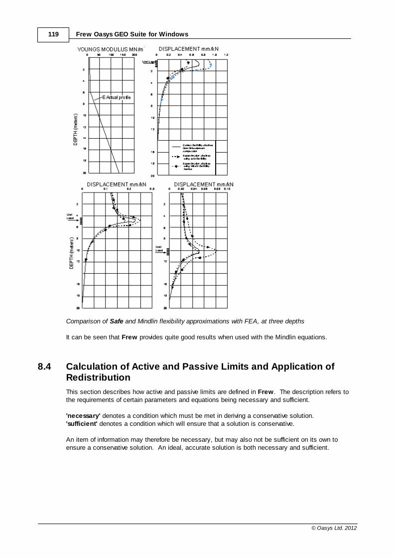
119 Frew Oasys GEO Suite for Windows
© Oasys Ltd. 2012
Comparison of Safe and Mindlin flexibility approximations with FEA, at three depths
It can be seen that Frew provides quite good results when used with the Mindlin equations.
8.4 Calculation of Active and Passive Limits and Application ofRedistribution
This section describes how active and passive limits are defined in Frew. The description refers tothe requirements of certain parameters and equations being necessary and sufficient.
'necessary' denotes a condition which must be met in deriving a conservative solution.'sufficient' denotes a condition which will ensure that a solution is conservative.
An item of information may therefore be necessary, but may also not be sufficient on its own toensure a conservative solution. An ideal, accurate solution is both necessary and sufficient.
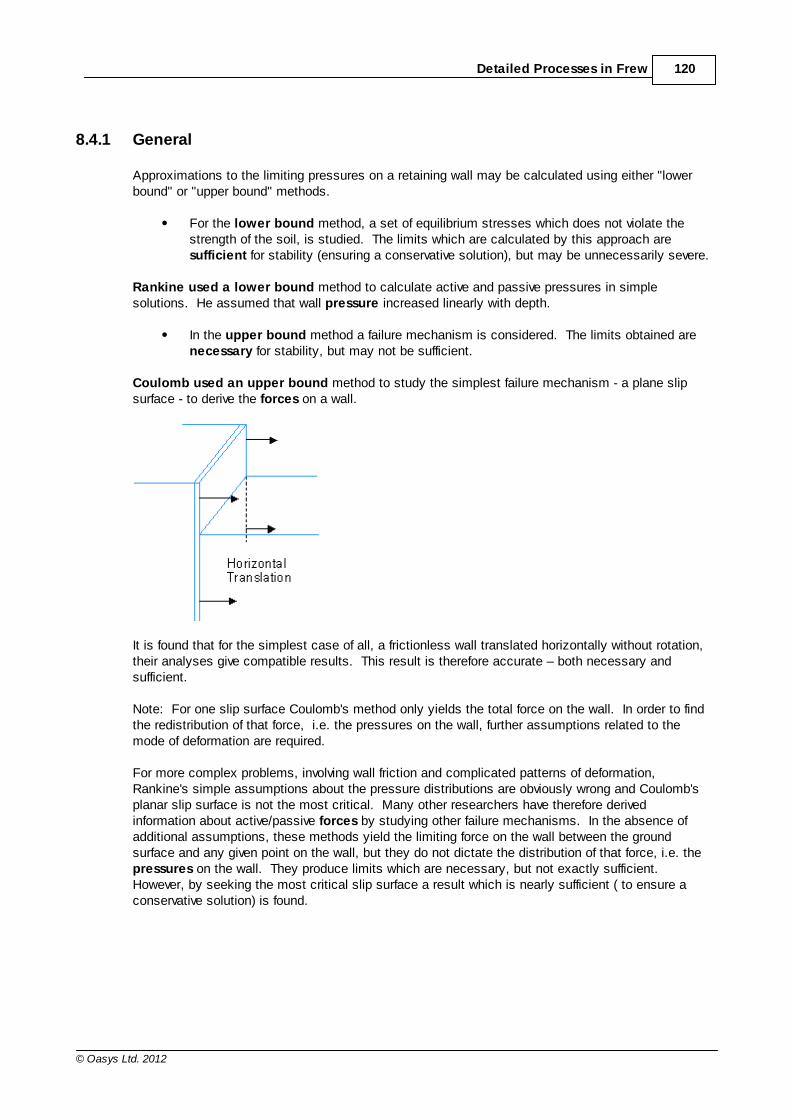
120Detailed Processes in Frew
© Oasys Ltd. 2012
8.4.1 General
Approximations to the limiting pressures on a retaining wall may be calculated using either "lowerbound" or "upper bound" methods.
For the lower bound method, a set of equilibrium stresses which does not violate thestrength of the soil, is studied. The limits which are calculated by this approach are sufficient for stability (ensuring a conservative solution), but may be unnecessarily severe.
Rankine used a lower bound method to calculate active and passive pressures in simplesolutions. He assumed that wall pressure increased linearly with depth.
In the upper bound method a failure mechanism is considered. The limits obtained arenecessary for stability, but may not be sufficient.
Coulomb used an upper bound method to study the simplest failure mechanism - a plane slipsurface - to derive the forces on a wall.
It is found that for the simplest case of all, a frictionless wall translated horizontally without rotation,their analyses give compatible results. This result is therefore accurate – both necessary andsufficient.
Note: For one slip surface Coulomb's method only yields the total force on the wall. In order to findthe redistribution of that force, i.e. the pressures on the wall, further assumptions related to themode of deformation are required.
For more complex problems, involving wall friction and complicated patterns of deformation,Rankine's simple assumptions about the pressure distributions are obviously wrong and Coulomb'splanar slip surface is not the most critical. Many other researchers have therefore derivedinformation about active/passive forces by studying other failure mechanisms. In the absence ofadditional assumptions, these methods yield the limiting force on the wall between the groundsurface and any given point on the wall, but they do not dictate the distribution of that force, i.e. the pressures on the wall. They produce limits which are necessary, but not exactly sufficient.However, by seeking the most critical slip surface a result which is nearly sufficient ( to ensure aconservative solution) is found.
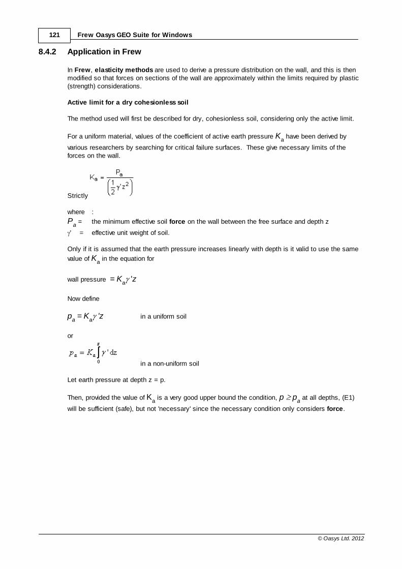
121 Frew Oasys GEO Suite for Windows
© Oasys Ltd. 2012
8.4.2 Application in Frew
In Frew, elasticity methods are used to derive a pressure distribution on the wall, and this is thenmodified so that forces on sections of the wall are approximately within the limits required by plastic(strength) considerations.
Active limit for a dry cohesionless soil
The method used will first be described for dry, cohesionless soil, considering only the active limit.
For a uniform material, values of the coefficient of active earth pressure Ka have been derived by
various researchers by searching for critical failure surfaces. These give necessary limits of theforces on the wall.
Strictly
where :
Pa = the minimum effective soil force on the wall between the free surface and depth z
' = effective unit weight of soil.
Only if it is assumed that the earth pressure increases linearly with depth is it valid to use the same
value of Ka in the equation for
wall pressure = Ka
'z
Now define
pa = K
a 'z in a uniform soil
or
in a non-uniform soil
Let earth pressure at depth z = p.
Then, provided the value of Ka is a very good upper bound the condition, p p
a at all depths, (E1)
will be sufficient (safe), but not 'necessary' since the necessary condition only considers force.
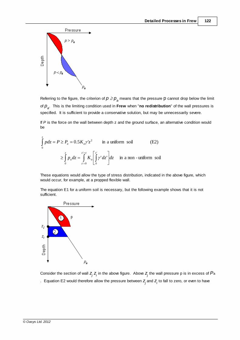
122Detailed Processes in Frew
© Oasys Ltd. 2012
Referring to the figure, the criterion of p pa means that the pressure p cannot drop below the limit
of pa. This is the limiting condition used in Frew when "no redistribution" of the wall pressures is
specified. It is sufficient to provide a conservative solution, but may be unnecessarily severe.
If P is the force on the wall between depth z and the ground surface, an alternative condition wouldbe
z zz
z
z
aa
z
aa
dzdzKdzp
zKPPpdz
0
'
0'
'
0
2
0
soil uniform-non ain ''
(E2) soil uniform ain '5.0
These equations would allow the type of stress distribution, indicated in the above figure, whichwould occur, for example, at a propped flexible wall.
The equation E1 for a uniform soil is necessary, but the following example shows that it is notsufficient.
Consider the section of wall zj z
i in the above figure. Above z
j the wall pressure p is in excess of Pa
. Equation E2 would therefore allow the pressure between zj and z
i to fall to zero, or even to have
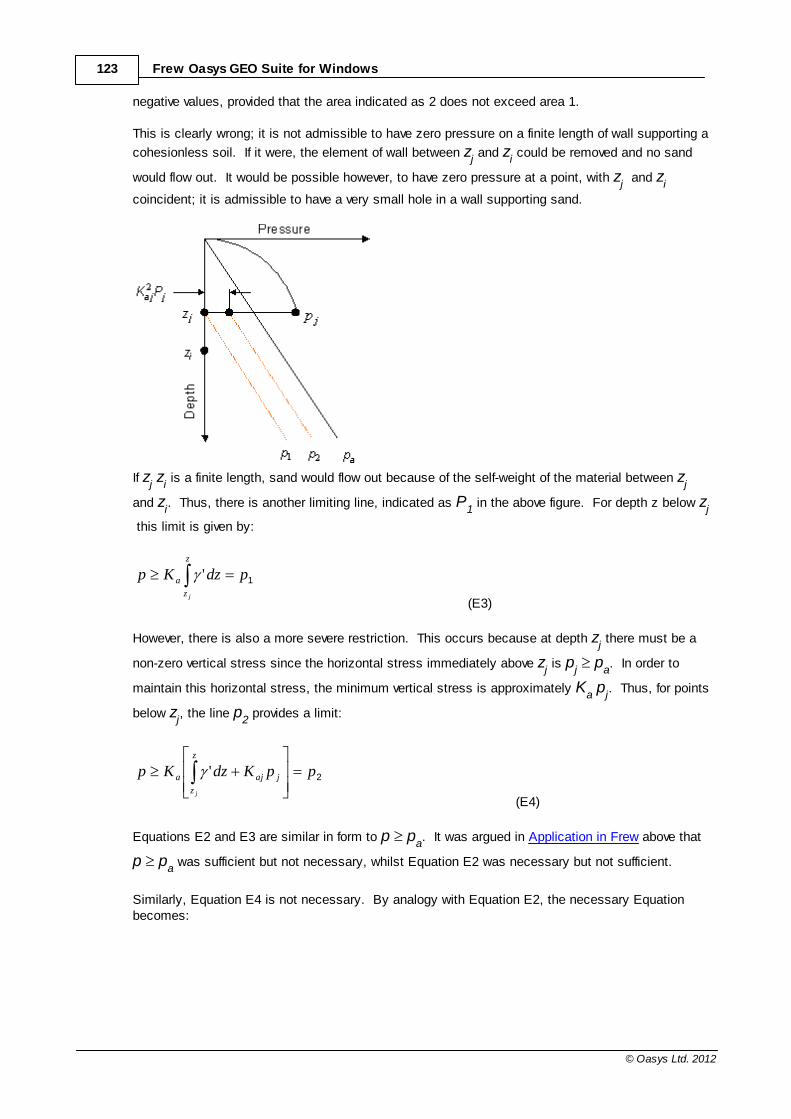
123 Frew Oasys GEO Suite for Windows
© Oasys Ltd. 2012
negative values, provided that the area indicated as 2 does not exceed area 1.
This is clearly wrong; it is not admissible to have zero pressure on a finite length of wall supporting a
cohesionless soil. If it were, the element of wall between zj and z
i could be removed and no sand
would flow out. It would be possible however, to have zero pressure at a point, with zj and z
i
coincident; it is admissible to have a very small hole in a wall supporting sand.
If zj z
i is a finite length, sand would flow out because of the self-weight of the material between z
j
and zi. Thus, there is another limiting line, indicated as P
1 in the above figure. For depth z below z
j
this limit is given by:
z
z
a
j
pdzKp 1'
(E3)
However, there is also a more severe restriction. This occurs because at depth zj there must be a
non-zero vertical stress since the horizontal stress immediately above zj is p
j p
a. In order to
maintain this horizontal stress, the minimum vertical stress is approximately Ka p
j. Thus, for points
below zj, the line p
2 provides a limit:
2ppKdzKpz
z
jaja
j
'
(E4)
Equations E2 and E3 are similar in form to p pa. It was argued in Application in Frew above that
p pa was sufficient but not necessary, whilst Equation E2 was necessary but not sufficient.
Similarly, Equation E4 is not necessary. By analogy with Equation E2, the necessary Equationbecomes:
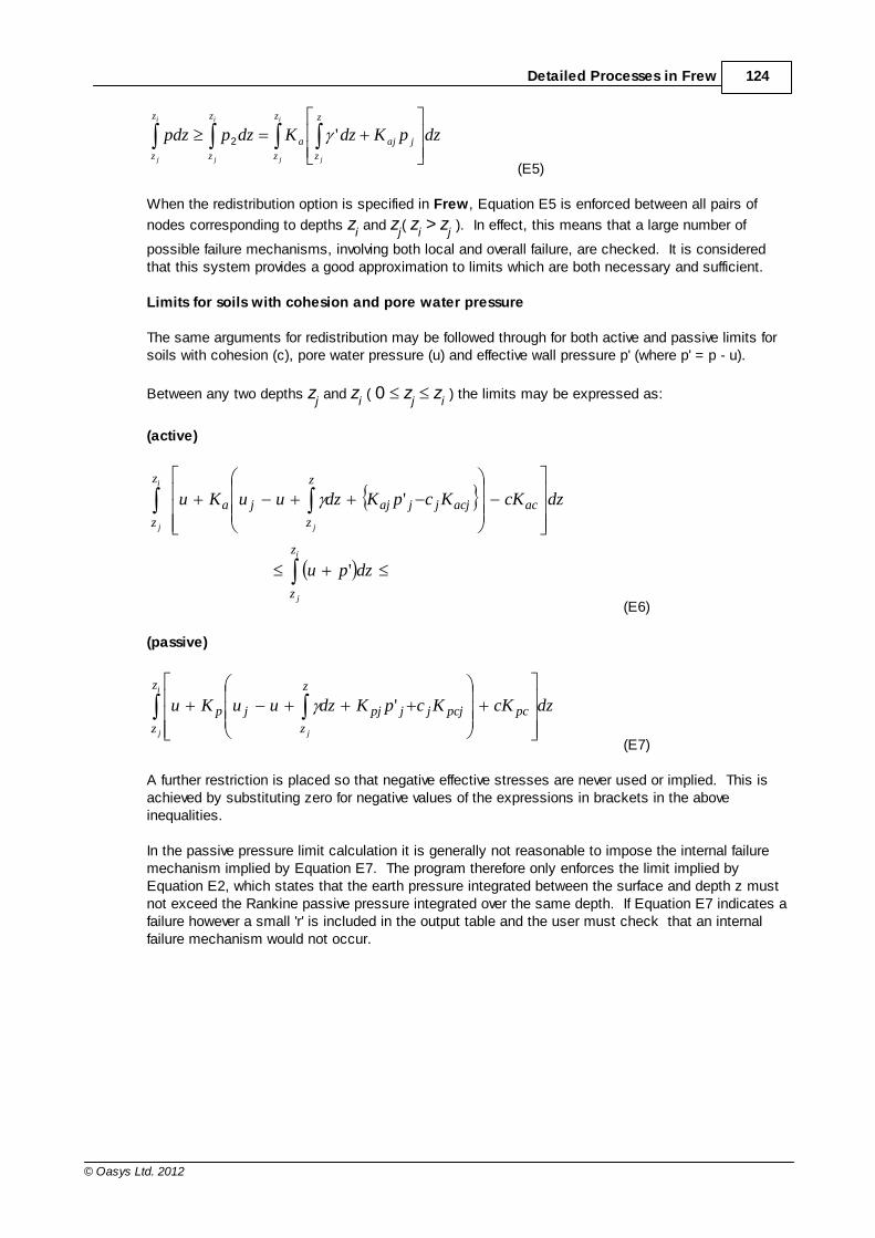
124Detailed Processes in Frew
© Oasys Ltd. 2012
i
j
i
j
i
j j
z
z
z
z
z
z
z
z
jaja dzpKdzKdzppdz '2
(E5)
When the redistribution option is specified in Frew, Equation E5 is enforced between all pairs of
nodes corresponding to depths zi and z
j( z
i > z
j ). In effect, this means that a large number of
possible failure mechanisms, involving both local and overall failure, are checked. It is consideredthat this system provides a good approximation to limits which are both necessary and sufficient.
Limits for soils with cohesion and pore water pressure
The same arguments for redistribution may be followed through for both active and passive limits forsoils with cohesion (c), pore water pressure (u) and effective wall pressure p' (where p' = p - u).
Between any two depths zj and z
i ( 0 z
j z
i ) the limits may be expressed as:
(active)
i
j
j
i
j
z
z
ac
z
z
acjjjajja
z
z
dzpu
dzcKKcpKdzuuKu
'
'
(E6)
(passive)
dzcKKcpKdzuuKui
j j
z
z
pc
z
z
pcjjjpjjp '
(E7)
A further restriction is placed so that negative effective stresses are never used or implied. This isachieved by substituting zero for negative values of the expressions in brackets in the aboveinequalities.
In the passive pressure limit calculation it is generally not reasonable to impose the internal failuremechanism implied by Equation E7. The program therefore only enforces the limit implied byEquation E2, which states that the earth pressure integrated between the surface and depth z mustnot exceed the Rankine passive pressure integrated over the same depth. If Equation E7 indicates afailure however a small 'r' is included in the output table and the user must check that an internalfailure mechanism would not occur.
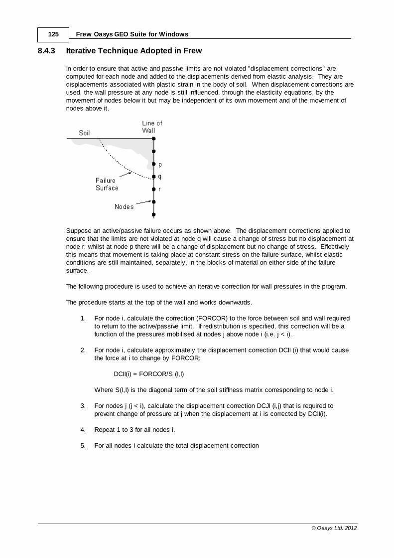
125 Frew Oasys GEO Suite for Windows
© Oasys Ltd. 2012
8.4.3 Iterative Technique Adopted in Frew
In order to ensure that active and passive limits are not violated "displacement corrections" arecomputed for each node and added to the displacements derived from elastic analysis. They aredisplacements associated with plastic strain in the body of soil. When displacement corrections areused, the wall pressure at any node is still influenced, through the elasticity equations, by themovement of nodes below it but may be independent of its own movement and of the movement ofnodes above it.
Suppose an active/passive failure occurs as shown above. The displacement corrections applied toensure that the limits are not violated at node q will cause a change of stress but no displacement atnode r, whilst at node p there will be a change of displacement but no change of stress. Effectivelythis means that movement is taking place at constant stress on the failure surface, whilst elasticconditions are still maintained, separately, in the blocks of material on either side of the failuresurface.
The following procedure is used to achieve an iterative correction for wall pressures in the program.
The procedure starts at the top of the wall and works downwards.
1. For node i, calculate the correction (FORCOR) to the force between soil and wall requiredto return to the active/passive limit. If redistribution is specified, this correction will be afunction of the pressures mobilised at nodes j above node i (i.e. j < i).
2. For node i, calculate approximately the displacement correction DCII (i) that would causethe force at i to change by FORCOR:
DCII(i) = FORCOR/S (I,I)
Where S(I,I) is the diagonal term of the soil stiffness matrix corresponding to node i.
3. For nodes j (j < i), calculate the displacement correction DCJI (i,j) that is required toprevent change of pressure at j when the displacement at i is corrected by DCII(i).
4. Repeat 1 to 3 for all nodes i.
5. For all nodes i calculate the total displacement correction
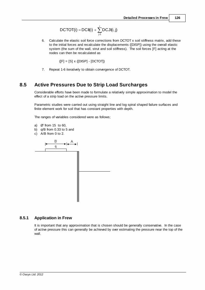
126Detailed Processes in Frew
© Oasys Ltd. 2012
i
1j-
j)DCJI(i, DCII(i) DCTOT(i)
6. Calculate the elastic soil force corrections from DCTOT x soil stiffness matrix, add theseto the initial forces and recalculate the displacements ([DISP]) using the overall elasticsystem (the sum of the wall, strut and soil stiffness). The soil forces [F] acting at thenodes can then be recalculated as
([F] = [S] x ([DISP] - [DCTOT])
7. Repeat 1-6 iteratively to obtain convergence of DCTOT.
8.5 Active Pressures Due to Strip Load Surcharges
Considerable efforts have been made to formulate a relatively simple approximation to model theeffect of a strip load on the active pressure limits.
Parametric studies were carried out using straight line and log spiral shaped failure surfaces andfinite element work for soil that has constant properties with depth.
The ranges of variables considered were as follows;
a) Ø' from 15 to 60, b) q/B from 0.33 to 5 and c) A/B from 0 to 2.
8.5.1 Application in Frew
It is important that any approximation that is chosen should be generally conservative. In the caseof active pressure this can generally be achieved by over estimating the pressure near the top of thewall.
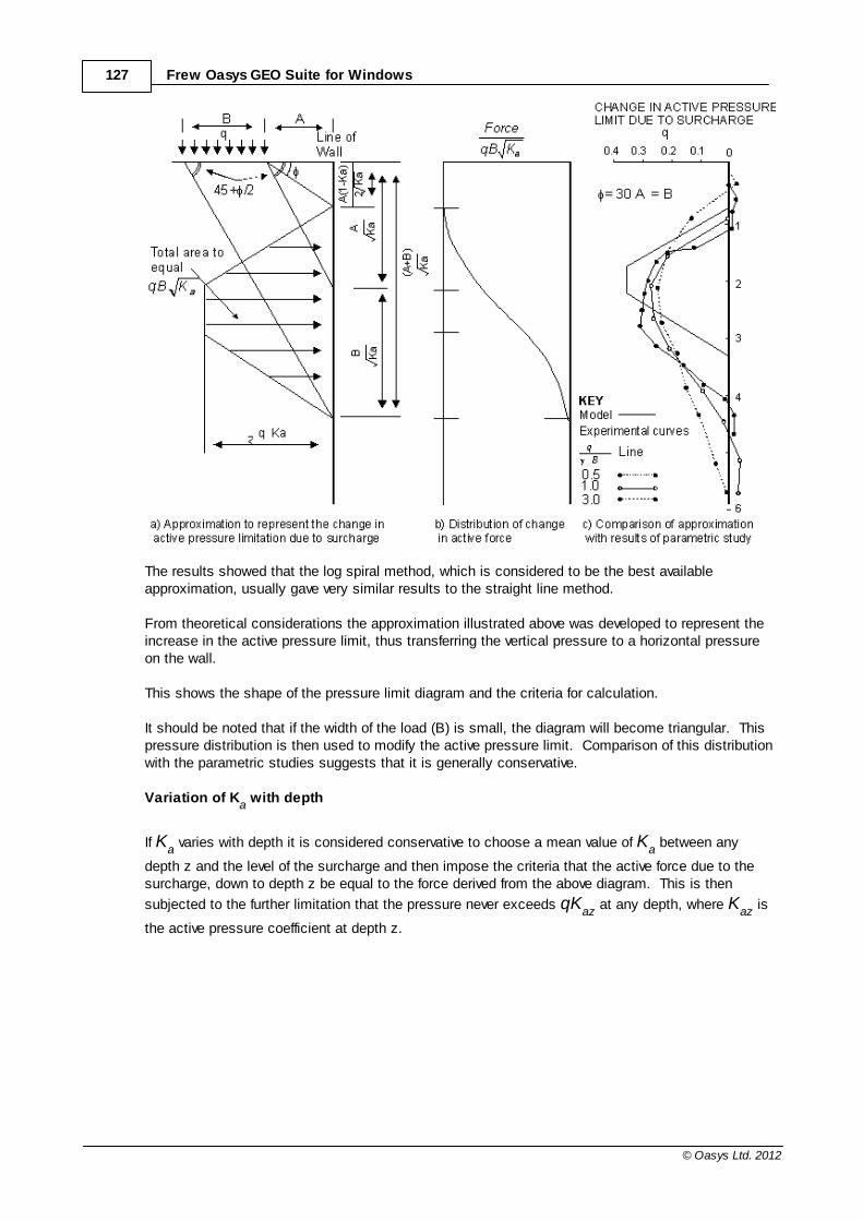
127 Frew Oasys GEO Suite for Windows
© Oasys Ltd. 2012
The results showed that the log spiral method, which is considered to be the best availableapproximation, usually gave very similar results to the straight line method.
From theoretical considerations the approximation illustrated above was developed to represent theincrease in the active pressure limit, thus transferring the vertical pressure to a horizontal pressureon the wall.
This shows the shape of the pressure limit diagram and the criteria for calculation.
It should be noted that if the width of the load (B) is small, the diagram will become triangular. Thispressure distribution is then used to modify the active pressure limit. Comparison of this distributionwith the parametric studies suggests that it is generally conservative.
Variation of Ka with depth
If Ka varies with depth it is considered conservative to choose a mean value of K
a between any
depth z and the level of the surcharge and then impose the criteria that the active force due to thesurcharge, down to depth z be equal to the force derived from the above diagram. This is then
subjected to the further limitation that the pressure never exceeds qKaz
at any depth, where Kaz
is
the active pressure coefficient at depth z.
128Detailed Processes in Frew
© Oasys Ltd. 2012
8.5.2 Passive Pressures Due to Strip Load Surcharges
Frew calculates the increase in passive pressure due to a uniformly distributed load (udl), but cannot make an allowance for strip load surcharges.
The program assumes that the passive pressure at depth z is equal to:
uKcKP pzpp 2'
where 'z is the vertical effective stress at depth z set equal to
zudl is the sum of vertical pressure of all udl surcharges specified above z.
When there is wall friction .
For strip load surcharges the user must adjust Kp (by adding additional soil layers if necessary) to
allow for any increase in the passive pressure. This could be done using a series of trial failuresurfaces to determine the passive pressure at any location.
Alternatively the user should check through and calculate the following requirements detailed here toderive the most suitable increase in the passive pressures.
Requirement 1 – General passive wedge.Requirement 2 – Check of the depth of the influence of the load.Requirement 3 – For a uniform surcharge.Requirement 4 – General application.
Note : The problem becomes more difficult if Kp varies with depth. A simple expedient would be to
use equations specified in Requirement 4, with the appropriate value of Kp at each depth.
This can be unsafe, however, if a soil with high Kp overlies a soil with low K
p. Requirement 1, which
limits the total passive force effect to , could be violated for the less frictional soil.
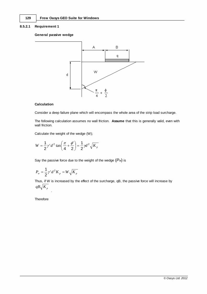
129 Frew Oasys GEO Suite for Windows
© Oasys Ltd. 2012
8.5.2.1 Requirement 1
General passive wedge
Calculation
Consider a deep failure plane which will encompass the whole area of the strip load surcharge.
The following calculation assumes no wall friction. Assume that this is generally valid, even withwall friction.
Calculate the weight of the wedge (W);
pKddW 22
2
1
242
1 'tan'
Say the passive force due to the weight of the wedge (Pw) is
ppw KWKdP 2
2
1'
Thus, if W is increased by the effect of the surcharge, qB, the passive force will increase by
pKqB.
Therefore
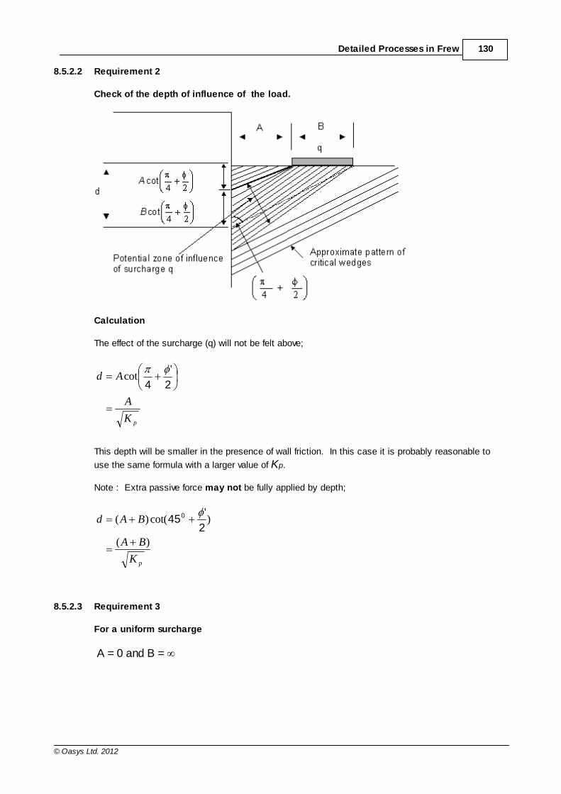
130Detailed Processes in Frew
© Oasys Ltd. 2012
8.5.2.2 Requirement 2
Check of the depth of influence of the load.
Calculation
The effect of the surcharge (q) will not be felt above;
pK
A
Ad24
'cot
This depth will be smaller in the presence of wall friction. In this case it is probably reasonable to
use the same formula with a larger value of Kp.
Note : Extra passive force may not be fully applied by depth;
pK
BA
BAd
)(
)'
cot()(2
450
8.5.2.3 Requirement 3
For a uniform surcharge
A = 0 and B =
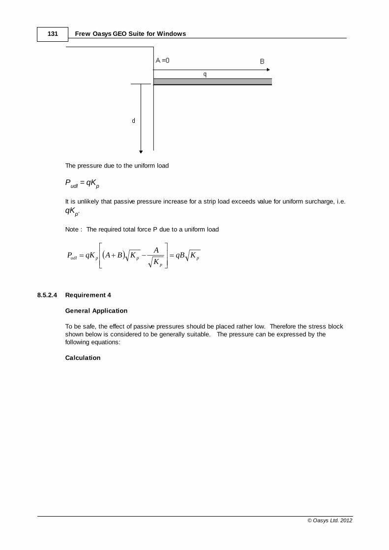
131 Frew Oasys GEO Suite for Windows
© Oasys Ltd. 2012
The pressure due to the uniform load
Pudl
= qKp
It is unlikely that passive pressure increase for a strip load exceeds value for uniform surcharge, i.e.
qKp.
Note : The required total force P due to a uniform load
p
p
ppudl KqBK
AKBAqKP
8.5.2.4 Requirement 4
General Application
To be safe, the effect of passive pressures should be placed rather low. Therefore the stress blockshown below is considered to be generally suitable. The pressure can be expressed by thefollowing equations:
Calculation
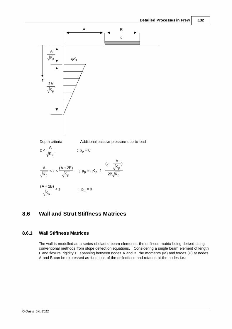
132Detailed Processes in Frew
© Oasys Ltd. 2012
0= p ; z<K
)B2+A(
KB2
)K
Az(
1qK=p ; K
)B2+A(<z<
K
A
0=p ; K
A<z
load to due pressure passive tional Addi criteria Depth
pp
p
p
pppp
pp
8.6 Wall and Strut Stiffness Matrices
8.6.1 Wall Stiffness Matrices
The wall is modelled as a series of elastic beam elements, the stiffness matrix being derived usingconventional methods from slope deflection equations. Considering a single beam element of lengthL and flexural rigidity EI spanning between nodes A and B, the moments (M) and forces (P) at nodesA and B can be expressed as functions of the deflections and rotation at the nodes i.e.:

133 Frew Oasys GEO Suite for Windows
© Oasys Ltd. 2012
Where A , B and A , B, represent the deflections and rotations at nodes A and B respectively
referred to the neutral axis of the beam. The above equations can be re-written in matrix form as:
[M] = [A] [ ] + [B] [ ] (G1)
and
[P] = [C] [ ] + [A]T [ ] (G2)
where [A], [B] and [C] are functions of the element lengths and flexural rigidity (EI), and [ ] and [
] are the nodal horizontal displacements and rotations.
If there are no moments applied to the wall [ ] can be eliminated to give
[P] = [S] [ ] (G3)
in which [S] is the wall stiffness matrix given by
[S] = [C] - [A]T + [B]-1 [A] (G4)
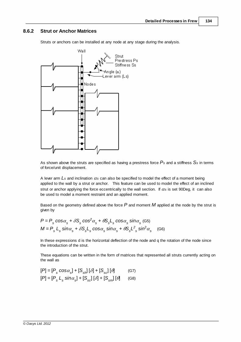
134Detailed Processes in Frew
© Oasys Ltd. 2012
8.6.2 Strut or Anchor Matrices
Struts or anchors can be installed at any node at any stage during the analysis.
As shown above the struts are specified as having a prestress force Ps and a stiffness Ss in termsof force/unit displacement.
A lever arm Ls and inclination s can also be specified to model the effect of a moment being
applied to the wall by a strut or anchor. This feature can be used to model the effect of an inclined
strut or anchor applying the force eccentrically to the wall section. If s is set 90Deg, it can also
be used to model a moment restraint and an applied moment.
Based on the geometry defined above the force P and moment M applied at the node by the strut isgiven by
P = Ps cos
s + S
s cos2
s + S
sL
s cos
s sin
s (G5)
M = Ps L
s sin
s + S
sL
s cos
s sin
s + S
sL2
s sin2
s(G6)
In these expressions d is the horizontal deflection of the node and q the rotation of the node sincethe introduction of the strut.
These equations can be written in the form of matrices that represented all struts currently acting onthe wall as
[P] = [Ps cos
s] + [S
sh] [ ] + [S
sc] [ ] (G7)
[P] = [Ps L
s sin
s] + [S
sc] [ ] + [S
sm] [ ] (G8)
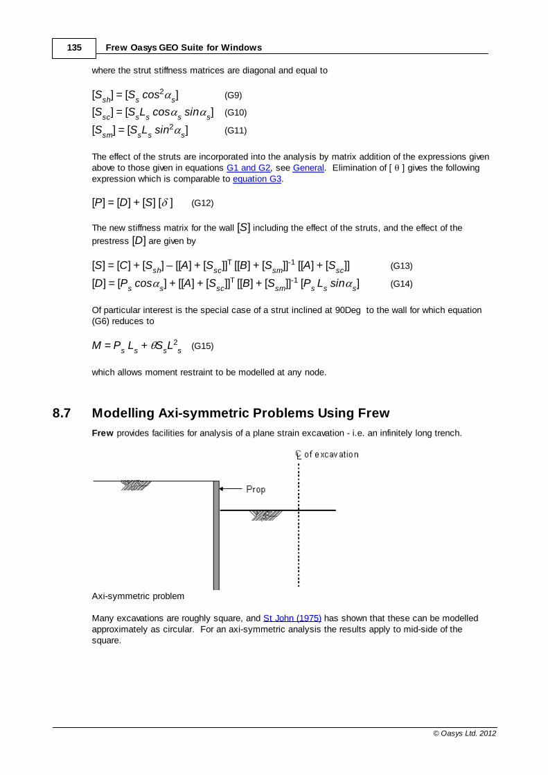
135 Frew Oasys GEO Suite for Windows
© Oasys Ltd. 2012
where the strut stiffness matrices are diagonal and equal to
[Ssh
] = [Ss cos2
s] (G9)
[Ssc
] = [SsL
s cos
s sin
s] (G10)
[Ssm
] = [SsL
s sin2
s] (G11)
The effect of the struts are incorporated into the analysis by matrix addition of the expressions givenabove to those given in equations G1 and G2, see General. Elimination of [ ] gives the followingexpression which is comparable to equation G3.
[P] = [D] + [S] [ ] (G12)
The new stiffness matrix for the wall [S] including the effect of the struts, and the effect of the
prestress [D] are given by
[S] = [C] + [Ssh
] – [[A] + [Ssc
]]T [[B] + [Ssm
]]-1 [[A] + [Ssc
]] (G13)
[D] = [Ps cos
s] + [[A] + [S
sc]]T [[B] + [S
sm]]-1 [P
s L
s sin
s] (G14)
Of particular interest is the special case of a strut inclined at 90Deg to the wall for which equation(G6) reduces to
M = Ps L
s + S
sL2
s (G15)
which allows moment restraint to be modelled at any node.
8.7 Modelling Axi-symmetric Problems Using Frew
Frew provides facilities for analysis of a plane strain excavation - i.e. an infinitely long trench.
Axi-symmetric problem
Many excavations are roughly square, and St John (1975) has shown that these can be modelledapproximately as circular. For an axi-symmetric analysis the results apply to mid-side of thesquare.
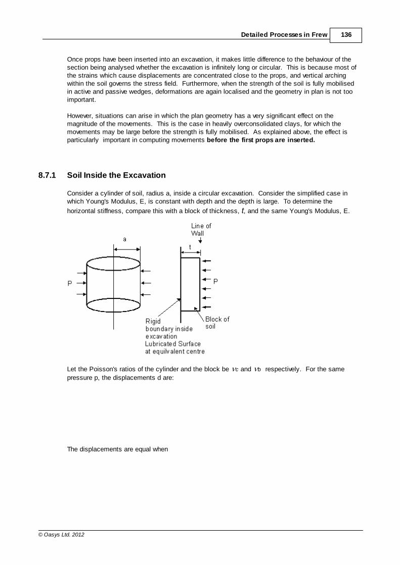
136Detailed Processes in Frew
© Oasys Ltd. 2012
Once props have been inserted into an excavation, it makes little difference to the behaviour of thesection being analysed whether the excavation is infinitely long or circular. This is because most ofthe strains which cause displacements are concentrated close to the props, and vertical archingwithin the soil governs the stress field. Furthermore, when the strength of the soil is fully mobilisedin active and passive wedges, deformations are again localised and the geometry in plan is not tooimportant.
However, situations can arise in which the plan geometry has a very significant effect on themagnitude of the movements. This is the case in heavily overconsolidated clays, for which themovements may be large before the strength is fully mobilised. As explained above, the effect isparticularly important in computing movements before the first props are inserted.
8.7.1 Soil Inside the Excavation
Consider a cylinder of soil, radius a, inside a circular excavation. Consider the simplified case inwhich Young's Modulus, E, is constant with depth and the depth is large. To determine the
horizontal stiffness, compare this with a block of thickness, t, and the same Young's Modulus, E.
Let the Poisson's ratios of the cylinder and the block be c and b respectively. For the same
pressure p, the displacements d are:
The displacements are equal when
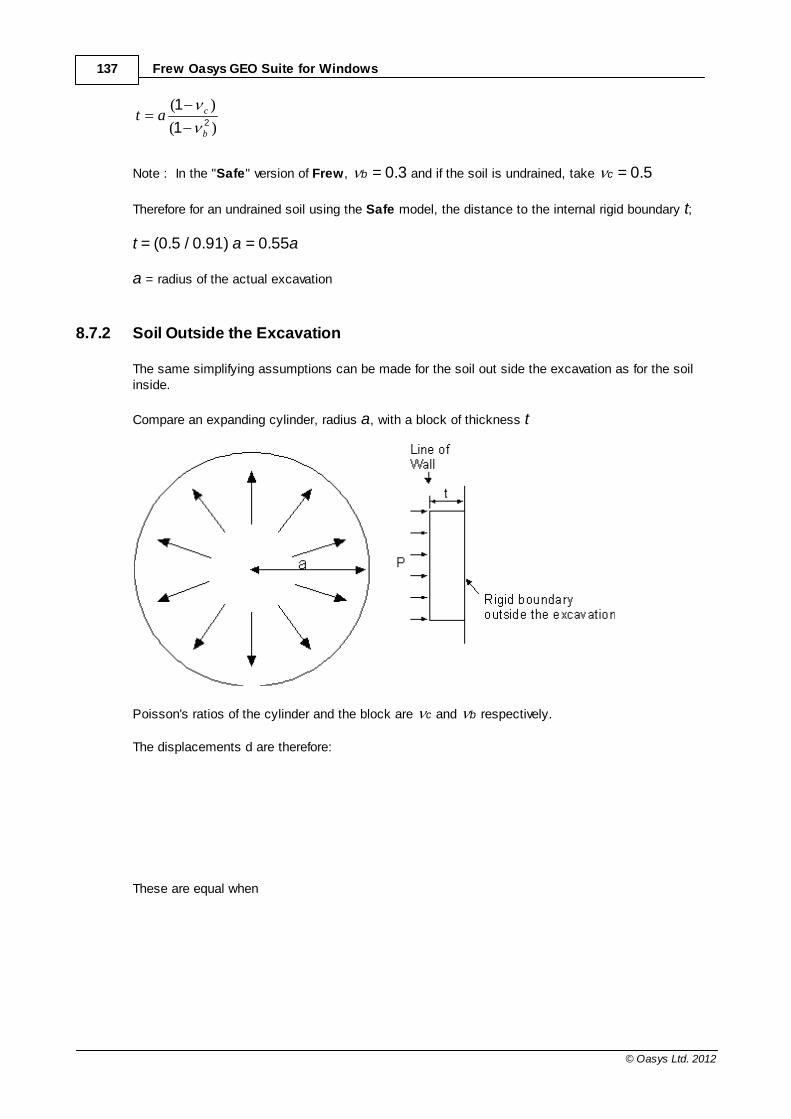
137 Frew Oasys GEO Suite for Windows
© Oasys Ltd. 2012
)(
)(21
1
b
cat
Note : In the "Safe" version of Frew, b = 0.3 and if the soil is undrained, take c = 0.5
Therefore for an undrained soil using the Safe model, the distance to the internal rigid boundary t;
t = (0.5 / 0.91) a = 0.55a
a = radius of the actual excavation
8.7.2 Soil Outside the Excavation
The same simplifying assumptions can be made for the soil out side the excavation as for the soilinside.
Compare an expanding cylinder, radius a, with a block of thickness t
Poisson's ratios of the cylinder and the block are c and b respectively.
The displacements d are therefore:
These are equal when
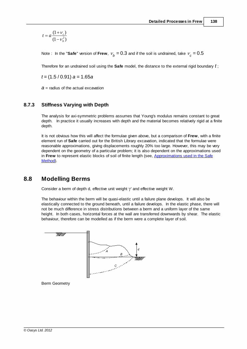
138Detailed Processes in Frew
© Oasys Ltd. 2012
)1(
)1(2b
cat
Note : In the "Safe" version of Frew, b = 0.3 and if the soil is undrained, take
c = 0.5
Therefore for an undrained soil using the Safe model, the distance to the external rigid boundary t ;
t = (1.5 / 0.91) a = 1.65a
a = radius of the actual excavation
8.7.3 Stiffness Varying with Depth
The analysis for axi-symmetric problems assumes that Young's modulus remains constant to greatdepth. In practice it usually increases with depth and the material becomes relatively rigid at a finitedepth.
It is not obvious how this will affect the formulae given above, but a comparison of Frew, with a finiteelement run of Safe carried out for the British Library excavation, indicated that the formulae werereasonable approximations, giving displacements roughly 20% too large. However, this may be verydependent on the geometry of a particular problem; it is also dependent on the approximations usedin Frew to represent elastic blocks of soil of finite length (see, Approximations used in the SafeMethod).
8.8 Modelling Berms
Consider a berm of depth d, effective unit weight ' and effective weight W.
The behaviour within the berm will be quasi-elastic until a failure plane develops. It will also beelastically connected to the ground beneath, until a failure develops. In the elastic phase, there willnot be much difference in stress distributions between a berm and a uniform layer of the sameheight. In both cases, horizontal forces at the wall are transferred downwards by shear. The elasticbehaviour, therefore can be modelled as if the berm were a complete layer of soil.
Berm Geometry
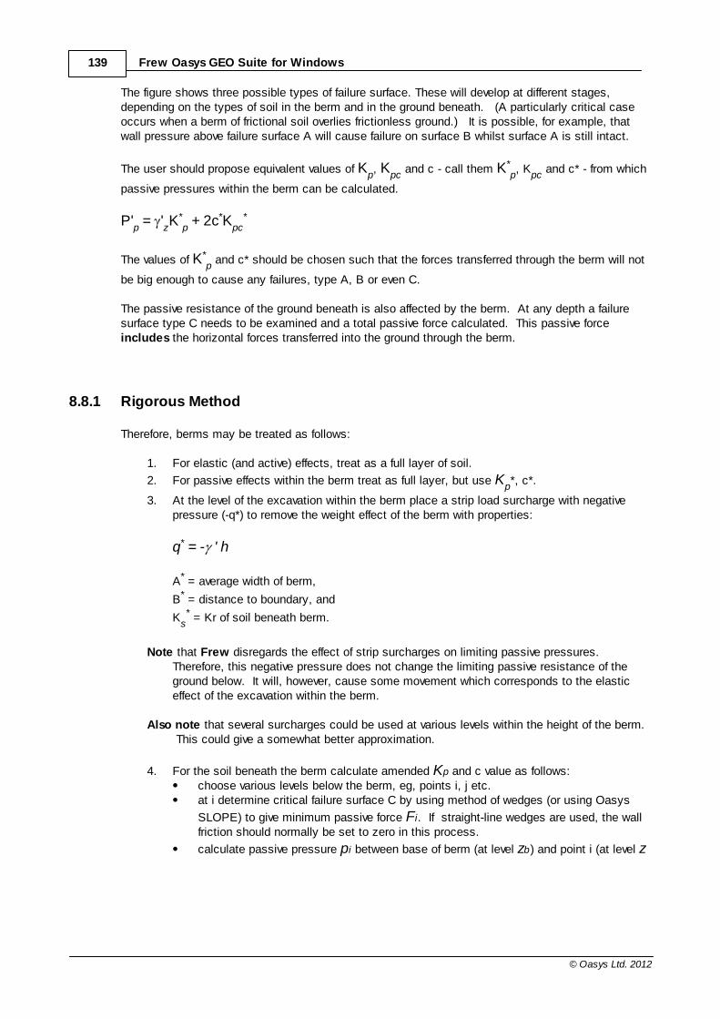
139 Frew Oasys GEO Suite for Windows
© Oasys Ltd. 2012
The figure shows three possible types of failure surface. These will develop at different stages,depending on the types of soil in the berm and in the ground beneath. (A particularly critical caseoccurs when a berm of frictional soil overlies frictionless ground.) It is possible, for example, thatwall pressure above failure surface A will cause failure on surface B whilst surface A is still intact.
The user should propose equivalent values of Kp, K
pc and c - call them K*
p, K
pc and c* - from which
passive pressures within the berm can be calculated.
P'p = '
zK*
p + 2c*K
pc*
The values of K*p and c* should be chosen such that the forces transferred through the berm will not
be big enough to cause any failures, type A, B or even C.
The passive resistance of the ground beneath is also affected by the berm. At any depth a failuresurface type C needs to be examined and a total passive force calculated. This passive force includes the horizontal forces transferred into the ground through the berm.
8.8.1 Rigorous Method
Therefore, berms may be treated as follows:
1. For elastic (and active) effects, treat as a full layer of soil.
2. For passive effects within the berm treat as full layer, but use Kp*, c*.
3. At the level of the excavation within the berm place a strip load surcharge with negativepressure (-q*) to remove the weight effect of the berm with properties:
q* = - ' h
A* = average width of berm,
B* = distance to boundary, and
Ks* = Kr of soil beneath berm.
Note that Frew disregards the effect of strip surcharges on limiting passive pressures.Therefore, this negative pressure does not change the limiting passive resistance of theground below. It will, however, cause some movement which corresponds to the elasticeffect of the excavation within the berm.
Also note that several surcharges could be used at various levels within the height of the berm. This could give a somewhat better approximation.
4. For the soil beneath the berm calculate amended Kp and c value as follows:choose various levels below the berm, eg, points i, j etc.at i determine critical failure surface C by using method of wedges (or using Oasys
SLOPE) to give minimum passive force Fi. If straight-line wedges are used, the wallfriction should normally be set to zero in this process.
calculate passive pressure pi between base of berm (at level zb) and point i (at level z
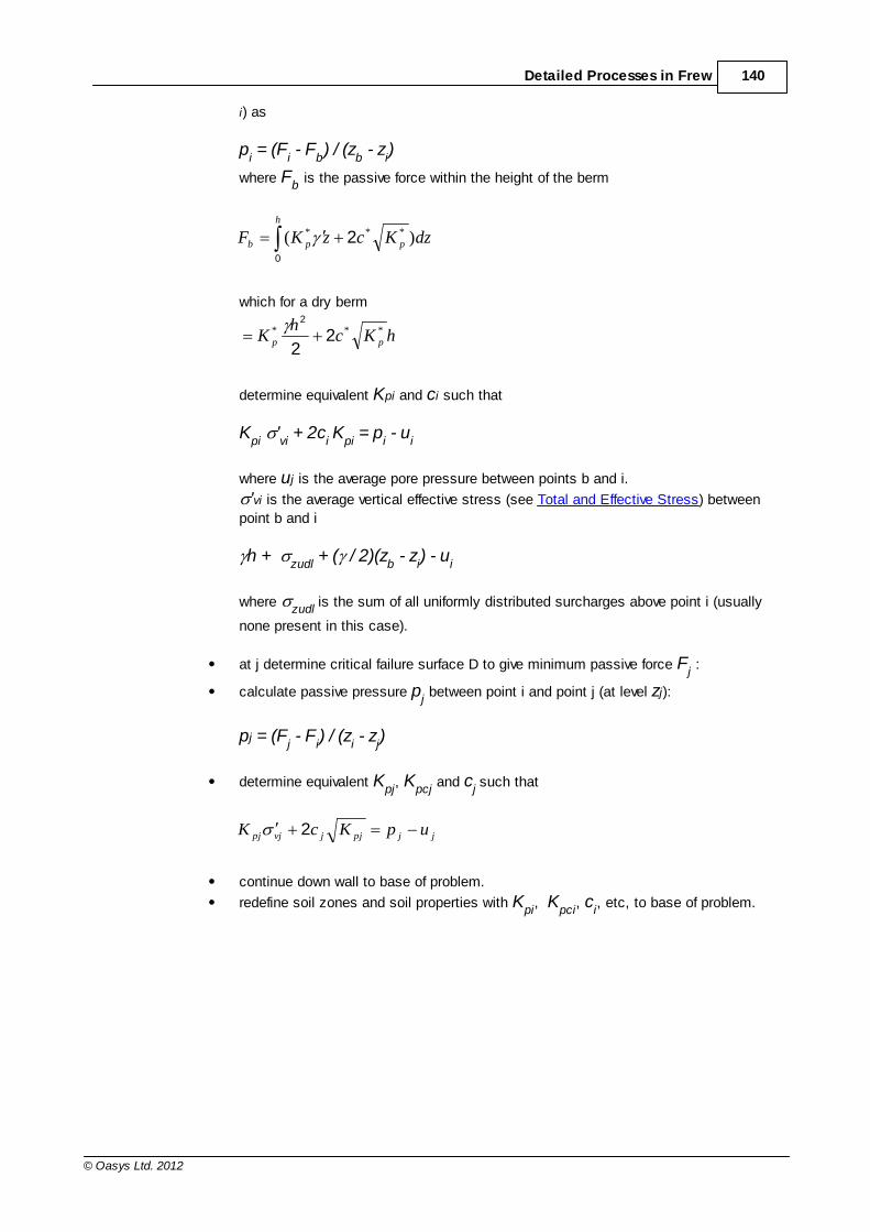
140Detailed Processes in Frew
© Oasys Ltd. 2012
i) as
pi = (F
i - F
b) / (z
b - z
i)
where Fb is the passive force within the height of the berm
h
ppb dzKczKF0
2 )( ***
which for a dry berm
hKch
K pp*** 2
2
2
determine equivalent Kpi and ci such that
Kpi
'vi + 2c
i K
pi = p
i - u
i
where uj is the average pore pressure between points b and i.
'vi is the average vertical effective stress (see Total and Effective Stress) between
point b and i
h + zudl
+ ( / 2)(zb - z
i) - u
i
where zudl
is the sum of all uniformly distributed surcharges above point i (usually
none present in this case).
at j determine critical failure surface D to give minimum passive force Fj :
calculate passive pressure pj between point i and point j (at level zj):
pj = (Fj - F
i) / (z
i - z
j)
determine equivalent Kpj
, Kpcj
and cj such that
jjpjjvjpj upKcK 2
continue down wall to base of problem.
redefine soil zones and soil properties with Kpi
, Kpci
, ci, etc, to base of problem.
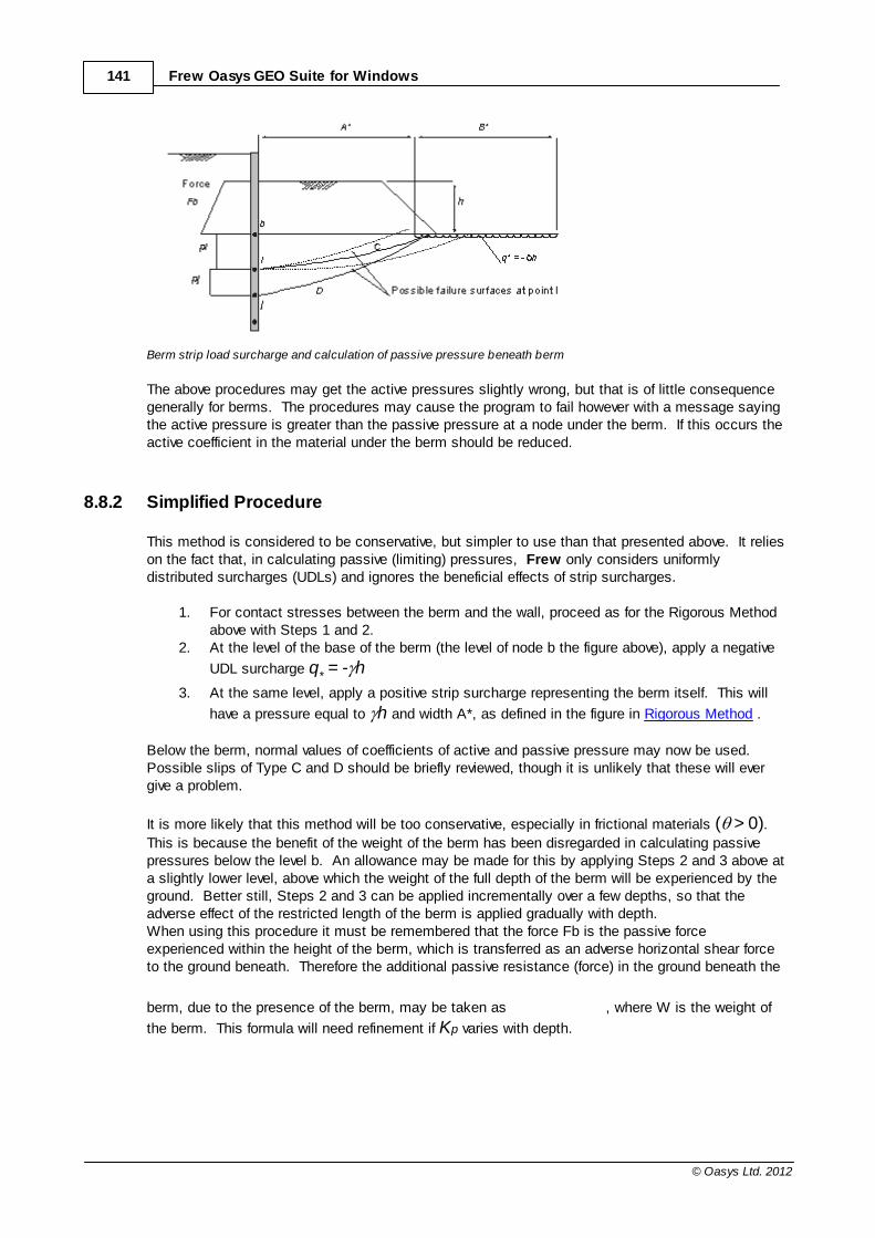
141 Frew Oasys GEO Suite for Windows
© Oasys Ltd. 2012
Berm strip load surcharge and calculation of passive pressure beneath berm
The above procedures may get the active pressures slightly wrong, but that is of little consequencegenerally for berms. The procedures may cause the program to fail however with a message sayingthe active pressure is greater than the passive pressure at a node under the berm. If this occurs theactive coefficient in the material under the berm should be reduced.
8.8.2 Simplified Procedure
This method is considered to be conservative, but simpler to use than that presented above. It relieson the fact that, in calculating passive (limiting) pressures, Frew only considers uniformlydistributed surcharges (UDLs) and ignores the beneficial effects of strip surcharges.
1. For contact stresses between the berm and the wall, proceed as for the Rigorous Methodabove with Steps 1 and 2.
2. At the level of the base of the berm (the level of node b the figure above), apply a negative
UDL surcharge q* = - h
3. At the same level, apply a positive strip surcharge representing the berm itself. This will
have a pressure equal to h and width A*, as defined in the figure in Rigorous Method .
Below the berm, normal values of coefficients of active and passive pressure may now be used. Possible slips of Type C and D should be briefly reviewed, though it is unlikely that these will evergive a problem.
It is more likely that this method will be too conservative, especially in frictional materials ( > 0).This is because the benefit of the weight of the berm has been disregarded in calculating passivepressures below the level b. An allowance may be made for this by applying Steps 2 and 3 above ata slightly lower level, above which the weight of the full depth of the berm will be experienced by theground. Better still, Steps 2 and 3 can be applied incrementally over a few depths, so that theadverse effect of the restricted length of the berm is applied gradually with depth.When using this procedure it must be remembered that the force Fb is the passive forceexperienced within the height of the berm, which is transferred as an adverse horizontal shear forceto the ground beneath. Therefore the additional passive resistance (force) in the ground beneath the
berm, due to the presence of the berm, may be taken as , where W is the weight of
the berm. This formula will need refinement if Kp varies with depth.

142Detailed Processes in Frew
© Oasys Ltd. 2012
8.9 Creep and Relaxation
There is often a requirement to model creep in Frew. Usually this refers to the creep of concretestructures which structural engineers normally represent by a change of Young's modulus. However,it cannot be represented so simply in Frew.
Elastic moduli are defined as ratios of stress to strain. The stresses and strains used in this ratiomay be either cumulative values (starting from zero stress and zero strain), or incremental values.
The above shows these two possibilities for a point X on a non-linear stress-strain curve.
The modulus in terms of cumulative stress and strain is commonly referred to as a secant modulus,whilst the modulus related to a small increment of stress and strain at point X is a tangent modulus.
Note : It is also possible to have an incremental secant modulus which approximates to the tangentmodulus for small increments.In describing the change of stiffness from short-term to long-term as a change of stiffness modulus,structural engineers are referring to secant moduli. But it is important to realise that Frew usestangent (incremental) moduli as its basic data. This means that merely changing stiffnessmoduli, when nothing else is changed, will have no effect at all.
8.9.1 Changing From Short Term to Long Term Stiffness
The following shows the type of stress-strain curve required for a change from short-term to long-termstiffness.
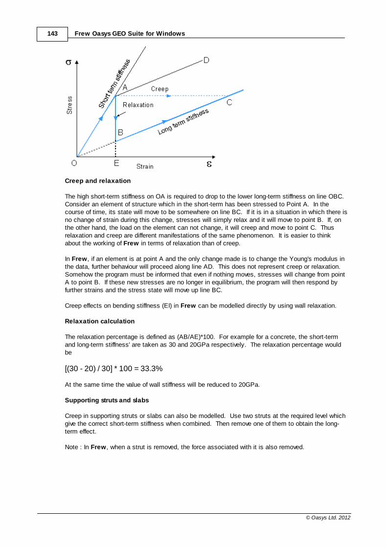
143 Frew Oasys GEO Suite for Windows
© Oasys Ltd. 2012
Creep and relaxation
The high short-term stiffness on OA is required to drop to the lower long-term stiffness on line OBC. Consider an element of structure which in the short-term has been stressed to Point A. In thecourse of time, its state will move to be somewhere on line BC. If it is in a situation in which there isno change of strain during this change, stresses will simply relax and it will move to point B. If, onthe other hand, the load on the element can not change, it will creep and move to point C. Thusrelaxation and creep are different manifestations of the same phenomenon. It is easier to thinkabout the working of Frew in terms of relaxation than of creep.
In Frew, if an element is at point A and the only change made is to change the Young's modulus inthe data, further behaviour will proceed along line AD. This does not represent creep or relaxation. Somehow the program must be informed that even if nothing moves, stresses will change from pointA to point B. If these new stresses are no longer in equilibrium, the program will then respond byfurther strains and the stress state will move up line BC.
Creep effects on bending stiffness (EI) in Frew can be modelled directly by using wall relaxation.
Relaxation calculation
The relaxation percentage is defined as (AB/AE)*100. For example for a concrete, the short-termand long-term stiffness' are taken as 30 and 20GPa respectively. The relaxation percentage wouldbe
[(30 - 20) / 30] * 100 = 33.3%
At the same time the value of wall stiffness will be reduced to 20GPa.
Supporting struts and slabs
Creep in supporting struts or slabs can also be modelled. Use two struts at the required level whichgive the correct short-term stiffness when combined. Then remove one of them to obtain the long-term effect.
Note : In Frew, when a strut is removed, the force associated with it is also removed.

144Detailed Processes in Frew
© Oasys Ltd. 2012
8.10 Undrained to drained behaviour - Manual Process
To effect a switch from undrained to drained behaviour without using Frew to calculate the undrainedpore pressures, the following procedure should be carried out. The user must first calculate and specify the profile of undrained pore pressures, then change themto the drained values.
Note: It is not sufficient merely to change to effective stress parameters and impose the final(drained) distribution of pore pressure.
The following procedure has been found to be satisfactory.
Note : In the Frew tabular output data P
e = apparent horizontal (effective) stress
Ve = apparent vertical (effective) stress
u = pore water pressure, specified by the user.
1. Tabulate the values of vertical and horizontal effective stresses given by Frew for Stage 0or the previous drained stage, for both the left and right sides of the wall. Add the userinput values of pore pressure u to obtain the total stresses.
2. Tabulate the corresponding values for the final undrained stage in the analysis.
3. Calculate the change in total horizontal h and vertical
v stresses between the two
stages.4. Calculate the "actual" change in pore water pressure due to movement in the wall between
the two stages.
This demands an understanding of the undrained stress path. For soils which are at yieldin shear, Skempton's pore pressure parameter A would be useful if its value can beassessed. If the soils have not reached yield, a modified value of A is required.
u = Bh + A(
v -
h) Skempton's equation.
In stiff clays, it may be assumed that the mean normal effective stress remains constantduring shearing. This assumption would not necessarily be appropriate to other soils andshould always be reviewed carefully. In the plane strain conditions of Frew, it amounts to:
u = (h +
v) / 2
5. Add u values to the user input values of u at stage 0.
6. Input this adjusted u value into the Frew analysis.
Three additional stages (A, B and C) are now required to complete the transition betweenundrained and drained behaviour.
7. Stage A. The new pore pressure profile should now be introduced into the next stage,
without changing the (undrained) strength criteria of the soils and keeping Kr = 1. Thiscauses Frew to recalculate effective stresses, but total stresses are unchanged and nomovement occurs.
8. Stage B. The soil strength parameters should then be changed to drained values,
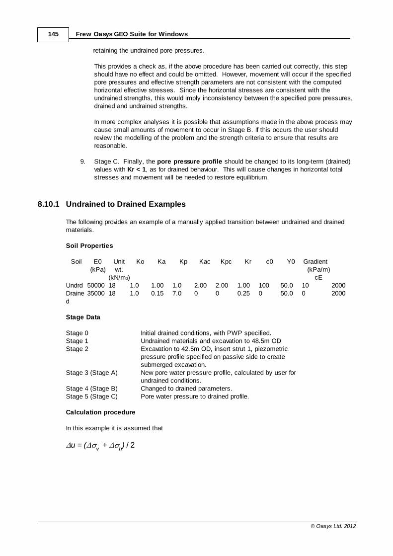
145 Frew Oasys GEO Suite for Windows
© Oasys Ltd. 2012
retaining the undrained pore pressures.
This provides a check as, if the above procedure has been carried out correctly, this stepshould have no effect and could be omitted. However, movement will occur if the specifiedpore pressures and effective strength parameters are not consistent with the computedhorizontal effective stresses. Since the horizontal stresses are consistent with theundrained strengths, this would imply inconsistency between the specified pore pressures,drained and undrained strengths. In more complex analyses it is possible that assumptions made in the above process maycause small amounts of movement to occur in Stage B. If this occurs the user shouldreview the modelling of the problem and the strength criteria to ensure that results arereasonable.
9. Stage C. Finally, the pore pressure profile should be changed to its long-term (drained)values with Kr < 1, as for drained behaviour. This will cause changes in horizontal totalstresses and movement will be needed to restore equilibrium.
8.10.1 Undrained to Drained Examples
The following provides an example of a manually applied transition between undrained and drainedmaterials.
Soil Properties
Soil E0(kPa)
Unitwt.
(kN/m3)
Ko Ka Kp Kac Kpc Kr c0 Y0 Gradient (kPa/m)
cEUndrd 50000 18 1.0 1.00 1.0 2.00 2.00 1.00 100 50.0 10 2000Drained
35000 18 1.0 0.15 7.0 0 0 0.25 0 50.0 0 2000
Stage Data
Stage 0 Initial drained conditions, with PWP specified.Stage 1 Undrained materials and excavation to 48.5m ODStage 2 Excavation to 42.5m OD, insert strut 1, piezometric
pressure profile specified on passive side to createsubmerged excavation.
Stage 3 (Stage A) New pore water pressure profile, calculated by user forundrained conditions.
Stage 4 (Stage B) Changed to drained parameters.Stage 5 (Stage C) Pore water pressure to drained profile.
Calculation procedure
In this example it is assumed that
u = (v +
h) / 2

146Detailed Processes in Frew
© Oasys Ltd. 2012
Note: Users should be aware that as Ko is used to calculate P
e in stage 0, total horizontal stress in
this stage should be calculated by adding Ko*u to P
e. In any other undrained stage K
a / K
p are used
and are equal to 1, therefore total horizontal stress can be calculated by simply adding u to Pe.
Pore water Pressure Calculations
Active Pressures
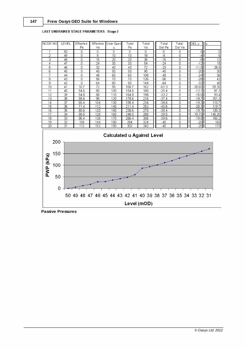
147 Frew Oasys GEO Suite for Windows
© Oasys Ltd. 2012
Passive Pressures

148Detailed Processes in Frew
© Oasys Ltd. 2012
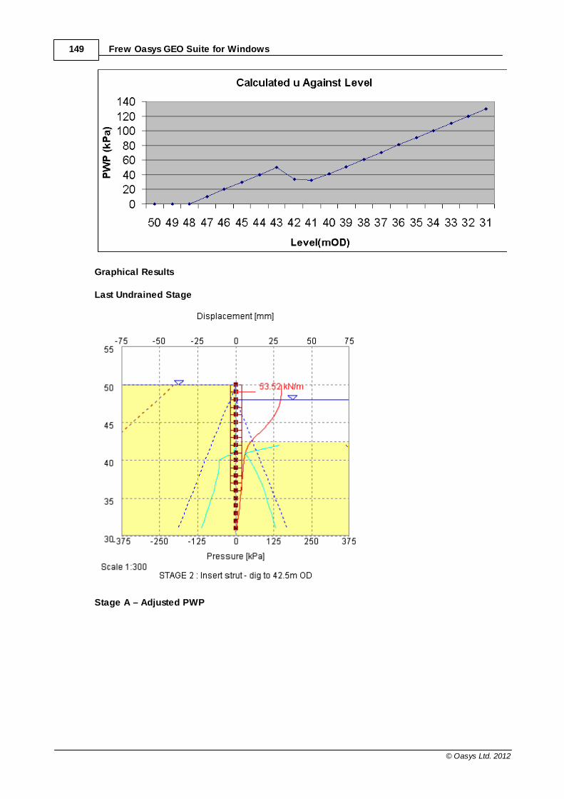
149 Frew Oasys GEO Suite for Windows
© Oasys Ltd. 2012
Graphical Results
Last Undrained Stage
Stage A – Adjusted PWP
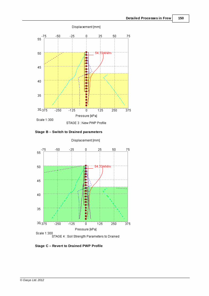
150Detailed Processes in Frew
© Oasys Ltd. 2012
Stage B – Switch to Drained parameters
Stage C – Revert to Drained PWP Profile
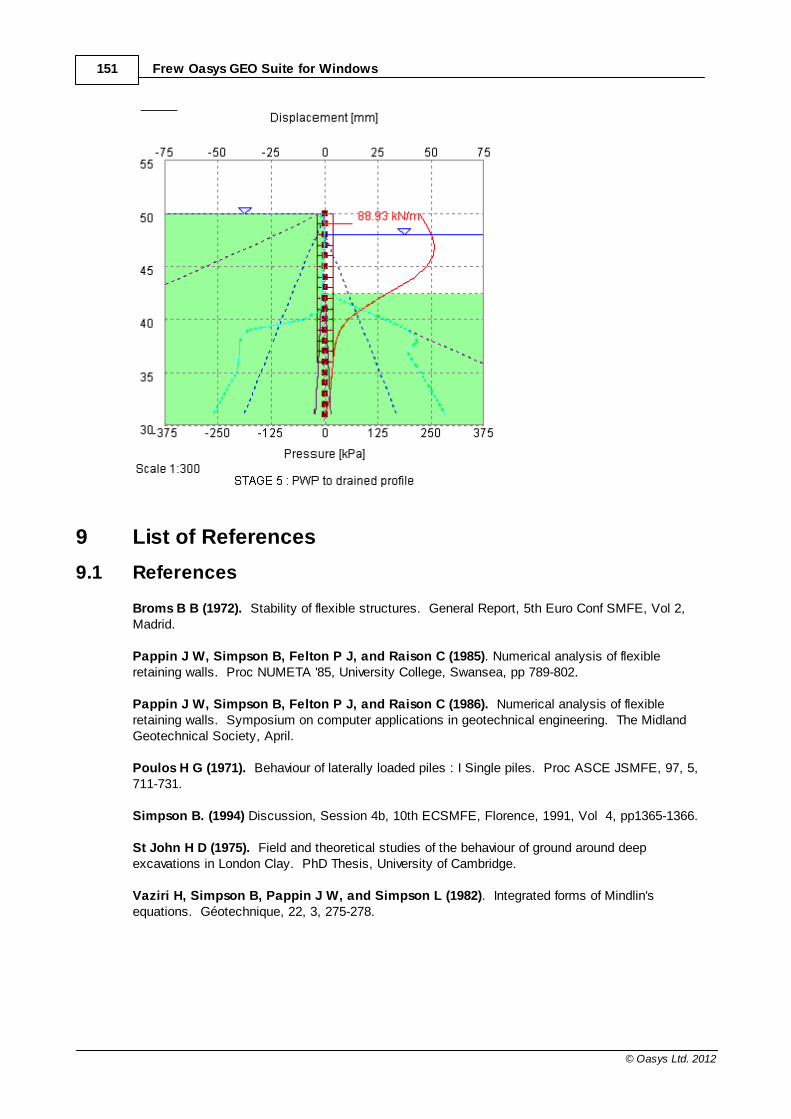
151 Frew Oasys GEO Suite for Windows
© Oasys Ltd. 2012
9 List of References
9.1 References
Broms B B (1972). Stability of flexible structures. General Report, 5th Euro Conf SMFE, Vol 2,Madrid.
Pappin J W, Simpson B, Felton P J, and Raison C (1985). Numerical analysis of flexibleretaining walls. Proc NUMETA '85, University College, Swansea, pp 789-802.
Pappin J W, Simpson B, Felton P J, and Raison C (1986). Numerical analysis of flexibleretaining walls. Symposium on computer applications in geotechnical engineering. The MidlandGeotechnical Society, April.
Poulos H G (1971). Behaviour of laterally loaded piles : I Single piles. Proc ASCE JSMFE, 97, 5,711-731.
Simpson B. (1994) Discussion, Session 4b, 10th ECSMFE, Florence, 1991, Vol 4, pp1365-1366.
St John H D (1975). Field and theoretical studies of the behaviour of ground around deepexcavations in London Clay. PhD Thesis, University of Cambridge.
Vaziri H, Simpson B, Pappin J W, and Simpson L (1982). Integrated forms of Mindlin'sequations. Géotechnique, 22, 3, 275-278.

152Brief Technical Description
© Oasys Ltd. 2012
10 Brief Technical Description
10.1 Suggested Description for Use in Memos/Letters, etc
Frew is a program used to analyse the behaviour of flexible retaining walls. It predicts thedisplacement, shear forces, and bending moments of the wall and the earth pressures each side ofthe wall resulting from a series of actions. These actions include excavation, filling, dewatering,changing soil or wall properties and applying or removing struts, anchors or surcharges. Theprogram models the soil as an elastic continuum and allows for soil failure by restricting the earthpressures to lie within the active or passive limits and also includes the effect of arching.
10.2 Brief Description for Inclusion in Reports
The following pages contain a summary of the analysis method used by Frew. It is intended thatthey can be copied and included with calculations or reports as the need arises.
Frew is a program to analyse the soil structure interaction problem of a flexible retaining wall, forexample a sheet pile or diaphragm wall.
The wall is represented as a line of nodal points and three stiffness matrices relating nodal forces todisplacements are developed. One represents the wall in bending and the others represent the soilon each side of the wall. The soil behaviour is modelled using one of three methods:
1. "Safe" flexibility method - the soil is represented as an elastic solid with the soilstiffness matrices being developed from pre-stored stiffness matrices calculated using the"Safe" finite element program. This method is ideally limited to a soil with linearlyincreasing stiffness with depth, but empirical modifications are used for other cases.
2. Mindlin method - the soil is represented as an elastic solid with the soil stiffness basedon the integrated form of the Mindlin Equations. This method can model a wall of limitedlength in plan but is ideally limited to a soil with constant stiffness with depth but againempirical modifications are used for other cases.
3. Subgrade reaction method - the soil is represented as a series of non interactivesprings. This method is considered to be unrealistic in most circumstances.
The program analyses the behaviour for each stage of the construction sequence. At each stage itcalculates the force imbalance at each node imposed by that stage and calculates displacementand soil stresses using the stiffness matrices. If the soil stresses are outside the active or passivelimiting pressures correction forces are applied and the problem solved iteratively until the stressesare acceptable. Allowance can be made for arching within the soil body when calculating the activeand passive limiting pressures.
The following input parameters are included in the analysis:
problem geometry including dig depths, distances to remote boundarieswall profile bending stiffness and creepsoil stratification, strength, density and stiffnessstruts (or anchors) including prestress, stiffness, inclination and a lever arm (to representrotational fixity).surcharges including depth and extentgroundwater levels and pore pressures each side of wall.

153 Frew Oasys GEO Suite for Windows
© Oasys Ltd. 2012
The program gives results for earth pressures, shear forces and bending moments in the wall, strutforces and displacements. These are presented in tabular form and can be plotteddiagrammatically. In addition the number of iterations, the displacement error between successiveinteractions and the maximum earth pressure error are output.
Full details of the assumptions and analysis methods are included in the following paper.
Pappin J W, Simpson B, Felton P J, and Raison C (1986). "Numerical analysis of flexibleretaining walls". Symposium on computer applications in geotechnical engineering. The MidlandGeotechnical Society, April.
11 Manual Example
11.1 General
The data input and results for the manual example are available to view in Frew data file (.fwd)format or pdf format in the 'Samples' sub-folder of the program installation folder. The example hasbeen created to show the data input for all aspects of the program and does not seek to provide anyindication of engineering advice.
Screen captures from this example have also been used throughout this document.
This example can be used by new users to practise data entry and get used to the details of theprogram.

Index 154
© Oasys Ltd. 2012
IndexA
Active and Passive Limits 8
Active earth pressure Axi-symmetric problems 135
Limits 11, 12, 119, 121, 125
Output 102
Pressures 15, 37, 120
Surcharges 70, 126
Surcharges: 126
Tolerance 62
Analysis Methods of 1
Procedure 11
Anchors 68, 134
Angle of friction 84
Assembling data 24
Axis Graphical output 102
Axi-symmetric Problems 135, 138
B
Backfill Effects of 16, 24
Modelling of 48
Batch plotting 105
Bending moments 11
berm 138
berms 138
Bitmaps In titles window 35
Boundary Distances 56
Horizontal rigid 56, 63
Vertical 56, 111
boundary distances 56, 75
C
Components of the User Interface 3
Convergence Control 61
Copy (graphics) 102
Creep 142
D
Damping coefficient 62
Data Checking 94
Data Entry 75
Deflection Calculation 132
Graphical representation 102
Direct Kp factors 72
Displacement Maximum incremental 63
Tolerance of 62
Drained materials 16, 18, 19, 21, 24, 37, 40, 69,145
E
Earth pressure at rest 18, 37
Effective stress 18
element edge loads 83
Example Analysis procedure 11, 12, 13
Manual 24
Excavation Effects of 16, 63, 70, 116
Modelling of 48, 135
Export 75
F
Factors of safety 72
File New FREW file 24
first stage material 86
Fixed and Free solution 57, 115
Fixed Earth Mechanisms 4
Fixed or Free solution 57
Free Earth Mechanisms 5
Frew Toolbar 3
G
'g' 86
Frew Oasys GEO Suite for Windows155
© Oasys Ltd. 2012
Gateway 3
Geometry 82
Global Data 24, 33, 35, 37, 40, 63, 66
global softening 60
Graphical Output 3, 102
Graphics Toolbar 3
Groundwater 75, 88Hydrostatic 51
Piezometric 51
I
Inserting Stages 41
Iterations Number of 62
K
K0 86
L
Lever arm 83
linear elasttic 84
M
Material Properties 37, 40
Materials 84
Mesh 82
Mindlin method Accuracy of 117
Application in FREW 116
Basic model 13, 56, 116
Mohr-Coulumb 84
N
New Stages 39, 40, 41
Nodes 1, 11, 24, 45, 49, 63, 100, 106
P
Partial Factors 72
Passive earth pressure 128Limits 11, 119, 121, 125
Output 37, 102
Pressures 15, 37
Surcharges 70
Passive earth pressure:Surcharges 128
Passive softening 60
passive softening depth 60
Poisson's ratio 84
pore pressure 88
Pressure 62
PressureTolerance of 62
R
Radius of influence 88
Redistribution 15, 58, 119
Relaxation 24, 49, 57, 142
Restraints 82
Results 35, 94, 100, 101, 102, 153
Rigid boundary 56
Runs 80
S
SAFE method 1, 12, 57, 106Accuracy of 13
Approximations 106
Fixed or free 57
Save Metafile 102
Scale Engineering 102
Shear Force 1, 100, 102
Soil strength factors 72
Soil Zones 45
Stage Changing titles 42, 43
Construction 1
Data 39
Deleting 42
Editing 41
Stage 0 11, 19, 24, 40
Stages 80
Standard Toolbar 3
Strip Loads 69, 70, 128Active pressures 126
Passive pressures 128
Struts 83Levels 63
Index 156
© Oasys Ltd. 2012
Struts 83Properties 1, 66, 132, 134
Sub-grade Reaction 14, 56, 111
Surcharge factors 72
Surcharges 69, 83Strip loads 15, 69, 128
Strip loads: 126
Uniformally distributed loads 18, 69, 70
T
Table View 3
Tabular Output 3
Tabulated Output 97
Titles 34, 43
Toolbar 3
U
Uniformally distributed loads 69, 70
Units 35
Unsupported features 89
User defined factors 72
User Interface 3
V
validation 75
void 84
W
Wall 84Data 11, 49
Deflection 102
Friction 13, 15, 115
Geometry 1, 24, 49
Relaxation 24, 49, 57
Stiffness 1, 39, 41, 42, 43, 44, 45, 49, 63, 66,68, 69, 70, 132
Stiffness: 40
wall data 75
Wall Friction 115
Y
Youngs modulus 57
Z
Zoom Facility 102

Endnotes 2... (after index)
157 Frew Oasys GEO Suite for Windows
© Oasys Ltd. 2012

Related Documents