Welcome message from author
This document is posted to help you gain knowledge. Please leave a comment to let me know what you think about it! Share it to your friends and learn new things together.
Transcript


Foundations of Electromagnetic Compatibility

Foundations of Electromagnetic Compatibility
with Practical Applications
Bogdan AdamczykEMC Educational Services LLCwww.emcspectrum.com

This edition first published 2017© 2017 John Wiley and Sons Ltd
All rights reserved. No part of this publication may be reproduced, stored in a retrieval system, or transmitted, in any form or by any means, electronic, mechanical, photocopying, recording or otherwise, except as permitted by law.Advice on how to obtain permission to reuse material from this title is available at http://www.wiley.com/go/permissions.
The right of Bogdan Adamczyk to be identified as the author of this work has been asserted in accordance with law.
Registered OfficesJohn Wiley & Sons, Inc., 111 River Street, Hoboken, NJ 07030, USAJohn Wiley & Sons Ltd, The Atrium, Southern Gate, Chichester, West Sussex, PO19 8SQ, UK
Editorial OfficeThe Atrium, Southern Gate, Chichester, West Sussex, PO19 8SQ, UK
For details of our global editorial offices, customer services, and more information about Wiley products visit us at www.wiley.com.
Wiley also publishes its books in a variety of electronic formats and by print‐on‐demand. Some content that appears in standard print versions of this book may not be available in other formats.
Limit of Liability/Disclaimer of WarrantyWhile the publisher and authors have used their best efforts in preparing this book, they make no representations or warranties with respect to the accuracy or completeness of the contents of this book and specifically disclaim any implied warranties of merchantability or fitness for a particular purpose. No warranty may be created or extended by sales representatives or written sales materials. The advice and strategies contained herein may not be suitable for your situation. You should consult with a professional where appropriate. Neither the publisher nor authors shall be liable for any loss of profit or any other commercial damages, including but not limited to special, incidental, consequential, or other damages.
Library of Congress Cataloging‐in‐Publication Data
Names: Adamczyk, Bogdan, 1960– author.Title: Foundations of electromagnetic compatibility with practical applications / Bogdan Adamczyk.Description: Hoboken, New Jersey : John Wiley & Sons, Inc., 2017. | Includes index.Identifiers: LCCN 2016047894 | ISBN 9781119120780 (hardback ; cloth) | ISBN 1119120780 (hardback ; cloth) | ISBN 9781119120797 (Adobe PDF) | ISBN 1119120799 (Adobe PDF) | ISBN 9781119120803 (ePub) | ISBN 1119120802 (ePub)Subjects: LCSH: Electromagnetic compatibility.Classification: LCC TK7867.2 .A33 2017 | DDC 621.382/24–dc23 LC record available at https://lccn.loc.gov/2016047894
Cover design by WileyFront Cover: The cover shows the EMC Center at GVSU created by Prof. Adamczyk
Set in 10/12pt Warnock by SPi Global, Pondicherry, India
10 9 8 7 6 5 4 3 2 1

v
Preface xiii
Part I Math Foundations of EMC 1
1 Matrix and Vector Algebra 31.1 Basic Concepts and Operations 31.2 Matrix Multiplication 51.3 Special Matrices 61.4 Matrices and Determinants 71.5 Inverse of a Matrix 91.6 Matrices and Systems of Equations 101.7 Solution of Systems of Equations 111.8 Cramer’s Rule 121.9 Vector Operations 131.9.1 Scalar Product 131.9.2 Vector Product 131.10 EMC Applications 141.10.1 Crosstalk Model of Transmission Lines 141.10.2 Radiated Susceptibility Test 171.10.3 s Parameters 20 References 21
2 Coordinate Systems 232.1 Cartesian Coordinate System 232.2 Cylindrical Coordinate System 252.3 Spherical Coordinate System 272.4 Transformations between Coordinate Systems 292.4.1 Transformation between Cartesian and Cylindrical Systems 292.4.2 Transformation between Cartesian and Spherical Systems 322.5 EMC Applications 332.5.1 Radiation Fields of an Electric Dipole Antenna 33 References 35
Contents
Contentsvi
3 Vector Differential Calculus 373.1 Derivatives 373.1.1 Basic Definition and Formulas 373.1.2 Composite Function and Chain Rule 393.1.3 Partial Derivative 393.2 Differential Elements 403.2.1 Differential Length Element 403.2.2 Differential Surface Element 433.2.3 Differential Volume Element 453.3 Constant‐Coordinate Surfaces 453.3.1 Cartesian Coordinate System 463.3.2 Cylindrical Coordinate System 463.3.3 Spherical Coordinate System 473.3.4 Differential Elements on Constant Coordinate Surfaces 483.4 Differential Operators 503.4.1 Gradient 503.4.2 Divergence 513.4.3 Curl 523.4.4 Laplacian 543.5 EMC Applications 553.5.1 Transmission‐Line Equations 553.5.2 Maxwell’s Equations in a Differential Form 563.5.3 Electromagnetic Wave Equation 57 References 57
4 Vector Integral Calculus 594.1 Line Integrals 594.1.1 Indefinite and Definite Integrals 594.1.2 Line Integral 614.1.3 Properties of Line Integrals 634.2 Surface Integrals 664.2.1 Double Integrals 664.2.2 Surface Integrals 674.3 Volume Integrals 714.4 Divergence Theorem of Gauss 714.5 Stokes’s Theorem 714.6 EMC Applications 724.6.1 Maxwell’s Equations in an Integral Form 724.6.2 Loop and Partial Inductance 724.6.3 Ground Bounce and Power Rail Collapse 74 References 79
5 Differential Equations 815.1 First Order Differential Equations – RC and RL Circuits 815.1.1 RC Circuit 815.1.2 RL Circuit 835.2 Second‐Order Differential Equations – Series and Parallel RLC Circuits 85
Contents vii
5.2.1 Series RLC Circuit 855.2.2 Parallel RLC Circuit 945.3 Helmholtz Wave Equations 955.4 EMC Applications 995.4.1 Inductive Termination of a Transmission Line 995.4.2 Ringing on a Transmission Line 103 References 108
6 Complex Numbers and Phasors 1096.1 Definitions and Forms 1096.2 Complex Conjugate 1116.3 Operations on Complex Numbers 1136.4 Properties of Complex Numbers 1186.5 Complex Exponential Function 1186.6 Sinusoids and Phasors 1196.6.1 Sinusoids 1196.6.2 Phasors 1216.7 EMC Applications 1236.7.1 Maxwell’s Equations in a Phasor Form 1236.7.2 Transmission Line Equations in a Phasor Form 1256.7.3 Magnetic Vector Potential 1256.7.4 Radiated Fields of an Electric Dipole 1286.7.5 Electric Dipole Antenna Radiated Power 137 References 140
Part II Circuits Foundations of EMC 141
7 Basic Laws and Methods of Circuit Analysis 1437.1 Fundamental Concepts 1437.1.1 Current 1437.1.2 Voltage 1437.1.3 Power 1447.1.4 Average Power in Sinusoidal Steady State 1457.2 Laplace Transform Basics 1477.2.1 Definition of Laplace Transform 1477.2.2 Properties of Laplace Transform 1497.2.3 Inverse Laplace Transform 1507.3 Fundamental Laws 1527.3.1 Resistors and Ohm’s Law 1527.3.2 Inductors and Capacitors 1547.3.3 Phasor Relationships for Circuit Elements 1567.3.4 s Domain Relationships for Circuit Elements 1587.3.5 Impedance in Phasor Domain 1607.3.6 Impedance in the s Domain 1637.3.7 Kirchhoff ’s Laws in the Time Domain 1647.3.8 Kirchhoff ’s Laws in the Phasor Domain 167
Contentsviii
7.3.9 Kirchhoff ’s Laws in the s Domain 1687.3.10 Resistors in Series and the Voltage Divider 1697.3.11 Resistors in Parallel and the Current Divider 1727.3.12 Impedance Combinations and Divider Rules in Phasor Domain 1767.4 EMC Applications 1837.4.1 Crosstalk between PCB Traces 1837.4.2 Capacitive Termination of a Transmission Line 184 References 187
8 Systematic Methods of Circuit Analysis 1898.1 Node Voltage Analysis 1898.1.1 Node Analysis for the Resistive Circuits 1898.2 Mesh Current Analysis 1928.2.1 Mesh Analysis for the Resistive Circuits 1928.3 EMC Applications 1958.3.1 Power Supply Filters – Common‐ and Differential‐Mode Current Circuit
Model 195 References 202
9 Circuit Theorems and Techniques 2039.1 Superposition 2039.2 Source Transformation 2079.3 Thévenin Equivalent Circuit 2119.4 Norton Equivalent Circuit 2179.5 Maximum Power Transfer 2209.5.1 Maximum Power Transfer – Resistive Circuits 2209.5.2 Maximum Power Transfer – Sinusoidal Steady State 2239.6 Two‐Port Networks 2249.7 EMC Applications 2369.7.1 Fourier Series Representation of Signals 2369.7.2 Maximum Power Radiated by an Antenna 2389.7.3 s Parameters 240 References 241
10 Magnetically Coupled Circuits 24310.1 Self and Mutual Inductance 24310.2 Energy in a Coupled Circuit 24810.3 Linear (Air‐Core) Transformers 25010.4 Ideal (Iron‐Core) Transformers 25110.5 EMC Applications 25510.5.1 Common‐Mode Choke 255 References 258
11 Frequency‐Domain Analysis 25911.1 Transfer Function 25911.2 Frequency‐Transfer Function 26711.2.1 Sinusoidal Steady‐State Output 268
Contents ix
11.3 Bode Plots 27211.4 Passive Filters 27711.4.1 RL and RC Low‐Pass Filters 27711.4.2 RL and RC High‐Pass Filters 28011.4.3 Series and Parallel RLC Bandpass Filters 28411.4.4 Series and Parallel RLC Band‐Reject Filters 28911.5 Resonance in RLC Circuits 29411.5.1 Resonance in Series RLC Bandpass Filter 29411.5.2 Resonance in Parallel RLC Bandpass Filter 30011.5.3 Resonance in Other RLC Circuits 30411.6 EMC Applications 30811.6.1 Non‐Ideal Behavior of Capacitors and Inductors 30811.6.2 Decoupling Capacitors 31011.6.3 EMC Filters 318 References 327
12 Frequency Content of Digital Signals 32912.1 Fourier Series and Frequency Content of Signals 32912.1.1 Trigonometric Fourier Series 32912.1.2 Exponential Fourier Series 33512.1.3 Spectrum of the Digital Clock Signals 33712.1.4 Spectral Bounds on Digital Clock Signals 34512.2 EMC Applications 34712.2.1 Effect of the Signal Amplitude, Fundamental Frequency, and Duty Cycle
on the Frequency Content of Trapezoidal Signals 347 References 351
Part III Electromagnetics Foundations of EMC 353
13 Static and Quasi‐Static Electric Fields 35513.1 Charge Distributions 35513.2 Coulomb’s Law 35613.3 Electric Field Intensity 35713.4 Electric Field Due to Charge Distributions 35813.5 Electric Flux Density 35913.6 Gauss’s Law for the Electric Field 36013.7 Applications of Gauss’s Law 36013.8 Electric Scalar Potential and Voltage 36713.9 Voltage Calculations due to Charge Distributions 36913.10 Electric Flux Lines and Equipotential Surfaces 37313.11 Maxwell’s Equations for Static Electric Field 37413.12 Capacitance Calculations of Structures 37413.12.1 Definition of Capacitance 37413.12.2 Calculations of Capacitance 37613.13 Electric Boundary Conditions 38013.14 EMC Applications 385
Contentsx
13.14.1 Electrostatic Discharge (ESD) 38513.14.2 Human‐Body Model 39213.14.3 Capacitive Coupling and Shielding 394 References 402
14 Static and Quasi‐Static Magnetic Fields 40314.1 Magnetic Flux Density 40314.2 Magnetic Field Intensity 40414.3 Biot–Savart Law 40414.4 Current Distributions 40514.5 Ampere’s Law 40614.6 Applications of Ampere’s Law 40714.7 Magnetic Flux 40914.8 Gauss’s Law for Magnetic Field 41014.9 Maxwell’s Equations for Static Fields 41014.10 Vector Magnetic Potential 41114.11 Faraday’s Law 41214.12 Inductance Calculations of Structures 41614.13 Magnetic Boundary Conditions 41814.14 EMC Applications 42314.14.1 Current Probes 42314.14.2 Magnetic Flux and Decoupling Capacitors 42614.14.3 Magnetic Coupling and Shielding 428 References 437
15 Rapidly Varying Electromagnetic Fields 43915.1 Eddy Currents 43915.2 Charge‐Current Continuity Equation 44015.3 Displacement Current 44115.4 EMC Applications 44415.4.1 Grounding and Current Return Path 44415.4.2 Common‐Impedance Coupling 448 References 452
16 Electromagnetic Waves 45316.1 Uniform Waves – Time Domain Analysis 45316.2 Uniform Waves – Sinusoidal Steady‐State Analysis 46016.3 Reflection and Transmission of Uniform Waves at Boundaries 46416.4 EMC Applications 46716.4.1 Electromagnetic Wave Shielding 467 References 474
17 Transmission Lines 47517.1 Transient Analysis 47517.1.1 Reflections on Transmission Lines 47817.1.2 Bounce Diagram 49317.1.3 Reflections at an Inductive Load 496
Contents xi
17.1.4 Reflections at a Capacitive Load 49917.1.5 Transmission Line Discontinuity 50117.2 Steady‐State Analysis 50917.2.1 Lossy Transmission Lines 50917.2.2 Standing Waves 51217.3 s Parameters 52017.4 EMC Applications 52717.4.1 Crosstalk between PCB traces 52717.4.2 LISN Impedance Measurement 53517.4.3 Preamp Gain and Attenuator Loss Measurement 540 References 542
18 Antennas and Radiation 54318.1 Bridge between the Transmission Line and Antenna Theory 54318.2 Hertzian Dipole Antenna 54418.3 Far Field Criteria 54818.3.1 Wire‐Type Antennas 54818.3.2 Surface‐Type Antennas 54918.4 Half‐Wave Dipole Antenna 55118.5 Quarter‐Wave Monopole Antenna 55418.6 Image Theory 55418.7 Differential‐ and Common‐Mode Currents and Radiation 55718.7.1 Differential‐ and Common‐Mode Currents 55718.7.2 Radiation from Differential‐ and Common‐Mode Currents 55918.8 Common Mode Current Creation 56518.8.1 Circuits with a Shared Return Path 56518.8.2 Differential Signaling 56918.8.3 Common‐Mode Current Creation 57018.9 Antenna Circuit Model 57118.9.1 Transmitting‐Mode Model 57118.9.2 Receiving‐Mode Model 57318.10 EMC Applications 57518.10.1 EMC Antenna Measurements 57518.10.2 Antenna VSWR and Impedance Measurements 57718.10.3 Comb Transmitter Measurements 579 References 582
Appendix A EMC Tests and Measurements 583A.1 Introduction – FCC Part 15 and CISPR 22 Standards 583A.1.1 Peak vs Quasi‐Peak vs Average Measurements 583A.1.2 FCC and CISPR 22 Limits 585A.2 Conducted Emissions 588A.2.1 FCC and CISPR 22 Voltage Method 591A.2.2 CISPR 25 Voltage Method 592A.2.3 CISPR 25 Current Probe Method 596A.3 Radiated Emissions 600A.3.1 Open‐Area Test Site (OATS) Measurements 602

Contentsxii
A.3.2 Semi‐Anechoic Chamber Measurements 603A.4 Conducted Immunity – ISO 11452‐4 608A.4.1 Substitution Method 613A.4.2 Closed‐Loop Method with Power Limitation 613A.5 Radiated Immunity 615A.5.1 Radiated Immunity – ISO 11452‐11 615A.5.2 Radiated Immunity – ISO 11452‐2 619A.6 Electrostatic Discharge (ESD) 620
Index 629

xiii
A few years ago when I was about to teach another EMC fundamentals course for the industry, I was contacted by some of the participants asking about a textbook for the course. Then I realized that there is no single self‐contained book covering the topics of mathematic, electric circuits and electromagnetics with the focus on EMC. There is a plethora of books devoted to each of these subjects separately and each written for a general audience. It was then that the idea of writing this book was born.
This text reviews the fundamentals of mathematics, electric circuits, and electromag-netics specifically needed for the study of EMC. Each chapter reviews the material per-tinent to EMC and concludes with practical EMC examples illustrating the applicability of the discussed topics. The book is intended as a reference and a refresher for both the practicing professionals and the new EMC engineers entering the field.
This book also provides a background material helpful in following the two classical texts on EMC: Clayton Paul’s “Introduction to Electromagnetic Compatibility” (Wiley, 2006) and Henry Ott’s “Electromagnetic Compatibility Engineering” (Wiley, 2009). Many formulas in those two books (presented without derivations) are derived from basic principles in this text.
This approach provides the reader with the understanding of the underlying assump-tions and the confidence in using the final results. This insight is invaluable in the field of EMC where so many design rules and principles are based on several approximations and are only valid when the underlying assumptions are met.
The author owes a great deal of gratitude for the insight and knowledge gained from the association with colleagues from the EMC lab at Gentex Corporation (Bill Spence and Pete Vander Wel) and the EMC specialists and friends at E3 Compliance LLC (Jim Teune and Scott Mee). The author would also like to thank Mark Steffka for his guidance and help over the past ten years. Finally, the author would like to acknowledge the support of Grand Valley State University and especially its engineering dean Paul Plotkowski who was instrumental in the creation of the EMC Center, greatly contributing to the EMC education and the publication of this book.
Bogdan AdamczykGrand Rapids, Michigan, September 2016
Preface


1
Part I
Math Foundations of EMC


Foundations of Electromagnetic Compatibility with Practical Applications, First Edition. Bogdan Adamczyk. © 2017 John Wiley & Sons Ltd. Published 2017 by John Wiley & Sons Ltd.
3
1
Matrices and determinants are very powerful tools in circuit analysis and electromag-netics. Matrices are useful because they enable us to replace an array of many entries as a single symbol and perform operations in a compact symbolic form.
We begin this chapter by defining a matrix, followed by the algebraic operations and properties. We will conclude this chapter by showing practical EMC‐related applica-tions of matrix algebra.
1.1 Basic Concepts and Operations
A matrix is a mathematical structure consisting of rows and columns of elements (often numbers or functions) enclosed in brackets (Kreyszig, 1999, p. 305).
For example,
A6 5 23 2 07 1 4
(1.1)
The entries in matrix A are real numbers. Matrices L and C in Eq. (1.2) are the matrices containing per‐unit‐length inductances and capacitances, respectively, representing a crosstalk model of transmission lines (Paul, 2006, p. 567). (We will discuss the details of this model later in this chapter.)
L C
l ll l
c c cc c c
G m
m R
G m m
m R m, (1.2)
We denote matrices by capital boldface letters. It is often convenient, especially when discussing matric operations and properties, to represent a matrix in terms of its gen-eral entry in brackets:
A a
a a aa a a
a a a
ij
n
n
m m mn
11 12 1
21 22 2
1 2
��
� � � ��
(1.3)
Matrix and Vector Algebra
Foundations of Electromagnetic Compatibility4
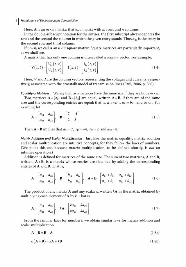
Here, A is an m × n matrix; that is, a matrix with m rows and n columns.In the double‐subscript notation for the entries, the first subscript always denotes the
row and the second the column in which the given entry stands. Thus a23 is the entry in the second row and third column.
If m = n, we call A an n × n square matrix. Square matrices are particularly important, as we shall see.
A matrix that has only one column is often called a column vector. For example,
V Iz t
V z tV z t
z tI z tI z t
G
R
G
R,
, ,
, , ,
, (1.4)
Here, V and I are the column vectors representing the voltages and currents, respec-tively, associated with the crosstalk model of transmission lines (Paul, 2006, p. 566).
Equality of Matrices We say that two matrices have the same size if they are both m × n.Two matrices A = [aij] and B = [bij] are equal, written A = B, if they are of the same
size and the corresponding entries are equal; that is, a11 = b11, a12 = b12, and so on. For example, let
A B
a aa a
11 12
21 22
7 42 8, (1.5)
Then A = B implies that a11 = 7, a12 = −4, a21 = 2, and a22 = 8.
Matrix Addition and Scalar Multiplication Just like the matrix equality, matrix addition and scalar multiplication are intuitive concepts, for they follow the laws of numbers. (We point this out because matrix multiplication, to be defined shortly, is not an intuitive operation.)
Addition is defined for matrices of the same size. The sum of two matrices, A and B, written, A + B, is a matrix whose entries are obtained by adding the corresponding entries of A and B. That is,
A B A B
a aa a
b bb b
a b a11 12
21 22
11 12
21 22
11 11, ,
112 12
21 21 22 22
ba b a b (1.6)
The product of any matrix A and any scalar k, written kA, is the matrix obtained by multiplying each element of A by k. That is,
A A
a aa a k
ka kaka ka
11 12
21 22
11 12
21 22, (1.7)
From the familiar laws for numbers, we obtain similar laws for matrix addition and scalar multiplication.
A B B A (1.8a)
k k kA B A B (1.8b)
Matrix and Vector Algebra 5
A 0 A (1.8c)
A A 0 (1.8d)
1A A (1.8e)
0A 0 (1.8f )
There is one more algebraic operation: the multiplication of matrices by matrices. Since this operation does not follow the familiar rule of number multiplication we devote a separate section to it.
1.2 Matrix Multiplication
Matrix multiplication means multiplying matrices by matrices. Recall: matrices are added by adding corresponding entries, as shown in Eq. (1.6). Matrix multiplication could be defined in a similar manner:
A B AB
a aa a
b bb b
a b a11 12
21 22
11 12
21 22
11 11 12, ,
bba b a b incorrect
12
21 21 22 22 (1.9)
But it is not. Why? Because it is not useful.The definition of multiplication seems artificial, but it is motivated by the use of
matrices in solving the systems of equations.
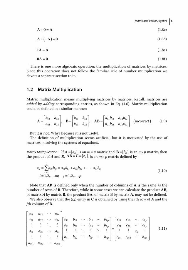
Matrix Multiplication If A [ ]aij is an m × n matrix and B [ ]bij is an n × p matrix, then the product of A and B, AB C [ ]cij , is an m × p matrix defined by
c a b a b a b a b
i m j p
ijk
n
ik kj i j i j in nj1
1 1 2 2
1 2 1 2
, , , ; , , , (1.10)
Note that AB is defined only when the number of columns of A is the same as the number of rows of B. Therefore, while in some cases we can calculate the product AB, of matrix A by matrix B, the product BA, of matrix B by matrix A, may not be defined.
We also observe that the (i,j) entry in C is obtained by using the ith row of A and the jth column of B.
a a aa a a
a a a
a a a
n
n
i i in
m m mn
11 12 1
21 22 2
1 2
1 2
��
� � � ��
� � � ��
b b b bb b b b
b b b b
j p
j p
n n nj n
11 12 1 1
21 22 2 2
1 2
� �� �
� � � � � �� � pp
p
p
ij
m m mp
c c cc c c
cc c c
11 12 1
21 22 2
1 2
��
� � ��
(1.11)
Foundations of Electromagnetic Compatibility6
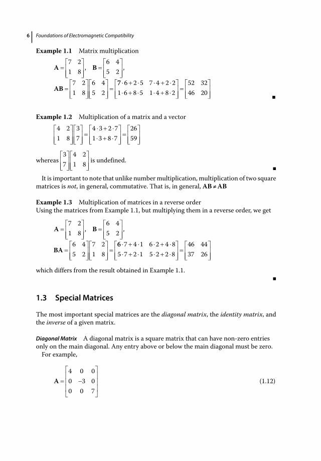
Example 1.1 Matrix multiplication
A B
AB
7 21 8
6 45 2
7 21 8
6 45 2
, ,
77 6 2 5 7 4 2 21 6 8 5 1 4 8 2
52 3246 20 ▪
Example 1.2 Multiplication of a matrix and a vector
4 21 8
37
4 3 2 71 3 8 7
2659
whereas 37
4 21 8 is undefined.
▪It is important to note that unlike number multiplication, multiplication of two square
matrices is not, in general, commutative. That is, in general, AB ≠ AB
Example 1.3 Multiplication of matrices in a reverse orderUsing the matrices from Example 1.1, but multiplying them in a reverse order, we get
A B
BA
7 21 8
6 45 2
6 45 2
7 21 8
, ,
66 7 4 1 6 2 4 85 7 2 1 5 2 2 8
46 4437 26
which differs from the result obtained in Example 1.1.▪
1.3 Special Matrices
The most important special matrices are the diagonal matrix, the identity matrix, and the inverse of a given matrix.
Diagonal Matrix A diagonal matrix is a square matrix that can have non‐zero entries only on the main diagonal. Any entry above or below the main diagonal must be zero.
For example,
A4 0 00 3 00 0 7
(1.12)
Matrix and Vector Algebra 7
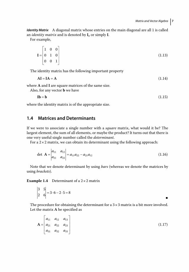
Identity Matrix A diagonal matrix whose entries on the main diagonal are all 1 is called an identity matrix and is denoted by In or simply I.
For example,
I1 0 00 1 00 0 1
(1.13)
The identity matrix has the following important property
AI IA A (1.14)
where A and I are square matrices of the same size.Also, for any vector b we have
Ib b (1.15)
where the identity matrix is of the appropriate size.
1.4 Matrices and Determinants
If we were to associate a single number with a square matrix, what would it be? The largest element, the sum of all elements, or maybe the product? It turns out that there is one very useful single number called the determinant.
For a 2 × 2 matrix, we can obtain its determinant using the following approach:
det A
a aa a a a a a
11 12
21 2211 22 21 12 (1.16)
Note that we denote determinant by using bars (whereas we denote the matrices by using brackets).
Example 1.4 Determinant of a 2 × 2 matrix
3 52 6 3 6 2 5 8
▪
The procedure for obtaining the determinant for a 3 × 3 matrix is a bit more involved.Let the matrix A be specified as
Aa a aa a aa a a
11 12 13
21 22 23
31 32 33
(1.17)
Foundations of Electromagnetic Compatibility8
Its determinant
det Aa a aa a aa a a
11 12 13
21 22 23
31 32 33
(1.18)
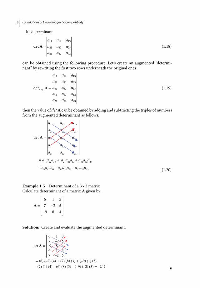
can be obtained using the following procedure. Let’s create an augmented “determi-nant” by rewriting the first two rows underneath the original ones:
detaug
a a aa a aa a aa a aa a a
A
11 12 13
21 22 23
31 32 33
11 12 13
21 22 23
(1.19)
then the value of det A can be obtained by adding and subtracting the triples of numbers from the augmented determinant as follows:
det A =
a11
a12
a13
a21
a22
a23
a31
a32
a33
a11
a12
a13
a21
a22
a23
= a11
a22
a33
+ a
21a
22a
13 + a
31a
12a
23
–a21
a12
a33
– a11
a32
a23
– a31
a22
a13 (1.20)
Example 1.5 Determinant of a 3 × 3 matrixCalculate determinant of a matrix A given by
A6 1 37 2 59 8 4
Solution: Create and evaluate the augmented determinant.
6 1 37 5
det A = 8 46 1 37 –2 5
–2–9
= (6) (–2) (4) + (7) (8) (3) + (–9) (1) (5)–(7) (1) (4) – (6) (8) (5) – (–9) (–2) (3) = –247 ▪
Matrix and Vector Algebra 9
Why do we need to know how to obtain a second‐ or third‐order determinant? Obviously, we could use a calculator or a software program to do that for us. There are numerous occasions when the software or a calculator would not be able to handle the calculations.
As we will later see, when discussing capacitive termination to a transmission line, we will need to obtain a symbolic solution in a proper form; even if we had access to a symbolic‐calculation software, its output, in most cases, would not be in a useful form.
When discussing Maxwell’s equations, we will need to evaluate a third‐order determi-nant whose entries are vectors, vector components, and differential operators. This can only be done by hand.
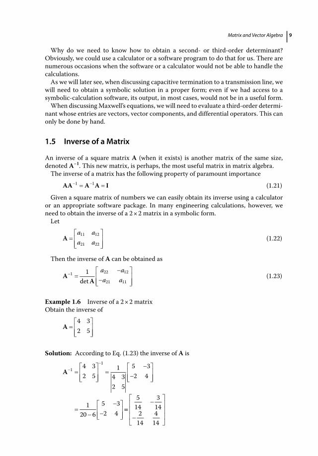
1.5 Inverse of a Matrix
An inverse of a square matrix A (when it exists) is another matrix of the same size, denoted A−1. This new matrix, is perhaps, the most useful matrix in matrix algebra.
The inverse of a matrix has the following property of paramount importance
AA A A I1 1 (1.21)
Given a square matrix of numbers we can easily obtain its inverse using a calculator or an appropriate software package. In many engineering calculations, however, we need to obtain the inverse of a 2 × 2 matrix in a symbolic form.
Let
A
a aa a
11 12
21 22 (1.22)
Then the inverse of A can be obtained as
A
A1 22 12
21 11
1det
a aa a (1.23)
Example 1.6 Inverse of a 2 × 2 matrixObtain the inverse of
A
4 32 5
Solution: According to Eq. (1.23) the inverse of A is
A 114 3
2 51
4 32 5
5 32 4
120 6
5 32 4
514
314
214
414

Foundations of Electromagnetic Compatibility10
Verification:
AA 14 32 5
514
314
214
414
20 614
12 1214
100 1014
6 2014
1 00 1
▪
1.6 Matrices and Systems of Equations
We will now explain the reason behind the “unnatural” definition of matrix multiplica-tion. Consider a system of equations:
a x a x a x ba x a x a x ba x a x a x
11 1 12 2 13 3 1
21 1 22 2 23 3 2
31 1 32 2 33 3 bb3
(1.24)
Let’s define three matrices as follows:
A xa a aa a aa a a
xxx
11 12 13
21 22 23
31 32 33
1
2
3
, ,, bbbb
1
2
3
(1.25)
Then the system of equations (1.24) can be written in compact form using matrices defined by Eq. (1.25) as
Ax b (1.26)
Since
Axa a aa a aa a a
xxx
a
11 12 13
21 22 23
31 32 33
1
2
3
111 1 12 2 13 3
21 1 22 2 23 3
31 1 32 2 33 3
x a x a xa x a x a xa x a x a x
bbb
1
2
3
b
(1.27)
and two matrices are equal when their corresponding entries are equal. Thus, Eqs (1.24) and (1.27) are equivalent.
Equation (1.26) shows one of the benefits of using matrices: a system of linear equa-tion can be expressed in a compact form. An even more important benefit is the fact that we can obtain the solution to the system of equations by manipulating the matrices in a symbolic form instead of the equations themselves. This will be shown in the next section.

Matrix and Vector Algebra 11
1.7 Solution of Systems of Equations
Consider a system of equations:
Ax b (1.28)
If the inverse of A exists, then premultiplication of Eq. (1.28) by A 1 results in
A Ax A b1 1 (1.29)
Since A−1A = I, it follows
Ix A b1 (1.30)
Because Ix = x, we obtain the solution to Eq. (1.28) as
x A b1 (1.31)
Example 1.7 Solution of systems of equations using matrix inverseObtain the solution of
4 3 122 5 8
1 2
1 2
x xx x
using matrix inversion.
Solution: Our system of equations in matrix form can be written as
4 32 5
128
1
2
xx
According to Eq. (1.31), the solution, therefore, can be written as
xx
1
2
14 32 5
128
Utilizing the result of Example 1.6, we have
xx
1
2
14 32 5
128
514
314
214
414
128
514
12 314
8
214
122 414
8
64
▪
Foundations of Electromagnetic Compatibility12
1.8 Cramer’s Rule
As we have seen, we can obtain a solution to a system of equations using matrix inver-sion. When dealing with 2 × 2 matrices, it is sometimes more expedient to use an alter-native approach using Cramer’s rule.
Let the system of equations be given by
a x a x ba x a x b
11 1 12 2 1
21 1 22 2 2 (1.32)
or in a matrix form:
Ax b (1.33)
where
A x b
a aa a
xx
bb
11 12
21 22
1
2
1
2, , (1.34)
The main determinant of the system is
D
a aa a
11 12
21 22 (1.35a)
Let’s create two additional determinants D1 by replacing the first column of D with the column vector b, and the determinant D2 by replacing the second column of D by the column vector b. That is,
D
b ab a1
1 12
2 22 (1.35b)
D
a ba b2
11 1
21 2 (1.35c)
Then the solution of the system of equations in (1.32) is
x D
Dx D
DD1
12
2 0, , (1.36)
Example 1.8 Solution of systems of equations using Cramer’s ruleWe will use the same system of equations as in Example 1.7.
4 3 122 5 8
1 2
1 2
x xx x
Matrix and Vector Algebra 13
Using Cramer’s rule we obtain the solutions as
x
x
1
2
12 38 5
4 32 5
12 5 8 34 5 2 3
6
12 38 5
4 32 5
44 8 2 124 5 2 3
4
which, of course, agrees with the solution of the previous example.
▪
1.9 Vector Operations
In this section we define two fundamental operations on them: scalar product and vector product.
1.9.1 Scalar Product
Scalar product (or inner product, or dot product) of two vectors A and B, denoted A B, is defined as
A B A B cos (1.37)
where 0 is the angle between A and B (computed when the vectors have their initial points coinciding).
Note that the result of a scalar product, as the name indicates, is a scalar (number).Also note that when two vectors are perpendicular to each other, their scalar product
is zero.
if 90 0cos (1.38)
The order of multiplication in a scalar product does not matter, that is,
A B B A (1.39)
1.9.2 Vector Product
Vector product (or cross product) of two vectors A and B, denoted A B, is defined as a vector V whose length is
V A B sin (1.40)
where γ is the angle between A and B, and whose direction is perpendicular to both A and B and is such that A, B, and V, in this order, form a right‐handed triple.
Foundations of Electromagnetic Compatibility14
Note that a vector product results in a vector. Also note that when two vectors are parallel to each other, their vector product is a zero vector.
if 0 0sin (1.41)
The order of multiplication in a vector product does matter, since
A B B A (1.42)
1.10 EMC Applications
1.10.1 Crosstalk Model of Transmission Lines
In this section we will show how the matrices can be used to describe a mathematical model of the crosstalk between wires in cables or between PCB traces.
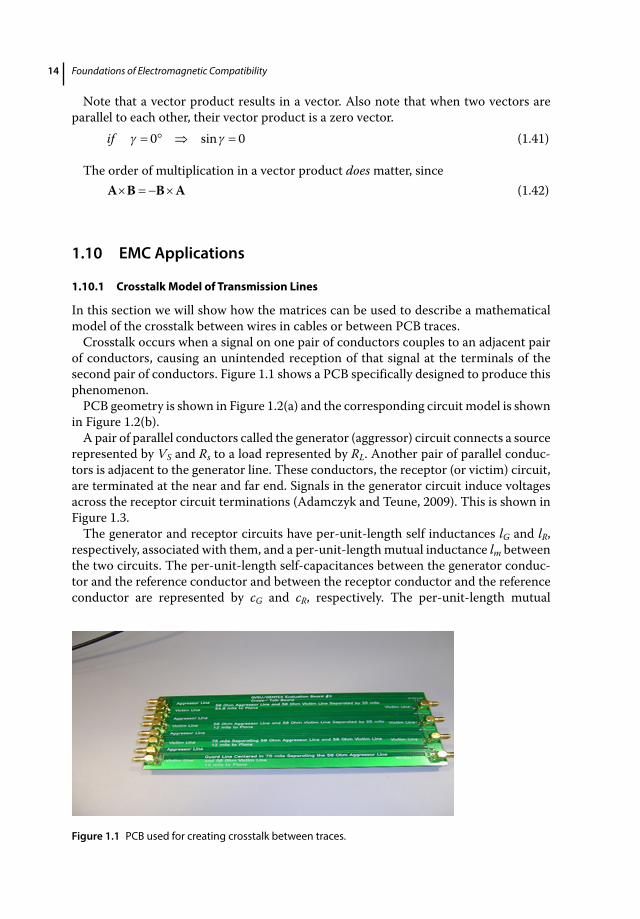
Crosstalk occurs when a signal on one pair of conductors couples to an adjacent pair of conductors, causing an unintended reception of that signal at the terminals of the second pair of conductors. Figure 1.1 shows a PCB specifically designed to produce this phenomenon.
PCB geometry is shown in Figure 1.2(a) and the corresponding circuit model is shown in Figure 1.2(b).
A pair of parallel conductors called the generator (aggressor) circuit connects a source represented by VS and Rs to a load represented by RL. Another pair of parallel conduc-tors is adjacent to the generator line. These conductors, the receptor (or victim) circuit, are terminated at the near and far end. Signals in the generator circuit induce voltages across the receptor circuit terminations (Adamczyk and Teune, 2009). This is shown in Figure 1.3.
The generator and receptor circuits have per‐unit‐length self inductances lG and lR, respectively, associated with them, and a per‐unit‐length mutual inductance lm between the two circuits. The per‐unit‐length self‐capacitances between the generator conduc-tor and the reference conductor and between the receptor conductor and the reference conductor are represented by cG and cR, respectively. The per‐unit‐length mutual
Figure 1.1 PCB used for creating crosstalk between traces.
Related Documents