Formal analysis of trace conditioning

Formal Analysis of Trace Conditioning 1

Running head: Formal Analysis of Trace Conditioning

Formal Analysis of Trace Conditioning

Tibor Bosse

Vrije Universiteit Amsterdam

Catholijn M. Jonker

Radboud Universiteit Nijmegen

Sander A. Los

Vrije Universiteit Amsterdam

Leendert van der Torre

University of Luxembourg

Jan Treur

Vrije Universiteit Amsterdam

Contact information:

Vrije Universiteit Amsterdam Department of Artificial Intelligence Room T3.20a De Boelelaan 1081a 1081 HV Amsterdam The Netherlands Email: [email protected] Office: +31 20 598 7750 Fax: +31 20 598 7653

Formal Analysis of Trace Conditioning 2

Formal Analysis of Trace Conditioning 3

Abstract

In the literature classical conditioning is usually described and analysed informally. If

formalisation is used, this is often based on mathematical models based on difference or

differential equations. This paper explores a formal description and analysis of the process of

trace conditioning, based on logical specification and analysis methods of dynamic properties of

the process. Specific types of dynamic properties are global dynamic properties, describing

properties of the process as a whole, or local dynamic properties, describing properties of basic

steps in a conditioning process. If the latter type of properties are specified in an executable

format, they provide a temporal declarative specification of a simulation model. By a software

environment these local properties can be used to actually perform simulation. Global properties

can be checked automatically for simulated or other traces. Using these methods the properties of

conditioning processes informally expressed by Los and Van Den Heuvel (2001) have been

formalised and verified against a specification of local properties based on Machado (1997)’s

differential equation model.

Formal Analysis of Trace Conditioning 4

Formal Analysis of Trace Conditioning

Introduction

A common approach to describe dynamics of cognitive processes is by relating sensory,

cognitive or behavioural states to previous or subsequent states. For example, this is shown in

approaches from what in Philosophy of Mind is called the functionalist perspective, where the

functional role of a mental state property is defined by its predecessor and successor states. Also

in Dynamical Systems Theory (DST), a relatively new approach to describe the dynamics of

cognitive processes, which subsumes connectionist modelling, e.g., (Port and Gelder, 1995),

relations of a state with previous and subsequent states are central. Gelder and Port (1995)

briefly explained what a dynamical system is in the following manner. A system is a set of

changing aspects (or state properties) of the world. A state at a given point in time is the way

these aspects or state properties are at that time; so a state is characterised by the state properties

that hold. The set of all possible states is the state space. A behaviour of the system is the change

of these state properties over time, or, in other words, a succession or sequence of states within

the state space. Such a sequence in the state space can be indexed, for example, by natural

numbers (discrete case) or real numbers (continuous case), and is also called a trace or

trajectory. Given these notions, the notion of state-determined system, adopted from (Ashby,

1960) is taken as the basis to describe what a dynamical system is:

‘A system is state-determined only when its current state always determines a unique future behaviour. (..) the future

behaviour cannot depend in any way on whatever states the system might have been in before the current state. In

other words, past history is irrelevant (or at least, past history only makes a difference insofar as it has left an effect

on the current state). (..) the fact that the current state determines future behaviour implies the existence of some rule

of evolution describing the behaviour of the system as a function of its current state.’ (Gelder and Port, 1995, p. 6).

Formal Analysis of Trace Conditioning 5

The assumption of state-based systems, which is fundamental for DST, entails a local

modelling perspective where states are related to immediate predecessor and successor states.

This local modelling perspective, which DST has in common with the functional perspective

based on causal relations mentioned earlier, is especially useful for simulation purposes.

However, more indirect or global temporal relations between states are beyond such a modelling

approach.

In more sophisticated cognitive processes, a cognitive state or a behaviour can be better

understood in a more global manner, e.g., in the way in which it depends on a longer history of

experiences or inputs. In experimental research, examples of such phenomena are usually

indicated as inter-trial or adaptive effects. Approaches to model such more sophisticated

cognitive processes require means to express a more advanced temporal complexity than for the

less sophisticated processes, where direct succession relations between states suffice as

appropriate means.

Various types of adaptive or learning behaviour are known and have been studied in some

depth. For example, for various forms of learned stimulus-response behaviours it has been

studied how they are determined by an attained cognitive state of the organism. Still, the

question remains how such attained cognitive states themselves depend on the previous history,

for example on a particular training session extending over a longer time period. Often insight is

obtained by formulating such more complex temporal relationships. However, usually such

complex temporal relationships are expressed purely informally, due to the lack of modelling

techniques that reach beyond the local perspective.

In order to temporally relate states to states at other points in time in a more global manner,

modelling approaches to dynamical systems of a different type have recently been proposed.

Formal Analysis of Trace Conditioning 6

Within the areas of Computer Science and Artificial Intelligence techniques have been developed

to analyse the dynamics of phenomena using logical means. Examples are dynamic and temporal

logic, and event and situation calculus; e.g., (Eck et al., 2001; Kowalski and Sergot, 1986; Reiter,

2001). These logical techniques allow to consider and relate states of a process at different points

in time, and in this sense reach beyond the local perspective. The form in which these relations

are expressed can cover qualitative aspects, but also quantitative aspects.

This paper addresses temporal aspects of conditioning and illustrates the usefulness of a

logical approach for the analysis and formalisation of such processes both at a local and at a

more global level. First a local perspective model for temporal conditioning in a high-level

executable format is presented. This executable model can be compared to (and was inspired by)

Machado (1997)’s differential equation model. Some simulation traces are shown and compared

to traces of Machado (1997)’s model.

Next, as part of a non-local perspective analysis, a number of relevant dynamic properties of

the conditioning process are identified and formalised. These dynamic properties were obtained

by formalising the informally expressed properties to characterise temporal conditioning

processes, as put forward by Los and Van Den Heuvel (2001). It has been automatically verified

that (under reasonable conditions) these global dynamic properties are satisfied by the simulation

traces.

Temporal Dynamics of Conditioning

Below, first some basic terminology used in the area of conditioning is introduced. Next,

based on this terminology, Machado (1997)’s differential equation model for conditioning is

briefly explained.

Formal Analysis of Trace Conditioning 7

Basic Concepts of Conditioning

The aim of research into conditioning is to reveal the principles that govern associative

learning. To this end, several experimental procedures have been developed. In classical

conditioning, an organism is presented with an initially neutral conditioned stimulus (e.g., a bell)

followed by an unconditioned stimulus (e.g., meat powder) that elicits an innate or learned

unconditioned response in the organism (e.g. saliva production for a dog). After acquisition, the

organism elicits an adaptive conditioned response (also saliva production in the example) when

the conditioned stimulus is presented alone. In operant conditioning, the production of a certain

operant response that is part to the volitional repertoire of an organism (e.g., bar pressing for a

rat) is strengthened after repeated reinforcement (e.g., food presentation) contingent on the

operant response.

In their review, Gallistel and Gibbon (2000) argued that these different forms of conditioning

have a common foundation in the adaptive timing of the conditioned (or operant) response to the

appearance of the unconditioned stimulus (or reinforcement). This feature is most apparent in an

experimental procedure called trace conditioning, in which a blank interval (or 'trace') of a

certain duration separates the conditioned and unconditioned stimulus (in classical conditioning)

or subsequent reinforcement phases (in operant conditioning). In either case, the conditioned (or

operant) response obtains its maximal strength, here called peak level, at a moment in time,

called peak time, that closely corresponds to the moment the unconditioned stimulus (or

reinforcement) occurs.

For present purposes, we adopt the terminology of an experimental procedure that is often

used to study adaptive timing and the possible role of conditioning in humans. In this procedure,

a trial starts with the presentation of a warning stimulus (S1; comparable to a conditioned

Formal Analysis of Trace Conditioning 8

stimulus). After a blank interval, called the foreperiod (FP), an imperative stimulus (S2,

comparable to an unconditioned stimulus) is presented to which the participant responds as fast

as possible. The reaction time (RT) to S2 is used as an estimate of the conditioned state of

preparation at the moment S2 is presented.

In this type of research, FP is usually varied at several discrete levels. That is, S2 can be

presented at several moments since the offset of S1, which are called critical moments. The

moment that is used for the presentation of S2 on any given trial is called the imperative moment

of that trial. A final distinction concerns the way the different levels of FP are presented to the

participant. In a pure block, the same FP is used across all trials of that block (and varied

between different pure blocks). That is, in a pure block there is one critical moment that

corresponds to the imperative moment on each trial. In a mixed block, all levels of FP occur

randomly across trials. That is, a mixed block has several critical moments, but on any specific

trial, only one of the moments is the imperative moment.

Modelling Conditioning by Differential Equations

Machado (1997) presented a basic model of the dynamics of a conditioning process. The

structure of this model, with an adjusted terminology as used by Los, Knol, and Boers (2001), is

shown in Figure 1. The model posits a layer of timing nodes (Machado calls these behavioral

states) and a single preparation node (called operant response by Machado). Each timing node

is connected both to the next (and previous) timing node and to the preparation node. The

connection between each timing node and the preparation node (called associative link both by

Machado and within the current paper) has an adjustable weight associated to it. Upon the

presentation of a warning stimulus, a cascade of activation propagates through the timing nodes

according to a regular pattern. Owing to this regularity, the timing nodes can be likened to an

Formal Analysis of Trace Conditioning 9

internal clock or pacemaker. At any moment, each timing node contributes to the activation of

the preparation node in accordance with its activation and its corresponding weight. The

activation of the preparation node reflects the participant's preparatory state, and is as such

related to reaction time for any given imperative moment.

The weights reflect the state of conditioning, and are adjusted by learning rules, of which the

main principles are as follows. First, during the foreperiod extinction takes place, which involves

the decrease of weights in real time in proportion to the activation of their corresponding timing

nodes. Second, after the presentation of the imperative stimulus a process of reinforcement takes

over, which involves an increase of the weights in accordance with the current activation of their

timing nodes, to preserve the importance of the imperative moment. In Machado (1997) the more

detailed dynamics of the process are given by a mathematical model (based on linear differential

equations), representing the (local) temporal relationships between the variables involved. For

example, d/dt X(t,n) = λX(t,n-1) - λX(t,n) expresses how the activation level of the n-th timing node

X(t+dt,n) at time point t+dt relates to this level X(t,n) at time point t and the activation level X(t,n-1)

of the (n-1)-th timing node at time point t. Similarly, as another example, d/dt W(t,n) = -

αX(t,n)W(t,n) expresses how the n-th weight W(t+dt,n) at time point t+dt relates to this weight

W(t,n) at time point t and the activation level X(t,n) of the n-th timing node at time point t.

Modelling in terms of Dynamic Properties

As discussed above, mathematical models based on differential equations can be used to

model (1) in a quantitative manner, (2) local temporal relationships within conditioning

processes. However, conditioning processes can also be characterised by temporal relationships

of a less local form. As an example, taken from Los and Van Den Heuvel (2001), a dynamic

property can be formulated expressing the monotonicity property that ‘ the response level

Formal Analysis of Trace Conditioning 10

increases before the critical moment is reached and decreases after this moment’. This is a more

global property, relating response levels at any two points in time before the critical moment (or

after the critical moment). Therefore it is useful to explore formalisation techniques, as an

alternative to differential equations, to express not only for local properties, but also for non-

local properties. A second limitation of differential equations is that they are based on

quantitative (calculational) relationships, whereas also non-quantitative aspects may play a role

(for example, the monotonicity property mentioned above). This suggests that it may be useful to

explore alternative formalisation techniques for dynamic properties of conditioning processes

that both allow to express quantitative and non-quantitative aspects.

As already mentioned in the Introduction, the approach presented in this paper indeed

introduces alternative formalisation languages to express dynamic properties of conditioning

processes, both for local and nonlocal properties and both for quantitative and non-quantitative

aspects. These formalisation languages are briefly introduced in the next section. After this

introduction, in a subsequent section first a model based on local properties of a conditioning

process is presented (comparable to and inspired by Machado’s model).

Languages to Model Dynamic Properties

The domain of reasoning about dynamical systems in disciplines such as the Behavioural

Sciences requires an abstract modelling form yet showing the essential dynamic properties. A

high-level language is needed to characterise and formalise dynamic properties of such a

dynamical system. To this end the Temporal Trace Language TTL is used as a tool; for previous

applications of this language to the analysis of (cognitive) processes, (see Jonker and Treur,

2002; Jonker and Treur, 2003a,b; Jonker, Treur, and Vries, 2002). Using this language, dynamic

properties can be expresed in informal, semi-formal, or formal format. Moreover, to perform

Formal Analysis of Trace Conditioning 11

simulations, models are desired that can be formalised and are computationally easy to handle.

These executable models are based on the socalled LEADSTO format which is defined as a

sublanguage of TTL (Bosse et al., 2005); for a previous application of this format for simulation

of cognitive processes, see (Jonker, Treur, and Wijngaards, 2003). The Temporal Trace

Language TTL is briefly defined as follows.

A state ontology is a specification (in order-sorted logic) of a vocabulary to describe a state

of a process. A state for ontology Ont is an assignment of truth-values true or false to the set

At(Ont) of ground atoms expressed in terms of Ont. The set of all possible states for state

ontology Ont is denoted by STATES(Ont). The set of state properties STATPROP(Ont) for state

ontology Ont is the set of all propositions over ground atoms from At(Ont). A fixed time frame T

is assumed which is linearly ordered, for example the natural or real numbers. A trace γ over a

state ontology Ont and time frame T is a mapping γ: T → STATES(Ont), i.e., a sequence of states γt

(t ∈ T) in STATES(Ont). The set of all traces over state ontology Ont is denoted by TRACES(Ont).

The set of dynamic properties DYNPROP(Ont) is the set of temporal statements that can be

formulated with respect to traces based on the state ontology Ont in the following manner.

These states can be related to state properties via the formally defined satisfaction relation |==,

comparable to the Holds-predicate in the Situation Calculus (cf. Reiter, 2001): state(γ, t) |== p

denotes that state property p holds in trace γ at time t. Based on these statements, dynamic

properties can be formulated , using quantifiers over time and the usual first-order logical

connectives ¬ (not), ∧ (and), ∨ (or), � (implies), ∀ (for all), ∃ (there exists); to be more formal:

formulae in a sorted first-order predicate logic with sorts T for time points, Traces for traces and

F for state formulae.

Formal Analysis of Trace Conditioning 12

To model basic mechanisms of a process at a lower aggregation level, direct temporal

dependencies between two state properties, the simpler LEADSTO format is used. This

executable format can be used for simulation and is defined as follows. Let α and β be state

properties. In LEADSTO specifications the notation α →→e, f, g, h β, means:

if state property α holds for a certain time interval with duration g, then after some delay

(between e and f) state property β will hold for a certain time interval h.

For a more formal definition, see (Jonker, Treur, and Wijngaards, 2003) and (Bosse et al.,

2005).

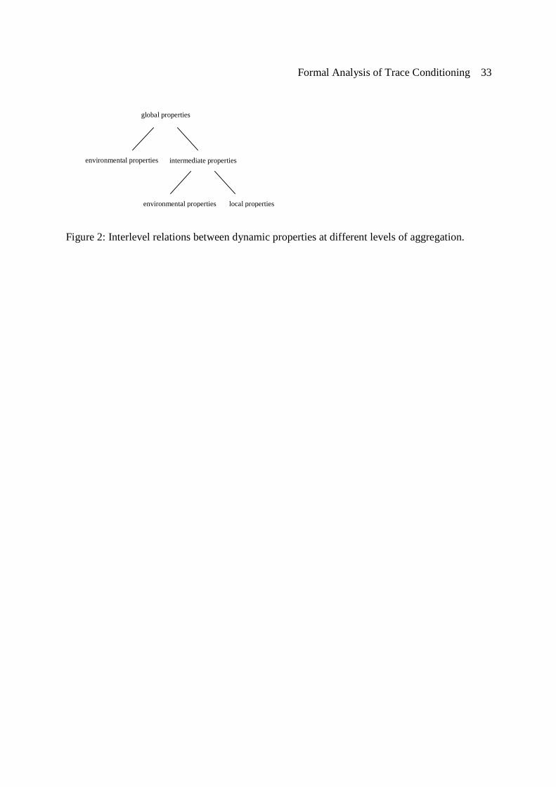
Types of Dynamic Properties

Dynamic properties of a conditioning process can be specfied at different levels of

aggregation. At the highest level, global dynamic properties, i.e., properties of the conditioning

process as a whole, can be expressed, for example indicating how a certain pattern of behaviour

has been changed by a conditioning process. At the lowest level of aggregation, local properties

are dynamic properties of the basic mechanisms of the conditioning process. Based on these

local properties, and certain conditions of the environment, the global properties of the system

emerge. Such conditions of the environment (of the subject) are characterised by environmental

properties. In laboratory circumstances, these properties are usually guaranteed by a specific

experimental design.

Local properties are logically related to global properties in the sense that the local properties

together with the relevant environmental properties entail the global properties. To clarify such

logical interlevel relations, it is often useful to specify dynamic properties at intermediate levels

of aggregation: intermediate properties. Thus the overall picture shown in Figure 2 is obtained.

Formal Analysis of Trace Conditioning 13

Local Dynamic Properties

This section presents the local properties (LPs) that were defined in order to describe the

conditioning process from a local perspective. These properties are executable dynamic

properties (in LEADSTO format) of the elements of this model. Within the dynamic properties

the following state properties are used:

X(n,u) Timing node n has activation level u. In the current simulation, n ranges over the discrete

domain [0,5]. Thus, our model consists of six timing nodes. The activation level u can take

any continuous value in the domain [0,1].

W(n,v) Associative link n has weight v. Again, n ranges over the discrete domain [0,5]. The weight v

can take any continuous value in the domain [0,1].

R(r) The preparation node has response strength r (a continuous value in the domain [0,1]).

S1(s) Warning stimulus S1 occurs with strength s. Within our example, s only takes the values 0.0 and

1.0. However, the model could be extended by allowing any continuous value in-between.

S2(s) Imperative stimulus S2 occurs with strength s.

Xcopy(n,u) Timing node n had activation level u at the moment of the occurrence of the last imperative

stimulus (S2). See dynamic property LP4 and LP6.

instage(ext) The process is in a stage of extinction. This stage lasts from the occurrence of S1 until the

occurrence of S2.

instage(reinf) The process is in a stage of reinforcement. This stage starts with the occurrence of S2, and lasts

during a predefined reinforcement period, (e.g. 3 seconds).

instage(pers) The process is in a stage of persistence. This stage starts right after the reinforcement stage, and

lasts until the next occurrence of S1.

As Machado (1997)’s model was used as a source of inspiration, for some of the properties

presented below the comparable differential equation within Machado's model is given as well.

However, since Machado's mathematical approach differs at several points from the logical

approach presented in this paper, there is not always a straightforward 1:1 mapping between both

formalisations. For instance, state property X(n,u) within our LEADSTO formalisation has a

slightly different meaning than the corresponding term X(t,n) in Machado's differential equations.

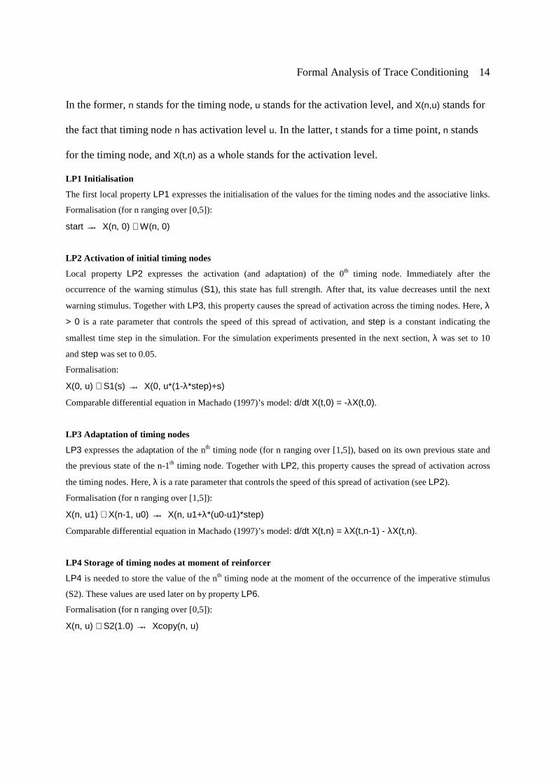
Formal Analysis of Trace Conditioning 14

In the former, n stands for the timing node, u stands for the activation level, and X(n,u) stands for

the fact that timing node n has activation level u. In the latter, t stands for a time point, n stands

for the timing node, and X(t,n) as a whole stands for the activation level.

LP1 Initialisation

The first local property LP1 expresses the initialisation of the values for the timing nodes and the associative links.

Formalisation (for n ranging over [0,5]):

start →→ X(n, 0) ∧ W(n, 0)

LP2 Activation of initial timing nodes

Local property LP2 expresses the activation (and adaptation) of the 0th timing node. Immediately after the

occurrence of the warning stimulus (S1), this state has full strength. After that, its value decreases until the next

warning stimulus. Together with LP3, this property causes the spread of activation across the timing nodes. Here, λ

> 0 is a rate parameter that controls the speed of this spread of activation, and step is a constant indicating the

smallest time step in the simulation. For the simulation experiments presented in the next section, λ was set to 10

and step was set to 0.05.

Formalisation:

X(0, u) ∧ S1(s) →→ X(0, u*(1-λ*step)+s)

Comparable differential equation in Machado (1997)’s model: d/dt X(t,0) = -λX(t,0).

LP3 Adaptation of timing nodes

LP3 expresses the adaptation of the nth timing node (for n ranging over [1,5]), based on its own previous state and

the previous state of the n-1th timing node. Together with LP2, this property causes the spread of activation across

the timing nodes. Here, λ is a rate parameter that controls the speed of this spread of activation (see LP2).

Formalisation (for n ranging over [1,5]):

X(n, u1) ∧ X(n-1, u0) →→ X(n, u1+λ*(u0-u1)*step)

Comparable differential equation in Machado (1997)’s model: d/dt X(t,n) = λX(t,n-1) - λX(t,n).

LP4 Storage of timing nodes at moment of reinforcer

LP4 is needed to store the value of the nth timing node at the moment of the occurrence of the imperative stimulus

(S2). These values are used later on by property LP6.

Formalisation (for n ranging over [0,5]):

X(n, u) ∧ S2(1.0) →→ Xcopy(n, u)

Formal Analysis of Trace Conditioning 15

LP5 Extinction of associative links

LP5 expresses the adaptation of the associative links during extinction, based on their own previous state and the

previous state of the corresponding timing node. Here, α is a learning rate parameter. For the simulation experiments

presented in the next section, the value 2 was chosen for α. Formalisation (for n ranging over [0,5]):

instage(ext) ∧ X(n, u) ∧ W(n, v) →→ W(n, v*(1-α*u*step))

Comparable differential equation in Machado (1997)’s model: d/dt W(t,n) = -αX(t,n)W(t,n)

LP6 Reinforcement of associative links

LP6 expresses the adaptation of the associative links during reinforcement, based on their own previous state and

the previous state of Xcopy. Here, β is a learning rate parameter. For the simulation experiments presented in the

next section, the value 2 was chosen for β.

Formalisation (for n ranging over [0,5]):

instage(reinf) ∧ Xcopy(n, u) ∧ W(n, v) →→ W(n, v*(1-β*u*step) + β*u*step)

Comparable differential equation in Machado (1997)’s model: d/dt W(t,n) = βX(T,n)[K-W(t,n)].

LP7 Persistence of associative links

LP7 expresses the persistence of the associative links at the moments that there is neither extinction not

reinforcement.

Formalisation (for n ranging over [0,5]):

instage(pers) ∧ W(n, v) →→ W(n, v)

LP8 Response function

LP8 calculates the response by adding the discriminative function of all states, i.e., their associative links multiplied

by the degree of activation of the corresponding state.

Formalisation:

W(1, v1) ∧ W(2, v2) ∧ W(3, v3) ∧ W(4, v4) ∧ W(5, v5) ∧ X(1, u1) ∧ X(2, u2) ∧ X(3, u3) ∧ X(4, u4) ∧ X(5,

u5) →→ R(v1*u1 + v2*u2 + v3*u3 + v4*u4 + v5*u5)

LP9 Initialisation of stage pers

LP9 expresses that the initial stage of the process is pers.

Formalisation:

start →→ instage(pers)

LP10 Transition to stage ext

LP10 expresses that the process switches to stage ext when a warning stimulus occurs.

Formalisation:

S1(1.0) →→ instage(ext)

Formal Analysis of Trace Conditioning 16

LP11 Persistence of stage ext

LP11 expresses that the process persists in stage ext as long as no imperative stimulus occurs.

Formalisation:

instage(ext) ∧ S2(0.0) →→ instage(ext)

LP12 Transition to stage reinf and pers

LP12 expresses that the process first switches to stage reinf for a while, and then to stage pers when an imperative

stimulus occurs. Notice that LP12a and LP12b must have different timing parameters to make sure both stages do

not occur simultaneously.

Formalisation:

S2(1.0) →→ instage(reinf) (LP12a)

S2(1.0) →→ instage(pers) (LP12b)

LP13 Persistence of stage pers

LP13 expresses that the process persists in stage pers as long as no warning stimulus occurs.

Formalisation:

instage(pers) ∧ S1(0.0) →→ instage(pers)

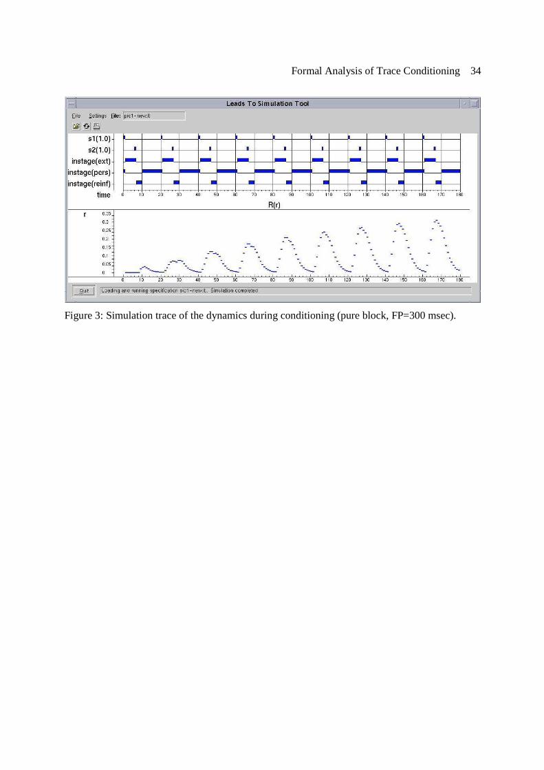
Simulation

Simulation of executable models is performed by a special software environment. This

software environment generates simulation traces of the conditioning process based on an input

consisting of dynamic properties in LEADSTO format (Bosse et al., 2005). A large number

(about 20) of such traces have been generated, with different parameters for foreperiod (50, 100,

150, 200, 300, 350, and 500 msec), selected on the basis of (Los, Knol, and Boers, 2001). An

example of such a trace can be seen in Figure 3. Here, time is on the horizontal axis. Each time

unit corresponds to 50 msec. The relevant state properties (S1, S2, instage(ext), instage(pers),

instage(reinf) and R) are on the vertical axis. A dark box on top of the line indicates that the

property is true during that time period.

This trace is based on all local properties presented above. For almost all properties, the

timing parameters (0,0,1,1) were used. Exceptions are the properties LP4, LP12a and LP12b. For

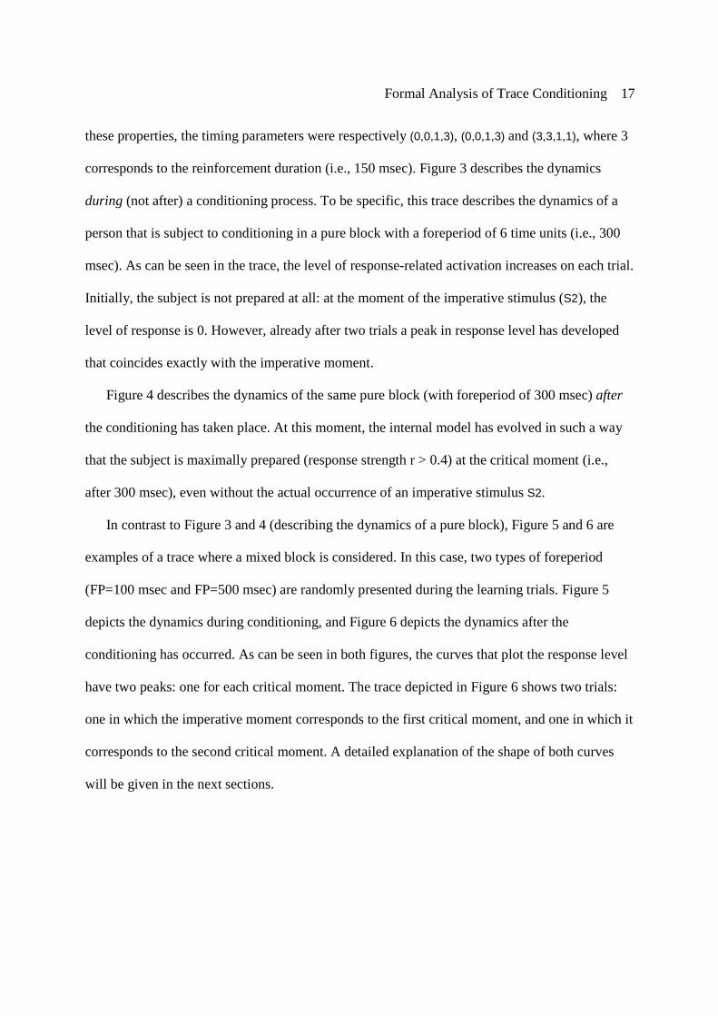
Formal Analysis of Trace Conditioning 17

these properties, the timing parameters were respectively (0,0,1,3), (0,0,1,3) and (3,3,1,1), where 3

corresponds to the reinforcement duration (i.e., 150 msec). Figure 3 describes the dynamics

during (not after) a conditioning process. To be specific, this trace describes the dynamics of a

person that is subject to conditioning in a pure block with a foreperiod of 6 time units (i.e., 300

msec). As can be seen in the trace, the level of response-related activation increases on each trial.

Initially, the subject is not prepared at all: at the moment of the imperative stimulus (S2), the

level of response is 0. However, already after two trials a peak in response level has developed

that coincides exactly with the imperative moment.

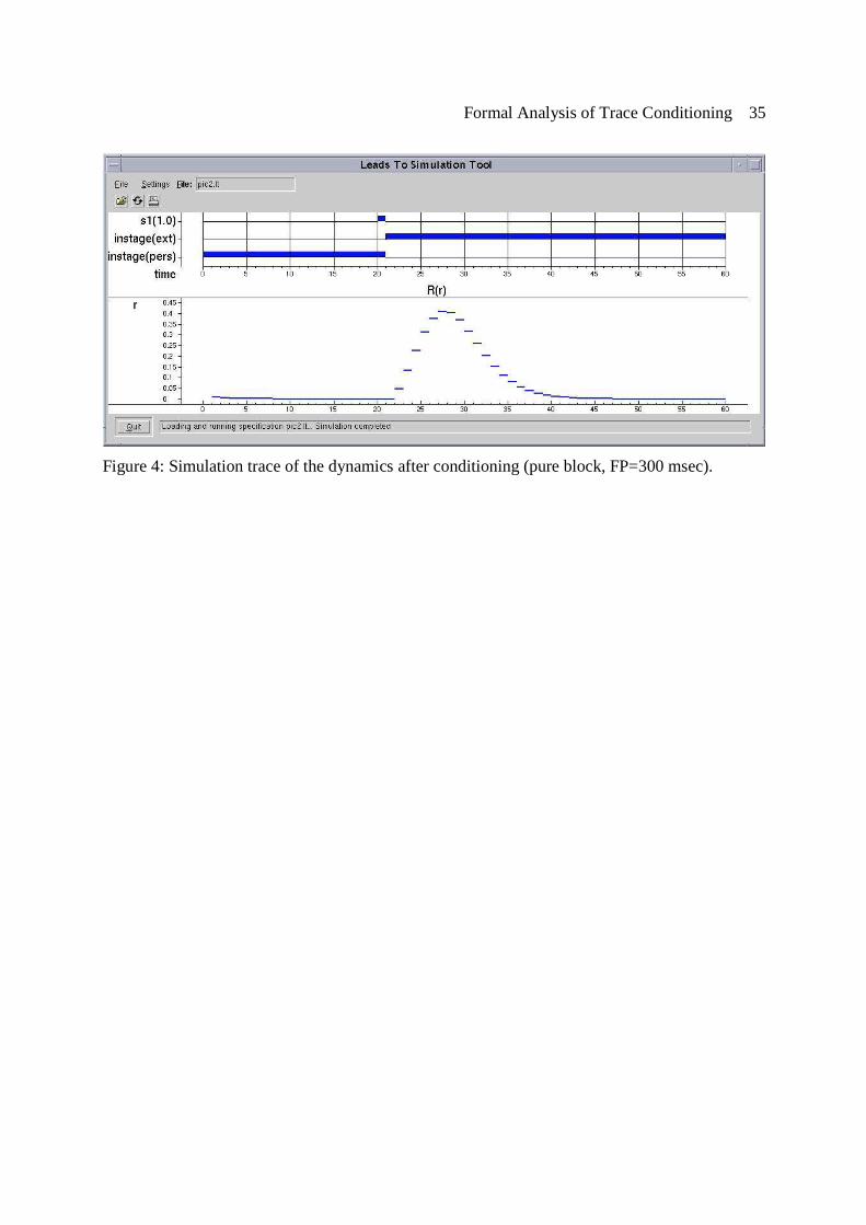
Figure 4 describes the dynamics of the same pure block (with foreperiod of 300 msec) after

the conditioning has taken place. At this moment, the internal model has evolved in such a way

that the subject is maximally prepared (response strength r > 0.4) at the critical moment (i.e.,

after 300 msec), even without the actual occurrence of an imperative stimulus S2.

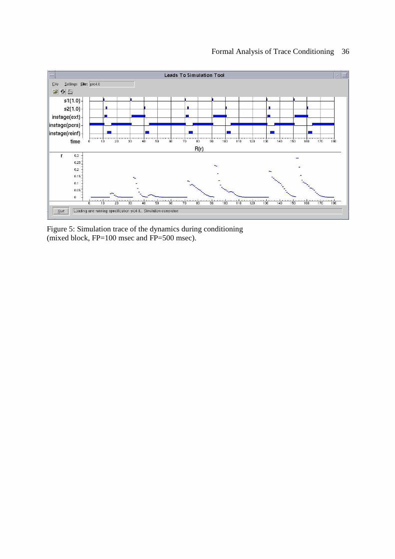
In contrast to Figure 3 and 4 (describing the dynamics of a pure block), Figure 5 and 6 are

examples of a trace where a mixed block is considered. In this case, two types of foreperiod

(FP=100 msec and FP=500 msec) are randomly presented during the learning trials. Figure 5

depicts the dynamics during conditioning, and Figure 6 depicts the dynamics after the

conditioning has occurred. As can be seen in both figures, the curves that plot the response level

have two peaks: one for each critical moment. The trace depicted in Figure 6 shows two trials:

one in which the imperative moment corresponds to the first critical moment, and one in which it

corresponds to the second critical moment. A detailed explanation of the shape of both curves

will be given in the next sections.

Formal Analysis of Trace Conditioning 18

As mentioned above, a number of similar experiments have been performed, with different

parameters for foreperiod and block type. The results were consistent with the date produced by

Machado.

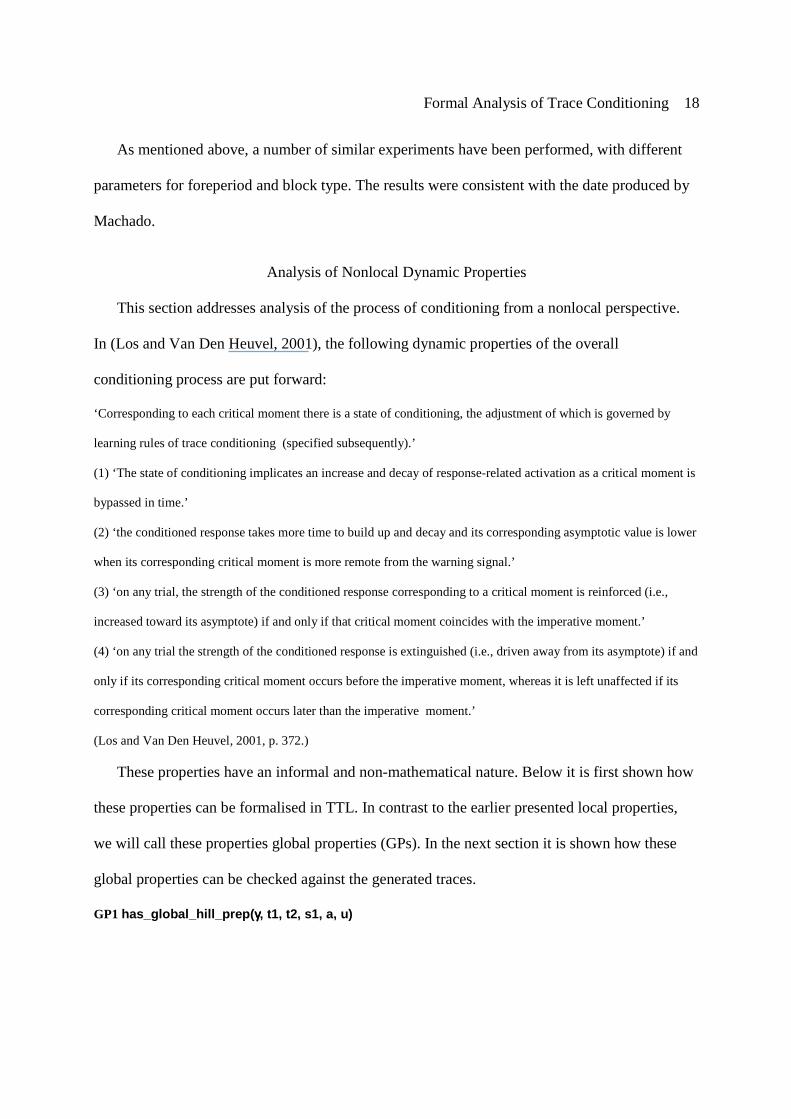
Analysis of Nonlocal Dynamic Properties

This section addresses analysis of the process of conditioning from a nonlocal perspective.

In (Los and Van Den Heuvel, 2001), the following dynamic properties of the overall

conditioning process are put forward:

‘Corresponding to each critical moment there is a state of conditioning, the adjustment of which is governed by

learning rules of trace conditioning (specified subsequently).’

(1) ‘The state of conditioning implicates an increase and decay of response-related activation as a critical moment is

bypassed in time.’

(2) ‘ the conditioned response takes more time to build up and decay and its corresponding asymptotic value is lower

when its corresponding critical moment is more remote from the warning signal.’

(3) ‘on any trial, the strength of the conditioned response corresponding to a critical moment is reinforced (i.e.,

increased toward its asymptote) if and only if that critical moment coincides with the imperative moment.’

(4) ‘on any trial the strength of the conditioned response is extinguished (i.e., driven away from its asymptote) if and

only if its corresponding critical moment occurs before the imperative moment, whereas it is left unaffected if its

corresponding critical moment occurs later than the imperative moment.’

(Los and Van Den Heuvel, 2001, p. 372.)

These properties have an informal and non-mathematical nature. Below it is first shown how

these properties can be formalised in TTL. In contrast to the earlier presented local properties,

we will call these properties global properties (GPs). In the next section it is shown how these

global properties can be checked against the generated traces.

GP1 has_global_hill_prep(γγγγ, t1, t2, s1, a, u)

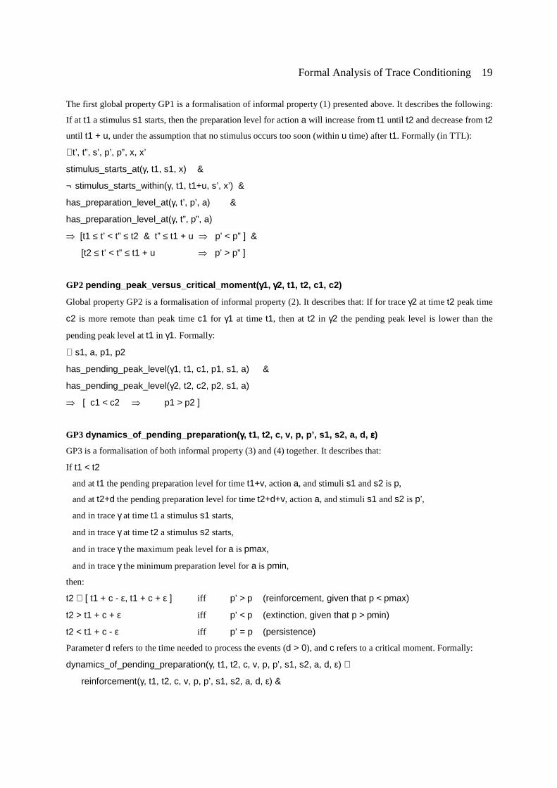
Formal Analysis of Trace Conditioning 19

The first global property GP1 is a formalisation of informal property (1) presented above. It describes the following:

If at t1 a stimulus s1 starts, then the preparation level for action a will increase from t1 until t2 and decrease from t2

until t1 + u, under the assumption that no stimulus occurs too soon (within u time) after t1. Formally (in TTL):

∀t’, t”, s’, p’, p”, x, x’

stimulus_starts_at(γ, t1, s1, x) &

¬ stimulus_starts_within(γ, t1, t1+u, s’, x’) &

has_preparation_level_at(γ, t’, p’, a) &

has_preparation_level_at(γ, t”, p”, a)

� [t1 ≤ t’ < t” ≤ t2 & t” ≤ t1 + u � p’ < p” ] &

[t2 ≤ t’ < t” ≤ t1 + u � p’ > p” ]

GP2 pending_peak_versus_critical_moment(γγγγ1, γγγγ2, t1, t2, c1, c2)

Global property GP2 is a formalisation of informal property (2). It describes that: If for trace γ2 at time t2 peak time

c2 is more remote than peak time c1 for γ1 at time t1, then at t2 in γ2 the pending peak level is lower than the

pending peak level at t1 in γ1. Formally:

∀ s1, a, p1, p2

has_pending_peak_level(γ1, t1, c1, p1, s1, a) &

has_pending_peak_level(γ2, t2, c2, p2, s1, a)

� [ c1 < c2 � p1 > p2 ]

GP3 dynamics_of_pending_preparation(γγγγ, t1, t2, c, v, p, p’, s1, s2, a, d, εεεε)

GP3 is a formalisation of both informal property (3) and (4) together. It describes that:

If t1 < t2

and at t1 the pending preparation level for time t1+v, action a, and stimuli s1 and s2 is p,

and at t2+d the pending preparation level for time t2+d+v, action a, and stimuli s1 and s2 is p’,

and in trace γ at time t1 a stimulus s1 starts,

and in trace γ at time t2 a stimulus s2 starts,

and in trace γ the maximum peak level for a is pmax,

and in trace γ the minimum preparation level for a is pmin,

then:

t2 ∈ [ t1 + c - ε, t1 + c + ε ] iff p’ > p (reinforcement, given that p < pmax)

t2 > t1 + c + ε iff p’ < p (extinction, given that p > pmin)

t2 < t1 + c - ε iff p’ = p (persistence)

Parameter d refers to the time needed to process the events (d > 0), and c refers to a critical moment. Formally:

dynamics_of_pending_preparation(γ, t1, t2, c, v, p, p’, s1, s2, a, d, ε) ⇔

reinforcement(γ, t1, t2, c, v, p, p’, s1, s2, a, d, ε) &

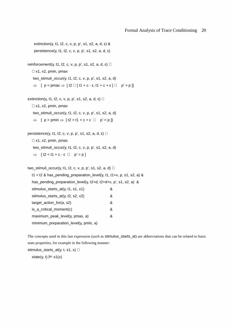
Formal Analysis of Trace Conditioning 20

extinction(γ, t1, t2, c, v, p, p’, s1, s2, a, d, ε) &

persistence(γ, t1, t2, c, v, p, p’, s1, s2, a, d, ε)

reinforcement(γ, t1, t2, c, v, p, p’, s1, s2, a, d, ε) ⇔

∀ x1, x2, pmin, pmax

two_stimuli_occur(γ, t1, t2, c, v, p, p’, s1, s2, a, d)

� [ p < pmax � [ t2 ∈ [ t1 + c - ε, t1 + c + ε ] ⇔ p’ > p ]]

extinction(γ, t1, t2, c, v, p, p’, s1, s2, a, d, ε) ⇔

∀ x1, x2, pmin, pmax

two_stimuli_occur(γ, t1, t2, c, v, p, p’, s1, s2, a, d)

� [ p > pmin � [ t2 > t1 + c + ε ⇔ p’ < p ]]

persistence(γ, t1, t2, c, v, p, p’, s1, s2, a, d, ε) ⇔

∀ x1, x2, pmin, pmax

two_stimuli_occur(γ, t1, t2, c, v, p, p’, s1, s2, a, d)

� [ t2 < t1 + c - ε ⇔ p’ = p ]

two_stimuli_occur(γ, t1, t2, c, v, p, p’, s1, s2, a, d) ⇔

t1 < t2 & has_pending_preparation_level(γ, t1, t1+v, p, s1, s2, a) &

has_pending_preparation_level(γ, t2+d, t2+d+v, p’, s1, s2, a) &

stimulus_starts_at(γ, t1, s1, x1) &

stimulus_starts_at(γ, t2, s2, x2) &

target_action_for(a, s2) &

is_a_critical_moment(c) &

maximum_peak_level(γ, pmax, a) &

minimum_preparation_level(γ, pmin, a)

The concepts used in this last expression (such as stimulus_starts_at) are abbreviations that can be related to basic

state properties, for example in the following manner:

stimulus_starts_at(γ, t, s1, x) ⇔

state(γ, t) |== s1(x)

Formal Analysis of Trace Conditioning 21

Checking Nonlocal Dynamic Properties on Traces

In addition to the software described in the Simulation section, other software has been

developed that takes traces and formally specified properties as input and checks whether a

property holds for a trace. Using automatic checks of this kind, the four formalised properties

based on (Los and Van Den Heuvel, 2001) have been checked against the traces depicted in

Figure 3 to 6. This section discusses the results of these checks.

GP1 has_global_hill_prep(γ, t1, t2, s1, a, u)

This property has been checked against several traces. An interesting observation concerning

these checks was the fact that the property does not hold for traces that describe the dynamics

during conditioning (like the traces in Figure 3 and 5). From this, we may conclude that in these

traces it is not the case that each critical moment corresponds to a single peak in response level.

However, when checking against traces describing the dynamics after conditioning (e.g.

Figure 4 and 6), the property does hold, as long as the parameters are well chosen. In particular,

the parameters should meet the following conditions:

γ = a trace describing the dynamics after a conditioning process (pure block or mixed block)

t1 = a time point when s1 occurs

t2 = t1+FP (where FP is the foreperiod during the preceding conditioning process)

s1 = the warning stimulus

a = the action for which the subject prepares after observing s1

u = iti (the intertrial interval during the preceding conditioning process)

To give an example, the following property meets these conditions: has_global_hill_prep(γ1,

20, 27, s1, a, 20), where γ1 is the trace provided in Figure 4. Thus, for this trace the following

holds: if at time point 20 a stimulus s1 starts, then the preparation level for action a increases

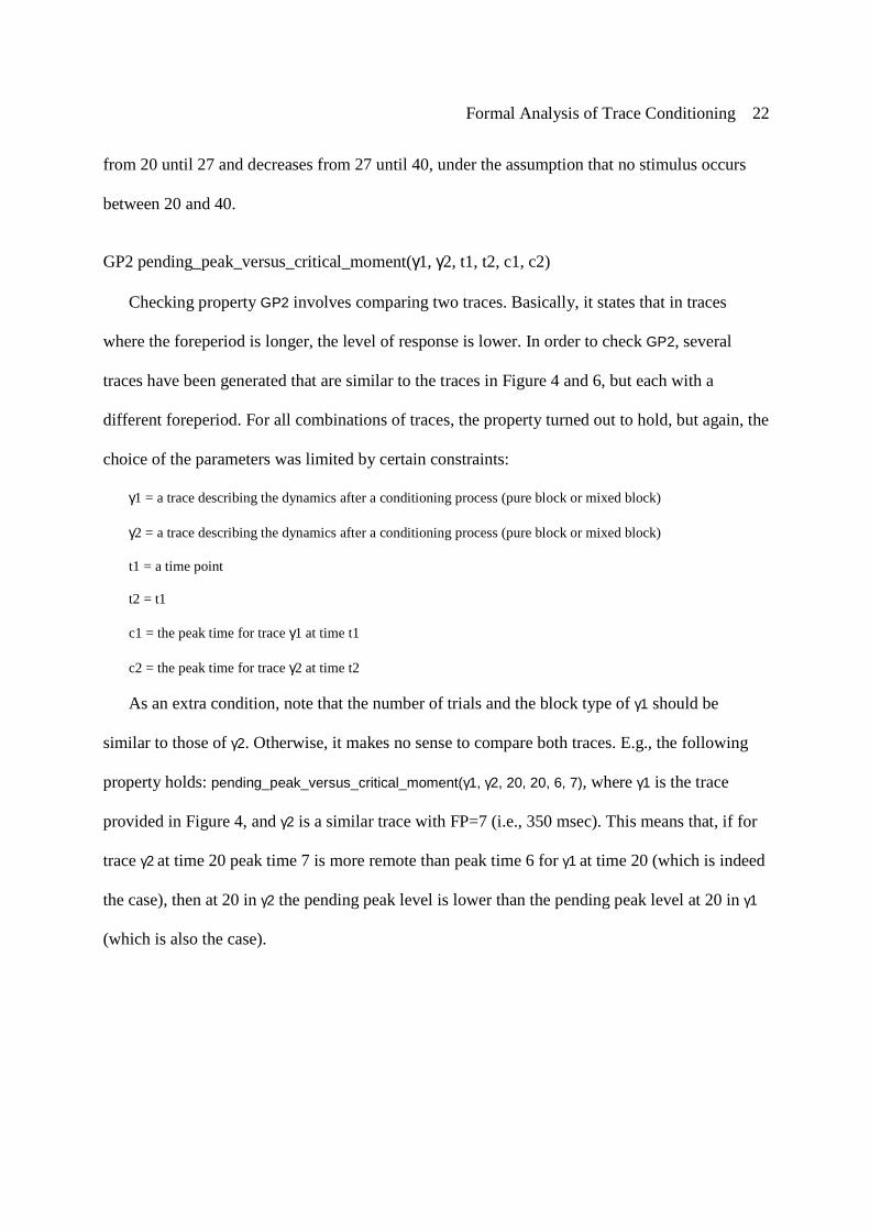
Formal Analysis of Trace Conditioning 22

from 20 until 27 and decreases from 27 until 40, under the assumption that no stimulus occurs

between 20 and 40.

GP2 pending_peak_versus_critical_moment(γ1, γ2, t1, t2, c1, c2)

Checking property GP2 involves comparing two traces. Basically, it states that in traces

where the foreperiod is longer, the level of response is lower. In order to check GP2, several

traces have been generated that are similar to the traces in Figure 4 and 6, but each with a

different foreperiod. For all combinations of traces, the property turned out to hold, but again, the

choice of the parameters was limited by certain constraints:

γ1 = a trace describing the dynamics after a conditioning process (pure block or mixed block)

γ2 = a trace describing the dynamics after a conditioning process (pure block or mixed block)

t1 = a time point

t2 = t1

c1 = the peak time for trace γ1 at time t1

c2 = the peak time for trace γ2 at time t2

As an extra condition, note that the number of trials and the block type of γ1 should be

similar to those of γ2. Otherwise, it makes no sense to compare both traces. E.g., the following

property holds: pending_peak_versus_critical_moment(γ1, γ2, 20, 20, 6, 7), where γ1 is the trace

provided in Figure 4, and γ2 is a similar trace with FP=7 (i.e., 350 msec). This means that, if for

trace γ2 at time 20 peak time 7 is more remote than peak time 6 for γ1 at time 20 (which is indeed

the case), then at 20 in γ2 the pending peak level is lower than the pending peak level at 20 in γ1

(which is also the case).

Formal Analysis of Trace Conditioning 23

GP3 dynamics_of_pending_preparation(γ, t1, t2, c, v, p, p’, s1, s2, a, d, ε)

Property GP3 combines property (3) and (4) as mentioned in the previous section. Basically,

the property consists of three separate statements that relate the strength of the conditioned

response (p) to the critical moment (t1+c) and the imperative moment (t2), by stating that:

p increases iff t2 = t1+c (GP3a)

p decreases iff t2 > t1+c (GP3b)

p remains the same iff t2 < t1+c (GP3c)

Also for this property, it is important to choose the parameters with care. They should meet

the following conditions in order for the property to make sense:

γ = a trace describing the dynamics after a conditioning process (pure block or mixed block)

t1 = a time point when S1 occurs

t2 = a time point when S2 occurs

c = a foreperiod within γ (such that c = t2-t1)

v = c

s1 = the warning stimulus

s2 = the imperative stimulus

a = the action for which the subject prepares after observing s1

d = long enough to process the events (e.g. iti)

ε = 0

An example of a property that meets these criteria is: dynamics_of_pending_preparation(γ, 10,

12, 10, 10, p, p', s1, s2, a, 18, 0), where γ is the trace depicted in Figure 6. However, even with

these parameter settings the property turned out not to hold. A close examination of Figure 6 will

reveal the cause of this failure. This trace describes a mixed block with two types of foreperiod

(FP=100 msec and FP=500 msec). At time point 10, a warning stimulus (S1) occurs. At this time

point, the pending preparation level for the latest critical moment (time point 20) has a certain

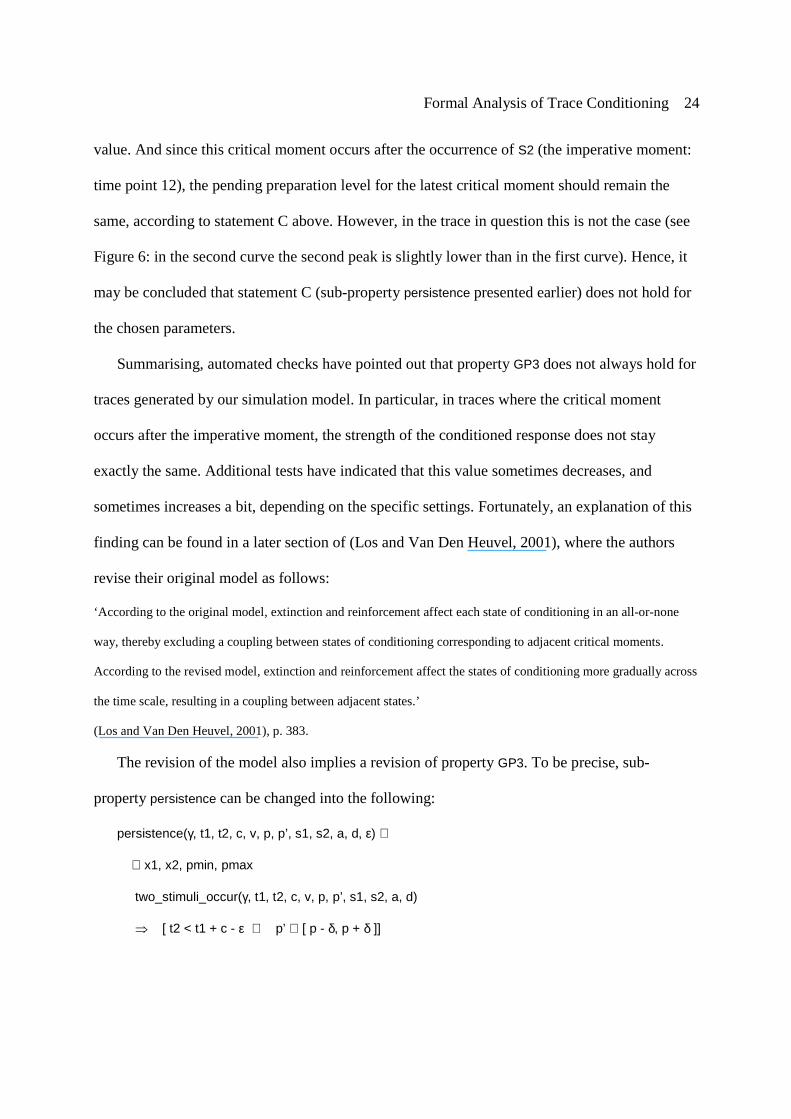
Formal Analysis of Trace Conditioning 24

value. And since this critical moment occurs after the occurrence of S2 (the imperative moment:

time point 12), the pending preparation level for the latest critical moment should remain the

same, according to statement C above. However, in the trace in question this is not the case (see

Figure 6: in the second curve the second peak is slightly lower than in the first curve). Hence, it

may be concluded that statement C (sub-property persistence presented earlier) does not hold for

the chosen parameters.

Summarising, automated checks have pointed out that property GP3 does not always hold for

traces generated by our simulation model. In particular, in traces where the critical moment

occurs after the imperative moment, the strength of the conditioned response does not stay

exactly the same. Additional tests have indicated that this value sometimes decreases, and

sometimes increases a bit, depending on the specific settings. Fortunately, an explanation of this

finding can be found in a later section of (Los and Van Den Heuvel, 2001), where the authors

revise their original model as follows:

‘According to the original model, extinction and reinforcement affect each state of conditioning in an all-or-none

way, thereby excluding a coupling between states of conditioning corresponding to adjacent critical moments.

According to the revised model, extinction and reinforcement affect the states of conditioning more gradually across

the time scale, resulting in a coupling between adjacent states.’

(Los and Van Den Heuvel, 2001), p. 383.

The revision of the model also implies a revision of property GP3. To be precise, sub-

property persistence can be changed into the following:

persistence(γ, t1, t2, c, v, p, p’, s1, s2, a, d, ε) ⇔

∀ x1, x2, pmin, pmax

two_stimuli_occur(γ, t1, t2, c, v, p, p’, s1, s2, a, d)

� [ t2 < t1 + c - ε ⇔ p’ ∈ [ p - δ, p + δ ]]

Formal Analysis of Trace Conditioning 25

Here, δ is a tolerance factor allowing a small deviation from the strength of the original

response. After adapting GP3 accordingly, the property turned out to hold.

Discussion

Two software environments have been developed to support the research reported here. First

a simulation environment has been used to generate simulation traces as shown. Second,

checking software has been used that takes traces and formally specified properties and checks

whether a property holds for a trace.

In comparison to Executable Temporal Logic (Barringer et al., 1996) our simulation

approach has possibilities to incorporate (real or integer) numbers in state properties, and in the

timing parameters e, f, g, h. Similarly, our approach to analysis has higher expressiveness than

approaches in temporal logic such as (Fisher and Wooldridge, 1997).

The present paper has confirmed that the assumptions of the informal conditioning model

proposed by Los and Van den Heuvel (2001) are global properties of the formal model

developed by Machado (1997), given certain restrictions of the parameter values, and given

slight adaptations of the persistence rule given by GP3C. This is an important finding, because

the global properties have proved to be highly useful in accounting for key findings in human

timing (Los and Van den Heuvel, 2001; Los et al., 2001).

One crucial finding the global properties can deal with effectively is the occurrence of

sequential effects of FP. These effects entail that on any given trial, RT is longer when the FP of

that trial is shorter than the FP of the preceding trial relative to when it is as long as or longer

than the FP of the preceding trial. Stated differently, RT is longer when the imperative moment

was bypassed during the FP on the preceding trial than when it was not bypassed during FP on

the preceding trial (e.g., Los and Van den Heuvel, 2001; Niemi and Naatanen, 1981). This

Formal Analysis of Trace Conditioning 26

finding is well accounted for by the learning rules formulated as GP3. According to GP3B, the

state of conditioning (p) associated with a critical moment is subject to extinction when a critical

moment is bypassed during FP (i.e., t2 > t1 + c), which is neither the case for the imperative

moment, where according to GP3A reinforcement occurs (i.e., t2 > t1 + c), nor for critical

moment beyond the imperative moment, where the state of conditioning persists according to

GP3C (i.e., t2 < t1 + c). Note that the adjustment of GP3C suggested by the present check of

nonlocal properties does not compromise the effectiveness of these learning rules, because the

tolerance factor δ is small relative to the extinction described by GP3B.

In fact, the addition of the tolerance area δ to GP3C, might prove to be helpful in accounting

for a more subtle effect in the extant literature. This concerns the finding that the FP-RT

functions obtained in pure and mixed blocks cross over at the latest critical moment. Specifically,

in pure blocks, the FP – RT function has been found to be upward sloping, given a minimal FP

of about 250 – 300 msec. By contrast, in mixed blocks, the RT is slowest at the shortest critical

moment (due to the influence of sequential effects described in the previous paragraph) and

decreases as a negatively accelerating function of FP. At the latest critical moment the pure and

mixed FP – RT functions come together, presumably because this moment is never bypassed

during FP on the preceding trial, allowing the state of conditioning to approach its asymptotic

value in either case. Sometimes, though, a cross-over of the two FP – RT functions is reported,

which has been shown to be particularly pronounced in certain clinical populations, such as

people diagnosed with schizophrenia (see Rist and Cohen, 1991, for a review). This finding may

be related to the failure to confirm GP3C without the allowance of a tolerance area δ. Thus, it

could be that, for certain parameter settings, the state of conditioning corresponding to the latest

critical moment approaches its asymptotic value more closely when a shorter FP occurred on the

Formal Analysis of Trace Conditioning 27

preceding trial (which is often the case in mixed blocks) than when the same FP occurred on the

preceding trial (as is always the case in pure blocks).

Finally, the present exploration holds the promise of deriving other global properties from the

formal model proposed by Machado (1997), which allows powerful new predictions. For

instance, one global property that appears to hold is that not only FP, but rather the total duration

of WS+FP influences the reaction time. Empirical work is currently in progress to test this

prediction.

Formal Analysis of Trace Conditioning 28

References

Ashby, R. (1960). Design for a Brain. Second Edition. Chapman & Hall, London.

Barringer, H., Fisher, M., Gabbay, D., Owens, R., and Reynolds, M. (1996). The Imperative

Future: Principles of Executable Temporal Logic, Research Studies Press Ltd. and John Wiley &

Sons.

Bosse, T., Jonker, C.M., Meij, L. van der, and Treur, J. (2005). LEADSTO: a Language and

Environment for Analysis of Dynamics by SimulaTiOn. In: Eymann, T. et al. (eds.), Proceedings

of the 3rd German Conference on Multi-Agent System Technologies, MATES'05. LNAI 3550.

Springer Verlag, pp. 165-178.

Busemeyer, J., and Townsend, J.T. (1993). Decision field theory: a dynamic-cognitive

approach to decision making in an uncertain environment. Psychological Review, vol. 100, pp.

432-459.

Fisher, M., and Wooldridge, M. (1997) On the Formal Specification and Verification of

Multi-Agent Systems. International Journal of Cooperative Information Systems, vol. 6, pp. 67-

94.

Gallistel, C.R. and Gibbon, J. (2000). Time, rate, and conditioning. Psychological Review,

vol. 107, pp. 289-344.

Gelder, T.J. van, and Port, R.F., (1995). It’s About Time: An Overview of the Dynamical

Approach to Cognition. In: (Port and van Gelder, 1995), pp. 1-43.

Jonker, C.M., and Treur, J. (2002). Analysis of the Dynamics of Reasoning Using Multiple

Representations. In: W.D. Gray and C.D. Schunn (eds.), Proceedings of the 24th Annual

Conference of the Cognitive Science Society, CogSci 2002. Mahwah, NJ: Lawrence Erlbaum

Associates, Inc., pp. 512-517.

Formal Analysis of Trace Conditioning 29

Jonker, C.M., and Treur, J. (2003a). A Temporal-Interactivist Perspective on the Dynamics

of Mental States. Cognitive Systems Research Journal, vol. 4, pp. 137-155.

Jonker, C.M., and Treur, J. (2003b). Modelling the Dynamics of Reasoning Processes:

Reasoning by Assumption. Cognitive Systems Research Journal, vol. 4, pp. 119-136.

Jonker, C.M., Treur, J., and Vries, W. de (2002). Temporal Analysis of the Dynamics of

Beliefs, Desires, and Intentions. Cognitive Science Quarterly, vol. 2, pp. 471-494.

Jonker, C.M., Treur, J., and Wijngaards, W.C.A. (2003). A Temporal Modelling

Environment for Internally Grounded Beliefs, Desires and Intentions. Cognitive Systems

Research Journal, vol. 4(3), pp. 191-210.

Kowalski, R., and Sergot, M. (1986). A logic-based calculus of events. New Generation

Computing, vol. 4, pp. 67-95.

Los, S.A., Knol, D.L., and Boers, R.M. (2001). The Foreperiod Effect Revisited:

Conditioning as a Basis for Nonspecific Preparation. Acta Psychologica, vol. 106, pp. 121-145.

Los, S.A., and Van Den Heuvel, C.E. (2001). Intentional and Unintentional Contributions to

Nonspecific Preparation During Reaction Time Foreperiods. Journal of Experimental

Psychology: Human Perception and Performance, vol. 27, pp. 370-386.

Machado, A. (1997). Learning the temporal Dynamics of Behaviour. Psychological Review,

vol. 104, pp. 241-265.

Niemi, P and Naatanen, R. (1981). Foreperiod and Simple Reaction Time. Psychological

Bulletin, vol 89, pp. 133-162.

Port, R.F., Gelder, T. van (eds.) (1995). Mind as Motion: Explorations in the Dynamics of

Cognition. MIT Press, Cambridge, Mass.

Formal Analysis of Trace Conditioning 30

Reiter, R. (2001). Knowledge in Action: Logical Foundations for Specifying and

Implementing Dynamical Systems. MIT Press.

Rist, F. and Cohen, C. (1991). Sequential effects in the reaction times of schizophrenics:

crossover and modality shift effects. In E.R. Steinhauer, J.H. Gruzelier, & J. Zubin, Handbook of

schizophrenia, vol. 5: Neuropsychology, psychophysiology and information processing (pp. 241-

271). Amsterdam: Elsevier.

Formal Analysis of Trace Conditioning 31

Author Note

Lourens van der Meij provided the technical support for the software environments used in

this project.

Formal Analysis of Trace Conditioning 32

S1

Timing nodes with activation level X

Preparation node

Associative links of variable weight W

Response strength R

Figure 1: Structure of Machado’s conditioning model (adjusted from Machado, 1997).

Formal Analysis of Trace Conditioning 33

environmental properties local properties

intermediate properties environmental properties

global properties

Figure 2: Interlevel relations between dynamic properties at different levels of aggregation.

Formal Analysis of Trace Conditioning 34

Figure 3: Simulation trace of the dynamics during conditioning (pure block, FP=300 msec).

Formal Analysis of Trace Conditioning 35

Figure 4: Simulation trace of the dynamics after conditioning (pure block, FP=300 msec).

Formal Analysis of Trace Conditioning 36

Figure 5: Simulation trace of the dynamics during conditioning (mixed block, FP=100 msec and FP=500 msec).

Formal Analysis of Trace Conditioning 37

Figure 6: Simulation trace of the dynamics after conditioning (mixed block, FP=100 msec and FP=500 msec).