European Journal of Scientific Research ISSN 1450-216X / 1450-202X Vol. 157 No 1 July, 2020, pp.27 - 42 http://www. europeanjournalofscientificresearch.com Forecasting the Exchange Rate of Kuwaiti Dinar (KWD) with the British Pound Sterling (GBP) Fatma Ali Alyousif College of Business studies, PAAET, Kuwait E-mail: [email protected] Bedour Mohammad Alsaleh Industrial Engineering Department, College of Engineering Kuwait University E-mail: [email protected] Amani Sulaiman Alrashdan College of Business studies, PAAET, Kuwait E-mail: [email protected] Abstract The study in this paper was attempted to build a statistical model for forecasting the GBP/KWD exchange rate. A variety of statistical time series techniques were analyzed such as exponential smoothing models, and ARIMA models including autoregressive and moving average process. The data was collected for five years started from 6 th of January 2014 till 8 th of November 2019. ARIMA (p,d,q) models were analyzed also to identify the adequate of the models, the stationary of the series was tested by applying the trend test such as ADF-Augmented Dickey-Fuller and PP-phillips-perron unit root tests. Performance of the competitive models for Arima models was assessed with AIC and BIC criteria. Statistical model fit measures indicate that the best candidate model among the competitive arima models was ARIMA (1,1,1): 1 1 9299 . 0 9139 . 0 - - - = t t t e Z Y . Statistical analysis for the exponential smoothing models were analyzed. The accuracy measures criteria such as: mean absolute error (MAE), and mean absolute percentage error (MAPE), sum square error (SSE), mean squared error(MSE),and mean percentage error(MPE) assessed. The results of the analysis reveal the fact that the best model among the exponential models was the single exponential smoothing model. Keywords: Exchange rates, Exponential smoothing, ARIMA. 2019 Mathematical subject classification: 62M10 Overview The local currency of the State of Kuwait is “Kuwaiti Dinar – K.D “, it was introduced in 1960 to replace the “Gulf Rupee “which was equal to “Indian Rupee “. Kuwaiti Dinar was equal to 1-pound sterling in 1960; it was issued by Central Bank of Kuwait. Due to the solid foundation of Kuwait economy, which is based on petroleum and foreign investments, the Kuwait Dinar became one of the highest valued monetary units in the world. Kuwaiti Dinar is linked to a basket of currencies since 2007, before that it was linked with U.S Dollar in the period from 2003 – 2007.

Welcome message from author
This document is posted to help you gain knowledge. Please leave a comment to let me know what you think about it! Share it to your friends and learn new things together.
Transcript
European Journal of Scientific Research
ISSN 1450-216X / 1450-202X Vol. 157 No 1 July, 2020, pp.27 - 42
http://www. europeanjournalofscientificresearch.com
Forecasting the Exchange Rate of Kuwaiti Dinar
(KWD) with the British Pound Sterling (GBP)
Fatma Ali Alyousif
College of Business studies, PAAET, Kuwait
E-mail: [email protected]
Bedour Mohammad Alsaleh
Industrial Engineering Department, College of Engineering
Kuwait University
E-mail: [email protected]
Amani Sulaiman Alrashdan
College of Business studies, PAAET, Kuwait
E-mail: [email protected]
Abstract
The study in this paper was attempted to build a statistical model for forecasting the
GBP/KWD exchange rate. A variety of statistical time series techniques were analyzed
such as exponential smoothing models, and ARIMA models including autoregressive and
moving average process. The data was collected for five years started from 6th
of January
2014 till 8th
of November 2019. ARIMA (p,d,q) models were analyzed also to identify the
adequate of the models, the stationary of the series was tested by applying the trend test
such as ADF-Augmented Dickey-Fuller and PP-phillips-perron unit root tests. Performance
of the competitive models for Arima models was assessed with AIC and BIC criteria.
Statistical model fit measures indicate that the best candidate model among the competitive
arima models was ARIMA (1,1,1): 11 9299.09139.0 −− −= ttt eZY .
Statistical analysis for the exponential smoothing models were analyzed. The
accuracy measures criteria such as: mean absolute error (MAE), and mean absolute
percentage error (MAPE), sum square error (SSE), mean squared error(MSE),and mean
percentage error(MPE) assessed. The results of the analysis reveal the fact that the best
model among the exponential models was the single exponential smoothing model.
Keywords: Exchange rates, Exponential smoothing, ARIMA.
2019 Mathematical subject classification: 62M10
Overview The local currency of the State of Kuwait is “Kuwaiti Dinar – K.D “, it was introduced in 1960 to
replace the “Gulf Rupee “which was equal to “Indian Rupee “. Kuwaiti Dinar was equal to 1-pound
sterling in 1960; it was issued by Central Bank of Kuwait. Due to the solid foundation of Kuwait
economy, which is based on petroleum and foreign investments, the Kuwait Dinar became one of the
highest valued monetary units in the world. Kuwaiti Dinar is linked to a basket of currencies since
2007, before that it was linked with U.S Dollar in the period from 2003 – 2007.
Forecasting the Exchange Rate of Kuwaiti Dinar (KWD) with the British Pound Sterling (GBP) 28
In this research, we attempt to study the exchange rate of Kuwaiti Dinar in term of the British
Sterling Pound (G.B.P). It is known that the exchange rate is a crucial element that plays an important
role in Kuwait economy with respect to trading and Oil export prices. The British Pound is one of the
major international currencies in the world. It is very well known that Kuwait has a strong relationship
with the United Kingdom of Britain, they share historic relations and Kuwait owns big investments in
the U. K, therefore it is important to study the behavior of the exchange rate of Kuwaiti Dinar in terms
of the British Sterling Pound (G.B.P).
Forecasting financial time series is essential to the investors and governments, by
understanding the movement of the exchange rate and its forecast, this helps the decision makers in
the country to design the best financial policy to achieve their goal of price stability, and monitoring
the foreign investments.
1. Introduction Forecasting the exchange rate is very important in money transactions. The exchange rate plays an
important rule in the economy and it has a significant impact in economy with respect to trading and
oil prices as well as monetary market. Therefore, it is important for the researcher in the area of finance
and economy to study the behavior of currencies and to forecast the fluctuations of the currencies over
time. In case of Kuwaiti Dinar, it pegged with a basket of different major currencies. One of the most
major currency that Kuwaiti Dinar was pegged with is the GBP. There are a lot of time series models
used for forecasting short term period data. ARIMA and exponential smoothing models can be used for
estimating and forecasting the exchange rate. The British Sterling Pound (GBP) is considered one of
the major international currency world wide and has a significant impact on the economy of most
countries through trade and monetary transactions, therefore, the Kuwaiti Dinar was pegged with GPB.
Study the exchange rate of currencies play an important role in the economy of the countries
with respect to give an indication of economy situation for example if the exchange rate of the currency
for the country is low against major international currencies that give indication of worse economy for
that country, but if the price of the exchange rate is high this indicate that the economy is in good
situation. Also the exchange rate of the currencies plays an important impact in business transaction
and oil prices, therefore it is important to built a statistical model for forecasting the exchange rate of
the currency in the sense that forecasting is very crucial in many types of organizations since
predictions of future events must be incorporated into the decision-making process. In finance, interest
rates must be predicted so that the new capital acquisitions can be planned and financed. Financial
planners must also forecast the exchange rate of currencies in money transaction market in order to
study the fluctuations of exchange rate prices and its impact in business market.
It is known that the exchange rate is very important in money transactions. The exchange rate
plays an important role in the economy and it has a significant impact in economy with respect to
trading and oil prices as well as monetary market. Therefore, it is important to study the behavior of
currencies and to forecast the fluctuations of the currencies over time. Forecasting financial time series
such as stock prices or exchange rates is important to the investors and the government. A good
forecasting of a financial time series requires strong domain knowledge and good analysis tools.
Economic vitality and inflation rate are highly affected by monetary policies. Financial players must be
sure about the monetary policies in the country they act which is possible by understanding movements
of exchange rates. Therefore, by understanding the movement of exchange rate better, the policy
makers will be able to extract the relevant information about the economic and financial conditions of
the economy. This will enable them to design a better monetary policy for the future which will help
them to achieve their desired objective of price stability and greater employment. Practically most of
the countries have been managed by floating exchange rate system in which the central bank restricts
the free movement of exchange rates. The interventions from central bank are needed to prevent
undesirable or disruptive movements in the exchange rates which cause harm both internal and external
sector of the economy. Similarly, firms or investors might wish to forecast exchange rates to make
asset allocation decisions. Exchange rate is the most important elements of monetary transmission
29 Fatma Ali Alyousif, Bedour Mohammad Alsaleh and Amani Sulaiman Alrashdan
process and movement in this price that has a significant pass-through to consumer price. Exchange
rate forecasting is an extensively discussed issue in the literature. Time series models such as ARIMA,
exponential smoothing methodology can be used for estimating, checking and forecasting exchange
rate. There has been an increased number of papers in the literature in recent years, applying several
methods and techniques for exchange rate prediction. Despite the general acceptance of exponential
smoothing, the choice of a specific smoothing model is often a difficult problem. This paper will
briefly cover more simple models, exponential smoothing models proposed by Holt and Brown.
Despite the simpler and clear mathematical tools, forecasting using exponential smoothing models
often leads to results comparable with the results obtained using ARIMA model. One of the major
motivation for this study was the non-existence of research in forecasting exchange rate using an
exponential smoothing models in the countries of the Gulf Cooperation Council’s (GCC) region.
2. Literature Review The important techniques for studying the behavior of the exchange rate of currencies with respect to
modeling and forecasting time series of the exchange rate data of the currencies is the exponential
smoothing models and ARIMA models. There was a lot of studies have been done in the literatures for
modeling and forecasting of the exchange rate values of the currencies. Empirical studies use some
approach like exponential smoothing models to forecast the exchange rate of Kuwaiti Dinar against
Euro and Winter's method was the most suitable for modeling KWD/Euro exchange rate [1]. Another
study was performed in order to illustrate predictability performance among different competitive
models of exponential smoothing models to forecast the exchange rate of Kuwaiti Dinar against US
Dollar. The results of the study reveals that the best models were the Triple Exponential Smoothing
(Winter's) [2]. One of the most and simple techniques used for forecasting the time series data which
fluctuated within short period of time is the simple exponential smoothing method, and it is the method
that use weighted moving average of past data as the basis for forecast [3].
Also, a debate through a survey of literature indicate that the exchange rate follows a random
walk or it can be modeled, recent studies in the literatures shows that the exchange rate can be modeled
using time series models such as exponential smoothing models and Arima models. Compared time
series models for the exchange rate based on out of sample forecasting accuracy have done and found
that in the short period of time random walk model outperforms a fundamental based in determination
the exchange rate.
3. The Scope of the Study The scope of the study is attempted to tackle the following goals:
1. The main goal of the study is to compare the predictability performance among different
competitive models to forecast the exchange rate of Kuwaiti Dinar against British pound
sterling in terms of international trade.
2. Study the contribution of the British Pound Sterling on the stability of Kuwaiti Dinar.
3. Study the impact of the exchange rate of the British pound sterling on Kuwait economy with
respect to trade transaction and oil export.
4. Methodology Data Analysis: The data of the exchange rate of British Sterling pound (GBP) against Kuwaiti Dinar
was collected in a daily basis for a period of five years which started from 6th
of January 2014 till 8
th
of November 2019.
Forecasting the Exchange Rate of Kuwaiti Dinar (KWD) with the British Pound Sterling (GBP) 30
A Descriptive Statistics for the Actual Data
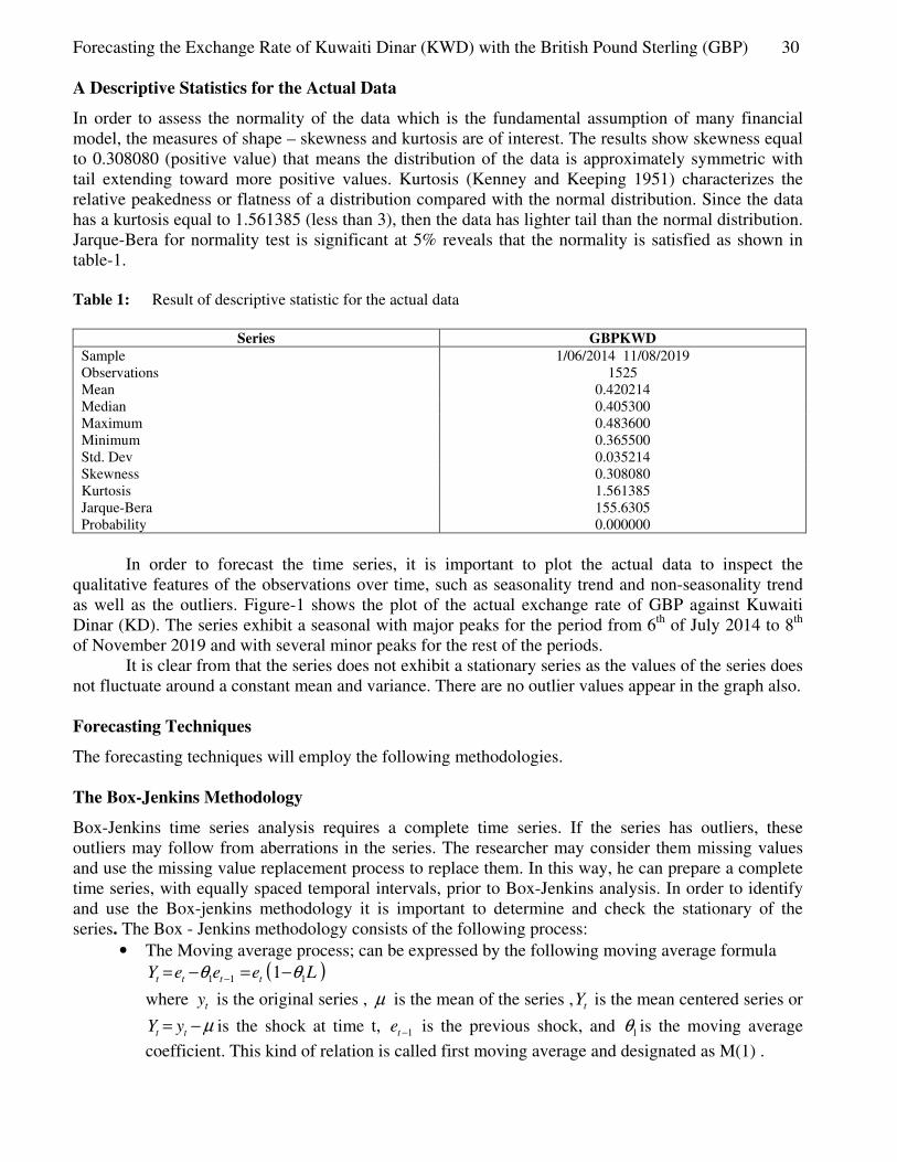
In order to assess the normality of the data which is the fundamental assumption of many financial
model, the measures of shape – skewness and kurtosis are of interest. The results show skewness equal
to 0.308080 (positive value) that means the distribution of the data is approximately symmetric with
tail extending toward more positive values. Kurtosis (Kenney and Keeping 1951) characterizes the
relative peakedness or flatness of a distribution compared with the normal distribution. Since the data
has a kurtosis equal to 1.561385 (less than 3), then the data has lighter tail than the normal distribution.
Jarque-Bera for normality test is significant at 5% reveals that the normality is satisfied as shown in
table-1.
Table 1: Result of descriptive statistic for the actual data
Series GBPKWD
Sample 1/06/2014 11/08/2019
Observations 1525
Mean 0.420214
Median 0.405300
Maximum 0.483600
Minimum 0.365500
Std. Dev 0.035214
Skewness 0.308080
Kurtosis 1.561385
Jarque-Bera 155.6305
Probability 0.000000
In order to forecast the time series, it is important to plot the actual data to inspect the
qualitative features of the observations over time, such as seasonality trend and non-seasonality trend
as well as the outliers. Figure-1 shows the plot of the actual exchange rate of GBP against Kuwaiti
Dinar (KD). The series exhibit a seasonal with major peaks for the period from 6th
of July 2014 to 8th
of November 2019 and with several minor peaks for the rest of the periods.
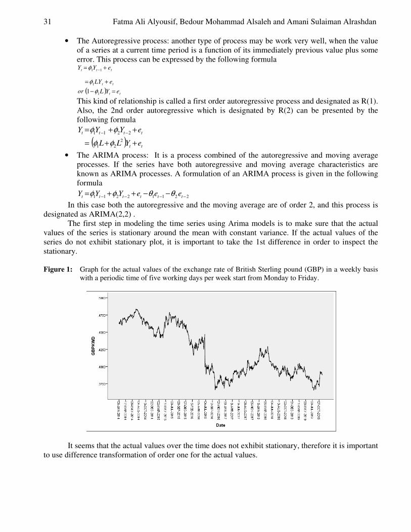
It is clear from that the series does not exhibit a stationary series as the values of the series does
not fluctuate around a constant mean and variance. There are no outlier values appear in the graph also.
Forecasting Techniques
The forecasting techniques will employ the following methodologies.
The Box-Jenkins Methodology
Box-Jenkins time series analysis requires a complete time series. If the series has outliers, these
outliers may follow from aberrations in the series. The researcher may consider them missing values
and use the missing value replacement process to replace them. In this way, he can prepare a complete
time series, with equally spaced temporal intervals, prior to Box-Jenkins analysis. In order to identify
and use the Box-jenkins methodology it is important to determine and check the stationary of the
series. The Box - Jenkins methodology consists of the following process:
• The Moving average process; can be expressed by the following moving average formula
( )LeeeY tttt 111 1 θθ −=−= − where ty is the original series , µ is the mean of the series , tY is the mean centered series or
µ−= tt yY is the shock at time t, 1−te is the previous shock, and 1θ is the moving average
coefficient. This kind of relation is called first moving average and designated as M(1) .
31 Fatma Ali Alyousif, Bedour Mohammad Alsaleh and Amani Sulaiman Alrashdan
• The Autoregressive process: another type of process may be work very well, when the value
of a series at a current time period is a function of its immediately previous value plus some
error. This process can be expressed by the following formula
( ) tt
tt
ttt
eYLor
eLY
eYY
=−
+=
+= −
1
1
11
1 φ
φ
φ
This kind of relationship is called a first order autoregressive process and designated as R(1).
Also, the 2nd order autoregressive which is designated by R(2) can be presented by the
following formula
( ) tt
tttt
eYLL
eYYY
++=
++= −−
2
21
2211
φφ
φφ
• The ARIMA process: It is a process combined of the autoregressive and moving average
processes. If the series have both autoregressive and moving average characteristics are
known as ARIMA processes. A formulation of an ARIMA process is given in the following
formula
22112211 −−−− −−++= tttttt eeeYYY θθφφ
In this case both the autoregressive and the moving average are of order 2, and this process is
designated as ARIMA(2,2) .
The first step in modeling the time series using Arima models is to make sure that the actual
values of the series is stationary around the mean with constant variance. If the actual values of the
series do not exhibit stationary plot, it is important to take the 1st difference in order to inspect the
stationary.
Figure 1: Graph for the actual values of the exchange rate of British Sterling pound (GBP) in a weekly basis
with a periodic time of five working days per week start from Monday to Friday.
It seems that the actual values over the time does not exhibit stationary, therefore it is important
to use difference transformation of order one for the actual values.
Forecasting the Exchange Rate of Kuwaiti Dinar (KWD) with the British Pound Sterling (GBP) 32
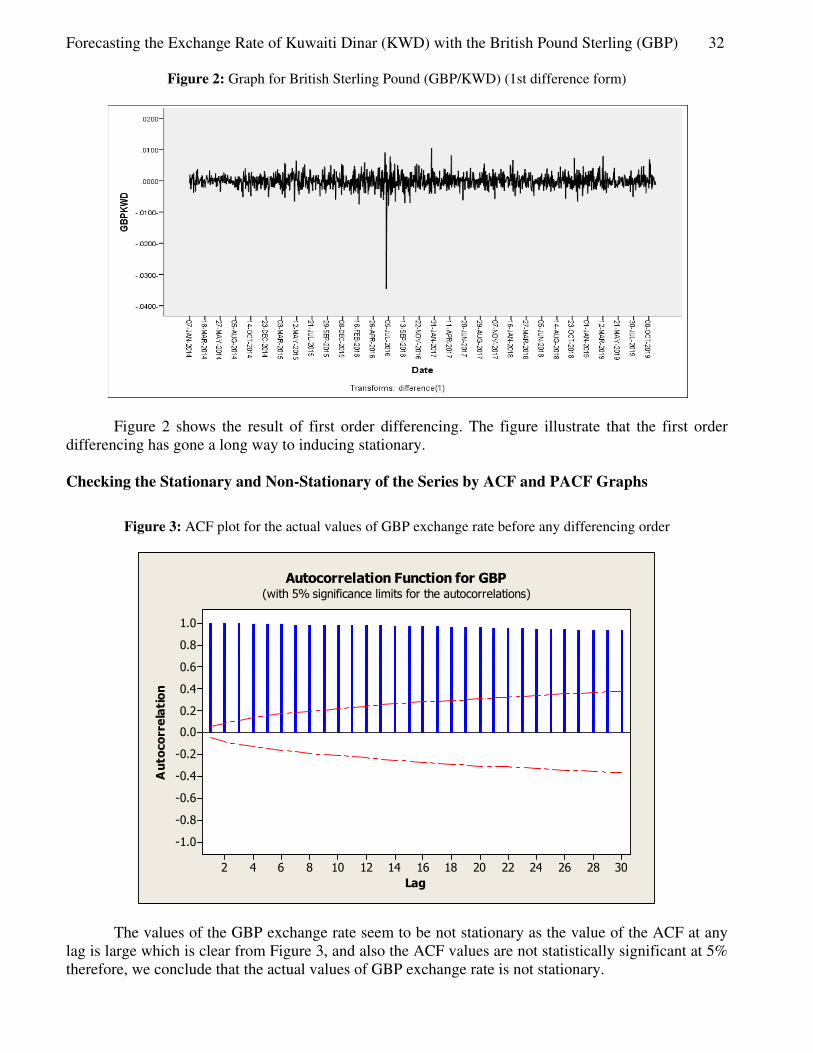
Figure 2: Graph for British Sterling Pound (GBP/KWD) (1st difference form)
Figure 2 shows the result of first order differencing. The figure illustrate that the first order
differencing has gone a long way to inducing stationary.
Checking the Stationary and Non-Stationary of the Series by ACF and PACF Graphs
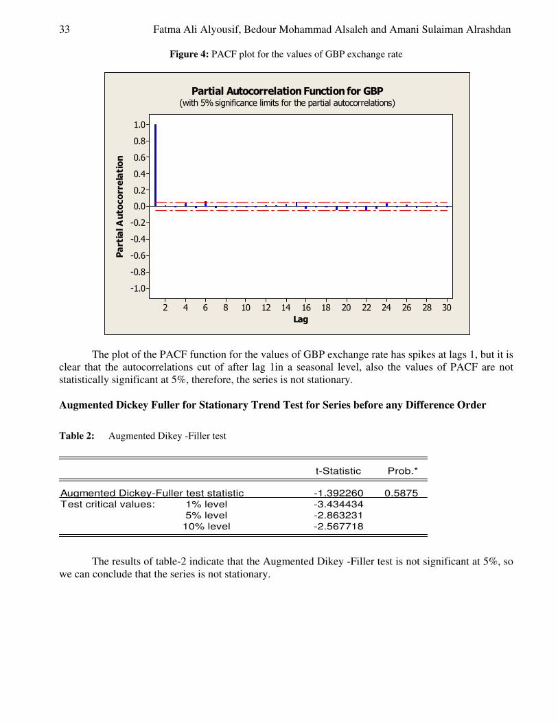
Figure 3: ACF plot for the actual values of GBP exchange rate before any differencing order
30282624222018161412108642
1.0
0.8
0.6
0.4
0.2
0.0
-0.2
-0.4
-0.6
-0.8
-1.0
Lag
Au
toco
rre
lati
on
Autocorrelation Function for GBP(with 5% significance limits for the autocorrelations)
The values of the GBP exchange rate seem to be not stationary as the value of the ACF at any
lag is large which is clear from Figure 3, and also the ACF values are not statistically significant at 5%
therefore, we conclude that the actual values of GBP exchange rate is not stationary.
33 Fatma Ali Alyousif, Bedour Mohammad Alsaleh and Amani Sulaiman Alrashdan
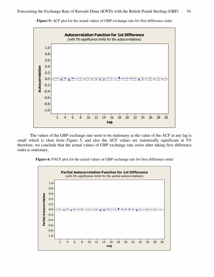
Figure 4: PACF plot for the values of GBP exchange rate
30282624222018161412108642
1.0
0.8
0.6
0.4
0.2
0.0
-0.2
-0.4
-0.6
-0.8
-1.0
Lag
Pa
rtia
l A
uto
co
rre
lati
on
Partial Autocorrelation Function for GBP(with 5% significance limits for the partial autocorrelations)
The plot of the PACF function for the values of GBP exchange rate has spikes at lags 1, but it is
clear that the autocorrelations cut of after lag 1in a seasonal level, also the values of PACF are not
statistically significant at 5%, therefore, the series is not stationary.
Augmented Dickey Fuller for Stationary Trend Test for Series before any Difference Order
Table 2: Augmented Dikey -Filler test
t-Statistic Prob.*
Augmented Dickey-Fuller test statistic -1.392260 0.5875
Test critical values: 1% level -3.434434
5% level -2.863231
10% level -2.567718
The results of table-2 indicate that the Augmented Dikey -Filler test is not significant at 5%, so
we can conclude that the series is not stationary.
Forecasting the Exchange Rate of Kuwaiti Dinar (KWD) with the British Pound Sterling (GBP) 34
Figure 5: ACF plot for the actual values of GBP exchange rate for first difference order
30282624222018161412108642
1.0
0.8
0.6
0.4
0.2
0.0
-0.2
-0.4
-0.6
-0.8
-1.0
Lag
Au
toco
rre
lati
on
Autocorrelation Function for 1st Difference(with 5% significance limits for the autocorrelations)
The values of the GBP exchange rate seem to be stationary as the value of the ACF at any lag is
small which is clear from Figure 5, and also the ACF values are statistically significant at 5%
therefore, we conclude that the actual values of GBP exchange rate series after taking first difference
order is stationary.
Figure 6: PACF plot for the actual values of GBP exchange rate for first difference order
30282624222018161412108642
1.0
0.8
0.6
0.4
0.2
0.0
-0.2
-0.4
-0.6
-0.8
-1.0
Lag
Pa
rtia
l A
uto
co
rre
lati
on
Partial Autocorrelation Function for 1st Difference(with 5% significance limits for the partial autocorrelations)
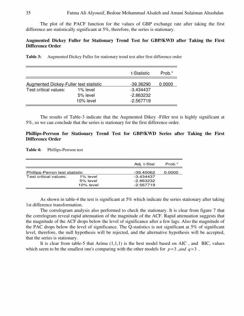
35 Fatma Ali Alyousif, Bedour Mohammad Alsaleh and Amani Sulaiman Alrashdan
The plot of the PACF function for the values of GBP exchange rate after taking the first
difference are statistically significant at 5%, therefore, the series is stationary.
Augmented Dickey Fuller for Stationary Trend Test for GBP/KWD after Taking the First
Difference Order
Table 3: Augmented Dickey Fuller for stationary trend test after first difference order
t-Statistic Prob.*
Augmented Dickey-Fuller test statistic -39.36290 0.0000
Test critical values: 1% level -3.434437
5% level -2.863232
10% level -2.567719
The results of Table-3 indicate that the Augmented Dikey -Filler test is highly significant at
5%, so we can conclude that the series is stationary for the first difference order.
Phillips-Perrson for Stationary Trend Test for GBP/KWD Series after Taking the First
Difference Order
Table 4: Phillips-Perrson test
Adj. t-Stat Prob.*
Phillips-Perron test statistic -39.40062 0.0000
Test critical values: 1% level -3.434437
5% level -2.863232
10% level -2.567719
As shown in table-4 the test is significant at 5% which indicate the series stationary after taking
1st difference transformation.
The correlogram analysis also performed to check the stationary. It is clear from figure 7 that
the correlogram reveal rapid attenuation of the magnitude of the ACF. Rapid attenuation suggests that
the magnitude of the ACF drops below the level of significance after a few lags. Also the magnitude of
the PAC drops below the level of significance. The Q-statistics is not significant at 5% of significant
level, therefore, the null hypothesis will be rejected, and the alternative hypothesis will be accepted,
that the series is stationary.
It is clear from table-5 that Arima (1,1,1) is the best model based on AIC , and BIC, values
which seem to be the smallest one's comparing with the other models for 3,3 == qandp .
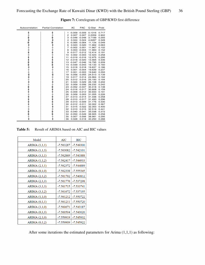
Forecasting the Exchange Rate of Kuwaiti Dinar (KWD) with the British Pound Sterling (GBP) 36
Figure 7: Correlogram of GBP/KWD first difference
Autocorrelation Partial Correlation AC PAC Q-Stat Prob
1 -0.009 -0.009 0.1316 0.717
2 0.007 0.007 0.2059 0.902
3 -0.048 -0.048 3.7189 0.293
4 0.024 0.024 4.6287 0.328
5 -0.065 -0.064 11.124 0.049
6 0.023 0.020 11.962 0.063
7 -0.002 0.001 11.967 0.102
8 0.003 -0.004 11.983 0.152
9 -0.017 -0.012 12.414 0.191
10 0.002 -0.003 12.423 0.258
11 -0.019 -0.016 12.975 0.295
12 -0.018 -0.020 13.465 0.336
13 -0.047 -0.046 16.795 0.209
14 -0.039 -0.043 19.133 0.160
15 0.018 0.018 19.637 0.186
16 0.001 -0.004 19.639 0.237
17 0.001 -0.003 19.640 0.293
18 0.056 0.055 24.513 0.139
19 0.017 0.014 24.964 0.162
20 0.012 0.016 25.193 0.194
21 0.024 0.029 26.108 0.202
22 0.009 0.006 26.232 0.242
23 -0.052 -0.047 30.418 0.138
24 -0.016 -0.017 30.808 0.159
25 -0.009 -0.012 30.933 0.191
26 0.009 0.003 31.055 0.226
27 -0.013 -0.014 31.338 0.258
28 -0.010 -0.017 31.493 0.296
29 -0.013 -0.009 31.776 0.330
30 -0.012 -0.011 32.002 0.367
31 0.015 0.022 32.353 0.400
32 0.010 0.015 32.516 0.441
33 -0.040 -0.041 35.038 0.372
34 -0.050 -0.049 38.905 0.258
35 0.007 0.006 38.981 0.295
36 0.028 0.018 40.250 0.288
Table 5: Result of ARIMA based on AIC and BIC values
After some iterations the estimated parameters for Arima (1,1,1) as following:
37 Fatma Ali Alyousif, Bedour Mohammad Alsaleh and Amani Sulaiman Alrashdan
Final Estimates of Parameters
Type Coef SE Coef T P
AR 1 0.9139 0.0274 33.30 0.000
MA 1 0.9299 0.0213 43.72 0.000
Constant -4.29903E-06 0.000004139 -1.04 0.299
Differencing: 1 regular difference
Number of observations: Original series 1525, after differencing 1524
Residuals: SS = 0.00795502 (backforecasts excluded)
MS = 0.00000523 DF = 1521
The constant term is not significant, therefore, it will be excluded from the model. The series
has zero mean after transferred to the first difference order.
The formula for future forecast can be written as: -
tttt aeZY +−= −− 1111 θφ
11 9299.09139.0 −− −= ttt eZY
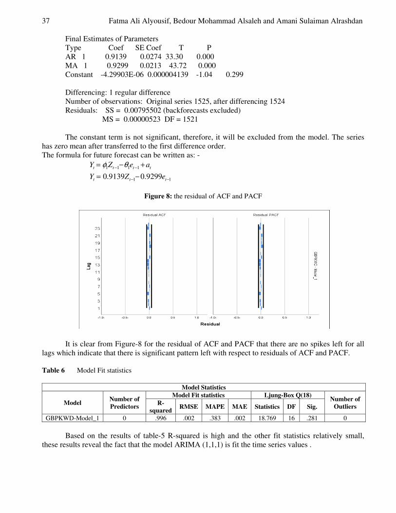
Figure 8: the residual of ACF and PACF
It is clear from Figure-8 for the residual of ACF and PACF that there are no spikes left for all
lags which indicate that there is significant pattern left with respect to residuals of ACF and PACF.
Table 6 Model Fit statistics
Model Statistics
Model Number of
Predictors
Model Fit statistics Ljung-Box Q(18) Number of
Outliers R-
squared RMSE MAPE MAE Statistics DF Sig.
GBPKWD-Model_1 0 .996 .002 .383 .002 18.769 16 .281 0
Based on the results of table-5 R-squared is high and the other fit statistics relatively small,
these results reveal the fact that the model ARIMA (1,1,1) is fit the time series values .
Forecasting the Exchange Rate of Kuwaiti Dinar (KWD) with the British Pound Sterling (GBP) 38
The Exponential Smoothing Models
A Single Exponential Smoothing (SES)
Suppose that the time series is described by the model where the average level
β�
may be slowly changing over time. Then the estimate of β�
made in time period T is given
by the smoothing equation where is smoothing constant between 0 and 1
and is the estimate of β�
made in time period T - 1.
A point forecast made in time period T for is Where .
This model is applied assuming that the series is stationary, without trend. Simple exponential
smoothing is used for short – range forecasting .The value of α is usually determined by minimizing
the sum of squares of the forecast errors.
Holt-Winters' Two-Parameter Double Exponential Smoothing (HDES)
Suppose that the time series described by the model
where the parameters β
� and 1β may be slowly changing over time.
two-parameter double exponential smoothing is a smoothing approach for forecasting such a time
series that employs two smoothing constants.
Suppose that in time period T-1 we have an estimate of the average level of the time
series That is, is an estimate of the intercept of the time series when the time origin is
considered to be time period T-1. Also suppose that in time period T — 1 we have an estimate
of the slope parameter 1β . If we observe Ty in time period T, then we can update
and then we can compute point estimate follows:
If we observe Ty in time period 'T, then
1. We obtain an updated estimate of the intercept parameter β�by using the equation
where α is a smoothing constant between 0 and 1.
2. We obtain an updated estimate of the slope parameter 1β by using the equation
where β is a smoothing constant between 0 and 1.
3. A point forecast of the future value made at time T is
This model is appropriate for series with linear trend and no seasonal variations.
Holt-Winters' Multiplicative Exponential Smoothing (HMES).
Winters' method is an exponential smoothing approach to handling seasonal data .Although the method
is not based on a formal statistical model , multiplicative Winters' method is generally considered to be
best suited to forecasting a time series that can be described by the equation
Where the time series parameters may be slowly changing over time.
The intercept is β� and the slope is 1β and SNt is the multiplicative seasonal factor .
Each of these three coefficients are defined by the following recursions:
where α is a smoothing constant between 0 and 1 .
where β is a smoothing constant between 0 and 1.
nyy ....,.........1 tty εβ +=�
( )Ta�
( ) ( ) ( )11 −−+= TayTa T ��αα α
( )1−Ta�
τ+Ty ( ).ˆ TayT �=+τ horizontimeaisτ
nyy ....,.........1
tt ty εββ ++= 1�
( )1−Ta�
( )1−Ta�
( )11 −Tb ( )1−Ta�
( )11 −Tb
( )Ta�
( ) ( ) ( ) ( )[ ]111 1 −+−−+= TbTayTa T ��αα
( )Tb1
( ) ( ) ( )[ ] ( ) ( )111 11 −−+−−= TbTaTaTb ββ��
τ+Ty
( ) ( ) ( )ττ TbTaTyT 1ˆ +=+ �
( ) ttt SNty εββ +×+= 1�
( )( )
( ) ( ) ( )[ ]111 1 −+−−+−
= TbTaLTsn
yTa
t
T��
αα
( ) ( ) ( )[ ] ( ) ( )111 11 −−+−−= TbTaTaTb ββ��
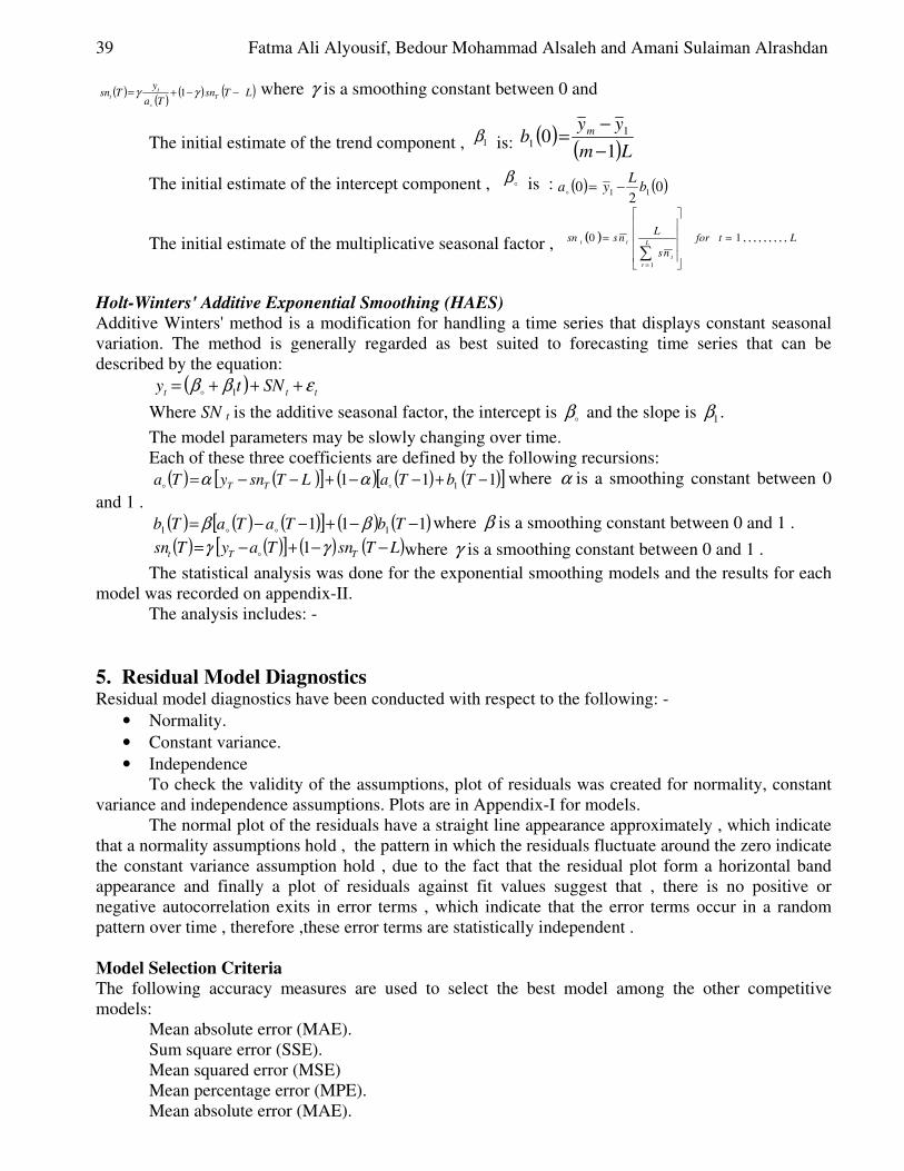
39 Fatma Ali Alyousif, Bedour Mohammad Alsaleh and Amani Sulaiman Alrashdan
where γ is a smoothing constant between 0 and
The initial estimate of the trend component , is:
The initial estimate of the intercept component , is :
The initial estimate of the multiplicative seasonal factor ,
Holt-Winters' Additive Exponential Smoothing (HAES)
Additive Winters' method is a modification for handling a time series that displays constant seasonal
variation. The method is generally regarded as best suited to forecasting time series that can be
described by the equation:
Where SN t is the additive seasonal factor, the intercept is β
� and the slope is 1β .
The model parameters may be slowly changing over time.
Each of these three coefficients are defined by the following recursions:
where α is a smoothing constant between 0
and 1 .
where β is a smoothing constant between 0 and 1 .
where γ is a smoothing constant between 0 and 1 .
The statistical analysis was done for the exponential smoothing models and the results for each
model was recorded on appendix-II.
The analysis includes: -
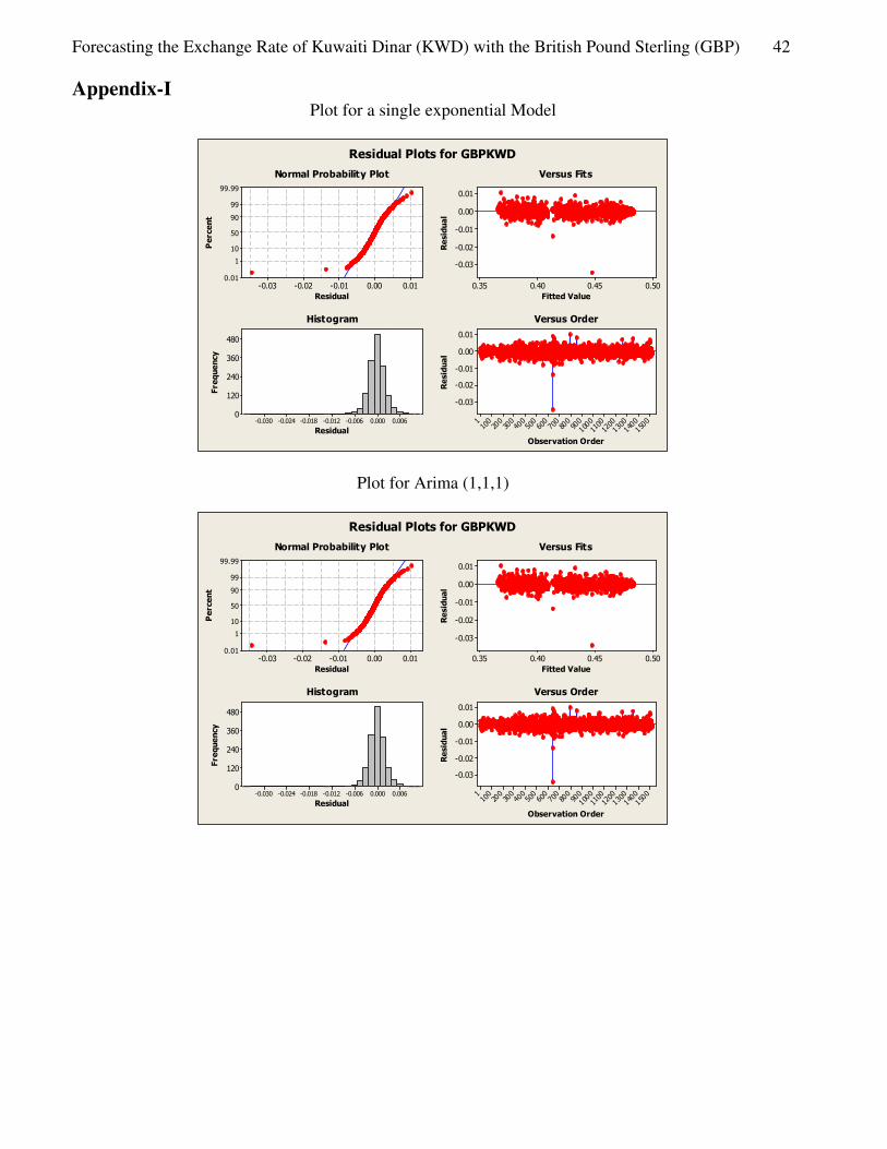
5. Residual Model Diagnostics Residual model diagnostics have been conducted with respect to the following: -
• Normality.
• Constant variance.
• Independence
To check the validity of the assumptions, plot of residuals was created for normality, constant
variance and independence assumptions. Plots are in Appendix-I for models.
The normal plot of the residuals have a straight line appearance approximately , which indicate
that a normality assumptions hold , the pattern in which the residuals fluctuate around the zero indicate
the constant variance assumption hold , due to the fact that the residual plot form a horizontal band
appearance and finally a plot of residuals against fit values suggest that , there is no positive or
negative autocorrelation exits in error terms , which indicate that the error terms occur in a random
pattern over time , therefore ,these error terms are statistically independent .
Model Selection Criteria
The following accuracy measures are used to select the best model among the other competitive
models:
Mean absolute error (MAE).
Sum square error (SSE).
Mean squared error (MSE)
Mean percentage error (MPE).
Mean absolute error (MAE).
( )( )
( ) ( )LTsnTa
yTsn T
tt −−+= γγ 1
�
1β ( )( )Lm
yyb m
10 1
1−
−=
�β ( ) ( )0
20 11 b
Lya −=
�
( ) Ltfor
ns
Lnssn
L
t
t
tt ,,,,,,,,,10
1
=
=
=
( ) ttt SNty εββ +++= 1�
( ) ( )[ ] ( ) ( ) ( )[ ]111 1 −+−−+−−= TbTaLTsnyTa TT ��αα
( ) ( ) ( )[ ] ( ) ( )111 11 −−+−−= TbTaTaTb ββ��
( ) ( )[ ] ( ) ( )LTsnTayTsn TTt −−+−= γγ 1�
Forecasting the Exchange Rate of Kuwaiti Dinar (KWD) with the British Pound Sterling (GBP) 40
These measures are used to compare the forecasting accuracy of the various models. The rule of
thump is the smaller of MAE, SSE, MSE, MPE and MAE the better is the forecasting ability. The
model with the smallest of the accuracy measures will be the best to be used for forecasting.
Table 7: Accuracy Indicators for each exponential model
Exponential Models Accuracy Indicators
MAE SSE MSE MPE MAPE
Single 0.001591 0.008038 0.000005 -0.014720 0.383021
Double Exp. Brown 0.001764 0.009594 0.000006 0.000579 0.424309
Double Exp. Holt 0.001656 0.008537 0.000006 -0.000258 0.398544
Winter's Multiplicative 0.001652 0.008486 0.000006 0.000876 0.397801
Winter's Additive 0.001652 0.008487 0.000006 0.000892 0.397789
An important objective of this study is to search the best predictive performance model among
all the competitive models, table-7 shows the summary results for all five exponential models, the best
one is based on the results of the analysis displayed on table-6, the single exponential model is the best
model comparing with the other models.
6. Conclusion It is concluded that this study assessed the capability of the forecasting models for forecasting the
exchange rate of KWD against GBP. The empirical results reveal the fact that ARIMA (1,1,1) model,
produce a superior result in forecasting KWD/GBP exchange rate data than the other Arima models.
Also, a single exponential model is the best model comparing to the other exponential smoothing
models based on the measure’s accuracy criteria.
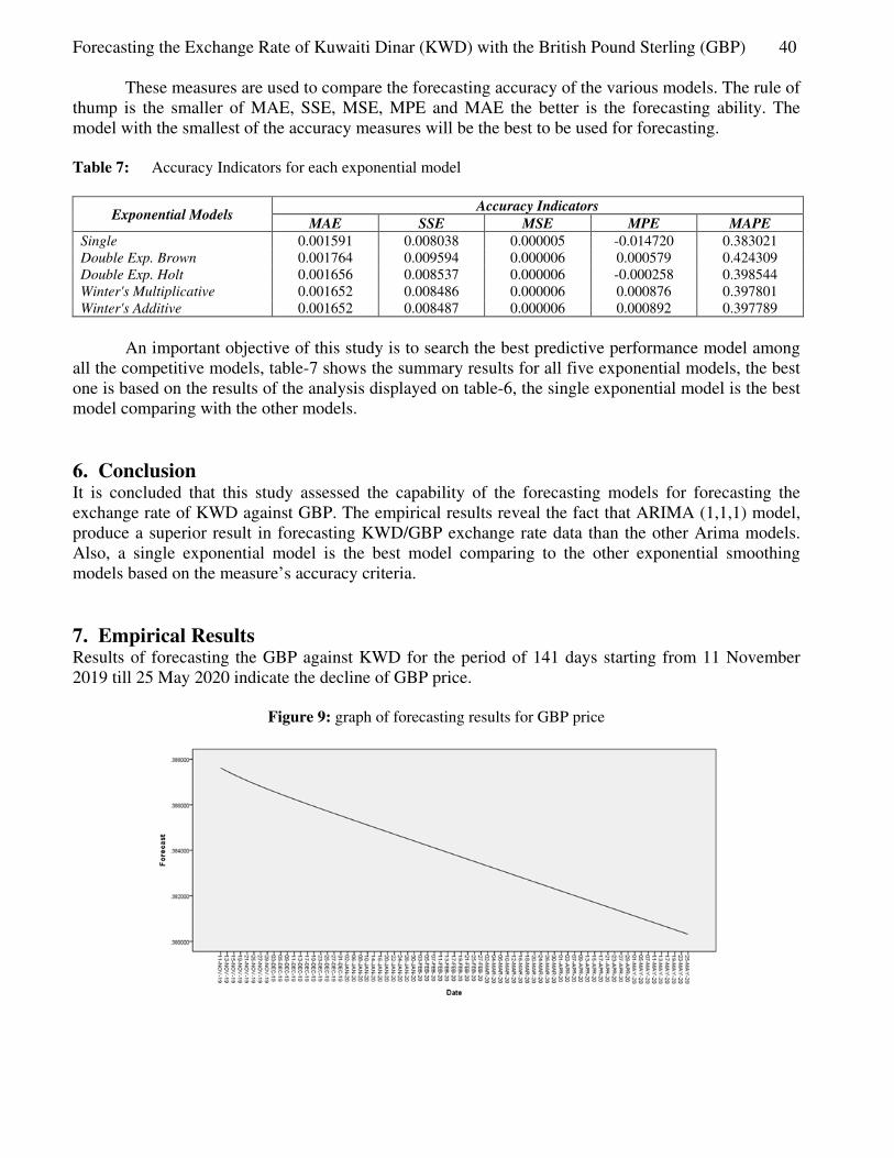
7. Empirical Results Results of forecasting the GBP against KWD for the period of 141 days starting from 11 November
2019 till 25 May 2020 indicate the decline of GBP price.
Figure 9: graph of forecasting results for GBP price
41 Fatma Ali Alyousif, Bedour Mohammad Alsaleh and Amani Sulaiman Alrashdan
References [1] Mohammad Al-Saleh, and Wafaa Al-Khariof, 2014. “Comparing the performance of
Exponential Smoothing Models for Forecasting Exchange”, European Journal of Scientific
Research 119, No 2, pp. 284-293.
[2] Wafaa Al-Khariof, and Adel Hussain Hammuda, 2015. “Comparing the Performance of Time
Series Models for Forecasting the Kuwaiti Dinar Against the UD Dollar “, European Journal of
Scientific Research 129, No 4, pp. 367-379.
[3] Eva Ostertagova, and Oskar Ostertage, 2012. “Forecasting Using Simple Exponential
Smoothing Method”, Acta Electrotechnica 12, No 3, pp. 62-66.
[4] Clark, T., and K. West, 2010. “Approximately Normal Tests for Equal Predictive Accuracy in
Nested Models”, Journal of Econometrics 138, pp. 291-311.
[5] Diebold, F., and R. Mariano, 2009. “Comparing Predictive Accuracy”, Journal of Business and
Economic Statistics 13, pp. 253-265.
[6] Clements, M., and D. Hendry, 1999. “Forecasting Non-Stationary Economic Time Series”,
Cambridge University Press.
[7] J. H. Wilson, and B. Keating. “Business Forecasting”, Irwin (5th edition).
[8] K. Styrin, 2008. “Exchange Rate Forecasting with Structural Shocks as Predictors”, Job Market Paper.
[9] F. Vitek, 2005. “The Exchange Rate Forecasting Puzzles”, University of British Columbia.
[10] Akaike, H., 1974. “A new Look at the Statistical Model identification”, IEEE Transaction of
Automatic control 19: 716-723.
[11] Bartolini, L. and Prati, A., 1999. “Soft exchange rate bands and speculative attacks: Theory, and
evidence from the ERM since August 1993", Journal of International Economics 49: 1—29.
[12] Bekaert, G. and Gray, S. F., 1998. “Target zones and exchange rates: An empirical
Investigation”, Journal of International Economics 45: 1—35.
[13] Bollerslev, T., 1986. “Generalized autoregressive conditional heteroskedasticity”, Journal of
Econometrics 31: 307—327.
[14] Brooks, C. and Rev´eiz, A. H., 2002. “A model for exchange rates with crawling bands - an
application to the Colombian peso”, Journal of Economics and Business 54: 483—503.
[15] Chung, C.-S. and Tauchen, G., 2001. “Testing target-zone models using efficient method of
moments”, Journal of Business and Economic Statistics 19: 255—269.
[16] Forbes, C. S. and Kofman, P., 2000. “Bayesian target zones”. Working Paper, Monash
University.
[17] Granger, C. W. J. and Ter¨asvirta, T., 1993. “Modelling Nonlinear Economic Relationships”,
Oxford University.
Forecasting the Exchange Rate of Kuwaiti Dinar (KWD) with the British Pound Sterling (GBP) 42
Appendix-I Plot for a single exponential Model
0.010.00-0.01-0.02-0.03
99.99
99
90
50
10
1
0.01
Residual
Pe
rce
nt
0.500.450.400.35
0.01
0.00
-0.01
-0.02
-0.03
Fitted Value
Re
sid
ua
l
0.0060.000-0.006-0.012-0.018-0.024-0.030
480
360
240
120
0
Residual
Fre
qu
en
cy
1500
1400
1300
1200
1100
100090
080
070
060
050
040
030
020
010
01
0.01
0.00
-0.01
-0.02
-0.03
Observation OrderR
esid
ua
l
Normal Probability Plot Versus Fits
Histogram Versus Order
Residual Plots for GBPKWD
Plot for Arima (1,1,1)
0.010.00-0.01-0.02-0.03
99.99
99
90
50
10
1
0.01
Residual
Pe
rce
nt
0.500.450.400.35
0.01
0.00
-0.01
-0.02
-0.03
Fitted Value
Re
sid
ua
l
0.0060.000-0.006-0.012-0.018-0.024-0.030
480
360
240
120
0
Residual
Fre
qu
en
cy
1500
1400
1300
1200
1100
100090
080
070
060
050
040
030
020
010
01
0.01
0.00
-0.01
-0.02
-0.03
Observation Order
Re
sid
ua
l
Normal Probability Plot Versus Fits
Histogram Versus Order
Residual Plots for GBPKWD
Related Documents