Forecasting MD707 Operations Management Professor Joy Field.

Forecasting

MD707 Operations Management

Professor Joy Field

Components of the Forecast

2

Forecasting using Judgment Methods

Sales force estimates

   Executive opinion

  Market research

   Delphi method

3

Forecasting using Time Series Methods

Naïve forecasts

Moving averages

Weighted moving averages

Exponential smoothing

Trend-adjusted exponential smoothing

Multiplicative seasonal method

4

Moving Average Method

Use a 3-month moving average, what is the forecast for month 5?

If the actual demand for month 5 is 805 customers, what is the forecast for month 6?

5

n

AMAF

n

iit

nt

1

Month Customers 1 800 2 740 3 810 4 790

F5

F6

Comparison of Three-Week and Six-Week

Moving Average Forecasts

6

Weighted Moving Average Method

Let Calculate the forecast for Month 5.

If the actual number of customers in month 5 is 805, what is the forecast for month 6?

7

11)1(1 ... tntnntnt AwAwAwF

Month Customers 1 800 2 740 3 810 4 790

.20.0 and ,30.0 ,50.0 321 www

F5

F6

Exponential Smoothing

Suppose What is the forecast for Month 5?

If the actual number of customers in month 5 is 805, what is the forecast for month 6?

8

11)1(F ttt AF

Month Customers 1 800 2 740 3 810 4 790

F3 783 0 20 customers and . .

F4

F5

6F

)(F

or

111 tttt FAF

Trend-Adjusted Exponential Smoothing

Using months 1-4, an initial estimate of the trend for Month 5 is 2 [(4-2+4)/3 = 2]. The starting forecast for month 5 is 54+2 = 56. Using and forecast the number of customers in month 6.

9

ttt

ttttt

tttt

TSTAF

TTAFTAFTT

TAFATAF

1

111 )(

)(S

Month Customers 1 48 2 52 3 50 4 54 5 55

3.0 4.0

5S

5T

6TAF

Trend-Adjusted Exponential Smoothing (cont.)

If the actual number of customers in month 6 is 58, what is the forecast for month 7?

10

6S

6T

7TAF

Multiplicative Seasonal Method Procedure

Calculate the trend line based on the available data using regression.

Calculate the centered moving average, with the number of periods equal to the number of seasons.

Calculate the seasonal relative for a period by dividing the actual demand for the period by the corresponding centered moving average.

Calculate the overall estimated seasonal relative by averaging the seasonal relatives from the same periods over the cycle.

Calculate the trend values for each of the periods to be forecast based on the trend line determined in Step 1.

To get a forecast for a given period in a future cycle, multiply the seasonal factor by the trend values.

11

Multiplicative Seasonal Method Example

Quarter Demand CMA (4 seasons)MA (2

periods)Seasonal Relatives

Normalized S.R.

Year 1, Q1 100

Year 1, Q2 400250

Year 1, Q3 300 261.5 1.15 1.16273

Year 1, Q4 200 274 0.73 0.75275

Year 2, Q1 192 285.5 0.67 0.69296

Year 2, Q2 408 298 1.37 1.40300

Year 2, Q3 384 Total 3.92 4

Year 2, Q4 216

Year 3, Q1 331 (trend value*) 227 (forecast)Year 3, Q2 344 (trend value*) 480 (forecast)Year 3, Q3 356 (trend value*) 417 (forecast)Year 3, Q4 369 (trend value*) 275 (forecast)

12

* Using regression, the trend line is 218.6 + 12.48t.

Linear Regression

where y = dependent (predicted) variable x = independent (predictor) variable a = y-intercept of the line (i.e., value of y when x = 0) b = slope of the line

13

y = a + bx

Linear Regression Line Relative to Actual Data

14

Regression Analysis Example

Weekx

(Price)y

(Appetizers)1 $2.70 760

2 3.50 510

3 2.00 980

4 4.20 250

5 3.10 320

6 4.05 480

15

An analyst for a chain of seafood restaurants is interested in forecasting the number of crab cake appetizers sold each week. He believes that the number sold has a linear relationship to the price and uses linear regression to determine if this is the case.

Regression Analysis Example (cont.)

Regression StatisticsMultiple R 0.843

R-Square 0.711

Adjusted R-Square 0.639

Standard Error 165.257

Observations 6

ANOVA

df SS MS F Significance F

Regression 1 269160 269160 9.856 0.035

Residual 4 109239 27309

Total 5 378400

Coefficients Standard Error t Stat P-value

Intercept 1454.6 295.9 4.92 0.008

Price ($) -277.6 88.4 -3.19 0.035

16

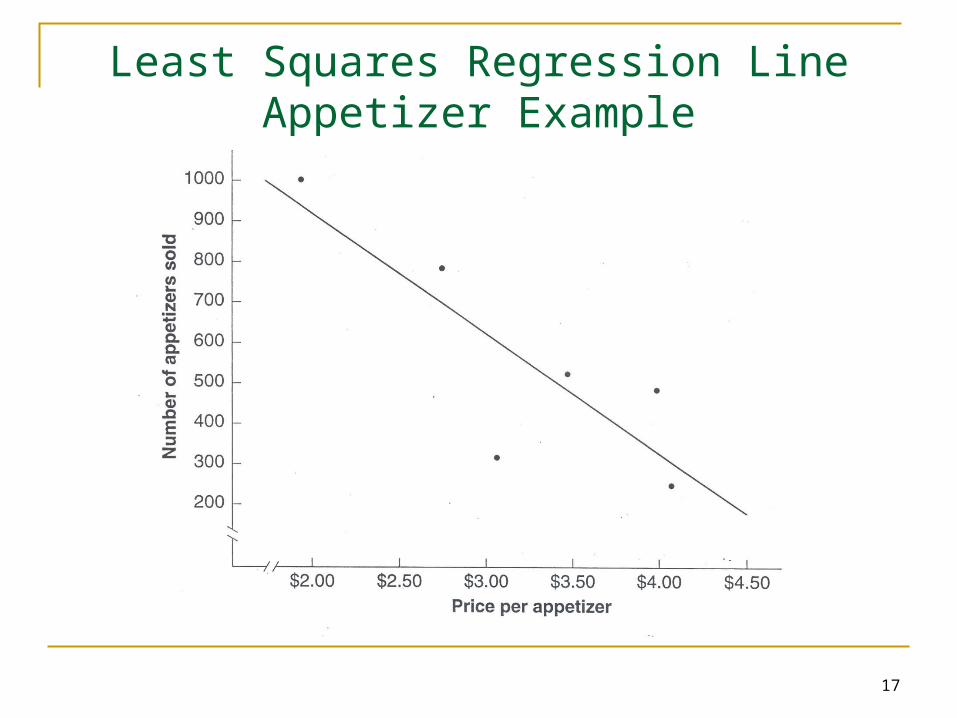
Least Squares Regression LineAppetizer Example

17

Interpretation of the Regression Intercept

18

Another Regression Analysis Example

Hours Score3.0 902.1 955.8 653.8 804.2 953.2 605.3 854.6 70

19

A professor is interested in determining whether average study hours per week is a good predictor of test scores. The results of her study are:

A student says: "Professor, what can I do to get a B or better on the next test. The professor asks, "On average, how many hours do you spend studying for this course per week?" The student responds, "About 2 hours." Use linear regression to forecast the student's test score.

Another Regression Analysis Example (cont.)

20

Regression StatisticsMultiple R 0.391R-Square 0.153Adjusted R-Square 0.0121Standard Error 13.544Observations 8

ANOVAdf SS MS F Significance F

Regression 1 199.2 199.2 1.09 0.3375Residual 6 1100.8 183.5Total 7 1300

Coefficients Standard Error t Stat P-valueIntercept 97.3 17.3 5.6 0.0013Study hours -4.3 4.2 -1.0 0.3375

Forecast Error Measures Bias

Average error

Variability Mean squared error (MSE)

Standard deviation (s)

Mean absolute error (MAD)

Mean percent absolute error (MAPE)

Relative bias Tracking signal (TS)

21

n

en

tt

1

11

2

n

en

tt

MSE

n

en

tt

1

nA

en

t t

t 1

)]100([

MAD1

n

tte

Summarizing Forecast Accuracy

Period Actual (A) Forecast (F) Error (E=A-F) Abs Error Error Sq[(Abs E)/A]

x 1001 113 95 18 18 324 15.93

2 85 80 5 5 25 5.88

3 96 103 -7 7 49 7.29

4 86 119 -33 33 1089 38.37

5 121 117 4 4 16 3.31

6 100 125 -25 25 625 25.00

7 142 67 75 75 5625 52.82

8 92 96 -4 4 16 4.35

9 72 116 -44 44 1936 61.11

Total -11 215 9705 214.06

MAD = 23.9

MSE = 1213.1

s = 34.8

MAPE = 23.8%

22

Tracking and Analyzing Forecast ErrorsPeriod Actual (A) Forecast (F) Error (E=A-F) Assessing bias:

10 102 130 -28 Cumulative forecast error (periods 1-9) = -11

11 107 102 5 MAD (periods 1-9) = 23.9

12 112 89 23 Tracking signal (periods 1-9) = -0.46

13 118 97 21

14 89 115 -26 Cumulative forecast error (periods 1-18) = -7

15 142 82 60 MAD (periods 1-18) = 26.28

16 100 130 -30 Tracking signal (periods 1-18) = -0.27

17 94 137 -43

18 111 89 22 Assessing error variability/size:

Total 4Standard deviation (periods 1-9) =2s control limits for errors: 0 +/- 2(34.8) =

34.80 +/- 69.6

23

-80

-60

-40

-20

0

20

40

60

80

10 11 12 13 14 15 16 17 18

2s Control Chart for Errors

UCL = 69.6

LCL = -69.6

Forecast Performance of Various Forecasting Methods for a Medical

ClinicMethod

Cumulative Sum of Forecast Errors

(CFE – bias)

Mean Absolute Deviation

(MAD - variability)Simple moving average

Three-week (n = 3) 23.1 17.1

Six-week (n = 6) 69.8 15.53-period weighted moving average w = 0.70, 0.20, 0.10 14.0 18.4

Exponential smoothing

= 0.1 65.6 14.8

= 0.2 41.0 15.3

24