Weather Forecasting for Ka-band Operations: Initial Study ...

1

IPN Progress Report 42-206 • August 15, 2016

Weather Forecasting for Ka-band Operations: Initial Study Results

David Morabito,* Longtao Wu,† and Stephen Slobin‡

* Communications Architectures and Research Section. † Instrument Software and Science Data Systems Section. ‡ Communications Ground Systems Section.

The research described in this publication was carried out by the Jet Propulsion Laboratory, California Institute of Technology, under a contract with the National Aeronautics and Space Administration. © 2016 California Institute of Technology. U.S. Government sponsorship acknowledged.

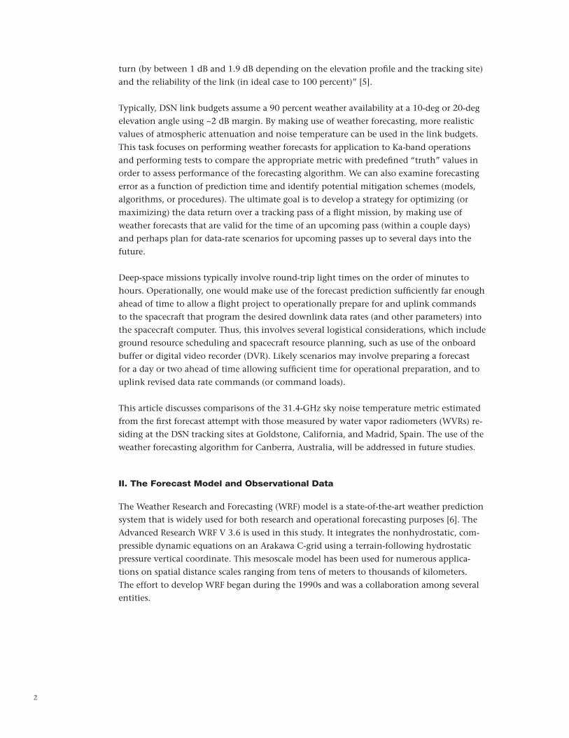
abstract. — As lower frequency bands (e.g., 2.3 GHz and 8.4 GHz) have become over-subscribed during the past several decades, NASA has become interested in using higher frequency bands (e.g., 26 GHz and 32 GHz) for telemetry, thus making use of the available wider bandwidth. However, these bands are more susceptible to atmospheric degradation. Currently, flight projects tend to be conservative in preparing their communications links by using worst-case or conservative assumptions. Such assumptions result in nonoptimum data return. We explore the use of weather forecasting for Goldstone and Madrid for differ-ent weather condition scenarios to determine more optimal values of atmospheric attenua-tion and atmospheric noise temperature for use in telecommunication link design. We find that the use of weather forecasting can provide up to 2 dB or more of increased data return when more favorable conditions are forecast. Future plans involve further developing the technique for operational scenarios with interested flight projects.

I. Introduction

As lower frequency bands have become oversubscribed during the past several decades, NASA has become interested in utilizing higher frequency bands for telemetry return, mak-ing use of the available wider bandwidths. However, the higher frequency bands are more susceptible to atmospheric degradation. Currently, flight projects tend to be conservative in preparing communications links, making use of worse-case or conservative assumptions (e.g., lowest elevation angle, maximum range distance, high weather availability). Such as-sumptions result in nonoptimum data return. In recent years, several methods of increasing data volume have been studied such as data-rate stepping (as the elevation angle changes during a tracking pass), automatic repeat query (ARQ) techniques, arraying, and site diver-sity [1–3]. An additional method to be discussed in this article is weather forecasting, which allows for more accurate atmospheric attenuation and noise temperature values to be used in telecommunication links [4]. Previous work exploring the use of weather forecasting for the Deep Space Network (DSN) found that forecasting “improves both the average data re-

2

turn (by between 1 dB and 1.9 dB depending on the elevation profile and the tracking site) and the reliability of the link (in ideal case to 100 percent)” [5].

Typically, DSN link budgets assume a 90 percent weather availability at a 10-deg or 20-deg elevation angle using ~2 dB margin. By making use of weather forecasting, more realistic values of atmospheric attenuation and noise temperature can be used in the link budgets. This task focuses on performing weather forecasts for application to Ka-band operations and performing tests to compare the appropriate metric with predefined “truth” values in order to assess performance of the forecasting algorithm. We can also examine forecasting error as a function of prediction time and identify potential mitigation schemes (models, algorithms, or procedures). The ultimate goal is to develop a strategy for optimizing (or maximizing) the data return over a tracking pass of a flight mission, by making use of weather forecasts that are valid for the time of an upcoming pass (within a couple days) and perhaps plan for data-rate scenarios for upcoming passes up to several days into the future.

Deep-space missions typically involve round-trip light times on the order of minutes to hours. Operationally, one would make use of the forecast prediction sufficiently far enough ahead of time to allow a flight project to operationally prepare for and uplink commands to the spacecraft that program the desired downlink data rates (and other parameters) into the spacecraft computer. Thus, this involves several logistical considerations, which include ground resource scheduling and spacecraft resource planning, such as use of the onboard buffer or digital video recorder (DVR). Likely scenarios may involve preparing a forecast for a day or two ahead of time allowing sufficient time for operational preparation, and to uplink revised data rate commands (or command loads).

This article discusses comparisons of the 31.4-GHz sky noise temperature metric estimated from the first forecast attempt with those measured by water vapor radiometers (WVRs) re-siding at the DSN tracking sites at Goldstone, California, and Madrid, Spain. The use of the weather forecasting algorithm for Canberra, Australia, will be addressed in future studies.

II. The Forecast Model and Observational Data

The Weather Research and Forecasting (WRF) model is a state-of-the-art weather prediction system that is widely used for both research and operational forecasting purposes [6]. The Advanced Research WRF V 3.6 is used in this study. It integrates the nonhydrostatic, com-pressible dynamic equations on an Arakawa C-grid using a terrain-following hydrostatic pressure vertical coordinate. This mesoscale model has been used for numerous applica-tions on spatial distance scales ranging from tens of meters to thousands of kilometers. The effort to develop WRF began during the 1990s and was a collaboration among several entities.

3

Our simulations are conducted with a parent grid at 27-km horizontal resolution and three nested grids at 9-km, 3-km, and 1-km horizontal resolutions. There are 50 model levels in the vertical from the surface up to 50 hPa (50 mb). An example of the domain coverages at the Deep Space Network tracking site at Goldstone, California, is shown in Figure 1.

Figure 1. The forecast domain coverage for Southern California centered at DSS-25 at Goldstone,

showing four nested domains of increasing resolution going from outer to inner domains.

The initial and boundary conditions for the WRF model are derived from the 1 deg × 1 deg Final (FNL) global tropospheric analyses produced by the National Centers for Environ-mental Prediction’s (NCEP’s) Global Forecast System (GFS) [7]. The 24-category U. S. Geological Survey (USGS) 30-s land cover data are used to represent topography and land cover in the model. For all current experiments, we employ the Thompson et al. (2008) [8] microphysical scheme, the Rapid Radiative Transfer Model for General Circulation Mod-els (RRTMG) shortwave and longwave schemes [9], Noah Land Surface scheme [10], and the Mellor–Yamada–Janjic planetary boundary layer (PBL) scheme [11]. The Kain–Fritsch cumulus scheme [12] is used in the 27-km and 9-km domain, while no cumulus scheme is used in the 3-km and 1-km inner grids. Other options of physical parameterizations are available in the WRF model, and can be tested to derive an optimized model setup for gen-erating forecasts at selected locations.

WVRs have been in operation at all three DSN tracking sites for several years (~10 to ~25 years depending upon site) and these provide the data in which to test and quantify the forecast performance. These instruments measure sky brightness temperature over different frequencies that reside near the water vapor absorption line at 22.235 GHz. The 31.4-GHz brightness temperature channel has been used to generate statistics of atmo-

45°N

40°N

35°N

30°N

25°N

125°W 120°W 115°W 110°W 105°W

d03

d04

d02

4

spheric attenuation and atmosphere noise temperature for the NASA DSN tracking sites, which are made available to flight projects and mission planners [13–14]. The multifrequen-cy sky brightness measurements output from the WVRs have also been used to generate estimates of wet path delay, liquid water content, and water vapor content for a variety of applications and their statistics have been characterized and reported on elsewhere [15]. In this article, we discuss results obtained from Advanced Water Vapor Radiometers (AWVRs), which have been deployed at Goldstone and Madrid. The AWVRs measure brightness temperatures (in K) at three different frequencies: 22.2 GHz, 23.8 GHz, and 31.4 GHz. The AWVRs have improved performance over earlier model WVRs and have the capability to “track” spacecraft such as during radio science experiments to allow for removal of atmo-spheric effects [16–18]. For the two Goldstone cases discussed in this article, we used data from the AWVR. For the test case of Madrid, the AWVR was not yet deployed, and we made use of data from an older-style WVR.

The 31.4-GHz brightness temperature measurements from the WVRs have been chosen as the prime metric by which to judge the performance of the weather forecasting tools, since they can be easily converted to atmospheric noise temperature (removing cosmic contribu-tion), and atmospheric attenuation at any elevation angle of interest.

WRF was used to generate meteorological profiles for a grid centered near the DSN 34-m- diameter, Ka-band-capable beam-waveguide (BWG) antennas at Goldstone and Madrid, where the WVRs reside (see Figures 1 and 2 for the case of DSS-25 at Goldstone). The output variables of the WRF model included height, temperature, absolute humidity, and liquid water content (LWC) for different time intervals (in 6-hr steps over 120 hr) past the forecast reference time. The output data from WRF are then referred to specific heights and pressure levels (see Figure 2 for an example on the scale and appearance of the first few vertical cells centered at DSS-25). These values over different vertical cells are required by the post-pro-cessing software, which integrates these to effective column values producing an estimate of the brightness temperature at 31.4 GHz at each forecast time. There are thus 31 levels above the surface (875 mb to 125 mb), plus the surface. These 32 levels define 31 layers (between the levels) along with a final layer 10 km thick that lies above the 125-mb level in order to account for the remaining atmosphere. Madrid will have the same number of total levels, but will have the surface, and levels from 900 mb, down to 150 mb.

The homogeneous atmospheric properties of each layer were calculated from the average of the temperature, pressure, and absolute humidity values at the top and bottom of each layer. For each of the constituents, there exists a specific attenuation at the frequency of interest. For oxygen, this is in dB/km as a function of temperature and pressure. For water vapor, this is in dB/km as a function of temperature, pressure, and absolute humidity (g/m3). For cloud liquid water, the specific attenuation is in dB/km per g/m3 of liquid water as a function of temperature. Detailed equations and a complete discussion of these rela-tionships is given in [19]. The total attenuation of each layer is obtained by multiplying the specific attenuation of each component in the layer by the thickness of that layer, and in the case of liquid water, also multiplying by the average LWC of the layer. The formulation that follows provides an overview of the process. A more detailed discussion of the “radia-tive transfer” calculation can be found in [20].

5

For each layer i, the total attenuation A ,i total is the sum of the individual contributors for that layer (all in dB):

.A A A A, , , ,i total i oxygen i water vapor i liquid water= + +

Since each layer is at a physical temperature greater than absolute zero, it radiates down-ward as a black body at temperature pT in K.

The noise temperature contribution of each layer iT (in K) is thus given as

piT T L11

i= -d n

where

pT = average physical temperature of the layer, K

Li = loss factor (>1) of the layer where L 10 /i

A 10i=

Ai = total attenuation (in positive numbers) of that layer, dB.

The net noise contribution at the surface of a single layer is the noise contribution above, reduced by the product of the loss factors for all layers lying below it, down to the surface.

L Ltotal ii

n

1= =%

where Li = loss factor of the ith individual layer, for the n layers from the surface up to the bottom of the radiating layer itself.

Thus, the net noise contribution of a single layer is /T Li total, and the noise contribution of the entire atmosphere, Tatm , is the sum of all the net noise contributions of the 32 total single layers.

The loss factor of the entire atmosphere is

L Latm ii 1

32

==%

where there are 32 total atmospheric layers, including the top 10-km-thick layer.

The sky brightness temperature Tsky as seen from the ground is defined as the noise con-tribution of the entire atmosphere plus the attenuated noise contribution of the cosmic microwave background. Thus,

/T T T Lsky atm cosmic atm= +

where Tcosmic = 2.725 K.

Comparisons were then made between the forecasted 31.4-GHz sky brightness temperature derived from the WRF forecasts and the “measured” WVR 31.4-GHz sky brightness temper-atures at each forecast time. Other parameters output from WRF were also cross compared,

6

such as with meteorological parameters (e.g., precipitable water vapor) extracted from the WVR data or parameters derived from nearby surface meteorological data.

III. Goldstone February 2003 Test Case

For the Goldstone desert climate, we first consider a case of extended periods of clear weather followed by periods of significant rainfall, which occurred during the month of February 2003. Here we analyze real data against “truth” data derived from on-site AWVR measurements (Section III.A). We next analyze the performance of the WRF forecast model against the “truth” data derived from AWVR measurements for selected periods during this month (Section III.B).

A. Clear Weather and Rain — Real Data

The FNL analysis, which provides initial and boundary conditions for the WRF model, uses observations to produce a representation of the atmospheric state through a data assimi-lation system. It is referred as “real data” in this article. In order to separate model biases from biases resulting from initial and boundary conditions, we tested the consistency of parameters derived from the FNL analysis with parameters derived from the AWVR zenith measurements. The FNL meteorological data (or “real” data) in the cells lying in a vertical column centered at DSS-25 were integrated and thus converted to 31.4-GHz sky brightness temperatures for comparison with the nearby AWVR measurements. Figure 2 displays an example of what the first few vertical cells from the surface look like overlaying the desert terrain centered near DSN station DSS-25 that are discussed here. The first two cells closest to the ground in Figure 2 show annotated examples of air temperature and humidity.

Figure 2. Example of the first few cells lying along vertical grid centered near DSN station DSS-25 at Goldstone.

T = 18.6 °CAH = 9.0 gm/m3

T = 20.8 °CAH = 9.4 gm/m3

7

Figure 3 displays the brightness temperature values from the FNL analysis of “real” data superimposed with the measurements from the AWVR for the month of February 2003. For the most part, the FNL values nicely track the AWVR measurements with differences of 1 to 2 K during “dry” periods, comparable to the absolute calibration error of the AWVR. The exceptions of higher discrepancies (several K) appear to occur during or just before periods of elevated rain “spikes” in AWVR measurements). Possible explanations include the prospect that the incoming “fronts” represented in the FNL data may be delayed in reaching the AWVR zenith line of sight. We do know that the period of vertical rainfall for Goldstone roughly covers the period from day 11.5 to day 14 (see Figure 4 bottom). Other explanations for the several K discrepancies are the focus of further study.

Figure 3. “Real” 31.4-GHz brightness temperature estimates from FNL analysis versus AWVR measurements

for February 2003 at Goldstone.

B. Clear Weather and Rain — Forecast

For the first forecast test case, WRF was used to generate meteorological profiles for a grid centered at the Goldstone 34-m Ka-band BWG antenna DSS-25 (where the AWVR resides) starting on February 10, 2003, at 0:00 UTC. The reference surface height was set at the altitude above mean sea level at the location height of the AWVR (978.5 m). Figure 1 depicts the forecast domain structure centered at DSS-25 in Goldstone used in the model simula-tions, where there are four nested domains of increasing resolution of 27 km, 9 km, 3 km, and 1 km, respectively. This nested domain setup allows for a sufficiently high-resolution forecast for Goldstone under limited computer resources over a short time period. This fore-cast included periods of very clear weather followed by a very rainy weather period, which in turn was followed by relatively clear weather.

The forecast output file was processed using a multilayer post-processing algorithm in order to generate predictions of 31.4-GHz brightness temperature at each forecast time (6 hr, 12 hr, 18 hr up to 120 hr) past February 10 0:00 UTC. These forecasted values are shown as blue-filled circles in Figure 4 (top). This metric was then compared against the equivalent from the “truth” dataset (Goldstone AWVR) which are shown as red data points in Figure 4 (top).

120

100

80

60

40

20

01 3 5 7 9 11 13 15 17

Brig

htne

ss T

emp

erat

ure,

K

Day of Month

19 21 23 25 27 29

FNL AWVR

8

140

120

100

80

18

16

14

12

10

8

6

4

2

0

60

40

20

0

6

16

14

12

10

8

6

4

2

0

5

4

3

2

1

010

10

11

11

12

12

13

13

14

14

15

15

16

16

17

17

Zen

ith B

right

ness

Tem

per

atur

e, K

Liq

uid

Wat

er, m

icro

nsR

ain

Rat

e, m

m/h

Tota

l Rai

nfal

l, m

m

Day of Month

Day of Month

Forecast Tsky AWVR Tsky AWVR Liquid Water

Total Rainfall Rain Rate

RainyPeriod

Figure 4. (Top) Comparison of sky brightness temperature at 31.4 GHz for Goldstone extracted from the February 10

00:00 UTC weather forecast (blue dots) and from the AWVR dataset (red dots). Also shown is the liquid water content

extracted from the AWVR (green dots) that coincides with the elevated sky brightness temperature estimates (see

right hand vertical axis). (Bottom) Rain data from Goldstone weather station (located at the site of 70-m antenna),

where blue dots denote total rainfall (mm) (reset to zero at end of each day) and red dots denote rain rate (mm/hr).

As seen from Figure 4 (top), we have very good agreement between forecast points (blue dots) and AWVR data (red dashes) during fairly clear weather before the onset of the rain near February 11 12:00 UTC. The divergence starting at about day 11.5 is thus coincident with the onset of rain (and/or significant cloud liquid) during this time. After the onset of rain, the forecast data (blue dots) again generally agree with the bottom envelope excur-sions of the AWVR data points (red dots). Also plotted in Figure 4 (top) is the liquid water content extracted from the AWVR data (green data points with right-hand vertical axis label, and purposely scaled to align with the brightness temperature curves at the start of the plot). Although the liquid water content is fairly small, the signature does show the increased activity coinciding with the highest sky noise temperature during the rainy period. Figure 4 (bottom) displays the rain gauge data from a weather station located at the Goldstone site (several km away). Note that the rain gauge dataset displays values while it is raining and at the end of each day shows the amount of total rain accumulated before it is reset.

9

Note that elevated forecast estimates in Figure 4 coincide with heavy rain periods (high rain rates) where there is also high variability in the AWVR 31.4-GHz sky temperature estimates. Model tuning may be needed and is expected to be explored in future study for a better representation during periods of rain. To better inspect how forecast error grows, a mostly clear sky case with humidity spanning virtually its full range of zenith values for Goldstone was identified for another test discussed next.

IV. Goldstone August 2003 Test Case

A. Significantly Varying Humidity Conditions — Real Data

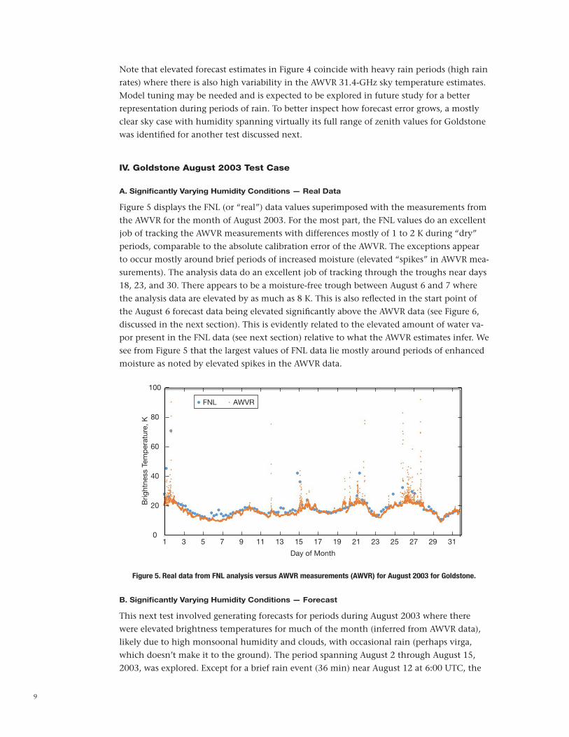
Figure 5 displays the FNL (or “real”) data values superimposed with the measurements from the AWVR for the month of August 2003. For the most part, the FNL values do an excellent job of tracking the AWVR measurements with differences mostly of 1 to 2 K during “dry” periods, comparable to the absolute calibration error of the AWVR. The exceptions appear to occur mostly around brief periods of increased moisture (elevated “spikes” in AWVR mea-surements). The analysis data do an excellent job of tracking through the troughs near days 18, 23, and 30. There appears to be a moisture-free trough between August 6 and 7 where the analysis data are elevated by as much as 8 K. This is also reflected in the start point of the August 6 forecast data being elevated significantly above the AWVR data (see Figure 6, discussed in the next section). This is evidently related to the elevated amount of water va-por present in the FNL data (see next section) relative to what the AWVR estimates infer. We see from Figure 5 that the largest values of FNL data lie mostly around periods of enhanced moisture as noted by elevated spikes in the AWVR data.

100

80

60

40

20

01 3 5 7 9 11 13 15 17

Brig

htne

ss T

emp

erat

ure,

K

Day of Month

19 21 23 25 27 29 31

FNL AWVR

Figure 5. Real data from FNL analysis versus AWVR measurements (AWVR) for August 2003 for Goldstone.

B. Significantly Varying Humidity Conditions — Forecast

This next test involved generating forecasts for periods during August 2003 where there were elevated brightness temperatures for much of the month (inferred from AWVR data), likely due to high monsoonal humidity and clouds, with occasional rain (perhaps virga, which doesn’t make it to the ground). The period spanning August 2 through August 15, 2003, was explored. Except for a brief rain event (36 min) near August 12 at 6:00 UTC, the

10

rest of the period involved high humidity and clouds. This period was broken up into sev-eral five-day forecast periods beginning August 2, 3, 4, 5, and 6 to examine the forecasted sky temperatures against the “envelope” of AWVR zenith 31.4-GHz sky temperature ranging from 10 K up to about 25 K.1 Thus, this series of weather forecasts includes five forecasts each covering five-day periods starting on successive days providing meteorological param-eter estimates at 6-hr intervals referenced to the following start times:

August 2, 2003 00:00 UTC, August 3, 2003 00:00 UTC, August 4, 2003 00:00 UTC, August 5, 2003 00:00 UTC, August 6, 2003 00:00 UTC. The period of August 2 to August 11 was chosen because AWVR noise temperature values exhibited wide variation and exceeded 15 K, indicating a significantly changing humid condition. This period is mostly very hot and humid, possibly with clouds. The results are depicted in Figure 6, showing the variation of brightness temperature at 31.4 GHz from August 2 to August 11, 2003. The parameters output from the forecasts occupied cells in vertical layers centered on DSS-25 that resides near the AWVR at Goldstone. These param-eters were input to the multilayer algorithm, which outputs the brightness temperature at 31.4 GHz to be compared to that measured by the Goldstone AWVR serving as the “truth”

1 2 3 4 5 6 7 8 9 10 11 12

40

30

20

10

0

Sky

Brig

htne

ss T

emp

erat

ure,

K

Day of Month

Aug 2 Forecast

Aug 3 Forecast

Aug 4 Forecast

Aug 5 Forecast

Aug 6 Forecast

AWVR 31.4 GHz

1 Whenever the 31.4-GHz zenith brightness temperatures lie above 25 or 30 K, it usually indicates that rain is occurring.

Figure 6. Comparison of 31.4-GHz sky brightness temperature extracted from the August 2–6 00:00 UTC

Goldstone weather forecasts (see legend) and from the AWVR dataset (brown curve). Initial forecast

points at 0:00 UTC reference time for each day are shown within red circles.

11

dataset. Note that in Figure 6, all forecast values (discrete points at 6-hr intervals with large symbols) follow the same trend as the AWVR (small discrete brown data points with ~min-ute resolution).

The data points involving the forecast start times are shown in Figure 6 as the first point for each plot symbol series (enclosed in red circles). The first points of the forecasts for Au-gust 2, 3, and 5 do an excellent job of lying on top of the AWVR data points. The August 6 forecast data point lies very close to the AWVR data. Only the August 4 initial forecast data point lies a little above the corresponding AWVR data points.

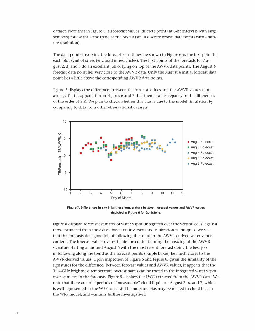
Figure 7 displays the differences between the forecast values and the AWVR values (not averaged). It is apparent from Figures 6 and 7 that there is a discrepancy in the differences of the order of 3 K. We plan to check whether this bias is due to the model simulation by comparing to data from other observational datasets.

1 2 3 4 5 6 7 8 9 10 11 12

10

5

0

–5

–10

TB(F

orec

ast)

– TB

(AW

VR

), K

Day of Month

Aug 2 Forecast

Aug 3 Forecast

Aug 4 Forecast

Aug 5 Forecast

Aug 6 Forecast

Figure 7. Differences in sky brightness temperature between forecast values and AWVR values

depicted in Figure 6 for Goldstone.

Figure 8 displays forecast estimates of water vapor (integrated over the vertical cells) against those estimated from the AWVR based on inversion and calibration techniques. We see that the forecasts do a good job of following the trend in the AWVR-derived water vapor content. The forecast values overestimate the content during the upswing of the AWVR signature starting at around August 6 with the most recent forecast doing the best job in following along the trend as the forecast points (purple boxes) lie much closer to the AWVR-derived values. Upon inspection of Figure 6 and Figure 8, given the similarity of the signatures for the differences between forecast values and AWVR values, it appears that the 31.4-GHz brightness temperature overestimates can be traced to the integrated water vapor overestimates in the forecasts. Figure 9 displays the LWC extracted from the AWVR data. We note that there are brief periods of “measurable” cloud liquid on August 2, 6, and 7, which is well represented in the WRF forecast. The moisture bias may be related to cloud bias in the WRF model, and warrants further investigation.

12

Figure 8. Integrated water vapor at Goldstone estimated from forecasts and post-processing

software (integrated over the vertical cells) against those estimated from AWVR

based on inversion and calibration techniques.

Figure 9. Liquid water content inferred from AWVR data for Goldstone during August 1–10, 2003.

1 2 3 4 5 6 7 8 9 10

4

3

2

1

0

Wat

er V

apor

Con

tent

, cm

Day of Month

AWVR

Aug 2 Forecast

Aug 3 Forecast

Aug 4 Forecast

Aug 5 Forecast

Aug 6 Forecast

1 2 3 4 5 6 7 8 9 10

100

80

90

70

60

50

40

30

20

10

0

Liq

uid

Wat

er, µ

m

Day of Month

13

However, on Figure 6, it is not obvious that the liquid water (shown in Figure 9) is signifi-cantly contributing to the noise temperature (the brown AWVR points). All or most of the variation in sky brightness temperature from 10 to 20 K appears to be due to water vapor. It is not clear whether the liquid water algorithm using AWVR data could be so sensitive as to detect an amount of liquid water that does not appear to have any noise temperature effect.

V. Madrid September 2000 — Varying Humid Conditions

The month of September 2000 was chosen as the first case to examine for Madrid. It is one of the few months in a three-year period that did not have significant amounts of rain. Fig-ure 10 displays the domain structure used by the forecast tool for Madrid. The domain sizes are 100 × 100 for all of the four horizontal resolutions at 27 km, 9 km, 3 km, and 1 km, respectively.

Figure 10. The forecast domain structure for Europe centered at DSS-54 in Madrid, Spain, showing four nested

domains (boxes) of increasing resolution going from outer to inner domains.

Figure 11 displays the FNL (or “real”) data values superimposed with the measurements from the WVR for the month of September 2000. For the most part, the FNL values do an excellent job of tracking the WVR measurements but with a “bias” of about 2 K (FNL lying above WVR). During periods of increased moisture (elevated “spikes” in WVR mea-surements), we note that the FNL values are devoid of moisture. The FNL data for Madrid do not exhibit performance as good as that achieved for data from Goldstone. These results suggest that initial datasets — such as European Centre for Medium-Range Weather

45°N

50°N

40°N

35°N

30°N

15°W 10°W 5°W 0° 5°E

d03d04

d02

14

Figure 11. Real data from FNL analysis versus WVR measurements for September 2000 for Madrid.

30

28

26

24

22

20

18

16

14

12

10

8

6

4

2

01 3 5 7 9 11 13 15 17 19 21 23 25 27 29 31

Brig

htne

ss T

emp

erat

ure,

K

Day of Month

FNL WVR

Forecasts (ECMWF) forecast; North American Mesoscale Forecast System (NAM) forecast — should be investigated during the next phase of the study. Other avenues to explore include revisiting the value of the water vapor absorption coefficient used in the conversion from the FNL/forecast output to sky brightness temperature estimation. These measurements were made with an older-style water vapor radiometer, not the AWVR.

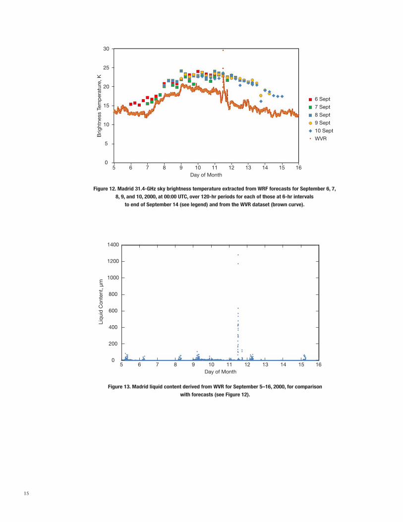
For the forecasting study, we selected a period to capture the large increase in sky tempera-ture (or hump) between days September 6 and 11, with a single rain spike (near day 11.5, as shown in Figure 11). Starting at calendar day September 6 at 00:00 UTC, we would start to see it. This is very similar to the Goldstone August 2003 case discussed previously (Sec-tion IV). Thus, forecasts were performed for calendar days September 6, 7, 8, 9, and 10 at 00:00 UTC, over 120-hr periods for each of those at 6-hr intervals, taking us out to the end of September 14 (see Figure 12). The minimum value of the 31.4-GHz brightness tempera-ture should be ~9.5 K, for dry clear conditions. Thus, it appears that the brightness tempera-ture signature for the entire month is elevated somewhat, due to water vapor or clouds.

We see from Figure 12 that the forecast values follow the general trend of the WVR data with a discrepancy on order of 5 K for most points, suggesting some evaluation of the fore-cast models for Madrid followed by model tuning is needed. Figure 13 displays the liquid content derived from the WVR data. We note only a single brief spike near day 11.5 in Figure 13, which coincides with the feature seen in the sky temperature data in Figure 12.

The forecasts do a reasonable job of also forecasting the surface air temperature when com-pared to surface weather data values as seen from Figure 14.

Figure 15 displays the surface water vapor pressure calculated from the local surface meteo-rological data at Madrid, which shows a trend similar to that of the 31.4-GHz brightness temperature in Figure 12. This is probably not surprising as one expects a high degree of

15

Figure 12. Madrid 31.4-GHz sky brightness temperature extracted from WRF forecasts for September 6, 7,

8, 9, and 10, 2000, at 00:00 UTC, over 120-hr periods for each of those at 6-hr intervals

to end of September 14 (see legend) and from the WVR dataset (brown curve).

30

25

20

15

10

5

05 6 7 8 9 10 11 12 13 14 15 16

Brig

htne

ss T

emp

erat

ure,

K

Day of Month

6 Sept

7 Sept

8 Sept

9 Sept

10 Sept

WVR

Figure 13. Madrid liquid content derived from WVR for September 5–16, 2000, for comparison

with forecasts (see Figure 12).

5 6 7 8 9 10 11 12 13 14 15 16

1400

1200

1000

800

600

400

200

0

Liq

uid

Con

tent

, µm

Day of Month

16

Figure 14. Forecast values of Madrid surface air temperature (red dots) for September 6–12 compared with air

temperature from Madrid weather tower (blue dots) for September 5–16, 2000.

40

30

20

10

05 6 7 8 9 10 11 12 13 14 15 16

Air

Tem

per

atur

e,°C

Day of Month

Surface Air Temperature Sept 6 Forecast

Figure 15. Surface water vapor partial pressure for Madrid calculated from surface meteorology data

during the selected forecast periods for September 5–16, 2000.

16

14

12

10

8

6

4

2

05 6 7 8 9 10 11 12 13 14 15 16

Vap

or P

artia

l Pre

ssur

e, m

b

Day of Month

17

correlation between the surface vapor pressure and brightness temperature (which includes contributions all along the vertical column). This is similar to what was observed with Goldstone forecasted water vapor content and WVR-derived water vapor content (see Fig-ure 8).

IV. Example of Forecasting Application in Telecommunications Link Calculations

To provide insight in how one may use the results of a forecast, we consider the case of the August 2003 forecast results (Section IV.B) for Goldstone at a 32-GHz Ka-band downlink frequency. Mission designers typically construct a conservative link such as at 90 percent weather conditions using either monthly or yearly statistics of atmospheric attenuation, and atmospheric noise temperature from the DSN telecommunications link design docu-ment [13]. For the analysis that follows, we ignore the small corrections needed to refer the 31.4-GHz sky noise temperature values to 32 GHz, and we also neglect adjustments for any bias between forecast values and AWVR values.

Given a pass occurring during the month of August at Goldstone where a large variation of atmospheric water vapor is present (depending upon conditions), link engineers take the August 90 percent cumulative distribution values of zenith atmospheric attenuation and zenith atmospheric noise temperature from [13] as input to link calculations. For the case of a 32-GHz downlink pass in August (we call this Case A), the DSN Telecommunications Link

Design Handbook 810-005 tables yield values of 18.91 K atmospheric noise temperature and –0.31 dB atmospheric attenuation at zenith for 90 percent weather. After applying adjust-ments in elevation angle (20 deg), and cosmic background using appropriate models [13], the resulting atmospheric noise temperature and atmospheric attenuation values are 51.66 K and –0.89 dB, respectively, as shown in Table 1 for Case A. The total system noise temperature is then calculated from the atmospheric noise temperature and applying the contributions due to microwave equipment for a 34-m BWG antenna [21] and adding the cosmic background contribution back in as shown in the last column of Case A in Table 1 as 83.41 K.

Table 1. Link advantage case for Goldstone summer climate (no cloud liquid).

Case 90 deg

A (810-005) –0.31 18.91 –0.89 51.66 83.41

B (Forecast) –0.12 7.30 –0.34 20.81 52.85

dB Advantage 0.56 1.98 2.54

90 deg 20 deg 20 deg 20 deg 20 deg

Attn, dB Tatm, K Attn, dB Tatm, K Top, K Total, dB

By contrast, we can compare the 18.91-K atmospheric noise temperature value of Case A with the minimum and maximum values of atmospheric noise temperature from inspec-tion of Figure 6 AWVR values (after removing cosmic background). These minimum and maximum values span from 7.3 K (10 K sky) to about 22.3 K (25 K sky), respectively, for the case of a humid summer day (no clouds). These values are consistent with the full range of water vapor density values derived from several years of historical WVR data [15], and thus cover the most conservative and optimistic cases during moisture-free conditions for Goldstone summer.

18

We can then consider the case of the most favorable weather conditions such as a 7.3-K zenith atmospheric noise temperature being applicable over the full duration of track-ing pass (typically 8 hr in duration) occurring within the next 1 or 2 days. Let us call this Case B, where there is a significant difference of the favorable 7.3-K zenith atmospheric noise temperature relative to the 18.9-K value that would normally be used in the conserva-tive link budget discussed for Case A above. This difference becomes more significant when considering a low elevation angle of 20 deg. After applying adjustments in elevation angle, cosmic background and microwave equipment using appropriate models [21], the resulting total system noise temperatures and atmospheric attenuations are as shown in the Case B row of Table 1. After applying the adjustments using appropriate models [13], the result-ing atmospheric noise temperature and atmospheric attenuation values are 20.81 K and 0.34 dB, respectively, as shown in Table 1 for Case B. The total system noise temperature is then calculated from the atmospheric noise temperature and applying the contributions due to microwave equipment for a 34-m BWG antenna [21] and adding the cosmic back-ground contribution back in as shown in the last column of Case A in Table 1 as 52.85 K.

We assume for simplicity that the data rate will scale according to received signal-to-noise ratio, where the received signal power will be degraded by atmospheric attenuation and the noise power will be degraded by total system noise temperature increase. To evaluate the dB difference Adv (or advantage) from going from Case A to Case B, we make use of the following formulation:

, ( )( )Adv dB SNR SNR dBdBA BD D= -

where

( ) logSNR Attn dB Top10 10D = -

is the contribution of SNR only due to atmospheric attenuation (Attn) and system noise temperature (Top) (which includes the atmospheric noise temperature (Tatm) contribu-tion), for the respective cases A and B. All common terms to the SNR should fall out in the differencing shown in Equation (1).

Thus, the dB advantage can be expressed as

, ( ) ( ) log logAdv dB Attn dB Attn dB T T10 10, ,B A op B op A10 10= - - -7 A Now, using values from Table 1, we get

, . . .. .log log dBAdv dB K K0 34 0 89 10 52 85 10 83 41 2 5410 10= - - - - - =_ i 7 A

The overall advantage in signal-to-noise ratio would be 2.54 dB at a 20-deg elevation angle. This implies that about 1.8 times more data can be downlinked during this period than if conservative 90 percent weather assumptions are used. We also consider the other extreme of the adverse (no moisture) case when the weather forecast predicts the worst-case zenith atmospheric noise temperature of 22.3 K (25 K sky brightness) where one would normally apply more atmospheric loss to the link tool values

(1)

19

and, hence, realize a lower data rate during the pass. In this case, the change would be on the order of 0.9 dB which lies well within the ~2 dB margin typically used in many link scenarios. In such cases, a project may opt not to go through the extra operational steps of changing data rates, and thus not uplink a new set of command parameters to override the default command parameters for those particular case scenarios.

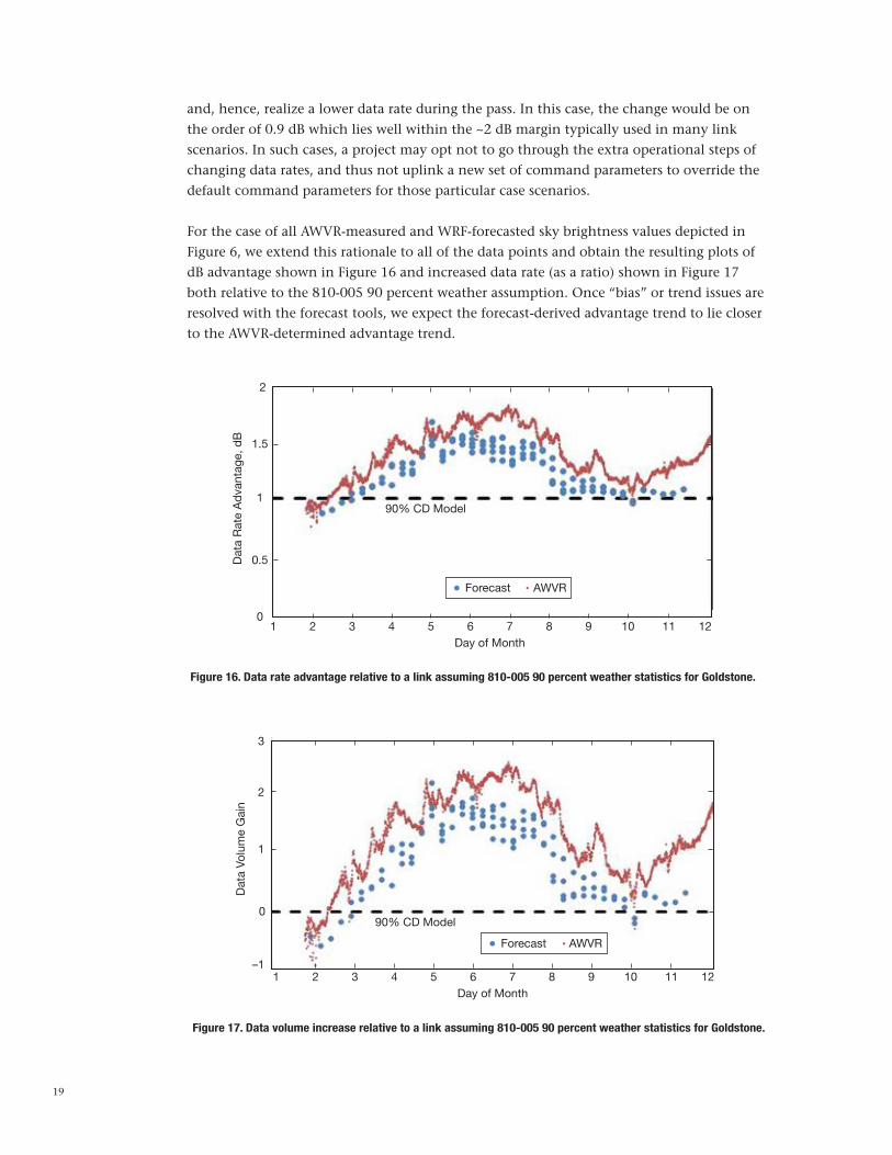
For the case of all AWVR-measured and WRF-forecasted sky brightness values depicted in Figure 6, we extend this rationale to all of the data points and obtain the resulting plots of dB advantage shown in Figure 16 and increased data rate (as a ratio) shown in Figure 17 both relative to the 810-005 90 percent weather assumption. Once “bias” or trend issues are resolved with the forecast tools, we expect the forecast-derived advantage trend to lie closer to the AWVR-determined advantage trend.

Figure 17. Data volume increase relative to a link assuming 810-005 90 percent weather statistics for Goldstone.

Figure 16. Data rate advantage relative to a link assuming 810-005 90 percent weather statistics for Goldstone.

2

1.5

1

0.5

01 2 3 4 5 6 7 8 9 10 11 12

Dat

a R

ate

Ad

vant

age,

dB

Day of Month

Forecast AWVR

90% CD Model

11 12

3

2

1

–11 2 3 4 5 6 7 8 9 10

Dat

a Vo

lum

e G

ain

Day of Month

Forecast AWVR

090% CD Model

20

Normally, one would use a single atmospheric noise temperature and atmospheric attenu-ation value in a link to cover a single several-hour pass. Here we assume that the 20-deg elevation point sets a single data rate to be used over an entire tracking pass, which is ap-plicable from rise to set. Other scenarios may include data rate stepping where a lower data rate is used during low elevation angle portions of a track near rise and set, and a higher data rate may be used at the higher elevation angle range in the middle of a track. Such scenarios are planned to be explored in further studies.

For cases such as rainy conditions, the situation becomes more complicated. Here a 200-K atmospheric noise temperature could result in many dB lower data rates and may require use of the X-band link at lower data rate (if accommodated) or Ka-band with some redun-dancy built into the downlink assuming periods of better and worst conditions. However, as one can see, the sky brightness temperature varies significantly during rain storms (Fig-ure 3, top). Thus, exploring such a scenario would require further study involving analysis of rain fade statistics along with fade durations for the site.

VII. Future Plans and Tests for Operational Weather Forecasting

Given that flight projects tend to set their downlink data rates anywhere from two weeks to several months in advance, the short-term utilization of weather forecasting techniques is unlikely or very limited in the context of current flight missions. However, the prospect of realizing increased data return during forecasted periods of favorable weather condi-tions may prompt some missions to explore using this technique under certain scenarios, or prompt future prospective missions to consider it in their pre-launch mission planning. Such scenarios also include the necessity of tightening link accuracy during events such as spacecraft safing, and partially compensating for degraded performance (e.g., traveling-wave tube amplifier lifetime) such as during extended mission phases. Another scenario could in-clude that of a Mars lander project where there is a major relay orbiter going into safe mode, and therefore scheduling and configuring for direct-to-Earth (DTE) passes in the short-term would be necessary. In this case, it would be important to know ahead of time, the forecast-ing of favorable or adverse (e.g., approaching rain storms) weather conditions to set the data rates for upcoming tracking passes.

Several of the above scenarios are applicable to the X-band (8.4-GHz) downlink where there may be advantages to using forecasting techniques (over using standard link assumptions). However, for the remainder of this section, we will focus on the use of the weather fore-casting at 32 GHz (Ka-band) for potential future missions that may wish to consider this technique.

Possible refinements to the weather forecasting process could involve incorporating the WVR data itself. At the very least, the last WVR data points prior to the start of the forecast period could be incorporated into the above scenario. Such applications could range any-where from applying a simple bias correction, a simple offset and rate (straight-line adjust-ment), or a Kalman filter derived trend into the forecast period ranging from a few hours to a day or longer. The Kalman filter approach would include an optimal weighting of forecast tool output values and WVR observational values occurring prior to and up to the forecast

21

start time. The net result, an extrapolated trend, will then extend into the forecast period, and a future study could compare this with the raw forecast, and WVR data collected (“after the fact”).

We plan to quantify how good the forecasting tools/models are (versus WVR) as a function of forecast time, identify any caveats with the current setup and identify steps for improve-ments. Such improvements include model tuning and folding in of other available nearby datasets into the forecasting set-up (data assimilation). We also plan to conduct mock tests by generating forecasts ahead of time and then compare results with “future” AWVR data. Additional tests may be performed with willing or participating projects interested in imple-menting weather forecasting into their operational scenarios.

For future forecasts, we may also make use of global/regional forecasts for boundary condi-tions at the 27-km domain. The accuracy of global forecasts may be lower than the analysis data we used here. We plan to run simulations to quantify such impacts in future studies.

It is planned to better evaluate how well the forecast values agree with the “measured” values extracted from the AWVR, how the error grows with forecast time, and identify what refinements (model tuning) can be realized in the algorithms and models to improve upon the forecast accuracy. In the WRF model, there are many choices of cloud microphysics, radiation, planetary boundary layer (PBL) schemes, etc., which may have significant impact on the model simulations. For improved forecasts, fine tuning of the model’s physical pa-rameterizations is needed and is identified for future work.

A possible operational scenario using weather forecasting may involve the following se-quence of events:

(1) Perform a forecast in advance of the pass delivering a sky brightness temperature TB (31.4 GHz) estimate referenced to zenith (perhaps with confidence limits) appropriate for a full track. There may be cases where multiple values may be delivered.

(2) The link engineer will convert TB (31.4 GHz) into atmospheric noise temperature at the appropriate frequency, e.g., Tatm (32 GHz).

(3) The Telecom Forecast Predictor (TFP or another link tool) will convert the Tatm (32 GHz, zenith) to atmospheric attenuation and atmospheric noise temperature for each link time tag at the elevation angle for that point during an upcoming tracking pass.

(4) The data rate for the pass (or multiple data rates) will be determined based on above parameter values, margin policy, elevation angles, etc. The data rate could be stepped at appropriate time instances during the pass. Uplink configuration parameters would then be delivered to the appropriate project team.

(5) A command load with new data rate(s) and other parameters applicable for the forecasted ground station pass would then be uplinked to the spacecraft replacing the default baseline parameters.

22

(6) During downlink operations, downlink telemetry performance would be moni-tored in real time. Increased data volume should then be realized.

Acknowledgments

We thank Steve Keihm for generating the AWVR and WVR datasets used in this comparison study; Connie Dang of Exelis for her assistance in providing DSN weather data; Jim Taylor and Ryan Mukai for informative discussions on potential use of weather forecasting for various flight project operational scenarios; and Faramaz Davarian, Stephen Townes, and Barry Geldzahler for supporting this work. We also thank Peter Kinman for well appreciated review comments.

References

[1] K.-M. Cheung, “Problem Formulation and Analysis of the 1-Hop ARQ Links,” The

Interplanetary Network Progress Report, vol. 42-194, Jet Propulsion Laboratory, Pasadena, California, pp. 1–15, August 15, 2013. http://ipnpr.jpl.nasa.gov/progress_report/42-194/194A.pdf

[2] S. Shambayati, “Maximization of Data Return at X-Band and Ka-Band on the DSN’s 34-Meter Beam-Waveguide Antennas,” The Interplanetary Network Progress Report, vol. 42-148, Jet Propulsion Laboratory, Pasadena, California, October–December 2001, pp. 1–20, February 15, 2002. http://ipnpr.jpl.nasa.gov/progress_report/42-148/148E.pdf

[3] David H. Rogstad, Alexander Mileant, and Timothy T. Pham, Antenna Arraying Tech-

niques in the Deep Space Network, Volume 6, New Jersey: John Wiley & Sons, 2005.

[4] F. Davarian, R. Mendoza, and B. Benjauthrit, “Forecasting of Weather Effects for the Deep Space Network,” 2005 IEEE Antennas and Propagation Society International Sympo-

sium, pp. 43–46 vol. 4A, 2005. http://dx.doi.org/10.1109/APS.2005.1552577

[5] S. Shambayati, “On the Benefits of Short-Term Weather Forecasting for Ka-band (32 GHz),” Proceedings, IEEE Aerospace Conference, Volume 3, pp. 1498, 2004. http://dx.doi.org/10.1109/AERO.2004.1367924

[6] W. C. Skamarock, J. B. Klemp, J. Dudhia, D. O. Gill, D. M. Barker, W. Wang, and J. G. Powers, A Description of the Advanced Research WRF, Version 3, NCAR Technical Note TN-468+STR, 113 pp., 2008.

[7] NCEP FNL Operational Model Global Tropospheric Analyses, April 1997 through June 2007. http://rda.ucar.edu/datasets/ds083.0/

23

[8] G. Thompson, P. R. Field, R. M. Rasmussen, and W. D. Hall, “Explicit Forecasts of Winter Precipitation Using an Improved Bulk Microphysics Scheme, Part II: Imple-mentation of a New Snow Parameterization,” Monthly Weather Review, vol. 136, no. 12, pp. 5095–5115, December 2008. http://dx.doi.org/10.1175/2008MWR2387.1

[9] M. J. Iacono, J. S. Delamere, E. J. Mlawer, M. W. Shephard, S. A. Clough, and W. D. Col-lins, “Radiative Forcing by Long-Lived Greenhouse Gases: Calculations with the AER Radiative Transfer Models, Journal of Geophysical Research, vol. 113, D13103, July 16, 2008. http://dx.doi.org/10.1029/2008JD009944

[10] M. B. Ek, K. E. Mitchell, Y. Lin, E. Rogers, P. Grunmann, V. Koren, G. Gayno, and J. D. Tarpley, “Implementation of Noah Land Surface Model Advances in the National Centers for Environmental Prediction Operational Mesoscale Eta Model,” Journal of

Geophysical Research, vol. 108, 8851, November 27, 2003. http://dx.doi.org/10.1029/2002JD003296, D22

[11] Z. I. Janjic, “The Step-Mountain Eta Coordinate Model: Further Developments of the Convection, Viscous Sublayer, and Turbulence Closure Schemes,” May 1, 1994. http://journals.ametsoc.org/doi/abs/10.1175/1520-0493%281994%29122%3C0927%3ATSMECM%3E2.0.CO%3B2

[12] J. S. Kain, “The Kain–Fritsch Convective Parameterization: An Update,” Journal of

Applied Meteorology, vol. 43, pp. 170–181, January 1, 2004. http://journals.ametsoc.org/doi/abs/10.1175/1520-0450%282004%29043%3C0170%3ATKCPAU%3E2.0.CO%3B2

[13] S. D. Slobin, “Atmospheric and Environmental Effects,” DSN Telecommunications Link

Design Handbook, DSN No. 810-005, Space Link Interfaces, Module 105, Rev. E, Jet Pro-pulsion Laboratory, Pasadena, California, October 22, 2015. http://deepspace.jpl.nasa.gov/dsndocs/810-005/105/105E.pdf

[14] D. D. Morabito,“A Comparison of Estimates of Atmospheric Effects on Signal Propaga-tion Using ITU Models: Initial Study Results,” The Interplanetary Network Progress Report, vol. 42-199, Jet Propulsion Laboratory, Pasadena, California, pp. 1–24, November 15, 2014. http://ipnpr.jpl.nasa.gov/progress_report/42-199/199D.pdf

[15] D. D. Morabito, S. Keihm, and S. Slobin, “A Statistical Comparison of Meteorological Data Types Derived from Deep Space Network Water Vapor Radiometers,” The Inter-

planetary Network Progress Report, vol. 42-203, Jet Propulsion Laboratory, Pasadena, California, pp. 1–21, November 15, 2015. http://ipnpr.jpl.nasa.gov/progress_report/42-203/203A.pdf

[16] C. Naudet, C. Jacobs, S. Keihm, G. Lanyi, R. Linfield, G. Resch, L. Riley, H. Rosenberger, and A. Tanner, “The Media Calibration System for Cassini Radio Science: Part I,” The

Telecommunications and Data Acquisition Progress Report, vol. 42-143, Jet Propulsion Laboratory, Pasadena, California, July–September 2000, pp. 1–8, November 15, 2000. http://ipnpr.jpl.nasa.gov/progress_report/42-143/143I.pdf

24 JPL CL#16-3606

[17] G. M. Resch, J. E. Clark, S. J. Keihm, G. E. Lanyi, C. J. Naudet, A. L. Riley, H. W. Rosen-berger, and A. B. Tanner, “The Media Calibration System for Cassini Radio Science: Part II,” The Telecommunications and Data Acquisition Progress Report, vol. 42-145, Jet Propulsion Laboratory, Pasadena, California, January–March 2001, pp. 1–20, May 15, 2001. http://ipnpr.jpl.nasa.gov/progress_report/42-145/145J.pdf

[18] G. M. Resch, S. J. Keihm, G. E. Lanyi, R. P. Linfield, C. J. Naudet, A. L. Riley, H. W. Rosenberger, and A. B. Tanner, “The Media Calibration System for Cassini Radio Sci-ence: Part III,” The Interplanetary Network Progress Report, vol. 42-148, Jet Propulsion Laboratory, Pasadena, California, October–December 2001, pp. 1–12, February 15, 2002. http://ipnpr.jpl.nasa.gov/progress_report/42-148/148H.pdf

[19] Fawwaz T. Ulaby, R. K. Moore, and Adrian K. Fung, Microwave Remote Sensing: Active

and Passive, Volume 1: Microwave Remote Sensing Fundamentals and Radiometry: Reading, Massachusetts, Addison-Wesley Publishing Company, 1981.

[20] S. D. Slobin, “Microwave Noise Temperature and Attenuation of Clouds: Statistics of These Effects at Various Sites in the United States, Alaska, and Hawaii,” Radio Science, vol. 17, no. 6, pp. 1443–1454, November–December 1982.

[21] S. D. Slobin, “34-m BWG Station Telecommunications Interfaces,” DSN Telecommuni-

cations Link Design Handbook, DSN No. 810-005, Space Link Interfaces, Module 104, Rev. H, Jet Propulsion Laboratory, Pasadena, California, March 5, 2015. http://deepspace.jpl.nasa.gov/dsndocs/810-005/104/104H.pdf