Fluidum Continuum Universalis - Introduction in Fluid Mechanical Physics

FLUIDUM CONTINUUM UNIVERSALIS

PART I

INTRODUCTION IN FLUID MECHANICAL PHYSICS

by

Arie M. DeGeus

Columbia, South Carolina, USA

September, A.D. 2000

iii

TABLE OF CONTENTS

PART I INTRODUCTION IN FLUID MECHANICAL PHYSICS

+ PREFACE vi SUMMARY vii INTRODUCTION xiv ACKNOWLEDGEMENTS xvi STATUS OF PHYSICS-A.D. 2000 xvii 1 PROPERTIES OF THE FLUIDIUM CONTINUUM 1

1.1 General Considerations........................................................................................1 1.2 Physical Characteristics .......................................................................................3 1.3 Method of Description.........................................................................................4

1.3.1 Method of Lagrange ....................................................................................4 1.3.2 Method of Euler...........................................................................................4

1.4 General Differential Equations in any “Continuum” in Motion or at Rest. ........5 1.5 Stationary Inviscid Irrotational Flow...................................................................7 1.6 Derivation of the Velocity Distribution.............................................................10 1.7 Applicable Laws ................................................................................................13 1.8 Potential and Kinetic Energy .............................................................................14 1.9 Pressure and Density in the Universal Fluidum Continuum .............................16 1.10 Determination of the density ρ in the FC in an area with “space-time

curvature”, as a function of 0ρ , *c , Ω , R and *mc mρ =∑ ) .....................................18 1.11 Velocity of “FC Energy” Waves .......................................................................19 1.12 Velocities Greater than C* (“Speed of Light”) ..................................................20 1.13 Wave and Vortex Phenominae in General.........................................................25

1.13.1 Wave Phenominae in General ...................................................................25 1.13.2 Considering the “bending” of light beams in “space-time curvature”: some examples 25 1.13.3 Vortex Phenominae in General..................................................................29

2 VORTEX PHENOMINAE 32 2.1 Open Fluid Flow Vortexes.................................................................................32

2.1.1 Rotational Energy (See Fig. 10) ................................................................33 2.1.2 Irrotational Flow........................................................................................33 2.1.3 “Helical component” Flow ........................................................................34 2.1.4 Total energy of all flows of the Open Vortex tube ....................................35 2.1.5 Values for: Rρ and Iρ as: ( )0,f R ρ ? ................................................35

2.2 Calculation of the So called “Root-Mean-Square” Velocity of the “Random Motion,” Corresponding to the Observed “Background Radiation” .............................36

2.2.1 Computation of the Average Velocity.......................................................37 2.2.2 Computation of the Average of the Square of the Velocity ......................37

iv

2.2.3 Calculation of the: rmsv of the “Random Motion” in the FC.....................38 2.2.4 Closed Fluid Flow Vortexes ......................................................................40 2.2.5 Interrelationship of the FC Density with Electro-magnetic Factors ..........42 2.2.6 Summary Considerations of Waves and Vortex Entities ..........................42

3 THE ELEMENTARY PARTICLES 44 3.1 The Electron-Neutrino .......................................................................................44

3.1.1 The Energy of the Electron-Neutrino and also of the Anti-Neutrino. .......45 3.1.2 Rotational Energy of the “Toroid” or Single Vortex-ring (See Figs. 18a and b ) 46 3.1.3 Circulatory irrotational Energy Through and Around the “Toroid” (See Fig. 19) 47 3.1.4 Cross-section and Velocity Distribution Outside the Neutrino .................48 3.1.5 Are there “higher harmonic orders” for the “toroid” ? (The size of neutrino’s) ..................................................................................................................49

3.2 The Muon-Neutrino ...........................................................................................50 3.2.1 Calculation of the magnitude of size of the muon-neutrino and associated vortex ring..................................................................................................................51

3.3 The Proton .........................................................................................................52 3.3.1 Calculation of the diameter of the outflow of “toroid” hole of the proton53 3.3.2 Calculation of the width of the split PRf (between the vortex rings of the proton) 55 3.3.3 The size of the vortex “eye-wall” diameter of the proton .........................58 3.3.4 The “mass” of the proton...........................................................................59 3.3.5 “Charge” and “Spin” of the Proton............................................................60

3.4 The Electron.......................................................................................................60 3.4.1 General considerations ...............................................................................60 3.4.2 Pressure and density “inside” the electron.................................................64 3.4.3 The electron “at rest”.................................................................................65 3.4.4 The Electron “in Motion” ..........................................................................67 3.4.5 Wave-particle duality for electrons ...........................................................68

3.5 Impulse-Interaction of Photons with Electrons Causes the “Compton Shift” for the Photons.....................................................................................................................70

4 HYDROGEN 72 4.1 Atomic Hydrogen ..............................................................................................72

4.1.1 “Fractional” states......................................................................................79 4.1.2 The reactivity of “fractional hydrogen”.....................................................82

4.2 Bi-electronic and Molecular Hydrogen .............................................................84 4.2.1 Derivation of a rule which governs the energy quantum levels. ...............85 4.2.2 Molecular (ordinary) hydrogen..................................................................86

4.3 Deuterium ..........................................................................................................87 4.4 Tritium ...............................................................................................................88

APPENDIX I 90 APPENDIX : II 95 BIBLIOGRAPHY 98 GLOSSARY 100 INDEX 106

vi

PREFACE

Writer’s opinion and findings by means of research of the “Fysis” of all things in this or these Universes coincide with Sir Isaac Newton’s scientific legacy as is laid own in his “Principia Mathematica”. All is deterministic ; nothing is left to chance and all inter-relationships are of a “clean-cut” elegance. One hundred fifteen years later ( 1812 ) we find the same vision with Pierre-Simon de Laplace in France as he states in his Theorie Analytique des Probabilites” :

“An Intellect which at any given moment knew all the forces which animate Nature and the mutual positions of the beings that comprise it; if this Intellect were vast enough to submit its data to analysis, could condense in a single formula the movement of the greatest bodies in the Universe and that of the lightest atom: for such an Intellect nothing could be uncertain, and the future just like the past would be present before its eyes”.

Writer also found that over and beyond the deterministic inter-relationships of the

“Fysis” of all things, that there is also a deterministic Maintenance Factor involved and connected to the continued existence of this or these Universes in its or their basic inter-relationships, which show mathematical elegance on a grand scale. The level of this book is such that it assumes at least under-graduate knowledge of calculus, general physics, fluid mechanics, nuclear physics and astronomy.

Writer, who humbly serves his Creator, feels greatly privileged that the Great Architect considers him worthy to be able to see, contemplate, and give form to the concepts and the establishment of the basic inter-relationships, which underlie and regulate all things. Many of the concepts and most derivations of inter-relationships in this book are new.

Columbia, South Carolina, USA, August A.D. 2000

A.M.D.G.

vii

SUMMARY Chapters: 1.1.0 The “Fluidum Continuum” ( = FC ) pervades all of space albeit at varying

densities as to certain locations. Varying densities are cause of “space-time curvature” and as such the density ( = ρ ) determines the phenomenon “mass” ( = m ) and the maximum allowable velocity in the FC, which is the “speed of light” ( =c ) at location. Energy is constituted by motion and by density in the FC. Motion in the FC is the sum-total of all motions: stationary, non-stationary, wave-type and vortex type, all of which can be super-positioned upon each other.

1.1.1 The Physical Characteristics are: Homogenous, Coheasive, Inviscid ( = friction-

less ) and Compressible. 1.1.2 The chosen method for describing the “Fluid Mechanics” is the ‘Euler’-method.

Vortex phenominae are characterized by: “Rotational Flow” ( R∝ ), “Irrotational Flow” ( 1/ R∝ ) and a “Helical Component” Flow, which is parallel to the “vortex-thread / centerline”. The velocity in the “eye-wall” of a vortex approximates the “speed of light” c . In the compressible FC is valid:

(Bernouilli for the FC) 2

1,21

2

. .ln2FC

vpK T

p∆

=

, wherein FCK = the

correspondent of the “gas-const. but for the FC, T = absolute temperature, p = pressure, v = velocity.

1.1.3 ( Away from “Black Holes” ) is valid, 2/ *P cρ = , and * 1. .FCc K T= , wherein

*c = “velocity of light” in “standard” space, which is space with a density 0ρ .

1.1.5 The “Gravitational Maintenance” inflow to “mass” is . 2kc

grav

mv

R= Ω ∑ , wherein

Ω = “gravitational constant” for the FC, kc km = Λ ”mass” of center k ,

( )ve venζ ρΛ = × , R = distance to center of the vortex. The “attraction force”

between groups of “mass” entities is 1 2

2c c

GM

m mG

R= Ω ∑ ∑ and the density

function for “space-time curvature” is 2 2

0 2 4

*.exp

2. *m

c Rρ ρ

Ω= −

viii

1.1.6 The maximum allowable velocities inside “vortex tubes” are higher than *c ,

. . . . 2. /i n s v t

ac P

Rρ= , ( a = radius of “vortex tube”, R = distance to center )

For “space-time curvature” the “first derivative” of c wrt R is

3

* 12

*.dc mdR c R

Ω= −

The maximum velocity allowed for an electron-neutrino in “space-time

curvature” is max 2

2 * 1*

2 *m

v cc

Ω = + Ξ , wherein, Ξ = projected distance

between the trajectory of the neutrino and the “mass” center. 1.1.7 The “bending of light” in the FC alongside an ”extended length” “mass” object (

e.g. a galactic plane ) is − 2

2 * 12 *

mx cα Ω

≈ ×Ξ ∆Ξ

( x = length axis, ∆ Ξ =distance

between paralleling beams , α = angle of deflection ) . The “bending of light” in

the FC around a “mass” point is * 1

2. *.m

cα

Ω− ≈ ×

Ξ ∆Ξ (this formulation can be used

for “gravitational lensing” as well)

2.1.1 The “Rates of Energy” for Vortex tubes are 3*4Rotational RE dLcπ

ρ= ,

3 ˆ* ln2 / 2

vIrrotational I

RE dLc

dπ

ρ =

, 3 ˆ* 2 ln4 / 2

vHelical R I

RE dLc

dπ

ρ ρ = +

,

wherein , d = diameter of “vortex tube”, whereby the “eye-wall” velocity is c , L is the length of the “vortex tube, vR = radius to where the “irrotational flow”

borders the “Brownian” motion in the FC , which relates to the 02.72 K “Background Radiation” temperature in the universe. 0.55Rρ ρ≈ × ; 0Iρ ρ≈ . The estimate for the “Root-Mean-Square” velocity of the “Brownian” motion in the FC is 285rmsv ≈ m/sec, the value for ˆ 525,000vR d≈ .The Rotational Energy rate of a “vortex tube” is independent of its diameter D , but is always

3*4 RdLcπ

ρ . The permeability× permitivity product is 0 0µ ε The relationship as to

density is 0 00

ρµ ε

ρ ρ∝

− .

ix

3.1.1 Neutrino / Anti-neutrino: The energy rates are 2 301.1 *

4Rotational nE d cπ

ρ≈ × and

2 30 *

4Irrotational nE d cπ

ρ= . 2 3. . 0.1 *

4HelicComp nE d cπ

ρ= ( is included in the Rotational

Energy rate ) 3.1.2 Muon-neutrino : 207E eV= , MuonD ≈ 199 10 m−× , “mass” 343.7 10 kg−≈ × . 3.1.4 Proton: “Eye-wall” diameter: PR el pod d d≈ = ; 3polar outflow PRd d− = × Total

“fluid-dynamic” energy rate is 306.00 . . *

4 PRd cπ

ρ≈ × . Potential Energy is

20.40 . *cρ≈ × ; density inside proton is 01.2insρ ρ≈ × , “mass” of the proton is

30.60 . PRdρ≈ × . This corresponds with the classical mass of 271.67 10 kg−× .

Calculatory estimate of PRd gives 151.09 10PRd m−≈ × . spinV at inside “toroid” hole

diameter is .064 *spinV c≈ × , and 263.2 10 ./sec.radω ≈ × ”Charge” energy rate

is 2 303.0 . . *

4 PRd cπ

ρ≈ × .

3.1.5 Electron: Calculatory estimate of eld is 1510eld m−≈ ; the diameter of the polar /

axial inflows ( electron “at rest” ) is 1

27 eld≈ ; fluid-dynamical “mass” of the

electron is 30.034 . eldρ≈ × . .064 *spinV c≈ × , and 2 3

0.06 . . *spin elE d cρ≈ ×

“Charge” energy rate is 2 30.00128 . . *eld cρ≈ × and “Angular Momentum”: / 2h (

/ 2h π=h : “Planck’s constant / 2π ’). The value of the angular momentum is 355.3 10−× . The electron “in motion” shows a spiraling trajectory ( 2 sine-wave

motions with 090 phase difference super-positioned on each other ) ; this proves the “Complimentarity Principle” of Bohr and gives confirmation of the Davisson-Germer experiment . Limitations are imposed for larger “particles” . The electron “grows” as it comes into “relativistic” velocities, the “toroid” hole diameter of the inflows enlarges, as does the outflow split; the internal fluid density lowers.

4.1.1 Hydrogen: 2

2 20

13.68n

H

eE eV

n a nπε= − = − , wherein n =quantum level ; e =elem.

charge; 0ε = permitivity; Ha = Bohr radius, Frequency of radiation when

electrons go from higher to lower quantum levels is 1 2E Eh

ν−

= . From

astronomical observations and findings in the laboratory, it became obvious that also “fractional states” can exist. The energy levels can be found by substitution

of “fractions” in energy formula 2

13.6 1 1 1, , , ,....

2 3 4nE eV nn

= − = Valid for

x

distances between proton and electron ( is Bohr radius ) is 2 9.053 10Ha n m−= × ×

and for orbit velocity is 2

6

0

1 12.2 10 /sec.

2ne

v mh n nε

= × = ×

Frequencies of emitted radiation are (“Rydberg” formula) , 22 2

2 1

1 1RZ

n nν

= −

,

wherein, 1Z = , and 4

2 308

meR

hε= =1.09 7 110 m−× . Total “fluid-dynamical”

energy rate of the hydrogen atom is 2 308.2 *

4 eld cπ

ρ≈ × . Reactions between

“fractional states” are governed by: ( ) ( ) ( )i k pn n nH H H H e photon+ −+ → + + + “Bi-

Electronic Hydrogen: “Angular Momentum of an electron is 2nh

rmvπ

= For the

quantum numbers of the energy states is valid 1 1

;k lk l

n np p

= = ;

1 1 1 *2 H

k l

mca

p p hα

+ = × × ×

( wherein , Ha = “Bohr radius”; α = ”fine

structure constant”is 22*e

hcπ 1

137≈ ;

*h

mc= Compton wavelength) . “Bi-electronic

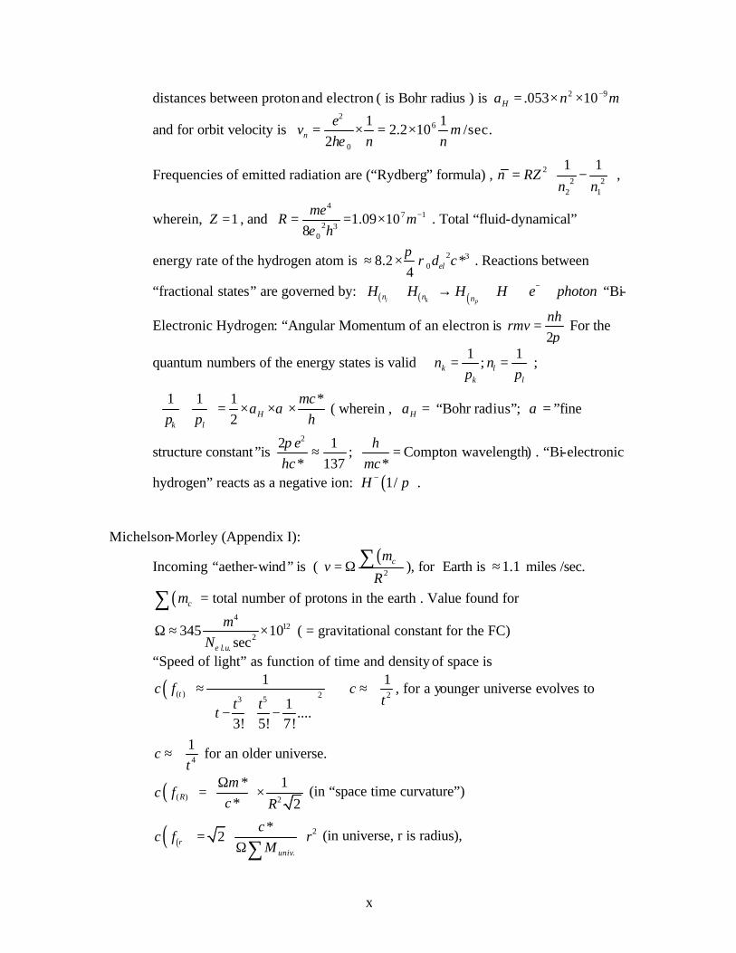
hydrogen” reacts as a negative ion: ( )1/H p− . Michelson-Morley (Appendix I):

Incoming “aether-wind” is ( ( )

2cm

vR

= Ω ∑ ), for Earth is 1.1≈ miles /sec.

( )cm∑ = total number of protons in the earth . Value found for 4

122

. .

345 10sece l u

mN

Ω ≈ × ( = gravitational constant for the FC)

“Speed of light” as function of time and density of space is

( )( ) 23 5

1

1....

3! 5! 7!

tc ft t

t

≈

− + −

2

1c

t⇒ ≈∝ , for a younger universe evolves to

4

1c

t≈∝ for an older universe.

( )( ) 2

* 1* 2

R

mc f

c RΩ = ×

(in “space time curvature”) ⇒

( )( ) 2

.

*2r

univ

cc f r

M

= Ω ∑

(in universe, r is radius),

xi

so 22

1r

t≈∝ evolves to 2

4

1r

t≈∝ as the universe ages.

Conclusion: 1

rt

≈∝ (young universe) evolves to 2

1r

t≈∝ (old universe).

xii

Fluid

Dynamic “Mass”

Classical Physics Mass

Fluid Dynamic Energy Rate

Classical Physics Energy

Fluid Dynamic Charge Force

Fluid Dynamic

Spin Energy Rate

Potential Energy Spin

Velocity

30dρ kg 2 3

0 *4

d cπ

ρ Joule 2 20 *d cρ 2 3

0 *d cρ Unit Expression

20 *cρ eV c*

. .e l uN kg 2 3.e l uN L T − 2 2MLT−

2. .e l uN LT − 2 3

. .e l uN L T − Dimensionality

1 2. .e l uN L T− − 1LT −

Electron-Neutrino/Anti-

Neurtino 36 10−≈ × 365 10−≈ × 1.1≈ 5eV< N.A. .1≈

.18≈ Muon-Neutrino 7.5≈ 343.7 10−× 2.0≈ 207eV N.A.

.064

6.00 .3≈ Proton/Anti-proton 60≈ 271.67 10−×

.40 938MeV 3.0≈

.064

.06≈ Elecron/ Positron “at rest”

Pos. 2.73 Neg. 2.70 Net .327

319.1 10−× 2.2≈ 511KeV .00128

.064

.29≈ Electron “in motion”

.99 *v c= 59≈ 271.65 10−≈ × 5.9≈ 900MeV≈ 2.9≈

.064

184.4 10 J−× Hydrogen

Atom 60.03≈ 271.67 10−≈ × 8.2≈ 938.5MeV≈ N.A. 6

1

2.2 10

.secm −

×

xiii

Classical Physics Constants

Boltzmann’s Constant 231.38 10 / .k J mol K−= × Charge electron 191.60 10e Coulomb−= × * Gas Constant 38.32 10 / /R J kg mol= × Gravitational Constant 116.66 10G Newton−= × Planck’s Constant 346.62 10h −= × secJ * Permitivity of Free Space 12

0 8.85 10 /Farad mε −= ×

Permeability of Free Space 0µ = 74 10 /Henry mπ −×

“Speed of Light” 8* 3 10 /secc m= × *

*) This is the same constant in the Fluidum Continuum with the same value. Fluidum Continuum Constants

Boltzmann’s Constant .BolFCk magnitude= of 210− ( 2 2 1L T − −Θ )

Density in “standard” space 0 magnitudeρ = of 610− ( 3. .e l uN L− )

Gravitational Constant ( univ ) 12345 10Ω = × 4 2. ./ sece l um N ( 14 2

. .e l uL N T− − )

Fluidum Constant FCp

K Tρ

=2

16 2 2*3.3 10 /secFC

cK m K

T= = × ( 2 2 1L T − −Θ )

Specific Heat Constant 4. .3 10 /FC e l u

UC J N K

T= ≈ × ( 12 2 1

. .e l uL T N −− −Θ )

“Eye-wall” Diameter of: a. Proton, Electron, Positron 1510PR el posd d d m−= = ≈

b. Muon-neutrino 199 10muond m−≈ ×

c. Electron-neutrino, aAnti-neutrino 193 10nd m−≈ × Root-mean-square velocity “Brownian” motion 285rmsv ≈ /secm

“Standard” Volume in “standard” space 1.00 3m “Standard” Mass in “standard” space 971.5 10≈ × Planck units of mass “Planck Length 354.05 10 m−≈ × “Planck Density 1031.5 10≈ × Planck 3/units m

( FCN is the number of elementary units in the Fluidum Continuum)

xiv

INTRODUCTION

The new approach to physics as contained in this book of 3 parts introduces an Energy Continuum which not only behaves like a fluidum, but is in actuality a “mass”-less fluidum, which consists of elementary units ζ , which are certainly not larger then 10 25− m and even could have a size as small as the “Planck length,” the definition of which is

“Planck length” = 3

.*

h Gc

, ( 1 )

wherein h = the Constant of Planck ( 6.62 x 10 34− j-sec ) , G = the Gravitational Constant ( 6.66 × 10 11− Newton ) and *c = the so called “speed of light”, which is the maximum possible velocity of a wave in such area of space , which has essentially a “flat” “space-time” characteristic. ( *c = 3 × 10 8 m sec 1− ) The “Planck-length” is 4.05 x 10 35− m. If this value is taken for the smallest possible 3-dimensional unit, we find for a “Planck-density,” 1.5 x 10 103 units m 3− . The Gravitational Constant is from classical physics and still refers to kilogram-mass. This constant has its analogous counterpart for the Energy Continuum or Fluidum Continuum. This constant which shall be indicated by Ω , is new to physics and can be defined as: the “gravitational maintenance factor” for the various types of vortex entities which exist in the Fluidum Continuum together with all the wave types. Ω is the proportionality factor between the (non-wave) velocity .gravv , which is perpendicular to a given cross-section in the Fluidum at a distance R from a center of vortex entities divided by the number of basic vortex entities which are being served with additional fluid energy. This quantity of “mass” vortex entities be indicated by Λ∑ . Formulations are:

2

.gravv RΩ =

Λ∑ ( 2 ) and, 3

.*FC

hPlancklength

cΩ

= ( 3 )

The size magnitude range with regard to most subject matters in Part I of this book is from the size of the hydrogen atom down to the “Planck- length FC ”. From “our reality” of 1 m it is 15 magnitudes down to the size of the electron and from the electron to the maximum size of the elementary units, ζ is 8 – 10 magnitudes down and from the size of ζ to the “Planck- length” is about another 10 magnitudes down. Part I mostly handles

physics phenominae in the size range: 10 2510 10− −− m. Since “Mass” in classical sense does not exist in the FC, the energy E is always expressed as a product of the “standard-density”: 0ρ , the square of the diameter of the elementary vortex: d and the third

power of the speed of light in “standard space”: 3*c . The exact definitions of these factors are in Part I. The so-called “Background radiation” ( 2.72K ) is not the last remainder of a so-called “Big Bang.” Its existence is responsible for a “Brownian” motion of the elementary units in the Fluidum, which has a “root-mean-square velocity,”

xv

rmsv , which has a estimated value of 285 m sec 1− . This “Brownian” motion is the reason that the “frictionless” character of the Fluidum is limited in the outermost range of the so-called “irrotational” flow, (which is the surrounding flow of all vortex type entities). The limit where the velocity of the “friction-less” “irrotational” flow equals the velocity of the random “Brownian” motion is calculated to be at a distance of 525,000 d ( d is the diameter of the elementary vortex ) in outward direction and it limits the energy of “open” vortexes , namely the energy of the irrotational flow is maximally 26× the energy of the “rotational” flow. In the case of “closed” vortexes there is always a total energy balance between the “rotational” flow together with the “helical component” flow and the “circulatory” flow, which is “irrotational”. The “Brownian” motion, which is random, is not fully ”friction- less” or “super-fluid”; it causes the slightest of drag in the outer-most range of the “irrotational” flow and is therefore also cause for the need (although infinitesimal) for additional fluid energy over time. This inflow of additional fluid toward vortex entities in the Fluidum is called “Gravitation”. This subject matter is being discussed in all 3 Parts of this book. Curiously calculations with regard to the electron show that the “rotational” and “irrotational” energies of its elementary “vortex rings” is greater than the energy equivalent of its “mass” in classical physics’s sense. This has led to the undeniable conclusion of the existence of “Fractional Mass” / “Negative Mass”. A new postulate as to what the phenomenon “Mass” means can and shall now be defined. The existence of “Fractional Mass”and associated “Fractional / Negative Energy” is directly linked to the “collapse of matter” and the physics of extreme “space-time curvature”. This also gives credence to phenominae which take place in the so called “ergosphere” of active black holes. Also parallels can be seen with the so-called “Penrose process”, whereby energy can be “borrowed” between entities. In the case of the hydrogen atom, reduction in energy of its electron translates into a smaller size of the “circulatory” ( = “irrotational”) flow “envelope” , which causes the electron to descend from the “ground-state” to lower quantum levels in the fluid dynamic flow “chalice”. All “fractional states” are very stable. This descent through lower quantum levels is accompanied by photon emission just as is the case by descent from “excited states” to the “ground-state”. Writer developed a process whereby this energy is being “harvested” for multiple beneficial uses.

xvi

ACKNOWLEDGEMENTS

In the late 1970’s writer met Arnold G. Gulko. At that time Mr. Gulko practiced patent law in Crystal City, VA. His office was located within walking distance from the US Patent and Trademark Office. Mr. Gulko did patent work for me which was mostly in the realm of thermo-dynamic processes, particularly relating to “alternative energy” applications. It was the time of the Carter Administration and of the promotion of “alternative energy”. The “gas-lines” were fresh in the memory. Mr. James Schlesinger was at the helm of ERDA ( = Energy Re-Development Administration). Writer got government grants for developing certain devices in solar and wind energy applications. Mr. Gulko, who I saw regularly, familiarized me with new physics, which had been pioneered before by Mr. C. F. Krafft, in live patent examiner at the Patent and Trademark Office. This science of physics, which involves the micro- as well as the macrocosmological phenominae, is “Fluid Mechanics” based; it is in essence a revival of the “aether” or Fluidum Continuum theories. Writer studied Gulko’s “Vortex Theory” and was astounded by its truth and logic in the research and development in many matters of physics. Over the years Mr. Gulko expanded the Fluidum Continuum theories, particularly in the field of astronomy. Writer is thankful for having met Mr. Gulko who is a great thinker in the fields of physics and related astronomy. Writer then started his own research and put mathematics and fluid mechanics to work on concepts from Planck, Gulko and Winterberg. Writer added and corrected, while keeping the developing theoretical knowledge on a sound mathematical footing. This brought new inter-relationships in elementary physics to light, which provided new nuclear processes, which were proven to be correct in the laboratory. In 1999 writer met Prof. Thomas G. Stanford, who teaches Chemical Engineering at the University of South Carolina. Professor Stanford is knowledgeable in many disciplines in the exact sciences; his personal scientific library is bigger than the one at his department; he is always willing to be my sounding board and reviewed the developing science on a continuing basis. Working with him is always a pleasure. This bodes well for Parts II and III. of this book. Also thanks to my nephew Ir. J.M.Verheij for his help and commentary.

xvii

STATUS OF PHYSICS-A.D. 2000

Early into the 20th century, physics experienced a golden period of scientific discoveries and expansion of knowledge, with Einstein’s relativity theories forming the “crown” piece.

With Heisenberg and others like Born and Schrodinger came the quantum mechanics, which parts away from deterministic, measurable and verifiable physics.

Writer also uses some of ‘classical’ quantum mechanics as a “useful tool” as Einstein used to say. Quantum mechanics developed further with little opposition. Even the educated public was and is not capable of evaluating quantum mechanics at the level it came to. In the 50-ties no one questioned the ‘physics community’, particularly after the successful development of the A- and H bombs, which elevated physicists to a status, where no one could really question them as to the merits of going into certain directions of research. The physics of the A- and H-bombs and Nuclear Fission in general (as it is being applied in nuclear power plants) are relatively simple and the achievements in this area stand for the last major advancements in physics. The necessity to limit nuclear waste and the need for inexhaustible and inexpensive fuel started the research in thermo-nuclear fusion. This multi-billion dollar program failed. No Tokamak ever ran for any length of time in any country. No “overunity” or “breakeven” has ever been achieved. Nevertheless the ‘physics community’ continues into this direction while there is no hope for reaching commercial viability.

In the 1980-ties “cold fusion” looked to be a possibility, which was short- lived simply because the rate of reactions was too slow. Recently there have been slightly better results. Even while the “cold fusioneers” are down, the physics community keeps fighting them (e.g. R. Park, who calls “cold fusion” fraudulent and also Huizenga with a book, titled: “Cold fusion, the fiasco of the 20-th century). The real fiasco is thermo-nuclear fusion, which wasted billions of dollars. “Cold fusion costed only pocket money. Funding for “thermo-nuclear fusion” in the US is curbed now, however CERN’s activities have increased. Writer predicts that some of their programs, particularly those who look for exotic particles, will be of little merit.

How did physics get to the point of not being able to go forward? The answer lies in quantum mechanics, the success of which can be attributed to (quoting Dr. R. L. Mills of Blacklight Power Inc.): (1) the lack of rigor and unlimited tolerance to ad hoc assumptions in violation with physics laws, (2) fantastical experimentally immeasurable corrections such as virtual particles, vacuum polarizations, effective nuclear charge, shielding, ionic character, compactified dimensions and renormalization, (3) curve fitting parameters that are justified solely on the basis of that they force the theory to match the data. Quantum mechanics is now in a state of crisis with constantly modified versions of

xviii

matter represented as undetectable miniscule vibrating strings that exist in many un-observable hyperdimensions, that can travel back and forth between interconnected parallel universes. Recent data show that the expansion of the universe is accelerating. This observation has shattered the long-standing unquestionable “doctrine” of the origin of the universe as being a “Big Bang”. The “Bohr” Theory as well as “Schrodinger’s wave equation” show enormous problems in certain areas, which simply are never being addressed by the physics community. Schrodinger himself even disliked the incompleteness in validity; however since there was never anything better in that period of the 20-th century the Schrodinger equation became “the accepted truth”. Herewith we shall address a simple example, which shows the incompleteness and invalidity of some of the “Bohr” Theory: At 0K , the velocity of the electron in a hydrogen atom would become = 0, according to formulation:

average kinetic energy = 21 32 2

mC kT= (k = Boltzmann’s Constant ) ( 4 )

However the relatively strong “Coulombic attraction” force between the proton and the electron still exists and should cause the instantaneous joining and annihilation of the charges. This does not happen; the electron stays away from the proton at a certain distance, which will be explained by writer in chapter 4.1.1 and a calculation shall be made as to this distance. Also the so called “Strong Force” and the “Weak Interaction” are objectionable; they are artificial contrivances brought into being, by lack of better understanding of nuclear structure and nuclear synthesis during the period of the 1930-ies, because of the success in the acceptance of quantum mechanics, which ousted other theoretical proposals at that time. These forces do not exist. The nuclei of the elements are kept together by a ‘mechanism’, whereby the electro-negative end of the neutrons keep the protons in place by way of attraction. One electro-negative end can keep two protons in check. (See Chapters 10 of Part II) . The neutron is a composite “particle”, witness of which is the half- life of 11 minutes and there being β emission; the ‘cigar-like’ neutron is a proton at one end and an electron at the other; both are being kept together as well as kept apart at a certain distance by an anti-neutrino.

The Electro-Magnetic Force, Spin and Magnetism are all fluid-mechanical phenominae and Gravitation is ‘represented’ by the pressure/density-gradient in the Fluidum Continuum. The “Holy Grail” in physics today is to unite the 4 Forces of classical physics. (e.g. : See Scientific American , Millennium Issue , Dec., 1999 , pages 68-75 ) Writer states: two of classical physics’ forces do not exist and the other two are fluid-mechanical phenominae; so no forces need to be united and certainly not in the 11th dimension and at an energy level of 10 18 Giga-electronVolts. Also there are no merits in finding out what happened before 10 43− second (so called quantum gravity period) after a “Big Bang”, which likely never happened as “Cyclicity” of the Universe(s) is recently becoming more and more apparent. The “Quark Theory” has some validity (for about 1/3 of the whole), however quarks have no “particle” (in the classical sense) nature, but are also and only fluid-mechanical phenominae. See Chapter 6.3 of Part II, where the interrelationship insofar it exists shall be shown. “Space-time” ( 4-dimensional) and “Space-time curvature” are great concepts; they are highly useful tools; they are extensively being used and integrated into the physics of the Fluidum Continuum , as are

xix

many parts of ‘Relativity Theory’ related concepts. The inter-relationships with the fluidum density and the gravitation phenomenon are also contained within this book.

A totally new approach to physics is being introduced herewith and this approach is “Fluid Mechanical” in character. This was not done before, but the research of it, resulted in new insights. Discoveries have recently been made, e.g. other forms of hydrogen, including so-called “Fractional Hydrogen” and “Bi-Electronic Hydrogen”. This in turn has led to discovery of new energy generating processes and to the creation of new materials, hitherto unknown and of extreme importance. Also nuclear transmutations which never were searched for or known have recently been found by writer and associates in the laboratory. These new processes and related technologies, which are supposedly impossible in the sense of classical physics, supply ample proof for the correctness of the underlying theories and the validity of the new concepts and new postulates as shall be introduced in this book. Physics shall never be the same and astronomy shall be affected similarly.

Page 1

PART 1

INTRODUCTION IN FLUID MECHANICAL PHYSICS

1 PROPERTIES OF THE FLUIDIUM CONTINUUM

1.1 General Considerations

Over the last few centuries many men of intelligence have wondered and contemplated about the existence of a substance or medium, which provided for the propagation of “light”, electro-magnetic waves in general, and of magnetic and electric force fields. ‘Sound-waves had air as a gas to propagate itself through’ was the reasoning and therefore “light,” the wave character of which had been discovered by Huyghens, should have a medium for its propagation as well. These two matters show close parallelism. In earlier years the medium through which “light” or waves, like radio waves propagated was called “aether” or “luminoferous aether”. The term was kept in use even till after the Second World War. Writer still remembers his father (who was also an amateur radio-set builder) telling him that the radio waves went via the “aether””. Writer went during his education in classical physics to “vacuum” and afterwards after many years of research and auto-didactism in the new physics back to the “aether” under the name “Fluidum Continuum”, which hereafter shall be abbreviated to FC. Many “aether” “models” were theoretically developed by scientists, especially by: M. Planck (for reference, see F. Winterberg, 1990 Z. Naturforschung 45, Planck Aether Model of a Unified Field Theory , and Z. Naturforschung 46, A Model of the Aether comprised of dynamical Toroidical Vortex Rings). Winterberg made substantial contributions, as did some Russians at their ‘Academy’. Important work was done by C. F, Krafft in the US, which was followed by extensive work by A. G. Gulko with his “Vortex Theory”, all of which will be referred to in extenso. Planck also discovered the “discrete quanta”, in which “light”/ electro-magnetic waves came or could be absorbed. The first episode of the “wave-particle duality” was born herewith. Expansion of this concept to “matter / mass” having also wave characteristics came with DeBroglie. This forms the second episode of what is now known as the “Complimentarity Principal” which was formulated by Bohr. Writer agrees 100% with the duality principle with regard to “waves,” however with regard to “matter / mass” he agrees only partially. Similarly writer agrees with some of Bohr’s formulations as well as with Schrodinger’s but only in limited areas of application.

Page 2

In this new fluid mechanical approach in the FC physics, which is more basic than classical elementary physics a number of concepts change, like “particle” becomes “closed fluid flow entity”, which is an entity, which is made up out of one or more “vortex rings”, whereby the largest entity consists of five “vortex rings”, all of which have a common axis of rotation. There are new more basic concepts for “mass”, “density”, “maximum velocity of a wave in the FC” and some other new concepts or definitions for “charge”, “spin”, “torsion fields” and “magnetism”.

The FC pervades all of space, albeit at varying densities as to certain locations. “Space-time curvature” relates to this, which shall be shown in several Chapters. Large parts of the observable “local universe”, where “space-time” is essentially “flat” have a corresponding fairly constant density, which we shall name the “standard” density and which shall be indicated hereafter by 0ρ .

The existence of the FC cannot be proven directly, however it can be proven indirectly and by association. The Michelson-Morley experiment, which was conducted to directly indicate the existence of the FC, was unsuccessful. This was puzzling and disturbing to most scientists of that period. Lorentz had an explanation for this mishap, namely: ‘the contraction of material bodies when moving’ (in the direction of motion). When this modification was applied to the Michelson-Morley interferometer the overall effect was nullified. Writer highly recommends this subject matter as it is being handled in the book: “Six not so easy pieces” by Feynman in his chapter of “Special Relativity Theory”. The scientific community accepted the “Lorentz contraction” as the explanation, but it was quite artificial, with which writer agrees. Since other experiments conducted at that time period in an effort to discover an “aether-wind” also met with difficulties, the accepted opinion became as it was voiced by Poincare: “that it was impossible to discover an aether-wind by means of any experiment”. Einstein then also showed why the experiment could not work. This closed the case for the existence of an “aether” at that time and this conclusion is still adheared to in today’s physics. This conclusion is wrong: writer agrees that on the earth’s surface the execution of the 1887 Michelson-Morley experiment might not succeed. However, this does not disprove the existence of an “aether” either. Michelson remained convinced that there was an aether until his death. Writer is of the opinion that all who looked at the results of the Michelson-Morley experiment overlooked a most basic, important aspect. Namely: When the earth moves through the aether it was assumed that the aether-wind came tangentially past the surface; the apparatus was set up for this. However, the aether-wind is strictly perpendicular to the earth’s surface right at the surface. This also was remarked by A. G. Gulko. For this situation the apparatus would have to be constructed differently. This subject matter shall be addressed in Appendix I. In light of this, writer suggests that the Michelson-Morley experiment be reconsidered and a new proposal shall be made for a test on earth and / or in space, and with the apparatus positioned on a radial to the Sun or Jupiter. This proposal is taken up in Part I as Appendix I. See also Part II, Chapters 5.1 and 5.2

One indirect strong indication for the existence of the FC was found when using synchrotrons in tests where electrons were accelerated to substantial relativistic velocities

Page 3

(greater than 90% of the “speed of light”) and under vacuum conditions: ‘A densification of radiation’ was noticed extending away from the moving electron in a cone- like pattern, like that observation of the sound-wave densification when an object moves through air at a velocity close to the speed of sound. Magnetism is also a clear direct (made visible by its action) proof for the existence of the FC. ‘Iron filings, being magnetized themselves, line up like boats in flowing rivers within the FC’. (See also Chapter 8 in Part II)

1.2 Physical Characteristics

Since Huyghens’ discoveries in 17th century Holland, we know that the medium through which electromagnetic waves (including “light,” which is electromagnetic radiation with wavelengths between approximately 400 and 700 nm) propagate is of a fluid- like nature and the wave phenominae therein were indicated by many scientists in numerous tests. The properties of the FC are: A. Homogenous: there is no other substance and there are no entities of a substance

of a differing nature anywhere in the FC in the observable universe. B. Coheasive: the basic elementary units of the FC stay together, even to the point

of the density of the FC approaching zero. C. Inviscid or super-fluid: which means that there is no friction* within the FC and

between its basic elementary units. (*this matter shall be discussed in several Chapters)

D. Compressable: like a regular ideal gas).

Besides wave-phenominae, which have been studied extensively by scientists like Huyghens, Planck, Schrodinger, Compton and others, a fluidum like the FC, which has characteristics as mentioned above, can also produce vortex phenominae. Both phenominae can occur and also simultaneously occur with other types of motion in the FC. The motion in the FC at any given point in time is the sum-total of all: stationairy, non-stationairy, wave and vortex type motions.

Vortex phenominae have been studied by scientists like Helmholtz, Thomson, von Karmann and others and many books in fluid mechanics carry the subject matter (e.g. Fundamentals of Fluid Mechanics by Munson, Young and Okiishi). However, the subject matter always relates to fluidae, which consist of atoms or molecules, but not out of elementary “massless” units of which the FC is formed. This book will extensively address the vortex phenominae. This includes all “open vortexes” and all “closed fluid flow vortexes” and “composites” thereof, which are known as “particles.”

The vortex phenominae have led to new insights, new concepts and numerous discoveries and related calculations of inter-relationships, particularly in the area of elementary physics, all of which are likely to lead to a new age of great advancement in

Page 4

physics. New materials of superior properties and new inexpensive, large-scale propulsion systems for ‘deep space’ exploration are now showing up as result of this newly acquired knowledge.

1.3 Method of Description

There are several ways to describe the flow of fluidae. The best known of these are the method of Lagrange and the method of Euler.

1.3.1 Method of Lagrange

Application of this method means that every elementary unit of the Fluidum, being ( dx , dy , dz ) in Cartesian coordinates, is being followed in its motion. The traveled distance, velocity, acceleration, pressure, density and temperature are characteristics of the elementary unit which is being considered and are functions of the boundary values or conditions of the concerned elementary unit at the beginning point and also as a function of time. This method finds substantial application in Meteorology.

1.3.2 Method of Euler

Applying this method means that at any given point in space through which there is motion or flow of a fluidum at any given point of space and time (x, y, z, t) the values of the velocity, acceleration, density etc. in the fluidum for that elementary unit ( dx , dy , dz ) which passes through the concerned point in space at the concerned time is being given. The identity of the elementary unit is of no importance in the method of Euler. Velocity, acceleration, density, etc. are now functions of the three space coordinates and of time, F( x , y , z , t ). In utilizing this method of description and if one describes the values of: velocity, acceleration, density, etc. and /or whichever else is of interest in all points of space, then the concept of a “field” is being established and in this case a “flow field” (at the considered point of time). The flow of the fluidum is such that each quantity which passes through, is instantly followed by a new quantity. (This is the so-called “Continuity” concept). Definition: The “velocity field” is that “field” which is obtained at time point t, which

shows the velocity vectors in each point of that “field” V ( x, y, z, t ). Definition: A “streamline” is a line which lies in the “velocity fie ld” in such a manner

that at time point t, each of its points lies tangentially to the velocity vector.

Page 5

Definition: A “stream function,” ( , , )x y zψ , can be formulated as 2 2 2

2 2 20

x y zψ ψ ψ∂ ∂ ∂

+ + =∂ ∂ ∂

. For two-dimensional flow, we have 2 2

2 20

x yψ ψ∂ ∂

+ =∂ ∂

,

with the stream function being ( , )x yψ . In this case, the velocities are

uyψ∂

=∂

, and, vxψ∂

= −∂

This is in line with the ‘continuity equation’ for steady flow: ( ) ( ) ( )

0u v w

t x y zρ ρ ρρ ∂ ∂ ∂∂

+ + + =∂ ∂ ∂ ∂

, .tρ

ρ∂

+ ∇ ∨∂

= 0 ( 5 )

For areas in space where the density is constant: .ρ∇ ∨ = 0 ( 6 )

and: 0u v wx y z

∂ ∂ ∂+ + =

∂ ∂ ∂ ( 7 )

Definition: A “stationary field” is one in which velocity, density, et cetera at each point

have values which are constant with time.

Fluid Mechanics has largely accepted the Euler method and it is this method which is used in this book. For aid of understanding of formulations, laws and derivations which are going to be used in the following chapters, “An introduction of the Euler method in fluid mechanics” is given herewith. This method is valid for the FC with its characteristics as are noted in Chapter 1.3.2.

1.4 General Differential Equations in any “Continuum” in Motion or at Rest.

The body and surface forces on an elementary unit ( , ,x y zδ δ δ ) are shown in

Fig. 1.( x - coordinate forces are drawn in only ) and the forces in the directions , ,x y z are: x xF maδ δ= , y yF maδ δ= , z zF maδ δ= and , m x y zδ ρδ δ δ= ( 8 )

Page 6

It now results for the forces on the elementary volume unit that the elementary volume unit cancels out so:

yxxx zxx

u u u ug u v w

x y z t x y z

τσ τρ ρ

∂ ∂ ∂ ∂ ∂ ∂ ∂+ + + = + + + ∂ ∂ ∂ ∂ ∂ ∂ ∂

( 9 )

xy yy zy

yv v v v

g u v wx y z t x y z

τ σ τρ ρ

∂ ∂ ∂ ∂ ∂ ∂ ∂+ + + = + + + ∂ ∂ ∂ ∂ ∂ ∂ ∂

( 10 )

yzxz zzz

w w w wg u v w

x y z t x y z

ττ σρ ρ

∂ ∂ ∂ ∂ ∂ ∂ ∂+ + + = + + + ∂ ∂ ∂ ∂ ∂ ∂ ∂

( 11 )

The FC is inviscid or frictionless; this eliminates the τ ’s so the pressure p , is the negative of normal stress, xx yy zzp σ σ σ− = = = : This leads to the Euler equations of motion:

xp u u u u

g u v wx t x y z

ρ ρ ∂ ∂ ∂ ∂ ∂

− = + + + ∂ ∂ ∂ ∂ ∂ ( 12 )

yp v v v v

g u v wy t x y z

ρ ρ ∂ ∂ ∂ ∂ ∂

− = + + + ∂ ∂ ∂ ∂ ∂ ( 13 )

zp w w w w

g u v wz t x y z

ρ ρ ∂ ∂ ∂ ∂ ∂

− = + + + ∂ ∂ ∂ ∂ ∂ ( 14 )

Page 7

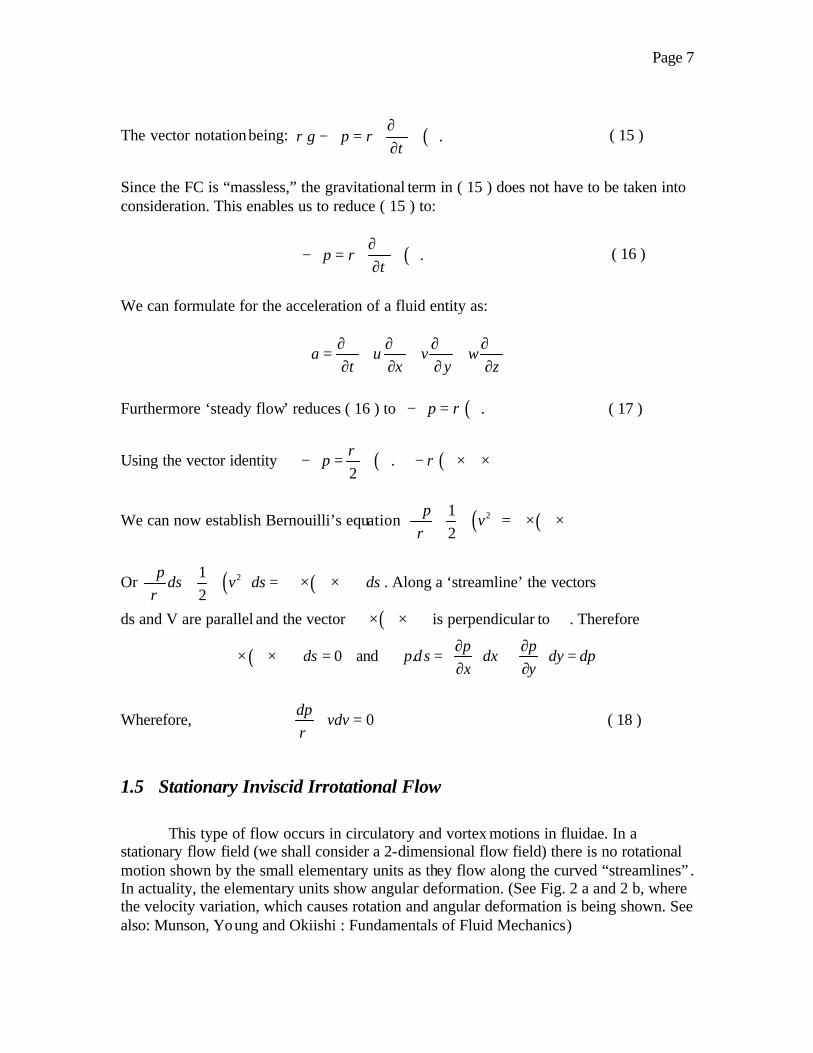
The vector notation being: ( ).g pt

ρ ρ∂ ∨ − ∇ = + ∨ ∇ ∨ ∂

( 15 )

Since the FC is “massless,” the gravitational term in ( 15 ) does not have to be taken into consideration. This enables us to reduce ( 15 ) to:

( ).pt

ρ∂ ∨ −∇ = + ∨ ∇ ∨ ∂

( 16 )

We can formulate for the acceleration of a fluid entity as:

a u v wt x y z

∂ ∨ ∂ ∨ ∂ ∨ ∂ ∨= + + +

∂ ∂ ∂ ∂

Furthermore ‘steady flow’ reduces ( 16 ) to ( ).p ρ−∇ = ∨ ∇ ∨ ( 17 )

Using the vector identity ( ) ( ).2

pρ

ρ−∇ = ∇ ∨ ∨ − ∨ × ∇ × ∨

We can now establish Bernouilli’s equation ( ) ( )212

pv

ρ∇

+ ∇ = ∨ × ∇×∨

Or ( ) ( )212

pds v ds ds

ρ∇

+ ∇ = ∨ × ∇ × ∨ . Along a ‘streamline’ the vectors

ds and V are parallel and the vector ( )∨ × ∇×∨ is perpendicular to ∨ . Therefore

( ) 0ds∨ × ∇ × ∨ = and .p p

pds dx dy dpx y

∂ ∂ ∇ = + = ∂ ∂

Wherefore, 0dp

vdvρ

+ = ( 18 )

1.5 Stationary Inviscid Irrotational Flow

This type of flow occurs in circulatory and vortex motions in fluidae. In a stationary flow field (we shall consider a 2-dimensional flow field) there is no rotational motion shown by the small elementary units as they flow along the curved “streamlines” . In actuality, the elementary units show angular deformation. (See Fig. 2 a and 2 b, where the velocity variation, which causes rotation and angular deformation is being shown. See also: Munson, Young and Okiishi : Fundamentals of Fluid Mechanics)

Page 8

In interval tδ , OA and OB will rotate through angles δα and δβ to positions OA’ and OB’ Angular velocity of OA

0OA tLimtδ

δαω

δ→=

For small angles

( )/tan

v x x txδ δ

δα δαδ

∂ ∂≈ =

vt

xδ

∂=

∂

Wherefore ( )

0

/OA t

v x t vLim

t xδ

δϖ

δ→

∂ ∂ ∂= = ∂

With, vx

∂∂

being positive , OAϖ

will be counter-clockwise.

Similarly, OBuy

ϖ∂

=∂

. With uy

∂∂

being positive, OBϖ will be clockwise. The rotation

around the Z-axis is the average of the angular velocities OAϖ and OBϖ of the two mutually perpendicular OA and OB’. Consider counter-clockwise rotation being positive, then it follows that:

12z

v vx y

ϖ ∂ ∂

= − ∂ ∂ and

12x

w vy z

ϖ ∂ ∂

= − ∂ ∂ and

12y

u wz x

ϖ∂ ∂ = − ∂ ∂

In vector notation the combined vector is ˆˆ ˆ

x y zi j kϖ ϖ ϖ ϖ= + + ( 19 )

The rotation vector is ½ the curl of the velocity vector, thus 1 12 2

curlϖ = ∨ = ∇ × ∨

So,

ˆˆ ˆ

1 12 2

i j k

x y zu v w

∂ ∂ ∂ ∇ × ∨ = ∂ ∂ ∂

=1/2 ˆw vi

y z ∂ ∂

− + ∂ ∂ 1/2 ˆu w

jz x

∂ ∂ − + ∂ ∂ 1/2 ˆv u

kx y

∂ ∂− ∂ ∂

Page 9

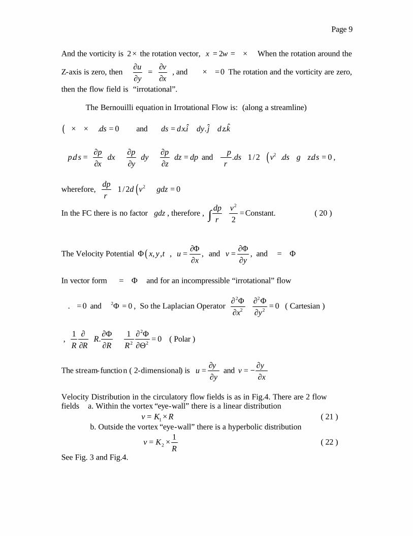
And the vorticity is 2 × the rotation vector, 2ξ ω= = ∇ × ∨ When the rotation around the

Z-axis is zero, then u vy x

∂ ∂ = ∂ ∂ , and 0∇ × ∨ = The rotation and the vorticity are zero,

then the flow field is “irrotational”.

The Bernouilli equation in Irrotational Flow is: (along a streamline) ( ). 0ds∨×∇×∨ = and ˆˆ ˆ. . .ds dxi dy j d z k= + +

.p p p

pds dx dy dz dpx y z

∂ ∂ ∂ ∇ = + + = ∂ ∂ ∂ and ( )2. 1 /2 . . 0

pds v ds g zds

ρ∇

+ ∇ + ∇ = ,

wherefore, ( )21/2 0dp

d v gdzρ

+ + =

In the FC there is no factor gdz , therefore , 2

2dp vρ

+ =∫ Constant. ( 20 )

The Velocity Potential ( ), ,x y tΦ , ,ux

∂Φ=

∂ and v

y∂Φ

=∂

, and ∨ = ∇ Φ

In vector form ∨ = ∇ Φ and for an incompressible “irrotational” flow

. 0∇ ∨ = and 2 0∇ Φ = , So the Laplacian Operator 2 2

2 20

x y∂ Φ ∂ Φ

+ =∂ ∂

( Cartesian )

, 2

2 2

1 1. 0R

R R R R∂ ∂Φ ∂ Φ + = ∂ ∂ ∂Θ

( Polar )

The stream-function ( 2-dimensional) is uyψ∂

=∂

and vxψ∂

= −∂

Velocity Distribution in the circulatory flow fields is as in Fig.4. There are 2 flow fields a. Within the vortex “eye-wall” there is a linear distribution 1v K R= × ( 21 ) b. Outside the vortex “eye-wall” there is a hyperbolic distribution

2

1v K

R= × ( 22 )

See Fig. 3 and Fig.4.

Page 10

1.6 Derivation of the Velocity Distribution

Equilibrium of forces gives ( )2

.p v

dnRd Rd dnn R

ϕ ρ ϕ∂

=∂

2p v

n Rρ

∂→ =

∂ ( 23 )

And 2

2p vρ

+ = Constant (Bernouilli), which means 2v v

vn R

ρ ρ∂

− =∂

p vv

n nρ

∂ ∂= −

∂ ∂

Wherefore v v dvn R dR

∂= − =

∂ and

dv dRv R

= − ; so ln ln ln .v R Const= − + ( 24 )

Or .

ln lnConst

vR

= ; so .Const

vR

= and Circulation Γ =2 .R vπ ( 25 )

v Rω= 2.Const Rω⇒ = . When R a= ⇒ v aω= ⇒ 2.Const aω=

So for ranges ,R a≤ v Rω= for : ,R a= v aω= and for ,R a≥ 2a

vR

ω=

Fig. 5 shows the Pressure Distribution. For circular motion p dpn dr

∂=

∂

Which gives 2p v

n Rρ∂

=∂

and when 2a

vR

ω= , then

2 4

3

dp adr R

ρω=

Page 11

So 2 4 2 4

3 21 / 2 .a a

p dR ConstR R

ρω ρω= = +∫ ( 26 )

Boundary Conditions give:

:R → ∞ 0p p= → 0K p=

:R a= 2 20

12

p p aρω= −

:R a≥ 4

20 2

12

ap p

Rρω= −

The FC has the property of being“ inviscid”/”frictionless”, wherefore the hyperbolic velocity distribution of the “irrotational” flow would lead to an infinite value at its center. However, the value of the velocity is limited by the “speed of light,”(which is the local “speed of light”; this subject matter shall discussed in the furtherance hereof). It is at this maximum velocity where the “eye-wall” is located and there the velocity approaches c ; at the “eye-wall” there is a slight rounding in the velocity distribution where the “rotational” flow converts into the “irrotational” flow. Keeping in mind that due to the already lower pressure and density at the “eye-wall” location that c should be somewhat greater than the “standard” *c , it is likely that the actual resulting c could have a value of 3× 10 8 m sec 1− or slightly better. So at the “eye-wall”, we have a cω = ( 27 ) Finding this reality shall prove of the utmost importance for establishing relationships and for calculations with regard to the vortex entities in the FC. Now therefore we can express the pressure distribution as follows:

,R a≥ 2

20 2

12

ap p c

Rρ= − ( 28 ), ,R a= 2

0

12

p p cρ= − ( 29 )

0 ,R a< < 2

2 20 2

12

Rp p c c

aρ ρ= − + ( 30 ), 0,R = 2

0p p cρ= − ( 31 )

The relationships between the “speed of light” and the pressure and density in the FC with regard to vortex entities can also be written as follows:

For ,R a≥ ( )02 Rp pR

ca ρ

−= ( 32 )

0 ,R a< < ( )2 2

0

2Rp p R

cω

ρ

−= + ( 33 )

,R a= (“eye-wall”) ( )02 EYEp p

cρ

− =

( 34 )

Page 12

0,R = ( center ) ( )0 CTRp pc

ρ

−= ( 35 )

Now whereas the FC has the property of being compressible, we shall now take

this into account with regard to the use of the formula of Bernouilli. (See also: Munson, Young and Okiishi : Fundamentals of Fluid Mechanics) Accounting for compressability

requires integration of dpρ∫ when ρ is not constant. In the FC we encounter the

condition of isothermal flow character. Reason being; the velocity of a wave in the FC is 3 8 110 .secm −× , which is the velocity with which elementary units in the FC transfer motion from one to another. Furthermore, the elementary units in the FC are in the magnitude of 10 25− m or smaller and it is even possible that these units are of a size magnitude of the “Planck” length. If we assume a value of 10 25− m, then it is clear that the motion transfer occurs between 3 3310× elementary units of the FC in a single second, which means that the FC is highly isothermal. Witness to this is also that the temperature of the “background radiation” in the universe is quite equal from location to location with exception to extended locations with substantial “space-time curvature” where, not surprisingly, deviations are being recorded. Due to the similarities let us now compare the FC with a perfect gas for which we have p

RTρ

= , when T = .Const Then for steady inviscid flow:

2

.2

dp vRT Const

ρ+ =∫ ( 36 )

Wherefore, along a streamline is valid: 2 2

1 2 1

2

ln2

p v vRT

p −

=

( 37 )

Also, ( )1 21

2 2

1p pp

p p−

= + , whereby we shall name 1 2

2

p pp

ε−

= , which can be termed to

be the ‘relative pressure change’. Further consideration being that for small values of ε , ( )ln 1 ε ε+ ≈ , which then leads again to the standard Bernouilli equation.

Transforming from an atomic or molecular gas to the FC, the gas-constant R

needs to be replaced by the counterpart constant which is valid in the FC, be indicated by

FCK xx Therefore, we can now substitute in ( 36 ) and ( 37 ) and validate for the FC

0FCdp

K T vdvρ

+ = ( 38 ) and 2

1

2

ln2FC

p vK T

p ∆

=

( 39 ).

Page 13

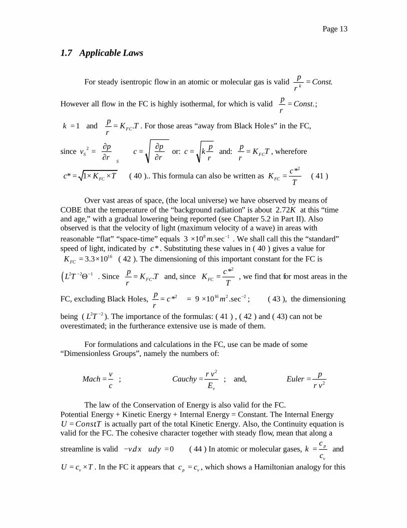
1.7 Applicable Laws

For steady isentropic flow in an atomic or molecular gas is valid .p

Constκρ

=

However all flow in the FC is highly isothermal, for which is valid .p

Constρ

= ;

1κ = and .FCp

K Tρ

= . For those areas “away from Black Holes” in the FC,

since 2S

S

pv

ρ ∂

= ⇒ ∂

pc

ρ ∂

= ∂ or:

pc k

ρ= and: FC

pK T

ρ= , wherefore

* 1 FCc K T= × × ( 40 ).. This formula can also be written as 2*

FCc

KT

= ( 41 )

Over vast areas of space, (the local universe) we have observed by means of

COBE that the temperature of the “background radiation” is about 2.72K at this “time and age,” with a gradual lowering being reported (see Chapter 5.2 in Part II). Also observed is that the velocity of light (maximum velocity of a wave) in areas with reasonable “flat” “space-time” equals 3 8 110 .secm −× . We shall call this the “standard” speed of light, indicated by *c . Substituting these values in ( 40 ) gives a value for 163.3 10FCK = × ( 42 ). The dimensioning of this important constant for the FC is

( )2 2 1L T − −Θ . Since .FCp

K Tρ

= and, since 2*

FCc

KT

= , we find that for most areas in the

FC, excluding Black Holes, 2*p

cρ

= = 9 16 2 210 .secm −× ; ( 43 ), the dimensioning

being ( 2 2L T − ). The importance of the formulas: ( 41 ) , ( 42 ) and ( 43) can not be overestimated; in the furtherance extensive use is made of them.

For formulations and calculations in the FC, use can be made of some “Dimensionless Groups”, namely the numbers of:

vMach

c= ;

2

v

vCauchy

Eρ

= ; and, 2

pEuler

vρ=

The law of the Conservation of Energy is also valid for the FC.

Potential Energy + Kinetic Energy + Internal Energy = Constant. The Internal Energy .U ConstT= is actually part of the total Kinetic Energy. Also, the Continuity equation is

valid for the FC. The cohesive character together with steady flow, mean that along a

streamline is valid . . 0v d x udy− + = ( 44 ) In atomic or molecular gases, p

v

c

cκ = and

vU c T= × . In the FC it appears that p vc c= , which shows a Hamiltonian analogy for this

Page 14

specific characteristic between atomic or molecular gases at the “critical point” condition and the FC. The specific heat constant for the FC will be named FCC .

1.8 Potential and Kinetic Energy

The existence of Potential Energy makes it possible for Kinetic Energy to come into being. The Potential Energy can be characterized by the pressure P and the Kinetic

Energy can be indicated by the term 212

vρ . The energy of the “Background Radiation”

is the Internal Energy U and can be expressed by the term FCC T× . ( 45 )

In this local universe it can be observed that once Potential Energy is converted into Kinetic Energy it remains Kinetic Energy and that there is no return to Potential Energy other than through the formation of the Protons or possible other vortex entities which have an internal fluid pressure higher than the “standard pressure” which generally prevails in the FC in vast areas of space where “space-time” is “flat”(see Chapter 3.1.4). This statement departs from concepts of classical physics, particularly relating to the concept of “Mass,” which is thought to contain or to be existing out of Potential Energy, which can be converted into Kinetic energy via the formula 2.E m c= . ( 46 ). However, Einstein and also Feynman state in their various publicized theories that the phenomenon “Mass” is created by the phenomenon of “space-time curvature”. Writer agrees and shall definitively show that “Mass” per-se (tangible) does not exist. It is the density distribution in the FC, (which roughly coincides or approximates “space-time curvature”) that determines the concept and quantity of “Mass”. Thus we have in FC physics the following definition for “Mass”: “For equal volumes of space, “mass” is the quotient between the value of the density ρ in the FC at the considered location and the average “standard density value” ( 0ρ ), which exists in those areas of the local universe where “space-time” is essentially flat”. Two important notes are to be included here: a. Writer shall show that this quotient can be less than 1, (e.g. for the electron, see

Chapter 3.4). This now leads to the introduction of the concept of either “Fractional Mass” or “Negative mass”. Associated therewith we also get the concept of “Fractional Energy” or “Negative Energy”, which concept can be considered as a calculatory one. However, the terminology and concept of “Borrowed Energy” as it is being used with regard to the so called Penrose process, which is an energy extraction process with regard to black holes shows the same aspects (see: A Journey into Gravity and Spacetime, by John A. Wheeler, pages 214 – 216 ). The concepts of “fractional / negative mass” and “fractional / negative energy”, as difficult as they may seem, are more than just calculatory ones.

Page 15

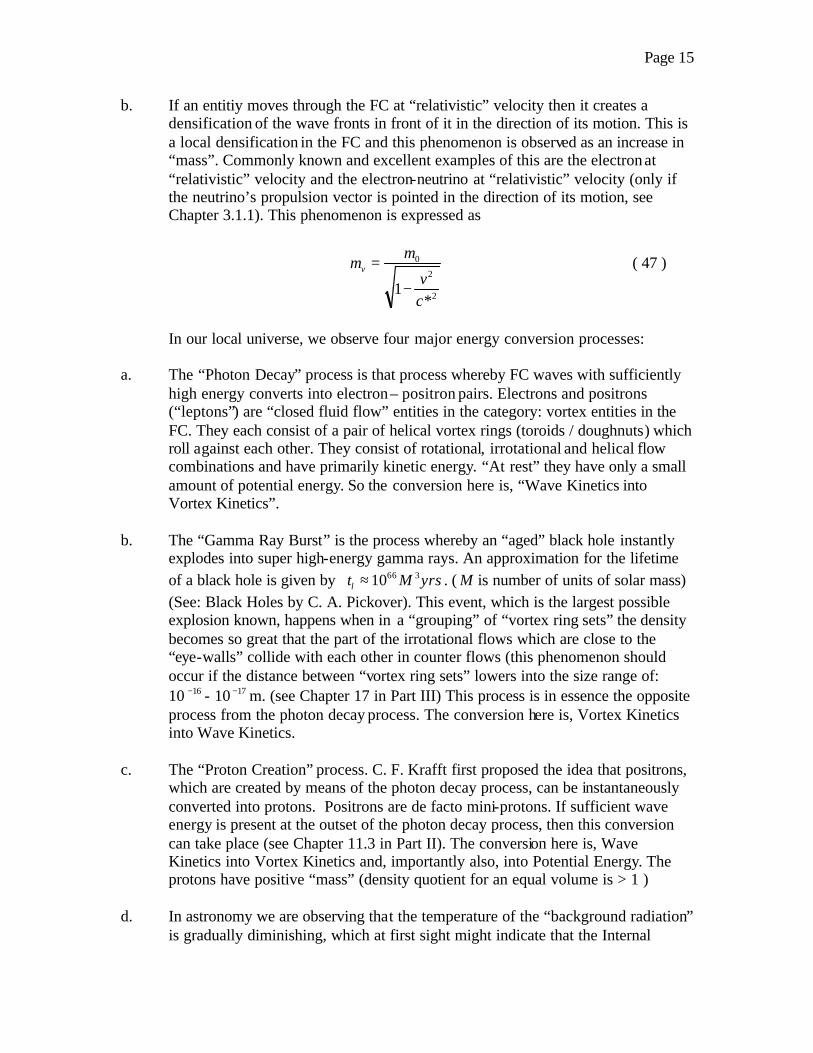
b. If an entitiy moves through the FC at “relativistic” velocity then it creates a densification of the wave fronts in front of it in the direction of its motion. This is a local densification in the FC and this phenomenon is observed as an increase in “mass”. Commonly known and excellent examples of this are the electron at “relativistic” velocity and the electron-neutrino at “relativistic” velocity (only if the neutrino’s propulsion vector is pointed in the direction of its motion, see Chapter 3.1.1). This phenomenon is expressed as

0

2

21*

vm

mvc

=

−

( 47 )

In our local universe, we observe four major energy conversion processes:

a. The “Photon Decay” process is that process whereby FC waves with sufficiently

high energy converts into electron – positron pairs. Electrons and positrons (“leptons”) are “closed fluid flow” entities in the category: vortex entities in the FC. They each consist of a pair of helical vortex rings (toroids / doughnuts) which roll against each other. They consist of rotational, irrotational and helical flow combinations and have primarily kinetic energy. “At rest” they have only a small amount of potential energy. So the conversion here is, “Wave Kinetics into Vortex Kinetics”.

b. The “Gamma Ray Burst” is the process whereby an “aged” black hole instantly

explodes into super high-energy gamma rays. An approximation for the lifetime of a black hole is given by 66 310lt M yrs≈ . ( M is number of units of solar mass) (See: Black Holes by C. A. Pickover). This event, which is the largest possible explosion known, happens when in a “grouping” of “vortex ring sets” the density becomes so great that the part of the irrotational flows which are close to the “eye-walls” collide with each other in counter flows (this phenomenon should occur if the distance between “vortex ring sets” lowers into the size range of: 10 16− - 10 17− m. (see Chapter 17 in Part III) This process is in essence the opposite process from the photon decay process. The conversion here is, Vortex Kinetics into Wave Kinetics.

c. The “Proton Creation” process. C. F. Krafft first proposed the idea that positrons,

which are created by means of the photon decay process, can be instantaneously converted into protons. Positrons are de facto mini-protons. If sufficient wave energy is present at the outset of the photon decay process, then this conversion can take place (see Chapter 11.3 in Part II). The conversion here is, Wave Kinetics into Vortex Kinetics and, importantly also, into Potential Energy. The protons have positive “mass” (density quotient for an equal volume is > 1 )

d. In astronomy we are observing that the temperature of the “background radiation”

is gradually diminishing, which at first sight might indicate that the Internal

Page 16

Energy of the FC is decreasing. This is puzzling, since energy conversion processes are subject to increase in entropy and energy dissipation means an increase in the “Brownian” motion. This is valid for atomic and molecular fluidae, but not necessarily for the FC. Writer found (see Parts II and III of this book) that the lowering of the temperature of the “background radiation” is caused by the expansion of the universe. The conversion here is nil. Internal Energy remains Internal Energy, albeit this energy is gradually at lower temperature due to the larger volume of space it is spread out over. The total quantity of internal energy increases continually, however, the expansion of the universe occurs still faster. The universal processes of ( a ) and ( b ) are key parts of an apparent Universe Cycle: Wave Kinetics into Vortex Kinetics and back to Wave Kinetics etc.

Comparison of the events of ( a ) and ( b ) with regard to energies: a. Gamma ray burst from the explosion of an “aged” black hole of galactic

proportion of say 300 billion solar masses produces energy of 595 10 Joule× . b. Photon decay conversion, whereby 1 electron and 1 positron are being formed

might take roughly 2 133.2 10MeV Joule−= × . The conclusion is that it takes roughly 721.5 10× events of process ( b ) to equal 1 event of process ( a ), which is the gamma ray burst of a proportion given herewith.

1.9 Pressure and Density in the Universal Fluidum Continuum

The laws of energy conservation and Bernouilli show that in the FC, (considering the flow along a streamline) a velocity increase means a decrease in pressure. Wave phenominae in the FC result from energy emissions resulting from explosions like Supernovae and Gamma Ray Bursts. The other flows are of a gravitational maintenance type. Vortex-type entities need to have an infinitesimal supply of new new fluid energy over time (see Chapter 5.2 in Part II), wherefore fluid flows towards each entity or groups of entities. In the case of groups of entities the flow at distance away from such a group, flows into the direction of the “mass” center, which is the geometric center of all locations with increased density within such group. Since entities or groups of entities vie for fluid from one and the same “space”, they also show the phenomenon of attracting each other. There is a Hamiltonian analogy between “centers of mass” in the sense of classical physics and “centers of fluid dynamic mass” in the FC. “Fluid dynamic mass” is the product of a “volume of space” times the density which exists in the concerned “volume of space.” This “volume of space” can be an area of “confinement” between vortex rings or an area of local densification of wave fronts (as occurs in front of vortex entities which travel at “relativistic” velocities). In the Introduction we launched the concept of “vortex entity mass”: Λ . Λ is different for each type of vortex entity and it stands for the product of the “volume in space” times its densityρ . The vortex entities

Page 17

consist of the elementary units ζ , which are the tri-dimensional units in the FC, which allow for the phenominae of irrotational and rotational flows. The “volume of space” for a certain vortex entity can be written as ven ζ× , wherein ven has a specific value for each type of vortex entity and the density for such “volume of space” (being “at rest”) be indicated by veρ . Each type of vortex entity has a specific veρ .(ve stands for vortex

entity). So, ( )ve venζ ρΛ = × . Let us consider a few locations of vortex entities in the FC:

1 2, ,..... pA A A , which have corresponding fluid dynamic mass quantities 1 2, ,....... pΛ Λ Λ . If

we choose a given point O in space, we now can assign vectors 1 2, ,.......... pOA OA OAuuuv uuuv uuuv

to these locations. Each vortex entity now has a momentum k kOA ×Λ

uuuuv , ( 1,2,.......k p= ), wherefore:

1 21 21

......p

pk k pOA OA OA OA× Λ = × Λ + × Λ + × Λ∑uuuuv uuuv uuuv uuuv

. We now define a new “mass” point,

Z , which comes in place of all the various “mass” point locations. For this point is

valid that the total “mass” is 1

tot

p

c km = Λ∑ ( 1,2,.....k p= ). ( cm is “mass” center )

The momentum of the total “mass” is 1

tot

p

c k kOZ m OA× = × Λ∑ , wherefore vector

1

1

p

k k

p

k

OAOZ

× Λ=

Λ

∑

∑ or

1

p

kOZ OA= ∑ .

Fig. 45

When we draw in all vectors then the resultant vector is OZ . We can now also conclude that the location of Z is independent of the choice of the location for the given point O . In the furtherance we shall indicate the fluid dynamic “mass” of a vortex entity

Page 18

or group of vortex entities by kcm with the understanding that this fluid dynamic “mass”

is located at its “mass center”, as defined in the above.

Let us now consider two “mass centers”. The inflow of fluid is always directed at the “mass center”. The velocity of the inflow .gravv , decreases with the square of the

distance 2R , from that center. Furthermore, the inflow volume is directly proportional with

kcm∑ ; this is valid for both “mass centers”, so for a point in between the 2 “mass centers” we have, that the “inflow draw”, which is represented by .gravv , can be expressed as being proportional with the formulation

1 2. 2

c cgrav

m mv

R

×∝∑ ∑ ( 48 )

The mutual “inflow draw” causes a fluid mechanical attractive force. The proportionality factor is: Ω .(this factor was defined in the Introduction).So the gravitational fluid maintenance force between entities or groups of entities, which is equivalent for Newton’s Law in the FC, can now be formulated as

1 2

2c c

GM

m mG

R

×= Ω ∑ ∑ ( 49)

1.10 Determination of the density ρ in the FC in an area with “space-time curvature”, as a function of 0ρ , *c , Ω , R and *mc mρ =∑ )

We have dp dv

vdR dR

ρ− = and 2*p

cρ

= , which results in 2*.d dv

c vdR dRρ

ρ− = ( 50 )

and 2

*mv

R= Ω , wherefore 3

*2

dv mdR R

Ω= − and

2 2

5

*2

dv mv

dR RΩ

= − ( 51 )

From ( 50 ) and ( 51 ) we find that 2 2

2 5

2 **

d mc R

ρρ

Ω− = − so

2 2

2 4

*ln .

2 *m

Constc R

ρΩ

− = +

For R = ∞ , 0ρ ρ= , therefore we obtain 0ln 0 .Constρ− = + , 2 2

0 2 4

*ln ln

2 *m

c Rρ ρ

Ω− + = ,

which results in :2 2

2 40

*ln

2 *m

c Rρρ

Ω= −

this result can be written as

2 2

2 4*

2 *0

mc Reρ ρ

Ω−

=

or as 2 2

0 2 4

*exp

2 *m

c Rρ ρ

Ω= − ( 52 )

Page 19

Formula ( 52 ) shows “space-time curvature” towards a center of “mass” in the sense of defining “mass” in FC physics. This formulation is valid until the perimeter of the “mass” which is

kcm∑ , is being reached. Within this perimeter, the relationship for ρ as function of 0ρ , R , Ω , *m and *c becomes roughly spherical. At the named perimeter the tangents of both functions are equal. (Other functions are valid in the immediate vicinity of black holes). ( )* *

0 , , , ,F R m cρ ρ= Ω is depicted in Fig. 6 .

In classical physics and using the classical sense of “mass”, “space-time curvature

has sometimes been formulated as follows:

( ) ( ) ( )3 2

. 1 1 8 2 8 22r

R MZ M r M M R M

M R

= − − + − − −

( ( )MR r≥ ) ( 53 )

In this formula, R = radius of “mass” , r = radial vector for ( )rZ ( a 3 – dimensional surface ) and M = ”mass” . In classical physics, the shape of “space-time curvature” within the radius of “mass” is also roughly spherical.

1.11 Velocity of “FC Energy” Waves

First we shall redefine “c ”, which is the so-called “speed of light” as “the maximum possible velocity physically allowed for a wave in the FC at a given location”. This defined velocity at any given location is a function of the density ρ . Over vast areas of space with “flat” “space-time” (i.e. a lack of “mass” concentrations) the density is quite constant and we already called this the “standard” density 0ρ . The maximum allowed velocity for a wave in this case is the “standard” velocity “c ”, which we shall write as *c . In areas with “space-time curvature” “c ” can be different and lower than

*c . In “open vortexes,” “c ” can be higher than *c . Planck’s formula for the energy of a wave

Page 20

hc

Eλ

= , ( 54 )

shows that if the wavelength approaches zero, then the energy required would be infinite, which is the case in classical and FC physics alike. When a vortex entity moves in the FC, it causes a wave densification in front of itself in the direction of its motion. This densification not only expresses itself as “mass” but since more energy is required as the densification increases ( = wavelength decreases), it creates a drag on the moving vortex entity. (See following Chapters, e.g. 3.1) However, if the moving entity enters a region of lower density “space-time curvature”) then it will require a higher velocity of the moving entity in order to build up the same densification level in front of it in the direction of its motion compared to moving through an area with the “standard” density. Therefore, the maximum possible velocity in the region of lower density, from an observation point in the area with standard density is higher than *c .

The dependence of the “speed of light” on the density of the FC has profound influence on General Relativity of Einstein as well as on subject matters like the Hubble Constant and on various other matters in physics and astronomy. In some cases profound adjustments are needed and in others, only slight adjustments or expansions for the purpose of wider validity. The density of the FC determines “space-time curvature “, therefore it also determines “mass” and the “maximum velocity of waves”. Density in the FC is one most important concept in the FC physics.

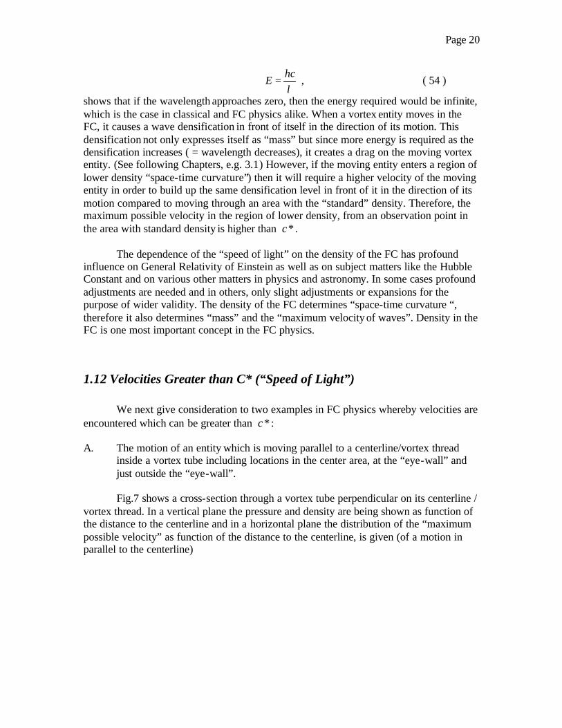
1.12 Velocities Greater than C* (“Speed of Light”)

We next give consideration to two examples in FC physics whereby velocities are encountered which can be greater than *c : A. The motion of an entity which is moving parallel to a centerline/vortex thread

inside a vortex tube including locations in the center area, at the “eye-wall” and just outside the “eye-wall”.

Fig.7 shows a cross-section through a vortex tube perpendicular on its centerline /

vortex thread. In a vertical plane the pressure and density are being shown as function of the distance to the centerline and in a horizontal plane the distribution of the “maximum possible velocity” as function of the distance to the centerline, is given (of a motion in parallel to the centerline)

Page 21

Fig. 7

The value for the rotational as well as for the irrotational tangential velocity at the location of the “eye-wall” approximates *c as has been shown in previously. In addition to these two flows there is still another flow component, which is parallel to the centerline. This latter component, either combined with the irrotational flow or the rotational flow, gives the total flow, which is then “helical” in character. The tangential components of both irrotational and rotational flow are substantially greater than the component which is parallel to centerline, except for in the centerline of the rotational flow. In the following calculatory overview, the parallel component is not being considered.

In Chapter 1.6 the Formulas ( 28 ) through ( 31 ) show the pressure distribution

over a cross-section inside as well as outside the “eye-wall”. Since in the FC, 2*P

cρ

= ,

the density ρ shows the same distribution. For the sake of simplified calculation, we shall assume a vortex having a pressure at the centerline of zero. Now

20 1 / 2eyeP P cρ= − and 2

0ctrP P cρ= − so 0ctrP = which gives 20P cρ=

and 2 2 21 12 2eyeP c c cρ ρ ρ= − =

Inside the vortex tube tan

cRv

a= and

2

2P vρ

= , wherefore 2 2

22c R

Pa

ρ=

For 0R = , 0P = and for R a= , 212eyec cρ= so 2.eye

Pc

ρ= and,

other than in vincinity of black holes, 2*P

cρ

= and 2. *eyec c= ( 55 )

Page 22

Inside the vortex tube (i.e. inside of “eye-wall”), we have 2.a P

cR ρ

= ( 56 )

Outside the vortex tube (i.e. outside of “eye-wall”), we have 02.P P R

caρ

−= ( 57 )

Equating these results at R a= , gives 0

12

P P= and 0

12

ρ ρ= .

Further outside the “eye-wall” c goes asymptotically to *c . These results are summarized in the table below.

R 0

PP

0

ρρ

*

cc

∞ 1 1 1

At “eye-wall” a 12

12

2

Inside Vortex tube 12

a 18

18

4 2

Inside Vortex tube 14

a 1

32

132

16 2

Inside Vortex tube 0 0 0 ∞

Consideration is given to the possibility for certain entities to be able to ‘travel’ inside a vortex tube, which is a motion which is mainly parallel to the centerline and in the positive direction of the helix. Spiraling around the centerline is presumed to be the most likely motion.

No group of entities, like atoms or molecules, or “composite particles,” like mesons or baryons, can survive entering a vortex tube in the FC where there is always a velocity at the “eye-wall” which approximates *c . Also, a proton, which has a higher density inside compared to density outside in the FC, cannot survive entry, tangentially or otherwise. However, there is a good chance that the electron, which has an internal fluid density which is much lower than the external fluid, when moving at relativistic speed (see Chapter 3.4.4) could enter the vortex tube if a tangential approach is taken. Inside the vortex tube, the electron would be transported at super high velocity in the positive direction of the helix, moving along a helical path where the pressure, while lower than outside the “eye-wall”, is always slightly higher than the pressure inside the electron. The electron-neutrino also has a chance surviving a tangential entry into a vortex tube. It is likely to disintegrate at the “eye-wall”, where the velocity is *c , however, if entry is made, then survival is likely as long as it moves in a helical path where the pressure along

Page 23

that path remains higher than the pressure inside its single toroidical vortex ring. This subject matter will be visited again in Part III. B. The motion of an entity going from “standard” density through a region with

considerable “space-time curvature”. This motion of a vortex entity through a region with considerable “space-time curvature” is depicted in Fig. 8 . Consider the vortex entity to be an electron-neutrino, which has its own propulsion.

The electron-neutrino moves essent ially at the velocity *c when it moves

through regions of “flat” “space-time”. As we shall see in Chapter 3.1 the electron-neutrino has a “propulsion vector flow” which at its perimeter has a velocity *c being slightly les at the center of the propulsion. Therefore, it moves through the FC essentially at velocity *c . In the following, there is an approximate determination of the velocity c of the electron-neutrino when it “cuts” through a “space-time curvature” region, deter- mined by *m , Ω , *c , 0ρ and Ξ . Here Ξ is the projected distance between the path of travel and the “mass” *m .

In formula ( 52 ) we saw that 2 2

0 2 4

*exp .

2 *m

c Rρ ρ

Ω= −

Now since 0P P

cρ−

∝ , and

2*P

cρ

= we have 0 0 1cρ ρ ρ

ρ ρ−

∝ ∝ − ;

0 1ddcdR dR

ρρ

−= =

02 2

0 2 4

1*

exp2. *

dm

c RdR

ρ

ρ−

Ω−

Name: 2 2

2 4

*2 *

mx

c R Ω

=

, so we can write:

0

0

1exp

dxdc

dR dR

ρρ

−−

= =

11xd

edR

− −

( )12

2

1 1 11 1 4

2x

x x

dc xe

dR e e R

−−

− −

= − × × − × −

, using exponential expansions gives

( )1

2 2 221 41 1 1 2 1 1 4

2 2! 2! 2!dc x x x x

x x xdR R

− = + + − + + − + − −

. Approximating by

discarding all terms with 2x leaves dcdR

= ( )( ) ( ) 3

1 1 2 2 1 2 * 11 2 1 4 / 1 2

2 *x x x m

x x x R xR R R c Rx x x

Ω+ − ≈ + ≈ ≈ ≈ ( 56 )

The velocity component derivative in the direction P – Q is 3

* 12 cos

*m

c Rϕ

Ω

What is the velocity of the electron-neutrino at location Q? (See Fig. 8)

Page 24

[ ]/ 2

/ 2

3 2 00

* 2 * 1* 2 cos . * sin

* 2 *QRR

m dR mv c d c

c R c R

ππ

ϕϕ

ϕ ϕ ϕΞΞ

== ∞=∞ =

Ω Ω = + = + ∫ ∫ ,

which gives 2

2 * 1*

2 *Qm

v cc

Ω = + Ξ ( 57 )

In Fig. 8 and above we show that the electron-neutrino, which has its own

propulsion vector with a velocity of about *c , reaches super- luminous velocities as it entered and trave led through a region with “space-time curvature”. This is due to the fact that lower density was encountered in this region. A higher maximum velocity is needed to get an equal densification of fluid in front of the electron-neutrino when compared to space which has the “standard” density 0ρ . As the electron-neutrino leaves the region with “space-time curvature” it slows down again to the velocity *c when it comes back to “standard” space. In the above calculation several approximations have been made and also no consideration has been given to the “bending” of the path of the electron-neutrino. The path “bends” just as is the case for a “beam of light”. If the “bending” of the path is accounted for, then extra terms need to be added into formula ( 57 ). A longer trajectory in “space-time curvature” means more time spent in this region and somewhat higher maximum velocity being achieved. In Part III the more general formulation shall be used when neutron stars and black holes shall be considered.

Various subject matters in this book describe that the local speed of light c depends on the dens ity ρ . However, one can say that there is also a time dependency because the density 0ρ is dependant on the volumetric state of the universe. This state is known to have changed over time due to the expans ion of the universe.

Page 25

1.13 Wave and Vortex Phenominae in General

1.13.1 Wave Phenominae in General

As was shown in the last chapter, the vortex entities and in particular the electron-neutrino, which travels through “standard” space (“flat “space-time”) at velocity *c , can reach super-luminous velocities in regions of considerable “space-time curvature.” The ability of a vortex entity to achieve super-luminous velocity is highly dependant on the velocity with which it approaches this low-density region. The velocity of approach should already be close to *c in order for the vortex entity to achieve super- luminous velocity. Therefore, super- luminosity can only be achieved by the electron-neutrino and by super high speed electrons and positrons.

The force causing the acceleration is the density gradient within the FC, and this

force is identical to the gravitational force. Einstein and Feynman state this too. Wave phenominae in “space-time curvature” are subject to “bending”, but by way of a different mechanism when compared with vortex entities which go through regions of low density which means they pass close by mass concentrations. A beam of light slows due to the fact that the “communication velocity” between the elementary units ζ in the FC becomes lower whenever the density lowers and the elementary units are more distant to each other. The lower the density of a region, the more slowing occurs, this means that “wave-fronts formed by parallel and adjacent light beams, which are traveling simultaneously through differing densities relative to each other, start to “angle”. Since the beams are perpendicular to the “wave-fronts”, they “angle” to the same degree. The “wave-fronts” will show curvature themselves. (The angling is greater as beams go “deeper” through “space-time curvature.) Einstein first discovered this and the phenomenon has been verified numerous times.

1.13.2 Considering the “bending” of light beams in “space-time curvature”: some examples

In Figs. 9 the line, AB is a wave-front. Two beams are traveling parallel to each

other through “standard” space and then enter a lower density region. Beam AA’ follows a trajectory which goes through higher density “terrain” compared to the trajectory which is occupied by beam BB’. Due to the differing densities along the paths of each beam, beam AA’ travels faster than beam BB’ and this results in wave-front A’B’ rotating relative to the original wave-front AB. Light beams are always perpendicular to their wave-fronts, which means that the beams angle to the same extent. The degree of this “bending” depends on the steepness of “space-time curvature” in the location where the beams cross. It also depends on the projected distance from the original beam trajectory to the outside of the “mass” center. A calculation of the inter- dependency of the various factors which play a role, shall be given herewith: Angle α can be expressed as α = F ( Ω , *m , *c , Ξ ). From the formulas ( 32 ) through ( 35 ) , formula’s ( 43 ) and ( 52 ),

Page 26

we have that for “space-time curvature” is valid 3

* 12

*dc mdR c R

Ω= . (See Figs. 9a, 9b

and 9c.) We shall now consider the calculation of the angling of “light” beams while they pass by either (A), an ‘extended- length’ “mass” object (like certain types of nebulae in space) or (B), a ‘point’ “mass” object (like high density stars, even neutron stars).

In both examples the beams pass by the objects at some distance Ξ , and the development considers only small angle deviation. No consideration is made for the fact that the actual deviations place the beams closer to the object and therefore increase the exponential part of the overall relationship. This will be addressed in Part III, Chapter 17, Black Holes, where is a general formulation which also accounts for this factor is presented and used to calculate the spiraling to below the “event horizon”.

Sub-A: (See Fig. 9a)

The beams are named (a) and (b). Name AA’ = BB’ = x . Name A’A’’= dx . Name MB’ = Ξ and name B’A’ = ∆Ξ . Since

/ .dc dR Const= along x , ( because of the ‘extended length “mass” object ) we can now equate

Page 27

( ) ( )a b

x dx xv v+

= , also tan /dxα = ∆Ξ and tanα α≈ for small angles,

so, dx α= ∆Ξ , also ( ) *Rv c=∞ = and ( )aR

dcv dR

dR

Ξ+∆Ξ

= ∞

= ∫ , ( )bR

dcv dR

dR

Ξ

= ∞

= ∫ ,

wherefore

R R

x xdc dcdR dRdR dR

αΞ+∆Ξ Ξ

=∞ = ∞

+ ∆Ξ=

∫ ∫ , and also valid is :

( ) ( )a b

dxx

v v=

−

and : 2

2 * 12 *

dc mdR

dR c RΩ

= −∫ , which makes : ( ) 2

2 *2 *b

R

dc mv dR

dR c

Ξ

= ∞

Ω= =

Ξ∫

( )av =

( ) ( )2 2

2 * 2 *2 2* *R

dc m mdR

dR c c

Ξ+∆Ξ

=∞

Ω Ω= − +

Ξ + ∆ Ξ Ξ∫ ( ) ( ) ( )2

2 *2 *

a b

mv v

c

Ω− = −

Ξ+∆Ξ

−( )

2 2

2 2

2 *.

2 * 2m

xc

αΩ

∆Ξ =Ξ + Ξ∆Ξ+∆Ξ

and ∆ Ξ < < Ξ , so 2∆Ξ and Ξ∆Ξ

can be disregarded, therefore we can have

2

2 * 1.

2 *m

x cα Ω

− ≈Ξ ∆Ξ

( 58 )

This logical formula shows a. The angling is proportionate with 21/ Ξ (twice as close = 4 × the angling) b. The angling is per unit of length (2× the lenght of the.“mass” =2× the angling) c. The angling is proportionate with 1/ ∆Ξ

The “bending” of light due to “space-time curvature” is cause for a host of phenominae, which are observed in deep space. The general term used is “gravitationa l lensing.” Multiple images can be produced and also image amplification is possible. If the alignment between the background light source and the lensing object is perfect, an image in the form of a ring is produced. If the alignment is not perfect or the lens is not symmetric, then multiple images or a number of small arcs are produced. Sub-B: (See Fig. 9b)

The bending of “light” beams while they pass by a ‘point’ “mass” object. The

nomenclature is that used in Sub-A. However, in this case dcdR

is not constant

along the paths of the beams x = cosR ϕ . We have

Page 28

( ) ( )

cosa avg b a v g

dxdR d

v vϕ ϕ=

− ∫∫ or tan .

cosavg

dR dvα

ϕ ϕ∆Ξ

=∆ ∫∫ in addition

we also have cosdc

v dR ddR

ϕ ϕ= ∫∫ , tanα α≈ ,

( )/ 2

2 0

*sin

2 *aR

mv

c Rπ

ϕΞ+∆Ξ

=∞

Ω= , ( )

/ 2

2 0

*sin

2 *bR

mv

c Rπ

ϕΞ

=∞

Ω= and,

( )

/ 2

0

2 2

sin* *

2 *2 *

Rm m

cc

παϕΞ

∞

∆Ξ=

Ω Ω−ΞΞ+∆Ξ

= Ξ . Therefore,

( )2 2

* 1 1. .

2 *mc

α Ω ∆ Ξ = Ξ −

ΞΞ+∆Ξ and,

α2 2

* 12 * 2

mc

Ω Ξ = − Ξ + Ξ∆Ξ+∆Ξ Ξ

1.∆Ξ

, ∆ Ξ < < Ξ gives,

α− ≈ * 1.

2 *m

cΩ

Ξ ∆Ξ ( 59 )

A myriad of subjects associated with wave phenominae and the interactions with

“particles” and the “wave-particle duality” (Complimentarity Principle of Bohr) have been researched and discussed by many scientists in the field of general physics. Writer refers to the multitude of textbooks which discuss these subjects and assumes that the reader has some familiarity.

Fig. 9 c Wave-fronts of “light” in “space-time curvature”

At locations distant from a “mass” concentration, corresponding to locations with relatively low density, the “angling” of the wave fronts or bending of the light is less. This is expressed by the formula for the gradient of the maximal velocity in

the direction of the “mass” center 3

* 12

*.dc mdR c R

Ω= ( 56 ) . The actual wave

fronts near a sufficiently strong “mass” concentration are steeply curved. Fig. 9c

Page 29

1.13.3 Vortex Phenominae in General

The vortex phenominae constitute all the “particles” and are equally as important as the wave phenominae in the FC. The scientists Helmholtz, Thomson, Planck, von Karmann, Mach and Hertz, and others did substantial research in the area of fluid mechanics. However, this research related mostly to fluidae which consist of atoms or molecules and not with a view towards the entities, which can and do exist in the FC. Also, the structures of such entities received little attention other than by a few scientists, among whom we cite Planck and Winterberg, (who still publicized rather recently) and also C. F. Krafft (now deceased) and recently A. G. Gulko. These scientists all proposed models with regard to “vortex physics” and checked them against reality. Mr. Gulko, who built upon Mr. Krafft’s work, has been very successful in this. It is upon the extensive work of these scientists that writer has been able to build in giving further underpinning to the theories and giving mathematical and fluid mechanical expression to them. The mathematical analyses have revealed new facts and understanding and have opened whole new areas in FC physics to investigation.

Thomson determined that the “circulation” along a “closed streamline” is constant and independent of time in inviscid irrotational flows. .sv ds ConstΓ = =∫Ñ ( 60 )

Also it is noted that streamlines in such flows remain in tact neither adding nor eliminating elementary fluid entities. Helmholtz indicates, and nature shows, that rotational flows exist within these irrotational flows, while the irrotational flows around those rotational flows remain in tact. It is further noted that vortex threads or centerlines, vortex tubes, and the irrotational flows, which are at the outside and around these experience continued fluctuations in shape. It can be stated that there are 3 “constitutional forms” in which vortexes exist: a. They go to infinity from −∞ to +∞ . These are the “open vortex tubes”. There are

strong indications that the open vortex tubes exist in many locations in the universe(s). Possibly there are a number of sizes (See Chapter 2.2.3.2 ).

b. They end on a border wall or fluidum surface. Also, one end may go to infinity,

while the other end terminates at a border surface of another hyperdimension (another universe).There are indications for occurrences of these phenominae.

c. They close into themselves and form “toroidical” / “doughnut” shapes. In this

manner all “particle”-type entities are formed and exist. Among the observed classes of “particle”- type entities we have:

1. “particles” without “mass” (classical or FC definition) 2. “particles” with “mass” ( classical or FC definition )

Page 30

3. “particles” with “negative” or “fractional” “mass” ( FC definition ) 4. “Anti-particles” of ( 1 ) , ( 2 ) and ( 3 ) 5. “Composite” “particles: (mesons and baryons) 6. Exotic short- lived “particles”

As vortex entities we have: Sub-1. A single rotating vortex ring of the first order size is called “neut rino”; this is the

electron-neutrino. Mathematics forbids any other than one single size (See Chapter 3.1.5). However, under certain conditions and as part of a vortex ring set or as part in a “composite” entity, the single vortex ring can exist in a stretched-out form. The neutrino is “super stable”.

Sub-2. A vortex ring pair, whereby the two rings roll against each other in such a manner

that there is a peripheral inflow and two polar outflows forms the “proton.” The polar outflows show “spin”. The “proton” is stable, but less stable than the “electron” and much less stable than the “neutrino.”

Sub-3. A vortex ring pair, whereby the two rings roll against each other in such a manner

that there are two spinning polar inflows and one peripheral outflow forms the “electron.” It has “mass” in the classical physics sense, but can also have “negative” or “fractional” mass in the FC physics sense (when in motion). The “electron” is stable, but less than the neutrino.

Sub-4. The “anti-neutrino” is identical to the “neutrino”, in that it consists of a single

vortex ring. The difference is in the mode of motion. The propulsion vector points forward in the direction of the motion. The “anti-neutrino” is stable.

Sub-5. The anti-proton is unstable. It resembles the electron at high relativistic velocity. Sub-6 The positron can be long-term stable, but can also decay into a “proton” if enough

energy is available in the fluid around it. This conversion process is highly important. (See the Photon Decay process in Part II, Chapter 11) It also explains the observable lack of “anti-matter in the universe.

If vortexes are formed in certain areas in space and within a given closed

circulatory region, then “counter-vortexes” must be created in such a way that the sum-total of all the circulations of all vortexes created and existing be equal to the total circulation of the original enclosing circulatory fluid system. (See the work of Thomson and von Karmann) For example, when two vortexes are created with circulations 1Γ and

2Γ , the enclosing circulatory system has a circulation: Total KΓ = , so 1 2 Total KΓ + Γ = Γ = and : 1 2KΓ = − Γ ( 61 ) This has been much demonstrated in laboratory tests. Particularly tests with liquid helium which has properties approaching those of the FC, show, that when a vortex is created, another, but counter-rotating one appears immediately. Also in nature, e.g. in

Page 31

hydrodynamic laboratory models, in aerodynamic / wind tunnel set-ups and in the “vortex trails” behind a moving ship. If an open vortex tube is created in the FC within a certain section of space which in itself has an overall closed circulation, (no matter the size) then a counter-rotating vortex tube is created as well. The same goes for the single vortex ring which is the electron-neutrino. When it gets formed, then another one which counter-rotates gets formed as well. However in this case both single vortex rings are identical. If one is rotating or counter-rotating only depends on the frame of reference of observation.

Page 32

2 VORTEX PHENOMINAE

2.1 Open Fluid Flow Vortexes

In space these Vortexes go from: −∞ to +∞ . As explained earlier, it is also possible that one end goes to infinity and the other end to a surface border of a hyperdimensional space like another universe or part universe.

For the characterization of “open vortexes, we note the following flow patterns, which are shown in a cross-sectional plane through an open vortex, which is perpendicular to the centerline or vortex thread: A. Rotational Flow, which occurs inside the so called “eye-wall” and which has a

linear velocity distribution. B. Irrotational Flow, which occurs outside the so called “eye-wall” and which In

addition there is a flow which is parallel to the centerline or vortex thread. This is the “helical component” * flow. This is a

C. Linear Flow parallel to the centerline. Its velocity distribution, cross-section- wise

is not linear; not outside the “eye-wall” or inside the “eye-wall”. D. Calculation of the energies of “open vortexes”.

*) The helical component causes a motion of the elementary fluid units inside the “eye-wall” of the vortex, but also to a lesser extent through the area of the “eye-wall” and even less outside the “eye-wall” area. It is possible that high velocities can be obtained close to and parallel to the centerline, these velocities can be super luminous as has been shown. It is entirely possible that certain vortex entities like the electron and the electron-neutrino can be transported or move on their own kinetic energy lengthwise through the open vortex tube, including to a hyperdimension.

Calculations of the energy of an open vortex tube as function of the “standard”

density, 0ρ , “standard” “speed of light”, *c , “eye-wall” diameter of the “standard” single vortex ring d , and the length of the tube, L .

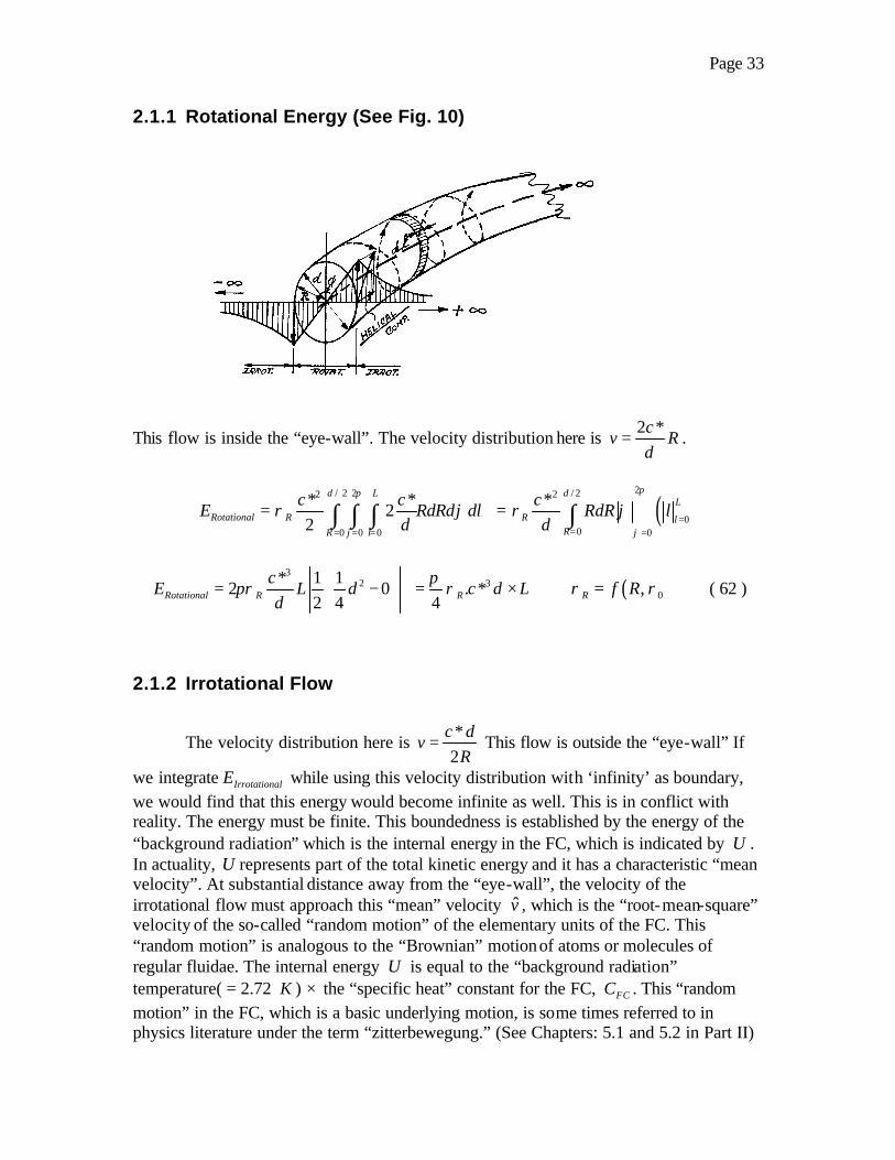
Page 33

2.1.1 Rotational Energy (See Fig. 10)

This flow is inside the “eye-wall”. The velocity distribution here is 2 *c

v Rd

= .

/ 2 22

0 0 0

* *2

2

d L

Rotational RR l

c cE RdRd dl

d

π

ϕ

ρ ϕ= = =

= ∫ ∫ ∫ ( )2/ 22

00 0

* dL

R lR

cRdR l

d

π

ϕ

ρ ϕ=

= =

= ∫

3

2* 1 12 0

2 4Rotational Rc

E L dd

πρ = −

3. *4 R c d Lπ

ρ= × ( )0,R f Rρ ρ= ( 62 )

2.1.2 Irrotational Flow

The velocity distribution here is *

2c d

vR

= This flow is outside the “eye-wall” If

we integrate IrrotationalE while using this velocity distribution with ‘infinity’ as boundary, we would find that this energy would become infinite as well. This is in conflict with reality. The energy must be finite. This boundedness is established by the energy of the “background radiation” which is the internal energy in the FC, which is indicated by U . In actuality, U represents part of the total kinetic energy and it has a characteristic “mean velocity”. At substantial distance away from the “eye-wall”, the velocity of the irrotational flow must approach this “mean” velocity v , which is the “root-mean-square” velocity of the so-called “random motion” of the elementary units of the FC. This “random motion” is analogous to the “Brownian” motion of atoms or molecules of regular fluidae. The internal energy U is equal to the “background radiation” temperature( = 2.72 K ) × the “specific heat” constant for the FC, FCC . This “random motion” in the FC, which is a basic underlying motion, is some times referred to in physics literature under the term “zitterbewegung.” (See Chapters: 5.1 and 5.2 in Part II)

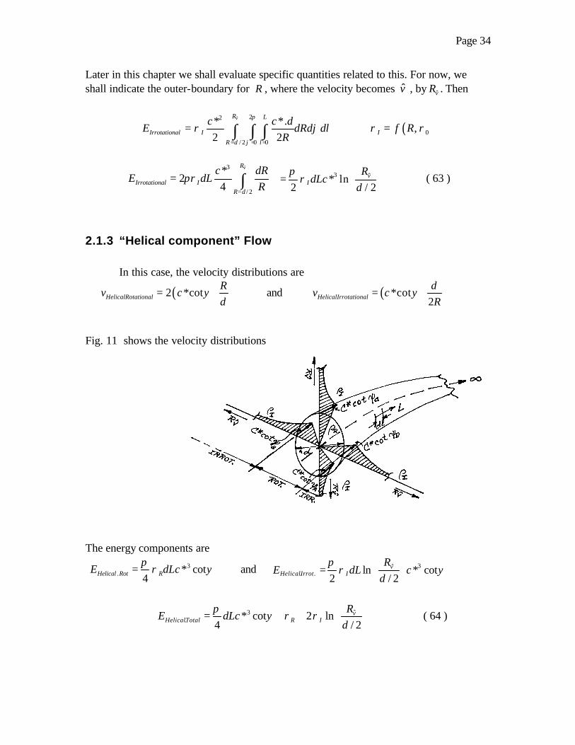
Page 34

Later in this chapter we shall evaluate specific quantities related to this. For now, we shall indicate the outer-boundary for R , where the velocity becomes v , by vR . Then

ˆ 22

/ 2 0 0

* *.2 2

vR L

Irrotational IR d l

c c dE dRd dl

R

π

ϕ

ρ ϕ= = =

= ∫ ∫ ∫ ( )0,I f Rρ ρ=

ˆ3

/ 2

*2

4

vR

Irrotational IR d

c dRE dL

Rπρ

=

= ∫ 3 ˆ* ln2 / 2

vI

RdLc

dπ

ρ =

( 63 )

2.1.3 “Helical component” Flow

In this case, the velocity distributions are

( )2 *cotHelicalRotational

Rv c

dψ= and ( )*cot

2HelicalIrrotational

dv c

Rψ=

Fig. 11 shows the velocity distributions The energy components are

3. * cot

4Helical Rot RE dLcπ

ρ ψ= and 3ˆ. . ln * cot

2 / 2v

HelicalIrrot I

RE dL c

dπ

ρ ψ =

3 ˆ. * cot 2 ln

4 / 2v

HelicalTotal R IR

E dLcd

πψ ρ ρ

= +

( 64 )

Page 35

2.1.4 Total energy of all flows of the Open Vortex tube

Here we have,

.OpenVortex Rot Irrot HelicalTotE E E E= + +∑ = 3 ˆ1 * cot 2 ln4 / 2

vR I

RdL c

dπ

ψ ρ ρ + +

( 65 )

2.1.5 Values for: Rρ and Iρ as: ( )0,f R ρ ?

We show in formulas ( 28 ) and ( 30 ) that for density outside the “eye-wall”

R a≥ , 2

20 2

12

ap p c

Rρ= − and for density inside the “eye-wall” 0 R a≤ ≤ ,

22 2

0 2

12

Rp p c c

aρ ρ= − +

Since in the FC 2pc

ρ= , we can have, for R a≥ ,

2

0 2

12

aR

ρ ρ ρ= − and

for 0 R a≤ ≤ , 2

0 2

12

Ra

ρ ρ ρ ρ= − +

So when R a≥ , 02

212aR

ρρ =

+ and when 0 R a≤ ≤ , 0

2

222Ra

ρρ =

− , when

12

a d=

we obtain for R a≥ , 02

218dR

ρρ =

+ and for 0 R a≤ ≤ , 0

2

2

22

Rd

ρρ =

− Now let

Rotational Rρ ρ= , be defined as the average density within the “eyewall”, / 2R d≤ and let Irrotational Iρ ρ= , be defined as: the average density outside the “eye-wall”, / 2R d≥ Then we have

/ 2

02

02

.22

2

d

RR

ddR

Rd

ρρ

=

=−

∫ , and / 2

02

525,0002

.525,0001

8

d

IR d

d dRdR

ρρ

=

=+

∫

The number 525,000d is an approximate limit of the irrotational flow due to the existence of a “random motion” in the FC, and corresponding to the observed “background radiation” temperature.

Page 36

Calculation of the averages of Rρ and Iρ can now be effected

02 ln ln34 4R

d d R dd d Rρ

ρ+ = + −

which results in 0.5493Rρ ρ= ( 66 )

0

122 2 21

/ 22 2 2 2I

arctgd R darctg

d R dRρ ρ

= − − −

which results in 0.9999Iρ ρ= ×

( 67 ) These values shall be considered again in Chapters 3.1.3, 3.4 and 3.5 as well as in Parts II and III. In Formulas ( 64 ) and ( 65 ) we can now substitute these values for Rρ and Iρ and obtain

( )3 ˆ. 0 *cot .55 2ln

4 / 2v

HelicalTotalR

E dL cd

πρ ψ

= +

( 64’)

and ( ) 3 ˆ. 0 1 *cot .55 2ln

4 / 2v

OpenVortexTotalR

E dL cd

πρ ψ

= + +

( 65’)

2.2 Calculation of the So called “Root-Mean-Square” Velocity of the “Random Motion,” Corresponding to the Observed “Background Radiation”

The similarities between the so-called “Brownian” motion in atomic or molecular

fluidae and the “random motion” in the FC are striking. Wherefore this calculation can be undertaken in a similar fashion. Herein we must replace “mass”, m with density 0ρ and also replace the number of molecules per unit volume, dn , by the number of the elementary units in the FC per unit FC volume, FCdn . Further we replace the Boltzmann

Constant . 2. * /BolFCK c T= and .BolFCK = .BolFC FCk Kχ= , wherein χ is a proportionality

constant. We also replace N the total number of molecules per unit volume with FCN ,

the total number of FC elementary units per unit volume. Now since 1

FCNPlancklength

=

we have 31/*FC

hN

cΩ

= . (See Introduction) The distribution function for a component of

the velocity, whereby no direction is preferred over any other, is a “Maxwell distribution”

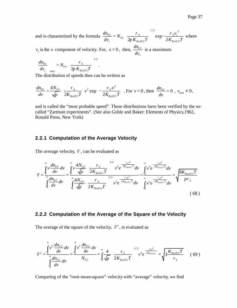
Page 37

and is characterized by the formula 1 /2 2

0 0

. .

exp2 2

FC xFC

x BolFC BolFC

dn vN

dv K T K Tρ ρ

π

= −

where

xv is the x component of velocity. For, 0x = , then, FC

x

dndv

is a maximum.

1/2

0

.max2

FCFC

x BolFC

dnN

dv K Tρ

π

=

.

The distribution of speeds then can be written as

220 0

. .

4 .exp

2 2FC FC

BolFC BolFC

dn N vv

dv K T K Tρ ρ

π

= −

. For 0v = , then 0FCdn

dv= , max 0v ≠ ,

and is called the “most probable speed”. These distributions have been verified by the so-called “Zartman experiments”. (See also Goble and Baker: Elements of Physics,1962, Ronald Press, New York)

2.2.1 Computation of the Average Velocity The average velocity, v , can be evaluated as

2

0

.

20

.

3/2220

.003/2

220

0 .0

42

42

BolFC

BolFC

vK TFCFC

BolFC

vFC K TFC

BolFC

Ndnv v e dvv dv

K Tdvv

dn Ndv v e dvdv K T

ρ

ρ

ρπ

ρπ

∞∞ −

∞ ∞ −

= =

∫∫

∫ ∫=

20

.

20

.

23

0 .

022

0

8BolFC

BolFC

vK T

BolFCv

K T

v e dvK T

v e dv

ρ

ρ πρ

∞ −

∞ −=

∫

∫

( 68 )

2.2.2 Computation of the Average of the Square of the Velocity The average of the square of the velocity, 2v , is evaluated as

20

.

2 23 / 2

22 40 0 0 .

. 00

0

43

2BolFC

FC FCv

K BolFC

FC BolFCFC

dn dnv dv v dv

dv dv K Tv v e

N K Tdndv

dv

ρρ

ρπ

∞ ∞

∞ −

∞

= = = =

∫ ∫∫

∫ ( 69 )

Comparing of the “root-mean-square” velocity with “average” velocity, we find

Page 38

that

.

0

3 BolFCrms

K Tv

ρ= which gives

31.085

8rmsvv

π= = ( 70 )

2.2.3 Calculation of the: rmsv of the “Random Motion” in the FC

The density 0ρ is the density in “standard” space, which means space away from

region(s) with “space-time curvature”. As will be discussed in following chapters, the density factor is mostly one of comparative nature and not of absolute value. In this calculation, we shall assume a value 0ρ = 610− . In the calculation of the energies of the proton and the electron this value shall be considered again. (See Chapters 3.3 and 3.4). T , the temperature of the background radiation is known to be 2.72K at this time. Question: What should be the value of a Boltzmann-type constant, which is valid for the

FC? Boltzmann’s Constant for atomic or molecular gases is 231.380 10j

mol K−×

⋅. Since

the FC behaves isothermally and since there are no entities to consider other than the elementary units of the FC, which are much smaller than atoms, the Avogadro number needs not to be considered, likewise we have no need for a molar Gas Constant. The

Boltzmann-type constant for the FC, .BolFCk =2

. .

*. .FC

BackgrRad

cK

Tχ χ= should be in the order

of magnitude of 210−≈ . The valuation of this Boltzmann-type constant for the FC shall be discussed in Part II, Chapter 5.1.2. In the following calculation we shall use 6

0 10ρ −= , which value shall be revisited in Chapters 3.4 and 3.5, where corroboration is found for this magnitude of value. Here we take .BolFCk = 210− , which gives

2

6

3 10 2.72285

10rmsv−

−

× ×= ≈ m/sec. ( 71 )

This value is highly plausible for the rmsv as being the velocity at the outer perimeter of the irrotational flow, particularly when compared to the value for the velocity at the “eye-wall”, which is roughly equal to 8* 3 10c = × m/sec.

2.2.3.1 Calculation of this “outer perimeter” of the irrotational flow

The velocity distribution is ˆ

*2 v

c dv

R= . Substitution of rmsv for v gives

8

ˆ3 10

525,0002 285v

dR d

×= =

× ( 72 )

Page 39

Substituting the value for ˆ 525,000vR d= in the formula for the energy of the irrotational flow, which is equation ( 63 ) gives

30

525,000* ln

2 / 2Irrotational

dE dLc

dπ

ρ =

, 3026 *

4dLc

πρ≈ × ( 73 )

For an “open vortex” we have 026Irrotational

Rotational R

EE

ρρ

≈ , and 0.55Rρ ρ≈

26/.55 47.3Irrotational

Rotational

EE

≈ ≈ ( 74 )

The sum-total for both energies for the open vortex 306.68 *dLcπρ≈ × ( 75 )

The energy for the helical motion is evaluated .1 ( )30 * .55 2 13 cot

4dLc

πρ ψ+ × ( 76 )

or 4.8≈ cotRotationalE ψ× . The evaluation for cotψ will be discussed in Chapters: 3.1.4, 3.3 and 3.4, where the “spin” phenominae will be discussed and evaluated.

2.2.3.2 Calculation of the energy of an open vortex tube with a larger “eye-wall” diameter

(See Fig. 12) Herein is shown an example of a rotational flow with an “eye-wall” diameter of

5 dΦ = × . Fig. 12 shows the velocity distributions of the rotational and irrotational flows. Since this open vortex did not yet tighten up to the maximum, there is a rotational flow within 5 dΦ = × . We ask: What are the velocities in P and Q? To answer we use an imaginary irrotational distribution represented in Fig. 12 by dotted lines. For this hyperbolic distribution is we have

*2

c dv

R= .

Now in P and Q, 2.5R d= × which gives *

5P Q

cv v= = . The rotational energy can now

be evaluated as

2.5 22

. 50 0 0

* 1 *2 2 5

d LR

Rotational dR l

c cE dRd dl

π

ϕ

ρϕ

×

Φ== = =

= ∫ ∫ ∫ = ( )( ) ( )3

2.5 2

0 0 0

*20

d LRcR l

πρϕ

×

Page 40

or 3

3. 5

*2 2.5 *

20 4R

Rotational d Rc

E L d dLcρ π

π ρΦ= = × × = ( 77 )

Wherefore we now find that the rotational or internal energy of an open vortex tube is independent of its diameter. Previously we found for the density as function of the radius of a vortex

Within the “eye-wall” is 02

2

22

Rd

ρρ =

− and outside 0

2

218dR

ρρ =

+ . For

the velocity v c= we found

Outside the “eye-wall” 02 2. * 1R

c cd

ρρ

= − ; inside the “eye-wall”

20

2

2* 1

Rc c

dρρ

= − + Figs. 43a and b show the respective density and maximum

velocity distributions Fig. 43 a: Fig 43 b:

2.2.4 Closed Fluid Flow Vortexes

Theoretically these closed fluid flow vortices can have any closed “flowing” shape. It is possible that in a fluidum and certainly in the FC an open vortex can close into itself and become a closed one. The complex photon decay process (See Part II, Chapter 11.1) is an example of a fluid-dynamical system, which has aspects of this kind . However, it is also possible that vortexes which are closed into themselves are at once created by a sudden jet-like phenomenon. Even with regular atomic or molecular fluidae

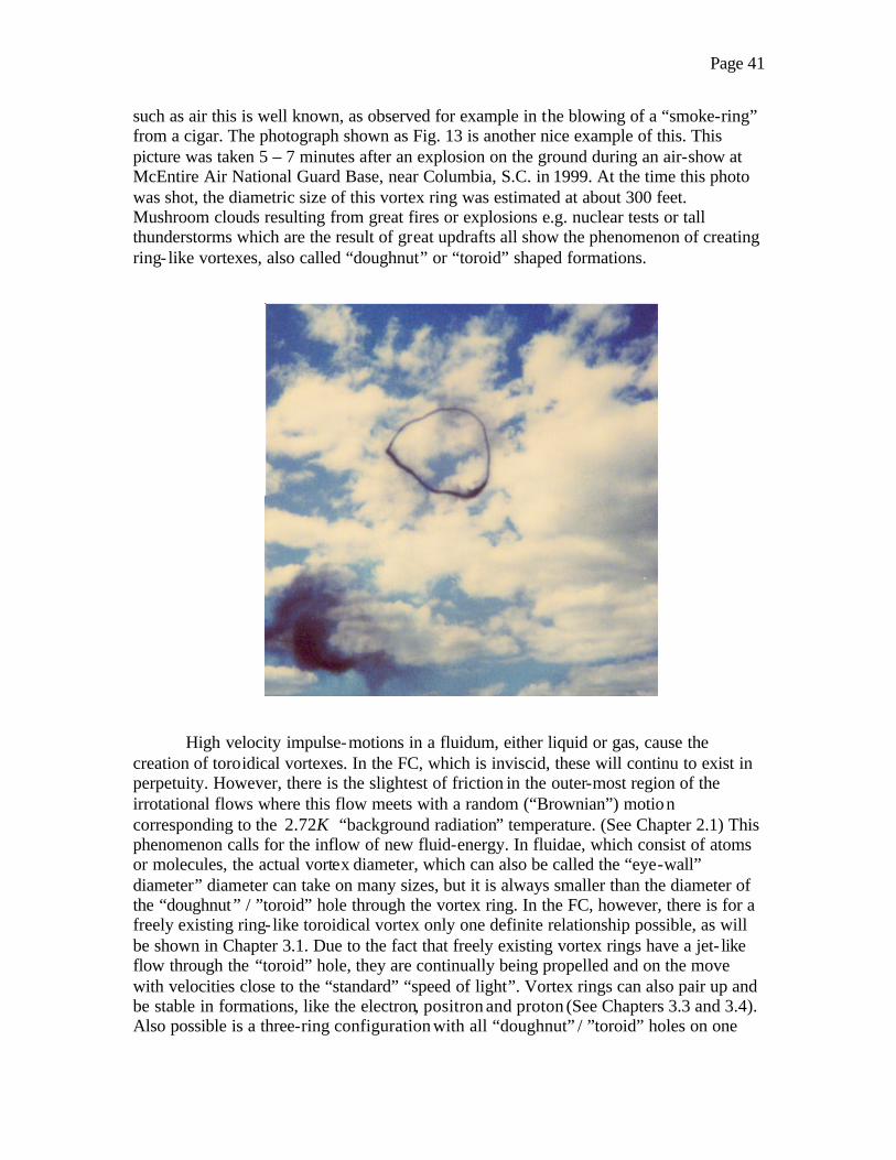
Page 41

such as air this is well known, as observed for example in the blowing of a “smoke-ring” from a cigar. The photograph shown as Fig. 13 is another nice example of this. This picture was taken 5 – 7 minutes after an explosion on the ground during an air-show at McEntire Air National Guard Base, near Columbia, S.C. in 1999. At the time this photo was shot, the diametric size of this vortex ring was estimated at about 300 feet. Mushroom clouds resulting from great fires or explosions e.g. nuclear tests or tall thunderstorms which are the result of great updrafts all show the phenomenon of creating ring- like vortexes, also called “doughnut” or “toroid” shaped formations.

High velocity impulse-motions in a fluidum, either liquid or gas, cause the creation of toroidical vortexes. In the FC, which is inviscid, these will continu to exist in perpetuity. However, there is the slightest of friction in the outer-most region of the irrotational flows where this flow meets with a random (“Brownian”) motion corresponding to the 2.72K “background radiation” temperature. (See Chapter 2.1) This phenomenon calls for the inflow of new fluid-energy. In fluidae, which consist of atoms or molecules, the actual vortex diameter, which can also be called the “eye-wall” diameter” diameter can take on many sizes, but it is always smaller than the diameter of the “doughnut” / ”toroid” hole through the vortex ring. In the FC, however, there is for a freely existing ring- like toroidical vortex only one definite relationship possible, as will be shown in Chapter 3.1. Due to the fact that freely existing vortex rings have a jet- like flow through the “toroid” hole, they are continually being propelled and on the move with velocities close to the “standard” “speed of light”. Vortex rings can also pair up and be stable in formations, like the electron, positron and proton (See Chapters 3.3 and 3.4). Also possible is a three-ring configuration with all “doughnut” / ”toroid” holes on one

Page 42

axis, this is the meson structure. Its stability when on its own is minimal. However, in bound states there is some stability. The five-ring configuration, with all “toroid” holes on one axis is also possible; this structure forms the neutron. It has a “half- life” of 11 minutes and it is built up as follows: “An electron at one end and a proton at the other end, held together as well as being kept apart by an anti-neutrino”. The 3-ring group composite of an anti-neutrino and an electron is also a meson. Therefore, one can justly state that the neutron consists of a proton and a meson.

Besides the rotary-type, rotational and irrotational, motions of the vortex rings they also display helical motion. This last named motion causes flows in or out of the “toroid” holes to have a twisting-type motion. This phenomenon is called “spin”. This will be discussed in the following Chapters where descriptions of every “particle” which displays “spin” are being presented.

A rule of thumb: “even numbered vortex ring set formations have “charge” and uneven numbered ones have no “charge ”. ”Positive charge” means outflow e.g. the proton and “negative charge” means inflow e.g. the electron.

2.2.5 Interrelationship of the FC Density with Electro-magnetic Factors

For permeability 0µ and permitivity 0ε , we have 0 0

1c

µ ε= ( 78 )

Also 0p pc

ρ−

∝ and since 2*p

cρ

= , therefore 0cρ ρ

ρ−

∝ . Combining with

( 78 ) we now obtain 0

0 0

1 ρ ρρµ ε−

∝ , which makes for 0 00

ρµ ε

ρ ρ∝

− ( 79 )

( 79 ) shows the dependence of these electro-magnetic factors as to the FC density.

2.2.6 Summary Considerations of Waves and Vortex Entities ( a ) From the chapters 1.1 and chapters 2.1 we can now conclude that in FC physics

we found that formulations for energy and rates of energy for waves and vortices respectively are expressed in the same dimensionalities and basic factors.( a ) Wave energy is expressed in a size ( = wavelength λ ) and in the local velocity of light ( = c ), which in turn depends on the local density ( = ρ ), which has a dependency on the “standard” density ( = 0ρ )

Page 43

( b ) Vortex energy rates are expressed in a size ( = “eye-wall” diameter of the elementary vortex d ) and in the “standard” velocity of light ( = *c ) and in the “standard” density ( = 0ρ )

These finding of fact are in full agreement with the convertibility processes which

are found in nature, namely the photon decay process, which stands for the conversion of waves into vortex entities (electron and positron) and the gamma ray burst, which stands for the conversion of vortex entities, which are compacted in an aged black hole into waves (high energy gamma rays).

Wave and vortex phenominae are two realms in which the most basic factors in

nature can interrelate with each other.

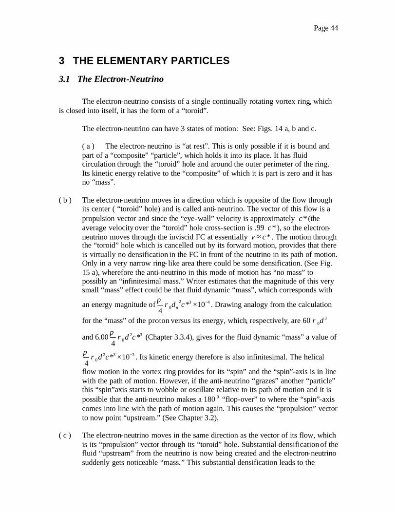
Page 44

3 THE ELEMENTARY PARTICLES

3.1 The Electron-Neutrino

The electron-neutrino consists of a single continually rotating vortex ring, which is closed into itself, it has the form of a “toroid”.

The electron-neutrino can have 3 states of motion: See: Figs. 14 a, b and c.

( a ) The electron-neutrino is “at rest”. This is only possible if it is bound and part of a “composite” “particle”, which holds it into its place. It has fluid circulation through the “toroid” hole and around the outer perimeter of the ring. Its kinetic energy relative to the “composite” of which it is part is zero and it has no “mass”.

( b ) The electron-neutrino moves in a direction which is opposite of the flow through

its center ( “toroid” hole) and is called anti-neutrino. The vector of this flow is a propulsion vector and since the “eye-wall” velocity is approximately *c (the average velocity over the “toroid” hole cross-section is .99 *c ), so the electron-neutrino moves through the inviscid FC at essentially *v c≈ . The motion through the “toroid” hole which is cancelled out by its forward motion, provides that there is virtually no densification in the FC in front of the neutrino in its path of motion. Only in a very narrow ring- like area there could be some densification. (See Fig. 15 a), wherefore the anti-neutrino in this mode of motion has “no mass” to possibly an “infinitesimal mass.” Writer estimates that the magnitude of this very small “mass” effect could be that fluid dynamic “mass”, which corresponds with

an energy magnitude of 2 3 40 * 10

4 nd cπ

ρ −× . Drawing analogy from the calculation

for the “mass” of the proton versus its energy, which, respectively, are 60 30dρ

and 6.00 2 30 *

4d c

πρ (Chapter 3.3.4), gives for the fluid dynamic “mass” a value of

2 30 *

4d c

πρ 310−× . Its kinetic energy therefore is also infinitesimal. The helical

flow motion in the vortex ring provides for its “spin” and the “spin”-axis is in line with the path of motion. However, if the anti-neutrino “grazes” another “particle” this “spin”axis starts to wobble or oscillate relative to its path of motion and it is possible that the anti-neutrino makes a 180 0 “flop-over” to where the “spin”-axis comes into line with the path of motion again. This causes the “propulsion” vector to now point “upstream.” (See Chapter 3.2).

( c ) The electron-neutrino moves in the same direction as the vector of its flow, which

is its “propulsion” vector through its “toroid” hole. Substantial densification of the fluid “upstream” from the neutrino is now being created and the electron-neutrino suddenly gets noticeable “mass.” This substantial densification leads to the

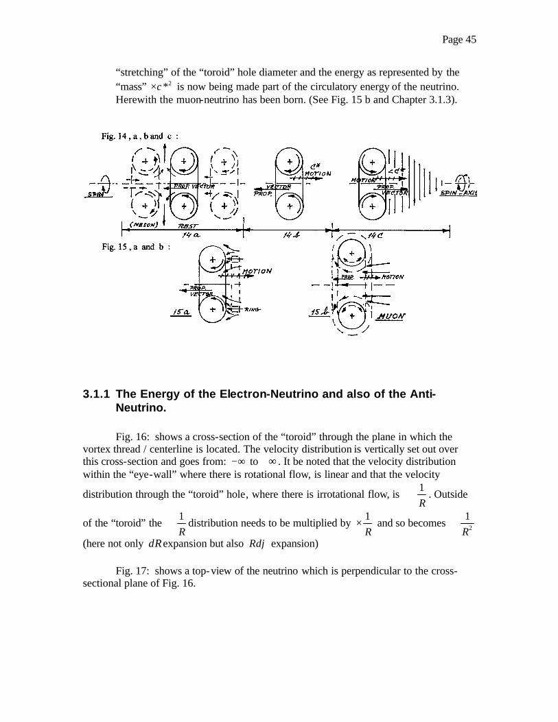
Page 45

“stretching” of the “toroid” hole diameter and the energy as represented by the “mass” 2*c× is now being made part of the circulatory energy of the neutrino. Herewith the muon-neutrino has been born. (See Fig. 15 b and Chapter 3.1.3).

3.1.1 The Energy of the Electron-Neutrino and also of the Anti-Neutrino.

Fig. 16: shows a cross-section of the “toroid” through the plane in which the

vortex thread / centerline is located. The velocity distribution is vertically set out over this cross-section and goes from: −∞ to +∞ . It be noted that the velocity distribution within the “eye-wall” where there is rotational flow, is linear and that the velocity

distribution through the “toroid” hole, where there is irrotational flow, is 1R

∝ . Outside

of the “toroid” the 1R

∝ distribution needs to be multiplied by 1R

× and so becomes 2

1R

∝

(here not only dRexpansion but also Rdϕ expansion)

Fig. 17: shows a top-view of the neutrino which is perpendicular to the cross-sectional plane of Fig. 16.

Page 46

3.1.2 Rotational Energy of the “Toroid” or Single Vortex-ring (See Figs. 18a and b )

Velocity distribution ( a ) translates into velocity distribution ( b ).

( a ) ( b )

The velocity distribution is linear: 2 *c

v Rd

= 02

2

22

R Rd

ρρ =

− ; 0.55Rρ ρ≈ , and

* / 2linv c= Hence, Rρ can be directly multiplied by linv and we have

Page 47

0

0

2 /3 3 / 2 2 2 20

. 2/ 2 / 2 0 0

2

2 * *2 2

2

d

RotTorR d

c cE RdRd Rd

R dd

ρ π π

ρ ρ ψ ϕ

ρψ ϕ

= = = =

=−

∫ ∫ ∫ ∫

3 / 2 22

. 0/ 2 0

* * 3.55

2 2. 2 2

d

RotTorR d

c c d dE Rd dR

d

π

ϕ

ρ ϕ= =

= − ∫ ∫

( )2 23 / 23 2

2 3. 0 00

/ 2

9 1* 4 4.55 .55 *4 2 2 2 2

d

RotTorR d

d dc RE c

π

ϕ

πρ ϕ ρ

==

= = −

2 30.55 *

2d c

πρ=

.RotationalTorE 2 30.55 *

2d c

πρ= ( 80 )

3.1.3 Circulatory irrotational Energy Through and Around the “Toroid” (See Fig. 19)

Here we have the energy of the flow “coming up” through the “toroid” is the

same as the energy “going down” around and outside the outer “eye-wall” perimeter.

Since 0Iρ ρ≅ , / 2 2 2

. 00 0

* *2 2

d

IrrotationalTorR

c d cE Rd dR

R

π

ϕ

ρ ϕ= =

= ∫ ∫

( ) ( ) [ ]3

/2 2 3. 0 00 0

** / 2 0

4 2d

IrrotationalTor R

c dE R c d d

π

ϕ

πρ ϕ ρ

= == = −

2 3. 0 *

4IrrotationalTorE d cπ

ρ= ( 81 )

Fig. 19:

Page 48

3.1.4 Cross-section and Velocity Distribution Outside the Neutrino

The velocity distribution outside the outer perimeter of the “eye-wall” is the

“irrotational” distribution1R

× , which is a 2

1R

relationship, i.e. 2

constv

R= . For / 2R d= ,

*v c= so, 2

4 *cconst

d= and 2 2

4 *cv

d R= .

Since no energy is added to the neutrino during its existence, ( This is not so with regard to the proton and the electron, which have need over time for infinitesimal addition of fluid energy.) all energies must be totally balanced.

We found that 2 3. 01.1 *

4RotTorE d cπ

ρ= × × and 2 3. 0 *

4IrrotTorE d cπ

ρ= ×

Since the rotational energy of the vortex ring causes and is in total harmony with, the circulatory energy which goes through the “toroid” and comes around the vortex ring, the difference between the two values which have been found for the rotational and irrotational energies equals the helical energy. This energy has a flow pattern which extends all throughout the inside of the vortex ring and minorly into the area outside the vortex ring.

Therefore, 2 30.1 *

4HelicalE d cπ

ρ= × ( 82 )

These values for the three types of energies which are identified with the vortex type entities are basic factors in the FC physics and are equally as important as Planck’s energy formula is for wave energy.

Fig. 20 shows a cross-sectional view (under angle ) of a vortex ring showing the velocity vectors of the helical component of the flow. For the helical energy we

have 2 30cot *

4Helical averagedE d cπ

ψ ρ= × and, cot / .1/1.1 .091averaged Hel RotE Eψ = = ≈

We note that cot averaged ψ has contributions at the top and bottom of the cross-section

of the vortex. These are . . .cot .091 2outer perimvort ψ = × and . . .

2cot .091

2inner perimvort ψ = × .

With this, we found the rotational velocity which exists at the inside perimeter of the “toroid.” This is also the “spin velocity” of the neutrino. SPINV = .064 *c× ( 83 ) Values for ψ are 0 ' 0 '

. .83 40 , 87 20outer perim inner perimψ ψ≈ ≈ and 0. 85 50'averageperimψ ≈ ( 84

Page 49

Fig. 20 Cross-section of vortex ring with helical velocity vectors

Since there is total harmony between the helical energy of the vortex ring and the rotational energy which is communicated to the circulatory flow through the “toroid” hole, we can state that .091SPIN Helical RotationalE E E≡ = ×

which gives 2 30.1 *

4SPINE d cπ

ρ≈ × ( 85 )

3.1.5 Are there “higher harmonic orders” for the “toroid” ? (The size of neutrino’s)

Let us examine the energy balance of a single vortex ring (“toroid”) having in this

example, a given diameter of the “toroid” hole which is twice the diameter d of the vortex ring. Here . 2toroidhole vortexd d= ( vortexd is“eye-wall” diameter ). Refer to Fig. 21, which shows a cross-section of this proposed vortex ring, together with the velocity distributions. In this case,

2 22

2 3. 0 0

0

* *.55 .4125 *

2 2

d

RotTorR d

c cE Rd dR d c

π

ϕ

ρ ϕ πρ= =

= = ×∫ ∫ ( a )

2 2

2 3. 0 0

0 0

* **

2 2 2

d

IrrotTorR

c d cE Rd dR d c

R

π

ϕ

πρ ϕ ρ

= =

= × =∫ ∫ 2 30.50 *d cπρ= × ( b )

We now find that the rotational energy would be smaller than the circulatory energy. This is impossible; the rotational energy which includes the helical energy must be at least equal or slightly more than the energy of the circulatory flow. In this example is shown

Page 50

that a larger diameter of the “toroid” hole compared to the vortex diameter is harmonically impossible. Fig. 21 Cross-section of a hypothetical vortex ring

3.2 The Muon-Neutrino

The Muon-Neutrino can be forced into existence. It is an unstable vortex entity with a short lifetime, namely 62 10−× seconds. It has a “mass” for that short time, the energy equivalent of which is 207eV . Fig 15b shows a cross-section of the muon neutrino.

The substantial densification which takes place when the vector of the circulatory flow through the “toroid” hole points “upstream”, causes the stretching of the vortex ring and enlargement of the diameter of the “toroid” hole in order to be able to “swallow” the densified fluid “prop” and making this densified fluid a part of its circulation while absorbing its associated energy. The proportions, as shown in Fig. 15 b, suggest that the “toroid” hole diameter should enlarge to at least 2.5 d× in order to facilitate the densified “prop”, which is directly “upstream” and in contact with the vortex ring, then becoming part of this ring, whereby this electron-neutrino is being converted into a muon-neutrino. From the value given for the energy of the muon-neutrino and taking the assumed value for 0ρ , which we use in several calculations in this book (See Chapters: 2.1 , 3.3, 3.4) we can establish a value for the stretched “toroid” hole diameter of the muon-neutrino.

Page 51

3.2.1 Calculation of the magnitude of size of the muon-neutrino and associated vortex ring

We have for the muon-neutrino

19207 1.602 10muonE Joule−= × × , and assume 60 10ρ −= , then 2 3

0 *2

d cπ

ρ≈

6 2 3 1910 * 2 207 1.602 102

d cπ − −≈ = × × × , so

192 36

24 6

414 1.602 10.8 10

27 10 10d

π

−−

−

× ×= = ×

× × ×2m ,

which gives 18.9 10muond −≈ × m, wherefore 19. 3.0 10elneutrinod −≈ × m ( 86 )

The diameter of the centerline of the muon vortex ring is 18

. . . 2.5 10muonvortcenterlD −≈ × m, so

the diameter of the outer perimeter of the vortex ring is 183 10−≈ × m.

Figs. 22a and b show a size comparison between the electron-neutrino and the muon-neutrino, which is based on an assumed value for the density, 6

0 10ρ −= . The outer diameter of a spherical volume in the FC (around the vortex ring) within which 99.99% of all circulatory (i.e. irrotational) energy is contained should be about 25 – 50 times greater than the outside diameter of the muon-neutrino. This gives a size for the muon neutrino of order 153 10−× to 1610− cm. The value for the outside diameter of the muon-neutrino vortex ring is about 2.0-2.5 1610−× cm. This value shows that the order of size of the muon-neutrino is between 400 to 500 times smaller than the size of the electron “at rest” , which has a size of about: 1310− cm. The size of the outside diameter of the vortex ring of the electron-neutrino is about 1500 to 1200 times smaller than the size of the electron “at rest”.

If we now determine the “mass” equivalent for the muon-neutrino

2*E

mc

= =19

3416

207 1.602 103.7 10

9 10

−−× ×

≈ ××

kg. Comparing this with the mass of the

electron, which is 319.1 10−× kg, then we find a “mass ratio of about: 2500. This corroborates quite well with the size ratio given above (Note: The size ratio needs to be multiplied by a factor with relation to the “mass” ratio). The tau-neutrino shall be discussed in Part II, Chapter 6.3.

Page 52

3.3 The Proton

The Proton consists of two vortex rings which stably roll against each other. Together with the electron, the positron and the anti-proton, it forms the group of “2 vortex ring”- combination structures. The anti-proton is not stable. For the stability of the proton a value is given like: > 4 2310× seconds. The “lives”of the electron and positron are indefinite, likely ∞ . The positron, which is structurely a mini-proton can convert into a proton if enough energy is present. This conversion mechanism can occur instantly in the photon decay process if the photons have sufficiently high energy (See Part II, Chapter 11). Figures 23 a, b and c show a cross- section and a left and right side view of the proton. The 2 vortex rings roll against each other in such a manner that there is a peripheral or equatorial inflow from all around the rings and 2 polar or axial outflows along a single axis, called here the “spin” axis.

Fig. 24 shows the same cross-section as in Fig. 23 b, but the fluid flow patterns and the velocity distributions have been added Fig. 24:

Page 53

The stability of the proton can now be understood. The axial momentum of both polar outflows cause reaction forces in the fluidum around the proton in opposite direction and those forces press the rings against each other. The peripheral or equatorial intake cross-section, which can be formulated as .PR PRf Dπ× is larger than the two cross-

sections of the polar outflows which can be formulated as ( )224 PR PRD dπ

× − . (This will

be corroborated in a subsequent calculation.) The smaller total outflow cross-sectional area compared to the inflow cross-sectional area, together with the fact that the “eye-wall” velocities of the continually rotating rings are equal for both cross-sectional areas, cause the fluid inside the proton to be compressed and the density “inside” to be higher than the density “outside” the proton. The increased density “inside” (location A in Fig.

24) presses the rings outwardly and this outward force, which is roughly 2

4D P

π≈ × ∆ is

countered by the reaction forces in the FC “outside” of the proton (location C in Fig. 24 ). Because of the fact that the “eye-wall” velocity (just like any “eye-wall” velocity) in the polar out flows is *c and because of the fact that the pressure “inside” the proton has a substantial P+∆ , we can conclude that the outflow velocity over the whole cross-section of the “throat” or “toroid” hole equals *c≈ . Fluid mechanics suggests that the actual velocity in between the “eye-walls” in the “throat” can be higher than *c (location B in in Fig. 24). However, with the rapidly expanding flow cross-sections outwardly from the “throats” this is actually not the case or a negligible factor. We can safely state that the “outflow velocity” in the “throats” is quite constant over the cross-sections and is essentially *c≈ . This important evaluation of the velocity of the polar outflows enables us to formulate the flows and corresponding energies for the proton, which in turn will provide dimensions. It also provides for an approach for the calculation of the : flows and corresponding energies and dimensions of the electron in chapter

3.1.5. Formula ( 80 ) shows that the rotational energy of a vortex ring is 2 301.1 *

4d c

πρ .

Size d , being the “eye-wall” diameter of the vortex ring, as used in formulations for the proton shall be indicated by PRd . PRd differs from and is bigger than neutrinod . However, since the origin of the proton rests in a positron to proton conversion, which can be a subsequent process to the photon decay process, (see Chapter 11) the “eye-wall” diameters of the vortex rings of the proton and of the electron and positron are the same.

PR el pod d d= = .

3.3.1 Calculation of the diameter of the outflow of “toroid” hole of the proton

The rotational energy of both rings is 2 302.2 *

4 PRd cπ

ρ≈ . This value is based on

vortex rings which have an outflow diameter PRd≈ and it includes the helical energy. Since no energy is added, (the infinitesimal amount of energy which is needed over

Page 54

extended time to compensate for the slightest of friction in the outermost region of the surrounding irrotational flow is not to be considered in this calculation) this rotational energy equals the energy of the circulation of the fluid through and around the vortex rings of the proton. The flow outside “eye-walls” of the vortex rings is always irrotational flow, whereby, 0Iρ ρ≈ ). For a complete energy balance we have

( ) ( )2

2 2 23 30 0 0

*2 * * 2.2 *

4 2 4 4PR PR PR PR PRc

D d c c D d d cπ π π

ρ ρ ρ− = − = ( 87 )

So ( )2 22.2PR PR PRD d d− = × , which gives 2.483PR PRD d= × . This gives diameter sizes of

the “throats” (i.e. the diameter of the outflows) being 1.48 d≈ ×

We now can conclude that due to the higher pressure of the fluid inside the proton

the rings are stretched to a factor 2.4

1.242

=≈

, therefore the rotational energy and also the

circulatory energy have increased to 302.72 *

4 PRd cπ

ρ× . The rotational energy increases

linearly, but the circulatory energy increases with the square of the size of PRD . In order to find the PRD for which the rotational energy equals the circulatory energy the following more general equation needs to be applied

( )2 23 30 0. * 2.2 *

4 2 4PR

PR PR PRPR

Dc D d d c

dπ π

ρ ρ− = × × , so ( )2 .2.2

2PR PR

PR PR

D dD d− = × .

This gives 2.732PR PRD d≈ × . Therefore the total equivalence between the rotational energy and the circulatory energy occurs at a value of

2.732PR PRD d= × , which gives 1.732PR PR PRD d d− = × or 3outflow PRd d= × ( 88 )

The rotational energy of the proton rings is ( 2.73

2.2 3.002

× = ) 2 303.00 *

4 PRd cπ

ρ× .

The circulatory energy is the same and the he lical energy was included in the rotational energy, wherefore the total “fluid-dynamical energy” of the proton is

2 306.00 *

4 PRd cπ

ρ× . ( 89 )

Page 55

3.3.2 Calculation of the width of the split PRf (between the vortex rings of the proton)

It will be shown that the cross-sectional area of the peripheral or equatorial inflow

is larger than the cross-sectional area of both outflows, wherefore we can conclude that there is a higher pressure and a higher density “inside” the proton. This energy of this “confined” fluid is a potential energy. This energy shall be calculated and in adding this to the fluid-dynamical energy we find the total energy of the proton.

From the densification ratio between the density “inside” the proton insρ and the density “outside” and at distance from the proton, which is 0ρ and from the value of the “internal volume” we shall be able to determine the “mass” of the proton. Also the “charge” energy rate and “charge” force of the proton shall be determined. This force is the force of the outflow, which shall be indicated as being positive.

Per definition: Outflows mean positive charge and inflows mean negative charge. Furthermore the “spin” energy, the “spin” velocity at the outflow diameter and the radial velocity in the outflows shall be determined.

3.3.2.1 Velocity distribution as shown by curve ( b )

Using velocity distribution const

vR

= (See Fig. 25 , line ( b ))

Fig. 25:

For / 2PRR d= , *v c= which gives *

2PRd c

vR

= . In order to find /PRf d we equate the

inflow energy with the outflow energies (outflow energy = circulatory energy)

Page 56

( )

/ 2 / 2

32 / 23

0 0

12*

3.00 * 2.734 2 / 2

PR PR

PR

d f

R dPR PR PR

PR

ddR

Rcd c d f

fπ

ρ ρ π

+

=

×

= × ×∫

( )/ 2 / 2

/ 2

3.00ln ln 1

1.365PR PR

PR

d fPR PR PR PRR d

PR PR PR PR

d d f dR

f f d f+

=

= = +

2.197 ln 1 PR

PR

fd

= +

, which gives 8.00PR PRf d= ( 94 )

( )

*.111 *

2 .50 4.00PR

centerPR

d cv c

d= =

+ ( 95 )

The inflow cross-sectional area is 22.73 8.00 68.62PR PR PRd d dπ × × =

The outflow cross-sectional areas are ( )2 22 3. 4.714 PR PRd dπ

× =

Ratio of inflow / outflow areas is 14.56 .

3.3.2.2 Calculation of the density “inside” the proton ( insρ )

Previously we determined that 0

23eye wallρ ρ− = . What is ρ over the inflow cross-

section? ( .111. *centerv c= ) Determining the averaged velocity in the inflow

( )

4.5

4.5/ 2/ 2

*2 1 1 4.5

* ln *ln4 8 8 .5

PR

P RPR

PR

d

dR dR d

PR

c ddR

R dv c R c

d d=

== = =

∫ ,

*ln9.274 *

8c

v c= =

Applying Bernouilli (from outside proton to inflow) 20

12Inflow InflowP P vρ= +

Divide by 0P , and since 2/ *P cρ = , therefore 2

0 0

11 .075 *

2 *Inflow Inflow c

c

ρ ρ

ρ ρ= +

0

11 1 .075

2Inflowρ

ρ = + ×

, this gives 0.96Inflowρ ρ= × , further “inside” , 0nsρ ρ> .

Consider the polar outflows where the velocity over the whole cross-section *c≈ .

(Bernouilli) 20

1 2*

2 3ins OutflowP P cρ= + × . Divide by OutflowP , since 2/ *P cρ = ,

therefore 2

22

1 1 *1 * 1 1.5

2 2 *Outflowins

Outflow Outflow

cc

P cρρ

ρ= + = + =

Page 57

3.3.2.3 Density “inside” the proton versus density “outside” 0/insρ ρ

The circulatory energy per polar outflow is 2 301.5 *

4 PRd cπ

ρ× . The outflow force

it exerts is 2 201.5 *

4 PRd cπ

ρ×

( ) ( )

2 22 20

00 0 0 02

2

1.5 * 1.5 *4 .202.73

4

PRPR

ins

PRout PR

d c d cP P P P P

dd d

πρ ρ

π

× ×= + = + = + ×

+ , so 0/ 1.2insρ ρ = ( 96)

This value will be used in the calculation for the “mass” of the proton.

Fig.25 shows one velocity distribution, which is shown by curve ( b ) and which

is 1R

∝ (from “eye-wall” to the center of the inflow). The distribution, which is shown by

curve ( a ) is 2

1R

∝ (from “eye-wall” to the center of the inflow). The first derivative of

the latter distribution at the “eye-wall” complies with the conditions for irrotational flow. It be noted that while the velocity distribution for irrotational flow inside toroid holes is

1R

∝ , that the velocity distribution for irrotational flow outside the toroid is 2

1R

∝

3.3.2.4 The velocity distribution as shown by curve ( a )

For curve a we have

2

2

*2 *

2 PR

c Rv c

f= + ,

/ 23/ 22

002 2

3* 2 * * 2 *2 / 2 2 / 2

PRPR

ff

R

PR PRPR PR

RR dR

c c c cv

f ff f=

= + = +

∫

3

3

2 ** * * 224 * .67 *2 2 6 3/ 2

PR

PR

fcc c cv c c

f= + = + = = × ( 97 )

Page 58

This averaged velocity differs much from the averaged velocity of the “hyperbolic” distribution, which is .274 *v c= × . With relatively large sizes of PRf and outflowd the velocity distribution of curve ( a ) and formula ( 97 ) cannot be used in case of the proton. However, if these sizes are small as is the case with the electron / positron then there is little difference in the results and either distribution can be used.

We wish to estimate the Pressure ratio . 0/InsidePRP P ? The outflow energy rate for

each “toroid” hole is 2 301.50 . . * ( )

4 PRd c Force velocityπ

ρ × . Therefore, the force with

which the vortex rings are being pressed together is 2 201.50 *

4 PRd cπ

ρ . The total area

inside the proton upon which the inside pressure is being exaerted is

.prinsA = 2 2(2.73 )4 4PR PRD dπ π

= . The pressure is( )

2 20

20

2

1.50 *4 .20 . *

2.734

PRd cP c

d

πρ

ρπ

∆ = =×

( 98 )

This pressure-difference is positive( > 0P ) and according to formula ( 43 ) 20 0. *P cρ= ,

We have . 0 0.20InsidePRP P P= + and . 01.20InsidePRρ ρ= × ( 99 )

The term 20..20 *cρ ( 98 ) represents a quantity of potential energy and manifests itself as

“mass”. This amount of energy is additional to the kinetic type energies, being the rotational-, the irrotational- and helical energies , the total of the rates of these

energies is totalE = 2 306.00 *

4 PRd cπ

ρ× . The potential energy is .40 20 *cρ ( 100 )

The dimensionality is 1 2elN L T− − ( elN is number of elementary units in FC )

3.3.3 The size of the vortex “eye-wall” diameter of the proton We have in physics 271.67 10prm kg−= × and ( ) ( )22 27 8* 1.67 10 3 10prE mc J−= × × ×

Assume a value for 60 10ρ −= and consider the energy rate of the proton per unit of time

(1 sec.). This gives 26 3 27 21.1 10 * 1 1.67 10 *PRd c cπ − −× × × × × = × × .

Therefore 27 6

30 158

1.67 10 101.18 10 1.09 10

1.5 3 10PRd mπ

−− −× ×

≈ = × = ×× × ×

( 101 )

This estimate did not include the value for the potential energy. If the potential

energy were added, then we find a slightly higher value for PRd . The exact value for 0ρ will be extensively researched in following chapters and in Parts II and III. Fig. 44 is a cross-sectional drawing of the proton with proportions as calculated above.

Page 59

Fig. 44:

3.3.4 The “mass” of the proton

As shall be clear from the foregoing chapters, “mass” as being something “tangible” does not exist. The phenomenon “mass” relates to either confined or non-confined locations in the FC where there is an altered density of the Fluidum compared to a “standard” density which prevails over vast areas in space (micro or macro). If the density 0ρ ρ> , then we can define this region to have “mass” and if the density 0ρ ρ< then we can define the region as having “fractional mass”. Since “fractional mass” falls short of “standard mass” we can also speak of “negative mass” by indicating the shortfall or difference relative to “standard mass”.

Furthermore, if a certain ρ∆ exists in a given volumetric area, then the “mass” is proportional to the product of the volume of the region multiplied by ρ∆ . spm Vol ρ∝ × ∆ ( 102 ) Where spVol is the volume of space in the FC. “Mass” which originates from non-confined altered density regions in the FC always relates to moving “particle”-type entities being at “relativistic” velocities. For example an electron at high velocity creates a densified fluid area in front of it in the direction of its motion, which can be expressed

as increased “mass” 2 21/ 1 / *vm v c∝ − . If the entity slows down again, then the value of the observed “mass” comes down again as per this formula. The “mass” of the proton, (See Formula ( 96 )) can be formulated as 01.20 PRvolρ× × .

Page 60

( ) ( )2 22.73 8.00 1.00 2.404 8PR PR PR PR PRvol d d d dπ π

π= × + − × × =

3 3 352.68 2.96 49.72PR PR PRd d d− = . Therefore the “fluid mechanical” “mass” of the proton is 3

01.20 49.72 PRdρ× 3060 PRdρ≈ ( 103 )

The proton has 2 outflows and 1 inflow. This corresponds in the Quark Theory with 2 “hadron” up-quarks and 1 down-quark.

3.3.5 “Charge” and “Spin” of the Proton

The polar / axial outflows have a circulatory energy of 2 303.0 *

4 PRd cπ

ρ× .

This circulatory energy incorporates a helical energy, which is roughly 1/10 of the

circulatory energy, so 2 300.3 *

4helical PRE d cπ

ρ≈ × , which is equal to the Spin energy.

The charge energy rate of the proton is 2 3. 03.0 *

4ch PRE d cπ

ρ≈ × , ( 104 )

So the total charge force is 2 203.0 *ch PRF d cρ≈ ( 104’)

The rotational velocity of the “spin” ( at the stretched diameter of 1.73 PRd ) is from

formula ( 83 ), .064 *SPINV c= × . Therefore .064 *

1.73 PR

cd

ω π×

=×

radians / second.

Substituting the value for *c and the estimated value for PRd calculated herein,

we obtain a spin angular velocity of 8

2618

.064 3 103.2 10 ./sec.

1.73 1.09 10radω π−

× ×= = ×

× ×( 105 )

3.4 The Electron

3.4.1 General considerations

The electron consists of two vortex rings which continually roll against each other. This rotation is in opposite direction relative to the rotation of the vortex rings of the proton. The electron together with the positron have their origin in the “photon decay process” which is described in Part II, Chapter 11. The positron and electron have vortex rings of the same size. However, the distance between the rings is not equal. The positron can instantly convert into a proton, when one or more high-energy photons hit the positron in such a fashion and with such sufficient density that the rings split open further

Page 61

so that the higher density of the in-flowing fluid has the force to establish a stretching of the vortex rings. (For a related calculation see Chapter 3.4 and Part II, Chapter 11)

The electron is the most important of all elementary vortex entities and also the

most stable. The high stability results because the fluid pressure, and therefore the density, inside the electron are relatively low compared to the pressure and density outside the electron, particularly when “in motion”. Therefore, there is a pressure gradient exerted on the vortex rings with a net force of

( ) ( )04P el el elF D d P Pπ

≈ + − ( 106 )

When the electron moves at relativistic velocities, the under-pressure increases. This pressure differential can then be greater and is over a larger area in comparison with the pressure differential and resulting forces which are exerted by the outflowing polar jets of the proton. The stability / life of the electron is virtually infinite. Writer is convinced that the electron can even survive a tangential entry into a vortex tube going through the “eye-wall” area where the fluid velocity is approximately *c , simply because the electron’s internal pressure and density are lower (wherefore it can maintain its integrity) than the pressure and density which are encountered in the “eye-wall.” (See Part III , Chapter 18)

The two vortex rings, which have rotations opposite those which characterize the proton, establish two polar / axial inflows and one peripheral / equatorial outflow. The polar / axial inflows have “spin” and the outflow is not straight radially, but curved radially, like a pinwheel. See Fig. 26 a , b and c , which show left and right views and a perpendicular cross-section through the electron. See Fig. 27 for a cross-section, which shows fluid flow patterns.

Page 62

With the electron, there is no stretching of the rings, but a shrinking of the inflow diameters, as calculations shall show. This means that in eld d<

In the following calculation, we chose the velocity distribution as shown in Fig.

25 by curve ( a ), whereby 2

1v

R∝ when calculated from the center while com-plying

with “irrotationality” near the “eye-wall”, where the first derivative of this curve is identical to the first derivative of the curve for the irrotational flow. Then we have

2

2

*2 *

2 in

c Rv c

d= + ( R is calculated from the center ), and

2*

3v c= .

Page 63

The rate of energy for the two inflows is 2

20

2 *2 *

4 3 2inc

d cπ

ρ× ,

hence 2 30 *

6Inflow inE d cπ

ρ= ( 107 )

This indicates a value of less than the rotational energy of the vortex rings which is

2 302 1.1 *

4 eld cπ

ρ× and the likelihood that in eld d< .

Equating the outflow energy rate with the inflow energy rate, we have

( )2

2 30 0

2 ** *

3 2 6in el el inc

d d f c d cπ

π ρ ρ+ = , so ( )

2

2in

elin el

df

d d=

+

It is well known that the ratio “mass” proton / “mass” electron is 1836. The values for their respective masses are 271.67 10 kg−× and 319.1 10 kg−× and their respective energy-content equivalents are 938MeV and 511KeV . These values were obtained by observations a.o. of deflections in electric fields .

The “electrical” properties of the proton and the electron arise directly from their “fluid-dynamical” properties, specifically from the circulatory flows, the energies of which are the factors, which determine the influence of “particles” upon each other. This “influence mechanism” from a “fluid dynamical” standpoint is observed and calculated with in Chapter 4.1 where the atomic structure of the hydrogen atom is being discussed. The “outflow” energy of the proton is directly connected to the 938MeV energy. The “inflow” energy of the electron is directly connected to the 511KeV energy.

The circulatory energy per each “outflow” of the proton is 2 301.5 *

4 PRd cπ

ρ .

The “eye-wall” diameters of the proton, electron and positron are the same, i.e.

PR el pod d d= = . Therefore the circulatory “inflow” energy rate for each of the polar /

axial “inflows” of the electron has the value

2 301.5 *

41836

eld cπ

ρ .

We also have 00.9Inflowρ ρ≈ × . This is expected because of the small magnitude of the

inflows of the electron and also because the “eye-wall” density is 0

23

ρ . Thus, the

“inflow” energy rate can be equated which gives

2 32 0

20

3*2 * 2 4* .9

4 3 2 1836

el

in

d ccd c

πρπ

ρ× = .

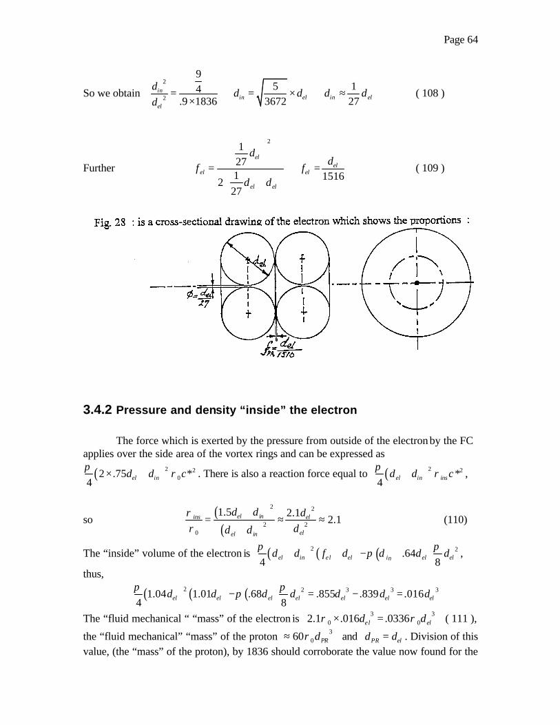
Page 64

So we obtain 2

2

95 14

.9 1836 3672 27in

in el in elel

dd d d d

d= ⇒ = × ⇒ ≈

× ( 108 )

Further

21271 1516227

elel

el el

el el

dd

f fd d

= ⇒ =

+

( 109 )

3.4.2 Pressure and density “inside” the electron

The force which is exerted by the pressure from outside of the electron by the FC applies over the side area of the vortex rings and can be expressed as

( )2 202 .75 *

4 el ind d cπ

ρ× + . There is also a reaction force equal to ( )2 2*4 el in insd d cπ

ρ+ ,

so ( )

( )

2 2

2 20

1.5 2.12.1el inins el

elel in

d d ddd d

ρρ

+= ≈ ≈

+ (110)

The “inside” volume of the electron is ( ) ( ) ( )2 2.644 8el in el el i el elnd d f d d d dπ π

π+ + − + ,

thus,

( ) ( ) ( )2 2 3 3 31.04 1.01 .68 .855 .839 .0164 8el el el el el el eld d d d d d dπ π

π− = − =

The “fluid mechanical “ “mass” of the electron is 3 30 02.1 .016 .0336el eld dρ ρ× = ( 111 ),

the “fluid mechanical” “mass” of the proton 3060 PRdρ≈ and PR eld d= . Division of this

value, (the “mass” of the proton), by 1836 should corroborate the value now found for the

Page 65

electron. Thus we have 60 30 eldρ / 1836 .0327= 3

0 eldρ . In view of several approximations which were applied, this is an excellent corroboration of fluid mechanical calculatory results when compared with the data, physics found over one half century ago.

Comparing the circulatory energy versus the rotational energy,

we find 1.5/1836

.0014.6

= . The rotational energy here is less, namely it is

approximately 2 30.55 1.1 *

4 eld cπ

ρ× × . The reason for this is that the diameter of the circle

of the vortex thread is only slightly more than half of the outside diameter of the standard single vortex ring, which has a “toroid” hole diameter, which is roughly equal to the “eye-wall” diameter.

3.4.3 The electron “at rest”

The “charge energy” rate for both vortex rings is .00128 2 30 *eld c F vρ = × ( 112 )

The two polar inflows have an attracting force of 2 20.00128 *eld cρ . The electron has two

rotating polar inflows. Also “inflow” means “negative charge”. From Quark Theory we know that two “lepton” down-quarks represent the inflows and the one up-quark represents the outflow. The attractive force between the proton and the electron is determined by the “charge energy” rate of the electron, which is the smaller of the two rates. This guarantees the possibility for a hydrogen atom to exist even at absolute zero temperature as will be shown in chapter 4.1. The charge of the electron is

191.60 10e Coulomb−= × . The force between charges is 1 22

04q q

Frπε

= . With these

expressions we obtain 2

2 20 12 2.00128 *

4 8.85 10ele

d cr

ρπ −× =

× × × The fluid force is

located close to the electron, r should be 910 m−≤ . Substituting known values for *c and e we find: 2 36

0 1.98 10eldρ −≈ × . With an assumed value for 60 `10ρ −= we find for

151.4 10eld m−≈ × . This value shall be commented on later in this chapter.

The “Spin” Energy is primarily determined by the helical energy, which is about 10% of the rotational energy. Therefore 2 3

0.06 *SPIN elE d cρ≈ × , and .064 *SPINV c≈ × . ( 113 ) This value is the same for the proton, the electron and the positron. Only the direction of spin changes with positive or negative charge. Due to the small size of the inflows, the angular velocity in the inflows is high. Taking for 151.4 10eld m−= × , we obtain

Page 66

25.064 *1.16 10 ./sec.

/27el

crad

dω π= ≈ × ( 114 )

Physics gives a value for the angular momentum

12 2

hπ

× =2h

. ( 115 )

(See Goudsmit and Uhlenbeck, 1925 publications) The dimensionality of Joule.sec is 2 1MLT − and the value of the angular momentum of formula ( 115 ) is 355.3 10−× The

dimensionality of a momentum is 1MLT − . Therefore ”Spin=1/2”, which is the value for several elementary “particles”, must have a dimensionality of 1 2L T− . Writer protests that “Tables” for “elementary particles” never show dimensionality for “spin”. Defining the “fluid mechanical” “spin momentum” as el SPINr m V× ×v .We assume the values: “mass”

30.034 eldρ≈ × , .064 *SPINV c≈ × , 6

0 10ρ −= and 151.4 10eld m−= × . Using these data we get a value for the momentum of 361.4 10−≈ × , which is quite close to the value of formula ( 115 ), which indicates again that we are close to a corroboration.

The circulatory flow is of the irrotational type and its influence extends far outside the vortex ring set. The velocity “outside” the ring-set decreases roughly with the square of the distance. If we can imagine an “energy envelope” to exist around the “4-lobed” shape of the irrotatonal flow pattern, which exists around the vortex ring set, we can safely state that 99.99% of all circulatory energy is contained within a radius of approximately 3 /210 eld× . With a generally accepted “outer size” or ”charge radius” of

the electron “at rest” of 15 145 10 10 m− −× − , we should find 16 155 10 10eld m− −≈ × − .Values for the so called “charge radius” r and 0ρ can be indicated by using the formulation for

the “charge energy”, 2er

. The “fluid-dynamical” “charge” force is 2 20.00128 *eld cρ× .

Equating these gives 38 3

210 16 30

2.56 10 10.11 10

1.28 9 10 1.96 10rρ

−−

−

× ×× = = ×

× × × ×. If we take for

1510r m−= , we would find that 60 10ρ −≈ , which shows good corroboration. In Chapter

3.3.3 we found an estimated value for 1510PRd m−≈ . As stated previously

el po PRd d d= ≈ .

If an exact value for the density in “standard” space 0ρ can be established then all becomes exact. In Parts II and III this valuation forms an important subject matter. It is obvious and known that the density of “standard” space is directly related to the expansion and contraction of the universe as a whole, ( )0 F tρ = , herein is t is time. In

previous chapters we found that ( )0*c F ρ= and ( )0 ,F Rρ ρ= , herein is R is the distance to a “space-time curvature” center. Therefore ( )0* , ,c F t Rρ= ( 118 )

Page 67

Formula ( 118 ) gives quite a shake to the postulates set in the early 20-th century , by Einstein and others. The magnetic moment of the electron, which is 4 *eleh m cπ= should roughly equate with the force of the “spin” energy

espr× . (See Formula ( 113 ) ). This

momentum is approximately 2 20.06 *

eel spd c rρ× . Equating gives

20

4.06

* e

elel sp

md r

cπ

ρ= × ( 119 )

It is reasonable (because of the small inflow diameter) to assume that .5

esp elr d≈ × .

Substitution of the known values gives 31

308

4 9.1 10.03

3 10 eldπ

ρ−× ×

≈ ××

which results in

3 360 1.3 10eldρ −≈ × . With 6

0 10ρ −= , we find for 121.1 10eld m−≈ × , which is at the high side, but not far away from corroboration. The results of previous comparisons between the values for the “fluid mechanical” factors and values for factors which are adhered to by classical physics gave good corroboration.

3.4.4 The Electron “in Motion”

When the electron attains relativistic velocities then, because of the densification of the FC “upstream” in its path of motion, the diameters of the “inflows” enlarge, which in turn causes enlargement of the “outflow” split. The size of the “confinement area” “inside” the electron grows, but the fluid density lowers. The increase in “mass” is strictly from the fluid densification in front of the moving electron. In tests whereby electrons were accelerated in synchrotrons, increases in “mass” have been achieved as high as 2500 times (Fermi Lab). Therefore it is possible that an electron becomes as big as a proton provided that the relativistic velocity is high enough. Whatever velocity is being reached, the vortex “eye-wall” diameters always remain the same. Other dimensions are subject to change. The motion of electrons in space when in an electrostatic, electromagnetic or magnetic field is highly curious. So is the motion in an atomic lattice. Besides the linear motion there are “sine-wave” motions in 2 planes, which are perpendicular to each other and both of which go through the path of travel. These motions are super-positioned on the linear motion which originates from the field. The overall motion is a “spiraling” one. When moving in a magnetic field the resulting motion can even be cycloidial and motion through solids can be spiraling also.

Electrons “at rest” always start moving if there is any density gradient. Due to their need for additional fluid energy over time, they always move toward higher density. This is the fluid dynamic “electron drift.” If an electron is being accelerated in an electrostatic or electromagnetic field, then as result of the deflection type force, which is exerted by the field, another rotation is being initiated, which is not around the “spin”-axis, but around an axis which is perpendicular to the “spin”-axis and which goes through the middle of the outflow split. This latter rotation is energy-wise much less powerful

Page 68

than the “spin” energy, but it plays an important role in the phenomenon of magnetism. (See Part II, Chapter 8)

3.4.5 Wave-particle duality for electrons

In the early years of the 20th century Planck had shown that electromagnetic waves show “particle” characteristics and that “light” came in “discrete quanta”. This duality is valid for 100% of the electromagnetic spectrum and photons of any energy level have a “mass” equivalent. For the energy as function of the wavelength we have the

known Planck formula hc

Eλ

= and the “mass” equivalent of photons is

*ph

hm

cλ= ( 120 )

The momentum E h

p mvc λ

= = = , the ‘de Broglie’ formula gives h

mvλ = ( 121 )

which shows the reciprocal proportionality between λ and p .

Wave-particle duality may be 100% correct with regard to waves, but is it also true that all matter can show wave characteristics? The answer is yes and no. The electron, positron and proton definitely have wave properties which they display when in motion and “lighter” atoms show wave properties too. However, most atoms and most molecules do not show wave characteristics. Classical physics teaches that all matter has wave equivalency and this equivalency is used not only as a calculatory tool. Writer agrees that all matter has wave equivalency insofar that matter is made up from “particles” for which the wave equivalency is valid. The explanation for this phenomenon as well as its limitations shall be given herewith, whereby the “Davisson-Germer experimentand its confirmation will be examined using “fluid-dynamics.” This enables us to define a criterion for wave-“particle” duality from the side of “matter”. Figs. 29 a and b show a top and side view of the actual path of an electron which is in motion in an electrostatic field.

Description: The electron travels from negative plate P to positive plate Q. Due to the electron’s need / voracity for additional fluid energy, the electron moves towards plate Q where the density in the FC is higher compared to the density at plate P .At position A, the “spin”-axis is in line with the path of travel and the negatively charged inflow incurs the repulsion force from the negative side of the field. This is a “deflecting” type force, which causes that the electron’s α -inflow is pushed out of alignment from “path of travel” OO’. Between the positions A and B the “spin”- axis increases its angle with the “path of travel”, then becomes perpendicular and moves through this position towards a next “spin”-axis alignment whereby the β in-flow is subjected to the repulsion force from negative plate P. What we are describing is a continuing rotation of the electron around axis YY’. We shall name the spin around this axis Yspin . This spin is perpendicular to Xspin , which is the main spin around the XX’ axis, which is the “spin”

Page 69

of the inflows of the electron. This Yspin occurs when the electron is “in motion”. Also it occurs when the electron is “at rest”, if simultaneously subjected to a magnetic field.

Y Xspin spinE E< .

The electron has a linear accelerating motion between the plates. As soon as there is an angle between spin axis XX’ and the “path of travel”, then there is a vector component of the linear motion which is perpendicular to spin axis XX’ and now the fast rotating (around XX’ axis) electron becomes subject to the “Magnus-Effect” , which is the fluid-dynamical phenomenon that a rotating body in a moving field is subject to either a lifting or a downing force depending on the direction of rotation relative to the motion through the field. The more angling between the XX’ axis and the “path of travel”, the greater the perpendicular component of the field motion onto the XX’ axis of rotation; the maximum being in position B where the angle is 90 0 . The force of the “Magnus Effect” increases from position A to position B, then decreases from position B to become zero in position C and whereas the electron has turned around now, its spin is opposite and the force of the “Magnus Effect” now increases but in downward direction, to become maximal in position D, then decreases again back to zero in position E. The conclusion is that this force describes a sine-wave, the frequency of which is determined by the spin around the YY’ axis. The actual motion deflection from the “path of travel” is 90 0 delayed in “phase.” (See Figs. 29 a and b, which illustrate these sine-wave motions.) During the angling between the XX’ axis and the “path of travel” there is also a component of the field which is then parallel to the XX’ axis and which causes the motion of the electron to be deflected sideward. This is shown in Fig. 29 in the horizontal plane. The size and angle of the two vectors are 90 0 out of “phase” and the sideward sinesoidic motion is 090 “ahead” of the motion in the vertical plane. This means that the resulting motion of the electron is a “spiral” around the linear “path of travel”.

The above description is also valid for the motion of a positron and for the motion of a proton whereby the opposite “charge” needs to be taken into account.” Davisson and Germer” could detect the wave characteristic of the electron due to its small “mass”. Accelerating a proton in a same field gives a protonλ which is smaller according to its greater “mass”. The wavelengths for certain “light atoms” can also show this effect on account of their spin, but are extremely small due to greater “masses” and can be out of range of measurement. (Even in case of the proton it is hard to detect the wave characteristic.) However, the spiraling of the polar outflows has been detected in tests whereby ‘polarized proton’ beams hit a liquid hydrogen target. If the spin of the target- protons was parallel to the spin of the oncoming protons then some of the oncoming protons were bounced off at large angles. With opposite spins between beam-protons and target-protons, the oncoming protons did not bounce off and moved right through the target. This phenomenon will be discussed in Part II, Chapter 6.

For the motion of electrons through a lattice of atoms, we have the ‘Bragg’ law,, which is ' 2 sinn dλ θ= , whereby ( )2 1' /n nλ λ= and 2 1/n n ( 122 )

Page 70

being the relative refractive index. Outside a lattice of atoms and in a force field we have

the de Broglie relationships 2 2 . .el kin el

h h hp m E m eV

λ = = = , ( 123 )

herein is kinE is the kinetic energy of electrons and V is the potential difference, which causes the acceleration in the field. Substituting the known values for , ,elh m e and

expressing V in volts, leads to the simplified expression 1.23

nmV

λ = ( 124 )

G. P. Thomson showed the wave characteristic of electrons in 1928 using a diffraction test, whereby clear interference results showed. These results were similar to the results which were achieved by Debye-Scherrer with X-ray diffraction. These results were empiric and did not show the fluid-dynamical causes, which are shown here. Spectral analyses can show multiple lines for a given element for a variety of reasons e.g. the isotope mix of that element or nuclear spin or nuclear magnetic moment. The formulation

which is used for this is 4 1836

BN

PR

ehM

µµ

π= = . ( 125 )

For “lighter” elements, nuclear spin can cause wave characteristics when in motion. However, “heavy” elements and molecular structures other than a few do not show wave characteristics when in motion, wherefore writer stated that the “particle–to-wave” part of the “Complementarity Principle” of Bohr is not universally true, but the Hamiltonian analogy can be fruitfully used in tandem with fluid-dynamical analysis in calculations of the physics of the electron.

3.5 Impulse-Interaction of Photons with Electrons Causes the “Compton Shift” for the Photons.

If we consider the conservation of energy and linear momentum, we have

21 2 2 2

1* 1

1 / *h h mc

v cν ν

= + −

− , and 2

2 20 sin sin

* 1 / *

h mvc v c

νθ φ= −

−, which gives

( )1 cos*el

hm c

λ θ∆ = − . The term *el

hm c

is called the “Compton” wavelength,

which is 122.43 10 m−× ( 126 )

Recently A. G. Gulko suggested a concept that this “Compton” wavelength is equal to the “length of the energy” in the electron’s circulatory flow. The shorter the wavelength, the higher the energy and thus the greater “mass”; this checks out in the formulation. In Part II, Chapter 11 this will be examined after complete fluid-dynamical analysis of the “photon decay” process. Also included there are: the fluid-dynamical analysis of the “Lorentz” force, the photon-electron “in motion” interaction, the electron in a magnetic field and the fluid dynamic “drift” of electrons in space

Page 71

Fig. 29 a and b: The total motion of the electron in an electrostatic field (Confirmation of Davisson-Germer Experiment )

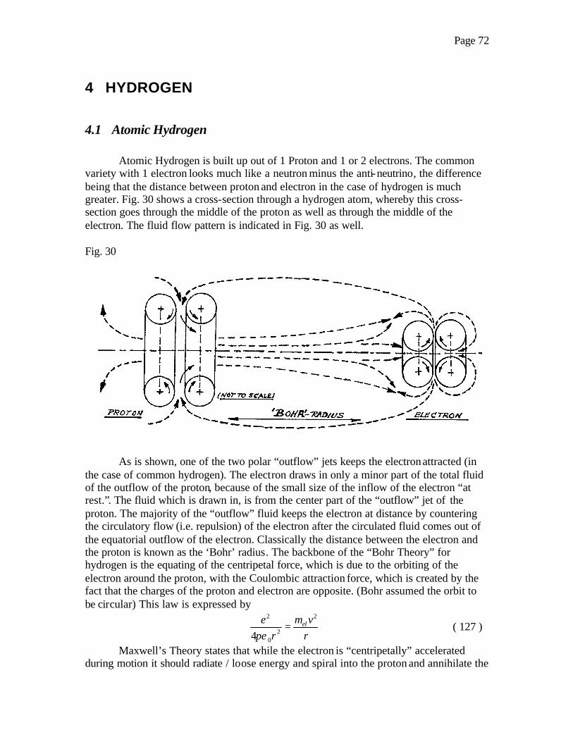
Page 72

4 HYDROGEN

4.1 Atomic Hydrogen

Atomic Hydrogen is built up out of 1 Proton and 1 or 2 electrons. The common variety with 1 electron looks much like a neutron minus the anti-neutrino, the difference being that the distance between proton and electron in the case of hydrogen is much greater. Fig. 30 shows a cross-section through a hydrogen atom, whereby this cross- section goes through the middle of the proton as well as through the middle of the electron. The fluid flow pattern is indicated in Fig. 30 as well. Fig. 30

As is shown, one of the two polar “outflow” jets keeps the electron attracted (in the case of common hydrogen). The electron draws in only a minor part of the total fluid of the outflow of the proton, because of the small size of the inflow of the electron “at rest.”. The fluid which is drawn in, is from the center part of the “outflow” jet of the proton. The majority of the “outflow” fluid keeps the electron at distance by countering the circulatory flow (i.e. repulsion) of the electron after the circulated fluid comes out of the equatorial outflow of the electron. Classically the distance between the electron and the proton is known as the ‘Bohr’ radius. The backbone of the “Bohr Theory” for hydrogen is the equating of the centripetal force, which is due to the orbiting of the electron around the proton, with the Coulombic attraction force, which is created by the fact that the charges of the proton and electron are opposite. (Bohr assumed the orbit to be circular) This law is expressed by

22

204

elm ver rπε

= ( 127 )

Maxwell’s Theory states that while the electron is “centripetally” accelerated during motion it should radiate / loose energy and spiral into the proton and annihilate the

Page 73

charges. To break this problem, quantization of the energy levels was assumed, because

these energy levels showed agreement with Rydberg’s formula: 2 2

1 1

f i

v Rn n

= −

( 128 )

herein is: 1109.7 1,2,3,..... 2,3,4,..... f i i fR cm n n n n−≈ = = > . Formula ( 128 ) is empirical and was achieved by work from ‘Balmer’ and later from ‘Rydberg’. This formula relates to the spectral lines of hydrogen. The quantization assumption and the ‘Rydberg’ formula confirmation relative to the energy levels of the electron in hydrogen

made for Bohr’s formulation, 2

2 20

13.68n

H

eE eV

n a nπε= − = − ( 129 )

Herein is quantum level, 1,2,3,...., Bohr radiusHn a= = . For 1 .053Hn a nm= ⇒ ≈ (130) 191.6 10e Coulomb−= × ; 12 1

0 8.8 10 .farad mε − −≈ × (is permitivity of the FC).

The energy, which is 12

of the potential energy, can be arrived at by using

Poisson’s formula, ( ) ( ) ( )2

0 0'

' '4 ' 4v

r dv er r

r r rρ

φ φπε πε

= − → = −−∫ (for point charge at r ) ;

wherefore the total energy is 2 2

08Z e

Erπε

= − (for hydrogen, 1Z = ) .

Bohr’s model is limitedly valid for hydrogen. There is no validity for Helium etc.

What happened was; ‘Newtonian’ mechanics were mixed with ‘Schrodinger’ quantum mechanics. ‘Newtonian’: for elliptic orbits is valid: ( ) ( )2m r r F rθ− =&&& , and

( )2 0m r rθ θ+ =& &&& ; which results in ‘Kepler’s law, which is

2 . /r const L mθ = =& ( 131 )

( )F r = central force, L = angular momentum and 1

ur

=

The general (any orbit) energy equation is ( )2 2

2 12 2

12

L uE m u E u

mδδθ

− = + +

( 132 )

The general solution leads to a simple formula ( with the eccentricity=0 ) for a circular

orbit, which is what Bohr used, being 2

2.2 orb

eE

n a= − ( 133 )

With quantum mechanics and using Schrodinger, ( )2

22 2

1, , , 0r t

tδ

θ φν δ

∇ − Ψ =

( 134 )

we can arrive at a similar result.

The spectral analyses of hydrogen gave us the ‘Lyman’, ‘Balmer,’ ‘Paschen, ’ etc. “series” with regard to the energy differentials between the quantum levels of the orbits in which the electron can be when in motion. When an electron changes orbit /quantum

Page 74

level (coming from a higher state and going to a lower one), a more or less energetic photon is being emitted and the frequency of the radiation which is obtained can be expressed by

1 2E Eh

ν−

= ( 135 )

Fig. 31: is a diagram, which shows the energy levels between infinity and the lowest energy state, which has been known for decades as the “ground state”. The energy differential between infinity and the “ground state” is 13.6eV . Fig. 32 shows 5 orbits “outside” the “ground state” and the ‘Lyman’ and ‘Balmer’ “series”:

Observations which were made as early as 2 decades ago detected spectral lines from sources in deep space in the “Soft X-ray to extreme left UV” range of the electromagnetic spectrum. It must be stated that the whole ranges of frequencies between 2 nm to 250 nm never drew anyone’s attention in astronomy until recently, which seems strange to writer. It now appears that background radiation of this frequency range can be found all over interstellar space and also in the corona of the sun. All other areas of the electromagnetic spectrum were always of interest and writer experienced while attempting to acquire observational instruments for detections for the range here indicated, that none were available. However, many types and makes of instruments are available for other frequencies. Writer hereby refers to research work done by ‘Labov and Bowyer,’ who found a number of frequencies, which can be attributed to hydrogen with energy states which are lower than the “ground state”. These states have now been named “fractional states” for the simple reason that these frequencies can be found by

substituting “fractions” e.g. 1 1 1

, , , .2 3 4

n etc= into the ‘Rydberg’ formula.

Page 75

These researchers also found “helium lines”. The majority of the spectral lines which were found corresponded with energy transitions of hydrogen between energy levels, which are below the “ground state” and which levels can be found by substituting “fractions” into the Rydberg formula. Fig. 33, which is taken up herewith shows a diagram of the energy levels of the “fractional states” of hydrogen for:

1 1 1 1 1 1, , , ,

2 3 4, 5 6 7n and= , it also shows the energy of the photons which are emitted and

which relate to the transition between the two energy levels; the corresponding wavelengths are shown as well. The distance Ha between electron and proton for the “fractional levels” can be calculated using 2 9.053 10Ha n m−= × × . ( 136 ) Fig, 33:

Rydbergn . .E GrSt→ (eV)

E → ∞ (eV)

E∆ (eV)

λ (Α)

1 “Ground State” 0 -13.6 i fn n→ 912.0

12

-40.8 -54.4 1

12

→

40.8 303.9

13

-108.8 -122.4

1 12 3

→

68.0

182.4

14

-204.0 -217.6 1 13 4

→

95.2 130.2

15

-326.4 -340.0 1 14 5

→

122.4 101.3

16

-476.0 -489.6 1 15 6

→

149.6 82.9

17

-652.8 -666.4 1 16 7

→

176.8 70.1

Page 76

For example the electron in the “ground state” has an energy of 511,000eV , so

for the 17

n = “fractional state,” the electron has an energy of 511,000-652.8=

510,347.2 eV . The relative energy change is rather small and the constitution of the electron is certainly not endangered. The vortex ring set which is at the center of the electron and its rotational and helical energy do not change, wherefore the energy reduction is in the circulatory flow and more specifically in the outermost range, which has the irrotational flow characteristic. So the overall “volume” of the roughly spherical embodiment of the circulatory energy becomes smaller at lower energy levels and then the electron can move in closer to the proton and form “fractional hydrogen.” This can be understood from Fig. 34, which shows a cross-section of the hydrogen atom and the overall fluid flow pattern.

Due to the much greater “mass” of the proton and its much greater circulatory energy the polar outflow of the proton is much greater than that the small inflow of the electron can handle. Only the very central portion of the “beam” which goes out from the proton becomes the inflow of the electron. The outflow of the proton gradually widens and the vast majority of this circulatory flow curves back for the return towards its own equatorial inflow. The flow lines, which are shown in Figs. 30 and 34, are “streamlines.” The circulatory flow of the electron collides with that part of the proton’s outflow which is right around the center “beam”. The center “beam” is absorbed by the electron’s inflow. (See zone ZZ’ in Fig. 30)

Colliding flows are totally destructive. Since the hydrogen atom’s constitution is stable a small diameter vortex ring might form in zone ZZ’ (See Fig. 34 ). As the drawing shows, this additional vortex ring largely supports the proper flow for both the circulatory flows of the proton and of the electron. The diameter of the circle of the vortex thread of this additional or 3-rd ring should be 2 eld≈ × + ; this vortex ring has only rotational flow and its diameter is small. At its “eye-wall” it has a velocity of much less than *c . Upon ionization, this ring disintegrates into low energy photons. This ring exists within the hydrogen atom and the ionization energy should be roughly equal to its rotational energy.

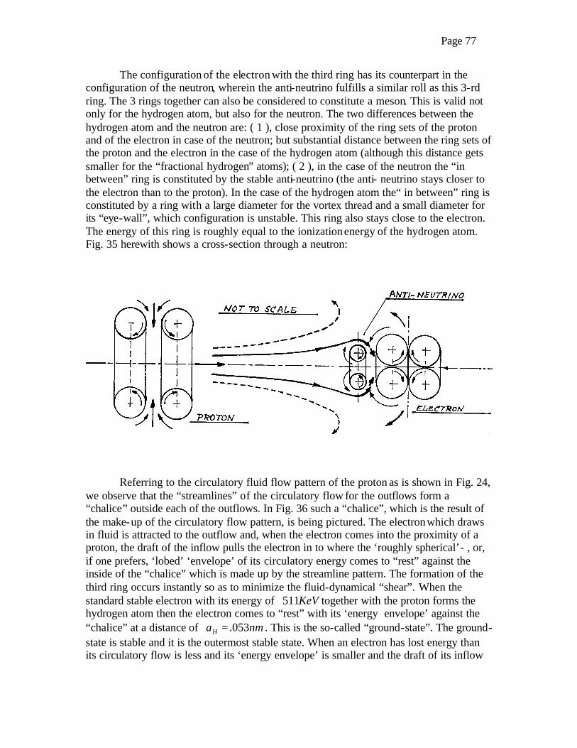
Page 77

The configuration of the electron with the third ring has its counterpart in the configuration of the neutron, wherein the anti-neutrino fulfills a similar roll as this 3-rd ring. The 3 rings together can also be considered to constitute a meson. This is valid not only for the hydrogen atom, but also for the neutron. The two differences between the hydrogen atom and the neutron are: ( 1 ), close proximity of the ring sets of the proton and of the electron in case of the neutron; but substantial distance between the ring sets of the proton and the electron in the case of the hydrogen atom (although this distance gets smaller for the “fractional hydrogen” atoms); ( 2 ), in the case of the neutron the “in between” ring is constituted by the stable anti-neutrino (the anti- neutrino stays closer to the electron than to the proton). In the case of the hydrogen atom the“ in between” ring is constituted by a ring with a large diameter for the vortex thread and a small diameter for its “eye-wall”, which configuration is unstable. This ring also stays close to the electron. The energy of this ring is roughly equal to the ionization energy of the hydrogen atom. Fig. 35 herewith shows a cross-section through a neutron:

Referring to the circulatory fluid flow pattern of the proton as is shown in Fig. 24, we observe that the “streamlines” of the circulatory flow for the outflows form a “chalice” outside each of the outflows. In Fig. 36 such a “chalice”, which is the result of the make-up of the circulatory flow pattern, is being pictured. The electron which draws in fluid is attracted to the outflow and, when the electron comes into the proximity of a proton, the draft of the inflow pulls the electron in to where the ‘roughly spherical’- , or, if one prefers, ‘lobed’ ‘envelope’ of its circulatory energy comes to “rest” against the inside of the “chalice” which is made up by the streamline pattern. The formation of the third ring occurs instantly so as to minimize the fluid-dynamical “shear”. When the standard stable electron with its energy of 511KeV together with the proton forms the hydrogen atom then the electron comes to “rest” with its ‘energy envelope’ against the “chalice” at a distance of .053Ha nm= . This is the so-called “ground-state”. The ground-state is stable and it is the outermost stable state. When an electron has lost energy than its circulatory flow is less and its ‘energy envelope’ is smaller and the draft of its inflow

Page 78

makes the electron move “deeper” into the “chalice” according to Equation ( 136 ), 2 9.053 10Ha n m−= × × .

Page 79

We note that in Fig. 36 n =1 , indicates the “ground”-state. 1n > , indicates the “excited” states.

1

, 1n pp

= > , indicates the “fractional” states.

The physics and spectral analyses of the “excited” states: The Lyman , Balmer

,etc.-series are well known and shall not be addressed other than to explain the essence “of being in an “excited” state”. Fig. 36 shows 2 “excited” states. When energy is added to the electron from the “ground” state to a higher quantum level, the increase in the size of the ‘energy envelope’ is less than the increase in size of the cross-section of the “chalice” for any given quantum level above the “ground” state. (Note that the back-curving of the streamlines of the circulatory flow of the proton increases rather rapidly.) With very small energy increases with the quantum levels above the “ground”-state the size of the electron enlarges only infinitesimally. So at higher quantum levels the electron can move rather freely in the now “wide” “chalice” and the electron’s kinetic energy increases at higher quantum levels and ionization is achieved after 13.6eV in energy has been added to the electron. For stability the electron needs to come back down to the “ground”-state.

4.1.1 “Fractional” states

The diagram of Fig. 33 shows the energy levels of the “fractional” states and the wavelengths of the emitted photons. All fractional states are stable just as the “ground”-state is and for the same reason. Fractional hydrogen is quite inert and can only interact with other elements, which present themselves as cat- ions. This can only occur if an additional electron is attached at the other outflow of the proton. The properties of materials so formed can be substantially different and here lies an area of enormous importance. According to reports, it seems that Blacklight Power Inc., Cranbury ,NJ. is active in the research and development of new materials based on “fractional” hydrogen. Writer’s company, AMDG Scientific Corp., which is active in the research and development of “fractional” hydrogen, presently emphasizes energy generating processes and derivatives thereof and plans to enter materials research in the near future.

Laboratory tests show that the “fractional” states can react with each other and

form new “lower” “fractional” states as well as a protons and photons. Reactions with deuterium look possible as well. The formulation of such a reaction between “fractional” states is as follows, ( ) ( ) ( )i k pn n n

H H H H e photon+ −+ → + + + ( 137 )

herein is i kn n≠ and, ,p i kn n n< . The energy of the photon equals the total energy of the “fractional” states before the reaction, minus the total energy of the products of the reaction.

Page 80

The interesting question is: How does one obtain “fractional” hydrogen and

how do reactions as shown by Formula ( 137 ) occur? Blacklight Power Inc. obtained a patent which relates to an electrolytic process(es) with potassium. The patent number ( US ) is 6,024,935. Writer’s company, AMDG Scientific Corp., applied for patents for a process which produces “fractional” hydrogen as well as for derivative nuclear transmutational processes. These processes are not electrolytic in nature and totally different from Blacklight Power’s. These processes of our company also occur in the corona of the sun and in numerous locations in deep space. These processes also involve other elements. There should be many locations in the universe where pressure and temperature together with availability of certain isotopes are conducive for the formation of “fractional” hydrogen. Information about these processes is proprietary.

In astronomy, scientists have struggled to find the vast amount of missing “mass” which might be present in our universe in order for it to stay together and expand only at the rate as we presently perceive. The answer lies in “fractional” hydrogen. There is to be an abundance of “fractional” hydrogen all over the universe. There are many “fractional” states in which hydrogen can exist and it is obvious that the universe contains much more “fractional” hydrogen than “ground” state. In the cosmos “fractional” hydrogen is hard to detect except when it is at high temperatures (e.g. in neighborhood of stars) where radiation can occur as result of transitions. Testimony to this are the reports of ‘Labov and Bowyer’ which refer to emissions in the ranges: 5.5< log T < 5.7, log T=6 and 6.6< log T < 6.8. The “fractional” hydrogen lines which were found in the spectrum of the corona of the sun likely are of the latter category since its temperature is found to be about 1.5 million K .

From the empirically acquired knowledge by Balmer, Rydberg et al we know that

the energy levels of the electron are quantised. Bohr determined that the angular

momentum can be quantised. We have: 2nh

r mvπ

× = and, 2 2

204

mv Zer rπε

= .Substitution

gives for 2 2

02n

n hr

me Zε

π= and for,

2

02nZe

vnhε

= , where Z =number of positive electronic

charges in the nucleus; Z =1 for hydrogen. With all known values substituted we find that the 2 9.053 10nr n nm−= × , which was formula ( 136 ). The sum total of the kinetic

and potential energy is 2 2

2

0 0

1 12 4 2 4

e eE mv

r rπε πε−

= + = − . Substituting nr r= , gives

4 2

2 2 220

1 13.68n

me ZE eV

n nhε= − = − . For the frequency of the emitted radiation going from state

1n down to state 2n we get 4 2

21 22 2 2 2 23

0 2 1 2 1

1 1 1 18

E E me ZRZ

h h h n n n nν

ε

= − = − = −

For the hydrogen electron we have 2

6 1

0

1 12.2 10 .sec

2ne

v mh n nε

−= = × ( 138 )

Page 81

What would be the lowest possible “fractional” state? Writer answers by noting that this is the transition where the energy requirement for the increase in kinetic energy equals the energy availability increase between a given transition and the next transition.

The kinetic energy is ( )2 212

m v m v≈ ∆ + ∆ ∆ , the first term is provided by the

“preservation of angular momentum” , the second term represents the relativistic energy increase. The transitional energy is

1 2 21

1 113.6x x

x x

En n

→ ++

= −

and, 6

1

1 12.2 10

x x

vn n+

∆ = × −

. We found for

1n = , that : 6 12.2 10 .secGround statev m −− = × . It is obvious that the

1100

n = state cannot be

reached, because substitution in formula ( 138 ) shows that we would be very close to velocity *c . The energy increase between 2 given transitions is

2 1 1 2 2 2 22 1 1

1 1 1 113.6x x x x

x x x x

E E En n n n+ → + + →

+ + +

∆ = − = − − −

( 139 )

Let 2

2*v

Xc

= , then the increase in kinetic energy between given transitions is

20 *

1kin

XE m c

X∆

∆ ≈∆ −

( 140 )

Equating ( 139 ) with ( 140 ) gives

19

2 2 2 220 2 1 1

13.6 1.6 10 1 1 1 1* 1x x x x

Xm c n n n n X

−

+ + +

× × ∆ − − − = ∆ −

( 141 )

When all the available energy is used for the increase in relativistic energy,

then 1

1X

X∆ = ∆

− , ( )

32

1 11

21f X

X−= − −

−& and, 1fX =& . Equating gives

( )32

11 1 .37

2X X−− − = ⇒ ≈ , 2 2 8 1/ * .37 .61 * 1.83 10 .secv c v c m −≈ ⇒ ≈ × ≈ × , and

6 81 12.2 10 1.83 10

83xx

nn

× = × ⇒ ≈ . Substituting in ( 141 ) and verifying the

“mass” increase, we find that the available transitional energy is

( ) ( ) 19 2 2 2 2 1813.6 1.6 10 85 84 84 83 4.35 10 Joule− −× × − − − = × . The increase in

relativistic energy is ( )20 85 832 22 2

85 83

1 1 12 1 / * 1 / *

n n

n n

m v vv c v c

= =

= =

− − − −

( )231 16 18 181 1 19.1 10 1.87 1.83 10 3.64 10 10

2 1 .62 1 .61Joule− − −

≈ × × × − − × = × × − −

Page 82

Given the approximations which were applied this is close corroboration. The difference of 18.71 10 4.4Joule eV−× = is the energy of the emitted photon. This energy is now close to zero and for the next transition no further energy will be emitted. We now observe that in the formation of the “fractional” states, at first the energy of the emitted photons increases rapidly as the “fractional” states go lower. However, due to the relativistic energy needs of the electron at higher angular velocities, i.e. at very low “fractional” states, the availability of energy for emission gradually decreases to zero.

We are now finding an anology with the physics of “Black Holes”, where no radiation can be emitted from below the “event horizon”. In the case of “fractional”

hydrogen, no radiative emission is possible below a “fractional” state of 1

84n = . Fig. 37

shows the energy of the photon, which is emitted as function of the “state”.

A similar analysis can made with the use of classical quantum mechanics, whereby the Sommerfeld formulation can be applied for 2 adjoining “fractional” quantum levels. In this case,

4 4

23 2

0

1 38 4nk

e ZE

n h k nµ

αε

= − −

( 142 )

where 22 1* 137e

hcπ

α = ≈ is the fine structure constant, and J d

khφ φ

= ∫Ñ is the azimuthal

quantum number, (from the angular momentum) and rn n k= + , r

r

p drn

h= ∫Ñ is the

radial quantum number, (from radial momentum). When we have substantially lower “fractional” states, the orbits become elliptic with strong precession, whereby the resulting motion describes “rosettes,”

4.1.2 The reactivity of “fractional hydrogen”

Referring to Fig. 33, we see that e.g. for the “fractional” state 13

n = the energy

of the electron already is 108.8eV− relative to the “ground”-state. So it becomes very difficult to pull this electron away from the proton and for all practical purposes “fractional” hydrogen below the first few “fractional” states is inert.

The “spin” of the proton is carried over to the electron via its outflow, the very center part of which becomes the inflow of the electron. The electron has its own “spin” around the same axis, which it has in common with the proton (See Figs. 30, 34). Due to the fact that the curved “pinwheel”- like equatorial outflow of the electron, which has the same rotational direction as its individual “spin”, cannot be rotation-wise in a collision type mode with the more major rotation, which surrounds it, (which is the rotation of the

Page 83

outflow of the proton), the individual “spin” of the electron can be added to the “spin” of the outflow of the proton, which it transfers to it. Since the individual “spins” were equal, this means when we observe from a frame of reference of the hydrogen atom, the “spin” of the electron has doubled. (See also Chapters 3.3 and 3.4). Fig. 37, which shows the energies of the emitted photon for all quantum levels

The energies of the hydrogen atom are:

The total “fluid dynamical” rate of energy of the proton 2 306.00 *

4 prd cπ

ρ=

And for the electron, also while ( pr eld d= ) 2 302.2 *

4 eld cπ

ρ≈

Total “fluid dynamical” energy rate of the atom is 2 308.2 *

4 eld cπ

ρ≈

Kinetic energy of “ground”-state electron is 31 6 2 1819.1 10 (2.2 10 ) 2.2 10

2Joule− −× × × × = ×

In the “ground”-state the constitutional energy of the electron is: 511,000eV .

At the “fractional” state of 1

84n = , the loss of energy is 13.6 7056 95,962eV× = , which

translates into 18.8% of the constitutional energy of the electron. The conclusion is, that the electron’s constitution is still “healthy”, in such a low “fractional” state. However, long before reaching such real low energy states another phenomenon takes place, namely that an another electron may be added to the same proton and then at the opposite side’s outflow. This matter will be discussed in Chapter 4.2

Summarizing, it must be stated that the “fractional” hydrogen formation processes are of immense importance for energy production and the released energy is much greater than with chemical reactions. For instance, when hydrogen and oxygen gases react to form water, the enthalpy of formation which then becomes available is 286 / 1.48kJ mol eV= . Compare this to the first step down in “fractionization,”

Page 84

11

2n = →

, whereby 40.8eV per hydrogen atom becomes available. The diagram of

Fig. 33 shows the energies which become available from transitions between lower quantum levels. The activation of these transitions occurs according to formula ( 137 ). When the proper catalyst is being applied, these transitions create an enormous amount of energy per hydrogen atom. Moreover, these reactions do not create radiation at a level which is harmful for humans and there are no nuclear waste products.

4.2 Bi-electronic and Molecular Hydrogen

Last year there was the introduction of bi-electronic hydrogen. In an article in Fusion Technology, Volume 37, 2000, R. N. Mills of Blacklight Power Inc., Cranbury, NJ., describes a number of the physical aspects of bi-electronic hydrogen in connection with the primarily electrolytical process technologies his firm is involved with. Writer knows from his own laboratory work that this form of hydrogen is present. It is likely that the acceptance of a new electron becomes more possible as the “fractional” state of the

attached electron is lower. Writer assumes that under given circumstances, that for 15

n <

the acceptance should become possible. For all practical purposes “fractional hydrogen”

is inert, other than maybe for the “fractional” states 1 1

,2 3

n = . That a “fractional

hydrogen” atom can accept another electron rather easily can be understood from FC physics and the fluid-dynamical constitutions of both the proton and the electron.

The additional electron attaches to that outflow of the proton which is at the opposite side from the location, which is occupied by a “fractional” state electron. Fig. 38 shows the cross-section of a bi-electronic hydrogen atom, whereby the newly attached electron is shown to be in its “ground”-state.

The article in Fusion Technology, Volume 37, March 2000 speaks about the electrons being indistinguishable from each other. Writer disagrees with this. The Pauli

Page 85

Exclusion Principle would be violated if this were so. However, once the “fractional” hydrogen atom has reacted with an electron, certain rules can be determined which govern this more complex 3-“particle”-entity system. It is possible for the newly attached electron (by means of interaction with a catalyst) to also come down to a “fractional” state.

4.2.1 Derivation of a rule which governs the energy quantum levels.

The angular momentum of an electron can be described as 2nh

r mvπ

× = . We shall

consider only those “fractional” states for either electron which are “non-relativistic”. Then we can state that 1 2 1 2 2m m m m m= ⇒ + = . The sum-total of both angular momentae when these electrons were still in their “ground” state is . .2 H grsta mv

Now .2k k l l H grstr v r v a v+ = 2 2

02

n hr

me Zε

π= and

2

02Ze

vnhε

=

Wherefore ( )2

0

22k l H

h en n a

m hπ ε+ = and,

1 1,k l

k l

n np p

= = where integers , 1k lp p ≥

so 2

20

1 1H

k l

e ma

p p hπε

+ =

=

1. .

2 H

mca

hα ( 143 )

or 1 1 . . . . .

2 .k l

Bohrrad FineStructConstp p Comptonwavelength

×+ = ×

=

9

9

1.053 10

137 .082 .00243 10

−

−

× ×≈

× ×

A bi-electronic hydrogen atom, which is created by adding 1 electron to the neutral combination of 1 proton and 1 electron reacts as a negative ion, and can have a number of

states which shall be indicated as 1

Hp

−

. Reactions with cations are possible (e.g.to

form hydrides). A formula for such hydrides can look like: . . '.nM H M anion , whereby 1

np

= is an integer and , 'M M are cat-ions. This formulation shows that polymeric

structures can be formed and this has been confirmed in the laboratory. It is now clear that a great many new molecules can be constructed, which promises an equally great number of new materials. Any moiety which has cation character can react. Also reactions with deuterons are possible. Binding energies have been calculated, the first four are:

( ) 1 1 11 .754; 3.047; 6.610; 11.23

2 3 4H n H n H n H n eV− − − − = = = = = = = =

The total “fluid dynamical” rate of energy of the bi-electronic hydrogen atom is

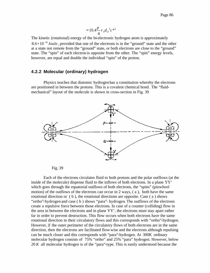
Page 86

2 3010.4 *

4 eld cπ

ρ≈

The kinetic (rotational) energy of the bi-electronic hydrogen atom is approximately 188.6 10 Joule−× , provided that one of the electrons is in the “ground” state and the other

at a state not remote from the “ground” state, or both electrons are close to the “ground” state. The “spin” of each electron is opposite from the other. The “spin” energy levels, however, are equal and double the individual “spin” of the proton.

4.2.2 Molecular (ordinary) hydrogen

Physics teaches that diatomic hydrogen has a constitution whereby the electrons are positioned in between the protons. This is a covalent chemical bond. The “fluid-mechanical” layout of the molecule is shown in cross-section in Fig. 39

Fig. 39

Each of the electrons circulates fluid to both protons and the polar outflows (at the inside of the molecule) dispense fluid to the inflows of both electrons. In a plane YY’ which goes through the equatorial outflows of both electrons, the “spins” (pinwheel motion) of the outflows of the electrons can occur in 2 ways, ( a ), both have the same rotational direction or ( b ), the rotational directions are opposite. Case ( a ) shows “ortho”-hydrogen and case ( b ) shows “para”- hydrogen. The outflows of the electrons create a repulsive force between those electrons. In case of a counter (colliding) flow in the area in between the electrons and in plane YY’, the electrons must stay apart rather far in order to prevent destruction. This flow occurs when both electrons have the same rotational direction in their circulatory flows and this corresponds with “ortho”-hydrogen. However, if the outer perimeter of the circulatory flows of both electrons are in the same direction, then the electrons are facilitated flow-wise and the electrons although repulsing can be much closer and this corresponds with “para”-hydrogen. At 300K ordinary molecular hydrogen consists of 75% “ortho” and 25% “para” hydrogen. However, below 20 K all molecular hydrogen is of the “para”-type. This is easily understood because the

Page 87

lower available energy at low temperature requires a “lower energy” and so a more compact configuration. Because of the fact that each proton’s outflow serves ( in the case of “para”-hydrogen ) two electrons with opposing “spins”, we can be certain that one proton will govern and be equal-rotational with one electron and that the other proton which is equal rotational with the other electron has an opposite “spin”. Also in this way the Pauli Exclusion Principle is not being violated. In Fig. 39 the positions P and Q schematically indicate the “para” configuration. Since each proton can now serve fluid to two electrons instead of one, some of the internal “confined” fluid (when the bond is being made) is being dispensed, which creates photons. This is the energy of formation. The “spin” axis XX’ goes through the outflows of the protons. The formation of molecules based on two “fractional” hydrogen atoms is impossible. However, two bi-electronic atoms can form a molecule, provided that the additional electron in case of each of the protons would be in the “ground” state. The configuration of this molecule is the same and as in Fig. 39. The calculation of the “fluid-dynamical” energy rate of the hydrogen molecule is not simply an addition of the energies of protons and electrons due to the unique configuration. This fluid dynamic energy rate is greater than

2 3016.4 *

4 eld cπ

ρ× .

4.3 Deuterium

Deuterium consists of a proton electron pair which captured a neutron. Fig. 35 shows a schematic cross-sectional layout of the neutron which basically makes for a short “cigar”- like shape in space. This was basically confirmed in 1961 by ‘R. Hofstadter’ as reported by L. Pauling and R. Pauling in “Chemistry” (W. H. Freeman & Co , 1975, page 683). This confirmation can also be seen in the sizes given: “the neutron can be described as involving a central ball of positive charge, extending to the radius of about .3 fm. Surrounding the ball is a shell, extending to about 1 fm with a negative charge. In addition there is a fringe of positive charge, which extends to about 1.5 fm”. Just as with the bi-electronic hydrogen atom it is possible that instead of an electron a neutron can be attracted with its negative end onto the polar outflow which is opposite from the polar outflow which already carries a “ground”-state or “fractional” state electron. If this occurs, deuterium is being formed. (In nature, the ratio deuterium to ordinary hydrogen is about 1 / 6000 ). If the opposite side of the proton has a “ground”-state electron than it can easily ionize and give a deuteron, ionization might still be possible for the first “fractional” state as well, but not likely beyond that state.

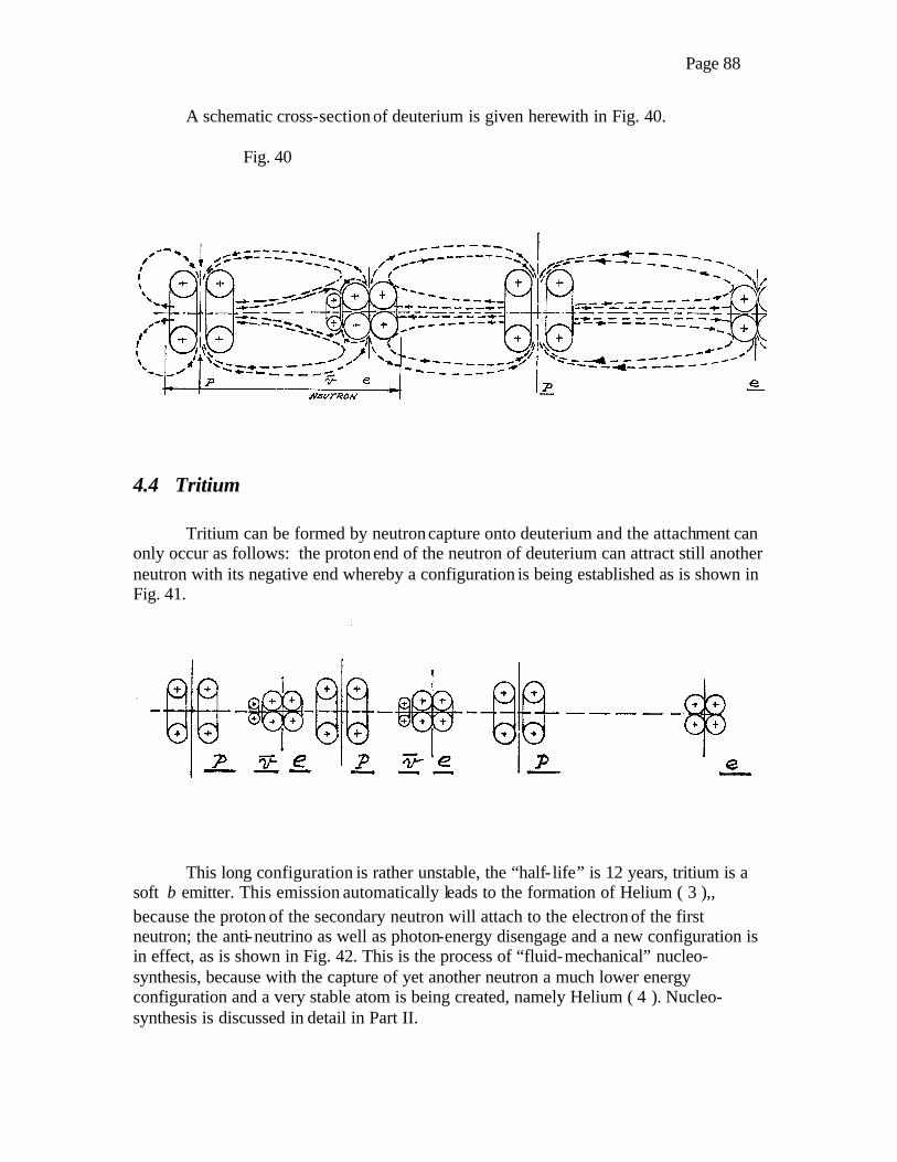
Page 88

A schematic cross-section of deuterium is given herewith in Fig. 40. Fig. 40

4.4 Tritium

Tritium can be formed by neutron capture onto deuterium and the attachment can only occur as follows: the proton end of the neutron of deuterium can attract still another neutron with its negative end whereby a configuration is being established as is shown in Fig. 41.

This long configuration is rather unstable, the “half- life” is 12 years, tritium is a soft β emitter. This emission automatically leads to the formation of Helium ( 3 ),, because the proton of the secondary neutron will attach to the electron of the first neutron; the anti-neutrino as well as photon-energy disengage and a new configuration is in effect, as is shown in Fig. 42. This is the process of “fluid-mechanical” nucleo-synthesis, because with the capture of yet another neutron a much lower energy configuration and a very stable atom is being created, namely Helium ( 4 ). Nucleo-synthesis is discussed in detail in Part II.

Page 89

Fig. 42

End of Part

Page 90

APPENDIX I

Michelson-Morley Experiment Revisited By: Arie M. DeGeus, 12-11-00

Copyright

There is no other cause as great as the mishap of the Michelson-Morley experiment, which contributed for physics: ( 1 ) to go with the concept of “vacuum” ,which would allow propagation of electromagnetic waves and: ( 2 ) to go very far in applying quantum mechanics and: ( 3 ) to go, since no major progress was achieved in decades, with many wild unverifiable theories and: ( 4 ) to make mention of certain theoretical achievements, which are unverifiable ( e.g. quarks, which are fluid-dynamical phenominae and which are non-matter or non-“mass” ) and: ( 5 ) to elevate certain theoretical achievements into dogmas upon which physics has been building forward. To make a certain theory into a dogma requires a lot more than that the concerned theory cannot be disproven in a certain relatively short period of time. The right intellect might still disprove the theory later on. Deterministic verification is the only way to build forward.

Since Michelson-Morley weighed- in so much with regard to condemning the

“aether” into oblivion, writer feels that it needs revisitation, in view of what was foundthrough close examination by writer.

Fig. 1 shows the set-up of the experiment as it was done in 1887. Assumptions were: 1. The earth moves through the “aether” and the “aether-wind” (relative motion

between the “aether and the earth) is therefore always “tangential” to its surface (parallel to the surface in a given location). For conducting the experiment, certain times in the day need to be considered and certain times in the year.

WRONG Answer: The relative motion between “aether” and earth is only perpendicular to the earth’s surface.

2. The velocity of the “aether-wind is 18 miles per second, which is the velocity of

the earth in its trajectory.

WRONG The velocity of a local relative motion between “aether” and earth is to be determined by the fluid mechanics of “space-time curvature”, with as parameters: the “fluid-dynamical” “mass” of the earth and the 6,400 km radius to the surface.

Page 91

3. It does not make any difference of how the frame with the mirrors is placed (the 90 degrees shift over); BC comes into the path of the “aether wind” and BE is perpendicular upon it. Correct: if the light source remains in the same position, but . . . WRONG If the light source is turned 90 degrees as well (see position: “A”)

Description of Michelson-Morley as the experiment was conducted: See Fig. 1. A

is the light source; B is the partially silvered glass plate; C and E are mirrors. All of this is mounted in a ridged frame and on a ridged base. The earth + apparatus moves to the right with velocity: u ; the distance between the point of reflection / transmission on plate B and mirrors C and E is L ; *c is the “standard” speed of light”. Consider the travel times of light to and from mirror E: While the light is on the way to E the apparatus moved over a distance 1.u t , and the mirror came to be located in E’.

1 2;B E E Bt time t time→ →= = . Valid for the “going” time is

1 1 1*. .*L

c t L u t tc u

= + ⇒ =−

;

Also valid for the “return” time is

2 2 2*. .*L

c t L u t tc u

= − ⇒ =+

Total time is ( )2 21 2 2 2

2 / *2 . * *

1 / *L c

t t L c c uu c

+ = − =−

( MM 1 )

Consider the travel times of light to and from mirror C: meanwhile this mirror moves over a distance: 3.u t to position C’. In the same time the light travels a distance: 3*.c t

3 ' 4 ' ' 3 4; ;B C C Bt time t time t t→ →= = = Valid for the going time is:

( ) ( )2 223 3*. .c t L u t= + or: ( ) 22 2 2

3*L c u t= − and : 3 2 2*

Lt

c u=

−;

3 4 3 2 2 2 2

2 2 / *2

* 1 / *

L L ct t t

c u u c+ = = =

− − ( MM. 2 )

As is obvious; the denominators in ( MM 1 ) and ( MM 2 ) differ, wherefore

interference should take place when the beams come back together. The experiment led to nil interference, which was not understood at that time. The reasons were the assumptions, which were made and these were incorrect. 90 0 rotation of the frame in the same plane makes no difference, however if the light source is moved to location “A” and pointed parallel and in the same direction as the incoming motion of the “aether-wind” in the FC, which is perpendicular to earth’s surface, then there is interference. This interference can be measured if the velocity of the incoming “aether-wind” is high enough in context with the speed of light.

Page 92

At the time of the test, explanation was made by ‘Lorentz’ for the reason of the mishap. This reason was the so-called ‘Lorentz contraction’. Lorentz suggested that material bodies contracted when in motion in the direction of such a motion.

2 20 1 / *L L u c= −P

Fig. 1: Sideview of the experimental set-up which was used for the Michelson-

Morley test:

What is the velocity of the incoming “aether-wind”, which is perpendicular to the earth’s surface? Mass of earth: 246 10 kg≈ × ; radius : 66.4 10 m× ; surface area : ( )2 14 24 5.1 10r mπ ≈ × ;

g: 29.81sec

m ;

“fluid-dynamic” “mass” of proton 3060 PRdρ≈ ;

assume for the value of 6

0 10ρ −= and 1510PRd m−= ; so, the “fluid-dynamic” “mass” of

the proton is 506 10−≈ × . The “fluid-dynamic” incoming velocity (see formulation ( 48 ))

is ( )

2cm

vR

= Ω ∑ ( MM 3 )

whereby, Ω = “gravitational maintenance proportionality factor” and ( )cm =∑ (number of all protons + neutrons in the earth ) 3

060 PRdρ× (Electronic mass is not being considered herein.)

What is the velocity of an incoming object due to gravitational attraction at the earth’s surface assuming no friction anywhere?

Page 93

( ) ( )66 6.4106.4 10

2 2 2( ) ( )2 2/ 4 1/4 / 4R R earth ea easurface

RR

M M Ma f v f R R dR R

R R Rπ π π

××

=∞=∞

= → = = −

∫

( )

24

26 6

6 101821 6557 1.1

sec sec6.4 10 4 6.4 10

m mileskph

π

×= = = =

× × × ( MM 4 )

In the original Michelson-Morley test, the value of 18 miles/sec. was being

considered as being easily measurable. In this calculation we find a velocity value, which is 17 times smaller. Writer is convinced that it should be possible to measure this velocity of 1.1 miles/sec provided that high quality optical materials are being applied and due to the fact that optical interference is sensitive. Also the use of coherent light (laser) which was not available to Michelson will be helpful in getting a good result. This velocity is 3 61.8 10 /sec 6 10 . *m c−≈ × = × ( MM 5 )

The number of all protons and neutrons in the earth is: 24

5127

6 103.6 10

1.67 10−

×≈ = ×

×.

Therefore, ( ) ( )351 51 6 45 203.6 10 60 3.6 10 60 10 10 2.16 10c PRm dρ − −≈ × = × × × × = ×∑ ,

which is the value for the “fluid-dynamic” “mass” of the earth. ( MM 6 ) We can now find a value for Ω .From ( MM 3 ) we have,

( )

( )262 412

14 2. .

1821 6.4 10345 10

2.16 10 secc e l u

vR mm N

× ×Ω = = ≈ ×

×∑ ( MM 7 )

This is the value for the “Fluid-Dynamical Gravitational Proportionality Factor”, which is the same as the “Fluid-Dynamical Gravitational Constant,” which should be valid for the universe as a whole.

The values for: 0, , PR el pod d dρΩ = = are the most important factor values in the universe, even more so than the speed of light , which is not constant and dependent on:

0 ,tρ and R , wherein, R is the distance to a center of “space-time curvature” . (See Appendix II.)

Writer now proposes to set up a similar experiment as the one by Michelson-Morley in 1887, thereby correcting for the wrongful assumptions which were made, which led to mistakes and failure. If the interference cannot be measured here on earth then it would be logical that the same test be undertaken in space either close and on a ‘radial’ to Jupiter, which has a mass of 318 × the mass of the earth or close and on a ‘radial’ to the sun, which has a mass of 3.3 510× × the mass of the earth. The new test, which we plan to make in early 2001 will make use of coherent light. The particulars of the test set-up are proprietary as of now.

Page 94

“Michelson-Morley” Experiment Revisited by: Arie M. DeGeus, 12-11-00

Columbia, S.C., USA Copyright

Page 95

APPENDIX : II

The “Speed of Light” as Function of: Time and the Density of Space

By: Arie M. DeGeus, 12-12-00 Copyright

In a series of recent publications mention is made that the “speed of light” has been slowing over the last 3 centuries . Some of the measurements:

In 1677 Roemer ( from the Io eclipses with Jupiter ) : 307,600 km/sec. In 1881 Michelson : 299,853 ,, ,, In 1885 Harvard : 299,921 ,, ,, In 1923 Michelson : 299,798 ,, ,, In 1933 Michelson : 299,774 ,, ,, In 1983 National Bureau of Standards : 299,782 ,, ,,

Setterfield and Norman (Australia) in “The Atomic Constants, Light and Time”

state that over the last 300 years there have been 163 measurements of the “speed of light” by 16 different methods. According to mathematician A. Montgomery (Canada), these measurements show a continuing slowing down, which is proportionate to

( )2cosec t , (with 99% accuracy) .This can also be written as

( )( ) 23 5 7

1

3! 5! 7!

tc ft t t

t

∝

− + −

( C 1 )

As discussed in various Chapters, including: 1.1.6 and 1.1.7 : the local “c ” is a

function of the density, which in turn is a function of the “standard” density in “standard” space and of the dis tance to a center of “space-time curvature.”

( )( ) ( )0 ,c f f Rρ ρ= ( C 2 )

The velocity of light in “standard” space is *c c= In “space-time curvature” are valid:

Formula ( 52 ) , 2 2

0 2 4

. *exp

2. *m

c Rρ ρ

Ω= × − , and ( C 3 )

Formula ( 56 ) , 3

* 12

*dc mdR c R

Ω = −

( C 4 )

Page 96

Herein is: Ω = “gravitational maintenance proportionality factor”, which is the “Gravitational Constant” for the universe as a whole. *m is the ”mass” corrected for “standard” space. The other 2 factors are explained above.

Assume the universe to be roughly spherical and having a radius r . The volume

of the universe is then 34.

3rπ . If after a period t∆ , the radius has increased by r∆ ,

then the volume of the universe has become ( )343

r rπ + ∆ , which is equal to

( ) ( ) 2 33 243 3

3r r r r r rπ + ∆ + ∆ + ∆ .

In a young universe, where ( ) ( ) 2 3 343

3Volumer r r r r rπ ∆ > ⇒ ∆ = ∆ + ∆ −

.

In an older universe, where ( )3 2 3 243 . 4 .

3Volumer r r r r r r rπ π >>∆ ⇒ ∆ = + ∆ − = ∆ .

Assume that we live in an older universe. Then the relative expansion is:

2

3

43

43

r r rrr

π

π

∆ ∆= and the rate of expansion is:

3 rr t

∆∆

( C 5 )

Taking only the first 2 terms in the denominator of Formula ( C 1 ) , then we have

( )

2 23 5 3 4 621

6 120 6 3 36f t

t t t t tt t t

c

∝ − + ∝ − ∝ − +

, or, 2 4

2

1

13 36

ct tt

≈∝

− +

Over a short period of time 2

1c

t≈∝ ( C 6 ) ; after a long period c slows

faster. The rate of decrease of 3

2dcc

dt t= ≈ − ( C 7 )

Now: 3

2dr dr dc drdt dc dt t dc

= = − ; 3

3

2 *(in space time curvature)

*2dr R cdt t m

= − − Ω

c (in “space-time curvature”), see ( C 3 ) is 3 2

* * 12

* 2 *dc m dR m

c dRdR c R Rc

Ω Ω= = − =∫ ∫

Outside “space-time curvature” and away from Black Holes is P

cρ

= .If the density in

space lowers, then the communication speed between the elementary entities lowers as well; in other words, the expansion of the universe means a lower “speed of light.”

From: ( C 4 ) we have ( ) 2

1 **2

R

mc f

cRΩ =

( C 8 )

Since the universe herein was assumed ‘round’/’spherical’, then the universe as a whole can be considered to be a reciprocal “space-time curvature” object, whereby the density

Page 97

decreases outwardly instead of inwardly. The formulation ( C 8 ) relates to a circular “space-time curvature” field. We can assume that the ‘density field’ of the observable universe is also roughly circular. For the universe, Formula ( C 8 ) translates into

( ) 2

.

*2r

univ

cc f r

M

= × Ω ∑

( C 9 )

From Formula ( C 6 ) we found that over a shorter period, 2

1c

t≈∝ and over a longer

period, 4

1c

t≈∝ From formula ( C 9 ) we found that, 2.c constr= (that is if the

“mass” of the universe remains constant) So, 22

1r

t≈∝ over a shorter period and

24

1r

t≈∝ over a longer period of time in the universe’s history. From Formulas ( C 6 )

and ( C 9 ) we can conclude 1

rt

≈∝ to 2

1t

over time (C 10 )

“The radius of the universe is proportionate with the reciprocal of “time” over a shorter period of its existence and proportionate with the reciprocal of the square of “time” after a long period.

The “Speed of Light” as Function of : Time and Density of Space

By: Arie M. DeGeus, 12-12-2000 Columbia, S.C., USA

Page 98

BIBLIOGRAPHY

Akimov, A. , Shipov, G., 1997 , “Torsion Fields and their Experimental Manifestations” . J. New Energy 2, 2 , 67-84.

Bostick, W. , 1966 , “Pair Production of Plasma Vortices”, Phys.Fluids , 9 , 2078-2080 .

Correa, P. , Correa, A. , 1995 , “Electromechanical Transduction of Plasma Pulses”. US.Pat.# 5,416,391 .

Durr, S. , Nunn, T. , Rempe, G. , Sept. 3, 1998 , Nature, Vol. 395, pp. 33-37. Einstein, A. , Podolsky, B. , Rosen, N., 1935 ,”Can Quantum Mechanical

Description of Physical Reality be Considered Complete ?” , Physical Review, 47, 777 .

Einstein, A. , 1911 , Annalen der Physik , 35. Fermi, E., 1950 , “Nuclear Physics” , University of Chicago Press , Revised

Edition. Feynman, R. , 1997 , “Six not so easy Pieces” , Addisson-Wesley Publishing Co.

Inc., Reading, Mass. Feynman, R. , 1985 , “The strange Theory of Light and Matter” , Princeton

University Press, Princeton, N.J. Feynman, R. , “Space-Time Approach to Quantum Electrodynamics” , Physical

Review, 76, 769. Goble, A. , Baker, D. , 1962 , “Elements of Modern Physics”, The Rona ld Press

Company, New York, N.Y. Gulko, A. , 1980 , “The Vortex Theory” , copyright by author , Wheaton , Md. Gulko, A. , 2000 , “Calculation of the Electron’s Characteristics from its

Geometry and Action” , copyright by author , Wheaton, Md. Gulko, A. ,1996-1999 , various articles in: “Tooth Maathian Review” and in:

“Reality & Meaning” , relating to: electrons, the shape of the nucleus, propgation of electromagnetic waves, etc.

Haisch, B. , 1996 , “Zero-Point-Field Induced Inertia and Gravitation” , Infinite Energy magazine , Concord, N.H.

Haus, H. , 1986 , “On the radiation from Point Charges” , Am. Journal of Physics , 54 , pp. 1126-1129.

Hofstadter, R. , 1961, Structure of the neutron; in “Chemistry”(see Pauling) Kiehn, R. , 1997, “The Chiral Vacuum”, http//www22.pair.com/csdc/pd2 . King, M. , 1994, “Vacuum Energy Vortices”, Proceedings Int. Symposium on

New Energy, 257-269. King, M. , 1989, “Tapping the Zero-Point Energy”, Paraclete Publishing ,

Provo, UT, 77106. Krafft, C. , 1960, “The Structure of the Atom” , copyright by author ,

Annandale, Va. Krafft, C. , 1956, “Glimpses of the unseen world” , The Borderland Sciences

Research Associates, San Diego, Ca. Labov, S. , Bowyer, S. , 1991, “Spectral observations in the extreme Ultra-

Violet background, The Astrophysical Journal, 371 , pp. 810-819.

Page 99

Mesyats, G. , 1996, “Electon Processes at the Cathode in a Vacuum Discharge”, Proceedings 17th Int. Symposium on Discharges and Electrical Insulation in Vacuum , 720-731.

Mills, R. , 1999, “The Grand Unified Theory of Classical Quantum Mechanics” Edition, Blacklight Power Inc. , Cranbury, N.J., distributed by Amazon.com.

Mills, R. , 2000, “Novel Hydrogen Compounds from a Potassium Carbonate Electrolytic Cell” , Fusion Technology , Vol. 37.

Mills, R. , 2000, “The Hydrogen Atom revisited” , Blacklight Power Inc., 493 Old Trenton Rd. , Cranbury, N.J.

Mills, R. , 2000 , “Low Energy Hydrogen Methods and Structures” , US. Pat. # 6,024,935.

Misner, C. , Thorne, K. , Wheeler, J. , 1970, “Gravitation” , W. H. Freeman & Co., Inc., New York , N.Y.

Munson, B. , Young, D. , Okiishi, T. , 1994, “Fundamentals of Fluid Mechanics” 2nd Edition, John Wiley & Sons Inc., New York, N.Y.

Panov, V, et al , 1998, ( Perin University ) “Torsion Fields and Experiments”, Journal, New energy 2, 3-4, 29-39 .

Pauling, L. , Pauling, P., 1975 , “Chemistry” , page 683 , W. H. Freeman & Co., Inc., New York, N. Y.

Puthoff, H. , 1989, “Source of Electromagnetic Zero-Point Energy”, Physical Review A, 40, 4857-4862.

Puthoff, H. , 1987, “Ground-state of Hydrogen as a Zero-Point-Fluctuation- Determined State” , Physical Review ,D, 35, 3266-3269.

Sacharov, A. , 1968, “Vacuum Quantum Fluctuations in Curved Space and the Theory of Gravitation”, Soviet Physics Doklady, Vol. 12, #11, 1040-1041.

Van de Putte, L. , 1958, “Technische Stromingsleer”, University for Technology , Delft, NL.

Wheeler, J. , 1962 , “Geometrodynamics”, Academic Press , New York, N.Y. Wheeler, J. , 1990 , “A Journey into Gravity and Space-Time”, W. H. Freeman

& Co., Inc. , New York, N.Y. Winterberg, F. , 1995, “Equivalence and Gauge in the Planck-Scale Aether

Model , Int. Journal of Theoretical Physics , Vol. 34 ,Nr. 2. Winterberg, F. , 1990, “Maxwell’s Equations and Einstein-Gravity in the

Planck Aether Model of a Unified Field Theory, Zeitung fur Naturforschung , 45 , 1102-1116.

Winterberg, F. , 1991, “Substratum Interpretation of the Quark-Lepton symmetries in the Planck Aether Model of a Unified Field Theory” , Zeitung fur Naturforschung 46, 551-559 : A model of the aether comprised of dynamic , toroidical vortex rings.

These references have information, which might have “touch-points” in certain aspects as to writer’s work, however writer disagrees with many parts of the theories therein.

Page 100

GLOSSARY Aether:

The “Fluidum” which pervades all of space albeit at varying densities as to certain locations.

Anti-“particle”: A “Closed fluid flow” “Vortex”-type “Entity” with an oppositely directed “Circulatory Flow” and oppositely rotating “Vortex Rings” when compared with the corresponding “particle” entity.

Anti-Proton: A “Vortex ring set” of the same size and proportionality as the Proton, but with “anti-particle” characteristics.

Axial Flow: Either inward or outward flow along the “axis of rotation”, which all “vortex rings” have in common.

Background radiation: Radiation which exists over the whole universe and which results from 2.72 K temperature, which represents the “Internal Energy” in the “Fluidum Continuum”; this radiation is quite uniform over the universe; this temperature lowers as the universe expands.

Beta-Emission: The ejection of an “electron”, which is accompanied by the ejection of an “anti-neutrino; beta emission results from “Neutron Decay

Bi-Electronic Hydrogen: Hydrogen atom with 2 electrons attached to its proton; there is 1 electron attached to each polar outflow of the proton; the energy states of the electrons can be “ground-state” or “fractional” and differ from each other.

Charge: a. Charge Energy rate, is the energy rate for the “polar flow”, which is either

an outward or an inward flow through the “toroid” holes of the “vortex rings”; these flows have a twisting or spinning motion; outward flow corresponds with Positive Charge and inward flow with Negative Charge

b. Charge Force equals the Charge Energy rate divided by *c ( is the speed of light in “standard” space )

Closed Fluid Flow: A circulatory flow in “vortex entities”, which remains constituted by the same “elementary units” of the fluid-in-motion; as “Closed Fluid Flow”-types we can distinguish: a. “Rotational” Flow, which is from the “eye-wall” to the center of the

vortex. b. Irrotational” or “Potential” Flow, which is outward from the “eye-wall”. c. “Helical Component” or “Parallel to the Vortex Thread” Flow , which is

part of the “Rotational Flow” as a whole.

Page 101

Circulation:

The flow along closed “streamlines.” Circulatory Flow:

That flow, which circulates continually through the “vortex ring set” and through its immediate surrounding space; this flow can also further circulate through a neighboring “vortex ring set “ before returning to the first “vortex ring set”; this flow is primarily “ir rotational”.

Electron: A “Vortex ring set”, in which the “toroidical” “vortex rings” roll against each other in such a manner that there are 2 inflows along the mutual axis of rotation of the vortex rings and 1 equatorial or peripheral out flow.

Elementary unit in the FC: Unit of fluid which consists of flows, like the “irrotational,” “rotational and “helical component” type; relative motion between the elementary units is frictionless; in the “irrotational flow”, the “angular deformation” characteristics shows. The size magnitude of the elementary units should be in the order of:

25 2710 10 m− −− , but this size could be as small as the “Planck length”. Energy envelope:

An imaginary spherical envelope which encloses 99.99% of the “irrotational flow (s)” of “vortex entities”; this envelope encloses the “lobed” type shapes of the circulatory flows of multi vortex ring entities.

Equatorial Flow: Either inward or outward flow through a circumferential “slit” area, which exists between “vortex rings” of a “vortex ring set” which is in continual rotation; the equatorial flow is identical to the “peripheral flow”.

Excited State: An energy state above the “ground-state”; the excited states are unstable.Electrons return from excited states back to “ground-state” under emission of a more or less energetic photon.

Eye-wall: That section of a vortex where the velocity is the highest and it is where the “rotational flow” of the inside of the vortex meets the “irrotational flow”, which exists outside the vortex; the velocity of the fluid at the eye-wall location approaches or is equal to the “speed of light.”

Fluidum Continuum: A medium with fluid- like characteristics which pervades all of space, albeit at varying densities as to certain locations: The Fluidum Continuum is identical to the “aether”. In the following, the term: Fluidum Continuum shall be abbreviated to: FC. The physical characteristics of the FC are: homogenous, coheasive, inviscid or super-fluid and compressible.

Page 102

Fractional Hydrogen:

Hydrogen atom whereby its electron is in an energy state which is below the “ground-state”; the “fractional states” are stable and the distance between the proton and the electron is less when compared with the “ground-state” hydrogen atom; also the electron is smaller in size and has slightly less “constitutional” energy.

Friction: The phenomenon of resistance to motion, which is caused by disorderly or random motion, either by bordering onto disorderly motion or by being inside of it.

Gravitation: The phenomenon of an inward flow of fluid in the FC towards a “vortex-type entity, or entities, or groups of entities, which have an “irrotational flow” as “circulatory flow”. New energy is being supplied by the fluid “in motion” in order to compensate for the slightest of “friction” which occurs in the outermost region of the “irrotational flow”, where it borders the disorderly “Brownian” motion in the FC, which manifests itself as the 2.72K temperature of the “Background radiation”.

Gravitational Constant : The proportionality factor between the gravitational force (which is mutual indraw force) between entities or groups of entities and the product of the “fluid-dynamical masses” of such entities or groups of entities divided by the the square of the distance between the centers of such “fluid dynamical masses”. (see “mass”); the origin is the need for additional fluid energy over time by all “vortex-type entities. (see Gravitation)

Ground-state: That energy state of the hydrogen atom which is the first “stable” state; the ground-state is the highest energy state of all “fractional states”, all of which are “stable”.

Helical Component Flow: A flow which is parallel to the centerline or “vortex thread” of either an “open vortex tube” or “closed vortex ring”; this component is part of all of the “rotationa l flow” and part of the innermost region of the “irrotational flow”, which is just outside the “eye-wall”; this flow is directional.

Internal energy: That part of the “kinetic energy” in the FC, which results solely from the random or “Brownian” motion. This energy is the product of a Constant: FCC (is the specific heat constant) and the absolute temperature T (2.72K ); this absolute temperature is dependent on the expansion or contraction of the universe.

Page 103

Irrotational Flow:

That flow in the inviscid / frictionless FC, which is characterized by the “angular deformation” of the individual elementary units of fluid as they flow along “streamlines” and alongside each other in adjoining “streamlines”. The velocity distribution of such a flow is hyperbolic; the maximum velocity is being reached at the “eye-wall”, where it is essentially *c .

Mass: Mass is the quotient between the Product of the density of a localized volumetric area of space × its volume and the Product of the “standard density” 0ρ × the volume of the “standard volume” in “standard space”. The phenomenon “mass” occurs in two categories: a. as result of altered density in localized confined or stably shaped volumetric

areas in the FC when compared with the “standard density” in “standard space”.

b. as result of densification of the fluid in front of a moving “vortex-type entity”; this mass phenomenon increases with the velocity of the “vortex entity” and decreases again when the same slows down.

Mass Deficit: A quantity of “mass” which converted from a “vortex status” to “wave status.” This quantity is usually expressed in “energy” ( 2*E mc= ).

Meson: A composite vortex ring entity, consisting of 3 vortex rings with a common axis of rotation: it consists of an electron and an ant i-neutrino, which might be “swollen” to the size of a “muon-neutrino”. The meson itself is unstable; however, if fluid-flow-wise bound to a proton, then there is some stability.

Negative Charge : The phenomenon of “polar / axial inflow” (as it occurs with the electron); this inflow has a rate of energy and as such an “indrawing” / “suction” force. There are 2 “polar inflows”, 1 for each “vortex ring”.

Neutron: A composite vortex ring entity, consisting of 5 vortex rings which have a common axis of rotation; it consists of a proton and an electron which are held together and kept apart by an anti-neutrino. It can also be said that the neutron consists of a proton and a meson. The neutron itself is somewhat stable (half- life = 11 minutes), however, if bound to protons with its negative end, then the neutron is long term stable.

Page 104

Open Vortexes:

“Vortex tubes” which are not closed into themselves but go from: −∞ to+∞ . Also they can end at a surface of another dimension either with one end, while the other end goes to ∞ ; or both ends can border onto surfaces of other ( hyper ) dimensions. Open vortex tubes are stable; they consist of: rotational , irrotational and helical component type flows.

Peripheral Flow: See: Equatorial flow.

Polar Flow: See: Axial flow.

Photon: An energy packet in the compressed zone of a propagating wave.

Positive Charge : The phenomenon of “polar / axial outflow” (as it occurs with the proton); this outflow has a rate of energy and as such exerts an outward force. There are two“polar outflows”; 1 for each “vortex ring”.

Positron: The “anti-particle” of the electron; initially with same size and proportionality as the electron. The positron can convert into a proton, provided that there is enough energy exerted onto the positron; otherwise the positron is stable.

Proton: A “vortex ring set”, in which the “toroidical” “vortex rings” roll against each other in such a manner that there is one equatorial / peripheral inflow in between the “eye-walls” of the “vortex rings” and two polar / axial out- flows centered around the axis of rotation and in opposite directions.

Quantum / Quanta: Quantative or discrete unit(s) of energy, the quantization being there for fluid-dynamical balancing in the wave- and vortex phenominae.

Quarks: Fluid-dynamical phenomenae as to inflows or outflows in and out of composites of “vortex rings”. Herein, only the “up” or “down” characteristics are considered acceptable. Characteristics as: “strangeness” and “flavor” are not recognized herein; they are quantum mechanical artificial contrivances.

Rotational Flow: That flow in the inviscid FC, which is characterized by equal radial velocities for all elementary units as they are positioned along “streamlines”; there is no relative motion between the “streamlines”; the velocity distribution is linear and goes from: 0 to essentially *c in the “eye-wall”.

Speed of Light: The maximum possible velocity for a wave or vortex entity in the FC; This velocity c is dependent on the local density ρ .

Page 105

Space-Time Curvature:

A concept for the purpose of stereometric visualization of the impact of “mass’ concentrations on characteristics of the FC with regard to locations of “mass” concentrations (the three dimensions are condensed to “flat space” and the factor “time” becomes the third coordinate).

Spin: The characteristic of rotation around an axis. All “vortex entities” display “spin.” The “spin” has a rate of energy, an angular momentum and as such a velocity, at the diameter of the in- or outflow openings of vortex rings. Electron-neutrino, muon-neutrino, electron, positron and the proton, all display “spin”.

Standard Density: That density which exists in all parts of space which are away from “space-time curvatory” occurrences. The density 0ρ is only dependant on the volumetric status of the universe.

Standard Mass: That “mass” which belongs the “standard volume” *Vol × the “standard density

0ρ . Standard Space:

Space at large, upon which all wave and vortex phenominae are superpositioned; so this space can also be defined as: all space away from “space-time curvature” occurrences. Standard space is time dependant.

Standard Speed of Light: The maximum possible velocity allowed for a wave or vortex entity in “standard space”. This velocity is at present about 83 10× m/sec.

Standard Volume: One cubic meter of “standard space” which contains 1031.5 10× units of space with the “Planck length” as its spatial coordinates .

Strong Force : A non-existing artificial contrivance; the strong force is supposed to hold the nucleus of an atom together; in reality this role is fulfilled by the negative ends of the neutrons; 1 negative end of a neutron can keep two protons at a given location.

Toroidical Vortex Ring: A vortex which is closed into itself within the FC; it has the shape of a toroid / doughnut. The flows which make up the total fluid motion are: rotational, irrotational and helical component (parallel to “vortex thread” / centerline) flows. The energy rates of those flows are in complete balance with each other.

Vortex Ring Set: A pair of vortex rings which roll against each other in continual stable motion. (See: Proton and Electron and their Anti-“particles”)

Vortex thread: The centerline of a vortex, either open or closed where the velocity of the rotational flow is zero.

Page 106

INDEX

2∇ , 9, 73 aether, xvi, 1, 90, 100, 101 aether-wind, x, 2, 90, 91, 92 angular momentum, ix, x, 66, 73, 80, 82,

85 angular velocity, 8, 60, 65 annihilation, xviii anti-matter, 30 anti-neutrino, ix, xviii, 30, 42, 44, 72,

77, 88 anti-neutrino eye-wall diameter, xiii anti-particle, 30, 100 anti-proton, 30, 52, 100 at rest, ix, 15, 17, 44, 51, 66, 67, 69, 72 atomic lattice, 67 average velocity, 37, 44 Avogadro, 38 Avogadro’s Number, 38 axial flow, 100 azimuthal quantum number, 82 background radiation, 12, 13, 15, 33, 35,

38, 41, 74, 100 Balmer, 73, 79, 80 bending of light, viii Bernouilli, vii, 10, 12, 16, 56 Bernouilli equation, 7, 9, 12 beta emission, 100 beta emitter, 88 Big Bang, xiv, xviii black hole, vii, xv, 13, 14, 15, 16, 19, 21,

24, 26, 43, 82, 96 Bohr, ix, xviii, 1, 28, 70, 73, 80 Bohr radius, ix, x, 72, 73 Boltzmann’s Constant, xiii, xviii, 36, 38 Boltzmann’s Constant in the FC, xiii, 36,

38 bombs, xvii Bragg’s law, 69 Brownian motion, xiv, xv, 33, 36, 102 Cartesian coordinate, 4 chalice, xv, 77, 79 charge, ix, xvii, 2, 42, 65, 66, 69, 73

charge energy, 60, 65, 66, 100 charge force, 60, 100 charge radius, 66 circulation, 10, 30, 31, 44, 50, 54, 101 circulatory energy, 45, 48, 49, 54, 55,

57, 60, 63, 65, 66, 76, 77 circulatory flow, 9, 49, 50, 63, 66, 70,

72, 76, 77, 79, 101 classical physics, xiv, xv, xviii, xix, 1,

14, 16, 19, 30, 67, 68 closed fluid flow, 100 cold fusion, xvii collision, 82 Complimentarity Principle, ix, 1, 28 Compton, 3 Compton wavelength, x, 70 configuration, 77, 87, 88 Conservation of Angular Momentum, 81 Conservation of Energy, 13, 16 Constant, gravitational, xiii, xiv, 96, 102 Constant, gravitational, for the FC, vii,

x, 93 continuity concept, 4 conversion, electron-neutrino - muon-

neutrino, 50 Coulombic attraction, xviii, 72 covalent bond, 86, 87 cross-section, 53, 56, 61, 76, 79, 84, 88 Davisson-Germer experiment, ix, 68, 69,

71 de Broglie, 68, 70 Debye-Scherrer, 70 densification of fluid, 15, 20, 24, 44, 50,

67, 103 densification of radiation, 3 densification of wave fronts, 15, 16 density distribution, vii, x, 14, 19, 21 density distribution in the FC, 14 density of the FC, vii, xiii, 3, 11, 20, 38,

59, 68 determinism, vi, xvii, 90 deuterium, 79, 87, 88

Page 107

deuteron, 87 diffraction, 70 doughnut, 15, 29, 41, 105 doughnut hole, ix, 42, 44, 45, 49, 50, 53,

58, 65, 100 e, xiii, 65, 72, 73 Einstein, xvii, 2, 14, 20, 25, 67, 98 electromagnetic spectrum, 68, 74 electron, x, xiv, xviii, 3, 14, 15, 16, 22,

30, 32, 38, 41, 42, 43, 48, 52, 53, 58, 59, 60, 61, 62, 63, 64, 65, 67, 68, 69, 70, 71, 72, 73, 75, 76, 77, 79, 80, 82, 83, 84, 85, 87, 88, 101

electron at rest, ix, 51, 66 electron charge, xiii, 65, 72 electron diameter, 53, 63, 83 electron diffraction, 70 electron drift, 67, 70 electron eye-wall diameter, xiii electron magnetic moment, 67 electron mass, ix, 51, 64 electron quantum level, ix electron spin, 69, 86 electron spin energy, 65 electron spiraling trajectory, ix, 69 electron volt, 63 electron volume, 64 electron-neutrino, viii, 22, 25, 30, 31, 32,

44, 50, 51 electron-neutrino at rest, 44 electron-neutrino diameter, 51 electron-neutrino eye-wall diameter, xiii electrostatic field, 68, 71 emission, xv, xviii, 82, 88 energy continuum, xiv energy dissipation, 16 energy envelope, 101 energy levels, ix, 73, 74, 75, 76, 79, 80,

86 energy, charge, 60, 65, 66, 100 energy, fractional, 14 energy, helical, 76 energy, internal, 13, 16, 33, 40, 102 energy, kinetic, xviii, 13, 14, 15, 32, 33,

44, 70, 79, 81, 102

energy, potential, ix, 13, 14, 15, 55, 58, 73, 80

energy, rotational, viii, 39, 48, 49, 53, 63, 65, 76

energy, vortex, 33, 34, 35, 43 energy, wave, 15, 42, 48 equatorial flow, 101 ether, xvi, 1, 90, 100, 101 ether-wind, x, 2, 90, 91, 92 Euler, vii, 4, 5 Euler equations, 6 eV, 63 excited state, xv, 101 Exclusion Principle, 85, 87 eye-wall, vii, viii, 9, 11, 20, 22, 32, 33,

35, 38, 40, 43, 44, 45, 47, 53, 57, 61, 62, 63, 65, 76, 77, 100, 101

eye-wall diameter, 39, 41, 49, 63, 67 farad, 73 Feynman, 2, 14, 25, 98 field, density, 97 field, electrostatic, 68, 71 field, flow, 4, 7, 9 fine structure constant, x, 82 fission, xvii flat space, 14, 105 flow field, 4 flow field, irrotational, 9 flow field, stationary, 7 flow, helical, 15 flow, irrotational, 15 flow, rotational, 15, 39 fluid dynamic energy, 87 fluid force, 65 fluid mechanics, vii, xvi, 3, 5, 7, 12 Fluidum Constant, xiii Fluidum Continuum, vii, xiii, xiv, xvi,

xviii, 1, 101 force, charge, 60, 100 force, gravitational, 18, 25, 102 force, indraw, suction, 18, 102 force, repulsive, 68, 86 fractional mass, xv, 30, 59 fractional states, ix, x, xv, 74, 75, 79,

102 frequency, 69, 72, 74, 80

Page 108

friction, vii, xv, 3, 41, 54, 92, 102 fusion, xvii gamma ray burst, 15, 16, 43 Gas Constant, xiii, 38 Gas Constant in the FC, 12 GeV, xviii Goble and Baker, 37 Gouldsmit and Uhlenbeck, 66 gravitation, xv, xix, 7, 102 gravitational attraction, 92 gravitational lensing, viii, 27 gravitational maintenance, vii, xiv, 16,

18, 92, 96 ground state, 74, 75, 76 ground-state, 102 Gulko, xvi, 1, 2, 29, 70 hadron, 60 half- life, xviii, 88, 103 Hamiltonian analogy, 13, 16, 70 Heisenberg, xvii helical component of flow, 100, 102 helical motion, 39, 42 helium, 30, 75 helium ( 3 ), 88 helium ( 4 ), 88 helium, spectral lines, 75 Helmholtz, 3, 29 Hertz, 29 Hofstadter, 87 Hubble Constant, 20 Huyghens, 1, 3 hydrides, 85 hydrogen energy levels, 79 hydrogen ground state, xv, 76, 83 hydrogen, “ortho”-, 86 hydrogen, “para”-, 86 hydrogen, bi-electronic, x, xix, 84, 85,

87, 100 hydrogen, diatomic, 86 hydrogen, fractional, xix, 76, 77, 79, 80,

82, 84, 102 hydrogen, spectral lines, 73, 74, 75 hyperdimensions, xviii, 29, 32 ideal gas, 3 inflow draw, 18 integer, 85

interference, 70, 91, 93 interferometer, 2 inviscid, vii, 3, 6, 11, 44, 103 ionization, 76, 79, 87 ionization energy, 76, 77 irrotational flow, viii, xv, 21, 33, 35, 38,

39, 45, 54, 57, 62, 76, 100, 103 isentropic flow, 13 isothermal flow, 12 isotope, 70 k, xiii, xviii, 36, 38 kBol.FC, xiii, 36, 38 KBol.FC, 36, 38 Kepler’s law, 73 KeV, 63 Krafft, xvi, 1, 15, 29 Labov and Bowyer, 74, 80 Lagrange, 4 Laplace, vi Laplacian operator, 9 lepton, 15, 65 linear momentum, 70 Lorentz, 92 Lorentz contraction, 2, 92 Lorentz force, 70 luminoferous aether, 1 Lyman, 73, 79 Mach, 29 magnetism, 2, 68 Magnus Effect, 69 mass, 103 mass center, 18 mass deficit, 103 Maxwell, 36, 72 meson, 42, 77, 103 MeV, 63 Michelson-Morley experiment, 90 Mills, xvii, 84 Munson, Young and Okiishi, 3, 7, 12 muon-neutrino, 45, 50, 51 muon-neutrino diameter, 51 muon-neutrino eye-wall diameter, xiii muon-neutrino mass, 51 n, nj, 73, 75, 76, 79, 80, 82, 83 negative charge, 42, 55, 65, 87, 103 negative energy, xv, 14

Page 109

negative mass, xv, 14, 30, 59 neutrino, ix, 15, 30, 45, 48, 77 neutron, 42, 72, 77, 87, 88, 92, 93, 103 neutron star, 24, 26 Newton, vi, xiv Newton’s Law in the FC, 18 NFC, 12, 36, 37, 101 No, 38 nuclear transmutations, xix Park, xvii Paschen, 73 Pauli Exclusion Principle, 85, 87 Pauling, 87 peripheral flow, 101 permeability, viii, 42 permeability of free space, xiii permitivity, viii, ix, 42, 73 permitivity of free space, xiii permitivity of the FC, 73 phase, ix, 69 photon, xv, 74, 79, 82, 83, 88 photon decay, 15, 16, 30, 40, 43, 52, 53,

60, 70 pinwheel, 61, 82, 86 Planck, xvi, 1, 3, 19, 29, 48, 68 Planck density, xiii, xiv Planck length, xiii, xiv, 12 Planck’s Constant, ix, xiii, xiv Planck-length FC , xiv Poincare, 2 Poisson’s formula, 73 positive charge, 42, 55, 87, 104 positron, 15, 16, 30, 41, 43, 52, 53, 58,

60, 68, 104 positron diameter, 63 positron eye-wall diameter, xiii positron spin energy, 65 positron spiraling trajectory, 69 precession, 82 pressure distribution, 10 pressure ratio, 58 propagation, 1, 90 proton, ix, x, xviii, 22, 30, 38, 41, 42, 44,

48, 52, 53, 54, 55, 56, 57, 58, 59, 60, 61, 63, 65, 67, 68, 72, 75, 76, 77, 79, 82, 84, 85, 87, 88, 92, 104

proton charge, 72 proton creation, 15 proton diameter, 63 proton eye-wall diameter, xiii proton mass, 64 proton spin energy, 65 proton spiraling trajectory, 69 quanta, 1, 68, 104 quantum gravity, xviii quantum levels, ix, xv, 73, 74, 79, 82, 84 quantum mechanics, xvii, xviii, 73, 82,

90 quantum number, x quark, xviii, 60, 65, 90, 104 Quark Theory, xviii, 60, 65 radial quantum number, 82 radius of the universe, 97 relativistic energy, 81 relativistic velocity, 30, 67 Relativity Theory, v, xix, 2 root-mean-square velocity, xiii, xiv, 33,

37 rotational flow, 21, 29, 32, 39, 45, 76,

100, 104 Rydberg, x, 73, 74, 75, 80 Rν, 39 scattering, 70 Schrodinger, 3, 73 Schrodinger’s equation, 73 Sommerfeld, 82 space-time curvature, vii, xv, xviii, 2, 12,

14, 19, 20, 23, 24, 25, 38, 66, 90, 93, 95, 96, 105

specific heat constant in the FC, xiii spectral lines, 70, 73, 74, 75 spectral lines of helium, 75 spectral lines of hydrogen, 73, 74, 75 speed of light, vii, xiii, xiv, 3, 11, 13, 19,

20, 24, 32, 41, 91, 93, 95, 96, 104 spin, 42, 52, 55, 60, 61, 65, 68, 82, 87,

105 spin angular momentum, 66 spin angular velocity, 48, 65 spin energy, 60, 65 stability, 42, 52, 53, 61, 79

Page 110

standard density, 14, 20, 66, 95, 103, 105

standard mass, 105 standard mass in the FC, xiii standard space, 105 standard speed of light, 105 standard volume, xiii, 103, 105 standard-density, xiv stationary field, 5 steady flow, 5, 7, 13 stream function, 5 streamline, 4, 7, 9, 12, 13, 16, 29, 76, 77 Strong Force, xviii, 105 Sun, corona of, 74, 80 super luminous, 32 supernovae, 16 superposition, 3 synchrotron, 2, 67 tau-neutrino, 51 temperature, absolute, vii, 102 Thomson, 3, 29, 30, 70 toroidical vortex ring, 105 tritium, 88 ultraviolet, extreme left, 74, 75 Unified Field Theory, 1 units, elementary in the FC, 12, 36, 101 universe, contraction / expansion, xviii,

16, 24, 66, 96, 102 universe, volume, 96 vacuum, xvii, 1, 3, 90 vector notation, 7, 8 vector, helical, 49 vector, parallel, 7 vector, perpendicular, 7, 69 vector, propulsion, 15, 23, 24, 30, 44 vector, radial, 19 vector, rotation, 8 velocity distribution, 11, 32, 33, 38, 45,

46, 48, 55, 57, 58, 62, 103 velocity field, 4 von Karmann, 3, 29, 30

vortex, vii, xiv, 3, 7, 9, 20, 21, 23, 29, 30, 32, 48, 66, 76

vortex diameter, 39, 40, 41, 43, 49, 50, 51, 67

vortex energy, 33, 34, 35, 43 vortex entities, xiv, xv, 11, 14, 15, 16,

18, 25, 30, 32, 43, 50, 61 vortex kinetics, 15, 16 vortex phenominae, 43 vortex ring, xv, 2, 15, 16, 23, 30, 31, 32,

41, 42, 44, 48, 49, 50, 52, 53, 58, 60, 61, 63, 64, 65, 66, 76

vortex ring pair, 30 vortex ring set, 42, 105 vortex thread, 20, 29, 32, 45, 65, 76, 77,

105 vortex tube, viii, 20, 21, 22, 29, 31, 40,

61 vortex, five-ring configuration, 2, 42 vortex, open, 3, 32, 39, 40, 104 vortex, three-ring configuration, 41, 76,

77 wave densification, 20 wave energy, 15, 42, 48 wave equation, xviii wave kinetics, 15, 16 wave phenominae, 16, 25 wave, electromagnetic, 3, 68, 90 wavelength, 20 wave-particle duality, 1, 28 Winterberg, xvi, 1, 29 X-ray diffraction, 70 Zartman experiment, 37 Λ, xiv, 17 Ω, xiv, 18, 23, 25, 27, 28 λ, 70, 75 ν, 72, 73, 74, 80 ρ, 17, 23, 24, 35, 36, 56 ρo, 23, 24, 35, 36, 38, 44, 46, 48, 49, 54,

56, 63, 64

ii

Writer in laboratory, Lexington, South Carolina, Summer, 2000