Fluid Mechanics

058:0160 Chapter 2Professor Fred Stern Fall 2013 1

Chapter 2: Pressure Distribution in a Fluid

Pressure and pressure gradient

In fluid statics, as well as in fluid dynamics, the forces acting on a portion of fluid (CV) bounded by a CS are of two kinds: body forces and surface forces.

Body Forces: act on the entire body of the fluid (force per unit volume).

Surface Forces: act at the CS and are due to the surrounding medium (force/unit area- stress).

In general the surface forces can be resolved into two components: one normal and one tangential to the surface. Considering a cubical fluid element, we see that the stress in a moving fluid comprises a 2nd order tensor.

σxz

σxy

y

x

z

σxx

Face

Direction


Since by definition, a fluid cannot withstand a shear stress without moving (deformation), a stationary fluid must necessarily be completely free of shear stress (σij=0, i ≠ j). The only non-zero stress is the normal stress, which is referred to as pressure:


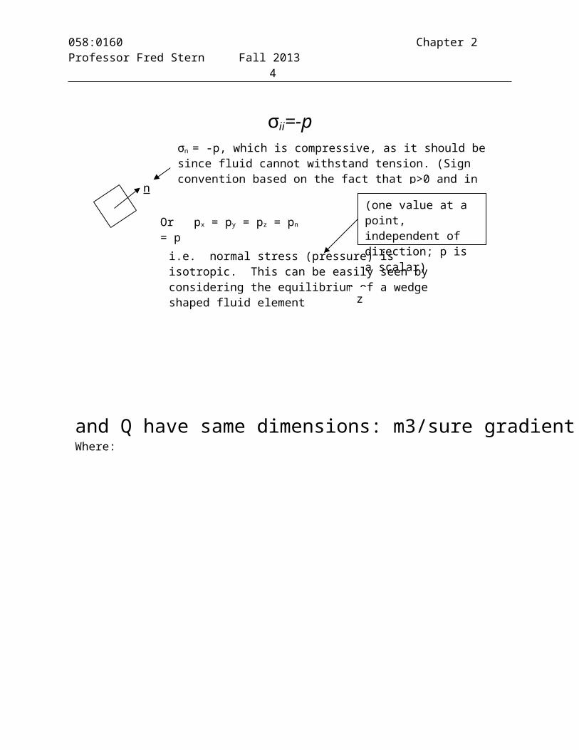
σii=-p

i.e. normal stress (pressure) is isotropic. This can be easily seen by considering the equilibrium of a wedge shaped fluid element

Or px = py = pz = pn = p

n

z

(one value at a point, independent of direction; p is a scalar)

and Q have same dimensions: m3/sure gradient or elevation gradient normal to streamline.cular motion, which decreaseWhere:

σn = -p, which is compressive, as it should be since fluid cannot withstand tension. (Sign convention based on the fact that p>0 and in the direction of –n)


Note: For a fluid in motion, the normal stress is different on each face and not equal to p.

σxx ≠ σyy ≠ σzz ≠ -pBy convention p is defined as the average of the normal stresses

The fluid element experiences a force on it as a result of the fluid pressure distribution if it varies spatially. Consider the net force in the x direction due to p(x,t).

The result will be similar for dFy and dFz; consequently, we conclude:

Or: force per unit volume due to p(x,t).

Note: if p=constant, .

dx

dz

dy

pdydz dydzdxx

pp

=


Equilibrium of a fluid element

Consider now a fluid element which is acted upon by both surface forces and a body force due to gravity

or (per unit volume)

Application of Newton’s law yields:

per unit

z g

(includes , since in general )

For ρ, μ=constant, the viscous force will have this form (chapter 4).

with

This is called the Navier-Stokes equation and will be discussed further in Chapter 4. Consider solving the N-S equation for p when a and V are known.

This is simply a first order PDE for p and can be solved readily. For the general case (V and p unknown), one

Viscous part

inertial pressure gradient

gravity viscous


must solve the NS and continuity equations, which is a formidable task since the NS equations are a system of 2nd

order nonlinear PDEs.We now consider the following special cases:

1) Hydrostatics ( )

2) Rigid body translation or rotation ( )

3) Irrotational motion ( )

also,


Case (1) Hydrostatic Pressure Distribution

z g

i.e. and

or

liquids ρ = constant (for one liquid)p = -ρgz + constant

gases ρ = ρ(p,t) which is known from the equation of state: p = ρRT ρ = p/RT

which can be integrated if T =T(z) is known as it is for the atmosphere.


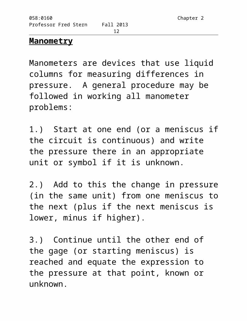
Manometry

Manometers are devices that use liquid columns for measuring differences in pressure. A general procedure may be followed in working all manometer problems:

1.) Start at one end (or a meniscus if the circuit is continuous) and write the pressure there in an appropriate unit or symbol if it is unknown.

2.) Add to this the change in pressure (in the same unit) from one meniscus to the next (plus if the next meniscus is lower, minus if higher).

3.) Continue until the other end of the gage (or starting meniscus) is reached and equate the expression to the pressure at that point, known or unknown.


Hydrostatic forces on plane surfaces

The force on a body due to a pressure distribution is:

where for a plane surface n = constant and we need only consider |F| noting that its direction is always towards the

surface: .

Consider a plane surface entirely submerged in a liquid such that the plane of the surface intersects the free-surface with an angle α. The centroid of the surface is denoted ( ).


Where is the pressure at the centroid.

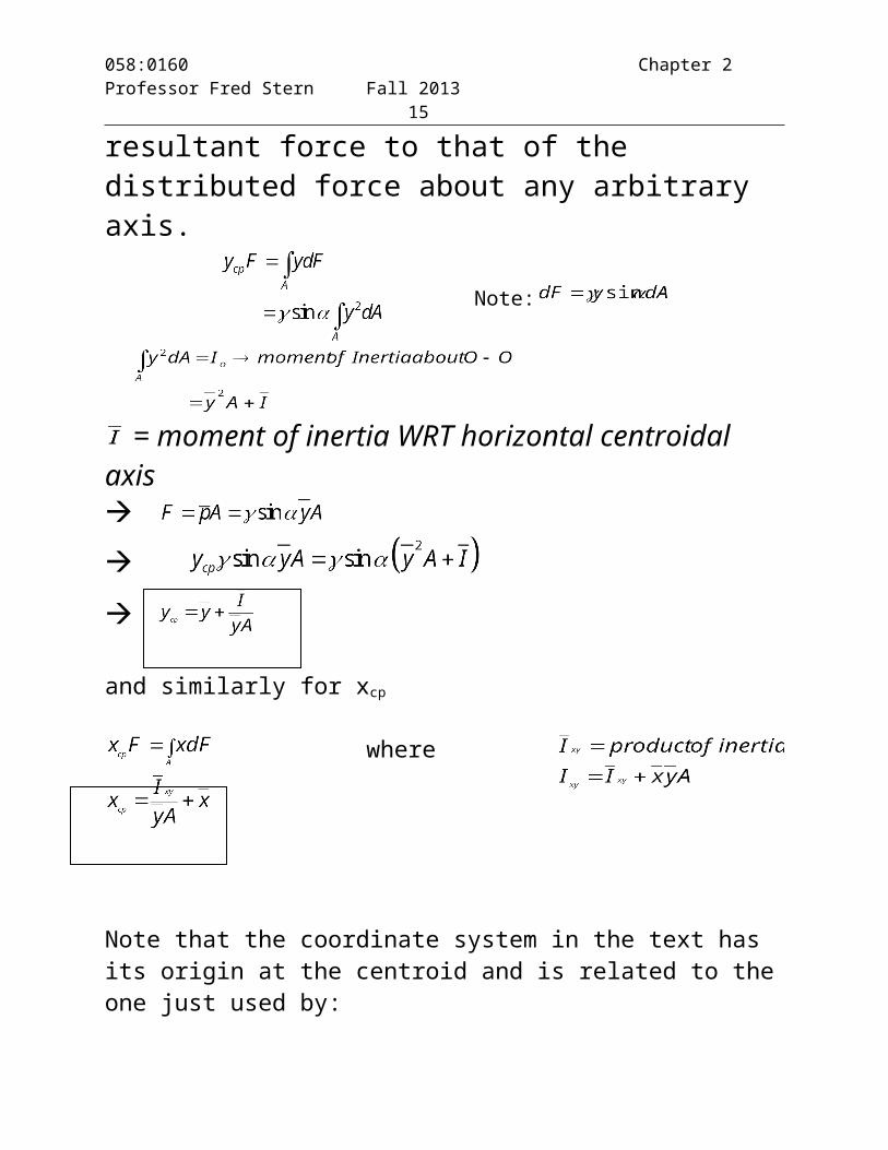
To find the line of action of the force which we call the center of pressure (xcp, ycp) we equate the moment of the resultant force to that of the distributed force about any arbitrary axis.

Note:

= moment of inertia WRT horizontal centroidal axis

and similarly for xcp

where

Note that the coordinate system in the text has its origin at the centroid and is related to the one just used by:

Hydrostatic Forces on Curved Surfaces


In general, Horizontal Components:

dAx = projection of n dA onto a plane perpendicular to x directiondAy = projection of n dA onto a plane perpendicular to y direction

The horizontal component of force acting on a curvedsurface is equal to the force acting on a vertical projectionof that surface including both magnitude and line of action and can be determined by the methods developed for plane surfaces.

Where h is the depth to any element area dA of the surface. The vertical component of force acting on a curved surface is equal to the net weight of the total column of fluid directly above the curved surface and has a line of action through the centroid of the fluid volume.

z

y

x


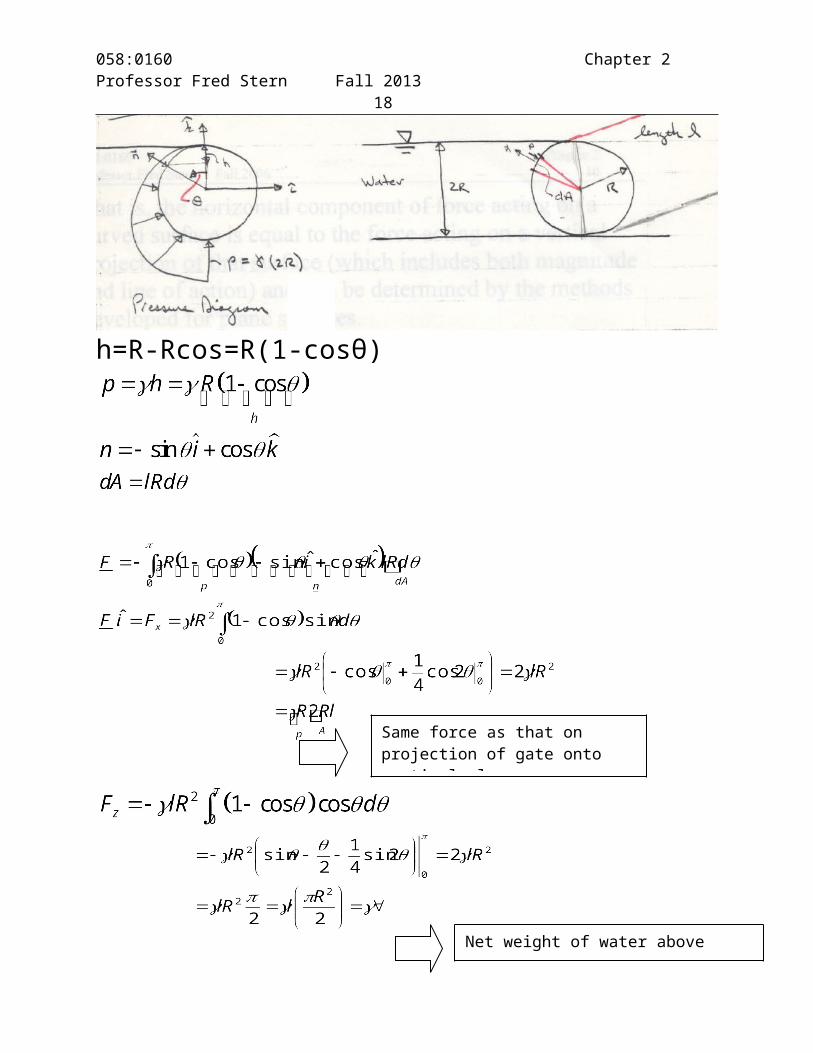
Example Drum Gate

h=R-Rcos=R(1-cosθ)

Same force as that on projection of gate onto vertical plane perpendicular direction

Net weight of water above curved surface


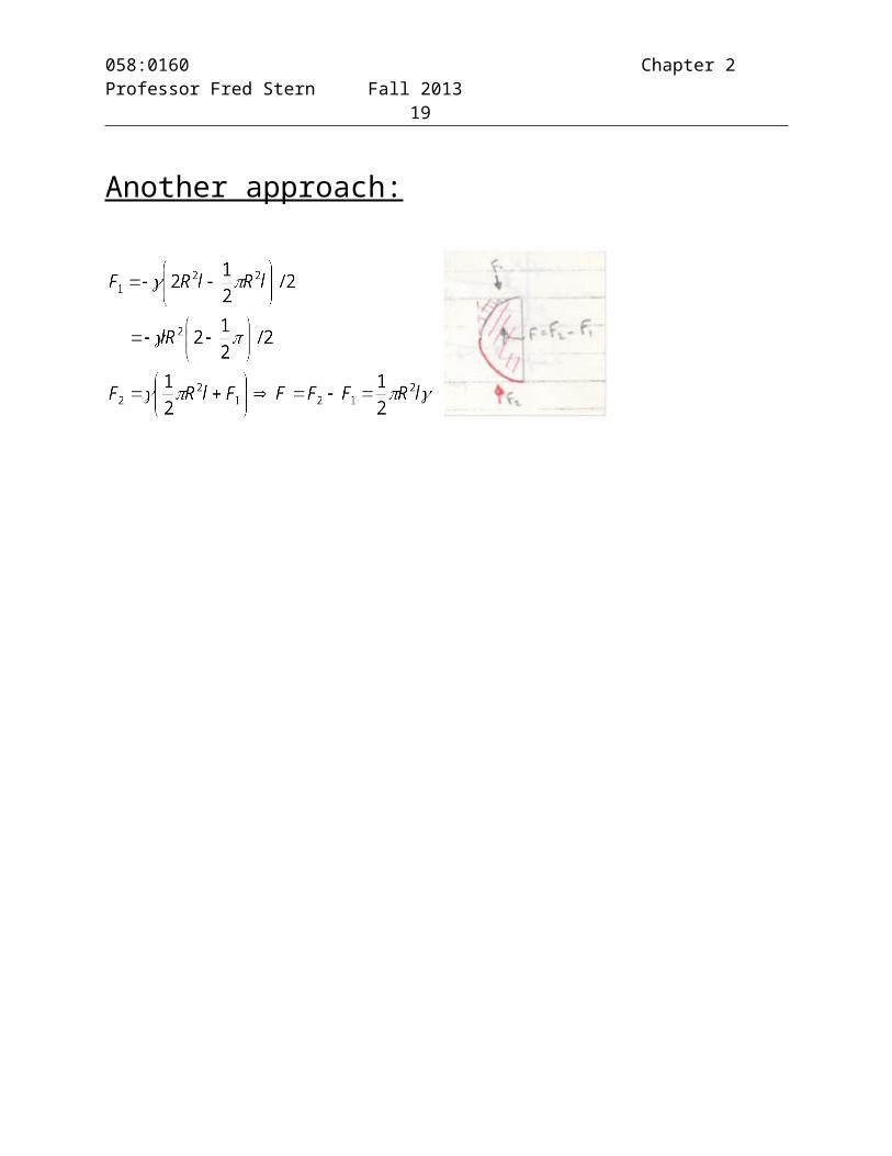
Another approach:


Hydrostatic Forces in Layered Fluids See textbook 2.7

Buoyancy and Stability

Archimedes Principle

= fluid weight above 2ABC – fluid weight above 1ADC

= weight of fluid equivalent to the body volume

In general, FB = ρg ( = submerged volume).

The line of action is through the centroid of the displaced volume, which is called the center of buoyancy.


Example

Weight of the block where

is displaced water volume by the block and is the specific weight of the liquid.

Instantaneous displaced water volume:

b

L

h

G

B

yy

G

ρb

d


Use initial condition ( ) to determine A and B:

Where

period Spar Buoy

We can increase period T by increasing block mass m and/or decreasing waterline area .

Stability: Immersed Bodies

Stable Neutral Unstable


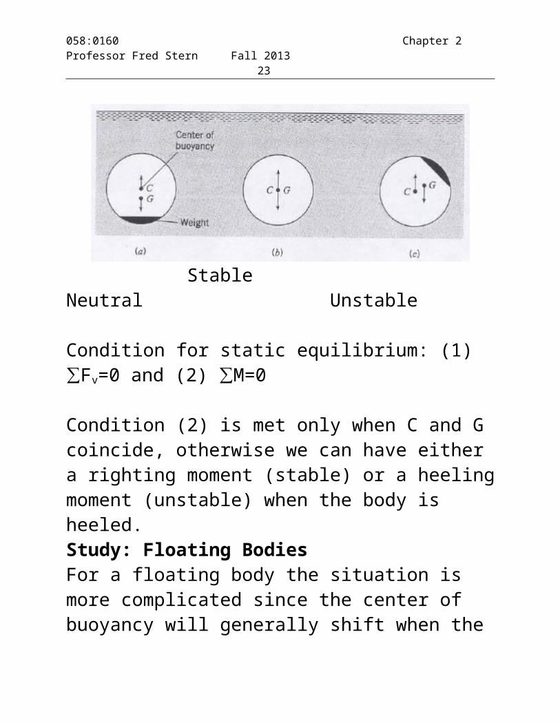
Condition for static equilibrium: (1) ∑Fv=0 and (2) ∑M=0

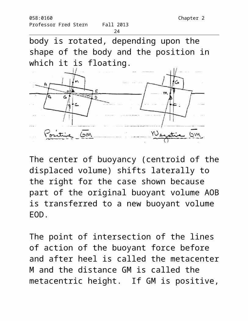
Condition (2) is met only when C and G coincide, otherwise we can have either a righting moment (stable) or a heeling moment (unstable) when the body is heeled.Study: Floating BodiesFor a floating body the situation is more complicated since the center of buoyancy will generally shift when the body is rotated, depending upon the shape of the body and the position in which it is floating.

The center of buoyancy (centroid of the displaced volume) shifts laterally to the right for the case shown because part of the original buoyant volume AOB is transferred to a new buoyant volume EOD.

The point of intersection of the lines of action of the buoyant force before and after heel is called the metacenter M and the distance GM is called the


metacentric height. If GM is positive, that is, if M is above G, then the ship is stable; however, if GM is negative, then the ship is unstable.


Consider a ship which has taken a small angle of heel α

1. α=small heel angle2. evaluate the lateral displacement of the center of

buoyancy, =3. then from trigonometry, we can solve for GM and

evaluate the stability of the ship: =centroid; CM=GM+CG

Recall that the center of buoyancy is at the centroid of the displaced volume of fluid (moment of volume about y-axis – ship centerplane)

This can be evaluated conveniently as follows: = moment of before heel (goes to zero due to

symmetry of original buoyant volume AKKD about centerplane)

- moment of AOB

+ moment of EOD


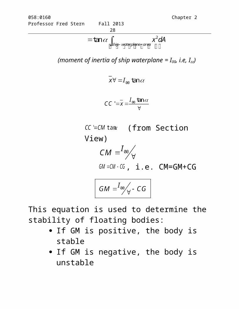
(moment of inertia of ship waterplane = I00, i.e, Izz)

(from Section View)

, i.e. CM=GM+CG


This equation is used to determine the stability of floating bodies:

If GM is positive, the body is stable If GM is negative, the body is unstable

Roll: The rotation of a ship about the longitudinal axis through the center of gravity.

Consider symmetrical ship heeled to a very small angle θ. Solve for the subsequent motion due only to hydrostatic and gravitational forces.

( = Δ)


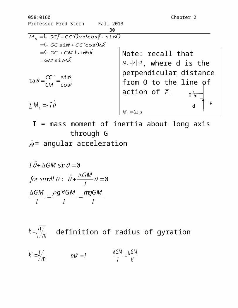
I = mass moment of inertia about long axis through G= angular acceleration

definition of radius of gyration

The solution to this equation is,

Note: recall that , where d is the perpendicular distance from O to the line of action of .

dO

F

0 for no initial velocity


where = the initial heel angle

= natural frequency

Simple (undamped) harmonic oscillation:

The period of the motion is

Note that large GM decreases the period of roll, which would make for an uncomfortable boat ride (high frequency oscillation).

Earlier we found that GM should be positive if a ship is to have transverse stability and, generally speaking, the stability is increased for larger positive GM. However, the present example shows that one encounters a “design tradeoff” since large GM decreases the period of roll, which makes for an uncomfortable ride.

Parametric Roll:


Case (2) Rigid Body Translation or Rotation

In rigid body motion, all particles are in combined translation and/or rotation and there is no relative motion between particles; consequently, there are no strains or strain rates and the viscous term drops out of the N-S equation .

from which we see that acts in the direction of , and lines of constant pressure must be perpendicular to this direction (by definition, is perpendicular to f = constant).

The general case of rigid body translation/rotation is as shown. If the center of rotation is at O where , the velocity of any arbitrary point P is:

Rigid body of fluid translating or rotating


where = the angular velocity vector

and the acceleration is:

1 = acceleration of O

2 = centripetal acceleration of P relative to O

3 = linear acceleration of P due to Ω

Usually, all these terms are not present. In fact, fluids can rarely move in rigid body motion unless restrained by confining walls for a long time.

1.) Uniform Linear Acceleration


p=constant

constant

1. increase in +x

2. decrease in +x

1. decrease in +z


2. decrease in +z but slower than g3. increase in +z

unit vector in the direction of :

lines of constant pressure are perpendicular to .

unit vector in direction of p=constant

angle between and x axes:

In general the pressure variation with depth is greater than in ordinary hydrostatics; that is:

which is > ρg


2). Rigid Body Rotation

Consider a cylindrical tank of liquid rotating at a constant rate Ω = Ω :

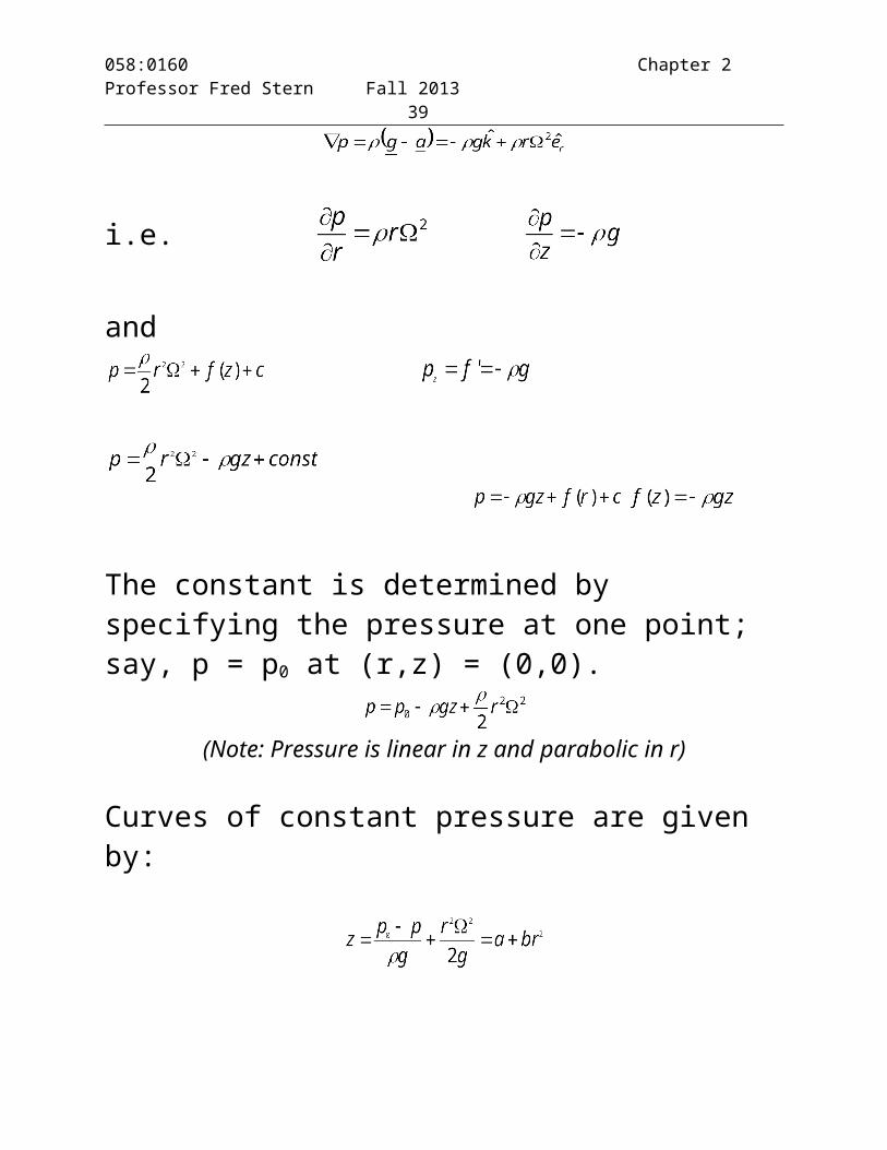
i.e.

and


The constant is determined by specifying the pressure at one point; say, p = p0 at (r,z) = (0,0).

(Note: Pressure is linear in z and parabolic in r)

Curves of constant pressure are given by:

which are paraboloids of revolution, concave upward, with their minimum points on the axis of rotation.

The position of the free surface is found, as it is for linear acceleration, by conserving the volume of fluid.


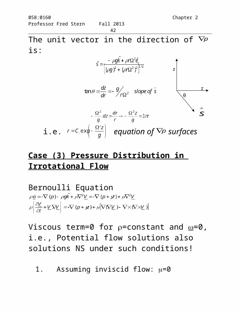
The unit vector in the direction of is:


i.e. equation of surfaces

Case (3) Pressure Distribution in Irrotational Flow

Bernoulli Equation

Viscous term=0 for =constant and =0, i.e., Potential flow solutions also solutions NS under such conditions!

1. Assuming inviscid flow: =0

Euler Equation

2. Assuming incompressible flow: =constant

3. Assuming steady flow:

θ

r

z


Consider:

perpendicular B= constant

perpendicular V and

Therefore, B=constant contains streamlines and vortex lines:


4. Assuming irrotational flow: =0

B= constant (everywhere same constant)

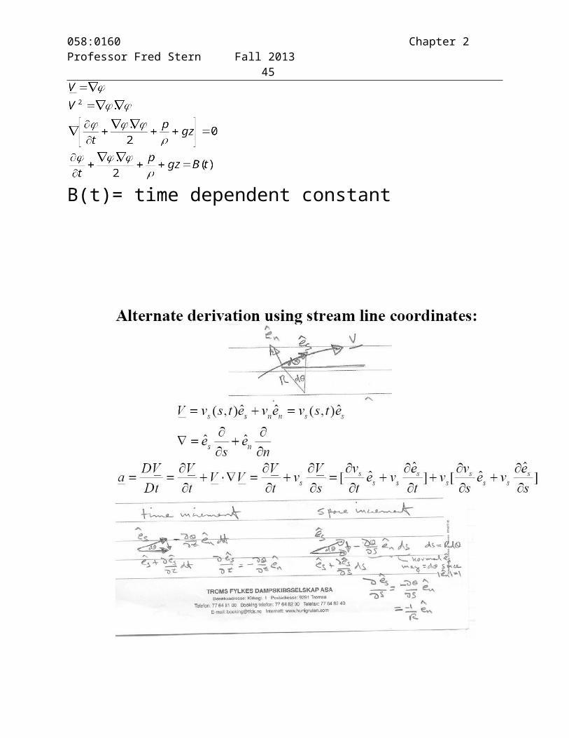
5. Unsteady irrotational flow

B(t)= time dependent constant



Larger speed/density or smaller R require larger pressure gradient or elevation gradient normal to streamline.


Flow Patterns: Streamlines, Streaklines, Pathlines

1)A streamline is a line everywhere tangent to the velocity vector at a given instant.

2)A pathline is the actual path traveled by a given fluid particle.

3)A streakline is the locus of particles which have earlier passed through a particular point.


Note:1. For steady flow, all 3 coincide.2. For unsteady flow, ψ(t) pattern changes with time,

whereas pathlines and streaklines are generated as the passage of time.

Streamline

By definition we must have which upon expansion yields the equation of the streamlines for a given time

s= integration parameter

So if (u,v,w) known, integrate with respect to s for t=t1

with IC (x0,y0,z0,t1) at s=0 and then eliminate s.

Pathline

The pathline is defined by integration of the relationship between velocity and displacement.

Integrate u,v,w with respect to t using IC ( ) then eliminate t.

Streakline


To find the streakline, use the integrated result for the pathline retaining time as a parameter. Now, find the integration constant which causes the pathline to pass through ( ) for a sequence of times . Then eliminate .

Example: an idealized velocity distribution is given by:

calculate and plot: 1) the streamlines 2) the pathlines 3) the streaklines which pass through ( ) at t=0.

1.) First, note that since w=0 there is no motion in the z direction and the flow is 2-D

and eliminating s


This is the equation of the streamlines which pass through ( ) for all times t.

2.) To find the pathlines we integrate

now eliminate t between the equations for (x, y)

This is the pathline through ( ) at t=0 and does not coincide with the streamline at t=0.

3.) To find the streakline, we use the pathline equations to find the family of particles that have passed through the point ( ) for all times .


The Stream Function

Powerful tool for 2-D flown in which V is obtained by differentiation of a scalar which automatically satisfies the continuity equation.


boundary conditions (4 required):

Irrotational Flow

Ψ and φ are orthogonal.

Steady constant property flow


i.e.

Geometric Interpretation of

Besides its importance mathematically also has important geometric significance.

= constant = streamlineRecall definition of a streamline:

Or =constant along a streamline and curves of constant are the flow streamlines. If we know (x, y) then we can plot = constant curves to show streamlines.

Physical Interpretation


(note that ψ and Q have same dimensions: m3/s)

i.e. change in is volume flux and across streamline .

Consider flow between two streamlines:


Incompressible Plane Flow in Polar Coordinates

Incompressible axisymmetric flow


Generalization

Steady plane compressible flow:

Now:

Change in is equivalent to the mass flux.

Fluid Mechanics

Documents

fluid force

fluid pressure distribution

moving fluid

fluid statics

stationary fluid

fluid elementconsider

fluid dynamics

body forces