September 6, 2011

Welcome message from author
This document is posted to help you gain knowledge. Please leave a comment to let me know what you think about it! Share it to your friends and learn new things together.
Transcript

September 6, 2011
UNIVERSITY OF NAIROBI
FACULTY OF SCIENCE
FIRST YEAR LECTURE NOTES
SMA 101: BASIC MATHEMATICS
First Edition
WRITTEN BY :
Dr. Bernard Mutuku Nzimbi
REVIEWED BY:
School of Mathematics, University of Nairobi
P.o Box 30197, Nairobi, KENYA.
EDITED BY:

Copyright c⃝ 2011 Benz, Inc. All rights reserved.
All rights reserved. No part of this publication may be reproduced, stored in a retrieval
system or transmitted in any form or by any means, electronic, mechanical, photocopy-
ing, recording or otherwise, without the prior permission of the publisher.
2

This page is intentionally left blank.
i
Contents
About the Author vi
Preface vii
Goals of a Basic Mathematics Course ix
1 ELEMENTARY SET THEORY 1
1.1 Introduction . . . . . . . . . . . . . . . . . . . . . . . . . . . . . . . . . . 1
1.2 Rudiments of Set Theory . . . . . . . . . . . . . . . . . . . . . . . . . . . 1
1.2.1 Notation and Terminology . . . . . . . . . . . . . . . . . . . . . . 2
1.2.2 Fundamental Operations on Sets . . . . . . . . . . . . . . . . . . 5
1.3 Laws of Set Theory . . . . . . . . . . . . . . . . . . . . . . . . . . . . . . 9
1.3.1 Venn Diagrams . . . . . . . . . . . . . . . . . . . . . . . . . . . . 11
1.3.2 Elements Argument Method . . . . . . . . . . . . . . . . . . . . . 16
1.4 Fundamental Counting Principle . . . . . . . . . . . . . . . . . . . . . . . 18
1.4.1 Counting and Venn Diagrams . . . . . . . . . . . . . . . . . . . . 20
1.5 Real Number Systems . . . . . . . . . . . . . . . . . . . . . . . . . . . . 26
1.5.1 Some Useful subsets of Real Numbers . . . . . . . . . . . . . . . . 29
1.5.2 Intervals . . . . . . . . . . . . . . . . . . . . . . . . . . . . . . . . 30
1.6 Application of Laws of Set Theory . . . . . . . . . . . . . . . . . . . . . . 34
1.7 Exercises . . . . . . . . . . . . . . . . . . . . . . . . . . . . . . . . . . . . 36
1.8 Complex Numbers . . . . . . . . . . . . . . . . . . . . . . . . . . . . . . 39
1.8.1 Arithmetic Operations of Complex Numbers . . . . . . . . . . . . 40
1.8.2 The Complex Plane or The Argand Diagram or The Gauss Plane 41
1.8.3 Conjugates, Absolute Values and Arguments of Complex Numbers 41
ii
1.8.4 Polar Form of a Complex Number . . . . . . . . . . . . . . . . . . 43
1.8.5 De Movrie’s Theorem . . . . . . . . . . . . . . . . . . . . . . . . . 44
1.8.6 Application of Polar Form in Computing Products and Quotients
of Complex Numbers . . . . . . . . . . . . . . . . . . . . . . . . 47
1.9 Exercises . . . . . . . . . . . . . . . . . . . . . . . . . . . . . . . . . . . . 48
2 ELEMENTARY LOGIC 50
2.1 Introduction . . . . . . . . . . . . . . . . . . . . . . . . . . . . . . . . . . 50
2.2 Mathematical Reasoning and Creativity . . . . . . . . . . . . . . . . . . 50
2.2.1 Inductive and Deductive Reasoning . . . . . . . . . . . . . . . . . 50
2.3 propositional Logic . . . . . . . . . . . . . . . . . . . . . . . . . . . . . . 51
2.3.1 Propositions and Truth Values . . . . . . . . . . . . . . . . . . . . 51
2.3.2 Logical Connectives and Truth Tables . . . . . . . . . . . . . . . . 53
2.3.3 Tautologies and Contradictions . . . . . . . . . . . . . . . . . . . 58
2.3.4 Logical Equivalence and Logical Implication . . . . . . . . . . . . 59
2.3.5 The Algebra of Logical Equivalence of Propositions . . . . . . . . 59
2.3.6 Relationship between Converse, Inverse and the Contrapositive of
a Conditional Proposition . . . . . . . . . . . . . . . . . . . . . . 61
2.4 Predicate Calculus . . . . . . . . . . . . . . . . . . . . . . . . . . . . . . 62
2.4.1 Universal Quantifier . . . . . . . . . . . . . . . . . . . . . . . . . 62
2.4.2 Existential Quantifier . . . . . . . . . . . . . . . . . . . . . . . . . 63
2.4.3 Negation of a Quantified Statement . . . . . . . . . . . . . . . . . 64
2.5 Application of Logic In Mathematical Proof . . . . . . . . . . . . . . . . 65
2.5.1 Proof by a Counter-example . . . . . . . . . . . . . . . . . . . . . 65
2.5.2 Direct Proof . . . . . . . . . . . . . . . . . . . . . . . . . . . . . . 66
2.5.3 Proof by Cases . . . . . . . . . . . . . . . . . . . . . . . . . . . . 66
2.5.4 Proof by the Contrapositive . . . . . . . . . . . . . . . . . . . . . 67
2.5.5 Proof by Contradiction . . . . . . . . . . . . . . . . . . . . . . . . 67
2.5.6 Proof by Mathematical Induction . . . . . . . . . . . . . . . . . . 68
2.6 Applications of Logic . . . . . . . . . . . . . . . . . . . . . . . . . . . . . 69
2.7 Exercises . . . . . . . . . . . . . . . . . . . . . . . . . . . . . . . . . . . . 70
iii
3 PERMUTATIONS AND COMBINATIONS 73
3.1 Introduction . . . . . . . . . . . . . . . . . . . . . . . . . . . . . . . . . . 73
3.2 Basic Counting Principle . . . . . . . . . . . . . . . . . . . . . . . . . . . 73
3.3 Permutations . . . . . . . . . . . . . . . . . . . . . . . . . . . . . . . . . 75
3.3.1 General Formula for P (n, r) . . . . . . . . . . . . . . . . . . . . . 76
3.3.2 Permutations of Repeated Objects . . . . . . . . . . . . . . . . . 77
3.4 Combinations . . . . . . . . . . . . . . . . . . . . . . . . . . . . . . . . . 79
3.4.1 Comparing Combinations and Permutations . . . . . . . . . . . . 79
3.4.2 Combinations with Repetition . . . . . . . . . . . . . . . . . . . . 81
3.5 Problems involving Both Permutations and Combinations . . . . . . . . . 81
3.6 Applications of Combinations . . . . . . . . . . . . . . . . . . . . . . . . 83
3.6.1 Binomial Theorem . . . . . . . . . . . . . . . . . . . . . . . . . . 83
3.7 Exercises . . . . . . . . . . . . . . . . . . . . . . . . . . . . . . . . . . . . 84
4 RELATIONS AND FUNCTIONS 87
4.1 Introduction . . . . . . . . . . . . . . . . . . . . . . . . . . . . . . . . . . 87
4.2 Cartesian Products and Relations . . . . . . . . . . . . . . . . . . . . . . 87
4.2.1 Relations on a Set . . . . . . . . . . . . . . . . . . . . . . . . . . 88
4.3 Properties of Relations . . . . . . . . . . . . . . . . . . . . . . . . . . . . 89
4.4 Combining Relations . . . . . . . . . . . . . . . . . . . . . . . . . . . . . 92
4.5 Functions . . . . . . . . . . . . . . . . . . . . . . . . . . . . . . . . . . . 93
4.6 Types of Functions . . . . . . . . . . . . . . . . . . . . . . . . . . . . . . 95
4.6.1 One-to-one Functions and Many-to-one Functions . . . . . . . . . 95
4.6.2 Onto Functions . . . . . . . . . . . . . . . . . . . . . . . . . . . . 96
4.6.3 Bijective Functions . . . . . . . . . . . . . . . . . . . . . . . . . . 96
4.7 Composition and Inverses of Functions . . . . . . . . . . . . . . . . . . . 97
4.7.1 Composition of Functions . . . . . . . . . . . . . . . . . . . . . . 97
4.7.2 Inverse of a Function . . . . . . . . . . . . . . . . . . . . . . . . . 98
4.7.3 The Vertical Line Test for a Function . . . . . . . . . . . . . . . . 99
4.8 Some Special Real Valued Functions . . . . . . . . . . . . . . . . . . . . 99
4.9 Some Classification of Real Valued Functions . . . . . . . . . . . . . . . . 105
4.9.1 Even Functions . . . . . . . . . . . . . . . . . . . . . . . . . . . . 105
iv
4.9.2 Odd Functions . . . . . . . . . . . . . . . . . . . . . . . . . . . . 105
4.9.3 Functions which are Neither Even nor Odd . . . . . . . . . . . . 105
4.9.4 Algebraic Functions . . . . . . . . . . . . . . . . . . . . . . . . . . 105
4.9.5 Irrational Functions and Rational Functions . . . . . . . . . . . . 106
4.10 Solved Problems . . . . . . . . . . . . . . . . . . . . . . . . . . . . . . . 106
4.11 Exercises . . . . . . . . . . . . . . . . . . . . . . . . . . . . . . . . . . . . 108
5 TRIGONOMETRY 110
5.1 Radian and Degree Measure of an Angle . . . . . . . . . . . . . . . . . . 110
5.2 Trigonometric Ratios . . . . . . . . . . . . . . . . . . . . . . . . . . . . . 111
5.3 Trigonometric Identities . . . . . . . . . . . . . . . . . . . . . . . . . . . 112
5.3.1 Cofunction Identities . . . . . . . . . . . . . . . . . . . . . . . . . 112
5.3.2 Pythagorean Identities . . . . . . . . . . . . . . . . . . . . . . . . 112
5.3.3 Sum and Difference Identities . . . . . . . . . . . . . . . . . . . . 114
5.3.4 Double-Angle Identities . . . . . . . . . . . . . . . . . . . . . . . 117
5.3.5 Half-Angle Identities . . . . . . . . . . . . . . . . . . . . . . . . . 118
5.4 Proving Identities . . . . . . . . . . . . . . . . . . . . . . . . . . . . . . . 119
5.5 Solving Trigonometric Equations . . . . . . . . . . . . . . . . . . . . . . 120
5.6 Exercises . . . . . . . . . . . . . . . . . . . . . . . . . . . . . . . . . . . . 123
Bibliography 125
v

About the Author
B.M. Nzimbi is a Lecturer in Pure Mathematics at the University of Nairobi. Dr. Nzimbi
received his B.sc in Mathematics and Computer Science from the University of Nairobi
(1995), Msc(Pure Mathematics) from University of Nairobi (1999), Msc(Mathematics)
from Syracuse University (New York, USA) (2004), and his Ph.D in Pure Mathematics
from University of Nairobi (2009), where he wrote his thesis in the area of Operator
Theory under the direction of Prof. J.M. Khalagai. Before joining the University of
Nairobi, he held a position at Catholic University of Eastern Africa (CUEA), where he
was a part-time lecturer.
Dr. Nzimbi has authored, co-authored and published numerous articles in professional
journals in the areas of Operator Theory and differential geometry. He is the author of
the textbooks ”Linear Algebra I ” and ”Linear Algebra II ”, which are extensively used
in the ODL programme at the University of Nairobi.
vi
Preface
The study of Basic Mathematics is indispensable for a prospective student of pure,
statistics or applied mathematics. It has become an integral part of the mathematical
background necessary for such diverse fields as mathematics, chemistry, physics, biology,
economics, psychology, sociology, education, political science, business, engineering and
even computer science.
In writing this book, I was guided by my long-standing experience and interest in teach-
ing Basic Mathematics. The book is based on my lecture notes for the course entitled
Basic Mathematics. The choice of material is not entirely mine, but laid down by the
University of Nairobi SMA101: Basic Mathematics syllabus.
For the student, my purpose was to introduce students studying sciences and social
sciences all the mathematical foundations they need for their future studies: elemen-
tary theory of sets, logic, counting techniques, relations and trigonometry and to treat a
number of practical applications from every-day situations to the biological, physical and
social sciences. This enables them to have an understanding of important mathematical
concepts together with a sense of why these concepts are important for applications.
For the instructor, my purpose was to design a flexible, comprehensive teaching tool
using proven pedagogical techniques in mathematics. I wanted to provide instructors
with a package of materials that they could use to teach Basic Mathematics effectively
and efficiently in the most appropriate manner for their particular set of students. I
hope I have accomplished these goals without watering down the material.
This text is designed as a one-semester introduction to mathematics course to be taken
by students in a wide variety of majors, including mathematics, actuarial science, statis-
tics, chemistry, physics, meteorology, geology, computer science,engineering, economics,
business and other social sciences. High school algebra is the only explicit prerequisite.
The core material of this book consists of five chapters: Chapter 1 is a brief introduction
to set theory. Chapter two contains elementary logic. Chapter 3....etc
Each chapter includes definitions, theorems and principles together with illustrative and
vii

other descriptive material, followed by several exercises of varying difficulty.
I finally wish to record my appreciation to my former students for their invaluable sug-
gestions and critical review of the manuscript that made the writing of this book easy.
Bernard Mutuku Nzimbi
Nairobi, 2011
viii
Goals of a Basic Mathematics Course
A Basic Mathematics course will enable students to learn a particular set of mathemat-
ical facts and how to apply them and how to think mathematically. To achieve this
goal, this text stresses set theory and mathematical reasoning and the different ways
problems are solved.
Special Features of this Book
Accessibility: There are no mathematical prerequisites beyond high school algebra
for this text. Each chapter begins at an easily understood and accessible level. Once
basic mathematical concepts have been developed, more difficult material and applica-
tions are presented.
Accessibility: This text has been carefully designed for flexible use. The depen-
dence of chapters has been minimized. Each chapter is divided into sections and each
section is divided into subsections that form natural blocks of material for teaching.
Instructors can easily pace their lectures using these blocks.
Writing Style: The writing style of this book is direct and pragmatic. Precise
mathematical language is used without excessive formalism and abstraction. Notations
are introduced and used when appropriate. Care has been taken to balance the mix of
notation and words in mathematical statements.
Mathematical Rigour and Precision: All definitions and theorems in this book
are stated extremely carefully so that students will appreciate the precision of language
and rigour need in mathematics. Proofs are motivated and developed and their steps
are carefully justified.
Figures and Tables: Figures and tables in this book are carefully presented and
illustrated.
Exercises: There is an ample supply of exercises in this book that develop basic
ix

skills and which are carefully graded for level of difficulty.
x
Chapter 1
ELEMENTARY SET THEORY
1.1 Introduction
Set theory is a natural choice of a field where students can first become acquainted with
an axiomatic development of a mathematical discipline.
The central concept in this chapter revolves around a set, which is simply a collection,
group, conglomerate, aggregate of objects.
All fundamental tools of elementary set theory as needed in mathematics and elsewhere
in the sciences and social sciences are included in detailed exposition in this chapter.
Objectives
At the end of this lecture, you should be able to:
• Define a set.
• Carry out some set operations.
• Apply set theory in solving some practical problems.
1.2 Rudiments of Set Theory
Definition 1.1 A set is any well-defined collection, group, aggregate, class or
conglomerate of objects.
These objects (which may be cities, years, numbers, letters, or anything else ) are called
1
elements of the set, and are often said to be members of the set.
A set is often specified by
⊙ listing its elements inside a pair of braces or curly brackets or parentheses
⊙ means of a property of its elements.
Example 1.1
The set whose elements are the first six letters of the alphabet is written
{a, b, c, d, e, f}
Example 1.2
The set whose elements are the even integers between 1 and 11 is written
{2, 4, 6, 8, 10}
We can also specify a set by giving a description of its elements (without actually listing
the elements).
Example 1.3
The set {a, b, c, d, e, f} can also be written
{The first six letters of the alphabet}
Example 1.4
The set {2, 4, 6, 8, 10} can also be written
{all even integers between 1 and 11}
1.2.1 Notation and Terminology
For convenience, we usually denote sets by capital letters of the alphabet A,B,C, and
so on. We use lowercase letters of the alphabet to represent elements of a set.
For a set A, we write x ∈ A if x is a member of A or belongs to A. We write x ̸∈ A to
mean that x is not a member of A or does not belong to A.
2
Example 1.5
If E denotes the set of even integers, then 4 ∈ E but 7 ̸∈ E.
Definition 1.2 An empty set is a set with no elements.
An empty set is usually denoted by ∅. It is a set that arises in a variety of guises.
Example 1.6
Let A = {x : x is a real number and x2 < 0}. Clearly A has no elements since the
square of any real number is non-negative.
Example 1.7
Let B = {People taller than the Eiffel Tower inFrance}. It is clear that B is empty.
Definition 1.3 Let A and B be two sets. If every element of A is an element of B, we
say that A is a subset of B, and we write A ⊆ B. We also say that A is contained
in B.
Definition 1.4 If A ⊆ B and B ⊆ A, then we say that A and B are equal, and write
A = B. Two sets A and B are said to be equal if and only if they contain exactly the
same elements. This is called the Principle of Extensionality.
Theorem 1.1 Let A and B be sets. If every element of A is an element of B and
every element of B is an element of A, then A = B.
Note that neither order nor repetition is of importance or relevance for a general set.
Consequently, we find, for example that {1, 2, 3} = {2, 2, 1, 3} = {1, 2, 1, 3, 1}.
Example 1.8
The following sets, although described differently, are equal.
1. The set of all real numbers such that x2 + 3x+ 2 = 0.
2. The set of all integers such that 1 ≤ x < 3.
3. The set containing exactly the natural numbers 1 and 2.
If S and T are two sets that do not contain exactly the same elements, then we say that
the sets are unequal and we write S ̸= T .
3
Definition 1.5 If A ⊆ B and A ̸= B, we say that A is a proper subset of B, or A
is properly contained in B, and write A ⊂ B.
We also write B ⊇ A instead of A ⊆ B and B ⊃ A instead of A ⊂ B.
Remark 1.1
Note that since the empty set ∅ has no elements, every element in ∅ is also in any given
set A. Hence ∅ ⊆ A. By the definition of subset, every set is a subset of itself. That is,
for any set A we have A ⊆ A.
Lemma 1.2 (Uniqueness of the Empty Set). There exists only one set with no
elements.
Proof. Assume A and B are sets with no elements. Then every element of A is an
element of B (since A has no elements). Similarly, every element of B is an element of
A (since B has no elements). Therefore, A = B, by the Principle of Extensionality. �
Definition 1.6 (Cardinality of a Set). The number of elements in a set A is called
the cardinality of A, and is denoted n(A) or |A|.
Note that cardinality of a set is always a non-negative integer or infinity. A set with one
element is called a singleton set. A set A is said to be finite if n(A) < ∞. A set A
is said to be infinite if n(A) = ∞.
Note that n(∅) = 0.
Definition 1.7 (Universal Set) A Universal set U is a set which contains all el-
ements under consideration. It is also called the universe of discourse or simply
universe.
Example 1.9
(a). If one considers the set of men and women, then a universal set is probably the set
of human beings.
(b). If one considers sets such as pigs, cows, chickens, or horses, the universal set is
probably the set of animals.
4
(c). IfA = {1, 2, 5} andB = {4, 7, 9}, then a universal set is probably U = {0, 1, 2, 3, 4, 5, 6, 7, 8, 9, 10}.
Note that a universal set is not unique, unless specified.
1.2.2 Fundamental Operations on Sets
We introduce simple set-theoretic operations on sets and prove some of their properties.
Given two or more sets, we can form a new set using these operations.
1. Complement of a Set
Let U be the universal set and let A be any set. The complement of A, written A{ or
sometimes A is defined as
A{ ={x ∈ U : x ̸∈ A
}Example 1.10
Let the universal set be U = {0, 1, 2, 3, 5, 6} and A = {3, 5}. Clearly, A{ = {0, 1, 2, 6}.2. Union of Sets
Let A and B be sets. The union of A and B, denoted by A ∪B is
A ∪B ={x : x ∈ A or x ∈ B or both
}More generally, if A1, A2, ..., An are sets, then their union is the set of all objects which
belong to at least one of them, and is denoted by
A1 ∪ A2 ∪ · · · ∪ An
or byn∪
i=1
Ai
This is the set of elements which belong to at least one Ai, i = 1, 2, ..., n.
Example 1.11
(a). IfA = {2, 5, 7} andB = {Tom,Bush,Mary}, thenA∪B = {2, 5, 7, T om,Bush,Mary}.(b). If A1 = {x, y, t, s}, A2 = {q, r, f}, A3 = {0, 1, 3, 4, 5, 6, 7, 8, 20}, then
A1 ∪ A2 ∪ A3 = {x, y, t, s, q, r, f, 0, 1, 3, 4, 5, 6, 7, 8, 20}
5
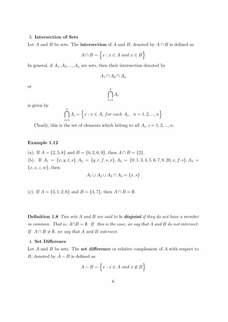
3. Intersection of Sets
Let A and B be sets. The intersection of A and B, denoted by A ∩B is defined as
A ∩B ={x : x ∈ A and x ∈ B
}In general, if A1, A2, ..., An are sets, then their intersection denoted by
A1 ∩ A2 ∩ An
orn∩
i=1
Ai
is given byn∩
i=1
Ai ={x : x ∈ Ai for each Ai, n = 1, 2, ..., n
}Clearly, this is the set of elements which belong to all Ai, i = 1, 2, ..., n.
Example 1.12
(a). If A = {2, 5, 8} and B = {0, 2, 6, 9}, then A ∩B = {2}.(b). If A1 = {x, y, t, s}, A2 = {q, r, f, s, x}, A3 = {0, 1, 3, 4, 5, 6, 7, 8, 20, x, f, s}, A4 =
{x, s, z, w}, thenA1 ∪ A2 ∪ A3 ∩ A4 = {x, s}
(c). If A = {3, 1, 2, 6} and B = {4, 7}, then A ∩B = ∅.
Definition 1.8 Two sets A and B are said to be disjoint if they do not have a member
in common. That is, A∩B = ∅. If this is the case, we say that A and B do not intersect.
If A ∩B ̸= ∅, we say that A and B intersect.
4. Set Difference
Let A and B be sets. The set difference or relative complement of A with respect to
B, denoted by A−B is defined as
A−B ={x : x ∈ A and x ̸∈ B
}6
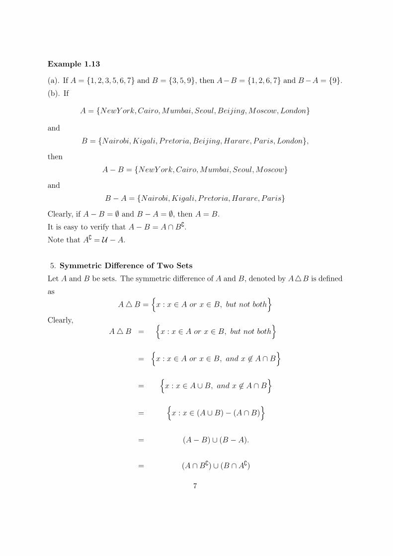
Example 1.13
(a). If A = {1, 2, 3, 5, 6, 7} and B = {3, 5, 9}, then A−B = {1, 2, 6, 7} and B−A = {9}.(b). If
A = {NewY ork, Cairo,Mumbai, Seoul, Beijing,Moscow, London}
and
B = {Nairobi,Kigali, Pretoria, Beijing,Harare, Paris, London},
then
A−B = {NewY ork, Cairo,Mumbai, Seoul,Moscow}
and
B − A = {Nairobi,Kigali, Pretoria,Harare, Paris}
Clearly, if A−B = ∅ and B − A = ∅, then A = B.
It is easy to verify that A−B = A ∩B{.
Note that A{ = U − A.
5. Symmetric Difference of Two Sets
Let A and B be sets. The symmetric difference of A and B, denoted by A△B is defined
as
A△B ={x : x ∈ A or x ∈ B, but not both
}Clearly,
A△B ={x : x ∈ A or x ∈ B, but not both
}=
{x : x ∈ A or x ∈ B, and x ̸∈ A ∩B
}=
{x : x ∈ A ∪B, and x ̸∈ A ∩B
}=
{x : x ∈ (A ∪B)− (A ∩B)
}= (A−B) ∪ (B − A).
= (A ∩B{) ∪ (B ∩ A{)
7
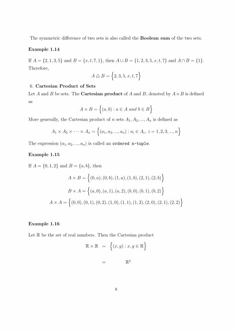
The symmetric difference of two sets is also called the Boolean sum of the two sets.
Example 1.14
If A = {2, 1, 3, 5} and B = {x, t, 7, 1}, then A∪B = {1, 2, 3, 5, x, t, 7} and A∩B = {1}.Therefore,
A△B ={2, 3, 5, x, t, 7
}6. Cartesian Product of Sets
Let A and B be sets. The Cartesian product of A and B, denoted by A×B is defined
as
A×B ={(a, b) : a ∈ A and b ∈ B
}More generally, the Cartesian product of n sets A1, A2, ..., An is defined as
A1 × A2 × · · · × An ={(a1, a2, ..., an) : ai ∈ Ai, i = 1, 2, 3, ..., n
}The expression (a1, a2, ..., an) is called an ordered n-tuple.
Example 1.15
If A = {0, 1, 2} and B = {a, b}, then
A×B ={(0, a), (0, b), (1, a), (1, b), (2, 1), (2, b)
}B × A =
{(a, 0), (a, 1), (a, 2), (b, 0), (b, 1), (b, 2)
}A× A =
{(0, 0), (0, 1), (0, 2), (1, 0), (1, 1), (1, 2), (2, 0), (2, 1), (2, 2)
}
Example 1.16
Let R be the set of real numbers. Then the Cartesian product
R× R ={(x, y) : x, y ∈ R
}= R2
8
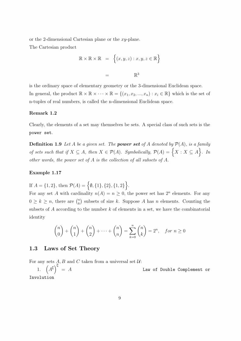
or the 2-dimensional Cartesian plane or the xy-plane.
The Cartesian product
R× R× R ={(x, y, z) : x, y, z ∈ R
}= R3
is the ordinary space of elementary geometry or the 3-dimensional Euclidean space.
In general, the product R× R× · · · × R = {(x1, x2, ..., xn) : xi ∈ R} which is the set of
n-tuples of real numbers, is called the n-dimensional Euclidean space.
Remark 1.2
Clearly, the elements of a set may themselves be sets. A special class of such sets is the
power set.
Definition 1.9 Let A be a given set. The power set of A denoted by P(A), is a family
of sets such that if X ⊆ A, then X ∈ P(A). Symbolically, P(A) ={X : X ⊆ A
}. In
other words, the power set of A is the collection of all subsets of A.
Example 1.17
If A = {1, 2}, then P(A) ={∅, {1}, {2}, {1, 2}
}.
For any set A with cardinality n(A) = n ≥ 0, the power set has 2n elements. For any
0 ≥ k ≥ n, there are(nk
)subsets of size k. Suppose A has n elements. Counting the
subsets of A according to the number k of elements in a set, we have the combinatorial
identity (n
0
)+
(n
1
)+
(n
2
)+ · · ·+
(n
n
)=
n∑k=0
(n
k
)= 2n, for n ≥ 0
1.3 Laws of Set Theory
For any sets A,B and C taken from a universal set U :1.
(A{
){= A Law of Double Complement or
Involution
9
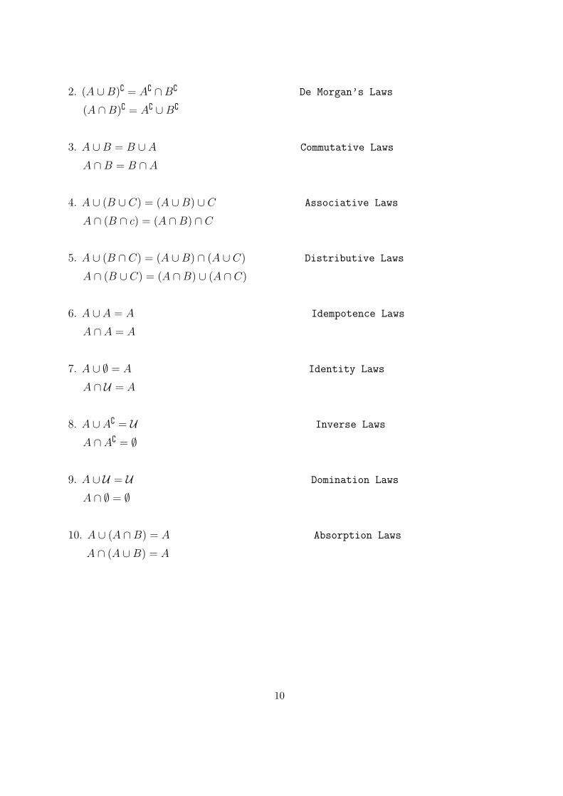
2. (A ∪B){ = A{ ∩B{ De Morgan’s Laws
(A ∩B){ = A{ ∪B{
3. A ∪B = B ∪ A Commutative Laws
A ∩B = B ∩ A
4. A ∪ (B ∪ C) = (A ∪B) ∪ C Associative Laws
A ∩ (B ∩ c) = (A ∩B) ∩ C
5. A ∪ (B ∩ C) = (A ∪B) ∩ (A ∪ C) Distributive Laws
A ∩ (B ∪ C) = (A ∩B) ∪ (A ∩ C)
6. A ∪ A = A Idempotence Laws
A ∩ A = A
7. A ∪ ∅ = A Identity Laws
A ∩ U = A
8. A ∪ A{ = U Inverse Laws
A ∩ A{ = ∅
9. A ∪ U = U Domination Laws
A ∩ ∅ = ∅
10. A ∪ (A ∩B) = A Absorption Laws
A ∩ (A ∪B) = A
10
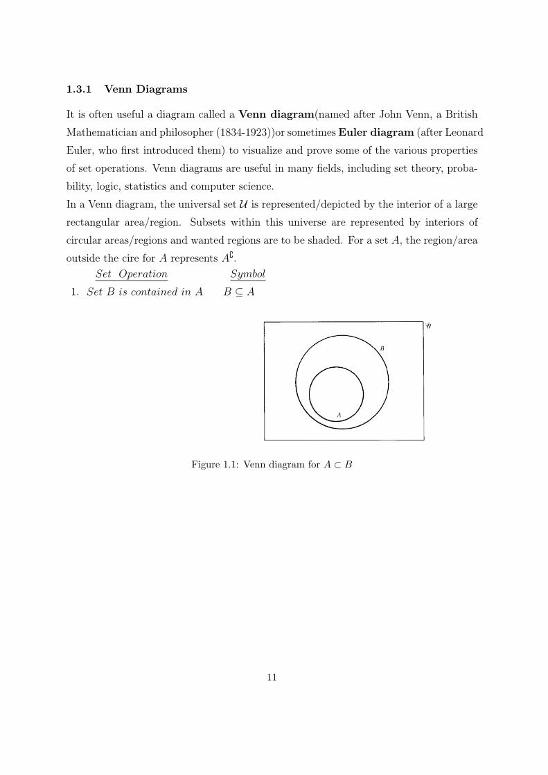
1.3.1 Venn Diagrams
It is often useful a diagram called a Venn diagram(named after John Venn, a British
Mathematician and philosopher (1834-1923))or sometimesEuler diagram (after Leonard
Euler, who first introduced them) to visualize and prove some of the various properties
of set operations. Venn diagrams are useful in many fields, including set theory, proba-
bility, logic, statistics and computer science.
In a Venn diagram, the universal set U is represented/depicted by the interior of a large
rectangular area/region. Subsets within this universe are represented by interiors of
circular areas/regions and wanted regions are to be shaded. For a set A, the region/area
outside the cire for A represents A{.
Set Operation Symbol
1. Set B is contained in A B ⊆ A
Figure 1.1: Venn diagram for A ⊂ B
11
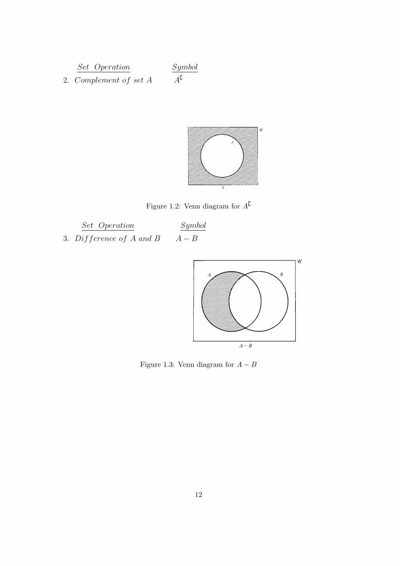
Set Operation Symbol
2. Complement of set A A{
Figure 1.2: Venn diagram for A{
Set Operation Symbol
3. Difference of A and B A−B
Figure 1.3: Venn diagram for A−B
12

Set Operation Symbol
4. Union of A and B A ∪B
Figure 1.4: Venn diagram for A ∪B
Set Operation Symbol
5. Intersection of A and B A ∩B
Figure 1.5: Venn diagram for A ∩B
13
Set Operation Symbol
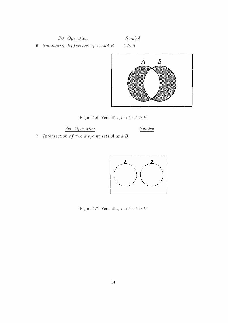
6. Symmetric difference of A and B A△B
Figure 1.6: Venn diagram for A△B
Set Operation Symbol
7. Intersection of two disjoint sets A and B
Figure 1.7: Venn diagram for A△B
14
Set Operation Symbol
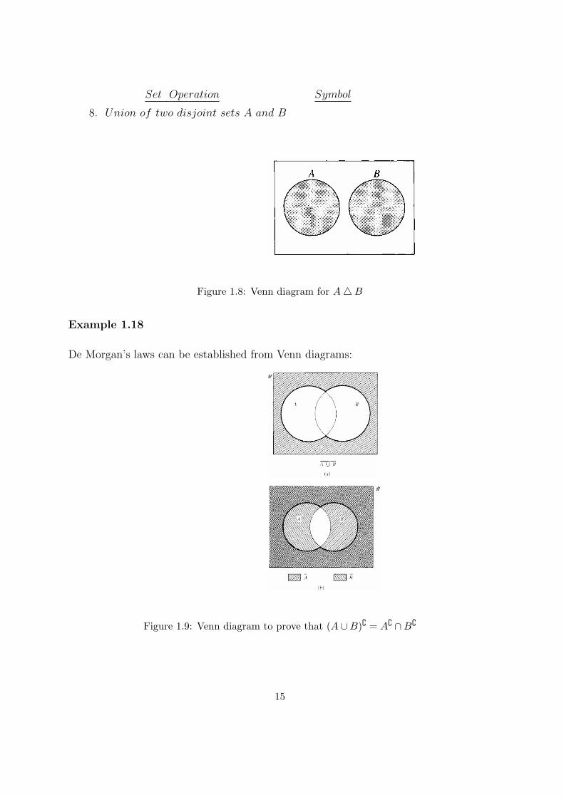
8. Union of two disjoint sets A and B
Figure 1.8: Venn diagram for A△B
Example 1.18
De Morgan’s laws can be established from Venn diagrams:
Figure 1.9: Venn diagram to prove that (A ∪B){ = A{ ∩B{
15
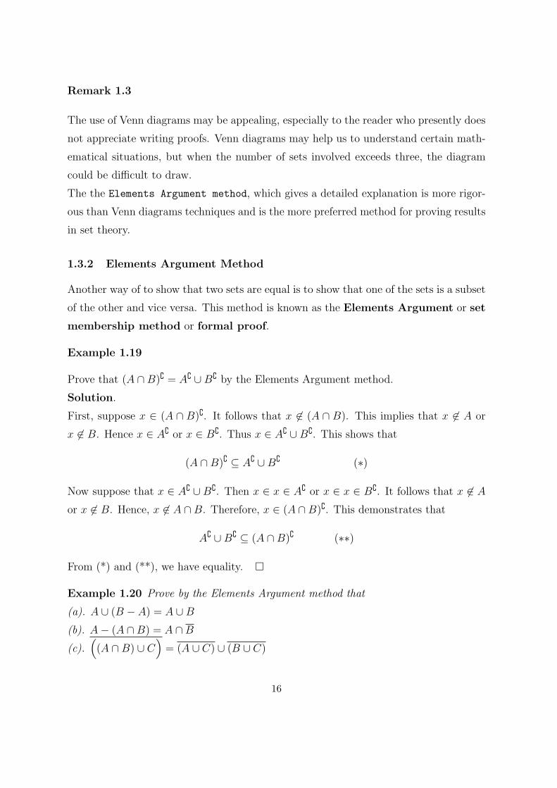
Remark 1.3
The use of Venn diagrams may be appealing, especially to the reader who presently does
not appreciate writing proofs. Venn diagrams may help us to understand certain math-
ematical situations, but when the number of sets involved exceeds three, the diagram
could be difficult to draw.
The the Elements Argument method, which gives a detailed explanation is more rigor-
ous than Venn diagrams techniques and is the more preferred method for proving results
in set theory.
1.3.2 Elements Argument Method
Another way of to show that two sets are equal is to show that one of the sets is a subset
of the other and vice versa. This method is known as the Elements Argument or set
membership method or formal proof.
Example 1.19
Prove that (A ∩B){ = A{ ∪B{ by the Elements Argument method.
Solution.
First, suppose x ∈ (A ∩ B){. It follows that x ̸∈ (A ∩ B). This implies that x ̸∈ A or
x ̸∈ B. Hence x ∈ A{ or x ∈ B{. Thus x ∈ A{ ∪B{. This shows that
(A ∩B){ ⊆ A{ ∪B{ (∗)
Now suppose that x ∈ A{ ∪ B{. Then x ∈ x ∈ A{ or x ∈ x ∈ B{. It follows that x ̸∈ A
or x ̸∈ B. Hence, x ̸∈ A ∩B. Therefore, x ∈ (A ∩B){. This demonstrates that
A{ ∪B{ ⊆ (A ∩B){ (∗∗)
From (*) and (**), we have equality. �
Example 1.20 Prove by the Elements Argument method that
(a). A ∪ (B − A) = A ∪B(b). A− (A ∩B) = A ∩B(c).
((A ∩B) ∪ C
)= (A ∪ C) ∪ (B ∪ C)
16
Solution
(a). Let x ∈ A∪ (B −A). Then x ∈ A or x ∈ B −A. This implies that x ∈ A or x ∈ B
and x ̸∈ A. This means that x ∈ A or x ∈ B or x ∈ A and x ̸∈ A. Therefore x ∈ A or
x ∈ B. That is, x ∈ A ∪B. This proves that
A ∪ (B − A) ⊆ A ∪B (∗)
Conversely, suppose x ∈ A∪B. Then x ∈ A or x ∈ B. Equivalently, x ∈ A or x ∈ B−∅.This means that x ∈ A or x ∈ B ∪ ∅. Thus, x ∈ A or x ∈ B ∪ (A− A). That is x ∈ A
or x ∈ B − A. This means that x ∈ A ∪ (B − A) . Thus
A ∪B ⊆ A ∪ (B − A) (∗∗)
From (*) and (**), equality follows. �
(b) and (c) are left as exercises.
Example 1.21 Let A,B and C be sets. Prove that
(a). A× (B ∪ C) = (A×B) ∪ (A× C)
(b). A× (B ∩ C) = (A×B) ∩ (A× C)
Proof.
(a). Suppose (x, y) ∈ A × (B ∪ C). Then x ∈ A and y ∈ B ∪ C. If y ∈ B, then
(x, y) ∈ A×B. If y ∈ C, then (x, y) ∈ A×C. In either case, (x, y) ∈ (A×B)∪ (A×C).Thus
A× (B ∪ C) ⊆ (A×B) ∪ (A× C) (∗)
Conversely, suppose (x, y) ∈ (A × B) ∪ (A × C). If (x, y) ∈ A × B, then x ∈ A and
y ∈ B, so y ∈ B ∪C and hence (x, y) ∈ A× (B ∪C). If (x, y) ∈ A×C, then x ∈ A and
y ∈ B ∪ C, so again (x, y) ∈ A× (B ∪ C). Thus
(A×B) ∪ (A× C) ⊆ A× (B ∪ C) (∗∗)
From (*) and (**), equality follows. �
17
(b). (x, y) ∈ A× (B ∩ C) if and only if x ∈ A and y ∈ B ∩ Cif and only if x ∈ A and y ∈ B and y ∈ C
if and only if x ∈ A and y ∈ B and x ∈ A and y ∈ C
if and only if (x, y) ∈ A×B and (x, y) ∈ A× C
if and only if (x, y) ∈ (A×B) ∩ (A× C). �
1.4 Fundamental Counting Principle
Some quite complex mathematical results rely for their proofs on counting arguments:
counting the numbers of elements of various sets, the number of ways in which a certain
outcome can be achieved, etc. Although counting may appear to be a rather elementary
exercise, in practice it can be extremely complex and rather subtle.
A counting problem is one that requires us to determine the number of elements in a
set.
Lemma 1.3 (Counting Principle 1) If A and B are disjoint sets, then
|A ∪B| = |A|+ |B|
In many applications, of course, more than two sets are involved. The above principle
easily generalizes to the following, which can be proved formally using mathematical
induction (see chapter 2).
Lemma 1.4 (Counting Principle 2) If A1, A2, ..., An are pairwise disjoint sets, then
|A1 ∪ A2 ∪ · · · ∪ An| = |A1|+ |A2|+ · · ·+ |An|
Sometimes the sets whose elements are to be counted will not satisfy the rather stringent
condition in Lemma 1.3 and Lemma 1.4.
Theorem 1.5 (Inclusion-Exclusion Principle) If A and B are finite sets, then
|A ∪B| = |A|+ |B| − |A ∩B|
Proof We can divide or partition A ∩B into subsets A−B, A ∩B and B −A, which
are disjoint and hence satisfy Counting Principle 2 in Lemma 1.4
18

Figure 1.10: Venn diagram for partition of (A ∪B)
Therefore, by the Counting Principle 2 in Lemma 1.4,
|A ∪B| = |A−B|+ |A ∩B|+ |B − A| (1.1)
The sets A and B can themselves be split into disjoint subsets A − B,A ∩ B and
B − A,A ∩B, respectively. Thus
|A| = |A−B|+ |A ∩B| (1.2)
and
|B| = |B − A|+ |A ∩B| (1.3)
It is a simple exercise to combine (1.1), (1.2) and (1.3) to produce the required result.
�
Remark 1.4
The Inclusion-Exclusion Principle is so called because to count the elements of A ∪ Bwe could have added the number of elements of A and the number of elements of B, in
which case we have included the elements of A ∩ B twice: once as elements of A and
once as elements of B. To obtain the correct number of elements in A ∪ B, we would
then need to exclude those in A ∩B once, so that overall they are just counted once.
The Inclusion-Exclusion Principle can be extended to more than two sets.
Theorem 1.6 If A,B and C are finite sets, then
|A ∪B ∪ C| = |A|+ |B|+ |C| − |A ∩B| − |B ∩ C| − |C ∩ A|+ |A ∩B ∩ C|.
Theorem 1.7 If A,B,C and D are finite sets, then
|A ∪B ∪ C ∪D| = |A|+ |B|+ |C|+ |D| − |A ∩B| − |A ∩ C| − |A ∩D|− |B ∩ C| − |B ∩D| − |C ∩D|+ |A ∩B ∩ C|+ |A ∩B ∩D|+ |A ∩ C ∩D|+ |B ∩ C ∩D| − |A ∩B ∩ C ∩D|.
19
Remark 1.5
The general pattern should be evident:
Add the cardinalities of each of the sets, subtract the cardinalities of the intersections
of all pairs of sets, ass the cardinalities of all intersections of the sets taken three at a
time, subtract cardinalities of all intersections of the sets taken four at a time, and so
on.
In general we have the generalized Inclusion-Exclusion Principle:
Theorem 1.8 (Generalized Inclusion-Exclusion Principle) Given a finite num-
ber of finite sets A1, A2, · · · , An, the number of elements in the union A1 ∪A2 ∪ · · · ∪An
is
|A1∪A2∪· · ·∪An| =n∑i
|Ai| −∑i<j
|Ai∩Aj| +∑i<j<k
|Ai∩Aj∩Ak| −· · · + (−1)n+1|A1∩A2∩· · ·∩An|
where the first sum is over all i, the second sum is over all pairs i, j, with i < j, the
third sum is over all triples i, j, k with i < j < k, and so forth.
1.4.1 Counting and Venn Diagrams
We can use Venn diagrams to solve counting problems.
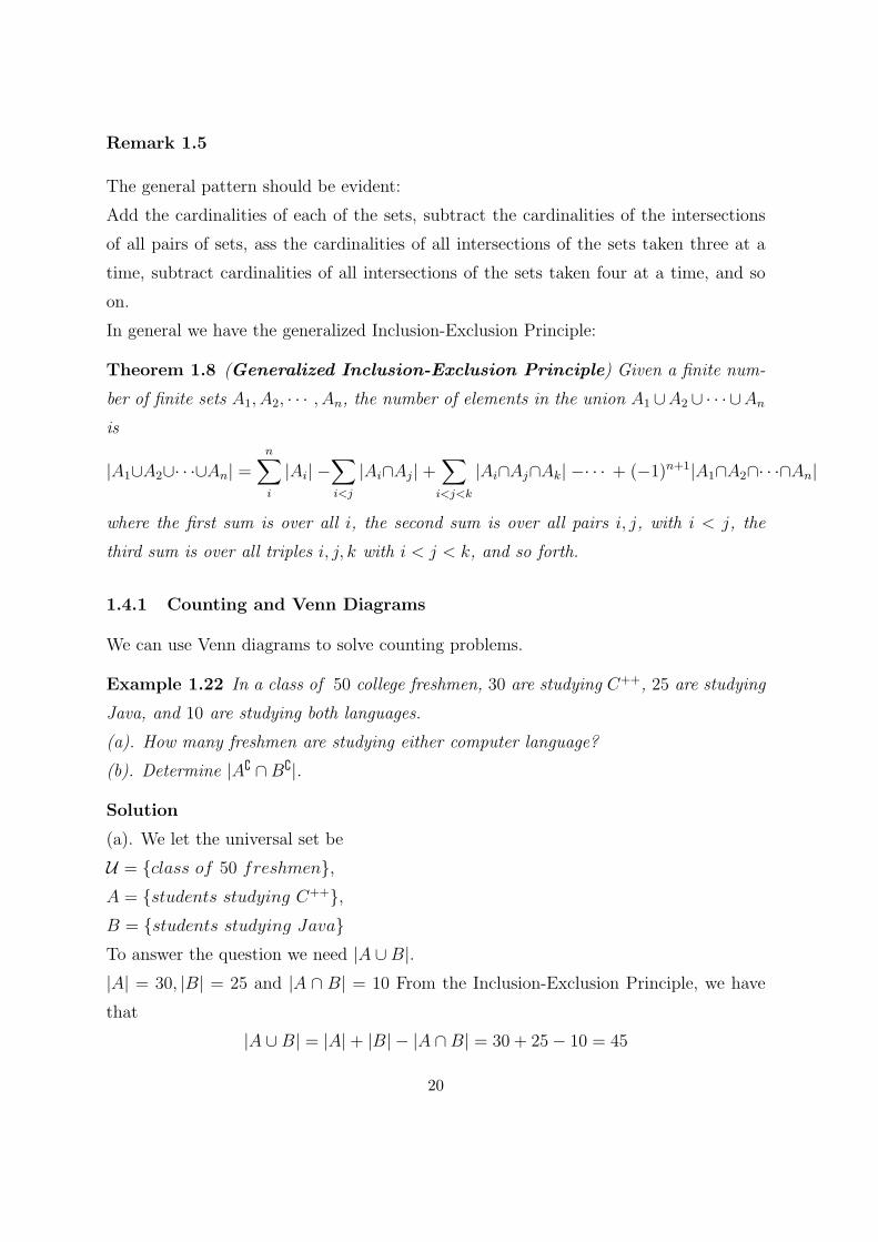
Example 1.22 In a class of 50 college freshmen, 30 are studying C++, 25 are studying
Java, and 10 are studying both languages.
(a). How many freshmen are studying either computer language?
(b). Determine |A{ ∩B{|.
Solution
(a). We let the universal set be
U = {class of 50 freshmen},A = {students studying C++},B = {students studying Java}To answer the question we need |A ∪B|.|A| = 30, |B| = 25 and |A ∩ B| = 10 From the Inclusion-Exclusion Principle, we have
that
|A ∪B| = |A|+ |B| − |A ∩B| = 30 + 25− 10 = 45
20
(b). By De Morgan’s Law A{ ∩B{ = (A ∪B){. Hence
|A{∩B{| = |(A∪B){| = |U|− |A∪B| = |U|− |A|− |B|+ |A∩B| = 50−30−25+10 = 5
Note that |A{∩B{| is the number of students who did not study any of the two languages.
This problem can be solved using a venn diagram.
Figure 1.11: Venn diagram Example 1.20
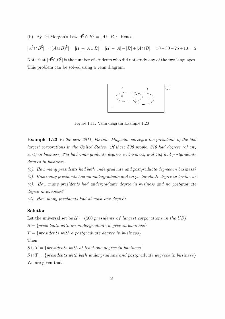
Example 1.23 In the year 2011, Fortune Magazine surveyed the presidents of the 500
largest corporations in the United States. Of these 500 people, 310 had degrees (of any
sort) in business, 238 had undergraduate degrees in business, and 184 had postgraduate
degrees in business.
(a). How many presidents had both undergraduate and postgraduate degrees in business?
(b). How many presidents had no undergraduate and no postgraduate degree in business?
(c). How many presidents had undergraduate degree in business and no postgraduate
degree in business?
(d). How many presidents had at most one degree?
Solution
Let the universal set be U = {500 presidents of largest corporations in the US}S = {presidents with an undergraduate degree in business}T = {presidents with a postgraduate degree in business}Then
S ∪ T = {presidents with at least one degree in business}S ∩ T = {presidents with both undergraduate and postgraduate degrees in business}We are given that
21
|S| = 238, |T | = 184, |S ∪ T | = 310
(a). The problem asks for |S ∩ T |. By the Inclusion-Exclusion Principle,
|S ∪ T | = |S|+ |T | − |S ∩ T |
Thus |S ∩ T | = |S|+ |T | − |S ∪ T | = 238 + 184− 310 = 112.
That is,exactly 112 of the presidents had both undergraduate and postgraduate degrees
in business.
(b). |S{ ∩ T {| = |(S ∪ T ){| = |U| − |S ∪ T | = 500− 310 = 190.
That is, exactly 190 of the presidents had no undergraduate degree and no postgraduate
degree in business.
The problem can be represented in A Venn diagram as below:
Figure 1.12: Venn diagram Example 1.21
(c). We need to find |S ∩ T {|. From the Venn diagram |S ∩ T {| = 126.
(d). At most one degree means either undergraduate or postgraduate degrees but not
both. We need to find |S △ T |. Clearly,
|S△T | = |(S−T )∪(T−S)| = |(S∪T )−(S∩T )| = |(S∪T )|−|(S∩T )| = 310−112 = 98
This result can also be obtained from the Venn diagram by adding the two numbers 126
and 72.
Example 1.24 Safaricom (Kenya Ltd) surveyed 400 of its customers to determine the
way they learned about the new Jibambie tariff. The survey shows that 180 learned
22
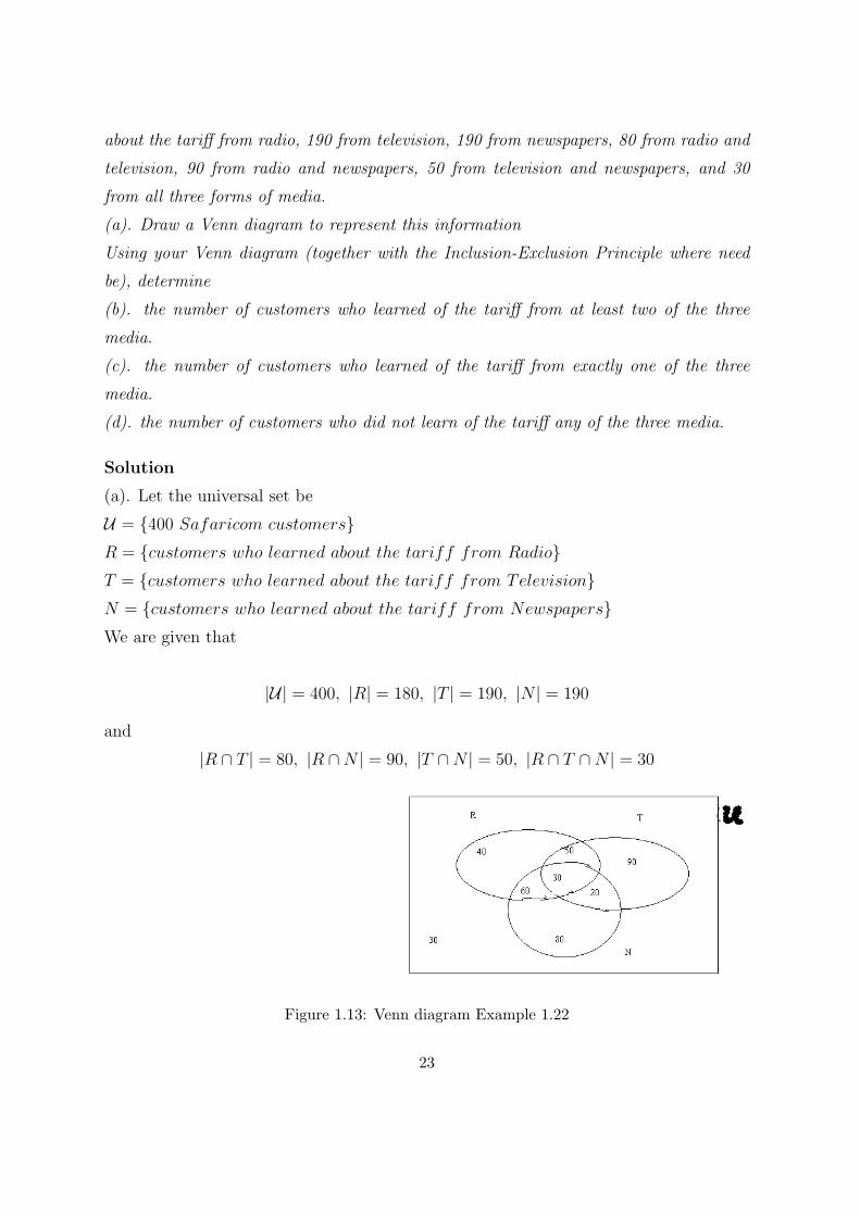
about the tariff from radio, 190 from television, 190 from newspapers, 80 from radio and
television, 90 from radio and newspapers, 50 from television and newspapers, and 30
from all three forms of media.
(a). Draw a Venn diagram to represent this information
Using your Venn diagram (together with the Inclusion-Exclusion Principle where need
be), determine
(b). the number of customers who learned of the tariff from at least two of the three
media.
(c). the number of customers who learned of the tariff from exactly one of the three
media.
(d). the number of customers who did not learn of the tariff any of the three media.
Solution
(a). Let the universal set be
U = {400 Safaricom customers}R = {customers who learned about the tariff from Radio}T = {customers who learned about the tariff from Television}N = {customers who learned about the tariff from Newspapers}We are given that
|U| = 400, |R| = 180, |T | = 190, |N | = 190
and
|R ∩ T | = 80, |R ∩N | = 90, |T ∩N | = 50, |R ∩ T ∩N | = 30
Figure 1.13: Venn diagram Example 1.22
23
b). At least two of the media means we add : 50,60, 20 and 30 to get 160. Thus exactly
160 customers learned of the tariff from at least two of the three media.
(c). Exactly one of the media means Radio only or Television only or Newspapers only.
From the Venn diagram we have: 40 + 90 + 80 = 210.
(d). We need |(R ∪ T ∪N){|. But
|(R ∪ T ∪N){| = |U − (R ∪ T ∪N)| = |U| − |R ∪ T ∪N | = 400− 370 = 30.
Example 1.25 Each of the 100 students in the first year of Open University’s Com-
puter Science Department studies at least one of the subsidiary subjects: mathematics,
electronics and accounting. Given that 65 study mathematics, 45 study electronics, 42
study accounting, 20 study mathematics and electronics, 25 study mathematics and ac-
counting, and 15 study electronics and accounting, find the number who study:
(a) all three subsidiary subjects;
(b) mathematics and electronics but not accounting;
(c) only electronics as a subsidiary subject.
Solution
Let U = {students in the first year of Utopias Computer Science Department}M = {students studying mathematics}E = {students studying electronics}A = {students studying accounting}.We are given the following information:
|U| = 100, |M | = 65, |E| = 45, |A| = 42, |M ∩ E| = 20, |M ∩ A| = 25, |E ∩ A| = 15.
Also, since every student takes at least one of three subjects as a subsidiary,
U = M ∪E ∪ A.
24
Let |M∩E∩A| = x. Figure 1.14 shows the cardinalities of the various disjoint subsets
of U . These are calculated as follows, beginning with the innermost region representing
M ∩ E ∩ A and working outwards in stages.
Figure 1.14: Venn diagram Example 1.22
By Counting Principle 1,
|M | = |M ∩ A ∩ E|+ |(M ∩ A)− E|
so
|(M ∩ A)− E| = |M ∩ A| − |M ∩ A ∩ E| = 25− x.
Similarly
|(M ∩ E)− A| = |M ∩ E| − |M ∩ E ∩ A| = 20− x
and
|(A ∩ E)−M | = |A ∩ E| − |M ∩ E ∩ A| = 15− x.
Now consider set M . By Counting Principle 2,
|M | = |M − (A ∪ E)|+ |(M ∩ A)− E|+ |(M ∩ E)− A|+ |M ∩ E ∩ A|
so
|M − (A ∪ E)| = |M | − |(M ∩ A)− E| − |(M ∩ E)− A| − |M ∩ E ∩ A|= 65− (25− x)− (20− x)− x
= 20 + x.
25
Similarly
|A− (M ∪ E)| = |A| − |(A ∩M)− E| − |(A ∩ E)−M | − |M ∩ E ∩ A|= 42− (25− x)− (15− x) + x
= 2 + x
and
|E − (M ∪ A)| = |E| − |(E ∩M)− A| − |(E ∩ A)−M | − |M ∩ E ∩ A|= 45− (20− x)− (15− x) + x
= 10 + x.
Now, using Counting Principle 2 again, |M ∪A∪E| = 100 is the sum of the cardinalities
of its seven disjoint subsets, so:
100 = (20 + x) + (2 + x) + (10 + x) + (25− x) + (20− x) + (15− x) + x
=⇒ 100 = 92 + x
=⇒ x = 8
This answers part (a).
We could now re-draw figure 1.14 showing the cardinality of each disjoint subset of
M ∪ A ∪ E. However, this is not necessary to answer the three parts of the question.
(b). The number of students who study mathematics and electronics but not accounting
is |(M ∩ E)− A| = 20− x = 20− 8 = 12.
(c). The number of students who study only electronics as a subsidiary subject is
|E − (M ∪ A)| = 10 + x = 10 + 8 = 18.
1.5 Real Number Systems
There are certain sets of numbers that appear frequently in set theory and in many
branches of mathematics. We begin this section by studying the decomposition of the
real line into the following subsets:
1.1 The Natural Numbers, N
N = {1, 2, 3, ...}
26

This set is also called the set of counting numbers.
Definition 1.10 A non-empty set X is said to be closed with respect to a binary oper-
ation ∗ if for all a, b ∈ X, we have a ∗ b ∈ X.
Note that N is closed with respect to the usual addition and usual multiplication but
not with respect to usual subtraction.
The set of natural numbers consists of the dark points on Fig. 1.15.
Figure 1.15: Set of Natural numbers
1.2 The Whole Numbers, W
W = {0, 1, 2, 3, ...}
Note that W = {0} ∪ N.Note that W is closed with respect to usual addition and multiplication but not under
subtraction.
The set of whole numbers consist of the numbers represented by the dark dots in Fig
1.16
Figure 1.16: Set of Whole numbers
1.3 The Integers, Z
Z = {...,−3,−2,−1, 0, 1, 2, 3, ...}
Note that Z = −N ∪W.
This system guarantees solutions to every equation x+ n = m with n,m ∈ W. Clearly,
27
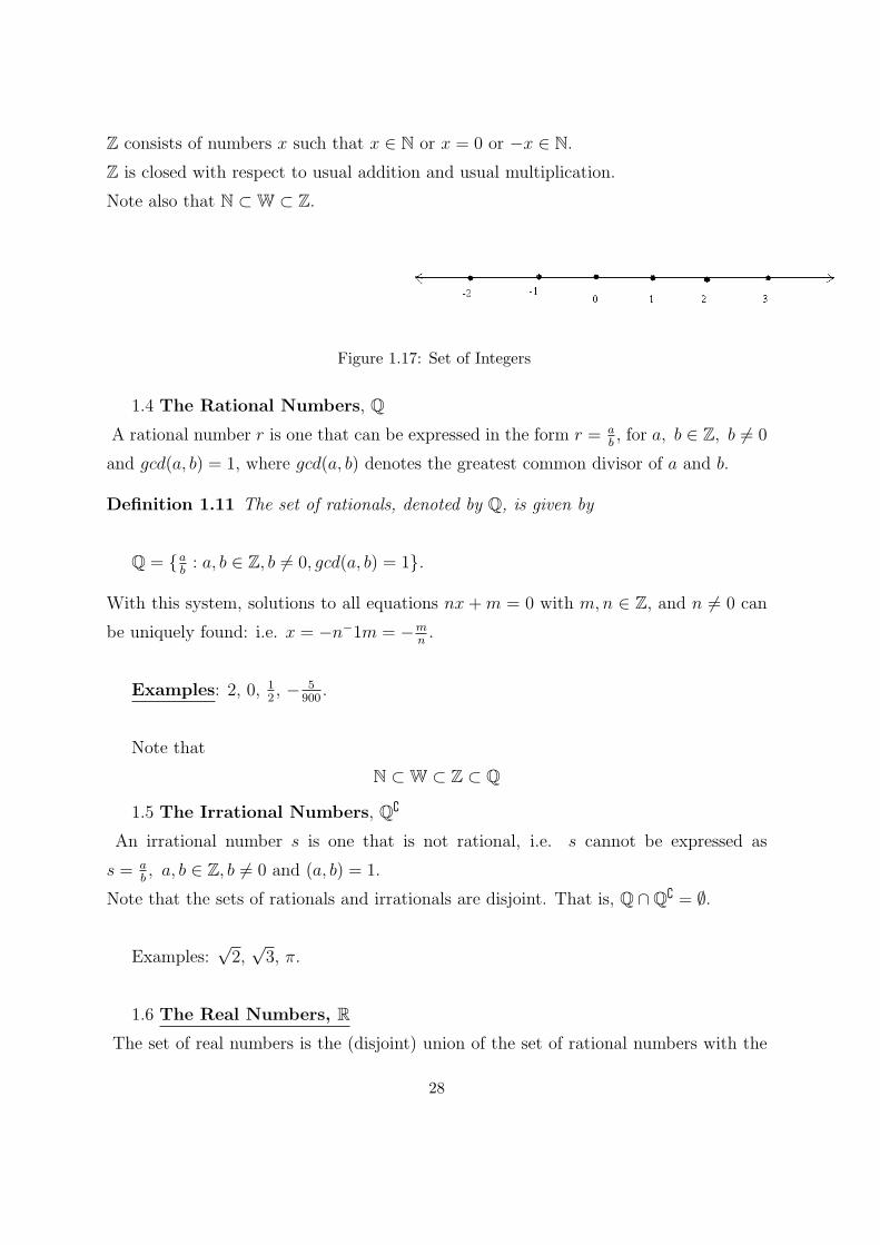
Z consists of numbers x such that x ∈ N or x = 0 or −x ∈ N.Z is closed with respect to usual addition and usual multiplication.
Note also that N ⊂ W ⊂ Z.
Figure 1.17: Set of Integers
1.4 The Rational Numbers, QA rational number r is one that can be expressed in the form r = a
b, for a, b ∈ Z, b ̸= 0
and gcd(a, b) = 1, where gcd(a, b) denotes the greatest common divisor of a and b.
Definition 1.11 The set of rationals, denoted by Q, is given by
Q = {ab: a, b ∈ Z, b ̸= 0, gcd(a, b) = 1}.
With this system, solutions to all equations nx +m = 0 with m,n ∈ Z, and n ̸= 0 can
be uniquely found: i.e. x = −n−1m = −mn.
Examples: 2, 0, 12, − 5
900.
Note that
N ⊂ W ⊂ Z ⊂ Q
1.5 The Irrational Numbers, Q{
An irrational number s is one that is not rational, i.e. s cannot be expressed as
s = ab, a, b ∈ Z, b ̸= 0 and (a, b) = 1.
Note that the sets of rationals and irrationals are disjoint. That is, Q ∩Q{ = ∅.
Examples:√2,
√3, π.
1.6 The Real Numbers, RThe set of real numbers is the (disjoint) union of the set of rational numbers with the
28
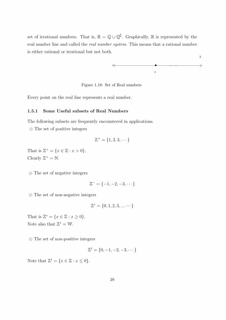
set of irrational numbers. That is, R = Q ∪ Q{. Graphically, R is represented by the
real number line and called the real number system. This means that a rational number
is either rational or irrational but not both.
Figure 1.18: Set of Real numbers
Every point on the real line represents a real number.
1.5.1 Some Useful subsets of Real Numbers
The following subsets are frequently encountered in applications.
⊙ The set of positive integers
Z+ = {1, 2, 3, · · · }
That is Z+ = {x ∈ Z : x > 0}.Clearly Z+ = N.
⊙ The set of negative integers
Z− = {−1,−2,−3, · · · }
⊙ The set of non-negative integers
Z∗ = {0, 1, 2, 3, ... · · · }
That is Z∗ = {x ∈ Z : x ≥ 0}.Note also that Z∗ = W.
⊙ The set of non-positive integers
Z† = {0,−1,−2,−3, · · · }
Note that Z† = {x ∈ Z : x ≤ 0}.
29
⊙ The set of positive rational numbers
Q+ = {x ∈ Q : x > 0}
⊙ The set of negative rational numbers
Q− = {x ∈ Q : x < 0}
⊙ The set of non-negative rational numbers
Q∗ = {x ∈ Q : x ≥ 0}
⊙ The set of non-positive rational numbers
Q† = {x ∈ Q : x ≤ 0}
⊙ The set of positive real numbers
R+ = {x ∈ R : x > 0}
⊙ The set of negative real numbers
R− = {x ∈ R : x < 0}
1.5.2 Intervals
Bounded intervals
Let a, b ∈ R and suppose that a < b. We define the following special sets called
intervals.
1. [a, b] = {x ∈ R : a ≤ x ≤ b}, called the closed interval between a and b.
2. (a, b) = {x ∈ R : a < x < b}, called the open interval between a and b.
3. (a, b] = {x ∈ R : a < x ≤ b} and [a, b) = {x ∈ R : a ≤ x < b} called the
half-open intervals between a and b.
30
These intervals are bounded since both a and b are real numbers.
Unbounded intervals
We define unbounded intervals:
4. [a,∞) = {x ∈ R : x ≥ a}
5. (a,∞) = {x ∈ R : x > a}
6. (−∞, b] = {x ∈ R : x ≤ b}
7. (−∞, b) = {x ∈ R : x < b}
Remark 1.6
We define (−∞,∞) = R. We also caution that −∞ and ∞ are not real numbers but ab-
stract symbols we use to symbolize ”smallest” and ”largest” real numbers, respectively.
The Extended Real Number System is obtained by adjoining a largest element ∞ and
a smallest element −∞, to the real line R to get:
R♯ = R ∪ {−∞,∞}
Definition 1.12 Let I be a nonempty set and U be a universal set. For each i ∈ I let
Ai ⊆ U . Then I is called an indexing set (or set of indices), and each i ∈ I is
called an index.
Under these conditions∪i∈I
Ai = {x : x ∈ Ai for at least one i ∈ I}
∩i∈I
Ai = {x : x ∈ Ai for every i ∈ I}
If the indexing set I is the set Z+ or N, we can write∪i∈Z+
Ai = A1 ∪ A2 ∪ · · · =∞∪i=1
Ai
31
and ∩i∈Z+
Ai = A1 ∩ A2 ∩ · · · =∞∩i=1
Ai
Example 1.26 Let I = {3, 4, 5, 6, 7}, and for each i ∈ I let Ai = {, 2, 3, ..., i} ⊆ U =
Z+.
Find
(a)∪i∈Z+
Ai
(b)∩i∈Z+
Ai
Solution (a). Note that
∪i∈I
Ai = A1 ∪ A2 ∪ · · · ∪ A7 =7∪
i=3
Ai = {1, 2, 3, 4, 5, 6, 7} = A7
(b). Clearly ∩i∈I
Ai = A1 ∩ A2 ∩ · · · ∩ A7 =7∩
i=3
Ai = {1, 2, 3} = A3
Example 1.27 Let U = R and I = R+. For each r ∈ R+, define Ar = [−r, r].Determine
(a)∪r∈I
Ar
(b)∩iI
Ar
Solution (a). It is easy to show that ∪r∈I
Ar = R
(b). ∩r∈I
Ar = {0}
Example 1.28 Let U = R and let I = N. For each n ∈ N, let An = [−2n, 3n].
Determine
(a). A3 − A4
32
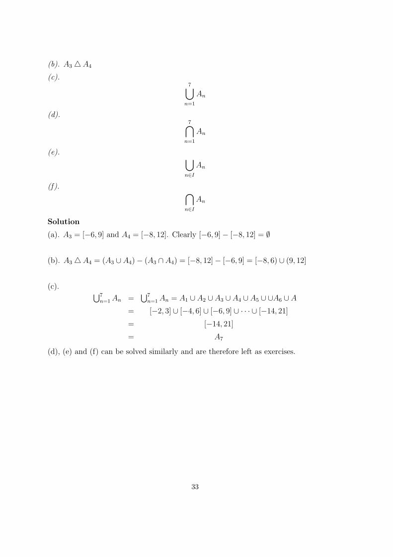
(b). A3 △ A4
(c).7∪
n=1
An
(d).7∩
n=1
An
(e). ∪n∈I
An
(f). ∩n∈I
An
Solution
(a). A3 = [−6, 9] and A4 = [−8, 12]. Clearly [−6, 9]− [−8, 12] = ∅
(b). A3 △ A4 = (A3 ∪ A4)− (A3 ∩ A4) = [−8, 12]− [−6, 9] = [−8, 6) ∪ (9, 12]
(c). ∪7n=1An =
∪7n=1An = A1 ∪ A2 ∪ A3 ∪ A4 ∪ A5 ∪ ∪A6 ∪ A
= [−2, 3] ∪ [−4, 6] ∪ [−6, 9] ∪ · · · ∪ [−14, 21]
= [−14, 21]
= A7
(d), (e) and (f) can be solved similarly and are therefore left as exercises.
33
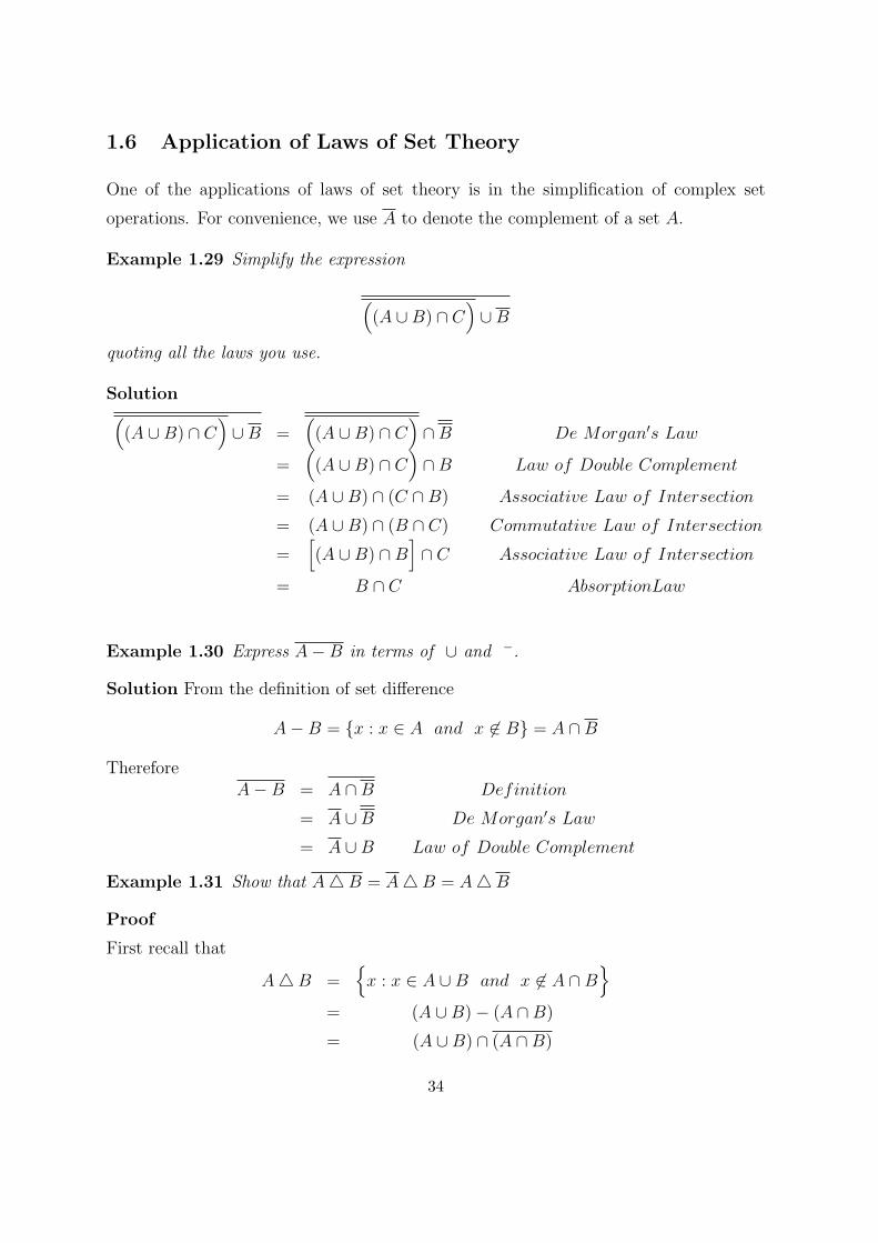
1.6 Application of Laws of Set Theory
One of the applications of laws of set theory is in the simplification of complex set
operations. For convenience, we use A to denote the complement of a set A.
Example 1.29 Simplify the expression
((A ∪B) ∩ C
)∪B
quoting all the laws you use.
Solution((A ∪B) ∩ C
)∪B =
((A ∪B) ∩ C
)∩B De Morgan′s Law
=((A ∪B) ∩ C
)∩B Law of Double Complement
= (A ∪B) ∩ (C ∩B) Associative Law of Intersection
= (A ∪B) ∩ (B ∩ C) Commutative Law of Intersection
=[(A ∪B) ∩B
]∩ C Associative Law of Intersection
= B ∩ C AbsorptionLaw
Example 1.30 Express A−B in terms of ∪ and −.
Solution From the definition of set difference
A−B = {x : x ∈ A and x ̸∈ B} = A ∩B
ThereforeA−B = A ∩B Definition
= A ∪B De Morgan′s Law
= A ∪B Law of Double Complement
Example 1.31 Show that A△B = A△B = A△B
Proof
First recall that
A△B ={x : x ∈ A ∪B and x ̸∈ A ∩B
}= (A ∪B)− (A ∩B)
= (A ∪B) ∩ (A ∩B)
34
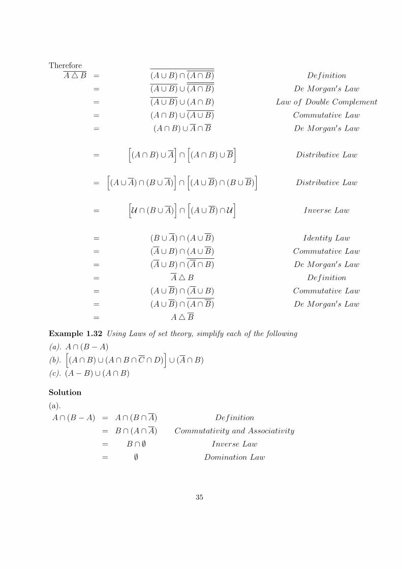
ThereforeA△B = (A ∪B) ∩ (A ∩B) Definition
= (A ∪B) ∪ (A ∩B) De Morgan′s Law
= (A ∪B) ∪ (A ∩B) Law of Double Complement
= (A ∩B) ∪ (A ∪B) Commutative Law
= (A ∩B) ∪ A ∩B De Morgan′s Law
=[(A ∩B) ∪ A
]∩[(A ∩B) ∪B
]Distributive Law
=[(A ∪ A) ∩ (B ∪ A)
]∩[(A ∪B) ∩ (B ∪B)
]Distributive Law
=[U ∩ (B ∪ A)
]∩[(A ∪B) ∩ U
]Inverse Law
= (B ∪ A) ∩ (A ∪B) Identity Law
= (A ∪B) ∩ (A ∪B) Commutative Law
= (A ∪B) ∩ (A ∩B) De Morgan′s Law
= A△B Definition
= (A ∪B) ∩ (A ∪B) Commutative Law
= (A ∪B) ∩ (A ∩B) De Morgan′s Law
= A△B
Example 1.32 Using Laws of set theory, simplify each of the following
(a). A ∩ (B − A)
(b).[(A ∩B) ∪ (A ∩B ∩ C ∩D)
]∪ (A ∩B)
(c). (A−B) ∪ (A ∩B)
Solution
(a).
A ∩ (B − A) = A ∩ (B ∩ A) Definition
= B ∩ (A ∩ A) Commutativity and Associativity
= B ∩ ∅ Inverse Law
= ∅ Domination Law
35
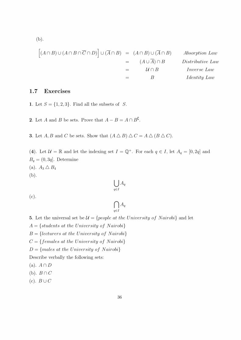
(b).[(A ∩B) ∪ (A ∩B ∩ C ∩D)
]∪ (A ∩B) = (A ∩B) ∪ (A ∩B) Absorption Law
= (A ∪ A) ∩B Distributive Law
= U ∩B Inverse Law
= B Identity Law
1.7 Exercises
1. Let S = {1, 2, 3}. Find all the subsets of S.
2. Let A and B be sets. Prove that A−B = A ∩B{.
3. Let A,B and C be sets. Show that (A△B)△ C = A△ (B △ C).
(4). Let U = R and let the indexing set I = Q+. For each q ∈ I, let Aq = [0, 2q] and
Bq = (0, 3q]. Determine
(a). A3 △B4
(b). ∪q∈I
Aq
(c). ∩q∈I
Aq
5. Let the universal set be U = {people at the University of Nairobi} and let
A = {students at the University of Nairobi}B = {lecturers at the University of Nairobi}C = {females at the University of Nairobi}D = {males at the University of Nairobi}Describe verbally the following sets:
(a). A ∩D(b). B ∩ C(c). B ∪ C
36
(d). A ∪ C(e). (A ∩D){
5. A large corporation classifies its many divisions by their performance in the preceding
year. Let
P = {divisions that made a profit}L = {divisions that had an increase in labour}T = {divisions whose total revenue increased}Describe symbolically the following sets:
(a). {divisions that had increases in labour costs or total revenue}(b). {divisions that did not make a profit}(c). {divisions that made a profit despite an increase in labour costs}(d). {divisions that had an increase in labour costs and either were unprofitableor did not increase their total revenue}(e). {profitable divisions with increases in labour costs and total revenue}(f). {profitable divisions that were unprofitable or did not have increasesin either labour costs or total revenue}
6. Prove by the Elements Argument method that
(a). A− (A ∩B) = A ∩B(b).
((A ∩B) ∪ C
)= (A ∪ C) ∪ (B ∪ C)
(c). A ∪ (B ∩ C) = (C ∪B) ∩ A
7. Let A = {0, 1}, B = {1, 2} and C = {0, 1, 2}. Find(a). A×B
(b). A×B × C
(c). |A×B × C|
8. Let A and B be non-empty sets. Prove that A×B = B × A if and only if A = B.
9. Draw Venn diagrams for each of the following sets. Shade the region corresponding
to each set.
37
(a). A ∩ (B ∪ C)(b). A ∩B ∩ C(c). A− (A−B)
10. In a survey of 1000 households, 275 owned a home computer, 455 a video, 405
two cars, and 265 households owned neither a home computer nor a video nor two cars.
Given that 145 households owned both a home computer and a video, 195 both a video
and two cars, and 110 both two cars and a home computer, find the number of house-
holds surveyed which owned
(a). a home computer, a video and two cars.
(b). a video only.
(c). two cars, a video but not a home computer.
(d). a video, a home computer but not two cars.
10. In a survey conducted on campus, it was found that students like watching the
Barclays Premier League teams: ManU, Chelsea and Arsenal. It was also found that
every student who is a fan of Arsenal is also a fan of ManU or Chlesea (or both), and 42
students were fans of ManU, 45 were fans of Chelsea, 7 where fans of both ManU and
Chelsea, 11 were fans of of both ManU and Arsenal, 28 were fans of both Chelsea and
Arsenal, and twice as many students were fans only of ManU as those who were fans
only of Chelsea.
Find the number of students in the survey who were fans of
(a). all three football clubs
(b). Arsenal
(c). only ManU.
11. Let A,B and C be sets.
(a). Prove that |A∪B∪C| = |A|+ |B|+ |C|− |A∩B|− |B∩C|− |C ∩A|+ |A∩B∩C|.(b). Determine |A ∪B ∪ C| when |A| = 100, |B| = 200 and |C| = 3000 if
(i). A ⊆ B ⊆ C.
(ii). A ∩B = A ∩ C = B ∩ C = ∅.
38
12. Given that |A| = 55, |B| = 40, |C| = 80, |A∩B| = 20, |A∩B∩C| = 17, |B∩C| = 24
and |A ∪ C| = 100, find
(a). |A ∩ C|(b). |C −B|(c). |(B ∩ C)− (A ∩B ∩ C)|
13. Find the following power sets
(a). P(∅)(b). P(P(∅))(c). P({∅}, {1, 2})
1.8 Complex Numbers
The last great extension of the real number system is to the set of complex numbers.
The need for complex numbers must have been felt from the time that the formula for
solving quadratic equations was discovered, especially due to the existence of square
roots of negative numbers. The use of complex numbers simplifies many problems from
the convergence of series to the evaluation of definite integrals. The set of real numbers
might seem to be a large enough set of numbers to answer all our mathematical questions
adequately. However, there are some natural mathematical questions that have no solu-
tion if answers are restricted to be real numbers. In particular, many simple equations
have no solution in the realm of real numbers. For example, x2 + 1 = 0. A solution
would require a number whose square is 1. For many centuries, mathematicians were
content with the answer, ”there is no such number.” Eventually, it became acceptable
to allow existence of a number i, called the imaginary unit, such that i2 = −1.
Definition 1.13 The set of complex numbers, denoted by C is defined as
C = {x+ iy : x, y ∈ R and i2 = −1}
Clearly R is a subset of C, since x+ 0i = x is a real number for every x.
N ⊆ W ⊆ Z ⊆ Q ⊆ R ⊆ C
39
1.8.1 Arithmetic Operations of Complex Numbers
Addition and multiplication of complex numbers are defined by
(a± bi) + (c± di) = (a) + (b± d)i
(a+ bi).(c+ di) = ac+ adi+ bci+ bdi2 = (ac− bd) + (ad+ bc)i
Addition, subtraction and multiplication of complex numbers is generally quite straight-
forward, requiring little more than the application of elementary algebra. However, di-
vision of complex numbers is not straightforward. We need to develop the theory to
enable us carry out division of complex numbers.
Definition 1.14 Let z = x + iy be a complex number. x is called the real part of z,
and denoted by Re(z), while y is the imaginary part of z, denoted by Im(z).
Two complex numbers are equal if and only if they have the same real part and the
same imaginary part. Let z = x+ iy be a complex number. If x = 0, then z is said to
be purely imaginary. If y = 0, then z is real. Note that 0 is the only number which
is at once real and purely imaginary.
Example 1.33 Let z1 = 2 + 3i and z2 = 4 + i. Find
(a). z1 + z2
(b). z1.z2
Solution
(a). z1 + z2 = (2 + 3i) + (4 + i) = (2 + 4) + (3 + 4)i = 6 + 7i
(b). z1.z2 = (2 + 3i).(4 + i) = 8 + 14i+ 3i2 = 8 + 14i− 3 = 5 + 14i
Example 1.34 Simplify, leaving your answer in the form a+ bi, a, b ∈ R(a). 5i4
(b).(8i)3
Solution
(a). 5i4 = 5i2.i2 = 5(−1)(−1) = 5
(b). (8i)3 = (8i).(8i).(8i) = 512i3 = 512i2.i = 512(−1)i = −512i
40
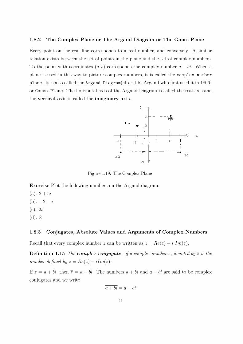
1.8.2 The Complex Plane or The Argand Diagram or The Gauss Plane
Every point on the real line corresponds to a real number, and conversely. A similar
relation exists between the set of points in the plane and the set of complex numbers.
To the point with coordinates (a, b) corresponds the complex number a + bi. When a
plane is used in this way to picture complex numbers, it is called the complex number
plane. It is also called the Argand Diagram(after J.R. Argand who first used it in 1806)
or Gauss Plane. The horizontal axis of the Argand Diagram is called the real axis and
the vertical axis is called the imaginary axis.
Figure 1.19: The Complex Plane
Exercise Plot the following numbers on the Argand diagram:
(a). 2 + 5i
(b). −2− i
(c). 2i
(d). 8
1.8.3 Conjugates, Absolute Values and Arguments of Complex Numbers
Recall that every complex number z can be written as z = Re(z) + i Im(z).
Definition 1.15 The complex conjugate of a complex number z, denoted by z is the
number defined by z = Re(z)− iIm(z).
If z = a + bi, then z = a − bi. The numbers a + bi and a − bi are said to be complex
conjugates and we write
a+ bi = a− bi
41
Theorem 1.9 For any complex conjugate numbers w and z.
(a). w + z = w + z
(b). w − z = w − z
(c). wz = w.z
(c). wz= w
z
(d). z = z
(f). z is real if and only if z = z
(d). z is purely imaginary if and only if z = −z(e). Re(z) = 1
2(z + z)
(f). Im(z) = 12i(z − z)
Remark 1.7
So far we are able to add and multiply complex numbers. When evaluating the quotient
of complex numbers a+bic+di
, we multiply both the numerator and denominator by the
complex conjugate of the denominator and simplify . This process is called complex
rationalization.
Example 1.35 Simplify the following, leaving your answer in the form a+bi, a, b ∈ R.(a). 5+2i
3+4i
(b). 5+2ii
Solution
(a). 5+2i3+4i
= (5+2i)(3−4i)(3+4i)(3−4i)
= 2325
− 1425
(b). 5+2ii
= (5+2i)(−i)(i)(−i)
= 2− 5i
Definition 1.16 If z = Re(z) + i Im(z) is a complex number, we define the absolute
value of z, denoted by |z| by
|z| =√(
Re(z))2
+(Im(z)
)2
,
where the square radical√
denotes the unique nonnegative square root.
This real number is also called the modulus of z. If z = a + bi, then |z| =√a2 + b2
and we write |a+ bi| =√a2 + b2.
42
Example 1.36 Let z = 4 + 3i. Find |z|.
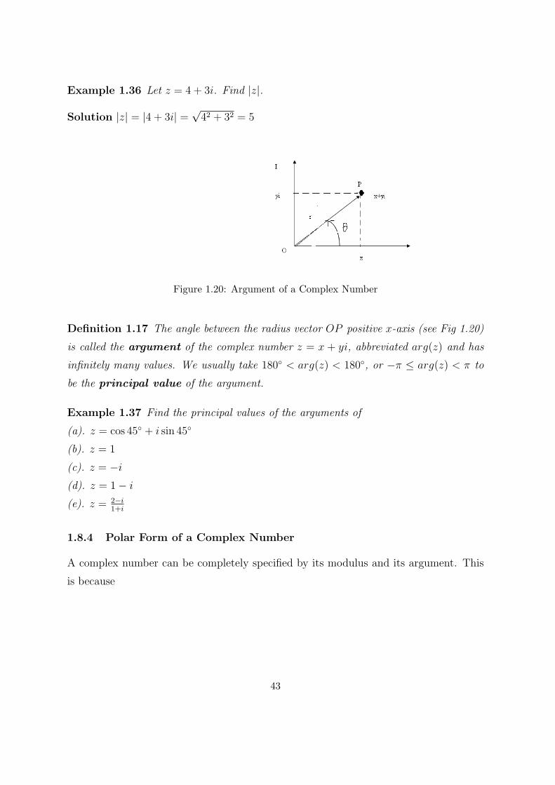
Solution |z| = |4 + 3i| =√42 + 32 = 5
Figure 1.20: Argument of a Complex Number
Definition 1.17 The angle between the radius vector OP positive x-axis (see Fig 1.20)
is called the argument of the complex number z = x + yi, abbreviated arg(z) and has
infinitely many values. We usually take 180◦ < arg(z) < 180◦, or −π ≤ arg(z) < π to
be the principal value of the argument.
Example 1.37 Find the principal values of the arguments of
(a). z = cos 45◦ + i sin 45◦
(b). z = 1
(c). z = −i(d). z = 1− i
(e). z = 2−i1+i
1.8.4 Polar Form of a Complex Number
A complex number can be completely specified by its modulus and its argument. This
is because
43
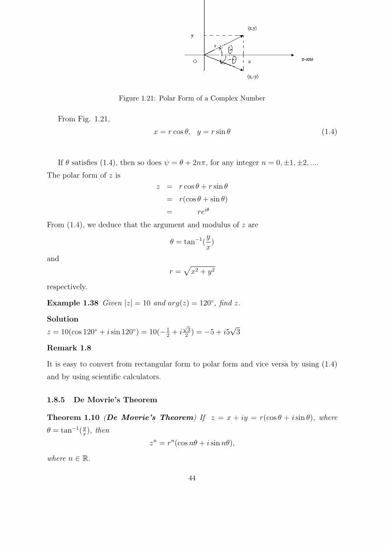
Figure 1.21: Polar Form of a Complex Number
From Fig. 1.21,
x = r cos θ, y = r sin θ (1.4)
If θ satisfies (1.4), then so does ψ = θ + 2nπ, for any integer n = 0,±1,±2, ....
The polar form of z is
z = r cos θ + r sin θ
= r(cos θ + sin θ)
= reiθ
From (1.4), we deduce that the argument and modulus of z are
θ = tan−1(y
x)
and
r =√x2 + y2
respectively.
Example 1.38 Given |z| = 10 and arg(z) = 120◦, find z.
Solution
z = 10(cos 120◦ + i sin 120◦) = 10(−12+ i
√32) = −5 + i5
√3
Remark 1.8
It is easy to convert from rectangular form to polar form and vice versa by using (1.4)
and by using scientific calculators.
1.8.5 De Movrie’s Theorem
Theorem 1.10 (De Movrie’s Theorem) If z = x + iy = r(cos θ + i sin θ), where
θ = tan−1( yx), then
zn = rn(cosnθ + i sinnθ),
where n ∈ R.
44
Proof De Moivre’s formula can be derived from Euler’s identity
eiθ = cos θ + i sin θ
and the exponential law
(eiθ)n = einθ
Thus (reiθ)n = rneinθ = rn cosnθ + irn sinnθ = rn(cosnθ + i sinnθ)
Remark 1.9
This formula (named after Abrahame de Moivre, 1667-1754) is useful in finding explicit
expressions for the n-th roots of complex numbers and more specifically n-th roots of
unity, which are complex numbers z such that zn = 1. The following are useful identities
⊙ e2nπi = 1
⊙ eπi2 = i
⊙ eπi = −1
If z is a complex number, written in polar form as
z = r(cos θ + i sin θ)
then
z1n =
[r(cos θ + i sin θ)
] 1n= r
1n
[cos
(θ + 2kπ
n
)+ i sin
(θ + 2kπ
n
)]where k is an integer. To get the n different roots of z one only needs to consider values
of k from 0 to n− 1. That is, k = 0, 1, 2, ..., n− 1.
If k = 0, then
r1n
[cos
( θn
)+ i sin
( θn
)]is called the principal n-th root of z.
The roots of unity are evenly distributed around the circle centered at the origin of
radius 1, starting with the first (real) root at 1 + 0i.
Example 1.39 Let z = 1+ i. Find z100, leaving your answer in the form a+bi a, b ∈R.
45
Example 1.40 Find the square roots of the complex number z = 9 + 9i. Leave your
answer in the form a+ bi a, b ∈ R.
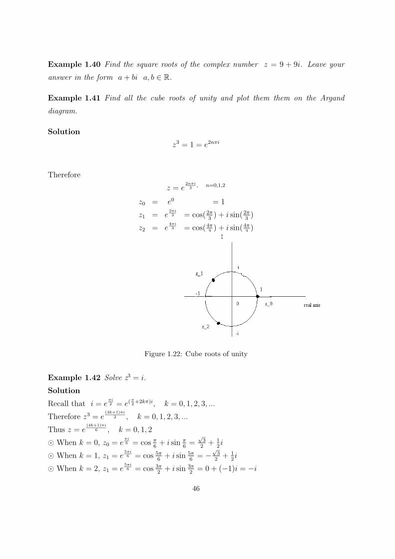
Example 1.41 Find all the cube roots of unity and plot them them on the Argand
diagram.
Solution
z3 = 1 = e2nπi
Therefore
z = e2nπi3
, n=0,1,2
z0 = e0 = 1
z1 = e2πi3 = cos(2π
3) + i sin(2π
3)
z2 = e4πi3 = cos(4π
3) + i sin(4π
3)
Figure 1.22: Cube roots of unity
Example 1.42 Solve z3 = i.
Solution
Recall that i = eπi2 = e(
π2+2kπ)i, k = 0, 1, 2, 3, ...
Therefore z3 = e(4k+1)πi
2 , k = 0, 1, 2, 3, ...
Thus z = e(4k+1)πi
6 , k = 0, 1, 2
⊙ When k = 0, z0 = eπi6 = cos π
6+ i sin π
6=
√32+ 1
2i
⊙ When k = 1, z1 = e5πi6 = cos 5π
6+ i sin 5π
6= −
√32+ 1
2i
⊙ When k = 2, z1 = e5πi6 = cos 3π
2+ i sin 3π
2= 0 + (−1)i = −i
46
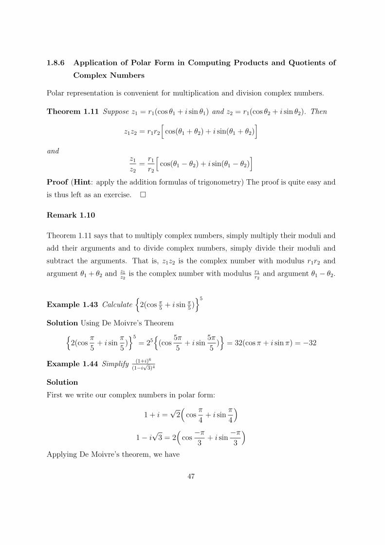
1.8.6 Application of Polar Form in Computing Products and Quotients of
Complex Numbers
Polar representation is convenient for multiplication and division complex numbers.
Theorem 1.11 Suppose z1 = r1(cos θ1 + i sin θ1) and z2 = r1(cos θ2 + i sin θ2). Then
z1z2 = r1r2
[cos(θ1 + θ2) + i sin(θ1 + θ2)
]and
z1z2
=r1r2
[cos(θ1 − θ2) + i sin(θ1 − θ2)
]Proof (Hint: apply the addition formulas of trigonometry) The proof is quite easy and
is thus left as an exercise. �
Remark 1.10
Theorem 1.11 says that to multiply complex numbers, simply multiply their moduli and
add their arguments and to divide complex numbers, simply divide their moduli and
subtract the arguments. That is, z1z2 is the complex number with modulus r1r2 and
argument θ1 + θ2 andz1z2
is the complex number with modulus r1r2
and argument θ1 − θ2.
Example 1.43 Calculate{2(cos π
5+ i sin π
5)}5
Solution Using De Moivre’s Theorem{2(cos
π
5+ i sin
π
5)}5
= 25{(cos
5π
5+ i sin
5π
5)}= 32(cosπ + i sin π) = −32
Example 1.44 Simplify (1+i)6
(1−i√3)4
Solution
First we write our complex numbers in polar form:
1 + i =√2(cos
π
4+ i sin
π
4
)1− i
√3 = 2
(cos
−π3
+ i sin−π3
)Applying De Moivre’s theorem, we have
47
(1 + i)6 = 8(cos
3π
2+ i sin
3π
2
)(1− i
√3)4 = 16
(cos
−4π
3+ i sin
−4π
3
)Hence
(1+i)6
(1−i√3)4
= 816
(cos(3π
2+ 4π
3) + i sin(3π
2+ 4π
3))
= 12
(cos(17π
6) + i sin(17π
6))
1.9 Exercises
1. Given that z = 3 + 4i and w = 12 + 5i, write down the moduli and arguments of
(a). z
(b). 1z
(c). zw
(c). zw
(d). w2
2. Simplify, leaving your answer in the form a+ bi, a, b ∈ R.(a). (1 + i)2
(b). (2− 2i)100
(c). 6+6i3+4i
(d). (3−3i)4
(√3+i)3
3. Find the values of a and b such that (a + ib)2 = i. Hence, or otherwise, solve the
equation z2 + 2z + 1− i = 0, leaving your answers in the form a+ bi, a, b ∈ R.
4. Let z = cos θ + i sin θ, where θ is real.
(a). Show that1
1 + z=
1
2
(1− i tan
θ
2
)(b). Express the following in the form a+ ib, where a and b are real functions of θ.
(i). 2z1+z2
48
(ii). 1−z2
1+z2
5. Mark on the Argand diagram the points representing the complex numbers
(a). 4 + 3i
(b). 4− 8i
(c). 4+3i4−3i
6. Find
(a). the square roots of z = 5 + 12i
(b). the 8th roots of unity.
7. Prove that the modulus of 2 + cos θ + i sin θ is (5 + 4 cos θ)12 . Hence show that the
modulus of
2 + cos θ + i sin θ
2 + cos θ − i sin θ
is 1.
49
Chapter 2
ELEMENTARY LOGIC
2.1 Introduction
Mathematical logic is the study of the processes used in mathematical deduction. The
subject has origins in philosophy, and indeed it is also a legacy from philosophy that we
can distinguish semantic reasoning (what is true) from syntactic reasoning (what can be
shown). Logic is used to establish the validity of arguments. The rules of logic give pre-
cise meaning to mathematical statements. In addition to mathematical reasoning, logic
has numerous applications in the design of computer circuits, construction of computer
programs, verification of correctness of computer programs, and so on.
2.2 Mathematical Reasoning and Creativity
Human beings are expected to express themselves creatively in various fields. Mathemat-
ics is one of these fields, not just because of its nature but the manner of its presentation.
2.2.1 Inductive and Deductive Reasoning
Reasoning, or drawing conclusions can be classified in tow categories, namely inductive
reasoning and deductive reasoning. When a person makes observations and on the
basis of these observations reaches conclusions, he/she is said to reason inductively.
For example, a young child touches a hot stove and concludes that stoves are hot. De-
50
ductive reasoning proceeds from assumptions rather than experience.
It is usually by inductive reasoning that mathematical results are discovered, and it is
by deductive reasoning that they are proved.
Inductive Reasoning
Inductive reasoning is essential to mathematical activity. To engage in it, one makes
observations, gets hunches, guesses, or makes conjectures.
Example 2.1 Given the sequence
2, 4, 6, 8,−
find the next number.
Solution It is probably 10, etc.
Deductive Reasoning
Arguments used in mathematical proofs most often proceed from some basic principles
which are known or assumed. Such arguments are deductive.
Definition 2.1 A proof is simply a convincing argument, a sequence of steps, an ex-
planation and communication of ideas; a line of argument sufficient to convince a person
of the validity of a certain result.
As we shall find out, a disproof is also a proof.
Example 2.2 If a figure is a triangle, then it is a polygon. Figure X is a triangle.
What conclusion can be drawn?
2.3 propositional Logic
In this section an elementary system of symbolic logic called propositional logic is pre-
sented. This system is built around propositions or statements.
2.3.1 Propositions and Truth Values
One of the basic ideas of logic is that of a proposition.
51
Definition 2.2 A proposition is a declarative sentence, assertion which is capable of
being classified as either true or false but not both.
Propositions are sometimes called statements.
Example 2.3 Examples of propositions are:
1. It is raining
2. 3 + 2 = 4
3. Nairobi is the capital city of Rwanda
4. 6 < 24
5. Tomorrow is my birthday
Remark 2.1
Note that the same proposition may be sometimes be true and sometimes false depending
on where and when it was stated and by whom. Whilst proposition 5 is true when
stated by anyone whose birthday is tomorrow is true, it is false when stated by anyone
else. Exclamations, questions and demands are not propositions since they can not be
classified/declared as either true or false.
Example 2.4 The following are not propositions
6. Come here !
7. Keep off the grass
8. Long live the Queen !
9. Did you finish your homework?
10. Don’t say that.
Definition 2.3 (Truth Values of a Proposition) The truth or falsity of a proposi-
tion is called truth value. The truth value of a proposition is either true or false but
not both. We denote the truth vales of propositions by T or F .
Propositions are conventionally symbolized using letters a, b, c, ... or A,B,C, ....
52
2.3.2 Logical Connectives and Truth Tables
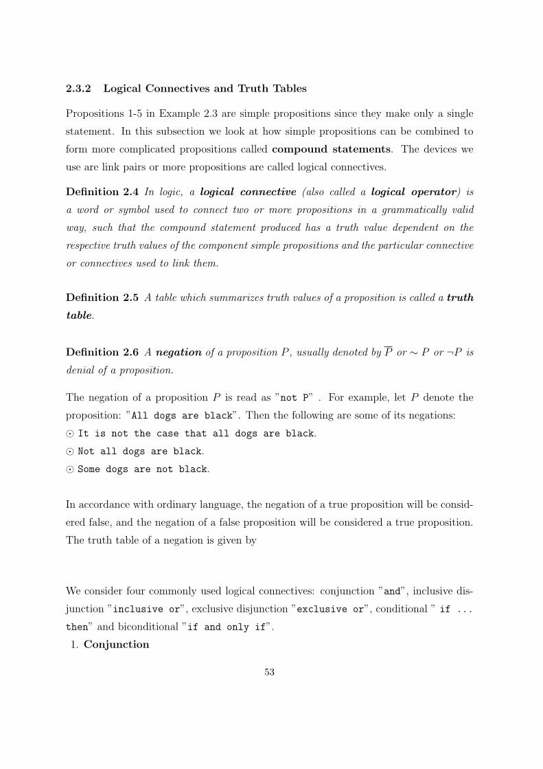
Propositions 1-5 in Example 2.3 are simple propositions since they make only a single
statement. In this subsection we look at how simple propositions can be combined to
form more complicated propositions called compound statements. The devices we
use are link pairs or more propositions are called logical connectives.
Definition 2.4 In logic, a logical connective (also called a logical operator) is
a word or symbol used to connect two or more propositions in a grammatically valid
way, such that the compound statement produced has a truth value dependent on the
respective truth values of the component simple propositions and the particular connective
or connectives used to link them.
Definition 2.5 A table which summarizes truth values of a proposition is called a truth
table.
Definition 2.6 A negation of a proposition P , usually denoted by P or ∼ P or ¬P is
denial of a proposition.
The negation of a proposition P is read as ”not P” . For example, let P denote the
proposition: ”All dogs are black”. Then the following are some of its negations:
⊙ It is not the case that all dogs are black.
⊙ Not all dogs are black.
⊙ Some dogs are not black.
In accordance with ordinary language, the negation of a true proposition will be consid-
ered false, and the negation of a false proposition will be considered a true proposition.
The truth table of a negation is given by
We consider four commonly used logical connectives: conjunction ”and”, inclusive dis-
junction ”inclusive or”, exclusive disjunction ”exclusive or”, conditional ” if ...
then” and biconditional ”if and only if”.
1. Conjunction
53
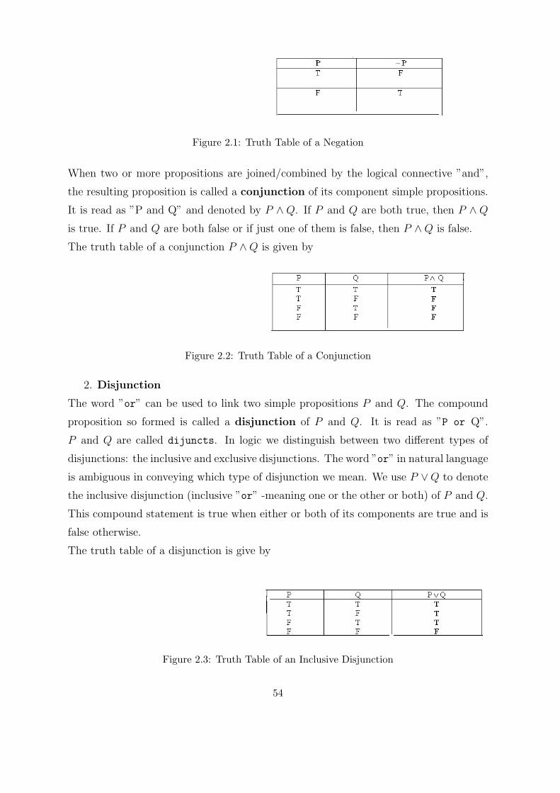
Figure 2.1: Truth Table of a Negation
When two or more propositions are joined/combined by the logical connective ”and”,
the resulting proposition is called a conjunction of its component simple propositions.
It is read as ”P and Q” and denoted by P ∧ Q. If P and Q are both true, then P ∧ Qis true. If P and Q are both false or if just one of them is false, then P ∧Q is false.
The truth table of a conjunction P ∧Q is given by
Figure 2.2: Truth Table of a Conjunction
2. Disjunction
The word ”or” can be used to link two simple propositions P and Q. The compound
proposition so formed is called a disjunction of P and Q. It is read as ”P or Q”.
P and Q are called dijuncts. In logic we distinguish between two different types of
disjunctions: the inclusive and exclusive disjunctions. The word ”or” in natural language
is ambiguous in conveying which type of disjunction we mean. We use P ∨Q to denote
the inclusive disjunction (inclusive ”or” -meaning one or the other or both) of P and Q.
This compound statement is true when either or both of its components are true and is
false otherwise.
The truth table of a disjunction is give by
Figure 2.3: Truth Table of an Inclusive Disjunction
54
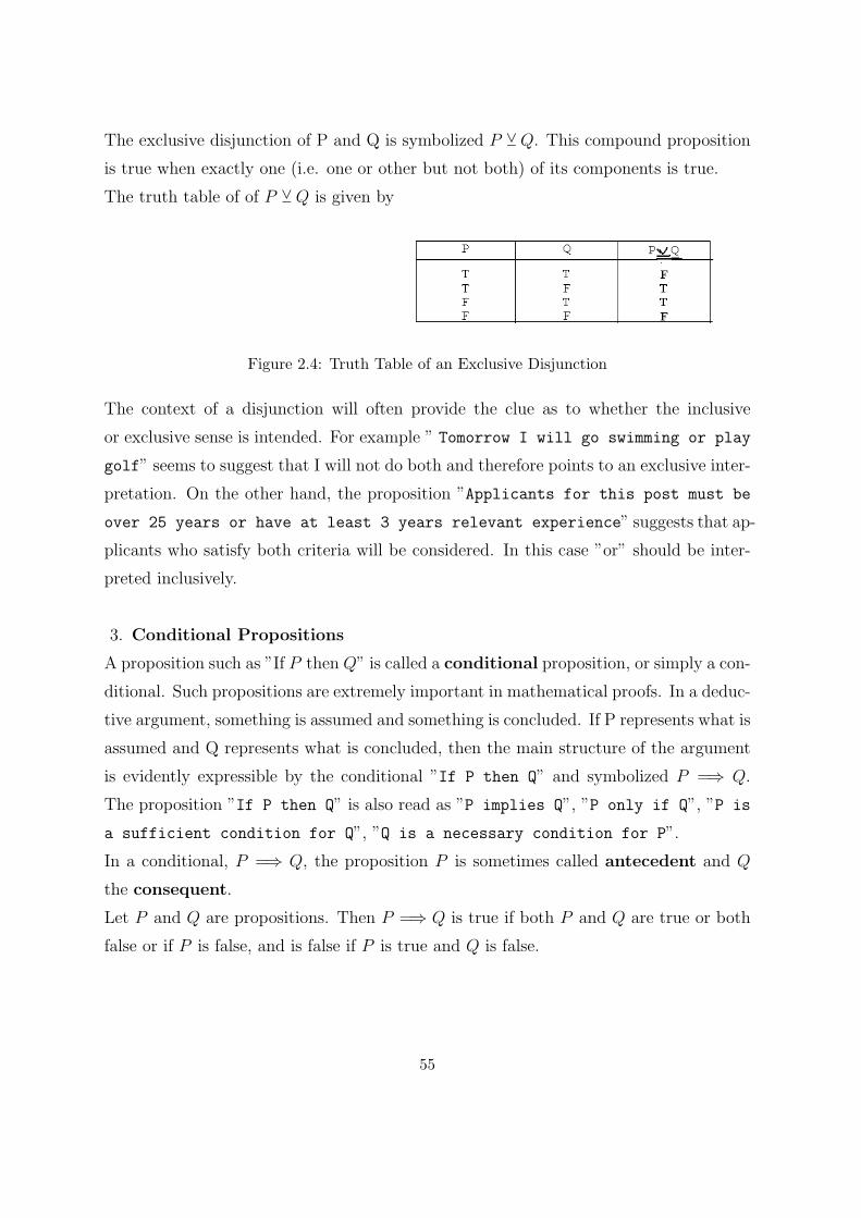
The exclusive disjunction of P and Q is symbolized P YQ. This compound proposition
is true when exactly one (i.e. one or other but not both) of its components is true.
The truth table of of P YQ is given by
Figure 2.4: Truth Table of an Exclusive Disjunction
The context of a disjunction will often provide the clue as to whether the inclusive
or exclusive sense is intended. For example ” Tomorrow I will go swimming or play
golf” seems to suggest that I will not do both and therefore points to an exclusive inter-
pretation. On the other hand, the proposition ”Applicants for this post must be
over 25 years or have at least 3 years relevant experience” suggests that ap-
plicants who satisfy both criteria will be considered. In this case ”or” should be inter-
preted inclusively.
3. Conditional Propositions
A proposition such as ”If P then Q” is called a conditional proposition, or simply a con-
ditional. Such propositions are extremely important in mathematical proofs. In a deduc-
tive argument, something is assumed and something is concluded. If P represents what is
assumed and Q represents what is concluded, then the main structure of the argument
is evidently expressible by the conditional ”If P then Q” and symbolized P =⇒ Q.
The proposition ”If P then Q” is also read as ”P implies Q”, ”P only if Q”, ”P is
a sufficient condition for Q”, ”Q is a necessary condition for P”.
In a conditional, P =⇒ Q, the proposition P is sometimes called antecedent and Q
the consequent.
Let P and Q are propositions. Then P =⇒ Q is true if both P and Q are true or both
false or if P is false, and is false if P is true and Q is false.
55
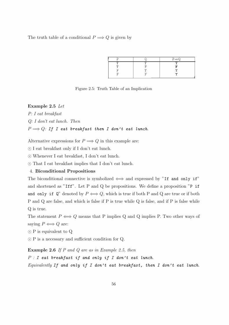
The truth table of a conditional P =⇒ Q is given by
Figure 2.5: Truth Table of an Implication
Example 2.5 Let
P: I eat breakfast
Q: I don’t eat lunch. Then
P =⇒ Q: If I eat breakfast then I don’t eat lunch.
Alternative expressions for P =⇒ Q in this example are:
⊙ I eat breakfast only if I don’t eat lunch.
⊙ Whenever I eat breakfast, I don’t eat lunch.
⊙ That I eat breakfast implies that I don’t eat lunch.
4. Biconditional Propositions
The biconditional connective is symbolized ⇐⇒ and expressed by ”If and only if”
and shortened as ”Iff”. Let P and Q be propositions. We define a proposition ”P if
and only if Q” denoted by P ⇐⇒ Q, which is true if both P and Q are true or if both
P and Q are false, and which is false if P is true while Q is false, and if P is false while
Q is true.
The statement P ⇐⇒ Q means that P implies Q and Q implies P. Two other ways of
saying P ⇐⇒ Q are:
⊙ P is equivalent to Q
⊙ P is a necessary and sufficient condition for Q.
Example 2.6 If P and Q are as in Example 2.5, then
P : I eat breakfast if and only if I don’t eat lunch.
Equivalently If and only if I don’t eat breakfast, then I don’t eat lunch.
56
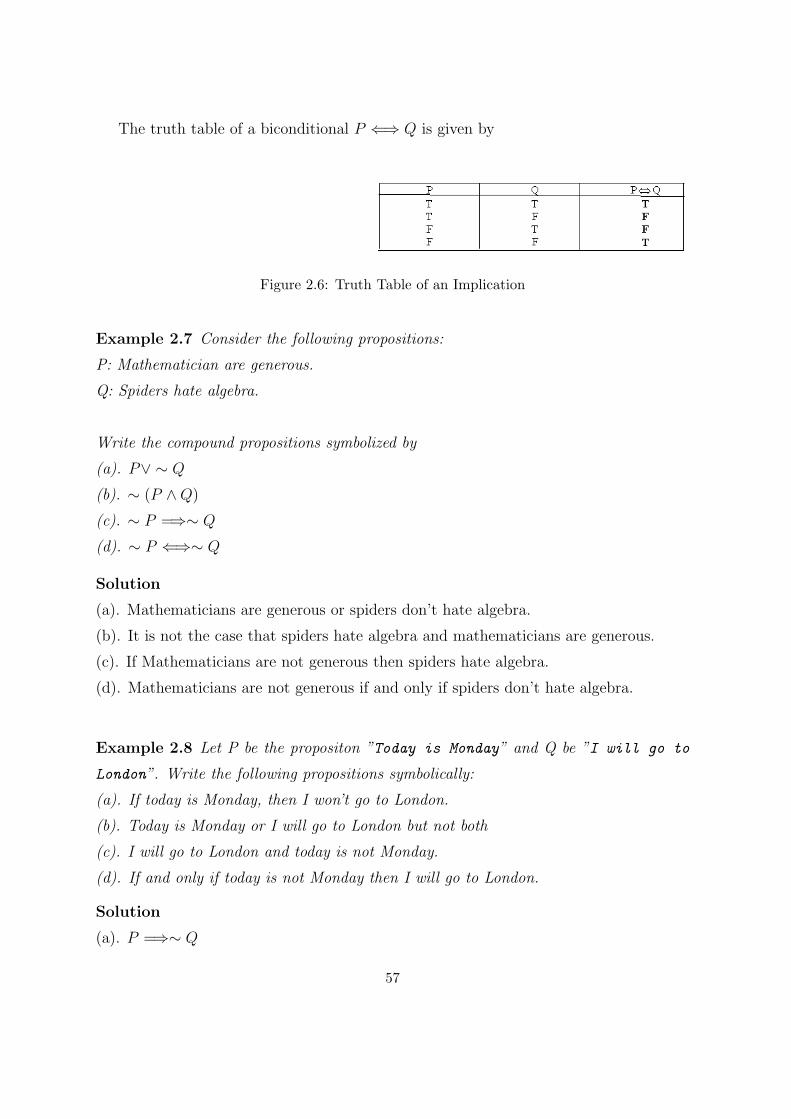
The truth table of a biconditional P ⇐⇒ Q is given by
Figure 2.6: Truth Table of an Implication
Example 2.7 Consider the following propositions:
P: Mathematician are generous.
Q: Spiders hate algebra.
Write the compound propositions symbolized by
(a). P∨ ∼ Q
(b). ∼ (P ∧Q)(c). ∼ P =⇒∼ Q
(d). ∼ P ⇐⇒∼ Q
Solution
(a). Mathematicians are generous or spiders don’t hate algebra.
(b). It is not the case that spiders hate algebra and mathematicians are generous.
(c). If Mathematicians are not generous then spiders hate algebra.
(d). Mathematicians are not generous if and only if spiders don’t hate algebra.
Example 2.8 Let P be the propositon ”Today is Monday” and Q be ”I will go to
London”. Write the following propositions symbolically:
(a). If today is Monday, then I won’t go to London.
(b). Today is Monday or I will go to London but not both
(c). I will go to London and today is not Monday.
(d). If and only if today is not Monday then I will go to London.
Solution
(a). P =⇒∼ Q
57
(b). P YQ(c). Q∧ ∼ P
(d). ∼ P ⇐⇒ Q.
Example 2.9 Construct truth tables for the following compound propositions.
(a). ∼ P ∨Q(b). ∼ P∧ ∼ Q
(c). ∼ Q =⇒ P
(d). ∼ P ⇐⇒∼ Q
Solution. Left as an exercise.
2.3.3 Tautologies and Contradictions
There are certain compound propositions which are always true no matter what the
truth values of their simple components are and there are others which are always false
regardless of the truth values of their components.
Definition 2.7 A tautology is a compound proposition which is true under all circum-
stances regardless of the truth values of its simple components.
A contradiction is a compound proposition which is false no matter what the truth
values of its simple components are.
We shall denote a tautology by t and a contradiction by c.
Example 2.10 The following are tautologies.
(a). P∨ ∼ P
(b). (P ∧Q)∨ ∼ (∧Q)
Solution Hint: Their truth tables return a column true values T .
Example 2.11 The following are contradictions.
(a). (P ∧Q) ∧ (∼ P ∨Q)(b). P∧ ∼ P
Solution Hint: Their truth tables return a column false values F .
58
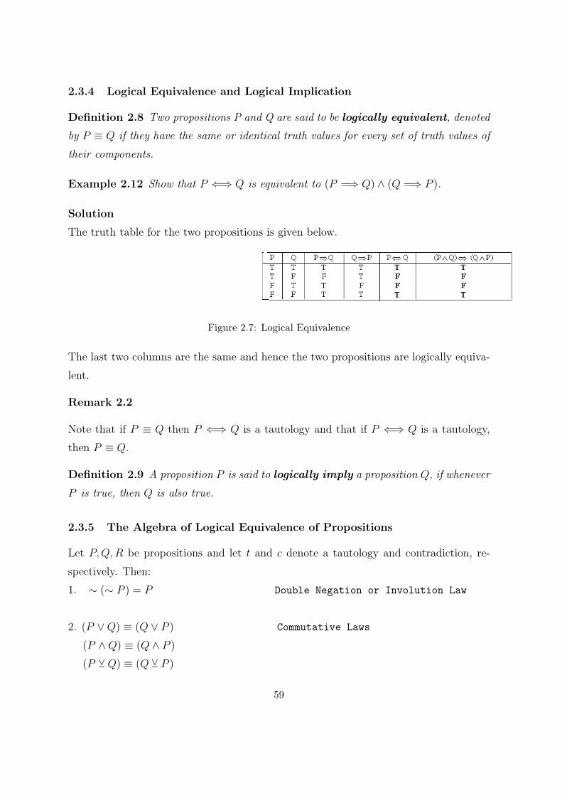
2.3.4 Logical Equivalence and Logical Implication
Definition 2.8 Two propositions P and Q are said to be logically equivalent, denoted
by P ≡ Q if they have the same or identical truth values for every set of truth values of
their components.
Example 2.12 Show that P ⇐⇒ Q is equivalent to (P =⇒ Q) ∧ (Q =⇒ P ).
Solution
The truth table for the two propositions is given below.
Figure 2.7: Logical Equivalence
The last two columns are the same and hence the two propositions are logically equiva-
lent.
Remark 2.2
Note that if P ≡ Q then P ⇐⇒ Q is a tautology and that if P ⇐⇒ Q is a tautology,
then P ≡ Q.
Definition 2.9 A proposition P is said to logically imply a proposition Q, if whenever
P is true, then Q is also true.
2.3.5 The Algebra of Logical Equivalence of Propositions
Let P,Q,R be propositions and let t and c denote a tautology and contradiction, re-
spectively. Then:
1. ∼ (∼ P ) = P Double Negation or Involution Law
2. (P ∨Q) ≡ (Q ∨ P ) Commutative Laws
(P ∧Q) ≡ (Q ∧ P )(P YQ) ≡ (Q Y P )
59
(P ⇐⇒ Q) ≡ (Q⇐⇒ P )
3. [(P ∨Q) ∨R] ≡ [P ∨ (Q ∨R)] Associative Laws
[(P ∧Q) ∧R] ≡ [P ∧ (Q ∧R)][(P YQ) YR] ≡ [P Y (Q YR)]
(P⇐⇒ Q) ⇐⇒ R ≡ P ⇐⇒ (Q⇐⇒ R)
4.(P∨Q) ∧R ≡ (P ∨Q) ∧ (P ∨R) Distributive Laws
(P ∧Q) ∨R ≡ (P ∧Q) ∨ (P ∧R)
5. P ∨ P ≡ P Idempotent Laws
P ∧ P ≡ P
6. P ∨ c ≡ P Identity Laws
P ∨ t ≡ t
P ∧ c ≡ c
P ∧ t ≡ P
7. P∨ ∼ P ≡ t Complement Laws
P∧ ∼ P ≡ c
∼ c ≡ t
∼ t ≡ c
8. ∼ (P ∨Q) ≡ (∼ P∧ ∼ Q) De Morgan’s Laws
∼ (P ∧Q) ≡ (∼ P∨ ∼ Q
9. (P =⇒ Q) ≡ (∼ Q =⇒∼ P )
10. (P =⇒ Q) ≡ (∼ P ∨Q) Implication
(P =⇒ Q) ≡ ∼ (P∧ ∼ Q)
11. (P ⇐⇒ Q) ≡ [(P =⇒ Q) ∧ (Q =⇒ P )] Equivalence
60
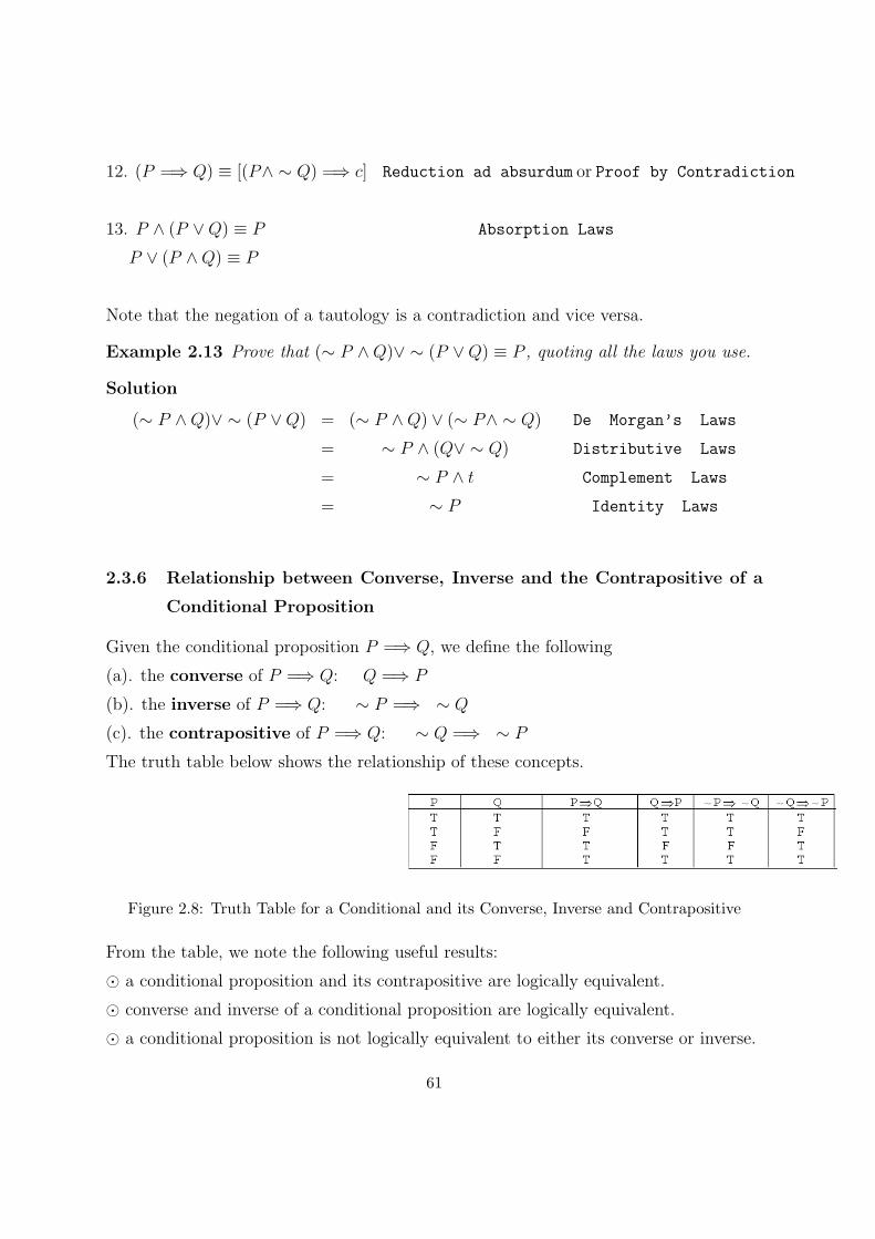
12. (P =⇒ Q) ≡ [(P∧ ∼ Q) =⇒ c] Reduction ad absurdum or Proof by Contradiction
13. P ∧ (P ∨Q) ≡ P Absorption Laws
P ∨ (P ∧Q) ≡ P
Note that the negation of a tautology is a contradiction and vice versa.
Example 2.13 Prove that (∼ P ∧Q)∨ ∼ (P ∨Q) ≡ P , quoting all the laws you use.
Solution
(∼ P ∧Q)∨ ∼ (P ∨Q) = (∼ P ∧Q) ∨ (∼ P∧ ∼ Q) De Morgan’s Laws
= ∼ P ∧ (Q∨ ∼ Q) Distributive Laws
= ∼ P ∧ t Complement Laws
= ∼ P Identity Laws
2.3.6 Relationship between Converse, Inverse and the Contrapositive of a
Conditional Proposition
Given the conditional proposition P =⇒ Q, we define the following
(a). the converse of P =⇒ Q: Q =⇒ P
(b). the inverse of P =⇒ Q: ∼ P =⇒ ∼ Q
(c). the contrapositive of P =⇒ Q: ∼ Q =⇒ ∼ P
The truth table below shows the relationship of these concepts.
Figure 2.8: Truth Table for a Conditional and its Converse, Inverse and Contrapositive
From the table, we note the following useful results:
⊙ a conditional proposition and its contrapositive are logically equivalent.
⊙ converse and inverse of a conditional proposition are logically equivalent.
⊙ a conditional proposition is not logically equivalent to either its converse or inverse.
61
Example 2.14 State the converse, inverse and contrapositive of the proposition ”If
Jack plays his guitar then Sara will sing.”
Solution
We define
P : Jack plays his guitar.
Q: Sara will sing
so that
P =⇒ Q: If Jack plays his guitar then Sarah will sing.
Converse: Q =⇒ P : If Sara will sing then Jack plays his guitar.
Inverse: ∼ P =⇒ ∼ Q: If Jack doesn’t paly his guitar then Sara won’t sing.
Contrapositive: ∼ Q =⇒ ∼ P : If Sara won’t sing then Jack doesn’t play his guitar.
2.4 Predicate Calculus
The sentence ”The number x is even” is not a statement because we do not know to
what x refers. For example if x = 3, then the statement is false. If x = 6, then the
statement is true.
Definition 2.10 An open sentence p(x) is a declarative sentence that becomes a state-
ment when x is given a particular value chosen from a universe of discourse of values
U .
An open sentence is also called a predicate. A predicate is a statement p(x1, x2, ..., xn)
involving variables x1, x2, ..., xn with the property that when x1, x2, ..., xn are given spe-
cific values, then resulting statement is either true or false(i.e., becomes a proposition).
Thus a predicate is a statement that could be a proposition, except for ambiguity that
exists because the scope or range of possibilities for the variables in the statement is not
specified. The scope of a variable is usually specified by the use of quantifiers.
2.4.1 Universal Quantifier
The statement ”For all x ∈ U , p(x)” is symbolized ∀x ∈ U , p(x). We call the symbol ∀the universal quantifier and we read it as ”for all”, ”for every”, ”for each”.
62
Example 2.15 ”For all x ∈ U , if x > 4, then x + 10 > 14” is a trues statement for
U = {1, 2, 3, ...}, the universe.
Example 2.16 Consider the proposition ”All rats are grey”. One way in which we can
paraphrase this proposition is ”For every x, if x is a rat, then x is grey”.
R(x): x is a rat
G(x): x is grey
We can then write ”All rats are grey” as
∀x[R(x) =⇒ G(x)
]Note that the statement ∀x ∈ U , p(x) is true if and only if p(x) is true for every x ∈ U .
Example 2.17 Let U = {1, 2, 3, 4, 5, 6}. Determine the truth value of the statement
∀x[(x− 4)(x− 8) > 0]
Solution
Let p(x) be the open sentence ”(x-4)(x-8)>0”. We consider the truth values of
p(1), p(2), ..., p(6). p(1) is true because (1 − 4)(1 − 8) = (−3)(−7) = 21 > 0. p(2)
and p(3) are also true. However, p(4) is false because (4− 4)(4− 8) = 0. We need not
check any other values from U .Therefore [∀x ∈ Up(x)] is false.
2.4.2 Existential Quantifier
The statement ”There exists an x in U such that p(x)” is symbolized ∃x ∈ U p(x). The
symbol is true if and only if there is at least one element x ∈ U such that p(x) is true.
The symbol ∃ is called the existential quantifier and is read as ”there exists x
such that p(x)”, ”for some x, p(x)”, or ”there is some x for which p(x)”.
Example 2.18 Consider the proposition ”some rats are grey”. That is, there is at least
one rat which is is grey. This can be paraphrased as ”There exists at least one x such
that x is a rat and x is grey”. Thus if we define
R(x): x is a rat
63
G(x): x is grey
and denote ”there exists at least one x” by ∃x, then ”some rats are grey” can be written
∃x[R(x) ∧G(x)
]Example 2.19 Symbolize ”some people think of no one but themselves”
Solution Define
p(x): x is a person
n(x): x thinks of no one but himself
Then ”some people think of no one but themselves” can be written
∃x[p(x) ∧ n(x)].
2.4.3 Negation of a Quantified Statement
The statement ∀x p(x) states that for all x in the universe of discourse, x has the
property defined by the predicate p. The negation of this statement is ∼ ∀x p(x), andstates that ”It is not the case that all x has the property defined by p”. That is, there
is at least one x that does not have the property p. This is symbolized by
∃x[∼ p(x)]
Therefore, for any predicate p(x), the statements
∼ ∀x p(x) and ∃x [∼ p(x)]
have the same truth tables and are therefore equivalent. That is
∼ ∀x p(x) ≡ ∃x [∼ p(x)]
Similarly, the negation of ∃x ∈ U p(x) symbolized by ∼ ∃x p(x), is equivalent to
∀x[∼ p(x)].
Note also that
∼ ∃x[∼ p(x)] ≡ ∀x p(x),
since∼ ∃x[∼ p(x)] ≡ ∀x[∼∼ p(x)]
≡ ∀x p(x)
64
Similarly, we can show that
∼ ∀x[∼ p(x)] ≡ ∃x p(x)
Example 2.20 We define the following on the universe of men.
M(x): x is mortal
C(x): x lives in the city
Symbolize the negation of the following propositions changing the quantifier.
(a). All men are mortal.
(b). Some men live in the city.
Solution
(a). The proposition can be symbolized by ∀x[∼M(x)]. The negation of this proposition
is give by
∼ ∀x[∼M(x)] ≡ ∃x M(x)
The resulting proposition is ”some men are mortal.”
(b). ”some men live in the city” is symbolized by ∃x C(x). Its negation is
∼ ∃x C(x) ≡ ∀x[∼ C(x)]
That is, ”All men live out of the city”.
Remark 2.3
Notice how moving the negation across a quantifier switches it from universal to exis-
tential and vice versa.
2.5 Application of Logic In Mathematical Proof
The discipline of Mathematics is characterized by the concept of proof. Many mathe-
matical theorem are statements that a certain implication is true. We give some methods
of proof.
2.5.1 Proof by a Counter-example
To show that a theorem or a step in a proof is false, it is enough to find a single case
where the implication does not hold. This is called proof by a counter-example.
65
Example 2.21 Consider the proposition P be
x2 < 1 =⇒ 0 < x < 1
It is easy to show that P is false by producing an x such that x2 < 1 but x ̸∈ (0, 1).
For instance, x = −12is a counter-example to the statement. This is a specific example
which proves that an implication is false.
2.5.2 Direct Proof
Most theorem in mathematics are stated as implications P =⇒ Q. Sometimes, it is
possible to prove such a statement directly ; that is, by establishing the validity of a
sequence of implications:
P =⇒ P1 =⇒ P2 =⇒ ... =⇒ Q
Example 2.22 Prove that for all real numbers x, x2 − 4x+ 17 ̸= 0.
Proof
Observe that x2− 4x+17 = (x− 2)2+13 is the sum of 13 and a number (x− 2)2, which
is never negative. So x2 − 4x+ 17 ≥ 13 for any x. In particular, x2 − 4x+ 17 ̸= 0 .
2.5.3 Proof by Cases
Sometimes a direct argument is made simpler by breaking it into a number of cases, one
of which must hold and each of which leads to the desired conclusion.
Example 2.23 Let n be an integer. Prove that 9n2 + 3n− 2 is even.
Proof We can consider the cases: n is even and n is odd.
Case 1: n is even.
The product of an even integer and any integer is even. Since n is even, 9n2 and 3n are
even too. Thus 9n2 + 3n− 2 is even since it is the sum of three even integers. Case 2:
n is odd.
The product of odd integers is odd. In this case, since n is odd, 9n2 and 3n are odd and
hence the sum 9n2 + 3n is even. So 9n2 + 3n− 2 is even.
66
2.5.4 Proof by the Contrapositive
Recall that a conditional proposition and its contrapositive are equivalent. Thus the
implication P =⇒ Q is true if and only if the contrapositive ∼ Q =⇒∼ P is true. If we
can establish the truth of the contrapositive, we can deduce that the conditional is also
true.
Example 2.24 If the average of four different integers is 10, prove that one of the
integers is greater than 11.
Proof
Let P and Q be the statements
P: ”The average of four integers, all different, is 10”.
Q: ”One of the fout=r integers is greater than 11”.
We are asked to prove the truth of P =⇒ Q. Instead we prove the truth of the contra-
position ∼ Q =⇒∼ P from which the truth follows. Call given integers a, b, c, d. If Q is
false, then each of these numbers is at most 11 and since they are different, the biggest
value for a+ b+ c+ d is 11 + 10 + 9+ 8 = 38. So the biggest possible average would be384, which is less than 10, so P is false.
2.5.5 Proof by Contradiction
Sometimes a direct proof of a statement P seems hopeless. We simply do not know how
to begin. In this case, we sometimes make progress by assuming that the negation of P
is true. If this assumption leads to a statement which is obviously false (an absurdity)
or to a statement which contradicts something else, then we will have shown that ∼ P
is false. So P must be true.
Example 2.25 Show that there is no largest integer.
Proof Let P be the statement ”There is no largest integer”. If P is false, then there is
a largest integer N . This is absurd, however, because N +1 is an integer larger than N .
Thus ∼ P is false, so P is true.
67
2.5.6 Proof by Mathematical Induction
Mathematical Induction is appropriate for proving that a result holds for all positive
integers. It consists of the following steps:
(a). Prove that the conjecture holds for n = 1
(b). Prove that, for all k ≥ 1, if the result holds for n = k, then it must also hold for
n = k + 1.
Theorem 2.1 (Principle of Finite Mathematical Induction) Let
p(m), p(m+ 1), ..., p(n)
be a finite sequence of propositions. If
(i). p(m) is true, and
(ii). p(k+1) is true whenever p(k) is true and m ≤ k ≤ n, then all the propositions are
true.
In many applications, m will be 0 or 1.
Theorem 2.2 (Principle of Infinite Mathematical Induction) Let
p(m), p(m+ 1), ...,
be a sequence of propositions. If
(i). p(m) is true, and
(ii). p(k+1) is true whenever p(k) is true and m ≤ k, then all the propositions are true.
Condition (i) is called the basis, and (ii) is called the inductive step. The basis is
easy to check; the inductive step is sometimes quite a bit more complicated to verify.
The principle tells that if we can show that (i) and (ii) holds, we are done.
Example 2.26 Prove by Mathematical Induction that for every positive integer n,
1 + 2 + 3 + ...+ n =n(n+ 1)
2
Proof
Let p(n) be the proposition
”1 + 2 + 3 + ...+ n =n(n+ 1)
2
”
68
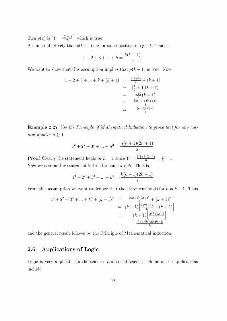
then p(1) is ”1 = 1(1+1)2
”, which is true.
Assume inductively that p(k) is true for some positive integer k. That is
1 + 2 + 3 + ...+ k =k(k + 1)
2.
We want to show that this assumption implies that p(k + 1) is true. Now
1 + 2 + 3 + ...+ k + (k + 1) = k(k+1)2
+ (k + 1)
= [k2+ 1](k + 1)
= k+22(k + 1)
= [(k+1)+1](k+1)2
= (k+1)(k+2)2
Example 2.27 Use the Principle of Mathematical Induction to prove that for any nat-
ural number n ≥ 1
12 + 22 + 33 + ...+ n2 =n(n+ 1)(2n+ 1)
6
Proof Clearly the statement holds or n = 1 since 12 = 1(1+1)(2+1)6
= 66= 1.
Now we assume the statement is true for some k ∈ N. That is,
12 + 22 + 33 + ...+ k2 =k(k + 1)(2k + 1)
6
From this assumption we want to deduce that the statement holds for n = k + 1. Thus
12 + 22 + 33 + ...+ k2 + (k + 1)2 = k(k+1)(2k+1)6
+ (k + 1)2
= (k + 1)[k(2k+1)
6+ (k + 1)
]= (k + 1)
[2k2+7k+6
6
]= (k+1)(k+2)(2k+3)
6
and the general result follows by the Principle of Mathematical induction.
2.6 Applications of Logic
Logic is very applicable in the sciences and social sciences. Some of the applications
include
69
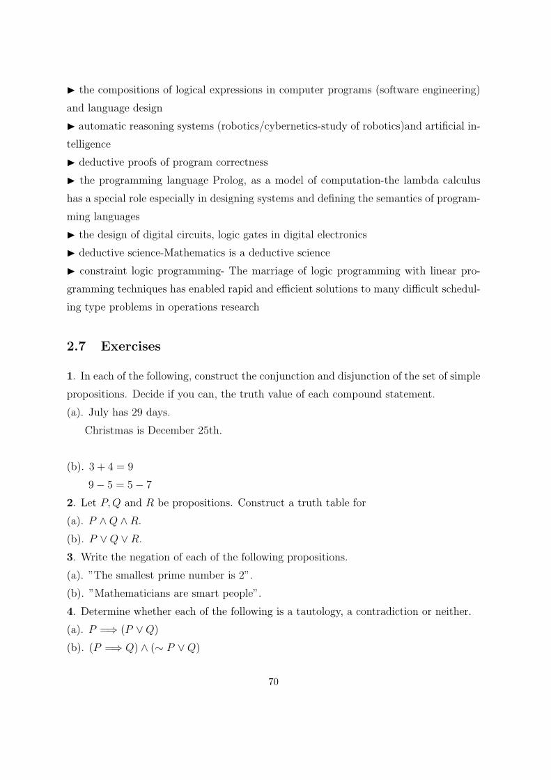
I the compositions of logical expressions in computer programs (software engineering)
and language design
I automatic reasoning systems (robotics/cybernetics-study of robotics)and artificial in-
telligence
I deductive proofs of program correctness
I the programming language Prolog, as a model of computation-the lambda calculus
has a special role especially in designing systems and defining the semantics of program-
ming languages
I the design of digital circuits, logic gates in digital electronics
I deductive science-Mathematics is a deductive science
I constraint logic programming- The marriage of logic programming with linear pro-
gramming techniques has enabled rapid and efficient solutions to many difficult schedul-
ing type problems in operations research
2.7 Exercises
1. In each of the following, construct the conjunction and disjunction of the set of simple
propositions. Decide if you can, the truth value of each compound statement.
(a). July has 29 days.
Christmas is December 25th.
(b). 3 + 4 = 9
9− 5 = 5− 7
2. Let P,Q and R be propositions. Construct a truth table for
(a). P ∧Q ∧R.(b). P ∨Q ∨R.3. Write the negation of each of the following propositions.
(a). ”The smallest prime number is 2”.
(b). ”Mathematicians are smart people”.
4. Determine whether each of the following is a tautology, a contradiction or neither.
(a). P =⇒ (P ∨Q)(b). (P =⇒ Q) ∧ (∼ P ∨Q)
70
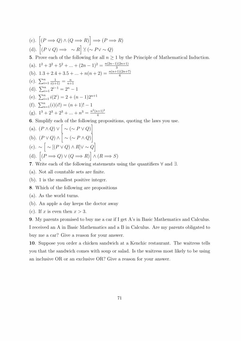
(c).[(P =⇒ Q) ∧ (Q =⇒ R)
]=⇒ (P =⇒ R)
(d).[(P ∨Q) =⇒ ∼ R
]Y (∼ P∨ ∼ Q)
5. Prove each of the following for all n ≥ 1 by the Principle of Mathematical Induction.
(a). 12 + 32 + 52 + ...+ (2n− 1)2 = n(2n−1)(2n+1)3
(b). 1.3 + 2.4 + 3.5 + ...+ n(n+ 2) = n(n+1)(2n+7)6
(c).∑n
i=11
i(i+1)= n
n+1
(d).∑n
i=1 2i−1 = 2n − 1
(e).∑n
i=1 i(2i) = 2 + (n− 1)2n+1
(f).∑n
n=1(i)(i!) = (n+ 1)!− 1
(g). 13 + 23 + 23 + ...+ n3 = n2(n+1)2
4
6. Simplify each of the following propositions, quoting the laws you use.
(a). (P ∧Q) ∨[∼ (∼ P ∨Q)
](b). (P ∨Q) ∧
[∼ (∼ P ∧Q)
](c). ∼
[∼ [(P ∨Q) ∧R]∨ ∼ Q
](d).
[(P =⇒ Q) ∨ (Q =⇒ R)
]∧ (R =⇒ S)
7. Write each of the following statements using the quantifiers ∀ and ∃.(a). Not all countable sets are finite.
(b). 1 is the smallest positive integer.
8. Which of the following are propositions
(a). As the world turns.
(b). An apple a day keeps the doctor away
(c). If x is even then x > 3.
9. My parents promised to buy me a car if I get A’s in Basic Mathematics and Calculus.
I received an A in Basic Mathematics and a B in Calculus. Are my parents obligated to
buy me a car? Give a reason for your answer.
10. Suppose you order a chicken sandwich at a Kenchic restaurant. The waitress tells
you that the sandwich comes with soup or salad. Is the waitress most likely to be using
an inclusive OR or an exclusive OR? Give a reason for your answer.
71
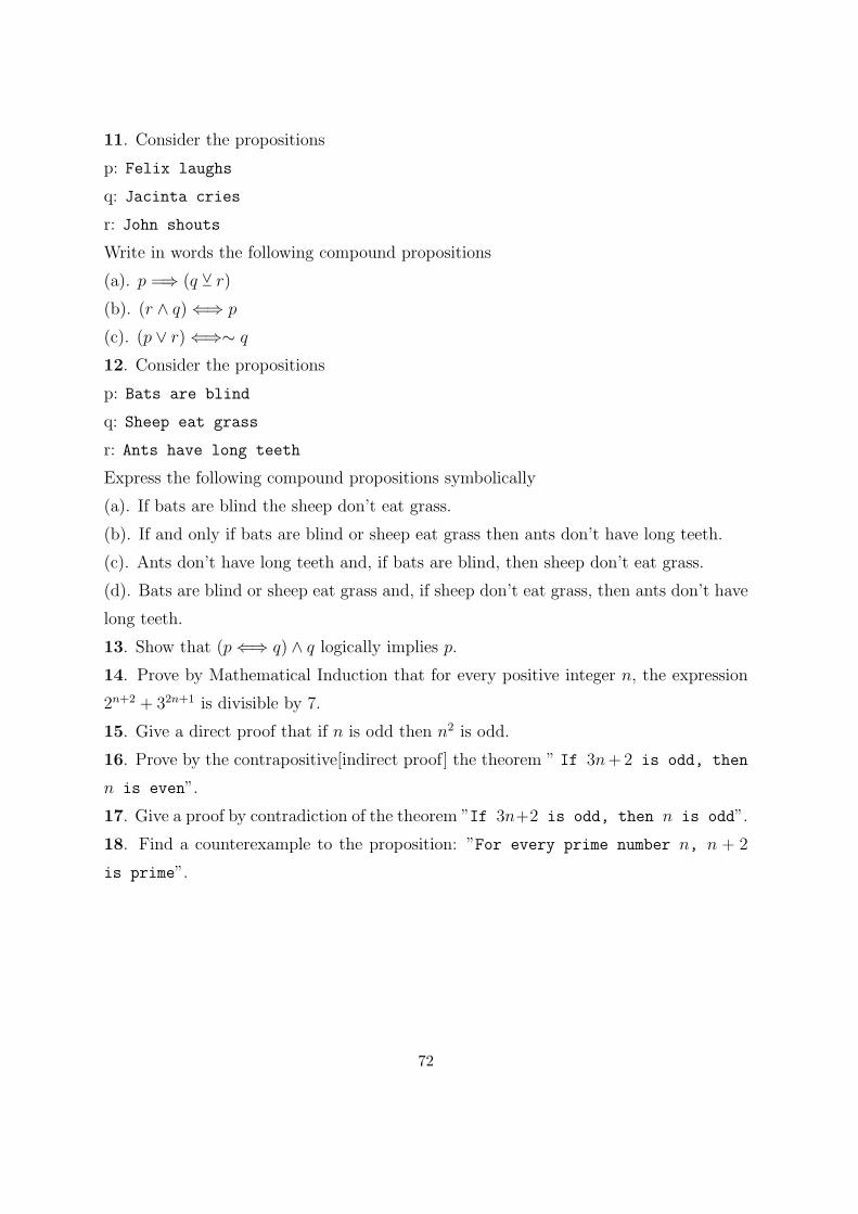
11. Consider the propositions
p: Felix laughs
q: Jacinta cries
r: John shouts
Write in words the following compound propositions
(a). p =⇒ (q Y r)(b). (r ∧ q) ⇐⇒ p
(c). (p ∨ r) ⇐⇒∼ q
12. Consider the propositions
p: Bats are blind
q: Sheep eat grass
r: Ants have long teeth
Express the following compound propositions symbolically
(a). If bats are blind the sheep don’t eat grass.
(b). If and only if bats are blind or sheep eat grass then ants don’t have long teeth.
(c). Ants don’t have long teeth and, if bats are blind, then sheep don’t eat grass.
(d). Bats are blind or sheep eat grass and, if sheep don’t eat grass, then ants don’t have
long teeth.
13. Show that (p⇐⇒ q) ∧ q logically implies p.
14. Prove by Mathematical Induction that for every positive integer n, the expression
2n+2 + 32n+1 is divisible by 7.
15. Give a direct proof that if n is odd then n2 is odd.
16. Prove by the contrapositive[indirect proof] the theorem ” If 3n+2 is odd, then
n is even”.
17. Give a proof by contradiction of the theorem ”If 3n+2 is odd, then n is odd”.
18. Find a counterexample to the proposition: ”For every prime number n, n + 2
is prime”.
72
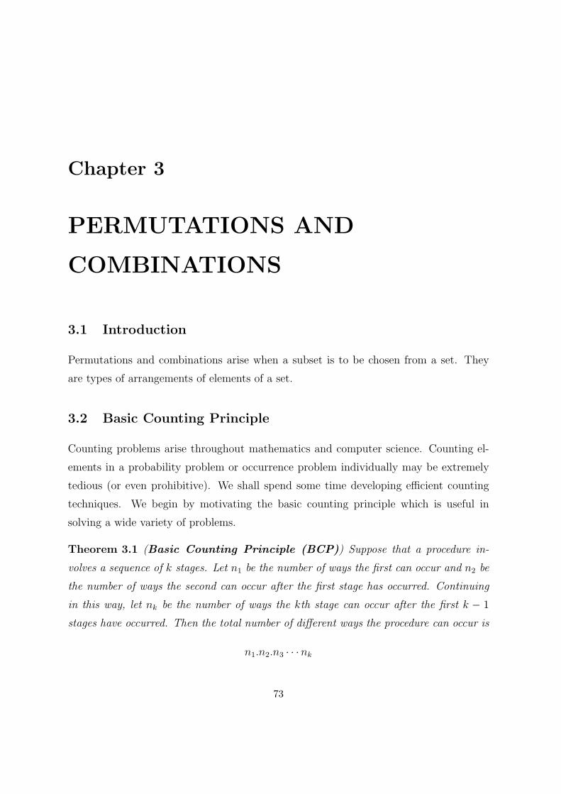
Chapter 3
PERMUTATIONS AND
COMBINATIONS
3.1 Introduction
Permutations and combinations arise when a subset is to be chosen from a set. They
are types of arrangements of elements of a set.
3.2 Basic Counting Principle
Counting problems arise throughout mathematics and computer science. Counting el-
ements in a probability problem or occurrence problem individually may be extremely
tedious (or even prohibitive). We shall spend some time developing efficient counting
techniques. We begin by motivating the basic counting principle which is useful in
solving a wide variety of problems.
Theorem 3.1 (Basic Counting Principle (BCP)) Suppose that a procedure in-
volves a sequence of k stages. Let n1 be the number of ways the first can occur and n2 be
the number of ways the second can occur after the first stage has occurred. Continuing
in this way, let nk be the number of ways the kth stage can occur after the first k − 1
stages have occurred. Then the total number of different ways the procedure can occur is
n1.n2.n3 · · ·nk
73
Example 3.1 (Travel Routes) Two roads connect cities A and B, four roads connect
B and C, and five roads connect C and D. To drive from A to B, to C, and then to city
D, how many different routes are possible?
Solution
Figure 3.1: Routes from A to D
Here we have a three-stage procedure: The first (A → B) has two possibilities, the
second (B→ C) has four possibilities, and the third (C→ D) has five.
By the Basic Counting Principle, the total number of routes is 2.4.5 = 40.
Example 3.2 The chairs of a lecture room are to be labeled with a letter of the alphabet
and a positive integer not exceeding 100. What is the largest number of chairs that can
be labeled differently?
Solution
The procedure of labeling a chair consists of two tasks, namely, assigning one of the
letters and the assigning one of the 100 possible integers. The first task can be done
in 26 different ways while the second task can be done in 100 different ways. By the
BCP, there are 26 × 100 = 2600 different ways that a chair can be labeled. Therefore
the largest number of chairs that can be labeled differently is 2600.
Example 3.3 In how many different ways can a quiz be answered under each of the
following conditions?
(a). The quiz consists of three multiple-choice questions with four choices for each.
74
(b). The quiz consist of three multiple-choice questions(with four choices for each) and
five true-false questions.
Solution
(a). Successively answering the three questions is a three-stage procedure. The first
question can be answered in any of four ways. Likewise, each of the other two questions
can be answered in four ways. By the Basic Counting Principle, the number of ways to
answer the quiz is
4.4.4 = 64
(b). Answering the quiz can be considered a two-stage procedure. First we can answer
the multiple-choice questions(first stage) and then we can answer the true-false ques-
tions(second stage). From part (a), the three multiple-choice questions can be answered
in 4.4.4 = 64 ways. Each of the true-false questions has two choices (true or false).
So the total number of ways of answering all five of them is 2.2.2.2.2 = 32. By the BCP,
the number of ways the entire quiz can be answered is
64.32 = 2048.
Example 3.4 (Letter arrangements) From the five letters A,B,C,D and E, how
many three-letter horizontal arrangements (called ”words”) are possible if no letter may
be repeated?
Solution
To form a word we must successively fill the positions the first, second and third posi-
tion/slots with letters. This is a three-stage procedure. For the first position, we can
choose any of the five letters. After filling the first position with some letter, we can fill
the second position with any of the remaining four letters. After that position is filled,
the third position can be filled with any of the three letters that have not yet been used.
By the Basic Counting Principle, the total number of three-letter words is
5.4.3 = 60.
3.3 Permutations
In Example 3.4, we selected three different letters from five letters and arranged them
in an order. Each result is called a permutation of the five letters taken three at a time.
75
Definition 3.1 An ordered arrangement of r objects, without repetition, selected from
n distinct objects is called a permutation of the n objects taken r at a time.
The number of such permutations is denoted P (n, r) or nrP. For instance Example 3.4
can be solved as: P (5, 3) = 5.4.3 = 60.
Using the Basic Counting Principle, we can calculate the number of ways n different
objects can be arranged in a specified order. The first object may be selected in n ways,
the second in (n − 1) ways, the third in (n − 2), and so on until only one choice is
remaining for the last object.So the total number of possible arrangements is
n(n− 1)(n− 2) · · · 3.2.1
This expression is normally abbreviated to n! (read as n factorial or factorial n).
Thus the number of permutations of n different objects is n!
3.3.1 General Formula for P (n, r)
In making an ordered arrangement of r objects from n objects,for the first position we
may choose any of the n objects. After the first position is filled, there remain n − 1
objects that may be chosen from for the second position. After that position is filled,
there are n − 2 objects that may be chosen for the third position. Continuing in this
way and using the Basic Counting Principle, we arrive at the following formula
P (n, r) = n(n− 1)(n− 2) · · · (n− r + 1)︸ ︷︷ ︸r factors
(3.1)
The formula P (n, r) can be expressed in terms of factorials. Multiplying the right
side of equation (3.1) by (n−r)(n−r−1)···2×1(n−r)(n−r−1)...2×1
gives
P (n, r) =n(n− 1)(n− 2) · · · (n− r + 1).(n− r)(n− r − 1) · · · 2× 1
(n− r)(n− r − 1) · · · 2× 1
The numerator is simply n! and the denominator is (n− r)! Thus we have the following
result: The number of permutations of n objects taken r at a time is given by
P (n, r) =n!
(n− r)!
76
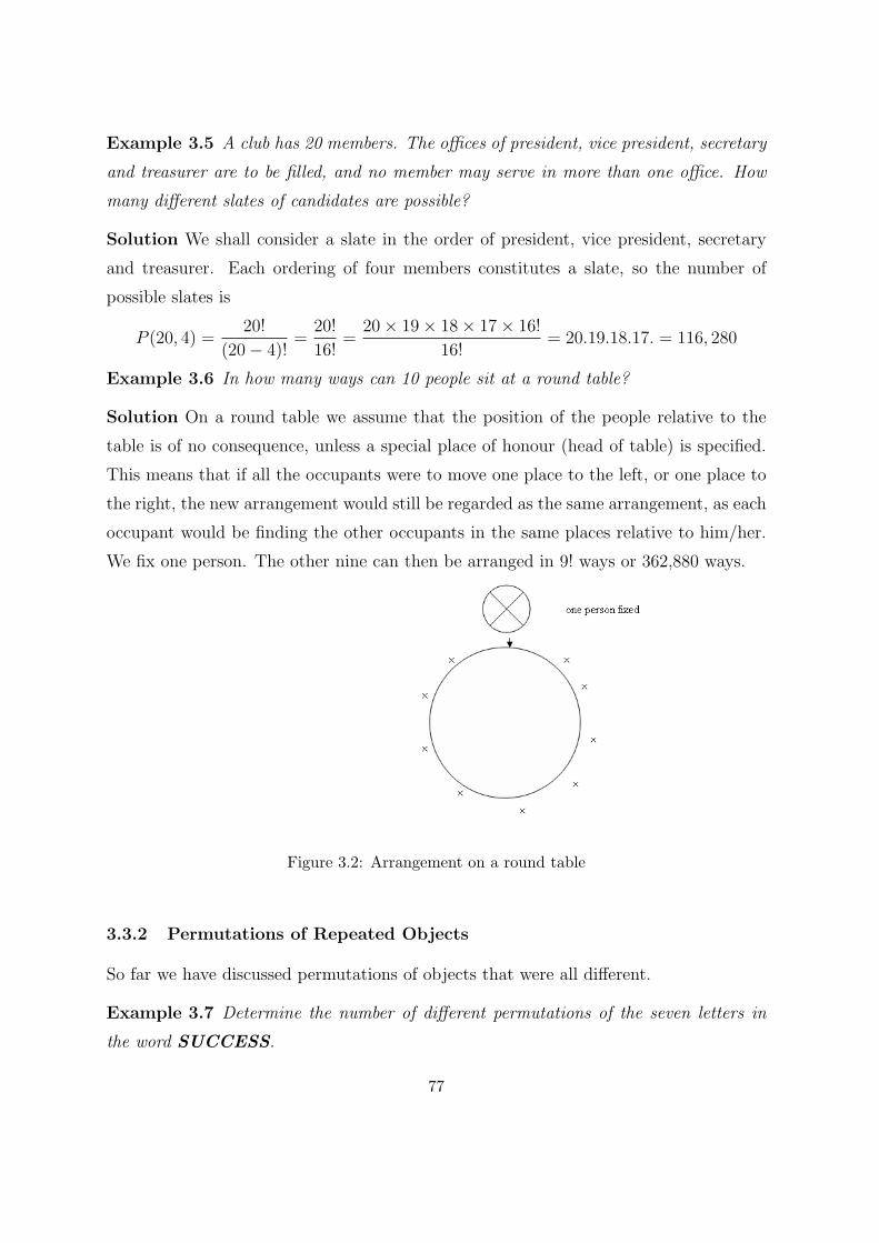
Example 3.5 A club has 20 members. The offices of president, vice president, secretary
and treasurer are to be filled, and no member may serve in more than one office. How
many different slates of candidates are possible?
Solution We shall consider a slate in the order of president, vice president, secretary
and treasurer. Each ordering of four members constitutes a slate, so the number of
possible slates is
P (20, 4) =20!
(20− 4)!=
20!
16!=
20× 19× 18× 17× 16!
16!= 20.19.18.17. = 116, 280
Example 3.6 In how many ways can 10 people sit at a round table?
Solution On a round table we assume that the position of the people relative to the
table is of no consequence, unless a special place of honour (head of table) is specified.
This means that if all the occupants were to move one place to the left, or one place to
the right, the new arrangement would still be regarded as the same arrangement, as each
occupant would be finding the other occupants in the same places relative to him/her.
We fix one person. The other nine can then be arranged in 9! ways or 362,880 ways.
Figure 3.2: Arrangement on a round table
3.3.2 Permutations of Repeated Objects
So far we have discussed permutations of objects that were all different.
Example 3.7 Determine the number of different permutations of the seven letters in
the word SUCCESS.
77
Solution The letters C nd S are repeated. If the two Cs were interchanged, the re-
sulting permutation would be indistinguishable from SUCCESS. Thus, the number of
distinguishable permutations is not 7! as it would be with 7 different objects.
We now give a formula to enable us solve similar problems.
Theorem 3.2 (Permutations with Repeated Objects)The number of distinguish-
able permutations of n objects such that n1 are of one type, n2 are of a second type,...,
and nk are of a kth type , where n1 + n2 + · · ·+ nk = n is
n!
n1! n2! · · · nk!
Using this formula, the answer to Example 3.6 is easy to find. Note that the word
SUCCESS has 7 characters: 3 Ss, 2 Cs, 1 U and 1 E. Therefore there are 7!3!2!1!1!
= 420
distinguishable words.
Example 3.8 (a).How many distinguishable arrangements are there of the word
MASSASAUGA?
(b). How many of these arrangements are the four A’s together?
Solution(a). Massasauga is a white venomous snake indigenous in North America.
Note that this word has 10 characters, some repeated: 4 As, 3 S, 1 M, 1 U, 1 G .
Therefore there are10!
4! 3! 1! 1! 1!= 25, 200
possible arrangements.
(b). If we tie the four A’s they form one object, denote it A. Now we have 7 characters
with some characters repeated: 1 A, 3 Ss, 1 M, 1 U, 1 G . Therefore there are
7!
3! 1! 1! 1! 1!= 840
arrangements in which all four A’s are together.
Remark 3.1
Cells or Compartments
Sometimes we want to find the number of ways in which objects can be placed into
”compartments” or cells. For example, suppose that from a group of five people, three
78
are to be assigned to room A and two to room B. In how many ways can this be done?
Obviously, order in which people are placed into the rooms is of no concern. The cells
remind us of those permutations with repeated objects.
Hence the five people can be assigned in
5!
3! 2!= 10
ways.
Example 3.9 A campaign manager must assign 15 campaigners to three matatus: 6 in
the first matatu, 5 in the second, and 4 in the third. In how many ways can this be done.
Solution Here people are placed into three cells (matatus): 6 in cell1, 5 in cell2, 4 in
cell 3. Thus there are15!
6! 5! 4!= 630, 630
ways.
3.4 Combinations
Definition 3.2 An arrangement of r objects, without regard to order and without repe-
tition, selected from n distinct objects is called a combination of n objects taken r at
a time.
The number of such combinations is denoted by nrC or n Cr or C(n, r) or
(nr
). Note
that ABC,BAC is one combination but two permutations.
3.4.1 Comparing Combinations and Permutations
Example 3.10 List all combinations and all permutations of the three letter A,B C
when they are taken two at a time.
Solution
The combinations are : AB, AC, BC
There are 3 combinations, so 32C = 3.
The permutations are:
79
AB BC AC
BA CB CA
Thus there are 6 permutations.
With this observation, we can determine a formula for(nr
). Suppose one such combina-
tion is
x1x2 · · ·xr
The number of permutations of these r objects is r! Listing all such combinations and
all permutations of these combinations, we obtain a list of permutations of the n objects
taken r at a time. ThusnrC. r! = P (n, r) =
n!
(n− r)!
Solving for nrC we get
nrC =
n!(n−r)!
r!=
n!
(n− r)! r!
Example 3.11 If a club has 20 members, how many different four-member committees
are possible?
Solution
Order is not important because no matter how the members of a committee are ar-
ranged, we have the same committee. Thus, we simply have to compute the number of
combinations of 20 objects taken four at a time,
204C =
20!
(20− 4)! 4!= 4845.
Example 3.12 In how many ways can a class of 20 children be split into two groups of
8 and 12 respectively if there are two twins in the class who must not be separated?
Solution Once the group of 8 has been selected then the remaining 12 children will
automatically comprise the other group.
For the selection of those to join the group of 8 we have two cases:
(i). the twins are included,
(ii). the twins are not included.
⊙ If the twins are included we have to select 6 other children from 18, i.e. this can be
done in(186
)ways.
⊙ If the twins are excluded we have to select 8 children, but still from 18 children, i.e.
80
this can be done in(188
)ways.
The total number of ways will be(18
6
)+
(18
8
)=
18!
12! 6!+
18!
10! 8!= 18, 564 + 43, 758 = 62, 322
ways.
3.4.2 Combinations with Repetition
When we wish to select r objects out of n objects, with repetition allowed/permitted
the number of combinations is(n+ r − 1
r
)=
(n+ r − 1)!
r! (n− 1)!
Example 3.13 A donut shop offers 20 kinds kinds of donuts. Assuming that there are
at least a dozen of each kind when we enter the shop, we can select a dozen donuts in
C(20 + 12− 1, 12) = C(31, 12) = 141, 120.525
ways.
Example 3.14 Four family members have just completed lunch and are ready to choose
their afternoon fruit. There are bananas, apples, pears, kwi, apricots, and oranges in
the house. In how many ways can a selection of four pieces of fruit be chosen?
Solution
Note that only the selection of varieties (not which person eats what fruit) is of interest
here. This is a combination with repetition problem. Thus the solution is
C(6, 4− 1, 4) = C(9, 4) =9!
4! 5!= 126.
3.5 Problems involving Both Permutations and Combinations
Some problems require the concepts of both permutations(arrangements) and combina-
tions.
Example 3.15 Consider the word TALLAHASSEE.
(a). How many distinguishable arrangements of the word are possible?
(b). How many of these arrangements have no adjacent A’s?
81
Solution
(a). The number of distinguishable arrangements is
11!
3! 2! 2! 2! 1! 1!= 831, 600.
(b). When we disregard the A’s, there are
8!
2! 2! 2! 1! 1!= 5040
ways to arrange the remaining letters. One of these 5040 ways is shown in the following
figure, where the arrows indicate nine possible locations for the three A’s.
Figure 3.3: Possible locations for the A’s
Three of these locations can be selected in(93
)= 84 ways, and because this is also
possible for all the other 5039 arrangements of E,E,E,T,L,L,S,H, by the Basic Counting
Principle, there are 5040× 84 = 423, 360 arrangements of the letters in TALLAHAS-
SEE with no consecutive A’s.
Example 3.16 How many committees of five people can be chosen from 20 men and 12
women
(a). if exactly three men must be on each committee?
(b). if at least four women must be on each committee?
Solution
(a). We must choose three men from 20 and two women from 12. This can be done in(20
3
).
(12
2
)= 1140× 66 = 75, 240
different ways.
(b). We calculate the cases of four women and five women separately and add the result.
The answer is (12
4
).
(20
1
)+
(12
5
).
(20
0
)= 495(20) + 792 = 10, 692
ways.
82
3.6 Applications of Combinations
3.6.1 Binomial Theorem
Theorem 3.3 (Binomial Theorem) For any x and y any natural number n,
(x+ y)n =∑n
k=0
(nk
)xn−kyk
= xn +(n1
)xn−1y +
(n2
)xn−2y2 + · · ·+
(n
n−1
)xyn−1 + yn
There are(nr
)ways in which r brackets can be chosen from n brackets, so the term
containing xr is nrCx
ryn−r
Example 3.17 (a).Use the binomial theorem to expand and simplify (1 + x)4.
(b). Use your result to approximate (1.1)4.
Solution
(a).
(1 + x)4 = 1 +(41
)x+
(42
)x2 +
(43
)x3 +
(41
)x4
= 1 + 4x+ 6x2 + 4x3 + x4
(b). Note that 1.1 = 1 + 0.1. Therefore
(1.1)4 = (1 + 0.1)4 = 1 + 0.4 + 0.06 + 0.004 + 0.0001 = 1.4641
Example 3.18 Prove that(n
0
)+
(n
1
)+
(n
2
)+ · · ·
(n
n
)= 2n
for all natural numbers n.
Solution
Using Theorem 3.3 with x = y = 1, we obtain
(1 + 1)n =n∑
k=0
(n
k
)1n−k1k =
n∑k=0
(n
k
)That is
2n =n∑
k=0
(n
k
)as desired.
83
3.7 Exercises
1. Determine the values of 64P,
100100C,
992C
2. Verify that(nr
)=
(n
n−r
).
3. In a 10-question examination, each question is worth 10 points and is marked right
or wrong. Considering the individual questions, in how many ways can a student score
80 or better?
4. In a certain African country, vehicle license plates consist of two letters of the alpha-
bet, followed by four digits from 0 to 9, 0 and 9 included.
(a). How many different license plates are there if the second letter on the plate is either
an ’O’ or a ’Q’ and the last digit is either a 3 or an 8?
(b). How many license plates are there if the first letter must be a ’K’ and the second
letter must be an ’A’ and the last digit must be 5?
5. Because of overcrowding, five people out of nine people can enter an elevator. How
many different groups can enter?
6. A carton contains 24 light bulbs, one of which is defective.
(a). In how many ways can three bulbs be selected?
(b). In how many ways can three bulbs be selected if one is defective.
7. How many distinguishable horizontal arrangements are there of the letters in the
word MISSISSIPPI?
8. A group of tourists is composed of six from Nairobi, seven from London and eight
from New York.
(a). In how many ways can a committee of six tourists be formed with two people from
each city?
(b). In how many ways can a committee of seven tourists be formed with at least two
tourists from each city?
9.(a). Find the Binomial expansion of (2x+ 3y)n.
(b). Find the coefficient of the fifth term.
(c). Use you result to find 45.
10. In how many ways can the letters in WONDERING be arranged with exactly
two consecutive vowels?
11. Francesca has 20 different books but the shelf in her dormitory residence will hold
84
only 12 of them.
(a). In how many ways can Francesca line up 12 of these books on her bookshelf?
(b). How many of the arrangements in part (a) include Francesca’s three books on Cal-
culus?
12. (a) Write down the first three terms in the expansion in ascending powers of x of
(i). (1− x2)10
(ii). (3− 2x)8
(b). Write down the Binomial expansion for (1+x)20, and use it to approximate (1.01)20,
leaving your answer in 5 decimal places.
13. There are 8 persons, including a married couple Mr and Mrs Bush, from which a
committee of 4 has to be chosen. In how many ways can the committee be chosen
(a). If both Mr and Mrs Bush are excluded,
(b). if Mrs Bush is included and Mr. Bush is excluded.
(c). if both Mr and Mrs Bush are included?
14. (a). Let n be a non-negative integer. Prove that
n∑k=0
(n
k
)2k = 3n
(b). Let n, r ∈ N. Prove that
n∑k=0
(k
r
)=
(n+ 1
r + 1
)(c). Let n ∈ N. Prove that
n∑k=0
(n
k
)2
=
(2n
n
)[Hint:
(nk
)2=
(nk
).(nk
). Now replace the second
(nk
)with an equivalent expression]. (d).
Prove that
r
(n+ 1
r
)= (n+ 1)
(n
r − 1
)15. How many code symbols can be formed using 5 out of the 6 letters G,H, I, J,K, L
if the letters
(a). cannot be repeated?
(b). can be repeated?
85

(c). cannot be repeated but must begin with K.
(d). cannot be repeated but must end with IGH?
86
Chapter 4
RELATIONS AND FUNCTIONS
4.1 Introduction
In this chapter we extend the concepts of sets to include the concepts of relation and
function. Relationships between elements of sets occur in many contexts. Such rela-
tionships are represented using the structure called a relation. Relations can be used to
solve problems such as determining which pairs of cities are linked by airline flights in a
network, or producing a useful way to store information in computer databases.
4.2 Cartesian Products and Relations
Recall that for sets A and B, the Cartesian product of A and B is
A×B = {(a, b) : a ∈ A, b ∈ B}
We say that the elements of A×B are ordered pairs.
Definition 4.1 For sets A,B, any subset of A × B is called a binary relation from
A to B. Any subset of A× A is called a binary relation on A.
The most direct way to express a relationship between two sets is to use ordered pairs
made up of two related elements. Thus a binary relation from A to B is a set R of
ordered pairs where the first element of each ordered pair comes from A and the second
element comes from B.
87
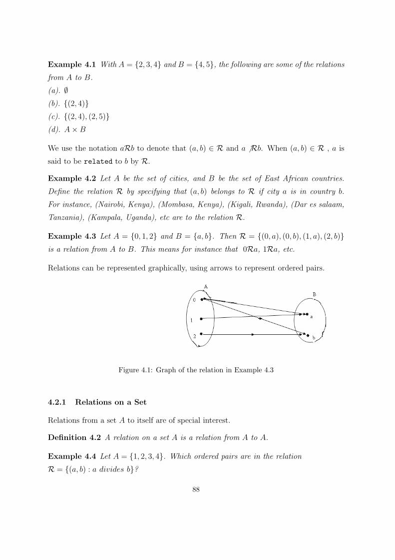
Example 4.1 With A = {2, 3, 4} and B = {4, 5}, the following are some of the relations
from A to B.
(a). ∅(b). {(2, 4)}(c). {(2, 4), (2, 5)}(d). A×B
We use the notation aRb to denote that (a, b) ∈ R and a ̸ Rb. When (a, b) ∈ R , a is
said to be related to b by R.
Example 4.2 Let A be the set of cities, and B be the set of East African countries.
Define the relation R by specifying that (a, b) belongs to R if city a is in country b.
For instance, (Nairobi, Kenya), (Mombasa, Kenya), (Kigali, Rwanda), (Dar es salaam,
Tanzania), (Kampala, Uganda), etc are to the relation R.
Example 4.3 Let A = {0, 1, 2} and B = {a, b}. Then R = {(0, a), (0, b), (1, a), (2, b)}is a relation from A to B. This means for instance that 0Ra, 1Ra, etc.
Relations can be represented graphically, using arrows to represent ordered pairs.
Figure 4.1: Graph of the relation in Example 4.3
4.2.1 Relations on a Set
Relations from a set A to itself are of special interest.
Definition 4.2 A relation on a set A is a relation from A to A.
Example 4.4 Let A = {1, 2, 3, 4}. Which ordered pairs are in the relation
R = {(a, b) : a divides b}?
88
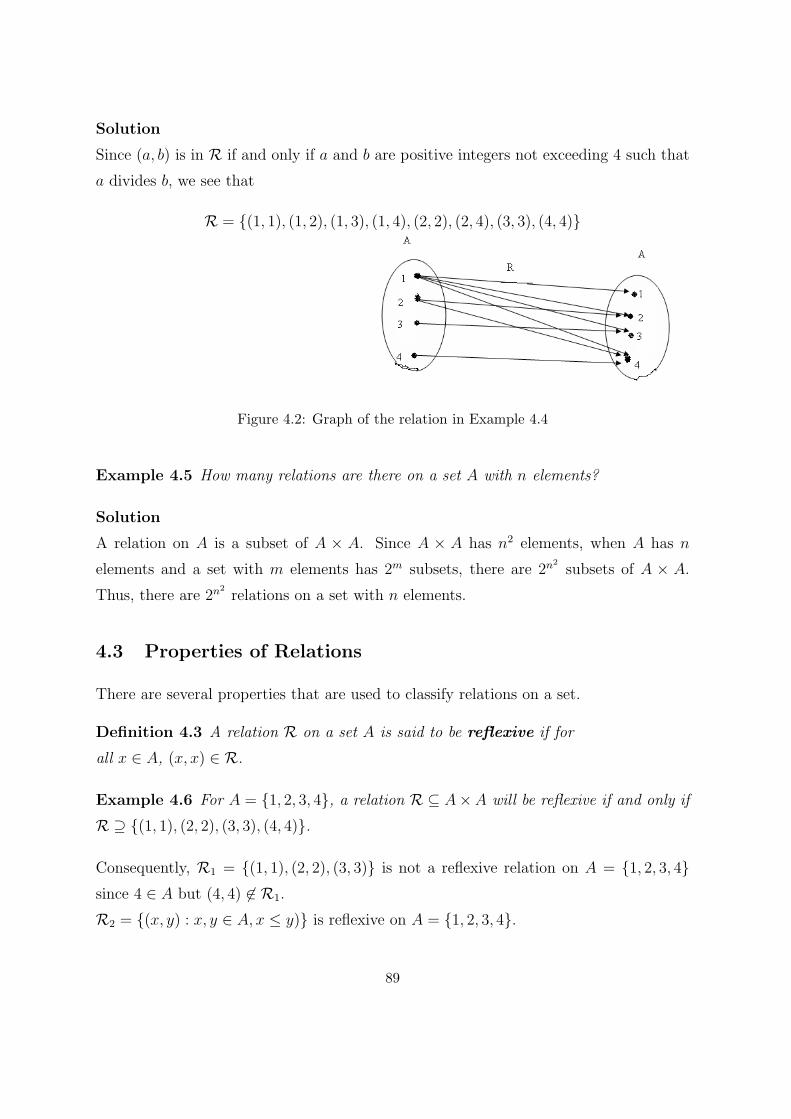
Solution
Since (a, b) is in R if and only if a and b are positive integers not exceeding 4 such that
a divides b, we see that
R = {(1, 1), (1, 2), (1, 3), (1, 4), (2, 2), (2, 4), (3, 3), (4, 4)}
Figure 4.2: Graph of the relation in Example 4.4
Example 4.5 How many relations are there on a set A with n elements?
Solution
A relation on A is a subset of A × A. Since A × A has n2 elements, when A has n
elements and a set with m elements has 2m subsets, there are 2n2subsets of A × A.
Thus, there are 2n2relations on a set with n elements.
4.3 Properties of Relations
There are several properties that are used to classify relations on a set.
Definition 4.3 A relation R on a set A is said to be reflexive if for
all x ∈ A, (x, x) ∈ R.
Example 4.6 For A = {1, 2, 3, 4}, a relation R ⊆ A×A will be reflexive if and only if
R ⊇ {(1, 1), (2, 2), (3, 3), (4, 4)}.
Consequently, R1 = {(1, 1), (2, 2), (3, 3)} is not a reflexive relation on A = {1, 2, 3, 4}since 4 ∈ A but (4, 4) ̸∈ R1.
R2 = {(x, y) : x, y ∈ A, x ≤ y)} is reflexive on A = {1, 2, 3, 4}.
89
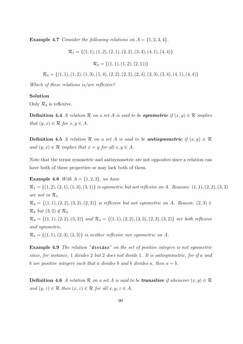
Example 4.7 Consider the following relations on A = {1, 2, 3, 4}.
R1 = {(1, 1), (1, 2), (2, 1), (2, 2), (3, 4), (4, 1), (4, 4)}
R2 = {(1, 1), (1, 2), (2, 1))}
R3 = {(1, 1), (1, 2), (1, 3), (1, 4), (2, 2), (2, 3), (2, 4), (3, 3), (3, 4), (4, 1), (4, 4)}
Which of these relations is/are reflexive?
Solution
Only R3 is reflexive.
Definition 4.4 A relation R on a set A is said to be symmetric if (x, y) ∈ R implies
that (y, x) ∈ R for x, y ∈ A.
Definition 4.5 A relation R on a set A is said to be antisymmetric if (x, y) ∈ Rand (y, x) ∈ R implies that x = y for all x, y ∈ A.
Note that the terms symmetric and antisymmetric are not opposites since a relation can
have both of these properties or may lack both of them.
Example 4.8 With A = {1, 2, 3}, we have
R1 = {(1, 2), (2, 1), (1, 3), (3, 1)} is symmetric but not reflexive on A. Reasons: (1, 1), (2, 2), (3, 3)
are not in R1.
R2 = {(1, 1), (2, 2), (3, 3), (2, 3)} is reflexive but not symmetric on A. Reason: (2, 3) ∈R2 but (3, 2) ̸∈ R2
R3 = {(1, 1), (2, 2), (3, 3)} and R4 = {(1, 1), (2, 2), (3, 3), (2, 3), (3, 2)} are both reflexive
and symmetric.
R5 = {(1, 1), (2, 3), (3, 3)} is neither reflexive nor symmetric on A.
Example 4.9 The relation ”divides” on the set of positive integers is not symmetric
since, for instance, 1 divides 2 but 2 does not divide 1. It is antisymmetric, for if a and
b are positive integers such that a divides b and b divides a, then a = b.
Definition 4.6 A relation R on a set A is said to be transitive if whenever (x, y) ∈ Rand (y, z) ∈ R then (x, z) ∈ R for all x, y, z ∈ A.
90
That is, if x ”is related to” y and y ”is related to” z, then x ”is related to” z, with y
playing the role of intermediary.
Example 4.10 The ”divides” relation on positive integers is transitive, since if a
divides b and b divides c, then there exists positive integers k and l such that b = ak and
c = bl. Hence c = bl = akl, so a divides c.
Example 4.11 If A = {1, 2, 3, 4}, then R1 = {(1, 1), (2, 3), (3, 4), (2, 4)} is a transitive
relation on A, whereas R2 = {(1, 3), (3, 2)} is not transitive because (1, 3), (3, 2) ∈ R2
but (1, 2) ̸∈ R2.
Definition 4.7 A relation R on a set A is said to be an equivalence relation if it is
reflexive, symmetric and transitive.
Definition 4.8 A relation R on a set A is said to be a partial order or a partial
ordering if it is reflexive, antisymmetric and transitive.
Example 4.12 If A = {1, 2, 3}, thenR1 = {(1, 1), ((2, 2), (3, 3)}R2 = {(1, 1), (2, 2), (2, 3), (3, 2), (3, 3)}R3 = {(1, 1), (1, 3), (2, 2), (3, 1), (3, 3)} and
R4 = {(1, 1), (1, 2), (1, 3), (2, 1), (2, 2), (2, 3), (3, 1), (3, 2), (3, 3)} are equivalence relations
on A.
Example 4.13 Let R be the relation on the set of real numbers R such that aRb iff
a− b is an integer. Is R an equivalence relation?
Solution
Since a− a = 0 is an integer for all real numbers a , aRa . Hence R is reflexive.
Now, suppose that aRb. Then a − b is an integer, so b − a is also an integer. Hence,
bRa. It follows that R is symmetric.
If aRb and bRc, then a− b and b− c are integers. Therefore a− c = (a− b) + (b− c) is
also an integer. Hence aRc. Thus, R is transitive.
91
4.4 Combining Relations
Since relations from A to B are subsets of A × B, two relations from A to B can be
combined in any way two sets can be combined as in Chapter 1.
Example 4.14 Let A = {1, 2, 3} and B = {1, 2, 3, 4}. The relations R1 = {(1, 1), (2, 2), (3, 3)}and R2 = {(1, 1), (1, 2), (1, 3), (1, 4)} can be combined to obtain
R1 ∪R2 = {(1, 1), (1, 2), (1, 3), (1, 4), (2, 2), (3, 3)}
R1 ∩R2 = {(1, 1)}
R2 −R1 = {(1, 2), (1, 3), (1, 4)}
Example 4.15 Let A and B be the set of students and the set of all courses at a certain
University, respectively. Suppose that R1 consists of all ordered pairs (a, b), where a is
a student who has taken course b, and R2 consists of all ordered pairs (a, b), where a is
a student who requires course b to graduate. What are the relations R1 ∪R2, R1 ∩R2,
R1 △R2, R1 −R2 and R2 −R1?
Solution
⊙ The relation R1 ∪ R2 consists of all ordered pairs (a, b), where a is a student who
either has taken course b or needs course b to graduate.
⊙ The relation R1 ∩ R2 is the set of all ordered pairs (a, b) where a is a student who
has taken course b and needs this course to graduate.
⊙ The relation R1 △ R2 consists of all ordered pairs (a, b) where student a has taken
course b but does not need it to graduate or needs course b to graduate but has not
taken it.
⊙ The relation R1 −R2 is the set of all ordered pairs (a, b), where student a has taken
course b but does not need it to graduate. That is, b is an elective course that a has
taken.
⊙ The relation R21R1 consists of all ordered pairs (a, b), where b is a course that student
a needs to graduate but has not taken.
92
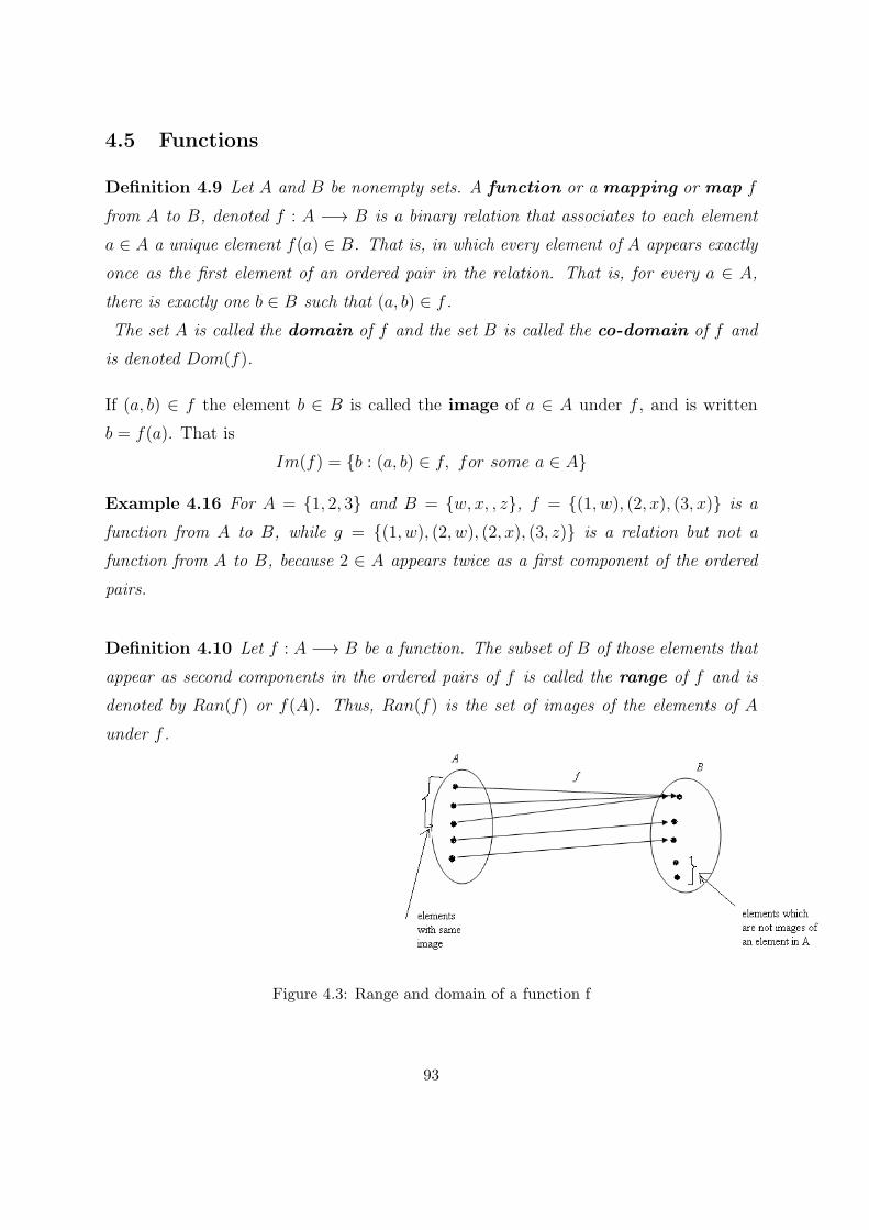
4.5 Functions
Definition 4.9 Let A and B be nonempty sets. A function or a mapping or map f
from A to B, denoted f : A −→ B is a binary relation that associates to each element
a ∈ A a unique element f(a) ∈ B. That is, in which every element of A appears exactly
once as the first element of an ordered pair in the relation. That is, for every a ∈ A,
there is exactly one b ∈ B such that (a, b) ∈ f .
The set A is called the domain of f and the set B is called the co-domain of f and
is denoted Dom(f).
If (a, b) ∈ f the element b ∈ B is called the image of a ∈ A under f , and is written
b = f(a). That is
Im(f) = {b : (a, b) ∈ f, for some a ∈ A}
Example 4.16 For A = {1, 2, 3} and B = {w, x, , z}, f = {(1, w), (2, x), (3, x)} is a
function from A to B, while g = {(1, w), (2, w), (2, x), (3, z)} is a relation but not a
function from A to B, because 2 ∈ A appears twice as a first component of the ordered
pairs.
Definition 4.10 Let f : A −→ B be a function. The subset of B of those elements that
appear as second components in the ordered pairs of f is called the range of f and is
denoted by Ran(f) or f(A). Thus, Ran(f) is the set of images of the elements of A
under f .
Figure 4.3: Range and domain of a function f
93
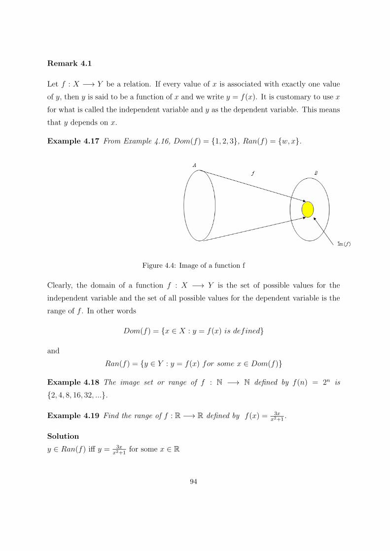
Remark 4.1
Let f : X −→ Y be a relation. If every value of x is associated with exactly one value
of y, then y is said to be a function of x and we write y = f(x). It is customary to use x
for what is called the independent variable and y as the dependent variable. This means
that y depends on x.
Example 4.17 From Example 4.16, Dom(f) = {1, 2, 3}, Ran(f) = {w, x}.
Figure 4.4: Image of a function f
Clearly, the domain of a function f : X −→ Y is the set of possible values for the
independent variable and the set of all possible values for the dependent variable is the
range of f . In other words
Dom(f) = {x ∈ X : y = f(x) is defined}
and
Ran(f) = {y ∈ Y : y = f(x) for some x ∈ Dom(f)}
Example 4.18 The image set or range of f : N −→ N defined by f(n) = 2n is
{2, 4, 8, 16, 32, ...}.
Example 4.19 Find the range of f : R −→ R defined by f(x) = 3xx2+1
.
Solution
y ∈ Ran(f) iff y = 3xx2+1
for some x ∈ R
94
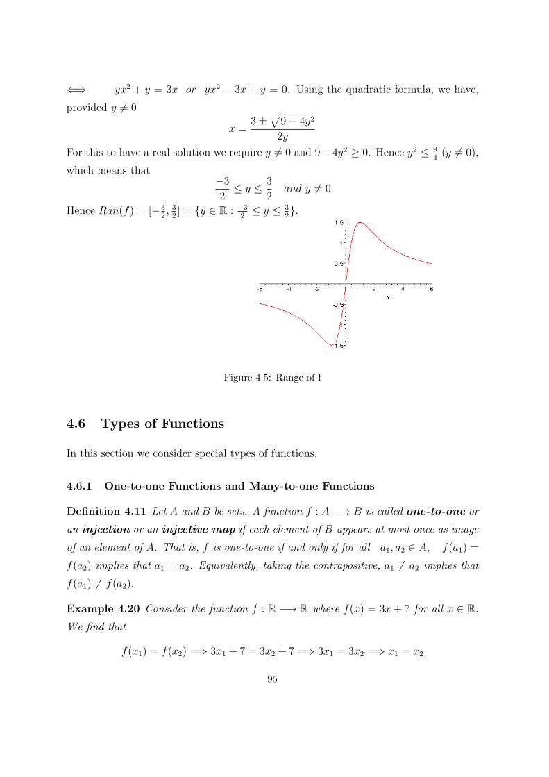
⇐⇒ yx2 + y = 3x or yx2 − 3x + y = 0. Using the quadratic formula, we have,
provided y ̸= 0
x =3±
√9− 4y2
2y
For this to have a real solution we require y ̸= 0 and 9− 4y2 ≥ 0. Hence y2 ≤ 94(y ̸= 0),
which means that−3
2≤ y ≤ 3
2and y ̸= 0
Hence Ran(f) = [−32, 32] = {y ∈ R : −3
2≤ y ≤ 3
2}.
Figure 4.5: Range of f
4.6 Types of Functions
In this section we consider special types of functions.
4.6.1 One-to-one Functions and Many-to-one Functions
Definition 4.11 Let A and B be sets. A function f : A −→ B is called one-to-one or
an injection or an injective map if each element of B appears at most once as image
of an element of A. That is, f is one-to-one if and only if for all a1, a2 ∈ A, f(a1) =
f(a2) implies that a1 = a2. Equivalently, taking the contrapositive, a1 ̸= a2 implies that
f(a1) ̸= f(a2).
Example 4.20 Consider the function f : R −→ R where f(x) = 3x + 7 for all x ∈ R.We find that
f(x1) = f(x2) =⇒ 3x1 + 7 = 3x2 + 7 =⇒ 3x1 = 3x2 =⇒ x1 = x2
95
So f is one-to-one.
Example 4.21 Suppose that g : R −→ R is given by g(x) = x4 − x for each x ∈ R.Then g(0) = 0 and g(1) = 0. Consequently, g is not one-to-one because there exist real
numbers x1, x2 where
g(x1) = g(x2) ̸=⇒ x1 = x2. (4.1)
Functions which satisfy (4.1) are called many-to-one functions.
4.6.2 Onto Functions
Definition 4.12 Let A and B be sets. A function f : A −→ B is called onto or
surjective or a surjection if f(A) = B. That is, if for all b ∈ B, there is at least one
a ∈ A with f(a) = b. That is, if Ran(f) = Co− domain of f .
Example 4.22 Consider the function f : R −→ R where f(x) = x3 for all x ∈ R.Clearly f is onto.
Example 4.23 The function g : R −→ R where f(x) = x2 for all x ∈ R is not onto.
No negative numbers appear in Ran(f). Here Ran(f) = [0,∞) ̸= R = Co− dom(f).
4.6.3 Bijective Functions
Definition 4.13 Let A and B be sets. A function f : A −→ B is called bijective or a
one-to-one correspondence if f is both one-to-one and onto.
Example 4.24 Consider the function f : R −→ R where f(x) = x + 2 for all x ∈ R.Clearly f is a bijection, since it is both one-to-one and onto.
96
4.7 Composition and Inverses of Functions
Definition 4.14 Let A be a set. The function f : A −→ A, defined by f(a) = a for all
a ∈ A, is called the identity function. The identity function on A is usually denoted
by 1A.
Definition 4.15 Let A and B be sets and let f, g : A −→ B be functions. We say that
f and g are equal and write f = g, if f(a) = g(a) for all a ∈ A.
4.7.1 Composition of Functions
Definition 4.16 Let A,B and C be sets. If f : A −→ B and g : B −→ C are
functions, we define the composite function, which is denoted by g ◦ f : A −→ C,
by (g ◦ f)(a) = g(f(a)
)for each a ∈ A.
Example 4.25 Let A = {1, 2, 3, 4}, B = {a, b, c} and C = {w, x, y, z}, with f : A −→B and g : B −→ C, given by f = {(1, a), (2, a), (3, b), (4, c)} and g = {(a, x), (b, y), (c, 2)}.For each element of A we find that:
(g ◦ f)(1) = g(f(1)) = g(a) = x
(g ◦ f)(2) = g(f(2)) = g(a) = x
(g ◦ f)(3) = g(f(3)) = g(b) = y
(g ◦ f)(4) = g(f(4)) = g(a) = z
Note that the composition f ◦ g is not defined in Example 4.25.
Example 4.26 Let f : R −→ R and g : R −→ R be defined by f(x) = x2 and
g(x) = x+ 5. Then
(g ◦ f)(x) = g(f(x)) = g(x2) = x2 + 5,
where as
(f ◦ g)(x) = f(g(x)) = f(x+ 5) = (x+ 5)2 = x2 + 10x+ 25
Note that f ◦ g ̸= g ◦ f in general. That is, composition of functions is not, in general,
commutative.
97
Theorem 4.1 Let A,B and C be sets and f : A −→ B and g : B −→ C be functions.
(a). If f and g are one-to-one then g ◦ f is one-to-one.
(b). If f and g are onto then g ◦ f is onto.
Proof
(a). To prove that g ◦ f : A −→ C is one-to-one, let a1, a2 ∈ A with (g ◦ f)(a1) =
(g ◦ f)(a2). Then (g ◦ f)(a1) = (g ◦ f)(a2) = g(f(a1)) = g(f(a2)) =⇒ f(a1) = f(a2),
because g is one-to-one.
Also, f(a1) = f(a2) =⇒ a1 = a2, because f is one-to-one. Consequently, g ◦ f is one-to-
one.
(b). If g◦f : A −→ C, let z ∈ C. Since g is onto, there exists y ∈ B with g(y) = z. With
f onto and y ∈ B, there is x ∈ A with f(x) = y. Hence z = g(y) = g(f(x)) = (g ◦f)(x).So Ran(g ◦ f) = C = co− domain of g ◦ f . This proves that g ◦ f is onto.
Remark 4.2 Note that function composition is, in general, an associative operation.
That is (h ◦ g) ◦ f = h ◦ (g ◦ f).
4.7.2 Inverse of a Function
Definition 4.17 Let A and B be sets and f : A −→ B be a function. We say that f is
invertible if there is a function g : B −→ A such that g ◦ f = 1A and f ◦ g = 1B.
Theorem 4.2 A function f : A −→ B is invertible if and only if it is one-to-one and
onto. The inverse relation
f−1 = {(b, a) : (a, b) ∈ f}
from B to A will be called the inverse of f and pronounced ”f inverse”.
Thus f and g in Definition 4.17 are inverses of each other.
Theorem 4.3 If f : A −→ B and g : B −→ C are invertible functions then g ◦ f :
A −→ C is invertible and
(g ◦ f)−1 = f−1 ◦ g−1
98
Remark 4.3 To find the inverse of an invertible function f : X −→ Y , defined by
y = f(x) (4.2)
We solve (4.2) for x (i.e. we make x the subject of the formula), then swap the roles of
x and y.
Example 4.27 If A = {1, 2, 3, 4} and B = {x, y, z, t}, and f = {(1, x), (2, y), (3, z), (4, t)}then f−1 = {(x, 1), (y, 2), (z, 3), (t, 4)}.
Note that (f−1)−1 = f .
Example 4.28 Let f, g : R −→ R is defined by f(x) = 2x − 3 and g(x) = x+15,
respectively. Find f−1 and g−1.
Solution
It is easy to verify that both f and g are bijective and so each has an inverse. According
to (4.2)
2x = y+3. Thus x = 12(y+3). We now swap the roles of x and y. Thus f−1(x) = 1
2(x+3).
Similarly, x + 1 = 5y. Thus x = 5y − 1. We now swap the roles of x and y to get
g−1(x) = 5x− 1.
Definition 4.18 To each function f : A −→ B , there corresponds the relation in A×Bgiven by {(a, f(a)) : a ∈ A}. We call this set the graph of f .
4.7.3 The Vertical Line Test for a Function
A curve in the (x, y)-plane is the graph of some function f : A −→ R where A ⊆ R if
and only if the following condition is satisfied.
⊙ Every vertical line in the plane meets the curve at most once.
4.8 Some Special Real Valued Functions
The following are some special functions.
1. Identity Function
99
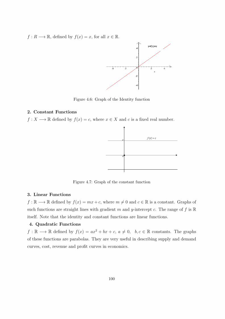
f : R −→ R, defined by f(x) = x, for all x ∈ R.
Figure 4.6: Graph of the Identity function
2. Constant Functions
f : X −→ R defined by f(x) = c, where x ∈ X and c is a fixed real number.
Figure 4.7: Graph of the constant function
3. Linear Functions
f : R −→ R defined by f(x) = mx+ c, where m ̸= 0 and c ∈ R is a constant. Graphs of
such functions are straight lines with gradient m and y-intercept c. The range of f is Ritself. Note that the identity and constant functions are linear functions.
4. Quadratic Functions
f : R −→ R defined by f(x) = ax2 + bx + c, a ̸= 0, b, c ∈ R constants. The graphs
of these functions are parabolas. They are very useful in describing supply and demand
curves, cost, revenue and profit curves in economics.
100
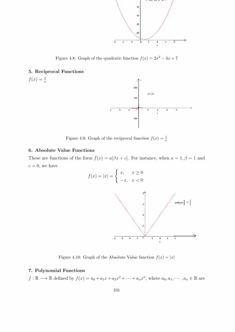
Figure 4.8: Graph of the quadratic function f(x) = 2x2 − 4x+ 7
5. Reciprocal Functions
f(x) = 1x
Figure 4.9: Graph of the reciprocal function f(x) = 1x
6. Absolute Value Functions
These are functions of the form f(x) = a|βx + c|. For instance, when a = 1, β = 1 and
c = 0, we have
f(x) = |x| =
{x, x ≥ 0
−x, x < 0
Figure 4.10: Graph of the Absolute Value function f(x) = |x|
7. Polynomial Functions
f : R −→ R defined by f(x) = a0+a1x+a2x2+ · · ·+anxn, where a0, a1, · · · , an ∈ R are
101
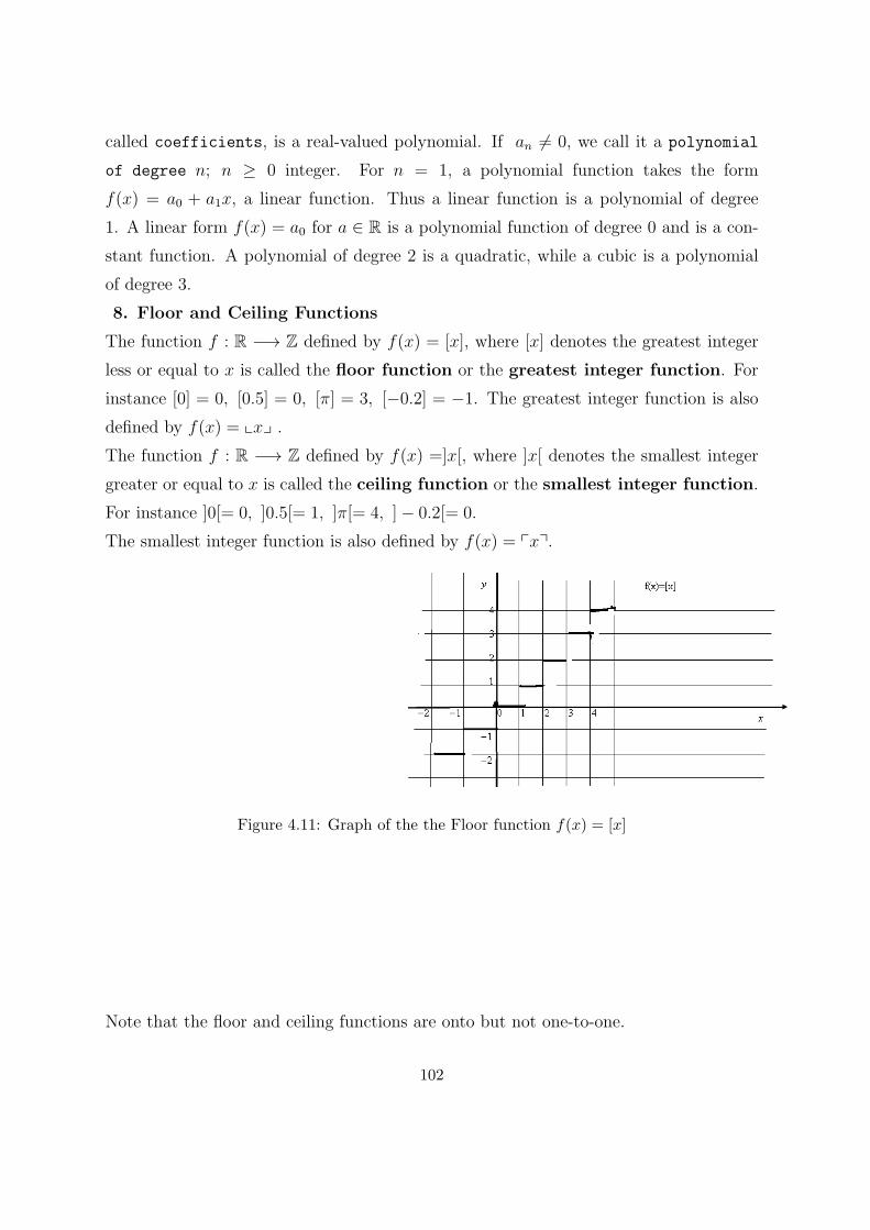
called coefficients, is a real-valued polynomial. If an ̸= 0, we call it a polynomial
of degree n; n ≥ 0 integer. For n = 1, a polynomial function takes the form
f(x) = a0 + a1x, a linear function. Thus a linear function is a polynomial of degree
1. A linear form f(x) = a0 for a ∈ R is a polynomial function of degree 0 and is a con-
stant function. A polynomial of degree 2 is a quadratic, while a cubic is a polynomial
of degree 3.
8. Floor and Ceiling Functions
The function f : R −→ Z defined by f(x) = [x], where [x] denotes the greatest integer
less or equal to x is called the floor function or the greatest integer function. For
instance [0] = 0, [0.5] = 0, [π] = 3, [−0.2] = −1. The greatest integer function is also
defined by f(x) = xxy .
The function f : R −→ Z defined by f(x) =]x[, where ]x[ denotes the smallest integer
greater or equal to x is called the ceiling function or the smallest integer function.
For instance ]0[= 0, ]0.5[= 1, ]π[= 4, ]− 0.2[= 0.
The smallest integer function is also defined by f(x) = pxq.
Figure 4.11: Graph of the the Floor function f(x) = [x]
Note that the floor and ceiling functions are onto but not one-to-one.
102
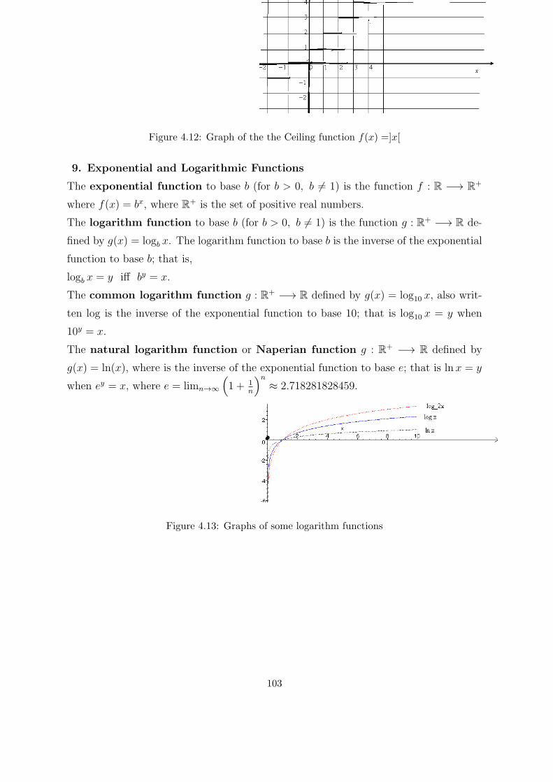
Figure 4.12: Graph of the the Ceiling function f(x) =]x[
9. Exponential and Logarithmic Functions
The exponential function to base b (for b > 0, b ̸= 1) is the function f : R −→ R+
where f(x) = bx, where R+ is the set of positive real numbers.
The logarithm function to base b (for b > 0, b ̸= 1) is the function g : R+ −→ R de-
fined by g(x) = logb x. The logarithm function to base b is the inverse of the exponential
function to base b; that is,
logb x = y iff by = x.
The common logarithm function g : R+ −→ R defined by g(x) = log10 x, also writ-
ten log is the inverse of the exponential function to base 10; that is log10 x = y when
10y = x.
The natural logarithm function or Naperian function g : R+ −→ R defined by
g(x) = ln(x), where is the inverse of the exponential function to base e; that is lnx = y
when ey = x, where e = limn→∞
(1 + 1
n
)n
≈ 2.718281828459.
Figure 4.13: Graphs of some logarithm functions
103
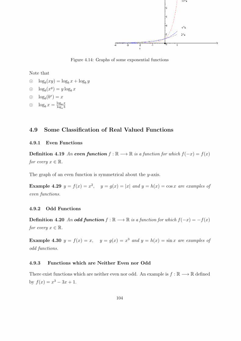
Figure 4.14: Graphs of some exponential functions
Note that
⊙ logb(xy) = logb x+ logb y
⊙ logb(xy) = y logb x
⊙ logb(bx) = x
⊙ logb x = loga xloga b
4.9 Some Classification of Real Valued Functions
4.9.1 Even Functions
Definition 4.19 An even function f : R −→ R is a function for which f(−x) = f(x)
for every x ∈ R.
The graph of an even function is symmetrical about the y-axis.
Example 4.29 y = f(x) = x2, y = g(x) = |x| and y = h(x) = cos x are examples of
even functions.
4.9.2 Odd Functions
Definition 4.20 An odd function f : R −→ R is a function for which f(−x) = −f(x)for every x ∈ R.
Example 4.30 y = f(x) = x, y = g(x) = x3 and y = h(x) = sinx are examples of
odd functions.
4.9.3 Functions which are Neither Even nor Odd
There exist functions which are neither even nor odd. An example is f : R −→ R defined
by f(x) = x3 − 3x+ 1.
104
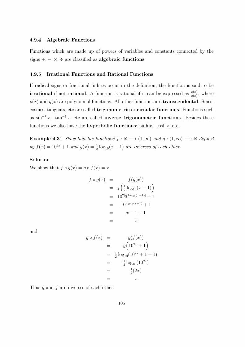
4.9.4 Algebraic Functions
Functions which are made up of powers of variables and constants connected by the
signs +,−,×,÷ are classified as algebraic functions.
4.9.5 Irrational Functions and Rational Functions
If radical signs or fractional indices occur in the definition, the function is said to be
irrational if not rational. A function is rational if it can be expressed as p(x)q(x)
, where
p(x) and q(x) are polynomial functions. All other functions are transcendental. Sines,
cosines, tangents, etc are called trigonometric or circular functions. Functions such
as sin−1 x, tan−1 x, etc are called inverse trigonometric functions. Besides these
functions we also have the hyperbolic functions: sinhx, coshx, etc.
Example 4.31 Show that the functions f : R −→ (1,∞) and g : (1,∞) −→ R defined
by f(x) = 102x + 1 and g(x) = 12log10(x− 1) are inverses of each other.
Solution
We show that f ◦ g(x) = g ◦ f(x) = x.
f ◦ g(x) = f(g(x))
= f(
12log10(x− 1)
)= 102[
12log10(x−1)] + 1
= 10log10(x−1) + 1
= x− 1 + 1
= x
andg ◦ f(x) = g(f(x))
= g(102x + 1
)= 1
2log10(10
2x + 1− 1)
= 12log10(10
2x)
= 12(2x)
= x
Thus g and f are inverses of each other.
105
4.10 Solved Problems
1. Let f, g, h, l(x) : R −→ R be the functions defined by f(x) = x2, g(x) =−4x2x−3
, h(x) =√6− x, l(x) = 1
x+3. Find the domain and range of each of these functions
Solution
Dom(f) = R,Ran(f) = [0,∞)
Dom(g) = {x ∈ R : x ̸= 32} = R− {3
2}
Ran(g) = {y ∈ R : y ̸= 0} = R− {0}
Dom(h) = (−∞, 6], since for y to be a real number, 6− x must be non-negative. This
happens only when 6− x ≥ 0 or 6 ≥ x.
Ran(h) = [0,∞), because√6− x is always non-negative.
Dom(l) = R− {−3}Ran(l) = R− {0}2. Determine whether or not each of the following relations is a function. If a relation
is a function, find its range.
(a). {(x, y) : x, y ∈ Z, y = x2 + 7}(b). {(x, y) : x, y ∈ R, y2 = x}(c). {(x, y) : x, y ∈ R, y = 3x+ 1}(d). {(x, y) : x, y ∈ Q, x2 + y2 = 1}Solution
(a). It is a relation and a function from Z to Z; Ran(f) = {7, 8, 11, 16, 23, · · · }(b). This is a relation but not a function.
(c). This is a relation and a function from R to R; Ran(f) = R(d). This is a relation from Q to Q but not a function.
3. For each of the following functions, determine whether it is one-to-one, onto and
determine its range.
(a). f : Z −→ Z, defined by f(x) = 2x+ 1
(b). f : Q −→ Q, defined by f(x) = 2x+ 1
106
(c). f : Z −→ Z, defined by f(x) = x3 − x
(d). f : R −→ R, defined by f(x) = ex
(e). f : [−π2, π2] −→ R, defined by f(x) = sinx
Solution
(a). f is one-to-one and not onto; the range of f is the set of odd integers.
(b). f is one-to-one and onto; Ran(f) = Q.
(c). f is not one-to-one and not onto; Ran(f) = {0,±6,±24,±60, · · · } = {n3 − n : n ∈Z}.(d). f is one-to-one but not onto; Ran(f) = (0,∞).
(e). f is one-to-one and not onto; Ran(f) = [0, 1].
4. Determine whether or not each of the following functions is a bijection. If a bijection,
find its inverse.
(a). f : R −→ R defined by f(x) = x−37
(b). f : R −→ R defined by f(x) = logex.
Solution
Easy and hence left as an exercise.
4.11 Exercises
1. Find the domain and range of the following functions
(a). f : R −→ R, defined by f(x) =√2x2 + 5x− 12
(b). f : R −→ R, defined by f(x) = xx2−5
2. Let f, g and h be the functions defined as follows
f : R −→ R, f(x) = x2 − 5,
g : Z −→ R, g(x) = 5xx2−2
h : R −→ R, f(x) = [x].
Find the following
(a). f(3)
(b). g(h(4.7))
(c). (f ◦ h)(x)(d). f ◦ (h ◦ g)(x)(e). f ◦ (h ◦ g)(−7)
107
3. Let A = {humans, livingordead} and let f and g be the functions A −→ A defined
by f(x) = the father of x and g(x) = the mother of x, respectively. Describe the
composite functions f ◦ f, f ◦ g, g ◦ f and g ◦ g.4. Show that each of the following is a bijection and find its inverse.
(a). f : R −→ R, defined by 5x+38
(b). f : R− {−1} −→ R− {3}, defined by f(x) = 3xx+1
5. Show that the functions f : R −→ (1,∞) and g : (1,∞) −→ R defined by f(x) =
32x + 1 and g(x) = 12log3(x− 1) are inverses of each other.
6. Let W,Z denote the set of whole numbers and integers, respectively. Give an example
of:
(a). a one-to-one function f : R −→ R which is not onto.
(b). a many-to-one function g : Z −→ W which is onto.
108
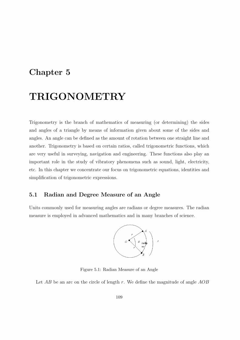
Chapter 5
TRIGONOMETRY
Trigonometry is the branch of mathematics of measuring (or determining) the sides
and angles of a triangle by means of information given about some of the sides and
angles. An angle can be defined as the amount of rotation between one straight line and
another. Trigonometry is based on certain ratios, called trigonometric functions, which
are very useful in surveying, navigation and engineering. These functions also play an
important role in the study of vibratory phenomena such as sound, light, electricity,
etc. In this chapter we concentrate our focus on trigonometric equations, identities and
simplification of trigonometric expressions.
5.1 Radian and Degree Measure of an Angle
Units commonly used for measuring angles are radians or degree measures. The radian
measure is employed in advanced mathematics and in many branches of science.
Figure 5.1: Radian Measure of an Angle
Let AB be an arc on the circle of length r. We define the magnitude of angle AOB
109
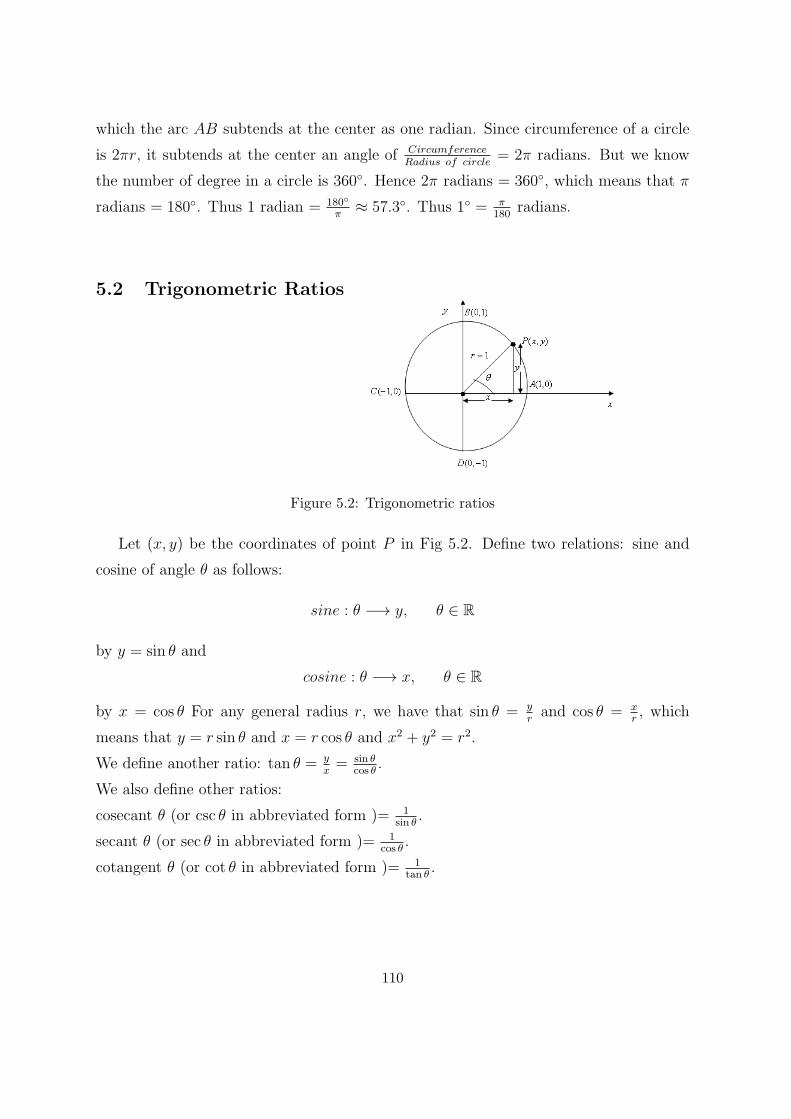
which the arc AB subtends at the center as one radian. Since circumference of a circle
is 2πr, it subtends at the center an angle of CircumferenceRadius of circle
= 2π radians. But we know
the number of degree in a circle is 360◦. Hence 2π radians = 360◦, which means that π
radians = 180◦. Thus 1 radian = 180◦
π≈ 57.3◦. Thus 1◦ = π
180radians.
5.2 Trigonometric Ratios
Figure 5.2: Trigonometric ratios
Let (x, y) be the coordinates of point P in Fig 5.2. Define two relations: sine and
cosine of angle θ as follows:
sine : θ −→ y, θ ∈ R
by y = sin θ and
cosine : θ −→ x, θ ∈ R
by x = cos θ For any general radius r, we have that sin θ = yrand cos θ = x
r, which
means that y = r sin θ and x = r cos θ and x2 + y2 = r2.
We define another ratio: tan θ = yx= sin θ
cos θ.
We also define other ratios:
cosecant θ (or csc θ in abbreviated form )= 1sin θ
.
secant θ (or sec θ in abbreviated form )= 1cos θ
.
cotangent θ (or cot θ in abbreviated form )= 1tan θ
.
110
5.3 Trigonometric Identities
5.3.1 Cofunction Identities
Let θ be a certain angle. We have
sin θ = cos(90◦ − θ) cos θ = sin(90◦ − θ)
tan θ = cot(90◦ − θ) cot θ = tan(90◦ − θ)
sec θ = csc(90◦ − θ) csc θ = sec(90◦ − θ)
We also have that
cos(−θ) = cos θ (cosine function is an even function)
sin(−θ) = − sin θ (sine function is an odd function)
tan(−θ) = − tan θ (tangent function is an odd function)
5.3.2 Pythagorean Identities
From Figure 5.2, using the right-angled triangle, we have that x2+y2 = 1 is the equation
of the unit circle in the xy-plane. For any point on the unit circle, the coordinates x
and y satisfy the equation x = cos θ, y = sin θ. Substituting in the equation of the unit
circle, we have that
cos2 θ + sin2 θ = 1 (5.1)
Dividing (5.1) by cos2 θ, we have
1 + tan2θ = sec2 θ (5.2)
Dividing (5.1) by sin2 θ, we have
1 + cot2 θ = csc2 θ (5.3)
We can factor, simplify and manipulate trigonometric expressions in the same way we
manipulate strictly algebraic expressions.
111
Example 5.1 Simplify cos θ(tan θ − sec θ).
Solutioncos θ(tan θ − sec θ) = cos θ tan θ − cos θ sec θ
= cos θ sin θcos θ
− cos θ 1cos θ
= sin θ − 1
Remark 5.1 Note that there is no general procedure for manipulating trigonometric
expressions, but it is often helpful to write everything in terms of sines and cosines and
apply known identities, where necessary.
Example 5.2 Simplify sin2 x cos2 x+ cos4 x.
Solution
sin2 x cos2 x+ cos4 x = cos2 x(sin2 x+ cos2 x)
= cos2 x(1)
= cos2 x
Example 5.3 Simplify each of the following trigonometric expressions
(a). cot(−θ)csc(−θ)
.
(b). 2 sin2 θ+sin θ−31−cos2 θ−sin θ
.
Solution
(a).
cot(−θ)csc(−θ)
=cos(−θ)sin(−θ)
1sin(−θ)
= cos(−θ)sin(−θ)
sin(−θ)= cos(−θ)= cos θ
(b).2 sin2 θ+sin θ−31−cos2 θ−sin θ
= 2 sin2 θ+sin θ−3sin2 θ−sin θ
= (2 sin θ+3)(sin θ−1)sin θ(sin θ−1)
= 2 sin θ+3sin θ
= 2 + 3sin θ
or 2 + 3 csc θ
112
5.3.3 Sum and Difference Identities
We now develop some important identities involving sum and difference of two angles.
For any given angles A and B, we have
sin(A+B) = sinA cosB + cosA sinB (5.4)
cos(A+B) = cosA cosB − sinA sinB (5.5)
Writing −B for B in (5.4) and (5.5) we get
sin(A−B) = sinA cosB − cosA sinB (5.6)
cos(A−B) = cosA cosB + sinA sinB (5.7)
Dividing (5.4) by (5.5) gives
tan(A+B) = sin(A+B)cos(A+B)
= sinA cosB+cosA sinBcosA cosB−sinA sinB
=sinA cosBcosA cosB
+ cosA sinBcosA cosB
cosA cosBcosA cosB
− sinA sinBcosA cosB
= tanA+tanB1−tanA tanB
(on dividing each term by cosA cosB and simplifying)
(5.8)
Replacing B by −B in (5.8) gives
tan(A−B) =tanA− tanB
1 + tanA tanB(5.9)
Adding (5.5) and (5.7) gives
2 cosA cosB = cos(A+B) + cos(A−B)
or
cosA cosB =1
2[cos(A+B) + cos(A−B)] (5.10)
Adding (5.4) and (5.6) gives
2 sinA cosB = sin(A+B) + sin(A−B)
113
or
sinA cosB =1
2[sin(A+B) + sin(A−B)] (5.11)
Subtracting (5.6) from (5.4) we have
2 cosA sinB = sin(A+B)− sin(A−B)
or
cosA sinB =1
2[sin(A+B)− sin(A−B)] (5.12)
Subtracting (5.7) from (5.5) gives
−2 sinA sinB = cos(A+B)− cos(A−B)
or
sinA sinB = −1
2[cos(A+B)− cos(A−B)] (5.13)
Identities (5.10), (5.11), (5.12) and (5.13) are called products of sines and cosines
identities.
From the above identities, it is easy to derive the following identities.
sinA+ sinB = 2 sin1
2(A+B) cos
1
2(A−B) (5.14)
sinA− sinB = 2 cos1
2(A+B) sin
1
2(A−B) (5.15)
cosA+ cosB = 2 cos1
2(A+B) cos
1
2(A−B) (5.16)
cosA− cosB = −2 sin1
2(A+B) sin
1
2(A−B) (5.17)
Proof
Let A+B = α and A−B = β so that A = 12(α+ β) and B = 1
2(α− β). Then
sin(A+B) + sin(A−B) = 2 sinA cosB
Thus
sinα+ sin β = 2 sin1
2(α+ β) cos
1
2(α− β)
This proves (5.14).
The other identities can be proved similarly and are left as exercises.
114
Example 5.4 Express each of the following as a sum or difference
(a). sin 40◦ cos 30◦.
(b). cos 110◦ sin 55◦
Solution
(a).
sin 40◦ cos 30◦ = 12[sin(40◦ + 30◦) + sin(40◦ − 30◦)]
= 12(sin 70◦ + sin 10◦)
(b).
cos 110◦ sin 55◦ = 12[sin(110◦ + 55◦)− sin(110◦ − 55◦)]
= 12(sin 165◦ − sin 55◦)
Example 5.5 Express each of the following as a product.
(a). sin 50◦ + sin 40◦
(b). sin 70◦ − sin 20◦
Solution
(a).
sin 50◦ + sin 40◦ = 2 sin 12(50◦ + 40◦) cos 1
2(50◦ − 40◦)
= 2 sin 45◦ cos 5◦
(b).
sin 70◦ − sin 20◦ = 2 cos 12(70◦ + 20◦) sin 1
2(70◦ − 20◦)
= 2 cos 45◦ sin 25◦
Example 5.6 Prove thatsin 4A+ sin 2A
cos 4A+ cos 2A= tan 3A
Solution
sin 4A+sin 2Acos 4A+cos 2A
=2 sin 1
2(4A+2A) cos 1
2(4A−2A)
2 cos 12(4A+2A) cos 1
2(4A−2A)
= sin 3Acos 3A
= tan 3A
Example 5.7 Prove that
sinA− sinB
sinA+ sinB=
tan 12(A−B)
tan 12(A+B)
115
SolutionsinA−sinBsinA+sinB
=2 cos 1
2(A+B) sin 1
2(A−B)
2 sin 12(A+B) cos 1
2(A−B)
= cot 12(A+B) tan 1
2(A−B)
=tan 1
2(A−B)
tan 12(A+B)
Example 5.8 Prove that
1 + cos 2x+ cos 4x+ cos 6x = 4 cosx cos 2x cos 3x
Solution
1 + cos 2x+ cos 4x+ cos 6x = 1 + (cos 2x+ cos 4x) + cos 6x
= 1 + 2 cos 3x cos x+ cos 6x
= (1 + cos 6x) + 1 + 2 cos 3x cosx
= 2 cos2 3x+ 1 + 2 cos 3x cosx
= 2 cos 3x(cos 3x+ cos x)
= 2 cos 3x(2 cos 2x cosx)
= 4 cos x cos 2x cos 3x
5.3.4 Double-Angle Identities
In (5.4), (5.5) and (5.8), if we let A = B = x, we have
sin 2x = sinx cos x+ cosx sinx
= 2 sin x cosx(5.18)
cos 2x = cosx cosx− sinx sinx
= cos2 x− sin2 x(5.19)
and in a similar manner
tan 2x =2 tanx
1− tan2 x(5.20)
Equation (5.19) can also be written as
cos 2x = cosx cosx− sinx sinx
= cos2 x− sin2 x
= 1− sin2 x− sin2 x
= 1− 2 sin2 x
= 2 cos2 x− 1
(5.21)
116
From (5.20) and (5.21), we obtain the following identities
sin2 x =1− cos 2x
2(5.22)
cos2 x =1 + cos 2x
2(5.23)
Dividing these two we have
tan2 x =1− cos 2x
1 + cos 2x(5.24)
Example 5.9 Find an equivalent expression for each of the following:
(a). sin 3θ in terms of function values of θ.
(b). cos3 x in terms of values of x or 2x, raised only to the first power.
Solution
(a).
sin 3θ = sin(2θ + θ)
= sin 2θ cos θ + cos 2θ sin θ
= (2 sin θ cos θ) cos θ + (2 cos2 θ − 1) sin θ
= 2 sin θ cos2 θ + 2 sin θ cos2 θ − sin θ
= 4 sin θ cos2 θ − sin θ
(b).
cos3 x = cos2 x cos x
= (1+cos 2x2
) cos x
= cosx+cosx cos 2x2
5.3.5 Half-Angle Identities
In (5.22), (5.23) and (5.24), if we replace x with x2and take square roots, we get
sinx
2= ±
√1− cosx
2(5.25)
cosx
2= ±
√1 + cosx
2(5.26)
tanx
2= ±
√1− cos x
1 + cosx=
sin x
1 + cosx=
1− sinx
sinx(5.27)
117
The use of + or − depends on the quadrant in which the angle x2is.
Also using the formula (5.20) and writing 2x = θ and so x = θ2, we have
tan θ =2 tan θ
2
1− tan2 θ2
or2t
1− t2
where t = tan θ2.
It is possible to find formulae for sin θ and cos θ in terms of t using aright-angled triangle.
It is easy to show that
sin θ =2t
1 + t2
and
cos θ =1− t2
1 + t2
Example 5.10 Find tan π8
Solution
tan π8= tan
π4
2=
sin π4
1+cos π4=
√2
2
1+√
22
=√2
2+√2=
√2− 1
Example 5.11 Simplify each of the following
(a). sinx cosx12cos 2x
(b). 2 sin2 x2+ cosx
Solution
(a). Multiply the numerator and denominator by 22and simplify using known identities
to get2 sinx coscos 2x
= sin 2xcos 2x
= tan 2x
(b).
2 sin2 x2+ cosx = 2(1−cosx
2) + cos x
= 1− cosx+ cosx
= 1
5.4 Proving Identities
We can use some known identities to prove other identities.
Example 5.12 Prove the identity
1 + sin 2θ = (sin θ + cos θ)2
118
Solution(sin θ + cos θ)2 = sin2 θ + 2 sin θ cos θ + cos2 θ
= 1 + 2 sin θ cos θ
= 1 + sin 2θ
We could also begin with the left side and obtain the right side:
1 + sin 2θ = 1 + 2 sin θ cos θ
= sin2 θ + 2 sin θ cos θ + cos2 θ
= (sin θ + cos θ)2
Example 5.13 Prove that
1
(cscθ − sin θ)(sec θ − cos θ)= tan θ + cot θ
Solution
We write the left hand side in terms of sin θ and cos θ:LHS = 1
( 1sin θ
−sin θ)( 1cos θ
−cos θ)
= 1(1−sin2 θ)
sin θ(1−cos2 θ)
cos θ
= sin θ cos θ(1−sin2 θ)(1−cos2 θ)
= sin θ cos θcos2 θ sin2 θ
= 1sin θ cos θ
We now write the right hand side in terms of sin θ and cos θ:
RHS = tan θ + cot θ
= sin θcos θ
+ cos θsin θ
= sin2 θ+cos2 θcos θ sin θ
= sin θ cos θcos2 θ sin2 θ
= 1sin θ cos θ
= LHS
5.5 Solving Trigonometric Equations
Example 5.14 Solve the equation
12 cos2 θ + sin θ = 11
on the domain 0◦ ≤ θ ≤ 360◦
119
Solution
Recall that cos2 θ = 1− sin2 θ.
12(1− sin2 θ) + sin θ = 11
12− 12 sin2 θ + sin θ = 11
or − 12 sin2 θ + sin θ = −1
or 12 sin2 θ − sin θ = 1 or 12 sin2 θ − sin θ − 1 = 0
or (3 sin θ − 1)(4 sin θ + 1) = 0
=⇒ sin θ = 13or sin θ = −1
4
=⇒ θ = 19.47◦ (principal value) or θ = 180◦ − 19.47◦ = 160.53◦(secondary value) or
θ = −14.48◦ (principal value) or − 165.52◦ (secondary value)
The general solution is θ = −14.48◦ + 360n◦ or −165.52◦ + 360n◦.
On domain 0◦ ≤ θ ≤ 360◦
θ = 345.52◦ or 194.48◦.
So the complete solution on domain 0◦ ≤ θ ≤ 360◦ is
θ = 19.47◦ or θ = 160.53◦
or
θ = 194.48◦ or θ = 345.52◦
Example 5.15 Find the general solution of the equation
12 sec2 θ − 13 tan θ − 9 = 0
Solution12 sec2 θ − 13 tan θ − 9 = 12(1 + tan2 θ)− 13 tan θ − 9 = 0
i.e. 12 + 12 tan2 θ − 13 tan θ − 9 = 0
i.e. 12 tan2 θ − 13 tan θ + 3 = 0
i.e. (4 tan θ − 3)(3 tan θ − 1) = 0
i.e. tan θ = 34or tan θ = 1
3
giving a general solution
θ = 36.87◦ + 180n◦ or θ = 18.43◦ + 180n◦, n ∈ Z.
Example 5.16 Find all angles θ in the domain −360◦ ≤ θ ≤ 360◦ for which sin θ =
0.3.
120
Solution
The principal value is 17.46◦. The secondary solution is in the second quadrant. That
is, 180◦ − 17.46◦ = 162.54◦.
One general solution is 17.46◦ + 360n◦.
We now try various values of n, starting with 0,±1,±2, until we find the solutions
exceeding the limits of the given domain.
n = 0, θ = 17.46◦
n = 1, θ = 377.46◦ too large
n = −1 θ = −342.54◦
n = −2 θ = −702.54◦ too large on the negative side
So far the general solution ◦17.46◦ + 360n◦ has yielded solutions
θ = 17.46◦, − 342.54◦.
The other general solution is 162.54◦ + 360n◦
n = 0, θ = 162.54◦
n = 1, θ = 522.54◦ too large
n = −1 θ = −197.46◦
n = −2 θ = −557.46◦ too large on the negative side
So the other general solution 162.54◦ + 360n◦ has yielded solutions
θ = 162.54◦, − 197.46◦.
Hence the solution on the domain −360◦ ≤ θ ≤ 360◦ is
θ = 17.46◦ or 162.54◦ or − 197.46◦.
Example 5.17 Solve using two methods the equation sin 6x − sin 2x = 0 giving the
general solution.
Solution
This equation can be solved by writing sin 6x = sin 2x and hence
6x = 2x+ 2πn
or 6x = π − 2x+ 2πn, n ∈ Zleading to x = πn
2
or x = π8+ πn
4, n ∈ Z
121
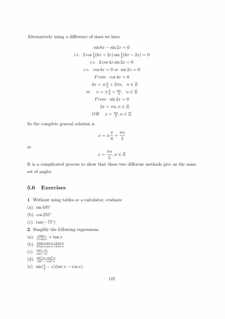
Alternatively using a difference of sines we have
sin 6x− sin 2x = 0
i.e. 2 cos 12(6x+ 2x) sin 1
2(6x− 2x) = 0
i.e. 2 cos 4x sin 2x = 0
i.e. cos 4x = 0 or sin 2x = 0
From cos 4x = 0
4x = ±π2+ 2πn, n ∈ Z
or x = ±π8+ πn
2, n ∈ Z
From sin 2x = 0
2x = πn, n ∈ ZOR x = πn
2, n ∈ Z
So the complete general solution is
x = ±π8+πn
2
or
x =πn
2, n ∈ Z
It is a complicated process to show that these two different methods give us the same
set of angles.
5.6 Exercises
1. Without using tables or a calculator, evaluate
(a). sin 105◦
(b). cos 255◦
(c). tan(−75◦)
2. Simplify the following expressions
(a). cosx1+sinx
+ tanx
(b). 4 tanx secx+2 secx6 tanx secx+2 secx
(c). csc(−x)cot(−x)
(d). sin4 x−cos4 xsinx − cos2 x
(e). sin(π2− x)(sec x− cos x)
122
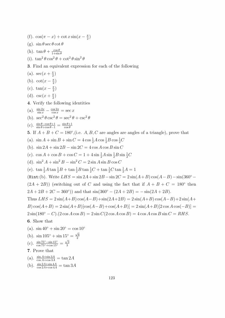
(f). cos(π − x) + cotx sin(x− π2)
(g). sin θ sec θ cot θ
(h). tan θ + cos θ1+sin θ
(i). tan2 θ cos2 θ + cot2 θ sin2 θ
3. Find an equivalent expression for each of the following
(a). sec(x+ π2)
(b). cot(x− π2)
(c). tan(x− π2)
(d). csc(x+ π2)
4. Verify the following identities
(a). sin 2xsinx
− cos 2xcosx
= sec x
(b). sec2 θ csc2 θ = sec2 θ + csc2 θ
(c). sin θ−cos θ+1sin θ+cos θ−1
= sin θ+1cos θ
5. If A+B + C = 180◦,(i.e. A,B,C are angles are angles of a triangle), prove that
(a). sinA+ sinB + sinC = 4 cos 12A cos 1
2B cos 1
2C
(b). sin 2A+ sin 2B − sin 2C = 4 cosA cosB sinC
(c). cosA+ cosB + cosC = 1 + 4 sin 12A sin 1
2B sin 1
2C
(d). sin2A+ sin2B − sin2C = 2 sinA sinB cosC
(e). tan 12A tan 1
2B + tan 1
2B tan 1
2C + tan 1
2C tan 1
2A = 1
(Hint:(b). Write LHS = sin 2A+sin 2B−sin 2C = 2 sin(A+B) cos(A−B)−sin(360◦−(2A + 2B)) (switching out of C and using the fact that if A + B + C = 180◦ then
2A+ 2B + 2C = 360◦)) and that sin(360◦ − (2A+ 2B) = − sin(2A+ 2B).
Thus LHS = 2 sin(A+B) cos(A−B)+sin(2A+2B) = 2 sin(A+B) cos(A−B)+2 sin(A+
B) cos(A+B) = 2 sin(A+B)[cos(A−B)+cos(A+B)] = 2 sin(A+B)[2 cosA cos(−B)] =
2 sin(180◦ − C).(2 cosA cosB) = 2 sinC(2 cosA cosB) = 4 cosA cosB sinC = RHS.
6. Show that
(a). sin 40◦ + sin 20◦ = cos 10◦
(b). sin 105◦ + sin 15◦ =√62
(c). sin 75◦−sin 15◦
cos 75◦+cos 15◦=
√33
7. Prove that
(a). sinA+sin 3AcosA+cos 3A
= tan 2A
(b). sin 2A+sin 4Acos 2A+cos 4A
= tan 3A
123
(c). sinA+sinBsinA−sinB
=tan 1
2(A+B)
tan 12(A+B)
(d). cosA+cosBcosA−cosB
= − cot 12(A−B) cot 1
2(A+B)
(e). sin θ + sin 2θ + sin 3θ = sin 2θ + (sin θ + sin 3θ) = sin 2θ(1 + 2 cos θ)
(f). cos θ + cos 2θ + cos 3θ = cos 2θ(1 + 2 cos θ)
(g). sin 2θ + sin 4θ + sin 6θ = (sin 2θ + sin 4θ) + 2 sin 3θ cos 3θ = 4 cos θ cos 2θ sin 3θ
(h). sin 3x+sin 5x+sin 7x+sin 9xcos 3x+cos 5x+cos 7x+cos 9x
= tan 6x
8. Prove that
(a). cos 130◦ + cos 110◦ + cos 10◦ = 0
(b). cos 220◦ + cos 100◦ + cos 20◦ = 0
Solutions to some selected problems
5(a). Note that A+B + C = 180◦
sinA+ sinB + sinC = (sinA+ sinB) + sinC
= 2 sin 12(A+B) cos 1
2(A−B) + sin(180◦ − (A+B))
= 2 sin 12(A+B) cos 1
2(A−B) + sin(A+B)
= 2 sin 12(A+B) cos 1
2(A−B) + 2 sin 1
2(A+B) cos 1
2(A+B)
= 2 sin 12(A+B)[cos 1
2(A−B) + cos 1
2(A+B)]
= 2 sin 12(A+B)[2 cos A
2cos(−B
2)]
= 2 sin 12(A+B)[2 cos A
2cos(B
2)]
= 2 sin(90◦ − C2)[2 cos A
2cos(B
2)]
= 2 cos C2.2 cos A
2. cos B
2(since sin(90◦ − C
2) = cos C
2)
= 4 cos 12A cos 1
2B cos 1
2C
124

Bibliography
[1] Goldstein L., Schneider D., Siegel M., Finite Mathematics Its Applications,
7th Ed., Prentice Hall, 1998.
[2] Ralph P. Grimaldi, Discrete and Combinatorial Mathematics An Applied Intro-
duction, 5th Ed.,Pearson Addison Wesley, 2004.
[3] Edgar G. Goodaire Michael M. Parmenter, Discrete Mathematics with
Graph Theory, 2nd Ed., 2002
[4] Kenneth A. Ross Charles R.B. Wright, Discrete Mathematics, 4th Ed., Pren-
tice Hall, 1999
125
Index
Counting
Principle, 18
Generalized Inclusion-Exclusion
principle, 21
inclusion-exclusion
principle, 18
principle
Generalized Inclusion-Exclusion , 21
absorption
law, 9
aggregate, 1
antecedent, 57
Argand
diagram, 42
argument
complex number, 44
associative
law, 9
basic
counting principle, 75
Biconditional
Proposition, 58
bijective
function, 98
binary
relation, 89
binomial theorem, 85
bounded
interval, 31
cardinality
set, 4
cartesian
plane, 8
product, 8
class, 1
collection, 1
combination, 75
commutative
law, 9
complement
set, 5
complex
conjugate, 42
rationalization, 43
number, 40
complex number
argument, 44
modulus, 43
complex number
polar form, 44
principal value, 44
126
composite
function, 99
compound
statement, 54
conditional
proposition, 57
conglomerate, 1
conjunction, 54
consequent, 57
contradiction, 60
contrapositive , 63
converse , 63
De Morgan’s
law, 9
De Movrie’s
theorem, 45
difference
set, 6
direct
proof , 68
disjoint
sets, 6
disjunction, 55
disjuncts, 55
distributive
law, 9
domination
law, 9
double
negation, 61
elements, 1
elements argument
method, 16
empty
set, 3
equal
sets, 3
equivalence
relation , 93
euclidean
space, 8
Euler
diagram, 11
existential
quantifier , 65
extended
real number system, 32
finite
set, 4
formal
proof, 16
function, 95
absolute value, 104
constant, 102
linear, 102
one-to-one, 97
polynomial, 104
quadratic, 102
range, 95
reciprocal, 104
Vertical Line Test, 101
algebraic, 107
127
bijective, 98
ceiling, 105
circular, 107
co-domain, 95
common logarithm, 106
composite, 99
domain, 95
even, 107
exponential, 106
floor, 105
greatest integer function, 105
hyperbolicl, 107
identity, 99
image, 95
inverse, 100
inverse trigonometric, 107
irrational, 107
logarithm, 106
logarithmic, 106
many-to-one, 98
Naperian, 106
natural logarithm, 106
odd, 107
one-to-one correspondence, 98
onto, 98
rational, 107
smallest integer function, 105
surjective, 98
transcedental, 107
trigonometric, 107
function
graph, 101
fundamental
counting principle, 18
graph
function, 101
greatest common divisor, 29
group, 1
idempotence
law, 9
identities
cofunction, 114
Double-Angles, 119
Half-Angle, 120
products of sines and cosines, 117
Pythagorean, 114
sum and difference, 115
identity
function, 99
law, 9
imaginary
axis, 42
part, 40
unit, 40
index, 32
infinite
set, 4
injection, 97
injective
map, 97
Integers, 28
intersection
set, 6
128
interval
bounded, 31
inverse
function, 100
law, 9
inverse , 63
invertible
function, 100
involution, 9
Irrational numbers, 29
laws
set theory, 35
logic
propositional, 52
logical
connective, 54
operator, 54
equivalence, 61
implication, 61
logically
equivalent, 61
map, 95
mapping, 95
mathematical
creativity, 51
logic, 51
proof , 67
reasoning, 51
measure
degree, 112
radian, 112
members, 1
modulus
complex number, 43
Natural numbers, 27
negation, 54
negative
integers, 30
rational numbers, 31
real numbers, 31
non-negative
integers, 30
rational numbers, 31
non-positive
integers, 30
rational numbers, 31
number
Rational , 29
number
Real, 27
onto
function, 98
open
sentence, 64
partial
order, 93
ordering, 93
permutation, 75
plane
cartesian, 8
polar form
129
complex number, 44
positive
integers, 30
rational numbers, 31
real numbers, 31
power
set, 9
predicate, 64
calculus , 64
principal value
complex number, 44
principle
finite mathematical induction , 70
inclusion-exclusion, 18
infinite mathematical induction , 70
principle of Extensionality, 3
product
Cartesian, 8
proof
by cases , 68
contradiction , 69
contrapositive , 68
counter-example , 67
direct , 68
mathematical , 67
mathematical induction , 69
proof
contradiction, 61
proper
subset, 3
properly
contained, 3
proposition
conditional, 57
propositional
logic, 52
propositions, 52
purely
imaginary, 41
quantified
statement , 66
quantifier
existential , 65
universal , 64
range, 95
Rational
number, 29
Rational numbers, 29
Real
line, 27
number, 27
real
complex number, 41
part, 40
Real Numbers, 29
reasoning
deductive, 51
inductive, 51
reasoning
semantic, 51
syntactic, 51
relation, 89
antisymmetric, 92
130
equivalence, 93
reflexive, 91
symmetric, 92
transitive, 92
semantic
reasoning, 51
set, 1
cardinality, 4
empty, 3
Boolean sum, 8
complement, 5
difference, 6
finite, 4
infinite, 4
intersection, 6
operations, 5
singleton, 4
union, 5
universal, 4
set
membership method, 16
singleton
set, 4
space
euclidean, 8
statement, 52
quantified , 66
subset, 3
surjection, 98
surjective
function, 98
symmetric difference
set, 7
syntactic
reasoning, 51
tautology, 60
trigonometric
identities, 113
ratios, 113
trigonometry, 112
truth
value, 53
truth
table, 54
unbounded
interval, 32
unequal
sets, 3
union
set, 5
universal
quantifier , 64
set, 4
universe, 4
universe of discourse, 4
venn
diagram, 10
Whole numbers, 28
131
Related Documents