Firm Investment and Stakeholder Choices: A Top …finance.wharton.upenn.edu/department/Seminar/micro/...Firm Investment and Stakeholder Choices: A Top-Down Theory of Capital Budgeting∗

Firm Investment and Stakeholder Choices:

A Top-Down Theory of Capital Budgeting∗

Andres Almazan

University of Texas

Zhaohui Chen

University of Virginia

Sheridan Titman

University of Texas and NBER

28 March 2010

Abstract

This paper provides a model of the capital budgeting process of a firm whose top

executives have private information. The success of the firm depends on the motivation

and efforts of its lower level managers (and other stakeholders) who try to infer the

information of the firm’s top executives from their actions. In particular, higher levels

of investment signal that the firm has promising prospects and induces its managers

to take actions that contribute to the firm’s success. In the presence of these effects,

capital budgeting rules not only play their traditional allocative role but also affect the

transmission of information from top to middle managers. In this setting, there can

arise a number of commonly observed investment distortions such as capital rationing,

investment rigidities, overinvestment, and inflated discount rates.

∗We would like to thank Adolfo de Motta and David Dicks and seminar participants at DePaul University,UCLA, University of Essex, UNC-Chapel Hill, University of Notre Dame and UT-Austin. Corresponding

author: [email protected].

1 Introduction

The capital budgeting process has been described (i.e., Brealey, Myers and Allen 2008) as

a combination of “bottom-up” procedures, where lower units solicit capital from headquar-

ters, and “top-down” procedures where headquarters use their discretion to allocate capital

downstream. An extensive literature has analyzed the incentive and information consider-

ations that can emerge in “bottom-up” capital allocation processes in which headquarters

allocate capital by reacting to solicitations from better informed lower units (e.g., Harris

and Raviv 1996 or Bernardo et al. 2004). However, up to now, the literature has not focused

“top-down” processes in which capital allocation decisions by better informed headquarters

convey information to lower units.1

As we analyze in this paper, top-down procedures are likely to reflect strategic consid-

erations that go beyond calculating the net present value of an investment. These strategic

issues arise because the investment choices of top managers convey information to lower

units and, more generally, to firms’ stakeholders. When this is the case, the procedures

that firms use to evaluate investments can influence how this information is interpreted.

As an illustration, consider the capital allocation decision of a large integrated oil com-

pany, such as British Petroleum (BP). For a firm like this, a major investment in biofuels is

likely to be viewed as an indication that the firm’s top management has favorable informa-

tion about the future prospects of these alternative sources of energy or, alternatively, that

it has serious concerns on the future of the more traditional sources of energy.2 A central

premise of our paper is that information conveyed by investment choices can have an impor-

tant influence on the stakeholders’ choices. For instance, employees in BP’s biofuel division

will be encouraged by the implications of the higher investment and will work harder. In-

deed, this incentive to exert effort will be especially strong if employees believe that capital

is tight and the firm is using very high hurdle rates to evaluate their investments.

To better understand how capital budgeting procedures and lower unit perceptions inter-

act we develop a simple model of an entrepreneurial firm whose production process requires

1Grinstein and Tolowsky (2004) find that, in the capital budgeting process, directors of S&P 500 firms

act both to “alleviate conflicts of interest between agents and principals and to communicate principals’

information to agents.”2In June 2007, after BP announced plans to invest $500M in biofuels, analysts at Global Insight stated

that it was the “first time BP has committed itself to such a large investment in biofuels research”. (See

www.ihsglobalinsight.com/SDA/SDADetail6147.htm).

1

a capital expenditure (i.e., an investment) by the firm’s owner (i.e., the entrepreneur) as

well as effort exerted by a lower level manager (i.e., an employee). Specifically, we consider

a framework where the entrepreneur has private information about the firm’s prospects,

chooses the level of investment, and promises the employee a bonus based on the firm’s

output. In this setting both the firm’s investment and the employee’s effort are more pro-

ductive when the future prospects of the firm are better. As a result, with full information,

it is optimal for the firm to invest more and for the employee to exert more effort when the

firm’s future prospects are more favorable. This in turn implies that when the entrepreneur

has private information, there is an incentive for the entrepreneur to overinvest relative to

the full information case, because doing so elicits additional effort from the employee.

Most of the intuition of our model can be illustrated in a setting in which the firm’s

prospects are one of two types, high or low and in which the firm can commit to an in-

vestment policy before observing the private information about its prospects. Within this

setting, two investment policies can emerge as optimal: (i) a separation policy in which a

high prospect firm invests more than a low prospect firm and (ii) a pooling policy in which

firms commit to a maximum investment level regardless of their types. With a separation

policy, the firm will tend to over-invest because of the benefits associated with conveying

favorable information. This cost of separation is offset by the benefits of investing more

when the marginal productivity of capital is higher. Hence, ex-ante, the choice between

the pooling and the separation policy is determined by a trade-off between the efficiency

gain associated with having an investment policy which incorporates the entrepreneur’s

information and the efficiency loss associated with over-investment.

Having established the incentive to overinvest and the potential benefits of committing

to a fixed level of investment we enrich the previous framework by adding a third party

to our model. In addition to the entrepreneur, who obtains information, and the employee

who exerts effort, we consider a third party that sets capital budgeting policies and offers a

compensation contract to the entrepreneur. One interpretation is that the third party is a

venture capitalist that provides funding for the firm and retains some control of its opera-

tions. Another is that the informed party is the manager of the division of a conglomerate

and the third party is either the executives at the firm’s headquarters or the firm’s board.

We investigate a number of additional issues within this three-party setting. First, we

2

consider the possibility that the board can force the entrepreneur to commit to using a

discount rate that may not equal the rate that would be used with symmetric information.

This could be a single discount rate that is independent of the magnitude of the investment

or it could be a function of the investment’s magnitude. Second, we consider how the

firm’s capital structure can be designed by the board to reduce inefficiencies in the capital

budgeting process.

The analysis of the three-party model demonstrate that several commonly observed

capital budgeting practices can enhance firm value. Specifically, the imposition by the

board of high discount rates can change the opportunity cost of capital for the entrepreneur

and hence offset the incentive to overinvest that arises when the level of investment conveys

information to stakeholders.3 Similarly, by using more debt financing, a Myers (1977) debt

overhang problem can arise that offsets the incentive to overinvest.

As we mentioned at the outset, our analysis of a “top-down” capital allocation process

is in contrast of the analysis of “bottom-up” process that is the focus of the exisiting

literature. Specifically, this literature examines the issue of how a firm may distort its

capital budgeting practices in order to induce managers to exert proper effort (Bernardo,

Cai, and Luo 2001, 2004, 2006), to curb managers’ empire building tendencies (e.g., Harris

and Raviv 1996, 1997, Marino and Matsusaka 2004, and Berkovitch and Israel 2004) or

to reveal their private information. This literature has also considered the trade-offs that

arise in the decision to delegate capital budgeting decisions to a better informed agent (e.g.,

Aghion and Tirole, 1997 and Burkart, Gromb, and Panunzi, 1997).

Our analysis also has implications that are similar to the agency literature that argues

that since managers get private benefits from managing larger enterprises, firm may exhibit

a tendency to overinvest (e.g., Jensen 1986, and Hart and Moore 1995). As we show, the

tendency to overinvest, as well as procedures that curb this tendency, can also arise within

a setting without managerial private benefits. Hence, in addition to offering a theory that

can rationalize capital budgeting rigidities in large corporations, we offer an explanation

for the high hurdle rates imposed by venture capitalists on the investment choices of young

start-up firms.4

3See Poterba and Summers (1995) who document the use of high-discount rates on American corporations

and Meier and Tarhan (2007) who provide evidence of what they refer to as a “hurdle rate puzzle” i.e., the

use of a discount rate that substantially exceeds estimates of their cost of capital.4Indeed, private equity firms and venture capitalist take this tendency to evaluate investments with very

3

Although the setting is very different, our analysis is actually closest to Hermalin (1998)

and Komai, Stegeman, and Hermalin (2007), who study the problem of leadership in

organizations.5 In these models, the leader is better informed than other team members

and credibly communicates his favorable information, which motivates his subordinates to

work harder, by exerting greater effort. There are, however, two key differences between

our setting and the setting considered in the leadership papers. First, in our setting, the

entrepreneur’s costly action (i.e., the investment choice) is contractible, while the leader’s

effort in the leadership models is not. Indeed, the capital budgeting policies that we explore

arise because of the contractibility of investment. Second, we introduce a third party that is

not involved in the production process but which has the authority to set investment rules

and to claim firm output. This allows us to depart from a team setting (where parties share

output) and instead focus on a setting in which parties that contribute to the production

process are not necessarily those claiming the output (i.e., a firm). As we show, the presence

of a third party who acts as “budget breaker” can broaden the contract space, and thus

provide the entrepreneur with incentives that lead to more efficient investment choices.6

More generally, our paper belongs to the principal-agent literature with informed princi-

pals. Among other things, this literature considers the effects of the principal’s information

on the optimal compensation contract (Beaudry 1994 and Inderst 2000), the value of the

private information to the principal (Chade and Silvers 2004 and Karle 2009) and the incen-

tives to disclose information (i.e., provide “advice”) to the agent (Strausz 2009). In contrast

to these models, the principal in our model not only designs the agent compensation but

also takes an action (i.e., makes an investment) that directly affects the firm’s production.

The rest of the paper is organized as follows. Section 2 presents the base model and

Section 3 analyzes it. Section 4 considers a modified setting with a board of directors and

considers a implementation of corporate budgeting practices and Section 5 presents our

conclusions.

high discount rates to an extreme, generally requiring “expected” internal rates of return on their new

investments that exceed 25%. Gompers (1999) describes the “venture capital” valuation method, where

discount rates of more than 50% per year are used.5See also Benabou and Tirole (2003) who consider the signaling effect of providing explicit incentives to

employees.6Holmstrom (1982) first pointed out the value of third parties who by threatening to break the budget

eliminate inefficiencies in team production. While in Holmstrom (1982), third parties act “off-equilibrium

path” in our setting, the third party breaks the budget in equilibrium in order to improve entrepreneurial

incentives to invest appropriately.

4

2 The model

We consider a firm that operates in a risk-neutral economy. The firm is run by an entre-

preneur (“the principal”) and requires the input from a penniless lower-level manager (“the

agent”) who is subject to limited liability and a zero reservation wage.7 The technology of

the firm is characterized by a (decreasing returns to scale) stochastic production function :

( ) = ( ) − 122. (1)

This technology combines two inputs, a capital investment (i.e., the firm’s scale) which

is subject to a quadratic cost () ≡ 122 and the agent’s effort , which influences whether

or not the firm is successful, i.e., ( ) = ( ).8 Specifically,

( ) =

(0 with prob. (1− )

0 with prob. (2)

where the probability of success is determined by (i) an exogenous random shock , which

is privately observed by the principal,

=

(1 with prob. (1− ) ≡ 1

1 with prob. ≡

and (ii) the agent’s privately exerted effort ∈ [0 1). The agent’s cost of effort is given by:

( ) =1

22

which is convex in (i.e., = ) and increases linearly with the firm’s scale (i.e., =

122).9 In what follows, we implicitly assume that is sufficiently large that the optimal

effort choice lies within the bounds [0 1).

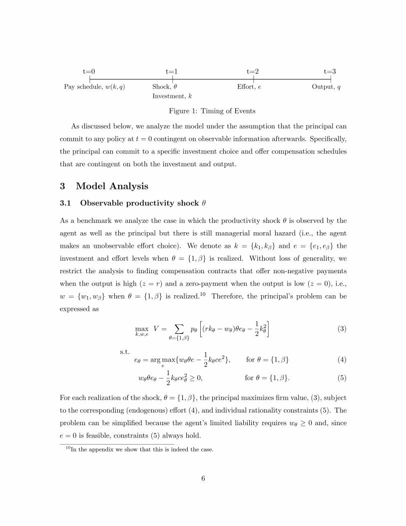
The timing of events is as follows: At = 0, before observing , the principal offers

the agent a compensation schedule contingent on the firm’s scale and the realized output:

( ). At = 1, the principal privately observes and chooses the scale . At = 2,

the agent makes an unobservable effort choice . At = 3, firm output is realized and

contracts are settled. Figure 1 summarizes the timing of events.

7In this section we identify the entrepreneur (the principal) with the firm. In Section 4, however, we

endogenize the entrepreneur’s payoffs by considering boards as principals who compensate the entrepreneur.8Alternatively, the firm’s production function can be expressed as ( ) = ( )

√2 − , i.e., the

scale of the firm increases by a factor of√2 per unit of capital invested.

9An alternative formulation in which effort costs are independent of the firm scale but in which production

costs are cubic on firm scale, i.e., () ≡ 3 is less tractable but produces similar results.

5

Pay schedule, ( )

t=0

Shock,

Investment,

t=1

Effort,

t=2

Output,

t=3

Figure 1: Timing of Events

As discussed below, we analyze the model under the assumption that the principal can

commit to any policy at = 0 contingent on observable information afterwards. Specifically,

the principal can commit to a specific investment choice and offer compensation schedules

that are contingent on both the investment and output.

3 Model Analysis

3.1 Observable productivity shock

As a benchmark we analyze the case in which the productivity shock is observed by the

agent as well as the principal but there is still managerial moral hazard (i.e., the agent

makes an unobservable effort choice). We denote as = {1 } and = {1 } theinvestment and effort levels when = {1 } is realized. Without loss of generality, werestrict the analysis to finding compensation contracts that offer non-negative payments

when the output is high ( = ) and a zero-payment when the output is low ( = 0), i.e.,

= {1 } when = {1 } is realized.10 Therefore, the principal’s problem can be

expressed as

max

=X

={1}

∙( − ) − 1

22

¸(3)

s.t. = argmax

{− 1

2

2} for = {1 } (4)

− 12

2 ≥ 0 for = {1 } (5)

For each realization of the shock, = {1 }, the principal maximizes firm value, (3), subjectto the corresponding (endogenous) effort (4), and individual rationality constraints (5). The

problem can be simplified because the agent’s limited liability requires ≥ 0 and, since = 0 is feasible, constraints (5) always hold.

10In the appendix we show that this is indeed the case.

6

By substituting the first-order condition of (4), (i.e., =) in (3) we get:

max

=X

={1}

∙( −)

− 122

¸ (6)

the solution of which leads to the following proposition:

Proposition 1 For = {1 } the optimal compensation, investment and effort are:

∗ =32

8, ∗ =

22

4and ∗ =

2. (7)

From Proposition 1, it follows that optimal compensation, investment and effort are

increasing in , i.e., ∗ ∗1, ∗ ∗1 and ∗ ∗1. Since effort is more valuable when the

firm’s prospects are better, it is efficient for the firm to invest more and to offer higher com-

pensation in order to induce greater managerial effort when the firm has better prospects.

It is illustrative to also describe the equilibrium relations among these endogenous vari-

ables. Specifically, one can check that (i) effort increases with managerial compensation

and decreases with investment, i.e., ∗ =∗

∗, and that (ii) compensation and investment

are proportional to each other, i.e., ∗ =2∗ . Alternatively expressed, this implies that the

optimal compensation is a sharing rule independent of , i.e.,∗

∗= 1

2. Finally, for future

comparisons, it is useful to express firm value in this benchmark case when is observable

as:

∗ =1

2

h(1− )∗

2

1 + ∗2

i. (8)

3.2 Unobservable productivity shock

The feasibility of the contractual arrangement described in Proposition 1 crucially hinges on

the fact that the agent can observe . When is unobservable to the agent, the principal’s

investment plays not only its usual allocating role but also conveys information about ,

which in turn affects the agent’s effort choice.

Technically, this setting is one of an informed principal and an agent who makes a costly

effort choice. In such a framework, the contract that maximizes firm value need not be a

direct mechanism where the principal and the agent commit to actions as a function of the

revealed by the principal (i.e., the revelation principle does not apply). This is because,

7

even though the principal can commit to any action after disclosing , the agent cannot

commit to a specific effort choice that is unobservable to anyone but the agent himself.11

In the appendix we show that the optimal contract consists of two investment-compensation

pairs, i.e., { } and { }. Within this set of contracts three possibilities arise. If theprincipal’s choices depend on the observed type, (i.e., the principal chooses and after

observing = 1 and 6= or 6= after observing = ), such choices communicate

the type to the agent. We refer to this case as separation. If, however, = and =

then the principal’s choices convey no information. We refer to this case as pooling. A third

possibility would be partial pooling where the principal mixes between these pairs.12 In what

follows, we search for the optimal contract under separation and pooling and compare firm

value when these contracts are implemented. As we show in the appendix, this is without

loss of generality since firm value under partial pooling is lower than firm value when either

the optimal separation or the optimal pooling contract is implemented.

3.3 Separation

With separation, the principal’s choices consist of two distinct managerial compensations

= {1

} and investment levels = {1 } which depend on . However, since

is unobservable to the agent, the principal’s choices are subject to incentive compatibility

(i.e., “truthtelling”) constraints.

We define as the firm value when the principal observes and chooses

and

for

= {1 }:

≡ ( −

)

− 12

2

(9)

where = argmax

{

−

2

} for = {1 } and denote = {1 }. The principal’s

problem can be expressed as:

max

=X

={1}

∙( −

) −

1

2

2

¸(10)

11See Bester and Strausz (2001) for an analysis of the optimal contract in a dynamic adverse selection

setting where the principal cannot commit to a specific allocation after the agent’s first period choice and

Strausz (2009) for a setting in which, similarly, to ours, the revelation principle lacks bite due to the

unobservability of the agent’s effort.12Formally, this situation would require us to define { } as the probabilities that the principal chooses

{( ) ( )} after observing {1 } and would require us to solve for the optimal level of informationrevelation, i.e, the optimal { }.

8

s.t.:

= argmax

{− 2} for = {1 } (11)

− 2 ≥ 0 for = {1 } (12)

≥

for = {1 } and 6= (13)

Formally, this problem is identical to the benchmark problem (3)-(5) where is observable

with the addition of the truthtelling constraints (13). To solve it, we ignore the IC constraint

of the high productivity firm (i.e., ≥ 1 ) and assume that the IC of the low productivity

firm binds (i.e., 11 = 1 ). We then substitute in the objective function (10), derive the

corresponding first order conditions and get:13

Proposition 2 The optimal managerial compensation and firm investment are:

∗ = {∗1∆∗} and ∗ = {∗1∆∗} (14)

where ∆ = max

½1+√1−1

1

¾. With these choices, the manager’s effort is ∗ = ∗ =

2

and the principal’s payoff is

∗ =1

2

h(1− )∗

2

1 + ∆(2−∆)∗2i. (15)

The intuition behind Proposition 2 can be illustrated by comparing it with the results

described in Proposition 1. In comparison to the observable case, there is no distortion in

compensation, investment or effort when = 1, i.e., ∗1 = ∗1 ;

∗1 = ∗1 and ∗1 = ∗1 but

when = , there is a distortion in compensation and investment which are both increased

by the factor ∆ (i.e., ∗ = ∆∗ and ∗ = ∆∗). Such an increase in investment and

compensation, offset any effect on effort which equals the effort of the benchmark case (i.e.,

∗ = ∗ ).

The distortion factor ∆ ≥ 1 is described by the expression max½1+√1−1

1

¾which

as a function of takes its maximum at = 2√3∼= 115 and reaches its minimum ∆ = 1

when ≥ ∗ ∼= 184. In other words, when ≥ ∗ there is no distortion in compensation

or investment which implies that the solution of the problem when is observable is also

implementable when the agent cannot observe .14

13A positive compensation when output is low (i.e., = 0) could, in principle, help the principal to signal

. In the appendix we show that this is not the case and that, as in the benchmark case, restricting to zero

compensation when the output is zero is without loss of generality.14See the appendix for more details on the relation between ∆ and .

9

It is worth noting that, in this setting, investment distortions provide a relatively efficient

signal relative to other potential signaling possibilities such as relying solely on a distorted

compensation policy. This is so because a type = 1 firm finds it relatively more costly to

overinvest than a type = firm since, given its lower expected productivity, the marginal

benefits of a high investment level are lower for the = 1 than for the = firm.15 In

contrast, signaling solely through the compensation does not work because, for incentive

reasons, compensation needs to be contingent on success and the probability of success is

higher when = . In these conditions, an increase in (i.e., if

1 and

increase by a

constant), is relatively more costly for a type firm than for a type 1 firm which implies

that signaling by distorting compensation is ineffective.16 Alternatively, the firm could burn

money (i.e., engage in wealth destruction regardless of the firm scale or output success) in

order to signal its type. Such a device, however, is also suboptimal relative to signaling by

distorting the firm scale. This is so because money burning is equally costly to both types of

firms and hence less efficient than signaling by overinvesting which is relatively more costly

for the low productivity firm.

3.4 Pooling

Alternatively, the principal can commit to make choices that are independent of and

then commit not to disclose his information on . In this case, we refer to and as the

compensation in case of success and the investment and to ≡ +(1−)1 as the averageproductivity shock. Therefore, the principal’s problem is:

max

= ( − )− 122 (16)

s.t.:

= argmax

{− 122} (17)

Since the firm’s investment does not convey information as (17) shows, the effort decision

is made based on the average type of the firm. The solution to this problem is given by:

15Since agent’s effort costs increase with the firm’s scale, the overinvestment distortion is accompanied by

a corresponding distortion in compensation in order to restore the proper effort incentives to the agent.16In the appendix we provide a more extensive analytical argument to show that other distortions in

compensation (e.g., increasing compensation in case of failure) are suboptimal as well.

10

Proposition 3 The optimal compensation and firm investment under pooling are:

∗ =32

8and ∗ =

22

4 (18)

With these choices, the agent’s effort is ∗ = 2and the principal’s payoff is ∗ =

12∗

2.

Under pooling, the agent’s effort is the average of the two efforts levels under the bench-

mark case when is observable and the compensation is a sharing rule as in separation on

the observable case i.e., ∗∗ =

12. In contrast to separation, however, the firm does not

incorporate information on the realized for their investment choices which means that the

firm overinvests when = 1 and underinvests when = .

Economically, the case of pooling is interesting since it shows that rigidities in investment

and compensation can be part of an optimal capital budgeting policy. In a strict sense, our

results show that setting a fixed investment level can be the optimal investment policy.

However, these results can be more liberally interpreted as specifying a limit on the amount

of capital that can be used by the firm. After observing the shock, an unconstrained high

productivity firm would like to invest above the limit imposed by the investment policy,

while the low productivity firm would just invest the investment limit only to mimic the high

productivity principal’s investment choice. This interpretation of pooling as an investment

limit is consistent with a number of studies that show that firms may exhibit a tendency

toward capital rationing when they allocate capital in different business units (e.g., Ross

1986 documents that from twelve firms examined in detail, six of them employ fixed capital

budgets).

3.5 Separation or Pooling?

Compared with the separation case, the benefit to the firm with the pooling contract is that

it does not have to overinvest nor overcompensate managers to signal its type. The cost,

however, is that the firm ignores its information and cannot tailor investment to marginal

productivity. The optimal choice between pooling and separation depends on the trade-off

between these costs and benefits as the next proposition shows.

Proposition 4 (Comparative statics) Separation is more likely to be the optimal policy:

(i) the lower the likelihood of a high productivity project (i.e., ) and

(ii) the larger the difference in productivity among projects (i.e., ).

11

The following figure illustrates the regions in the space ( ) where either policy is

optimal:

**

1

Separation

Pooling

**

1

** **

1

Separation

Pooling

**

1

**

It is worth noting that, as the previous graph illustrates, pooling is locally optimal, that

is, when productivity levels are sufficiently close (i.e., → 1) pooling is the optimal invest-

ment policy. To the extent that firms can exhibit a wide range of productivity levels, this

observation suggests that investment rigidities (i.e., discrete levels of investment) are likely

to be part of any optimal capital budgeting policy. This observation will have important

implications when we examine the continuum type version of the model discussed below.

To understand part i), it is helpful to consider cases where is close to 1 When is

large, the expected over investment cost for the type is large under separation. On the

other hand, under pooling, because the equilibrium investment is close to the type full-

information investment level, the inefficiency is small if the firm is of type Even though

for type 1 the investment inefficiency may be large, the expected cost is small because it

is unlikely for the firm to become type 1 Therefore the trade-off favors pooling when is

large. To understand part ii), it is helpful to consider cases where is large. On the one

hand, the efficiency loss due to pooling is large because the average investment is far from

both type 1 and type ’s full information level. On the other hand, the over investment

cost may not be large when is large. For example, when is close to ∗, type need only

to over invest a little bit in order to deter type 1 mimicking because the full information

investment level for type is already very high for a type 1 firm. Therefore the trade-off

12

favors separation when is large.

4 A three-party model: Corporate capital budgeting

Having established the incentive to overinvest and the potential benefits of committing

to specifying a maximum (fixed) investment level we extend the model to consider the

interplay of three parties in the capital budgeting process. In addition to the entrepreneur

(to whom we now refer to as a “CEO”) who obtains information and determines investment

expenditures, and the employee who exerts effort, we introduce a third party (i.e., a “board”)

that sets specific capital budgeting policies and offers compensation contracts to the CEO.

One interpretation is that the third party is a venture capitalist that provides funding for

the firm and retains some control of its operations. Another is that the informed party is

the manager of the division of a conglomerate and the third party includes executives at the

firm’s headquarters or are members of the board. In either interpretation, the third party

is an entity that has the authority to set the firm policy.

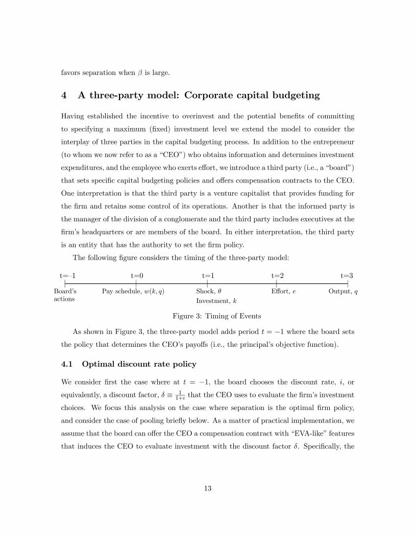
The following figure considers the timing of the three-party model:

Board’sactions

t=—1

Pay schedule, ( )

t=0

Shock,

Investment,

t=1

Effort,

t=2

Output,

t=3

Figure 3: Timing of Events

As shown in Figure 3, the three-party model adds period = −1 where the board setsthe policy that determines the CEO’s payoffs (i.e., the principal’s objective function).

4.1 Optimal discount rate policy

We consider first the case where at = −1, the board chooses the discount rate, orequivalently, a discount factor, ≡ 1

1+that the CEO uses to evaluate the firm’s investment

choices. We focus this analysis on the case where separation is the optimal firm policy,

and consider the case of pooling briefly below. As a matter of practical implementation, we

assume that the board can offer the CEO a compensation contract with “EVA-like” features

that induces the CEO to evaluate investment with the discount factor . Specifically, the

13

board will offer the CEO a share, , of the firm’s net value at = 3, where net firm value is

calculated as revenues minus wages and investment expenditures divided by the factor .17

Consider the problem encountered by the CEO at = 0 who faces a discount factor

imposed by the board to evaluate the firm’s investments. We denote by = {1 }, = {1 } and = {

1 } the investment, bonus and effort exerted after = {1 }

respectively. In addition, we refer to as the CEO’s payoff when, after observing , offers

and invests

for = {1 }:

≡ ( −

)

− 1

2

2

(19)

Formally, the CEO solves the following maximization problem:

max

=X

={1}[(

−

) −

1

2

2

] (20)

s.t.:

= argmax

{−

2} for = {1 } (21)

≥

for = {1 } and 6= (22)

Relative to the two-party case, the agent’s problem remains unchanged and the CEO

faces the same problem as the principal in the basic model except that the investment costs

are given by 12

2

rather than 12

2

. (Notice that since 0 is a constant it cancels out

in the previous problem, i.e., it does not have any effect on the CEO’s choices.) Following

the analysis in the last section the solution can be described as follows:

Lemma 1 The solution of the CEO problem with separation scales investment and wage

by and 2, respectively (i.e., ∗ = ∗ ∗ = 2∗

). The agent’s effort is unaffected:

∗ = ∗ .

At = −1 the board takes into account the distortion that the discount factor produceson the CEO’s behavior at = 0 and, consequently, chooses to maximize firm value:

max

=X

={1}[(

∗ − ∗

)∗ −

1

2∗

2

] (23)

The solution to the board’s problem is described in the following proposition.

17If 1 the firm would be subsidizing the use of capital and if 1 the firm would be taxing the use

of capital.

14

Proposition 5 If separation with overinvestment characterizes the CEO’s investment pol-

icy ( ∗) then the board distorts the discount rate upwards (∗ 1). If separation re-

quires no overinvestment ( ≥ ∗) then the board does not distort the discount rate (∗ = 1).

To better explain the intuition behind the previous proposition it is useful to notice that

in problem (23) the board maximizes firm value (i.e., the value determined by discounting

cashflows with = 1, the “correct” discount factor) by imposing 1 on the CEO when

∗. By maximizing a distorted measure of firm value, one in which cashflows are

discounted by 1, the CEO reduces the firm’s investment expenditures. Intuitively, the

benefits of distorting can be explained as follows. A lower reduces the incentives of a

CEO who observes = 1 to mimic the behavior of a CEO who observes = . A relaxed

IC constraint for = 1 reduces ’s cost to overinvest but creates some underinvestment

in = 1. In particular, an infinitesimal reduction from = 1 simultaneously diminishes

and . Since compensation and investment for the low type (

1 and 1) are at their

optimal levels, such a reduction has a second order effect on firm value, while the reduction

for the high type (a lower and

), which are set at local optima, has a first order effect

on firm value. (When separation entails no distortion, ≥ ∗, the optimal discount factor

is = 1, which keeps the investment and compensation policies undistorted.) We provide

the formal proof of these arguments in the appendix.

It should be noted that the ability to set a discount rate does not increase firm value

in the case of pooling. In this case, if the board sets 6= 1, the CEO distorts his choices

away from the optimal pooling choices (i.e., ∗and ∗). This reduces firm value since, by

construction, the optimal pooling choice maximizes firm value relative to the set of choices

that convey no information to the agent.18 As a result, separation is more likely to be

optimal when the hurdle rate is set by the board since a modified hurdle rate may improve

the separation policy but does not help the pooling policy.

It should be emphasized that the board creates value by altering the CEO’s objective

function, which in turn affects the set of CEO’s actions that are incentive compatible for a

given . Without the board, the CEO can also take actions that affect his ex-post investment

incentives. For instance, the CEO can change the IC conditions by committing to transfer

18In separation, a distorted may create value by enlarging the set of incentive compatible CEO policies.

Since the pooling choices are made by the CEO before observing the type, in pooling distorting does not

have the potential to increase firm value.

15

output to the agent (or to burn money) when his investment expenditures are high. These

commitments by the CEO are costly and as the analysis of the two party model shows

undesirable for the CEO. In contrast, when the board is the residual claimant, a CEO can

effectively encourage or prevent certain investment levels without burning nor transfering

output to any external party.

As we just discussed, imposing a higher discount rate (i.e., 1) can increase firm

value by reducing the overinvestment costs of separation when = . However, within this

setting the firm fails to achieve ∗ (i.e., the firm value when is observable) since it leads

to underinvestment when = 1. We conclude this section by considering whether a policy

of multiple hurdle rates (i.e., rates set as a function of the amount of capital invested) will

solve the problem. Proposition 6 confirms that this is indeed the case:

Proposition 6 For each there exists ∗ such that the firm follows the optimal investment

policy: 1∗1 = ∗1 and ∗ = ∗ and its value reaches ∗.

Proposition 6 implies that a policy that imposes higher hurdle rates for larger invest-

ments eliminates overinvestment when = without inducing underinvestment when = 1.

The proposition is thus consistent with the evidence presented in Ross (1986); firms appear

to have hurdle rates which are increasing in the size of the investment project. Nevertheless

other practical considerations outside this model could make a multiple rate policy hard to

implement. For instance, in the presence of multiple projects, multiple divisions or projects

that require staged investments having a rate which depends on the amount invested could

lead the CEO to take actions that “game” the nonlinearity inherent in the multiple hurdle

rate policy.

4.2 Optimal debt policy

In this section we relax the assumption that the board can directly impose a hurdle rate on

the CEO and consider instead how the board can use the firm’s financial policy to influence

the CEO’s behavior. Specifically, we consider a CEO who faces a debt level chosen by

the board at = −1. We denote by = {1 }, = {1 } and = {1

} the

investment, bonus and effort exerted after = {1 } respectively and, analogously to (19),define

≡ ( −

− )

− 1

2

2

as the CEO’s payoff when, after observing , offers

16

and invests

for = {1 }. Formally, the CEO’s problem is:

max

=X

={1}[(

−

− ) −1

2

2

] (24)

s.t.:

= argmax

{− ()} for = {1 } (25)

≥

for = {1 } and 6= (26)

Notice that, in contrast to problem (20) the cashflows are discounted at the appropriate

discount rate but the CEO is maximizing equity value rather than total firm value. Following

a similar approach as in previous cases (see the appendix for details), and focusing as before

on the case of separation, the solution to the CEO problem for the levered firm can be

described as follows:19

Lemma 2 The solution of the CEO problem with separation in the presence of a levered

capital structure reduces the wage, effort, and investment relative to the unlevered case:

∗ ∗

∗ ∗ and ∗ ∗ .

At = −1 the board chooses debt to solve the following problem:

max

=X

={1}[(

∗ −∗

)∗ −

1

2∗

2

] (27)

The solution to the board’s problem is described in the following proposition.

Proposition 7 If separation with overinvestment characterizes the CEO’s investment pol-

icy ( ∗) then the board chooses some debt to fund the project (∗ 0). If separation

implies no overinvestment ( ≥ ∗) then the board funds the project entirely with equity

(∗ = 0).

As with the distortion of hurdle rates, debt induces underinvestment to = 1 and

reduces overinvestment to = .20 Intuitively, leverage increases the mimicking costs of

19It is easy to show that positive leverage reduces firm value in the case of pooling, where the optimal

leverage is nil, i.e., ∗ = 0.20In (27), the board chooses to maximize firm value by affecting the incentives of the equity-value

maximizer CEO.

17

low quality firms to look like high quality ones. When 0 the marginal cost of increasing

is borne by the equityholders but benefits (in part) the bondholders and, since the chance

of success is lower for = 1, mimicking ∗ becomes less attractive for = 1. In short, in

this setting, debt overhang is a mechanism to create disincentives to “mimic”.

While this section focuses on the case where the board sets the financing policy, it is

useful to note that a similar logic would apply to the two-party model of Section 3. In such

a setting, a principal-owner may find it useful to fund operations with a positive amount

of debt in order to ameliorate his own overinvestment incentives even if the principal has

sufficient funds to make the investments. As the logic of Proposition 7 suggests, the use

of debt reduces the incentives of low productivity firms to make investments that partially

benefit the debtholders of the firm.

5 Concluding remarks

In this paper we have proposed a “top-down” theory of capital budgeting where top man-

ager’s actions motivate lower managers and the firm’s stakeholders to exert efforts on the

firm’s behalf. One of the main purposes of our approach is to help reconcile several dis-

connects between academic theory and industry practice about capital budgeting practices.

For example, while the NPV rule proposes using expected cash-flow estimates and expected

return on investments with equivalent risk to discount those expected cash-flows, in practice

there is a tendency to “inflate” cash-flow estimates and “inflated” hurdle rates.

A central premise of our paper is that the communication process between managers,

headquarters and other firm’s constituencies has a direct influence on the capital budgeting

process because the information conveyed by investment choices can have an important

influence on the stakeholders’ choices. Specifically, the stakeholders’ incentives to exercise

effort are affected by how costly stakeholders feel that capital is for the firm.

To explore the interaction between firm investments and stakeholder incentives, we

have examined two related models. First, we considered an entrepreneurial firm whose

production process requires a capital expenditure by the firm and effort by the employee.

In this setting, in which the principal obtains information that can be more efficiently

signaled with the firm’s investment policy, we show that there is a natural tendency for

firms toward overinvestment and a natural demand for capital budgeting modifications of

18

the NPV rule. Our main trade-off is between the efficiency gain associated with having an

investment policy which incorporates the entrepreneur’s information and the efficiency loss

associated with over-investment.

We then modified the analysis by introducing a third party with the authority to set

specific capital budgeting policies and to offer compensation contracts to the entrepreneur.

Within this setting we investigate the value of using a number of commonly observed capital

budgeting practices. We find that high hurdle rates, the use of debt financing and the use

of EVA managerial compensation can help to offset the overinvestment tendencies that

emanate from firms with private information about their prospects.

Our theory provides an alternative explanation for the observed overinvestment in firms.

While managerial private benefits are likely to provide impetus for excessive investment, in

this paper we show that overinvestment can be a second best response of a manager who

needs to communicate information to their subordinates or other stakeholders. While our

model provides a unique rationale for overinvestment in firms in which agency problems

are not a consideration (i.e., firms in which ownership and control are not separated), more

generally, the empirical relevance of our theory vis-a-vis a theory based on managerial

private benefits is an open question that we leave for future research.

19

6 Appendix: Proofs and other technical derivations

[To be completed]

Proof of Proposition 1

We denote as 0 = {10 0} the wage when = 0 and = 1 respectively. (In the

main text, we denote as = {1 } when = and = 1 .) Therefore the principal’s

problem can be expressed as:

max0

=X

={1}

∙( − ) −0(1− )− 1

22

¸(28)

s.t. = argmax

{+ 0(1− )− 1

2

2} for = {1 } (29)

+ 0(1− )− 12

2 ≥ 0 for = {1 } (30)

We prove that 0 = 0 by contradiction. If 0 0 and = 0 then setting 0 = 0

would increase firm value and induce a higher level of agent’s effort. If 0 0 and 0

then, by reducing 0 while keeping (−0) constant, firm value would increase without

affecting the incentives to exert effort. The previous reasoning implies that 0 = 0.

Imposing 0 = 0, we can obtain the optimal , and by substituting the first order

condition of the effort choice (29) and then solving in the first order conditions obtained by

deriving with respect to and .

Proof of Proposition 2

We distinguish two cases:

Case 1: ≥ ∗. In this case the unconstrained solution described in (7) satisfies ≥ 1

(i.e., IC) and 11 ≥ 1 (i.e., IC1). (Notice that IC1 can be expressed as

3(2− ) ≥ 1 orsimply as ≥ ∗.)

Case 2: ∗. In this case the unconstrained solution does not satisfy IC1 which forces us

to solve the problem in the general case in which 0 ≥ 0. (We denote as

0 = {10

0}

the wage when = 0 when = 1, respectively.) Ignoring IC (we will check it later) we

get the following program:

max0

(1− ) 11 +

(31)

20

s.t.:

= argmax

{+ 0(1− )−

2} for = {1 } (32)

− 2 ≥ 0 for = {1 } (33)

11 ≥ 1 (34)

where

0 ≡ 0

0 − [00 + (

0 − 00)

0 ]−

1

2

2

0

In the previous problem, = 1’s payoff is maximized as in the full information solution

because any deviation from such solution (i.e., 10 6= 0,

1 6= 21, or

1 6= ∗1) reduces

101

without helping with IC1. This implies that in the optimal solution: 10 = 0,

1 =

2∗1,

and 1 = ∗1. We impose such values and solve for = ’s optimal values:

max0

(1− ) 11 +

s.t. ∈ argmax

{0 + ( − 0)−

2} (35)

11 ≥ 1 (36)

Expression (36) can be writen as:

11 =1

2∗21 ≥ { − (

− 0)} −1

2

2

− 0 = 1 (37)

We define ≡−0

and express the first order condition of (35) as =

. We then

substitute it into the objective function and get

max

(1− )∗212+ {(1− )

− 12

2

− 0}

whose Lagrangian is:

= (1− )∗212+ {(1− )

− 12

2

−0}− {(1−)

− 12

2

−0 −12∗21 }+ 0 + .

By Kuhn-Tucker Theorem, the FOCs with respect to 0 and are:

− + = 0

( − )(1− 2) = 0 (38)

( − )(1− )

− ( − ) + = 0 (39)

21

Notice that since by (38), − = + ( − 1) 0 we must have ( − ) 0 That

is − = 0 which implies that 0 ≥ 0 is binding. Equation (39) also implies that∗ = (1 − )

. That is, type must overinvest. (38) implies that =

12

Solving for in the binding (37) after substituting =12and 0 = 0, we have

4− 122 −

∗212= 0 (40)

which has two real roots. But since =

4− 1

22 =

4( − 1) +

4− 1

22 ,

we get:

=

4( − 1) + ∗21

2(41)

where (41) follows because of (40). is increasing in As a result, the bigger root is

optimal. So we have ∗ =∗+p

∗2−∗21 2

Substituting ∗ =

22

4, we get ∗ = ∆∗ ∆ = 1

has too real roots, 1 and ∗ Because ∗ is the largest real root of ∆ = 1 and the fact that

for →∞ ∆ 1, it follows that ∆ 1 for 1 ∗

We now need to check if IC is satisfied. This is so provided that

≥ ∗1

4− ∗21

2= 11 + ∗1

4( − 1)

Substituting (41) and 11 =∗212, it is equivalent to ≥ ∗1which is satisfied since 1

and ∗ ∗1

The principal’s payoff is obtained by substituting (41):

∗ =∗212+

2

4( − 1). (42)

Proof of Proposition 4: The principal’s payoff under separation can be rewritten

as ∗ =∗12

2+ (1 − 1

)∆∗2 after substituting ∗ =

22

4into (42). Therefore, pooling

dominates separation if and only if

∗2

2− ∗21

2≥ (1− 1

)∆∗2 (43)

Substituting ∗ = 2

42 ∗ =

2

42 and∆ =

+√−1

2into (43), we have

[1+(−1)]42

− 12≥

(1 − 1)2( +

p2 − 1). Let ≡ [1+(−1)]4

2− 1

2− ( − 1)[2 +

p2 − 1] Pooling

dominates separation if and only if ≥ 0

22

We first fix and find ∗(). First notice that

¯=0

= ( − 1)[2− ( +p2 − 1)]

Since [2 − ( +p2 − 1)] ≥ 0 iff ≤ 2√

3,

¯=0≥ 0 if and only if ≤ 2√

3. In this

case, because () is convex in

0 for all 0 Together with ( = 0) = 0 we can

conclude 0 for all ∗() = 0 on (1 2√3]

If 2√3 then

¯=0

0. That is, 0 when is close to 0. We also know that

( = 1) ≥ 0 because ∗ ( = 1) =2

2achieves the full information payoff. We thus can

conclude that there exists a ∗() 0 such that = 0 by continuity By the convexity

of () we can conclude that () ≤ 0 for any 0 ≤ ≤ ∗(). Furthermore, because

0 = (∗)− (0) =R ∗0

()

R ∗0

(∗) =

(∗)∗we have

¯=∗

0 (44)

That is,

0 for all ∗ by convexity. Thus 0 for all ∗() Now we look at

( ∗()) = 0 Some tedious algebra shows that,

¯=∗

0 (45)

Applying the Implicit Function Theorem to ( ∗()) we have

∗

= −

¯=∗

¯=∗

0 (46)

the inequality follows because of (44) and (45). ∗() is thus strictly increasing on ( 2√3 ∗).

We denote ∗∗() : (0 1) → ( 2√3 ∗) the inverse function of ∗() We conclude the

proof by showing that for fixed () 0 if and only if ∗∗() ∗ Suppose

1 ∗∗ We have (1 ∗(1)) = 0 Since ∗(·) is strictly increasing, ∗(1) We

thus conclude that for ( 1) separation is optimal. The case where 1 ∗∗ is proved

symmetrically.

Proof of Proposition 5: First, we show that = 1 is not optimal. Take derivative of

with respect to , we have

=

(1)

(1)

+

()

()

+

(1)

(1)

+

()

23

Since () satisfies the FOC

¯()= 1

2

=

¯=1

= 0 Similarly, 1

= 0 at = 1 since

∗1 satisfies FOC 1

¯1=

∗1

= 1

¯=1

= 0 Finally,

¯=∗

=

¯=1

0 because

∗ ∗ Therefore, since()

0

¯=1

=

¯¯=1

()

¯=1

0

This implies that if we reduce we can strictly increase the value of

Second, we show that 1 cannot be optimal. We first check that the optimal contract

under 1 (

) satisfies the type 1’s IC under = 1. The type 1’s IC when 1 is

4∗ (1− 12)∗ − 4

∗2

2≤ 4∗1 (1− 1

2)∗1 − 4

∗212

(47)

Substitute the contract (

) into the situation where = 1 the type 1’s IC becomes

3∗ (1−

2)∗ − 4

∗2

2≤ 3∗1 (1−

2)∗1 − 4

∗212

(48)

Comparing the two inequality, we find that deducting 3∗ ( − 1)∗ from the LHS and

deducting 3∗1 ( − 1)∗1 on the RHS of (47) yields (48). But

3∗ ( − 1)∗ 3∗1 ( − 1)∗1 (49)

if and only if 1 Therefore, (48) is satisfied with strict equality. We can also check that

(

) satisfies all the constraints in program (35) to (36). As a result, (

) is strictly

suboptimal under = 1, since at the optimum type 1’s IC has to be binding. The firm

value when under (

) is thus less than =1 = ∗

Technically, reducing from 1 relaxes the type 1’s IC constraint, which is binding at = 1.

We can see this point by noticing that the inequality in (49) would flip for 1 Therefore,

(48) would imply (47). Reducing thus expands the opportunity set and as a result may

increase the value of the objective function.

Technical derivation 1: The optimal mechanism under non-commitment

Before proceeding to the optimal contract design, we need point out that the Revelation

Principal in the mechanism design literature [Laffont and Green (1977), Myerson (1979),

and Dasgupta, Hammand, and Maskin (1979] fails to hold here as shown by proposition 4.

This is because the agent’s effort choice is a function of the principal’s announcement. That

24

is, the agent’s effort choice has to maximize the agent’s payoff conditional on the principal’s

announcement. This incentive compatibility constraint breaks the equivalence between the

direct mechanism, in which the principal tells the truth, and the indirect mechanism in

which the principal does not.

It turns out that the optimal mechanism can be achieved by either pooling or separation.

To show that, we first show that it is without loss of generality to consider only two contracts

in our mechanism design.

Denote a contract ≡ (() ) Since revelation principal does not hold any more,

choosing a contract from the menu {}∈ may not fully reveal his type.21 Let () be theset of contracts that chooses with positive probability (and for a slight abuse of notation,

it also includes the probability of each type choosing , () for ∈ ()). Formally, the

principal’s problem is

max∈

X∈{1}

Pr()X

∈()()()

∈ argmax

{0 + ( −0 )[|]− ( )} (50)

0 + ( −0 )[|]− ( ) ≥ 0 (51)

() ≥ () for any ∈ () (52)

() ≥ 0 (53)X

() = 1 (54)

≥ 0 (55)

Let ≡ ( − ) where ≡ −0 . =

By the standard revealed

preference argument, we have the following result.

Lemma 3 (Monotonicity) In any mechanism, we have

i) if type picks contract with positive probability, and type 1 picks contract with

positive probability, then ≥ ;

ii) if type is indifferent between and with then type 1 strictly prefers

to ; If type 1 is indifferent between and with then type strictly prefers

to

21 need not be finite or even countable..

25

Proof: type 1 and ’s ICs imply

− 122 − 0 ≥ − 1

22 −0 (56)

and

− 122 − 0 ≥ − 1

22 −0 0 (57)

Adding up both inequalities yields

( − )( − 1) ≥ 0 (58)

which implies i). For part ii) we first consider type 0 IC (56). Indifference implies ( −) =

122 − 1

22 +

0−0 That is (−) 122 − 1

22 +0−0 which implies that

type 1 strictly prefers The case where type 1 is indifferent follows by similar argument.

q.e.d.

Lemma 4 For any mechanism, there is a mechanism with at most two contracts that is no

worse than the original one for either types.

Proof: There are two cases. First, in the original mechanism there are two contracts

∈ {1 } such that is chosen by type only. In this cases, a separation mechanismwith only two contracts, ∈ {1 } and type only chooses with probability 1 will

be no worse than the original mechanism. The reason is that for each type, () is the

best value it can achieve in the original mechanism by its IC and in the new mechanism it

achieves it with probability 1 Notice that satisfies all the constraints from (50) to (55).

Second, one type always pools with the other. We first consider the case where this

pooling type is More specifically, type 1 chooses any contract in () with positive

probability. And the probability that a type 1 chooses a contract from () is 1(()) ≤ 1By lemma 3, if there are two contracts and in (), then = = We now construct

the new mechanism. We first construct a contract 0 for both types to pool. Pick a contract,

in () such that [|] ≤ [|()] where [|()] ≡ [[|]| ∈ ()] is the

conditional expectation of on a contract ∈ () is chosen. We then modify to

0. We let type choose 0 with probability 1 and type 1 choose it with probability

1(()) Thus, [|0] = [|()]We will modify 0 so that 0 = 0(1−)[|0]

=

26

(1 − )[|1]

= Since [|0] ≥ [|] 0 ≤ We then increase 0 to 00

so that 122 + 0 =

1202 + 00 Thus

0 = {0 00} We can check that both type’s

payoff from choosing 0 are the same as that of choosing a contract in () in the original

mechanism Now we look at type 1 There are two cases. If 1(()) = 1 then we are done

because the original mechanism is the same as this one contract, 0 with both type pooling

on it If 1(()) 1 then exists a contract 1 so that only type 1 chooses with positive

probability in the original mechanism. We now keep 1 in the new mechanism and let type

1 chooses it with probability 1− 1(()) The new mechanism has tow contracts, 0 and

1We can see that type 1 is indifferent between the two and type strictly prefers 0 Each

type gets the same payoff as in the original mechanism.

The case where the pooling type is 1 is proved similarly. q.e.d.

Proposition 8 The principal’s optimal expected payoff is achieved if he chooses either pool-

ing or separation.

Proof: We only need to consider ∗ For ≥ ∗, separation achieves the full

information payoff. By lemma 4, we only need to consider two contracts as in the separation

case. However, each type of principal may select the contracts randomly, i.e., revealing

information partially. Now the mechanism is (

) As before, is the principal’s

claim and is her true type. The first two terms are as before, the last term, is the

probability that a type principal chooses ( ). Formally the contract design problem

is

max

X=1

()

∈ argmax

{0 + [

− 0

][|b]−

()} (59)

0+ [

− 0][|b]−

() ≥ 0 (60)

≥

for any 6= (61)

(1− )[ −

] = 0 for = 1 (62)

Notice that this problem is similar to optimization problem in the separation case with

two differences. First, the mechanism can be random; second, relatedly we have a new

constraint, (62), which is the complementary slackness constraint. It says that if type is

27

strictly better off choosing a contract, she will choose it with probability 1. On the other

hand, if she is indifferent between the two contracts, she can randomize. (62) is a natural

requirement for mixed strategies.

Notice that this program includes the full separation and full pooling equilibria studied

before. This is because for the separation case, = 1. In the pooling case, ( ) = (

) for all . In general, we need to consider three cases: I. Only type ’s IC of (61) is binding;

II. only type 1’s IC of (61) is binding; and III. both types ICs are binding.

Case I is impossible for the following reason. In this case, we can solve the problem

with only type 0s IC (thus ignore type 1’s IC and complementary slackness conditions).

However, we know that the full information allocation in subsection (3.1) satisfies all the

constraints. So the optimal solution should be the full information allocation (it should

be clear that the program cannot get a better solution than the full information case).

However, we know that is not possible since the full information allocation violates type 1’s

IC by assumption ∗.

Case III cannot be better than the pooling equilibrium studied in subsection 3.4. In case III,

both types of principal are indifferent between the two contracts. Therefore the objective

function becomes

max

X=1

1

that is, the objective function only depends on contract for type 1. Without loss of general-

ity, we assume [|1] ≤ []. That is, if the type 1 contract is chosen, the agent’s posterior

expectation of is lowered (this assumption is without loss of generality because we can

always define type 1 contract such that this assumption is satisfied). Now we claim that

the solution can never be strictly better than the pooling equilibrium studied in subsection

3.4. Otherwise, let the contract (1 1) be the contract in the pooling equilibrium. The

agent would exert a higher effort in the pooling case than here when (1 1) is chosen

since [|1] ≤ [] The contract satisfies the agent’s IR in the pooling case too because

(60) is satisfied and [|1] ≤ [] Therefore, under (1 1), the principal has a better

payoff than under (∗ ∗) because the agent’s effort is higher, which is a contradiction to

the optimally of the contract (∗ ∗)

Therefore, we only need to consider case II as the potential optimal mechanism. In this

case, the type 1 principal using a mixed strategy choosing the two contracts, and the type

28

always chooses ( ) Because when the type 1 chooses (1 1) she is fully revealed,

the allocation in this case is the same as in the full information case as argued in the proof

of proposition 2. Formally, the program is

max 1

(1− ) 11 + (63)

s.t. ∈ argmax

{0 + [ −0 ][|b = ]− ()} (64)

11 ≥ 1 (65)

≥ 0 (66)

≥ 0 (67)

0 ≤ 1 ≤ 1 (68)

By Bayes rule, [|b = ] = 1 + +(1−)1 ( − 1) Let [|b = ] = ∈ [()−1 1].

Because and 1 are one to one, we change the control variable 1 to

Similar to the proof of Proposition 2, we form the Lagrangian of the problem

= (1− )∗212+

½(1− )

− ()− 0

¾−

((1− )

− ()− 0 −

∗212

)+ 0 + ()

−( − 1)

By Kuhn-Tucker Theorem, we get the following FOCs with respect to 0 and

respectively

− + = 0 (69)

=1

2 (70)

( − )(1− )

− ( − ) + = 0 (71)

( − )()(1− )

− = 0 (72)

Similar argument as in the proof of Proposition 2, we have − 0 The last equation

thus implies that 0, which in turn implies that = 1 That is, the optimal solution is

actually the separation case as studied before. As a result, it is without loss of generality

to focus on only pooling and separating equilibria.

29

References

[1] Ambrose, M. L. and C. T. Kulik (1999) “Old Friends, New Faces: Motivation Research

in the 1990s” Journal of Management 25, pp. 231-92.

[2] Beaudry, P. (1994) “Why An Informed Principal May Leave Rents To An Agent”

International Economic Review 34, pp. 821-832.

[3] Benabou R. and J. Tirole (2003) “Intrinsic and Extrinsic Motivation” Review of Eco-

nomic Studies, 70, pp 489-520.

[4] Berkovitch E. and R. Israel (2004) “Why the NPV Criterion Does Not Maximize NPV,”

Review of Financial Studies 17, pp. 239-55.

[5] Bernardo, A., H. Cai, and J. Luo, (2001) “Capital Budgeting and Compensation with

Asymmetric Information and Moral Hazard,” Journal of Financial Economics 61, 311-

344.

[6] Bernardo, A., H. Cai, and J. Luo, (2004), “Capital Budgeting in Multi-Division Firms:

Information, Agency, and Incentives,” Review of Financial Studies 17, 739-767.

[7] Bernardo, A., J. Luo, and J. Wang, (2006), “A Theory of Socialistic Internal Capital

Markets,” Journal of Financial Economics 80, 485-509.

[8] Bester, H. and R. Strausz, (2001), “Contracting with Imperfect Commitment and the

Revelation Principle: The Single Agent Case,” Econometrica, vol. 69(4), pages 1077-98.

[9] Burkart, Mike, D. Gromb, and F. Panunzi, (1997) “Large Shareholders, Monitoring,

and the Value of the Firm,” The Quarterly Journal of Economics, MIT Press, vol.

112(3), pages 693-728, August. Burkart, Gromb and Panunzi (1997)

[10] Dasgupta, P., P. Hammond, and E. Maskin, (1979), “The Implementation of Social

Choice Rules: Some General Results on Incentive Compatibility,” Review of Economic

Studies, 46, pp. 185-216.

[11] Green J. and J-J. Laffont, (1977) “On the revelation of preferences for public goods,”

Journal of Public Economics, Elsevier, vol. 8(1), pages 79-93, August.

30

[12] Graham, J. and C. Harvey (2001), “The theory and practice of corporate finance:

evidence from the field,” Journal of Financial Economics, Elsevier, vol. 60(2-3), pages

187-243, May.

[13] Grinstein, Y. and E. Tolkowsky (2004), “The role of the board of directors in the

capital budgeting process — Evidence from S&P 500 Firms”. Woring paper.

[14] Gompers P. and J. Lerner (1999), “The Venture Capital Cycle” MIT Press.

[15] Harris, M. and A. Raviv (1996), “The Capital Budgeting Process: Incentives and In-

formation,” The Journal of Finance, 51, pp. 1139-1174.

[16] Harris, M. and A. Raviv (1998), “Capital Budgeting and Delegation,” Journal of Fi-

nancial Economics, 50, pp. 1139.

[17] Hart, O. and J. Moore (1995), “Debt and Seniority: An Analysis in the Role of Hard

Claims in Constraining Management,” American Economic Review, 85, pp. 567-85.

[18] Hermalin, B. (1998), “Toward an Economic Theory of Leadership: Leading by Exam-

ple,” American Economic Review 88, pp. 1188-1206.

[19] Holmstrom B. (1982), “Moral Hazard in Teams,” The Bell Journal of Economics, Vol.

13, No. 2 pp. 324-340

[20] Jensen, M., (1986) “The Agency Costs of Free Cash Flow: Corporate Finance and

Takeovers,” American Economic Review, 76.

[21] Komai M., StegemanM. and B. Hermalin. (2007) “Leadership and Information.”Amer-

ican Economic Review 97 (3), 944-947.

[22] Marino, A.M., and J.G., Matsusaka (2005) Decision processes, agency problems, and

information: an economic analysis of budget procedures. Review of Financial Studies,

18 pp. 301-325.

[23] Meier, I. and V. Tarhan (2007) “Corporate investment decision practices and the hurdle

rate premium puzzle”, working paper.

31

[24] Myers, S. (1977) Determinants of corporate borrowing, Journal of Financial Economics

5 pp. 147—175.

[25] Myerson, R. (1979) “Incentive compatibility and the bargaining problem”, Economet-

rica 47, 61-73.

[26] Poterba, J. and L. Summers (1995) “A CEO Survey of U.S. Companies’ Time Horizons

and Hurdle Rates,” Sloan Management Review, MIT, Fall.

[27] Strausz, R. (2009) “Entrepreneurial Financing, Advice, and Agency Costs,” Journal

of Economics and Management Strategy 18-3 pp. 845-870.

32