Firm Heterogeneity, New Investment, and Acquisitionsaspearot/AcqIncentivesSpearotvRR2_Final.pdf · Firm Heterogeneity, New Investment, and Acquisitions ... Mergers and acquisitions

Firm Heterogeneity, New Investment, and Acquisitions

Alan C. Spearot ∗

University of California - Santa Cruz

July 21, 2011

Abstract

This paper presents a model of investment in which heterogeneous firms choose between newinvestment and acquisitions. New investment involves purchasing a new plant for an existingvariety. Acquisitions involve purchasing a plant from a selling firm along with that firm’s es-tablished variety. In equilibrium, I show that the structure of demand matters for investmentdecisions. Using a variable-elasticity demand system, I show that if varieties within a differen-tiated industry are imperfect substitutes, mid productivity firms choose to invest. In contrast,I also show that as varieties approach perfect substitutability, high productivity firms choose toinvest. For both cases, within the region of investing firms, the most productive choose acqui-sitions over new investment. In analyzing firm-level data from Compustat, I find evidence thatsupports these predictions.

1 Introduction

Mergers and acquisitions (M&As) are an integral, and often very public, form of industrial real-location. From the merger of complementary resources to the takeover of inefficient firms, M&Asconstantly shape and reshape the landscape of domestic and international commerce. However,despite the attention given to M&As by firms, authorities, and the public at large, a fact often lostis that new capital investment is far more prominent. Indeed, while rarely a year goes by in whichfirms do not invest in new capital at some level, over the period 1980-2004, 50% of North AmericanIndustrial firms never engaged in acquisitions. Further, in many years, firms engaged in a very largeamount of new investment, often in excess of the largest acquisitions.1

∗Email: [email protected]. Address: Economics Department, 1156 High Street, Santa Cruz, CA, 95064. Tel.:+1 831 419 2813. I thank John Asker for helpful comments, along with three anonymous referees. I would also liketo thank Jim Anderson, Tor-Erik Bakke, Matilde Bombardini, Menzie Chinn, Federico Díez, Charles Engel, BruceHansen, John Kennan, Mina Kim, Phillip McCalman, Douglas Staiger, Robert Staiger for many helpful comments.This paper has benefited from presentations at UC-Davis, UC-Santa Cruz, Boston College, Syracuse, WashingtonState, SCCIE 2007 and EIIT 2006. All remaining errors are my own.

1According to Compustat over the period 1980-2004, while 99% of firms invest in any given year, the median firmhas at least one year in which total investment is roughly 5 times larger than their firm-level median over the period.Further, in section three, I detail how average new investment is in excess of average acquisitions in every year.

1

How do firms choose between new investment and acquisitions? Given the abundance of ev-idence suggesting that firms are heterogeneous (for example, in Bernard, Jenson, Redding, andSchott (2007), and Foster, Haltiwanger, and Syverson (2008)), one potential explanation is thatheterogeneous firm characteristics motivate investment decisions, both scale and composition. In-deed, the role of firm-heterogeneity within each industry is likely crucial, where if investments canaffect firm-level productivity, firms that are already large and productive in a given industry mayhave very different incentives to invest or acquire when compared with less productive firms. Fur-ther, the role of heterogeneity may differ from industry to industry, and may be crucial in terms ofcrafting appropriate policy for acquisitions. For example, if large firms in a given industry are morelikely to acquire than large firms in other industries, should we conclude that firms in the former areengaging in anti-competitive behavior? Or is there something fundamental related to the demandfor the products sold and the way in which the products are produced that yields these differencesacross industries?

While there exist a few exceptions, most models find that high productivity firms are the mostlikely to invest.2 This includes capital investment and acquisitions (Jovanovic and Rousseau, 2002),process investment (Bustos, 2010), foreign investment (Helpman, Melitz and Yeaple, 2004), andquality investment (Verhoogen, 2008) among others. However, a closer look at the data suggeststhat the analytical and empirical assumptions in previous models may be missing relevant details.Indeed, in Figure 1, I present (on the left) total firm-level investment (new capital investment andacquisitions) as a function of labor "productivity" (sales per worker), and (on the right) the valueshare of acquisitions in total investment at the firm level, also as a function of labor productivity.While the figure on the right, where acquisitions are preferred to new investment for high productiv-ity firms, is consistent with a number of models, the figure on the left is not.3 In particular, while alinear trend would be positive when regressing total investment on productivity, when allowing for anon-parametric relationship between productivity and investment, we find that middle productivityfirms engage in the largest amount of investment when compared with their SIC industry peers ineach year.

In this paper, I present a model that explains both of these patterns. In particular, I developa model in which heterogeneous firms choose between a number of capital investment options afterthe realization of productivity uncertainty. The key difference between investment types in themodel is that while both acquisitions and new investment involve purchasing an additional plant,

2A notable exception is Nocke and Yeaple (2007), which examines how the acquisition and investment behaviorof heterogeneous firms respond to various frictions in serving international markets. In their model, firms may wishto acquire the assets of a foreign firm if they are superior to using their own assets in serving a foreign market. Inequilibrium, acquisitions are undertaken by the most productive firms as long as capabilities are transferable acrossborders. If not, greenfield investment is undertaken by the most productive firms and acquisitions by the leastproductive.

3Along with the previous footnote, Jovanovic and Rousseau(2002) presents a model in which fixed costs foracquisitions and imperfect substitution between acquisitions and new investment yields an equilibrium in which highproductivity firms choose a larger share of acquisitions in total investment.

2

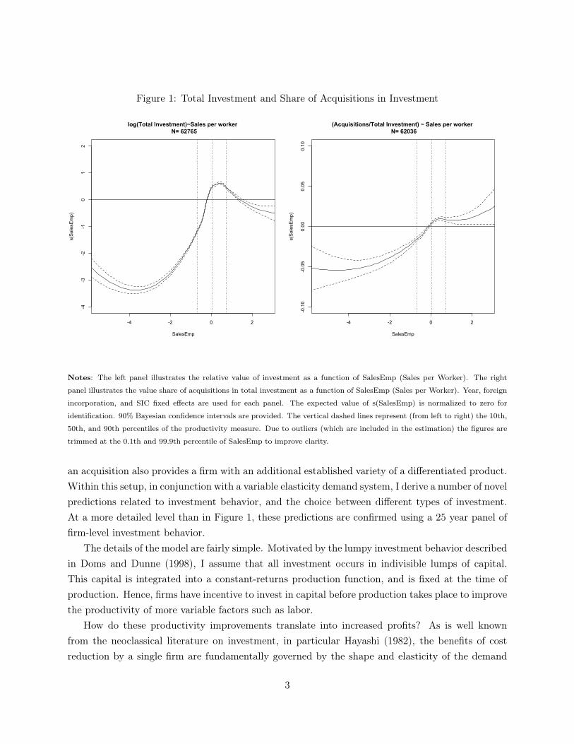
Figure 1: Total Investment and Share of Acquisitions in Investment

-4 -2 0 2

-4-3

-2-1

01

2

SalesEmp

s(SalesEmp)

log(Total Investment)~Sales per worker N= 62765

-4 -2 0 2

-0.10

-0.05

0.00

0.05

0.10

SalesEmp

s(SalesEmp)

(Acquisitions/Total Investment) ~ Sales per worker N= 62036

Notes: The left panel illustrates the relative value of investment as a function of SalesEmp (Sales per Worker). The right

panel illustrates the value share of acquisitions in total investment as a function of SalesEmp (Sales per Worker). Year, foreign

incorporation, and SIC fixed effects are used for each panel. The expected value of s(SalesEmp) is normalized to zero for

identification. 90% Bayesian confidence intervals are provided. The vertical dashed lines represent (from left to right) the 10th,

50th, and 90th percentiles of the productivity measure. Due to outliers (which are included in the estimation) the figures are

trimmed at the 0.1th and 99.9th percentile of SalesEmp to improve clarity.

an acquisition also provides a firm with an additional established variety of a differentiated product.Within this setup, in conjunction with a variable elasticity demand system, I derive a number of novelpredictions related to investment behavior, and the choice between different types of investment.At a more detailed level than in Figure 1, these predictions are confirmed using a 25 year panel offirm-level investment behavior.

The details of the model are fairly simple. Motivated by the lumpy investment behavior describedin Doms and Dunne (1998), I assume that all investment occurs in indivisible lumps of capital.This capital is integrated into a constant-returns production function, and is fixed at the time ofproduction. Hence, firms have incentive to invest in capital before production takes place to improvethe productivity of more variable factors such as labor.

How do these productivity improvements translate into increased profits? As is well knownfrom the neoclassical literature on investment, in particular Hayashi (1982), the benefits of costreduction by a single firm are fundamentally governed by the shape and elasticity of the demand

3

curve. As such, heterogeneous firms, which may operate at different demand elasticities, may havevastly different incentives to invest. To examine these issues, I utilize a common non-CES demandsystem (linear) in which varieties are imperfect substitutes and the absolute elasticity of demandis falling with quantity. Hence, high productivity firms tend to earn very little from a productivityimprovement through capital investment as they already produce near the point where revenues aremaximized. Low productivity firms also earn very little from investment, since any gains are tinydue to their intrinsically low productivity. Instead, I find that middle productivity firms have thehighest incentive to invest in additional capital.

The incentives above sufficiently characterize the incentives for new capital investment. However,acquisitions, which involve acquiring capital and an established variety, may be very different.Crucially, the aforementioned revenue constraints, which tend to bind for higher productivity firms,may be alleviated somewhat by adding a variety through an acquisition. Indeed, I show that whenan acquisition provides additional capital and management over a closely (though not perfectly)substitutable variety, the incentives for acquisition, while still highest for middle productivity firms,become skewed toward a region of higher productivity. Hence, the relative benefit of an acquisitionvis-a-vis new investment increases with productivity. Overall, I show that there exists an equilibriumof the model in which all investment behavior occurs in a middle region of productivity, with themost productive of firms in this region choosing acquisitions over new investment.

To evaluate the effects of substitution across varieties (both acquired and endowed), I examinehow the incentives for new investment and acquisitions change with the component of the demandcurve that governs product differentiation. Crucially, when consumers do not love variety, all va-rieties within the differentiated industry are perfect substitutes, and firms act like price takers.Critically, although price-taking behavior may imply that firms are small, the flat demand curvefunctionally provides firms an unbounded market in which to benefit from both types of capitalinvestment. Hence, as the model approaches this polar case, the incentives for new investment andacquisitions become more skewed toward higher productivity firms. However, the relative incentivesbetween new investment and acquisitions remain qualitatively similar. Overall, the model predictsthat different industry types - as measured by total product differentiation within each industry -exhibit qualitatively different investment incentives.

I test the predictions of the model using the Compustat North American Industrial database.As in Figure 1, and motivated by the non-monotonic nature of the predictions from the theoreticalmodel, I use non-parametric techniques to estimate the relationship between productivity and in-vestment behavior. Empirically, I find that firms in a middle range of productivity engage in thelargest amount of investment, whether it be new investment or acquisitions. This result is robustover a number of different measures of productivity. However, when looking at the relative choicebetween the two, I find that higher productivity firms choose a larger share of acquisitions in totalinvestment.

4

To evaluate the role of product differentiation within industries, I develop a method based on aHirshman-Herfindahl Index (HHI) over revenues to back-out the implied role of substitution acrossvarieties. While the specifics are presented in the paper, the essential intuition is that, holdingother factors constant (number of firms, skew of the productivity distribution), moving towarda price-taking (high substitution) environment tends to amplify the effect of firm heterogeneityon variation in sales. As this tends to disproportionately benefit high productivity (large) firms,this leads to a higher concentration (HHI) in sales. Thus, I categorize industries by their residualHHI after accounting for other factors. Estimating the model using industry subsets based ontheir implied substitutability, I show that for industries with a high implied substitutability, highproductivity firms engage in the largest amount of investment. In contrast, for industries with lowimplied substitutability, middle productivity firms engage in the largest amount of investment. Forboth cases, there is a positive relationship between productivity and the value share of acquisitionsin total investment. Finally, I show that for acquisitions, these relationships break down whenindustries have very few firms in each year (on average), suggesting that incentives may be differentwhen firms face few competitors.4

Outline

The rest of the paper is organized as follows. In section two, I present the basic investment model,detailing the fundamental incentives behind capital investment as a function of productivity, andthe difference between acquisitions and new investment. The equilibrium components of the modelare relegated to the technical appendix. In section three, I test the equilibrium predictions of sectiontwo. In section four, I conclude.

2 Model

In this section, I present a simple investment model in which firms of heterogeneous productivitychoose between new investment and acquisitions. I adopt simple assumptions to make the point thatwhile new investment and acquisitions share similar characteristics that influence overall investmentbehavior, the added variety that comes with an acquisition explains the composition of investment.A full industry equilibrium model, which solves for an endogenous acquisition price and proves thatan equilibrium exists, is presented in the appendix.

The model in this section starts from the point where a fixed measure of firms, each endowedwith an established variety and a lump of capital k that is tooled for their variety, realize theirproductivity level. It is assumed that the set of established varieties is fixed. That is, lags in research

4Traditional merger models such as Salant, Switzer and Reynolds, (1983), Deneckre and Davidson (1985), Perryand Porter (1985) and Farrell and Shapiro (1990) may be more relevant for industries in which firms have fewcompetitors.

5

and development prevent new varieties from being invented as a short to medium term response toproductivity shocks. In this sense, the model is understood as one of investment incentives in theshort to medium run.

Upon realizing their productivity, firms choose from four options. They may (1) invest in a newplant (lump of capital k) in their current variety, (2) acquire another firm, which includes that firm’splant and variety, (3) do nothing, or (4) sell their plant and variety to another firm and exit themarket. Importantly, while both acquisitions and new investment involve acquiring an additionalplant, the difference between the two forms of expansion is that with an acquisition, an additionalvariety is also acquired. Hence, the goal of this section is to not only examine the absolute incentivesof each investment choice as a function of productivity, but to also evaluate how the addition ofanother variety along with capital affects the relative incentives for acquisitions.

After investment decisions are made, firms produce varieties of a differentiated product forconsumers. Active firms are monopolists in their own varieties, though are assumed to be smallwhen facing aggregate industry variables. At this point, any capital accrued is fixed, and firms onlyprocure variable factors.

The model is solved by backward induction, and as such, I will begin by solving the firm’sproblem from the final stage.

2.1 Product Market Stage

Demand

To allow for a simple framework in which absolute elasticities are falling in quantity and firms canproduce multiple varieties, I utilize a simplified version of quadratic preferences from Mayer, Melitz,and Ottaviano (2009) and Dhingra (2010). Precisely, defining I as the set of firms and Ωi as the setof varieties produced by firm i, I assume that tastes of the representative consumer are characterizedas follows:

U = x0 +A

∫i∈I

∫l∈Ωi

qi,ldldi−1

2λγ

∫i∈I

(∫l∈Ωi

qi,ldl

)2

di− 1

2(1− λ) γ

∫i∈I

∫l∈Ωi

(qi,l)2 dldi (1)

In (1), consumers balance consumption across a numeraire commodity (x0) and a differentiatedindustry indexed over firms (i) and varieties (l). In the latter industry, the degree and compositionof product differentiation across these firms and varieties is characterized by γ and λ. Total productdifferentiation is characterized by γ, which is assumed to be greater than zero. When γ is positive,consumers optimally diversify consumption within the differentiated industry across some combina-tion of firms and varieties.5 Further, as γ falls, consumers view varieties as more substitutable. The

5γ is essentially a parameter that yields a larger disutility when consumers concentrate consumption within somelimited subset of firms and/or varieties.

6

composition of product differentiation is represented by λ ∈ [0, 1], which dictates the importanceof differentiation that is specific to firms (eg. Apple vs. Dell) relative to individual varieties (eg.MacBook Pro vs. Latitude). Precisely, as λ rises, a larger share of product differentiation is specificto firms, not varieties. Indeed, λ will control the degree to which varieties within a firm cannibalizeone another.6

Assuming that the representative consumer has sufficient income to consume within both thedifferentiated and numeraire industries, the solution to the consumer’s problem yields the followinginverse demand function for variety j produced by firm i.

pi,j = A− λγ∑

l∈Ωi,l 6=jqi,l − γqi,j (2)

To begin a discussion of (2), first consider γ, which is the parameter that governs overall prod-uct differentiation, and hence, the broad patterns of substitution within the differentiated sector.Conducting comparative statics on γ allows us to examine how the level of product differentiationaffects consumer and firm decisions while holding the composition of this differentiation constant.Generally, when γ rises, products are more differentiated, demand is steeper for a given variety andabsolute demand elasticities fall. As γ approaches zero, varieties approach perfect substitutabilitywithin and across firms, and all firms become price takers.

Next, λ represents the share of product differentiation that is derived from the aggregate varietyprovided by each firm, and is taken as given by firms throughout the analysis.7 In particular,adjusting λ allows us to examine changes to the source of differentiation while holding total productdifferentiation constant. For example, when λ rises, the consumer focuses attention toward theaggregate variety provided by each firm rather than individual varieties. Indeed, higher λ representsa case where demand for each variety within a firm is cannibalized to a larger extent by demand forother varieties within the same firm. At the limits, if λ = 1, varieties within the firm are perfectlysubstitutable (full cannibalization), but imperfect substitutes outside of the firm. In contrast, λ = 0,varieties within the firm are not any more substitutable than they are outside the firm.

Finally, note that in this model, it may be that a firm only produces one variety, in whichcase

∑l∈Ωi,l 6=j qi,l = 0. In this case, the only component relevant for pricing is total product

differentiation, γ.6Nocke and Yeaple (2006) uses a CES demand system to examine mergers for scope, though does not allow for

any intra-firm cannibalization through cross-price effects as I do in this manuscript. Instead, they assume that thereis an efficiency loss associated with acquiring additional varieties.

7Unlike Sweeting (2010), I do not allow firms to choose the location of competing varieties within the firm.

7

Capital and Costs

Capital influences firm decisions through the cost function. As originally used in Perry and Porter(1985), I assume the following cost function (which itself originates from a Cobb-Douglas productionfunction) for variety j produced by firm i:

C (qi,j |αi, v,Ki,j) =1

2·q2i,j

αiKi,j(3)

In (3), αi is firm-level productivity. Productivity across firms is continuously distributed accordingto G(α), defined over α ∈ (0,∞). Firm-level productivity is transferrable across all holdings ofcapital, and thus all varieties, within the firm. The variable Ki,j represents capital accumulatedduring the initial stage and investment stage by firm i for variety j. Critically, it is held fixed whenproducing varieties for the product market.8

Product Market Profits

At this stage, I begin to restrict the structure of the model as described in the introduction of thissection. Precisely, I assume that a firm produces at most two varieties. Under this assumption, anddropping i′s for the remainder of the paper, the maximization problem of a firm with two potentialvarieties is written as follows:

π(α,K1,K2) = maxq1,q2

(A− γq1 − γλq2)q1 + (A− γq2 − γλq1)q2 +

1

2

q21

αK1+

1

2

q22

αK2

(4)

Here, α represents firm-level productivity, and K1 and K2 are the capital levels associated withvarieties 1 and 2, respectively. Again, as variety specific capital is fixed at the time of production,marginal costs for each variety are increasing in quantity.

As written in (1), I assume that firms have no effect on A. This implies that firms are small,and that even if they acquire another firm, there is no change in the residual demand for eachvariety. This is a strong assumption that implies a very strict form of nesting in the consumer’sdecision (in concert with the assumption of monopolistic competition).9 However, the focus of thissection is to evaluate how investment incentives change with productivity, and in particular, howthe addition of a variety through acquisitions affects the relative incentives for acquisitions vis-a-visnew investment. The assumption of small firms that may add varieties through acquisitions greatlysimplifies the presentation of these incentives. I will return to this assumption in the latter part ofthe empirical section, focusing on industries that are more likely to be oligopolistic.

In the product market stage, there are potentially three types of active firms: those that did8Indeed, the fixed nature of capital is why the underlying Cobb-Douglas production function does not yield a

constant unit-cost function in this model.9Essentially, this implies that consumers choose firm first, and then from their chosen firm’s set of varieties.

8

nothing in the investment stage, those that invested in their endowed variety, and those that acquiredanother firm. For those firms that did nothing during the investment stage, they produce subjectto their endowed capital level k. Adopting the convention that a firm’s endowed variety is labeledas variety 1, we have that K1 = k, and K2 = 0 for firms that do not invest. Subject to these capitalholdings, profits are written as:

π(α, k, 0) =A2αk

2(2γαk + 1)(5)

Next, consider a firm that invested in its own variety in the investment stage. For simplicity, assumethat the firm has added an additional lump of capital to its current variety.10 Hence, K1 = 2k, andK2 = 0. Subject to these capital holdings, profits are written as:

π(α, 2k, 0) =A2αk

(4γαk + 1)(6)

Finally, consider a firm that has acquired another firm in the investment stage, which includes alump of capital k, and a variety that is attached to it. Hence, K1 = k, and K2 = k. Subject tothese capital holdings, profits are written as:

π(α, k, k) =A2αk

(2αγλk + 2γαk + 1)(7)

The profit functions in (5), (6), and (7) exhibit a number of intuitive features. First, for λ < 1,it is straightforward to show that π(α, k, k) > π(α, 2k, 0). Abstracting from the costs of eachoption that occur in a previous stage, acquiring another firm, which includes a lump of capital kand another variety, is always preferred to investing in a lump of capital in the firm’s endowedvariety. Intuitively, acquiring another firm provides the benefits of additional capital, without thefull reduction in demand elasticity (cannibalization) that would occur by doing so in the firm’scurrent variety. This point is sharpened by noting that when λ < 1, ∂π(α,k,k)

∂α > ∂π(α,2k,0)∂α for all

α. That is, this difference becomes larger when productivity increases. As higher productivityfirms operate on a less elastic portion of the demand curve, issues of demand elasticity are morepronounced, and the benefit of an acquisition relative to new investment is enhanced. In a moment,I will fully characterize the profit functions, and differences between them, as a function of α.

Finally, note that when λ = 1, π(α, k, k) = π(α, 2k, 0). Here, a firm that acquires operates twoidentical plants (lumps of capital) that produce perfectly substitutable varieties within the firm.This is a qualitatively identical outcome to when a firm invests in another plant for its endowedvariety. That is, given the cost specification in (3), equalizing marginal cost across plants that

10The technical appendix offers a case in which firms may choose capital in any amount. The fundamental invest-ment incentives do not change qualitatively when firms can by any amount of capital.

9

produce perfectly substitutable varieties is the same as doubling the size of a firm’s existing plant.11

I now roll back to the investment stage to further evaluate differences in profits as a function ofproductivity, along with introducing the fixed costs associated with investment options.

2.2 Investment Stage

Subject to profits earned in the product market, firms make investment choices in the previousstage. As described in the introduction, firms choose one of four options in the investment stage.This decision can be characterized by the following discrete choice problem:

V (α) = max Ra − π(α, k, 0), 0, π(α, 2k, 0)− π(α, k, 0)− FI , π(k, k)− π(k, 0)−Ra (8)

For reasons which will become clear, I write the profits of each option relative to the "outside option"of doing nothing. In the first entry of (8), the benefit of selling relative to doing nothing is writtenas Ra−π(α, k, 0), where Ra is the acquisition price that is paid to the selling firm. Next, the benefitof doing nothing relative to itself is zero. In the third entry of (8), the benefit of new investmentrelative to doing nothing is π(α, 2k, 0)− π(α, k, 0)− FI , where FI is the fixed cost of investing in anew lump of capital. Finally, π(k, k)− π(k, 0)−Ra represents the benefit of acquisitions relative todoing nothing, where Ra is again the price of the acquisition. As written in (8), firms choose theoption which maximizes profits at their level of productivity, α.

Moving forward, I will first characterize the incentives for acquisitions and new investment asa function of productivity. This will be sufficient to show how the incentives for new investmentand acquisitions are consistent with the patterns summarized in Figure 1. The remaining compo-nents of the equilibrium acquisition model are relegated to the appendix, where I show that thereexist parameter values such that an acquisition equilibrium exists, and that the equilibrium yieldsacquisition behavior consistent with all elements of Figure 1.

New Investment

The key to the model is how incentives for each type of investment, which are defined as the profitsearned from the investment relative to doing nothing, change with productivity. To begin, focus onthe incentive function for new investment, ΠI(α) = π(α, 2k, 0)−π(α, k, 0). These are the additionalprofits that a firm receives, relative to doing nothing, if it engages in new investment. As a functionof model parameters, ΠI(α) is written as:

ΠI(α) =A2αk

2(4γαk + 1)(2γαk + 1)(9)

11This is true for a general Cobb-Douglas production function. This derivation is available upon request.

10

It is straightforward to show that ΠI(α) equals zero when α = 0, and approaches zero when α→∞.Indeed, the maximum of ΠI(α) occurs at α = αI ≡

√2

4γk . The intuition for these properties lie at theheart of the demand-cost framework. The least efficient firms are limited by a steep marginal costschedule. Whether or not they invest, they are still quite unproductive, and the absolute gains fromnew investment are tiny. The most efficient firms are constrained not by costs, but by the structureof market demand. Specifically, the highest productivity firms operate on a less-elastic portion ofthe demand curve, which limits the incentive to expand production after purchasing a lump of newcapital. Firms in a mid-range of productivity are constrained by neither, and earn relatively highreturns from new investment.

To examine how total product differentiation affects investment incentives, note how γ affectsthe productivity level at which ΠI(α) is maximized. Indeed, as γ falls the productivity level at whichΠI(α) is maximized rises, and in the limit, approaches infinity. As γ governs demand elasticitiesat a given level of quantity, γ will have a profound effect on the firms which find new investmentprofitable. I will return to this point later in this section, and in the empirics.

Finally, note that these results are not specific to the linear demand assumption that is employedthroughout the paper. In the technical appendix, using a model of marginal capital purchases andthe cost function in (3), I show that the marginal value of added capital is highest for firms in amid-range of productivity as long as the elasticity of the marginal revenue curve with respect toquantity is finite, negative, and falling sufficiently with higher quantity. This is not satisfied whenfirms are price takers, or when firms produce subject to standard CES demand. However, this issatisfied by linear demand, and a larger class of demand functions.

Acquisitions

Next, consider the incentive function for an acquisition, ΠM (α) = π(k, k) − π(k, 0). As a functionof model parameters:

ΠM (α) =A2αk(2γαk − 2αγλk + 1)

2(2γαk + 2αγλk + 1)(2γαk + 1)(10)

To begin the analysis of ΠM (α), note when λ = 1, the two varieties are perfectly substitutablewithin the firm, and the acquisition incentive function ΠM (α) simplifies to A2αk

2(4γαk+1)(2γαk+1) , whichis the same incentive function as in ΠI(α). Hence, when varieties are perfect substitutes within thefirm, but imperfect substitutes across firms, those firms in a mid-range of productivity have thehighest incentive to acquire another firm.

At the other extreme, when λ = 0, ΠM (α) = A2αk2(2γαk+1) = π(α, k, 0). In this case, varieties

are not substitutable within the firm, and acquiring an additional unit of capital simply doublesthe profits of holding one lump of capital (no cannibalization of one variety by another variety).Further, for this case, the incentives to acquire another firm are increasing in productivity.

11

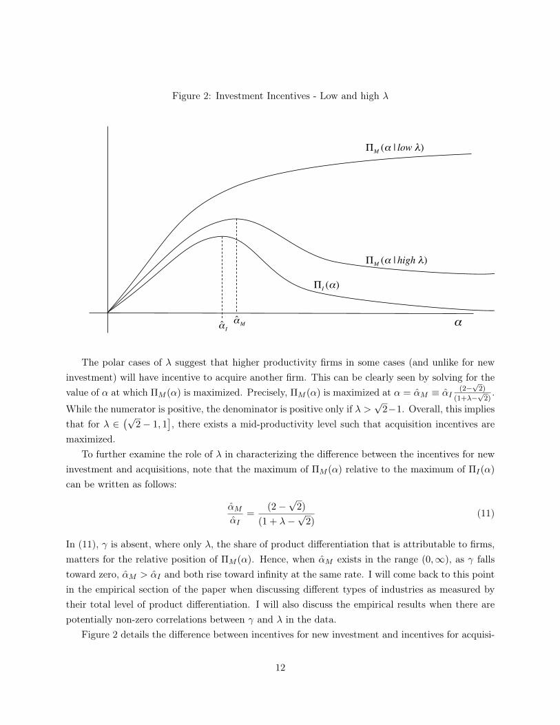
Figure 2: Investment Incentives - Low and high λ

€

α

€

ΠM (α | low λ)

€

ˆ α M

€

ˆ α I

€

ΠM (α | high λ)

€

ΠI (α)

The polar cases of λ suggest that higher productivity firms in some cases (and unlike for newinvestment) will have incentive to acquire another firm. This can be clearly seen by solving for thevalue of α at which ΠM (α) is maximized. Precisely, ΠM (α) is maximized at α = αM ≡ αI (2−

√2)

(1+λ−√

2).

While the numerator is positive, the denominator is positive only if λ >√

2−1. Overall, this impliesthat for λ ∈

(√2− 1, 1

], there exists a mid-productivity level such that acquisition incentives are

maximized.To further examine the role of λ in characterizing the difference between the incentives for new

investment and acquisitions, note that the maximum of ΠM (α) relative to the maximum of ΠI(α)

can be written as follows:

αMαI

=(2−

√2)

(1 + λ−√

2)(11)

In (11), γ is absent, where only λ, the share of product differentiation that is attributable to firms,matters for the relative position of ΠM (α). Hence, when αM exists in the range (0,∞), as γ fallstoward zero, αM > αI and both rise toward infinity at the same rate. I will come back to this pointin the empirical section of the paper when discussing different types of industries as measured bytheir total level of product differentiation. I will also discuss the empirical results when there arepotentially non-zero correlations between γ and λ in the data.

Figure 2 details the difference between incentives for new investment and incentives for acquisi-

12

tions. As long as λ < 1, ΠM (α) is always larger than ΠI(α). Further, as detailed in Figure 2, anddiscussed above, ∂ΠM (α)

∂α > ∂ΠI(α)∂α for λ < 1. Hence, the relative advantage of acquisitions over new

investment increases with productivity. The intuition for this property is straightforward. Whenallowing for new investment within a firm’s endowed variety, the crucial issue is how improvementsto variable factor productivity map into higher sales and profits. When absolute demand elasticitiesfall with higher quantities, high productivity firms have a relatively difficult time increasing salesafter increasing their capital stock. A solution to this issue is to invest in another variety, whichgiven the short-medium run nature of the model, is done so by acquisitions. Hence, high produc-tivity firms have the highest incentive to acquire another firm, both in absolute terms, and relativeto new investment.

A few features of Figure 2 worth reinforcing again are that when λ is relative high, the incentivesfor both new investment and acquisitions are highest in a middle range of productivity. However, therelative attractiveness of acquisitions increases with productivity. Both predictions are consistentwith the features in Figure 1, and I examine both predictions at a detailed level in the forthcomingempirical section. In particular, I will develop a proxy for γ - the measure of total substitutabilitywithin the differentiated industry - where the model predicts that incentives for investment of bothkinds shift toward higher productivity firms at the same rate as γ falls.

For interested readers, the remaining elements of the investment model, including equilibriumcomponents, are presented in the technical appendix. In particular, I account for the different fixedcosts of each investment option, and acquisition costs that are endogenous through a market clearingcondition for firms. In equilibrium, I show that when λ is relatively close to one and FI not toolarge, all investment occurs in a middle range of productivity, with the more productive firms inthis region choosing acquisitions over new investment.

3 Empirics

In this section, I test the predictions of the model as they relate to the relationship between produc-tivity and investment behavior, the choice of investment type, and the relationship between productsubstitutability and investment behavior. To begin the empirical section, I will describe the data,the measure of productivity, and the estimation procedure.

The sample of active firms is constructed using the Compustat North American Industrialdatabase. Within the mergers/investment literature, this database has also been used by Jovanovicand Rousseau (2002), Rhodes-Kropf and Robinson (2008) and Breinlich (2008). The time periodof analysis is 1980-2004. The primary sample is constructed using firms from industries with SICcodes less than 4000. These are primarily agricultural, commodity, and manufacturing firms. Thiswill yield a sample of 7,702 firms totaling 62,765 observations.

The primary productivity measure will be sales per worker for firm i in year t, which is labeled

13

SalesEmpi,t. The motivation for using sales per worker is that it has a structural relationship to αk,which is the firm-level measure in the model that predicts investment behavior. I provide a derivationof this relationship in Appendix C. To measure sales per worker, I first construct a naive measureby dividing yearly net sales of firm i in year t (Salesi,t) in millions of dollars (Compustat item 12)by yearly employment in millions of workers (Compustat item 29 divided by 1000). However, twoadditional steps are taken to yield a measure which is both easily interpretable, and closely appliedto the theory. First, I take the natural log of sales per worker to control for outliers which willdistort the illustrations required for a non-parametric analysis. Second, the model detailed abovedescribes static investment choices within a given industry. Thus, log sales per worker is demeanedwithin SIC-year pairs, yielding the final measure, SalesEmpi,t.

I use a simple nonparametric specification to estimate the relationship between productivity andinvestment activity. The procedure I use is an "additive model", which allows for joint estimationof both parametric and nonparametric components of an empirical specification. Following theprocedure in Wood (2007), using the MGCV package for R, I estimate the following model:

Outcomei,t+1 = s(SalesEmpi,t) +−→β OtherOtheri,t + εi,t (12)

Equation (12) estimates the relationship between the right-hand side variables in the current periodand an outcome at the firm level in the next period. Using this approach prevents an obviousendogeneity problem between the outcome and covariates from the same period. Thus, investmentbehavior covers the period 1981-2004, and firm and industry covariates cover 1980-2003. In (12),Outcomei,t is some outcome measure for firm i in year t. I will focus on four outcomes: log value ofacquisitions (Computstat item 129), log value of new capital investment (Computstat item 30), logvalue of total investment (both new investment and acquisitions), and the value share of acquisitionsin total investment.12 Further, the term Othert,i includes Year, SIC, and foreign incorporation fixedeffects (the latter being a dummy variable identifying firms incorporated in Canada).

In (12), s(SalesEmpi,t) represents a smooth function in SalesEmpi,t. For identification pur-poses, Es() = 0, where s() measures the relative effect of its argument. Conveniently, zero willalways measure the average value of the outcome after accounting for fixed effects, and thus, evaluat-ing s() and its confidence bands relative to zero will facilitate a hypothesis test of whether predictedinvestment activity is above or below average. To facilitate relatively quick estimation, s() will beestimated using a penalized cubic-spline regression. This allows for a generally specified smoothfit, along with a penalty in the likelihood function for too much "wiggliness". The optimal degreeof smoothing is chosen by a generalized cross-validation procedure.

12For values of the outcome that are equal to zero, I add $1 before taking logs. This is mostly applicable foracquisitions, where roughly 75% of firms do not acquire in each year. However, the results for acquisitions arequalitatively similar when using a binary outcome variable, and are available upon request. For new investment,rarely a year goes by in which a firm does not invest in new property plants and equipment, and as such, thisassumption is largely irrelevant for new investment and total investment.

14

Figure 3: Descriptive Measures: New Investment, Acquisitions

1980 1985 1990 1995 2000

020

4060

80100

Year

Val

ue (M

illio

ns)

Average value acquisitions

Average value new investment

1980 1985 1990 1995 2000

0.0

0.2

0.4

0.6

0.8

1.0

Year

Share

Value share of new investment in total investment

Share of firms that acquire

For the baseline results, along with SalesEmpi,t, I will also use a version that corrects forwithin-firm autocorrelation, and an auxiliary measure of TFP. The latter measure is calculated bycollecting the residual after regressing the log of sales on capital and labor.13 Note that, unlikeSalesEmpi,t, TFPi,t is not structurally related to the theory, since Sales is used as the regressandrather than output. However, as it is used in a multitude of productivity studies, I will presentresults using TFP for comparison with SalesEmpi,t.

To get a sense of how investment behavior has evolved over time, Figure 3 presents descriptivemeasures for average firm-level new investment and acquisitions in each year in the left panel, andthe value share of new investment in total investment and the share of firms that acquire for eachyear in the right panel. In the left panel, we see that investment behavior has increased over time,whether it be acquisitions or new investment. However, new investment behavior appears to be lessvariable relative to trend, which is not shocking given that new investment includes smaller yearlyinvestments such as machine replacement. In the right panel, we see that acquisition behavior hasslowly become more prevalent over time, starting at roughly 20% in 1980, and increasing to around

13Precisely, TFP will be defined as the residual from the following regression:

log(NetSalesi,t) = βTFPcap log(Capi,t) + βTFPEmp log(Empi,t) + (13)−→β TFPsic SIC +

−→β TFPyear Y ear + βTFPcan FINC + εi,t

Here, along with previously defined variables, Capi,t is the value of property, plants and equipment (Compustat item8)

15

30% after 2000. This can also be seen in the value share of new investment in total investment,which while noisy, appears to be falling over sample period.

Baseline Results

Using the three productivity measures, the results from estimating equation (12) for the four invest-ment outcomes are presented in Figures 5, 6, and 7. In all three figures, I find significant supportfor the model. Looking at acquisitions and new investment separately, I show that for each, middleproductivity firms tend to engage in more investment relative to their SIC peers in each year. Whenaggregating all investment together, I find the same result. For all investment types, there existsa range of firms above the 90th percentile of sales per worker for which investment is significantlybelow average. Finally, within the subset of firms that do invest, as productivity increases, firmschoose a larger share of acquisitions in total investment. This result is slightly less impressive forTFP , though it is still the case that the highest productivity firms choose a share of acquisitionsin total investment that is significantly above average.

The Role of Substitution

The strongest support for the model will be in analyzing investment incentives across differentindustry types in terms of how consumers value product variety. In section two, the parameterγ, which captured the consumer’s total love of variety in the differentiated industry, also governedthe degree to which incentives for both acquisitions and new investment were skewed toward highproductivity firms. For all values of γ, αM > αI . However, as γ → 0 while holding λ fixed, bothαM and αI approached infinity at the same rate. Hence, if I can construct a suitable measure forγ, I can evaluate the incentives for investment across different industry types. I now will argue thatsuch a measure exists. Then, I will construct subsets of the data according to their implied value ofγ, and estimate (12) for each subset to evaluate whether incentives change across different industrytypes.

The key to constructing a measure for γ is noting that in low γ industries, productivity differenceswill be most apparent in observable sales outcomes. That is, when varieties within the differentiatedindustry are more substitutable, observed sales heterogeneity should be larger. To capture this ideausing a common measure, I will leverage the properties of a Hirschmann-Herfindahl Index (HHI) inpre-acquisition sales to back-out an implied measure of γ. To see how this measure works, definethe observed HHI over pre-acquisition sales for industry k in year t as follows:

HHIk,t =

∑i∈Sk,t Sales

2i,t(∑

i∈Sk,t Salesi,t

)2 (14)

In (14), Sk,t is set of varieties in industry k in year t, and Salesi,t is the net sales of variety i in year

16

t. In the appendix, I prove the following relationship between HHIk,t and γ.

Lemma 1 Holding Sk,t fixed,∂HHIk,t

∂γ < 0

Proof. See Appendix.Thus, as γ falls to zero and consumers value variety less, productivity differences are enhanced

in terms of observed sales concentrations. This causes the HHI to rise. The intuition is subtle,though straightforward. Lower values of γ imply that consumers care less about variety and moreabout the average price of varieties. Hence, consumers shift on the margin away from high-price(low-productivity) varieties to lower price (high productivity) varieties. Overall, concentration ofsales increases.

There are a number of other factors that can affect HHIk,t. For one, increasing the numberof varieties will tend to reduce HHIk,t. Also, a productivity distribution which is skewed heavilytoward larger firms may increase HHIk,t. Further, the set Sk,t may be endogenous. Thus, whileLemma 1 is proven rigorously, it is meant to provide an example of how γ affects sales concentrationwithin this particular economic environment.

With this in mind, to "recover" gamma, I exploit the residual variation in concentration afterregressing log(HHIk,t) on log(Nk,t), the log of the number of firms in SIC industry k in year t,log(Skewk,t), the log ratio of maximum productivity to median productivity for SIC industry k inyear t, and log(AvgSalesEmpk,t), which is the log of average sales per worker for SIC industry i inyear t. The results from doing so are presented below:

log(HHIk,t) = − 0.231(0.0237)

− 0.5014(0.00691)

log(Nk,t) + 0.0912(0.0105)

log(Skewk,t)− 0.0811(0.00982)

log(AvgSalesEmpk,t)

R2 = 0.562

Here, as expected, more firms leads to a lower value of HHIk,t. Further, Skewk,t has a positiveeffect on HHIk,t. Intuitively, this implies that concentration is high when the most productive firmis more productive relative to the industry median. Finally, AvgSalesEmpk,t has a negative effecton concentration.

To rank industries in terms of their implied value of γ, I first collect the residuals from (15),which are at the SIC-year level. Then, I will use two methods to classify industries by their impliedvalue of γ. First, I will simply group industries into terciles of residuals in each year. Precisely,within each year, those in the lowest tercile of residuals will be labeled as having a "high" relativevalue of γ. That is, after accounting for factors that are not directly related to γ, SICs within eachyear with relatively low concentration will tend to have a higher implied value of γ. Similarly, thesecond tercile of the residuals will be labeled as "mid" values of gamma, and the highest labeledas "low" values of γ. This approach will be referred to as "Method 1". For a second approach, Itake the residuals and take averages over years for each SIC industry. Then, I construct terciles

17

as described above using the average residuals for each SIC industry. The crucial difference withabove is that I am now restricting tercile assignment to be invariant over time. This approach willbe referred to as "Method 2".

Next, I estimate the model over different data subsets defined by the method used to back-outγ, and their tercile of implied γ. The results from doing so for acquisitions, new investment andtotal investment, are presented in Figures 8, 9 and 10. Within each Figure, there are six panelswith two rows and three columns. "Method 1" is used for the top row of results, and "Method 2"is used for the bottom row of results. Further, implied values of γ go from low to high as we movefrom left to right across columns in each Figure. In Figures 8, 9 and 10, middle productivity firmshave the highest incentive to invest only if the implied value of γ is relatively high. This is the casewhen using "Method 1" (allowing for implied γ′s to change over time), and when using "Method2" (restricting that implied γ′s are time invariant). Precisely, looking at the far right panels in eachfigure, we see that for high values of γ, investment of all types is significantly below average forfirms above the 90th percentile of sales per worker. In contrast, in the left panels of each figure,where γ is relatively low, investment is well above average for high productivity firms. Hence, theimplied value of γ relates to the qualitative features of investment incentives as the theory predicts.

Next, in Figure 11, I examine the relative incentives between acquisitions and new investment. Incontrast with the absolute incentives for acquisitions and new investment, the relative incentives foracquisitions compared with new investment should not change qualitatively with γ. Regardless of thelevel of γ, as productivity increases, firms tend to prefer acquisitions to new investment. The resultsin Figure 11 are supportive of this prediction. While there are a few hints of non-monotonicity inthe estimated non-parametric functions for mid-γ, in no cases is the acquisition share for the mostproductive firms significantly different from the highest point of the non-parametric fit. Hence,across different values of γ, the data support the prediction that as productivity increases, firmstend to prefer acquisitions to new investment.

One criticism of the above analysis is that λ is held fixed and close to one. In reality, theremay be potential correlations in the relationship between γ and λ that complicate the discussion ofFigure 8. Indeed, in Figure 8, low-γ industries display acquisition incentives that are increasing inproductivity, and high-γ industries display acquisition incentives that are highest in a mid-range ofproductivity. The only way that these results are inconsistent with the theoretical model in sectiontwo is if there is a strong negative relationship between γ and λ in the data.14 In other words, asproducts become more differentiated, the firm level component of differentiation becomes irrelevant.While there is no way to test this hypothesis without estimating a full demand model, I view this asbeing unlikely. This would imply that in the most differentiated industries (e.g. motor vehicles orcomputers), on average, there is a relatively small firm-level component of product differentiation.

14Precisely, defining λ as a function of γ, ∂αM∂γ

> 0 if ∂λ∂γ

< − 1+λ−√2

γ. That is, the maximum of the incentive

function rises with product differentiation if there is a strong negative correlation between λ and γ.

18

Another potential criticism of the above approach, especially in-light of using residual HHIk,t toback-out values of γ, is that I am still not controlling properly for industries that have relatively fewfirms. That is, the framework of monopolistic competition that is the basis for the model in sectiontwo may not be suitable for describing investment behavior in oligopolistic industries. Of particularconcern is that it may be appropriate for large firms in these industries to internalize the effectsof their investment decisions on industry level measures. To see this, first consider how large firmsmight affect industry aggregates through new investment. By investing in new capital, they add tothe total industry capital stock, increasing average labor productivity, but without directly reducingthe number of firms. This would tend to make the industry more competitive, not less competitive,and shift down the residual demand for all varieties, A. Hence, market concentration does notincrease the incentives for new investment for high productivity firms. In contrast, consider a largefirm that acquires another large firm, where the remaining firms are either few or small fringe firms.Within this concentrated setting, A may rise after an acquisition since there will be one large firmin the market rather than two. Hence, larger (productive) firms, which may have paltry acquisitionincentives when A is fixed, now may have additional incentives for an acquisition when they acquiretheir primary competitor in a concentrated market. Hence, in concentrated settings and unlike newinvestment, we could expect to see acquisition incentives where high productivity firms are morelikely to acquire independent of γ.

To evaluate how the empirical incentives for investment change when industries contain relativelyfew firms, I use the following procedure along with implied γ’s from "Method 1". First, I calculatethe average number of firms listed in Compustat for each SIC industry in each year. Then, I classifySIC industries as either above median or below median in terms of the average number of firmslisted per year. The median across SIC industries is approximately 7 firms listed per year. Then, Iestimate the model using subsets of the data based on their terciles of implied gamma and relativenumber of firms per year.

The results from doing so are illustrated in Figures 12, 13, 14 and 15. Here, we see that theresults for new investment and total investment in Figures 13 and 14 do not depend on the relativevalue of N in each year. Specifically, for low implied γ, new investment is significantly larger thanaverage for high productivity firms. For higher implied γ, new investment is above average formiddle productivity firms and below average for high productivity firms.

In contrast, when we look at acquisition behavior as a function of productivity in Figure 12,we see that for industries with an above median number of firms in each year, the results conformwith the previous results presented in Figure 8. However, for industries with relatively few firmsin each year, we see that empirical acquisition incentives are quite different. In particular, forthe two lowest terciles of implied γ, we see that acquisition incentives are always largest for highproductivity firms. For the highest tercile of implied γ, there is no significant relationship betweenacquisition behavior and productivity. As discussed above, these results suggest that large firms

19

in industries with relatively few competitors are accounting for their effect on industry aggregatesthrough investment, in particular, acquisitions.

Longer Investment Windows

In (12), investment behavior is regressed on observables from the previous period. It is likely,however, that corporate expansion occurs in periods longer than one year. In this subsection, Ievaluate the model over a longer window of investment activity.

As I have a 25 year panel of firm-level behavior, I split up the panel in 5 year increments. Withineach, I measure productivity in the first year (eg. 1980) and investment behavior over the next fouryears (eg. 1981-1984). Productivity is measured exactly as described above (for the first year ineach five year window). For investment behavior, I measure the log value of acquisitions, the logvalue of new investment, the log value of total investment, and the value share of acquisitions intotal investment over the four year window. Given these variable definitions, I drop firms within afive year window that do not report data over all five years. Thus, along with evaluating investmentbehavior over a longer period, it should be understood that these results are interpretable only forcontinuing firms.

The results from running (12) using wider investment windows over different subsets of implied γare presented in Figures 16, 17, 18, and 19. In the first three, we see that despite the longer windowsof acquisition activity, the results support the model. That is, when γ is relatively low, acquisitionand investment behavior is skewed toward higher productivity firms. When γ is relatively high,investment is highest in a middle region of productivity. In the fourth, Figure 19, we see that asproductivity increases, high productivity firms are more likely to choose acquisitions over investment.Indeed, the longer investment windows seem to smooth out some of the non-monotonicity for mid-γ panels in Figure 11. Overall, I find that using a longer investment window does not have aqualitative effect on investment behavior.

4 Conclusion

This paper explores the relationship between industry-level characteristics and firm-level investmentbehavior. In particular, I show that a critical factor influencing firm-level investment behavior isthe degree to which consumers love variety. When varieties are imperfect substitutes and firm-leveldemand elasticities fall with output, mid productivity firms have the largest incentive to invest.However, when varieties are close to perfect substitutes, high productivity firms have the largestincentive to invest. For both cases, within the region of firms that do invest, high productivity firmstend to prefer acquisitions. In evaluating 25 years of data from Compustat, I find sharp evidencefor all predictions of the model.

Future work is bound to focus on two areas: matching in the acquisition market, and foreign

20

acquisitions. With regard to the former, part of the simplicity of the model is based on theassumption of a common price of acquired capital within each industry. In reality, acquisitionprices are bargained after potential matches are identified, and there is likely a tremendous amountof uncertainty within each potential acquisition. With regard to the latter, a large share of FDIinvolves the transfer of ownership across borders. While a companion paper (Spearot, 2011) extendsthe acquisition components of the above model to a setting with multiple countries and trade costs,more work is needed to precisely address the welfare effects of foreign acquisitions vis-a-vis otherforms of market-entry.

21

References

[1] Bernard, Andrew, Bradford Jenson, Stephen Redding, and Peter Schott (2007), "Firms inInternational Trade", Journal of Economic Perspectives, Vol. 21-3, pp. 105-130.

[2] Breinlich, Holger (2008), "Trade Liberalization and Industrial Restructuring through Mergersand Acquisitions," forthcoming Journal of International Economics Vol. 76-2

[3] Compustat Users Guide, The McGraw-Hill Companies, Inc., 2003

[4] Denececkre, Ray and Carl Davidson (1985), "Incentives to Form Coalitions with BertrandCompetition", Rand Journal of Economics, vol. 16-4 pp. 473-486.

[5] Dhingra, Swati (2010), "Trading away wide brands for cheap brands", mimeo London Schoolof Economics.

[6] Doms, Mark, and Timothy Dunne (1998), "Capital Adjustment Patterns in ManufacturingPlants", Review of Economic Dynamics, vol 1, pp. 409-429.

[7] Farrell, Joseph and Carl Shapiro (1990), "Horizontal Mergers: An Equilibrium Analysis",American Economic Review, vol. 80-1, pp. 107-126.

[8] Foster, Lucia, John Haltiwanger, and Chad Syverson (2008), "Reallocation, Firm Turnover,and Efficiency: Selection on Productivity or Profitability?", American Economic Review, Vol.98-1, pp. 394-425.

[9] Hayashi, Fumio (1982), "Tobin’s Marginal q and Average q: A neoclassical Interpretation",Econometrica, vol. 50, pp. 213-223

[10] Helpman, Elhanan, Marc Melitz and Stephen Yeaple (2004), "Exports versus FDI with hetero-geneous firms." American Economic Review, vol 94, 300–316.

[11] Jovanovic, Boyan and Peter Rousseau (2002), "The Q-Theory of Mergers, " American Eco-nomic Review, vol. 92, pp. 198-204.

[12] Maksimovic, Vojislav and Gordon Phillips (2001), "The Market for Corporate Assets: WhoEngages in Mergers and Asset Sales and Are There Efficiency Gains?", The Journal of Finance,No. 6, pp. 2011-2052.

[13] Mayer, Thierry, Marc J. Melitz and Gianmarco I. P. Ottaviano (2009), "Market size, Compe-tition and the Product Mix of Exporters", mimeo.

[14] Nocke, Volker and Stephen Yeaple (2007), “Cross-Border Mergers and Acquisitions versusGreenfield Foreign Direct Investment: The Role of Firm Heterogeneity”, Journal of Inter-national Economics, 2007, vol. 72-2, pp. 336-365.

22

[15] Nocke, Volker and Stephen Yeaple (2006), "Globalization and Endogenous Firm Scope", mimeoUniversity of Pennsylvania.

[16] Perry, Martin and Robert Porter (1985), "Oligopoly and the Incentive for Horizontal Merger",American Economic Review, vol. 75, pp. 219-227.

[17] Matthew Rhodes-Kropf and David Robinson (2008), "The Market for Mergers and the Bound-aries of the Firm", The Journal of Finance, Vol 83-3, pp. 1169-1211.

[18] Salant, Stephen W., Sheldon Switzer and Robert J. Reynolds (1983), "Losses from HorizontalMerger: The Effects of an Exogenous Change in Industry Structure on Cournot-Nash Equilib-rium", The Quarterly Journal of Economics, vol. 98, pp. 185-199.

[19] Spearot, Alan C. (2011), "Market Access, Investment, and Heterogeneous Firms", mimeo Uni-versity of California at Santa Cruz

[20] Sweeting, Andrew (2010), "The effects of mergers on product positioning: evidence from themusic radio industry", Rand Journal of Economics, Vol. 41-2, pp. 372-397.

[21] Verhoogen, Eric (2008), "Trade, Quality Upgrading and Wage Inequality in the Mexican Man-ufacturing Sector", Quarterly Journal of Economics, 123-2, pp. 489-530.

[22] Wood, Simon (2007), "The MGCV Package", www.r-project.org.

23

A Technical Appendix

In this appendix, I fully characterize the equilibrium of a model subject to incentives described insection two. There, I detailed the incentives for acquisitions and new investment in terms of what isearned in the product market. Now, I add in the fixed costs required for each investment type, andderive when a firm of productivity α prefers one type of investment over another. Then, I prove thatthere exist parameter values such that an equilibrium is unique and supports the behavior detailedin Figure 1.

To characterize the remaining incentives and equilibrium of the model, I will henceforth assumethat λ is relatively close to one, where the incentives to acquire another firm are highest in a middlerange of productivity and lim

α→∞ΠM (α) is not too high (this will be made precise below).

A.1 Investment Choice

To characterize the investment choice problem, I will first compare each option in the investmentstage to the outside option of doing nothing. Then, I will compare the two expansion options toone another. Finally, I will present the acquisition market clearing condition, which sets the stagefor solving the equilibrium of the model.

New investment

I will now compare new investment (I) to doing nothing (N). To begin, assume that FI is notprohibitively large, where FI < max

αΠI(α).15. Defining αI and αI as the values of α such that

ΠI(α) = FI , the following lemma follows directly from the shape of ΠI(α)

Lemma 2 For finite γ, the choice between doing nothing (N) and investing in new capital (I) as afunction of productivity is summarized as follows:

For α ∈ [0, αI ] , N Iα ∈ (αI , αI) , I Nα ∈ [αI ,∞) , N I

Proof. Immediate from shape of ΠI(α).The intuition for Lemma 2 is as discussed in section two. Firms in a middle range of productivity

have the highest incentive to invest in new capital relative to doing nothing given the demandstructure detailed in (2). However, this does not imply that middle productivity firms necessarilyinvest in new capital, since there are other options related to acquisitions and selling. I now discussthese options relative to doing nothing.

Acquisitions

With the fixed cost Ra detailed in (8), firms are indifferent between doing nothing and acquiringanother firm when ΠM (α) = Ra. Since I assume that λ is close to one, if Ra is neither triviallysmall or large (not close to zero or above the maximum of ΠM (α)), there will exist two productivity

15This assumes that investment is not trivially unprofitable for all firms

24

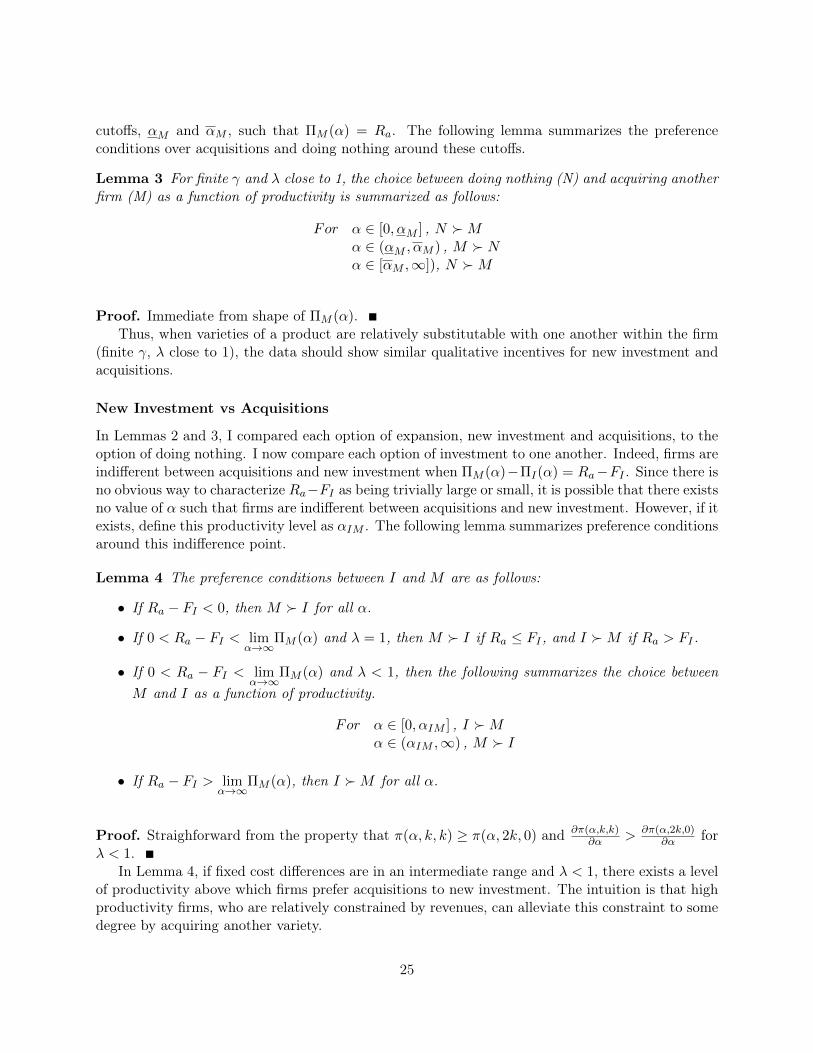
cutoffs, αM and αM , such that ΠM (α) = Ra. The following lemma summarizes the preferenceconditions over acquisitions and doing nothing around these cutoffs.

Lemma 3 For finite γ and λ close to 1, the choice between doing nothing (N) and acquiring anotherfirm (M) as a function of productivity is summarized as follows:

For α ∈ [0, αM ] , N Mα ∈ (αM , αM ) , M Nα ∈ [αM ,∞]), N M

Proof. Immediate from shape of ΠM (α).Thus, when varieties of a product are relatively substitutable with one another within the firm

(finite γ, λ close to 1), the data should show similar qualitative incentives for new investment andacquisitions.

New Investment vs Acquisitions

In Lemmas 2 and 3, I compared each option of expansion, new investment and acquisitions, to theoption of doing nothing. I now compare each option of investment to one another. Indeed, firms areindifferent between acquisitions and new investment when ΠM (α)−ΠI(α) = Ra−FI . Since there isno obvious way to characterize Ra−FI as being trivially large or small, it is possible that there existsno value of α such that firms are indifferent between acquisitions and new investment. However, if itexists, define this productivity level as αIM . The following lemma summarizes preference conditionsaround this indifference point.

Lemma 4 The preference conditions between I and M are as follows:

• If Ra − FI < 0, then M I for all α.

• If 0 < Ra − FI < limα→∞

ΠM (α) and λ = 1, then M I if Ra ≤ FI , and I M if Ra > FI .

• If 0 < Ra − FI < limα→∞

ΠM (α) and λ < 1, then the following summarizes the choice betweenM and I as a function of productivity.

For α ∈ [0, αIM ] , I Mα ∈ (αIM ,∞) , M I

• If Ra − FI > limα→∞

ΠM (α), then I M for all α.

Proof. Straighforward from the property that π(α, k, k) ≥ π(α, 2k, 0) and ∂π(α,k,k)∂α > ∂π(α,2k,0)

∂α forλ < 1.

In Lemma 4, if fixed cost differences are in an intermediate range and λ < 1, there exists a levelof productivity above which firms prefer acquisitions to new investment. The intuition is that highproductivity firms, who are relatively constrained by revenues, can alleviate this constraint to somedegree by acquiring another variety.

25

Selling

To complete the discussion of options in the investment stage, I will now characterize the decisionto sell and exit. As detailed above, firms that acquire pay the target firm Ra for their capital andvariety. Hence, a firm is indifferent between selling and doing nothing if Ra = π(α, k, 0). Labelingthe productivity level at which this occurs as αs, the following lemma summarizes the choice betweendoing nothing and selling.

Lemma 5 The choice between selling (S) and doing nothing (N) as a function of productivity issummarized as follows:

For α ∈ [0, αs] , S Nα ∈ (αs,∞) , N S

Proof. Straighforward when noting that π(α, k, 0) is increasing in productivity.In Lemma 5, the least productive firms sell. They simply do not earn enough profits in the

product market.

A.2 Equilibrium

I will now prove that there exists an equilibrium for λ close to one that conforms with the empiricalsection of the paper and the motivating plots in Figure 1. Before proving the equilibrium, I mustspecify the acquisition market clearing condition. Labeling ΘB and ΘS as the measures of buyingand selling firms, respectively, the acquisition market clearing condition is written as:∫

α∈ΘS

g(α)dα =

∫α∈ΘB

g(α)dα (15)

I will offer a more precise characterization of (15) as I prove the equilibrium below.To start my proof, I prove a result for any equilibrium when λ = 1.

Lemma 6 If λ = 1, any equilibrium must satisfy Ra ≤ FI .

Proof. Suppose to the contrary that Ra > FI . Ra > 0 implies that there exists a positive measureof selling firms. However, since ΠM (α|λ = 1) = ΠI(α), firms choose the option which minimizesfixed costs. When Ra > FI , that option is new investment, and there is no acquisition demand.Hence, the acquisition market clearing condition in (15) is not satisfied. Thus, Ra > FI cannot bean equilibrium when λ = 1

Next, I prove a result for an auxiliary game in which there is no option of new investment. Inthe full game, I will use this result to characterize the "type" of equilibrium.

Lemma 7 Suppose that new investment is not an option. For this case, there exists a value Ra = Rasuch that the acquisition market clearing condition in (15) is satisfied and the equilibrium sorting offirms is as follows.

For α ∈ [0, αS), firms sellα ∈ [αS , αM ], firms do nothingα ∈ (αM , αM ) , firms acquireα ∈ [αM ,∞), firms do nothing

26

Proof. First, I will prove optimal acquisition behavior for an arbitrary value of Ra that is nottrivially too large. Precisely, I will show that αS < αM < αM . Once I show this, the preferenceconditions are immediate from Lemmas 3 and 5.

The condition αM < αM is satisfied by definition. To show that αS < αM first note that fromthe definitions of αS and αM it must be the case that:

π (αM , k, k)− π (αM , k, 0) = Ra = π (αS , k, 0)

Rearranging,1

2π (αM , k, k)− π (αM , k, 0) = π (αS , k, 0)− 1

2π (αM , k, k)

Since 12π (αM , k, k) < π (αM , k, 0) for λ > 0 (diminishing returns to capital), the RHS must also be

negative in equilibrium. This is only possible if αS < αM .Next, subject to this acquisition behavior, the acquisition market clearing condition is written

as: ∫ αS

0g(α)dα =

∫ αM

αM

g(α)dα

It is straightforward to show that there exists a unique market clearing price Ra = Ra. By Lemma5, acquisition supply is rising in Ra from zero. That is, the range (0, αS) expands with higher Ra.Also, given the shape of ΠM (α), acquisition demand is falling in Ra, eventually reaching zero. Thatis, (αM , αM ) shrinks with Ra. Hence, by the intermediate value theorem, there exists a Ra = Rasuch that the acquisition market clears, subject to the equilibrium behavior summarized above.

Now, I am in a position to prove the three equilibrium cases of the model when λ = 1.

Lemma 8 Suppose that λ = 1. The equilibrium to the investment stage problem is as follows:

• If FI > Ra, then Ra = Ra < FI , no new investment occurs in equilibrium, and acquisitionbehavior occurs as summarized in Lemma 7.

• If FI = Ra, then Ra = Ra = FI , no new investment occurs in equilibrium, and acquisitionbehavior occurs as summarized in Lemma 7.

• If FI < Ra, then Ra = FI and optimal investment decisions are characterized as follows:

For α ∈ [0, αS), firms sellα ∈ [αS , αI ], firms do nothingα ∈ (αI , αI) , firms acquire or invest in new capitalα ∈ [αI ,∞), firms do nothing

Here, G(αS) firms acquire, and G(αI)−G(αI)−G(αS) invest in new capital.

Proof. The key to proving both cases is nothing that ΠM (α|λ = 1) = ΠI(α). That is, productmarket incentives are identical for acquisitions and new investment when varieties within the firmare perfectly substitutable. Hence, firms choose the option that minimizes fixed costs.

27

In the first case, where FI > Ra, if firms choose only acquisitions, there exists a market clearingprice at which the fixed cost of acquisitions is less than the fixed cost of new investment. Hence,new investment never occurs, and the equilibrium is identical to Lemma 7. When the prices areequal, FI = Ra, firms are indifferent between investment options, but to satisfy the acquisitionmarket clearing condition, all firms must acquire. If some margin of firms decide to invest instead,the acquisition price will fall, leading all firms to acquire. Hence, when FI = Ra, all firms mustacquire.

When FI < Ra, some new investment occurs in equilibrium. To see why, suppose that Ra > FI .For this case, there is no acquisition demand since the acquisition price is greater than the fixed newinvestment cost. Thus, Ra > FI cannot be an equilibrium. When Ra < FI , only acquisitions occur,but since Ra < FI < Ra, Ra being the price at which the acquisition market clears with no newinvestment, there is a shortage of selling firms, which pushes the acquisition price back up to FI .At Ra = FI , firms are indifferent between acquisitions and new investment, where firms randomlyassign to investment and acquisitions to maintain the condition that Ra = FI . Precisely, G(αS)firms acquire, and G(αI)−G(αI)−G(αS) invest in new capital. Any deviation from these sharesresults in one of the prior two conditions, which are not equilibria.

In Lemma 8, I have proven that there exist two types of equilibria when λ = 1. When FI > Ra,new investment does not occur since the fixed cost is too high relative to the acquisition price. Incontrast, when FI < Ra, the parameters of the model are such that there is insufficient supply ofassets to satisfy acquisition demand relative to the additional option of new investment. Hence, themechanism of the acquisition market halts when Ra = FI , where firms then randomly sort into newinvestment and acquisitions such that the acquisition market clearing condition is satisfied.

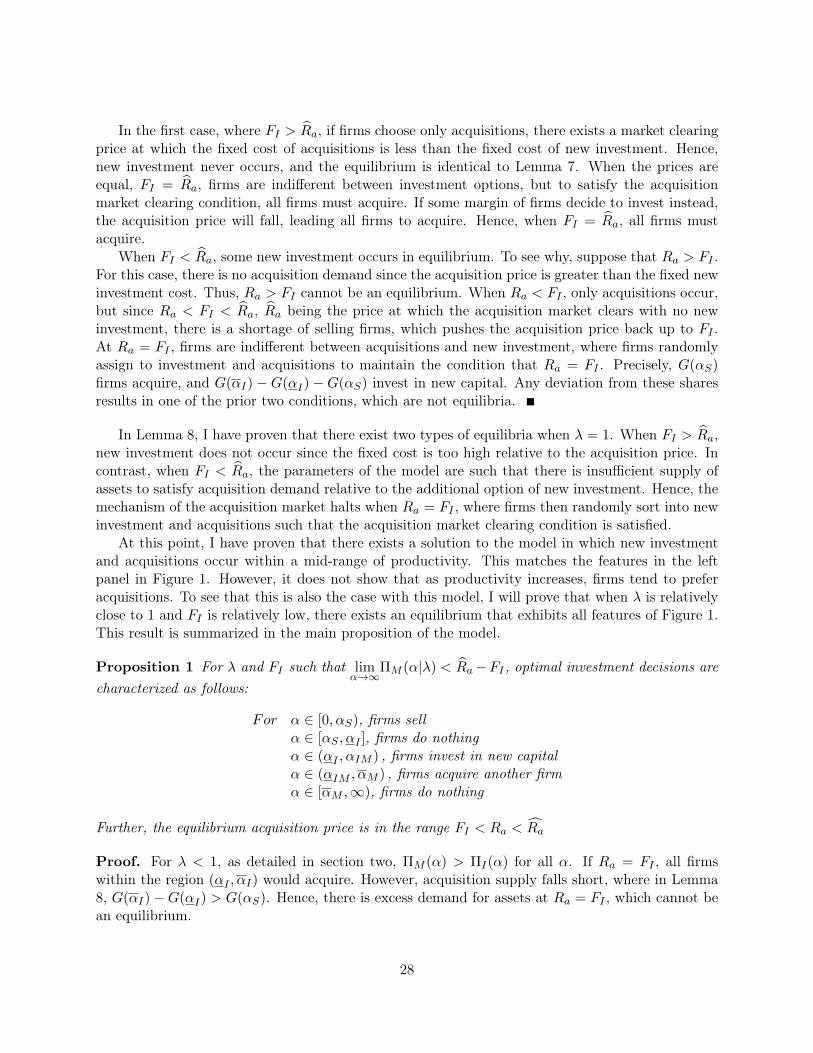
At this point, I have proven that there exists a solution to the model in which new investmentand acquisitions occur within a mid-range of productivity. This matches the features in the leftpanel in Figure 1. However, it does not show that as productivity increases, firms tend to preferacquisitions. To see that this is also the case with this model, I will prove that when λ is relativelyclose to 1 and FI is relatively low, there exists an equilibrium that exhibits all features of Figure 1.This result is summarized in the main proposition of the model.

Proposition 1 For λ and FI such that limα→∞

ΠM (α|λ) < Ra−FI , optimal investment decisions arecharacterized as follows:

For α ∈ [0, αS), firms sellα ∈ [αS , αI ], firms do nothingα ∈ (αI , αIM ) , firms invest in new capitalα ∈ (αIM , αM ) , firms acquire another firmα ∈ [αM ,∞), firms do nothing

Further, the equilibrium acquisition price is in the range FI < Ra < Ra

Proof. For λ < 1, as detailed in section two, ΠM (α) > ΠI(α) for all α. If Ra = FI , all firmswithin the region (αI , αI) would acquire. However, acquisition supply falls short, where in Lemma8, G(αI)−G(αI) > G(αS). Hence, there is excess demand for assets at Ra = FI , which cannot bean equilibrium.

28

Figure 4: Equilibrium - λ close to 1, FI not too large

€

α€

ΠM (α)

€

ΠI (α)

€

FI

€

Ra

S N N I M €

π (α,k,0)

Next, suppose that Ra = Ra. For this case, acquisition demand is zero, since given that FIsatisfies lim

α→∞ΠM (α|λ) < Ra−FI , no firms find an acquisition profitable relative to new investment

(Lemma 4). On the supply side, there is a positive measure of selling firms, since Ra > 0. Giventhe excess supply of selling firms, this cannot be an equilibrium.

In equilibrium, it must be the case that FI < Ra < Ra. To derive the sorting for firms, note thatsince Ra < Ra, the share of firms that sell must be less than in the auxiliary game. However, thetotal share of firms that invest or acquire is larger than the auxiliary game, since both FI and Raare both less than Ra. Hence, it must be the case that both acquisitions and new investment occurwhen FI < Ra < Ra. Given Lemma 4 implies that when λ < 1 the benefit of acquisitions relativeto new investment increases with productivity, we have the sorting of firms in the Proposition.

The equilibrium described in Proposition 1 is depicted in Figure 4. In equilibrium, the leastproductive firms sell, as the acquisition price is greater than the outside option of doing nothing,and both investment and acquisition provide paltry returns relative to fixed costs. Of the remainingactive firms, those in a middle range of productivity invest, with the highest productivity firms inthis range choosing acquisitions over new investment. Again, the key to the proof is that, when λis close to one and FI is relatively small ( lim

α→∞ΠM (α|λ) < Ra − FI), the share of investing firms

must be larger than the share of firms that are willing to sell. Hence, some fraction of the investingfirms must choose new investment over acquisitions, and given that λ < 1, Lemma 4 requires thatfirms choosing new investment over acquisitions are relatively less productive. Hence, we have thesorting described in Proposition 1, and detailed in Figure 4.

29

B Technical Appendix - Demand Characteristics

The primary result of the model is that mid productivity firms have the highest incentive to invest innew capital, and acquire when λ is close to one. In deriving this result, the assumed demand functionmakes analysis particularly clean and instructive. However, this begs the following question: whatare the general characteristics of demand required to deliver this particular result? To address thisquestion, I will consider a monopolist producing subject to a general inverse demand function P (q),and the same cost function as listed in (3).

Note that the crucial feature of the model is how the marginal value of additional capitalchanges with productivity. While ∂Π

∂k > 0 for every firm, and thus all firms earn some returnsfrom investment, ∂2Π

∂k∂α may change sign depending on a firm’s productivity level. The followingproposition summarizes the properties of ∂2Π

∂k∂α .

Proposition 2 ∂Π∂k > 0 for all α. Assuming that ∂MR(q)

∂q < 0, ∂2Π∂k∂α > 0 if ∂MR(q)

∂qq

MR(q) > −1,

and ∂2Π∂k∂α < 0 otherwise.

Proof. As in standard monopoly models, optimal output is determined by:

P ′ · q + P =q

αk(16)

By the envelope theorem, the marginal value of additional capital can be written as:

∂Π

∂k=

(P ′ · q + P − q

αk

)︸ ︷︷ ︸

=0

∂q

∂k+

q2

αk2

=q2

αk2> 0 (17)

Note that the marginal value of additional capital (net of capital costs) is always positive. Using(16), equation (17) can be written as:

∂Π

∂k= α

(P ′ · q + P

)2= α (MR(q))2

Differentiating with respect to α, we get:

∂2Π

∂k∂α= (MR(q))2 + 2α (MR(q))

∂MR(q)

∂q

∂q

∂α

Note that using (16) ∂q∂α is written as,

∂q

∂α=

kMR(q)

1− αk ∂MR(q)∂q

30

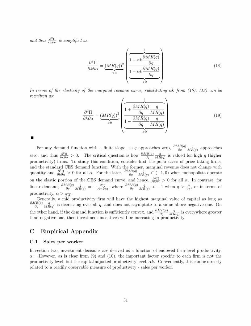
and thus ∂2Π∂k∂α is simplified as:

∂2Π

∂k∂α= (MR(q))2︸ ︷︷ ︸

>0

?︷ ︸︸ ︷1 + αk

∂MR(q)

∂q

1− αk∂MR(q)

∂q︸ ︷︷ ︸>0

(18)

In terms of the elasticity of the marginal revenue curve, substituting αk from (16), (18) can berewritten as:

∂2Π

∂k∂α= (MR(q))2︸ ︷︷ ︸

>0

?︷ ︸︸ ︷1 +

∂MR(q)

∂q

q

MR(q)

1− ∂MR(q)

∂q

q

MR(q)︸ ︷︷ ︸>0

(19)

For any demand function with a finite slope, as q approaches zero, ∂MR(q)∂q

qMR(q) approaches

zero, and thus ∂2Π∂k∂α > 0. The critical question is how ∂MR(q)

∂qq

MR(q) is valued for high q (higherproductivity) firms. To study this condition, consider first the polar cases of price taking firms,and the standard CES demand function. With the former, marginal revenue does not change withquantity and ∂2Π

∂k∂α > 0 for all α. For the later, ∂MR(q)∂q

qMR(q) ∈ (−1, 0) when monopolists operate

on the elastic portion of the CES demand curve, and hence, ∂2Π∂k∂α > 0 for all α. In contrast, for

linear demand, ∂MR(q)∂q

qMR(q) = − 2γq

A−2γq , where∂MR(q)∂q

qMR(q) < −1 when q > A

4γ , or in terms ofproductivity, α > 1

2γk .Generally, a mid productivity firm will have the highest marginal value of capital as long as

∂MR(q)∂q

qMR(q) is decreasing over all q, and does not asymptote to a value above negative one. On

the other hand, if the demand function is sufficiently convex, and ∂MR(q)∂q

qMR(q) is everywhere greater

than negative one, then investment incentives will be increasing in productivity.

C Empirical Appendix

C.1 Sales per worker

In section two, investment decisions are derived as a function of endowed firm-level productivity,α. However, as is clear from (9) and (10), the important factor specific to each firm is not theproductivity level, but the capital adjusted productivity level, αk. Conveniently, this can be directlyrelated to a readily observable measure of productivity - sales per worker.

31

To see this, first note from above that optimal pre-investment quantity and price are written as:

q(αk) =Aαk

2γαk + 1

p(αk) = Aγαk + 1

2γαk + 1

Thus, sales of each variety can be written as:

Sales(αk) = A2αk(γαk + 1)

(2γαk + 1)2 (20)

Next, note that from the assumed cost function in (3), variable input requirements are equal toq2

αk . Assuming that labor is the primary variable input, optimal labor procurement as a functionof capital adjusted productivity is written as:

L(αk) =A2αk

(2γαk + 1)2

Thus, the pre-acquisition level of sales per worker is written as:

Sales

L(αk) = (γαk + 1)

Clearly, within a given industry (in which the parameter γ is common across firms), sales per workeris linearly related to the critical term of interest, αk. Defining S ≡ Sales

L (αk) − 1 = γαk > 0 asan adjusted sales per worker, I can thus estimate αk by controlling for any industry-year specificeffects embodied in γ.

C.2 HHI Proof

In this appendix, I prove that, holding Sk,t fixed,∂HHIk,t

∂γ < 0. Recall that:

HHIk,t =

∑i∈Sk,t Sales

2i,t(∑

i∈Sk,t Salesi,t

)2

First, substitute for Salesk,t from the definition of pre-acquisition sales in Sales(αk) in (20).

HHIk,t =

∑i∈Sk,t

(A2αik(γαik+1)

(2γαik+1)2

)2

(∑i∈Sk,t

A2αik(γαik+1)

(2γαik+1)2

)2

Clearly, the A2 terms in HHIk,t can be cancelled out. Defining φi = αik(γαik+1)

(2γαik+1)2, we have:

HHIk,t =

∑i∈Sk,t φ

2i(∑

i∈Sk,t φi

)2

32

Differentiating with respect to γ, and dropping t′s for convenience, we have:

∂HHIk∂γ

=2(∑

i∈Sk φi

)3

∑i∈Sk

φi∂φi∂γ

∑i∈Sk

φi −∑i∈Sk

φ2i

∑i∈Sk

∂φi∂γ

Note that ∂φi

∂γ = −φiλi, where λi = 2γ(αik)2+3αikγ(2γ(αik)2+3αik)+1

. Substituting −φiλi for ∂φi∂γ , we have:

∂HHIk∂γ

= − 2(∑i∈Sk φi

)3

∑i∈Sk

φ2iλi

∑i∈Sk

φi −∑i∈Sk

φ2i

∑i∈Sk

φiλi

Further simplification yields:

∂HHIk∂γ

= − 2(∑i∈Sk φi

)3

∑i∈Sk

∑j∈Sk

φ2iφj (λi − λj)

To sign

∑i∈Sk

∑j∈Sk φ

2iφj (λi − λj), note that for any pair of varieties l and k (that is adding

φ2iφj (λi − λj) when i = l,j = k and i = k,j = l), the components of the double summation can be

written as φ2l φk(λl − λk) + φ2

kφl(λk − λl). This can be simplified as:

φ2l φk(λl − λk) + φ2

kφl(λk − λl) = φlφk (φl(λl − λk) + φk(λk − λl))= φlφk (φl − φk) (λl − λk)

It is straightforward to show that φ and λ are both increasing in α. Hence, when αl 6= αk,φlφk (φl − φk) (λl − λk) > 0. When αl = αk, then φlφk (φl − φk) (λl − λk) = 0. Overall, as long asthere is some variation in productivity,

∑i∈Sk

∑j∈Sk φ

2iφj (λi − λj) > 0, and hence, ∂HHIk∂γ < 0.

33

Figure 5: Baseline Nonparametric Results - Sales Per Worker

-4 -2 0 2

-4-3

-2-1

01

2

SalesEmp

s(SalesEmp)

log(Acquisitions)~Sales per worker N= 62765

-4 -2 0 2

-4-3

-2-1

01

2

SalesEmp

s(SalesEmp)

log(New Investment)~Sales per worker N= 62765

-4 -2 0 2

-4-3

-2-1

01

2

SalesEmp

s(SalesEmp)

log(Total Investment)~Sales per worker N= 62765

-4 -2 0 2

-0.10

-0.05

0.00

0.05

0.10

SalesEmp

s(SalesEmp)

Share Acquisitions ~ Sales per worker N= 62036

Notes: Each panel illustrates the relative value of an investment type (Acquisitions, New Investment, Total Investment, and

Acquisition Share) as a function of SalesEmp (Sales per Worker). Year, foreign incorporation, and SIC fixed effects are used

for each panel. The expected value of s(SalesEmp) is normalized to zero for identification. 90% Bayesian confidence intervals

are provided. The vertical dashed lines represent (from left to right) the 10th, 50th, and 90th percentiles of the productivity

measure. Due to outliers (which are included in the estimation) the figures are trimmed at the 0.1th and 99.9th percentile of

SalesEmp to improve clarity.

34

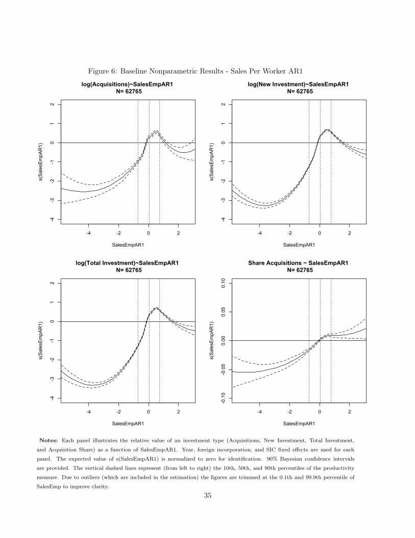
Figure 6: Baseline Nonparametric Results - Sales Per Worker AR1

-4 -2 0 2

-4-3

-2-1

01

2

SalesEmpAR1

s(SalesEmpAR1)

log(Acquisitions)~SalesEmpAR1 N= 62765

-4 -2 0 2

-4-3

-2-1

01

2

SalesEmpAR1

s(SalesEmpAR1)

log(New Investment)~SalesEmpAR1 N= 62765

-4 -2 0 2

-4-3

-2-1

01

2

SalesEmpAR1

s(SalesEmpAR1)

log(Total Investment)~SalesEmpAR1 N= 62765

-4 -2 0 2

-0.10

-0.05

0.00

0.05

0.10

SalesEmpAR1

s(SalesEmpAR1)

Share Acquisitions ~ SalesEmpAR1 N= 62765

Notes: Each panel illustrates the relative value of an investment type (Acquisitions, New Investment, Total Investment,

and Acquisition Share) as a function of SalesEmpAR1. Year, foreign incorporation, and SIC fixed effects are used for each

panel. The expected value of s(SalesEmpAR1) is normalized to zero for identification. 90% Bayesian confidence intervals

are provided. The vertical dashed lines represent (from left to right) the 10th, 50th, and 90th percentiles of the productivity

measure. Due to outliers (which are included in the estimation) the figures are trimmed at the 0.1th and 99.9th percentile of

SalesEmp to improve clarity.

35

Figure 7: Baseline Nonparametric Results - TFP

-4 -2 0 2

-4-3

-2-1

01

2

TFP

s(TFP)

log(Acquisitions)~TFP N= 62765

-4 -2 0 2

-4-3

-2-1

01

2

TFP

s(TFP)

log(New Investment)~TFP N= 62765

-4 -2 0 2

-4-3

-2-1

01

2

TFP

s(TFP)

log(Total Investment)~TFP N= 62765

-4 -2 0 2

-0.10

-0.05

0.00

0.05

0.10

TFP

s(TFP)

Share Acquisitions ~ TFP N= 62765

Notes: Each panel illustrates the relative value of an investment type (Acquisitions, New Investment, Total Investment,

and Acquisition Share) as a function of TFP. Year, foreign incorporation, and SIC fixed effects are used for each panel. The

expected value of s(TFP) is normalized to zero for identification. 90% Bayesian confidence intervals are provided. The vertical

dashed lines represent (from left to right) the 10th, 50th, and 90th percentiles of the productivity measure. Due to outliers

(which are included in the estimation) the figures are trimmed at the 0.1th and 99.9th percentile of TFP to improve clarity.

36

Figure8:

Non

-param

etricresultsan

dim

pliedga

mma,

Acquisition

s

-4-2

02

-4-2024

SalesEmp

s(SalesEmp)lo

g(A

cqui

sitio

ns)~

Sale

s pe

r wor

ker

low

gam

ma,

Met

hod

1, N

= 25

921

-4-2

02

-4-2024

SalesEmp

s(SalesEmp)

log(

Acq

uisi

tions

)~Sa

les

per w

orke

r m

id g

amm

a, M

etho

d 1,

N=

1623

1

-4-2

02

-4-2024

SalesEmp

s(SalesEmp)

log(

Acq

uisi

tions

)~Sa

les

per w

orke

r h

igh

gam

ma,

Met

hod

1, N

= 20

613

-4-2

02

-4-2024

SalesEmp

s(SalesEmp)

log(

Acq

uisi

tions

)~Sa

les

per w

orke

r lo

w g

amm

a, M

etho

d 2,

N=

2786

4

-5-4

-3-2

-10

12

-4-2024

SalesEmp

s(SalesEmp)

log(

Acq

uisi

tions

)~Sa

les

per w

orke

r m

id g

amm

a, M

etho

d 2,

N=

1343

8

-6-4

-20

2

-4-2024SalesEmp

s(SalesEmp)

log(

Acq

uisi

tions

)~Sa

les

per w

orke

r h

igh

gam

ma,

Met

hod

2, N

= 21

463

Not

es:Eachpa

nelrepresents

theno

n-pa

rametricrelation

ship

betw

eenSa

lesE

mp(Sales

perworker)

andacqu

isitionactivity

forsubsetsof

theda

tadefin

edby

their

impliedγ.Year,foreignincorporation,

andSIC

fixed

effects

areused

foreach

panel.The

expe

cted

valueof

s(Sa

lesE

mp)

isno

rmalized

tozero

foridentification.

90%

Bayesianconfi

denceintervalsareprovided.The

vertical

dashed

lines

represent(from

left

torigh

t)the10th,50th,an

d90th

percentilesof

theprod

uctivity

measure.

Due

toou

tliers

(which

areinclud

edin

theestimation)

thefig

ures

aretrim

med

atthe0.1than

d99.9th

percentile

ofSa

lesE

mpto

improveclarity.

37

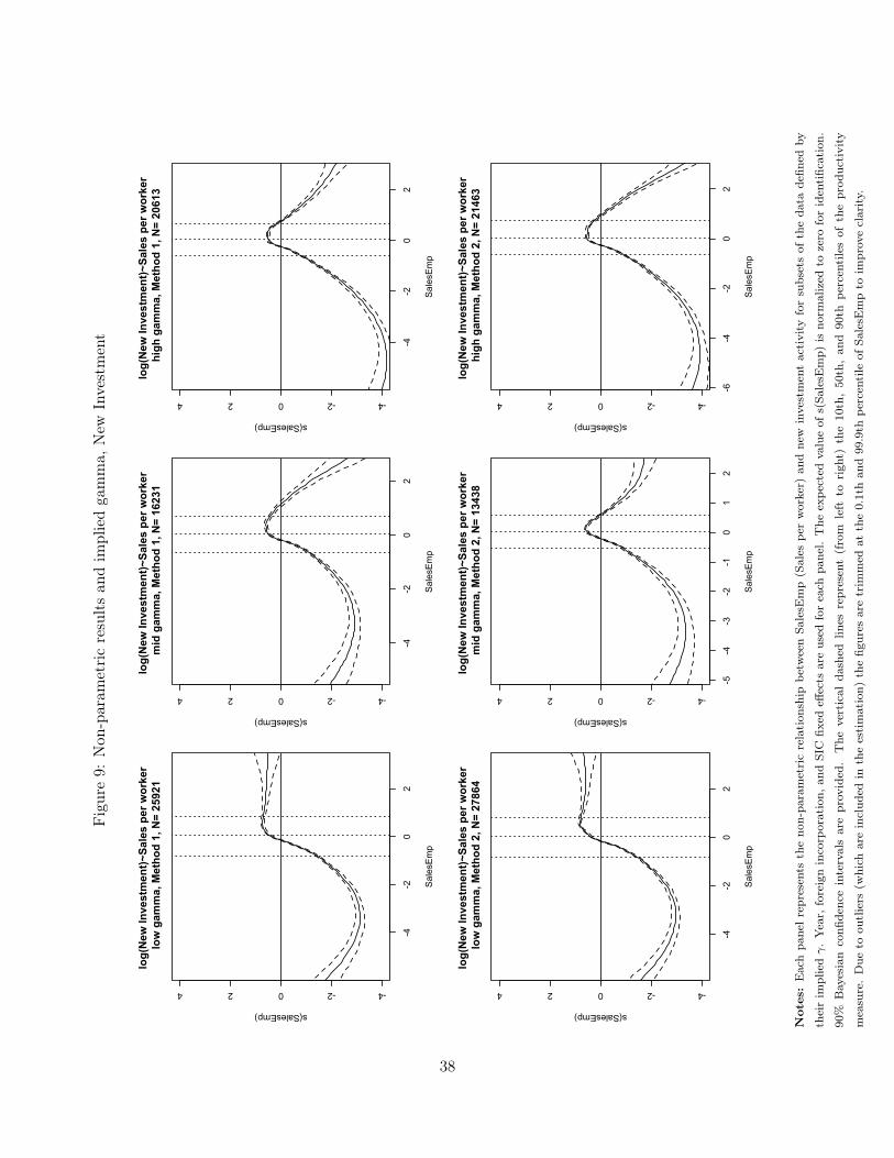
Figure9:

Non

-param

etricresultsan

dim

pliedga

mma,

New

Investment

-4-2

02

-4-2024

SalesEmp

s(SalesEmp)lo

g(N

ew In

vest

men

t)~Sa

les

per w

orke

r lo

w g

amm

a, M

etho

d 1,

N=

2592

1

-4-2

02

-4-2024

SalesEmp

s(SalesEmp)

log(

New

Inve

stm

ent)~

Sale

s pe

r wor

ker

mid

gam

ma,

Met

hod

1, N

= 16

231

-4-2

02

-4-2024

SalesEmp

s(SalesEmp)

log(

New

Inve

stm

ent)~

Sale

s pe

r wor

ker

hig

h ga

mm

a, M

etho

d 1,

N=

2061

3

-4-2

02

-4-2024

SalesEmp

s(SalesEmp)

log(

New

Inve

stm

ent)~

Sale

s pe

r wor

ker

low

gam

ma,

Met

hod

2, N

= 27

864

-5-4

-3-2

-10

12

-4-2024

SalesEmp

s(SalesEmp)

log(

New

Inve

stm

ent)~

Sale

s pe

r wor

ker

mid

gam

ma,

Met

hod

2, N

= 13

438

-6-4

-20

2

-4-2024SalesEmp

s(SalesEmp)

log(

New

Inve

stm

ent)~

Sale

s pe

r wor

ker

hig

h ga

mm

a, M

etho

d 2,

N=

2146

3

Not

es:Eachpa

nelrepresents

theno

n-pa

rametricrelation

ship

betw

eenSa

lesE

mp(Sales

perworker)

andnew

investmentactivity

forsubsetsof

theda

tadefin

edby

theirim

pliedγ.Year,foreignincorporation,

andSIC

fixed

effects

areused

foreach

panel.The

expe

cted

valueof

s(Sa

lesE

mp)

isno

rmalized

tozero

foridentification.

90%

Bayesianconfi

denc

eintervalsareprov

ided.

The

vertical

dashed

lines

represent(from

left

torigh

t)the10th,50th,an

d90th

percentilesof

theprod

uctivity

measure.Due

toou

tliers

(which

areinclud

edin

theestimation)

thefig

ures

aretrim

med

atthe0.1than

d99.9th

percentile

ofSa

lesE

mpto

improveclarity.

38

Figure10

:Non

-param

etricresultsan

dim

pliedga

mma,

Total

Investment

-4-2

02

-4-2024

SalesEmp

s(SalesEmp)lo

g(To

tal I

nves

tmen

t)~Sa

les

per w

orke

r lo

w g

amm

a, M

etho

d 1,

N=

2592

1

-4-2

02

-4-2024

SalesEmp

s(SalesEmp)

log(

Tota

l Inv

estm

ent)~

Sale

s pe

r wor

ker

mid

gam

ma,

Met

hod

1, N

= 16

231

-4-2

02

-4-2024

SalesEmp

s(SalesEmp)

log(

Tota

l Inv

estm

ent)~

Sale

s pe

r wor

ker

hig

h ga

mm

a, M

etho

d 1,

N=

2061

3

-4-2

02

-4-2024

SalesEmp

s(SalesEmp)

log(

Tota

l Inv

estm

ent)~

Sale

s pe

r wor

ker

low

gam

ma,

Met

hod

2, N

= 27

864

-5-4

-3-2

-10

12

-4-2024

SalesEmp

s(SalesEmp)

log(

Tota

l Inv

estm

ent)~

Sale

s pe

r wor

ker

mid

gam

ma,

Met

hod

2, N

= 13

438

-6-4

-20

2

-4-2024SalesEmp

s(SalesEmp)

log(

Tota

l Inv

estm

ent)~

Sale

s pe

r wor

ker

hig

h ga

mm

a, M

etho

d 2,

N=

2146

3

Not

es:Eachpa

nelrepresents

theno

n-pa

rametricrelation

ship

betw

eenSa

lesE

mp(Sales

perworker)

andtotalinvestmentactivity

forsubsetsof

theda

tadefin

edby

theirim

pliedγ.Year,foreignincorporation,

andSIC

fixed

effects

areused

foreach

panel.The

expe

cted

valueof

s(Sa

lesE

mp)

isno

rmalized

tozero

foridentification.

90%

Bayesianconfi

denc

eintervalsareprov

ided.

The

vertical

dashed

lines

represent(from

left

torigh

t)the10th,50th,an

d90th

percentilesof

theprod

uctivity

measure.Due

toou

tliers

(which

areinclud

edin

theestimation)

thefig

ures

aretrim

med

atthe0.1than

d99.9th

percentile

ofSa

lesE

mpto

improveclarity.

39

Figure11

:Non

-param

etricresultsan

dim

pliedga

mma,

Acquisition

Share

-4-2

02

-0.10-0.050.000.050.10

SalesEmp

s(SalesEmp)A

cqui

sitio

n Sh

are~

Sale

s pe

r wor

ker

low

gam

ma,

Met

hod

1, N

= 25

566

-4-2

02

-0.10-0.050.000.050.10

SalesEmp

s(SalesEmp)

Acq

uisi

tion

Shar

e~Sa

les

per w

orke

r m

id g

amm

a, M

etho

d 1,

N=

1605

0

-4-2

02

-0.10-0.050.000.050.10

SalesEmp

s(SalesEmp)

Acq

uisi

tion

Shar

e~Sa

les

per w

orke

r h

igh

gam

ma,

Met

hod

1, N

= 20

420

-4-2

02

-0.10-0.050.000.050.10

SalesEmp

s(SalesEmp)

Acq

uisi

tion

Shar

e~Sa

les

per w

orke

r lo

w g

amm

a, M

etho

d 2,

N=

2748

2

-5-4

-3-2

-10

12

-0.10-0.050.000.050.10

SalesEmp

s(SalesEmp)

Acq

uisi

tion

Shar

e~Sa

les

per w

orke

r m

id g

amm

a, M

etho

d 2,

N=

1331

4

-4-2

02

-0.10-0.050.000.050.10SalesEmp

s(SalesEmp)

Acq

uisi

tion

Shar

e~Sa

les

per w

orke

r h

igh

gam

ma,

Met

hod

2, N

= 21

240

Not

es:Eachpa

nelrepresents

theno

n-pa

rametricrelation

ship

betw

eenSa

lesE

mpan

dthevalueshareof

acqu

isitions

intotalinvestmentforsubsetsof

theda

ta

defin

edby

theirim

pliedγ.Year,

foreignincorporation,

andSIC

fixed

effects

areused

foreach

panel.

The

expe

cted

valueof

s(Sa

lesE

mp)

isno

rmalized

tozero

for

identific

ation.

90%

Bayesianconfi

denceintervalsareprovided

.The

vertical

dashed

lines

represent(from

left

torigh

t)the10th,50th,an

d90th

percentilesof

the

prod

uctivity

measure.Due

toou

tliers

(which

areinclud

edin

theestimation)

thefig

ures

aretrim

med

atthe0.1than

d99.9th

percentile

ofSa

lesE

mpto

improveclarity.

40

Figure12

:Non

-param

etricresults,

impliedga

mma,

andnu

mbe

rof

firms-Acquisition

s

-3-2

-10

12

-4-2024

SalesEmp

s(SalesEmp)

log(

Acq

uisi

tions

)~Sa

les

per w

orke

r S

ICs

with

avg

(N) b

elow

sam

ple

med

ian

low

gam

ma,

N=

3598

-3-2

-10

12

-4-2024

SalesEmp

s(SalesEmp)

log(

Acq

uisi

tions

)~Sa

les

per w

orke

r S

ICs

with

avg

(N) b

elow

sam

ple

med

ian

mid

gam

ma,

N=

3353

-4-3

-2-1

01

2

-4-2024

SalesEmp

s(SalesEmp)

log(

Acq

uisi

tions

)~Sa

les

per w

orke

r S

ICs

with

avg

(N) b

elow

sam

ple

med

ian

hig

h ga

mm

a, N

= 32

48

-6-4

-20

2

-4-2024

SalesEmp

s(SalesEmp)

log(

Acq

uisi

tions

)~Sa

les

per w

orke

r S

ICs

with

avg

(N) a

bove

sam

ple

med

ian

low

gam

ma,

N=

2232

3

-4-2

02

-4-2024

SalesEmp

s(SalesEmp)lo

g(A

cqui

sitio

ns)~

Sale

s pe

r wor

ker

SIC

s w

ith a

vg(N

) abo

ve s

ampl

e m

edia

n m

id g

amm

a, N

= 12

878

-4-2

02

-4-2024

SalesEmp

s(SalesEmp)

log(

Acq

uisi

tions

)~Sa

les

per w

orke

r S

ICs

with

avg

(N) a

bove

sam

ple

med

ian

hig

h ga

mm

a, N

= 17

365

Not

es:Eachpa

nelrepresents

theno

n-pa

rametricrelation

ship

betw

eenSa

lesE

mp(Sales

perworker)

andacqu

isitionactivity

forindu

stry

subsetsof

theda

tadefin

ed

bytheirim

pliedγ(using

Metho

d1)

andtheiraveragenu

mbe

rof

firmspe

ryear

relative

tothemedianof

thefullsample.

Year,

foreignincorporation,

andSIC

fixed

effects

areused

foreach

panel.The

expe

cted

valueof

s(Sa

lesE

mp)

isno

rmalized

tozero

foridentification.

90%

Bayesianconfi

denceintervalsareprov

ided.The

vertical

dashed

lines

represent(from

left

torigh

t)the10th,50th,an

d90th

percentilesof

theprod

uctivity

measure.Due

toou

tliers

(which

areinclud

edin

theestimation)

the

figures

aretrim

med

atthe0.1than

d99.9th

percentile

ofSa

lesE

mpto

improveclarity.

41

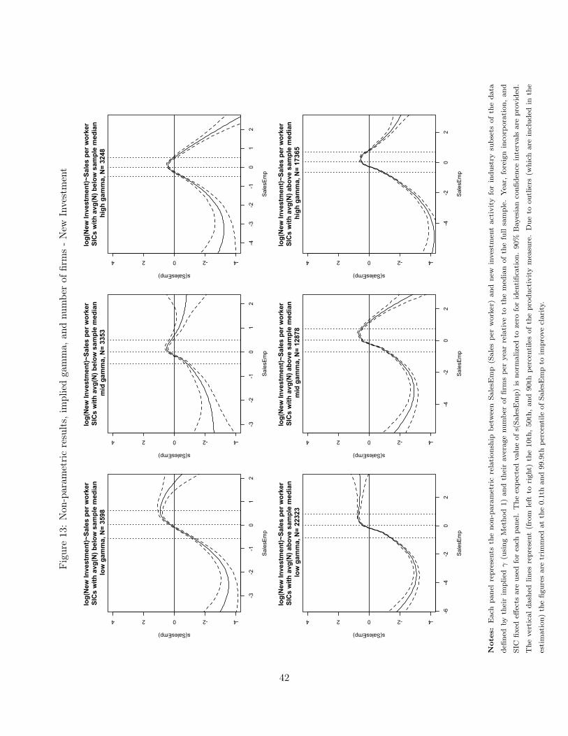
Figure13

:Non

-param

etricresults,

impliedga

mma,

andnu

mbe

rof

firms-New

Investment

-3-2

-10

12

-4-2024

SalesEmp

s(SalesEmp)

log(

New

Inve

stm

ent)~

Sale

s pe

r wor

ker

SIC

s w

ith a

vg(N

) bel

ow s

ampl

e m

edia

n lo

w g

amm

a, N

= 35

98

-3-2

-10

12

-4-2024

SalesEmp

s(SalesEmp)

log(

New

Inve

stm

ent)~

Sale

s pe

r wor

ker

SIC

s w

ith a

vg(N

) bel

ow s

ampl

e m

edia

n m

id g

amm

a, N

= 33

53

-4-3

-2-1

01

2

-4-2024

SalesEmp

s(SalesEmp)

log(

New

Inve

stm

ent)~

Sale

s pe

r wor

ker

SIC

s w

ith a

vg(N

) bel

ow s

ampl

e m

edia

n h

igh

gam

ma,

N=

3248

-6-4

-20

2

-4-2024

SalesEmp

s(SalesEmp)

log(

New

Inve

stm

ent)~

Sale

s pe

r wor

ker

SIC

s w

ith a

vg(N

) abo

ve s

ampl

e m

edia

n lo

w g

amm

a, N

= 22

323

-4-2

02

-4-2024

SalesEmp

s(SalesEmp)lo

g(N

ew In

vest

men

t)~Sa

les

per w

orke

r S

ICs

with

avg

(N) a

bove

sam

ple

med

ian

mid

gam

ma,

N=

1287

8

-4-2

02

-4-2024

SalesEmp

s(SalesEmp)

log(

New

Inve

stm

ent)~

Sale

s pe

r wor

ker

SIC

s w

ith a

vg(N

) abo

ve s

ampl

e m

edia

n h

igh

gam

ma,

N=

1736

5

Not

es:Eachpa

nelrepresents

theno

n-pa

rametricrelation

ship

betw

eenSa

lesE

mp(Sales

perworker)

andnew

investmentactivity

forindu

stry

subsetsof

theda

ta

defin

edby

theirim

pliedγ(using

Metho

d1)

andtheiraveragenu

mbe

rof

firmspe

ryear

relative

tothemedianof

thefullsample.

Year,

foreignincorporation,

and

SIC

fixed

effects

areused

foreach

panel.

The

expe

cted

valueof

s(Sa

lesE

mp)

isno

rmalized

tozero

foridentification.

90%

Bayesianconfi

denceintervalsareprov

ided.

The

vertical

dashed

lines

represent(from

left

torigh

t)the10th,50th,an

d90th

percentilesof

theprod

uctivity

measure.Due

toou

tliers

(which

areinclud

edin

the

estimation)

thefig

ures

aretrim

med

atthe0.1than

d99.9th

percentile

ofSa

lesE

mpto

improveclarity.

42

Figure14

:Non

-param

etricresults,

impliedga

mma,

andnu

mbe

rof

firms-Total

Investment

-3-2

-10

12

-4-2024

SalesEmp

s(SalesEmp)

log(

Tota

l Inv

estm

ent)~

Sale

s pe

r wor

ker

SIC

s w

ith a

vg(N

) bel

ow s

ampl

e m

edia

n lo

w g

amm

a, N

= 35

98

-3-2

-10

12

-4-2024

SalesEmp

s(SalesEmp)

log(

Tota

l Inv

estm

ent)~

Sale

s pe

r wor

ker

SIC

s w

ith a

vg(N

) bel

ow s

ampl

e m

edia

n m

id g

amm

a, N

= 33

53

-4-3

-2-1

01

2

-4-2024

SalesEmp

s(SalesEmp)

log(

Tota

l Inv

estm

ent)~

Sale

s pe

r wor

ker

SIC

s w

ith a

vg(N

) bel

ow s

ampl

e m

edia

n h

igh

gam

ma,

N=

3248

-6-4

-20

2

-4-2024

SalesEmp

s(SalesEmp)

log(

Tota

l Inv

estm

ent)~

Sale

s pe

r wor

ker

SIC

s w

ith a

vg(N

) abo

ve s

ampl

e m

edia

n lo

w g

amm

a, N

= 22

323

-4-2

02

-4-2024

SalesEmp

s(SalesEmp)lo

g(To

tal I

nves

tmen

t)~Sa

les

per w

orke

r S

ICs

with

avg

(N) a

bove

sam

ple

med

ian

mid

gam

ma,

N=

1287

8

-4-2

02

-4-2024

SalesEmp

s(SalesEmp)

log(

Tota

l Inv

estm

ent)~

Sale

s pe

r wor

ker

SIC

s w

ith a

vg(N

) abo

ve s

ampl

e m

edia

n h

igh

gam

ma,

N=

1736

5

Not

es:Eachpa

nelrepresents

theno

n-pa

rametricrelation

ship

betw

eenSa

lesE

mp(Sales

perworker)

andtotalinvestmentactivity

forindu

stry

subsetsof

theda

ta

defin

edby

theirim

pliedγ(using

Metho

d1)

andtheiraveragenu

mbe

rof

firmspe

ryear

relative

tothemedianof

thefullsample.

Year,

foreignincorporation,

and

SIC

fixed

effects

areused

foreach

panel.

The

expe

cted

valueof

s(Sa

lesE

mp)

isno

rmalized

tozero

foridentification.

90%

Bayesianconfi

denceintervalsareprov

ided.

The

vertical

dashed

lines

represent(from

left

torigh

t)the10th,50th,an

d90th

percentilesof

theprod

uctivity

measure.Due

toou

tliers

(which

areinclud

edin

the

estimation)

thefig

ures

aretrim

med

atthe0.1than

d99.9th

percentile

ofSa

lesE

mpto

improveclarity.

43

Figure15

:Non

-param

etricresults,

impliedga

mma,

andnu

mbe

rof

firms-Acquisition

Share

-3-2

-10

12

-0.10-0.050.000.050.10

SalesEmp

s(SalesEmp)

Acq

uisi

tion

Shar

e~Sa

les

per w

orke

r S

ICs

with

avg

(N) b

elow

sam

ple

med

ian

low

gam

ma,

N=

3561

-3-2

-10

12

-0.10-0.050.000.050.10

SalesEmp

s(SalesEmp)

Acq

uisi

tion

Shar

e~Sa

les

per w

orke

r S

ICs

with

avg

(N) b

elow

sam

ple

med

ian

mid

gam

ma,

N=

3327

-4-3

-2-1

01

2

-0.10-0.050.000.050.10

SalesEmp

s(SalesEmp)

Acq

uisi

tion

Shar

e~Sa

les

per w

orke

r S

ICs

with

avg

(N) b

elow

sam

ple

med

ian

hig

h ga

mm

a, N

= 32

31

-4-2

02

-0.10-0.050.000.050.10

SalesEmp

s(SalesEmp)

Acq

uisi

tion

Shar

e~Sa

les

per w

orke

r S

ICs

with

avg

(N) a

bove

sam

ple

med

ian

low

gam

ma,

N=

2374

4

-4-2

02

-0.10-0.050.000.050.10

SalesEmp

s(SalesEmp)A

cqui

sitio

n Sh

are~

Sale

s pe

r wor

ker

SIC

s w

ith a

vg(N

) abo

ve s

ampl

e m

edia

n m

id g

amm

a, N

= 10

076

-6-4

-20

2

-0.10-0.050.000.050.10

SalesEmp

s(SalesEmp)

Acq

uisi

tion

Shar

e~Sa

les

per w

orke

r S

ICs

with

avg

(N) a

bove

sam

ple

med

ian

hig

h ga

mm

a, N

= 18

097

Not

es:Eachpa

nelrepresentstheno

n-pa

rametricrelation

ship

betw

eenSa

lesE

mp(Sales

perworker)

andthevalueshareof

acqu

isitions

intotalinv

estm

entforindu

stry

subsetsof

theda

tadefin

edby

theirim

pliedγ(using

Metho

d1)

andtheiraveragenu

mbe

rof

firmspe

ryear

relative

tothemedianof

thefullsample.

Year,

foreign

incorporation,

andSIC

fixed

effects

areused

foreach

panel.

The

expe

cted

valueof

s(Sa

lesE

mp)

isno

rmalized

tozero

foridentification.

90%

Bayesianconfi

dence

intervalsareprovided.The

vertical

dashed

lines

represent(from

left

torigh

t)the10th,5

0th,

and90th

percentilesof

theprod

uctivity

measure.Due

toou

tliers

(which

areinclud

edin

theestimation)

thefig

ures

aretrim

med

atthe0.1than

d99.9th

percentile

ofSa

lesE

mpto

improveclarity.

44

Figure16

:Non

-param

etricresultsan

dim

pliedga

mma,

Acquisition

s,Lo

ngRun

-4-2

02

-4-2024

SalesEmp

s(SalesEmp)lo

g(Lo

ng A

cqui

sitio

ns)~

Sale

s pe

r wor

ker

low

gam

ma,

Met

hod

1, N

= 26

32

-4-3

-2-1

01

2

-4-2024

SalesEmp

s(SalesEmp)

log(

Long

Acq

uisi

tions

)~Sa

les

per w

orke

r m

id g

amm

a, M

etho

d 1,

N=

1473

-4-2

02

-4-2024

SalesEmp

s(SalesEmp)

log(

Long

Acq

uisi

tions

)~Sa

les

per w

orke

r h

igh

gam

ma,

Met

hod

1, N

= 21

45

-4-2

02

-4-2024

SalesEmp

s(SalesEmp)

log(

Long

Acq

uisi

tions

)~Sa

les

per w

orke

r lo

w g

amm

a, M

etho

d 2,

N=

2667

-4-3

-2-1

01

2

-4-2024

SalesEmp

s(SalesEmp)

log(

Long

Acq

uisi

tions

)~Sa

les

per w

orke

r m

id g

amm

a, M

etho

d 2,

N=

1394

-4-3

-2-1

01

2

-4-2024SalesEmp

s(SalesEmp)

log(

Long

Acq

uisi

tions

)~Sa

les

per w

orke

r h

igh

gam

ma,

Met

hod

2, N

= 21

89

Not

es:Eachpa

nelrepresents

thefiv

e-year

non-pa

rametricrelation

ship

betw

eenSa

lesE

mpan

dacqu

isitionactivity

forindu

stry

subsetsof

theda

tadefin

edby

their

impliedγ.Year,foreignincorporation,

andSIC

fixed

effects

areused

foreach

panel.The

expe

cted

valueof

s(Sa

lesE

mp)

isno

rmalized

tozero

foridentification.

90%

Bayesianconfi

denceintervalsareprovided.The

vertical

dashed

lines

represent(from

left

torigh

t)the10th,50th,an

d90th

percentilesof

theprod

uctivity

measure.

Due

toou

tliers

(which

areinclud

edin

theestimation)

thefig

ures

aretrim

med

atthe0.1than

d99.9th

percentile

ofSa

lesE

mpto

improveclarity.

45

Figure17

:Non

-param

etricresultsan

dim

pliedga

mma,

New

Investment,

Long

Run

-4-2

02

-4-2024

SalesEmp

s(SalesEmp)lo

g(Lo

ng N

ew In

vest

men

t)~Sa

les

per w

orke

r lo

w g

amm

a, M

etho

d 1,

N=

2632

-4-3

-2-1

01

2

-4-2024

SalesEmp

s(SalesEmp)

log(

Long

New

Inve

stm

ent)~

Sale

s pe

r wor

ker

mid

gam

ma,

Met

hod

1, N

= 14

73

-4-2

02

-4-2024

SalesEmp

s(SalesEmp)

log(

Long

New

Inve

stm

ent)~

Sale

s pe

r wor

ker

hig

h ga

mm

a, M

etho

d 1,

N=

2145

-4-2

02

-4-2024

SalesEmp

s(SalesEmp)

log(

Long

New

Inve

stm

ent)~

Sale

s pe

r wor

ker

low

gam

ma,

Met

hod

2, N

= 26

67

-4-3

-2-1

01

2

-4-2024

SalesEmp

s(SalesEmp)

log(

Long

New

Inve

stm

ent)~

Sale

s pe

r wor

ker

mid

gam

ma,

Met

hod

2, N

= 13

94

-4-3

-2-1

01

2

-4-2024SalesEmp

s(SalesEmp)

log(

Long

New

Inve

stm

ent)~

Sale

s pe

r wor

ker

hig

h ga

mm

a, M

etho

d 2,

N=

2189

Not

es::

Eachpa

nelrepresents

thefiv

e-year

non-pa

rametricrelation

ship

betw

eenSa

lesE

mpan

dnew

investmentactivity

forindu

stry

subsetsof

theda

tadefin

edby

theirim

pliedγ.Year,foreignincorporation,

andSIC

fixed

effects

areused

foreach

panel.The

expe

cted

valueof

s(Sa

lesE

mp)

isno

rmalized

tozero

foridentification.

90%

Bayesianconfi

denc

eintervalsareprov

ided.

The

vertical

dashed

lines

represent(from

left

torigh

t)the10th,50th,an

d90th

percentilesof

theprod

uctivity

measure.Due

toou

tliers

(which

areinclud

edin

theestimation)

thefig

ures

aretrim

med

atthe0.1than

d99.9th

percentile

ofSa

lesE

mpto

improveclarity.

46

Figure18

:Non

-param

etricresultsan

dim

pliedga

mma,

Total

Investment,

Long

Run

-4-2

02

-4-2024

SalesEmp

s(SalesEmp)lo

g(Lo

ng T

otal

Inve

stm

ent)~

Sale

s pe

r wor

ker

low

gam

ma,

Met

hod

1, N

= 26

32

-4-3

-2-1

01

2

-4-2024

SalesEmp

s(SalesEmp)

log(

Long

Tot

al In

vest

men

t)~Sa

les

per w

orke

r m

id g

amm

a, M

etho

d 1,

N=

1473

-4-2

02

-4-2024

SalesEmp

s(SalesEmp)

log(

Long

Tot

al In

vest

men

t)~Sa

les

per w

orke

r h

igh

gam

ma,

Met

hod

1, N

= 21

45

-4-2

02

-4-2024

SalesEmp

s(SalesEmp)

log(

Long

Tot

al In

vest

men

t)~Sa

les

per w

orke

r lo

w g

amm

a, M

etho

d 2,

N=

2667

-4-3

-2-1

01

2

-4-2024

SalesEmp

s(SalesEmp)

log(

Long

Tot

al In

vest

men

t)~Sa

les

per w

orke

r m

id g

amm

a, M

etho

d 2,

N=

1394

-4-3

-2-1

01

2

-4-2024SalesEmp

s(SalesEmp)

log(

Long

Tot

al In

vest

men

t)~Sa

les

per w

orke

r h

igh

gam

ma,

Met

hod

2, N

= 21

89

Not

es:Eachpa

nelrepresents

thefiv

e-year

non-pa

rametricrelation

ship

betw

eenSa

lesE

mpan

dtotalinvestmentactivity

forindu

stry

subsetsof

theda

tadefin

edby

theirim

pliedγ.Year,foreignincorporation,

andSIC

fixed

effects

areused

foreach

panel.The

expe

cted

valueof

s(Sa

lesE

mp)

isno

rmalized

tozero

foridentification.

90%

Bayesianconfi

denc

eintervalsareprov

ided.

The

vertical

dashed

lines

represent(from

left

torigh

t)the10th,50th,an

d90th

percentilesof

theprod

uctivity

measure.Due

toou

tliers

(which

areinclud

edin

theestimation)

thefig

ures

aretrim

med

atthe0.1than

d99.9th

percentile

ofSa

lesE

mpto

improveclarity.

47

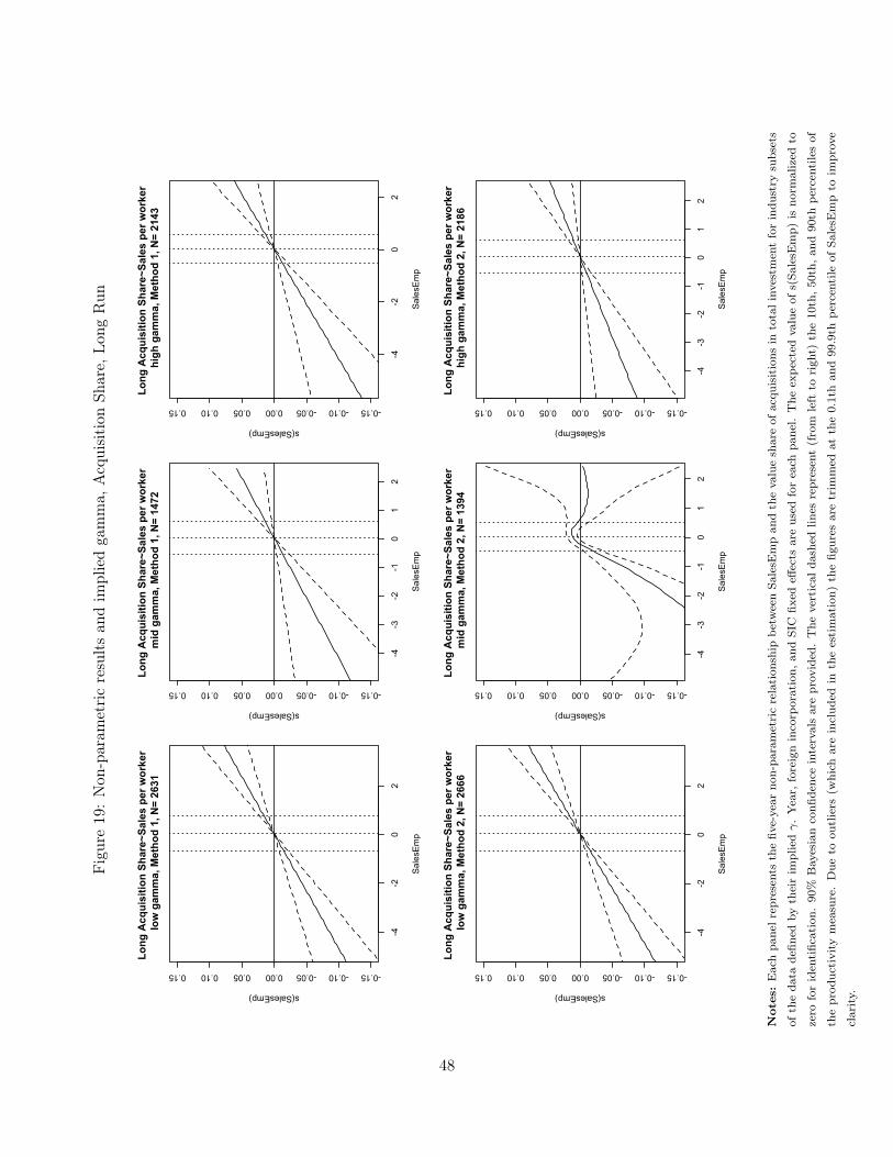
Figure19

:Non

-param

etricresultsan

dim

pliedga

mma,

Acquisition

Share,

Long

Run

-4-2

02

-0.15-0.10-0.050.000.050.100.15

SalesEmp

s(SalesEmp)

Long

Acq

uisi

tion

Shar

e~Sa

les

per w

orke

r lo

w g

amm

a, M

etho

d 1,

N=

2631

-4-3

-2-1

01

2

-0.15-0.10-0.050.000.050.100.15

SalesEmp

s(SalesEmp)

Long

Acq

uisi

tion

Shar

e~Sa

les

per w

orke

r m

id g

amm

a, M

etho

d 1,

N=

1472

-4-2

02

-0.15-0.10-0.050.000.050.100.15

SalesEmp

s(SalesEmp)

Long

Acq

uisi

tion

Shar

e~Sa

les

per w

orke

r h

igh

gam

ma,

Met

hod

1, N

= 21

43

-4-2

02

-0.15-0.10-0.050.000.050.100.15

SalesEmp

s(SalesEmp)

Long

Acq

uisi

tion

Shar

e~Sa

les

per w

orke

r lo

w g

amm

a, M

etho

d 2,

N=

2666

-4-3

-2-1

01

2

-0.15-0.10-0.050.000.050.100.15

SalesEmp

s(SalesEmp)Lo

ng A

cqui

sitio

n Sh

are~

Sale

s pe

r wor

ker

mid

gam

ma,

Met

hod

2, N

= 13

94

-4-3

-2-1

01

2

-0.15-0.10-0.050.000.050.100.15

SalesEmp

s(SalesEmp)

Long

Acq

uisi

tion

Shar

e~Sa

les

per w

orke

r h

igh

gam

ma,

Met

hod

2, N

= 21

86

Not

es:Eachpa

nelrepresentsthefiv

e-year

non-pa

rametricrelation

ship

betw

eenSa

lesE

mpan

dthevalueshareof

acqu

isitions

intotalinv

estm

entforindu

stry

subsets

oftheda

tadefin

edby

theirim

pliedγ.Year,foreignincorporation,

andSIC

fixed

effects

areused

foreach

panel.The

expe

cted

valueof

s(Sa

lesE

mp)

isno

rmalized

to

zero

foridentification.

90%

Bayesianconfi

denceintervalsareprovided.The

vertical

dashed

lines

represent(from

left

torigh

t)the10th,50th,an

d90th

percentilesof

theprod

uctivity

measure.Due

toou

tliers

(which

areinclud

edin

theestimation)

thefig

ures

aretrim

med

atthe0.1than

d99.9th

percentile

ofSa

lesE

mpto

improve

clarity.

48