Finite Euclidean and Non-Euclidean Geometries R. De Vogelaere 1 1 Department of Mathematics University of California, Berkeley, CA arXiv:1909.02673v1 [math.MG] 5 Sep 2019

Welcome message from author
This document is posted to help you gain knowledge. Please leave a comment to let me know what you think about it! Share it to your friends and learn new things together.
Transcript
Finite Euclidean and Non-Euclidean Geometries
R. De Vogelaere1
1Department of Mathematics
University of California, Berkeley, CA
arX
iv:1
909.
0267
3v1
[m
ath.
MG
] 5
Sep
201
9

2
Foreword
The author of this monograph was my father, Professor Rene De Vogelaere. He receivedhis PhD in Mathematics in 1948 from the University Louvain, Belgium. Shortly after grad-uation, he immigrated to Canada and taught at l’Universite Laval in Quebec, followed byNotre Dame in South Bend, Indiana and then the University of California, Berkeley, wherehe spent most of his career. He studied and taught a wide range of subjects, including differ-ential equations, numerical analysis, number theory, group theory, and Euclidean geometry,to mention a few.
Georges Lemaıtre, the founder of the “Big Bang” theory, was my father’s thesis advisorand lifelong mentor. He was often a guest in our home, and at these meetings he encouragedmy father to study astronomy and planetary motion. After earning his doctorate degree,Professor Lemaıtre spent a year working with Arthur Eddington. Professor Eddington postu-lated that there were a finite number of protons in the universe. This is known as Eddington’snumber.
Rene spent much of his career modeling the continuous world with discrete, finite num-bers. In the late 70’s he asked himself: what if the world was discrete rather than continuous?Would the proofs found in different mathematical branches still work? That is when his re-search in finite geometry began, culminating in this monograph, to which he dedicated thelast 10 years of his life. In my family, I was the only one who had studied math at thegraduate level, and so I was uniquely qualified to share in the excitement of his discoveriesand the number of theorems he was able to prove. He was like an archeologist having founda new field of dinosaur bones—discovering something new, then examining and documentingit. He taught classes on his findings, and wrote many papers (see the bibliography). He didnot publish his book; there were too many exciting theorems to prove, which were muchmore interesting to him than working with a publisher.
Upon his passing in 1991, I inherited his unfinished book. I worked with a good friendand past classmate, Michael Thwaites, to try to compile the book written in LaTeX. But lifewas busy with family and work. It wasn’t easy stepping into my father’s shoes to completethis very involved task. Throughout the following 25 years, I looked for a way to preservethe book and disseminate its knowledge. Eventually technology and the right person cametogether. One late evening I was discussing my father’s Finite Geometry book with WilliamGilpin. He has just completed his PhD in Physics from Stanford University. He knew LaTeXvery well, and was able to assemble all the files. He also knew of the Cornell’s arXiv andrecommended posting it there. It is the perfect place to store Professor De Vogelaere’smagnum opus.
I would like to thank:
- My mother, Elisabeth De Vogelaere, who made it possible for my father to dedicatehis career to mathematics, which he loved
- Arthur Eddington, for inspiring my father

3
- Georges Lemaıtre, for inspiring and teaching my father
- The University of California, Berkeley, for providing the facilities and allowing himtime to do his research, as well as for archiving the work he did over the 43 years ofhis career.
- Michael Thwaites, for helping me get started on the book, and for encouraging me tocontinue the work
- My wife Cynthia Haines, for carefully keeping and storing the computer disks, files andpapers all these years
- My daughter Beth, for finding William Gilpin
- William Gilpin, for his extreme generosity of time to rapidly assemble the book andfor facilitating having it stored at Cornell’s arXiv.
- My siblings, Helene, Andrew, and Gabrielle for their patience and faith that this wouldhappen!
- And Cornell’s arXiv, for being there to disseminate knowledge.
Charles De VogelaereMountain View, CA
August 2019

4

Contents
0 Preface 15
1 MAIN HISTORICAL DEVELOPMENTS 251.0 Introduction. . . . . . . . . . . . . . . . . . . . . . . . . . . . . . . . . . . . 251.1 Before Euclid. . . . . . . . . . . . . . . . . . . . . . . . . . . . . . . . . . . . 26
1.1.1 The Babylonians and Plimpton 322. . . . . . . . . . . . . . . . . . . . 261.1.2 The Pythagorean school. . . . . . . . . . . . . . . . . . . . . . . . . . 27
1.2 Euclidean Geometry. . . . . . . . . . . . . . . . . . . . . . . . . . . . . . . . 281.2.1 Euclid.(3-th Century B.C.) . . . . . . . . . . . . . . . . . . . . . . . . 281.2.2 Menelaus (about 100 A.D) and Ceva (1647-1734?). . . . . . . . . . . 331.2.3 Euler (1707-1783) and Feuerbach (1800-1834). . . . . . . . . . . . . . 341.2.4 The Geometry of the Triangle. Lemoine (1840-1912). . . . . . . . . . 35
1.2 Projective Geometry. . . . . . . . . . . . . . . . . . . . . . . . . . . . . . . . 361.2.1 The preparation. Menaechmus (about 340 B.C.), Apollonius (260?
B.C - 200? B.C.), Pappus (300 - ?). . . . . . . . . . . . . . . . . . . . 361.2.2 Gerard Desargues (1593-1661) and Blaise Pascal (1623-1662). . . . . 371.2.3 Lazare Carnot (1783-1823). . . . . . . . . . . . . . . . . . . . . . . . 381.2.4 Jean Poncelet (1788-1867). . . . . . . . . . . . . . . . . . . . . . . . . 381.2.5 Joseph Gergonne (1771-1858). . . . . . . . . . . . . . . . . . . . . . . 391.2.6 Michel Chasles (1793-1880). . . . . . . . . . . . . . . . . . . . . . . . 39
1.3 Relation between Projective and Euclidean Geometry. . . . . . . . . . . . . . 391.3.0 Introduction. . . . . . . . . . . . . . . . . . . . . . . . . . . . . . . . 391.3.1 Affine Geometry. . . . . . . . . . . . . . . . . . . . . . . . . . . . . . 401.3.2 Involutive geometry. . . . . . . . . . . . . . . . . . . . . . . . . . . . 41
1.4 Analytic Geometry. . . . . . . . . . . . . . . . . . . . . . . . . . . . . . . . . 431.4.1 Rene Descartes (1596-1650)[La Geometrie]. . . . . . . . . . . . . . . . 431.4.2 After Descartes. . . . . . . . . . . . . . . . . . . . . . . . . . . . . . . 441.4.3 Jean Poncelet (1788-1867). . . . . . . . . . . . . . . . . . . . . . . . . 451.4.4 James Singer on Difference sets and finite projective Geometry. . . . 46
1.5 Trigonometry and Spherical Trigonometry. . . . . . . . . . . . . . . . . . . . 501.5.1 Aryabatha I (476-?). . . . . . . . . . . . . . . . . . . . . . . . . . . . 501.5.2 Jean Henri Lambert (1728-1777). . . . . . . . . . . . . . . . . . . . . 511.5.3 Menelaus of Alexandria (about 100 A. D.) . . . . . . . . . . . . . . . 511.5.4 al-Battani, or Albategnius (850?-929?). . . . . . . . . . . . . . . . . . 52
1.6 Algebra, Modular Arithmetic. . . . . . . . . . . . . . . . . . . . . . . . . . . 61
5

6 CONTENTS
1.6.0 Introduction. . . . . . . . . . . . . . . . . . . . . . . . . . . . . . . . 611.6.1 The integers. . . . . . . . . . . . . . . . . . . . . . . . . . . . . . . . 611.6.2 The integers modulo p. . . . . . . . . . . . . . . . . . . . . . . . . . . 611.6.3 Quadratic Residues and Primitive Roots. . . . . . . . . . . . . . . . . 651.6.4 Non Linear Diophantine Equations and Geometry. . . . . . . . . . . . 671.6.5 Farey sets and Partial Ordering. . . . . . . . . . . . . . . . . . . . . . 681.6.6 Complex and quaternion integers. . . . . . . . . . . . . . . . . . . . . 741.6.7 Loops. . . . . . . . . . . . . . . . . . . . . . . . . . . . . . . . . . . . 751.6.8 Groups. . . . . . . . . . . . . . . . . . . . . . . . . . . . . . . . . . . 761.6.9 Veblen-Wederburn system. . . . . . . . . . . . . . . . . . . . . . . . . 771.6.10 Ternary Rings. . . . . . . . . . . . . . . . . . . . . . . . . . . . . . . 791.6.11 Felix Klein (1849-1925). Transformation groups. . . . . . . . . . . . . 801.6.12 Functions. . . . . . . . . . . . . . . . . . . . . . . . . . . . . . . . . . 801.6.13 Cyclotomic polynomials. Constructibility with ruler and compass. . . 81
1.7 The real numbers. . . . . . . . . . . . . . . . . . . . . . . . . . . . . . . . . . 811.7.1 The arithmetization of analysis. [Karl Weierstrass (1815-1897) and
Riemann (1826-1866)] . . . . . . . . . . . . . . . . . . . . . . . . . . 811.7.2 Algebraic and transcendental numbers. [Hermite (1822-1901) and Lin-
demann (1852-1939)] . . . . . . . . . . . . . . . . . . . . . . . . . . . 821.8 The pendulum and the elliptic functions. . . . . . . . . . . . . . . . . . . . . 82
1.8.0 Introduction. . . . . . . . . . . . . . . . . . . . . . . . . . . . . . . . 821.8.1 The pendulum. . . . . . . . . . . . . . . . . . . . . . . . . . . . . . . 831.8.2 The elliptic integral and the arithmetico-geometric mean. . . . . . . . 871.8.3 The elliptic functions of Jacobi. . . . . . . . . . . . . . . . . . . . . . 891.8.4 The theta functions of Jacobi. . . . . . . . . . . . . . . . . . . . . . . 911.8.5 Spherical trigonometry and elliptic functions. . . . . . . . . . . . . . 921.8.6 The p function of Weierstrass. . . . . . . . . . . . . . . . . . . . . . . 931.8.7 References. . . . . . . . . . . . . . . . . . . . . . . . . . . . . . . . . 931.8.8 Texts on and tables of elliptic Functions. . . . . . . . . . . . . . . . . 94
1.9 Model of Finite Euclidean Geometry in Classical Euclidean Geometry. . . . . 951.9.0 Introduction. . . . . . . . . . . . . . . . . . . . . . . . . . . . . . . . 951.9.1 Points and lines in finite Euclidean geometry. . . . . . . . . . . . . . 961.9.2 Parallels, parallelograms, distance. . . . . . . . . . . . . . . . . . . . 1041.9.3 Perpendicularity. . . . . . . . . . . . . . . . . . . . . . . . . . . . . . 1061.9.4 Circles, tangents and diameters. . . . . . . . . . . . . . . . . . . . . . 1081.9.5 The ideal line, the isotropic points and the isotropic lines. . . . . . . 1151.9.6 Equality of angles and measure of angles. . . . . . . . . . . . . . . . . 1181.9.7 Finite trigonometry. . . . . . . . . . . . . . . . . . . . . . . . . . . . 123
1.10 Axiomatic . . . . . . . . . . . . . . . . . . . . . . . . . . . . . . . . . . . . . 1251.10.0 Introduction to Axiomatic. . . . . . . . . . . . . . . . . . . . . . . . . 1251.10.1 The Perspective Plane. . . . . . . . . . . . . . . . . . . . . . . . . . . 1261.10.2 Veblen-Wedderburn Planes. . . . . . . . . . . . . . . . . . . . . . . . 1331.10.3 Moufang Planes. . . . . . . . . . . . . . . . . . . . . . . . . . . . . . 1361.10.4 Desarguesian Planes. . . . . . . . . . . . . . . . . . . . . . . . . . . . 1391.10.5 Pappian planes. . . . . . . . . . . . . . . . . . . . . . . . . . . . . . . 140

CONTENTS 7
1.10.6 Separable Pappian Planes. . . . . . . . . . . . . . . . . . . . . . . . . 1411.10.7 Continuous Pappian or Classical Projective Planes. . . . . . . . . . . 1441.10.8 Isomorphisms of Synthetically and Algebraically defined Planes. . . . 1441.10.9 Examples of Perspective Planes. . . . . . . . . . . . . . . . . . . . . . 1451.10.10 Collineations and Correlations in Perspective to Pappian Planes. . . . 1471.10.11 Three Nets in Perspective Geometry. . . . . . . . . . . . . . . . . . . 1481.10.12 Bibliography. . . . . . . . . . . . . . . . . . . . . . . . . . . . . . . . 150
1.11 Mechanics. . . . . . . . . . . . . . . . . . . . . . . . . . . . . . . . . . . . . . 1521.11.0 Introduction. . . . . . . . . . . . . . . . . . . . . . . . . . . . . . . . 1521.11.1 Kepler (1571-1630). . . . . . . . . . . . . . . . . . . . . . . . . . . . . 1521.11.2 Newton (1642-1727). . . . . . . . . . . . . . . . . . . . . . . . . . . . 1531.11.3 Hamilton (1805-1865). . . . . . . . . . . . . . . . . . . . . . . . . . . 1531.11.4 Preliminary remarks extending mechanics to finite geometry. . . . . . 1561.11.5 Eddington (18?-1944). The cosmological constant. . . . . . . . . . . . 157
1.12 Description of Algorithms and Computers. . . . . . . . . . . . . . . . . . . . 1581.13 Notes. . . . . . . . . . . . . . . . . . . . . . . . . . . . . . . . . . . . . . . . 159
1.13.1 On Babylonian Mathematics. . . . . . . . . . . . . . . . . . . . . . . 1591.13.2 On Plimpton 322, Pythagorean numbers in Babylonean Mathematics. 159
1.90 Answers to problems and miscellaneous notes. . . . . . . . . . . . . . . . . . 1621.90.1 Algebra and modular arithmetic. . . . . . . . . . . . . . . . . . . . . 1621.90.2 Linear Associative Planes. . . . . . . . . . . . . . . . . . . . . . . . . 1621.90.3 Veblen-Wedderburn Planes. . . . . . . . . . . . . . . . . . . . . . . . 163
2 FINITE PROJECTIVE GEOMETRY 1652.0 Introduction. . . . . . . . . . . . . . . . . . . . . . . . . . . . . . . . . . . . 1652.1 Synthetic Finite Projective Geometry. . . . . . . . . . . . . . . . . . . . . . . 165
2.1.0 Introduction. . . . . . . . . . . . . . . . . . . . . . . . . . . . . . . . 1652.1.1 Notation. . . . . . . . . . . . . . . . . . . . . . . . . . . . . . . . . . 1652.1.2 Axioms. . . . . . . . . . . . . . . . . . . . . . . . . . . . . . . . . . . 1662.1.3 Axiom (the finite field). . . . . . . . . . . . . . . . . . . . . . . . . . 1672.1.4 Basic consequences. . . . . . . . . . . . . . . . . . . . . . . . . . . . . 1672.1.5 The Theorem of Desargues. . . . . . . . . . . . . . . . . . . . . . . . 1682.1.6 Configurations. . . . . . . . . . . . . . . . . . . . . . . . . . . . . . . 1692.1.7 Other Configurations. . . . . . . . . . . . . . . . . . . . . . . . . . . 1732.1.8 Proof of the Theorem of Desargues. The hexagon of Pappus-Brianchon.
The configuration of Reidemeister. . . . . . . . . . . . . . . . . . . . 1782.1.9 The extended Pappus configuration and a remarkable Theorem. . . . 1822.1.10 Duality. . . . . . . . . . . . . . . . . . . . . . . . . . . . . . . . . . . 1872.1.11 Complete quadrangles and homologic quadrangles. . . . . . . . . . . 1872.1.12 Collineation and Correlation. . . . . . . . . . . . . . . . . . . . . . . 1892.1.13 Finite projective planes for small p. . . . . . . . . . . . . . . . . . . . 1902.1.90 Answer to exercises. . . . . . . . . . . . . . . . . . . . . . . . . . . . 1952.1.91 Relation between Synthetic and Algebraic Finite Projective Geometry. 197
2.2 Algebraic Model of Finite Projective Geometry. . . . . . . . . . . . . . . . . 1982.2.0 Introduction. . . . . . . . . . . . . . . . . . . . . . . . . . . . . . . . 198

8 CONTENTS
2.2.1 Representation of points, lines and incidence. . . . . . . . . . . . . . 1992.2.2 Line through 2 points and point through 2 lines. . . . . . . . . . . . . 2002.2.3 The model satisfies the axioms of the projective Pappus plane of order
p. . . . . . . . . . . . . . . . . . . . . . . . . . . . . . . . . . . . . . . 2012.2.4 Finite vector calculus and simple applications. . . . . . . . . . . . . . 2042.2.5 Anharmonic ratio, harmonic quatern, equiharmonic quatern. . . . . . 2062.2.6 Projectivity of lines and involution on a line. . . . . . . . . . . . . . . 2112.2.7 Collineation, central collineation, homology and elation. . . . . . . . . 2152.2.8 Correlations, polarity. . . . . . . . . . . . . . . . . . . . . . . . . . . 2182.2.9 Conics. . . . . . . . . . . . . . . . . . . . . . . . . . . . . . . . . . . . 2202.2.10 The general conic. . . . . . . . . . . . . . . . . . . . . . . . . . . . . 2242.2.11 The Theorem of Pascal and Brianchon. . . . . . . . . . . . . . . . . . 2262.2.12 The Theorems of Steiner, Kirkman, Cayley and Salmon. . . . . . . . 2312.2.13 Bezier Curves for drawing Conics, Cubics, . . . . . . . . . . . . . . . . . 2352.2.14 Projectivity determined by a conic. . . . . . . . . . . . . . . . . . . . 2392.2.15 Cubics. . . . . . . . . . . . . . . . . . . . . . . . . . . . . . . . . . . . 2402.2.16 Other models for projective geometry. . . . . . . . . . . . . . . . . . . 2412.2.17 Notes. . . . . . . . . . . . . . . . . . . . . . . . . . . . . . . . . . . . 243
2.3 Geometric Models on Regular Pythagorean Polyhedra. . . . . . . . . . . . . 2432.3.0 Introduction. . . . . . . . . . . . . . . . . . . . . . . . . . . . . . . . 2432.3.1 The selector. . . . . . . . . . . . . . . . . . . . . . . . . . . . . . . . 2442.3.2 The tetrahedron. . . . . . . . . . . . . . . . . . . . . . . . . . . . . . 2472.3.3 The cube. . . . . . . . . . . . . . . . . . . . . . . . . . . . . . . . . . 2482.3.4 The dodecahedron. . . . . . . . . . . . . . . . . . . . . . . . . . . . . 2502.3.5 Difference Sets with a Difference. . . . . . . . . . . . . . . . . . . . . 2522.3.6 Generalization of the Selector Function for higher dimension. . . . . . 2552.3.7 The conics on the dodecahedron. . . . . . . . . . . . . . . . . . . . . 2592.3.8 The truncated dodecahedron. . . . . . . . . . . . . . . . . . . . . . . 273
3 FINITE PRE INVOLUTIVE GEOMETRY 2913.1 An Overview of the Geometry of the Hexal Complete 5-Angles. . . . . . . . 291
3.1.0 Introduction. . . . . . . . . . . . . . . . . . . . . . . . . . . . . . . . 2913.1.1 Notation and application to the special configuration of Desargues and
to the pole and polar of with respect to a triangle. . . . . . . . . . . . 2923.1.2 An overview of theorems associated with equality of distances and
angles. The ideal line, the orthic line, the line of Euler, the circle ofBrianchon-Poncelet, the circumcircle, the point of Lemoine. . . . . . . 296
3.1.3 The fundamental 3 ∗ 4 + 11 ∗ 3 & 3 ∗ 5 + 10 ∗ 3 configuration. . . . . . 2993.1.4 An overview of theorems associated with bisected angles. The in-
scribed circle, the point of Gergonne, the point of Nagel. . . . . . . . 3003.2 The Geometry of the Hexal Complete 5-Angles. . . . . . . . . . . . . . . . . 303
3.2.0 Introduction. . . . . . . . . . . . . . . . . . . . . . . . . . . . . . . . 3033.2.1 The points of Euler, the center of the circle of Brianchon-Poncelet, and
of the circumcircle, the points of Schroter, the point of Gergonne ofthe orthic triangle, the orthocentroidal circle. . . . . . . . . . . . . . 304

CONTENTS 9
3.2.2 Isotropic points and foci of conics. . . . . . . . . . . . . . . . . . . . . 3053.2.3 Perpendicular directions. . . . . . . . . . . . . . . . . . . . . . . . . . 3053.2.4 The circle of Taylor, the associated circles, the circle of Brocard the
points of Tarry and Steiner, the conics of Simson and of Kiepert, theassociated circumcircles, the circles of Lemoine. . . . . . . . . . . . . 306
3.2.5 Theorems associated with bisected angles. The outscribed circles, thecircles of Spieker, the point of Feuerbach, the barycenter of the ex-cribed triangle. . . . . . . . . . . . . . . . . . . . . . . . . . . . . . . 308
3.2.6 Duality and symmetry for the inscribed circle. . . . . . . . . . . . . . 3133.2.7 Summary of the incidence properties obtained so far . . . . . . . . . 3143.2.8 The harmonic polygons. [Casey] . . . . . . . . . . . . . . . . . . . . . 3193.2.9 Cubics. . . . . . . . . . . . . . . . . . . . . . . . . . . . . . . . . . . . 3223.2.10 The cubics of Grassmann. . . . . . . . . . . . . . . . . . . . . . . . . 3273.2.11 Grassmannian cubics in Involutive Geometry. . . . . . . . . . . . . . 3333.2.12 Answer to . . . . . . . . . . . . . . . . . . . . . . . . . . . . . . . . . 3413.2.13 The cubics of Tucker. . . . . . . . . . . . . . . . . . . . . . . . . . . . 3423.2.14 NOTES . . . . . . . . . . . . . . . . . . . . . . . . . . . . . . . . . . 3453.2.15 The cubic of 17 points. . . . . . . . . . . . . . . . . . . . . . . . . . . 3483.2.16 The cubic of 21 points. . . . . . . . . . . . . . . . . . . . . . . . . . . 3513.2.17 The Barbilian Cubics. . . . . . . . . . . . . . . . . . . . . . . . . . . 351
3.3 Finite Projective Geometry. . . . . . . . . . . . . . . . . . . . . . . . . . . . 3573.3.0 Introduction. . . . . . . . . . . . . . . . . . . . . . . . . . . . . . . . 357
3.4 Finite Involutive Geometry. . . . . . . . . . . . . . . . . . . . . . . . . . . . 3583.4.0 Introduction. . . . . . . . . . . . . . . . . . . . . . . . . . . . . . . . 3583.4.1 Fundamental involution, perpendicularity, circles. . . . . . . . . . . . 3593.4.2 Altitudes and orthocenter. . . . . . . . . . . . . . . . . . . . . . . . . 3613.4.3 The geometry of the triangle, I. . . . . . . . . . . . . . . . . . . . . . 3613.4.4 The geometry of the triangle. II. . . . . . . . . . . . . . . . . . . . . 3683.4.5 Geometry of the triangle. III. . . . . . . . . . . . . . . . . . . . . . . 3703.4.6 Geometry of the triangle. IV. . . . . . . . . . . . . . . . . . . . . . . 3703.4.7 Geometry of the triangle. V. . . . . . . . . . . . . . . . . . . . . . . . 3713.4.8 Sympathic projectivities. . . . . . . . . . . . . . . . . . . . . . . . . . 3733.4.9 Equiangularity. . . . . . . . . . . . . . . . . . . . . . . . . . . . . . . 3743.4.10 Equidistance, congruence. . . . . . . . . . . . . . . . . . . . . . . . . 3763.4.11 Special triangles. . . . . . . . . . . . . . . . . . . . . . . . . . . . . . 3773.4.12 Other special triangles. . . . . . . . . . . . . . . . . . . . . . . . . . . 3803.4.13 Geometry of the triangle. V. . . . . . . . . . . . . . . . . . . . . . . . 381
3.90 Answers to problems and miscellaneous notes. . . . . . . . . . . . . . . . . . 3813.90.1 Answer to exercises. . . . . . . . . . . . . . . . . . . . . . . . . . . . 382
4 FINITE INVOLUTIVE SYMPATHIC AND GALILEAN GEOMETRY 3954.0 Introduction. . . . . . . . . . . . . . . . . . . . . . . . . . . . . . . . . . . . 3954.1 Finite involutive geometry. . . . . . . . . . . . . . . . . . . . . . . . . . . . . 396
4.1.9 Theorems in finite involutive Geometry, which do not correspond toknown theorems in Euclidean Geometry. . . . . . . . . . . . . . . . . 396

10 CONTENTS
4.1.10 The geometry of the triangle of degree 2. . . . . . . . . . . . . . . . . 3964.1.11 Some theorems involving circles. . . . . . . . . . . . . . . . . . . . . . 3964.1.12 The parabola, ellipse and hyperbola. . . . . . . . . . . . . . . . . . . 3974.1.13 Cartesian coordinates in involutive Geometry. . . . . . . . . . . . . . 3994.1.14 Correspondence between circles in finite and classical Euclidean geom-
etry. . . . . . . . . . . . . . . . . . . . . . . . . . . . . . . . . . . . . 4024.1.15 Answers to problems. . . . . . . . . . . . . . . . . . . . . . . . . . . . 4044.1.9 The conic of Kiepert. . . . . . . . . . . . . . . . . . . . . . . . . . . . 4074.1.10 The Theorem of Vectem and related results. . . . . . . . . . . . . . . 4124.1.11 Representation of involutive geometry on the dodecahedron. . . . . . 417
4.2 Finite Sympathic Geometry. . . . . . . . . . . . . . . . . . . . . . . . . . . . 4194.2.0 Introduction. . . . . . . . . . . . . . . . . . . . . . . . . . . . . . . . 4194.2.1 Trigonometry in a Finite Field for p. The Hyperbolic Case. . . . . . . 4194.2.2 Trigonometry in a Finite Field for q = pe. The Hyperbolic Case. . . . 4224.2.1 Trigonometry in a Finite Field for p. The Hyperbolic Case. . . . . . . 4254.2.2 Trigonometry in a Finite Field for q = pe. The Hyperbolic Case. . . . 4284.2.3 Trigonometry in a Finite Field for q = pe. The Elliptic Case. . . . . . 4304.2.4 Periodicity. . . . . . . . . . . . . . . . . . . . . . . . . . . . . . . . . 4404.2.5 Orthogonality. . . . . . . . . . . . . . . . . . . . . . . . . . . . . . . . 4414.2.6 Conics in sympathic geometry. . . . . . . . . . . . . . . . . . . . . . . 4424.2.7 Regular polygons and Constructibility. . . . . . . . . . . . . . . . . . 4434.2.8 Constructibility of the second degree. . . . . . . . . . . . . . . . . . . 445
4.4 Contrast with classical Euclidean Geometry. . . . . . . . . . . . . . . . . . . 4454.4.0 Introduction. . . . . . . . . . . . . . . . . . . . . . . . . . . . . . . . 445
4.3 Parabolic-Euclidean or Cartesian Geometry. . . . . . . . . . . . . . . . . . . 4464.3.0 Introduction. . . . . . . . . . . . . . . . . . . . . . . . . . . . . . . . 4464.3.1 Fundamental Definitions. . . . . . . . . . . . . . . . . . . . . . . . . . 4474.3.2 The Geometry of the Triangle in Galilean Geometry. . . . . . . . . . 4494.3.3 The symmetric functions. . . . . . . . . . . . . . . . . . . . . . . . . 451
4.5 Transformation associated to the Cartesian geometry. . . . . . . . . . . . . . 4524.5.0 Introduction. . . . . . . . . . . . . . . . . . . . . . . . . . . . . . . . 4524.5.1 The geometry of the triangle, the standard form. . . . . . . . . . . . 4534.5.2 The cubic γ a of Gabrielle. . . . . . . . . . . . . . . . . . . . . . . . . 457
4.6 Problems . . . . . . . . . . . . . . . . . . . . . . . . . . . . . . . . . . . . . . 4634.6.1 Problems for Affine Geometry. . . . . . . . . . . . . . . . . . . . . . . 4644.6.2 Problems for Involutive Geometry. . . . . . . . . . . . . . . . . . . . 464
4.90 Answers to problems and miscellaneous notes. . . . . . . . . . . . . . . . . . 465
5 FINITE NON-EUCLIDEAN GEOMETRY 4795.0 Introduction. . . . . . . . . . . . . . . . . . . . . . . . . . . . . . . . . . . . 4795.1 Finite Polar geometry. . . . . . . . . . . . . . . . . . . . . . . . . . . . . . . 480
5.1.0 Introduction. . . . . . . . . . . . . . . . . . . . . . . . . . . . . . . . 4805.1.1 The ideal conic, elliptic, parabolic and hyperbolic points and lines. . . 4805.1.2 Circles in finite polar geometry. . . . . . . . . . . . . . . . . . . . . . 4835.1.3 Perpendicularity. . . . . . . . . . . . . . . . . . . . . . . . . . . . . . 485

CONTENTS 11
5.1.4 Special triangles. . . . . . . . . . . . . . . . . . . . . . . . . . . . . . 4865.1.5 Mid-points, medians, mediatrices, circumcircles. . . . . . . . . . . . . 4885.1.6 The center V of a triangle. . . . . . . . . . . . . . . . . . . . . . . . . 4905.1.7 An alternate definition of the center V of a triangle. . . . . . . . . . . 4925.1.8 Intersections of the 4 circumcircles. . . . . . . . . . . . . . . . . . . . 4945.1.9 Other results in the geometry of the triangle. . . . . . . . . . . . . . . 4975.1.10 Circumcircle of a triangle with at least one ideal vertex. . . . . . . . . 4995.1.11 The parabola in polar geometry. . . . . . . . . . . . . . . . . . . . . . 5005.1.12 Representation of polar geometry on the dodecahedron. . . . . . . . . 504
5.2 Finite Non-Euclidean Geometry. . . . . . . . . . . . . . . . . . . . . . . . . . 5105.2.0 Introduction. . . . . . . . . . . . . . . . . . . . . . . . . . . . . . . . 5105.2.1 Trigonometry for the general triangle. . . . . . . . . . . . . . . . . . . 5105.2.2 Trigonometry for the right triangle. . . . . . . . . . . . . . . . . . . . 5135.2.3 Trigonometry for other triangles . . . . . . . . . . . . . . . . . . . . . 513
5.3 Tri-Geometry . . . . . . . . . . . . . . . . . . . . . . . . . . . . . . . . . . . 5145.3.1 The primitive case. . . . . . . . . . . . . . . . . . . . . . . . . . . . . 5145.3.2 The case of 1 root. Inverse geometry. . . . . . . . . . . . . . . . . . . 5205.3.4 The case of a double root and a single root. . . . . . . . . . . . . . . 5245.3.5 The case of a triple root. Solar geometry. . . . . . . . . . . . . . . . . 5265.3.6 The case of 3 distinct roots. . . . . . . . . . . . . . . . . . . . . . . . 5285.3.7 Conjecture. . . . . . . . . . . . . . . . . . . . . . . . . . . . . . . . . 5305.3.8 Notes. . . . . . . . . . . . . . . . . . . . . . . . . . . . . . . . . . . . 5335.3.9 On the tetrahedron. . . . . . . . . . . . . . . . . . . . . . . . . . . . 535
6 GENERALIZATION TO 3 DIMENSIONS 5376.0 Introduction. . . . . . . . . . . . . . . . . . . . . . . . . . . . . . . . . . . . 537
6.0.1 Relevant historical background. . . . . . . . . . . . . . . . . . . . . . 5386.0.2 Grassmann algebra applied to incidence properties of points, lines and
planes . . . . . . . . . . . . . . . . . . . . . . . . . . . . . . . . . . . 5386.1 Affine Geometry in 3 Dimensions. . . . . . . . . . . . . . . . . . . . . . . . . 545
6.1.0 Introduction. . . . . . . . . . . . . . . . . . . . . . . . . . . . . . . . 5456.1.1 The ideal plane and parallelism. . . . . . . . . . . . . . . . . . . . . . 545
6.2 Polar Geometry in 3 Dimensions. . . . . . . . . . . . . . . . . . . . . . . . . 5476.2.0 Introduction. . . . . . . . . . . . . . . . . . . . . . . . . . . . . . . . 5476.2.1 The fundamental quadric, poles and polars. . . . . . . . . . . . . . . 5486.2.2 Orthogonality in space and the ideal polarity. . . . . . . . . . . . . . 5506.2.3 The general tetrahedron. . . . . . . . . . . . . . . . . . . . . . . . . . 5546.2.4 The orthogonal tetrahedron. . . . . . . . . . . . . . . . . . . . . . . . 5606.2.5 The isodynamic tetrahedron. . . . . . . . . . . . . . . . . . . . . . . . 5636.1.3 The orthogonal tetrahedron. . . . . . . . . . . . . . . . . . . . . . . . 5636.1.4 The isodynamic tetrahedron. . . . . . . . . . . . . . . . . . . . . . . . 5676.1.5 The antipolarity. . . . . . . . . . . . . . . . . . . . . . . . . . . . . . 5686.1.6 Example. . . . . . . . . . . . . . . . . . . . . . . . . . . . . . . . . . 573
6.90 Answers to problems and miscellaneous notes. . . . . . . . . . . . . . . . . . 580

12 CONTENTS
7 QUATERNIONIAN GEOMETRY 5837.0 Introduction. . . . . . . . . . . . . . . . . . . . . . . . . . . . . . . . . . . . 5837.1 Quaternionian Geometry over the reals. . . . . . . . . . . . . . . . . . . . . . 584
7.1.1 Points, Lines and Polarity. . . . . . . . . . . . . . . . . . . . . . . . . 5847.1.2 Quaternionian Geometry of the Hexal Complete 5-Angles. . . . . . . 589
7.2 Finite Quaternionian Geometry. . . . . . . . . . . . . . . . . . . . . . . . . . 5957.2.1 Finite Quaternions. . . . . . . . . . . . . . . . . . . . . . . . . . . . . 5957.2.2 Example in a finite quaternionian geometry. . . . . . . . . . . . . . . 596
7.3 Miniquaternionian Plane Ψ of Veblen-Wedderburn. . . . . . . . . . . . . . . 5987.3.0 Introduction. . . . . . . . . . . . . . . . . . . . . . . . . . . . . . . . 5987.3.1 Miniquaternion near-field. . . . . . . . . . . . . . . . . . . . . . . . . 5987.3.2 The miniquaternionian plane Ψ. . . . . . . . . . . . . . . . . . . . . . 600
7.4 Axiomatic. . . . . . . . . . . . . . . . . . . . . . . . . . . . . . . . . . . . . . 6077.4.1 Veblen-MacLagan planes. . . . . . . . . . . . . . . . . . . . . . . . . 6077.4.2 Examples of Perspective planes. . . . . . . . . . . . . . . . . . . . . . 608
7.5 Desarguesian Geometry. . . . . . . . . . . . . . . . . . . . . . . . . . . . . . 6107.5.1 Desarguesian Geometry of the Hexal Complete 5-Angles. . . . . . . . 6117.5.2 Perpendicularity mapping. . . . . . . . . . . . . . . . . . . . . . . . . 615
7.6 The Hughes Planes. . . . . . . . . . . . . . . . . . . . . . . . . . . . . . . . . 6167.6.0 Introduction. . . . . . . . . . . . . . . . . . . . . . . . . . . . . . . . 6167.6.1 Nearfield and coordinatization of the plane. . . . . . . . . . . . . . . 6167.6.2 Miniquaternion nearfield. . . . . . . . . . . . . . . . . . . . . . . . . . 6187.6.3 The first non-Pappian plane, by Veblen and Wedderburn. . . . . . . . 6207.6.4 The miniquaternionian plane Ψ. . . . . . . . . . . . . . . . . . . . . . 621
7.7 Axiomatic. . . . . . . . . . . . . . . . . . . . . . . . . . . . . . . . . . . . . . 6277.7.1 Veblen-MacLagan planes. . . . . . . . . . . . . . . . . . . . . . . . . 6277.7.2 Examples of Perspective planes. . . . . . . . . . . . . . . . . . . . . . 628
7.8 Bibliography. . . . . . . . . . . . . . . . . . . . . . . . . . . . . . . . . . . . 6287.90 Answer to problems and Comments. . . . . . . . . . . . . . . . . . . . . . . 630
8 FUNCTIONS OVER FINITE FIELDS 6338.0 Introduction. . . . . . . . . . . . . . . . . . . . . . . . . . . . . . . . . . . . 6338.1 Polynomials over Finite Fields. . . . . . . . . . . . . . . . . . . . . . . . . . 633
8.1.1 Definition and basic properties. . . . . . . . . . . . . . . . . . . . . . 6338.1.2 Derivatives of polynomials. . . . . . . . . . . . . . . . . . . . . . . . . 634
8.2 Orthogonal Polynomials over Finite Fields. . . . . . . . . . . . . . . . . . . . 6348.2.0 Introduction. . . . . . . . . . . . . . . . . . . . . . . . . . . . . . . . 6348.2.1 Basic Definitions and Theorems. . . . . . . . . . . . . . . . . . . . . . 6348.2.2 Symmetry properties for the Polynomials of Chebyshev of the first and
second kind. . . . . . . . . . . . . . . . . . . . . . . . . . . . . . . . . 6368.2.3 Symmetry properties for the Polynomials of Legendre. . . . . . . . . 6378.2.4 Symmetry properties for the Polynomials of Laguerre. . . . . . . . . . 6398.2.5 Symmetry properties for the Polynomials of Hermite. . . . . . . . . . 640
8.3 Addition Formulas for Functions on a Finite Fields. . . . . . . . . . . . . . . 6428.3.0 Introduction. . . . . . . . . . . . . . . . . . . . . . . . . . . . . . . . 642

CONTENTS 13
8.3.1 The Theorem of Ungar. . . . . . . . . . . . . . . . . . . . . . . . . . 6428.3.2 The case of 3 functions. . . . . . . . . . . . . . . . . . . . . . . . . . 6438.3.3 The case of 4 Functions. . . . . . . . . . . . . . . . . . . . . . . . . . 6558.3.4 The case of 5 functions. . . . . . . . . . . . . . . . . . . . . . . . . . 657
8.4 Application to geometry. . . . . . . . . . . . . . . . . . . . . . . . . . . . . . 6588.4.0 Introduction. . . . . . . . . . . . . . . . . . . . . . . . . . . . . . . . 6588.4.1 k-Dimensional Affine Geometry. . . . . . . . . . . . . . . . . . . . . . 6588.4.2 Ricatti geometry. . . . . . . . . . . . . . . . . . . . . . . . . . . . . . 6678.4.3 3 - Dimensional Equidistance Curves. . . . . . . . . . . . . . . . . . . 6768.4.4 Generalization of the Selector Function. . . . . . . . . . . . . . . . . . 681
8.5 Generalization of the Spheres in Riccati Geometry. . . . . . . . . . . . . . . 6848.5.1 Dimension k. . . . . . . . . . . . . . . . . . . . . . . . . . . . . . . . 6848.5.2 Dimension 3. . . . . . . . . . . . . . . . . . . . . . . . . . . . . . . . 6858.5.3 Dimension 4. . . . . . . . . . . . . . . . . . . . . . . . . . . . . . . . 691
9 FINITE ELLIPTIC FUNCTIONS 6939.0 Introduction. . . . . . . . . . . . . . . . . . . . . . . . . . . . . . . . . . . . 6939.1 The Jacobi functions. . . . . . . . . . . . . . . . . . . . . . . . . . . . . . . . 693
9.1.1 Definitions and basic properties of the Jacobian elliptic group. . . . . 6939.1.2 Finite Jacobian elliptic groups for small p. . . . . . . . . . . . . . . . 6989.1.3 Finite Jacobian Elliptic Function. . . . . . . . . . . . . . . . . . . . . 7009.1.4 Identities and addition formulas for finite elliptic functions. . . . . . . 7019.1.5 Double and half arguments. . . . . . . . . . . . . . . . . . . . . . . . 7049.1.6 The Jacobi Zeta function. . . . . . . . . . . . . . . . . . . . . . . . . 7069.1.7 Example. . . . . . . . . . . . . . . . . . . . . . . . . . . . . . . . . . 7079.1.8 Other results. . . . . . . . . . . . . . . . . . . . . . . . . . . . . . . . 7099.1.9 Isomorphisms and homomorphisms. . . . . . . . . . . . . . . . . . . . 709
9.2 Applications. . . . . . . . . . . . . . . . . . . . . . . . . . . . . . . . . . . . 7129.2.1 The polygons of Poncelet. . . . . . . . . . . . . . . . . . . . . . . . . 712
9.3 The Weierestrass functions. . . . . . . . . . . . . . . . . . . . . . . . . . . . 7139.3.1 Complex elliptic functions. . . . . . . . . . . . . . . . . . . . . . . . . 7139.3.2 Weiertrass’ elliptic curves and the Weierstrass elliptic functions. . . . 7149.3.3 The isomorphism between the elliptic curves in 3 and 2 dimensions. . 7189.3.4 Correspondance between the Jacobi elliptic curve (cn, sd) and the
Weierstrass elliptic curve . . . . . . . . . . . . . . . . . . . . . . . . . 7219.4 Complete elliptic integrals of the first and second kind. . . . . . . . . . . . . 7239.5 P-adic functions, polynomials, orthogonal polynomials. . . . . . . . . . . . . 729
9.5.1 Trigonometric Functions. . . . . . . . . . . . . . . . . . . . . . . . . . 7339.5.2 Integration. . . . . . . . . . . . . . . . . . . . . . . . . . . . . . . . . 737
9.6 P-adic field. . . . . . . . . . . . . . . . . . . . . . . . . . . . . . . . . . . . . 7379.6.1 Generalities. . . . . . . . . . . . . . . . . . . . . . . . . . . . . . . . . 7379.6.2 Extension to the half argument. . . . . . . . . . . . . . . . . . . . . . 7439.6.3 The logarithm. . . . . . . . . . . . . . . . . . . . . . . . . . . . . . . 7459.6.4 P-adic Geometry and Related Finite Geometries. . . . . . . . . . . . 748

14 CONTENTS
10 DIFFERENTIAL EQUATIONS AND FINITE MECHANICS 75110.0 Introduction. . . . . . . . . . . . . . . . . . . . . . . . . . . . . . . . . . . . 75110.1 The first Examples of discrete motions. . . . . . . . . . . . . . . . . . . . . . 751
10.1.1 The harmonic polygonal motion. . . . . . . . . . . . . . . . . . . . . 75110.1.2 The Parabolic Motion. . . . . . . . . . . . . . . . . . . . . . . . . . . 75410.1.3 Attempts to Generalize Kepler’s Equation. . . . . . . . . . . . . . . . 75510.1.4 The circular motion. . . . . . . . . . . . . . . . . . . . . . . . . . . . 755
10.2 Approximation to the Solution of Differential Equations. . . . . . . . . . . . 75610.2.0 Introduction. . . . . . . . . . . . . . . . . . . . . . . . . . . . . . . . 75610.2.1 Some Algorithms. . . . . . . . . . . . . . . . . . . . . . . . . . . . . . 756
10.3 The Parabolic Motion. . . . . . . . . . . . . . . . . . . . . . . . . . . . . . . 75710.3.0 Introduction. . . . . . . . . . . . . . . . . . . . . . . . . . . . . . . . 757
10.4 Attempts to Generalize Kepler’s Equation. . . . . . . . . . . . . . . . . . . . 75810.4.1 The circular motion. . . . . . . . . . . . . . . . . . . . . . . . . . . . 758
10.5 Approximation to the Solution of Differential Equations. . . . . . . . . . . . 75910.5.1 On the existence of primitive roots. . . . . . . . . . . . . . . . . . . . 760
11 COMPUTER IMPLEMENTATION 76311.0 Introduction. . . . . . . . . . . . . . . . . . . . . . . . . . . . . . . . . . . . 763

Chapter 0
Preface
Purpose
The purpose of this book and of others that are in progress is to give an exposition ofGeometry from a point of view which in some sense complements Klein’s Erlangen program.The emphasis is on extending the classical Euclidean geometry to the finite case, but it goesway beyond that.
Plan
In this preface, after a brief introduction, which gives the main theme, and was presented insome details at the first Berkeley Logic Colloquium of Fall 1989, I present the main results,according to a synthetic view of the subject, rather that chronologically. First, some varia-tion on the axiomatic treatment of projective geometry, then new results on quaternioniangeometry, then results in geometry over the reals which are generalized over arbitrary fields,then those which depend on properties of finite fields, then results in finite mechanics. Therole of the computer, which was essential for these inquires is briefly surveyed. The method-ology to obtain illustrations by drawings is described. The interaction between Teaching andResearch is then given. I end with a table which enumerates enclosed additional materialwhich constitutes a small but representative part of what I have written.
Introduction
My inquiry started with rethinking Geometry, by examining first, what could be preservedamong the properties of Euclidean geometry when the field of reals is replaced by a finitefield. This led me to a separation of the notions concerned with the distance between 2 pointsand the angle between an ordered pair of lines, into two sets, those concerned with equalityand those concerned with measure. Properties relating to equality are valid for a Pappiangeometry, whatever the underlying field, those pertaining to measure require specifying thefield.I have also come to the conclusion that the more fruitful approach to the axiomatic of Eu-clidean geometry is to reduce it to that of Projective geometry followed by a preferenceof certain elements, namely the isotropic points on the ideal line. This preference can be
15

16 CHAPTER 0. PREFACE
presented alternately by choosing 2 points relatively to a triangle of coordinates, namelythe barycenter and the orthocenter. The barycenter is used to define the ideal line, theorthocenter is then used to define the fundamental involution of this line, for which theisotropic points are the (imaginary) fixed points. This program extends to all non-Euclideangeometries.The preference method, which I call the “Berkeley Program”, can be considered as the syn-thetic equivalent of the group theoretical relations between geometries, as advocated in FelixKlein’s Erlangen program.When I refer to Euclidean geometry, I always mean that the set of points and lines of thegeometry of Euclid have been completed by the ideal line and the ideal points on that line.
Axiomatic of projective geometry
Projective GeometryAxiomatic.The approach, used by Artzy, has the advantage of giving the equivalence between the syn-thetic axioms and the algebraic axioms, at each stage of the axiomatic development: forperspective planes, Veblen-Wedderburn planes, Moufang planes, Desarguesian planes, Pap-pian planes, ordered planes, and finally, projective planes. I have revised it, to give a uniformtreatment (particularly lacking at the intermediate step of the Veblen-Wedderburn plane, inwhich, for instance, vectors are introduced by Artzy and others, to prove commutativity ofaddition) and by giving, for all proofs, explicit, rather than implicit constructions, togetherwith drawings.Notation.The Theorems of Desargues, Pappus and Pascal play an important role in synthetic proofs inProjective geometry. A notation has been introduced for the repeated use of these theoremsand their converse, in an efficient and unambiguous way. A notation for configurations hasbeen introduced, which further helps in distinguishing non isomorphic configurations.
Desarguesian geometry
Quaternionian Geometry.With Relative Preference of 2 Points.A quaternionian plane is a well known, particularly important, example of a Desarguesianplane. I have introduced in it, the relative preference of 2 points, the barycenter and thecobarycenter and have obtained several Theorems, which in the sub-projective planes ofthe geometry correspond to Theorems in involutive geometry which are associated with thecircumcircle and with the point of Lemoine. But these Theorems cannot be consideredas simple generalizations. For instance, in the involution on the ideal line, defined by thecircumcircular polarity, which corresponds to a circumcircle, the direction of a side and that

17
of the comedian, which generalizes an altitude, are not corresponding elements, althoughthese correspond to each other, in the sub-projective planes. Moreover, what I call theLemoine polarity degenerates in the sub-projective planes into all the lines through the pointof Lemoine. The proofs given are all algebraic. These investigations are just the beginningof what should become a very rich field of inquiries.
Finite Quaternionian Geometry.The Theorems in quaternionian geometry were conjectured using a geometry whose pointsand lines are represented by 3 homogeneous coordinates in the ring of finite quaternions overZp. In the corresponding plane, the axioms of allignment are not allways satisfied. If theyare, Theorems and proofs for the quaternionian plane extend to the finite case.
Pappian geometry over arbitrary fields
Pappian Geometry.This can be considered as a projective geometry over an arbitrary field.On Steiner’s Theorem.Pappus’ Theorem is one of the fundamental axioms of Projective geometry. If the 3 pointson one of the lines are permuted, we obtain 6 Pappian lines which pass 3 by 3 through 2points, this is the Theorem of Jakob Steiner. By duality, we can obtain from these, 6 pointson 2 lines. That these 2 lines are the same as the original ones is a new Theorem. Detailedcomputer analysis of the mapping in special cases leads to conjectures in which twin primesappear to play a role.Generalization of Wu’s Theorem.I obtained some 80 new Theorems in Pappian geometry, generalizing a Theorem, in projectivegeometry, of Wen-Tsen Wu, related to conics through 6 Pascal points of 6 points on a conic,I have obtained a computer proof for all of these Theorems by means of a single program,which includes convincing checks, and then succeeded in obtaining a synthetic proof for eachof these Theorems, using several different patterns and approaches including duality andsymmetry. These proofs have benefited from the projective geometry notation. Drawingshave been made for a large number of these Theorems which have suggested 2 new Theoremsand a (solid) Conjecture. Many of the Theorems can be considered as Theorems in Euclideangeometry, (only one of which was known, the Theorem of Brianchon-Poncelet), others canbe considered as Theorems in Affine or in Galilean geometry.Generalization of Euclidean Theorems.The Theorems, given for involutive geometry, can be considered, alternately, as Theorems inPappian geometry, because they involve only the preference of 2 elements of the projectiveplane and not additional axioms.
Involutive Geometry.I call involutive plane, a Pappian plane in which I prefer 2 points relative to a triangle, M ,the barycenter and M , the orthocenter. M allows for the definition of the ideal line, Mallows, subsequently, for the definition of the fundamental involution on that line.Generalization of Theorems in Euclidean and Minkowskian Geometry over Arbitrary Fields.

18 CHAPTER 0. PREFACE
In this, which constitues the more extensive part of my research, I have generalized, whenthe involution is elliptic, a very large number of Theorems in Euclidean geometry, namelythose which are characterized by not using the measure of distance and of angles and notinvolving elements whose construction leads to more than one solution. When the funda-mental involution is hyperbolic, each of the Theorems gives a corresponding Theorem in thegeometry of Hermann Minkowski.Symmetry and Duality.The barycenter and orthocenter have a symmetric role for many Theorems of Euclideangeometry, the line of Euler and the circle of Brianchon-Poncelet being the simpler examples.This has been systematically exploited, to almost double the number of Theorems knownin that part of Euclidean geometry which involves congruence and not measure. Dualitycan also be extended to Euclidean geometry by associating to M and M , the ideal line andthe orthic line and vice-versa. This also has been systematically exploited to help me, inobtaining constructions of new elements, and should be helpful in future constructions.Notation.A set of notations was introduced, to allow for a compact description of some 1006 defini-tions, 1073 conclusions and for the corresponding proofs. The counts correspond to one formof counting, other forms give higher numbers. All these Theorems are valid for any Pappianplane and give directly both statement and new proofs in both Euclidean and Minkowskiangeometry.The Geometry of the Triangle.During the period 1870 to 1900, there was an explosion of results in what has been calledthe geometry of the triangle, prepared by Theorems due to Leonhard Euler, Jean Poncelet,Charles Brianchon, Emile Lemoine and others. The synthesis of the subject was never suc-cessfully accomplished, not only because of the wealth of Theorems, but because of thedifficulty of insuring that elements defined differently were in fact, in general, distinct. Theproofs, used in involutive geometry, not only throw a new light on the reason for the explo-sive number of results for the geometry of the triangle but also gives a exhaustive syntheticview of the subject.Diophantine Equations.Because an algebraic expression of the homogeneous coordinates of points and lines andthe coefficients for conics is given in terms of polynomials in 3 variables, a large number ofparticular results on diophantine equations in 3 variables are implicitly obtained in theseinvestigations.Construction with the Ruler only.In all of the classical investigations, the most extensive one being that of Henri Lebesgue,the impression is given that the compass is indispensable for most constructions in geometry.More than half of the Theorems for which a count is given above, can be characterized asusing the ruler only. Implicit, in this part of my Research, is, that many constructions, whichusually or by necessity were assumed to require the compass, in fact need the ruler only, thesimplest one is that for constructing the perpendicular to a line. The more remarkable oneis that the circles of Apollonius can be constructed with the ruler only. These are defined asthe circles which have as diameter the intersections of the bisectrices of an angle of a trianglewith the opposite sides. It is this reduction to construction with the ruler alone, which allowsfor the straigthforward proofs which constitutes a major success of these investigations.

19
Construction with the Ruler and Compass.The construction with compass can be envisioned as follows. Given M and M , by findingthe intersection of 2 circles centered at 2 of the vertices of a triangle with the adjacent sidesand by constructions with the ruler, we can construct the bissectrices of these angles, theincenter (center of the inscribed circle) and the point of Joseph Gergonne (the common inter-section of the lines through a vertex of the triangle and the point of tangency of the inscribedcircle with the opposite side). From these, a very large number of other points, lines andcircles can be constructed with the ruler only, for instance, the point of Karl Feuerbach, theexcribed circles and the circles of Spieker. One can therefore, in the framework of involutivegeomatry, prefer instead of M and M , the incenter I and the point of Gergonne J . Startingfrom I and J , we can construct M and M , using the ruler alone. This allows to extend theproof methodology considerably, allowing the generalization to arbitrary fields of Theoremsinvolving elements whose construction, in the classical case, would requires the compass.Cubics.Very little has been written on the construction of cubics by the ruler. Starting with thework of Herman Grassmann of R. Tucker and of Ian Barbilian, I have obtaining a few resultsin this direction, one of which, incidentally, gives a illustration of the procedure of construc-tion with the compass as I am envisioning it, which is much simpler than those involvingbissectrices.
Galilean geometry.When the fundamental involution is parabolic and when the field is the field of reals, thegeometry is called Galilean, because its group is the group of Galilean transformations ofclassical mechanics. Extending to the Pappian case and starting from the definitions andconclusions of involutive geometry, I have made appropriate modifications to obtain Theo-rems which are valid in Galilean geometry, but I have not yet completed the careful checkthat is required to insure the essential accuracy. Again a very large number of Theoremshave been obtained, which are new, even in the case of the field of reals.
Polar Geometry.The extension, to n dimensions, can be obtained using an appropriate adaptation of thealgebra of Herman Grassmann. A first set of Theorems has been obtained in the case of 3dimensions, again for a Pappian space over arbitrary fields, in which preference is given toone plane, the ideal plane and one quadric. These Theorems generalize Theorems on thetetrahedron due to E. Prouhet, Carmelo Intrigila and Joseph Neuberg. The special case ofthe orthogonal tetrahedron has also been studied in a way which puts in evidence the reasonsbehind many of the Theorems obtained in this case.
Non-Euclidean Geometry.The beginning of the preference approach to obtain new results in non-Euclidean geometrywas started in January 1982. The confluence, in the case of a finite field, of the geometries ofJanos Bolyai and of Nikolai Lobachevsky was then explored. A new point, called the centerof a triangle was discovered and its properties were proven.

20 CHAPTER 0. PREFACE
Pappian geometry over finite fields
The Case of Finite Fields.All the results given for involutive geometry and in the following sections are true, irrespectiveof fields. In what follows, we describe results for finite fields.
Projective Geometry.Representation on Pythagorean and Archimedean solids.Fernand Lemay has shown how to represent the projective planes corresponding to theGalois fields, 2, 3 and 5 respectively on the tetrahedron, the cube (or octahedron) and thedodecahedron (or icosahedron). I have shown, that if we choose instead of the Pythagoreansolids, the Archimedean ones, the results extend to 22 and the 5-gonal antiprism and to32 and the truncated dodecahedron. I have studied also the corresponding representationsof the conics on the dodecahedron. This is useful for the representation on it of the finitenon-Euclidean Geometry associated with GF (5).
Involutive Geometry.Partial Ordering.In the case of finite fields, ordering and therefore the notions of limits and continuity are notpresent. By using Farey sets or, alternately, by using a symmetry property of the continuedfraction algorithm, I have introduced partial ordering in Zp. If only, the properties of orderhave to be preserved which are related to the additive inverse and multiplicative inverse,then a Theorem of Mertens allows me to estimate the cardinality of the ordered subset of Zpby .61 p, when p is large. The cardinality is decreased logarithmicaly, by a factor 2, for eachadditional operation of addition and multiplication, for which order needs to be preserved.Orthogonal polynomials.Orthogonal polynomials can be defined in a straightforward way in Zp. For those I havestudied, it turns out, that the classical scaling used in defining the classical orthogonal poly-nomials, there is a symmetry which is exibited in each case, with the exception of those ofCharles Hermite. In this case, by using an alternate scaling, with different expressions forthe polynomials of even and odd degree, symmetry can also be obtained.Finite Trigonometry.Ones the measure of angles between an ordered pair of non ideal lines and the measure of thesquare of the distance between two ordinary points has been defined, it is straightforwardto obtain the trigonometric functions in Zp. There are in fact, for each prime p, two sets oftrigonometric functions, one corresponding to the circular ones, one to the hyperbolic ones.The proofs required, depend on the existence of primitive roots, in the case correspondingto Minkowskian geometry, and on a generalization to the Galois field GF (p2) in the casecorresponding to Euclidean geometry.Finite Riccati Functions.The functions of Vincenzo Riccati, which are generalization of the trigonometric functionshave been defined and studied in the finite case. They enable the definition of a Riccatigeometry. An invariant defines distances, the addition formulas, which correspond to multi-plication of associated Toeplitz matrices, define addition of angles. This again should be afruitful field of inquiry.Finite Elliptic Functions.After I conjectured that the Theorem of Poncelet on polygons inscribed to a conic and cir-

21
cumscribed to an other conic extended to the finite case, I knew that Finite Elliptic functionscould be defined in the finite case, because I had learned from Georges Lemaıtre the rela-tion between Theorems on elliptic functions and the Theorem of Poncelet. The functions Idefined, correspond to the functions sn, cn and dn of Karl Jacobi. After I found that JohnTate had defined the Weierstrass type of finite elliptic functions I established the relationbetween the 2.Construction with the compass.In the case of finite fields, the points I and J will only exist if 2 and therefore all angles ofthe triangle are even. Prefering I and J instead of M and M , insures that the triangle iseven.
Isotropic Geometry.Many of the Theorems in involutive and polar geometry do not apply to the case of fieldsof characteristic 2, because the diagonal points of a complete quadrilateral are collinear, be-cause every conics has all its tangents incident to a single point and because in the algebraicformulations, 2, which occurs in many of the algebraic expressions involved in correspondingproofs of involutive geometry is to be replaced by 0. I call isotropic plane, a Pappian plane,with field of characteristic 2 and with the relative preference of 2 points, M , the barycenterand, O, the center. The orthocenter does not exist when the characteristic is 2 becauseeach line can be considered as perpendicular to itself. The difference sets of J. Singer, calledselectors by Fernand Lemay, were an essential tool in these investigations. In an honor The-sis, Mark Spector, now a Graduate Student in Physics at M.I.T. wrote a program to checkthe consistency of the notation in the statements of the Theorems and the accuracy of theproofs. He obtained new results. My results on cubics are not retained in his honors Thesis.Some of the results in isotropic geometry were anticipated by the work of J. W. Archbold,Lawrence Graves, T. G. Ostrom and D. W. Crowe.
Finite mechanics and simplectic integration
I was asked to participate in a discussion, Spring 1988, at Los Alamos, on the field of sim-plectic integration which I originated in 1955. Simplectic integration methods are methodsof numerical integration which preserve the properties of canonical or simplectic transforma-tions. It then occured to me, that these methods were precisely what was needed to extendto the finite case the solution of problems in Mechanics. I had searched for a solution to thisproblem since I obtained, as first example, the solution, using finite elliptic functions, forthe motion in Zp of the pendulum with large amplitude, as well as the polygonal harmonicmotion, whose study was suggested by a Theorem of John Casey, and led to an equationsimilar to Kepler’s equation.More specifically, whenever the classical Hamiltonian describing a motion has no singulari-ties, a set of difference equations can be produced whose solutions at successive steps havethe properties associated with simplectic transformations. To confirm the solidity of this ap-proach, I studied, in detail, the bifurcation properties for one particular Hamiltonian. Thestudy can be made in a more complete fashion than in the classical case and requires a much

22 CHAPTER 0. PREFACE
simpler analysis using the p-adic analysis of Kurt Hensel.
The role of the computer for conjectures and verification
The computer was an essential tool in the conjecture part of the Research described above,in the verification of the order of the statements and to insure the consistency of the notationused in the statements of the Theorems as well as in the verification of the proofs. In partic-ular, the Theorem refered to in the Steiner section was conjectured from examples from finitegeometry. All of the Theorems generalizing Wu’s Theorem were conjectured by examining,in detail, one appropriately chosen example, for a single finite field. Many Theorems in in-volutive geometry and all the Theorems in quaternionian geometry were so conjectured andthe methodology used was such that almost all conjectures could be proven. The remainingones could easily be disposed of, by a counterexample or algebraically. The only exceptionare the conjectures, indicated in the section on Steiner’s Theorem, which refer to twin primes.
Illustrations by drawings
Responding to natural requests for figures which illustrate the many Theorems obtained, Ihave also prepared a large number of drawings. These have been done for the case of the fieldof reals and therefore in the framework of classical Euclidean geometry. These are created bymeans of a VMS-BASIC program, which constructs a POSTSCRIPT file, for any set a data,including points, lines, conics and cubics. The position of the labels of points and lines canbe adjusted by adding the appropriate information to the data file in order to position thelabels properly. One such illustration was chosen by George Bergman, for this years posteron “Graduate opportunities in Mathematics for minority and women students”.
Interaction between research and teaching
These 2 obligations are for me very closely intertwined, my specific contributions to teachingare given in a separate document. The conjecture aspect of my research was exclusivelydependent on VMS-BASIC programs which were a natural extension of programs which Iwrote for my classes. Many of the proofs are dependent on material contained in notes Iprepared for students while teaching courses not related to my original specialty of Numeri-cal Analysis and of Ordinary Differential Equations.Many results have been presented in courses, a few, in Computation Mathematics, (Math.100), Abstract Algebra (Math. 113) and Number Theory (Math. 115), a large number, ina seminar on Geometry, 2 years ago, and in Foundations of Geometry (Math. 255), Fall 1989.

23
Notes and publication
The scope of the results and their constant interaction during the years made it impracticalto publish incrementally without slowing down considerably the pace of the inquiry. I haveonly given a brief overview in 1983 and in 1986.
Finite Euclidean and non-Euclidean Geometry with application to the finitePendulum and the polygonal harmonic Motion. A first step to finite Cosmology.The Big Bang and Georges Lemaıtre, Proc. Symp. in honor of 50 years after hisinitiation of Big-Bang Cosmology, Louvain-la-Neuve, Belgium, October 1983., D.Reidel Publ. Co, Leyden, the Netherlands. 341-355.
Geometrie Euclidienne finie. Le cas p premier impair. La Gazette des Sci-ences Mathematiques du Quebec, Vol. 10, Mai 1986.
Basic Discoveries in Mathematics using a Computer. Symposium on Mathe-matics and Computers, Stanford, August 1986.
A short guide to the reader.
The reader may want to start directly with Chapter II and to read sections of the introductoryChapter as needed. He may perhaps wish to read the section on a model of finite Euclideangeometry with the framework of classical geometry, if he wishes to be more confortable aboutthe generalization of the Euclidean notions to the finite case. If at some stage the readerswants a more tourough axiomatic treatment it will want to read the section on axiomatic ofthe first Chapter.
Chapter II is written in terms of finite projective geometry associated to the prime p,but, except in obvious places, all definitions and Theorem apply to Pappian planes overarbitrary fields. Among the new results, included in this Chapter, are, a Theorem relatedto the Steiner-Pappus Theorem, considerations on a “general conic”, a description of theTheorems of Steiner, Kirkmanm Cayley and Salmon in terms of permutation maps. Afterdescribing the representation of the finite projective planes for p = 2, 3 and 5 on Pythagoriansolids, the generalization to the projective plane of order p2 on the truncated dodecahedronis given as well as that of the plane of order on the antiprism. Difference sets involving nonprimitive polynomials are studied which allow a definition of the notion of distance for affineas well as other planes.
Attention is also drawn to Bezier curves, which have not yet entered the classical reper-toire of Projective Geometry. These are used extensively in the computer drawing of curvesand surfaces.
One of the reason for the historical delay of extended the Euclidean notions associatedwith distance between points and angle between lines is the lack of early distinction betweenequality and measure. Equality is a simpler notion which can be dealt with over arbitraryfields, while measure requires greater care. This is examplified by the comment on finiteprojective geometries by O’Hara and Ward, p. 289.

24 CHAPTER 0. PREFACE
Their analytic treatment involves the theory of numbers, and, in particular thetheory of numerical congruences; it may be assumed that the synthetic treatmentof them is correspondingly complicated.
It is my fondest hope that some of the material on finite geometry will be assimilatedto form the basis of renewal of the teaching of geometry at the high school level, combinedwith a well-thought related use of computers at that level.

Chapter 1
MAIN HISTORICALDEVELOPMENTS
1.0 Introduction.
In this chapter, I give the main historical developments in Mathematics which have a bear-ing on the generalization of Euclidean Geometry to the finite case and to non EuclideanGeometries.What could be consider as the first contribution to Mathematics which covers number theory,geometry and trigonometry is a tablet in the Plimpton collection, this is briefly describedand discussed in a note at the end of the Chapter. The key to the treatment of geometry andits use of continuity dates from the discovery of the irrationals by the school of Pythagoras.This is commented upon to suggest an alternative which is consistent with finite Euclideangeometry. I thought it would be handy for many readers to have at hand the definitions andpostulates of Euclid, as well as a brief description of his 13 books, if only to see how we havetravelled in getting a more precise description of concepts and theorems in geometry. Dis-tances play an essential, if independent role, in the development of geometry, until recently,after some comments on the subject, I give some post Euclidean theorems involving distnaceson the sides of a triangle due to Menelaus and Ceva. The geometry of the triangle, whichhas played an important historical role, is illustrated by theorems due to Euler, Brianchonand Poncelet, Feuerbach, Lemoine and Schroter.I then review quickly some of the major developments in projective geometry due to Menaech-mus, Apollonius, Desargues, Pascal, MacLaurin, Carnot, Poncelet, Gergonne and Chasles.In the next section, I start the process of going back from projective, to affine, to involutive,to Euclidean geometry.I then review the algebraization of geometry starting with Descartes and Poncelet and endingwith James Singer, who spured by a paper of Veblen and MacLagan-Wedderburn, introducedthe notion of difference sets which allows the representation of every point and line in a finitePappian plane by an integer, allowing an easy determination of incidence, without coordi-natization.This is followed by a section on trigonometry which gives the Lambert formulas valid in thecase of finite fields.
25

26 CHAPTER 1. MAIN HISTORICAL DEVELOPMENTS
The section on algebra is for the reader which has been away from the subject for some time.It includes algorithms to solve linear diophantine equations and to obtain the representationof numbers as sum of 2 squares, the definition of primitive roots and the application to theextraction of square roots in a finite field, contrasting with the solution of the school ofPythagoras.The section on Farey sets includes original material on partial ordering of distances, whichat least suggest that the essential notion of ordering in the classical case can be extended tothe finite case.Definition of complex and quaternion integers, loops, groups, Veblen-Wedderburn systemsand ternary rings are given as a preparation for the section on axiomatic. The importantrelevant contributions of Klein, Gauss, Weierstrass, Riemann, Hermite and Lindenbaum arethen recalled.The subject of elliptic functions and the application of geometry to mechanics has lost, atthe present time, the great interest it had during last century. Because this too generalizesto the finite case and because this is not now part of the Mathematics curriculum, I havea long section introducing one of its components, the motion of the pendulum to introduceelliptic integrals, the elliptic functions of Jacobi as well as his theta functions, ending withthe connection given first by Lagrange between spherical trigonometry and elliptic functions.To add credibility to the existence of non Euclidean geometries, models were divised to givemodels within the framework of Euclidean geometry. The next section gives a model of finiteEuclidean geometry also within this framework. It can be used as an introduction to thesubject.The axiomatic of geometry in the next section is done using a uniform treatment, and explicitconstructions. It includes a plane which is, like the Moufang plane, intermediate betweenthe Veblen-Wedderburn plane and the Desaguesian plane. The geometry of Lenz-Barlottiof type I.1 discovered by Veblen and MacLagan-Wedderburn and studied by Hughes is anexample of this intermediate plane.
1.1 Before Euclid.
1.1.1 The Babylonians and Plimpton 322.
Introduction.
Besides estimating areas and volumes, the Babylonians had a definite interest in so calledPythagorian triples, integers a, b and c such that a2 = b2 + c2.
In tablet 322 of the Plimpton library collection from Columbia University, dated 1900 to1600 B.C., a table gives, with 4 errors, and in hexadesimal notation, 15 values of
a, b, and (ac)2 = sec2(B),
corresponding to angles varying fairly regularly from near 45• to near 32•. (See Note 1.13.2).
It is still debated if their interest was purely arithmetical or was connected with geometry(See Note 1.13.1).

1.1. BEFORE EUCLID. 27
1.1.2 The Pythagorean school.
That the ratio of the length of the sides of a triangle is equal to the ratio of 2 integers wasfirst contradicted by the counterexample of an isosceles right triangle A0, A1, A2, with rightangle at A0 and with sides a1 and hypothenuse a0. The theorem of Pythagoras states that
a20 = a2
1 + a21 = 2a2
1, a0 > a1 > 0. (1)If a0 and a1 are positive integers, it follows from the fact that the square of an odd integeris odd and that of an even integer is even, and from (1), that a2
0 and therefore a0 is even,therefore a0 = 2a2 and
a21 = 2a2
2, a1 > a2 > 0. (2)The argument can be repeated indefinitely and an infinite sequence of decreasing positiveintegers is obtained,
a0 > a1 > . . . > an > . . . > 0. (3)But this contradicts the fact that only a finite number of positive integers exist which areless than a0.Geometrically, the proof follows from the following figure:
@@@@
@@@@@@
@@
@@
a0
a2 a1a3
This argument has been refined through the ages, by a careful construction of the inte-gers, see for instance the Appendix by Professor A. Morse in Professor J. Kelley’s book onTopology, by an analysis of their divisibility properties (see the Theorem of Aryabatha) andby their ordering properties (the well ordering axiom of the integers). What is implicit inthe geometry considered by the Greeks, after Pythagoras, is that the circle with center A1
and radius a0 meets the line through A1 and A0 at a point, but this assumption is not madeexplicitely. From it follows the existence of points on the line corresponding to the irrational√
2 and also the existence of the unrelated irrationals,√
3, . . . ,√
17, . . . , more generally,√p, for p prime, eventually this lead Euclid to consider that the set of points on each line
forms a continuous set.Moreover the theorem of Pythagoras assumes the axiom on parallels of Euclid.In finite affine geometry, I will keep the axiom of parallels but assume that the number ofpoints on each line is finite. In finite Euclidean Geometry most of the notions of ordinaryEuclidean geometry are preserved, the measure of angles presents no difficulties and themeasure of distances requires the introduction of one irrational. On the other hand circlesmeet half of the lines through their center in 2 points and the other half in no point and
√2
need not be irrational. See 1.6.3.

28 CHAPTER 1. MAIN HISTORICAL DEVELOPMENTS
1.2 Euclidean Geometry.
1.2.1 Euclid.(3-th Century B.C.)
The greek geometer Euclid (300 B.C) constructed a careful theory of geometry based on theprimary notions of points, lines and planes and on a set of axioms, the last one being theaxiom on parallels.His first 3 books are devoted to a study of the triangle, of the circle and of similitude.I will list here the definitions, postulates and common notions as translated by Heath, p.153 to 155:
Definitions.
0. A point is that which has no parts.
1. A line is breadthless length.
2. The extremities of a line are points.
3. A straight line is a line which lies evenly with the points on itself.
4. A surface is that which has length and breath only.
5. The extremities of a surface are lines.
6. A plane surface is a surface which lies evenly with the straight lines on itself.
7. A plane angle is the inclination to one another of two lines in a plane which meet oneanother and do not lie in a straight line.
8. And when the lines containing the angle are straight, the angle is called rectilinear.
9. When a straight line set up on a straight line makes the adjacent angles equal to oneanother, each of the equal angles is right, and the straight line standing on the otheris called a perpendicular to that on which it stands.
10. An obtuse angle is greater than the right angle.
11. An acute angle is an angle less than a right angle.
12. A boundary is that which is an extremity of anything.
13. A figure is that which is contained by any boundary or boundaries.
14. A circle is a plane figure contained by one line such that all the straight lines fallingupon it from one point among those lying within the figure are equal to one another.
15. And the point is called the center of the circle.

1.2. EUCLIDEAN GEOMETRY. 29
16. A diameter of the circle is any straight line through the center and terminated in bothdirections by the circumference of the circle, and such a straight line also bisects thecircle.
17. A semicircle is the figure contained by the diameter and the circumference cut off byit. And the center of the semicircle is the same as that of the circle.
18. Rectilineal figures are those which are contained by straight lines, trilateral figuresbeing those contained by three, quadrilateral those contained by four, and multilateralthose contained by more than four straight lines.
19. Of trilateral figures, an equilateral triangle is that which has its three sides equal, anisosceles triangle that which has two of its sides alone equal, and a scalene trianglethat which has its three sides unequal.
20. Further, of trilateral figures, a right-angled triangle is that which has a right angle,an obtuse-angled triangle that which has an obtuse angle, and an acute-angled trianglethat which has three angles acute.
21. Of quadrilateral figures, a square is that which is both equilateral and right-angled; anoblong that which is right-angled but not equilateral; a rhombus that which is equilat-eral but not right-angled; and a rhomboid that which has opposites sides and anglesequal to one another but is neither equilateral or right-angled. And let quadrilateralsother than these be called trapezia.
22. Parallel straight lines are straight lines which, being in the same plane and beingproduced indefinitely in both directions, do not meet one another in either direction.
Postulates.
Let the following be postulated.
0. To draw a straight line from one point to any point.
1. To produce a finite straight line continuously in a straight line.
2. To desribe a circle with any center and distance.
3. That all right angles are equal to one another.
4. That, if a straight line falling on two straight lines make the interior angles on thesame side less than two right angles, the two straight lines, if produced indefinitely,meet on that side on which are the angles less than the two right angles.

30 CHAPTER 1. MAIN HISTORICAL DEVELOPMENTS
Common notions.
0. Things which are equal to the same thing are also equal to one another.
1. If equals be added to equals, the wholes are equal.
2. If equals be subtracted from equals, the remainders are equal.
3. Things which coincide with one another are equal to one another.
4. The whole is greater than the part.
Short description of the Books of Euclid.
The work of Euclid consists of 13 books which contain propositions which are either theoremsproving properties of geometrical figures or theorems concerned with proving that certainfigures can be constructed. It also consists of a study of integers, rationals and reals.
- Book 1 is devoted mainly to congruent figures, area of triangles and culminates withthe Theorem of Pythagoras (Proposition 47).
- Book 2 is concerned with construction of which the following is typical, determine Pon AB such that AP 2 = AB.BP .
- Book 3 studies in detail circles, tangent to circles, tangent circles.
- Book 4 constructs polygons inscribed and outscribed to circles.
- Book 5 gives the theory of proportions.
- Book 6 applies the theory of proportions to geometrical figures.
- Book 7 studies integers, their greatest common divisor (Proposition 2) and their leastcommon multiple (Proposition 34).
- Book 8 studies proportional numbers.
- Book 9 studies geometrical progression, in Proposition 20, the proof that the numberof primes is infinite is given.
- Book 10 studies the commensurables and incommensurables.
- Book 11 is on 3 dimensional or solid geometry.
- Book 12 studies similar figures in solid geometry.
- Book 13 studies properties of pentagons and decagons as well as the regular solids.

1.2. EUCLIDEAN GEOMETRY. 31
Comment.
These definitions, postulates and axioms have been discussed since the time of Euclid. Thereader is urged to study some of these discussion, for instance those in the book of Heath.Already Proclus (see Paul van Eecke) criticizes Postulate 5, and claim that it should beproven. Let me only observe here that except for the notion of being on the same side andthe notion of continuity, which are absent from finite Euclidean geometry, in some sense allof the definitions and postulates given above are valid in finite Euclidean geometry. It shouldbe stressed that the expression “produced indefinitely“ (eis apeiron) cannot be translatedby “to infinity” (see Heath, p. 190).Heath observes also (p. 234) that Euclid implies that “straight lines and circles determineby their intersections other points in addition to those given“ and that “the existence of suchpoints of intersection must be postulated”. He concludes that “the deficiency can only bemade good by the Principle of Continuity“ and proceed by giving the axioms of Killing.We will see that the alternate route of finite Euclidean geometry disposes of the problemquite differently and that some figures cannot always be constructed.It will also be seen that the great emphasis given to distance between points and angles oftwo straight lines and their equality are notions which we will derive from more basic notionsand that following the point of view adopted since the 19-th century no attempt will be madeto define points and lines, as in Euclid, but we will give instead properties that they possess.In this connection the critique of Laurent, H., 1906, p.69 is of interest:
Euclid and Legendre have imagined that the word ‘distance’ has a mean-ing and they believed that the proofs using superposition have a ‘logical’ value.Moreover few of the present day geometers have observed that Legendre andEuclid have erred. And that is, I believe, one of the more curious psychologicalphenomenons that for more than two thousand years one does geometry withoutrealizing that its fundamental propositions have no sense from a ‘logical’ pointof view 1.
I will now state a few theorems which play an important role in Part II. a few of whichare not in Euclid or Legendre.
Definition.
The altitude through A0 is the line through A0 which is perpendicular to A1A2. The foot ofthe altitude through A0 is the point H0 on the altitude and on A1A2.
Theorem.
The altitudes through A0, A1 and A2 are concurrent in H.
1Euclide et Legendre se sont figure que le mot ‘distance’ avait un sens et ils ont cru que les demonstrationspar superposition avaient une valeur ‘logique’. D’ailleurs peu de geometres aujourd’hui s’apercoivent queLegendre et Euclide ont divague. Et c’est la, a mon avis, un des phenomenes psychologiques les pluscurieux que, depuis plus de deux milles ans, on fait de le geometrie sans s’apercevoir que ses propositionsfondamentales n’ont aucun sens au point de vue ‘logique’.

32 CHAPTER 1. MAIN HISTORICAL DEVELOPMENTS
Definition.
The point H is called the orthocenter.
Theorem.
Let M0 be the mid-point of A1A2, let M1 be the mid-point of A2A0 and let M2 be the mid-pointof A0A1, then A0M0, A1M1 and A2M2 are concurrent in M.
Definition.
The point M is called the barycenter or center of mass.
Definition.
m0 is the mediatrix of A1A2 if m0 passes through M0 and is perpendicular to A1A2.
Theorem. [Euclid, Book 4, Proposition 5.]
The mediatrices m0, m1 and m2 are concurrent in O.
Definition.
The point O is called the center of the circumcircle of the triangle A0A1A2.
Theorem. [Euler]
The points H, M and O are on the same line e.
Definition.
The line e is called the line of Euler.
Comment.
The usual proof of 1.2.1 is geometric. The proof given by Euler is entirely algebraic. It isbased on an expression for the distances of HG, HO and OG in terms of the sides of thetriangle. Let a, b and c be the sides of the triangle. Let
p = a+ b+ c, q = bc+ ca+ ab, r = abc,(the symmetric functions of a, b and c).The area A is given by AA = 1
16(−p4 + 4ppq − 8pr) 2.
Euler obtainsHM HM = 1
4rrAA− 4
9(pp− 2q),
HO HO = 916
rrAA− (pp− 2q),
MO MO = 116
rrAA− 1
9(pp− 2q).
2I use here the notation of Euler and of mathematicians before the middle of the 19th century, namelyAA for A.A.

1.2. EUCLIDEAN GEOMETRY. 33
Therefore MO = 12HM = 3
2HO and HO = HM + MO therefore the points H, M and O
are collinear.If I is the center of the inscribed circle, Euler determines also HI, GI and IO.
Theorem. [Euclid, Book 3, Propositions 35 and 36.]
If 2 lines through M, not on a circle meet that circle, the first one in A and B, the secondone in C and D, then
|MA||MB| = |MC||MD|.
Theorem.
Let A0A1A2 be a triangle and H0H1H2 be the feet of the perpendiculars from the vertices tothe opposite sides. then A0H0 bisects the angle H1H0H2.
Proof: If H is the orthocenter, the quadrangle HH1A2H0 can be inscribed in a circleand therefore the angles A0H0H1 and H2A2A0 are equal. Similarly the angles H2H0A0 andA0A1H1 are equal, but the angles H2A2A0 and A0A1H1 are equal because there sides areperpendicular, therefore A0H0H1 and A0A1H1 are equal.
Definition.
The triangle H0H1H2 is called the orthic triangle.
1.2.2 Menelaus (about 100 A.D) and Ceva (1647-1734?).
Introduction.
The following theorems give a metric characterization of three points on the sides of a trianglewhich are collinear or which are such that the line joining these points to the opposite vertexare concurrent. For these theorems, an orientation is provided on each of the sides andtherefore the distances have a sign. The theorems are as follows:
Theorem. [Menelaus]
If X0 is on a0, X1 is on a1 and X2 is on a2, then the points X0, X1 and X2 are collinear iff|A1X0||A2X1||A0X2| = |A2X0||A0X1||A1X2|.
Theorem. [Ceva]
If X0 is on a0, X1 is on a1 and X2 is on a2, then the lines A0X0, A1X1 and A2X2 areconcurrent iff
|A1X0||A2X1||A0X2| = −|A2X0||A0X1||A1X2|.The following theoremis a direct consequence of the theorem of Ceva.Theorem . . . see
Coxeter, I believe I saw it later ???
34 CHAPTER 1. MAIN HISTORICAL DEVELOPMENTS
Theorem.
Let X be a point not on the sides of a triangle A0A1A2, let X0, X1, X2 be the intersectionof XA0 with A1A2, of XA1 with A2A0, and of XA2 with A0A1,, let Y0, Y1, Y2 be the otherintersection of the circle through X0, X1 and X2 with the sides of the triangle, then A0Y0,A1Y1 and A2Y2 are concurrent.
Proof: If we eliminate |AiXj| from the relation of Ceva and from the relations|A0X2||A0Y2| = |A0X1||A0Y1||A1X0||A1Y0| = |A1X2||A1Y2||A2X1||A2Y1| = |A2X0||A2Y0|
obtained from Theorem 1.2.1, we obtain|A1Y0||A2Y1||A0Y2| = −|A2Y0||A0Y1||A1Y2|.
Therefore by the Theorem of Ceva, the lines A0Y0, A1Y1 and A2Y2 are concurrent.
1.2.3 Euler (1707-1783) and Feuerbach (1800-1834).
Inroduction.
The geometry of the triangle has its origin in the following theorems.
Theorem.
The 3 medians of a triangle meet at a point called the barycenter or, in mechanics, the centerof mass.
Theorem.
The 3 altitudes of a triangle meet at a point called the orthocenter.
Theorem.
The 3 mediatrices of a triangle meet at a point which is the center of the circumcircle.
Theorem.
The 3 bisectrices of a triangle meet at a point which is the center of the inscribed circle.
Theorem. [Euler]
The points H, G and O are on a line, called the line of Euler, moreover|HG = 2|GO| and |HO| = 3|GO|.
The proof of Euler is algebraic. He determines the distance HG, GO and HO in termsof the length of the sides of the triangle. Other distances are also determined in the samepaper.

1.2. EUCLIDEAN GEOMETRY. 35
Theorem. [Brianchon and Poncelet]
The mid-points of the sides of a triangle, the feet of the altitudes and the mid-points of thesegments joining the orthocenter to the vertices of the triangle are on a circle, called thecircle of Brianchon-Poncelet. It is also called the 9 point circle or the circle of Feuerbach,who discovered it independently, and improperly the circle of Euler.
Theorem. [Feuerbach]
The circle of Brianchon-Poncelet is tangent to the inscribed circle and to the three excribedcircles, the point of tangency for the inscribed circle is called the point of Feuerbach.
The proof given by Feuerbach is algebraic and trigonometric in character. It expressesdistances in terms of the length of the sides and of the trigonometric functions of the anglesof the triangle.
1.2.4 The Geometry of the Triangle. Lemoine (1840-1912).
Introduction.
An interesting development of Euclidean geometry occured during the 19-th century, knownunder the name of the geometry of the triangle. The activity in this area was most intenseduring the period 1870-1900. A large number of elementary results were obtained especiallyin Belgium and France, but also in England, Germany and elsewhere. Strictly speaking,the Theorem of Euler of 1.2.3 can be considered as the first important new result in thisconnection since Euclid. Others which prepared the way were the theorems of Brianchon-Poncelet of 1.2.3 and the Theorem of Feuerbach of 1.2.3. A few theorems will be extractedfrom the long list.
Theorem. [Schroter]
If a× b denotes the point on a and b and A×B denotes the line through A and B,Let
F0 := (M1 ×H2)× (M2 ×H1),F1 := (M2 ×H0)× (M0 ×H2),F2 := (M0 ×H1)× (M1 ×H0).G0 := (M1 ×M2)× (H1 ×H2),G1 := (M2 ×M0)× (H2 ×H0),G2 := (M0 ×M1)× (H0 ×H1).
0. F0, F1 and F2 are on the line e of Euler.
1. A0 ×G0, A1 ×G1 and A2 ×G2 are parallel and are perpendicular to e.
2. A0, F0, G1 and G2 are collinear, and so are A1, F1, G2 and G0 as well as A2, F2, G0
and G1.
3. G0, G1, G2 are the vertices of a triangle conjugate to the circle of Brianchon-Poncelet.

36 CHAPTER 1. MAIN HISTORICAL DEVELOPMENTS
4. M0 ×G0, M1 ×G1 and M2 ×G2 pass through the same point S.
5. H0 ×G0, H1 ×G1 and H2 ×G2 pass through the same point S ′.
6. S and S ′ are on the circle of Brianchon-Poncelet.
7. S and S ′ are on the polar of H with respect to the triangle A0, A1, A2.
S and S ′ are called the points of Schroter.The proof of this Theorem published by Schroter in “Les Nouvelles Annales de Mathematiques”
in 1864, was obtained by several people. The published proof is that of a student of Sainte-Barbe, L. Lacachie. The Theorem is generalized to Projective Geometry in III.D8.1,D8.2,C8.0.It is stated in finite involutive geometry in III.??.
1.2 Projective Geometry.
1.2.1 The preparation. Menaechmus (about 340 B.C.), Apollo-nius (260? B.C - 200? B.C.), Pappus (300 - ?).
The projective geometry has its source in the discovery of the conic sections, the ellipse,the parabola and the hyperbola, which is ascribed by Proclus to the Greek mathematicianMenaechmus, a pupil of Plato and Eudoxus. The conic sections were studied by Aristaeusthe Elder, Euclid, Archimedes, Pappus of Alexandria and finally by Apollonius of Perga.The conics are defined as the intersection of a (circular) cone by a plane not passing throughits vertex. If we make a cut of the cone with a plane through the vertex we obtain two linesc1 and c2. Line a is the cut of a plane giving an hyperbola, line b is the cut of a plane givinga parabola, line c gives an ellipse and line d gives the special case of a circle.
V
c1
PPPPPPPPPPPPPPPPPPPc2
a
d
AAAAAAAAAA
bPPPPPPPPPPPPPPPPPPPc
Among the many contributions of Pappus I will cite the discovery that the anharmonicratio of 4 points is unchanged after projection, where the anharmonic ratio of A, B, C andD is dist(C,A) dist(D,B
dist(C,B) dis(D,A). This is a fundamental property in geometry.
The important notion of point at infinity can be traced to Kepler, in 1604, and Desargues,in 1639 (see Heath, I, p. 193). This leads to the notion of the extended Euclidian plane whichcontains besides the ordinary points, the directions, each one is what is what is common tothe set of parallel line, and the set of all directions, or line at infinity.

1.2. PROJECTIVE GEOMETRY. 37
1.2.2 Gerard Desargues (1593-1661) and Blaise Pascal (1623-1662).
Introduction.
The extensive study of the conics by Apollonius was eventually taken up again by Pascal.One of his many new results is Theorem 2.2.11 which allows the construction 2.2.11 and1.2.2 of a conic using the ruler only. The second construction is attributed to MacLaurin.But the two constructions are closely related to each other as will be seen. The Theorem ofPascal was generalized to n dimension by Arthur Buchheim in 1984.
Notation.
I will introduce in III.?? detailed notations which allow a compact description of construc-tions. For instance,
a0 := A1 × A2
means that the line a0 is defined as the line through the 2 points A1 and A2.
Theorem. [Pascal]
Given the points A0, A1, A2, A3, A4 and A5.Let P0 be the point common to A0×A1 and A3×A4, let P1 be the point common to A1×A2
and A4×A5, let P2 be the point common to A2×A3 and A5×A0. A necessary and sufficientcondition for A0, A1, A2, A3, A4 and A5 to be on the same conic is that P0, P1 and P2 becollinear.
This theorem leads to 2 construction of conics.
Construction.[Pascal]
Given 5 points A0, A1, A2, A3 and A4. To each line through A4 corresponds a point A5 onthe conic.
a0 := A0 × A1, a1 := A1 × A2, a2 := A2 × A3, a3 := A3 × A4,P0 := a0 × a3, a4 is an arbitrary line through A4,P1 := a1 × a4, e := P0 × P1, P2 := e× a2,a5 := A0 × P2, A5 := a4 × a5.
Construction. [MacLaurin] 3
If the sides of a triangle pass through three fixed points, and two vertices trace straight lines,the third vertex will trace a conic through two of the given points.
The proof follows from Pascal’s Theorem. The construction can be given in the followingexplicit form:
A0, A1, A2, A3, A4 are 5 given points.To each line l through P0 will correspond a point A5 on the conic.
a0 := A0 × A1, a1 := A1 × A2, a2 := A2 × A3, a3 := A3 × A4,P0 := a0 × a3, P1 := l × a1, P2 := l × a2,
3as stated by Braikenridge

38 CHAPTER 1. MAIN HISTORICAL DEVELOPMENTS
a4 := A4 × P1, a5 := A0 × P2, A5 := a4 × a5.The triangle is P1, P2, A5, P1 is on a1, P2 is on a2, P1 × P2 passes through P0, P1 × A5
passes through A4, P2 × A5 passes through A0.
Comment.
Pascal would not have easily accepted a finite geometry. Indeed in his “Pensees”, he says(p. 567),
that there are no geometers which do not believe that space is infinitely divisible.
Also discussing both the infinitely large and the infinitely small, he writes (p. 564)
In one word, whatever the motion, whatever the number, whatever the space,whatever the time, there is always one which is larger and one which is smaller,in such a way they they sustain each other between nothing and infinity, beingalways infinitely removed from those extremes. All these truths cannot be proven,and still they are the foundations and the principles of geometry.
1.2.3 Lazare Carnot (1783-1823).
A contemporary of Poncelet, Carnot obtained many results of which the following is in theline of Manelaus and Ceva applied to conics.
Theorem. [Carnot]
If a conic cuts the side A × B of a triangle A,B,C at C1 and C2, and similarly the sideB × C cut the conic at A1 and A2 and the side C × A at B1 and B2, then the orienteddistances satisfy
AC1.AC2.BA1.BA2.CB1.CB2 = AB1.AB2.BC1.BC2.CA1.CB2
This is generalized to curves of degree n.4
Theorem.
Let A0B0C0 be a triangle and X be a point not on its sides,Let A0 ×X meet A1 ×A2 at X0, A1 ×X meet A2 ×A0 at X1 and A2 ×X meet A0 ×A1 atX2. Let Y0 be a point on A1 ×A2, Y 1 be a point on A2 ×A0 and Y 2 be a point on A0 ×A1,then a necessary and sufficient condition for X0, X1, X2, Y0, Y1, Y2 to be on the same conicis that the lines A0 × Y0, A1 × Y1, A2 × Y2 be concurrent.
This is a consequence of the Theorem of Carnot.
1.2.4 Jean Poncelet (1788-1867).
The work of Poncelet done while a prisoner of Russia at the end of Napoleon’s campaign,was fundamental in isolating those properties of Euclidean geometry which are independent
4Eves p.358

1.3. RELATION BETWEEN PROJECTIVE AND EUCLIDEAN GEOMETRY. 39
of the notions of distances and measure of angles and dependent only on incidence propertiesand appropriate axioms which involve only incidence. One of is celebrated Theorems is thefollowing.
Theorem.
If a n sided polygon is inscribed in a conic and outscribed to an other conic, then if with startfrom any point on the first conic and draw a tangent to the second, then obtain the otherintersection with the first conic and repeat the construction, the new polygon closes after nsteps.
There are many proofs of this Theorem. The proofs which are done using the theory ofelliptic functions, suggested to me that the Jacobi elliptic functions could be generalized tothe finite case.
1.2.5 Joseph Gergonne (1771-1858).
Gergonne was the first to recognize the property of duality which plays a fundamental rolein projective geometry.5
1.2.6 Michel Chasles (1793-1880).
Chasles greatest contribution to projective geometry, according to Coolidge 6 is the study ofthe cross ratio also called anharmonic ratio.7
1.3 Relation between Projective and Euclidean Geom-
etry.
1.3.0 Introduction.
Projective geometry is concerned only with those properties in geometry which are preservedunder projection. Euclidean, as well as non Euclidean geometry can be derived from projec-tive geometry. The connection through transformation groups will be described in section1.6.11.
The first connection goes back to the work of Poncelet, but it is has been deemphasizedin the teaching of the subject, except for the first step (affine geometry). I will presentlysummarize this approach. Terms which are unknown to the reader, will be defined in thelater Chapters.
In projective geometry, no line is distinguished from any other, no point is similarly dis-tinguished. The main notions are those of incidence, perspectivity, projectivity, involution
5Coxeter, p.136p.96.7See also Coxeter, p.165.1G13.TEX [MPAP], September 9, 2019
40 CHAPTER 1. MAIN HISTORICAL DEVELOPMENTS
and polarity, the last notion leading naturally to conics. Euclidean geometry can be consid-ered as derived from projective geometry by choosing some elements in it and distinguishingthem from all others. I will proceed in 3 steps.
1.3.1 Affine Geometry.
Introduction.
In this first step one line is distinguished. This line is called the ideal line, or line at infinity.When we do so, we obtain the so called affine geometry. Points fall now into two categories,the ordinary points, which are not on the ideal line and the ideal points which are. Lines fallin two categories, the ideal line and the others which we can call ordinary. From the basicnotion of parallelism follow the derived notions of parallelogram, equality of vectors on thesame line or on parallel lines, trapeze or rhombus, mid-point, barycenter, center of a conic,area of triangles.
Definition.
Two distinct ordinary lines are parallel iff their common point is an ideal point.
Definition.
A vector-
B,C is an ordered pair of points.
Definition.
If the lines B × C and D × E are parallel, the vectors-
B,C and-
D,E are equal iff the linesB ×D and C × E are also parallel.
Definition.
If B, C, D and E are on the same line, the vectors-
B,C and-
D,E are equal iff there exists2 points F and G on a parallel line, such that
-B,C =
-F,G and
-F,G =
-D,E. This definition
has, of course, to be justified. It can be replaced by:-
B,C and-
D,E are equal iff thereexists a parabolic projectivity, with the fixed point being the ideal point on the line, whichassociates C to B and E to D.
Definition.
The center of a conic is the pole of the ideal line, in the polarity whose fixed points are theconic.
Definition.
Two points are conjugate iff one is on the polar of the other.

1.3. RELATION BETWEEN PROJECTIVE AND EUCLIDEAN GEOMETRY. 41
Theorem.
Conjugate points on a given line determine an involution.
Definition.
A parabola is a conic tangent to the ideal line. The point of tangency is called the directionof the parabola.
Example.
The parabola y2 = 4cx, in homogeneous coordinates isY 2 = 4cXZ. (1)
Its intersection with Z = 0 is Y = 0. The parabola is tangent to Z = 0 at (1,0,0).
Definition.
The focus of a parabola is the intersection of the ordinary tangents to the parabola fromthe isotropic points. The directrix of the parabola is the polar of the focus. The axis of theparabola is the line through the focus and the direction of the parabola. The vertex of theparabola is the point of the parabola on its axis.
Example.
The tangent to the parabola at (X0, Y0, 1) is2c X − Y0 Y + 2c X0 Z = 0. (2)
It passes through the isotropic point (1, i, 0) if 2c = Y0 i, hence because of (1), X0 = −c.The tangent is therefore X + Y i − c = 0. The tangent from the other isotropic point isX − Y i− c = 0. They both intersect at (c, 0, 1).The polar is obtained by substituting in (2) this point for (X0, Y0, 1), this gives X = −c Z.The axis is Y = 0, the vertex is (0,0,1).
Comment.
The terminology can be changed by accepting as points and lines only those which areordinary. An ideal point is renamed a direction. We obtain in this way, something which iscloser to the terminology used by Euclid.
1.3.2 Involutive geometry.
Introduction.
The second step consists in considering the involutions on the ideal line. Among all theinvolutions we can distinguish one of them and call it the fundamental involution. Threecases are possible, the involution may have 2 fixed ideal points, in which case it is calledhyperbolic, one fixed point in which case it is called parabolic and no fixed point, in whichcase it is called elliptic. If we extend the projective geometry to the complex case, these

42 CHAPTER 1. MAIN HISTORICAL DEVELOPMENTS
ideal points then exist, but are not real.The elliptic case, which leads to Euclidean Geometry and the hyperbolic case which leadsto the Geometry of Minkowski can be studied together. The parabolic case, which leads tothe Galilean Geometry is studied separately.Using the fundamental involution, either elliptic or hyperbolic, we can introduce the basicnotion of perpendicularity and from it follow the derived notion of right triangle, rectangle,altitude, orthocenter, circle, equal segment, isosceles and equilateral triangles, center ofcircumcircle, Euler line, circle of Brianchon-Poncelet.
In the alternate second step, one involution with 2 real fixed points is distinguished. It isonly if we stay with real projective geometry as opposed to complex projective geometry thatthe hyperbolic involutive geometry is distinct from the elliptic involutive geometry. Stayingwith real projective geometry, the notions which are introduced can be given the same nameas in the elliptic involutive geometry, the definitions may differ slightly, but properties arequite analogous.
Definition.
When the fundamental involution has no real fixed points, I will call the geometry ellipticinvolutive geometry.When the fundamental involution has no real fixed points, I will call the geometry hyperbolicinvolutive geometry.
Definition.
The fixed points of the fundamental involution are called isotropic points. Any ordinary linethrough an isotropic point is called an isotropic line. Strictly speaking, the ideal points arethose on the ideal line which are not isotropic, and the ordinary lines are those which arenot isotropic.
Definition.
Two lines are perpendicular iff their ideal points are pairs of the fundamental involution.
Definition.
A conic is a circle iff the involution that the conic determines on the ideal line is the funda-mental involution.
Theorem.
A conic which passes through the 2 isotropic points is a circle .
Definition.
A segment [AB] is an unordered pair of points.
1.4. ANALYTIC GEOMETRY. 43
Definition.
The segment [AB] and the segment [CD] are equal iff the point E constructed in such a waythat ACDE is a parallelogram, is such that E and B are on the same circle centered at A.
Definition.
The center of a circle is the intersection of the tangents to the circle at the isotropic points.
Comment.
A geometry could also be constructed in which the correspondence on the ideal line associatesevery point to one of them. This corresponds, using algebra, to the transformation
T (x) = ax+bcx−a , aa+ bc = 0.
This is the parabolic involutive geometry.Before leaving the subject of involutive geometry, I would like to make the following
observation, which will be useful to understand terminology in non-Euclidean geometry.The step to construct non-Euclidean geometry from projective geometry, which correspondto involutive geometry, is to choose a particular conic as ideal, or set of ideal points. In viewof the fact that a line conic can degenerate in the set of lines passing through either oneor the other of 2 points, we can observe that the ideal in the involutive geometry is such adegenerate conic. This analogy will be pursued to define, using the ideal conic, notions innon-Euclidean geometry which are related to notions of Euclidean geometry and will help inan economy of terminology, but nothing more.
1.4 Analytic Geometry.
1.4.1 Rene Descartes (1596-1650)[La Geometrie].
The prime motivation of Descartes when he wrote, “La Geometrie” appears to have been along standing problem, the determination of the locus of Pappus.8
In present day notation, given lines li and angles αi, the problem is to determine the locusof a point C and its αi projections Ui on li, such that the angle of C × Ui with li is αi, andfor instance, with i = 0,1,2, 3, such that
|CU0| |CU2| = k |CU1| |CU3|. (1)Descartes chooses as axis l0 and u0 := C × U0, he chooses also some orientation which
allows him to associate to the points on these axis, some real number. If x := |U0, A1|,y := |C,U0|, ai := |A1, Ai|, i = 1, 2, 3, if Xi are the intersection of li with a, then the pre-scribed angles imply by similarity
|U0Xi||U0Ai| = bi
e, |CUi||CXi| = ci
e,
for some bi, ci and unit of distance e.The distances |CUi| are linear functions of x and y and therefore replacing in (1) gives theequation of a conic through A1. By symmetry, the conic passes through A3, B1 and B3.
1G14.TEX [MPAP], September 9, 20198p. 8

44 CHAPTER 1. MAIN HISTORICAL DEVELOPMENTS
Indeed,|CU0| = y,,U0A1 = x, U0X1 = b1
ex, |CX1| = |CU0|+ |U0X1| = y + b1
e, CU1 = (y + b1
e) c1e,
|U0A2| = x+ a2, U0X2 = (x+ a2) b2e, CX2 = y + (x+ a2) b2
e,
CU2 = (y + (x+ a2) b2e
) c2e, CU3 = (y + (x+ a3) b3
e) c3e.
Nowhere, in his work are the axis or arrows on them indicated specifically or are the axischosen at a right angle, except if convenient to solve the problem at hand.
1.4.2 After Descartes.
Using modern terminology, the problem posed by Descartes, was to construct an algebraicstructure which is isomorphic to Euclidean geometry. More precisely the problem is to ob-tain algebraic elements P ′ which are in one to one correspondence with points P, algebraicelements l′ which are in one to one correspondence with lines l, an algebraic relation P ′ ·l′ = 0associated to the incidence relation in geometry, P is on l or l is through P, written P · l = 0,such that if l′ corresponds to l and P ′ to P, P ′ · l′ = 0 if and only if P · l = 0.Similar correspondences have to be given for perpendicularity, equality of angles and seg-ments, measure of angle and segments, etc. Descartes’ solution is to choose 2 lines xx andyy in the Euclidean plane and to associate, if these are perpendicular, to a point P the 2real numbers x and y which are the distances from P to yy and to xx.
P ′ = δ(P ) = (x, y).This correspondence is not one to one. If x, y 6= 0, there are four points which will givethe same pair (x, y). To solve this problem a sign must be associated to the distances, cor-responding to an orientation on the lines xx and yy. Usually, with xx horizontal and yyvertical, x is positive to the right of yy, y is positive above xx.The distance between (x, y) and (x′, y′) of the points P and Q is given by√
(x′ − x)2 + (y′ − y)2.To represent the lines, several choices are possible, one such choice, is the pair [m, b], whereb is the (oriented) slope and b it the distance from the intersection of the line with yy, theso called y intercept. In this case, if (x, y) corresponds to the point P and [m, b] to the linel, (x, y) is on [m, b] if and only if
y = mx+ b.Perpendicularity of [m, b] and [n, c] is defined by m n = −1.The difficulty of this representation is that lines perpendicular to xx do not have a (finite)slope. Reversing the role of xx and yy does not help.An other representation of lines that can be chosen, is to take the pair l0, l1 of the distancesl1 and l0 from the origin to the intersection of the line l with xx and yy,
l′ = δ(l) = l0, l1,with the incidence property represented by the relation
l0x+ l1y − l0l1 = 0.In particular, the points (l1, 0) and (0, l0) are on l′. The perpendicularity property of l′ andm′ is represented by the bilinear relation
l0m1 + l1m0 = 0.This again is not suitable because this representation fails for lines through the origin.

1.4. ANALYTIC GEOMETRY. 45
The correspondence finally chosen by Descartes is a triple of real numbers [a, b, c] which areobtained from l0, l1 and l0 l1 by multiplication by some arbitrary non zero real k.
[a, b, c] = k[l0, l1, l0l1].For a line through the origin c = 0, b
ais the slope, A line parallel to yy is represented by
(1, 0, c) where −c is the x intercept.The incidence property is the familiar linear relation
ax+ by + c = 0.But it is important to realize that the correspondence is not one to one. The line is rep-resented by the set of all triples corresponding to all the possible value of k, a so calledequivalence class, the numbers a, b, c are called the homogeneous coordinates of the line.Perpendicularity of [a, b, c] and [a′, b′, c′] is represented by
aa′ + bb′ + cc′ = 0.By analogy, one could represent points by a triple (x, y, 1) or by any equivalent set (X, Y, Z) =k(x, y, 1), k 6= 0. This implies that Z = k 6= 0 and X = kx, Y = ky or x = X
Z, y = Y
Z.
The incidence property is thenaX + bY + cZ = 0. (2)
(X, Y, Z) are the so called homogeneous coordinates of an algebraic point.
1.4.3 Jean Poncelet (1788-1867).
Poncelet was one of the first to take full advantage of the fact that parallel lines define adirection, which can be called the point at infinity and that all the points at infinity can beconsidered to be on a line, the line at infinity. This constitutes the decisive step towards thedevelopment of projective geometry.The algebraic points (X, Y, 0), with X and Y not both 0, correspond to these new geometricpoints, They are all on the line [0,0,1] which is the line at infinity. The distance between thealgebraic points (X, Y, Z) and (X ′, Y ′, Z ′), with Z and Z ′ 6= 0, is given by√
(X′
Z′− X
Z)2 + (Y
′
Z′− Y
Z)2.
Comment.
The extension of the Euclidian plane by adding the points at infinity and a line at infinityis distinct from the extension of the complex plane, in which to all the points x+ iy, x andy real (and i2 = -1), we add 1 point at infinity. In a complex plane, all lines pass throughthe point at infinity.
It is not the place here to review all the other basic formulas of analytic geometry.However, there is an important consequence of the isomorphism between synthetic geometryand analytic geometry, which is implicit in the work of Poncelet and is associated to theproperties of circles, which was the basis of Poncelet’s method to obtain properties for conicsin general.
The equation of a circle of center (a, b) and radius R is(x− 1)2 + (y − b)2 = R2,
or in homogeneous coordinates,(X − aZ)2 + (Y − bZ)2 = R2Z2.
The points on the circle and on the line at infinity Z = 0 satisfy

46 CHAPTER 1. MAIN HISTORICAL DEVELOPMENTS
X2 + Y 2 = 0,which has no real solution. The introduction of complex numbers, whose use had becomestandard by the time of Poncelet, suggested the definition of a complex analytic geometry,with elements
(X, Y, Z) = k(X, Y, Z), k, X, Y, Z complex, k 6= 0 and not all X, Y, Z equal to zero,and with elements
(a, b, c) = k′(a, b, c), k′, a, b, c complex, k′ 6= 0 and not all a, b, c equal to zero, Theincidence property being again (1).The complex elements which are not real correspond to new points and lines in syntheticgeometry, the complex points and the complex lines. In this structure, (1, i, 0) and (1,−i, 0)are 2 points on the line at infinity which are also on every circle. They are called isotropicpoints and play an essential role in both Euclidean geometry, extended to the complex andin what I call involutive geometry.
1.4.4 James Singer on Difference sets and finite projective Geom-etry.
Introduction.
Inspired by the paper of Veblen and MacLagan-Wedderburn of 1907, Singer introduced inOctober 1934 (Singer, 1938, Baumert, 1971) the important concept of cyclic difference setswhich allows for an arithmetization of projective geometry which is as close to the syntheticpoint of view as is possible. With this notion, it becomes possible to label points andhyperplanes in N dimensional projective geometry of order pk. With it, in the plane, it isnot only trivial to determine all the points on a line, and lines incident to a point but alsothe lines through 2 points and points on 2 lines.Completely independently, one of my first students at the “Universite Laval”, Quebec City,made the important discovery that the regular polyhedra can be used as models for finitegeometries associated with 2, 3 and 5. Then, he introduced the nomenclature of selector(selecteur) for the notion of cyclic difference sets, to construct an appropriate numberingof the points and lines on the polyhedra. The definition of selector function and selectorcorrelation is implicit in his work.The notion of cyclic difference sets makes duality explicit through the correlation, which isthe polarity when p ≥ 5, introduced by Fernand Lemay.
After defining selector and selector function, I associate with them points and lines in theprojective plane, represented by integers and give Singer’s results which prove the existenceof selectors using the notion of primitive polynomials, 1.4.4.
1.4.4 is a special case of what is needed to determine when an irreducible polynomial is aprimitive polynomial. 9 1.4.4 gives a form of the primitive polynomial and the generator, sochosen that the polynomials whose coefficient define the homogeneous coordinates of pointsand lines satisfy the same 4 term recurrence relation.
9Baumert, p. 101

1.4. ANALYTIC GEOMETRY. 47
Definition.
Given a power q = pk of a prime p, a selector or difference set is a subset of q + 1 distinctintegers, such that their q(q + 1) differences modulo n := q2 + q + 1 are all of the integersfrom 1 to q2 + q.
Example. [Singer.]
The following are selectors with q = pk :For p = 2 : 0, 1, 3, modulo 7.For p = 3 : 0, 1, 3, 9, modulo 13.For q = 22 : 0, 1, 4, 14, 16, modulo 21.For p = 5 : 0, 1, 3, 8, 12, 18, modulo 31.For p = 7 : 0, 1, 3, 13, 32, 36, 43, 52, modulo 57.For q = 23 : 0, 1, 3, 7, 15, 31, 36, 54, 63, modulo 73.For q = 32 : 0, 1, 3, 9, 27, 49, 56, 61, 77, 81, modulo 91.For q = 11 : 0, 0, 1, 3, 12, 20, 34, 38, 81, 88, 94,104, 109 modulo 133.
Theorem.
If si, i = 0 to p is a selector then, for any j,
0. s′i = a+ ksi+j, is also a selector.
The indices are computed modulo q + 1 and the selector numbers, modulo n.
Definition.
If a = 1 and k = −1, the selector s′i := 1 − si is called the complementary selector orco-selector of si. The selectors obtained using k = 2, 1
2, are called respectively bi-selector,
semi-selector.
Example.
0. For q = 4, other selectors are 10, 12, 17, 18, 21 and 0, 1, 6, 8, 18.
1. For p = 7, ifthe selector is 0, 1, 7,24,36,38,49,54,thenthe co-selector is 0, 1, 4, 9,20,22,34,51,the bi-selector is 0, 1, 5,27,34,37,43,45,the semi-selector is 0, 1, 9,11,14,35,39,51.
Definition.
The selector function f is the function from Zn to Znf(sj − si) = si, i 6= j.

48 CHAPTER 1. MAIN HISTORICAL DEVELOPMENTS
Theorem.
f(j − i)− i = f(i− j)− j.
Example.
For p = 3, and n = 13, the selector function associated with the selector 0,1,3,9 isi 1 2 3 4 5 6 7 8 9 10 11 12
f(i) 0 1 0 −4 −4 3 −4 1 0 3 3 1
Definition.
Given a selector, points in the projective plane associated with q = pk, with n = q2 + q + 1elements are integers in Zn, and lines are integers in Zn followed by ∗, with the incidencedefined bya is on b∗ iff f(a+ b) = 0 or a+ b = 0.
Theorem.
0. a× b = (f(b− a)− a)∗.
1. a∗ × b∗ = f(b− a)− a.
2. a on b∗ ⇒ b on a∗.
The Statements immediately reflect the duality in projective geometry.
Example.
For p = 3, and the selector 0,1,3,9, the lines and the points on them arelines 0∗ 1∗ 2∗ 3∗ 4∗ 5∗ 6∗ 7∗ 8∗ 9∗ 10∗ 11∗ 12∗
points 0 12 11 10 9 8 7 6 5 4 3 2 1on 1 0 12 11 10 9 8 7 6 5 4 3 2∗ 3 2 1 0 12 11 10 9 8 7 6 5 4
9 8 7 6 5 4 3 2 1 0 12 11 10
Theorem.
In the projective geometry associated with q = pk and the selector s0, s1, . . . , sqi+ s0, i+ s1, . . . , i+ sp
are the q + 1 points on the line −i∗, the addition being done modulo n = q2 + q + 1.
Definition. [Singer]
P is a primitive polynomial in the Galois Field GF (pk) iff P is of degree k and Ipk−1
is thesmallest power of I, modulo P , which is identical to 1.

1.4. ANALYTIC GEOMETRY. 49
Example.
0. I3 + I + 1 = 0 is primitive in GF (23).
With 2 ≡ 0 modulo 2, we have, modulo P, I3 = I + 1, I4 = I2 + I,I5 = I2 + I + 1, I6 = I2 + 1, I7 = 1.
It is well known that
Theorem.
A primitive polynomial always exists.
Theorem.
P is a primitive polynomial of degree m over the Galois field GF (q), iff P is an irreduciblepolynomial of degree m over GF (q) and for a given primitive root ρ of GF (qm), P (ρ) = 0.
Theorem. [Singer]
For each value of q = pk, a selector can be obtained by choosing a primitive polynomial ofdegree 3 over GF (q). It is, with 0, the set of exponents of I such that the coefficient of I2 is0.
Example.
For p = 3, P = I3 − I + 1, I3 = I − 1, I4 = I2 − I, I5 = I2 − I + 1, I6 = I2 + I + 1,I7 = I2− I − 1, I8 = I2 + 1, I9 = I + 1, I10 = I2 + I, I11 = I2 + I − 1, I12 = I2− 1, I13 = 1.Therefore the selector is 0, 1, 3, 9.
Theorem.
Let the primitive polynomial be P3 := I3 + bI − c and the generator be G := I + g,let g′ := 3g2 + b, h′ = g3 + bg + c, h = 1
h′,
let J (n) := h−nG−n+1 ∗G−n, then
0. 0. G2 = I2 + 2gI + g2,1. G3 = 3gI2 + (3g2 − b)I + (g3 + c),2. G−1 = hI2 − ghI + (g2 + b)h,3. G−2 = g′h2I2 + (1− g′gh)hI + (−2gh+ g′(g2 + b)h2).
1. 0. Gn+3 = 3gGn+2 − g′Gn+1 + h′Gn,1. Gn = h(g′Gn+1 − 3gGn+2 +Gn+3).
2. 0. J (0) = I2,1. J (1) = gI2 + I,2. J (2) = (g2 − b)I2 + 2gI + 1.
3. 0. J (n+3) = 3gJ (n+2) − g′J (n+1) + h′J (n),1. J (n) = h(g′J (n+1) − 3gJ (n+2) + J (n+3)).

50 CHAPTER 1. MAIN HISTORICAL DEVELOPMENTS
In other words the 4 term recurrence relation is the same for the points associated to Gn
(1.) as for the lines associated to J (n) (3.).
Proof: 0.0. is immediate.G3 = (I + g)3, or because of P3 we get 0.1. Eliminating 1, I and I2 from G1, G2 and G3
gives G3 = 3gG2 − g′G+ h′. Multiplying by Gn gives 1.0 hence 1.1.From this recurrence relation is it easy to get 0.2. and 0.3. J (n) := h−nG1−n ∗G−n, this giveseasily 2.0., 2.1, 2.2. We should be careful not to scale.The definition of J (n) impliesJ (n+3) = h−n−3G−n−2 ∗G−n−3
= h−n−2G−n−2 ∗ (g′G−n−2 − 3gG−n−1 +G−n)= 3gJ (n+2) − h−n−2G−n ∗G−n−2
= 3gJ (n+2) − h−n−1G−n × (g′G−n−1 − 3gG−n +G−n+1)= 3gJ (n+2) − g′J (n+1) + h′J (n).
Example.
p = 5, g = −2, b = −1, c = 2, g′ = 1, h′ = 1, h = 1,P3 = I3 − I − 2, G3 = −G2 −G+ 1. J (3) = −J (2) − J (1) + 1.
i Gi J (i) i Gi J (i) i Gi J (i)
−2 (1, 3, 2) [3, 3, 1] 9 (2, 4, 3) [0, 4, 2] 20 (4, 2, 4) [3, 2, 4]−1 (1, 2, 3) [4, 2, 1] 10 (0, 2, 3) [3, 2, 0] 21 (4, 4, 0) [4, 4, 4]
0 (0, 0, 1) [1, 0, 0] 11 (2, 4, 4) [1, 4, 2] 22 (1, 1, 3) [4, 1, 1]1 (0, 1, 3) [3, 1, 0] 12 (0, 3, 1) [1, 3, 0] 23 (4, 2, 1) [0, 2, 4]2 (1, 1, 4) [0, 1, 1] 13 (3, 0, 3) [1, 0, 3] 24 (4, 1, 1) [0, 1, 4]3 (4, 3, 4) [3, 3, 4] 14 (4, 1, 0) [4, 1, 4] 25 (3, 3, 1) [4, 3, 3]4 (0, 2, 0) [0, 2, 0] 15 (3, 2, 3) [1, 2, 3] 26 (2, 3, 4) [1, 3, 2]5 (2, 1, 0) [2, 1, 2] 16 (1, 2, 0) [1, 2, 1] 27 (4, 0, 1) [0, 0, 4]6 (2, 0, 4) [1, 0, 2] 17 (0, 2, 2) [2, 2, 0] 28 (2, 0, 1) [3, 0, 2]7 (1, 1, 1) [2, 1, 1] 18 (2, 3, 1) [3, 3, 2] 29 (1, 3, 2) [3, 3, 1]8 (4, 0, 0) [4, 0, 4] 19 (4, 2, 2) [1, 2, 4] 30 (1, 2, 3) [4, 2, 1]
The selector is
0,1,4,10,12,17. Line 1∗ is incident to points -1=30, 0,3,9,11 and 16.
1.5 Trigonometry and Spherical Trigonometry.
1.5.1 Aryabatha I (476-?).
The first known table of trigonometric functions correspondscrd(α) = 2sin(1
2α)
and to α = 0 to 90o step 15′, using two sexadesimal places. for instance, crd(36o) =2sin(18o) =; 37, 4, 55. (See . . . ).The trigonometric functions were first defined as ratios of the sides of a triangle by Rhaticus,who constructed 10 place tables for sin, cos, tan, cot, sec and cosec, in increments of 10′′,
1G15.TEX [MPAP], September 9, 2019

1.5. TRIGONOMETRY AND SPHERICAL TRIGONOMETRY. 51
and 15 place tables for sin, with first second and third difference. They were edited byPiticus.
1.5.2 Jean Henri Lambert (1728-1777).
Lambert gives, in 1770 (I, 190-191), the values of the trigonometric function sine for argu-ments in units π
60.
These require s3 =√
3, s2 =√
22, s5 =
√5, s5p =
√5 + s5, s5m =
√5− s5.
His table can then be rewritten as follows: sin(1) = −s3 s5p+s5p+s2 s3 s5+s2 s5−s2 s3−s28
,sin(2) = 2s2 s3 s5m−s5−1
8,
sin(3) = s5 s2+s2−s5m4
,
sin(4) = 2s2 s5p−s3 s5+s38
,sin(5) = s3 s2−s2
2,
sin(6) = s5−14,
sin(7) = s3 s5m+s5m−s2 s3 s5+s2 s5−s2 s3+s28
,sin(8) = −2s2 s5m+s3 s5+s3
8,
sin(9) = −s5 s2+s2+s5p4
,
sin(10) = 12sin(11) = s3 s5p−s5p+s2 s3 s5+s2 s5−s2 s3−s2
8,
sin(12) = 12s2 s5m,
sin(13) = −s3 s5m+s5m+s2 s3 s5+s2 s5+s2 s3+s28
,
sin(14) = 2s2 s3 s5p−s5+18
,sin(15) = s2,sin(16) = 2s2 s5p+s3 s5−s3
8,
sin(17) = s3 s5m+s5m+s2 s3 s5−s2 s5+s2 s3−s28
,sin(18) = s5+1
4,
sin(19) = s3 s5p+s5p−s2 s3 s5+s2 s5+s2 s3−s28
,sin(20) = 3s
2,
sin(21) = s5 s2−s2+s5p4
,sin(22) = 2s2 s3 s5m+s5+1
8,
sin(23) = s3 s5m−s5m+s2 s3 s5+s2 s5+s2 s3+s28
,sin(24) = 1
2s2 s5p,
sin(25) = s3 s2+s22
,
sin(26) = 2s2 s3 s5p+s5−18
,sin(27) = s5 s2+s2+s5m
4,
sin(28) = 2s2 s5m+s3 s5+s38
,
sin(29) = s3 s5p+s5p+s2 s3 s5−s2 s5−s2 s3+s28
,sin(30) = 1.
These tables are given here, because they can be used in the case of finite fields forappropriate values of p.
1.5.3 Menelaus of Alexandria (about 100 A. D.)
The first appearance of a spherical triangle is in book I of Menelaus’ treatise Sphaerica,known through its translation into Arabic. In it appears the first time a study of spherical
52 CHAPTER 1. MAIN HISTORICAL DEVELOPMENTS
triangles and of the formula for a spherical triangle ABC with points L,M,N on the sidescorresponding to IV.. . . ?
sin(AN)sin(BL)sin(CM) = −sin(NB)sin(LC)sin(MA).
1.5.4 al-Battani, or Albategnius (850?-929?).
The law of cosine for a spherical triangle was given by al-Battani, it will be generalized tofinite non-Euclidean geometry in IV.. . . 2.0.The formula, for a spherical right triangle, called Geber’s Theorem, will be generalized inIV . . . 1.1.
Introduction.
This section uses extensively, material learned from Professor George Lemaıtre, in his classon Analytical Mechanics, given to first year students in Engineering and in Mathematics andPhysics, University of Louvain, Belgium, 1942. We first determine the differential equationfor the pendulum 6.1.3. using the Theorem of Toricelli 6.1.1. , we then define the ellipticintegral of the first kind and the elliptic functions of Jacobi 6.1.5., we then derive the Landentransformation which relates elliptic functions with different parameters 6.1.10., use it toobtain the Theorem of Gauss which determines the complete elliptic integrals of the firstkind from the arithmetico-geometric mean of its 2 parameters 6.1.14. and obtain the additionformulas for the these functions 6.1.16. using the Theorem of Jacobi on pendular motionswhich differ by their initial condition 6.1.7. We also derive the Theorem of Poncelet on theexistence of infinitely many polynomials inscribed in one conic and circumscribed to another6.1.9. We state, without proof, the results on the imaginary period of the elliptic functions ofJacobi 6.1.19. and 6.1.20. A Theorem of Lagrange is then given which relates identities forspherical trigonometry and those for elliptic function 6.1.23. Finally we state the definitionsand some results on the theta functions. Using this approach, the algebra is considerablysimplified by using geometrical and mechanical considerations.
Theorem. [Toricelli]
If a mass moves in a uniform gravitational field its velocity v is related to its height h by
0. v =√
2g(h0 − h),
where g is the gravitational constant and h0 is a constant, corresponding to the height atwhich the velocity would be 0.
Proof: The laws of Newtonian mechanics laws imply the conservation of energy. In thiscase the total energy is the sum of the kinetic energy 1
2mv2 and the potential energy mgh,
therefore12mv2 +mgh = mgh0, for some h0.
Definition.
A circulatory pendular motion is the motion of a mass m restricted to stay on a verticalfrictionless circular track, whose total energy allows the mass to reach with positive velocity

1.5. TRIGONOMETRY AND SPHERICAL TRIGONOMETRY. 53
the highest point on the circle. An oscilatory pendular motion is one for which the totalenergy is such that the highest point on the circle is not reached. The mass in this caseoscillates back and forth. The following Theorem gives the equation satisfied by a pendularmotion.
Theorem.
If a mass m moves on a vertical circle of radius R, with lowest point A, highest point B andcenter O, its position M at time t, can be defined by 2φ(t) = ∠(AOM) which satisfies
0. Dφ =√a2 − c2sin2φ, where
1. a2 := 2gh01
4R2 , c2 = g
R, for some h0.
Proof: If the height is measured from A,h(t) = R−Rcos(2φ(t)) = 2Rsin2φ(t),
the Theorem of Toricelli givesRD(2φ)(t) = v(t) =
√2gh0 − 4gRsin2φ(t),
hence 0. The motion is circulatory if h0 > 2R or a > c, it is oscilatory if 0 < h0, 2R or c > a.
Notation.
0. k := ca, b2 := a2 − c2, k′ := b
a,
Definition.
If a = 1, and we express t in terms of φ(t),
0. t =∫ φ(t)
01√
1−k2sin2 . The integral 0. is called the incomplete elliptic integral of the firstkind. Its inverse function φ is usually noted
1. am(t), the amplitude function,The functions
2. sn := sin am, cn := cos am, dn :=√
1− k2sn2,are called the elliptic functions of Jacobi.
3. K :=∫ 1
2π
01√
1−k2sin2 . is called the complete integral of the first kind, it gives half the
period, Ka, for the circular pendulum. The functions which generalize tan, cosec, . . . are
4. ns := 1sn, nc := 1
cn, nd := 1
dn,
5. sc := sncn, cd := cn
dn, ds := dn
sn,
6. cs := cndn, dc := dn
cn, sd := sn
dn.

54 CHAPTER 1. MAIN HISTORICAL DEVELOPMENTS
Theorem.
If
0. s1 := sn(t1), c1 = cn(t1), d1 = dn(t1) and
1. s2 := sn(t2), c2 = cn(t2), d2 = dn(t2),we have
2. sn2 + cn2 = 1, dn2 + k2sn2 = 1, dn2 − k2cn2 = k′2.
3. 1− k2s21s
22 = c2
1 + s21d
22 = c2
2 + s22d
21.
Theorem. [Jacobi]
Let M(t) describes a pendular motion, Given the circle γ which has the line r at height h0
as radical axis and is tangent to AM(t0), if N(t)M(t) remains tangent to that circle, thenN(t) also describes a pendular motion, with N(t0) = A.
Proof: With the abbreviation M = M(t), N = N(t), let NM meets r at D, let M ′, N ′
be the projections of M and N on r, let T be the point of tangency of MN with γ ,
0. DM DN = DT 2,therefore
1. DTND
= DMDT
= DT−DMND−DT = MT
NT=√
DTND
DMDT
=√
DMND
=√
M ′MN ′N
When t is replaced by t+ ε,
2. vMvN
= limM(t+ε)−M(t)N(t+ε)−N(t)
= lim M(t)TN(t+ε)T
= MTNT
,
because the triangles T,M,M(t+ε) and T,N,N(t+ε) are similar, because ∠(T,N,N(t+ε) = ∠(T,M(t+ ε),M) as well as ∠(M(t+ ε), T,M) = ∠(N(t+ ε), T,N).Therefore
3. vMvN
=√
M ′MN ′N
.
The Theorem of Toricelli asserts that vM =√
2gM ′M, this implies, as we have just seen,vN =
√2gN ′N, therefore N describes the same pendular motion with a difference in the
origin of the independent variable.
Corollary.
If M = B and N = A, the line M(t) × N(t) passes through a fixed point L on the verticalthrough O called point of Landen.Moreover, if b := BL and a := LA, we have
vMvN
= ba
and h0 = a2
a−b .This follows at once from from 6.1.7.2. and 6.1.7.1.

1.5. TRIGONOMETRY AND SPHERICAL TRIGONOMETRY. 55
Theorem. [Poncelet
Given 2 conics θ and γ , if a polygon Pi, i = 0 to n, Pn = P0, is such that Pi is on θ andPi × Pi+1 is tangent to γ , then there exists infinitely many such polygons.Any such polygon is obtained by choosing Q0 on θ drawing a tangent Q0Q1 to γ, with Q1
on θ and successively Qi, such that Qi is on θ and Qi−1 × Qi is tangent to γ, the Theoremasserts that Qn = Q0.
The proof follows at once from 6.1.7. after using projections which transform the circleθ and the circle γ into the given conics. The Theorem is satisfied if the circle have 2 pointsin common or not.
Theorem.
If M(t) describes a circular pendular motion, then the mid-point M1(t) of M(t) and M(t+K)describes also a circular pendular motion. More precisely, M1(t) is on a cicle with diameterLO, with LA = a, LB = b, and if φ1(t) = ∠(O,L,M1(t),
0. t =∫ φ(t)
0Dφ∆
= 12
∫ φ1(t)
0Dφ1∆1.
where
1. ∆2 := a2cos2φ+ b2sin2φ and ∆21 := a2
1cos2φ1 + b2
1sin2φ1,
where the relation between φ and φ1 is given by
2. tan(φ1 − φ) = k′tanφ, or
3. sin(2φ− φ1) = k1sinφ1,with
4. a1 := 12(a+ b), b1 :=
√ab, c1 := 1
2(a− b), therefore
5. a = a1 + c1, b = a1 − c1, c = 2√a1c1.
Proof: First, it follows from the Theorem of Toricelli that the velocity vA at A and vBat B satisfy
vA =√
2gh0 = 2Ra, vB =√
2gh0 − 2R =√
4R2a2 − 4c2R2 = 2Rb,therefore BL
LA= b
a.
If P is the projection of L on BM and Q the projection of L on AM,LM2 = LP 2 + LQ2 = a2cos2φ+ b2sin2φ = ∆2.LQ = LMcos(φ1 − φ) = acosφ.
We can proceed algebraically. Differentiating 2. givesa(1 + tan2(φ1 − φ))(Dφ1 − Dφ) = b(1 + tan2φ)Dφ, or a(1 + tan2(φ1 − φ))Dφ1 = (a(1 +tan2(φ1 − φ) + b(1 + tan2φ))Dφ
= (a+ b+ b2
atan2φ+ btan2φ)Dφ
= (a+ b)(1 + batan2φ)Dφ
= (a+ b)(1 + tanφtan(φ1 − φ))Dφ,or
acos2(φ1−φ)
Dφ1 = 2a1cos(2φ−φ1)
cosφcos(φ1−φ)Dφ, or

56 CHAPTER 1. MAIN HISTORICAL DEVELOPMENTS
Dφacosφ
cos(φ1−φ)= Dφ1
2a1cos(2φ−φ1),
or because LM = ∆Dφ∆
= Dφ12∆1
.We can also proceed using kinematics.
The velocity at M isvM = 2RDφ = 2R∆,
If we project the velocity vector on a perpendicualr to LM,LMDφ1 = vMcos(2φ1 − φ) = 2Rcos(2φ1 − φ)∆φ.
ThereforeDφ∆
= Dφ12Rcos(2φ1−φ)
= a12R
Dφ1∆1
= Dφ12∆1
.
Definition.
The transformation from φ to φ1 is called the forward Landen transformation. The trans-formation from φ1 to φ is called the backward Landen transformation.
Comment.
The formulas 3. and 1. are the formulas which are used to compute t from φ(t). Theformulas 4. and 2. are used to compute φ(t) from t.
Theorem. [Gauss]
Given a0 > b0 > 0, let
0. ai+1 := 12(ai + bi),
1. bi+1 :=√aibi,
then the sequence ai and bi have a common limit a∞. The sequence ai is monotonicallydecreasing and the sequence bi is monotonically increasing.
Proof: Becauseai > a1+1, bi+1 > bi,
it follows that the sequence ai is bounded below by b0, the sequence bi is bounded above bya0, therefore both have a limit a∞ and b∞. Taking the limit of 0. gives at once a∞ = b∞.
Theorem.
For the complete integrals we have
0. Ka
=∫ 1
2π
01√
a2cos2+b2sin2 =π2
a∞.
Proof: If φ(K) = π2, then φ1(K) = π, therefore
1. K =∫ π
2
0Dφ∆
=∫ π
0Dφ12∆1
= 12
∫ π2
0Dφ1∆1
+ 12
∫ ππ2
Dφ1∆1
=∫ π
0Dφ1∆1
=∫ π
2
0Dφn∆n
=∫ π
2
01a∞
=π2
a∞.
1.5. TRIGONOMETRY AND SPHERICAL TRIGONOMETRY. 57
Lemma.
0. c2 = c1cn(t1 + t2) + d2s1sn(t1 + t2),
1. d2 = d1dn(t1 + t2) + k2s1c1sn(t1 + t2).
Proof: We use the Theorem 6.1.7. of Jacobi. Let R be the radius of θ and O its center,let r be the radius of γ and O′ its center, let s := OO′. Let A, N, M ′, M be the positionof the mass at time 0, t1, t2, t1 + t2.The lines A×M ′ and N ×M are tangent to the same circle γ at T ′ and T.Let X be the intersection of O ×M and O′ × T, 2φ := ∠(A,O,N),
2. 2φ′ := ∠(A,O,M),we have ∠(N,O,M) = 2(φ′ − φ), ∠(M,X, T ) = φ′ − φ, ∠(T,O′, O) = φ′ + φ.If we project MOO′ on O′T,
r = Rcos(φ′ − φ)scos(φ′ + φ), or
3. r = (R + s)cosφcosφ′ + (R− s)sinφsinφ′.φ = amt1, φ
′ = am(t1 + t2),sinφ′ = sn(t1 + t2), cosφ′ = cn(t1 + t2),sinφ = sn t1 = s1,cosφ = cn t1 = c1,
when t1 = 0,cos(∠(A,B,M ′) = cn t2 = c2 = BM ′
AB= O′T ′
AO′= r
R+s,
the ratio of the velocities isvM′vA
= dn t2dn 0
= d2 = TM ′
AT= O′B
AO′= R−s
R+s, substituting in 2. gives 0.
The proof of 1. is left as an exercise.
Theorem. [Jacobi]
0. sn u1cn u2dn u2+sn u2cn u1dn u1sn(u1+u2)
= 1− k2sn2u1sn2u2.
1. cn u1cn u2−sn u1dn u1sn u2dn u2cn(u1+u2)
= 1− k2sn2u1sn2u2.
2. dn u1dn u2−k2sn u1sn u2cn u1cn u2dn(u1+u2)
= 1− k2sn2u1sn2u2.
Proof: Let w = 11−k2s21s22
.
Let s1, s2, . . . denote sn u1, sn u2, . . ., define S and C such thatsn(u1 + u2) = Sw, cn(u1 + u2) = Cw.
The 6.1.15.0. givesc2 = c1Cw + d2s1Sw or
3. c1Cw = −d2s1Sw + c2,6.1.6.2. gives
S2w2 + C2w2 = 1,eliminating C gives the second degree equation in Sw:

58 CHAPTER 1. MAIN HISTORICAL DEVELOPMENTS
(c21 + d2
2s21(Sw)2 − 2s1c2d2(Sw) + c2
2 − c21 = 0,
one quarter of the discriminant iss2
1c22d
22 − (c2
2 − c21)(c2
1 + d22s
21)
= s21c
22d
22 − c2
1c22 + c4
1 − s21c
22d
22 + s2
1c21d
22
= c21(c2
1 − c22 + s2
1d22) = c2
1s22d
21,
thereforeSw = (s1c2d2 ± c1d1s2)w.
One sign correspond to one tangent from M to γ , the other to the other tangent,therefore one corresponds to the addition, the other to the subtration formula. Fromthe special case k = 0, follows that, by continuity, the + sign should be used. Thisgives 0., 1. follows from 3, 2. is left as an exercise.
Corollary.
0. sn(u+K) = cd(u), cn(u+K) = −k′sd(u), dn(u+K) = k′nd(u).
1. sn(u+ 2K) = −sn(u), cn(u+ 2K) = −cn(u), dn(u+ 2K) = dn(u).
2. sn(u+ 4K) = sn(u), cn(u+ 4K) = cn(u), dn(u+ 4K) = dn(u).
Definition.
K ′(k2) = K(k′2).
Theorem.
0. 0. ksn I + iK ′ = sn,1. ikcn I + iK ′ = ds,2. idn I + iK ′ = cs,
1. 0. sn I + 2iK ′ = sn,1. cn I + 2iK ′ = −cn,2. dn I + 2iK ′ = −dn,
Theorem.
0. sn has periods 4K and 2iK ′ and pole ±iK ′,
1. cn has periods 4K and 4iK ′ and pole ±iK ′,
2. dn has periods 2K and 4iK ′ and pole ±iK ′.
Theorem.
0. k = 0⇒ sn = sin, cn = cos, dn = 1,
1. k = 1⇒ sn = tanh, cn = sech, dn = sech.

1.5. TRIGONOMETRY AND SPHERICAL TRIGONOMETRY. 59
Theorem. [Lagrange]
From the addition formulas of elliptic functions we can derive those for a spherical triangleas follows. Let
0. u1 + u2 + u3 = 2K,define
1. sina := −snu1, cosa := −cnu1,sinb := −snu2, cosb := −cnu2,sinc := −snu3, cosc := −cnu3,sinA := −ksnu1, cosA := −dnu1,sinB := −ksnu2, cosB := −dnu2,sinC := −ksnu3, cosC := −dnu3,then to any formula for elliptic functions of u1, u2, u3, corresponds a formula for aspherical triangle with angles A, B, C and sides a, b, c. For instance,
2. sinAsina
= sinBsinb
= sinCsinc
= k.
3. cosa = cosbcosc+ sinbsinccosA,
4. cosA = −cosBcosC + sinBsinCcosa,
5. sinBcotA = cosccosB + sinccota.
Proof. 2. follows from the definition. 3. follows from c2 = c1cn(t1 + t2) +d2s1sn(t1 + t2) after interchanging t1 and t2 and using
6. 0. sn(t1 + t2) = sn(2K − t1 − t2) = sn t3 = s3,1. cn(t1 + t2) = −cn(2K − t1 − t2) = −cn t3 = −c3,2. dn(t1 + t2) = dn(2K − t1 − t2) = dn t3 = d3,similarly, 4. follows from
c2 = c1cn(t1 + t2) + d2s1sn(t1 + t2)after interchanging t1 and t2 and using 6 and 5. from
sn t2dn t1 = cn t1sn(t1 + t2)− sn t1dn t2cn(t1 + t2)after division by sn t1.
Definition.
Given the parameter q, called the nome,
0. q := e−πK′K ,
the functions
1. θ1 := 2q14
∑∞n=0(−1)nqn(n+1)sin(2n+ 1)I
2. θ2 := 2q14
∑∞n=0 q
n(n+1)cos(2n+ 1)I
3. θ3 := 1 + 2∑∞
n=1 qn2cos2nI
4. θ4 := 1 + 2∑∞
n=1(−1)nqn2cos2nI are the theta functions of Jacobi.
60 CHAPTER 1. MAIN HISTORICAL DEVELOPMENTS
Definition.
The functions, with v = π I2K)
0. θs := 2Kθ1vDθ1(0)
, θc := θ2vθ2(0)
, θd := θ3vθ3(0)
, θn := θ4vθ4(0)
,are called the theta functions of Neville.
Theorem.
If p, q denote any of s, c, d, n,pq = θp
θq. For instance
sn = θsθn
= 2Kθ1vDθ1(0)
. θ4(0)θ4v .
Theorem.
The Landen transformation replaces the parameter q, by q2.
References.
Jacobi, Fundamenta Nava Theoriae Funktionum Ellipticarum, 1829.Legendre, Traite des fonctions elliptiques et des integrales elliptiques. III, 1828.Gauss, Ostwald Klasiker?Landen John, Phil. Trans. 1771, 308.Abel, Oeuvres, 591.Bartky, Numerical Calculation of generalized complete integrals, Rev. of Modern Physics,1938, Vol. 10, 264-Lemaitre G. Calcul des integrales elliptiques, Bull. Ac. Roy. Belge, Classe des Sciences, Vol.33, 1947, 200-211.Fettis, Math. of Comp., 1965.Appell, Cours de Mechanique,
Notes
(Dy)2 = C0(y2 − A0)(y2 +B0),(Dz)2 = C1(z2 − A1)(z2 +B1),z = d(y + 1
y), l 6= 0, d > 0.
The equations are compatible iff (l in the beginning of next expres.?)
d2(1− 2y2
)C0(y2 + A0)(y2 +B0) = C1(d2(y2+ly
)2 + A1)(d2(y2+ly
)2 + A1)
this requires√l to be a root of one of the factore of the second member, let it be the second
factor, this impliesd24l +B1 = 0,
then, the second factor becomes,d2(y
2+ly
)2 +B1 = d2((y2+ly
)2 − 4K) = d2(y2−ly
)2
therefore√l is a double root of the second memeber and
C0(y4 + (A0 +B0)y2 + A0B0) = d2C1(y4 + (2l + A1)y2 + l2), therefore

1.6. ALGEBRA, MODULAR ARITHMETIC. 61
C0 = d2C1, A0B0 =B2
1
16d4, A0 +B0 =
A1− 12B1
d2,
For real transformations, A0B0 > 0, if j0 = sign(B0) and j1 = sgn(B1),B1 = 4j0d
2√A0B0, A1 = d2(A0 +B0 + 2j1
√A0B0
= j0(√|A0|+ j0j1
√|B0|)2.
If we want A1 B1 ¿0 then j0 = j1.
1.6 Algebra, Modular Arithmetic.
1.6.0 Introduction.
Geometry can be handled synthetically, with little or no reference to algebra. But it wasdiscovered little by little that an underlying algebraic structure lurks behind geometry. Ifwe deal with a geometry with a finite number of points on each line, we have to deal withan underlying algebraic structure which involves a finite number of integers. Such structurepresented itself in connection with application of mathematics to astronomy (and astrology),in studying the relative motion of sun and moon and the relative motion of the planets,mainly Jupiter. If the smallest unit of time used is t, the period of the sun around the earth,is s.t, the position of the sun is the same after 2 revolutions hence 2s is equivalent to s and2s+ 1 is equivalent to s+ 1 as well as 1. This led to the notion of working modulo s.
1.6.1 The integers.
Definition.
p is a prime iff p is an integer larger than 1, which is only divisible by 1 and p.
Restriction.
In the sequel, it is always assumed that p is odd.
1.6.2 The integers modulo p.
Introduction.
Although much of what I will do can be generalized, to the case of powers of primes, I will,for simplicity, restrict myself to the case of a prime p.
Definition.
The integers modulo p are the integers x satisfying0 ≤ x < p.
The set of these integers is denoted Zp. The operations modulo p are defined in terms ofthe operations on the integers as follows:
1G16.TEX [MPAP], September 9, 2019

62 CHAPTER 1. MAIN HISTORICAL DEVELOPMENTS
Definition.
0. If x and y are integers modulo p, addition modulo p, denoted +p is defined as the leastnon negative remainder of the division of the integer x+ y by p.
1. Multiplication modulo p, denoted .p, is defined as the least non negative remainder ofthe division of x.y by p.
2. Subtraction modulo p, denoted −p, is defined as the inverse operation of addition,c+p b = a =⇒ a−p b = c.
3. Division modulo p, denoted /p, is defined as the inverse operation of addition, c.pb =a =⇒ a/pb = c, provided b 6= 0.
Convention.
As I will not use simultaneously 2 different primes, and as it will usually be clear from thecontext that the addition, multiplication, . . . , are done modulo p, I will replace +p by +,. . . . An alternate notation, useful when several different moduli are used, is to use
a+ b ≡ c (mod p).
Example.
We have, 0 +5 3 = 3, 5 +7 4 = 2, 5 +11 6 = 0.Modulo 7: 5 + 4 = 2, 5− 4 = 1, 5.4 = 6, 5/4 = 3, 5 + 0 = 5.Modulo 7: the inverses of 1 through 6 are respectively 1, 4, 5, 2, 3, 6. Modulo 11: 9 + 5 = 3,9− 5 = 4, 9.5 = 1, 9/5 = 4, 9.0 = 0.
Comment.
Addition, subtraction and multiplication are easy to perform, moreover hand calculatorsand languages for microprocessors have functions which allow easy computations. Divisionrequires either a table of inverses or the inverses can be obtained, for large primes p, usingthe Euclid-Aryabatha algorithm. 10 11
Algorithm. [Euclid]
Let a ≥ b > 0. We determine in successiona0 := a, a1 := b, q1, a2, q2, . . . , an = 0 3
0. aj−1 := ajqj + aj+1, 0 ≤ aj+1 < aj.
10To appreciate this contribution of the Hindus, Aryabatha lived at the end of the fifth Century, while anequivalent algorithm was only developed in the Western World by Bachet de Meziriac in 1624.
11Pulverizing a is meant to convey what we would now express by finding the inverse of a modulo n.

1.6. ALGEBRA, MODULAR ARITHMETIC. 63
Algorithm. (Pulverizer of Aryabatha)
Given q1, q2, . . . , qn−1, determinebn−1 := 0, bn−2 := 1,
0. bj−1 := bjqj + bj+1, for j = n− 2, . . . , 1.
Algorithm. (Continued fraction algorithm)
Given q1, q2, . . . , qn−1, determinec0 := 0, c1 := 1, d0 := 1, d1 := 0,
0. cj+1 := cjqj + cj−1, for j = 1, . . . , n− 1.1. dj+1 := djqj + dj−1, for j = 1, . . . , n− 1.
Algorithm.
uj := c2j + d2
j .vj := cjcj+1 + djdj+1.
Example.
Let a = 10672 and b = 4147, 1.6.2, 1.6.2, 1.6.2 and 1.6.2 give↑ b0 = 1 75 ↓ c0 = 0 d0 = 1
a0 = 10672 = 4147.2+ 2378 b1 = 6 8 c1 = 1 d1 = 0a1 = 4147 = 2378.1+ 1769 b2 = 39 c2 = 2 d2 = 1a2 = 2378 = 1769.1+ 609 b3 = 29 c3 = 3 d3 = 1a3 = 1769 = 609.2+ 551 b4 = 10 c4 = 5 d4 = 2a4 = 609 = 551.1+ 58 b5 = 9 c5 = 13 d5 = 5a5 = 551 = 58.9+ 29 b6 = 1 c6 = 18 d6 = 7a6 = 58 = 29.2+ 0 ↑ b7 = 0 c7 = 1 75 d7 = 6 8a7 = 2 9 ↓ c8 = 3 68 d8 = 1 43
n = 8 , 4147 · 175− 10673 · 68 = 29.
u7 = 35249, u8 = 155873, v7 = 74124.
The bold-faced number are initial values, the italicized numbers are final values. Notice that all
a’s have to be computed before the b’s are computed, but this is not so for the c’s and the d’s.
For instance, for the line starting with a3, 1769 and 609 come from the preceding line, 2 is the
quotient of the division of 1769 by 609 and 551 is the remainder,
b4 = q5.b5 + b6 = 1.9 + 1 = 10.
c4 = c3.q3 + c2 = 3.1 + 2 = 5, d4 = d3.q3 + d2 = 1.1 + 1 = 2.
Observe that 175 and 68 are obtained in 2 different ways.
Definition.
The greatest common divisor of a and b is the largest positive integer which divides a and b,it is denoted (a, b).
Theorem.
0. The algorithm 1.6.2 terminates in a finite number of steps.
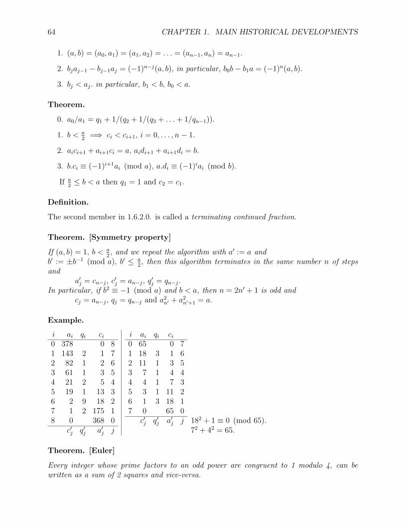
64 CHAPTER 1. MAIN HISTORICAL DEVELOPMENTS
1. (a, b) = (a0, a1) = (a1, a2) = . . . = (an−1, an) = an−1.
2. bjaj−1 − bj−1aj = (−1)n−j(a, b), in particular, b0b− b1a = (−1)n(a, b).
3. bj < aj. in particular, b1 < b, b0 < a.
Theorem.
0. a0/a1 = q1 + 1/(q2 + 1/(q3 + . . .+ 1/qn−1)).
1. b < a2
=⇒ ci < ci+1, i = 0, . . . , n− 1.
2. aici+1 + ai+1ci = a, aidi+1 + ai+1di = b.
3. b.ci ≡ (−1)i+1ai (mod a), a.di ≡ (−1)iai (mod b).
If a2≤ b < a then q1 = 1 and c2 = c1.
Definition.
The second member in 1.6.2.0. is called a terminating continued fraction.
Theorem. [Symmetry property]
If (a, b) = 1, b < a2, and we repeat the algorithm with a′ := a and
b′ := ±b−1 (mod a), b′ ≤ a2, then this algorithm terminates in the same number n of steps
anda′j = cn−j, c
′j = an−j, q
′j = qn−j.
In particular, if b2 ≡ −1 (mod a) and b < a, then n = 2n′ + 1 is odd andcj = an−j, qj = qn−j and a2
n′ + a2n′+1 = a.
Example.
i ai qi ci i ai qi ci0 378 0 8 0 65 0 71 143 2 1 7 1 18 3 1 62 82 1 2 6 2 11 1 3 53 61 1 3 5 3 7 1 4 44 21 2 5 4 4 4 1 7 35 19 1 13 3 5 3 1 11 26 2 9 18 2 6 1 3 18 17 1 2 175 1 7 0 65 08 0 368 0 c′j q′j a′j j 182 + 1 ≡ 0 (mod 65).
c′j q′j a′j j 72 + 42 = 65.
Theorem. [Euler]
Every integer whose prime factors to an odd power are congruent to 1 modulo 4, can bewritten as a sum of 2 squares and vice-versa.

1.6. ALGEBRA, MODULAR ARITHMETIC. 65
Example.
13 = 22 + 32, 52 = 42 + 62.585 = 92 + 242 = 122 + 212.
1.6.3 Quadratic Residues and Primitive Roots.
Definition.
n is a quadratic residue of p iff there exist a integer x such that x2 is congruent to n modulop. We write, with Gauss, n R p. n is a non residue of p, if there are no integer whose squareis congruent to n modulo p, and we write n N p.
Theorem.
The product of 2 quadratic residues or of 2 non residues is a quadratic residue. The productof a quadratic residue by a non residue is a non residue.
Theorem. [Fermat]
If a is not divisible by p then ap−1 ≡ 1 (mod p).
Definition.
g is a primitive root of p iff ai ≡ 1 (mod p) and 0 < i < p =⇒ i = p − 1. In other words,p− 1 is the smallest positive power of g which is congruent to 1 modulo p.
Notation. [Euler]
φ(n) denotes the number of integers betweem 1 and p, relatively prime to p.
Theorem. [Gauss]
0. There are φ(p− 1) primitive roots of p.
1. If g is a primitive root of p, all primitive roots are gi with (i, p− 1) = 1.
Example.
For p = 13, 2 is a primitive root,i 0 1 2 3 4 5 6 7 8 9 10 11 12 (mod 12)gi 1 2 4 −5 3 6 −1 −2 −4 5 −3 −6 1 (mod 13)
The other primitive roots are 25 = 6, 27 = −2 and 211 = −6.The easiest method to obtain all inverses moudo p is to first obtain a primitive root andthen to use gi . (gp−1−i)−1 = 1.
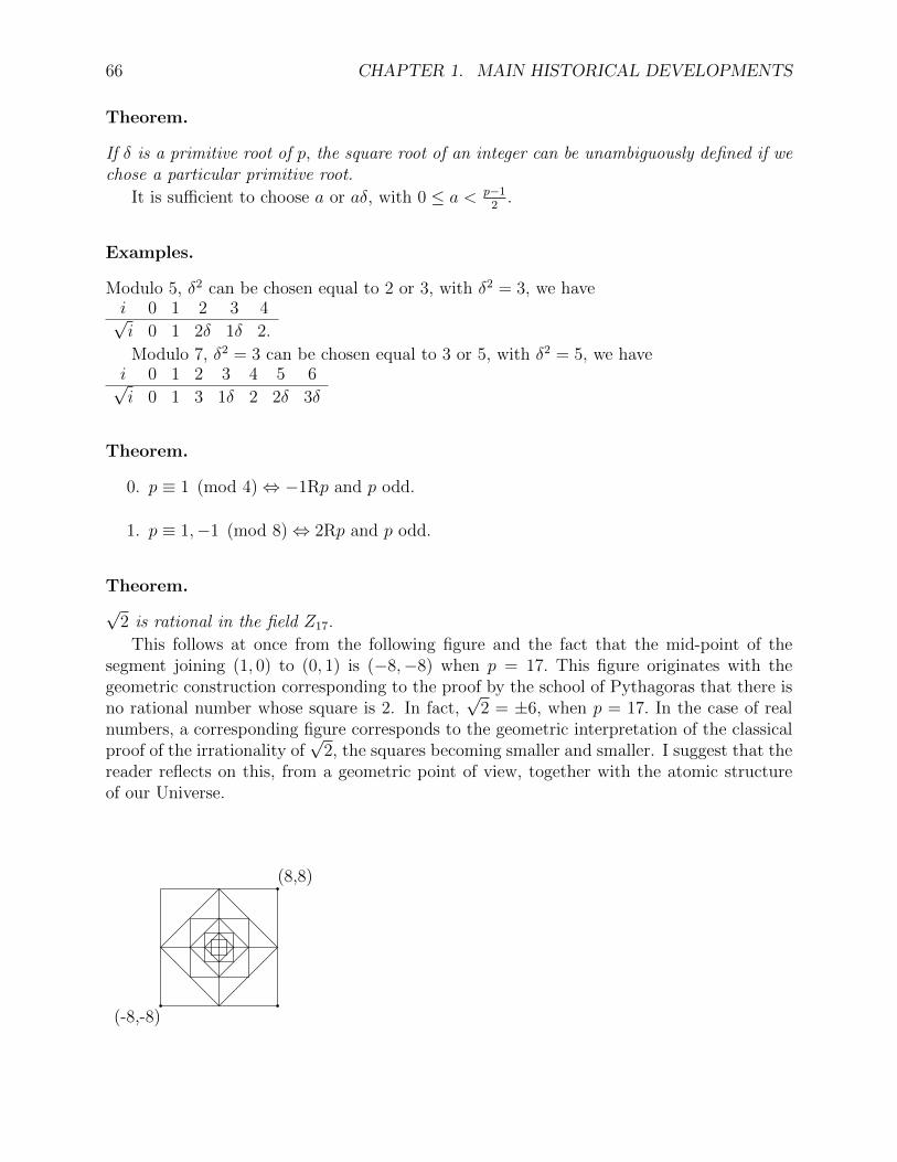
66 CHAPTER 1. MAIN HISTORICAL DEVELOPMENTS
Theorem.
If δ is a primitive root of p, the square root of an integer can be unambiguously defined if wechose a particular primitive root.
It is sufficient to choose a or aδ, with 0 ≤ a < p−12.
Examples.
Modulo 5, δ2 can be chosen equal to 2 or 3, with δ2 = 3, we havei 0 1 2 3 4√i 0 1 2δ 1δ 2.
Modulo 7, δ2 = 3 can be chosen equal to 3 or 5, with δ2 = 5, we havei 0 1 2 3 4 5 6√i 0 1 3 1δ 2 2δ 3δ
Theorem.
0. p ≡ 1 (mod 4)⇔ −1Rp and p odd.
1. p ≡ 1,−1 (mod 8)⇔ 2Rp and p odd.
Theorem.√
2 is rational in the field Z17.
This follows at once from the following figure and the fact that the mid-point of thesegment joining (1, 0) to (0, 1) is (−8,−8) when p = 17. This figure originates with thegeometric construction corresponding to the proof by the school of Pythagoras that there isno rational number whose square is 2. In fact,
√2 = ±6, when p = 17. In the case of real
numbers, a corresponding figure corresponds to the geometric interpretation of the classicalproof of the irrationality of
√2, the squares becoming smaller and smaller. I suggest that the
reader reflects on this, from a geometric point of view, together with the atomic structureof our Universe.
@@@@
@@@@@@
@@
@@
q
q q(-8,-8)
(8,8)

1.6. ALGEBRA, MODULAR ARITHMETIC. 67
1.6.4 Non Linear Diophantine Equations and Geometry.
Introduction.
There has been, historically, a constant interplay between geometry and diophantine equa-tions, the former suggesting problems of the latter kind which also indicate the interest ofhaving problems in geometry solved using integers only. As evidence I will give just one suchproblem considered by Euler12.
Definition.
The median problem consists in constructing a triangle with integer sides and medians.
Theorem.
If ai are the length of the sides and gi are twice the length of the medians, then
0. 2a2i+1 + 2a2
i−1 = a2i + g2
i .
Proof:a2
0 + a22 − 2a0a2cos(A1) = a2
1,14a2
0 + a22 − a0a2cos(A1) = 1
4g2
0,eliminating the terms involving the angle gives
2a21 + 2a2
2 = a20 + g2
0.
Theorem. [Euler]
The solution of the preceding problem can be expressed in terms of 2 parameters a and b,using
C = (4ab)2, D = (9a2 + b2)(a2 + b2), F = 2(3a2 + b2)(3a2 − b2),a0 = 2a(D − F ), a1 + a2 = 2a(C +D), a1 − a2 = 2b(C −D),g0 = 2b(D + F ), g1 + g2 = 6a(C −D), g1 − g2 = 2b(C +D),
Theorem. [Euler]
An other solution can be obtained corresponding to a′ = b and b′ = 3a for whicha′i = gi and g′i = 3ai.
An example is provided with the pair (1,2) giving the pair (2,3) in the Example. In factwe have the following
Theorem.
If both a and b are not divisible by 3, then 3|gi and 3 does not divide a0 therefore the precedingTheorems gives a solution and for this solution b′ is divisible by 3.
Indeed, a2 ≡ b2 ≡ 1, C ≡ F ≡ 1, D ≡ −1, a0 ≡ −a, −a1 ≡ a2 ≡ b, gi ≡ 3. It is thereforesufficient, if we use Theorem 1.6.4 to consider all pairs in which one of the integers in thepair is divisible by 3. Similarly we have the following Theorem.
12Opera Minora Collecta, II, (1778) 294-301, (1779) 362-365, (1782) 488-491

68 CHAPTER 1. MAIN HISTORICAL DEVELOPMENTS
Theorem.
If a is not divisible by 3 and b is divisible by 9, then 9|ai, 27|/ai, 27|gi and the solution is thesame as that obtained from a′ = b/3 and b′ = a.
Proof:If 9|b, then modulo 27, C ≡ 0, D ≡ 9 and F ≡ 18, therefore 9|a(0) but 27|/a(0) while 27|g(i).
Example.
The solutions for the pairs (a, b) =(1,3), (1,2), (2,3), (1,6), (3,1), (3,5) are given by Euler.Except for the pair (1,2), They are ordered by increasing maximum values of ai.a 1 1 2 1 5 3 ∗4 7 3 5 ∗3b 3 2 3 6 3 1 3 3 5 6 2a0 3 158 68 314 145 477 184 1099 2547 2690 1926a1 1 127 85 159 207 277 739 810 2699 5277 3985a2 2 131 87 325 328 446 1077 1339 2704 5953 6101g0 1 204 158 404 529 569 1838 1921 4765 10924 10124g1 5 261 131 619 463 881 1357 2312 4507 7583 8123g2 4 255 127 377 142 640 5 1391 4498 5893 1399
a 3 11 3 8 ∗7 ∗3 10 ∗3b 7 3 4 3 6 11 3 13a0 8163 12287 8874 18288 42 40563 59820 75123a1 5050 6416 13703 11663 15091 4232 32621 6953a2 5897 9897 14671 19105 20567 28531 51439 58580g0 7343 11281 26968 25838 36076 4301 61982 36283g1 13316 21370 20005 35537 24865 70006 106699 134543g2 12227 16921 17827 23999 5699 50125 81481 89174
The pair (1,2) corresponds to a degenerate triangle (1+2=3).The pairs marked with ∗ are solutions only in a geometry with complex coordinates becauseai+1 + ai−1 < ai for some i. The other degenerate solutions are obtained by observing that,in Euler’s proof, other solutions are obtained when b2 = a2 or 9a2.
1.6.5 Farey sets and Partial Ordering.
Introduction.
The basic idea is the following, a subset T1(n), n > 0, of the set Zp can be placed into one toone correspondance with the set Hn of irreducible rationals whose numerator, in modulus,and denominator are not larger than n, provided 2n2 − 2n + 1 < p. The ordering ≤ inHn ∈ Q induces an ordering in T1(n) such that a ≤ b and b ≤ c =⇒ a ≤ c and −b ≤ −a.If, morever, 0 ≤ a then b−1 ≤ a−1. If order is to be preserved, when we do one additionor one multiplication, we have to use T2(n) := T1(n′) instead of T1(n), with n = 2n′2. Thisinsures that the sum or product of 2 elements in T2(n) is in T1(n). T1, T2 are defined as thesets T1(n), T2(n) corresponding to the largest n. This can be repeated for a finite numberof additions and multiplications provided p is large enough.

1.6. ALGEBRA, MODULAR ARITHMETIC. 69
Hn is related to the Farey set Fn which is its subset in [0,1]. Farey sets have been used, forinstance, by my colleague and friend Professor R. Sherman Lehman to factor medium sizednumbers.The cardinality of the partially ordered set is estimated in 1.6.5.The complement (Zp−Hn−±
√−1) can be partitioned into 4 sets ε, −ε, λ and −λ which
might play the role of the sets of smallest elements and the sets of largest elements as given in1.6.5 to 1.6.5.Given an integer k, we can determine the corresponding irreducible rationals,or in which of the small or large set k belongs, using algorithm 1.6.5, which depends on thesymmetry Theorem 1.6.2. We end by contrasting with the notion of continuity in the set ofreal numbers.
Definition.
A Farey set Fn is the set of irreducible rationals aibi, in ascending order, between 0 and 1,
whose numerator and denominator do not exceed n.A Haros set Hn is the set of irreducible rationals ai
bi, in ascending order, between −n and n,
whose numerator, in modulus, and denominator do not exceed n.
Theorem. [Haros]
If aibi
and ai+1
bi+1are any 2 successive rationals of a Farey set Fn, then
0. ai+1bi − aibi+1 = 1.
1. The numerators and denominators of 2 successive rationals are relatively prime.
2. aibi
= ai−1+ai+1
bi−1+bi+1.
3. The set Fn can be constructed starting from 01
and 11
by inserting rationals using formula2 while the resulting numerators and denominators of the second member are not largerthan n.
For a proof see Hardy and Wright, p. 23 to 26.The set Hn can be deduced from Fn, by multiplicative symmetry with respect to 1 and thenby additive symmetry with respect to 0. It can also be obtained from −n
1and n
1using formula
2, but reduction is required and the termination condition is not as simple as for the set Fn.
Definition.
A set S is partially ordered by ≤ iff, with a, b, c ∈ S,
0. a ≤ a for all a in S,
1. a ≤ b and b ≤ a =⇒ a = b.
2. a ≤ b and b ≤ c =⇒ a ≤ c.
But, for any 2 distinct elements a and b in S, we need not have a ≤ b orb ≤ a.

70 CHAPTER 1. MAIN HISTORICAL DEVELOPMENTS
Notation.
a < b if a ≤ b and a 6= b.
Definition.
We define the set T1(n) by:
0. The set T1(n) := aibi, ai and bi relatively prime, |ai| ≤ n, 0 < bi ≤ n .
Theorem.
If 0 < n and 2n(n− 1) + 1 < p or equivalently if 0 < n <√
2p−1+12
,
0. there is a bijection between the irreducible rationals in Hn and the elements in thesubset T1(n) ∈ Zp.
1. If the order in T1(n) is that induced by the order in Hn ∈ Q and ifx, y ∈ T1(n), then0. the set Hn is partialy ordered,1. x < y ⇒ −y < −x,2. 0 < x < y ⇒ 0 < 1/y < 1/x.
Proof: It is sufficient to prove, that under the given hypothesis, if aibi
andajbj
are any
2 distinct elements in Q, they correspond to distinct elements of T1(n) in Zp. Indeed, ifrs≡ t
uthen ru − ts ≡ 0 modulo p, but |ru − ts| ≤ n2 + (n − 1)2 = 2n(n − 1) + 1 < p,
hence, by hypothesis, rs
= tu. The bound cannot be improved for T1, because, n
n−1≡ −n−1
n
if n2 + (n− 1)2 = p, whose positive root is√
2p−1+12
, and the sequence of primes of the formm2+1
2is infinite.
Definition.
For a given p, let np be the largest positive integer such that
0. 2np(np − 1) + 1 < p,then0. T1 := T1(np),
1. T2 := T1([√
np2
]).
Theorem.
If x, y, x′, y′ ∈ T2,
0. x.y, x+ y ∈ T1,
1. 0 < x′, x < y ⇒ x.x′ < y.x′.
2. x ≤ y, x′ ≤ y′ ⇒ x+ x′ ≤ y + y′.

1.6. ALGEBRA, MODULAR ARITHMETIC. 71
Indeed, if |a|, |b|, |c|, |d| ≤ m := [√
np2
] then |ad + bc| ≤ 2m2, |ac| ≤ m2, and |bd| ≤ m2,
therefore if x, y, x′, y′ ∈ T2, x+ x′ and y + y′ ∈ T1(2m2) = T1(np) = T1.Of course, for multiplication only, we could replace 2m2 by m2.
Example.
In this, and in other examples, I have chosen as representative of an element in Zp, thatwhich is in modulus less than p
2.
0. For p = 31, n31 = 4, T1 = T1(4) is−4 < −3 < −2 < 14 < 9 < −1 < 7 < −11 < 15 < 10 < −8 < 0< 8 < −10 < −15 < 11 < −7 < 1 < −9 < −14 < 2 < 3 < 4.Indeed, the Farey set F4 is01< 1
4< 1
3< 1
2< 2
3< 3
4< 1
1,
the values in Z31 are0 < 8 < −10 < −15 < 11 < −7 < 1,
their inverses are4 > 3 > 2 > −14 > −9 > 1.
T2 = T1(1) is−1 < 0 < 1.
For one multiplication we could use T ′2 = T1(2) (22 = 4) which is−2 < −1 < 15 < 0 < −15 < 1 < 2.
1. For p = 617, n617 = 18, the positive elements of T1 are240 < −254 < 270 < 288 < −44 < 95 < −257 < −56 < −185 < −137
< 109 < −77 < −41 < 88 < 190 < 103 < −145 < −112 < 193 < 247< −132 < −274 < 285 < 218 < −154 < −82 < −168 < −34 < −176 < −36< 62 < −237 < 116 < 206 < −290 < −220 < −224 < −231 < −142 < −171< −123 < 73 < −51 < −264 < 39 < 69 < −280 < −47 < 165 < −181< −308 < 182 < −164 < 48 < 281 < −68 < −38 < 265 < 52 < −72< 124 < 172 < 143 < 232 < 225 < 221 < 291 < −205 < −115 < 238< −61 < 37 < 177 < 35 < 169 < 83 < 155 < −217 < −284 < 275< 133 < −246 < −192 < 113 < 146 < −102 < −189 < 89 < 42 < 78< −108 < 138 < 186 < 57 < 258 < −94 < 45 < −287 < −269 < 255< −239 < 1< −253< 271 < 289 < −43 < 96 < −256 < −55 < −184 < −136 < −76 < −40< −87 < 191 < 104 < −111 < 248 < −131 < −273 < 286 < −153 < −167< −175 < 63 < −236 < 207 < −223 < −230 < −141 < −122 < −50 < −263< 70 < −279 < −307 < 282 < −67 < 266 < 125 < 233 < 226 < −204< −60 < 178 < 156 < 276 < −245 < −101 < 90 < 79 < 139 < 2< −75 < −86 < 105 < 249 < −152 < −174 < 208 < −121 < −262 < −306< 267 < 126 < −203 < 157 < −244 < −100 < 3 < 250 < −151 < 209< −120 < −305 < 127 < −202 < 158 < 4 < −150 < 210 < −304 < −201< 5 < 211 < −303 < −200 < 6 < −302 < 7 < −301 < 8 < −300< 9 < 10 < 11 < 12 < 13 < 14 < 15 < 16 < 17 < 18.

72 CHAPTER 1. MAIN HISTORICAL DEVELOPMENTS
The positive elements in T2 = T1(3) are206 < −308 < −205 < 1 < −307 < 2 < 3.
Theorem (Mertens).∑nb=1(φ(b)) = 3n2
π2 +O(nlog(n)),
where the last notation implies that the error divided by nlog(n) is bounded as n tends toinfinity.
Theorem.
The number of terms in T1 is of the order of6π2p+O(p
12 log(p)),
or approximately 0.6079p.
This follows at once from the fact that the number of irreducible rationals with denomi-nator b is φ(b), from T1 = 4
∑nb=2(φ(b)) + 3 from p = 2n2 + O(n), from φ(1) = 1 and from
the Theorem of Mertens.For p = 31, 23 = .74p, for p = 617, 405 = .656p.
The following Theorem gives a method to determine if a given integer in Zp is in T1.
Algorithm. [Modified continued fraction]
Given a0 := p, let n := np, 0 < a1 := a < p2, c0 := 0, d0 = 1, c1 := 1, d1 := 0, i := 1
l: qi := ai−1/ai, ai+1 = ai−1 − aiqi,ci+1 = ci−1 + ciqi, di+1 = di−1 + diqi,if ai+1 ≥ ci+1 then begin i := i+ 1; goto l end,
if ai < n then a ≡ (−1)iai+1
ci+1(mod p) ∈ T1,
if ci+1 < n then a ≡ (−1)iciai
(mod p) ∈ T1,
if aiai+1 > cici+1 then a ∈ (−1)i+1λ,if aiai+1 < cici+1 then a ∈ (−1)iε,if aiai+1 = cici+1 then a = −1/a.
i is therefore the largest index for which ai ≥ ci.We observe that if we start with a′ := a and b′ := ±b−1 (mod a), the + sign is to be chosenwhen n is even, and that by the symmetry property, when the algorithm stops, c′j ≥ a′j,c′j+1 < a′j+1, therefore j = i+ 1 and we have consistent conditions.
Example.
For p = 31, n31 = 4,
0. if a = 14, the continued fraction algorithm gives

1.6. ALGEBRA, MODULAR ARITHMETIC. 73
i ai qi ci i ai qi ci i ai qi ci0 31 0 5 0 31 0 6 0 31 0 31 14 2 1 4 1 12 2 1 5 1 6 5 1 22 3 4 2 3 2 7 1 2 4 2 1 6 5 13 2 1 9 2 3 5 1 3 3 3 0 31 04 1 2 11 1 4 2 2 5 25 0 31 0 5 1 2 13 1
6 0 31 0c′j q′j a′j j c′j q′j a′j j c′j q′j a′j j
1. For a = 14, i = 2, 14.2− 31.1 = −3, | − 3| ≤ 4, 14 ≡ −32
(mod 31), which is in T1.
2. For a = 12, i = 3, 12.3 − 31.1 = 5 > 4, 14 ≡ 53
(mod 31), which is not in T1. But12 ∈ −ε and 13 ∈ −λ.
3. For a = 6, i = 1, 6.1− 31.1 = −25, | − 25| > 4, 6 ≡ −61
(mod 31), which is in T1. But6 ∈ λ and 5 ∈ −ε.
4. In conclusion, λ = 6,−13, ε = −5,−12.
Example.
For p = 617, the elements in λ and, below them, their inverse in ε, are given below. Thosein −λ and −ε are obtained by replacing x by −x.λ : 19 20 21 23 24 25 26 28 29 30 32 53 58ε : 65 216 -235 161 180 -74 -261 -22 -234 144 135 163 -117λ : 64 80 85 91 92 -98 -99 106 107 -118 -119 128 129ε : -241 54 -196 278 -114 -170 -268 -227 173 183 -140 188 -110λ : 159 160 162 187 -195 -197 -198 -199 213 214 215 -228 -229ε : 260 27 -179 33 -212 -166 -134 31 -84 -222 -66 46 -97λ : -242 -243 251 252 259 -272 277 -293 -294 -296 -297 -298 -299ε : 283 -292 59 -71 81 93 -49 219 149 -148 -295 147 130
Definition.
Let x ∈| T1, let ai and ci be defined as in 1.6.5, with b replaced by x and let ai+1 and ci+1
be the next pair, let a′i and c′i, a′i+1 and c′i+1, be the corresponding quadruple for b′ := ±x−1,
the sign so chosen that b′ < a/2, if
0. c′i+1 = ai, a′i+1 = ci, c
′i = ai+1, a
′i = ci+1,
then
1. 0. aiai+1 < cici+1 and i even ⇒ x ∈ ε,1. aiai+1 < cici+1 and i odd ⇒ x ∈ −ε,
2. 0. aiai+1 > cici+1 and i+ 1 even ⇒ x ∈ λ,1. aiai+1 > cici+1 and i+ 1 odd ⇒ x ∈ −λ.
and we have the partial ordering of these sets by <<,−λ << −ε << 0 << ε << λ.
74 CHAPTER 1. MAIN HISTORICAL DEVELOPMENTS
Theorem.
0. x ∈ ε⇒ −x ∈ −ε, 1/x ∈ λ, −1/x ∈ −λ.
1. For a given p, all integers in the set [0, p− 1] are either in the set T1(np) or in one ofthe sets ε, −ε, λ, or −λ, with the exception of ±
√−1 when p ≡ −1 (mod 4).
We leave the proof as an exercise.
Theorem.
If for all ε ∈ (0, ε1) ∃ δ(ε) > 0 3x0 − δ(ε) < x < x0 + δ(ε)⇒ |f(x)− f(x0)| < ε, then f is continuous at x0.
Indeed for the continuity criterium, we can choose δ(ε) = δ(ε1) for ε ≥ ε1.
Comment.
The preceding Theorem is implicit in most text. In the older texts, it is alluded to by addingin the definition of continuity the phrase “however small is ε”. If we choose ε1 = 10−100, say,and assume that for a given f and x0, the hypothesis of the preceding Theorem is satisfied,it follows that the continuity at x0 depends only on the value of the function in the interval(x0 − 10−100, x0 + 10−100). If we now try to give an example from the world we live in, nomeaning can be given to physical objects which have distances from each other less thanε1. The definition of continuity gives therefore problems of interpretation in Atomic Physics.The same is true is Cosmology when the distances are of the order of the dimension of theUniverse. Continuity requires the notion of ordered set. We need to apply the more generalconcept of partialy ordered set, to allow for a criterium which test values which are small,but not too small, or large but not too large. This is what is achieved using Farey sets.
1.6.6 Complex and quaternion integers.
Introduction.
Hamilton introduced the notion of quaternions, to try to generalize the notion of complexnumber for application to 3 dimensional geometry.The elements are of the form a+ bi + cj + dk, with a, b, c, d not all zero, with
j.k = −k.j = i,k.i = −i.k = j, i.j = −j.i = k, i.i = j.j = k.k = 0,and real numbers commute with i, j, k, addition of quaternions is commutative and isdistributive over multiplication.
Definition.
Given a prime p and a non quadratic residue d, the set of complex integers Cp is the seta+ bδ, a, b ∈ Zp, δ2 = d.
The operations are those of addition,(a0 + b0δ) + (a1 + b1δ) = a2 + b2δ,
where a2 := a0 + a1 (mod p), b2 := b0 + b1 (mod p).

1.6. ALGEBRA, MODULAR ARITHMETIC. 75
and of multiplication,(a0 + b0δ).(a1 + b1δ) = a3 + b3δ,
where a3 := a0.a1 + b0.b1.d (mod p), b3 := a0.b1 + a1.b0 (mod p).This is entirely similar to the introduction of complex numbers,
δ2 = d replacing i2 = −1.
Example.
For p = 5 and d = 2,(1 + δ) + (1 + 3δ) = 2 + 4δ,(1 + δ).(1 + 3δ) = 2 + 4δ.
Definition.
A quaternion integer is a quaternion with coefficients in Zp.
Theorem.
If p ≡ 1, 3 (mod 8), the quaternion integers are isomorphic to 2 by 2 matrices over Zp.
The isomorphisms is deduced from the correspondance
1 ∼(
1 00 1
), i ∼
(1 bb −1
), j ∼
(−b 11 b
), k ∼
(0 1−1 0
),
with b2 = −2. For instance, for p = 11, b = 3, for p = 17, b = 7.
Theorem.
0. The quaternions form a skew field (or division ring).
1. The quaternion integers form a non commutative ring with unity for which if a rightinverse exists then it is also a left inverse.
1.6.7 Loops.
Definition.
A loop (L,+) is a non empty set of elements L together with a binary operation “ + ” suchthat, if l1, l2, l3, are elements in L,
0. l1 + l2 is a well defined element of L.
1. There exists a neutral element e ∈ L, such that e + l1 = l1 + e = l1.
2. l1 + x = l2 has a unique solution x ∈ L, denoted x = l1 ` l2 (or x = l1 \ l2, for (L, .)),
3. y + l1 = l2 has a unique solution y ∈ L denoted y = l2 a l1, (or y = l2 / l1, for (L, .))

76 CHAPTER 1. MAIN HISTORICAL DEVELOPMENTS
1.6.8 Groups.
Definition.
A group (G, .) is a non empty set of elements G together with an operation . such that
0. If g1 and g2 are any elements of G, g1.g2 is a well defined element of G.
1. The operation is associative, or for any elements g1, g2, g3 of G,(g1.g2).g3 = g1.(g2.g3).
2. There exists a neutral element e in G, such that for all elementsg ∈ G, e.g = g.e = g.
3. Every element g of G has an inverse, written g−1, such thatg.g−1 = g−1.g = e.
Notation.
If the operation is noted + instead of ., the neutral element is called a zero and is noted 0.
Comment.
(G,+) or (G, .) is often abbreviated as G, if the operation is clear from the context.
Theorem.
In a group, the neutral element is unique and in element has only one inverse.
Definition.
A group (G,+) is abelian or commutative iff for every element g1 and g2 of G,g1.g2 = g2.g1.
Notation.
In a group (G,+), we define
0. g = e, 1.g = g, (n+1).g = n.g+g and (−n).g = −(n.g) where n is any positive integer.
In a group (G, .), we use instead of 0.g, 1.g and n.g, g0 g1 and gn, where n is any positive ornegative integer.
Definition.
A cyclic group (G, .) is a group for which there exist an element g, called a generator of thegroup such that every element if G is of the form gn. (n.g if the operation is +).
1.6. ALGEBRA, MODULAR ARITHMETIC. 77
Examples.
0. (Z,+) is a cyclic group, 1 and −1 are generators.
1. (Zp,+), p prime, is a cyclic group, every element different from 0 is a generator.
2. (Zn,+), n composite, is an abelian group which is not cyclic.
3. (Zp − 0, .), p prime, is a cyclic group, any primitive root is a generator.
1.6.9 Veblen-Wederburn system.
Definition.
A Veblem-Wederburn system (Σ,+, ·), is a set Σ, containing at least the elements 0 and 1which is such that for a, b, c ∈ Σ,
0. Σ is closed under the binary operations “ + ” and ” · ” ,
1. (Σ,+) is an abelian group,
2. (Σ− 0, ·) is a loop,
3. (a+ b) · c = a · c + b · c,
4. a · 0 = 0,
5. is right distributive,(a+ b) · c = a · c+ b · c.
6. a 6= b⇒ x · a = x · b+ c has a unique solution.
Definition.
A division ring is a Veblen-Wederburn system which is left distributive.
Definition.
A alternative division ring is a division ring for which for all elements a 6= 0, the right inverseaR and left inverse aL are equal, so that we can write it as a−1 and such that for all b in theset
(a · b) · b−1 = b−1 · (b · a) = a.
Theorem.
In an alternative division ring,(b · a) · a = b · a2, a · (a · b) = a2 · b.

78 CHAPTER 1. MAIN HISTORICAL DEVELOPMENTS
Definition.
The Cayley numbers or octaves consist of (p + qe,+, ·), with (see also Stevenson p. 379)
0. p and q are quaternions over the reals,
1. (p + qe) + (p′ + q′e) = (p + p′) + (q + q′)e,
2. (p + qe) · (p′ + q′e) = (pp′ − q′q + q′p + qp′e,
Comment.
With l and l′ denoting i or j or k,e · l = −l · e = −le,l2 = (l · e)2 = −1,e · (le) = −(le) · e = l,(le) · l′ = −(ll′e), l 6= l′ ⇒ (le) · (l′e) = −ll′.
Definition.
The conjugate of an octave o = p + qe is defined byo = p− qe,
the norm of an octave is defined byN(o) = o · o.
Theorem.
If o = p + qe, then
0. o = o,
1. o · o′ = o′ · o,
2. N(o) = N(o) = N(p) +N(q),
3. N(o) = 0 iff o = 0,
4. N(o · o′) = N(o)N(o′).
Theorem.
0. The octaves is an alternative division ring which is non associative.
For instance, (i · j) · e = ke, and i · (j · e) = −ke.

1.6. ALGEBRA, MODULAR ARITHMETIC. 79
1.6.10 Ternary Rings.
Definition.
A ternary ring (Σ, ∗) is a set of elements Σ with at least 2 distinct elements 0 and 1, togetherwith an ternary operation “ ∗ ” such that if a1, a2, a3, a4 are elements in Σ, then
0. a1 ∗ a2 ∗ a3 is a well defined element of Σ,
1. a1 ∗ 0 ∗ a2 = a2,
2. 0 ∗ a1 ∗ a2 = a2,
3. 1 ∗ a1 ∗ 0 = a1,
4. a1 ∗ 1 ∗ 0 = a1,
5. a1 6= a2 ⇒ x ∗ a1 ∗ a3 = x ∗ a2 ∗ a4, has a unique solution x ∈ Σ,
6. a1 ∗ a2 ∗ y = a3 has a unique solution y ∈ Σ,
7. a1 6= a2 ⇒ a1 ∗ x ∗ y = a3 and a2 ∗ x ∗ y = a4 have a unique solution (x, y), x ∈ Σ,y ∈ Σ.
Theorem.
0. a 6= 0⇒ ∃aR 3 a · aR = 1, aR is called the right inverse of a.
1. a 6= 0⇒ ∃aL 3 aL · a = 1, aL is called the left inverse of a.
Definition.
The addition in a ternary ring is defined bya + b := a ∗ 1 ∗ b,
the multiplication in a ternary ring is defined bya · b := a ∗ b ∗ 0.
Theorem.
In a ternary ring (Σ, ∗),
0. (Σ,+) is a loop with neutral element 0.
1. (Σ− 0, ·) is a loop with neutral element 1 and a · 0 = 0 · a = 0..
80 CHAPTER 1. MAIN HISTORICAL DEVELOPMENTS
1.6.11 Felix Klein (1849-1925). Transformation groups.
The approach which has dominated the non axiomatic study of geometry during the last onehundred years has been influenced, almost exclusively13, by the celebrated Inaugural addressgiven by Felix Klein, when he became Professor of the Faculty of Philosophy of Universityof Erlangen and a member of its senate in 1872. In it14, Klein states that Geometriesare characterized by a subgroup of the projective group, with, for instance, the group ofcongruences characterizing the Euclidean Geometry. The success of this approach to thestudy of Geometry has been such that in may very well have led to the decline of thesynthetic Research and Teaching. It is hopped that this work, with its underlying program,which I call the Berkeley program, will revitalize the subject from the high school level on.
1.6.12 Functions.
Definition.
A function f from a set D to a set R is a set of ordered pairs (d0, r0), d0 in D, r0 in R, suchthat if to pairs have the same first elements, they have the same second element. We writer0 = f(d0).
Definition.
The domain of a function is the set D′ which is the union of all the first elements of thepairs, the range of a function is the set R′ which is the union of all the second pairs.
Definition.
A function is one to one or bijective iff for every pair (d0, r0) (d1, r1) such that r0 = r1 thend0 = d1.
Theorem.
If a function is one to one, the set of pairs (r0, d0) is a function f−1 from R to D.
Definition.
The function f−1 is called the inverse of f.
Definition.
Given 2 functions f and g such that the domain of g is a subset of the range of f, thecomposition g f is the function (d0, g(d0)).
13Diedonne characterizes it as a “ligne de partage des eaux” in the reedition of the French translation14Abhandlungen, p.460-497

1.7. THE REAL NUMBERS. 81
Theorem.
The composition is associative. In other words,(h g) f = h (g f).
1.6.13 Cyclotomic polynomials. Constructibility with ruler andcompass.
One of the most extensive type of problems in Euclidean Geometry is the constructibilityof geometric figures using the ruler and the compass. The construction of regular poly-gons lead Gauss, in his celebrated Disquisitiones Arithmeticae of 1801, to the study of rootsof cyclotomic polynomials and his discovery that the regular polygon with 17 sides is soconstructible. More generally, this is the case whenever the number of sides has the form2n∏Fijj , where the Fj’s are Fermat primes (of the form 2k + 1) 15. In so doing Gauss intro-
duced, for the special case of cyclotomic equations, the method, which could be describedas baby Galois Theory, which was generalized by Galois to the case of general polynomialequations. But in his case Gauss gives explicitely the various subgroups required to analyzecompletely the solution to the problem.The general problem of constructibility has been extensively studied, I will mention onlyhere the work Emile Lemoine (1902), of Henri Lebesgue (1950) and of A. S. Smogorzhevskii(1961). In finite geometry, it would appear at first that the ruler is sufficient for all con-structions because any point in the plane can be obtained from 4 points forming a completequadrangle. But this interpretation should be rejected in favor of that which implies thatthe construction of geometric figures should be given completely independently of the prime,or power of prime, which characterizes the finite Euclidean geometry. The impression isgiven that with the ruler very little can be constructed. One of the consequences of theresults of Chapter 3, is to demonstrate, that both in the finite and classical case many morepoints, lines, circles, . . . can be constructed with the ruler than heretofore assumed, and thatit is a useful exercise to reduce the problem of construction with the compass to that of afew points obtained with it and then the ruler alone. This is pursued extensively startingwith the construction, first of the center of the inscribed circle. Of note is that the circle ofApollonius can be constructed with the ruler alone.
1.7 The real numbers.
1.7.1 The arithmetization of analysis. [Karl Weierstrass (1815-1897) and Riemann (1826-1866)]
In his Introduction to the History of Mathematics, Eves 16 ascribed the beginning the arith-metization of analysis by Weierstrass and his followers to the problem presented by the
15Gauss gives, in n. 366, the polygons with number of sides less than 300, constructible with rule andcompass, namely, 2, 4, 8, 16, 32, 64, 128, 256, 3, 6, 12, 24, 48, 96, 192, 5, 10, 20, 40, 80, 160,15, 30, 60, 120, 240, 17, 34, 68, 136, 272, 51, 102, 204, 85, 170, 255, 257.
1G17.TEX [MPAP], September 9, 201916p.426

82 CHAPTER 1. MAIN HISTORICAL DEVELOPMENTS
existence (Riemann, 1874) of a continuous curve having no tangents at any of its points andthat (Riemann) of a function which is continuous for all irrational values and discontinuousfor all rational values in its domain of definition.
1.7.2 Algebraic and transcendental numbers. [Hermite (1822-1901) and Lindemann (1852-1939)]
Introduction.
We have seen that the Pythagoreans discovered that if we want any circle centered at theorigin and passing to a point with rational coordinates to intersect always the x axis, ir-rationals have to be introduced. If that was all that was desired, it would be sufficient toconstruct first the extension field
Q(√
2) = u+ v√
2,where u and v are in Q then
Q(√
2(√
5) = u1 + v1√
5,where u1 and v1 are in Q(
√2), . . . . The successive integers 5, 13, 17 are all the primes
congruent to 1 modulo 4, because of the result of Euler . . . and because all we would needwas to obtain the square root of integers which can be written as a sum of 2 squares.But, in fact we would like that circles centered at the origin, through a point with coordi-nates in one of these extension fields also intersect the x axis at a number in our system.This requires the introduction of algebraic numbers:
Definition.
An algebraic number is one which can be obtained as the real solution of a polynomial withinteger coefficients.A transcendental number is a real number which is not algebraic.
Example.√
2 is algebraic, being a root of x2 − 2 = 0,An outstanding problems of the last part of the 19-th century was the following, is π, whichis the limit of the ratio of the length of a regular polygon with n sides to the diameter,algebraic or not.The proof that it was not algebraic was first give by Lindemann in 1882, using an earlierresult of Hermite of 1973, that e is not algebraic.
1.8 The pendulum and the elliptic functions.
1.8.0 Introduction.
This section uses extensively, material learned from George Lemaıtre, in his class on Analyt-ical Mechanics, given to first year students in Engineering and in Mathematics and Physics,University of Louvain, Belgium, 1942 and from de la Vallee Poussin in his class on elliptic

1.8. THE PENDULUM AND THE ELLIPTIC FUNCTIONS. 83
functions in 1946.We first determine the differential equation for the pendulum 1.8.1 using the Theorem ofToricelli 1.8.1, we then define the elliptic integral of the first kind and the elliptic functionsof Jacobi 1.8.2 and 1.8.3, we then derive the Landen transformation which relates ellipticfunctions with different parameters 1.8.1, use it to obtain the Theorem of Gauss which deter-mines the complete elliptic integrals of the first kind from the arithmetico-geometric mean ofits 2 parameters 1.8.2. and obtain the addition formulas for the these functions 1.8.3 usingthe Theorem of Jacobi on pendular motions which differ by their initial condition 1.8.1. Wealso derive the Theorem of Poncelet on the existence of infinitely many polynomials inscribedin one conic and circumscribed to another 1.8.1. We state, without proof, the results on theimaginary period of the elliptic functions of Jacobi 1.8.3 and 1.8.3. A Theorem of Lagrangeis then given which relates identities for spherical trigonometry and those for elliptic func-tion 1.8.5. Finally we state the definitions and some results on the theta functions. Usingthis approach, the algebra is considerably simplified by using geometrical and mechanicalconsiderations.For references, see, Landen (1771), Legendre (1828), Jacobi (1829), Eisenstein (1847), La-grange (Oeuvres), Gauss (Ostwald Klassiker), Abel (Oeuvres), Weierstrass (Werke), Cayley(1884), Emch (1901), Appell (1924), Bartky (1938), Lemaıtre (1947), Fettis (1965).
1.8.1 The pendulum.
Theorem. [Toricelli]
If a mass moves in a uniform gravitational field, its velocity v is related to its height h by
0. v =√
2g(h0 − h),
where g is the gravitational constant and h0 is a constant, corresponding to the height atwhich the velocity would be 0.
Proof: The laws of Newtonian mechanics laws imply the conservation of energy. In thiscase the total energy is the sum of the kinetic energy 1
2mv2 and the potential energy mgh,
therefore12mv2 +mgh = mgh0, for some h0.
Definition.
A circulatory pendular motion is the motion of a mass m restricted to stay on a verticalfrictionless circular track, whose total energy allows the mass to reach with positive velocitythe highest point on the circle. An oscilatory pendular motion is one for which the totalenergy is such that the highest point on the circle is not reached. The mass in this caseoscillates back and forth. The following Theorem gives the equation satisfied by a pendularmotion.
Theorem.
If a mass m moves on a vertical circle of radius R, with lowest point A, highest point B andcenter O, its position M at time t, can be defined by

84 CHAPTER 1. MAIN HISTORICAL DEVELOPMENTS
2φ(t) = ∠(AOM) which satisfies
0. Dφ =√a2 − c2sin2φ, where
1. a2 := gh02R2 , c
2 = gR, for some h0.
2. D2φ = − g2Rsin (2φ).
Proof: If the height of the mass is measured from A,h(t) = R−Rcos(2φ(t)) = 2Rsin2φ(t),
the Theorem of Toricelli givesRD(2φ)(t) = v(t) =
√2gh0 − 4gRsin2φ(t),
hence 0.The motion is circulatory if h0 > 2R or a > c, it is oscilatory if 0 < h0 < 2R or c > a.2, follows by squaring 0 and taking the derivative.
Notation.
0. k := ca, b2 := a2 − c2, k′ := b
a, m := k2.
Theorem. [Jacobi]
Let M(t) describes a pendular motion. Given the circle γ which has the line r at height h0
as radical axis and is tangent to AM(t0), if N(t)M(t) remains tangent to that circle, thenN(t) describes the same pendular motion, with N(t0) = A.
Proof: With the abbreviation M = M(t), N = N(t), let NM meets r at D, let M ′, N ′
be the projections of M and N on r, let T be the point of tangency of MN with γ,
0. DM DN = DT 2,therefore
1. DTND
= DMDT
= DT−DMND−DT = MT
NT=√
DTND
DMDT
=√
DMND
=√
M ′MN ′N
When t is replaced by t+ ε,
2. vMvN
= limM(t+ε)−M(t)N(t+ε)−N(t)
= lim M(t)TN(t+ε)T
= MTNT
,
because the triangles T,M,M(t+ε) and T,N,N(t+ε) are similar, because ∠(T,N,N(t+ε) = ∠(T,M(t+ ε),M) as well as ∠(M(t+ ε), T,M) = ∠(N(t+ ε), T,N).Therefore
3. vMvN
=√
M ′MN ′N
.
The Theorem of Toricelli asserts that vM =√
2gM ′M, this implies, as we have just seen,vN =
√2gN ′N, therefore N describes the same pendular motion with a difference in the
origin of the independent variable.

1.8. THE PENDULUM AND THE ELLIPTIC FUNCTIONS. 85
Corollary.
If M = B and N = A, the line M(t) × N(t) passes through a fixed point L on the verticalthrough O.Moreover, if b := BL and a := LA, we have
vMvN
= ba
and h0 = a2
a−b .
This follows at once from from 1.8.1.2, and 1.
Definition.
The point L of the preceding Corollary is called point of Landen.
Theorem. [Poncelet]
Given 2 conics θ and γ , if a polygon Pi, i = 0 to n, Pn = P0, is such that Pi is on θ andPi × Pi+1 is tangent to γ , then there exists infinitely many such polygons.Any such polygon is obtained by choosing Q0 on θ drawing a tangent Q0Q1 to γ, with Q1
on θ and successively Qi, such that Qi is on θ and Qi−1 × Qi is tangent to γ, the Theoremasserts that Qn = Q0.
The proof follows at once from 1.8.1, after using projections which transform the circleθ and the circle γ into the given conics.The Theorem is satisfied if the circle have 2 points in common or not.
Theorem.
If M(t) describes a circular pendular motion, then the mid-point M1(t) of M(t) and M(t+K)describes also a circular pendular motion. More precisely, M1(t) is on a circle with diameterLO, with LA = a, LB = b, and ifφ1(t) = ∠(O,L,M1(t),
0. t =∫ φ(t)
0Dφ∆
= 12
∫ φ1(t)
0Dφ1∆1.
where
1. ∆2 := a2cos2φ+ b2sin2φ and ∆21 := a2
1cos2φ1 + b2
1sin2φ1,
where the relation between φ and φ1 is given by
2. tan(φ1 − φ) = k′tanφ, or
3. sin(2φ− φ1) = k1sinφ1,with
4. k′ := ba, k1 := c1
a1,
5. a1 := 12(a+ b), b1 :=
√ab, c1 := 1
2(a− b), therefore
6. a = a1 + c1, b = a1 − c1, c = 2√a1c1.
86 CHAPTER 1. MAIN HISTORICAL DEVELOPMENTS
Proof: First, it follows from the Theorem of Toricelli that the velocity vA at A and vBat B satisfy
vA =√
2gh0 = 2Ra, vB =√
2gh0 − 2R =√
4R2a2 − 4c2R2 = 2Rb,therefore BL
LA= b
a.
If P is the projection of L on BM and Q the projection of L on AM,LM2 = LP 2 + LQ2 = a2cos2φ+ b2sin2φ = ∆2.LQ = LMcos(φ1 − φ) = acosφ.
We can proceed algebraically. Differentiating 2. givesa(1 + tan2(φ1 − φ))(Dφ1 −Dφ) = b(1 + tan2φ)Dφ,ora(1 + tan2(φ1 − φ))Dφ1 = (a(1 + tan2(φ1 − φ) + b(1 + tan2φ))Dφ
= (a+ b+ b2
atan2φ+ btan2φ)Dφ
= (a+ b)(1 + batan2φ)Dφ
= (a+ b)(1 + tanφtan(φ1 − φ))Dφ,or
acos2(φ1−φ)
Dφ1 = 2a1cos(2φ−φ1)
cosφcos(φ1−φ)Dφ, or
Dφacosφ
cos(φ1−φ)= Dφ1
2a1cos(2φ−φ1),
or because LM = ∆Dφ∆
= Dφ12∆1
.We can also proceed using kinematics.
The velocity at M isvM = 2RDφ = 2R∆,
If we project the velocity vector on a perpendicualr to LM,LMDφ1 = vMcos(2φ1 − φ) = 2Rcos(2φ1 − φ)∆φ.
ThereforeDφ∆
= Dφ12Rcos(2φ1−φ)
= a12R
Dφ1∆1
= Dφ12∆1
.
Definition.
The transformation from φ to φ1 is called the forward Landen transformation.The transformation from φ1 to φ is called the backward Landen transformation.
These transformations have also been applied to the integrals of the second kind and ofthe third kind.
Comment.
The formulas 3. and 1. are the formulas which are used to compute t from φ(t). Theformulas 4. and 2. are used to compute φ(t) from t.
Comment
Given the first order differential equations,(Dy)2 = C0(y2 + A0)(y2 +B0),(Dz)2 = C1(z2 + A1)(z2 +B1),
with

1.8. THE PENDULUM AND THE ELLIPTIC FUNCTIONS. 87
z = d(y + ly), l 6= 0, d > 0.
These equations are compatible iffd2(1− l
y2)2C0(y2 + A0)(y2 +B0) = C1(d2(y
2+ly
)2 + A1)(d2(y2+ly
)2 +B1)
this requires√l to be a root of one of the factors of the second member, let it be the second
factor, this impliesd24l +B1 = 0,
then, the second factor becomes,d2(y
2+ly
)2 +B1 = d2((y2+ly
)2 − 4l) = d2(y2−ly
)2,
therefore√l is a double root of the second member and
C0(y4 + (A0 +B0)y2 + A0B0) = d2C1(y4 + (2l + A1
d2)y2 + l2), therefore
C0 = d2C1, A0B0 =B2
1
16d4, A0 +B0 =
A1− 12B1
d2,
For real transformations, A0B0 > 0, if j0 = sign(B0) and j1 = sign(B1),B1 = 4j1d
2√A0B0, A1 = d2(A0 +B0 + 2j1
√A0B0
= j0d2(√|A0|+ j0j1
√|B0|)2.
If we want A1B1 > 0 then j0 = j1.
1.8.2 The elliptic integral and the arithmetico-geometric mean.
Introduction.
Gauss began his investigations after he showed that the length of the lemniscate could becomputed from the arithmetico geometric mean of
√2 and 1. More precisely, the lemniscate
is the curve r2 = cos(2θ), in polar coordinates. A quarter of its length is given by the integral∫ 1
0
dr√1− r4
,
which is easily deduced from the general formula for the square of the arc length in polarcoordinates, ds2 = dr2 + r2(dθ)2.
Gauss observed that to 9 decimal places the integral was 1.311028777 and so is π/2
agm(√
2,1,
where agm(a, b) denotes the arithmetico geometric mean of 2 numbers, defined below.
Theorem. [Gauss]
Given a0 > b0 > 0, let
0. ai+1 := 12(ai + bi),
1. bi+1 :=√aibi,
2. The sequences ai and bi have a common limit a∞.
3. The sequence ai is monotonically decreasing and the sequence bi is monotonically in-creasing.
Proof: Becauseai > a1+1, bi+1 > bi,
it follows that the sequence ai is bounded below by b0, the sequence bi is bounded above bya0, therefore both have a limit a∞ and b∞. Taking the limit of 0. gives at once a∞ = b∞.

88 CHAPTER 1. MAIN HISTORICAL DEVELOPMENTS
Definition.
a∞ is called the arithmetico-geometric mean of a0 and b0.
Example.
With a0 =√
2 and b0 = 1,a1 = 1.207106781, b1 = 1.189207115,a2 = 1.198156948, b2 = 1.198123521,a3 = 1.198140235, b2 = 1.198140235.
Definition.
If a = 1, and we express t in terms of φ(t),
0. t =∫ φ(t)
01√
1−k2sin2 . This integral is called the incomplete elliptic integral of the firstkind. Its inverse function φ is usually noted
1. am := φ, the amplitude function,
2. K :=∫ π
2
01√
1−k2sin2 is called the complete integral of the first kind, it gives half the
period, Ka, for the circular pendulum.
Theorem.
0. For the circulatory pendulum, the angle 2φ between the lowest position of the mass andthat at time t is given by φ = am(at). The coordinates are R sin(2φ), R−R cos(2φ).
1. For the oscillatory pendulum, if the highest point is 2Rsin2(α) above the lowest point,the angle 2θ between the lowest position of the mass and that at time t is given bysinθ = sinφ sinα where φ is given by φ = am(at, sin2α).
Theorem.
For the complete integrals we have
0. Ka
=∫ π
2
01√
a2cos2+b2sin2 =π2
a∞.
Proof: If φ(K) = π2, then φ1(K) = π, therefore
1. K =∫ π
2
0Dφ∆
=∫ π
0Dφ12∆1
= 12
∫ π2
0Dφ1∆1
+ 12
∫ ππ2
Dφ1∆1
=∫ π
0Dφ1∆1
=∫ π
2
0Dφn∆n
=∫ π
2
01a∞
=π2
a∞.

1.8. THE PENDULUM AND THE ELLIPTIC FUNCTIONS. 89
1.8.3 The elliptic functions of Jacobi.
Definition.
The functions
0. sn := sin am, cn := cos am, dn :=√
1− k2sn2,are called the elliptic functions of Jacobi.
The functions which generalize tan, cosec, . . . are
1. ns := 1sn, nc := 1
cn, nd := 1
dn,
2. sc := sncn, cd := cn
dn, ds := dn
sn,
3. cs := cndn, dc := dn
cn, sd := sn
dn.
Theorem.
If
0. s1 := sn(t1), c1 = cn(t1), d1 = dn(t1) and
1. s2 := sn(t2), c2 = cn(t2), d2 = dn(t2),we have
2. sn2 + cn2 = 1, dn2 + k2sn2 = 1, dn2 − k2cn2 = k′2.
3. 1− k2s21s
22 = c2
1 + s21d
22 = c2
2 + s22d
21.
Lemma.
0. c2 = c1cn(t1 + t2) + d2s1sn(t1 + t2),
1. d2 = d1dn(t1 + t2) + k2s1c1sn(t1 + t2).
Proof: We use the Theorem 1.8.1 of Jacobi. Let R be the radius of θ and O its center,let r be the radius of γ and O′ its center, let s := OO′. Let A, N, M ′, M be the position ofthe mass at time 0, t1, t2, t1 + t2.The lines A×M ′ and N ×M are tangent to the same circle γ at T ′ and T.Let X be the intersection of O ×M and O′ × T, 2φ := ∠(A,O,N),
2. 2φ′ := ∠(A,O,M),we have ∠(N,O,M) = 2(φ′ − φ), ∠(M,X, T ) = φ′ − φ, ∠(T,O′, O) = φ′ + φ.If we project MOO′ on O′T,
r = Rcos(φ′ − φ)scos(φ′ + φ), or
3. r = (R + s)cosφcosφ′ + (R− s)sinφsinφ′.φ = amt1, φ
′ = am(t1 + t2),sinφ′ = sn(t1 + t2), cosφ′ = cn(t1 + t2),sinφ = sn t1 = s1,cosφ = cn t1 = c1,

90 CHAPTER 1. MAIN HISTORICAL DEVELOPMENTS
when t1 = 0,cos(∠(A,B,M ′) = cn t2 = c2 = BM ′
AB= O′T ′
AO′= r
R+s,
the ratio of the velocities isvM′vA
= dn t2dn 0
= d2 = TM ′
AT= O′B
AO′= R−s
R+s, substituting in 2. gives 0.
The proof of 1. is left as an exercise.
Theorem. [Jacobi]
0. sn u1cn u2dn u2+sn u2cn u1dn u1sn(u1+u2)
= 1− k2sn2u1sn2u2.
1. cn u1cn u2−sn u1dn u1sn u2dn u2cn(u1+u2)
= 1− k2sn2u1sn2u2.
2. dn u1dn u2−k2sn u1sn u2cn u1cn u2dn(u1+u2)
= 1− k2sn2u1sn2u2.
Proof: Let w = 11−k2s21s22
.
Let s1, s2, . . . denote sn u1, sn u2, . . ., define S and C such thatsn(u1 + u2) = Sw, cn(u1 + u2) = Cw.
The 1.8.3.0. givesc2 = c1Cw + d2s1Sw or
3. c1Cw = −d2s1Sw + c2,
1.8.3.2. givesS2w2 + C2w2 = 1,
eliminating C gives the second degree equation in Sw:(c2
1 + d22s
21(Sw)2 − 2s1c2d2(Sw) + c2
2 − c21 = 0,
one quarter of the discriminant iss2
1c22d
22 − (c2
2 − c21)(c2
1 + d22s
21)
= s21c
22d
22 − c2
1c22 + c4
1 − s21c
22d
22 + s2
1c21d
22
= c21(c2
1 − c22 + s2
1d22) = c2
1s22d
21,
thereforeSw = (s1c2d2 ± c1d1s2)w.
One sign correspond to one tangent from M to γ , the other to the other tangent, thereforeone corresponds to the addition, the other to the subtration formula. From the special casek = 0, follows that, by continuity, the + sign should be used. This gives 0., 1. follows from3, 2. is left as an exercise.
Corollary.
0. sn(u+K) = cd(u), cn(u+K) = −k′sd(u), dn(u+K) = k′nd(u).
1. sn(u+ 2K) = −sn(u), cn(u+ 2K) = −cn(u), dn(u+ 2K) = dn(u).
2. sn(u+ 4K) = sn(u), cn(u+ 4K) = cn(u), dn(u+ 4K) = dn(u).
Definition.
K ′(k2) = K(k′2).

1.8. THE PENDULUM AND THE ELLIPTIC FUNCTIONS. 91
Theorem.
0. 0. ksn I + iK ′ = sn,1. ikcn I + iK ′ = ds,2. idn I + iK ′ = cs,
1. 0. sn I + 2iK ′ = sn,1. cn I + 2iK ′ = −cn,2. dn I + 2iK ′ = −dn,
Theorem.
0. sn has periods 4K and 2iK ′ and pole ±iK ′,
1. cn has periods 4K and 4iK ′ and pole ±iK ′,
2. dn has periods 2K and 4iK ′ and pole ±iK ′.
Theorem.
0. k = 0⇒ sn = sin, cn = cos, dn = 1,
1. k = 1⇒ sn = tanh, cn = sech, dn = sech.
1.8.4 The theta functions of Jacobi.
Definition.
Given the parameter q, called the nome,
0. q := e−πK′K ,
the functions
1. θ1 := 2q14
∑∞n=0(−1)nqn(n+1)sin(2n+ 1)I
2. θ2 := 2q14
∑∞n=0 q
n(n+1)cos(2n+ 1)I
3. θ3 := 1 + 2∑∞
n=1 qn2cos2nI
4. θ4 := 1 + 2∑∞
n=1(−1)nqn2cos2nI are the theta functions of Jacobi.
Definition.
The functions, with v = π I2K
0. θs := 2K θ1vDθ1(0)
, θc := θ2vθ2(0)
, θd := θ3vθ3(0)
, θn := θ4vθ4(0)
,are called the theta functions of Neville.

92 CHAPTER 1. MAIN HISTORICAL DEVELOPMENTS
Theorem.
If p, q denote any of s, c, d, n,pq = θp
θq.
For instancesn = θs
θn= 2Kθ1v
Dθ1(0). θ4(0)θ4v .
Theorem.
The Landen transformation replaces the parameter q, by q2.
1.8.5 Spherical trigonometry and elliptic functions.
Theorem. [Lagrange]
From the addition formulas of elliptic functions, we can derive those for a spherical triangleas follows. Let
0. u1 + u2 + u3 = 2K,define
1. sina := −snu1, cosa := −cnu1,sinb := −snu2, cosb := −cnu2,sinc := −snu3, cosc := −cnu3,sinA := −k snu1, cosA := −dnu1,sinB := −k snu2, cosB := −dnu2,sinC := −k snu3, cosC := −dnu3,then to any formula for elliptic functions of u1, u2, u3, corresponds a formula for aspherical triangle with angles A, B, C and sides a, b, c. For instance,
2. sinAsina
= sinBsinb
= sinCsinc
= k.
3. cosa = cosb cosc+ sinb sinc cosA,
4. cosA = −cosB cosC + sinB sinC cosa,
5. sinB cotA = cosc cosB + sinc cota.
Proof. 2. follows from the definition. 3. follows fromc2 = c1cn(u1 + u2) + d2s1sn(u1 + u2) after interchanging u1 and u2 and using
6. 0. sn(u1 + u2) = sn(2K − u1 − u2) = sn u3 = s3,1. cn(u1 + u2) = −cn(2K − u1 − u2) = −cn u3 = −c3,2. dn(u1 + u2) = dn(2K − u1 − u2) = dn u3 = d3,similarly, 4. follows from
c2 = c1cn(u1 + u2) + d2s1sn(u1 + u2)after interchanging u1 and u2 and using 6, and 5. from
sn u2dn u1 = cn u1sn(u1 + u2)− sn u1dn u2cn(u1 + u2)after division by sn u1.

1.8. THE PENDULUM AND THE ELLIPTIC FUNCTIONS. 93
1.8.6 The p function of Weierstrass.
Introduction.
Because it is not germane in this context, I will only mention briefly the important contri-bution of Weierstrass, which proved that all doubly periodic meromorphic functions can beexpressed in terms of one of them, the p function. The addition formulas for this functionanf for the Jacobi functions and many other properties generalize to the finite case (DeVogelaere, 1983)..
1.8.7 References.
0. Abel, Niels Henrik, Oeuvres Completes, Nouv. ed., publiees aux frais de l’Etat norvegienpar L. Sylow et S. Lie, Christiania, Grondahl & Son, 1881, Vol. 1,2.
1. Appell, Paul Emile & Dautheville, S., Precis de Mecanique Rationnelle, Paris, Gauthier-Villars, 1924, 721 pp.
2. Bartky, Numerical Calculation of Generalized Complete Integrals, Rev. of ModernPhysics, 1938, Vol. 10, 264-
3. Cayley, Arthur, On the Addition of Elliptic Functions, Messenger of Mathematics, Vol.14, 1884, 56-61.
4. Cayley, Arthur, Note sur l’Addition des Fonctions Elliptiques, Crelle J., Vol. 41, 57-65.
5. De Vogelaere, Rene, Finite Euclidean and non-Euclidean Geometry with applicationto the Finite Pendulum and the Polygonal Harmonic Motion. A First Step to FiniteCosmology. The Big Bang and Georges Lemaıtre, Proc. Symp. in honor of 50 yearsafter his initiation of Big-Bang Cosmology, Louvain-la-Neuve, Belgium, October 1983.,D. Reidel Publ. Co, Leyden, the Netherlands. 341-355.
6. Eisenstein, Ferdinand Gotthold Max, Mathematische Abhandlungen, besonders ausdem Gebiete der hoheren Arithmetik und den elliptischen Functionen, Mit einer Vorredevon C.F. Gauss. (Reprografischer Nachdruk der Ausg., Berlin 1847.) Hildesheim, G.Olms, 1967.
7. Emch, An Application of Elliptic Functions, Annals of Mathematics, Ser. 2, Vol. 2,1901. III.4.4.0.
8. Fettis, Henri E., Math. of Comp., 1965.
9. Gauss, Carl Friedrich, Ostwald Klassiker der Exakten Wissenschaften, Nr 3.
10. Jacobi, Karl Gustav Jakob, Fundamenta Nova Theoriae Funktionum Ellipticarum,1829.
11. Landen, John, Phil. Trans. 1771, 308.

94 CHAPTER 1. MAIN HISTORICAL DEVELOPMENTS
12. Lagrange, Joseph Louis, comte, Oeuvres, publiees par les soins de m. J.-A. Serret, sousles auspices de Son Excellence le ministre de l’instruction publique, Paris, Gauthier-Villars, 1867-92.
13. Legendre, Adrien Marie, Traite des Fonctions Elliptiques et des Integrales Euleriennes,avec des tables pour en faciliter le calcul numerique, Paris, Huzard-Courcier, Vol. 1-3,1825-1828.
14. Lemaıtre, Georges, Calcul des Integrales Elliptiques, Bull. Ac. Roy. Belge, Classe desSciences, Vol. 33, 1947, 200-211.
15. Weierstrass, Karl, Mathematische Werke, Hildesheim, G. Olms, New York, JohnsonReprint 1967.
1.8.8 Texts on and tables of elliptic Functions.
0. Abramowitz, Milton & Stegun, Irene A. Edit., Handbook of Mathematical Functions,U.S. Dept of Commerce, Nat. Bur. of Stand., Appl. Math, Ser., number 55, 1964,1046 pp.
1. Adams, Edwin Plimpton, Ed., Smithsonian Mathematical Formulae and Tables ofElliptic Functions, under the direction of Sir George Greenhill, 3d reprint, City ofWashington, 1957, Its Smithsonian miscellaneous collections, v.74, no.1, SmithsonianInstitution, Publication 2672.
2. Halphen, Georges Henri, Traite des Fonctions Elliptiques et de leurs Applications,Paris, Gauthier-Villars, 1886-91.
3. Hancock, Harris, Lectures on the Theory of Elliptic Functions, v. 1. 1st ed., 1stthousand, New York, J. Wiley, 1910. Dover Publ., 1958.
4. Jahnke, Eugen & Emde, Fritz, Tables of Functions with Formulae and Curves, 4th ed.,New York, Dover Publications, 1945.
5. Jahnke, Eugen & Emde, Fritz & Losch, Friedrich, Tables of Higher Functions, 6th ed.rev. by Losch, New York, McGraw-Hill, 1960.
6. Jordan, Camille, Fonctions Elliptiques, New York, Springer-Verlag, 1981.
7. King, Louis Vessot, On the Direct Numerical Calculations of Elliptic Functions andIntegrals, Cambridge, Eng., Univ. Press, 1924.
8. Lang, Serge, Elliptic functions, 2nd ed., New York, Springer-Verlag, 1987, Graduatetexts in mathematics, 112.
9. Mittag-Leffler, Magnus Gustaf, An Introduction to the Theory of Elliptic Functions,Lancaster, Pa., 1923, Hamburg, Germany, Lutcke & Wulff.
1.9. MODEL OF FINITE EUCLIDEANGEOMETRY IN CLASSICAL EUCLIDEANGEOMETRY.95
10. Neville, Eric Harold, Elliptic Functions, a primer, Prepared for publication by W. J.Langford, 1st d. Oxford, New York, Pergamon Press, 1971.
11. Neville, Eric Harold, Jacobian Elliptic Functions, Oxford, The Clarendon Pr., 1944.
12. Oberhettinger, Fritz Wilhelm & Magnus, Wilhelm, Anwendung der elliptischen Funk-tionen in Physik und Technik, Berlin, Springer, 1949, Die Grundlehren der mathema-tischen Wissenschaften in Einzeldarstellungen, Bd. 55.
13. Riemann, Bernhard, Elliptische Functionen, Mit zusatzen herausgegeben von HermannStahl . . . Leipzig, B. G. Teubner, 1899.
14. Schuler, Max & Gebelein, H., Eight and Nine Place Tables of Elliptical Functions basedon Jacobi Parameter q, with an English text by Lauritz S. Larsen, Berlin, Springer-Verlag, 1955, XXIV+296 pp.
15. Spenceley, G.W. & Spenceley, R.M., Smithsonian Elliptic Functions Tables, Washing-ton, Smithsonian Institution 1947, Smithsonian miscellaneous collections v. 109.
16. Sturm, Charles Francois, Cours d’Analyse de l’Ecole Polytechnique, revu et corrige parE. Prouhet et augmente de la Theorie elementaire des fonctions elliptiques, par H.Laurent, 14. ed., rev. et mise au courant du nouveau programme de la licence, par A.de Saint-Germain, Paris, Gauthier-Villars, 1909.
17. Tannery, Jules & Molk, Jules, Elements de la theorie des fonctions elliptiques, Paris,Gauthier-Villars, Vol. 1-4, 1893-1902.
18. Tolke, Friedrich, Praktische Funktionenlehre, Berlin, Springer, Vol. I to VI ab. Vol. 3and 4 deal with the elliptic functions of Jacobi.
19. Tricomi, Francesco Giacomo, Elliptische Funktionen, ubers. und bearb. von Maximil-ian Krafft. Leipzig, Akademische Verlagsgesellschaft Geest & Portig, 1948, Mathematikund ihre Anwendungen in Physik und Technik, Bd. 20.
20. Whittaker, Edmund Taylor & Watson, G. N., A Course of Modern Analysis, an intro-duction to the general theory of infinite processes and of analytic functions, Cambridge,Eng., Univ. Pr., 1963, 606 pp., (1927).
1.9 Model of Finite Euclidean Geometry in Classical
Euclidean Geometry.
1.9.0 Introduction.
The purpose of this section is to give an informal introduction to finite Euclidean geometryfor those familiar with classical Euclidean geometry and analytic geometry.The definitions of points and lines will be given in terms of equivalence classes. The Theoremswill be derived from these definitions or can be derived from the classical Theorems. I will

96 CHAPTER 1. MAIN HISTORICAL DEVELOPMENTS
restrict myself to the 2 dimensional case and will not attempt to give the most general results.In particular, I will assume that distances are defined in only one way.In this restricted framework there is one finite geometry for each prime integer p. p is assumedto be larger than 2, non degenerate circles require p larger than 3. The examples correspondto small p. The reader is encouraged to think of the implications when p is very large, forinstance of the order of 1032 say, and is looking at points with coordinates of the order of108 to 1020.
1.9.1 Points and lines in finite Euclidean geometry.
Notation.
A point P ′ in Euclidean geometry will be denoted by its cartesian coordinates ((x, y)) givenbetween double parenthesis. A line l′ will be denoted by the coefficients [[a, b, c]] of itsequation
ax+ by + c = 0,given between double brackets. These coefficients are not unique. They can be replaced by
[[ka, kb, kc]]where k is any real number different from 0.For the points P and lines l in finite geometry, I will use the same notation with singleparenthesis and single brackets.
Definition.
Given a prime p, if x is an integer, x mod p denotes the smallest positive remainder of thedivision of x by p.
For instance, 28mod 13 = 2, −5mod 11 = 6.
We observe that if x and y are non negative integers less than p, for any integers l and m,x+ lp mod p = x, y +mpmod p = y.
Definition.
Let x and y be integers. For any integers l and m, the points((x+ lp, y +mp))
are called equivalent points. A set of equivalent points is called a point (x, y) in finitegeometry.
Let a, b, c be integers, a and b not both zero. For any integers l, m and n, the lines[[k(a+ lp), k(b+mp), k(c+ np)]], k 6= 0,
are called equivalent lines. A set of equivalent lines is called a line in finite geometry.If P = (x+mp, y + np) is on l = [a+ k′p, b+m′p, c+ n′p], then
(a+ k′p)(x+mp) + (b+m′p)(y + np) + (c+ n′p) = 0and therefore
(ax+ by + c)mod p = 0,this is 1.9.1 below. This method of reducing modulo p allows us to extend many of theproperties of Euclidean geometry to the finite case.

1.9. MODEL OF FINITE EUCLIDEANGEOMETRY IN CLASSICAL EUCLIDEANGEOMETRY.97
Example.
Let p = 7. The line a = [[1,−1,−5]] is equivalent to the lines a0 = [[1,−1,−12]], a1 =[[1,−1, 2]], a2 = [[1,−1, 9]].The line b = [[1, 2,−17]] is equivalent to the lines b0 = [[1, 2,−3]], b1 = [[1, 2,−10]], b2 =[[1, 2,−24]], b3 = [[1, 2,−31]].The intersection P = ((9, 4)) of a and b is equivalent to the points all labelled Q, ((2, 4)),((16, 4)), ((2, 11)), ((9, 11)), ((16, 11)). Only one of the points equivalent to P is in thedomain
0 ≤ x, y < p, namely ((2, 4)).

98 CHAPTER 1. MAIN HISTORICAL DEVELOPMENTS
^
y
. . Qb2 . . . . . . Qb3 . . . . . . Qb4 .
. a2 . . b2 . . . a1 . . b3 . . . a . .
a2 . . . . . b2 a1 . . . . . b3 a . . .
. b . . . . a1 . b2 . . . . a . b3 . .
. . . b . a1 . . . . b2 . a . . . . b3
__________________________
. . . . a1 b . | . . . . a b2 . . . . .
|
b1 . . a1 . . . | b . . a . . . b2 . . a0
|
. . Qb1 . . . . | . . Pb . . . . . . Qb2 .
|
. a1 . . b1 . . | . a . . b . . . a0 . .
|
a1 . . . . . b1| a . . . . . b a0 . . .
|
. b0 . . . . a | . b1 . . . . a0 . b . .
|
. . . b0 . a . | . . . b1 . a0 . . . . b
x >
Equivalence of points and lines.Fig.0a, p = 7.
In Fig.0a, I have not given those lines which are equivalent to a but have a different slope,if R is any point on such a line which is in the lower right square it is either Q or a pointlabelled a or a1.In finite geometry, we do not distinguish points labelled a1 from those labelled a or the pointslabelled b0 and b1 from those labelled b. We have therefore Fig.0b below.

1.9. MODEL OF FINITE EUCLIDEANGEOMETRY IN CLASSICAL EUCLIDEANGEOMETRY.99
^
y
__________________________
. . . . a b . |
|
b . . a . . . |
|
. . Qb . . . . |
|
. a . . b . . |
|
a . . . . . b |
|
. b . . . . a |
|
. . . b . a . | x >
Points and lines in finite Euclidean geometry.Fig.0b, p = 7.
The point Q = (2, 4) is on the lines a = [1, 6, 2] = [4, 3, 1] and b = [1, 2, 4] = [2, 4, 1] inthe finite Euclidean geometry associated with p = 7.Observe that from one point on a, the others are obtained by moving one to the right andone up, for b, we move 2 to the right and one down. Observe also what happens at theboundary using, if needed Fig. 0a.
If we attempt to use the equivalence method when p is not a prime, the situation for 6points is typical. If a = [[1, 1,−5]], b = [[1, 3, 1]] and c = [[1, 3, 4]], the points P = ((2, 3))and Q = ((5, 0)) are both on the lines a and b, while the lines a and c or their equivalenthave no point in common with coordinates reduced modulo 6.
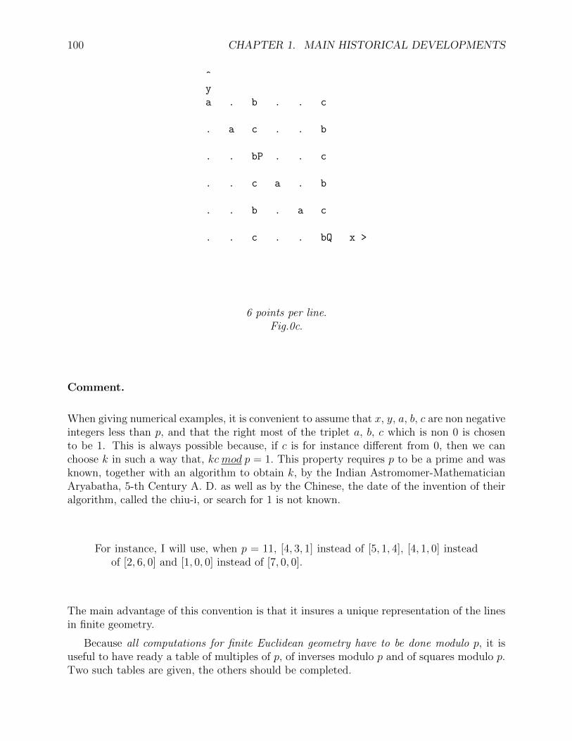
100 CHAPTER 1. MAIN HISTORICAL DEVELOPMENTS
^
y
a . b . . c
. a c . . b
. . bP . . c
. . c a . b
. . b . a c
. . c . . bQ x >
6 points per line.Fig.0c.
Comment.
When giving numerical examples, it is convenient to assume that x, y, a, b, c are non negativeintegers less than p, and that the right most of the triplet a, b, c which is non 0 is chosento be 1. This is always possible because, if c is for instance different from 0, then we canchoose k in such a way that, kc mod p = 1. This property requires p to be a prime and wasknown, together with an algorithm to obtain k, by the Indian Astromomer-MathematicianAryabatha, 5-th Century A. D. as well as by the Chinese, the date of the invention of theiralgorithm, called the chiu-i, or search for 1 is not known.
For instance, I will use, when p = 11, [4, 3, 1] instead of [5, 1, 4], [4, 1, 0] insteadof [2, 6, 0] and [1, 0, 0] instead of [7, 0, 0].
The main advantage of this convention is that it insures a unique representation of the linesin finite geometry.
Because all computations for finite Euclidean geometry have to be done modulo p, it isuseful to have ready a table of multiples of p, of inverses modulo p and of squares modulo p.Two such tables are given, the others should be completed.

1.9. MODEL OF FINITE EUCLIDEANGEOMETRY IN CLASSICAL EUCLIDEANGEOMETRY.101
p = 7,i 0 1 2 3 4 5 6p i 0 7 14 21 28 35 421i
− 1 4 5 2 3 6i2 0 1 4 2 2 4 1p = 11,i 0 1 2 3 4 5 6 7 8 9 10p i 0 11 22 33 44 55 66 77 88 99 1101i
− 1 6 4 3 9 2 8 7 5 10i2 0 1 4 9 5 3 3 5 9 4 1p = 13,i 0 1 2 3 4 5 6 7 8 9 10 11 12p i1i
i2
p = 17,i 0 1 2 3 4 5 6 7 8 9 10 11 12p i1i
i2
i 13 14 15 16p i1i
i2
p = 19,i 0 1 2 3 4 5 6 7 8 9 10 11 12p i1i
i2
i 13 14 15 16 17 18p i1i
i2
Theorem.
A point (x, y) is on a line [a, b, c] if and only if(ax+ by + c)mod p = 0.
For instance, with p = 11, from ((12, 14)) on the line [[16,−10, 4]], it follows that(1, 2) is on line [5, 1, 4] or [4, 3, 1].
Theorem.
There are p2 points and p2 + p lines.
102 CHAPTER 1. MAIN HISTORICAL DEVELOPMENTS
Theorem.
2 distinct points determine a unique line.
Moreover, if A = (A0, A1) and B = (B0, B1), the line a through A and B is a = [A1 −B1, B0 − A0, A0B1 −B0A1].
For instance, for p = 11, if A = (9, 8) and B = (8, 6), a = [2, 10, 1].
Theorem.
2 distinct lines have at most one point in common.Moreover, if l = [l0, l1, l2] and m = [m0,m1,m2], let d := l0m1 − l1m0, if d is different from0, then the point P common to l and m is
P = ( l1m2−l2m1
d, l2m0−l0m2
d).
For instance, with p = 11, if l = [2, 10, 1] and m = [9, 9, 1], d = 5,15mod 11 = 9, P = (1 . 9, 7 . 9) = (9, 8).
Definition.
If 2 lines have no points in common, they are called parallel.This will occur if d = 0, because of 1.9.1.
For instance, with p = 11, a = [2, 10, 1] is parallel to b = [5, 3, 1].
The following figure gives also a representation of points in finite geometry. The rep-resentative which is chosen is that with integer coordinates, non negative and less than p(0 ≤ x, y < p).The reader is asked to ignore for now the information at the left of the figure. The possiblepoints are indicated with “.”, a named point has its name just to the right of it. All pointson a line a are indicated by replacing “.” by ”a”. If 2 lines have a point in common, one ofthe 2 lines is chosen. The other could be indicated by the reader, if he so desires.

1.9. MODEL OF FINITE EUCLIDEANGEOMETRY IN CLASSICAL EUCLIDEANGEOMETRY.103
Example.
. ^
y
bDb . . . . . c . b . . a
. . . . c . . . . bA . .
. . c . . . . aB . . b .
. . . . . a . . . . . cC
. b . a . . . . . cD . .
. a b . . . . c . . . .
. . . b . c . . . . a .
. . . c b . . . a . . .
cDa c . . . b a . . . . .
. . . . a . b . . . c .
. . a . . . . b c . . . x >
Points, lines and parallels.Fig. 1, p = 11.
The points are A = (8, 9), B = (6, 8), C = (10, 7), the line a = [10, 2, 1] is the line throughA and B, it passes through the points (0,5), (2,6), (4,7), (6,8), (8,9), (10,10), (1,0), (3,1),(5,2), (7,3) and (9,4). The line b = [9, 9, 1] is the line through A and C. The line c = [3, 5, 1]passes through C, has no points in common with a and therefore is parallel to a. The line d,which is not indicated on the picture, is parallel to b and passes through B. The point D ison c and d.As an exercise determine the coordinates of D and the other points of d.
Notation.
To ease description of constructions in geometry, I have introduced the notation A×B, forthe line l through the distinct points A and B, and l ×m, for the point C common to thedistinct lines l and m.

104 CHAPTER 1. MAIN HISTORICAL DEVELOPMENTS
Comment.
If p is very large, and the unit used for the representation is very small, the Angstrom =10−8 cm, say, the points on a line will appear as we imagine them in the classical case. Butit is clear that they are not connected. Connectedness is a property in classical Euclideangeometry, which has no counterpart in the finite case. Moreover, the finite case should, whenfully understood, give a better model for a world which is atomic, whatever the smallestparticle is and which is finite, whatever the size of the universe is.
1.9.2 Parallels, parallelograms, distance.
Introduction.
Parallels have been defined in 1.9.1. In this section, I will give properties of parallel linesand define parallelograms. It is appropriate at this stage to define distances between points.In the finite case, the square of a distance is the appropriate basic concept, if we do notwant to introduce “imaginaries”. Properties of the parallelogram allow us then to derive aconstruction for the mid-point of a segment. The barycenter will be define in section 1.9.4.
Theorem.
Given a line l and a point P not on l, there exists a unique line m through P parallel to l.Moreover, if P = (P0, P1) and l = [l0, l1, l2] then
m = [l0, l1,−(P0l0 + P1l1)],
Definition.
Given 3 points A, B, C not on the same line, let c be the line through C parallel to the linea through A and B, let d be the line through A parallel to the line b trough B and C, A,B, C, D is called a parallelogram. The lines A × C and B ×D are called diagonals, theirintersection is called the center of the parallelogram.
Comment.
In Euclidean geometry, opposites sides of a parallelogram are equal. To generalize, I observefirst, that distances in Euclidean geometry are always considered positive. This is consistentwith the distance of AB equal to the distance of BA. But when working modulo p, we cannotintroduce positive numbers, keeping the requirement that the product and sum of positiveintegers modulo p is positive. Also not every integer modulo p has a square root hence weuse the square of the distance instead. To use a terminology reminiscent of that used inEuclid’s time, I will say the square on AB, for the square of the distance between A and B.
Definition.
Given 2 points A = (A0, A1) and B = (B0, B1), the square on AB, denoted (AB)2 is(B0 − A0)2 + (B1 − A1)2 mod p.

1.9. MODEL OF FINITE EUCLIDEANGEOMETRY IN CLASSICAL EUCLIDEANGEOMETRY.105
For instance, for p = 19, if A = (8, 11), B = (12, 9), the square on AB is(AB)2 = (16 + 4) mod 19 = 1. But, for p = 13, the square on AB, whereA = (1, 2) and B = (2, 7) is (1 + 25)mod 13 = 0, therefore the square can bezero for distinct points A and B. See 1.9.5.
Definition.
2 segments AC and BD are equal if the square on AC equals the square on BD.I write AC = BD.
For instance, with p = 19, if A = (7, 11), B = (11, 9), C = (9, 7) and D = (9, 13)then (AC)2 = 1, (BD)2 = 1, (AB)2 = 1, (CD)2 = 17. Therefore AC = BD.
Definition.
A point M on the line through A and C such that the square on AM is equal to the squareon CM is called the mid-point of AC.
Theorem.
In a parallelogram A, B, C, D, with A×B parallel to C×D and A×D parallel to B×C,the square on AB is equal to the square on CD, the square on AD is equal to the square onBC. The center M is the midpoint of the diagonals A× C and B ×D.
Moreover, if A = (A0, A1), B = (A0 +B0, A1 +B1), D = (A0 + C0, A1 + C1),then C = (A0 +B0 + C0, A1 +B1 + C1), M = (A0 + B0+C0
2, A1 + B1+C1
2),
(AB)2 = (CD)2 = B20 +B2
1 , (AD)2 = (BC)2 = C20 + C2
1 ,(AM)2 = (MC)2 = 1
4((B0 + C0)2 + (B1 + C1)2).
Example.
The given points are A = (7, 11), B = (9, 13), C = (11, 9). D = (9, 7), M = (9, 10).(AB)2 = (CD)2 = 1, (AD)2 = (BC)2 = 8. (AM)2 = (MC)2 = 5, (BM)2 = (MD)2 = 9.

106 CHAPTER 1. MAIN HISTORICAL DEVELOPMENTS
. ^
y
. . c . . . . . . . . . . . d a . b . .
.Df c . . . d . . b . . . . . a . . . . .
. . . . . . . . . . . . . a . d . . b c
. . . . . . d . . b . . a . . . . . c .
. . . . . . . . . . . a . . . . d c . b
. . . . . . . d . . bB. . . . . c . . .
. b . . . . . . . a . . . . . c . d . .
. . . . . . . . dA. . b . . c . . . . .
.Dm . b . . . . a . . .M. . c . . . . d .
dDb . . . . . a . . d . . cC. . . . . . .
. . . b . a . . . . . c . . . . . . . d
. . . . a . . . . . dD. . b . . . . . .
. d . a b . . . . c . . . . . . . . . .
. . a . . . . . c . . d . . b . . . . .
. a d . . b . c . . . . . . . . . . . .
. . . . . . c . . . . . d . . b . . . a
. . . d . c b . . . . . . . . . . . a .
cDa . . . c . . . . . . . . d . . b a . .
. . . c d . . b . . . . . . . . a . . . x >
Parallelogram and mid-point of A B.Fig. 2, p = 19.
1.9.3 Perpendicularity.
Introduction.
The perpendicularity of lines is defined. Theorem 1.9.3 follows from the correspondingtheorem in classical geometry and from the analytical property of perpendicular lines adaptedmodulo p.An application giving the orthocenter of a triangle is also given.
Definition.
Two lines l = [l0, l1, l2] and m = [m0,m1,m2] are perpendicular iffl0m0 + l1m1 mod p = 0.
For instance, with p = 11, l = [7, 6, 1] and m = [3, 2, 1] are perpendicular.
Theorem.
If 2 lines l and m are perpendicular to the same line a, then they are parallel.
1.9. MODEL OF FINITE EUCLIDEANGEOMETRY IN CLASSICAL EUCLIDEANGEOMETRY.107
For instance, with p = 11, l = [9, 1, 1] and m = [1, 5, 1] are perpendicular toa = [6, 1, 1] and are parallel.
Theorem.
Given a triangle A, B, C with sides a, b and c, if p is the perpendicular from A to a, q isthe perpendicular from B to b and r the perpendicular from C to c, then the three lines p, qand r have a point H in common.
Definition.
The lines p, q and r of Theorem 1.9.3 are called altitudes, the point H is called the orthocenterof the triangle A, B, C.
Example.
The given points are A = (8, 4), B = (4, 8), C = (3, 2), the sides are a = [1, 9, 1], b = [6, 7, 1],c = [10, 10, 1], the altitudes are p = [1, 6, 1], q = [2, 3, 1], r = [10, 1, 1] and the orthocenter isH = (7, 6).As an exercise, indicate on the figure one of the sides and compare how points are derivedfrom each other with those of the perpendicular line, c and r are the easiest, b and q themore difficult.

108 CHAPTER 1. MAIN HISTORICAL DEVELOPMENTS
. ^
y
.Dc r q . . . p . . . . .
. p . . . . . . . q . r
.Db . . . . qB . p . . r .
. q p . . . . . . r . .
. . . . . . . . qH . . .
pDp . . p q . . r . . . .
qDq . . . . . r . . pA . q
. . . . p r . q . . . .
.Da . . q rC . . . . . p .
rDr . . r . p . . . . q .
. . r . . . q . . . . p x >
The orthocenter H of A, B, C.Fig. 3, p = 11.
1.9.4 Circles, tangents and diameters.
Introduction.
Having the notion of distance, we can define a circle. Having a diameter A,B we candefine the tangent at A as the perpendicular to A × B. The medians and barycenter aredefined and the relation between the center of a circumcircle and the mediatrices of the sidesis given. The proofs depend on the following Theorem:
Given a prime p, there exists a circle C ′ of radius r′ in Euclidean geometry which containsrepresentatives P ′ of each point P of a circle C of radius r := r′ mod p in finite Euclideangeometry.
For instance, when p = 19, the circle C of radius 1 contains the points (0, 1),(3, 7), (2, 4), and therefore the points (7, 3), (3,−7), (7,−3), (−3, 7), (−7, 3),(−3,−7), (−7,−3), (4, 2), (2,−4), (4,−2), (−2, 4), (−4, 2), (−2,−4), (−4,−2),(1, 0), (0,−1), (−1, 0) altogether 20 points.
02 + 752 = 602 + 452 = 212 + 722 = 752, therefore, in Euclidean Geometry,((0, 75)), (60, 45)), ((21, 72)) are on the circle C ′ of radius r′ = 75, moeover

1.9. MODEL OF FINITE EUCLIDEANGEOMETRY IN CLASSICAL EUCLIDEANGEOMETRY.109
r′mod19 = −1, 60mod19 = 3, 45mod19 = 7, 21mod19 = 2, 72mod19 = −4.Appropriate change of signs give the other points, for instance ((-60,45))corresponds to (-3,-7) is also on C ′.
We can also replace in the Theorem just quoted the radius r′ by the radius squarer′2 = r′2.The following solutions are especially attractive, because the points on the circle in theEuclidian plane are also the representatives in the finite Euclidean plane.
p r′2 points5 1 (0, 1)5 2 (1, 1)5 3 (2, 2)5 4 (0, 2)7 5 (1, 2)7 13 (2, 3)
11 25 (0, 5), (3, 4)13 25 (0, 5), (3, 4)17 65 (1, 8), (4, 7)
Definition.
Given a point A and an integer d, the points P such that the square on PA is equal to d areon a circle of center A and radius square d.
Notation.
From here on, it is often more convenient to have the origin at the center of the figure. Wewill then replace the condition
0 ≤ x, y, a, b, c < pby
−p2< x, y, a, b, c < p
2.
Theorem.
For a circle centered at the origin,if (x, 0) (x 6= 0) is a point, so are (−x, 0), (0, x), (0,−x),if (x, x) (x 6= 0) is a point, so are (x,−x), (−x, x), (−x,−x),if (x, y) is a point (x 6= y, both non zero), so are (y, x), (−x, y), (y,−x), (x,−y), (−y, x),(−x,−y), (−y,−x).
Example.
. ^
y
. . . . . . . . . . . .

110 CHAPTER 1. MAIN HISTORICAL DEVELOPMENTS
. . c . . . . . . . c .
. . . . . c . c . . . .
. . . . . . . . . . . .
. . . c . . . . . c . .
. . . . . . .A . . . . . x >
. . . c . . . . . c . .
. . . . . . . . . . . .
. . . . . c . c . . . .
. . c . . . . . . . c .
. . . . . . . . . . . .
Circle of center A. Fig. 4, p = 11.
A = (0, 0), the points labelled c are on a circle with center A and with radius square10. The line [0,1,0] through A has no point in common with the circle, the line [1,-3,0] has2 points in common with the circle, (3,1) and (3,-1), the line [1,-1,0] has also 2 points incommon with the circle, (4,4) and (-4,-4).
Exercise.
Indicate on the Fig. 4 by r the points on a circle with radius square 3.
Theorem.
If p+1 is divisible by 4, there are p+1 points on the circle. Otherwise, there are p−1 pointson the circle.
Definition.
If a line t through a point P on a circle has no other points in common with the circle, it iscalled a tangent to the circle.
Theorem.
If a line l through a point P of a circle is not tangent to it, it intersects the circle at an otherpoint Q.

1.9. MODEL OF FINITE EUCLIDEANGEOMETRY IN CLASSICAL EUCLIDEANGEOMETRY.111
Definition.
A line through the center of a circle is called a diameter.
Theorem.
Half of the diameters have 2 points in common with the circle, half of them of no points incommon with the circle.
Theorem.
The tangent at a point A of a circle is perpendicular to the diameter passing through A.
Example.
Given the point A = (6, 6) and the radius square 5, the points labeled c are on the circlecentered at A. The tangent t at P = (4, 7) is [9, 1, 1]. The point C = (2, 3) is ont the tangent.The line d = [3, 6, 1] is a diameter through P.

112 CHAPTER 1. MAIN HISTORICAL DEVELOPMENTS
. ^
y
. t . . . . . c . . d .
dDd d . . . . t . . . . .
. . . d . . c . c . . t
. . . . . tP . . . c . .
tDt . . c . . . dA . . t c
. . . . t c . . . d . .
. . . . . . c . c t . d
. . d tC . . . . . . . .
. . . . d . . c t . . .
. . t . . . d . . . . .
. . . . . . . t d . . . x >
Circle, tangent and diameter. Fig. 5, p = 11.
Exercise.
Determine the other point Q on d and the circle and the tangent at Q.
Theorem.
If B and C are points on a diameter of a circle and on the circle and A is an other point ofthe circle, A×B is perpendicular to A× C.
Definition.
The medians of a triangle are the lines joining the vertices to the mid-points of the oppositeside.
Theorem.
The medians of a triangle have a point G in common.

1.9. MODEL OF FINITE EUCLIDEANGEOMETRY IN CLASSICAL EUCLIDEANGEOMETRY.113
Definition.
The point G of 1.9.4 is called the barycenter of the triangle.
Definition.
The anti-complementary triangle D,E, F has its side E×F through A parallel to B×C,and similarly for E and F.
Theorem.
The mid-points M, N, O of the sides of the triangle A,B,C are also the mid-points ofAD, BE and CF.
Example.
.Da ^
y
. . . . o m n . . . . . . . . . . . . .
. . . . n . . o . . . . . . . m . . . .
o . n . . . m . . . o . . . . . . . . .
. . . . . . . . . . . . . o . . m . . n
. . . . . . . mA. . . . . . . . oFnE. .
.Dc . . . . . . . . . . . . . . n . m . o
. . . o . . . . m . . . . n . . . . . .
. . . . . . oO. . . . nN. . . . . . m .
. . . . . . . . . oG. . . . . . . . . .
m . . . . . . n . . . . o . . . . . . m
. . . . . nB. . . . mM. . . . oC. . . .
. m . n . . . . . . . . . . . . . . o .
. n o . . . . . . . . m . . . . . . . .
.Db . m . . o . . . . . . . . . . . . n .
. . . . . . . . o . . . m . . . n . . .
. . . m . . . . . . . o . . n . . . . .
n . . . . . . . . . . . n mDo . . . . .
. . . . m . . . . . n . . . . . . o . .
. o . . . . . . n . . . . . m . . . . . x >
Medians and barycenter. Fig. 6a, p = 19.
The given points are A = (6, 14), B = (4, 8), C = (14, 8).The anti-complementary points are D = (12, 2), E = (16, 14), F = (15, 14).The mid-points are M = (12, 2), N = (15, 14), O = (16, 14).The medians are m = [16, 8, 1], n = [8, 3, 1], o = [13, 1, 0]. The barycenter is G = (8, 10).

114 CHAPTER 1. MAIN HISTORICAL DEVELOPMENTS
Exercise.
Indicate on Fig. 6a, the line F ×D through 2 mid-points and observe that F ×D is parallelto C × A.
Definition.
The mediatrix of AB is the line through the mid-point of AB perpendicular to A×B.
Theorem.
The mediatrices of the sides of a triangle pass through the center of the circumcircle of thetriangle.
Example.
.Da$ ^
y
. . q . r . . c . . p . . c . . . . . .
. . . . . . q r . . p . . . . . . . . .
rDr . . . . . . . . . rZ. . . . . . . . .
qDq . . . . . . . . . p . . r q . . . . .
. . . . . . . cA. . p . . c . . rF.Eq .
.Dc . . q . . . . c . p . c . . . . . . r
. . . r . . c q . . p . . . c . . . . .
. . c . . . rO. . . p qN. . . . . . c .
. . . . . . . . . r p . . . . q . . . .
. . . . . . . . . . p . r . . . . . . q
. . . . q cB. . . . pM. . . . cC. . . .
. . . . . . . . q . p . . . . . . . r .
. . r . . . . . . . p . q . . . . . . .
.Db . . . . c . . . . p . . . . c q . . .
. q . . . . . . r . p . . . . . . . . .
. . . . . q . . . . p r . . . . . . . .
. . c . . . . . . q p . . .Dr . . . c .
. . . . . . c . . . p . . q c . . r . .
pDp r . . . . . . c . p . c . . . . q . . x >
Mediatrices and center of circumcircle. Fig. 6b, p = 19.
The given points are the same as in Example 1.9.4. The mediatrices p = [2, 0, 1], q =[13, 14, 1], r = [13, 1, 0] pass through the center Z = (9, 16) of the circumcircle C of thetriangle A,B,C.

1.9. MODEL OF FINITE EUCLIDEANGEOMETRY IN CLASSICAL EUCLIDEANGEOMETRY.115
Exercise.
Determine the radius square of the circle and check that (AZ)2 = (BZ)2 = (CZ)2.Check that if Y is some point on q, (AY )2 = (CY )2.
Theorem.
If A, B, C and D are points on a circle and AB is parallel to CD then the square on ACequals the square on BD and the square on AD equals the square on BC.
1.9.5 The ideal line, the isotropic points and the isotropic lines.
Introduction.
It is now time to explain the points located at the left of each figure. In classical geometry, theplane can be extended to contain elements which are not points but have similar properties.For instance, all lines which are parallel to a given line l have no points in common, but theyall have the same direction. A direction is also called a point at infinity or an ideal point.If we extend the Euclidean plane in this way we see that 2 points ideal or not determine aunique line, with the exception of 2 ideal points. To have no exceptions, we also introduce theline at infinity or ideal line, which contains all ideal points. This extended Euclidean plane,which is unfortunately not part of high school education, is a first step to the understandingof projective geometry. Other notions which are known to those familiar with complexEuclidean geometry are the isotropic points, the isotropic lines and their properties. Thesenotions also extend to the finite case and, with the definition of distance used, give rise toreal points when the prime is of the form 4k+ 1. The distance between points which are notboth ordinary is not defined.
To represent points we will now use, as for lines, 3 coordinates, not all 0, and (x, y, z)will not be considered distinct from (kx, ky, kz), k 6= 0.The ordinary points (x, y) will also be noted (x, y, 1) or (kx, ky, k).
Definition.
The ideal line is the line [0, 0, 1], the ideal points or directions are the points (P0, P1, 0).
Definition.
A point P = (P0, P1, P2) is on a line l = [l0, l1, l2] ifP0l0 + P1l1 + P2l2 mod p = 0.
Theorem.
All p + 1 ideal points are on the ideal line. There are p2 + p + 1 ordinary and ideal pointsand p2 + p+ 1 ordinary and ideal lines.
116 CHAPTER 1. MAIN HISTORICAL DEVELOPMENTS
Theorem.
If 2 lines l and m are parallel, they have an ideal point in common or have the same direction.Moreover, if l = [l0, l1, l2] this point is Dl = (l1,−l0, 0) and if m = [m0,m1,m2], then
d := l0m1 − l1m0 = 0.
Definition.
If 2 lines l and m are perpendicular, their ideal points or directions are said to be perpendic-ular.
Moreover, if the direction of l is Dl = (l1,−l0, 0), that of m is Dm = (l0, l1, 0).
Comment.
The ideal points are represented to the left of the figures. (1,0,0) is at the top the otherpoints are from the bottom up (0,1,0), (1,1,0), (2,1,0), (3,1,0), . . ..
Example.
In Fig. 1, the point Da = (2, 1, 0) is the ideal point on a = [10, 2, 1], and c = [3, 5, 1], thepoint Db = (10, 1, 0) is the ideal point on b = [9, 9, 1] and d.
In Fig. 2, the points Da = (1, 1, 0), Db = (9, 1, 0), Df = (17, 1, 0), Dm = (10, 1, 0) arerespectively the ideal points on a = [5, 14, 1], b = [3, 11, 1], f = [17, 15, 1], m = [14, 12, 1]. mis the mediatrix of AC.
In Fig. 3, Da = (2, 1, 0) and Dp = (5, 1, 0), Db = (8, 1, 0) and Dq = (4, 1, 0), Dc =(10, 1, 0) and Dr = (1, 1, 0) are the direction of pairs of perpendicular lines.
In Fig. 5, Dd = (9, 1, 0) is the direction of the diameter d = [3, 6, 1]. Dt = [6, 1, 0] is thedirection perpendicular to Dd and of the tangent t = [9, 1, 1].
Definition.
The isotropic points are the ideal points (i, 0, 1) and (−i, 0, 1) where i is a solution of i2+1 = 0.
Theorem.
The isotropic points exist if p is of the form 4k + 1 (or p is congruent to 4 modulo 1), theydo not, otherwise.
The proof of this result goes back to Euler.
For instance, if p = 5, i = 2, if p = 13, i = 5, if p = 17, i = 4.
Definition.
In the extended Euclidean plane, (X0, X1, X2) is on the circle with center (C0, C1, C2) andradius square R2 if
0. (X0 − C0X2)2 + (X1 − C1X2)2 = R2X22 .
If X2 = 1, we obtain the usual equation.
1.9. MODEL OF FINITE EUCLIDEANGEOMETRY IN CLASSICAL EUCLIDEANGEOMETRY.117
Theorem.
When the isotropic points exist, they are on each of the circles.Indeed, if X0 = i, X1 = 1 and X2 = 0, 1.9.50 becomes i2 + 1 = 0.
Definition.
The isotropic lines are any ordinary line passing through an isotropic point.
Theorem.
The isotropic lines are perpendicular to themselves.
Theorem.
The isotropic lines through the center of a circle are tangent to that circle at the isotropicpoint.
Theorem.
If A and B are ordinary points on the same isotropic line, the square on AB is 0.Indeed, if A = (A0, A1, 1) and B = (B0, B1, 1), the line A × B which is [A1 − B1, B0 −
A0, A0B1 − A1B0] passes through (i, 1, 0) if(A1 −B1)i = A0 −B0.
But the square on AB is (A0 −B0)2 + (A1 −B1)2 = (A1 −B1)2(i2 + 1) = 0.
Comment.
Because of 1.9.5, when p is congruent to 1 modulo 4, it is possible for the square on AB tobe 0 for distinct points A and B.
Example.
The circle C of center A = (8, 8) passes through P = (4, 10) and through the isotropicpoints J = (4, 1, 0) and K = (13, 1, 0). The isotropic lines through A are j = [5, 14, 1] andk = [14, 5, 1].

118 CHAPTER 1. MAIN HISTORICAL DEVELOPMENTS
i ^
y
i . . . . . . j . . . k . . . . . .
i . . j . . . . . . . . . . . k . .
i . k . . . . . c . c . . . . . j .
cK . . . . . k . . . . . j . . . . .
i . . . . . . c j . k c . . . . . .
i . . . j . . . . . . . . . k . . .
i k . . . cP. . . . . . . c . . . j
i . . c . k . . . . . . . j . c . .
i . . . . . . . . kA. . . . . . . .
i . . c . j . . . . . . . k . c . .
i j . . . c . . . . . . . c . . . k
i . . . k . . . . . . . . . j . . .
cJ . . . . . . c k . j c . . . . . .
i . . . . . j . . . . . k . . . . .
i . j . . . . . c . c . . . . . k .
i . . k . . . . . . . . . . . j . .
i . . . . . . k . . . j . . . . . . x >
Ideal line, isotropic points and isotropic lines. Fig. 7, p = 17.
1.9.6 Equality of angles and measure of angles.
Introduction.
The definition of angles is the most difficult aspect of finite geometry. To approach thesubject, I will give a construction which obtains points on a circle which are equidistant. Ifwe obtain in this way all 2q = p+ 1 or p− 1 distinct points on the circle, then the smallestangle or unit angle can be defined. The proof that this is always possible will be given.The equidistance follows from that in Euclidean geometry, for the same construction, butto better illustrate, I will give an independent argument in 1.9.6 Examples for p = 11, 13and 17 have been chosen, because in these particular cases, the points on the circle in finiteEuclidean geometry are also points on a circle in classical Euclidean geometry.
Construction.
Given a diameter of a circle with the points A0 and Aq on it and an other point A1 on thecircle, I will construct A2, A3, . . . , as follows.Let C be the center of the circle, A2 is such that Aq × A2 is parallel to C × A1, and suchthat A0 × A2 is perpendicular to C × A1 (A0 × A2 is parallel to the tangent at A1). Givensome point Aj different from A1, Aj + 1 is such that A0 ×Aj + 1 is parallel to A1 ×Aj andAq × Aj + 1 is perpendicular to A1 × Aj. Using j = 2, 3, . . . , we obtain A3, A4, . . . .
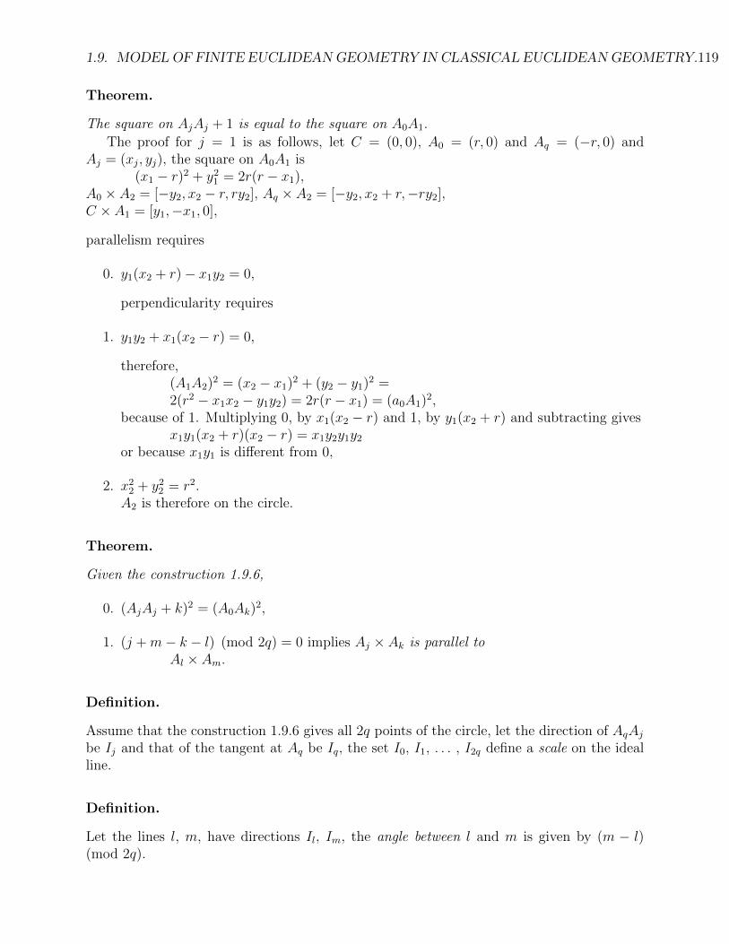
1.9. MODEL OF FINITE EUCLIDEANGEOMETRY IN CLASSICAL EUCLIDEANGEOMETRY.119
Theorem.
The square on AjAj + 1 is equal to the square on A0A1.
The proof for j = 1 is as follows, let C = (0, 0), A0 = (r, 0) and Aq = (−r, 0) andAj = (xj, yj), the square on A0A1 is
(x1 − r)2 + y21 = 2r(r − x1),
A0 × A2 = [−y2, x2 − r, ry2], Aq × A2 = [−y2, x2 + r,−ry2],C × A1 = [y1,−x1, 0],
parallelism requires
0. y1(x2 + r)− x1y2 = 0,
perpendicularity requires
1. y1y2 + x1(x2 − r) = 0,
therefore,(A1A2)2 = (x2 − x1)2 + (y2 − y1)2 =2(r2 − x1x2 − y1y2) = 2r(r − x1) = (a0A1)2,
because of 1. Multiplying 0, by x1(x2 − r) and 1, by y1(x2 + r) and subtracting givesx1y1(x2 + r)(x2 − r) = x1y2y1y2
or because x1y1 is different from 0,
2. x22 + y2
2 = r2.A2 is therefore on the circle.
Theorem.
Given the construction 1.9.6,
0. (AjAj + k)2 = (A0Ak)2,
1. (j +m− k − l) (mod 2q) = 0 implies Aj × Ak is parallel toAl × Am.
Definition.
Assume that the construction 1.9.6 gives all 2q points of the circle, let the direction of AqAjbe Ij and that of the tangent at Aq be Iq, the set I0, I1, . . . , I2q define a scale on the idealline.
Definition.
Let the lines l, m, have directions Il, Im, the angle between l and m is given by (m − l)(mod 2q).
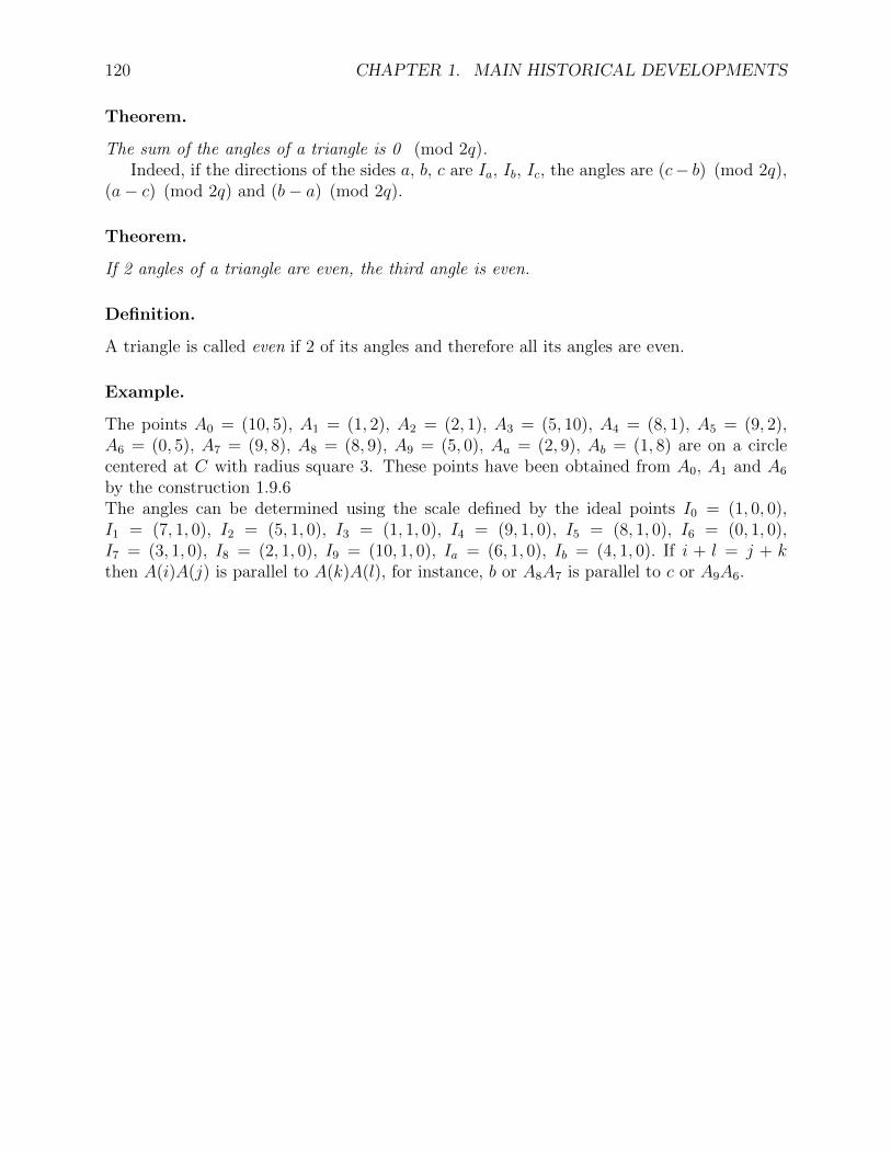
120 CHAPTER 1. MAIN HISTORICAL DEVELOPMENTS
Theorem.
The sum of the angles of a triangle is 0 (mod 2q).Indeed, if the directions of the sides a, b, c are Ia, Ib, Ic, the angles are (c− b) (mod 2q),
(a− c) (mod 2q) and (b− a) (mod 2q).
Theorem.
If 2 angles of a triangle are even, the third angle is even.
Definition.
A triangle is called even if 2 of its angles and therefore all its angles are even.
Example.
The points A0 = (10, 5), A1 = (1, 2), A2 = (2, 1), A3 = (5, 10), A4 = (8, 1), A5 = (9, 2),A6 = (0, 5), A7 = (9, 8), A8 = (8, 9), A9 = (5, 0), Aa = (2, 9), Ab = (1, 8) are on a circlecentered at C with radius square 3. These points have been obtained from A0, A1 and A6
by the construction 1.9.6The angles can be determined using the scale defined by the ideal points I0 = (1, 0, 0),I1 = (7, 1, 0), I2 = (5, 1, 0), I3 = (1, 1, 0), I4 = (9, 1, 0), I5 = (8, 1, 0), I6 = (0, 1, 0),I7 = (3, 1, 0), I8 = (2, 1, 0), I9 = (10, 1, 0), Ia = (6, 1, 0), Ib = (4, 1, 0). If i + l = j + kthen A(i)A(j) is parallel to A(k)A(l), for instance, b or A8A7 is parallel to c or A9A6.
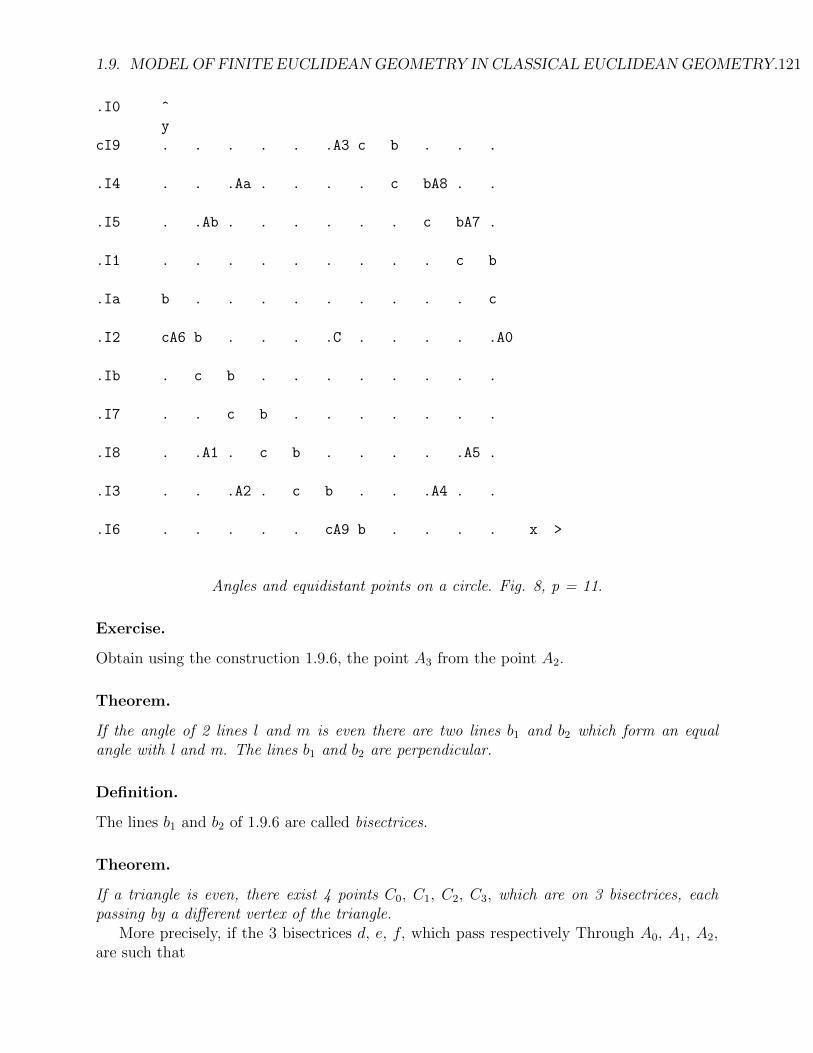
1.9. MODEL OF FINITE EUCLIDEANGEOMETRY IN CLASSICAL EUCLIDEANGEOMETRY.121
.I0 ^
y
cI9 . . . . . .A3 c b . . .
.I4 . . .Aa . . . . c bA8 . .
.I5 . .Ab . . . . . . c bA7 .
.I1 . . . . . . . . . c b
.Ia b . . . . . . . . . c
.I2 cA6 b . . . .C . . . . .A0
.Ib . c b . . . . . . . .
.I7 . . c b . . . . . . .
.I8 . .A1 . c b . . . . .A5 .
.I3 . . .A2 . c b . . .A4 . .
.I6 . . . . . cA9 b . . . . x >
Angles and equidistant points on a circle. Fig. 8, p = 11.
Exercise.
Obtain using the construction 1.9.6, the point A3 from the point A2.
Theorem.
If the angle of 2 lines l and m is even there are two lines b1 and b2 which form an equalangle with l and m. The lines b1 and b2 are perpendicular.
Definition.
The lines b1 and b2 of 1.9.6 are called bisectrices.
Theorem.
If a triangle is even, there exist 4 points C0, C1, C2, C3, which are on 3 bisectrices, eachpassing by a different vertex of the triangle.
More precisely, if the 3 bisectrices d, e, f, which pass respectively Through A0, A1, A2,are such that
122 CHAPTER 1. MAIN HISTORICAL DEVELOPMENTS
0. (angle(d, a) + angle(e, b) + angle(f, c)) (mod 2q) = qthen
d, e and f have a point in common.
Definition.
The 4 points C0, C1, C2, C3 are called center of the tangent circles.
Theorem.
There exist a circle with center Ci tangent to each of the sides of the triangle.

1.9. MODEL OF FINITE EUCLIDEANGEOMETRY IN CLASSICAL EUCLIDEANGEOMETRY.123
Example.
. ^
y
. r . c . . . . .B0 . . . a . . . r
c . . . . cA1 . . . . . . . . . . .
. . . . . . . c . . . . . . a . . .
r . . . . . a . . c . . . . . . . .
. . .B1 . . . . . . . c . . . a . .
. . . . . . r a . . . . r c . . . .
. . . . . . r . . . . . r . . c a .
. . . . . . . . a . . . . . . . . cA0
a . c . . . . . . . . . . . . . . a x >
. . . . c . . . . a . . . . . . . .B2
. a . . . . c . . . . . . . . . . .
. r . . . . . . c . a . . . . . . r
r . aA2 . . . . r . c . . . . . . .
. . . . . . . r . . . a c . . . . .
. . . a . . . . . .I. . . . c . . .
. . . . . . . r . . . r a . . . c .
. c . . a . . . r . r . . . . . . .
Bissectrices and inscribed circle. Fig.9, p = 17.
The given triangle is A0 = (8, 1, 1), A1 = (−4, 7, 1), A2 = (−7,−4). Its sides are a =[2, 1, 1], b = [−7, 4, 1], c = [5,−7, 1]. The bisectrices meet the circle at B0 = (−1, 8), B1 =(−7, 4), B2 = (8,−1). They are d = [8, 3, 1], e = [−3, 3, 1], f = [−4, 3, 1] and have the pointI = (0,−6) in common. The tangent circle r has radius square 5. Its points of contact witha, b, c are respectively (2,-5), (-3,3), (1,-4). Only a and c are given on the Figure, not toclutter it. The other centers of tangent circles are (-1,4), (3,-3) and (-2,5).
Exercise.
Determine that b is tangent to the circle r and that (−1, 4) is indeed a center of a tangentcircle.
1.9.7 Finite trigonometry.
Definition.
If r = 1 and the construction 1.9.6 gives all 2q points Aj = (xj, yj) of the circle with radiussquare 1. I define
sin(2j) := yj, cos(2j) := xj.

124 CHAPTER 1. MAIN HISTORICAL DEVELOPMENTS
Comment.
Because, in general, several points A1 can be chosen, there are several distinct but relatedtrigonometric functions sine and cosine. Each corresponds to a different choice of the unitangle. This is similar to the real case in which many different units are used, those withangles in radians, degrees, grades, for instance.
Comment.
I will develop the properties of the trigonometric functions and obtain functions which canbe considered as an analogue of the hyperbolic functions. An efficient method to obtainthem for large p will also be given.
Example.
For p = 11,i Ai angle(i)− 180i A′i1 (−4,−3) 3687 ((−4,−3))2 (−3,−4) 7374 ((7
5, 24
5))
3 (0, 5) 11061 ((4425,−117
25))
4 (3,−4) 14748 ((−527125, 336
125))
5 (4,−3) 18435 ((3116625
, 237625
))6 (−5, 0) 22122 ((−11753
3125,−10296
3125))
If Ai = (−4,−3), then 42 + 32 = 52, cos(i) = −45
= −3 andsin(i) = −3
5= −5.
For p = 13,i Ai angle(i)− 180i A′i1 (−3,−4) 5313 ((−3,−4))2 (−4,−3) 10626 ((−7
5, 24
5))
3 (0, 5) 15939 ((11725,−44
25))
4 (4,−3) 21252 ((−527125,−336
125))
5 (3,−4) 26565 ((237625, 3116
625))
6 (−5, 0) 31878 ((117533125
,−102963125
))
For p = 17,i Ai angle(i)− 180i A′i−1 (8, 1) −7125 ((8, 1))1 (8,−1) 7250 ((8,−1))3 (−4, 7) 21375 ((488
64,−191
65))
5 (7,−4) 35625 ((276884225
,−198414225
))7 (−1, 8) 49875 ((1426888
274625,−1692991
274625))
9111315

1.10. AXIOMATIC 125
Exercise.
Continue the last table obtaining the missing values.
Exercise.
Obtain trigonometric functions for p = 11 and check the familiar identities
0. sin2(x) + cos2(y) = 1,
1. sin(x+ y) = sin(x)cos(y) + sin(y)cos(x),
2. cos(x+ y) = cos(x)cos(y)− sin(x)sin(y),
Notation.
In a finite field there is no ambiguity in defining π := 2q.
1.10 Axiomatic
1.10.0 Introduction to Axiomatic.
The axiomatic study of Geometry has a long history, starting with Euclid. Among the mainearlier contributors are Giovanni Saccheri (1667-1733), Karl Gauss (1777-1855), Janos Bolyai(1802-1860), Nikolai Ivanovich Lobachevsky (1792-1856), de Tilly (1837-1906)17, Pieri, CarlMenger, Oswald Veblen (1880-1960), William Young (1863-1942), Julius Dedekind, FrederigoEnriques (1871-1946), I. Schur, David Hilbert (1862-1943), Marshall Hall and Alfred Tarski(1901-1983).To obtain a clear understanding of the relation between the synthetic and the algebraicpoint of view, an important step was the realization of the connection between the Axiomof Pappus and the commutativity of multiplication, first considered by Schur, in 1898, thenby Hilbert in 1899 (p. 71), by Artin in 1957 and many others, see Artzy (1965), Hartshorne(1967).A detailed history of the developments concerning Finite Geometry can be obtained fromthe monumental work of Dembowsky, 1968 and Pickert (Chapter 12).For some authors, the word projective geometry as moved away from its original meaning,to become a synonym of incidence geometry. I will not follow that practice.
What follows can be used to obtain a justification of the relation between the syntheticand algebraic axioms of Chapter II. With the exception of the proof of associativity andcommutativity of addition, I have borrowed heavily from Artzy’s book, which contains proofsnot given here, increasing the formalism to prepare for eventual computarization.
The axioms will progress from those ofthe perspective plane, with (Σ,+, ·) a ternary ring, (A ∗B ∗ C) and (Σ,+), (Σ− 0, ·) are
0G19.TEX [MPAP], September 9, 201917Blumenthal considers than in the paper of 1892, de Tilly makes a fundamental contribution by intro-
ducing n-point relations to characterize a space metrically.
126 CHAPTER 1. MAIN HISTORICAL DEVELOPMENTS
loops,to Veblen-Wedderburn plane, with (Σ,+, ·) a quasifield, (linear, right distributivity) and(Σ,+) an Abelian group,to Moufang plane, with (Σ,+, ·) an alternative division ring (left distributivity, right andleft inverse property),to Desarguesian plane, with (Σ,+, ·) a skew field, (associativity of multiplication),to Pappian plane, with (Σ,+, ·) a field, ( commutativity of multiplication),to Separable Pappian plane, with (Σ,+, ·) an ordered field,to Continuous Pappian plane with (Σ,+, ·) the field of reals.The definitions of Desargues and Pappus configurations, given in Chapter II, will not berepeated here.
1.10.1 The Perspective Plane.
Introduction.
Marshall Hall and D.T. Perkins independently succeeded to construct an algebraic structure,called ternary ring, 1.10.1 to coordinatize 1.10.1 the perspective plane1.10.1. Theorem 1.10.1shows that the first 4 conditions of the definition of a ternary ring are associated with theincidence property 1.10.1.3 and the others with Theorem 1.10.1. Theorem 1.10.1 proves thatthe set of the ternary ring is a loop under addition and multiplication.
Axioms. [Of Allignment]
Given a set of elements called points and a set of elements called lines with the relation ofincidence, such that
0. 2 points are incident to one and only one line.
1. 2 lines are incident to one and only one point.
2. there exists at least 4 points, any 3 of which are not collinear,
we say that the axioms of allignment are satisfied.
The terminology is that of Seidenberg, 1962, p. 56.
Definition.
A perspective plane is a set of points and lines satisfying the axioms of alignment. It is alsocalled a rudimentary projective plane. (Artzy, p. 201.)
Theorem.
Duality is satisfied in a perspective plane.
Menger gives a self dual set of equivalent axioms.

1.10. AXIOMATIC 127
Definition.
Given a point P and 2 lines a and b not incident to P, a perspectivity Π(P, a, b) is thecorrespondance between Ai ι a and Bi ι b, with Bi := (P × Ai)× b.Π−1(P, a, b) := Π(P, b, a) is the inverse correspondance which associates to Bi,Ai = (P ×Bi)× a.I will also use the notation Π(P,Ai, Bi).A projectivity is a perspectivity or the composition of 2 or more perspectivities.
Theorem.
Π is a bijection.
Definition.
Given a line m, we say that l is m-parallel to l′ iff l, l′ and m are incident and we writel //m l
′ and Iml := l ×m.Iml is called the m-direction of l.
Definition.
Given a linem, 2 pointsA andA′, not onm and a pointB neither onm nor on a := A×A′, thetranslation T m,BAA′ is the transformation which associates to I, I if I ιm and to points P neitheron a, nor on m the point P ′ := (P ×ImA×A′)×(A′×ImA×P ), and to C ιa, C ′ := (ImB×C×B′)×a,where B′ := T m,BAA′ (B).
Definition. [Marshall Hall] 18
(Σ, ∗) is a ternary ring iff Σ is a set and ∗ is an operation which associates to an orderedtriple in the set an element in the set satisfying the following properties
0. A ∗ 0 ∗ C = C,
1. 0 ∗B ∗ C = C,
2. 1 ∗B ∗ 0 = B,
3. A ∗ 1 ∗ 0 = A,
4. A ∗B ∗X = D has a unique solution X,
5. B1 6= B2 =⇒ X ∗B1 ∗ C1 = X ∗B2 ∗ C2 has a unique solution X,
6. A1 6= A2 =⇒ A1 × X × X ′ = D1 and A2 × X × X ′ = D2 have a unique solution(X,X’).
181943, also unpublished work by D. T. Perkins

128 CHAPTER 1. MAIN HISTORICAL DEVELOPMENTS
Theorem.
X ∗ 1 ∗ 1 = 0 has a unique solution X.
Proof: 1.10.1.0 implies X ∗ 0 ∗ 0 = 0, 1 6= 0, the Theorem follows from 1.10.1.5.
Definition.
A perspective plane can be coordinatized as follows, (Fig. 20a’)H0.0. Q0, Q1, Q2, U , 4 points, no 3 of which are collinear,D0.0. q0 := Q0 ×Q1, q1 := Q2 ×Q0, m := q2 := Q1 ×Q2,D0.1. v := Q2 × U , i := Q0 × U , V := i× q2, I := v × q0,D0.2. u := V × I.Let Σ be the set of points on q2, distinct from Q2. Define 0 := Q1, 1 := V .
The point Q2 is represented by (∞), ∞ being a new symbol.The points Q on q2, distinct from Q2 are represented by the element Q in Σ, placed betweenparenthesis, Q = (Q).A point P not on q2 is represented by a pair of elements (P0, P1) in Σ defined by (Fig. 20a”)
P0 := (((((P ×Q2)× i)×Q1)× v)×Q0)× q2,P1 := (((P ×Q1)× v)×Q0)× q2.
In particular, if a point A is on q0, then its second coordinate A1 = 0, we represent itsfirst coordinate by A, if a point C is on q1, then its first coordinate C0 = 0, we represent itssecond coordinate by C. Points on v have first coordinate 1.
The line q2 is represented by [∞],a line l0 through Q2 distinct from q2 is represented by [A], with a× q0 = (A, 0),a line m not through Q2 is represented by the pair M0,M1], where (M0) is the representationof the point m× q2 and where the point m× q1 on q1 is (0,M1).
Let P := ((A, 0)×Q2)× ((B)× (0, C)) = (A, Y ). Y is a function of A, B and C whichwe denote by
Y := A ∗B ∗ C.
Theorem.
There is a bijection between the points (A, 0) on q0, (0, A) on q1 and (A) on q2.
Proof: We use the perspectivity Π(Q2, q0, i), followed by Π(Q1, i, q1), or Π(Q1, q1, u),followed by Π(Q0, u, q2).
Comment.
If P = (P0, P1), all points on P × Q2 have the same first coordinate, P0, in particular,(P × Q2) × q0 = (P0, 0), all points on P × Q1 have the same second coordinate, P1, inparticular, (P ×Q1)× q1 = (0, P1).
In Euclidean Geometry, if q0 is the x axis, q1 is the y axis q2 is the ideal line andU = (1, 1, 1), (A,B) corresponds to (A,B, 1), (A) to (1, A, 0) which is the direction of lineswith slope A, (∞) to (0, 1, 0) which is the direction of y axis. The slope of the line joiningthe origin to (A,B, 1) is B
A.

1.10. AXIOMATIC 129
Theorem.
The incidence, noted “ι” satisfies,
0. (Q) ι [∞],
1. (P0) ι [P0, P1],
2. (P0, P1) ι [P0]),
3. (P0, P1) ι [M0,M1] iff P1 = P0 ∗M0 ∗M1.
Theorem.
0. (R0, R1) ι (Q2 × (A, 0)) =⇒ R0 = A,
1. (S0, S1) ι (Q1 × (0, C)) =⇒ S1 = C,
2. X := v × (Q0 × (B)) =⇒ X = (1, B),
3. (Y0, Y1) ι (Q0 × V ) =⇒ Y0 = Y1.
Theorem.
The pespective plane as coordinatized in 1.10.1 satisfies the properties of a ternary ring. Inparticular
0. the unique solution X of A∗B ∗X = D is the second coordinate of the point ((A,D)×(B))× q1,
1. with B1 6= B2, the unique solution X of X ∗B1 ∗C1 = X ∗B2 ∗C2 is the first coordinateof the point ((0, C1)× (B1))× ((0, C2)× (B2)),
2. with B1 6= B2, the unique solution (X,X ′) of A1×X×X ′ = D1 and A2×X×X ′ = D2
is given byX := ((A1, D1)× (A2, D2))× q2, X
′ := ((A1, D1)× (A2, D2))× q1,
Proof: For 0. to 3. of 1.10.1, we consider the points(R0, R1) := ((A, 0)×Q2)× ((0)× (0, C)) = (A,A ∗ 0 ∗ C) = (A,C),(S0, S1) := ((Q0 ×Q2)× ((B)× (0, C)) = (0, 0 ∗B ∗ C) = (0, C),X := ((1, 0)×Q2)× ((B)× (0, 0)) = (1, 1 ∗B ∗ 0) = (1, B),(Y0, Y1) := ((A, 0)×Q2)× ((V )× (0, 0)) = (A,A ∗ 1 ∗ 0) = (A,A).
Theorem.
The pespective plane satisfies also the properties:
0. X ∗ B ∗ C = D has a unique solution, the first coordinate of the point ((0, D)× q1)×((B)× (0, C)),
1. A∗X ∗C = D has a unique solution, the coordinate of the point ((A,D)× (0, C))× q2,
Proof: For 0, (X, Y ) ι [B,C], (X, Y ) ι [0, D], therefore Y = X ∗ B ∗ C = X ∗ 0 ∗D = D.For 1, (A,D) ι [X,C] therefore D = A ∗X ∗ C.

130 CHAPTER 1. MAIN HISTORICAL DEVELOPMENTS
Example.
Q0 = (0, 0), Q1 = (0), Q2 = (∞), U = (1, 1), V = (1), I = (1, 0), u = [1, z] with 1∗ 1∗ z = 0.q0 = [0, 0], q1 = [0], q2 = [∞], v = [1], i = [1, 0],Let (see Fig. 20a’)D0.3, J := u× q1 j := U ×Q1, W := j × q1, w := J ×Q1,D0.4. T := v × w, t := V ×W, R := t× q0, r := T ×Q0, S := r × q2,then, with S = (S),J = (0, S), j = [0, 1], W = (0, 1), w = [0, S], T = (1, S), t = [1, 1], r = [S, 0], R = (y, 0) withy ∗ 1 ∗ 1 = 0.
Definition.
The dual coordinatization can also be chosen. I will use the subscript d to indicate the dualrepresentation,The notation in the preceding example is chosen to allow the dual coordinatization using aselements of Σ the lines through a given point (∞). We choose (∞)d as Q2. The line q2 isrepresented by [∞]d, the line l0 := Q2 × (L0, 0) is represented by [l0]d = [L0], the line n notthrough Q2 is represented by [n0, n1]d, with
n0 := (((((l × q2)× I)× q1 × V )× q0)×Q2,n1 := (((l × q1 × V )× q0)×Q2.
in this case q0 = [0, 0]d, q1 = [0]d, q2 = [∞]d, u = [1, 1]d,, w = [0, 1]d, i = [1, 0]d, butj = [0, R]d, with t× q0 = (R, 0)d and t = [1, R]d. The representation of points is done duallyas in 1.10.1, with N represented by (N0, N1)d, with N ×Q2 = [N0]d and N ×Q1 = [0, N1]d.
Theorem.
0. (Σ,+) is a loop, with 0 as neutral element,
1. (Σ− 0, ·) is a loop with 1 as neutral element.
Proof: For the addition, the neutral element property follows from 1.10.1.1 with B = 1and from .3. The solution property follows from 1.10.1.4 and .6 with B = 1.For the multiplication, the neutral element property follows from 1.10.1.3 and 4. The solutionproperty follows from 1.10.1.4 and .5 with C = 0.
Theorem.
If the number of elements in Σ is a small number n,
0. If n = 2,3,4,5, there is only one perspective plane,
1. If n = 6, there is no perspective plane,
2. If n = 14,21,22,30,33,38,42,46,54,57,62,66,69,70,77, 78,86,93,94,. . . ,
3. If n = 10, there is no perspective plane,
1.10. AXIOMATIC 131
0, is easily settled, see II1, originates with the problem of the 36 officers, Euler (1782), was settled by Tarry (1900),2, depends on the next Theorem,3, has a long history, and was finaly proven, using computers, by Lam, Thiel and Swiercz(1989), see also Lam (1991).
Theorem. [Bruck and Ryser]
If n ≡ 1, 2 mod 4 and there are no integers x, y such that x2 + y2 = n then there are noperpective plane of order n.
Notation.
A+B := A ∗ 1 ∗B,A ·B := A ∗B ∗ 0,A+ (A ` B) = B, (B a A) + A = B.When A 6= 0, A · (A \B) = B, (B/A) · A = B.
In the Euclidean case, the line joining the point (A,A+ B) to the point (0, B) has slope1 and the slope of the line joining Q0 to (A,A.B) is C = A.B.
Definition.
A ternary ring (Σ, ∗) is linear iff for every A, B, C in the set(A ∗B ∗ 0) ∗ 1 ∗ C = A ∗B ∗ C.
Theorem.
If a ternary ring is linear thenA ∗B ∗ C = A ·B + C.
Axiom. [Fano]
The diagonal points of every quadrangle are not collinear.
Axiom. [N-Fano]
The diagonal points of every quadrangle are collinear.
Definition.
A Fano plane is a perspective plane which satisfies the N-Fano axiom.
Theorem.
In a Fano plane A+ A = 0.Proof: For the quadrangle Q0 = (0, 0), XA = (A, 0), YA = (0, A), A0 = (A,A), 2 of the
diagonal points are on q2, therefore the third diagonal point is V = (Q0×A0)× q2, therefore(A,A ∗ 1 ∗ A) coincides with XA and A+ A = 0.

132 CHAPTER 1. MAIN HISTORICAL DEVELOPMENTS
Exercise.
0. Prove that in a Fano plane (A ∗ B) ∗ (A ·B) = 0.
1. Determine a subset of quadrangles with collinear diagonal points which justify the pre-ceding property in a perspective plane.
2. Same question for the property A + A = 0.
Definition.
Two triangles APQ and A′P ′Q′ are m-parallel iffA× P //m A
′ × P ′, A×Q //m A′ ×Q′, P ×Q //m P
′ ×Q′.
Theorem.
If A ι l, l′ := A′ × Iml and P ι l then P ′ ι l′.In general, a line n not through A is not transformed into a line. For this to be so, if
P ι n and Q ι n, we want P ′ := T mAB(P ) and Q′ := T mAA′(Q) to be collinear with ImP×Q. Thissuggest the following Definition.
Axiom. [Of Desargues]
In a perspective plane, given any 2 triangles Ai, ai and Bi, bi,let ci := Ai ×Bi, and Ci := ai × bi, incidence(ci, C) =⇒ incidence(Ci, c).C is called the center, c is called the axis of the configuration.I write Desargues(C, Ai, Bi; 〈Ci〉, c).
Axiom. [Elated Desargues]
The Elated Desargues axiom is the special case when we restrict Desargues’ axiom to thecase when the axis c passes through the center C of the configuration. More specifically, C ιc,and for the 2 triangles Ai and Bi,let Ci := (Ai+1 × Ai−1)× (Bi+1 ×Bi−1),ci := (Ai ×Bi), ci ι C, i = 0, 1, 2, incidence(A0 × Aj, B0 ×Bj, c), j = 1, 2,=⇒ incidence(A1 × A2, B1 ×B2, c). We write
Elated-Desargues(C, Ai, Bi; 〈Ci〉, c).The terminology comes from that in projective geometry, which calls elation, a collineation
with an axis of fixed point and a center of fixed lines, with the center on the axis. This axiomis also called the minor Desargues axiom, see for instance Artzy, p. 210.
Theorem.
Given 2 triangles Ai and Bi, let Ci := (Ai+1×Ai−1)× (Bi+1×Bi−1), Ci := Ai×Bi, andC := c1 × c2,
〈Ci, c〉 and C ι c =⇒ c0 ι C. We writeElated-Desargues−1(c, Ai, Bi; 〈c0, c1, c2〉, C)
Proof: Desargues(C0, A1, B1, C2, A2, B1, C1; 〈B0, A0, C〉, c).

1.10. AXIOMATIC 133
1.10.2 Veblen-Wedderburn Planes.
Definition.
A Veblen-Wedderburn plane is a perspective plane for which the elated Desargues axiom issatisfied on a specific line of the plane.
Comment.
In all the construction that follow, H0.0 and .1, D0.0 to .4, of 1.10.1 and 1.10.1 will beassumed, but not all these constructions are necessarily required.
Lemma. [For the linearity property.]
H1.0. XA = (A, 0), YC := (0, C), (B), (See Fig. 21a)D1.0. jb := Q0 ×B, j′b := YC ×B, j1 := Q0 × V, j′1 := YC × V,D1.1. x := XA ×Q2, K := x× jb, k0 := K ×Q1, L := k0 × j1,D1.2. K ′ := x× j′b, c := L×Q2, L
′ := c× j′1, k′0 := L′ ×K ′,C1.0. Q1 ι k
′0.
Moreover,K = (A,A ·B), L = (A ·B,A ·B), K ′ = (A,A ∗B ∗ C), L′ = (A ·B,A ·B + C),C1.0 =⇒ A ∗B ∗ C = A ·B + C.
Proof:Elated-Desargues(Q2, Q0, K, L, YC , K ′, L′; 〈Q1, V, B〉, q2) =⇒ Q1 ι k
′0.
Lemma. [For the additive associativity law]
H1.0. XA, XB, YC , (See Fig. 21b)D1.0. a := XA ×Q2,D1.1. b := XB ×Q2, B1 := b× i, x1 := B1 ×Q1, Y1 := x1 × q1,D1.2. i2 := Y1 × V, A1 := i2 × a, x3 := A1 ×Q1, D1 := x3 × i,D1.3. d := D1 ×Q2, i1 := YC × V, D2 := d× i1,D1.4. B2 := i1 × b, x2 := B2 ×Q1, Y2 := x2 × q1,D1.5. i3 := Y2 × V, A2 := i3 × a, x4 := A2 ×D2,D1.6. e1 := A1 ×B1, e2 := A2 ×B2, E := e1 × e2,C1.0. E ι q2,C1.1. Q1 ι x4,
Moreover,B1 = (B,B), YB = (0, B), A1 = (A,A+B), D1 = (A+B,A+B),B2 = (B,B + C), Y1 = (0, B + C), A2 = (A,A+ (B + C)),D2 = (A+B, ((A+B) + C),C1.1. =⇒ A+ (B + C) = (A+B) + C.
Proof:19
Elated-Desargues(Q2, A1, B1, Y1; A2, B2, Y2; 〈Q1, V, E〉, q2),
19variant due to Michael Sullivan, October 24, 1989.
134 CHAPTER 1. MAIN HISTORICAL DEVELOPMENTS
=⇒ Elated-Desargues−1(q2, A1, B1, D1; A2, B2, D2; 〈V,Q1, E〉, Q2)=⇒ Q1 ι x4.
Corollary.
If 2 m-parallelograms Aj and Bj, j = 0, 1, 2, 3, are such thatAk ×Bk //m A0 ×B0, k = 1, 2, the same is true for k = 3. (See Fig. 21e)21e?
The parallelograms for which the proof is given in the Lemma areA1, YB, Y1, A2 and D1, B1, B2, D2.
Lemma. [For the right distributive law]
H1.0. XA = (A, 0), Y1 = (0, B), (C), (See Fig. 21c)D1.0. x := XA ×Q2,D1.1. x1 := Q1 × Y1, B1 := x1 × i, i1 := Y1 × V, A1 := i1 × x,D1.2. x3 := A1 ×Q1, F1 := x3 × i, f := F1 ×Q2, c1 := Q0 × C,D1.3. b := B1 ×Q2, B2 := b× c1, F2 := f × c1,D1.4. x2 := B2 ×Q1, Y2 := x2 × q1, e1 := Y2 × A1, e2 := B2 × F1,D1.5. E := e1 × e2,D1.6. c2 := Y2 × C, A2 := c2 × x, x4 := A2 × F2,C1.0. E ι q2.C1.1. Q1 ι x4.
Moreover,B1 = (B,B), A1 = (A,A+B), F1 = (A+B,A+B), B2 = (B,B · C),F2 = (A+B, (A+B) · C), Y2 = (0, B · C), A2 = (A,A ∗ C ∗ (B · C)), andC1.1 =⇒ (A+B) · C = A · C +B · C.
Proof:Elated-Desargues(Q1, Y1, A1, Y2, B1, F1, B2; 〈E,Q2, V 〉, q2) =⇒ E ι q2.Elated-Desargues−1(q2, A2, A1, Y2, F2, F1, B2; 〈E,C,Q2〉, Q1) =⇒ Q1 ι x4.Finally, from C1.0 follows (A+B) ·C = A ∗C ∗ (B ·C), but by linearity, the second memberequals A · C +B · C.
Exercise.
Determine the identity corresponding to C1.0 or to the m-parallelism of Y2×A1 and B2×F1.
Lemma. [For the commutativity law]
H1.0. A1, B1, (See Fig. 21d)D1.0. a0 := A1 ×Q0, A := a0 × q2, a2 := A×B1,D1.1. b0 := B1 ×Q0, B := b0 × q2, b2 := A1 ×B, D := b2 × a2,D1.2. x1 := A1 ×Q1, YA := x1 × q1, b1 := YA ×B,D1.3. y2 := B1 ×Q2, B2 := y2 × b1, x2 := B2 ×D, y1 := A1 ×Q2,D1.4. x3 := B1 ×Q1, YB := x3 × q1, a1 := YB × A, A2 := a1 × y1,C1.0. Q1 ι x2,C1.1. A2 ι x2,

1.10. AXIOMATIC 135
Moreover,if A1 = (XA, YA), and B1 = (XB, YB), then A2 = (XA, YA + YB), B2 = (XB, YB + YA),C1.0 and .1 =⇒ YA + YB = YB + YA.
Proof:Elated-Desargues(B, Q0, YA, A1, B1, B2, D; 〈Q1, A,Q2〉, q2) =⇒ Q1 ι x2.Elated-Desargues(A, Q0, YB, B1, A1, A2, D; 〈Q1, B,Q2〉, q2) =⇒ A2 ι x2.therefore A2 and B2 have the same second coordinate Y .Because A1 ι a0 ι (A), YA = XA ·A, by construction and because of linearity, A2 = (XA, XA ∗A ∗ YB) = (XA, XA · A+ YB) similarly YB = XB ·B, and B2 = (XB, XB ·B + YA).
Corollary.
If we make the same constructions as in the lemma with A = B = J, thenQ1 ι (A2 ×B2).
Lemma. [Addition an Negation in Veblen-Wedderburn planes.]
H0.0. YA, YB, (Fig.21e)D1.0. i1 := YA × V, i2 := YB × V,D1.1. x1 := YA ×Q1, A1 := x1 × i, a := A1 ×Q2, A2 := a× i2,D1.2. x3 := YB ×Q1, B1 := x3 × i, b := B1 ×Q2, B2 := b× i1,D1.3. x2 := A2 ×B2,C1.0. Q1 ι x2,D2.0. U1 := x1 × v, c := U1 ×Q0, A := c× q2,D2.1. c− := YA × I, A− := c−×q2,Moreover,If YA = (0, A) and YB = (0, B), then A1 = (A,A), B1 = (B,B), A2 = (A,A + B), B2 =(B,B + A),U1 = (1, A), A = (A), A− = (−A).
Theorem.
In a Veblen-Wedderburn plane, the ternary ring (Σ,*) is a quasifield in the terminology ofDembowski (p. 129):
0. (Σ, ∗) is linear, a ∗ b ∗ c = a · b + c,
1. (Σ,+) is an abelian group,
2. (Σ− 0, ·) is a loop,
3. (Σ, ∗) = (Σ,+, ·) is right distributive, (a+ b) · c = a · c+ b · c.
4. a 6= b =⇒ x · a = x · b+ c has a unique solution.
Theorem.
In a Veblen-Wedderburn plane with ideal line m, T m,BAA′ (C), C ιA×A′, is independent of B.We can therefore use T mAA′ as notation for a translation.

136 CHAPTER 1. MAIN HISTORICAL DEVELOPMENTS
Definition.
m-equality is defined by[A,A′] =m [P, P ′] iff P ′ = T mAA′(P ).
Theorem.
In a Veblen-Wedderburn plane we can use systematically 3 coordinates as follows(Q2) is equivalent to (0, 1, 0),(P0) is equivalent to (1, P0, 0),(P0, P1) is equivalent to (P0, P1, 1),[q2] is equivalent to [0, 0, 1],[M0] is equivalent to [1, 0,−M0],[M0,M1] is equivalent to [M0,−1,M1].A point (P0, P1, P2) is incident to the line [l0, l1, l2] iff
P0l0 + P1l1 + P2l2 = 0.Proof: In the general case, because of linearity, a point (P0, P1) is incident to the line
[M0,M1] if P1 = P0 ·M0 +M1, which we can rewriteP0 ·M0 + P1 · (−1) + 1 ·M1.
The other correspondances can be verified using 1.10.1.
Theorem.
In a Veblen-Wedderburn plane with ideal line m, m-equality is an equivalence relation.
1.10.3 Moufang Planes.
Definition.
A Moufang plane is a Veblen-Wedderburn plane in which the elated Desargues axiom issatisfied for every line in the plane. (See Fig. 3f).
Theorem.
Duality is satisfied in a Moufang plane.
Definition.
The C-Desargues Configuration is a Desargues Configuration, for which 2 correspondingsides intersect on the line joining the other vertices. The point of intersection will be under-lined.
Lemma.
The Elated-Desargues Configuration for all lines in the planes implies the C-Desargues Con-figuration.

1.10. AXIOMATIC 137
Proof: (See Fig 3f.) To prove C-Desargues(C, Ai, B0, B1, B2; 〈Ci〉, c), we apply Elated-Desargues−1(c0, A1, B1, C2, A2, B2, C1; 〈B0, A0, C〉, C0).
Definition.
The 1-Desargues Configuration is a Desargues Configuration, for which the vertex of 1 tri-angle is on the side of the other, this vertex will be underlined.
Lemma.
The Elated-Desargues Configuration for all lines in the planes implies the 1-Desargues Con-figuration.
Proof: (See Fig 3b.) To prove 1-Desargues(C, Ai, Bi; 〈C0, C1, C2〉, c), we apply Elated-Desargues(B0, A0, C1, C2, C,B2, B1; 〈C0, A1, A2〉, a0).
Theorem.
In a Moufang plane
0. the C-Desargues Theorem is true.
1. the 1-Desargues Theorem is true.
Lemma. [For the left distributive law]
H1.0. XA = (A, 0), (B), (C), (See Fig. 22a)D1.0. a := XA ×Q2, c1 := Q0 × C, U1 := c1 × u, x1 := U1 ×Q1,D1.1. Y1 := x1 × q1, b1 := Y1 ×B, U2 := b1 × u,D1.2. A1 := a× c1, x2 := A1 ×Q1, Y2 := x2 × q1,D1.3. b2 := Y2 ×B, A2 := b2 × a, d := U2 ×Q0,C1.0. A2 ι d.
Moreover,U1 = (1, C), Y1 = (0, C), U2 = (1, 1 ∗ B ∗ C), A1 = (A,A · C), Y2 = (0, A · C), A2 =(A,A ∗B ∗ (A · C),C1.0 =⇒ A ·B)+(A ·C) = A∗B ∗ (A ·C) = A · (1∗B ∗C) = A · ((1 ·B)+C) = A · (B+C).
Proof:C-Desargues(Q0, Y1, U1, U2, Y2, A1, A2; 〈Q2, B,Q1〉, q2)=⇒ ((UA1 × A2)× (U1 × U2)) ι (Y1 × Y2).
Lemma. [For the inverse property]
H1.0. A, (See Fig. 22b)D1.0. a := XA ×Q2, A0 := a× j, A1 := a× i,D1.1. a1 := A1 ×Q1, A2 := a1 × u, a0 := A0 ×Q0, A3 := a0 × u,D1.2. a2 := A2 ×Q0, A4 := a2 × j,D1.4. a3 := A3 ×Q1, a4 := A4 ×Q2, A5 := a3 × a4,D1.5. d1 := A0 × A2, d2 := A3 × A4, E := d1 × d2,
138 CHAPTER 1. MAIN HISTORICAL DEVELOPMENTS
C1.0. E ι q2,C1.1. A5 ι i.
Moreover,A0 = (A, 1), A1 = (A,A), A2 = (1, A), A4 = (AL, 1), A3 = (1, AR),A5 = (AL, AR),C1.1 =⇒ AL = AR.
Proof:1-Desargues(Q0, A0, A2, A1, A3, A4, U; 〈Q1, Q2, E〉, q2) =⇒ E ι q2.1-Desargues−1(Q0, A4, A3, A5, A2, A0, U; 〈Q1, Q2, E〉, q2) =⇒ A5 ι i.
Notation.
If B 6= 0, we write B−1 = BR.
Lemma. [For the right inverse property]
H1.0. XA, B, (See Fig. 22c)D1.0. a := XA ×Q2, A1 := a× i, b := Q0 ×B, C2 := j × b,D1.1. c := C2 ×Q2, C1 := c× i, x1 := C1 ×Q1, U1 := x1 × u,D1.2. A2 := a× b, x3 := A2 ×Q1, AB2 := x3 × i, ab := AB2 ×Q2,D1.3. b′ := U1 ×Q0, AB1 := ab× b′, x2 := A1 × AB1,D1.4. d := U1 × A1, e := U × A2, S := d× e,C1.0. S ι q0, C1.1. Q1 ι x2.
Moreover,A1 = (A,A), C2 = (B−1, 1), C1 = B−1, B−1), U1 = (1, B−1), A2 = (A,A · B), AB2 =(A ·B,A ·B), AB1 = (A ·B, (A ·B) ·B−1),C1.1 =⇒ (A ·B) ·B−1 = A.
Proof:1-Desargues(Q2, U1, A1, C1, U,A2, C2; 〈Q0, Q1, S〉, q0) =⇒ S ι q0.1-Desargues−1(Q2, U1, A1, AB1, U,A2, AB2; 〈Q0, Q1, S〉, q0) =⇒ Q1 ι x2.
Lemma. [For the left inverse property]
H1.0. XA, B, (See Fig. 22d)D1.2. b := Q0 ×B, U3 := b× u, x3 := U3 ×Q1,D1.3. a := XA ×Q2, A1 := a× j, b′ := Q0 × A1, U1 := b′ × u,D1.4. x1 := U1 ×Q1, C1 := x1 × i, c := C1 ×Q2, C2 := c× x3,D1.5. A2 := a× b, x2 := A2 ×Q1, U2 := x2 × u,D1.6. ab := U2 ×Q0,D1.7. r1 := U × A2, r2 := U3 × C1, R := r1 × r2,C1.0. R ι q2,C1.1. C2 ι ab,
Moreover,A1 = (A, 1), A2 = (A,A · B), U1 = (1, A−1), U3 = (1, B), U2 = (1, A · B), C1 = (A−1, A−1),C2 = (A−1, A−1 · (A ·B)).C1.1 =⇒ A−1 · (A ·B) = B.

1.10. AXIOMATIC 139
Proof:1-Desargues(Q0, A1, U, A2, U1, C2, U3; 〈R,Q2, Q1〉, q2)=⇒ 1-Desargues−1(q2, U,U2, A2, C1, C2, U3; 〈Q1, R,Q2〉, Q0) =⇒ C2 ι ab.
Theorem.
With the coordinatization of the plane as given in 1.10.1,
0. the ternary ring (Σ,+, ·) is left distributive, orA · (B + C) = A ·B + A · C.
1. B 6= 0 =⇒ BR = BL = B−1,
2. (A ·B) ·B−1 = B−1 · (B · A) = A for all A.
In other words, (Σ,+, ·) is an alternative division ring.
1.10.4 Desarguesian Planes.
Definition.
A Desarguesian plane is a plane in which the Desargues Axiom is always satisfied.
Theorem.
Duality is satisfied in a Desarguesian plane.
Comment.
Instead of the Axiom of Desargues one can use the equivalent axiom of Reidemeister (SeeTheorem II.2.1.8 and Klingenberg, 1955).
Lemma. [For Associativity]
H1.0. XA, B, C, (See Fig. 23.)D1.0. b := Q0 ×B, c := Q0 × C, U1 := b× u, x1 := U1 ×Q1,D1.1. D1 := x1 × i, d := D1 ×Q2, D2 := d× c, x2 := D2 ×Q1,D1.2. U2 := x2 × u, bc := U2 ×Q0,D1.3. a := XA ×Q2, A1 := a× b, x3 := A1 ×Q1, AB1 := x3 × i,D1.4. ab := AB1 ×Q2, AB2 := ab× c, x4 := AB2 ×Q1, A2 := x4 × a,D1.5. r1 := U1 ×D2, r2 := A1 × AB2, R := r1 × r2,C1.0. A2 ι bc,
Moreover,A1 = (A,A ·B), AB1 = (A ·B,A ·B), AB2 = (A ·B, (A ·B) · C),A2 = (A,A · (B · C)), U1 = (1, B), D1 = (B,B), D2 = (B,B · C), U2 = (1, B · C).C1.0 =⇒ A · (B · C) = (A ·B) · C.
Proof:Desargues(Q0, D1, D2, U1, AB1, AB2, A1; 〈R,Q1, Q2〉, q2)=⇒ Desargues−1(q2, U2, U1, D2, A2, A1, AB2; 〈R,Q1, Q2〉, Q0) =⇒ A2 ι bc.
140 CHAPTER 1. MAIN HISTORICAL DEVELOPMENTS
Theorem.
With the coordinatization of the plane as given in 1.10.1,
0. (Σ, ·) is associative,A · (B · C) = (A ·B) · C.
In other words, (Σ,+, ·) is a skew field.
Theorem.
If a Desarguesian plane we use the coordinates of 1.10.2, we can make them homogeneousby multiplying the coordinates of points to the left by the same element in the set Σ, andthose of lines to the right by the same element in the set Σ.
Associativity of multiplication is essential to allow for the left equivalence of points andthe right equivalence of lines.
1.10.5 Pappian planes.
Axiom. [Of Pappus]
In a perspective plane: If Ai are 3 distinct points on a line a and Bi are 3 distinct points ona line b and Ci := (Ai+1 ×Bi−1)× (Ai−1 ×Bi+1 then incidence(Ci).
I write Pappus(Ai, Bi; Ci).
Definition.
A Pappian plane is a plane in which the Pappus Axiom is always satisfied.
Comment.
There are other axioms which are equivalent to that of Pappus. The Fundamental axiomand Axiom A (See Seidenberg, p. 25 and Chapter IV). The Fundamental axiom states thatthere is at most one projectivity which associates 3 given distinct collinear points into 3given distinct collinear. Axiom A states that if a projectivity which associates a line l into adistinct line l′ leaves l × l′ invariant then it is a perspectivity.
Theorem.
Duality is satisfied in a Pappian plane.
Theorem.
A Pappian plane is a Desarguesian plane.

1.10. AXIOMATIC 141
Lemma. [For Commutativity]
H1.0. (A), (B), (See Fig. 24)D1.0. a := Q0 × A, b := Q0 ×B, U1 := a× u,D1.1. x1 := U1 ×Q1, C1 := x1 × i, c := C1 ×Q2, C2 := c× b,D1.2. U2 := b× u,D1.3. x2 := U2 ×Q1, D1 := x2 × i, d := D1 ×Q2, D2 := d× a,D1.4. x3 := C2 ×D2,C1.0. D2 ι x3,
Moreover,U1 = (1, A), U2 = (1, B), C1 = (A,A), D1 = (B,B), C2 = (A,AB), D2 = (B,BA), C1.0=⇒ A ·B = B · A.
Proof:Pappus(〈D1, C1, Q0〉, 〈U1, U2, Q2〉; 〈C2, D2, Q2〉) =⇒ D2 ι x3.
Theorem.
With the coordinatization of the plane as given in 1.10.1,
0. (Σ, ·) is commutative,a · b = b · a.
In other words, (Σ,+, ·) is a field.
Theorem.
The field of a Pappus-Fano plane has characteristic 2. Vice-versa if a field has characteristic2, the corresponding Pappian plane satisfies the axiom N-Fano.
Proof: We have seen than in a Fano plane A + A = 0, for all A ∈ Σ, therefore thecharacteristic of the field is 2. To prove the converse,we choose as coordinates of the verticesof the quadrangle A0 = (1, 0, 0), A1 = (0, 1, 0), A2 = (0, 0, 1) and M = (1, 1, 1), the diagonalelements are M0 = (0, 1, 1), M1 = (1, 0, 1), M2 = (1, 1, 0), which are collinear iff 1 + 1 = 0.
1.10.6 Separable Pappian Planes.
Axiom. [Of separation]
In a perspective plane, if Ai, i = 0, 1, 2, 3, 4 are distinct points on the same line:
0. There are at least 4 points on a line.
1. σ(A0, A1|A2, A3) =⇒ σ(A0, A1|A3, A2) and σ(A3, A2|A0, A1)
2. only one of the relations σ(A0, A1|A2, A3), σ(A0, A2|A1, A3), σ(A0, A3|A1, A2) holds.
3. σ(A0, A1|A2, A3) and σ(A1, A2|A3, A4) =⇒ σ(A0, A4|A2, A3).
4. Π(P,Aj, A′j), j = 0, 1, 2, 3, and σ(A0, A1|A2, A3) =⇒ σ(A′0, A
′1|A′2, A′3).
142 CHAPTER 1. MAIN HISTORICAL DEVELOPMENTS
Definition.
A separable Pappian plane is a Pappian plane in which the separation axioms are satisfied.
Theorem.
0. σ(A0, A1|A2, A3) =⇒ σ(A1, A0|A2, A3), σ(A0, A1|A3, A2), σ(A1, A0|A3, A2),σ(A2, A3|A0, A1), σ(A2, A3|A1, A0) σ(A3, A2|A0, A1), σ(A3, A2|A1, A0).
1. σ(A0, A1|A2, A3)andσ(A1, A2|A3, A4) =⇒ σ(A0, A4|A1, A2),
Notation.
When we use 1.10.6.3 or 1.10.6.1, I will underline the element in each quadruple of pointwhich is distinct, to ease the application of the axiom and write, for instance
σ(A0, A1|A2, A3) and σ(A1, A2|A3, A4) =⇒ σ(A0, A4|A2, A3), orσ(A3, A2|A1, A0) and σ(A2, A1|A3, A4) =⇒ σ(A0, A4|A2, A1).
Theorem.
In a Pappus-Fano plane, given a harmonic quadrangle A,B,C,D, (See Fig. 2a”), P,R|U, V ,where P , R are diagonal points and U , V are the intersection with P ×R of the sides of thequadrangle which are not incident to P or R.
Proof:Π(C, P,U,R, V , D,Q,B, V ), Π(A, D,Q,B, V , R,U, P, V ), thereforeP,R|U, V =⇒ R,P |U, V , while P,U |R, V =⇒ R,U |P, V , P, V |U,R =⇒ R, V |U, P , thelast 2 conclusions are contradicted by 1.10.6.2.
Corollary.
(O,∞|A,−A).
Definition.
Given Ai, i = 0, 1, 2 on a line a, a segment seg(A0, A1 \ A2) is the set of points A ι a suchthat σ(A0, A1|A,A2).
Lemma.
If Ai ∈ Σ and σ(A0, A1|A2, A3),
0. σ(P + A0, P + A1|P + A2, P + A3),
1. P 6= 0 =⇒ σ(P · A0, P · A1|P · A2, P · A3).
2. More generally, if Π is a projectivity which associates toX, (A ·X +B) · (C ·X +D), A · C ·D 6= 0, A ·D 6= B · C,then σ(Π(A0),Π(A1),Π(A2),Π(A3)).

1.10. AXIOMATIC 143
The same properties hold if one of the Ai is replaced by∞ and we use∞+A =∞ and withA 6= 0, ∞ · A =∞.
Proof:Π(V, q1, p) Π(Q1, p, q1) transforms (0, Ai) into (P, P + Ai) into (0, P + Ai).Π(Q1, q1, i) Π(Q2, i, Q0 × (P )) Π(Q2, i, Q0 × (P )) transforms (0, Ai) into (Ai, Ai) into(Ai, P · Ai) into (0, P · Ai). The rest of the proof is left as an exercise.
Lemma.
In a separable Pappian plane, the characteristic is not 2.Proof: If the characteristic was 2 and A is different from 0, 1 and ∞,
either σ(0, 1|A,∞) or σ(0, A|∞, 1) or σ(0,∞|1, A).In the first case, adding 1 or A gives σ(1, 0|A+ 1,∞) or σ(A,A+ 1|0,∞), combining givesσ(1, A|0,∞) which contradicts σ(0, 1|A,∞). In the second case we add 1 or A and in thethird case we add 1 or A+ 1 and proceed similarly to show contradiction.
Definition.
P is positive, or P > 0, iff σ(0,∞| − 1, P ).P is negative, or P < 0, iff −P > 0 or iff σ(0,∞| − 1,−P ) or iff σ(0,∞|1, P ).
Theorem.
0. 1 > 0.
1. A,B ∈ Σ, A > 0 and B > 0 =⇒ A+B > 0.
2. A ∈ Σ, either A = 0 or A > 0 or −A > 0.
3. A,B ∈ Σ, A > 0 and B > 0 =⇒ A ·B > 0.
Proof:For 0, we use Corollary 1.10.6.For 1, A > 0 =⇒ σ(0,∞| − 1, A) by the projectivity which associates to X, A−X − 1,
4. σ(A− 1,∞|A,−1),B > 0 =⇒ σ(0,∞|−1, B) =⇒ (adding A) σ(A,∞|A−1, A+B) =⇒ (combining with 4.)σ(−1, A+B|A,∞), with σ(0,∞| − 1, A) =⇒ σ(0, A+B|A,∞), with σ(0,∞|−1, A) =⇒σ(−1, A+B|0,∞) =⇒ A+B > 0.For 2, by the definition of A > 0 or −A > 0, it follows that A is not 0. A > 0 and −A > 0are also mutually exclusive, otherwize A + (−A) = 0 would be positive. If A = −1, then−A = 1 > 0. It remains to examine for a given A distinct from 0 and -1, the 3 possibilities,σ(0,−1|A,∞) and σ(0,∞| − 1, 1) =⇒ σ(1, A|0,∞) =⇒ A < 0.σ(0, A|∞,−1) and σ(0,∞| − 1, 1) =⇒ σ(1, A|0,∞) =⇒ A < 0.σ(0,∞| − 1, A) =⇒ A > 0.For 3, σ(0,∞| − 1, B) =⇒ σ(0,∞| − A,A ·B),A > 0 =⇒ not σ(0,∞| − 1,−A), therefore either σ(0,−1|∞,−A) or σ(−1,∞|0,−A). Inthe first case, σ(0,∞| − A,A ·B) and σ(0,−1|∞,−A) =⇒ σ(−1, A ·B|0,∞).In the second case, σ(0,∞| − A,A ·B), and σ(−1,∞|0,−A) =⇒ σ(−1, A ·B|0,∞).

144 CHAPTER 1. MAIN HISTORICAL DEVELOPMENTS
Theorem.
With the coordinatization of the separable Pappian plane as given in 1.10.1,
0. (Σ,+, ·) is an ordered field.
1.10.7 Continuous Pappian or Classical Projective Planes.
Axiom. [Of continuity]
Let S ⊂ (seg(A,C \ B), S non empty, ∃L and U 3 all P ∈ S, σ(AP |LU) =⇒ ∃G and H3 σ(LP |GU) and σ(UP |HL).
Definition.
A Continuous Pappian or Classical Projective Plane is a separable plane for which the con-tinuity axiom is satisfied.
Theorem.
The field associated to a Continuous Pappian plane is the real field R.
1.10.8 Isomorphisms of Synthetically and Algebraically definedPlanes.
Introduction.
We have seen that we can coordinatize the various perspective planes by ternary rings whichhave special properties. The converse is also true. If a ternary rings has appropriate prop-erties there exists a plane as defined above which is isomorphic to it. More specifically:
Theorem.
There is an isomorphism between
0. perspective planes and ternary rings (Σ, ∗).
1. Veblem-Wedderburn planes and ternary rings with the properties 1.90.2.
2. Moufang planes and alternative division rings.
3. Desarguesian planes and skew fields.
4. Papian planes and fields.
1.10. AXIOMATIC 145
1.10.9 Examples of Perspective Planes.
Definition.
A Moulton plane (1902) is the set of points in the Euclidean plane coordinatized with Carte-sian coordinates and the lines,
0. the ideal line, [0,0,1],
1. the lines [m,−1, n], m ≤ 0,
2. the lines consisting of two parts, first, the subset of [m,−1, n], m > 0, which is in thelower half plane or on the ideal line, second, the subset of [m/2,−1, n], m > 0, whichis in the upper half plane.
Theorem.
0. The Moulton plane is a perspective plane.
1. The Moulton plane is not a Veblen-Wedderburn plane.
Proof: See Artzy, p. 210.
Definition.
A 2-Q plane is defined like a quaternion plane with ij = −ji = k replaced by ij = −ji = 2k.
Theorem.
0. The 2-Q plane is a Veblen-Wedderburn plane.
1. The 2-Q plane is not a Moufang plane.
Proof: See Artzy, p. 226.
Definition.
A Cayleyian plane is defined like a quaternion plane, using Cayley numbers instead of quater-nions.
Theorem.
0. The Cayleyian plane is a Moufang plane.
1. The Cayleyian plane is not a Desarguesian plane.
Proof: See Artzy, p. 226.
Definition.
A quaternion plane is defined using quaternions as coordinates instead of real numbers.

146 CHAPTER 1. MAIN HISTORICAL DEVELOPMENTS
Theorem.
0. The quaternion plane is a Desarguesian plane.
1. The quaternion plane is not a Pappian plane.
Proof: See Artzy, p. 226.
Definition.
A finite Pappian plane is a Pappian plane for which the number of points on one line isfinite. The field associated to it is therefore a finite field which is necessarily a Galois fieldGF (pk) with p prime, the number of points being pk + 1.
Theorem.
0. The finite Pappian plane is a Pappian plane.
1. The finite Pappian plane is not a Separable Pappian plane.
Proof: See Artzy, p. 210.
Definition.
If the field is the field of rationals, the Pappian plane is called the Rational Pappian plane.
Theorem.
0. The Rational Pappian plane is a Separable Pappian plane.
1. The Rational Pappian plane is not a Continous Pappian plane.
Proof: See Artzy, p. 210.
Exercise.
Give a synthetic definition of a
0. The rational Pappian plane.
1. The quaternion plane.
2. The Cayleyian plane.
3. 2-Q plane.
It is clear how to proceed for the rational plane, immitating the definition of the rationalnumbers as equivalence classes of the integers. It is not known to me how to solve the otherexercises.

1.10. AXIOMATIC 147
1.10.10 Collineations and Correlations in Perspective to PappianPlanes.
Introduction.
For collineations, correlations and polarities in finite planes, see Dembowski, section 3.3 andChapter 4.
Definition.
Given 1.10.1,we say that the vectors AA′ and PP ′ are m-equal and we writeAA′ =m PP ′.
Definition.
In a Veblen-Wedderburn plane with ideal line m, the elements of the set V are the equivalenceclasses of m−equal vectors and the addition of vectors is defined by
P1P2 +Q2Q3 := P1P3,where
0. Q2 = P2 =⇒ P3 = Q3,
1. P2, Q2, Q3 non collinear =⇒ P3 is the point defined by P2P3 =m Q2Q3,
2. if P2, Q2, Q3 collinear and X is not on Q2 × Q3 =⇒ P3 is the point defined byP2P3 =m Q2Q3, P2P3 =m Q2Q3.
Theorem.
The addition of vectors is well defined and (V ,+) is an abelian group.
This follows from the fact that any vector is equivalent to a vector (0, 0)(A,B) for someA and B 1.90.2.1.
Theorem.
The translations in a Veblen-Wedderburn plane with ideal line m are collineations, in otherwords, the image of points P on a fixed line l are points P ′ on a line l′. Each collineation isan elation with axis m and center m× (A× A′).
Theorem.
For any line n, the n-translations in a Moufang plane are collineations, in other words, theimage of points P on a fixed line l are points P ′ on a line l′. Each collineation is an elationwith axis n and center n× (A× A′).

148 CHAPTER 1. MAIN HISTORICAL DEVELOPMENTS
Definition.
In a in Veblen-Wedderburn Plane the pre correlation configuration is defined as follows, (SeeFig. 25)Hy0. Qi, u ι Q2, i, a, b, a′ ι Q0,De. U1 := u× a, D2 := d× a, x1 := U1 ×Q1, C1 := x1× i,De. c := C1 ×Q2, C2 := c× b, U2 := b× u, x2 := U2 ×Q1,De. D1 := x2× i, d := D1 ×Q2, D2 := d× a, x3 := D2 ×Q1,De. D′2 := a′ × x3, d
′ := D′2 ×Q2, D′1 := d′ × i, x′2 := D′1 ×Q1,
De. U ′2 := x′2× u, b′ := U ′2 ×Q0, B′ := b′ × q2, U
′1 := a′ × u,
De. x′1 := U ′1×Q1, C′1 := x′1× i, c′ := C ′1 ×Q2, C
′2 := c′ × b′,
De. x′3 := C2 ×Q1,Hy1. C ′2 ι x
′3,Let (A) = a× q2, (B) = b× q2, (A′) = a′ × q2, (B′) = b′ × q2,
then D2 = (B,B · A, D′2 = (B′, B′ · A′), C2 = (A,A · B, C ′2 = (A′, A′ · B′), If b′ or B′ ischosen in such a way that B · A = B′ · A′, the configuration requires A · B = A′ · B′. Thisdefines a correspondance γ between X = A ·B and X ′ = B · A.
Exercise.
If we associate to (Q), [Q] and to (P0, P1), [P0γ, P1γ], is the correspondance is a correlation?If not which of the axioms given below are required for the correspondance to be a correlation.
1.10.11 Three Nets in Perspective Geometry.
Definition.
A three net associated to the 3 points A, B, C in a perspective plane is the set of points Pin the plane and the set of lines P × A, P ×B, P × C.
Theorem.
The coordinates of the lines of the three net associated to the points (0), (1), (∞) are [0, P0],[1, P1], [P2], where
P0 := (((P × (0))× v)×Q0)× q2,P1 := (((((P × (1))× q1))× (0))× v)×Q0)× q2,P2 := (((((P × (∞))× i)× (0))× v)×Q0)× q2.
Lemma.
Let YA = (0, A), YB = (0, B), then(((Q0 × (1))× (YA × (0)))× (∞))× (((Q0 × (∞))× (YB × (0)))× (1)) = (A,A+B).
Definition.
Given Q′0 = (F, F +G), the F-G-sum of A and B, A⊕B is defined by(((Q′0 × (1))× (YA × (0)))× (∞))× (((Q′0 × (∞))× (YB × (0)))× (1)) = (X,A⊕B).

1.10. AXIOMATIC 149
Theorem.
A⊕B = (A a G) + (F ` B).X = A a G.
Proof:XA := ((Q′0 × (1))× (YA × (0)) = (X,A) and X +G = A, therefore X = A a G.FB := ((Q′0 × (∞))× (YB × (0)) = (F,B),if YZ := ((F,B)× (1))× q1 = (0, Z), then C = F + Z and Z = F ` C,finally XY := (XA × (∞)) × (FB × (1) = (XA × (∞)) × (YZ × (1) = (X,A ⊕ B), therefore(A⊕B) = X + Z, substituting for X and Z gives the Theorem.
Theorem.
(Σ,⊕) is a loop.The neutral element is F +G.The solutions of A⊕B = C are given by
A = (C a (F ` B)) +G, B = F + ((A a G) ` C).Proof: The solutions follow directly from the preceding Theorem, the neutral element
property follows from(F +G)⊕H = ((F +G) a G) + (F ` H) = F + (F ` H) = H,H ⊕ (F +G) = (H a G) + (F ` (F +G)) = (H a G) +G = H.
Theorem.
The coordinates of the lines of the three net associated to the points Q0, Q1, Q2 are [P1, 0],[0, P0], [P2], where
P0 := (((P × (0))× v)×Q0)× q2,P1 := (P ×Q0)× q2,P2 := (((((P × (∞))× i)× (0))× v)×Q0)× q2.
Exercise.
Determine Theorems analogous to those associated with (0), (1) and (∞). See Artzy, p. 206and p.210, 15.

150 CHAPTER 1. MAIN HISTORICAL DEVELOPMENTS
1.10.12 Bibliography.
0. Artin, Emil, Geometric Algebra, New York, Interscience Publishers, 1957. Inter-science tracts in pure and applied mathematics, no. 3.
1. Artzy, Rafael, Linear Geometry, Reading Mass., Addison-Wesley, 1965, 273 pp.
2. Bolyai, Farkas, Tentamen Juventutem Studiosam ein Elementa Mathiseos Parae, in-troducendi, Maros-Vasarhely, 1829, see Smith D. E. p. 375.
3. Bolyai, Janos, The Science Absolute of Space Independent of the Truth and Falsity ofEuclid’s Axiom XI, transl. by Dr George Brus Halstead, Austin, Texas, The Neomon,Vol. 3, 71 pp, 1886.
4. Bolyai, Janos, Appendix, the theory of space, with introduction, comments, and ad-denda, edited by Ferenc Karteszi, supplement by Barna Szenassy, Amsterdam, NewYork, North-Holland, New York, Sole distributors for the U.S.A. and Canada, Else-vier Science Pub. Co., 1987, North-Holland mathematics studies, 138.
5. Bruck R. H. and Ryser H. J., The non existence of certain finite projective planes,Can. J. Math., Vol. 1, 1949, 88-93.
6. Dedekind, Julius Wilhelm, Stetigkeit und Irrationalen Zahlen, 1872, see Smith D. E.,p. 35. (I,9,p.1)
7. Dembowski, Peter, Finite Geometries, Ergebnisse der Mathematik und ihrer Grenzge-biete, Band 44, Springer, New-York, 1968, 375 pp.
8. Enriques, Federigo, Lezioni di Geometria Proiettiva, Bologna, 1904, French Transl.,Paris 1930.
9. Enriques, Federigo, Lessons in Projective Geometry, transl. from the Italian by HaroldR. Phalen. Annandale-on-Hudson, N.Y., printed by the translator, [1932?].
10. Euler, Leonhard, Recherches sur une nouvelle espece de quarres magiques, Verh. Zeeuwsch.Genootsch. Wetensch. Vlissengen, Vol. 9, 1782, 85-239.
11. Fano, Gino, Sui Postulati Fondamentali della Geometria Proiettiva, Giorn. di mat.,Vol. 30, 1892, 106-132. (PG(n, p))
12. Hall, Marshall, Jr, Projective Planes, Trans. Amer. Math. Soc., Vol. 54, 1943,229-277.
13. Hartshorne, Robin C., Foundation of Projective Geometry, N. Y. Benjamin, 1967,161 pp.
14. Hilbert, David, Grundlagen der Geometrie, 1899, tr. by E. J. Townsend, La Salle, Ill.,Open Court Publ. Cp., 1962, 143 pp.

1.10. AXIOMATIC 151
15. Hilbert, David, The Foundations of Geometry, authorized transl. by E.J. Townsend. . . Chicago, The Open court publishing company; London, K. Paul, Trench, Trubner& co., ltd., 1902.
16. Klingenberg, Wilhelm, Beweis des Desargueschen Satzes aus der Reidemeisterfigur undVerwandte Satze. Abh. Math. Sem. Hamburg, Vol. 19, 1955, 158-175.
17. Klingenberg, Wilhelm, Grundlagen der Geometrie, Mannheim, Bibliographisches Insti-tut, 1971, B. I.-Hochschulskripten 746-746a.
18. Lam, C. W. H., The Search for a Finite Projective Planes of Order 10, Amer. Math.Monthly, Vo. 98, 1991, 305-318.
19. Lam, C. W. H., Thiel, L. H. & Swiercz S., The non existence of finite projective planesof order 10, Can. J. of Mat., Vol. 41, 1989, 1117-1123.
20. Lobachevskii, Nikolai Ivanovich, see Norden A., Elementare Einfuhrung in die LobachewskischeGeometrie, Berlin, VEB Deuscher Verlag der Wissenschaften, 1958, 259 pp.
21. Lobachevskii, Nikolai Ivanovich, Geometrical Researches on the Theory of Parallels,translated from the original by George Bruce Halsted, Austin, University of Texas,1891.
22. Menger, Karl, Untersunchungen uber allgemeine Metrik, Math. Ann. Vol. 100, 1928,75-163.
23. Moufang, Ruth, Alternatievkorper und der Satz vom Vollstandigen Vierseit, Abh.Math. Sem. Hamburg, Vol. 9, 1933, 207-222.
24. Pickert. Gunter, Projektive Ebenen, Berlin, Springer, 1955, 343 pp.
25. Pieri, Un Sistema di Postulati per la Geometria Proiettiva, Rev. Mathem. Torino,Vol 6, 1896. See also Atti Torino, 1904, 1906.
26. Pieri, I Principii della Geometria di Posizione, composti in Sistema Logico Deduttivo,Mem. della Reale Acad. delle Scienze di Torino, serie 2, Vol.48, 1899, 1-62.
27. Reidemeister, Kurt, Grundlagen der Geometrie, Berlin, Springer, Grundl. der math.Wissens. in Einz., Vol. 32, 1968, (1930),
28. Saccheri, Giovanni Girolamo, Euclides ab omni Naevo Vindicatus, Milan, 1732. tr.George Halstead, London Open Court Pr. 1920, 246 pp. See Stackel.
29. Schur, Friedrich, Grundlagen der Geometrie, mit 63 figuren im text. Leipzig, Berlin,B. G. Teubner, 1909.
30. Schur, Issai, Gesammelte Abhandlungen, Hrsg. von Alfred Brauer u. Hans Rohrbach,Berlin, Heidelberg, New York: Springer, 1973.

152 CHAPTER 1. MAIN HISTORICAL DEVELOPMENTS
31. Stackel, Paul Gustav, Die Theorie der Parallellinien von Euklid bis auf Gauss, eineUrkundensammlung zur Vorgeschichte der nichteuklidischen Geometrie, in Gemein-schaft mit Friedrich Engel, hrsg. von Paul Stackel, New York, Johnson Reprint Corp.,1968, Bibliotheca mathematica Teubneriana, Bd. 41.
32. Tilly, Joseph Marie de, Essai sur les Principes fondamentaux de Geometrie et deMecanique, Bruxelles, Mayolez, 1879, 192 pp. Also, Mem. Soc. science phys. etnatur. de Bordeaux, Vol III, Ser. 2, cahier 1.
33. Tilly, Joseph Marie de, Essai de Geometrie Analytique Generale, Bruxelles, 1892.
34. Tarry, G., Le probleme des 36 officiers, C. R. Assoc. Franc. Av. Sci., Vol. 1 (1900),122-123, Vol. 2 (1901), 170-203.
35. Veblen, Oswald & Wedderburn, Joseph Henri MacLagan, Non-Desarguesian and non-Pascalian Geometries, Trans. Amer. Math. Soc., Vol. 8, 1907, 279-388.
36. Veblen, Oswald & Young, John, Projective Geometry, Wesley, Boston, I, 1910, II,1918.
1.11 Mechanics.20
1.11.0 Introduction.
Geometry is to be the support of the description of phenomenon in the real world. I willbriefly review Newton’s laws and 2 results to be generalized, the central force theorem ofHamilton and the motion of the pendulum.
1.11.1 Kepler (1571-1630).
Introduction.
Among many of the contribution of Kepler those which perpetuate his name are his 3 lawsof Mechanics and his equation discovered from 1605 to 1621. The first and third law are inAstronomi Nova, the second law and his equation in section V of his Epitome. . . . We alsoknow that an ellipse can be generated by moving a segment of length a+ b with one point onan axis and the other point on a perpendicular axis. 1.11.1.2 shows that the angle of the lineis also the eccentric anomaly.?
2030.10.87

1.11. MECHANICS. 153
Theorem.
If a point P (x, y) is restricted to move on an ellipse with major axis 2a, minor axis 2b andeccentricity e, and origin at a focus,
0. x = a(cos E − e), y = b sin E,where E is the excentric anomaly.IfE(0) = 0, then x(0) = ae, y(0) = 0.Let I be the identity function, the motion preserves area iff Kepler’s equation
1. I = E − esin Eis satisfied.
If v := ∠(A,F, P ), called true anomaly then
2. tanv = bsinEa(cosE−e) .
Finally, if the line through P makes an angle E with AF, and intersect the major axisat L and the minor axis at M,
3. PL = b, PM = a.
Let A be twice the area (0, 0), (a, 0), (x, y) along the ellipse, divided by ab.Let T be twice the area of the triangle (0, 0), (x, y), (x′, y′) divided by ab, then
4. T = xy′ − x′y= (cos E − e)sin E ′ − (cos E ′ − e)sin E= sin (E ′ − E)− e(sin E ′ − sin E),
If E ′ = E + ∆E, and ∆E is small, then
5. ∆A = (1− ecos E)∆E.
Integrating gives
6. A = E − e sin E.
Therefore, if the area A is a linear function, with a proper choice of the unit of time,A = I and we have 1. Vice-versa, if 1. is satisfied then comparing 6, and 1, gives A = Iand the area is proportional to the time.
1.11.2 Newton (1642-1727).
1.11.3 Hamilton (1805-1865).
Theorem. [Hamilton]
Assuming Newton’s law, if a mass is to move on an ellipse, under a force passing through afixed point (central force),
0. this force is proportional to the distance to the center and inversely proportional tothe cube of the distance to the polar of the center of force.
154 CHAPTER 1. MAIN HISTORICAL DEVELOPMENTS
1. the relation between the eccentric anomaly E and the time t is given by aE(t)+c sin(E(t)) = C t.
Consider a conic with major axis of length 2a on the x axis, with minor axis of length2b and with center at (c, d), the parametric representation is
2. x = c+ a cos E, y = d+ b sin E.
The acceleration is
3.0. D2x = −a cos E(DE)2 − a sin ED2E,
1. D2y = −b sin E(DE)2 + b cos ED2E,
If we accept Newton’s law, the acceleration has to be in the direction of the force, if theforce is f E g E, where
4. (g E)2 = (c+ a cos E)2 + (d+ b sin E)2,g E being the distance to the center of force,
5.0. D2x = f E(c+ a cos E),
1. D2y = f E(d+ b sin E),
6 0. −a cos E(DE)2 − a sin ED2E = f E(c+ a cos E),
1. −b sin E(DE)2 + b cos ED2E = f E(d+ b sin E),hence equating 3.0 and 5.0 as well as 3.1 and 5.1 we get 6.0 and 6.1, the combinations
(−b sin E) 6.0.+ (a cos E) 6.1. and(−b cos E) 6.0.− (a sin E) 6.1.
give
7.0. ab D2E = f E(ad cos E − bc sin E),
1. ab (DE)2 = −f E(ad sin E + bc cos E + ab).
Taking the derivative of this equation and subtracting 2DE times 7.0. gives
8. D(f E)(ad sin E + bc cos E + ab) + 3f E(ad cos E − bc sin E)DE = 0.
Integrating gives
9. f E(ad sin E + bc cos E + ab)3 = −aC1
for some constant C1, but the polar of the origin is the lineb2cx+ a2dy − b2c2 − a2d2 + a2b2 = 0,
therefore the distance of (x, y) to it is proportional tob2c(c+ acos E) + a2d(d+ bsin E)− b2c2 − a2d2 + a2b2
or to

1.11. MECHANICS. 155
10. bc cos E + ad sin E + ab,hence part 1 of the theorem.
Replacing in 7.1. f E by its value gives(DE)2 = C
(ad sinE+bc cosE+ab)2,
therefore C1 must be positive.
Let C1 = C2, then
11. (ad sin E + bc cos E + ab)DE = C,and we obtain a generalization of Kepler’s equation
12. −ad cos E + bc sin E + ab E = CI,
Let e and A be such that
13. bc = ab e cos(A), ad = ab e sin(A),then
14. e2 = ( ca)2 + (d
b)2,
15. tan(A) = adbc.
Let
16. F = E − A and M = CI − ab A,then
17. e sin(F ) + F = M.
Comment.
If the center of the conic is the center of force, c = d = 0, f E is a constant and the forceis proportional to the distance. If the center of force is on the conic, 1.11.3.7 becomes
f E(ab)3(1− cos (E − E0))3 = −aC1,when the center of force is c+ acos(E0), d+ bsin(E0).When the conic is a circle,
g E2 = 2a2(1− cos (E − E0))2,therefore, the force is inversely proportional to the 5-th power of the distance.?
Comment.
1.11.3.8 is proportional to g E ifh2((c+ a cos E)2 + (d+ b sin E)2) = (a d sin E + b c cos E + a b)2
expanding will give terms in cos2, sin cos, sin, cos and 1.The coefficient of sin cos must be 0, hence cd = 0.Let d = 0, the sin term disappears and the coefficients of 1, cos E, cos2 E give
h2(c2 + b2) = a2b2,h2(2ac) = 2b2ac,h2(a2 − b2) = b2c2,

156 CHAPTER 1. MAIN HISTORICAL DEVELOPMENTS
henceh = b and a2 = b2 + c2
or
e := ca
=√
1− ba
2.
Definition.
Given a curve (x, y), the hodograph of the curve is the curve (Dx,Dy).
Comment.
The concept was first introduced by Mobius (Mechanik des Himmels, (1843)), the name waschosen by Hamilton when he gave, independently, the definition in the Proc. Roy. IrishAcad., Vol. 3, (1845-1847) pp. 344-353.
Theorem.
If the force is central, and the center is chosen as the origin, the hodograph of the hodographis the original curve.
Indeed, the hodograph is (D2x,D2y) = f E(x, y).
Theorem.
If the central force obeys Newton’s law, the hodograph of the ellipse, 0.0. is the circleb2((Dx)2 + (Dy)2) + 2a e CDy − C2 = 0,
The proof is straightforward, the verification usingDx = −a sin EDE, Dy = b cos EDE and 1.11.3.9, .16 is even simpler.
If the equation of the circle is(−Rsin(G), −k +Rcos(G)),
equating to (−asin EDE, bcos EDE) for E = 0 and π and therefore G = 0 and π, givesbC = ab(−k +R)(1 + E), −bC = ab(−k −R)(1− e), therefore−k +R = C
a(1+e)), k +R = C
a(1−e) ,hence
R = C(ab)2, k = Re.
moreovercos(G) = e+ b2
a2cosE
1+e cosE .
1.11.4 Preliminary remarks extending mechanics to finite geome-try.
Introduction.
The generalization of classical mechanics to finite geometry turned out to be a thorny task.

1.11. MECHANICS. 157
Lemma.
If x0, y0 is a solution ofx(p+ 1)− yp = 1,
all solutions are given byx = x0 + kp, y = y0 + k(p+ 1),
orx ≡ x0 (mod p), y ≡ y0 (mod p+ 1).
Definition.
Kepler’s equation associated to the prime p is given by(e sin E)(p+ 1)− (E −M)p = 1.
This definition can be justified as follows, first when p is very large, we get the classicalKepler equation. Moreover from Lemma 10.4.1. all solutions are such that esinE are equalmodulo p and E−M are equal modulo p+ 1 which are precisely the congruence relations fore, sin E and for E −M.
Example.
For p = 101, . . .
Theorem.
(Of the circular hodograph of Hamilton). . . .
1.11.5 Eddington (18?-1944). The cosmological constant.
Starting with the work of Edwin P. Hubble,(1934) there had been mounting observationalastronomical evidence that the Universe is finite. This lead, Monseigneur Georges Lemaıtreto his hypothesis of the Primeval Atom and Sir Arthur Eddington to a possible a prioridetermination of the cosmical number N = 3.68.2256 = 2.361079. In his article published in1944, in the Proc. of the Camb. Phil. Soc., he first describes the number “picturesquely asthe number of protons and electrons in the universe“ and “interprets it by the considerationof a distribution of hydrogen in equilibrium at zero temperature, because the presence of thematter produces a curvature in space, the curvature causes the space to close when the numberof particles contained in it reaches the total N”.
If the work of Eddington would be reexamined today, protons and electron would probablybe replaced by quarks, if it were to be reexamined at some time in the future some otherparticles might play the fundamental role. In any case the lectures of Lemaıtre and the workof Eddington have been a primary motivation for my work on finite Euclidean and non-Euclidean geometry. As will be examined in more details when application will be made tothe finite pendulum, some elementary particle occupies a position and the possible positionsare discrete, they do this at a certain time, but again the time is not a continuous functionbut a discrete monotonic function. The fact that there are no infinitesimals in finite geometry

158 CHAPTER 1. MAIN HISTORICAL DEVELOPMENTS
may very well be related to the uncertainty principle of Heisenberg (1927).H. Pierre Noyes and ANPA
1.12 Description of Algorithms and Computers.
All the earlier proofs in Mathematics were constructive, these proofs not only showed theexistence of objects, for instance the existence of the orthocenter of a triangle, where the 3perpendiculars from the vertex to the opposite sides meet, but also how to construct that point,by giving an explicit construction for a perpendicular to a line from a point outside it. Littleby little mathematicians have used more and more proofs using non constructive arguments,which show the existence of the object in question, without giving a method of construction.Such proofs are essential when no finite construction is possible, and are considered by manyas intellectually superior to a constructive proof when this one is possible. In finite geometry,it is desirable to limit oneself to constructive proofs, although this is not always possible, ata given point in time. I will give 2 examples later, the proof of Aryabatha’s theorem and theproof of the existence of primitive roots. Because in a finite geometry it is not easy to rely ontools such as the straightedge or the compass to experiment for the purpose of conjecturingtheorems, it is useful if not necessary to rely on computer experiments. Moreover, althoughthe simpler algorithm were for centuries given in the vernacular language, see for instancethe description of the so called Chinese remainder theorem by Ch’in Chiui-Shao, in UlrichLibbrecht’s translation, often the description avoids special cases or is ambiguous. Carefuldescription of algorithms started to appear with the advent of computers. 21
The first formula oriented language was FORTRAN which evolved to FORTRAN 4 thenFORTRAN 77. It was developed enpirically. ALGOL was developed in 1958 and its syntaxcarefully defined in 1960 using the Backus normal form to attempt to define a priori an algo-rithmic language with a carefully constructed block structure. Its immediate successors wereALGOL 68 and PASCAL. APL was developped by Iverson to describe carfully the logic ofthe hardware of computers. It was magistrally adapted for the programming of Mathematicalproblems. LISP and its family of languages were developed when a list structure is required.BASIC was created at Dartmouth, to allow all undergraduates to learn programming in afriendly environment. It is the language which has evolved the most since its early days es-pecially by a small group at the Digital Equipment Corporation. This is the language whichI found most useful to discover mathematical conjectures because of the flexibility it offersin changing the program while in core and in examining easily, when needed, intermediateresults without prior planning. MAXIMA and its family of languages, MABEL, MATHE-MAICA and other recently developed languages are sure to play a more and more importantrole in discoveries.
Elsewhere, I will describe some of the BASIC programs, that I have written to investigatenew areas of Mathematics, as well as the style used in the program descriptions and in theirdocumentation and use.
21Already in 1957, Lemaıtre used precise descriptions to communicate by letter with a person doing hiscalcultations on a EUCLID mechanical calculator.

1.13. NOTES. 159
1.13 Notes.
1.13.1 On Babylonian Mathematics.
Besides estimating areas and volumes, the Babylonians had a definite interest in so calledPythagorian triples, integers a, b and c such that a2 = b2 +c2. It is still debated if their inter-est was purely arithmetical or was connected with geometry. On the one hand Neugebauer,states“It is easy to show that geometrical concepts play a very secondary part in Babylonean alge-bra, however extensively a geometrical terminology is used.” (p. 41)However, more recent discoveries, let him state (p.46), that these “contributions lie in thedirection of geometry”. One tablet computes the radius r of a circle which circumscribesan isosceles triangle of sides 50, 50 and 60. An other tablet gives the regular hexagon, andfrom this the approximation
√3 = 1; 45(1 + 45
60) can be deduced. . . . (
√2 = 1; 25), . . .π = 3;
7, 30(318), . . . ”.
He also describes, with Sachs, the data contained in tablet 322 of the Plimpton library col-lection from Columbia University (see Neugebauer and Sachs, vii and 38-41) as clearly in-dicating a relationship with right triangles “with angles varying regularly between almost 45degrees to almost 31 degrees”, while Bruins interpretation of the same table is purely al-gebraic. In fact the variation although monotonic is not that regular and the last trianglecorresponds to 31.84 degrees.FreibergThe tablet, dated 1900 to 1600 B.C., gives, with 4 errors, and in hexadesimal notation 15values of
a, b, and (ac)2 = sec2(B)
where B is the angle opposite b,from 249159[159]15 or 1691197155
3600
to 5356[1]23134640 or 179776001296000
.Where the values between brackets are reconstructed values and 56 should be corrected to 28.
1.13.2 On Plimpton 322, Pythagorean numbers in BabyloneanMathematics.
The tablet gives in hexadesimal notation columns I, II, III and IV, except for the line labelled11a in column IV. diff. is the difference between the numbers in column IV. The numbers inthe second line give, in hexadesimal notation u
vand v
u, for instance 2; 24 = 2 + 24
60= 12
5.

160 CHAPTER 1. MAIN HISTORICAL DEVELOPMENTS
IV III II Iv u a c b B (a
c)2 diff.
1 5 12 169 120 119 44.7603 1.98342; 24, 0; 25,
2 27 64 4825 3456 3367 44.2527 1.9492 −.0342442; 22, 13, 20, 0; 25, 18, 45,
3 32 75 6649 4800 4601 43.7873 1.9188 −.0303562; 20, 37, 30, 0; 25, 36,
4 54 125 18541 13500 12709 43.2713 1.8862 −.0325542; 18, 53, 20, 0; 25, 55, 12,
5 4 9 97 72 65 42.0750 1.8150 −.0712402; 15, 0; 26, 40,
6 9 20 481 360 319 41.5445 1.7852 −.0298152; 13, 20, 0; 27,
7 25 54 3541 2700 2291 40.3152 1.7200 −.0652092; 9, 36, 0; 27, 46, 40,
8 15 32 1249 960 799 39.7703 1.6927 −.0272742; 8, 0; 28, 7, 30,
9 12 25 769 600 481 38.7180 1.6427 −.0500402; 5, 0; 28, 48,
10 40 81 8161 6480 4961 37.4372 1.5861 −.0565472; 1, 30, 0; 29, 37, 46, 40,
11 1 2 5 4 3 36.8699 1.5625 −.0236232; 0; 30,
11a 64 125 19721 16000 11529 35.7751 1.5192 −.0432901; 57, 11, 15, 0; 30, 43, 12,
12 25 48 2929 2400 1679 34.9760 1.4894 −.0297931; 55, 12, 0; 31, 15,
13 8 15 289 240 161 33.8550 1.4500 −.0393991; 52, 30, 0; 32,
14 27 50 3229 2700 1771 33.2619 1.4302 −.0197791; 51, 6, 40, 0; 32, 24,
15 5 9 106 90 56 31.8908 1.3872 −.043078∗1; 48, 0; 33, 20,
There are 2 interpretations for the method of obtaining this table. The method of Neuge-bauer and Sachs, assumes the knowledge of the formulae
a = u2 + v2, b = u2 − v2, c = 2uv.It was proven later that all integer solutions of a2 = b2 + c2, can be obtained from theseformulae and that the values of a, b and c are relatively prime if u and v are relatively primeand not both odd. They observe that u and v are always regular, it is, have only 2, 3 and 5 asdivisors, this implies that the reciprocals have a finite representation if we use hexadesimalnotation.This point of view is confirmed if we observe that u and v are precisely all the regular num-bers, which are relatively prime, satisfying

1.13. NOTES. 161
0. (√
2− 1)u < v < u <= 125,
except for the added pair, 11a, u = 125, v = 64. The first condition corresponds to requiringthat the triangle has an angle B opposite b less than 45 degrees. In this range, only one pairis such that u and v are both odd. This is the pair u = 9, v = 5, which gives a = 106, b = 56,c = 90. The values a = 53, b = 45, c = 28, could have been obtained with u = 7 and v = 2,but these numbers are not both regular. It is interesting that one of the errors occurs for thispair, a being divided by 2 but not b.The other point of view is presented by Bruins which claims that a and b are obtained froma subset of tables of reciprocals, which we could write u
vand v
u, giving the values of a and b,
because of(uv
+ vu)2 = (u
v− v
u)2 + 22,
after removing the common factors, which are necessarily 2, 3 or 5. This would give thetable for monotonically varying values of a
c.
We have given the corresponding hexadesimal values of uv
and vu
on alternate lines.Condition 0. adds credibility to the point of view of Neugebauer and would strengthen thegeometrical content of the table. A hope to get a deciding clue from one of the errors in thetable is not easily fulfilled. Indeed the second line gives for a and b, 11521 and 3367, insteadof 4825 and 3367.One explanation, which I consider farfetched, is given by Gillings. He assumes that 11521is obtained using (64 + 27)2 + 2 ∗ 27 ∗ 60. This requires several errors, first to add beforesquaring, then to add 2 ∗ 27 ∗ 60, which is explained by Gillings by the use of
u2 + v2 = (u+ v)2 − 2uvwith − replaced by + and v = 64 replaced by v = 60. An other explanation, only slightlyless farfetched is to observe that, if we use Bruins approach, both numbers 2; 22, 13, 20 and0; 25, 18, 45 have to be divided 3 times by 5, (or multiplied by 12 in hexadesimal notation).This gives for a, 1, 20, 25 in base 60. If we assume that the scribe wrote instead 1, 20, , 25,using a large space, rather than a small one, and multiplies by 12 twice more, we get 3,12,1.An other explanation could start by explaining why the scribe computed instead of
(64(= 60 + 4))2 + (27(= 24 + 3))2 = 4825,(100(= 60 + 40))2 + (39(= 36 + 3))2 = 11521.
The argument could be decided if other tablets which continue this table are found. The tablePlimpt.tab, gives the values for angles less than 31.5 degrees, using criteria 0.There is an other minor controversy in the literature concerning the fact that the 1 in columnIV is visible or not in the tablet. If the opinion is taken, which is contrary to Neugebauer,that 1 is not there, column I is then ( b
c)2 = tan2(angle opposite b) = (1
2(uv− v
u))2 instead of
(ac)2 = (1
2(uv
+ vu))2.
CHAPTER I
FINITE PROJECTIVE

162 CHAPTER 1. MAIN HISTORICAL DEVELOPMENTS
GEOMETRY
1.90 Answers to problems and miscellaneous notes.
1.90.1 Algebra and modular arithmetic.
Example.
Modulo 7, the inverses of 1 through 6 are respectively1, 4, 5, 2, 3, 6.
Answer to ??.
Notes for section on axiomatic, Pieri (coxeter, p. 12), Menger (Coxeter, p. 14) Dedekind(Coxeter, p 22), Enriques (Coxeter, p.22)
The following does not work, leave for examination of other types, 1 where the triangleshave sides through Q1 and Q2 may give something, see also Pickert p. 74,75,80
1.90.2 Linear Associative Planes.
Axiom. [2-point Desargues]
The 2-point Desargues axiom is the special case when we restrict Desargues’ axiom to thecase when the center C of the configuration is one of 2 given points Q1 or Q2 of the givenaxis c. More specifically, C ι c, and for the 2 triangles Ai and Bi,?let Ci := (Ai+1 × Ai−1)× (Bi+1 ×Bi−1),ci := (Ai ×Bi), ci ι C, i = 0, 1, 2, incidence(A0 × Aj, B0 ×Bj, c), j = 1, 2,=⇒ incidence(A1 × A2, B1 ×B2, c). We write
2-point-Desargues(C, Ai, Bi; 〈Ci〉, c).
Theorem.
Given 2 triangles Ai and Bi, let Ci := (Ai+1×Ai−1)× (Bi+1×Bi−1), Ci := Ai×Bi, andC := c1 × c2,
〈Ci, c〉 and C ι c =⇒ c0 ι C. We write2-point-Desargues−1(c, Ai, Bi; 〈c0, c1, c2〉, C)
Proof: 2-point-Desargues(C0, A1, B1, C2, A2, B1, C1; 〈B0, A0, C〉, c).
Definition.
A linear associative plane is a perspective plane for which the 2-point Desargues axiom issatisfied for 2 specific points on a specific line of the plane.
If the line is q2 and the points are Q1 and Q2, we have

1.90. ANSWERS TO PROBLEMS AND MISCELLANEOUS NOTES. 163
Theorem.
In a linear associative plane, the ternary ring (Σ,*) is a . . . , more specifically:
0. (Σ, ∗) is linear, a ∗ b ∗ c = a · b + c,
1. (Σ,+) is a group,
2. (Σ− 0, ·) is a loop,
3. (Σ, ∗) = (Σ,+, ·) is right distributive, (a+ b) · c = a · c+ b · c.
4. a 6= b =⇒ x · a = x · b+ c has a unique solution.
before
1.90.3 Veblen-Wedderburn Planes.

164 CHAPTER 1. MAIN HISTORICAL DEVELOPMENTS

Chapter 2
FINITE PROJECTIVE GEOMETRY
2.0 Introduction.
In Section 1, I give the axiomatic definition of synthetic projective geometry. In Section 2,I give an algebraic model of projective geometry. Although I will use, whenever possible asynthetic proof, I will use extensively an algebraic proof to proceed more expeditiously, if notmore elegantly. The reader is encouraged to replace these by the more satisfying syntheticproofs. In Section 3, I discuss the geometric model of the projective plane of order 2, 3 and5, discovered by Fernand Lemay and relate each model to classical configurations.
2.1 Synthetic Finite Projective Geometry.
2.1.0 Introduction.
Projective Geometry implies usually that when we write down the equivalent algebraic axioms,the underlying field is the field of reals. Most of the properties that I will discuss in thisChapter and in the next one are valid whatever the field chosen. To deal with a set ofAxioms which characterize the plane, in a simpler setting, I will assume instead that thefield is finite. See 2.1.3. Most properties generalize to any field.
2.1.1 Notation.
The objects or elements of plane projective geometry are points and lines. The relationbetween points and lines is called incidence. A point and a line are incident if and only ifthe point is on the line or if the line passes through the point.Identifiers are sequences of letters and digits, starting with a letter. If the first letter is alower case letter, the identifier will denote a line. If the first letter is an upper case letter,the identifier will denote a point. If the line ab is constructed as the line through the pointsA and B, we write
ab := A×B.If the point A0 is constructed as the point on both a1 and a2, we write
1G20.TEX [MPAP], September 9, 2019
165

166 CHAPTER 2. FINITE PROJECTIVE GEOMETRY
A0 := a1 × a2.The symbol “ := ” pronounced “is defined as” indicates a definition of a new point or of anew line. The symbol “×” will be justified in 2.2.2.
A · ab = 0, or A ι ab,is an abbreviation for the statement “the point A is on the line ab ”.
A · ab 6= 0 or A ι− ab,is an abbreviation for the statement “the point A is not on the line ab”.
A = B, x = y,are abbreviations for “the points A and B or the lines x and y”, all previously defined, “areidentical”.
A,B,C or a, b, cdenotes a triangle with vertices A, B and C or sides a, b and c.
For Projective Geometry over fields we will use the following Axioms.
2.1.2 Axioms.
Of incidence and existence or of allignment:
0. Given 2 distinct points, there exists one and only one line incident to, or passingthrough, the 2 points.
1. Given 2 distinct lines, there exists one and only one point incident to, or on, the 2lines.
2. There exists at least 4 points, any 3 of which are not collinear.
Of Pappus:
3. Let A0, A1, A2 be distinct points on a,let B0, B1, B2 be distinct points on b.Let C0 be the intersection of A1 ×B2 and A2 ×B1 or
C0 := (A1 ×B2)× (A2 ×B1).Similarly, let
C1 := (A2 ×B0)× (A0 ×B2), C2 := (A0 ×B1)× (A1 ×B0),then the points C0, C1, C2 are collinear. (Fig. 1a)
Notation.
The subscript i is usually restricted to the set 0,1,2 and addition is then done modulo 3. Iwrite
Pappus(〈Ai〉, 〈Bi〉; 〈Ci〉) or more generallyPappus(〈Ai〉[, a], 〈Bi〉[, b]; 〈Ci〉[, c][, X]).
where “〈Xi〉” indicate that the points Xi are collinear, where the brackets indicate that whatis between them need not be given, and where X, if written, is the intersection of a and b.
The axiom is trivially satisfied if X is one of the points Ai or Bi. If the axiom is used inproofs, it is always assumed that the points Ai and Bi are distinct from X.

2.1. SYNTHETIC FINITE PROJECTIVE GEOMETRY. 167
Any plane satisfying the allignment axioms and the axiom of Pappus is called a Pappianplane. For Projective Geometry over a specific field we will add one axiom or a set ofassociated axioms, for instance, for finite Projective Geometry over a Zk
p , we add
2.1.3 Axiom (the finite field).
On the line l there are exactly pk + 1 points, p a prime.
Exercise.
Write down the appropriate existence axiom associated with the fields,
0. R, classical Projective Geometry ,
1. C, complex Projective Geometry,
2. Q, rational Projective Geometry.
2.1.4 Basic consequences.
Theorem.
0. Each line is incident to exactly pk + 1 points.
1. Each point is incident to exactly pk + 1 lines.
2. There are exactly p2k + pk + 1 points and lines.
The proof is left as an exercise.
Corollary.
There exists at least 4 lines, any 3 of which are not incident.
Comment.
If, contrary to 2.1.2.2, there is only one point P not on the line l, the geometry reduces to l,to a pencil of p+ 1 lines through P, to P and to a set of p+ 1 points on l. The axiom ofPappus is satisfied vacuously because no 2 distinct lines contain 3 points each.
Definition.
The line through C0, C1 and C2, in the axiom of Pappus, is called the Pappus line.

168 CHAPTER 2. FINITE PROJECTIVE GEOMETRY
Notation.
I introduce in the next Chapter a detailed notation for algebraic projective geometry. Anincomplete notation for the synthetic approach will now be introduced. The purpose is toformalize the Theorems, without the details of the approach of Russell and Whitehead.
〈Xi〉 or (〈Xi〉, x) indicates that the points Xi are collinear and distinct, on x,〈xi〉 or (〈xi〉, X) indicates that the lines xi are incident and distinct, through X,Xi indicates that the points Xi are distinct and not collinear, in other words form
a triangle and similarly for the sides, xi.incidence(A,B,C[, l]) or incidence(Aj[, l]), j ∈ 0, 1, . . . , k, k ≤ 2,
is used to state that the points A, B, C or the points Aj are on the same line l. “[, l]”indicates that the name of the line need not be given explicitely.
incidence(a, b, c[, L]) or incidence(aj[, L])is the corresponding statement for lines a, b, c or aj incident to the point L.No. Pappus(〈Ai〉, 〈Bi〉; 〈Ci〉) and the corresponding axioms can be written,
in greater detail, as follows.Hy0. 〈Ai〉.Hy1. 〈Bi〉.De. Ci := (Ai+1 ×Bi−1)× (Ai−1 ×Bi+1).Co. 〈Ci〉.
“No” is an abbreviation for “nomenclature” or “notation”, “Hy”, for “hypothesis”, “De”,for “Definition”, “Co” for “conclusion”.
Notice that the order of the points is important.The reciprocal,
Pappus−1(〈Ai〉, 〈Ci〉; 〈Bi〉)exchanges Hy1. and Co. and follows from
Pappus(〈Ai〉, 〈Ci〉; 〈Bi〉).In a statement, different letters indicate different elements with no special relationship
between them except as stated in the hypothesises “Hy”.
Theorem.
Pappus(〈Ai〉, 〈Bi〉; 〈Ci〉) =⇒ Pappus(〈A0, B1, C2〉, 〈B0, C1, A2〉; 〈C0, A1, B2〉).
2.1.5 The Theorem of Desargues.
Theorem. [Desargues]
Hy0. Ai, Bi,De0. ci := Ai ×Bi,Hy1. C ι ci,De1. ai := Ai+1 × Ai−1,De2. bi := Bi+1 ×Bi−1,De3. Ci := ai × bi,Co. (〈Ci〉, c).No. Desargues(C, Ai[, ai], Bi[, bi]; 〈Ci〉[, 〈ci〉][, c]).

2.1. SYNTHETIC FINITE PROJECTIVE GEOMETRY. 169
This is the notation for the following statements.Given two triangles A0, A1, A2 and B0, B1, B2, such that the lines A0×B0, A1×B1 andA2 ×B2 have a point C in common. Let
C0 := (A1 × A2)× (B1 ×B2), C1 := (A2 × A0)× (B2 ×B0),C2 := (A0 × A1)× (B0 ×B1).
Then C0, C1, C2 are incident to the same line c (Fig. 3a). It is assumed that the trianglesare distinct and that the lines ci are distinct.
This theorem can be proven using the incidence axioms in 3 dimensions. In 2 dimensions,it can be taken as an axiom or it can be derived from the axiom of Pappus, see 2.1.8. But theaxiom of Pappus does not derive from the incidence axioms and the Theorem of Desarguestaken as axiom.
Theorem.
The axiom of incidence and the axiom of Pappus 2.1.2.4. imply the Theorem of Desargues.See 2.1.8.
2.1.6 Configurations.
Introduction.
One of the characteristics of synthetic geometry is to start from a set of points and lines,to construct from them new points and lines and to extract known sets which have knownproperties. Hence, it is useful to describe some of the important sets, which are called con-figurations. We have seen 2 such configurations. In that of Pappus, we have 9 points and 9lines. In that of Desargues, we have 10 points and 10 lines. I will define here the completequadrangle and the complete quadrilateral configuration, the special Desargues configuration,as well as closely related configurations. To characterize the configuration further, I will usethe following notation:
Notation.
10 ∗ 3 & 10 ∗ 3, (11)indicates that each of the 10 points are incident to 3 lines, that each of the 10 lines areincident to 3 points and that the construction requires 11 independent data elements (2 fora given point or line, 1 for a point on a given line or a line through a given point). Or
3 ∗ 6 + 8 ∗ 3 & 12 ∗ 3 + 3 ∗ 2,indicates that 3 points are incident to 6 lines, that 8 points are incident to 3 lines and that12 lines are incident to 3 points and that 3 lines are incident to 2 points. The order chosenis that of decreasing number of incident elements.
The notation does not uniquely define the configuration but is a useful tool.
Definition.
A confined configuration is a configuration in the description of which “ ∗ 2 ” does not occur.Except for the triangle and the complete quadrangle or quadrilateral, I will restrict the word

170 CHAPTER 2. FINITE PROJECTIVE GEOMETRY
configuration to confined configuration and will use the adjective “non confined” otherwize.A self dual type configuration is one for which the information to the left of “ & ” is thesame as that to the right.
It should not be confused with the notion of self dual configuration that will be introducedlater. A self dual configuration is a self dual type configuration but not vice-versa.
Theorem.
The configuration of Pappus is of type 9 ∗ 3 & 9 ∗ 3, (10). It can be viewed as a degeneratecase of that of Pascal. See 2.2.11. Hence the alternate name Pappus-Pascal hexagon: If thealternate points of the hexagon A0, A1, A2, A3, A4, A5 are on 2 lines, the three pairs ofopposites sides of the hexagon meet in 3 collinear points P0, P1 and P2.
The correspondence between this notation and that used in the Theorem of Pappus is:A0, A1, A2, A3, A4, A5, P0, P1, P2,B2, A1, B0, A2, B1, A0, C0, C2, C1.
Theorem.
The configuration of Desargues is of type 10 ∗ 3 & 10 ∗ 3, (11).It can also be viewed as consisting of 2 pentagons which are inscribed one into the other.The points P0, P1, P2, P3, P4 and the points Q0, Q1, Q2, Q3, Q4 being such that P0 is onQ0 ×Q1, P1 is on Q1 ×Q2, P2 is on Q2 ×Q3, P3 is on Q3 ×Q4 and P4 is on Q4 ×Q0. Q0 ison P1 × P3, Q1 is on P2 × P4, Q2 is on P3 × P0, Q3 is on P4 × P1 and Q4 is on P0 × P2.
The correspondence between this notation and that used in the Theorem of Desargues is:P0, P1, P2, P3, P4, Q0, Q1, Q2, Q3, Q4,B1, A0, B2, A1, C1, C2, B0, C, A2, C0.
Definition.
A complete quadrangle is a configuration consisting of 4 points A0, A1, A2, A3, no 3 ofwhich are on the same line and of the 6 lines through each pair of points: a0 := A0 × A1,a1 := A0 × A2, a2 := A0 × A3, a3 := A2 × A3, a4 := A3 × A1, a5 := A1 × A2. (Fig. 2a)It is of type
4 ∗ 3 & 6 ∗ 2, (8).
Definition.
The 3 points D0 := a0 × a3, D1 := a1 × a4 and D2 := a2 × a5 are called the diagonal pointsof the complete quadrangle.The lines di joining the diagonal points are called diagonal lines.These form, together with the quadrangle configuration, the completed non confined quad-rangle configuration. See Fig. 2a’.
Definition.
Given a complete quadrangle, a conic2 pseudo non confined configuration is the sub config-uration consisting of 3 of the points and the 3 lines joining these points to the 4-th one. It

2.1. SYNTHETIC FINITE PROJECTIVE GEOMETRY. 171
is of type1 ∗ 3 + 3 ∗ 1 & 1 ∗ 3 + 3 ∗ 1. (8)
See 2.2.11.
Definition.
Given a complete quadrangle, a completed quadrangle configuration is the configurationconsisting of the complete quadrangle, the diagonal points and the lines joining the diagonalpoints.
Theorem.
0. If p = 2 the completed quadrangle configuration is of type7 ∗ 3 & 7 ∗ 3, (8).
See 2.1.13 and 2.2.11
1. If p > 2, it is of type3 ∗ 4 + 4 ∗ 3 & 6 ∗ 3 + 3 ∗ 2 (8)
and is not confined.
Definition.
A complete n-angle is a configuration consisting of n points no 3 of which are on the sameline and of the n(n−1)
2lines through each pair of points.
Theorem.
A complete 5-angle does not exist if p < 5. Indeed, on the line through 2 of the points, wemust have 3 other points which are the intersection with the 3 pairs of lines through theother 3 points. We must have therefore at least 5 points on each line.
Exercise.
For which value of p does a complete n-angle exist for n > 5?
Definition.
A complete quadrilateral is a configuration consisting of 4 lines a0, a1, a2, a3, no 3 of whichare incident to the same point and of the 6 points through each pair of lines: A0 := a0 × a1,A1 := a0 × a2, A2 := a0 × a3, A3 := a2 × a3, A4 := a3 × a1, A5 := a1 × a2. (Fig. 2b)It is of type
6 ∗ 2 & 4 ∗ 3, (8).
172 CHAPTER 2. FINITE PROJECTIVE GEOMETRY
Definition.
The 3 lines A0 × A3, A1 × A4 and A2 × A5 are called the diagonal lines of the completequadrilateral.The points joining the diagonal lines are called diagonal points. These together with the com-plete quadrilateral configuration form the completed quadrilateral non confined configuration(Fig. 2b’).
Definition.
The special Desargues configuration, consists of 13 points and 13 lines obtained as follows.A0, A1, A2, C is a complete quadrilateral,
a0 := A1 × A2, a1 := A2 × A0, a2 := A0 × A1,c0 := C × A0, c1 := C × A1, c2 := C × A2,B0 := a0 × c0, B1 := a1 × c1, B2 := a2 × c2,b0 := B1 ×B2, b1 := B2 ×B0, b2 := B0 ×B1,C0 := a0 × b0, C1 := a1 × b1, C2 := a2 × b2,r0 := A0 × C0, r1 := A1 × C1, r2 := A2 × C2,R0 := r1 × r2, R1 := r2 × r0, R2 := r0 × r1,c := C1 × C2. (Fig. 3e’)
This configuration is also called the quadrangle-quadrilateral configuration. The quad-rangle is Ri, C or ci, ri, the quadrilateral is bi, c or Ci, Bi. The diagonal points areAi and the diagonal lines, ai.
Comment.
The dual construction can be obtained with the upper case letters exchanged for the lowercase ones except for the exchange of Bi and ri and bi and Ri.This configuration plays an essential role in Euclidean Geometry. An example consist ofa triangle Ai, C the barycenter, ai, the sides, ci, the medians, Bi, the mid-points, bi,the sides of the complementary triangle, Ci, the directions of the sides, ri, the sides of theanticomplementary triangle, Ri, its vertices, c, the ideal line.
Definition.
Given a complete quadrangle-quadrilateral configuration, a conic3 pseudo non confined con-figuration is the sub configuration consisting of the quadrangleRi, C and the quadrilateral bi, c. It is of type
1 ∗ 3 + 3 ∗ 1 & 1 ∗ 3 + 3 ∗ 1 (8).See 2.2.11.
Theorem. [Special Desargues]
0. C0 is on c,
1. R0 is on c0, R1 is on c1, R2 is on c2.

2.1. SYNTHETIC FINITE PROJECTIVE GEOMETRY. 173
2. If p = 3 the special Desargues configuration is of type13 ∗ 4 & 13 ∗ 4 (8)
See 2.1.6If p > 3, it is of type
9 ∗ 4 + 4 ∗ 3 & 9 ∗ 4 + 4 ∗ 3, (8).
3. If we exclude r0, r1, r2, R0, R1, R2, we obtain a special case of the Desargues configu-ration in which
P0 is on A1 × A2, P1 is on A2 × A0 and P2 is on A0 × A1.
The proof will be given in section 2.1.8.
Definition.
c is called the polar of C with respect to the triangle A0, A1, A2. C is called the pole of cwith respect to the triangle.
Notation.
Part of Definition 2.1.6 and Theorem 2.1.6 can be noted as follows.No. Special Desargues(C,Ai;Ci, c).De0. ai := Ai+1 × Ai−1.De1. Bi := ai × (C × Ai).De2. Ci := ai × (Bi+1 ×Bi−1).Co. (〈Ci〉, c).
Exercise.
Construct the configuration starting from Ri, C, and prove the 4 incidence properties corre-sponding to 2.1.6 in this construction.
Exercise.
For p = 3, prove that Bi is on ri and C is on c. See also 2.2.11.
For a connection between conics and the quadrangle-quadrilateral configuration, whenp = 3, see 2.2.11.
2.1.7 Other Configurations.
Introduction.
There exist 2 other configurations of type 9 ∗ 3 & 9 ∗ 3, these will be constructed and defined.Many special cases of Desargues configurations will be defined, as well as the extended specialDesargues configuration and the dodecahedral configuration. I end by making some commentson the complete triangle in the more general case of the perspective plane.

174 CHAPTER 2. FINITE PROJECTIVE GEOMETRY
Definition.
H0.0. Ai, M, d0,H0.1. A0 ι d0,D0.0. ai := Ai+1×Ai−1,D1.0. d1 := M×A1, d2 := M×A2,D1.1. Bi := di×ai,D1.2. mm0 := B1×B2, MA0 := mm0×a0,D1.3. eul := M×MA0, C0 := eul×d0,D1.4. c2 := B2×C0, c1 := B1×C0,D1.5. C1 := d1×c2, C2 := d2×c1, c0 := C1×C2,thenC0.0. B0 ι c0, (Fig. 1c’)
This defines the extended 2-Pappus Configuration.
Definition.
The 2-Pappus Pseudo Configuration is the subset of the extended 2-Pappus Configurationconsisting of the point Ai, Bi, Ci and of the lines ai, bi, ci (Fig. 1c).
Theorem.
The extended 2-Pappus Configuration is of type3 ∗ 4 + 8 ∗ 3 & 3 ∗ 4 + 8 ∗ 3, (9).
The 2-Pappus Pseudo Configuration is of type9 ∗ 3 & 9 ∗ 3, (9).
The proof is left as an exercise.
Definition.
H0.0. Ai, M, c2,H0.1. A1 ι c2,D0.0. ai := Ai+1×Ai−1,D1.0. X0 := c2×a1,D1.1. ma1 := M×A1, ma2 := M×A2, B1 := ma1×a1, B2 := ma2×a2,D1.2. x0 := X0×B2, X1 := a0×x0, x1 := X1×M, C1 := x1×c2,D1.3. b0 := B1×B2, C0 := b0×c2, c0 := A2×C1,D1.4. c1 := A0×C0, C2 := c0×c1,D1.5. b1 := B2×C1, b2 := B1×C2, B0 := b1×b2,thenC1.0. B0 ι a00, (Fig. 1d’)
This defines the extended 1-Pappus Configuration.
Definition.
The 1-Pappus Pseudo Configuration is the subset of the extended 1-Pappus Configurationconsisting of the point Ai, Bi, Ci and of the lines ai, bi, ci, (Fig. 1d).

2.1. SYNTHETIC FINITE PROJECTIVE GEOMETRY. 175
Theorem.
The extended 1-Pappus Configuration is of type1 ∗ 5 + 4 ∗ 4 + 7 ∗ 3 & 3 ∗ 4 + 11 ∗ 3, (9).
The 1-Pappus Pseudo Configuration is of type9 ∗ 3 & 9 ∗ 3, (9).
Definition.
There are many special cases of the Desargues configuration.
0. 1-Desargues(Ai, B0, B1, B2, 〈Ci〉), in which B0 ι a0 (Fig. 3b).
1. 2-Desargues(A0, A1, A2, Bi, 〈Ci〉), in which A1 ι b1 and A2 ι b2
(Fig. 3c).
2. 1-1-Desargues(A0, A1, A2, B0, B1, B2, 〈Ci〉), in which A0 ι b0 and B0 ι a0 (Fig. 3d).
3. 3-Desargues(Ai, Bi, 〈Ci〉), in which Bi ι ai (Fig. 3e).
4. C-Desargues(Ai, Bi, 〈C0, C1, C2〉), in which C0 ι c0 (Fig. 3f).
5. C-1-Desargues(Ai, Bi, 〈C0, C1, C2〉), in which B1 ι a1 and C2 ι c2
(Fig. 3g).
6. Elated-Desargues(C, Ai, B0, B1, B2, 〈Ci〉, c), in which C ι c (Fig. 3h).
In each case the additional incident point(s) is (are) underlined.
Definition.
The extended special Desargues or extended quadrangle-quadrilateral configuration, consistsof 25 points and 25 lines, those of 2.1.6 and
PQi := pi+1 × qi−1, QPi := qi+1 × pi−1,QRi := qi × ri, PRi := p× ri,pqi := Pi+1 ×Qi−1, qpi := Qi+1 × Pi−1,qri := Qi ×Ri, pri := P ×Ri.
Theorem.
All 25 points are on the 6 lines pi, ri of the quadrangle Qi, P. All 25 lines are on the 6points Pi, Ri of the quadrilateral qi, p.If p = 5 the extended special Desargues configuration is of type
10 ∗ 6 + 15 ∗ 4 & 10 ∗ 6 + 15 ∗ 4.If p > 5 it is of type
10 ∗ 6 + 3 ∗ 4 + 12 ∗ 2 & 10 ∗ 6 + 3 ∗ 4 + 12 ∗ 2, (8).

176 CHAPTER 2. FINITE PROJECTIVE GEOMETRY
Definition.
The conical points and lines of the extended quadrangle-quadrilateral configuration are the 6points and 6 lines
AFi := ai+1 × pri−1, FAi := pri+1 × ai−1,afi := Ai+1 × PRi−1, fai := PRi+1 × Ai−1,
Theorem.
AFi · pqi+1 = FAi · qpi−1 = 0.
Proof: To show that AF0 · pq1 = 0, we can use the dual of Desargues’ theorem applied top0, p, p1 = R1, Q2, R0
anda1, p2, r1 = Q1, P1, A2
with axial pointsA0, R2, A1 on the axis a2
and therefore central lines QR1, PQ0, a0 on the center AF2.
Comment.
We will see in 2.2.11 that the conical points are points on a conic. The conic thereforeappears in a natural way for p = 5, in which case there are exactly 25 + 6 points and lines.(The Pascal line of N1,M2, N0,M1, N2,M0 is R0, R1, R2.) Although, in some sense, the conicexits already for p = 2 and p = 3, see 2.1.6, 2.2.11.
Definition.
In view of 2.3.4, we define as the dodecahedral configuration, the configuration obtained byadding the 6 conical points to the extended special Desargues configuration.
Theorem.
If p = 5, the dodecahedral configuration is of type25 ∗ 6 & 25 ∗ 6.
If p > 5, the dodecahedral configuration is of type13 ∗ 6 + 3 ∗ 4 + 12 ∗ 3 + 3 ∗ 2 & 13 ∗ 6 + 3 ∗ 4 + 12 ∗ 3 + 3 ∗ 2.
Proof: The first part follows from 2.1.7 and 2.1.7. For p = 5, all the points and lines ofthe dodecahedral configuration are distinct and are all the points and lines of the correspond-ing finite projective geometry. Any of the 6 conical points can be chosen to construct theextended special Desargues configuration. Moreover, pqi contains also PRi, QPi and FAi+1;qpi contains PRi, PQi and AFi−1; qri contains QPi, FAi, QRi+1 and QRi−1; pri containsPQi, QRi, FAi−1 and AFi+1; fai contains QPi+1 QRi and AFi; afi contains PQi−1, QRi
and FAi.
We leave, as an exercise, the proof of the following Theorem and the generalization ofthe definitions given therein.

2.1. SYNTHETIC FINITE PROJECTIVE GEOMETRY. 177
Theorem.
The dodecahedral configuration can be continued indefinitely.
Starting with A0 = (1,0,0), A1 = (0,1,0), A2 = (0,0,1) and P = (1, 1, 1), the coordinatesof the points and lines obtained by replacing lower case letter by the corresponding upper caseletter are the same, e.g. p = [1, 1, 1].These are
A0 = (1, 0, 0), R0 = [0, 1,−1], P0 = (0, 1, 1), Q0 = (−1, 1, 1),PQ0 = (−1, 2, 1), QP0 = (−1, 1, 2),QR0 = (2, 1, 1), PR0 = (−2, 1, 1),AF0 = (2, 0,−1), FA0 = (2,−1, 0),
More points arePGi := pi+1 × gi−1, GPi := gi+1 × pi−1,AGi := ai+1 × gi−1, GAi := gi+1 × ai−1,QRQRi := qri+1 × qri−1, PQQPi := PQi ×QPi,
and the lines are defined similarly, e.g.pgi := Pi+1 ×Gi−1.
We havePG0 = (−1, 3, 1), GP0 = (−1, 1, 3),AG0 = (2, 0, 1), GA0 = (2, 1, 0),QRQR0 = (−3, 1, 1), PQQP0 = (3, 1, 1).
and we haveGPi · qpi+1 = PGi · pqi−1 = 0,GAi · pqi = AGi · qpi = 0,QRQRi · ri = 0.
Besides the conicAFi, FAi = 2(X2
0 +X21 +X2
1 ) + 5(X1X2 +X2X0 +X0X1) = 0,there are many more, such as
PQi, QPi = (X20 +X2
1 +X21 ) + 6(X1X2 +X2X0 +X0X1) = 0,
PGi, GPi = (X20 +X2
1 +X21 ) + 11(X1X2 +X2X0 +X0X1) = 0,
AGi, GAi = 2(X20 +X2
1 +X21 )− 5(X1X2 +X2X0 +X0X1) = 0.
Comment.
We started with the special Desargues configuration with 13 points (and lines) which are allof the points when p = 3, the extended special Desargues configuration consists of adding18 points and lines which are 31 distinct points and lines when p = 5. It would appearthat we could extend the construction in such a way that we get from the configuration with31 points a configuration with 57 points which would be all distinct when p = 7, of 133points which would be all distinct when p = 11, . . . . But this is not possible. For p = 7,(1, 1,−1) × (2,−1, 0) gives (1,2,3) and by symmetry we get 5 other points but the points(0,1,3) give by symmetry (3, 0, 1) = (1, 0,−2) which has already been constructed. Moreover,the point (1, 2,−3) gives by symmetry (−3, 1, 2) = (1, 2,−3) hence for p = 7, the same point.It is therefore not clear how to proceed in a systematic way. This may be related to the factthat there are only 5 regular polyhedra which are associated to p = 2, 3 and 5. See Section 3.
178 CHAPTER 2. FINITE PROJECTIVE GEOMETRY
Exercise.
Rewrite the statement of Theorem 2.1.6. in the form of a necessary and sufficient conditionfor A1, A3, A5 to be collinear, given that A0, A2 and A4 are collinear.
Exercise.
Let ω satisfy ω2 + ω + 1 = 0.Let P0 = (0, 1,−1), Q0 = (0, 1,−ω), R0 = (0, 1,−ω2),P1 = (−1, 0, 1), Q1 = (−ω, 0, 1), R1 = (−ω2, 0, 1),P2 = (1,−1, 0), Q2 = (1,−ω, 0), R2 = (1,−ω2, 0),then, withp = [1, 1, 1], q = [1, ω2, ω], r = [1, ω, ω2],p0 = [1, 0, 0], q[0] = [1, ω, ω], r0 = [1, ω2, ω2],
0. ω3 = 1,
1. incidence(Pi, p), incidence(Qi, q), incidence(Ri, r),
2. incidence(Pi, Qi, Ri, pi),
3. incidence(Pi, Qi+1, Ri−1, qi),incidence(Pi, Qi−1, Ri+1, ri),
4. the configuration is therefore of type 9 ∗ 4 & 12 ∗ 3.
This configuration is that of the 9 inflection points of the cubic, X30 +X3
1 +X32 +kX0X1X2 = 0.
Comment.
Let A0, A1, A2, A3 be a complete quadrangle and D0, D1, D2 be the diagonal points, severalsituation are possible in a perspective plane (See I).
0. The diagonal points are always collinear, in this case, we have the N-Fano Configura-tion, N-Fano(A,B,C,D; 〈P,Q,R〉).
1. The diagonal points are never collinear,in this case, we have the Fano Configuration,Fano(A,B,C,D; P,Q,R).
2. The diagonal points are sometimes collinear,in this case, we have either the pseudo con-figuration, (A,B,C,D, 〈P,Q,R〉) or the pseudo configuration, (A,B,C,D, P,Q,R).
Notice the “;” in the first 2 cases.
2.1.8 Proof of the Theorem of Desargues. The hexagon of Pappus-Brianchon. The configuration of Reidemeister.
Proof of the Theorem of Desargues.
Proof: The proof that Theorem 2.1.5 follows from the axioms of incidence and of Pappuswill now be given.

2.1. SYNTHETIC FINITE PROJECTIVE GEOMETRY. 179
Cronheim (1953)1 showed that the proof reduces to 2 cases. In the first one, a permutationof the indices 0, 1, 2 is chosen in such a way that A0 ι− b0 and B2 ι− a2. In the second one,except perhaps for an exchange of Ai and Bi, Bi ι ai.
In the first case (Hessenberg, 1905), letHe1.0. A0 ι− b0, B2 ι− a2,De1.0. d := A0 ×B2, D := d× c1, e := D × C2, E := e× b1,De1.1. f := D × C0, F := f × a1, G := a2 × b0, g := F ×G.De2.0. X := d× a0, Y := d× b2, Z := d× g,The Pappus-Pascal hexagon D, A1, A0, A2, B2, C0 =⇒ G, C and F are collinear.The Pappus-Pascal hexagon D, B1, B2, B0, A0, C2 =⇒ G, C and E are collinear.Hence A0, F, E, D, B2, G is a Pappus-Pascal hexagon and C0, C1 and C2 are collinear. Itis easy to verify that, because of He1.0, X is distinct from D,A0, B2, A2, C0, A1, that Y isdistinct from D,B2, A0, B0, C2, B1 and that Z is distinct from A0, D,B2, E,G, F.
This will be abbreviated as follows.Pr1.0. Pappus(〈D,A0, B2〉, d, 〈A2, C0, A1〉, a0; 〈G,C, F 〉, X),Pr1.1. Pappus(〈D,B2, A0〉, d, 〈B0, C2, B1〉, b2; 〈G,C,E〉, Y ),Pr1.2. (〈E,G, F 〉, g),Pr1.3. Pappus(〈A0, D,B2〉, d, 〈E,G, F 〉, g; 〈Ci〉, Z),Pr1.4. 〈Ci〉.
In the second case (Cronheim, 1953), we have the 3-Desargues configuration (Fig. 3e),letDe3.0. r2 := A2 × C2, R0 := c0 × r2, R1 := c1 × r2,De4.0. X := c2 × b2,Pr3.0. Pappus(〈C,A2, B2〉, c2, 〈C2, B1, B0〉, b2; 〈C0, A0, R1〉, r0, X),Pr3.1. Pappus(〈C,A2, B2〉, c2, 〈C2, B0, B1〉, b2; 〈C1, A1, R0〉, r1, X),Pr3.2. Pappus(〈R0, B0, A0〉, c0, 〈B1, R1, A1〉, c1; 〈C0, C1, C2〉, c, C).
Exercise.
Prove the Theorem of Cronheim, on the reduction to 2 cases, refered to in 2.1.8.
Theorem. [Dual of Pappus]
If the alternate sides of the hexagon a0, a1, a2, a3, a4, a5 pass through 2 points, three pairsof opposites points of the hexagon are on 3 lines p0, p1 and p2 which pass through the samepoint. See 2.1.10. (Fig. 1b)
We write dual-Pappus(〈a2, a0, a4〉, 〈a5, a3, a1〉, 〈p0, p1, p2〉).Proof: Let A0 := a0 × a1, A1 := a1 × a2, A2 := a2 × a3, A3 := a3 × a4, A4 := a4 × a5,
A5 := a5 × a0.Let B0 := a0×a2, B1 := a1×a3, p0 := A0×A3, p1 := A1×A4, p2 := A2×A5, B2 := p0× p2.By hypothesis, B0 · a4 = B1 · a5 = 0. B0, A2, A5, B1, A0, A3 is a Pappus-Pascal hexagon,therefore A1, B2 and A4 are collinear, in other words p1 passes through B2.
1Proc. Amer. Math. Soc., 4, 219-221.
180 CHAPTER 2. FINITE PROJECTIVE GEOMETRY
Definition.
The preceding configuration is a degenerate form of that of Brianchon. I will call it thePappus-Brianchon hexagon. The point common to p0, p1 and p2 is called the Pappus point.
Proof of the special Desargues Theorem.
The proof of Theorem 2.1.6 is as follows: 0. is a direct consequence of 2.1.8. 1. follows fromthe Axiom of Pappus 2.1.2.4. applied to the points P1, A2, R1 and P2, A1, R2, proving thatQ0, P0 and P are collinear.
Exercise.
The proof 2.1.8 of Theorem 2.1.6 is only given in the general case. Describe all the exceptionalcases and give a proof for each case.
Definition.
The Reidemeister configuration consists of 11 pointsA0, A1, A2, B00, B11, B22, B33, B01, B10, B23, B32,and 15 lines,a0, a1, a2, b00, b01, b02, b03, b10, b11, b12, b13, b20, b21, b22, b23:Let A0, A1, A2 be a triangle, a0 := A1 × A2, a1 := A2 × A0, a2 := A0 × A1,let b00, b01, b02 be 3 lines through A0 distinct from a1 and a2,let B00, B22 be points on b01 not on a0, b10 := A1 × B00, b12 := A1 × B22, b20 := A2 × B00,b22 := A2 × B22, B01 := b00 × b10, B23 := b00 × b12, B10 := b02 × b20, B32 := b02 × b22,b11 := A1 × B10, b13 := A1 × B32, b21 := A2 × B01, b23 := A2 × B23, B11 := b11 × b21,B33 := b13 × b23, b03 := B11 ×B33. (Fig. 11a)
Lemma.
Let c00 := B01 ×B10, c01 := B32 ×B23, C0 := c00 × c01, thenincidence(C0, A1, A2).
Proof:Desargues(A0, B00 B10 B01, B22 B32 B23;C0 A1 A2, a0).
Theorem. [Reidemeister]
0. A0 · b03 = 0.
1. The Reidemeister configuration is of type3 ∗ 6 + 8 ∗ 3 & 12 ∗ 3 + 3 ∗ 2.
Proof: After using the preceding Lemma, we useDesargues(a0, c00, b11, b21, c01, b13, b23; 〈b03, b00, b02〉, A0).

2.1. SYNTHETIC FINITE PROJECTIVE GEOMETRY. 181
Theorem.
Letc02 := B11 ×B22,c12 := B01 ×B32,c22 := B23 ×B10,
thenincidence(ci2, C).
Proof:Desargues−1(a2, b00, b12, c20, b02, b11, c21; 〈c02, c12, c22〉, C),
Theorem.
Letc00 := B01 ×B10, c01 := B32 ×B23,c10 := B10 ×B22, c11 := B23 ×B11,c20 := B22 ×B01, c21 := B11 ×B32,Ci := ci0 × ci1,
thenincidence(Ci, c).
Proof: Using the preceding Theorem,Desargues(C, B22, B01, B10, B11, B32, B23; 〈Ci〉, c).
Exercise.
Letc′00 := B00 ×B11, c
′01 := B22 ×B33,
c′10 := B00 ×B32, c′11 := B01 ×B33,
c′20 := B00 ×B23, c′21 := B10 ×B33,
thenincidence(Ci, C
′i+1, C
′i−1).
Definition.
The extended Reidemeister configuration consists of the points A0, A1, A2, Bjj, j = 0,1,2,3,B01, B10, B23, B32, C, Ci, C
′i, i = 0,1,2, and of the lines a0, a1, a2, bij, i = 0,1,2, j =
0,1,2,3, cik, c′ik, c
′i,, i, = 0,1,2, k = 0,1, c0, see Fig. 11f.
Exercise.
Prove
0. that for given A0, A1, A2, B01, B10, the correspondance between B22 and B33 is aprojectivity with center AEul0 on A1 × A2 (See 2.2.6).

182 CHAPTER 2. FINITE PROJECTIVE GEOMETRY
1. The lines b01 and b03 coincide if the point B10 is on the conic through B01 tangent atA1 to A1 × A0 and tangent at A2 to A2 × A0, represented by the matrix 2 0 0
0 0 −10 −1 0
2. that if we permute cyclically A0, A1, A2,, then
0. the lines B00×B11 and the 2 other corresponding lines pass through the same point K.
1. the lines A0 ×B22 and the 2 other corresponding lines pass through the same point P .The same is true for the lines A0 ×B33 and the 2 other corresponding lines, giving P .
This configuration, see Fig. 26b, which I will call the K-Reidemeister configuration ispart of the Hexal configuration studied in Chapter III, with the correspondance
Ai B01 B10 b00 b10 b21 b02 b11 b20 c00 c′00
Ai M M ma0 ma1 ma2 ma0 ma1 ma2 eul mMa0
B00 B11 b01 b03
Maa0 Ma0 cc0 cc0
2.1.9 The extended Pappus configuration and a remarkable The-orem.
Introduction.
If we permute in all possible way the 6 points of the Pappus configuration we obtain 6 Pappuslines. I prove in Theorem 2.1.9. that these pass 3 by 3 through 2 points. We obtain thereforea dual configuration, which therefore determines 6 Pappus points, which are 3 by 3 on 2 lines.I prove in Theorem 2.1.9 that these lines are the 2 original ones of the Pappus configuration.The points are not, in general the same. The proof of the first Theorem is synthetic, I haveno synthetic proof of the second Theorem. The algebraic proof uses a notation introduced inChapter III. Special cases of this configuration have been studied, but because some of theresults are still at the conjecture stage, these will not be discussed here, others are given asexercises.The term “rotate the points M0, M1, M2“ means that we take the even permutations of M0,M1, M2, namely M1, M2, M0 and M2, M0, M1.The notation is explained, in details, in Chapter III.
Theorem. [Steiner (Pappus)] 2
If we fix the points M0, M1, M2 on d and rotate the points M0, M1, M2 on d, we obtainthe 3 Pappus lines m0, m1, m2. These pass through the point D. Similarly if we reverse theorder of the points of d and rotate, we obtain 3 other Pappus lines, m0, m1, m2. These passthrough the point D. In detail, letH0. Mi, M i,
2Steiner, Werke, I, p. 451

2.1. SYNTHETIC FINITE PROJECTIVE GEOMETRY. 183
D0. ai := Mi ×M i,D1. bi := Mi+1 ×M i−1, bi := M i+1 ×Mi−1,D2. Li := bi × bi,D3. Ni := ai × bi, N i := ai × bi,D4. m0 := L1 × L2,D5. m1 := N1 ×N2, m2 = N1 ×N2,D6. D := m1 ×m2,D7. Qi := ai+1 × ai−1,D8. Pi := bi+1 × bi−1, P i := bi+1 × bi−1,D9. mi := Pi × P i,D10. D := m1 ×m2,thenC0. m0.L0 = 0(∗).C1. m1.N0 = m2 ·N0 = 0(∗).C2. D.m0 = 0.C3. mi ·Qi = 0.C4. D ·m0 = 0(∗). See Fig. 9,
Proof: A synthetic proof is as follows, C0, C1, C3, are direct consequences of Pappus’theorem applied toPappus(〈M0,M1,M2〉, d, 〈M0,M1,M2, 〉, d; 〈L0, L1, L2〉,m0)Pappus(〈M2,M0,M1〉, d, 〈M1,M2,M0, 〉, d; 〈N0, N1, N2〉,m0)Pappus(〈M1,M2,M0〉, d, 〈M2,M0,M1, 〉, d; 〈N0, N1, N2〉,m0)Pappus(〈M0,M1,M2〉, d, 〈M0,M1,M2, 〉, d; 〈L0, L1, L2〉,m0)M2, M0, M1 or M1, M2, M0 and M2, M1, M0, or M0, M2, M1 or M1, M0, M2. Thetriangles Li, Ni, N i have m0 as axis of perspectivity for i = 1 and 2 therefore they have acenter of perspectivity D, by Desargues. I also note that for i = 2 and 0 the axis is m1 andfor i = 0 and 1 the axis is m2. Hence C2. Symmetrically we get C4.
For an algebraic proof, useful because of 2.1.9, letH0. M0 = (0, 1,−1),M1 = (−1, 0, 1),M2 = (1,−1, 0)H1. M0 = (0,m2,−m1),M1 = (−m2, 0,m0), M2 = (m1,−m0, 0).thenP0. a0 = [1, 0, 0].P1. b0 = [m0,m1,m0], b0 = [m0,m0,m2].P2. L0 = (m2
0−m1m2,m0(m2−m0),−m0(m0−m1)).P3. N0 = (0,m0,−m1), N0 = (0,m2,−m0).P4. m0 = [m0(m1+m2),m1(m2+m0),m2(m0+m1)],P5. m1 = [m0m1,m1m2,m2m0],m2 = [m2m0,m0m1,m1m2],P6. D = (m1m2(m2
0−m1m2),m2m0(m21−m2m0),m0m1(m2
2−m0m1)).P7. Q0 = (1, 0, 0).P8. P0 = (m2(m1−m2),m2(m0−m1),m1(m2−m0)),
P 0 = (m1(m1−m2),m2(m0−m1),m1(m2−m0)).P9. m0 = [0,m1(m2−m0),−m2(m0−m1)],P10. D = (m1m2(m2−m0)(m0−m1),m2m0(m0−m1)(m1−m2),
m0m1(m1−m2)(m2−m0)).
184 CHAPTER 2. FINITE PROJECTIVE GEOMETRY
Definition.
The configuration of Theorem 2.1.9 which consists of 26 points and 17 lines is called theextended Pappus configuration.
It is of type 6 ∗ 4 + 20 ∗ 3 & 9 ∗ 6 + 6 ∗ 4 + 2 ∗ 3. (10)It can also be viewed, because of the synthetic proof as a multiple Desargues configuration,
with 3 triangles perspective from D and 3 triangles perspective from D′ in which the axis ofone are the concurrent lines of the other.
Definition. [Steiner]
The sub-configuration consisting of the points Li, Ni, N i, Qi, Pi, P i, D, D and of the linesai, bi, bi, mi, mi, is called the Steiner configuration. It is of type
20 ∗ 3 & 15 ∗ 4. (10)
Comment.
Part of a dual of the extended configuration is described in sections 1, 3 and 4 of the involutivegeometry of the triangle. The relation between the notations is as follows:d d Mi M i ai bi bi Li Ni N i
M M mai mai Ai Maai Maai mMai cci ccim0 m1 m2 D Qi Pi P i mi DK P P pp ai papi papi Papi pap
In particular, K is the point of Lemoine. On the other hand there is the followingcorrespondence mi and the dual of abr1i, D and the dual of Ste, which passes through BRaand Abr.
Theorem.
If we make the dual construction starting with m0, m1, m2 on D and mi on D, the pointsMai dual of mi is on the original line d and those Mai dual of mi is on the original line d:C5. Mai · d = 0.C6. Mai · d = 0. See Fig. 10,
Proof: An algebraic proof is as follows. 3
P’0. A0 = (2m1m2(m1−m2),m2(m1+m2)(m0−m1),m1(m1+m2)(m2−m0)).A1 = (m1m2(m0−m1),m0(m2
1+m2m0 − 2m0m1),m0m1(m1−m2)),A2 = (m1m2(m2−m0),m2m0(m1−m2),−m0(m2
2 − 2m2m0+m0m1)),P’1. B0 = (m1m2(m2−m0),m2m0(m1−m2),m1(m2
2 − 2m1m2+m0m1)),B1 = (−m1(m2
0+m1m2 − 2m0m1),m2m0(m0−m1),m0m1(m2−m0)),B2 = (m2(m2+m0)(m0−m1), 2m2m0(m2−m0),m0(m1−m2)(m2+m0)),B0 = (m1m2(m0−m1),−m2(m2
1 − 2m1m2+m2m0),m0m1(m1−m2)),B1 = (m1(m2−m0)(m0+m1),m0(m1−m2)(m0+m1), 2m0m1(m0−m1)),B2 = (m2(m2
0+m1m2 − 2m2m0),m2m0(m0−m1),m0m1(m2−m0)).P’2. l0 = [2m3
1m2 + 2m32m1−m3
2m0−m31m0 − 5m2
1m22−m2
2m20
3The reader will want to wait to check these algebraic manipulations until the notation has been explained.

2.1. SYNTHETIC FINITE PROJECTIVE GEOMETRY. 185
−m20m2
1+m0m1m2(m0 + 2m1 + 2m2),m1(m2
2m1 − 2m21m2+m2
0m2 − 2m22m0 − 2m2
0m1+m21m0 + 3m0m1m2),
m2(m21m2 − 2m2
2m1+m20m1 − 2m2
1m0 − 2m20m2+m2
2m0 + 3m0m1m2),l1 = [m0(s21 − 6m2m1m0), 4
m1(3m30 + 4m2
1m0 − 5m1m20 − 2m2
0m2+m0m22+m2
2m1 − 2m2m21),
−(m1+m0)(m1m20+m0m2
2+m2m21 − 2(m2
1m0+m20m2+m2
2m1)+ 3m2m1m0)],
l2 = [m0(s21 − 6m1m2m0),−(m2+m0)(m2m2
0+m0m21+m1m2
2 − 2(m22m0+m2
0m1+m21m2)
+ 3m1m2m0),m2(3m3
0 + 4m22m0 − 5m2m2
0 − 2m20m1+m0m2
1+m21m2 − 2m1m2
2)],P’3. n0 = [−(m1+m2)(m1m2
2+m2m20+m0m2
1 − 2(m21m2+m2
2m0+m20m1)
+ 3m0m1m2),m1(3m3
2 + 4m21m2 − 5m1m2
2 − 2m22m0+m2m2
0+m20m1 − 2m0m2
1),m2(s21 − 6m0m1m2),
n0 = [(m1+m2)(−(m21m2+m2
2m0+m20m1) + 2(m2
2m1+m20m2+m2
1m0)− 3m0m1m2),
m1(s21 − 6m0m1m2),m2(3m3
1 − 5m21m2 + 4m2
2m1 − 2m22m0+m2
0m2+m20m1 − 2m0m2
1)],l2 = (l10, l12, l11)(m1,m0,m2).n0 = (l12, l11, l10)(m2,m1,m0).n1 = (l01, l02, l00)(m2,m0,m1).n2 = (l11, l12, l10)(m2,m0,m1).
P’4. Ma0 = (2m0−m1−m2, 2m1−m2−m0, 2m2−m0−m1).P’5. Ma1 = (2m1−m2−m0, 2m0−m1−m2, 2m2−m0−m1),
Ma2 = (2m2−m0−m1, 2m1−m2−m0, 2m0−m1−m2).P’7. q0 = [−m0(m3
1(m2+m0)+m32(m0+m1)−m2
1m22 − 2m2
2m20 − 2m2
0m21
+m0m1m2(5m0 − 2m1 − 2m2)),−m1m2(−(m2
1m2+m22m0+m2
0m1) + 2(m22m1+m2
0m2+m21m0)
− 3m0m1m2),m1m2(−2(m2
1m2+m22m0+m2
0m1 + (m22m1+m2
0m2+m21m0)
+ 3m0m1m2)],P’8. p0 = [−m2m0(s21 − 6m0m1m2),
−m1(m2+m0)(−(m21m2+m2
2m0+m20m1) + 2(m2
2m1+m20m2+m2
1m0)− 3m0m1m2),
−m2(m30m2 − 2m3
0m1 + 3m21m2
2+m22m2
0 + 4m20m2
1
−m0m1m2(2m2 + 5m1))],p0 = [−m0m1(s21 − 6m0m1m2),−m1(m3
0m1 − 2m30m2 + 3m2
1m22+m2
0m21 + 4m2
2m20
−m0m1m2(2m1 + 5m2)),m2(m0+m1)(−2(m2
1m2+m22m0+m2
0m1) + (m22m1+m2
0m2+m21m0)
+ 3m0m1m2)].P’9. Ma0 = (m1m2(2m1m2−m2m0−m0m1),m2m0(2m0m1−m1m2−m2m0),
4s21 is the symmetric function in mi, namely, m20(m1+m2)+m2
1(m2+m0)+m22(m0+m1).

186 CHAPTER 2. FINITE PROJECTIVE GEOMETRY
m0m1(2m2m0−m0m1−m1m2),Ma1 = (m1m2(2m2m0−m0m1−m1m2),m2m0(2m1m2−m2m0−m0m1),
m0m1(2m0m1−m1m2−m2m0)),Ma2 = (m1m2(2m0m1−m1m2−m2m0),m2m0(2m2m0−m0m1−m1m2),
m0m1(2m1m2−m2m0−m0m1)).
Comment.
Continuing 2.1.9 we have the following relation between the above notation and that in theinvolutive geometry of the triangle.d d Mi M i
pp pap K, P, P Papiai bi bikpa0, tpa1, tpa2 tpa2, tpa0, kpa1 tpa1, kpa2, tpa0
Li Ni N i
Ttp0, Tkp1, Tkp2 Tkp1, T tp2, Tkp0 Tkp2, Tkp0, T tp1
mi D mi Dapai M apa0, apa2, apa1 MQi Pi P i
Ttp0, Tkp1, Tkp2 Tkp2, Tkp0, T tp1 Tkp1, T tp2, Tkp0
Definition.
The mapping which associates to the points Mi and M i, the points Mai and Mai, is calledthe Pappus-dual-Pappus mapping.
Exercise.
If a0, a1 and a2 have a point in common, prove that the elements defined in 2.1.9 andtheir dual defined in 2.1.9 determine a self-dual configuration and the points Mai and Maicoincide, as a set, with the points Mi and M i. If p > 5, there are 29 points and 29 lines.If p = 5, there are 25 points and 25 lines, the type is
10 ∗ 6 + 4 ∗ 5 + 11 ∗ 4 & 10 ∗ 6 + 4 ∗ 5 + 11 ∗ 4.If p = 7, it is of type
12 ∗ 6 + 8 ∗ 5 + 9 ∗ 4 & 12 ∗ 6 + 8 ∗ 5 + 9 ∗ 4.If p > 7, it is of type
12 ∗ 6 + 4 ∗ 5 + 1 ∗ 4 + 12 ∗ 3 & 12 ∗ 6 + 4 ∗ 5 + 1 ∗ 4 + 12 ∗ 3.The configuration is therefore distinct from the extended special Desargues configuration of2.1.7.Prove that the 6 points and lines left over are also on a conic, as in 2.1.7.

2.1. SYNTHETIC FINITE PROJECTIVE GEOMETRY. 187
2.1.10 Duality.
Introduction.
This important concept, prepared by the work of Maurolycus and Poncelet, was introduced byJoseph Diaz Gergonne. We observe that if we join Theorem 2.1.8 to the axioms 2.1.2 and toTheorems 2.1.4, and then exchange the words line and point, we obtain the same statementsin some other order. Therefore in any result obtained, we can exchange the words line andpoint.
Definition.
The method of obtaining from a result an other result by exchange of the words line and pointis called duality. In particular, the Theorem of Desargues 2.1.5, becomes:
Theorem. [Dual of Desargues’ Theorem]
Given two triangles a0, a1, a2 and b0, b1, b2, such that the points a0 × b0, a1 × b1 anda2 × b2 are on the same line c. Let c0 := (a1 × a2) × (b1 × b2), c1 := (a2 × a0) × (b2 × b0),c2 := (a0 × a1)× (b0 × b1). Then c0, c1, c2 are incident to the same point C. Fig. 3a)This is the dual of Theorem 2.1.5.
Comment.
Fig. 1a and 1b are dual of each other, so are Fig. 2a and 2b, Fig. 2a’ and 2b’, Fig. 9 and10.Fig. 3a, Fig. 3e, Fig. 3h are self dual.
2.1.11 Complete quadrangles and homologic quadrangles.
Theorem.
If 2 quadrangles A0, A1, A2, A3 and A′0, A′1, A′2, A′3 are such that none of their pointsand none of their lines coincide and are such that 5 of their corresponding lines are on thesame line p, then the 6-th pair of lines intersect on p.
Proof: Using the notation 2.1.6 and “′” for the second quadrangle, let Bk := ak×a′k, k =0 to 5 and let B0, B1, B2, B3, B4, be all on the line p. Theorem 2.1.10, dual of Desargues canbe applied to the triangles A0, A2, A3 and A′0, A′2, A′3 then to the triangles A0, A3, A1and A′0, A′3, A′1. The consequence is that the lines A0×A′0, A2×A′2, A3×A′3 have a point Pin common which is also on A1×A′1. Therefore the Theorem of Desargues can be applied tothe triangles A0, A1, A2 and A′0, A′1, A′2 which implies that the lines a5 and a′5 intersecton the line p.Or using the synthetic notation, let bj := Aj × A′j, j = 0 to 3Desargues−1(p, a3, a2, a1, A0, A2, A3, a′3, a′2, a′1; A′0, A′2, A′3; 〈b0, b2, b3〉, P ),Desargues−1(p, a4, a0, a2, A0, A3, A1, a′4, a′0, a′2; A′0, A′3, A′1; 〈b0, b3, b1〉, , Q),=⇒ P = (A0 × A′0)× (A3 × A′3) = Q,=⇒ Desargues(P, A0, A1, A2, a5, a0, a1, A′0, A′1, A′2, a′5, a′0, a′1; 〈B5, B0, B1〉, p),
188 CHAPTER 2. FINITE PROJECTIVE GEOMETRY
Definitions.
The quadrangles of Theorem 2.1.11 are said to be homologic. p is called the axis and P thecenter of the homology.
Corollary.
If two complete quadrangles with no points and lines in common are such thatK := a0 × a3 is on a′0 and a′3, L := a1 × a4 is on a′1 and a′4,M := a2 × a′2 is on K × L,
thenN := a5 × a′5 is also on K × L.
Construction.
Given three points K, L, M on a line p, choose arbitrarily a point A0 not on p and a pointA1 on A0 ×K distinct from A0 and K. Define
A3 := (A1 × L)× (A0 ×M), A2 := (A3 ×K)× (A0 × L),N := (A1 × A2)× (K × L). See Fig. 2a”.
It follows from 2.1.9 that N is independent of the choice of A0 and A1.
Definition.
N is called the harmonic conjugate of M with respect to K and L.
Theorem.
If each line has q + 1 points on it, let l(n, q) denote the number of points on a complete n-angle, let l∗(n, q) denote the number of points not on a complete n-angle, let L(n, q) denotethe number of complete n-angles,0. l(n, q) = nn−1
2q − n(n− 3)n
2−3n+68
.
1. l∗(n, q) = q2 − (n+ 1)n−22q + (n− 2)n
3−4n2+7n−48
.2. L(n+ 1, q) = 1
n+1L(n, q)l∗(n, q).
3. l(n+ 1, q)− l(n, q) = nq − 12(n− 1)(n2 − 2n+ 2).
Proof. l(n+ 1, q) is obtained from l(n, q) by adding points on each of the n lines throughthe new point An and through one of the old points A say, plus the new point itself. On eachof the lines An×A, we have q+1 points from which we have to subtract the points A and Anas well as the points on the (n− 1)n−2
2lines through each pair of the old points, A excluded.
This givesn(q + 1− 1
2(n− 1)(n− 2)− 2) + 1 = nq − 1
2(n3 − 3n3 + 4n− 2).
Using l(1, q) = 1, 0. follows by induction, 1. follows from l∗(n, q) = q2 + q + 1 − l(n, q),2. follows from the fact that to each complete n-angle and each point not on its sides isassociated a complete (n+ 1)-angle each being counted n+ 1 times.

2.1. SYNTHETIC FINITE PROJECTIVE GEOMETRY. 189
Exercise.
0. l(I, q) is a polynomial of degree 4, its successive forward differences at 0 are 1, q − 1,0 and −3.
1. l∗(52
+ x, q) = l∗(52− x, q)
2. l∗(n, I) is a quadratic function. Its discriminant is −14(n− 2)(n− 3)(n2 − 5n+ 2), its
successive forward differences at 0 are 4, −5, 6 and −6.The discriminant is negative if n > 4.
Table.
n l(n, q) l∗(n, q) discr. L(n, q)0 0 q2 + q + 1 −3 11 1 (q + 1)q 1 q2 + q + 12 q + 1 q2 0 1
2!q(q + 1)(q2 + q + 1)
3 3q (q − 1)2 0 13!q3(q + 1)(q2 + q + 1)
4 6q − 5 (q − 2)(q − 3) 1 14!q3(q2 − 1)(q3 − 1)
5 10q − 20 q2 − 9q + 21 −3 15!q3(q2 − 1)(q3 − 1)(q − 2)(q − 3)
6 15q − 547 21q − 1198 28q − 230
Exercise.
Complete the last 3 lines of the preceding table.
2.1.12 Collineation and Correlation.
Definition.
A collineation consists of a one to one function γ from the set of points of the plane ontoitself, such that all points on a line have their image also on a line and of the induced functionγ′ from the set of lines of the plane onto itself.
Definition.
A correlation consists of a one to one function ρ from the set of lines of the plane onto itself,such that all lines through a point have their image also through a point and of the inducedfunction ρ′ from the set of points of the plane onto itself.
Theorem.
If the geometry is of prime order, a collineation or a correlation is determined by the imageof a complete quadrangle onto a complete quadrangle or quadrilateral. (See 2.2.7)

190 CHAPTER 2. FINITE PROJECTIVE GEOMETRY
2.1.13 Finite projective planes for small p.
Introduction.
There is a well known, see for instance Stevenson, p. 72, or Dembowski, p. 144, 14. thatthere is, up to isomorphism, only one plane satisfying the incidence axioms, the axiom ofPappus and the finite field axiom 2.1.3. In the general case, the proof will require a fullknowledge of the material not only of section 1, but also of the existence of fundamentalprojectivities of order p − 1 and p + 1. The axiom of Pappus is not required for p ≤ 7, asproven by MacInnes in 1907 for p = 2, 3 and 5. For p = 7, see Bose and Nair, 1941, Hall1953, 1954b, Pierce, 1953, Pickert, 1955.
Theorem.
For p = 2,
0. There exists, up to isomorphism, only one plane satisfying the incidence axioms.
1. The diagonal points of a complete quadrangle configuration are collinear.
Proof: Assume that line [3] contains the points (0), (1) and (2). Let (3) be an otherpoint. Define line [0] as the line through (1) and (3), we abbreviate this as [0] := (1)× (3).Similarly, [1] := (0)× (3), [2] := (2)× (3). Let the third point on [0] be (5), on [1] be (4) andon [2] be (6). Let [4] := (4)× (6), [5] := (5)× (6), [6] := (4)× (5). The incidence propertiesimply (0) is on [5], which we abbreviate (0) · [5] = 0, similarly (1) · [4] = 0 and (2) · [6] = 0.This completes the incidence tables:line : Points on line Point : lines through Point0 : 1 3 5 0 : 1 3 51 : 0 3 4 1 : 0 3 42 : 2 3 6 2 : 2 3 63 : 0 1 2 3 : 0 1 24 : 1 4 6 4 : 1 4 65 : 0 5 6 5 : 0 5 66 : 2 4 5 6 : 2 4 5
Theorem.
For p = 3,
0. there exists, up to isomorphism, only one plane satisfying the incidence axioms.
Proof: Assume that the line [4] contains the points (0), (1), (2) and (3). Let (4) be apoint not on [4]. Let [0] := (1)× (4), [1] := (0)× (4), [2] := (3)× (4), [3] := (2)× (4). Let (7)and (10) be the other points on [0]. Let [7] := (0)× (10), [10] := (0)× (7), [9] := (2)× (10),[11] := (2) × (7), [8] := (3) × (10), [12] := (3) × (7). Let (9) := [2] × [10], (11) := [2] × [7],(8) := [3] × [10], (12) := [3] × [7], (5) := [1] × [9], (6) := [1] × [8]. Let [5] := (1) × (9),[6] := (1)× (8).

2.1. SYNTHETIC FINITE PROJECTIVE GEOMETRY. 191
At this stage with have the following incidence table:line : Points on line Point : lines through Point0 : 1 4 7 10 0 : 1 4 7 101 : 0 4 5 6 1 : 0 4 5 62 : 3 4 9 11 2 : 3 4 9 113 : 2 4 8 12 3 : 2 4 8 124 : 0 1 2 3 4 : 0 1 2 35 : 1 9 5 : 1 96 : 1 8 6 : 1 87 : 0 10 11 12 7 : 0 10 11 128 : 3 6 10 8 : 3 6 109 : 2 5 10 9 : 2 5 10
10 : 0 7 8 9 10 : 0 7 8 911 : 2 7 11 : 2 712 : 3 7 12 : 3 7
It remains to complete the table using the incidence axioms:Line [8] contains (3), (6) and (10), but (3) is already on line [2] with (4) hence (4) cannotbe on [8]. Similarly (3) excludes (9), (11), (0), (1), (2), (6), (7); (6) excludes (5) and (10)excludes (12). The only point left is (8).Line [9] contains (2), (5) and (10), (2) excludes (4), (8), (12), (0), (1), (3), (7) and (10)excludes (11), (3), (6), only (9) remains.Line [5] contains (1) and (9), (1) excludes (4), (7), (10), (0), (2), (3), (8) and (10) excludes(11), (5), only (6) and (12) remain.Line [6] contains (1) and (8), (1) excludes (4), (7), (10), (0), (2), (3), (6), (9), (12), only(5) and (11) remain.Line [11] contains (2) and (7), (2) excludes (4), (8), (12), (0), (1), (3), (5), (9), (10), only(6) and (11) remain.Line [12] contains (3) and (7), (3) excludes (4), (9), (11), (0), (1), (2), (6), (8), (10), only(5) and (12) remain.This completes the incidence tables:line : Points on line Point : lines through Point
5 : 1 6 9 12 5 : 1 6 9 126 : 1 5 8 11 6 : 1 5 8 118 : 3 6 8 10 8 : 3 6 8 109 : 2 5 9 10 9 : 2 5 9 10
11 : 2 6 7 11 11 : 2 6 7 1112 : 3 5 7 12 12 : 3 5 7 12
Exercise.
D and D, are harmonic conjugates to d and d. Comes from Steiner for conics.
Exercise.
Let. . . complete this, change notation for BM in D2.

192 CHAPTER 2. FINITE PROJECTIVE GEOMETRY
D0. AMi := ai+1 ×mi+1,D2. BMi := mi+1 × bi−1,D3. abi := BMi+1 × AMi−1,thenC0. Pi.abi = 0.
Proof: ab2 is the axis of perspectivity of the triangles N0,with center of perspectivity M0.
Comment.
A configuration associated to antipolarity in 3 dimensions implies a configuration of 20 pointsand 22 lines in 2 dimensional geometry, see VI.6.1.5.
INTEGRATE THEREDx. cei := MMai+1 ×MMai−1,
MMai−1,Dy. PQi := cei × cei,Px. ce0 = [m1(m1−m2),m2(m0−m1),m1(m2−m0)],
ce0 = [m2(m1−m2),m2(m0−m1),m1(m2−m0)],Py. PQ0 = (0,m1(m2−m0),−m2(m0−m1)).
Examples.
In the following examples we can replace γ and γ′ by ρ and ρ′. ρ composed with ρ′ gives acollineation σ. Properties and special cases of collineations and correlations will be discussedin 2.1.12 and 2.2.8. In these examples, the complete quadrangle in the domain is always(0), (1), (6), (12). t(i) denotes the smallest positive integer such that (γt)(i) = i. C3 = C3
1
indicates that the function γ of the collineation C3 corresponds to the function γ of thecollineation C1 composed with itself 3 times. The examples will be used in 1.8.12.
For p = 5, 4 points? 0,1,6,12C0 4 image points? 1,6,12,3i 0 1 2 3 4 5 6 7 8 9 10 11 12 13 14 15
γ(i) 1 6 21 11 26 16 12 22 7 17 27 2 3 0 4 5γ′(i) 5 10 18 26 14 22 0 2 1 4 3 9 17 30 13 21t(i) 31 31 31 31 31 31 31 31 31 31 31 31 31 31 31 31i 16 17 18 19 20 21 22 23 24 25 26 27 28 29 30
γ(i) 30 20 10 25 15 18 13 8 28 23 24 29 9 14 19γ′(i) 7 11 20 24 28 8 29 25 16 12 6 23 15 27 19t(i) 31 31 31 31 31 31 31 31 31 31 31 31 31 31 31C1 4 image points? 1,6,12,5i 0 1 2 3 4 5 6 7 8 9 10 11 12 13 14 15
γ(i) 1 6 16 26 11 21 12 27 17 7 22 2 5 4 0 3γ′(i) 5 10 22 14 26 18 0 3 4 1 2 9 21 13 30 17t(i) 24 24 24 6 24 24 24 6 24 24 24 24 24 1 6 24i 16 17 18 19 20 21 22 23 24 25 26 27 28 29 30
γ(i) 30 15 25 10 20 18 23 28 8 13 24 19 14 9 29γ′(i) 7 28 24 20 11 8 12 16 25 29 6 19 27 15 23t(i) 6 24 24 24 24 24 24 6 24 24 24 24 24 24 6

2.1. SYNTHETIC FINITE PROJECTIVE GEOMETRY. 193
C2 = C21 4 image points? 6,12,5,21
i 0 1 2 3 4 5 6 7 8 9 10 11 12 13 14 15γ(i) 6 12 30 24 2 18 5 19 15 27 23 16 21 11 1 26γ′(i) 18 2 12 30 6 24 5 14 26 10 22 1 8 13 23 28t(i) 12 12 12 3 12 12 12 3 12 12 12 12 12 1 3 12i 16 17 18 19 20 21 22 23 24 25 26 27 28 29 30
γ(i) 29 3 13 22 20 25 28 14 17 4 8 10 0 7 9γ′(i) 3 27 25 11 9 4 21 7 29 15 0 20 19 17 16t(i) 3 12 12 12 12 12 12 3 12 12 12 12 12 12 3
C3 = C31 4 image points? 12,5,21,18
i 0 1 2 3 4 5 6 7 8 9 10 11 12 13 14 15γ(i) 12 5 29 8 16 25 21 10 3 19 28 30 18 2 6 24γ′(i) 24 22 21 23 0 25 18 30 6 2 12 10 4 13 16 27t(i) 8 8 8 2 8 8 8 2 8 8 8 8 8 1 2 8i 16 17 18 19 20 21 22 23 24 25 26 27 28 29 30
γ(i) 9 26 4 23 20 13 14 0 15 11 17 22 1 27 7γ′(i) 14 19 29 9 1 26 8 3 15 17 5 11 20 28 7t(i) 2 8 8 8 8 8 8 2 8 8 8 8 8 8 2
C4 = C41 4 image points? 5,21,18,25
i 0 1 2 3 4 5 6 7 8 9 10 11 12 13 14 15γ(i) 5 21 9 17 30 13 18 22 26 10 14 29 25 16 12 8γ′(i) 25 12 8 16 5 29 24 23 0 22 21 2 26 13 7 19t(i) 6 6 6 3 6 6 6 3 6 6 6 6 6 1 3 6i 16 17 18 19 20 21 22 23 24 25 26 27 28 29 30
γ(i) 7 24 11 28 20 4 0 1 3 2 15 23 6 19 27γ′(i) 30 20 15 1 10 6 4 14 17 28 18 9 11 27 3t(i) 3 6 6 6 6 6 6 3 6 6 6 6 6 6 3
C5 = C61 4 image points? 18,25,13,4
i 0 1 2 3 4 5 6 7 8 9 10 11 12 13 14 15γ(i) 18 25 27 3 9 11 13 28 8 23 1 7 4 29 21 15γ′(i) 15 8 26 3 24 17 29 7 18 21 4 12 0 13 14 11t(i) 4 4 4 1 4 4 4 1 4 4 4 4 4 1 1 4i 16 17 18 19 20 21 22 23 24 25 26 27 28 29 30
γ(i) 19 17 16 0 20 2 6 12 24 30 26 14 5 22 10γ′(i) 16 9 28 2 22 5 6 23 27 19 25 10 1 20 30t(i) 1 4 4 4 4 4 4 1 4 4 4 4 4 4 1
C6 = C81 4 image points? 13,4,11,2
i 0 1 2 3 4 5 6 7 8 9 10 11 12 13 14 15γ(i) 13 4 10 24 27 16 11 0 15 14 12 19 2 7 25 26γ′(i) 28 26 0 30 29 27 17 14 25 4 6 8 18 13 23 1t(i) 3 3 3 3 3 3 3 3 3 3 3 3 3 1 3 3i 16 17 18 19 20 21 22 23 24 25 26 27 28 29 30
γ(i) 22 3 29 6 20 30 5 21 17 9 8 1 18 28 23γ′(i) 3 10 19 12 21 24 5 7 20 11 15 22 2 9 16t(i) 3 3 3 3 3 3 3 3 3 3 3 3 3 3 3

194 CHAPTER 2. FINITE PROJECTIVE GEOMETRY
C7 = C121 4 image points? 16,30,29,9
i 0 1 2 3 4 5 6 7 8 9 10 11 12 13 14 15γ(i) 16 30 14 3 23 7 29 5 8 12 25 28 9 22 2 15γ′(i) 11 18 25 3 27 9 20 7 28 5 24 0 15 13 14 12t(i) 2 2 2 1 2 2 2 1 2 2 2 2 2 1 1 2i 16 17 18 19 20 21 22 23 24 25 26 27 28 29 30
γ(i) 0 17 19 18 20 27 13 4 24 10 26 21 11 6 1γ′(i) 16 21 1 26 6 17 29 23 10 2 19 4 8 22 30t(i) 1 2 2 2 2 2 2 1 2 2 2 2 2 2 1
C8 4 image points? 0,1,12,19i 0 1 2 3 4 5 6 7 8 9 10 11 12 13 14 15
γ(i) 0 1 3 5 2 4 12 14 11 13 15 17 19 16 18 20γ′(i) 10 26 14 18 5 22 6 7 0 8 9 1 25 30 15 20t(i) 4 5 20 20 20 20 1 1 4 4 4 5 20 20 20 20i 16 17 18 19 20 21 22 23 24 25 26 27 28 29 30
γ(i) 22 24 21 23 25 27 29 26 28 30 7 9 6 8 10γ′(i) 21 19 28 3 12 11 2 29 17 23 16 13 27 24 4t(i) 5 20 20 20 20 5 20 20 20 20 5 20 20 20 20
C9 = C28 4 image points? 0,1,19,23
i 0 1 2 3 4 5 6 7 8 9 10 11 12 13 14 15γ(i) 0 1 5 4 3 2 19 18 17 16 20 24 23 22 21 25γ′(i) 9 16 15 28 22 2 6 7 10 0 8 26 23 4 20 12t(i) 2 5 10 10 10 10 1 1 2 2 2 5 10 10 10 10i 16 17 18 19 20 21 22 23 24 25 26 27 28 29 30
γ(i) 29 28 27 26 30 9 8 7 6 10 14 13 12 11 15γ′(i) 11 3 27 18 25 1 14 24 19 29 21 30 13 17 5t(i) 5 10 10 10 10 5 10 10 10 10 5 10 10 10 10
C10 = C48 4 image points? 0,1,26,7
i 0 1 2 3 4 5 6 7 8 9 10 11 12 13 14 15γ(i) 0 1 2 3 4 5 26 27 28 29 30 6 7 8 9 10γ′(i) 0 11 12 13 14 15 6 7 8 9 10 21 24 22 25 23t(i) 1 5 5 5 5 5 1 1 1 1 1 5 5 5 5 5i 16 17 18 19 20 21 22 23 24 25 26 27 28 29 30
γ(i) 11 12 13 14 15 16 17 18 19 20 21 22 23 24 25γ′(i) 26 28 30 27 29 16 20 19 18 17 1 5 4 3 2t(i) 5 5 5 5 5 5 5 5 5 5 5 5 5 5 5
C11 4 image points? 0,1,26,14i 0 1 2 3 4 5 6 7 8 9 10 11 12 13 14 15
γ(i) 0 1 5 4 3 2 26 29 27 30 28 11 14 12 15 13γ′(i) 0 11 15 14 13 12 6 8 10 7 9 16 19 17 20 18t(i) 1 4 4 4 4 4 1 4 4 4 4 4 4 4 4 4i 16 17 18 19 20 21 22 23 24 25 26 27 28 29 30
γ(i) 21 24 22 25 23 6 9 7 10 8 16 19 17 20 18γ′(i) 21 22 23 24 25 1 4 2 5 3 26 30 29 28 27t(i) 4 4 4 4 4 4 4 4 4 4 1 2 2 2 2

2.1. SYNTHETIC FINITE PROJECTIVE GEOMETRY. 195
C12 4 image points? 0,6,12,23i 0 1 2 3 4 5 6 7 8 9 10 11 12 13 14 15
γ(i) 0 6 9 7 10 8 12 15 13 11 14 24 23 22 21 25γ′(i) 5 26 18 10 22 14 1 4 3 0 2 6 23 15 27 19t(i) 5 5 5 5 5 5 5 5 5 5 5 5 5 5 5 5i 16 17 18 19 20 21 22 23 24 25 26 27 28 29 30
γ(i) 18 19 20 16 17 30 27 29 26 28 2 5 3 1 4γ′(i) 16 12 8 29 25 11 20 24 28 7 21 9 17 30 13t(i) 1 5 5 5 5 5 5 5 5 5 5 5 5 5 5C13 4 image points? 11,7,2,12i 0 1 2 3 4 5 6 7 8 9 10 11 12 13 14 15
γ(i) 11 7 24 28 20 5 2 17 29 23 10 13 12 15 14 0γ′(i) 15 27 6 19 23 5 30 1 25 20 10 0 12 11 14 13t(i) 4 4 4 4 4 1 4 4 4 4 1 4 1 4 1 4i 16 17 18 19 20 21 22 23 24 25 26 27 28 29 30
γ(i) 25 27 18 3 9 19 22 4 30 8 26 1 21 16 6γ′(i) 29 7 18 21 4 28 22 9 2 16 26 17 3 8 24t(i) 4 4 1 4 4 4 1 4 4 4 1 4 4 4 4C14 4 image points? 10,25,11,0i 0 1 2 3 4 5 6 7 8 9 10 11 12 13 14 15
γ(i) 10 25 15 1 30 20 11 23 17 29 2 9 0 6 8 7γ′(i) 29 27 30 0 28 26 7 15 4 18 21 17 23 10 11 2t(i) 31 31 31 31 31 31 31 31 31 31 31 31 31 31 31 31i 16 17 18 19 20 21 22 23 24 25 26 27 28 29 30
γ(i) 18 22 14 5 26 3 21 28 12 19 27 24 4 16 13γ′(i) 12 5 16 25 8 22 6 13 3 20 1 19 24 9 14t(i) 31 31 31 31 31 31 31 31 31 31 31 31 31 31 31C15 4 image points? 13,17,24,12i 0 1 2 3 4 5 6 7 8 9 10 11 12 13 14 15
γ(i) 13 17 30 21 9 5 24 27 16 4 10 15 12 0 14 11γ′(i) 13 17 30 21 9 5 24 27 16 4 10 15 12 0 14 11t(i) 0 1 2 3 4 5 6 7 8 9 10 11 12 13 14 15i 16 17 18 19 20 21 22 23 24 25 26 27 28 29 30
γ(i) 8 1 18 28 23 3 22 20 6 29 26 7 19 25 2γ′(i) 8 1 18 28 23 3 22 20 6 29 26 7 19 25 2t(i) 16 17 18 19 20 21 22 23 24 25 26 27 28 29 30
2.1.90 Answer to exercises.
Answer to 2.1.4.First, prove that there are exactly p+1 lines through P, more generally through any point noton l. Then, prove that on any line m distinct from l and not incident to both P and Q, thereare exactly p + 1 points. If Q is not on the line join Q to all the points on l and determinethe intersection with m. Then, for P ×Q determine a point on an other line through P whichis not on l and repeat the argument just given. To count the points, observe that any point
196 CHAPTER 2. FINITE PROJECTIVE GEOMETRY
different from P is on a line through P. There are exactly p+ 1 such lines and on each thereare p points distinct from P hence altogether (p+ 1)p+ 1 points.
Answer to2.1.7.
Given the hexagon A0, A1, A2, A3, A4, A5, such that the alternate vertices A0, A2 and A4are collinear. The necessary and sufficient condition for A1, A3 and A5 to be collinear isthat the points P0, P1 and P2 be collinear. The necessary condition follows using 1.5.1. onthe hexagon A0, P0, A2, P1, A1, P2.
Answer to2.1.6.
The construction isr0 := P ×Q0, r1 := P ×Q1, r2 := P ×Q2,p0 := Q1 ×Q2, p1 := Q2 ×Q0, p2 := Q0 ×Q1,A0 := p0 × r0, A1 := p1 × r1, A2 := p2 × r2,a0 := A1 × A2, a1 := A2 × A0, a2 := A0 × A1,P0 := a0 × r0, P1 := a1 × r1, P2 := a2 × r2,q0 := P1 × P2, q1 := P2 × P0, q2 := P0 × P1,R0 := a0 × q0, R1 := a1 × q1, R2 := a2 × q2,p := R1 ×R2.
We have to proveR0 is on p and Ri is on pi.
. . . ..This gives the configuration
p on Ri; ai on Pi, Ri, Ai+1, Ai−1; pi on Ai, Ri, Qi+1, Qi−1,qi on Ri, Pi+1, Pi−1; ri on P,Ai, Pi, Qi.
Similarly for lower case and upper case exchanged.If p = 3, qi and p must contain a fourth point which is one of the 13 known point. Bynecessity P is on p and Qi is on qi. See 2.1.13
Answer to2.1.8 and 2.1.8.
I will not repeat the computations of Chapter III.b01 = b03 if m0
m2= −m1
−m0, therefore if M is on the conic X2
0 −X1X2 = 0, which is represented
by the matrix
∣∣∣∣∣∣−2 0 00 0 −10 −1 0
∣∣∣∣∣∣.If B22 = (a,m1,m0), then b12 = [m0, 0,−a], b22 = [m,−a, 0], B23 = (a,m0,m0), B32 =(a,m1,m2), b23 = [m0,−a, 0], b13 = [m2, 0,−a], B33 = (a,m0,m2), hence B33 · b03, hence2.1.8.B22×B33 = [m1m2−m2
0,−a(m2−m0), a(M−0−m1)], line incident to (0,m0−m1,m2−m0) =AEul0, hence 2.1.8.0. 1, and 2, follow from Chapter III.

2.1. SYNTHETIC FINITE PROJECTIVE GEOMETRY. 197
2.1.91 Relation between Synthetic and Algebraic Finite Projec-tive Geometry.
Introduction.
I start with affine geometry by choosing a particular line m as the ideal line and 2 ordinarylines x and y which intersect at O, as well as an ordinary point M on neither x nor y.I will first associate to ordinary points on the line integers from 0 to p − 1, by definingthe successor. I will then define addition of points on the line and prove commutativityusing the axiom of Pappus. I will then define multiplication of points on the line and provecommutativity using the axiom of Pappus. It remains to prove the distributivity law.
Definition.
Let Y := x×m, M1 := (Y ×M)× y.A0 := O,Ai+1 := (((Ai ×M1)×m)×M)× x, for i = 0, 1, . . . until An = A0.Ai+1 is called the successor of A0.
Theorem.
n = p.Proof: The parabolic projectivity associates to A0, A1, σ with fixed point Y which as-
sociates to A0, A1, associates to Ai, Ai+1. By definition σn = ε, the identity mapping. Ifn < p, any other ordinary point on the line distinct from Ai has therefore the same periodn, after exausting all points in the line it follws that n must divide p, therefore n = p. Wecould also give a group theory proof of this Theorem and use the Theorem of Lagrange.
Definition.
Given 2 points A and B on x, the addition of the 2 points, C := A+B is defined as follows,. . . ..
Theorem.
The addition is commutative, in other words, A+B = B + A.Let u := Y ×M , A0 := (M2 ×B)×m, A1 := (M1 × A)×m,
C0 := (A1 ×M1)× (X ×B1), C1 := (A0 ×M1)× (X ×B0).The axiom of Pappus applied to the points A0, A1, X on m and B0, B1, M1 on u impliesthat A0 ×B1, B0 × A1 intersect on the line A×B, therefore C = D or A+B = B + A.
Definition.
Given 2 points A and B on x, the multiplication of the 2 points, C := A · B is defined asfollows,Let X := y ×m, M0 := (M ×X)× x, Z := (M0 ×M1)×m,B′ := (B × Z)× y, A′′ := (A×M1)×m, C := (A′′ ×B′)× x.

198 CHAPTER 2. FINITE PROJECTIVE GEOMETRY
Theorem.
The multiplication is commutative, in other words, A ·B = B · A.
Proof: We have by definitionA′ := (A× Z)× y, B′′ := (B ×M1)×m, D := (B′′ ×A′)× x, The axiom of Pappus appliedto the points A′, B′, M ′ on y and A′′, B′′, Z on m implies that A′′ × B′, B′′ × A′ intersecton the line A×B, therefore C = D or A ·B = B · A.
Theorem.
The distributive law applies, in other wordsA · (B + C) = (A ·B) + (A · C).
Proof: Let Z be a point on m distinct from X and Y .Let B′ := (B × Z)× y, C ′ := (C × Z)× y, BpC ′ := (BpC × Z)× y,Let A′′ be the direction of M1 × A or (M1 × A)×m.B×AtB, B×AtB and B×AtB have the same direction therefore, if U := (B×Y )×(ZtC×X,then OB = AtCU , therefore AtCAtB + C = OAtB, therefore. . . ..
2.2 Algebraic Model of Finite Projective Geometry.
2.2.0 Introduction.
In the general descriptions, I will from time to time give, between braces, information tothe reader with advanced knowledge. This information is not required for the reader withoutprior knowledge, and may be explained in later sections or not. In the next paragraph, thereare several examples of such use of braces. To construct finite Euclidean geometries I willuse a model which depends on the field of integers modulo p. The properties of the integersZ are assumed. The model will be constructed in 4 steps.In the first step, described in this section, I will not distinguish between points and directions,and use the well known algebraization of the finite projective plane associated with a Galoisfield, corresponding to the prime p, see also I.3.In the second step, (Section 8) I will introduce an ideal line which plays the role of line atinfinity in the Euclidean plane, the notion of parallelism and of mid-points.In the third step (III.1), I will introduce the notion of perpendicularity associated to aninvolution on the ideal line. All these steps are valid in any field.In the fourth step (III.2 and 3), I will introduce measure of angles and of distances, togetherwith a finite trigonometry.
1G21.TEX [MPAP], September 9, 2019

2.2. ALGEBRAIC MODEL OF FINITE PROJECTIVE GEOMETRY. 199
2.2.1 Representation of points, lines and incidence.
Definition.
A point is represented by an ordered triple of integers modulo p, placed between parenthesis.Not all 3 integers can be simultaneously 0. Two triples are equivalent iff one of them can bederived from the other using multiplication, modulo p, by an integer which is not zero modulop.
Example.
If p = 3, there are 13 points:(0,0,1), (0,1,0), (0,1,1), (0,1,2), (1,0,0), (1,0,1),(1,0,2), (1,1,0), (1,1,1), (1,1,2), (1,2,0), (1,2,1), (1,2,2).
(2,2,0) is the same as (1,1,0), (2,1,2) is the same as (1,2,1).
Convention.
When I will compute numerically, I will always choose the representation of triples in sucha way that the first non zero integer in the triple is 1. This representation will be called thenormal representation. When I perform algebraic manipulations, I will multiply by the mostconvenient expression, to simplify the components or, if appropriate, to make the symmetryevident.
Notation.
A more compact notation for the triples is to use a single integer, as follows,(0) for (0, 0, 1),(i+ 1) for (0, 1, i), 0 ≤ i < p,((i+ 1)p+ j + 1) for (1, i, j), 0 ≤ i, j < p.
When there is no ambiguity, I will often drop the parenthesis.
Exercise.
Justify the Notation 2.2.1 and therefore check that there are p2 +p+1 points in the projectivegeometry associated to p.
Definition.
A line is represented by an ordered triple of integers, modulo p, placed between brackets.Again, not all 3 integers can be simultaneously equal to 0, and 2 triples which can be obtainedfrom each other by multiplication of each integer by the same non zero integer modulo p areconsidered equal.
Notation.
The notation [0] for [0,0,1], . . . , similar to 2.2.1 will be used for lines. I will, also drop thebracket around the single integer, if there is no ambiguity.

200 CHAPTER 2. FINITE PROJECTIVE GEOMETRY
Definition.
The point P = (P0, P1, P2) and the line l = [l0, l1, l2] are incident, or P is on l or l goesthrough P , iff
P · l := P0.l0 + P1.l1 + P2.l2 = 0 (mod p)).P and l are not incident iff P · l 6= 0.
Example.
For p = 5, (1,0,1) is on [1,2,4], (1,2,3) is on [1,4,2].The points (5) = (0,1,4), (10) = (1,0,4), (14) = (1,1,3), (18) = (1,2,2), (22) = (1,3,1),(26) = (1,4,0) are the 6 points on the line [12] = [1,1,1].
2.2.2 Line through 2 points and point through 2 lines.
Definition.
I recall the definition of the cross product of 2 three dimensional vectors.X ∗ Y := (X0, X1, X2) ∗ (Y0, Y1, Y2) :=
(X1Y2 −X2Y1, X2Y0 −X0Y2, X0Y1 −X1Y0)
Notation.
When I use the cross product of 2 vectors and then normalize using the convention 2.2.1, Iwill use the symbol “ × ”, which recalls the symbol “∗“, instead of that symbol. The resultis unique, if I compute numerically. It is not unique, if I proceed algebraically. In this case,equality implies that an appropriate scaling has been used on either side of the equation oron both sides. See Chapter V, for some examples.
Theorem.
P ×Q is the line through the distinct points P and Q.p× q is the point on the distinct lines p and q.
This follows from (P ×Q) · P = (P ×Q) ·Q = 0 or (p× q) · p = (p× q) · q = 0.
Example.
For p = 5, [1, 1, 3] := (1, 2, 4)× (1, 3, 2) and (1, 1, 3) := [1, 2, 4]× [1, 3, 2].
Theorem.
0. k1A ∗B−k2C ∗D is a line incident to A×B and C ×D.
1. The lines k0A ∗B−k1C ∗D, k1C ∗D−k2E ∗ F and k2E ∗ F−k0A ∗B, are incident.

2.2. ALGEBRAIC MODEL OF FINITE PROJECTIVE GEOMETRY. 201
Example.
For any p, let A = (0,1,1), B = (1,2,1), C = (2,1,1), D = (1,3,1), E = (2,4,1), F =(4,3,1), then A ∗ B = [−1, 1,−1], C ∗D = [−2,−1, 5], E ∗ F = [1, 2,−10]. If k0 = k1 = k2
= 1, we obtain the lines [1, 2,−6], [−3,−3, 15], [2, 1,−9] incident to (4,1,1).
Comment.
The algebraic method allows the representation of points or lines by a single symbol. Thismethod which was well used in 19-th Century text, see for instance Salmon, 1879, ChapterXIV, has somehow fallen in disfavor.
2.2.3 The model satisfies the axioms of the projective Pappusplane of order p.
Introduction.
After proving that the algebraic model satisfies the axioms of finite projective geometry, Igive construction of points on a line whose coordinates have a simple algebraic relationship.These could be used as a tool for the construction of points whose coordinates are known interms of points contructed earlier. The notation O + kM used in Theorem 2.2.2 is partiallyjustified in section 2.2.4.
Theorem.
Each line l contains exactly p+ 1 points, each point P is on exactly p+ 1 lines, thereforeThe model satisfies axiom 2.1.2.3 and its dual.
Proof: We want to find the points (x, y, z) on the line [a, b, c]. At least one of the 3integers, a, b or c is different from 0, let it be c, in this case x and y cannot both be 0. Givenx and y we can solve ax + by + cz = 0 for the integer z, using the algorithm of Euclid-Aryabatha, z := −(a x+ b y)/c. (See I.??)If x = 1, to each value of y from 0 to p− 1 corresponds a value of z, namely −(a+ b y)/c.If x = 0 and y = 1, we obtain one value of z, namely −b/c.Therefore we obtain altogether p+ 1 points.Exchanging brackets and parenthesis gives the dual property.
Theorem.
The model satisfies the axiom 2.1.2.4. of Pappus.Proof: I will give the proof in the special case in which the lines are [0] = [0,0,1] and [1]
= [0,1,0].The general case can be deduced from general considerations on projectivity or can be provendirectly. This direct proof is left as an exercise.We choose A0 = (1,a0, 0), A1 = (1,a1, 0), A2 = (1,a2, 0) and B0 = (1, 0,b0), B1 = (1, 0,b1),B2 = (1, 0,b2), with a0a1a2b0b1b2 6= 0. Then
C0 = (a2b2−a1b1, a1a2(b2−b1), b1b2(a2−a1)),

202 CHAPTER 2. FINITE PROJECTIVE GEOMETRY
C1 = (a0b0−a2b2, a2a0(b0−b2), b2b0(a0−a2)),C2 = (a1b1−a0b0, a0a1(b1−b0), b0b1(a1−a0)).
It is easy to verify that a0b0C0+a1b1C1+a2b2C2 = 0, therefore the points C0, C1 and C2 arecollinear as will be seen shortly, in 2.2.4.The special cases, where A2 = (0, 1, 0) or B2 = (0, 0, 1) or a0 or b0 = 0, can be verified easily.
Theorem.
The algebraic model satisfies the axioms 2.1.2 of finite projective geometry and therefore itcan be used to prove all the theorems of finite projective geometry.
Definition.
Given a triangle a0, a1, a2, and 2 arbitrary lines, x and y, the Pappus line of x and y, isthe line z associated to the application of the axiom of Pappus to the intersection with x andy of the lines a0, a1 and a2.
Theorem.
If a0 = [1, 0, 0], a1 = [0, 1, 0], a2 = [0, 0, 1], if x = [x0,x1,x2] and y = [y0,y1,y2] then thePappus line of x and y is
z = [x0y0(x1y2+x2y1),x1y1(x2y0+x0y2),x2y2(x0y1+x1y0)].
The proof is left as an exercise. Hint: One of the 3 points on z is(x2
0y1y2−x1x2y20,x0y0(x2y0−x0y2),x0y0(x1y0−x0y1)).
Comment.
Definition 2.2.3 may be new, it was suggested by one of the construction in a triangle of thepoint of Lemoine from the barycenter and orthocenter. See 4.2.12. The operation of derivingz from x and y is commutative but is not associative.
Exercise.
Verify that if p = 2 and p = 4 the diagonal points of a complete quadrangle are collinear.For p = 2, choose one such quadrangle. For p = 4, the coordinates of the points are u+ vξ ,where u, v ∈ Z2 and ξ2 + ξ + 1 = 0. Choose a quadrangle which is not in the subspace v = 0.
Exercise.
Prove algebraically the 2 cases of the Theorem of Desargues.
Definition.
Let the coordinates of the distinct points O = (o0,o1,o2) and M = (m0,m1,m2) be normalized,O+xM is the point on O ×M whose coordinates are (o0+x m0,o1+x m1,o2+x m2).

2.2. ALGEBRAIC MODEL OF FINITE PROJECTIVE GEOMETRY. 203
Comment.
The following Theorem relates specific constructions in projective geometry to algebraic op-erations, nothing is claimed as to the projective properties of the operation “+”, these willrequire the introduction of preferences associated with affine and Euclidean geometries. Inthis Theorem we have not used the notation “∗“ which appears in section 2.2.4, this thereason why the notation O + kM used in Theorem 2.2.2 is only partially justified in section2.2.4.
Theorem. [Baker]
Let A, B, C, E be points on the line a := O ×M such thatA = O+aM, B = O+bM, C = O+cM, E = O+M, the following constructions gives pointsO+xM, A′ for x = −a, D for x = a+b, D′ for x = a+b+c,L for x = ab, I for x = a−1.
Let P be a point not on a and let Q be a point on A× P, distinct from A and P .
0. Letq := O ×Q, U := q × (P ×M),p := O × P, V := p× (Q×M),A′ := (U × V )× a,
thenA′ = O+(-a)A.
1. Letpb := P ×B, R := pb× (O ×Q),b := R×M ,pa := A× P, S := pa× b,c := Q×M,T := pb× c,D := (S × T )× a,
thenD = O+(a+b)M.
2. LetR′ := (O × T )× b,T ′ := (C ×R′)× c,D′ := (S × T ′)× a,
thenD′ = O+(a+b+c)M.
3. LetJ := pa× (E ×R),K := pb× (J ×M),L := (Q×K)× a,
thenL = O+abM.

204 CHAPTER 2. FINITE PROJECTIVE GEOMETRY
4. LetG := (P × E)× c,H = (Q× E)× p,I = (G×H)× a,
thenI = O+a−1M.
Proof: Choose the coordinate system such thatO = (1, 0, 0), M = (0, 1, 0), P = (0, 0, 1), then, for some a, b, c and q 6= 0,
A = (1,a,0), B = (1,b,0), C = (1,c,0), E = (1,1,0), Q = (1,a,q).For 0, we have a = [0,0,1], q = [0,q,−a], U = (0,a,q), p = [0,1,0], V = (1,0,q), A′ =(1,-a,0).For 1, we have pb = [b,−1,0], R = (a,ab,bq), b = [bq,0,−a], pa = [a,−1,0],
S = (a,a2,bq), c = [q,0,−1], T = (1,b,q), D = (1,a+b,0).For 2, we have R′ = (a,b2,bq), T ′ = (b,bc+b2−ac,bq), D′ = (1, a+ b+ c, 0).For 3, we have J = (a(b−1),a2(b−1),bq(a−1)), K = (a(b−1),ab(b−1),bq(a−1)),
L = (1,ab,0).For 4, we have G = (1,1,q), H = (1−a,0,1), I = (a,1,0).
Exercise.
Give constructions
0. associated with the associativity, commutativity and distributivity rules (a + b) + c =a + (b + c), (a b) c = a (b c), b + a = a + b,b a = a b and a (b + c) = a b + a c.
1. for F = O+ab−1M.
2.2.4 Finite vector calculus and simple applications.
Introduction.
The following properties generalize, to the finite case, well known properties of vector calculus.Capital letters will represent points, lower case letters will represent lines, the role of pointsand lines can be interchanged because of duality. I have chosen to give at once the relationswhich directly apply to geometry rather than those which correspond to vector calculus. Thesewould be obtained if all lower case letters are replaced by upper case letters. 1 or 2 of Theorem2.2.4 justify the representation of any point on the line A ∗B by kA+ lB.
Theorem.
0. A ∗B = −B ∗ A.
1. (A ∗B) ∗ c = (A · c)B − (B · c) A.
2. a ∗ (B ∗ C) = (a · C)B − (a ·B) C.

2.2. ALGEBRAIC MODEL OF FINITE PROJECTIVE GEOMETRY. 205
3. (A ∗B) · C = (B ∗ C) · A = (C ∗ A) ·B= −(B ∗ A) · C = −(C ∗B) · A = −(A ∗ C) ·B.
4. (A ∗B) · (c ∗ d) = (A · c)(B · d)− (A · d)(B · c).
5. (A ∗B) ∗ (C ∗D) = (A · (C ∗D))B − (B · (C ∗D))A.
6. (C ∗ A) ∗ (A ∗B) = ((A ∗B) · C) A.
7. ((A ∗B) · C) P = ((B ∗ C) · P ) A+ ((C ∗ A) · P )B + ((A ∗B) · P ) C.
8. (A ∗B) ∗ C + (B ∗ C) ∗ A+ (C ∗ A) ∗B = 0.
Proof: The proof of 0 is immediate, the proof of 1. follows from the computation of anyof the components of the triples on both sides, for the 0-th component,(A2B0 − A0B2)c2 − (A0B1 − A1B0)c1 = (A1c1 + A2c2)B0 − (B1c1 +B2c2)A0,adding and subtracting A0 B0 c0 gives the 0-th component of the second member of 1. 2,follows from 0 and 1. 3, give various expressions of the 3 by 3 determinant constructed withthe 3 triples as the 3 columns, namelyA0B1C2 + A1B2C0 + A2B0C1 − A0B2C1 − A1B0C2 − A2B1C0.for 4, (A ∗B) · (C ∗D) = ((C ∗D) ∗ A) ·B = (A · C)(D ·B)− (A ·D) · (C ·B).because of 3 and then 1.6, follows from 1.7, follows from 0, 1 and 2 applied to (B ∗ A) ∗ (C ∗ P ).8, follows from 1.
Theorem.
A, B and C are collinear iff (A ∗B) · C = 0.
Proof: This an immediate consequence of the fact that (A ∗B) ·C = 0 iff C is on the lineA ∗B.
Theorem. [Fano]
If p is odd and A,B,C,D is a complete quadrangle, the intersections b ∗ b1, c ∗ c1, d ∗ d1
of the opposite sides are not collinear.
Proof: (b ∗ b1) ∗ (c ∗ c1) ∗ (d ∗ d1)= 2((B ∗ C) ·D)((C ∗D) · A)((D ∗ A) ·B)((A ∗B) · C) 6= 0,
by repeated use of 2.2.4.0 to .3.
Comment.
p = 2 is excluded, because in this case, the preceding Theorem is false, in fact every completequadrangle has its diagonal collinear. I leave as an exercise the determination of where theabove theory breaks down.
206 CHAPTER 2. FINITE PROJECTIVE GEOMETRY
Comment.
In algebraic manipulations, although Ai = ai+1 × ai−1, we can not use this expression whenthe sum of two or more terms is involved, because the scaling to go from “∗” to “ × ” isdifferent for each index i. It is therefore essential to do these algebraic manipulations using“∗“. For the various proof, ai will always denote Ai+1 ∗ Ai−1 and use will often been madeof the following Theorem:
Theorem.
If ai := Ai+1 ∗ Ai−1 and t := (A0 ∗ A1) · A2, thenai+1 ∗ ai−1 = tAi.
Again, i = 0, 1, 2 and subscript addition is made modulo 3.Proof: The conclusion follows from 2.2.4.7 and from 2.2.4.3.
Comment.
The identity 2.2.4.8 is the fundamental identity in Lie algebras. The set of points or the setof lines form a Lie algebra, if we use as multiplication “∗”. See, for instance, Cohn, Liegroups.
Notation.
det(A,B,C) will denote (A ∗B) · C = (B ∗ C) · A = (C ∗ A) ·B =.
Theorem.
det(A,C,E) det(B,D,E) det(A,B, F ) det(C,D, F )= det(A,C, F ) det(B,D, F ) det(A,B,E) det(C,D,E) iff
(((A× E)× (D × C))× ((E ×B)× (C × F ))) · ((B ×D)× (A× F )) = 0.Proof: By 2.2.4.1 and .2, the second equation is equivalent to
((A× E)× (D × C)) · (C × F ) ((B ×D)× (A× F )) · (E ×B) =((A× E)× (D × C)) · (E ×B) ((B ×D)× (A× F )) · (C × F ),
by 2.2.4.3 this is equivalent to((D × C)× (C × F )) · (A× E) ((E ×B)× (B ×D)) · (A× F ) =
((E ×B)× (A× E)) · (D × C) ((A× F )× (C × F )) · (B ×D),by 2.2.4.6 this is equivalent to(det(C,F,D) C) · (A× E) (det(B,D,E)B) · (A× F ) =
(det(A,B,E) E) · (D × C) (det(A,F,C) F ) · (B ×D).This can be considered as an algebraic form of Pascal’s Theorem. for the order A,E,B,D,C, F.
2.2.5 Anharmonic ratio, harmonic quatern, equiharmonic quatern.
Convention.
In this section, I will use the convention that if point is on the line [0,1,0],(∞, 0, 1) denotes the point (1, 0, 0).

2.2. ALGEBRAIC MODEL OF FINITE PROJECTIVE GEOMETRY. 207
Definition.
Given 4 points on the line [0,1,0],A0 = (m0, 0, 1), A1 = (m1, 0, 1), A2 = (m2, 0, 1), A3 = (m3, 0, 1).The anharmonic ratio is defined by
anhr(A0, A1, A2, A3) := anhr(m0,m1,m2,m3) := (m2−m0)(m3−m1)(m2−m1)(m3−m0)
.If mi =∞ then the 2 factors containing mi are dropped, e.g.if m0 =∞ then anhr(A0, A1, A2, A3) := anhr(∞,m1,m2,m3) := m3−m1
m2−m1.
Lemma.
Let a, b, c and d be such that ad− bc 6= 0, if t(m) := am+bcm+d
thenanhr(m0,m1,m2,m3) = anhr(t(m0), t(m1), t(m2), t(m3)).
If we project 4 points Ai on a onto 4 points Bi on b from the point B, it is easy to see thateach coordinate of B is a linear functions of m, therefore the ratio of 2 of some specificatecoordinates of B are functions of the form t(m). This justifies the following 2 Theorems.
Theorem.
Given 4 points Bi on a line b, the anharmonic ratio of the 4 points is the anharmonic ratioof the 4 ratios obtained by dividing the j-th coordinate of Bi by the k-th coordinate forappropriate j 6= k.
Theorem.
If 4 pointsBi are obtained by successive projections from 4 pointsAi, then anhr(B0, B1, B2, B3)= anhr(A0, A1, A2, A3).
Theorem.
If r :=anhr(A0, A1, A2, A3), then if we permute the points in all possible way we obtain, ingeneral 6 different values of the anharmonic ratio:For the anharmonic ratio isA0, A1, A2, A3 A1, A0, A3, A2 A2, A3, A0, A1 A3, A2, A1, A0 rA0, A1, A3, A2 A1, A0, A2, A3 A2, A3, A1, A0 A3, A2, A0, A1
1r
A0, A2, A1, A3 A1, A3, A0, A2 A2, A0, A3, A1 A3, A1, A2, A0 1− rA0, A2, A3, A1 A1, A3, A2, A0 A2, A0, A1, A3 A3, A1, A0, A2
11−r
A0, A3, A1, A2 A1, A2, A0, A3 A2, A1, A3, A0 A3, A0, A2, A1r−1r
A0, A3, A2, A1 A1, A2, A3, A0 A2, A1, A0, A3 A3, A0, A1, A2rr−1
Theorem.
There are 3 cases for which the 6 values are not distinct:0. 0,∞, 1, 1,∞, 0, when 2 points are identical.1. −1,−1, 2, 1
2, 2, 1
2.
2. v, 1v, 1v, v, v, 1
v, with v2 − v + 1 = 0 or v = 1+
√−3
2
v is real, if p ≡ 1 (mod 6).

208 CHAPTER 2. FINITE PROJECTIVE GEOMETRY
For instance, if p = 7, then v = −2 or 3, if p = 19, then v = −7 or 8.
Theorem.
Given a complete quadrangle A,B,C,D, the intersection of 2 of lines through oppositevertices and the line through 2 diagonal points make a harmonic quatern with these diagonalpoints. More precisely, let E := (A × B) × (C ×D) and F := (A ×D) × (B × C) be 2 ofthe diagonal points, let a := E × F , G := a × (B × D) and H := a × (A × C), then r :=anhr(E,F,G,H) = −1.
Let I be the third diagonal point, projecting the 4 points from B on A×C and these fromD on a gives r = anhr(A,C, I,H) = anhr(F,E,G,H) = 1
r, therefore r2 = 1 but we do not
have case 0, r = 1, therefore r = −1 which is case 1.
Definition.
In the special case of the preceding Theorem:Case 1, we say that A2, A3 are harmonic conjugate of A0, A1, or that A0, A1, A2, A3 form aharmonic quatern.Case 2, we say that A0, A1, A2, A3 form a equiharmonic quatern.
Definition.
The pre-equiharmonic non confined configuration is defined as follows:Given a complete quadrangle A,B, F,K, determine
q := A×B, p := A× F, b := B × F, r := A×K, f := B ×K,H := p× f, J := b× r,
choose C on q, distinct from A and B, determinec := C ×K, P := b× c, R := p× c, g := C × F, Q := f × g, L := g × r,d := P × L, h := Q×R, D := d× h.
Theorem.
Given 2.2.5
1. D · q = 0.
2. J · h = 0⇒ H · d = 0.
3. The geometric condition J · h = 0 is equivalent toA,B,C,D is an equiharmonic quatern.
Proof: Let A = (0, 0, 1), B = (0, 1, 1), F = (1, 0, 1), K = (1, 1, 1). We have q = [1, 0, 0],p = [0, 1, 0], b = [−1,−1, 1], r = [−1, 1, 0], f = [0,−1, 1], H = (1, 0, 0), J = (1, 1, 2). LetC = (0,c,1), then c = [1−c,−1,c], g = [c,1,−c], P = (1−c,1,2−c), R = (c,0,c−1), Q =(c−1,c,c), L = (c,c,c+1), d = [c2−c+1,2c−1,−c2], h = [c2−c,2c−1,−c2], D = (0,c2,2c−1).J · h = 0 or H · d = 0 are equivalent to c2−c+1 = 0.

2.2. ALGEBRAIC MODEL OF FINITE PROJECTIVE GEOMETRY. 209
Definition.
Given 2.2.5 and J ·h = 0, the pre-equiharmonic configuration is then called an equiharmonicconfiguration.
Theorem.
A pre-equiharmonic configuration is of type10× 3 + 2× 2 & 7× 4 + 2× 3,
unless it is equiharmonic, in which case, it is of type12× 3 & 9× 4.
The sets of 4 points on each of the 9 lines is an equiharmonic quatern.Proof: The configuration, with projections as given below is as follows.

210 CHAPTER 2. FINITE PROJECTIVE GEOMETRY
Points: lines: fromA : q, p, r, q : A, B, C, D,B : q, b, f, p : A, F, R, H, P (Q,H)C : q, c, g, r : A, J, K, L, P (Q,K)D : q, h, d, b : F, B, P, J, R (L, J)P : b, c, d, f : H, B, K, Q, R (L,K)R : p, c, h, c : R, K, C, P, H (J,K)H : p, f, d, g : F, Q, C, L, H (J, L)K : r, f, c, d : L, H, P, D, K (F,H)Q : f, g, h, h : J, Q, R, D, K (F,R)L : r, g, d,J : r, b, h,F : p, b, g,
If we project A,B,C,D from P on p we get A,F,R,H; if we project A,B,C,D from Q on pwe get A,H, F,R; therefore r = 1
1−r . To establish the results for the other sets, it is sufficientto project from a point, those of the line q. The points on each line have been arrangedcorrespondingly. For instance, for f, the point of projection is R and the lines are p, c andh; if the point of projection is L, the order is K, B, Q, H, (the second point corresponds toA or B for p and r the others are obtained circularly).
Exercise.
Prove that the configuration of 2.1.7 is equiharmonic.
Exercise.
Study the configuration which starts with P0, P1, P3, P5 and P7 on P1 × P5. Constructsl0 := P0 × P1, l1 := P0 × P3, l3 := P0 × P5, l5 := P3 × P5, l4 := P1 × P5, l8 := P3 × P7,P6 := l2 × l8, l3 := P1 × P6, P4 := l1 × l3, l7 := P4 × P7, P2 := l0 × l5.Using a coordinate system such that P0 = (1, 0, 0), P1 = (0, 1, 0), P3 = (0, 0, 1) and P5 =(1, 1, 1), determine an algebraic condition involving the coordinates of P7 for P2 to be on l7.Prove that if P2 is on l7, the configuration is of type 8× 3 & 8× 3.
Exercise.
Study the configuration which starts with A0, A1, B0, B1 and A2 on A0 × A1, constructsd0 := A0 ×B0, d1 := A1 ×B1, d3 := A0 ×B1, d4 := A1 ×B0, d6 := A2 ×B0, d8 := A2 ×B1,a := A0 × A1, b := B0 × B1, P := a × b, C0 := d3 × d4, C1 := d1 × d6, C2 := d0 × d8,a0 := C0 × C1, d5 := A0 × C1, d7 := A1 × C2, B2 := d5 × d7.Determine a geometric condition on A2 for P,A0, A1, A2 to be an equiharmonic quatern,prove that in this case P , B0, B1, B2 is also a equiharmonic quatern.

2.2. ALGEBRAIC MODEL OF FINITE PROJECTIVE GEOMETRY. 211
2.2.6 Projectivity of lines and involution on a line.
Introduction.
In the next section we will study algebraically the isomorphisms of the plane into itself. Thespecial case of the mapping of a line of the plane into a line will be defined here. Thejustification will follow from the general definition. Such a mapping is called a projectivity.Special cases will be studied and appropriate constructions will be given. The notion ofamicable projectivities, which are at the basis of the definition of equality of angles is alsointroduced. The concept of harmonic conjugates is due to LaHire5. The term projectivitywill be used here only for correspondances between points on lines not for correspondance ofa plane with itself as done by some authors. Theorem 2.2.6 gives a construction, when 2points A and B are fixed, and D corresponds to C.
Convention.
For simplicity, I will assume that the line is [0,0,1], the last component of all the points is0, I will therefore only write the first 2 components.
Definition.
The mapping which associates to the point (x0, x1) the point (y0, y1) given by(y0) = (ab)(x0),(y1) = (cd)(x1)
with ad− bc 6= 0, is called a projectivity.
Theorem.
If C is the intersection of c and A×B, the point D such that A, B, C and D form a harmonicquatern is given by
D := B · cA+ A · cB.
Definition.
D is called the harmonic conjugate of C with respect to A and B.
Theorem.
0. If K = (1, k, 0), L = (1, l, 0) and M = (1,m, 0) then N, the conjugate of M withrespect to K and L, is given by
N = (2m− l − k, k m+ l m− 2k l, 0).
1. If N is the harmonic conjugate of M with respect to K and L,
thenM is the harmonic conjugate of N with respect to K and L,
5Coxeter, p.16

212 CHAPTER 2. FINITE PROJECTIVE GEOMETRY
K is the harmonic conjugate of L with respect to M and N , andL is the harmonic conjugate of L with respect to M and N.
Theorem.
If A := (1, 0, 0), B := (0, 0, 1), C := (1, k, 0), D := (1, l, 0), the projectivity on c := A × Bwhich associates A to A, B to B and C to D, can be constructed by choosing a line b througha, dictinct from c, a line a through b distinct from c, a point P on a not on b or c, then
S := (P × C)× b, T := (P ×D)× b.The mapping N of M := (1,m, 0) is obtained by the construction
Q := (M × S)× a, N := (Q× T )× c and N = (k, lm, 0).The proof is left as an exercise.
Theorem.
Let u := lk, φ(M) = (1, um, 0) and φj(M) = (1, ujm, 0). If u is a primitive root of p, the
projectivity has order p− 1.The proof is left as an exercise.
Theorem.
If K, L and M are distinct, N is distinct from M.Proof. The last theorem would imply that m(2m−l−k) = km+lm−2klor(m−l)(k−m) =
0.
Theorem.
If K and M are exchanged and L is replaced by N, then N is replaced by L.Indeed, n(2m−k− l) = km+ lm−2k l can be written l(2k−m−n) = mk+nk−2mn.The following theorem gives a construction of a projectivity on a line in which Bi corre-
sponds to Ai, i = 0, 1, 2.
Theorem.
Given Ai, Bi, i = 0, 1, 2, 6 points on a line u, such that the Ai are distinct and the Bi aredistinct. Choose the line s 6= u and the point S, with S · u 6= 0, S · s 6= 0.ConstructCi := (S ×Ai)× s, Dj := (B0 ×Cj)× (C0 ×Bj), j = 1, 2, d := D1 ×D2, then for any Al onu, constructCl := (S × Al)× s, Dl := (B0 × Cl)× d, Bl := (C0 ×Dl)× u.The mapping which associates Bl to Al is a projectivity.
Theorem.
Given A0 = (1, 0, 0), A1 = (1, a1, 0), A2 = (1, a2, 0) and B0 = (0, 1, 0), B1 = (1, b1, 0),B2 = (1, b2, 0), then the projectivity which is defined in the preceding theorem and associates

2.2. ALGEBRAIC MODEL OF FINITE PROJECTIVE GEOMETRY. 213
to Ai, Bi, i = 0, 1, 2, associates toAj = (1, aj, 0), the pointBj = ((a2 − a1)aj, (a2b2 − a1b1)aj − a1a2(b2 − b1), 0), j > 2.
The proof is left as an exercise.
Theorem.
Let g = a2 b2−a1 b12(a2−a1 ) and h = a1 a2
b2−b1a2−a1 ,
The projectivity, which associates to (1, u, 0), (1, 2g − hu), 0)
0. is an involution iff g = 0,
1. is an hyperbolic projectivity if g2 − h is a quadratic residue modulo p,
2. is an elliptic projectivity if g2 − h is a non residue and
3. is a parabolic projectivity if h = g2, the fixed point being g.
Proof. If we eliminate u1 from u1 = 2g− hu0
and u0 = 2g− hu1, we get 2g(u2
0−g u0 +h). Ifthis relation is to be satisfied for all u0, it is necessary that g = 0. The condition is sufficientbecause if φ(u) := h
u, then φ φ is the identity.
Theorem.
Given 3 distinct points A0, A1 and A2 on the line a and 3 distinct points B0, B1 and B2 onthe line b,let A2 = r0A0 + r1A1 and B2 = s0B0 + s1B1, thenif Aj = t0A0 + t1A1, Bj = φ(Aj) := s0t0
r0B0 + s1t1
r1B1
is a projectivity which associates Aj to Bj for all j.Proof. The correspondance clearly associates Aj to Bj for j = 0, using t1 = 0, for j = 1
using t0 = 0 and for j = 2 using t0 = r0 and t1 = r1. The proof that it is a projectivity is leftas an exercise.
Theorem.
0. If the lines a and b of the preceeding Theorem coincide, there exists constants f0, f1,f2 and f3 such that
Bj = (f0t0 + f1t1)A0 + (f2t0 + f3t1)A1.If B0 = b00A0 + b01A1 and B1 = b10A0 + b11A1, thenf0 = s0b00
r0, f1 = s1b10
r1,f2 = s0b01
r0, f3 = s1b11
r1.
1. The values t0 and t1 for which Aj is a fixed point, in other words, for which Aj = Bj
satisfyf1t
21 − (f3 − f0)t0t1 − f2t
20 = 0.
2. The projectivity is hyperbolic, parabolic or elliptic if(f3 − f0)2 + 4f1f2 is positive, zero or negative.

214 CHAPTER 2. FINITE PROJECTIVE GEOMETRY
3. The projectivity is an involution iff f0 + f3 = 0.
The proof is left as an exercise.
Definition.
Using the notation of 2.2.6 and of 2.2.6 with primes used for an other projectivity, we saythat 2 projectivities on the same line are amicable iff there exists a constant k different from0 such that
f ′1 = kf1, f′2 = kf2, f
′3 − f ′0 = k(f3 − f0).
Theorem.
Two amicable projectivities are either both hyperbolic, or both parabolic or both elliptic. Ifthey are both hyperbolic, they have the same fixed points.
Example.
For p = 5, a projectivity φ associates toA0 = (5), A1 = (10), A2 = (14), (18), (22), (26), B0 = (26), B1 = (5), B2 = (18), (22), (10), (14).r0 = r1 = 1, s0 = 1, s2 = −2, b00 = −1, b01 = 1, b10 = 1, b11 = 0, f0 = −1, f1 = −2, f2 = 1,f3 = 0. A second projectivity φ′ associates toA′0 = (5), A′1 = (10), A′2 = (14), (18), (22), (26), B′0 = (18), B′1 = (14), B′2 = (10), (5), (26), (22).r′0 = r′1 = 1, s′0 = −1, s′2 = 2, b00′ = 2, b01′ = 1, b′10 = 1, b′11 = 1, f ′0 = −2, f ′1 = 2, f ′2 = −1,f ′3 = 2. φ′ is an involution an f ′0 + f ′3 = 0. φ and φ′ are sympathic, with k = −1. The fixedpoints are complex and correspond to t0 = 1 and t1 = 1 +
√−2 or t1 = 1−
√−2.
Comment.
The definition 2.2.6 will be used in III.1.3. to define equality of angles.
Theorem.
If x is one of the coordinates, the projectivity takes the formF (x) = a+bx
c+dx
and the fixed points are the roots ofdx2 + (c− b)x− a = 0.
Exercise.
Prove that the following construction defines a projectivity on u in which Ai+1 corresponds toAi, the points A0 to A3 being given. Let lf is a line through A2 distinct from u, E is a point onlf distinct from A2, F is a point on lf distinct from A2 and E, ld is a line through A0 distinctfrom u, D1 := lf × ld, D is a point on A1 ×D1 distinct from A1 and D1, E0 := (A0 × E)×(A1×F ), E2 := (A3×F )×(E×(ld×(A2×D))), Ai+1 := (((((Ai×D)× ld)×E)× le)×F )×i,i = 4, . . . . The preceding construction is less efficient than that in 2.2.6.
1G22.TEX [MPAP], September 9, 2019

2.2. ALGEBRAIC MODEL OF FINITE PROJECTIVE GEOMETRY. 215
2.2.7 Collineation, central collineation, homology and elation.
Introduction.
Collineations, which are isomorphisms of the plane onto itself have been defined in 2.1.12.They will now be studied algebraically. The point mapping which associates points to pointsis represented by a non singular matrix, and so is the line mapping which associates lines tolines. Two matrices which can be obtained from each other by multiplication, modulo p, byan integer different from 0 correspond to the same collineation.
Theorem.
Given 2 complete quadrangles Aj and Bj, j = 0,1,2,3,Let ai := Ai+1 ∗ Ai−1 and bi := Bi+1 ∗Bi−1,let A3 = r0A0 + r1A1 + r2A2, B3 = s0B0 + s1B1 + s2B2
qi := siri, ui := qi+1qi−1,
then, up to a proportionality constant, qi = bi·B3
ai·A3.
Moreover,
0. the mapping γ defined byBl := γ(Al) := q0(a0 · Al)B0 + q1(a1 · Al)B1 + q2(a2 · Al)B2
is the point mapping of a collineation which associates to Aj, Bj for j = 0 to 3.
1. the mapping γ′ defined byγ′(al) := u0(A0 · al)b0 + u1(A1 · al)b1 + u2(A2 · al)b2 is the corresponding line mapping.
Proof: By hypothesis, r0 6= 0, because A3 is not on A1 × A2, similarly, r1, r2, as well ass0, s1 and s2 are 6= 0, therefore, q0, q1 and q2 are well defined and 6= 0.a0 · A3 = (A1 ∗ A2) · (r0A0 + r1A1 + r2A2) = r0 det(A0, A1, A2),similarly, ai · A3 = ri det(A0, A1, A2), bi ·B3 = ri det(B0, B1, B2),hence the alternate expression for qi.0. follows from 2.2.4 by observing that (Ai ∗ A3) ∗ ai = ri+1Ai+1 − ri−1Ai−1.The details are left as an exercise.If M and N are any 2 points on al and al = M ∗N,γ′(al) = γ′(M ∗N) = γ(M) ∗ γ(N)
= q1q2(a1 ·M a2 ·N − a2 ·M a1 ·N)b0 + . . .= q1q2((a1 ∗ a2).(M ∗N))b0 + . . . ,= u0t(A0 · al)b0 + . . . ,
because of 2.2.4. Dividing by t, we get 1.
Theorem.
If a collineation transforms each of the points of a complete quadrangle into itself, everypoint is transformed into itself.
Definition.
The collineation of 2.2.7 is called the identity collineation ε.

216 CHAPTER 2. FINITE PROJECTIVE GEOMETRY
Comment.
Theorem 2.2.6 for 1 dimensional sets and Theorem 2.2.7 for 2 dimensional sets generalizeby induction to n dimensions.
Example.
For p = 5, let A0 = (0) = (0, 0, 1), A1 = (1) = (0, 1, 0), A2 = (6) = (1, 0, 0) and A3 = (12) =(1, 1, 1),let B0 = (1), B1 = (6), B2 = (12), B3 = (3) = (0, 1, 2), to obtain the point mapping γwhich associates to Aj, Bj, a0 = [0, 0,−1], a1 = [0,−1, 0], a2 = [−1, 0, 0], b0 = [0,−1, 1],b1 = [−1, 0, 1], b2 = [0, 0,−1].q0 = −1, q1 = −2, q2 = 2, u0 = −4, u1 = −2, u2 = 2, therefore
γ
XYZ
=
−2 2 0−2 0 1−2 0 0
XYZ
=
−2X + 2Y−2X + Z−2X
,γ′
xyz
=
0 2 00 0−1 −2 −2
xyz
=
2y−z
−2x− 2y + z
.
Comment.
The following mapping can be used in certain cases but not in all cases:φ(M) := q0(M · A)φ(A) + q1(M ·B)φ(B) + q2(M · C)φ(C), withq0 = 1
A·P (φ(B) ∗ φ(C))φ(P ), q1 = 1B·P (φ(C) ∗ φ(A))φ(P ),
q2 = 1C·P (φ(A) ∗ φ(B))φ(P ).
Indeed, one of the scalar product A ·P or B ·P or C ·P can be 0, and cases exists for whichwhatever permutation of the 4 points A, B, C and P is used, the same difficulty occurs.
Theorem.
2.2.7 can be rewritten using matrix notation. Let a be a matrix whose rows are the compo-nents of the sides of the triangle A0, A1, A2, ai,j := aj,i, etc.Let Q be the matrix Qi,i := qi, Qi,j := 0 for i 6= j,let Ui,i := qi+1qi−1, Ui,j := 0, i 6= j.Let Al and Bl be column vectors,then M := B Q aT defines the collineation Bl = M Al and M′ := b U AT gives bl = M′al.Moreover M′ = M−1 is the adjoint matrix.
Example.
Let A0 = (7), A1 = (15), A2 = (19), A3 = (28),B0 = (27), B1 = (3), B2 = (10), B3 = (14).
B =
1 0 1−1 1 01 2 −1
, Q =
−2 0 00 −1 00 0 2
, aT =
0 1 12 2 −2−1 2 1
,

2.2. ALGEBRAIC MODEL OF FINITE PROJECTIVE GEOMETRY. 217
M = B Q aT =
−2 2 0−2 0 −1−2 0 0
,
b =
−1 −1 22 −2 −2−1 −1 1
, U =
−2 0 00 1 00 0 2
, AT =
1 0 11 1 −11 2 −2
,
m = b U AT =
0 2 00 0 1−2 −2 −1
,
Definition.
A collineation is called a central collineation if the collineation transforms every point of agiven line into itself, and it is not the identity.The line is called the axis of the central collineation.
Theorem.
Let a collineation be given by 2 complete quadrangles with 2 fixed points A0 and B0 and 2other pairs A2, B2 and A3, B3, the necessary and sufficient condition for this collineation tobe a central collineation is that A2 × A3, B2 ×B3 and A0 × A1 have a point in common.
Theorem.
In a central collineation, if Bl corresponds to Al and is distinct from Al, then Al×Bl passesthrough a fixed point F.
Definition.
F is called the center of the central collineation.
Definition.
A central collineation is a homology iff its center is not on its axis.A central collineation is an elation iff its center is on its axis.
Comment.
Theorem 2.2.7 or 2.2.7 could serve as an alternate definition of collineation.oreo
Exercise.
Characterize the matrix of a central collineation, and of an elation.
218 CHAPTER 2. FINITE PROJECTIVE GEOMETRY
Notation.
When matrices are used to represent collineations correlations it is convenient to have anotation for the inverse matrix scaled by a convenient non zero factor, meaning that eachentry is multiplied by that factor, N I will be used.
2.2.8 Correlations, polarity.
Introduction.
Correlations have been defined in 2.1.12. Their algebraic study follows directly from that ofcollineations. Their importance is due to their intimate relation with conics as will be seenin 2.2.9.
Definition.
The mapping which associates to the point (m), the line [m], for all m = 0top2k +pk is calleda basic duality. It will be denoted by δ.
Theorem.
The mapping δ is a correlation.
Theorem.
Given a point collineation γ and the corresponding line collineation γ′, then the mappingρ := δ γ
is a point correlation, and the corresponding line correlation isρ′ := δ γ′.
In particular,if Q = γ(P ) and q = γ′(p), then ρ(P ) = Q and ρ′(p) = q.
Theorem.
Given a complete quadrangle Aj and a complete quadrilateral bj, j = 0, 1, 2, 3,Let ai := Ai+1 ∗ Ai−1 and Bi = bi+1 ∗ bi−1,A3 = r0A0 + r1A1 + r2A2, b3 = s0b0 + s1b1 + s2b2
qi := siri, ui := qi+1qi−1,
then qi := Bi·b3ai·A3
.Moreover, the correlation which associates to Aj, aj, j = 0 to 3, is given by
0. the point to line mappingbl := ρ(Al) := q0(a0.Al)b0 + q1(a1.Al)b1 + q2(a2.Al)b2,
1. and the line to point mapping ρ′(al) := u0(A0.al)B0 + u1(A1.al)B1 + u2(A2.al)B2.
The proof follows from 2.2.6 and from 2.2.8.

2.2. ALGEBRAIC MODEL OF FINITE PROJECTIVE GEOMETRY. 219
Example.
For p = 5, the correlation ρ defined byρ(0) = [0], ρ(1) = [1], ρ(6) = [12], ρ(12) = [19], = (1,2,3), impliesa0 = [0, 0, 1], a1 = [0, 1, 0], a2 = [1, 0, 0] andρ′(a0) = (1, 0,−1), ρ′(a1) = (1,−1, 0), ρ′(a2) = (−1, 0, 0).q0 = 2, q1 = 1, q2 = 1, u0 = 1, u1 = 2, u2 = 2, thereforeρ(X, Y, Z) = [−X,−X − Y,−X − 2Z], ρ′[x, y, z] = (2x− 2y − z, 2y, z).
Theorem.
Using the notation of 2.2.6, 2.2.6, and 2.2.8 can be written in matrix notation.Let Qi,i := Qi and Qi,j := 0 for i 6= j,let Ri,i := qi+1qi−1 and Ri,j := 0 for i 6= j, thenN := b R aT defines a correlation bl = N Al, and N′ := B V AT determines Bl = N′al.Moreover N′ = N−1T is the adjoint matrix.
Definition.
A polarity is a correlation which satisfiesρ′ ρ = ε.
In this case ρ(P ) is called the polar of P and ρ′(p) is called the pole of p.
Example.
The correlation which associates to A = (0), B = (1), C = (6) and P = (13) the lines [11],[7], [2] and [15], is a polarity andρ(X, Y, Z) = [Y + Z,X + Z,X + Y ], ρ′[x, y, z] = (−x+ y + z, x− y + z, x+ y − z).
Theorem.
If M is a matrix associated to a correlation, then this correlation is a polarity iff the matrixis symmetric, in other words iff M = MT .
Comment.
Theorem 2.2.8 or 2.2.8 could serve as an alternate definition of correlations.
Definition.
A degenerate line correlation ρd corresponds to a function which associates to the set ofpoints in the plane, lines which are obtained by multiplying the vector associated to the pointto the left by the matrix
D =
0 −U2 U1
U2 0 −U0
−U1 U0 0
.
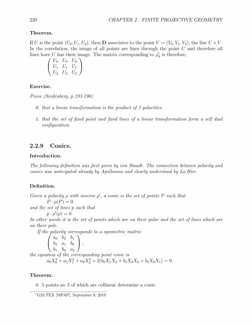
220 CHAPTER 2. FINITE PROJECTIVE GEOMETRY
Theorem.
If U is the point (U0, U1, U2), then D associates to the point V = (V0, V1, V2), the line U ×V .In the correlation, the image of all points are lines through the point U and therefore alllines have U has their image. The matrix corresponding to ρ′d is therefore, U0 U0 U0
U1 U1 U1
U2 U2 U2
.
Exercise.
Prove (Seidenberg, p.193-196)
0. that a linear transformation is the product of 2 polarities.
1. that the set of fixed point and fixed lines of a linear transformation form a self dualconfiguration.
2.2.9 Conics.
Introduction.
The following definition was first given by von Staudt. The connection between polarity andconics was anticipated already by Apollonius and clearly understood by La Hire.
Definition.
Given a polarity ρ with inverse ρ′, a conic is the set of points P such thatP · ρ(P ) = 0.
and the set of lines p such thatp · ρ′(p) = 0.
In other words it is the set of points which are on their polar and the set of lines which areon their pole.
If the polarity corresponds to a symmetric matrix a0 b2 b1
b2 a1 b0
b1 b0 a2
,
the equation of the corresponding point conic isa0X
20 + a1X
21 + a2X
22 + 2(b0X1X2 + b1X2X0 + b2X0X1) = 0.
Theorem.
0. 5 points no 3 of which are collinear determine a conic.
1G23.TEX [MPAP], September 9, 2019

2.2. ALGEBRAIC MODEL OF FINITE PROJECTIVE GEOMETRY. 221
1. the conic through A, B, C, D and E is given byk1[A×B] ×× [C ×D] = k2[A×D] ×× [B × C],
withk1 = [A×D] · E . [B × C] · E, k2 = [A×B] · E . [C ×D] · E.
Example.
Given the data of 2.2.2, the conic through A, B, C, D and E is2X2
0 −X21 − 4X2
2 + 5X1X2 − 4X2X0 = 0.
Exercise.
Prove that a conic has p+ 1 points in a finite projective plane associate with p.
If we join one point P to the p others we obtain p lines through P therefore the left overline is the tangent at P .
Comment.
For p = 3, the conic has 4 points, hence it cannot be constructed by giving 5 points, but itcan be constructed if we give 4 points and a tangent at one of these points or 3 points andthe tangents at 2 of these points. See 2.1.6.For p = 2, a conic can be constructed using 3 non collinear points and the tangents at 2 ofthese points.
Theorem.
The pole of [1,1,1] with respect to the conicb0X1X2 + b1X2X0 + b2X0X1ρ + (X0 +X1 +X2)(u0X0 + u1X1 + u2X2) = 0,is(b0(−b0 + b1 + b2) + 2u0b0 − u1(b0 + b1 − b2)− u2(b0 − b1 + b2), . . . , . . .).
Theorem.
The pole of [1,1,1] with respect to the conicc0X1X2 + c1X2X0 + c2X0X1 + u0X
20 + u1X
21 + u2X
22 = 0,
is(c0(−c0 + c1 + c2)− 2u1c1 − 2u2c2 + 4u1u2, . . . , . . .).
Example.
For p = 13, if b0 = 1, b1 = 6, b2 = 2, u0 = −5, u1 = 4, u2 = 2,then c0 = −4, c1 = 2, c2 = 5, and the pole of [1,1,1] is (1,6,3) = (95).

222 CHAPTER 2. FINITE PROJECTIVE GEOMETRY
Theorem.
Given the conica0X
20 + a1X
21 + a2X22 + b0X1X2 + b1X2X0 + b2X0X1 = 0.
and a point (P0, P1, P2), with P2 6= 0, on the conic, all the points are given byX0 = a1P0u
2 − (2a1P1 + b0P2)uv − (a0P0 + b2P1 + b1P2)v2,X1 = −(b2P0 + a1P1 + b0P2)u2 − (2a0P0 + b1P2)uv + a1P0v
2,X2 = a1P2u
2 + b2P2uv + a0P2v2,
using the p+ 1 values of the homogeneous pair (u, v).Proof: The points (v, u, 0) on [0,0,1] joined to P is the line
l = [−P2u, P2v, P0u− P1v].X is on l iff P2X1v = P2X0u− P0X2u+ P1X2v, substituting in the equation of the conic, ifA is the coefficient of X2
0 and B that of X22 , using the property of the products of the roots of
the equations gives P2X2 = A, P0X0 = B, this gives X0 and X2, substituting in l gives X1.
Theorem. [Chasles]
Given the configuration of Desargues 2.1.5 there exists a conic such that Ai is the pole ofbi := Bi+1 ×Bi−1 and vice-versa.Clearly Bi is also the pole of ai := Ai+1 × Ai−1.
Proof: Let A0 = (1, 0, 0), A1 = (0, 1, 0), A2 = (0, 0, 1), C = (1, 1, 1), c = (c0, c1, c2) andB0 = (b, 1, 1). We haveC0 = (0, c2,−c1), C1 = (−c2, 0, c0), C2 = (c1,−c0, 0), b1 = [c0, c1,−bc0 − c1], b2 = [c0,−bc0 −c2, c2], B1 = (c1, (b − 1)c0 + c1, c1), B2 = (c2, c2, (b − 1)c0 + c2). The transformation whichassociates to ai, kiBi, withk0 := c1c2, k1 := c2, k2 := c1 is bc1c2 c1c2 c1c2
c1c2 ((b− 1)c0 + c1)c2 c1c2
c1c2 c1c2 ((b− 1)c0 + c2)c1
,
is a line to point polarity because the representative matrix is symmetric. Its inverse caneasily be obtained by determining b0. This is left as an exercise.
Notation.
If u = [u0, u1, u2] and v = [v0, v1, v2] are 2 lines, thenu ×× v = (u0X0 + u1X1 + u2X2)(v0X0 + v1X1 + v2X2).
Definition.
Given 2 conics α and β if there exist integers k and l and lines u and v such thatkα + lβ = u ×× v,
then v is called the radical axis with respect to u of α and β .
Lemma.
If N is a symmetric matrix and A and B are 2 vectors, then A · (N B) = B · (N A).

2.2. ALGEBRAIC MODEL OF FINITE PROJECTIVE GEOMETRY. 223
Theorem.
A conic or the corresponding polarity determines an involution on every line, by associatingto each point its conjugate on that line. Moreover if A0 and B0 are conjugates as well as A1
and B1, if Al = t0A0 + t1A1 its conjugate Bl is given by Bl = ((A1.B0)t0 + (A1.B1)t1)A0 −((A0.B0)t0 + (A0.B1)t1)A0.This property follows from the notion of conjugates and from Bl = (A1∗A0)∗(t0NA0+t1NA1),with B0 = NA0 and B1 = NA1. The Lemma confirms the involutive property.
Example.
For p = 5, starting with A(0) = (6), A(1) = 1, A(2) = 0, A(3) = 12, the quadrangle-quadrilateral configuration isa1,2 = [6], a2,0 = [1], a0,1 = [0], a0,3 = [5], a1,3 = [10], a2,3 = [26], D0 = (2), D1 = (7),D2 = (11), d0 = [30], d1 = [27], d2 = [15], A0,3 = (5), A1,3 = (10), A2,3 = (26), A1,2 = (24),A2,0 = (17), A0,1 = (13), a0 = [24], a1 = [17], a2 = [13], a3 = [12].
Example.
The points and lines of the extended quadrangle-quadrilateral configuration are those of 2.2.9and B1,0 = (9), B2,1 = (16), B0,2 = (3), B2,0 = (21), B0,1 = (4), B1,2 = (8), B0,3 = (15),B1,3 = (27), B2,3 = (30), B3,0 = (18), B3,1 = (22), B3,2 = (14), b1,0 = [4], b2,1 = [8],b0,2 = [21], b2,0 = [3], b0,1 = [9], b1,2 = [16], b0,3 = [2], b1,3 = [7], b2,3 = [11], b3,0 = [18],b3,1 = [22], b3,2 = [14].
Example.
The conical points and lines of the extended quadrangle- quadrilateral configuration are the 6points and 6 lines C1,0 = (20), C2,1 = (29), C0,2 = (19), C2,0 = (28), C0,1 = (23), C1,2 = (25),c1,0 = [20], c2,1 = [29], c0,2 = [19], c2,0 = [28], c0,1 = [23], c1,2 = [25].
Definition.
A degenerate conic is a set of points and lines represented by an equation corresponding toa singular 3 by 3 symmetric matrix.
Exercise.
Describe all the types of degenerate conics.
Exercise.
The number of conics, degenerate or not is (q2 + q + 1)(q3 + 1),The number of degenerate conics are
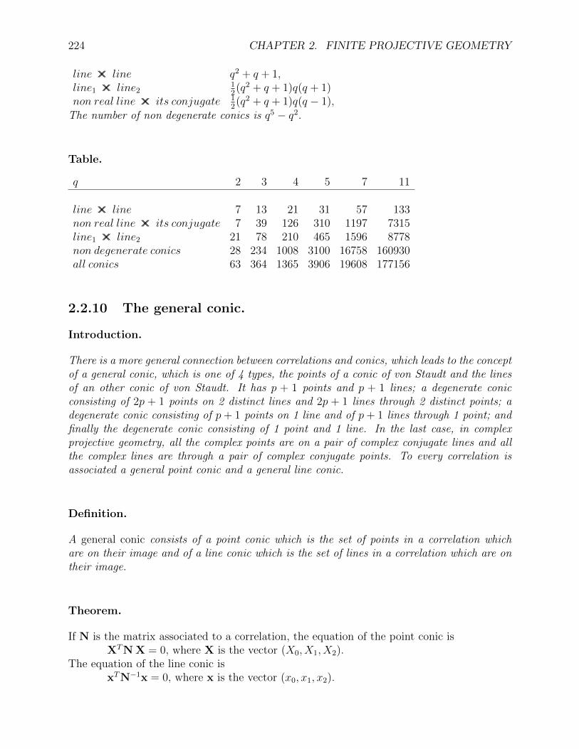
224 CHAPTER 2. FINITE PROJECTIVE GEOMETRY
line ×× line q2 + q + 1,line1 ×× line2
12(q2 + q + 1)q(q + 1)
non real line ×× its conjugate 12(q2 + q + 1)q(q − 1),
The number of non degenerate conics is q5 − q2.
Table.
q 2 3 4 5 7 11
line ×× line 7 13 21 31 57 133non real line ×× its conjugate 7 39 126 310 1197 7315line1 ×× line2 21 78 210 465 1596 8778non degenerate conics 28 234 1008 3100 16758 160930all conics 63 364 1365 3906 19608 177156
2.2.10 The general conic.
Introduction.
There is a more general connection between correlations and conics, which leads to the conceptof a general conic, which is one of 4 types, the points of a conic of von Staudt and the linesof an other conic of von Staudt. It has p + 1 points and p + 1 lines; a degenerate conicconsisting of 2p + 1 points on 2 distinct lines and 2p + 1 lines through 2 distinct points; adegenerate conic consisting of p+ 1 points on 1 line and of p+ 1 lines through 1 point; andfinally the degenerate conic consisting of 1 point and 1 line. In the last case, in complexprojective geometry, all the complex points are on a pair of complex conjugate lines and allthe complex lines are through a pair of complex conjugate points. To every correlation isassociated a general point conic and a general line conic.
Definition.
A general conic consists of a point conic which is the set of points in a correlation whichare on their image and of a line conic which is the set of lines in a correlation which are ontheir image.
Theorem.
If N is the matrix associated to a correlation, the equation of the point conic isXTN X = 0, where X is the vector (X0, X1, X2).
The equation of the line conic isxTN−1x = 0, where x is the vector (x0, x1, x2).

2.2. ALGEBRAIC MODEL OF FINITE PROJECTIVE GEOMETRY. 225
Theorem.
Let A be the most general antisymmetric matrix,
A =
0 −w vw 0 −u−v u 0
,
all the correlations associated to N + A define the same point conic.
Definition.
Given a matrix N, its symmetric part NS is defined byNS := N+NT
2,
and its antisymmetric part NA byNA := N−NT
2.
Theorem.
Given a correlation ρ, ρ′.If T is on the point conic, then ρ(T ) is on the line conic.If t is on the line conic, then ρ′(t) is on the point conic.The general conic degenerates if det(N) = 0.The center corresponds to the vector which is the homogeneous solution of NSC = 0, andthe central line, to that of (NS)−1c = 0.
Definition.
Given a general conic, the tangent t at the point T of the point conic is defined by t := NST.The contact T of a line t which belongs to a line conic is defined by T := (NS)−1t.
Theorem.
If the correlation is a polarity then the tangent at a point T of a point conic is on thecorresponding line conic. Similarly, the contact of a line t of line conic is on the correspondingpoint conic.
Theorem.
If a conic is non degenerate, the necessary and sufficient condition for the set of tangents toa point conic to coincide with the set of lines on the line conic is that the correlation be apolarity.
Proof: Let N be the matrix associated to the correlation. The line conic is xTN−1x = 0.The tangents t = NSX to the point conic are ontT (NS)−1N(NS)−1 t = 0.If ρ is a polarity, N = NS and N−1 = NS−1N(NS)−1. Vice-versa,if N−1 = (NS)−1N(NS)−1 then NS = N(NS)−1N.Therefore, using N = NS + NA, 2NA = −NA(NS)−1NA,

226 CHAPTER 2. FINITE PROJECTIVE GEOMETRY
transposing, −2NA = −NA(NS)−1NA, because NAT = −NA, thereforeNA = 0, N is symmetric and therefore ρ is a polarity.
2.2.11 The Theorem of Pascal and Brianchon.
Introduction.
A fundamental theorem associated to conics was discovered by Blaise Pascal. It allows con-struction of any point on a conic given by 5 points and in particular the other intersectionof a line through one point of a conic. See I, . . . .
There is a general principle of linear construction that if a point or line is uniquelydefine, that point or line can be obtained by a linear construction. The points of intersectionof a conic with a general line are not uniquely defined and therefore do not admit a linearconstruction on the other hand if the line passes to a known point of the conic, the otherintersection of the line and the conic is uniquelly defined. The Pascal construction of 2.2.11is a solution to this problem which follows from the following Theorem.
Theorem [Pascal].
If 6 points A0, A1, A2, A3, A4, A5 are on a conic and the Pascal points are defined asP0 := (A0 × A1)× (A3 × A4),P1 := (A1 × A2)× (A4 × A5),P2 := (A2 × A3)× (A5 × A0),
then the points P0, P1, P2 are collinear (Pascal, 1639, Lemma 1 and 3).There are “degenerate” forms of this theorem in which 2 consecutive points coincide and
the cord is replaced by the tangent at these points for instance if the tangent at A0 is t0, thePascal points are
P0 := t0 × (A3 × A4),P1 := (A0 × A2)× (A4 × A5),P2 := (A2 × A3)× (A5 × A0),
and the points P0, P1, P2 are collinear.Proof: The Theorem of Pascal will now be proven in the 4 cases, 6 points, 5 points and
the tangents at one of them, 4 points and the tangents at 2 of them and finally 3 points andtheir tangents. In each case, the coordinates will be chosen to simplify the algebra. See also2.2.2.
0. Let the 6 points of the conic be A0, C0, A1, B1, A2, B2. Choose the coordinates suchthat A0 = (1, 0, 0), A1 = (0, 1, 0) and A2 = (0, 0, 1), choose the barycenter M = (1, 1, 1)at the intersection of A1 ×B1 and A2 ×B2, let the line A0 ×B0 be [0, r,−s].Because the conic passes through Ai, it has an equation of the form0. uX1X2 + vX2X0 + wX0X1 = 0.A1 ×B1 = A1 ×M = [1, 0,−1], A2 ×B2 = A2 ×M = [1,−1, 0], therefore,
B1 = (u+ w,−v, u+ w), B2 = (u+ v, u+ v,−w),C0 = (−urs, s(vr + ws), r(vr + ws)),hence the Pascal points are
P0 = (A0 × C0)× (B1 × A2) = (s(u+ w),−vs,−vr),
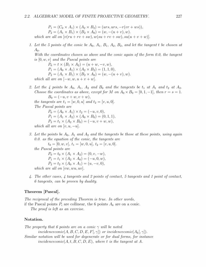
2.2. ALGEBRAIC MODEL OF FINITE PROJECTIVE GEOMETRY. 227
P1 = (C0 × A1)× (A2 ×B2) = (urs, urs,−r(vr + ws)),P2 = (A1 ×B1)× (B2 × A0) = (w,−(u+ v), w).
which are all on [v(ru+ rv + sw), w(su+ rv + sw), su(u+ v + w)].
1. Let the 5 points of the conic be A0, A1, B1, A2, B2, and let the tangent t be chosen atA0.With the coordinates chosen as above and the conic again of the form 0.0, the tangentis [0, w, v] and the Pascal points are
P0 = t× (B1 × A2) = (u+ w,−v, w),P1 = (A0 × A1)× (A2 ×B2) = (1, 1, 0),P2 = (A1 ×B1)× (B2 × A0) = (w,−(u+ v), w).
which all are on [−w,w, u+ v + w].
2. Let the 4 points be A0, A1, A2 and B0 and the tangents be t1 at A1 and t2 at A2.Choose the coordinates as above, except for M on A0×B0 = [0, 1,−1], then r = s = 1.
B0 = (−u, v + w, v + w),the tangents are t1 = [w, 0, u] and t2 = [v, u, 0].The Pascal points are
P0 = (A0 × A1)× t2 = (−u, v, 0),P1 = (A1 × A2)× (A0 ×B0) = (0, 1, 1),P2 = t1 × (A2 ×B0) = (−u, v + w,w),
which all are on [v, u,−u].
3. Let the points be A0, A1 and A2 and the tangents be those at these points, using again0.0. as the equation of the conic, the tangents are
t0 = [0, w, v], t1 = [w, 0, u], t2 = [v, u, 0].the Pascal points are
P0 = t0 × (A1 × A2) = (0, v,−w),P1 = t1 × (A2 × A0) = (−u, 0, w),P2 = t2 × (A0 × A1) = (u,−v, 0),
which are all on [vw,wu, uv].
4. The other cases, 4 tangents and 2 points of contact, 5 tangents and 1 point of contact,6 tangents, can be proven by duality.
Theorem [Pascal].
The reciprocal of the preceding Theorem is true. In other words,if the Pascal points Pi are collinear, the 6 points Ak are on a conic.
The proof is left as an exercise.
Notation.
The property that 6 points are on a conic γ will be notedincidenceconic(A,B,C,D,E, F [, γ]) or incidenceconic(Ak[, γ]).
Similar notation will be used for degenerate or for dual forms, for instanceincidenceconic(A, t, B,C,D,E), where t is the tangent at A.

228 CHAPTER 2. FINITE PROJECTIVE GEOMETRY
incidenceconic(a, b, c, d, e, f) where a, b, c, d, e, f are 6 tangents to the conic.Theorem 2.2.11 will be denoted as follows.No. Pascal(Ak[, ak]; 〈Pi[, p]〉)Hy. incidenceconic(Ak).De. Pi := (Ai × Ai+1)× (Ai+3 × Ai+4)Co. 〈Pi, p〉.
If tk is the tangent at Ak, Ak is followed by tk.The Pascal line associated to the points Ak will be denoted by p := Pascal(Ak).
Definition.
The dual of the Theorem of Pascal is called the Theorem of Brianchon. Brianchon discoveredthe Theorem before Gergonne discovered the important principle of duality.In the degenerate case of a triangle inscribed in a conic and of the triangle outscribed to theconic at these points (2.2.11.3), the line is called the Pascal line of the triangle and the pointof the dual Theorem, the Brianchon point of the triangle. von Staudt (1863) calls them, poleand polar of the triangle.
Theorem. [Generalization of von Staudt]
If p is the Pascal line of the hexagon A0, A1, A2, A3, A4, A5 inscribed in a conic γ and P isthe Brianchon point of the outscribed hexagon formed by the tangents at Aj, then P is thepole of p.
The proof follows at once from the properties of poles and polars.
Corollary. [von Staudt]
If A0, A1, A2 is a triangle inscribed in a conic, then its Pascal line is the polar of itsBrianchon point.
Theorem. [von Staudt]
If 2 triangles A0, A1, A2 and B0, B1, B2 are inscribed in a conic γ and are perspectivewith center C and axis c, and P , Q are their Brianchon pointa and p and q are theirPascal lines, tehn 〈P,Q,C; pq〉 and 〈p, q, c;PQ〉, moreover, quatern(P,Q,C, pq × c) andquatern(p, q, c, PQ× C).
Notation.
(Ai,j,k) := det(Ai, Aj, Ak).
Theorem.
If 6 points Ak, k = 0 to 5, are on a conic then(Ak+2,k+3,k+1)(Ak+3,k+4,k)(Ak+4,k+5,k+1)(Ak+5,k,k+2)
− (Ak+2,k+3,k)(Ak+3,k+4,k+1)(Ak+4,k+5,k+1)(Ak+5,k,k+2)

2.2. ALGEBRAIC MODEL OF FINITE PROJECTIVE GEOMETRY. 229
+ (Ak+3,k+4,k+1)(Ak+4,k+5,k+2)(Ak+5,k,k+2)(Ak,k+1,k+3)− (Ak+3,k+4,k+1)(Ak+4,k+5,k+2)(Ak+5,k,k+3)(Ak,k+1,k+2) = 0.
The addition for the subscript is done modulo 6.
Proof: The Theorem will be proven for k = 0. Let ak := Ak × Ak+1. The Pascal pointsare Pk := ak × ak+3, we have
(P0,1,2) := det(P0, P1, P2) = (P0 ∗ P1) · P2 = 0,butP0 = (A0 ∗ A1) ∗ (A3 ∗ A4) = det(A0, A3, A4)A1 − det(A1, A3, A4)A0,
= (A0,3,4)A1 − (A1,3,4)A0,similarly,
P1 = (A1,4,5)A2 − (A2,4,5)A1,P2 = (A2,5,0)A3 − (A3,5,0)A2 = (A0,2,5)A3 − (A0,3,5)A2,
thereforedet(P0, P1, P2) = (A0,3,4)(A1,4,5)(A0,2,5)(A1,2,3)− (A1,3,4)(A1,4,5)(A0,2,5)(A0,2,3)
+(A1,3,4)(A2,4,5)(A0,2,5)(A0,1,3)− (A1,3,4)(A2,4,5)(A0,3,5)(A0,1,2) = 0.
Construction.
point Pascal(A0, A1, A2, A3, A4, A′5; [P0, P1, P2, ]A5)
is used as an abbreviation for the Pascal constructionP0 := (A0 × A1)× (A3 × A4),P1 := (A1 × A2)× (A4 × A′5),P2 := (A2 × A3)× (P0 × P1),A5 := (A4 × A′5)× (P2 × A0).It gives the point A5 on the conic through A0 to A5 on the line A4 × A′5. linePascal(a0, a1, a2, a3, a4, a
′5; [p0, p1, p2, ]a5)
is used for the dual construction.
Theorem.
When p = 2, the points and lines of a conic2 configuration 2.1.6 are the points and lines ofa conic.
Proof: The Pascal points are the diagonal points of the complete quadrangle configurationwhich are collinear because of Theorem 2.1.13.
Theorem.
Let p = 3, in a quadrangle quadrilateral configuration, Qi, P, qi, p (2.1.6), there is a conicwhose tangent at P is p and at Qi is pi.In other words the elements of a conic3 configuration (2.1.6 are the points and lines of aconic.
Proof: From 2.1.6, Qi is on qi, the Pascal-Brianchon theorem givesPascal(P, p,Qi+1, qi+1, Qi−1, qi−1; 〈R0, Pi−1, Pi+1, p〉).

230 CHAPTER 2. FINITE PROJECTIVE GEOMETRY
Theorem.
The conical points of Definition 2.1.7 are on a conic and the conical lines are on a conic.
Proof: Pascal(AF0, FA2, AF0, FA2, AF0, FA2; 〈R1, R2, R3, p〉.
Theorem.
The following points of the extended Pappus configuration are on a conic, 1 point on eachof the lines d, d, say M0 and M0 and the intersection with the lines joining the other pointssay a1 and a2 with the lines joining M0 or M0 with the other points on d or d.This gives the 18 conics
0. Mi, N i+1, Ni+1,M i, N i−1, Ni−1,
1. Mi, P i−1, Pi−1,M i, P i+1, Pi+1,
2. Mi+1, N i+1, Li−1,M i−1, N i−1, Li−1,
3. Mi+1, Qi−1, P i−1,M i−1, Qi+1, P i−1,
4. Mi−1, Qi+1, Pi+1,M i+1, Qi−1, Pi−1,
5. Mi−1, Li+1, N i+1,M i+1, Li−1, N i−1.
Proof: This follows from Pascal’s Theorem applied to the points in the given order, orderwhich was chosen in such a way that the Pascal line was always m0, containing P0, P 0, Q0
and D. Exchanging Ni+1 and N i−1 for 0. gives an other Pascal line m0. The 9 Pappus linesare therefore the Pascal lines of the 18 conics.
Theorem.
The conics 0. and 1. have the same tangent at their common point.
Proof: The coefficients of conic 0. are, for i = 0, a0 = m0m1m2,a1 = m2
1m2, a2 = m22m1, b0 = m1m2(m1 +m2), b1 = m2(m2
1 +m2m0),b2 = m1(m2
2 +m0m1),This follows easily because M0, M0 are on a0, giving a1, a2 and b0, N1, N1 are on a1, thisgives a0 and b1, N2, N2 are on a2, giving b2. The coefficients of conic 1, for i = 0 are thesame except for a0 = m0(m2
1 − m1m2 + m22). The algebra is simplified by noting that the
equation for P1 and P 1, gives after subtraction b1 from a2 and b0, and for P2 and P 2, givesafter subtraction b2 from a1 and b0.
The Theorem follows at once. The tangent at M0 is[m0(m1 +m2 −m1m2,m1m2,m1m2] and at M0 is [m1 +m2 −m0,m1,m2].
Exercise.
Study the configuration of all 18 conics associated to the extended Pappus configuration.
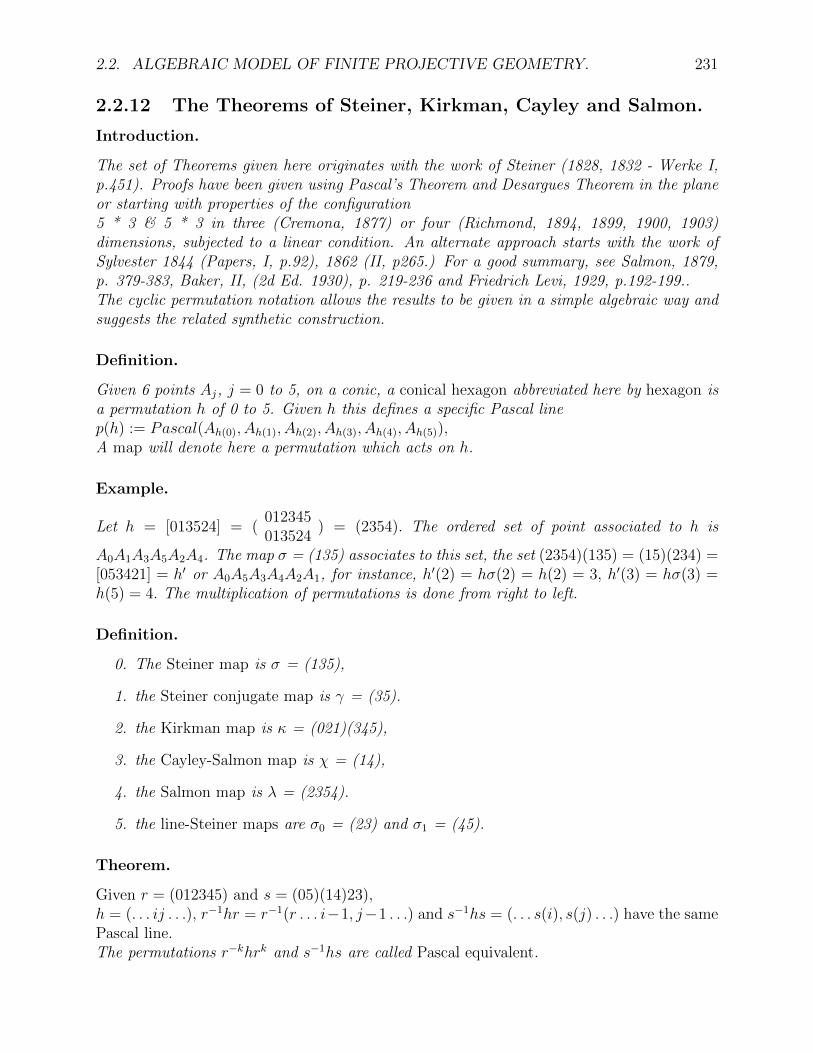
2.2. ALGEBRAIC MODEL OF FINITE PROJECTIVE GEOMETRY. 231
2.2.12 The Theorems of Steiner, Kirkman, Cayley and Salmon.
Introduction.
The set of Theorems given here originates with the work of Steiner (1828, 1832 - Werke I,p.451). Proofs have been given using Pascal’s Theorem and Desargues Theorem in the planeor starting with properties of the configuration5 * 3 & 5 * 3 in three (Cremona, 1877) or four (Richmond, 1894, 1899, 1900, 1903)dimensions, subjected to a linear condition. An alternate approach starts with the work ofSylvester 1844 (Papers, I, p.92), 1862 (II, p265.) For a good summary, see Salmon, 1879,p. 379-383, Baker, II, (2d Ed. 1930), p. 219-236 and Friedrich Levi, 1929, p.192-199..The cyclic permutation notation allows the results to be given in a simple algebraic way andsuggests the related synthetic construction.
Definition.
Given 6 points Aj, j = 0 to 5, on a conic, a conical hexagon abbreviated here by hexagon isa permutation h of 0 to 5. Given h this defines a specific Pascal linep(h) := Pascal(Ah(0), Ah(1), Ah(2), Ah(3), Ah(4), Ah(5)),A map will denote here a permutation which acts on h.
Example.
Let h = [013524] = (012345013524
) = (2354). The ordered set of point associated to h is
A0A1A3A5A2A4. The map σ = (135) associates to this set, the set (2354)(135) = (15)(234) =[053421] = h′ or A0A5A3A4A2A1, for instance, h′(2) = hσ(2) = h(2) = 3, h′(3) = hσ(3) =h(5) = 4. The multiplication of permutations is done from right to left.
Definition.
0. The Steiner map is σ = (135),
1. the Steiner conjugate map is γ = (35).
2. the Kirkman map is κ = (021)(345),
3. the Cayley-Salmon map is χ = (14),
4. the Salmon map is λ = (2354).
5. the line-Steiner maps are σ0 = (23) and σ1 = (45).
Theorem.
Given r = (012345) and s = (05)(14)23),h = (. . . ij . . .), r−1hr = r−1(r . . . i−1, j−1 . . .) and s−1hs = (. . . s(i), s(j) . . .) have the samePascal line.The permutations r−khrk and s−1hs are called Pascal equivalent.

232 CHAPTER 2. FINITE PROJECTIVE GEOMETRY
Theorem.
0. (024), (042), (153) are Pascal equivalent to the Steiner map (135).
1. (02), (04), (13), (15), (24) are Pascal equivalent to the Steiner conjugate map (35).
2. (012)(354),(015)(243), (045)(132), (051)(234), (054)(123) are Pascal equivalent tothe Kirkman map (021)(345).
3. (03), (25) are Pascal equivalent to the Cayley-Salmon map (14).
4. (0132), (0215), (0451), (0534), (1243) are Pascal equivalent to the Salmon map(2354).
5. (024), (042), (153) are Pascal equivalent to the line-Steiner maps (23) and (45).
Theorem. [Steiner (Pascal)]
0. 〈p(h), p(hσ), p(hσ2);S(h)〉, S(h) is called the Steiner point of h.
1. S(hγ), called the Steiner conjugate point of h, is on the polar of S(h) with respect tothe conic.
2. there are 10 pairs of conjugate Steiner points.
See 2.1.9.Proof: Let h = [012345] = (). I will use here the abbreviations
ij for the line Ai × Aj,ijkl for the Pascal point (Ai × Aj × (Ak × Al).
p(h) = P0 × P ′0, with P0 = 0134, P ′0 = 0523,p(hκ) = P1 × P ′1, with P1 = 0125, P ′1 = 1423,p(hκ2) = P2 × P ′2, with P2 = 2534, P ′2 = 0514,Let Q0 := (P1 × P2)× (P ′1 × P ′2) = 2514,Q1 := (P2 × P0)× (P ′2 × P ′0) = 3450,Q2 := (P0 × P1)× (P ′0 × P ′1) = 0123,Pascal(A1A4A3A2A5A0; 〈Q0, Q1, Q2〉), thereforeDesargues−1(P0, P1, P2, P ′0, P ′1, P ′2; 〈Q0, Q1, Q2〉, S(h)),orDesargues−1(2435, 0312, 0514, p34125, p25135, p35124p13245× p12354, 1245, 0523,
p12345, p13245, p12354; 〈S(e), S(σ), S(σ2〉, s(e)),
Theorem. [Kirkman 1849, 1850]
0. 〈p(h), p(hκ), p(hκ2);K(h)〉, K(h) is called the Kirkman point of h.
1. there are 60 Kirkman points which are 3 by 3 on the 60 Pascal lines, giving a configu-ration of type 60 * 3 & 60 * 36.
6Levi, p. 194

2.2. ALGEBRAIC MODEL OF FINITE PROJECTIVE GEOMETRY. 233
Proof: Let h = [012345] = (). The proof, for i = 0 is as follows.p(h) = P0 × P ′0, with P0 = 0134, P ′0 = 0523,p(hκ) = P1 × P ′1, with P1 = 0134, P ′1 = 1245,p(hκ2) = P2 × P ′2, with P2 = 2534, P ′2 = 0312,Let Q0 := (P1 × P2)× (P ′1 × P ′2) = 0325,Q1 := (P2 × P0)× (P ′2 × P ′0) = 0145,Q2 := (P0 × P1)× (P ′0 × P ′1) = 1234,Pascal(A2A5A4A3A0A1; 〈Q0, Q1, Q2〉), thereforeDesargues−1(P0, P1, P2, P ′0, P ′1, P ′2; 〈Q0, Q1, Q2〉, S(h)),orPascal(014235) =⇒ 〈1435, 0524, 0123; p14235〉,Desargues−1(p14235, 0523, 1423, 0514, 14, 05, 23, 0134, 0135, 1235,
35, p12435, 01; 〈p12345, p14523, p21435〉, K(e)),
Theorem [Salmon]
If 2 triangles have their vertices on a conic, their sides are tangent to a conic7.Proof:
Desargues−1(0135, 0145, 0245, 45, p14523, 01, 0234, 1234, 1235,12, p21435, 34; 〈1245, K(e), 0134;P 〉).
Exercise.
Prove 〈p12345, p125423, p34215〉.
Theorem. [Steiner]
0. 〈S(h), S(hσ0), S(hσ1); s(h)〉, s(h) is called the Steiner line of h,
1. S(hσ0σ1) ι s(h),
2. there are 15 Steiner lines s(h).
The proofs follows from 2.2.11.0 and from the fact that the Brianchon lines of the conicinscribed in the 2 triangles are Pascal lines of the original conic.
Theorem. [Cayley and Salmon]
0. 〈K(hχ), K(hχ), K(hχ); cs(h)〉, cs(h) is called the Cayley-Salmon line of h,
1. S(h) ι cs(h),
2. there are 20 Cayley-Salmon lines.
3. The 60 Kirkman points, the 20 Steiner points, the 60 Pascal lines and the 20 Cayley-Salmon lines form a 80 ∗ 4&80 ∗ 4 configuration (See Levi, p. 199).
7Salmon, p. 381

234 CHAPTER 2. FINITE PROJECTIVE GEOMETRY
Theorem.
18 Pascal points and 12 Pascal lines are used in the preceding Theorem and these are verticesand sides of 3 complete quadrilaterals.
Theorem. [Salmon]
0. 〈cs(h), cs(hλ), cs(hλ2);Sa(h)〉, Sa(h) is called the Salmon point of h,
1. cs(hλ3) ι Sa(h),
2. there are 15 Salmon points Sa(h).
Theorem.
In the preceding Theorem:
0. Each of the 24 Pascal lines occurs exactly twice.
1. The Pascal points of h occur 4 times, the other 30 Pascal points occur twice.
2. The 3 Pascal points of h, the 8 points S(hλi), Ki(hχ), i = 0, 1, 2, 3 and the 12 associatedPascal lines form a pseudo configuration of type
3 ∗ 4 + 8 ∗ 3 & 12 ∗ 3, (11).
Example.
In all cases h = e = [012345] = ().
0. The Theorem of Steiner.S(e) ι S(σ0) ι S(σ1) ι S(σ0σ1) ι
() = [012345] (23) = [013245] (45) = [012354] (23)(45) = [013254](135) = [032541] (1235) = [023541] (1345) = [032451] (12345) = [023451](153) = [052143] (1523) = [053142] (1453) = [042153] (14523) = [043152]〈〈p12345, p14523, p34125〉, 〈p13245, p14523, p24135〉, 〈p12354, p15423, p35124〉,〈p13254, p15432, 15234〉〉. (Fig. 200b)
1. The Theorem of Cayley-Salmon.S(e) ι K(χ) ι K(σχ) ι K(σ2χ) ι
() = [012345] (14) = [042315] (1435) = [042531] (1453) = [042153](135) = [032541] (024531) = [204153] (0241) = [204315] (024351) = [204531](153) = [052143] (043512) = [420531] (045312) = [420153] (0412) = [420315]〈〈p12345, p14523, p34125〉, 〈p42315, p23514, p24135〉, 〈p13524, p25134, p15342〉,〈p35124, p21354, p24513〉〉. (Fig. 200b’)
2. The Theorem of Salmon.Add to Example 1, (Fig. 200b” and b4)

2.2. ALGEBRAIC MODEL OF FINITE PROJECTIVE GEOMETRY. 235
S(λ) ι K(λ) ι K(λσχ) ι K(λσ2χ) ι(2354) = [013524] (12354) = [023514] (12345) = [023451] (123) = [023145]
(15)(234) = [053421] (031) = [302145] (03541) = [302514] (03451) = [302451](1423) = [043125] (02)(1345) = [230451] (02)(13) = [230145] (02)(1354) = [230514]
〈〈p13524, p12435, p43125〉, 〈p23514, p21453, p32154〉, 〈p15432, p25143, p14523〉,〈p23145, p24513, p32415〉〉.(Fig.200b1)
S(λ) ι K(λ) ι K(λσχ) ι K(λσ2χ) ι(25)(34) = [015432] (134)(25) = [035412] (1325) = [035241] (13)(254) = [035124](14325) = [045231] (054231) = [503124] (052341) = [503412] (051)(23) = [503241](12543) = [025134] (0322)(15) = [350241] (031542) = [350124] (034152) = [350412]〈〈p15432, p13254, p25134〉, 〈p21453, p31245, p24135〉, 〈p14253, p34125, p12435〉,〈p35124, p32415, p41235〉〉.(Fig.200b2)
S(λ) ι K(λ) ι K(λσχ) ι K(λσ2χ) ι(2453) = [04253] (15324) = [054213] (15)(24) = [054321] (15243) = [054132](1245) = [024351] (0431)(25) = [405132] (041)(253) = [405213] (04251) = [405321]
(13)(245) = [034152] (05142) = [540321] (052)(143) = [540132] (0532)(14) = [540213]〈〈p14253, p15342, p25143〉, 〈p31245, p42315, p32154〉, 〈p12345, p43125, p13254〉,〈p23145, p41235, p21354〉〉. (Fig. 200b3)
Exercise.
0. Give the geometric interpretation of the Theorems in this section.
1. Determine the pseudo configuration associated to the Theorem of Salmon.
2.2.13 Bezier Curves for drawing Conics, Cubics, . . . .
Introduction.
The drawing of curves is facilitated by the notion of Bezier curves. These originate withthe work of de Casteljau at Citroen in 1959 and were popularized and generalized by Bezier.To describe easily complicated curves in 2, 3, . . . dimensions, we start with a Bezier poly-gon 2.2.13 to construct a parametric representation of points on the curve iteratively. Theassociated theory is briefly given here. The curve can be expressed in terms of the Bezierpolygon by means of Bernstein polynomials (2.2.13), the derivatives and differences of thecurve can be similarly expressed and related to each other. The example for a curve whosei-th coordinates can be approximated by cubic polynomials is given in 2.2.13.
Theorem.
Let P := (w0(1− I)2, 2w1I(1− I), w2I2), w0w1w2 6= 0 then
0. P is the parametric equation of a conic, which passes through the points P (0) =(1, 0, 0), P (1) = (0, 0, 1), P (∞) = (w0,−2w1, w2),
1. the tangent t at P is[w1w2I
2,−w2w0I(1− I), w0w1(1− I)2],

236 CHAPTER 2. FINITE PROJECTIVE GEOMETRY
in particular, the tangent at P (0) is [0, 0, 1], at P (1) is [1, 0, 0], (which meet at U =(0, 1, 0)) and at P (∞) is
[w1w2, w2w0, w0w1],
2. t meets t(0) atT = [w0(1− I), w1I, 0],
in particular, T (∞) = [−w0, w1, 0],
3. the anharmonic ratioanhr(U, P (0), T (∞), T ) = w0−w1
w0I.
The proof starts with the observation that the coordinates P0, P1, P2, satisfy the equation4w2
1P0P2 = w2w0P21 ,
which is indeed the equation of a conic with the prescribed properties. The correspondingpolarity matrix is 0 0 2w2
1
0 −w2w0 02w2
1 0 0
.
Notice that T (0) = (1, 0, 0) and is not undefined.The tangent can either be obtained from the polarity or using P ×DP , where its direction
DP = (−w0(1− I), w1(1− 2I), w2I).The last statement of the Theorem is associated with the four tangents Theorem of J.
Steiner. It can be used as a method to draw conics. In the excellent language Postcript(see Reference Manual), a general method is given to draw curves based on rhe work of deCateljau and Bezier as well as a method to draw ellipses using the Euclidean concepts ofrotation and scaling differently in the direction of its axis. This method does not allow todraw hyperbolas or parabolas and ignores the fact that a conic is a projective concept. Thefollowing gives a method which allows to draw conics using 3 points A, B, C, and the tangentstA, tB at two of the 2 points.It is then generalized to other curves.
Algorithm.
If the barycentric coordinates are chosen in such a way that A = (1, 0, 0), B = (0, 0, 1),tA × tB = (0, 1, 0) and C = (1, 1, 1), then the points on the conic are given by P of thepreceding Theorem, with, for instance, w0 = 2, w1 = −1, w2 = 2. In the case of a finite field,we compute P for each element of the field or for an appropriate subset of it. In the caseof the field of reals, we can compute P for tan(πt), t = 0 to 1, avoiding 1/2, a section ofthe conic can be obtained by appropriately limiting the set t, joining the successive pointsby segments will automatically give the asymptotes for an hyperbola, which is appropriatebecause their directions are indeed points in the Euclidean plane, as we prefer to consider it(in its extended form). An other approach is to limit the domain of P to [0, 1] to obtain onesection of the conic and to replace w1 by −w1, which is equivalent to compose P with I
2I−1,
to obtain the complement, see Farin, p.185.For some of the Theorems, see Farin.In what follows, the superscript of B, P and P are indices and not exponents.
2.2. ALGEBRAIC MODEL OF FINITE PROJECTIVE GEOMETRY. 237
Definition.
The Bernstein polynomials are
Bni :=
(ni
)I i(1− I)n−i, 0 ≤ i ≤ n.
By convention Bn−1 = Bn
n+1 := 0.In particular,
B20 = (1− I)2, B2
1 = 2I(1− I), B22 = I2.
Theorem.
0. B00 = 1, Bn
i = (1− I)Bn−1i + IBn−1
i−1 ,
1. DBni = n(Bn−1
i−1 −Bn−1i ).
2.∑n
j=0 Bnj = 1.
Definition.
A weighted point P is a set of 3 non homogeneous coordinates which are not all 0. Wecan add weighted points and multiply by scalars, but two weighted points which differ by amultiplicative constant are not equivalent. I will use the notation P for the equivalent point.
Definition. [de Casteljau]
Given n+ 1 weighted points P0, P1, . . . , Pn, called the Bezier polygon, defineP0i := Pi, 0 ≤ i ≤ n,
Pji := (1− I) Pj−1
i + I Pj−1i+1 , 1 ≤ j ≤ n, 0 ≤ i ≤ n− j.
Pn := Pn0 ,
The curve P n is called the de Casteljau curve of order n.The same curve is also called the Bezier curve.
Theorem.
0. P n(0) = P0, Pn(1) = Pn.
1. Pji =
∑jk=0 Pi+kB
jk, 0 ≤ j ≤ n, 0 ≤ i ≤ n− j,
in particular,
2. Pn =∑n
k=0 PkBnk ,
3. DPn = n∑n−1
k=0(Pk+1 −Pk)Bn−1k .
Definition.
∆Qk = Qk+1 −Qk,∆r+1Qk = ∆rQk+1 −∆rQk,
238 CHAPTER 2. FINITE PROJECTIVE GEOMETRY
Theorem.
∆Q0 =∑r
k=0(−1)r−j(rj
)Qi+k.
Theorem.
DrPn = n!(n−r)!
∑n−rk=0 ∆rPkB
n−rk .
DrPn = n!(n−r)!∆
rPn−r0 .
In particular,DPn = n(Pn−1
1 −Pn−10 ).
Curves with cubic parametrization.
For n = 3,P3 = P0(1− I)3 + 3P1(1− I)2I + 3P2(1− I)I2 + P3I
3.DP3(0) = P1 −P0,DP3(1) = P3 −P2.
In other words the direction of the tangents at the end points is that of the line joining theend points to the nearest point.
If the cubic associated with the i-th coordinate of the curve P 3 isf = c0 + c1I + c2I
2 + c3I3,
then the i-th coordinate aj of the Bezier polygon Pj is given bya0 = c0, a1 = c0 + 1
3b1, a2 = a1 + 1
3(c1 + c2), a3 = c0 + c1 + c2 + c3.
Indeed, a0(1− I)3 + 3a1(1− I)2I + 3a2(1− I)I2 + a3I3 = f.
These last formulas allows for the determination of the weighted points Pi of the cubic(approximation) given the 3 non homogeneous coordinates of the parametrized curve. If thecubic associated with the i-th coordinate reduces to a linear function then Pi = P3(i/3),i = 0, 1, 2, 3.
It is often convenient to choose −1 and 1 for the end points instead of 0 and 1 bymeans of a change of variable. If g = d0 + d1I + d2I
2 + d3I3 is the new polynomial, f =
c0 +c1I+c2I2 +c3I
3 = gφ, with φ = 2I−1. In this case, we obtain the symmetric formulas,a0 = d0−d1 +d2−d3, a1 = d0− 1
3d1− 1
3d2 +d3, a2 = d0 + 1
3d1− 1
3d2−d3, a2 = d0 +d1 +d2 +d3,
Example.
For the curve (I − 3I3, 1 − I2, 1), for the first coordinate, d0 = d2 = 0, d1 = 1,, d3 = −3,therefore a0 = 2, a1 = −10
3, a2 = 10
3, a3 = −2. for the second coordinate, d1 = d3 = 0,
d0 = 1,, d2 = −1, therefore a0 = 0, a1 = 43, a2 = 4
3, a3 = 0. Therefore the Bezier polygon is
P0 = (2, 0, 1), P1 = (−103, 4
3, 1), P2 = (10
3, 4
3, 1), P3 = (−2, 0, 1).
This gives the Cartesian coordinates of the following points on the curve associated withi/20, i = 0 to 20:2.000,0.00; 1.287,0.19; 0.736,0.36; 0.329,0.51; 0.048,0.64; -0.125,0.75, -0.208,0.84, -0.219,0.91,-0.176,0.96, -0.097,0.99; 0.000,1.00; 0.097,0.99; 0.176,0.96; 0.219,0.91; 0.208,0.84; 0.125,0.75;-0.048,0.64; -0.329,0.51; -0.736,0.36; -1.287,0.19; -2.000,0.00.The complement of the curve using i/20
2i/20−1is

2.2. ALGEBRAIC MODEL OF FINITE PROJECTIVE GEOMETRY. 239
2.0000,0.0000; 3.0041,-0.2346; 4.6094,-0.5625; 7.3178,-1.0408; . . . , -7.3178,-1.0408;-4.6094,-0.5625;-3.0041,-0.2346;-2.0000, 0.0000.
Problem.
Given a curve in the plane, what are the condition for a representation of the 3 non-homogeneous coordinates by polynomials of degree n. For conics, we have seen that n = 2.
2.2.14 Projectivity determined by a conic.
Definition.
Joining 2 distinct points of a conic, is to determine the line through the 2 points. Joining apoint of a conic to itself is to determine the tangent to the conic at that point.
Example.
For p = 3, The conic X2 + 2Y Z = 0 has the points (0), (1), (13), (17), (25) and (29).The tangents at (X0, Y0, Z0) is [X0, Z0, Y0].The tangent at (0) is [1] and the tangent at (1) is [0].These points joined to (0) give the lines [6], [26], [16], [21], [11]. These points joined to (1)give [0], [8], [10], [7], [9].These lines determine on the ideal line [12], the projectivity which associates to(26), (5), (14), (18), (22), (26), the points (5), (26), (18), (22), (10), (14).This is precisely the projectivity φ of 2.2.6.
Theorem.
Let N be a symmetric matrix associated to a conic.
0. P is on the conic if P ·NP = 0.
1. If P is on the conic and C is not, the other point on the conic, if any, isP + yC, with y = −2C·NP
C·NC .
Proof: (P + yC) ·N(P + yC) = 0,or
P ·NP + yC ·NP + yP ·NC + y2C ·NC = 0,but P · NP = 0 and C · NC 6= 0 and N is symmetric, therefore C · NP = P · NC, hencey = −2C·NP
C·NC .
Theorem.
Let l be a line and A, B be 2 points on the line but not on the conic associated with thesymmetric matrix N ,let a := A ·NA, b := B ·NB, c := A ·NB = B ·NA,let C be an arbitrary point on the line, C = A+ kB.Let P1 and P2 be 2 distinct points on the conic, let a1 = (P1 · A ∗ P2), b1 := (P1 · B ∗ P2),

240 CHAPTER 2. FINITE PROJECTIVE GEOMETRY
c1 := (A ·B ∗P1), c2 := (A ·B ∗P2), d1 := A ·NP1, d2 := B ·NP2. If C ×P1 meets the conicat Q and P2 ×Q meets l at D, then
0. D = ((aa1) + 2(ca1 − d1c1)k + (ba1 + 2d2c1)k2)B−((ab1 − 2d1c2) + 2(cb1 − d2c2)k + bb1k
2A.
1. The correspondance berween C and D is a projectivity.
Proof: Q = (C ·NC)P1 − 2(C ·NP1)C,D = (A ∗B) ∗ (P2 ∗Q) = (A · P2 ∗Q)B − (B · P2 ∗Q)A
= (Q · A ∗ P2)B − (Q ·B ∗ P2)A= ((C ·NC)(P1 · A ∗ P2)− 2(C ·NP1)(C · A ∗ P2))B− ((C ·NC)(P1 ·B ∗ P2)− 2(C ·NP1)(C ·B ∗ P2))A,
but C ·NC = a+ 2kc+ k2bthereforeD = ((a+ 2ck + bk2)a1 − 2(d1 + kd2)(−c1k))B−((a+ 2kc+ bk2)b1 − 2(d1 + d2k)(c2))A
Theorem.
If the line l is [1, 1, 1] then the conic X2 + Y 2 + kZ2 = 0 determines on l the involution ηη(1, Y,−1− Y ) = (1, f(Y ),−1− f(Y )), with
f(Y ) = −( 1+k)+kYk+(1+k)Y
.
Proof. The point (1, Y,−1 − Y ) on l has the polar [1, Y,−k(1 + Y )], which meets l at(Y + k(1 + Y ),−1− k(1 + Y ), 1− Y ) = (1, f(Y ),−1− f(Y )).
2.2.15 Cubics.
Notation.
In this section, the cubic is denoted by γ , (I, i) will denote an inflection point and thecorresponding tangent, (A, a) a point on the cubic and its tangent,
Theorem.
Given I, there exists 3 (Ai, ai) such that ai · I = 0 and Ai are collinear.
Theorem.
Let Bj, j = 0 to 5 be on γ and a conic θ , if Cj is the third point on Bj ×Bj+3, then Cj arecollinear.
Corollary.
Given (Ai, ai), i = 0 to 2, let Bi be the other point on ai then Bi are collinear.

2.2. ALGEBRAIC MODEL OF FINITE PROJECTIVE GEOMETRY. 241
Corollary.
If Bk, k = 0 to 3 are on γ. Let a conic θl meet γ also at Cl,0 and Cl,1, Cl,0 × Cl,1 passesthrough a fixed point D of γ.
Theorem.
The third point on I1 × I2 is an inflection point.
Theorem.
Given (Al, al), l = 0, 1, and Bl is the other point on al, (A0 × A1) × (B0 × B1) is on thecubic.
Theorem.
The anharmonic ratio of the 4 tangents through A distinct from a is constant.
2.2.16 Other models for projective geometry.
Introduction.
Many models can be derived from the model given in section 1. This is most easily ac-complished by starting with a correspondence between points in the plane and adjusting forspecial cases. One such correspondence is (x0, x1, x2) to ( 1
x0, 1x1, 1x2
), and will be studied insome detail. It assumes some given triangle A0, A1, A2, whose vertices have coordinates(1, 0, 0), (0, 1, 0), (0, 0, 1).
Definition.
In inversive geometry, the “points” are the points (x0, x1, x2), with x0x1x2 6= 0 together withthe lines [0, x1, x2], [x0, 0, x2], [x0, x1, 0],the “lines” are the point conics
a0x1x2 + a1x2x0 + a2x0x1 = 0.degenerate or not. A “point” is on a “line”, which is a non degenerate point conic, iff itbelongs to it or is tangent to it. If the point conic degenerates in 2 lines, one which is a sideof the triangle and the other passes through the opposite vertex, then the “points” who belongto it are the two lines and the points on the line through the opposite vertex but not on thesides of triangle. If the point conic degenerates in 2 lines, which are 2 sides of the triangle,the “points” which belong to it are the lines through the common vertex.
Example.
The “line” x1x2 + 2x2x0 + 3x0x1 = 0 belongs to the “points”(−x1x2, (2x1+3x2)x2, (2x1+3x2)x1), (2x1+3x2)x1x2 6= 0 and to the “points” [0, 3, 2], [3, 0, 1],[2, 1, 0] tangent respectively at A0, A1 and A2.
1G24.TEX [MPAP], September 9, 2019

242 CHAPTER 2. FINITE PROJECTIVE GEOMETRY
The “line” 2x2x0 + 3x0x1 = 0 belongs to the “points” (x0, 2,−3), x0 6= 0 and to the “points”[1,0,0] and [0,3,2].The “line” x1x2 = 0 belongs to the “points” [0, x1, x2].
Theorem.
The model 2.2.16 satisfies the axioms 2.1.2 of projective geometry.This is most easily seen if we associate to the point P = (x0, x1, x2), x0x1x2 6= 0 the
“point” P ′ = ( 1x0, 1x1, 1x2
) or (x1x2, x2x0, x0x1), to the point Q0 = (0, x1, x2), the “point”Q′0 = [0, x1,−x2], to the point Q1 = (x0, 0, x2), the “point” Q′1 = [x0, 0,−x2], to the pointQ2 = (x0, x1, 0), the “point” Q′2 = [x0, x1, 0], and to the line l = [a0, a1, a2], the line l′,a0x1x2 + a1x2x0 + a2x0x1 = 0.
Indeed if P · l = 0, P ′ is on l′ and if Q0 · l = 0, a1x1 + a2x2 = 0, while the tangent to l′
at A0 is [0, a2, a1] = [0, x1,−x2].
Theorem.
The “lines” are the conics through the vertices A0, A1, A2.
Theorem.
The “conics” are the quartics0. b0x
21x
22 + b1x
22x
20 + b2x
20x
21+
(c0x0 + c1x1 + c2x2)x0x1x2 = 0.The quartic has double points (or nodes) at the vertices A0, A1, A2.The branches through A0 are real if and only if c2
0 > 4b1b2,the branches through A1 are real if and only if c2
1 > 4b2b0,the branches through A2 are real if and only if c2
2 > 4b0b1.Vice versa if a quartic as double points at A0, A1 and A2 it is of the form 0.
Theorem.
If the quartic has double points with real branches at A0, A1 and A2, the tangents P ′0P′1 at A0,
P ′2P′3 atA1 and P ′4P
′5 atA2 are such that ifK ′0 is the tangent to the conic (A0, (A1, P
′3), (A2, P
′4)),
if K ′1 is the tangent to the conic (A1, (A2, P′5), (A0, P
′0)), and if K ′2 is the tangent to the conic
(A2, (A0, P′1), (A1, P
′2)), then there is a conic through A0, A1, A2 with tangents K ′0, K
′1, K
′2.
This is a direct consequence of the Theorem of Pascal associated to the model.
Theorem.
If a quartic has double points with real branches at A0, A1 and A2, then the 6 tangents atthese points belong to the same line conic.
Proof: Let the tangents at A0, A1, A2 be [0, 1, z], [0, 1, z′], [x, 0, 1], [x′, 0, 1], [1, y, 0],[1, y′, 0],the tangents [0, 1, z] at A0 satisfy b1z2 + c0z + b2, therefore zz′ = b2
b1, similarly, yy′ = b0
b2and
xx′ = b1b0.

2.3. GEOMETRIC MODELS ON REGULAR PYTHAGOREAN POLYHEDRA. 243
On the other hand, applying Brianchon’s theorem to these tangents gives the Brianchon lines[0, x′y,−1], [−1, 0, y′z], [z′x,−1, 0] and these belong to the same point if x′yy′zz′x = 1.This conjecture was most strongly confirmed by a computer program and proven within anhour.
Theorem.
If b0 = 0, then the quartic degenerates in the side A1 ×A2 and a cubic with double point atA0 passing through A1 and A2.
The conic c1c2yz + b1c1zx + b2c2xy = 0 plays, in the invertible geometry, the role of the“line” tangent at the “point” [1,0,0].
2.2.17 Notes.
Theorem. [Jones]
Let n be even. If an n-gon is inscribed in a conic and n-1 sides meet a line at fixed points,then the n-th side also meets the line at a fixed point and dually.
Theorem. [Jones]
The preceding Theorem, when n = 4 is equivalent to Pascal’s Theorem.
2.3 Geometric Models on Regular Pythagorean Poly-
hedra.
2.3.0 Introduction.
Completely independently, one of my first student at the “Universite Laval”, Quebec City,made the important discovery that the regular polyhedra can be used as models for finitegeometries associated with 2, 3 and 5. Then, he introduced the nomenclature of selector(selecteur) for the notion of cyclic difference sets, introduced by J. Singer, in 1938, to la-bel points and hyperplanes in N dimensional projective geometry of order pk (See Baumert,1971) and to construct an appropriate numbering of the points and lines on the polyhedra.Except for the fundamental contribution of Singer, the introduction of selector polarity (pre-pared by the use of f(a+b) instead of f(a−b) in the definition of incidence), the introductionof auto-polars and those on the conics for the dodecahedron, all the results in this section aredue to Fernand Lemay.
Clearly we have only to study the tetrahedron, the cube and the dodecahedron, because theoctahedron is dual to the cube and the icosahedron is dual to the dodecahedron.
1G25.TEX [MPAP], September 9, 2019

244 CHAPTER 2. FINITE PROJECTIVE GEOMETRY
2.3.1 The selector.
Introduction.
The important concept of the cyclic difference sets allows for an arithmetization of projectivegeometry which is as close to the synthetic point of view as is possible. With it, it is notonly trivial to determine all the points on a line, and lines incident to a point, but also thelines through 2 points and points on 2 lines. This concept makes duality explicit through thecorrelation, which is a polarity when p ≥ 5. The definitions of selector function and selectorcorrelation is implicit in Lemay’s work.
Definition.
A difference set associated to q = pk is a set of q + 1 integers s0, s1, . . . , sq such that theq2 +q diferences si−sj, i 6= j modulo n := q2 +q+1 are distinct and different from 0. Whenapplied to Geometry, I will prefer the terminology of Lemay and use the synonym selector.The elements of the selector are called selector numbers.
Theorem. [Singer]
For any q = pk there exists difference sets.
Theorem.
If si, i = 0 to q, is a difference set and k is relatively prime to n, then
0. s′i = a+ ksi+1, is also a difference set.The indices are computed modulo q + 1 and the selector numbers, modulo n.
Using 0, we can always find a selector for which 0 and 1 are selector numbers.
Example. [Singer]
The following are difference sets associated with q = pk :For p = 2 : 0, 1, 3 modulo 7.For p = 3 : 0, 1, 3, 9 modulo 13.For q = 22 : 0, 1, 4, 14, 16 modulo 21.For p = 5 : 0, 1, 3, 8, 12, 18 modulo 31.For p = 7 : 0, 1, 3, 13, 32, 36, 43, 52 modulo 57.For q = 23 : 0, 1, 3, 7, 15, 31, 36, 54, 63 modulo 73.For q = 32 : 0, 1, 3, 9, 27, 49, 56, 61, 77, 81 modulo 91.For q = 11 : 0, 1, 3, 12, 20, 34, 38, 81, 88, 94, 104, 109 modulo 133.
Definition.
If a = 1 and k = −1, the selector s′i := 1 − si is called the complementary selector or co-selector of si.The selectors obtained using k = 2, 1
2, −2, −1
2are called respectively bi-selector, semi-
selector, co-bi-selector, co-semi-selector.
2.3. GEOMETRIC MODELS ON REGULAR PYTHAGOREAN POLYHEDRA. 245
Example.
For q = 4, other selectors are10, 12, 17, 18, 21, 0, 5, 20, 7, 17 and 0, 1, 6, 8, 18.
For p = 7, ifthe selector is 0, 1, 7, 24, 36, 38, 49, 54, thenthe co-selector is 0, 1, 4, 9, 20, 22, 34, 51,the bi-selector is 0, 1, 5, 27, 34, 37, 43, 45,the co-bi-selector is 0, 1, 13, 15, 21, 24, 31, 53,the semi-selector is 0, 1, 9, 11, 14, 35, 39, 51,the co-semi-selector is 0, 1, 7, 19, 23, 44, 47, 49.
Program.
All selectors derived by multiplication from one of them are given in [113]MODP30.
Definition.
The selector function f associated to the selector si is the function from Zn to Znf(0) = 0, f(sj − si) = si, i 6= j.
Example.
For p = 2, the selector function associated with 0, 1, 3mod 7 isi 0 1 2 3 4 5 6f(i) 0 0 1 0 3 3 1
For p = 3, the selector function associated with 0, 1, 3, 9mod 13 isi 0 1 2 3 4 5 6 7 8 9 10 11 12f(i) 0 0 1 0 −4 −4 3 −4 1 0 3 3 1
For p = 5, the selector function associated with 0, 1, 3, 8, 12, 18mod 31 isi 0 1 2 3 4 5 6 7 8 9 10 11 12 13 14 15f(i) 0 0 1 0 8 3 12 1 0 3 8 1 0 18 18 3i 16 17 18 19 20 21 22 23 24 25 26 27 28 29 30f(i) 18 1 0 12 12 18 12 8 8 18 8 12 3 3 1
Theorem.
0. f(j − i)− i = f(i− j)− j (mod n).
Points, lines and incidence in the 2 dimensional geometry associated with q = pk andn := q2 + q + 1 are defined as follows.
Definition.
The points are elements of the set 0, 1, . . . , n− 1,The lines are elements of the set 0, 1, . . . , n− 1.A point a is incident to a line b iff f(a+ b) = 0.

246 CHAPTER 2. FINITE PROJECTIVE GEOMETRY
Notation.
The points are denoted by a lower case letter or by an integer in Zn. The lines are denotedby a lower case letter or by an integer in Zn followed by an asterix. The line incident to thepoints a and b is denoted a× b, the point incident to the lines a∗ and b∗ is denoted a∗ × b∗.
Theorem.
Given a selector sj associated with q = pk and the corresponding selector function f :
0. The q + 1 points incident to or on the line i∗ are sj − i mod n.
1. The q + 1 lines incident to or on the point i are (sj − i mod n)∗.
2. a 6= b =⇒ a× b = (f(b− a)− a)∗.
3. a 6= b =⇒ a∗ × b∗ = f(b− a)− a.
4. a on b∗ iff b on a∗.
The statements in the preceding Theorem reflect the duality in projective geometry.
Definition.
The selector polarity is the correlation which associates to the point i the line i∗. The pointsx which are on x∗ are called auto-polars.
The name “polarity” is appropriate because of 2.3.1.4.The selector polarity and the auto-polars play an important role in a natural way of labelingthe elements of the Pythagorean solids.
Theorem.
The auto-polars are given byai = si
2, modulo n.
Indeed we should have for an auto-polar x, x = si − x.
Definition.
A primitive polynomial of degree 3 over GF (q), is an irreducible polynomial P of degree 3such that
Ik 6= 1 for k = 1 to q − 2,where I is the identity function and 1 the constant polynomial 1.The multiplication is done modulo P and polynomials which differ by a multiplicative constant 6=0 modulo q are equivalent.
Theorem. [Singer]
For each value of q = pk a selector can be obtained by choosing a primitive polynomial ofdegree 3 over GF (q). The selector is the set of exponents of I between 0 and q− 2 which areof degree less than 2.
2.3. GEOMETRIC MODELS ON REGULAR PYTHAGOREAN POLYHEDRA. 247
Example.
For p = 3, P = I3 − I + 1,I0 = 1, I1 = I, I2 = I2, I3 = I − 1, I4 = I2 − I, I5 = I2 − I + 1, I6 = I2 + I + 1,I7 = I2 − I − 1, I8 = I2 + 1, I9 = I + 1, I10 = I2 + I, I11 = I2 + I − 1, I12 = I2 − 1 and wehave I13 = 1.Therefore the selector is 0, 1, 3, 9.
2.3.2 The tetrahedron.
Introduction.
I have found useful to introduce the adjectives vertex, edge and in later sections, face, todistinguish points and lines which have different representation in the Pythagorean solids.
Definition.
The points in the tetrahedron model consist of
0. The 4 vertex-points, which are the 4 vertices (or the opposite planes or the line throughthe center C of the tetrahedron perpendicular to one of the 4 planes).
1. The 3 edge-points, which are the pairs of orthogonal edges, (or the mid-points of 3 nonorthogonal edges or the line through these points and the center C).
The lines in the tetrahedron model consist of
2. The 6 edge-lines, which are incident to the 2 vertex-points and to the edge-point onthem.
3. The tetrahedron-line, which is incident to the 3 edge-points.
Theorem.
The model satisfies the axioms of projective geometry for p = 2.
Theorem.
With the selector 0,1,3 mod 7, the 3 points, 0, 4 and 5 are auto-polars. It is thereforenatural to associate them to the 3 edge-points. These points are on the line 3∗, it is naturalto associate it to the tetrahedral line. Any of the vertex-points can be chosen as the polar 3 of3∗. We will choose the 3 adjacent edge-lines as 0∗, 4∗ and 5∗ such that 0·0∗ = 4·4∗ = 5·5∗ = 0.The other vertex-points are the third point on 0∗, 4∗ and 5∗, therefore 2 is on the line and2∗ is the line orthogonal to the line associated to 5, similarly for 1 and 1∗, to 0 and 6 and 6∗,to 4.
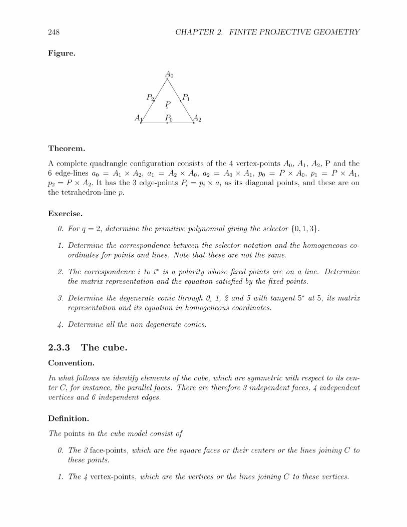
248 CHAPTER 2. FINITE PROJECTIVE GEOMETRY
Figure.
TTTTTTT
qA1 aP0 qA2
qP2 qP1
aA0
aP
Theorem.
A complete quadrangle configuration consists of the 4 vertex-points A0, A1, A2, P and the6 edge-lines a0 = A1 × A2, a1 = A2 × A0, a2 = A0 × A1, p0 = P × A0, p1 = P × A1,p2 = P × A2. It has the 3 edge-points Pi = pi × ai as its diagonal points, and these are onthe tetrahedron-line p.
Exercise.
0. For q = 2, determine the primitive polynomial giving the selector 0, 1, 3.
1. Determine the correspondence between the selector notation and the homogeneous co-ordinates for points and lines. Note that these are not the same.
2. The correspondence i to i∗ is a polarity whose fixed points are on a line. Determinethe matrix representation and the equation satisfied by the fixed points.
3. Determine the degenerate conic through 0, 1, 2 and 5 with tangent 5∗ at 5, its matrixrepresentation and its equation in homogeneous coordinates.
4. Determine all the non degenerate conics.
2.3.3 The cube.
Convention.
In what follows we identify elements of the cube, which are symmetric with respect to its cen-ter C, for instance, the parallel faces. There are therefore 3 independent faces, 4 independentvertices and 6 independent edges.
Definition.
The points in the cube model consist of
0. The 3 face-points, which are the square faces or their centers or the lines joining C tothese points.
1. The 4 vertex-points, which are the vertices or the lines joining C to these vertices.

2.3. GEOMETRIC MODELS ON REGULAR PYTHAGOREAN POLYHEDRA. 249
2. The 6 edge-points, which are the edges, or the mid-points of the edges or the linesjoining C to these points.
The lines in the cube model consist of
3. The 3 face-lines, corresponding to a face f, which are incident to the 2 face-points andto the 2 edge-points in the plane through C parallel to f.
4. The 4 vertex-lines, corresponding to a vertex V, which are ncident to the vertex-pointsV and to the 3 edge-points not adjacent to V.
5. The 6 edge-lines, corresponding to an edge e, which are incident to the face-pointperpendicular to e, to the 2 vertex-points and the edge-point on e.
Theorem.
The cube model satisfies the axioms of projective geometry for p = 3.
Theorem.
With the selector 2.3.1 for p = 3, the auto-polars are 0, 7, 8 and 11. If we examine thequadrangle-quadrilateral configuration, we observe that p and qi are the lines which requirea 4-th point, it is easy to verify that, with p = 3, P is on p and Qi is on qi. Moreover0∗ · 0 = 0, this suggest to take P = 0, Qi = 7, 8, 11. Henceri := P ×Qi = 9, 1, 3; pi := Qi+1 ×Qi−1 = 5, 2, 6;Ai := ri × pi = 4, 12, 10; ai := Ai+1 × Ai−1 = Ai; Pi := ai × ri = pi;qi := Pi+1 × Pi−1 = Qi; Ri := ai × qi = ri; p := R1 ×R2 = p.
Theorem.
Because of 2.3.3, the vertex-points are auto-polars, we can choose them as 0, 7, 8 and 11, theother elements of the cube follow from 2.3.3. The edge-points are Ri and Pi, the face-pointsare Ai.
Figure.
q
8Q1 a
9R0 q
11Q2
q0
P a5
P0 q7
Q0
a2P1 b
10A2 a
1R1
q 11 a 9 q 8a 6 b12A1 a 3R2
a6
P2
b4
A0
q0
a2

250 CHAPTER 2. FINITE PROJECTIVE GEOMETRY
Exercise.
0. For p = 3, determine the primitive polynomial giving the selector 0, 1, 3, 9.
1. Determine the correspondence between the selector notation and the homogeneous co-ordinates for points and lines. Note that these are not the same.
2. The correspondence i to i∗ is a polarity whose fixed points are on a line. Determinethe matrix representation and the equation satisfied by the fixed points.
3. Determine the degenerate conic through 0, 1, 2 and 5 with tangent 4∗ at 5, its matrixrepresentation and its the equation in homogeneous coordinates. Hint: use 2.2.11.
4. Determine all the conics.
2.3.4 The dodecahedron.
Convention.
In what follows we identify elements of the dodecahedron which are symmetric with respectto its center C, for instance, the parallel faces. There are therefore 6 independent faces,536 = 10 independent vertices and 5
26 = 15 independent edges.
Definition.
The points in the dodecahedron model consist of
0. The 6 face-points, which are the pentagonal faces or their center or the lines joiningC to these points.
1. The 10 vertex-points, which are the vertices or the lines joining C to these vertices.
2. The 15 edge-points, which are the edges, or the mid-points of the edges or the linesjoining C to these points.
The lines in the dodecahedron model consist of
3. The 6 face-lines, which are incident to the corresponding face-point F and to the 5edge-points in the plane through C perpendicular to CF.
4. The 10 vertex-lines, corresponding to a vertex V , which are incident to the 3 edge-points in the plane through C perpendicular to CV and to the 3 vertex-points whichjoined to V form an edge.
5. The 15 edge-lines, corresponding to an edge E, which are incident to the 2 face-points,the 2 vertex-points and the 2 edge-points in the plane through C and E.
Theorem.
The dodecahedron model satisfies the axioms of projective geometry for p = 5.

2.3. GEOMETRIC MODELS ON REGULAR PYTHAGOREAN POLYHEDRA. 251
Example.
For p = 5, the selector function associated with the selector 0, 1, 3, 8, 12, 18 isi 0 1 2 3 4 5 6 7 8 9 10 11 12 13 14 15f(i) 0 0 1 0 8 3 12 1 0 3 8 1 0 −13 −13 3type f e e e f v f v e f v v e v e s
i 16 17 18 19 20 21 22 23 24 25 26 27 28 29 30f(i) −13 1 0 12 12 −13 12 8 8 −13 8 12 3 3 1type f f e v v v e e v e e e e v e
The auto-polars are 0, 4, 6, 9, 16, 17.The “type” is explained in the following Theorem.
Theorem.
A natural labeling of the points of the dodecahedron and of the dodecahedral configuration,associated with the selector 2.3.1, for p = 5, can be obtained as follows. If we examine thedodecahedron configuration,
FAi · fai = AFi · afi = 0,it is therefore natural to choose FAi and AFi as the auto-polars, but this cannot be donearbitrarily. Let us choose any 3 of them as FAi, 0, 16 and 17. To obtain P and Ai, we canproceed as follows.pqi = FAi × FAi+1 = 18, 15, 1; PQi = pqi;PRi = pqi × FAi−1 = 14, 3, 2;qpi = PRi × PQi = 25, 28, 30;AFi = QPi ×QPi+1 = 6, 4, 9;ai = FAi+1 × AFi−1 = 23, 26, 8; Ai = ai;p = PR1 × PR2 = 29.We therefore choose P = 29 and Ai = 23, 26, 8. We obtain, according to 2.1.6, 2.1.7 and2.1.7:ai = Ai, ri = 20, 5, 10,Pi = 11, 13, 24, qi = 19, 7, 21, Ri = ri, pi = Pi, p = 29,PQi = pqi = 18, 15, 1, QPi = qpi = 25, 28, 30,QRi = qri = 12, 27, 22, PRi = pri = 14, 3, 2,AFi = afi = 6, 4, 9, FAi = fai = 0, 16, 17.
Therefore the face-points are FAi, AFi; the vertex-points are pi, qi, ri; the edge-points areAi, PQi, QPi, QRi, PRi.
Figure.
Q2
21
QR1 o o PQ1
27 FA0 15
R2 o 0 P0
10 11
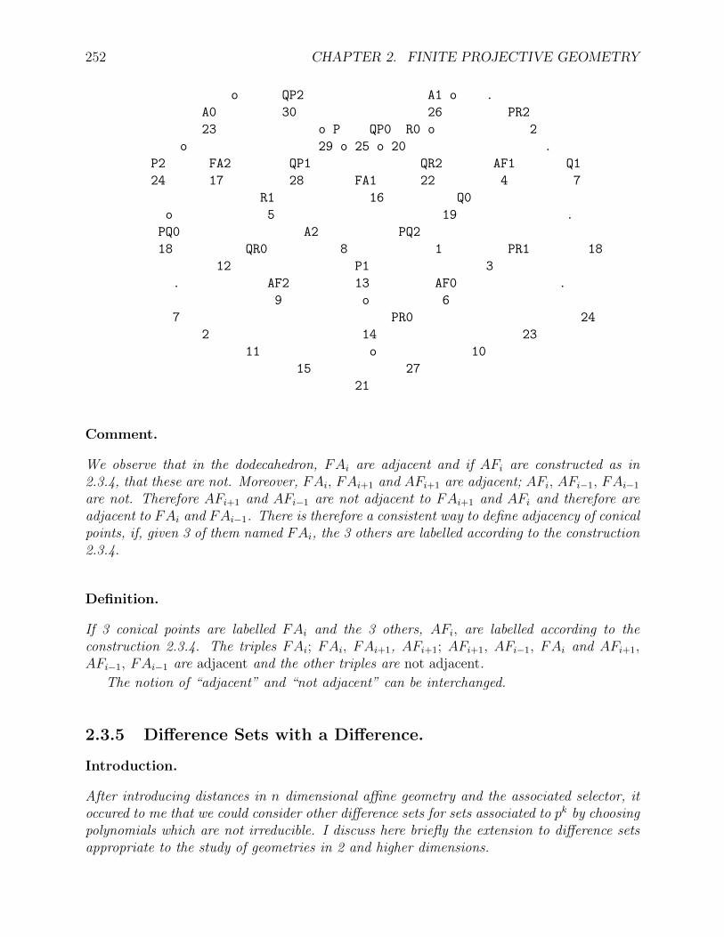
252 CHAPTER 2. FINITE PROJECTIVE GEOMETRY
o QP2 A1 o .
A0 30 26 PR2
23 o P QP0 R0 o 2
o 29 o 25 o 20 .
P2 FA2 QP1 QR2 AF1 Q1
24 17 28 FA1 22 4 7
R1 16 Q0
o 5 19 .
PQ0 A2 PQ2
18 QR0 8 1 PR1 18
12 P1 3
. AF2 13 AF0 .
9 o 6
7 PR0 24
2 14 23
11 o 10
15 27
21
Comment.
We observe that in the dodecahedron, FAi are adjacent and if AFi are constructed as in2.3.4, that these are not. Moreover, FAi, FAi+1 and AFi+1 are adjacent; AFi, AFi−1, FAi−1
are not. Therefore AFi+1 and AFi−1 are not adjacent to FAi+1 and AFi and therefore areadjacent to FAi and FAi−1. There is therefore a consistent way to define adjacency of conicalpoints, if, given 3 of them named FAi, the 3 others are labelled according to the construction2.3.4.
Definition.
If 3 conical points are labelled FAi and the 3 others, AFi, are labelled according to theconstruction 2.3.4. The triples FAi; FAi, FAi+1, AFi+1; AFi+1, AFi−1, FAi and AFi+1,AFi−1, FAi−1 are adjacent and the other triples are not adjacent.
The notion of “adjacent” and “not adjacent” can be interchanged.
2.3.5 Difference Sets with a Difference.
Introduction.
After introducing distances in n dimensional affine geometry and the associated selector, itoccured to me that we could consider other difference sets for sets associated to pk by choosingpolynomials which are not irreducible. I discuss here briefly the extension to difference setsappropriate to the study of geometries in 2 and higher dimensions.

2.3. GEOMETRIC MODELS ON REGULAR PYTHAGOREAN POLYHEDRA. 253
Definition.
A difference set associated to q = pk and to a polynomial of degree 3 with one root, is a set ofq integers s0, s1, . . . , sq−1 such that the q2− q differences si− sj, i 6= j modulo n = q2− 1are distinct and different from 0 modulo q + 1.A difference set associated to q = pk and to a polynomial of degree 3 with two roots, is a setof q − 1 integers s0, s1, . . . , sq−2 such that the q2 − 3q + 2= (q − 1)(q − 2) differences si − sj, i 6= j modulo n = q2 − q are distinct and different from0 modulo q and modulo q − 1.
When applied to Geometry, I will prefer the terminology of Lemay and use the synonymselector. The elements of the selector are called selector numbers.
Theorem.
There exists always a polynomial P of degree 3 with one root or 2 roots such that I is agenerator of the multiplicative group of polynomials, of degree at most 2, with coefficientsin Zp, normalized to have the coefficient of the highest power 1, which are relatively primeto P . The selector numbers are the powers of I modulo P which are polynomials of degreeat most 1.
The proof can be adapted easily from that of the irreducible case and is left as an exercise.
Example.
For p = 3, P = I3 + I + 1,I0 = 1, I1 = I, I2 = I2, I3 = I + 1,I4 = I2 + I, I5 = I2 − I − 1, I6 = I2 − I + 1, I7 = I2 + 1,and we have I8 = 1. Therefore the selector is 0, 1, 3.
Example.
The following are difference sets associated with q = pk :For p = 3 : I3 + I + 1, root 1, selector 0,1,3 (mod 8).
I3 + I2 − I − 1, roots 2,2,1, selector 0,1 (mod 6).For p = 5 : I3 − I − 1, root 2, selector 0,1,3,11,20 (mod 24).
I3 − 2I − 1, roots 3,3,4, selector 0,1,3,14 (mod 20).For p = 7 : I3 − I2 − 2, root 5, selector 0,1,7,11,29,34,46 (mod 48).
I3 − 3I − 2, roots 2,6,6, selector 0,1,3,11,16,20 (mod 42).For q = 11 : I3 − I − 1, root 6,
selector 0,1,3,28,38,46,67,90,101,107,116 (mod 120).I3 − I2 − I − 1, roots 7,7,9,selector 0,1,9,15,36,38,43,62,94,107 (mod 110.)
Definition.
The selector function f associated to the selector si is the function from Zn to Zn f(sj −si) = si, i 6= j, for all other values f(l) = −1.

254 CHAPTER 2. FINITE PROJECTIVE GEOMETRY
Example.
For p = 5, the selector function associated with 0, 1, 3, 11, 20 isi 0 1 2 3 4 5 6 7 8 9 10 11f(i) −1 0 1 0 20 20 −1 20 3 11 1 0
i 12 13 14 15 16 17 18 19 20 21 22 23f(i) −1 11 11 20 11 3 −1 1 0 3 3 1
Theorem.
0. If the defining polynomial has 1 root then the selector has n := p elements, the selectorfunction has p2 − 1 elements and is −1 for the p− 1 multiples of p+ 1.
1. If the defining polynomial has 2 distinct roots then the selector has n := p−1 elements,the selector function has p(p− 1) elements and is −1 for the 2p− 1 multiples of p andp− 1.
Theorem.
0. If f(i− j) 6= −1 then f(j − i)− i = f(i− j)− j.
Points, lines and incidence in the 2 dimensional geometry associated with q = pk andn := q2 + q + 1 are defined as follows.
Definition.
The points are elements of the set 0, 1, . . . , n-1, the lines are elements of the set 0, 1,. . . , n− 1, a point a is incident to a line b iff f(a+ b) = 0.
Notation.
The points are denoted by a lower case letter or by an integer in Zn. The lines are denotedby a lower case letter or by an integer in Zn followed by an asterix. The line incident to thepoints a and b is denoted a× b, the point incident to the lines a∗ and b∗ is denoted a ∗×b ∗ .
We leave as an exercise to state and prove Theorems analogous to those in Section 2.3.1.
Definition.
The dual affine plane, is a Pappian plane in which we prefer the “special“ points which arethose on a line l and a point P not on l and the “special” lines which are those through Pand the line l.
Th dual affine geometry can be studied by associating with it a polynomial which has 1root. I give here some examples of Desargues, Pappus and Pascal configurations.
I illustrate Pappus and Desargues configurations using the notation of 2.1.2 and of 2.1.5and give the points on a conic obtained using Pascal’s construction.

2.3. GEOMETRIC MODELS ON REGULAR PYTHAGOREAN POLYHEDRA. 255
Example.
For p = 11, with the polynomial I3 − I − 1, we havePappus(〈89, 51, 79〉, 69∗, 〈33, 88, 110, 〉, 13∗; 〈92, 71, 6〉, 95∗),with Ai+1 ×Bi−1 = (56∗, 87∗, 32∗) and Ai−1 ×Bi+1 = (28∗, 77∗, 115∗).Desargues(98, 7, 1, 70, 37∗, 31∗, 100∗, 60, 98, 73, 50∗, 47∗, 60∗;〈70, 76, 7〉, 〈60∗, 89∗, 50∗〉, 31∗),Desargues(111, 115, 69, 13, 54∗, 33∗, 51∗, 41, 119, 10, 91∗, 80∗, 117∗;〈67, 68, 70〉, 〈5∗, 47∗, 110∗〉, 53∗),From Pascal’s construction we obtain the following points are on a conic: 9,10,33,51,58,60,74,77,79,87,96,98.
Exercise.
Define a geometry corresponding to a polynomial which has 2 roots.
2.3.6 Generalization of the Selector Function for higher dimen-sion.
Introduction.
I will briefly stae one result for dimensions 3 and 4 concerning defining polynomials associ-ated to the non irreducible case and illustrate for dimnesions 3, 4 and 5.
Theorem.
If the Pi denotes a primitive polynomial of degree i.
0. For k = 3, the defining polynomials P can have the following form,P4, P1P3, P
21P2,
there are p4 + p3 + p2 + p+ 1, p4− 1, p4− p polynomials relatively prime to P, in theserespective cases.
1. For k = 4, the defining polynomials P can have the following form,P5, P1P4, P
21P3, P2P3.
there are p5 + p4 + p3 + p2 + p+ 1, (p3− 1)(p+ 1), p5− 1, p5− p polynomials relativelyprime to P, in these respective cases.
Proof: The polynomials in the sets are those which are relatively prime to the definingpolynomial. There are pk homogeneous polynomials of degree k. If, for instance, k = 4 andthe defining polynomial P is P2P3, there are p2 + p + 1 polynomials which are multiple ofP 2 and p+ 1, which are multiples of P3, hence p4 + p3 + p2 + p+ 1− (p2 + p+ 1)− (p− 1)polynomials relatively prime to P.

256 CHAPTER 2. FINITE PROJECTIVE GEOMETRY
Example.
a0, a1,. . .ak represent Ik+1 − a0Ik − a1I
k−1 − ak.k p period def. pol. |sel.| roots of def. pol.3 3 40 2, 1, 1, 1 13 −−
26 1, 1, 1, 1 9 124 0, 1, 1, 1 8 2, 2
5 156 1, 2, 0, 2 31 −−124 1, 0, 0, 2 25 4120 0, 0, 1, 2 24 4, 4
7 400 0, 1, 1, 4 57 −−342 0, 0, 1, 1 49 3336 0, 0, 3, 1 48 5, 5
11 1464 0, 0, 2, 5 133 −−1330 0, 0, 1, 1 121 31320 1, 5, 2, 4 120 1, 1
4 3 121 2, 0, 0, 0, 1 40 −−104 0, 1, 0, 0, 1 35 (I2 + I − 1)(I3 − I2 + I + 1)80 0, 2, 0, 0, 1 27 278 1, 0, 0, 0, 1 26 2, 2
5 781 4, 0, 0, 0, 1 156 −−744 2, 2, 0, 0, 1 149 (I2 + I + 2)(I3 + 2I2 − I + 2)624 2, 0, 0, 0, 1 125 3620 3, 0, 1, 0, 1 124 3, 3
7 2801 3, 0, 0, 0, 1 400 −−2736 6, 0, 0, 0, 1 391 (I2 + 2I − 2)(I3 − I2 − 3I − 3)2400 3, 1, 0, 0, 1 343 32394 0, 3, 3, 0, 1 342 5, 5
11
11 16105 0, 0, 10, 0, 9 1464 −−15960 0, 0, 0, 10, 8 1451 (I2 + I−)(I3 − I2 − I−)14640 0, 0, 0, 10, 9 1331 1014630 0, 0, 0, 9, 7 1330 3, 3
13 30941 8, 0, 0, 0, 1 2380 −−30744 5, 0, 0, 0, 1 2365 (I2 − 3I + 6)(I3 − 2I2 + I + 2)28560 2, 0, 0, 0, 1 2197 1128548
5 3 364 1, 0, 0, 0, 0, 1 121 −−242 1, 1, 0, 0, 0, 1 81 2240 1, 2, 1, 0, 0, 1 80 2, 2

2.3. GEOMETRIC MODELS ON REGULAR PYTHAGOREAN POLYHEDRA. 257
Definition.
Given a selector s, the selector function associates to the integers in the set Zn a set of p+ 1integers or p integers obtained as follows,
s(j) ∈ fi iff sel(l)− sel(j) = i for some l.
Theorem.
0. f(i) is the set of points on the line i∗ × 0∗.
1. f(i) − j, where we subtract j from each element in the set, is the set of points in(i+ j)∗ × j∗, equivalently
2. f(i− j)− j, is the set of points in i∗ × j∗.
3. a∗ × b∗ × c∗ = ((a− i)∗ × (b− i)∗ × (c− i)∗)− i.
Theorem.
0. If the defining polynomial is primitive, then
0. |s| = pk−1p−1
,
1. if i ≡/ pk−1p−1
, |f(i)| = p+ 1.
1. If the defining polynomial has one root, then
0. |s| = pk,
1. if i 6= 0, |f(i)| = p,
2. If the defining polynomial has a double root, then
0. |s| = pk − 1,
1. if i ≡/ p, p2 − 1, |f(i)| = p,
2. if i ≡ p and i 6= 0, |f(i)| = p− 1,
Example.
0. k = 3, p = 3, defining polynomial I4 − 2I3 − I2 − I − 1 = (I − 1)(I3 − I + 1),selector: 0, 1, 2, 9, 10, 13, 15, 16, 18, 20, 24, 30, 37

258 CHAPTER 2. FINITE PROJECTIVE GEOMETRY
selector function:0 −1 −1 −1 −1 14 1 2 10 16 28 2 9 13 301 0 1 9 15 15 0 1 9 15 29 1 13 20 242 0 13 16 18 16 0 2 24 37 30 0 10 20 303 10 13 15 37 17 1 13 20 24 31 9 10 18 244 9 16 20 37 18 0 2 24 37 32 9 10 18 245 10 13 15 37 19 1 18 30 37 33 9 16 20 376 9 10 18 24 20 0 10 20 30 34 15 16 24 307 2 9 13 30 21 9 16 20 37 35 2 15 18 208 1 2 10 16 22 2 15 18 20 36 1 13 20 249 0 1 9 15 23 1 18 30 37 37 0 13 16 18
10 0 10 20 30 24 0 13 16 18 38 2 15 18 2011 2 9 13 30 25 15 16 24 30 39 1 2 10 1612 1 18 30 37 26 15 16 24 3013 0 2 24 37 27 10 13 15 37
1. k = 3, p = 3, defining polynomial I4 − I3 − I2 − I − 1 = (I − 1)2(I2 + I − 1),selector: 0, 1, 2, 8, 11, 18, 20, 22, 23selector function:0 −1 −1 −1 7 1 11 20 14 8 20 23 21 1 2 231 0 1 22 8 0 18 20 15 8 11 22 22 0 1 222 0 18 20 9 2 11 18 16 2 11 18 23 0 11 233 8 20 23 10 1 8 18 17 1 11 20 24 2 20 224 18 22 23 11 0 11 23 18 0 2 8 25 1 2 235 18 22 23 12 8 11 22 19 1 8 186 2 20 22 13 −1 −1 −1 20 0 2 8
2. k = 3, p = 3, defining polynomial I4 − I2 − I − 1.selector: 0, 1, 2, 4, 14, 15, 19, 21selector function:0 −1 −1 −1 6 15 19 −1 12 2 14 −1 18 1 21 −11 0 1 14 7 14 19 21 13 1 2 15 19 0 2 192 0 2 19 8 −1 −1 −1 14 0 1 14 20 1 4 193 1 21 −1 9 15 19 −1 15 0 4 −1 21 0 4 −14 0 15 21 10 4 14 15 16 −1 −1 −1 22 2 4 215 14 19 21 11 4 14 15 17 2 4 21 23 1 2 15
Example.
In the case of Example 2.3.6.0. If we denote by i†, the lines 0∗ × i∗, these lines, which aresets of 4 points can all be obtained from1† = 0, 1, 9, 15, 2† = 0, 13, 16, 18, 4† = 9, 16, 20, 37 and10† = 0, 10, 20, 30 by adding an integer modulo n.1† + 0 = 1†, 9†, 15†, 1† + 1 = 39†, 8†, 14†,
1† + 9 = 6†, 31†, 32†, 1† + 15 = 34†, 25†, 26†,2† + 0 = 2†, 24†, 37†, 2† + 2 = 22†, 35†, 38†, 2† + 37 = 3†, 5†, 27†,

2.3. GEOMETRIC MODELS ON REGULAR PYTHAGOREAN POLYHEDRA. 259
2† + 24 = 13†, 16†, 18†,4† + 0 = 4†, 21†, 33†, 4† + 4 = 17†, 29†, 36†, 4† + 21 = 12†, 19†, 23†,
4† + 33 = 7†, 11†, 28†,10† + 0 = 10†, 20†, 30†.
2.3.7 The conics on the dodecahedron.
Introduction.
The reader may want to skip this section until he has become familiar with conics. In it, wesummarize the various types and sub-types of conics as they relate to the representation ofthe finite projective plane, for p = 5, on the dodecahedron. We will see later, IV.1.12. thatthe dodecahedron can also be used to represent the finite polar and the finite non-Euclideangeometry, for p = 5.
Definition.
The conics are all of the same type if the classification into face-points, vertex-points andedge-points is the same. The conics are of the same sub-type if they can be derived from eachother using any of the 60 collineations which exchange face-points.
Notation.
In the following Theorem we use the notation“60 fffvve, 30 C1 (6,9,17;11,29;22), 30 C2 (9,16,17;7,13;15).“to indicate that we have 60 conics with 3 face-points, 2 vertex-lines and 1 edge-line. Theseare of the sub-type C1 and C2. An example of a conic of a given sub-type is provided inparenthesis, “;” separates points of a different classification, these points are given in theorder, face-point, vertex-point, edge-point, and in the same classification in increasing order.A pictorial representation of the sub-types is given in Figure 2.3.7.

260 CHAPTER 2. FINITE PROJECTIVE GEOMETRY
Theorem.
The 31.30.25.16. 66!
= 3100 conics are of the following type and sub-type.
1 ffffff, 1 A (0, 4, 6, 9, 16, 17).30 ffffee, 30 B (6, 9, 16, 17; 2, 22).60 fffvve, 30 C1 (6, 9, 17; 11, 29; 22), 30 C2 (9, 16, 17; 7, 13; 15).
120 fffvee, 30 D1 (9, 16, 17; 7; 1, 25), 30 D2 (9, 16, 17; 5; 1, 18),30 D3 (0, 4, 6, ; 5; 1, 4), 30 D4 (0, 4, 6; 13; 18, 30).
30 ffvvvv, 15 E1 (0, 4; 5, 11, 13, 20), 15 E2 (0, 4; 7, 19, 21, 29).60 ffvvve, 60 F (0, 4; 11, 13, 29; 8).
360 ffvvee, 30 G1 (0, 4; 11, 20; 1, 14), 30 G2 (0, 4; 5, 13; 3, 30),30 G3 (0, 4; 7, 21; 18, 27), 30 G4 (0, 4; 19, 21; 12, 28),60 G5 (0, 4; 11, 29; 1, 22), 60 G6 (0, 4; 5, 11; 14, 18),60 G7 (0, 4; 21, 29; 1, 27), 60 G8 (0, 4; 5, 21; 2, 27).
180 ffveee, 30 H1 (0, 4; 11; 8, 22, 25), 30 H2 (0, 4; 13; 8, 15, 22),60 H3 (0, 4; 21; 2, 18, 28), 60 H4 (0, 4; 21; 1, 22, 30).
135 ffeeee, 15 I1 (0, 4; 2, 15, 22, 25), 30 I2 (0, 4; 2, 12, 14, 15),30 I3 (0, 4; 15, 18, 22, 30), 60 I4 (0, 4; 1, 15, 25, 30).
12 fvvvvv, 6 J1 (16; 7, 10, 11, 21, 24), 6 J2 (16; 5, 13, 19, 20, 29).120 fvvvve, 60 K1 (16; 5, 10, 13, 19; 27), 60 K2 (6; 5, 7, 10, 11; 26).300 fvvvee, 30 L1 (4; 10, 11, 20; 1, 12), 30 L2 (0; 5, 10, 13; 27, 30),
60 L3 (16; 11, 21, 24; 12, 18), 60 L4 (0; 10, 11, 20; 1, 15),60 L5 (0; 7, 10, 21, 3, 22), 60 L6 (0; 5, 11, 13; 12, 26).
480 fvveee, 30 M1 (9; 11, 21; 2, 14, 28), 30 M2 (0; 10, 20; 25, 28, 30),60 M3 (17; 19, 21; 2, 23, 25), 60 M4 (0; 19, 24; 2, 14, 15),60 M5 (9; 10, 20; 1, 15, 18), 60 M6 (16; 20, 29; 12, 27, 28),60 M7 (9; 7, 29; 8, 12, 30), 60 M8 (16; 24, 21; 1, 12, 26),60 M9 (17; 7, 21; 3, 8, 14).
480 fveeee, 60 N1 (0; 10; 3, 15, 27, 30), 60 N2 (0; 10; 14, 15, 18, 30),60 N3 (0; 10; 12, 14, 22, 30), 60 N4 (0; 13; 1, 23, 27, 30),60 N5 (0; 10; 1, 2, 27, 28), 60 N6 (0; 13; 1, 26, 28, 30),60 N7 (0; 13; 2, 3, 15, 22), 60 N8 (0; 13, 2, 12, 22, 23).
12 feeeee, 6 O1 (16; 1, 8, 22, 25, 28), 6 O2 (16; 3, 12, 14, 26, 30).10 vvvvvv, 10 P (5, 7, 10, 11, 21, 29).60 vvvvee, 30 Q1 (10, 11, 20, 29; 15, 27), 30 Q2 (29, 5, 13; 21; 1, 12).
240 vvveee, 30 R1 (10, 21, 29; 3, 18, 23), 30 R2 (10, 11, 20; 23, 27, 30),30 R3 (10, 21, 29; 14, 26, 28), 30 R4 (10, 20, 24; 3, 18, 23),60 R5 (10, 21, 29; 3, 25, 28), 60 R6 (11, 13, 29; 1, 8, 15).
270 vveeee, 15 S1 (11, 20; 3, 18, 27, 30), 15 S2 (11, 20; 2, 15, 22, 25),30 S3 (11, 20; 1, 2, 12, 22), 30 S4 (11, 20; 1, 14, 18, 30),30 S5 (7, 21; 18, 22, 25, 27), 30 S6 (7, 21; 2, 12, 14, 15),30 S7 (7, 21; 3, 12, 14, 30), 30 S8 (7, 21; 8, 12, 14, 26),60 S9 (7, 21; 2, 3, 18, 25).
120 veeeee, 30 T1 (21; 3, 12, 14, 22, 28), 30 T2 (5; 3, 8, 22, 26, 28).60 T3 (24; 3, 12, 14, 22, 27).
20 eeeeee, 10 U1 (1, 2, 14, 18, 25, 30), 10 U2 (3, 12, 14, 15, 25, 27).

2.3. GEOMETRIC MODELS ON REGULAR PYTHAGOREAN POLYHEDRA. 261
The proof of the decomposition into types was done using a computer program which took22 minutes to run an an IBM PC.
Figure.
The pictorial representation of a conic of a given sub-type on the dodecahedron is as follows.
A: the 6 faces.
B: f . f
.
. . . .
. .
o o
f f
. . .
. .
C1: . o . C2: f . f
. . .
f . . . .
o . o o
. . f
. . . . .
. f . f . . o .
. . . . .
. .
. o
D1: o D2: . . .
f . f . .
f
. . .
. . . . . .
. . o o o
f
o o . f . f .
. . . . . .
. .
. . . .

262 CHAPTER 2. FINITE PROJECTIVE GEOMETRY
D3: . . . D4: . . .
. . o o
f f f f f
. . . .
o o . .
. . . . . .
. . . . . .
. o . . o .
. . . .
. . . .
E1: o . o E2:
o o
. . . .
. . .
. .
. . . f . f .
. o .
. . .
. f . f . . .
o o
. o .
. .
. .
F: . o o
. .
. .
. .
. o .
. f . f .
. . .
. .
. o
. o
G1: G2: o . o
. .
. . . .
. o .
. .
. f . f . . .

2.3. GEOMETRIC MODELS ON REGULAR PYTHAGOREAN POLYHEDRA. 263
o . o
. o .
. . . f . f .
. .
. . .
o . . .
. .
. o
G3: G4:
o o o .
. . . .
o . o . . .
. f . f . . f . f .
. . . . . .
. . . .
. . . o
o .
o .
G5: G6: o . .
. o
o . . o
. . .
. .
. f . f . . .
o o .
. o .
. . . f . f .
. .
. . .
. . . .
. .
o .
G7: G8: o . .
. o
. . . .
. . .
. o
. f . f . o .
. . o
. . o
. . . f . f .
. o
. . .
. . . .

264 CHAPTER 2. FINITE PROJECTIVE GEOMETRY
. .
H1: . o . H2: . o o
. . . .
. . . .
. . . o
. o . . . .
. f . f . . f . f .
. . . . . .
o o o .
. . . .
o . . .
H3: . . . H4: . . .
. . o .
. o . .
o . o .
o . . . . o
. f . f . . f . f .
. . . . . .
. . . .
. . . o
I1: I2: . . .
. .
o o o o
. . .
. .
. f . f . o o
. . .
. . .
o o . f . f .
. .
. . .
. .
. .

2.3. GEOMETRIC MODELS ON REGULAR PYTHAGOREAN POLYHEDRA. 265
o
I3: I4:
. . . .
. o . o
o . . . . o
. f . f . . f . f .
. . o . . .
o . . o
. . . .
J1: . . . J2: .
. . o
. . . .
o o o o
. . f
. o . . .
o . o o . o
. . . . .
. .
. .
f
K1: f K2: . . .
o o
. . . .
. o . f
. .
. . . . .
. o .
. . .
o . o . o
o .
. . o
. .
o .
L1: o . o L2: . . .
. . . .
f f
. . . .
. . o o
o . o . o .

266 CHAPTER 2. FINITE PROJECTIVE GEOMETRY
. . . o . o
. o . . . .
. . . .
. . . .
L3: L4: o . o
o o
. o o .
. . . f
. .
o o . . .
. o .
. . .
. . . . .
. .
f o . .
. .
. .
L5: o . o L6: . . .
. . . .
f f
. . . .
. . . o
. . . . o .
. o o o . .
. . . . . .
. o p .
. . o .
M1: o M2: o
. .
. . . . . o o .
. . o o
f f
o o . .
o . o . . .
. . o .
M3: . o . M4: . o .
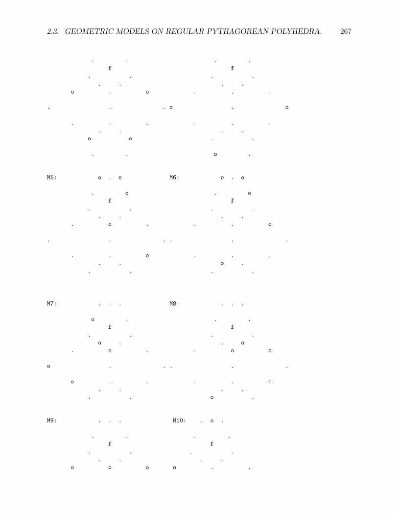
2.3. GEOMETRIC MODELS ON REGULAR PYTHAGOREAN POLYHEDRA. 267
. . . .
f f
. . . .
. . . .
o . o . . .
. . . o . o
. . . . . .
. . . .
o o . .
. . o .
M5: o . o M6: o . o
. o . o
f f
. . . .
. . . .
. o . . . o
. . . . . .
. . o . . .
. . o .
. . . .
M7: . . . M8: . . .
o . . .
f f
. . . .
o . . o
. o . . o o
o . . . . .
o . . . . o
. . . .
. . o .
M9: . . . M10: . o .
. . . .
f f
. . . .
. . . .
o o o o . .

268 CHAPTER 2. FINITE PROJECTIVE GEOMETRY
. . . . o o
. . o . .
. . . .
. o . o
o
N1: . . . N2:
. .
o . . .
f o o o
. .
o o . f o .
. o .
. . .
. . . . .
. .
. . .
o .
. .
N3: . . . N4: o o .
. . . .
f
. o . .
. o o o
o . . . . .
. . . . f o .
. . . . . .
. o . .
. . . .
o . . .
N5: . . . N6: . . .
. . o o
f f
. . . .
o . . .
. o o . . .
. . . . . .

2.3. GEOMETRIC MODELS ON REGULAR PYTHAGOREAN POLYHEDRA. 269
o . . . o .
. . . o
. . . .
. . o .
o . o .
N7: . . . N8: . . .
. . . .
f f
. . . .
o . . .
o . . o . o
. . . . . .
. o o o o .
. . . .
. . . .
o
O1: . O2: o
. .
. o o . o . . o
. . . .
f
o o . .
. o . . . .
. . o o
f
P:
o .
. .
. o .
o . o
. o .
. .
. o
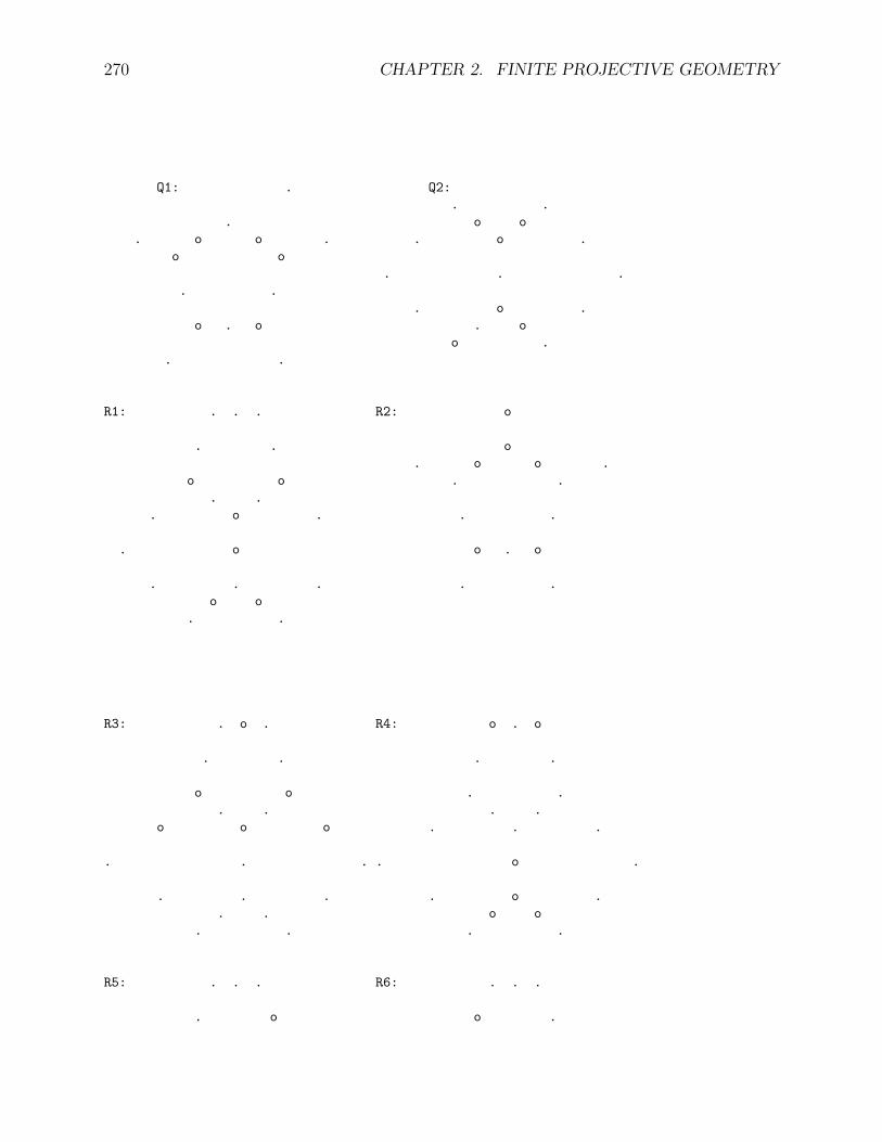
270 CHAPTER 2. FINITE PROJECTIVE GEOMETRY
Q1: . Q2:
. .
. o o
. o o . . o .
o o
. . .
. .
. o .
o . o . o
o .
. .
R1: . . . R2: o
. . o
. o o .
o o . .
. .
. o . . .
. o o . o
. . . . .
o o
. .
R3: . o . R4: o . o
. . . .
o o . .
. . . .
o o o . . .
. . . . o .
. . . . o .
. . o o
. . . .
R5: . . . R6: . . .
. o o .
2.3. GEOMETRIC MODELS ON REGULAR PYTHAGOREAN POLYHEDRA. 271
o o o o
. . . o
. o o o . .
. . . . .
. . . . . .
o . . .
. . . o
. .
S1: S2:
. . . .
. . o o
o o o . o .
. . . . . .
o o o . o .
. . o o
. . . .
o . . o
S3: S4:
. . . .
o . . .
. o . o o .
. . . . . .
. o . . o o
o . . .
. . . .
o . o .
o
S5: . . . S6: .
. . .
. o o .
o o o o
. .
o . o o o
. . . . . .

272 CHAPTER 2. FINITE PROJECTIVE GEOMETRY
. . . . .
o o
. .
S7: . . . S8: . o .
o o o o
o o o o
. . . .
. . . . . .
. . . . o .
o . o
. .
. .
. .
S9:
o o
o .
o . .
. . .
o . .
. o
. .
. .
T1: . . . T2: o o .
o o o .
. . . .
. . . o
o . o . . o
. o . . . o .
. o . . . .
. . . .
. . . .
T3: . . .
o .

2.3. GEOMETRIC MODELS ON REGULAR PYTHAGOREAN POLYHEDRA. 273
. .
. .
. o o
. o
. . o
o .
. .
U1: . . . U2: . o .
o o . .
. . . .
. . o o
o . o . . .
. . . . o .
. . . o . o
o o . .
. . . .
The family of types of conics was determined interactively using a computer program.
2.3.8 The truncated dodecahedron.
Introduction.
After defining convex uniform polyhedra, whose notion may go back to Archimedes and werefully studied by Kepler, we will show that one of them, the truncated dodecahedron can beused as a model for the finite projective plane of order 32.
Definition.
A polyhedron with regular faces, in Euclidean 3-space is uniform if it has symmetry operationstaking a given vertex into any other vertex, otherwize it is non-uniform. If, in addition, allfaces are congruent, the polyhedra is regular.
Theorem. [Euclid]
There are 5 convex regular polyhedra.
Notation. [See Johnson.]
In the following Theorem, we use the following notation, developped by several Mathemati-cians. n denotes a regular polygon with n sides, (n.q.n.q) denotes a vertex with adjoiningfaces successively with n, q, n, q sides, < n.q > denotes an edge ajoining a face with n sidesand one with q sides.

274 CHAPTER 2. FINITE PROJECTIVE GEOMETRY
Theorem. [Kepler]
Besides regular prisms and antiprisms, there are 13 convex uniform, non-regular polyhedra.These are Name Faces Vertices Edges
Cuboctahedron 83, 64 12(3.4.3.4) 24 < 3.4 >Icosidodecahedron 203, 125 30(3.5.3.5) 60 < 3.5 >Truncated tetrahedron 43, 46 12(3.62) 12 < 3.6 >, 6 < 6.6 >Truncated octahedron 64, 86 24(4.62) 24 < 4.6 >, 12 < 6.6 >Truncated cube 83, 68 24(3.82) 24 < 3.8 >, 12 < 8.8 >Truncated icosahedron 125, 206 60(5.62) 60 < 5.6 >, 30 < 6.6 >Truncated dodecahedron 203, 1210 60(3.102) 60 < 3.10 >, 30 < 10.10 >Rhombicuboctahedron 83, 184 24(3.43) 24 < 3.4 >, 24 < 4.4 >Rhombicosidodecahedron 203, 304, 60(3.4.5.4) 60 < 3.4 >, 60 < 4.5 >
125Truncated cuboctahedron 124, 86, 48(4.6.8) 24 < 4.6 >, 24 < 4.8 >,
68 24 < 6.8 >Truncated 304, 206, 120(4.6.10) 60 < 4.6 >, 60 < 4.10 >,
icosidodecahedron 1210 60 < 6.10 >Snubcuboctahedron 323, 64 24(34.4) 36 < 3.3 >, 24 < 3.4 >Snubicosidodecahedron 803, 125 60(34.5) 90 < 3.3 >, 60 < 3.5 >n− gonal prism n4, 2n 2n(42.n) n < 4.4 >, 2n < 4.n >n− gonal antiprism 2n3, 2n 2n(33.n) 2n < 3.3 >, 2n < 3.n >
Theorem. [N. W. Johnson]
There are 92 convex non-uniform regular-faced polyhedra.The fact that all vertices are of the same type does not insure uniformity, as the example
of the elongated square gyrobicupola of J. C. P. Miller shows. This non-uniform polyhedrahas the same characteristics as the rhombicuboctahedron, but has the part below the 8 squaresturned 45 degrees.
Before discussing the truncated dodecahedron as a model for the Pappian plane associatedwith 32, I will discuss the pentagonal antiprism as a model for the Pappian plane associatedwith 22.
Notation.
I identify elements which are symmetrical with respect to the center of the antiprism. Forthe pentagonal antiprism, with i = 0, 1, 2, 3, 4, I will denote by ti, the 5 triangular faces, byvi, the 5 vertices, by ei, the 5 pentagonal-triangular edges, by fi, the 5 triangular-triangularedges and by p, pentagonal face. We have altogether 21 elements to represents the 21 pointsin the plane associated with 22.
Theorem.
For q = 22,
0. The selector is 0, 1, 4, 14, 16.
1. The corresponding selector function f is, and the representation of the points on theantiprism are

2.3. GEOMETRIC MODELS ON REGULAR PYTHAGOREAN POLYHEDRA. 275
i 0 1 2 3 4 5 6 7 8 9 10f(i) 0 0 14 1 0 16 16 14 14 16 4
repr. of points v2 e2 v4 f3 f2 t3 t1 v0 v1 e0 e3
repr. of lines v2 t2 v4 f3 f2 e3 e1 v0 v1 t0 t3
i 11 12 13 14 15 16 17 18 19 20f(i) 14 4 1 0 1 0 4 4 16 1
repr. of points v3 f4 f1 p t0 t2 e1 f0 e4 t4repr. of lines v3 f4 f1 p e0 e2 t1 f0 t4 e4
2. The incidence properties aree∗i ι vi, ei±2, ti±1,t∗i ι vi, ti±2, fi±1,f ∗i ι vi, ei±1, fi±1,v∗i ι p, vi, ei, ti, fi,p ι vi.
Proof: I leave as an exercise the determination of the fundamental polynomial and thecorresponding selector.The selector function follows easily from its definition.The selector polarity which associates i to i∗ has the fixed points 7,8,11,0 and 2 on the line14∗. I will associates to 14 and to 14∗ the pentagonal face and its incident points or lines tovi. Starting from that, one of the possible solution is given in 1. Notice that I use the samecorrespondance between ei, vi and fi for the points and the lines but exchange ti and ei toget the corresponding points and lines.
Figure.
The corresponding drawing for the Projective plane over 22 is given page . . . .
Notation.
For the truncated dodecahedron, I will denote by t, a triangular face, by d, a decagonal face,by v, a vertex, by e, a < 10, 10 > edge and by u, a < 3.10 > edge. The lower case notationis used indifferently for points and lines, the upper case notation for points.
Lemma.
If xY denotes the number of points of type Y incident to a line of type x, then2|fY , 5|dY , 3|tY for Y 6= T, 3|tT − 1.
Proof: For instance, there are 10 T -points, each is adjacent to 10 lines; on the otherhand, the 30 e-lines are adjacent to 30 eT triangles, the 15 f -lines are adjacent to 15 fTtriangular-points, . . . . This implies
30eT + 15fT + 30vT + 10tT + 6dT = 100, which gives, modulo 2, fT = 0, modulo 5,dT = 0, modulo 3, tT = 1.

276 CHAPTER 2. FINITE PROJECTIVE GEOMETRY
Theorem.
For q = 32, a primitive polynomial is
0. I3 − I − ε,with ε = 1 + α, an 8-th root of unity and α2 = −1.The powers of ε are 1, 1 + α, −α, 1− α, −1, −1− α, α, −1 + α.
The corresponding selector is
1. 0, 1, 3, 9, 27, 49, 56, 61, 77, 81.The corresponding selector function is
2. 0 1 2 3 4 5 6 7 8 9 10 11 12 13 14 15 16 17 18 19 20 21 22 23
0 1 0 77 56 3 49 1 0 81 81 49 81 77 77 61 77 9 81 61 56 27 77
t e e e d e e v v v v e u u e v e u v u u v e u
0 1 2 56 57 24 21 54 48 9 10 66 65 19 30 16 15 39 18 13 23 6 32 20
24 25 26 27 28 29 30 31 32 33 34 35 36 37 38 39 40 41 42 43 44 45 46
3 56 1 0 49 27 61 61 49 61 27 56 56 81 56 61 9 77 49 49 56 49 3
v u u v t u v v v v v v u u u u u v v u v e t
5 89 80 49 50 69 14 63 22 41 45 88 58 87 74 17 85 33 64 73 53 34 84
47 48 49 50 51 52 53 54 55 56 57 58 59 60 61 62 63 64 65 66 67 68 69
9 1 0 27 49 9 3 27 1 0 61 3 81 1 0 56 77 27 27 81 27 9 49
t v v t u u v v d v u u t u v u e v u v u v u
47 8 27 28 67 83 44 7 60 3 4 36 59 55 77 78 31 42 12 11 51 72 29
70 71 72 73 74 75 76 77 78 79 80 81 82 83 84 85 86 87 88 89 90
77 81 9 27 3 77 1 0 3 61 1 0 9 9 56 9 61 81 3 3 1
t v e u u d t e d u d v v u t u t u e d e
86 71 68 43 38 79 76 61 62 75 26 81 82 52 46 40 70 37 35 25 90
3. 0, 46, 47, 50, 59, 70, 28, 76, 84, 86.
The letters refer to the type. The last row gives the conjugate, for instance, 61 is theconjugate of 77.
Proof: To retrieve the primitive polynomial associated with S, the selector 1, because3 ∈ S, I3 = βI + γ, β and γ are chosen in such a way that I56 has no term of second degree.The computations are facilitated by preparing first a table giving g(i) 3
1 + εi = εg(i), 0 ≤ i ≤ t,and by use of the convention ε−1 = 0.
The conjugates are obtained when α is replaced by −α.
Heuristics.
The truncated dodecahedron has 182 faces, vertices and edges. using symmetry with respectto the center we expect that a model can be found for the projective geometry of order 32,with 91 points and with 10 points on each line . We will solve simultaneously the followingproblems, discover appropriate incidence properties, associate to the vertices, integers from0 to 90 to take advantage of the selector and determine a fundamental projectivity on a line

2.3. GEOMETRIC MODELS ON REGULAR PYTHAGOREAN POLYHEDRA. 277
to prepare for a representation of finite Euclidean geometry. I will describe here some of thesteps which have led me to the solution given in 2.3.8 to 2.3.8.
The auto-correlates should be the points of a conic γ. I will choose this conic as a circlein the corresponding Euclidean plane. The intersection of the lines 0 × 70 = 77∗ and of46× 28 = 72∗, which is 75, is chosen as the center of the circle. The points on the polar 75∗
are 2, 6, 16, 17, 19, 25, 43, 65, 72, 77.To obtain a fundamental projectivity, we want to choose 2 points, A, B, on the circle and
project from them any point X on the circle onto 75∗, giving XA and XB, XA correspondsto XB, we want to choose A and B such that the projectivity is of order 10. A trial gave aprojectivity of order 5, it was then easy to obtain one of order 10 using A = 0 and B = 50.The computations start as follows: 0× 0 = 0∗ × 75∗ = 77× 0 = 0∗ with 0 as the other pointon γ.50× 0 = 27∗ × 75∗ = 65× 0 = 27∗ with 50 as the other point on γ.50× 50 = 50∗ × 75∗ = 6× 0 = 3∗ with 46 as the other point on γ.50× 46 = 31∗ × 75∗ = 25× 0 = 56∗ with 84 as the other point on γ.. . . . Hence the projectivity 2.3.8 and the equidistant points 0, 50, 46, 84, 47, 70, 86, 28, 76,59 on γ .
With one d-face chosen as 75∗, the 10 t-faces are subdivided into 2 sets, those adjacentto the d-face and those which are not. The vertices of the pentagonal points 0, 46, 47, 86,76 are chosen for the successive triangles adjacent to the d-face. The diametrically oppositepoint, e. g. 70 of 0 is chosen for the triangle not adjacent to the d-face but adjacent to thetriangle 0.
Because 0× 46 = 3, 46× 47 = 45, . . . , 0× 70 = 77, 50× 86 = 6, I chose the pentagonalside 3 for the e-point between the t-points 0 and 46, . . ., the diameter 77 for the e-pointbetween the t-points 0 and 70, . . .. Because 5|75Y , we chose these 10 e-points as incident to75∗.
These consideration suggest Definition 2.3.8 and Theorems 2.3.8 and 2.3.8.
Definition.
The points in the truncated dodecahedron model consist of
0. The 10 triangular face-points T.
1. The 6 decagonal face-points D.
2. The 30 vertex-points V.
3. The 30 triangular-decagonal edge-points U.
4. The 15 decagonal-decagonal edge-points E.
The lines in the truncated dodecahedron model consist of
0. The 10 triangular face-lines t. Each is incident to itself as a point, to the 3 adjacent< 12.12 > edge-points E, and to the 6 vertex-points V which are the vertices of thetriangle adjacent to the 3 edge-points which are not themselves adjacent to these points.For instance, for t = 0, the incident points are0(T ), 1(E), 77(E), 3(E), 56(V ), 61(V ), 27(V ), 81(V ), 9(V ), 49(V ) :

278 CHAPTER 2. FINITE PROJECTIVE GEOMETRY
o 61 27 o
. 1 77 .
56 o o . . o o 81
o _0
. . .
. o 3 . .
. . .
. o o .
. 49 9 .
1. The 6 decagonal face-lines d. Each is incident to its 5 < 3.12 > edges U , and the 5< 12.12 > edges E adjacent to its 5 adjacent triangles.For instance 75(d) is incident to25(U), 43(U), 65(U), 17(U), 19(U)and2(E), 6(E), 16(E), 77(E), 72(E) :
.
o72
.
. o .
. 19 .
o . . . . o
77 o 17 25 o 2
. _75 .
. .
o 65 43 o
. .
. .
16 o o 6
. .
2. The 30 vertex-lines v. Each is incident to the < 12.12 > edge E0 adjacent to it andto the vertex at the other end of it, to the 2 triangular points T1 and T2 adjacent tothe other edges E1 and E2, to the 2 < 12.12 > edges E3 and E4 opposite to E1 or E2
belonging to the same decagon as v, to the vertices adjacent to E3 or E4 closest to v,to the < 3.12 > edges U belonging to the same decagon as T1 or T2 and the triangleopposite E0.For instance, 9(v) is adjacent to72(E), 68(V ), 0(T ), 47(T ), 85(E), 40(E), 82(V ), 40(V ), 83(U), 52(U) :
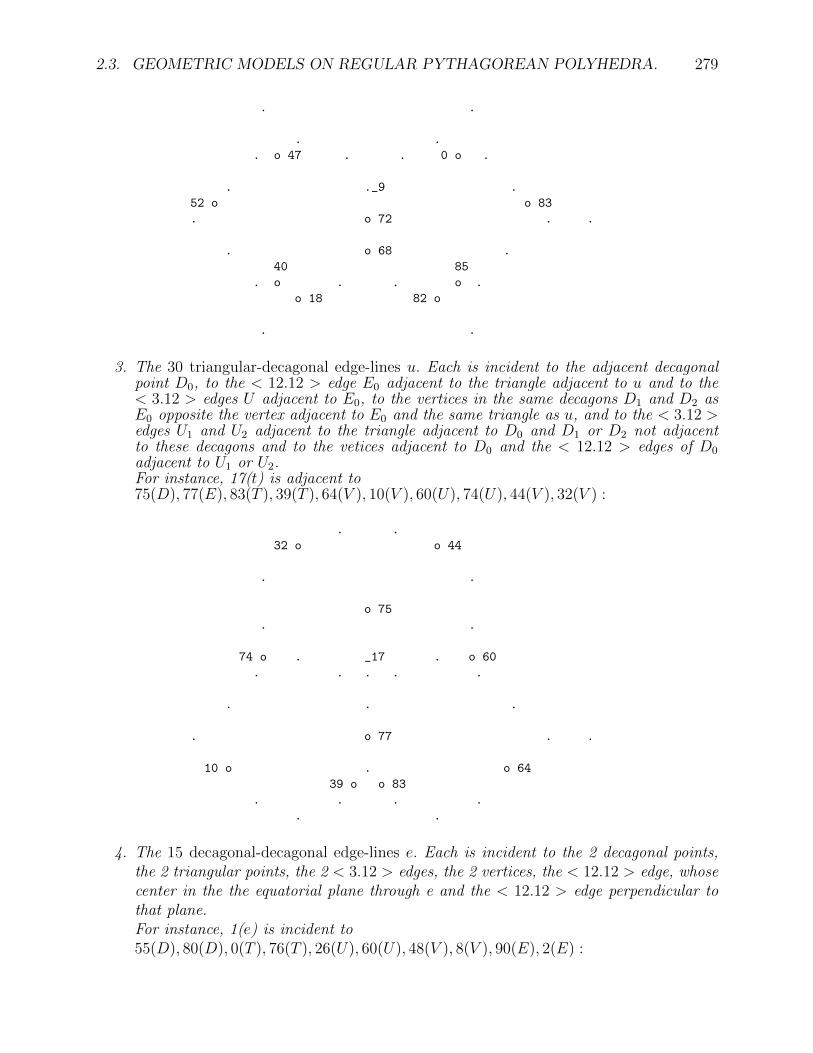
2.3. GEOMETRIC MODELS ON REGULAR PYTHAGOREAN POLYHEDRA. 279
. .
. .
. o 47 . . 0 o .
. ._9 .
52 o o 83
. o 72 . .
. o 68 .
40 85
. o . . o .
o 18 82 o
. .
3. The 30 triangular-decagonal edge-lines u. Each is incident to the adjacent decagonalpoint D0, to the < 12.12 > edge E0 adjacent to the triangle adjacent to u and to the< 3.12 > edges U adjacent to E0, to the vertices in the same decagons D1 and D2 asE0 opposite the vertex adjacent to E0 and the same triangle as u, and to the < 3.12 >edges U1 and U2 adjacent to the triangle adjacent to D0 and D1 or D2 not adjacentto these decagons and to the vetices adjacent to D0 and the < 12.12 > edges of D0
adjacent to U1 or U2.For instance, 17(t) is adjacent to75(D), 77(E), 83(T ), 39(T ), 64(V ), 10(V ), 60(U), 74(U), 44(V ), 32(V ) :
. .
32 o o 44
. .
o 75
. .
74 o . _17 . o 60
. . . . .
. . .
. o 77 . .
10 o . o 64
39 o o 83
. . . .
. .
4. The 15 decagonal-decagonal edge-lines e. Each is incident to the 2 decagonal points,the 2 triangular points, the 2 < 3.12 > edges, the 2 vertices, the < 12.12 > edge, whosecenter in the the equatorial plane through e and the < 12.12 > edge perpendicular tothat plane.For instance, 1(e) is incident to55(D), 80(D), 0(T ), 76(T ), 26(U), 60(U), 48(V ), 8(V ), 90(E), 2(E) :

280 CHAPTER 2. FINITE PROJECTIVE GEOMETRY
. o .
. 90 .
. .
o 55
. .
. 26 .
. . o . .
o 0
. o 48 . 2
. _1 . . o .
. o 8 .
o 76
. . o . .
. 60 .
. .
o 80
. .
. .
. (o) .
(90)
Theorem.
The truncated docecahedron model satisfies the axioms 2.1.2 for q = 32.
Figure.
The corresponding drawing for the Projective plane over 32 is given page . . . .
Theorem.
A fundamental projectivity on line 75∗ is(77, 65, 6, 25, 72, 17, 16, 43, 2, 19).
The elements are alternately of type v and u.
Exercise.
Given the selector function f of 2.3.8 and the 6 dodecagonal faces, 4, 55, 75, 78, 80, 89,reconstruct the preceding figure using the following rules, which are first examplified,
0. 4(D)×89(D) = 5∗ (e), 5 is the decagonal-decagonal edge line which is in the equatorialplane through the center of the decagons 4 and 89.
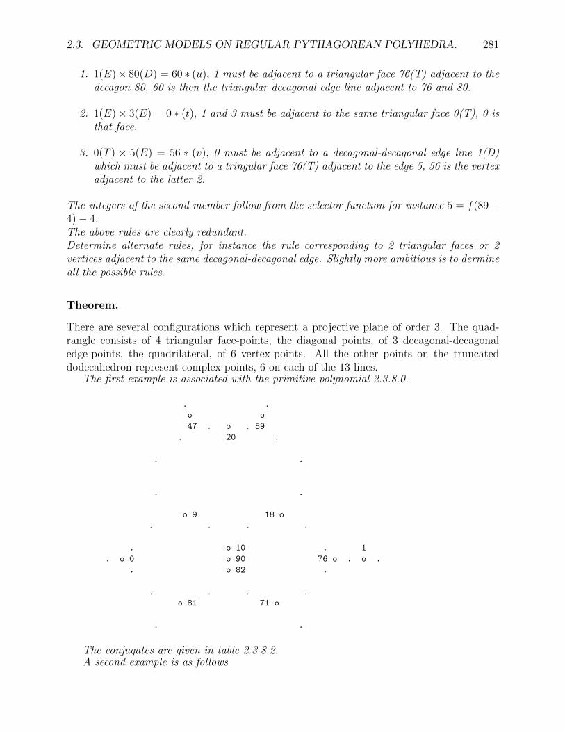
2.3. GEOMETRIC MODELS ON REGULAR PYTHAGOREAN POLYHEDRA. 281
1. 1(E)× 80(D) = 60 ∗ (u), 1 must be adjacent to a triangular face 76(T) adjacent to thedecagon 80, 60 is then the triangular decagonal edge line adjacent to 76 and 80.
2. 1(E)× 3(E) = 0 ∗ (t), 1 and 3 must be adjacent to the same triangular face 0(T), 0 isthat face.
3. 0(T ) × 5(E) = 56 ∗ (v), 0 must be adjacent to a decagonal-decagonal edge line 1(D)which must be adjacent to a tringular face 76(T) adjacent to the edge 5, 56 is the vertexadjacent to the latter 2.
The integers of the second member follow from the selector function for instance 5 = f(89−4)− 4.The above rules are clearly redundant.Determine alternate rules, for instance the rule corresponding to 2 triangular faces or 2vertices adjacent to the same decagonal-decagonal edge. Slightly more ambitious is to dermineall the possible rules.
Theorem.
There are several configurations which represent a projective plane of order 3. The quad-rangle consists of 4 triangular face-points, the diagonal points, of 3 decagonal-decagonaledge-points, the quadrilateral, of 6 vertex-points. All the other points on the truncateddodecahedron represent complex points, 6 on each of the 13 lines.
The first example is associated with the primitive polynomial 2.3.8.0.
. .
o o
47 . o . 59
. 20 .
. .
. .
o 9 18 o
. . . .
. o 10 . 1
. o 0 o 90 76 o . o .
. o 82 .
. . . .
o 81 71 o
. .
The conjugates are given in table 2.3.8.2.A second example is as follows

282 CHAPTER 2. FINITE PROJECTIVE GEOMETRY
82 10
o o o
. 90 .
. .
. .
86 o . . o 84
. . . .
. o 8 . 2
. o 1 o o o
. o 48 . 7 54
. . . .
. .
o 46 o 70
. .
o 80
. .
. .
. (o) .
(90)
on the t-line 708, the conjugates are 21(V ) and 11(E), 22(E) and 77(E), 24(V ) and30(V ).on the e-line 1∗, the conjugates are 0(T ) and 76(T ), 26(U) and 60(U), 55(D) and 80(D).on the v-line 8∗, the conjugates are 41(V ) and 83(U), 53(V ) and 73(U), 19(U) and 69(U).
Proof: For the conjugates we use the Pascal construction to determine the 6-th point onthe line on a conic through 4 real points and 1 complex point.
Exercise.
For q = 22,
0. determine the primitive polynomial giving the selector 0, 1, 4, 14, 16.
1. Determine the correspondance between the selector notation and the homogeneous co-ordinates for points and lines. Note that these are not the same.
2. The correspondance i to i∗ is a polarity whose fixed points are on a line. Determinethe matrix representation, the polar of (X, Y, Z) and the equation satisfied by the fixedpoints.
3. Determine the fundamental projectivity on the line 14∗ using a point conic which hasno points on 14∗.

2.3. GEOMETRIC MODELS ON REGULAR PYTHAGOREAN POLYHEDRA. 283
4. Illustrate Pascal’s Theorem.
Exercise.
0. Explore the usefulness of the truncated cuboctahedron less the hexagonal faces and the< 4.8 > edges as a model for the projective geometry of order 7.
1. Show that the 14-gonal antiprism can be used as a model for the projective geometry oforder 7. More generally,
2. Show that the n-gonal antiprism can be used as a model for the projective geometry oforder q = pk when p ≡ −1 (mod 4), with n = q2+q
4.
3. Show that the n-gonal antiprism can be used as a model for the projective geometry oforder q = pk when q ≡ 1 (mod 12), with n = q2+q
2. Finally,
4. Show that the n-gonal prism can be used as a model for the projective geometry of orderq = pk when q ≡ −1 (mod 3), with n = q2+q
3.
5. is there a general theory when using prisms or antiprisms?
Exercise.
For q = 23.
0. to 4. Answer question similar to those of 2.3.8
5. Show that the 18-gonal antiprism can be used as a model for the projective geometry oforder 23. More generally,
6. Show that the n-gonal antiprism can be used as a model for the projective geometry oforder q = 2k, with n = q2+q
4.
Answer to 2.3.2.
0. For q = 2, the primitive polynomial giving the selector 0, 1, 3, isI3 + I + 1.
The auto-correlates are 0 11 2 7 8.The selector function isi 0 1 2 3 4 5 6 7 8 9 10 11
f(i) 0 14 1 0 16 16 14 14 16type F0 V0 F4 V2 T0 T2 V1 F3 F1 T3 E2 F2
i 12 13 14 15 16 17 18 19 20f(i) 4 1 0 1 0 4 4 16 1type T4 E1 P V3 E0 T1 E3 V4 E4

284 CHAPTER 2. FINITE PROJECTIVE GEOMETRY
1. The correspondence between the selector notation and the homogeneous coordinates forpoints and lines is
i I i i∗
0 1 6∗ : 1, 2, 4,1 I 1∗ : 0, 2, 6,2 I2 0∗ : 0, 1, 3,3 I + 1 5∗ : 2, 3, 5,4 I2 + I 3∗ : 0, 4, 5,5 I2 + I + 1 4∗ : 3, 4, 6,6 I2 + 1 2∗ : 1, 5, 6.
2. The matrix representation is
M =
1 0 10 1 01 0 0
,M−1 =
0 0 10 1 01 0 1
. and the equation satisfied by the
fixed points is (X0 +X1)2 = 0.
3. The degenerate conic through 0, 1, 2 and 5 with tangent 5∗ at 5, is represented by thematrix
N =
0 1 11 0 01 0 0
.
The polar of 0 is 0∗, of 1 is 0∗, of 2 is 5∗, of 4 is 4∗, of 5 is 5∗ of 6 is 6∗ and of 3 isundefined. The equation in homogeneous coordinates is X0(X1 +X2) = 0.
4. A circle with center 14 can be constructed as follows. I first observe that a directionmust be orthogonal to itself. Indeed, if 0 is a direction, the others form an angle 1,2,3,4mod 5, we cannot play favorites and must choose 0. If A0 = 1, C × A0 and thereforethe tangent has direction 0, A0 × Ai+1 has direction i mod 5 or are the points 0, 7, 8,2, 11.
It is natural to choose the pentagonal face-point as 14, and the edge-points on thepentagon as 0, 8, 11, 7, 2. The points on the circle 1, 6, 3, 15, 19 are chosen asthe vertex-points opposite the corresponding edge-point, 1 opposite 0, 6 opposite 8, . . . .This gives the types, with subscripts indicated in 0. and the definition:
The points are represented on the 5-anti-prism as follows. The pentagonal face-point,P, the 5 triangular face-points, Ti, the 5 vertex-points, Vi, the 5 triangular-triangularedge-points, Ei, the 5 pentagonal-triangular edge-points Fi.
The lines are represented on the 5-anti-prism as follows. The pentagonal face-line, f,which is incident to Fi, the 5 triangular face-lines, ti, which are incident to Fi, Fi, Ti+1,Ti−1, Ei+2, Ei−2. If f is the pentagonal edge of ti and V, V ′ are on f , Fi is on it, Ti+1
(Ti−1) share V (V ′), Ei+2 (Ei−2) are on an edge through V (V ′) not on tithe 5 vertex-lines, vi, which are incident toFi, Vi+2, Vi−2, Ei+1, Ei−1. If t is the face with vi on its pentagonal edge these are allthe vertices, and edge-points on it distinct from vi.the 5 triangular-triangular edge-lines, ei, which are incident to Fi, Ti+2, Ti−2, Vi+1,

2.3. GEOMETRIC MODELS ON REGULAR PYTHAGOREAN POLYHEDRA. 285
Vi−1. Vi+1 and Vi−1 are on the same edge as ei, the line which joins the center C of theantiprism to Ei is parallel to the edge containing Fi, Ti+2 and Ti−2 are the triangularfaces which are not adjacent to Ei or Fi.
the 5 pentagonal-triangular edge-lines. fi, which are incident to P, Ti, Vi, Ei, Fi. Ti isadjacent to fi, Vi is opposite fi, Ei joined to the center of the antiprism is parallel toTi.
Answer to 2.3.3.For p = 3,
0. The primitive polynomial giving the selector 0, 1, 3, 9 is I3 − I − 1.
1. The correspondence between the selector notation and the homogeneous coordinates forpoints and lines isi I i i∗
0 1 12∗ : 1, 2, 4, 10,1 I 1∗ : 0, 2, 8, 12,2 I2 0∗ : 0, 1, 3, 9,3 I + 1 7∗ : 2, 6, 7, 9,4 I2 + I 3∗ : 0, 6, 10, 11,5 I2 + I + 1 4∗ : 5, 9, 10, 12,6 I2 + 2I + 1 10∗ : 3, 4, 6, 12,7 I2 + I + 2 6∗ : 3, 7, 8, 10,8 I2 + 1 2∗ : 1, 7, 11, 12,9 I + 2 11∗ : 2, 3, 5, 1110 I2 + 2I 9∗ : 0, 4, 5,7,11 I2 + 2I + 2 5∗ : 4, 8, 9, 11,12 I2 + 2 8∗ : 1, 5, 6, 8.
2. The matrix representation of the polarity i to i∗ is
M =
1 0 10 1 01 0 0
, M−1 =
0 0 10 1 01 0 2
.
The equation satisfied by the fixed points is X20 +X2
1 + 2X2X0 = 0.
3. The degenerate conic through 0, 1, 2 and 5 with tangent 4∗ at 5, is obtained by con-structing the quadrangle-quadrilateral configuration starting with P = 5 and Qi =0, 1, 2. We obtain qi = 3∗, 2∗, 7∗, which are the tangents at Qi. The matrix repre-sentation is
N =
0 1 11 0 11 1 0
with equation X1X2 +X2X0 +X0X1 = 0.
We can check that the polar of 10 = 3∗ × 4∗ is 9∗ = 0× 5.
Answer to ??.

286 CHAPTER 2. FINITE PROJECTIVE GEOMETRY
0. For q = 22, the primitive polynomial giving the selector 0, 1, 4, 14, 16 is I3− I2− I− ε, with
ε2 + ε+ 1 = 0.
1. The correspondence between the selector notation and the homogeneous coordinates areas follows, i∗ has the homogeneous coordinates associated with I i.
i I i i∗0 1 20∗
1 I 14∗
2 I2 0∗
3 I2 + I + ε 10∗
4 I + ε 219∗
5 I2 + ε 2I4∗
6 I2 + ε 2I + 118∗
7 I2 + 1 15∗
8 I2 + ε 3∗
9 I2 + ε2I + ε 5∗
10 I2 + εI + 1 9∗
11 I2 + ε2 13∗
12 I2 + εI + ε 11∗
13 I2 + I + ε2 6∗
14 I + 1 2∗
15 I2 + I 1∗
16 I + ε 12∗
17 I2 + εI 16∗
18 I2 + εI + ε2 17∗
19 I2 + ε2I + ε2 8∗
20 I2 + I + 1 7∗
To obtain the last column, for row 9, [1, ε2, ε] = (1, 1, 1)× (1, ε, 0) = 20× 17 = 5 ∗ .
2. The correspondence i to i∗ is a polarity whose fixed points are on a line. The matrixrepresentation is obtained by using the image of 4 points.
0 = (0,0,1), M(0) = 0∗ = [1, 0, 0],1 = (0,1,0), M(1) = 1∗ = [1, 1, 0],2 = (1,0,0), M(2) = 2∗ = [0, 1, 1],18 = (1, ε, ε2), M(18) = 18∗ = [1, ε2, 1].
The first 3 conditions give the polarity matrix asThe last condition gives βε+ αε2 = 1, γ + βε = ε2, γ = 1. Hence γ = 1, β = 1, α = 1.Therefore
M =
0 1 11 1 01 0 0
, M−1 =
0 0 10 1 11 1 1
.
Note that M is real and could have been obtained from the reality and non singularityconditions, giving directly α = β = γ = 1.The polar of (X0, X1, X2) is [X1 +X2, X0 +X1, X0].

2.3. GEOMETRIC MODELS ON REGULAR PYTHAGOREAN POLYHEDRA. 287
The fixed points (X0, X1, X2) satisfy X21 = 0 corresponding to 14∗.
3. A point conic with no points on 14 is 1, 3, 4, 5,13,the corresponding line conic is 15,19,10,16, 8.Projecting from 1 and 3, 1, 3, 5,13, 4,we get the fundamental projectivity, 8, 2,11, 0, 7 on 14∗.
4. To illustrate Pascal’s Theorem, because there are only 5 points on a conic, we need touse the degenerate case. The conic through 0, 1, 2 and the conjugate points 9 and 18is The last condition gives βε+ αε2 = 1, γ + βε = ε2, γ = 1.
Hence γ = 1, β = 1, α = 1. Therefore
M =
0 1 11 1 01 0 0
, M−1 =
0 0 10 1 11 1 1
.
Note that M is real and could have been obtained from the reality and non singularityconditions, giving directly α = β = γ = 1.The polar of (X0, X1, X2) is [X1 +X2, X0 +X1, X0].The fixed points (X,X1, X2) satisfy X2
1 = 0 corresponding to 14∗.
5. A point conic with no points on 14 is 1, 3, 4, 5,13, 0 1 11 0 11 1 0
The tangents at (0,0,1), (0,1,0), (1,0,0), (1, ε2, ε), (1, ε, ε2) are [1,1,0], [1,0,1], [0,1,1],[1, ε2, ε), (1, ε, ε2], or 1∗, 15∗, 2∗, 5∗, 17∗. On the other hand, using Pascal’s Theorem,the tangent at 0 is given by((((0× 1)× (9× 18))× ((18× 0)× (1× 2)))× (2× 9))× 0
= (((0∗ × 7∗)× (4∗ × 20∗))× 12∗)× 0= (((14× 17) = 8∗)× 12∗or13)× 0 = 1∗.
Answer to??.
For q = 57, choose the auto-correlates as point on a circle although 0 is on the circle drawas it is the center. With the succession of points Xi,xi = 0×Xi 36, 1, 52, 43, 3, 32, 13,Xi 16, 35, 18, 50, 29, 26, 30,yi+1 = Xi−1 ×Xi+1 22, 42, 8, 14, 10, 28, 44,yi+2 = Xi−2 ×Xi+2 34, 2, 41, 17, 40, 20, 23,yi+3 = Xi−3 ×Xi+3 7, 31, 6, 27, 54, 25, 39,yi+1 × xi 21, 51, 5, 46, 33, 4, 45,yi+2 × xi 24, 56, 48, 15, 49, 38, 47,yi+3 × xi 53, 12, 37, 9, 55, 11, 19.
This gives all the points in the projective plane of order 7. We observe
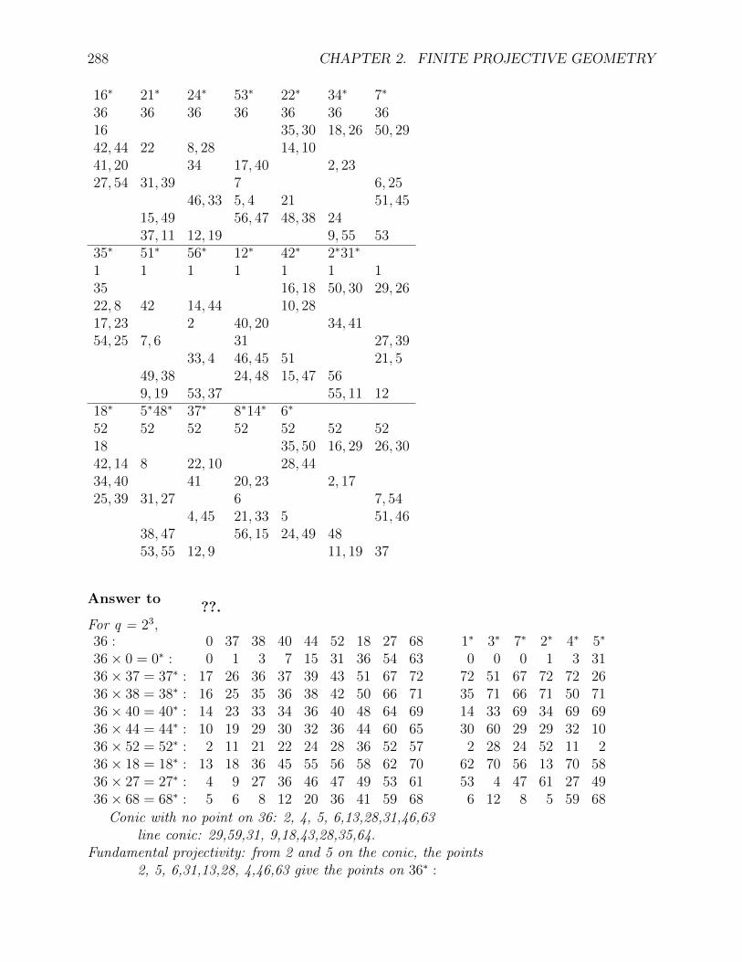
288 CHAPTER 2. FINITE PROJECTIVE GEOMETRY
16∗ 21∗ 24∗ 53∗ 22∗ 34∗ 7∗
36 36 36 36 36 36 3616 35, 30 18, 26 50, 2942, 44 22 8, 28 14, 1041, 20 34 17, 40 2, 2327, 54 31, 39 7 6, 25
46, 33 5, 4 21 51, 4515, 49 56, 47 48, 38 2437, 11 12, 19 9, 55 53
35∗ 51∗ 56∗ 12∗ 42∗ 2∗31∗
1 1 1 1 1 1 135 16, 18 50, 30 29, 2622, 8 42 14, 44 10, 2817, 23 2 40, 20 34, 4154, 25 7, 6 31 27, 39
33, 4 46, 45 51 21, 549, 38 24, 48 15, 47 569, 19 53, 37 55, 11 12
18∗ 5∗48∗ 37∗ 8∗14∗ 6∗
52 52 52 52 52 52 5218 35, 50 16, 29 26, 3042, 14 8 22, 10 28, 4434, 40 41 20, 23 2, 1725, 39 31, 27 6 7, 54
4, 45 21, 33 5 51, 4638, 47 56, 15 24, 49 4853, 55 12, 9 11, 19 37
Answer to??.
For q = 23,36 : 0 37 38 40 44 52 18 27 68 1∗ 3∗ 7∗ 2∗ 4∗ 5∗
36× 0 = 0∗ : 0 1 3 7 15 31 36 54 63 0 0 0 1 3 3136× 37 = 37∗ : 17 26 36 37 39 43 51 67 72 72 51 67 72 72 2636× 38 = 38∗ : 16 25 35 36 38 42 50 66 71 35 71 66 71 50 7136× 40 = 40∗ : 14 23 33 34 36 40 48 64 69 14 33 69 34 69 6936× 44 = 44∗ : 10 19 29 30 32 36 44 60 65 30 60 29 29 32 1036× 52 = 52∗ : 2 11 21 22 24 28 36 52 57 2 28 24 52 11 236× 18 = 18∗ : 13 18 36 45 55 56 58 62 70 62 70 56 13 70 5836× 27 = 27∗ : 4 9 27 36 46 47 49 53 61 53 4 47 61 27 4936× 68 = 68∗ : 5 6 8 12 20 36 41 59 68 6 12 8 5 59 68
Conic with no point on 36: 2, 4, 5, 6,13,28,31,46,63line conic: 29,59,31, 9,18,43,28,35,64.
Fundamental projectivity: from 2 and 5 on the conic, the points2, 5, 6,31,13,28, 4,46,63 give the points on 36∗ :

2.3. GEOMETRIC MODELS ON REGULAR PYTHAGOREAN POLYHEDRA. 289
38, 0,68,27,52,37,40,18,44.empty

290 CHAPTER 2. FINITE PROJECTIVE GEOMETRY

Chapter 3
FINITE PRE INVOLUTIVEGEOMETRY
3.1 An Overview of the Geometry of the Hexal Com-
plete 5-Angles.
3.1.0 Introduction.
In the geometry of Euclid, not every pair of lines have a point in common, namely the paral-lel ones. I call Euclidean Geometry, that geometry which consists in completing the plane ofEuclid by the ideal points and the lines of Euclid by the ideal line. To each set of parallel linescorrespond its direction or point at infinity or ideal point. The line at infinity or ideal line isincident to all ideal points. Figures Pl and St may help the reader to visualize. In Fig. Pl,projecting the line b on the line c from the point P establishes a one to one correspondancebetween the points on these lines, if we include the ideal point Ci, on c, corresponding toBi and the ideal point B∞, on b, corresponding to C∞. Replacing lines b and c by planes,perpendicular to the plane P of figure establishes a one to one correspondance between a linethrough C∞ perpendicular to P and the ideal line through B∞.This led to the concept of perspectivity, which I have schematized in Fig. St. In it, the shad-ing, corresponds to the method used by Chinese artists to represent distances in paintings.The tiling corresponds to the method used by Western painters. Johannes Vermeer’s use ofperspective in his paintings was so accurate as to allow P. T. A. Swillens to reconstruct, fromthe size of a chair, in the painting, not only the size of the rooms, but also to estimate theheight of the artist.Affine geometry is obtained from Euclidean geometry by discarding the notions associatedwith congruences of figures, projective geometry is obtained by discarding the notion of paral-lelism, thereby making the properties of any point or line in the plane indistinguishable fromthat of any other.I will describe at a later time, how I was lead to the discovery of finite Euclidean geometryand to the extension of many of the properties of Euclidean geometry. While working out aproof for these results, it occured to me, that the results can be placed in the framework of fi-nite projective geometry. I will, as I proceed, make the connection with the results in classical
291

292 CHAPTER 3. FINITE PRE INVOLUTIVE GEOMETRY
Euclidean geometry. The results can be considered as proceeding from an, apparently new,configuration consisting of 14 points and 13 lines. This configuration is defined starting froman ordered complete 5-angle, A0, A1, A2, M and M, in which the first 3 points can be rotatedand the last 2 points interchanged. In other words the configuration is the same if we replaceA0, A1 and A2 by A1, A2 and A0 and independently M by M and M by M. In involutivegeometry, (the Euclidean geometry without measure of angles and distances), we define alti-tudes and their intersection, the orthocenter, we define medians and their intersection, thebarycenter. In the generalization to projective geometry, the orthocenter and the barycenterbecome two arbitrary points, whose role is interchangeable. The proofs are constructive, andthe only construction required are those of lines through 2 given points and of points at theintersection of two given lines, but these constructions must be valid for all p. They do notinvolve the construction of an arbitrary line through a given point, as required to obtain, forinstance, an arbitrary point on a conic, by the construction of Pascal or of MacLaurin.No special relations will be assumed here between the points obtained during the construc-tion. The special relation M on the polar of M with respect to the triangle A0, A1, A2 willbe studied in Chapter IV,in the section on Cartesian geometry and the special case where M and M are respectivelyon the polar of M and M with respect to the triangle will also be discussed elsewhere.The beginning of a synthetic proof is given in section 4.3. Synthetic proofs are highly desir-able and are from my point of view more elegant, but require much more time to develop.The constructions and statements are given in a compact found using a notation which willnow be explained.
3.1.1 Notation and application to the special configuration of De-sargues and to the pole and polar of with respect to a tri-angle.
Introduction.
In the preceding Chapter, I have introduced a notation for points, lines, incidence and state-ments. Additional notation is given here for conics, for points on conics and tangents toconics and a notation which allows to describe at once 3 points or 6 points associated to atriangle.
Notation.
The identifier for a point conic will be a lower case Greek letter or an identifier starting witha lower case preceded by a backward quote “ ‘ ”. The identifier for a line conic will be anupper case Greek letter or an identifier starting with an upper case preceded by a backwardquote “ ‘ ”.
The subscript i, will have the values 0, 1 and 2. Hence Ai denotes 3 points A0, A1 andA2.
If subscripts involve the letter i and addition, the addition is done modulo 3, for instance,ai := Ai+1 × Ai+2
is equivalent to
3.1. AN OVERVIEWOF THEGEOMETRYOF THE HEXAL COMPLETE 5-ANGLES.293
a0 := A1 × A2, a1 := A2 × A0, a2 := A0 × A1.It represents the construction of the sides a0, a1 and a2 of a triangle with vertices A0, A1
and A2.
To indicate that a conic γ is constructed as that conic which passes through the 5 distinctpoints P0, P1, P2, P3, and P4, we write
γ := conic(P0, P1, P2, P3, P4).To indicate that a conic γ1 is constructed as that conic whose tangent at P0 is a0 and at P2
is a2 and passes also by P4, we writeγ1 := conic((P0, a0), (P2, a2), P4). or γ1 := conic(P0, a0, P2, a2, P4).
When 3 lines xi are concurrent, the intersection X can be obtained using any of the threepairs. I have chosen, arbitrarily,
X := x1 × x2(∗),as a reminder that 2 other definitions of X could have been chosen. In the special case, x1
= x2, the other choiceX := x0 × x1,
will be used. “ (*) ” denotes therefore not only a Definition but also a Theorem or Conclusion.A similar notation will be used for conics.
X · γ = 0 and Xi · γ = 0, are the notations corresponding to the point X is on theconic γ and the triple X0, X1, X2 is on the conic γ.
P = Pole(p, α ), is the notation for P is the pole of p with respect to the conic α .γ is a circle = 0 or γ is a cocircle is either an hypothesis, to indicate a prefered conic
from which all other circles are defined or a Conclusion,X = Center(γ) and X = Cocenter(γ) is an abbreviation for X is the center of the
conic γ (not necessarily a circle) and X is the cocenter of the conic γ, in other words X,(X) is the polar of m (m) with respect to γ. See section 4.3.3.
Example.
With this notation, the special configuration of Desargues of 0.4.6. can be defined byai := Ai+1 × Ai−1, ri := P × Ai,Pi := ai × ri, qi := Pi+1 × Pi−1,Ri := ai × qi, pi := Ai ×Ri,Qi := pi+1 × pi−1, p := R1 ×R2(∗),
and the conclusions of the special Desargues Theorem are implied by the last Definition-Conclusion and by the Conclusion,
Qi · ri = 0.Let P = (p0, p1, p2), and A0 = (1, 0, 0), A1 = (0, 1, 0), A2 = (0, 0, 1), then
a0 = [1, 0, 0], r0 = [0, p2,−p1],P0 = (0, p1, p2), q0 = [−p1p2, p2p0, p0p1],R0 = (0, p1,−p2), p0 = [0, p2, p1],Q0 = (−p0, p1, p2), p = [p1p2, p2p0, p0p1].

294 CHAPTER 3. FINITE PRE INVOLUTIVE GEOMETRY
Example.
For p = 3, prove that if A0 = (1, 0, 0), A1 = (0, 1, 0), A2 = (0, 0, 1) and P = (1, 1, 1) then theother elements of the quadrangle quadrilateral configuration II.2.1.6 are
P0 = (0, 1, 1), Q0 = (−1, 1, 1), R0 = (0, 1,−1), . . . , anda0 = [1, 0, 0], p = [1, 1, 1],p0 = [0, 1, 1], q0 = [−1, 1, 1], r0 = [0, 1,−1], . . . and that
the conic of II.2.2.11 isX2
0 +X21 +X2
2 = 0.
Theorem.
With the above notation, the polar p can be obtained algebraically from the pole P or thepole P from the polar p using the first or the second formula:
0. pAi = P ∗ Ai, Pai = p ∗ ai,
1. pAi = (P · ai)Ai − (Ai · ai)P, Pai = (p · Ai)ai − (ai · Ai)p,
2. pi = (P · ai+1)(P · ai−1)Ai+1 ∗ Ai−1 + (P · ai+1)(Ai−1 · ai−1)P ∗ Ai+1
− (P · ai−1)(Ai+1 · ai+1)P ∗ Ai−1,Pi = (p · Ai+1)(p · Ai−1)ai+1 ∗ ai−1 + (p · Ai+1)(ai−1 · Ai−1)p ∗ ai+1
− (p · Ai−1)(ai+1 · Ai+1)p ∗ ai−1.
3. Pai = (P · ai+1)Ai+1 − (P · ai−1)Ai−1,PAi = (p · Ai+1)ai+1 − (p · Ai−1)ai−1.
4. p = 1P ·a0a0 + 1
P ·a1a1 + 1P ·a2a2, P = 1
p·A0A0 + 1
p·A1A1 + 1
p·A2A2.
Proof: Only the first part of 2 to 4 needs to be proven, because of duality. To obtain 2,we use P ∗P = 0 and Ai+1 ∗P = −P ∗Ai+1. To obtain 3, we recall that ai = Ai+1 ∗Ai−1, weuse Ai ∗aj = 0 when i 6= j and Ai ∗ai = (A0 ∗A1) ·A2 = t, then divide by t and by P ·ai 6= 0.To obtain 4, we use p = Ri+1 ∗Ri−1. We divide by (P · ai)(P · ai+1)(P · ai−1 6= 0, and obtainp = Ai+1 ∗ 1
P ·aiAi−1 + Ai−1 ∗ 1P ·ai+1
Ai + Ai ∗ 1P ·ai−1
Ai+1, or
p = 1P ·aiai + 1
P ·ai+1ai+1 + 1
P ·ai−1ai−1.
Example.
For p = 13, Ai = (36(1, 1, 9), 27(1, 1, 0), 151(1, 10, 7)), P = (68(1, 4, 2)),ai = [175(1, 12, 5), 150(1, 10, 6), 170(1, 12, 0)], ri = [77, 138, 31],Si = (143, 63, 33), pi = [108, 46, 37], Ri = (48, 16, 32),p = 1
7a0 + 1
1a1 + 1
10a2 = 2a0 + a1 + 4a2 = [124], pi = [140, 176, 106],
Pi = (51, 132, 84), P = 111A0 + 1
9A1 + 1
6A2 = 6A0 + 3A1 + 11A2 = (68).

3.1. AN OVERVIEWOF THEGEOMETRYOF THE HEXAL COMPLETE 5-ANGLES.295
Definition.
An hexal complete 5-angle configuration, is a configuration which starts with an ordered setof 5 points A0, A1, A2, M and M.
In the configuration obtained from it, if a point X0 is constructed, 5 other points are ob-tained. X1 is obtained by replacing A0, A1, A2 by A1, A2, A0; X2 is obtained by replacing thesame points by A2, A0, A1 and the points X i are obtained by exchanging in the constructionof Xi, M and M. The same holds for lines. The first letter has a macron placed above it inthe naming of the construction which exchanges M and M. In the group of permutation onthe 5 points of the complete 5-angle, the figure is invariant under the cyclic group generatedby the permutation
(A0A1A2MM)(A1A2A0MM).
In special cases, several of these elements or all of the elements may coincide.
Comment.
We know from II.1.5.6. that a complete 5-angle requires p ≥ 5, therefore, the definition andresults that follow are non vacuous only if p ≥ 5. We introduce here a terminology inspiredfrom corresponding terms in Euclidean geometry. In some instances, the correspondencewill be made explicitly. For instance, the line m which will be constructed corresponds tothe ideal line or line at infinity in Euclidean geometry, we will therefore call m the idealline. In the symmetry which exchanges M and M , to m corresponds m, which will be calledthe coideal line. m corresponds to the orthic axis. The conic θ which will be constructedcorresponds to the circumcircle and the conic γ to the circle of Brianchon-Poncelet also calledthe nine-point circle.
Definition.
θ and any conic δ, (δ) such that there exists a radical axis u, (u) with respect to m (m) iscalled a circle (cocircle) and u is called the radical (coradical) axis of θ and δ, (δ).
Algebraically, we have, for some integers k1, k2 and k3,k1δ + k2θ = k3(m) ×× (u),
where θ, m, δ and u are expressed exactly as in the corresponding expressions P0.7, P1.19,1.20, . . . , below.
A triangle consists of its vertices and its sides. When we want to be specific we will useeither or both, for instance the given triangle can be written as Ai or ai or Ai, ai.To each of the section of this Theorem corresponds a sequence of theorems in Euclideangeometry which will be given in the corresponding sections of Chapter IV.
We will give separately the construction of the various points and lines of the hexal con-figuration (zetetic part) and the proof that the construction satisfies the given properties(poristic part).

296 CHAPTER 3. FINITE PRE INVOLUTIVE GEOMETRY
3.1.2 An overview of theorems associated with equality of dis-tances and angles. The ideal line, the orthic line, the lineof Euler, the circle of Brianchon-Poncelet, the circumcircle,the point of Lemoine.
Introduction.
As the generalization proceeds, the 4 points on the line of Euler, become 10 points on itsgeneralization. The 9 (or 12) points on the circle of Brianchon-Poncelet (also called circleof Euler) become 20 points on the corresponding conic. New results, which will be given inpart III, are further consequences.The definitions are numbered starting with D, the conclusions are numbered stating with C,the proofs, which consist of the algebraic expressions of the various points, lines and conics,which can easily be checked and from which the conclusions can easily be verified, have anumber corresponding to the definition, starting with P.The numbering in this overview is the same as the number in the complete theory, given inChapter 5 and 6.
Theorem.
If we derive a point X and a line x by a given construction from Ai, M and M , with thecoordinates as given in G0.0 and G0.1, below, and the point X and line x are obtain by thesame construction interchange M and M ,
X = (f0(m0,m1,m2), f1(m0,m1,m2), f2(m0,m1,m2)),x = [g0(m0,m1,m2), g1(m0,m1,m2), g2(m0,m1,m2)],
=⇒X = (m0f0(m−1
0 ,m−11 ,m−1
2 ),m1f1(m−10 ,m−1
1 ,m−12 ),m2f2(m−1
0 ,m−11 ,m−1
2 )),x = [m−1
0 g0(m−10 ,m−1
1 ,m−12 ),m−1
1 g1(m−10 ,m−1
1 ,m−12 ),m−1
2 g2(m−10 ,m−1
1 ,m−12 )].
Proof: The point collineation C =
q0 0 00 q1 00 0 q2
, associates to (1,1,1), (q0, q1, q2), and
to (m0,m1,m2), (r0, r1, r2), if ri = qimi.In the new system of coordinates,X = (q0f0(q−1
0 r0, q−11 r1, q
−12 r2), q1f1(q−1
0 r0, q−11 r1, q
−12 r2), q2f2(q−1
0 r0, q−11 r1, q
−12 r2)).
Exchanging qi and ri and then replacing qi by 1 and ri by mi is equivalent to substituting mi
for qi and 1 for ri, which gives X. x is obtained similarly.
The line collineation is q−10 0 00 q−1
1 00 0 q−1
2
.
Theorem.
Given a complete 5-angle, 5 distinct points, no 3 of which are on the same line, A0, A1, A2,M and M, Ai are called the vertices, M is called the barycenter and M, the orthocenter.

3.1. AN OVERVIEWOF THEGEOMETRYOF THE HEXAL COMPLETE 5-ANGLES.297
1. The ideal line and the orthic line. See Fig. 1,
H0.0. Ai,H0.1. M, M ,D0.0. ai := Ai+1 × Ai−1,D0.1. mai := M × Ai,mai := M × Ai,D0.2. Mi := mai × ai,M i := mai × ai,D0.3. mmi := Mi+1 ×Mi−1,mmi := M i+1 ×M i−1,D0.4. MAi := ai ×mmi,MAi := ai ×mmi,D0.7. m := MA1 ×MA2(∗), m := MA1 ×MA2(∗).
The nomenclature:N0.0. ai are the sides.N0.3. mai are the medians, mai are the comedians or
mai are the altitudes, mai are the coaltitudes,N0.4. Mi are the mid-points of the sides.
M i are the feet or the feet of the altitudes,N0.5. (Mi,mmi) is the complementary triangle,
(M i, mmi) is the orthic triangle,N0.6. MAi are the directions of the sides,N0.8. m is the ideal line corresponding to the line at infinity,
m is the coideal line or the orthic line, which is the polarof M with respect to the triangle.
Proof:P0.0. a0 = [1, 0, 0],P0.1. ma0 = [0, 1,−1], ma0 = [0,−m2,m1],P0.2. M0 = (0, 1, 1), M0 = (0,m1,m2),P0.3. mm0 = [−1, 1, 1], mm0 = [−m1m2,m2m0,m0m1],P0.4. MA0 = (0, 1,−1), MA0 = (0,m1,−m2),P0.7. m = [1, 1, 1], m = [m1m2,m2m0,m0m1],
2. The line of Euler and the circle of Brianchon-Poncelet. See Fig. 2, 2b.
LetD1.0. eul := M ×MD1.20. γ := conic(M0,M1,M2,M1,M2)(∗),thenC1.1 γ is a circle, γ is a cocircle = 0.
The nomenclature:N1.0. eul is the line of Euler.N1.11. γ is the circle of Brianchon-Poncelet. In Euclidean geometry, the circle ofBrianchon-Poncelet, is also called the circle of 9 points or circle of Feuerbach or,improperly, the circle of Euler. It passes through the midpoints of the sides, the feet ofthe altitudes and the midpoints of the segment joining the vertices to the orthocenter.The Definition-Conclusion D1.20. corresponds to the first part of the Theorem ofBrianchon-Poncelet.
298 CHAPTER 3. FINITE PRE INVOLUTIVE GEOMETRY
Proof:P1.0. eul = [m1 −m2,m2 −m0,m0 −m1],P1.20. γ : m1m2X
20 +m2m0X
21 +m0m1X
22
−m0(m1 +m2)X1X2 −m1(m2 +m0)X2X0 −m2(m0 +m1)X0X1 = 0,γ−1 : m2
0(m1 −m2)2x20 +m2
1(m2 −m0)2x21 +m2
2(m0 −m1)2x22
− 2m1m2(m0(3s1− 2m0) +m1m2)x1x2
− 2m2m0(m1(3s1− 2m1) +m2m0)x2x0
− 2m0m1(m2(3s1− 2m2) +m0m1)x0x1.
3. The circumcircle. See Fig. 4, 4b.
LetD1.6. Immi := m×mmi, Immi := m×mmi,D1.7. tai := Ai × Immi,D1.19. θ := conic(A1, ta1, A2, ta2, A0),thenC1.2. Immi · tai = 0.H1.1. θ is a circle = θ is a cocircle = 0.
The nomenclature:N1.4. Immi are the directions of the antiparallels ai with respect
to the sides ai+1 and ai−1.N1.5. tai are the tangents at Ai to the circumcircle,N1.10. θ is the circumcircle.
Proof:P1.6. Imm10 = (m0(m1 −m2),−m1(m2 +m0),m2(m0 +m1)),
Imm10 = (m0(m2 −m1),−m1(m2 +m0),m2(m0 +m1)),P1.7. ta0 = [0,m2(m0 +m1),m1(m2 +m0)],P1.19. θ : m0(m1 +m2)X1X2 +m1(m2 +m0)X2X0
+m2(m0 +m1)X0X1 = 0,2θ + γ = (m) ×× (m).θ−1 : m2
0(m1 +m2)2x20 +m2
1(m2 +m0)2x21 +m2
2(m0 +m1)2x22
− 2m1m2(m2 +m0)(m0 +m1)x1x2
− 2m2m0(m0 +m1)(m1 +m2)x2x0
− 2m0m1(m1 +m2)(m2 +m0)x0x1 = 0,
4. The point of Lemoine. See Fig. 3.
LetD1.2. Maai := mai+1 ×mai−1, Maai := mai−1 ×mai+1,D1.3. mMai := Maai ×Maai,D1.4. K := mMa1 ×mMa2(∗),D1.8. Ti := tai+1 × tai−1,D12.1. ati := Ai × Ti,
The nomenclature:N1.5. (Ti, tai) is the tangential triangle,
3.1. AN OVERVIEWOF THEGEOMETRYOF THE HEXAL COMPLETE 5-ANGLES.299
N12.1. ati are the symmedians, of d’Ocagne,N1.2. K is the point of Lemoine, also called point of Grebe or of Lhuillier.
Proof:P1.2. Maa0 = (m0,m1,m0), Maa0 = (m0,m0,m2),P1.3. mMa0 = [q0,m0(m2 −m0),−m0(m0 −m1)],P1.4. K = (m0(m1 +m2),m1(m2 +m0),m2(m0 +m1)),P1.8. T0 = (−m0(m1 +m2),m1(m2 +m0),m2(m0 +m1)),P12.1. at0 = [0,m2(m0 +m1),−m1(m2 +m0)],
3.1.3 The fundamental 3 ∗ 4 + 11 ∗ 3 & 3 ∗ 5 + 10 ∗ 3 configuration.
Introduction.
It would be desirable to have a synthetic proof of the sequence of Theorems given in thisand in the following Chapters. In many instances, it is not difficult to obtain it, using thestandard Theorems of projective geometry, mainly those of Pappus, Desargues and Pascal.In other cases, the proof is less obvious. Theorem 4.3.1., which can be considered as thestarting point, has a first part which required additional constructions. The proof impliesthe validity of the extension of all the Theorems to finite projective geometries associated toGalois fields of order pk, p > 3 and to the projective geometries associated to the field ofrationals, the field of reals, the field of complex numbers, the real p-adic field, the complexp-adic field, . . .. For the second part, the proof is synthetic.
Theorem.
Let A0, A1, A2, M and M be a complete 5-angle, see Fig. 0,ai := Ai+1 × Ai−1
mai := M × Ai, mai := M × AiMi := mai × ai, M i := mai × ai,Maai := mai+1 ×mai−1,cci := Ai ×Maai,P := cc1 × cc2(∗),CAi := cci × ai,caai := CAi+1 × CAi−1,ci := Mi+1 ×M i−1,CCi := ai × cip := CC1 × CC2(∗),γ := conic(Mi,M1,M2)(∗). thenCCi · caai = 0.
The configuration involves the 14 points Ai, Mi, M i, Ci, M and M and the 13 lines ai,mai, mai, ci and p.
Proof: For the first part, (see Fig. 0’)dual-Pappus(〈ma2,ma0,ma1〉, 〈ma1,ma2,ma0〉; 〈cc0, cc1, cc2〉, P ),therefore cci are incident to P ,Desargues(P, Ai, CAi; 〈CCi〉, p),

300 CHAPTER 3. FINITE PRE INVOLUTIVE GEOMETRY
therefore caai × ai are incident to p,Desargues−1(cc0, ma1, cc1, a1, ma2, cc2, a2; 〈caa0, c0, a0〉, CC0)therefore caa0, c0 and a0 are incident to CC0.
For the second part, the Theorem of Pascal implies that the points M0, M0, M1, M1, M2,M2, are on a conic, because the points C0, C1 and C2 are collinear.The conic may degenerate in two lines. This will occur if, for instance, M0 is on M1 ×M2
and in this case M0 is on M1 ×M2. Indeed,
Theorem.
Let A0, A1, A2, M and M be a complete 5-angle such that M0, M1 and M2 are collinearthen M0, M1 and M2 are collinear.
Proof: A synthetic proof is as follows. Let E := M0 × (M ×M), the Theorem of Pappusapplied to AjMMj and A0M0M for j = 1 and 2 implies that M0, E, M j are collinear,therefore M0 M1 and M2 are collinear.
Theorem.
If m = [1, 1, 1] and m = [m0,m1,m2], then with respect to the line conica00x
20 + a11x
21 + a22x
22 + 2(a12x1x2 + a20x2x0 + a01x0x1) = 0
the pole of m is(a00 + a01 + a20, a01 + a11 + a12, a20 + a12 + a22)
and the pole of m is(a00m1m2 + a01m2m0 + a02m0m1, a01m1m2 + a11m2m0 + a12m0m1,
a20m1m2 + a12m2m0 + a22m0m1).
3.1.4 An overview of theorems associated with bisected angles.The inscribed circle, the point of Gergonne, the point ofNagel.
Introduction.
I will now give a construction associated to a conic inscribed in a triangle. The degeneratecase of the Theorem of Brianchon implies that if JJi are the points of contact on Ai+1×Ai−1,then the lines Ai × JJi pass through a point J. We can choose arbitrarily a point I or itspolar i. The construction in Theorem 3.12 determines a pair of points M and M which in thecase of Euclidean geometry will correspond to the barycenter and to the orthocenter. As willbe seen later, the function which associates M, M to J, I is not one to one. It is thereforenecessary to start with this construction if we want to extend to projective geometry that partof the geometry of the triangle which is related to the inscribed circles. In this case, Part 0.should precede Part 1.
Theorem.
Given a complete 5-angle, 5 distinct points, no 3 of which are on the same line, A0, A1, A2,J and I, Ai are called the vertices,

3.1. AN OVERVIEWOF THEGEOMETRYOF THE HEXAL COMPLETE 5-ANGLES.301
J, is the point of Gergonne andI, is the center of the inscribed circle.
0. The barycenter and orthocenter derived from the point of Gergonne and the center ofthe inscribed circle.
LetH0.0. Ai, (See Fig. 20b)H0.2. J, I,D0.0. ai := Ai+1 × Ai−1,D0.8. jai := J × Ai,D0.9. JJi := jai × ai,D0.10. ji := JJi+1 × JJi−1,D0.11. Jai := ji × ai,D0.23’. jii := JJi × I,D0.26. Jiai := jii+1 × ai−1, Jiai := jii−1 × ai+1,D0.27. jiai := Jiai+1 × Jai−1, jiai := Jiai−1 × Jai+1,D0.28. Jaii := jiai+1 × ji−1, Jaii := jiai−1 × ji+1,D20.0. Jii := jaii+1 × jaii−1,D20.22. ι := conic(JJ0, JJ1, JJ2, Ji1, Ji2)(∗),D0.5’. mi := Jaii × Jaii,D0.6. MMi := mi+1 ×mi−1,D0.1’. mai := Ai ×MMi,D0.4’. MAi := mi × ai,D0.7. m := MA1 ×MA2(∗),D0.H. M := ma1 ×ma2(∗),D0.25’. IMai := m× jii,D0.1’. mai := Ai × Imai,D0.H. M := ma1 ×ma2(∗),thenC0.2. ai · ι = 0.C0.5. mi · Ai = 0.C20.3. ι is a circle = 0.C20.4. I = Center(ι).
The nomenclature:N20.3. ι is the inscribed circle,N0.12. JJi are the Gergonnian points, these are the points of contact of the inscribed circlewith the sides of the triangle.Jai is the pole of jai with respect to the inscribed circle.Jii is the point of the inscribed circle diametrically opposite to JJi.Again, M is the barycenter and M is the orthocenter.
Proof:For a synthetic proof see section . . . G272.tex.Let A0 = (1, 0, 0), A1 = (0, 1, 0), A2 = (0, 0, 1), J = (j0, j1, j2), I = (i0, i1, i2),m is constructed in such a way that I is the pole of m with respect to ι , therefore if the linem is chosen to be [1, 1, 1], then
302 CHAPTER 3. FINITE PRE INVOLUTIVE GEOMETRY
0. I = (j0(j1 + j2), j1(j2 + j0), j2(j0 + j1)), therefore there is no loss of generality if we set
1. i0 := j0(j1 + j2), i1 := j1(j2 + j0), i2 := j2(j0 + j1). We will use the abbreviations forsymmetric functions of j0, j1, j2 using “p“ instead of “s” as used for the symmetricfunctions of m0,m1,m2. For instance,
2. p11 = j1j2 + j2j0 + j0j1.
P0.0. a0 = [1, 0, 0].P0.8. ja0 = [0, j2,−j1].P0.9. JJ0 = (0, j1, j2).P0.10. j0 = [−j1j2, j2j0, j0j1].P0.11. Ja0 = (0, j1,−j2).P0.23. ji0 = [j1j2(j1 − j2), j2j0(j1 + j2),−j0j1(j1 + j2)].P0.26. Jia0 = (j0(j2 − j0), j1(j2 + j0), 0), Jia0 = (j0(j1 − j0), 0, j2(j0 + j1)).P0.27. jia0 = [j1j2(j0 + j1), j2j0(j0 + j1), j0j1(j1 − j0)],
jia0 = [j1j2(j2 + j0), j2j0(j2 − j0), j0j1(j2 + j0)].P0.28. Jai0 = (j0(j1 + j2),−j1j2, j1j2), Jai0 = (j0(j1 + j2), j1j2,−j1j2).P20.0. Ji0 = (j0(j1 + j2)2, j1j
22 , j
21j2).
P20.22. ι : j21j
22X
20 + j2
2j20X
21 + j2
0j21X0X1
− 2j0j1j2(j0X1X2 + j1X2X0 + j2X0X1) = 0.j−1θ + ι = −i ×× [j2
1j22 , j
22j
20 , j
20j
21 ].
ι−1 : j1j2x1x2 + j2j0x2x0 + j0j1x0x1 = 0.P0.25. IMa0 = (j0(j1 + j2)2, j1(j2
2 − p11), j2(j21 − p11)).
P0.12. ma0 = [0, j2(j21 − p11),−j1(j2
2 − p11)].P0.16. M = (j0(j2
1 − p11)(j22 − p11), j1(j2
2 − p11)(j20 − p11), j2(j2
0 − p11)(j21 − p11)).
For mi, MMi, mai, MAi, m and M, see 3.7.The following relations are useful in the derivation of some of the formulas either given aboveor given below:
0. m0 = j0(j21 − p11)(j2
2 − p11)
1. m1 +m2 = −j0(j1 + j2)2(j20 − p11),
2. m0(m1 +m2) = (j0(j1 + j2))2jp, with
3. jp = −(j20 − p11)(j2
1 − p11)(j22 − p11)
4. m1 −m2 = −(j1 − j2)(j20 − p11)(p11 + j1j2)
5. m0(m1 −m2) = −j0(j1 − j2)(p11 + j1j2)(j20 − p11)
6. s1 = 4j0j1j2p11,
7. s1 +m0 = j0(...),
8. j1m2 − j2m1 = (j22 − j2
1)(j20 − p11)p11,
9. m1m2 = −j1j2(j20 − p11)jp.
1G27.TEX [MPAP], September 9, 2019

3.2. THE GEOMETRY OF THE HEXAL COMPLETE 5-ANGLES. 303
3.2 The Geometry of the Hexal Complete 5-Angles.
3.2.0 Introduction.
Section . . . contains a synthesis of a very large number of Theorems in Euclidean Geometry,using the presentation introduced in section i. This is followed by a proof given also as insection 1.The set of Theorems includes some which are always valid, some which are valid when thegiven triangle has a tangent circle and some which are valid when the point of Steven exits.In the second case I indicate that the definitions and Theorem are meaningful by labeling thesection with (J). In the third case I label the section with (Mu), if neither case apply I labelthe section with (M). Definitions and conclusions contained in sections without (M), (J) or(Mu) are always meaningful.I start with a triangle Ai.In case (M), I choose the barycenter M and the orthocenter M .In case (Mu), I choose the barycenter M = (m0, m1, m2) and the point of Steven,
Mu = (√
m0,√
m1,√
m2). This assumes that km0,km1 and km2 are quadratic residuesfor some k. I then determine the orthocenter from M and Mu.In case (J), I assume that the triangle has a tangent circle and derive the orthocenter fromthe barycenter and the point of Gergonne J . The point J , if it exist is such that the con-structions obtained by use J instead of J give eventually M instead of M and vice-versa. Ifthe J does not exist these constructions are meaningless. The construction in the rightmostcolumn of the sections marked with (J) should therefore be ignored.At the end of section 0, whatever the variant, the ideal line and orthic line have been con-structed as well as the medians and altitudes, mid-points, the feet, and the complemantaryand anticomplematary triangles.In section 1, we construct the line eul of Euler, the point K of Lemoine, the circumcircle θand the circle γ of Brianchon-Poncelet. Hypothesis . . .
Because in finite geometry If the section starts with (M), (J) or (Mu), it is only to Inthis Chapter, I will give systematically most of the results which generalize the known resultsof the geometry of the triangle in classical Euclidean geometry. In 5.1. and in 5.4. thecorresponding constructions can be done with the ruler alone. In 5.5. the correspondingconstructions in classical Euclidian geometry would require also the compass. (#) is usedto indicate Theorems obtained starting June 10, 1982, by systematically obtaining incidencerelations on 2 examples and verifying that the conjecture so obtained is indeed a Theorem.
What corresponds to isotropic points and foci of conics in the hexal complete 5-anglesconfiguration is given in 5.2. and what corresponds to perpendicular directions,in 5.3. Asummary of all incidence properties obtained in this Chapter is given in 5.7. to allow aneasier access to the results.

304 CHAPTER 3. FINITE PRE INVOLUTIVE GEOMETRY
3.2.1 The points of Euler, the center of the circle of Brianchon-Poncelet, and of the circumcircle, the points of Schroter, thepoint of Gergonne of the orthic triangle, the orthocentroidalcircle.
Theorem.
Given a complete 5-angle, 5 distinct points, not 3 of which are on the same line, A0, A1,A2, M and M, The vertices Ai are those of a triangle, M is the barycenter and M is theorthocenter.
Proof of Theorem 5.1.1.
The algebraic proof will be summarized by giving the coordinates of the points and linesconstructed in 5.1.1. The incidence properties follow from straightforward computation ofscalar products or substitution in the equation of the conics.For triples, the coordinates of the 0-th subscript will be given. The coordinates of subscript1 and 2 are obtained by applying the mapping ρ and ρ 2 to it. ρ is defined as follows,we substitute m1,m2,m0 for m0,m1,m2 in each of the components, and rotate these, the0-th coordinate becoming the first, the first coordinate becoming the second and the secondcoordinate becoming the 0-th. For instance, from em0 of 5.0. we get
em1 = [s1 +m1,m2 −m0,−(s1 +m1)] and em2 = [−(s1 +m2), s1 +m2,m0 −m1].
The hypothesis imply, m 6= 0, m 6= 0, m 6= 0, m 6= m2, m 6= m0 and m 6= m1.I will use the usual abbreviations for the symmetric functions,
s1 := m0 +m1 +m2, s11 := m1m2 +m2m0 +m0m1,s2 := m2
0 +m21 +m2
2, etc.and
q0 := m20 −m1m2, q1 := m2
1 −m2m0, q2 := m22 −m0m1,
and the identity(m1 +m2)(m2 +m0)(m0 +m1) = s211 + 2s111.
The dual of the reciprocal of all elements have also been included.
Comment.
To determine in succession the homogeneous coordinates, we have used the definition. Tocheck the results, if for instance x := P × Q, we can simply verify x · P = x · Q = 0. Theconstruction asserts implicitly that for x := P ×Q, in general, P and Q are distinct, in otherwords for some value of p and some M, P and Q are distinct. It may of course happen thatfor a particular example P = Q, 2 cases are possible, the coordinates of x, for this example,are not all 0, this means that some alternate construction, using for instance one of theconclusions, will determine x, in the other case, x can not be constructed. For instance, forp = 37 and M = (202) = (1, 4, 16), Ste = AA1 = (880), but stAA1 = (472) = (1, 11, 27)is well defined but cannot be obtained using Ste × AA1. On the hand, for any p, if M =(1, p− 1, p− 1), F 0 = M0 = (0, 1, 1) and fm0 = (0, 0, 0) and is therefore undefined.
3.2. THE GEOMETRY OF THE HEXAL COMPLETE 5-ANGLES. 305
Comment.
The determination of a conic, with known intersections X1, X2 with a0, Y1, Y2 with b0 andZ1, Z2 with a2, can be obtained easily.
3.2.2 Isotropic points and foci of conics.
Introduction.
The following pairs of point can not be obtained by the construction involving only intersectionof known lines or lines through known points, they are sufficiently important to be defined.
Definition.
I, I ′ = m× γ, I, I ′ = m× γ.The first pair corresponds to the isotropic points, the second pair to the co-isotropic points.
Theorem.
With the definitions of Theorem 5.1, we haveI, I
′= (m0(m1 +m2),−m1(m2 + jσ),−m2(m1 − jσ)),
j = +1 or −1, σ :=√−s11,
I, I ′ = (m0(m1 +m2),−m0m1 − jτ,−m2m0 + jτ), wherej := +1 or −1, τ :=
√−m0m1m2s1.
Definition.
F is a focus of a non degenerate conic iff both F × I and F × I are tangent to the conic.
Theorem.
If the conic is not a parabola, there are 4 foci, real or complex.
3.2.3 Perpendicular directions.
Definition.
Two directions IA and IB are perpendicular iff one direction is on the polar of the otherwith respect to any circle. We will write IA ⊥ IB.
Theorem.
Let (X0, X1, X2) be an ideal point, the perpendicular direction is(m0(m1X2 −m2X1),m1(m2X0 −m0X2),m2(m0X1 −m1X0)),
306 CHAPTER 3. FINITE PRE INVOLUTIVE GEOMETRY
Theorem.
(X0, X1, X2) and (Y0, Y1, Y2) are perpendicular directions if
0. m1m2X0Y0 +m2m0X1Y1 +m0m1X2Y2 = 0.
Theorem.
The following are perpendicular directions. Let D0. Imeul = (s1 − 3m0, s1 − 3m1, s1 −3m2),thenC0. MAi ⊥ Imai.C1. Imi ⊥ Imi.C2. I ⊥ I, I ′ ⊥ I ′.C3. EUL ⊥ Imeul.See also C12.4, C12.5, C16.7,
Exercise.
Construct Imeul of the preceding Theorem.
3.2.4 The circle of Taylor, the associated circles, the circle of Bro-card the points of Tarry and Steiner, the conics of Simsonand of Kiepert, the associated circumcircles, the circles ofLemoine.
Introduction.
Besides the properties given in Theorem 5.1.1., many other properties of Euclidean geometrygeneralize to projective geometry. These will now be stated. The numeration started inTheorem 5.1.1. is continued.
Theorem.
Given the hypothesis of Theorem 5.1.1. and the points and lines defined (or constructed) inthat Theorem.
Notation.
To make some of the algebraic expression less cumbersome, we have often used the symmetricfunctions
s1 := m0 +m1 +m2,s11 := m1m2 +m2m0 +m0m1,s2 := m2
0 +m21 +m2
2,s21 := m2
0(m1 +m2) +m21(m2 +m0) +m2
2(m0 +m1).and similarly in the equations for conics other symmetric functions. We have also used, attimes,
3.2. THE GEOMETRY OF THE HEXAL COMPLETE 5-ANGLES. 307
q0 := m20 −m1m2, q1 := m2
1 −m2m0, q2 := m22 −m0m1,
and the following identities in the calculations:m1q0 +m2q1 +m0q2 = 0andm2q0 +m0q1 +m1q2 = 0.
Proof of Theorem 5.4.1..
The proof is given in the same way as the proof of 5.1.1.
Proof of Theorem 5.4.3., P.15.16..
The details of the proof to obtain the equation of the circle of Brocard will now be given. Theequation of a conic which has the radical axis m with the circle γ is
0. m0(m1 +m2)X1X2 +m1(m2 +m0)X2X0 +m2(m0 +m1)X0X1
+(X0 +X1 +X2)(u0x0 + u1X1 + u2X2) = 0.u0, u1 and u2 are determined in such a way that the conic passes through Br3i. ForBr30 we have
X0 +X1 +X2 = 4m1m2 +m2m0 +m0m1,and for the first line of 0.
(4m1m2 +m2m0 +m0m1)(m1m2(m2 +m0)(m0 +m1)).Hence we have to solve
2m1m2u0 +m1(m2 +m0)u1 +m2(m0 +m1)u2 +m1m2(m2 +m0)(m0 +m1) = 0,m0(m1 +m2)u0 + 2m2m0u1 +m2(m0 +m1)u2 +m2m0(m0 +m1)(m1 +m2) = 0,m0(m1 +m2)u0 +m1(m2 +m0)u1 + 2m0m1u2 +m0m1(m1 +m2)(m2 +m0) = 0.
Replacing u0, u1 and u2 in terms of v0, v1 and v2, given byv0 := u0
m1m2, v1 := u1
m2m0, v2 := u2
m0m1, weget
2m1m2v0 +m1(m2 +m0)v1 +m2(m0 +m1)v2 + (m2 +m0)(m0 +m1) = 0,m0(m1 +m2)v0 + 2m2m0v1 +m2(m0 +m1)v2 + (m0 +m1)(m1 +m2) = 0,m0(m1 +m2)v0 +m1(m2 +m0)v1 + 2m0m1v2 + (m1 +m2)(m2 +m0) = 0.
The determinant is D = −6s222 + 2s33. The numerator for v0 is E(m0 +m1)(m2 +m0)with E = (s211 − s22).Hence the solution for u0.To obtain P15.16., we have to determine
u1 + u2 +m0(m1 +m2) = m0(m1+m2)(D+Es11+Em1m2)D
= m0(m1+m1)(−3s222+s33+Em1m2)D
,because Es11 = s211s11 − s22s11. But (s211 − s22)s11 = 3s222 − s33, hence the equationfor PUb.
To obtain the relation between θ and β , knowing thatAθ + β = B(m) ×× (lem),
it is easy to obtain A and B, for instance, K.β givesA(3m0m1m2(m1 +m2)(m2 +m0)(m0 +m1))= B(2s113m0m1m2(m1 +m2)(m2 +m0)(m0 +m1))
therefore with B = 1, A = 2s11.
ADD PERPENDICULARITY, e.g. IiIi ⊥ Iaii. Cross refer. at end of G2705

308 CHAPTER 3. FINITE PRE INVOLUTIVE GEOMETRY
3.2.5 Theorems associated with bisected angles. The outscribedcircles, the circles of Spieker, the point of Feuerbach, thebarycenter of the excribed triangle.
Introduction.
I will now give a construction associated to a conic inscribed in a triangle. The degeneratecase of the Theorem of Brianchon implies that if JJi are the points of contact on Ai+1Ai−1,then the lines Ai×JJi pass through a point J. We can choose arbitrarily a point I or its polari. The construction in Theorem 5.5.1. determines a pair of points M and M which in thecase of Euclidean geometry will correspond to the barycenter and to the orthocenter. As willbe seen later, the function which associates M, M to J, I is not one to one. It is thereforenecessary to start with this construction if we want to extend to projective geometry thatpart of the geometry of the triangle which is related to the inscribed circles. Part 0. shouldtherefore precede Part 1. of Theorem 5.1.1. Part 20. given next follows Part 19. of Theorem5.1.1.
IN THE NEXT SECTION REVERSE THE ORDER. FIRST SHOW THAT THE pointdiametrically opposed to JJ0 is on the line m0 × j2 × JJ1, then that m0 × j2 is on the linej0 × a0 and ij0 × a1
STUDY from which it follows that m0× j2 defines m0 with A0 and can be obtained from JJi.
Heuristics.
Before giving the construction I will look back at Euclidean geometry and determine propertieswhich have guided me in the construction given below. Let I be the center of the circle ιinscribed in the triangle (A0, A1, A2), let JJi be the point of contact with ai, let mi be theparallel to ai through Ai.First, if Ja0 := j0 × a0, Jia2 := a1 × ji0, and Jai0 := j2 ×m0, then Ja0, Jia2 and Jai0 arecollinear because they are the Pascal points of the hexagon with cords or tangents j0, a1, j2,a0, ji0, jai1. If we start from Ai, J and I we can therefore construct JJi, Ja0, Jia2, Jai0and m0, hence MA0 := a0×m0, similarly we can construct MA1 and therefore the ideal linem := MA0 ×MA1. (The construction below is a variant which uses a “symmetric” pointJai0 also on m0.) From m we can derive the barycenter M as the polar of m with respect tothe triangle Ai. Next, the conic through JJi with tangent a1, a2 can be defined as a circle,the altitude ma0 can be obtained as parallel to I × JJ0 and therefore the orthocenter M canbe constructed.Finally, let jai1 := Jai0 × JJ2 and Ji0 := jai1 × ji0, I claim that Ji0 is on the inscribedcircle. Indeed, first the triangles (JJi−1, Ai, JJi+1) are isosceles triangles, then, for i = 0,the triangle (JJ1, A0, Jai0) which is similar to the triangle (JJ1, A2, JJ0) is therefore anisosceles triangle and |A0, Jai0| = |A0, JJ1| = |A0, JJ2|. Therefore angle(A0, JJ2, Jai0) =12(π − angle(JJ2, A0, Jai0)) = 1
2angle(A0, A1, A2) = angle(A0, A1, I), therefore j0 is parallel
to A1 × I and therefore perpendicular to j1, it follows that (Ji0, JJ0) is a diameter.We can therefore construct Ji0 on ι .

3.2. THE GEOMETRY OF THE HEXAL COMPLETE 5-ANGLES. 309
Proof of Theorem 5.5.2..
0. Asyntheticproofof . . . isasfollows.Pascal′sTheoremgivesct(ji0, a0, j1, a2, j0, jai2?) = (Jia1, Ja0)⇒ Jai0 ⇒ jai2 ⇒ Ji0.ct(ji0, a0, j2, a1, j0, jai1?) = (Jia2, Ja0)⇒ Jai0 ⇒ jai1 ⇒ Ji0, hence 0.0 and 0.2.ct(j2, a1, jai2, jai1, a2, j1) = (Jai0, A0, Jai0),which are therefore collinear, hence 0.3.ct(jai1, j1, a0, j2, jai2, tangent(Ji0)) =(Jai0, Jai0,MA0), hence 0.4.Imi is the pole of jii, therefore i is the polar of I, hence 0.5.
The coordinates of the various points are easy to derive. Let A0 = (1, 0, 0), A1 =(0, 1, 0), A2 = (0, 0, 1), J = (j0, j1, j2), I = (i0, i1, i2),m is constructed in such a way that I is the pole of m with respect to ‘ι , therefore ifthe line m is chosen to be [1, 1, 1], then
1. I = (j0(j1 + j2), j1(j2 + j0), j2(j0 + j1)), therefore there is no loss of generality if we set
2. i0 := j0(j1 + j2), i1 := j1(j2 + j0), i2 := j2(j0 + j1).We will use the abbreviations for symmetric functions of j0, j1, j2 using “p” instead of“s” as used for the symmetric functions of m0,m1,m2. For instance,
3. p11 = j1j2 + j2j0 + j0j1. We have also expressed the coordinates in terms of i0, i1 andi2. The symmetric functions of i0, i1 and i2 use “o” instead of “s”. The expression ofj0, j1 and j2 in terms of i0, i1 and i2 is given by
4. j0 = (o1−2i1)(o1−2i2)ip
, . . . , where
5. ip2 = 2(o1 − 2i0)(o1 − 2i1)(o1 − 2i2). This alternate notation has the advantage thatthe information on the associate construction for the excribed circles is obtained byreplacing either i0 by −i0, or i1 by −i1, or i2 by −i2.
Proof of Theorem 5.5.2., P21.8.
The proof or the preceding theorem is straightforward, I will only give details for the deter-mination of π : Let C be the symmetric matrix associated to the polarity of pi, let M be thematrix whose i-th column are the coordinates of mi, let J be the matrix whose i-th columnare the coordinates of Mnai, let K be a diagonal matrix of unknown scaling factors k0, k1,k2.
CJ = MKorC = MKJ−1expresses the fact that mi is the polar of Mnai.
J−1 =
p11 2j0j1 − p11 2j2j0 − p11
2j0j1 − p11 p11 2j1j2 − p11
2j2j0 − p11 2j1j2 − p11 p11
.
The problem is now reduced to a set ot 3 homogeneous equations in the unknowns k0, k1, k2,

310 CHAPTER 3. FINITE PRE INVOLUTIVE GEOMETRY
which express the symmetry of C, namely, after simplification,−j0j1k0 + j0j1k1 + j2(j1 − j0)k2 = 0,j0(j2 − j1)k0 − j1j2k1 + j1j2k2 = 0,j2j0k0 + j1(j0 − j2)k1 − j2j0k2 = 0,
giving k0 = j1j2, k1 = j2j0, k2 = j0j1.
Comment.
The following alternate definition for Nagel’s point which is clearly more clumsy:oi := O × I,Ioi := i× oi,nm := M × Ioi,N := nm×mi,
We haveoi = [j1j2(j1 − j2)(j2 + j0)(j0 + j1), j2j0(j2 − j1)(j0 + j1)(j1 + j2),j0j1(j0 − j2)(j1 + j2)(j2 + j0)],Ioi = (j0(j1 + j2)(p21− 2j0p11), . . .),nm = [j0(j2
1 − j22)(j2
0 − p11), . . . ], done backward from N.We also have
mj = [j1 − j2, j2 − j0, j0 − j1],
Comment.
An alternate method to obtain quickly the relation between the barycentric coordinates of thepoint of Gergonne and of the orthocenter is as follows.Let n0 = m0(m1 +m2), . . . , we known that are circles are
n0x1x2 + . . .− (X0 +X1 +X2)(u0X0 + . . .) = 0.the line equation of the inscribed circle is
j1j2x1x2 + . . . = 0to express that it is a circle we can use
A = 2adjoint(B),where A is the polarity matrix associated to the general circle and B the matrix associatedto (2). The constant is arbitrary and reflect the chosen scaling.
A =
−2u0 n2 − u0 − u1 n1 − u2 − u0
n2 − u0 − u1 −2u1 n0 − u1 − u2
n1 − u2 − u0 n0 − u1 − u2 −2u2
,B =
0 j0j1 j2j0
j0j1 0 j1j2
j2j0 j1j2 0
.
This gives at onceu0 = (j1j2)2 andn0 = 2j2
0j1j2 + u1 + u2 = (j0(j1 + j2))2.
Comment.
To obtain the points of contact of the outscribed circle ι 0, Let J0 be the corresponding pointof Gergonne [g0, g1, G2]. We have
g0(g1 +G2) = −j0(j1 + j2),g1(G2 + g0) = j1(j2 + j0),

3.2. THE GEOMETRY OF THE HEXAL COMPLETE 5-ANGLES. 311
G2(g0 + g1) = j2(j0 + j1),adding 2 equations and subtracting the third gives
g1G2 = p11, G2g0 = −j0j1, g0g1 = −j2j0, with p11 = j1j2 + j2j0 + j0j1.Hence with an appropriate constant of proportionality,
(g0, g1, G2) = (−j0j1j2, j2p11, j1p11).Therefore the points of contact with a0, a1 and a2 are
Na0 = (0, j2, j1), Nai0 = (j2j0, 0,−p11), Nai0 = (j0j1,−p11, 0).
Theorem.
The isogonal transformation of J isisog(J) = (j0(j1 + j2)2, j1(j2 + j0)2, j2(j0 + j1)2),−j0j1(j2 + j0)(p1 + j2)),
Proof:x0 = [−j1j2, j2j0, j0j1],
X0 = (j0(j2 + j1), j1(j2 + j0),−j2(j0 + j1)),Y0 = (j0(j2 + j0), j1(j2 + j0), 2j2j0),y0 = [j1j2(j2 + j0)(j0 + j1), j2j0(j0j1 − j1j2 + 3j2j0 + j2
0),Z0 = (j0(j2
1 + j22 − j1j2 − j0j1), j1(j2 + j0)2, j1(j0 + j1)2),
z0 = [0, j2(j0 + j21),−j1(j2 + j0)2], hence the Theorem.
Definition.
Many other constructions can be easily derived from the following operation called the dualconstruction. Instead of the quintuple Ai, M, M, consider instead the quintuple Ai, M,M′:= Tmm.
The construction associated to every point X = (X0, X1, X2), a point X ′ whose coordinatesare the reciprocal X ′ = (X1X2, X2X0, X0X1) and to every line x = (x0, x1, x2) the reciprocalx′ = (x1x2, x2x0, x0x1).A few of the dual points and lines are not new but most are and lead easily to the constructionof important points and lines. See for instance the exercise on the line of Longchamps. Wehave ma′i = mai, M
′i = Mi, m
′i = mi, Im
′i = Imi, AC
′i = ACi, i
′ = i, O′ = K, oa′i = ati,
S′= S, Ima′i = Imai, K
′ = O, ok′ = ok.An example is given in ex3.3.
Corollary.
We can now summarize incidence properties associated with the historically important lineof Euler and circle of Brianchon- Poncelet.
0. The following 14 points are on the line of Euler: the barycenter M, the orthocenterM, the point PP of D3.3, the center EE and cocenter EE of the circle of Brianchon-Poncelet, the center O and cocenter O of the circumcircle, the points Am, Am of D7.9,the points Di of D8.4, the center G and the cocenter G of the orthocentroidal circle.

312 CHAPTER 3. FINITE PRE INVOLUTIVE GEOMETRY
1. The following 24 points are on the conic of Brianchon-Poncelet: the midpoints Mi, thefeet M i, the Euler points Ei, Ei, the points Fi and F i of D6.2, points of Schroter Sand S, the points of Feuerbach, Fe and Fei.
The complete set of incidence properties are given in detail in section 5.7.
Comment.
Given the algebraic coordinates of a point it is sometimes difficult to obtain a constructionstarting from M and M. One additional tool is provided by using homologies. We will givehere an example, which allows the easy construction of other points on the line of Euler.
Definition.
A barycentric homology is a homology with center M and axis m.
Example.
One such homology and its inverse is
D =
0 1 11 0 11 1 0
,D−1 =
−1 1 11 −1 11 1 −1
.
Theorem.
The transforms of the 14 points on the line of Euler, given in 5.10.0 are as follows:D(M) = M,D(M) = O,D(PP ) = (q1 + q2, q2 + q0, q0 + q1),D(EE) = (3s1 −m0, 3s1 −m1, 3s1 −m2),D(EE) = (3s11 −m1m2, 3s11 −m2m0, 3s11 −m0m1),D(O) = EE,D(O) = (s21 −m2
0(m1 +m2), s21 −m21(m2 +m0), s21 −m2
2(m0 +m1)),D(Am) = M,D(Am) = (s21 − s111 −m0s11, s21 − s111 −m1s11, s21 − s111 −m2s11),D(D0) = (m0(m1 +m2)− 2m1m2,m0(m2 +m0)− 2m1m2,m0(m0 +m1)− 2m1m2),D(G) = (5s1 − 3m0, 5s1 − 3m1, 5s1 − 3m2),D(G) = (s21 − 9s111 −m0s11, s21 − 9s111 −m1s11, s21 − 9s111 −m2s11),
Exercise.
Complete the table for the inverse transform, DT-1T(M) = M,DT-1T(M) = (s1 − 3m0, s1 − 3m1, s1 − 3m2).Observe that DT-1T(M).m = 0.
3.2. THE GEOMETRY OF THE HEXAL COMPLETE 5-ANGLES. 313
3.2.6 Duality and symmetry for the inscribed circle.
Introduction.
. . .
Theorem.
If m1 + m2, m2 + m0 and m0 + m1 are all quadratic residues or or non quadratic residue,then both the dual of the inscribed circle and the symmetric of the inscribed circle are real.Moreover, if i and j are the dual of I and J and if I and J are the symmetric of I and Jthen
0. i = [√m1 +m2,
√m2 +m0,
√m0 +m1],
1. j = [(−i0 + i1 + i2)−1, (i0 − i1 + i2)−1, (i0 + i1 − i2)−1]and
2. I = (m0i0,m1i1,m2i2),
3. J = (m0j0,m1j1,m2j2),
Proof:For the symmetric case, I × (a0 × (A0 × J)), A0 ×MA0 and m are concurrent, moreover Iis the pole of m with respect to ι .Therefore,
4. J1(I2m0(m1 +m2) + I0m1m2) =J2(I0m1m2 + I1m0(m1 +m2)),
and in view of P0.15,
5. I0 = J0J1m2m0 + J2J0m0m1. This relation and the 2 others obtained by circularitygive
−I0m1m2 + I1m2m0 + I2m0m1 = 2J−1
2 m2
Using 4, we get
I2
0(m2−m1)
m20− I2
1(m1+m2)
m21
+ I2
2(m1+m2)
m22
= 0,
as well as 2 other similar equations. These equations are compatible and give using theminors
( I0m0
)2 = m1 +m2, ( I1m1
)2 = m2 +m0, ( I2/m2
)
2= m0 +m1.
For the dual case, it follows from .1 and .6 (G2722), that the coordinates of I are proportionalto√m0(m1 +m2), . . ., those of the dual are obtained by replacing m0 by m1m2, . . . .
Theorem.
If m0, m1 and m2 are all quadratic residues or all non quadratic residues, then the dual ofthe symmetric of the inscribed circle is real. Morover if j and i are the dual of the symmetricof J and I, then
314 CHAPTER 3. FINITE PRE INVOLUTIVE GEOMETRY
0. 0.i = [√
m1+m2
m0,√
m2+m0
m1,√
m0+m1
m2], and
1.j = [(m0(−m0i0 +m1i1 +m2i2))−1,(m1(m0i0 −m1i1 +m2i2))−1,(m2(m0i0 +m1i1 −m2i2))−1].
Example.
For p = 29, if M = (60) and M = (258) = (1, 7, 25), (1, m2+m0
m1+m2, m0+m1
m2+m0) = (1,−1,−7), with a
choice of the square roots, i0 = 1, i1 = -12, i2 = -14, hence i = [538] and j = [1,−2,−9] =[833]. Moreover I = (1, 3,−2) = (144), and J = (1,−14, 7) = (472). (m0,m1,m2) =(1, 7, 25), with a choice of the square roots, (
√m0,√m1,√m2) = (1, 6, 5), hence i = [1,−2, 3] =
[816] and j = [1, 7,−14] = [248]. then J = (164), I = (448), I = (144), J = (472), andi = [538], j = [833], i = [816], j = [248].
3.2.7 Summary of the incidence properties obtained so far
Introduction.
The incidence properties of points, lines and conics will now be summarized. There areseveral reasons for doing this. First, having so many elements, it is difficult to keep in onesmind at any one time all of the properties given above. Second, it is important to insurethat the elements obtained are in general distinct. Third, it is important to obtain from theelements defined any incidence properties not already discovered. For this purpose, I createa program, which, for given examples, determine all incidence properties, by comparison, itwas possible to eliminate a few incidence properties which were peculiar to a given example,for the others attempting an algebraic proof determined if the incidence property was indeedgeneral. Quite a few new Theorems were obtained in this way. They have been indicated by(#).
I have ordered them in the order of the definitions. The notation is self explanatory.
Theorem.
The incidence properties are as follows:
Proof of Theorem 6.1.1.
Exercise.
Construct the vertical tangent of the parabola of Kiepert and prove that it is[m0(m1 −m2)(s1 − 3m1)(s1 − 3m2),m1(m2 −m0)(s1 − 3m2)(s1 − 3m0),m2(m0 −m1)(s1 − 3m0)(s1 − 3m1)].
Exercise.
Construct the conic of Jerabek (Vigarie, N.99),m0(m2
1 −m22)X1X2 +m1(m2
2 −m20)X2X0
+m2(m20 −m2
1)X0X1 = 0.

3.2. THE GEOMETRY OF THE HEXAL COMPLETE 5-ANGLES. 315
Comment.
There exist a large number of conditional theorems. For instance, if s21 + 12s11 = 0 thenG · i = G · i = 0.An example is provided by p = 29, m0 = 1, m1 = 6, m2 = 11, corresponding to J = 94,I = 315.
Exercise.
The line of Simson.LetD.0. Yi := X × Imi,D.1. y := Y1 × Y2,H.0. X · θ = 0,thenC.0. Y0 · y = 0.
P.0. Y0 = (),P.1. y = [((m1 +m2)(X1 +X2)−m0X0)X1X2, ((m2 +m0)(X2 +X0)−m1X1)X2X0, ((m0 +m1)(X0 +X1)−m2X2)X0X1].
Exercise.
The excribed circles.
Let iii[i] := radical axis(iota[i+1],iota[i-1]),
then
iii[i]\cdot En = 0.
Ex g277, iii[] = [647,435,847],
Ex4.0, iii[] = [873,651,964],
Ex5.0, iii[] = [723,837,965].
The conic of Neuberg. (Mathesis, Ser.2, Vol.6, p. 95).
P40.2. ‘Neuberg: m_0m_1m_2(m_0 X_0^2 + m_1 X_1^2 + m_2 X_2^2)
+ s11( m_0(m_1+m_2)X_1X_2 + m_1(m_2+m_0)X_2X_0
+ m_2(m_0+m_1)X_0X_1) = 0.
(Bastin, Mathesis, p.97)
Exercise.
(Neuberg, see Casey, no 80,81,82)The barycenter of the triangle Ste, BRa,Abr (see D16.5,14,16) is M . BRa × Abr =[m1m2(m2 −m0)(m0 −m1),m2m0(m0 −m1)(m1 −m2),m0m1(m1 −m2)(m2 −m0)].
Exercise.
Some points on the circumcircle.Construct the points Miqmi on θ and aci distinct from Ai and the points Miqmi on θ and
316 CHAPTER 3. FINITE PRE INVOLUTIVE GEOMETRY
on aci distinct from Ai.
Answer to
(partial).Miqm[0] = (m0(m1 +m2),m1(m1 −m2),m2(m2 −m1)),Miqm[0] = (m1 +m2,m2 −m1,m1 −m2),
Example.
p = 29, Ai = (30, 1, 0), M = (60), M = (215),Miqmi = (545, 512, 699), Miqmi = (115, 261, 855).
Exercise.
The point of Miquel.Given an arbitrary line which does not pass through the vertices and is neither the ideal orcoideal line, q = [q0, q1, q2], Let Qi := q × ai. Determineµiqi := conic(I ′, I ′′, Ai, Qi+1, Qi−1),
µiqi := conic(I′, I′′, Ai, Qi+1, Qi−1),
Construct the point Miq which is on µiqi and θ,the point Miq which is on µiqi and θ,the circle µq of Miquel which passes through the center of µiqiand the cocircle µq which passes through the center of µiqi.The following special cases are of interest:q = m, in which case Miq = Miq, which we denote Miqi,q = e, we then denote the point and copoint of Miquel by Miqe and Miqe,q = mi, giving Miqmi of Exercise ¡...¿ above,q = mi, giving Miqmi of Exercise ¡...¿ above.
Answer to
(Partial)miq0 = (q0− q1)(q0− q2)(m0(m1 +m2)X1X2 + ...)+ (X0 +X1 +X2)(m2(m0 +m1)q1(q0− q2)X1 +m1(m2 +m0)q2(q0− q1)) = 0.miq0 = (m0q0 − m1q1)(m0q0 − m2q2)(m0(m1 + m2)X0X2 + ...) + (m1m2X0 + m2m0X1 +m0m1X2)
((m0 +m1)q1(m0q0−m2q2)X1 + (m2 +m0)q1(m0q0−m1q1)X2) = 0.Miq = (m0(m1 +m2)q1q2(q0− q2)(q1− q0),m1(m2 +m0)q2q0(q1− q0)(q2− q1),m2(m0 +m1)q0q1(q2− q1)(q0− q2)),Miq = ((m1 +m2)q1q2(m0q0−m1q1)(m0q0−m2q2), (m2 +m0)q2q0(m1q1−m2q2)(m1q1−m0q0)),(m0 +m1)q0q1(m2q2−m0q0)(m2q2−m1q1)),Miqi = ((m1 + m2)(m2 −m0)(m0 −m1), (m2 + m0)(m0 −m1)(m1 −m2), (m0 + m1)(m1 −m2)(m2 −m0)),Miqe = (m0(m1 + m2)(m2 − m0)(m0 − m1)(m0 − 2m1 + m2)(m0 + m1 − 2m2),m1(m2 +

3.2. THE GEOMETRY OF THE HEXAL COMPLETE 5-ANGLES. 317
m0)(m0 −m1)(m1 −m2)(m1 − 0m2 +m0)(m1 +m2 − 0m0),m2(m0 +m1)(m1 −m2)(m2 −m0)(m2 − 1m0 +m1)(m2 +m0 − 1m1)),
Miqe = ((m1 +m2)(m2 −m0)(m0 −m1)(2m2m0 −m1(m2 +m0))(2m0m1 −m2(m0 +m1)),(m2 +m0)(m0 −m1)(m1 −m2)(2m0m1 −m2(m0 +m1))(2m1m2 −m0(m1 +m2)),(m0 +m1)(m1 −m2)(m2 −m0)(2m1m2 −m0(m1 +m2))(2m2m0 −m1(m2 +m0))).
Exercise.
(Sondat, See Mathesis, Ser. 2, Vol.6, pp. 81-83)Let B0 · µiq0 = 0, letD.0. b1 := B0 ×Q1, b2 := Q2 ×B0,D.1. B1 := muiq1 × b2 −Q2, B2 := muiq2 × b1 −Q1,D.2. b0 := B1 ×B2,D.3. abi := Ai ×Bi,D.4. S := ab1 × ab2,LetS1 ·muiq1 = 0, S2 · µiq2 = 0,D.5. sa1 := S1 × A1, sa2 := S2 × A2,D.6. T := sa1 × sa2,D.7. sa0 := T × A0,D.8. S0 := muiq0 × sa0 − A0,D.9. σ := conic(Si, S, T ),C.0. Q[0] · b0 = 0.C.1. S · ab[0] = 0.C.2. S · θ = 0.C.3. σisacircle,C.4. T = M ==¿ center(σ) · q = 0.¡...¿ double check the above.
Exercise.
Construct the point common to the circumcircle and the circle through Ai, M i+1 and M i−1.(See also the transformation of Hamilton.
Partial Answer to
a) The center is Ei,xi := Ei × Immi,yi := O × Imi,Zi := xi × yi,zi := Ai × Zi,zi corresponds to the perpendicular to O × Ei, hence contains the desired intersection HHi.x0 = [m1m2(s1 +m0),−m2(2m0s1 +m1(m1 +m2)),−m1(2m2
0 + 3m0m1 +m2s1)],y0 = [−(s1 +m0),m1 +m2,m1 +m2],Z0 = ((m2
1−m22)(m0+m2),m1(s1+m0)(m0+2m2),−m2(s1+m0)s1), z0 = [0,m2s1,m1(m0+
2m2)],

318 CHAPTER 3. FINITE PRE INVOLUTIVE GEOMETRY
The rest of the construction is that of Pascal:aai := Ai+1 × AAi−1,ZZi := aai × zi,zzi := Imi+1 × ZZi−1,Yi := ai+1 × zzi−1,yyi := Yi+1 × AAi−1,Miqmi := yyi+1 × zi.
Exercise.
0. Complete a section on the conic of Nagel, withν := conic(JJ0, JJ1, JJ2, Na1, Na2),νi := conic(. . .),
1. Give a construction for the other intersection of the conic with Jai and Nai.
2. Give a construction for the center of the conic.
3. Are there some other points on this conic which have already been constructed or thatyou can construct?
Partial Answer to
µ = j0j1j2(X20 +X2
1 +X22 )− j0(j2
1 + j22)X1X2 − . . . = 0, ¡...¿ not checked
other intersection with Ja0 = (p2 + j20), j0j1, j2j0),
other intersection with Na0 = (p22 + j21j
22 , j0j1j
22 , j0j
21j2),
center (. . . ?)(j0(j41(j2−j0)+j4
2(j1−j0)+j21j
22(2j0+3j1+3j2)+j2
0j21(j1+3j2)+j2
2j20(3j1+j2)), . . .)
Exercise.
The circles of Lemoine-Tucker.D.0. Xi := K − xAi, x is some integer,D.1. xi := Xi+1 ×Xi−1,D.2. XXi := xi+1 × ai−1,D.3. XX i := xi−1 × ai+1,D.4. ξ := conic(XX0, XX1, XX2, XX1, XX2),thenC.0. xi · Imi = 0.C.1. ξ ·XX0 = 0.C.2. ξ is a circle.D.0., can be replaced by a construction which start with a point X0 on the symmedian at0,the parallel through X0 to the side a2 or a1 intersect the symmedians at1 or at2 at X1 or X2.Proof.P.0. X0 = (m0(m1 +m2) + x,m1(m2 +m0),m2(m0 +m1)),P.1. x0 = [m0(m1 +m2),m0(m1 +m2),−s11 −m0m1 + x],P.2. XX0 = (s11 +m2m0 − x,m1(m2 +m0), 0),P.3. XX0 = (s11 +m0m1 − x, 0,m2(m0 +m1)),

3.2. THE GEOMETRY OF THE HEXAL COMPLETE 5-ANGLES. 319
P.4. (2s11 − x)2θ − (m) ×× (u) = 0, withu0 = m1m2(m2 +m0)(m0 +m1)(s11 +m1m2 − x),. . . .
Comment.
The following are special cases:x = 0 gives the first circle of Lemoine lambda1,x = s11 gives the second circle of Lemoine lambda2,x = . . . gives the circle of Taylor,x = 2s11 gives the degenerate circle (i) ×× (i),x = 1
0gives θ.
Exercise.
3.2.8 The harmonic polygons. [Casey]
Definition.
Given a conic θ and a point K not on the conic, an inscribed polygon Ai, i = 0, ...n− 1 is aharmonic polygon if (Ai−1, Ai, Ai+1, A
′i) is harmonic for all i, where
kai := K × Ai,A′i := θ × kai − Ai,k := polar(K),Bi := polar(kai),K is called the point of Lemoine of the polygon,k is called the line of Lemoine.
Theorem.
If Ai, i = 0 to n− 1 is a harmonic polygon then A′i, i = 0 to n− 1 is a harmonic polygon.
Construction.
Given K, A0, A1,construct k, ka0, B0, ka1, B1,for i = 1 to n− 1begin
kai := polarAi, Bi := kai × k, ci := Ai−1 × Bi, Ai+1 :=θ × ci − Ai−1, end
Construction.
Details.H.0. x(A1 −B1) = y(A0 −B0) +B0A1 − A0B1
H.1. x2 + y2 = 1,thenC.0. y2((A0−B0)2+(A1−B1)2)+2y(A0−B0)(B0A1−A0B1)+(B0A1−A0B1)2−(A1−B1)2 = 0,

320 CHAPTER 3. FINITE PRE INVOLUTIVE GEOMETRY
C.1. y = −2(A0B0)(B0A1 − A0B1)/((A0 −B0)2 + (A1 −B1)2)− A1.CHECK THE ABOVE ¡...¿
Example.
For p = 31,let K = (0,−8, 1), A0 = (1, 0, 1), A1 = (), then Ai = (1, 0, 1),
Exercise.
Complete a section on polars of the vertices with respect to the conic of Brianchon-Poncelet.
0. Give an explicit construction for the tangents to gamma at the mid-points and at thefeet.
1. Give an explicit construction for the polar ppi of Ai with respect to γ.
2. Verify that the intersections PPi := ppi × Ai are collinear on pp.
This result can be used as the starting point for special results in the geometry of the tetrahe-dron. (An other approach is suggested by the theorem ¡...¿). The lines ai and pp correspondto the ideal lines in the four faces of a tetrahedron whose opposite vertices are perpendicular.The tetrahedron so obtained have the additional properties that Ai ×Mi are concurrent aswell as Ai ×M i.
Comment.
An other model of projective geometry within projective geometry is suggested by the follow-ing.Associate to the point (X0, X1, X2), the point (X1X2, X2X0, X0X1),associate to the line [a0, a1, a2], the conic
a0X1X2 + a1X2X0 + a2X0X1 =0 .The ideal is the conic
X1X2 +X2X0 +X0X1 =0,and the coideal is
m0X1X2 +m1X2X0 +m2X0X1 = 0.Some care has to be exercised because if, for instance, two of the coordinates X0, X1, X2 are0, the image is not defined.In the following definition “Point’” and “Line” is used for the new objects which have theproperties of “point” and “line” defined above.
Definition.
Given a triangle (A0, A1, A2), (a0, a1, a2),the Points are
- the points not on the sides of the triangle,

3.2. THE GEOMETRY OF THE HEXAL COMPLETE 5-ANGLES. 321
- the line through the vertices, (including a0, a1, a2),
the Lines are
- the conics through A0, A1 and A2, including the degenerate conics which consist ofone side and a line through the opposite vertex.
A Point is on a Line if
- . . .
If two of the points are the isotropic points, the lines become the circles passing througha given point. A large number of properties of circles as well as properties of projectivegeometry can be obtained by pursuing this approach. In particular a study of the quarticswhich are associated to the circles is of interest.An early reference on circular triangles is by Miquel, J. de Liouville, Vol. 9, 1844, p. 24.
Special cases. 2 Special cases are of interest.
Notation.
P :== p1 × p2 does not denote an actual construction, but a construction in which p1 or p2
are assumed to be known.“==” was suggested by the mode of drawing using dashed lines rather than continuous ones.In the example below, D is not known, hence we can not construct A×D.
The following problem is of interest.
Exercise.
Given 2 conics with 3 points in common, determine by a linear construction the fourth pointon both conics.One solution is the following.Let A,B,C be the known points and D be the unknown point. Let E and F be on the firstconic γ, U and V on the second conic γ′. Determine first by the Pascal’s constructionpoint Pascal(U, V, C,B,A,E;E ′), and point Pascal(A,B,C, U, V, E;E ′), E ′ on γ′ and A×E,F ′ on γ′ and B × F ,let K :== (D × A) × (C × B), L := (A × E) × (B × F ), M :== (E × C) × (F × D),M ′ :== (E ′ × C)× (F ′ ×D),then Pascal(D,A,E,C,B, F ;K,L,M), and Pascal(D,A,E ′, C,B, F ′;K,L,M ′). This impliesincidence(L,M,M ′).Using Desargues−1(〈L,M ′,M〉, C,E,E ′, D,F, F ′;G), it follows that D is incident toc×G, withG := (E × F )× (E ′ × F ′),the triangles C,E,E ′ and D,F, F ′ being perspective.D follows from point Pascal(B,A,E, F, C,G;D).
322 CHAPTER 3. FINITE PRE INVOLUTIVE GEOMETRY
Construction.
The complete construction is the following:P0 := (U × V ) × (B × A), P1 := (V × C) × (A × E), P2 := (C × B) × (P0 × P1), E ′ :=(A× E)× (P2 × U),P ′1 := (V × C)× (B × F ), P ′2 := (C × A)× (P0 × P ′1), F ′ := (C × A′)× (P ′2 × U),G := (E × F )× (E ′ × F ′),Q0 := (B × A) × (F × C), Q1 := (A × E) × (C × G), Q2 := (E × F ) × (Q0 × Q1),D := (C ×G)× (Q2 ×B).
An other solution is the following
Theorem.
Let tA and tB be the tangents to the first conic at A and at B,let t′A and t′B the tangents to the second conic at A and B,O1 := tA × tB, O′1 := t′A × t′B, oo′ := O1 ×O′1, ab := A×B, BA′ := tB × t′A, AB′ := tA × t′B,ab′ := BA′ × AB′, E := ab × ab′, cd := C × E, bc := B × C, F := bc × oo′, ad := A × F,D := ad× cd,thenD is on conic(A, tA, B, tB, C) and conic(A, t′A, B, t
′B, C).
Proof: Assume that A and B are the isotropic points then the 2 conics are circles. Oand O′ are their centers. cd ⊥ oo′. Therefore (A,B,D, ab× oo′) is a harmonic quatern. bcand ad meet on oo′. This can be checked using A = (1, i, 0), B = (1,−i, 0), C = (0, 1, 1),D = (0,−1, 1), oo′ = [1, 0, 0], bc = [−i,−1, 1], ad = [i,−1,−1], F = (0, 1, 1).
3.2.9 Cubics.
Introduction.
Cubics have extensively studied by Newton, MacLaurin, Gergonne, Plucker, Salmon, . . . .I will give here a few properties, many of which generalize to higher degree curves, most ofthem taken from Salmon, 1979, sections 29 to 31 and 148 to 159?:
Theorem.
All cubics which pass trough 8 fixed points pass also through a ninth.
Definition.
If 9 points are on a one parameter family of non degenerate cubics, we say that they form acubic configuration. This configuration is not confined.
Theorem. [MacLaurin]
Let A0, to A7 be 8 points of a cubic, such that A0, A1, A2, A3, A4, A5, are on a conic α andA0, A1, A2, A3, A6, A7, are on a conic β then (A4×A5)× (A6×A7) is on the cubic and the9 points form a cubic configuration.
3.2. THE GEOMETRY OF THE HEXAL COMPLETE 5-ANGLES. 323
Proof: This follows when the preceding Theorem is applied to the degenerate cubics con-sisting of the conic α and the line A6 × A7 and the conic β and the line A4 × A5.
Corollary.
If 2 lines meet a cubic at points B0,i and B1,i then the 3 points B2,i on the cubic and onB0,i ×B1,i are collinear,or equivalentlyIf 6 points Bj, j = 0 to 5, are on a cubic and 2 of the points Ci := (Bi × Bi+1) × (Bi+3 ×Bi+4) are on the cubic then the third point is on the cubic and the 9 points form a cubicconfiguration.
Proof: This follows when the preceding Theorem is applied to the degenerate conics αthrough B0,i and B1,i and beta through Bi,0 and Bi,1.
The alternate form corollary gives Pappus’ Theorem when the cubic degenerates into 3lines.
Notation.
I will write C9(B0, B1, B2, B3, B4, B5;C0, C1, C2).
Theorem. [Salmon]
The 3 parameter family of cubics through the 6 points Ai and Bi, which are not on a conicis
Σi=0,1,2si(Ai ×Bi) ×× (Ai+1 × Ai−1) ×× (Bi+1 ×Bi−1)= (Ai+1 ×Bi−1) ×× (Ai−1 ×Bi) ×× (Ai × Ai+1).
Proof: It is easy to verify that each of the points is on each of the 4 degenerate cubicsand that these are independent.There are many alternate forms possible, I have chosen the above one which displays a usefulsymmetry property.
Definition.
The tangential point of a point C on a cubic is the third intersection of the tangent at Cwith the cubic.
Corollary.
If 3 points of a cubic are on a line a, their tangential points are on a line s.
This follows from the degenerate case B0,i = B1,i.
Definition.
The line s is called the satellite of the line a.

324 CHAPTER 3. FINITE PRE INVOLUTIVE GEOMETRY
Notation.
Given 2 points A and B on a cubic, the third point on the cubic and the line A×B is denotedA ? B.
Theorem.
Given 6 lines ai and bi and their 9 intersectionsi j := ai × bj,
0. These 9 points form a cubic configuration.
1. If C0 is a point on 11 × 22, the cubic of the family through the points i j and C0 aresuch that if we define the following points,Ci := i+ 1, i+ 1 ? i− 1, i− 1, Di := i+ 1, i− 1 ? i− 1, i+ 1,Ei := i, i+ 1 ? i− 1, i, Ei := i+ 1, i ? i, i− 1,Fi := i, i ? i+ 1, i− 1, F i := i, i ? i− 1, i+ 1,Cci := Ci+1 ? Ci−1, Cdi := Ci+1 ? Di−1, Dci := Di+1 ? Ci−1,CFi := Ci ? Fi, Cfi := Ci+1 ? Fi−1, F ci := Fi+1 ? Ci−1,CFi := Ci ? Fi, Cfi := Ci+1 ? Fi−1, F ci := Fi+1 ? Ci−1,CF i := Ci ? F i, Cf i := Ci+1 ? F i−1, F ci := F i+1 ? Ci−1,DEi := Di ? Ei, Dei := Di+1 ? Ei−1, Edi := Ei+1 ? Di−1,DEi := Di ? Ei, Dei := Di+1 ? Ei−1, Edi := Ei+1 ? Di−1,DFi := Di ? Fi, DF i := Di ? F i,Eei := Ei+1 ? Ei−1, EFi := Ei ? Fi, Efi := Ei+1 ? Fi−1,Fei := Fi+1 ? Ei−1, Ef i := Ei+1 ? F i−1, Fei := F i+1 ? Ei−1,Eei := Ei+1 ? Ei−1, EF i := Ei ? F i, Efi := Ei+1 ? Fi−1,F ei := Fi+1 ? Ei−1, Ef i := Ei+1 ? F i−1, Fei := F i+1 ? Ei−1,FF i := Fi ? F i,C ′i := Ci ? Ci, D
′i := Di ? Di,
E ′i := Ei ? Ei, E′i := Ei ? Ei, F
′i := Fi ? Fi, F
′i := F i ? F i,
Ki := Ci ? i+ 1, i− 1, Ki := Ci ? i− 1, i+ 1,Li := Di+1 ? i− 1, i− 1, Li := Di−1 ? i+ 1, i+ 1,Mi := Ei ? i, i, M i := Ei ? i, i, Ni := Ei ? i− 1, i+ 1, N i := Ei ? i+ 1, i− 1,Pi := Fi+1 ? i+ 1, i, P i := F i+1 ? i, i+ 1,Qi := Fi−1 ? i, i− 1, Qi := F i−1 ? i− 1, i,
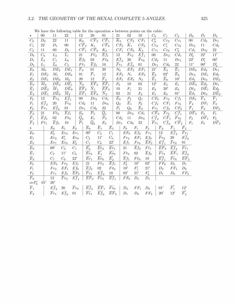
3.2. THE GEOMETRY OF THE HEXAL COMPLETE 5-ANGLES. 325
We have the following table for the operation ? between points on the cubic:? 00 11 22 12 20 01 21 02 10 C0 C1 C2 D0 D1 D2
C0 D0 22 11 K0 CF 2 CF 1 K0 CF2 CF1 C ′0 Cc2 Cc1 00 Cd2 Dc1
C1 22 D1 00 CF 2 K1 CF 0 CF2 K1 CF0 Cc2 C ′1 Cc0 Dc2 11 Cd0
C2 11 00 D2 CF 1 CF 0 K2 CF1 CF0 K2 Cc1 Cc0 C ′2 Cd1 Dc0 22
D0 C0 L2 L1 21 Fe2 Ef1 12 Fe2 Ef1 00 Dc2 Cd1 D′0 22′ 11′
D1 L2 C1 L0 Ef2 02 Fe0 Ef2 20 Fe0 Cd2 11 Dc1 22′ D′1 00′
D2 L1 L0 C2 Fe1 Ef0 10 Fe1 Ef0 01 Dc1 Cd0 22 11′ 00′ D′2
E0 M0 DE2 DE1 F 0 01 20 N0 EF2 EF1 21′ E2 E1 DE0 Ed2 De1E1 DE2 M1 DE0 01 F 1 12 EF2 N1 EF0 E2 02′ E0 De2 DE1 Ed0E2 DE1 DE0 M2 20 12 F 2 EF1 EF0 N2 E1 E0 10′ Ed1 De0 DE2
E0 M0 DE2 DE1 N0 EF 2 EF 1 F0 10 02 12′ E2 E1 DE0 Ed2 De1E1 DE2 M1 DE0 EF 2 N1 EF 0 10 F1 21 E2 20′ E0 De2 DE1 Ed0E2 DE1 DE0 M2 EF 1 EF 0 N2 02 21 F2 E1 E0 01′ Ed1 De0 DE2
F0 12 Fe2 Ef1 00 Dc2 Cd1 E0 P2 Q1 CF0 Fc2 Cf1 DF0 F 2 F 1
F1 Ef2 20 Fe0 Cd2 11 Dc0 Q2 E1 P0 Cf2 CF1 Fc0 F 2 DF1 F 0
F2 Fe1 Ef0 01 Dc1 Cd0 22 P1 Q0 E2 Fc1 Cf0 CF2 F 1 F 0 DF2
F 0 21 Fe2 Ef1 E0 P 2 Q1 00 Dc2 Cd1 CF 0 Fc2 Cf1 DF 0 F2 F1
F 1 Ef2 02 Fe0 Q2 E1 P 0 Cd2 11 Dc0 Cf2 CF 1 Fc0 F2 DF 1 F0
F 2 Fe1 Ef0 10 P 1 Q0 E2 Dc1 Cd0 22 Fc1 Cf0 CF 2 F1 F0 DF 2
? E0 E1 E2 E0 E1 E2 F0 F1 F2 F 0 F 1 F 2
E0 E′0 Ee2 Ee1 00′ C2 C1 EF0 Ef2 Fe1 12 Ef2 Fe1
E1 Ee2 E′1 Ee0 C2 11′ C0 Fe2 EF1 Ef0 Fe2 20 Ef0
E2 Ee1 Ee0 E′2 C1 C0 22′ Ef1 Fe0 EF2 Ef1 Fe0 01
E0 00′ C2 C1 E′0 Ee2 Ee1 21 Ef2 Fe1 EF 0 Ef2 Fe1
E1 C2 11′ C0 Ee2 E′1 Ee0 Fe2 02 Ef0 Fe2 EF 1 Ef0
E2 C1 C0 22′ Ee1 Ee0 E′2 Ef1 Fe0 10 Ef1 Fe0 EF 2
F0 EF0 Fe2 Ef1 21 Fe2 Ef1 F ′0 10′ 02′ FF0 D2 D1
F1 Fe2 EF1 Ef0 Ef2 02 Fe0 10′ F ′1 21′ D2 FF1 D0
F2 Fe1 Ef0 EF2 Fe1 Ef0 10 02′ 21′ F ′2 D1 D0 FF2
F 0 12 Fe2 Ef1 EF 0 Fe2 Ef1 FF0 D2 D1
ovF ′0 01′ 20′
F 1 Ef2 20 Fe0 Ef2 EF 1 Fe0 D2 FF1 D0 01′ F′1 12′
F 2 Fe1 Ef0 01 Fe1 Ef0 EF 2 D1 D0 FF2 20′ 12′ F′2
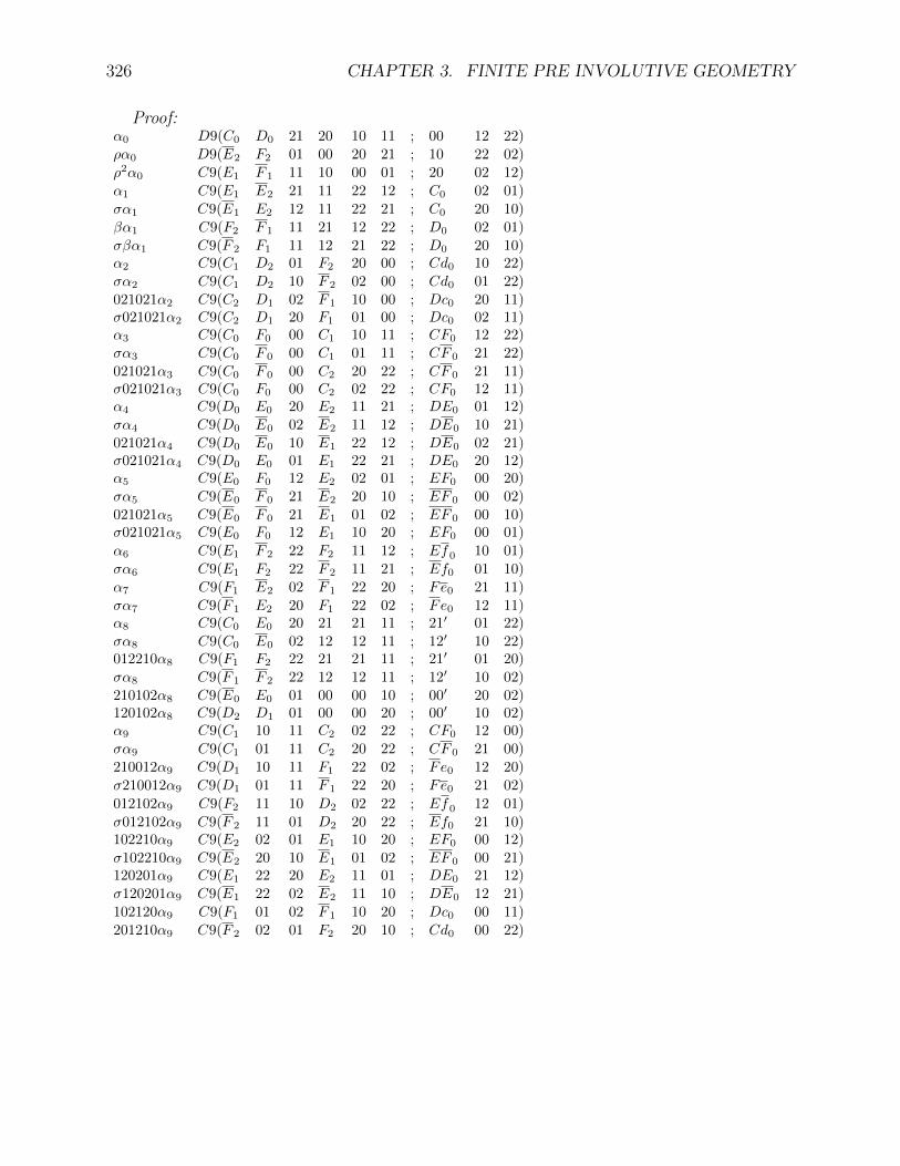
326 CHAPTER 3. FINITE PRE INVOLUTIVE GEOMETRY
Proof:α0 D9(C0 D0 21 20 10 11 ; 00 12 22)ρα0 D9(E2 F2 01 00 20 21 ; 10 22 02)ρ2α0 C9(E1 F 1 11 10 00 01 ; 20 02 12)α1 C9(E1 E2 21 11 22 12 ; C0 02 01)σα1 C9(E1 E2 12 11 22 21 ; C0 20 10)βα1 C9(F2 F 1 11 21 12 22 ; D0 02 01)σβα1 C9(F 2 F1 11 12 21 22 ; D0 20 10)α2 C9(C1 D2 01 F2 20 00 ; Cd0 10 22)σα2 C9(C1 D2 10 F 2 02 00 ; Cd0 01 22)021021α2 C9(C2 D1 02 F 1 10 00 ; Dc0 20 11)σ021021α2 C9(C2 D1 20 F1 01 00 ; Dc0 02 11)α3 C9(C0 F0 00 C1 10 11 ; CF0 12 22)σα3 C9(C0 F 0 00 C1 01 11 ; CF 0 21 22)021021α3 C9(C0 F 0 00 C2 20 22 ; CF 0 21 11)σ021021α3 C9(C0 F0 00 C2 02 22 ; CF0 12 11)α4 C9(D0 E0 20 E2 11 21 ; DE0 01 12)σα4 C9(D0 E0 02 E2 11 12 ; DE0 10 21)021021α4 C9(D0 E0 10 E1 22 12 ; DE0 02 21)σ021021α4 C9(D0 E0 01 E1 22 21 ; DE0 20 12)α5 C9(E0 F0 12 E2 02 01 ; EF0 00 20)σα5 C9(E0 F 0 21 E2 20 10 ; EF 0 00 02)021021α5 C9(E0 F 0 21 E1 01 02 ; EF 0 00 10)σ021021α5 C9(E0 F0 12 E1 10 20 ; EF0 00 01)
α6 C9(E1 F 2 22 F2 11 12 ; Ef0 10 01)σα6 C9(E1 F2 22 F 2 11 21 ; Ef0 01 10)α7 C9(F1 E2 02 F 1 22 20 ; Fe0 21 11)σα7 C9(F 1 E2 20 F1 22 02 ; Fe0 12 11)α8 C9(C0 E0 20 21 21 11 ; 21′ 01 22)σα8 C9(C0 E0 02 12 12 11 ; 12′ 10 22)012210α8 C9(F1 F2 22 21 21 11 ; 21′ 01 20)σα8 C9(F 1 F 2 22 12 12 11 ; 12′ 10 02)210102α8 C9(E0 E0 01 00 00 10 ; 00′ 20 02)120102α8 C9(D2 D1 01 00 00 20 ; 00′ 10 02)α9 C9(C1 10 11 C2 02 22 ; CF0 12 00)σα9 C9(C1 01 11 C2 20 22 ; CF 0 21 00)210012α9 C9(D1 10 11 F1 22 02 ; Fe0 12 20)σ210012α9 C9(D1 01 11 F 1 22 20 ; Fe0 21 02)
012102α9 C9(F2 11 10 D2 02 22 ; Ef0 12 01)σ012102α9 C9(F 2 11 01 D2 20 22 ; Ef0 21 10)102210α9 C9(E2 02 01 E1 10 20 ; EF0 00 12)σ102210α9 C9(E2 20 10 E1 01 02 ; EF 0 00 21)120201α9 C9(E1 22 20 E2 11 01 ; DE0 21 12)σ120201α9 C9(E1 22 02 E2 11 10 ; DE0 12 21)102120α9 C9(F1 01 02 F 1 10 20 ; Dc0 00 11)201210α9 C9(F 2 02 01 F2 20 10 ; Cd0 00 22)

3.2. THE GEOMETRY OF THE HEXAL COMPLETE 5-ANGLES. 327
3.2.10 The cubics of Grassmann.
Definition.
Given 6 lines ai and bi, among the 15 intersections we choose the following 9,D1.0. Ai := ai+1 × ai−1,D1.1. Bi := bi+1 × bi−1,D1.2. Ei := ai × bi,the non confined configuration consisting of these 9 points and 6 lines each containing 3 ofthe points is called a Grassmann configuration. It is noted (Ai, Bi, Ei).
Theorem. [Grassmann]
Given 2 triangles Ai, ai and Bi, bi, the locus of the points X is a cubic, if X is such thatthe points obtained by finding the intersections of the lines joining X to the vertices of oneof the triangles and the corresponding sides of the second triangle, namely (X×Ai)× bi, arecollinear.
Theorem.
LetD2.0. aBi := Ai+1 ×Bi−1, aBi := Ai−1 ×Bi+1,D2.1. ABi := aBi × aBi,D2.2. abEi := ABi+1 × Ei−1, abEi := ABi−1 × Ei+1,D2.3. DEi := abEi × abEi,D2.4. dei := DEi × Ei,D2.5. abi := Ai ×Bi,D2.6. Di := dei × abi,D2.6. bai := ABi+1 × ABi−1,D2.8. abdi := Di × ABi,D2.9. Ci := bai × abdi,D4.0. aei := Ai × Ei, bei := Bi × Ei,D4.1. cei := Ci × Ei,D4.2. aabi := Ai × ABi, babi := Bi × ABi,D4.3. Fi := bei × aabi, F i := aei × babi,D4.4. fi := Fi+1 × Fi−1, f i := F i+1 × F i−1,D4.5. A′i := cei × f i, B′i := cei × fi,D4.6. aCi := Ai+1 × Ci−1, aCi := Ai−1 × Ci+1,D4.6. bCi := Bi+1 × Ci−1, bCi := Bi−1 × Ci+1,D4.7. CFi := bCi × bCi, CF i := aCi × aCi,D4.8. cDi := Ci+1 ×Di−1, cDi := Ci−1 ×Di+1,D4.9. aFi := Ai+1 × Fi−1, aF i := Ai−1 × Fi+1,D4.10. Cdi := cDi × aFi, Dci := cDi × aF i,D4.11. aDi := Ai+1 ×Di−1, aDi := Ai−1 ×Di+1,D4.12. eFi := Ei+1 × Fi−1, eF i := Ei−1 × Fi+1,D4.13. Efi := aDi × eFi, Fei := aDi × eF i,
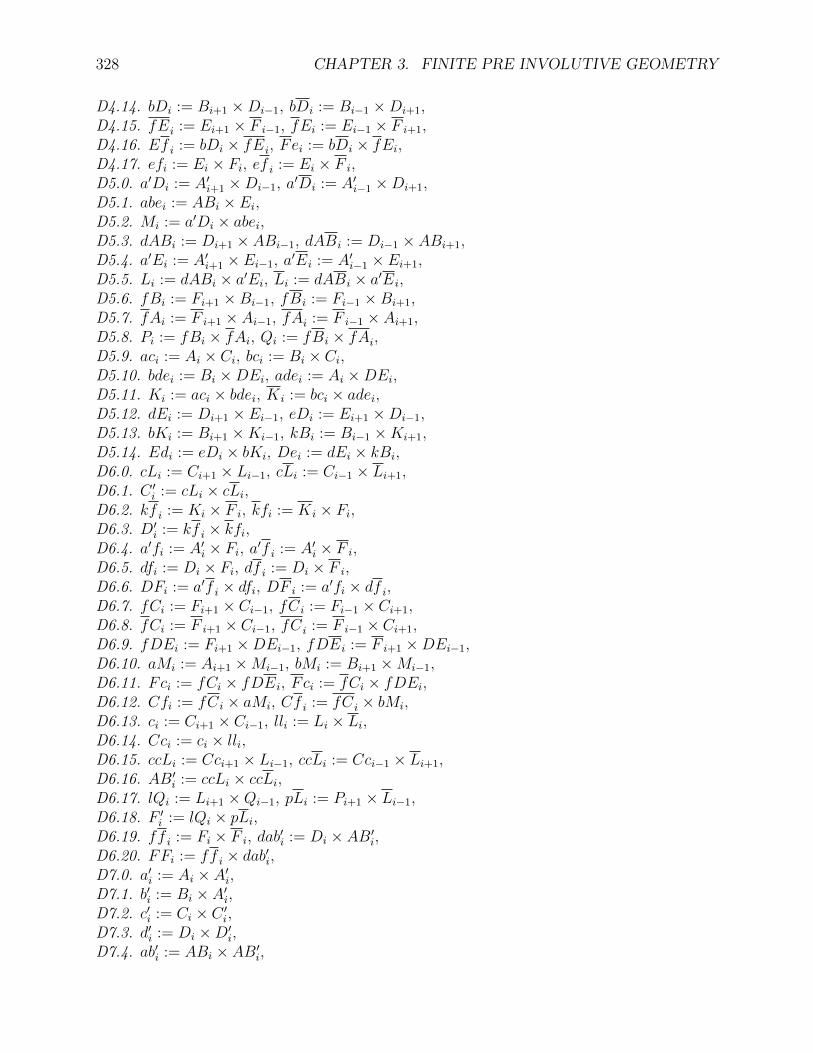
328 CHAPTER 3. FINITE PRE INVOLUTIVE GEOMETRY
D4.14. bDi := Bi+1 ×Di−1, bDi := Bi−1 ×Di+1,D4.15. fEi := Ei+1 × F i−1, fEi := Ei−1 × F i+1,D4.16. Ef i := bDi × fEi, Fei := bDi × fEi,D4.17. efi := Ei × Fi, ef i := Ei × F i,D5.0. a′Di := A′i+1 ×Di−1, a
′Di := A′i−1 ×Di+1,D5.1. abei := ABi × Ei,D5.2. Mi := a′Di × abei,D5.3. dABi := Di+1 × ABi−1, dABi := Di−1 × ABi+1,D5.4. a′Ei := A′i+1 × Ei−1, a
′Ei := A′i−1 × Ei+1,D5.5. Li := dABi × a′Ei, Li := dABi × a′Ei,D5.6. fBi := Fi+1 ×Bi−1, fBi := Fi−1 ×Bi+1,D5.7. fAi := F i+1 × Ai−1, fAi := F i−1 × Ai+1,D5.8. Pi := fBi × fAi, Qi := fBi × fAi,D5.9. aci := Ai × Ci, bci := Bi × Ci,D5.10. bdei := Bi ×DEi, adei := Ai ×DEi,D5.11. Ki := aci × bdei, Ki := bci × adei,D5.12. dEi := Di+1 × Ei−1, eDi := Ei+1 ×Di−1,D5.13. bKi := Bi+1 ×Ki−1, kBi := Bi−1 ×Ki+1,D5.14. Edi := eDi × bKi, Dei := dEi × kBi,D6.0. cLi := Ci+1 × Li−1, cLi := Ci−1 × Li+1,D6.1. C ′i := cLi × cLi,D6.2. kf i := Ki × F i, kfi := Ki × Fi,D6.3. D′i := kf i × kfi,D6.4. a′fi := A′i × Fi, a′f i := A′i × F i,D6.5. dfi := Di × Fi, df i := Di × F i,D6.6. DFi := a′f i × dfi, DF i := a′fi × df i,D6.7. fCi := Fi+1 × Ci−1, fCi := Fi−1 × Ci+1,D6.8. fCi := F i+1 × Ci−1, fCi := F i−1 × Ci+1,D6.9. fDEi := Fi+1 ×DEi−1, fDEi := F i+1 ×DEi−1,D6.10. aMi := Ai+1 ×Mi−1, bMi := Bi+1 ×Mi−1,D6.11. Fci := fCi × fDEi, F ci := fCi × fDEi,D6.12. Cfi := fCi × aMi, Cf i := fCi × bMi,D6.13. ci := Ci+1 × Ci−1, lli := Li × Li,D6.14. Cci := ci × lli,D6.15. ccLi := Cci+1 × Li−1, ccLi := Cci−1 × Li+1,D6.16. AB′i := ccLi × ccLi,D6.17. lQi := Li+1 ×Qi−1, pLi := Pi+1 × Li−1,D6.18. F ′i := lQi × pLi,D6.19. ff i := Fi × F i, dab
′i := Di × AB′i,
D6.20. FFi := ff i × dab′i,D7.0. a′i := Ai × A′i,D7.1. b′i := Bi × A′i,D7.2. c′i := Ci × C ′i,D7.3. d′i := Di ×D′i,D7.4. ab′i := ABi × AB′i,
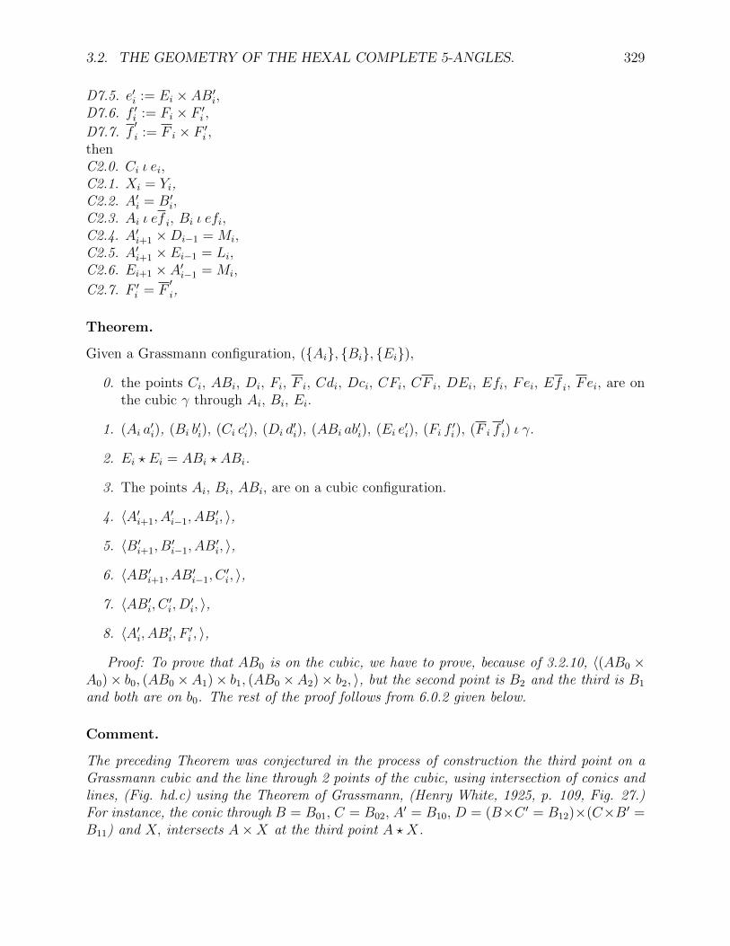
3.2. THE GEOMETRY OF THE HEXAL COMPLETE 5-ANGLES. 329
D7.5. e′i := Ei × AB′i,D7.6. f ′i := Fi × F ′i ,D7.7. f
′i := F i × F ′i ,
thenC2.0. Ci ι ei,C2.1. Xi = Yi,C2.2. A′i = B′i,C2.3. Ai ι ef i, Bi ι efi,C2.4. A′i+1 ×Di−1 = Mi,C2.5. A′i+1 × Ei−1 = Li,C2.6. Ei+1 × A′i−1 = Mi,
C2.7. F ′i = F′i,
Theorem.
Given a Grassmann configuration, (Ai, Bi, Ei),
0. the points Ci, ABi, Di, Fi, F i, Cdi, Dci, CFi, CF i, DEi, Efi, Fei, Ef i, Fei, are onthe cubic γ through Ai, Bi, Ei.
1. (Ai a′i), (Bi b
′i), (Ci c
′i), (Di d
′i), (ABi ab
′i), (Ei e
′i), (Fi f
′i), (F i f
′i) ι γ.
2. Ei ? Ei = ABi ? ABi.
3. The points Ai, Bi, ABi, are on a cubic configuration.
4. 〈A′i+1, A′i−1, AB
′i, 〉,
5. 〈B′i+1, B′i−1, AB
′i, 〉,
6. 〈AB′i+1, AB′i−1, C
′i, 〉,
7. 〈AB′i, C ′i, D′i, 〉,
8. 〈A′i, AB′i, F ′i , 〉,
Proof: To prove that AB0 is on the cubic, we have to prove, because of 3.2.10, 〈(AB0 ×A0)× b0, (AB0 ×A1)× b1, (AB0 ×A2)× b2, 〉, but the second point is B2 and the third is B1
and both are on b0. The rest of the proof follows from 6.0.2 given below.
Comment.
The preceding Theorem was conjectured in the process of construction the third point on aGrassmann cubic and the line through 2 points of the cubic, using intersection of conics andlines, (Fig. hd.c) using the Theorem of Grassmann, (Henry White, 1925, p. 109, Fig. 27.)For instance, the conic through B = B01, C = B02, A
′ = B10, D = (B×C ′ = B12)×(C×B′ =B11) and X, intersects A×X at the third point A ? X.

330 CHAPTER 3. FINITE PRE INVOLUTIVE GEOMETRY
Theorem.
We have the following table for the operation ? between points on a Grassmann cubic:? AB0 AB1 AB2 A0 A1 A2 B0 B1 B2
AB0 AB′0 C2 C1 F0 B2 B1 F 0 A2 A1
AB1 C2 AB′1 C0 B2 F1 B0 A2 F 1 A0
AB2 C1 C0 AB′2 B1 B0 F2 A1 A0 F 2
A0 F0 B2 B1 A′0 E2 E1 D0 AB2 AB1
A1 B2 F1 B0 E2 A′1 E0 AB2 D1 AB0
A2 B1 B0 F2 E1 E0 A′2 AB1 AB0 D2
B0 F 0 A2 A1 D0 AB2 AB1 A′0 E2 E1
B1 A2 F 1 A0 AB2 D1 AB0 E2 A′1 E0
B2 A1 A0 F 2 AB1 AB0 D2 E1 E0 A′2
? AB0 AB1 AB2 A0 A1 A2 B0 B1 B2 C0 C1 C2 D0 D1 D2
C0 D0 AB2 AB1 K0 CF 2 CF 1 K0 CF2 CF1 C ′0 Cc2 Cc1 AB0 Cd2 Dc1
C1 AB2 D1 AB0 CF 2 K1 CF 0 CF2 K1 CF0 Cc2 C ′1 Cc0 Dc2 AB1 Cd0
C2 AB1 AB0 D2 CF 1 CF 0 K2 CF1 CF0 K2 Cc1 Cc0 C ′2 Cd1 Dc0 AB2
D0 C0 L2 L1 B0 Fe2 Ef1 A0 Fe2 Ef1 AB0 Dc2 Cd1 D′0 AB′
2 AB′1
D1 L2 C1 L0 Ef2 B1 Fe0 Ef2 A1 Fe0 Cd2 AB1 Dc1 AB′2 D′
1 AB′0
D2 L1 L0 C2 Fe1 Ef0 B2 Fe1 Ef0 A2 Dc1 Cd0 AB2 AB′1 AB′
0 D′2
E0 M0 DE2 DE1 F 0 A2 A1 F0 B2 B1 A′0 E2 E1 DE0 Ed2 De1
E1 DE2 M1 DE0 A2 F 1 A0 B2 F1 B0 E2 A′1 E0 De2 DE1 Ed0
E2 DE1 DE0 M2 A1 A0 F 2 B1 B0 F2 E1 E0 A′2 Ed1 De0 DE2
F0 A0 Fe2 Ef1 AB0 Dc2 Cd1 E0 P2 Q1 CF0 Fc2 Cf1 DF0 F 2 F 1
F1 Ef2 A1 Fe0 Cd2 AB1 Dc0 Q2 E1 P0 Cf2 CF1 Fc0 F 2 DF1 F 0
F2 Fe1 Ef0 A2 Dc1 Cd0 AB2 P1 Q0 E2 Fc1 Cf0 CF2 F 1 F 0 DF2
F 0 B0 Fe2 Ef1 E0 P2 Q1 AB0 Dc2 Cd1 CF 0 Fc2 Cf1 DF 0 F2 F1
F 1 Ef2 B1 Fe0 Q2 E1 P0 Cd2 AB1 Dc0 Cf2 CF 1 Fc0 F2 DF 1 F0
F 2 Fe1 Ef0 B2 P1 Q0 E2 Dc1 Cd0 AB2 Fc1 Cf0 CF 2 F1 F0 DF 2
? E0 E1 E2 F0 F1 F2 F 0 F 1 F 2
E0 AB′0 C2 C1 B0 Ef2 Fe1 A0 Ef2 Fe1
E1 C2 AB′1 C0 Fe2 B1 Ef0 Fe2 A1 Ef0
E2 C1 C0 AB′2 Ef1 Fe0 B2 Ef1 Fe0 A2
F0 B0 Fe2 Ef1 F ′0 A′
2 A′1 FF0 D2 D1
F1 Ef2 B1 Fe0 A′2 F ′
1 A′0 D2 FF1 D0
F2 Fe1 Ef0 B2 A′1 A′
0 F ′2 D1 D0 FF2
F 0 A0 Fe2 Ef1 FF0 D2 D1 F ′0 A′
2 A′1
F 1 Ef2 A1 Fe0 D2 FF1 D0 A′2 F ′
1 A′0
F 2 Fe1 Ef0 A2 D1 D0 FF2 A′1 A′
0 F ′2
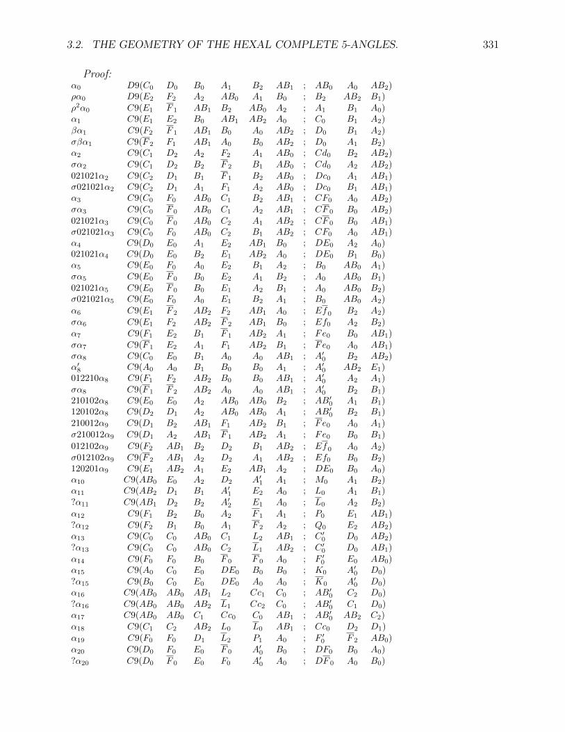
3.2. THE GEOMETRY OF THE HEXAL COMPLETE 5-ANGLES. 331
Proof:α0 D9(C0 D0 B0 A1 B2 AB1 ; AB0 A0 AB2)ρα0 D9(E2 F2 A2 AB0 A1 B0 ; B2 AB2 B1)ρ2α0 C9(E1 F 1 AB1 B2 AB0 A2 ; A1 B1 A0)α1 C9(E1 E2 B0 AB1 AB2 A0 ; C0 B1 A2)βα1 C9(F2 F 1 AB1 B0 A0 AB2 ; D0 B1 A2)σβα1 C9(F 2 F1 AB1 A0 B0 AB2 ; D0 A1 B2)α2 C9(C1 D2 A2 F2 A1 AB0 ; Cd0 B2 AB2)σα2 C9(C1 D2 B2 F 2 B1 AB0 ; Cd0 A2 AB2)021021α2 C9(C2 D1 B1 F 1 B2 AB0 ; Dc0 A1 AB1)σ021021α2 C9(C2 D1 A1 F1 A2 AB0 ; Dc0 B1 AB1)α3 C9(C0 F0 AB0 C1 B2 AB1 ; CF0 A0 AB2)σα3 C9(C0 F 0 AB0 C1 A2 AB1 ; CF 0 B0 AB2)021021α3 C9(C0 F 0 AB0 C2 A1 AB2 ; CF 0 B0 AB1)σ021021α3 C9(C0 F0 AB0 C2 B1 AB2 ; CF0 A0 AB1)α4 C9(D0 E0 A1 E2 AB1 B0 ; DE0 A2 A0)021021α4 C9(D0 E0 B2 E1 AB2 A0 ; DE0 B1 B0)α5 C9(E0 F0 A0 E2 B1 A2 ; B0 AB0 A1)σα5 C9(E0 F 0 B0 E2 A1 B2 ; A0 AB0 B1)021021α5 C9(E0 F 0 B0 E1 A2 B1 ; A0 AB0 B2)σ021021α5 C9(E0 F0 A0 E1 B2 A1 ; B0 AB0 A2)
α6 C9(E1 F 2 AB2 F2 AB1 A0 ; Ef0 B2 A2)σα6 C9(E1 F2 AB2 F 2 AB1 B0 ; Ef0 A2 B2)α7 C9(F1 E2 B1 F 1 AB2 A1 ; Fe0 B0 AB1)σα7 C9(F 1 E2 A1 F1 AB2 B1 ; Fe0 A0 AB1)σα8 C9(C0 E0 B1 A0 A0 AB1 ; A′
0 B2 AB2)α′8 C9(A0 A0 B1 B0 B0 A1 ; A′
0 AB2 E1)012210α8 C9(F1 F2 AB2 B0 B0 AB1 ; A′
0 A2 A1)σα8 C9(F 1 F 2 AB2 A0 A0 AB1 ; A′
0 B2 B1)210102α8 C9(E0 E0 A2 AB0 AB0 B2 ; AB′
0 A1 B1)120102α8 C9(D2 D1 A2 AB0 AB0 A1 ; AB′
0 B2 B1)210012α9 C9(D1 B2 AB1 F1 AB2 B1 ; Fe0 A0 A1)σ210012α9 C9(D1 A2 AB1 F 1 AB2 A1 ; Fe0 B0 B1)
012102α9 C9(F2 AB1 B2 D2 B1 AB2 ; Ef0 A0 A2)σ012102α9 C9(F 2 AB1 A2 D2 A1 AB2 ; Ef0 B0 B2)120201α9 C9(E1 AB2 A1 E2 AB1 A2 ; DE0 B0 A0)α10 C9(AB0 E0 A2 D2 A′
1 A1 ; M0 A1 B2)α11 C9(AB2 D1 B1 A′
1 E2 A0 ; L0 A1 B1)?α11 C9(AB1 D2 B2 A′
2 E1 A0 ; L0 A2 B2)α12 C9(F1 B2 B0 A2 F 1 A1 ; P0 E1 AB1)?α12 C9(F2 B1 B0 A1 F 2 A2 ; Q0 E2 AB2)α13 C9(C0 C0 AB0 C1 L2 AB1 ; C ′
0 D0 AB2)?α13 C9(C0 C0 AB0 C2 L1 AB2 ; C ′
0 D0 AB1)α14 C9(F0 F0 B0 F 0 F 0 A0 ; F ′
0 E0 AB0)α15 C9(A0 C0 E0 DE0 B0 B0 ; K0 A′
0 D0)?α15 C9(B0 C0 E0 DE0 A0 A0 ; K0 A′
0 D0)α16 C9(AB0 AB0 AB1 L2 Cc1 C0 ; AB′
0 C2 D0)?α16 C9(AB0 AB0 AB2 L1 Cc2 C0 ; AB′
0 C1 D0)α17 C9(AB0 AB0 C1 Cc0 C0 AB1 ; AB′
0 AB2 C2)α18 C9(C1 C2 AB2 L0 L0 AB1 ; Cc0 D2 D1)α19 C9(F0 F0 D1 L2 P1 A0 ; F ′
0 F 2 AB0)α20 C9(D0 F0 E0 F 0 A′
0 B0 ; DF0 B0 A0)?α20 C9(D0 F 0 E0 F0 A′
0 A0 ; DF 0 A0 B0)

332 CHAPTER 3. FINITE PRE INVOLUTIVE GEOMETRY
α21 C9(F1 C2 AB1 F 1 DE2 E1 ; Fc0 AB0 B1)?α21 C9(F 1 C2 AB1 F1 DE2 E1 ; Fc0 AB0 A1)α22 C9(C1 F2 E2 M2 A1 AB0 ; Cf0 B2 AB2)
?α22 C9(C1 F 2 E2 M2 B1 AB0 ; Cf0 A2 AB2)α23 C9(F0 F0 D2 L1 Q2 A0 ; F ′
0 F 1 AB0)?α23 C9(F0 F0 D1 L2 P1 A0 ; F ′
0 F 2 AB0)α24 C9(D0 D0 C0 K0 F 0 B0 ; D′
0 AB0 A0)?α24 C9(D0 D0 C0 K0 F0 A0 ; D′
0 AB0 A0)α25 C9(E1 D2 B2 B1 K2 C2 ; Ed0 A2 E0)?α25 C9(E2 D1 B1 B2 K1 C1 ; De0 A1 E0)α26 C9(C0 F0 A0 B0 AB′
0 AB0 ; CF0 AB0 D0)?α26 C9(C0 F 0 B0 A0 AB′
0 AB0 ; CF 0 AB0 D0)α27 C9(F0 F 0 B0 D0 AB′
0 AB0 ; FF0 AB0 A0)
Theorem.
Given a Grassmann configuration (Ai, Bi, Ei), THe tangential points at Ai and Bi
are the same, in the above case A′i, it will be added to the configuration after a semi colon.
Lemma.
If (Ai, Bi, Ei, A′i), is a Grassmann configuration so is
0. (Ai, Bi, Ei),,where
ABi := Ai+1 ? Bi−1, and Ci := ABi+1 ? ABi−1.
1. (Fi, F i, A′i),,where
Fi := ABi ? Ai, and F i := ABi ? Bi,
This follows at once from grom 6.0.2.
Theorem.
Given a Grassmann configuration (Ai, Bi, Ei; ABi), the following are also Grass-mann configurations:
0. (ABi, Ei, Ci; AB′i),
1. (Fi, F i, A′i; F ′i),
2. (DEi, Ci, Ci ? AB′i),
3. (Di, A′i, AB′i; d′i).
Proof: This follows by repeated applications of the Lemma 3.2.10.

3.2. THE GEOMETRY OF THE HEXAL COMPLETE 5-ANGLES. 333
3.2.11 Grassmannian cubics in Involutive Geometry.
Definition.
In involutive geometry I will give the name of Grassmannian cubic to the special case wherethe 6 lines are mi and mi.
Theorem.
The correspondence between the elements as given above and those of involutive geometryis as followsAi = CFi Bi = CF i Ei = DEi ABi = Ci = Cci Fi = Ki F i = Ki
MMi MMi Ai ATi Fi F i
Efi = Cf i Ef i = Cfi Fei = Fci Fei = Fci A′i = Mi Li = Cdi Li = Dci Pi Qi
Efi Ef i Fei Fei MM ′i Li Li Pi Qi
ai bi aBi aBi abi ei aei bei baimmi mmi ci ci ai aeULi nmi nmi eul
Theorem.
0. The Grassmann cubic passes through the points MMi, MMi, Ai, Di.
1. Its equation ism0(m1 + m2)X1X2((m2 + m0)X1 + (m0 + m1)X2)m1(m2 + m0)X2X0((m0 +
m1)X2 + (m1 + m2)X0)m2(m0 + m1)X0X1((m1 + m2)X0 + (m2 + m0)X1) + (s21 +2s111)X0X1X2 = 0
Proof: Using 3.2.9 on the points Ai and ATi, we obtain the given form, to determine thecoefficients gi of X1X2((m2 + m0)X1 + (m0 + m1)X2), . . . and g of X0X1X2 we impose thecondition that the cubic passes through MMi, this gives the system of equations
. . . .
Theorem.
LetD2.0. aBi := Ai+1 ×Bi−1, aBi := Ai−1 ×Bi+1,D2.1. ABi := aBi × aBi,D2.2. abEi := ABi+1 × Ei−1, abEi := ABi−1 × Ei+1,D2.3. DEi := abEi × abEi,D2.4. dei := DEi × Ei,D2.5. abi := Ai ×Bi,D2.6. Di := dei × abi,D2.6. bai := ABi+1 × ABi−1,D2.8. abdi := Di × ABi,D2.9. Ci := bai × abdi,D4.0. aei := Ai × Ei, bei := Bi × Ei,

334 CHAPTER 3. FINITE PRE INVOLUTIVE GEOMETRY
D4.1. cei := Ci × Ei,D4.2. aabi := Ai × ABi, babi := Bi × ABi,D4.3. Fi := bei × aabi, F i := aei × babi,D4.4. fi := Fi+1 × Fi−1, f i := F i+1 × F i−1,D4.5. A′i := cei × f i, B′i := cei × fi,D4.6. aCi := Ai+1 × Ci−1, aCi := Ai−1 × Ci+1,D4.6. bCi := Bi+1 × Ci−1, bCi := Bi−1 × Ci+1,D4.7. CFi := bCi × bCi, CF i := aCi × aCi,D4.8. cDi := Ci+1 ×Di−1, cDi := Ci−1 ×Di+1,D4.9. aFi := Ai+1 × Fi−1, aF i := Ai−1 × Fi+1,D4.10. Cdi := cDi × aFi, Dci := cDi × aF i,D4.11. aDi := Ai+1 ×Di−1, aDi := Ai−1 ×Di+1,D4.12. eFi := Ei+1 × Fi−1, eF i := Ei−1 × Fi+1,D4.13. Efi := aDi × eFi, Fei := aDi × eF i,D4.14. bDi := Bi+1 ×Di−1, bDi := Bi−1 ×Di+1,D4.15. fEi := Ei+1 × F i−1, fEi := Ei−1 × F i+1,D4.16. Ef i := bDi × fEi, Fei := bDi × fEi,D4.17. efi := Ei × Fi, ef i := Ei × F i,D5.0. a′Di := A′i+1 ×Di−1, a
′Di := A′i−1 ×Di+1,D5.1. abei := ABi × Ei,D5.2. Mi := a′Di × abei,D5.3. dABi := Di+1 × ABi−1, dABi := Di−1 × ABi+1,D5.4. a′Ei := A′i+1 × Ei−1, a
′Ei := A′i−1 × Ei+1,D5.5. Li := dABi × a′Ei, Li := dABi × a′Ei,D5.6. fBi := Fi+1 ×Bi−1, fBi := Fi−1 ×Bi+1,D5.7. fAi := F i+1 × Ai−1, fAi := F i−1 × Ai+1,D5.8. Pi := fBi × fAi, Qi := fBi × fAi,D5.9. aci := Ai × Ci, bci := Bi × Ci,D5.10. bdei := Bi ×DEi, adei := Ai ×DEi,D5.11. Ki := aci × bdei, Ki := bci × adei,D5.12. dEi := Di+1 × Ei−1, eDi := Ei+1 × Ei−1,D5.13. bKi := Bi+1 ×Ki−1, kBi := Bi−1 ×Ki+1,D5.14. Edi := eDi × bKi, Dei := dEi × kBi,D6.0. cLi := Ci+1 × Li−1, cLi := Ci−1 × Li+1,D6.1. C ′i := cLi × cLi,D6.2. kf i := Ki × F i, kfi := Ki × Fi,D6.3. D′i := kf i × kfi,D6.4. a′fi := A′i × Fi, a′f i := A′i × F i,D6.5. dfi := Di × Fi, df i := Di × F i,D6.6. DFi := a′f i × dfi, DF i := a′fi × df i,D6.7. fCi := Fi+1 × Ci−1, fCi := Fi−1 × Ci+1,D6.8. fCi := F i+1 × Ci−1, fCi := F i−1 × Ci+1,D6.9. fDEi := Fi+1 ×DEi−1, fDEi := F i+1 ×DEi−1,D6.10. aMi := Ai+1 ×Mi−1, bMi := Bi+1 ×Mi−1,D6.11. Fci := fCi × fDEi, F ci := fCi × fDEi,

3.2. THE GEOMETRY OF THE HEXAL COMPLETE 5-ANGLES. 335
D6.12. Cfi := fCi × aMi, Cf i := fCi × bMi,D6.13. ci := Ci+1 × Ci−1, lli := Li × Li,D6.14. Cci := ci × lli,D6.15. ccLi := Cci+1 × Li−1, ccLi := Cci−1 × Li+1,D6.16. AB′i := ccLi × ccLi,D6.17. lQi := Li+1 ×Qi−1, pLi := Pi+1 × Li−1,D6.18. F ′i := lQi × pLi,D6.19. ff i := Fi × F i, dab
′i := Di × AB′i,
D6.20. FFi := ff i × dab′i,D7.0. a′i := Ai × A′i,D7.1. b′i := Bi × A′i,D7.2. c′i := Ci × C ′i,D7.3. d′i := Di ×D′i,D7.4. ab′i := ABi × AB′i,D7.5. e′i := Ei × AB′i,D7.6. f ′i := Fi × F ′i ,D7.7. f
′i := F i × F ′i ,
thenC2.0. Ci ι ei,C2.1. Xi = Yi,C2.2. A′i = B′i,C2.3. Ai ι ef i, Bi ι efi,C2.4. A′i+1 ×Di−1 = Mi,C2.5. A′i+1 × Ei−1 = Li,C2.6. Ei+1 × A′i−1 = Mi,
C2.7. F ′i = F′i,
Proof: H0.0. m0 = [0, 1, 1], m0 = [0,m2,m1],D1.0. MM0 = (−1, 1, 1), MM0 = (m0,−m1,−m2)D0.10. A0 = (1, 0, 0)D0.10. a0 = [1, 0, 0]D.. ma0 = [0, 1,−1], ma0 = [0,m2,−m1],D.. eul0 = [m1−m2,−(m2−m0),−(m0−m1)],D.. y0 = [m1−m2,−(m2 +m0),−(m0 +m1)],D.. y 0 = [m1−m2,m2 +m0,m0 +m1],D.. AT0 = (0,m0 +m1,−(m2−m0)),D.. k = [m1 +m2,m2 +m0,m0 +m1],D.. tAM0 = [s1 +m0,m2 +m0,m0 +m1],D.. tAM0 = [s11 +m1m2,m0(m2 +m0),m0(m0 +m1)],D.. F0 = (s11 +m1m2,−m1(s1 +m0),−m2(s1 +m0)),D.. F 0 = (m0(s1 +m0),−(s11 +m1m2),−(s11 +m1m2)),D.. ff0 = [m1(m1−m2), s11 +m2m0,m1(s1 +m2)],D.. D0 = (m1 +m2)q0,−m1(m1−m2)(m2 +m0),m2(m0 +m1)(m1−m2)),D.. eul = [m1−m2,m2−m0,m0−m1],

336 CHAPTER 3. FINITE PRE INVOLUTIVE GEOMETRY
D.. aAT0 = [0,m2 +m0,m0 +m1)],D.. f 0 = [(m1 +m2)q0,−(m2 +m0)(s11 +m2m0),−(m0 +m1)(s11 +m0m1),D.. MM ′
0 = (m0(m1−m2)(m2+m0)(m0+m1),−(m0+m1)(m1+m2)q0, (m1+m2)(m2+m0)q0),D.. 0 = [(m1−m2)(s11 +m2m0),m1(m2−m0)2,m2q1−m0q2 +m0m1(m1−m2)],D.. 0 = [s11 +m2m0,m0(s1 +m1), 0],D.. Fe0 = (m0(s1+m1)(m2q1−m0q2+m0m1(m1−m2)),−(s11+m2m0)(m2q1−m0q2+m0m1(m1−m2)), (s11 +m2m0)(m1q2−m0q1−m2m0(m1−m2)),D.. 0 = [],D.. 0 = [],D.. Ef0 = (m0(s1 +m2)(m1q2−m0q1−m2m0(m1−m2), (s11 +m0m1)(m2q1−m0q2 +m0m1(m1−m2)),−(s11 +m0m1)(m1q2−m0q1−m2m0(m1−m2))),D.. 0 = [],D.. 0 = [],D.. Fe0 = ((s11 +m2m0)(m1q2−m0q1−m2m0(m1−m2), (s11 +m0m1)(m1q2−m0q1−m2m0(m1−m2),−(s11 +m0m1)(m2q1−m0q2 +m0m1(m1−m2)),D.. 0 = [],D.. 0 = [],D.. Ef 0 = ((s11 +m0m1)(m2q1−m0q2 +m0m1(m1−m2),m1(s1 +m2)(m1q2−m0q1−m2m0(m1−m2),−m2(s1 +m2)(m2q1−m0q2 +m0m1(m1−m2)),D.. 0 = [],D.. 0 = [],D.. Ed0 = (m0(m1 +m2)2(m2 +m0)(m0−m1),−m1q2(2m1(m1 +m2) + (m2 +m0)(m0 +m1)), s21 + 2s111),D.. 0 = [],D.. 0 = [],D.. De0 = (m0(m1 +m2)2(m2−m0)(m0 +m1), s21 + 2s111,m2q1(2m2(m1 +m2) + (m2 +m0)(m0 +m1))),D.. 0 = [],D.. 0 = [],D.. L0 = ((m2 + m0)q1(m02 + m1m2 + 3m0(m1 + m2),m1(m1 + m2)(m2 − m0)(m02 +m1m2 + 3m0(m1 +m2),−(m1 +m2)(m2−m0)(s21 + 2s111)),D.. 0 = [],D.. 0 = [],D.. L0 = ((m0 + m1)q2(m02 + m1m2 + 3m0(m1 + m2), (m0 − m1)(m1 + m2)(s21 +2s111),−m2(m0−m1)(m1 +m2)(m02 +m1m2 + 3m0(m1 +m2)),D.. 0 = [],D.. 0 = [],D.. P0 = (m0(m1 + m2)2(m2 − m0)(m0 + m1), (s21 + 2s111)q1,−m2q1(m02 + m1m2 +3m0(m1 +m2)),D.. 0 = [],D.. 0 = [],D.. Q0 = (m0(m1+m2)2(m2+m0)(m0−m1),−m1q2(m02+m1m2+3m0(m1+m2),−(s21+2s111)q2),

3.2. THE GEOMETRY OF THE HEXAL COMPLETE 5-ANGLES. 337
Theorem.
We have the following table for the operation ? between points on the Grassmannian cubic:? AT0 AT1 AT2 MM0 MM1 MM2 MM0 MM1 MM2 A0 A1 A2 D0 D1 D2
AT0 D0 AT2 AT1 F0 MM2 MM1 F 0 MM2 MM1 MM ′0 A2 A1 AT0 L2 L1
AT1 AT2 D1 AT0 MM2 F1 MM0 MM2 F 1 MM0 A2 MM ′1 A0 L2 AT1 L0
AT2 AT1 AT0 D2 MM1 MM0 F2 MM1 MM0 F 2 A1 A0 MM ′2 L1 L0 AT2
MM0 F0 MM2 MM1 MM ′0 A2 A1 D0 AT2 AT1 F 0 MM2 MM1 MM0 Ef2 Fe1
MM1 MM2 F1 MM0 A2 MM ′1 A0 AT2 D1 AT0 MM2 F 1 MM0 Fe2 MM1 Ef0
MM2 MM1 MM0 F2 A1 A0 MM ′2 AT1 AT0 D2 MM1 MM0 F 2 Ef1 Fe0 MM2
MM0 F 0 MM2 MM1 D0 AT2 AT1 MM ′0 A2 A1 F0 MM2 MM1 MM0 Ef2 Fe1
MM1 MM2 F 1 MM0 AT2 D1 AT0 A2 MM ′1 A0 MM2 F1 MM0 Fe2 MM1 Ef0
MM2 MM1 MM0 F 2 AT1 AT0 D2 A1 A0 MM ′2 MM1 MM0 F2 Ef1 Fe0 MM2
A0 MM ′0 A2 A1 F 0 MM2 MM1 F0 MM2 MM1 D0 AT2 AT1 A0 De2 Ed1
A1 A2 MM ′1 A0 MM2 F 1 MM0 MM2 F1 MM0 AT2 D1 AT0 Ed2 A1 De0
A2 A1 A0 MM ′2 MM1 MM0 F 2 MM1 MM0 F2 AT1 AT0 D2 De1 Ed0 A2
D0 AT0 L2 L1 MM0 Fe2 Ef1 MM0 Fe2 Ef1 A0 Ed2 De1 D′0 D2 D1
D1 L2 AT1 L0 Ef2 MM1 Fe0 Ef2 MM1 Fe0 De2 A1 Ed1 D2 D′1 D0
D2 L1 L0 AT2 Fe1 Ef0 MM2 Fe1 Ef0 MM2 Ed1 De0 A2 D1 D0 D′2
F0 MM0 Fe2 Ef1 AT0 L2 L1 A0 P2 Q1 MM0 Fe2 Ef1 FD0 F 2 F 1
F1 Ef2 MM1 Fe0 L2 AT1 L0 Q2 A1 P0 Ef2 MM1 Fe0 F 2 FD1 F 0
F2 Fe1 Ef0 MM2 L1 L0 AT2 P1 Q0 A2 Fe1 Ef0 MM2 F 1 F 0 FD2
F 0 MM0 Fe2 Ef1 A0 P2 Q1 AT0 L2 L1 MM0 Fe2 Ef1 FD0 F2 F1
F 1 Ef2 MM1 Fe0 Q2 A1 P0 L2 AT1 L0 Ef2 MM1 Fe0 F2 FD1 F0
F 2 Fe1 Ef0 MM2 P1 Q0 A2 L1 L0 AT2 Fe1 Ef0 MM2 F1 F0 FD2
? F0 F1 F2 F 0 F 1 F 2
F0 F ′0 MM ′
2 MM ′1 D′
0 D2 D1
F1 MM ′2 F ′
1 MM ′0 D2 D′
1 D0
F2 MM ′1 MM ′
0 F ′2 D1 D0 D′
2
F 0 D′0 D2 D1 F ′
0 MM ′2 MM ′
1
F 1 D2 D′1 D0 MM ′
2 F ′1 MM ′
0
F 2 D1 D0 D′2 MM ′
1 MM ′0 F ′
2
338 CHAPTER 3. FINITE PRE INVOLUTIVE GEOMETRY
Proof:

3.2. THE GEOMETRY OF THE HEXAL COMPLETE 5-ANGLES. 339
α0 D9(C0 D0 MM0 MM1 MM2 AT1 ; AT0 MM0 AT2)ρα0 D9(E2 F2 MM2 AT0 MM1 MM0 ; MM2 AT2 MM1)ρ2α0 C9(E1 F 1 AT1 MM2 AT0 MM2 ; MM1 MM1 MM0)α1 C9(E1 A2 MM0 AT1 AT2 MM0 ; AT0 MM1 MM2)βα1 C9(F2 F 1 AT1 MM0 MM0 AT2 ; D0 MM1 MM2)σβα1 C9(F 2 F1 AT1 MM0 MM0 AT2 ; D0 MM1 MM2)α2 C9(C1 D2 MM2 F2 MM1 AT0 ; L0 MM2 AT2)σα2 C9(C1 D2 MM2 F 2 MM1 AT0 ; L0 MM2 AT2)021021α2 C9(C2 D1 MM1 F 1 MM2 AT0 ; L0 MM1 AT1)σ021021α2 C9(C2 D1 MM1 F1 MM2 AT0 ; L0 MM1 AT1)α3 C9(C0 F0 AT0 AT1 MM2 AT1 ; MM0 MM0 AT2)σα3 C9(C0 F 0 AT0 AT1 MM2 AT1 ; MM0 MM0 AT2)021021α3 C9(C0 F 0 AT0 AT2 MM1 AT2 ; MM0 MM0 AT1)σ021021α3 C9(C0 F0 AT0 AT2 MM1 AT2 ; MM0 MM0 AT1)α4 C9(D0 A0 MM1 A2 AT1 MM0 ; A0 MM2 MM0)021021α4 C9(D0 A0 MM2 A1 AT2 MM0 ; A0 MM1 MM0)α5 C9(E0 F0 MM0 A2 MM1 MM2 ; MM0 AT0 MM1)σα5 C9(E0 F 0 MM0 A2 MM1 MM2 ; MM0 AT0 MM1)021021α5 C9(E0 F 0 MM0 A1 MM2 MM1 ; MM0 AT0 MM2)σ021021α5 C9(E0 F0 MM0 A1 MM2 MM1 ; MM0 AT0 MM2)
α6 C9(E1 F 2 AT2 F2 AT1 MM0 ; Ef0 MM2 MM2)σα6 C9(E1 F2 AT2 F 2 AT1 MM0 ; Ef0 MM2 MM2)α7 C9(F1 A2 MM1 F 1 AT2 MM1 ; Fe0 MM0 AT1)σα7 C9(F 1 A2 MM1 F1 AT2 MM1 ; Fe0 MM0 AT1)σα8 C9(C0 A0 MM1 MM0 MM0 AT1 ; A′
0 MM2 AT2)α′8 C9(MM0 MM0 MM1 MM0 MM0 MM1 ; A′
0 AT2 A1)012210α8 C9(F1 F2 AT2 MM0 MM0 AT1 ; A′
0 MM2 MM1)σα8 C9(F 1 F 2 AT2 MM0 MM0 AT1 ; A′
0 MM2 MM1)210102α8 C9(E0 A0 MM2 AT0 AT0 MM2 ; AB′
0 MM1 MM1)120102α8 C9(D2 D1 MM2 AT0 AT0 MM1 ; AB′
0 MM2 MM1)210012α9 C9(D1 MM2 AT1 F1 AT2 MM1 ; Fe0 MM0 MM1)σ210012α9 C9(D1 MM2 AT1 F 1 AT2 MM1 ; Fe0 MM0 MM1)
012102α9 C9(F2 AT1 MM2 D2 MM1 AT2 ; Ef0 MM0 MM2)σ012102α9 C9(F 2 AT1 MM2 D2 MM1 AT2 ; Ef0 MM0 MM2)120201α9 C9(E1 AT2 MM1 A2 AT1 MM2 ; A0 MM0 MM0)α10 C9(AT0 A0 MM2 D2 A′
1 MM1 ; M0 MM1 MM2)α11 C9(AT2 D1 MM1 A′
1 A2 MM0 ; L0 MM1 MM1)?α11 C9(AT1 D2 MM2 A′
2 A1 MM0 ; L0 MM2 MM2)α12 C9(F1 MM2 MM0 MM2 F 1 MM1 ; P0 A1 AT1)?α12 C9(F2 MM1 MM0 MM1 F 2 MM2 ; Q0 A2 AT2)α13 C9(C0 AT0 AT0 AT1 L2 AT1 ; C ′
0 D0 AT2)?α13 C9(C0 AT0 AT0 AT2 L1 AT2 ; C ′
0 D0 AT1)α14 C9(F0 F0 MM0 F 0 F 0 MM0 ; F ′
0 A0 AT0)α15 C9(MM0 AT0 A0 A0 MM0 MM0 ; F0 A′
0 D0)?α15 C9(MM0 AT0 A0 A0 MM0 MM0 ; ovF0 A′
0 D0)α16 C9(AT0 AT0 AT1 L2 Cc1 AT0 ; AB′
0 AT2 D0)?α16 C9(AT0 AT0 AT2 L1 Cc2 AT0 ; AB′
0 AT1 D0)α17 C9(AT0 AT0 AT1 Cc0 AT0 AT1 ; AB′
0 AT2 AT2)α18 C9(C1 AT2 AT2 L0 L0 AT1 ; Cc0 D2 D1)α19 C9(F0 F0 D1 L2 P1 MM0 ; F ′
0 F 2 AT0)α20 C9(D0 F0 A0 F 0 A′
0 MM0 ; DF0 MM0 MM0)?α20 C9(D0 F 0 A0 F0 A′
0 MM0 ; DF 0 MM0 MM0)

340 CHAPTER 3. FINITE PRE INVOLUTIVE GEOMETRY
α21 C9(F1 AT2 AT1 F 1 A2 A1 ; Fc0 AT0 MM1)?α21 C9(F 1 AT2 AT1 F1 A2 A1 ; Fc0 AT0 MM1)α22 C9(C1 F2 A2 M2 MM1 AT0 ; MM0 MM2 AT2)?α22 C9(C1 F 2 A2 M2 MM1 AT0 ; MM0 MM2 AT2)α23 C9(F0 F0 D2 L1 Q2 MM0 ; F ′
0 F 1 AT0)?α23 C9(F0 F0 D1 L2 P1 MM0 ; F ′
0 F 2 AT0)α24 C9(D0 D0 AT0 F0 F 0 MM0 ; D′
0 AT0 MM0)?α24 C9(D0 D0 AT0 ovF0 F0 MM0 ; D′
0 AT0 MM0)α25 C9(E1 D2 MM2 MM1 F2 AT2 ; Ed0 MM2 A0)?α25 C9(E2 D1 MM1 MM2 F1 AT1 ; A0 MM1 A0)α26 C9(C0 F0 MM0 MM0 AB′
0 AT0 ; MM0 AT0 D0)?α26 C9(C0 F 0 MM0 MM0 AB′
0 AT0 ; MM0 AT0 D0)α27 C9(F0 F 0 MM0 D0 AB′
0 AT0 ; FF0 AT0 MM0)
Exercise.
Study the Grassmannian cubic when the 6 lines are mmi and mmi.

3.2. THE GEOMETRY OF THE HEXAL COMPLETE 5-ANGLES. 341
3.2.12 Answer to3.2.11.
Definition.
In involutive geometry I will give the name of Grassmannian cubic to the special case wherethe 6 lines are mmi and mmi.
Theorem.
The correspondence between the elements as given above and those of involutive geometryis as followsAi Bi Ei ABi Ci = CciMi M i EULi Di Aeuliai bi aBi aBi abi ei aei bei baimmi mmi ci ci ai aeULi nmi nmi eul
Theorem.
0. The Grassmann cubic passes through the points Mi, M i, EULi, Di.
1. Its equation is ?g0X0(−X0 + X1 + X2)(−m1m2X0 + m2m0X1 + m0m1X2) + g1X1(X0 −X1 +
X2)(m1m2X0 −m2m0X1 +m0m1X2)+ g2X2(X0 +X1−X2)(m1m2X0 +m2m0X1−m0m1X2) = 8m0m1m2(m2X0 +m0X1−m0X2)(−m1X0 +m0X1 +m1X2)(m2X0 −m2X1 +m1X2)where
g0 = (m1 −m2)(s21 − 2m0(m21 +m2
2 −m1m2)), . . .
Proof: Using 3.2.9 on the points Mi and M i, we obtain the given form, to determinegi we impose the condition that the cubic passes through EULi, with EUL0 = (−m0(m1 −m2),m1(m2 −m0),m2(m0 −m1)), this gives the system of equations
4m1m2(m0 −m1)s1 + 4m1m2(m2 −m0)s2 = (m0 −m1)(m2 −m0)(m1 +m2)2,4m2m0(m0 −m1)s0 + 4m2m0(m1 −m2)s2 = (m1 −m2)(m0 −m1)(m2 +m0)2,4m0m1(m2 −m0)s0 + 4m0m1(m1 −m2)s1 = (m2 −m0)(m1 −m2)(m0 +m1)2,the si are proportional to (m1 − m2)(s21 − 2m0(m2
1 + m22 − m1m2)) and the constant of
proprtionality is easily determined by substitution into one of the equations.Verify that (0,m0 −m1,−(m2 −m0)) is on the cubic.

342 CHAPTER 3. FINITE PRE INVOLUTIVE GEOMETRY
3.2.13 The cubics of Tucker.1
Lemma.
0. m2(m0 −m1)q1 +m1(m2 −m0)q2 = (m21 −m2
2)q0.
1. m0(m1 −m2)q1q2 +m1(m2 −m0)q2q0 +m2(m0 −m1)q0q1
= −s1s11(m1 −m2)(m2 −m0)(m0 −m1).
2. m1m2(m2 −m0)(m0 −m1)q0 +m2m0(m0 −m1)(m1 −m2)q1
+m0m1(m1 −m2)(m2 −m0)q2 = −(q0q1q2)2.
Definition.
Let Ai and Q be a complete quadrilateral, the family of cubics associated to Aiand Q are thecubics through Ai, Qi and tangent at Ai to aqi, withq, the polar of Q with respect to Ai,Qi := ai × q, aqi := Ai ×Qi.
Theorem.
If Q = (T0, T1, T2), the Tucker family of cubics is(T0X1X2 + T1X2X0 + T2X0X1)(T1T2X0 + T2T0X1 + T0T1X2)
= kT0T1T2X0X1X2.
Any point R distinct from Ai and Q is on one and only one of these cubics, notedTucker(Q)(R).
Theorem.
If R = (R0, R1, R2) is on Tucker(M), so areisobaric(R) or (R0, R1, R2), (R2, R0, R1), (R1, R2, R0),semi reciprocal(R) or (R0, R2, R1), (R2, R1, R0), (R1, R0, R2),reciprocal(R) or (R1R2, R2R0, R0R1), (R0R1, R1R2, R2R0), (R2R0, R0R1, R1R2),iso reciprocal(R) or (R1R2, R0R1, R2R0), (R0R1, R2R0, R1R2), (R2R0, R1R2, R0R1).
Theorem.
The following are special cases of Tucker cubics:k = 1/0, for R · ai = 0, Tucker(Q)(R) = a0 ×× a1 ×× a2.k = 0, for R ·m = 0 or on conic(Q) := conic(A1, aq1, A2, aq2, A0),where aqi := Ai ×Qi,Tucker(Q)(R) = conic(Q) ×× m. k = 1, for R · aqi = 0, Tucker(Q)(R) = aq0 ×× aq1 ×× aq2.k = 9, Tucker(Q)(Q). Finally the constant k is the same for Tucker(Q)(R) and for Tucker(R)(Q).
1Tucker, Messenger of Mathematics, Ser. 2, Vol. 17, 1887-1888, p. 103

3.2. THE GEOMETRY OF THE HEXAL COMPLETE 5-ANGLES. 343
Theorem.
0. conic(K) = θ.
1. Tucker(M)(M) is incident to Ai, MAi, M, PO, PO, MAI, P, P , Atmi,
2. Tucker(M)(M) is incident to Ai, MAi, M, Atmi, Tmm, Tmm, Tmm.
3. Tucker(M)(K) is incident to Ai, MAi, K, Br1i, Br, Br
4. Tucker(M)(K) is incident to Ai, Imi, K, Br1i.
5. Tucker(M)(O) is incident to Ai, MAi, 0, LEM ,
6. Tucker(M)(O) is incident to . . .
Theorem.
In the finite case, there are p+1 such cubics, each has besides the 6 vertices Ai and Qi of thecomplete quadrilateral, a number of points which is a multiple of 6 except when k = 1
0and
1, when it is 3(p− 2), k = 0, when it is 2p− 5−(−3p
), k = 9 when it is p− 5−
(−3p
).(
−3p
)is the Jacobi symbol = 1 when p = 1 (mod 6) and = -1 when p = 5 (mod 6).
Construction of the cubic of Tucker(M)(M) by the ruler only.
H0.0. Ai, See Fig. t and t’H0.1. M, M,D0.0 to .5, construct ai, mai, mai, Mi, M i, mmi, MAi, mmi, mi,D1.2, D3.0, 3.1, D4.12 and D4.26 construct Maai, Maai, cci, cci, MMbi,
MMbi, mni, mni, PO, PO.We then proceed as followsD80.0. Aai := M,PO, PO,D80.0. aaAi := Ai+1 × Aai−1, aaAi := Ai−1 × Aai+1,D80.0. Adi := aaAi × aaAi,D80.0. maaAi := MAi+1 × Aai−1, maaAi := MAi−1 × Aai+1,D80.0. Abi := maaAi ×maaAi,D80.0. aabi := Ai+1 × Abi−1, aabi := Ai−1 × Abi+1,D80.0. Aci := aabi × aabi,
D80.1. aaaai := Aai+1 × Aai−1, acaci := Aci+1 × Aci−1,D80.1. Bai := aaaai × acaci,D80.1. aaaci := Aai+1 × Aci−1, aaaci := Aai−1 × Aci+1,D80.1. Bci := aaaci × aaaci,D80.1. abAi := Ai+1 ×Bai−1, abAi := Ai−1 ×Bai+1,D80.1. Bdi := abAi × abAi,

344 CHAPTER 3. FINITE PRE INVOLUTIVE GEOMETRY
D80.1. mabAi := MAi+1 ×Bai−1, mabAi := MAi−1 ×Bai+1,D80.1. Bbi := mabAi ×mabAi,
D80.2. babai := Bai+1 ×Bai−1, bcbci := Bci+1 ×Bci−1,D80.2. Cai := babai × bcbci,D80.2. babci := Bai+1 ×Bci−1, babci := Bai−1 ×Bci+1,D80.2. Cci := babci × babci,D80.2. acAi := Ai+1 × Cai−1, acAi := Ai−1 × Cai+1,D80.2. Cdi := acAi × acAi,D80.2. macAi := MAi+1 × Cai−1, macAi := MAi−1 × Cai+1,D80.2. Cbi := macAi ×macAi,D80.3. ‘Tucker := cubic(Ai,mmi,MA1,MA2,M),
C80.0. MA0 · ‘Tucker = 0,C80.0. PO · ‘Tucker = 0, PO · ‘Tucker = 0,C80.0. iOK · ‘Tucker = 0,C80.0. Ba0 · iOK = 0,C80.0. (Bai × Aai) · ‘Tucker = 0, at Aai?C80.0. (Bbi × Abi) · ‘Tucker = 0, at Abi?C80.0. (Bci−1 × Adi) · ‘Tucker = 0,at Adi?C80.0. (Bdi+1 × Aci) · ‘Tucker = 0,at Aci?C80.1. Abi, Aci, Adi · ‘Tucker = 0,C80.1. Bai, Bbi, Bci, Bdi · ‘Tucker = 0,C80.1. Cai, Cbi, Cci, Cdi · ‘Tucker = 0, C80.2. Adi · tmmi = 0,C80.2. Aci ·mIAi = 0,C80.2. Abi ·mAMi = 0,C80.2. Aci · (MAi × Adi) = 0,C80.2. Bai · pOLi = 0,we can continue indefinitely.
The cubic of Tucker(M)(M).
I have determined all the intersections of the following lines with the cubic of Tucker(M)(M).mmi : Ai, Ai,MAi,ai : Ai+1, Ai−1,MAi,mai : Ai,M,MNai,mni : Ai, PO,MNai+1,mni : Ai, PO,MNai−1,mIAi : Ai,MAI,Atmi,cci : Ai, P, Atmi+1,cci : Ai, P , Atmi+1,m : MAi,maMi : MAi,M,Atmi,aaMi : MAi+1, PO,Atmi−1,aaM i : MAi−1, PO,Atmi+1,

3.2. THE GEOMETRY OF THE HEXAL COMPLETE 5-ANGLES. 345
tmmi : MAi, P ,MNai−1,tmmi : MAi, P ,MNai+1,mpo : M,PO, PAMmpo : M,PO, , PAMıPOK : M,MAI,: M,P,: M,P ,pOL : PO, PO, POl,: MAi,MNAi,MAI,pmai : P,MAI, , PAMpmai : P ,MAI, , PAMpp : P, P , POl,
Notation.
The correspondance between the notation used here and that used in EUC. is as follows:aaAi aaAi maaAi maaAi
mn1,ma2,mn0 mn2,mn0,ma1 aaM0,maM2, aaM1 aaM0, aaM2,maM1
3.2.14 NOTES
Vigarie (Mathesis. Serie 1, Vol. 9, 1889, Suppl. pp. 1-26 gives the distances to the sides δa,δb, δc, the normal coordinates x, y, z which are proportional to these, and or the barycentriccoordinates α, β, γ, which are proportional to ax, by, cz, where a, b, c are the lengths of thesides.These are given in terms of a, b, c and the trigonometric functions of the angles of thetriangle. To obtain our barycentric coordinates it is sufficient to replace in α, β and γ,
a2 by m0(m1 +m2), or a by a0 = j j0(j1 + j2),b2 by m1(m2 +m0), or b by a1 = j j1(j2 + j0),c2 by m2(m0 +m1), or c by a2 = j j2(j0 + j1),
and to replace the trigonometric functions as follows:sinA by sa0, cosA by cm1+m2
a0, tanA by tm0,
sinB by sa1, cosB by cm2+m0
a1, tanB by tm1,
sinC by sa2, cosC by cm0+m1
a2, tanC by tm2,
wherep11 = j1j2 + j2j0 + j0j1,j2 = (p11 − j2
0)(p11 − j21)(p11 − j2
2),s2 = m0+m1+m2
(m1+m2)(m2+m0)(m0+m1)= p11( 2
j(j1+j2)(j2+j0)(j0+j1))2,
c2 = m0m1m2
(m1+m2)(m2+m0)(m0+m1), c = j
(j1+j2)(j2+j0)(j0+j1),
t = sc.
(Vigarie’s notation is here given between quotes.Twice the area “2S” by a0a1a2s,m0 +m1 +m2 = 4j0j1j2p11,m0m1m2 = j0j1j2jp
2,(”2S”)2 = m0m1m2(m0 +m1 +m2) = (2j0j1j2 jp)
2p11,

346 CHAPTER 3. FINITE PRE INVOLUTIVE GEOMETRY
the radius of the inscribed circle “r” by r2 = (j0j1j2)2/p11.Moreovera+ b+ c = 2j p11,b+ c− a = j j0(j1 + j2),b2 − c2 = m0(m1 −m2),b+ c = j(p11 + j1j2),b2 + c2 − a2 = 2m1m2.
The coordinates are given for the following points, I give first Vigarie’s notation and under
it my notation.
G K H O Ho Ω1 Ω2 I Ia Ib IcM K M O MAI Br Br I I0 I1 I2
O9 Ic(26) ν Γ ν‘1 ν ′b ν ′c Γ′a Γ′b Γ′cEE En EE N JIo 32 Jδ Jρ N R ρ ρ′ V W
Tar Ste BRa BraV2 W2 P P2 D D2 Z A1 B1 C1
Tbb Tnn Bro Br10 Br11 Br12
A2 B2 C2 A3 B3 C3
Br30 Br31 Br32 Br20 Br21 Br22
58 59 60 61 62 63 64 δ0 δ 67mmi m mi ji mfi m aia ati lem o ok68 69 Σ1 Σ′1 Σ′′1 Σ2 IO KHo HHo
bbr eul
In our notation we have,”D” = (m1m2(m2 +m0)(m0 +m1), . . .),”I0” = (j1j2(j2 + j0)(j0 + j1),. . . )”Jδ” = (j0j1(j1 + j2)(j2 + j0), j1j2(j2 + j0)(j0 + j1), j2j0(j0 + j1)(j1 + j2)),”Jρ” = (j2j0(j0 + j1)(j1 + j2), j0j1(j1 + j2)(j2 + j0), j1j2(j2 + j0)(j0 + j1)),”P2” = inverse(”P”)”P2” = ((s11 +m2m0)(s11 +m0m1), . . .)”41” = (m1m2(m2 +m0)(m0 +m1), . . .).
The equations are given for the following lines, mi, mi, Xi+1×Xi−1, where Xi = ai×aii,mi], ı, Ii+1× Ii−1, ati, “65”, “66”, ok, “line of Brocard” := Br1×Br2, e, “70”, “71”, “72”.
The equations of the circles.θ, ι, ιi, γ, ”78”, polarcircle : m1m2X02+m2m0X12+m0m1X22 = 0, couldonlyfindtheobviousI, andI[i]onit”79”, anticomplementaryof”78” :(X0+X1+X2)(m0(m1+m2)X0+m1(m2+m0)X1+m2(m0+m1)X2)−m0(m1+m2)X1X2+m1(m2+m0)X2X0+m2(m0+m1)X0X1) = 0,m0(m1+m2)X02+m1(m2+m0)X12+m2(m0+m1)X22 + 2(m1m2X1X2 + m2m0X2X0 + m0m1X0X1) = 0 β,,“81” family of Circles ofTucker“, λ1, lambda2, ”Circle of Taylor ‘Tay?“, ”Circles of Neuberg“ (D35.4), ”86“ ”Circlesof M’Cay“ ”87“:‘alphap[i] ”Circles of Apolonius“, ”88“: family of ”Circles of Schoute“,
The equations are given for other curves,
The conic of Brocard (D36.19), the conic of Lemoine (D36.7), also mentioned by Neu-berg, memoire sur le tetraedre, p.5 VI,iM := I ×M, ıM := I ×M

3.2. THE GEOMETRY OF THE HEXAL COMPLETE 5-ANGLES. 347
i′M := I ′ ×M, ı′ := I′ ×M
. . .−1 · iM = . . .−1 · i′M = . . .−1 · i = . . .−1 · i′M .Hence the foci of . . . are M and K andthe cofoci of . . . are M and K.MK = (5s11 − 3m1m2, 5s11 − 3m2m0, 5s11 − 3m0m1),MK = (m0(5s1 − 3m0),m1(5s1 − 3m1),m2(5s1 − 3m2)),. . .−1 : (s11 + 3m1m2)x1x2 + (s11 + 3m2m0)x2x0 + (s11 + 3m0m1)x0x1 = 0.. . .−1 : (5m1m2 −m2
0 +m21 +m2
2)x1x2 + . . . = 0.points of contact0 = ((s11 + 3m2m0)(s11 + 3m0m1), . . .).These are the feet of the symedians of A1MA2.points of contact0 = ((5m2m0 +m2
0 −m21 +m2
2)(5m0m1 +m20 +m2
1 −m22), . . . ).
the conic K (D36.2),
the conic of Simmons (92),
the conic of Steiner (S36.3),
the ”hyperbola“ of Kiepert (D16.19),
the first parabolas of Artzt (D36.8),
The second parabolas of Artzt (96):
Artzt2:
The parabolas of Brocard (97):
Brocard1:
Brocard2:
Focus(Kiepert2).theta = 0.
The conic of Jerabek (99):
Jerabek = inverse(e)Jerabek: m0(m2
1 −m22)X1X2 +m1(m2
2 −m20)X2X0 +m2(m2
0 −m21)X0X1 = 0.
The conic centrally associated to a point (99’):conic(X). Given X = (X0, X1, X2),Let Xi := ai × (Ai ×X),conic(X) := conic(Xi,×poleofi),conic(X): (−X0 +X1 +X2)X2
1X22 X
20 + . . . −2(X3
0X1X2 X1X2 + . . .) = 0.I := conic(I),
”I“ no point on it The conic I (100):supplementary(θ) = I,I: (j1j2)3((j0 + j1)(j2 + j0))2 X2
0 + . . . -2( (j0(j1 + j2))3j1j2(j0 + j1)(j2 + j0)X1X2 + . . . ) = 0
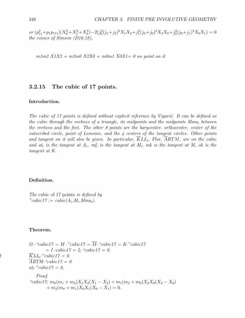
348 CHAPTER 3. FINITE PRE INVOLUTIVE GEOMETRY
or (p211+p1p111)(X2
0 +X21 +X2
2 )−2(j20(j1+j2)2X1X2+j2
1(j2+j0)2X2X0+j22(j0+j1)2X0X1) = 0
the conics of Simson (D16.18),
m1m2 X1X2 + m2m0 X2X0 + m0m1 X0X1= 0 no point on it
3.2.15 The cubic of 17 points.
Introduction.
The cubic of 17 points is defined without explicit reference by Vigarie. It can be defined asthe cubic through the vertices of a triangle, its midpoints and the midpoints Mmai betweenthe vertices and the feet. The other 8 points are the barycenter, orthocenter, center of theoutscribed circle, point of Lemoine, and the 4 centers of the tangent circles. Other pointsand tangent on it will also be given. In particular, KLLi, Flor, ARTM , are on the cubicand ati is the tangent at Ai, mfi is the tangent at Mi, mk is the tangent at M, ok is thetangent at K.
Definition.
The cubic of 17 points is defined by”cubic17 := cubic(Ai,Mi,Mmai).
Theorem.
O ·“cubic17 = M ·”cubic17 = M ·“cubic17 = K·”cubic17= I ·cubic17 = Ii·“cubic17 = 0.
KLLi·”cubic17 = 0.19.7.82ARTM·“cubic17 = 0.3.7.91ati·”cubic17 = 0,
Proof.“cubic17: m0(m1 +m2)X1X2(X1 −X2) +m1(m2 +m0)X2X0(X2 −X0)
+m2(m0 +m1)X0X1(X0 −X1) = 0.

3.2. THE GEOMETRY OF THE HEXAL COMPLETE 5-ANGLES. 349
Theorem.
M M O K Flor ARTM C17a C17b C17c C17d
M K O M M ARTM Flor C17bM C17a M ARTM K MO Flor K O ?K O MFlor ARTM ? O ? MARTM Flor K ? M MC17a C17b M ? ?C17b C17aC17c ARTM C17d ? ? M ? ?
Ai Mi Mmai KLLiM Mi Ai KLLi MmaiM Mmai C17di Ai C17biO KLLi Mi C17ci AiK Ai Mmai Mi C17diFlor C17di C17bi Mmai C17eiARTM C17ci KLLi C17fi Mi
C17a C17fi C17ci ? KLLiC17b C17bi C17ei C17di C17giC17c C17di C17bi ? ?
Ai Mi Mmai KLLiAi K M M OMi M O K ARTMMmai M K C17ci MKLLi O ARTM M C17a
Ai−1 Mi−1 Mmai−1 KLLi−1
Ai+1 Mi Ai KLLi MmaiMi+1 Ai Mmai Mi C17diMmai+1 KLLi Mi C17ci AiKLLi+1 Mmai C17di C17bi Mi
Exercise.
Construct the tangents to ”cubic17 at Mmai and at M .
Exercise.
Give properties of ”cubic17 := cubic(Ai,M i,Mmai).
Partial answer to 3.2.14
The tangent at Mma0 is[(m1−m2)(s1− 2m0), (m1 +m2)(s1− 2m1),−(m1 +m2)(s1− 2m2)].

350 CHAPTER 3. FINITE PRE INVOLUTIVE GEOMETRY
The tangent at M is[m1m2(m1−m2)(s1− 2m0),m2m0(m2−m0)(s1− 2m1),
m0m1(m0−m1)(s1− 2m2)].A0⊕A0 = K, A1⊕A2 = M0, A0⊕M0 = M, A0⊕Mma0 = M , A1⊕Mma2 = KLL0,A0 ⊕KLL0 = O, M0⊕M0 = K, M1⊕M2 = Mma0,M0 ⊕KLL0 = ARTM, M1 ⊕KLL2 = C17a0,O⊕O = Flor, whereFlor = ((m1 +m2)(s1− 2m1)(s1− 2m2), (m2 +m0)(s1− 2m2)(s1− 2m0),
(m0 +m1)(s1− 2m0)(s1− 2m1)),tangent at M is [m1m2(m1−m2)(s1− 2m0), . . .].M ×M = (m0(m1 +m2)(s1− 2m1)(s1− 2m2)(s22− 2m02), . . .),M × Flor = [(m1−m2)(s1− 2m0), (m2−m0)(s1− 2m1), (m0−m1)(s1− 2m2)],M × ARTM = [(m1−m2)(s1− 2m0)(s2− 2m02), . . .],M ⊕ ARTM = K,K × Flor = [(m1−m2)(m2 +m0)(m0 +m1)(s1− 2m0)2, . . .],C17a = (m0(m1 + m2)(s1 − 2m1)(s1 − 2m2)(s2 − 2m02), . . .), C17b = ((s1 − 2m0)(s2 −2m12)(s2− 2m22), . . .),4.7.91C17c = ((m1 +m2)(s1− 2m1)(s1− 2m2)), . . .),4.7.91C17d = ((s2− 2m12)(s2− 2m22)(s3− s21− 2s2m0), . . .),4.7.91C17b0 = (2m0(m1 +m2)(s1− 2m1)(s1− 2m2), s1(s1− 2m1)(s2− 2m22),
s1(s1− 2m2)(s2− 2m12)),4.7.91C17c0 = ((m1 +m2)(s1− 2m1)(s1− 2m2),m1s1(s1− 2m1),m2s1(s1− 2m2)),C17d0 = (m0s1, (m2 +m0)(s1− 2m2), (m0 +m1)(s1− 2m1)),C17e0 = ((s2− 2m12)(s2− 2m22)(s3− s21− 2s111),
−2m1(m2+m0)(s2−2m12)(s3−2m23−s21+2m2(m02+m12)+2s111), −2m2(m0+m1)(s2− 2m22)(s3− 2m13 − s21 + 2m1(m22 +m02) + 2s111)),C17f0 = (s1(s2− 2m22)(s2− 2m12), 2m1(m2 +m0)(s1− 2m2)(s2− 2m12),
− 2m2(m0 +m1)(s1− 2m1)(s2− 2m22)),C17g0 = ((m1 + m2)s1(s1 − 2m0)(s1 − 2m1)(s1 − 2m2)(s3 − s21 + 2s111 + 2m2(s2 −2m22))((s3 − s21 + 2s111 + 2m1(s2 − 2m22))), −m1(s3 − s21 − 2s111)(s3 − s21 +2s111+2m1(s2−2m12))(s4+2s22−4(m24 +m02m12)), −m2(s3−s21−2s111)(s3−s21 + 2s111 + 2m2(s2− 2m22))(s4 + 2s22− 4(m14 +m22m02)),4.7.91
Answer to3.2.14
O · ”cubic17 = M·”cubic17 = M · ”cubic17 = K ·”cubic17= 0.KLLi · ”cubic17 = 0.19.7.82ati · ”cubic17 = 0,”cubic17:m2
0(m1 +m2) X1X2 (m2X1 −m1X2) + m21(m2 +m0) X2X0 (m0X2 −m2X0)
+ m22(m0 +m1) X0X1 (m1X0 −m0X1) = 0.

3.2. THE GEOMETRY OF THE HEXAL COMPLETE 5-ANGLES. 351
3.2.16 The cubic of 21 points.
cubic21
3.2.17 The Barbilian Cubics.
Introduction.
In posthumously published works of Dan Barbilian, also known in his native RoumanianCountry as the poet Eon Barbu, the following Theorem is proven. The loci of the pseudocenters of the isotropic cubics which pass through the vertices of a complete quadrilateraland 2 of its diagonal elements is a circle. I observed that in the case where the isotropicpoints are the fixed points of the involution determined by the 3 pairs of opposite sides of thequadrilateral, the third diagonal point is also on the cubics. It is this family of cubics whichwill be studied now, to which I will give the name of the Poet-Mathematician Barbilian.
Definition.
An isotropic cubic is a cubic which passes through the isotropic points.The pseudo center of an isotropic cubic is the intersection of its tangents at the isotropicpoints.2
Theorem. [Barbilian]
The family of isotropic cubic through the vertices Bj of a complete quadrangle and 2 of itsdiagonal points A1 := (B0×B2)× (B1×B3) and A2 := (B0×B1)× (B2×B3) has a circle asthe locus of the pseudo centers. This circle is the Miquel circle of the complete quadrangleand the 2 diagonal points.
I remind the reader that this circle passes through the center of the circumcircles of thetriangles B0, B1, A1, B2, B3, A1, B0, B2, A2, B1, B3, A2. See g334
Definition.
The isotropic cubics through the vertices of a triangle, the feet and the orthocenter will becalled Barbilian cubics.
Corollary.
The family of Barbilian cubics has a circle as the locus of its pseudo centers.
In this case, B0 = A0, B1 = M1, B2 = M2, B3 = M and the circles circumscribed toB2, B3, A1, B1, B3, A2 pass through the point of Miquel, M0.
2The isotropic points are also called circular points. Barbilian calls a pseudo center, a pseudo focus.
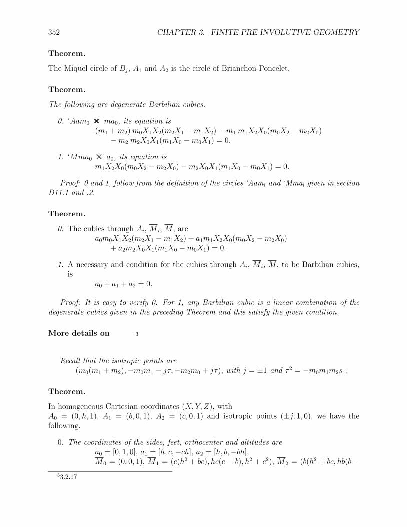
352 CHAPTER 3. FINITE PRE INVOLUTIVE GEOMETRY
Theorem.
The Miquel circle of Bj, A1 and A2 is the circle of Brianchon-Poncelet.
Theorem.
The following are degenerate Barbilian cubics.
0. ‘Aam0 ×× ma0, its equation is(m1 +m2)m0X1X2(m2X1 −m1X2)−m1 m1X2X0(m0X2 −m2X0)−m2 m2X0X1(m1X0 −m0X1) = 0.
1. ‘Mma0 ×× a0, its equation ism1X2X0(m0X2 −m2X0)−m2X0X1(m1X0 −m0X1) = 0.
Proof: 0 and 1, follow from the definition of the circles ‘Aami and ‘Mmai given in sectionD11.1 and .2.
Theorem.
0. The cubics through Ai, M i, M , area0m0X1X2(m2X1 −m1X2) + a1m1X2X0(m0X2 −m2X0)
+ a2m2X0X1(m1X0 −m0X1) = 0.
1. A necessary and condition for the cubics through Ai, M i, M , to be Barbilian cubics,is
a0 + a1 + a2 = 0.
Proof: It is easy to verify 0. For 1, any Barbilian cubic is a linear combination of thedegenerate cubics given in the preceding Theorem and this satisfy the given condition.
More details on 3
Recall that the isotropic points are(m0(m1 +m2),−m0m1 − jτ,−m2m0 + jτ), with j = ±1 and τ 2 = −m0m1m2s1.
Theorem.
In homogeneous Cartesian coordinates (X, Y, Z), withA0 = (0, h, 1), A1 = (b, 0, 1), A2 = (c, 0, 1) and isotropic points (±j, 1, 0), we have thefollowing.
0. The coordinates of the sides, feet, orthocenter and altitudes area0 = [0, 1, 0], a1 = [h, c,−ch], a2 = [h, b,−bh],M0 = (0, 0, 1), M1 = (c(h2 + bc), hc(c − b), h2 + c2), M2 = (b(h2 + bc, hb(b −
33.2.17

3.2. THE GEOMETRY OF THE HEXAL COMPLETE 5-ANGLES. 353
c), h2 + b2),M = (0, bc,−h),m0 = [1, 0, 0], m1 = [c,−h,−bc], m2 = [b,−h,−bc].
1. The circle through A1, A2, M1, M2 isαm0 : X2 + Y 2 + bcZ2 − (b+ c)ZX = 0.
2. The circle through A0, M , M1, M2 isµa0 : h(X2 + Y 2)− hbcZ2 + (bc− h2)XY = 0.
3. The Barbilian cubics arekαm0 ×× X + lµa0 ×× Y = 0.
4. The pseudo center is, with d = k(b+ c) + l(bc− h2),(kd,−lhd, 2(k2 + l2h2)).
5. This is a parametric equation of the circle of Brianchon-Poncelet:2h(X2 + Y 2)− (h2 − bc)XY − h(b+ c)ZX = 0.
6. The transformation from barycentric to Cartesian coordinates is 0 b ch 0 01 1 1
and its inverse is 1h(c−b)
0 c− b 0−h −c chh b −bh
,
where the barycentric coordinates of the orthocenter are given bym0 = bc(c−b)
h2+bc, m1 = −c, m2 = b,
provided h2 = m1m2s1m0
.
7. The barycentric coordinates of the pseudo center are easily derived using the value ofh and of
m0d = km0(m2 −m1)− l(s111 −m1m2s1).
The details of the proof is left to the reader.
Answer to 4
0, is straigthforward.For 1, αm0 is u[h, b,−hb] ×× [h, c,−hc] = v[c,−h,−bc] ×× [b,−h,−bc].With j2 = −1, u = (cj − h)(bj − h), v = (hj + b)(hj + c) = −u.After dividing by h2 + bc we get the equation 1.For 2, µa0 is u[h, b,−hb] ×× [c,−h,−bc] = v[h, c,−hc] ×× [b,−h,−bc].u = (hj + c)(bj − h), v = (hj + b)(cj − h) = u.After dividing by c− b we get the equation 2.For 4, the tangent at (j, 1, 0), obtained by evaluating the first partial derivatives at thatpoint, is
[−2k + 2lhj, 2kj + 2lh, k(b+ c) + l(bc− h2)].The tangent at the other isotropic point is obtained by replacing j by −j.
43.2.17

354 CHAPTER 3. FINITE PRE INVOLUTIVE GEOMETRY
Their intersection is 4, after dividing by 4j. It is easy to verify that 5, is the equation of acircle through M i, and that the pseudo center is on it for all values of k and l.For 5, the coordinates of vertices Ai give the coefficients of the matrix. The transform of(m0,m1,m2) is (m1b + m2c, hm0, s1). Comparing with (0, bc,−h) gives 5. 6, is straightfor-ward. For 7, we need to related the cubics in Cartesian and barycentgric coordinates.If weuse k’ and l’ for the barycentric case, comparison of the coefficients of X2
2X0 in baricentriccoordiantes givesk′m2
1m0 = kc(2bc − bc − c2) = kc2(b − c), and l′m0m1 = lh(hc2 − hbc) = lh2(c − b). Usingproportionality we can therefore write 7.The pseudo center will be (0,0,1) if d = 0, this gives
k = h2 − bc = m1m2(s1+m0)m0
, l = m2 −m1.
Substituting, we get, after division by m1m2m−10 , k′ = s1 +m0, l
′ = (m1 −m2)s1, hencea0 = −(m1 +m2)(s1 +m0), a1 = (2m1−m2)s1 +m0m1, a1 = (2m1−m2)s1 +m0m1. To checkthis independently, we should verify that M0 × I0 is tangent to the cubic for these values ofk′ and l′. (0, 0, 1)×(m0(m1 +m2),−m0m1−jτ,−m2m0 +jτ) = [m0m1 +jτ,m0(m1 +m2), 0].
Theorem.
Given an Barbilian cubic Γ, there exists a line l and a circumscribed conic φ such thatΓ = θ ×× l +m ×× φ.
More specifically, with l0 arbitrary,l = [l0, l0 − a2, l0 + a1],φ = b0m0X1X2 + b1m1X2X0 + b2m2X0X1 = 0, withb0 = −m2a1 +m1a2− (m1 +m2)l0, b1 = −m2a1− (m2 +m0)l0, b2 = m1a2−
(m0 +m1)l0.Proof: Identification of the coefficients of X2
1X2 and X22X1 gives
a0m2 = (m1 +m2)l1 + b0, −a0m1 = (m1 +m2)l2 + b0,subtracting gives, a0 = l1 − l2, and similarly a1 = l2 − l0, and a2 = l0 − l1.By substitution, we obtain b0 and similarly b1 and b2, using a0 + a1 + a2 = 0.
Definition.
l is called a radical axis of Γ, φ is called the corresponding radical conic of Γ.θ could be replaced by an other circle.
Theorem.
0. The non trivial ideal point is (a0, a1, a2).
1. The tangent at the non trivial ideal point, or asymptote is[m0a1a2(m2a1 −m1a2),m1a2a0(m0a2 −m2a0),m2a0a1(m1a0 −m0a1)].
Proof: This follows from the fact that the non trivial ideal point is m × l. The tangentis obtain by taking the partial derivatives respectively with respect to X0, X1 and X2 at(a0, a1, a2). The first one ism1a1a2(m0a2 − 2m2a0)−m2a1a2(m0a1 − 2m1a0) = −m0a1a2(m2a1 −m1a2).

3.2. THE GEOMETRY OF THE HEXAL COMPLETE 5-ANGLES. 355
Comment.
Special Barbilian cubics can be obtained by combining the equations of Theorem 3.2.17 Forinstance,βa0 follows from adding the equations 0, for indices 0,1 and 2 respectively multiplied by m0,m1 and m2.βa1, by using on the equations 0, the multipliers m1m2, m2m0 and m0m1.βa2, by using on the equations 1, equal multipliers.
Theorem.
The Barbilian cubic βa0 :m0(m1 −m2)X1X2(m2X1 −m1X2) +m1(m2 −m0)X2X0(m0X2 −m2X0)
+m2(m0 −m1)X0X1(m1X0 −m0X1) = 0has the following properties:
0. A radical axis is −mai, with mai = [m0,m1,m2].
1. The corresponding radical conic has the equationm0(m2
1 +m22)X1X2 +m1(m2
2 +m20)X2X0 +m2(m2
0 +m21)X0X1.
2. The non trivial ideal point is MK = (m1 −m2,m2 −m0,m0 −m1).
3. The asymptote is[m0(m2−m0)(m0−m1)(s2−m0s1),m1(m0−m1)(m1−m2)(s2−m1s1),m2(m1−
m2)(m2 −m0)(s2 −m2s1)].
4. The tangent at Ai is mkai, withmka0 = [0,m0 −m1,−(m2 −m0)].
Theorem.
The Barbilian cubic βa1 :m2
0(m1 −m2)X1X2(m2X1 −m1X2) +m21(m2 −m0)X2X0(m0X2 −m2X0)
+m22(m0 −m1)X0X1(m1X0 −m0X1) = 0
has the following properties:
0. A radical axis is −m.
1. The corresponding radical conic is 2m0m1m2‘Steiner, with‘Steiner = m0X1X2 +m1X2X0 +m2X0X1 = 0,
2. The non trivial ideal point is EUL withEUL = (m0(m1 −m2),m1(m2 −m0),m2(m0 −m1)).
3. The asymptote is m.
4. The tangent at Ai is mkai, withmka0 = [0,m0 −m1,−(m2 −m0)].
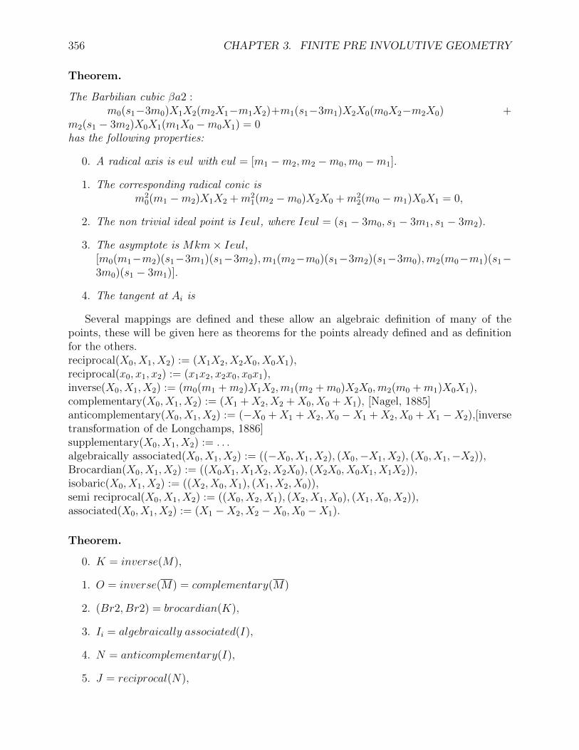
356 CHAPTER 3. FINITE PRE INVOLUTIVE GEOMETRY
Theorem.
The Barbilian cubic βa2 :m0(s1−3m0)X1X2(m2X1−m1X2)+m1(s1−3m1)X2X0(m0X2−m2X0) +
m2(s1 − 3m2)X0X1(m1X0 −m0X1) = 0has the following properties:
0. A radical axis is eul with eul = [m1 −m2,m2 −m0,m0 −m1].
1. The corresponding radical conic ism2
0(m1 −m2)X1X2 +m21(m2 −m0)X2X0 +m2
2(m0 −m1)X0X1 = 0,
2. The non trivial ideal point is Ieul, where Ieul = (s1 − 3m0, s1 − 3m1, s1 − 3m2).
3. The asymptote is Mkm× Ieul,[m0(m1−m2)(s1−3m1)(s1−3m2),m1(m2−m0)(s1−3m2)(s1−3m0),m2(m0−m1)(s1−3m0)(s1 − 3m1)].
4. The tangent at Ai is
Several mappings are defined and these allow an algebraic definition of many of thepoints, these will be given here as theorems for the points already defined and as definitionfor the others.reciprocal(X0, X1, X2) := (X1X2, X2X0, X0X1),reciprocal(x0, x1, x2) := (x1x2, x2x0, x0x1),inverse(X0, X1, X2) := (m0(m1 +m2)X1X2,m1(m2 +m0)X2X0,m2(m0 +m1)X0X1),complementary(X0, X1, X2) := (X1 +X2, X2 +X0, X0 +X1), [Nagel, 1885]anticomplementary(X0, X1, X2) := (−X0 + X1 + X2, X0 −X1 + X2, X0 + X1 −X2),[inversetransformation of de Longchamps, 1886]supplementary(X0, X1, X2) := . . .algebraically associated(X0, X1, X2) := ((−X0, X1, X2), (X0,−X1, X2), (X0, X1,−X2)),Brocardian(X0, X1, X2) := ((X0X1, X1X2, X2X0), (X2X0, X0X1, X1X2)),isobaric(X0, X1, X2) := ((X2, X0, X1), (X1, X2, X0)),semi reciprocal(X0, X1, X2) := ((X0, X2, X1), (X2, X1, X0), (X1, X0, X2)),associated(X0, X1, X2) := (X1 −X2, X2 −X0, X0 −X1).
Theorem.
0. K = inverse(M),
1. O = inverse(M) = complementary(M)
2. (Br2, Br2) = brocardian(K),?
3. Ii = algebraically associated(I),
4. N = anticomplementary(I),
5. J = reciprocal(N),

3.3. FINITE PROJECTIVE GEOMETRY. 357
6. Ni = algegraically associated(N),
7. Ji = reciprocal(Ni).
Definition.
The following are the definition of other points.
0. H0 := reciprocal(M)
1. Ic := complementary(I),
2. I0 := reciprocal(I),
3. “Center of equal parallels” := anticomplememtary(I0),
4. (”Jδ”, ”Jρ”) := Brocardian(I).
Exercise.
Define in terms of the above functions as many points as you can in Theorem . . . .
Exercise.
Determine, for many of the points of Definition . . . a linear construction and determine theirbarycentric coordinates.
3.3 Finite Projective Geometry.
3.3.0 Introduction.
The Theorems given here are deduced from Theorems of Involutive Geometry.
Theorem.
Given 6 points Ai and Bi, forming an hexagon inscribed to a conic α and outscribed to another conic β. Let C be the point common to Ai ×Bi. Let Ti be the vertices of the tangentsto α at Ai.
0. The lines Bi × Ti have a point D in common.
1. The line C × D passes through the pole of with respect to the triangle Ai of theDesargues line of the perspective triangles Ti and Bi.
The Theorem generalizes a Theorem of Kimberling 3.4.6 and 3.4.6 using 3.4.6.

358 CHAPTER 3. FINITE PRE INVOLUTIVE GEOMETRY
Theorem.
Given the special Desargues configuration with the points Ai on the lines of the triangleMM0,MM1,MM2 with center of perspectivity M . Let m be an arbitrary line and MAibe its intersection with the side ai of the triangle A0, A1, A2, if TMai is the intersectionof the line MMi+1 MAi−1 and the line MMi−1 MAi+1, then the lines joining the points Aito the TMai have a point ARTM in common.
The Theorem generalizes a Theorem of Kimberling 3.4.3 assuming that the excenters arereplaced by the vertices of the anti complimentary triangle and the direction of the altitudesare replaced by the intersections of the orthic line with the side of the triangle.
Definition.
The point ARTM is called the point of Luke.
3.4 Finite Involutive Geometry.
3.4.0 Introduction.
I will now describe the Theorems of involutive Geometry in the traditional way, refering forto proofs of the corresponding sections of the hexal configuration.Starting with affine geometry, we obtain an involutive geometry, if we choose among allthe possible involutions on the ideal line, a particular one, called fundamental involution.We could also start directly from projective geometry and choose among all the possibleinvolutions one involution on one of all the possible lines.This involution can be given in many ways,
0. by 2 points, the fixed points of the involution,
1. by 2 pairs of corresponding points on a line,
2. by a polarity and a line which does not belong to its line conic,
3. by an hexal complete 5-angle, . . . . See II.3.
The definitions will be given in terms of the fundamental involution. Because this involutioncan be elliptic or hyperbolic, there are 2 distinct types of real involutive geometries, ellipticand hyperbolic. I will study them together and give theorems, in the hyperbolic case, whichin some cases can be used as an alternate definition of the concepts. Such theorems will benoted with (H. D.). When the additional notions of measure of distance and angles willhave been introduced, the elliptic involutive geometry will become the Euclidean Geometryand the hyperbolic one, will be that of Minkowski. A third geometry which correspondsto the confluence of the 2 fixed points of the involution will be considered later, it is theparabolic (involutive) geometry which becomes the Galilean geometry.Among the many ways of starting I will give one. It is a good Exercise to ask students totry other approaches.I will choose one line m as the ideal line and a conic, given by 5 points (again an other set

3.4. FINITE INVOLUTIVE GEOMETRY. 359
of 5 elements can be chosen) as the defining circle. Mid points of the side of a triangle canbe obtainred by the construction of the pole of a line with respect to a triangle, see 3.1.1.Using the mid-points of the sides we can derive the barycenter.For perpandicularity, we choose one of the point A on the conic, determine its tangent tA,the parallel tangent tB, by a construction which is the dual of that of finding the secondpoint of intersection of a line with the conic, and the point of contact B. A×B is a diameter.Perpendicular directions are obtsined as follows. If Ip is an ideal point, we determine thesecond intersection P of A×Ip with the conic, the perpendicular direction is then (P×B)×m.We can therefore construct the altitudes and therefore the orthocenter.
3.4.1 Fundamental involution, perpendicularity, circles.
Definition.
Starting with an affine geometry associated to p, a particular involution on the ideal linewill be called the fundamental involution.
Definition.
If the fundamental involution is hyperbolic, its fixed points are called isotropic points, theother points on the ideal line will be called ideal points or directions. (In a hyperbolicinvolutive geometry, the isotropic points are no more called ideal points). The lines throughthe isotropic points, distinct from the ideal line, are called isotropic lines.The lines which are neither ideal or isotropic are called ordinary lines, the points whichare not ideal or isotropic points are called ordinary points, ordinary lines or points willabbreviated from now on by lines or points. On an ordinary line, there are p ordinary pointsand one ideal point.
Definition.
Corresponding pairs of points in the fundamental involution are called perpendicular idealpoints or perpendicular directions. 2 lines whose ideal points are perpendicular directions arecalled perpendicular lines.Some obvious results follow from these definitions and from those of the corresponding affinegeometry. For instance:
Theorem.
All the lines perpendicular to a given line are parallel.
Definition.
If the involution defined by a conic on the ideal line is the same as the fundamental involution,the corresponding conic is called a circle and the corresponding polarity is called a circularity.

360 CHAPTER 3. FINITE PRE INVOLUTIVE GEOMETRY
Theorem. (H. D)
In a hyperbolic involutive geometry, a necessary and sufficient condition for a conic to be acircle is that it passes through the isotropic points.
Definition.
The center of a conic is the pole of the ideal line in the corresponding polarity. (See II.2.3.0).
Theorem. (H. D)
In a hyperbolic geometry, the center of a circle is the intersection of its isotropic tangents.
Definition.
A diameter of a conic is a line passing through its center (See II.2.3.1).
Definition.
A mediatrix of 2 points A and B on a line l, which is not an isotropic line, is the lineperpendicular to l through the mid-point of A B. (See II.6.2.6)
Example.
In the examples of involutive and Euclidean geometry, I will make one of 2 choices for theideal line and for the defining circle.
0. In the first choice,0.[1, 1, 1] is the ideal line, as in affine geometry.1.X02 + X12 + k X22 = 0, k 6= −1
2, is the defining circle,
−(1 + 2k) N p for the elliptic case, −(1 + 2k) R p for the hyperbolic case.2. Let δ2 := −1− 2k.
If k 6= −1, the isotropic points (1, y,−1− y) correspond to the roots y1 and y2
of3. (1 + k)y2 + 2ky + (1 + k) = 0.or with4. k′ = 2k
1+k),
to the roots of5. y2 + k′y + 1 = 0.Therefore
y1 = −k+δ1+k
and y2 = −k−δ1+k
.If k = −1, the isotropic points are (0,1,-1) and (1,0,-1).The polar of (X0, X1, X2) is [X0, X1, kX2],The direction perpendicular to (X0, X1,−X0−X1) is(kX0 + (1 + k)X1,−(1 + k)x0− kX1, X0−X1).If k = −1
2, the conic 0.1. is tangent to the ideal line.

3.4. FINITE INVOLUTIVE GEOMETRY. 361
1. In the second choice,0.[0, 0, 1] is the ideal line, as in Euclidean geometry.1.kX02 +X12 = X22, k 6= 0, the defining circle,
−k N p for the elliptic case,−k R p for the hyperbolic case.δ2 := −k.If k = 0, the conic 1.1. is tangent to the ideal line.The isotropic points are (1, δ, 0) and (1,−δ, 0).The polar of (X0, X1, X2) is [kX0, X1,−X2].The direction perpendicular to (X0, X1, 0) is (X1,−kX0, 0).
3.4.2 Altitudes and orthocenter.
Definition.
In a triangle Ai, the altitude mai from Ai is the line through Ai which is perpendicular tothe opposite side ai := Ai+1 × Ai−1 (C0.1,N0.3).
Theorem.
The altitudes mai of a triangle are concurrent at a point M . (D0.12)
Definition.
The point M is called the orthocenter of the triangle.(N0.2)
Theorem.
The necessary and sufficient condition for a triangle to be a right triangle at Ai is that itsorthocenter M coincides with Ai.
Theorem.
The necessary and sufficient condition for a triangle to be an isosceles triangle is that theorthocenter be on the altitude from Ai and distinct from the center of mass.
Theorem.
The necessary and sufficient condition for a triangle to be an equilateral triangle is that theorthocenter and the barycenter coincide.
3.4.3 The geometry of the triangle, I.
Introduction.
We are now ready to give a large number of results of finite involutive geometry associatedto a scalene triangle whose vertices A0, A1, A2 and whose sides a0, a1, a2 are ordinary.
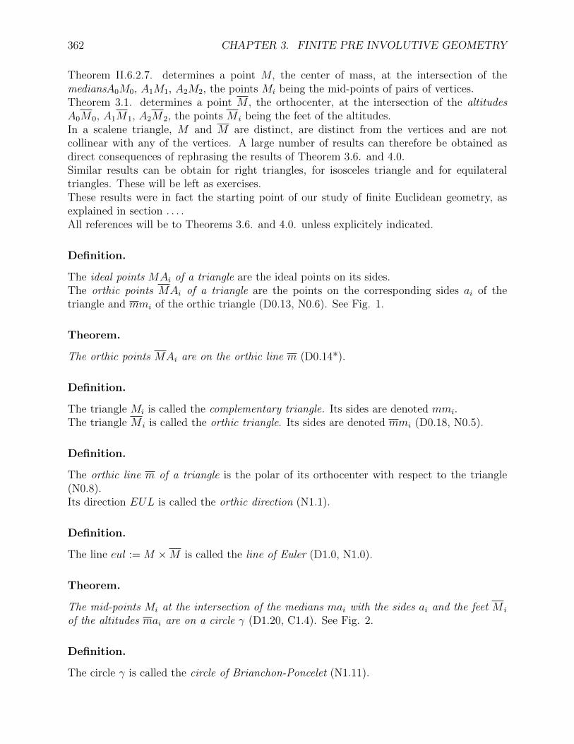
362 CHAPTER 3. FINITE PRE INVOLUTIVE GEOMETRY
Theorem II.6.2.7. determines a point M, the center of mass, at the intersection of themediansA0M0, A1M1, A2M2, the points Mi being the mid-points of pairs of vertices.Theorem 3.1. determines a point M, the orthocenter, at the intersection of the altitudesA0M0, A1M1, A2M2, the points M i being the feet of the altitudes.In a scalene triangle, M and M are distinct, are distinct from the vertices and are notcollinear with any of the vertices. A large number of results can therefore be obtained asdirect consequences of rephrasing the results of Theorem 3.6. and 4.0.Similar results can be obtain for right triangles, for isosceles triangle and for equilateraltriangles. These will be left as exercises.These results were in fact the starting point of our study of finite Euclidean geometry, asexplained in section . . . .All references will be to Theorems 3.6. and 4.0. unless explicitely indicated.
Definition.
The ideal points MAi of a triangle are the ideal points on its sides.The orthic points MAi of a triangle are the points on the corresponding sides ai of thetriangle and mmi of the orthic triangle (D0.13, N0.6). See Fig. 1.
Theorem.
The orthic points MAi are on the orthic line m (D0.14*).
Definition.
The triangle Mi is called the complementary triangle. Its sides are denoted mmi.The triangle M i is called the orthic triangle. Its sides are denoted mmi (D0.18, N0.5).
Definition.
The orthic line m of a triangle is the polar of its orthocenter with respect to the triangle(N0.8).Its direction EUL is called the orthic direction (N1.1).
Definition.
The line eul := M ×M is called the line of Euler (D1.0, N1.0).
Theorem.
The mid-points Mi at the intersection of the medians mai with the sides ai and the feet M i
of the altitudes mai are on a circle γ (D1.20, C1.4). See Fig. 2.
Definition.
The circle γ is called the circle of Brianchon-Poncelet (N1.11).

3.4. FINITE INVOLUTIVE GEOMETRY. 363
Theorem.
If Maai (Maai) is the intersection of the median mai+1 (mai−1) with the altitude mai−1
(mai+1), then the lines mMai joining Maai and Maai have a point K in common (D1.2,D1.3, D1.4*). See Fig. 3.
Definition.
The point K is called the point of Lemoine (N1.2).
Definition.
The circumcircle θ of a triangle A0, A1, A2 is the circle passing through the vertices of thetriangle (D1.19, H1.1, N1.10).
Theorem.
The line tai through the vertex Ai parallel to the side mi of the orthic triangle is the tangentat Ai to the circumcircle (D1.7, D1.19*). See Fig. 4.
Definition.
The triangle with sides tai is called the tangential triangle. Its vertices are denoted by Ti(D1.8, N1.5).
Definition.
The mixed triangles are the triangles with respective sidesci := Mi+1 ×M i−1 and ci := M i+1 ×Mi−1 (D1.13, N1.6).
The mixed feet are the points CCi, (CCi) on the side of the given triangle and the corre-sponding side ci, (ci) of the mixed triangle (D1.14, N1.7). Dee Fig. 5.
Theorem.
The mixed feet CCi, (CCi) of a mixed triangle are collinear on the line p (p) (D1.15*).
Definition.
The line p and p are called the mixed lines of a triangle (N1.8).
Theorem.
The mixed lines p and p of a triangle meet at the point PP which is on the line of Euler(D1.16, C1.0).
Definition.
PP is called the mixed center of the triangle (N1.9).

364 CHAPTER 3. FINITE PRE INVOLUTIVE GEOMETRY
Definition.
The intersection IMai of a median with the orthic line is called a medorthic point (D0.15,N0.9).
Definition.
The intersection of the lines mei (mei) joining the medorthic points IMai+1 (IMai−1) tothe foot M i−1 (M i+1) are called the points of Euler EEi (Eulerian points Ei) (D5.0, D5.1).Fig. 6.
Theorem.
The points of Euler EEi are the mid-points of the segment joining the orthocenter M to thevertex Ai (D5.1, C5.3).
Theorem.
The points of Euler EEi are on the circle of Brianchon-Poncelet (C5.5).The Eulerian point EEi is on the median mai as well as on the circle of Brianchon-Poncelet(C5.0, C5.5).
Theorem.
The lines emi joining the mid-points Mi to the Eulerian points EEi are concurrent at a pointEE.The lines emi joining the feet M i to the Eulerian points EEi are concurrent at a point EE(D5.2, D5.3*).EE is on the line of Euler and is the center of the circle of Brianchon-Poncelet.EE is on the line of Euler and is the pole of the orthic line with respect to the circle ofBrianchon-Poncelet (C5.1, C5.4, N5.1).
Definition.
The mediatrix mfi is the line through through the mid-point Mi perpendicular to the corre-sponding side ai (D6.0, N6.0).
Theorem.
The vertex Ti of the tangential triangle is on the mediatrix mfi (D6.0, C6.8, N6.0).The mediatrices mfi are concurrent at a point O.The diameters mfi of the circle of Brianchon-Poncelet which pass through the feet of thealtitudes pass through the same point O (D6.4*, N6.1).
Definition.
O is the circumcenter or center of the circumcircle (N6.1).

3.4. FINITE INVOLUTIVE GEOMETRY. 365
Theorem.
The circumcenter O is on the line of Euler.The point O is on the line of Euler (C6.1).
Definition.
An equilateral conic is a conic whose ideal points are harmonic conjugates of the isotropicpoints.An coequilateral conic is a conic whose points on the orthic line are harmonic conjugates ofthe coisotropic points.
We leave as an exercise the pproof of the following Theorem and Corollary.
Theorem.
If an conic passes through the vertices of the triangle
0. it is equilateral if and only if it passes through the orthocenter.Its center is on the circle of Brianchon-Poncelet.
1. it is coequilateral if and only if it passes through the barycenter.Its cocenter is on the circle of Brianchon-Poncelet.
Corollary.
A conica0X
20 + a1X
21 + a2X
22 + b0X1X2 + b1X2X0 + b2X0X1 = 0,
0. is equilateral if and only ifm1m2(a1 + a2 − b0) +m2m0(a2 + a0 − b1) +m0m1(a0 + a1 − b2) = 0.
1. it is coequilateral if and only ifm0(m2
1a1 +m22a2−m1m2b0)+m1(m2
2a2 +m20a0−m2m0b1)+m2(m2
0a0 +m21a1−
m0m1b2) = 0.
Definition.
The conic of Kiepert is the conic circumscribed to the triangle passing through the barycenterand the orthocenter. (D3.8.)The conic of Jerabek is the conic circumscribed to the triangle passing through the orthocenterand the point of Lemoine. (D36.16.)These are therefore equilateral. (C3.3 and C36.). The center of one conic is the cocenter ofthe other and these are on the circle of Brianchon-Poncelet (C8.9 and C36.18.)
Definition.
The circle through the vertices Ti of the tangential triangle is the circle of Neff.

366 CHAPTER 3. FINITE PRE INVOLUTIVE GEOMETRY
Theorem.
0. The circle of Neff is a cocircle.
1. The ortic line is the radical axis of the circle of Neff and both the circumcircle and thecircle of Brianchon-Poncelet.
Definition.
A triangle of Neff is a triangle whose orthocenter is on the conic.
Exercise.
Prove that in a triangle of Neff, one of the sides of the tangential triangle is a diameter ofthe circle of Neff. Determine other conditions for this to happen. xxx
Definition.
The points EULi at the intersection of the corresponding sides of the complementary triangleand of the orthic triangle are called the complorthic points (D8.0, N8.0).The lines aeULi joining the complorthic points are called complorthic lines (D8.3, N8.1).The triangle whose vertices are the complorthic points is called the complorthic triangle(N8.2).
Definition.
The intersections of corresponding sides of the mixed triangles are the mixed points Di (D8.4,N8.4).
Theorem.
0. The mixed points Di and Di are on the line of Euler (C8.2).
1. The vertex Ai and the mixed point Di are on the complorthic line aeULi. (C8.1, C8.3).
2. The lines nmi joining the mid-points of the sides to corresponding complorthic pointsEULi are concurrent in a point S.
3. The lines nmi joining the feet of the altitudes to the corresponding complorthic pointsEULi are concurrent in a point S (D8.1, D8.2*).
Definition.
The points S and S are the point and copoint of Schroter (N8.3).

3.4. FINITE INVOLUTIVE GEOMETRY. 367
Theorem.
S is the point of Miquel of the quadrangle ai+1, ai−1, mai+1, mai−1. S is therefore also onthe circles through Ai, M, M i+1, M i−1 of center Ei and on the circles through Ai+1, Ai−1,M i of center Mi. (See .)
Theorem.
0. The points of Schroter are on the circle of Brianchon-Poncelet (C8.8).
1. The first point of Schroter S, the Eulerian point EEi and the mixed point Di are onthe same line si
2. The second point of Schroter S, the point of Euler point EEi and the mixed point Di
are on the same line si. (D8.5, C8.4).
Theorem.
The conic through the barycenter M , the orthocenter M and the feet Gmi of the perpen-dicular iMAi from M to the corresponding altitude mai are on a circle ‘omicron (D10.3,D10.4, D10.7, C10.7).This circle passes also through the perpendiculars Gmi which are the feet of the perpendicu-lars gmi from M to the corresponding median mai. M,M is a diameter whose mid-pointis G (C10.1, C10.8). See Fig. 9.
Definition.
‘omicron is called the orthocentroidal circle (N10.2).
Theorem.
If we join . . . .(D6.1, D10.1, D10.2, D10.3*).
Definition.
The G is the center of the orthocentroidal circle ‘omicron (N10.13).
Theorem.
The line bei is parallel to the median mai (D10.5, N10.0, C10.2).
Theorem.
The 3 circles, the circumcircle θ, the circle γ of Brianchon-Poncelet and the orthocentroidalcircle ‘omicron have the same radical axis m. (C1.5, C10.9)

368 CHAPTER 3. FINITE PRE INVOLUTIVE GEOMETRY
Definition.
An orthocentric quadrangle is . . . .An example is provided by the circumcentral orthocentric quadrangle (N10.1).
3.4.4 The geometry of the triangle. II.
Theorem.
The line tmi through the mid-point Mi parallel to the side mi of the orthic triangle is tangentat Mi to the circle of Brianchon-Poncelet. (D12.0, C12.11)
Definition.
The line ati joining the vertex Ai of the triangle to the vertex Ti of the tangential triangleare called the symmedians (D12.1, N12.0).
Theorem.
The symmedians ati are concurrent at a point K (C12.6).
Theorem.
The point K of Lemoine, the first point S of Schroter and the point G are collinear on theline gk.The point K of Lemoine, the second point S of Schroter and the point G are collinear onthe line gk (D12.2, C12.7).
Definition.
Te tangential point AMai (AMai) is the intersection od the parallel ami+1 (ami−1) throughAi−1 (Ai+1) to the altitude mai and the parallel ami−1 (ami+1) through Ai to mai+1 (mai−1)(D6.8, D14.4, N14.0).
Definition.
The tangential circle χai (χai) is the circle though the vertices Ai+1 and Ai−1 tangent atAi−1 (Ai+1) to the side ai+1 (ai−1) (D14.13, C14.8, C14.5).
Theorem.
The tangential circle χai (χai) passes through the tangential point AMai+1 (AMai−1)(D14.13).
Definition.
The parallels of Lemoine kki are the lines through the point K of Lemoine parallel to thesides of the triangle (D15.0, N15.0). See Fig. 13.

3.4. FINITE INVOLUTIVE GEOMETRY. 369
Definition.
The vertices Br1i of the first triangle of Brocard are the intersections of the mediatrices mfiwith the parallels of Lemoine kki (D15.1, N15.1).
Theorem.
The lines br0i joining the vertices of a triangle Ai to the corresponding vertex Br1i of thefirst triangle of Brocard are concurrent at a point BR0 (D15.2, D15.3*).
Theorem.
The lines bri (bri) joining the vertices Ai−1 (Ai+1) to the vertices Br1i+1 (Br1i−1) of the firsttriangle of Brocard are concurrent at a point Br (Br (D15.4, D15.5*).
Definition.
The point Br (Br) is called the first (second) point of Brocard (N15.4).
Definition.
d2trbrThe points Br2i at the intersection of the parallel ok1i to the side ai through the centerO of the circumcircle and the perpendicular kmi to ai through the point K of Lemoine arethe vertices of the second triangle of Brocard (D13.4, D13.3, D15.6, N15.2).
Theorem.
The lines br3i joining corresponding vertices Br1i and Br2i of the first and second triangleof Brocard are concurrent at a point Bro (D15.9, D15.10*).
Definition.
The cross tangential line mffi is the line through the tangential points AMai+1 and AMai−1
(D15.7, N15.6).
Definition.
The vertices of the third triangle of Brocard Br3i are the intersections of the cross tangentialline mffi and the corresponding symmedian ati (D15.8, N15.3).
Theorem.
The vertices Br1i, Br2i and Br3i of the first, second and third triangle of Brocard, the firstand second point of Brocard Br1 and Br2, the center O of the circumcircle and the pointK of Lemoine are on a circle β with center Bro, the mid-point of K,O (D15.18, C15.17,C15.18, C15.12, C15.13, C15.7).

370 CHAPTER 3. FINITE PRE INVOLUTIVE GEOMETRY
Definition.
The circle β is called the circle of Brocard (N15.6).
Definition.
The conics of Tarry ‘Tarry[i] are the conics through the barycenter M and through 2 vertices,tangent there to the side through the third vertex, Ai. (N19.0.)
Theorem.
Let Apt0, (Apt0) be the intersection of the line through A0 parallel to the median ma1 (ma2)with the line through A2 (A1) parallel to the median ma0 and circularly for Apt1, (Apt1),Apt2, (Apt2), then the line Apt0 × (Apt0) is the tangent common to ‘Tarry1 and ‘Tarry2
with Apt0 and Apt0 as point of contact. (D19.7, C19.0, D33.7, C33.5, C33.6.)From the coordinates associated with the symmetric Theorem using M instead of M , it
is easy to solve the problem of C. Bindschelder, El. Math. 1990, p. 56.
3.4.5 Geometry of the triangle. III.
Definition.
The line of Schroter, pap is . . . . (N4.1) It is tangent to the conics of Steiner, Lemoine andSimmons, (P. de Lepiney, Math. 1922-133)(C36.7) !dont have def. of Lemoine and Sim-mons, these are of the form b0x1x2 + b1x2x0 + b2x0x1 = 0, with b0m0(m1−m2) + b1m1(m2−m0)+b2m2(m0−m1) = 0. !MK.Center(‘Lemoine) = 0,36.15 no??? MK.Center(‘Simmons) =0,??
3.4.6 Geometry of the triangle. IV.
Theorem. [Kimberling]
0. The lines joining the vertices Ti of the tangential triangle to the second intersection Bi
of the medians mai with the circumcircle θ are concurent at a point CK. (C47.0.)
1. The lines joining the vertices Ti of the tangential triangle to the second intersection Bi
of the altitudes mai with the circumcircle are concurent at a point C K. (C47.0.)
Definition.
The points CK and CK just defined is called respectively the point and copoint of Kimberling.(N47.0.)
Theorem. [Kimberling]
The point and copoint of Kimberling are on the line of Euler. (C47.4) See 3.3.0

3.4. FINITE INVOLUTIVE GEOMETRY. 371
Theorem.
0. Desargues(M, Ai, Bi, ee). (D47.21)
1. Desargues(M, Ai, Bi, ee). (D47.21)
2. Desargues(CK, Ti, Bi,m). (C47.6)
3. Desargues(M, Ai, Bi,m). (C47.6)
Theorem. [Sekigichi]
The set of points on a triangle at which the sum of the distances to the sides is equal to thearithmetic mean of the lengths of the altitudes is a segment of a line through the barycenter.(Amer. Math. Monthly, 1981, 349 and 1984, 257.)
Definition.
The line defined in the preceding Theorem is called the line of Sekiguchi.
Theorem.
The line of Sekiguchi is perpendicular to the line ok joining the center O of the circumcircleto the point K of Lemoine.
The segment [A0, Sek0] is equal to the segment M1, A1, (D18.27), the segment [M0, Set1]is equal to the segment A2,M2, (D18.28), the line sek2 joining Sek0 and Set1 has the direc-tion of O ×K (C18.23).
3.4.7 Geometry of the triangle. V.
Definition.
The triangle of Nagel, Nai has as its vertices the point of contact of the i-th exscribedcircles with the i-th side.(N21.0.)
Definition.
The conic of Feuerbach is the conic through the vertices of the triangle, the point of GergonneJ and the incenter I. (N20.6.)
Theorem. [Feuerbach]
The conic of Feuerbach is an equilateral hyperbola, it passes through the orthocenter and thepoint of Nagel, it is tangent at I to the line throughI and O (Thebault), it has the point ofFeuerbach as its center. (D20.23., C20.14, C20.15, C20.17,C23.8.) See also Neuberg, Math.1922-51-90.

372 CHAPTER 3. FINITE PRE INVOLUTIVE GEOMETRY
Theorem. [Kimberling]
If Kim0 is the intersection of the lines from the center I1 and I2 of the excribed circles on theexterior bissectrix through A0 perpendicular respectively to the sides a2 and a1, then the linekimc0 joining Kim0 to A0 and the similarly obtained lines kimc1 and kimc2 have a pointKim in common. (D21.30.) See 3.3.0
Definition.
The point Kim is called the excribed point of Kimberling. (N21.5.)
Theorem.
The point of Kimberling is on the conic of Feuerbach. (C21.11.)
Theorem.
If Kid0 is the intersection of the lines from the center I1 and I2 of the excribed circles on theexterior bissectrix through A0 and respectively the points MA2 and M1 on the orthic line mand the sides a2 and a1, then the line kidc0 joining Kid0 to A0 and the similarly obtainedlines kidc1 and kidc2 have a point Kid in common. (D21.26.)
Definition.
The point Kid is called the excribed orthic point. (N21.4.)
Theorem.
The barycentric coordinates of the incenter I are proportional to the lengths of the sides ofthe triangle.
Exercise.
Prove that the point En is the centroid of a wire of uniform density forming the sides of thetriangle Ai. See C. J. Bradley, Math. Gazette, 1989, p. 44. for the latter.
Definition. [Mandart]
The conic of Nagel is the conic tangent at the vertices of the triangle of Nagel to the sidesof the triangle.(N27.0)
Theorem. [Mandart and Neuberg]
The center of the conic of Nagel is on the conic of Feuerbach. C27.1. (Math. 1922-125)
Definition. [Mandart]
The cercle of Nagel is the circle circumscribed to the triangle of Nagel.(Math. 1922-125)

3.4. FINITE INVOLUTIVE GEOMETRY. 373
Theorem.
The complimentary point En of the incenter I is the center of gravity of the perimeter of thetriangle. (See Math. 1889, Suppl. p. 8, 26)
3.4.8 Sympathic projectivities.
Introduction.
This section discusses is some detail the notion of equality of angles in involutive geometry.
Definition.
A sympathic projectivity is one which is amicable with the fundamental involution. (II,1.5.10)
Theorem. (H. D.)
If the involutive geometry is hyperbolic, a sympathic projectivity has 2 fixed points, theisotropic points.
Theorem.
The sympathic projectivities form an Abelian group under composition.Moreover, using 1.0.10.0.4., if
fb(y) = −1+byb+k′+y
,then
fb1 fb2 = fb3, with b3 = −1+b1b2k′+b1b2
.
Proof.fb1(fb2(y)) = (−(b1 + b2 + k′) + (−1+b1b2)y
(b1+k′(b2 + k′)− 1 + (b1 + b2 + k′)y),
dividing numerator and denominator by b1 + b2 + k′ gives the conclusion of the Theorem.See also . . . , Section 7.
Example.
The method of obtaining sympathic projectivities will be studied in section . . .. It will beseen that all are powers of a sympathic projectivity S which is of order p-1 in the hyperboliccase and of power p+1 in the elliptic case. This generating projectivity is not unique, choos-ing one of these as fundamental sympathic projectivity will constitute the next step towardsEuclidean geometry, the sympathic geometry. The fundamental involution is S( p−1
2) or S( p+1
2).
With p = 7, (elliptic), we will choose k = 0, δ2 = 6,The sympathic projectivities are Si, i = 0 to 7, withS(1, j,−1− j) = (2− 3j, 3 + 2j,−5 + j),S(0, 1, 6) = (1, 4, 2), or

374 CHAPTER 3. FINITE PRE INVOLUTIVE GEOMETRY
S,=, ( 7, 14, 20, 26, 32, 38, 44, 50)(38, 44, 26, 14, , 7, 20, 50, 32) = S7,
S2 = ( 7, 14, 20, 26, 32, 38, 44, 50)(20, 50, 14, 44, 38, 26, 32, , 7) = S6,
S3 = ( 7, 14, 20, 26, 32, 38, 44, 50)(26, 32, 44, 50, 20, 14, , 7, 38) = S5.
The fundamental involution isS4,=, ( 7, 14, 20, 26, 32, 38, 44, 50)
(14, 7, 50, 32, 26, 44, 38, 20).The isotropic points are (1, δ,−1− δ), (1,−δ,−1 + δ)With p = 7, (hyperbolic), we will choose k = 1, δ = 2,The sympathic projectivities are Si, i = 0 to 5, withS = (26, 38, 7, 14, 20, 32, 44, 50)
(26, 38, 44, 20, 7, 14, 50, 32) = S5,S2 = (26, 38, 7, 14, 20, 32, 44, 50)
(26, 38, 50, 7, 44, 20, 32, 14) = S4,The fundamental involution isS3 = (26, 38, 7, 14, 20, 32, 44, 50)
(26, 38, 32, 44, 50, 7, 14, 20).The isotropic points are (26) = (1,2,4) and (38) = (1,4,2).anti. . . .
3.4.9 Equiangularity.
Definition.
An angle is an ordered pair a, b of ordinary lines a and b.
Definition.
Two angles a, b and a1, b1 are equal and we writea, b = a1, b1,
if the ideal points on these lines, A, B, A1, B1 are such that there exists a sympathicprojectivity which associates A to B and A1 to B1. Compare with Coxeter, p. 9 and p.125).
Notation.
In view of 2.3., we will also use A,B = A1, B1 instead of a, b = a1, b1, where A, B,A1, B1 are the ideal points on a, b, a1, b1.
Example.
For p = 5, starting with Example II.1.5.12. if φ′ is used to to define the fundamentalinvolution, then φ is a sympathic projectivity. We have the equality of angles (10),(5) =(5),(26) = (26),(14) = (14),(18) = (18),(22) = (22),(10) and of angles (10),(14)= (5),(18) = (26),(22) = (14),(10).

3.4. FINITE INVOLUTIVE GEOMETRY. 375
Theorem.
If a and b are perpendicular, then a, b = b, a. If c and d are also perpendicular, thena, b = (c, d.
Definition.
If a and b are perpendicular, the angle a, b is called a right angle.
Definition.
If a and b are not parallel and c, through a × b, is such that a, c = c, a, c is called abisectrix of a, b. If a bisectrix exist, we say that the angle a, b can be bisected.
Theorem.
If the ideal points on a and b are (1, a1,−1 − a1) and (1, b1,−1 − b1), then the ideal point(1, z,−1− z) on the bisectrix c of a, b satisfies the second degree equation
0. (k′ + a1 + b1)z2 − 2(a1b1 − 1)z − (a1 + b1 + k′a1b1) = 0, with k′ = 2k1+k)
.
1. The discriminant of 0. ist′ = (a2
1 + k′a1 + 1)(b21 + k′b1 + 1)
2. Moreover,0. if t′ 6= 0 is a quadratic residue, the bisectrices are real and perpendicular to eachother,1. if t′ is a non residue, there are no real bisectrices,2. if a or b is an isotropic line, t′ = 0, the bisectrices coincide with the isotropic line,3. if both a and b are isotropic, the bisectrices are undefined,4. if a and b are parallel, the bisectrices do not exist but the directions given by 0. arethat of a and of the perpendicular to a.
Proof: Let the sympathic projectivity which associates to the ideal points on a and c theideal points on c and b, have the form
f(x) = a′+b′xc′+d′x
,then
z(c′ + d′a1) = a′ + b′a1,b1(c′ + d′z) = a′ + b′z.
Because of 0.0.10., d′ = −a′ = 1 + k, c′ − b′ = 2k.Substituting and multiplying the first equation by (c1 − b1), the second by (c1 − a1) andadding, we obtain the equation 0.If a1 corresponds to an isotropic point, a2
1 + k′a1 + 1 = 0, t′ = 0, the roots of 0. area1b1−1k′+a1+b1
= a1a1b1−1
a2+k′a1+b1a11
= a1.
If a1 = b1, 0. can be written (z−a)((k′+ 2a1)z+ (2 +k′a) = 0. The perpendicularity followsfrom 1.9.6.

376 CHAPTER 3. FINITE PRE INVOLUTIVE GEOMETRY
Example.
For p = 7, hyperbolic case, let the ideal point on “a“ be (32) and on “b” be (20), a1 = 3,b1 = 1, k = k′ = 1, 0. is 5z2 - 4z = 0, with roots 0 and 5 giving the points (14) and (44). Ifa1 = b1 = 0, one root is 0, the other is 5.
Definition.
The angle between distinct non isotropic lines is even if and only if the angle can be bisected.
Theorem.
Under the hypothesis of Theorem 0.2.7., an angle is even if a21 + k′a1 + 1 and b2
1 + k′b1 + 1are both quadratic residues or both non residues.
The proof follows at once from . . .
Theorem.
The relation “even” is a equivalence relation.Again this follows from . . . .
Definition.
The sum of two angles . . .. . . circle, angle at the center, rotation.
3.4.10 Equidistance, congruence.
congruence (translation composed with rotation)
Theorem.
Any congruence can be written as the composition of a translation rotation and a translation.
Definition.
A segment [A,B] is an unordered pair of ordinary points A and B.. . . not on the same isotropic line?
Definition.
Two segments are equal iff
Theorem.
If [A,B] = [B,C] and C is on A×B, then either A = C or B is the mid-point of [A,C].. . . equality of segments on parallel line iff equal in the affine sense or AB = CD in affine
sense or BA = CD

3.4. FINITE INVOLUTIVE GEOMETRY. 377
Theorem.
A,B = C,D implies [A,B] = [C,D].equal. on non parallel segment using translation and circle may have to use tangent to
circledef. of congruence.
3.4.11 Special triangles.
Definition.
A right triangle is a triangle with 2 perpendicular sides. If a1 and a2 are perpendicular wesay that the triangle is a right triangle at A0.
Theorem.
A necessary and sufficient condition for a triangle to be a right triangle at A0 is that m1 =m2 = 0.
Exercise.
If we start with Ai, M and M in involutive geometry, we cannot derive the properties ofthe right triangles. Other elements have to be prefered. Make an appropriate choice andconstruct enough elements to determine θ and γ.
Answer to 3.4.11.To obtain the coordinates, we replace
m0, m1, m2 by 1, εm1, εm2,and when the coordinates contain terms of different order of ε, we neglect the terms of higherorder.For instance,q0 = 1, q1 = −m2, q2 = −m1,θ : m0(m1 +m2)X1X2 +m1(m2 +m0)X2X0 +m2(m0 +m1)X0X1 = 0,becomesθ : (m1 +m2)X1X2 +m1X2X0 +m2X0X1 = 0,Of course many points or lines will coincide and some of the construction which are invalidmust be replaced by other constructions but the coordinates do not have to be rewritten.For instance,A0 = MM0 = IMa0,, m = m0 = mm0 = ta0, ma0 = mk, MA0 = TAa0, eul = ma0,EUL = Imm0, ta0 = m, Aat0 = M0.
We can start, for instance, with Ai, M and K = (m1+m2,m1,m2), on mm0, we construct,as usual, mai, Mi, mmi, MAi, mi, MMi, m. Thenmk := M ×K, mk = [m1 −m2,−m1,m2],ati := K × Ai, at0 = [0,m2,−m1], at1 = [m2, 0,−(m1 +m2)],Aati := ati × ai, Aat1 = (m1 +m2, 0,m2),Iati := m× ati, Iat0 = (m1 +m2,−(2m2 +m1),m2),

378 CHAPTER 3. FINITE PRE INVOLUTIVE GEOMETRY
tai := Ai × Iati, ta0 = [0,m2,m1], ta1 = [m2, 0,m1 +m2],TAa0 := ta0 × a0, TAa[0] = (0,m1,−m2).In general, the construction cannot be done for all 3 elements, but can done simultaneouslyfor the elements with index 1 and 2, we can use j for 1 and −j for 2.θ = conic(A0, ta0, A1, A2,MM0),θ : (m1 +m2)X1X2 +m1X2X0 +m2X0X1 = 0,γ := conic(Mi, Aat0, A0),γ : m2X
21 +m1X
22 − (m1 +m2)X1X2 −m1X2X0 −m2X0X1 = 0.
When we start with J and M , the triangle is a right triangle if I×J1 //a2 and I×J2 //a1.Moreover, j2
0 = p11, m1 = j1(j2 +j0)(j2−j0), m2 = j2(j0 +j1)(j0−j1). The usual constructiongives M0 = Aat0, then at0 := A0 × Aat0, K := at0 ×mm0.
Definition.
An isosceles triangle Ai at A0 is a triangle whose angles A0 A1 A2 and A1 A2 A0 are equal.What about right isosceles?
Theorem.
A necessary and sufficient condition for a triangle to be an isosceles triangle at A0 is thatm1 = m2.
Theorem.
If ABC is an isosceles triangle at A, then the sides AB and AC are equal.
Theorem.
If ABC is an isosceles triangle, then the angle (A×B,A× C) is even.
Definition.
A triangle ABC is an equilateral triangle iff it is isosceles at B and C.
Theorem.
A necessary and sufficient condition for a triangle to be an equilateral triangle at A0 is thatm0 = m1 = m2.
Theorem.
If a triangle is equilateral, then all its angles ABC, BCA and CAB are equal and all itssides are equal.
Definition.
A triangle which is neither a right triangle nor an isosceles triangle, and therefore not anequilateral triangle is called a scalene triangle.
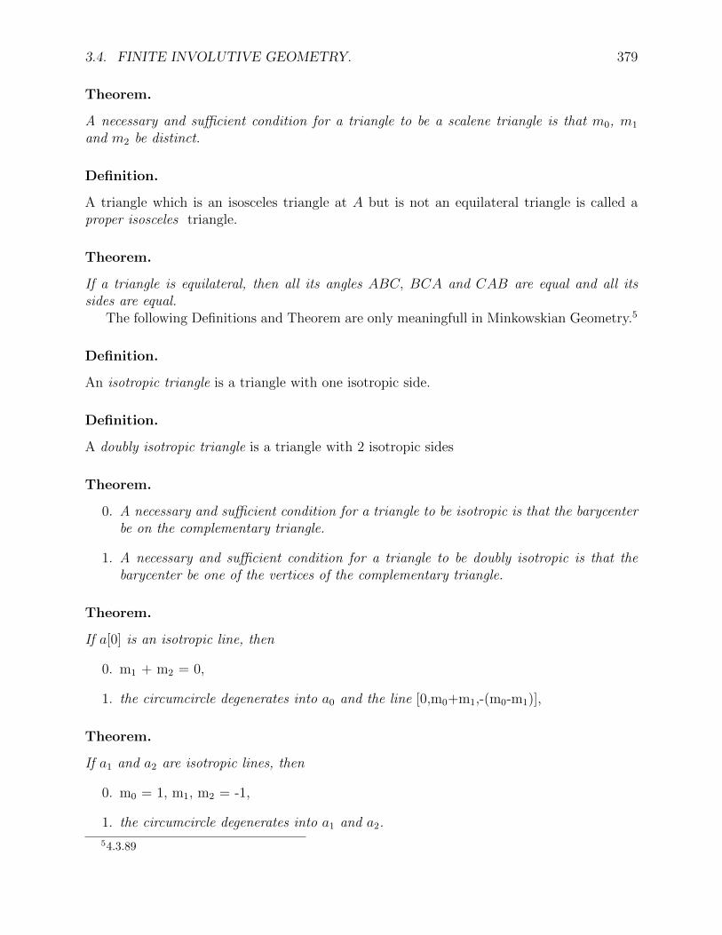
3.4. FINITE INVOLUTIVE GEOMETRY. 379
Theorem.
A necessary and sufficient condition for a triangle to be a scalene triangle is that m0, m1
and m2 be distinct.
Definition.
A triangle which is an isosceles triangle at A but is not an equilateral triangle is called aproper isosceles triangle.
Theorem.
If a triangle is equilateral, then all its angles ABC, BCA and CAB are equal and all itssides are equal.
The following Definitions and Theorem are only meaningfull in Minkowskian Geometry.5
Definition.
An isotropic triangle is a triangle with one isotropic side.
Definition.
A doubly isotropic triangle is a triangle with 2 isotropic sides
Theorem.
0. A necessary and sufficient condition for a triangle to be isotropic is that the barycenterbe on the complementary triangle.
1. A necessary and sufficient condition for a triangle to be doubly isotropic is that thebarycenter be one of the vertices of the complementary triangle.
Theorem.
If a[0] is an isotropic line, then
0. m1 + m2 = 0,
1. the circumcircle degenerates into a0 and the line [0,m0+m1,-(m0-m1)],
Theorem.
If a1 and a2 are isotropic lines, then
0. m0 = 1, m1, m2 = -1,
1. the circumcircle degenerates into a1 and a2.
54.3.89

380 CHAPTER 3. FINITE PRE INVOLUTIVE GEOMETRY
3.4.12 Other special triangles.
Introduction.
There are many other types of triangles that can be defined. I will give here 2 exampleswhich allow the constructions of configurations of the type 9 * 3 & 9 * 3, distinct from thatof Pappus. For the first one, if we choose B1 = M1, B2 = M2 and C1 = M, the constructionof Section 19 gives C0 = Mam2, C2 = Tara0, B0 = tara2 × tarb2. from P19.7, follows thatB0 · a0 = 0 iff q0 = 0. This suggest the definition of a triangle of Tarry and the constructionof the 1-Pappus configuration.A similar approach determines the construction of the 2-Pappus configuration.
Definition.
The 1-Pappus configuration is the set of points1-Pappus(Ai, Bi, Ci),
such that Ai, Bi, Ci are 3 triangles and incidence(Ai, Ci, Ci−1), incidence(Bi+1, Bi−1, Ci).
Definition.
The 2-Pappus configuration is the set of points2-Pappus(Ai, Bi, Ci),
such that Ai, Bi, Ci are 3 triangles and incidence(Ai, Bi, Ci), incidence(Bi, Ci+1, Ci−1).
Definition.
A triangle of Tarry is a triangle which is not a right triangle whose point of Tarry is welldefined and coincides with one of the vertices of the triangle.
Theorem.
A necessary and sufficient condition for a triangle to be a triangle of Tarry at A0 is thatq0 = 0.
The proof follows at once from mi 6= 0 and from P16.3.Moreover, if q0 = q1 = 0, then the point of Tarry is undefined.
Corollary.
A necessary and sufficient condition for a triangle to be a triangle of Tarry at A0 is that theorthocenter be on the conic of Tarry.
Theorem.
M · ‘Tarry[0]⇒ 1-Pappus(Ai, Tarb2 M1 M2,Mam2 M Tara0).

3.90. ANSWERS TO PROBLEMS AND MISCELLANEOUS NOTES. 381
Theorem.
In Involutive Geometry, A0 = (x, y, 1), A1 = (0, 0, 1), A2 = (1, 0, 1), M = (1 + x, y, 3),M = (xy, x(1− x), y) is a triangle of Tarry iff
u2 − (1 + 2y2)u+ y4 = 0 and x2 − x+ u = 0.Proof: Assuming that m = [0, 0, 1] and X2
0 + X21 = X2
2 is a circle, a trivial computationdetermines M and M as given. The conic of Tarry is
a0 ×× a0 + ka1 ×× a2 = 0,where k is determined in such a way that M · ‘Tarry = 0, this gives k = 1. To insure thatM is on the conic of Tarry gives after division by u := x(1− x),
u+ (y2 − u)(u− y2) = 0, a simple discussion determines that 0 < y ≤√
32.
Definition.
An Eulerian triangle is a triangle for which the line of Euler is parallel to one of its sides.
Theorem.
A necessary and sufficient condition for a triangle to be an Eulerian triangle for side a0 isthat 2m0 = m1 +m2.
The proof follows at once from P1.17.
Theorem.
eul // a0 ⇒ 2-Pappus(Ai,M0 M1 M2,M Tarc0 Tarc0).
3.4.13 Geometry of the triangle. V.
(bissectrices)
CHAPTER II
FINITE PROJECTIVE
GEOMETRY
3.90 Answers to problems and miscellaneous notes.
Answer to 2.2.3.Let A0 = (1, 0, 0), A1 = (0, 1, 0), A2 = (0, 0, 1), C = (1, 1, 1), B0 = (b0, 1, 1), B1 = (1, b1, 1),

382 CHAPTER 3. FINITE PRE INVOLUTIVE GEOMETRY
B2 = (1, 1, b2),by hypothesis, bi 6= 1, b2 6= 0, b1b2 6= 1 and 2− b0 − b1 − b2 + b0b1b2 6= 0 (because of Bi.a0 = [1, 0, 0], b0 = [1− b1b2,−(1− b2),−(1− b1)],c0 = [0, 1,−1], C0 = (0, 1− b1,−(1− b2)),c = [(1− b1)(1− b2), (1− b2)(1− b0), (1− b0)(1− b1)], d = [0, b2,−1],D = (b2, 1, b2), e = [b2(1− b1), b2(1− b0),−1 + b0 − b2 + b1b2],E = (1− b0 + b2b0 − b1b2 − b2
2b0 + b22b0b1, 1− b0 + b2 − 2b1b2 − b2
2 + b22b1 + b0b1b2,
b2(2 − b0 − b1 − b2 + b0b1b2)), f = [1 − b1b2,−b2(1 − b2),−b2(1 − b1)], F = (b2(1 −b1), 0, 1− b1b2), G = (1− b2, 1− b1b2, 0),g = [1− b1b2,−(1− b2),−b2(1− b1)],X = (0, 1, b2), Y = (1− b0 − b2 + b0b1b2,−(1− b1),−b2(1− b1)),Z = (1− b2 + b2
2 − b12b1, 1− b1b2, b2(1− b2)).
3.90.1 Answer to exercises.
Exercise. [Pappus]
Defineα := (A0 ∗ A1) · A2, β := (B0 ∗B1) ·B2,α1,2 := (A1 ∗ A2) ·B1, β1,2 := (B1 ∗B2) · A1,α2,0 := (A2 ∗ A0) ·B2, β2,0 := (B2 ∗B0) · A2,α0,1 := (A0 ∗ A1) ·B0, β0,1 := (B0 ∗B1) · A0,
Using 2.3.17.0,C0 = (A1 ∗B2) ∗ (A2 ∗B1 = ((A1 ∗B2) ·B1)B2 − ((B2 ∗ A2) ·B1)A1
= α1,2B2 − β1,2A1,similarly,C1 = α2,0B0 − β2,0A2,C2 = α0,1B1 − β0,1A0, therefore(C0 ∗ C1) · C2 = βα1,2α2,0α0,1 − αβ1,2β2,0β0,1 + α2,0α1,2β2,0β0,1 − β2,0α1,2α2,0β0,1
+α0,1β1,2α2,0β0,1 − β0,1β1,2α2,0α0,1 + α1,2β1,2β2,0α0,1 − β1,2α1,2β2,0α0,1
= βα1,2α2,0α0,1 − αβ1,2β2,0β0,1.Therefore, if the points A0, A1, A2 and the points B0, B1, B2 are collinear, α = 0 and β = 0,therefore (C0 ∗ C1) · C2 = 0 and the points C0, C1, C2 are collinear by 2.3.18.
Exercise.
(Harmonic quatern). a = [0, 0, 1], let A = (0, 0, 1), A×K = [k,−1, 0],let B = (1, k, 1), l 6= 0 and 1.B × L = [l,−1, k − l], A × M = [m,−1, 0], D = (l − k,ml − mk, l − m), D × K =[k(l −m),m− l, (l − k)(m− k)], A× L = [l,−1, 0], C = (m− k, lm− lk, l −m), B × C =[2kl − km− lm, 2m− k − l, (k − l)(k −m)], N = (2m− l − k, km+ lm− 2kl, 0).
Exercise.
(Projectivity). Choose b = [0, 1, 0], a = [1, 0, 0] and P = (0, 1, 1). c = [0, 0, 1], S = (1, 0,−k),T = (1, 0,−l), Q = (0,m, k), N = [k,ml, 0].

3.90. ANSWERS TO PROBLEMS AND MISCELLANEOUS NOTES. 383
Exercise.
(Projectivity with 3 pairs). C0 = (1, 0,−1), Cj = (1, aj,−1 − aj), j > 0, with obviousnotation,Dj = (1,−ajbj,−1 − aj), j = 1, 2, t = (a1a2(b2 − b1) + a2b2 − a1b1, a1 − a2, a2b2 − a1b1),Dj = (a2 − a1, a1b1 − a2b2 − a1a2(b2 − b1), (a1 − a2)(1 + aj)), j > 2, hence Bj given above.
Answer to 2.6.14.
In part, the coefficients of A0 and A1 in Al and Bl must be proportional, therefore, f0t0+f1t1f2t0+f3t1
=t0t1, this gives 1.
Answer to 2.3.7.
For p = 2, if A[] = ((1, 0, 0), (1, 0, 1), (1, 1, 0), (1, 1, 1)), and the diagonal points are Bi,A0 × A1 = [0, 1, 0], A2 × A3 = [1, 1, 0], B0 = (0, 0, 1). A1 × A2 = [1, 1, 1], A3 × A0 = [0, 1, 1],B1 = (0, 1, 1). A0 × A2 = [0, 0, 1], A1 × A3 = [1, 0, 1], B2 = (0, 1, 0). The diagonal points areon [1,0,0]. For p = 4, the coordinates are 0, 1, x, y = 1 + x. The addition and multiplicationtables are
+ 0 1 x y · 0 1 x y0 0 1 x y 0 0 0 0 01 1 0 y x 1 0 1 x yx x y 0 1 x 0 x y 1y y x 1 0 y 0 y 1 x
If A[] = ((1, 0, 0), (1, 0, 1), (1, x, 0), (1, y, 1)),A0 ×A1 = [0, 1, 0], A2 ×A3 = [x, 1, 1], B0 = (1, 0, x). A1 ×A2 = [x, 1, x], A3 ×A0 = [0, 1, y],B1 = (1, 1, x). A0 ×A2 = [0, 0, 1], A1 ×A3 = [y, 0, y], B2 = (0, 1, 0). The diagonal points areon [x, 0, 1].
Answer to 2.5.10.
In part,C2 = (c, 1 − c, 1), a0 = (1, c,−c − 1), b = [1, 0, 0], B2 = (c2 − c + 1,−c + 1, 1). A geometriccondition is a0 · C2 = 0 or b ·B2 = 0. The configuration is then of type
6 ∗ 4 + 3 ∗ 3 + 1 ∗ 2 & 2 ∗ 4 + 9 ∗ 3.
Notes.
On 2.2.2:Commutativity implies that if
J ′ := (B × P )× (E ×Q), J = (b(a− 1), b2(a− 1), a(b− 1)),K ′ := (A× P )× (J ′ ×M), K = (b(a− 1), ab(a− 1), a(b− 1)),thenL · (J ′ ×K ′) = 0.
The constructionD′′ := (R× T ′)× a, with D” = (1,b+c)

384 CHAPTER 3. FINITE PRE INVOLUTIVE GEOMETRY
is related to the associative property(a+ b) + c = a+ (b+ c).
Before2.2.9
Theorem.
. . . describe the degenerate conic, perhaps in 2.10.8 . . . determine the collineation which leavea general conic fixed also special case when it is a conic.
Examples.
For p = 5,C0
0 1 2 3 4 5 6 7 8 9101112131415161718192021222324252627282930
4 4 2 4 4 4 4 4 2 4 4 4 4 4 1 4 4 4 4 4 2 2 4 4 4 1 4 1 4 4 4
N =
2 −2 02 0 −12 0 0
, N I =
0 2 00 0 −1−2 −2 1
.
Point conic and its mapping 0 1, 1 6, 10 27, 14 4, 23 8, 27 29,Line conic and its mapping 1 10, 4 14, 6 0, 8 1, 27 23, 29 27,Points on line conic and tangent, 0 16, 1 0, 10 22, 14 4, 23 14, 27 29,Lines on line conic and contact, 1 7, 4 14, 6 5, 8 13, 27 29, 29 27.The equation of the point conic is X2 + 2YZ + ZX = 0.The equation of the line conic is −2z2 + yz - zx + xy = 0.C1
0 1 2 3 4 5 6 7 8 9101112131415161718192021222324252627282930
6 6 3 6 6 6 6 3 6 6 6 6 6 3 6 6 6 1 6 3 6 6 6 6 6 3 3 6 6 6 6
N =
−2 2 0−2 0 −1−2 0 0
, N I =
0 −2 00 0 −12 2 1
.
Point conic and its mapping 0 1, 1 6, 10 22, 12 5, 18 25, 29 9,Line conic and its mapping 1 10, 5 18, 6 0, 9 1, 22 12, 25 29,C2
0 1 2 3 4 5 6 7 8 9101112131415161718192021222324252627282930
10 51010 2101010 5 21010 2 510101010 510 21010 11010 110 51010
N =
0 1 −21 1 0−1 1 0
, N I =
0 0 2−2 −2 −12 −2 −1
.
Point conic and its mapping 0 6, 5 18, 6 5, 15 26, 19 22, 21 25,22 28, 23 14, 24 17, 25 4, 27 10,The center is (23), the points are on [21] or [2].

3.90. ANSWERS TO PROBLEMS AND MISCELLANEOUS NOTES. 385
Line conic and its mapping 4 6, 5 24, 6 5, 10 22, 14 23, 17 27,18 25, 22 21, 25 15, 26 0, 28 19,The central line is [18], the lines pass through (4) or (12).The equation of the point conic is Y 2 + YZ + 2ZX + 2XY = 0.The equation of the line conic is y2 - 2z2 -yz - 2zx + xy = 0.C3
0 1 2 3 4 5 6 7 8 9101112131415161718192021222324252627282930
4 4 4 4 4 2 4 4 4 1 4 4 4 2 4 1 4 2 4 4 4 2 4 4 4 4 4 4 4 4 1
Point conic and its mapping 7 10, 9 19, 11 30, 12 18, 29 27, 30 7,Line conic and its mapping 7 30, 10 12, 18 29, 19 9, 27 11, 30 7,C4
0 1 2 3 4 5 6 7 8 9101112131415161718192021222324252627282930
5 5 5 5 5 5 5 5 5 5 5 5 5 5 5 5 5 1 5 5 5 5 5 5 5 5 5 5 5 5 5
Point conic and its mapping 11 29, 14 12, 17 24, 19 28, 26 15, 27 23,Line conic and its mapping 12 26, 15 19, 23 14, 24 17, 28 11, 29 27,C5
0 1 2 3 4 5 6 7 8 9101112131415161718192021222324252627282930
5 5 5 1 5 5 5 5 5 5 5 5 5 5 5 5 5 5 5 5 5 5 5 5 5 5 5 5 5 5 5
Point conic and its mapping 2 27, 3 3, 8 8, 10 1, 16 19, 18 16,Line conic and its mapping 1 8, 3 3, 8 18, 16 16, 19 2, 27 10,C6
0 1 2 3 4 5 6 7 8 9101112131415161718192021222324252627282930
5 5 5 5 5 5 5 5 5 5 5 5 5 5 5 1 5 5 5 5 5 5 5 5 5 5 5 5 5 5 5
Point conic and its mapping 9 14, 10 12, 15 26, 18 29, 23 21, 24 17,Line conic and its mapping 12 18, 14 23, 17 10, 21 24, 26 15, 29 9,C7
0 1 2 3 4 5 6 7 8 9101112131415161718192021222324252627282930
5 5 5 1 5 5 5 5 5 5 5 5 5 5 5 5 5 5 5 5 5 5 5 5 5 5 5 5 5 5 5
Point conic and its mapping 0 16, 3 3, 8 8, 11 28, 16 0, 28 11,Line conic and its mapping 0 11, 3 3, 8 28, 11 0, 16 16, 28 8,C8
0 1 2 3 4 5 6 7 8 9101112131415161718192021222324252627282930
10101010 5 1 51010 2101010 2 51010 1101010 2101010 51010 510 2
N =
1 0 01 1 01 0 2
, N I =
1 −1 20 1 00 0 −2
.
Point conic and its mapping 17 24, the center is (17).
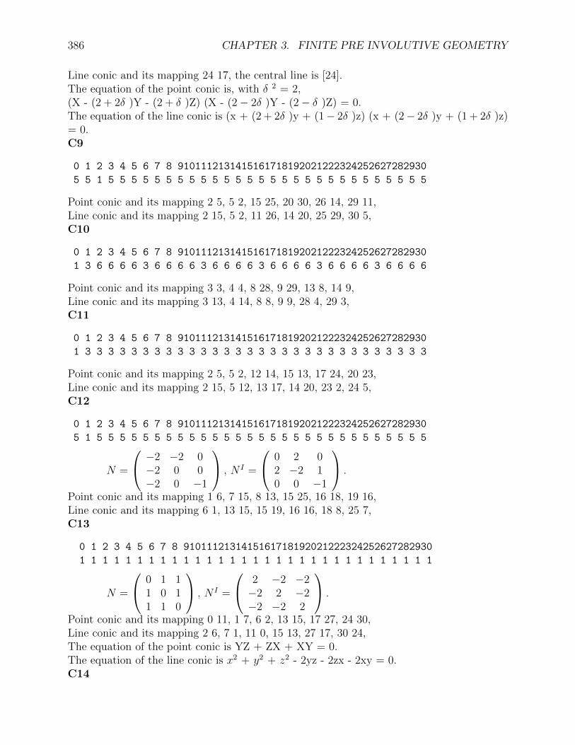
386 CHAPTER 3. FINITE PRE INVOLUTIVE GEOMETRY
Line conic and its mapping 24 17, the central line is [24].The equation of the point conic is, with δ 2 = 2,(X - (2 + 2δ )Y - (2 + δ )Z) (X - (2− 2δ )Y - (2− δ )Z) = 0.The equation of the line conic is (x + (2 + 2δ )y + (1− 2δ )z) (x + (2− 2δ )y + (1 + 2δ )z)= 0.C9
0 1 2 3 4 5 6 7 8 9101112131415161718192021222324252627282930
5 5 1 5 5 5 5 5 5 5 5 5 5 5 5 5 5 5 5 5 5 5 5 5 5 5 5 5 5 5 5
Point conic and its mapping 2 5, 5 2, 15 25, 20 30, 26 14, 29 11,Line conic and its mapping 2 15, 5 2, 11 26, 14 20, 25 29, 30 5,C10
0 1 2 3 4 5 6 7 8 9101112131415161718192021222324252627282930
1 3 6 6 6 6 3 6 6 6 6 3 6 6 6 6 3 6 6 6 6 3 6 6 6 6 3 6 6 6 6
Point conic and its mapping 3 3, 4 4, 8 28, 9 29, 13 8, 14 9,Line conic and its mapping 3 13, 4 14, 8 8, 9 9, 28 4, 29 3,C11
0 1 2 3 4 5 6 7 8 9101112131415161718192021222324252627282930
1 3 3 3 3 3 3 3 3 3 3 3 3 3 3 3 3 3 3 3 3 3 3 3 3 3 3 3 3 3 3
Point conic and its mapping 2 5, 5 2, 12 14, 15 13, 17 24, 20 23,Line conic and its mapping 2 15, 5 12, 13 17, 14 20, 23 2, 24 5,C12
0 1 2 3 4 5 6 7 8 9101112131415161718192021222324252627282930
5 1 5 5 5 5 5 5 5 5 5 5 5 5 5 5 5 5 5 5 5 5 5 5 5 5 5 5 5 5 5
N =
−2 −2 0−2 0 0−2 0 −1
, N I =
0 2 02 −2 10 0 −1
.
Point conic and its mapping 1 6, 7 15, 8 13, 15 25, 16 18, 19 16,Line conic and its mapping 6 1, 13 15, 15 19, 16 16, 18 8, 25 7,C13
0 1 2 3 4 5 6 7 8 9101112131415161718192021222324252627282930
1 1 1 1 1 1 1 1 1 1 1 1 1 1 1 1 1 1 1 1 1 1 1 1 1 1 1 1 1 1 1
N =
0 1 11 0 11 1 0
, N I =
2 −2 −2−2 2 −2−2 −2 2
.
Point conic and its mapping 0 11, 1 7, 6 2, 13 15, 17 27, 24 30,Line conic and its mapping 2 6, 7 1, 11 0, 15 13, 27 17, 30 24,The equation of the point conic is YZ + ZX + XY = 0.The equation of the line conic is x2 + y2 + z2 - 2yz - 2zx - 2xy = 0.C14

3.90. ANSWERS TO PROBLEMS AND MISCELLANEOUS NOTES. 387
0 1 2 3 4 5 6 7 8 9101112131415161718192021222324252627282930
2 2 1 2 2 2 2 2 2 1 2 2 2 2 2 1 1 2 2 2 2 2 1 2 2 1 2 2 1 2 2
N =
1 −2 11 −1 00 2 −1
, N I =
1 1 20 −1 −21 1 1
.
Point conic and its mapping 2 15, 9 29, 15 7, 16 18, 22 21, 28 4,The points are on [19].Line conic and its mapping 4 28, 7 15, 15 2, 18 16, 21 22, 29 9,The lines pass through (25).C15
0 1 2 3 4 5 6 7 8 9101112131415161718192021222324252627282930
2 2 2 2 2 1 2 2 2 2 1 2 1 2 1 2 2 2 1 2 2 2 1 2 2 2 1 2 2 2 2
N = N I =
1 −2 −2−2 1 −2−2 −2 1
Point conic and its mapping 19 28, 20 23, 23 20, 25 29, 28 19, 29 25,Line conic and its mapping 19 28, 20 23, 23 20, 25 29, 28 19, 29 25,The equation of the point conic is X2 + Y 2 + Z2 + Y Z + ZX +XY = 0.The equation of the line conic is x2 + y2 + z2 + yz + zx+ xy = 0.
Answer to 2.2.9.For p = 13, points on the conic are, (0,1,1) = (2), (0,1,2) = (3), (1,0,1) = (15), (1,0,4) =(18), (1,1,0) = (27), (1,2,0) = (40).The point conic is2, 3, 15, 18, 27, 35, 40, 51,133,135,146,151,158,168,the line conic is111, 83,156,121,179, 22, 98,148,112,129, 86, 25,165,166.The representative matrix is 1 −4 1
−4 −6 −21 −2 −3
(0,1,2) = (13) and (1,0,12) = (26) are on [1,1,1], the polars are [1,6,5] = [97] and [0,1,11] =[12]. Hence the pole of [1,1,1] is (1,6,3) = (95).1.− 6 + 3.1− 4.5− 2.(−3) = −17 = −46.(−3) + 8.6− 2.(−6)− (−5).5) = 67 = 2,2.5 + 4.2− (−5).(−3)− 4.(−6) = 27 = 1, (−4, 2, 1) = (1, 6, 3).
Answer to 2.2.9.A × B = [1,−1, 1], C × D = [2, 1,−5], A × D = [2,−1, 1], B × C = [1, 1,−3], k1 = 1.3,k2 = −1.3, therefore the conic is, after dividing by 3,(X0 −X1 +X2)(2X0 +X1 − 5X2) + (2X0 −X1 +X2)(X0 +X1 − 3X2) = 0,which gives twice the result of the Example.

388 CHAPTER 3. FINITE PRE INVOLUTIVE GEOMETRY
Answer to 2.3.2.
0. For q = 2, the primitive polynomial giving the selector 0, 1, 3, isI3 + I + 1.
The auto-correlates are 0 11 2 7 8.The selector function isi 0 1 2 3 4 5 6 7 8 9 10 11
f(i) 0 14 1 0 16 16 14 14 16type F0 V0 F4 V2 T0 T2 V1 F3 F1 T3 E2 F2
i 12 13 14 15 16 17 18 19 20f(i) 4 1 0 1 0 4 4 16 1type T4 E1 P V3 E0 T1 E3 V4 E4
1. The correspondence between the selector notation and the homogeneous coordinatesfor points and lines is
i I i i∗
0 1 6∗ : 1, 2, 4,1 I 1∗ : 0, 2, 6,2 I2 0∗ : 0, 1, 3,3 I + 1 5∗ : 2, 3, 5,4 I2 + I 3∗ : 0, 4, 5,5 I2 + I + 1 4∗ : 3, 4, 6,6 I2 + 1 2∗ : 1, 5, 6.
2. The matrix representation is
M =
1 0 10 1 01 0 0
,M−1 =
0 0 10 1 01 0 1
. and the equation satisfied by the
fixed points is (X0 +X1)2 = 0.
3. The degenerate conic through 0, 1, 2 and 5 with tangent 5∗ at 5, is represented by thematrix
N =
0 1 11 0 01 0 0
.
The polar of 0 is 0∗, of 1 is 0∗, of 2 is 5∗, of 4 is 4∗, of 5 is 5∗ of 6 is 6∗ and of 3 isundefined. The equation in homogeneous coordinates is X0(X1 +X2) = 0.
4. A circle with center 14 can be constructed as follows. I first observe that a directionmust be orthogonal to itself. Indeed, if 0 is a direction, the others form an angle 1,2,3,4mod 5, we cannot play favorites and must choose 0. If A0 = 1, C × A0 and thereforethe tangent has direction 0, A0 × Ai+1 has direction i mod 5 or are the points 0, 7, 8,2, 11.
It is natural to choose the pentagonal face-point as 14, and the edge-points on thepentagon as 0, 8, 11, 7, 2. The points on the circle 1, 6, 3, 15, 19 are chosen as thevertex-points opposite the corresponding edge-point, 1 opposite 0, 6 opposite 8, . . . .This gives the types, with subscripts indicated in 0. and the definition:

3.90. ANSWERS TO PROBLEMS AND MISCELLANEOUS NOTES. 389
The points are represented on the 5-anti-prism as follows. The pentagonal face-point,P, the 5 triangular face-points, Ti, the 5 vertex-points, Vi, the 5 triangular-triangularedge-points, Ei, the 5 pentagonal-triangular edge-points Fi.
The lines are represented on the 5-anti-prism as follows. The pentagonal face-line, f,which is incident to Fi, the 5 triangular face-lines, ti, which are incident to Fi, Fi, Ti+1,Ti−1, Ei+2, Ei−2. If f is the pentagonal edge of ti and V, V ′ are on f , Fi is on it, Ti+1
(Ti−1) share V (V ′), Ei+2 (Ei−2) are on an edge through V (V ′) not on tithe 5 vertex-lines, vi, which are incident toFi, Vi+2, Vi−2, Ei+1, Ei−1. If t is the face with vi on its pentagonal edge these are allthe vertices, and edge-points on it distinct from vi.the 5 triangular-triangular edge-lines, ei, which are incident to Fi, Ti+2, Ti−2, Vi+1,Vi−1. Vi+1 and Vi−1 are on the same edge as ei, the line which joins the center C of theantiprism to Ei is parallel to the edge containing Fi, Ti+2 and Ti−2 are the triangularfaces which are not adjacent to Ei or Fi.
the 5 pentagonal-triangular edge-lines. fi, which are incident to P, Ti, Vi, Ei, Fi. Ti isadjacent to fi, Vi is opposite fi, Ei joined to the center of the antiprism is parallel toTi.
Answer to 2.3.3.For p = 3,
0. The primitive polynomial giving the selector 0, 1, 3, 9 is I3 − I − 1.
1. The correspondence between the selector notation and the homogeneous coordinatesfor points and lines isi I i i∗
0 1 12∗ : 1, 2, 4, 10,1 I 1∗ : 0, 2, 8, 12,2 I2 0∗ : 0, 1, 3, 9,3 I + 1 7∗ : 2, 6, 7, 9,4 I2 + I 3∗ : 0, 6, 10, 11,5 I2 + I + 1 4∗ : 5, 9, 10, 12,6 I2 + 2I + 1 10∗ : 3, 4, 6, 12,7 I2 + I + 2 6∗ : 3, 7, 8, 10,8 I2 + 1 2∗ : 1, 7, 11, 12,9 I + 2 11∗ : 2, 3, 5, 1110 I2 + 2I 9∗ : 0, 4, 5,7,11 I2 + 2I + 2 5∗ : 4, 8, 9, 11,12 I2 + 2 8∗ : 1, 5, 6, 8.
2. The matrix representation of the polarity i to i∗ is
M =
1 0 10 1 01 0 0
, M−1 =
0 0 10 1 01 0 2
.
The equation satisfied by the fixed points is X20 +X2
1 + 2X2X0 = 0.

390 CHAPTER 3. FINITE PRE INVOLUTIVE GEOMETRY
3. The degenerate conic through 0, 1, 2 and 5 with tangent 4∗ at 5, is obtained by con-structing the quadrangle-quadrilateral configuration starting with P = 5 and Qi =0, 1, 2. We obtain qi = 3∗, 2∗, 7∗, which are the tangents at Qi. The matrix repre-sentation is
N =
0 1 11 0 11 1 0
with equation X1X2 +X2X0 +X0X1 = 0.
We can check that the polar of 10 = 3∗ × 4∗ is 9∗ = 0× 5.
Answer to 2.3.8.
0. For q = 22, the primitive polynomial giving the selector 0, 1, 4, 14, 16 is I3− I2− I− ε, with
ε2 + ε+ 1 = 0.
1. The correspondence between the selector notation and the homogeneous coordinatesare as follows, i∗ has the homogeneous coordinates associated with I i.
i I i i∗0 1 20∗
1 I 14∗
2 I2 0∗
3 I2 + I + ε 10∗
4 I + ε 219∗
5 I2 + ε 2I4∗
6 I2 + ε 2I + 118∗
7 I2 + 1 15∗
8 I2 + ε 3∗
9 I2 + ε2I + ε 5∗
10 I2 + εI + 1 9∗
11 I2 + ε2 13∗
12 I2 + εI + ε 11∗
13 I2 + I + ε2 6∗
14 I + 1 2∗
15 I2 + I 1∗
16 I + ε 12∗
17 I2 + εI 16∗
18 I2 + εI + ε2 17∗
19 I2 + ε2I + ε2 8∗
20 I2 + I + 1 7∗
To obtain the last column, for row 9, [1, ε2, ε] = (1, 1, 1)× (1, ε, 0) = 20× 17 = 5 ∗ .
2. The correspondence i to i∗ is a polarity whose fixed points are on a line. The matrixrepresentation is obtained by using the image of 4 points.
0 = (0,0,1), M(0) = 0∗ = [1, 0, 0],

3.90. ANSWERS TO PROBLEMS AND MISCELLANEOUS NOTES. 391
1 = (0,1,0), M(1) = 1∗ = [1, 1, 0],2 = (1,0,0), M(2) = 2∗ = [0, 1, 1],18 = (1, ε, ε2), M(18) = 18∗ = [1, ε2, 1].
The first 3 conditions give the polarity matrix asThe last condition gives βε+ αε2 = 1, γ + βε = ε2, γ = 1. Hence γ = 1, β = 1, α = 1.Therefore
M =
0 1 11 1 01 0 0
, M−1 =
0 0 10 1 11 1 1
.
Note that M is real and could have been obtained from the reality and non singularityconditions, giving directly α = β = γ = 1.The polar of (X0, X1, X2) is [X1 +X2, X0 +X1, X0].The fixed points (X0, X1, X2) satisfy X2
1 = 0 corresponding to 14∗.
3. A point conic with no points on 14 is 1, 3, 4, 5,13,the corresponding line conic is 15,19,10,16, 8.Projecting from 1 and 3, 1, 3, 5,13, 4,we get the fundamental projectivity, 8, 2,11, 0, 7 on 14∗.
4. To illustrate Pascal’s Theorem, because there are only 5 points on a conic, we need touse the degenerate case. The conic through 0, 1, 2 and the conjugate points 9 and 18is The last condition gives βε+ αε2 = 1, γ + βε = ε2, γ = 1.
Hence γ = 1, β = 1, α = 1. Therefore
M =
0 1 11 1 01 0 0
, M−1 =
0 0 10 1 11 1 1
.
Note that M is real and could have been obtained from the reality and non singularityconditions, giving directly α = β = γ = 1.The polar of (X0, X1, X2) is [X1 +X2, X0 +X1, X0].The fixed points (X,X1, X2) satisfy X2
1 = 0 corresponding to 14∗.
5. A point conic with no points on 14 is 1, 3, 4, 5,13, 0 1 11 0 11 1 0
The tangents at (0,0,1), (0,1,0), (1,0,0), (1, ε2, ε), (1, ε, ε2) are [1,1,0], [1,0,1], [0,1,1],[1, ε2, ε), (1, ε, ε2], or 1∗, 15∗, 2∗, 5∗, 17∗. On the other hand, using Pascal’s Theorem,the tangent at 0 is given by((((0× 1)× (9× 18))× ((18× 0)× (1× 2)))× (2× 9))× 0
= (((0∗ × 7∗)× (4∗ × 20∗))× 12∗)× 0= (((14× 17) = 8∗)× 12∗or13)× 0 = 1∗.
Answer to 2.3.8.For q = 57, choose the auto-correlates as point on a circle although 0 is on the circle drawas it is the center. With the succession of points Xi,

392 CHAPTER 3. FINITE PRE INVOLUTIVE GEOMETRY
xi = 0×Xi 36, 1, 52, 43, 3, 32, 13,Xi 16, 35, 18, 50, 29, 26, 30,yi+1 = Xi−1 ×Xi+1 22, 42, 8, 14, 10, 28, 44,yi+2 = Xi−2 ×Xi+2 34, 2, 41, 17, 40, 20, 23,yi+3 = Xi−3 ×Xi+3 7, 31, 6, 27, 54, 25, 39,yi+1 × xi 21, 51, 5, 46, 33, 4, 45,yi+2 × xi 24, 56, 48, 15, 49, 38, 47,yi+3 × xi 53, 12, 37, 9, 55, 11, 19.
This gives all the points in the projective plane of order 7. We observe16∗ 21∗ 24∗ 53∗ 22∗ 34∗ 7∗
36 36 36 36 36 36 3616 35, 30 18, 26 50, 2942, 44 22 8, 28 14, 1041, 20 34 17, 40 2, 2327, 54 31, 39 7 6, 25
46, 33 5, 4 21 51, 4515, 49 56, 47 48, 38 2437, 11 12, 19 9, 55 53
35∗ 51∗ 56∗ 12∗ 42∗ 2∗31∗
1 1 1 1 1 1 135 16, 18 50, 30 29, 2622, 8 42 14, 44 10, 2817, 23 2 40, 20 34, 4154, 25 7, 6 31 27, 39
33, 4 46, 45 51 21, 549, 38 24, 48 15, 47 569, 19 53, 37 55, 11 12
18∗ 5∗48∗ 37∗ 8∗14∗ 6∗
52 52 52 52 52 52 5218 35, 50 16, 29 26, 3042, 14 8 22, 10 28, 4434, 40 41 20, 23 2, 1725, 39 31, 27 6 7, 54
4, 45 21, 33 5 51, 4638, 47 56, 15 24, 49 4853, 55 12, 9 11, 19 37
Answer to
2.3.8.For q = 23,

3.90. ANSWERS TO PROBLEMS AND MISCELLANEOUS NOTES. 393
36 : 0 37 38 40 44 52 18 27 68 1∗ 3∗ 7∗ 2∗ 4∗ 5∗
36× 0 = 0∗ : 0 1 3 7 15 31 36 54 63 0 0 0 1 3 3136× 37 = 37∗ : 17 26 36 37 39 43 51 67 72 72 51 67 72 72 2636× 38 = 38∗ : 16 25 35 36 38 42 50 66 71 35 71 66 71 50 7136× 40 = 40∗ : 14 23 33 34 36 40 48 64 69 14 33 69 34 69 6936× 44 = 44∗ : 10 19 29 30 32 36 44 60 65 30 60 29 29 32 1036× 52 = 52∗ : 2 11 21 22 24 28 36 52 57 2 28 24 52 11 236× 18 = 18∗ : 13 18 36 45 55 56 58 62 70 62 70 56 13 70 5836× 27 = 27∗ : 4 9 27 36 46 47 49 53 61 53 4 47 61 27 4936× 68 = 68∗ : 5 6 8 12 20 36 41 59 68 6 12 8 5 59 68
Conic with no point on 36: 2, 4, 5, 6,13,28,31,46,63line conic: 29,59,31, 9,18,43,28,35,64.
Fundamental projectivity: from 2 and 5 on the conic, the points2, 5, 6,31,13,28, 4,46,63 give the points on 36∗ :38, 0,68,27,52,37,40,18,44.
394 CHAPTER 3. FINITE PRE INVOLUTIVE GEOMETRY

Chapter 4
FINITE INVOLUTIVE SYMPATHICAND GALILEAN GEOMETRY
4.0 Introduction.
In part II, I have given a construction of a finite projective geometry associated to a primep. In it, there is no notion of parallelism, equality of segments or of angles, perpendicularity,etc . I have then obtained the well known finite affine geometry. In it, we have the notion ofparallel lines, equality of segments on a given line or on parallel lines, but we have no circles,no notion of equality on non parallel lines, no perpendicularity, etc . It is the purpose ofPart III to construct a finite Euclidean geometry in which these notions as well as measureof angles and distances can be obtained.
In the first step, which I will call involutive geometry, I choose an involution on theideal line. This involution either is elliptic, in which case it has no real fixed points oris hyperbolic, in which case it has 2 real fixed points. The elliptic case resembles morethe standard Euclidean geometry, while the hyperbolic case is easier to deal with, but theproperties of both geometries go hand in hand. In it we define circles and perpendicularity. Aprinciple of compensation, which is not evident in the classical case, makes its appearance.For instance, if we consider the lines through the center of a circle, half of them do notintersect the circle, but the other half do and then at two points. As an other example, notall triangles have an inscribed circle, only roughly one in 4 has, but these have 4 inscribedcircles. In the involutive geometry, I also define the equality of angles and the equality ofsegments.
In the second step, I will introduce the sympathic geometry, in which we have the notionof measure of angle. The algebraic development suggests a finite trigonometry. In fact 2 suchtrigonometries are required for each prime, corresponding to the elliptic and to the hyperboliccase. The trigonometry for the elliptic case is obtained easily from the notion of primitiveroots associated to p. The trigonometry for the hyperbolic case, requires a generalization.
In the last step, I introduce the notion of measure of distances and obtain the finiteEuclidean geometry.
1G30.TEX [MPAP], September 9, 2019
395

396 CHAPTER 4. FINITE INVOLUTIVE SYMPATHIC AND GALILEAN GEOMETRY
4.1 Finite involutive geometry.
4.1.9 Theorems in finite involutive Geometry, which do not cor-respond to known theorems in Euclidean Geometry.
The Theorems in finite Euclidean Geometry fall also in several categories. The first one, . . .The theorems are a direct consequence of . . . .
The proof follows by assuming like in section . . . that m corresponds to the line at infinityand . . . . The reference in parenthesis is to the section ¡?¿ in Theorem . . . .
Theorem.
0. Let M1 × H2 meet A1 × A2 in C0, . . . , then the points C0, C1 and C2 are on thesame line p.
1. Let H1M2 meet A1A2 in D0, . . . , then the points D0, D1 and D2are on the same line q.
2. The intersection P of p and q is on the line eul of Euler.
Proof: Use AA1, 3.0, 3.1, with H0 = M0, M0 = M0, C0 = C0, D0 = C 0, p = p andq = p.
4.1.10 The geometry of the triangle of degree 2.
. . . Involves problems of the second degree, bisectrices, inscribed circles for even triangles.
4.1.11 Some theorems involving circles.
Introduction.
It is not my intention to devlop here the extensive theory on circles for involutive geometryover arbitrary fields. I will simply give an example which illustrates how the problem canbe approached effectively.
Definition.
Let θ be a defining circle and m, the ideal line, any circle γ can be written asγ = θ + (m) ×× (r),
where (r) = [r0, r1, r2] is a given constant times the radical axis with θ. The 3 dimensionalrepresentation of the circle γ is defined by the point, with coordinates r0, r1 and r2. I willwrite (r)3 := (r0, r1, r2)3 for that representation. θ is represented by the origin. A degeneratecircle (m) ×× (r) is represented by the direction of r.
Exercise.
What is the representation of tangent circles.
4.1. FINITE INVOLUTIVE GEOMETRY. 397
Lemma.
If γ0 and γ1 are circles, represented by (r0)3 and (r1)3, then the family of circles throughtheir intersections is represented by
(r0)3 + k(r1)3,with k an arbitrary element in the field together with∞, where∞ represents γ1. The additionis that of vectors in 3 dimensions and the multiplication by k the scalar multiplication.
I will also denote the family byγ0 + kγ1.
One can also use the homogeneous representation,k0γ0 + k1γ1.
Strictly speaking, this is the representation used in the proofs, although I have used the nonhomogeneous representation to simplify the writing.
Theorem. [Bundle]
Let γj, j = 0 to 3, be 4 circles, if there is a circle α which passes through the intersection ofthe circles γ0 and γ1, as well as the intersection of γ2 and γ3, then there is a circle β passingthrough the intersections of γ0 and γ2, as well as those of γ1 and γ3.
This is the so called bundle Theorem. 1
Proof: If rj)3 is the representation of γj. The family through the first 2 circles is repre-sented by (r0)3 + k(r1)3 and that through the last 2 circles by
(r2)3 + l(r3)3, the hypothesis concerning the circle α implies(r0)3 + k(r1)3 = u((r2)3 + l(r3)3, which can be rewritten(r0)3 +u(r2)3 = −k((r2)3 +ul(r3)3), which gives the conclusion concerning the circle
β.
4.1.12 The parabola, ellipse and hyperbola.
Introduction.
The parabola, ellipse and hyperbola have already be defined in affine geometry. Here westudy their properties in involutive geometry.
The parabola.The ellipse and hyperbola.If we assume that the isotropic points are (δ, 1, 0) and (−δ, 1, 0), where δ2 = d = N p, we
will see that by an appropriate . . . transformation, these can be reduced toX02
A+ X12
B= X22.
Recall also that i2 = −1.
Definition.
The isotropic tangents are isotropic lines tangent to the conic. The foci are the intersectionof 2 isotropic tangents through 2 different isotropic points.
1see Dembosky, p. 256

398 CHAPTER 4. FINITE INVOLUTIVE SYMPATHIC AND GALILEAN GEOMETRY
Theorem.
Given the conicX02
A+ X12
B= X22.
D0. C = A+Bd,then
C0. The point polarity is B 0 00 A 00 0 −AB
C1. The line polarity is A 0 0
0 B 00 0 −1
C2. The isotropic tangents through (δ, 1, 0) are
(1,−δ,√C) and (1,−δ,−sqrtC)
C3. The foci are
C3.0. (−√C, 0, 1), (
√C, 0, 1),
C3.1. (0,−√C, δ), (0,
√C, δ),
C4.0. C =Rp⇒ the foci C.3.0. are real, the foci C.3.1. are not.
C4.1. C =Np⇒ the foci C.3.1. are real, the foci C.3.0. are not.
Theorem.
Given the conic
D0. X02
A+ X12
B= X22.
H1.0. A =Rp, B =Rp,
D1.0. a =√A, b =
√B,
H1.1. A =Np, B =Np,
D1.1. a =√
Ad, b =
√Bd,
H1.2. A =Rp, B =Np,
D1.2. a =√A, b =
√Bd,
H1.3. A =Np, B =Rp,

4.1. FINITE INVOLUTIVE GEOMETRY. 399
D1.3. a =√
Ad, b =
√B, then the conic takes the form
C1.0. x2
a2+ y2
b2= 1,
C1.1. dx2
a2+ dy
2
b2= 1,
C1.2. x2
a2+ dy
2
b2= 1,
C1.3. dx2
a2+ y2
b2= 1,
Theorem.
H0.0. p = −1mod4andAB = Rp,or
H0.1. p = 1mod4andAB = Np,then
C0. the conic is an ellipse,
Theorem.
H0.0. p ≡ 1 (mod 4) and AB R p,or
H0.1. p ≡ −1 (mod 4) and AB N p,then
C0. the conic is a hyperbola.The ideal points on it are
C1.0. (abi, 1, 0), (−a
bi, 1, 0),
C1.1. (ab, 1, 0), (−a
b, 1, 0).
4.1.13 Cartesian coordinates in involutive Geometry.2
Introduction.
Notation.
A pair of reals between parenthesis will denote the Cartesian coordinates of a point. Wecannot choose a pair of reals between brackets to denote the x and y intercept of a line inthe Cartesian plane, because we have then no way to represents lines through the origin. Wewill therefore use triplets, with the last non zero coordinate normalized to 1.
25.7.83

400 CHAPTER 4. FINITE INVOLUTIVE SYMPATHIC AND GALILEAN GEOMETRY
Theorem.
If we choose as x axis the line [0,1,0] and as y axis [1,0,0], then we have the correspondence:C(i, j, 1) = (i, j),C[i, j, k] = [ i
k, jk, 1], k 6= 0,
C[i, j, 0] = [ ij, 1, 0], j 6= 0,
C[i, 0, 0] = [1, 0, 0].
Theorem.
Given a triangle whose vertices have the Cartesian coordinates(0, a), (b, 0), (c, 0), a 6= 0, b 6= c.
0. The point whose barycentric coordinates are (q0, q1, q2), with q0+q1+q2 6= 0,corresponds to the point whose Cartesian coordinates are( bq1+cq2q0+q1+q2
, aq0q0+q1+q2
).REDO 1. IN view of the preceding theorem
1. The line, distinct from the ideal line, whose barycentriccoordinates are[l0, l1, l2]corresponds to the line whose intercepts arebl2−cl1l2−l1 ,
bl2−cl1(c−b)l0−cl1+bl2)
,if bl2− cl1 = 0
and ((c− b)l0− cl1 + bl2) 6= 0, it corresponds to0, l2−l1
(c−b)l0−cl1+bl2),
and ((c− b)l0− cl1 + bl2) = 0, it corresponds to1, 0,
2. The values of the coordinates of the orthocenter arem0 = bc(b− c), m1 = c(a2 + bc), m2 = −b(a2 + bc).
Definition. 3
The following mapping associates to the non ideal points in the finite Euclidean plane asso-ciated to p, points in the classical Euclidean plane.
T (i, j) = (i+ kp, j + lp), where k and l are any integers.
Theorem.
Let d = i1j2− i2j1, then (i1, j1)x(i2, j2) = [ j1−j2d, i2−i1
d, 1], d 6= 0,
(i1, j1)x(i2, j2) = [ j1−j2i2−i1 , 1, 0], d = 0, i2 6= i1,
(i1, j1)x(i2, j2) = [1, 0, 0], d = 0, i2 = i1, j2 6= j1.For the following see ..[1,135]/cartes
313.11.83

4.1. FINITE INVOLUTIVE GEOMETRY. 401
Example.
For p = 13, let the circles beCr: x2 + y2 = r2.The points on the circles are
C1: (1, 0), (−1, 0), (0, 1), (0,−1), (6, 2), (−6, 2), (6,−2), (−6,−2), (2, 6), (−2, 6), (2,−6), (−2,−6),
C2: (2, 0), (−2, 0), (0, 2), (0,−2), (4, 1), (−4, 1), (4,−1), (−4,−1), (1, 4), (−1, 4), (1,−4), (−1,−4),
C3: (3, 0), (−3, 0), (0, 3), (0,−3), (6, 5), (−6, 5), (6,−5), (−6,−5), (5, 6), (−5, 6), (5,−6), (−5,−6),
C4: (4, 0), (−4, 0), (0, 4), (0,−4), (5, 2), (−5, 2), (5,−2), (−5,−2), (2, 5), (−2, 5), (2,−5), (−2,−5),
C5: (5, 0), (−5, 0), (0, 5), (0,−5), (4, 3), (−4, 3), (4,−3), (−4,−3), (3, 4), (−3, 4), (3,−4), (−3,−4),
C6: (6, 0), (−6, 0), (0, 6), (0,−6), (3, 1), (−3, 1), (3,−1), (−3,−1), (1, 3), (−1, 3), (1,−3), (−1,−3),
The isotropic lines through the origin contain the points:i0: (0, 0), (1,−5), (2, 3), (3,−2), (4, 6), (5, 1), (6,−4),
(−1, 5), (−2,−3), (−3, 2), (−4,−6), (−5,−1), (−6, 4),i1: (0, 0), (1, 5), (2,−3), (3, 2), (4,−6), (5,−1), (6, 4),
(−1,−5), (−2, 3), (−3,−2), (−4, 6), (−5, 1), (−6,−4),If we join the origin to the points (1,k) and (1,l) we obtain perpendicular directions, withk,l = 0,oo; 1,-1; 2,6; 3,4; -2,-6; -3,-4.
For p = 13, let the circles beCr: x2 − 6xy + y2 = r2.The points on the circles are
C1: (0, 1), (1, 0), (1, 6), (4, 4), (4,−6), (6, 1), (6,−4),
C2: (0, 2), (1,−2), (1,−5), (2, 0), (2,−1), (5, 5), (5,−1),
C3: (0, 3), (1, 1), (1, 5), (3, 0), (3, 5), (5, 1), (5, 3),
C4: (0, 4), (2, 3), (2,−4), (3, 2), (3, 3), (4, 0), (4,−2),
C5: (0, 5), (4, 5), (4, 6), (5, 0), (5, 4), (6, 4), (6, 6),
C6: (0, 6), (2, 2), (2,−3), (3,−2), (3,−6), (6, 0), (6,−3),
as well as the points symmetric with respect to the origin.If we join the origin to the points (1,k) and (1,l) we obtain perpendicular directions, withk,l = 0,-4; 1,-1; 2,-5; 3,oo; 4,-2, 5,-6; 6,-3.
For p = 11, let the circles beCr: exx2 − 4xy + y2 = r2.The points on the circles are
C1: (0, 1), (1, 4), (4, 4),

402 CHAPTER 4. FINITE INVOLUTIVE SYMPATHIC AND GALILEAN GEOMETRY
C2: (0, 2), (2,−3), (3, 3),
C3: (0, 3), (1, 1), (1, 3),
C4: (0, 4), (4, 5), (5, 5),
C5: (0, 5), (2, 2), (2,−5),
as well as the points symmetric with respect to the diagonals, (i, j) here means (i, j),(j, i), (−i,−j), (−j,−i).The isotropic points arel0: ex(0, 0), (1, 3), (1, 4), (2,−3), (2,−5), (3,−2), (3, 1),
(4,1),(4,5),(5,-2),(5,4),l1 : ex (0,0),(1,-3),(1,-4),(2,3),(2,5),(3,2),(3,-1),
(4,−1), (4,−5), (5, 2), (5,−4),If we join the origin to the points (1, k) and (1, l) we obtain perpendicular directions, withk, l = 0,-5; 1,-1; 2,∞; 3,5; 4, -2.
For p = 11, let the circles beCr: exx2 + y2 = r2.The points on the circles are
C1: (0,1), (3,5),
C2: (0,2), (1,5),
C3: (0,3), (2,4),
C4: (0,4), (1,2),
C5: (0,5), (3,4),
as well as the points symmetric with respect to the 2 axis and the diagonals.(i, j) here means (i, j), (i,−j), (j, i), (j,−i), (−i,−j), (−i, j), (−j,−i), (−j, i).If we join the origin to the points (1, k) and (1, l) we obtain perpendicular directions, withk, l = 0,∞; 1,-1; 2,5; 3,-4; 4,-3; -2,-5.
4.1.14 Correspondence between circles in finite and classical Eu-clidean geometry.
Introduction.
Theorem.
To the point (x, y), in classical geometry, on a circle centered at the origin and of radius r,corresponds, if r is not congruent to 0 modulo p, the point (x/rmodp, y/rmodp) on a circleof radius 1 in the finite geometry associated to p.Vice-versa, given a point P = (x, y) on a circle of radius 1 in the finite geometry associatedto p, we can always find a point on a circle in the classical geometry which is one of therepresentatives of P , in the mapping given in . . . .
The proof is left to the reader. The first part is trivial, the second part is not trivial. Seealso [135]FINPYT.BAS

4.1. FINITE INVOLUTIVE GEOMETRY. 403
Example.
For p = 13,(2,6) for r = 1 is associated to (15,20) for r = 25.
For p = 29,(5,11) for r = 1 is associated to (24,18) for r = 30.(8,13) for r = 1 is associated to (108,45) for r = 117.(6,9) for r = 1 is associated to (180,96) for r = 204.
Theorem.
There exist a circle of radius u in R2 which contains all the representatives of a circle in Z2p .
Indeed, for the radius 1, for instance, if one of the representatives is on the circle x2 +y2 = r21
and if s1 = 1/r1, thenu = ri(si + kip), for all i,
by finite induction, ifu = r1(s1 + pk1) = r2(s2 + pk2),
thenr1k1 − r2k2 = (r2s2 − r1s1)/p,
this givesk1 = a1 + r2k
′2 and with s′2 = (s1 + a1p)/r2,
u = r1r2(s′2 + pk′2), . . . .
Example.
For p = 29, for r = 1, we start withpoint in Z2
29 ri si5,11 5 68,13 13 96,9 25 7
then5k1 − 13k2 = 3, a1 = −2, s′2 = −4,u = 5.13(−4 + 29k′2),13k′2 − 5k3 = 3, a2 = 1, s′3 = 5,u = 5.13.5(5 + 29k′3),
hence the suitable circle in R2 with smallest radii has radius u = 1625 and contains thepoints
in R2 in Z229
-1300,-975 5,11;-1500,-625 8,13;-1560,-455 6,9.

404 CHAPTER 4. FINITE INVOLUTIVE SYMPATHIC AND GALILEAN GEOMETRY
4.1.15 Answers to problems.
Answer to 1.13.1.
For the second part.The problem can be restated successively as follows, given a solution of0. x2 + y2 = z2, there exist i, j, k such that (x+ ip)2 + (y + jp)2 = (z + kp)2, or there existu and v such that
u2 − v2 = x, 2uv = y, u2 + v2 = z,eliminating v from the first 2 equations and using 0., gives
u2 = r+x2, v2 = r−x
2,
r+x2
need not be a quadratic residue, therefore we use insteadu2 = b r+x
2, v2 = b r−x
2, c = 1/b,
this gives u and v,x+ ip = (u2 − v2)c, y + ip = 2uvc, z + ip = (u2 + v2)c.
A more careful discussion will show that signs may have to be changed and the role of x andy interchanged.For instance, for p = 13 and 22 +62 = 12, b = -2, c = 6, u2 = (−5)(−2) = 62, v2 = (6)(−2) =12, hence x+ ip = 35, −(y + jp) = 72, z + kp = 222.For p = 17, and x = 4, y = 6, z = 1, b = 3, c = 6, u2 = (6)(3) = 12, v2 = (12)(3) = 22,hence after interchange of x and y, x+ ip = 72, y + jp = 210, z + kp = 222.For p = 19 and 32+72 = 12, b = 2, c = 10, u2 = (2)(2) = 22, v2 = (−1)(2) = 62, hence−(x+ ip) = 320, −(y + jp) = 240, z + kp = 400.
(AFTER INVOLUTIVE GEOMETRY)
Comment.
For the following theorem, I will not give a linear construction, although one could be given.The theorem is a generalization of the Theorem of Miquel and can be further generalized inthe context of Gaussian geometry.
Notation.
If u and v are 2 lines and ξ is a conic,ξ − u ×× v = 0,
is equivalent toξ(X)− (u ·X) (v ·X) = 0.
This should be moved before the definition of circles.
Theorem.
The radical axis of the 2 circlesµj := θ −m ×× uj, j = 0, 1
is u1 − u0.Indeed, µ1(X)− µ0(X) = −(m ·X) ((u1 − u0) ·X) = 0 therefore
µ1 = µ0 −m ×× (u1 − u0).

4.1. FINITE INVOLUTIVE GEOMETRY. 405
Theorem.
The radical axis of each pair of 3 circles are concurrent.
Proof: Let the 3 circles beµi := θ −m ×× ui,
ui are the radical axis of these circles with θ.the 3 radical axis are u2− u1, u0− u2, u1− u0, but u2− u1 = (u0− u2) + (u1− u0), thereforeone of the axis passes through the intersections of the other 2.
Theorem. [Miquel]
H0. Ni · ai = 0,H1. Ni ·m 6= 0,D0. µi := circle(Ai, Ni+1, Ni−1),D1. Miquel := (µ1 × µ2)−N0,thenC0. Miquel × µ0 = 0.
The nomenclature.N0. Miquel is called the point of Miquel associated to Ni.
Proof. LetN0 = (0, 1, q0), N1 = (q1, 0, 1), N2 = (1, q2, 0).
H1. implies that 1 + qi 6= 0.If the equation of µ0 a circle is
θ −m ×× u0 = 0, with u0 = [u0,0, u0,1, u0,2],m = [1, 1, 1]andθ = m′0X1X2 +m′1X2X0 +m′2X0X1
m = [1, 1, 1]. with m′0 = m0(m1 +m2), . . . ).D0. implies, for i = 0,
u0 = [0,m′2
1+q2,q1m′11+q1
].
Let Miquel = (X0, X1, X2). If the 3 circles have a point in common, it is on the intersectionof the 3 radical axis ui, it is therefore necessary that
(ui − ui+1) ·Miquel = 0, i = 0, 1, 2,therefore
Miquel = (u1 − u2)× (u2 − u0),this gives after simplification,
Miquel = (m′0
1+q0(−q0m′01+q0
+q0q1m′11+q1
+m′2
1+q2, . . .).
It remains to verify that Miquel belongs to µi.First, ui ·Miquel = m′0m
′1m′2
1+q0q1q21+q0
(1 + q1)(1 + q2)),
second, m ·Miquel = − q0m′0m′0
(1+q0)2+ . . . +m′1m
′2
1+q1q2(1+q1)(1+q2)
+ . . ..
It is straigthforward to verify that the product of these two expressions is precisely m′0X1X2+m′1X2X0 +m′2X0X1.

406 CHAPTER 4. FINITE INVOLUTIVE SYMPATHIC AND GALILEAN GEOMETRY
Theorem. [Miquel]
H0. n := N1 ×N2, n ·N0 = 0.D0. n = [n0, n1, n2],thenC0. Miquel · θ = 0.C1. q0 = −n1
n2, q1 = −n2
n0, q2 = −n0
n1.
C2. Miqnel = (n1n2m′0n1−n2
,n2n0m′1n2−n0
,n0n1m′2n0−n1
).The condition that the points Ni be collinear is precisely 1 + q0q1q2 = 0, but in this case
θ = 0 as follows from the expression ui ·Miquel. It is straightforward to verify C1 and C2.
Corollary.
0. The circles µfi circumscribed to Ai,MAi+1,MAi−1 have a point Fock in common.1. Fock is in the circumcircle θ.2. µfi = θ +m ×× [0, m2m0(m0+m1)
m0−m1,−m2m0(m0+m1)
m0−m1].
3. Fock = (m0(m1+m2)(m2−m0)(m0−m1),m1(m2+m0)(m0−m1)(m1−m2),m2(m0+m1)(m1 −m2)(m2 −m0)). 4
This is the special case when n is the orthic line m = [m0,m1,m2].The point Fock had been constructed before (D38.9) and proven to be on θ (C38.4).
Theorem. [Miquel]
D0. Ni,j := midpoint(Ai, Nj),D1. ni,j := mediatrix(Ai, Nj),D2. Ci := ni,i+1 × ni,i−1,D3. φ := circle(C0, C1, C2),thenC0. O · φ = 0.
Proof:P0. N0,1 = (1 + 2q1, 0, 1), N0,2 = (2 + q2, q2, 0).P1. n0,1 = [m2 +m0,m0− (1 + 2q1)m2,−(1 + 2q1)(m2 +m0)],
n0,2 = [−q2(m0 +m1), (2 + q2)(m0 +m1), (2 + q2)m1− q2m0].P2. C0 = (m0(1 + 2q1 + q1q2)m0 + (2 + q2)(1 + q1)m1 + (1 + 2q1)(1 + q2)m2),
(m2 +m0)((1 + q1)m0 + (q1q2 − 1)m1),(m0 +m1)((1− q1q2)m2 + (1 + q2)m0).
P3. φ : . . .
Problem.
The following question suggests itself. Letν := circle(N0, N1, N2).
What relation exists between all circles ν having the same point of Miquel?Same question in the case for which the point of Miquel is on θ.
422.12.88

4.1. FINITE INVOLUTIVE GEOMETRY. 407
Theorem . . . states that all the circles are lines and . . . that one of these lines is that of Simsonand Wallace. Again what is the relation between these lines?
Theorem. [Simson and Wallace]
H0. X · θ = 0,D0. ni := X × Im i,D1. Ni := ni × ai,D2. n := N1 ×N2,thenC0. N0 · n = 0(∗).C1. (W ×Ni) ⊥ ai.?
Proof:P0. n0 = [m1X2 −m2X1, (m1 +m2)X2 +m2X0,−m1X0 − (m1 +m2)X1].P1. N0 = (0,m1X0 + (m1 +m2)X1,m2X0 + (m1 +m2)X2).P2. n = [X1X2(−m0X0 + (m1 +m2)(X1 +X2)),X2X0(−m1X1 + (m2 +m0)(X2 +X0)),
X0X1(−m2X2 + (m0 +m1)(X0 +X1))].To obtain the last expression we use in each coordinate the relation H0,m0(m1 +m2)X1X2 +m1(m2 +m0)X2X0 +m2(m0 +m1)X0X1 = 0.
MAY WANT TO REFER HERE TO THE FOLLOWING BUT MOVE IT AS APPLI-CATION OF PARABOLAS.
Theorem.
The set of lines having the same point X of Miquel are on a line parabola5:C0. mup−1(X) :
X0u0(u1− u2)/m′0 = X1u1(u2− u0)/m′1 = X2u2(u0− u1)/m′2.µp(X) : (X1X2m
′0U0)2 + (X2X0m
′1U1)2 + (X0X1m
′2U2)2
−2X0X1X2(X0m′1m′2U1U2 +X1m
′2m′0U2U0 +X2m
′0m′1U0U1).
C1. ai · µp(X) = 0.C2. The line of Simson and Wallace is the tangent at the vertex.C3. The point of Miquel is its focus.
Proof. C2 of Theorem . . . gives C0.
4.1.9 The conic of Kiepert.
Introduction.
The conic of Kiepert has been constructed in 5.4.1.D3.8.6.Kiepert showed that, in the classical case, if Vi is a point on the mediatrix mfi such that
angle(A1, A2, V0) = angle(A2, A0, V1 = angle(A0, A1, V2),then vi := Ai × Vi have a point V in common which is on a hyperbola, now known as the
530.12.82613.1.83
408 CHAPTER 4. FINITE INVOLUTIVE SYMPATHIC AND GALILEAN GEOMETRY
hyperbola of Kiepert. After proving this Theorem in the finite case, I will consider severalspecial cases of interest, which can be obtained either by a linear or by a second degreeconstruction. In the latter case, if the angle is π
4, the point is called the point of Vectem, to
which is associated a special chapter of the classical theory of the geometry of the triangle.The cases when the angle is π
3and π
6are also discussed and a new property is obtained.
Theorem.
Let7
H0.0. X · θ = 0.
G0.0. X = (X0, X1, X2).
D1.0. x1 := A1 ×X,
P1.0. x1 = [X2, 0,−X0],
D1.1. V0 := x1×mf0,
P1.1. V0 = ((m1 +m2)X0, (m1 +m2)X2 − (m1−m2)X0, (m1 +m2)X0).
D1.2. v0 := A0 × V0,
P1.2. v0 = [0, (m1 +m2)X2, (m1−m2)X0 − (m1 +m2)X2].
D1.3. x2 := A2 × V0,
P1.3. x2 = [(m1 +m2)X2 − (m1−m2)X0,−(m1 +m2)X0, 0].
D1.4. x3 := Ma0 ×X,
P1.3. x3 = [−X1 −X2, X0, X0].
D1.5. Y = x2× x3.
P1.4. Y = ((m1 +m2)X0, (m1 +m2)X2 − (m1−m2)X0,(m1−m2)X0 + (m1 +m2)X1)
D2.0. x4 := A0 ×X,
P2.0. x4 = [0, X2,−X1].
D2.1. X1 := x4×m,
P2.1. X1 = (X1 +X2,−X1,−X2).
D2.2. x5 := A2 ×X1,
P2.2. x5 = [X1, X1 +X2, 0].
715.9.86

4.1. FINITE INVOLUTIVE GEOMETRY. 409
D2.3. V1 := mf1 × x5,
P2.3. V1 = ((m2 +m0)(X1 +X2), (m2 +m0)X1, 2m2X1 + (m2 +m0)X2).
D2.4. v1 := A1 × v1,
P2.4. v1 = [2m2X1 + (m2 +m0)X2), 0,−(m2 +m0)(X1 +X2)].
D3.0. y4 := A0 × Y,
P3.0. y4 = [0, Y2,−Y1].
D3.1. Y 1 := y4×m,
P3.1. Y 1 = (Y1 + Y2,−Y1,−Y2).
D3.2. y5 := A1 × Y 1,
P3.2. y5 = [Y2, 0, Y1 + Y2].
D3.3. V2 := mf1 × y5,
P3.3. V2 = ((m0 +m1)(Y1 + Y2), (m0 +m1)Y1 + 2m1Y2,−(m0 +m1)Y2).
D3.4. v2 := A2 × V2,
P3.5. v2 := [(m0 +m1)Y1 + 2m1Y2,−(m0 +m1)(Y1 + Y2), 0].
D4.0. V = v0 × v1,
P4.0. V = (u(X1 +X2),(m2+m0)((m0−m1)(m1−m2)X0−2m1(m1+m2)X1+uX2, 2m2(m0+
m1)(m1 +m2)X1 + uX2),whereu := (m1 +m2)(m2 +m0)(m0 +m1).then
C0.0. V · v2 = 0.
C0.1. V · κiepert = 0.
The construction is based onangle(X,A1, A2) = angle(A1, A2, Y ) = angle(X,A0, A2) = angle(A0, A2, V1),implying the parallelism of A0 ×X and A2 × V1 and symmetrically for V2.For P4.0., after replacing Y0, Y1 and Y2 by their values from P1.4., the equation for θ is usedto express X0X1 in terms of X2X0 and X1X2.
Exercise.
To complete the proof of x.x.1., the 2 special case X = A0 and X = A1 should be considered.This is left as an exercise.In the first case x4 should be replaced by the tangent ta0 at A, in the second case x1 shouldbe replaced by the tangent ta1 at A1.

410 CHAPTER 4. FINITE INVOLUTIVE SYMPATHIC AND GALILEAN GEOMETRY
Exercise.
Proceed in the inverse order and construct X from V. Prove that if V is on κiepert then Xis on θ .
Exercise.
Study the projectivity which associates to (X0, X1, X2), the point (V0, V1, V2), as given byP4.0. without assuming that (X0, X1, X2) is on θ. Determine 4 points and their images andconstruct any of these points if they have not been constructed in this book.
The following are special cases.X = A2, α = 0 gives V = M.σ = π
2gives V = M.
σ = π4
gives the point of Vectem (see below).σ = π
3gives the equilateral point (see below) σ = π
6gives the hexagonal point (see below)
σ = angle(Ai−1, Ai, Ai+1) gives V = Ai.Other angles give V = Tar. (5.4.1.D16.3.), V = Br0. (5.4.1.D15.3.) V = Br0. (5.4.1.D15.3.)
and V = En. (5.4.1.D21.10)
D5.0. Mami := mai+1 ×mai−1, Mami := mai+1 ×mai−1,
D5.1. Aei := ai × e,
D5.2. maei := Aei+1 ×Mami−1,maei := Aei+1 ×Mami−1,
D5.3. MMai := maei × ai,MMai := maei × ai,
D5.4. mm := MMa1 ×MMa2,mm := MMa1 ×MMa2,then
C5.0. ni ·Kiepert1 = 0.
C5.1. mm ·Kiepert1 = mm ·Kiepert1 = 0.
C5.2. mm ·K = mm ·K = 0.
C5.3. ]S is the center of Kiepert1, S is the cocenter8.The nomenclature:
Proof.
P5.0. Mam0 = (m0,m1,m0),Mam0 = (m0,m0,m2),
P5.1. Ae0 = (0,m0−m1,m0−m2),
P5.2. mae0 = [m2(m1−m2),m1(m2−m0),m2(m0−m1)],mae0 = [m1(m2−m1),m2(m0−m2),m1(m1−m0)],
815.1.83

4.1. FINITE INVOLUTIVE GEOMETRY. 411
P5.3. MMa0 = (0,m2(m0−m1),m1(m0−m2)),MMa0 = (0,m1(m1−m0),m2(m2−m0)),
P5.4. mm = [m0(m1−m2),m1(m2−m0),m2(m0−m1)],mm = [m1m2(m1−m2),m2m0(m2−m0),m0m1(m0−m1)],
The tangent at Tar is[m1m2q02(m2−m1),m2m0q12(m0−m2),m0m1q22(m1−m0)].
The tangent at Br0 is[m03(m1+m2)2(m1−m2),m13(m2+m0)2(m2−m0), m23(m0+m1)2(m0−
m1)].The tangent at Br0 is
[m1m2(m1 + m2)2(m1 − m2),m2m0(m2 + m0)2(m2 − m0), m0m1(m0 +m1)2(m0−m1)].
Example.
With p = 13, A[] = (14, 1, 0), M = (28), M = (44), Mam0 = (41, 29, 70), Mam0 =(31, 42, 106), Ae0 = (4, 25, 79), mae0 = [138, 81, 145], mae0 = [151, 84, 141], MMa0 =(9, 20, 131), MMa0 = (7, 19, 144), mm = [146], mm = [136],V = ( a
sin(A−α), bsin(B−α)
, csin(C−α)
).
Theorem.
If V σ = (V0, V1, V2) is associated with the angle σ, thenV −σ = ((m1−m2)(m2 +m0)(m0 +m1)V0 + 2m0(m1 +m2)(m2−m0)V1
+ 2m0(m0−m1)(m1 +m2)V2,2m1(m1−m2)(m2 +m0)V0 + (m2−m0)(m0 +m1)(m1 +m2)V1
+ 2m1(m2 +m0)(m0−m1)V2) + 2m2(m0 +m1)(m1−m2)V0,2m2(m2−m0)(m0 +m1)V1 + (m0−m1)(m1 +m2)(m2 +m0)V2).
Proof:vi := V × Ai, v0 = [0, V2,−V1].Vi := vi ×mfi,V0 = ((m1 +m2)(V2 − V1), (m1−m2)V1, (m1−m2)V2).vai = Ai+1 × Vi−1,va0 = [(m0 +m1)(V0 − V1), 0, (m0−m1)V0].vai = Ai−1 × Vi+1,va0 = [(m2 +m0)(V2 − V0), (m2−m0)V0, 0].V ai = m× vai,V a0 = ((m0−m1)V0, 2m1V0 − (m0 +m1)V1,−(m0 +m1)(V0 − V1)).V ai = m× vai,V a0 = ((m2−m0)V0, (m2 +m0)(V2 − V0),−2m2V0 + (m2 +m0)V2)).vbi := V ai × Ai,V b0 = [0, (m0 +m1)(V0 − V1), 2m1V0 − (m0 +m1)V1].vbi := V ai × Ai,vb0 = [0, 2m2V0 − (m2 +m0)V2, (m2 +m0)(V2 − V0)].

412 CHAPTER 4. FINITE INVOLUTIVE SYMPATHIC AND GALILEAN GEOMETRY
V −σi := vbi+1 × vbi−1,V −σ0 = ((m1 +m2)(V2 − V1), 2m1V2 − (m1 +m2)V1,−2m2V1 + (m1 +m2)V2).v−σi := V −σi × Ai,v−σ0 = [0, 2m2V1 − (m1 +m2)V2, 2m1V2 − (m1 +m2)V1].V −σ = v−σ1 × v−σ2 ,V −σ · v−σ0 = 0(∗).
For the determination of V −σ, I have multiplied the components by m1−m2and used the property that V σ is on κiepert to eliminate V1V2. Every component is thendivisible by V0.
Example.
p = 11, M = (1, 2, 4),V σ = (1,−5,−4), V −σ = (1, 4, 3),Vi = (1,−2, 5), (1, 1,−4), (1,−5,−4), V −i = (1, 5, 1), (1, 4, 3), (1, 4, 2), the sides of these triangles arevvi = [1, 0, 3], [0, 1, 7], [1, 3, 1], vv−i = [1,−3, 0], [1,−2,−2], [0, 1,−5]. vvi × vv−i =(1, 4,−4), (1,−4,−1), (1,−1, 2), which have [1,4,7] in common.
Exercise
. x.x.x. defines a projectivity which fixes the conic of κiepert. Determine other propertiesof this projectivity.
Exercise.
Construct Vπ2−σ and V
π2
+σ and obtain properties involving these points and V σ, V −σ andlines derived from these.
4.1.10 The Theorem of Vectem and related results.
Introduction.
In classical Euclidean Geometry, the construction of the point of Vectem starts with thatof squares on the sides of the triangle, outside of it. In the finite case, there is ambiguityand the squares need not exist. It is easy to determine the intersections of the circle κ1
with the perpendicular through A1 to a0. This leads to the expression for X1,0 given below.To insure the consistency associated to the outside condition of the classical case I havestarted with that definition for X1,0, chosen X2,0 on κ2 and the perpendicular at A2 toa0 in such a way that X1,0 × X2,0 is parallel to a0. X2,1, X0,2 and X0,1, X1,2, are definedusing the symmetry operation ρ , defined in section ?.?.?. Because α is obtained in section?.?.?. using a square root operation the definitions can be repeated using −α instead ofα, the corresponding elements are denoted with a superscript -. These have been givenexplicitely. The conclusions have not been written explicitely. To each conclusion (and
4.1. FINITE INVOLUTIVE GEOMETRY. 413
proof) coreesponds an other one by exchanging no superscript with the superscript − and αby −α .
Explicit expression for distances and area, if needed, are given uding the same notationas in the conclusions, replacing C by F.
One could also proceed by first choosing one of the intersections of κ1 with A1× Ima0 asX1.0 and constructing all the other points. For instance, X2,0 by (A2× Ima0)×X1,0×MA0,X0,1 by (A0 × Ima1)× (ma2 × (A0 ×X1,0)), etc.
Theorem.
H0.0. X1,0 := (m0(m1 + m2), α − m0m1,−m2m0), X1+i,i := ρiX1,0, X2,0 := (m0(m1 +m2),−m0m1, α−m2m0), X2+i,i := ρiX2,0,
H0.1. X−1,0 := (m0(m1 + m2),−α − m0m1,−m2m0), X−1+i,i := ρiX−1,0, X−2,0 := (m0(m1 +
m2),−m0m1,−α−m2m0), X−2+i,i := ρiX−2,0,
D0.1. xi,j,k := Ai ×Xj,k, i 6= k. x−i,j,k := Ai ×X−j,k, i 6= k.
D0.2. Vi := xi+1,i−1,i × xi−1,i+1,i, V−i := x−i+1,i−1,i × x−i−1,i+1,i,
D0.3. Wi := xi+1,i,i+1 × xi−1,i,i−1, W−i := x−i+1,i,i+1 × x−i−1,i,i−1,
D0.4. Ui := xi+1,i−1,i+1 × xi−1,i+1,i−1, U−i := x−i+1,i−1,i+1 × x−i−1,i+1,i−1,
D0.5. vi := AivVi, v−i := Ai × V −i ,
D0.6. wi := Xi+1,i−1 ×Xi−1,i+1, w−i := X−i+1,i−1 ×X−i−1,i+1,
D0.7. V := v1 × v2, V− := v−1 × v−2 ,
D0.8. v := V × V −.
D1.0. Ixi,j,k := m× xi,j,k, j 6= k.
D1.1. Ivi = m× vi,
D1.2. Iwi = m× wi,then
C0.0. (Xi+1,i ×Xi−1,i) ·MAi = 0.
C0.1. V · v0 = 0(∗).
C0.2. Ui ·mai = 0.
C0.3. Wi · wi = 0.
C0.4. Wi · vi = 0.
C0.5. V −i · wi = 0.

414 CHAPTER 4. FINITE INVOLUTIVE SYMPATHIC AND GALILEAN GEOMETRY
C0.6. xi+1,i,i+1???xi−1,i,i−1.
C0.7. vi · wi.
C0.8. dist2(Ai+1, Xi+1,i) = dist2(Ai−1, Xi−1,i) = dist2(A1+1, A1−1).
C0.9. dist2(Ai+1, Xi,i+1) = dist2(Ai−1, Xi,i−1).
C0.10. dist2(Ai, Vi) = dist2(Vi+1, Vi−1).
C0.11. Area(Ai, Xi,i+1, Xi,i−1) = Area(A0, A1, A2).
P0.1. x0,0,1 = [0,m2,m2 +m0].x0,0,2 = [0,m0 +m1,m1].x0,2,0 = [0, α−m2m0,m0m1].x0,1,0 = [0,m2m0, α−m0m1].x0,2,1 = [0,m1m2− α,m1(m2 +m0)].x0,1,2 = [0,m2(m0 +m1),m1m2− α].
P0.2. V0 = (m0(m1 +m2), α−m0m1, α−m2m0).
P0.3. W0 = (m0(m1 +m2)α−m0m1m2(s1 +m0),m1m2(α−m0m1),m1m2(α−m2m0)).
P0.4. U0 = (−m0m1m2,m1(α−m1m2),m2(α−m1m2)).
P0.5. v0 = [0,m2m0− α, α−m0m1].
P0.6. w0 = [2m1m2α,m2m0(m1s1 − α),m0m1(m2s1 − α)].
P0.7. V = ((α−m2m0)(α−m0m1), (α−m0m1)(α−m1m2), (α−m1m2)(α−m2m0)).
P0.8. v = [(m1−m2)(m0s1−m1m2), (m2−m0)(m1s1−m2m0), (m0−m1)(m0s1−m1m2)].
F0.6. dist2(A0, X2,0) = 2α− 2m0m1−m2(m0 +m1).dist2(A0, X1,0) = 2α− 2m2m0−m1(m2 +m0).
P1.0. Ix0,0,1 = (m0,−(m2 +m0),m2).Ix0,0,2 = (m0,m1,−(m0 +m1)).Ix0,2,0 = (α−m0(m1 +m2),m0m1,m2m0− α).Ix0,1,0 = (m0(m1 +m2)− α, α−m0m1,−m2m0).Ix0,2,1 = (α−m1(2m2 +m0),m1(m2 +m0),m1m2− α).Ix0,1,2 = (m2m0 + α,m1m2− α,−m2(m0 +m1)).
P1.1. Iv0 = (m0(m1 +m2)− 2α, α−m0m1, 4−m2m0).
P1.2. Iw0 = (m0(m1−m2)α,m1(m2m0s1 − (2m2 +m0)α,m2((2m1 +m0)α−m0m1s1)).
The nomenclature:

4.1. FINITE INVOLUTIVE GEOMETRY. 415
Theorem.
0. 2Area(A1, A2, X2,1) = −m0m1.
1. 2Area(A1, A2, X0,1) = α−m0m1.
2. dist2(V1, V2) =
Comment.
The isotropic points are real if −α is a quadratic residue (5.5.2.) if p ≡ 1 (mod 4), there arep − 1 ordinary points on any circle and π = p − 1 is divisible by 4, therefore a square canbe constructed, the diagonals forming the angle π
4with the sides, this is consistent with the
fact that Xi,j are integers. If α is imaginary and p ≡ −1 (mod 4), then π = p+ 1 is divisibleby 4 and the same situation exist.
The equilateral and hexagonal points.
Let β = α√3,
H0.0. V ei = κi+1 × κi−1,V e
0 = (m0(m1 +m2), β −m0m1, β −m2m0).
D0.0. veai := Vi+1 × Ai−1,vea0 = [m1(m2 +m0),m0m1− β, 0].veai := Vi−1 × Ai+1,vea0 = [m2(m0 +m1), 0,m2m0− β].
D0.1. V eai := veai+1 ×MAi−1,V ea0 = (β −m0m1,m1(m2 +m0),m1m2 + β)).V eai := veai−1 ×MAi+1,V ea0 = (β −m2m0),−m1m2− β,m2(m0 +m1)).
D0.2. vebi := V eai+1 ×Mi−1,veb0 = [m2(m0 +m1),−m2(m0 +m1), 2β +m2(m0−m1)].vebi := V eai−1 ×Mi+1,veb0 = [m1(m2 +m0), 2β −m1(m2−m0)],−m1(m2 +m0).
D0.3. V ebi := vebi × veai,V eb0 = (β −m2m0, 3β −m1m2,m2(m0 +m1)).V ebi := veb i × veai,V eb0 = (β −m0m1,m1(m2 +m0), 3β −m1m2).
D0.4. veci := vV ebi × Ai,vec0 = [0,−m2(m0 +m1), 3β −m1m2].veci := vV ebi × Ai,vec0 = [0, 3β −m1m2,−m1(m2 +m0)].

416 CHAPTER 4. FINITE INVOLUTIVE SYMPATHIC AND GALILEAN GEOMETRY
D0.5. V hi := veci+1 × veci−,V h
0 = (m0(m1 +m2), 3β −m0m1, 3β −m2m0).
D1.0 vvei := V ei+1 × V e
i−1,vve0 = [β +m1m2, 2β −m2(m0 +m1), 2β −m1(m2 +m0)].
D1.1. vvhi := V hi+1 × V h
i−1,vvh0 = [m1m2− β, 2β −m2(m0 +m1), 2β −m1(m2 +m0)].
D1.2. V ehi := vvei × vvhi,V eh0 = (0,−(2β −m1(m2 +m0)), 2β −m2 ∗ (m0 +m1)).
D1.3. veh := V eh1 × V eh2,veh = [(2β −m1(m2 +m0))(2β −m2(m0 +m1)),
(2β −m2(m0 +m1))(2β −m0(m1 +m2)),(2β −m0(m1 +m2))(2β −m1(m2 +m0))].
then
C0.0. V ei ·mfi = 0.
C0.1. V e · ve0 = 0(∗).
C0.2. V h · κiepert = 0
C0.3. V h · vh0 = 0(∗).
C0.4. V e · κiepert = 0
C0.5. V ehi · ai = 0.
C0.6. V eh0 · veh = 0(∗).The nomenclature:
N0.0. V ei are the equilateral points, such that
angle(V ei , Ai+1, Ai−1) = π
3.
V e0 is therefore on κi+1 and κi−1.
N0.1. V hi are the hexagonal points, such that
angle(V hi , Ai+1, Ai−1) = π
6.
V h0 is therefore the barycenter of the equilateral triangle (V e
i , Ai+1, Ai−1).
Answer to x.x.4.
X = A0 gives V = A1,X = A1 gives
V = ((m2 +m0)(m0 +m1), 2m1(m2 +m0), 2m2(m0 +m1)),X = A2 gives V = M.X = (m1 +m2,−(m1−m2),m1−m2) gives V = A2.

4.1. FINITE INVOLUTIVE GEOMETRY. 417
4.1.11 Representation of involutive geometry on the dodecahe-dron.
Introduction.
When p = 5, it is natural to try to represent involutive geometry on the dodecahedron. Themost natural choice, for the ideal line, in the hyperbolic case is an edge-line. We can choosetwo face-points as the isotropic points. In the elliptic case, the simplest choice for the idealline appears to be a vertex-line. The fundamental involution associates to a vertex-point anedge-point.
Definition.
In the case of hyperbolic involutive geometry, the isotropic points are chosen as 2 face-points.
Theorem.
With the chosen fundamental involution, the perpendicular direction of a vertex-point is avertex point and to an edge-point is an edge-point.
Example.
If the isotropic points are 0 and 4, the perpendicular directions are 10 and 24 as well as 23and 26.
Theorem.
There are 100 circles in a hyperbolic involutive geometry.Number of center sub− types
2 f B,G3;D2, H1.2 f B,G4;D3, H2.2 v C1, D4;G1, I3.2 v C2, D1;G2, I2.4 v B,H4;G6, G7.1 s A,E1;E2, I1.4 s B, I4;F,H3.4 s C1, D2;D1, G8.4 s C2, D3;D4, G5.
Proof: For the type ffffss, out of 15 quadruples only 6 contain 2 given ones, thereforethe number of conics must be divided by 15
6.
For the type fffxxx, out of 20 triples only 4 contain 2 given ones, hence the number ofconics must be divided by 20
4= 5.
For the type ffxxxx, out of 15 pairs, only one is the given one, therefore, the number ofconics is to be divided by 15.As a check there are 25 ∗ 16 ∗ 6
24= 100 conics through 2 given points.
More precisely the conics are1 of type ffffff, sub-type A.

418 CHAPTER 4. FINITE INVOLUTIVE SYMPATHIC AND GALILEAN GEOMETRY
12 of type ffffss, sub-type B.12 of type fffvvs, 6 of sub-type C1, 6 of sub-type C2.24 of type fffvss, 6 each of sub-type D1, D2, D3 and D4.2 of type ffvvvv, 1 each of sub-type E1, E2.4 of type ffvvvs, sub-type F.24 of type ffvvss, 2 each of sub-type G1 to G4 and 4 each of type G5 to G8.12 of type ffvsss, 2 each of sub-type H1, H2 and 4 each of sub-type H3, H4.9 of type ffssss, 1 of sub-type I1, 2 each of sub-type I2, I3, and 1 of sub-type
I4.The centers and their relationship to the conic have been determined using the program[130]DODECA.
Theorem.
In the case of elliptic involutive geometry, if a vertex-line is chosen as the ideal line, thereexists an elliptic projectivity which associates, alternately, to a vertex-point, an edge-pointand to an edge-point, a vertex-point.
Definition.
The projectivity of Theorem 4.1.11 is chosen as the fundamental projectivity.
Example.
We can choose as ideal line 5∗ and as fundamental projectivity (7,13,23,27,29,26).
Theorem.
Given a center, there are 4 circles with 6 ordinary points on them. 2 have a diameter inthe direction of a ideal face-point and 2 have a diameter in the direction of the other idealface-point.
Theorem.
There are 100 circles in an elliptic involutive geometry.Number of center sub− types
3 f H1,M1;S2, G4.3 f H2,M4;S1, G3.1 v A, P ;U1, U2.6 v I4, S5;H3, F.3 s I2, G1;L1,M3.3 s I3, G2;L2,M2.6 s H4, S8;G6, G7.
Proof: The proof was done using the program [130] EUCLID5 and the interactive program[130] DODECA. The semi colon separates the circles whose diameter have a different idealface-points.

4.2. FINITE SYMPATHIC GEOMETRY. 419
The details are on G331.PRN.
4.2 Finite Sympathic Geometry.
4.2.0 Introduction.
See Example 1.10 . . . Measure of angles, separate from measure of distances,2 triangles having the same angles are similar, their sides are not equal.For measure of distances we can do it starting from a unit (2 ordinary distinct points) on alllines which have the same parity (even or odd), the other parity requires an other unit, thetwo become connected as a subset of sympathic projectivity which is Euclidean geometry.Although we could have subordinated measure of angles to measure of distance we prefer todo the reverse.
4.2.1 Trigonometry in a Finite Field for p. The Hyperbolic Case.
Introduction.
The trigonometry associated to the finite Euclidean plane with real isotropic points willfirst be defined and studied in this section for the finite field Zp. Theorems 1.4. and 1.6.determine sin(1) and cos(1) from which all other values can be obtained using the additionformulas. In section 2, definitions and results will be extended, for the finite field associatedto pe, with proofs left as an exercise.
Definition.
Given the sets Z of the integers, Zp of the integers modulo p, Zp−1 of the integers modulop− 1, let δ be a square root of a non quadratic residue of p, I define π as follows
π := p− 1.Therefore π
2is an integer.
The problem addressed here is to construct 2 functions sine or sin and cosine or coswith domain Z and range Zp, δZp which satisfy:
The Theorem of Pythagoras,
0. 0.sin2(x) + cos2(x) = 1,
The addition formulas,1.sin(x+ y) = sin(x)cos(y) + cos(x)sin(y),2.cos(x+ y) = cos(x)cos(y)− sin(x)sin(y).
The periodicity property
1. 0.sin(2π + x) = sin(x), cos(2π + x) = cos(x),
The symmetry properties
1G34.TEX [MPAP], September 9, 2019
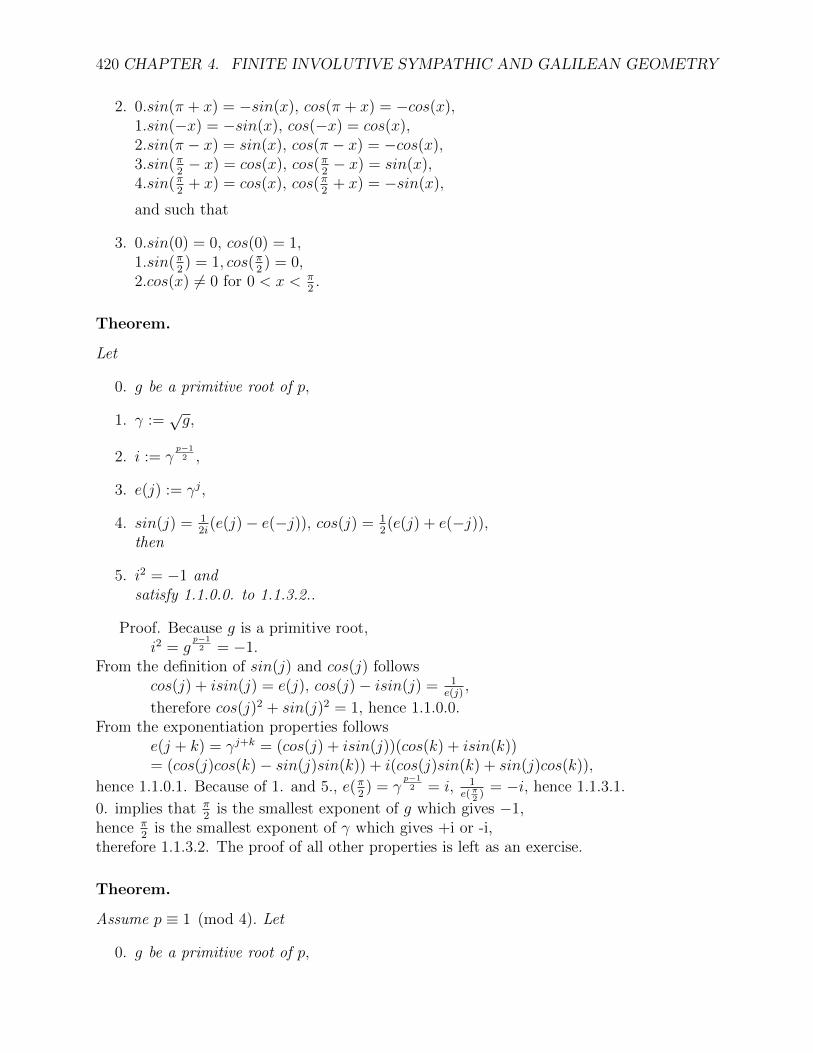
420 CHAPTER 4. FINITE INVOLUTIVE SYMPATHIC AND GALILEAN GEOMETRY
2. 0.sin(π + x) = −sin(x), cos(π + x) = −cos(x),1.sin(−x) = −sin(x), cos(−x) = cos(x),2.sin(π − x) = sin(x), cos(π − x) = −cos(x),3.sin(π
2− x) = cos(x), cos(π
2− x) = sin(x),
4.sin(π2
+ x) = cos(x), cos(π2
+ x) = −sin(x),
and such that
3. 0.sin(0) = 0, cos(0) = 1,1.sin(π
2) = 1, cos(π
2) = 0,
2.cos(x) 6= 0 for 0 < x < π2.
Theorem.
Let
0. g be a primitive root of p,
1. γ :=√g,
2. i := γp−12 ,
3. e(j) := γj,
4. sin(j) = 12i
(e(j)− e(−j)), cos(j) = 12(e(j) + e(−j)),
then
5. i2 = −1 andsatisfy 1.1.0.0. to 1.1.3.2..
Proof. Because g is a primitive root,i2 = g
p−12 = −1.
From the definition of sin(j) and cos(j) followscos(j) + isin(j) = e(j), cos(j)− isin(j) = 1
e(j),
therefore cos(j)2 + sin(j)2 = 1, hence 1.1.0.0.From the exponentiation properties follows
e(j + k) = γj+k = (cos(j) + isin(j))(cos(k) + isin(k))= (cos(j)cos(k)− sin(j)sin(k)) + i(cos(j)sin(k) + sin(j)cos(k)),
hence 1.1.0.1. Because of 1. and 5., e(π2) = γ
p−12 = i, 1
e(π2
)= −i, hence 1.1.3.1.
0. implies that π2
is the smallest exponent of g which gives −1,hence π
2is the smallest exponent of γ which gives +i or -i,
therefore 1.1.3.2. The proof of all other properties is left as an exercise.
Theorem.
Assume p ≡ 1 (mod 4). Let
0. g be a primitive root of p,

4.2. FINITE SYMPATHIC GEOMETRY. 421
1. i := gp−14 , δ := γ = sqr(g), g′ := −g p−3
2 ,then
2. sin(1) = ig′−12δ, cos(1) = g′+1
2δ.
Proof: gg′ = −g p−12 = 1, i2 = g
p−12 = −1.
δ−1 = δ/g = g′δ,hence
sin(1) = δ−δ−1
2i= −i1−g′
2δ,
cos(1) = δ+δ−1
2= 1+g′
2δ.
Theorem.
Assume p ≡ −1 (mod 4). Let
0. g be a primitive root of p,
1. δ := i or δ2 := −1, g′ := −g p−34 ,
then
2. sin(1) = (g − 1)g′ 12, cos(1) = (g + 1)g′ 1
2δ.
Proof: gg′2 = gp−12 = −1 = 1/δ2, therefore γg′ = 1/δ,
γ−1 = g′δ and γ = gg′δ,hence
sin(1) = γ−γ−1
2i= 1
2(g − 1)g′,
cos(1) = γ+γ−1
2= 1
2(g + 1)g′δ.
Example.
For p = 13, g = δ2 = 2, i = −5, g′ = −6, theni sin(i) cos(i) tan(i)0 0 1 01 −2δ 4δ 62 −6 −2 33 6δ 6δ 14 −2 −6 −45 4δ −2δ −26 1 0 ∞
For p = 11, g = 2, g′ = −4, δ2 = −1, theni sin(i) cos(i) tan(i)0 0 1 01 −2 5δ −4δ2 2δ 4 −5δ3 4 2δ −2δ4 5δ −2 3δ5 1 0 ∞
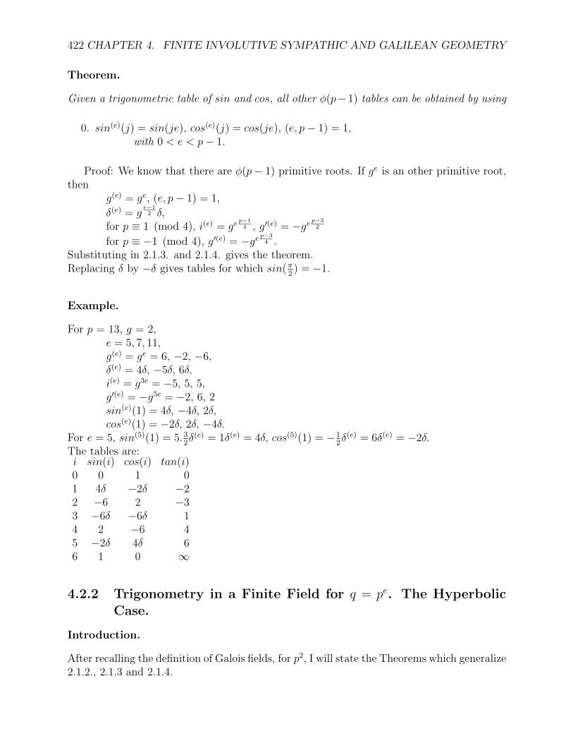
422 CHAPTER 4. FINITE INVOLUTIVE SYMPATHIC AND GALILEAN GEOMETRY
Theorem.
Given a trigonometric table of sin and cos, all other φ(p−1) tables can be obtained by using
0. sin(e)(j) = sin(je), cos(e)(j) = cos(je), (e, p− 1) = 1,with 0 < e < p− 1.
Proof: We know that there are φ(p− 1) primitive roots. If ge is an other primitive root,then
g(e) = ge, (e, p− 1) = 1,
δ(e) = ge−12 δ,
for p ≡ 1 (mod 4), i(e) = gep−14 , g′(e) = −ge p−3
2
for p ≡ −1 (mod 4), g′(e) = −ge p−34 .
Substituting in 2.1.3. and 2.1.4. gives the theorem.Replacing δ by −δ gives tables for which sin(π
2) = −1.
Example.
For p = 13, g = 2,e = 5, 7, 11,g(e) = ge = 6, −2, −6,δ(e) = 4δ, −5δ, 6δ,i(e) = g3e = −5, 5, 5,g′(e) = −g5e = −2, 6, 2sin(e)(1) = 4δ, −4δ, 2δ,cos(e)(1) = −2δ, 2δ, −4δ.
For e = 5, sin(5)(1) = 5.32δ(e) = 1δ(e) = 4δ, cos(5)(1) = −1
2δ(e) = 6δ(e) = −2δ.
The tables are:i sin(i) cos(i) tan(i)0 0 1 01 4δ −2δ −22 −6 2 −33 −6δ −6δ 14 2 −6 45 −2δ 4δ 66 1 0 ∞
4.2.2 Trigonometry in a Finite Field for q = pe. The HyperbolicCase.
Introduction.
After recalling the definition of Galois fields, for p2, I will state the Theorems which generalize2.1.2., 2.1.3 and 2.1.4.

4.2. FINITE SYMPATHIC GEOMETRY. 423
Definition.
Let n be a non quadratic residue, the set of elements in the Galois field p2, GF (p2), arethe polynomials of degree 0 or 1, for which addition is performed modulo p and multi-plication is performed modulo I2 − n. More specifically (uI + v) + (u′I + v′) =(u+ u′ mod p)I + (v + v′ mod p,
(uI + v).(u′I + v′) = (uv′ + u′v mod p)I + (vv′ + nuu′ mod p).Moreover (uI + v)−1 = −uI+v
v2−nu2 .More generally, if P is a primitive polynomial of degree n, i.e. a polynomial which has nofactors with coefficients in Zp, the set of elements in the Galois field pe, GF (pe), are the poly-nomials of degree less than e, for which addition is performed modulo p and multiplicationis performed modulo P.
Notation.
uI + v will be written u.v or up+ v.tI2 + uI + v will be written t.u.v or tp2 + up+ v, . . . .
Example.
Let q = 52, n = 3, g = I + 1 = 1.1 = 6, then9
g−1 = −2.2 = 3.2 = 17, g2 = 2.− 1 = 2.4 = 14, g4 = 1.− 2 = 1.3 = 8, g6 = 0.− 2 = 0.3 = 3,g12 = 0.− 1 = 0.4 = 4, hence −g11 = g−1.
Theorem.
2.1.1. generalizes for pe.The proof as well as the proof of the other theorems in this section are left as exercises.
Theorem.
Assume q = pe ≡ 1 (mod 4). Let
0. g be a primitive root of pe,
1. i := gq−14 , δ := sqr(g), g′ := −g q−3
2 ,then
2. sin(1) = i(g′ − 1)δ 12, cos(1) = (g′ + 1)δ 1
2.
Theorem.
Assume q = pe ≡ −1 (mod 4). Let
0. g be a primitive root of pe,
926.10.82

424 CHAPTER 4. FINITE INVOLUTIVE SYMPATHIC AND GALILEAN GEOMETRY
1. g′ = −g q−34 , δ2 = −1, g−1 = −g q−3
2 ,then
2. sin(1) = (g − 1)g′ 12, cos(1) = (g + 1)g′δ 1
2.
Example.
For q = 52, n = 3, δ2 = g = 6, i = g6 = 3, g′ = −g11 = 17,sin(1) = 2.4δ = 14δ, cos(1) = 4.4δ = 24δ.sin(2) = (−1.0).(2.2)−−2.− 1 = 3.4 = 19, cos2(1) = (2.− 1).(1.1) = 1.0,cos(2) = 2cos2(1)− 1 = 2.0− 0.1 = 2.− 1 = 2.4 = 14.This gives the Table:k sin(k) cos(k)0 0 11 14δ 24δ2 19 143 20δ 21δ4 3 105 4δ 12δ6 20 207 12δ 4δ8 10 39 21δ 20δ10 14 1911 24δ 14δ12 1 0
Exercise.
Verify the following and construct the corresponding trigonometric table.
0. For q = 132, n = −2, δ2 = g = 15, i = g42 = 8, g′ = −g83 = −147, g167 = 35,sin(1) = 110δ, cos(1) = 18δ,
1. For q = 72, n = 3, δ2 = −1, g = 8,sin(1) = 3.4.δ = 25δ, cos(1) = 2.2δ = 18δ,
2. For q = 112, δ2 = 13,sin(1) = 0.2δ = 2δ, cos(1) = 8.1δ = 89δ,
3. For q = 132, δ2 = 15,sin(1) = 11.0δ = 143δ, cos(1) = 3.1δ = 40δ,
4. For q = 172, δ2 = 20,sin(1) = 11.16δ = 203δ, cos(1) = 7.5δ = 124δ,
5. For q = 53, δ2 = 9,sin(1) = 3.3.0δ = 90δ, cos(1) = 4.4.1δ = 121δ,sin(2) = 87, cos(2) = 110.

4.2. FINITE SYMPATHIC GEOMETRY. 425
4.2.1 Trigonometry in a Finite Field for p. The Hyperbolic Case.
Introduction.
The trigonometry associated with the finite Euclidean plane with real isotropic points willfirst be defined and studied in this section for the finite field Zp. Theorems 4.2.1 and 4.2.1determine sin(1) and cos(1) from which all other values can be obtained using the additionformulas of 4.2.1.In section 4.2.2, definitions and results will be extended, for the finite field associated withpe, with proofs left as an exercise.The trigonometry associated with the finite Euclidean plane with no real isotropic pointswill obtained in section 4.2.3, sin(1) and cos(1) will be determined, for the general case pe
in 4.2.3 and 4.2.3.
Definition.
Given the setsZ of the integers,Zp of the integers modulo p,Zp−1 of the integers modulo p− 1,let δ be a square root of a non quadratic residue of p.
π := p− 1.The problem addressed here is to construct 2 functions sine or sin and cosine or cos with
domain Z and range Zp ∪ δZp which satisfy:
The Theorem of Pythagoras,
0. sin2(x) + cos2(x) = 1.
The addition formulas,
1. 0. sin(x+ y) = sin(x)cos(y) + cos(x)sin(y),1. cos(x+ y) = cos(x)cos(y)− sin(x)sin(y).
The periodicity property
2. sin(2π + x) = sin(x), cos(2π + x) = cos(x),
The symmetry properties
3. 0. sin(π + x) = −sin(x), cos(π + x) = −cos(x),1. sin(−x) = −sin(x), cos(−x) = cos(x),2. sin(π − x) = sin(x), cos(π − x) = −cos(x),3. sin(π
2− x) = cos(x), cos(π
2− x) = sin(x),
4. sin(π2
+ x) = cos(x), cos(π2
+ x) = −sin(x),
and such that1G35.TEX [MPAP], September 9, 2019

426 CHAPTER 4. FINITE INVOLUTIVE SYMPATHIC AND GALILEAN GEOMETRY
4. 0. sin(0) = 0, cos(0) = 1,1. sin(π
2) = 1, cos(π
2) = 0,
2. sin(x) 6= ±1 for 0 < x < π2.
Theorem.
Let
0. g be a primitive root of p,
1. γ :=√g,
2. ι := γp−12 ,
3. e(j) := γj,then
4. ι2 = −1 and
5. sin(j) = e(j)−e(−j)2ι
, cos(j) = e(j)+e(−j)2
,satisfy 4.2.1.0 to .4.
Proof. Because g is a primitive root,ι2 = g
p−12 = −1.
From the definition of sin(j) and cos(j) followscos(j) + ιsin(j) = e(j), cos(j)− ιsin(j) = e(j)−1,
therefore cos(j)2 + sin(j)2 = 1, hence 4.2.1.0.From the exponentiation properties follows
e(j + k) = γ(j+k) = (cos(j) + ιsin(j))(cos(k) + ιsin(k))= (cos(j)cos(k)− sin(j)sin(k)) + ι(cos(j)sin(k)− sin(j)cos(k)), hence 4.2.1.1.
From 5 and 4.2.1.1 follows 4.2.1.3.0, implies that π
2is the smallest exponent of g which gives -1, hence π
2is the smallest exponent
of γ which gives +ι or −ι, therefore 4.2.1.4.2. The proof of all other properties is left as anexercise. The next 2 Theorems give sin(1) and cos(1) first when ι ∈ Zp, then when this isnot the case.
Theorem.[Hyperbolic case]
Assume p ≡ 1 (mod 4). Let
0. g be a primitive root of p,
1. i := ι := gp−14 , δ := γ =
√g, g′ := −g p−3
2 ,then
2. sin(1) = ig′−12δ, and cos(1) = g′+1
2δ.
Proof: gg′ = −g p−12 = 1, i2 = g
p−12 = −1. δ−1 = δg−1 = g′δ ,
hencesin(1) = δ−δ−1
2i= −i1−g′
2δ, and cos(1) = δ+δ−1
2= 1+g′
2δ.

4.2. FINITE SYMPATHIC GEOMETRY. 427
Theorem.[Hyperbolic case]
Assume p ≡ −1 (mod 4). Let
0. g be a primitive root of p,
1. δ := ι or δ2 := gp−12 = −1, g′ := −g p−3
4 ,then
2. sin(1) = (g−1)g′
2, cos(1) = (g+1)g′
2δ.
Proof: gg′2 = gp−12 = −1 = δ−2. Because γ :=
√g, by taking square roots, γg′ = δ−1,
γ−1 = g′δ and γ = gg′δ ,hencesin(1) = γ−γ−1
2ι= (g−1)g′
2, cos(1) = γ+γ−1
2= (g+1)g′
2δ.
Example.
For p = 13, g = δ2 = 2, i = −5, g′ = −6, thenj sin(j) cos(j) tan(j)0 0 1 01 −2δ 4δ 62 −6 −2 33 6δ 6δ 14 −2 −6 −45 4δ −2δ −26 1 0 ∞
For p = 11, g = 2, g′ = −4, δ2 = −1. thenj sin(j) cos(j) tan(j)0 0 1 01 −2 5δ −4δ2 2δ 4 −5δ3 4 2δ −2δ4 5δ −2 3δ5 1 0 ∞
Theorem.
Given a trigonometric table of sin and cos, all other φ(p−1) tables can be obtained by using
0. sin(e)(j) = sin(je), cos(e)(j) = cos(je), (e, p− 1) = 1, with 0 < e < p− 1.
Proof: We know that there are φ(p− 1) primitive roots.If g(e) is an other primitive root, theng(e)e = ge, (e, p− 1) = 1, δ(e) = g
e−12 δ ,
for p ≡ 1 (mod 4), ie = gep−14 , g′e = −ge p−3
2 ,
for p ≡ −1 (mod 4), g′e = −ge p−34 .
Substituting in 2.1.3. and 2.1.4. gives the theorem.Replacing δ by −δ gives tables for which sin(π
2) = −1.

428 CHAPTER 4. FINITE INVOLUTIVE SYMPATHIC AND GALILEAN GEOMETRY
Example.
For p = 13, g = 2,e 5 7 11
g(e) = ge 6 −2 −6δe 4δ −5δ 6δie = g3e −5 5 5g′e = −g5e −2 6 2sin(e)(1) 4δ −4δ 2δcos(e)(1) −2δ 2δ −4δ
For e = 5, sin(5)(1) = 5.32δe = 1δe = 4δ, cos(5)(1) = −1
2δe = 6δe = −2δ.
The tables are:j sin(j) cos(j) tan(j)0 0 1 01 4δ −2δ −22 −6 2 −33 −6δ −6δ 14 2 −6 45 −2δ 4δ 66 1 0 ∞
4.2.2 Trigonometry in a Finite Field for q = pe. The HyperbolicCase.
Introduction.
After recalling the definition of Galois fields, I will generalize Theorems 4.2.1, 4.2.1 and 4.2.1.
Definition.
Let n be a non quadratic residue, the set of elements in the Galois field GF (p2), associatedwith p2, are the polynomials of degree 0 or 1, for which addition is performed modulo p andmultiplication is performed modulo P := I2 − n. More specifically
(uI + v) + (u′I + v′) = (u+ u′ mod p)I + (v + v′ mod p),(uI + v) · (u′I + v′) = (uv′ + u′v mod p)I + (vv′ + nuu′ mod p).
Moreover (uI + v)−1 = −uI+vv2−nu2 .
More generally, if P is a primitive polynomial of degree n, i.e. a polynomial which hasno factors with coefficients in Zp, the set of elements in the Galois field GF (pe), are thepolynomials of degree less than e, for which addition and multiplication is performed moduloP.
Notation.
uI + v will be written u.v or up+ v, tI2 + uI + v will be written t.u.v or tp2 + up+ v.

4.2. FINITE SYMPATHIC GEOMETRY. 429
Example.
Let q = 52, n = 3, g = I + 1 = 1.1 = 6, theng−1 = −2.2 = 3.2 = 17, g2 = 2.− 1 = 2.4 = 14, g4 = 1.− 2 = 1.3 = 8, g6 = 0.− 2 = 0.3 = 3,g12 = 0.− 1 = 0.4 = 4, hence −g11 = g−1.
Theorem.
Theorems 4.2.1, 4.2.1 and 4.2.1 generalize, with p replaced by q := pe.
Example.
For q = 52, n = 3, δ2 = g = 6, i = g6 = 3, g′ = −g11 = 17,sin(1) = 2.4δ = 14δ, cos(1) = 4.4δ = 24δ.sin(2) = (−1.0) · (2.2) − −2. − 1 = 3.4 = 19, cos2(1) = (2. − 1) · (1.1) = 1.0, cos(2) =2cos2(1)− 1 = 2.0− 0.1 = 2.− 1 = 2.4 = 14.This gives the Table:k sin(k) cos(k)0 0 11 14δ 24δ2 19 143 20δ 21δ4 3 105 4δ 12δ6 20 207 12δ 4δ8 10 39 21δ 20δ
10 14 1911 24δ 14δ12 1 0
Exercise.
Verify the following and construct the corresponding trigonometric table.
0. For q = 132, n = −2, δ2 = g = 15, i = g42 = 8, g′ = −g83 = −147, g167 = 35,sin(1) = 110δ, cos(1) = 18δ,
1. For q = 72, n = 3, δ2 = −1, g = 8, sin(1) = 3.4.δ = 25δ,cos(1) = 2.2δ = 18δ,
2. For q = 112, δ2 = 13, sin(1) = 0.2δ = 2δ, cos(1) = 8.1δ = 89δ,
3. For q = 132, δ2 = 15, sin(1) = 11.0δ = 143δ, cos(1) = 3.1δ = 40δ,
4. For q = 172, δ2 = 20, sin(1) = 11.16δ = 203δ, cos(1) = 7.5δ = 124δ,
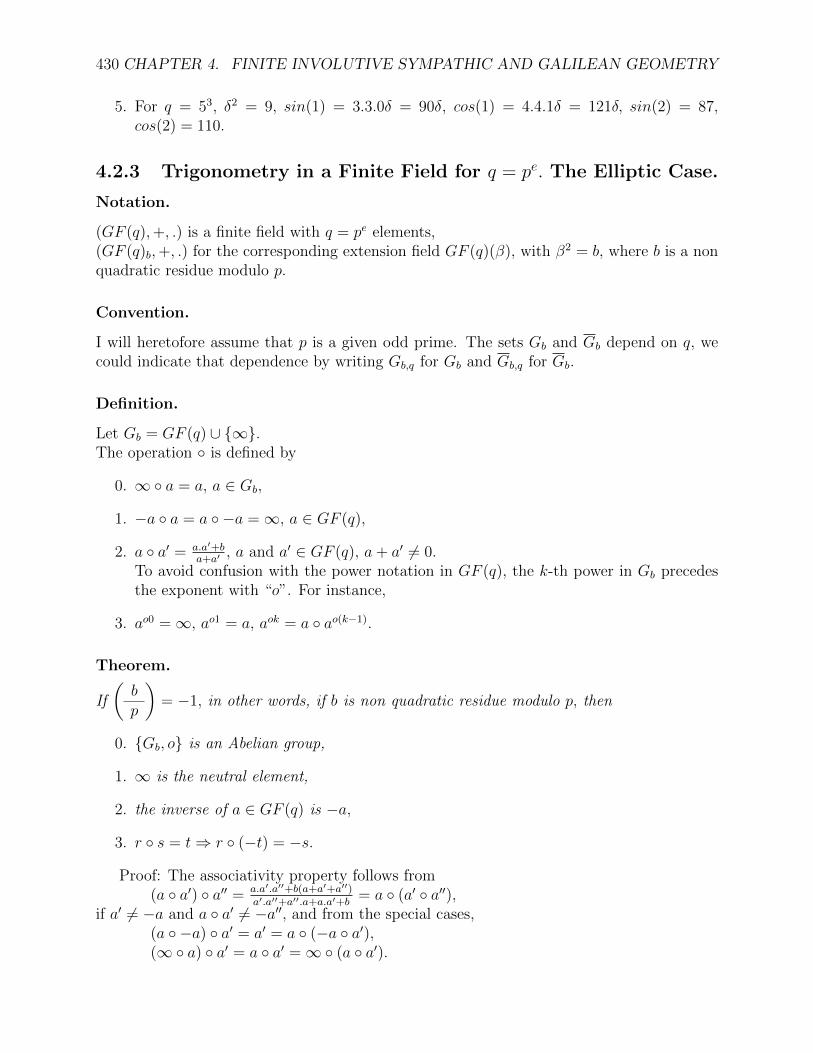
430 CHAPTER 4. FINITE INVOLUTIVE SYMPATHIC AND GALILEAN GEOMETRY
5. For q = 53, δ2 = 9, sin(1) = 3.3.0δ = 90δ, cos(1) = 4.4.1δ = 121δ, sin(2) = 87,cos(2) = 110.
4.2.3 Trigonometry in a Finite Field for q = pe. The Elliptic Case.
Notation.
(GF (q),+, .) is a finite field with q = pe elements,(GF (q)b,+, .) for the corresponding extension field GF (q)(β), with β2 = b, where b is a nonquadratic residue modulo p.
Convention.
I will heretofore assume that p is a given odd prime. The sets Gb and Gb depend on q, wecould indicate that dependence by writing Gb,q for Gb and Gb,q for Gb.
Definition.
Let Gb = GF (q) ∪ ∞.The operation is defined by
0. ∞ a = a, a ∈ Gb,
1. −a a = a −a =∞, a ∈ GF (q),
2. a a′ = a.a′+ba+a′
, a and a′ ∈ GF (q), a+ a′ 6= 0.To avoid confusion with the power notation in GF (q), the k-th power in Gb precedesthe exponent with “o”. For instance,
3. ao0 =∞, ao1 = a, aok = a ao(k−1).
Theorem.
If
(bp
)= −1, in other words, if b is non quadratic residue modulo p, then
0. Gb, o is an Abelian group,
1. ∞ is the neutral element,
2. the inverse of a ∈ GF (q) is −a,
3. r s = t⇒ r (−t) = −s.
Proof: The associativity property follows from(a a′) a′′ = a.a′.a′′+b(a+a′+a′′)
a′.a′′+a′′.a+a.a′+b= a (a′ a′′),
if a′ 6= −a and a a′ 6= −a′′, and from the special cases,(a −a) a′ = a′ = a (−a a′),(∞ a) a′ = a a′ =∞ (a a′).
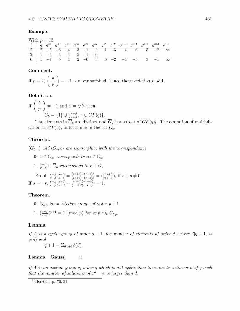
4.2. FINITE SYMPATHIC GEOMETRY. 431
Example.
With p = 13,b g go2 go3 go4 go5 go6 go7 go8 go9 go10 go11 go12 go13 go14
2 2 −5 −6 −4 3 −1 0 1 −3 4 6 5 −2 ∞2 1 −5 4 −4 5 −1 ∞6 1 −3 5 4 2 −6 0 6 −2 −4 −5 3 −1 ∞
Comment.
If p = 2,
(bp
)= −1 is never satisfied, hence the restriction p odd.
Definition.
If
(bp
)= −1 and β =
√b, then
Gb = 1 ∪ r+βr−β , r ∈ GF (q).
The elements in Gb are distinct and Gb is a subset of GF (q)b. The operation of multipli-cation in GF (q)b induces one in the set Gb.
Theorem.
(Gb, .) and (Gb, o) are isomorphic, with the correspondance
0. 1 ∈ Gb, corresponds to ∞ ∈ Gb,
1. r+βr−β ∈ Gb corresponds to r ∈ Gb.
Proof: r+βr−β .
s+βs−β = (rs+b)+(r+s)β
(rs+b)−(r+s)β= ( rs+β
rs−β ), if r + s 6= 0.
If s = −r, r+βr−β .
s+βs−β = (r+β)(−r+β)
(−r+β)(−r−β)= 1,
Theorem.
0. Gb,p is an Abelian group, of order p+ 1.
1. ( r+βr−β )p+1 ≡ 1 (mod p) for any r ∈ Gb,p.
Lemma.
If A is a cyclic group of order q + 1, the number of elements of order d, where d|q + 1, isφ(d) and
q + 1 = Σd|q+1φ(d).
Lemma. [Gauss] 10
If A is an abelian group of order q which is not cyclic then there exists a divisor d of q suchthat the number of solutions of xd = e is larger than d.
10Herstein, p. 76, 39

432 CHAPTER 4. FINITE INVOLUTIVE SYMPATHIC AND GALILEAN GEOMETRY
Lemma.
The polynomialRd := (r + β)d − (r − β)d
has at most d roots in Gd.Proof: Dividing by β, we obtain a polynomial in Zp of degree d− 1, which has therefore
at most d− 1 roots for z ∈ Zp or d roots in Gd (∞ being a root).
Example.
With p = 13, b = 2, if Sd is the set of roots of Rd
d = 1, S1 = ∞.d = 2, S2 = 0 ∪ S1,d = 7, S7 = ±1,±4,±5 ∪ S1,d = 14, S14 = ±2,±3,±6 ∪ S7 ∪ S2.
Theorem.
(Gb,p, .) is a cyclic group of order p+ 1.(Gb,p, o) is a cyclic group of order p+ 1.
Example.
2 is a generator of G13,2, 1 is a generator of G13,6.
Theorem.[Elliptic case]
Given q = pe ≡ 1 (mod 4). Let
0. b be a non quadratic residue,
1. rb be a generator of Gb,
2. i2 := −1,
3. β2 := b,
4. r := ro p−1
4b ,
then
5. sin(1) = r2+br2−b , cos(1) = −2ri
r2−bβ.
Proof: Let σ = rb+βrb−β
, then σp+1 = 1 and 0 < i < p+ 1⇒ σi 6= 1.
ρ2 = σ ⇒ ρ2(p+1) = 1 and 0 < i < 2(p+ 1)⇒ ρi 6= 1.
If we take square roots twice, ρp+12 = ±i, we want ρ
p+12 = σ
p+14 = i, then ρ = cos(1)+isin(1),
and ρ2(p+1) = cos(2(p+ 1)) + isin(2(p+ 1)) = 1.
If r = ro p−1
4b , then ρ
p−12 = σ
p−14 = r+β
r−β , or i = ρp+12 = ρρ
p−12 = ρ r+β
r−β , or cos(1) + i sin(1) =
ρ = i r−βr+β
, cos(1)− i sin(1) = ρ−1 = −i r+βr−β ,

4.2. FINITE SYMPATHIC GEOMETRY. 433
thereforecos(1) = −2i r β 1
r2−β2 , sin(1) = r2+β2
r2−β2 .
Example.
q = 13, i = 5, b = β2 = 6, rb = 1, r = 5, r2 = −1, sin(1) = 3, cos(1) = −4β.k sin(k) cos(k) tan(k) atan(kβ)0 0 1 0β 01 3 −4β −5β −32 2β −4 6β 43 5 −3β −1β 64 −3β 5 2β 55 −4 2β 4β −16 −4β 3 3β 27 1 0β ∞ −2
q b i r sin(1) cos(1)5 2 2 2 −2 −β
17 4 3 6 −5 −3β29 12 2 7 −2 −10β37 6 2 5 6 −β41 9 2 −17 −5 −19β
Theorem.[Elliptic case]
Given q = pe ≡ −1 (mod 4). Let
0. b be a non quadratic residue,
1. rb be a generator of Gb,
2. ι2 := −1, δ := ι,
3. β2 := b,
4. r := ro p+1
4b ,
then
5. cos(1) = rb√b−r2b
δ, sin(1) = rcos(1)rb
.
Proof: The proof proceeds at first as in 4.2.3. r+βr−β = i, therefore r = −βi, this establishes
the relationship between the sign for the square root of -1 and b.
cos(2) = 12(σ + σ−1) =
r2b+b
r2b−band sin(2) = 1
2i(σ − σ−1) = 2rb
r2b−b.
2cos2(1) = 1 + cos(2)⇒ cos(1) = rb√r2b−b
,
moreoverrbb−rb
= −cos2(1), sin(1) follows from 2sin(1)cos(1) = sin(2) = 2rcos2(1)rb
, insuring the consis-
tency between the signs of sin(1) and cos(1) to insure that sin(π2) = 1.

434 CHAPTER 4. FINITE INVOLUTIVE SYMPATHIC AND GALILEAN GEOMETRY
Example.
q = 11, δ2 = −1, b = 2, rb = 1, r = −3, cos(1) = δ, sin(1) = −3δ.k sin(k) cos(k) tan(k) atan(kβ)1 −3δ 1δ −3 32 −5 −3 −2 −23 4δ 4δ 1 −14 −3 −5 5 −55 1δ −3δ −4 46 1 0 ∞ −4
q b rb r sin(1) cos(1)3 2 1 1 δ δ7 3 1 2 3δ −2δ
19 2 1 6 6δ δ23 5 1 8 4δ −11δ31 3 1 −11 −13δ 4δ43 3 5 −13 −7δ 6δ47 5 4 18 3δ −15δ.
Theorem.
If as usual, π := p+ 1 in the elliptic case or π := p− 1 in the hyperbolic case, then
0. 3 | π ⇒ sin(π6) = 1
2, cos(π
6) =
√3
2.
1. 4 | π ⇒ cos(π4) =
√2
2.
2. 5 | π ⇒ cos(π5) =
√5+14, cos(2π
5) =
√5−14,
sin(π5) =
√10−2
√5
4, sin(2π
5) =
√10+2
√5
4.
In the classical case, there is no ambiguity of sign, because 0 < x < π2
=⇒ sin(x), cos(x) >0. This is not the case in a finite field, the formulas can only give the trigonometric functions
up to the sign, or alternately one of the values of√
3,√
2√
5,√
10± 2√
5 can be derivedfrom cos(π
6), cos(π
4), cos(π
5), sin(π
5) and sin(2π
5).
Example.
p = 11, elliptic case, sin(2) = −5, cos(2) = −3 =⇒√
3 = 5,with δ2 = −1, cos(3) = 4δ =⇒
√2 = −3δ.
p = 11, hyperbolic case, cos(2) = 4, cos(4) = −2 =⇒√
5 = 4,with γ2 = −3, sin(2) = −4γ =⇒
√2 = −5γ, sin(4) = γ =⇒
√−4 = 4γ.
p = 19, elliptic case, cos(5) = −9δ =⇒√
2 = δ,with δ2 = 2, cos(4) = −2 =⇒ cos(8) = 7 =⇒
√5 = −9,
sin(4) = 4 =⇒√
9 = −3, sin(8) = 3 =⇒√−8 = −7.

4.2. FINITE SYMPATHIC GEOMETRY. 435
Definition.
Lemma.
If rb is a generator of Gb and b′ := br2b, then
0. krb is a generator of Gbk2 ,
1. 1 is a generator of Gb′ .
Theorem.
0. There exists always fundamental roots.
1. There exist 12φ(p+ 1) fundamental roots associated with p.
Example.
6, 7 and 8 are the fundamental roots for p = 13,6, 7 and 12 are the fundamental roots for p = 17,3, 11, 18 and 27 are the fundamental roots for p = 29,6, 14, 15, 18, 19, 20, 23, 24 and 32 are the fundamental roots for p = 37,12, 13, 28, 29, 30 and 35 are the fundamental roots for p = 41.
Theorem.
Given an involution, I(x) = ax+bcx−a , aa + bc 6= 0, an amicable projectivity, in other words a
projectivity with the same fixed points, real or complex, is given byT (x) = (a+f)x+b
cx−a+f,
where f = ±√
(aa+ bc)/d).
Proof: If
(dp
)= −1 then Fd is a fundamental projectivity:
Fd = y+dy+1
.In view of 4.2.3, we have Fd = y 1.
Comment.
( r+βr−β )e ≡ 1, for e|p+ 1 =⇒ (r + β)e − (r − β)e ≡ 0,
dividing by β , we obtain a polynomial in Zp of degree e − 1, which has therefore at moste− 1 roots for z in Zp or e roots in G (∞ being a root). We want to show that (G , .) andtherefore (G,∞) are cyclic groups.
Theorem.
Let
0. r0 = 1, r1 = r, ri+1 = ri r,

436 CHAPTER 4. FINITE INVOLUTIVE SYMPATHIC AND GALILEAN GEOMETRY
1. xi ≡ 1/ri(∈ G ),
2. ui+1 ≡ rui + sui−1, u0 = 0, u1 = 1,vi+1 ≡ rvi + svi−1, v0 = 2, v1 = r,
3. 4s ≡ d− r2,
4. α = r+√d
2and β = r−
√d
2,
then
5. xi+1 ≡ rxi+1dxi+r
(mod p), x0 = 0,
6. r = α + β,√d = α− β, s = −αβ.
7. ui = (αi − βi)/√d, vi = αi + βi,
8. 2ui+j = uivj + viuj, 2vi+j = vivj + buiuj,
9. ui+1(bui + rvi)− vi+1(rui + vi) = 0,
10. xivi = ui.
Proof: (rui + sui−1) = (α+β)(αi−βi)−αβ(αi−1−βi−1)√d
= αi+1−βi+1√d
= ui+1.Substituting in 2. with j = 1 after multiplication by 2 gives((uiv1 + viu1)(bui + rvi)− (viv1 + buiu1)(rui + vi)
= u2i (bv1 − rbu1) + uivi(bu1 + rv1 − rv1 − bu1) + v2
i (ru1 − v1) = 0.Morover,
rui+vidui+rvi
= (α+β)(αi−βi)+(α−β)(αi+βi)
((α−β)(αi−βi)+(α+β)(αi+βi))√d
= ui+1
vi+1= xi+1.
Example.
For p = 7, elliptic case, ι2 = −1,Ak = (cos(k), sin(k), 1)
are points on the conicx2 + y2 = z2.
If we define it as a circle and z = 0 as the ideal line, the isotropic points are not real and wehave a Euclidean geometry.The center of the circle, which is the pole of z = 0 is (0,0,1). There are 8 real points on thecircle,
A0 = (1, 0, 1), A2 = (−2,−2, 1), A4 = (0, 1, 1), A6 = (2,−2, 1),A8 = (−1, 0, 1), A10 = (2, 2, 1), A12 = (0,−1, 1), A14 = (−2, 2, 1).
The distances on the lines a2k = O × A2k, k = 0, 1, 2, 3, are real.a0 = [0, 1, 0], a2 = [2,−2, 0], a4 = [1, 0, 0], a6 = [1, 1, 0].The other lines through O intersect the circle at complex points:
A1 = (2ι, 4ι, 1), A3 = (4ι, 2ι, 1), A5 = (−4ι, 2ι, 1),A7 = (−2ι, 4ι, 1), A9 = (−2ι,−4ι, 1), A11 = (−4ι,−2ι, 1),A13 = (4ι,−2ι, 1), A15 = (2ι,−4ι, 1).

4.2. FINITE SYMPATHIC GEOMETRY. 437
These are on the lines a2k+1 = O × A2k+1, k = 0, 1, 2 , 3,a1 = [−2, 1, 0], a3 = [1,−2, 0], a5 = [1, 2, 0], a7 = [2, 1, 0].
If B1 = (1, 2, 1) is a real point on a1, B1 is on a circlex2 + y2 = 5z2.
this circle intersects a2k+1 at real points and a2k at complex points. The distances betweenpoints on a1 are multiples of ι, because
√5 = 3ι. The same is true on the lines a3, a5, a7.
Definition.
The smallest j such that uj ≡ 0 (mod p) is called the rank of apparition of p. Hence
Theorem.
For a fixed r there are 12φ(p+ 1) values of s in [1, p− 1] for which the rank of apparition is
p+ 1. More generally, there are φ( e2) values of s in [1, p− 1] for which the rank of apparition
is e, e divides p+ 1, e > 2.
Theorem.
If b is a fundamental root modulo p, thenb = Np, 1− b = Np.
Comment.
For p = 17, 11Np, 7Np, but 7 is not a fundamental root.
Theorem.
For a given p, the setsSh = cos2(j), j = 1, . . . , p−3
2, in the hyperbolic case and
Se = cos2(j), j = 1, . . . , p−12, in the elliptic case are
independent of the choice of the primitive root or of the fundamental root.
Example.
p = 11, Sh = 4, 5, 7, 8, Se = 2, 3, 6, 9, 10p = 29, Sh = 3, 5, 6, 7, 11, 12, 15, 18, 19, 23, 24, 25, 27,
Se = 2, 4, 8, 9, 10, 13, 14, 16, 17, 20, 21, 22, 26, 28.
Theorem.
0. Let sin(j) ∈ Zp − 0 − 1,if p ≡ −1 (mod 4), then sin(j)sin(k) 6= 1, for all k,if p ≡ 1 (mod 4), then sin(j)sin(k) = 1 for some k.

438 CHAPTER 4. FINITE INVOLUTIVE SYMPATHIC AND GALILEAN GEOMETRY
1. sin(j)γ∈ Zp − 0
if p ≡ 1 (mod 4), then sin(j)sin(k) 6= 1, for all k,if p ≡ −1 (mod 4), then sin(j)sin(k) = 1, for some k.

4.2. FINITE SYMPATHIC GEOMETRY. 439
Example.
. . . Give examples of associated fundamental sympathic projectivities, see 1.10.If T (r) = r+d
r+1. For p = 7, d = 3, (5 is the other choice)
r ∞ 0 1 2 3 4 5 6T (r) 1 3 2 4 5 0 6 ∞
. . . talk about transformations such as r = 2s leading to the form used in 1.10S(s) = 2s+b
2−3s.
Example.
For p = 13, (see g35.bas .5.)A = (0, 1, 0), Aj = (1, j, 0), j = 0, . . . , q − 1, A × Aj = [0, 0, 1], dj = dist(A,Aj) :cos(dj) = j√
1+j2, sin(dj) = 1√
1+j2,
j√
1 + j2 sin(dj) cos(dj) dj0 1 1 0 1
2
1 . . . .
tan(dist(Aj, Ak)) = k−j1+jk
tan(dist(A,Ak) = − 1k
tan(dist(Aj, Al)) = tan(dist(Aj, Ak) + dist(Ak, Al)).Indeed, the second member is(k−j)(1+lk)+(l−k)(1+jk)(1+jk)(1+lk)−(k−j)(l−k)
= (l−j)(1+k2)(1+lj)(1+k2)
= tan(dist(Aj, Al)).andtan(dist(Aj, Al)) = tan(dist(Aj, A) + dist(A,Al))Indeed, the second member is1j− 1l
1+ 1kl
= l−j1+kl
= tan(dist(Aj, Al)).
j \ k 0 1 2 3 4 5 60 3
121112
1012
412
512
1 912
812
712
112
212
2 112
412
1112
512
612
3 212
512
112
612
712
4 812
1112
712
612
112
56 7
121012
612
512
1112
A 612
912
512
412
1012
1112
Example.
p = 13, h, the correspondence between the point Aj = (1, j, 0) and d(j) isj 0 −2 −3 1 4 6 ∞ −6 −4 −1 3 212d(j) 0 1 2 3 4 5 6 7 8 9 10 11i = ±5 corresponds to the ideal point, d(5) = d(−5) =∞.
elliptic case:jδ 0 3 −1 −2 4 −5 6 ∞ −6 5 −4 2 1 −3d(j) 0 1 2 3 4 5 6 7 8 9 10 11 12 13

440 CHAPTER 4. FINITE INVOLUTIVE SYMPATHIC AND GALILEAN GEOMETRY
tan(dist(Aj, Ak)) = d(k)−d(j)1+d(j)d(k)
.
4.2.4 Periodicity.
Definition.
Let f be a function, g(0) is arbitrary,g(i+ 1) = ai+ g(i) + f(i) + f(i+ 1),
where a is such thatg(T ) = g(0),
and we writeg = Tf.
Theorem.
If f is a periodic function with period T, then0. g is periodic.1. f odd ⇒ geven.
Example.
i 0 1 2 3 4 5 6 7 8 9 10f(i) 1 −3 −1 1 3 −1 3 1 −1 −3 1g(i) 0 −2 −6 −6 −2 0 2 6 6 2 0
In this example a = 0.
Example.
i 0 1 2 3 4 5f(i) 0 4 7 7 4 0g(i+ 1
2) 0 9 −8 9 0
h(i)− ai 0 0 9 1 −9 −9h(i) 0 −2 5 −5 2 0
In this example a = −−95.
Definition.
Let f be a function. Let g be defined byg(i+ 1
2) = u(fi, fi+1),
where u is symmetric in its arguments,we write
g = Uf.Let h be defined by
h(0) is arbitrary,h(i+ 1) = ai+ h(i) + g(i+ 1
2),
h(T ) = h(0).
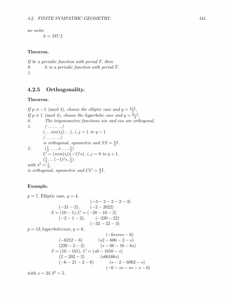
4.2. FINITE SYMPATHIC GEOMETRY. 441
we writeh = MUf.
Theorem.
If be a periodic function with period T, then0. h is a periodic function with period T.1.
4.2.5 Orthogonality.
Theorem.
If p ≡ −1 (mod 4), choose the elliptic case and q = p+12,
If p ≡ 1 (mod 4), choose the hyperbolic case and q = p−12,
0. The trigonometric functions sin and cos are orthogonal.1. ( . . . .. ..)
(. . . sin(ij) . . .), i, j = 1 to q − 1( . . . .. ..)is orthogonal, symmetric and SS = q
2I.
2. (12. . . ..s . . . ..1
2)
C = (scos(ij)(−1)is), i, j = 0 to q + 1,(1
2. . . (−1)js..1
2)
with s2 = 12,
is orthogonal, symmetric and CC = q2I.
Example.
p = 7, Elliptic case, q = 4,(−3− 2− 2− 2− 3)
(−21− 2), (−2− 2022)S = (10− 1), C = (−20− 10− 2)
(−2− 1− 2), (−220− 22)(−32− 22− 3)
p = 13, hyperboliccase, q = 6,(−6sssss− 6)
(−6212− 6) (s2− 606− 2− s)(220− 2− 2) (s− 66− 16− 6s)
S = (10− 101), C = (s0− 1010− s)(2− 202− 2) (s66166s)(−6− 21− 2− 6) (s− 2− 6062− s)
(−6− ss− ss− s− 6)with s = 2δ, δ2 = 5.

442 CHAPTER 4. FINITE INVOLUTIVE SYMPATHIC AND GALILEAN GEOMETRY
4.2.6 Conics in sympathic geometry.
Theorem.
X0i = acos(2i), X1i = bsin(2i), X2i = 1.X0i = a
δcos(2i+ 1), X1i = b
δsin(2i+ 1), X2i = 1.
X0i = acos(2i), X1i = bδsin(2i), X2i = 1.
X0i = aδcos(2i+ 1), X1i = bsin(2i+ 1), X2i = 1.
Example.
Let p = 11, a = 1, b = 2, δ = i, i2 = −1.In the elliptic case, . . . gives X02 +X12 2
4= 1 :
(1, 0), (−3, 1), (−5, 5), (0, 2), (5, 5), (3, 1),(−1, 0), (3,−1), (5,−5), (0,−2), (−5,−5), (−3,−1).. . . gives−X02 −X12 2
4= 1 :
(1, 5), (4,−3), (−3, 2), (3, 2), (−4,−3), (−1, 5),(−1,−5), (−4, 3), (3,−2), (−3,−2), (4, 3), (1,−5).In the hyperbolic case, . . . givesX02 − 1
4X12 = 1 :
(1, 0), (4, 4), (−2,−1), (2,−1), (−4, 4),(−1, 0), (−4,−4), (2, 1), (−2, 1), (4,−4).The asymptotic directions are (5,1,0) and (−5, 1, 0).. . . gives−X02 + 1
4X12 = 1 :
(5,−4), (2,−3), (0, 2), (−2,−3), (−5,−4),(−5, 4), (−2, 3), (0,−2), (2, 3), (5, 4).The asymptotic directions are (5,1,0) and (−5, 1, 0).
Example.
Let p = 13, a = 1, b = 2, δ = 2, i = 5.In the elliptic case, . . . givesX02 + 1
2X12 = 1 :
(1, 0), (−4,−3), (5,−2), (3, 6), (−3, 6), (−5,−2), (4,−3),(−1,−0), (4, 3), (−5, 2), (−3,−6), (3,−6), (5, 2), (−4, 3).. . . gives2X02 + 1
4X12 = 1 :
(3, 6), (−1,−3), (5, 5), (0, 2), (−5, 5), (1,−3), (−3, 6),(−3,−6), (1, 3), (−5,−5), (0,−2), (5,−5), (−1, 3), (3,−6).In the hyperbolic case, . . . givesX02 + 1
4X12 = 1 :
(1, 0), (−2, 1), (−6,−4), (0, 2), (6,−4), (2, 1),(−1, 0), (2,−1), (6, 4), (0,−2), (−6, 4), (−2,−1),the asymptotic directions are (4,1,0) and (−4, 1, 0).

4.2. FINITE SYMPATHIC GEOMETRY. 443
. . . gives2X02 + 1
2X12 = 1 :
(4,−4), (6,−1), (−2,−5), (2,−5), (−6,−1), (−4,−4),(−4, 4), (−6, 1), (2, 5), (−2, 5), (6, 1), (4, 4),the asymptotic directions are (4,1,0) and (−4, 1, 0).
4.2.7 Regular polygons and Constructibility.
Definition.
A regular polygon . . .because the angles are multiples of 2r
p−1or 2r
p+1.
The only regular polygons are those whose number of sides is a divisor of p − 1 or p +1. If we give the unit angle then we can define “convex polygons” and “star polygons”,find appropriate names.The constructibility by rule and compass in Euclidean geometry corresponds here to thosewhich demand the solution of equations of the first and second degree.The work of Gauss on cyclotomic polynomials extend immediately to the finite case becauseof Theorem . . . on trigonometric functions.
Theorem.
0. For a regular polygon of n sides to exist, n must divide . . .1. For a regular polygon to be constructible using only equations of the second degree,n must have the form 2i0pi11 p
i22 . . . p
ikk , where i0 is a non negative integer, i1, i2, . . . ik, are 0
or 1 and pj are primes of the form 2k + 1, namely, 3, 5, 17, 257, 65537, . . . .All square roots are integers except perhaps the last one.
Theorem.
For triangles.
cos(2r3
) = 12, sin(2r
3) =
√32.
Example.
p = 5, elliptic case,cos(2r
3) = 3, sin(2r
3) =√
2.p = 7, hyperbolic case,cos(2r
3) = 4, sin(2r
3) =√
6,p = 23, elliptic case,cos(2r
3) = 12, sin(2r
3) = 8.
Theorem.
For hexagons, we first obtain the triangle and then usecos(2r
6) = sin(2r
3), sin(2r
6) = cos(2r
3).

444 CHAPTER 4. FINITE INVOLUTIVE SYMPATHIC AND GALILEAN GEOMETRY
Example.
p = 23, elliptic case,cos(2r
6) = 8, sin(2r
6) = 12.
Theorem.
For pentagons. The polynomial to solve isx2 − x+ 1 = 0,
cos(2r5
) = x2, sin(2r
5) =
√1− x2
4.
Example.
p = 11, hyperbolic case, γ2 = 8.
x1 = (1 +√
52
= 1+72
= 4, x2 = 1−72
= −3,
cos1(2r5
) = 2, cos2(2r5
) = 4,
sin1(2r5
) =√−3 = γ, sin2(2r
5) =√−4 = −4γ.
The choice of 1 or 2 is arbitrary as is the choice of the sign of the coefficient of γ. The secondcase corresponds to sin(2r
5) of the trigonometric table, trig.tab.
The first, corresponds to sin(6r5
) of the same table.p = 19, elliptic case, δ2 = 10. x = 1+9
2= 5,
cos1(2r5
) = 52
= −7 = cos(6r5
) of trig.tab.
sin1(2r5
) =√
9 = 3 = sin(6r5
).
Theorem.
For decagons, we first obtain the pentagon and then use cos( 2r10
) =
√(1+cos 2r
5
2, sin( 2r
10) =
sin2r5
2cos( 2r10
.
Example.
p = 19, elliptic case,cos1( 2r
10) =√−3 = 4 = cos( 6r
10), sin1( 2r
10) = 3
8= −2.
Theorem.
For 17 sided polygons. The polynomials to solve are in succession:u2 + u+ 4 = 0, of which we choose 1 root,v2 − uv − 1 = 0,v′ = −3+6v−v3
2,
w2 − vw + v′ = 0,cos( 2r
p+j) = w
2, sin( 2r
p+j) =
√1− (w
2)2.
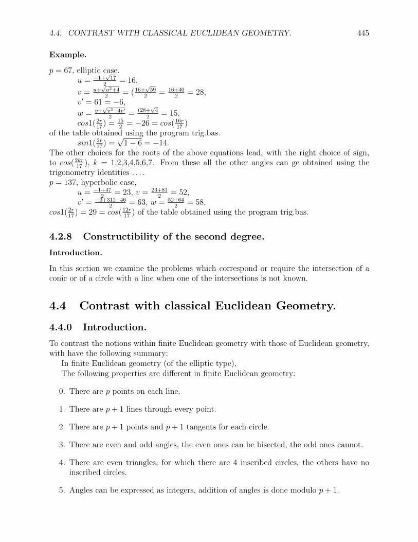
4.4. CONTRAST WITH CLASSICAL EUCLIDEAN GEOMETRY. 445
Example.
p = 67, elliptic case.u = −1+
√17
2= 16,
v = u+√u2+42
= (16+√
592
= 16+402
= 28,v′ = 61 = −6,
w = v+√v2−4v′
2= (28+
√4
2= 15,
cos1( 2r17
) = 152
= −26 = cos(16r17
)of the table obtained using the program trig.bas.
sin1( 2r17
) =√
1− 6 = −14.The other choices for the roots of the above equations lead, with the right choice of sign,to cos(2kr
17), k = 1,2,3,4,5,6,7. From these all the other angles can ge obtained using the
trigonometry identities . . . .p = 137, hyperbolic case,
u = −1+472
= 23, v = 23+812
= 52,v′ = −3+312−46
2= 63, w = 52+64
2= 58,
cos1( 2r17
) = 29 = cos(12r17
) of the table obtained using the program trig.bas.
4.2.8 Constructibility of the second degree.
Introduction.
In this section we examine the problems which correspond or require the intersection of aconic or of a circle with a line when one of the intersections is not known.
4.4 Contrast with classical Euclidean Geometry.
4.4.0 Introduction.
To contrast the notions within finite Euclidean geometry with those of Euclidean geometry,with have the following summary:
In finite Euclidean geometry (of the elliptic type),The following properties are different in finite Euclidean geometry:
0. There are p points on each line.
1. There are p+ 1 lines through every point.
2. There are p+ 1 points and p+ 1 tangents for each circle.
3. There are even and odd angles, the even ones can be bisected, the odd ones cannot.
4. There are even triangles, for which there are 4 inscribed circles, the others have noinscribed circles.
5. Angles can be expressed as integers, addition of angles is done modulo p+ 1.
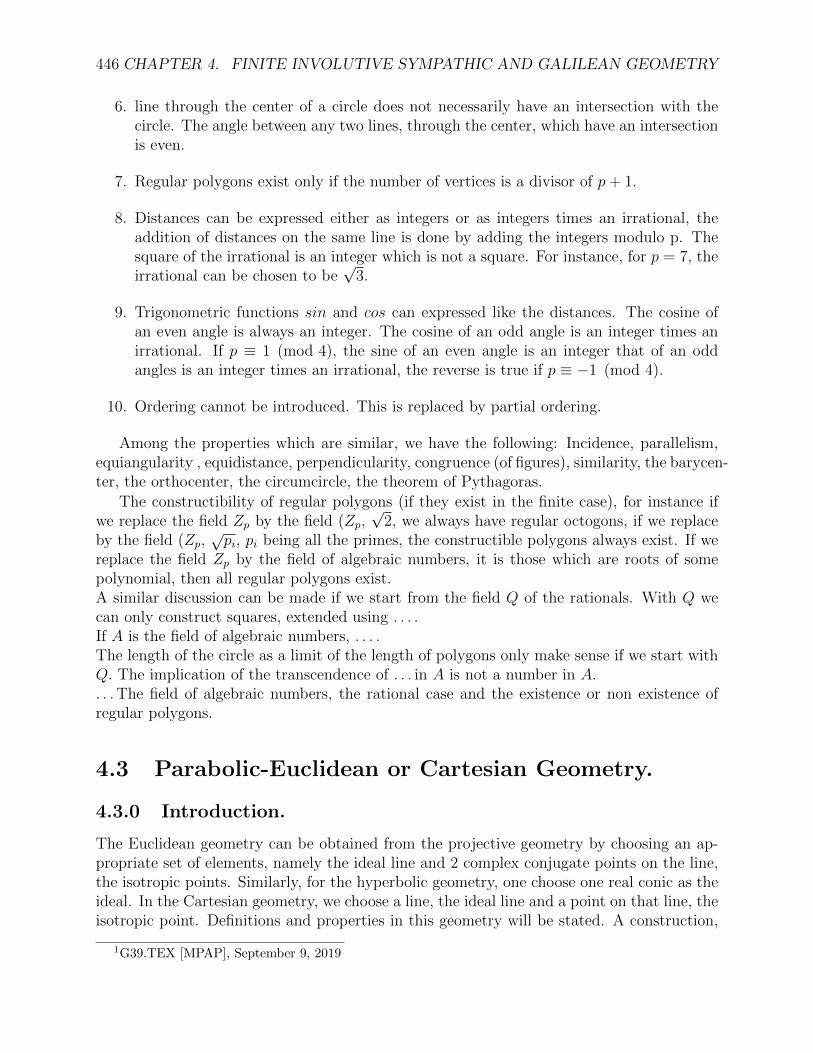
446 CHAPTER 4. FINITE INVOLUTIVE SYMPATHIC AND GALILEAN GEOMETRY
6. line through the center of a circle does not necessarily have an intersection with thecircle. The angle between any two lines, through the center, which have an intersectionis even.
7. Regular polygons exist only if the number of vertices is a divisor of p+ 1.
8. Distances can be expressed either as integers or as integers times an irrational, theaddition of distances on the same line is done by adding the integers modulo p. Thesquare of the irrational is an integer which is not a square. For instance, for p = 7, theirrational can be chosen to be
√3.
9. Trigonometric functions sin and cos can expressed like the distances. The cosine ofan even angle is always an integer. The cosine of an odd angle is an integer times anirrational. If p ≡ 1 (mod 4), the sine of an even angle is an integer that of an oddangles is an integer times an irrational, the reverse is true if p ≡ −1 (mod 4).
10. Ordering cannot be introduced. This is replaced by partial ordering.
Among the properties which are similar, we have the following: Incidence, parallelism,equiangularity , equidistance, perpendicularity, congruence (of figures), similarity, the barycen-ter, the orthocenter, the circumcircle, the theorem of Pythagoras.
The constructibility of regular polygons (if they exist in the finite case), for instance ifwe replace the field Zp by the field (Zp,
√2, we always have regular octogons, if we replace
by the field (Zp,√pi, pi being all the primes, the constructible polygons always exist. If we
replace the field Zp by the field of algebraic numbers, it is those which are roots of somepolynomial, then all regular polygons exist.A similar discussion can be made if we start from the field Q of the rationals. With Q wecan only construct squares, extended using . . . .If A is the field of algebraic numbers, . . . .The length of the circle as a limit of the length of polygons only make sense if we start withQ. The implication of the transcendence of . . . in A is not a number in A.. . . The field of algebraic numbers, the rational case and the existence or non existence ofregular polygons.
4.3 Parabolic-Euclidean or Cartesian Geometry.
4.3.0 Introduction.
The Euclidean geometry can be obtained from the projective geometry by choosing an ap-propriate set of elements, namely the ideal line and 2 complex conjugate points on the line,the isotropic points. Similarly, for the hyperbolic geometry, one choose one real conic as theideal. In the Cartesian geometry, we choose a line, the ideal line and a point on that line, theisotropic point. Definitions and properties in this geometry will be stated. A construction,
1G39.TEX [MPAP], September 9, 2019

4.3. PARABOLIC-EUCLIDEAN OR CARTESIAN GEOMETRY. 447
which allows an elementary algebraic proof of the properties, will be given. The transforma-tions leaving invariant the equality of angles and distances will be studied in a model of thegeometry in the Euclidean plane, giving a justification for the name of the geometry.
We start with a projective plane associated to an arbitrary field. A specific line, i, in thatplane is chosen, called the ideal line. A specific point, I, on that line is also chosen, calledthe isotropic point. Because a line is chosen, we can use all the concepts of affine geometry.In particular, 2 lines are called parallel if they have the same ideal point. The mid-point of2 points A, B is the harmonic conjugate with respect to A, B of the ideal point on A× B.A parabola is a conic tangent to the ideal line.
I now will define new concepts in the Cartesian geometry. To focus the attention ona specific set of properties, I have chosen properties which have been inspired by thoseassociated to the geometry of the triangle. Because we want properties which are true inany field, it is not appropriate to derive them by a limiting procedure. I have therefore statedand proven them independently from the corresponding properties in Euclidean geometryand have indicated the correspondence by giving the same name as that of the correspondingelement in Euclidean geometry, but without giving the justification.
The configuration should give theorems in 2 ways 11, using . . . .The equality of angles is associated with a parabolic projectivity (with 2 coincident fixedpoints).Recall the construction of a parabolic projectivity on i, let I1, I2 be a pair, the point I4,corresponding to I3, is obtained as follows,given A, choose B on A× I,C := (A× I2)× (B × I1), c := I × C,D := (B × I3)× c, a := A×D, thenI4 := a× i.
Measure of distances and of angles.
The measure of angles and distances play a fundamental role in the geometry of Euclidand in the study of non Euclidean geometry by de Tilly. On the other hand, starting fromprojective geometry, these notions are derived notions. The appropriate definitions for themeasure of distances and of angles will be given first in the case of a real field using a modelon the Euclidean plane with given perpendicular axis x and y through a point O and theline l with equation y = 1. This will justify the name of Cartesian geometry.12
4.3.1 Fundamental Definitions.
Definition.
In in affine geometry let us choose one point on the ideal line as a double isotropic point.This point will be called the isotropic point or sun. The associated geometry will be calledparabolic-euclidean or Cartesian.
112.3.83126.3.83

448 CHAPTER 4. FINITE INVOLUTIVE SYMPATHIC AND GALILEAN GEOMETRY
Definition.
Any line through the sun is called an isotropic line or solar axis. A parabola with the sunas ideal point is called a parcircle.
Comment.
There is a configuration which is a special case of the hexal configuration which allows thestudy of the geometry of the triangle in the Cartesian geometry. Indeed it is sufficient tochoose M to be the isotropic point.
Example.
xi+1 := xi + 1mod p is such a projectivity.With p = 5,X = 0, 1, 2, 3, 4, 0,. . . . Hence both angles and distances can be represented by an integer modulo p.The circle is replaced by a parcircle,
Notation.
Let π be the parabolic projectivity with the ideal point as fixed point:0. pi = (x, x+ 1).
Theorem.
pii = (x, x+ i), i ∈ R,therefore, if the coordinates of the point P are xP and yP and if the parallels to the lines aand b through O meet l at A and B, we are justified to give the following
Definition.
dist(P,Q) = yQ − yP .angle(a, b) := xB − xA.
We have
Theorem.
Given any 3 points A, B and C and any 3 lines a, b and c,dist(A,C) + dist(C,B) + dist(B,A) = 0,angle(a, c) + angle(c, b) + angle(b, a) = 0.
Comment.
Because, in both instances, the notion of measure are associated with the coordinates of a1 dimensional set of points, both measure of distances and of angles can be given a sign. Ofcourse what we obtain is not a metric but a semi metric because

4.3. PARABOLIC-EUCLIDEAN OR CARTESIAN GEOMETRY. 449
|dist(A,B)| ≤ |dist(A,C)|+ |dist(C,B)|,but dist(P,Q) = 0 does not imply P = Q but only yP = yQ.
In the case of a Gaussian field, if [0,0,1] is the ideal line and (0,1,0) is the isotropic point,we can give
Definition.
dist((A0, A1, 1), (B0, B1, 1)) := B1− A1mod pk,angle([a0,−1, a2], [b0,−1, b2]) := b0− a0mod pk,
Theorem.
The set of points Q such that angle AQB is constant is a parcircle13.
Theorem.
The set of points Q such that angle QA0 = angle AQO isosceles triangle) is a set of 2 lines(which can coincide), A × S and B × S, such that O is equidistant in the Euclidean sensefrom these 2 lines.
Proof:A′ := (B ×O)× (A× S), B′ := (A×O)× (B × S),I1 := i× (B ×O), I2 := i× (A×B) = i× (A′ ×B′),I3 := i× (A×O),
then (I1, I2) = (I2, I3) and ABO is an isosceles triangle. (Ii, Ij) denotes the angle of anypair of lines through Ii and Ij on i.Any other point D on B × S is such that ADO is an isosceles triangle.
Definition.
AO = BO either if A, B and I are collinear, or if A′B′ is parallel to AB whereA′ = (B ×O)× (A× S)andB′ = (A×O)× (B × S).
Definition.
Two lines are antiparallel if . . . .
4.3.2 The Geometry of the Triangle in Galilean Geometry.
Definition.
A line in a triangle is a symmedian if . . . .
133.3.83

450 CHAPTER 4. FINITE INVOLUTIVE SYMPATHIC AND GALILEAN GEOMETRY
Comment.
We could also define measure of distance and angles dualy14.(A,B) = (C,D) if ((I × A), (I × B))and((I × C), (I × D)) are corresponding pairs in anparabolic projectivity with fixed line i.If we use as model in the Euclidean plane the line at infinity as the ideal line and the pointin the direction of the x axis as the sun all points on a line through the sun are equidistantfrom points on another line through the sun the measure of distances between the pointscan be chosen as the measure of the distances between the lines. Therefore, the distancebetween A := (a0, a1, 1) and B := (b0, b1, 1) is b1− a1.The angle between a := [1,−a1, 0] and b := [1,−a2, 0] is a2−a1. a corresponds to X = a1Y,if α is the angle with the y axis in the clockwise direction, tan(α) = a1, the “sun” angle isdoubled if the tangent is doubled.
Definition.
The line of Euler is . . . .
Definition.
The circumparcircle
Definition.
The first circle of Lemoine.
Definition.
The second circle of Lemoine.
Definition.
The circle of Brocard.
The Brianchon-Poncelet-Feurbach theorem becomes15
Theorem.
Given a triangle Ai, ai and the parcircle ι tangent to ai. Let M be any point not on theside of the triangle or on i, Let Mi := (M × Ai)× ai, the parcircle γ through Mi is tangentto the parcircle ι .By duality, let m be a line not through Ai or I, let mi := (m× ai)×Ai, the parcircle tangentto mi is tangent to the parcircle ι.
144.3.83153.3.83
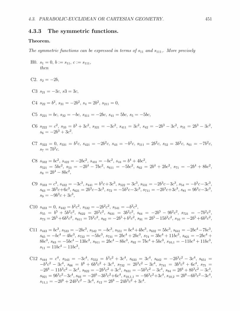
4.3. PARABOLIC-EUCLIDEAN OR CARTESIAN GEOMETRY. 451
4.3.3 The symmetric functions.
Theorem.
The symmetric functions can be expressed in terms of s11 and s111,. More precisely
H0. s1 = 0, b := s11, c := s111,then
C2. s2 = −2b,
C3 s21 = −3c, s3 = 3c,
C4 s22 = b2, s31 = −2b2, s4 = 2b2, s211 = 0,
C5 s221 = bc, s32 = −bc, s311 = −2bc, s41 = 5bc, s5 = −5bc,
C6 s222 = c2, s33 = b3 + 3c2, s321 = −3c2, s411 = 3c2, s42 = −2b3 − 3c2, s51 = 2b3 − 3c2,s6 = −2b3 + 3c2.
C7 s322 = 0, s331 = b2c, s421 = −2b2c, s43 = −b2c, s511 = 2b2c, s52 = 3b2c, s61 = −7b2c,s7 = 7b2c.
C8 s332 = bc2, s422 = −2bc2, s431 = −bc2, s44 = b4 + 4bc2,s521 = 5bc2, s53 = −2b4 − 7bc2, s611 = −5bc2, s62 = 2b4 + 2bc2, s71 = −2b4 + 8bc2,s8 = 2b4 − 8bc2,
C9 s333 = c3, s432 = −3c3, s441 = b3c+3c3, s522 = 3c3, s531 = −2b3c−3c3, s54 = −b3c−3c3,s63 = 3b3c+6c3, s621 = 2b3c−3c3, s72 = −5b3c−3c3, s711 = −2b3c+3c3, s81 = 9b3c−3c3,s9 = −9b3c+ 3c3,
C10 s433 = 0, s442 = b2c2, s532 = −2b2c2, s541 = −b2c2,s55 = b5 + 5b2c2, s622 = 2b2c2, s631 = 3b2c2, s64 = −2b5 − 9b2c2, s721 = −7b2c2,s73 = 2b5 +6b2c2, s811 = 7b2c2, s82 = −2b5 +b2c2, s91 = 2b5−15b2c2, s10 = −2b5 +6b2c2,
C11 s443 = bc3, s533 = −2bc3, s542 = −bc3, s551 = bc4 +4bc3, s632 = 5bc3, s641 = −2bc4−7bc3,s65 = −bc4 − 4bc3, s722 = −5bc3, s731 = 2bc4 + 2bc3, s74 = 3bc4 + 11bc3, s821 = −2bc4 +8bc3, s83 = −5bc4− 13bc3, s911 = 2bc4− 8bc3, s92 = 7bc4 + 5bc3, s10,1 = −11bc4 + 11bc3,s11 = 11bc4 − 11bc3,
C12 s444 = c4, s543 = −3c4, s552 = b3c2 + 3c4, s633 = 3c4, s642 = −2b3c2 − 3c4, s651 =−b3c2 − 3c4, s66 = b6 + 6b3c2 + 3c4, s732 = 2b3c2 − 3c4, s741 = 3b3c2 + 6c4, s75 =−2b6 − 11b3c2 − 3c4, s822 = −2b3c2 + 3c4, s831 = −5b3c2 − 3c4, s84 = 2b6 + 8b3c2 − 3c4,s921 = 9b3c2−3c4, s93 = −2b6−3b3c2+6c4, s10,1,1 = −9b3c2+3c4, s10,2 = 2b6−6b3c2−3c4,s11,1 = −2b6 + 24b3c2 − 3c4, s12 = 2b6 − 24b3c2 + 3c4.
452 CHAPTER 4. FINITE INVOLUTIVE SYMPATHIC AND GALILEAN GEOMETRY
Theorem.
Given a triangle Ai a point M not on the sides of the triangle and a point M on the polarm of M with respect to the triangle.
0. γ is a parcircle,
1. θ is a parcircle,
2. χ1i and χ2i are parcircles.
Proof: We will use the abbreviations11 = m1m2 +m2m0 +m0m1 and we havem02 −m1m2 = m12 −m2m0 = m22 −m0m1= m12 +m22 +m1m2 = −s11.
s11 +m1m2 = −(m12 +m22), . . . . s11 +m02 = m1m2, . . . .2s11 −m1m2 = m1m2− 2m02, (m1−m2)2 = −(s11 + 3m1m2).
COMPARE Mmm and jia, Mmm and jia.
Theorem.
The conicm0X1X2 +m1X2X0 +m2X0X1 = 0
passes through M, Ai, andZZi = (m0,−(m1−m2),m1−m2),
the tangent at Ai is aci,the tangent at M is mai = [m0,m1,m2],the tangent at ZZi is [(m1−m2)2,m0m1,m2m0]16.
4.5 Transformation associated to the Cartesian geom-
etry.
4.5.0 Introduction.
Such transformation must preserve measure of angles and distances.
Theorem.
The transformations associated to the Cartesian geometry are represented by unit uppertriangular matrices in the Euclidean The following are subgroups of these transformationThe translations 1 0 v
0 1 w0 0 1
.
The shears
161.3.83

4.5. TRANSFORMATION ASSOCIATED TO THE CARTESIAN GEOMETRY. 453 1 u v0 1 00 0 1
,
and the special shears 1 u 00 1 00 0 1
.
Indeed,
Definition.
Theorem.
Given a point P, the set of points whose polars with respect to a triangle pass through Pare on a conic through the vertices of the triangle and vice-versa.
Proof. The pole of [q0, q1, q2] is (q1q2, q2q0, q0q1). It is on line (a0, a1, a2) if a0q1q2 +a1q2q0 +a2q0q1 = 0.
Definition.
Given a triangle, the point of Lemoine of a conic through the vertices of the triangle is thepoint P of the preceding Theorem.
Definition.
Given a triangle, the line of Lemoine of a conic tangent to the triangle is the set of pointswhose polars with respect to the triangle are tangent to the conic.
Corollary.
The point of Lemoine of the circumcircle is the classical point of Lemoine. The point ofLemoine of the conic of Simsom m0m1X1X2 + . . . = 0 is Tmm = (m0m1,m1m2,m2m0),The line of Lemoine of the inscribed conic is [j1j2, j2j0, j0j1], it is the line through Jai.
4.5.1 The geometry of the triangle, the standard form.
Introduction.
In this section, we do give only a representative set of Theorems using a form similar to thatfound in works on Geometry since Euclid. Many more Theorems can be deduced from thecompact form given in section 9.5. The vertices of the triangle are denoted by A0, A1, A2,its sides by a0, a1, a2.
Definition.
A Fano line p of a point P is the line through the diagonal points of the quadrangle A0, A1,A2, P.

454 CHAPTER 4. FINITE INVOLUTIVE SYMPATHIC AND GALILEAN GEOMETRY
Definition.
The cocenter M of a triangle is the Fano point of the ideal line m. (D0.1., .2., .12.)
Construction.
Given a triangle Ai, the ideal line m and the center M , we can obtain a conic as follows. Thetangents to the conic θ at the vertices of the triangle are be constructed using m i = M xAi. Any point on the conic and on a given line through one of its points, are be obtainedusing the construction of Pascal.
Definition.
The conic
θ
constructed in 9.6.3. is by definition a circle the circumcircle of the triangle. (D1.12., H1.0.)
Definition.
The Euler line of a triangle is the line eul through the cocenter and the center of the triangle.(D1.0.)
Definition.
The central parallels kki are the lines parallel to the sides of a triangle passing through thecenter M . (D1.1.)
Theorem.
The central parallels kki intersect the sides ai+1 andai−1 at points K A i−1 and K A i+1 which are on a circle λ . (D1.2., D2.11., C2.1.,
C2.2.)
Definition.
The circle λ is called central circle.
Theorem.
The circumcircle and the central circle are tangent at a point LO. (C23.0.)
Definition.
The central points M i of a triangle are the intersection of a tangent at a vertex with theopposite sides. (D0.11.)

4.5. TRANSFORMATION ASSOCIATED TO THE CARTESIAN GEOMETRY. 455
Definition.
The central line m of a triangle is the Fano line of its center M . (D0.12.)
Definition.
The associated circles α i are the circles through the center M of the triangle and its verticesAi+1 and Ai−1. (D3.6., C3.1.)
Definition.
The center-vertex circles κ ci and κ ci are the circles centered at one vertex of a trianglepassing through an other vertex. (D4.12., C4.0.)
Definition.
The bissectrices ii of a triangle are the lines through a vertex Ai such that the lines formsequal angles with the sides of the triangle passing through Ai.
Theorem.
The bissectrices have a point I in common. (9.5.5., D0.3.)
Definition.
The bissector is the point I common to the bissectrices ii. (D.0.3.) The bissector line i is theFano line of the bissector. (D20.1)
Comment.
The sides of a triangle do not have a point in common, therefore, there is no circle tangentto its sides.
Definition.
The circles of Apollonius α pi are the circles centered at a central point M i through a oppositevertex Ai. (D5.12., C5.0., C5.1.) They have a common tangent with the circumcircle (C5.3.).The point of contact with the side ai is on the bissectrix through Ai. (C22.1.)
Theorem.
The circles of Apollonius have the same radical axis, l mm, which is the common tangent ofthe circumcircle and the central circle. (C6.2., C2.6.)
Definition.
The sun MI is the direction of the bissector line. (D24.0.)

456 CHAPTER 4. FINITE INVOLUTIVE SYMPATHIC AND GALILEAN GEOMETRY
Definition.
Any parabola, i.e. a conic tangent to the ideal line, whose ideal point is the sun MI is calleda sun-parabola.
Comment.
In the isotropic geometry, the center of a parabola is an ideal point which is not necessarilyits ideal point.
Definition.
The center-cocenter conic γ is the conic through the vertices of the triangle, its center andits cocenter. (D7.10.)
Theorem.
The center-cocenter conic is a sun-parabola. (C24.1.)
Definition.
The tangential circles χ ti (χ t i) are the circles tangent to ai+1(ai−1) at Ai−1(Ai+1) passingthrough Ai+1(Ai−1). (D7.8., C7.0.)
Theorem.
The other intersections K Li and K L i with the tangential circles and the sides of thetriangles are on a conic ξ which is a sun-parabola. (D3.1., D7.9., C7.2., D24.2.)
Theorem.
The cocircumcircle θ is the conic through the vertices of the triangle for which the tangentsare parallel to the opposite side. (D1.12., D0.1., C1.0.)
Definition.
Let Eul and E ul be the points of contact of the circumcircle and of the co-circumcircle withthe line of Euler, the conic ι through these points and circumscribed to the triangle is calledthe bissector conic. (D20.19., C20.2., C20.3.)
Theorem.
The center of the bissector conic is the bissector point. (C20.7.)
Comment.
9.6.28. is an alternate definition fron that given in D20.19.

4.5. TRANSFORMATION ASSOCIATED TO THE CARTESIAN GEOMETRY. 457
4.5.2 The cubic γ a of Gabrielle.
Introduction.
This section and the related section 11. was conceived after my daugther asked when I wouldname a Theorem for her. It concerns a general construction which starts from a parabola andconstructs points on a cubic of which several are assoiated to the geometry of the triangle.
Definition.
Let x = (x0,x1,x2) be any line of the dual of the sun-parabola Γ , 0. (m1+m2)x1x2+(m2 +m0)x2x0 + (m0 +m1)x0x1 = 0.Let k ki = [m1+m2,m2,m1]. The following constructs points X = (X0,X1,X2) of the curveγ a called the cubic of Gabrielle: D1. Xi := xxk ki,D2. xi := XixAi,D3. X := x1xx2.D4. γa := X.
Definition.
A parametric representation of a curve, with constraint arbitrary point are given in termsof 3 homogeneous parameters subjected to an homogeneous relation R between these 3parameters.
Theorem.
The curve γ a is a point cubic, with axis 0. df = [m03(m1+m2)2,m13(m2+m0)2,m23(m0+m1)2].It contains the points Ai, M i, M, M , LM. A parametric representation, with constraint9.7.1.0., is 1. (x1x2(m0(m1 +m2)(x1 + x2) +m1m2x0),
x2x0(m1(m2 +m0)(x2 + x0) +m2m0x1),x0x1(m2(m0 +m1)(x0 + x1) +m0m1x2)),
Its equation in homogeneous coordinates is P4. γa : m0X0(X12 +X22)+m1X1(X22 +X02) +m2X2(X02 +X12) = 0.Proof: Definition 9.7.1. gives P1. X0 = (m1x1 +m2x2,m1x0 + (m1 +m2)x2,m2x0 +(m1 +m2)x1),P2. x0 = [0,m2x0 + (m1 +m2)x1,m1x0 + (m1 +m2)x2],P3. X = ((m2x0 + (m1 +m2)x1)(m0x1 + (m2 +m0)x2),
(m1x0 + (m1 +m2)x2)(m2x1 + (m2 +m0)x0),(m2x0 + (m1 +m2)x1)(m2x1 + (m2 +m0)x0)),
if we multiply all coordinates by x2 and use 9.7.1.0. we get 9.7.3.1. By a long algebraicverification it can be shown that the equation P4. is satisfied by 1.

458 CHAPTER 4. FINITE INVOLUTIVE SYMPATHIC AND GALILEAN GEOMETRY
Theorem.
A parametric representation, with constraint 0. x0 + x1 + x2 = 0is 1. (x1x2(m1x1 +m2x2), x2x0(m2x2 +m0x0), x0x1(m0x0 +m1x1)).2. Thepoint1.isthepointonthecubicγaandtheline
[x0, x1, x2]throughMdistinctfromM.3. ThereisonelinemiwhereMisatriplepoint.
Proof: Let (X0,X1,X2) be any point on the line [x0,x1,x2] passing through M, eliminatingX0 between the equation of the cubic γ a and X0x0 +X1x1 +X2x2 = 0gives
(X1 +X2)2(X1(m0x1(x1 + x2) +m1x12) +X2(m0x2(x1 + x2) +m2x22)) = 0or X1 = x0x2(m0x0 +m2x2), X2 = x0x1(m0x0 +m1x1),because of 0., by symmetry we get 1. X1+X2 = 0, gives the point M and because (X1+X2)is a double factor this point has to be counted twice, hence 2., the point M is a node. Thepoint 1. coincides with M iff the 3 coordinates are equal, the first 2 give after eliminationof x0, (m0 + m1)x12 = (m2 + m0)x22, hence x1 = i2+i0, x2 = i0+i1, by symmetry x0 =i1+i2, hence 3.
Theorem.
If the point of contact of a line [x0,x1,x2] through LM with the cubic γ a is (X0,X1,X2),then 0. X02 = m0x1x2(m1x1 +m2x2), X12 = m1x2x0(m2x2 +m0x0),
X22 = m2x0x1(m0x0 +m1x1).We have 1. m0m1x1 +m2m0x1 +m0m1x2 = 0and 2. x0X0 + x1X1 + x2X2 = 0.Eliminating X0 between 2. and the equation of the cubic gives (m2X2+m1X1)(m2x1(m0x0+m1x1)X12 +m1x2(m0x0 +m2x2)X22) = 0, becauseof1.The first factor corresponds to the point LM, the other factor has a double root which gives0.
Definition.
The cubic χ of Charles is the cubic through the points Mi, M i, LMi.
Theorem.
Let 0. a := m0m1m2,1. a0 := m0(m12 +m22 +m1m2), a1 := m1(m22 +m02 +m2m0),
a2 := m2(m02 +m12 +m0m1),then 2. χ : a(X03 +X13 +X23)
+a0X1X2(X1 +X2) + a1X2X0(X2 +X0) + a2X0X1(X0 +X1) = 0.3. Thetangentat(X0, X1, X2)is
[aX02 + a2X12 + a1X22, aX12 + a0X22 + a2X02,aX22 + a1X02 + a0X12],
4. Theotherpoint(Y 0, Y 1, Y 2)onthetangent[x0, x1, x2]at(X0, X1, X2), isobtainedbyeliminatingZ0from2., where

4.5. TRANSFORMATION ASSOCIATED TO THE CARTESIAN GEOMETRY. 459
(X0, X1, X2)isreplacedby(Z0, Z1, Z2)andx0Z0 + x1Z1 + x2Z2 = 0.ThecoefficientofZ23isY 1X12andthatofZ13isY 2X22.
Proof: For 4. we observe that the elimination should lead to the equation (X2Z1+X1Z2)2(Y 2Z1 + Y 1Z2) = 0.An illustration of 4. is given by 12.4.
Conjecture.
Given 9 points Ai, Bi, Ci, on a cubic such that Ai, Bi Ci and (A0, B0, C0), (A1, B1, C1) arecollinear, then (A2, B2, C2) are collinear.
Corollary.
If 3 points Ai are on a cubic, the third point Ci on the tangent to the cubic at Ai are alsocollinear.
Example.
For q = 16, i0 = 1, i1 = ε 8, i2 = ε 3, m0 = 1,m1 = ε,m2 = ε6,H0.0. M = 253, E0.10. M = 184, H0.1. Ai = 2, 1, 0,H0.2. I = 130,
E0.0. ai = 0∗, 1∗, 272∗,E0.1. mi = 253∗, 2∗, 136∗, E0.9.m i = 179∗, 89∗, 90∗,E0.2. Mi = 136, 272, 137, E0.11.M i = 15, 115, 91,E0.3. ii = 125∗, 6∗, 233∗,E0.4. Ii = 238, 232, 234,E0.5. imi = 44∗, 102∗, 339∗,
im i = 4∗, 151∗, 168∗,E0.6. Tmi = 194, 14, 16,
Tm i = 3, 30, 195,E0.7. tmi = 61∗, 180∗, 15∗,
tm i = 271∗, 203∗, 194∗,E0.8. IAi = 94, 240, 133,
IA i = 101, 215, 183,E0.12. m = 137∗,m = 189∗,
E1.0. eul = 20,E1.1. kki = 152∗, 205∗, 96∗, kk i = 258∗, 21∗, 147∗,E1.2. KAi = 234, 127, 30, K Ai = 195, 31, 237,
KA i = 126, 16, 255, K A i = 180, 128, 204,E1.3. kli = 203∗, 233∗, 236∗, k li = 126∗, 194∗, 202∗,
kl i = 15∗, 134∗, 237∗, k l i = 127∗, 29∗, 14∗,E1.4. Bi = 147, 61, 102, B i = 101, 47, 37,

460 CHAPTER 4. FINITE INVOLUTIVE SYMPATHIC AND GALILEAN GEOMETRY
E1.5. bbi =E1.6. Euli = 116, 254, 256,E1.7. Bai =
Ba i =E1.8. tBi =E1.9. KKi = 147, 5, 200, K Ki = 101, 199, 143,E1.10. euli = 88∗, 135∗, 255∗,E1.11. TT =
E1.12. θ = 0, 1, 2, 40, 61, 102, 123, 145, 147,90∗, 89∗, 179∗, 96∗, 120∗, 92∗, 71∗, 49∗, 216∗,172, 197, 211, 223, 229, 235, 249, 250,104∗, 270∗, 152∗, 10∗, 225∗, 20∗, 205∗, 54∗,
E2.0. timi = 118∗, 45∗, 16∗, t imi = 182∗, 101∗, 140∗,E2.1. LIi = 63, 193, 239, L Ii = 181, 203, 64,E2.2. lii = 192∗, 62∗, 238∗, l ii = 13∗, 30∗, 63∗,E2.3. Atmi = 211, 50, 208, A tmi = 151, 217, 242,E2.4. lti = 125∗, 254∗, 181∗, l ti = 125∗, 237∗, 31∗,E2.5. LM = 155, L M = 163,E2.6. LTi = 238, 135, 182, L Ti = 238, 232, 32,E2.7. lm = 98∗, l m = 162∗,E2.8. LMM = 96, L MM = 174,
LM M = 118, L M M = 265,E2.9. tKKLi =
tKKL i =E2.10. lmm = 83∗, l mm = 92∗,
lm m = 49∗, l m m = 110∗,
E3.0. kai = 255∗, 61∗, 203∗, k ai = 233∗, 88∗, 126∗,ka i = 193∗, 15∗, 5∗, ka i = 254∗, 127∗, 271∗,
E6.13. Γ = 0, 1, 33, 41, 51, 93, 105, 111, 129,116∗, 254∗, 161∗, 235∗, 253∗, 43∗, 11∗, 70∗, 260∗,137, 169, 171, 186, 189, 241, 270, 272,96∗, 107∗, 218∗, 268∗, 174∗, 213∗, 184∗, 256∗,
E7.1. TMi = 171, T mi = 225,
E8.0. dti = 139∗, 227∗, 239∗,dt i = 91∗, 151∗, 138∗,
E8.1. Dui = 116, 6, 16,Du i = 90, 30, 117,
E9.0. Ebi = 133, 251, 212, E bi = 150, 55, 167,
4.5. TRANSFORMATION ASSOCIATED TO THE CARTESIAN GEOMETRY. 461
Eb i = 189, 111, 261, E b i = 9, 257, 146,E9.2. edi = 226∗, 68∗, 256∗, e di = 183∗, 121∗, 123∗,
ed i = 128∗, 44∗, 144∗, e d i = 158∗, 185∗, 16∗,
E11.19. Dhi = 177, 103, 75, D hi = 133, 253, 183,Dh i = 83, 159, 122, D h i = 253, 34, 22,
E11.20. dii = 180, 127, 13, d ii = 180, 3, 253,di i = 204, 5, 193, d i i = 204, 114, 2,
E11.21. Dji = 100, 111, 261, D ji = 100, 124, 253,
E11.22. dki = 27∗, 83∗, 35∗, d ki = 92∗, 71∗, 216∗,dk i = 23∗, 35∗, 224∗,
E11.23. dui = 88∗, 232∗, 15∗,du i = 114∗, 203∗, 116∗,
E11.24. Dli = 101, 185, 104,Dl i = 101, 247, 190,
E11.25. Dmi = 204, 134, 203,Dm i = 14, 15, 29,
E11.26. Dni = 30, 205, 255,Dn i = 16, 204, 180,
E11.27. dn = 33∗,dn = 100∗,
E11.28. Do = 200,Do = 174,
E11.29. dp = 102∗,dp = 55∗,
E11.30. Dq = 178,E11.31. dr = 26∗,
E11.32. γa = 0, 1, 2, 15, 40, 80, 91, 100, 103,181∗, 254∗, 125∗, 121∗, 234∗, 208∗, 245∗, 133∗, 78∗,115, 124, 155, 169, 178, 184, 253, 263,118∗, 149∗, 39∗, 119∗, 26∗, 49∗, 83∗, 100∗,
γ a = 0, 1, 2, 53, 100, 111, 136, 137, 153,31∗, 237∗, 125∗, 141∗, 173∗, 70∗, 200∗, 226∗, 41∗,163, 184, 225, 250, 253, 261, 265, 272,18∗, 92∗, 111∗, 113∗, 110∗, 75∗, 246∗, 117∗,
E12.0. Nai = 89, 8, 194, N ai = 272, 205, 204,E12.1. nai = 7∗, 61∗, 115∗, n ai = 204∗, 29∗, 2∗,E12.2. Nbi = 248, 129, 55, N bi = 29, 70, 251,E12.3. nci = 8∗, 263∗, 144∗, n ci = 158∗, 245∗, 218∗,E12.4. lMMi = 192∗, 180∗, 31∗, l MMi = 114∗, 30∗, 7∗,E12.5. ndi = 263∗, 58∗, 239∗, n di = 103∗, 18∗, 66∗,

462 CHAPTER 4. FINITE INVOLUTIVE SYMPATHIC AND GALILEAN GEOMETRY
E12.6. Nei = 124, 243, 197, N ei = 208, 24, 249,E12.7. nfi = 80∗, 157∗, 257∗,E12.8. ngi = 182∗, 101∗, 140∗, n gi = 118∗, 45∗, 16∗,E12.9. Nhi = 106, 103, 134, N hi = 186, 228, 222,E12.10. lI = 170∗, l I = 52∗,E12.11. Nii = 98, 262, 54, N ii = 170, 18, 258,
Ni i = 86, 210, 260, N i i = 218, 35, 41,E12.12. nji = 179∗, 140∗, 147∗, n ji = 253∗, 239∗, 118∗,E12.13. nki = 32∗, 139∗, 200∗, n ki = 221∗, 164∗, 223∗,
nk i = 252∗, 144∗, 117∗, n k i = 213∗, 48∗, 158∗,E12.14. Nli = 95, 134, 189, N li = 83, 124, 186,
Nl i = 157, 136, 157, N l i = 20, 228, 115,E12.15. nl = 99∗, n l = 150∗,
nl = 119∗, n l = 161∗,E12.16. nmi = 268∗, 60∗, 66∗, n mi = 98∗, 152∗, 47∗,E12.17. npi = 47∗, 44∗, 109∗, n pi = 265∗, 268∗, 121∗,
np i = 76∗, 123∗, 253∗, n p i = 140∗, 116∗, 76∗,E12.18. nqi = 24∗, 139∗, 257∗, n qi = 48∗, 11∗, 223∗,
nq i = 146∗, 198∗, 78∗, n q i = 82∗, 18∗, 172∗,E12.19. Nri = 157, 137, 254, N ri = 15, 20, 15,
Nr i = 134, 78, 198, N r i = 198, 13, 83,E12.20. nr = 252∗, n r = 218∗,
nr = 202∗, n r = 191∗,
E12. .NDi = 256, 186, 13,E12. .
χ = 13, 15, 20, 78, 83, 91, 95, 103, 106, 115, 116, 124, 131,261∗, 218∗, 96∗, 195∗, 197∗, 245∗, 193∗, 1∗, 10∗, 158∗, 157∗, 131∗, 269∗,15, 20, 137, 272, 91, 222, 83, 103, 228, 116, 131, 157, 198,
134, 136, 137, 157, 186, 189, 198, 222, 228, 254, 256, 272,146∗, 144∗, 263∗, 119∗, 87∗, 49∗, 165∗, 178∗, 60∗, 257∗, 80∗, 8∗,254, 256, 13, 136, 189, 78, 115, 95, 134, 106, 124, 186,(thesearethetangentsandtheotherpointonthetangent)
E19.4. lI = 170∗, l I = 52∗,E19.5. LJ = 11,
E22.0. iAi = 179∗, 237∗, 3∗,E22.1. IA = 230,E22.2. ab = 224∗,E22.6. Iai = 15, 126, 4,E22.7. ia = 112∗,
E25.0. Dk = 176,

4.6. PROBLEMS 463
E25.1. dl = 100∗,
Given the center C of a circle and one of its points A, the point X on any line x throughA (or y through C) can be obtained by construction y through C (or x through A) such thatthe angle XAC = angle BCX. The above as to be reviewed. A construction of a point on agiven tangent (or radius) follows. There must be a simpler way. Let the given points be A0,A1, A2, let the center be C, let the radius-tangent be t, Mt := t x m, find A4 on the circleand A0 x Mt, find A5 on the circle and A1 x Mt, let Y := (A0 x A1) x (A4 x A5), (C x Y)x t is the point of contact with the circle. To find the bissectrix of an angle A−1 A0 A1 weuse the above construction with the tangent-radius Cx(mx(A−1xA1) the ?? point X on thecircle is also on the bissectrix.
Notation.
Angles and directions will be denoted by an upper case letter and a lower case letter under-lined.
Theorem.
If the angle of the direction of the sides bi is nbi, then the angle of the direction of the tangentis di+1 + di+2 − dimodq + 1.
Theorem.
If the direction of ai is ai, the angles at Ai are Ai = ai+1 − ai−1modq + 1.
Theorem.
0. The angle of the direction of the center of χ1i isc1i = ai + Ai−1,thatofthecenterofχ2iisc2i = ai − Ai+1.
1. The center of χ1i is (Ai+1xM)xai+1,c1i
thatofχ2iis(Ai−1xM)xai−1,c2i
4.6 Problems
.
464 CHAPTER 4. FINITE INVOLUTIVE SYMPATHIC AND GALILEAN GEOMETRY
4.6.1 Problems for Affine Geometry.
Theorem.
If m is the ideal line, and A = (A0, A1, A2), B = (B0, B1, B2) then
0. the mid-point A+B of A and B isA+B = (m ·B)A+ (m · A)B.
1. the symmetric 2B − A of A with respect to B is2B − A = 2(m · A)B − (m ·B)A.
Theorem.
The mid-points of the diagonals of a complete quadrilateral are collinear. D37.5, C37.15.(020, Chou and Schelter 1986, p. 18)
Definition.
The line of the preceding Theorem is called the mid-line of the complete quadrilateral.
Theorem.
Given a complete 5-lines, the mid-lines of the 5 complete quadrilaterals obtained by sup-pressiong any of the 5 lines have a point in common. (025, Chou and Schelter 1986, p.19)
Theorem.
Given a triangle Ai, and a point M0, let Mj be the symmetric of Mj−1 with respect toAj−1 (mod 3), then
0. Mi+3 is the symmetric of Mi with respect to MMi+1, vertex of the anticomplementarytriangle of Ai.
1. M6 = M0.
2. Mi,Mi+3,Mi+1,Mi+4 are parallelograms.
4.6.2 Problems for Involutive Geometry.
Theorem.
The perpendicular direction to (IX0, IX1, IX2) is (m0(m1 − m2)I0 + m0(m1 + m2)(I1 −I2),m1(m2 −m0)I1 +m1(m2 +m0)(I2 − I0),m2(m0 −m1)I2 +m2(m0 +m1)(I0 − I1)).
Theorem. [Buterfly Theorem]
If a quadrangle is inscribed in a circle with cent O, then a diagonal point, D, is the midpointof the intersection with the other sides of a perpendicular through D to O ×D.(041, Chou(1984), p.269.)

4.90. ANSWERS TO PROBLEMS AND MISCELLANEOUS NOTES. 465
4.90 Answers to problems and miscellaneous notes.
Answer to 4.6.1.Let the lines be ai,m and m′ = [m′0,m
′1,m
′2].
The midlines arel4 = [s1 − 2m0, s1 − 2m1, s1 − 2m2],l3 = [s′1 − 2m′0, s
′1 − 2m′1, s
′1 − 2m′2], with s′1 = m′0 +m′1 +m′2,
MA1 +M′A2 = (m′0(m2 −m0)−m0(m′0 −m′1),m′1(m0 −m2),m2(m′0 −m′1)).
M′A1 +MA2 = (m0(m′2 −m′0)−m′0(m0 −m1),m1(m′0 −m′2),m′2(m0 −m1)).
l0 = [m1m2m′0(s′1 − 2m′0) − m′1m
′2m0(s2 − 2m0),m′2m0(2m′0(m0 − m1) − m′1(s1 − 2m1)) −
m2m′0(2m0(m′0−m′1)−m1(s′1−2m′1)),m′1m0(2m′0(m2−m0)+m′2(s1−2m2))−m1m
′0(2m0(m′2−
m′0) +m1(s′1 − 2m′2))],The common point isP = (m′0(m1−m2)−m0(m′1−m′2),m′1(m2−m0)−m1(m′2−m′0),m′2(m0−m1)−m2(m′0−m′1)).
Answer to 4.6.1.Let M0 = (m0,m1,m2), with m0 +m1 +m2 = 1.M1 = 2A0 −M0 = (2−m0,−m1,−m2),M2 = 2A1 −M1 = (−2 +m0, 2 +m1,m2),M3 = 2A2 −M2 = (2−m0,−2−m1, 2−m2),M4 = 2A0 −M3 = (m0, 2 +m1,−2 +m2),M5 = 2A1 −M4 = (−m0,−m1, 2−m2),M6 = 2A2 −M5 = (m0,m1,m2).
Answer to 4.6.2.Let 3 of the points be Ai, let D := (0, 1, x), be on a0, then the 4-th point is (y, 1, x), with
y = − m0(m1+m2)xm2(m0+m1)+m1(m2+m0)x
. O = (m1 +m2,m2 +m0,m0 +m1),
D ×O = [(m2 +m0)x− (m0 +m1),−(m1 +m2)x, (m1 +m2)],its direction is ((m1 +m2)(m2x+m1),m2(m2 +m0)x− s11−m2m0),m1(m0 +m1) +x(s11 +m0m1)).The direction perpendicular to D ×O is(m0(m1−m2)(m1 +m2)(m2x+m1)+m0(m1 +m2)(m2(m2 +m0)x−s11−m2m0)−m1(m0 +m1) + x(s11 +m0m1)),m1(m2 −m0)m2(m2 +m0)x− s11 −m2m0) +m1(m2 +m0)(m1(m0 +m1) +x(s11 +m0m1)− (m1 +m2)(m2x+m1)),m2(m0−m1)m1(m0 +m1) +x(s11 +m0m1) +m2(m0 +m1)((m1 +m2)(m2x+m1)−m2(m2 +m0)x− s11 −m2m0))).. . . .
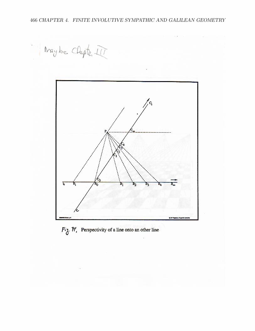
466 CHAPTER 4. FINITE INVOLUTIVE SYMPATHIC AND GALILEAN GEOMETRY

4.90. ANSWERS TO PROBLEMS AND MISCELLANEOUS NOTES. 467
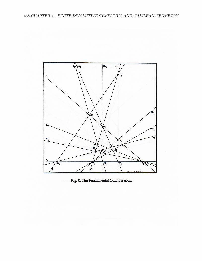
468 CHAPTER 4. FINITE INVOLUTIVE SYMPATHIC AND GALILEAN GEOMETRY

4.90. ANSWERS TO PROBLEMS AND MISCELLANEOUS NOTES. 469

470 CHAPTER 4. FINITE INVOLUTIVE SYMPATHIC AND GALILEAN GEOMETRY

4.90. ANSWERS TO PROBLEMS AND MISCELLANEOUS NOTES. 471

472 CHAPTER 4. FINITE INVOLUTIVE SYMPATHIC AND GALILEAN GEOMETRY
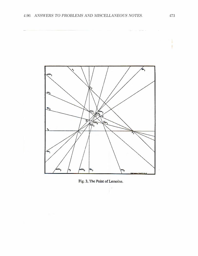
4.90. ANSWERS TO PROBLEMS AND MISCELLANEOUS NOTES. 473

474 CHAPTER 4. FINITE INVOLUTIVE SYMPATHIC AND GALILEAN GEOMETRY

4.90. ANSWERS TO PROBLEMS AND MISCELLANEOUS NOTES. 475

476 CHAPTER 4. FINITE INVOLUTIVE SYMPATHIC AND GALILEAN GEOMETRY

4.90. ANSWERS TO PROBLEMS AND MISCELLANEOUS NOTES. 477
478 CHAPTER 4. FINITE INVOLUTIVE SYMPATHIC AND GALILEAN GEOMETRY

Chapter 5
FINITE NON-EUCLIDEANGEOMETRY
5.0 Introduction.
In Chapter IV, Finite Euclidean geometry was constructed. In it, we have seen that theangles can be given as integers. In the finite hyperbolic Euclidean geometry, the angles canbe represented by elements in Zp−1 and in finite elliptic Euclidean geometry by elements inZp+1. The distances can, in either case, be represented elements in Zp or by δ times anelement in Zp, where δ is such that δ2 is a non quadratic residue in Zp.I made many attempts to define angles and distances for a geometry which can be consideredas the finite form of non-Euclidean geometry. The clue was finely provided by the work ofLaguerre. I will show that using this definition, both angles and distances can be treated sym-metrically, or to use a mathematical terminology, that we have duality between the notionsof angle of 2 lines and distance of 2 points.
For those familiar with non-Euclidean geometry, in the classical case, there is a distinc-tion between the hyperbolic non-Euclidean geometry of Lobatchevski and the elliptic non-Euclidean geometry of Bolyai. The axioms, in a form already familiar to Saccheri, are:there exists a triangle whose sum of interior angles is equal to (Euclidean), smaller than(Lobatchevski) or greater than (Bolyai) 180 degrees.
In the hyperbolic case, the set of lines through a point P not on a line l is subdivided into2 sets, those which intersect l and those who do not. If we assume continuity, there are 2lines which form the boundary of either set and are called parallels. The simplest model isobtained by starting with the 2 dimensional projective plane and choosing a given conic asideal. We define as points those inside the conic and as lines the portion of the lines of theprojective plane inside the conic. The parallels to l from a point P not on l are those whichpass through the intersection of l with the conic.
In the elliptic case, there are no parallels, the lines always intersect. The simplest modelis obtained by choosing a sphere in 3 dimensional Euclidean geometry. We define as linesthe great circles of a sphere and as points the points of the sphere, identifying each point withits antipode.
In the finite case, there is no distinction between the elliptic and the hyperbolic case.
479

480 CHAPTER 5. FINITE NON-EUCLIDEAN GEOMETRY
Indeed in finite projective geometry, the inside or the outside of a conic cannot be defined.Instead, for some lines there are no parallels and for others the situation is analogous tothat described in the classical hyperbolic case. For those who like to refer to some geometricpicture, the image of the geometry on the sphere will be useful although imperfect. I willrefer to it from time to time. Again, although I would find it more satisfactory to proceedsynthetically, I will proceed algebraically to reach the goal more quickly.
In finite Euclidean geometry, I proceeded from projective geometry in 3 steps, affine ge-ometry, involutive geometry and Euclidean geometry. Here I will proceed in 2 steps, polargeometry and non Euclidean geometry.
In the involutive geometry, an involution on the ideal line is chosen, from which thenotions of perpendicularity and circles are derived. In finite projective geometry, no coniccan be distinguished from any other. To define finite non-Euclidean geometry, I proceed in 2steps. In the first step, I define the finite polar geometry by chosing, or better still, preferinga specific polarity, or equivalently a specific conic. From it, the notions of parallelism, circles,equality of segments, . . . , are derived. In the second step, I introduce the notions of measureof distances and measure of angles, in this case also, the ideal conic plays again an essentialrole.
5.1 Finite Polar geometry.
5.1.0 Introduction.
After defining the geometry starting from a finite projective geometry in which a given polarityis preferred, I define elliptic, parabolic and hyperbolic points and lines. I then define circleswithout using the notion of distance, equidistance and the dual notion of equiangularity are,as in finite Euclidean geometry derived notion. After defining perpendicularity, I definespecial triangles using equidistance and right angles. I then proceed to define mid-points,medians and mediatrices and finally the circumcircles of a triangle. A new point, which Icall the center of a triangle is defined using 2 independent methods. This point also exists inclassical non-Euclidean geometry, but I have not found any reference in the literature. Theintersection of the circumcircles of a triangle are obtained and constructed. Various resultsobtained while studying the center of a triangle are derived. The circumcircle for the specialcase of a triangle with an ideal vertex is studied and finally the properties of the parabola aregiven in detail.
5.1.1 The ideal conic, elliptic, parabolic and hyperbolic points andlines.
Definition.
Among all the conics in the plane, the chosen one is called the ideal conic or the ideal. Thepoints on the conic are called ideal points or parabolic points. The lines tangent to the conicare called ideal lines or parabolic lines. They could also be called isotropic, by analogy withthe Euclidean case, but I will not use this terminology.A line which intersects the ideal in 2 real points is called a hyperbolic line, a point which is

5.1. FINITE POLAR GEOMETRY. 481
incident to 2 ideal lines is called a hyperbolic point.A line which does not contain ideal points or a point which is not on an ideal line is calledelliptic.A point or a line is said to be an ordinary point if the point or the line is either elliptic orhyperbolic.Two points or two lines are said to be of the same type if they are both either elliptic orhyperbolic. Points of the same type are necessarily ordinary.
Convention.
By convention, the conic chosen for the algebraic derivation isX ·X = 0 or X2
0 +X21 +X2
2 = 0.
Example.
For p = 13, the ideal points are 6, 9, 19, 22, 57, 62, 69, 76, 79, 118, 134, 141, 148, 153.
Theorem.
The polar of A = (A0, A1, A2) with respect to the ideal conic is a = [A0, A1, A2].
Notation.
The polar of A will be denoted a, the pole of a, A.This notation should not be confused with the notation in section . . . on finite projectivegeometry.
Theorem.
With j = +1 or −1, the ideal points on the line a = [a0, a1, a2] are
0. if a21 + a2
2 6= 0,(a2
1 + a22, −a0a1 + ja2
√d, −a0a2 − ja1
√d), where
d = −(a20 + a2
1 + a22),
1. if a21 + a2
2 = 0 and a1.a2 6= 0,(0, a1 + ja2
√−1, a2 − ja1
√−1),
2. if a1 = a2 = 0,(0, 1, j
√−1).
Example.
For p = 13, let a = [124] = [1, 8, 6], then d = 3,√d = 4, the ideal points on a are (−4,−8−
2,−6− 6) = (1, 9, 3) = (134) and (−4,−8 + 2,−6 + 6) = (1, 8, 0) = (118).

482 CHAPTER 5. FINITE NON-EUCLIDEAN GEOMETRY
Theorem.
The point A = (A0, A1, A2) and the line a = [A0, A1, A2] are
0. parabolic, iff A · A = 0,
1. elliptic, iff −A · A is a non quadratic residue modulo p,in other words,if there is no integer x such that
x2 = −A · A,
2. hyperbolic, iff −A · A is a quadratic residue modulo p.
Example.
For p = 13, (6) = (0,1,5) is parabolic, (172) = (1,12,2) is elliptic and (124) = (1,8,6) ishyperbolic.
Theorem.
0. There are p+ 1 parabolic or ideal points,
1. There are p(p−1)2
elliptic points,
2. There are p(p+1)2
hyperbolic points.
Proof: Each of the p + 1 parabolic line meets the other p parabolic lines in a hyperbolicpoint.
Definition.
Two lines are parallel if they have an ideal point in common.Two points are parallel if they have an ideal line in common.
Example.
For p = 13, (61) = (1,3,8) and (71) = (1,4,5) are parallel, they are on [134] = [1,9,3].
Theorem.
The intersections of the sides of a triangle with the polars of the opposite vertex with respectto any conic are collinear.
This follows at once from II.2.2.4.7 if we choose the coordinates in such a way that theconic is the ideal conic.

5.1. FINITE POLAR GEOMETRY. 483
5.1.2 Circles in finite polar geometry.
Introduction.
There are 3 kinds of circles in polar geometry.A hyperbolic circle is a conic tangent to the ideal conic at 2 distinct points. Its center is theintersection of these tangents.An elliptic circle is a conic tangent to the ideal conic at 2 distinct complex conjugate points.A parabolic circle is one for which the two points of tangency coincide.I will give now the corresponding algebraic definition, when convention 5.1.1 is used.Having introduced the notion of circles, it is natural to define the notion of equidistancebetween points and equiangularity between lines. When measure of angles and distances willbe introduced, the compatibility of the 2 concepts equivalence and measure will be made clear.
Definition.
The circles of center C = (C0, C1, C2) are the conics with equationX ·X + k(X · C)2 = 0.
Definition.
The line c = [C0, C1, C2] is called the central line of the circle.
Theorem.
The central line is the polar of the center in the polarity associated to the circle as well asin the polarity associated to the ideal conic.
Definition.
A circle is called hyperbolic if its center is hyperbolic, elliptic, if its center is elliptic andparabolic if its center is a parabolic or ideal point.
Theorem.
The ordinary points on a circle are all either hyperbolic or elliptic.Proof: If k is a quadratic residue modulo p, then −X · X is a quadratic residue and X
is necessarily hyperbolic. If k is a non residue, then −X · X is a non residue and X isnecessarily elliptic.
Theorem.
If a circle is hyperbolic, the lines through the center and the ideal points on the central lineare tangent to both the ideal conic and the circle. If the circle is parabolic, the center C isan ideal point and its polar is the tangent at the ideal point to both the ideal conic and thecircle.

484 CHAPTER 5. FINITE NON-EUCLIDEAN GEOMETRY
All hyperbolic circles can be constructed using the degenerate form of Pascal’s construc-tion. The following Theorem allows the construction of parabolic circles and of many ellipticcircles.
Theorem.
For any circle of center C and central line c through a point X1 not on c, if I1 is an idealpoint on C × X1 and I2 is a distinct ideal point not on c and I1 × I2 meets c in X0 thenX2 := (X0 ×X1)× (C × I2) is also on the circle.
Theorem.
If a circle of center C is not parabolic, let A and B be arbitrary points on the circle, let Mand N be the other ideal points on C × A and C × B, then the central line, A × B andM ×N pass through the same point.
Example.
For p = 13, (see g13.tab)
0. One of the hyperbolic circles of center (124) has the equation6(x2 + y2 + z2) + (x+ 8y + 6z)2 = 0,or 7x2 + 5y2 + 3z2 + 5yz − zx+ 3xy = 0.
It contains the ideal points 118 and 134 and the elliptic points 2, 7, 44, 46, 54, 56,105, 111, 135, 151, 158, 164.
1. One of the elliptic circles with center (172) has equation2(x2 + y2 + z2 + (x− y + 2z)2 = 0,or 3x2 + 3y2 + 6z2 − 4yz + 4zx− 2xy = 0.
It contains the elliptic points 7, 13, 15, 21, 41, 44, 70, 77, 98, 111, 116, 151, 156, 169.
2. One of the parabolic circles with center (6) has the equation(x2 + y2 + z2) − (y + 5z)2 = 0,or x2 + 2z2 + 3yz = 0.
It contains the ideal point 6 and the hyperbolic points 1, 33, 39, 81, 89, 100, 101, 109,110, 121, 129, 171, 177.
Definition.
Two circles are parallel if they have one ideal point in common. Two circles are concentricif they have the same center.
Theorem.
Two concentric circles have all their ideal points in common. One for the parabolic circles,2 for the hyperbolic circles.
5.1. FINITE POLAR GEOMETRY. 485
Definition.
The points A and B are equidistant from the point C iff there exists a circle of center Cpassing through both A and B.
Theorem.
A and B are equidistant from C iff(A · C)2 (B ·B) = (B · C)2 (A · A).
This suggest the more general definition:
Definition.
The distance between the points A and B is the same as the distance between the points Cand D iff
(A ·B)2 (C · C)(D ·D) = (C ·D)2 (A · A)(B ·B).The angle between the lines a and b is the same as the angle between the lines c and d iff
(a · b)2 (c · c)(d · d) = (c · d)2 (a · a)(b · b).
Definition.
The angle between a and b is a right angle iff a · b = 0 and the distance between A and B isa right distance iff A ·B = 0.
Comment.
Although the distance between 2 points A and B has not yet been defined, I will by conventionuse the notation d(A,B). This will be acceptable, in polar geometry, as long as the notationappears in both sides of an equality. I will later define the distance between 2 points andshow that it is consistent with 5.1.2.
Theorem.
The notion of equidistance between pairs of points and the notion of equiangularity betweenpairs of lines is an equivalence relation, in other words, the relation isreflexive: d(A,B) = d(B,A),symmetric: d(A,B) = d(C,D) =⇒ d(C,D) = d(A,B),transitive: d(A,B) = d(C,D) and d(C,D) = d(E,F ) =⇒ d(A,B) = d(E,F ).
5.1.3 Perpendicularity.
Definition.
The line b is perpendicular to the line a iff b passes through the pole A of a with respect tothe ideal conic, in other words, when a and b are conjugates with respect to the ideal conic.

486 CHAPTER 5. FINITE NON-EUCLIDEAN GEOMETRY
Theorem.
If the line b is perpendicular to a, thenb · a = 0.
In other words, the angle between a and b is a right angle.This follows at once from 5.1.2.
Theorem.
The perpendicular h0, h1, h2 from the vertices A0, A1, A2 of a triangle to the opposite sideshave a point H in common. Moreover,
h0 = (A2 · A0) A1 − (A0 · A1) A2,h1 = (A0 · A1) A2 − (A1 · A2) A0,h2 = (A1 · A2) A0 − (A2 · A0) A1.H = (A2 · A0)(A0 · A1) A1 ∗ A2 + (A0 · A1)(A1 · A2) A2 ∗ A0
+(A1 · A2)(A2 · A0) A0 ∗ A1.Proof: h0 := A0 ∗ (A1 ∗ A2), is indeed a line through A0 perpendicular to A1 ∗A 2. The
results follow easily from II.2.2.4. Related results are obtained in 5.1.4.
Definition.
hi are called the altitudes of the triangle. The point H is called the orthocenter.
Example.
For p = 13, if A0 = (0) = (0, 0, 1), A1 = (18) = (1, 0, 4), A2 = (67) = (1, 4, 1), thenh0 = (27) = [1, 1, 0], h1 = [1, 4, 3], h2 = [1, 0, 12] and H = (171) = (1, 12, 1).
Comment.
Section 7 could be placed here, but then the motivation would be absent.
5.1.4 Special triangles.
Definition.
A right, double right, polar triangle is a triangle which has one, two or three right angles.A right sided or double right sided triangle is a triangle for which the distance between onepair or two pairs of vertices is a right distance.
Examples.
For p = 13 : The triangle A = (8) = (0, 1, 7), B = (17) = (1, 0, 3), C = (36) = (1, 1, 9), withsides [44] = [1,2,4], [150] = [1,10,6], [161] = [1,11,4] is a right triangle at B.The triangle A = (44), B = (17), C = (36), with sides [44], [130] = [1,8,12], [161] is adouble right triangle at B and C. The triangle A = (44), B = (17), C = (161), with sides[44], [17] [161] is a polar triangle.

5.1. FINITE POLAR GEOMETRY. 487
Exchanging vertices and sides, we obtain, by duality, examples of right sided and double rightsided triangles.
Definition.
A triangle is isosceles if 2 pairs of vertices are equidistant.A triangle is equilateral if all 3 pairs of vertices are equidistant.
Theorem.
0. If a triangle ABC is such that d(A,B) = d(A,C), thend(a, b) = d(a, c).
1. If a triangle ABC is such that d(A,B) = d(B,C) = d(A,C), thend(a, b) = d(a, c) = d(b, c).
Proof: The second part follows, by transitivity, from the first part. For the first part, letus set p = A ·A, q = B ·B, r = C ·C, t = B ·C, u = C ·A, v = A ·B. The hypothesis implies
v2r = u2q = s.We want to prove that
w = (a · b)2c · cdoes not change when we exchange b and c or q and r as well as u and v. Using II.2.2.4.2and .3, a · b = ut− vr and c · c = pq − v2,therefore
w = (u2t2 + v2r2 − 2tuvr)(pq − v2)= pt2s− t2u2v2 + psqr − s2 − 2ptqruv − 2tsuv.
Example.
For p = 13 : The triangle A = (172) = (1, 12, 2), B = (7) = (0, 1, 6), C = (13) = (0, 1, 12),with sides a = [14] = [1, 0, 0], b = [182] = [1, 12, 12], c = [74] = [1, 4, 8] is an isoscelestriangle. The triangle A = (172), B = (7), C = (15) = (1, 0, 1), with sides a = [104] =[1, 6, 12], b = [182], c = [74] is an equilateral triangle.
Theorem.
In a polar triangle, each vertex is the pole of the opposite side and the distance between thevertices is a right distance.
Definition.
Two triangles are dual of each other iff the sides of one are the polar of the vertices of theother.
Example.
The dual of the triangle of example 5.1.3 is, with p = 13,A0 = (173) = (1, 12, 3), A1 = (53) = (1, 3, 0), A2 = (1) = (0, 1, 0).
488 CHAPTER 5. FINITE NON-EUCLIDEAN GEOMETRY
Theorem.
A polar triangle is its own dual.
Theorem.
The altitudes of a triangle and of its dual coincide. The orthocenter of a triangle and of itsdual coincide.
The proof is left as an exercise.
5.1.5 Mid-points, medians, mediatrices, circumcircles.
Introduction.
For this section, the analogy with the model of the non-Euclidean geometry on the sphere isuseful. We recall that each point has 2 representations on the sphere, which are antipodes ofeach other. If we take 2 points A and B, let A′ and B′ be their antipodes, there are 2 pointson the great circle, (in the plane through the center of the sphere) which are equidistant fromA and B, namely a point on the arc AB and a point on the arc A′B, which is the antipode ofthe mid-point on the arc AB′. But the analogy is not complete, in the finite case, it is onlywhen the points are of the same type that mid-points exist. There is about 1 chance in 2 thatthe points are not of the same type, there are then no mid-points, there is about 1 chancein 2 that they are of the same type, there are then 2 mid-points, this is an other example ofwhat I call the law of compensation.To simplify the algebra, I will introduce a scaling in 5.1.5. The scaling contains an arbitrarysign, which may be thought as corresponding to the 2 representations on the sphere. Thesystematic way which is chosen could be replaced by some other one. The choice is influencedby the choice of a primitive root of p and the sign of the square root and depends on the rule. . . . Having the concept of mid-points, we can consider those of the vertices of a triangle, ifthe vertices are scaled, we can define interior and exterior mid-points. Again, the choice isarbitrary and depends on the rule . . . .To each side correspond 2 medians, these meet 3 by 3 in 4 points corresponding to thebarycenter. Again the analogy with the geometry on the sphere is useful, the 4 barycenterscan be considered as corresponding to the triangles ABC, A′BC, AB′C, ABC ′.A similar treatment can be made for the mediatrices which meet 3 by 3 in 4 points, each isthe center of a circumcircle of the triangle ABC.But, again, the analogy with the geometry on the sphere is not complete. Given a triangle,there are about 3 chances in 4 that the 3 vertices are not all of the same type, in this casethere is no barycenter and no circumcircle. In about 1 chance out of 4, the 3 points are of thesame type, and there are 4 barycenters and 4 circumcircles. Again this is the compensation.If the vertices of the triangle are of the same type, the 4 lines joining a barycenter to thecorresponding center of a circumcircle can be considered as generalizations of the line ofEuler. It is natural to conjecture that these four lines are concurrent. This is indeed thecase. The surprise is that this point V is not the orthocenter. The coordinates of V are realeven if the vertices of the triangle are not of the same type. V must therefore be obtainablein an independent way. One such method is described in section 7.

5.1. FINITE POLAR GEOMETRY. 489
I first recall the convention of I.??.
Convention.
Given δ a specific square root of a specific non quadratic residue of p, we choose the squareroot a of a quadratic residue or the square root aδ, of a non residue in such a way that0 ≤ a < p−1
2.
Notation.
Using the preceding convention, a square root is uniquely defined. It is convenient to introducean other scaling for points and lines different from that given in II.2.2.1.If A = (A0, A1, A2) and A is not an ideal point,
A′ = A√−A·A .
|A| =√−A · A is called the length of A. Either each component is an integer, or
each component is an integer divided by δ , in this last case we say that A′ is pure imaginary.
Theorem.
If A is hyperbolic, A′ is real, if A is elliptic, A′ is pure imaginary. Moreover A′ · A′ = −1.
Definition.
Given 2 points A and B of the same type, M on A×B is called a mid-point of [A,B] iff thedistances MA and MB are equal.
Theorem.
The mid-points of [A,B] are M = A′ +B′ and M− = A′ −B′.Proof: Because of 5.1.2, d(M,A) = d(M,B) if
(M · A′)2 = (M ·B′)2,or if (A′ · A′)2 + (A′ ·B′)2 + 2(A′ · A′)(A′ ·B′)
= (B′ ·B′)2 + (B′ · A′)2 + 2(B′ ·B′)(B′ · A′),which is satisfied because of A′ · A′ = B′ ·B′ = −1 and
A′ ·B′ = B′ · A′.The proof is similar for M−.
Definition.
M is called the interior mid-point, M− is called the exterior mid-point.
Example.
For p = 13, the mid-points of (44) = (1,2,4) and (164) = (1,11,7) are (115) = (1,7,10) and
(124) = (1,8,6). Indeed |44| =√
5, |164| =√
11, hence, |44||164| =
√−8−2
=√
4 = 2, therefore
the mid-points are (1,2,4) + 2(1,11,7) = (3,24,18) = (1,8,6) and (1, 2, 4) − 2(1, 11, 7) =

490 CHAPTER 5. FINITE NON-EUCLIDEAN GEOMETRY
(−1,−20,−10) = (1, 7, 10).With δ2 = 8, A′ = A
δ, B′ = B
(6δ, therefore the interior mid-point is A + 1
6B = A − 2B =
(1, 7, 10) and the exterior mid-point is A− 16B = A+ 2B = (1, 8, 6).
Definition.
m is called a mediatrix of [A,B] iff m is perpendicular to A × B and passes through amid-point of [A,B].
Theorem.
m := A′ −B′ passes through M = A′ +B′ andm− := A′ +B′ passes through M− = A′ −B′.
Proof: m is perpendicular to A×B becausem · (A ∗B) = m · (A′ ∗B′) = A′ · (A′ ∗B′)−B′ · (A′ ∗B′) = 0.
m passes through M, because m ·M = (A′−B′) ·(A′+B′) = A′ ·A′−B′ ·B′ = −1−(−1) = 0.
Theorem.
The set of points equidistant from A and B are on m or m′.
Definition.
In a triangle, the line joining a vertex to the interior (exterior) mid-points of the oppositeside is called an interior (exterior) median.
Theorem.
If a triangle is isosceles, with d(A0, A1) = d(A0, A2), then a median through A0 is also amediatrix.
5.1.6 The center V of a triangle.
Theorem.
Let Mi and M−i be the interior and exterior mid-points of Ai−1 and Ai+1, let ni and n−i be
the interior and exterior medians associated to Ai.
0. G3 := n0 × n1 ⇒ G3 · n2 = 0. (*)
1. Gi := ni × n−i+1 ⇒ Gi · n−i−1 = 0(*).Let mi and m−i be the interior and exterior mediatrices of Ai+1Ai−1.
2. O3 := m0 ×m1 ⇒ O3 ·m2 = 0.(*)
3. Oi := mi ×m−i+1 ⇒ Oi ·m−i−1 = 0.(*)
4. ej := Oj ×Gj and V := e0 × e1 ⇒ V · e2 = V · e3 = 0.(*)

5.1. FINITE POLAR GEOMETRY. 491
The proof follows from Theorem 4.4.12. As in finite Euclidean geometry “*” indicatesthat there are equivalent definitions, for instance 0 could be written G3 := n1 × n2 andG3 · n0 = 0.
Definition.
By analogy with Euclidean geometry, the points Gj are called the barycenters of the triangle.The points Oj are called the centers of the circumcircles of the triangle.The lines ej are called the lines of Euler of the triangle.
Definition.
V is called the center of the triangle.
Theorem.
Let A′i be the normalized coordinates of the vertices of a triangle1.
0. The mid points are A′i−1 + jiA′i+1, ji = +1 or −1.
1. The mediatrices are A′i−1 − jiA′i+1.
2. The medians ni are A′i × (A′i−1 + jiA′i+1).
3. Choosing j0j1j2 = 1, the medians meet 3 by 3 at the 4 barycenters which are A′0 +j2A
′1 + j1A
′2.
4. The mediatrices meet 3 by 3 at the 4 centers of circumcircles, which areA′1 ∗ A′2 + j2A
′2 ∗ A′0 + j1A
′0 ∗ A′1.
5. The Euler lines, joining Gj to Oj are, with d′i = A′i−1 · A′i+1, (j0d′1 − d′2)A′0 + (j2d
′2 −
j0d′0)A′1 + (d′0 − j′2d′1)A′2.
6. The Euler lines intersect at V andV = d′0A
′1 ∗ A′2 + d′1A
′2 ∗ A′0 + d′2A
′0 ∗ A′1.
7. Moreover, V = A0 ·A0A1 ·A2A1 ∗A2 +A1 ·A1A2 ·A0A2 ∗A0 +A2 ·A2A0 ·A1A0 ∗A1.
8. V exists when the triangle is not a polar triangle.
Proof: 0. and 1. follow from . . . . For 2., the intersection of n1 and n2 isn1 ∗ n2 = −A′0(A′2 · (A′1 ∗ A′0))+j1A
′2(A′0 · (A′1 ∗ A′2))
+j0j1A′1(A′0 · (A′1 ∗ A′2))
= A′0 + j0j1A′1 + j1A
′2.
The same point is obtained if j0j1 = j2 or if j0j1j2 = 1. There are 4 points corresponding toj0 = +or − 1 and j1 = +or − 1.The proof of 3. is similar. The proof of 4. to 8. is left as exercises.
121.9.81
492 CHAPTER 5. FINITE NON-EUCLIDEAN GEOMETRY
Comment.
Reality requires, because A′i = Ai|Ai| that the lengths |Ai| be either all real or all imaginary,
hence:
Theorem.
The mid-points, mediatrices, medians, barycenter and center of circumcircles are real if andonly if the vertices are either all elliptic or all hyperbolic. V is always real.
Example.
For p = 13, the triangle A0 = (58) = (1, 3, 5), A1 = (51) = (1, 2, 11), A2 = (159) = (1, 11, 2),has all its vertices hyperbolic.Let A′0 = (6, 5, 4), A′1 = (6,−1, 1), A′2 = (6, 1,−1). The mid-points of A1 and A2 are (14) =(1,0,0) and (13) = (0,1,12). All the mid-points are (14), (13); (115), (12); (139), (8).The mediatrices are [13], [14]; [12], [115]; [8], [139].The medians are [3], [126]; [91], [176]; [76], [161].The interior mediatrices [13], [12], [8] meet at O3 = (14).The centers of the circumcircles are (56), (8), (12) and (14).The interior medians [3], [91], [76] meet at G3 = (33).The barycenters are (152), (179), (106), and (33).The center of the triangle is V = (152).
5.1.7 An alternate definition of the center V of a triangle.
Notation.
From here on, the following notation will be used systematically:
0. ai := Ai+1 × Ai−1
1. ni := Ai+1∗Ai−1
ai,which means that
Ai+1 ∗ Ai−1 = niai, defines ni,ni is the normalization factor, see 2.3.2. and 2.3.11.
2. li := Ai · Ai,
3. di := Ai+1 · Ai−1,
4. t := (A0 ∗ A1) · A2.Similarly,
5. Ni := ai+1∗ai−1
Ai,which means that
ai+1 ∗ ai−1 = NiAi, defines Ni,
6. Li := ai · ai,
7. Di := ai+1 · ai−1,
8. T := (a0 ∗ a1) · a2.

5.1. FINITE POLAR GEOMETRY. 493
Theorem.
0. t = n1n2N0 = n2n0N1 = n0n1N2.
1. n2iLi = n2
i ai · ai = li+1li−1 − d2i .
2. ni+1ni−1Di = ni+1ni−1ai+1 · ai−1
= di+1di−1 − dili.
3. n0n1n2T = t2.
and the dual relations
4. T = N1N2n0 = N2N0n1 = N0N1n2.
5. N2i li = N2
i Ai · Ai= Li+1Li−1 −D2
i .
6. Ni+1Ni−1di = Ni+1Ni−1Ai+1 · Ai−1
= Di+1Di−1 −DiLi.
7. N0N1N2t = T 2.
Theorem.
0. ai+1 ∗ ai−1 = tAi,
1. niai ∗ Ai = di−1Ai−1 − di+1Ai+1.
2. niai ∗ Ai+1 = li+1Ai−1 − diAi+1.
3. niai ∗ Ai−1 = diAi−1 − li−1Ai+1.
The proof follows easily from 2.3.17. and from 4.6.0.
Example.
For p = 13, withA[] = (0) = (0, 0, 1), (18) = (1, 0, 4), (67) = (1, 4, 1) , thena[] = [173] = [1, 12, 3], [53] = [1, 3, 0], [1] = [0, 1, 0] .l[] = [1, 4, 5], d[] = [5, 1, 4], n[] = [10, 4, 1],L[] = (11, 10, 1), D[] = (3, 12, 11), N [] = (1, 3, 4),t = [4], T = (3).

494 CHAPTER 5. FINITE NON-EUCLIDEAN GEOMETRY
Theorem.
Let h be the polar of H with respect to the triangle. Let Ki be the intersection of h and ai,2
let vi be the perpendicular at Ai to A[i]×Ki.Then vi have a point in common V 3.Moreover, if we define
0. ui := di+1di−1 − dili,we have
1. h = u0a0 + u1a1 + u2a2.
2. Ki = ui−1 Ai+1 − ui+1 Ai−1.
3. vi = (d2i+1li+1 − d2
i−1li−1) Ai − (didi+1li − di−1li−1li) Ai+1 + (didi−1li − di+1li+1li) Ai−1.
4. V = d0l0 A1 ∗ A2 + d1l1 A2 ∗ A0 + d2l2 A0 ∗ A1.
Proof: Because of 5.1.3,H = d1d2a0 + d2d0a1 + d0d1a2,after simplification,H · a0 = (d0d1 − d2l2)(d2d0 − d1l1),using the definition 0, H · a0 = u2u1, and because of 2.3.20, after multiplication by u0u1u2,we obtain 1.Ki := H ∗ ai, gives 2, after division by t.Ai ∗Ki = ui+1ai+1 + ui−1ai−1,therefore,Vi = Ai ∗ (Ai ∗Ki),substituting and using 2.3.17.0., we get
Vi = (ui−1di−1 − ui+1di+1) Ai −ui−1li Ai+1 + ui+1li Ai−1,replacing ui by its value, we get, 3, from which we obtain
v1 ∗ v2 = d0l0 A1 ∗ A2 + d1l1 A2 ∗ A0 + d2l2 A0 ∗ A1,after dividing each term by(d2
2d1l2 + d21d0l1 + d0l0l1l2 − d3
0l0 − 2d1d2l1l2).
5.1.8 Intersections of the 4 circumcircles.
Introduction.
In this section we study the 4-th point of intersection of the 4 circumcircles of a triangle.The expression for these 6 points is given in 5.1.8. A construction in the case where thecenters of the 2 circles are given is described in 5.1.8.
213.10.81319.10.81
5.1. FINITE POLAR GEOMETRY. 495
Notation.
Ci denotes the circumcircle with center Ci.Xj,k denotes the intersection of Cj and Ck distinct from the vertices of the triangle Ai, nor-malized to A′i.
ai := A′i · A′2,d := A′0 ∗ (A′1 ∗ A′2).
Theorem. 4
The intersections of the circumcircles of a triangle Ai are given, using5.1.8.X0,3 = (1 + a0) A′0 + (a2 − a1) (A′1 − A′2),X1,3 = (1 + a1) A′1 + (a0 − a2) (A′2 − A′0),X2,3 = (1 + a2) A′2 + (a1 − a0) (A′0 − A′1),X1,2 = (1− a0) A′0 + (a1 + a2) (A′1 + A′2),X2,0 = (1− a1) A′1 + (a2 + a0) (A′2 + A′0),X0,1 = (1− a2) A′2 + (a0 + a1) (A′0 + A′1).
Proof: Let Bi := A′i+1 ∗ A′i−1, thenC0 = −B0 +B1 +B2,C3 = B0 +B1 +B2,
the circles with these centers arekX2 = (X · C3)2 and kX2 = (X · C0)2,
they pass through the vertex A0 of the triangle ifk − 1 = (A0 ·B0)2 = d2
and therefore also through the vertices A1 and A2 if k = −d2. X is common to the 2 circlesif X · C0 = jX · C3 (j = +1 or −1),j = +1 leads to the vertices A′1 or A′2, j = −1 gives
X · (C0 + C3) = 2X · (B1 +B2) =2X · (A′0 ∗ (A′1 − A′2)) = 0.
therefore, for some l, and with M−0 = A′1 − A′2,
X = lA′0 +M−0 ,
henceX2 = −l2 + (M−
0 )2 + 2lA′0 ·M−0 , and
X · C3 = (lA′0 +M−0 ) · (B0 + A0 ∗M−
0 ) = lA′0 ·B0 = ld.X is on the circles C3 if
−d2(−l2 + (M−0 )2 + 2lA′0 ·M−
0 ) = l2d2,therefore
l = − (M−0 )2
2A′0·M−0
= −−2(1+a0)2(a2−a1
hence the expression for X0,3. The other points are derived similarly.
Corollary.
The intersections X1,3 and X2,3 coincide if1− a0 + a1 + a2 = 0
4Salzbourg-Innsbruck 29-30.9.83

496 CHAPTER 5. FINITE NON-EUCLIDEAN GEOMETRY
andX1,3 = X2,3 = −A′0 + A′1 + A′2,
with similar expressions for other pairs.
The proof is straightforward.
Example.
With the triangle of 5.1.6, ai = 5,,X0,3 =X1,3 =X2,3 =X1,2 =X2,0 =X0,1 =
Theorem.
Let M0,0, M0,1 be the mid-points of a0, . . . , in the algebraic order defined above, then
0. the dual lines are the mediatrices,the dual of M0,1 passes through M0,1 , . . .
1. the points M0,1, M1,0, M2,0 are on o0,the points M0,0, M1,1, M2,0 are on o1,the points M0,0, M1,0, M2,1 are on o2,the points M0,1, M1,1, M2,1 are on o3.
2. the dual of oi is the center Oi of one of the 4 circumcircles of the triangle Ai.
3. By duality, the mediatrices m0,0, m1,1, m2,1 are on O0, . . . .
Let m′0,0, m′0,1, . . . be the medians A0 ·M0,0, A0 ·M0,1, . . . then
4. the medians m′0,0, m′1,1, m
′2,1 are on G0,
the medians m′0,1, m′1,0, m
′2,1 are on G1,
the medians m′0,1, m′1,1, m
′2,0 are on G2,
the medians m′0,0, m′1,0, m
′2,0 are on G3.
Notation.
u ∗ v is the vector (u1v2 − u2v1, u2v0 − u0v2, u0v1 − u1v0)u ×× v is the vector (u1v2 + u2v1, u2v0 + u0v2,
u0v1 + u1v0)u O v is the vector (u0v0, u1v1, u2v2))
5.1. FINITE POLAR GEOMETRY. 497
Algorithm.
Given two circles through the points Ai, with centers C0 and C1, With j in the set 0, 1 andi in the set 0, 1, 2, and addition within the indices done modulo 2,
dj := Cj O Cj,Bi := ai+1Xai+2,L := d0 ∗ d1,fi := Bi · L,G := f O f,si := ai+1ai+2
Ai,
O :=∑3
i=0(siGiAi).
Theorem.
O is the 4-th point common to the two circles.
5.1.9 Other results in the geometry of the triangle.
Introduction.
The following results were obtained while searching for a construction of V, independent fromthe centers of mass and center of circumcircles.
Theorem.
Let I be an ideal point on the line I ×B. LetJ := (B ·B) I − 2(I ·B)B,
then J is the other ideal point on I ×B.
Example.
For p = 13,Let I = (22) = (1, 0, 8) and B = (4) = (0, 1, 3), thenJ = −3(1, 0, 8) + 4(0, 1, 3) = (1, 3, 4) = (57).The line I × J is [48] = [1, 2, 8].
Theorem.
Let a be an ordinary line and B an ordinary point not on a.Let I and K be the ideal points on a and J and L be the other ideal points on I × B andK ×B, let c := J ∗ JJ, then
c = (B ·B) a− 2(a ·B)B.Proof: With a = I ∗K,
J = (B ·B) I − 2(I ·B)B, L = (B ·B)K − 2(K ·B)B, henceL ∗ J = (B ·B)2 K ∗ I + 2(B ·B)((K ·B) I − (I ·B)K) ∗B,= (B ·B)(−(B ·B) a+ 2((K ∗ I) ∗B) ∗B)
because of 2.3.17.0.,

498 CHAPTER 5. FINITE NON-EUCLIDEAN GEOMETRY
= (B ·B)(−(B ·B) a− 2(a ∗B) ∗B),= (B ·B)(−(B ·B) a+ 2(B ·B) a− 2(a ·B)B)
because of 2.3.17.0., hence the Theorem.
Example.
For p = 13, let a = [139] = [1, 9, 8] and B = (4), then c = −3[1, 9, 8]− 1[0, 1, 3] = [1, 5, 9] =[88].The ideal points are I = 22, J = 57, K = 76, L = 79.
Definition.
c as defined in the preceding theorem is called the conjugate of a with respect to B.
Theorem.
The linesxi+1Ai+1 − xi−1Ai−1 + yi−1ni−1ai−1 − yi+1ai+1
are concurrent at the point∑i(yi+1yi−1t+ (xidi+1 − xi−1li−1)yi+1 + (xidi−1 − xi+1li+1)yi−1) Ai
+∑
i(xi+1xi−1ni) ai.
Theorem.
Given a triangle Ai with sides ai, let bi be the conjugate of ai with respect to Ai. Assumethat the bi are not collinear. Let Bi be the vertices of the triangle bi, then
0. Ai ×Bi are concurrent at W0.
1. Ai × bi are concurrent at H.
2. Bi × bi are concurrent at W1.Moreover,
3. bi = liAi+1 ∗ Ai−1 − 2tAi.
4. Bi = −3li−1li+1Ai + 2li−1di−1Ai+1
+2li+1di+1Ai−1 + 4tAi+1 ∗ Ai−1.
5. Ai ∗Bi = li+1di+1Ai ∗ Ai−1 − li−1di−1Ai+1 ∗ Ai+2tdi+1Ai+1 − 2tdi−1Ai−1.
6. W0 =∑
i((−3li−1li+1di−1di+1)Ai + 2di(li−1d2i−1 + li+1d
2)i+1Ai
+4tdi+1di−1Ai+1 ∗ Ai−1).
7. Ai × bi = di+1Ai+1 − di−1Ai−1.
8. H = d1d2A1 ∗ A2 + d2d0A2 ∗ A0 + d0d1A0 ∗ A1.

5.1. FINITE POLAR GEOMETRY. 499
9. Withxi = 8t2di + 2li+1li−1di+1di−1 − l0l1l2di andyi = 4tlidi,Bi × bi = xi+1Ai+1 − xi−1Ai−1 + yi−1Ai ∗ Ai+1 − yi+1Ai−1 ∗ Ai.
10. W1 =
Proof: 3., is immediate,Using 2.3.17.0 and 1.7.2., we obtain .4 after division by t,5. and 6. after division by t, 7. after division by li.8. is immediate and is indeed the same as 1.3.3.
Example.
For p = 13, using the same triangle as Example 1.7.4.Bi = 9 = (0, 1, 8), 137 = (1, 9, 6), 61 = (1, 3, 8),bi = 180 = [1, 12, 10], 101 = [1, 6, 9], 80 = [1, 5, 1],W0 = 7 = (0, 1, 6), H = 171 = (1, 12, 1), W1 = 77 = (1, 4, 11).
Exercise.
Using the dual triangle, Ai = 175, 53, 1, determine Bi, bi and W0, H and W1.
5.1.10 Circumcircle of a triangle with at least one ideal vertex.
Introduction.
In the preceding section I have dealt with circumcircles through 3 ordinary points. I will nowdiscuss the case when 1 or more points are ideal points.
Theorem.
The only circle through 3 distinct ideal points is the ideal conic, X2 = 0.
Theorem.
The only circle through 2 distinct ideal points A and B and through an ordinary point C is(c · C)2X2 − (c ·X)2C2 = 0, where
c := A×B.
Example.
p = 11, A = (31) = (1, 3, 2), B = (26) = (1, 2, 4),C = 54 = (1, 6, 4). The circumcircle through A, B and C is
X20 +X2
1 +X22 = 4(X0 − 2X1 −X2)2.
500 CHAPTER 5. FINITE NON-EUCLIDEAN GEOMETRY
Theorem.
There are 2 circles through 1 ideal point A and through two distinct ordinary points B andC not collinear with A.
Theorem.
Let X be a point not on the sides of a triangle Ai. Let Xi be the intersection with ai of theline Ai ×X, or
Xi := (Ai ×X)× ai,Let ξ be a circle through Xi.Let Yi be the other intersection of ai with ξ ,let yi := Ai × Yi,then the lines yi have a point Y in common.
Comment.
The theorem 5.1.10 is analogous to theorem . . . in Euclidean geometry. It follows from itsgeneralization . . . to projective geometry.Because of the clear connection with the Theorem of Ceva, I have the following:
Definition.
The correspondence X to the various points Y associated to the several circumcircles throughXi, is called the Ceva correspondence. I will ignore those points Y which happen to coincidewith a vertex of the triangle.
Comment.
Clearly if Y is associated to X, X is associated to Y in a Ceva correspondence. But wecannot call this an involution because the correspondence is not one to one or bijective.
Program.
The program NETR1.BAS determines the Ceva correspondence. It is illustrated in NETR1.HOM.
5.1.11 The parabola in polar geometry.
Introduction.
In this section I have defined a parabola for non Euclidean geometry and many of the re-lated elements of the parabola, by analogy with the definitions of Euclidean geometry. Byduality we essentially double the number of these elements, for instance to the focus in Eu-clidean geometry corresponds the focal point and the focal line. The basic equation is givenby 5.1.11.0.

5.1. FINITE POLAR GEOMETRY. 501
Definition.
A parabola is a conic which is tangent at one point to the ideal conic and at one point only.This point is called the isotropic point of the parabola, the tangent is called the isotropic lineof the parabola.
Definition.
A focal tangent t1 of a parabola is an ideal tangent to the parabola which is not isotropic.A focal point F1 is an ideal point which is not isotropic. There are 2 focal points F1 andF2 which are either real or complex conjugate.
Definition.
The focus F of a parabola is the intersection of the focal tangents. The focal line f of aparabola is the line through the focal points.
Theorem.
The focus is not on the isotropic line. The focus is not an ideal point.Proof: In the first case, through the focus we could draw 3 tangents to the parabola. In
the second case, the parabola would be tangent at a second point to the ideal conic and wouldtherefore be a circle.
Definition.
The director D of a parabola is the pole of its focal line with respect to the parabola.
Definition.
The axis a of a parabola is the line through its focus and its isotropic point.The axial point A of a parabola is the point on the focal line and on the isotropic line.
Definition.
The vertex V of a parabola is the ordinary point on the parabola and its axis.The vertical line v of a parabola is the ordinary tangent through the axial point.
Theorem.
A parabola with isotropic point I and focal tangent f is
0. 2(I ·X)(f ·X) = t(X ·X), f · I 6= 0, f · f 6= 0, t 6= 0, t 6= f · I.
The polar of X0 is
1. (I ·X0)f + (f ·X0)I − tX0.
The pole of a is

502 CHAPTER 5. FINITE NON-EUCLIDEAN GEOMETRY
2. (f ∗ I) · aI ∗ f + t(a · f)I + t(a · I)f + (t2 − 2tI · f)a.
Proof: 0, follows from the general equation of a conic through the intersections of theideal and the lines I and f, see . . . and from 5.1.11.11.4.0, represents a degenerate conic corresponding to the lines I and f if t = 0 and to the linesI × F1 and I × F2 if t = f · I.The proof of the last fact is left as an exercise. 1 follows from 0. See . . . . 2 is obtained bychosing 2 points on a, a ∗ I and f ∗ a, and determining the intersection of the polars of theselines.(f ∗ I) · a is a factor of each term.
Example.
For p = 13, I = (1, 5, 0), f = [1, 1, 4], t = 4,The parabola is
2(x+ 5y)(x+ y + 4z) = 4(x2 + y2 + z2).The polar of X0 = (x0, y0, z0) is
[−x0 + 3y0 + 2z0, 3x0 + 3y0− 3z0, 2x0− 3y0− 2z0].The pole of a = [a0, b0, c0] is
[a0 + c0, b0 + 5c0, a0 + 5b0 + 6c0].The director D is (1,-1,6).The axial point A is I ∗ f = (1, 5, 5).With v2 = −2, the ideal points on the parabola are I and
F1 = (1, 3 + 3v,−1− 4v), F2 = (1, 3− 3v,−1 + 4v).The tangent at F1 is
f1 = (v − 6)[6 + v, 2− 5v,−5− v] = [1,−2 + 6v, 6 + v]The ideal lines t1 = [1, 3, 4] and t2 = [1,−5, 0] are tangent to the parabola at T1 = (1, 2,−5)and T2 = (2,−5, 2), they meet at the focus F = (1,−5,−3).The directrix is [1,4,4].The axis a is I ∗ F = [1, 5, 5].The vertex V is (1,-2,-6).The tangent at the vertex is [1,4,1].The vertical line v is [1,4,1].
Theorem.
The polar of X is∑
j Ai,jXj, withAj,j = 2Ijfj − t,Aj,k = Ijfk + Ikfj, j 6= k,
The pole of a is∑
k Bj,kak, withBj,j = t2 − 2t(I · f − Ijfj)− (I ∗ f)2
j ,Bj,k = t(Ijfk + Ikfj)− (I ∗ f)j(I ∗ f)k.
The dual equation of the conic is2(I · x)(F · x) = u(x · x),
The pole of x is (I · x)F + (F · x)I − ux and F and u follow from . . .if Ij 6= frac10, u = (I0B0,0 + I1B1,1, −2I0I1B0,1),
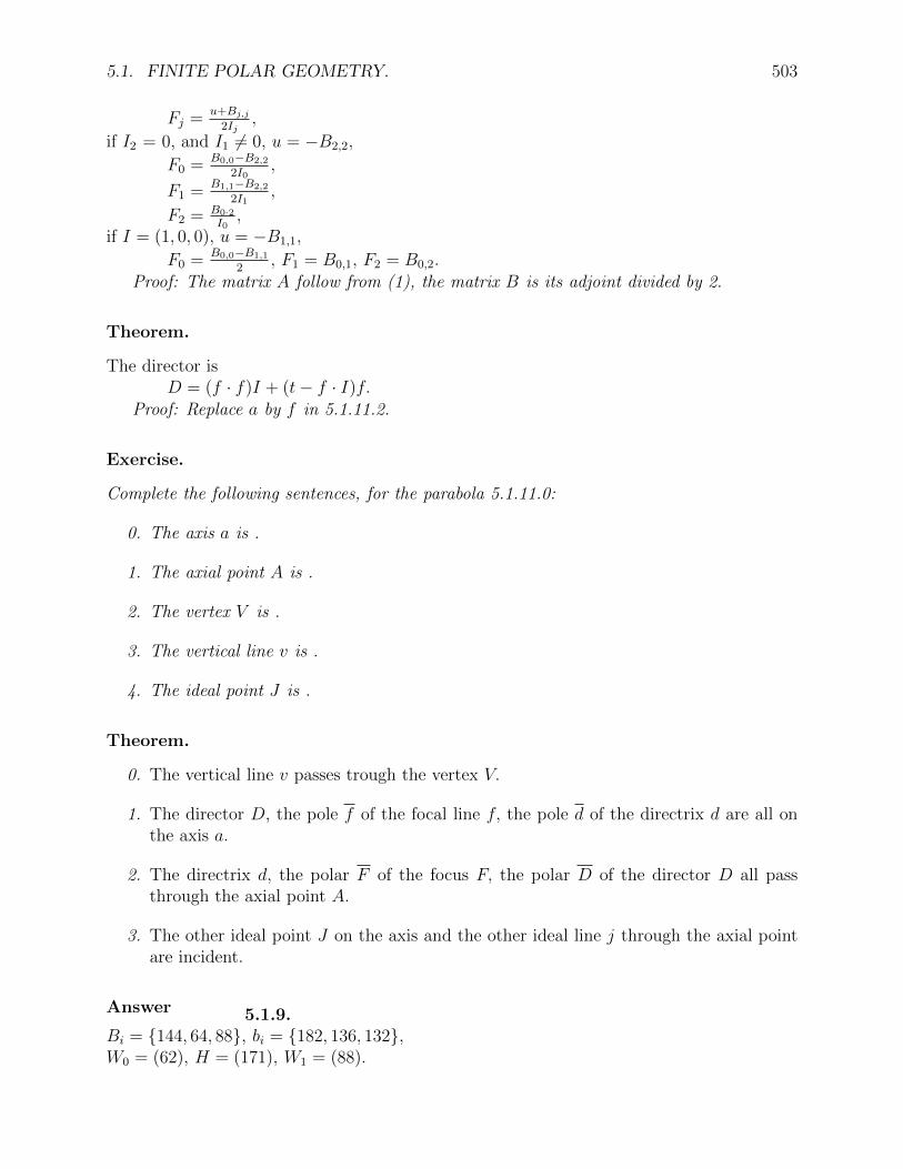
5.1. FINITE POLAR GEOMETRY. 503
Fj =u+Bj,j
2Ij,
if I2 = 0, and I1 6= 0, u = −B2,2,
F0 = B0,0−B2,2
2I0,
F1 = B1,1−B2,2
2I1,
F2 = B0·2I0,
if I = (1, 0, 0), u = −B1,1,
F0 = B0,0−B1,1
2, F1 = B0,1, F2 = B0,2.
Proof: The matrix A follow from (1), the matrix B is its adjoint divided by 2.
Theorem.
The director isD = (f · f)I + (t− f · I)f.
Proof: Replace a by f in 5.1.11.2.
Exercise.
Complete the following sentences, for the parabola 5.1.11.0:
0. The axis a is .
1. The axial point A is .
2. The vertex V is .
3. The vertical line v is .
4. The ideal point J is .
Theorem.
0. The vertical line v passes trough the vertex V.
1. The director D, the pole f of the focal line f, the pole d of the directrix d are all onthe axis a.
2. The directrix d, the polar F of the focus F, the polar D of the director D all passthrough the axial point A.
3. The other ideal point J on the axis and the other ideal line j through the axial pointare incident.
Answer 5.1.9.Bi = 144, 64, 88, bi = 182, 136, 132,W0 = (62), H = (171), W1 = (88).

504 CHAPTER 5. FINITE NON-EUCLIDEAN GEOMETRY
5.1.12 Representation of polar geometry on the dodecahedron.
Introduction.
When p = 5, the representation of polar geometry on the dodecahedron is suggested by thefact that the 6 faces form a conic which can be chosen as the ideal.
Definition.
Using the dodecahedral representation, the conic which consists of the 6 face-points is theideal conic.
Theorem.
The 15 side-points are hyperbolic and the 10 vertex-points are elliptic.
This follows at once from the incidence definitions, II.2.3.4.
Theorem.
With the ideal conic of type A,the 3 . 15 conics of type I3, E1 and E2 are hyperbolic circles,the 4 . 6 conics of type J1, J2, O1, O2 are parabolic circles andthe 3 . 10 conics of type P, U1 and U2 are elliptic circles.
Although this should be placed in the Chapter on non-Euclidean geometry, we have.
Theorem.
With a particular choice of unit, the radii of the various sub-types are as follows,U1 and E2 are π
6, U2 and E1 are π
3, P and I3 are π
3.
Example.
Computations relating to g434.PRN:If we use as primitive polynomial I3 − I − 2, we obtain the correspondence:
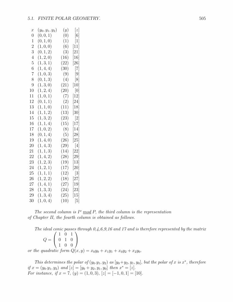
5.1. FINITE POLAR GEOMETRY. 505
x (y0, y1, y2) (y) [z]0 (0, 0, 1) (0) [6]1 (0, 1, 0) (1) [1]2 (1, 0, 0) (6) [11]3 (0, 1, 2) (3) [21]4 (1, 2, 0) (16) [16]5 (1, 3, 1) (22) [26]6 (1, 4, 4) (30) [7]7 (1, 0, 3) (9) [9]8 (0, 1, 3) (4) [8]9 (1, 3, 0) (21) [10]
10 (1, 2, 4) (20) [0]11 (1, 0, 1) (7) [12]12 (0, 1, 1) (2) [24]13 (1, 1, 0) (11) [18]14 (1, 1, 2) (13) [30]15 (1, 3, 2) (23) [2]16 (1, 1, 4) (15) [17]17 (1, 0, 2) (8) [14]18 (0, 1, 4) (5) [28]19 (1, 4, 0) (26) [25]20 (1, 4, 3) (29) [4]21 (1, 1, 3) (14) [22]22 (1, 4, 2) (28) [29]23 (1, 2, 3) (19) [13]24 (1, 2, 1) (17) [20]25 (1, 1, 1) (12) [3]26 (1, 2, 2) (18) [27]27 (1, 4, 1) (27) [19]28 (1, 3, 3) (24) [23]29 (1, 3, 4) (25) [15]30 (1, 0, 4) (10) [5]
The second column is Ix mod P, the third column is the representationof Chapter II, the fourth column is obtained as follows.
The ideal conic passes through 0,4,6,9,16 and 17 and is therefore represented by the matrix
Q =
1 0 10 1 01 0 0
or the quadratic form Q(x, y) = x0y0 + x1y1 + x0y2 + x2y0.
This determines the polar of (y0.y1, y2) as [y0+y2, y1, y0], but the polar of x is x∗, thereforeif x = (y0.y1, y2) and [z] = [y0 + y2, y1, y0] then x∗ = [z].For instance, if x = 7, (y) = (1, 0, 3), [z] = [−1, 0, 1] = [10].

506 CHAPTER 5. FINITE NON-EUCLIDEAN GEOMETRY
Example.
The hyperbolic circles have as center a edge-point.Those with center 8 = 0∗ × 8∗ and through the point u can be constructed as follows, letup = 0 × (4 × u), given any line v through 0, such that u · v 6= 0, the Pascal constructiongives the other point on the conic and v using
((((v × 4)× up)× 8)× u)× v.This gives, with the radii determined below:0,4;;2,15,22,25 of type ffssss and sub-type I3, radius π
3.
0,4;;5,11,13,20 of type ffvvvv and sub-type E1, radius π4.
0,4;;7,19,21,29 of type ffvvvv and sub-type E2. radius π6.
Before having obtained a synthetic construction of the parabolic and elliptic circles wehave used the algebraic definition.The algebraic definition is
kxTQx− (xTQC)2 = 0,with C on the ideal conic, for parabolic circles and C a vertex-point for elliptic circles.For k = 0, the circle degenerates in (a double) line, consisting of the points at distance π
2
from C.
Let C = 0, the polar 0∗ = [1, 0, 0], hence the parabolic circles arek(x2
0 − x21 + 2x2x0) + x2
0 = 0.With k′ = 1
k, the points are (0,0,1) = 0, and (1, x1, 2(1− k′ + x1)2. This gives for,
k = −1, (1,0,4) = 30, (1,1,1) = 25, (1,4,1) = 27, (1,2,2) = 26, (1,3,2) = 15, in view of thetable above. Hencek = 4, 0,30,25,27,26,15 of type fsssss and sub-type O1.k = 2, 0,11,21,20,10,29 of type fvvvvv and sub-type J2.k = 3, 0,7,13,19,24,5 of type fvvvvv and sub-type J1.k = 1, 0,2,14,22,23,28 of type fsssss and sub-type O2.
Let C = 5, the polar 5∗ = [1,−1,−2], hence the circles arek(x2
0 + x21 + 2x2x0)− (x0 − x1 − 2x2)2 = 0.
The points are,(0, 1, 2±
√−k and (1, x1,−k + 2(x1 − 1)±
√k2 − k(x2
1 − x1 + 2).This gives, for k = −1,(0,1,3) = 8, (0,1,1) = 12, (1,4,2) = 22, (1,2,3) = 23, (1,3,2) = 15,
(1, 3, 3) = 22, in view of the table above.Hence, with the radii determined below:k = 4, 8,12,22,23,15,28) of type ssssss and sub-type U2, radius π
4.
k = 2, 11,21,24,10,19,20 of type vvvvvv and sub-type P, radius π3
k = 3, 5, radius 0.k = 1, 1,18,2,30,14,25 of type ssssss and sub-type U1, radius π
6.
To summarize, we see that, with the ideal conic of type A,the 3 . 15 conics of type I3, E1 and E2 are hyperbolic circles,the 4 . 6 conics of type J1, J2, O1, O2 are parabolic circles andthe 3 . 10 conics of type P, U1 and U2 are elliptic circles.

5.1. FINITE POLAR GEOMETRY. 507
Exercise.
For a synthetic construction of the parabolic circles and some elliptic ones, we can useIV.1.2.7. This is a good exercise.
Example of Distances.
We recall the trigonometric tables for p = 5:With δ = 2,x sin(x) cos(x) x sin(x) cos(x)0 0 1 0 0 11 2δ 2δ 1 −2 δ2 1 0 2 δ −2
3 1 0
cos2(d) 0 1 2 3 4dπ
12
0 16
14
13
where cos(d(C,X)) = Q(X,C)2
Q(X,X)= k
Q(C,C).
Hence the distances, recorded above. For instance, in the case of elliptic circles, forC = 5 = (1, 3, 1) and X = 8 = (0, 1, 3), Q(C,C) = 2, Q(X,X) = 1, Q(X,C) = 1,cos2(d(C,X)) = 3, d(C,X) = π
4. Hence
for k = −1, the radius is π4,
for k = 2, cos2(d(C,X)) = −1, d(C,X) = π3,
for k = 3, d(C,X) = 0,for k = 1, d(C,X) = π
6.
In the case of hyperbolic circles with C = 8 and X = 5, we have d(8, 5) = π4, the other radii
are obtained directly,
cos2(d(8, 2)) = (−2)2
1.1= −1, hence d(8, 2) = π
4,
cos2(d(8, 7)) = (−2)2
1.2= 2, hence d(8, 7) = π
6.
Example.
Computations relating to g434.PRN: If we use as primitive polynomial I3− I − 2, we obtainthe correspondence:

508 CHAPTER 5. FINITE NON-EUCLIDEAN GEOMETRY
x (y0, y1, y2) (y) [z]0 (0, 0, 1) (0) [6]1 (0, 1, 0) (1) [1]2 (1, 0, 0) (6) [11]3 (0, 1, 2) (3) [21]4 (1, 2, 0) (16) [16]5 (1, 3, 1) (22) [26]6 (1, 4, 4) (30) [7]7 (1, 0, 3) (9) [9]8 (0, 1, 3) (4) [8]9 (1, 3, 0) (21) [10]
10 (1, 2, 4) (20) [0]11 (1, 0, 1) (7) [12]12 (0, 1, 1) (2) [24]13 (1, 1, 0) (11) [18]14 (1, 1, 2) (13) [30]15 (1, 3, 2) (23) [2]16 (1, 1, 4) (15) [17]17 (1, 0, 2) (8) [14]18 (0, 1, 4) (5) [28]19 (1, 4, 0) (26) [25]20 (1, 4, 3) (29) [4]21 (1, 1, 3) (14) [22]22 (1, 4, 2) (28) [29]23 (1, 2, 3) (19) [13]24 (1, 2, 1) (17) [20]25 (1, 1, 1) (12) [3]26 (1, 2, 2) (18) [27]27 (1, 4, 1) (27) [19]28 (1, 3, 3) (24) [23]29 (1, 3, 4) (25) [15]30 (1, 0, 4) (10) [5]
The second column is Ix mod P, the third column is the representationof Chapter II, the fourth column is obtained as follows.
The ideal conic passes through 0,4,6,9,16 and 17 and is therefore represented by the matrix
Q =
1 0 10 1 01 0 0
or the quadratic form Q(x, y) = x0y0 + x1y1 + x0y2 + x2y0.
This determines the polar of (y0.y1, y2) as [y0+y2, y1, y0], but the polar of x is x∗, thereforeif x = (y0.y1, y2) and [z] = [y0 + y2, y1, y0] then x∗ = [z].For instance, if x = 7, (y) = (1, 0, 3), [z] = [−1, 0, 1] = [10].

5.1. FINITE POLAR GEOMETRY. 509
Example.
The hyperbolic circles have as center a edge-point.Those with center 8 = 0∗ × 8∗ and through the point u can be constructed as follows, letup = 0 × (4 × u), given any line v through 0, such that u · v 6= 0, the Pascal constructiongives the other point on the conic and v using
((((v × 4)× up)× 8)× u)× v.This gives, with the radii determined below:0,4;;2,15,22,25 of type ffssss and sub-type I3, radius π
3.
0,4;;5,11,13,20 of type ffvvvv and sub-type E1, radius π4.
0,4;;7,19,21,29 of type ffvvvv and sub-type E2. radius π6.
Before having obtained a synthetic construction of the parabolic and elliptic circles wehave used the algebraic definition.The algebraic definition is
kxTQx− (xTQC)2 = 0,with C on the ideal conic, for parabolic circles and C a vertex-point for elliptic circles.For k = 0, the circle degenerates in (a double) line, consisting of the points at distance π
2
from C.
Let C = 0, the polar 0∗ = [1, 0, 0], hence the parabolic circles arek(x2
0 − x21 + 2x2x0) + x2
0 = 0.With k′ = 1
k, the points are (0,0,1) = 0, and (1, x1, 2(1− k′ + x1)2. This gives for,
k = −1, (1,0,4) = 30, (1,1,1) = 25, (1,4,1) = 27, (1,2,2) = 26, (1,3,2) = 15, in view of thetable above. Hencek = 4, 0,30,25,27,26,15 of type fsssss and sub-type O1.k = 2, 0,11,21,20,10,29 of type fvvvvv and sub-type J2.k = 3, 0,7,13,19,24,5 of type fvvvvv and sub-type J1.k = 1, 0,2,14,22,23,28 of type fsssss and sub-type O2.
Let C = 5, the polar 5∗ = [1,−1,−2], hence the circles arek(x2
0 + x21 + 2x2x0)− (x0 − x1 − 2x2)2 = 0.
The points are,(0, 1, 2±
√−k and (1, x1,−k + 2(x1 − 1)±
√k2 − k(x2
1 − x1 + 2).This gives, for k = −1,(0,1,3) = 8, (0,1,1) = 12, (1,4,2) = 22, (1,2,3) = 23, (1,3,2) = 15,
(1, 3, 3) = 22, in view of the table above.Hence, with the radii determined below:k = 4, 8,12,22,23,15,28) of type ssssss and sub-type U2, radius π
4.
k = 2, 11,21,24,10,19,20 of type vvvvvv and sub-type P, radius π3
k = 3, 5, radius 0.k = 1, 1,18,2,30,14,25 of type ssssss and sub-type U1, radius π
6.
To summarize, we see that, with the ideal conic of type A,the 3 . 15 conics of type I3, E1 and E2 are hyperbolic circles,the 4 . 6 conics of type J1, J2, O1, O2 are parabolic circles andthe 3 . 10 conics of type P, U1 and U2 are elliptic circles.
510 CHAPTER 5. FINITE NON-EUCLIDEAN GEOMETRY
Exercise.
For a synthetic construction of the parabolic circles and some elliptic ones, we can useIV.1.2.7. This is a good exercise.
Example of Distances.
We recall the trigonometric tables for p = 5:With δ = 2,x sin(x) cos(x) x sin(x) cos(x)0 0 1 0 0 11 2δ 2δ 1 −2 δ2 1 0 2 δ −2
3 1 0
cos2(d) 0 1 2 3 4dπ
12
0 16
14
13
where cos(d(C,X)) = Q(X,C)2
Q(X,X)= k
Q(C,C).
Hence the distances, recorded above. For instance, in the case of elliptic circles, forC = 5 = (1, 3, 1) and X = 8 = (0, 1, 3), Q(C,C) = 2, Q(X,X) = 1, Q(X,C) = 1,cos2(d(C,X)) = 3, d(C,X) = π
4. Hence
for k = −1, the radius is π4,
for k = 2, cos2(d(C,X)) = −1, d(C,X) = π3,
for k = 3, d(C,X) = 0,for k = 1, d(C,X) = π
6.
In the case of hyperbolic circles with C = 8 and X = 5, we have d(8, 5) = π4, the other radii
are obtained directly,
cos2(d(8, 2)) = (−2)2
1.1= -1, hence d(8, 2) = π
4,
cos2(d(8, 7)) = (−2)2
1.2= 2, hence d(8, 7) = π
6.
5.2 Finite Non-Euclidean Geometry.
5.2.0 Introduction.
5.2.1 Trigonometry for the general triangle.
Introduction.
Spherical trigonometry refers to the relation between the measure of angles and arcs of atriangle on a sphere.The formulas of al-Battani (Albategnius, about 920 A.D.) and of Jabir ibn Aflah (Geber,about 1130 A.D.) have to be adapted to the finite case in which the sine of an angle in thefirst 2 quadrants cannot be considered as positive. There are several possible solutions. Oneof these will be given in Theorem 5.2.1.Let A, B, C be the vertices of a triangle, a, b, c be its sides.

5.2. FINITE NON-EUCLIDEAN GEOMETRY. 511
The measure of the angle between b and c will be denoted A, . . . .The distance between the points B and C will be denoted a, . . . .
Definition.
Let A, B, C be 3 points on the spherex2 + y2 + z2 = 1,
of center O = (0, 0, 0, 1).The direction DA of A is the ideal point on OA.The side a = B,C is a section of the circle Ca which is the intersection of the sphere andthe plane O×B×C. The spherical distance of the side a, also denoted a is the angle betweenthe directions DB and DC.The angle BAC, also denoted A is the angle of the directions of the tangents at A to thecircles Cb and Cc.
Theorem.
Between the trigonometric functions of the angles and sides of a general triangle we have therelations:
0. |sina|sinA
= |sinb|sinB
= |sinc|sinC
= r.
1. 0. cosA = cosBcosC + sinBsinCcosa,1. cosB = cosCcosA+ sinCsinAcosb,2. cosC = cosAcosB + sinAsinBcosc.
2. 0. cosa = cosbcosc+ |sinb||sinc|cosA,1. cosb = cosccosa+ |sinc||sina|cosB,2. cosc = cosacosb+ |sina||sinb|cosC.
3. 0. sinA = cos2B−cos2CsinBcosCcosc−sinCcosBcosb ,
1. sinB = (cos2C−cos2AsinCcosAcosa−sinAcosCcosc ,
2. sinC = (cos2A−cos2BsinAcosBcosb−sinBcosAcosa .
4. 0. |sina| = cos2b−cos2c|sinb|cosccosC−|sinc|cosbcosB ,
1. |sinb| = cos2c−cos2a|sinc|cosacosA−|sina|cosccosC ,
2. |sinc| = cos2a−cos2b|sina|cosbcosB−|sinb|cosacosA .
5. 0. cosA = sinBcosBcosc−sinCcosCcosbsinBcosCcosc−sinCcosBcosb ,
1. cosB = sinCcosCcosa−sinAcosAcoscsinCcosAcosa−sinAcosCcosc ,
2. cosC = sinAcosAcosb−sinBcosBcosasinAcosBcosb−sinBcosAcosa .
6. 0.cosa = |sinb|cosbcosC−|sinc|cosccosB|sinb|cosccosC−|sinc|cosbcosB ,
1.cosb = |sinc|cosccosA−|sina|cosacosC|sinc|cosacosA−|sina|cosccosC ,
2.cosc = |sina|cosacosB−|sinb|cosbcosA|sina|cosbcosB−|sinb|cosacosA .
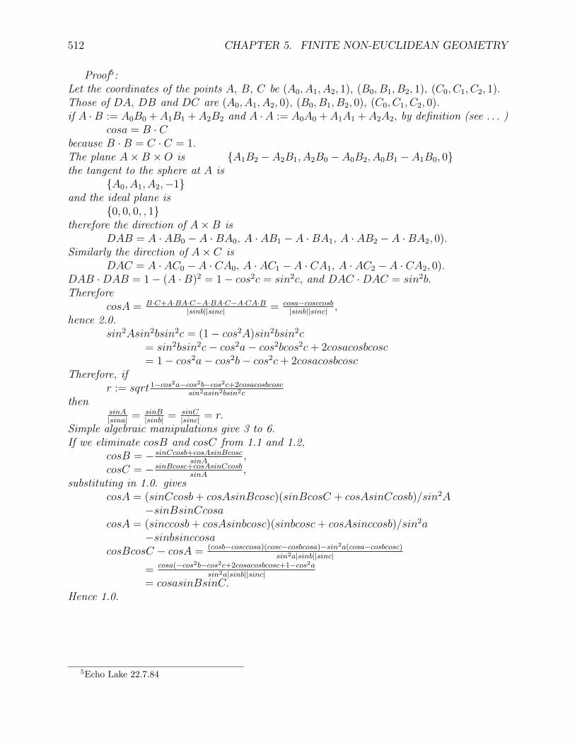
512 CHAPTER 5. FINITE NON-EUCLIDEAN GEOMETRY
Proof5:Let the coordinates of the points A, B, C be (A0, A1, A2, 1), (B0, B1, B2, 1), (C0, C1, C2, 1).Those of DA, DB and DC are (A0, A1, A2, 0), (B0, B1, B2, 0), (C0, C1, C2, 0).if A ·B := A0B0 +A1B1 +A2B2 and A ·A := A0A0 +A1A1 +A2A2, by definition (see . . . )
cosa = B · Cbecause B ·B = C · C = 1.The plane A×B ×O is A1B2 − A2B1, A2B0 − A0B2, A0B1 − A1B0, 0the tangent to the sphere at A is
A0, A1, A2,−1and the ideal plane is
0, 0, 0, , 1therefore the direction of A×B is
DAB = A · AB0 − A ·BA0, A · AB1 − A ·BA1, A · AB2 − A ·BA2, 0).Similarly the direction of A× C is
DAC = A · AC0 − A · CA0, A · AC1 − A · CA1, A · AC2 − A · CA2, 0).DAB ·DAB = 1− (A ·B)2 = 1− cos2c = sin2c, and DAC ·DAC = sin2b.Therefore
cosA = B·C+A·BA·C−A·BA·C−A·CA·B|sinb||sinc| = cosa−cosccosb
|sinb||sinc| ,hence 2.0.
sin2Asin2bsin2c = (1− cos2A)sin2bsin2c= sin2bsin2c− cos2a− cos2bcos2c+ 2cosacosbcosc= 1− cos2a− cos2b− cos2c+ 2cosacosbcosc
Therefore, ifr := sqrt1−cos2a−cos2b−cos2c+2cosacosbcosc
sin2asin2bsin2c
thensinA|sina| = sinB
|sinb| = sinC|sinc| = r.
Simple algebraic manipulations give 3 to 6.If we eliminate cosB and cosC from 1.1 and 1.2,
cosB = − sinCcosb+cosAsinBcoscsinA
,cosC = − sinBcosc+cosAsinCcosb
sinA,
substituting in 1.0. givescosA = (sinCcosb+ cosAsinBcosc)(sinBcosC + cosAsinCcosb)/sin2A
−sinBsinCcosacosA = (sinccosb+ cosAsinbcosc)(sinbcosc+ cosAsinccosb)/sin2a
−sinbsinccosacosBcosC − cosA = (cosb−cosccosa)(cosc−cosbcosa)−sin2a(cosa−cosbcosc)
sin2a|sinb||sinc|
= cosa(−cos2b−cos2c+2cosacosbcosc+1−cos2asin2a|sinb||sinc|
= cosasinBsinC.Hence 1.0.
5Echo Lake 22.7.84
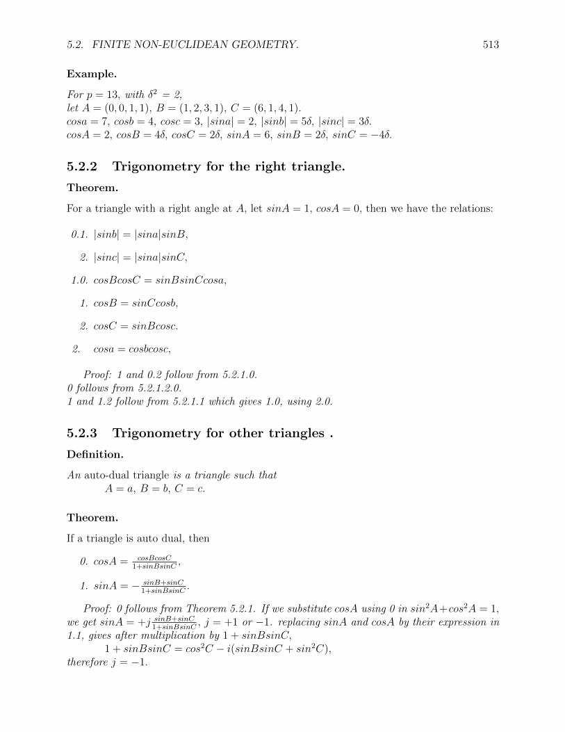
5.2. FINITE NON-EUCLIDEAN GEOMETRY. 513
Example.
For p = 13, with δ2 = 2,let A = (0, 0, 1, 1), B = (1, 2, 3, 1), C = (6, 1, 4, 1).cosa = 7, cosb = 4, cosc = 3, |sina| = 2, |sinb| = 5δ, |sinc| = 3δ.cosA = 2, cosB = 4δ, cosC = 2δ, sinA = 6, sinB = 2δ, sinC = −4δ.
5.2.2 Trigonometry for the right triangle.
Theorem.
For a triangle with a right angle at A, let sinA = 1, cosA = 0, then we have the relations:
0.1. |sinb| = |sina|sinB,
2. |sinc| = |sina|sinC,
1.0. cosBcosC = sinBsinCcosa,
1. cosB = sinCcosb,
2. cosC = sinBcosc.
2. cosa = cosbcosc,
Proof: 1 and 0.2 follow from 5.2.1.0.0 follows from 5.2.1.2.0.1 and 1.2 follow from 5.2.1.1 which gives 1.0, using 2.0.
5.2.3 Trigonometry for other triangles .
Definition.
An auto-dual triangle is a triangle such thatA = a, B = b, C = c.
Theorem.
If a triangle is auto dual, then
0. cosA = cosBcosC1+sinBsinC
,
1. sinA = − sinB+sinC1+sinBsinC
.
Proof: 0 follows from Theorem 5.2.1. If we substitute cosA using 0 in sin2A+cos2A = 1,we get sinA = +j sinB+sinC
1+sinBsinC, j = +1 or −1. replacing sinA and cosA by their expression in
1.1, gives after multiplication by 1 + sinBsinC,1 + sinBsinC = cos2C − i(sinBsinC + sin2C),
therefore j = −1.

514 CHAPTER 5. FINITE NON-EUCLIDEAN GEOMETRY
Notation.
A = (s, c), is an abbreviation for sinA = s, cosA = c.
Example.
For p = 13, let a = A = (−4,−4δ), b = B = (−6,−2), c = C = (3, 5δ), we easily verify5.2.3.0 and .1:cosA = −4δ = − 2.5δ
1+3.−6), sinA = −4 = − 3−6
1+3.−6.
5.3 Tri-Geometry
5.3.1 The primitive case.
Introduction.
To a given polynomial P3 of the third degree, we can associate a selector. The first case I willconsider is that when the polynomial has no integer roots or is primitive. To a given suchpolynomial corresponds a selector called the fundamental selector and a tri-geometry withnon-integer isotropic points and lines. To this fundamental selector we can associate others,see g25.prn, The semi-selector gives conics associated to the auto-polars, the co-selector andthe bi-selector are associated to the point-conics 6 and line-conics through the isotropic points,the bi-selector and the co-selector to the point-conics and line-conics tangent to the isotropiclines. Examples indicated that the other selectors do not give lines or conics or, in general,cubics. It is an open question if they have any geometrical significance.
Definition.
If s is the selector, the selector function is a function from Zp2+p+1 to Zp2+p+1 given by
0. f(sj − si) := si, i 6= j, f(0) = −1.
Theorem.
The selector for the c-lines is the co-selector of the lines. More precisely,
0. sc(i) = 1− s(i).The selector function for c-lines is given by
1. f c(i) = 1− f(−i).
Theorem.
0. a× b = (f(b− a)− a)∗.
1. a∗ × b∗ = f(b− a)− a.617.3.86

5.3. TRI-GEOMETRY 515
2. a is on b∗ iff f(a+ b) = 0 or f(a+ b) = −1.
3. the points on a∗ are s(i)− a, i = 0 to p.
4. acb = (1− f(b− a)− b)c.
5. accbc = 1− f(b− a)− b.
6. a is on bc iff f(−a− b) = 1.
7. the points on ac are 1− a− s(i), i = 0 to p.
Definition.
Let c∗ := a× b. Let a = s(i)− c, let b = s(j)− c, the gap of a and b, writtengap(b, a) := j − i mod p+ 1.
Let c := a∗ × b∗. Let a∗ = s(i)− c, let b∗ = s(j)− c, the gap of a∗ and b∗, writtengap(b∗, a∗) := j − i mod p+ 1.
Theorem.
Let a0 be a point on b0, let let ai be on bi, such thatgap(ai, a0) + gap(bi, b0) = 0,
the points ai are on a c-line through a0 tangent to b0.
Table.
The selector for some values of p and equivalent ones which are not complementary (obtainedby reversing the order are
p = 3, 0: 0,1,3,9. 1: 0,1,4,6.p = 5, 0: 0,1,3,8,12,18. 1: 0,1,3,10,14,26. 2: 0,1,4,6,13,21.
3: 0,1,4,10,12,17. 4: 0,1,8,11,13,17.p = 7, 0: 0,1,3,13,32,36,43,52. 1: 0,1,4,9,20,22,34,51.
2: 0,1,4,12,14,30,37,52. 3: 0,1,5,7,17,35,38,49.4: 0,1,5,27,34,37,43,45. 5: 0,1,7,19,23,44,47,49.
p = 11, 0: 0,1,3,12,20,34,38,81,88,94,104,109.1: 0,1,3,15,46,71,75,84,94,101,112,128.2: 0,1,3,17,21,58,65,73,100,105,111.3: 0,1,3,17,29,61,80,86,91,95,113,126.4: 0,1,4,12,21,26,45,+68,84,97,99,127.5: 0,1,4,16,50,71,73,81,90,95,101,108.6: 0,1,4,27,51,57,79,89,100,118,120,125.7: 0,1,5,12,15,31,33,39,56,76,85,98.8: 0,1,5,21,24,39,49,61,75,92,125,127.9: 0,1,5,24,44,71,74,80,105,112,120,122.10: 0,1,5,25,28,68,78,87,89,104,120,126.11: 0,1,6,18,39,68,79,82,98,102,124,126.

516 CHAPTER 5. FINITE NON-EUCLIDEAN GEOMETRY
12: 0,1,8,21,33,36,47,52,70,74,76,124.13: 0,1,9,19,24,31,52,56,58,69,72,98.14: 0,1,15,18,20,24,31,52,60,85,95,107.15: 0,1,15,25,45,52,58,61,63,80,84,92.16: 0,1,16,21,24,49,51,58,62,68,80,94.17: 0,1,23,37,57,62,75,83,86,90,92,102.
Example.
Let p = 3. If we use the selector 0,1,3,9 and use the representation on the cube (g25.prn),the complementary selector 0,1,5,11 gives the c-lines which can be classified as follows: 3 oftype V V SS, 2 vertex-points and 1 side-point through each.
More precisely, two of 2 adjacent vertex-points and 1 side-point through each, suchthat no 2 are in the same face, one of 2 opposite vertex-points and 2 adjacent side-pointsone through each.3 of type FSSS, 1 face-point, 1 side-point in it and 2 opposite side-points in an other face.3 of type FV SS, 1 face-point, two adjacent side-points in it and a vertex point on one of theside-points.3 of type FSV V, 1 face-point, two adjacent vertex-points in it and a side-point through oneof the vertex-points.1 of type V FFF, 1 vertex-point and the 3 face-points.Clearly the converse is not true. For instance, only one of the 4 vertex-points can serve forthe last case given.
Example.
Let p = 7, P3 = I3 + 2,The powers of I + 3 are:
0 0 0 1, 0 1 3, 1 −1 2, 1 3 2, 1 3 3,5 1 2 0, 1 −3 1, 0 1 −1, 1 2 −3, 1 2 2,
10 1 3 −2, 1 0 1, 1 −2 −2, 1 −1 −1, 1 −2 1,15 1 2 1, 1 0 3, 1 1 0, 1 −1 3, 1 0 0,20 1 0 −3, 1 −1 1, 1 −1 −3, 1 −3 −2, 0 1 2,25 1 −2 −1, 1 0 2, 1 3 −1, 1 −1 −2, 1 1 3,30 1 −2 0, 1 1 −2, 1 2 −2, 1 −2 −3, 1 −2 3,35 1 −3 0, 0 1 1, 1 −3 3, 0 1 0, 1 3 0,40 1 −2 2, 1 3 −3, 1 1 −3, 1 0 −1, 1 2 3,45 1 −1 0, 1 2 −1, 1 1 −1, 1 −3 −3, 0 1 −2,50 1 1 1, 1 1 2, 1 3 1, 1 −3 −1, 0 1 −3,55 1 0 −2, 1 −3 2,
Example,
p = 7, P3 = I3 + 2,0∗: 0 1 7 24 36 38 49 541∗: 0 6 23 35 37 48 53 56

5.3. TRI-GEOMETRY 517
7∗: 0 17 29 31 42 47 50 5124∗: 0 12 14 25 30 33 34 4036∗: 0 2 13 18 21 22 28 4538∗: 0 11 16 19 20 26 43 5549∗: 0 5 8 9 15 32 44 4654∗: 0 3 4 10 27 39 41 52The points 0,3,8,19,21,33,50,56 are on a c-line through 0.The points 0,5,16,18,30,47,53,54 are on a c-line through 0.
The part proving that co-, bi- and semi-selectors are conics was proven before this date 7.The equation of the conics through 2 coordinate points was also obtained earlier. It remainsto prove that the 2 are identical.
Lemma.
0. If i is an element of the co-selector, the tangent is (1− 2i)∗.
1. If i is an element of the bi-selector, the tangent is (a− i2)∗, for some a.
Proof:For 0, (1− 2i)∗ is on i because f(1− i) = 0 if i is an element of the co-selector. It remainsto prove that it is the only point on (1− 2i)∗. For 2, by duality?
Theorem.
Let S be a selector8.
0. The points associated to the co-selector are on a conic which passes through theisotropic points.
1. The points associated to the bi-selector are on a conic which is tangent to the isotropiclines.
2. The points associated to the semi-selector are on a conic for which the isotropic triangleis a polar triangle.
3. The conics of the same family are such that 2 distinct points determine a conic and 2distinct conics have exactly one point in common.
Proof: Le P3 = I3 + bI − c9.For 0. Consider the selector associated to the line through 0 = G0 and 1 = G = I + g. LetGi = I + h. The corresponding point on the co-selector is G−i+1. We obtain
G−i+1 = (g − h)I2 − h(g − h)I + (g(b+ h2) + c)It is easy to check that that point is on the conic
(bg + c)X20 + gX2
1 − gX0X1 −X1X2
and that the isotropic points are on this conic.
731.3.86817.3.8692.4.86

518 CHAPTER 5. FINITE NON-EUCLIDEAN GEOMETRY
Part 1, follows by duality in view of Lemma 3.2.10.1.For 2, because the line i∗ is on the point i, the correspondance which associates i∗ to i is
a polarity and the points on their polars is a conic, the auto-polar conic. These points aresuch that f(2i) = 0, where f is the selector function and therefore the solutions i are pointscorresponding to the semi-selector10. In view of g142.prn, the symmetric matrix M2 whichrepresents the auto-conic satisfies for some values of u, v, w u gv (g2 − b)w
0 v 2gw0 0 w
=
a0 b2 b1
b2 a1 b0
b1 b0 a2
0 0 10 1 2g1 g g2
.
The inverse of the last matrix is g2 −g 1−2g 1 0
1 0 0
.
Multiplying the first matrix by this last matrix gives, because of the symmetry,u = 1, v = 1, w = 1 and with b = s11,
M2 =
−s11 0 10 1 01 0 0
.
This matrix clearly associates to the pole (1,−(π1 + ρ2), ρ1ρ2) the polar, [ρ20, ρ0, 1], because
s1 = 0.
Answer to 5.3.1.0.I fill in here some of the details:If (I + g) ∗ (I + h)−1 = uI2 + vI + w,then ((v + uh)I2 + (w + vh− ub) + (wh+ uc) = k(I + g),therefore
v = −uh, wh+ uc = g(w − uh2 − ub) oru = g − h, v = −h(g − h), w = g(b+ h2) + c.
The conic through the isotropic points and through the points 0 and 1 is of the form a0X20 +
gX21 −X1X2 + b1X2X0 + b2X0X1.
To insure that it passes through the isotropic points gives 3 linear equations for a0, b0 andb2. It is easiest to check a posteriori that
(bg + c)X20 + gX2
1 − gX2X0 −X1X2
passes through the isotropic points, for instance through (1, ρ0, r1ρ2) :g(ρ1ρ2 + ρ2ρ0 + ρ0ρ1 + ρ2
0 − ρ1ρ2) + (c− ρ0ρ1ρ2) = 0.The point (u, v, w) is on the conic because
(bg + c)(g − h)2 + gh2(g − h)2 − g(g − h)w + h(g − h)w= (g − h)2(bg + c+ gh2 − g(b+ h2)− c) = 0.
Definition.
The mapping which associates to a point P corresponding to Gk, the point Q correspondingto G−k is called the inversion mapping.
1031.3.86

5.3. TRI-GEOMETRY 519
Theorem.
If P3 = I3 + bI − c,
0. The inversion mapping T associates to (x, y, z), (X, Y, Z) withX = bx2 + y2 − xz,Y = cx2 − yz,Z = (bx− z)2 + by2 − cxy.T T (x, y, z)= (c2x3 + bcx2y + b2x2z − 3cxyz − 2bxz2 + cy3 + by2z + z3).(x, y, z) ?
Example.
p = 7, P3 = I3 + 2,
selector: 0 1 7 24 36 38 49 54
selector function:
0 1 2 3 4 5 6 7 8 9 10 11 12 13 14 15 16 17 18 19 20 21 22 23
-1 0 36 54 54 49 1 0 49 49 54 38 24 36 24 49 38 7 36 38 38 36 36 1
24 25 26 27 28 29 30 31 32 33 34 35 36 37 38 39 40 41 42 43 44 45 46 47
0 24 38 54 36 7 24 7 49 24 24 1 0 1 0 54 24 54 7 38 49 36 49 7
48 49 50 51 52 53 54 55 56
1 0 7 7 54 1 0 38 1
c-selector: 0 1 4 9 20 22 34 51
c-selector fuction:
0 1 2 3 4 5 6 7 8 9 10 11 12 13 14 15 16 17 18 19 20 21 22 23
-1 0 20 1 0 4 51 51 1 0 51 9 22 9 20 51 4 34 4 1 0 1 0 34
24 25 26 27 28 29 30 31 32 33 34 35 36 37 38 39 40 41 42 43 44 45 46 47
34 9 51 34 51 22 4 20 34 1 0 22 22 20 20 22 51 20 9 34 22 34 20 4
48 49 50 51 52 53 54 55 56
9 9 1 0 9 4 4 22 1
12× 22 = 42∗, 12c22 = 39c, 52∗ is tangent at 12 to 39c, 32∗ is tangent at 22 to 39c, 49c istangent at 12 to 42∗, 29c is tangent at 22 to 42∗, 32∗ × 52∗ = 6, 29cc49c = 28. 6× 28 = 30∗,6c28 = 51c, 52∗ is tangent at 6 to 51c, 8∗ is tangent at 28 to 51c, 16c is tangent at 6 to 30∗,29c is tangent at 28 to 30∗, 8∗ × 52∗ = 14, 29cc16c = 50. There appears to be no connection.
the c-lines (conics through the isotropic points) are−2mX2
0 + lX21 + 3kX2
2 −mX1X2 − lX2X0 − kX0X1 = 0.the c-line with l = m = 0 is
0, 1, 0; 1, 0, 0; 1, 3, 1; 1, 3, 6; 1, 5, 2; 1, 5, 5; 1, 6, 3; 1, 6, 4 or 12, 18, 19, 22, 27, 38, 40,52,the 57 others are all obtained by adding a constant, for instance, if we add 38 we get 50, 56,0, 3, 8, 19, 21, 33 or 1,1,1; 0,0,1; 1,4,5; 1,3,2; 1,2,4; 1,0,0; 1,6,1; 1,5,4which corresponds to k = m = 0,if we add 19 we get 31, 37, 38, 41,46, 0, 2, 14, (k = l = 0)
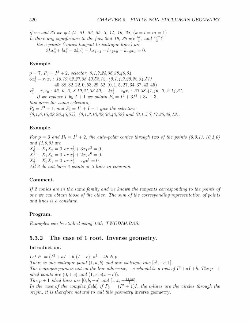
520 CHAPTER 5. FINITE NON-EUCLIDEAN GEOMETRY
if we add 33 we get 45, 51, 52, 55, 3, 14, 16, 28, (k = l = m = 1)Is there any significance to the fact that 19, 38 are 57
3, and 2.57
3?
the c-points (conics tangent to isotropic lines) are3kx2
0 + lx21 − 2kx2
2 − kx1x2 − lx2x0 − kx0x1 = 0.
Example.
p = 7, P3 = I3 + 2, selector, 0,1,7,24,36,38,49,54,3x2
0 − x1x2 : 18,19,22,27,38,40,52,12, (0,1,4,9,20,22,34,51)40, 38, 32, 22, 0, 53, 29, 52, (0, 1, 5, 27, 34, 37, 43, 45)
x21 − x2x0 : 56, 0, 3, 8,19,21,33,50, −2x2
2 − x0x1 : 37,38,41,46, 0, 2,14,31,If we replace I by I + 1 we obtain P3 = I3 + 3I2 + 3I + 3,
this gives the same selectors,P3 = I3 + 1, and P3 = I3 + I − 1 give the selectors(0,1,6,15,22,26,45,55), (0,1,3,13,32,36,43,52) and (0,1,5,7,17,35,38,49).
Example.
For p = 3 and P3 = I3 + 2, the auto-polar conics through two of the points (0,0,1), (0,1,0)and (1,0,0) areX2
0 −X1X2 = 0 or x20 + 3x1x
2 = 0,X2
1 −X2X0 = 0 or x21 + 2x2x
0 = 0,X2
2 −X0X1 = 0 or x22 − x0x
1 = 0.All 3 do not have 3 points or 3 lines in common.
Comment.
If 2 conics are in the same family and we known the tangents corresponding to the points ofone we can obtain those of the other. The sum of the corresponding representation of pointsand lines is a constant.
Program.
Examples can be studied using 130\ TWODIM.BAS.
5.3.2 The case of 1 root. Inverse geometry.
Introduction.
Let P3 = (I2 + aI + b)(I + c), a2 − 4b N p.There is one isotropic point (1, a, b) and one isotropic line [c2,−c, 1].The isotropic point is not on the line otherwize, −c whould be a root of I2 +aI+ b. The p+1ideal points are (0, 1, c) and (1, x, c(x− c)).The p+ 1 ideal lines are [0, b,−a] and [1, x,−1+ax
b].
In the case of the complex field, if P3 = (I2 + 1)I, the c-lines are the circles through theorigin, it is therefore natural to call this geometry inverse geometry.

5.3. TRI-GEOMETRY 521
Definition.
The pseudo-bi-selector is the set 2si,The pseudo-semi-selector is the set 1
2si,
Example.
p = 5. With P3 = I3 − I2 − 2I − 3, a generator is I + 2, its powers are0, 0, 1 0, 1, 2 1, 4, 4 1, 2, 3 0, 1, 1 1, 3, 2 1, 0, 2 1, 3, 4 1, 2, 1 0, 1, 01, 2, 0 0, 1, 3 1, 0, 1 1, 1, 0 1, 1, 2 1, 4, 3 1, 4, 2 1, 1, 1 1, 0, 0 1, 4, 11, 3, 0 1, 3, 3 1, 1, 4 1, 2, 4
The lines are0 [1,0,0]: 0,1,4,9,11 and (0,1,4)1 [1,2,4]: 1,2,5,10,12 and (1,1,3) . . . ..The selector function isi 1 2 3 4 5 7 8 9 10 11 13 14 15 16 17 19 20 21 22 23
f(i) 0 9 1 0 4 4 1 0 1 0 11 11 9 9 11 9 4 4 11 1The isotropic line [1,1,1], the isotropic point is (1,0,3). The ideal lines are [j] = j, j +
6, j + 12, j + 18, for j = 0 to 5.I will now examine the case when Zp is replace by an infinite field R, for instance.p = 7, P3 = I3 + I, G = I + 3,
0, 0, 1 0, 1, 0 0, 1, 1 0, 1, 2 0, 1, 3 0, 1, 4 0, 1, 5 0, 1, 6 1, 0, 0 1, 0, 10, i 0I , 0i 46, 12∗ 29, 28∗ 1, 20∗ 7, 44∗ 11, 4∗ 34, 36∗ 4I , 0∗ I, 16∗
1, 0, 2 1, 0, 3 1, 0, 4 1, 0, 5 1, 0, 6 1, 1, 0 1, 1, 1 1, 1, 2 1, 1, 3 1, 1, 416, 8∗ 40, 32∗ 24, 40∗ 8, 24∗ 32, 4∗ 6I , 46∗ 12, 14∗ 14, 6∗ 21, 30∗ 25, 38∗
1, 1, 5 1, 1, 6 1, 2, 0 1, 2, 1 1, 2, 2 1, 2, 3 1, 2, 4 1, 2, 5 1, 2, 6 1, 3, 015, 22∗ 43, 2i 5I , 7∗ 44, 23∗ 23, 15∗ 38, 39∗ 35, 47∗ 37, 31∗ 18, 3i 1I , 11∗
1, 3, 1 1, 3, 2 1, 3, 3 1, 3, 4 1, 3, 5 1, 3, 6 1, 4, 0 1, 4, 1 1, 4, 2 1, 4, 34, 27∗ 27, 19∗ 41, 43∗ 22, 3∗ 42, 35∗ 39, 7i 7I , 29∗ 28, 45∗ 45, 37∗ 47, 13∗
1, 4, 4 1, 4, 5 1, 4, 6 1, 5, 0 1, 5, 1 1, 5, 2 1, 5, 3 1, 5, 4 1, 5, 5 1, 5, 610, 21∗ 6, 5∗ 33, 1i 3I , 1∗ 20, 17∗ 17, 9∗ 26, 33∗ 5, 41∗ 19, 25∗ 30, 5i
1, 6, 0 1, 6, 1 1, 6, 2 1, 6, 3 1, 6, 4 1, 6, 5 1, 6, 62I , 34∗ 36, 2∗ 2, 42∗ 3, 18∗ 31, 26∗ 9, 10∗ 13, 6i
The real isotropic point is denoted by I, the real isotropic line by i. 1×9 = (−1)−1 = 7i,(0, 1, 3)×(1, 6, 5) = [1, 3, 6]. 9∗×17∗ = (−1)−1 = 7I , [1, 5, 2]× [1, 5, 1] = (1, 4, 0) 11. Observethat kI corresponds to IG′I , with G′ = I + 3 (mod I2 + 1).
The selector is 0,1,7,11,29,34,46.The co-selector is 0,1,3,15,20,38,42.The pseudo-bi-selector is 0, 2, 14, 22, 10, 20, 44, 4I.The corresponding tangents to the bi-conic are i, 47∗, 41∗, 37∗, 19∗, 2∗, 14∗, 0∗which is a member of the dual of the co-selector family 12.The pseudo-semi-selector is 0, 17, 23, 24, 41, 47, 2I , 6I.The corresponding tangents to the semi-conic are 0∗, 17∗, 23∗, 24∗, 41∗, 47∗, 2i, 6i.
117.4.86129.4.86
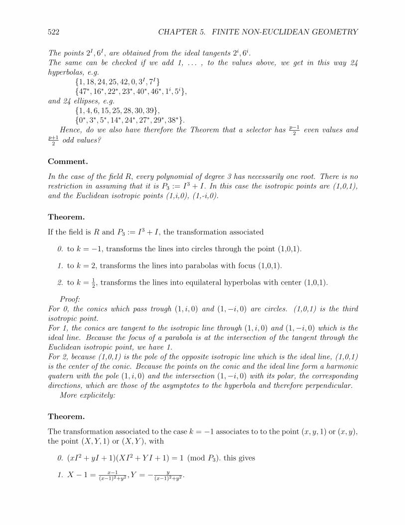
522 CHAPTER 5. FINITE NON-EUCLIDEAN GEOMETRY
The points 2I , 6I , are obtained from the ideal tangents 2i, 6i.The same can be checked if we add 1, . . . , to the values above, we get in this way 24hyperbolas, e.g.
1, 18, 24, 25, 42, 0, 3I , 7I47∗, 16∗, 22∗, 23∗, 40∗, 46∗, 1i, 5i,
and 24 ellipses, e.g.1, 4, 6, 15, 25, 28, 30, 39,0∗, 3∗, 5∗, 14∗, 24∗, 27∗, 29∗, 38∗.
Hence, do we also have therefore the Theorem that a selector has p−12
even values andp+1
2odd values?
Comment.
In the case of the field R, every polynomial of degree 3 has necessarily one root. There is norestriction in assuming that it is P3 := I3 + I. In this case the isotropic points are (1,0,1),and the Euclidean isotropic points (1,i,0), (1,-i,0).
Theorem.
If the field is R and P3 := I3 + I, the transformation associated
0. to k = −1, transforms the lines into circles through the point (1,0,1).
1. to k = 2, transforms the lines into parabolas with focus (1,0,1).
2. to k = 12, transforms the lines into equilateral hyperbolas with center (1,0,1).
Proof:For 0, the conics which pass trough (1, i, 0) and (1,−i, 0) are circles. (1,0,1) is the thirdisotropic point.For 1, the conics are tangent to the isotropic line through (1, i, 0) and (1,−i, 0) which is theideal line. Because the focus of a parabola is at the intersection of the tangent through theEuclidean isotropic point, we have 1.For 2, because (1,0,1) is the pole of the opposite isotropic line which is the ideal line, (1,0,1)is the center of the conic. Because the points on the conic and the ideal line form a harmonicquatern with the pole (1, i, 0) and the intersection (1,−i, 0) with its polar, the correspondingdirections, which are those of the asymptotes to the hyperbola and therefore perpendicular.
More explicitely:
Theorem.
The transformation associated to the case k = −1 associates to to the point (x, y, 1) or (x, y),the point (X, Y, 1) or (X, Y ), with
0. (xI2 + yI + 1)(XI2 + Y I + 1) = 1 (mod P3). this gives
1. X − 1 = x−1(x−1)2+y2
, Y = − y(x−1)2+y2
.

5.3. TRI-GEOMETRY 523
2. The point Q = (X, Y ) and the point P = (x, y) are on a line through (1,0), the productof the distances to that point is 1, and the points P and Q are separated by (1,0).
Proof:0, gives with I3 replaced by −I and I4 replaced by −I2,
−xX + x+X + yY = 0,−xY − yX + y + Y = 0.
solving for X and Y gives easily 1.Moreover,
X−1Y
= −x−1y,
Theorem.
The transformation associated to the case k = 2 associates to to the point (x, y, 1) or (x, y),the point (X, Y, 1) or (X, Y ), with
0. (XI2 + Y I + 1) = (xI2 + yI + 1)2 (mod P3).this gives
1. X − 1 = y2 − (x− 1)2,Y = −2y(x− 1).
2. The line associated to a(x− 1) + by + c is the parabola(−2ab2(X − 1) + b(a2 − b2)Y − 2ac2)2 = 4(a2 + b2)c2(c2 − b2(X − 1)− abY ).
Proof: 0, gives with I3 replaced by −I and I4 replaced by −I2, we obtain at once 1. For2, to simplify let us write the line as y = mx′ + d, with x′ := x − 1, m = −a
band d = − c
b.
Expressing y in terms of x′ gives, with X ′ := X − 1,2mX ′ + (m2 − 1)Y = 2(m2 + 1)dx′ + 2md2 andX ′ +mY = −(m2 + 1)x′2 + d2
eliminating x′ gives 2.
Theorem.
The transformation associated to the case k = 12
associates to the point (x, y, 1) or (x, y),the point (X, Y, 1) or (X, Y ), with
0. (XI2 + Y I + 1)2 = (xI2 + yI + 1) (mod P3).
this gives
1. x− 1 = Y 2 − (X − 1)2, y = −2Y (X − 1).
2. The line associated to a(x− 1) + by + c is the hyperbolaa(Y 2 − (X − 1)2)− 2bY (X − 1) + c = 0.
Proof: 0, gives with I3 replaced by −I and I4 replaced by −I2, we obtain at once 1.

524 CHAPTER 5. FINITE NON-EUCLIDEAN GEOMETRY
Theorem.
0. The lines joining the points associated to the selector and their inverse are tangent toa conic.
2y2 + bz2 + xz = 0 or 2bX2 − Y 2 − 8XZ = 0.
1. The lines joining the points associated to the co-selector and their inverse are tangentto a conic.
Proof: The points of the selector are I − h, their inverse is I2 + hI + h2 + b. The linethrough these points is [−2h2 − b, h, 1].
Problem.
Complete a set of axioms of inverse geometry using an appropriate form of the axiom ofPappus:
0. Given 2 distinct points, there exist one and only one line incident to, or passing through,the 2 points, or the points are parallel.
1. Given 2 distinct lines, there exists one and only one point incident to, or on, the 2lines, or the lines are parallel.
2. There exists at least one line l and two distinct points P and Q not incident to l.
3. On the line l there are exactly p points, p an odd prime.
4. Given a line l and a point P not on the line, there exists one and only one line parallelto l through P.
5. Given a point P and a line l not through the point, there exists one and only one pointparallel to P on l.
5.3.4 The case of a double root and a single root. 13
14
Introduction.
There is no ambiguity to call this also the case of 2 roots.
Definition.
The selector function is a function from the set Zp(p−1) − 0 (mod p) − 0 (mod p − 1)into Zp(p−1), with
f(i− j) = i− j (mod p(p− 1)), for all i and j on [1, 0, 0].
1316.5.851428.2.86

5.3. TRI-GEOMETRY 525
Example.
p = 5 The cyclic group is0,0,1 0,1,1 1,2,1 1,2,4 1,4,1 1,0,1 1,3,3 0,1,3 1,4,3 1,2,31,0,2 1,1,1 1,4,2 1,1,2 1,1,4 1,0,3 1,4,4 1,3,2 0,1,2 1,3,2.The lines are0 [1,0,0]: 0,1,7,18 and (0,1,0), (0,1,4)19 [1,4,1]: 1,2,8,19 and (1,1,0), (1,0,4)18 [1,2,0]: 2,3,9,0 and (1,2,0), (1,2,2)17 [1,3,2]: 3,4,10,1 and (1,3,0), (1,1,3). . . .
The selector isi 1 2 3 6 7 9 11 13 14 17 18 19
f(i) 0 18 18 1 0 18 7 7 7 1 0 1If f(j−i) does not exist, then if j−i ≡ (mod 4), the points are on a line through (1,4,0).
If f(j − i) does not exist, then if j − i ≡ (mod 5), the points are on a line through (1,0,0).Otherwize, the line if f(j − i)− i (mod 20).
There is no restriction in assuming that P3 := I3 − I2.
Definition.
The bi-isotropic point is I0 := (1,−1, 0),the isotropic point is I1 := (1, 0, 0).The bi-isotropic line is i0 := [0, 0, 1],the isotropic line is i1 := [1, 1, 1].
Theorem.
0. The points associated to the co-selector are on a conic, the co-conic, which passesthrough the isotropic point I1 and is tangent to the isotropic line i1 at the co-isotropicpoint I0.
1. The points associated to the bi-selector are on a conic, the bi-conic, which is tangentto the co-isotropic line i1 and is tangent to the isotropic line i0 at the isotropic pointI1.
2. The points associated to the semi-selector are on a conic, the semi-conic, which istangent to the isotropic line i0 at the co-isotropic point I0 and is such that the polarof the isotropic point I1 is the co-isotropic line i1.
Proof:For 0, The conic of 3.1.8.0. reduces to
(k − l)Y 2 +mZ2 + (m− l)Y Z + (m− k)ZX + (k − l)XY = 0,which passes through I1 and for which [1,1,1] is the polar of (1,−1, 0).For 1,. . . .For 2,. . . .
526 CHAPTER 5. FINITE NON-EUCLIDEAN GEOMETRY
5.3.5 The case of a triple root. Solar geometry.15
Introduction.
In this case the . . . There is one special point and a line belonging to each other. The specialpoint and the special lines are called respectively the isotropic point and the isotropic line.The other points on the isotropic line are called ideal points. The other lines through theisotropic point are called ideal line. The other points and lines are called ordinary.
Theorem.
0. There are p ideal points, p ideal lines.
1. There are p2 ordinary points, p2 ordinary lines.
2. The isotropic line belongs to 1 isotropic point and p ideal points.
3. The isotropic point belongs to 1 isotropic line and p ideal lines.
4. The ideal lines belong to . . . .
5. The ordinary lines belong to . . . .
Comment.
In the parabolic-Euclidean or sun-geometry, among all points and lines of projective geometry,one point and a line through it are preferred, in this case this is also true, but if we representthis geometry in the Cartesian plane and choose the isotropic line as the line at infinity andthe isotropic point as the direction of the x axis, the c-lines are parabolas which have . . . . Itis therefore natural, by analogy to choose the names solar geometry and bi-solar geometry,for the geometry in question.
Lemma.
0. X21 − 2X2(X0 + aX1) = 0
and
1. Y 21 − 2Y2(Y0 + aY1) = 0
implies
2. (X1Y2 +X2Y1)2 − 2X2Y2(X0Y2 +X2Y0 +X1Y1 + a(X1Y2 +X2Y1)) = 0.
Proof: The first member of 2. is the sum of the first member of 0 and 1 multipliedrespectively by Y 2
2 and X22 .
1518.2.86
5.3. TRI-GEOMETRY 527
Theorem.
Let a = 0, generators of T are I + 1 and I + 2. The cyclic group of order p generated by I+bcorresponds to points on the conic
X21 − 2X2(X0 + aX1) = 0
where a := 12b. The cyclic group of order p generated by I2 + I + 1
2corresponds to points on
the conicX2
1 − 2X2X0 = 0.Proof:
The point (X0, X1, X2) corresponds to the polynomial X0I2 +X1I +X2.
The product of (X0I2 + X1I + X2) and (Y0I
2 + Y1I + Y2) is (X0Y2 + X2Y0 + X1Y1, X1Y2 +X2Y1, X2Y2). The Theorem folllows at once from Lemma . . . .
Definition.
The selector function is a function from Zp ×× Zp to Zp ×× Zp . . . .
Definition.
The ideal lines can be represented by [i], i ∈ Zp.The points on [i] are (j, i+ j mod p).
Theorem.
0. (x, y)× (x′, y′) = (f(x′ − x, y′ − y)− (x, y)mod Zp ×× Zp).
1. [x, y]× [x′, y′] = [f(x′ − x, y′ − y)− (x, y)mod Zp ×× Zp].
2. (x, y) · [x′, y′] iff f(x′ − x, y′ − y) = (0, 0).
Example.
For p = 3, the selector function isx 0, 1 0, 2 1, 0 1, 2 2, 0 2, 1
f(x) 0, 0 0, 1 0, 0 0, 1 1, 0 1, 0With the exponents in the order exponent of b then exponent of a,
points line0, 0 0, 1 1, 0 0, 00, 1 0, 2 1, 1 0, 20, 2 0, 0 1, 2 0, 11, 0 1, 1 2, 0 2, 01, 1 1, 2 2, 1 2, 21, 2 1, 0 2, 2 2, 12, 0 2, 1 0, 0 1, 02, 1 2, 2 0, 1 1, 22, 2 2, 0 0, 2 1, 1
The points on the 3 ideal lines are

528 CHAPTER 5. FINITE NON-EUCLIDEAN GEOMETRY
[0] = 0,0 1,1 2,2[1] = 0,1 1,2 2,0[2] = 0,2 1,0 2,1
Example.
If p = 7 and P 3 = I3 then the group T is0, 0, 1 0, 1, 2 1, 4, 4 1, 2, 6 1, 6, 3 1, 1, 6 1, 5, 40, 1, 1 1, 3, 2 1, 3, 5 1, 5, 2 0, 1, 5 1, 0, 3 1, 5, 31, 2, 1 1, 3, 4 1, 2, 3 1, 0, 5 1, 6, 5 1, 3, 3 1, 6, 41, 1, 5 1, 0, 1 1, 4, 1 1, 5, 5 0, 1, 3 1, 5, 6 0, 1, 61, 3, 6 1, 1, 1 1, 1, 3 1, 4, 2 1, 4, 3 1, 3, 1 1, 0, 61, 4, 5 1, 1, 4 1, 2, 5 1, 4, 6 1, 0, 2 1, 1, 2 1, 6, 61, 6, 1 1, 6, 2 1, 0, 4 1, 2, 4 1, 2, 2 1, 5, 1 0, 1, 4
A selector ise, a, b, ab4, a3b4, a3b6, a6b6. points on [1,0,0].
The conics are0, 0, 1 0, 1, 1 1, 2, 1 1, 1, 5 1, 3, 6 1, 4, 5 1, 6, 10, 0, 1 0, 1, 2 1, 4, 4 1, 2, 6 1, 6, 3 1, 1, 6 1, 5, 50, 0, 1 0, 1, 3 1, 6, 2 1, 3, 3 1, 2, 5 1, 5, 3 1, 4, 20, 0, 1 0, 1, 4 1, 1, 2 1, 4, 3 1, 5, 5 1, 2, 3 1, 3, 20, 0, 1 0, 1, 5 1, 3, 4 1, 5, 6 1, 1, 3 1, 6, 6 1, 2, 40, 0, 1 0, 1, 6 1, 5, 1 1, 6, 5 1, 4, 6 1, 3, 5 1, 1, 10, 0, 1 1, 1, 4 1, 4, 1 1, 5, 2 1, 2, 2 1, 3, 1 1, 6, 4
The line is [0,1,0] with points (1, 0, 1) · (1, 0, c) = (1, 0, c1+c)
)
0, 0, 1 1, 0, 1 1, 0, 4 1, 0, 5 1, 0, 2 1, 0, 3 1, 0, 6.Other points are on [0,0,1].
They all have a contact of order 2 at (0,0,1) with tangent [1,0,0].
5.3.6 The case of 3 distinct roots.16
Definition.
If the roots are a, b, c,
0. The polynomial which has 2 of the roots corresponds to a point called isotropic point.
1. The 3 lines through 2 of the 3 isotropic points are called isotropic lines.
2. Any non isotropic line through an isotropic point is called an ideal line.
3. Any non isotropic point on an isotropic line is called an ideal point.
1621.2.86

5.3. TRI-GEOMETRY 529
Example.
p = 7, a = 1, b = 2, c = 417.
0. The isotropic points are A0 = (1, 1, 1), A1 = (1, 2, 4), A2 = (1, 4, 2).
1. The isotropic lines are a0 = [1, 1, 1], a1 = [1, 4, 2], a2 = [1, 2, 4].
2. The generators of the group are α = (0,1,2) and β = (0, 1, 1).
3. The ideal lines through A0 are[1, 3, 0] = S0 = e, b2, b4, a3, a3b2, a3b4,[1, 4, 3] = bS0,[0, 1, 3] = aS0,[1, 5, 6] = abS0,[1, 0, 5] = a2S0,[1, 6, 2] = a2bS0.
4. The ideal lines through A1 are[1, 5, 0] = S1 = e, a2, a4, ab3, a3b3, a5b3,[1, 2, 6] = aS1,[1, 3, 4] = bS1,[1, 0, 3] = abS1,[0, 1, 5] = b2S1,[1, 6, 5] = b2aS1.
5. The ideal lines through A2 are[1, 6, 0] = S2 = e, a2, a2b2, a4b4, a4b, b3, a2b5,[1, 1, 5] = abS2,[1, 5, 1] = aS2,[1, 0, 6] = a2bS2,[0, 1, 6] = bS2,[1, 3, 3] = ab2S2.
6. A selector is (e, b5, ab5, a2b3, a5b3) giving the points(0, 0, 1), (1, 6, 1), (1, 6, 3), (1, 6, 6), (1, 6, 4) on [110],
the ideal points on this line are (1,6,0), (1,6,5), (1,6,2).The 36 other lines are obtained by multiplication by any of the elements in the group,e.g. if we multiply to the left by a5b5, the points are (0,1,4), (1,6,4), (1,2,2), (1,3,6),(1,0,1), and the ideal points are (1,1,5), (1,5,0), (1,4,3).
Notes.
We have therefore the following operations:l := P ×Q, L := p× qR := P •Q, r := p • q?
17earlier version

530 CHAPTER 5. FINITE NON-EUCLIDEAN GEOMETRY
where • is done modulo a polynomial of degree 3. If the polynomial is primitive the propertiesare well known, what is probably new is what happens when the polynomial is not primitive.If it has 3 roots it makes sense to normalize to have the isotropic points at (1,0,0), (0,1,0)and (0,0,1), but I do not see how this can be done in view of the fact that an isotropic pointcorresponds to (I − a)(I − b).
Definition.
Given a polynomial of the third degree with 3 distinct roots, a line generator is a generatorof a cyclic group of order p− 1 whose elements correspond to p− 1 points of a line throughone of the isotropic points, the last point is an ideal point on the isotropic line which doesnot belong to the isotropic point.
Definition.
Two line generators are said to be independent if they are associated to lines through distinctisotropic points.
Why did I not worry about this when constructing an example and use simply distinctlines?
5.3.7 Conjecture.18
Given a polynomial of the third degree with 3 distinct roots, there exists 2 independent linegenerators.
Comment.
I will choose the roots to be 0, 1 and -1. P3 = I3 − I.The isotropic points are A0 = (1, 0,−1), A1 = (1, 1, 0), A2 = (1,−1, 0).The isotropic lines are a0 = [0, 0, 1], a1 = [1, 1, 1], a2 = [1,−1, 1].
Conjecture.
With the choice just given, there exist an x such thatif y = −2(x+ 1), (1, 0, x), (1, 1, 1y), (x+ y + 1, x+ 1, xy) are line generators correspondingto lines [0, 1, 0], [1,−1, 0], [1, 1,−2x+y+2
xy] through A0, A1 and A2.
1824.2.86

5.3. TRI-GEOMETRY 531
Example.
p = 3, 0, 0, 1 1, 1, 21, 0, 1 1, 2, 2
p = 5, 0, 0, 1 1, 1, 1 1, 1, 4 1, 1, 21, 0, 1 1, 4, 2 1, 2, 4 1, 3, 31, 0, 2 1, 2, 3 1, 4, 4 0, 1, 31, 0, 3 0, 1, 2 1, 3, 4 1, 4, 1
p = 7, roots 1, 2, 4,0, 0, 1 1, 2, 0 1, 2, 1 1, 2, 5 1, 2, 2 1, 2, 31, 0, 1 1, 3, 2 1, 5, 5 1, 4, 0 1, 1, 6 1, 6, 31, 4, 4 0, 6, 4 1, 1, 4 1, 5, 4 0, 1, 0 1, 0, 41, 1, 3 1, 0, 2 1, 6, 1 1, 4, 1 0, 1, 1 1, 3, 51, 4, 1 1, 5, 3 1, 0, 0 0, 1, 2 1, 1, 2 1, 3, 61, 6, 6 1, 5, 2 1, 1, 0 1, 4, 5 1, 3, 1 0, 1, 4
I3 − 1 = 0
The lines are obtained form(0, 0, 1), (0, 1, 2), (0, 1, 0), (0, 1, 1), (0, 1, 4)
or 0,0 4,3 2,4 3,4 5,5for instance, adding 2,3 modulo 6,6
2, 30, 0, 4, 15, 11, 2or (1,5,4),(0,0,1),(1,5,3),(1,5,2),(1,5,5) on [1,4,0].
The c-lines are all obtained from(0, 0, 1), (0, 1, 4), (1, 0, 2), (1, 5, 5), (1, 6, 4)
or 0,0 5,5 3,1 1,2 2,1for instance, adding 3,2 modulo 6,6 gives
3, 2 2, 1 0, 3 4, 4 5, 3or (1,6,1),(1,6,4),(1,2,5),(1,1,2),(1,4,5).
p = 11, line generators: (1,0,1), (1,1,7), (1,10,2).p = 13, line generators: (1,0,1), (1,1,9), (1,12,2).p = 17, line generators: (1,0,2), (1,1,11), (1,16,4).
Definition.
A selector is a set of p− 2 elements P ikQ
jk which are on an ordinary line.
Theorem.
Given 2 independent line generators P and Q, the isotropic lines are obtained as cosets ofthe cyclic groups generated by P, Q and P •Q.The ordinary lines are obtained by multiplication modulo P3, P lQm by the elements of aselector.
We may want to put this in a section on triangular geometry.In this geometry we have ordinary, ideal and isotropic points, ordinary, ideal and isotropic
lines, and c-lines. These are represented by conics through the isotropic points, the ideal c-lines are the degenerate conics consisting of an isotropic line and an ideal line to the opositeisotropic point. The isotropic c-lines are the degenerate conics consisting of two isotropic

532 CHAPTER 5. FINITE NON-EUCLIDEAN GEOMETRY
lines. The lines and the c-lines can be interchanged. If the c-lines are considered as lines,then the lines are c-lines, in other words if we start with a geometry where we define the conicsthrough 3 given points as lines, the conics are represented by lines. Pascal’s Theorem givesthe following, consider a line l, with points P2i on ai, and 3 other points P1, P3, P5, this linecan be considered a c-conic, indeed, the c-lines through successive points are the degeneratec-lines or ideal c-lines, a0 = (A0 × P1) + a0, a1 = (A2 × P1) + a2, a2 = (A2 × P3) + a2,a3 = (A1 × P3) + a1, a4 = (A1 × P5) + a1, a5 = (A0 × P5) + a0.The c-Pascal points are Q0 = (A1 × P3) × (A0 × P1), Q1 = (A2 × P1) × (A1 × P5), Q2 =(A0 × P5)× (A2 × P3).These points are on a conic, with A0, A1, A2 because the Pascal line for the sequence A0,Q0, A1, Q1, A2, Q2, gives the Pascal points P1, P3, P5. This can be used to study what couldbe called a bi-triangular geometry.
Comment.
The c-lines can be deduced from the line by the transformation which associates, in general,to (X0, X1, X2), (X1X2, X2X0, X0X1), a conic becomes then a quadric with double points,isolated or not in the case or a real field. A conic through A1, A2, but not through A0, becomesa quadric which degenerates in a1, a2 and a conic through A1, A2 but not A0.
Comment.
We could choose as isotropic points, in a model of this geometry in the Euclidean plane, withCartesian coordinates, by choosing one of them at the origin, and the 2 others at the directionof the axis. The c-lines are then hyperbolas passing through the origin, with asymptotes inthe direction of the axis.
Problem.
Study the axiomatic of the triangular geometry and obtain Theorems in it. Circles could beconics through 2 of the isotropic points.
Problem.
Study the axiomatic of the triangular bi-geometry and obtain Theorems in it.
Comment.
The analysis can be repeated in the form of Euclidean geometry by considering the non-homogeneous points (x, y) and the homogeneous lines [a, b, c]. This can be done directly orinfered from the cases 1, 2 and 4 above, with one of the isotropic lines playing the role of theline at infinity in Euclidean geometry.
5.3. TRI-GEOMETRY 533
5.3.8 Notes.
In G45, I give a special case of the following Theorem valid when s1 = a = 0, this generalizesthe Theorem, with b = s11 and c = s111.It was obtained earlier.
Theorem.
The symmetric functions of the roots ares1 := ρ0 + ρ1 + ρ2 = a,s11 := ρ1ρ2 + ρ2ρ0 + ρ0ρ1 = b,s111 := ρ0ρ1ρ2 = c,s2 := ρ2
0 + ρ21 + ρ2
2 = a2 − 2b,s21 := ρ2
0(ρ1 + ρ2) + ρ21(ρ2 + ρ0) + ρ2
2(ρ0 + ρ1) = ab− 3c,s3 := ρ3
0 + ρ31 + ρ3
2 = a(a2 − 3b) + 3c,s211 := ac,s22 := b2 − 2ac,s31 := a(ab− c)− 2b2,s4 := a(a3 − 4ab+ 4c) + 2b2.
Theorem.
0. The conic which pass through the isotropic points isk((b2 − 2ac)X2
0 + bX21 + 3X2
2
+2aX1X2 + 2(a2 − 2b)X2X0 − (3c− ab)X0X1)+l(bcX2
0 + 3cX21 + aX2
2
+2bX1X2 − (3c− ab)X2X0 + 2acX0X1)+m(3c2X2
0 + acX21 + (a2 − 2b)X2
2
−(3c− ab)X1X2 + 2(b2 − 2ac)X2X0 + 2bcX0X1) = 0,
1. which is tangent to the isotropic lines isk(3x2
0 + (a2 + b)x21 + acx2
2
−(3c+ ab)x1x2 + 2bx2x0 − 4ax0x1)+l(ax2
0 + a(a2 − 2b) + 3c)x21 + (a2 − 2b)cx2
2
−(a(ab+ c)− 2b2)x1x2 − (3c− ab)x2x0 − 2(a2 − b)x0x1)+m((a2 − 2b)x2
0 + a(a3 − 3ab+ 4c)x21 + (a(a2 − 3b) + 3c)cx2
2
+(a(−a2b+ 3b2 − ac)− bc)x1x2 + (a(ab− c)− 2b2)x2x0
−(a(2a2 − 5b) + 3c)x0x1) = 0.
Proof:The degenerate conics through the isotropic points are
α0(ρ21X0 + ρ1X1 +X2)(ρ2
2X0 + ρ2X1 +X2))+α1(ρ2
2X0 + ρ2X1 +X2)(ρ20X0 + ρ0X1 +X2))
+α2(ρ20X0 + ρ0X1 +X2)(ρ2
1X0 + ρ1X1 +X2)) = 0.If we choose, in succession, α0 = α1 = α2 = 1, α0 = ρ0, α1 = ρ1, α2 = ρ2, and α0 = ρ2
0,α1 = ρ2
1, α2 = ρ22,

534 CHAPTER 5. FINITE NON-EUCLIDEAN GEOMETRY
we obtain respectively the expressions whose coefficients are k, l and m. Similarly for thec-points we start with the degenerate conics tangent to the isotropic lines, which are
α0(x0 − (ρ2 + ρ0)x1 + ρ2ρ0x2)(x0 − (ρ0 + ρ1)x1 + ρ0ρ1x2))+α1(x0 − (ρ0 + ρ1)x1 + ρ0ρ1x2)(x0 − (ρ1 + ρ2)x1 + ρ1ρ2x2))+α2(x0 − (ρ1 + ρ2)x1 + ρ1ρ2x2)(x0 − (ρ2 + ρ0)x1 + ρ2ρ0x2)) = 0.
The following Theorem was develppoed to prove the relation between the conics associatedto the co, bi and semi-selectors but were found not to be needed. It is now an answer to anexercise.
Answer to exercise .
Let s1 = 0, the conic through (0,1,0), (0,0,1)
0. which passes through the isotropic points is
s111X20 −X1X2 = 0.
1. which is tangent to the isotropic lines is
x20 − s111x1x2 + s11x2x0 = 0.
or(s111X0 + s11X1)2 − 4s111X1X2 = 0,
2. which has the isotropic triangle as polar triangle is
s111X20 − 2s11X0X1 + 2X1X2 = 0.
Proof: Using
3. ρ1 + ρ2 = −ρ0, we can check
for 0, ρ0ρ1ρ2 − (ρ1 + ρ2)ρ1ρ2 = 0,for 1, ρ4
0 − ρ0ρ1ρ2ρ0 + (ρ1ρ2 + ρ2ρ0 + ρ0ρ1)ρ20 = 0,
for 2,
ρ30
ρ20
ρ0
=
s111 −s11 0−s11 0 1
0 1 0
1−ρ1 − ρ2
ρ1ρ2
.
Exercise.
Let s1 = 0. Determine the conic through (0,1,0), (0,0,1),
0. which passes through the isotropic points,
1. which is tangent to the isotropic lines,
2. which has the isotropic triangle as polar triangle.

5.3. TRI-GEOMETRY 535
Comment.
To obtain the statements of the preceding Theorem, I will illustrate for the case 2. If theconic is represented by the symmetric matrix 1 γ β
γ 0 αβ α 0
.
The condition that I0 is the pole of i0 givesµ ρ2
0 = 1− γ(ρ1 + ρ2) + βρ1ρ2,µ ρ0 = γ + αρ1ρ2,µ = β − α(ρ1 + ρ2).
Eliminating µ from the first 2 and the last 2 equations gives1− γ(ρ1 + ρ2) + βρ1ρ2 − γρ0 − αρ0ρ1ρ2 = 0,γ + αρ1ρ2 − βρ0 + α(ρ0ρ1 + ρ0ρ2) = 0,
or using 3,1 + βρ1ρ2 − αs111 = 0,γ + αs11 − βρ0 = 0.
Because the conic cannot depend on individual values of ρ0, ρ1, ρ2, β = 0 and then α = 1s111
and γ = −αs11.
5.3.9 On the tetrahedron.
Example.
Let the roots be 0,1,2,3 and p = 5,the isotropic points are (1,-1,1,-1), (1,0,1,0), (1,1,-2,0), (1,2,2,0).P4 = I4 − I3 + I2 − I, therefore, I5 = I (mod P4) and I6 = I2modP3.The cubic surface is given by∣∣∣∣∣∣∣∣
k l m nZ + T Y + Z X + Y XX − Z T − Y Z − x YY + Z X + Y X + T Z
∣∣∣∣∣∣∣∣ = 0.
For instance, a point on I0 × I1 is (u+ v,−u, u+ v,−u) and∣∣∣∣∣∣∣∣k l m nv v v u+ v0 0 0 −uv v v u+ v
∣∣∣∣∣∣∣∣ = 0,
because 2 rows are equal.Similarly for a point on I2 × I3, (u+ v, 2u+ v, 2u− 2v, 0),∣∣∣∣∣∣∣∣
k l m n2u− 2v 4u− v 3u+ 2v u+ v−u+ 3v −2u− v u− 3v 2u+ v4u− v 3u+ 2v u+ v 2u− 2v
∣∣∣∣∣∣∣∣ = 0, because the sum of the last 3 rows is equal to
0 (mod 5).No other conditions are needed to obtain a family of cubics with 3 parameters because if theisotropic points are chosen as (1,0,0,0), (0,1,0,0), (0,0,1,0), (0,0,0,1) the cubic is

536 CHAPTER 5. FINITE NON-EUCLIDEAN GEOMETRY
d0X1X2X3 + d1X2X3X0 + d2X3X0X1 + d3X0X1X2 = 0.
Example.
19 For the semi-transformation, let p = 5 and P4 = I4−I3 +I2−I, (X, Y, Z, T )2 = (x, y, z, t)gives
x = 2XT + 2Y Z + (2XZ + Y 2)y = 2Y T + Z2 − (2XZ + Y 2) +X2,z = 2ZT + (2XZ + Y 2) + 2XY,t = T 2.
A plane k, l,m, n is therefore transforned in the quadric represented by the symmetricmatrix
l m k − l +m km k − l +m k l
k − l +m k l mk l m n
. The isotropic points are (1,-1,1,-1), (1,0,1,0),
(1,1,-2,0), (1,2,2,0),and the corresponding isotropic planes are0,0,0,1, 1,1,1,1, -2,-1,2,1, 2,-1,-2,1.It is easy to check the latter are the polar of the former, independently from k, l, m, n. Itis easy to verify that the quadric which have the isotropic tetrahedron as polar tetrahedronform a 3 parameter family and that this generalizes to n dimensions.
Exercise.
Study the relation which exist between the correspondance between a pair of points and thepair obtained at the intersection of the tangents at the 2 points to the c-line through thesepoints and the intersection of the c-lines tangent to the line through the 2 points at the twopoints.Hint: Study first how to obtain from the point on any other line through a point and thec-line that line through the point which is tangent to the c-line.
Definition.
Let lc be a line through P, . . . .
1914.4.86

Chapter 6
GENERALIZATION TO 3DIMENSIONS
6.0 Introduction.
I will sketch here part of the generalization to 3 dimensions of what has been presented inthe preceding parts. It will be obvious how to generalize further to n dimensions. After abrief look at the history, I will review the application of Grassmann algebra to the incidenceproperties of the fundamental objects in 3 dimensions, the points, the lines and the planes.
The finite polar geometry will be introduced in section 6.2. It is obtain by preferinga plane, the ideal plane, to which correspond the notions of affine geometry, parallelism,mid-points, equality of segments on parallel lines, and a quadric, the fundamental quadric,which, together with the ideal plane, allow for the definition of spheres and therefore equalityof distances between unordered pairs of points as well as orthogonality or more generallyequality of angles between ordered pair of lines.To illustrate properties in 3 dimensions, the geometry of the triangle in involutive geometrywill be generalized, in section 6.2.3 to the study of the general tetrahedron in finite polargeometry. In the classical case, the first work on the subject is that of Prouhet, this wasfollowed by important memoirs of Intrigila and Neuberg.We will see that a special case occurs very naturally, that of the orthogonal tetrahedron,studied in section 6.2.4. We will see that the success of the theory of this special case isexplained by the generalization to 3 dimension of the symmetry which exists in 2 dimensionswhen we exchange the barycenter and the orthocenter.The isodynamic tetrahedron is studied in section 6.2.5.
The generalization of many other 3 dimensional and n dimensional concepts is left to thereader.
This part ends with an introduction to the anti-polar geometry 6.1.5.
537

538 CHAPTER 6. GENERALIZATION TO 3 DIMENSIONS
6.0.1 Relevant historical background.
Introduction.
In the classical case, the extension to 3 dimensions is already given by Euclid. The earlierdefinitions of conics derives from the circular cone in 3 dimensions. Of note is also the factthat the 2-dimensional Desargues’ theorem derives directly from the incidence properties in3 dimensions. Although the algebraic notation of analytic geometry, introduced by Descartesimmediately extends and at once suggests to go beyond the observable to 4 and to n dimen-sions, it is not suitable if we progress from finite polar geometry - where equality of distanceand angles are defined and are not primary notions - to finite 3 dimensional Euclidean ge-ometry. Instead, I will use the notation of exterior algebra introduced by Grassmann.
6.0.2 Grassmann algebra applied to incidence properties of points,lines and planes
Introduction.
After introducing in 6.0.2 the algebraic representation of points, lines and planes in Z3p , I
recall the basic concepts and properties of the exterior algebra of Grassmann (6.0.2 to 6.0.2),I define the incidence relations (6.0.2) and derive the associated properties (6.0.2, 6.0.2 to6.0.2).
Definition.
The points and planes in 3 dimensions will be represented using 4 homogeneous coordinates.(Not all coordinates are 0, and if all coordinates are multiplied modulo p by the same nonzero element in Zp, we obtain the same point or plane.)Points will be denoted by a capital letter and the coordinates will be placed between parenthe-sis. Planes will be denoted by a capital letter preceded by the symbol “|“ or by a calligraphicletter and the coordinates will be placed between braces.The lines will be represented by 6 homogeneous coordinates [l0, l1, l2, l3, l4, l5], such that l0l5 +l1l4 + l2l3 = 0.This part of the definition will be justified in 6.0.2.4 and 6.0.2.The normalization will again be such that the leftmost non zero coordinate is 1.
Example.
Let p = 7,P := (2, 4, 6, 1) = (1, 2, 3, 4), l := [3, 3, 1, 4, 3, 5] = [1, 1, 5, 6, 1, 4],Q := 5, 1, 1, 1 = 1, 3, 3, 3 are respectively a point, aline and a plane.
Notation.
To define algebraically the incidence properties, I will use Grassmann algebra with exteriorproduct multiplication. If e0, e1, e2, e3 are “unit” vectors, we write

6.0. INTRODUCTION. 539
0. P := (P0, P1, P2, P3) := P0 e0 + P1 e1 + P2 e2 + P3 e3.
1. l := [l0, l1, l2, l3, l4, l5]:= l0 e0 ∨ e1 + l1 e0 ∨ e2 + l2 e0 ∨ e3 + l3 e1 ∨ e2 + l4 e3 ∨ e1 + l5 e2 ∨ e3,
with
2. l0 l5 + l1 l4 + l2 l3 = 0.
3. Q := Q0, Q1, Q2, Q3:= Q0 e1 ∨ e2 ∨ e3 +Q1 e3 ∨ e2 ∨ e0 +Q2 e3 ∨ e0 ∨ e1 +Q3 e1 ∨ e0 ∨ e2.
In each case not all coefficients are zero.The specific notation for l and Q will is justified in 6.0.2. For Q the order of the unitvectors is chosen in such a way that the last ones are consecutive, e3, e0, e1, e2. Ifcondition 2 is not satisfied, the 2-form will be denoted using an identifier starting witha lower case letter and followed by “′ ”. If an identity is satisfied for the general 2-forml′ as well as for the line l, I will use the notation l′ (see for instance 6.0.2).
I recall:
Definition.
The exterior product is defined by using the usual rules of algebra, namely, commutativity,associativity, neutral element property and distributivity with the exception
ei ∨ ej = −ej ∨ ei which gives, in particular, ei ∨ ei = 0.
Lemma.
(ei ∨ ej) ∨ (ek ∨ el) = (ek ∨ el) ∨ (ei ∨ ej).
Theorem.
P ∨Q = −Q ∨ P, l′ ∨m′ = m′ ∨ l′.
Corollary.
P ∨ P = 0.
Definition.
Given any expression involving points, lines or planes using the Grassmann representation,the dual of an expression is obtained by replacing the coefficient by itself and
ei0 ∨ . . . ∨ eik−1by j eik ∨ . . . ∨ ei3
where i0, . . . , ik−1, ik, . . . i3 is a permutation of 0,1,2,3 and j = 1 if the permutation is even,−1 if the permutation is odd.

540 CHAPTER 6. GENERALIZATION TO 3 DIMENSIONS
Theorem.
0. dual(P ) = P0 e1 ∨ e2 ∨ e3 + P1 e3 ∨ e2 ∨ e0 + P2 e3 ∨ e0 ∨ e1 + P3 e1 ∨ e0 ∨ e2.
1. dual(l′) = l0 e2 ∨ e3 + l1 e3 ∨ e1 + l2 e1 ∨ e2 + l3 e0 ∨ e3 + l4 e0 ∨ e2 + l5 e0 ∨ e1.
Because of the notation 6.0.2.1, duality, for a line, simply reverses the order of thecomponents of l.
Notation.
0. P · Q := Q · P := dual(P ∨Q),
1. l′ ∧ P := P ∧ l′ := dual(dual(P) ∨ dual(l′)).
2. P ∧Q := Q∧ P := dual(dual(P) ∨ dual(Q)).
Definition.
A point P is incident to a line l iffP ∨ l = 0.
A point P is incident to a plane Q iffP ∨Q = 0.
A line l is incident to a plane Q iffl ∧Q = 0.
Theorem.
0. P ∨Q = (P0Q1 − P1Q0) e0 ∨ e1 + (P0Q2 − P2Q0) e0 ∨ e2
+(P0Q3 − P3Q0) e0 ∨ e3 + (P1Q2 − P2Q1) e1 ∨ e2
+(P3Q1 − P1Q3) e3 ∨ e1 + (P2Q3 − P3Q2) e2 ∨ e3.
1. P ∨Q = (P2Q3 − P3Q2) e0 ∨ e1(P3Q1 − P1Q3) + e0 ∨ e2
+(P1Q2 − P2Q1) e0 ∨ e3 + (P0Q3 − P3Q0) e1 ∨ e2
+(P0Q2 − P2Q0) e3 ∨ e1 + (P0Q1 − P1Q0) e2 ∨ e3.
2. P ∨ l′ = (P1l5 + P2l4 + P3l3) e1 ∨ e2 ∨ e3
+(−P0l5 + P2l2 − P3l1) e3 ∨ e2 ∨ e0
+(−P0l4 − P1l2 + P3l0) e3 ∨ e0 ∨ e1
+(−P0l3 + P1l1 − P2l0) e1 ∨ e0 ∨ e2.
3. P ∨ l′ = (P1l0 + P2l1 + P3l2) e1 ∨ e2 ∨ e3
+(−P0l0 + P2l3 − P3l4) e3 ∨ e2 ∨ e0
+(−P0l1 − P1l3 + P3l5) e3 ∨ e0 ∨ e1
+(−P0l2 + P1l4 − P2l5) e1 ∨ e0 ∨ e2.
4. l′ ∨m′ = (l0m5 + l1m4 + l2m3 + l3m2 + l4m1 + l5m0) e0 ∨ e1 ∨ e2 ∨ e3.
5. P ∨Q = (P0Q0 + P1Q1 + P2Q2 + P3Q3) e0 ∨ e1 ∨ e2 ∨ e3.

6.0. INTRODUCTION. 541
6. P ∨ (P ∨ l′) = 0.
7. Q∨ (Q∧ l′) = 0.
8. 0. (P ∨ l′) ∧ l′ = −(l0l5 + l1l4 + l2l3)P.1. (P ∨ l) ∧ l = 0.
9. 0. (Q∧ l′) ∨ l′ = −(l0l5 + l1l4 + l2l3)Q.1. (Q∧ l) ∨ l = 0.
The proof is straightforward or follows from duality.The condition 6.0.2.2 that a sextuple be a line is precisely chosen to insure 8.1 and 9.1.
Example.
For p = 7, given P0 := (1, 2, 3, 4), P1 := (1, 0, 1, 1), P2 := (1, 1, 0, 1), P3 := (1, 0, 0, 1),l0 := [1, 1, 5, 6, 1, 4], l1 := [1, 6, 0, 6, 1, 1], Q0 := 1, 3, 3, 3,Q1 := 1, 5, 0, 6, we can easily verifyP0 and P1 are incident to l0, P1 and P2 are incident to l1,P0, P1, P2, l0 and l1 are incident to Q0, P3 and l0 are incident to Q1.
Notation.
As for 2 dimensional finite projective geometry, we will make use of a compact notation,assuming that the elements are ordered as if the 4 or 6 normalized coordinates were formingan integer in base p. We have the correspondence
(0) := (0, 0, 0, 1), [0] := [0, 0, 0, 0, 0, 1],(1) := (0, 0, 1, 0), [1] := [0, 0, 0, 0, 1, 0],(p+ 1) := (0, 1, 0, 0), [p+ 1] := [0, 0, 0, 1, 0, 0],(p2 + p+ 1) := (1, 0, 0, 0), [p2 + p+ 1] := [0, 0, 1, 0, 0, 0],
[p3 + p2 + p+ 1] := [0, 1, 0, 0, 0, 0],[p4 + p3 + p2 + p+ 1] := [1, 0, 0, 0, 0, 0].
Example.
Continuing Example 6.0.2,P0 = (180), P1 = (65), P2 = (107), P3 = (58), l0 = [7222], l1 = [17509], Q0 = 228,Q1 = 308.
Theorem.
P and Q are distinct iff P ∨Q 6= 0.Proof: By Corollary 6.0.2, if P and Q are not distinct, Q = kP, k 6= 0 and P ∨ Q =
P ∨ kP = 0. If P ∨ Q = 0, let P0 be a coefficient of P different from 0, 6.0.2.0 givesP0Q1 = P1Q0, P0Q2 = P2Q0, P0Q3 = P3Q0, therefore if Q0 = 0 then Q1 = Q2 = Q3 = 0,and Q is not a point.If Q0 6= 0, I can, by homogeneity choose Q0 = P0 and then Q1 = P1, Q2 = P2 and Q3 = P3
or Q = P.
542 CHAPTER 6. GENERALIZATION TO 3 DIMENSIONS
Theorem.
Given 2 distinct points P and Q, there exist one and only one line l = P ∨Q incident to Pand Q.
Proof: Because of associativity, P ∨(P ∨Q) = 0 and (P ∨Q)∨Q = 0, therefore l = P ∨Qis incident to both P and Q and l 6= 0 because P and Q are distinct.The line is unique. Let P ∨Q 6= 0, P ∨ l = Q ∨ l = 0, l 6= 0.Because P ∨Q 6= 0, one of the coordinates is different from 0, let it beP0Q1 − P1Q0. Theorem 6.0.2.1 gives 4 equations associated to P ∨ l = 0 and 4 equationsassociated to Q ∨ l = 0, the last equations are
−P0l3 + P1l1 − P2l0 = 0−Q0l3 +Q1l1 −Q2l0 = 0.
Multiplying the first by −Q0 and the second by P0 gives
0. (P0Q1 − P1Q0)l1 = (P0Q2 − P2Q0)l0,
Similarly multiplying by −Q1 and P1 gives
1. (P0Q1 − P1Q0)l3 = (P1Q2 − P2Q1)l0,
The third equation of each set gives similarly
2. (P0Q1 − P1Q0)l2 = (P0Q3 − P3Q0)l0,
3. (P0Q1 − P1Q0)l4 = (P3Q1 − P1Q3)l0,
If we add the first equations for P ∨ l = 0 multiplied by −Q0 and −Q1, we get
4. (P0Q1 − P1Q0)l5 = −Q1P3l1 +Q1P2l2 +Q0P3l3 +Q0P2l4 = 0.Because l0 6= 0, the first parenthesis is different from 0, otherwise, it follows from 0,1, 2 and 3 then l1 = l3 = l2 = l4 = 0, and from 4 that l5 = 0. We can, because ofhomogeneity write
l0 = P0Q1 − P1Q0,it follows that
l1 = P0Q2 − P2Q0.l3 = P1Q2 − P2Q1.
and from 2 and 3,l2 = P0Q3 − P3Q0,l4 = P3Q1 − P1Q3,
Replacing in 4, gives(P0Q1 − P1Q0)l5 = Q1P2(P0Q3 − P3)Q0)−Q1P3(P0Q2 − P2Q0)
+Q0P2(P3Q1 − P1Q3) +Q0P3(P1Q2 − P2Q1)= (P0Q1 − P1Q0)(P2Q3 − P3Q2).
hencel5 = P2Q3 − P3Q2.
Therefore l = P ∨Q.
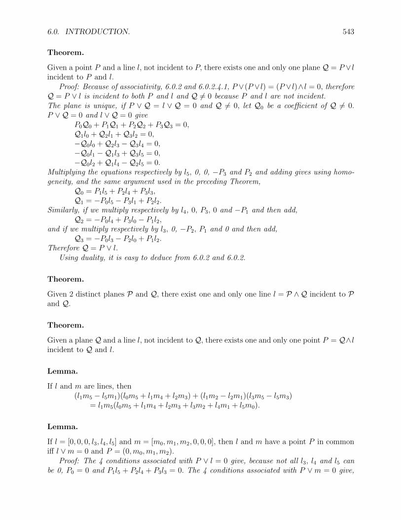
6.0. INTRODUCTION. 543
Theorem.
Given a point P and a line l, not incident to P, there exists one and only one plane Q = P ∨ lincident to P and l.
Proof: Because of associativity, 6.0.2 and 6.0.2.4.1, P ∨(P ∨ l) = (P ∨ l)∧ l = 0, thereforeQ = P ∨ l is incident to both P and l and Q 6= 0 because P and l are not incident.The plane is unique, if P ∨ Q = l ∨ Q = 0 and Q 6= 0, let Q0 be a coefficient of Q 6= 0.P ∨Q = 0 and l ∨Q = 0 give
P0Q0 + P1Q1 + P2Q2 + P3Q3 = 0,Q1l0 +Q2l1 +Q3l2 = 0,−Q0l0 +Q2l3 −Q3l4 = 0,−Q0l1 −Q1l3 +Q3l5 = 0,−Q0l2 +Q1l4 −Q2l5 = 0.
Multiplying the equations respectively by l5, 0, 0, −P3 and P2 and adding gives using homo-geneity, and the same argument used in the preceding Theorem,
Q0 = P1l5 + P2l4 + P3l3,Q1 = −P0l5 − P3l1 + P2l2.
Similarly, if we multiply respectively by l4, 0, P3, 0 and −P1 and then add,Q2 = −P0l4 + P3l0 − P1l2,
and if we multiply respectively by l3, 0, −P2, P1 and 0 and then add,Q3 = −P0l3 − P2l0 + P1l2.
Therefore Q = P ∨ l.Using duality, it is easy to deduce from 6.0.2 and 6.0.2.
Theorem.
Given 2 distinct planes P and Q, there exist one and only one line l = P ∧Q incident to Pand Q.
Theorem.
Given a plane Q and a line l, not incident to Q, there exists one and only one point P = Q∧lincident to Q and l.
Lemma.
If l and m are lines, then(l1m5 − l5m1)(l0m5 + l1m4 + l2m3) + (l1m2 − l2m1)(l3m5 − l5m3)
= l1m5(l0m5 + l1m4 + l2m3 + l3m2 + l4m1 + l5m0).
Lemma.
If l = [0, 0, 0, l3, l4, l5] and m = [m0,m1,m2, 0, 0, 0], then l and m have a point P in commoniff l ∨m = 0 and P = (0,m0,m1,m2).
Proof: The 4 conditions associated with P ∨ l = 0 give, because not all l3, l4 and l5 canbe 0, P0 = 0 and P1l5 + P2l4 + P3l3 = 0. The 4 conditions associated with P ∨m = 0 give,

544 CHAPTER 6. GENERALIZATION TO 3 DIMENSIONS
because not all m0, m1 and m2 can be 0, P1 = m0, P2 = m1, P3 = m2, substituting in theremaining equation gives the equivalence with l ∨m = 0.
Lemma.
If l5m5 6= 0 and l1m5 6= l5m1, if P is on l and m, then l and m have a point P in commoniff l ∨m = 0 and
P = (l0m5 + l1m4 + l2m3, l3m4 − l4m3, l5m3 − l3m5, l4m5 − l5m4).Proof: The first component of P ∨ l = 0 and of P ∨m = 0 implies P1 = k0(l4m3− l3m4),
P2 = k0(l3m5 − l5m3) and P3 = k0(l5m4 − l4m5). Similarly, the second components impliesP0 = k1(l1m2− l2m1), P2 = k1(l1m5− l5m1) and P3 = k1(l2m5− l5m2). Consistency implies
(l1m5 − l5m1)(l5m4 − l4m5) = (l3m5 − l5m3)(l2m5 − l5m2).or
l5m5(l3m2 + l2m3 + l1m4 + l4m1) +m25(−l1l4 − l2l3)
+ l25(−m1m4 −m2m3)= l5m5(l3m2 + l2m3 + l1m4 + l4m1 + l0m5 + l5m0),
because l and m are lines. Chosing k1 = (l3m5− l5m3)/(l1m5− l5m1) and k0 = −1 gives theexpression for P using Lemma 6.0.2.
Theorem.
If 2 distinct lines l and m are such that l∨m = 0, they are incident to a point noted l×× m andto a plane noted lXm. Vice-versa, if 2 distinct lines are incident to the same point or the sameplane then l ∨m = 0. Moreover, if l = [l0, l1, l2, l3, l4, l5] and m = [m0,m1,m2,m3,m4,m5],then one of the following will give the point l ×× m
0. (l0m5 + l1m4 + l2m3, l3m4 − l4m3, l5m3 − l3m5, l4m5 − l5m4).
1. (l1m2 − l2m1, l4m1 + l3m2 + l0m5, l1m5 − l5m1, l2m5 − l5m2),
2. (l2m0 − l0m2, l0m4 − l4m0, l5m0 + l3m2 + l1m4, l2m4 − l4m2).
3. (l0m1 − l1m0, l0m3 − l3m0, l1m3 − l3m1, l5m0 + l4m1 + l2m3).
and the plane l X m
4. l5m0 + l4m1 + l3m2, l2m1 − l1m2, l0m2 − l2m0, l1m0 − l0m1.
5. l4m3 − l3m4, l5m0 + l2m3 + l1m4, l4m0 − l0m4, l3m0 − l0m3.
6. l3m5 − l5m3, l5m1 − l1m5, l4m1 + l2m3 + l0m5, l3m1 − l1m3.
7. l5m4 − l4m5, l5m2 − l2m5, l4m2 − l2m4, l3m2 + l1m4 + l0m5.
The proof follows by a judicious application of the Lemmas.
Exercise.
If l and m are lines and l ∨m = 0 then l ∨ (l ×× m) = (l ×× m) ∨m = 0.

6.1. AFFINE GEOMETRY IN 3 DIMENSIONS. 545
Exercise.
If l ×× m and l Xm are defined by 6.0.2.0 and .4, then (l ×× m) ∨ (l X m) = 0.
6.1 Affine Geometry in 3 Dimensions.
6.1.0 Introduction.
To define a 3 dimensional Euclidean geometry, I will start with a preferred plane I to whichare associated the notions of affine geometry. Just as in the case of the Pappian plane, wecan define the notions of parallelism, mid-point, equality of segments (ordered pair of points)on parallel lines. It is convenient to intoduce a matrix notation to express parallelism andin later sections polarity and orthogonality. Bold faced letters will be used for matrices. Thecoordinates of points, lines and planes will have associated with them vectors which will beconsidered as row vectors.
6.1.1 The ideal plane and parallelism.
Definition.
The preferred plane is called the ideal plane. There is no restriction in chosing the ideal planeI = 1, 1, 1, 1 because the coordinates of I simply corresponds to those of the unit point(1,1,1,1) and can be considered as the polar of the unit point with respect to the tetrahedronof the coordinate system (1,0,0,0), (0,1,0,0), (0,0,1,0), (0,0,0,1).
Definition.
The points in the ideal plane are called the ideal points, the lines in the ideal plane are calledthe ideal lines.
Definition.
Two lines are parallel iff they are incident to I at the same point.Two planes are parallel iff they are incident to I on the same line.A plane Q and a line l are parallel iff the line Q∧ I is incident to the point I ∧ l.
Definition.
L :=
1 1 1 0 0 0−1 0 0 1 −1 0
0 −1 0 −1 0 10 0 −1 0 1 −1
, P :=
0 0 1 −10 −1 0 10 1 −1 01 0 0 −11 0 −1 01 −1 0 0
.

546 CHAPTER 6. GENERALIZATION TO 3 DIMENSIONS
Theorem.
If l is a line then LlT is the direction of the line l .If P is a plane then PPT is the direction of the plane P .
The proof follows from 6.0.2.3 and 1. Notice that P is obtained from the transpose of Lby exchanging row i with row 5− i, i = 0,1,2.
Theorem.
Let Q := Q0,Q1,Q2,Q3 and l := [l0, l1, l2, l3, l4, l5],The plane Q is parallel to the line l iff
0. QLlT = 0, or−Q0(l0 + l1 + l2) +Q1(l0 − l3 + l4) +Q2(l1 + l3 − l5) +Q3(l2 − l4 + l5) = 0.
The proof follows from the property that the direction LlT of the line l is incident to theplane Q. Alternately, we can obtain the Theorem by introducing first, directional correspon-dance.
Definition.
Let P := (P0, P1, P2,−(P0 + P1 + P2)) be an ideal point. Letm := [m0,m1,m2,m3,m4,m5] be an ideal line. These point and line can also be determinedby 3 well chosen coordinates. The coordinates of points are placed between double parenthesisand that of lines, between double brackets, while the point P as viewed as a point in the planeis denoted (P ) and the line as [m].One of the good choices is [[m3,−m1,m0]], indeed, in the ideal plane, m0 e0 +m1 e1 +m2 e2
is the dual of m0 e1 ∨ e2 + m1 e2 ∨ e0 + m2 e0 ∨ e1, while the 3 chosen components givem3 e1∨e2−m1 e0∨e2 +m0 e0∨e1. The other components are m2 = −m0−m1, m4 = m3−m0,m5 = m1 +m3.We have P T = U (P )T and [m]T = V mT , with
U =
1 0 00 1 00 0 1−1 −1 −1
and V =
0 0 0 1 0 00 −1 0 0 0 01 0 0 0 0 0
.
The correspondence which associates to P = (P0, P1, P2, P3) in the 3 dimensional spacethe point (P ) = (P0, P1, P2) in the 2 dimensional plane I, and which associates to the linem = [m0,m1,m2,m3,m4,m5], in the 3 dimensional space the line [m] = [[m3,−m1,m0]], inthe 2 dimensional plane I, is called the directional correspondence.
Theorem.
The directional correspondence is a homomorphism from the 3 dimensional space onto theideal plane.
Theorem.
V P = UT .

6.2. POLAR GEOMETRY IN 3 DIMENSIONS. 547
Theorem.
If P and m are in the ideal plane, P is on m, iff (P ) is on [m], iff(P ) · (m) = ((P0, P1, P2)) · [[m3,−m1,m0]] = P0m3 − P1m1 + P2m0 = 0.
Alternate Proof of 6.1.1.
For instance, to the point Il and line iQ of Theorem 6.1.1, correspond, the point (Il) and theline [iQ] in I.
(Il) = ((l0 + l1 + l2,−l0 + l3 − l4,−l1 − l3 + l5)),[iQ] = [[Q0 −Q3,Q1 −Q3,Q2 −Q3]],
Q is parallel to l iff−(l0 + l1 + l2)(Q0 −Q3) + (−l0 + l3 − l4)(Q3 −Q1)− (−l1 − l3 + l5)(Q2 −Q3) = 0which is 6.1.1.0.
Theorem.
The mid-point of two points A = (a0, a1, a2, a3) and B = (b0, b1, b2, b3) is(b0 + b1 + b2 + b3)A+ (a0 + a1 + a2 + a3)B.
Notation.
The mid-point of A and B is denoted by A+B.
Exercise.
Generalize the construction of the polar p of a point P with respect to a triangle to that ofthe polar P of a point P with respect to a tetrahedron and prove that if P = (p0, p1, p2, p3)then P = P1P2P3,P2P3P0,P3P0P1,P0P1P2.
6.2 Polar Geometry in 3 Dimensions.
6.2.0 Introduction.
To define a polar geometry in 3 dimensions, I will start with an affine Geometry in 3 di-mansions and a preferred non degenerate quadric θ which is not tangent to the ideal plane I.Using the ideal plane and the prefered quadric we can define orthogonality, spheres, centers,equality of pairs of points and lines, . . . .
The preferred quadric is represented by a symmetric 4 by 4 matrix F, which associates toa 4-vector representing a point (pole), a 4-vector representing a plane (polar). Its adjoint Ggives the correspondance from polar to pole. From F, we can derive a 6 by 6 matrix H whichgives the correspondance between a line and its polar. From F we can also derive a polarityin the ideal plane represented by a 3 by 3 matrix J3, giving the correspondance from pole topolar and its adjoint K3, giving the correspondance from polar to pole from which we canderive perpendicularity between a line and a plane, the direction of the line giving the poleand the direction of the plane giving the polar. The 6 by 6 matrix J, derived from J3, allows

548 CHAPTER 6. GENERALIZATION TO 3 DIMENSIONS
for a direct check of the orthogonality of 2 lines and the 4 by 4 matrix K, derived from K3,allows for a direct check of the orthogonality of 2 planes.
6.2.1 The fundamental quadric, poles and polars.
Introduction.
The properties of pole and polar are properties in Pappian Geometry. They are easily gener-alized by using a 4 dimension collinearity which transforms the fundamental quadric into anarbitrary quadric or by chosing a coordinate system with the four base points on the quadric.
Definition.
The preferred quadric is called the fundamental quadric. There is no restriction in chosingthe fundamental quadric θ as follows, because it simply assumes that the quadric passesthrough the base points (1,0,0,0), (0,1,0,0), (0,0,1,0), (0,0,0,1). Let
0. F :=
0 n0 n1 n2
n0 0 n3 n4
n1 n3 0 n5
n2 n4 n5 0
,
1. Θ := (X0, X1, X2, X3)F(X0, X1, X2, X3)T
= n0X0X1 + n1X0X2 + n2X0X3 + n3X1X2 + n4X3X1 + n5X2X3 = 0.
The condition of non degeneracy and non tangency are
2. d := det(F) =n2
0n25 + n2
1n24 + n2
2n23 − 2(n0n1n4n5 + n1n2n3n4 + n2n0n3n5) 6= 0,
3. t := n3n4n5 + n1n2n5 + n0n2n4 + n0n1n3 + 2n0n5(n0 + n5)+ 2n1n4(n1 + n4) + 2n2n3(n2 + n3)− (n0n5 + n1n4 + n2n3)n 6= 0,
wheren := n0 + n1 + n2 + n3 + n4 + n5.
The condition t 6= 0 will be verified in 6.2.1.
Definition.
In polar geometry, the points in the ideal plane which are not on the quadric are called theideal points, all lines in the ideal plane which are not tangent to the quadric are the ideallines.
Definition.
The points in the ideal plane and the quadric are the isotropic points. The lines in the idealplane tangent to the quadric are the isotropic lines.If the isotropic points are real, the polar geometry is said to be hyperbolic, if there are no

6.2. POLAR GEOMETRY IN 3 DIMENSIONS. 549
real isotropic points, it is said to be elliptic, if there is exactly one isotropic point, the quadricbeing tangent to the plane, the geometry is said to be parabolic.
Again as for the involutive geometry, I will not study the parabolic case and will studytogether the elliptic and hyperbolic case.
Definition.
The polar of the point P = (P0, P1, P2, P3), is the planeQT := FP T = n0P1 + n1P2 + n2P3, n0P0 + n3P2 + n4P3,
n1P0 + n3P1 + n5P3, n2P0 + n4P1 + n5P2.P is called the pole of the plane Q.
Theorem.
P T = GQTwhere G is the adjoint of F:G =
2n3n4n5 n5(n0n5−n2n3−n1n4) n4(n1n4−n0n5−n2n3) n3(n2n3−n1n4−n0n5)n5(n0n5−n2n3−n1n4) 2n1n2n5 n2(n2n3−n1n4−n0n5) n1(n1n4−n0n5−n2n3)n4(n1n4−n0n5−n2n3) n2(n2n3−n1n4−n0n5) 2n0n2n4 n0(n0n5−n2n3−n1n4)n3(n2n3−n1n4−n0n5) n1(n1n4−n0n5−n2n3) n0(n0n5−n2n3−n1n4) 2n0n1n3
.
Theorem.
I is tangent to the fundamental quadric iff(1, 1, 1, 1)G1, 1, 1, 1T = 0
ort = 0.
where t is defined in 6.2.1.
2t is simply the sum of all the elements of G.
Theorem.
If Q is on the polar P of P then its polar Q is incident to P.
The proof is left as an exercise. The theorem justifies the following definition:
Definition.
A line m is a polar of a line l iff it is the line common to all the polars of the points of l.

550 CHAPTER 6. GENERALIZATION TO 3 DIMENSIONS
Theorem.
Let H :=n1n4 − n2n3 n5n1 −n5n2 n5n3 n5n4 −n2
5
−n4n0 n2n3 − n0n5 n4n2 n4n3 −n24 n4n5
n3n0 −n3n1 n0n5 − n1n4 −n23 n3n4 n3n5
−n2n0 −n2n1 −n22 n0n5 − n1n4 n2n4 −n2n5
−n1n0 −n21 −n1n2 −n1n3 n2n3 − n0n5 n1n5
−n20 −n0n1 −n0n2 n0n3 −n0n4 n1n4 − n2n3
,
then the polar m of l is given bymT = HlT .
MoreoverH H = dI,
where I is the identity matrix and d is the determinant of F given in 6.2.1.3.The proof is left as an exercise. As a hint, consider 2 points P and Q on l = P ∨Q and
their polar FP and FQ.
Definition.
The center of a quadric is the pole of I,
Example.
The pole of 1,0,0,0 is(2n3n4n5, n5(n0n5 − n2n3 − n1n4), n4(n1n4 − n0n5 − n2n3),
n3(n2n3 − n1n4 − n0n5)).The center of the fundamental quadric is(2n3n4n5 + n0n5(n5 − n3 − n4) + n1n4(n4 − n5 − n3) + n2n3(n3 − n4 − n5),2n5n1n2 + n3n2(n2 − n5 − n1) + n4n1(n1 − n2 − n5) + n0n5(n5 − n1 − n2),2n2n4n0 + n5n0(n0 − n2 − n4) + n1n4(n4 − n0 − n2) + n3n2(n2 − n4 − n0),2n0n1n3 + n2n3(n3 − n0 − n1) + n4n1(n1 − n3 − n0) + n5n0(n0 − n1 − n3).
6.2.2 Orthogonality in space and the ideal polarity.
Introduction.
Prefering both an ideal plane and a fundamental quadric allows us to define othogonalityof lines and planes with lines and planes. After defining the polarity in the ideal plane,induced by the fundamental quadric, we use it to derive the 3 conditions which express theorthogonality of lines and planes and the condition which express the orthogonality of 2 linesor of 2 planes.
Definition.
A line is orthogonal to a plane iff the polar of its ideal point is incident to the ideal line ofthe plane. A line is orthogonal to a line iff the polar of its ideal point is incident to the ideal

6.2. POLAR GEOMETRY IN 3 DIMENSIONS. 551
point of the other line. A plane is orthogonal to a plane iff the ideal line of one is the polarof the ideal line of the other.
Definition.
The ideal polarity is the polarity induced in the ideal plane I by the polarity defined by thequadric θ.
Notation.
It is sometimes convenient to use an other notation for the elements of the fundamentalquadric.nij = nji is the coefficient of XiXj in the equation of the fundamental quadric, more specifi-cally,n01 := n0, n02 := n1, n03 := n2, n12 := n3, n31 := n4 and n23 := n5.The elements of the matices K3 and of K are more easily expressed in terms of iii and iij,using ijkl for permutation of 0123,
iii = −(n2kl + n2
lj + n2jk + 2(nljnkl + nklnjk + njknlj),
iij = (nik − nil)(njk − njl) + nkl(3nij + 2nkl − n),with n := n01 + n02 + n02 + n12 + n31 + n23.For instance,
i00 = −(n212 + n2
31 + n223 + 2(n31n23 + n23n12 + n12n31,
i01 = (n02 − n03)(n12 − n13) + n23(3n01 + 2n23 − n),
Theorem.
The point to line ideal polarity in given by the matrix
J3 = UT F U =
−2n2 n0 − n2 − n4 n1 − n2 − n5
n0 − n2 − n4 −2n4 n3 − n4 − n5
n1 − n2 − n5 n3 − n4 − n5 −2n5
.
The adjoint matrix K3 gives the line to point ideal polarity.
K3 =
i00 i01 i02
i01 i11 i12
i02 i12 i22
.
Indeed given a point (P ) in I, U(P ) gives the coordinates of P is space, multiplication tothe left by F determines the polar plane P. PP gives the direction iP of P, muiltiplicationto the left by V gives the 3 coordinates (iP) of the direction in the ideal plane, using 6.1.1gives J3.
For the adjoint matrix,i00 = 4n4n5 − (n3 − n4 − n5)2 = −(n2
3 + n24 + n2
5) + 2(n4n5 + n5n3 + n3n4
= −(n212 + n2
31 + n223 + 2(n31n23 + n23n12 + n12n31.
i01 = (n3 − n4 − n5)(n1 − n2 − n5) + 2n5(n0 − n2 − n4)= (n12 − n13 − n23)(n02 − n03 − n23) + 2n23(n01 − n03 − n13)= (n02 − n03)(n12 − n13) + n23(3n01 + 2n23 − n).

552 CHAPTER 6. GENERALIZATION TO 3 DIMENSIONS
Theorem.
0. det(J3) = 2t.
1. The ideal polarity is not degenerate.
Theorem.
If P is on the conic associated with the idea polarity then P is on the fundamental quadric.
Theorem.
Letla := l0 + l1 + l2, lb := −l0 − l4 + l3, lc := −l1 − l3 + l5, ld := −l2 − l5 + l4,iP := P ∧I, iQ := Q∧I, Il := l∧I, Im := m∧I. then [la, lb, lc, ld] = Il = Ll.
0. A line l = [l0, l1, l2, l3, l4, l5] is orthogonal to the planeP = P0, P1, P2, P3 iff
0. [iP ] = J3(Il), or if for some k 6= 0,1. k(P3 − P0) = lan2 + lb(n0 − n4) + lc(n1 − n5) + ldn2,
k(P3 − P1) = la(n2 − n0) + lb(−n4) + lc(n3 − n5) + ldn4,k(P3 − P2) = la(n2 − n1) + lb(n3 − n4) + lc(−n5) + ldn5.
Other relations can be derived from these, e.g.2. k(P1 − P0) = lan0 + lbn0 + lc(n1 − n3) + ld(n2 − n4),
k(P2 − P0) = lan1 + lb(n0 − n3) + lcn1 + ld(n2 − n5),
1. A line l = [l0, l1, l2, l3, l4, l5] is orthogonal to the linem = [m0,m1,m2,m3,m4,m5] iff
0. (Im)J3(Il) = 0,or1. −((l0 + l1 + l2)(m0 +m4 −m3) + (m0 +m1 +m2)(l0 + l4 − l3))n0
− ((l0 + l1 + l2)(m1 +m3 −m5) + (m0 +m1 +m2)(l1 + l3 − l5))n1
− ((l0 + l1 + l2)(m2 +m5 −m4) + (m0 +m1 +m2)(l2 + l5 − l4))n2
+ ((l0 + l4 − l3)(m1 +m3 −m5) + (m0 +m4 −m3)(l1 + l3 − l5))n3
+ ((l0 + l4 − l3)(m2 +m5 −m4) + (m0 +m4 −m3)(l2 + l5 − l4))n4
+ ((l1 + l3 − l5)(m2 +m5 −m4) + (m1 +m3 −m5)(l2 + l5 − l4))n5 = 0.ormJl = 0, with J =
−2n0 −n0 − n1 + n3 −n0 − n2 + n4 n0 − n1 + n3 −n0 + n2 − n4 n1 − n2 − n3 + n4−n0 − n1 + n3 −2n1 −n1 − n2 + n5 n0 − n1 − n3 −n0 + n2 + n3 − n5 n1 − n2 + n5−n0 − n2 + n4 −n1 − n2 + n5 −2n2 n0 − n1 − n4 + n5 −n0 + n2 + n4 n1 − n2 − n5n0 − n1 + n3 n0 − n1 − n3 n0 − n1 − n4 + n5 −2n3 n3 + n4 − n5 n3 − n4 + n5−n0 + n2 − n4 −n0 + n2 + n3 − n5 −n0 + n2 + n4 n3 + n4 − n5 −2n4 −n3 + n4 + n5
n1 − n2 − n3 + n4 n1 − n2 + n5 n1 − n2 − n5 n3 − n4 + n5 −n3 + n4 + n5 −2n5
.
2. A plane P = P0, P1, P2, P3 is orthogonal to the planeQ = Q0, Q1, Q2, Q3 iff
0. (iQ)K3(iP)T = 0,or1. QKPT = 0,

6.2. POLAR GEOMETRY IN 3 DIMENSIONS. 553
where K is the symmetric matrix
K =
i00 i01 i02 i03
i10 i11 i12 i13
i20 i21 i22 i23
i30 i31 i32 i33
.
Example.
The pole of the line I ∧ A0 = [[1, 0, 0]], is ((i00, i01, i02)), which givesIQ0 = (i00, i01, i02,−(i00 + i01 + i02)), hence if foot0 := (A0 ∨ IQ0) ∧ A0, thenfoot0 = (0, i01, i02, i03), withi03 = −(i00 + i01 + i02) = (n0 − n1 − n3)(n4 − n3 − n5) + 2n3(n2 − n1 − n5).
Definition.
The defining quadric and any other which has the the same ideal polarity is called a sphere.
Theorem.
All spheres degenerate or not are given byΦ := k1Θ + k2 I ×× R.
with not both k1 and k2 equal to 0 and R a plane, distinct from the ideal plane.A sphere can be reduced to a point or be degenerate in the ideal plane and an other plane,
when k1 = 0.
Definition.
The plane R of the preceding Theorem is called the radical plane of the 2 spheres Θ and Φ.
Exercise.
Give an example of a sphere which reduces to a single point.
Theorem.
Given 2 ordinary points A and B, on a sphere and the polar of the ideal point on A× B isincident to A×B at C, then C is independent of the sphere. C is called mid-point of (A,B).
Exercise.
Generalize the construction of the polar p of a point P with respect to a conic to that of thepolar P of a point P with respect to a quadric.
Exercise.
Give a construction of the mid-point of 2 points.

554 CHAPTER 6. GENERALIZATION TO 3 DIMENSIONS
6.2.3 The general tetrahedron.
Introduction.
The study of the geometry of the triangle can be generalized in 3 dimensions to the study of thegeneral tetrahedron. A special case occurs very naturally, that of the orthogonal tetrahedron,studied in section 6.2.4.
Notation.
Let IV be the set 0, 1, 2, 3 and V I be the set 0, 1, 2, 3, 4, 5, let d be a function from theset IV ×× IV to the set V I defined by
d0,1 = 0, d0,2 = 1, d0,3 = 2,d1,2 = 3, d3,1 = 4, d2,3 = 5,
di,i is undefined, di,j = dj,i. d−1 denotes the inverse function.
Similarly, let e be a function from the set IV ×× IV ×× IV to the set V I defined bye1,2,3 = 0, e2,3,0 = 1, e3,0,1 = 2, e0,1,2 = 3,
ei,j,k unchanged when we permute indices and ei,j,k undefined if 2 indices are equal. e−1
denotes its inverse.
Notation.
a ×× b indicates first that the lines a and b have a point P in common and second define P.The plane through the lines a and b is similarly denoted by aX b. See 3.2.D.12. In this section,the indices i, j, k, l are in the set 0, 1, 2, 3, the indices u, v are in the set 0, 1, 2, 3, 4, 5.Unless indicated explicitely the indices i, j, k, l or u, v in a given statement are distinct.li,j or ldi,j represent the same line, the second forms indicates explicitely the mapping usedto map the 2 dimensional array into a 1 dimensional array.The set IJ := (0, 1), (0, 2), (0, 3), (1, 2), (3, 1), (2, 3).The set JI := (1, 0), (2, 0), (3, 0), (2, 1), (1, 3), (3, 2).The definitions only define the object u(i, j), (i, j) ∈ IJ and not that (i, j) is in the set IJunless indicated explicitely.If (j, i) ∈ JI , then u(i, j) = u(j, i).If a definition is followed by (∗), this means that one of several definitions can be used,those not used are Theorems, for instance in D1.12. O1 can be defined by facealtitude0,1 ××facealtitude3,1, and O1 ∨ facealtitude2,1 = 0. A quadric is denoted by a greek letter, θ say,the point quadric is then denoted by Θ, the plane quadric by |Θ.
Comment.
In this section, I will only give the expression of one of the points in a set, the others areobtained as follows, if a point Pnu is defined symmetrically from A1, A2 and A3 the pointPnv is obtained as follows,
let nu = ndi,j then nv = ndi+1,j+1.
where the addition witin the subscripts is done modulo 4.In particular,
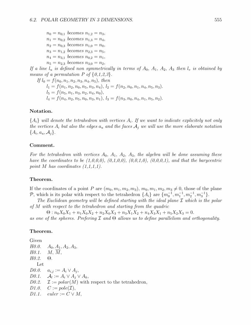
6.2. POLAR GEOMETRY IN 3 DIMENSIONS. 555
n0 = n0,1 becomes n1,2 = n3,n1 = n0,2 becomes n1,3 = n4,n2 = n0,3 becomes n1,0 = n0,n3 = n1,2 becomes n2,3 = n5,n4 = n3,1 becomes n0,2 = n1,n5 = n2,3 becomes n3,0 = n2,
If a line lu is defined non symmetrically in terms of A0, A1, A2, A3 then lv is obtained bymeans of a permutation P of 0,1,2,3.
If l0 = f(n0, n1, n2, n3, n4, n5), thenl1 = f(n1, n2, n0, n5, n3, n4), l2 = f(n2, n0, n1, n4, n5, n3).l5 = f(n5, n1, n3, n2, n4, n0),l4 = f(n4, n2, n5, n0, n3, n1), l3 = f(n3, n0, n4, n1, n5, n2).
Notation.
Ai will denote the tetrahedron with vertices Ai. If we want to indicate explicitely not onlythe vertices Ai but also the edges au and the faces Aj we will use the more elaborate notationAi, au,Aj.
Comment.
For the tetrahedron with vertices A0, A1, A2, A3, the algebra will be done assuming thesehave the coordinates to be (1,0,0,0), (0,1,0,0), (0,0,1,0), (0,0,0,1), and that the barycentricpoint M has coordinates (1,1,1,1).
Theorem.
If the coordinates of a point P are (m0,m1,m2,m3), m0,m1,m2,m3 6= 0, those of the planeP , which is its polar with respect to the tetrahedron Ai are m−1
0 ,m−11 ,m−1
2 ,m−13 .
The Euclidean geometry will be defined starting with the ideal plane I which is the polarof M with respect to the tetrahedron and starting from the quadric
Θ : n0X0X1 + n1X0X2 + n2X0X3 + n3X1X2 + n4X3X1 + n5X2X3 = 0.as one of the spheres. Prefering I and Θ allows us to define parallelism and orthogonality.
Theorem.
GivenH0.0. A0, A1, A2, A3,H0.1. M, M,H0.2. Θ.
LetD0.0. ai,j := Ai ∨ Aj,D0.1. Al := Ai ∨ Aj ∨ Ak,D0.2. I := polar(M) with respect to the tetrahedron,D1.0. C := pole(I),D1.1. euler := C ∨M,

556 CHAPTER 6. GENERALIZATION TO 3 DIMENSIONS
D1.2. APi := pole(Ai),D1.3. medi := C ∨ Ai,D1.4. Imedi := I ∧medi,D1.5. alti := Ai ∨ Imedi,D1.6. Footi := Ai ∧ alti,D1.7. ipai,j := Imedi ∨ Imedj, (i, j) ∈ IJ ,D1.8. Perpi,j := ipa(i, j) ∨ Ai, (i, j) ∈ IJ ,
Perpj,i := ipa(i, j) ∨ Aj, (j, i) ∈ JI ,D1.9. Facefooti,j := Perpi,j ∧ ak,l, (i, j) ∈ IJ or JI ,D1.10. facealtitudei,j := Facefooti,j ∨ Ai, (i, j) ∈ IJ or JI ,D1.11. Oi := facealtitudej,i ×× facealtitudek,i, i, j, k distinct(∗),D1.12. Midi := Footi +Oi,D1.13. midi := Midi ∨ Imedi,D1.14. H := mid0 ×× mid1, (∗)D1.15. η :=quadric through alti(∗),thenC1.0. M = C +HC1.1. H ∨ euler = 0.C1.2. Footij = Footji .C1.3. Oi ∨ η = 0.The nomenclature or alternate definitions:
Ai are the vertices,M is the barycenter,
N0.0. au are the edges,N0.1. Ai are the faces,
The tetrahedron is (Ai, au,Ai),N0.2. I is the ideal plane,N1.0. C is the center of the circumsphere,N1.1. euler is the line of Euler,N1.2. APi is the pole of the face Ai,N1.3. medi is the mediatrix of the face Ai,N1.4. Imedi is the ideal point on the mediatrix medi,N1.5. alti is the altitude corresponding to A0,N1.6. Footi is the foot of alti, corresponding to Ai,N1.7. ipai,j is the direction of the planes perpendicular to ak,l,N1.8. Perpi,j, (i, j) ∈ IJ , is the plane perpendicular to ak,l through Ai,
Perpj,i, (j, i) ∈ JI , is the plane perpendicular to ak,l through Aj,N1.9. Facefooti,j, (i, j) ∈ IJ or JI , is theface-foot in the face Aj, on the edge
opposite Ai, Ai ∨ Facefooti,j is perpendicular to ak,l,N1.10. facealtitudei,j, (i, j) ∈ IJ or JI , is the face-altitude in the face Aj
through the vertex Ai, perpendicular to ak,l,N1.11. Oi is the orthocenter of Ai,N1.12. midi is the perpendicular to Ai through Mi,N1.13. H is the center of the hyperboloid η.N1.14. η is the hyperboloid of Neuberg.

6.2. POLAR GEOMETRY IN 3 DIMENSIONS. 557
Proof:G0.0. A0 = (1, 0, 0, 0).G0.1. M = (1, 1, 1, 1).G0.2. Θ : n0X0X1 + n1X0X2 + n2X0X3 + n3X1X2 + n4X3X1 + n5X2X3 = 0.P0.0. a0 = [1, 0, 0, 0, 0, 0].P0.1. A0 = 1, 0, 0, 0.P0.2. I = 1, 1, 1, 1.P1.0. C = (
2n3n4n5 + n0n5(n5 − n3 − n4) + n1n4(n4 − n5 − n3) + n2n3(n3 − n4 − n5),2n5n1n2 + n3n2(n2 − n5 − n1) + n4n1(n1 − n2 − n5) + n0n5(n5 − n1 − n2),2n2n4n0 + n5n0(n0 − n2 − n4) + n1n4(n4 − n0 − n2) + n3n2(n2 − n4 − n0),2n0n1n3 + n2n3(n3 − n0 − n1) + n4n1(n1 − n3 − n0) + n5n0(n0 − n1 − n3).
P1.1. euler = [2n5(n3n4−n1n2)+(n1n4−n2n3)(n2+n4−n1−n3)+n0n5(n1+n2−n3−n4),2n4(n5n3 − n2n0) + (n2n3 − n0n5)(n0 + n3 − n2 − n5) + n1n4(n2 + n0 − n5 − n3),2n3(n4n5 − n0n1) + (n0n5 − n1n4)(n1 + n5 − n0 − n4) + n2n3(n0 + n1 − n4 − n5),2n2(n1n5 − n0n4) + (n0n5 − n1n4)(n4 + n5 − n0 − n1) + n2n3(n0 + n4 − n1 − n5),2n1(n0n3 − n2n5) + (n2n3 − n0n5)(n5 + n3 − n2 − n0) + n1n4(n2 + n5 − n0 − n3),2n0(n2n4 − n1n3) + (n1n4 − n2n3)(n3 + n4 − n1 − n2) + n5n0(n1 + n3 − n2 − n4),P1.2. AP0 = (2n3n4n5, n5(n0n5 − n2n3 − n1n4), n4(n1n4 − n0n5 − n2n3),
n3(n2n3 − n1n4 − n0n5)).P1.3. med0 = [n5(n5 − n3 − n4), n4(n4 − n5 − n3), n3(n3 − n4 − n5),
n4(n1 − n2)− n5(n0 − n2), n5(n0 − n1)− n3(n2 − n1),n3(n2 − n0)− n4(n1 − n0)].
P1.4. Imed0 = (n23 + n2
4 + n25 − 2(n4n5 + n5n3 + n3n4),
−n5(3n0 + 2n5 − n)− (n1 − n2)(n3 − n4),−n4(3n1 + 2n4 − n)− (n2 − n0)(n5 − n3),−n3(3n2 + 2n3 − n)− (n0 − n1)(n4 − n5))).
P1.5. alt0 = [n5(3n0 + 2n5 − n) + (n1 − n2)(n3 − n4),n4(3n1 + 2n4 − n) + (n2 − n0)(n5 − n3),n3(3n2 + 2n3 − n) + (n0 − n1)(n4 − n5), 0, 0, 0].
P1.6. Foot0 = (0, n5(3n0 + 2n5 − n) + (n1 − n2)(n3 − n4),n4(3n1 + 2n4 − n) + (n2 − n0)(n5 − n3),n3(3n2 + 2n3 − n) + (n0 − n1)(n4 − n5)],
P1.7. ipa0 = [2n5, n3 − n4 − n5,−n3 + n4 − n5,−n1 + n2 + n5,−n1 + n2 − n5,− n1 + n2 + n3 − n4.
P1.8. Perp0,1 = 0,−n4 + n3 + n2 − n1,−n5 + n2 − n1, n5 + n2 − n1,Perp1,0 = n4 − n3 − n2 + n1, 0,−n5 + n4 − n3, n5 + n4 − n3.
P1.9. Facefoot0,1 = (0, 0,−n1 + n2 + n5, n1 − n2 + n5),Facefoot1,0 = (0, 0,−n3 + n4 + n5, n3 − n4 + n5).
P1.10. facealtitude0,1 = [0,−n1 + n2 + n5, n1 − n2 + n5, 0, 0, 0],facealtitude1,0 = [0, 0, 0, n3 − n4 − n5, n3 − n4 + n5, 0].
P1.11. O0 = (0, n25 − (n3 − n4)2, n2
4 − (n5 − n3)2, n23 − (n4 − n5)2).
P1.12. Mid0 = (0, n5(3n0 + n5 − n) + (n3 − n4)(n1 − n2 + n3 − n4),n4(3n1 + n4 − n) + (n5 − n3)(n2 − n0 + n5 − n3),n3(3n2 + n3 − n) + (n4 − n5)(n0 − n1 + n4 − n5)),
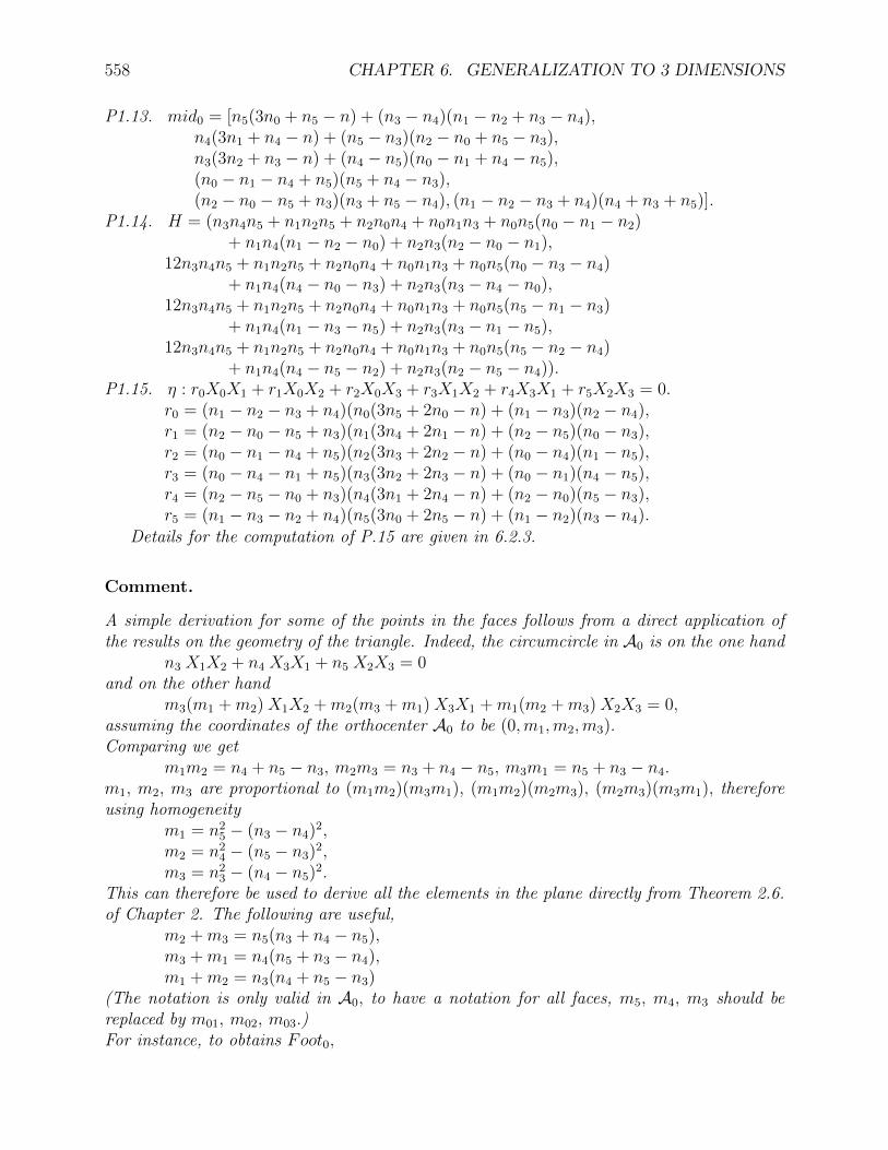
558 CHAPTER 6. GENERALIZATION TO 3 DIMENSIONS
P1.13. mid0 = [n5(3n0 + n5 − n) + (n3 − n4)(n1 − n2 + n3 − n4),n4(3n1 + n4 − n) + (n5 − n3)(n2 − n0 + n5 − n3),n3(3n2 + n3 − n) + (n4 − n5)(n0 − n1 + n4 − n5),(n0 − n1 − n4 + n5)(n5 + n4 − n3),(n2 − n0 − n5 + n3)(n3 + n5 − n4), (n1 − n2 − n3 + n4)(n4 + n3 + n5)].
P1.14. H = (n3n4n5 + n1n2n5 + n2n0n4 + n0n1n3 + n0n5(n0 − n1 − n2)+ n1n4(n1 − n2 − n0) + n2n3(n2 − n0 − n1),
12n3n4n5 + n1n2n5 + n2n0n4 + n0n1n3 + n0n5(n0 − n3 − n4)+ n1n4(n4 − n0 − n3) + n2n3(n3 − n4 − n0),
12n3n4n5 + n1n2n5 + n2n0n4 + n0n1n3 + n0n5(n5 − n1 − n3)+ n1n4(n1 − n3 − n5) + n2n3(n3 − n1 − n5),
12n3n4n5 + n1n2n5 + n2n0n4 + n0n1n3 + n0n5(n5 − n2 − n4)+ n1n4(n4 − n5 − n2) + n2n3(n2 − n5 − n4)).
P1.15. η : r0X0X1 + r1X0X2 + r2X0X3 + r3X1X2 + r4X3X1 + r5X2X3 = 0.r0 = (n1 − n2 − n3 + n4)(n0(3n5 + 2n0 − n) + (n1 − n3)(n2 − n4),r1 = (n2 − n0 − n5 + n3)(n1(3n4 + 2n1 − n) + (n2 − n5)(n0 − n3),r2 = (n0 − n1 − n4 + n5)(n2(3n3 + 2n2 − n) + (n0 − n4)(n1 − n5),r3 = (n0 − n4 − n1 + n5)(n3(3n2 + 2n3 − n) + (n0 − n1)(n4 − n5),r4 = (n2 − n5 − n0 + n3)(n4(3n1 + 2n4 − n) + (n2 − n0)(n5 − n3),r5 = (n1 − n3 − n2 + n4)(n5(3n0 + 2n5 − n) + (n1 − n2)(n3 − n4).
Details for the computation of P.15 are given in 6.2.3.
Comment.
A simple derivation for some of the points in the faces follows from a direct application ofthe results on the geometry of the triangle. Indeed, the circumcircle in A0 is on the one hand
n3 X1X2 + n4 X3X1 + n5 X2X3 = 0and on the other hand
m3(m1 +m2)X1X2 +m2(m3 +m1)X3X1 +m1(m2 +m3)X2X3 = 0,assuming the coordinates of the orthocenter A0 to be (0,m1,m2,m3).Comparing we get
m1m2 = n4 + n5 − n3, m2m3 = n3 + n4 − n5, m3m1 = n5 + n3 − n4.m1, m2, m3 are proportional to (m1m2)(m3m1), (m1m2)(m2m3), (m2m3)(m3m1), thereforeusing homogeneity
m1 = n25 − (n3 − n4)2,
m2 = n24 − (n5 − n3)2,
m3 = n23 − (n4 − n5)2.
This can therefore be used to derive all the elements in the plane directly from Theorem 2.6.of Chapter 2. The following are useful,
m2 +m3 = n5(n3 + n4 − n5),m3 +m1 = n4(n5 + n3 − n4),m1 +m2 = n3(n4 + n5 − n3)
(The notation is only valid in A0, to have a notation for all faces, m5, m4, m3 should bereplaced by m01, m02, m03.)For instance, to obtains Foot0,

6.2. POLAR GEOMETRY IN 3 DIMENSIONS. 559
ia0 := |A0|I = [0, 0, 0, 1, 1, 1] = [[1, 0, 0]],P ia0 := pole(ia0) ∈ I = ((i00, i01, i02)) = (i00, i01, i02, i03),
with i03 = −i00 − i01 − i02 = (n0 − n1 − n3)(n4 − n3 − n5) + 2n3(n2 − n1 − n5).hence Foot0 := (A0 ∨ Pia0)A0 = (0, i01, i02, i03). Hence
Footi,i = 0,fIJ := Footij = Footji = (ni,k − ni,l)(nj,k − nj,l) + nk,l(3ni,j + 2nk,l − n)for i 6= j, and i, j, k, l a permutation of 0,1,2,3.
Hence the Theorem as well as C1.3.Similarly the center of the circumcircle ∈ A0 is
(0, n5(n3 + n4 − n5), n4(n5 + n3 − n4), n3(n4 + n5 − n3)).
Theorem.
Let ri,j be the coordinate of XiXj in η.Let the coordinates of the feet Foot0, Foot1, Foot2, Foot3 be (0, f01, f02, f03), (f10, 0, f12, f13),(f20, f21, 0, f23), (f30, f31, f32, 0),then
ri,j = fk,l(fi,kfj,l − fi,lfj,k), where i, j, k, l is an even permutation of 0,1,2,3.
Proof: Let the inverse fJI of fIJ modulo p be denoted gIJ .If all fij 6= 0, expressing the fact that the quadric contains the altitudes gives the equations(0) f01r0 + f02r1 + f03r2 = 0, (1) g01r5 + g02r4 + g03r3 = 0,(2) f10r0 + f12r3 + f13r4 = 0, (3) g10r5 + g12r2 + g13r1 = 0,(4) f20r1 + f21r3 + f23r5 = 0, (5) g20r4 + g21r2 + g23r0 = 0,(6) f30r2 + f31r4 + f32r5 = 0, (7) g30r3 + g31r1 + g32r0 = 0.Equations (0) and (7) are obtained by substituting in the equation of the quadric, Xi bykAi + Footi,g30, g31, g32 are proportional to f01f02, f03f01, f02f03, and therefore to f−1
03 , f−102 , f
−101 .
We solve (0) with respect to r0, and (3) with respect to r5, in terms of r1 and r2, (5) givesr4, substitution in (6) gives an homogeneous equation in terms of r1 and r2 only, hence afterdivision by f01f03 + f02f13
r0,2 = r1 = f13(f03f21 − f01f23), r0,3 = r2 = −f12(f02f31 − f01f32).equations (0) give r0, (5) gives r4, (7) gives r3 and (1) gives r5. Hence
r0,1 = r0 = −f23(f03f12 − f02f13),r1,2 = r3 = f03(f10f23 − f13f20),r3,1 = r4 = f02(f30f12 − f32f10),r2,3 = r5 = f01(f20f31 − f21f30),
equations (2) and (4) can be used as a check. Summarizing the results gives the Theorem.Simplifying by a common factor, we obtain P1.15.
Theorem.
LetD2.0. Iau := au ∧ I,D2.1. Polarau := polar(Iau),then

560 CHAPTER 6. GENERALIZATION TO 3 DIMENSIONS
C2.0. ipau ∧ Polar5−u = 0.Nomenclature:N2.0. Iau are the ideal points on the edges au,N2.1. polarau is the equatorial plane perpendicular to au.
Proof.P2.0. Ia0 = (1,−1, 0, 0).P2.1. Polara0 = −n0, n0, n1 − n3, n2 − n4.
6.2.4 The orthogonal tetrahedron.
Definition.
A tetrahedron is orthogonal iff the 3 pairs of opposite sides are perpendicular.
Lemma.
a0 · a5 = 0 iff n1 + n4 = n2 + n3,a0 · a1 = 0 iff n3 = n0 + n1,a1 · a2 = 0 iff n5 = n1 + n2,a2 · a0 = 0 iff n4 = n2 + n0.
The first condition expresses the orthogonality of opposite sides, the other conditions theorthogonality of adjacent sides.
Theorem.
The tetrahedron is orthogonal iff the parameters of the circumsphere satisfyn0 + n5 = n1 + n4 = n2 + n3.
Proof. The perpendicularity of A0 ∨ A1 and A2 ∨ A3 implies, because of 6.2.2.1, withlj = mj = 0, except for l0 = m5 = 1,
n1 − n3 = n2 − n4 or n1 + n4 = n2 + n3,Similarly that of A0 ∨ A2 and A1 ∨ A3 implies
n0 + n5 = n2 + n3.
Theorem.
Given an orthogonal tetrahedron whose adjacent sied are not orthogonal, let
0. m0 = (n0 + n1 − n3)−1, m1 = (n3 + n4 − n5)−1,m2 = (n5 + n1 − n2)−1, m3 = (n2 + n4 − n0)−1,
then
1. n0 = (m0 +m1)m2m3, n1 = (m0 +m2)m3m1, n2 = (m0 +m3)m1m2,n3 = (m1 +m2)m0m3, n4 = (m3 +m1)m0m2, n5 = (m2 +m3)m0m1.
Proof: The non othogonality of adjacent sides implies that the mj are well defined. Weobtain, because of the orthogonality of opposite sides,
m−10 +m−1
1 = 2n0, m−12 +m−1
0 = 2n1, m−11 +m−1
2 = 2n3,
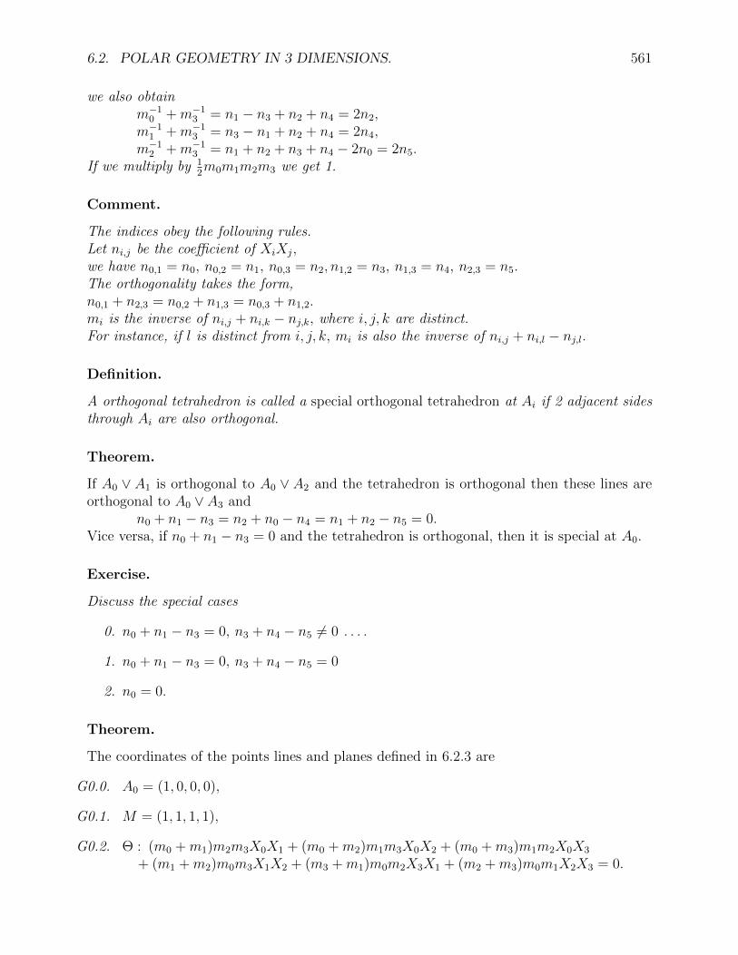
6.2. POLAR GEOMETRY IN 3 DIMENSIONS. 561
we also obtainm−1
0 +m−13 = n1 − n3 + n2 + n4 = 2n2,
m−11 +m−1
3 = n3 − n1 + n2 + n4 = 2n4,m−1
2 +m−13 = n1 + n2 + n3 + n4 − 2n0 = 2n5.
If we multiply by 12m0m1m2m3 we get 1.
Comment.
The indices obey the following rules.Let ni,j be the coefficient of XiXj,we have n0,1 = n0, n0,2 = n1, n0,3 = n2, n1,2 = n3, n1,3 = n4, n2,3 = n5.The orthogonality takes the form,n0,1 + n2,3 = n0,2 + n1,3 = n0,3 + n1,2.mi is the inverse of ni,j + ni,k − nj,k, where i, j, k are distinct.For instance, if l is distinct from i, j, k, mi is also the inverse of ni,j + ni,l − nj,l.
Definition.
A orthogonal tetrahedron is called a special orthogonal tetrahedron at Ai if 2 adjacent sidesthrough Ai are also orthogonal.
Theorem.
If A0 ∨ A1 is orthogonal to A0 ∨ A2 and the tetrahedron is orthogonal then these lines areorthogonal to A0 ∨ A3 and
n0 + n1 − n3 = n2 + n0 − n4 = n1 + n2 − n5 = 0.Vice versa, if n0 + n1 − n3 = 0 and the tetrahedron is orthogonal, then it is special at A0.
Exercise.
Discuss the special cases
0. n0 + n1 − n3 = 0, n3 + n4 − n5 6= 0 . . . .
1. n0 + n1 − n3 = 0, n3 + n4 − n5 = 0
2. n0 = 0.
Theorem.
The coordinates of the points lines and planes defined in 6.2.3 are
G0.0. A0 = (1, 0, 0, 0),
G0.1. M = (1, 1, 1, 1),
G0.2. Θ : (m0 +m1)m2m3X0X1 + (m0 +m2)m1m3X0X2 + (m0 +m3)m1m2X0X3
+ (m1 +m2)m0m3X1X2 + (m3 +m1)m0m2X3X1 + (m2 +m3)m0m1X2X3 = 0.

562 CHAPTER 6. GENERALIZATION TO 3 DIMENSIONS
P0.0. a0 = a0,1 = [1, 0, 0, 0, 0, 0],
P0.1. A0 = 1, 0, 0, 0,
P0.2. I = 1, 1, 1, 1,
P1.0. C = (−m0 +m1 +m2 +m3,m0 −m1 +m2 +m3,m0 +m1 −m2 +m3,m0 +m1 +m2 −m3),
P1.1. euler = [m0 −m1,m0 −m2,m0 −m3,m1 −m2,m3 −m1,m2 −m3],
P1.2. AP0 = (m0(m1 +m2)(m3 +m1)(m2 +m3),−m1(m2 +m3)(m0m1 +m2m3),−m2(m3 +m1)(m0m2 +m3m1),−m3(m1 +m2)(m0m3 +m1m2)),
P1.3. med0 = [m2 +m3,m3 +m1,m1 +m2,m2 −m1,m1 −m3,m3 −m2],
P1.4. Imed0 = (−(m1 +m2 +m3),m1,m2,m3),
P1.5. alt0 = [m1,m2,m3, 0, 0, 0],
P1.6. Foot0 = (0,m1,m2,m3),
P1.7. ipa0,1 = [m2 +m3,−m2,−m3,m2,−m3, 0]
P1.8. Perp0,1 = Perp1,0 = 0, 0,−m3,m2,
P1.9. Facefoot0,1 = Facefoot1,0 = (m0,m1, 0, 0),
P1.10. facealtitude0,1 = [0,m2,m3, 0, 0, 0], facealtitude1,0 = [0, 0,m0, 0,m1, 0],
P1.11. O0 = (0,m1,m2,m3),
P1.12. Mid0 = (0,m1,m2,m3),
P1.13. mid0 = altitude0,
P1.14. H = (m0,m1,m2,m3),
P1.15. Hyperboloid :m2m3 X0X1−m1m3 X0X2−m0m2 X1X3 +m0m1 X2X3 = 0
orm2m3 X0X1−m1m2 X0X3−m0m3 X1X2 +m0m1 X2X3 = 0.
Exercise.
Construct a quadric generalizing the conic of Brianchon-Poncelet, and verify that its equationis
m1m2m3 X20 + . . .−m2m3(m0 +m1)X0X1 + . . . = 0.
Determine points on this quadric by linear constructions which are in none of the faces.

6.2. POLAR GEOMETRY IN 3 DIMENSIONS. 563
Exercise.
Construct a quadric which generalizes the sphere of Prouhet, passing through the barycentersand orthocenters of the faces and verify that its equation is
3(m0 +m1)m2m3X0X1 + . . .−2(X0 +X1 +X2 +X3)(m1m2m3X0 + . . .) = 0.
(Coolidge, Treatise, p. 237)
6.2.5 The isodynamic tetrahedron.
Definition.
A symmedian is a line joining a vertex to the point of Lemoine of the opposite face.
Definition.
An isodynamic tetrahedron is a tetrahedron in which 3 of the symmedians are concurrent.
Theorem.
A tetrahedron is isodynamic iffn0n5 = n1n4 = n2n3.
Proof:Let Ki be the symmedian in the place Ai, let ki := Ai ×Ki,
K0 = (0, n5, n4, n3), K1 = (n5, 0, n2, n1),K2 = (n4, n2, 0, n0), K3 = (n3, n1, n0, 0).
k0 = [n5, n4, n3, 0, 0, 0], k1 = [n5, 0, 0, n2, n1, 0] and k2 = [0, n4, 0, n2, 0, n0].k0 and k1 are coplanar if n1n4 = n2n3, k0 and k2 are coplanar if n0n5 = n2n3, hence thetheorem.
Theorem.
In an isodynamic tetrahedron all 4 symmedians are concurrent.
6.1.3 The orthogonal tetrahedron.
Definition.
A tetrahedron is orthogonal iff opposite sides are perpendicular.
Lemma.
a0 · a5 = 0 iff n1 + n4 = n2 + n3,a0 · a1 = 0 iff n3 = n0 + n1,a1 · a2 = 0 iff n5 = n1 + n2,a2 · a0 = 0 iff n4 = n2 + n0.

564 CHAPTER 6. GENERALIZATION TO 3 DIMENSIONS
Theorem.
The tetrahedron is orthogonal iff the parameters of the circumsphere satisfyn0 + n5 = n1 + n4 = n2 + n3.
Proof: The perpendicularity of A0∨A1 and A2∨A3 implies (0, 0, 1,−1)F(1,−1, 0, 0)T = 0,or(n1 − n3)− (n2 − n4) = 0 or
n1 + n4 = n2 + n3,Similarly that of A0 ∨ A2 and A1 ∨ A3 implies
n0 + n5 = n2 + n3.
Theorem.
If n0 +n1−n3 6= 0, n3 +n4−n5 6= 0, n5 +n1−n2 6= 0, n2 +n4−n0 6= 0, and the tetrahedronis orthogonal. Let
0. m0 = (n0 + n1 − n3)−1, m1 = (n3 + n4 − n5)−1,m2 = (n5 + n1 − n2)−1, m3 = (n2 + n4 − n0)−1,
then
1. n0 = (m0 +m1)m2m3, n1 = (m0 +m2)m3m1, n2 = (m0 +m3)m1m2,n3 = (m1 +m2)m0m3, n4 = (m3 +m1)m0m2, n5 = (m2 +m3)m0m1.
Proof: We obtain at once,m−1
0 +m−11 = 2n0, m
−12 +m−1
0 = 2n1, m−11 +m−1
2 = 2n3,using 1.3.3., we also obtain
m−10 +m−1
3 = n1 − n3 + n2 + n4 = 2n2,m−1
1 +m−13 = n3 − n1 + n2 + n4 = 2n4,
m−12 +m−1
3 = n1 + n2 + n3 + n4 − 2n0 = 2n5.If we multiply by 1
2m0m1m2m3 we get 1.
Comment.
?? when hyp. of prec theorem replace 6= 0 by = 0, see Theorem 3.7.
Comment.
The indices obey the following rules.Let n0,1 be the coefficient of X0X1, . . . ,we have n0,1 = n0, n0,2 = n1, n0,3 = n2,
n1,2 = n3, n1,3 = n4, n2,3 = n5.The orthogonality takes the form,n0,1 + n2,3 = n0,2 + n1,3 = n0,3 + n1,2.mi is the inverse of ni,j + ni,k − nj,k, where i, j, k are distinct.For instance, if l is distinct from i, j, k, mi is also the inverse of ni,j + ni,l − nj,l.
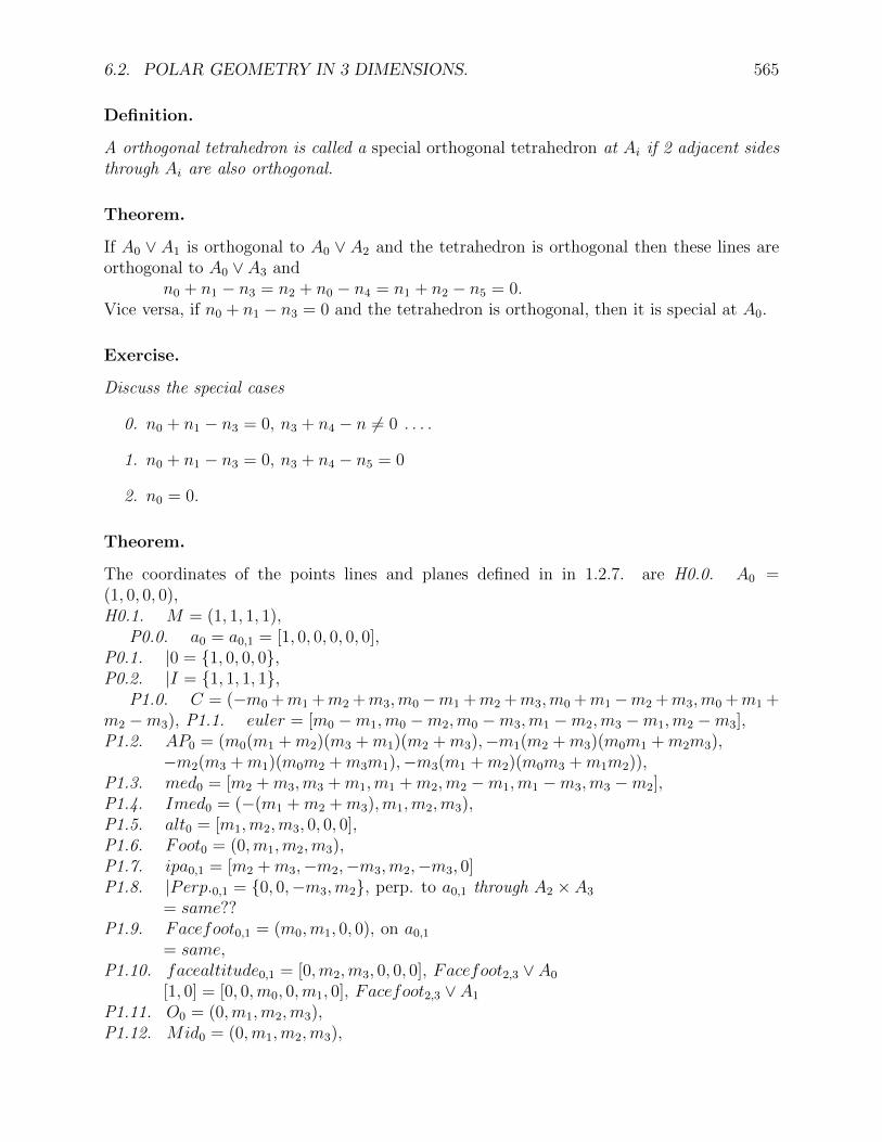
6.2. POLAR GEOMETRY IN 3 DIMENSIONS. 565
Definition.
A orthogonal tetrahedron is called a special orthogonal tetrahedron at Ai if 2 adjacent sidesthrough Ai are also orthogonal.
Theorem.
If A0 ∨ A1 is orthogonal to A0 ∨ A2 and the tetrahedron is orthogonal then these lines areorthogonal to A0 ∨ A3 and
n0 + n1 − n3 = n2 + n0 − n4 = n1 + n2 − n5 = 0.Vice versa, if n0 + n1 − n3 = 0 and the tetrahedron is orthogonal, then it is special at A0.
Exercise.
Discuss the special cases
0. n0 + n1 − n3 = 0, n3 + n4 − n 6= 0 . . . .
1. n0 + n1 − n3 = 0, n3 + n4 − n5 = 0
2. n0 = 0.
Theorem.
The coordinates of the points lines and planes defined in in 1.2.7. are H0.0. A0 =(1, 0, 0, 0),H0.1. M = (1, 1, 1, 1),
P0.0. a0 = a0,1 = [1, 0, 0, 0, 0, 0],P0.1. |0 = 1, 0, 0, 0,P0.2. |I = 1, 1, 1, 1,
P1.0. C = (−m0 +m1 +m2 +m3,m0−m1 +m2 +m3,m0 +m1−m2 +m3,m0 +m1 +m2 −m3), P1.1. euler = [m0 −m1,m0 −m2,m0 −m3,m1 −m2,m3 −m1,m2 −m3],P1.2. AP0 = (m0(m1 +m2)(m3 +m1)(m2 +m3),−m1(m2 +m3)(m0m1 +m2m3),
−m2(m3 +m1)(m0m2 +m3m1),−m3(m1 +m2)(m0m3 +m1m2)),P1.3. med0 = [m2 +m3,m3 +m1,m1 +m2,m2 −m1,m1 −m3,m3 −m2],P1.4. Imed0 = (−(m1 +m2 +m3),m1,m2,m3),P1.5. alt0 = [m1,m2,m3, 0, 0, 0],P1.6. Foot0 = (0,m1,m2,m3),P1.7. ipa0,1 = [m2 +m3,−m2,−m3,m2,−m3, 0]P1.8. |Perp.0,1 = 0, 0,−m3,m2, perp. to a0,1 through A2 × A3
= same??P1.9. Facefoot0,1 = (m0,m1, 0, 0), on a0,1
= same,P1.10. facealtitude0,1 = [0,m2,m3, 0, 0, 0], Facefoot2,3 ∨ A0
[1, 0] = [0, 0,m0, 0,m1, 0], Facefoot2,3 ∨ A1
P1.11. O0 = (0,m1,m2,m3),P1.12. Mid0 = (0,m1,m2,m3),
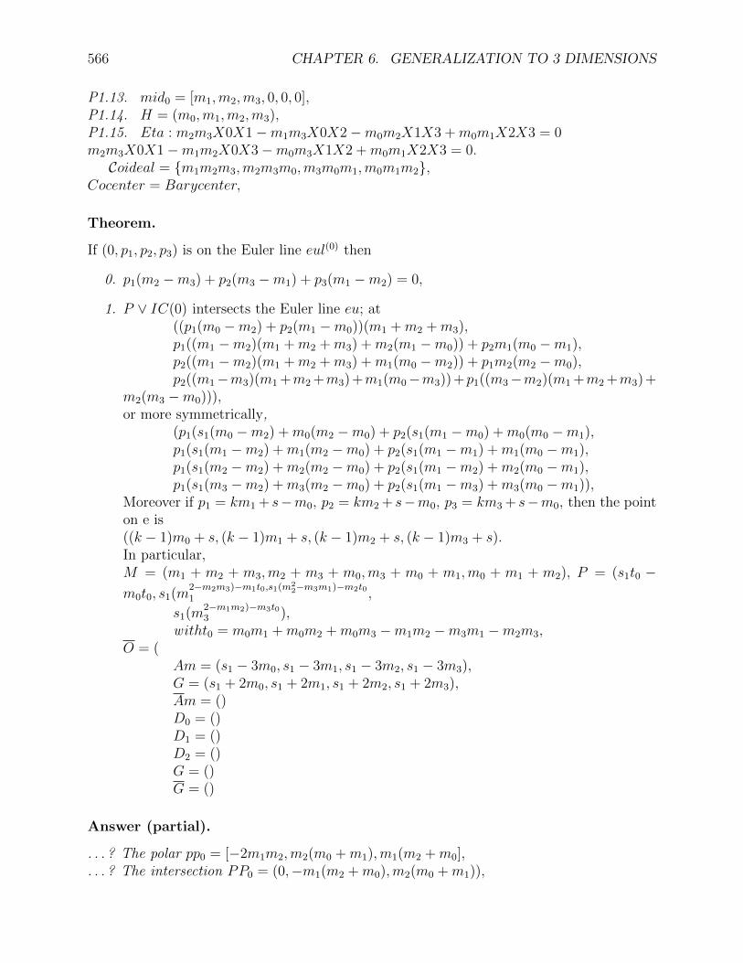
566 CHAPTER 6. GENERALIZATION TO 3 DIMENSIONS
P1.13. mid0 = [m1,m2,m3, 0, 0, 0],P1.14. H = (m0,m1,m2,m3),P1.15. Eta : m2m3X0X1−m1m3X0X2−m0m2X1X3 +m0m1X2X3 = 0m2m3X0X1−m1m2X0X3−m0m3X1X2 +m0m1X2X3 = 0.Coideal = m1m2m3,m2m3m0,m3m0m1,m0m1m2,
Cocenter = Barycenter,
Theorem.
If (0, p1, p2, p3) is on the Euler line eul(0) then
0. p1(m2 −m3) + p2(m3 −m1) + p3(m1 −m2) = 0,
1. P ∨ IC(0) intersects the Euler line eu; at((p1(m0 −m2) + p2(m1 −m0))(m1 +m2 +m3),p1((m1 −m2)(m1 +m2 +m3) +m2(m1 −m0)) + p2m1(m0 −m1),p2((m1 −m2)(m1 +m2 +m3) +m1(m0 −m2)) + p1m2(m2 −m0),p2((m1−m3)(m1 +m2 +m3)+m1(m0−m3))+p1((m3−m2)(m1 +m2 +m3)+
m2(m3 −m0))),or more symmetrically,
(p1(s1(m0 −m2) +m0(m2 −m0) + p2(s1(m1 −m0) +m0(m0 −m1),p1(s1(m1 −m2) +m1(m2 −m0) + p2(s1(m1 −m1) +m1(m0 −m1),p1(s1(m2 −m2) +m2(m2 −m0) + p2(s1(m1 −m2) +m2(m0 −m1),p1(s1(m3 −m2) +m3(m2 −m0) + p2(s1(m1 −m3) +m3(m0 −m1)),
Moreover if p1 = km1 + s−m0, p2 = km2 + s−m0, p3 = km3 + s−m0, then the pointon e is((k − 1)m0 + s, (k − 1)m1 + s, (k − 1)m2 + s, (k − 1)m3 + s).In particular,M = (m1 + m2 + m3,m2 + m3 + m0,m3 + m0 + m1,m0 + m1 + m2), P = (s1t0 −m0t0, s1(m
2−m2m3)−m1t0,s1(m22−m3m1)−m2t0
1 ,
s1(m2−m1m2)−m3t03 ),
w itht0 = m0m1 +m0m2 +m0m3 −m1m2 −m3m1 −m2m3,O = (
Am = (s1 − 3m0, s1 − 3m1, s1 − 3m2, s1 − 3m3),G = (s1 + 2m0, s1 + 2m1, s1 + 2m2, s1 + 2m3),Am = ()D0 = ()D1 = ()D2 = ()G = ()G = ()
Answer (partial).
. . . ? The polar pp0 = [−2m1m2,m2(m0 +m1),m1(m2 +m0],
. . . ? The intersection PP0 = (0,−m1(m2 +m0),m2(m0 +m1)),

6.2. POLAR GEOMETRY IN 3 DIMENSIONS. 567
. . . ? pp = [m1m2(m2 +m0)(m0 +m1),m2m0(m0 +m1)(m1 +m2),m0m1(m1 +m2)(m2 +m0)].
Point “O“, intersection of perpendicular to faces through their barycenter(special case of . . . with k = 0 hence“O” = (s1 −m0, s1 −m1, s1 −m2, s1 −m3).“Conjugate tetrahedron”,“A′0” = (−2s1 − 2m0, s1 + 2m1, s1 + 2m2, s1 + 2m3),barycenter of faces of [A′[i]] are“M ′
0” = (0,m1,m2,m3), which are the orthocenters of the faces,Perpendiculars through M ′
0 to the faces, (which are parallel to those of [A[]] meet at“O′” = (3s1 − 4m0, 3s1 − 4m1, 3s1 − 4m2, 3s1 − 4m3).Hence his theorem: Then he generalizes the circle of Brianchon-Poncelet and gives its centeras the midpoint of H and “O”I believe his “O” is my G.Orthocenter,barycenter and “O” are collinear
6.1.4 The isodynamic tetrahedron.
Definition.
A symmedian is a line joining a vertex to the point of Lemoine of the opposite face.
Definition.
An isodynamic tetrahedron is a tetrahedron in which 3 of the symmedians are concurrent.
Theorem.
A tetrahedron is isodynamic iffn0n5 = n1n4 = n2n3.
Proof:K0 = (0, n5, n4, n3), K1 = (−n5, 0, n2,−n1),K2 = (−n4,−n2, 0, n0), K3 = ().
k0 and k1 are coplanar if n1n2 = n2n3, k0 and k2 are coplanar if n0n5 = n2n3, hence thetheorem.
Theorem.
In an isodynamic tetrahedron all 4 symmedians are concurrent.
In 3 dimensions start with A0 = (1, 0, 0, 0), . . ., A3 = (0, 0, 0, 1), and with M = (1, 1, 1, 1)and M = (m0,m1,m2,m3). M corresponds to the barycenter, M to the intersection of thelines joining the orthocenter of the faces to the opposite vertex and A[] to the vertices of anorthogonal tetrahedron. See . . .
. Theorem. Prove that the tetrahedron is orthogonal.
. Theorem. Prove that the circumscribed quadric is given by(m0 +m1)m2m3X0X1 + . . . = 0.

568 CHAPTER 6. GENERALIZATION TO 3 DIMENSIONS
. Theorem. Construct a quadric generalizing the conic of Brianchon- Poncelet, and verifythat its equation is
m1m2m3X20 + . . .−m2m3(m0 +m1)X0X1 + . . . = 0.
Determine points on this quadric by linear constructions which are in none of the faces.. Theorem. Construct a quadric which generalizes the sphere of Prouhet, passing through
the barycenters and orthocenters of the faces and verify that its equation is3(m0 +m1)m2m3X0X1 + . . .−2(X0 +X1 +X2 +X3)(m1m2m3X0 + . . .) = 0.
(Coolidge, Treatise, p. 237)Point “O“, intersection of perpendicular to faces through their barycenter (special case of . . .with k = 0 hence“O” = (s1 −m0, s1 −m1, s1 −m2, s1 −m3)“Conjugate tetrahedron”,“A′0” = (−2s1 − 2m0, s1 + 2m1, s1 + 2m2, s1 + 2m3),barycenter of faces of [A′[i]] are“M ′
0” = (0,m1,m2,m3),which are the orthocenters of the faces,Perpendiculars through M ′
0 to the faces, (which are parallel to those of [A[]] meet at“O′” = (3s1 − 4m0, 3s1 − 4m1, 3s1 − 4m2, 3s1 − 4m3),Hence his theorem:Then he generalizes the circle of Brianchon-Poncelet and gives its center as the midpoint ofH and “O”I believe his “O” is my G.Orthocenter,barycenter and “O” are collinear.
6.1.5 The antipolarity.
Definition.
Consider the 2-form [l0, l1, l2, l3, l4, l5] with
0. l0l5 + l1l4 + l2l3 6= 0,the point to plane antipolarity associates to a point P a plane P := l′ ∨ P,the plane to point antipolarity associates to a plane P a point P := l′P .
Theorem.
The point to plane antipolarity can be represented by an antisymmetric matrix
P =
0 l5 l4 l3−l5 0 l2 −l1−l4 −l2 0 l0−l3 l1 −l0 0
The plane to point antipolarity is represented by the antisymmetric matrix
Q =
0 l0 l1 l2−l0 0 l3 −l4−l1 −l3 0 l5−l2 l4 −l5 0

6.2. POLAR GEOMETRY IN 3 DIMENSIONS. 569
both have determinant (l0l5 + l1l4 + l2l3)2 6= 0.
Theorem.
If P is associated to P in an antipolarity then P is associated to |P and |P is incident to P.
The proof is left as an exercise.
Theorem.
Let
0. d := l0l5 + l1l4 + l2l3,
the planes associated in the antipolarity 6.1.5 to the points of a line m are all incidentto a line q and if
1. L := l dual(l)T − dI,then
2. L =−l1l4 − l2l3 l0l4 l0l3 l0l2 l0l1 l20
l1l5 −l0l5 − l2l3 l1l3 l1l2 l21 l0l1l2l5 l2l4 −l0l5 − l1l4 l22 l2l1 l2l0l3l5 l3l4 l23 −l0l5 − l1l4 l3l1 l3l0l4l5 l24 l4l3 l4l2 −l0l5 − l2l3 l4l0l25 l5l4 l5l3 l5l2 l5l1 −l1l4 − l2l3
3. q = Lm.
4. det(L) = −d6.
The proof is left as an exercise.
Example.
Let p = 29, l′ = [1, 4, 3, 11, 4, 10] = [3644209],E0. d = 1.
E2. L =
9 4 11 3 4 1
11 −14 −14 12 −13 41 12 3 9 12 3−6 −14 5 3 −14 1111 −13 −14 12 −14 413 11 −6 1 11 9
E3. m = 732541, 25620, 871, 30, 1, 0.
q = 20154561, 8595176, 4156378, 3635799, 3644412, 3644208.

570 CHAPTER 6. GENERALIZATION TO 3 DIMENSIONS
Theorem.
The antipolarity of vertices, faces and edges of a tetrahedron follows from what follows.GivenH.0. l′ = [l0, l1, l2, l3, l4, l5],H.1. Ai,letD0.0. ai,j := Ai ∨ Aj,D0.1. Ai := aj,k ∨ Al,D1.0. Bi := l′ ∨ Ai, Bi := l′Ai,D1.1. bai := |Bi|Ai, bai := Bi ∨ Ai,D1.2. Ni,j := ak,lBj,Ni,j := ai,j ∨Bj,D1.3. ni,j := Bi ∨ Aj,D1.4. bd(i,j) := |Bi|Bj,thenC1.0. Bi ∨ Bj = 0.C1.1. Ni,j ∨Nj,i = 0.C1.2. Ni,j ∨ ni,j = 0,C1.3. ni,j = |Bj|Ai.C1.4. bd(i,j) = Bk ∨Bl.C1.5. bu = Lau.
Proof.P1.0. B0 = 0,−l5,−l4,−l3.
B0 = (0,−l0,−l1,−l2).P1.1. ba0 = [0, 0, 0, l3, l4, l5].
ba0 = [l0, l1, l2, 0, 0, 0].P1.2. N1,2 = (0, 0, l1, l2).
N1,2 = 0, 0, l4, l3.P1.3. n1,2 = [0, 0, 0, l1,−l2, 0].P1.4. b0 = [−l1l4 − l2l3, l1l5, l2l5, l3l5, l4l5, l25].
Corollary.
If l is a line and the definitions of Theorem 6.1.5 hold then all the conclusions of 6.1.5 hold.Moreover bu = l for all u.The mapping is not one to one. The image of a point P is the plane P ∨ l, the image of theplane Q is the point Q∨ l.
Example.
Let p = 29, l′ = [1, 4, 3, 11, 4, 10] = [3644209], A = (871, 30, 1, 0),E0.0. a = [732541, 25260, 871, 30, 1, 0].E0.1. A = 871, 30, 1, 0.E1.0. B = 382, 1463, 7606, 22969.
B = (149, 1397, 9293, 16386).E1.1. ba = [139, 220389, 805824, 3570916],

6.2. POLAR GEOMETRY IN 3 DIMENSIONS. 571
ba = [3634832, 741908, 33687, 1203].
E1.2. N =
−− 9 33 146
27 −− 875 139337 883 −− 9281
378 1248 16009 −−
.
N =
−− 11 34 378
19 −− 883 145149 878 −− 7599
233 1103 22737 −−
.
E1.3. n =
−− 639 56 26
659374 −− 25285 889903264 732889 −− 1422
9219913 745997 40398 −−
.E1.4. b = [20154561, 8595176, 4156378, 3635799, 3644412, 3644208].
Example.
Let p = 29, l = [3623186] = [1, 4, 2,−14, 4, 12], A = (871, 30, 1, 0),E1.0 B = 343, 1577, 13493, 18590.
B = (148, 1281, 10148, 23752).E1.1. ba = [286, 391098, 781435, 3574280],
ba = [3610443, 745272, 34514, 935].
E1.2. N =
−− 16 32 146
22 −− 875 127735 897 −− 10122
784 1045 23578 −−
.
N =
−− 12 53 320
28 −− 881 156744 878 −− 13486
233 929 18532 −−
.
E1.3. n =
−− 436 57 26
537429 −− 25285 885854486 733295 −− 1393
19121847 751884 47967 −−
.
E1.4. bu = [3623186].
Theorem.
An antipolarity can be determined as follows,Given 4 points Ai, a line ba0 ∈ A0 = A1 ∨ A2 ∨ A3,a line ba1 ∈ A1 := A2 ∨ A3 ∨ A0 and a point B0 on n0,1 = A1 ∨ (ba1 ×× a5) but not on ((ba0
×× a4) ∨ A0) ×× (ba1 ×× a2) ∨ A1)) ∨ ((ba0 ×× a3) ∨ A0) ×× (ba1 ×× a1) ∨ A1))(= B2 ∨B3).Proof. Let us choose the Ai as basis for the coordinate system.
ba0 = [0, 0, 0, l3, l4, l5] determines l3, l4, l5.ba1 = [0, l1, l2, 0, 0, l5] determines after scaling l1 and l2.
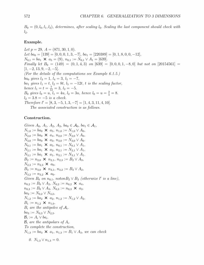
572 CHAPTER 6. GENERALIZATION TO 3 DIMENSIONS
B0 = (0, l0, l1, l2), determines, after scaling l0. Scaling the last component should check withl2.
Example.
Let p = 29, A = (871, 30, 1, 0).Let ba0 = [139] = [0, 0, 0, 1, 3,−7], ba1 = [220389] = [0, 1, 8, 0, 0,−12],N0,1 = ba1 ×× a5 = (9), n0,1 := N0,1 ∨ A1 = [639].Finally let B0 = (149) = (0, 1, 4, 3) on [639] = [0, 0, 0, 1,−8, 0] but not on [20154561] =[1,−2, 13, 9,−2,−5].(For the details of the computations see Example 6.1.5.)ba0 gives l3 = 1, l4 = 3, l5 = −7,ba1 gives l1 = t, l2 = 8t, l5 = −12t, t is the scaling factor,hence l1 = t = 7
12= 3, l2 = −5.
B0 gives l0 = u, l1 = 4u, l2 = 3u, hence l0 = u = 34
= 8.l2 = 3.8 = −5 is a check.Therefore l′ = [8, 3,−5, 1, 3,−7] = [1, 4, 3, 11, 4, 10].
The associated construction is as follows.
Construction.
Given A0, A1, A2, A3, ba0 ∈ A0, ba1 ∈ A1,N1,0 := ba0 ×× a5, n1,0 := N1,0 ∨ A0,N2,0 := ba0 ×× a4, n2,0 := N2,0 ∨ A0,N3,0 := ba0 ×× a3, n3,0 := N3,0 ∨ A0.N0,1 := ba1 ×× a5, n0,1 := N0,1 ∨ A1,N2,1 := ba1 ×× a2, n2,1 := N2,1 ∨ A1,N3,1 := ba1 ×× a1, n3,1 := N3,1 ∨ A1.B2 := n2,0 ×× n2,1, n2,3 := B2 ∨ A3,N2,3 := n2,3 ×× a0,B3 := n3,0 ×× n3,1, n3,2 := B3 ∨ A2,N3,2 := n3,2 ×× a0.Given B0 on n0,1, notonB2 ∨B3 (otherwize l′ is a line),n0,2 := B0 ∨ A2, N0,2 := n0,2 ×× a4,n0,3 := B0 ∨ A3, N0,3 := n0,3 ×× a3.ba2 := N0,2 ∨N3,2,N1,2 := ba2 ×× a2, n1,2 := N1,2 ∨ A2,B1 := n1,2 ×× n1,0.Bi are the antipoles of Ai.ba3 := N0,3 ∨N2,3.Bi := Ai ∨ bai.Bi are the antipolars of Ai.To complete the construction,N1,3 := ba3 ×× a1, n1,3 := B1 ∨ A3, we can check
0. N1,3 ∨ n1,3 = 0.

6.2. POLAR GEOMETRY IN 3 DIMENSIONS. 573
Theorem.
In the geometry of the triangle if A3 is M, ba0 is m, and ba1 is an arbitrary line and B0 is anarbitrary point on (ba1 × (A2 ×M))× A1, the configuration of 6.1.5 consisting of 20 pointsA, B and N, and of 22 lines a, ba, n, satisfies 6.1.5.0.
Theorem.
D1.0. Par := P ∨ a5−r,D1.1. Pabr := Parb5−r,D1.2. P := Pab0 ∨ Pab1 ∨ Pab2,thenC1.0. P ∨ P = 0,C1.1. P = P ∨ l′.
Example.
With p, l′ and A as in Example 6.1.5.Let P = (1742) = (1, 1, 1, 1), then Pa = 24419, 1683, 899, Pab = (2357, 3443, 25116),P = 9747.Let P = (5350) = (1, 5, 9, 13),then Pa = 20214, 1335, 891), Pab = (5356, 5363, 3726), P = 2611.
Exercise.
The antipolarity associates to a point quadric Alpha, a plane quadric Beta, the points of oneare on the tangent of the other. Study this correspondance in detail.
6.1.6 Example.
Case 0.
p = 13, Barycenter = 366, n = 1, 3, 6, 7, 10, 12, m = 1, 2, 4, 5,The tetrahedron is orthogonal.Barycenter = (366)Ideal = 366A = (183, 14, 1, 0)a = [30941, 2380, 183, 14, 1, 0]Center = (1244)PoleofA = (1509, 525, 271, 60)mediatrix = [271483, 148770, 212411, 132416]IC = (387, 747, 591, 579)altitude = [107836, 32527, 2726, 330]Foot = (49, 240, 526, 573)ipa = [85840, 136570, 110191, 374757, 58939, 29111]Perp. = 8, 24, 92, 188, 222, 1197
= 8, 24, 92, 188, 222, 1197

574 CHAPTER 6. GENERALIZATION TO 3 DIMENSIONS
Facefoot = (12, 23, 40, 188, 235, 521)= (12, 23, 40, 188, 235, 521)
facealtitude = [26547, 50714, 88063, 31006, 187, 2718]= [40, 18, 12, 2388, 32462, 326]
Orthocenters = (49, 240, 526, 573)Mid = (49, 240, 526, 573)mid = [107836, 32527, 2726, 330]Orthocenter = (578)Coideal = 1504Cocenter = (366)Barycenter(check)= (366)Hyperboloid : 1110035, 4011203
The coordinates of IC are (1,1,2,9), (1,3,4,5), (1,2,5,5), (1,2,4,6),those of Foot are (0,1,2,9), (1,0,4,5), (1,2,0,5), (1,2,4,0),those of the CenterofHyperboloid are (1, 2, 4, 5),the hyperboloids are
(−2r1 + 4r2)X0X1 + r1X0X2 + r2X0X3
−r2X1X2 + 3r1X3X1 + (5r1 + 3r2)X2X3 = 0.
Case 1.
p = 13, Barycenter = 1504, n = 1, 3, 6, 7, 10, 12, m = 1, 2, 4, 5,The tetrahedron is orthogonal.The Center is an ideal point.Barycenter = (1504)Ideal = 578A = (183, 14, 1, 0)a = [30941, 2380, 183, 14, 1, 0]Center = (2368)
Case 2.
p = 13, Barycenter = 366, n = 1, 5, 2, 6, 4, 10,The Center is an ideal point.Barycenter = (366)Ideal = 366A = (183, 14, 1, 0)a = [30941, 2380, 183, 14, 1, 0]Center = (2248)
Case 3.
p = 13, Barycenter = 366, n = 1, 4, 10, 9, 2, 5, m = 1, 8, 4, 2,The tetrahedron is orthogonal.Barycenter = (366)Ideal = 366
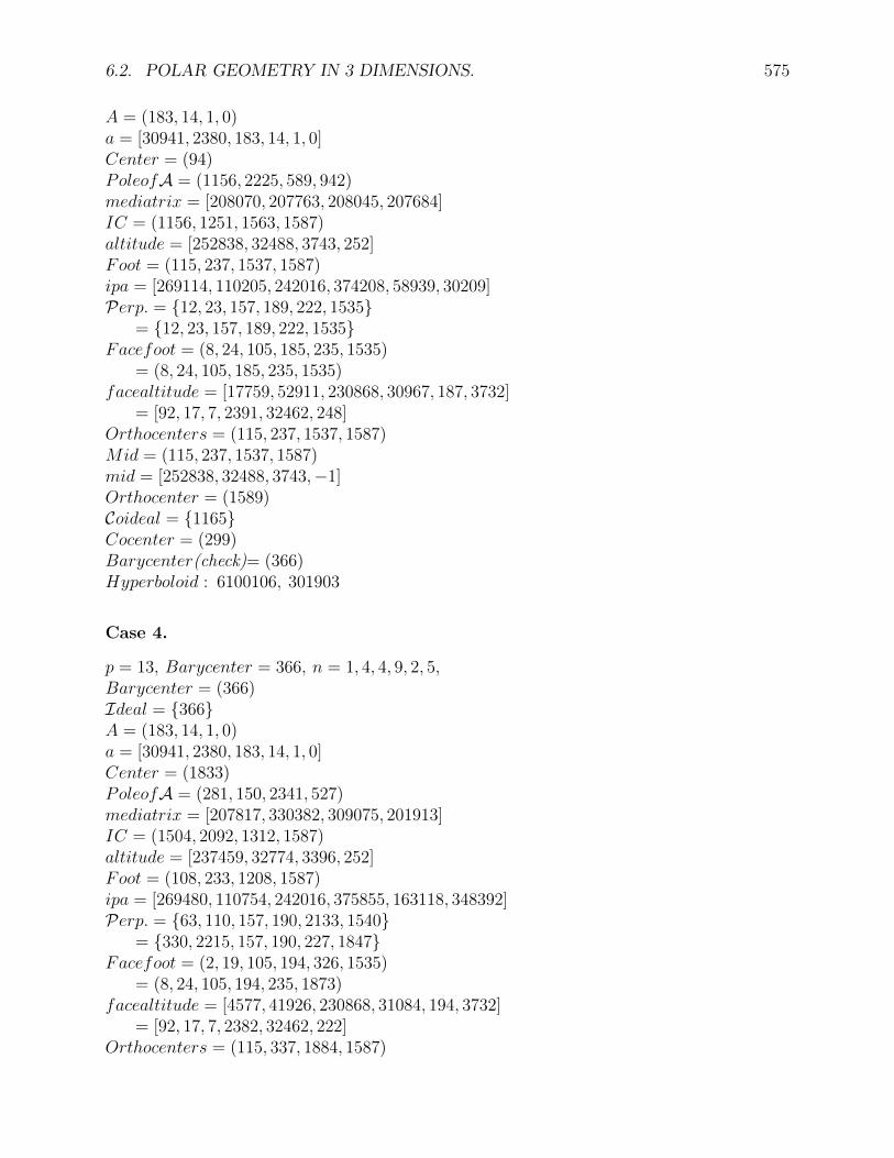
6.2. POLAR GEOMETRY IN 3 DIMENSIONS. 575
A = (183, 14, 1, 0)a = [30941, 2380, 183, 14, 1, 0]Center = (94)PoleofA = (1156, 2225, 589, 942)mediatrix = [208070, 207763, 208045, 207684]IC = (1156, 1251, 1563, 1587)altitude = [252838, 32488, 3743, 252]Foot = (115, 237, 1537, 1587)ipa = [269114, 110205, 242016, 374208, 58939, 30209]Perp. = 12, 23, 157, 189, 222, 1535
= 12, 23, 157, 189, 222, 1535Facefoot = (8, 24, 105, 185, 235, 1535)
= (8, 24, 105, 185, 235, 1535)facealtitude = [17759, 52911, 230868, 30967, 187, 3732]
= [92, 17, 7, 2391, 32462, 248]Orthocenters = (115, 237, 1537, 1587)Mid = (115, 237, 1537, 1587)mid = [252838, 32488, 3743,−1]Orthocenter = (1589)Coideal = 1165Cocenter = (299)Barycenter(check)= (366)Hyperboloid : 6100106, 301903
Case 4.
p = 13, Barycenter = 366, n = 1, 4, 4, 9, 2, 5,Barycenter = (366)Ideal = 366A = (183, 14, 1, 0)a = [30941, 2380, 183, 14, 1, 0]Center = (1833)PoleofA = (281, 150, 2341, 527)mediatrix = [207817, 330382, 309075, 201913]IC = (1504, 2092, 1312, 1587)altitude = [237459, 32774, 3396, 252]Foot = (108, 233, 1208, 1587)ipa = [269480, 110754, 242016, 375855, 163118, 348392]Perp. = 63, 110, 157, 190, 2133, 1540
= 330, 2215, 157, 190, 227, 1847Facefoot = (2, 19, 105, 194, 326, 1535)
= (8, 24, 105, 194, 235, 1873)facealtitude = [4577, 41926, 230868, 31084, 194, 3732]
= [92, 17, 7, 2382, 32462, 222]Orthocenters = (115, 337, 1884, 1587)

576 CHAPTER 6. GENERALIZATION TO 3 DIMENSIONS
Mid = (112, 194, 194, 1587)mid = [246391, 173899, 316701,−1]Centerofhyperb. = (194)Coideal = −2Cocenter = (−2)Barycenter(check)= (366)Hyperboloid : 9800114
The coordinates of Center are (1, 9, 9, 12),those of IC are (1, 7, 10, 8), (1, 11, 3, 11), (1, 6, 8, 11), (1, 8, 4, 0),those of Foot are (0, 1, 7, 3), (1, 0, 3, 11), (1, 6, 0, 11), (1, 8, 4, 0),those of orthocenters are (0, 1, 7, 10), (1, 0, 11, 11), (1, 10, 0, 11), (1, 8, 4, 0),those of the CenterofHyperboloid are (1, 0, 0, 11),the hyperboloid is
X0X1 − 2X0X2 − 6X3X1 −X2X3 = 0.
Case 5.
p = 17, Barycenter = 614, n = 1, 2, 5, 4, 11, 10,Barycenter = (614)Ideal = 614A = (307, 18, 1, 0)a = [88741, 5220, 307, 18, 1, 0]Center = (2954)PoleofA = (3872, 3441, 1230, 2256)mediatrix = [174494, 1146461, 1279312, 787119]IC = (4484, 2739, 4436, 1700)altitude = [904299, 91648, 9268, 541]Foot = (184, 427, 4368, 1684)ipa = [170402, 88127, 1190767, 798046, 722183, 136312]Perp. = 121, 198, 91, 548, 3911, 1187
= 511, 2041, 3605, 1762, 407, 4829Facefoot = (12, 23, 86, 318, 341, 3486)
= (0, 0, 239, 312, 477, 2908)facealtitude = [59263, 113306, 422825, 88928, 309, 8399]
= [1, 0, 5, 5232, 90764, 443]Orthocenters = (0, 346, 2919, 3656)Mid = (173, 7, 29, 2687)mid = [850281, 37068, 146789, 323376]Centerofhyperb. = (2687)Coideal = −2Cocenter = (−2)Barycenter(check)= (614)Hyperboloid : 42149113
The coordinates of the Center are (1, 9, 2, 12),those of IC are (1, 14, 7, 12), (1, 8, 7, 1), (1, 14, 4, 15), (1, 4, 13, 16),

6.2. POLAR GEOMETRY IN 3 DIMENSIONS. 577
those of Foot are (0, 1, 9, 13), (1, 0, 7, 1), (1, 14, 0, 15), (1, 4, 13, 0),those of orthocenters are (0, 0, 0, 1), (1, 0, 2, 5), (1, 9, 0, 11), (1, 11, 10, 0),those of the CenterofHyperboloid are (1, 8, 4, 0),the hyperboloid is
2X0X1 +X0X2 + 7X0X3 − 4X1X2 − 8X3X1 − 2X2X3 = 0.
Case 6.
p = 17, Barycenter = 614, n = 1, 5, 2, 11, 4, 10,Barycenter = (614)Ideal = 614A = (307, 18, 1, 0)a = [88741, 5220, 307, 18, 1, 0]Center = (3114)PoleofA = (3984, 3313, 2240, 1262)mediatrix = [95281, 167230, 631754, 493841]IC = (4564, 2643, 1748, 4612)altitude = [1218731, 93484, 6380, 373]Foot = (248, 331, 1476, 4608)ipa = [1427515, 407150, 88127, 875734, 799871, 561605]Perp. = 41, 107, 198, 567, 1922, 4653
= 319, 3493, 2041, 3783, 372, 1395Facefoot = (15, 22, 103, 317, 392, 2908)
= (1, 31, 1, 309, 494, 3486)facealtitude = [74002, 108393, 506346, 88911, 312, 7821]
= [18, 22, 0, 5235, 90475, 409]Orthocenters = (1, 394, 3496, 3095)Mid = (61, 4, 2623, 205)mid = [304633, 22454, 1185019, 18414]Centerofhyperb. = (2623)Coideal = −2Cocenter = (−2)Barycenter(check)= (614)Hyperboloid 321051114
The coordinates of Center are (1, 9, 12, 2),those of Centerofhyperboloid are (1, 8, 0, 4).Observe that the last 2 coordinates are exchanged.
Case 7.
p = 17, Barycenter = 614, n = 1, 2, 5, 4, 6, 10,THE QUADRIC IS DEGENERATE

578 CHAPTER 6. GENERALIZATION TO 3 DIMENSIONS
Case 8.
p = 13, Barycenter = 1165, n = 1, 4, 10, 9, 2, 5, m = 1, 8, 4, 2,The tetrahedron is orthogonal.The Center is an ideal point.Barycenter = (1165)Ideal = 1589A = (183, 14, 1, 0)a = [30941, 2380, 183, 14, 1, 0]Center = (501)
Case 9.
p = 19, Barycenter = 762, n = 1, 5, 3, 11, 15, 10,Barycenter = (762)Ideal = 762A = (381, 20, 1, 0)a = [137561, 7240, 381, 20, 1, 0]Center = (5279)PoleofA = (2484, 3802, 1813, 6007)mediatrix = [2260013, 884810, 642183, 1463793]IC = (597, 128, 4864, 6754)altitude = [82689, 115, 11573, 431]Foot = (12, 15, 4731, 6746)ipa = [881367, 14830, 1375219, 884015, 884396, 386372]Perp. = 63, 216, 149, 500, 3383, 3644
= 738, 6887, 2775, 2190, 450, 5872Facefoot = (12, 23, 77, 396, 438, 1103)
= (15, 32, 191, 395, 495, 2186)facealtitude = [82689, 158138, 528524, 137846, 384, 7962]
= [115, 27, 11, 7245, 142254, 647]Orthocenters = (203, 452, 2201, 1217)Mid = (296, 541, 2557, 1882)mid = [233678, 882463, 2451610, 1218391]Centerofhyperb. = (2557)Coideal = −2Cocenter = (−2)Barycenter(check)= (762)Hyperboloid : 10870118
Case 10.
p = 29, Barycenter = 1742, n = 1, 5, 3, 11, 4, 10,Barycenter = (1742)Ideal = 1742A = (871, 30, 1, 0)

6.2. POLAR GEOMETRY IN 3 DIMENSIONS. 579
a = [732541, 25260, 871, 30, 1, 0]Center = (7629)PoleofA = (13904, 3284, 4290, 19705)mediatrix = [5332964, 18533938, 781117, 7231524]IC = (11875, 23216, 15207, 13667)altitude = [13487988, 743909, 39576, 1283]Foot = (553, 1350, 15178, 13660)ipa = [8254786, 6197397, 2802094, 15763096, 16443405, 9610961]Perp. = 484, 433, 109, 27, 11978, 11805
= 1317, 18560, 11630, 1716, 976, 378Facefoot = (17, 40, 436, 871, 1567, 17691)
= (26, 51, 88, 878, 1422, 871)facealtitude = [415484, 976431, 10634475, 732541, 895, 42080]
= [146, 38, 28, 25282, 740951, 871]Orthocenters = (109, 1574, 871, 18242)Mid = (512, 1462, 34, 24564)mid = [12490883, 8959529, 853649, 15467561]Centerofhyperb. = (19403)Coideal = 4265Cocenter = (759)Barycenter(check)= (1742)Hyperboloid : 5714192025
Case 11.
p = 29, Barycenter = 19403, n = 1, 5, 3, 11, 4, 10,Barycenter = (19403)Ideal = 4265A = (871, 30, 1, 0)a = [732541, 25260, 871, 30, 1, 0]Center = (759)PoleofA = (13904, 3284, 4290, 19705)mediatrix = [18523362, 18533938, 18522525, 18526776]IC = (13904, 18759, 19848, 1960)altitude = [21121745, 751739, 43780, 1691]Foot = (866, 1098, 19384, 1944)ipa = [1759206, 15692546, 12959255, 7495237, 10224187, 21187915]Perp. = 399, 566, 324, 1401, 8614, 8443
= 1194, 10989, 10499, 20218, 1650, 14791Facefoot = (17, 32, 784, 889, 1567, 14327)
= (20, 34, 523, 878, 1161, 8440)facealtitude = [415484, 781319, 19121847, 733063, 895, 38716]
= [320, 55, 13, 25282, 748520, 1451]Orthocenters = (527, 1574, 8458, 14617)Mid = (202, 901, 7622, 19518)

580 CHAPTER 6. GENERALIZATION TO 3 DIMENSIONS
mid = [4930377, 15804147, 19711544, 3631884]Centerofhyperb. = (6873)Coideal = 22214Cocenter = (17926)Barycenter(check)= (19403)Hyperboloid : 21181812216
6.90 Answers to problems and miscellaneous notes.
Theorem.
If (0, p1, p2, p3) is on the Euler line eul then
0. p1(m2 −m3) + p2(m3 −m1) + p3(m1 −m2) = 0,
1. P ∨ IC(0) intersects the Euler line eul at((p1(m0 −m2) + p2(m1 −m0))(m1 +m2 +m3),
p1((m1 −m2)(m1 +m2 +m3) +m2(m1 −m0)) + p2m1(m0 −m1),p2((m1 −m2)(m1 +m2 +m3) +m1(m0 −m2)) + p1m2(m2 −m0),p2((m1 −m3)(m1 +m2 +m3) +m1(m0 −m3))
+ p1((m3 −m2)(m1 +m2 +m3) +m2(m3 −m0))),or more symmetrically,(p1(s1(m0 −m2) +m0(m2 −m0) + p2(s1(m1 −m0) +m0(m0 −m1),
p1(s1(m1 −m2) +m1(m2 −m0) + p2(s1(m1 −m1) +m1(m0 −m1),p1(s1(m2 −m2) +m2(m2 −m0) + p2(s1(m1 −m2) +m2(m0 −m1),p1(s1(m3 −m2) +m3(m2 −m0) + p2(s1(m1 −m3) +m3(m0 −m1)).
Moreover, if p1 = km1 + s−m0, p2 = km2 + s−m0, p3 = km3 + s−m0,then the point on eul is((k − 1)m0 + s, (k − 1)m1 + s, (k − 1)m2 + s, (k − 1)m3 + s).In particular,M = (m1 +m2 +m3,m2 +m3 +m0,m3 +m0 +m1,m0 +m1 +m2),P = (s1t0 −m0t0, s1(m2
1 −m2m3)−m1t0, s1(m22 −m3m1)−m2t0,
s1(m23 −m1m2)−m3t0),
with t0 = m0m1 +m0m2 +m0m3 −m1m2 −m3m1 −m2m3,O = (Am = (s1 − 3m0, s1 − 3m1, s1 − 3m2, s1 − 3m3),G = (s1 + 2m0, s1 + 2m1, s1 + 2m2, s1 + 2m3),Am = (D0 = ()D1 = ()D2 = ()G = ()G = ()

6.90. ANSWERS TO PROBLEMS AND MISCELLANEOUS NOTES. 581
Answer to ??.
Answer (partial).
. . . ? The polar pp0 = [−2m1m2,m2(m0 +m1),m1(m2 +m0],
. . . ? The intersection PP0 = (0,−m1(m2 +m0),m2(m0 +m1)),
. . . ? pp = [m1m2(m2 +m0)(m0 +m1),m2m0(m0 +m1)(m1 +m2),m0m1(m1 +m2)(m2 +m0)].Point “O“, intersection of perpendicular to faces through their barycenter
(special case of . . . with k = 0 hence“O” = (s1 −m0, s1 −m1, s1 −m2, s1 −m3).“Conjugate tetrahedron”,“A′0” = (−2s1 − 2m0, s1 + 2m1, s1 + 2m2, s1 + 2m3),barycenter of faces of [A′[i]] are“M ′
0” = (0,m1,m2,m3), which are the orthocenters of the faces,Perpendiculars through M ′
0 to the faces, (which are parallel to those of [A[]] meet at“O′” = (3s1 − 4m0, 3s1 − 4m1, 3s1 − 4m2, 3s1 − 4m3).Hence his theorem: Then he generalizes the circle of Brianchon-Poncelet and gives its centeras the midpoint of H and “O”I believe his “O” is my G.Orthocenter,barycenter and “O” are collinear

582 CHAPTER 6. GENERALIZATION TO 3 DIMENSIONS

Chapter 7
QUATERNIONIAN GEOMETRY
7.0 Introduction.1
It is a classical result, (see Artin, Harsthorne) that if the coordinates which are used to definea projective geometry are elements of a non commutative division ring, then Desargues’Theorem is true, but Pappus’ Theorem is, in general, not true. More precisely, Pappus’theorem implies that the division ring or skew fielf is commutative. I will prove here detailledgeometric properties which justify the definitions of medians and circumcircular polarity ina quaternionian plane.
The results were conjectured by taking the coordinates in the ring with unity associatedwith quaternions over the finite field Zp, p prime. This is not a division ring because a finitedivision ring is a field. In this geometry, not all points define a line and vice-versa. Thesituation is similar to that described by Knuppel and Salow, for the case of a commutativering with unity. This generalization merits to be explored in detail.
In involutive Geometry, we started with the triangle Ai, ai, the barycenter M and theorthocenter M . We constructed the medians mai, the altitudes mai, the mid-points Mi, thefeet M i, the complementary triangle (Mi,mmi), the orthic triangle M i,mmi, the idealpoints MAi, the orthic points MAi, the ideal line m, the orthic line m, the orthic directions,Immi, the tangential triangle Ti, tai, the symmedians ati and the point of Lemoine K.Moreover the same tangential triangle Ti can be obtained if we interchange the role of M andM.I attempted the same construction for the Geometry over the quaternion skew field. In thiscase, however, the lines ati are not concurrent, in general, but form a triangle Ki and thereexists a polarity in which Ki is the pole of ai and therefore Ai is the pole of ati. This polaritydegenerates into all the lines through K in the involutive Geometry.
The plane corresponding to the involutive plane is defined by chosing a complete 5-anglein the quaternionian plane. 3 points are the vertices of the basic triangle, 1 is the barycenter,1 is the cobarycenter. We define the ideal line as the polar of the barycenter with respect to thetriangle and as comedians, the lines joining the vertices of the triangle to the cobarycenter.It can be shown that there is a polarity which associates to the vertices of the triangle 3 ofthe lines through them, corresponding to the tangential lines in Euclidean geometry, but, in
122.1.87
583
584 CHAPTER 7. QUATERNIONIAN GEOMETRY
general, the involution defined by this polarity on the ideal line, does not have the directionsof the sides and the direction of the comedians as corresponding points.
7.1 Quaternionian Geometry over the reals.
7.1.1 Points, Lines and Polarity.
Notation.
Identifiers, starting with a lower case letter, will denote quaternions, q denotes the conjugateof q, q′, the conjugate inverse, qn := q q = q q, q−n := (qn)−1.
Definition.
The elements and incidence in Quaternionian geometry in 2 dimensions are defined as fol-lows.
0. The points are (q0, q1, q2) with right equivalence,
1. The lines are [l0, l1, l2] with right equivalence,
2. A point P is incident to a line l iffP · l :=
∑2i=0 P ili = 0.
Condition 2 is consistent with equivalence and can also be writtenl · P = 0.
I prefered it, because the usual form∑2
i=0 Pili = 0 implies∑2
i=0 liP i = 0.We remind the reader of the following
Theorem.
In any skew field, if a matrix A has a left inverse and a right inverse, these are equal.Proof: Let C be the left inverse of A and B be its right inverse, by associativity of
matrices,C = C(AB) = (CA)B = B.
Lemma.
0. pi 6= qi, i = 1, 2 =⇒ (1, p1, p2)× (1, q1, q2)= [(p′1 − q′1)−1(p′1p2 − q′1q2)(p2 − q2)−1, (p1 − q1)−1,−(p2 − q2)−1],
1. (1, p1, p2)× (1, p1, q2) = [p1,−1, 0],
2. (0, 0, 1)× (1, p1, 0) = [p1,−1, 0],
3. (0, 0, 1)× (0, 1, 0) = [1, 0, 0].

7.1. QUATERNIONIAN GEOMETRY OVER THE REALS. 585
Proof: Let the line be [x0, x1, x2], we must havex0 + p1x1 + p2x2 = 0, and x0 + q1x1 + q2x2 = 0, subtracting gives(p1 − q1) + x1(p2 − q2)x2 = 0,hence x1 and x2. x0 follows from substitution into the second equation.
Theorem.
A quaternionian geometry is a perspective geometry.
Lemma.
Let ai and bi be different from 0. The points P0 := (0, q1, r2), P1 := (r0, 0, q2), P2 := (q0, r1, 0)are collinear iff
(q2r′2)(q1r
′1)(q0r
′0) = −1 and the line is given by any of the triples [r′0q2, q
′1r2,−1], [−1, r′1q0, q
′2r0], [r′2q1,−1, q′0r1].
Proof: Let y := [y0, y1,−1] := P0 × P1, we haveq1y1 + r2 = 0 and r0y0 + q2 = 0, this gives the first form y. To verify that P2 is on y, weneed q′0r
′0q2 + r1q
′1r2 = 0.
Lemma.
In a quaternionian geometry the Theorem of Desargues is satisfied.
Proof: We can always choose the coordinates of Ai and C as followsA0 = (1, 0, 0), A1 = (0, 1, 0), A2 = (0, 0, 1), C = (1, 1, 1).
It follows thata0 = [1, 0, 0], a1 = [0, 1, 0], a2 = [0, 0, 1],c0 = [0, 1,−1], c1 = [−1, 0, 1], c2 = [1,−1, 0],
It follows that Bi areB0 = (q0, 1, 1), B1 = (1, q1, 1), B2 = (1, 1, q2),
thereforeb0 = [0, q1 − 1,−(q2 − 1)], b1 = [−(q0 − 1), q2 − 1, 0],
b2 = [q0 − 1,−(q1 − 1), 0],B0 = (q0, 1, 1), B1 = (1, q1, 1), B2 = (1, 1, q2),C0 = (0, q1 − 1, q2 − 1), C1 = (q0 − 1, q2 − 1, 0),
C2 = (q0 − 1, q1 − 1, 0),the Theorem follows from Lemma 7.1.1.
Theorem.
A quaternionian geometry is a Desarguesian geometry.
Notation.
To give an explicit way of indicating that a 3 by 3 matrix is a point or line collineation ora correlation from points to lines or from lines to point a parenthesis is used on the sideof the point and a bracket on the side of a line. This notation is used when we give the
586 CHAPTER 7. QUATERNIONIAN GEOMETRY
table of elements. It could also be used in connection with the bold face letter representingcollineation or correlation. This notation is only useful when we apply algebra to geometry.
Theorem.
If C is a point collineation, the line collineation is C′T .In particular, the point collineation which associates to Ai, Ai and to (1, 1, 1), (q0, q1, q2) is q0 0 0
0 q1 00 0 q2
,
and the line collineation is q′0 0 00 q′1 00 0 q′2
.Proof: If Q is the image of P , and m is the image of l, we want
0 = P · l = ΣP ili = ΣC−1
ij Qjli = ΣQjC′ijli = ΣQjmj = 0,
for all points P and incident lines l. This requiresmj = ΣC′Tji li.
Definition. 2
A Hermitian matrix M is a matrix which is equal to its conjugate transpose.
M defines a transformation from points to line,
M−1, the inverse, defines the transformation from lines to points.
Theorem.
If M is Hermitian and p = MP, q = MQ and P · q = 0 then Q · p = 0.
Proof: Q · p =∑
iQipi=∑
i
∑j QiMi,jPj
=∑
j
∑i(QiM j,i)Pj
=∑
j
∑i (Mj,iQi)Pj
=∑
j qjPj = q · P = 0.
Theorem.
0. The transformation defined by a Hermitian matrix is a polarity.
1. The columns of a polarity M are the polars of the points Ai, withA0 = (1, 0, 0), A1 = (0, 1, 0), A2 = (0, 0, 1).
2. The columns of a inverse polarity M−1 are the poles of the lines ai, with a0 = [1, 0, 0],a1 = [0, 1, 0], a2 = [0, 0, 1].
213.12.86
7.1. QUATERNIONIAN GEOMETRY OVER THE REALS. 587
Definition.
Polar points are points incident to their polar. Polar lines are lines incident to their pole.
Comment.
A polar line can contain infinitely many polar points. For instance, let the polarity be 1 −1 −1−1 1 −1−1 −1 1
. P := (0, 1, 1), has for polar p = [1, 0, 0]. A point Q := (0, 1, q), on
p has for polar [1 + q, q, 1]. Q is a polar point if <(q) = 0. Therefore all the points(0, 1, a1i + a2j + a3k) are polar points on [1,0,0].
Lemma.
Letci := qi−1qiqi+1 + qi+1qiqi−1 = 2Re(qi−1qiqi+1),
if qiqi 6= 0 thenc0 = c1 = c2
and we definec := c0.
Proof:q2q2c0 = q2c0q2 = q2(q2q0q1 + q1q0q2)q2 = q2q2(q0q1q2) + (q2q1q0)q2q2
= q2q2(q0q1q2 + q2q1q0) = q2q2c1.
Theorem.
Letai = ai,bi := ai+1ai−1 − qiqi,ri := qi−1qi+1 − aiqi,
then a0 q2 q1
q2 a1 q0
q1 q0 a2
b0 r2 r1
r2 b1 r0
r1 r0 b2
= d E,
where E is the identity matrix andd := a0a1a2 − a0q0q0 − a1q1q1 − a2q2q2 + 2Re(q2q0q1).
Moreover,bi = bi,ai := bi+1bi−1 − riri,qi := ri−1ri+1 − biri,
Proof: For instance,a0b0 + q2r2 + q1r1 = a0a1a2 − a0q0q0 + q2q0q1 − q2a2q2 + q1q0q2 − q1a1q1 = d
anda0r2 + q2b1 + q1r0 = a0q1q0 − a0a2q2 + q2a2a0 − q2q1q1 + q1q1q2 − q1a0q0 = 0.The second part of the proof is obtained similarly or follows from 7.1.1.1.

588 CHAPTER 7. QUATERNIONIAN GEOMETRY
The 2 parts of the following Lemma use different approaches to the problem of constructingpolarities.
Lemma.
0. If all the components of the lines xi are non zero and the i-th component of xi is real,necessary and sufficient conditions for xi to be polars of Ai are
0. x−1i+1,i−1xi−1,i+1 = ki, ki real.
1. k0k1k2 = 1.
1. Let 3 points have coordinatesP0 = (a0, q2, q
−11 ), P1 = (q−1
2 , a1, q0), P2 = (q1, q−10 , a2),
where ai = ai, then, if the norm of q0q1q2 = 1 and if the matrix P is obtained bymultiplying the column vectors Pi respectively by 1, qn2 ,
1qn1, this matrix defines a polarity
which associates the lines ai to the points Pi.
Proof: For part 0, the condition that the i-th component of xi is real can always be satisfiedby multiplying the components of xi by xii.It remains to find real numbers which multiplied by xi give the columns of an Hermitianmatrix. Considering the elements x01 and x10 requires x10 = x01k2, k2 real, or more generally0. Multiplying the first and second column by k1 and k−1
1 requires condition 1, for the elementsin position 12 and 21 to be conjugates of each other.
For the second part, the matrix is then a0 q2 q′1q2 qn2a1 qn2 q0
q−11 qn2 q0 q−n1 a2
.
Exercise.
State and prove the Theorem which extends the preceding Theorem to the case where someof the components of the vectors xi are 0, or some of the qi are 0.
Lemma. 3
unj 6= 0, vnj 6= 0, j = 1, 2, and d0 := u1u−12 + v1v
−12 , e0 := u2u
−11 + v2v
−11 ,
⇒ u−11 d0v2 = u−1
2 e0v1 anddn0v
n2u
n2 = en0v
n1u
n1 .
Proof: u−11 d0v2 = u−1
2 v2 + u−11 v1 and u−1
2 e0v1 = u−11 v1 + u−1
2 v2.
Lemma.
(u0u1u2v0v1v2)n 6= 0,di := ui+1u
−1i−1 + vi+1v
−1i−1, d := d0d1d2,
315.1.87
7.1. QUATERNIONIAN GEOMETRY OVER THE REALS. 589
ei := ui−1u−1i+1 + vi−1v
−1i+1, e := e0e1e2,
⇒ dn = en.
Proof: This follows from Lemma 7.1.1, taking norms and using the fact that the norm ofa product is the product of the norms.
7.1.2 Quaternionian Geometry of the Hexal Complete 5-Angles.
Notation.
In what follows, I will use the same notation as in involutive Geometry, namely,l := P ×Q, means that the line l is defined as the line incident to P and Q.If subscripts are used these have the values 0, 1 and 2 and the computation is done modulo3,P · l = 0 means that the point P is incident to the line l.When 3 lines intersect, this intersection can be defined in 3 ways, this has been indicated byusing (*) after the definition and implies a Theorem.
σ := polarity((Mi, ai)).implies that σ is the polarity which associates M0 to a0, M1 to a1 and M2 to a2.
m = polar(σ,M).implies that in the polarity σ, m is the polar of M.The labeling used is “H,“ for Hypothesis, “D”, for definitions, “C“, for conclusions,“N”, fornomenclature, “P“, for proofs, this labelling being consistent with that of the correspondingdefinitions. The example given is associated to the quaternions over Z19, the labelling is “E”and is consistent with the corresponding definitions.Because any 3 pairs of points and lines do not necessarily define a polarity, if a polarity isdefined it implies a conclusion (or Theorem) I have therefore replaced “D“ by “DC”.
The special configuration of Desargues.
With this notation, the special configuration of Desargues can be defined byai := Ai+1 × Ai−1, qai = Q× Ai,Qi := ai × qai, qqi := Qi+1 ×Qi−1,QAi := ai × qqi, qi := Ai ×QAi,QQi := qi+1 × qi−1, q := QA1 ×QA2(∗),
and the other conclusion of the special Desargues Theorem can be written,QQi · qai = 0.
Let Q and Ai beQ = (q0, q1, q2), and A0 = (1, 0, 0), A1 = (0, 1, 0), A2 = (0, 0, 1),
then we have the following results, not obtained in the given order,A0 = (1, 0, 0), a0 = [1, 0, 0],Q = (q0, q1, q2), q = [q′0, q
′1, q′2],
QA0 = (0, q1,−q2), qa0 = [0, q′1,−q′2],Q0 = (0, q1, q2), q0 = [0, q′1, q
′2],
QQ0 = (−q0, q1, q2), qq0 = [−q′0, q′1, q′2],
The self duality of the configuration corresponds to the replacement of points by lines

590 CHAPTER 7. QUATERNIONIAN GEOMETRY
where upper case letters are replaced by lower case letters and coordinates by their conjugateinverse.
Fundamental Hypothesis, Definitions and Conclusions.
The ideal line and the coideal line.Given
H0.0. Ai,H0.1. M, M,LetD1.0. ai := Ai+1 × Ai−1,D1.1. mai := M × Ai, mai := M × Ai,D1.2. Mi := mai × ai, M i := mai × ai,D1.3. eul = M ×M,DC1.4. σ := polarity((Mi, ai)), σ := polarity((M i, ai)),D2.0. mmi := Mi+1 ×Mi−1, mmi := M i+1 ×M i−1,D2.1. MAi := ai ×mmi, MAi := ai ×mmi,D2.2. mi := Ai ×MAi, mi := Ai ×MAi,D2.3. MMi := mi+1 ×mi−1, MMi := mi+1 ×mi−1,D2.4. m := MA1 ×MA2 (∗), m := MA1 ×MA2 (∗),D2.5. Imai := m×mai, Imai := m×mai,D2.6. IMai := m×mai, IMai := m×mai,D2.7. iMAi := M ×MAi, ıMAi := M ×MAi,thenC2.0. m = polar(σ,M), m = polar(σ,M).C2.1. mmi = polar(σ,Ai), mmi = polar(σ,Ai).C2.2. mai = polar(σ,MAi), mai = polar(σ,MAi).C2.3. iMAi = polar(σ, Imai), ıMAi = polar(σ, Imai).LetD3.0. mfi := Mi × IMai, mfi := M i × IMai,D3.1. O := mf1 ×mf2(∗), O := mf1 ×mf2(∗),D3.2. Mfai := ai+1 ×mfi−1, Mfai := ai+1 ×mfi−1,
Mfai := ai−1 ×mfi+1, Mfai := ai−1 ×mfi+1,D3.3. mfai := Mfai+1 × Ai−1, mfai := Mfai+1 × Ai−1,
mfai := Mfai−1 × Ai+1, mfai := Mfai−1 × Ai+1,D3.4. Mfmi := mfai ×mi, Mfmi := mfai ×mi,thenC3.0. O · eul = O · eul = 0.C3.1. Mfmi ·mfai = Mfmi ·mfai = 0.LetD4.0. Immi := m×mmi, Immi := m×mmi,D4.1. tai := Ai × Immi,D4.2. Ti := tai+1 × tai−1,D4.3. ati := Ai × Ti,D4.4. Ki := ati+1 × ati−1,

7.1. QUATERNIONIAN GEOMETRY OVER THE REALS. 591
D4.5. TAai := tai × ai,D4.6. poKi := Taai+1 × Taai−1,DC4.7. θ := polarity((Ai, tai)),DC4.8. λ := polarity((Ai, ati)),thenC4.0. Immi · tai = 0.C4.1. Ti ·mfi = 0.C4.2. ai := polar(θ, Ti).C4.3. ai := polar(λ,Ki).
The nomenclature:N0.0. Ai are the vertices of the triangle,N0.1. M is the barycenter, M is the cobarycenter.N1.0. ai are the sides.N1.1. mai are the medians, mai are the comediansN1.2. Mi are the mid-points of the sides. M i are the feet of the comediansN1.3. eul is the line of Euler,N1.4. σ is the Steiner polarity. σ is the co-Steiner polarity.N2.0. Mi,mmi is the complementary triangle,
M i,mmi is the orthic triangle,N2.1. MAi are the directions of the sides,N2.2. MMi,mi is the anticomplementary triangle.N2.3. m is the ideal line corresponding to the line at infinity,
m is the orthic line which is the polar of M with respect to the triangle.N2.4. Imai are the directions of the medians.
IMai are the directions of the comedians.N3.0. mfi are the mediatrices,N3.1. O is the center,N3.2. Mfmi are the trapezoidal points,N4.0. Immi are the directions of the antiparallels of aiwith respect to the
sides ai+1 and ai−1.N4.1. (Ti, tai) is the tangential triangle,N4.2. ati are the symmedians,N4.3. Ki is the triangle of Lemoine.N4.4. θ is the circumcircular polarityN4.5. λ is the Lemoine polarity.
Theorem.
If we derive a point X and a line x by a given construction from Ai, M and M , with thecoordinates as given in G0.0 and G0.1, below, and the point X and line x are obtain by thesame construction interchange M and M ,
X = (f0(m0,m1,m2), f1(m0,m1,m2), f2(m0,m1,m2)),x = [g0(m0,m1,m2), g1(m0,m1,m2), g2(m0,m1,m2)],
=⇒X = (m0f0(m−1
0 ,m−11 ,m−1
2 ),m1f1(m−10 ,m−1
1 ,m−12 ),m2f2(m−1
0 ,m−11 ,m−1
2 )),

592 CHAPTER 7. QUATERNIONIAN GEOMETRY
x = [m′0g0(m−10 ,m−1
1 ,m−12 ),m′1g1(m−1
0 ,m−11 ,m−1
2 ),m′2g2(m−10 ,m−1
1 ,m−12 )].
Proof: The point collineation C =
q0 0 00 q1 00 0 q2
, associates to (1,1,1), (q0, q1, q2), and
to (m0,m1,m2), (r0, r1, r2), if ri = qimi.In the new system of coordinates,X = (q0f0(q−1
0 r0, q−11 r1, q
−12 r2), q1f1(q−1
0 r0, q−11 r1, q
−12 r2), q2f2(q−1
0 r0, q−11 r1, q
−12 r2)).
Exchanging qi and ri and then replacing qi by 1 and ri by mi is equivalent to substituting mi
for qi and 1 for ri, which gives X. x is obtained similarly.The line collineation is q′0 0 0
0 q′1 00 0 q′2
.Exercise.
Prove that if a point to line polarity [P) has its i, j-th elementPij = f(m0,m1,m2),
then the i, j-th element of the polarity obtained by the same construction, after exchange ofM and M , is
Pij = m′if(m−10 ,m−1
1 ,m−12 )m−1
j .Similarly, for a line to point polarity (P−1]
(P−1]ij = g(m0,m1,m2), =⇒ (P−1
]ij = mig(m−10 ,m−1
1 ,m−12 )mj.
Lemma.
m−11 (m0 +m1)(m0 −m1)−1 = −(m−1
0 +m−11 )(m−1
0 −m−11 )−1m−1
1 .This Lemma is useful in checking equivalent representations of coordinates of points and
lines.
Notation.
ri := (m−1i−1 +m−1
i )−1(m−1i+1 −m−1
i−1),si := −(m−1
i−1 +m−1i )−1(m−1
i +m−1i+1),
ti := s−1i+1s
−1i−1,
fi := si − s−1i+1s
−1i−1,
gi := ti − t−1i+1t
−1i−1.
Lemma.
0. s0s1s2 = −1.
1. norm(t0t1t2) = 1.
2. s′2f 2s−10 = −f2s1.
3. t′2f 2t−10 = −f2t1.

7.1. QUATERNIONIAN GEOMETRY OVER THE REALS. 593
Proof: For 0, we use Lemma 7.1.1 and obtain 1, from the definition of ti. For 2, wesubstitute f2 by its definition and compare the terms of both sides of the equality which havethe same sign.
Proof of 7.1.2.
LetG0.0. A0 = (1, 0, 0), A1 = (0, 1, 0), A2 = (0, 0, 1),G0.1. M = (1, 1, 1), M = (m0,m1,m2),thenP1.0. a0 = (1, 0, 0), a1 = (0, 1, 0), a2 = (0, 0, 1),P1.1. ma0 = [0, 1,−1], ma0 = [0,m′1,−m′2],P1.2. M0 = (0, 1, 1), M0 = (0,m1,m2),P1.3. eul = [1, (m1 −m2)−1(m2 −m0), (m1 −m2)−1(m0 −m1)],
P1.4. S =
1 −1 −1−1 1 −1−1 −1 1
, S−1 =
0 1 11 0 11 1 0
.S =
m−n0 −m′0m−11 −m′0m−1
2
−m′1m−10 m−n1 −m′1m−1
2
−m′2m−10 −m′2m−1
1 m−n2
,
S−1
=
0 m0m1 m0m2
m1m0 0 m1m2
m2m0 m2m1 0
.P2.0. mm0 = [1,−1,−1], mm0 = [m′0,−m′1,−m′2],P2.1. MA0 = (0, 1,−1), MA0 = (0,m1,−m2),P2.2. m0 = [0, 1, 1], m0 = [0,m′1,m
′2],
P2.3. MM0 = (1,−1,−1), MM0 = (m0,−m1,−m2),P2.4. m = [1, 1, 1], m = [m′0,m
′1,m
′2],
P2.5. Ima0 = (2,−1,−1), Ima0 = (2m0,−m1,−m2),P2.6. IMa0 = (m1 +m2,−m1,−m2), IMa0 = (m0(m−1
1 +m−12 ),−1,−1),
P2.7. iMA0 = [2,−1,−1], ıMA0 = [2m′0,−m′1,−m′2],P3.0. mf0 = [(m1 +m2)′(m1 −m2), 1,−1],
mf0 = [m′0(m−11 +m−1
2 )′(m′1 −m′2),m′1,−m′2, 1],P3.1. O = (m1 +m2,m2 +m0,m0,m1),
O = (m0(m−11 +m−1
2 ),m1(m−12 +m−1
0 ),m2(m−10 +m−1
1 )),P3.2. Mfa0 = (1, 0,−(m0 +m1)(m0 −m1)−1),
Mfa0 = (m0, 0,−m2(m−10 +m−1
1 )(m−10 −m−1
1 )−1),Mfa0 = (1,m′2(m2 +m0)(m2 −m0)−1, 0),Mfa0 = (m0,m1(m−1
2 +m−10 )(m−1
2 −m−10 )−1, 0),
P3.3. mfa0 = [(m1 +m2)′(m1 −m2), 1, 0],mfa0 = [m′0(m−1
1 +m−12 )′(m′1 −m′2),m′1, 0],
mfa0 = [(m1 +m2)′(m1 −m2), 0,−1],mfa0 = [m′0(m−1
1 +m−12 )′(m′1 −m′2), 0,−m′2],
P3.4. Mfm0 = ((m1 +m2)(m1 −m2)−1,−1, 1),Mfm0 = (m0(m−1
1 +m−12 )(m−1
1 −m−12 )−1,−m1,m2),
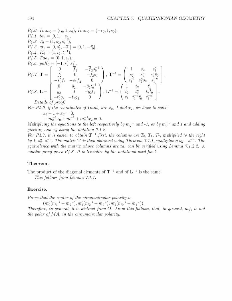
594 CHAPTER 7. QUATERNIONIAN GEOMETRY
P4.0. Imm0 = (r0, 1, s0), Imm0 = (−r0, 1, s0),P4.1. ta0 = [0, 1,−s′0],P4.2. T0 = (1, s2, s
−11 ),
P4.3. at0 = [0, s′2,−s1] = [0, 1,−t′0],P4.4. K0 = (1, t2, t
−11 ),
P4.5. Taa0 = (0, 1, s0),P4.6. poK0 = [−1, s′2, s1],
P4.7. T =
0 f 2 −f 2s−10
f2 0 −f2s1
−s′0f2 −s1f 2 0
, T−1 =
1 s2 s′1s2 sn2 sn2s0
s−11 sn2s0 s−n1
.P4.8. L =
0 g2 −g2t−10
g2 0 −g2t1−t′0g2 −t1g2 0
, L−1 =
1 t2 t′1t2 tn2 tn2 t0t1 t−n1 t′0 t−n1
.Details of proof:
For P4.0, if the coordinates of Imm0 are x0, 1 and x2, we have to solvex0 + 1 + x2 = 0,−m−1
0 x0 +m−11 +m−1
2 x2 = 0.Multiplying the equations to the left respectively by m−1
2 and -1, or by m−10 and 1 and adding
gives x0 and x2 using the notation 7.1.2.For P4.7, it is easier to obtain T−1 first, the columns are T0, T1, T2, multiplied to the rightby 1, sn2 , s
−n1 . The matrix T is then obtained using Theorem 7.1.1, multiplying by −s−n1 . The
equivalence with the matrix whose columns are tai can be verified using Lemma 7.1.2.2. Asimilar proof gives P4.8. It is trivialize by the notationb used for t.
Theorem.
The product of the diagonal elements of T−1 and of L−1 is the same.This follows from Lemma 7.1.1.
Exercise.
Prove that the center of the circumcircular polarity is(m′0(m−1
1 +m−12 ),m′1(m−1
2 +m−10 ),m′2(m−1
0 +m−11 )).
Therefore, in general, it is distinct from O. From this follows, that, in general, mfi is notthe polar of MAi in the circumcircular polarity.

7.2. FINITE QUATERNIONIAN GEOMETRY. 595
7.2 Finite Quaternionian Geometry.
7.2.1 Finite Quaternions.
Definition.
Finite Quaternions over Zp are associative elements of the formq0 + q1i + q2j + q3k,
where qi are elements of Zp and i, j, k are such thati2 = j2 = −1 and k = ij = −ji.
Theorem.
i, j, k satisfyk2 = −1, i = jk = −kj, j = ki = −ik.
This follows at once from associativity.
Theorem.
Finite quaternions in Zp can be represented by 2 by 2 matrices over Zp.In particular, if j2
0 + j21 = −1, then we can represent
1 by
(1 00 1
), i by
(0 1−1 0
), j by
(j0 j1
j1 −j0
), k by
(j1 −j0
−j0 −j1
).
Comment.
If p ≡ 1 (mod 4), we can find an interger j0 such that j20 = −1, and choose j1 = 0.
Example.
0. p = 5, we can represent
1 by
(1 00 1
), i by
(0 1−1 0
), j by
(2 00 −2
), k by
(0 −2−2 0
).
1. p = 7, we can represent
1 by
(1 00 1
), i by
(0 1−1 0
), j by
(−3 22 3
), k by
(2 33 −2
).
Finite quaternions will be represented by an integer using the following notation.
Notation.
In the example the quaternion over Zp,q = q0 + q1i+ q2j + q3k
is represented byq = q0 + q1p+ q2p
2 + q3p3, 0 ≤ qi < p.
For instance, when p = 19, the representation of 18+3i+6j is 2222, of 11+10i+4j+3kis 22222, of 16 + 8i+ 18j is 6666 and of 14 + 12i+ 13j + 9k is 66666.

596 CHAPTER 7. QUATERNIONIAN GEOMETRY
7.2.2 Example in a finite quaternionian geometry.
Let p = 19,
G0.0. A0 = (1, 0, 0), A1 = (0, 1, 0), A2 = (0, 0, 1),
G0.1. M = (1, 2222, 22222), M = (1, 6666, 66666),
then
E1.0. a0 = [1, 0, 0], a1 = [0, 1, 0], a2 = [0, 0, 1],
E1.1. mai =[0,1,13827], [22219,0,1], [1,6378,0],
mai =[0,1,41987], [66657,0,1], [1,3333,0],
E1.2. Mi =(0,1,48176), (22219,0,1), (1,2222,0),
M i =(0,1,21174), (70903,0,1), (1,6666,0),
E1.3. eul =[1,35222,126587],
E1.4 S =
1 868 1153416378 13 82528
22222 48176 18
, S−1 =
0 5034 1153412222 0 116883
22222 13827 0
,S =
1 1835 334345407 14 88952
104133 48615 11
, S−1
=
0 443 696586789 0 92894
67891 44653 0
,E2.0. mmi =[1,6378,22222], [2205,1,13827], [22219,48173,1],
mmi =[1,3333,70894], [6653,1,41987], [66657,21177,1],
E2.1. MAi =(0,1,82525), (115341,0,1), (1,5017,0),
MAi =(0,1,116386), (66657,0,1), (1,573,0),
E2.2. mi =[0,1,116874], [115341,0,1], [1,861,0],
mi =[0,1,95573], [70903,0,1], [1,3906,0],
E2.3. MMi =(1,5017,115338), (868,1,82525), (115341,116883,1),
MMi =(1,573,70894), (3903,1,116386), (66657,95586,1),
E2.4. m =[1,861,115338], m =[1,3906,66666],
E2.5. Imai =(1,6128,61279), (624,1,41443), (61290,123602,1),
Imai =(1,3906,35637), (2132,1,58383), (101928,116383,1),
E2.6. IMai =(1,31398,82872), (70470,1,745), (35569,2751,1),
IMai =(1,84862,112419), (112219,1,114203), (4535,17280,1),
E2.7. iMAi =[2,6378,22222], [2205,2,13827], [22219,48173,2],
ıMAi =[2,3333,70894], [6653,2,41987], [66657,21177,2],
E3.0. mfi =[1,57399,96485], (22698,1,119282), (59539,116028,1),
mfi =[1,17052,63592), (87814,1,43860), (49067,45624,1),
E3.1. O =(1,39571,2622), O =(1,26376,18393).
E3.2. Mfai =(1,0,59534), (57399,1,0), (0,119282,1),
Mfai =(1,22693,0), (0,1,116019), (96498,0,1),
Mfai =(1,0,49068), (17053,1,0), (0,43863,1),
Mfai =(1,87803,0), (0,1,45633), (63575,0,1),
E3.3. mfai =(1,57399,0], [0,1,119282], [59539,0,1],
mfai =(1,0,96485], [22698,1,0], [0,116028,1],
mfai =(1,17052,0], [0,1,43860], [49067,0,1],
mfai =(1,0,63592], [87814,1,0], [0,45624,1],
E3.4. Mfmi =(1,57399,57265), (10093,1,49647), (92996,18940,1),

7.2. FINITE QUATERNIONIAN GEOMETRY. 597
Mfmi =(1,39191,23604), (90214,1,112020), (72715,69295,1),
E3.5. iMAi =[1,6628,76281], [1112,1,7094], [76270,89247,1],
ıMAi =[1,5096,35637], [3336,1,21174], [101928,79188,1],
E4.0. Immi =(1,101541,76547), (91854,1,115568),(74057,64703,1),
Immi =(1,36019,60652),(45706,1,21992), (63503,72857,1),
E4.1. tai =[0,1,19660], [64952,0,1], [1,51999,0],
E4.2. Ti =(1,115899,64951), (51988,1,114948), (39743,19651,1),
E4.3. ati =[0,1,86571], [100052,0,1], [1,66787,0],
E4.4. Ki =(1,52716,100037), (66802,1,11323), (84095,86576,1),
E4.5. Taai =(0,1,114948), (39743,0,1), (1,115899,0),
E4.6. poKi =[1,51999,39734], [115882,1,19660], [64952,1149331],
E4.7. T =
0 126353 4660410833 0 1038890969 127181 0
, T−1 =
1 21317 72608115899 14 3244364951 105118 2
,E4.8. L =
0 66802 8409570412 0 6673753448 70833 0
, L−1 =
1 84484 3750852716 14 35592
100037 101959 2
.
Except for interchanges the computation of × is done as followswe normalize l2 to 1l0.P0 + l1.P1 + P2 = 0,l0.Q0 + l1.Q1 +Q2 = 0,Multiplying the first by P−1
0 .Q0 to the right and subtract from the second equation givesl1(Q1 − P1P
−10 Q0) + (Q2 − P2P
−10 Q0) = 0,
therefore if r3 := (Q1 − P1P−10 Q0)−1 and r4 = −(Q2 − P2P
−10 Q0), then
l1 = the conjugate of r4.r3 andl0 = − the conjugate of (l)1p1 + p2)p−1
0 .
The interchange is done as followsif P0 = 0, then we exchange Pi and Qi,if after exchange, P0 = 0, we consider all permutations sub0, sub1, sub2, of the subscripts 0,1 and 2 .
Correspondance in Z19 between representation and quaternion.representation r i j k for
2222 18 2 6 0 M22222 11 10 4 36666 16 ∗ 8 18 0 M
66666 14 12 13 935222 15 10 2 5 eul
126587 9 12 8 18

598 CHAPTER 7. QUATERNIONIAN GEOMETRY
7.3 Miniquaternionian Plane Ψ of Veblen-Wedderburn.
7.3.0 Introduction.
Starting with the work of L. E. Dickson of 1905, non-Desarguesian planes of order 9 werediscovered by Veblen and Wedderburn in 1907, I will here consider only one of these whichis self dual, and for which non trivial polarities exists, and refer to the work of G. Zappa(1957), T. G. Ostrom (1964), D. R. Hughes (1957) and T. G. Room and P. B. Kirkpatrick(1971) for further reading.
The synthetic definition used can be traced to Veblen and Wedderburn, who first considerpoints obtained by applying a transformation (see p. 383), later generalized by J. Singer.The notation is inspired by Room and Kirkpatrick (see Table 5.5.4) using the same methodI used for the finite plane reversing the indices for lines.An alternate definition, (5.6.1), is given by Room and Kirkpatrick.
7.3.1 Miniquaternion near-field.
Definition.
A near-field (N,+, ) is a set N with binary operations such that
0. N is finite,
1. (N,+) is an Abelian group, with neutral element 0,
2. (N − 0, ) is an group, with neutral element 1,
3. is right distributive over +, or(ξ + η) ζ = ξ ζ + η ζ, for all ξ, η, ζ ∈ N
4. ξ 0 = 0, for all ξ ∈ N .
Theorem.
In any near-field,
0. 0 ξ = 0, for all ξ ∈ N .
1. ξ η = 0 =⇒ ξ = 0 or η = 0.
2. 1,−1 6= 0.
Theorem.
In any near-field of order 9,
0. 0, 1,−1 ≈ Z3.
1. ξ + ξ + ξ = 0, for all ξ ∈ Q9,
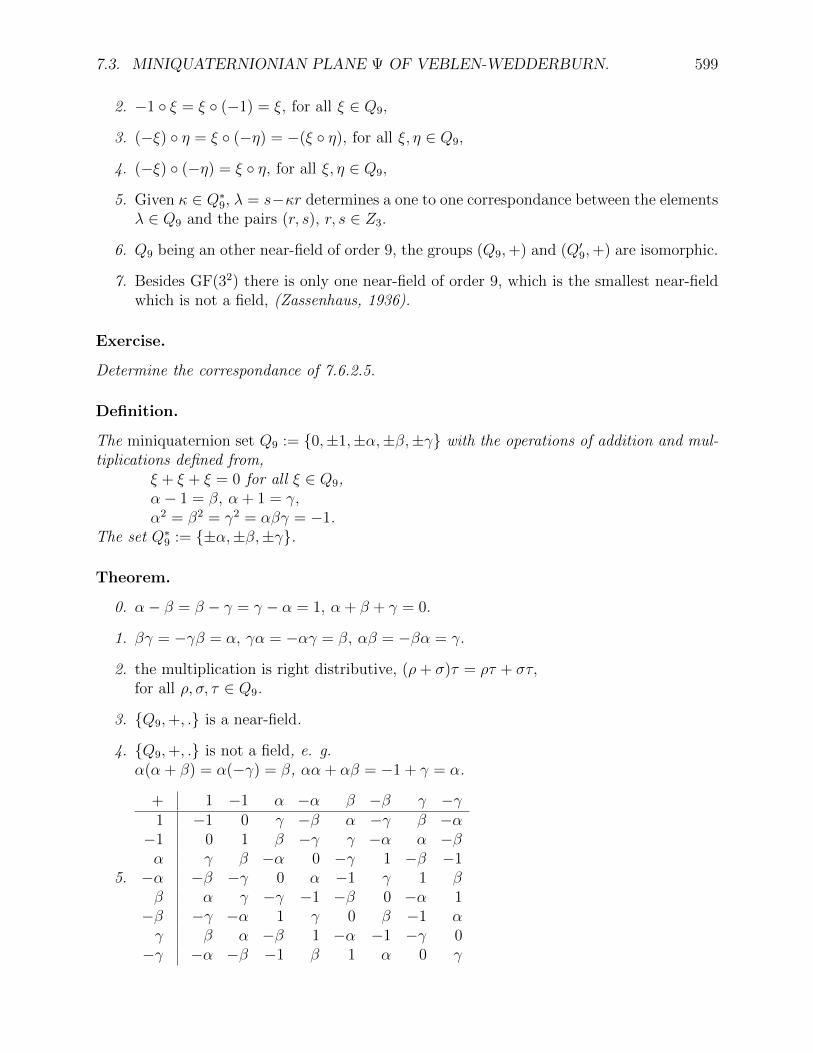
7.3. MINIQUATERNIONIAN PLANE Ψ OF VEBLEN-WEDDERBURN. 599
2. −1 ξ = ξ (−1) = ξ, for all ξ ∈ Q9,
3. (−ξ) η = ξ (−η) = −(ξ η), for all ξ, η ∈ Q9,
4. (−ξ) (−η) = ξ η, for all ξ, η ∈ Q9,
5. Given κ ∈ Q∗9, λ = s−κr determines a one to one correspondance between the elementsλ ∈ Q9 and the pairs (r, s), r, s ∈ Z3.
6. Q9 being an other near-field of order 9, the groups (Q9,+) and (Q′9,+) are isomorphic.
7. Besides GF(32) there is only one near-field of order 9, which is the smallest near-fieldwhich is not a field, (Zassenhaus, 1936).
Exercise.
Determine the correspondance of 7.6.2.5.
Definition.
The miniquaternion set Q9 := 0,±1,±α,±β,±γ with the operations of addition and mul-tiplications defined from,
ξ + ξ + ξ = 0 for all ξ ∈ Q9,α− 1 = β, α + 1 = γ,α2 = β2 = γ2 = αβγ = −1.
The set Q∗9 := ±α,±β,±γ.
Theorem.
0. α− β = β − γ = γ − α = 1, α + β + γ = 0.
1. βγ = −γβ = α, γα = −αγ = β, αβ = −βα = γ.
2. the multiplication is right distributive, (ρ+ σ)τ = ρτ + στ,for all ρ, σ, τ ∈ Q9.
3. Q9,+, . is a near-field.
4. Q9,+, . is not a field, e. g.α(α + β) = α(−γ) = β, αα + αβ = −1 + γ = α.
5.
+ 1 −1 α −α β −β γ −γ1 −1 0 γ −β α −γ β −α−1 0 1 β −γ γ −α α −βα γ β −α 0 −γ 1 −β −1−α −β −γ 0 α −1 γ 1 ββ α γ −γ −1 −β 0 −α 1−β −γ −α 1 γ 0 β −1 αγ β α −β 1 −α −1 −γ 0−γ −α −β −1 β 1 α 0 γ
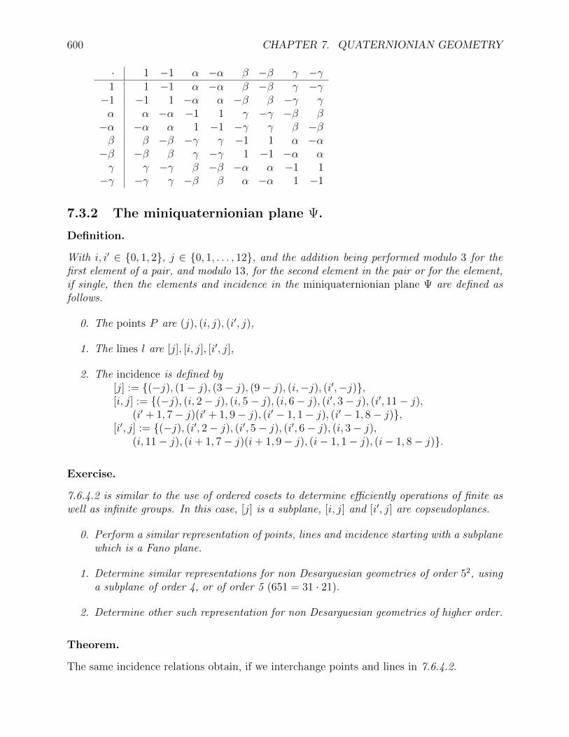
600 CHAPTER 7. QUATERNIONIAN GEOMETRY
· 1 −1 α −α β −β γ −γ1 1 −1 α −α β −β γ −γ−1 −1 1 −α α −β β −γ γα α −α −1 1 γ −γ −β β−α −α α 1 −1 −γ γ β −ββ β −β −γ γ −1 1 α −α−β −β β γ −γ 1 −1 −α αγ γ −γ β −β −α α −1 1−γ −γ γ −β β α −α 1 −1
7.3.2 The miniquaternionian plane Ψ.
Definition.
With i, i′ ∈ 0, 1, 2, j ∈ 0, 1, . . . , 12, and the addition being performed modulo 3 for thefirst element of a pair, and modulo 13, for the second element in the pair or for the element,if single, then the elements and incidence in the miniquaternionian plane Ψ are defined asfollows.
0. The points P are (j), (i, j), (i′, j),
1. The lines l are [j], [i, j], [i′, j],
2. The incidence is defined by[j] := (−j), (1− j), (3− j), (9− j), (i,−j), (i′,−j),[i, j] := (−j), (i, 2− j), (i, 5− j), (i, 6− j), (i′, 3− j), (i′, 11− j),
(i′ + 1, 7− j)(i′ + 1, 9− j), (i′ − 1, 1− j), (i′ − 1, 8− j),[i′, j] := (−j), (i′, 2− j), (i′, 5− j), (i′, 6− j), (i, 3− j),
(i, 11− j), (i+ 1, 7− j)(i+ 1, 9− j), (i− 1, 1− j), (i− 1, 8− j).
Exercise.
7.6.4.2 is similar to the use of ordered cosets to determine efficiently operations of finite aswell as infinite groups. In this case, [j] is a subplane, [i, j] and [i′, j] are copseudoplanes.
0. Perform a similar representation of points, lines and incidence starting with a subplanewhich is a Fano plane.
1. Determine similar representations for non Desarguesian geometries of order 52, usinga subplane of order 4, or of order 5 (651 = 31 · 21).
2. Determine other such representation for non Desarguesian geometries of higher order.
Theorem.
The same incidence relations obtain, if we interchange points and lines in 7.6.4.2.
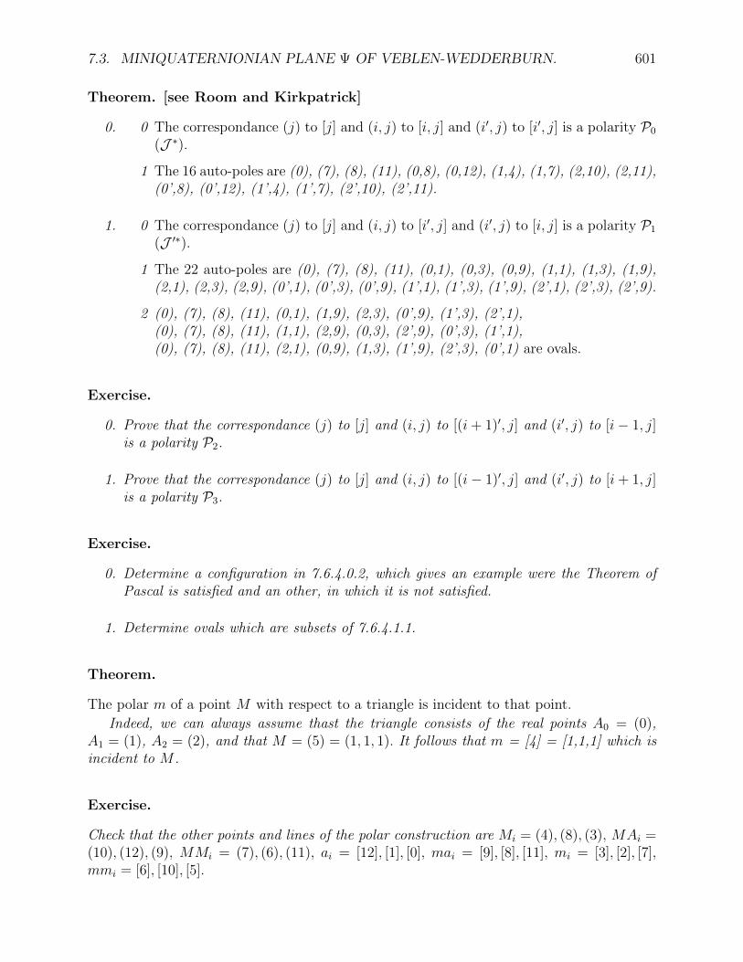
7.3. MINIQUATERNIONIAN PLANE Ψ OF VEBLEN-WEDDERBURN. 601
Theorem. [see Room and Kirkpatrick]
0. 0 The correspondance (j) to [j] and (i, j) to [i, j] and (i′, j) to [i′, j] is a polarity P0
(J ∗).
1 The 16 auto-poles are (0), (7), (8), (11), (0,8), (0,12), (1,4), (1,7), (2,10), (2,11),(0’,8), (0’,12), (1’,4), (1’,7), (2’,10), (2’,11).
1. 0 The correspondance (j) to [j] and (i, j) to [i′, j] and (i′, j) to [i, j] is a polarity P1
(J ′∗).
1 The 22 auto-poles are (0), (7), (8), (11), (0,1), (0,3), (0,9), (1,1), (1,3), (1,9),(2,1), (2,3), (2,9), (0’,1), (0’,3), (0’,9), (1’,1), (1’,3), (1’,9), (2’,1), (2’,3), (2’,9).
2 (0), (7), (8), (11), (0,1), (1,9), (2,3), (0’,9), (1’,3), (2’,1),(0), (7), (8), (11), (1,1), (2,9), (0,3), (2’,9), (0’,3), (1’,1),(0), (7), (8), (11), (2,1), (0,9), (1,3), (1’,9), (2’,3), (0’,1) are ovals.
Exercise.
0. Prove that the correspondance (j) to [j] and (i, j) to [(i+ 1)′, j] and (i′, j) to [i− 1, j]is a polarity P2.
1. Prove that the correspondance (j) to [j] and (i, j) to [(i− 1)′, j] and (i′, j) to [i+ 1, j]is a polarity P3.
Exercise.
0. Determine a configuration in 7.6.4.0.2, which gives an example were the Theorem ofPascal is satisfied and an other, in which it is not satisfied.
1. Determine ovals which are subsets of 7.6.4.1.1.
Theorem.
The polar m of a point M with respect to a triangle is incident to that point.
Indeed, we can always assume thast the triangle consists of the real points A0 = (0),A1 = (1), A2 = (2), and that M = (5) = (1, 1, 1). It follows that m = [4] = [1,1,1] which isincident to M .
Exercise.
Check that the other points and lines of the polar construction are Mi = (4), (8), (3), MAi =(10), (12), (9), MMi = (7), (6), (11), ai = [12], [1], [0], mai = [9], [8], [11], mi = [3], [2], [7],mmi = [6], [10], [5].

602 CHAPTER 7. QUATERNIONIAN GEOMETRY
Theorem. [see Room and Kirkpatrick]
0. The planes obtained by taking the complete quadrangle associated with 3 real pointsA0, A1, A2, and a point M which such that none of the lines M ×Ai are real are Fanoplanes associated with Z2.
1. There are (1613.12.9).24 = 5616 Fano planes that contain 3 real points.
Example.
The following is a Fano plane (0), (1), (2), (0,3), (2,1), (0’,12), (1,0), [12], [1], [0], [0’,0],[0,12], [2’,11], [0’,7].
Exercise.
Determine the Fano plane associated with (0), (1), (2), (0,7).
Comment.
The correspondance between the notation of Veblen-Wedderburn and Room-Kirkpatrick isV eblen−Wedderburn aj bj cj dj ej fj gjRoom−Kirkpatrick kj aj bj cj a′j b′j c′jDe V ogelaere [−j] [0,−j] [1,−j] [2,−j] [0′,−j] [1′,−j] [2′,−j]V eblen−Wedderburn Aj Bj Cj Dj Ej Fj Gj
Room−Kirkpatrick Kj A′j C′
j B′j Aj Cj Bj
De V ogelaere (j) (0, j) (1, j) (2, j) (0′, j) (1′, j) (2′, j)
Example. [Veblen-Wedderburn]
With the notation(C〈c0, c1, c2〉, A0, A1, A2a0, a1, a2, B0, B1, B2b0, b1, b2;C0, C1, C2d0, d1, d2), with di := Ci+j × Ci−j,the following configuration shows that the Desargues axiom is not satisfied((0)〈[0, 0], [1′, 0], [2, 0]〉, (0, 1), (1, 7), (1′, 2[1, 1], [0′, 8], [0′, 9], (2, 3), (0′3), (2, 1)[0, 11], [2′, 7], [10];(2′, 5), (0, 10), (1′, 3)[2, 1], [1, 0], [0, 4]).
Definition.
The Singer matrix G :=
0 0 11 0 10 1 0
. Its powers Gk are the columns
k, k + 1, k + 2 ofk = 0 1 2 3 4 5 6 7 8 9 10 11 12
1 0 0 1 0 1 1 1 −1 −1 0 1 −10 1 0 1 1 1 −1 −1 0 1 −1 1 00 0 1 0 1 1 1 −1 −1 0 1 −1 1
Problem.
Can we characterize the plane Ψ using Theorem 7.6.4.0.

7.3. MINIQUATERNIONIAN PLANE Ψ OF VEBLEN-WEDDERBURN. 603
move to g6a.tex:
Answer to 7.6.2.
κ λ = 0 1 −1 α −α β −β γ −γα r 0 0 0 −1 1 −1 1 −1 1
s 0 1 −1 0 0 −1 1 1 −1β r 0 0 0 −1 1 −1 1 −1 1
s 0 1 −1 1 −1 0 0 −1 1γ r 0 0 0 −1 1 −1 1 −1 1
s 0 1 −1 −1 1− 1 0 0
Definition.
The elements and incidence in the miniquaternionian plane Ψ are defined as follows.
0. The points are (ξ0, ξ1, ξ2) with right equivalence,
1.
2. A point P is incident to a line l iff
Definition. [Veblen-Wedderburn]
The points P are (x, y, 1), (x, 1, 0), (1, 0, 0), the lines l are [1, b, c], [0, 1, c], [0, 0, 1], and theincidence is P · l = 0.
Theorem. [Veblen-Wedderburn]
0. [1, b, c]× [1, b′, c′] = (−(yb+ c), y, 1), with y(b− b′) = −(c− c′).
1. [1, b, c]× [0, 1, c′] = (c′b− c,−c′, 1),
2. [1, b, c]× [0, 0, 1] = (−b, 1, 0),
3. [0, 1, c]× [0, 1, c′] = (1, 0, 0),
4. [0, 1, c]× [0, 0, 1] = (1, 0, 0),
Theorem. [Veblen-Wedderburn]
Let (a(b+c) = ab+ac)
0. M :=
1 0 1−1 0 0
0 −1 −1
.
1. A0 := (−1, 0, 1), B0 := (−γ, α, 1), C0 := (β,−α, 1), D0 := (−β, γ, 1), E0 := (α,−γ, 1),F0 := (γ,−β, 1), G0 := (−α, β, 1),

604 CHAPTER 7. QUATERNIONIAN GEOMETRY
2. Aj := MjA0, Bj := MjB0, . . . , for j = 0 to 12,
3. a0 := [1, 1, 1], b0 := [1, α, 1], c0 := [1,−α, 1], d0 := [1, γ, 1], e0 := [1,−γ, 1], f0 :=[1,−β, 1], g0 := [1, β, 1],
then
4. a0 = A0, A1, A3, A9, B0, C0, D0, E0, F0, G0,b0 = A0, B1, B8, D3, D11, E2, E5, E6, G7, G9,c0 = A0, C1, C8, E7, E9, F3, F11, G2, G5, G6,d0 = A0, B7, B9, D1, D8, F2, F5, F6, G3, G11,e0 = A0, B2, B5, B6, C3, C11, E1, E8, F7, F9,f0 = A0, C7, C9, D2, D5, D6, E3, E11, F1, F8,g0 = A0, B3, B11, C2, C5, C6, D7, D9, G1, G8,
5. A0 = a0, a4, a10, a12, b0, c0, d0, e0, f0, g0,B0 = a0, b5, b12, d4, d6, e7, e8, e11, g2, g10,C0 = a0, c5, c12, e2, e10, f4, f6, g7, g8, g11,D0 = a0, b2, b10, d5, d12, f7, f8, f11, g4, g6,E0 = a0, b7, b8, b11, c4, c6, e5, e12, f2, f10,F0 = a0, c1, c10, d7, d8, d11, e4, e6, f5, f12,G0 = a0, b4, b6, c7, c8, c11, d2, d10, g5, g12,
6. Xj ι xk =⇒ Xj+l mod 13 ι xk+l mod 13.
7. M2 =
1 −1 0−1 0 −1
1 1 1
,M3 =
−1 0 0−1 1 0
0 −1 0
,M4 =
−1 −1 11 0 −11 0 0
,M5 =
0 −1 11 1 −11 0 1
,
M6 =
1 −1 −10 1 −11 −1 0
,M7 =
−1 1 −1−1 1 1−1 0 1
,M8 =
1 1 01 −1 1−1 −1 1
,M9 =
0 0 1−1 −1 0
0 −1 1
,
M10 =
0 −1 −10 0 −11 −1 −1
,M11 =
1 1 10 1 −1−1 1 1
,M12 =
0 −1 0−1 −1 −1
1 1 0
,M13 =
1 0 00 1 00 0 1
.
Proof: [x, y, z] ι β? iff x(Mk00 + Mk
20) + y(Mk01 + Mk
21) + z(Mk02 + Mk
22) + (zMk10 + yMk
11 +zMk
22)β = 0, . . . .
Example. [Veblen-Wedderburn]
With the notation(C〈c0, c1, c2〉, A0, A1, A2a0, a1, a2, B0, B1, B2b0, b1, b2;C0, C1, C2d0, d1, d2), with di := Ci+j × Ci−j,the following configuration shows that the Desargues axiom is not satisfied(A0〈b0, f0, d0〉, B1, C7, F2c12, e5, e4, D3, E3, D1b2, g6, a3;G5, B10, F3d12, c0, b9).

7.3. MINIQUATERNIONIAN PLANE Ψ OF VEBLEN-WEDDERBURN. 605
Partial answer to7.6.4.
For n = 72, 2451 = 57.43, for n = 92, 6643 = 91.73, for n = 112, 14763 = 57.259, Forn = 132, 28731 = 3.9577.
Answer to7.6.4.
The other points are (1,1), (0’,12), (0’,0), the lines are [12], [1], [0], [1’,0], [0,12], [0,11]and the polar of (0,7) is [0’,6].
Answer to7.6.4.
(7)× (8) = [6], [6]× [0] = (3), (8)× (0) = [1], [1]× [7] = (2), (0)× (7) = [9], [9]× [8] = (5),〈(3), (2), (5); [11]〉.(7) × (8) = [6], [6] × [0, 1] = (1′, 7), (8) × (0, 1) = [0, 5], [0, 5] × [7] = (0′, 6), (0, 1) × (7) =[2′, 6], [2′, 6]× [8] = (2, 5), (2, 5) is not incident to (1′, 7)× (0′6) = [2, 2].This has not been checked.
From Dembowski, p. 129
Definition.
A linear ternary ring (Σ,+, ·) is called a cartesian field iff (Σ,+) is associative and is there-fore a group.
Definition.
A cartesian field is called a quasifield iff the right distributivity law holds:(x+ y)z = xz + yz.
Artzy adds that xa = xb + c has a unique solution, but this is a property (28). This isVeblen-Wedderburn.
Definition.
A quasifield is called a semifield iff the left distributivity law holds:z(x+ y) = zx+ zy.
Definition.
A quasifield is called a nearfield iff (Σ, ·) is associative and is therefore a group.
Definition.
A semifield is called a alternative field iff x2y = x(xy) and xy2 = (xy)y.

606 CHAPTER 7. QUATERNIONIAN GEOMETRY
Theorem.
P is (p, L) transitive iff P is (p, L) Desarguesian. p is point, L is a line. Dembowski p.123,16
Let Q0 = (79), Q1 = (80), Q2 = (90), and U = (81) then q2 = [79], q0 = [90], q1 = [80],v = [88], i = [78], V = (78), I = (82), j = [89], W = (89),Points on q2 : 86,12,25,38,51,64,77Points on q1 : 85,11,24,37,50,63,7611×12 = [7] : 84(78, 86), 8(51, 25), 43(77, 64), 48(86, 38), 52(12, 12), 54(25, 78), 66(64, 80), 72(38, 51),11×25 = [61] : 82(78, 80), 0(64, 64), 18(12, 51), 28(51, 78), 33(77, 12), 58(38, 86), 61(86, 25), 62(25, 38),11×38 = [75] : 81(78, 78), 4(38, 25), 14(12, 80), 19(77, 86), 36(51, 64), 70(64, 38), 73(25, 51), 74(86, 12),11×51 = [4] : 87(86, 86), 1(38, 80), 2(77, 78), 46(25, 64), 55(78, 38), 57(51, 12), 69(64, 51), 75(12, 25),11×64 = [8] : 83(86, 78), 7(64, 25), 10(77, 51), 42(78, 12), 47(12, 64), 53(51, 80), 65(38, 38), 71(25, 86),11×77 = [68] : 88(86, 80), 5(38, 64), 13(51, 51), 21(77, 38), 30(25, 12), 32(64, 86), 67(12, 78), 68(78, 25),Coordinates of points:
(0) 64, 64 38, 80 77, 78 78, 51 38, 25 38, 64 51, 86 64, 25(8) 51, 25 86, 77 77, 51 80, 77 12 51, 51 12, 80 64, 78
(16) 78, 77 12, 38 12, 51 77, 86 51, 38 77, 38 86, 64 64, 77(24) 80, 64 25 77, 77 25, 80 51, 78 78, 64 25, 12 25, 77(32) 64, 86 77, 12 64, 12 86, 51 51, 64 80, 51 38 25, 25(40) 77, 80 38, 78 78, 12 77, 64 77, 25 12, 86 25, 64 12, 64(48) 86, 38 38, 12 80, 38 51 12, 12 51, 80 25, 78 78, 38(56) 51, 77 51, 12 38, 86 12, 77 38, 77 86, 25 25, 38 80, 25(64) 64 38, 38 64, 80 12, 78 78, 25 64, 51 64, 38 25, 86(72) 38, 51 25, 51 86, 12 12, 25 80, 12 77 78 80, 80(80) 0 78, 78 78, 80 86, 78 78, 86 80, 86 86 86, 86(88) 86, 80 80, 78 ∞
Coordinates of lines:[0] 78, 38 38 77, 78 12, 12 51, 77 86, 38 12, 86 12, 77[8] 64, 77 77, 25 64, 12 80, 25 51, 80 78, 12 12 64, 78
[16] 25, 25 77, 64 86, 12 25, 86 25, 64 51, 64 64, 38 51, 25[24] 80, 38 77, 80 78, 25 25 51, 78 38, 38 64, 51 86, 25[32] 38, 86 38, 51 77, 51 51, 12 77, 38 80, 12 64, 80 78, 77[40] 77 38, 78 51, 51 12, 38 86, 77 51, 86 51, 38 25, 38[48] 38, 64 25, 51 80, 64 12, 80 78, 51 51 25, 78 64, 64[56] 38, 25 86, 51 64, 86 64, 25 12, 25 25, 77 12, 64 80, 77[64] 38, 80 78, 64 64 12, 78 77, 77 25, 12 86, 64 77, 86[72] 77, 12 38, 12 12, 51 38, 77 80, 51 25, 80 78, 80 ∞[80] 80 78, 78 86 86, 78 86, 86 80, 86 86, 80 78, 86[88] 78 80, 78 80, 80
[80] : 11(80, 77), 24(80, 64), 37(80, 51), 50(80, 38), 63(80, 25), 76(80, 12), 79(80, 80), 85(80, 86), 89(80, 78), 90(/infty)B = A+ α, (A,B) ι [V, Y ], V = (78), (76) = (80, 12) = (0, α), Y × V = (78)× (76) = [13].[13] : 78(78), 15(64, 78), 18(12, 51), 19(77, 86), 68(78, 25), 76(80, 12), 46(25, 64), 48(86, 38), 53(51, 80), 60(38, 77)hence 12 = 80 + α, 51 = α+ α = −α, 25 = 78 + α = 1 + α = γ, 64 = 25 + γ = γ + γ = −β,38 = 86 + α = −1 + α = β, 77 = 38 + α = β + α = −γ.
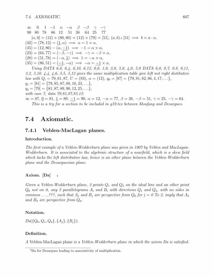
7.4. AXIOMATIC. 607
∞ 0 1 −1 α −α β −β γ −γ90 80 78 86 12 51 38 64 25 77
[α, 0] = (12)× (80, 80) = (12)× (79) = [51], (a, b) ι [51] =⇒ b = a · α.(42) = (78, 12) = (1, α) =⇒ α = 1× α,(45) = (12, 86)− (α,−1) =⇒ −1 = α× α,(23) = (64, 77) = (−β,−γ) =⇒ −γ = −β × α,(28) = (51, 78) = (−α, 1) =⇒ 1 = −α× α,(35) = (86, 51) = (−1,−α) =⇒ −α = −1× α,
Using DATA 6,0, 6,4, 6,10, 6,12, 0,0, 1,0, 2,0, 3,0, 4,0, 5,0 DATA 6,0, 0,7, 0,8, 0,11,3,2, 3,10, 4,4, 4,6, 5,5, 5,12 gives the same multiplication table give left not right distibutivelaw with Qi = 79, 81, 87, U = (83), α = (12), q0 = [87] = 79, 81, 82, 86, 4, 17, . . .,q1 = [81] = 79, 85, 87, 88, 10, 23, . . .,q2 = [79] = 81, 87, 89, 90, 12, 25, . . .,with case 7, data 79,81,87,83,12:∞ = 87, 0 = 81, 1 = 89, −1 = 90, α = 12, −α = 77, β = 38, −β = 51, γ = 25, −γ = 64.
This is a try for a section to be included in g19.tex between Moufang and Desargues.
7.4 Axiomatic.
7.4.1 Veblen-MacLagan planes.
Introduction.
The first example of a Veblen-Wedderburn plane was given in 1907 by Veblen and MacLagan-Wedderburn. It is associated to the algebraic structure of a nearfield, which is a skew fieldwhich lacks the left distributive law, hence is an other plane between the Veblen-Wedderburnplane and the Desarguesian plane.
Axiom. [Da] 4
Given a Veblen-Wedderburn plane, 2 points Q1 and Q2 on the ideal line and an other pointQ0 not on it, any 2 parallelograms Ai and Bi with directions Q1 and Q2, with no sides incommon . . . ,???, such that Aj and Bj are perspective from Q0 for j = 0 To 2, imply that A3
and B3 are perspective from Q0.
Notation.
Da(Q0, Q1, Q2, Aj, Bj).
Definition.
A Veblen-MacLagan plane is a Veblen-Wedderburn plane in which the axiom Da is satisfied.
4Da for Desargues leading to associativity of multiplication.

608 CHAPTER 7. QUATERNIONIAN GEOMETRY
Lemma. [For Associativity]
H1.0. A0, a12, x, (See Fig. 2?.)D1.0. a01 := Q1 × A0, a02 := Q2 × A0,D1.1. A1 := a01 × a12, A2 := a02 × a12,D1.2. a13 := Q2 × A1, a23 := Q1 × A2, A3 := a13 × a23,D2.0. a0 := Q0 ×A0, a1 := Q0 ×A1, a2 := Q0 ×A2, a3 := Q0 ×A3, D2.1. B0 := a0 × y,b01 := Q1 ×B0, b02 := Q2 ×B0,D2.1. B1 := b1×b01, B2 := b2×b02, D2.2. b13 := Q2×B1, b23 := Q1×B2, B3 := b13×b23,C1.0. B3 ι b3,MoreoverA0 = (A,B), A1 = (A′, B), A2 = (A,B′), A3 = (A′, B′), B0 =Proof: Da(Q0, Q1, Q2, Aj, Bj).
Theorem.
In a Veblen-MacLagan plane, the ternary ring (Σ, ∗) is a nearfield.:
0. (Σ,+) is an Abelian group,
1. (Σ− 0, ·) is a group,
2. (Σ, ∗) = (Σ,+, ·) is right distributive, (a+ b) · c = a · c+ b · c.
7.4.2 Examples of Perspective planes.
Theorem.
0. The Cayleyian plane is not a Veblen-MacLagan plane.replace Desarg.?
Definition.
A miniquaternion plane . . . .
Theorem.
0. A miniquaternion plane is a Veblen-MacLagan plane.
1. A miniquaternion plane is not a Moufang plane.
Tables.
The following are in an alternate notation the known table for p = 3 and a new table forp = 5. The other incidence are obtained by adding one to the subscripts of the lines andsubtracting one for the subscript of the points.
Selectors for Ψ plane, when p = 3:
(000) : [002], [005], [006], [101], [108], [117], [119], [123], [1311],
(010) : [012], [015], [016], [113], [1111], [121], [138], [107], [109],

7.4. AXIOMATIC. 609
(020) : [022], [025], [026], [127], [139], [103], [1011], [111], [118],
(100) : [102], [105], [106], [001], [008], [017], [019], [023], [0311],
(110) : [112], [115], [116], [013], [0111], [021], [038], [007], [009],
(120) : [122], [125], [126], [027], [039], [003], [0011], [011], [018],
Selectors for Ψ plane, when p = 5:
(000) : [006], [0021], [0016], [1218], [1225], [135], [1313], [034], [1022], [0228],
[2012], [2023], [2024], [2026], [211], [2110], [2414], [248], [319], [3127], [3415], [3419], [2229], [2320], [303],
(010) : [0125], [0119], [016], [1312], [1326], [1418], [1421], [0422], [1128], [0327],
[213], [215], [2129], [2113], [2220], [229], [201], [2010], [3216], [3215], [304], [308], [2314], [2424], [3123],
(020) : [0226], [028], [0225], [143], [1413], [1012], [106], [0028], [1227], [0415],
[2223], [2218], [2214], [2221], [2324], [2316], [2120], [219], [3319], [334], [3122], [3110], [241], [2029], [325],
(030) : [0313], [0310], [0326], [1023], [1021], [113], [1125], [0127], [1315], [004],
[235], [2312], [231], [236], [2429], [2419], [2224], [2216], [348], [3422], [3228], [329], [2020], [2114], [3318],
(040) : [0421], [049], [0413], [115], [116], [1223], [1226], [0215], [144], [0122],
[2418], [243], [2420], [2425], [2014], [208], [2329], [2319], [3010], [3028], [3327], [3316], [2124], [221], [3412],
(100) : [109], [1019], [1026], [026], [0212], [0321], [0323], [1118], [145], [0022],
[3027], [3015], [3024], [3016], [214], [218], [2428], [2410], [3320], [3325], [3229], [3213], [311], [3414], [203],
(110) : [1116], [118], [1113], [0325], [033], [046], [045], [1212], [1018], [0228],
[3115], [314], [3129], [3119], [2222], [2210], [2027], [209], [3424], [3426], [3314], [3321], [3220], [301], [2123],
(120) : [1219], [1210], [1221], [0426], [0423], [0025], [0018], [133], [1112], [0227],
[324], [3222], [3214], [328], [2328], [239], [2115], [2116], [3029], [3013], [341], [346], [334], [3120], [225],
(130) : [138], [139], [136], [0013], [005], [0126], [0112], [1423], [123], [0315],
[3322], [3328], [331], [3310], [2427], [2416], [224], [2219], [3114], [3121], [3020], [3025], [3429], [3224], [2318],
(140) : [1410], [1416], [1425], [0121], [0118], [0213], [023], [105], [1323], [044],
[3428], [3427], [3420], [349], [2015], [2019], [2322], [238], [321], [326], [3124], [3126], [3014], [3329], [2412],
(200) : [206], [2021], [2016], [3218], [3225], [335], [3313], [234], [3022], [2228],
[0012], [0023], [0024], [0026], [011], [0110], [0414], [048], [119], [1127], [1415], [1419], [0229], [0320], [103],
(210) : [2125], [2119], [216], [3312], [3326], [3418], [3421], [2422], [3128], [2327],
[013], [015], [0129], [0113], [0220], [029], [001], [0010], [1216], [1215], [104], [108], [0314], [0424], [1123],
(220) : [2226], [228], [2225], [343], [3413], [3012], [306], [2028], [3227], [2415],
[0223], [0218], [0214], [0221], [0324], [0316], [0120], [019], [1319], [134], [1122], [1110], [041], [0029], [125],
(230) : [2313], [2310], [2326], [3023], [3021], [313], [3125], [2127], [3315], [204],
[035], [0312], [031], [036], [0429], [0419], [0224], [0216], [148], [1422], [1228], [129], [0020], [0114], [1318],
(240) : [2421], [249], [2413], [315], [316], [3223], [3226], [2215], [344], [2122],
[0418], [043], [0420], [0425], [0014], [008], [0329], [0319], [1010], [1028], [1327], [1316], [0124], [021], [1412],
(300) : [309], [3019], [3026], [226], [2212], [2321], [2323], [3118], [345], [2022],
[1027], [1015], [1024], [1016], [014], [018], [0428], [0410], [1320], [1325], [1229], [1213], [111], [1414], [003],
(310) : [3116], [318], [3113], [2325], [233], [246], [245], [3212], [3018], [2228],
[1115], [114], [1129], [1119], [0222], [0210], [0027], [009], [1424], [1426], [1314], [1321], [1220], [101], [0123],
(320) : [3219], [3210], [3221], [2426], [2423], [2025], [2018], [333], [3112], [2227],
[124], [1222], [1214], [128], [0328], [039], [0115], [0116], [1029], [1013], [141], [146], [134], [1120], [025],
(330) : [338], [339], [336], [2013], [205], [2126], [2112], [3423], [323], [2315],

610 CHAPTER 7. QUATERNIONIAN GEOMETRY
[1322], [1328], [131], [1310], [0427], [0416], [024], [0219], [1114], [1121], [1020], [1025], [1429], [1224], [0318],
(340) : [3410], [3416], [3425], [2121], [2118], [2213], [223], [305], [3323], [244],
[1428], [1427], [1420], [149], [0015], [0019], [0322], [038], [121], [126], [1124], [1126], [1014], [1329], [0412],
An abbreviated form is as follows:
The array for the indices:i 0 1 2 3 4ai 24 29 14 1 20bi 3 23 5 18 12ci 22 28 27 15 4di 16 19 8 10 9ei 26 13 21 6 25
Selectors for the Ψ plane, when p = 5:(00
0) : [00e2
], [00e3
], [00d0
], [13e1
], [13b2
], [12e4
], [12b3
], [02c1
] [03c4
], [10c1
],
[20b1
], [20b4
], [20a0
], [20e0
], [24a2
], [24d2
], [21a3
], [21d3
],
[34d1
], [34c3
], [31d4
], [31c2
], [22a1
], [23a4
], [30b0
],
(100) : [10
d1], [10
d4], [10
e0], [03
b1], [03
e2], [02
b4], [02
e3], [14
b2], [11
b3], [00
c0],
[30c2
], [30c3
], [30a0
], [30d0
], [32a1
], [32e1
], [33a4
], [33e4
],
[24c1
], [24d3
], [21c4
], [21d2
], [34a2
], [31a3
], [20b0
],
(200) : [20
e2], [20
e3], [20
d0], [33
e1], [33
b2], [32
e4], [32
b3], [22
c1] [23
c4], [30
c1],
[00b1
], [00b4
], [00a0
], [00e0
], [04a2
], [04d2
], [01a3
], [01d3
],
[14d1
], [14c3
], [11d4
], [11c2
], [02a1
], [03a4
], [10b0
],
(300) : [30
d1], [30
d4], [30
e0], [23
b1], [23
e2], [22
b4], [22
e3], [34
b2], [31
b3], [20
c0],
[10c2
], [10c3
], [10a0
], [10d0
], [12a1
], [12e1
], [13a4
], [13e4
],
[04c1
], [04d3
], [01c4
], [01d2
], [14a2
], [11a3
], [00b0
],
7.5 Desarguesian Geometry.5
I will attempt to generalize the results of quaternionian geometry to Desarguesian geometry.It is not clear to me now that polarities exist in general. Indded, we have seen that we canconstruct a system of homogeneous coordinates over a skew field, for which the incidenceproperty is ΣPili = 0, with right equivalence for the lines l anf left equivalence for the pointsP . A line collineation can be represented by a matrix, m = Cll while a point collineation re-quires, P T = QTCp, to allow for right and left equivalence. For a polarity, these equivalencesdo not appear to be compatible with a matrix transformation.
It should be kept in mind that every skew field which is not a filed has a non trivial subfield
522.1.87
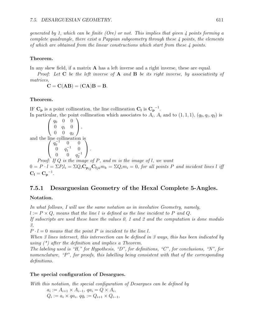
7.5. DESARGUESIAN GEOMETRY. 611
generated by 1, which can be finite (Ore) or not. This implies that given 4 points forming acomplete quadrangle, there exist a Pappian subgeometry through these 4 points, the elementsof which are obtained from the linear constructions which start from these 4 points.
Theorem.
In any skew field, if a matrix A has a left inverse and a right inverse, these are equal.Proof: Let C be the left inverse of A and B be its right inverse, by associativity of
matrices,C = C(AB) = (CA)B = B.
Theorem.
IF Cp is a point collineation, the line collineation Cl is Cp−1.
In particular, the point collineation which associates to Ai, Ai and to (1, 1, 1), (q0, q1, q2) is q0 0 00 q1 00 0 q2
,
and the line collineation is q−10 0 00 q−1
1 00 0 q−1
2
.
Proof: If Q is the image of P , and m is the image of l, we want0 = P · l = ΣPili = ΣQiCpijCljkmk = ΣQimi = 0, for all points P and incident lines l iff
Cl = Cp−1.
7.5.1 Desarguesian Geometry of the Hexal Complete 5-Angles.
Notation.
In what follows, I will use the same notation as in involutive Geometry, namely,l := P ×Q, means that the line l is defined as the line incident to P and Q.If subscripts are used these have the values 0, 1 and 2 and the computation is done modulo3,P · l = 0 means that the point P is incident to the line l.When 3 lines intersect, this intersection can be defined in 3 ways, this has been indicated byusing (*) after the definition and implies a Theorem.The labeling used is “H,” for Hypothesis, “D”, for definitions, “C”, for conclusions, “N”, fornomenclature, “P”, for proofs, this labelling being consistent with that of the correspondingdefinitions.
The special configuration of Desargues.
With this notation, the special configuration of Desargues can be defined byai := Ai+1 × Ai−1, qai = Q× Ai,Qi := ai × qai, qqi := Qi+1 ×Qi−1,
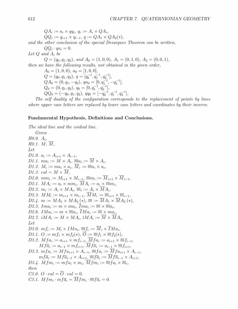
612 CHAPTER 7. QUATERNIONIAN GEOMETRY
QAi := ai × qqi, qi := Ai ×QAi,QQi := qi+1 × qi−1, q := QA1 ×QA2(∗),
and the other conclusion of the special Desargues Theorem can be written,QQi · qai = 0.
Let Q and Ai beQ = (q0, q1, q2), and A0 = (1, 0, 0), A1 = (0, 1, 0), A2 = (0, 0, 1),
then we have the following results, not obtained in the given order,A0 = (1, 0, 0), a0 = [1, 0, 0],Q = (q0, q1, q2), q = [q−1
0 , q−11 , q−1
2 ],QA0 = (0, q1,−q2), qa0 = [0, q−1
1 ,−q−12 ],
Q0 = (0, q1, q2), q0 = [0, q−11 , q−1
2 ],QQ0 = (−q0, q1, q2), qq0 = [−q−1
0 , q−11 , q−1
2 ],The self duality of the configuration corresponds to the replacement of points by lines
where upper case letters are replaced by lower case letters and coordinates by their inverse.
Fundamental Hypothesis, Definitions and Conclusions.
The ideal line and the coideal line.Given
H0.0. Ai,H0.1. M, M,LetD1.0. ai := Ai+1 × Ai−1,D1.1. mai := M × Ai, mai := M × Ai,D1.2. Mi := mai × ai, M i := mai × ai,D1.3. eul = M ×M,D2.0. mmi := Mi+1 ×Mi−1, mmi := M i+1 ×M i−1,D2.1. MAi := ai ×mmi, MAi := ai ×mmi,D2.2. mi := Ai ×MAi, mi := Ai ×MAi,D2.3. MMi := mi+1 ×mi−1, MMi := mi+1 ×mi−1,D2.4. m := MA1 ×MA2 (∗), m := MA1 ×MA2 (∗),D2.5. Imai := m×mai, Imai := m×mai,D2.6. IMai := m×mai, IMai := m×mai,D2.7. iMAi := M ×MAi, ıMAi := M ×MAi,LetD3.0. mfi := Mi × IMai, mfi := M i × IMai,D3.1. O := mf1 ×mf2(∗), O := mf1 ×mf2(∗),D3.2. Mfai := ai+1 ×mfi−1, Mfai := ai+1 ×mfi−1,
Mfai := ai−1 ×mfi+1, Mfai := ai−1 ×mfi+1,D3.3. mfai := Mfai+1 × Ai−1, mfai := Mfai+1 × Ai−1,
mfai := Mfai−1 × Ai+1, mfai := Mfai−1 × Ai+1,D3.4. Mfmi := mfai ×mi, Mfmi := mfai ×mi,thenC3.0. O · eul = O · eul = 0.C3.1. Mfmi ·mfai = Mfmi ·mfai = 0.

7.5. DESARGUESIAN GEOMETRY. 613
LetD4.0. Immi := m×mmi, Immi := m×mmi,D4.1. tai := Ai × Immi,D4.2. Ti := tai+1 × tai−1,D4.3. ati := Ai × Ti,D4.4. Ki := ati+1 × ati−1,D4.5. TAai := tai × ai,D4.6. poKi := Taai+1 × Taai−1,thenC4.0. Immi · tai = 0.C4.1. Ti ·mfi = 0.
The nomenclature:N0.0. Ai are the vertices of the triangle,N0.1. M is the barycenter, M is the orthocenter.N1.0. ai are the sides.N1.1. mai are the medians, mai are the altitudesN1.2. Mi are the mid-points of the sides. M i are the feet of the altitudesN1.3. eul is the line of Euler,N2.0. Mi,mmi is the complementary triangle,
M i,mmi is the orthic triangle,N2.1. MAi are the directions of the sides,N2.2. MMi,mi is the anticomplementary triangle.N2.3. m is the ideal line corresponding to the line at infinity,
m is the orthic line which is the polar of M with respect to the triangle.N2.4. Imai are the directions of the medians.
IMai are the directions of the altitudes.N3.0. mfi are the mediatrices,N3.1. O is the center,N3.2. Mfmi are the trapezoidal points,N4.0. Immi are the directions of the antiparallels of aiwith respect to the
sides ai+1 and ai−1.N4.1. (Ti, tai) is the tangential triangle,N4.2. ati are the symmedians,N4.3. Ki is the triangle of Lemoine.
Theorem.
If we derive a point X and a line x by a given construction from Ai, M and M , with thecoordinates as given in G0.0 and G0.1, below, and the point X and line x are obtain by thesame construction interchange M and M ,
X = (f0(m0,m1,m2), f1(m0,m1,m2), f2(m0,m1,m2)),x = [g0(m0,m1,m2), g1(m0,m1,m2), g2(m0,m1,m2)],
=⇒X = (f0(m−1
0 ,m−11 ,m−1
2 )m0, f1(m−10 ,m−1
1 ,m−12 )m1, f2(m−1
0 ,m−11 ,m−1
2 )m2),x = [m−1
0 g0(m−10 ,m−1
1 ,m−12 ),m−1
1 g1(m−10 ,m−1
1 ,m−12 ),m−1
2 g2(m−10 ,m−1
1 ,m−12 )].

614 CHAPTER 7. QUATERNIONIAN GEOMETRY
Proof: The point collineation Cp =
q0 0 00 q1 00 0 q2
, associates to (1,1,1), (q0, q1, q2),
and to (m0,m1,m2), (r0, r1, r2), if ri = miqi.In the new system of coordinates,X = (f0(q−1
0 r0, q−11 r1, q
−12 r2)q0, f1(q−1
0 r0, q−11 r1, q
−12 r2q1), f2(q−1
0 r0, q−11 r1, q
−12 r2)q2).
Exchanging qi and ri and then replacing qi by 1 and ri by mi is equivalent to substituting mi for qiand 1 for ri, which gives X. x is obtained similarly.
The line collineation is q−10 0 0
0 q−11 0
0 0 q−12
.
Notation.
ai := (m−1i+1 −m
−1i−1)(m−1
i−1 +m−1i )−1,
si := −(m−1i +m−1
i+1)(m−1i +m−1
i−1)−1,ti := si+2si+1,fi := si − s−1
i+1s−1i−1,
gi := t−1i − ti+1ti−1.
Proof of 7.5.1.
LetG0.0. A0 = (1, 0, 0), A1 = (0, 1, 0), A2 = (0, 0, 1),G0.1. M = (1, 1, 1), M = (m0,m1,m2),thenP1.0. a0 = (1, 0, 0), a1 = (0, 1, 0), a2 = (0, 0, 1),P1.1. ma0 = [0, 1,−1], ma0 = [0,m−1
1 ,−m−12 ],
P1.2. M0 = (0, 1, 1), M0 = (0,m1,m2),P1.3. eul = [1, (m1 −m2)−1(m2 −m0), (m1 −m2)−1(m0 −m1)],
P2.0. mm0 = [1,−1,−1], mm0 = [m−10 ,−m−1
1 ,−m−12 ],
P2.1. MA0 = (0, 1,−1), MA0 = (0,m1,−m2),P2.2. m0 = [0, 1, 1], m0 = [0,m−1
1 ,m−12 ],
P2.3. MM0 = (1,−1,−1), MM0 = (m0,−m1,−m2),P2.4. m = [1, 1, 1], m = [m−1
0 ,m−11 ,m−1
2 ],P2.5. Ima0 = (2,−1,−1), Ima0 = (2m0,−m1,−m2),P2.6. IMa0 = (m1 +m2,−m1,−m2), IMa0 = ((m−1
1 +m−12 )m0,−1,−1),
P2.7. iMA0 = [2,−1,−1], ıMA0 = [2m−10 ,−m−1
1 ,−m−12 ],
P3.0. mf0 = [(m1 +m2)−1(m1 −m2), 1,−1],mf0 = [m−1
0 (m−11 +m−1
2 )−1(m−11 −m
−12 ),m−1
1 ,−m−12 , 1],
P3.1. O = (m1 +m2,m2 +m0,m0 +m1),O = ((m−1
1 +m−12 )m0, (m
−12 +m−1
0 )m1, (m−10 +m−1
1 )m2),P3.2. Mfa0 = (1, 0,−(m0 −m1)−1(m0 +m1)),
Mfa0 = (m0, 0, (m−10 −m
−11 )(m−1
0 +m−11 )−1m2),
Mfa0 = (1, (m2 −m0)−1(m2 +m0), 0),Mfa0 = (m0, (m
−12 −m
−10 )−1(m−1
2 +m−10 )m1, 0),
P3.3. mfa0 = [(m1 +m2)−1(m1 −m2), 1, 0],

7.5. DESARGUESIAN GEOMETRY. 615
mfa0 = [m−10 (m−1
1 +m−12 )−1(m−1
1 −m−12 ),m−1
1 , 0],mfa0 = [(m1 +m2)−1(m1 −m2), 0,−1],mfa0 = [m−1
0 (m−11 +m−1
2 )−1(m−11 −m
−12 ), 0,m−1
2 ],P3.4. Mfm0 = ((m1 +m2)(m1 −m2)−1,−1, 1),
Mfm0 = ((m−11 −m
−12 )−1(m−1
1 +m−12 )m0,−m1,m2),
P4.0. Imm0 = (a0, 1, s0), Imm0 = (−a0, 1, s0),P4.1. ta0 = [0, 1,−s−1
0 ],P4.2. T0 = (1, s2, s
−11 ), ?
P4.3. at0 = [0, s−12 ,−s1] = [0, 1,−t0],
P4.4. K0 = (1, t−12 , t1),
P4.5. Taa0 = (0, 1, s0),P4.6. poK0 = [−1, s−1
2 , s1],
Details of proof:For P4.0, if the coordinates of Imm0 are x0, 1 and x2, we have to solve
x0 + 1 + x2 = 0, −x0m−10 +m−1
1 + x2m−12 = 0.
Multiplying the equations to the right respectively by m−12 , and -1 or by m−1
0 and 1 and adding givesx0 and x2 using the notation 7.5.1.
7.5.2 Perpendicularity mapping.
Definition.
Given M and a direction Ix, the perpendicular direction Iy is defined by the following constructionD5.0. b := A0 × Ix,D5.1. B := b× a0,D5.2. c := B × IMa2,D5.3. C := c×ma0,D5.4. d := C ×A1,D5.5. Iy := d×m,
Theorem.
If Ix = (−1− q, q, 1) and Iy = (1− r, r, 1) thenr = .
Proof:P5.0. b = [0,−q−1, 1],P5.1. B = (0, q, 1),P5.2. c = [x,−q−1, 1], with x = m−1
0 (m0 +m1 +m1q−1),
P5.3. C = (y,m1,m2), with y = (m1q−1 −m2)x−1,
P5.4. d = [y−1, 0,−m−12 ],
P5.5. Iy = (y, z,m2), with z = −y −m2,Therefore r = −m−1
2 (y +m2) = −m−12 (m2 + (m1q
−1 −m2)(m0 +m1 +m1q−1)−1m0).
If the skew field we therefore have−m2(r + 1)m−1
0 ((m0 +m1)q +m1) = m1 −m2q.−rm−1
0 (m0 +m1)q − rm−10 m1 −m−1
0 m1q −m−12 m1 = 0.
which is, in general, not an involution.

616 CHAPTER 7. QUATERNIONIAN GEOMETRY
7.6 The Hughes Planes.
7.6.0 Introduction.
There are essentially 2 methods to algebraize a plane. The first one which start with the work ofDesargues coordinatized the plane using 2 coordinates, the difficulty of representing the ideal pointsor points at infinity can be dealt with by using 3 homogeneous coordinates. This approach hasbeen generalized to perspective planes, for which the only axioms are those of incidence, by usingas coordinates, elements of a ternary ring instead of elements in a field. This generalization wasgiven by Marshall Hall in 1943, but its origin can be found, for the case of nearfields, introducedby Dickson (1905), in the most remarkable paper of Veblen and MacLagan-Wedderburn in 1907 (p.380-382).In this paper they give, independently from Vahlen the first example of non Pappian Geometry.The indpendent result consited in showing that quaternions could be used as coordinates for such ageometry.The second approach, which can be used in finite planes, is to construct a difference set, of q = pk
integers as a subset 0, . . . , q2+q from which the points incident to each line, and the lines incidentto every point can be completely derived. This approach was fully examined for the finite Pappianplanes by J. Singer in 1938, but it again can be traced in the paper of 1907 (p. 383 and 385).Moreover, the generalization to non Desarguesian planes is given explicitely for a plane of order 9,called Ψ plane by Room and Kirkpatrick.I do prefer, when applying the notion of difference sets to geometry, to use, instead of it, theterminology of selector introduced by Fernand Lemay, in 1979. (See his most accessible paper of1983.)It is the second approach, that I am exploring in this paper, gives many of the results in the formof conjectures.We will see that to give the incidence properties for planes of the Ψ type and order p2 we have togive p selectors of p elements, and in a particular notation the points which are incident to p−1
2lines from which all other incidences can be derived. The notation is such that the same incidencetables are valid for the points on any line, giving rise to a fundamental polarity.One of the advantages of the selector approach is to eliminate the need of addition and multiplicationtables in the particular nearfield which greatly simplifies the exploration of new properties with acomputer. Many of the planes are special case of Hughes planes, hence the tiltle of the section.
I will assume that p is an odd prime.
7.6.1 Nearfield and coordinatization of the plane.
Definition. [Dickson]
A left nearfield (N,+, ) is a set N with binary operations such that
0. N is finite,
1. (N,+) is an Abelian group, with neutral element 0,
2. (N − 0, ) is an group, with neutral element 1,
3. is left distributive over +, orζ (ξ + η) = ζ ξ + ζ η, for all ξ, η, ζ ∈ N
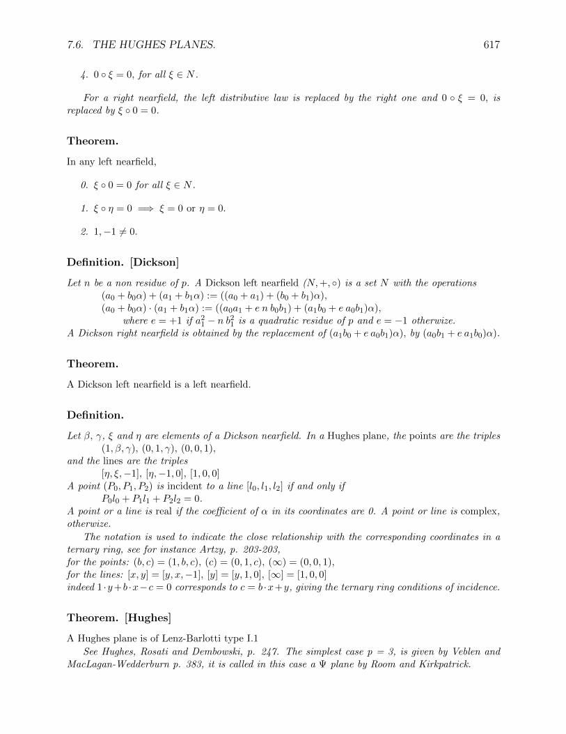
7.6. THE HUGHES PLANES. 617
4. 0 ξ = 0, for all ξ ∈ N .
For a right nearfield, the left distributive law is replaced by the right one and 0 ξ = 0, isreplaced by ξ 0 = 0.
Theorem.
In any left nearfield,
0. ξ 0 = 0 for all ξ ∈ N .
1. ξ η = 0 =⇒ ξ = 0 or η = 0.
2. 1,−1 6= 0.
Definition. [Dickson]
Let n be a non residue of p. A Dickson left nearfield (N,+, ) is a set N with the operations(a0 + b0α) + (a1 + b1α) := ((a0 + a1) + (b0 + b1)α),(a0 + b0α) · (a1 + b1α) := ((a0a1 + e n b0b1) + (a1b0 + e a0b1)α),
where e = +1 if a21 − n b21 is a quadratic residue of p and e = −1 otherwize.
A Dickson right nearfield is obtained by the replacement of (a1b0 + e a0b1)α), by (a0b1 + e a1b0)α).
Theorem.
A Dickson left nearfield is a left nearfield.
Definition.
Let β, γ, ξ and η are elements of a Dickson nearfield. In a Hughes plane, the points are the triples(1, β, γ), (0, 1, γ), (0, 0, 1),
and the lines are the triples[η, ξ,−1], [η,−1, 0], [1, 0, 0]
A point (P0, P1, P2) is incident to a line [l0, l1, l2] if and only ifP0l0 + P1l1 + P2l2 = 0.
A point or a line is real if the coefficient of α in its coordinates are 0. A point or line is complex,otherwize.
The notation is used to indicate the close relationship with the corresponding coordinates in aternary ring, see for instance Artzy, p. 203-203,for the points: (b, c) = (1, b, c), (c) = (0, 1, c), (∞) = (0, 0, 1),for the lines: [x, y] = [y, x,−1], [y] = [y, 1, 0], [∞] = [1, 0, 0]indeed 1 ·y+b ·x−c = 0 corresponds to c = b ·x+y, giving the ternary ring conditions of incidence.
Theorem. [Hughes]
A Hughes plane is of Lenz-Barlotti type I.1
See Hughes, Rosati and Dembowski, p. 247. The simplest case p = 3, is given by Veblen andMacLagan-Wedderburn p. 383, it is called in this case a Ψ plane by Room and Kirkpatrick.

618 CHAPTER 7. QUATERNIONIAN GEOMETRY
Theorem.
A real line has p+ 1 real and p2 − p complex points incident to it.A complex line has 1 real and p2 complex points incident to it.
See, for instance, Room and Kirkpatrick.
Theorem.
The p selectors and the negative inverses of the fundamental selector modulo p2 + p + 1 form apartition of the set 1, . . . , p2 + p.
Theorem.
The p4 + p2 + 1 points are partitioned into p2 + p+ 1 real points and p− 1 phyla of complex points.Each phylum consists of p classes. Each class consists of p2 +p+ 1 points, which form by definitiona coplane.
Starting with the work of L. E. Dickson of 1905, non-Desarguesian planes of order 9 werediscovered by Veblen and Wedderburn in 1907, I will here consider only one of these which is selfdual, and for which non trivial polarities exists, and refer to the work of G. Zappa (1957), T. G.Ostrom (1964), D. R. Hughes (1957) and T. G. Room and P. B. Kirkpatrick (1971) for furtherreading.
The synthetic definition used can be traced to Veblen and Wedderburn, who first consider pointsobtained by aplying a transformation (see p. 383), later generalized by J. Singer. The notationis inspired by Room and Kirkpatrick (see Table 5.5.4) using the same method I used for the finiteplane reversing the indices for lines.An alternate definition, (5.6.1), is given by Room and Kirkpatrick.
7.6.2 Miniquaternion nearfield.
Theorem.
In any left nearfield Q9, of order 9,
0. 0, 1,−1 ≈ Z3.
1. ξ + ξ + ξ = 0, for all ξ ∈ Q9,
2. −1 ξ = ξ (−1) = ξ, for all ξ ∈ Q9,
3. (−ξ) η = ξ (−η) = −(ξ η), for all ξ, η ∈ Q9,
4. (−ξ) (−η) = ξ η, for all ξ, η ∈ Q9,
5. Given κ ∈ Q∗9 := Q9 − 0, λ = s − κr determines a one to one correspondance between theelements λ ∈ Q9 and the pairs (r, s), r, s ∈ Z3.
6. Q9 being an other nearfield of order 9, the groups (Q9,+) and (Q′9,+) are isomorphic.
7. Besides GF(32) there is only one nearfield of order 9, which is the smallest nearfield which isnot a field, (Zassenhaus, 1936).

7.6. THE HUGHES PLANES. 619
Exercise.
Determine the correspondance of 7.6.2.5.
Definition.
The left miniquaternions is the set Q9 := 0,±1,±α,±β,±γ with the operations of addition andmultiplications defined from,
ξ + ξ + ξ = 0 for all ξ ∈ Q9,α− 1 = β, α+ 1 = γ,α2 = β2 = γ2 = −αβγ = −1.
The set Q∗9 := ±α,±β,±γ.For the right miniquaternions, we replace αβγ = 1 by αβγ = −1.
Theorem.
0. α− β = β − γ = γ − α = 1, α+ β + γ = 0.
1. −βγ = γβ = α, −γα = αγ = β, −αβ = βα = γ.
2. the multiplication is left distributive, τ(ρ+ σ) = τρ+ τσ,for all ρ, σ, τ ∈ Q9.
3. Q9,+, . is a left nearfield.
4. Q9,+, . is not a field, e. g.α(α+ β) = α(−γ) = β, αα+ αβ = −1 + γ = α.
5.
+ 1 −1 α −α β −β γ −γ1 −1 0 γ −β α −γ β −α−1 0 1 β −γ γ −α α −βα γ β −α 0 −γ 1 −β −1−α −β −γ 0 α −1 γ 1 ββ α γ −γ −1 −β 0 −α 1−β −γ −α 1 γ 0 β −1 αγ β α −β 1 −α −1 −γ 0−γ −α −β −1 β 1 α 0 γ
· 1 −1 α −α β −β γ −γ1 1 −1 α −α β −β γ −γ−1 −1 1 −α α −β β −γ γα α −α −1 1 −γ γ β −β−α −α α 1 −1 γ −γ −β ββ β −β γ −γ −1 1 −α α−β −β β −γ γ 1 −1 α −αγ γ −γ −β β α −α −1 1−γ −γ γ β −β −α α 1 −1
For the right miniquaternions, we change the sign of the products in 1. and exchange rows andcolumns for the multiplication table, e.g. αβ = γ.
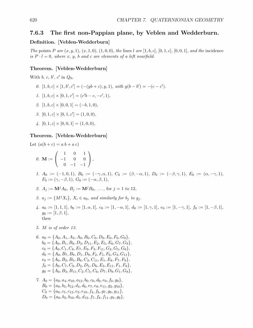
620 CHAPTER 7. QUATERNIONIAN GEOMETRY
7.6.3 The first non-Pappian plane, by Veblen and Wedderburn.
Definition. [Veblen-Wedderburn]
The points P are (x, y, 1), (x, 1, 0), (1, 0, 0), the lines l are [1, b, c], [0, 1, c], [0, 0, 1], and the incidenceis P · l = 0, where x, y, b and c are elements of a left nearfield.
Theorem. [Veblen-Wedderburn]
With b, c, b′, c′ in Q9,
0. [1, b, c]× [1, b′, c′] = (−(yb+ c), y, 1), with y(b− b′) = −(c− c′).
1. [1, b, c]× [0, 1, c′] = (c′b− c,−c′, 1),
2. [1, b, c]× [0, 0, 1] = (−b, 1, 0),
3. [0, 1, c]× [0, 1, c′] = (1, 0, 0),
4. [0, 1, c]× [0, 0, 1] = (1, 0, 0),
Theorem. [Veblen-Wedderburn]
Let (a(b+ c) = a b+ a c)
0. M :=
1 0 1−1 0 0
0 −1 −1
,
1. A0 := (−1, 0, 1), B0 := (−γ, α, 1), C0 := (β,−α, 1), D0 := (−β, γ, 1), E0 := (α,−γ, 1),F0 := (γ,−β, 1), G0 := (−α, β, 1),
2. Aj := MjA0, Bj := MjB0, . . . , for j = 1 to 12,
3. aj := M jXi, Xi ∈ a0, and similarly for bj to gj.
4. a0 := [1, 1, 1], b0 := [1, α, 1], c0 := [1,−α, 1], d0 := [1, γ, 1], e0 := [1,−γ, 1], f0 := [1,−β, 1],g0 := [1, β, 1],then
5. M is of order 13.
6. a0 = A0, A1, A3, A9, B0, C0, D0, E0, F0, G0,b0 = A0, B1, B8, D3, D11, E2, E5, E6, G7, G9,c0 = A0, C1, C8, E7, E9, F3, F11, G2, G5, G6,d0 = A0, B7, B9, D1, D8, F2, F5, F6, G3, G11,e0 = A0, B2, B5, B6, C3, C11, E1, E8, F7, F9,f0 = A0, C7, C9, D2, D5, D6, E3, E11, F1, F8,g0 = A0, B3, B11, C2, C5, C6, D7, D9, G1, G8,
7. A0 = a0, a4, a10, a12, b0, c0, d0, e0, f0, g0,B0 = a0, b5, b12, d4, d6, e7, e8, e11, g2, g10,C0 = a0, c5, c12, e2, e10, f4, f6, g7, g8, g11,D0 = a0, b2, b10, d5, d12, f7, f8, f11, g4, g6,

7.6. THE HUGHES PLANES. 621
E0 = a0, b7, b8, b11, c4, c6, e5, e12, f2, f10,F0 = a0, c2, c10, d7, d8, d11, e4, e6, f5, f12,G0 = a0, b4, b6, c7, c8, c11, d2, d10, g5, g12,
8. Xj ι xk =⇒ Xj+l mod 13 ι xk+l mod 13.
Given a0, to g0, it is easy to verify that A0 is on all these lines and determine B0 to G0 all ona0 and B0 on b0, C0 on c0, . . . .Having determined, the other points using 2, it is easy to verify which points are on b0, . . . .The notation helps gretaly in justifyong that 2 points have one and only one line in common and 2liners have only one point in common. The notation can be made even more compact. See 7.6.4.
The following are the powers of M .
M2 =
1 −1 0−1 0 −1
1 1 1
, M3 =
−1 0 0−1 1 0
0 −1 0
, M4 =
−1 −1 11 0 −11 0 0
, M5 =
0 −1 11 1 −11 0 1
,
M6 =
1 −1 −10 1 −11 −1 0
, M7 =
−1 1 −1−1 1 1−1 0 1
, M8 =
1 1 01 −1 1−1 −1 1
, M9 =
0 0 1−1 −1 0
0 −1 1
,
M10 =
0 −1 −10 0 −11 −1 −1
, M11 =
1 1 10 1 −1−1 1 1
, M12 =
0 −1 0−1 −1 −1
1 1 0
, M13 =
1 0 00 1 00 0 1
.
Example. [Veblen-Wedderburn]
With the notationnon−Desargues(C〈c0, c1, c2〉, A0, A1, A2a0, a1, a2, B0, B1, B2b0, b1, b2;C0, C1, C2d0, d1, d2), with di := Ci+j × Ci−j ,the following configuration shows that the Desargues axiom is not satisfiednon−Desargues(A0〈b0, f0, d0〉, B1, C7, F2c12, e8, e9, D3, E3, D1b11g7, a3;G5, B10, F3d1, c0, b9).
7.6.4 The miniquaternionian plane Ψ.
Definition.
With i ∈ 0, 1, 2, i′ ∈ 0′, 1′, 2′, j ∈ 0, 1, . . . , 12, and the addition being performed modulo 3 forthe first element of a pair, and modulo 13, for the second element in the pair or for the element,if single, then the elements and incidence in the miniquaternionian plane Ψ are defined as follows.(See 7.6.4
0. The 91 points P are (j), (i, j), (i′, j),
1. The 91 lines l are [j], [i, j], [i′, j],
2. The incidence is defined by[j] := (−j), (1− j), (3− j), (9− j), (i,−j), (i′,−j),[i, j] := (−j), (i, 2− j), (i, 5− j), (i, 6− j), (i′ + 1, 3− j), (i′ + 1, 11− j),
(i′ − 1, 7− j)(i′ − 1, 9− j), (i′, 1− j), (i′, 8− j),[i′, j] := (−j), (i′, 2− j), (i′, 5− j), (i′, 6− j), (i− 1, 3− j), (i− 1, 11− j),
(i+ 1, 7− j)(i+ 1, 9− j), (i, 1− j), (i, 8− j).
giving the 10 points on each line. i and i′ in the same definiton correspond to the same integer, 0,03-’ or 1, 1’ . . . .

622 CHAPTER 7. QUATERNIONIAN GEOMETRY
Exercise.
7.6.4.2 is similar to the use of ordered cosets to determine efficiently operations of finite as well asinfinite groups. In this case, [j] is a subplane, [i, j] and [i′, j] are copseudoplanes.
0. Perform a similar representation of points, lines and incidence starting with a subplane whichis a Fano plane.
1. Determine similar representations for non Desarguesian geometries of order 52, using a sub-plane of order 4, or of order 5 (651 = 31 · 21).
2. Determine other such representation for non Desarguesian geometries of higher order.
Theorem.
The same incidence relations obtain, if we interchange points and lines in 7.6.4.2.
Theorem. [see Room and Kirkpatrick]
0. 0 The correspondance (j) to [j] and (i, j) to [i, j] and (i′, j) to [i′, j] is a polarity P0 (J ∗).
1 The 16 auto-poles are (0), (7), (8), (11), (0,8), (0,12), (1,4), (1,7), (2,10), (2,11),(0’,8), (0’,12), (1’,4), (1’,7), (2’,10), (2’,11).
1. 0 The correspondance (j) to [j] and (i, j) to [i′, j] and (i′, j) to [i, j] is a polarity P1 (J ′∗).
1 The 22 auto-poles are (0), (7), (8), (11), (0,1), (0,3), (0,9), (1,1), (1,3), (1,9), (2,1),(2,3), (2,9), (0’,1), (0’,3), (0’,9), (1’,1), (1’,3), (1’,9), (2’,1), (2’,3), (2’,9).
2 (0), (7), (8), (11), (0,1), (1,9), (2,3), (0’,9), (1’,3), (2’,1),(0), (7), (8), (11), (1,1), (2,9), (0,3), (2’,9), (0’,3), (1’,1),(0), (7), (8), (11), (2,1), (0,9), (1,3), (1’,9), (2’,3), (0’,1) are ovals.
Exercise.
0. Prove that the correspondance (j) to [j] and (i, j) to [(i + 1)′, j] and (i′, j) to [i − 1, j] is apolarity P2.
1. Prove that the correspondance (j) to [j] and (i, j) to [(i − 1)′, j] and (i′, j) to [i + 1, j] is apolarity P3.
Exercise.
0. Determine a configuration in 7.6.4.0.2, which gives an example were the Theorem of Pascalis satisfied and an other, in which it is not satisfied.
1. Determine ovals which are subsets of 7.6.4.1.1.
Theorem.
The polar m of a point M with respect to a triangle is incident to that point.
Indeed, we can always assume thast the triangle consists of the real points A0 = (0), A1 = (1),A2 = (2), and that M = (5) = (1, 1, 1). It follows that m = [4] = [1,1,1] which is incident to M .

7.6. THE HUGHES PLANES. 623
Exercise.
Check that the other points and lines of the polar construction are Mi = (4), (8), (3), MAi =(10), (12), (9), MMi = (7), (6), (11), ai = [12], [1], [0], mai = [9], [8], [11], mi = [3], [2], [7], mmi =[6], [10], [5].
Theorem. [see Room and Kirkpatrick]
0. The planes obtained by taking the complete quadrangle associated with 3 real points A0,A1, A2, and a point M which such that none of the lines M × Ai are real are Fano planesassociated with Z2.
1. There are (1613.12.9).24 = 5616 Fano planes that contain 3 real points.
Notation.
For a Fano subplane with 7 elements, I will use the notation associated with the selector 0, 1, 3 andconstruction:Given a complete quadrangle 0, 1, 2, 5,0∗ := 0× 1, 6∗ := 1× 2, 1∗ := 2× 0, 5∗ := 2× 5, 3∗ := 0× 5, 2∗ := 1× 5,3 := 0∗ × 5∗, 4 := 6∗ × 3∗, 6 := 1∗ × 2∗, 4∗ := 3x6. The Fano plane propery implies 4ι4∗.The configuration is denoted by Fano(0, 1, 2, 3, 4, 5, 6, 0∗, 1∗, 2∗, 3∗, 4∗, 5∗, 6∗).
Example.
The following is a Fano plane configuration: Fano((0), (1), (2), (2, 0), (1, 1), (0, 3), (1′, 12),[0], [1], [0, 12], [1′, 0], [1′, 6], [0′, 11], [12]).
Exercise.
Determine the Fano plane associated with (0), (1), (2), (0,7).
Comment.
The correspondance between the notation of Veblen-Wedderburn and Room-Kirkpatrick isV eblen−Wedderburn aj bj cj dj ej fj gjRoom−Kirkpatrick kj aj bj cj a′j b′j c′jDe V ogelaere [−j] [0,−j] [2′,−j] [1,−j] [0′,−j] [1′,−j] [2,−j]V eblen−Wedderburn Aj Bj Cj Dj Ej Fj Gj
Room−Kirkpatrick Kj A′j C′
j B′j Aj Cj Bj
De V ogelaere (j) (0′, j) (2, j) (1′, j) (0, j) (1, j) (2′, j)
Example. [Veblen-Wedderburn]
The example 7.6.3 becomes with the above notation((0)〈[0, 0], [1′, 0], [2, 0]〉, (0, 1), (1, 7), (1′, 2[1, 1], [0′, 8], [0′, 9], (2, 3), (0′3), (2, 1)
[0, 11], [2′, 7], [10];(2′, 5), (0, 10), (1′, 3)[2, 1], [1, 0], [0, 4]).
Problem.
Can we characterize the plane Ψ using Theorem 7.6.4.0.

624 CHAPTER 7. QUATERNIONIAN GEOMETRY
Definition.
The Singer matrix G :=
0 0 11 0 10 1 0
. Its powers Gk are the columns
k, k + 1, k + 2 ofk = 0 1 2 3 4 5 6 7 8 9 10 11 12
1 0 0 1 0 1 1 1 −1 −1 0 1 −10 1 0 1 1 1 −1 −1 0 1 −1 1 00 0 1 0 1 1 1 −1 −1 0 1 −1 1
move to g6a.tex:
Answer to 7.6.2.
κ = λ = 0 1 −1 α −α β −β γ −γα r 0 0 0 −1 1 −1 1 −1 1
s 0 1 −1 0 0 −1 1 1 −1
β r 0 0 0 −1 1 −1 1 −1 1s 0 1 −1 1 −1 0 0 −1 1
γ r 0 0 0 −1 1 −1 1 −1 1s 0 1 −1 −1 1 1− 1 0 0
For −α, −β, −γ, change the sigh
of r.
Definition.
The elements and incidence in the miniquaternionian plane Ψ are defined as follows.
0. The points are (ξ0, ξ1, ξ2) with right equivalence,
1.
2. A point P is incident to a line l iff

7.6. THE HUGHES PLANES. 625
Partial answer to 7.6.4.
For n = 72, 2451 = 57.43, for n = 92, 6643 = 91.73, for n = 112, 14763 = 57.259, For n = 132,28731 = 3.9577.
Answer to 7.6.4.
We have Fano((0), (1), (2), (1′0), (2, 1), (0, 7), (1′, 12), [0], [1], [0, 12], [2′, 0], [1′, 6], [0,−2], [12]).
Answer to 7.6.4.
(7) × (8) = [6], [6] × [0] = (3), (8) × (0) = [1], [1] × [7] = (2), (0) × (7) = [9], [9] × [8] = (5),〈(3), (2), (5); [11]〉.(7)×(8) = [6], [6]×[0, 1] = (1′, 7), (8)×(0, 1) = [0, 5], [0, 5]×[7] = (0′, 6), (0, 1)×(7) = [2′, 6], [2′, 6]×[8] = (2, 5), (2, 5) is not incident to (1′, 7)× (0′6) = [2, 2].This has not been checked.
From Dembowski, p. 129
Definition.
A linear ternary ring (Σ,+, ·) is called a cartesian field iff (Σ,+) is associative and is therefore agroup.
Definition.
A cartesian field is called a quasifield iff the right distributivity law holds:(x+ y)z = xz + yz.
Artzy adds that xa = xb + c has a unique solution, but this is a property (28). This is Veblen-Wedderburn.
Definition.
A quasifield is called a semifield iff the left distributivity law holds:z(x+ y) = zx+ zy.
Definition.
A quasifield is called a nearfield iff (Σ, ·) is associative and is therefore a group.
Definition.
A semifield is called a alternative field iff x2y = x(xy) and xy2 = (xy)y.
Theorem.
P is (p, L) transitive iff P is (p, L) Desarguesian. p is point, L is a line. Dembowski p.123, 16Let Q0 = (79), Q1 = (80), Q2 = (90), and U = (81) then q2 = [79], q0 = [90], q1 = [80],
v = [88], i = [78], V = (78), I = (82), j = [89], W = (89),Points on q2 : 86,12,25,38,51,64,77Points on q1 : 85,11,24,37,50,63,76

626 CHAPTER 7. QUATERNIONIAN GEOMETRY
11×12 = [7] : 84(78, 86), 8(51, 25), 43(77, 64), 48(86, 38), 52(12, 12), 54(25, 78), 66(64, 80), 72(38, 51),11×25 = [61] : 82(78, 80), 0(64, 64), 18(12, 51), 28(51, 78), 33(77, 12), 58(38, 86), 61(86, 25), 62(25, 38),11×38 = [75] : 81(78, 78), 4(38, 25), 14(12, 80), 19(77, 86), 36(51, 64), 70(64, 38), 73(25, 51), 74(86, 12),11× 51 = [4] : 87(86, 86), 1(38, 80), 2(77, 78), 46(25, 64), 55(78, 38), 57(51, 12), 69(64, 51), 75(12, 25),11×64 = [8] : 83(86, 78), 7(64, 25), 10(77, 51), 42(78, 12), 47(12, 64), 53(51, 80), 65(38, 38), 71(25, 86),11×77 = [68] : 88(86, 80), 5(38, 64), 13(51, 51), 21(77, 38), 30(25, 12), 32(64, 86), 67(12, 78), 68(78, 25),Coordinates of points:
(0) 64, 64 38, 80 77, 78 78, 51 38, 25 38, 64 51, 86 64, 25(8) 51, 25 86, 77 77, 51 80, 77 12 51, 51 12, 80 64, 78
(16) 78, 77 12, 38 12, 51 77, 86 51, 38 77, 38 86, 64 64, 77(24) 80, 64 25 77, 77 25, 80 51, 78 78, 64 25, 12 25, 77(32) 64, 86 77, 12 64, 12 86, 51 51, 64 80, 51 38 25, 25(40) 77, 80 38, 78 78, 12 77, 64 77, 25 12, 86 25, 64 12, 64(48) 86, 38 38, 12 80, 38 51 12, 12 51, 80 25, 78 78, 38(56) 51, 77 51, 12 38, 86 12, 77 38, 77 86, 25 25, 38 80, 25(64) 64 38, 38 64, 80 12, 78 78, 25 64, 51 64, 38 25, 86(72) 38, 51 25, 51 86, 12 12, 25 80, 12 77 78 80, 80(80) 0 78, 78 78, 80 86, 78 78, 86 80, 86 86 86, 86(88) 86, 80 80, 78 ∞
Coordinates of lines:[0] 78, 38 38 77, 78 12, 12 51, 77 86, 38 12, 86 12, 77[8] 64, 77 77, 25 64, 12 80, 25 51, 80 78, 12 12 64, 78
[16] 25, 25 77, 64 86, 12 25, 86 25, 64 51, 64 64, 38 51, 25[24] 80, 38 77, 80 78, 25 25 51, 78 38, 38 64, 51 86, 25[32] 38, 86 38, 51 77, 51 51, 12 77, 38 80, 12 64, 80 78, 77[40] 77 38, 78 51, 51 12, 38 86, 77 51, 86 51, 38 25, 38[48] 38, 64 25, 51 80, 64 12, 80 78, 51 51 25, 78 64, 64[56] 38, 25 86, 51 64, 86 64, 25 12, 25 25, 77 12, 64 80, 77[64] 38, 80 78, 64 64 12, 78 77, 77 25, 12 86, 64 77, 86[72] 77, 12 38, 12 12, 51 38, 77 80, 51 25, 80 78, 80 ∞[80] 80 78, 78 86 86, 78 86, 86 80, 86 86, 80 78, 86[88] 78 80, 78 80, 80
[80] : 11(80, 77), 24(80, 64), 37(80, 51), 50(80, 38), 63(80, 25), 76(80, 12), 79(80, 80), 85(80, 86), 89(80, 78), 90(/infty)B = A+ α, (A,B) ι [V, Y ], V = (78), (76) = (80, 12) = (0, α), Y × V = (78)× (76) = [13].[13] : 78(78), 15(64, 78), 18(12, 51), 19(77, 86), 68(78, 25), 76(80, 12), 46(25, 64), 48(86, 38), 53(51, 80), 60(38, 77)hence 12 = 80 + α, 51 = α + α = −α, 25 = 78 + α = 1 + α = γ, 64 = 25 + γ = γ + γ = −β,38 = 86 + α = −1 + α = β, 77 = 38 + α = β + α = −γ.∞ 0 1 −1 α −α β −β γ −γ90 80 78 86 12 51 38 64 25 77
[α, 0] = (12)× (80, 80) = (12)× (79) = [51], (a, b) ι [51] =⇒ b = a · α.(42) = (78, 12) = (1, α) =⇒ α = 1× α,(45) = (12, 86)− (α,−1) =⇒ −1 = α× α,(23) = (64, 77) = (−β,−γ) =⇒ −γ = −β × α,(28) = (51, 78) = (−α, 1) =⇒ 1 = −α× α,(35) = (86, 51) = (−1,−α) =⇒ −α = −1× α,
Using DATA 6,0, 6,4, 6,10, 6,12, 0,0, 1,0, 2,0, 3,0, 4,0, 5,0 DATA 6,0, 0,7, 0,8, 0,11, 3,2,3,10, 4,4, 4,6, 5,5, 5,12 gives the same multiplication table give left not right distibutive law withQi = 79, 81, 87, U = (83), α = (12), q0 = [87] = 79, 81, 82, 86, 4, 17, . . .,

7.7. AXIOMATIC. 627
q1 = [81] = 79, 85, 87, 88, 10, 23, . . .,q2 = [79] = 81, 87, 89, 90, 12, 25, . . .,with case 7, data 79,81,87,83,12:∞ = 87, 0 = 81, 1 = 89, −1 = 90, α = 12, −α = 77, β = 38, −β = 51, γ = 25, −γ = 64.
This is a try for a section to be included in g19.tex between Moufang and Desargues.
7.7 Axiomatic.
7.7.1 Veblen-MacLagan planes.
Introduction.
The first example of a Veblen-Wedderburn plane was given in 1907 by Veblen and MacLagan-Wedderburn. It is associated to the algebraic structure of a nearfield, which is a skew field whichlacks the left distributive law, hence is an other plane between the Veblen-Wedderburn plane andthe Desarguesian plane.
Axiom. [Da] 6
Given a Veblen-Wedderburn plane, 2 points Q1 and Q2 on the ideal line and an other point Q0 noton it, any 2 parallelograms Ai and Bi with directions Q1 and Q2, with no sides in common . . . ,???,such that Aj and Bj are perspective from Q0 for j = 0 To 2, imply that A3 and B3 are perspectivefrom Q0.
Notation.
Da(Q0, Q1, Q2, Aj, Bj).
Definition.
A Veblen-MacLagan plane is a Veblen-Wedderburn plane in which the axiom Da is satisfied.
Lemma. [For Associativity]
H1.0. A0, a12, x, (See Fig. 2?.)D1.0. a01 := Q1 ×A0, a02 := Q2 ×A0,D1.1. A1 := a01 × a12, A2 := a02 × a12,D1.2. a13 := Q2 ×A1, a23 := Q1 ×A2, A3 := a13 × a23,D2.0. a0 := Q0 × A0, a1 := Q0 × A1, a2 := Q0 × A2, a3 := Q0 × A3, D2.1. B0 := a0 × y,b01 := Q1 ×B0, b02 := Q2 ×B0,D2.1. B1 := b1 × b01, B2 := b2 × b02, D2.2. b13 := Q2 ×B1, b23 := Q1 ×B2, B3 := b13 × b23,C1.0. B3 ι b3,MoreoverA0 = (A,B), A1 = (A′, B), A2 = (A,B′), A3 = (A′, B′), B0 =Proof: Da(Q0, Q1, Q2, Aj, Bj).
6Da for Desargues leading to associativity of multiplication.

628 CHAPTER 7. QUATERNIONIAN GEOMETRY
Theorem.
In a Veblen-MacLagan plane, the ternary ring (Σ, ∗) is a nearfield.:
0. (Σ,+) is an Abelian group,
1. (Σ− 0, ·) is a group,
2. (Σ, ∗) = (Σ,+, ·) is right distributive, (a+ b) · c = a · c+ b · c.
7.7.2 Examples of Perspective planes.
Theorem.
0. The Cayleyian plane is not a Veblen-MacLagan plane.replace Desarg.?
Definition.
A miniquaternion plane . . . .
Theorem.
0. A miniquaternion plane is a Veblen-MacLagan plane.
1. A miniquaternion plane is not a Moufang plane.
Tables.
The following are in an alternate notation the known table for p = 3 and a new table for p = 5.The other incidence are obtained by adding one to the subscripts of the lines and subtracting onefor the subscript of the points.
7.8 Bibliography.
1. Artzy, Rafael, Linear Geometry, Reading Mass., Addison-Wesley, 1965, 273 pp.
2. Baumert, Leonard D., Cyclic Difference Sets, N. Y., Springer, 1971.
3. Dembowski, Peter, Finite Geometries, Ergebnisse der Mathematik und ihrer Grenzgebiete,Band 44, Springer, New-York, 1968, 375 pp.
4. Dickson, Gottingen Nachrichten, 1905, 358-394.
5. Hall, Marshall, Projective Planes , Trans. Amer. Math. Soc., Vol. 54, 1943, 229-277.
6. Hughes, D. R., A class of non-Desarguesian projective planes, Canad. J. of Math., Vol. 9,1957, 378-388. (I,9.p.1)
7. Lemay, Fernand, Le dodecaedre et la geometrie projective d’ordre 5, p. 279-306 of Johnson,Norman L., Kallaher, Michael J., Long Calvin T., Edit., Finite Geometries, N. Y., MarcelDekker Inc. 1983.

7.8. BIBLIOGRAPHY. 629
8. Maclagan-Wedderburn, J. H., A theorem on finite algebras, Trans. Amer. Math. Soc., Vol.6, 1905, 349. (A finite skew-field is a field)
9. Moore, E. H., Mathematical Papers, Chicago Congress, 1893, 210-226. (Def. of GaloisFields.)
10. Room, Thomas Gerald and Kirkpatrick P. B., Miniquaternion geometry; an introduction tothe study of projective planes, Cambridge [Eng.] University Press, 1971.
11. Rosati, L. A., I gruppi di collineazioni dei pliani di Hughes. Boll. Un. Mat. Ital. Vol. 13,505-513.
12. Singer, James, A Theorem in Finite Projective Geometry and some applications to numberTheory, Trans. Amer. Math. Soc., Vol. 43, 1938, 377-385
13. Vahlen, Karl Theodor, Abstrakte Geometrie, Untersuchungen uber die Grundlagen der Euk-lidischen und nicht-Euklidischen Geometrie, Mit 92 abbildungen im text, 2., neubearb. aufl.Leipzig, S. Hirzel, 1940, Series title: Deutsche mathematik, im auftrage der Deutschenforschungsgemeinschaft, 2. beiheft.
14. Veblen, Oswald & Bussey, W. H., Finite Projective Geometries, Trans. Amer. Math. Soc.,Vol. 7, 1906, 241-259. (On PG(n, pk))
15. Veblen, Oswald, and Wedderburn, Jospeh Henri MacLagan, Non-Desarguesian and non-Pascalian geometries, Trans. Amer. Math. Soc., Vol. 8, 1907, 379-388.
16. Zappa, G. Sui gruppi di collineazioni dei paini di Hughes, Boll. Un. Mat. Ital. (3), Vol. 12,1957, p. 507-516.

630 CHAPTER 7. QUATERNIONIAN GEOMETRY
7.90 Answer to problems and Comments.
Notation.
uij := qiq−1j − rir
−1j ,
vij := qiq−1j + rir
−1j ,
si := −v−1i,i−1vi,i+1,
ai := −v−1i−1,iui−1,i+1,
ti := si+2si+1,fi := si − s−1
i+1s−1i−1,
gi := t−1i − ti+1ti−1,
ki := q′i−1qi+1,li := r′i−1ri+1.
Exercise.
Prove q−11 u12r2 + q−1
2 u20r0 + q−10 u01r1 = 0,
associated with M · eul = 0.
The proof follows form substitution of uij by their definition.
Exercise.
Prove u12u−102 u01 = −u10u
−120 u21, associated with 2 equivalent forms of eul one for which the first
coordinate is one and the other obtain by “rotation”, the second coordinate being one.
Form the definition of u02 it follows by multiplication to the right or left by u−102 , that
q0q−12 u−1
02 − r0r−12 u−1
02 = 1,u−1
02 q0q−12 − u
−102 r0r
−12 = 1.
Moreover,u20 = q2q
−10 − r2r
−10 = −q2q
−10 u02r2r
−10
oru−1
20 = r0r−12 u−1
02 q0q−12 .
If we substitute in the identity to prove, with both terms in the second member, u12, u01, u10
and u21, by their definition, we getq1q−12 u−1
02 q0q−11 − q1q
−12 u−1
02 r0r−11
− r0r−11 u−1
02 q1q−12 + r0r
−11 u−1
02 r1r−12
− q1q−10 r0r
−12 u−1
02 q0q−12 q2q
−11 + q1q
−10 r0r
−12 u−1
02 q0q−12 r2r
−11
+ r1r−10 r0r
−12 u−1
02 q0q−12 q2q
−11 − r1r
−10 r0r
−12 u−1
02 q0q−12 r2r
−11 = 0,
because terms 3 and 7 cancel, terms 1 and 5 as well as 4 and 8 give 1 and -1, terms 2 and 6 give0 by application of the identities given at the begginning of the proof.
Lemma.
0. norm(s0s1s2) = 1.
1. norm(t0t1t2) = 1.
2. s′2f2s−10 = −f2s1.
3. t2g2t0 = −g2t−11 .

7.90. ANSWER TO PROBLEMS AND COMMENTS. 631
Proof: For 0, we use Lemma 7.1.1 and obtain 1, from the definition of ti. For 2, we substitutef2 by its definition and compare the terms of both sides of the equality which have the same sign.
Proof of 7.1.2.
LetG0.0. A0 = (1, 0, 0), A1 = (0, 1, 0), A2 = (0, 0, 1),G0.1. M = (q0, q1, q2), M = (r0, r1, r2),thenP1.0. a0 = (1, 0, 0), a1 = (0, 1, 0), a2 = (0, 0, 1),P1.1. ma0 = [0, q′1,−q′2], ma0 = [0, r′1,−r′2],P1.2. M0 = (0, q1, q2), M0 = (0, r1, r2),P1.3. eul = [1,−u′12u02,−u′21u01],
P1.4. S =
q−n0 −q′0q−11 −q′0q
−12
−q′1q−10 q−n1 −q′1q
−12
−q′2q−10 −q′2q
−11 q−n2
, S−1 =
0 q0q1 q0q2
q1q0 0 q1q2
q2q0 q2q1 0
.
S =
r−n0 −r′0r−11 −r′0r
−12
−r′1r−10 r−n1 −r′1r
−12
−r′2r−10 −r′2r
−11 r−n2
, S−1
=
0 r0r1 r0r2
r1r0 0 r1r2
r2r0 r2r1 0
.
P2.0. mm0 = [−q′0, q′1, q′2], mm0 = [−r′0, r′1, r′2],P2.1. MA0 = (0, q1,−q2), MA0 = (0, r1,−r2),P2.2. m0 = [0, q′1, q
′2], m0 = [0, r′1, r
′2],
P2.3. MM0 = (−q0, q1, q2), MM0 = (−r0, r1, r2),P2.4. m = [q′0, q
′1, q′2], m = [r′0, r
′1, r′2],
P2.5. Ima0 = (−2q0, q1, q2), Ima0 = (−2r0, r1, r2),Ima0 = (−q0(q−1
1 r1 + q−12 r2), r1, r2), Ima0 = (−r0(r−1
1 q1 + r−12 q2), q1, q2),
P2.6. iMA0 = [2q′0,−q′1,−q′2], ıMA0 = [2r′0,−r′1,−r′2],
P3.0. mf0 = [k1v′21u21, k
−10 ,−1], mf0 = [l1v
′21u21,−l−1
0 , 1],P3.1. O = [], O = [],P3.2. Mfa0 = (k2, 0,−k′0v10u
−110 ), Mfa0 = (l2, 0, l
′0v10u
−110 ),
Mfa0 = (1, k′2v02u′02, 0), Mfa0 = (1,−l′2v02u
′02, 0),
P3.3. mfa0 = (k1v′21u21, k
−10 , 0), mfa0 = (l1v
′21u21,−l−1
0 , 0),mfa0 = (k1v
−121 u21, 0,−1), mfa0 = (l1v
−121 u21, 0, 1),
P3.4. Mfm0 = (k−11 v21u
−121 ,−k0, 1), Mfm0 = (l−1
1 v21u−121 , l0,−1),
P4.0. Imm0 = (a0, 1, s0), Imm0 = (−a0, 1, s0),P4.1. ta0 = [0, 1,−s′0],P4.2. T0 = (1, s2, s
−11 ),
P4.3. at0 = [0, s′2,−s1] = [0, 1,−t0],P4.4. K0 = (1, t−1
2 , t1),P4.5. Taa0 = (0, 1, s0),P4.6. poK0 = [−1, s′2, s1],
P4.7. T =
0 f2 −f2s−10
f2 0 −f2s1
−s′0f2 −s1f2 0
, T−1 =
1 s2 s′1s2 sn2 s−n1 s−1
0
s−11 sn2s0 s−n1
.
P4.8. L =
0 g2 −g2t0g2 0 −g2t
−11
−t0g2 −t′1g2 0
, L−1 =
1 t′2 t1t−12 t−n2 tn1 t0t1 tn1 t0 tn1
.

632 CHAPTER 7. QUATERNIONIAN GEOMETRY
Proof:For P4.0, if the coordinates of Imm0 are x0, 1 and x2, we have to solve
q−10 x0 + q−1
1 + q−12 x2 = 0,
− r−10 x0 + r−1
1 + r−12 x2 = 0.
Multiplying the equations to the left respectively by q2 and −r2, or by q0 and r0 and adding givesx0 and x2 using the notation 7.90.For P4.7, it is easier to obtain T−1 first, the columns are T0, T1, T2, multiplied to the right by 1,sn2 , s
−n1 . The matrix T is then obtained using Theorem 7.1.1, multiplying by −s−n1 . The equivalence
with the matrix whose columns ate tai can be verified using Lemma 7.90.2. A similar proof givesP4.8.
Theorem.
The product of the diagonal elements of T−1 and of L−1 is the same.This follows from Lemma 7.1.1.The correspondance between the definitions in EUC and here is as follows
D0.0 D1.0 D0.1 D1.1 D0.2 D1.2 D1.0 D1.3 D36.12 DC1.4D0.3 D2.0 D0.4 D2.1 D0.5 D2.2 D0.6 D2.3 D0.7 D2.4D10.3 D2.5 D0.25 D2.6 D10.3 D2.7 D6.0 D3.0 D6.4 D3.1? D3.2 ? D3.3 D14.0?D3.4 D1.6 D4.0 D1.7 D4.1D1.8 D4.2 D12.1 D4.3 D1.2 D4.4 D1.4 D4.4 D1.9 D4.5D15.12?D4.6 D1.19 DC4.7 DC4.8

Chapter 8
FUNCTIONS OVER FINITEFIELDS
8.0 Introduction.
Notation.
The first notation is standard, the second is useful for Theorem 8.2.1.2.1.(a)i :=
∏i−10 (a+ i) = a(a+ 1) . . . (a+ i− 1).
[a]i :=∏i−1
0 (a+ 2i) = a(a+ 2) . . . (a+ 2i− 2).
Notation.
The following notation, favored on the European continent, but seldom used elsewhere, is quiteuseful:
0!! := 12n!! := 2.4. . . . .2n.(2n+ 1)!! := 1.3. . . . .(2n+ 1).
8.1 Polynomials over Finite Fields.
8.1.1 Definition and basic properties.
Introduction.
In a finite field, we can define polynomials of degree up to p − 1. These are determined by theirvalues at i in Zp. If these are defined in the real field with rational coefficients, the definition andproperties automatically extend to the finite field.
Definition.
A polynomial is a function a0Ip−1 + a1I
p−2 + . . .+ ap−1
which associates to x ∈ Zp the integera0x
p−1 + a1xp−2 + . . .+ ap−1.
The polynomial is of degree k iff a0 . . . ap−k−1 are congruent to 0 modulo p and ap−k is not.
633

634 CHAPTER 8. FUNCTIONS OVER FINITE FIELDS
Theorem. [Lagrange]
Given k + 1 distinct integers xi (modulo p), k < p, and given k + 1 integers fi, ∃ a polynomial Pof degree k 3
P (xi) = fi, i = 0 to k.
8.1.2 Derivatives of polynomials.
Definition.
The derivative of the polynomial 8.1.1.0 is (p− 1)a0Ip−2 + (p− 2)a1I
p−3 + . . .+ ap−2.
8.2 Orthogonal Polynomials over Finite Fields.
8.2.0 Introduction.
The main purpose of writing this Chapter is connected with interesting symmetry properties of theorthogonal polynomials, in Zp. In the classical theory there is a scaling factor which is arbitrairelychosen for each of the families of orthogonal polynomials. For some time now, the same scalingfactor, in each case, is universely used. When determining values of the Chebyshev polynomials forsome small values of p, I was struck by the symmetry properties given in 8.2.2 and 8.2.2. Theseproperties are dependent on the scaling factors and it turns out that the unanimously acceptedones are essentially the only ones giving this property. The same property has been found for thepolynomials of Legendre and of Laguerre. For the polynomial of Hermite this is not the case. I havesucceeded in obtaining some scaling, given in 8.2.5 for which a symmetry can be obtained. Thisscaling is given by expressions which are different for the even and for the odd Hermite polynomials,therefore the recurrence relation has a constant whose expression differs for even and odd indices.It is therefore possible to give an a-posteriori justification of the scaling factor for the classicalpolynomial, and there is some reason to introduce a different scaling for the Hermite polynomials.The case of the Jacobi polynomials with 2 parameters a and b is left as an exercise. With a = b,again a scaling is required to obtain symmetry.
8.2.1 Basic Definitions and Theorems.
Introduction.
For orthogonal polynomials, recurrence relations, differential equations and values of the coefficientsgeneralize automatically, from the classical case. Therefore, we have the definitions 8.2.1 and thetheorems 8.2.1 to 8.2.1.
Definition.
The polynomials of Chebyshev of the first (Tn) and of the second kind (Un), of Legendre (Pn), ofLaguerre (Ln) and of Hermite (Hn) are defined by the recurrence relations:
0. T0 := 1, T1 := I, Tn+1 := 2(2I − 1)Tn − Tn−1,
1. U0 := 1, U1 := 2I, Un+1 := 2(2I − 1)Un − Un−1,

8.2. ORTHOGONAL POLYNOMIALS OVER FINITE FIELDS. 635
2. P(a)0 := 1, P
(a)1 := I,
(n+ 2a+ 1) P(a)n+1 := (2n+ 2a+ 1)I P
(a)n − n P (a)
n−1, a ≥ 0, n < p− 1− 2a,
3.0. L0 := 1, L1 := 1− I,(n+ 1)Ln+1 := (2n+ 1− I)ILn − nLn−1, n < p− 1,
1. L(a)0 := 1, L
(a)1 := a+ 1− I,
(n+ 1)L(a)n+1 := (2n+ a+ 1− I)L
(a)n − (n+ a)L
(a)n−1, n < p− 1,
4. H0 := 1, H1 := 2I, Hn+1 := 2IHn − 2nHn−1.
The Legendre polynomial is Pn := P(0)n and P
(a)n := n!a!
(n+a)! P(a,b)n , where P
(a,b)n , are the polyno-
mials of Jacobi, scaled so that P(a)n (1) = 1.
L(a)n are the generalized Laguerre polynomials and Ln = L
(0)n .
See for instance Handbook of Mathematical functions, p. 782.
Theorem.
If Xn,j denotes the coefficient of Ij in the polynomial Xn,
0. Tn,n−2j = 12n2(n−2j)(−1)j (n−j−1)!
j!(n−2j)! ,
1. Un,n−2j = 12n2(n−2j)(−1)j (n−j)!
j!(n−2j)! ,
2.0. Pn,n−2j = 2(−n)(−1)j (2n−2j)!j!(n−j!(n−2j)! ,
1. P(a)2n,2j = (−1)(n− j)
(nj
)[2a+2n+1]j [2j+1]n−j
[2a+2]n,
P(a)2n,2j = (−1)(n− j)
(nj
)[2a+2n+3]j [2j+3]n−j
[2a+2]n,
3.0. Ln,j = (−1)j n!(n−j)!j!2 ,
1. L(a)n,j = (−1)j (n+a)!
(n−j)!(a+j)!j! ,
4. Hn,n−2j = n!2(n−2j)(−1)j 1j!(n−2j)! ,
See for instance Handbook of Mathematical functions, p. 775.
Theorem.
The polynomials of Chebyshev, of the first (Tn) and of the second kind (Un), of Legendre (Pn), ofLaguerre (Ln) and of Hermite (Hn) satisfy by the differential equations
0. (1− I2)D2Tn − IDTn + n2Tn = 0,
1. (1− I2)D2Un − 3IDUn + n(n+ 2)Un = 0,

636 CHAPTER 8. FUNCTIONS OVER FINITE FIELDS
2. (1− I2) D2P(a)n − 2(a+ 1)I)DP
(a)n + n(n+ 2a+ 1) P
(a)n = 0,
3.0. ID2Ln + (1− I)DLn + nLn = 0.
1. ID2L(a)n + (a+ 1− I)DL
(a)n + nL
(a)n = 0.
4. D2Hn − 2IDHn + 2nHn = 0.
See for instance Handbook of Mathematical functions, p. 781.
Theorem.
0. Tn(1) = 1, DTn(1) = n2.
1. Un(1) = n+ 1, DUn(1) = n(n+1)(n+2)3 .
2. P(a)n (1) = 1, DP
(a)n (1) = −n(n+2a+1)
2(a+1) .
3.0. Ln(0) = 1, DLn(0) = −n.
1. L(a)n =
(n+ an
), DL
(a)n = −
(n+ an− 1
).
4. H2n(0) = (−1)n (2n)!n! , DH2n(0) = 0. H2n+1(0) = 0, DH2n+1(0) = (−1)n+1 (2n)!
n! .
Comment.
It is easy to verify that, contrary to the classical case, the roots of the orthogonal polynomials arenot necessarily in Zp. For instance, T2 has a root in Zp iff 2 R p or p ≡ ±1 (mod 8).
Program.
[m130]FIN ORTHOG.HOM illustates the use of the program [m130]FIN ORTHOG.BAS, whichdetermines these various orthogonal polynomials. [m130]FIN ORTHOG.NOT are notes tracingsome of the steps leading to the conjectures proven here.
8.2.2 Symmetry properties for the Polynomials of Chebyshev ofthe first and second kind.
Theorem.
0. Tp+i,j = Tp−i,j .
1. Ti+2pk,j = −Ti+pk,j = Ti,j , j < p.
Proof:
Tp+i,j = (−1)12
(p+i−j)2j( 12
(p+i+j)−1)! 12
(p+i)
( 12
(p+i−j))!j!
= (−1)12
(p+i−j)(−1)12
(p−i−j)(−1)12
(p−i+j+i) 2j( 12
(p−i+j−2))! 12
(p−i)( 12
(p−i−j))!j!

8.2. ORTHOGONAL POLYNOMIALS OVER FINITE FIELDS. 637
= (−1)12
(p−i−j)2j( 12
(p−i+j−2))! 12
(p−i)( 12
(p−i−j))!j!= Tp−i,j .
Example.
For p = 5,T0 = −T10 = T20 = 1.T1 = −T9 = −T11 = T19 = +I.T2 = −T8 = −T12 = T18 = −1 + 2I2.T3 = −T7 = −T13 = T17 = +2I − I3.T4 = −T6 = −T14 = T16 = 1 + 2I2 − 2I4.T5 = T15 = 0.
Theorem.
0. Up−1+i,j = Up−1−i,j .
1. Ui+2pk,j = −Ui+pk,j = Ui,j , j < p.
Proof:
Up−1+i,j = (−1)( 12
(p−1+i−j) ( 12
(p−1+i+j))!2j
( 12
(p−1+i−j))!j!
= (−1)( 12
(p−1+i−j)(−1)( 12
(p−i−j−1))(−1)(
12 (p−i+j−1))( 1
2(p−i+j−1))!2j
( 12
(p−1+i−j))!j!
= (−1)( 12
(p−1+i−j)2j( 12
(p−1−i+j))!12
((p−1−i−j))!j!= Up−1−i,j .
Example.
For p = 5,U0 = U8 = −U10 = −U18 = 1.U1 = U7 = −U11 = −U17 = 2I.U2 = U6 = −U12 = −U16 = −1− I2.U3 = U5 = −U13 = −U15 = I − 2I3.U4 = −U14 == 1− 2I2 + I4.U9 = −U19 == 0.
8.2.3 Symmetry properties for the Polynomials of Legendre.
Introduction.
Theorem. 1
Pa)p−1−2a−n = P
(a)n , n ≤ p−1
2 − a.Proof:
Let p′ = 12(p− 1). The recurrence relations 8.2.1.2 imply
124.11.83 and 17.2.89

638 CHAPTER 8. FUNCTIONS OVER FINITE FIELDS
(p′ + 1)Pp′+1 = −p′Pp′−1,hence Pp′+1 = Pp′−1.They can also be written,
(n+ 1)Pp−n−2 = −(2n+ 1)Pp−n−1 − nPp−n.Therefore, starting from Pp′ and from Pp′−1 and Pp′+1, we obtain by induction Pp−1−n = Pn.
Example.
Forp = 11,P0 = P10 = 1,P1 = P9 = I,P2 = P8 = 5− 4I2,P3 = P7 = 4I − 3I3,P4 = P6 = −1− I2 + 3I4,P5 = −5I + 5I3 + I5,
Forp = 13,P0 = P12 = 1,P1 = P11 = I,P2 = P10 = 6− 5I2,P3 = P9 = 5I − 4I3,P4 = P8 = 2 + 6I2 + 6I4,P5 = P7 = −3I + I3 + 3I5,P6 = −6− 4I2 − I4 − I6,
Theorem.
2 Pp−1−n = Pn, n < p.?
P(a)0 = 1,
P(a)1 = I,
P(a)2 = −1+(2a+3)I2
2(a+1) ,
P(a)3 = −−3I+(2a+5)I3
22(a+1)(a+2),
P(a)4 = 3−6(2a+5)I2+(2a+5)(2a+7)I4
22(a+1)(a+2),
P(a)5 = 15I−10(2a+7)I3+(2a+7)(2a+9)I5
22(a+1)(a+2),
Example.
Forp = 11, a = 2
P(2)0 = 1,
P(2)1 = I,
P(2)2 = −2 + 3I2,
P(2)3 = 5I − I3,
P(2)4 = −2 + 3I2,
P(2)5 = I,
P(2)6 = 1,
Forp = 13, a = 2
P(2)0 = 1,
P(2)1 = I,
P(2)2 = 2− I2,
P(2)3 = 6I − 5I3,
P(2)4 = −4− 6I2 − 2I4,
P(2)5 = 6I − 5I3,
P(2)6 = 2− I2,
P(2)7 = I,
P(2)8 = 1,
220.11.87

8.2. ORTHOGONAL POLYNOMIALS OVER FINITE FIELDS. 639
8.2.4 Symmetry properties for the Polynomials of Laguerre.
Theorem (La).
0. Lp−1−i,j = (−1)jLi+j,j , 0 ≤ i, j, i+ j < p.
Proof:
1. Ln,j = (−1)j 1j!
(nj
).
See for instance, Handbook p.775.
Example.
For p = 7,L0 = 1.L1 = 1− I.L2 = 1− 2I − 3I2.L3 = 1− 3I − 2I2 + I3.L4 = 1 + 3I + 3I2 − 3I3 − 2I4.L5 = 1 + 2I − 2I2 + 3I3 − 3I4 − I5.L6 = 1 + I − 3I2 + I3 − 2I4 + I5 − I6.
Theorem (La).
0. L(a)p−a−1−i,j = (−1)j+a Li+j,j(a), 0 ≤ i, j, i+ j < p− a.
1. L(a)j,j = −(a− 1)! Ip−a, 0 < a, p− a ≤ j < p.
2. L(a)i,j = 0, a > 0, j < p− a ≤ i < p.
The proof is left to the reader.
Example.
For p = 13, a = 5
L(5)0 = 1.
L(5)1 = 6− I.
L(5)2 = −5 + 6I − 6I2.
L(5)3 = 4− 2I + 4I2 + 2I3.
L(5)4 = −4− 6I + 5I2 + 5I3 + 6I4.
L(5)5 = 5− 2I − 5I2 − I3 − 5I4 + 4I5.
L(5)6 = −6 + 6I − 4I2 + 5I3 + 5I4 + 5I5 − 5I6.
L(5)7 = −1− I + 6I2 + 2I3 − 6I4 + 4I5 + 5I6 − 3I7.
L(5)8 = 2I8.
L(5)9 = 2I8 − 6I9.
L(5)10 = 2I8 + I9 − 2I10.
L(5)11 = 2I8 − 5I9 − 6I10 − I11.
L(5)12 = 2I8 + 2I9 + I10 − 4I11 − I12.

640 CHAPTER 8. FUNCTIONS OVER FINITE FIELDS
8.2.5 Symmetry properties for the Polynomials of Hermite.
Definition.
The scaled Hermite polynomials are defined by
0. Hs0 = 1,
1. Hs1 = I,
2. [12n]Hs
n = anIHsn−1 − 1
2(n− 1)Hsn−2,
where an = 1 if n is even and an = [12n], the largest integer in 1
2n if n is odd.
Example.
In the fields Q or R,Hs
2 = −12 + I2,
Hs3 = −3
2I + I3,Hs
4 = 38 −
32I
2 + 12I
4,Hs
5 = 158 I −
52I
3 + 12I
5,Hs
6 = − 516 + 15
8 I2 − 5
4I4 + 1
6I6,
Hs7 = −35
16I + 358 I
3 − 74I
5 + 16I
7.
Theorem.
Hs2n(0) = (−1)n (2n−1)!!
(2n)!! , DHs2n(0) = 0.
Hs2n+1(0) = 0, DHs
2n+1(0) = (−1)n (2n+1)!!(2n)!! .
Lemma.
In Zp, p > 2,
0. (p− 1)! = −1.
1. (p− 1− i)! = (−1)(i+1) 1i! , 0 ≤ i < p.
2.
(p− 1− i
j
)= (−1)j
(i+ jj
), 0 ≤ i, j, i+ j < p.
3.
(kp+ ij
)=
(ij
), j < p.
4. (p− 2− i)!! i!! = (−1)12k(p− 1− k − i)!!(k + i− 1)!! 0 ≤ i < p− 1, 0 < k + i < p.
Proof: 0, is the well known Theorem of Wilson. 1, can be considered as a generalization.(p− 1− i)! = (−1)i(p− 1) . . . (i+ 1)
= (−1)i (p−1)!i!
= (−1)(i+1) 1i! .
For 2, (p−1−i)!(p−1−i−j)!j! = (−1)(i+1) (i+j)!
(−1)i+j+1i!j!= (−1)j
(i+ jj
).

8.2. ORTHOGONAL POLYNOMIALS OVER FINITE FIELDS. 641
Lemma.
Modulo p, p > 2,
0. ((p− 2)!!)2 = (−1)12
(p−1)
1. (p− 1)!!(p− 2)!! = −1.
0.0. (p− 2− i)!!i!! = (−1)s(p− 2)!!,where s = 1
2 i when i is even and s = 12 (p-2-i) when i is odd.
1. or where s = [12([1
2p] + 1 + i)] + [14(p+ 1)].
0 and 1 are well known and are given for completeness. for 2, if i is even,(p− 2− i)!!i!! = (p− i)!!(i− 2)!!( i
p−i or −1)
= (−1)( 12i)(p− 2)!!0!!.
if i is odd,(p− 2− i)!!i!! = (p− 4− i)!!(i+ 2)!!(p−2−i
i+2 or −1)
= (−1)12
(p−2−i)(0)!!p − 2!!. 2.1, can be verified by choosing p = 1, 3, 5, 7 and i =0, 1, 2, 3, 4.
Theorem.
For scaled Hermite
0. Hsi+j,j = 0, 0 ≤ i, j, i odd.
1. Hsp−1−i,j = Hs
i+j,j , 0 ≤ i, j, ieven, j even, i+ j < p.
2. Hsp−2−i,j = Hs
i+j,j , 0 ≤ i, j, ieven, j odd, i+ j < p.
The proof is left as an exercise.
Example.
For p = 11,Hs
0 = 1.Hs
1 = I.Hs
2 = 5 + I2
Hs3 = 4I + I3
Hs4 = −1 + 4I2 − 5I4
Hs5 = −5I + 3I3 − 5I5
Hs6 = −1− 5I2 − 4I4 + 2I6
Hs7 = 4I + 3I3 + I5 + 2I7
Hs8 = 54I2 − 4I4 + 4I6 − 5I8
Hs9 = I + I3 − 5I5 + 2I7 − 5I9.
Hs10 = 1 + I2 − 5I4 + 2I6 − 5I8 − I10.

642 CHAPTER 8. FUNCTIONS OVER FINITE FIELDS
Problem.
The Jacobi polynomials can be defined by
Ps(a,b)0 := 1, P
(a,b)1 := a−b+(a+b+2)I
2(a+1) ,
2(n+ 1)(n+ a+ b+ 1)(2n+ a+ b) P(a,b)n+1 :=
((2n+ a+ b+ 1)(a2 − b2)
+ (2n+ a+ b)(2n+ a+ b+ 1)(2n+ a+ b+ 2)I) P(a,b)n
−2(n+a)(n+ b)(2n+a+ b+ 2)P(a,b)n−1 . Determine an appropriate scaling for the Jacobi
polynomials that gives symmetry properties which generalize those of the special case where a = b.
8.3 Addition Formulas for Functions on a Finite Fields.
8.3.0 Introduction.
Ungar, gave recently the addition formulas associated with a generalization of the trigonometric andhyperbolic functions by Ricatti. This suggested the extension to the finite case. Section 1, is theTheorem of Ungar, the special case for 3 functions is given in 8.3.2, with the associated invariant8.3.2.2. The invariant defines the distances, addition, which in fact corresponds to the multiplicationof associated Toeplitz matrices gives the angles. For 3 dimensions we have 2 special cases, p ≡ 1(mod 3) and p ≡ −1 (mod 3). In the latter case all non isotropic direction form a cycle. In theformer case, we can consider that the set of (p−1)2 non isotropic directions corresponds to a directproduct of 2 cyclic groups of order p− 1, I conjecture (14) that there are always pairs of generatorswhich are closely related called special generators (13). This is extended to more than 3 functionsin 8.3.3. The connection with difference sets is given at the end of that chapter.
8.3.1 The Theorem of Ungar.
Theorem. [Ungar]
If f is a solution of
0. Dn+1f + anDnf + . . .+ a0f = 0, an+1 = 1,
1. Dnf(0) = 1, Dkf(0) = 0, 0 ≤ k < n,
then
2. f(x+ y) =∑n
m=0 am+1∑m
k=0Dkf(x)Dm−kf(y).
More generally, if
3. Dkf(0) = dk, 0 ≤ k ≤ n,
then
4.∑n
m=0 am+1∑m
k=0Dkf(x)Dm−kf(y)
=∑n
m=0 am+1∑m
k=0 dkDm−kf(x+ y).
Proof: See Abraham Ungar, 1987.

8.3. ADDITION FORMULAS FOR FUNCTIONS ON A FINITE FIELDS. 643
Example.
0.0. am = 0, 0 ≤ m ≤ n, f = In
n! ,
1. (x+ y)n =∑n
k=0
(nk
)xkyn−k.
1.0. n = 0, a1 = 1, a−1 = 0, f = eI ,
1. ex+y = exey.
2.0. n = 1, a2 = 1, a1 = 0, a0 = 1, f = sin,
1. sin(x+ y) = sin(x)cos(y) + cos(x)sin(y).
3.0. n = 1, a2 = 1, a1 = 0, a0 = −1, f = sinh,
1. sinh(x+ y) = sinh(x)cosh(y) + cosh(x)sinh(y).
4. an+1 = 1, ak = 0, 0 < k ≤ n, a0 = −j, where j = ±1,
Dif = R(jn,0) =∑∞
k=0Irk−i
(rk−i)! , where r = n+ 1,
(j = −1?)1. R(−n,0)(x+ y) = R(−n,0)(x)R(−n,n)(y)
+R(−n,1)(x)R(−n,n−1)(y) + . . . .+R(−n,0)(x)R(−n,n)(y).
(j = −1?)These are, with my notation, the functions of Vincenzo Ricatti. In particular, when n = 2,?we have the following Theorem.
Theorem.
If n is odd, then
0. R(−n,0) = R(n.0)(−I).
1. R(−n,j) = (−1)jR(n.j)(−I).
8.3.2 The case of 3 functions.
Theorem.
Let
0. f = R(2,0), g = R(2,1)h = R(2,2),
then
1. f(x+ y) = f(x)h(y) + g(x)g(y) + h(x)f(y),g(x+ y) = g(x)h(y) + h(x)g(y) + f(x)f(y),h(x+ y) = h(x)h(y) + f(x)g(y) + g(x)f(y),
2. f3 + g3 + h3 − 3fgh = 1.

644 CHAPTER 8. FUNCTIONS OVER FINITE FIELDS
3. (f(x)h(y) + g(x)g(y) + h(x)f(y))3
+(g(x)h(y) + h(x)g(y) + f(x)f(y))3
+(h(x)h(y) + f(x)g(y) + g(x)f(y))3
−3(f(x)h(y) + g(x)g(y) + h(x)f(y))(g(x)h(y) + h(x)g(y) + f(x)f(y))(h(x)h(y) + f(x)g(y) + g(x)f(y))
= (f(x)3 + g(x)3 + h(x)3 − 3f(x)g(x)h(x))(f(y)3 + g(y)3 + h(y)3 − 3f(y)g(y)h(y)).
Proof:g = Df, h = Dg = D2f, f = Dh = D2g = D3f,f, g and h satisfy the same differential equation, whose Wronskian is constant this gives
det
∣∣∣∣∣∣f g hg h fh f g
∣∣∣∣∣∣ = −1.
Theorem.
The solution of 8.3.2, f, g, h is given by
0. f = AeI +BeβI + Ceβ−1I ,
1. g = AeI +BβeβI + Cβ−1eβI ,
2. h = AeI +Bβ−1eβI + Cβ−1eβI ,where
3. β2 + β + 1 = 0,
4. A = 13 , B = 1
3β, C = 13β−1.
Corollary.
f = e−12Icos(
√3
2 I),
g = e−12Icos((
√3
2 + π3 )I),
h = e−12Icos((
√3
2 −π3 )I),
is a solution of D3f = f.
I examined the more general case3 starting from f1, g1, h1 and using the addition formulas, itappears that the period is always p− 1 and that if
f3 + g3 + h3 − 3fgh = 1 then we havef(π3 ) = g(2π
3 ) = 0 when p ≡ 1 (mod 6).
Application to the case of 3 dimensional Affine geometry associated to p4.
Lemma.
Let
37.12.8748.12.87

8.3. ADDITION FORMULAS FOR FUNCTIONS ON A FINITE FIELDS. 645
0. T (x, y, z) := x3 + y3 + z3 − 3xyz, L(x, y, z) := x+ y + z,S(x, y, z) := x2 + y2 + z2 − yz − zx− xy,
thenT (x, y, z) = L(x, y, z)S(x, y, z).
0.0. If −3Np or p ≡ 2 (mod 3), then the only points of S = 0 are(a, a, a).
1. If −3Rp or p ≡ 1 (mod 3), thenS(x, y, z) = (x+ τy + τ ′z)(x+ τ ′y + τz), withτ := 1
2(−1 +√−3τ ′) := 1
2(−1−√−3).
2. The number of lines through the origin on T (x, y, z) = 0 is3p if p ≡ 1 (mod 3)
andp+ 2 if p ≡ −1 (mod 3).
Proof: The number of lines through the origin is the same as the number of points in a planenot through the origin which are on the ideal line or on S.If p ≡ 1 (mod 3), this gives (p+ 1) + 1,if p ≡ −1 (mod 3), this gives 3(p+ 1)− 3.
Definition.
Let T be the set of points (x, y, z) 3
0. x3 + y3 + z3 − 3xyz = 1.
Let the addition in T be defined by
1. (x, y, z) + (x′, y′, z′) := (yy′ + xz′ + zx′, xx′ + yz′ + zy′, zz′ + xy′ + yx′)
Theorem.
0. (T ,+)is an Abelian group with neutral element (0, 0, 1).
1. (x, y, z) + (x′, y′, z′) + (x′′, y′′, z′′)= (x(x′y′′ + y′x′′ + z′z′′) + y(x′x′′ + y′z′′ + z′y′′) + z(x′z′′ + y′y′′ + z′x′′),x(x′z′′ + y′y′′ + z′x′′) + y(x′y′′ + y′x′′ + z′z′′) + z(x′x′′ + y′z′′ + z′y′′),x(x′x′′ + y′z′′ + z′y′′) + y(x′z′′ + y′y′′ + z′x′′) + z(x′y′′ + y′x′′ + z′z′′)).
2. (x, y, z) + (y2 − zx, x2 − yz, z2 − xy) = (0, 0, 1).
Corollary.
0. 2(x, y, z) = (y2 + 2zx, x2 + 2yz, z2 + 2xy).
1. 3(x, y, z) = (3(x2y + y2z + z2x), 3(x2z + y2x+ z2y, 1 + 9xyz)).

646 CHAPTER 8. FUNCTIONS OVER FINITE FIELDS
Theorem.
If
0. (xn, yn, zn) := n(x, y, z) then
1. xn + yn + zn = (x+ y + z)n.
2. xk(p−1)+i + yk(p−1)+i + zk(p−1)+i = xi + yi + zi.
Theorem.
Let
0. u2 = −3x2 + 2sx− s2
3 + 43s
1. y = 12(s− x± u),
2. z = s− x− y, then(x, y, z) ∈ T .
Proof:Substitute z by s− x− y ∈ x3 + y3 + z3 − 3xyz − 1 = 0 gives3s y2 − 3s(s− x)y + (3s x2 − 3s2 x+ s3 − 1) = 0,dividing by 3s, the discriminant is the second member of 0.
Definition.
0. The distance d between 2 points (x, y, z) and (x′, y′, z′) is given byd3(x, x′) := (x′ − x)3 + (y′ − y)3 + (z′ − z)3 − 3(x′ − x)(y′ − y)(z′ − z).
1. If the distance between 2 distinct points is 0, the line incident to the 2 points is called isotropic.
Theorem.
The isotropic lines are those on the surface T(x,y,z) = 0.
Lemma.
d3(x, x′) = d3(0, x)− d3(0, x′)− 3(x(x′2 − y′z′) + y(y′2 − z′x′) + z(z′2 − x′y′))+3(x′(x2 − yz) + y′(y2 − zx) + z′(z2 − xy)).
Theorem.
0. d(P,Q) = −d(Q,P ).
1. If P = (0, 0, 0, 1), then P ×Q is isotropic iff Q is on the line l joining P to (1,1,1,1) or on aline through P perpendicular to l.
The ideal points on the surface satisfy5
x3 + y3 + z3 − 3xyz = 0.
511.12.87
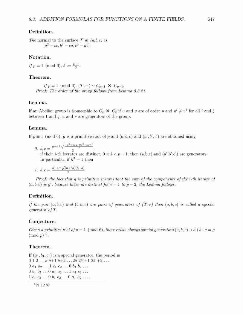
8.3. ADDITION FORMULAS FOR FUNCTIONS ON A FINITE FIELDS. 647
Definition.
The normal to the surface T at (a,b,c) is[a2 − bc, b2 − ca, c2 − ab].
Notation.
If p ≡ 1 (mod 6), δ := p−13 .
Theorem.
If p ≡ 1 (mod 6), (T ,+) ∼ Cp−1 ×× Cp−1.Proof: The order of the group follows from Lemma 8.3.2?.
Lemma.
If an Abelian group is isomorphic to Cq ×× Cq if u and v are of order p and ui 6= vj for all i and jbetween 1 and q, u and v are generators of the group.
Lemma.
If p ≡ 1 (mod 6), g is a primitive root of p and (a, b, c) and (a′, b′, c′) are obtained using
0. b, c =g−a±
√−g2+6ag−9a2+4g−1
3
2if their i-th iterates are distinct, 0 < i < p− 1, then (a,b,c) and (a’,b’,c’) are generators.In particular, if h3 = 1 then
1. b, c =h−a±
√(h+3a)(h−a)
2
Proof: the fact that g is primitive insures that the sum of the components of the i-th iterate of(a, b, c) is gi, because these are distinct for i = 1 to p− 2, the Lemma follows.
Definition.
If the pair (a, b, c) and (b, a, c) are pairs of generators of (T,+) then (a, b, c) is called a specialgenerator of T.
Conjecture.
Given a primitive root of p ≡ 1 (mod 6), there exists always special generators (a, b, c) 3 a+b+c = g(mod p) 6.
Theorem.
If (a1, b1, c1) is a special generator, the period is0 1 2 . . . δ δ+1 δ+2 . . . 2δ 2δ +1 2δ +2 . . .0 a1 a2 . . . 1 c1 c2 . . . 0 b1 b2 . . .0 b1 b2 . . . 0 a1 a2 . . . 1 c1 c2 . . .1 c1 c2 . . . 0 b1 b2 . . . 0 a1 a2 . . . .
621.12.87

648 CHAPTER 8. FUNCTIONS OVER FINITE FIELDS
For (b1, a1, c1) the period, scaled again is0 1 2 . . . δ δ +1 δ +2 . . . 2δ 2δ +1 2δ +2 . . .0 b1 b2 . . . 0 a1 a2 . . . 1 c1 c2 . . .0 a1 a2 . . . 1 c1 c2 . . . 0 b1 b2 . . .1 c1 c2 . . . 0 b1 b2 . . . 0 a1 a2 . . . .
Algorithm.
For a given p, we determine the smallest positive primitive root g, then for increasing values of a,we determine b and c using 8.3.2.0, if c(delta) = 1 we permute a, b, c, in the order
b, a, c, c, b, a, a, c, b, c, a, b, b, c, a,unless p ≡ 1 (mod 9), in which case we try a new p, if c(delta) = 0, we save the period and permute,if c(delta) = 0 and the values of a(i), b(i), c(i) are not distinct from some i, from the correspondingsaved values, we permute again, if we exaust the permutations, we ignore this value of a. When wehave obtained (a, b, c) such that the first a(delta) = -1 and and the second = 1 we exchange.
Example.
0. p = 7, gi = 1, 3, 2, 6, 4, 5, T =0 1 2 3 4 5 6 7 8(0, 0, 1) (0, 0, 2) (0, 0, 4) (0, 1, 0) (0, 2, 0) (0, 4, 0) (1, 0, 0) (1, 3, 6) (1, 5, 5)(0, 0, 1) (0, 0, 1) (0, 0, 1) (0, 1, 0) (0, 1, 0) (0, 1, 0) (1, 0, 0) (5, 1, 2) (2, 3, 3)9 10 11 12 13 14 15 16 17(1, 6, 3) (2, 0, 0) (2, 3, 3) (2, 5, 6) (2, 6, 5) (3, 1, 6) (3, 2, 3) (3, 3, 2) (3, 4, 5)(5, 2, 1) (1, 0, 0) (2, 3, 3) (5, 2, 1) (5, 1, 2) (1, 5, 2) (3, 2, 3) (3, 3, 2) (2, 5, 1)18 19 20 21 22 23 24 25 26(3, 5, 4) (3, 6, 1) (4, 0, 0) (4, 3, 5) (4, 5, 3) (4, 6, 6) (5, 1, 5) (5, 2, 6) (5, 3, 4)(2, 1, 5) (1, 2, 5) (1, 0, 0) (5, 2, 1) (5, 1, 2) (2, 3, 3) (3, 2, 3) (2, 5, 1) (1, 2, 5)27 28 29 30 31 32 33 34 35(5, 4, 3) (5, 5, 1) (5, 6, 2) (6, 1, 3) (6, 2, 5) (6, 3, 1) (6, 4, 6) (6, 5, 2) (6, 6, 4)(1, 5, 2) (3, 3, 2) (2, 1, 5) (2, 5, 1) (1, 5, 2) (2, 1, 5) (3, 2, 3) (1, 2, 5) (3, 3, 2)
+ 0 9 4 29 20 270 0 9 4 29 20 27
30 30 35 13 24 26 1110 10 31 2 21 3 3234 34 8 17 16 7 335 5 18 6 14 1 12
22 22 15 19 23 25 28
When scaled the group is isomorphic to C6 ×× C2, we have the equivalences,0,1,2; 3,4,5; 6,10,20; 7,13,22; 8,11,23; 9,12,21; 14,27,3; 15,24,33; 16,28,35; 17,25,30; 18,29,32;19,26,34.We have the table
+ 0 9 3 18 6 140 0 9 3 18 6 14
16 16 7 15 19 8 17
1. p = 13, gi = 1, 2, 4, 8, 3, 6, 12, 11, 9, 5, 10, 7, the scaled period is

8.3. ADDITION FORMULAS FOR FUNCTIONS ON A FINITE FIELDS. 649
(0, 0, 1) (7, 1, 6) (7, 9, 11) (11, 10, 6),(1, 0, 0) (6, 7, 1) (11, 7, 9) (6, 11, 10),(0, 1, 0) (1, 6, 7) (9, 11, 7) (10, 6, 11),
2. p = 19, gi = 1, 2, 4, 8, 16, 13, 7, 14, 9, 18, 17, 15, 11, 3, 6, 12, 5, 10, the scaled period is(0, 0, 1), (3, 9, 8), (15, 1, 4), (8, 13, 18), (7, 5, 8), (11, 0, 9)(1, 0, 0), (8, 3, 9), (4, 15, 1), (18, 8, 13), (8, 7, 5), (9, 11, 0)(0, 1, 0), (9, 8, 3), (1, 4, 15), (13, 18, 8), (5, 8, 7), (0, 9, 11)
Example.
The following are special generators, for the given primitive root, which is the smallest positive one:p g sp.gen. p g sp.gen. p g sp.gen.7 3 (6, 1, 3) 283 3 (3, 158, 125) 631 3 (324, 4, 306)13 2 (1, 2, 12) 307 5 (4, 192, 116) 643 11 (152, 0, 502)19 2 (6, 18, 16) 313 10 (5, 21, 297) 661 2 (2, 134, 527)31 3 (30, 4, 0) 331 3 (0, 237, 97) 673 5 (3, 52, 623)37 2 (18, 7, 14) 337 10 (180, 0, 167) 691 3 (425, 0, 269)43 3 (8, 35, 3) 349 2 (50, 299, 2) 709 2 (424, 3, 284)61 2 (3, 2, 58) 367 6 (22, 346, 5) 727 5 (377, 352, 3)67 2 (2, 12, 55) 373 2 (53, 6, 316) 733 6 (1, 541, 197)73 5 (4, 12, 62) 379 2 (5, 200, 176) 739 3 (0, 400, 342)79 3 (5, 42, 35) 397 5 (8, 22, 372) 751 3 (4, 426, 324)97 5 (24, 3, 75) 409 21 (390, 38, 2) 757 3 (5, 122, 632)103 5 (79, 25, 4) 421 2 (6, 5, 412) 769 11 (1, 404, 375)109 6 (13, 0, 102) 433 5 (3, 273, 162) 787 2 (411, 3, 375)127 3 (77, 0, 53) 439 15 (0, 264, 190) 811 3 (0, 188, 626)139 2 (107, 31, 3) 457 13 (14, 456, 0) 823 3 (15, 0, 811)151 6 (106, 51, 0) 463 3 (0, 335, 331) 829 2 (7, 572, 252)157 5 (4, 39, 119) 487 3 (39, 0, 551) 853 2 (155, 698, 2)163 2 (2, 29, 134) 499 7 (1, 87, 418) 859 2 (228, 625, 8)181 2 (2, 36, 145) 523 2 (310, 6, 209) 877 2 (10, 5, 864)193 5 (122, 3, 73) 541 2 (93, 3, 447) 883 2 (147, 6, 732)199 5 (30, 5, 167) 547 2 (335, 2, 212) 907 2 (553, 2, 354)211 2 (33, 2, 178) 571 3 (7, 8, 559) 919 7 (129, 0, 727)223 3 (138, 0, 88) 577 5 (4, 300, 278) 937 5 (7, 493, 442)229 6 (1, 168, 66) 601 7 (138, 463, 7) 967 5 (3, 661, 308)241 7 (20, 4, 224) 607 3 (0, 441, 169) 991 6 (8, 228, 761)271 6 (159, 7, 111) 613 2 (3, 50, 562) 997 7 (0, 625, 379)277 5 (11, 5, 266) 619 2 (5, 65, 551)
Lemma.
If p ≡ −1 (mod 6),
0. si := Pi0 + Pi1 + P12 ⇒ si = si1.
1. fi := P 2i0 + P 2
i1 + P 212 − (Pi1P12 + P12Pi0 + Pi0Pi1)⇒ fi = f i1.

650 CHAPTER 8. FUNCTIONS OVER FINITE FIELDS
Lemma.
If p ≡ −1 (mod 6), if g is a primitive root of p,
Proof: Let . . .To determine what happens for the solutions for i = 1, 2, . . . p− 1:let g be a generator for p, we want To determine what happens for the solutions for i ≡ 0 (mod p−1):
a+ b+ c = 1, a2 + b2 + c2 − (bc+ ca+ ab) = 1, ⇒(a+ b+ c)2 = 1, bc+ ca+ ab = 0,
given a, b+ c = 1− a, bc = a(a− 1),
b, c =1−a±
√(a−1)(1−3a)
2special solutions (1, 0, 0), (−1
3 ,23 ,
23), 2(−1
3 ,23 ,
23) = (0, 1, 0), 2(2
3 ,−13 ,
23) = (1, 0, 0), there should be
p+1−3−32 = p−5
2 possible values of a.
Notation.
ε := (0, 0, 1), α := (1, 0, 0), β := (0, 1, 0).
Theorem.
If p ≡ −1 (mod 6), and 3δ = p2 − 1, then
0. (T ,+) ∼ C3δ.
1. If h is a generator of this group then hδ = (0, 1, 0) or (1, 0, 0), in the former case, we willchoose g = h−1 otherwizewe will choose g = h.
2. If gi = (a, b, c), then gi+δ = (c, a, b), gi+2δ = (b, c, a), gpi = (b, a, c), gpi+δ = (c, b, a),gpi+2δ = (a, c, b)7.
3. d(Pi, Pp+(p+1)l+(p−1)kj+i) = d(Pi, P1+(p+1)l−(p−1)kj+i).
4. d(Pi, P(p+1)l+(p−1)kj+i) = d(Pi, P(p+1)l−(p−1)kj+i).
Proof:If p ≡ −1 (mod 6), to any of the p2 − 1 line through the origin which does not pass through(1,1,1,1) and is not in the plane perpendicular to this last line, associate a point a, b, c, 1 say letu := a3+b3+c3−3abc, u 6= 0 and u has a unique cube root v in Zp, therefore the point (av ,
bv ,
cv ) ∈ T .
(a, b, c) + (1, 0, 0) = (c, a, b), (a, b, c) + (0, 1, 0) = (b, c, a).
Lemma.
Proof: φ (p2 − 1) = 2 φ (p-1) φ (p+1),
Example.
p = 11, g = 7,
713.12.87

8.3. ADDITION FORMULAS FOR FUNCTIONS ON A FINITE FIELDS. 651
Lemma.
0. (a+ b+ c)(a2 + b2 + c2 − bc− ca− ab) = a3 + b3 + c3 − 3abc.
1. Given a and g, a primitive root of p, then
b, c =g−a±
√−g2+6ag−9a2+4g−1
3
2
Proof: a+b+c = g and a2 +b2 +c2−bc−ca−ab = g−1 ⇒ (a+b+c)2 = g2 and bc+ca+ab = 0,
therefore b+ c = g−a and bc = g2−g−1
3 −a(g−a), hence b and c are roots of a quadratic equations,this gives 1.
Theorem.
If p ≡ −1 (mod 6),
0. A necessary condition for (a, b, c) in T to be a generator is that a+ b+ c be a primitive rootfor p.
1. If (a, b, c) is a generator such that (a, b, c)δ = (1, 0, 0),
2.0. p ≡ 2 (mod 9), or p ≡ 11 (mod 18)⇒(b, c, a)δ = ε, (c, a, b)δ = β, (c, b, a)δ = ε, (a, c, b)δ = α, (b, a, c)δ = β,
0. p ≡ 5 (mod 9), or p ≡ 5 (mod 18)⇒(b, c, a)δ = β, (c, a, b)δ = ε, (c, b, a)δ = α, (a, c, b)δ = ε, (b, a, c)δ = β,
1. p ≡ 8 (mod 9), or p ≡ 17 (mod 18)⇒(b, c, a)δ = α, (c, a, b)δ = α, (c, b, a)δ = β, (a, c, b)δ = β, (b, a, c)δ = β,
1. p(u, v, w) = (v, u, w).
Definition.
Given a generator (a, b, c) and a non isotropic scaled direction (u, v, w) the corresponding angulardirection is the multiplier i such that i(a,b,c) = (u,v,w).
Conjecture. 8
0. angular direction(Pi+k, Pi) = i+ angular direction(Pk, P0)(mod p2 − 1).
1. angular direction(O,Mi) = i + angular direction(0,M0), where Mi is the mid-point of(Pi, Pi+1).
2. angulardirection(O,Ni) = i+angulardirection(0, N0), where Ni is the mid-point of (Pi−1, Pi+1).
3. angular direction(Pi, Ni) = i+ angular direction(P0, N0).
828.12.87

652 CHAPTER 8. FUNCTIONS OVER FINITE FIELDS
Example.
p = 17, generator (13, 4, 3),angular direction((0, 0, 1), (13, 4, 3)) = 164,angular direction((0, 0, 1), (9, 6, 1)) = 224,M0 = (15, 2, 2), angular direction(O,M0) = 60,N1 = (13, 3, 6), angular direction(O,N0) = 33,angular direction(P1, N1) = 40.
Corollary.
The coordinates of the normal to the surface T are those of −p(a, b, c)9.
Lemma.
If (a, b, c) is a generator and gi is a primitive root of p, then
0. i, prime, ≡ 1 (mod 3)⇒ (gi)δ = α.?
1. i, prime, ≡ 2 (mod 3)⇒ (gi)δ = β.?
2. i is not a prime ⇒ (gi)δ = ε.
Example.
The following table gives generators (a, b, c) for the given values of p and g,α,ε , β −ε , α , β α , β , ε −α , ε , β α , α , α −β , β , β
928.12.87
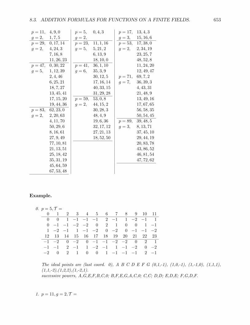
8.3. ADDITION FORMULAS FOR FUNCTIONS ON A FINITE FIELDS. 653
p = 11, 4, 9, 0 p = 5, 0, 4, 3 p = 17, 13, 4, 3g = 2, 1, 7, 5 g = 2, g = 3, 15, 16, 6p = 29, 0, 17, 14 p = 23, 11, 1, 16 p = 53, 17, 38, 0g = 2, 4, 24, 3 g = 5, 5, 21, 2 g = 2, 2, 34, 19
7, 16, 8 6, 13, 9 23, 25, 711, 26, 23 18, 10, 0 48, 52, 8
p = 47, 0, 30, 22 p = 41, 36, 1, 10 11, 24, 20g = 5, 1, 12, 39 g = 6, 35, 3, 9 12, 49, 47
2, 4, 46 30, 12, 5 p = 71, 69, 7, 26, 25, 21 17, 16, 14 g = 7, 36, 39, 318, 7, 27 40, 33, 15 4, 43, 3113, 45, 41 31, 29, 28 21, 48, 917, 15, 20 p = 59, 53, 0, 8 13, 49, 1619, 44, 36 g = 2, 44, 15, 2 17, 67, 65
p = 83, 62, 23, 0 30, 28, 3 56, 58, 35g = 2, 2, 20, 63 48, 4, 9 50, 54, 45
4, 11, 70 19, 6, 36 p = 89, 39, 48, 550, 29, 6 32, 17, 12 g = 3, 8, 13, 718, 16, 61 27, 21, 13 37, 45, 1027, 9, 49 18, 52, 50 29, 44, 1977, 10, 81 20, 83, 7821, 13, 51 43, 86, 5225, 18, 42 46, 81, 5435, 31, 19 47, 72, 6245, 64, 5967, 53, 48
Example.
0. p = 5, T =0 1 2 3 4 5 6 7 8 9 10 110 0 1 −1 −1 −1 2 −1 1 −2 −1 10 −1 −1 −2 −2 0 2 1 0 0 1 −11 −2 −1 1 −1 −2 0 −2 0 −1 −1 −2
12 13 14 15 16 17 18 19 20 21 22 23−1 −2 0 −2 0 −1 −1 −2 −2 0 2 1−1 −1 2 −1 1 −2 −1 1 −1 −2 0 −2−2 0 2 1 0 0 1 −1 −1 −1 2 −1
The ideal points are (last coord. 0), A B C D E F G (0,1,-1), (1,0,-1), (1,-1,0), (1,1,1),(1,1,-2),(1,2,2),(1,-2,1).successive powers, A,G,E,F,B,C,0; B,F,E,G,A,C,0; C,C; D,D; E,D,E; F,G,D,F.
1. p = 11, g = 2, T =

654 CHAPTER 8. FUNCTIONS OVER FINITE FIELDS
0 1 2 3 4 5 6 7 8 9 10 11 12 13 14 15 160 1 −5 0 −2 4 5 1 −3 −4 4 3 −3 5 4 4 −40 3 3 −4 3 −3 −3 −4 0 −1 −5 1 −3 −3 5 −2 −21 4 0 −1 3 −2 1 5 −3 1 2 4 4 4 −5 −3 −2
17 18 19 20 21 22 23 24 25 26 27 28 29 30 31 32 33−2 4 1 −3 −5 3 −3 −4 −5 5 −2 −4 2 2 −3 −2 −4
4 3 −1 −4 5 −5 5 −4 5 1 0 −1 0 −5 5 2 00 −2 −4 −3 −3 0 4 1 −1 −3 4 −1 5 4 −5 −2 −1
34 35 36 37 38 39 40 41 42 43 44 45 46 47 48 49 505 5 4 1 4 2 1 4 0 −1 3 −2 1 5 −3 1 24 −5 4 5 −2 5 0 1 −5 0 −2 4 5 1 −3 −4 4−5 −1 −5 −4 3 0 0 3 3 −4 3 −3 −3 −4 0 −1 −5
. . .
2. p = 17, g = 3, T = (0, 0, 1), (1, 2, 3), (10, 13, 13), (1, 7, 4), (4, 13, 4), (8, 0, 16),(6, 6, 13), (9, 16, 6), (14, 1, 1), (11, 2, 15), (1, 13, 1), (13, 8, 1),(5, 5, 3), (11, 9, 7), (7, 1, 1), (7, 12, 1), (12, 11, 12), (2, 1, 3),
(11, 11, 14), (1, 4, 7), (1, 10, 10), (16, 0, 8), (5, 15, 5), (16, 9, 6),(4, 4, 8), (11, 15, 2), (14, 9, 9), (1, 8, 13), (15, 0, 15), (9, 11, 7),(5, 5, 16), (7, 1, 12), (1, 0, 0), (3, 1, 2), (13, 10, 13), (4, 1, 7),
. . . .
Example.
A generator associated to the given primitive root is such that (a, b, c)δ = α = (1, 0, 0), with δ :=p2−1
3 .

8.3. ADDITION FORMULAS FOR FUNCTIONS ON A FINITE FIELDS. 655
p g generator5 2 (0, 4, 3)
11 2 (1, 3, 4)17 3 (3, 4, 13)23 5 (0, 7, 12)29 2 (0, 4, 7)41 6 (0, 2, 17)47 5 (0, 7, 37)53 2 (0, 6, 20)59 2 (0, 3, 11)71 7 (0, 8, 54)83 2 (0, 6, 60)89 3 (0, 6, 77)
101 2 (0, 7, 60)107 2 (0, 2, 29)113 3 (0, 3,−12)???131 2 (0, 4, 18)137 3 (0, 2,−25)149 2 (0, 3,−53)167 5 (0, 7,−2)173 2 (0, 3, 71)179 2 (0, 4, 36)191 19 (0, 5,−83)197 2 (0, 19, 61)
See [M130] RICATTI. for more.
8.3.3 The case of 4 Functions.
Definition.
The set R4 is the set of elements
0. (x, y, z, t) 3 x, y, z, t ∈ Zp and−(x2 − z2)2 + (y2 − t2)2 + 4((x2 + z2)yt− (y2 + t2)xz) = 1,with addition
1. (x, y, z, t) + (x′, y′, z′, t′) = (xt′ + tx′ + yz′ + zy′, xx′ + zz′ + yt′ + ty′,xy′ + yx′ + zt′ + tz′, yy′ + tt′ + xz′ + zx′).
Theorem.
(R4,+) is an Abelian group.
Conjecture.
0. If p ≡ 1 (mod 4) then the maximum period is p− 1.
1. If p ≡ −1 (mod 4) then the maximum period is p2 − 1 10.
1022.12.87
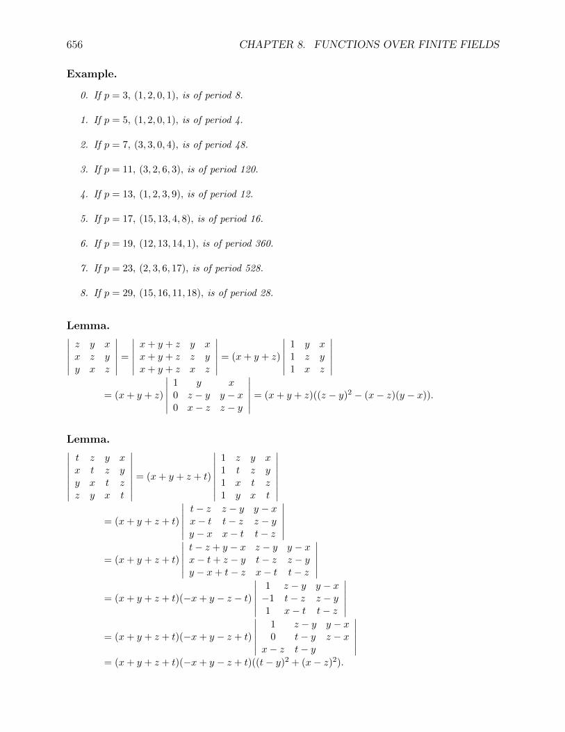
656 CHAPTER 8. FUNCTIONS OVER FINITE FIELDS
Example.
0. If p = 3, (1, 2, 0, 1), is of period 8.
1. If p = 5, (1, 2, 0, 1), is of period 4.
2. If p = 7, (3, 3, 0, 4), is of period 48.
3. If p = 11, (3, 2, 6, 3), is of period 120.
4. If p = 13, (1, 2, 3, 9), is of period 12.
5. If p = 17, (15, 13, 4, 8), is of period 16.
6. If p = 19, (12, 13, 14, 1), is of period 360.
7. If p = 23, (2, 3, 6, 17), is of period 528.
8. If p = 29, (15, 16, 11, 18), is of period 28.
Lemma.∣∣∣∣∣∣z y xx z yy x z
∣∣∣∣∣∣ =
∣∣∣∣∣∣x+ y + z y xx+ y + z z yx+ y + z x z
∣∣∣∣∣∣ = (x+ y + z)
∣∣∣∣∣∣1 y x1 z y1 x z
∣∣∣∣∣∣= (x+ y + z)
∣∣∣∣∣∣1 y x0 z − y y − x0 x− z z − y
∣∣∣∣∣∣ = (x+ y + z)((z − y)2 − (x− z)(y − x)).
Lemma.∣∣∣∣∣∣∣∣t z y xx t z yy x t zz y x t
∣∣∣∣∣∣∣∣ = (x+ y + z + t)
∣∣∣∣∣∣∣∣1 z y x1 t z y1 x t z1 y x t
∣∣∣∣∣∣∣∣= (x+ y + z + t)
∣∣∣∣∣∣t− z z − y y − xx− t t− z z − yy − x x− t t− z
∣∣∣∣∣∣= (x+ y + z + t)
∣∣∣∣∣∣t− z + y − x z − y y − xx− t+ z − y t− z z − yy − x+ t− z x− t t− z
∣∣∣∣∣∣= (x+ y + z + t)(−x+ y − z − t)
∣∣∣∣∣∣1 z − y y − x−1 t− z z − y1 x− t t− z
∣∣∣∣∣∣= (x+ y + z + t)(−x+ y − z + t)
∣∣∣∣∣∣1 z − y y − x0 t− y z − x
x− z t− y
∣∣∣∣∣∣= (x+ y + z + t)(−x+ y − z + t)((t− y)2 + (x− z)2).
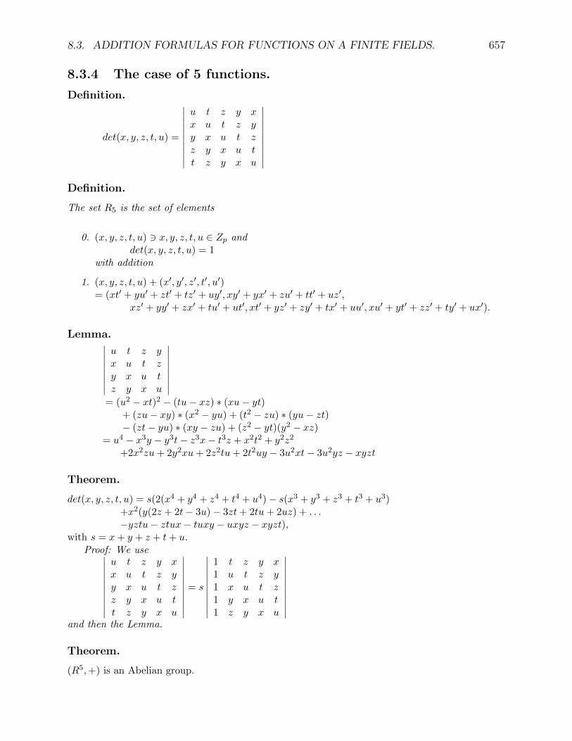
8.3. ADDITION FORMULAS FOR FUNCTIONS ON A FINITE FIELDS. 657
8.3.4 The case of 5 functions.
Definition.
det(x, y, z, t, u) =
∣∣∣∣∣∣∣∣∣∣u t z y xx u t z yy x u t zz y x u tt z y x u
∣∣∣∣∣∣∣∣∣∣Definition.
The set R5 is the set of elements
0. (x, y, z, t, u) 3 x, y, z, t, u ∈ Zp anddet(x, y, z, t, u) = 1
with addition
1. (x, y, z, t, u) + (x′, y′, z′, t′, u′)= (xt′ + yu′ + zt′ + tz′ + uy′, xy′ + yx′ + zu′ + tt′ + uz′,
xz′ + yy′ + zx′ + tu′ + ut′, xt′ + yz′ + zy′ + tx′ + uu′, xu′ + yt′ + zz′ + ty′ + ux′).
Lemma.∣∣∣∣∣∣∣∣u t z yx u t zy x u tz y x u
∣∣∣∣∣∣∣∣= (u2 − xt)2 − (tu− xz) ∗ (xu− yt)
+ (zu− xy) ∗ (x2 − yu) + (t2 − zu) ∗ (yu− zt)− (zt− yu) ∗ (xy − zu) + (z2 − yt)(y2 − xz)
= u4 − x3y − y3t− z3x− t3z + x2t2 + y2z2
+2x2zu+ 2y2xu+ 2z2tu+ 2t2uy − 3u2xt− 3u2yz − xyzt
Theorem.
det(x, y, z, t, u) = s(2(x4 + y4 + z4 + t4 + u4)− s(x3 + y3 + z3 + t3 + u3)+x2(y(2z + 2t− 3u)− 3zt+ 2tu+ 2uz) + . . .−yztu− ztux− tuxy − uxyz − xyzt),
with s = x+ y + z + t+ u.Proof: We use∣∣∣∣∣∣∣∣∣∣
u t z y xx u t z yy x u t zz y x u tt z y x u
∣∣∣∣∣∣∣∣∣∣= s
∣∣∣∣∣∣∣∣∣∣1 t z y x1 u t z y1 x u t z1 y x u t1 z y x u
∣∣∣∣∣∣∣∣∣∣and then the Lemma.
Theorem.
(R5,+) is an Abelian group.

658 CHAPTER 8. FUNCTIONS OVER FINITE FIELDS
Conjecture.
0. If p ≡ 1 (mod 10) then the maximum period is p− 1.
1. If p ≡ 9 (mod 10) then the maximum period is p2 − 1 11.
2. If p ≡ ±3 (mod 10) then the maximum period is p4 − 112.
For examples see 8.4.1.
8.4 Application to geometry.
8.4.0 Introduction.
To define distances in a sub geometry of affine k-dimensional geometry, we have to define a ho-mogeneous function f(P ) of degree k. We can then either define the distance between 2 points Pand Q by the k-th root of f(Q− P ) or the hypercube between 2 points P and Q by f(Q,P ). I willnot discuss here the extension of a 2-dimensional distance to n-dimension as is done in Euclideangeometry.To define angles, we can associate to a point P, a k by k matrix by a bijection, if the set of thesematrices, which are of determinant 1, form a subset of an Abelian group under matrix multiplica-tion, with generator G0, . . .Gl, we can define then angular direction of a point associated to thematrix Gi00 . . .Gill by (i0, . . . , il).We can also define f(P ) as the determinant of the associated matrix. If in the 2 dimensional realaffine geometry, we associate to (x, y) the matrix(
y x−x y
),
then f(x, y) = x2+y2, the matrices of determinant 1 for an Abelian group with generator x = sin(1),y = cos(1), and we obtain the 2-dimensional Euclidean distance and angle.If in the 2-dimensional real affine geometry, we associate to (x, y) the matrix(
y xx y
),
then f(x, y) = y2 − x2, the matrices of determinant 1 for an Abelian group with generator x =sinh(1), y = cosh(1), and we obtain the 2-dimensional Minkowskian distance and angle.This will now be extended using the generalization of the hyperbolic functions by Ricatti.
8.4.1 k-Dimensional Affine Geometry.
Definition.
In k-dimensional affine geometry we define the Ricatti function as the function which associates tothe point P = (P0, . . . , Pk−1), the Toeplitz matrix T, defined by Ti,j = Pk−1−i+j , 0 ≤ i, j <k,where the subscripts computation is done modulo k.
1124.12.871222.12.87

8.4. APPLICATION TO GEOMETRY. 659
Theorem.
The matrix multiplication defines an addition (which is a convolution) for the points as follows, ifT is associated to P and U, to Q, TU is associated to R with
P Q := Ri =∑
j PjQi−1−j .For instance,
0. k = 3,(P Q)0 = P0Q2 + P1Q1 + P2Q0,(P Q)1 = P0Q0 + P1Q2 + P2Q1,(P Q)2 = P0Q1 + P1Q0 + P2Q2.
1. k = 4,(P Q)0 = P0Q3 + P1Q2 + P2Q1 + P3Q0,(P Q)1 = P0Q0 + P1Q3 + P2Q2 + P3Q1,(P Q)2 = P0Q1 + P1Q0 + P2Q3 + P3Q2,(P Q)3 = P0Q2 + P1Q1 + P2Q0 + P3Q3.
Corollary.
The set of matrices, associated to all the non ideal points of k-dimensional affine geometry withdeterminant 1, form an abelian group under matrix multiplication.
Theorem.
If p = k then Pi = δi,0 has period p. Moreover, the j-th iterate P (j) is such that P(j)i = δj,i.
Theorem.
Let det(. . . , z, y, x) denote the determinant of the Toeplitz matrix associated with P = (x, y, z, . . .),let s be the sum of the components of P, then
0. k = 3,det(zyx) = x3 + y3 + z3 − 3xyz = s((z − y)2 − (x− z)(y − x)).
1. k = 4,det(tzyx) = s(−x+ y − z + t)((t− y)2 + (x− z)2).
2. k = 5,det(x, y, z, t, u) = s(2(x4 + y4 + z4 + t4 + u4)− s(x3 + y3 + z3 + t3 + u3)
+x2(y(2z + 2t− 3u)− 3zt+ 2tu+ 2uz) + . . .−yztu− ztux− tuxy − uxyz − xyzt).
In the following examples we have obtained what a cyclic generator of what appears to be thelongest period, without examining the details of the structure of the solution.

660 CHAPTER 8. FUNCTIONS OVER FINITE FIELDS
Example.
0. k = 4.p period cyclic generator3 8 (1, 2, 0, 1),5 4 (1, 2, 0, 1),7 48 (3, 3, 0, 4),
11 120 (3, 2, 6, 3),13 12 (1, 2, 3, 9),17 16 (15, 13, 4, 8),19 360 (12, 13, 14, 1),23 528 (2, 3, 6, 17),29 28 (15, 16, 11, 18).
1. k = 5.p period cyclic generator3 80 (1, 1, 0, 1, 2),5 5 (1, 0, 0, 0, 0),7 2400 (1, 2, 4, 1, 4),
11 10 (4, 2, 1, 4, 2).13 28560 (3, 5, 1, 11, 8)17 83520 (9, 7, 8, 2, 11),19 18 (7, 16, 15, 2, 0),23 279840 (14, 12, 4, 7, 14),29 840 (13, 8, 25, 5, 9),31 30 (26, 30, 11, 2, 27).
2. k = 6,p period cyclic generator3 6 (0, 1, 1, 2, 1, 0),5 24 (0, 2, 4, 1, 0, 0),7 6 (3, 5, 0, 6, 1, 2),
11 120 (5, 9, 2, 4, 2, 2),13 12 (3, 8, 4, 2, 1, 10)17 288 (2, 12, 5, 14, 4, 3),19 18 (2, 12, 5, 14, 4, 3),23 528 (3, 16, 20, 4, 13, 18),29 840 (10, 2, 8, 22, 14, 4),31 30 (1, 11, 7, 4, 29, 13),
3. k = 7,

8.4. APPLICATION TO GEOMETRY. 661
p period cyclic generator3 728 (1, 2, 2, 1, 0, 1, 1, 1),5 15624 (0, 0, 4, 3, 0, 0, 0),7 7 (1, 0, 0, 0, 0, 0, 0),
11 1330 (0, 1, 8, 4, 3, 4, 4),13 168 (6, 3, 11, 2, 4, 2, 0),17 24137568 (3, 10, 13, 16, 3, 4, 5),19 47045880 (18, 10, 17, 5, 14, 9, 5),23 12166 (0, 17, 4, 7, 3, 15, 5),29 28 (26, 7, 9, 10, 15, 7, 15),31 (6) 887503680 (26, 26, 15, 18, 26, 22, 19),37 (3) 50652 (9, 9, 18, 31, 0, 27, 25),41 (2) 1680 (7, 10, 22, 32, 27, 2, 27).
4. k = 8,p period cyclic generator3 8 (1, 2, 2, 1, 0, 1, 1, 1),5 24 (2, 0, 3, 3, 1, 4, 4, 0),7 48 (1, 3, 0, 0, 3, 3, 4, 3),
11 120 (5, 1, 9, 9, 4, 8, 2, 8),13 168 (7, 11, 5, 4, 12, 9, 5, 1),17 16 (9, 13, 7, 10, 0, 15, 4, 3),19 360 (18, 11, 4, 13, 8, 1, 7, 16),23 528 (9, 10, 22, 4, 8, 17, 16, 11),29 840 (28, 1, 14, 21, 9, 26, 14, 5),31 960 (28, 6, 30, 20, 25, 1, 30, 18),37 1368 (0, 21, 5, 5, 28, 36, 9, 9),41 40 (16, 30, 30, 27, 14, 18, 18, 17),
5. k = 9,p period cyclic generator3 18 (0, 2, 2, 1, 2, 2, 0, 1, 1),5 15624 (1, 1, 2, 0, 1, 1, 4, 1, 1), may not be largest period7
111317 288 (15, 8, 16, 15, 9, 13, 7, 10, 12),19 18 (2, 4, 15, 11, 6, 11, 4, 0, 6),23293137 36 (5, 27, 14, 9, 28, 24, 20, 12, 11)
Example.
Here we have written j when the maximum period is pj − 1, unless the number is underlined inwhich case the period is given.

662 CHAPTER 8. FUNCTIONS OVER FINITE FIELDS
k \ p 3 5 7 11 13 17 19 23 29 31 37 413 k 2 1 2 1 2 1 2 2 1 1 24 2 1 2 2 1 1 2 2 1 2 1 15 4 k 4 1 4 4 2 4 2 1 4 16 k 2 1 2 1 2 1 2 2 1 1 27 6 6 k 3 2 6 6 3 1 6 3 28 2 2 2 2 2 1 2 2 2 2 2 19 k 6 3 6 3 2 1 6 6 3 1 6
10 4 2k 4 1 4 4 2 4 2 1 4 111 5 5 10 k 10 10 10 1 10 5 5 ≥ 1012 2k 2 2 2 1 2 2 2 2 2 1 213 3 4 12 12 k 6 ≥ 12 6 3 4 ≥ 10 ≥ 1014 6 6 3k 3 2 6 6 3 1 6 3 215 16k 8k 4 2 4 4 2 4 2 1 4 216 4 4 2 4 4 1 4 2 4 2 4 217 16 16 16 ≥ 16 4 − 8 ≥ 16 ≥ 16 ≥ 16 ? ?19 18 5 3 3 ≥ 18 9 − 9 ≥ 18 6 2 ?
k \ p 43 47 53 59 61 67 71 73 79 83 89 973 1 2 2 2 1 1 2 1 1 2 2 14 2 2 1 2 1 2 2 1 2 2 1 15 4 4 4 2 1 4 1 4 2 4 2 46 1 2 2 2 1 1 2 1 1 2 2 17 1 6 3 6 6 3 1 6 3 2 6 28 2 2 2 2 2 2 2 1 2 2 1 19 3 6 2 6 3 3 2 1 3 6 2 3
10 4 4 4 2 1 4 1 4 2 4 2 411 2 5 5 5 ≥ 10 1 5 ≥ 10 ≥ 10 ≥ 10 1 512 2 2 2 2 1 2 2 1 2 2 2 113 6 4 1 ≥ 8 3 ≥ 8 ≥ 8 4 1 4 ≥ 7 ≥ 714 1 6 3 6 6 3 1 6 3 2 6 215 4 4 4 2 1 4 2 4 2 4 2 416 4 2 4 4 4 4 2 2 2 4 2 117 8 ? ? 8 ≥ 16 2 ? ? ? ≥ 8 4 ?19 ? 9 ≥ 9 ≥ 9 ? ? ? ≥ 9 101 ≥ 9 103 ≥ 9
Moreover it appears that
\em k | 18 | 20 | 21 | 22 | 24 | 25 |
26 | 27
| 3 k | 5 k | 3 104k | 11 5k | 3 k | 5 k |
13 2k | 3 k
| | | 7 6k | | | | |
\em k | 28 | 30 | 33 | 34 | 35 | 36 |
38 | 39
| 7 12k | 3 8k | 3 22k | 17 $8kL\hti-1/$ |
5 .k | 3 .k | 19 9k | 3 .k
| | 5 4k | 11 40k | | 7 560k | |
| 13 .k
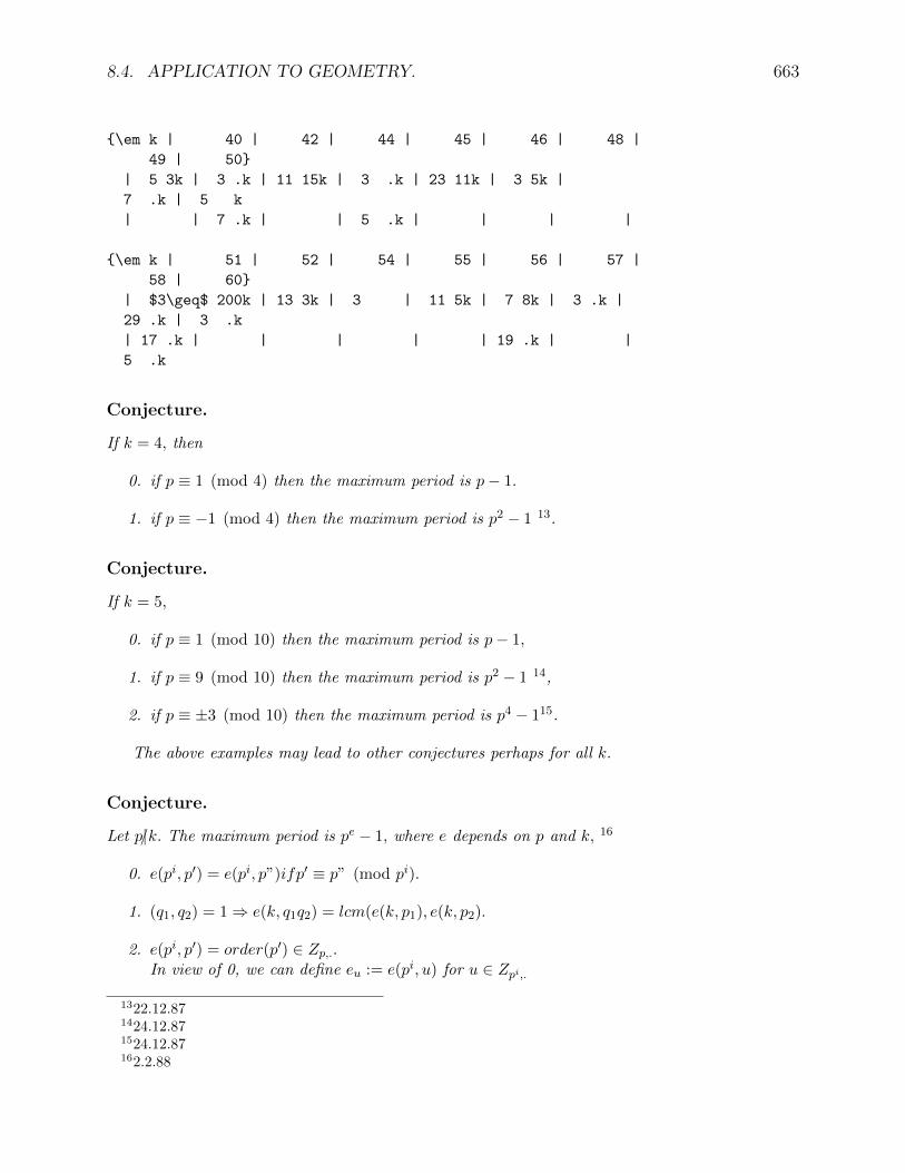
8.4. APPLICATION TO GEOMETRY. 663
\em k | 40 | 42 | 44 | 45 | 46 | 48 |
49 | 50
| 5 3k | 3 .k | 11 15k | 3 .k | 23 11k | 3 5k |
7 .k | 5 k
| | 7 .k | | 5 .k | | | |
\em k | 51 | 52 | 54 | 55 | 56 | 57 |
58 | 60
| $3\geq$ 200k | 13 3k | 3 | 11 5k | 7 8k | 3 .k |
29 .k | 3 .k
| 17 .k | | | | | 19 .k | |
5 .k
Conjecture.
If k = 4, then
0. if p ≡ 1 (mod 4) then the maximum period is p− 1.
1. if p ≡ −1 (mod 4) then the maximum period is p2 − 1 13.
Conjecture.
If k = 5,
0. if p ≡ 1 (mod 10) then the maximum period is p− 1,
1. if p ≡ 9 (mod 10) then the maximum period is p2 − 1 14,
2. if p ≡ ±3 (mod 10) then the maximum period is p4 − 115.
The above examples may lead to other conjectures perhaps for all k.
Conjecture.
Let p|/k. The maximum period is pe − 1, where e depends on p and k, 16
0. e(pi, p′) = e(pi, p”)ifp′ ≡ p” (mod pi).
1. (q1, q2) = 1⇒ e(k, q1q2) = lcm(e(k, p1), e(k, p2).
2. e(pi, p′) = order(p′) ∈ Zp,..In view of 0, we can define eu := e(pi, u) for u ∈ Zpi,.
1322.12.871424.12.871524.12.87162.2.88
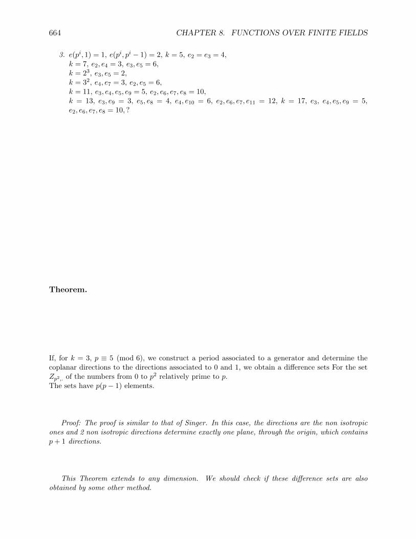
664 CHAPTER 8. FUNCTIONS OVER FINITE FIELDS
3. e(pi, 1) = 1, e(pi, pi − 1) = 2, k = 5, e2 = e3 = 4,k = 7, e2, e4 = 3, e3, e5 = 6,k = 23, e3, e5 = 2,k = 32, e4, e7 = 3, e2, e5 = 6,k = 11, e3, e4, e5, e9 = 5, e2, e6, e7, e8 = 10,k = 13, e3, e9 = 3, e5, e8 = 4, e4, e10 = 6, e2, e6, e7, e11 = 12, k = 17, e3, e4, e5, e9 = 5,e2, e6, e7, e8 = 10, ?
Theorem.
If, for k = 3, p ≡ 5 (mod 6), we construct a period associated to a generator and determine thecoplanar directions to the directions associated to 0 and 1, we obtain a difference sets For the setZp2,. of the numbers from 0 to p2 relatively prime to p.The sets have p(p− 1) elements.
Proof: The proof is similar to that of Singer. In this case, the directions are the non isotropicones and 2 non isotropic directions determine exactly one plane, through the origin, which containsp+ 1 directions.
This Theorem extends to any dimension. We should check if these difference sets are alsoobtained by some other method.
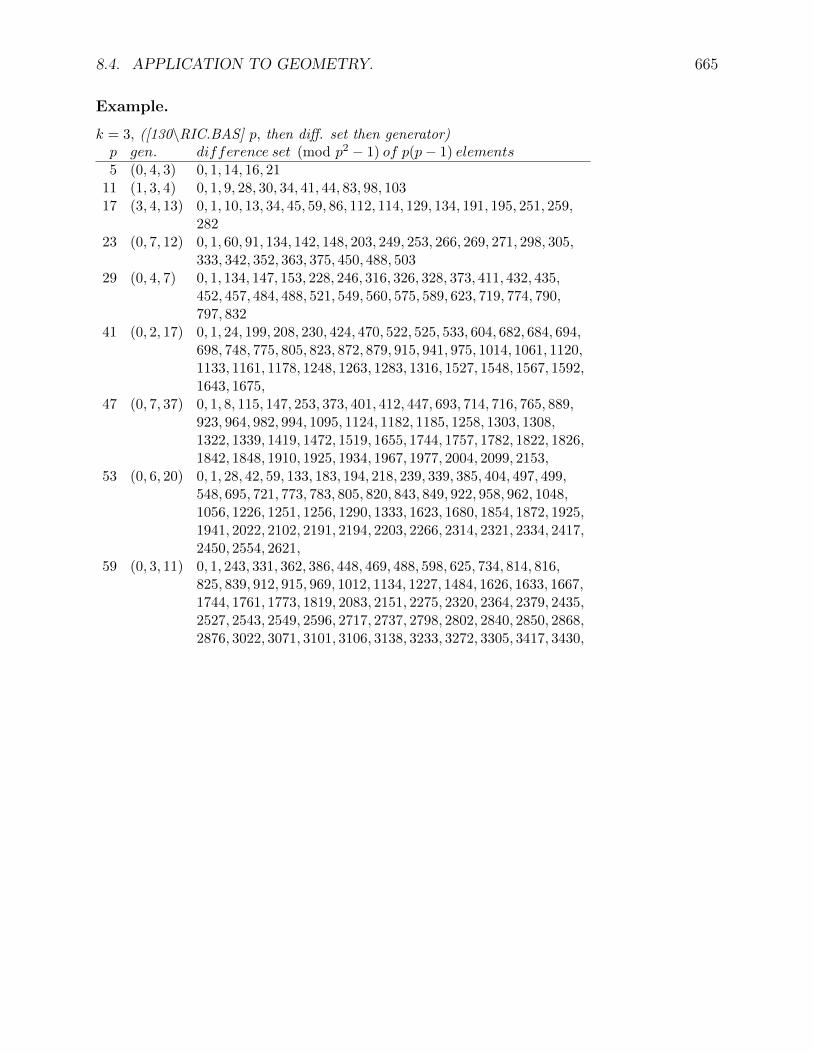
8.4. APPLICATION TO GEOMETRY. 665
Example.
k = 3, ([130\RIC.BAS] p, then diff. set then generator)p gen. difference set (mod p2 − 1) of p(p− 1) elements5 (0, 4, 3) 0, 1, 14, 16, 21
11 (1, 3, 4) 0, 1, 9, 28, 30, 34, 41, 44, 83, 98, 10317 (3, 4, 13) 0, 1, 10, 13, 34, 45, 59, 86, 112, 114, 129, 134, 191, 195, 251, 259,
28223 (0, 7, 12) 0, 1, 60, 91, 134, 142, 148, 203, 249, 253, 266, 269, 271, 298, 305,
333, 342, 352, 363, 375, 450, 488, 50329 (0, 4, 7) 0, 1, 134, 147, 153, 228, 246, 316, 326, 328, 373, 411, 432, 435,
452, 457, 484, 488, 521, 549, 560, 575, 589, 623, 719, 774, 790,797, 832
41 (0, 2, 17) 0, 1, 24, 199, 208, 230, 424, 470, 522, 525, 533, 604, 682, 684, 694,698, 748, 775, 805, 823, 872, 879, 915, 941, 975, 1014, 1061, 1120,1133, 1161, 1178, 1248, 1263, 1283, 1316, 1527, 1548, 1567, 1592,1643, 1675,
47 (0, 7, 37) 0, 1, 8, 115, 147, 253, 373, 401, 412, 447, 693, 714, 716, 765, 889,923, 964, 982, 994, 1095, 1124, 1182, 1185, 1258, 1303, 1308,1322, 1339, 1419, 1472, 1519, 1655, 1744, 1757, 1782, 1822, 1826,1842, 1848, 1910, 1925, 1934, 1967, 1977, 2004, 2099, 2153,
53 (0, 6, 20) 0, 1, 28, 42, 59, 133, 183, 194, 218, 239, 339, 385, 404, 497, 499,548, 695, 721, 773, 783, 805, 820, 843, 849, 922, 958, 962, 1048,1056, 1226, 1251, 1256, 1290, 1333, 1623, 1680, 1854, 1872, 1925,1941, 2022, 2102, 2191, 2194, 2203, 2266, 2314, 2321, 2334, 2417,2450, 2554, 2621,
59 (0, 3, 11) 0, 1, 243, 331, 362, 386, 448, 469, 488, 598, 625, 734, 814, 816,825, 839, 912, 915, 969, 1012, 1134, 1227, 1484, 1626, 1633, 1667,1744, 1761, 1773, 1819, 2083, 2151, 2275, 2320, 2364, 2379, 2435,2527, 2543, 2549, 2596, 2717, 2737, 2798, 2802, 2840, 2850, 2868,2876, 3022, 3071, 3101, 3106, 3138, 3233, 3272, 3305, 3417, 3430,

666 CHAPTER 8. FUNCTIONS OVER FINITE FIELDS
p gen. difference set (mod p2 − 1) of p(p− 1) elements71 (0, 8, 54) 0, 1, 339, 345, 406, 542, 687, 821, 907, 989, 1171, 1294, 1429,
1443, 1502, 1522, 1553, 1617, 1628, 1650, 1691, 1737, 1792, 1828,1946, 2108, 2125, 2229, 2237, 2247, 2266, 2281, 2461, 2500, 2503,2550, 2655, 2743, 2768, 2966, 2970, 3019, 3028, 3035, 3127, 3195,3280, 3328, 3360, 3405, 3426, 3431, 3617, 3912, 3996, 4019, 4031,4162, 4273, 4343, 4400, 4460, 4490, 4514, 4590, 4592, 4630, 4673,4686, 4836, 5013,
83 (0, 6, 60) 0, 1, 182, 187, 214, 255, 500, 503, 565, 590, 596, 827, 1353, 1389,1406, 1456, 1501, 1555, 1577, 1629, 1690, 1720, 1900, 2039, 2067,2136, 2250, 2261, 2265, 2336, 2645, 2704, 2737, 2783, 2785, 2792,2984, 3250, 3271, 3479, 3641, 3711, 3723, 3746, 3760, 3868, 3902,3953, 4053, 4063, 4071, 4194, 4296, 4309, 4353, 4459, 4568, 4592,4611, 4675, 4722, 4738, 4764, 4896, 4973, 5013, 5093, 5191, 5230,5346, 5366, 5490, 5550, 5616, 5654, 5710, 5844, 5922, 6279, 6337,6611, 6683, 6712,
89 (0, 6, 77) 0, 1, 11, 323, 584, 613, 697, 739, 804, 940, 1052, 1256, 1273, 1430,1535, 1816, 1820, 1871, 1896, 2030, 2280, 2347, 2566, 2598, 2648,2743, 2781, 3096, 3352, 3496, 3624, 3790, 3831, 3868, 3887, 3922,3927, 3953, 3974, 4115, 4179, 4293, 4397, 4445, 4478, 4561, 4736,4815, 4885, 4971, 5074, 5082, 5098, 5268, 5280, 5369, 5426, 5479,5556, 5679, 5830, 5858, 6067, 6135, 6138, 6184, 6259, 6303, 6683,6783, 6822, 6852, 7024, 7047, 7195, 7197, 7255, 7269, 7289, 7501,7544, 7562, 7589, 7682, 7691, 7697, 7704, 7822, 7858,
101 (0, 7, 60) 0, 1, 40, 354, 640, 885, 888, 1015, 1031, 1072, 1120, 1125, 1217,1273, 1361, 1461, 1487, 1569, 1580, 1634, 1638, 1683, 1754, 1993,2069, 2128, 2223, 2321, 2656, 2773, 2837, 2872, 3052, 3180, 3383,3458, 3548, 3830, 3987, 4019, 4093, 4385, 4676, 4688, 4719, 4942,4957, 4975, 5449, 5477, 5647, 5765, 5874, 5947, 5970, 6030, 6142,6194, 6264, 6349, 6489, 6621, 6790, 6800, 6901, 6923, 7064, 7315,7317, 7528, 7657, 7665, 7686, 7695, 7720, 7737, 7799, 7886, 7970,8148, 8198, 8225, 8408, 8474, 8598, 8634, 8795, 8931, 9038, 9052,9099, 9177, 9190, 9214, 9258, 9389, 9408, 9475, 9856, 9876, 10194
107 (0, 2, 29) 0, 1, 29, 224, 230, 300, 471, 497, 538, 789, 1049, 1190, 1193, 1276,1467, 1509, 1566, 1709, 1774, 1919, 2067, 2598, 2834, 2859, 3009,3023, 3028, 3230, 3334, 3395, 3450, 3474, 3571, 3732, 3856, 3941,4166, 4292, 4329, 4369, 4381, 4449, 4561, 4595, 4615, 4713, 5053,5388, 5395, 5743, 5747, 6086, 6276, 6298, 6345, 6752, 6788, 6848,6901, 6922, 7031, 7033, 7327, 7602, 7632, 7696, 7704, 7739, 7958,8096, 8211, 8238, 8249, 8366, 8688, 8704, 8779, 8823, 8872, 8956,9001, 9019, 9034, 9051, 9107, 9173, 9232, 9346, 9355, 9436, 9482,9802, 9850, 9860, 9873, 9960, 10247, 10446, 10549, 10735, 10827,10866, 10928, 11033, 11084, 11115, 11289

8.4. APPLICATION TO GEOMETRY. 667
p gen. difference set (mod p2 − 1) of p(p− 1) elements131 (0, 4, 18) 0, 1, 8, 49, 136, 674, 699, 811, 843, 954, 1044, 1198, 1217, 1338,
1376, 1615, 1753, 2201, 2215, 2225, 2309, 2321, 2443, 2635, 2662,2702, 2704, 2843, 2936, 3284, 3782, 4495, 4881, 4947, 5006, 5039,5042, 5304, 5386, 5433, 5513, 5623, 5629, 5794, 6032, 6133, 6183,6198, 6353, 6611, 6648, 6828, 6954, 7168, 7365, 7417, 7437, 7468,7567, 7621, 8051, 8160, 8343, 8389, 8411, 9030, 9048, 9242, 9300,9323, 9339, 9885, 10100, 10173, 10330, 10642, 10924, 10959,11195, 11266, 11295, 11380, 11440, 11526, 11571, 11628, 11792,12096, 12159, 12272, 12488, 12644, 12688, 12923, 12934, 13220,13425, 13446, 13588, 13649, 13934, 13938, 14393, 14511, 14704,14721, 14819, 14893, 14971, 15041, 15118, 15146, 15295, 15325,15359, 15414, 15582, 15744, 15749, 15931, 16022, 16294, 16401,16427, 16480, 16489, 16802, 16845, 16858, 16962, 17085
137 (0, 2, 112) 0, 1, 61, 213, 288, 306, 353, 531, 568, 652, 686, 755, 900, 1118,1175, 1185, 1763, 2101, 2179, 2322, 2473, 2489, 2578, 2763, 2785,2920, 3102, 3142, 3155, 3339, 3468, 3509, 3538, 3776, 4101, 4157,4320, 4403, 4436, 4479, 4569, 4575, 4601, 4737, 4829, 5239, 5250,5277, 5486, 5822, 5881, 5945, 6056, 6339, 6430, 6791, 7095, 7107,7278, 7366, 7535, 7636, 7996, 8116, 8182, 8226, 8262, 8491, 8591,9106, 9164, 9250, 9295, 9577, 9703, 10031, 10034, 10059, 10138,10187, 10235, 10524, 10747, 10801, 11185, 11302, 11309, 11326,11570, 11781, 11790, 11820, 12163, 12461, 12512, 12567, 12586,12649, 12654, 13083, 13168, 13374, 13394, 13489, 13694, 14017,14432, 14800, 14894, 15147, 15256, 15386, 15534, 15681, 15683,15923, 16392, 16695, 16875, 16890, 16898, 17071, 17092, 17106,17205, 17627, 17804, 17978, 18264, 18326, 18378, 18424, 18428,18505, 18536, 18578, 18697
8.4.2 Ricatti geometry.
Introduction.
It occured to me that just like in 3 dimensional Euclidean geometry, the geometry on the sphere canbe used as a model for the non euclidean geometry of elliptic type, in the same way the geometryon the surface T : x3 +y3 + z3−3xyz = 1, can be used as a model for an other geometry, if p ≡ −1(mod 6). I will call this geometry, Ricatti geometry. It turns out that this geometry is more akinto an Euclidean geometry. It can be considered as starting from a dual affine geometry in whichwe prefer a line (the ideal line) and a point (the ideal point) which is not on the line. The linecorresponds to the intersection with t = 0 of the plane x + y + z = 0, the point to the direction ofthe line through the origin and the point (1, 1, 1).
Definition.
Given p ≡ −1 (mod 6), the group (T ,+) is cyclic (8.3.2. We determine a generator (a, b, c) of thegroupt using in part 8.3.2. The points on T are labelled according to i(a, b, c) from 0 to p2− 2. Thelines are the set of points on T and a plane through the origin distinct from [1, 1, 1, 1] and whichdoes not contain the line from the origin to (1, 1, 1, 1). The line through i and i+ 1 is labelled −i∗.
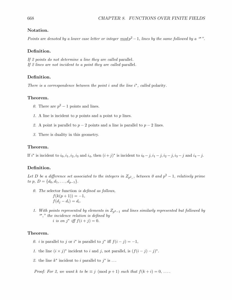
668 CHAPTER 8. FUNCTIONS OVER FINITE FIELDS
Notation.
Points are denoted by a lower case letter or integer modp2−1, lines by the same followed by a “∗”.
Definition.
If 2 points do not determine a line they are called parallel.If 2 lines are not incident to a point they are called parallel.
Definition.
There is a correspondence between the point i and the line i∗, called polarity.
Theorem.
0. There are p2 − 1 points and lines.
1. A line is incident to p points and a point to p lines.
2. A point is parallel to p− 2 points and a line is parallel to p− 2 lines.
3. There is duality in this geometry.
Theorem.
If i∗ is incident to i0, i1, i2, i3 and i4, then (i+ j)∗ is incident to i0− j, i1− j, i2− j, i3− j and i4− j.
Definition.
Let D be a difference set associated to the integers in Zp2,., between 0 and p2 − 1, relatively primeto p, D = d0, d1, . . . , dp−1.
0. The selector function is defined as follows,f(k(p+ 1)) = −1,f(dj − di) = di.
1. With points represented by elements in Zp2−1 and lines similarly represented but followed by“∗,” the incidence relation is defined by
i is on j∗ iff f(i+ j) = 0.
Theorem.
0. i is parallel to j or i∗ is parallel to j∗ iff f(i− j) = −1,
1. the line (i× j)∗ incident to i and j, not parallel, is (f(i− j)− j)∗.
2. the line k∗ incident to i parallel to j∗ is . . .
Proof: For 2, we want k to be ≡ j (mod p+ 1) such that f(k + i) = 0, . . . .

8.4. APPLICATION TO GEOMETRY. 669
Example.
p = 5, D = 0, 1, 14, 16, 21,i 0 1 2 3 4 5 6 7 8 9 10 11
f(i) −1 0 14 21 21 16 −1 14 16 16 14 14
i 12 13 14 15 16 17 18 19 20 21 22 23f(i) −1 1 0 1 0 21 −1 21 1 0 16 1
Examples of such differences sets are given in 8.4.1.
Example.
p = 5, the computations are done mod 24.
0. The coordinates of the i-th point on T are ai, bi, ci, the distance between j and j + i is
di =3√a3i + b3i + (ci − 1)3 − 3aibi(ci − 1).
i 0 1 2 3 4 5 6 7 8 9 10 11ai 0 0 1 −1 −1 −1 2 −1 1 −2 −1 1bi 0 −1 −1 −2 −2 0 2 1 0 0 1 −1ci 1 −2 −1 1 −1 −2 0 −2 0 −1 −1 −2di 0 3 1 1 0 3 3 4 0 4 1 4
i 12 13 14 15 16 17 18 19 20 21 22 23ai −1 −2 0 −2 0 −1 −1 −2 −2 0 2 1bi −1 −1 2 −1 1 −2 −1 1 −1 −2 0 −2ci −2 0 2 1 0 0 1 −1 −1 −1 2 −1di 0 2 4 1 0 1 2 2 0 4 4 2
1. The line i∗ is incident to the points −i, 1− i, 14− i, 16− i, 21− i.
2. The point i is parallel to i+ 6, i+ 12 and i− 6.
3. The angle between lines j∗ and (j + i)∗ is di.
In particular,0∗ : 0, 1, 14, 16, 21, is parallel to 6∗, 12∗, 18∗,1∗ : 23, 0, 13, 15, 20, is parallel to 7∗, 13∗, 19∗,14∗ : 10, 11, 0, 2, 7,16∗ : 8, 9, 22, 0, 5,21∗ : 3, 4, 17, 19, 0,23∗ : 1, 2, 15, 17, 22.on 0∗, the distances are
0 1 14 16 210 0 3 4 0 41 2 0 1 1 0
14 1 4 0 1 416 0 4 4 0 321 1 0 1 2 0

670 CHAPTER 8. FUNCTIONS OVER FINITE FIELDS
The “circles” of radius r and center 0 arer points on1 2, 3, 10, 13, 15, 174 7, 9, 11, 14, 21, 222 18, 19, 233 1, 5, 60 0, 4, 8, 12, 16, 20
Example
Let p = 11,i 0 1 2 3 4 5 6 7 8 9 10 11 12 13 14 15ai 0 1 6 0 9 4 5 1 8 7 4 3 8 5 4 4bi 0 3 3 7 3 8 8 7 0 10 6 1 8 8 5 9ci 1 4 0 10 3 9 1 5 8 1 2 4 4 4 6 8di 0 8 10 3 2 1 10 3 2 1 0 8 7 6 9 8
i 16 17 18 19 20 21 22 23 24 25 26 27 28 29 30 31ai 7 9 4 1 8 6 3 8 7 6 5 9 7 2 2 8bi 9 4 3 10 7 5 6 5 7 5 1 0 10 0 6 5ci 9 0 9 7 8 8 0 4 1 10 8 4 10 5 4 6di 8 4 6 9 0 10 10 6 5 6 1 2 8 8 0 2
i 32 33 34 35 36 37 38 39 40 41 42 43 44 45 46 47ai 9 7 5 5 4 1 4 2 1 4 0 10 3 9 1 5bi 2 0 4 6 4 5 9 5 0 1 6 0 9 4 5 1ci 9 10 6 10 6 7 3 0 0 3 3 7 3 8 8 7di 9 3 9 6 7 10 7 2 0 3 5 8 2 8 1 10
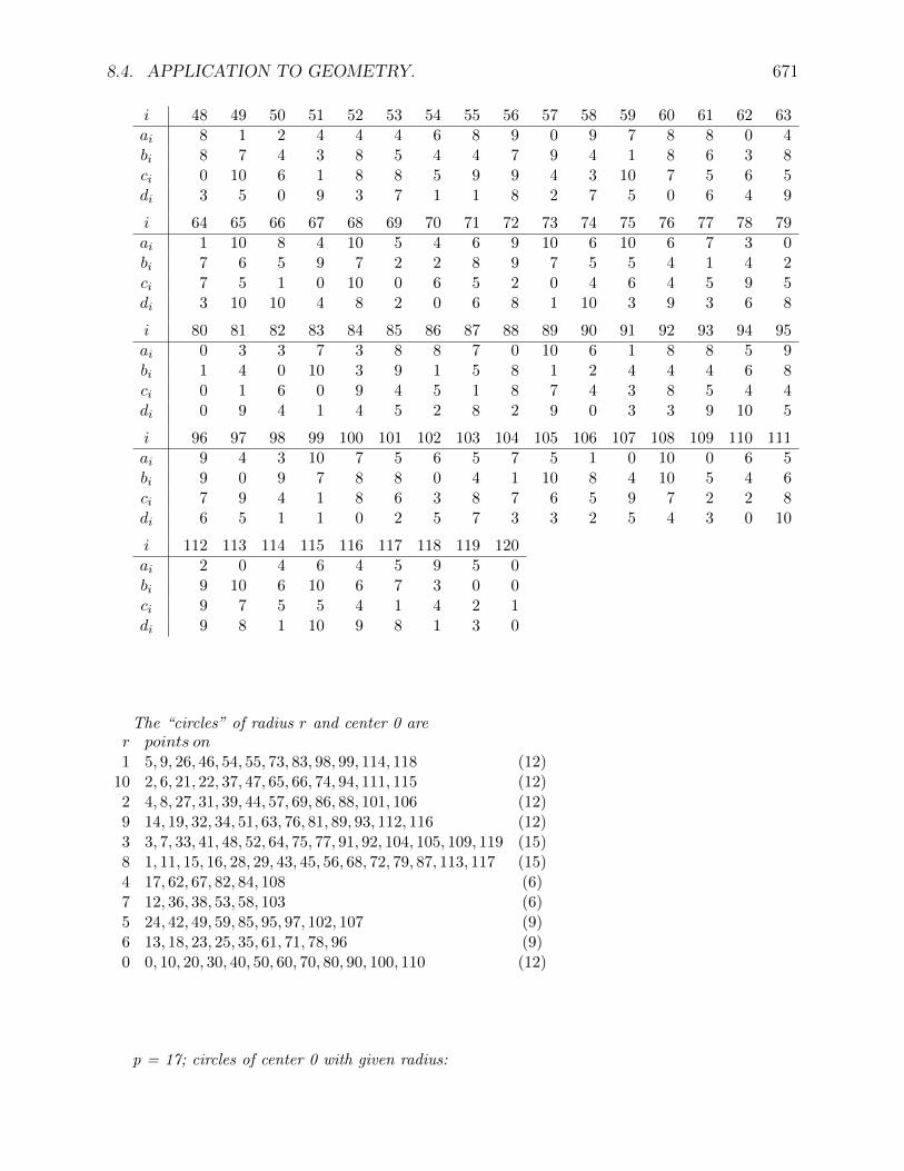
8.4. APPLICATION TO GEOMETRY. 671
i 48 49 50 51 52 53 54 55 56 57 58 59 60 61 62 63ai 8 1 2 4 4 4 6 8 9 0 9 7 8 8 0 4bi 8 7 4 3 8 5 4 4 7 9 4 1 8 6 3 8ci 0 10 6 1 8 8 5 9 9 4 3 10 7 5 6 5di 3 5 0 9 3 7 1 1 8 2 7 5 0 6 4 9
i 64 65 66 67 68 69 70 71 72 73 74 75 76 77 78 79ai 1 10 8 4 10 5 4 6 9 10 6 10 6 7 3 0bi 7 6 5 9 7 2 2 8 9 7 5 5 4 1 4 2ci 7 5 1 0 10 0 6 5 2 0 4 6 4 5 9 5di 3 10 10 4 8 2 0 6 8 1 10 3 9 3 6 8
i 80 81 82 83 84 85 86 87 88 89 90 91 92 93 94 95ai 0 3 3 7 3 8 8 7 0 10 6 1 8 8 5 9bi 1 4 0 10 3 9 1 5 8 1 2 4 4 4 6 8ci 0 1 6 0 9 4 5 1 8 7 4 3 8 5 4 4di 0 9 4 1 4 5 2 8 2 9 0 3 3 9 10 5
i 96 97 98 99 100 101 102 103 104 105 106 107 108 109 110 111ai 9 4 3 10 7 5 6 5 7 5 1 0 10 0 6 5bi 9 0 9 7 8 8 0 4 1 10 8 4 10 5 4 6ci 7 9 4 1 8 6 3 8 7 6 5 9 7 2 2 8di 6 5 1 1 0 2 5 7 3 3 2 5 4 3 0 10
i 112 113 114 115 116 117 118 119 120ai 2 0 4 6 4 5 9 5 0bi 9 10 6 10 6 7 3 0 0ci 9 7 5 5 4 1 4 2 1di 9 8 1 10 9 8 1 3 0
The “circles” of radius r and center 0 arer points on1 5, 9, 26, 46, 54, 55, 73, 83, 98, 99, 114, 118 (12)
10 2, 6, 21, 22, 37, 47, 65, 66, 74, 94, 111, 115 (12)2 4, 8, 27, 31, 39, 44, 57, 69, 86, 88, 101, 106 (12)9 14, 19, 32, 34, 51, 63, 76, 81, 89, 93, 112, 116 (12)3 3, 7, 33, 41, 48, 52, 64, 75, 77, 91, 92, 104, 105, 109, 119 (15)8 1, 11, 15, 16, 28, 29, 43, 45, 56, 68, 72, 79, 87, 113, 117 (15)4 17, 62, 67, 82, 84, 108 (6)7 12, 36, 38, 53, 58, 103 (6)5 24, 42, 49, 59, 85, 95, 97, 102, 107 (9)6 13, 18, 23, 25, 35, 61, 71, 78, 96 (9)0 0, 10, 20, 30, 40, 50, 60, 70, 80, 90, 100, 110 (12)
p = 17; circles of center 0 with given radius:

672 CHAPTER 8. FUNCTIONS OVER FINITE FIELDS
0 : 0, 16, 32, 48, 64, 80, 96, 112, 128, 144, 160, 176, 192, 208, 224, 240, 256, 272 (18)1 : 29, 60, 62, 73, 89, 111, 118, 133, 145, 147, 156, 159, 161, 162, 190, 195, 202, 205,
216, 235, 245, 251, 266, 278 (24)2 : 24, 47, 67, 120, 151, 186, 223, 253, 263, 269, 275, 282 (12)3 : 1, 8, 17, 38, 66, 70, 136, 219, 236, 258, 267, 268 (12)4 : 18, 39, 74, 78, 87, 100, 106, 109, 113, 125, 134, 174, 193, 260, 262 (15)5 : 23, 59, 92, 103, 110, 124, 139, 142, 165, 180, 213, 234 (12)6 : 3, 33, 36, 41, 42, 44, 50, 51, 55, 56, 71, 77, 88, 101, 121, 138, 157, 172, 273, 274, 277 (21)7 : 2, 4, 7, 9, 34, 61, 63, 68, 91, 107, 119, 153, 173, 198, 207 (15)8 : 5, 27, 31, 40, 45, 46, 57, 58, 76, 84, 85, 97, 104, 105, 122, 130, 140, 171, 189, 194,
206, 209, 239, 276 (24)9 : 12, 49, 79, 82, 94, 99, 117, 148, 158, 166, 183, 184, 191, 203, 204, 212, 230, 231,
242, 243, 248, 257, 261, 283 (24)10 : 81, 90, 115, 135, 169, 181, 197, 220, 225, 227, 254, 279, 281, 284, 286 (15)11 : 11, 14, 15, 116, 131, 150, 167, 187, 200, 211, 217, 232, 233, 237, 238, 244, 246,
247, 252, 255, 285 (21)12 : 54, 75, 108, 123, 146, 149, 164, 178, 185, 196, 229, 265 (12)13 : 26, 28, 95, 114, 154, 163, 175, 179, 182, 188, 201, 210, 214, 249, 270 (15)14 : 20, 21, 30, 52, 69, 152, 218, 222, 250, 271, 280, 287 (12)15 : 6, 13, 19, 25, 35, 65, 102, 137, 168, 221, 241, 264 (12)16 : 10, 22, 37, 43, 53, 72, 83, 86, 93, 98, 126, 127, 129, 132, 141, 143, 155, 170, 177,
199, 215, 226, 228, 259 (24)The points common to the circles given above and noted i : if the radius is i are given below if
there are points which are common with

8.4. APPLICATION TO GEOMETRY. 673
center 1, radius 1: 30,61,63,74,90,112,119,134,146,148,157,160,162,
163,191,196,203,206,217,236,246,252,267,279
0: 112,160; 1: 162; 3: 236,267; 4: 74,134; 6: 157;
7: 61,63,119; 8: 206; 9: 148,191,203; 10: 90,279;
11: 217,246,252; 12: 146,196; 13: 163; 14: 30;
center 1, radius 2: 25,48,68,121,152,187,224,254,264,270,276,283
0: 48,224; 6: 121; 7: 68; 8: 276; 9: 283; 10: 254; 11: 187;
13: 270; 14: 152; 15: 25,264;
center 1, radius 3: 2,9,18,39,67,71,137,220,237,259,268,269
2: 67,269; 3: 268; 4: 18,39; 6: 71; 7: 2,9; 10: 220; 11: 237;
15: 137; 16: 259;
center 1, radius 4: 19,40,75,79,88,101,107,110,114,126,135,175,194,261,
263
2: 263; 5: 110; 6: 88,101; 7: 107; 8: 40,194; 9: 79,261; 10: 135;
12: 75; 13: 114,175; 15: 19; 16: 126;
center 1, radius 5: 24,60,93,104,111,125,140,143,166,181,214,235
1: 60,111,235; 2: 24; 4: 125; 8: 104,140; 9: 166; 10: 181;
13: 214; 16: 93,143;
center 1, radius 6: 4,34,37,42,43,45,51,52,56,57,72,78,89,102,122,139,
158,173,274,275,278
1: 89,278; 2: 275; 4: 78; 5: 139; 6: 42,51,56,274; 7: 4,34,173;
8: 45,57,122; 9: 158; 14: 52; 15: 102; 16: 37,43,72;
center 1, radius 7: 3,5,8,10,35,62,64,69,92,108,120,154,174,199,208
0: 64,208; 1: 62; 2: 120; 3: 8; 4: 174; 5: 92; 6: 3; 8: 5; 12: 108;
13: 154; 14: 69; 15: 35; 16: 10,199;
center 1, radius 8: 6,28,32,41,46,47,58,59,77,85,86,98,105,106,123,131,
141,172,190,195,207,210,240,277
0: 32,240; 1: 190,195; 2: 47; 4: 106; 5: 59; 6: 41,77,172,277;
7: 207; 8: 46,58,85,105; 11: 131; 12: 123; 13: 28,210; 15: 6;
16: 86,98,141;
center 1, radius 9: 13,50,80,83,95,100,118,149,159,167,184,185,192,204,
205,213,231,232,243,244,249,258,262,284
0: 80,192; 1: 118,159,205; 3: 258; 4: 100,262; 5: 213; 6: 50;
9: 184,204,231,243; 10: 284; 11: 167,232,244; 12: 149,185;
13: 95,249; 15: 13; 16: 83;
center 1, radius 10: 82,91,116,136,170,182,198,221,226,228,255,280,282,
285,287
2: 282; 3: 136; 7: 91,198; 9: 82; 11: 116,255,285; 13: 182;
14: 280,287; 15: 221; 16: 170,226,228;

674 CHAPTER 8. FUNCTIONS OVER FINITE FIELDS
center 1, radius 11: 12,15,16,117,132,151,168,188,201,212,218,233,234,
238,239,245,247,248,253,256,286
0: 16,256; 1: 245; 2: 151,253; 5: 234; 8: 239; 9: 12,117,212,248;
10: 286; 11: 15,233,238,247; 13: 188,201; 14: 218; 15: 168; 16: 132;
center 1, radius 12: 55,76,109,124,147,150,165,179,186,197,230,266
1: 147,266; 2: 186; 4: 109; 5: 124,165; 6: 55; 8: 76; 9: 230;
10: 197; 11: 150; 13: 179;
center 1, radius 13: 27,29,96,115,155,164,176,180,183,189,202,211,215,
250,271
0: 96,176; 1: 29,202; 5: 180; 8: 27,189; 9: 183; 10: 115; 11: 211;
12: 164; 14: 250,271; 16: 155,215;
center 1, radius 14: 21,22,31,53,70,153,219,223,251,272,281,0
0: 0,272; 1: 251; 2: 223; 3: 70,219; 7: 153; 8: 31; 10: 281;
14: 21; 16: 22,53;
center 1, radius 15: 7,14,20,26,36,66,103,138,169,222,242,265
3: 66; 5: 103; 6: 36,138; 7: 7; 9: 242; 10: 169; 11: 14; 12: 265;
13: 26; 14: 20,222;
center 1, radius 16: 11,23,38,44,54,73,84,87,94,99,127,128,130,133,142,
144,156,171,178,200,216,227,229,260
0: 128,144; 1: 73,133,156,216; 3: 38; 4: 87,260; 5: 23,142; 6: 44;
8: 84,130,171; 9: 94,99; 10: 227; 11: 11,200; 12: 54,178,229;
16: 127;
center 2, radius 1: 31,62,64,75,91,113,120,135,147,149,158,161,163,164,
192,197,204,207,218,237,247,253,268,280
0: 64,192; 1: 62,147,161; 2: 120,253; 3: 268; 4: 113; 7: 91,207;
8: 31; 9: 158,204; 10: 135,197; 11: 237,247; 12: 75,149,164;
13: 163; 14: 218,280;
center 2, radius 2: 26,49,69,122,153,188,225,255,265,271,277,284
6: 277; 7: 153; 8: 122; 9: 49; 10: 225,284; 11: 255; 12: 265;
13: 26,188; 14: 69,271;
center 2, radius 3: 3,10,19,40,68,72,138,221,238,260,269,270
2: 269; 4: 260; 6: 3,138; 7: 68; 8: 40; 11: 238; 13: 270;
15: 19,221; 16: 10,72;
center 2, radius 4: 20,41,76,80,89,102,108,111,115,127,136,176,195,262,
264
0: 80,176; 1: 89,111,195; 3: 136; 4: 262; 6: 41; 8: 76; 10: 115;
12: 108; 14: 20; 15: 102,264; 16: 127;
center 2, radius 5: 25,61,94,105,112,126,141,144,167,182,215,236
0: 112,144; 3: 236; 7: 61; 8: 105; 9: 94; 11: 167; 13: 182; 15: 25;
16: 126,141,215;

8.4. APPLICATION TO GEOMETRY. 675
center 2, radius 6: 5,35,38,43,44,46,52,53,57,58,73,79,90,103,123,140,
159,174,275,276,279
1: 73,159; 2: 275; 3: 38; 4: 174; 5: 103; 6: 44;
8: 5,46,57,58,140,276; 9: 79; 10: 90,279; 12: 123; 14: 52; 15: 35;
16: 43,53;
center 2, radius 7: 4,6,9,11,36,63,65,70,93,109,121,155,175,200,209
3: 70; 4: 109; 6: 36,121; 7: 4,9,63; 8: 209; 11: 11,200; 13: 175;
15: 6,65; 16: 93,155;
center 2, radius 8: 7,29,33,42,47,48,59,60,78,86,87,99,106,107,124,132,
142,173,191,196,208,211,241,278
0: 48,208; 1: 29,60,278; 2: 47; 4: 78,87,106; 5: 59,124,142;
6: 33,42; 7: 7,107,173; 9: 99,191; 11: 211; 12: 196; 15: 241;
16: 86,132;
center 2, radius 9: 14,51,81,84,96,101,119,150,160,168,185,186,193,205,
206,214,232,233,244,245,250,259,263,285
0: 96,160; 1: 205,245; 2: 186,263; 4: 193; 6: 51,101; 7: 119;
8: 84,206; 10: 81; 11: 14,150,232,233,244,285; 12: 185; 13: 214;
14: 250; 15: 168; 16: 259;
center 2, radius 10: 83,92,117,137,171,183,199,222,227,229,256,281,283,
286,0
0: 0,256; 5: 92; 8: 171; 9: 117,183,283; 10: 227,281,286; 12: 229;
14: 222; 15: 137; 16: 83,199;
center 2, radius 11: 13,16,17,118,133,152,169,189,202,213,219,234,235,
239,240,246,248,249,254,257,287
0: 16,240; 1: 118,133,202,235; 3: 17,219; 5: 213,234; 8: 189,239;
9: 248,257; 10: 169,254; 11: 246; 13: 249; 14: 152,287; 15: 13;
center 2, radius 12: 56,77,110,125,148,151,166,180,187,198,231,267
2: 151; 3: 267; 4: 125; 5: 110,180; 6: 56,77; 7: 198;
9: 148,166,231; 11: 187;
center 2, radius 13: 28,30,97,116,156,165,177,181,184,190,203,212,216,
251,272
0: 272; 1: 156,190,216,251; 5: 165; 8: 97; 9: 184,203,212; 10: 181;
11: 116; 13: 28; 14: 30; 16: 177;
center 2, radius 14: 22,23,32,54,71,154,220,224,252,273,282,1
0: 32,224; 2: 282; 3: 1; 5: 23; 6: 71,273; 10: 220; 11: 252;
12: 54; 13: 154; 16: 22;
center 2, radius 15: 8,15,21,27,37,67,104,139,170,223,243,266
1: 266; 2: 67,223; 3: 8; 5: 139; 8: 27,104; 9: 243; 11: 15; 14: 21;
16: 37,170;
center 2, radius 16: 12,24,39,45,55,74,85,88,95,100,128,129,131,134,
143,145,157,172,179,201,217,228,230,261
0: 128; 1: 145; 2: 24; 4: 39,74,100,134; 6: 55,88,157,172;
8: 45,85; 9: 12,230,261; 11: 131,217; 13: 95,179,201;
16: 129,143,228;

676 CHAPTER 8. FUNCTIONS OVER FINITE FIELDS
8.4.3 3 - Dimensional Equidistance Curves.
Introduction.
On the surface T , for p ≡ −1 (mod 5), we can define besides lines (intersection with a planethrough the origin), circles (pts equidistant using the cubic function from a given point), line-circle(set of tangents in space to the circles), podars (set of points where tangents in space intersect T ),mediatrices (set of points equidistant from 2 points). This section describes those curves.
Definition.
The circles are the set of points on T such that the cubic distance from a given point on T , calledthe center of the circle, is a given integer r, called the radius of the circle.
Theorem.
The circles of radius r and center (0, 0, 1), are the points (x, y, z) which satisfy 0. and 1. or 0. and2.
0. x3 + y3 + z3 − 3xyz = 1.
1. x3 + y3 + z3 − 3z2 + 3z − 1− 3xyz + 3xy = r3.
2. 3z2 − 3z − 3xy = −r3.
Definition.
A line-circle is the set of lines tangent in space to a circle.
Theorem.
The line-circle associated to the circles in 8.4.3 have at (x, y, z) the direction (∆x,∆y,∆z) givenby
0. ∆x = xz2 + z′y2, ∆y = −yz2 − z′x2, ∆z = −xx2 + yy2,where
1. x2 = x2 − yz, y2 = y2 − zx, z2 = z2 − xy, z′ = 2z − 1.
Proof: the component of the direction satisfy(x2 − yz)∆x+ (y2 − zx)∆y + (z2 − xy)∆z = 0,−y∆x− x∆y + (2z − 1)∆z = 0,
hence 0.
Definition.
A podar is set of points where tangents in space intersect T.

8.4. APPLICATION TO GEOMETRY. 677
Theorem.
The coordinates of points on the podar associated to the circle in 8.4.3 are the points (x+ t∆x, y+t∆y, z + t∆z) where t satisfies
0. t = −3x∆x2+y∆y2+z∆z2(∆x+∆y+∆z (∆x2 + ∆y2 + ∆z2)).
where
1. ∆x2 = ∆x2 −∆y∆z,∆y2 = ∆y2 −∆z∆x,∆z2 = ∆z2 −∆x∆y.
Proof. A point (x + t∆x, y + t∆y, z + t∆z) on the line (x, y, z) with direction (∆x,∆y,∆z) ison T if t satisfies the cubic equation,(∆x+ ∆y + ∆z)(∆x2 + ∆y2 + ∆z2)t3 + 3(x∆x2 + y∆y2 + z∆z2)t2
+ 3(x2∆x+ y2∆y + z2∆z)t+ (x3 + y3 + z3 − 3xyz − 1) + 1 = 0,the coefficient of t0 is 0 because (x, y, z) is on T , that of t is 0 because it is x2(xz2 + z′y2) +y2(−yz2 − z′x2) + z2(−xx2 + yy2) = 0.
Theorem.
0. If the tangent k∗ at i to the circle, centered at 0 of radius r, meets T at j, then the tangent(k+2i)∗ at −i to the circle, centered at 0 of radius −r (mod p), meets T at j − 2i.
1. If the tangent at i to the circle, centered at 0 of radius r, meets T at j parallel to i, then thetangent at −i to the circle, centered at 0 of radius −r (mod p), meets T at j − 2i parallel to−i.

678 CHAPTER 8. FUNCTIONS OVER FINITE FIELDS
Example.
Let p = 11,r = 1,circle 5 9 26 46 54 55 73 83 98 99 114 118podar 92 15 113 43 51 52 4 44 107 45 81 97
line−circle 29∗ 19∗ 8∗ 118∗ 110∗ 109∗ 30∗ 0∗ 22∗ 119∗ 40∗ 32∗
r = 10,circle 2 6 21 22 37 47 65 66 74 94 111 115podar 101 93 87 31 118 98 62 63 71 61 117 82
line−circle 28∗ 28∗ 77∗ 98∗ 46∗ 56∗ 99∗ 98∗ 90∗ 60∗ 37∗ 39∗
r = 2circle 4 8 27 31 39 44 57 69 86 88 101 106podar 28 59 36 118 6 68 36 66 95 49 98 85
line−circle −− 95∗ 93∗ 3∗ 115∗ −− 93∗ 95∗ 34∗ 115∗ 63∗ 44∗
r = 9circle 14 19 32 34 51 63 76 81 89 93 112 116podar 113 16 113 43 48 42 100 48 56 102 43 20
line−circle 16∗ 25∗ 51∗ 86∗ 113∗ 87 −− 73∗ 65∗ 27∗ 111∗ −−r = 3circle 3 7 33 41 48 52 64 75 77 91104 105 109 119podar 9 88 99 107 48 58 73 84 8 97
line−circle 25∗ 76∗ 65∗ 57∗ −− 96∗ 56∗ 45∗ 26∗ 57∗
r = 3circle 92 104 105 109 119podar 38 83 84 40 80
line−circle 6∗ 46∗ 45∗ 114∗ 84∗
r = 8circle 1 11 15 16 28 29 43 45 56 68podar 82 62 114 115 94 35 94 54 65 74
line−circle 82∗ 92∗ 15∗ 14∗ 70∗ 119∗ 60∗ 75∗ 64∗ 80∗
r = 8circle 72 79 87 113 117podar 72 25 33 74 3
line−circle −− 19∗ 11∗ 90∗ 31∗
r = 4circle 17 62 67 82 84 108podar 41 113 91 43 84 108
line−circle −− 41∗ −− 1∗ −− −−r = 7circle 12 36 38 53 58 103podar 12 36 119 77 109 7
line−circle −− −− 45∗ −− 45∗ −−r = 5circle 24 42 49 59 85 95 97 102 107podar 24 21 73 83 16 56 103 111 53
line−circle −− 108∗ −− −− 18∗ 108∗ 51∗ 18∗ 111∗
r = 6circle 13 18 23 25 35 61 71 78 96podar 79 27 29 106 86 85 95 57 96
line−circle 85∗ 102∗ 5∗ 58∗ 68∗ −− −− 72∗ −−
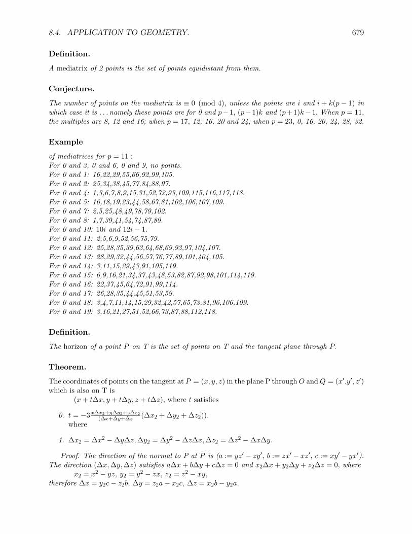
8.4. APPLICATION TO GEOMETRY. 679
Definition.
A mediatrix of 2 points is the set of points equidistant from them.
Conjecture.
The number of points on the mediatrix is ≡ 0 (mod 4), unless the points are i and i+ k(p− 1) inwhich case it is . . . namely these points are for 0 and p−1, (p−1)k and (p+ 1)k−1. When p = 11,the multiples are 8, 12 and 16; when p = 17, 12, 16, 20 and 24; when p = 23, 0, 16, 20, 24, 28, 32.
Example
of mediatrices for p = 11 :For 0 and 3, 0 and 6, 0 and 9, no points.For 0 and 1: 16,22,29,55,66,92,99,105.For 0 and 2: 25,34,38,45,77,84,88,97.For 0 and 4: 1,3,6,7,8,9,15,31,52,72,93,109,115,116,117,118.For 0 and 5: 16,18,19,23,44,58,67,81,102,106,107,109.For 0 and 7: 2,5,25,48,49,78,79,102.For 0 and 8: 1,7,39,41,54,74,87,89.For 0 and 10: 10i and 12i− 1.For 0 and 11: 2,5,6,9,52,56,75,79.For 0 and 12: 25,28,35,39,63,64,68,69,93,97,104,107.For 0 and 13: 28,29,32,44,56,57,76,77,89,101,404,105.For 0 and 14: 3,11,15,29,43,91,105,119.For 0 and 15: 6,9,16,21,34,37,43,48,53,82,87,92,98,101,114,119.For 0 and 16: 22,37,45,64,72,91,99,114.For 0 and 17: 26,28,35,44,45,51,53,59.For 0 and 18: 3,4,7,11,14,15,29,32,42,57,65,73,81,96,106,109.For 0 and 19: 3,16,21,27,51,52,66,73,87,88,112,118.
Definition.
The horizon of a point P on T is the set of points on T and the tangent plane through P.
Theorem.
The coordinates of points on the tangent at P = (x, y, z) in the plane P throughO andQ = (x′.y′, z′)which is also on T is
(x+ t∆x, y + t∆y, z + t∆z), where t satisfies
0. t = −3x∆x2+y∆y2+z∆z2(∆x+∆y+∆z (∆x2 + ∆y2 + ∆z2)).
where
1. ∆x2 = ∆x2 −∆y∆z,∆y2 = ∆y2 −∆z∆x,∆z2 = ∆z2 −∆x∆y.
Proof. The direction of the normal to P at P is (a := yz′ − zy′, b := zx′ − xz′, c := xy′ − yx′).The direction (∆x,∆y,∆z) satisfies a∆x+ b∆y + c∆z = 0 and x2∆x+ y2∆y + z2∆z = 0, where
x2 = x2 − yz, y2 = y2 − zx, z2 = z2 − xy,therefore ∆x = y2c− z2b, ∆y = z2a− x2c, ∆z = x2b− y2a.

680 CHAPTER 8. FUNCTIONS OVER FINITE FIELDS
A point (x + t∆x, y + t∆y, z + t∆z) on the line (x, y, z) with direction (∆x,∆y,∆z) is on T if tsatisfies the cubic equation,(∆x + ∆y + ∆z)(∆x2 + ∆y2 + ∆z2)t3 + 3(x∆x2 + y∆y2 + z∆z2)t2 + 3(x2∆x + y2∆y + z2∆z)t +(x3 + y3 + z3 − 3xyz − 1) + 1 = 0,the coefficient of t0 is 0 because (x, y, z) is on T, that of t is 0 because it is x2(y2c− z2b) + y2(z2a−x2c) + z2(x2b− y2a) = 0.
Algorithm.
To determine the horizon as 0 we determine for each point with z = 1, on which the line 0×sel(i) itis located, if x+y = 0, the point is the ideal point, if x = 0 or y = 0, 0 is a triple contact, if it is onno line 0×sel(i), then it corresponds to points parallel to it. This is implement in [\130\RIC.BAS]option 12.
Proof: The horizon of P of 0 are the points on T and z = 1 or x3 + y3 − 3xy = 0, those in theplane x = kt, y = lt satisfy (k3 + l3)t− 3kl = 0 and t = 0, twice. If k = 0 or l = 0 then t = 0 is atriple root, if k = −l, or x+ y = 0, then the point is an ideal point. In all other cases, t = 3kl
k3+l3).
Example.
For p = 11, the points H on the horizon of 0 have their tangent t and the points Q on T for whichthe tangent is t∗ given byH t∗ Q0 1∗ 8, 27, 29, 33, 40, 43, 82, 97, 102, 119(y = 0)
41∗ 3, 42, 57, 62, 79, 80, 88, 107, 109, 113(x = 0)6 28∗ 2, 6, 13, 16, 55, 70, 75, 92, 93, 1019 0∗ 1, 9, 28, 30, 34, 41, 44, 83, 98, 103
24 −− 12, 24, 36, 48, 60, 72, 84, 96, 10851 103∗ 17, 18, 26, 45, 47, 51, 58, 61, 100, 11566 98∗ 5, 22, 23, 31, 50, 52, 56, 63, 66, 10581 83∗ 15, 20, 37, 38, 46, 65, 67, 71, 78, 8187 34∗ 7, 10, 49, 64, 69, 86, 87, 95, 114, 11699 30∗ 4, 11, 14, 53, 68, 73, 90, 91, 99, 118
117 44∗ 39, 54, 59, 76, 77, 85, 104, 106, 110, 117∞ 9∗ 19, 21, 25, 32, 35, 74, 89, 94, 111, 112
Conjecture.
The points on the horizon of 0 are multiples of 3.
Example.
The horizon of 0 is for
0. p = 5,selector 0 1 14 16 21 −−horizon 0 15 ∞ 0 3 18
1. p = 11,selector 0 1 9 28 30 34 41 44 83 98103 −−horizon 9 0 ∞ 6 99 87 0117 81 66 51 24

8.4. APPLICATION TO GEOMETRY. 681
2. p = 17,selector 0 1 10 13 34 45 59 86 112 114 129 134horizon 114 111 24 246 225 150 0 165 210 81 159 213selector 191 195 251 259 282 −−horizon ∞ 93 0 141 120 108
3. p = 23,selector 0 1 60 91 134 142 148 203 249 253 266 269horizon 0 270 273 180 69 387 471 285 279 366 3 219selector 271 298 305 333 342 352 363 375 450 488 503 −−horizon 81 231 426 444 33 0 498 402 453 ∞ 294 408
8.4.4 Generalization of the Selector Function.
Introduction.
The selector function was introduced by Fernand Lemay to determine easily from the selector, pointson 2 lines, lines incident to 2 points, points on lines or lines incident to points. This notion isgeneralized to 3 and more? dimensions.
Definition.
defining polynomial
Theorem.
If the Pi denotes a primitive polynomial of degree i, for k = 3, the defining polynomials P can havethe following form,
P4, P1P3, P21P2,
there are p4 + p3 + p2 + p+ 1, p4 − 1, p4 − p polynomials relatively prime to P, in these respectivecases.For k = 4, the defining polynomials P can have the following form,
P5, P1P4, P21P3, P2P3.
there are p5 + p4 + p3 + p2 + p+ 1, (p3 − 1)(p+ 1), p5 − 1, p5 − p polynomials relatively prime toP, in these respective cases.
Proof: The polynomials in the sets are those which are relatively prime to the defining polyno-mial. There are pk homogeneous polynomials of degree k. If, for instance, k = 4 and the definingpolynomial P is P2P3, there are p2 + p+ 1 polynomials which are multiple of P 2 and p+ 1, whichare multiples of P3, hence p4 + p3 + p2 + p+ 1− (p2 + p+ 1)− (p− 1) polynomials relatively primeto P.
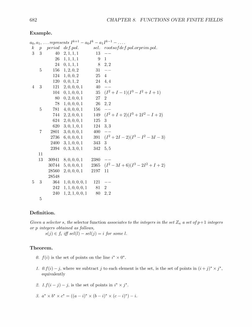
682 CHAPTER 8. FUNCTIONS OVER FINITE FIELDS
Example.
a0, a1, . . . represents Ik+1 − a0Ik − a1I
k−1 − . . . .k p period def.pol. sel. rootsofdef.pol.orprim.pol.3 3 40 2, 1, 1, 1 13 −−
26 1, 1, 1, 1 9 124 0, 1, 1, 1 8 2, 2
5 156 1, 2, 0, 2 31 −−124 1, 0, 0, 2 25 4120 0, 0, 1, 2 24 4, 4
4 3 121 2, 0, 0, 0, 1 40 −−104 0, 1, 0, 0, 1 35 (I2 + I − 1)(I3 − I2 + I + 1)80 0, 2, 0, 0, 1 27 278 1, 0, 0, 0, 1 26 2, 2
5 781 4, 0, 0, 0, 1 156 −−744 2, 2, 0, 0, 1 149 (I2 + I + 2)(I3 + 2I2 − I + 2)624 2, 0, 0, 0, 1 125 3620 3, 0, 1, 0, 1 124 3, 3
7 2801 3, 0, 0, 0, 1 400 −−2736 6, 0, 0, 0, 1 391 (I2 + 2I − 2)(I3 − I2 − 3I − 3)2400 3, 1, 0, 0, 1 343 32394 0, 3, 3, 0, 1 342 5, 5
1113 30941 8, 0, 0, 0, 1 2380 −−
30744 5, 0, 0, 0, 1 2365 (I2 − 3I + 6)(I3 − 2I2 + I + 2)28560 2, 0, 0, 0, 1 2197 1128548
5 3 364 1, 0, 0, 0, 0, 1 121 −−242 1, 1, 0, 0, 0, 1 81 2240 1, 2, 1, 0, 0, 1 80 2, 2
5
Definition.
Given a selector s, the selector function associates to the integers in the set Zn a set of p+1 integersor p integers obtained as follows,
s(j) ∈ fi iff sel(l)− sel(j) = i for some l.
Theorem.
0. f(i) is the set of points on the line i∗ × 0∗.
1. 0.f(i)− j, where we subtract j to each element is the set, is the set of points in (i+ j)∗× j∗,equivalently
2. 1.f(i− j)− j, is the set of points in i∗ × j∗.
3. a∗ × b∗ × c∗ = ((a− i)∗ × (b− i)∗ × (c− i)∗)− i.

8.4. APPLICATION TO GEOMETRY. 683
Definition.
Theorem.
Theorem.
0. If the defining polynomial is primitive, then
1. 0. |s| = pk−1p−1 ,
2. 1. if i 6= 0, |f(i)| = p+ 1
3. If the defining polynomial has one root, then
4. 0. |s| = pk,
5. 1. if i 6= 0, |f(i)| = p,
6. If the defining polynomial has one root, then
7. 0. |s| = pk − 1,
8. 1. if i?, |f(i)| = p,
9. 2. if i?, |f(i)| = p− 1,
10. If the defining polynomial has one quadratic factor, then
11. 0. |s| = (pk − 1)(p+ 1)?,
12. 1. if i?, |f(i)| = p,
Example.
0. k = 3, p = 3, defining polynomial I4 − 2I3 − I2 − I − 1.selector: 0 1 2 9 10 13 15 16 18 20 24 30 37selector function:
0 −1 −1 −1 −1 14 1 2 10 16 28 2 9 13 301 0 1 9 15 15 0 1 9 15 29 1 13 20 242 0 13 16 18 16 0 2 24 37 30 0 10 20 303 10 13 15 37 17 1 13 20 24 31 9 10 18 244 9 16 20 37 18 0 2 24 37 32 9 10 18 245 10 13 15 37 19 1 18 30 37 33 9 16 20 376 9 10 18 24 20 0 10 20 30 34 15 16 24 307 2 9 13 30 21 9 16 20 37 35 2 15 18 208 1 2 10 16 22 2 15 18 20 36 1 13 20 249 0 1 9 15 23 1 18 30 37 37 0 13 16 18
10 0 10 20 30 24 0 13 16 18 38 2 15 18 2011 2 9 13 30 25 15 16 24 30 39 1 2 10 1612 1 18 30 37 26 15 16 24 3013 0 2 24 37 27 10 13 15 37

684 CHAPTER 8. FUNCTIONS OVER FINITE FIELDS
1. k = 3, p = 3, definingpolynomialI4 − I3 − I2 − I − 1.selector: 0 1 2 8 11 18 20 22 23selector function:0 −1 −1 −1 7 1 11 20 14 8 20 23 21 1 2 231 0 1 22 8 0 18 20 15 8 11 22 22 0 1 222 0 18 20 9 2 11 18 16 2 11 18 23 0 11 233 8 20 23 10 1 8 18 17 1 11 20 24 2 20 224 18 22 23 11 0 11 23 18 0 2 8 25 1 2 235 18 22 23 12 8 11 22 19 1 8 186 2 20 22 13 −1 −1 −1 20 0 2 8
2. k = 3, p = 3, definingpolynomialI4 − I2 − I − 1.selector: 0 1 2 4 14 15 19 21selector function:0 −1 −1 −1 6 15 19 −1 12 2 14 −1 18 1 21 −11 0 1 14 7 14 19 21 13 1 2 15 19 0 2 192 0 2 19 8 −1 −1 −1 14 0 1 14 20 1 4 193 1 21 −1 9 15 19 −1 15 0 4 −1 21 0 4 −14 0 15 21 10 4 14 15 16 −1 −1 −1 22 2 4 215 14 19 21 11 4 14 15 17 2 4 21 23 1 2 15
Example.
In the case of Example 3.6.x.0. if we denote by i%, the lines 0∗ × i∗, these lines, which are sets of4 points can all be obtained from1% = 0, 1, 9, 15, 2% = 0, 13, 16, 18, 4% = 9, 16, 20, 37 and10% = 0, 10, 20, 30 by adding an integer modulo n.1% + 0 = 1%, 9%, 15%, 1% + 1 = 39%, 8%, 14%, 1% + 9 = 6%, 31%, 32%, 1% + 15 = 34%, 25%, 26%,2% + 0 = 2%, 24%, 37%, 2% + 2 = 22%, 35%, 38%, 2% + 37 = 3%, 5%, 27%, 2% + 24 = 13%, 16%, 18%,4% + 0 = 4%, 21%, 33%, 4% + 4 = 17%, 29%, 36%, 4% + 21 = 12%, 19%, 23%,
4% + 33 = 7%, 11%, 28%,10% + 0 = 10%, 20%, 30%.
Definition.
Conjecture.
8.5 Generalization of the Spheres in Riccati Geometry.
8.5.1 Dimension k.
Introduction.
If we choose the “sphere“ x3 + y3 + z3 − 3xyz = 1 in 3 dimension we do not obtain for a givenprime all periods as we do with the selector. We have to generalyze using what is derived fromdifferential equations with constant coefficients in which the coefficient of the k − 1-th derivative iszero to obtain a constant Wronskian. But, just as in the case of 2 dimensions, to obtain all sets oftrigonometric functions, corresponding to the circular and hyperbolic functions, for all p, we have

8.5. GENERALIZATION OF THE SPHERES IN RICCATI GEOMETRY. 685
to introduce in 3 dimension a cubic non residue if there is any, . . . I will first recall same wellknown definitions and Theorems of linear differential equations.
Definition.
Given a linear differential equation Dkx = C0x+C1Dx+ . . . Ck−2Dk−2x, and k solutions yi
of these equations, the Wronskian is the matrix of functions whose j-th row are the j-th derivativesof yi, for i = 0 to k − 1.
Theorem.
0. The functions yi are independent solution iff the determinant of the Wronskian is differentfrom 0 for a particular value of the independent variable.
1. The determinant of the Wronskian is a constant function.
2. If W (0) = E, then W (x+ y) = W (x)W (y).
Theorem.
If the linear differential equation 8.5.1.0. is such that Ci are constant functions then any linearcombination of x and its derivatives is also a solution of 8.5.1.0.
Comment.
If we choose x such that its derivatives are 0 except the k − 1-th, chosen equal to 1, it is easy toobtain independent solutions using linear combination of x and its derivatives to insure W (0) = E.If det(W (t)) = 1, then det(W (nt)) = 1 and the surface Dix(nt), i = 0 to k− 1, can be chosen as a“sphere” in k-dimension and n as the angle between the directions joining the origin to the points(Dix((n+ a)t)) and (Dix(at)).
Notation.
Given 2 solutions x and x′ of 8.5.1.0. and a parameter t let xi := Djx(it) and x′i := Djx′(it),yi,j := xix
′j + xjx
′i, i 6= j
yi,i := xix′i,
8.5.2 Dimension 3.
Theorem.
For k = 3, let
0.0. D3x0 = C0x0 + C1Dx0,with
0.1. Dx0(0) = 0, Dx0 = x1(0) = 0, D2x0(0) = x2(0) = 1,then
1.0. the set of functions x2 − C1x0, x1, x0 are independent

686 CHAPTER 8. FUNCTIONS OVER FINITE FIELDS
1. their Wronskian is
W =
∣∣∣∣∣∣x2 − C1x0 x1 x0
C0x0 x2 x1
C0x1 C0x0 + C1x1 x2
∣∣∣∣∣∣3. W (0) = E.
2. The distance from (0, 0, 0) to (x0, x1, x2) isC2
0x30 + C0x
31 + x3
2 − 3x0x1x2 − C1x21x2 − C1x
22x0 + 2C0C1x
20x1
+ C21x0x
21.
3. The addition formulas arex′′0 = y0,2 + y1,1 − C1y0,0,x′′1 = y1,2 + C0y0,0,x′′2 = y2,2 + C0y0,1 + C1y1,1.
4. The tangent plane at (x0, x1, x2) is[3C2
0x20 − 3C0x1x2 − C1x
22 + 4C0C1x0x1 + C2
1x21,
3C0x21 − 3C0x2x0 + 2C0C1x
20 − 2C1x1x2 + 2C2
1x0x1,3x2
2 − 3C0x0x1 − 2C1x2x0 − C1x21].
Definition.
If
0. p ≡ 1 (mod 6), then ν3 = n is a non cubic residue and the functions are not necessary real,we therefore denote then by ξi instead of xi and express ξi in terms of a power of ν and aninteger xi as follows,
1. x0(3i) = x0(3i), ξ1(3i) = x1(3i)ν, ξ2(3i) = x2(3i)ν2, ξ0(3i + 1) = x0(3i)ν2, ξ1(3i + 1) =x1(3i+ 1), ξ2(3i) = x2(3i)ν, ξ0(3i+ 2) = x0(3i)ν, ξ1(3i+ 2) = x1(3i+ 2)ν2, ξ2(3i) = x2(3i).Moreover C1 is replaced by C1ν
2.
The addition formulas become, for instance,
2. x0(3i) = x0(1)x2(3i− 1) + x2(1)x0(3i− 1)n+ x1(1)x1(3i− 1)−C1x0(1)x0(3i− 1)n,x1(3i) = x1(1)x2(3i− 1) + x2(1)x1(3i− 1) + C0x0(1)x0(3i− 1),x2(3i) = x2(1)x2(3i− 1)n+ C0(x0(1)x1(3i− 1) + x1(1)x0(3i− 1)n)+C1x1(1)x1(3i− 1)n.
3. x0(3i+ 1) = x0(1)x2(3i) + x2(1)x0(3i)n+ x1(1)x1(3i)n−C1x0(1)x0(3i)n,x1(3i+ 1) = x1(1)x2(3i) + x2(1)x1(3i)n+ C0x0(1)x0(3i),x2(3i+ 1) = x2(1)x2(3i) + C0(x0(1)x1(3i) + x1(1)x0(3i))+C1x1(1)x1(3i)n.
4. x0(3i+ 2) = x0(1)x2(3i+ 1) + x2(1)x0(3i+ 1) + x1(1)x1(3i+ 1)−C1x0(1)x0(3i+ 1),x1(3i+ 2) = (x1(1)x2(3i+ 1) + x2(1)x1(3i+ 1)n) + C0x0(1)x0(3i+ 1),x2(3i+ 2) = x2(1)x2(3i+ 1)n+ C0(x0(1)x1(3i+ 1) + x1(1)x0(3i+ 1))+C1x1(1)x1(3i+ 1)n.

8.5. GENERALIZATION OF THE SPHERES IN RICCATI GEOMETRY. 687
Theorem.
(on the period special case for type 1 and 2 and p ≡ 1 (mod 6))The period for type 0, 1 and 2 is respectively p2 + p+ 1, p2 − 1, p2 − p.
Notation.
The period in k-dimension, which depends on the type is denoted by π k.
Theorem.
(on the selector)
Example.
For k = 3, (See \130 RIC.BAS)
0. p = 5,type period C0, C1 x0(1), x1(1), x2(1)
0 31 1, 3 0, 3, 11 24 1, 0 0, 4, 32 20 1, 2 0, 2, 1
1. p = 7, ν = 2,type period C0, C1 x0(1), x1(1), x2(1)
0 57 1, 0 0, 5, 61 48 1, 1 0, 5, 42 42 3, 3 0, 3, 0
2. p = 11,type period C0, C1 x0(1), x1(1), x2(1)
0 133 1, 3 0, 1, 61 120 1, 0 0, 2, 52 110 1, 5 0, 1, 4
3. p = 13, ν = 2,type period C0, C1 x0(1), x1(1), x2(1)
0 183 1, 0 0, 7, 31 168 1, 1 1, 1, 102 156 4, 1 0, 7, 0
4. p = 17,type period C0, C1 x0(1), x1(1), x2(1)
0 307 1, 4 0, 1, 21 288 1, 0 0, 2, 32 272 1, 12 0, 2, 10
5. p = 19, ν = 2,type period C0, C1 x0(1), x1(1), x2(1)
0 381 1, 0 0, 3, 71 360 1, 1 0, 5, 62 342 4, 2 0, 2, 11

688 CHAPTER 8. FUNCTIONS OVER FINITE FIELDS
6. p = 23,type period C0, C1 x0(1), x1(1), x2(1)
0 553 1, 3 0, 1, 161 528 1, 0 0, 2, 92 506 1, 1 0, 1, 1
7. p = 29,type period C0, C1 x0(1), x1(1), x2(1)
0 871 1, 1 0, 1, 11 840 1, 0 0, 2, 132 812 1, 10 0, 3, 7
8. p = 31, ν = 3,type period C0, C1 x0(1), x1(1), x2(1)
0 993 2, 0 0, 3, 241 960 1, 2 0, 4, 52 930 6, 3 0, 3, 29
Example.
For k = 3, (See [m130] WRONSKI.BAS)The table also includes the coordinates of a line,e.g., for p = 5, type 0, 3∗ = [2, 0, 3].
0. p = 5, type 0, C0 = 1, C1 = 3,i 0 1 2 3 4 5 6 7 8 9 10 11 12 13 14 15x0 0 0 4 2 2 3 4 1 2 4 1 1 1 3 4 0x1 0 3 1 0 2 2 4 2 4 4 0 0 4 2 2 3x2 1 1 3 4 0 4 1 4 0 2 0 3 1 0 2 2l∗ 11 14 28 29 19 20 2 23 24 8 0 10 27 15 4 5
i 16 17 18 19 20 21 22 23 24 25 26 27 28 29 30x0 4 1 4 0 2 0 3 1 0 2 2 4 2 4 4x1 4 1 2 4 1 1 1 3 4 0 4 1 4 0 2x2 4 2 4 4 0 0 4 2 2 3 4 1 2 4 1l∗ 6 18 30 94 1 21 13 12 22 3 16 17 7 25 26
selector: 0, 1, 15, 19, 21, 24selector function:
−1 0 19 21 15 19 15 24 24 15 21 21 19 19 1 015 15 1 0 1 0 24 1 0 21 24 19 24 21 1
1. p = 5, type 1, C0 = 1, C1 = 0,i 0 1 2 3 4 5 6 7 8 9 10 11x0 0 0 1 4 4 4 2 4 1 3 4 1x1 0 4 4 3 3 0 2 1 0 0 1 4x2 1 3 4 1 4 3 0 3 0 4 4 3
i 12 13 14 15 16 17 18 19 20 21 22 23x0 4 3 0 3 0 4 4 3 3 0 2 1x1 4 4 2 4 1 3 4 1 4 3 0 3x2 3 0 2 1 0 0 1 4 4 4 2 4
selector: 0, 1, 14, 16, 21,−−

8.5. GENERALIZATION OF THE SPHERES IN RICCATI GEOMETRY. 689
selector function:−1 0 14 21 21 16 −1 14 16 16 14 14−1 1 0 1 0 21 −1 21 1 0 16 1
2. p = 5, type 2, C0 = 1, C1 = 2,i 0 1 2 3 4 5 6 7 8 9 10 11 12 13 14 15 16 17 18 19x0 0 0 4 2 1 2 3 0 2 4 2 3 3 1 1 1 4 3 0 4x1 0 2 4 2 3 3 1 1 1 4 3 0 4 0 0 4 2 1 2 3x2 1 1 4 3 0 4 0 0 4 2 1 2 3 0 2 4 2 3 3 1
selector: 0, 1, 7, 18,−−,−−selector function:
−1 0 18 18 −1 −1 1 0 −1 18 −1 7 −1 7 7 −1 −1 1 0 1
3. p = 7, type 0, n = 5, C0 = 1, C1 = 0,i 0 1 2 3 4 5 6 7 8 9 10 11 12 13 14 15 16 17 18 19x0 0 0 4 3 5 2 1 0 2 3 1 4 3 3 1 4 6 4 3 0x1 0 5 6 5 0 5 3 6 4 4 1 6 1 5 6 3 2 6 2 2x2 1 6 5 5 3 3 0 5 3 0 1 0 2 6 6 2 4 3 1 0
i 20 21 22 23 24 25 26 27 28 29 30 31 32 33 34 35 36 37 38 39x0 3 5 1 0 3 2 5 1 5 2 5 3 3 5 2 4 5 6 4 1x1 4 3 3 2 6 0 1 6 0 3 0 4 4 5 4 5 6 2 0 0x2 0 5 6 3 6 2 0 6 6 2 5 6 6 3 1 5 5 6 0 2
i 40 41 42 43 44 45 46 47 48 49 50 51 52 53 54 55 56x0 2 6 4 4 0 2 4 0 6 0 1 1 1 1 3 4 4x1 3 4 6 5 6 0 5 4 4 3 4 5 6 3 3 3 4x2 3 2 0 6 4 1 2 3 6 3 6 2 3 4 5 3 5
selector: 0, 1, 7, 19, 23, 44, 47, 49selector function:
−1 0 47 44 19 44 1 0 49 49 47 47 7 44 44 49 7 47 1 044 23 1 0 23 19 23 49 19 47 19 49 44 47 23 23 44 7 19 197 23 7 1 0 19 1 0 1 0 7 7 49 23 47 49 1
4. p = 7, type 1, n = 2, C0 = 1, C1 = 1,i 0 1 2 3 4 5 6 7 8 9 10 11 12 13 14 15x0 0 0 4 5 4 4 1 3 1 6 6 0 3 1 0 6x1 0 5 3 2 6 5 3 2 1 0 5 2 4 2 4 2x2 1 4 5 5 2 5 4 2 2 1 6 2 1 3 0 5
i 16 17 18 19 20 21 22 23 24 25 26 27 28 29 30 31x0 5 1 3 6 5 1 4 0 6 1 2 1 2 1 3 3x1 6 6 1 6 2 1 1 4 3 1 4 5 0 6 0 4x2 0 1 1 1 0 0 1 3 1 1 2 6 2 5 5 0
i 32 33 34 35 36 37 38 39 40 41 42 43 44 45 46 47x0 4 3 1 4 4 2 5 4 2 6 0 3 0 2 2 2x1 4 4 0 0 4 5 4 4 1 3 1 6 6 0 3 1x2 6 2 0 5 3 2 6 5 3 2 1 0 5 2 4 2
selector: 0, 1, 11, 14, 23, 42, 44,−−selector function:

690 CHAPTER 8. FUNCTIONS OVER FINITE FIELDS
−1 0 42 11 44 44 42 42 −1 14 1 0 11 1 0 44−1 42 44 23 42 23 1 0 −1 23 23 44 14 42 14 11−1 11 14 14 23 11 11 23 −1 1 0 1 0 14 44 1
5. p = 7, type 2, n = 5, C0 = 3, C1 = 3,i 0 1 2 3 4 5 6 7 8 9 10 11 12 13 14 15x0 0 0 2 0 6 5 5 2 5 6 6 0 6 1 5 3x1 0 3 0 6 4 4 2 4 2 6 0 2 1 4 1 0x2 1 0 2 6 4 3 6 2 2 0 2 5 6 1 0 4
i 16 17 18 19 20 21 22 23 24 25 26 27 28 29 30 31x0 0 1 4 3 0 2 4 4 6 1 1 3 2 5 1 6x1 5 6 3 0 3 4 6 2 1 5 1 2 4 5 6 6x2 6 1 0 3 6 2 2 5 4 1 3 6 5 2 2 6
i 32 33 34 35 36 37 38 39 40 41x0 4 4 6 4 1 6 5 4 2 3x1 6 6 6 5 6 4 6 2 1 0x2 2 2 5 2 6 6 3 5 0 0
selector: 0, 1, 3, 11, 16, 20,−−,−−selector function:
−1 0 1 0 16 11 −1 −1 3 11 1 0 −1 3 −1 10 3 −1 1 −1 20 20 −1 20 16 16 −1 16 −1 11 11
20 11 −1 −1 16 20 3 3 1
Definition.
0. The direction dir(i, j) of 2 points i and j on the “sphere“ is the direction of the line associatedto the 2 points.
1. A triangle (i, j, k) is isosceles iff j − i = k − j.
2. The planar direction pl(i, j) of 2 points i and j on the “sphere” is when C0 = 1 and C1 = 0that of the normal to the plane passing through the origin, i and j.
3. The t plane t∗(i) at the point i is the plane through the origin parallel to the tangent planeat i.
Theorem. 17
0. dir(i, j) = dir(i+ k, j + k)− k.
1. if c0 = 1 and c1 = 0 then pl(i, j) = pl(i+ k, j + k) + pk.
2. if c0 = 1 and c1 = 0 then n(i) = −pi,
3.0 For types 0 and 1, the correspondance i, n(i) is a bijection.
1. For type 2, there are 2p−3 values of n which are undefined because the length of the normalis 0 (ideal point).
4. For types 0 and 1, t∗(i) + i = t∗(j) + j.
1710.2.88
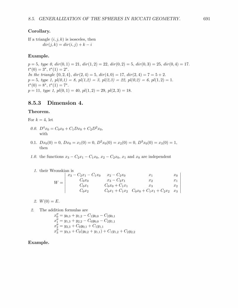
8.5. GENERALIZATION OF THE SPHERES IN RICCATI GEOMETRY. 691
Corollary.
If a triangle (i, j, k) is isosceles, thendir(j, k) = dir(i, j) + k − i
Example.
p = 5, type 0, dir(0, 1) = 21, dir(1, 2) = 22, dir(0, 2) = 5, dir(0, 3) = 25, dir(0, 4) = 17.t∗(0) = 3∗, t∗(1) = 2∗.In the triangle 0, 2, 4, dir(2, 4) = 5, dir(4, 0) = 17, dir(2, 4) = 7 = 5 + 2.p = 5, type 1, pl(0,1) = 8, pl(1,2) = 3, pl(2,3) = 22, pl(0,2) = 6, pl(1, 2) = 1.t∗(0) = 8∗, t∗(1) = 7∗.p = 11, type 1, pl(0, 1) = 40, pl(1, 2) = 29, pl(2, 3) = 18.
8.5.3 Dimension 4.
Theorem.
For k = 4, let
0.0. D4x0 = C0x0 + C1Dx0 + C2D2x0,
with
0.1. Dx0(0) = 0, Dx0 = x1(0) = 0, D2x0(0) = x2(0) = 0, D3x0(0) = x3(0) = 1,then
1.0. the functions x3 − C2x1 − C1x0, x2 − C2x0, x1 and x0 are independent
1. their Wronskian is
W =
∣∣∣∣∣∣∣∣x3 − C2x1 − C1x0 x2 − C2x0 x1 x0
C0x0 x3 − C2x1 x2 x1
C0x1 C0x0 + C1x1 x3 x2
C0x2 C0x1 + C1x2 C0x0 + C1x1 + C2x2 x3
∣∣∣∣∣∣∣∣2. W (0) = E.
2. The addition formulas arex′′0 = y0,3 + y1,2 − C1y0,0 − C2y0,1
x′′1 = y1,3 + y2,2 − C0y0,0 − C2y1,1
x′′2 = y2,3 + C0y0,1 + C1y1,1
x′′3 = y3,3 + C0(y0,2 + y1,1) + C1y1,2 + C2y2,2
Example.

692 CHAPTER 8. FUNCTIONS OVER FINITE FIELDS

Chapter 9
FINITE ELLIPTIC FUNCTIONS
9.0 Introduction.
The success of the study of the harmonic polygons of Casey (II.6.1), suggested the study of thepolygons of Poncelet. After having conjectured that the Theorem of Poncelet, as given in I.2.2.generalized to the finite case, and because one of the proof of this Theorem, in the classical case,is by means of elliptic functions, this suggested that these too could be generalized to the finitecase. Just as the additions properties were used to define the trigonometric functions, the sameproperties were generalized to the finite case. It was soon realized that the poles of the ellipticfunctions correspond to values, which in the finite case are outside of the finite field. The basicdefinitions and properties of section 1 do not give directly functions but an abelian group structureon a set E, whose elements are, in general, triplets of integers modulo p. In section 2, this structurewill be described as the direct product of the Klein 4-group and an abelian group which can be usedas seen in section 3 to define 3 functions which generalize, in the finite case, the functions sn, cnand dn of Jacobi.
In this Chapter, j and j′ will denote +1 or −1.
9.1 The Jacobi functions.
9.1.1 Definitions and basic properties of the Jacobian elliptic group.
Introduction.
Given p and m different from 0 and 1, we will define in 3.1.1, the set E = E(p,m) and, in 3.1.7.,an operation “+” from E ×× E into E. The basic result that (E,+) is an abelian group is given in3.1.15.
Definition.
Given s, c, d ∈ Zp. The elements of E are(s, c, d)
such thatD0. s2 + c2 = 1 and d2 +m s2 = 1.as well as, when −1 and −m are quadratic residues,
(∞, c∞, d∞), where c2 = −1 and d2 = −m.
693

694 CHAPTER 9. FINITE ELLIPTIC FUNCTIONS
Notation.
i :=√−1, m1 := 1−m, k :=
√m, k1 :=
√m1.
Theorem.
H0. (s, c, d), (s1, c1, d1), (s2, c2, d2) ∈ E,H1. j = +1 or −1,thenC0. d2 −m c2 = m1.C1. c2 +m1s
2 = d2.C2. c2 + s2d2 = d2 +m s2c2 = 1−m s4.C3. m(1− c)(1 + c) = (1− d)(1 + d).C4. (c+ d)(1 + jd) = (1 + j c)(j m1 + d+m c).C5. m(c+ d)(1− j c) = (1− j d)(j m1 + d+m c)C6. d2 −m s2c2 = d2 + c2(d2 − 1).C7. d2
1d22 +mm1s
21s
22 = m1 −m c2
1c22.
C8. (d1s1c2 + d2s2c1)(d1d2 −m s1s2c1c2) = (s1c2d2 + s2c1d1)(d21d
22 +mm1s
21s
22).
Proof: Each of the identities can easily be verified using Definition 1.1. If C3, is writtenC3’ m(1− j c)(1 + j c) = (1− j d)(1 + j d),then C5, follows from C4.
Lemma.
H0. m s20s
21 = 1,
thenC0. d2
0 = −m s20c
21, d
21 = −m s2
1c20,
C1. (s0c1d1)2 = (s1c0d0)2,C2. (c0c1)2 = (d0s0d1s1)2,C3. (d0d1)2 = (m s0c0s1c1)2,C4. s0s1 6= 0.
Lemma.
H0. m s20s
21 = 1,
H1. s0c1d1 = −j s1c0d0,thenC0. c0c1 = j d0s0d1s1,C1. d0d1 = j m s0c0s1c1.C2. c0 = 0⇒ d1 = 0 and c1 6= 0.
c1 = 0⇒ d0 = 0 and c0 6= 0.
Proof: If c0 = c1 = 0 then s20 = s2
1 = 1 hence m = 1, which is excluded.
Lemma.
H0. (s0c1d1)2 = (s1c0d0)2,thenC0. s0 = j s1 or m s2
0s21 = 1.

9.1. THE JACOBI FUNCTIONS. 695
Definition.
The addition is defined as follows:Let D = 1−m s2
0s21.
If D 6= 0, thenD0. (s0, c0, d0) + (s1, c1, d1) = ( s0c1d1+s1c0d0
D , c0c1−d0s0d1s1D , d0d1−m s0c0s1c1D ),
If D = 0, s0c1d1 = s1c0d0, c0 6= 0 and c1 6= 0, thenD1. (s0, c0, d0) + (s1, c1, d1) = (∞, c∞, d∞),
where c = c1s1d0
and d = d1s1c0
,If D = 0, s0c1d1 = −s1c0d0, c0 6= 0 and c1 6= 0, then
D2.0. (s0, c0, d0) + (s1, c1, d1) = (s20−s21
2s0c1d1,c20+c212c0c1
,d20+d212d0d1
),If D = 0, s0c1d1 = j s1c0d0, c0 = 0 and c1 6= 0, then
D2.1. (s0, c0, d0) + (s1, c1, d1) = (∞, c∞, d∞),
where c = −d0s1c1
and d =d30
m s0c31.
If D = 0, s0c1d1 = j s1c0d0, c0 6= 0 and c1 = 0, thenD2.2. (s0, c0, d0) + (s1, c1, d1) = (∞, c∞, d∞),
where c = −d1s0c0
and d =d31
m s1c30.
If s0 6= 0, thenD3.0. (∞, c∞, d∞) + (s0, c0, d0)
= (s0, c0, d0) + (∞, c∞, d∞) = ( −cdm s0, dd0m s0
, cc0m s0
).If s0 = 0, then
D3.1. (∞, c∞, d∞) + (0, c0, d0)= (0, c0, d0) + (∞, c∞, d∞) = (∞, c d0∞, d c0∞).
D4. (∞, c0∞, d0∞) + (∞, c1∞, d1∞) = (0, d0d1m , c0c1).
Example.
With p = 11, m = 3, (− 111) = (− 3
11) = −1,E = (0, 1, 1), (0, 1,−1), (0,−1, 1), (0,−1,−1),
(1, 0, 3), (1, 0,−3), (−1, 0, 3), (−1, 0,−3),(5, 3, 5), (5, 3,−5), (5,−3, 5), (5,−3,−5),(−5, 3, 5), (−5, 3,−5), (−5,−3, 5), (−5,−3,−5).
If the elements of E in the above order are abbreviated 0,1,2, . . . ,15, then the addition table is

696 CHAPTER 9. FINITE ELLIPTIC FUNCTIONS
+ 0 1 2 3 4 5 6 7 8 9 10 11 12 13 14 150 0 1 2 3 4 5 6 7 8 9 10 11 12 13 14 151 1 0 3 2 7 6 5 4 13 12 15 14 9 8 11 102 2 3 0 1 6 7 4 5 14 15 12 13 10 11 8 93 3 2 1 0 5 4 7 6 11 10 9 8 15 14 13 124 4 7 6 5 2 1 0 3 10 13 14 9 8 15 12 115 5 6 7 4 1 2 3 0 9 14 13 10 11 12 15 86 6 5 4 7 0 3 2 1 12 11 8 15 14 9 10 137 7 4 5 6 3 0 1 2 15 8 11 12 13 10 9 148 8 13 14 11 10 9 12 15 4 1 2 5 0 7 6 39 9 12 15 10 13 14 11 8 1 6 7 2 5 0 3 410 10 15 12 9 14 13 8 11 2 7 6 1 4 3 0 511 11 14 13 8 9 10 15 12 5 2 1 4 3 6 7 012 12 9 10 15 8 11 14 13 0 5 4 3 6 1 2 713 13 8 11 14 15 12 9 10 7 0 3 6 1 4 5 214 14 11 8 13 12 15 10 9 6 3 0 7 2 5 4 115 15 10 9 12 11 8 13 14 3 4 5 0 7 2 1 6
Example.
With p = 13, m = 3, (− 113) = (− 3
13) = 1,E = (0, 1, 1), (0, 1,−1), (0,−1, 1), (0,−1,−1),
(∞, 5∞, 6∞), (∞, 5∞,−6∞), (∞,−5∞, 6∞), (∞,−5∞,−6∞),(6, 2, 6), (6, 2,−6), (6,−2, 6), (6,−2,−6),(−6, 2, 6), (−6, 2,−6), (−6,−2, 6), (−6,−2,−6).
If the elements of E in the above order are abbreviated 0,1,2, . . . , 15, then the addition table is+ 0 1 2 3 4 5 6 7 8 9 10 11 12 13 14 150 0 1 2 3 4 5 6 7 8 9 10 11 12 13 14 151 1 0 3 2 6 7 4 5 13 12 15 14 9 8 11 102 2 3 0 1 5 4 7 6 14 15 12 13 10 11 8 93 3 2 1 0 7 6 5 4 11 10 9 8 15 14 13 124 4 6 5 7 3 1 2 0 12 14 13 15 11 9 10 85 5 7 4 6 1 3 0 2 10 8 11 9 13 15 12 146 6 4 7 5 2 0 3 1 9 11 8 10 14 12 15 137 7 5 6 4 0 2 1 3 15 13 14 12 8 10 9 118 8 13 14 11 12 10 9 15 7 1 2 4 0 5 6 39 9 12 15 10 14 8 11 13 1 4 7 2 6 0 3 510 10 15 12 9 13 11 8 14 2 7 4 1 5 3 0 611 11 14 13 8 15 9 10 12 4 2 1 7 3 6 5 012 12 9 10 15 11 13 14 8 0 6 5 3 4 1 2 713 13 8 11 14 9 15 12 10 5 0 3 6 1 7 4 214 14 11 8 13 10 12 15 9 6 3 0 5 2 4 7 115 15 10 9 12 8 14 13 11 3 5 6 0 7 2 1 4
Theorem.
C0. (s0, c0, d0) + (j′s0, jc0, j j′d0) = (0, j, j j′).
C1. (∞, c∞, d∞) + (∞, j c∞, j′ d∞) = (0,−j′,−j).C2. −(s0, c0, d0) = (−s0, c0, d0).

9.1. THE JACOBI FUNCTIONS. 697
C3. −(∞, c∞, d∞) = (∞,−c∞,−d∞).C4. (s0, c0, d0) + (0, j, j j′) = (js0, j
′c0, j j′d0).
C5. (∞, c∞, d∞) + (0, j′, j) = (∞, jc∞, j′d∞).
Theorem.
H0. (s0, c0, d0) + (s1, c1, d1) = (s2, c2, d2),thenC0. (s0, c0, d0) + (−s1,−c1, d1) = (−s2,−c2, d2).C1. (s0, c0, d0) + (s1,−c1,−d1) = (s2,−c2,−d2).C2. (s0, c0, d0) + (−s1, c1,−d1) = (−s2, c2,−d2).
Notation.
We will use the notation, which is customary in abelian groups with addition as operation symbol,n(s0, c0, d0) = (n− 1)(s0, c0, d0) + (s0, c0, d0), n ∈ Z
using induction starting with n = 0 or n = −1.
Theorem.
C0. n(−s0,−c0,−d0) = j n(s0, c0, d0), with j = (−1)n.
Theorem.
D0. D2 := 1−m s4,thenC0. 2(s, c, d) = (2s c d
D2, c
2−s2d2D2
, d2−m s2c2
D2).
Theorem.
(E,+) is an abelian group. Its order is divisible by 4.
The proof, although tedious, is straigthforward. The closure follows from the definition .6.Associativity follows, non trivially from .6. The neutral element is (0, 1, 1). The additive inverseelement of (s, c, d) is given by 1.10. C2. and C3.
Definition.
The group (E,+) is called the Jacobian elliptic group associated to the prime p and the integerm ∈ Zp.
Corollary.
The following constitute special cases.
0. For m = 0, the elements of the group are(sink, cosk, 1)and(sink, cosk,−1),
and the addition formulas reduce to(sink, cosk, j1) + (sinl, cosl, j2) =(sin(j1k + j2l), cos(j2k + j2l), j1j2), j1 and j2 are +1 or −1.

698 CHAPTER 9. FINITE ELLIPTIC FUNCTIONS
1. For m = 1, the elements of the group are(tanhk, cosechk, cosechk), (tanhk, cosechk,−cosechk)and if c2 = −1,(∞, c∞, c∞), (∞,−c∞, c∞), (∞, c∞,−c∞), (∞,−c∞,−c∞).and the addition formulas correspond totanhk0 + tanhk1 = tanhk0+tanhk1
1+tanhk0tanhk1.
cosech(k0 + k1) = cosechk0cosechk11+tanhk0tanhk1
.
Comment.
To remove some of the mystery associated with some of the formulas just given, assume that thefinite field is replaced by the field of reals. For instance, D4, is obtained by replacing in D0, c byi s, d by i k s, c1 by i s1, d1 by i k s1 and letting s and s1 tend to infinity.
9.1.2 Finite Jacobian elliptic groups for small p.
Introduction.
It can be shown that (E,+) is isomorphic to the direct product of the Klein 4-group and the groupE associated to the finite Weierstrass p function introduced by Professor Tate and that the kernelof a homomorphism between the 2 groups is the subgroup of (E,+) of elements with s = 0. A lessprecise form of this Theorem is given in 2.1. and is illustrated by the examples given in this sectionand prepares for the definition of finite Jacobi elliptic functions. In many cases the generator ofthe larger group allows the inclusion of one of the generators of the Klein 4-group.
Theorem.
(E,+) is isomorphic to Z2 ×× Z2n or to Z4 ×× Z4n.
Example.
In the example the generators of the factor groups will be given. The additional information in thesecond column will be explained in the Chapter on isomorphisms and homomorphisms.

9.1. THE JACOBI FUNCTIONS. 699
p m E is isomorphic generatorto Zi ×× Zn of Zi and Zn
3 2 Z2 ×× Z2 (0, 1,−1), (0,−1, 1)5 3 Z2 ×× Z2 (0, 1,−1), (0,−1, 1)
2 = m′(2)Z2 ×× Z4 (0, 1,−1), (1, 0, 2)4 = mj(2) ′′ (0, 1,−1), (∞, 2∞,∞)
7 3 Z2 ×× Z2 (0, 1,−1), (0,−1, 1)2 Z2 ×× Z4 (0,−1, 1), (2, 2, 0)
4 = m′′(2) ′′ (0, 1,−1), (1, 0, 2)6 = m′(4) ′′ (0, 1,−1), (1, 0, 3)
5 Z2 ×× Z6 (0, 1,−1), (2,−2, 3)11 5 Z2 ×× Z4 (0,−1, 1), (3, 5, 0)
8 = m′(9) ′′ (0, 1,−1), (1, 0, 2)9 = m′′(5) ′′ (0, 1,−1), (1, 0, 5)
2 Z2 ×× Z6 (0, 1,−1), (3, 5, 4)6 ′′ (0, 1,−1), (5, 3, 4)10 ′′ (0,−1, 1), (5, 3,−2)3 Z2 ×× Z8 (0, 1,−1), (5, 3, 5)
4 = m′′(3) ′′ (0,−1, 1), (3, 5, 3)7 = m′(3) ′′ (0, 1,−1), (3, 5, 2)
13 2 = m′(2) Z2 ×× Z4 (0, 1,−1), (1, 0, 5)12 = mj(2) = m′′(12) ′′ (0, 1,−1), (∞, 5∞,∞)4 = m′(10) = m′′(10) Z4 ×× Z4 (∞, 5∞, 3∞), (1, 0, 6)
10 = mj(4) ′′ (∞, 5∞, 4∞), (1, 0, 2)6 Z2 ×× Z6 (0, 1,−1), (2, 6, 4)
8 = mj(6) ′′ (0,−1, 1), (6, 2, 5)3 = mj(11) Z2 ×× Z8 (0, 1,−1), (6, 2, 6)5 = mj(9) ′′ (0, 1,−1), (6, 2, 4)9 = m′′(3) ′′ (0, 1,−1), (2, 6, 2)11 = m′(5) ′′ (0, 1,−1), (2, 6, 3)7 = mj(7) Z2 ×× Z10 (0,−1, 1), (2, 6,−5)
17 2 = m′(2) Z4 ×× Z4 (∞, 4∞, 7∞), (1, 0, 4)9 = m′′(2) = mj(9) ′′ (∞, 4∞, 5∞), (1, 0, 3)
16 = mj(2) = m′′(16) ′′ (∞, 4∞, 1∞), (1, 0, 6)6 Z2 ×× Z6 (0, 1,−1), (3, 3, 7)
12 = mj(6) ′′ (0, 1,−1), (4, 6, 8)4 Z2 ×× Z8 (0, 1,−1), (3, 3, 4)
5 = mj(13) ′′ (0, 1,−1), (6, 4, 5)13 = m′′(4) = mj(5) ′′ (0, 1,−1), (6, 4, 3)14 = mj(4) = m′(5) ′′ (0, 1,−1), (4, 6, 7)
7 Z2 ×× Z10 (0, 1,−1), (4,−6, 5)11 = mj(7) ′′ (0, 1,−1), (3, 3,−2)
3 Z2 ×× Z12 (0, 1,−1), (4, 6, 2)8 ′′ (0, 1,−1), (4, 6, 3)
10 = m′(3) = mj(8) ′′ (0, 1,−1), (3, 3, 8)15 = mj(3) = m′′(8) ′′ (0, 1,−1), (3, 3, 6)
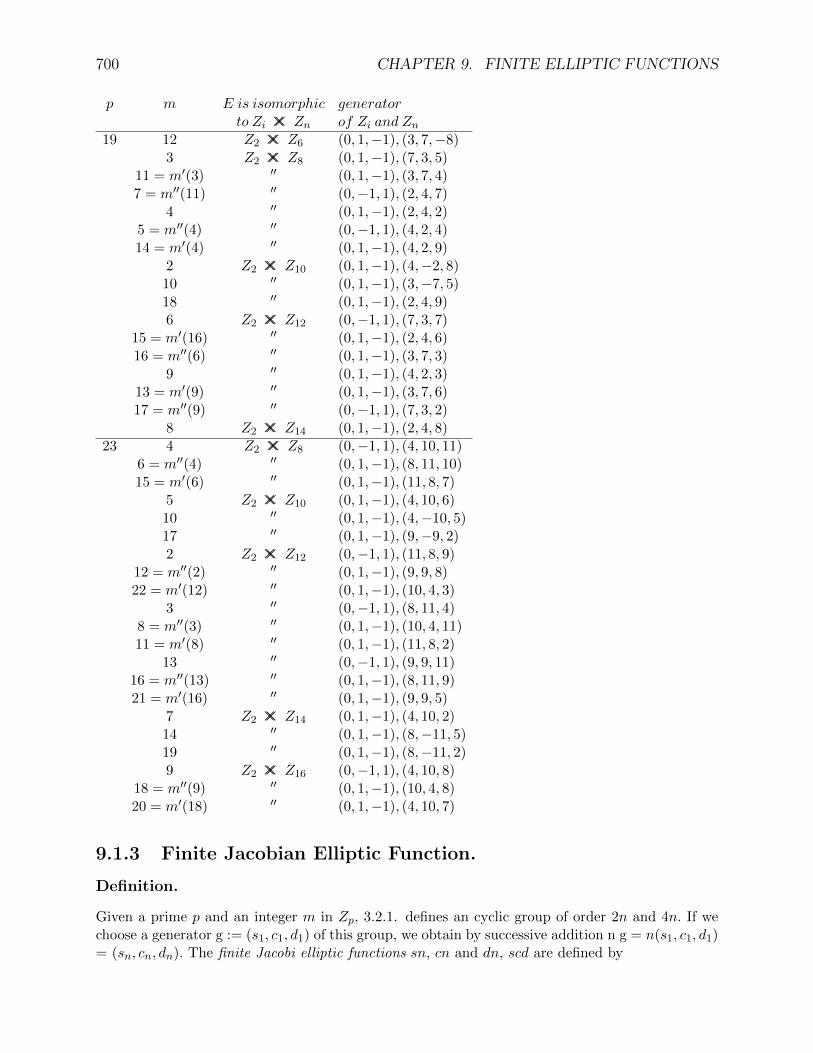
700 CHAPTER 9. FINITE ELLIPTIC FUNCTIONS
p m E is isomorphic generatorto Zi ×× Zn of Zi and Zn
19 12 Z2 ×× Z6 (0, 1,−1), (3, 7,−8)3 Z2 ×× Z8 (0, 1,−1), (7, 3, 5)
11 = m′(3) ′′ (0, 1,−1), (3, 7, 4)7 = m′′(11) ′′ (0,−1, 1), (2, 4, 7)
4 ′′ (0, 1,−1), (2, 4, 2)5 = m′′(4) ′′ (0,−1, 1), (4, 2, 4)14 = m′(4) ′′ (0, 1,−1), (4, 2, 9)
2 Z2 ×× Z10 (0, 1,−1), (4,−2, 8)10 ′′ (0, 1,−1), (3,−7, 5)18 ′′ (0, 1,−1), (2, 4, 9)6 Z2 ×× Z12 (0,−1, 1), (7, 3, 7)
15 = m′(16) ′′ (0, 1,−1), (2, 4, 6)16 = m′′(6) ′′ (0, 1,−1), (3, 7, 3)
9 ′′ (0, 1,−1), (4, 2, 3)13 = m′(9) ′′ (0, 1,−1), (3, 7, 6)17 = m′′(9) ′′ (0,−1, 1), (7, 3, 2)
8 Z2 ×× Z14 (0, 1,−1), (2, 4, 8)23 4 Z2 ×× Z8 (0,−1, 1), (4, 10, 11)
6 = m′′(4) ′′ (0, 1,−1), (8, 11, 10)15 = m′(6) ′′ (0, 1,−1), (11, 8, 7)
5 Z2 ×× Z10 (0, 1,−1), (4, 10, 6)10 ′′ (0, 1,−1), (4,−10, 5)17 ′′ (0, 1,−1), (9,−9, 2)2 Z2 ×× Z12 (0,−1, 1), (11, 8, 9)
12 = m′′(2) ′′ (0, 1,−1), (9, 9, 8)22 = m′(12) ′′ (0, 1,−1), (10, 4, 3)
3 ′′ (0,−1, 1), (8, 11, 4)8 = m′′(3) ′′ (0, 1,−1), (10, 4, 11)11 = m′(8) ′′ (0, 1,−1), (11, 8, 2)
13 ′′ (0,−1, 1), (9, 9, 11)16 = m′′(13) ′′ (0, 1,−1), (8, 11, 9)21 = m′(16) ′′ (0, 1,−1), (9, 9, 5)
7 Z2 ×× Z14 (0, 1,−1), (4, 10, 2)14 ′′ (0, 1,−1), (8,−11, 5)19 ′′ (0, 1,−1), (8,−11, 2)9 Z2 ×× Z16 (0,−1, 1), (4, 10, 8)
18 = m′′(9) ′′ (0, 1,−1), (10, 4, 8)20 = m′(18) ′′ (0, 1,−1), (4, 10, 7)
9.1.3 Finite Jacobian Elliptic Function.
Definition.
Given a prime p and an integer m in Zp, 3.2.1. defines an cyclic group of order 2n and 4n. If wechoose a generator g := (s1, c1, d1) of this group, we obtain by successive addition n g = n(s1, c1, d1)= (sn, cn, dn). The finite Jacobi elliptic functions sn, cn and dn, scd are defined by

9.1. THE JACOBI FUNCTIONS. 701
sn(n) := sn, cn(n) := cn, dn(n) := dn, scd(n) := (sn, cn, dn).The period is denoted by 4K.
Example.
For p = 11, m = 3, K = 2, — For p = 13, m = 3, K = 2,i sn(i) cn(i) dn(i) i sn(i) cn(i) dn(i)0 0 1 1 0 0 1 11 −5 3 −5 1 6 2 62 1 0 3 2 ∞ −5∞ −6∞3 −5 −3 −5 3 −6 −2 −64 0 −1 1 4 0 −1 −15 5 −3 −5 5 6 −2 −66 −1 0 3 6 ∞ 5∞ 6∞7 5 3 −5 7 −6 2 68 0 1 1 8 0 1 1
Definition.
0. ns := 1sn , nc := 1
cn , nd := 1dn ,
1. sc := sncn , cd := cn
dn , ds := dnsn ,
2. cs := cnsn , dc := dn
cn , sd := sndn .
The notation is due to Glaisher, Glaisher, J.W.L., On elliptic functions, Messenger of Mathe-matics, Vol. 11, 1881, 81-95.
9.1.4 Identities and addition formulas for finite elliptic functions.
Introduction.
The formulas given in this section are for the most part the same as in the real case. Theorem 9.1.4gives the addition formulas. Theorem 9.1.4, which may be new is needed to prove the additionformula for the Jacobi Zeta function. Theorem 9.1.4 is given for sake of completeness. It is clearlyless elegant than 9.1.4.
Lemma.
1−ms20s
21 = c2
1 + d20s
21 = d2
0 +ms20c
21.
Theorem.
0. sn2(u)cn2(v)dn2(v)− sn2(v)cn2(u)dn2(u)= (1−msn2(u)sn2v)(sn2(u)− sn2(v).
1. cn2(u)cn2(v)− sn2(u)sn2(v)dn2(u)dn2(v= (1−msn2(u)sn2v)(1− sn2(u)− sn2(v).
2. dn2(u)dn2(v)−m2sn2(u)sn2(v)cn2(u)cn2(v= (1−msn2(u)sn2v)(1−msn2(u)−msn2(v) +msn2(u)sn2(v).

702 CHAPTER 9. FINITE ELLIPTIC FUNCTIONS
Theorem.
0. sn(u+ v) = sn2(u)−sn2(v)sn(u)cn(v)dn(v)−sn(v)cn(u)dn(u) .
1. cn(u+ v) = 1−sn2(u)−sn2(v)cn(u)cn(v)+sn(u)sn(v)dn(u)dn(v) .
2. dn(u+ v) = 1−msn2(u)−msn2(v)+msn2(u)sn2(v)dn(u)dn(v)+msn(u)sn(v)cn(u)cn(v) .
3. cn(u+ v) = sn(u)cn(u)dn(v)−sn(v)cn(v)dn(u)sn(u)cn(v)dn(v)−sn(v)cn(u)dn(u) , for u 6= (v).
4. dn(u+ v) = sn(u)dn(u)cn(v)−sn(v)dn(v)cn(u)sn(u)cn(v)dn(v)−sn(v)cn(u)dn(u) , for u 6= (v).
Formulas 0., 3. and 4. are due to Cayley (1884).
Theorem.
0. −mcn(u)cn(v)cn(u+ v) + dn(u)dn(v)dn(u+ v) = 1−m.
1. dn(v)dn(u+ v) +mcn(u)sn(v)sn(u+ v) = dn(u).
2. sn(v)dn(u)sn(u+ v) + cn(v)cn(u+ v) = cn(u).
Theorem.
0. sn(u+ v + w)(sn(v)sn(u+ w)− sn(w)sn(u+ v))= sn(u)(sn(v)sn(u+ v)− sn(w)sn(u+ w)).
1. sn(a0 − a1)sn(a1 − a2)sn(a2 − a0)−sn(a1 − a2)sn(a2 − a3)sn(a3 − a1)+sn(a2 − a3)sn(a3 − a0)sn(a0 − a2)−sn(a3 − a0)sn(a0 − a1)sn(a1 − a3) = 0 1.
Proof: If we write u = a0 − a1, v = a1 − a2, w = a3 − a0, then u+ v = a0 − a2,u + w = a3 − a1, u + v + w = a3 − a2 and we obtain 0, from 1. To prove 1, let us introduce thenotation
s0 := sna0, s1 := sna1, s2 := sna2, s3 := sna3.and similarly for ci and di. Let
B0 := (s21 − s2
2)(s22 − s2
3)(s23 − s2
1)(s0c1d1 + s1c0d0)(s0c2d2 + s2c0d0)(s0c3d3 + s3c0d0).
Let B1, B2, B3 be obtained by adding 1, 2, 3 modulo 4 to each digit, using 9.1.4.0 in 1. andreducing to the same denominator, we have to prove that
B0 −B1 +B2 −B3 = 0.Using .0.D0.,B0 = (s4
1(s23 − s2
2) + s42(s2
1 − s23) + s4
3(s22 − s2
1))(s1s2s3c0d0(1− s2
0)(1−ms20)
+s2s3s0c1d1(1− s20)(1−ms2
0)
13.11.83

9.1. THE JACOBI FUNCTIONS. 703
+s3s0s1c2d2(1− s20)(1−ms2
0)+s0s1s2c3d3(1− s2
0)(1−ms20)
+s30c1d1c2d2c3d3
+s20s1c2d2c3d3c0d0
+s20s2c3d3c0d0c1d1
+s20s3c0d0c1d1c2d2)
thereforeB0 −B1 +B2 −B3 =
(s1s2s3c0d0(s40s
41(s2
3 − s22)(m−m) + . . .
+s40s
21s
22(1 +m− 1−m) + . . .
+s40s
21(1− 1) + . . .) + . . .)
+(s0c1d1c2d2c3d3(s40s
21s
22(1− 1) + . . .
+s20s
41s
22(−1 + 1) + . . .
+s41s
22s
23(−1 + 1) + . . .) + . . .) = 0.
The given terms come froms4
1(s23 − s2
2)s1s2s3c0d0ms40 in B0 and from the term in B1
corresponding to the term s43(s2
2 − s21)s0s1s2c3d3ms
40 in B0,
the term inB2 corresponding to−s42s
23s3s0s1c2d2(−1−m)s2
0 inB0 and the term inB1, to−s43s
21s0s1s2c3d3(−1−
m)s20 in B0, the term in B2 corresponding to −s4
2s23s3s0s1c2d2 in B0 and the term in B3, to
−s41s
22s2s3s0c1d1 in B0, the term in B2 corresponding to −s4
2s23s
20s2c3d3c0d0c1d1 in B0 and the
term in B1, to −s43s
21s
20s3c0d0c1d1c2d2 in B0, the term −s4
1s22 s
30c1d1c2d2c3d3 in B0 and the term in
B2, to s43s
22s
20s2c3d3c0d0c1d1 in B0 and the term in B2 corresponding to −s4
3s21s
20s2c3d3c0d0c1d1 in
B0 and the term in B3, to −s42s
23s
20s1c2d2c3d3c0d0 in B0, The reduction involves 4(6.2.2 + 4.3.4 +
4.3.2)+4(3+6+3)2 terms, which exausts the list of 4(6(4.4+4)) = 480 terms in B0−B1 +B2−B3.
Comment.
Formula 9.1.4.0, should be compared with the formula of Jacobi, (Crelle Vol. 15)sn(u+ v + w)sn(u)(1−msn(v)sn(w)sn(u+ v)sn(u+ w))= sn(u+ v)sn(u+ w)− sn(v)sn(w).
Formulas 9.1.4.0. to 1. should also be compared with the formulas of Glaisher (1881) and of Cayley(Crell Vol. 41),
Corollary.
0. sn(u+ 1) = sn(1)(sn(1)sn(2)−sn(u−1)sn(u))sn(1)sn(u)−sn(2)sn(u−1) , u = 3, . . . .
Proof: Use 9.1.4.0. with u = v = 1 and w = u− 1,
Theorem.
0. cn(u+ v + w) =
sn(u)dn(v)dn(w)(cn(v)cn(u+ v)− cn(w)cn(u+ w))−dn(u)(sn(v)cn(v)dn(w)− sn(w)cn(w)dn(v))
dn(u)(sn(v)dn(w)cn(u+w)−sn(w)dn(v)cn(u+v)) .
1. sd(a1 − a2)cn(a1 − a2)− sd(a3 − a0)cn(a3 − a0)= sd(a0 − a1)(cn(a0 − a2)cn(a2 − a1)− cn(a0 − a3)cn(a3 − a1))−cn(a2 − a3)(cn(a2 − a0)sd(a0 − a3)− sd(a2 − a1)cn(a1 − a3))

704 CHAPTER 9. FINITE ELLIPTIC FUNCTIONS
Proof: One proof is to derive first 9.1.4.1. using the same method as in 9.1.4, the other is toset a3 = 0 and derive the corresponding formula using 9.1.4.
9.1.5 Double and half arguments.
Theorem.
0. sn(2u) = 2sn(u)cn(u)dn(u)1−msn4(u)
.
1. cn(2u) = cn2(u)−sn2(u)dn2(u)1−msn4(u)
= cn2(u)−sn2(u)dn2(u)cn2(u)+sn2(u)dn2(u)
.
2. dn(2u) = dn2(u)−msn2(u)cn2(u)1−msn4(u)
.
= dn2(u)+cn2(u)(dn2(u)−1)1−msn4(u)dn2(u)−cn2(u)(dn2(u)−1)
.
Theorem.
D0. s1 :=√
1−c1+d ,
D1. c1 :=√
1+d1+d ,
D2. d1 := s(c+d)(1+c)(1+d)s1c1
,thenC0. d2
1 = c+d1+c ,
C1. 2(s1, c1, d1) = (s, c, d).
Proof. C0. follows directly from D0. to D1. It is not used to define d1 to insure that 2(s1, c1, d1)is (s, c, d) not (−s, c, d).The formulas can be derived starting from
d21 −ms2
1c21 = d(1−ms4
1).Expressing c2
1 and d21 in terms of s2
1 givesm(1 + d)s4
1 − 2ms21 + 1− d = 0, hence
s21 =
m+j√m2−m(1−d2)
m(1+d) ,where j = +1 or −1, hence
s21 = 1−jc
1+d .therefore
c21 = jc+d
1+d and d21 = m1+d+jmc
1+d = jc+d1+jc .
It remains to verify, by substitution, for c and s.For c,
c21 − s2
1d21 = 2jc(jc+d)
(1+d)(1+jc) , therefore j = 1.For s,
1 +ms41 = 1 + m(1−c)2
(1+d)2= 1 + 1−c
1+d1−d1+c
= 2(c+d)(1+d)(1+c) = 2s1c1d1
s ,
2s1c1d1 =√
1−j c1+j c
j c+d1+d = 2s(c+d)
(1+c)(1+d)
= 2j1 s (jc+d)(1+j c)(1+d) ,
j1 = +1 or −1 has to be determined once the square roots have been chosen unambiguously.
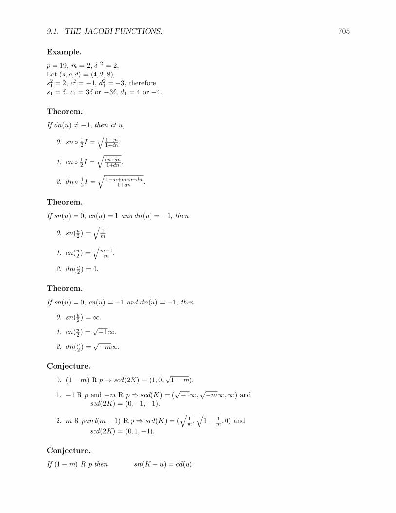
9.1. THE JACOBI FUNCTIONS. 705
Example.
p = 19, m = 2, δ 2 = 2,Let (s, c, d) = (4, 2, 8),s2
1 = 2, c21 = −1, d2
1 = −3, therefores1 = δ, c1 = 3δ or −3δ, d1 = 4 or −4.
Theorem.
If dn(u) 6= −1, then at u,
0. sn 12I =
√1−cn1+dn .
1. cn 12I =
√cn+dn1+dn .
2. dn 12I =
√1−m+mcn+dn
1+dn .
Theorem.
If sn(u) = 0, cn(u) = 1 and dn(u) = −1, then
0. sn(u2 ) =√
1m
1. cn(u2 ) =√
m−1m .
2. dn(u2 ) = 0.
Theorem.
If sn(u) = 0, cn(u) = −1 and dn(u) = −1, then
0. sn(u2 ) =∞.
1. cn(u2 ) =√−1∞.
2. dn(u2 ) =√−m∞.
Conjecture.
0. (1−m) R p⇒ scd(2K) = (1, 0,√
1−m).
1. −1 R p and −m R p⇒ scd(K) = (√−1∞,
√−m∞,∞) and
scd(2K) = (0,−1,−1).
2. m R pand(m− 1) R p⇒ scd(K) = (√
1m ,√
1− 1m , 0) and
scd(2K) = (0, 1,−1).
Conjecture.
If (1−m) R p then sn(K − u) = cd(u).

706 CHAPTER 9. FINITE ELLIPTIC FUNCTIONS
9.1.6 The Jacobi Zeta function.
Introduction.
Definitions 9.1.6 are inspired by the relation which exist, in the real case, between the Jacobi Zetafunction, the θ functions and the Weierstrass ζ function. See Handbook p.578, 16.34 and p.650,18.10.7.
Definition.
The function u is defined by:u(1) := 0,u(i+ 1) := u(i)−msn(1)sn(i)sn(i+ 1).
Definition.
The Jacobi Zeta function Z is defined byZ(1) := −u(K)
K .Z(i) := u(i) + Z(1)i, i 6= 1.
Theorem.
0. Z(u+ v) = Z(u) + Z(v)−msn(u)sn(v)sn(u+ v).
1. Z(u+ v) = Z(u) + Z(v) +msd(u)(cn(v)cn(u+ v)− cn(u))
2. Z(u+ v) = Z(u) + Z(v) + sc(u)(dn(v)dn(u+ v)− dn(u))
Proof of 0. The formula is true, by definition, for v = 1. It follows by induction on v and from. . . 9.1.4 Indeed,
Z(u+ v + 1) = Z(u+ v) + Z(1)−msn(1)sn(u+ v)sn(u+ v + 1)= Z(u) + Z(v) + Z(1)−msn(u)sn(v)sn(u+ v)−msn(1)sn(u+ v)sn(u+ v + 1)= Z(u)+Z(v+1)+msn(1)sn(v)sn(v+1)−msn(u)sn(v)sn(u+v)−msn(1)sn(u+v)sn(u+
v + 1)= Z(u) + Z(v + 1)−msn(u)sn(v + 1)sn(u+ v + 1).
The proof of 1. and 2. is left as an exercise. Hint: Use 9.1.4.
Theorem.
0. Z(K − u) = −Z(u) +msn(u)cd(u).
1. Z(12K) = m
2 sn(K2 )cd(K2 ), if K is even.
2. Z(K) = 0.
3. Z(K + u) = −Z(K − u).
4. Z(2K − u) = −Z(2K + u).
5. Z(2K + u) = Z(u).
Proof: 0, follows from the additional formula for Z eta(K − u) and from . . . 9.1.5 See Example3.1.1. and \130 elliptic.bas
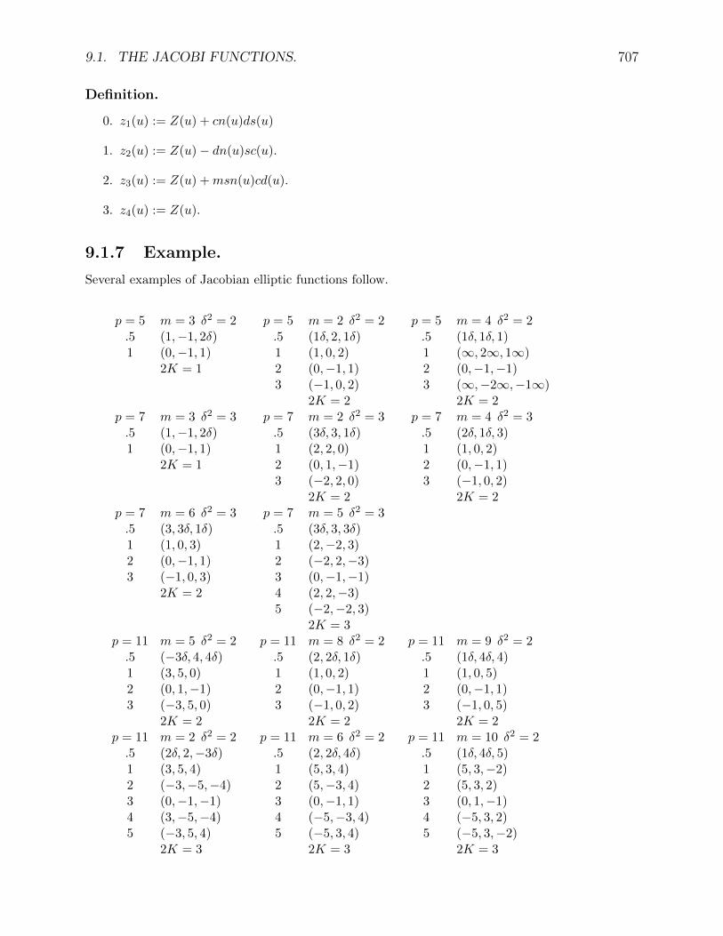
9.1. THE JACOBI FUNCTIONS. 707
Definition.
0. z1(u) := Z(u) + cn(u)ds(u)
1. z2(u) := Z(u)− dn(u)sc(u).
2. z3(u) := Z(u) +msn(u)cd(u).
3. z4(u) := Z(u).
9.1.7 Example.
Several examples of Jacobian elliptic functions follow.
p = 5 m = 3 δ2 = 2 p = 5 m = 2 δ2 = 2 p = 5 m = 4 δ2 = 2.5 (1,−1, 2δ) .5 (1δ, 2, 1δ) .5 (1δ, 1δ, 1)1 (0,−1, 1) 1 (1, 0, 2) 1 (∞, 2∞, 1∞)
2K = 1 2 (0,−1, 1) 2 (0,−1,−1)3 (−1, 0, 2) 3 (∞,−2∞,−1∞)
2K = 2 2K = 2p = 7 m = 3 δ2 = 3 p = 7 m = 2 δ2 = 3 p = 7 m = 4 δ2 = 3.5 (1,−1, 2δ) .5 (3δ, 3, 1δ) .5 (2δ, 1δ, 3)1 (0,−1, 1) 1 (2, 2, 0) 1 (1, 0, 2)
2K = 1 2 (0, 1,−1) 2 (0,−1, 1)3 (−2, 2, 0) 3 (−1, 0, 2)
2K = 2 2K = 2p = 7 m = 6 δ2 = 3 p = 7 m = 5 δ2 = 3.5 (3, 3δ, 1δ) .5 (3δ, 3, 3δ)1 (1, 0, 3) 1 (2,−2, 3)2 (0,−1, 1) 2 (−2, 2,−3)3 (−1, 0, 3) 3 (0,−1,−1)
2K = 2 4 (2, 2,−3)5 (−2,−2, 3)
2K = 3p = 11 m = 5 δ2 = 2 p = 11 m = 8 δ2 = 2 p = 11 m = 9 δ2 = 2.5 (−3δ, 4, 4δ) .5 (2, 2δ, 1δ) .5 (1δ, 4δ, 4)1 (3, 5, 0) 1 (1, 0, 2) 1 (1, 0, 5)2 (0, 1,−1) 2 (0,−1, 1) 2 (0,−1, 1)3 (−3, 5, 0) 3 (−1, 0, 2) 3 (−1, 0, 5)
2K = 2 2K = 2 2K = 2p = 11 m = 2 δ2 = 2 p = 11 m = 6 δ2 = 2 p = 11 m = 10 δ2 = 2.5 (2δ, 2,−3δ) .5 (2, 2δ, 4δ) .5 (1δ, 4δ, 5)1 (3, 5, 4) 1 (5, 3, 4) 1 (5, 3,−2)2 (−3,−5,−4) 2 (5,−3, 4) 2 (5, 3, 2)3 (0,−1,−1) 3 (0,−1, 1) 3 (0, 1,−1)4 (3,−5,−4) 4 (−5,−3, 4) 4 (−5, 3, 2)5 (−3, 5, 4) 5 (−5, 3, 4) 5 (−5, 3,−2)
2K = 3 2K = 3 2K = 3

708 CHAPTER 9. FINITE ELLIPTIC FUNCTIONS
p = 11 m = 3 δ2 = 2 p = 11 m = 4 δ2 = 2 p = 11 m = 7 δ2 = 2.5 (5δ, 5δ, 4) .5 (4δ, 1δ, 4) .5 (5δ, 5δ, 5)1 (−5, 3,−5) 1 (3, 5, 3) 1 (−3, 5, 2)2 (1, 0, 3) 2 (5, 3, 0) 2 (1, 0, 4)3 (−5,−3,−5) 3 (3, 5,−3) 3 (−3,−5, 2)4 (0,−1, 1) 4 (0, 1,−1) 4 (0,−1, 1)5 (5,−3,−5) 5 (−3, 5,−3) 5 (3,−5, 2)6 (−1, 0, 3) 6 (−5, 3, 0) 6 (−1, 0, 4)7 (5, 3,−5) 7 (−3, 5, 3) 7 (3, 5, 2)
2K = 4 2K = 4 2K = 4p = 13 m = 2 δ2 = 2 p = 13 m = 12 δ2 = 2 p = 13 m = 4 δ2 = 2.5 (−5δ, 4, 3δ) .5 (3δ, 6δ, 2) .5 (1δ,−5, 4δ)1 (1, 0, 5) 1 (∞, 5∞, 1∞) 1 (1, 0, 6)2 (0,−1, 1) 2 (0,−1,−1) 2 (0,−1, 1)3 (−1, 0, 5) 3 (∞,−5∞,−1∞) 3 (−1, 0, 6)
2K = 2 2K = 2 2K = 2p = 13 m = 10 δ2 = 2 p = 13 m = 6 δ2 = 2 p = 13 m = 8 δ2 = 2.5 (3, 3δ, 1δ) .5 (−5, 1δ, 6δ) .5 (1δ,−5,−5δ)1 (1, 0, 2) 1 (2, 6, 4) 1 (6, 2, 5)2 (0,−1, 1) 2 (2,−6, 4) 2 (6, 2,−5)3 (−1, 0, 2) 3 (0,−1, 1) 3 (0, 1,−1)
2K = 2 4 (−2,−6, 4) 4 (−6, 2,−5)5 (−2, 6, 4) 5 (−6, 2, 5)
2K = 3 2K = 3p = 13 m = 3 δ2 = 2 p = 13 m = 5 δ2 = 2 p = 13 m = 9 δ2 = 2.5 (−5δ, 4, 6δ) .5 (3δ, 3, 1δ) .5 (6δ, 6δ, 4)1 (6, 2, 6) 1 (−6, 2, 4) 1 (2, 6, 2)2 (∞,−5∞,−6∞) 2 (1, 0, 3)2 (∞,−5∞,−2∞)3 (−6,−2,−6) 3 (−6,−2, 4) 3 (−2,−6,−2)4 (0,−1,−1) 4 (0,−1, 1) 4 (0,−1,−1)5 (6,−2,−6) 5 (6,−2, 4) 5 (2,−6,−2)6 (∞, 5∞, 6∞) 6 (−1, 0, 3)6 (∞, 5∞, 2∞)7 (−6, 2, 6) 7 (6, 2, 4) 7 (−2, 6, 2)
2K = 4 2K = 4 2K = 4p = 13 m = 11 δ2 = 2 p = 13 m = 7 δ2 = 2.5 (1δ,−5, 3δ) .5 (−5δ, 4, 1δ)1 (2, 6, 3) 1 (2, 6,−5)2 (1, 0,−4) 2 (6,−2, 3)3 (2,−6, 3) 3 (6,−2,−3)4 (0,−1, 1) 4 (2, 6, 5)5 (−2,−6, 3) 5 (0, 1,−1)6 (−1, 0,−4) 6 (−2, 6, 5)7 (−2, 6, 3) 7 (−6,−2,−3)
2K = 4 8 (−6,−2, 3)9 (−2, 6,−5)
2K = 5

9.1. THE JACOBI FUNCTIONS. 709
9.1.8 Other results.
Theorem.
H0.
(1−mp
)= 1,
then C0. (1, 0, k1) ∈ E,C1. (1, 0, k1) + (1, 0, k1) = (0,−1, 1).
Definition.
Let e = (s, c, d), s 6=∞,sin(2e) := 2s c, cos(2e) := c2 − s2.
Can this be justified?This is done better using sn = sin am, cn = cos am.
Theorem?.
sin(2e0 + 2e1) = . . ..
Theorem. [Landen]
Let H0. e0 := (s0, c0, d0) ∈ E,H1. s0 c0 d0 6= 0, s0 6= oo,H2. e1 := (s1, c1, d1) := (s0, c0, d0) + (1, 0, k1),
H3. l(2e0) := sin(2e1) cos(2e0)−cos(2e1) sin(2e0)sin(2e0)−sin(2e1) ,
then C0. l(e0) = 1−k11+k1
.
l or l(p,m) is the Landen constant associated to p and m.
Proof.P0. e1 = ( cd ,−
k1 sd , k1d ).
P1. l(e0) =k1(s2−c2)+c2−k21 s2
d2+k1= 1−k1
1+k1.
Comment.
We can replace in the above Theorem (1, 0, k1) by (−1, 0, k1), this gives the same constant l.We can also replace k1 by −k1, this gives the constant
l1 = 1l .
9.1.9 Isomorphisms and homomorphisms.
Theorem.
If k1 is real, there exists an isomorphism φ′ between the elliptic group associated to m and thatassociated to
m′ = mm−1) ,
φ′(s, c, d) := (k1 sd , cd ,1d)
φ′(s, c, 0) := (∞, ck1s)∞, 1
k1s∞),
φ′(∞, c∞, d∞) := (k1d ,cd , 0).

710 CHAPTER 9. FINITE ELLIPTIC FUNCTIONS
Corollary.
If k1 is real the order of the group associated to m and to mm−1) are the same.
Theorem. [Jacobi]
If k is real, there exists an isomorphism φ′′ between the elliptic group associated to m and thatassociated to
m′′ = 1m ,
φ′′(s, c, d) := (k s, d, c)φ′′(∞, c∞, d∞) := (∞, dk ∞,
ck ∞).
Corollary.
If k is real the order of the group associated to m and to 1m are the same.
Theorem. [Jacobi]
If p ≡ 1 (mod 4), there exists an isomorphism φ1 between the elliptic group associated to m andthat associated to
mj = m1,φ1(s, c, d) := (
√−1 sc ,
1c ,
dc ),
φ1(s, 0, d) := (∞, c√−1s)∞, d√
−1s)∞),
φ1(∞, c∞, d∞) := (√−1c , 0, dc ).
Corollary.
If p ≡ 1 (mod 4), the order of the group associated to m and to m1 are the same.
Theorem. [Gauss]
If k is real, there exist a homomorphism φG from the elliptic group associated to m and thatassociated to
mG = 4k(1+k)2
,
φG(s, c, d) := ( (1+k)sD , c dD ,
2D − 1), where D = 1 + k s2,
φG(s, c, d) := (∞, c d(1+k)s ∞,
2(1+ks)∞), if 1 + ks2 = 0.
φG(∞, c∞, d∞) := (0, c d,−1). CHECK cdThe kernel of the homomorphism is (0,1,1), (0,-1,-1).The image of the homomorphism is a subgroup of index 2.
Corollary.
If k is real the order of the group associated to m and to 4k(1+k)2
are the same.
Theorem. [Landen]
If k1 is real, there exist a homomorphism φL from the elliptic group associated to m and thatassociated to
mL = (1−k11+k1
)2,

9.1. THE JACOBI FUNCTIONS. 711
φL(s, c, d) := ( (1+k1)s cd , 1+k1
m(d2−k1)
d , 1−k1m
d2+k1d ),
φL(s, c, 0) := (∞,− km s c ∞,
k(1+k1
2s c)∞),
φL(∞, c∞, d∞) := (∞, d2
m c) ∞,d2
(1+k1)
2c)∞),
The kernel of the homomorphism is (0,1,1), (0,-1,1).The image of the homomorphism is a subgroup of index 2.
Corollary.
If k1 is real the order of the group associated to m and +o(1−k11+k1
)2 are the same.
Definition.
The amplitude function is defined bysin am = sn, cos am = cn.
The example below gives sin(2k), cos(2k) under sin and cos.
Theorem.
C0. D am = dn,C1. D sin = cos, D cos = −sin.C2. D sn = cn dn, D cn = −sn dn, D dn = −m sn cn.C3. D2(2am) = −m sin (2am)
Proof: Using the derivative of composition of functions,D sn = D(sin am) = cos amD am = cn dn.
The other relations in C2, follow from sn2 + cn2 = 1 and dn2 +m sn2 = 1. C3, follows fromD2(2am) = 2D dn = −2m sn cn = −m2sin amcos am = −m sin (2am).
Comment.
The derivatives will have to be defined in a separate section. Somehow the connection with p-adicfunctions will have to be involved.If |h| < 1, thensin(x+ h) = sin(x) cos(h) + cos(x) sin(h),sin(x+ h)− sin(x) = sin(x) (cos(h)− 1) + cos(x) sin(h),butsin(h) = h+ o(h) and cos(h)− 1 = h2 + o(h),hencesin(x+h)−sin(x)
h = cos(x) + o(1) and D sin = cos.
For the elliptic functions, we have, see for instance Handbook, l. c., p. 575, 16.22.1 to .3 andam(h) = h− h3
3! m+ h5
5! m(4 +m)− . . . ,sn(h) = h+ o(h),cn(h) = 1 + o(h),dn(h) = 1 + o(h),am(h) = h+ o(h).Hence sn(x + h) − sn(x) = sn(x)(cn(h) dn(h) − 1) + cn(x) dn(x) sn(h) = h(cn(x) dn(x)) + o(h),thereforeD sn = cn dn.D (sin am) = cos amD am = cn dn, therefore D am = dn.

712 CHAPTER 9. FINITE ELLIPTIC FUNCTIONS
9.2 Applications.
9.2.1 The polygons of Poncelet.
Definition.
Let us associated to e = (s, c, d) the point P (e) = (sin(e), cos(e), 1).The set of points P (e0 +j e), j = 0, 1, . . . are the vertices of a polygon called the polygon of Poncelet.
Theorem. [Poncelet]
The sides P (e0 + j e)× P (e0 + j e+ e) are tangent to a circle.
Proof. Lete1 := e0 + j e, e2 := e1 + e,P1 := P (e1), P2 := P (e2), thenP1 = (2s1c1, c
21 − s2
1, 1),e1 = (s1, c1, d1),e2 = ( s c1d1+s1c d
D , c c1−d s d1s1D , d d1−m s c s1c1D ),
with D = 1−m s2s21,
P2 = (2 (s c1d1+s1 c d)(c c1−d s d1s1)D2 ,
(c c1−d s d1s1)2−(s c1d1+s1c d)2
D2 , 1),P1 × P2 = [. . .].
Corollary. [Landen]
The lines P... × P... pass through a fixed point L := (0, l, 1) called the point of Landen.
This is a special case of the Theorem of Poncelet, when(s0, c0, d0) = (1, 0, k1).
Construction.
Determination of Poncelet’s polygons.Let the outscribed circle θ be
X20 + (X1 − d1)2 = S2,
let the inscribed circle γ beR2(t20 + t21) = (c1t1 + t2)2,
Given a point P = (P0, P1, P2) on θ and a tangent t = (t0, t1, t2) to γ through P, the other tangentu = (u0, u1, u2) is given by
u1 = t2(P 20 −R2P 2
2 ), u2 = t1(P 20 c
21 −R2(P 2
0 + P 21 ), u0 = −P1u1+P2u2
P0.
Given a tangent t to γ and a point on it and θ, the other point Q = (Q0, Q1, Q2) common to t andθ is given by
Q2 = 1, Q1 = 2t20d1−t1t2t20+t21
, Q0 = −Q1t1+t2t0
.

9.3. THE WEIERESTRASS FUNCTIONS. 713
9.3 The Weierestrass functions.
9.3.1 Complex elliptic functions.
Definition.
Given g, a non residue of p, or
(g
p
)= −1, then
Cp,g = Cp is the set of pairs (a, b), a, b ∈ Zp such that(a, b) + (c, d) = (a+ b, c+ d),(a, b).(c, d) = (a c+ b d g, a d+ b c).
We could also write (a, b) as a+ bγ , with γ2 = g.
Definition.
Given s, c, d ∈ Cp, we can repeat definition . . . .
Definition.
2 of the functions are pure imaginary, the third is real,3 types S, C, D.
Theorem.
H0. δ2 = d,D0. e1 := (s1δ, c1δ, d1), e2 := (s2, c2, d2),
e3 := (s3δ, c3δ, d3),D1. D4 := 1−m d s2
1s22,
D2. s4 := s1c2d2+s2c1d1D4
, c4 := c1c2−s1s2d1d2D4
,
d4 := d1d2−m d s1s2c1c2D4
,Hence replace md by m′
D3. D5 := 1−m d2s31s
23,
s5 := (s1c3d3+s3c1d1)dD5
, c5 := (c1c3s1+s3d1d3)dD5
,
d5 := d1d3−m d2s1s3c1c3D5
,H1. D4 6= 0, D5 6= 0,thenC0. e1 + e2 = (s4δ, c4δ, d4),C1. e1 + e3 = (s5, c5, d5).C2. 2n e1 ∈ E, (2n+ 1)e1 ∈ S.
Definition.
(a, b) > 0 if b = 0 and 0 < a < p2
or if 0 < b < p2 .
Comment.
All that has been said above can be repeated.

714 CHAPTER 9. FINITE ELLIPTIC FUNCTIONS
9.3.2 Weiertrass’ elliptic curves and the Weierstrass elliptic func-tions.
Introduction.
The modern work on elliptic curves starts and ends with the elliptic curves of Weierstrass. I referthe reader to Lang S.
Theorem.
Let D0. e3 := −1+m3 ,
D1. g2 = 4m2−m+1
3 , g3 = 427(m+ 1)(m− 2)(2m− 1).
D2. ∆ := g32 − 27g2
3, J :=g32∆ ,
D3. pn := e3 + 1s2, Dpn := −2 cd
s3,
D4. e2 := 2−4m3 ,
D5. g′2 := 4316m2 − 16m+ 1, g′3 := 8
27(2m− 1)(32m2 − 32m− 1),
D6. ∆′ := g′32 − 27g
′23 , J
′ =g′32
∆′ ,
D7. qn := e2 + 1+c1−c , Dqn := −4d(1+c)2
s3,
thenC0. Dpn2 = 4pn3 − g2pn− g3.C1. Dqn2 = 4qn3 − g′2qn− g′3.C2. ∆ = 3(12m(m− 1))2, J = (m2 −m+ 1)3( 2
27m(m−1))2.
C3. ∆′ = 256m(m− 1), J ′ = (16m2 − 16m+ 1)3 1108m(m−1) .
The proof is straithforward. Substituting D2 in C0, multiplying by s4 and expressing c2 and d2
in terms of s2 gives a polynomial of the second degree in s2. The coefficients of 1, s2 and s4 give inturn, e3, g2 and g3.Substituting D5 in C1, multiplying by (1− c)2 gives similarly a polynomial of the second degree inx := 1-c. The coefficients of 1, x and x3 give in turn e2, g
′2 and g′3.
pn corresponds to the Weierstrass P function and Dpn to its derivative.The formulas correspond to those of real elliptic functions with the ratio of the period ω and thecomplete elliptic integral K set to 1.(See for instance Handbook for Mathematical functions, p649, 18.9.1, 2,3,4,5,8,9 and 11).
Example.
With p = 7, m = 2, then e3 = −1, g2 = 3, g3 = −1,with p = 7, m = 6, then e3 = 0, g2 = 3, g3 = 0.with p = 19, k2 = 2, then e3 = 18, g2 = 4, g3 = 0,
e2 = 17, g′2 = 6, g′3 = −1,sn cn dn sin cos am pn Dpn qn Dqn
0 0 1 1 0 1 0 ∞ ∞ ∞ ∞1 4 2 8 7 3 8 5 9 −5 52 7 3 6 4 −2 1 6 2 −6 −83 7 3 −6 −2 4 1 6 −2 −6 84 4 2 −8 3 7 8 5 −9 −5 −55 0 1 −1 1 0 0 ∞ ∞ ∞ ∞
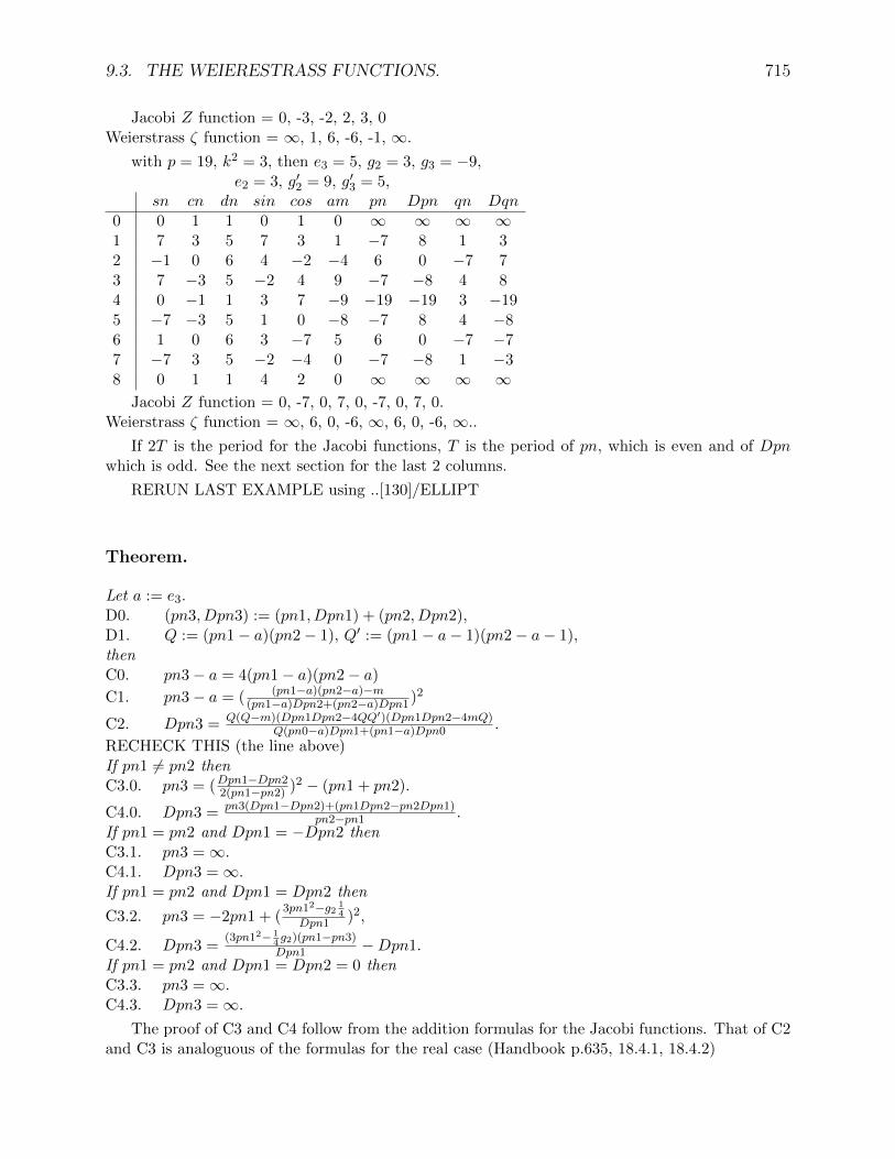
9.3. THE WEIERESTRASS FUNCTIONS. 715
Jacobi Z function = 0, -3, -2, 2, 3, 0Weierstrass ζ function = ∞, 1, 6, -6, -1, ∞.
with p = 19, k2 = 3, then e3 = 5, g2 = 3, g3 = −9,e2 = 3, g′2 = 9, g′3 = 5,
sn cn dn sin cos am pn Dpn qn Dqn0 0 1 1 0 1 0 ∞ ∞ ∞ ∞1 7 3 5 7 3 1 −7 8 1 32 −1 0 6 4 −2 −4 6 0 −7 73 7 −3 5 −2 4 9 −7 −8 4 84 0 −1 1 3 7 −9 −19 −19 3 −195 −7 −3 5 1 0 −8 −7 8 4 −86 1 0 6 3 −7 5 6 0 −7 −77 −7 3 5 −2 −4 0 −7 −8 1 −38 0 1 1 4 2 0 ∞ ∞ ∞ ∞
Jacobi Z function = 0, -7, 0, 7, 0, -7, 0, 7, 0.Weierstrass ζ function = ∞, 6, 0, -6, ∞, 6, 0, -6, ∞..
If 2T is the period for the Jacobi functions, T is the period of pn, which is even and of Dpnwhich is odd. See the next section for the last 2 columns.
RERUN LAST EXAMPLE using ..[130]/ELLIPT
Theorem.
Let a := e3.D0. (pn3, Dpn3) := (pn1, Dpn1) + (pn2, Dpn2),D1. Q := (pn1− a)(pn2− 1), Q′ := (pn1− a− 1)(pn2− a− 1),thenC0. pn3− a = 4(pn1− a)(pn2− a)
C1. pn3− a = ( (pn1−a)(pn2−a)−m(pn1−a)Dpn2+(pn2−a)Dpn1)2
C2. Dpn3 = Q(Q−m)(Dpn1Dpn2−4QQ′)(Dpn1Dpn2−4mQ)Q(pn0−a)Dpn1+(pn1−a)Dpn0 .
RECHECK THIS (the line above)If pn1 6= pn2 thenC3.0. pn3 = (Dpn1−Dpn2
2(pn1−pn2) )2 − (pn1 + pn2).
C4.0. Dpn3 = pn3(Dpn1−Dpn2)+(pn1Dpn2−pn2Dpn1)pn2−pn1 .
If pn1 = pn2 and Dpn1 = −Dpn2 thenC3.1. pn3 =∞.C4.1. Dpn3 =∞.If pn1 = pn2 and Dpn1 = Dpn2 then
C3.2. pn3 = −2pn1 + (3pn12−g2 1
4Dpn1 )2,
C4.2. Dpn3 =(3pn12− 1
4g2)(pn1−pn3)
Dpn1 −Dpn1.If pn1 = pn2 and Dpn1 = Dpn2 = 0 thenC3.3. pn3 =∞.C4.3. Dpn3 =∞.
The proof of C3 and C4 follow from the addition formulas for the Jacobi functions. That of C2and C3 is analoguous of the formulas for the real case (Handbook p.635, 18.4.1, 18.4.2)
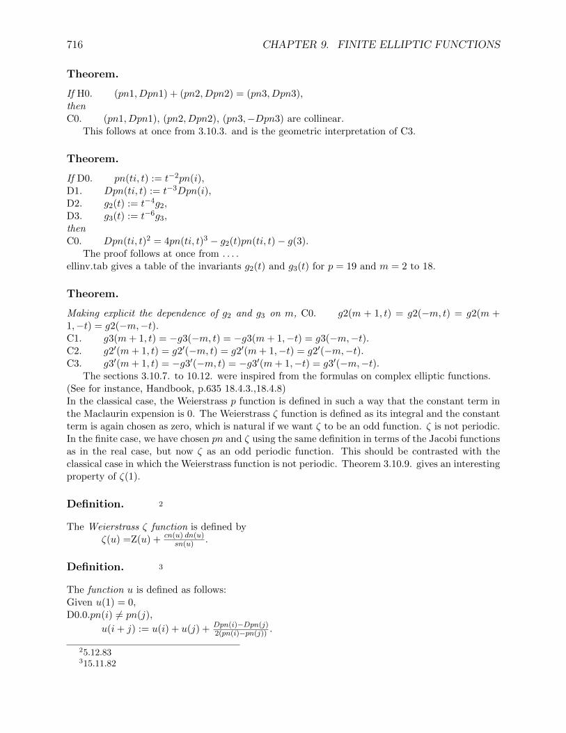
716 CHAPTER 9. FINITE ELLIPTIC FUNCTIONS
Theorem.
If H0. (pn1, Dpn1) + (pn2, Dpn2) = (pn3, Dpn3),thenC0. (pn1, Dpn1), (pn2, Dpn2), (pn3,−Dpn3) are collinear.
This follows at once from 3.10.3. and is the geometric interpretation of C3.
Theorem.
If D0. pn(ti, t) := t−2pn(i),D1. Dpn(ti, t) := t−3Dpn(i),D2. g2(t) := t−4g2,D3. g3(t) := t−6g3,thenC0. Dpn(ti, t)2 = 4pn(ti, t)3 − g2(t)pn(ti, t)− g(3).
The proof follows at once from . . . .ellinv.tab gives a table of the invariants g2(t) and g3(t) for p = 19 and m = 2 to 18.
Theorem.
Making explicit the dependence of g2 and g3 on m, C0. g2(m + 1, t) = g2(−m, t) = g2(m +1,−t) = g2(−m,−t).C1. g3(m+ 1, t) = −g3(−m, t) = −g3(m+ 1,−t) = g3(−m,−t).C2. g2′(m+ 1, t) = g2′(−m, t) = g2′(m+ 1,−t) = g2′(−m,−t).C3. g3′(m+ 1, t) = −g3′(−m, t) = −g3′(m+ 1,−t) = g3′(−m,−t).
The sections 3.10.7. to 10.12. were inspired from the formulas on complex elliptic functions.(See for instance, Handbook, p.635 18.4.3.,18.4.8)In the classical case, the Weierstrass p function is defined in such a way that the constant term inthe Maclaurin expension is 0. The Weierstrass ζ function is defined as its integral and the constantterm is again chosen as zero, which is natural if we want ζ to be an odd function. ζ is not periodic.In the finite case, we have chosen pn and ζ using the same definition in terms of the Jacobi functionsas in the real case, but now ζ as an odd periodic function. This should be contrasted with theclassical case in which the Weierstrass function is not periodic. Theorem 3.10.9. gives an interestingproperty of ζ(1).
Definition. 2
The Weierstrass ζ function is defined byζ(u) =Z(u) + cn(u) dn(u)
sn(u) .
Definition. 3
The function u is defined as follows:Given u(1) = 0,D0.0.pn(i) 6= pn(j),
u(i+ j) := u(i) + u(j) + Dpn(i)−Dpn(j)2(pn(i)−pn(j)) .
25.12.83315.11.82

9.3. THE WEIERESTRASS FUNCTIONS. 717
D0.1. pn(i) = pn(j)andDpn(i) 6= Dpn(j), u(i+ j) =∞.D1.0. Dpn(i) 6= 0, u(2i) := 2u(i) +
3pn(i)2− 14g2
Dpn(i) .
D1.1. Dpn(i) = 0, 12pn(i)2 = g(2), u(2i) =∞.D2.0. u(0) = u(T ) =∞.T is the period . . . .
Theorem.
There exist a constant ζ(1) such thatu(j) + j ζ(1) = u(T − j) + (T − j)ζ(1), j = 1 to T
2 − 1.Proof. . . . ?
Theorem.
The Weierstrass ζ function is related to the u function byζ(j) := u(j) + j ζ(1).
Comment.
The definitions and theorems can be repeated replacing respectively pn, Dpn, u, ζ by qn, Dqn, v,ζ ′, but we have the additional property of the next Theorem.
Theorem.
ζ ′(T2 ) = 0.Proof. . . . ?
Theorem.
ζ and ζ ′ are odd functions and their period is either T2 or T.
Notation.
card(X) denotes the cardinality of the set X.
Theorem.
If p ≡ −1 (mod 4), then
0. card(g2, g3) + card(g2,−g3) = 2(p+ 1).If p ≡ 1 (mod 4), then
1. card(g2, g3) = card(g2,−g3).
Corollary.
If p ≡ −1 (mod 4), then card(g2, 0) = p+ 1.
Comment.
Examples can be obtained using P.BAS see P.HOM.

718 CHAPTER 9. FINITE ELLIPTIC FUNCTIONS
Definition.
The function Ke is defined by−p < Ke(m) ≡ K(m) < p, Ke(m) is even.
Theorem. [Hasse conjectured by Artin]
−2√p < Ke(m) < 2
√p.
Conjecture. 4
0. Given an integer x in the range−2√p < x < 2
√p.
then there exist a pair (g2, g3) such that the corresponding Weierstrass elliptic curve W2 hascard p+ 1 + x and the corresponding group is abelian.This has been verified up to p = 475.
1. If the cardinality of W2 is divisible by 4 and W2 is not abelian, then there exist a J2 or aJ3 isomorphic to W26.
2. If e1 + e2 + e3 = 0, ei − ek are all non quadratic residue, and j′ 6= 0, then the elliptic groupis isomorphic to
C4l+2 ×× C2 for some 4l.This has been verified up to p = 97. See g7622, Example.
.
Comment.
If for a given m we obtain J3(m) and J2(m) and the corresponding W2 and W2′, card(W2) =card(W2′) but W2 and W2′ are not necessarily isomorphic. E.g. p = 17, J3(−2) = C2 ×× C12,J2(−2) = C24.
Comment 7
Excluding (g2, g3) = (0, 0), if j′ 6= 0, 1 there exists 2 sets of elliptic curves, corresponding to (g2, g3)and (g2,−g3). What is the connection between the structure if any?None except that concerning cardinality. E.g. p = 31, W2(1, 5) ∼ C37, W2(1,−5) ∼ C9 ×× C3,W2(3, 11) ∼ C28, W2(3,−11) ∼ C12 ×× C3.
9.3.3 The isomorphism between the elliptic curves in 3 and 2 di-mensions.
This should be integrated with 3.1.
44.1.8454.1.8466.1.8476.1.84

9.3. THE WEIERESTRASS FUNCTIONS. 719
Introduction.
The usual correspondance in the real field between the functions sn, cn and dn of Jacobi and P,DP of Weierstrass should be modified to insure an isomorphism between the 3 dimensional ellipticcurve associated to (sn, cn, dn) and the 2 dimensional elliptic curve associated to (P,DP ). Thisrequires in fact to associate, in the real case to sn(t), P (2t).
.
Theorem.
The curve (P, P ′) has a singularity when m = 0 and m = 1, When m = 0, the singularity is (−13 , 0),
because −13 is a double root of 4p3 - g2 p - g3, the regular solution when P ′ = 0 is (2
3 , 0).When m = 1, the singularity is (1
3 , 0), because 13 is a double root of 4p3 − g2p − g3, the regular
solution when P ′ = 0 is (−23 , 0).
Definition.
Let (s, c, d) in E, if m = 0 we add the restriction d = 1, if m = 1, we add the restriction c = d. Lete3 := −1+m
3 , e2 := e3 + 1, e1 := e3 + m,
0. T (s, c, d) := (e3 + 1+d1−c , 2
(c+d)(1+d)s(c−1) ),
ifs 6= frac10,∞.
1. 0.T (0, 1, 1) := (∞,∞), 1.T (0, 1,−1) := (e1, 0), m 6= 0, 1, item 2.T (0,−1, 1) := (e2, 0), item3.T (0,−1,−1) := (e3, 0),
(when m = 0, d = 1, when m = 1, d = −1),
2. T (∞, c∞, d∞) := (e3 − dc , 2
(c+d)dc ),
(m 6= 0, for m = 1 and c =√−1, T (∞, c∞, c∞) = (−5
3 , 4c)).
3. e1 = 2m−13 , e2 = 2−m
3 .
. . . D0. gives s1 = 1−c1+d , c1 =
√c+d1+d ,
d1 = s(c+d)(1+c)(1+d) s1 c1
.
Theorem.
Let a := p′
2(p−e3)(p−e3−1) , then
0. a2 6= 0,−1⇒ T−1(p, p′) = (s, c, d), where
c := 1−a21+a2
, s := c−1a , d := (1− c)(p− e3)− 1.
1. a2 = −1⇒ T−1(p, p′) = (∞, a∞, a(e3 − p)∞).
2. 0.T−1(e[3], 0) = (0,−1,−1), for m 6= 0. 1.T−1(e[3]+1, 0) = (0,−1, 1), for m 6= 1. 2.T−1(e[3]+m, 0) = (0, 1,−1), for m 6= 0, 1.
3. T−1(∞,∞) = (0, 1, 1).
Proof: If a2 6= 0,−1, solving (1 − c)(p − 33) = 1 + d and sp′ = −2(c + d)(p − e3) for c givesc− 1 = a s. Hence (c− 1)2 = a2(1− c)2, but c 6= 1, 1− c = a2(1 + c), hence c, s = c−1
a = −2 a1+a2
and d.

720 CHAPTER 9. FINITE ELLIPTIC FUNCTIONS
Theorem.
Let g2 := 4m2−m+1
3 and g3 := 427(m− 2)(2m− 1)(m+ 1), let T (s, cd) = (p, p′), then
0. p′2 = 4p3 − g2p− g3.
Definition.
The bijection defined by 9.3.3 and justified by 9.3.3 defines an [isomorphism between the 3 dimen-sional elliptic curve of . . . and the 2 dimensional elliptic curve 9.3.3.0.
Definition.
The invariant j of sec-tell32a.0. isj := 2633j′, with
j′ :=g32
g32−g23.
Theorem.
0. g32 − g2
3 = (m(m− 1))2.
1. j = 2633 (m2−m+1)3
(m(m−1))2.
2. If j is given and M is a solution of 1, the other solutions are 1−m, 1m , 1− 1
m ,1
1−m ,m
1−m .
Example.
For p = 11, let u := m(m − 1), j′ = −3 corresponds to u = 1,−2,−5 or m = −3, 4, 3,−2,−4, 5giving
K(j) = 4 or −4.j′ = 4 corresponds to u = 2,−3 or m = 2,−1,−5 giving K(j) = 0.j′ =∞ corresponds to u = 0 or m = 0, 1 giving K(j) = 1 or −1.j′ = 0 corresponds to u = −1 or m = −5 + 2δ, giving K(j) = 0.
Theorem.
Given e1, e2 and e3 such thatH.0. e1 + e2 + e3 = 0,H.1. ei are distinct,Let m := e1−e3
e2−e3 ,e2 − e3 = d,g2 := 4(e2
3 − e1e2),g3 := 4e1e2e3.
thenC.0. (dp) = 1⇒ J3(m) ∼W2(g2, g3).C.1. (dp) = −1⇒ (p+ 1− |J3(m)|)− (−1p)(p+ 1− |W2(g2, g3)|) = 0.
Proof: Let c2 = 1d , e
′i = c2 ei, then e′1 = e′3 +m and e′2 = e′3 + 1. . . .

9.3. THE WEIERESTRASS FUNCTIONS. 721
9.3.4 Correspondance between the Jacobi elliptic curve (cn, sd)and the Weierstrass elliptic curve
Definition.
Let m1 := 1−m, e2 := 21−2m3 .
0. T (cn, sd) := (e2 + 1+cn1−cn ,−4sdm1+m cn2
(1−cn2),
if cn 6= 1.
1. T (1, 0) := (∞,∞),
2. T (∞, sd) := (e2 − 1,−4msd),
3. If − m1m = b2then
T (b,∞) = (e2 + 1+b1−b , 0).
Theorem.
Let a := p− e2 + 1, then
0. a 6= 0, cn := a−2a ,
m1 +mcn2 6= 0thenT−1(p, p′) = (cn, sd),
where sd := P ′ (1−cn)2
−4(m1+mcn2),
m1 +mcn2 = 0 then T−1(p, p′) = (cn,∞),
1. T−1(∞,∞) = (1, 0).
2. a = 0⇒ T−1(p, p′) = (∞, p′
−4m).
3. T (−1, 0) = (e2, 0).
4. If T−1(x, 0) = (y,∞) and x 6= e2 thenm(m− 1) = d2 andx = e1 or e3 = − e2
2 ± 2d.
Theorem.
Let g2 := 43(16m2 − 16m+ 1) and
g3 := 827(2m− 1)(32m2 − 32m− 1),
let T (cn, sd) = (P, P ′), then
0. P ′2 = 4P 3 − g2P − g3.
Definition.
The bijection defined by 9.3.4 and justified by 9.3.4 defines an isomorphism between the 2 dimen-sional elliptic curve of . . . and the 2 dimensional elliptic curve sec-tell32a.0.

722 CHAPTER 9. FINITE ELLIPTIC FUNCTIONS
Theorem.
Using 9.3.3,
0. g32 − g2
3 = 256m(m− 1).
1. j = 16 (16m2−16m+1)3
m(m−1) .
Corollary.
Let c :=√
1− 1m , p = e2 + 1+c
1−c , using e2 from 9.3.4 and g2, g3 from sec-tjacweia, then
p3 − g2p− g3 = −1.. . . DOUBLE CHECK THIS.
The proof follows from the fact that the denominator m1 +m cn in 9.3.4.0. cannot be zero.
Theorem.
Given e1, e2 and e3 such that H.0. e1 + e2 + e3 = 0,H.1. 1− ( e1−e33e2
)2 = f2,H.2. ei are distinct,Let m := 1
2(1 + 1d),
d = 21−2m3e2
,
g2 := 4(e23 − e1e2),
g3 := 4e1e2e3.thenC.0. (dp) = 1⇒ J3(m) ∼W2(g2, g3).C.1. (dp) = −1⇒ (p+ 1− |J3(m)|)− (−1− p)(p+ 1− |W2(g2, g3)|) = 0.
Proof: Let e′i = c2 ei. We have a J2(m) if e′2 = 21−2m3 and e′1 − e′3 = 4d = 4
√m(m1 − 1)
because of . . . .

9.4. COMPLETE ELLIPTIC INTEGRALS OF THE FIRST AND SECOND KIND. 723
Example.
p e1, e2, e3 g2, g3 j′ m′ structure13 1, 3, 9 0, 4 0 −5 C6 ×× C2
29 1, 9, 19 −13,−12 13 3 C14 ×× C2
37 1, 6, 30 −13, 17 −6 −14 C22 ×× C2
2, 15, 20 0,−5 0 −5 C14 ×× C2
41 1, 13, 27 −6, 10 −6 −12 C18 ×× C2
53 1, 19, 33 −13, 17 −17 −22 C30 ×× C2
1, 20, 32 −12, 16 −21 3 C22 ×× C2
61 1, 8, 52 −13, 17 15 −23 C30 ×× C2
1, 29, 31 7,−3 26 11 C30 ×× C2
2, 26, 33 0,−29 0 −28 C38 ×× C2
73 1, 8, 64 0, 4 0 C42 ×× C2
1, 15, 57 15,−11 13 −21 C42 ×× C2
1, 29, 43 −20, 24 −7 −29 C34 ×× C2
89 1, 13, 75 20,−16 44 −26 C50 ×× C2
1, 25, 63 23,−19 −12 −30 C42 ×× C2
1, 29, 59 13,−9 15 24 C42 ×× C2
97 1, 8, 88 1, 3 2 −39 C50 ×× C2
1, 18, 78 14,−10 −17 −20 C50 ×× C2
1, 35, 61 0, 4 0 C42 ×× C2
1, 38, 58 15,−11 7 −19 C42 ×× C2
. . . ..113 . . .
1, 22, 90 −6, 10 21 C58 ×× C2
. . .
9.4 Complete elliptic integrals of the first and second
kind.
Introduction.
Several conjectures appear to justify the terminology of complete elliptic integrals of the first andsecond kind for the functions K and E defined below. The definitions are inspired from thedefinitions in the real and complex fields. Their importance is associated with Conjecture 9.4. Byconvention in this section I will use
q := [p2 ] = p−12 .
Again I denotes the identity function (I(i) = i), D denotes the derivative operator and f g denotesthe function which is obtained by composition from the functions f and g.
Definition. 8
0. Kj := ( (2j−1)!!2j !!)2, (mod p), 0 ≤ j ≤ q.
88-10.12.83

724 CHAPTER 9. FINITE ELLIPTIC FUNCTIONS
1. E′j := Kj2j
2j−1) , j = 0 to q,
2. E0 := 1, Ej := − Kj2j−1 , j = 1 to q,
Definition.
0. K :=∑q
j=0(KjIj),
1. E′ :=∑q
j=0(E′jIj),
2. E :=∑q
j=0(EjIj),
Example.
For p = 11,j K E′ E D B C K ′′ all[j]0 1 0 1 −5 −5 −4 (1)1 3 −5 −3 5 −2 −3 12 1 5 −4 −1 2 −2 (−5)3 1 −1 2 5 −4 −2 −44 3 5 −2 −5 −3 −1 (−4)5 1 −5 −5 0 1 0 −1
For p = 13,j K E′ E D B C K ′′ all[j]0 1 0 1 −6 −6 5 11 −3 −6 3 1 −4 −6 (1)2 4 1 3 −1 5 1 −63 −3 −1 −2 −1 −2 −2 (−5)4 4 −1 5 1 3 4 −65 −3 1 −4 −6 3 −1 (4)6 1 −6 −6 0 1 0 2
See 9.4 and 9.4.
Lemma.
0. Kj = Kq−j , 0 ≤ j ≤ q.
1. E′j = E′q+1−j , 0 < j ≤ q.
2. E′j = 2j−12j Kj−1, 0 < j ≤ q.
3. Ej+1 = (2j−1)(2j−3)4j2
Ej , 0 < j ≤ q.
4. 2jKj − (2j + 1)Kj−1 = 2jEj , 0 < j ≤ q.
5. 2jEj + E′j = 0, 0 ≤ j ≤ q.
6. 2(j + 1)E′j+1 − 2jE′j − Ej = 0, 0 ≤ j < q.
The proof9 follows at once from Lemma 3.0.8.4 (g730) and from 9.4.
910.12.83

9.4. COMPLETE ELLIPTIC INTEGRALS OF THE FIRST AND SECOND KIND. 725
Theorem.
(see KE.NOT)K( 1
m) = (mp)K(m), 0 < m < p.Proof.
K( 1m) = mqK(m), because of 9.4.0 and mq = (mp) by the Theorem of Euler. See for instance
Adams and Goldstein, p. 107.
Corollary.
p ≡ 1 (mod 4)⇒ K(−1) = 0.
Theorem.
0. 2IDK +K − 2DE′ = 0.
1. 2(1− I)DK −K − 2DE = 0.
2. 2IDE + E′ = 0.
3. 2(1− I)DE′ − E = 0.
Proof: This follow immediately from the definitions, for instance, the coefficient of Ij is2jKj +Kj − 2(j + 1)E′j+1 = 0for0 ≤ j < q,
and that of Iq = 0 because 2q + 1 = p = 0.
Corollary.
0. K(0) = 2DE′(0) = E(0) = 1.
1. DK(0)−DE(0) = 12 .
2. E′(0) = 0.
3. K(1) = −2DE(1) = 2DE′(1)− 2DK(1) = −E′(1).
4. E(1) = 0.
Theorem.
0. 4D(I(1− I)DK)−K := 0.
1. 4ID((1− I)DE′) + E′ := 0.
2. 4(1− I)D(IDE) + E := 0.
3. K = E + E′.
This derives from 9.4 by elimination, for instance, eliminating E’ from 2 and 3 gives4(1− I)D(IDE) = −2(1− I)DE′ = −E4ID((1− I)DE′) = 2IDE = −E′.
1, times I gives4I(1− I)DK − 2IK − 4IDE = 0,

726 CHAPTER 9. FINITE ELLIPTIC FUNCTIONS
using 2 and 0 gives4I(1− I)DK − 2IK + 2E′ = 0,4D(I(1− I)DK)− 2D(IK) + 2IDK +K = 0.
Finally, it follows from 9.4.0 and 1 that D(K − E − E′) = 0, but K(0) = E(0) + E′(0) = 1, hence3.
Definition.
0. K ′′j := ((2j−3)(2j−7)...)2
j! (mod p),
1. K ′′ :=∑ q
2j=0(Kq−2jI
(q−2j)).
Lemma.
0.0. p ≡ 1 (mod 4)⇒ K ′′iseven,
1. p ≡ −1 (mod 4)⇒ K ′′isodd.
1. (q − j + 2)(q − j + 3)K ′′q−j+2 = (2q − 4j + 1)2K ′′q−j , 1 < j ≤ q.
2. D((1− 4I2)DK ′′)−K ′′ = 0.
3. cK ′′ are, for arbitrary constant c, the only solutions of 2.
To prove 3., we substitute∑qj=0(Xq−jI
(q−j)),in 2, this gives
−(2q + 1)2Xq)I(q) − (2q − 1)2Xq−1)I(q−1)
+∑q
j=2((q − j + 2)(q − j + 3)Xq−j+2 − (2q − 4j + 1)2Xq−j)Iq−j = 0.
The coefficient of Iq is zero because 2q + 1 = 0, hence Xq is arbitrary. The coefficient of I(q−1)
must be zero, therefore Xq−1 = Xq−3 = . . . = 0.
Lemma.
0. K (1− I) satisfies 9.4.0.
1. E (1− I) satisfies 9.4.1.
2. K (I + 12) satisfies 9.4.2.
3. K ′′ = sK ′′ (−I).
4. K = sK (1− I).
5. E = sE′ (1− I).
For instance,K (1− I) = 4(D(I(1− I)DK) (1− I)= −4D((1− I)IDK (1− I))
= 4D((1−I)ID(K (1−I))). Hence 0. 3, from 9.4.0 and s = (−1)p−12 . K = cK ′′ (I− 1
2) =scK ′′ (1
2 − I) = sK (1 − I), hence 4. Finally, E (1 − I) and E′ satisfy the same differentialequation, of second order, moreover E(1) = sE′(0) = 0 and DE(1) = −sDE′(0) because of . . . andof K(1) = sK(0) hence 5.

9.4. COMPLETE ELLIPTIC INTEGRALS OF THE FIRST AND SECOND KIND. 727
Corollary.
0. K(m) = sK(1−m), with s = (−1)q.
1. K( mm−1)) = ( m2
1−m))K(m), 2 < m < p− 1.
2. E(m) + sE(1−m) = K(m)
3. E(m)K(m) + E(1−m)
K(1−m) = 1.
4. mRp, k2 = m⇒ K( 4k1+k)
2)= K(m), 2 < m < p− 1.
5. 1−mRp, k2 = 1−m⇒ K(((1− k)(1 + k))2) = K(m), 2 < m < p− 1.
4 and 5 are still conjectures.
Corollary.
(−1)k∑j
k=0( (2j−1)!!(2j)!! )2
(jk
)= (−1)q( (2k−1)!!
(2k)!! )2.
Exchanging k and j, 1. follows from Lemma 3.0.x. of g730. Theorem 7.
Corollary.
0. p ≡ −1 (mod 4)⇒ K(p+12 ) = 0,
1. p ≡ 1 (mod 4)⇒ K(p+12 ) = 2E(p+1
2 ).
Conjecture.
With the exception of p = 7, K(3) = 3(= −4),m 6= 0, 1, |K(m)| < p
2 ⇒ K(m) ≡ p+ 1 (mod 4).
Corollary.
p ≡ 1 (mod 4),⇒ K(m) 6= 0.
Example.
For p = 11,m K E′ E D B C K ′′ E
K all(m)0 1 0 1 1 1 1 0 11 −1 −1 0 5 −5 5 −4 02 0 −1 1 −4 −5 −4 4 ∞3 4 −4 −3 2 3 2 4 24 4 −5 −2 3 4 3 0 55 −4 4 3 −3 −2 −3 −1 26 0 −5 5 0 −1 0 1 ∞7 4 −3 −4 2 1 2 0 −18 −4 2 5 0 −1 0 −4 −49 −4 3 4 −2 −1 −2 −4 −110 0 −1 1 −4 −5 −4 4 ∞

728 CHAPTER 9. FINITE ELLIPTIC FUNCTIONS
For p = 13,m K E′ E D B C K ′′ E
K all(m)0 1 0 1 1 1 1 1 11 1 1 0 6 −6 6 4 02 6 6 0 −6 6 −6 −4 03 −2 3 −5 1 2 1 −4 −44 −2 1 −3 3 4 3 −4 −55 −2 −3 1 −5 −6 −5 −1 66 2 4 −2 5 4 5 2 −17 −6 −3 −3 4 3 4 2 −68 2 −2 4 −2 −3 −2 −1 29 −2 1 −3 3 4 3 −4 −510 −2 −3 1 −6 −5 −6 −4 611 −2 −5 3 −3 −4 −3 −4 512 6 0 6 −1 0 −1 4 1
Definition.
By analogy with the case of the real or complex field,
0. Dj := Kj+1 − Ej+1, 0 ≤ j < q, Dq := 0.
1. Bj := Kj −Dj , 0 ≤ j ≤ q.
2. Cj := Dj+1 −Bj+1, 0 ≤ j < q, Cq := 0.
3. D :=∑q
j=0(DjIj),
4. B :=∑q
j=0(BjIj),
5. C :=∑ q
2j=0(CjI
j).
Theorem.
0. Dj = Ej+1, 0 ≤ j < q.
1. Bj = Eq−j , 0 ≤ j ≤ q.
2. D = E′
I .
3. IB = IE + (I − 1)E′.
4. I2C = (2− I)E′ − IE.
5. I2C = 2E′ − IK. ?

9.5. P-ADIC FUNCTIONS, POLYNOMIALS, ORTHOGONAL POLYNOMIALS. 729
9.5 P-adic functions, polynomials, orthogonal polyno-
mials.
Comment.
In a p-adic field, we can define polynomials of degree up to p − 1. These are determined by theirvalues at i in Zp. If these are defined in the real field with rational coefficient, the definition andproperties are automatically extended to the p-adic field. For orthogonal polynomials, recurrencerelations, differential equations and values of the coefficients generalize automatically. Therefore,we have the definitions 1. and the theorems 2. and 3.
Definition.
The polynomials of Chebyshev of the first (Tn) and of the second kind (Un), of Legendre (Pn), ofLaguerre (Ln) and of Hermite (Hn) are defined by the differential equations:
0. (1− I2)D2Tn − IDTn + n2Tn ≡ 0,Tn(0) ≡ 1, DTn(0) ≡ .
1. (1− I2)D2Un − 3IDUn + n(n+ 2)Un ≡ 0,Un(0) ≡ 1, DUn(0) ≡ .
2. (1− I2)D2Pn − 2IDPn + n(n+ 1)Pn ≡ 0,Pn(0) ≡ 1, DPn(0) ≡ .
3. ID2Ln + (1− I)DLn + n ≡ 0.
4. D2Hn − 2IHn + 2n ≡ 0.
Theorem.
If Xn,j denotes the coefficient of Ij in the polynomial Xn, then
0. Tn,n−2j ≡ n2 2(n−2j)(−1)j (n−j−1)!
j!(n−2j)! ,
1. Un,n−2j ≡ n2 2(n−2j)(−1)j (n−j)!
j!(n−2j)!),
2. Pn,n−2j ≡ 2(−n)(−1)j (2n−2j)!j!(n−j)!(n−2j)! ,
3. Ln,j ≡ (−1)j n!(n−m)!(m!)2
,
4. Hn,n−2j ≡ n!2(n−2j)(−1)j 1j!(n−2j)! ,
See for instance Handbook of Mathematical functions, p. 775.
Theorem.
0. T01, T1 ≡ I, Tn+1 ≡ 2(2I − 1)Tn − Tn−1,
1. U0 ≡ 1, U1 ≡ 2I, Un+1 ≡ 2(2I − 1)Un − Un−1,
2. P0 ≡ 1, P1 ≡ I, (n+ 1)Pn+1 ≡ −(2n+ 1)IPn − nPn−1,

730 CHAPTER 9. FINITE ELLIPTIC FUNCTIONS
3. P0 ≡ 1, P1 ≡ I, (n+ 1)Pn+1 ≡ (2n+ 1− I)Pn − nPn−1,
4. H0 ≡ 1, H1 ≡ 2I, Hn+1 ≡ 2IHn − 2nHn−1.
See for instance Handbook of Mathematical functions, p. 782.
Theorem (T).
Ti+2pk,j = −Ti+pk,j = Ti,j , j < p.
Proof:
Tp+i,j ≡ (−1)p+i−j
2 2jp+i+j
2−1)! p+i
2
( p+i−j2
)!j!
≡ (−1)p+i−j
2 (−1)p−i−j
2 (−1)p−i+j+i
2 2j( p−i+j−2
2)! p−i
2
( p−i−j2
)!j!
≡ (−1)p−i−j
2 2jp−i+j−2
2)! p−i
2
( p−i−j2
)!j!
≡ Tp−i,j .
Theorem (U).
0. Ui+2pk,j = −Ui+pk,j = Ui,j , j < p.
1. Up−1+i,j ≡ (−1)p−1+i−j
2( p−1+i+j
2)!2j
( p−1+i−j2
)!j!
2. Up−1+i,j ≡ (−1)p−1+i−j
2 (−1)p−i−j−1
2
3. (−1)p−i+j−1
2( p−i+j−1
2)!2j
( p−1+i−j2
)!j!
4. Up−1−i,j ≡ (−1)p−1+i−j
2 2j( p−1−i+j
2)!
( p−1−i−j2
)!j!≡ Up−1−i,j .
Theorem (Le). 10
Pp−1−n = Pn, n < p.
Proof: The polynomials can be defined by the recurrence relations,P0 = 1, P1 = I, (n+ 1)Pn+1 = (2n+ 1)IPn − nPn−1, n < p− 1.
The last equation is valid for n+ 1 = p and therefore Pp can be considered as 0 as far as the proofof the theorem is concerned. They satisfy the Rodrigues’ formula
Pn = 12nn!D
n(I2−1)n
ThereforePp−1 = 1
(2p−1( p−12
)!)2D(p−1)(−I2)( p−1
2)
= (−1)p−12
(p−1)!
2p−1( p−12
!)2,
but 2(p−1) = 1, (p− 1)! = −1, and
(p−12 !)2 = (−1)( p−1
2)(p− 1)!
because p−i2 = −p+i
2 , hencePp−1 = 1.
1024.11.83

9.5. P-ADIC FUNCTIONS, POLYNOMIALS, ORTHOGONAL POLYNOMIALS. 731
By convention we can write Pp = P−1 = 0, if we replace in the recurrence relation n by p− n− 1we obtain
(n+ 1)Pp−n−2 = (2n+ 1)Pp−n−1 − nPp−n,and therefore, by induction,
Pp−1−n = Pn.
Example.
p = 11, see orthog, 120.P0 = 1,P1 = I,P2 = 5− 4I2,P3 = 4I − 3I3,P4 = −1− I2 + 3I4,P5 = −5I + 5I3 + I5,P6 = −1− I2 + 3I4,P7 = 4I − 3I3P8 = 5− 4I2,P9 = I,P10 = 1.
For p = 13,P0 = P12 = 1,P1 = P11 = I,P2 = P10 = 6− 5I2,P3 = P9 = 5I − 4I3,P4 = P8 = 2 + 6I2 + 6I4,P5 = P7 = −3I + I3 + 3I5,P6 = −6− 4I2 − I4 − I6,
Theorem (La).
Theorem (H).
Definition.
The scaled Hermite polynomials are defined by
0. H0 = 1,
1. H1 = I,
2. [n2 ]Hn = anHn−1 − n−12 Hn−2,
where an = 1 if n is even and an = [n12 ], the largest integer in n
2 if n is odd.
Example.
H2 = −12 + I2,
H3 = −32I + I3,
H4 = 38 −
32I
2 + 12I
4,H5 = 15
8 I −52I
3 + 12I
5,

732 CHAPTER 9. FINITE ELLIPTIC FUNCTIONS
H6 = − 516 + 15
8 I2 − 5
4I4 + 1
6I6,
H7 = −3516I + 35
8 I3 − 7
4I5 + 1
6I7.
Lemma.
Modulo p, p > 2,
0. (p− 1)! ≡ −1.
1. (p− 1− i)! ≡ (−1)(i+1) 1i! , 0 ≤ i < p.
2.
(p− 1− i
j
)≡ (−1)j
(i+ jj
), 0 ≤ i, j, i+ j < p.
3.
(kp+ ij
)≡(ij
), j < p.
4. (p− 2− i)!!i!! ≡ (−1)k12 (p− 1− k − i)!!(k + i− 1)!!
0 ≤ i < p− 1, 0 < k + i < p.
Proof: 0. is the well known Theorem of Wilson. 1, can be considered as a generalization.(p− 1− i) ≡ (−1)i(p− 1) . . . (i+ 1)
≡ (−1)i (p−1)!i!
≡ (−1)i+1 1i! .
For 2. (p−1−i)!(p−1−i−j)!j!
≡ (−1)(i+1) (i+j)!(−1)i+j+1i!j!
≡ (−1)j(i+ jj
).
Lemma.
Modulo p, p > 2,
0. ((p− 2)!!)2 ≡ (−1)( p−12 )
1. (p− 1)!!(p− 2)!! ≡ −1.
2. 0.(p− 2− i)!!i!!(−1)s(p− 2)!!,where s = i1
2w ≡ n i is even
and s = p−2−i2 when i is odd. 1. or where s = [
[ p2
]+1+i
2 ] + [p+14 ].
0, and 1 are well known and given for completeness. 2, if i is even,(p− 2− i)!!i!!(p− i)!!(i− 2)!!(i 1
p−i) or −1)
(−1)(i 12
)(p− 2)!!0!!.if i is odd,
(p− 2− i)!!i!!(p− 4− i)!!(i+ 2)!!(p−2−ii+2 or −1)
≡ (−1)( p−2−i2
))(0)!!p− 2!!.2.1, can be verified by choosing p = 1, 3, 5, 7 and i = 0, 1, 2, 3, 4.

9.5. P-ADIC FUNCTIONS, POLYNOMIALS, ORTHOGONAL POLYNOMIALS. 733
Theorem (La).
0. Lp−1−i,j ≡ (−1)jLi+j,j , 0 ≤ i, j, i+ j < p.
Proof:
For 0,Ln,j = (−1)j(nj
)1j! . See for instance, Handbook p.775.
Lemma.11∑
((2j − 1)!!(2k)!! 1(2j) !!(2k − 1)!!))2j! 1
k!(j−k) !)
= (−1)([p12 ]− k), j = k to [p1
2 ].
This is needed for g761, . . . . Not yet proven.The expression which is summed in the first member can be replaced by
((2j)!(2k!)
)2k!
j!(j−k)!22(j−k).
9.5.1 Trigonometric Functions.
Introduction.
. Connection with p-adic fields. In p-adic fields, introduced by Kurt Hensel, trigonometric functionsare defined. The connection between these and those obtained in finite fields has to be explored.To that effect, 2 programs have been written, padic.bas and sin.bas. The first program obtains thefunctions sin and cos for arguments which are congruent to 0 modulo p. For instance to 74
Example.
x sin(x) cos(x)12 0.4333 0.4343 1.0605
0.1 0.1011 1.03310.2 0.2012 1.05620.3 0.3062 1.06220.4 0.4013 1.06550.5 0.5062 1.05160.6 0.6061 1.03440.01 0.0100 1.0003
1110.12.83

734 CHAPTER 9. FINITE ELLIPTIC FUNCTIONS
Example.
In base 7 and 74, we have for the elliptic casey sin(y) cos(y) sin(y) cos(y)0 0 1 0.000 1.000 0.000 1.0002 2 2 2.126 2.406 2.653 2.6534 1 0 1.053 0.514 1.000 0.0006 2 5 2.054 5.143 2.653 5.0138 0 6 0.332 6.606 0.000 6.000
10 5 5 5.444 5.352 . . . ..12 6 0 6.631 0.61414 5 2 5.030 2.60116 0 1 0.101 1.033
If we observe that0.332 = −0.434 and 6.606 = −1.060,
we get the first clue for the relation between the functions in the p-adic field and in base 74.
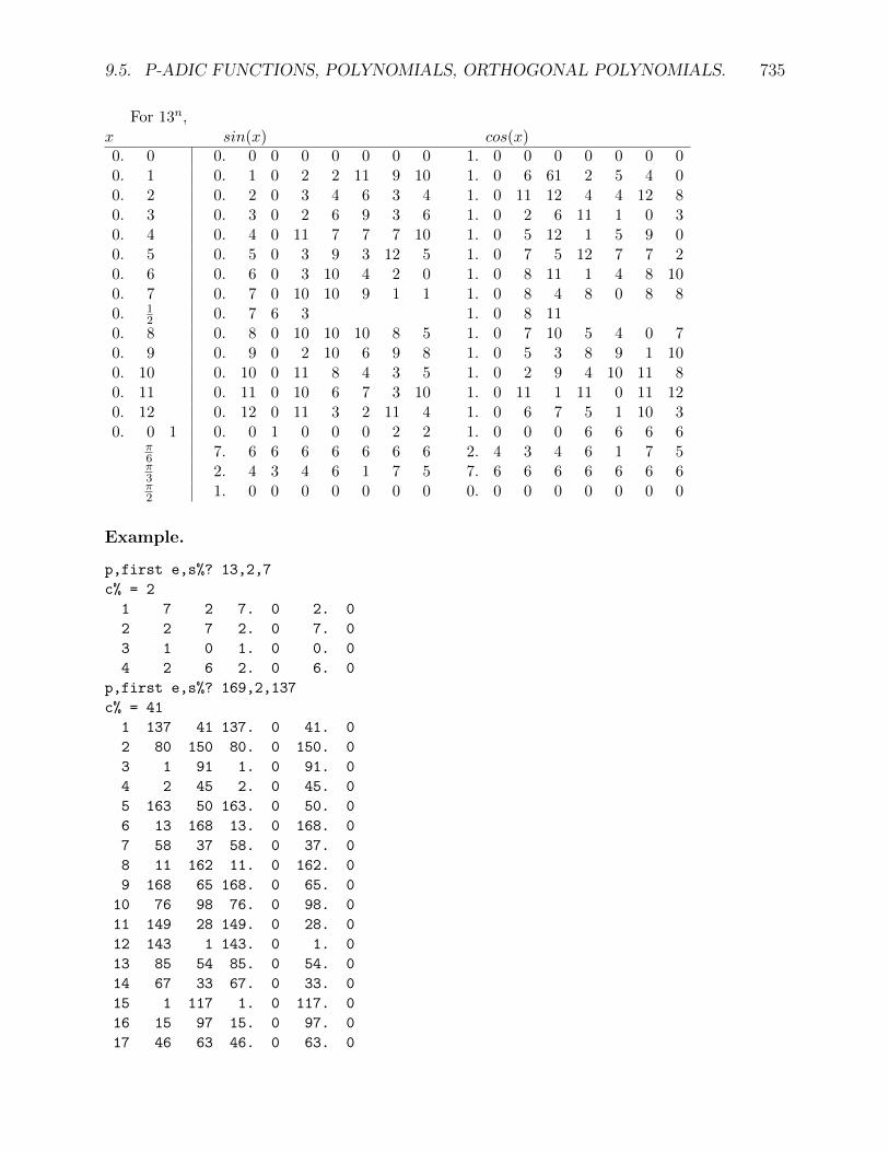
9.5. P-ADIC FUNCTIONS, POLYNOMIALS, ORTHOGONAL POLYNOMIALS. 735
For 13n,x sin(x) cos(x)0. 0 0. 0 0 0 0 0 0 0 1. 0 0 0 0 0 0 00. 1 0. 1 0 2 2 11 9 10 1. 0 6 61 2 5 4 00. 2 0. 2 0 3 4 6 3 4 1. 0 11 12 4 4 12 80. 3 0. 3 0 2 6 9 3 6 1. 0 2 6 11 1 0 30. 4 0. 4 0 11 7 7 7 10 1. 0 5 12 1 5 9 00. 5 0. 5 0 3 9 3 12 5 1. 0 7 5 12 7 7 20. 6 0. 6 0 3 10 4 2 0 1. 0 8 11 1 4 8 100. 7 0. 7 0 10 10 9 1 1 1. 0 8 4 8 0 8 80. 1
2 0. 7 6 3 1. 0 8 110. 8 0. 8 0 10 10 10 8 5 1. 0 7 10 5 4 0 70. 9 0. 9 0 2 10 6 9 8 1. 0 5 3 8 9 1 100. 10 0. 10 0 11 8 4 3 5 1. 0 2 9 4 10 11 80. 11 0. 11 0 10 6 7 3 10 1. 0 11 1 11 0 11 120. 12 0. 12 0 11 3 2 11 4 1. 0 6 7 5 1 10 30. 0 1 0. 0 1 0 0 0 2 2 1. 0 0 0 6 6 6 6
π6 7. 6 6 6 6 6 6 6 2. 4 3 4 6 1 7 5π3 2. 4 3 4 6 1 7 5 7. 6 6 6 6 6 6 6π2 1. 0 0 0 0 0 0 0 0. 0 0 0 0 0 0 0
Example.
p,first e,s%? 13,2,7
c% = 2
1 7 2 7. 0 2. 0
2 2 7 2. 0 7. 0
3 1 0 1. 0 0. 0
4 2 6 2. 0 6. 0
p,first e,s%? 169,2,137
c% = 41
1 137 41 137. 0 41. 0
2 80 150 80. 0 150. 0
3 1 91 1. 0 91. 0
4 2 45 2. 0 45. 0
5 163 50 163. 0 50. 0
6 13 168 13. 0 168. 0
7 58 37 58. 0 37. 0
8 11 162 11. 0 162. 0
9 168 65 168. 0 65. 0
10 76 98 76. 0 98. 0
11 149 28 149. 0 28. 0
12 143 1 143. 0 1. 0
13 85 54 85. 0 54. 0
14 67 33 67. 0 33. 0
15 1 117 1. 0 117. 0
16 15 97 15. 0 97. 0
17 46 63 46. 0 63. 0

736 CHAPTER 9. FINITE ELLIPTIC FUNCTIONS
18 39 168 39. 0 168. 0
19 110 24 110. 0 24. 0
20 24 110 24. 0 110. 0
21 168 39 168. 0 39. 0
22 63 46 63. 0 46. 0
23 97 15 97. 0 15. 0
24 117 1 117. 0 1. 0
25 33 67 33. 0 67. 0
26 54 85 54. 0 85. 0
27 1 143 1. 0 143. 0
28 28 149 28. 0 149. 0
29 98 76 98. 0 76. 0
30 65 168 65. 0 168. 0
31 162 11 162. 0 11. 0
32 37 58 37. 0 58. 0
33 168 13 168. 0 13. 0
34 50 163 50. 0 163. 0
35 45 2 45. 0 2. 0
36 91 1 91. 0 1. 0
37 150 80 150. 0 80. 0
38 41 137 41. 0 137. 0
39 1 0 1. 0 0. 0
40 41 32 41. 0 32. 0
Comment.
Using s1 = x, s2i+1 = six2 (2i−1)2
2i(2i+1) ,
and arcsin(x) = s1 + s3 + . . . ,arcsin(.7, 6, 6, 6, 6, 6, 6) = .7, 6, 9, 12, 9, 6, 5andsin(.7, 6, 9, 12, 9, 6, 5) = .7, 6, 6, 6, 6, 6, 6 = (.1, 0, 0, 0, 0, 0, 0)modulo 169, at 13 we read 85 and 54 corresponding to.76 and .24hence π
6 correspond to arcsin(.7, 6, 6) = .7, 6, 9 and p to .3, 0, 5, 11, 7, 1, 7If we use the program padic.bas we can, given sin(α) and cos(α), obtained using 115a n2adic,determine sin(iα) and cos(iα).For p = 13, using sin(α) ≡ 7mod 13, we get (mod p3) all distinct values except(0, 2, 5, 6, 7, 8, 11) 169± 1.The non zero numbers in the parenthesis are the non residues.This indicates that the connection is tenuous.
Theorem. 12
If s(1) ≡ g (mod pn), where g is a primitive root of p, then . . .
Let s1 = c2 = 12 = 6.666 . . . , c1 = s2 =
√32 = 2.12 . . . ,
given ξ, determine s = sin(ξ), c = cos(ξ), in the p-adic field, (ξ ≡ 0 (mod p),
1211.10.82

9.6. P-ADIC FIELD. 737
determine,s(i) = sin(iξ)cp(i) + cos(iξ)sp(i), c(i) = cos(iξ)cp(i)− sin(iξ)sp(i).(ξ was control H −)?
9.5.2 Integration.
Definition. 13
1. Int2j2i sin = cos(2j)− cos(2i).
2. Mid2j2i sin = sin(2i+ 1) + sin(2i+ 3) + . . .+ sin(2j − 1).
3. Trap2j2i sin = 1
2sin(2) + sin(2i+ 2) + . . .+ sin(2j − 2) + 12sin(2j).
4. Simpson2j2i sin = sin(2i) + 4sin(2i+ 2) + 2sin(2i+ 4) + 4sin(2i+ 6)
+ . . .+ 4sin(2j − 2) + sin(2j).
Theorem.
Int2j2i sin = −2sin(1)Mid2j2i sin
= −2tan(1) Trap2j2i sin
= −2 sin(2)2+cos(2) Simpson
2j2i sin.
9.6 P-adic field.
9.6.1 Generalities.
Notation.
Writing x = x0 + x1p+ x2p2 + x3p
3 + . . . in the formx = x0.x1x2x3 . . ., we will also write
x ≡ x0 (mod p), x ≡ x0.x1 (mod p2), . . . .We have, for instance,
0. 12 = 0. 7 6 6 6 6 6 6.
Example.
p = 5, up to p6,12 = 3.22222, indeed, 2 3 = 6 ≡ 1 (mod 5),2 (3.2) = 2.13 = 26 ≡ 1 (mod 52), . . . .−1/2 = 2.22222, −.1/2 = .22222, −.01/2 = .02222.
Definition.
In the p-adic field, the exponetial, logarithmic and trigonometric functions are defined by:exp(x) := 1 + x+ 1
2!x2 + 1
3!x3 + . . . , for |x| < . . ..
log(x) := x− 12x
2 + 13x
3 + . . . , for |x| <.
1317.12.82

738 CHAPTER 9. FINITE ELLIPTIC FUNCTIONS
sin(x) := x− 13!x
3 + 15!x
5 − . . ., for |x| ≤ p−1
cos(x) := 1− 12!x
2 + 14!x
4 − . . . , for |x| ≤ p−1.
Example.
p = 5, x = 0.1,
1 = 1.00000 00x = 0.10000 00 x = 0.10000 00x2/2 = 0.03222 22 −x2 1
2 = 0.02222 22x3/1.1 = 0.00140 40 x3 1
3 = 0.00231 31x4/4.4 = 0.00044 34 −x4 1
4 = 0.00011 11x5/.44 = 0.00044 34 x5/.1 = 0.00010 00x6/.4301 = 0.00004 03 −x6/1.1 = 0.00000 40x7/.31031 = 0.00000 24 x7/2.1 = 0.00000 03x8/.422422 = 0.00000 04exp(0.1) = 1.13341 24 log(1.1) = 0.12320 14x = 0.10000 00 1 = 1.00000 00−x3/1.1 = 0.00404 04 −x2 1
2 = 0.02222 22x5/.44 = 0.00044 34 x4/4 = 0.00044 34−x7/.31031 = 0.00000 30 −x6/1.1 = 0.00001 41
x8/.422422 = 0.00000 04sin(0.1) = 0.10443 24 cos(1.1) = 1.02213 03
Example.
For p = 13,x sin(x) cos(x)0. 1 0. 1 0 2 2 11 9 10, 1. 0 6 6 12 5 4 00. 2 0. 2 0 3 4 6 3 4, 1. 0 11 12 4 4 12 80. 3 0. 3 0 2 6 9 3 6, 1. 0 2 6 11 1 0 30. 4 0. 4 0 11 7 7 7 10, 1. 0 5 12 1 5 9 00. 5 0. 5 0 3 9 3 12 5, 1. 0 7 5 12 7 7 20. 6 0. 6 0 3 10 4 2 0, 1. 0 8 11 1 4 8 100. 7 0. 7 0 10 10 9 1 1, 1. 0 8 4 8 0 8 80. 1
2 0. 7 6 3 0 5 5 7, 1. 0 8 1 10 0 1 00. 8 0. 8 0 10 10 10 8 5, 1. 0 7 10 5 4 0 70. 9 0. 9 0 2 10 6 9 8, 1. 0 5 3 8 9 1 100. 10 0. 10 0 11 8 4 3 5, 1. 0 2 9 4 10 11 80. 11 0. 11 0 10 6 7 3 10, 1. 0 11 1 11 0 11 120. 12 0. 12 0 11 3 2 11 4, 1. 0 6 7 5 1 10 30. 0 1 0. 0 1 0 0 0 2 2, 1. 0 0 0 6 6 6 60. 11 1 0. 11 1 10 4 10 9 1, 1. 0 11 3 3 10 11 10. 0 2 0. 0 2 0 0 0 3 4, 1. 0 0 0 11 12 12 120. 10 2 0. 10 2 11 12 2 1 8, 1. 0 2 2 1 1 3 30. 0 3 0. 0 3 0 0 0 2 6, 1. 0 0 0 2 6 6 6
Definition.
The Chebyshev polynomials are defined by the recurrence relationTi+1(x) := −Ti−1(x) + 2xTi(x), i = 1, 2, . . . , with

9.6. P-ADIC FIELD. 739
T0(x) := 1, T1(x) := x.
Definition.
For p ≡ 1 (mod 4), a root c1 of Ti is called a primitive root modulo p, if all the roots of Ti,c1, c3, . . . , c2i−1
can be obtained from it using the addition formulas,c1 := c1, c3 := 4c13 − 3c1, c2i+1 := −c2i−3 + 2c2i−1(2c12 − 1), i = 2, . . . , i− 1.
Example.
For p = 13, the roots of T3 = 4x3 − 3x are 0, 2 and −2. 2 and −2 are primitive roots.If c1 = c1 = 2 then c3 = 0, c5 = −2.For p = 17, T4(x) = 8x4 − 8x2 + 1, which has the primitive roots 4,−4, 6,−6.
Notation.
For p ≡ 1 (mod 4), the roots of T p−14
will be denoted,
cos(α), cos(3α), . . . , cos(p−32 α).
with α = πp−12
.
We will also definecos(0α) := 1,cos(2kα) := −cos((2k − 2)α) + 2c1cos((2k − 1)α),k = 1, . . . , p−1
4 .
sin(kα) = cos((p−14 − k)α).
Example.
For p = 13, α = π6 , δ
2 = 2,(the lines k = 1
2 ,32 , . . . will be explained in 1.1, 1.2),
k sin(kα) cos(kα)

740 CHAPTER 9. FINITE ELLIPTIC FUNCTIONS
0 0. 0 0 0 0 0 0 0 1. 0 0 0 0 0 0 012 9. 7 1 1 0 9 12 0 δ 2. 1 8 7 6 2 6 7 δ1 7. 6 6 6 6 6 6 6 2. 4 3 4 6 1 7 432 6. 6 6 6 6 6 6 6 δ 6. 6 6 6 6 6 6 6 δ2 2. 4 3 4 6 1 7 4 7. 6 6 6 6 6 6 652 2. 1 8 7 6 2 6 7 δ 9. 7 1 1 0 9 12 0 δ3 1. 0 0 0 0 0 0 0 0. 0 0 0 0 0 0 072 2. 1 8 7 6 2 6 7 δ 4. 5 11 11 12 3 0 12 δ4 2. 4 3 4 6 1 7 4 6. 6 6 6 6 6 6 692 6. 6 6 6 6 6 6 6 δ 7. 6 6 6 6 6 6 6 δ5 7. 6 6 6 6 6 6 6
11. 8 9 8 6 11 5 8112 9. 7 1 1 0 9 12 0 δ
11. 11 4 5 6 10 6 5 δ6 0. 0 0 0 0 0 0 0
12. 12 12 12 12 12 12 12132 4. 5 11 11 12 3 0 12 δ
11. 11 4 5 6 10 6 5 δ7 6. 6 6 6 6 6 6 6
11. 8 9 8 6 11 5 8152 7. 6 6 6 6 6 6 6 δ 7. 6 6 6 6 6 6 6 δ8 11. 8 9 8 6 11 5 8 6. 6 6 6 6 6 6 6
172 11. 11 4 5 6 10 6 5 δ 4. 5 11 11 12 3 0 12 δ9 12. 12 12 12 12 12 12 12 0. 0 0 0 0 0 0 0
192 11. 11 4 5 6 10 6 5 δ 9. 7 1 1 0 9 12 0 δ
10 11. 8 9 8 6 11 5 8 7. 6 6 6 6 6 6 6212 7. 6 6 6 6 6 6 6 δ 6. 6 6 6 6 6 6 6 δ
11 6. 6 6 6 6 6 6 6 2. 4 3 4 6 1 7 4232 4. 5 11 11 12 3 0 12 δ 2. 1 8 7 6 2 6 7 δ
12 0. 0 0 0 0 0 0 0 1. 0 0 0 0 0 0 0
In this particular case, sin(α) = 12 , cos(α) =
√3
2 , are sufficient to obtain the entries 0, 1, 2, . . . ,12, in the table.We have therefore a first method of obtaining tables of trigonometric functions in a finite field14.We choose x, such that |x| = p−1, therefore |kx| ≤ p−1. ( If |x| < p−1, primitivity is not insured.See 1.3.)We compute sin(k x) and cos(i x) by Maclaurin series, (see 0.1.) and use the addition formulassin(k(α+x)) = sin(kpα)cos(kx)+cos(kpα)sin(kx), cos(k(α+x)) = cos(kpα)cos(kx)−sin(kpα)sin(kx),where kp is k (mod p).
Example.
For p = 13, and x = 0. 1,(The lines k = 1
2 ,32 , . . . willbeexplainedin1.3).
k sin(k(α+ x)) cos(k(α+ x))
1412.10.82

9.6. P-ADIC FIELD. 741
12 9. 8 2 11 7 1 5 9 δ 2. 3 7 12 12 12 11 1 δ1 7. 8 0 4 3 7 4 5 2. 10 8 7 2 10 10 632 6. 2 6 10 8 11 2 2 δ 6. 10 12 0 3 3 5 7 δ2 2. 5 12 3 5 5 1 0 7. 2 10 6 12 2 11 452 2. 4 11 4 4 7 6 4 δ 9. 2 11 4 4 2 10 1 δ3 1. 0 2 6 11 1 0 3 0. 10 12 10 6 3 9 672 2. 2 11 4 2 8 8 2 δ 4. 11 8 8 0 12 4 5 δ4 2. 2 0 11 5 1 11 10 6. 11 6 10 6 9 12 092 6. 5 4 1 7 4 9 2 δ 7. 5 2 2 7 5 9 0 δ5 7. 9 8 12 12 9 1 1 11. 12 1 7 5 3 7 5
112 9. 9 3 0 3 0 5 5 δ 11. 7 2 1 8 7 3 3 δ
6 0. 7 12 9 2 8 10 12 12. 12 4 1 11 8 4 20. 1 1
2 4. 5 10 4 8 7 1 10 δ 11. 11 2 9 10 12 1 2 δ7 6. 5 12 12 1 12 6 5 11. 5 0 5 11 0 7 52. 1 1
2 7. 0 0 4 6 1 11 11 δ 7. 12 5 8 7 11 2 6 δ8 11. 4 8 6 4 5 11 6 6. 9 3 2 8 6 8 14. 1 1
2 11. 6 8 1 3 6 3 2 δ 4. 9 6 0 7 10 12 2 δ9 12. 12 7 9 4 3 11 2 0. 9 0 2 10 6 9 86. 1 1
2 11. 12 8 7 3 11 6 6 δ 9. 0 11 7 11 0 9 2 δ
10 11. 0 6 7 4 10 9 1 7. 0 10 7 2 3 6 08. 1 1
2 7. 4 5 9 12 6 4 3 δ 6. 4 0 12 2 12 2 12 δ11 6. 2 1 10 3 11 10 1 2. 3 6 11 0 10 4 1210. 1 1
2 4. 2 7 8 9 4 10 4 δ 2. 7 6 7 7 12 9 1112 0. 12 0 11 3 2 11 4 1. 0 6 7 5 1 10 311. 1 1
2 9. 6 3 1 9 11 1 4 δ 2. 12 5 5 0 2 9 110. 1 7. 6 8 10 12 0 7 10 2. 4 9 10 11 5 4 11. 2 1
2 6. 9 11 0 4 6 7 5 δ 6. 3 6 4 12 2 2 1 δ1. 1 2. 11 2 1 9 11 6 8 7. 4 3 4 3 6 1 113. 2 1
2 2. 8 3 4 5 2 3 6 δ 9. 4 2 4 12 3 0 9 δ2. 1 1. 0 11 10 10 7 2 5 0. 11 11 9 10 7 2 105. 2 1
2 2. 11 2 0 10 2 0 5 δ 4. 0 7 0 0 12 5 9 δ3. 1 2. 9 6 4 3 12 4 7 6. 0 4 6 9 10 2 97. 2 1
2 6. 11 2 0 2 12 9 0 δ 7. 11 4 4 1 12 8 3 δ4. 1 7. 11 9 3 11 12 4 10 11. 6 5 5 1 10 10 29. 2 1
2 9. 11 8 0 12 9 2 12 δ 11. 3 4 7 9 10 3 7 δ5. 1 0. 8 11 9 9 12 5 11 12. 12 5 12 7 1 5 711. 2 1
2 4. 7 7 12 11 6 6 4 δ 11. 2 5 1 12 10 10 3 δ6. 1 6. 7 1 6 3 1 8 4 11. 11 0 6 6 2 8 60. 3 1
2 7. 6 10 9 6 10 5 4 δ 7. 6 2 3 0 4 2 10 δ
A second method to obtain trigonometric tables in finite fields is to start with sin(α) such thatx0.x1 is a primitive root for p2 and cos(α) =
√1− sin2(α) and use the addition formulas to obtain
in successionsin(kα) and cos(kα) for k = 2, 3, . . . . For instance, we have the following
Example.
For q = 134 and sin(α) = 7. 8 0 4, thencos(α) = 2.10 8 7, the period is 12.133 and

742 CHAPTER 9. FINITE ELLIPTIC FUNCTIONS
k sin(kα) cos(kα)1 7. 8 0 4 2. 10 8 72 2. 5 12 3 7. 2 10 63 1. 0 2 6 0. 10 12 104 2. 2 0 11 6. 11 6 105 7. 9 8 12 11. 12 1 76 0. 7 12 9 12. 12 4 17 6. 5 12 12 11. 5 0 58 11. 4 8 6 6. 9 3 29 12. 12 7 9 0. 9 0 210 11. 0 6 7 7. 0 10 711 6. 2 1 10 2. 3 6 1112 0. 12 0 11 1. 0 6 70. 1 7. 6 8 10 2. 4 9 1011. 1 0. 11 1 10 1. 0 11 30. 2 2. 4 4 4 7. 6 2 1110. 2 0. 10 2 11 1. 0 2 20. 3 1. 0 0 0 0. 0 10 12
Theorem.
If sinh(x) = x+ 13!x
3 + 15!x
5 + . . . , |x| ≤ p−1,and cosh(x) = 1 + 1
2!x2 + 1
4!x4 + . . . , |x| ≤ p−1,
thensin(xi) = isinh(x), cos(xi) = cosh(x),
Example.
With p = 11,sin(0.12 i) = 0. 6 5 810 3 8 0 i, cos(0.12 i) = 1. 0 7 9 5 7 0 2.sin(0.1i) =0. 1 0 2 9 0 9 6 i, cos(0.1i) =1. 0 6 5 0 5 9 6.
Example.
For p = 11 and x = . 1, Using 6.1.13 andsin(α2 ) = 9. 3 5 9 2 2 410 and cos(α2 ) = 5. 7 6 3 0 4 6 9 i,sin(α) = 2.10 5 5 6 5 6 6 i and cos(α) = 4. 919 3 8 7 9 4of 1.6, we obtainsin((α+1
2 )i) = 9. 6 910 9 2 1 0 i, cos((α+12 )i) = 5. 8 610 0 0 7 2, sin((α+ 1)i) = 2. 3 5 7 8 5 5 2 i,
cos((α+ 1)i) = 4. 0 1 210 6 810.The table can be computed from the first values the second are used here as a check:k sin(k(α+ x)/2) cos(k(α+ x)/2)

9.6. P-ADIC FIELD. 743
0. 0 0. 0 0 0 0 0 0 0 1. 0 0 0 0 0 0 01. 0 9. 6 9 10 9 2 1 0 5. 8 6 10 0 0 7 2 i2. 0 2. 3 5 7 8 5 5 2 i 4. 0 1 2 10 6 8 103. 0 4. 6 5 4 8 0 9 8 2. 4 2 1 0 3 3 1 i4. 0 5. 3 2 8 0 5 3 7 i 9. 2 5 0 0 9 10 55. 0 1. 0 10 9 8 0 6 4 0. 3 5 4 6 0 0 9 i6. 0 5. 2 1 8 5 2 4 9 i 2. 0 4 10 4 9 10 07. 0 4. 5 10 1 4 2 6 8 9. 8 6 7 7 3 4 1 i8. 0 2. 5 6 4 3 2 10 4 i 7. 9 8 2 0 10 10 89. 0 9. 9 4 10 3 10 1 9 6. 1 1 0 9 3 4 1 i
10. 0 0. 6 10 2 7 2 7 10 i 10. 10 3 4 6 3 9 90. 1 2. 7 2 5 3 7 0 2 6. 3 3 9 5 2 10 4 i1. 1 9. 9 0 9 0 0 5 0 i 7. 0 10 5 5 7 2 72. 1 7. 3 9 9 9 5 4 8 9. 4 4 6 2 4 1 7 i3. 1 6. 6 3 4 0 5 9 8 i 2. 5 2 6 2 7 4 14. 1 10. 10 8 9 6 0 8 7 0. 2 6 10 2 2 3 3 i5. 1 6. 9 6 7 1 2 5 7 i 9. 7 2 7 3 2 10 86. 1 7. 6 5 9 9 7 0 2 2. 0 1 5 8 0 0 1 i7. 1 9. 3 8 0 9 9 6 8 i 4. 2 4 4 1 4 9 108. 1 2. 9 5 8 7 1 7 6 5. 10 5 5 8 1 1 10 i9. 1 0. 10 0 9 7 9 9 0 i 1. 0 6 4 6 8 8 6
10. 1 9. 0 1 8 8 0 2 7 5. 6 1 3 4 9 9 5 i
0. 2 2. 10 9 3 7 3 9 5 i 4. 9 1 3 5 1 9 61. 2 4. 8 9 5 5 6 3 4 2. 8 5 8 0 0 2 6 i2. 2 5. 5 5 6 8 8 7 9 i 9. 8 5 0 3 10 3 23. 2 1. 0 8 5 3 9 2 5 0. 4 4 1 9 9 0 6 i4. 2 5. 0 0 2 7 6 10 0 i 2. 6 7 10 3 4 0 65. 2 4. 3 1 0 4 4 6 5 9. 1 7 10 8 2 10 0 i6. 2 2. 9 4 8 7 7 9 0 i 7. 7 3 6 9 3 10 77. 2 9. 4 10 6 3 3 0 7 6. 10 4 2 0 9 10 0 i8. 2 0. 7 9 3 9 1 3 4 i 10. 10 2 6 8 4 8 89. 2 2. 2 1 2 3 7 1 10 6. 5 0 10 10 2 1 5 i
10. 2 9. 2 6 3 4 6 7 5 i 7. 2 7 6 0 1 10 30. 3 7. 1 3 0 7 10 10 1 9. 0 0 3 10 10 2 10 i1. 3 6. 4 3 0 9 3 9 2 i 2. 10 2 3 7 6 3 02. 3 10. 10 4 9 7 9 9 0 0. 1 7 7 1 6 1 9 i3. 3 6. 0 0 10 3 3 8 3 i 9. 1 9 3 1 1 6 34. 3 7. 8 1 5 1 4 6 8 2. 7 1 5 10 2 10 5 i5. 3 9. 10 8 5 1 5 10 4 i 4. 4 0 1 0 4 5 26. 3 2. 3 1 0 6 0 8 0 5. 1 10 0 0 4 9 0 i7. 3 0. 9 1 6 7 2 5 2 i 1. 0 2 7 9 4 0 2
9.6.2 Extension to the half argument.
Introduction.
The tables of trigonometric functions can be extended to the half arguments. These are requiredfor the angles in finite Euclidean geometry.

744 CHAPTER 9. FINITE ELLIPTIC FUNCTIONS
Theorem.
If g is a primitive root of p, and δ2 = g, then c1′ = cos(α12)δ−1 is a primitive root of
S′p−12
= T p−12 (δI),
where I is the identity function.Indeed, T2n = Tn (2I2 − 1). The other roots are denoted by c2′, c3′, . . . .
Example.
For p = 13, g = 2,S′6 = 256I6 − 192I4 + 36I2 − 1,
c1′ = cos(α12)δ−1 = 2. 1 8 7 6 2 6 7, from which we derive the values in 0.6. for i = 1
2 ,32 , . . . , 11
2 .
Comment.
The method given at the end of section 0.6. enables to complete the table of Example 0.7. Alter-nately, if g is a primitive root for p2, p ≡ 1 (mod 4), we know that g is a primitive root for pe,e = 3, 4, . . . .
If δ2 = g, sin(α/2) = δ√
1−cos(α)2g and cos(α1
2) = δ√
1+cos(α)2g .
Example.
For p = 13,sin(α1
2)δ−1 =√
(3. 7 7 412 310 4) = 9. 8 211 7 1 5 9 δ, cos(α12)δ−1 =
√(4.1211 1 7 2 9 1) = 2. 3
712121211 1 δ.One of the signs of the square roots can be chosen arbitrarily, the other must be chosen in such away thatsin(α) = 2g sin(α1
2)cos(α12).
Theorem.
For p ≡ −1 (mod 4), with δ2 = −1,cos(α/2)δ−1 is a primitive root of
V p−32
= (T p−12I−1) (δI).
sin(α/2) is a primitive root ofU p−3
2= (T p−1
2I−1)
√1− I2.
Example.
For p = 11, δ2 = −1, α = π5 ,
V4 = 16I4 + 20I2 + 5,with roots 5. 7 6 3 0 4 6 9 and 2.10 5 5 6 5 6 6,
U4 = 16I4 − 12I2 + 1,with roots 9. 3 5 9 2 2 410 and 4. 910 3 8 7 9 4. Hence, k sin(kα) cos(kα)
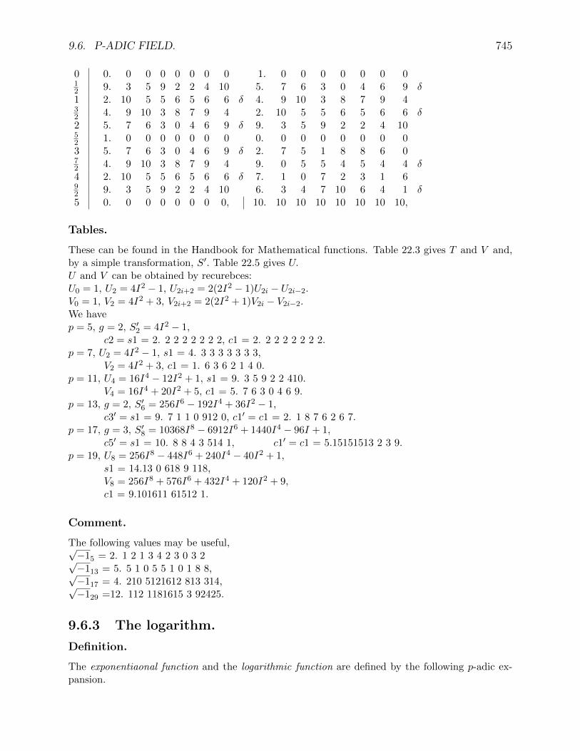
9.6. P-ADIC FIELD. 745
0 0. 0 0 0 0 0 0 0 1. 0 0 0 0 0 0 012 9. 3 5 9 2 2 4 10 5. 7 6 3 0 4 6 9 δ1 2. 10 5 5 6 5 6 6 δ 4. 9 10 3 8 7 9 432 4. 9 10 3 8 7 9 4 2. 10 5 5 6 5 6 6 δ2 5. 7 6 3 0 4 6 9 δ 9. 3 5 9 2 2 4 1052 1. 0 0 0 0 0 0 0 0. 0 0 0 0 0 0 03 5. 7 6 3 0 4 6 9 δ 2. 7 5 1 8 8 6 072 4. 9 10 3 8 7 9 4 9. 0 5 5 4 5 4 4 δ4 2. 10 5 5 6 5 6 6 δ 7. 1 0 7 2 3 1 692 9. 3 5 9 2 2 4 10 6. 3 4 7 10 6 4 1 δ5 0. 0 0 0 0 0 0 0, 10. 10 10 10 10 10 10 10,
Tables.
These can be found in the Handbook for Mathematical functions. Table 22.3 gives T and V and,by a simple transformation, S′. Table 22.5 gives U.U and V can be obtained by recurebces:U0 = 1, U2 = 4I2 − 1, U2i+2 = 2(2I2 − 1)U2i − U2i−2.V0 = 1, V2 = 4I2 + 3, V2i+2 = 2(2I2 + 1)V2i − V2i−2.We havep = 5, g = 2, S′2 = 4I2 − 1,
c2 = s1 = 2. 2 2 2 2 2 2 2, c1 = 2. 2 2 2 2 2 2 2.p = 7, U2 = 4I2 − 1, s1 = 4. 3 3 3 3 3 3 3,
V2 = 4I2 + 3, c1 = 1. 6 3 6 2 1 4 0.p = 11, U4 = 16I4 − 12I2 + 1, s1 = 9. 3 5 9 2 2 410.
V4 = 16I4 + 20I2 + 5, c1 = 5. 7 6 3 0 4 6 9.p = 13, g = 2, S′6 = 256I6 − 192I4 + 36I2 − 1,
c3′ = s1 = 9. 7 1 1 0 912 0, c1′ = c1 = 2. 1 8 7 6 2 6 7.p = 17, g = 3, S′8 = 10368I8 − 6912I6 + 1440I4 − 96I + 1,
c5′ = s1 = 10. 8 8 4 3 514 1, c1′ = c1 = 5.15151513 2 3 9.p = 19, U8 = 256I8 − 448I6 + 240I4 − 40I2 + 1,
s1 = 14.13 0 618 9 118,V8 = 256I8 + 576I6 + 432I4 + 120I2 + 9,c1 = 9.101611 61512 1.
Comment.
The following values may be useful,√−15 = 2. 1 2 1 3 4 2 3 0 3 2√−113 = 5. 5 1 0 5 5 1 0 1 8 8,√−117 = 4. 210 5121612 813 314,√−129 =12. 112 1181615 3 92425.
9.6.3 The logarithm.
Definition.
The exponentiaonal function and the logarithmic function are defined by the following p-adic ex-pansion.

746 CHAPTER 9. FINITE ELLIPTIC FUNCTIONS
D.0. exp(x) = 1 + x+ . . .+ 1n!x
n + . . . , |x| < 1.D.1. log(1 + x) = x− 1
2x2 + . . .+ (−1)n 1
nxn + . . . , |x| < 1.
The classical theorem is (See for instance Koblitz, 1977.)
Theorem.
. . .
Motivation.
For p = 5,log(−4) = log(1− 5) = 0.41041,log(1.1) = log(1 + 5) = 0.12420,log(−4.1) = log(1− 10) = 0.32314.
If we want log(xy) = log(x) + log(y) to hold, we have 3 equations to determine log(−1), log(2) andlog(3). log(1.3) and log(−4.4) can be used as check. This gives
log(−1) = 0,log(2) = 0.23240,log(3) = 0.43134.
Clearly we now have a function which is not a bijection, for instance,log(1.20230) = 0.23420.
This suggest that we can extend the range of definition of the logarithm function. The equationxp−1 ≡ 1 (mod p) has p − 1 roots, 1,2, . . . ,p − 1, therefore the equation xp−1 = 1 has p − 1 rootsin the p-adic field, with first digit 1,2, . . . , p− 1.In general the roots are 1, x1, x2, . . . , −x2, −x1, −1.
Algorithm.
If g is a primitive root in Zp, the corresponding primitive root g′ ∈ . . . can be obtained by Newton’smethod:
y := g,
y = y − 1p−12
(y + 1y
p−32 for i = 1 to n.
Theorem.
Algorithm 9.6.3 determines the first 2n digits of g′.
Theorem.
Given a prime p, a primitive root g ∈ Zp and x, H0. |x| = 1,D0. x0 = ind(int(x)),where ind is the index function in Zp associated to g,D1. y := x/g
′x0 − 1D2. z := y − 1
2y2 + . . .+ 1
n(−y)n
thenC0. |z| < 1.C1. logp,g(x) = x0, z

9.6. P-ADIC FIELD. 747
Example.
For p = 5, x1 = 2.1213423.(All the roots are 1, 2 .1213423, −2.1213423 = 3.3231021, −1 = 4.4444444)
For p = 7, x1 = 2.4630262, x2 = 3.4630262.
For p = 11, x1 = 2.10 4 9 1 2 3 9, x2 = 3. 0 1 2 3 610 8,x3 = 4. 7 9 5 2 9 8 0, x4 = 5. 2 5 1 7 8 510.
For p = 13, x1 = 2. 6 2 2 4 2 5 8, x2 = 3.11 6 9 7 2 4 4,x3 = 4.11 6 9 7 2 4 4, x5 = 5. 5 1 0 5 5 1 0x6 = 6. 1 910 3 5 6 4.
For p = 17, x1 = 2. 9 312 914 1 5, x2 = 3.13 2 3 011 4 0,x3 = 4. 210 5121612 8, x4 = 5. 9 0 516 9 1 5,x5 = 6. 214 4 1 6 2 3, x6 = 7. 4 216 11514 2,x7 = 8. 6 1 415 116 2.
For p = 19, x1 = 2. 614 414131014, x2 = 3.16 7 8161815 1,x3 = 4. 51717 5 614 0, x4 = 5. 3 3131113 716,x5 = 6.12 21714181716, x6 = 7.15 7 0 118 0 4,x7 = 8.15 7 0 118 0 4, x8 = 9. 118 21712 5 1.
For p = 23, x1 = 2.11211015 2 912, x2 = 3. 51717 71821 7,x3 = 4.2122 4 7 81622, x4 = 5. 1 219 8 2 919,x5 = 6.201517 114 720, x6 = 7.1519 5 8 81519,x7 = 8.171710171911 3, x8 = 9. 713 1 7191512,x9 =10.11 72112221517, x10=11. 81017 3 31922.
The logarithmic functions as defined is not one to one. p − 1 arguments give the same value.To make it one to one we give the following
Definition.
Given a primitive root g,logp,g(x) = i0, x0, logp(x),i0 ∈ (Z,+), x0 ∈ (Zp−1,+), logp(x) ∈ . . . .
where|x| = p−i0, gx0 = int(x), and logp(x) is the p-adic logarithm.i0 is called the characteristic, x0, the index and logp(x), the mantissa.
Example.
For p = 5 and g = 2,log5,2(1.0000000) = 0, 0., log5,2(2.1213423) = 1, 0.,log5,2(3.3231021) = 3, 0., log5,2(4.4444444) = 2, 0..
Theorem.
H0. |x|, |y| = 1.C0. logp,g(x ∗ y) = logp,g(x) + logp,g(y).
748 CHAPTER 9. FINITE ELLIPTIC FUNCTIONS
Problem.
Extend the definition to allow |x|, |y| to be anything using the relation C.0. and the idea ofmantissa.
9.6.4 P-adic Geometry and Related Finite Geometries.
Introduction.
Some thought on finite geometry for different powers of p and the p-adic geometry.
Given p, if we take the points on a line, with coordinates of the form x0. . . . these are indistin-guishable if we use the p-adic valuation to the precision 1.If we consider the points x0.x1, these are distinguishable to the precision 1 but not to the precision1p .They can be considered, if p is 5 say, to have a color associated to the various digits of x0 the colors“purple, blue, green, yellow, orange, red.” As we proceed to the next digit all yellows becomesub-colours proceeding from yellow to orange.We can with more discrimination distinguish them. We can proceed further . . . .We observe also that, in this scheme of things, what is a shade of yellow for one is a shade of greenfor some one else. This is associated to a change of origin.When this is transfered to angles this will give different trigonometric tables associated to differentvalues of x.
Comment. 15
The trigonometric functions work as follows.In the hyperbolic case,for p, the period is 2(p− 1),for p2, the period is 2p(p− 1), . . . .The factor 2 corresponds to the fact, that just as in Euclidean geometry the total angle is 2π, lineswhich form an angle π correspond to the same direction.For the hyperbolic case, there are 2 real isotropic points,There are on the ideal linep+ 1 points,p− 1 ideal (non isotropic) points for the p-geometry,p2 − 1 ideal points for the p2-geometry, of which p2 − p are not included in the preceding set.The hyperbolic trigonometry associated to p2 is presumably for these p2 − p directions . . . .For the elliptic case, the period is 2(p+ 1) as one would expect for the p-geometry.For the p2 case, the period of the trigonometric functions is p2 + p. I do not yet understand howthis comes into the picture.
Definition. 16
p-ADIC GEOMETRY
Let p ≡ −1 (mod 4), let z = 0 be the ideal line, let x2 + y2 = z2 be a circle.There are no solutions of x2 + y2 = 0, therefore the isotropic points are not real.
1519.10.821621.10.82

9.6. P-ADIC FIELD. 749
If z 6= 0, then we can normalize using z = 1, consider x2 + y2 = 1.Let |x| ≥ |y|. If |x| > 1 then there are no solutions.(Hint: divide by p|x| and work modulo p)
Lemma.
If s = sin(α) is a root of . . . thensin(pα) = sin(α), cos(pα) = cos(α).
Theorem.
Let s = sin(α) be a root of . . . .If |sin(β)− sin(α)| < 1 then
limn→∞sin(pnβ) = sin(α).If |x| = 1, there are solutions, x = x0.x1x2 . . . . Let |x0| be a primitive solution of the polynomial. . . .let x1. be . . . .To x corresponds the pair (x, y) = (sin(α), cos(α)),Let X(x) = sin(pα), then the sequence x,X(x), X2(x), . . . convergences to x′. Moreover x′ is a rootof . . .
Example.
p = 11, let x = sin(α) = 3, X(3. 0 0 0 0 0 0 0) = 3. 0 2 8 011 4 6,cos(pα) = 10.103125741,
X(3. 0 2 0 0 0 0 0) = 3. 0 2 6 0 71212,X(3. 0 2 6 0 0 0 0) = 3. 0 2 6 7 612 2,X(3. 0 2 6 7 0 0 0) = 3. 0 2 6 71211 2,X(3. 0 2 6 712 0 0) = 3. 0 2 6 71212 1,X(3. 0 2 6 71212 0) = 3. 0 2 6 71212 2.
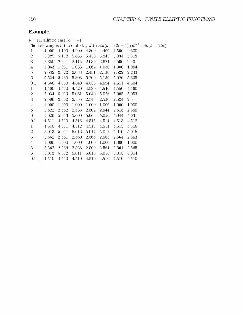
750 CHAPTER 9. FINITE ELLIPTIC FUNCTIONS
Example.
p = 11, elliptic case, g = −1The following is a table of sin, with sin(k = (2l + 1)α)δ−1, sin(k = 2lα)1 4.000 4.100 4.200 4.300 4.400 4.500 4.6002 5.325 5.112 5.665 5.450 5.245 5.034 5.5123 2.350 2.241 2.115 2.030 2.624 2.506 2.4314 1.063 1.031 1.033 1.064 1.050 1.000 1.0545 2.632 2.322 2.033 2.451 2.130 2.522 2.2436 5.524 5.430 5.303 5.200 5.130 5.026 5.6350.1 4.566 4.550 4.540 4.536 4.524 4.511 4.5041 4.500 4.510 4.520 4.530 4.540 4.550 4.5602 5.034 5.013 5.061 5.040 5.026 5.005 5.0533 2.506 2.562 2.556 2.543 2.530 2.524 2.5114 1.000 1.000 1.000 1.000 1.000 1.000 1.0005 2.522 2.562 2.533 2.504 2.544 2.515 2.5556 5.026 5.013 5.000 5.063 5.050 5.044 5.0310.1 4.511 4.510 4.516 4.515 4.514 4.513 4.5121 4.510 4.511 4.512 4.513 4.514 4.515 4.5162 5.013 5.011 5.016 5.014 5.012 5.010 5.0153 2.562 2.561 2.560 2.566 2.565 2.564 2.5634 1.000 1.000 1.000 1.000 1.000 1.000 1.0005 2.562 2.566 2.563 2.560 2.564 2.561 2.5656 5.013 5.012 5.011 5.010 5.016 5.015 5.0140.1 4.510 4.510 4.510 4.510 4.510 4.510 4.510

Chapter 10
DIFFERENTIAL EQUATIONS ANDFINITE MECHANICS
10.0 Introduction.
In the context of Finite Geometry, we should examine the subject of Differential Equations, theirapproximation and the application to finite mechanics.I will describe the first success associated with the harmonic polygonal motion, then . . .
10.1 The first Examples of discrete motions.
10.1.1 The harmonic polygonal motion.
Introduction.
In classical Euclidean geometry as well as in finite Euclidean geometry I define the harmonicpolygonal motion as the motion which associates to linearly increasing time successive points of theharmonic polygon. I will determine, for the classical case, the differential equation of the motion, byconsidering first points which are close to each other 10.1.1. I will then prove that this equation issatisfied when points are not close to each other 10.1.1. The equation bears ressemblance with theequation of Kepler. Because the method uses derivatives of functions of the trigonometric functionsonly and in view of the method of Hensel for p-adic functions, the result extend automatically tothe finite case.
Definition.
Given a conic
0. A(E) = (acos(E), bsin(E), 1),and the point of Lemoine K = (q, 0), given the correspond harmonic polygon of Casey (g2734,p.5 . . . ), Ai, we define the harmonic polygonal motion by
1. A(E(t0 + i h)) = Ai.
751

752 CHAPTER 10. DIFFERENTIAL EQUATIONS AND FINITE MECHANICS
Theorem.
Let
0. r = qa ,
if h is small, the motion satisfies the differential equation
1. C DE = 1− r cos(E),for some constant of integration C.
Proof: The polar k of K is
2. k = [ qa2, 0,−1],
the polar a(E) of A(E) is
3. a(E) = [ cos(E)a , sin(E)
b ,−1],
it meets k at
4. B(E) = (a2sin(E), b(q − acos(E)), qsin(E)).
the condition that Ai−1 ×Ai+1 passes through B(E(t)) gives
5.
∣∣∣∣∣∣a2sin(E(t)) b(q − acos(E(t))) qsin(E(t))
acos(E(t− h)) bsin(E(t− h)) 1acos(E(t+ h)) bsin(E(t+ h)) 1
∣∣∣∣∣∣ = 0.
Let
6. s(t) = 12(E(t+ h) + E(t− h)), d(t) = 1
2(E(t+ h)− E(t− h)), then to the second order in h,with k = 1
2h2,
s = E + kD2E, d = hDE,
7. cos(s) = cos(E)− ksin(E)D2E, sin(s) = sin(E) + kcos(E)D2E, cos(d) = 1− k(DE)2.Replacing the determinant by that obtained by using instead of the last 2 lines their halfsum and their half difference, gives after division of the first row and first column by a andthe second column by b,∣∣∣∣∣∣
sin(E) r − cos(E) rsin(E)cos(s)cos(d) sin(s)cos(d) 1−sin(s)sin(d) cos(s)sin(d) 0
∣∣∣∣∣∣ = 0.
Dividing the last row by sin(d) and expanding with respect to the first row gives, afterchanging sign,
8. sin(E)cos(s) + (r − cos(E))sin(s)− rsin(E)cos(d) = 0,or, after using 7 and dividing by k,
9. (1− rcos(E))D2E = rsin(E)(DE)2,integrating gives 1, with some appropriate constant C,
10. (1− ecos(E))DE = C. This is tantalizing close to Kepler’s equation.
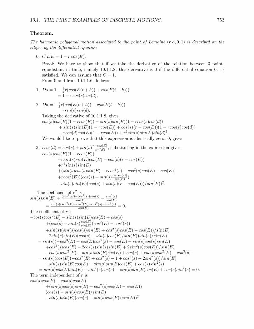
10.1. THE FIRST EXAMPLES OF DISCRETE MOTIONS. 753
Theorem.
The harmonic polygonal motion associated to the point of Lemoine (r a, 0, 1) is described on theellipse by the differential equation
0. C DE = 1− r cos(E).
Proof: We have to show that if we take the derivative of the relation between 3 pointsequidistant in time, namely 10.1.1.8, this derivative is 0 if the differential equation 0. issatisfied. We can assume that C = 1.From 0 and from 10.1.1.6. follows
1. Ds = 1− 12r(cos(E(t+ h)) + cos(E(t− h)))
= 1− rcos(s)cos(d),
2. Dd = −12r(cos(E(t+ h))− cos(E(t− h)))= rsin(s)sin(d).
Taking the derivative of 10.1.1.8, givescos(s)cos(E)(1− rcos(E))− sin(s)sin(E)(1− rcos(s)cos(d))
+ sin(s)sin(E)(1− rcos(E)) + cos(s)(r − cos(E))(1− rcos(s)cos(d))− rcos(d)cos(E)(1− rcos(E)) + r2sin(s)sin(E)sin(d)2.
We would like to prove that this expression is identically zero. 0, gives
3. rcos(d) = cos(s) + sin(s) r−cos(E)sin(E) , substituting in the expression gives
cos(s)cos(E)(1− rcos(E))−rsin(s)sin(E)cos(E) + cos(s)(r − cos(E))+r2sin(s)sin(E)+(sin(s)cos(s)sin(E)− rcos2(s) + cos2(s)cos(E)− cos(E)
+rcos2(E))(cos(s) + sin(s) r−cos(E)sin(E) )
−sin(s)sin(E)(cos(s) + sin(s)(r − cos(E)))/sin(E))2.
The coefficient of r2 issin(s)sin(E) + (cos2(E)−cos2(s))sin(s)
sin(E) − sin3(s)sin(E)
= sin(s)(sin2(E)+cos2(E)−cos2(s)−sin2(s)sin(E) = 0.
The coefficient of r is−cos(s)cos2(E)− sin(s)sin(E)cos(E) + cos(s)
+(cos(s)− sin(s) cos(E)sin(E)(cos2(E)− cos2(s))
+sin(s)(sin(s)cos(s)sin(E) + cos2(s)cos(E)− cos(E))/sin(E)−2sin(s)sin(E)(cos(s)− sin(s)cos(E)/sin(E))sin(s)/sin(E)
= sin(s)(−cos3(E) + cos(E)cos2(s)− cos(E) + sin(s)cos(s)sin(E)+cos2(s)cos(E)− 2cos(s)sin(s)sin(E) + 2sin2(s)cos(E))/sin(E)−cos(s)cos2(E)− sin(s)sin(E)cos(E) + cos(s) + cos(s)cos2(E)− cos3(s)
= sin(s)(cos(E)(−cos2(E) + cos2(s)− 1 + cos2(s) + 2sin2(s))/sin(E)−sin(s)sin(E)cos(E)− sin(s)sin(E)cos(E) + cos(s)sin2(s)
= sin(s)cos(E)sin(E)− sin2(s)cos(s)− sin(s)sin(E)cos(E) + cos(s)sin2(s) = 0.The term independent of r iscos(s)cos(E)− cos(s)cos(E)
+(sin(s)cos(s)sin(E) + cos2(s)cos(E)− cos(E))(cos(s)− sin(s)cos(E)/sin(E)−sin(s)sin(E)(cos(s)− sin(s)cos(E)/sin(E))2

754 CHAPTER 10. DIFFERENTIAL EQUATIONS AND FINITE MECHANICS
= (cos(s)− sin(s)cos(E)/sin(E))(sin(s)cos(s)sin(E) + cos2(s)cos(E)− cos(E)− sin(s)cos(s)sin(E)+sin2(s)cos(E)) = 0.
Theorem. 1
Let e′2 = 1− e2, then
0. e′ tan(12e′M) = (1 + e) tan(1
2E).
Theorem.
0. If t(M) = tan(12E) and 2
1. k = e+1e−1 ,
2. t′i =√−kt(Mi),
then
3. t′1+2 =t′1+t′21−t′1t′2
.
Example.
For p = 13 and e = 2, k = 3 andM 0 1 2 3 4 5 6 7 8 9 10 11 12t(M) 0 1 7 11 8 4 ∞ 9 5 2 6 12 0t′M 0 6 3 1 −4 −2 ∞ 2 4 −1 −3 −6 012E 0 3 7 1 4 6 8 11 5 9
For p = 13 and e = 3, k = 2 andM 0 1 2 3 4 5 6 7 8 9 10 11 12 13t(M) 0 2 12 4 8 7 3 ∞ 10 6 5 9 1 11
12E 0
Programs.
The programs pl.bas and planet.bas . . .
Exercise.
Prove that the acceleration is1−r cosE
C2 (−(a cosE, b sinE, 0) + r(a cos(2E), b sin(2E), 0))
10.1.2 The Parabolic Motion.
Introduction.
The parabola has been studied in g33. Galileo Galilei was the first to show that the motion of aparticle in a uniform gravitional field is a parabola. (Love, p.45) The result extend to the finitecase.
126.6.83229.6.83

10.1. THE FIRST EXAMPLES OF DISCRETE MOTIONS. 755
Theorem.
In both the infinite and finite cases, the solution ofmD2x = 0 and mD2y = −mg
isx(t) = v0t, y(t) = −1
2gt2 + v1t, or
y = ax2 + bx, witha := − g
2v20, b := v1
v0.
Proof: Comparing the equation in the form(x+ b
2a)2 = ya + ( b
2a)2.with the standard equation y2 = 4cx shows that the vertex V and the directrix d are
V = ( b2a , (
b2a)2),
d : y =v20+v21
2g = v2
2gcorresponding to the Torricelli law.
Example.
For p = 7, g = 1 and v0 = v1 = 4, then a = −2, b = 1,y(x) = −2x2 + x = 1− 2(x− 2)2,x 0 1 2 3 −3 −2 −1 0y 0 −1 1 −1 0 −3 −3 1z 1 1 1 1 1 1 1 0t 0 2 −3 −1 1 3 −2
10.1.3 Attempts to Generalize Kepler’s Equation.
Introduction.
I have made many attempts to generalize Kepler’s equation or the simple planetary motion tothe finite case. In section . . . , I examine the use of p-adic function to obtain a solution in theneighbourhood of a circular motion.
10.1.4 The circular motion.
Definition.
The circular motion is defined byx(t) = cos(t), y(t) = sin(t),Dx(t) = −sin(t), Dy(t) = cos(t).
This assumes that the unit of distance is chosen as the radius of the circle and the unit of time ischosen in such a way that the period is 2π.
756 CHAPTER 10. DIFFERENTIAL EQUATIONS AND FINITE MECHANICS
10.2 Approximation to the Solution of Differential Equa-
tions.
10.2.0 Introduction.
To approximate the solution of differential equations it is important to insure that essential proper-ties are preserved. In particular, for conservative systems, the same should hold. In this connection,I developed in 1956 a method of first order and a method of second order which are contact trans-formations and therefore preserve the essential properties of conservative systems. These will beapplied to the finite case.
10.2.1 Some Algorithms.
Algorithm.
The first order algorithm is defined by
Theorem.
Algorithm.
The second order algorithm for the solution of the differential equationD2x = f x, x(0) = x0, Dx(0) = Dx0,
is defined byxi+1 = xi + hDxi + 1
2h2fi,Dxi+1 = Dxi + 1
2h(fi+1 + fi),where
fi := f(xi).
Definition.
A mapping is reversible iff
Theorem.
Given the Algorithm 10.2.1, the mapping is reversible.
Proof: If we solve for xi and Dxi, we getDxi = Dxi+1 − h
2 (fi+1 + fi),xi = xi+1 − hDxi − 1
2h2fi,
= xi+1 − hDxi+1 + 12h
2(fi + fi+1).
Definition.
A mapping is symplectic iff
Theorem.
The mapping defined in algorithm 10.2.1 is symplectic.
Proof:

10.3. THE PARABOLIC MOTION. 757
Example.
Let x and f be one dimensional, letf(x) = −x− 2x3,
let Dx0 = 0, we have the following solutions, for h = 1 and various initial conditions (x(0), Dx(0) =0).p = 11,
i 0 1 2 3 4 5 6 7 8
(x,Dx)i 1, 0 5, 3 −4, 2 −2, 0 −4,−2 5,−3 1, 03, 0 2, 1 5, 2 −5, 2 −2, 1 −3, 0 −2,−1 −5,−2 5,−24, 0 4, 05, 0 4,−1 3,−2 0,−3 −3,−2 −4,−1 −5, 0 −4, 1 −3, 2
p = 13,i 0 1 2 3 4 5 6 7 8
(x,Dx)i 1, 0 6,−6 2, 0 6, 6 1, 03, 0 −6, 2 −6,−2 3, 04, 0 3, 3 −3, 3 −4, 0 −3,−3 3,−3 4, 05, 0 1, 1 −6, 4 −4, 3 0, 4 4, 3 6, 4 −1, 1 −5, 06, 0 −5, 6 5, 6 −6, 0 5,−6 −5,−6 6, 0
Theorem.
If we apply the mapping 10.2.1 toD2x = −x, x(0) = 0, Dx(0) = 1,
we obtain, up to a scaling factor the trigonometric functions.
Example.
With p = 13 and h = 1,i 0 1 2 3 4 5 6 7
8 9 10 11 12 13 14(x,Dx)i 0, 1 1,−5 3,−3 −5,−4 −5, 4 3, 3 1, 5 0,−1
?(δx,Dx)((i) = (sin, cos)(−10i), if sin(1) = 3 and cos(1) = 3δ, with δ2 = 2.
Program.
[130] PENDUL(um)
10.3 The Parabolic Motion.
10.3.0 Introduction.
The parabola has been studied in g33. Galileo Galilei was the first to show that the motion of aparticle in a uniform gravitional field is a parabola. (Love, p.45) The result extend to the finitecase.
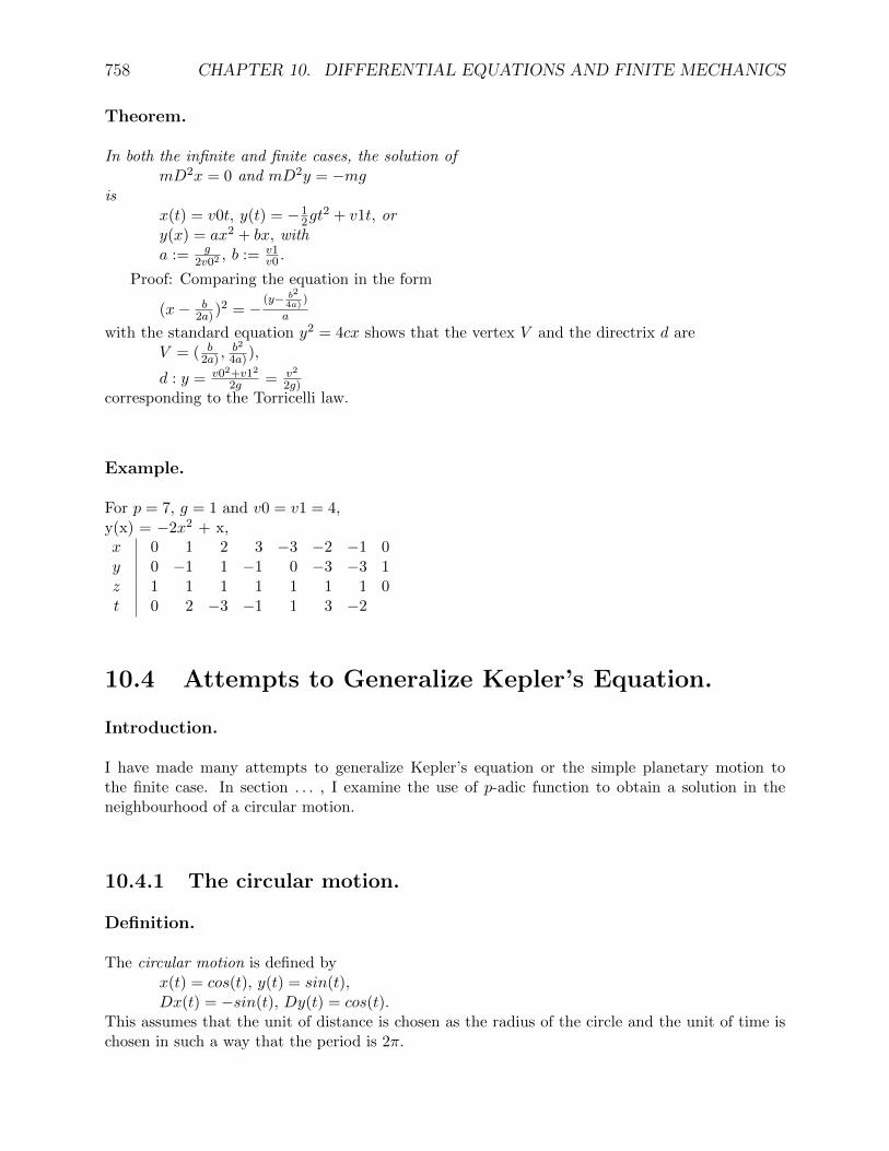
758 CHAPTER 10. DIFFERENTIAL EQUATIONS AND FINITE MECHANICS
Theorem.
In both the infinite and finite cases, the solution ofmD2x = 0 and mD2y = −mg
isx(t) = v0t, y(t) = −1
2gt2 + v1t, or
y(x) = ax2 + bx, witha := g
2v02, b := v1
v0 .
Proof: Comparing the equation in the form
(x− b2a))2 = −
(y− b2
4a))
a
with the standard equation y2 = 4cx shows that the vertex V and the directrix d areV = ( b
2a) ,b2
4a)),
d : y = v02+v12
2g = v2
2g)corresponding to the Torricelli law.
Example.
For p = 7, g = 1 and v0 = v1 = 4,y(x) = −2x2 + x,x 0 1 2 3 −3 −2 −1 0y 0 −1 1 −1 0 −3 −3 1z 1 1 1 1 1 1 1 0t 0 2 −3 −1 1 3 −2
10.4 Attempts to Generalize Kepler’s Equation.
Introduction.
I have made many attempts to generalize Kepler’s equation or the simple planetary motion tothe finite case. In section . . . , I examine the use of p-adic function to obtain a solution in theneighbourhood of a circular motion.
10.4.1 The circular motion.
Definition.
The circular motion is defined byx(t) = cos(t), y(t) = sin(t),Dx(t) = −sin(t), Dy(t) = cos(t).
This assumes that the unit of distance is chosen as the radius of the circle and the unit of time ischosen in such a way that the period is 2π.

10.5. APPROXIMATION TO THE SOLUTION OF DIFFERENTIAL EQUATIONS. 759
10.5 Approximation to the Solution of Differential Equa-
tions.
Introduction.
To approximate the solution of differential equations it is important to insure that essential proper-ties are preserved. In particular, for conservative systems, the same should hold. In this connection,I developed in 1956 a method of first order and a method of second order which are contact trans-formations and therefore preserve the essential properties of conservative systems. These will beapplied to the finite case.
Algorithm.
The first order algorithm is defined by
Theorem.
Algorithm.
The second order algorithm for the solution of the differential equationD2x = f x, x(0) = x0, Dx(0) = Dx0,
is defined byxi+1 = xi + hDxi + 1
2h2fi,Dxi+1 = Dxi + 1
2h(fi+1 + fi),where
fi := f(xi).
Definition.
A mapping is reversible iff
Theorem.
Given the Algorithm 4.1.3., the mapping is reversible.
Proof: If we solve for xi and Dxi, we getDxi = Dxi+1 − h
2 (fi+1 + fi),xi = xi+1 − hDxi − 1
2h2fi, = xi+1 − hDxi+1 + 1
2h2(fi + fi+1).
Definition.
A mapping is iff
Theorem.
The mapping defined in algorithm 4.1.3. is
Proof:

760 CHAPTER 10. DIFFERENTIAL EQUATIONS AND FINITE MECHANICS
Example.
Let x and f be one dimensional, letf(x) = −x− 2x3,
let Dx0 = 0, we have the folowing solutionsp = 11,
i 0 1 2 3 4 5 6 78 9 10 11
(x,Dx)i 1, 0 5, 3 −4, 2 −2, 0 −4,−2 5,−33, 0 2, 1 5, 2 −2, 1 −3, 0 −2,−1 −5,−2 5,−2
2,−14, 05, 0 4,−1 3,−2 0,−3 −3,−2 −4,−1 −5, 0 −4, 1
−3, 2 0, 3 3, 2 4, 1p = 13,i 0 1 2 3 4 5 6 7
8 9 10 11 12 13 1415
(x,Dx)i 1, 0 6,−6 2, 0 6, 63, 0 −6, 2 −6,−24, 0 3, 3 −3, 3 −4, 0 −3,−3 3,−35, 0 1, 1 −6, 4 −4, 3 0, 4 4, 3 6, 4 −1, 1
−5, 0 −1,−1 6,−4 4,−3 0,−4 −4,−3 −6,−41,−1
6, 0 −5, 6 5, 6 −6, 0 5,−6 −5,−6
Theorem.
If we apply the mapping 0.3. to D2x = −x, x(0) = 0, Dx(0) = 1,we obtain, up to a scaling factor the trigonometric functions.
Example.
With p = 13 and h = 1,i 0 1 2 3 4 5 6 7
8 9 10 11 12 13 14(x,Dx)i 0, 1 1,−5 3,−3 −5,−4 −5, 4 3, 3 1, 5 0,−1
(δx,Dx)((i) = (sin, cos)(−10i), if sin(1) = 3 and cos(1) = 3δ, with δ2 = 2.
Program.
[130] PENDUL(um)
10.5.1 On the existence of primitive roots.
Introduction.
I will first give a non constructive proof of the existence of primitive roots and the give a construc-tion. The first proof insures that the construction is always successful.
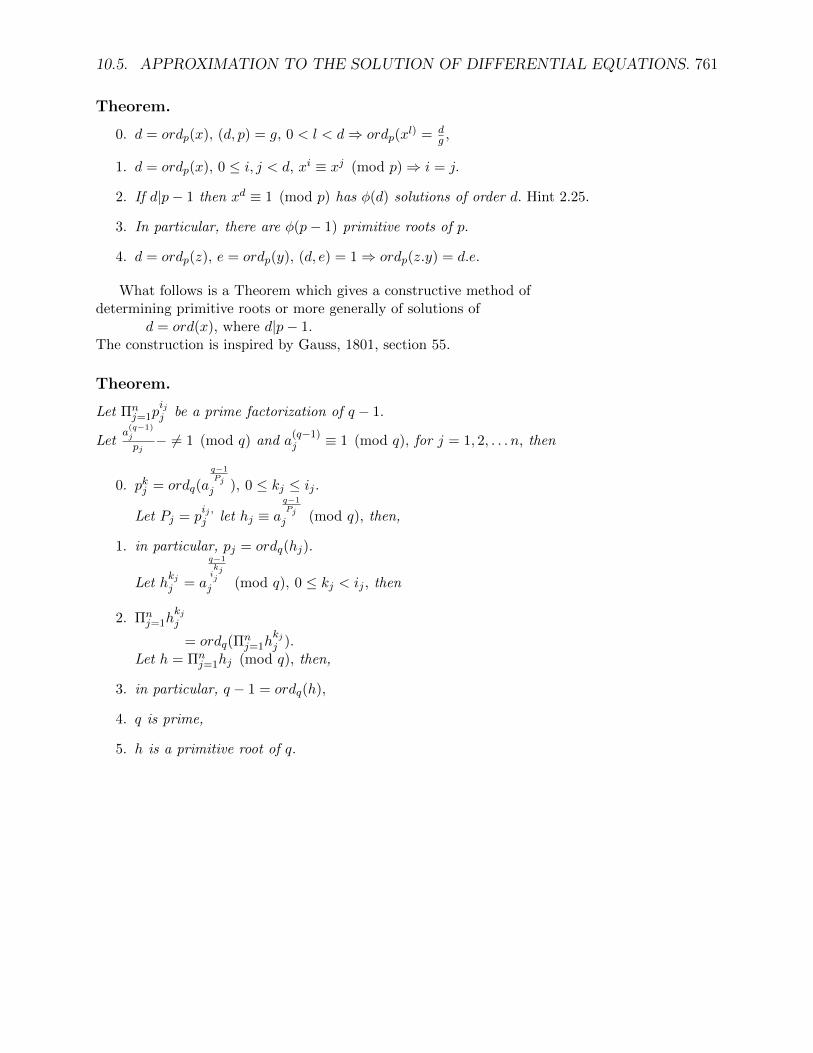
10.5. APPROXIMATION TO THE SOLUTION OF DIFFERENTIAL EQUATIONS. 761
Theorem.
0. d = ordp(x), (d, p) = g, 0 < l < d⇒ ordp(xl) = d
g ,
1. d = ordp(x), 0 ≤ i, j < d, xi ≡ xj (mod p)⇒ i = j.
2. If d|p− 1 then xd ≡ 1 (mod p) has φ(d) solutions of order d. Hint 2.25.
3. In particular, there are φ(p− 1) primitive roots of p.
4. d = ordp(z), e = ordp(y), (d, e) = 1⇒ ordp(z.y) = d.e.
What follows is a Theorem which gives a constructive method ofdetermining primitive roots or more generally of solutions of
d = ord(x), where d|p− 1.The construction is inspired by Gauss, 1801, section 55.
Theorem.
Let Πnj=1p
ijj be a prime factorization of q − 1.
Leta(q−1)j
pj− 6= 1 (mod q) and a
(q−1)j ≡ 1 (mod q), for j = 1, 2, . . . n, then
0. pkj = ordq(a
q−1Pj
j ), 0 ≤ kj ≤ ij .
Let Pj = pij ,j let hj ≡ a
q−1Pj
j (mod q), then,
1. in particular, pj = ordq(hj).
Let hkjj = a
q−1
ikjj
j (mod q), 0 ≤ kj < ij , then
2. Πnj=1h
kjj
= ordq(Πnj=1h
kjj ).
Let h = Πnj=1hj (mod q), then,
3. in particular, q − 1 = ordq(h),
4. q is prime,
5. h is a primitive root of q.

762 CHAPTER 10. DIFFERENTIAL EQUATIONS AND FINITE MECHANICS
Chapter 11
COMPUTER IMPLEMENTATION
11.0 Introduction.
One of the tradition of Mathematicians is to discover properties by working on special cases or ex-amples, this is especially so at the beginning of many branches of Mathematics, geometry, numbertheory, algebra, . . . . This was certainly the tradition kept up by Euler, see . . . , by Gauss, see . . . .In Euclidean geometry, the special cases were obtained by drawing a reasonably accurate figure,in number theory by numerical computation, and in algebra by algebraic manipulations. All threecan now be done accurately and with great speed using computers and these are now becomingmore and more available to every one.Depending on our training or, I believe, on the structure of our individual brain, such experimen-tation is almost essentail for many to obtain a thourough understanding of basic concepts.To help in the understanding of the material given above and, I hope, to help the reader in thediscovery of new properties, it is becoming essentail to provide him with the tools to realize quicklycomputer programs.When the subject matter is well settled and the experimentation is not at the basic level, a higherlevel non interactive language such as FORTRAN, ALGOL, PASCAL, PL1, ADA, is an excel-lent choice. When this is not the case, an interactive language such as BASIC or APL is by farpreferable. BASIC, BASIC+, BASIC+ extended.
Hardware, operating system, files, interaction, language, compiler, interpreter.
763

764 CHAPTER 11. COMPUTER IMPLEMENTATION

REFERENCES
1. Adobe Systems, Postscript Language, Tutorial and Cookbook, N. Y., Addison- Wesley, 1985,243 pp.
2. Adobe Systems, Postscript Language, Reference Manual, N. Y., Addison-Wesley, 1985, 319pp.
3. Apollonius, A treatise on Conic Sections, ed. Th. L. Heath, Cambridge, 1896.
4. Apollonius, Les Coniques d’Apollonius de Perge, trans. P. ver Ecke, Bruges, Belgique, 1923.
5. Artin, E., Geometric Algebra, N. Y., Interscience, 1957.
6. Artzy, Rafael, Linear Geometry, Reading Mass., Addison-Wesley, 1965, 273 pp.
7. Aryabhata I, The Aryabhatiya of Aryabhata, Tranlated with notes by Walter Eugen Clark,Chicago, Ill. Univ. of Chicago Press, 1930.
8. Aryabhata I, Aryabhatiya, Ed. by Kripa Shandar Shukla, New Delhi, Indian Nat. Sc.Acad.,1976. 219 pp.
9. Baker, Henry, Frederick, Principles of Geometry, Vol. 1 to 4, Cambridge Univ. Press 1, 1929,195 pp. 2, 1930, 259 pp.
10. Barbilian, Dan, (or Barbu, Ion), Pagini Inedite, Vol. 2, Bucarest, Ed. Albatros, 1984, 292 pp.
11. Baumert, Leonard D., Cyclic Difference Sets, N. Y., Springer, 1971.
12. Bezier, P., Definition numerique des courbes et surfaces, I, II, Automatismes, Vol. 11, 1966,625-632 and 12, 1967, 17-21. Also Vol. 13, 1968 and Thesis, Univ. of Paris VI, 1977.
765
766 CHAPTER 11. COMPUTER IMPLEMENTATION
13. Bezier, P., The Mathematical Basis of UNISURF CAD System. London, Butterworths, 1986.
14. Bezier, P., Numerical Control; Mathematics and Applications (transl. by R. Forrest). New-York, John Wiley, l972.
15. Bolyai, Farkas, Tentamen Juventutem Studiosam ein Elementa Mathiseos Parae introducendi,Maros-Vasarhely, 1829, see Smith D. E. p. 375.
16. Bolyai, Janos, Appendix of Bolyai, Farkas.
17. Bolyai, Janos, The science absolute of space independent of the truth and falsity of Euclid’sAxiom XI, translated by Dr. George Brus Halstead, Austin,Texas, The Neomon, Vol. 3, 71pp, 1886.
18. Borsuk, Karol and Szmielew Wanda, Foundations of Geometry, Amsterdam, North-Holland,1960, 444 pp.
19. Boubals, J. de Math. Elem. (de Longchamps et Bourget), 1891, p.218. (points of, on thecircle of Brianchon-Poncelet)
20. Brahmegupta and Bhascara, Algebra with Arithmetic and Mensuration, from the Sanscriptof Brahmegupta and Bhascara, translated by Henry Thomas Cole-brooke, London, JohnMurray, 1817.
21. Braikenridge, William, Exercitatio geometrica, London, 1733.
22. Brianchon, Charles, Poncelet, Jean, Recherches sur la determination d’une hyperboie equilatreau moyen de quatre conditions donnees, Ann. de Math., Vol. 11, 1820-1821 , p. 205-220, seeSmith, D. E., p. 337.
23. Buchheim Arthur, An extension of Pascal’s theorem to space of three dimensions. Messengerof Mathematics, Ser. 2, Vol. 14, 1984, 74-75.
24. Casey John, Sequel to Euclid, London, 1881, p.101 for III.4.4.0.
25. Charles, Michel, Appercu historique sur l’origine et le developement des methodes en geometrie,2e Edition, Paris, 1875.
26. Ch’in, Chiu-Shao, see Libbrecht, Ulrich.

11.0. INTRODUCTION. 767
27. Chou, Shang-Ching, Proving Elementary Geometry Theorems using Wu’s Algorithm. Con-temporary Mathematics, Bledsoe, W. W., and Loveland, D. W. Ed., Amer. Math. Soc. Vol.29, 1984 243-286.
28. Clebsch, Rudolf Frederich Alfred, Vorlesungen uber Geometrie, p.312
29. Coolidge, Julian, The Elements of non-Euclidean Geometry. Oxford Clarendon Press,1909,291 pp.
30. Coolidge, Julian, A treatise on the Circle and the Sphere, Oxford, Clarendon Press, 1916.603 pp., III.4.4.0.
31. Coolidge, Julian, A History of geometrical methods. Oxford Clarendon Press, 1940, 451 pp.
32. Coolidge, Julian, A History of the Conic Sections and Quadric Surfaces. Oxford ClarendonPress, 1945, 214 pp.
33. Coxeter, H. S. M., The Real projective Plane, New-York, McGraw-Hill, 1949, 196 pp.
34. Coxeter H. S. M. and Greitzer, S. L., Geometry Revisited, N. Y. Random House, 1967, 193 pp.
35. Coxeter H. S. M. and Moser, W. O. J., Generators and relations for discrete groups. Springer,1957.
36. Dalle A. et De Waele C., Geometrie plane. Namur, Belgique, Wesmael-Charlier, 1936, 408 pp.
37. David Antoine, 2000 Theormes et Problmes de Geometrie avec Solutions. Namur, Belgique,Wesmael-Charlier, 1956, 1055 pp.
38. de Casteljau, P., Outillages methodes calcul. Technical Report, Citron, Paris 1959, See also1963.
39. de Casteljau, P., Shapes Mathematics and CAD. Kogan Page, London, 1986.
40. Dembowski, Peter, Finite Geometries, Ergebnisse der Mathematik und ihrer Grenzgebiete,Band 44, Springer, New-York, 1968, 375 pp.
768 CHAPTER 11. COMPUTER IMPLEMENTATION
41. Desargues, Gerard, Brouillon d’un projet d’une atteinte aux evnements des rencontres d’uncne avec un plan, Paris, 1639. See Smith D. E., p. 307.
42. Descartes, Rene, La Geometrie, Nouv. Ed., Paris Hermann, 1886, 91 pp.
43. De Vogelaere, R., Finite Euclidean and non-Euclidean Geometry with application to the fi-nite Pendulum and the polygonal harmonic motion. A first step to finite Cosmology. TheBig Bang and Georges Lemaitre, Proc. Symp. in honor of 50 years after his initiation of Big-Bang Cosmology, Louvain-la-Neuve, Belgium, October 1983., D. Reidel Publ. Co, Leyden,the Netherlands. 341-355.
44. De Vogelaere, R., Geometrie Euclidienne finie. Le cas p premier impair. La Gazette desSciences Mathematiques du Quebec, Vol. 10, Mai 1986.
45. Dieudonne, Jean, La geometrie des groupes classiques, Berlin, Springer, Ergebnisse Der Math.und ihrer Grenzgebiete, 1963, 125 pp.
46. Donath, E. Die merkwurdigen Punkte und linien des Dreiecks, Berlin, VEB Deutscher Verlagder Wissenshaften, 1968.
47. Emmerich A., Die Brocarsschen Gebilde, Berlin, Verlag Georg Reimer, 1891,
48. Engle and Staeckel, Theorie der Parallellinien von Euklid bis auf Gauss, Leipzig, 1895. (SeeMathesis, Ser. 2, Vol. 6, 1896, Suppl. pp. 1-11 or Rev. des quest. scient. Ser. 2, Vol. 8,1895, pp. 603-612)
49. Enriques, Frederigo, Lezioni di geometria proiettiva, Bologna, 1904, French Translation, Paris1930
50. Euclides, Les oeuvres en grec, en latin et en francais, par Peyrard, Paris, Patris, 1814, 519 pp.
51. Evans, Anthony B., On planes of prime order with translations and homologies, J. of Geom-etry, 34, 1989, 36-41. (Desarguesian planes)
52. Eves, Howard, An Introduction to the History of Mathematics, New-York, Holt, Reinehartand Winston, 1953, 588 pp.
53. Fano, Sui postulati fondamentali della geometria proiettiva, Giorn. di mat., Vol. 30, 1892,106-132. (PG(n,p))
11.0. INTRODUCTION. 769
54. Farin, Gerald, Curves and Surfaces for Computer Aided and Geometric Design, New-York,Acad. Press, 1988, 334 pp..
55. Feuerbach, Karl, Grundriss zu analytischen Untersuchungen der dreyeckigen Pyramide, Nurem-berg, 1827.
56. Feuerbach, Karl, Eigenschaften einiger merkwurdigen Punkte des geradlinigen Dreiecks.Nurnberg, Riegel und Wiessner, 1822, 16+62 pp.
57. Fontene, G., Extension du Theorme de Feuerbach. Nouv. Ann. de Math., Ser.4, Vol. 5, 1905.
58. Forder, Henry, George, The Foundations of Euclidean Geometry, Cambridge Univ. P., 1927,repr. N. Y. Dover P., 1958, 349 pp.
59. Forder, Henry, George, Higher Course Geometry, Cambridge Univ. P., 1931, 264 pp.
60. Forder, Henry, George, The Calculus of Extension, New-York, Chelsea Pub. Co., 1960.
61. Freudenthal, Oktaven, Ausnahmen gruppen und Oktavengeometgrie, Uttrecht, Utrecht Univ.1960.
62. Fritz, Kurt von, The discovery of incommensurability by Hippasus of Metapontum, Annalsof Math., Vol. 46, 1945, 242-264. Also Studies in Presocratic Philosophy, Furley David andAllen R. E. Rdit. New-York, Humanities P., 1970, pp.382-412.
63. Gauss, Carl, Disquisitiones Arithmeticae, Lipsiae, Fleicher, 1801. Translated by Clarke,Arthur, S.J., New Haven, Yale Univ. P. 1966, 473 pp.
64. Gergonne, Joseph, Diaz, circle inscrit Nagel cerele exinscrit.
65. Gergonne, Joseph, Diaz, Annales de Mathematiques, 1827, Vol. 17, p. 220 and 1829, Vol.19, p. 97 and 129.
66. Greenberg, M., Euclidean and Non-Euclidean Geometries, San Francisco, Freeman, 1974.
67. Hagge, Der Fuhrrnannsche Kreis und der Brocardsche Kreis, Zeitschrift fur rnathematischeUrnterricht, vol. 38, 1907.

770 CHAPTER 11. COMPUTER IMPLEMENTATION
68. Hall, Marshall, Projective Planes , Trans. Amer. Math. Soc., Vol. 54, 1943, 229-277
69. Hall, Marshall, Jr, Projective Planes and related Topics, Calif. Inst. of Technology, April1954, 77 pp.
70. Hartshorne, Robin C., Foundation of Projective Geometry, N. Y. Benjamin, 1967, 161 pp.
71. Heath, Sir Thomas, The thirteen books of Euclid’s elements, Vol. 1, Cambridge UniversityPress, 1908. 424 pp. Other Edition, “The Classics of the St John’s program,” Annapolis,The St. John’s College Press, 1947.
72. Heath, Sir Thomas, Diophantus of Alexandria, 2nd Edition, Cambridge University Press,1910.
73. Heath, Sir Thomas, A Manual of Greek Mathematics, Oxford Univ. P., 1931, 551 pp.
74. Heidel, W. A . The Pythagoreans and Greek Mathematics, Amer. J. of Philology, Vol. 61,1940, 1-33. Also Studies in Presocratic Philosophy, Furley David and Allen R. E. Edit. NewYork, Humanities P., 1970, pp. 350-381.
75. Hensel, Kurt Theorie der algebraischen Zahlen, Berlin, Teubner, 1908, 349 pp.
76. Hensel, Kurt, Zahlentheorie, Berlin, Goeschen’sche Verslaghandlung, 1913, 356 pp.
77. Hessenberg G., Math. Ann., Vol. 61, 1905, pp. 161-172.
78. Hilbert D., Grurdlagen der Geometrie, 1899, tr. by E. J. Townsend, La Salle, Ill., OpenCourt Publ. Cp., 1962, 143 pp.
79. Hilbert D. und Cohn-Vossen S., Auschauliche Geometrie, Berlin, Springer, 1932, 310 pp.
80. Hirschfeld, J. W. P., Projective geometries over finite fields, Oxford, Clarendon Press, 1979.474 pp.
81. Hughes, D. R., A class of non-Desargesian projective planes, Canad. J. of Math., 1957, VoI.9, 378-388. (I.9.p.1)

11.0. INTRODUCTION. 771
82. lntrigila, Carmelo, Sul Tretraedro, Rend. della R. Accad. delle Scienze di Napoli, Vol.22,1883, pp. 69-92.
83. Iversen, Birger, An Invitation to Geometry, Math. Inst. Aarhus Univ. Lect. Notes Series,No 59, 1989, 186 pp.
84. Jacobi, Karl Gustav, Crelle J. fur Reine und Angewandte Mathernatik, Vol. 15, 199-204,Werke, I, p.336, (4)).
85. Jarnefelt G. and Kustaanheimo Paul, An Observation on Finite Geometries. Den II. Skan-dinavische matematikerkongress, Trondheim, August 1949, 166-182.
86. Jarnefelt G. , Reflections on a finite Approximation to Euclidean Geometry. Physical andAstronomical Prospects. Suomalaisen Tiedeakatemian Toimituksia, Ser. A, 1951, No 96.
87. Johnson, Norman L., Kallaher, Michael J., Long Calvin T., Edit. Finite Geometries, N. Y.,Marcel Dekker Inc. 1983.
88. Johnson, Roger A., Modern Geometry, Houghton Mifflin Co, 1929, 319 pp.
89. Karteszi, F. Introduction to finite geometries. Amsterdam, North Hollard Publ. Co., 1976,266 pp.
90. Kirk, G. S., Popper on Science and the Presocratics. Mind, Vol 69, 1960, 318- 339. AlsoStudies in Presocratic Philosophy, Furley David and Allen P. E. Edit. New-York, HumanitiesP., 1970, pp.154-177.
91. Klein Felix, Geometry, N.Y. MacMillan, 1939.
92. Klein, Felix, Famous Problems of Elementary Geometry, tr. by W.W. Beman and D. E.Smith, 1897, N.Y. Ginn, Reprinted in Famous Problems and other Monographs. New York,Chelsea, 1955.
93. Knuppel, Frieder and Salow, Edzard, Plane elliptic geometry over rings. Pacific Journal ofMathematics. Vol. 123, (1986), 337-384.
94. Koblitz Neal, A Short Course on Some Current Research in p-adic Analysis (Talks at HanoiMath. Inst., July 1978), 66 pp. (Prof. Ogus)

772 CHAPTER 11. COMPUTER IMPLEMENTATION
95. Koblitz Neal, p-adic Numbers, p-adic Analysis and Zeta-Functions, Springer- Verlag, N.Y.,1977, 124 pp.
96. Lachlan, On Poristic Systems of Circles, Messenger of Mathematics, vol. 16, 1887.
97. Laguerre, Edmond Nicolas, Oeuvres, 2 Vol. Paris, Gauthier-VilIars, 1898-1905. (I,9.,p1)
98. Lebesgue, Henri, Lecons sur les constructions geometliques, Paris, Gauthier- Villars, 1950,304 pp.
99. Lehmer, D. H., An elementary course in synthetic projective geometry. Boston, 1917 andBerkeley, California, Univ. of Calif. Pr., 1933, 123 pp.
100. Lemaıtre Georges. l’Hygrothse de l’Atome Primitif, Essai de Cosmogonie, Neucgatel, Ed. duGriffon, 1946, 201 pp.
101. Lemaıtre Georges. The Primeval Atom, A Hypothesis of the Origin of the Universe. Trans.by Betty and Serge Korff, van Nostran, N. Y., 1950, 186 pp.
102. Lemay, Fernand, Imagination dissidente, Bull. de I’APAME mars 1979.
103. Lemay, Fernand, Motivation intrinsque, Bull. de I’APAME, novembre 1979.
104. Lemay, Fernand, Le dodecadre et la geometrie projective d’ordre 5, see Johnson N. L., 279-306
105. Lemoine, Emile, Proprietes relatives a deux points du plan d’un triangle qui se deduisentd’un point K quelconque du plan comme les points de Brocard se deduisent du point deLemoine. Mathesis, Ser.1, Vol. 6, 1886, Suppl. 1-27.
106. Lemoine, Emile, 1902, Geometrogtaphie, C. Naud, Paris
107. Lemoine, Emile, J. de Math. Elem. (de Longchamps et Bourget), 1889, p.93 1890, p.118,(point of, on the circle of Brianchon-Poncelet)
108. Libbrecht, Ulrich, Chinese Mathematics in the Thirteenth Century, The Shu- Shu-Chiui-Chang of Ch’in, Chiu-Shao, Cambridge, MIT Press, 1973, 555 pages.
11.0. INTRODUCTION. 773
109. Lobachevskii, Nikolai, Ivanovich, see Nolden. A., Elementare Einfulrung in die LobachewskischeGeometrie, Berlin, VEB Deuscher Verlag der Wissenschaften, 1958, 259 pp.
110. MacLaurin, Colin,Phil. Trans. Roy. Soc. London, 1735. (On Pascal Constr)
111. Mansion, Paul, Premiers Principes de !a Metageometrie ou Geornetrie generale, Mathesis,Ser. 2, Vol. 6, 1896, Suppl. 1-46.
112. Mascheroni L. Geometrie du Compas, translated in French Carette A.M., Paris 1798
113. Maxwell, E. A., The methods of plane projective geometry based on the use of general ho-mogeneous coordinates. Cambridge Univ. Press, 1952. 230 pp.
114. Menger, K., Untersunchunten uber allgemeine Metrik, Math. Ann. Vol. 100, 1928, 75-163.
115. Michel, Charles, Complements de geometrie moderne, Paris, Vuibert, 1926. harmonic poly-gons, p. 272.
116. Michel, Paul-Henri, De Pythagorea Euclide, Paris, Les Belles Lettres, 1950, 699 pp.
117. Miquel, Auguste, Theormes de geornetrie, J. de Liouvilie, Vol. 3, 1838, p.486.
118. Miquel, Auguste, Memoires de Geormetrie, J. de Mathematiques Pures et Appliquees, (J. deLiouville), Vol. 9, 1844, p.24.
119. Mbius August, Werke, (Calcul Barycentrique)
120. Moise, Edwin E., Elementary Geometry from an advanced standpoint, Palo Alto, Addison-Wesley, 1963, 419 pp.
121. Moufang, Ruth, Alternatievkrper und der Satz vom vellstndigen Vierseit, Abh. Math. Sem.Hamburg, Vol. 9, 1933, 207-222.
122. Moulton, F. R., A simple non-Desarguesian plane Geometry, Trans. Amer. Math. Soc. Vol.3, 1902, 192-195.
123. Nagel, Chretien Henty, Untersuchungen uber die wichtigsten zum Dreicke gehoerige Kreise,1836.

774 CHAPTER 11. COMPUTER IMPLEMENTATION
124. Neuberg, Joeeph, Memoire sur le tetradre, Memoires couronnes de l’Academie de Belgique,Vol. .37, 1886, pp. 3-72.
125. O’Hara, C. W. and Ward, D. R., An introduction to Projective Geometry, London, OxfordUni, P., 1937, 298 pp.
126. Ostrom, T, G., Finite translation planes, Lecture Notes in Math., Number 158, Berlin,Springer, 1970.
127. Ostrom, T. G., Some translation planes that are not well known, Technical Report, N. 13,Department of Math. Washington State Univ., 1968, 49 pp.
128. Pascal, Blaise, Pensees, Nouv. Ed., Philippe Sellier, 1976, 543 pp.
129. Pascal, Blaise, Essay sur les couiques, 1639, see Smith, D. E., p, 326.
130. Pascal, Blaise, Oeuvres, Ed. Brunschvig et Boutroux, I, p. 252, (on Pascal, Constr.)
131. Pasch, Moritz, Vorlesungen uber neuere Geometrie, Leipzig, Teubner, 1882, 202 pp.
132. Pasch, Moritz und Dehn, Max, Vorlesungen uber neuere Geouretrie, Berlin,
133. Pickert. G., Projektive Ebenen, Berlin, Springer, 1955, 343 pp.
134. Pieri, Un sistema di postulati per la geometria proieitiva, Rev. Mathem. Torino, Vol 6, 1896.See also Atti Torino, 1904, 1906.
135. Pieri, I principii della geornetria di posizione, composti in sistema logico deduttivo, Mem.della Reale Acad. delle Scienze di Torino, serie 2, Vol.48, 1899, pp 1-62.
136. Playfair, John, Elements of Geometry, Philadelphia, Lippincoot & Co, 1864, 318 pp
137. Plucker, Julius, Analitische geometrie Entwickelungen, Voi 1 and 2 1828-1831 Crelle, Vol.5,1830, Vol.12 (1834). Springer, 1976, 275 pp.
138. Plucker, Julius, Theorie der algebraischen Curven 1839
11.0. INTRODUCTION. 775
139. Poncelet, Jean, Victor, Application d’Analyse et de Geometrie, Paris, Mallet- Bachelier, I,1862, 563 pp., II, 1864, 602 pp.
140. Poncelet, Jean. Victor, Traite des proprietee projectives des figures, Paris, Gauthier- Villars,I, 1865, 428+xii pp. II, 1866, 452+vi pp.
141. Popper, Sir Karl, Back to the Presocratics, Proc. of the Aristotelian Society, Vol. 59, 1958-9,1-24, also Studies in Presocratic Philosophy, Furley David and Allen R. E. Edit. New York,Humanities P., 1970, pp.130-153.
142. Prouhet, , Analogies du triangle et du tetradre, Nouv. Ann. de Math., Serie 2, Vol. 2, 1863,p.138.
143. Reidemeister, K,, Grundlagen der Geometrie, Berlin, Springer, Grundl, der math,Wissens inEinz., Vol. 32, 1968,
144. Robert, Alain; Elliptic curves, Lecture Notes in Mathematics, Berlin, Springer, Vol. 326,1973, 264 pp.
145. Roberts, Michael, On the analogues of the Nine-Point Circle in the Space of Three Dimen-sions, Proc. London Math. Soc., Vol. 19, 1878.
146. Roberts, Samuel, Proc. London Math Soc., Vol 12, 117. (Generalization of Miquel to tetra-hedron)
147. Robinson, A., Non-standard Analysis, North-Holland, Amsterdam, 1974, 293 pp.
148. Robinson, G. de B., The foundations of Geometry, Toronto, 1940.
149. Saccheri, Giovanni Girolamo, Euclides ab omni naevo vindicatus Milan, 1732. Tr. GeorgeHalstead, London Open Court Pr. 1920, 246 pp. See Engel and Stackel.
150. Salmon, George, A treatise on Conic. Sections, 6-th ed. London 1879.
151. Salmon, George, A treatise on the higher plane curves, 3d ed. Dublin, Hodges, Foster andFiggis, 1879, 395 pp.
152. Schwabhuser W., Szmielew W., Tarski.A, Metamathdmatische Methoden in der Geometrie,N. Y, Springer, 1980, 482 pp.

776 CHAPTER 11. COMPUTER IMPLEMENTATION
153. Segre, B, Lectures on modern Geometry. Rome, Cremonese, 1961, 479 pp.
154. Segre, C, Un,nuovo campo di ricerche geometriche, Atti R. Acad. Sc. Torino, Vol 25, 1889,430-457.
155. Seidenberg, Lectures in Projective Geometry, Princeton N. J., van Nostrand, 1962, 230 pp.
156. Shively, Levi S., An Introduction to Modern Geometry, N. Y., John Wiley, 1939. 167 pp.
157. Smith, David, Eugene, History of Mathematics, Vol. I, II.
158. Smith, David, Eugene, A Source Book of Mathematics, N. Y. McGraw Hill, 1929,701 pp.
159. Smogorzhevskii, A. S., The ruler in Geometrical Constructions, tr. by Halina Moss, NewYork, Blaisdell, 1961.
160. Sommerville, Duncan, Bibliography of non-Euclidean Geometry, London, Harrison, 1911, 403pp.
161. Spieker, Ein merkwurdiger Kreis um der Schwerpunkt des Perimeters des geradlinigen Dreiecksals Analogon des Kreises der neun. Punkte, Grunert’s Archiv, Vol. 51,1870.
162. Staudt, K. G. C. von, Geometrie der Lage, Nuremberg 1847
163. Staudt, K. G. C. von, Beitrage zur Geometrie der Lage, Nuremberg 1857.
164. Steiner, Jacob, Geometrical Constructions with a Ruler, tr. by M. E. Stark, ed. by R C.Archibald, New York Scripta Mathematica, 1950.
165. Steiner, Jakob, Collected. Works; Vol. I,. pp. 43 and 135 for III.4.4.0.
166. Stevenson, F.W., Projective Planes, W.E. Freeman and Co, 1972, 416 pp.
167. Stroeker, R. J., Brocard Points, Circulant Matrices, and Descates’ Folium; Math. Magazine,Vol. 61,1988, 172-187

11.0. INTRODUCTION. 777
168. Tarski, Alfred, What is Elementary Geometry, The axiomatic method with special referenceto Geometry and Physics, Studies in Logic and the Foundation of Mathematics, North-Holland, Amsterdam, 1959, 16-29, Collected. Works, IV, 17-32.
169. Taurinus, Theorie der Pallellinien. 1825, 102pp.
170. Taurinus, Geometriae primia Elementa, 1826, 76pp.
171. Taylor, H. M., On a six point circle connected with a triangle, Messenger of Mathematics,Vol 11, 177-179. (Circle of Taylor).
172. Taylor, H. M., The Porism of the ring of circles touching two circles, Messenger of Mathe-matics, Vol. 7, 1878. III.4.4.0.
173. Taylor, W. W., On the ring of circles touching two circles, Messenger of Mathematics, Vol.7, 1878. III.4.4.0.
174. Terquem, Orly, Consideration sur le triangle rectiligne, Nouv. Ann. de Math., Serie 1, Vol.1, 1842, 196-200
175. Thomas, Ivor, Greek Mathematics, Cambridge, Mass., Harvard Univ. P., Vol. 1. 1939, 505pp.
176. Thureau-Dangin, F. Textes Mathematiques Babyloniens, Leiden 1938.
177. Tilly, Joseph Marie de, Essai sur les Principes fondamentaux de Geometrie et de Mecanique,Bruxelles, Mayolez, 1879 192 pp. Also, Mem. Soc. scinc. phys. et natur. de Bordeaux, VolIII Ser. 2, cahier l.
178. Tilly, Joseph Marie de, Essai de Geometrie analytique generale, Bruxelles 1892. Blumenthalconsiders than in this paper Tilly makes a fundamental contribution by introducing n-pointrelations to characterize a space metrically.
179. Tucker, R., The “cosine” orthocenters of a triangle and a cubic through them Messenger ofMathematics, Ser 2, Vol. 17, pp. 97-103. (10 distances between 5 points!)
180. Vahlen, Ueber Steinersche Kugelketten, Zeitschrift fur Mathematik und Physik, Vol. 41,1896, III.4.4.0.
778 CHAPTER 11. COMPUTER IMPLEMENTATION
181. van der Waerden, Mathematics and Astronomy in Mesopotamia, Dict. of Scientific Bibliog-raphy, Vol 15.
182. Veblen, Oswald, and Bussey, W. H., Trans. Amer. Math. Soc., Vol. 7, 1906, 241-259.(PG(n,pk))
183. Veblen, Oswald, and Young, John, Projective Geometry, Wesley, Boston, I, 1910, II, 1918
184. Ver Eecke, Paul, Proclus de Lycie, Les commentaires sur le premier livre des elementsd’Euclide, Bruges, Desclee De Brouwer, 1948, 372 pp.
185. Verriest, Gustave, Elements de Geometrie Projective, Louvain, Feyaerts, 1930, 412 pp.
186. Vigarie, Emile, Premier inventaire de la geometrie du triangle, Mathesis, Ser. 1, Vol. 9, 1889,Suppl. pp. 1-26.
187. Vigarie, Emile, La bibliographie de Ia geometrie du triangle, Mathesis, Ser. 2, VoI. 6, 1896,Suppl. 1-14. (603 articles)
188. Vuibert, Sur la Geometrie classique du Triangle.
189. Walker, R., Cartesian and Projective Geometry., London, Edward Arnold and Co, 1953, 320pp.
190. Whitehead, Alfred, The Axioms of Projective Geometry, Cambridge, 1906.
191. Wu, Wen-Tsun, On the Decision Problem and the Mechanization of Theorem-Proving inElementary Geometry, Contemporary Mathematics, Bledsoe, W. W., and Loveland, D. W.Ed., Amer. Math, Soc. VoI. 29, 1984 213-234.
192. Wu, Wen-Tsun, Some Recent Advances in Mechanical Theorem-Proving of Geometries. Con-temporary Mathematics, Bledsoe, W. W., and Loveland, D.W. Ed., Amer. Math. Soc. Vol.29, 1984 215-242.
193. Young, John, Projective geometry, 4th Carus Monograph, Chicago, 1930.
Related Documents