Final Report with Figures - University of Toronto

Parallelizing Face Detection in Software

Joshua San Miguel Jordan Saleh Michelle Wong Department of Electrical and Computer Engineering

University of Toronto

Abstract As “smart” mobile devices become more common, users want to use the integrated high-‐resolution cameras and displays in novel ways. Face detection has become one of the most widely used computer vision applications, as it forms the basis of motion tracking and camera autofocus. It is often performed on a real-‐time video stream, which places tight constraints on the frame rate and processing speed. While previous work has looked into acceleration using hardware (e.g. FPGAs and GPUs), it is worthwhile to explore software optimizations that can be easily implemented on mobile devices, where face detection will be used most commonly. 1. Introduction Face detection has become one of the most commonly used computer vision applications. It serves as the basis of many tracking applications, including optical flow (i.e. motion tracking). It is also used to track gestures, such as in the Microsoft Xbox Kinect game system, and to autofocus on a face in a simple point-‐and-‐shoot camera. Its variety of uses relies on the assumption that face detection can be performed in real-‐time on a streamed video feed. Real-‐time constraints are strict and require that processing be efficient. In its current state, software face detection cannot meet the frame rate requirements that real-‐time processing imposes. However, as opposed to the numerous hardware implementations currently available, a software implementation of face detection is most portable to mobile platforms. This work shows that by optimizing the OpenCV software implementation of face detection, real-‐time frame rates can be achieved without sacrificing detection accuracy. We explore different levels of parallelization granularity and find that a combination of parallel techniques yields the best results. Specifically, we present three major contributions to the optimization of software face detection.

1. The face detection algorithm involves code that result in load imbalance between threads. We present static and dynamic load balancing schemes that improve thread use. We show that this results in increased performance, especially in light of real-‐time constraints.

2. Multiple levels of parallelization granularity are needed to optimize software face detection. The overhead due to parallelization makes fine-‐grained techniques, which are commonly used in hardware implementations, infeasible. Multiple coarser-‐grained techniques can yield better execution time.

3. The correct level of granularity is extremely important, due to the inherent load imbalance in the face detection code. While coarse-‐grained parallelization is desirable due to the reduced overhead, the coarsely separated workload can cause imbalance between threads. We present a strategy for combining different techniques to obtain coarse-‐grained parallelization that balances the workload in a fine-‐grained manner.

The original code used is drawn from two open source projects: MEVBench and OpenCV. With further refinement, it is possible that the modifications made may be contributed back to the original projects. In the meantime, the modified optimized code for face detection is available on online at http://github.com/miwong/MEVBench and http://github.com/miwong/OpenCV. 2. Viola-‐Jones Algorithm The Viola-‐Jones algorithm [1] is currently the most commonly used face detection algorithm. It describes a novel and optimized method of accurately detecting faces in an efficient manner. The algorithm consists of three main steps:

1. Training the classifiers that will eventually serve as templates to detect faces. 2. Organizing the classifiers in a cascade that allows for efficient face detection during runtime. 3. Sweeping across the image and across scaled versions of the image to detect faces at different locations and sizes.

These steps are described in further detail below. 2.1 Training Classifiers

The Viola-‐Jones algorithm relies on a set of classifiers that represent common features of faces. In the most common implementation, it uses the Haar classifiers [2], which are rectangular and are shown in Figure 1. These classifiers represent features on a face that often result in a large difference in intensity. For example, the vertical classifier with two rectangles represent the eye and the cheek of a face, which normally horizontally adjacent with the eye having a higher intensity. Three-‐rectangle features are also used and Figure 1 shows one representing the mouth. More complex diagonal classifiers are used

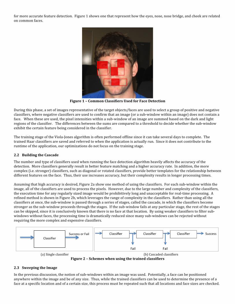
for more accurate feature detection. Figure 1 shows one that represent how the eyes, nose, nose bridge, and cheek are related on common faces.

Figure 1 – Common Classifiers Used for Face Detection

During this phase, a set of images representative of the target objects/faces are used to select a group of positive and negative classifiers, where negative classifiers are used to confirm that an image (or a sub-‐window within an image) does not contain a face. When these are used, the pixel intensities within a sub-‐window of an image are summed based on the dark and light regions of the classifier. The differences between the sums are compared to a threshold to decide whether the sub-‐window exhibit the certain feature being considered in the classifier. The training stage of the Viola-‐Jones algorithm is often performed offline since it can take several days to complete. The trained Haar classifiers are saved and referred to when the application is actually run. Since it does not contribute to the runtime of the application, our optimizations do not focus on the training stage. 2.2 Building the Cascade

The number and type of classifiers used when running the face detection algorithm heavily affects the accuracy of the detection. More classifiers generally result in better feature matching and a higher accuracy rate. In addition, the more complex (i.e. stronger) classifiers, such as diagonal or rotated classifiers, provide better templates for the relationship between different features on the face. Thus, their use increases accuracy, but their complexity results in longer processing times. Assuming that high accuracy is desired, Figure 2a show one method of using the classifiers. For each sub-‐window within the image, all of the classifiers are used to process the pixels. However, due to the large number and complexity of the classifiers, the execution time for any regularly sized image would be prohibitively long and unacceptable for real-‐time processing. A refined method is shown in Figure 2b, which leverages the range of complexity in the classifiers. Rather than using all the classifiers at once, the sub-‐window is passed through a series of stages, called the cascade, in which the classifiers become stronger as the sub-‐window proceeds through the stages. If the sub-‐window fails at any particular stage, the rest of the stages can be skipped, since it is conclusively known that there is no face at that location. By using weaker classifiers to filter sub-‐windows without faces, the processing time is dramatically reduced since many sub-‐windows can be rejected without requiring the more complex and expensive classifiers.

(a) Single classifier (b) Cascaded classifiers

Figure 2 – Schemes when using the trained classifiers 2.3 Sweeping the Image

In the previous discussion, the notion of sub-‐windows within an image was used. Potentially, a face can be positioned anywhere within the image and be of any size. Thus, while the trained classifiers can be used to determine the presence of a face at a specific location and of a certain size, this process must be repeated such that all locations and face sizes are checked.

Classifier

Success or Fail

This requires an exhaustive search throughout the image and scaled versions of the image, shown in Figure 3. A sub-‐window is created and swept across the image, with each relocation requiring a new iteration through the cascaded classifiers. To detect faces of different sizes, the original image is scaled; thus, the relative size of the sub-‐window is larger and running the same classifiers will detect the presence of larger faces. This process is repeated until the sub-‐window size exceeds the scaled image size.

Figure 3 – Sweeping the sub-‐window across scaled versions of the original image When detecting faces of different sizes, it is also possible to scale the sub-‐window rather than scaling the original image. This ensures that details from the original image are not lost as its size is reduced. This alternative method was proposed by the original Viola-‐Jones implementation [1]; however, the OpenCV [3] implementation uses the image scaling method. Because our optimizations were written for the OpenCV implementation, and since reducing the image size saves processing time, the scaling method was not changed in our code modifications. 3. MEVBench and OpenCV In this section, the MEVBench [4] suite and the OpenCV [3] libraries are introduced. These libraries serve as the base for our optimizations, which target specific functions and applications within the code. Both MEVBench and OpenCV support PC (x86) and mobile (ARM) platforms. While the final goal is to optimize the face detection application for mobile devices, where it will be most used often, the results shown in Section 5 were obtained from a computer using the x86 architecture. However, since the optimizations were implemented in software and do not rely on the architecture or specialized chips (such as GPUs), it should be relatively simple to port them to mobile platforms in future work. 3.1 MEVBench

The Mobile Embedded Vision Benchmark (i.e. MEVBench) [4] is a collection of benchmarks created to evaluate the performance of computer vision applications across various mobile platforms. It contains a number of different computer vision benchmarks. Some are already multi-‐threaded; however, the most relevant benchmark, FaceDetection, is single-‐threaded. The majority of the work in the FaceDetection benchmark is performed by the OpenCV library. The left portion of Figure 4 shows the overall structure of the code in MEVBench. After the initialization is performed, the code reads the image using faceDetectionGetNextFrames(), which returns a Mat (i.e. matrix) object. This matrix represents a frame, which, along with other configuration parameters, is passed into the OpenCV function CascadeClassifier::detectMultiScale(). The function adds Rect values to the faces argument (represented as a vector<Rect>), with each rectangle representing the location and size of a detected face. If the showWindow configuration is set for the FaceDetection benchmark, which is the case for our experiments, the rectangles are drawn onto a copy of the original frame and the resulting image can be shown on the monitor or saved into a file. Although the MEVBench FaceDetection benchmark is limited to the detection of faces in a single image, real life applications of face detection generally requires a video stream to be processed. Since such input data can yield more ways in which to optimize the code, support for the reading, processing, and writing of video files was implemented. This involved using OpenCV’s VideoCapture class to read the video frames and the VideoWriter class to output video frames augmented with outlined faces. This addition to MEVBench required minimal changes, as the code structure was already quite modular and was designed for future extensions such as this.

Figure 4 – Code structure and calling paths within MEVBench and OpenCV for the FaceDetection application

3.2 OpenCV

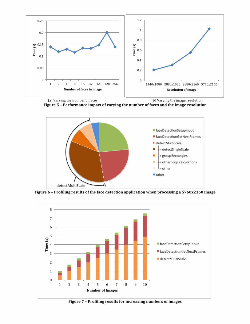
As previously mentioned, the bulk of the face detection processing is performed by the OpenCV library. OpenCV is a commonly used collection of computer vision algorithms. It has been ported for a variety of different platforms and architectures. For face detection, the CascadeClassifier class within the objdetect module is used. The detectMultiScale() function first converts the original image into a gray scale image, since the classifiers use only the pixel intensity, and removing the other (colour) channels reduces the size of the matrix being processed. Within a loop that scales the image repeatedly by an increasing factor (with the increase rate taken from the scaleFactor argument), the detectSingleScale() function is called on the scaled image. This function loops through all locations in the image and runs the cascaded classifiers (implemented in the FeatureEvaluator class) on every possible sub-‐window. After all faces have been found, the groupRectangles() function is called to assemble similar face rectangles together (in terms of location and size). This ensures that each face is only counted once, which is especially necessary in the case where the size of a face may result in detection at two different image scaling factors. 4. Parallelization and Optimizations When performing face detection, there are several input factors that can affect the performance of the algorithm. One such factor may be the number of faces in an image or frame since the presence of a face requires that the sub-‐window will never be rejected in the cascade process. By the nature of the Viola-‐Jones algorithm, the most complex classifiers must be used more often when there are more faces. Another factor affecting performance may be the resolution of the image or the video. A greater resolution results in more pixel data being read in, processed, and written out. It also results in a larger image size, which requires a greater number of iterations to scale when detecting faces of different sizes. Figure 5a shows profiling results when varying the number of faces in an image, while maintaining the same image resolution. Figure 5b shows the results when varying the image resolution while maintain the same number of faces. It is apparent that while varying the number of faces within an image can have some impact on the performance, this is much less pronounced than the drastic performance decline caused by increasing the resolution of the image. The results shown in Figure 5 suggest that the impediment to scaling software face detection lies not in the cascaded classifiers but in the code surrounding them. That is, the way in which the classifiers are used on the scaled images are causing the performance decline. A further look into the performance breakdown of the algorithm when processing an HD-‐quality image is shown in Figure 6.

faceDetectionGetNextFrames()

detectMultiScale(frame)

<draw face outlines on frame>

frame

face outline rects

<convert to grayscale>

<scale image>

detectSingleScale(frame)

groupRectangles(rects)

grayscale frame

scaled frame

new factor

face outline rects

<run FeatureEvaluator>

new location

MEVBench OpenCV

(a) Varying the number of faces (b) Varying the image resolution

Figure 5 – Performance impact of varying the number of faces and the image resolution

Figure 6 – Profiling results of the face detection application when processing a 5760x2160 image

Figure 7 – Profiling results for increasing numbers of images

0

0.05

0.1

0.15

0.2

0.25

1 2 4 8 16 32 64 128 256

Time (s)

Number of faces in image

0

0.2

0.4

0.6

0.8

1

1.2

1440x1080 2880x1080 2880x2160 5770x2160

Time (s)

Resolution of image

0

1

2

3

4

5

6

7

8

1 2 3 4 5 6 7 8 9 10

Time (s)

Number of Images

faceDetectionSetupInput

faceDetectionGetNextFrames

detectMultiScale

The profiling results from Figures 5 and 6 show that optimization efforts should be focused on code that has a direct impact on the image resolution. More specifically, the functions that contribute most to the execution time are detectMultiScale(), and within it, detectSingleScale(). Another function of note is faceDetectionGetNextFrames(), which handles the input of image data. It may appear that the faceDetectionSetupInput() function is also important to parallelize. However, Figure 7 shows that as the number of images increase (in a loose simulation of sequential video frames), this is merely an initialization function. While optimizing for a single image may be useful, the goal of this work is to optimize for real-‐time video processing, which involves processing thousands of frames/images. Thus, we prioritize the optimization of functions whose execution time scales with the increasing number of images. This leads to the formation of three focus areas for parallelization and optimization. In order of increasingly coarse-‐grained parallelization, these focus areas are listed below.

1. Optimize within detectSingleScale() by parallelizing the “sweeping” loop and reorganizing the memory access pattern within the sub-‐window iterations.

2. Optimize outside detectSingleScale() but within detectMultiScale() by parallelizing the “factor” loop that scales the image to detect faces of different sizes.

3. Optimize outside of OpenCV but within MEVBench by parallelizing the input, processing, and output of different frames from a video stream.

These three focus areas are very similar to those identified by previous efforts to parallelize the face detection application [9][10]. 4.1 Optimizations Within detectSingleScale()

As previously mentioned, the detectSingleScale() function implements the sub-‐window sweeping across an image. This function has already been parallelized using the parallel_for directive from Intel’s Threading Building Blocks (TBB) [5]. This was possible because each sub-‐window within the image can be independently processed by the classifiers. Thus, by duplicating the classifiers, it is relatively simple to parallelize the sweeping (in this particular implementation, each thread receives a group of rows to process, as shown in Figure 8). This parallelization can be considered embarrassingly parallel, as no shared memory or conflicts occur between the threads. While this boosts performance considerably, as shown in Figure 9, we would identify areas of nontrivial parallelism. As shown later, more coarse-‐grained parallelization resulted in better performance. Within each thread in the TBB parallel_for directive, the manner in which it accesses the image pixels can affect the cache behavior of the computer. As the sub-‐windows are shifted across the iterations, each sub-‐window overlaps with its neighbors. To obtain optimal cache behavior and reuse cache lines as much as possible, neighboring sub-‐windows should be accessed together. To avoid evicting necessary cache lines, a type of tiling scheme would be most appropriate. The original and proposed memory access patterns are shown in Figure 10. Ideally, some improvement should be seen by changing the memory patterns; however, due to the extra loop overhead and the read-‐only nature of the algorithm, the results in Section 5 show that improvement was minimal.

Figure 8 – TBB parallelization within detectSingleScale()

maximum: 100 blocks

Thread 1

Thread 2

Thread n

…

…

…

subwindows

Figure 9 – Performance benefit of TBB parallelization in detectSingleScale()

(a) Original memory access pattern (b) Proposed tiling pattern

Figure 10 – Optimizing cache behavior by tiling memory accesses 4.2 Optimizations Within detectMultiScale()

Parallelization within detectSingleScale() is rather fine-‐grained and requires a great deal of overhead. Optimizations can also be performed on a coarser scale within detectMultiScale(), which handles the image scaling. The majority of the code in this function is inside a large loop that scales the image by a specified scaleFactor in every iteration. Since there is no data modified in the image and no computations requiring data from differently scaled images, an intuitive optimization is parallelization of this “factor” loop. A possible solution may be a thread pool with factors assigned to each thread. Each thread would then scale the image based on its given factor and pass the image data to detectSingleScale(). It would appear that assigning different scaleFactors to different threads would be trivial and fall under the category of “embarrassingly parallel”. However, as the image size is reduced with larger factors, the amount of work that is performed within the iteration decreases since there is less sweeping required. Figure 11 shows that the amount of work performed by an iteration (measured in terms of execution time) decreases as the factor values increase. We note that the small peak at iteration 5 is due to a change in the step interval when sweeping the sub-‐window and is specific to the OpenCV implementation. The data in the graph suggests that a naïve distribution of factors to threads (i.e. assigning a group of factors to each thread) would result in an imbalance of work, which is undesirable and will reduce the parallelization benefits. A load-‐balancing scheme is required and in this work, both static and dynamic load balancing were explored. While most of the code within the CascadeClassifier class in OpenCV is reentrant, the classifier calculations require that sums be stored and compared. The classifier work is performed within the FeatureEvaluator class, which is a member of CascadeClassifier. Parallelization requires that copies of the FeatureEvaluator be made to ensure consistent results. These are stored in an array, with each thread assigned a different copy.

0

0.5

1

1.5

2

2.5

Without parallel_for With parallel_for

Time (s)

faceDetectionSetupInput

faceDetectionGetNextFrames

detectMultiScale

-‐> detectSingleScale

-‐> groupRectangles

-‐> other loop calculations

-‐> other

Other

Per thread: Per thread:

Figure 11 – Workload over loop iterations in detectMultiScale()

4.2.1 Static Load Balancing Static load balancing relies on an initial configuration for the distribution of work. The scheme is unchanged as the application runs. To ensure that each thread receives an approximately equal amount of work, a round-‐robin scheme was implemented. Figure 12a shows the distribution scheme, which assigns each factor to a different thread as the factor increase. For the detectMultiScale() workload, each thread is assigned a starting factor and a per thread scale factor as follows (where scaleFactor is the original number by which the factor should increase):

threadStartFactor = 1 × (scaleFactor thread id) threadScaleFactor = scaleFactor number of threads

This ensures that all factors are handled and that the result does not change. This also ensures that each thread must process both small and large factors to balance the workload. The main drawback with static load balancing is that it cannot adapt to changing workloads. In this particular application, the round-‐robin scheme was chosen because it allows the load to be distributed somewhat evenly, since the relative workload between different factors is mostly constant. However, when distributing factors to each thread, the thread that receives the first (i.e. smallest) factor reduces the image size the least and must perform the greatest amount of work. In addition, if many faces in the image were detected at one particular factor, this may cause the assigned thread to take a slightly longer time to execute since it must undergo the full cascade many times. This load imbalance between the threads can be solved using dynamic load balancing.

(a) Static (b) Dynamic

Figure 12 – Load balancing for the “factor” loop within detectMultiScale()

Thread 1

Thread 2

Thread 3

Thread 4

factors 1.0 1.1 1.21 1.331 1.4641 1.6105 1.7716

globalFactor

Thread 1

Thread 2

Thread 3

Thread 4

× 1.1

lock read + increment

4.2.2 Dynamic Load Balancing Dynamic load balancing is a concept where the amount of work assigned to each thread is adjusted based on the current workload of the thread. Thus, the distribution of work can change while the program is running. For detectMultiScale(), dynamic load balancing was implemented by using a ticket-‐like system. The “ticket dispenser” is a globalFactor variable, protected by a lock. Each thread begins by atomically obtaining the next factor from globalFactor and incrementing it by the original scaleFactor. After processing the scaled, the process is repeated until there are no more factors to distribute. The scheme is shown in Figure 12b. The dynamic load balancing scheme improves on the static scheme because threads are assigned new work (i.e. assigned a new factor) once it has completed processing the previous factor. Thus, if a particular factor results in a large image size or many faces being detected, the overall system is still balanced because the other threads will account for the remaining work (i.e. the other factors that must be processed). 4.3 Optimizations Across Video Frames

The final focus area for parallelization is across calls to detectMultiScale() when processing different frames within a video file. Because the goal of this work involves targeting applications of face detection, which involve processing real time video streams, it was important to ensure that optimizations account for the input and output frame order. In this work, we do not consider out-‐of-‐order schemes, since output buffering to preserve frame order requires extra effort, and the input video stream limits the number of frames to the capturing device’s frame rate. A common parallelization technique for real time video processing is pipelining. Video processing code generally consists of three sections that can be run independently for different frames: video input (faceDetectionGetNextFrames), video processing (detectMultiScale), and video output (VideoWriter). Data is passed between the stages for each frame, but no data is shared as different stages process different frames. Therefore, these code sections can be used as the pipeline stages, as shown in Figure 13. We previously mentioned in Section 3.2 that the groupRectangles() function within detectMultiScale() also works independently from the other code in the function. This was used as another stage, forming a four-‐stage pipeline. In addition, the “factor” loops within detectMultiScale() are independent and can be divided into multiple stages. Alternatively, our load-‐balanced parallelization of the “factor” loop, discussed in the previous section, can be used within the pipeline. This would combine the coarse-‐grained parallelization of the pipeline with the finer-‐grained parallelization of detectMultiScale(). For synchronization purposes, each stage must start and end at the same time. This requires that threads wait for other threads at certain locations in the code. This was achieved by using a global pthread_barrier object. In each thread, after an iteration of the stage has been completed, pthread_barrier_wait() is called such that all threads are synchronized before any proceeds to the next iteration. Thus, the frame data remains consistent as the frame passes through the stages. An additional concern revolves around the passing of frames between stages. Rather than copying the pixel matrix for each stage, which can take a significant amount of time due to the large volume of data, the frames are stored in an array. In each thread, we update a thread-‐specific index to the current frame for that particular stage. Because barriers are used to synchronize the threads, the index updates can be controlled by having each thread increment the variable (modular the number of stages) prior to each pthread_barrier_wait() call. Thus, the frames at each index should propagate through the stages in the correct order.

Figure 13 – Pipelining video frames

5. Experimental Results All of the optimizations and parallelization discussed in Section 4 were added to MEVBench and OpenCV. Experiments were performed to test the performance benefit of the proposed solutions. Table 1 shows the hardware and software components used to obtain the results. To obtain consistent results, a sample 5760x2160 image containing 128 faces was used to test the parallelization with a frame. To test the video parallelization, we used a 52 second video containing a slideshow of 1440x1080 images with the number of faces increasing from 1 to 256 faces, then decreasing back to 1 face. For both the sample image and video, the specified resolutions are HD-‐quality or better. A higher resolution was chosen for the experiments involving a single image because we wanted to obtain accurate timing results (execution time was extremely short) and we wanted to see all areas where improvement was possible. These sample inputs are shown in Figure 14.

Hardware Specifications Software Specifications Processor Intel core i7-‐3770 Operating System Ubuntu 12.04, 64-‐bit

Processor speed 3.40 GHz gcc 4.6.3 Number of cores 4 pthreads 0.3-‐3 Number of threads 8 TBB 4.0+r233-‐1

L1 Cache 32 KB data, 32 KB instr. OpenCV 2.4.2 L2 Cache 256 KB MEVBench v.03 L3 Cache 8 MB

Table 1 – Experimental Setup

getNext Frame

detect MultiScale

video Writer

getNext Frame

detect MultiScale

video Writer

getNext Frame

detect MultiScale

video Writer

getNext Frame

detect MultiScale

video Writer

getNext Frame

detectMultiScale videoWriter

getNext Frame

detectMultiScale videoWriter

getNext Frame

detect MultiScale

group Rectangles

video Writer

getNext Frame

detect MultiScale

group Rectangles

video Writer

getNext Frame

detectMult1

detectMult2

group Rectangles

video Writer

getNext Frame

detectMult1

detectMult2

group Rectangles

video Writer

getNext Frame

detectMulti group Rectangles

video Writer

detectMulti

getNext Frame

detectMulti group Rectangles

video Writer

detectMulti

No pipeline

2-‐stage

3-‐stage

4-‐stage

5-‐stage

4-‐stage parallelized

(a) Image (5760x2160, 128 faces)

… (b) Video (1440x1080, 1-‐256 faces)

Figure 14 – Experimental inputs for image and video

Timing results were obtained by using the std::chrono library from the 2011 C++ standard. This library facilitates measurements of system time (i.e. wall clock time) within a program. Manually instrumenting the code allowed us to obtain fine-‐grained timing results regarding specific functions and blocks of code, which is a large advantage over using the generic time program (which only measures overall program time). There are automatic profiling tools, such as gprof, available; however, to profile the OpenCV library, such tools generally require libraries to be statically compiled and linked. While it is possible to statically link OpenCV, it required significant effort to find all dependent libraries. Due to time constraints, it was decided that the effort necessary to achieve static linking and automatic profiling could be better used in implementing optimizations. While manually instrumenting the code can add to the execution time, using automatic profiling tools will also affect performance and it is assumed that these side effects are minimal. The POSIX thread (pthread) library was used to implement the thread creation and synchronization. While more user-‐friendly parallel libraries exist (such as OpenMP), the pthread library allowed greater control over parallelization and customized load balancing implementations. The library has also been ported to a number of different platforms, which eases future implementation of our optimizations on mobile devices. Within this library, the thread, lock, and barrier constructs were used. 5.1 Cache Tiling within detectSingleScale()

Figure 15 shows the performance results of cache tiling when sweeping the sub-‐window over the image. It was found that a tile size of 150 pixels in the horizontal direction yielded the best performance. The speedup is minimal, which is due to a number of reasons. Cache tiling involves breaking loops into multiple nested loops, which increases overhead due to extra loop initialization. The modification to the loop can also affect the behavior of branch predictors due to changes in the loop stride. Also, since the processing only involves reading the pixel data within the matrix, the original implementation did not have significant cache coherence traffic, which tiling generally improves upon. Lastly, the sub-‐windows can act as tiles themselves, as all classifier processing is grouped into the sub-‐window blocks. Our additional cache tiling can then be interpreted as double tiling, which may improve performance in some situations. In this particular case, with the increased overhead and the lack of cache coherence benefits, it does not result in any significant performance advantage and is not used in our final optimized solution. Nevertheless, because the speedup achieved is above 1 despite the tiling overhead, we can assume that some performance benefit arose from the proposed memory access pattern. On other systems where the architecture or memory access time may differ, the speedup may be greater and it is worthwhile to test this proposed optimization further when porting to another system.

Figure 15 – Performance results from cache tiling scheme

5.2 Static vs. Dynamic Load Balancing within detectMultiScale()

When detectMultiScale()was parallelized, two load balancing techniques were proposed. Figure 16 shows the effects of both static and dynamic load balancing within detectMultiScale(), using varying numbers of threads and with the parallel_for parallelization in detectSingleScale() removed. In all cases, the dynamic scheme outperformed the static scheme, which shows that the benefits of a balanced workload overshadow the overhead of distributing work during runtime. An interesting observation gleaned from Figure 16 is the decreasing gain of the dynamic scheme over the static scheme as the number of threads increase. At six threads, the dynamic scheme had a speedup of 1.124 over the static scheme, while a lower speedup of 1.031 was seen when ten threads were used. It is possible that increasing the number of threads reduced the imbalance in the static scheme, since each thread has less work and the effects of particularly work-‐intensive factors are less likely to be compounded within a single thread. In addition, it is possible that the overhead in the dynamic scheme increased as the number of threads increased. In the static scheme, once the initial distribution of work was completed, there was no further overhead. Thus, increasing the number of threads affected only the initialization phase, which would result in a minimal increase in overhead time. However, in the dynamic scheme, each thread must atomically access the globalFactor variable and increment it after handling each factor. As the number of threads increase, the contention for the lock increases as well, which directly affects the average time a thread must wait. This may explain the decline in the performance gain for the dynamic scheme. The increased lock contention can also explain why the performance of the dynamic scheme decreases as the number of threads increased from eight to ten threads.

Figure 16 – Performance speedup from static and dynamic load balancing within detectMultiScale()

1 1.008967994

0

0.2

0.4

0.6

0.8

1

1.2

Original With tiling

Speedup

0

0.5

1

1.5

2

2.5

No parallelization of factor loop

6 Threads 8 Threads 10 Threads

Speedup

Static

Dynamic

It is worthwhile to investigate the overhead in the dynamic load balancing scheme. From previous profiling analysis, we found that when the parallel_for optimization is removed, the “factor” loop within detectMultiScale() accounts for approximately 69.4% of the total execution time. From Amdahl’s law [6], the theoretical maximum speedup achieved by parallelizing this loop with eight threads is 2.547.

𝑠𝑝𝑒𝑒𝑑𝑢𝑝 =1

1 − 𝑃 + 𝑃𝑛=

1

1 − 0.694 + 0.6948= 2.547

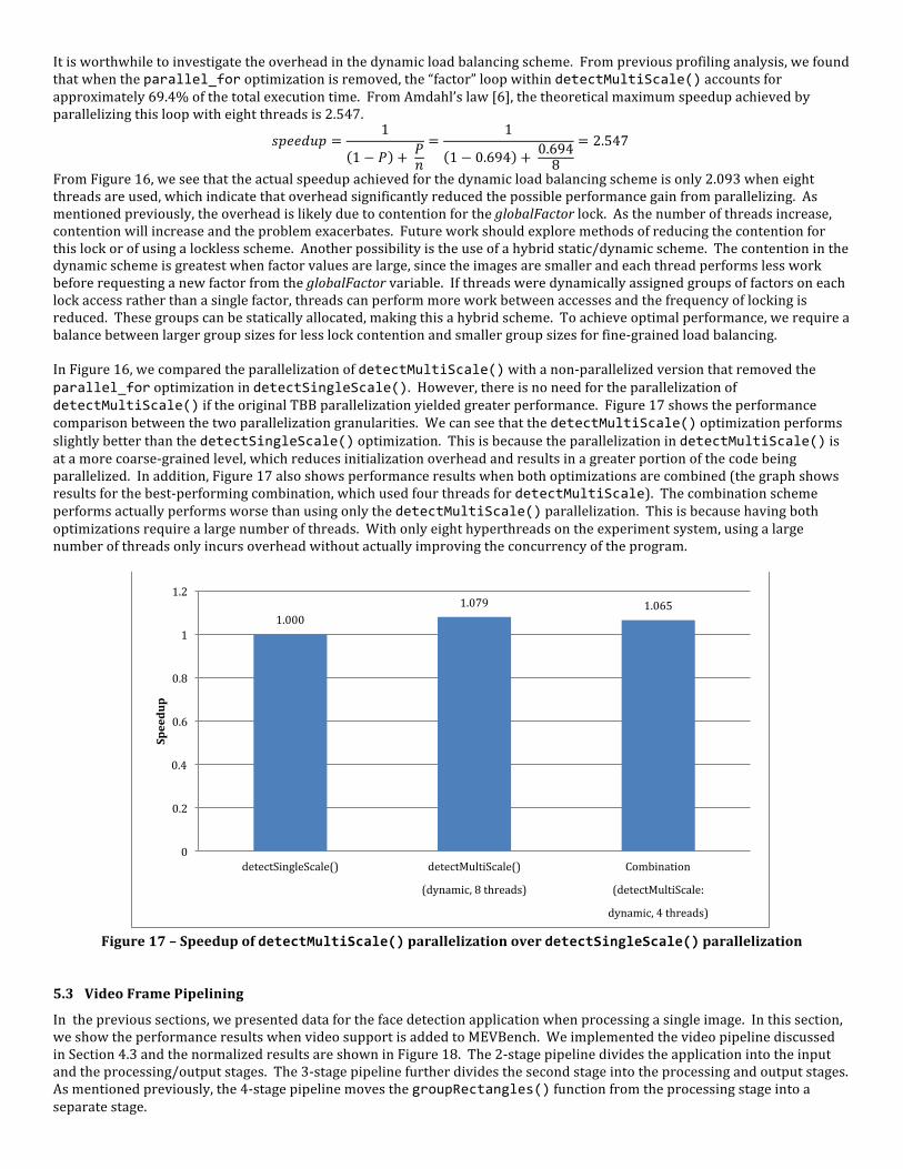
From Figure 16, we see that the actual speedup achieved for the dynamic load balancing scheme is only 2.093 when eight threads are used, which indicate that overhead significantly reduced the possible performance gain from parallelizing. As mentioned previously, the overhead is likely due to contention for the globalFactor lock. As the number of threads increase, contention will increase and the problem exacerbates. Future work should explore methods of reducing the contention for this lock or of using a lockless scheme. Another possibility is the use of a hybrid static/dynamic scheme. The contention in the dynamic scheme is greatest when factor values are large, since the images are smaller and each thread performs less work before requesting a new factor from the globalFactor variable. If threads were dynamically assigned groups of factors on each lock access rather than a single factor, threads can perform more work between accesses and the frequency of locking is reduced. These groups can be statically allocated, making this a hybrid scheme. To achieve optimal performance, we require a balance between larger group sizes for less lock contention and smaller group sizes for fine-‐grained load balancing. In Figure 16, we compared the parallelization of detectMultiScale() with a non-‐parallelized version that removed the parallel_for optimization in detectSingleScale(). However, there is no need for the parallelization of detectMultiScale() if the original TBB parallelization yielded greater performance. Figure 17 shows the performance comparison between the two parallelization granularities. We can see that the detectMultiScale() optimization performs slightly better than the detectSingleScale() optimization. This is because the parallelization in detectMultiScale() is at a more coarse-‐grained level, which reduces initialization overhead and results in a greater portion of the code being parallelized. In addition, Figure 17 also shows performance results when both optimizations are combined (the graph shows results for the best-‐performing combination, which used four threads for detectMultiScale). The combination scheme performs actually performs worse than using only the detectMultiScale() parallelization. This is because having both optimizations require a large number of threads. With only eight hyperthreads on the experiment system, using a large number of threads only incurs overhead without actually improving the concurrency of the program.

Figure 17 – Speedup of detectMultiScale() parallelization over detectSingleScale() parallelization

5.3 Video Frame Pipelining

In the previous sections, we presented data for the face detection application when processing a single image. In this section, we show the performance results when video support is added to MEVBench. We implemented the video pipeline discussed in Section 4.3 and the normalized results are shown in Figure 18. The 2-‐stage pipeline divides the application into the input and the processing/output stages. The 3-‐stage pipeline further divides the second stage into the processing and output stages. As mentioned previously, the 4-‐stage pipeline moves the groupRectangles() function from the processing stage into a separate stage.

1.000 1.079 1.065

0

0.2

0.4

0.6

0.8

1

1.2

detectSingleScale() detectMultiScale() Combination

(dynamic, 8 threads) (detectMultiScale:

dynamic, 4 threads)

Speedup

In this work, pipelining is the coarsest level of parallelization, with less than 2% of the code executing sequentially. Ideally, the speedup in throughput should roughly equal the number of stages in the pipeline. Figure 18 show that although performance increases as the program is broken down into more stages, speedups do not exceed 1.6. Figure 19 provide a more detailed look into the breakdown of each stage and in the leftmost section, we see that the low speedup is due to imbalance between the different stages. We initially chose the stages because they are naturally independent sections of code; however, we see that this does not necessarily translate to an even distribution of work between the threads. To obtain ideal speedups, the workload in each stage should be equal. Unsurprisingly, Figure 19 shows that the bottleneck is the processing stage running detectMultiScale(). We note that the optimizations mentioned in Section 4.2 have not been implemented when obtain this set of data. To obtain further speedup, we must reduce the execution time of the detectMultiScale() stage. Figure 19 also shows performance results when detectMultiScale() is divided into two stages, creating a 5-‐stage pipeline. Although we do not present results for deeper pipelines, we can use pipelines of arbitrary depth by continuing to distribute the factors used in detectMultiScale() to different stages. However, there are two main disadvantages when depending the pipeline in this manner. Firstly, while having more pipeline stages increases throughput, it also increases per-‐frame latency. In a 5-‐stage pipeline, a frame that enters a camera’s lens is only visible to the user five frames later. Delays greater than this begin to exhibit a perceivable lag, which is undesirable to the user. Secondly, separating detectMultiScale() into different pipeline stages is very coarse-‐level parallelization and requires distributing chunks of consecutive factors to different stages/threads. As shown previously in Figure 11, the workload varies for different factor values. Proper balancing between each stage would require fine-‐tuning the number of factors assigned to each stage. This is sensitive to the resolution of the video, since the amount of scaling required depends on the size of the frame. This chunk distribution of factors is also more coarse-‐grained than the static load balancing scheme mentioned previously and thus, is likely to yield worse results. Therefore, although the 5-‐stage pipeline does reduce the execution time, a different method is preferable. The middle section of Figure 19 show results obtained when the parallelization techniques from Section 4.2 are applied to the detectMultiScale() stage (the dynamic load balancing scheme is used with six threads). This is referred to as the 4-‐stage parallelized pipeline, since there are essentially four stages of execution but one stage is further parallelized with helper threads. We see that this improves upon the 5-‐stage pipeline by reducing the execution time of the detectMultiScale() stage. The main contributor to the increased performance is the better workload balancing due to the fine-‐grained dynamic load balancing scheme. Figure 20 show the final speedup results, with the 4-‐stage parallelized pipeline scheme achieving a speedup of 1.734. While this is a promising result, future work can focus on reducing the execution time of detectMultiScale() further by reducing the overhead of the dynamic load balancing scheme. As mentioned previously, a hybrid static/dynamic scheme may yield better results.

Figure 18 – Overall speedups achieved with different numbers of pipeline stages

0

0.2

0.4

0.6

0.8

1

1.2

1.4

1.6

No Pipeline 2-‐Stage Pipeline 3-‐Stage Pipeline 4-‐Stage Pipeline

Speedup

Figure 19 – Performance benefits of parallelizing and pipelining the detectMultiScale() stage

Figure 20 – Overall speedup of face detection for videos

5.4 Real-‐time Frame Rate

The overall speedup presented in Figure 20 is useful when batch video post-‐processing is needed, but it does not address the frame rate constraints that real-‐time processing imposes. The frame rate used must be sufficiently low such that all processing work can be performed within a cycle. This requires that frame rate be based on the maximum execution time of any stage. Figure 21 show the execution time of the synchronized pipeline stages, with the time required for the barrier wait included. The number of faces in the fames increases near the middle of the video, which is evident from the peaks present around frames 600 and 800. We see that as the pipeline depends, the frame span decreases. In addition, the 4-‐stage parallelized pipeline results in lower leaks than the 5-‐stage pipeline, which implies that a higher frame rate can be supported. Using the maximum frame span for the most optimized scheme (0.079s), we obtain a supported frame rate of 12.66 fps. While real-‐time video generally uses higher frame rates, this result is comparable to frame rates obtained by FPGA and GPU implementations. In addition, the results gathered in this work were obtained for HD-‐quality images and videos, whereas

0

10

20

30

40

50

60

70

80

90

4-‐Stage Pipeline 4-‐Stage Parallelized Pipeline

5-‐Stage Pipeline

Time (s)

totalTime

inputFramesStage

detectMultiStage(s)

groupRectsStage

videoWriteStage

0

0.2

0.4

0.6

0.8

1

1.2

1.4

1.6

1.8

2

No Pipeline 5-‐Stage Pipeline 4-‐Stage Parallelized Pipeline

Speedup

previous work in hardware optimization have obtained slightly greater frame rates for lesser-‐quality videos (e.g. VGA resolutions). The peaks that appear in Figure 21 seem to suggest that the number of faces in a frame directly influences the time taken to process this frame. This seems to contradict the original profiling results, which showed that image resolution impacts execution time more than the number of faces. It is possible that as the application is parallelized and the effect of the resolution decreases, the execution time of the cascaded classifiers become more important. In actuality, as Figure 21 shows, the increased number of faces in the frames becomes the bottleneck for the maximum frame rate supported. To achieve higher frame rates, future work should focus on optimizing the cascade so that execution time does not scale with the number of faces. Much of the previous work in face detection has focused on this portion of the application, although with the parallelization done in hardware. It may be possible to translate the hardware implementation into software code to optimize the classifiers.

Figure 21 – Running average of the frame span as a video is processed

6. Related Work Computer vision algorithms, such as face detection, have gained more research interest in recent years with the increased use of their applications on mobile devices. Due to the intensive processing required for face detection, and computer vision programs in general, previous work on parallelizing the Viola-‐Jones algorithm has been focused on hardware approaches. These approaches generally involve using multiple instances of various hardware components. Cho et al. [7] presented a FPGA implementation that pipelined each classifier into five generic stages of computations. Multiple pipelined classifiers are accessed in parallel, with each classifier assigned to process different training data using a round-‐robin method of distribution. This is very fine-‐grained parallelization, whereas our work focuses on more coarse-‐grained parallelization that will incur less overhead in a software implementation. McCready [8] presents a reconfigurable hardware implementation of face detection using nine FPGA boards, with many of the fine-‐tuned optimizations specific to the hardware. This work is limited to the face detection algorithm and cannot be reconfigured for other computer vision applications. Several works [9][10] presented FPGA implementations using scaled images instead of scaled sub-‐windows (similar to this work) and parallelizing the classifiers within the cascade. Once again, parallelizing within the classifiers is more fine-‐grained than the solutions presented by this work. Yang et al. [11] presented another FPGA implementation addressing different granularities of parallelization, similar to this work. However, the frame rate achieved was quite low and unsuitable for real-‐time processing. GPU implementations of the Viola-‐Jones algorithm have been explored as well [12][13]. These take advantage of different parallelization granularities, as this work did, and are also based on the OpenCV implementation. They achieve good speedups and are comparable to previous FPGA implementations. This work avoided using specific hardware acceleration such as GPUs, as many mobile devices do not contain such specialized chips.

7. Conclusion and Future Work In this work, we investigated software parallelization of the Viola-‐Jones face detection algorithm. For a single image we were able to parallelize the face detection method at a coarser grain then what was previously provided in OpenCV. This resulted in an 8% speedup over the original OpenCV implementation. We then improved a video implementation of the face detection program by pipelining the process into four separate stages and using the parallelization implemented for a single image. These allowed us to achieve a speedup of 73.4%. Our supported frame rate is 12.66 fps, which is comparable to frame rates achieved using hardware optimizations. Through the parallelization effort, we found that a combination of coarse and fine-‐grained parallelization is needed for the face detection application, since we want to reduce overhead but still maintain fine-‐grained load balancing. Future work for the project may include a port of the optimizations to a mobile platform such as Android or iOS. This would target a greater range of uses for the face detection application. The power constraints that mobile devices face may result in additional effort to ensure that the extra threads do not detrimentally affect battery life. Another area of improvement lies in reducing the overhead in our dynamic load balancing scheme, which produced the best results. A lock-‐less scheme would be most desirable. If this is not achievable, a hybrid static/dynamic scheme may result in better performance, since the static grouping of work can reduce contention on the global lock. Lastly, as the performance increases due to the parallelization implemented, the number of faces within a frame has a more pronounced effect on the frame span. Effort should be made to optimize this portion of the application. These changes would benefit not only this project, but for all uses of object tracking involving OpenCV’s CascadeClassifier class. References [1] Viola, Paul, and Michael Jones. "Rapid object detection using a boosted cascade of simple features." In Computer Vision

and Pattern Recognition, 2001. CVPR 2001. Proceedings of the 2001 IEEE Computer Society Conference on, vol. 1, pp. I-‐511. IEEE, 2001.

[2] Lienhart, Rainer, and Jochen Maydt. "An extended set of haar-‐like features for rapid object detection." In Image

Processing. 2002. Proceedings. 2002 International Conference on, vol. 1, pp. I-‐900. IEEE, 2002 [3] Opencv. [Online]. Available: http://opencv.willowgarage.com/wiki/. [4] Clemons, Jason, Haishan Zhu, Silvio Savarese, and Todd Austin. "MEVBench: A mobile computer vision benchmarking

suite." In Workload Characterization (IISWC), 2011 IEEE International Symposium on, pp. 91-‐102. IEEE, 2011. [5] Thread Building Blocks. [Online]. Available: http://threadingbuildingblocks.org/. [6] Amdahl, Gene M. "Validity of the single processor approach to achieving large scale computing capabilities." In

Proceedings of the April 18-‐20, 1967, spring joint computer conference, pp. 483-‐485. ACM, 1967. [7] Cho, Junguk, Bridget Benson, Shahnam Mirzaei, and Ryan Kastner. "Parallelized architecture of multiple classifiers for

face detection." InApplication-‐specific Systems, Architectures and Processors, 2009. ASAP 2009. 20th IEEE International Conference on, pp. 75-‐82. IEEE, 2009.

[8] McCready, Rob. "Real-‐time face detection on a configurable hardware system."Field-‐Programmable Logic and

Applications: The Roadmap to Reconfigurable Computing (2000): 157-‐162. [9] Wei, Yu, Xiong Bing, and Charayaphan Chareonsak. "FPGA implementation of AdaBoost algorithm for detection of face

biometrics." In Biomedical Circuits and Systems, 2004 IEEE International Workshop on, pp. S1-‐6. IEEE, 2004. [10] Hiromoto, Masayuki, Kentaro Nakahara, Hiroki Sugano, Yukihiro Nakamura, and Ryusuke Miyamoto. "A specialized

processor suitable for adaboost-‐based detection with haar-‐like features." In Computer Vision and Pattern Recognition, 2007. CVPR'07. IEEE Conference on, pp. 1-‐8. IEEE, 2007.

[11] Yang, Ming, Ying Wu, James Crenshaw, Bruce Augustine, and Russell Mareachen. "Face detection for automatic exposure control in handheld camera." In Computer Vision Systems, 2006 ICVS'06. IEEE International Conference on, pp. 17-‐17. IEEE, 2006.

[12] Hefenbrock, Daniel, Jason Oberg, Nhat Thanh, Ryan Kastner, and Scott B. Baden. "Accelerating viola-‐jones face detection

to fpga-‐level using gpus." InField-‐Programmable Custom Computing Machines (FCCM), 2010 18th IEEE Annual International Symposium on, pp. 11-‐18. IEEE, 2010.

[13] Harvey, Jesse Patrick. "GPU acceleration of object classification algorithms using NVIDIA CUDA." PhD diss., Rochester

Institute of Technology, 2010.

Final Report with Figures - University of Toronto

Documents