Design and Demonstration of a Heat Exchanger for a Compact Natural Gas Compressor Major Qualifying Project Report submitted to the faculty of WORCESTER POLYTECHNIC INSTITUTE in partial fulfillment of the requirements for the Degree of Bachelor of Science of MECHANICAL ENGINEERING Submitted by: Jessica Holmes Calvin Lam Bradford Marx Andrew Nelson Christopher O’Brien Project Advisor: Prof. Simon Evans Project Sponsor: OsComp Systems Project Website: https://sites.google.com/site/oscompmqp/ Certain materials are included under the fair use exemption of the U.S. Copyright Law and have been prepared according to the fair use guidelines and are restricted from further use.

Welcome message from author
This document is posted to help you gain knowledge. Please leave a comment to let me know what you think about it! Share it to your friends and learn new things together.
Transcript

Design and Demonstration of a Heat Exchanger
for a Compact Natural Gas Compressor
Major Qualifying Project Report submitted to the faculty of
WORCESTER POLYTECHNIC INSTITUTE
in partial fulfillment of the requirements for the Degree of Bachelor of Science of
MECHANICAL ENGINEERING
Submitted by:
Jessica Holmes
Calvin Lam
Bradford Marx
Andrew Nelson
Christopher O’Brien
Project Advisor:
Prof. Simon Evans
Project Sponsor:
OsComp Systems
Project Website: https://sites.google.com/site/oscompmqp/
Certain materials are included under the fair use exemption of the U.S. Copyright Law and have been prepared
according to the fair use guidelines and are restricted from further use.

1
Acknowledgements
Our team would like to express our most sincere appreciation to the following
individuals. Without their knowledge, enthusiasm, and dedication, the success of our project
would never have been possible.
Professor Simon Evans, WPI - For all his advice, guidance, and organization throughout the
entirety of this project.
Andrew Nelson, OsComp Systems - For all of his excellent suggestions and guidance throughout
the project. His strong work ethic and high expectations were what drove our team to succeed.
Pedro Santos, OsComp Systems – For providing us the opportunity and resources to work on a
real-world problem and utilize our knowledge obtained here at WPI.
Neil Whitehouse, WPI – For assisting us with the manufacturing aspect to the project and taking
the time to provide us with knowledge and assistance whenever we asked.
Adam Sears, WPI – For allowing us to use lab space in the Washburn Shops building and
providing us with any resources we needed to achieve our objectives.
Greg Overton, WPI – For assisting us with machining our copper parts, which played an
essential role in completing the project.
Mike Beliveau, Aavid Thermalloy – For assisting us with obtaining heat pipes in a timely manner
and alleviating the cost of our project.
Serena Lin, Enertron Inc. – For providing us with the necessary information on heat pipes, which
was required to design our model, as well as her patience in order to do so.
Barbara Furhman, WPI – For assisting the team with obtaining all necessary parts and
equipment to complete our project.
2
Abstract
Natural gas is an important fossil fuel. In order to optimize the transportation of natural
gas from the source to the consumers, it must first be compressed. As natural gas is compressed,
the temperature increases significantly and must be cooled before it can be processed further.
However, current heat exchangers for this application are large and inefficient for a natural gas
compression skid. As these devices must operate in locations where there is a limited amount of
space, such as offshore oil platforms, it is crucial to reduce the footprint as much as possible. The
goal of this project was to design a more efficient and compact heat exchanger to be used in
conjunction with OsComp's rotary, positive-displacement natural gas compressor. The design
incorporated heat pipes as a means to improve the efficiency of the overall heat transfer. The
design has a total footprint of 0.871 m^2, which is 21.5% smaller than an industry standard heat
exchanger of the same specification (1.1 m^2). To demonstrate the feasibility of a heat-pipe
forced convection cooler; a scaled-down test stand was manufactured and tested.

3
Table of Contents
Acknowledgements ....................................................................................................................................... 1
Abstract ......................................................................................................................................................... 2
List of Figures ............................................................................................................................................... 5
List of Tables ................................................................................................................................................ 6
1. Introduction .............................................................................................................................................. 7
2. Background ............................................................................................................................................... 8
2.1 Thermodynamic and Heat Transfer Concepts .................................................................................... 8
2. 2 Compressors..................................................................................................................................... 11
2.3 Heat Exchangers ................................................................................................................................ 11
2.3.1 Heat Transfer Process ................................................................................................................ 11
2.3.2 Construction ............................................................................................................................... 13
2.3.3 Heat Transfer Mechanisms ........................................................................................................ 15
2.4 Heat Pipes ......................................................................................................................................... 16
2.4.1 Types of Heat Pipes .................................................................................................................... 17
3. Methodology ........................................................................................................................................... 19
3.1 Design Requirements ........................................................................................................................ 19
3.2 Design Process .................................................................................................................................. 19
3.2.1 Concepts Considered ................................................................................................................. 20
3.2.2 Decision Matrix .......................................................................................................................... 28
3.3 Final Design ....................................................................................................................................... 30
3.4 Manufacturing .................................................................................................................................. 31
4. Testing ..................................................................................................................................................... 34
4.1 Heat Pipe Experiments ...................................................................................................................... 34
4.2 Scale Model Experiments .................................................................................................................. 37
4.2.1 Assembly of Demonstrator ........................................................................................................ 37
4.2.2 Assembly of Test Apparatus ....................................................................................................... 39
4.2.3 Experimental Setup .................................................................................................................... 41
4.2.4 Scaling Procedure ....................................................................................................................... 41
5. Analysis ................................................................................................................................................... 44
5.1 Performance ..................................................................................................................................... 44
5.1.1Temperature Profiles .................................................................................................................. 44

4
5.1.2 Heat Pipe Performance .............................................................................................................. 48
5.1.3 Cooling Performance ................................................................................................................. 52
5.1.4 Scaling Analysis .......................................................................................................................... 52
5.1.5 Demonstrator Analytical Analysis .............................................................................................. 53
5.2 Cost ................................................................................................................................................... 55
6. Conclusions ............................................................................................................................................. 56
7. Recommendations .................................................................................................................................. 57
7.1 Heat Pipe Selection ........................................................................................................................... 57
7.2 Manufacturing .................................................................................................................................. 58
7.3 Conducting Experiments ................................................................................................................... 58
8. References .............................................................................................................................................. 60
Appendices .................................................................................................................................................. 61
Appendix A - Authorship ......................................................................................................................... 61
Appendix B – Properties Used ................................................................................................................ 61
Appendix C - Budget................................................................................................................................ 62
Appendix D - CAD Drawings and Pictures ............................................................................................... 63
Appendix E - Experimental Setup Pictures .............................................................................................. 66
Appendix F - LabView Setup for Data Acquisition .................................................................................. 69
Appendix G - Mathcad Calculations ........................................................................................................ 71
G.1 Fin Analysis and Optimization ...................................................................................................... 71
G.2 Scaling Calculations ...................................................................................................................... 74
G.3 Cradle Heat Pipe Design Analysis ................................................................................................. 79
G.4 Demonstrator Analytical Analysis ................................................................................................. 85
Appendix H - Quotes ............................................................................................................................... 91
H.1 Quote - Current Cooler Competitor ............................................................................................. 91
H.2 Aavid Thermalloy Quote - Heat Pipes ........................................................................................... 95
H.3 ACT Quote - Heat Pipes ................................................................................................................ 96
H.4 Enertron Inc. Heat Pipe Quote (Unofficial)................................................................................... 97
H.5 Noren Products Heat Pipe Quote (Unofficial) .............................................................................. 97
Appendix I - Contacts .............................................................................................................................. 98
I.1 WPI ................................................................................................................................................. 98
I.2 OsComp Systems ............................................................................................................................ 98

5
I.3 Heat Pipe Manufacturers ............................................................................................................... 99
List of Figures
Figure 1: Thermal resistance for a tube ........................................................................................................ 9
Figure 2: Heat exchanger classification according to transfer process ...................................................... 12
Figure 3: Plate heat exchanger ................................................................................................................... 14
Figure 4: Shell-and-tube heat exchanger .................................................................................................... 15
Figure 5: Heat Pipe Operation (Gilmore, 2002) .......................................................................................... 16
Figure 6: Flat Heat Pipes ............................................................................................................................. 17
Figure 7: Variable-Conductance Heat Pipes ................................................................................................ 18
Figure 8: Spiral heat exchanger (Cesco, 2011) ............................................................................................ 20
Figure 9: Two section heat exchanger ........................................................................................................ 21
Figure 10: Thermoelectric Cooler Operation (TE Technology Inc., 2010) ................................................... 22
Figure 11: Sample Thermoelectric Cooler (Snake Creek Laser, 2011) ........................................................ 23
Figure 12: Compact cooler .......................................................................................................................... 24
Figure 13: Deployable radiator preliminary concept (Gilmore) .................................................................. 25
Figure 14: "Panels with heat pipes" preliminary concept .......................................................................... 26
Figure 15: "Panels with heat pipes" preliminary design concept, inside view ........................................... 26
Figure 16: Thermacore's heat exchangers (Thermacore, 2009) ................................................................. 28
Figure 17: Full Model .................................................................................................................................. 30
Figure 18: Cradle with Heat Pipe ................................................................................................................ 31
Figure 19: Cradle (ideal) .............................................................................................................................. 32
Figure 20: Cradle (modified) ....................................................................................................................... 32
Figure 21: Heat pipe experimental set-up .................................................................................................. 34
Figure 22: Thermal resistance vs. Heat Pipe Length (Enerton, 2011) ......................................................... 35
Figure 23: Average heat load vs. thermal resistance of a heat pipe .......................................................... 36
Figure 24: Thermal resistance over time .................................................................................................... 36
Figure 25: CAD model of demonstrator ...................................................................................................... 37
Figure 26: 7 Cradle Demonstrator Layout ................................................................................................... 38
Figure 27: 14 Cradle Demonstrator Layout ................................................................................................. 39
Figure 28: Final Demonstrator .................................................................................................................... 40
Figure 29: Temperature Profile - Fan off, 7 heat pipes ............................................................................... 45
Figure 30: Temperature Profile - Fan off, 14 heat pipes ............................................................................. 46
Figure 31: Temperature Profile - Fan off, 7 pipes, increased flow rate ...................................................... 46
Figure 32: Temperature Profile: Fan on, 7 heat pipes ................................................................................ 47
Figure 33: Temperature Profile: Fan on, 14 heat pipes .............................................................................. 47
Figure 34: Temperature Profile - Fan on, 14 heat pipes, long duration (33 minutes) ................................ 48
Figure 35: Temperature Change across heat pipe 1 for the 7 heat pipe demonstrator............................. 49
Figure 36: Temperature Change across heat pipe 3 for the 7 heat pipe demonstrator............................. 49
Figure 37: Performance of Heat Pipe 1 for the 7 heat pipe demonstrator ................................................ 50
Figure 38: Performance of Heat Pipe 3 for the 7 heat pipe demonstrator ................................................ 50
Figure 39: Performance of Heat Pipe 3 for the 14 heat pipe demonstrator .............................................. 51

6
Figure 40: Performance of Heat Pipe 14 for the 14 heat pipe demonstrator ............................................ 51
Figure 41: Preliminary design model, using heat pipe concept .................................................................. 63
Figure 42: Preliminary design drawing, using heat pipe concept ............................................................... 63
Figure 43: Preliminary demonstrator model .............................................................................................. 64
Figure 44: Cradle drawing ........................................................................................................................... 64
Figure 45: Demonstrator drawing ............................................................................................................... 65
Figure 46: Close up picture of heat pipe ..................................................................................................... 66
Figure 47: Securing copper for machining .................................................................................................. 66
Figure 48: Exhaust outlet connecting to cooler .......................................................................................... 67
Figure 49: Final setup of demonstrator 1 ................................................................................................... 67
Figure 50: Final setup of demonstrator 2 ................................................................................................... 68
Figure 51: LabView Virtual Instrument ....................................................................................................... 69
Figure 52: LabView Block Diagram .............................................................................................................. 70
Figure 53: Fin Optimization ......................................................................................................................... 73
List of Tables
Table 1: Decision matrix .............................................................................................................................. 28
Table 2: Heat load vs. thermal resistance of heat pipes ............................................................................. 35
Table 3: Outlet temperature for each experiment ..................................................................................... 52
Table 4: Scaling Analysis.............................................................................................................................. 53
Table 5: Equipment and materials cost breakdown ................................................................................... 55
Table 6: Project Budget ............................................................................................................................... 62
Table 7: Fin Optimization 1 ......................................................................................................................... 72
Table 8: Fin Optimization 2 ......................................................................................................................... 72

7
1. Introduction
Natural gas is found in oil or gas wells and consists primarily of methane (85% to 95%
by volume) in addition to trace amounts of other gases. Natural gas is used in many applications
such as power generation and running industrial equipment. Compression of this gas is necessary
to maximize the amount that can be stored and transported. Traditional natural gas compression
systems require multiple compression and cooling stages to achieve high pressure ratios and
reduce the temperature increases caused by compression, respectively. Since the gas is at
different pressures after each stage, multiple pieces of equipment are required which greatly
increases the amount of space the equipment occupies. If the natural gas could be compressed in
fewer cycles, the size of the compression platform could be greatly reduced. This is particularly
important on oil rigs and other locations where space is limited.
OsComp Systems, founded in 2009 by Pedro Santos, has created a new compressor that
uses a single stage to achieve pipeline pressures at higher efficiency and energy density, leading
to a smaller size. Their compressor uses dynamic liquid injection to achieve near-isothermal
compression. Since the gas is cooled within the compressor, the entire compression can be done
in one cycle, and this allows the compressor to be packaged on a smaller frame.
Currently, the largest component on the compressor platform is the cooler. The
compressor skid holds the compressor and all other components required to keep it running. The
cooler is used to cool the engine fluids, from the engine running the compressor, the natural gas
coolant, and the natural gas itself. Current industry standard coolers are approximately 7x3x4
meters [84 m3 in volume] and have a flow rate of 378 SCFM. If the cooler could be redesigned
as a more efficient component, the size could be reduced, allowing for a smaller compression
skid. This is important because transporting the heavy, bulky skids is expensive and difficult.
This becomes even more important in off-shore and under-sea applications where optimizing
8
footprint is of the utmost importance. The goal of this project is to design a cooler that is more
efficient and compact than industry standard to be used in conjunction with OsComp's rotary,
positive-displacement natural gas compressor. The objective of our project is to design a working
cooler section and to build a test model. This test model will be a scale version of the full unit.
2. Background
2.1 Thermodynamic and Heat Transfer Concepts
The two main modes of heat transfer associated with this cooler are convection and
conduction. Convection refers to heat transfer between a surface and a moving fluid (Atlas
Copco, 2010). Here, a fluid can be considered either a gas or a liquid. This type of heat transfer
is characterized by a convection coefficient . Conduction is heat transfer through the direct
contact of particles, whether it is a solid or a stationary fluid (Atlas Copco, 2010). It is
characterized by a thermal conductivity . Each type of heat transfer provides a thermal
resistance, which is helpful in calculating the amount of heat that is transferred in a system.
In a heat exchanger, heat is first transferred from the hot fluid to the tube or pipe wall by
convection. Next, heat is transferred through the wall by conduction. Finally, through
convection, heat is transferred from the wall to the cold fluid (Cengel et al., 2008). Using the
subscript to identify variables inside the tube and the subscript to identify variables outside
the tube, the thermal resistance for all three modes of heat transfer taking place can be defined,
along with an equivalent thermal circuit shown in Figure 1. The equations for each thermal
resistance are described in Equations (1) through (3). Equation (4) is the equivalent resistance for
the entire tube.

9
Figure 1: Thermal resistance for a tube
(1)
(2)
(3)
(4)
The thermal resistance for convection is dependent on the convection coefficient and
the surface area , on which the heat transfer is to occur. For the inner surface area of circular
tubes, , where is the inner diameter of the tube and is the length of the tube.
Similarly, for the outer surface area of a tube, . The thermal resistance for
conduction is a function of the thermal conductivity , the length of the tube , and the ratio
between the outer and inner diameters,
. Since the heat transfer modes act in series, the total
thermal resistance is equal to the sum of these three resistances. From this resistance, the rate of
heat being transferred in this process can be determined, using equation (5).
(5)
In Equation (5), is the temperature difference between the outlet and inlet, and is
the overall heat transfer coefficient. To simplify calculation of the overall heat transfer
coefficient, the thermal resistance in the wall may be approximated as zero, since the thickness
of the wall is very small. The inner and outer surface areas of the pipe are also considered to be

10
equal. As a result, the overall heat transfer coefficient can be calculated from the two convection
coefficients:
(6)
The values of the overall heat transfer coefficient will range from approximately 10
for gas-to-gas heat exchangers to approximately 10,000 for heat
exchangers that involve phase changes (Cengel et al., 2008).
Because heat exchangers are made to operate for long periods of time without any change
in their operating conditions, they can be analyzed as steady-flow devices, where the mass flow
rate in each fluid will remain constant (Cengel et al., 2008). Fluid properties including
temperature and velocity at inlets or outlets will also remain constant. Fluid streams experience
little to no change in velocities or elevations, meaning that both kinetic and potential energy can
be considered negligible.
The first law of thermodynamics states that energy cannot be created nor destroyed;
therefore energy must be conserved in a closed system (Atlas Copco, 2010). For a heat
exchanger, this means that the rate of heat transfer from the hot fluid must be equal to the rate of
heat transfer to the cold fluid. Using as a subscript to describe the cold fluid and the subscript
as an indicator for the hot fluid, the following equations can be written for the rate of heat
transfer for the system. Using the mass flow rates, , the specific heats, , and the inlet and
outlet temperatures, and :
(7)
(8)
Equations (7) and (8) can be rewritten and simplified in terms of the heat capacity rate .
The heat capacity rate is the product of the mass flow rate and the specific heat of the fluid. It

11
represents the rate of heat transfer required to change the temperature of a fluid stream by 1°C. In
a heat exchanger, fluids with a large heat capacity rate will experience a smaller temperature
change (Cengel et al., 2008). Conversely, there will be a larger temperature change in fluids with
a small heat capacity.
2. 2 Compressors
Various techniques for compression are used in products on the market today. Cooling
liquid-injected compression, which is utilized by OsComp Systems, is the process of injecting
liquid into a gas during compression. The coolant absorbs heat generated during the compression
process, sometimes evaporating as a result. This cools the gas during compression, allowing for
high pressure ratios in a single stage and eliminating the need for inter-stage cooling sections in
the system. This is different from industry standard natural gas compressors or reciprocating
piston compressors, as they will fail catastrophically when liquids are included in the gas stream.
OsComp’s compressor utilizes a novel design which uniquely allows for liquid injection and wet
gas compression.
2.3 Heat Exchangers
A heat exchanger is a device that is used to transfer thermal energy between two or more
fluids. Heat exchangers are classified according to the heat transfer process, number of fluids,
construction, surface compactness, flow arrangements, and heat transfer mechanisms. Two fluids
are commonly used in heat exchangers, with one fluid being cooled and another fluid acting as a
coolant. However, “as many as twelve fluid streams have been used in some chemical processes
(e.g., air separation systems and purification/liquefaction of hydrogen) (Shah 2003).”
2.3.1 Heat Transfer Process
Heat exchangers can be classified as devices that transfer heat either directly or
indirectly. A direct contact heat exchanger transfers energy directly from one fluid to another,

12
usually separated by a barrier. Indirect contact heat exchangers utilize an intermediate medium to
transfer the thermal energy between fluids. There are also different classifications within each of
these types of exchangers, as illustrated below in Figure 2.
Figure 2: Heat exchanger classification according to transfer process
There are three arrangements within the indirect-contact heat exchanger: direct transfer,
storage, and fluidized bed. In the direct transfer setup, heat is transferred continuously from the
hot fluid to a dividing wall and from the dividing wall to the cold fluid. Although two (or more)
fluids flow simultaneously, the fluids never mix because each fluid is flowing in a separate
passage. Examples of direct-transfer heat exchangers are tubular, plate-type, and extended
surface (fin) exchangers. “In the storage type exchanger, both fluids flow alternatively through
the same flow passages, creating intermittent heat transfer. In a fluidized-bed heat exchanger,
one side of a two-fluid exchanger is immersed in a bed of finely divided solid material, such as a
tube bundle immersed in a bed of sand or coal particles.” (Shah 2003)
In direct-contact heat exchangers, the fluids come into direct contact when transferring
heat. The fluid types associated with these heat exchangers can be two immiscible fluids, a gas
and a liquid, or a liquid and a vapor. Typical applications involved heat and mass transfer, such
as in evaporative cooling. It is rare that applications only involve sensible heat transfer. With
respect to indirect- contact heat exchangers, direct-contact can achieve very high heat transfer
13
rates, are relatively inexpensive, and do not suffer from fouling since there is no wall between
the two fluids (Shah 2003).
2.3.2 Construction
There are four main construction types of heat exchangers: tubular, plate-type, extended
surface (fin), and regenerative. There are other constructions available that may be classified as
one of these types but have some unique features compared to the conventional type of
exchanger.
Tubular heat exchangers are generally built of circular tubes. However, elliptical,
rectangular, and round/flat twisted tubes can also be used. There is considerable flexibility in this
design as the core geometry can be varied easily. This is done by changing the tube diameter,
length, and arrangement. These exchangers can be designed for high pressures relative to the
environment as well as high pressure differences between fluids. Primary heat transfer
applications include liquid-to-liquid and liquid-to-phase change (condensing or
evaporating).Tubular heat exchangers can be used for gas-to-liquid and gas-to-gas heat transfer
applications when the operating temperature and/or pressure is very high, or if fouling is a severe
problem on at least one fluid side. (Shah 2003)
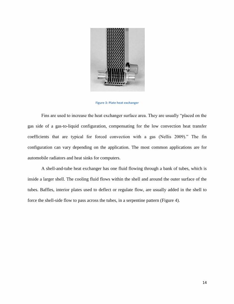
The plate heat exchanger, shown in Figure 3 below, is often used for two liquid streams.
This type of exchanger consists of many individual plates that are stacked together, refer to
Figure 3. The plates are corrugated, forming flow channels between the adjacent plates. This
type of heat exchanger is compact and easy to disassemble for cleaning. It is also relatively easy
to increase or decrease their size as needed by adding or removing plates.
14
Figure 3: Plate heat exchanger
Fins are used to increase the heat exchanger surface area. They are usually “placed on the
gas side of a gas-to-liquid configuration, compensating for the low convection heat transfer
coefficients that are typical for forced convection with a gas (Nellis 2009).” The fin
configuration can vary depending on the application. The most common applications are for
automobile radiators and heat sinks for computers.
A shell-and-tube heat exchanger has one fluid flowing through a bank of tubes, which is
inside a larger shell. The cooling fluid flows within the shell and around the outer surface of the
tubes. Baffles, interior plates used to deflect or regulate flow, are usually added in the shell to
force the shell-side flow to pass across the tubes, in a serpentine pattern (Figure 4).

15
Figure 4: Shell-and-tube heat exchanger
2.3.3 Heat Transfer Mechanisms
The basic heat transfer mechanisms incorporated in heat exchangers are single-phase
convection, two-phase convection, and combined convection and radiation heat transfer. The
convection can either be free or forced in any case. Any of these mechanisms can be active on
each fluid side of the heat exchanger, either individually or in combination, depending on the
configuration (Shah, 2003).

2.4 Heat Pipes
Heat pipes are used to transport large quantities of heat from one location to another
without the use of electricity. Utilizing a closed, two-phase, fluid cycle with a hot interface
(evaporator) and a cold interface (condenser), heat pipes utilize the properties of gravity or
capillary action, provided by a wick, and pressure differential to transport liquid and vapors.
Heat pipes are extensively used for cooling systems in spacecraft and for cooling various modern
computer system components, including central and graphical processing units.
As illustrated above in Figure 5, a heat pipe consists of a wick and a vapor space. The
wick contains the liquid phase and the vapor space contains the vapor phase, where both are at
saturation. At the evaporator, the incoming heat raises the temperature inside and the liquid
evaporates, travelling to the other end. This lowers the pressure in the evaporator end because
less liquid remains. The local vapor pressure at the condenser end raises, as it must remain in
saturation with the heated liquid. This pressure difference is sufficient enough to draw liquid
from the condenser toward the evaporator, while the heated vapors in the evaporator flow toward
the condenser, which is now at a lower pressure. The vapors then condense when they come in
contact with the condenser’s lower surface temperature. This cycle is repeated to transfer heat
(Gilmore, 2002).
Figure 5: Heat Pipe Operation (Gilmore, 2002)
17
2.4.1 Types of Heat Pipes
There are various types of heat pipes available, ranging from constant-conductance heat
pipes and diode heat pipes to variable-conductance heat pipes (VCHPs) and hybrid systems.
Constant-conductance heat pipe designs are among the most basic and are categorized according
to their 4 types of wick structure: groove, which has many small slots around the inside of the
pipe to carry liquid back; mono-groove, which uses one larger groove instead of many smaller
grooves; composite, which layers material around the inside of the pipe to carry the liquid back;
and artery & tunnel, which provides one or more extra unrestricted liquid flow paths in addition
to composites.
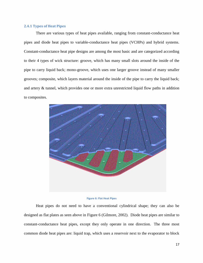
Figure 6: Flat Heat Pipes
Heat pipes do not need to have a conventional cylindrical shape; they can also be
designed as flat plates as seen above in Figure 6 (Gilmore, 2002). Diode heat pipes are similar to
constant-conductance heat pipes, except they only operate in one direction. The three most
common diode heat pipes are: liquid trap, which uses a reservoir next to the evaporator to block

18
vapor travel; liquid blockage, which uses a reservoir by the condenser which fills and empties
with liquid to block vapor travel; and gas blockage which also uses a reservoir next to the
evaporator, but is filled with a non-condensable gas to block vapor travel (Gilmore, 2002).
Variable-conductance heat pipes, as shown in Figure 7 below, utilize gas reservoirs.
Figure 7: Variable-Conductance Heat Pipes
These reservoirs are filled with a non-condensable gas to control the operating area of the
condenser based on the evaporator temperature. The benefit of this type of heat pipe is to reduce
the volume of control gas and open up more area of the condenser for heat pipe operation
(Gilmore, 2002). Hybrid systems are extensions of capillary-pumped loop designs. Coolant is
vaporized as part of this, and major benefits of this system are its ability to be operated without a
separate driving unit and being suitable for light-weight miniaturized electronics (Gilmore,
2002).
19
3. Methodology
3.1 Design Requirements
With the goal of the project to design a more efficient and compact heat exchanger to be
used in conjunction with OsComp's rotary, positive-displacement natural gas compressor, the
next step was to create a list of design specifications and requirements to follow as initial design
ideas took shape. After speaking with our sponsor and examining their natural gas compressor,
we learned that the temperature of the natural gas entering our heat exchanger is 104º Celsius
and the desired exit temperature is 60 ºC. The design must handle the pressure of the compressed
natural gas at 10.55 MPa and be able to continuously run for months at a time. The natural gas
flows at a rate of 0.473m3/sec and has a density of 53.33 kg/m
3. Our sponsor is interested in
seeing innovative or novel ideas, encouraging us to stay away from more traditional designs such
as shell-and-tube and plate heat exchangers. Finally, the design is desired to be smaller than
commercial natural gas heat exchangers currently available on the market. For comparison, we
used an industry standard after-cooler section quote, given to us by our sponsor, which has a total
volume of 0.55 m3, broken up into a length of 1.619 m, a width of 0.343 m, and a height of 0.991
m.
3.2 Design Process
Each member of the design team came up with a preliminary design for a more compact
method of cooling natural gas. These concepts were each analyzed in great detail to help
determine which concepts we would continue to explore. First, we used a decision matrix to
narrow our design options down to two concepts. Then, we conducted further analysis to
compare both final concepts and make a decision on which path to pursue. We started with five
unique designs, detailed below, and ended up pursuing a heat pipe based design with copper
cradles.

20
3.2.1 Concepts Considered
Spiral Heat Exchanger
Spiral heat exchangers feature two fluids in counter flow. In this set-up, the hot fluid is
cooled by a colder fluid. They are often used in paper processing and refineries, and are
beneficial due to their anti-fouling designs and compact design. Some challenges with using
spiral heat exchangers are that they can only cool one fluid, and that the coolant flow must be a
forced flow. We chose not to use a spiral heat exchanger due to the lack of scalability and the
fact that only one fluid can be cooled in each heat exchanger. A diagram of the spiral heat
exchanger model is shown in Figure 8.
Figure 8: Spiral heat exchanger (Cesco, 2011)

21
Two Section Heat Exchanger
Figure 9: Two section heat exchanger
A two section heat exchanger, shown in Figure 9, was developed as another possible
cooler design. Made out of aluminum, this design operates by running the hot gas through the
yellow sections and coolant through the blue sections. The pipe bends back and forth to create a
stacked, staggered pattern in order to reduce the overall size. Baffles within the blue section of
the tube help support the yellow section and direct the flow of coolant. In order to manufacture,
wire EDM or aluminum extrusion should be considered. The advantages of this design are that
the multiple passes allow for longer duration of contact with coolant and provide a large heat
transfer surface area. However, this design was not chosen for further analysis because it became
apparent that the length needed to sufficiently cool the natural gas would make the design too
large.
Thermoelectric Cooler
An additional method for cooling the natural gas that was considered was the use of
thermoelectric coolers. These coolers utilize the thermoelectric effect (also known as the Peltier
effect), in which an induced voltage between two different metals creates a temperature

22
difference. Although they contain no moving parts, thermoelectric coolers are characterized by
poor efficiency ratings (Avallone, 2007). Ultimately, we did not continue with the thermoelectric
concept for our design because of the high amount of electrical energy required to operate it, the
relatively high cost for individual coolers, and its poor scalability. Mounting the coolers to a
cylindrical pipe would also be challenging, especially with a large heat sink attached to each
cooler. Figure 10 and Figure 11 below show how a thermoelectric cooler operates and a sample
thermoelectric cooler, respectively.
Figure 10: Thermoelectric Cooler Operation (TE Technology Inc., 2010)

23
Figure 11: Sample Thermoelectric Cooler (Snake Creek Laser, 2011)
Compact Heat Exchanger
When exploring the different types of heat exchanger, there was one particular
classification that seemed to fit well for our application. The idea of a compact heat exchanger
was intriguing because of the ability to cool a fluid over a large heat transfer surface area while
occupying a relatively small amount of space. They are commonly used in applications that have
limitations on weight and volume.
The original compact cooler concept, inspired by a thermal-fluid textbook, Fundamentals
of Thermal-Fluid Sciences by Y.A. Cengel, R. H. Turner, and J.M. Cimbala, consists of multiple
tubes passing through a large amount of thin plates. Air is forced through the plates using a fan.
The plates increase thermal conductivity, meaning that the greater number of plates used in a
design, the greater the amount of heat can be removed from the system. After several iterations,
the final compact cooler design that was developed featured one tube that is looped back and
forth between each end of the cooler, with each pass going through thin aluminum plates. This
configuration results in a tube length long enough so that the natural gas can be cooled to the
necessary temperature. At the same time, by looping the tube, size and footprint are both
minimized. Figure 12 shows the configuration of the model with the looped tubes.

24
Figure 12: Compact cooler
This concept presented several manufacturing challenges, and after further analysis, it
was realized that this design, even with the pipe looped back and forth, would still have to be
quite large if it were to cool the natural gas to the desired temperature. Due to these reasons, we
ultimately did not further pursue this design concept.
Deployable Radiator
Another concept we developed was inspired by the deployable radiators found on the
International Space Station. Our initial background research confirmed that aircraft and
spacecraft required compact thermal control devices since they had limited space available.

25
Figure 13: Deployable radiator preliminary concept (Gilmore)
In order to reduce the large footprint of a typical heat exchanger, we modified the
deployable radiator concept, shown in Figure 13 to be used on Earth. The base would provide a
smaller footprint and have numerous panels extend upwards. Each panel would be equipped with
heat pipes to further increase the heat transfer rate. The panels themselves help increase the
surface area available to mount the heat pipes as well as dissipate larger amounts of heat. The
panels also would have the ability to retract when not in use, which would make transportation
and instillation easier. However, we learned from OsComp that this feature was not necessary or
very beneficial.
Panels with Heat Pipes
The deployable radiator concept was further modified to improve the structural integrity
as well as ensure an easier manufacturing process. The panels would be mounted horizontally
and stacked vertically. Each panel would have heat pipes mounted on its surface, with the
condenser region extending off the edge of the panel. The compressed natural gas would enter

26
and exit at the base of the cooler and would snake through the panels. Schematics of this design
are described below in Figure 14 and Figure 15.
Figure 14: "Panels with heat pipes" preliminary concept
Figure 15: "Panels with heat pipes" preliminary design concept, inside view

27
Similar to the deployable radiator concept, the panels are meant to increase the surface
area and allow the heat pipes to be mounted to them. However, this design had a few potential
issues. First, there was concern with the pressure loss in the system from the natural gas pipes
snaking within the panels. Second, there would be a significant masking effect due to the panels
and heat pipes being stacked directly over each other. This would not allow the cooler to be as
effective. Lastly, it would cost a significant amount of money to manufacture due to the intricate
piping throughout the heat exchanger.
Thermacore’s Heat Exchangers
The team researched current heat exchangers on the market to determine if they could
somehow be integrated in our design concepts. Thermacore Thermal Management Solutions’ air-
to-air heat exchangers presented a few concerns. The primary concern was that the heat
exchanger had to be mounted in such a manner where the natural gas flows through the lower
half of the heat exchanger. This presented a challenge in terms of manufacturing our design
concept. Also, the heat exchangers are not meant for compressed natural gas, which meant that
corrosion could occur over time. Lastly, the unit’s performance was insufficient for our
application. Thermacore’s liquid-to-air heat exchanger also could not handle the volumetric flow
rate required for the coolant. Refer to Figure 16 for examples of Thermacore’s current air-to-air
and liquid-to-air heat exchangers.

28
Figure 16: Thermacore's heat exchangers (Thermacore, 2009)
3.2.2 Decision Matrix
After the deployable radiator concept was discontinued, our five remaining preliminary
designs were evaluated using the following decision matrix (Table 1). From this, we were able to
eliminate the spiral heat exchanger, two section heat exchanger, and thermoelectric cooler from
final design contention.
Table 1: Decision matrix
RATINGS
Compact
Heat
Exchanger
Thermoelectric
Cooler
Spiral Heat
Exchanger
Two Section
Heat
Exchanger
Panels with
Heat Pipes
Size
4 3 4 2 4
Footprint
4 4 5 2 5
Power Consumption 4 2 4 3 5
Manufacturability 5 4 4 3 4
Scalability 5 3 1 2 4
Cost
4 2 2 2 3
SCORING Weight
Compact
Heat
Exchanger
Thermoelectric
Cooler
Spiral Heat
Exchanger
Two Section
Heat
Exchanger
Panels with
Heat Pipes
Size 25 100 75 100 50 100
Footprint 25 100 100 125 50 125
Power
Consumption 20 80 40 80 60 100
Manufacturability 10 50 40 40 30 40
Scalability 10 50 30 10 20 40
Cost 10 40 20 20 20 30
SUM 100 420 305 375 230 435

29
Since the compact heat exchanger and the panels with heat pipes had the two highest
scores, they were the two designs we selected for further analysis. The conclusion of this
analysis was that a heat pipe based approach would be the least expensive, most innovative, and
best way to reduce size and increase efficiency for a natural gas cooler model. Figure 41 and
Figure 42, in Appendix D - CAD Drawings and Pictures, are drawings of our preliminary design
featuring heat pipes in cradles, which is the same concept used in our final design.

30
3.3 Final Design
Using the heat pipe in cradles concept for our final design, the heat pipes we used are
8mm in diameter and 150 mm long, utilize a sintered-powder wick, and are filled with water as
their working fluid. At the top of each heat pipe are 18 aluminum fins, 20 mm long by 25 mm
wide and 0.4 mm thick with a space of 2.5 mm between each fin. The stainless steel gas pipes
are connected in parallel with each other and the natural gas flows through the pipes
simultaneously. Forced air convection is used to cool the heat pipes by means of a fan blowing
across the three rows of pipes. Below in Figure 17 is a picture of the full design.
.
Figure 17: Full Model
Utilizing heat pipes spread out along multiple 5-ft long sections of steel pipe, each heat
pipe is inserted into a copper cradle, which is attached around the gas pipe. Thermal grease is
applied between the heat pipe & cradle, and the cradle & steel gas pipe to enhance the heat
transfer between the separate parts. Figure 18 below is a picture of the cradle with the heat pipe
and steel gas pipe inserted.

31
Figure 18: Cradle with Heat Pipe
There are a total of 419 cradles and heat pipes in the full design and forty-two 5-ft section
gas pipes; with 10 cradles and heat pipes on each. These gas pipes are arranged in 3 columns of
14 rows to minimize the masking effect caused by the heat pipes blocking each other as the fan
blows across. The length of the design is 1.524 m and the width of the design is 0.572 m,
resulting in a footprint of 0.871 m2. The height of the design is 2.393 m, which results in a total
volume of 2.084 m3.
3.4 Manufacturing
To run our experiment, we constructed a scale demonstrator. There was one component,
the copper cradles, which we had to manufacture ourselves and another, the heat pipes with fins,
which we had to have an outside company manufacture for us.
32
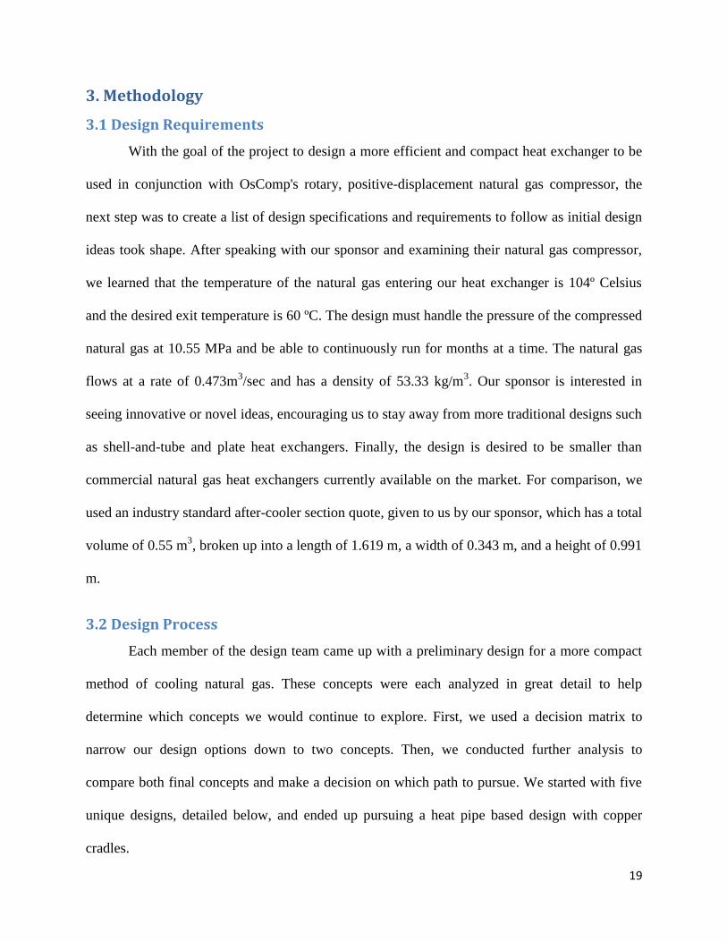
Figure 19: Cradle (ideal)
Our original design, illustrated above in Figure 19, was designed for curved heat pipes
and to minimized weight. We discovered that the heat pipes could not be bent the way we
wanted and had to change the design to utilize straight heat pipes. The design was also changed
to minimize manufacturing time as opposed to weight. These changes resulted in the final design
shown below in Figure 20. Our final design is not the ideal size as the stock was purchased
before the design changes so it was made using 1.5-in square stock instead of 5/8-in square
stock.
Figure 20: Cradle (modified)

33
Each cradle is made of two pieces of 1.5-in square stock and mated around the natural
gas pipes as shown in Figure 20. All the cradles were machined on a HAAS VF4 CNC machine.
There are two different milling methods that we could have tried to make our cradle pieces,
drilling and surfacing. We used the drilling method, which uses only drilling operations, to make
the cradles for our test unit. The other method is surfacing, which slowly removes material off
the surface of the part. Although we did not use this method because it is slower, it could have
allowed us to use fewer drill bits and is slightly more reliable.
There are many challenges to milling copper. The major challenges are that copper is
soft, has a low melting point, and work-hardens. Work-hardening is when a material gets
stronger and more resistant to deformation as it is deformed or worked. This means that any
material removal tool will not last as long as it would with a non-work-hardening material. Due
to those challenges and the costs of copper, it is recommended to look into various forms of
casting. Casting would reduce material waste, and for a full heat exchanger, could greatly reduce
costs.

34
4. Testing
4.1 Heat Pipe Experiments
Figure 21: Heat pipe experimental set-up
In order to verify the capabilities of a heat pipe, we set up an experiment. A sketch of the
set up for our heat pipe experiments, with the heat pipe in a vertical orientation, is shown above
in Figure 21. We filled a beaker with water and placed it on a hot plate. One thermocouple was
placed in the water, while the other thermocouple was attached to the end of a heat pipe. The
heat pipe was then placed in the water, and thermocouple readings were taken for one minute
using a LabView virtual instrument. From these readings, we were able to determine the
temperature drop between the two ends of the pipe. By determining the conduction through the
water, we determined the thermal resistance of the heat pipe.
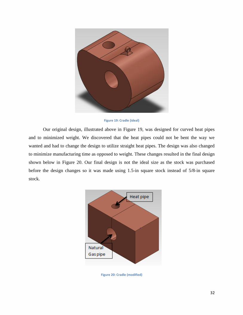
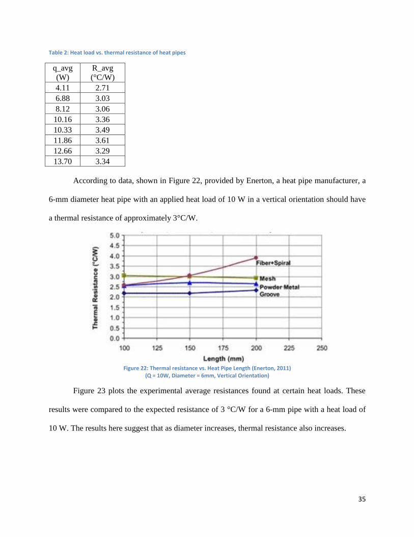
Table 2, shown below, compares the thermal resistances of the 10x140 mm heat pipe
with various applied heat loads.
35
Table 2: Heat load vs. thermal resistance of heat pipes
q_avg
(W)
R_avg
(°C/W)
4.11 2.71
6.88 3.03
8.12 3.06
10.16 3.36
10.33 3.49
11.86 3.61
12.66 3.29
13.70 3.34
According to data, shown in Figure 22, provided by Enerton, a heat pipe manufacturer, a
6-mm diameter heat pipe with an applied heat load of 10 W in a vertical orientation should have
a thermal resistance of approximately 3°C/W.
Figure 22: Thermal resistance vs. Heat Pipe Length (Enerton, 2011)
(Q = 10W, Diameter = 6mm, Vertical Orientation)
Figure 23 plots the experimental average resistances found at certain heat loads. These
results were compared to the expected resistance of 3 °C/W for a 6-mm pipe with a heat load of
10 W. The results here suggest that as diameter increases, thermal resistance also increases.

36
Figure 23: Average heat load vs. thermal resistance of a heat pipe
(Diameter = 10mm, Vertical Orientation)
Figure 24 shows the thermal resistances of the 10 x 140-mm pipe with an average applied
heat load of 10.2 W over a one minute interval. The downward slope suggests that with time, the
thermal resistance of the heat pipe decreased. This trend was consistent throughout each of our
experimental trials. After about 50 seconds, the thermal resistance approached a steady state of
about 3°C/W.
Figure 24: Thermal resistance over time
0.00
0.50
1.00
1.50
2.00
2.50
3.00
3.50
4.00
0.00 5.00 10.00 15.00
Resistance (°C/W)
Heat Load (W)
Experimental Data (Diameter = 10mm
Enerton = 6mm
0
0.5
1
1.5
2
2.5
3
3.5
4
4.5
0 10 20 30 40 50 60
Resistance (°C/W)
Time (s)

37
4.2 Scale Model Experiments
Due to the availability of fluid sources, limited access to manufacturing facilities, and
time constraints, a full-scale cooler could not be produced. We constructed a demonstrator to test
the cooling capacity for a small section of pipe to compare to the full-scale cooler.
Figure 25: CAD model of demonstrator
4.2.1 Assembly of Demonstrator
The following steps were used to construct the demonstrator:
1. Steel piping with a diameter of 5/8 inches was used to carry the hot fluid.
2. 90° elbow pipe connections were used to attach two piping segments for a parallel flow,
and T-style pipe connections were attached between the parallel pipe segments to divide
and later combine the inlet and outlet flows for the demonstrator.
3. The length of the demonstrator was 41 ½ in (including the 90° elbow connections on each
end).
4. Fourteen copper cradles (shown in Figure 18 above) (two pieces each) were
manufactured to attach the heat pipes to these steel pipes.
5. Thermal grease was applied between the steel pipes and these copper cradles as well as
between the heat pipes and the cradles to improve heat transfer in these regions.

38
6. The spacing between cradles along the sections of the cooler ranged from 2 inches to 4 ½
inches, and the two cradle pieces for each were clamped together around the steel pipe to
hold them in place.
Diagrams of the demonstrator cradle layouts are shown in Figure 26 and Figure 27 below.
The initial tests consisted of 7 heat pipes and cradles in total, while 14 heat pipes and cradles
were used for the tests after additional cradles were manufactured. Figure 26 shows the
demonstrator arrangement with 7 cradles and heat pipes (all dimensions in inches), while Figure
27 shows the demonstrator arrangement with 14 cradles and heat pipes.
Figure 26: 7 Cradle Demonstrator Layout
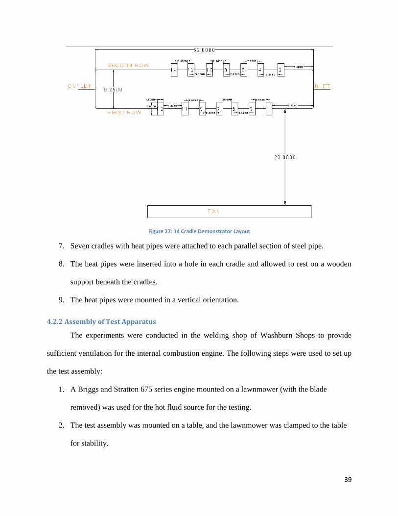
39
Figure 27: 14 Cradle Demonstrator Layout
7. Seven cradles with heat pipes were attached to each parallel section of steel pipe.
8. The heat pipes were inserted into a hole in each cradle and allowed to rest on a wooden
support beneath the cradles.
9. The heat pipes were mounted in a vertical orientation.
4.2.2 Assembly of Test Apparatus
The experiments were conducted in the welding shop of Washburn Shops to provide
sufficient ventilation for the internal combustion engine. The following steps were used to set up
the test assembly:
1. A Briggs and Stratton 675 series engine mounted on a lawnmower (with the blade
removed) was used for the hot fluid source for the testing.
2. The test assembly was mounted on a table, and the lawnmower was clamped to the table
for stability.

40
3. The muffler of the engine was removed to improve flow, and a fitting was welded to
attach the engine exhaust (at 7/8 inches) to the demonstrator inlet (at 5/8 inches).
4. A wooden frame was built to support the demonstrator piping sections during the
experiments.
5. A 3-foot diameter Utilitech industrial fan (Model Number HVD-36A), operated on the
“Low” setting, was placed 23 inches away from the demonstrator to match the air flow
velocity (approximately 4.5 mph) of the full-scale cooler.
(120V AC 60 Hz 3.8A 420W)
The final demonstrator setup is shown in Figure 28 below. Additional pictures of the
demonstrator setup may be found in Appendix E - Experimental Setup Pictures.
Figure 28: Final Demonstrator

41
4.2.3 Experimental Setup
1. The computer software LabView was used to create a data acquisition instrument for the
test. Screenshots of the software setup may be found in Appendix F - LabView Setup for
Data Acquisition.
2. Samples were taken at a rate of 6 Hz.
3. 11 Type-K thermocouples were mounted along the test apparatus to measure temperature
changes
a. 1 thermocouple was mounted at the engine exhaust to measure the temperature at
the cooler inlet. This thermocouple could not be soldered because the
temperatures at the exhaust were high enough to melt the solder, so the leads were
twisted together to form a connection.
b. 1 thermocouple was mounted at the demonstrator outlet after the flows were
combined.
c. 7 thermocouples were mounted on the bases of heat pipes on alternating cradles.
d. 1 thermocouple was mounted at the top of the second heat pipe in the row closest
to the fan.
e. 1 thermocouple was mounted at the top of the final heat pipe in the second row.
4. 1 Hedland (MFG H671A-150) flow meter was mounted on the demonstrator outlet to
measure the flow rate through the demonstrator.
4.2.4 Scaling Procedure
After performing our experiments, we needed to interpret our results and determine how
to compare them with the full scale cooler model. Essentially, we must know the requirements
needed for our model to able to cool natural gas to a desired temperature. We developed a

42
method in which we can determine the length of the natural gas pipe and the number of heat
pipes that would be necessary in order to effectively cool the gas to a temperature of 60°C.
1. First, we ran each experiment using our demonstrator and evaluate the average change in
temperature ( ) between the beginning and the end of the pipe. We also determined a density
for the fluid from the inlet temperature. Flow rate for the working fluid and the air across the fins
will remain constant throughout the entire experiment.
2. Using our thermal resistance model, we calculated the total thermal resistance of the
demonstrator using exhaust properties. This thermal resistance was called .
3. Next, we applied the same thermal resistance model to our full scale analytical model. The
length and number of heat pipes were changed in the calculation to match the parameters
determined from our analytical model. The resulting thermal resistance was labeled as .
4. To compare the theoretical and experimental heat loads, we created a ratio R in which
. This ratio will allow a comparison between the thermal resistance from the
demonstrator and our analytical model.
5. We then calculated the thermal resistance for our demonstrator once again, only this time, we
used the parameters of natural gas as the hot fluid. This resistance was named .
6. Using the ratio R, which was previously calculated, we found the thermal resistance that
would be required for a full size model to be able to cool the natural gas. This final thermal
resistance was called , and was solved using the equation .
7. Two of the variables associated with our thermal resistance model that we can control are the
total length of the cooler and the number of heat pipes being used. We created a table comparing
both values, analyzed their effect on the total thermal resistance, and then found the minimum

43
values which can yield the proper change in temperature. The appropriate length and number of
heat pipes were arranged in a fashion so the size and footprint of the cooler would be minimized.

44
5. Analysis
5.1 Performance
Eight different experiments were performed using our demonstrator, with engine exhaust
from a lawnmower as our hot fluid. Each experiment had variations in number of heat pipes and
cradles, type of convection (free or forced), flow rate, and time duration. The eight different
experiments run with the demonstrator were:
1. Without heat pipes and with the fan off (free convection)
2. Without heat pipes and with the fan on (forced convection)
3. With 7 heat pipes and with the fan off
4. With 7 heat pipes and with the fan on
5. With 7 heat pipes, the fan off, an increased flow rate
6. With 14 heat pipes and with the fan off
7. With 14 heat pipes and with the fan on
8. With 14 heat pipes and with the fan on over a long duration
The long-duration test was run for 33 minutes, while the rest were run for approximately 7-8
minutes. Flow rate, measured at 0.002 m³/s, was kept constant for all tests except one in which
the throttle was adjusted to increase the flow rate. The throttle was adjusted, but the flow meter
used was unable to measure the flow and failed catastrophically, likely due to the highly
unsteady flow produced by the lawnmower at this higher flow rate.
5.1.1Temperature Profiles
For the six experiments which were run with heat pipes, thermocouples were utilized to
gain a temperature profile across the cooler. For the 7 heat pipe set up, a thermocouple was
placed on every cradle, and additional thermocouples were attached to two of the heat pipes.
This allowed us to monitor how the heat pipes were performing. For the 14 heat pipe set up, a
45
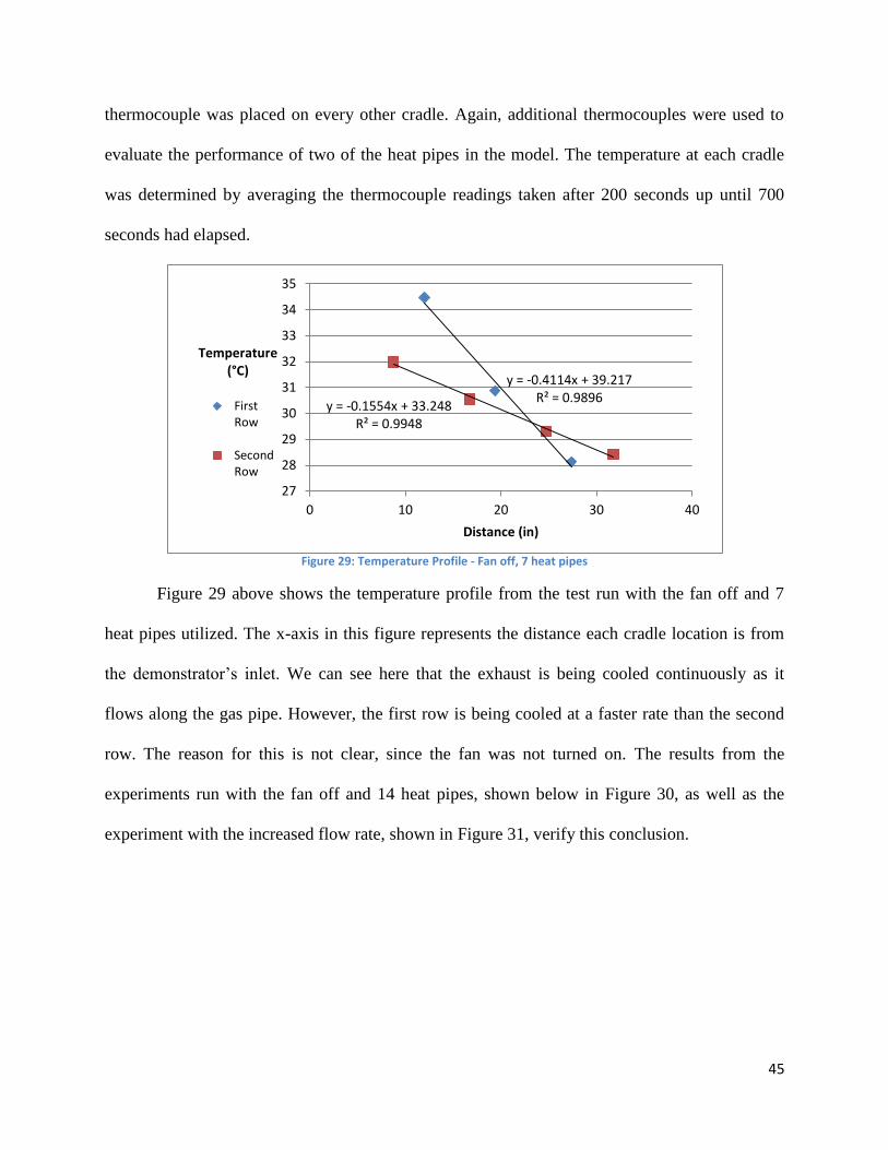
thermocouple was placed on every other cradle. Again, additional thermocouples were used to
evaluate the performance of two of the heat pipes in the model. The temperature at each cradle
was determined by averaging the thermocouple readings taken after 200 seconds up until 700
seconds had elapsed.
Figure 29: Temperature Profile - Fan off, 7 heat pipes
Figure 29 above shows the temperature profile from the test run with the fan off and 7
heat pipes utilized. The x-axis in this figure represents the distance each cradle location is from
the demonstrator’s inlet. We can see here that the exhaust is being cooled continuously as it
flows along the gas pipe. However, the first row is being cooled at a faster rate than the second
row. The reason for this is not clear, since the fan was not turned on. The results from the
experiments run with the fan off and 14 heat pipes, shown below in Figure 30, as well as the
experiment with the increased flow rate, shown in Figure 31, verify this conclusion.
y = -0.4114x + 39.217 R² = 0.9896
y = -0.1554x + 33.248 R² = 0.9948
27
28
29
30
31
32
33
34
35
0 10 20 30 40
Temperature (°C)
Distance (in)
First Row
Second Row

46
Figure 30: Temperature Profile - Fan off, 14 heat pipes
Figure 31: Temperature Profile - Fan off, 7 pipes, increased flow rate
For the first and second row, the temperatures and slopes in Figure 30 are close, which
was what we expected. When the flow rate was increased, temperature profile in Figure 31 is
opposite to that of Figure 29, with the second row experiencing a sharper decrease in
temperature. Also, the temperatures with the increased flow rate were higher than the
experiments at lawnmower’s normal flow rate.
As we turned the fan on for the tests, we expected that the temperature profile for the first
row would be lower than the profile for the second row, since the first row is closer to the fan.
y = -0.2836x + 38.992 R² = 0.825
y = -0.1465x + 33.579 R² = 0.8782
25
27
29
31
33
35
37
0 10 20 30 40
Temperature (°C)
Distance (in)
First Row
Second Row
y = -0.058x + 40.904 R² = 0.7761
y = -0.3478x + 43.6 R² = 0.8117
31
33
35
37
39
41
43
0 10 20 30 40
Temperature (°C)
Distance (in)
First Row
Second Row

47
However, the first test ran with the fan on, which featured 7 heat pipes, did not exhibit any
significant temperature changes between the two rows until the exhaust reached the end of the
pipe, where, contrary to what was expected, the second row experienced the drop in temperature.
These results are shown below in Figure 32.
Figure 32: Temperature Profile: Fan on, 7 heat pipes
When the same test was run with 14 heat pipes, the difference in temperature that we
were anticipating was experienced. The results for this experiment are shown below in Figure 33.
Figure 33: Temperature Profile: Fan on, 14 heat pipes
y = -0.0293x + 31.326 R² = 0.8642
y = -0.2151x + 33.948 R² = 0.8881
25
26
27
28
29
30
31
32
33
0 10 20 30 40
Temperature (°C)
Length (in)
First Row
Second Row
y = -0.1222x + 33.39 R² = 0.7654
y = -0.5858x + 48.989 R² = 0.9756
25
27
29
31
33
35
37
39
41
0 10 20 30 40
Temperature (°C)
Length (in)
First Row
Second Row

48
Overall, the results from the experiments with 7 heat pipes were inconsistent and led to a
lot of uncertainty. The results from the experiments with 14 heat pipes were more consistent, like
the ones in Figure 30 and Figure 33, and therefore more meaningful.
The temperature profile for the long duration test is shown below in Figure 34. This
temperature profile was significant because it best showed the difference the fan has on cooling.
The temperatures for the first row were, on average, about 6°C cooler than the temperatures for
the second row. The averages were taken after 200 second up until 33 minutes had elapsed.
Figure 34: Temperature Profile - Fan on, 14 heat pipes, long duration (33 minutes)
5.1.2 Heat Pipe Performance
For each experiment that included heat pipes, two heat pipes were hooked up to
thermocouples. For these two heat pipes, one thermocouple was attached to the base of the heat
pipe, while the other was attached to the top of the heat pipe. The intent is to determine the
performance of the heat pipes and observe how much heat they remove from the exhaust. From
the temperature readings, we were able to see how the heat pipes performed under the variety of
conditions provided in our tests. For the 7 heat pipe demonstrator, temperature readings were
taken from Heat Pipes 1 and 3 (refer to Figure 26). For the 14 heat pipe demonstrator,
temperature readings were taken from Heat Pipes 3 and 14 (refer to Figure 27).
y = -0.1222x + 33.39 R² = 0.7654
y = -0.1927x + 41.374 R² = 0.6952
25
27
29
31
33
35
37
39
41
0 10 20 30 40
Temperature (°C)
Length (in)
First Row
Second Row

49
Figure 35 shows the performance of Heat Pipe 1 during the three experiments ran with
the 7 heat pipe demonstrator. The performance of Heat Pipe 3 is shown in Figure 36. In general,
Heat Pipe 3 experienced a larger temperature difference, implying that the heat pipes at the end
of the demonstrator remove more heat.
Figure 35: Temperature Change across heat pipe 1 for the 7 heat pipe demonstrator
Figure 36: Temperature Change across heat pipe 3 for the 7 heat pipe demonstrator
Figure 35 and Figure 36 also suggest that as the base temperature of the heat pipe
increases, the temperature change across the heat pipe increases. To better evaluate the
0
1
2
3
4
5
6
7
8
9
10
Temp Change (°C)
no fan with 7 heat pipes (Base Temp = 34.5 degC)
with fan and with 7 heat pipes (Base Temp = 30.9 degC)
no fan, with 7 heat pipes, adjusted throttle (Base Temp = 40.1 degC)
0
2
4
6
8
10
12
Temp Change (°C)
no fan with 7 heat pipes (Base Temp = 28.1 degC)
with fan and with 7 heat pipes (Base Temp = 30.5 degC)
no fan, with 7 heat pipes, adjusted throttle (Base Temp = 39.2 degC)
50
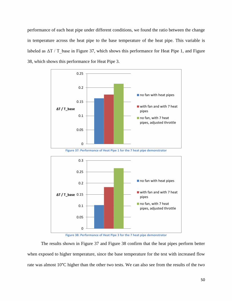
performance of each heat pipe under different conditions, we found the ratio between the change
in temperature across the heat pipe to the base temperature of the heat pipe. This variable is
labeled as ΔT / T_base in Figure 37, which shows this performance for Heat Pipe 1, and Figure
38, which shows this performance for Heat Pipe 3.
Figure 37: Performance of Heat Pipe 1 for the 7 heat pipe demonstrator
Figure 38: Performance of Heat Pipe 3 for the 7 heat pipe demonstrator
The results shown in Figure 37 and Figure 38 confirm that the heat pipes perform better
when exposed to higher temperature, since the base temperature for the test with increased flow
rate was almost 10°C higher than the other two tests. We can also see from the results of the two
0
0.05
0.1
0.15
0.2
0.25
ΔT / T_base
no fan with heat pipes
with fan and with 7 heat pipes
no fan, with 7 heat pipes, adjusted throttle
0
0.05
0.1
0.15
0.2
0.25
0.3
ΔT / T_base
no fan with heat pipes
with fan and with 7 heat pipes
no fan, with 7 heat pipes, adjusted throttle
51
experiments run with the regular flow rate that the heat pipes appear to perform slightly more
effectively with the fan turned on.
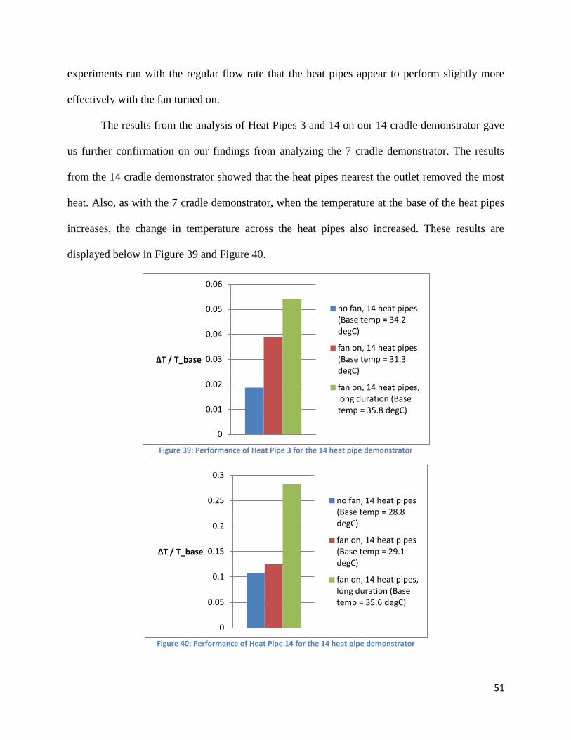
The results from the analysis of Heat Pipes 3 and 14 on our 14 cradle demonstrator gave
us further confirmation on our findings from analyzing the 7 cradle demonstrator. The results
from the 14 cradle demonstrator showed that the heat pipes nearest the outlet removed the most
heat. Also, as with the 7 cradle demonstrator, when the temperature at the base of the heat pipes
increases, the change in temperature across the heat pipes also increased. These results are
displayed below in Figure 39 and Figure 40.
Figure 39: Performance of Heat Pipe 3 for the 14 heat pipe demonstrator
Figure 40: Performance of Heat Pipe 14 for the 14 heat pipe demonstrator
0
0.01
0.02
0.03
0.04
0.05
0.06
ΔT / T_base
no fan, 14 heat pipes (Base temp = 34.2 degC)
fan on, 14 heat pipes (Base temp = 31.3 degC)
fan on, 14 heat pipes, long duration (Base temp = 35.8 degC)
0
0.05
0.1
0.15
0.2
0.25
0.3
ΔT / T_base
no fan, 14 heat pipes (Base temp = 28.8 degC)
fan on, 14 heat pipes (Base temp = 29.1 degC)
fan on, 14 heat pipes, long duration (Base temp = 35.6 degC)

52
5.1.3 Cooling Performance
The ultimate goal of the demonstrator is to cool the exhaust passed through it. For each
test, an average outlet temperature was averaged over the 200s to 700s time interval (with the
exception of the long duration trial, in which the outlet temperature was averaged from 200s to
the full 33 minutes). These calculations are found below in Table 3, arranged from the highest to
lowest temperature. The average inlet temperature for the experiments was 420.9°C.
Table 3: Outlet temperature for each experiment
EXPERIMENT OUTLET (°C)
increased flow rate 131.8
7 heat pipes, no fan 47.7
no heat pipes, no fan 44.9
no heat pipes, with fan 42.4
7 heat pipes, with fan 38.4
long duration 28.9
14 heat pipes, no fan 26.7
14 heat pipes, with fan 24.6
The first conclusion that can be reasoned from these results is that increasing the flow
rate of the hot fluid will decrease the cooler’s ability to cool the fluid. This is logical, as the
faster the fluid moves, the less time it will have to be exposed to the heat pipes and convection
across the pipes. Speaking of convection, another inference that we can make is that forced
convection slightly improves the cooler’s performance. On average, the addition of the fan
lowered outlet temperature by 4.6°C. The most significant conclusion we can draw here is that as
the number of heat pipes increase, the cooler performance also increases, a conclusion which we
expected to be able to make.
5.1.4 Scaling Analysis
The final step in the analysis of our data was to scale our results to determine the
minimum length and number of heat pipes our design must feature in order to sufficiently cool

53
the natural gas. The gas must be cooled from 105°C to 60°C, a change in temperature of 45°C (or
45 K). Table 4 below shows a comparison between results calculated with our analytical model,
our scaled experimental results, and the industry standard for natural gas coolers. The
calculations used for our analytical model analysis are shown in Appendix G.3 Cradle Heat Pipe
Design Analysis, the calculations for our scaled experiment are shown in Appendix G.2 Scaling
Calculations, and the properties used to make such calculations are listed in Appendix B –
Properties Used.
Table 4: Scaling Analysis
Analytical Model Scaled Experiment Industry Standard
Length (m) 64 42 Could not be determined
Number of Heat Pipes 419 275 N/A
Footprint (m²) 0.871 0.871 1.1
Volume (m³) 2.084 1.445 1.1
From our scaling analysis, we were able to shorten our cooler length by 34%, decrease
the number of heat pipes by 34%, and shrink the cooler’s volume by 31%, in comparison to our
analytical model. The footprint remained the same because, as with the analytical model, there
would be three columns of tubes, with the tubes remaining at a length of 5 feet. We will also
keep the same distance between the heat pipes. However, with this arrangement, we would be
able to decrease the height of the cooler. A possible reason for the overestimate in our analytical
model may be because we neglected the convective heat transfer from the gas and heat pipes.
5.1.5 Demonstrator Analytical Analysis
In order to support and verify our demonstrator’s data, we constructed an analytical model of
the demonstrator to compare the experiment’s results against. To provide the most accurate
comparison as possible, we focused on the 14 heat pipes experiment with the fan running and
defined certain variables such as:

54
Number of heat pipes = 14
Number of fins on each heat pipe = 18
Measured distance of the setup
Inlet and outlet temperature of the experiment = 420.9 C and 24.6 C respectively
Specific Heat of engine exhaust = 1.327 kJ/kg*K
Thermal Conductivity of engine exhaust = 0.034 W/m*K
Viscosity of engine exhaust = 2.17x10⁻⁵
kg/m*s
Molecular Weight of engine exhaust = 30 g/mol
These defined variables allowed us to construct a model which would tell us two things, the
required maximum resistance of the demonstrator for this experiment, and the calculated
resistance of the demonstrator. To calculate the maximum required resistance of the
demonstrator involved defining the number of fins and their size, the number of heat pipes, the
entrance and exit temperature of the demonstrator and the overall size and dimensions.
Calculating the conductive and convective resistance through the demonstrator gave us the
required resistance of 60.035 K/W. To find the calculated resistance of the demonstrator, we
defined the specifications of the test engine and the fan, such as the flow rate, the specific heat of
the engine exhaust, the viscosity, and the thermal conductivity of the exhaust. Solving for the
thermal resistance of the complete system resulted in a calculated resistance of 62.61 K/W. By
comparing these two resistances, we can gauge the accuracy of the experimental data against the
analytical data, and thus verify the accuracy of the full model analysis. If the analytical model of
the demonstrator were completely accurate, then the required maximum resistance and the
calculated resistance would be equivalent. As such, this means that there is an error of 4.11%
between the experiment’s data and the analytical model’s results. Refer to Appendix G.4
Demonstrator Analytical Analysis for the full calculation.

55
5.2 Cost
Based on the sizing calculated for our scaling model, a full heat exchanger unit would
cost an estimated $27,725 if made using the drilling method, and $32,593 if made using the
surfacing method. These estimates assume a machinist rate of $100 per hour. The materials cost
is $15,230. The machining time for the cradles requires 109 hours for drilling, and 166 hours for
surfacing. The time is the deciding factor between which method is more expensive. However,
both methods are more expensive than the competitor quote of $24,269. These cost estimates are
based on the two milling methods we explored. It is likely that using casting would reduce the
overall manufacturing cost making it more competitively priced. Table 5 below shows the full
breakdown of the equipment and materials costs of these two methods. Refer to Appendix C -
Budget for a complete breakdown of the project budget.
Table 5: Equipment and materials cost breakdown
Cost Category Drilling Surfacing
Equipment 8mm drill bits $157.96 $157.96
5/8in drill bits $999.46 N/A
#7 drill bits $25.95 $25.95
10-24 tap $523.25 $523.25
1/4 ball EM N/A $101.29
3/16 EM N/A $81.48
Total $1,706.62 $889.93
Materials Copper $947.92 $947.92
Steel Pipe $845.88 $845.88
Connectors $3,843.84 $3,843.84
Heat Pipes $9,465.75 $9,465.75
Screws $24.99 $24.99
Total $15,128.38 $15,128.38
Total $16,835.00 $16,018.31

56
6. Conclusions
From our scaling analysis, we were able to conclude that our model will have a
significantly smaller footprint (21.5%) compared to the current cooler on the market. This proves
that the design is a viable solution for OsComp Systems. However, we would recommend
conducting further experiments with the following considerations to further validate our findings.
The ventilation fan in the welding lab appeared to be much stronger than the flow rate
presented by our fan. This may explain why the fan had an insignificant effect on the cooler
performance. This judgment was simply made by comparing to the strengths of the fans by
placing our hand close to the duct and behind the fan we used in our experiment. Due to WPI’s
safety regulations, we were required to have the ventilation fan on at all times during the
experiments. This means that we cannot accurately estimate the effect of the forced convection
on the system.
An additional conclusion we can draw here is that as the number of heat pipes increase,
the cooler performance also increases, a conclusion which we expected to be able to make.
Simply stated, the increase in the number of cradles and heat pipes allowed for more heat to be
removed from the exhaust.

57
7. Recommendations
7.1 Heat Pipe Selection
There are many factors that affect the performance of a heat pipe. The material, working
fluid, and wick structure should remain the same for this application, which is copper, water, and
sintered powder metal. However, there are additional parameters that could be adjusted to yield a
higher performance. Increasing the diameter of the heat pipe would allow for greater power
carrying capacity. Increasing the lengths of the evaporator and condenser regions would also
improve the heat removal capabilities since this would increase the surface area for the heat to
pass through and dissipate.
A heat pipe performs at its best when gravity is assisting the device. Therefore, we
recommend the heat pipes stay at 90 degrees, which is in the vertical position with respect to the
ground. Also, a higher operating temperature will allow a greater maximum heat removal from
the system. We also recommend keeping the heat pipe completely straight. Although heat pipes
can still function with bends, this decreases the performance of the device and could bring about
leakage problems.
Lastly, we recommend looking into the fin analysis further. Our calculations were based
on the fundamental equations found in any heat transfer textbook; refer to Appendix G.1 Fin
Analysis and Optimization. However, they seem a little too small compared to the typical heat
sinks on the market. We would recommend increasing the length and width of the fins as long as
the efficiency is greater than 70%. The fin thickness and spacing should remain the same, as they
reflect the industry standard. The number of fins required per heat pipe is dependent on the
length of the condenser region and would therefore be adjusted accordingly.

58
7.2 Manufacturing
Casting the cradles instead of milling them may reduce equipment cost. It will also
reduce material use, as less material will be thrown out as chips. It also means the material can
be bought in the cheapest form not as the appropriately sized stock. Finally it will be easier to get
a better weight balance with casting as curved sections do not significantly increase production
difficulty.
Since copper is a soft material, it is possible that the threads on the inside of our design
will pull out during practical use. If that is an issue, helicoils could be installed in the holes, or
the holes could be changed to through holes and have a nut on the other side. However, we
would also recommend looking into other materials for the cradle pieces, possibly a grade of
aluminum. Copper was chosen for its strong heat transfer properties but is not an ideal metal to
machine.
7.3 Conducting Experiments
Since compressed natural gas is not a safe fluid to work with in an academic setting, we
were forced to seek alternative heat sources. However, using CNG would yield more accurate
results. The % error would be reduced since the calculations to scale the properties of engine
exhaust to CNG would no longer be required in the analysis. We would also recommend using a
more consistent fluid source, in terms of its flow rate. The lawnmower engine we used to
conduct our experiments has a pulsing flow, which doesn’t reflect the ideal conditions for our
application.
The unsteadiness in the flow turned out to be stronger than we anticipated, introducing
substantial vibrations into the system. Adding fixtures, such as brackets, to securely mount the
steel pipes and heat pipes to the base support would reduce this effect. Also, using a higher

59
quality flow meter would yield more accurate results. Between the intermittent flow rate and the
vibrations present in the system, our flow meter failed shortly after our initial experiments.
Lastly, increasing the size of the scale model would give a better indication of the
cooler’s performance. Having additional sections, steel pipes with heat pipes mounted onto them,
would allow for the stacking and masking effects to be tested. These alternative test setups would
be critical in testing the design further.

60
8. References
Atlas Copco 2010, Compressed Air Manual, Atlas Copco Airpower NV, Belgium.
Avallone, E.A., Baumeister, T. & Sadegh, A.M. 2007, Marks' Standard Handbook for
Mechanical Engineers, 11th edn, McGraw-Hill. Chapter 19.
Cengel, Y.A., Turner, R.H. & Cimbala, J.M. 2008, Fundamentals of Thermal-Fluid Sciences, 3rd
edn, McGraw-Hill, New York, NY.
Cesco. 2011. “All-welded Spiral Heat Exchangers”. Retrieved on October 2011 from
http://www.gocesco.com/all_weldedspiralheatexchangers.html.
Choi Mun-cheol. 2005. Capillary pumped loop system. Retrieved October 5, 2011 from
http://www.google.com/patents?hl=en&lr=&vid=USPAT6880625&id=4t8TAAAAEBAJ
&oi=fnd&dq=Capillary+pumped+loop+system&printsec=abstract#v=onepage&q&f=fals
e
Enerton. 2011. “Designing with Heat Pipes” Retrieved on January 2011 from
http://www.enertron-inc.com/enertron-products/heat-pipe-design.php.
Gilmore, D.G. Spacecraft Thermal Control Handbook, Volume 1 - Fundamental
Technologies (2nd Edition), American Institute of Aeronautics and
Astronautics/Aerospace Press.
Kazama, T. & Totten, G. 2006, "Compressors and Vacuum Pumps" in Handbook of Lubrication
and Tribology CRC Press, pp. 1-61.
Nellis, G. & Klein, S. Heat Transfer, Cambridge University Press. 2009. Chapter 8.
Available:http://www.knovel.com/web/portal/browse/display?_EXT_KNOVEL_DISPL
AY_bookid=3703
Shah, R.K., Sekulić, & , D.P. Fundamentals of Heat Exchanger Design, John Wiley & Sons.
2003. Chapter 1. Available:http://www.knovel.com/web/portal/browse/display?
_EXT_KNOVEL_DISPLAY_bookid=3007
Snake Creek Lasers. 2011. “Laser Subcomponents”. Retrieved on October 2011 from
http://www.snakecreeklasers.com/products/laser-subcomponents.aspx
TE Technology, Inc. 2010. “How does a thermoelectric module work?” Retrieved on
October 2011 from http://www.tetech.com/FAQ-Technical-Information.html.
Thermacore. 2009. “Heat Exchangers and System Level Cooling Products”. Retrieved on
October 2011 from http://www.thermacore.com/documents/system-level-cooling-
products.pdf.
"Wet compression adds power, flexibility to aeroderivative GTs", 2005; Power, vol. 149, no. 4,
pp. 52-52.

61
Appendices
Appendix A - Authorship
Section Peer Reviewers Abstract Team Team
1, 3.2.1, 3.4, 5.2 Jess Calvin & Brad
2.1, 3.2.0,4,8, 4.1, 4.2.4, 5.1 Brad Andy & Chris
2.2, 3.2.3, 4.2.0-3 Andy Chris & Jess
2.3, 3.2.5-7, 6, 7 Chris Jess & Calvin
2.4, 3.1, 3.2.2, 3.3, 5.1.5 Calvin Brad & Andy
Appendix B – Properties Used
The following assumptions were made in our calculations and analysis of our designs:
CNG pipes:
- Material: Aluminum alloy 2024
- 100% heat transfer efficiency from CNG pipes to heat pipes
- Used only for cooling CNG
- Thermal conductivity: 143 W/m*K
Air Properties:
- Density = 1.185 kg/m³
- Specific Heat = 1.005 kJ/kg*K
- Viscosity = 1.983x10⁻⁵
kg/m*s
CNG Properties:
- Density = 53.334 kg/m³
- Flow rate = 0.473 m³/s
- Specific Heat = 2.26 kJ/kg*K
- Thermal Conductivity = 0.035 W/m*K
- Viscosity = 1.1x10⁻⁵
kg/m*s
- Molecular Weight = 16.044 g/mol
Exhaust Properties:
- Specific Heat = 1.327 kJ/kg*K
- Thermal Conductivity = 0.034 W/m*K
- Viscosity = 2.17x10⁻⁵
kg/m*s
- Molecular Weight = 30 g/mol

62
Appendix C - Budget
Table 6: Project Budget
Vendor Quantity Item Individual Price Total Price
Enertron 2 Heat Pipes 26.82 53.64
MSC Direct 1 Copper Bar, 7ft 669.01 669.01
MSC Direct 1 Screws, box of 100 31.38 31.38
OnlineMetals 2 Steel Rod, 5ft 30.21 60.42
MSC Direct 1 Copper Bar, 1ft 114.21 114.21
MSC Direct 1 Male Connector 24.28 24.28
MSC Direct 1 Thermalcouple wire 89.97 89.97
MSC Direct 1 Flowmeter 318.52 318.52
Northern Tools 1 Motor (Returned S&H) 20 20
Aavid Thermalloy 15 Heat Pipes w/ fins 54.09 811.35
MSC Direct 6 Jobber Drill Bits 3.59 21.54
MSC Direct 2 Thermal Paste, 8oz tube 27.3 54.6
MSC Direct 4 Flute Taps 14.75 59
McMaster-Carr 4 5/8" 90 degree elbows 21.89 87.56
McMaster-Carr 2 5/8" T-connectors 26.62 53.24
McMaster-Carr 1 1" to 1/2" reducer 90.41 90.41
McMaster-Carr 1 1/2" to 5/8" reducer 37.76 37.76
OnlineMetals 1 1" OD pipe , 1ft 13.2 13.2
OnlineMetals 1 1/2" OD pipe, 1ft 5.08 5.08
OnlineMetals 1 5/8" OD pipe, 2ft 15.26 15.26
MSC Direct 6 5/8in Jobber Drill Bits 23.68 142.08
MSC Direct 4 5/8in Drill Bits 28.71 114.84
MSC Direct 3 5/8in TG collet 24.69 74.07
Total Price 2961.42

63
Appendix D - CAD Drawings and Pictures
Figure 41: Preliminary design model, using heat pipe concept
Figure 42: Preliminary design drawing, using heat pipe concept

64
Figure 43: Preliminary demonstrator model
Figure 44: Cradle drawing

65
Figure 45: Demonstrator drawing

66
Appendix E - Experimental Setup Pictures
Figure 46: Close up picture of heat pipe
Figure 47: Securing copper for machining

67
Figure 48: Exhaust outlet connecting to cooler
Figure 49: Final setup of demonstrator 1

68
Figure 50: Final setup of demonstrator 2

69
Appendix F - LabView Setup for Data Acquisition
Figure 51: LabView Virtual Instrument
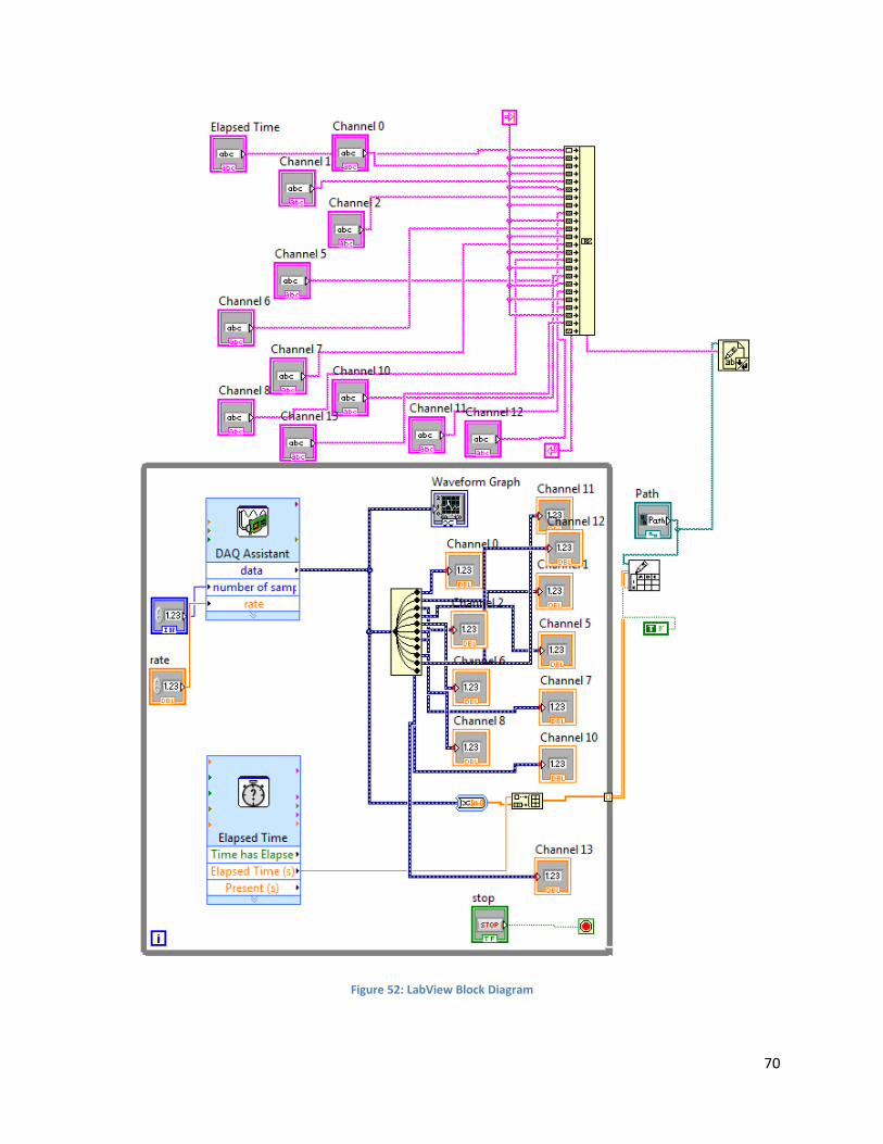
70
Figure 52: LabView Block Diagram

71
Appendix G - Mathcad Calculations
G.1 Fin Analysis and Optimization
d 8mm diameter of heat pipe
L1 2cm Length of fin
w 2.5cm width of fin
t 0.4mm thickness of fin
Tb 150°C 423.15K Base temp of the fin
thermal conductivity of fin (aluminum, pure @ 150C, which is 300F)
http://www.engineeringtoolbox.com/thermal-conductivity-metals-d_858.html k 134W
m K
Tinfinity 50°C 323.15K Temp. of the fluid (air)
h 100W
m2
K
Convection coefficient of fluid (air)
a) convection heat transfer
b Tb Tinfinity 100K P 2 w 2 t fin perimeter
Ac w t cross sectional area of fin
Af P L1 2d
2
2
2w t surface area of the fin
M h P k Ac b 8.251W
Fin parameters
m12 h( )
k t61.085
1
m
qf M
sinh m1 L1 h
m1 k
cosh m1 L1
cosh m1 L1 h
m1 k
sinh m1 L1
6.961W Fin heat transfer rate
f
qf
h Af b 0.744
fin efficiency
f
qf
h Ac b69.611 fin effectiveness
Rtf
b
qf
14.366K
W thermal resistance of fin
T1 b1
cosh m1 L1 h
m1 k
sinh m1 L1
Tinfinity 376.834K temp. at the tip of fin

72
Table 7: Fin Optimization 1
Given Data: diameter of heat pipe 8 mm
Length of heat pipe 150 mm thickness of fin 0.4 mm fin spacing
2.5 mm
Assumptions: Fin material aluminum, pure
thermal conductivity of fin (k) 134 W/mK http://www.engineeringtoolbox.com/thermal-conductivity-metals-d_858.html convection coeffcient of fluid (h) 100 W/m^2K
Base Temp (T.b) 150 C Temp. of fluid (air - T.infinity) 50 C forced convection
Length of condenser region 60 mm Length of evaporator region 45 mm Number of fins 20
Lc/(spacing+thickness)
Variables: Length of fin Width of fin
Table 8: Fin Optimization 2
Length (cm)
Width (cm) Efficiency Effectiveness
2 1 0.871 70.428 2 1.25 0.824 70.157 2 1.5 0.796 69.975
Potential fin arrangements, above line (>70% efficiency) 2.25 1 0.785 73.66
2 1.75 0.777 69.845 2 2 0.763 69.748 2 2.25 0.752 69.672 2.25 1.25 0.749 73.376 2 2.5 0.744 69.611 2 2.75 0.738 69.561 2 3 0.732 69.52 2.25 1.5 0.726 73.186 2.5 1 0.712 76.13 2.25 1.75 0.711 73.05 2.25 2 0.7 72.948
2.25 2.25 0.692 72.869 2.25 2.5 0.685 72.805

73
2.5 1.25 0.684 75.836 2.25 2.75 0.68 72.753 2.25 3 0.676 72.71 2.5 1.5 0.666 75.64 2.5 1.75 0.654 75.499 2.75 1 0.651 77.999 2.5 2 0.645 75.394 2.5 2.25 0.638 75.312 2.5 2.5 0.633 75.246 2.75 1.25 0.628 77.699 2.5 2.75 0.628 75.192 2.5 3 0.625 75.147 2.75 1.5 0.613 77.498 2.75 1.75 0.603 77.354 3 1 0.598 79.405 2.75 2 0.596 77.246 2.75 2.25 0.59 77.161 2.75 2.5 0.586 77.094 2.75 2.75 0.582 77.039 3 1.25 0.579 79.099 2.75 3 0.579 76.993 3 1.5 0.567 78.895 3 1.75 0.558 78.748 3 2 0.552 78.638 3 2.25 0.547 78.552 3 2.5 0.544 78.484 3 2.75 0.541 78.247 3 3 0.538 78.381
Figure 53: Fin Optimization
0.7
0.75
0.8
0.85
0.9
2 2.25 2.5 2.75 3
Effi
cen
cy
Fin Length (cm)
Fin Length vs. Efficency (>70%)
w=1
w=1.25
w=1.5
w=1.75
w=2
w=2.25
w=2.5
w=2.75

74
G.2 Scaling Calculations
Demonstrator Geometry
Inner Diameter Outer Diameter
Inner Radius Outer Radius
Length
Cross sectional of Area
Surface Area of Pipe
Full Size Model Geometry
Diameter and cross-sectional area is the same
Length
Surface Area
Determining the density of the exhaust gas constant:
Measured Parameters:
Inlet Temperature
Outlet Temperature
Outlet Pressure
Measure Outlet Flow rate
Guess
kJ 1000J
Di 13.386mm Do 15.875mm
ri
Di
26.693 10
3 m ro
Do
27.938 10
3 m
Ldemo 52in 1.321m
Across
4Di
2 1.407 10
4 m
2
ALdemo Di Ldemo 0.056m2
Lfull 64.008m
ALfull Di Lfull 2.692m2
R 8.314J
mol K
T1 402K
T2 29K
P2 101325Pa
FlowSCFM 40ft
3
min0.019
m3
s
1 0.912kg
m3
2 1

75
Standard Pressure
Standard Temperature
True Outlet Flow rate
Inlet Viscosity
Mass flow rate
Inlet Flow rate
Average Density
Average Velocity
Reynolds number
Surface roughness
Friction factor
Friction loss
Inlet Pressure
PStd 101325Pa
TStd 273.15K
Flow2
PStd FlowSCFM T2
P2 TStd2.004 10
3
m3
s
1 2.17105
kg
m s
massflow 2 Flow2 1.828 103
kg
s
Flow1
massflow
1 Across14.242
m
s
avg
1 2
20.912
kg
m3
Vavg
Flow1
Flow2
Across
214.242
m
s
ReD
avg Vavg Di
1
8.012 103
0.015103
m
For ReD 8.012 103
and
Di
1.121 103
f1.325
ln
Di
3.7
5.74
ReD0.9
20.035
hf fLdemo
Di
Vavg
2
2 g 35.358m
P1 hf avg g P2 1.016 105
Pa

76
Inlet Density
Molecular weight
Inlet Density iterate until density matches
Exhaust Characteristics Natural Gas Characteristics
Density
Flow rate
Mass flow rate
Specific Heat
Thermal Conductivity
Viscosity
Prandtl Number
Reynolds Number
Nusselt Number
Convection Coefficient
Change in temp
1mol
P1
R T130.411
mol
m3
MW 0.030kg
mol
1 1mol MW 0.912kg
m3
ex 1 0.912kg
m3
ng 53.334kg
m3
Vex Flow2 2.004 103
m
3
s Vng 0.473
m3
s
mex ex Vex 1.829 103
kg
s mng ng Vng 25.227
kg
s
cpex 1.327kJ
kg K cpng 2.26
kJ
kg K
kex 0.034W
m K kng 0.035
W
m K
ex 1 2.17 105
kg
m s ng 1.110
5
kg
m s
Prex
cpex ex
kex
0.847 Prng
cpng ng
kng
0.71
Reex ReD 8.012 103
Reng
ng Vng Di
Across ng2.181 10
8
Nuex 0.023Reex0.8
Prex0.3
Nung 0.023Reng0.8
Prng0.33
Nuex 29.046 Nung 9.631 104
hex
Nuex kex
Di
73.775W
m2
K
hng
Nung kng
Di
2.518 105
W
m2
K
T ex T1 T2 373K T full 45K

77
Thermal Resistance Model: Demonstrator with exhaust
Convection
Conduction
Number of heat pipes
Number of fins
Heat Pipe Resistance
Fin resistance
Total HP Resistance
Total Resistance
Thermal Resistance Model: Full size model with exhaust
Convection
Conduction
Number of heat pipes
Number of fins
Heat Pipe Resistance
Fin resistance
Rconvex1
hex ALdemo0.244
K
W
Rcondex
lnro
ri
2 Ldemo kex0.604
K
W
nhp 14
nfin 18
Rhp 3K
W
Rfin 12.293K
W
Rfintot
Rfin
nfin
0.683K
W
Rhptotex1
nhp
Rhp
nhp
Rfintot
0.04K
W
Rex Rconvex Rcondex Rhptotex 0.888K
W
Rnohp Rconvex Rcondex 0.848K
W
Rconvfull1
hex ALfull5.036 10
3
K
W
Rcondfull
lnro
ri
2 Lfull kex0.012
K
W
nhpfull 419
nfin 18
Rhp 3K
W
Rfin 12.293K
W

78
Total HP Resistance
Total Resistance
Ratio between demonstrator and full size model
Thermal Resistance Model: Demonstrator with natural gas
Convection
Convection
Number of heat pipes:
Number of fins:
Heat Pipe Resistance
Fin resistance
Total HP Resistance
Total Resistance
RESISTANCE FOR FULL MODEL WITH NATURAL GAS
With 42 meters in length and 275 heat pipes, the thermal resistance of our model would be 0.013 K/W
Rfintot 0.683K
W
Rhptotfull1
nhpfull
Rhp
nhpfull
Rfintot
1.328 103
K
W
Rfull Rconvfull Rcondfull Rhptotfull 0.019K
W
RRex
Rfull
47.155
Rconvng1
hng ALdemo7.149 10
5
K
W
Rcondng
lnro
ri
2 Ldemo kng0.587
K
W
nhpng1 nhp 14
nfin 18
Rhp 3K
W
Rfin 12.293K
W
Rfintot 0.683K
W
Rhptotng1
nhpng1
Rhp
nhpng1
Rfintot
0.04K
W
Rng1 Rconvng Rcondng Rhptotng 0.627K
W
Rngfinal
Rng1
R0.013
K
W

79
G.3 Cradle Heat Pipe Design Analysis
Unit definition
Inside/Outside Diameter of natural gas
Tube
Wall Thickness
Forty-two tubes at 5 ft for 210ft
total. 3 rows of 14 pipes stacked. Total Length of Gas Pipe
Breakdown of Design
Surface area of inside of pipe
inner/outer pipe radius
Temperature of Natural Gas In/Out
Flow Rate of Gas
Gauge pressure of water in heat
pipe
Standard Pressure
Absolute pressure of
water in heat pipe
Gas Constant, Methane
http://www.engineeringtoolbox.com/individual-universal-gas-constant-d_588.html
Standard volumetric flow
rate of gas
Standard Pressure
Standard Temperature
Natural Gas Volume Flow
kJ 1000J
Do 15.875mm 0.625 in Di 13.386mm 0.527 in
Tp 1.27mm 0.05 in
Li 64.008m 210 ft
Ltube 1.524m 5 ft
Wtube .2286m 0.75 ft Htube 2.32932m 7.642 ft
Ain Di Li 2.692m2
ri
Di
26.693mm ro
Do
27.938mm
Tgasin 377.928K Tgasout 333.15K
Flowgas 0.005459m
3
s
Pg 20.265kPa 0.02 MPa
Ps 101.325kPa
Pa Ps Pg 0.122MPa
R 518.3J
kg K
Vscfm 870ft
3
min0.411
m3
s
Pstd 101325Pa 0.101 MPa
Tstd 273.15K
Vactual
Pstd Vscfm Tgasin Pa Tstd
0.473m
3
s
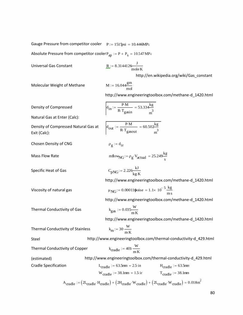
80
Gauge Pressure from competitor cooler
Absolute Pressure from competitor cooler
Universal Gas Constant
http://en.wikipedia.org/wiki/Gas_constant
Molecular Weight of Methane
http://www.engineeringtoolbox.com/methane-d_1420.html
Density of Compressed
Natural Gas at Enter (Calc):
Density of Compressed Natural Gas at
Exit (Calc):
Chosen Density of CNG
Mass Flow Rate
Specific Heat of Gas
http://www.engineeringtoolbox.com/methane-d_1420.html
Viscosity of natural gas
http://www.engineeringtoolbox.com/methane-d_1420.html
Thermal Conductivity of Gas
http://www.engineeringtoolbox.com/methane-d_1420.html
Thermal Conductivity of Stainless
Steel
http://www.engineeringtoolbox.com/thermal-conductivity-d_429.html
Thermal Conductivity of Copper
(estimated)
http://www.engineeringtoolbox.com/thermal-conductivity-d_429.html
Cradle Specification
P 1515psi 10.446MPa
Pap P Ps 10.547MPa
R 8.3144126J
mole K
M 16.044gm
mol
dinP M
R Tgasin53.334
kg
m3
doutP M
R Tgasout60.502
kg
m3
g din
mflowNG g Vactual 25.249kg
s
CpNG 2.226kJ
kg K
NG 0.000110poise 1.1 105
kg
m s
kgas 0.035W
m K
km 30W
m K
kcradle 401W
m K
Lcradle 63.5mm 2.5 in Hcradle 63.5mm
Wcradle 38.1mm 1.5 in Tcradle 38.1mm
Acradle 2Lcradle Hcradle 2Hcradle Wcradle 2Lcradle Wcradle 0.018m2

81
Prandtl Number
Reynolds Number Turbulent if > 2300
Masking Effect
distance along pipe 1.524 meters = 5 ft
distance across pipes 1.067 mm = 3.5 ft
tube diameter
dimensionless longitudinal distance
dimensionless tangential distance
Nusselt Number
Heat Transfer Coefficient of Gas
convective resistance from NG to pipe
conductive resistance through the pipe
conductive resistance through cradle
http://en.wikipedia.org/wiki/Thermal_conductivity
FIN DESIGN
fin thickness assume square fins
gap between fins
PrNG CpNG
kgas
0.7
ReD
4 mflowNG
Di NG2.183 10
8
ST 1.524m
SL 1.067m
D 5.875mm
sl
SL
D181.617
st
ST
D259.404
Nu 0.023ReD0.8
Pr0.33
9.59 104
hNG
kgas
Di
Nu 2.507 105
W
m2K
Rng1
hNG Di Li1.482 10
6
K
W
Rpipe
lnro
ri
2 km Li1.413 10
5
K
W
Rcradle
Tcradle
Acradle kcradle5.355 10
3
K
W
thickness .4mm t thickness
.4mm 0.016in1
16in 0.063in
gap 2.5mm
2mm 0.079in1
8in 0.125in
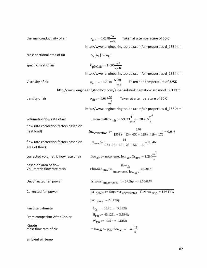
82
thermal conductivity of air Taken at a temperature of 50 C
http://www.engineeringtoolbox.com/air-properties-d_156.html
cross sectional area of fin
specific heat of air
http://www.engineeringtoolbox.com/air-properties-d_156.html
Viscosity of air Taken at a temperature of 325K
http://www.engineeringtoolbox.com/air-absolute-kinematic-viscosity-d_601.html
density of air Taken at a temperature of 50 C
http://www.engineeringtoolbox.com/air-properties-d_156.html
volumetric flow rate of air
flow rate correction factor (based on
heat load)
flow rate correction factor (based on
area of flow)
corrected volumetric flow rate of air
based on area of flow
Volumetric flow rate ratio
Uncorrected fan power
Corrected fan power
Fan Size Estimate
From competitor After Cooler
Quote
mass flow rate of air
ambient air temp
kair 0.0278W
m K
Ac wf wf t
CpNGair 1.005kJ
kg K
air 2.029105
kg
m s
air 1.097kg
m3
uncorrectedflow air 59933ft
3
min28.285
m3
s
flowcorrection176
1969 483 650 119 419 1760.046
Crarea14
92 56 65 23 56 140.046
flowair uncorrectedflow air Crarea 1.294m
3
s
Flowrateratio
flowair
uncorrectedflow air
0.046
fanpower uncorrected 57.2hp 42.654kW
Fanpower fanpower uncorrected Flowrateratio 1.951kW
Fanpower 2.617 hp
Lfan 63.75in 5.312 ft
Hfan 43.125in 3.594 ft
Wfan 13.5in 1.125 ft
mflowair air flowair 1.42kg
s

83
Prandtl number
average gas temp at
surface of pipe
air contact surface area
air contact perimeter
hydraulic diameter
Reynolds number
turbulent flow
Correction/arrangement factor
Nusselt number of Air
with Correction Factor
Convective heat transfer coefficient
of air
perimeter of fin
corrected fin length
thermal resistance of fin
with convection off end
for fin with convection off end, p695
Rate of heat transfer out of natural
gas required
Maximum resistance to achieve required heat
transfer
Tinf 273.15 50( )K 323.15K
Prair
CpNGair air
kair
0.734
Tsurf
Tgasin Tgasout
2355.539K
Aair wf n n wf gap
pair wf n n 2 wf gap
Dhair wf n 4Aair wf n pair wf n
Reair wf n 4 mflowair
Dhair wf n air
Fa 1 0.1 sl0.34
st
19.163
Nuair wf n 0.023Reair wf n 0.8
Prair0.33
Fa
hair wf n kair
pair wf n Nuair wf n
pfin wf 2 wf 2 t
mfin wf n 2 hair wf n
kair t
Lc Lf Lft
2
Rfin wf Lf n 1
hair wf n pfin wf kair Ac wf tanh mfin wf n Lc Lf
Qratemax mflow NG CpNG Tgasin Tgasout 2.517MW
Rtmax
Tsurf Tinf
Qratemax
1.287 105
K
W
AA 10 Rtmax 1.287 104
K
W

84
Using These to check
16 heat pipes per gas pipe
with 15.5 gas pipes
number of heat pipes
resistance of one heat pipe
maximum allowable total fin
resistance
resistance of single fin
fin width 127 mm = 5 in
fin length resistance independent of L
number of fins per bank
maximum resistance of fins
calculated resistance per fin, make less than Rifin
logic statement to help optimize design and reduce potential for human error
Required condenser region length 50mm max
Design Footprint
Design Volume
BB Rng Rpipe Rcradle 5.371 103
K
W
AA BB 5.242 103
K
W
nhp 419
Rihp 0.18K
W
Rfinmax 42 Rtmax Rng Rpipe Rcradle nhp Rihp 2.204K
W
Rifin n( ) n Rfinmax
w 2.5cm
L 2cm
nfin 17
Rifin nfin 37.467K
W
Rfin w L nfin 93.246K
W
current if Rifin nfin Rfin w L nfin "more" "less" "more"
smaller if Rifin nfin 1 Rfin w L nfin 1 "smallest" "fewer" "smallest"
if current "less" smaller "smallest" "end" "iterate"( ) "iterate"
condenser length t nfin gap nfin 1 46.8 mm
Footprint Ltube Wfan Wtube 0.871m2
Volume Footprint Htube 2.029m3
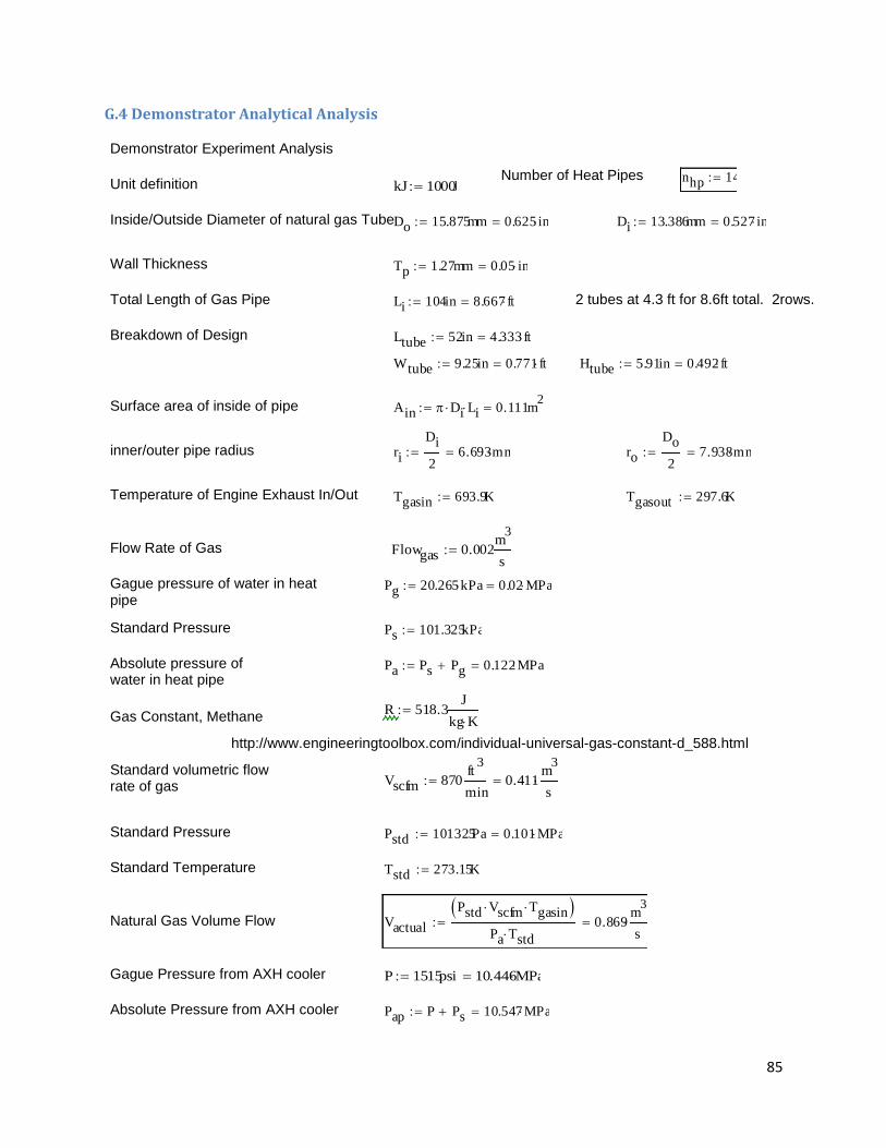
85
G.4 Demonstrator Analytical Analysis
Demonstrator Experiment Analysis
Number of Heat Pipes Unit definition
Inside/Outside Diameter of natural gas Tube
Wall Thickness
Total Length of Gas Pipe 2 tubes at 4.3 ft for 8.6ft total. 2rows.
Breakdown of Design
Surface area of inside of pipe
inner/outer pipe radius
Temperature of Engine Exhaust In/Out
Flow Rate of Gas
Gague pressure of water in heat pipe
Standard Pressure
Absolute pressure of water in heat pipe
Gas Constant, Methane
http://www.engineeringtoolbox.com/individual-universal-gas-constant-d_588.html
Standard volumetric flow rate of gas
Standard Pressure
Standard Temperature
Natural Gas Volume Flow
Gague Pressure from AXH cooler
Absolute Pressure from AXH cooler
nhp 14kJ 1000J
Do 15.875mm 0.625 in Di 13.386mm 0.527 in
Tp 1.27mm 0.05 in
Li 104in 8.667 ft
Ltube 52in 4.333 ft
Wtube 9.25in 0.771ft Htube 5.91in 0.492 ft
Ain Di Li 0.111m2
ri
Di
26.693mm ro
Do
27.938mm
Tgasin 693.9K Tgasout 297.6K
Flowgas 0.002m
3
s
Pg 20.265kPa 0.02 MPa
Ps 101.325kPa
Pa Ps Pg 0.122MPa
R 518.3J
kg K
Vscfm 870ft
3
min0.411
m3
s
Pstd 101325Pa 0.101 MPa
Tstd 273.15K
Vactual
Pstd Vscfm Tgasin Pa Tstd
0.869m
3
s
P 1515psi 10.446MPa
Pap P Ps 10.547MPa
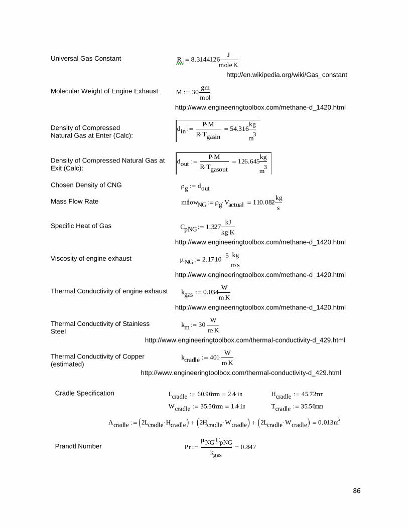
86
Universal Gas Constant
http://en.wikipedia.org/wiki/Gas_constant
Molecular Weight of Engine Exhaust
http://www.engineeringtoolbox.com/methane-d_1420.html
Density of Compressed Natural Gas at Enter (Calc):
Density of Compressed Natural Gas at Exit (Calc):
Chosen Density of CNG
Mass Flow Rate
Specific Heat of Gas
http://www.engineeringtoolbox.com/methane-d_1420.html
Viscosity of engine exhaust
http://www.engineeringtoolbox.com/methane-d_1420.html
Thermal Conductivity of engine exhaust
http://www.engineeringtoolbox.com/methane-d_1420.html
Thermal Conductivity of Stainless Steel
http://www.engineeringtoolbox.com/thermal-conductivity-d_429.html
Thermal Conductivity of Copper (estimated)
http://www.engineeringtoolbox.com/thermal-conductivity-d_429.html
Cradle Specification
Prandtl Number
R 8.3144126J
mole K
M 30gm
mol
dinP M
R Tgasin54.316
kg
m3
doutP M
R Tgasout126.645
kg
m3
g dout
mflowNG g Vactual 110.082kg
s
CpNG 1.327kJ
kg K
NG 2.17105
kg
m s
kgas 0.034W
m K
km 30W
m K
kcradle 401W
m K
Lcradle 60.96mm 2.4 in Hcradle 45.72mm
Wcradle 35.56mm 1.4 in Tcradle 35.56mm
Acradle 2Lcradle Hcradle 2Hcradle Wcradle 2Lcradle Wcradle 0.013m2
PrNG CpNG
kgas
0.847
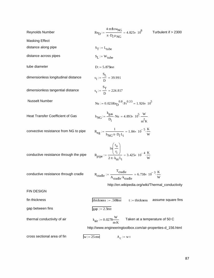
87
Reynolds Number Turbulent if > 2300
Masking Effect
distance along pipe
distance across pipes
tube diameter
dimensionless longitudinal distance
dimensionless tangential distance
Nusselt Number
Heat Transfer Coefficient of Gas
convective resistance from NG to pipe
conductive resistance through the pipe
conductive resistance through cradle
http://en.wikipedia.org/wiki/Thermal_conductivity
FIN DESIGN
fin thickness assume square fins
gap between fins
thermal conductivity of air Taken at a temperature of 50 C
http://www.engineeringtoolbox.com/air-properties-d_156.html
cross sectional area of fin
ReD
4 mflowNG
Di NG4.825 10
8
ST Ltube
SL Wtube
D 5.875mm
sl
SL
D39.991
st
ST
D224.817
Nu 0.023ReD0.8
Pr0.33
1.926 105
hNG
kgas
Di
Nu 4.893 105
W
m2K
Rng1
hNG Di Li1.84 10
5
K
W
Rpipe
lnro
ri
2 km Li3.425 10
4
K
W
Rcradle
Tcradle
Acradle kcradle6.738 10
3
K
W
thickness .508mm t thickness
gap 2.5mm
kair 0.0278W
m K
w 25 mm Ac w t

88
specific heat of air
http://www.engineeringtoolbox.com/air-properties-d_156.html
Viscosity of air Taken at a temperature of 325K
http://www.engineeringtoolbox.com/air-absolute-kinematic-viscosity-d_601.html
density of air Taken at a temperature of 50 C
http://www.engineeringtoolbox.com/air-properties-d_156.html
volumetric flow rate of air
flow rate correction factor based on heat load
flow rate correction factor based on area of flow
corrected volumetric flow rate of air based on area of flow
Volumetric flow rate ratio
Uncorrected fan power
Corrected fan power
Fan Used for Testing Size Estimate
mass flow rate of air
ambient air temp
Prandtl number
average gas temp at surface of pipe
CpNGair 1.005kJ
kg K
air 2.029105
kg
m s
air 1.097kg
m3
uncorrectedflow air 59933ft
3
min28.285
m3
s
flowcorrection176
1969 483 650 119 419 1760.046
Crarea14
92 56 65 23 56 140.046
flowair uncorrectedflow air Crarea 1.294m
3
s
Flowrateratio
flowair
uncorrectedflow air
0.046
fanpower uncorrected 420W 0.42 kW
Fanpower fanpower uncorrected Flowrateratio 0.019kW
Fanpower 0.026 hp
Lfan 12in 1 ft
Hfan 36in 3 ft
Wfan 36in 3 ft
mflowair air flowair 1.42kg
s
Tinf 273.15 50( )K 323.15K
Prair
CpNGair air
kair
0.734
Tsurf
Tgasin Tgasout
2495.75K

89
air contact surface area
air contact perimeter
hydraulic diameter
Reynolds number turbulent flow
Correction/arrangement factor
Nusselt number of Air with Correction Factor
Convective heat transfer coefficient of air
perimeter of fin
thermal resistance of fin with convection off end
for fin with convection off end, p695
Rate of heat transfer out of natural gas required
Maximum resisance to achieve required heat transfer
number of heat pipes
resistance of one heat pipe (average)
maximum allowable total fin resistance
resistance of single fin
fin width 25 mm = .984 in
Aair n( ) n w gap( )
pair n( ) n 2 w gap( )
Dhair n( ) 4Aair n( )
pair n( )
Reair n( )4 mflowair
Dhair n( ) air
Fa 1 0.1sl0.34
st
5.001
Nuair n( ) 0.023Reair n( )0.8
Prair0.33
Fa
hair n( )kair
pair n( )Nuair n( )
w 25 mm L 20mm pfin 2 w 2 L
mfin n( )2 hair n( )
kair t
Rfin w L n( )1
hair n( ) pfin kair Ac 2 tanh mfin n( ) L
Qratemax mflow NG CpNG Tgasin Tgasout 57.891 MW
Rtmax
Tsurf Tinf
Qratemax
2.981 106
K
W
nhp 14
Rihp 3.236K
W
Rfinmax 1 2 Rtmax Rng Rpipe Rcradle nhp Rihp 3.335K
W
Rifin n( ) n Rfinmax
w 25 mm

90
fin length 20 mm = .787 in
number of fins per bank
Maximum resistance of fins
calculated resistance per fin, make less than Rifin
logic statement to help optimize design and reduce potential for human error
Required condeser region length
Design Footprint
Design Volume
L 20mm
nfin 18
Rifin nfin 60.035K
W
Rfin w L nfin 62.61K
W
current if Rifin nfin Rfin w L nfin "more" "less" "more"
smaller if Rifin nfin 1 Rfin w L nfin 1 "smallest" "fewer" "smallest"
if current "less" smaller "smallest" "end" "iterate"( ) "iterate"
condenser length t nfin gap nfin 1 51.644mm
Footprint Ltube Wfan Wtube 1.518m2
Volume Footprint Htube 0.228m3

91
Appendix H - Quotes H.1 Quote - Current Cooler Competitor
92

93

94

95
H.2 Aavid Thermalloy Quote - Heat Pipes

96
H.3 ACT Quote - Heat Pipes

97
H.4 Enertron Inc. Heat Pipe Quote (Unofficial)
Hi Chris,
1. 20 fins with 35x35mm size is manufacturable and recommended.
2. Quote: Total $2,000 including heat pipes, fins, assembly labor, NRE Tooling, for 15
heat pipe assemblies.
Leadtime: 5~6 weeks;
Paid in full upfront;
FOB Enertron Taiwan factory.
Let me know if you have any questions. Thanks
Serena Lin Thermal Application Engineer ENERTRON, Inc. P 480-649-5400 Ext 210 F 480-649-5434 www.enertron-inc.com
H.5 Noren Products Heat Pipe Quote (Unofficial)
Hi Calvin,
I have a couple of questions before we can move forward with a quote for you .
1)we use mesh wick not a sintered powder wick .Do you need a sintered powder wick ?
2)this may be expensive in manufacturing around $ 245 dollars each .Small quantity .
3)We can do best effort to reach 123watts that would bring the price down some .
4) we will need to expand the heat pipe to hold the fins .If we solder now we add a
plating cost .
After you answer my questions I can give you a better quote .Let me know how you want
to proceed?
Thank you for the opportunity.
Regards
Eric Gaillant
Production Sales Engineer

98
Appendix I - Contacts
I.1 WPI
Simon Evans – Mechanical Engineering Professor
o Email: [email protected]
o Office: (508) 831-5462
o Bio: http://www.me.wpi.edu/People/Evans/
Neil Whitehouse – Lab Machinist II, Higgins Shops
o Email: [email protected]
o Office: (508) 831-5219
Barbara Furhman – Administrative Assistant VI, Purchasing
o Email: [email protected]
o Office: (508) 831-6046
I.2 OsComp Systems
Andrew Nelson – Mechanical Engineer
o Email: [email protected]
o Mobile: (617) 544-7208
Pedro Santos – CEO
o Email: [email protected]

99
I.3 Heat Pipe Manufacturers
Mike Beliveau – Sales Engineer, Aavid Thermalloy
o Email: [email protected]
o Office: (603) 223-1810
o https://www.aavidthermalloy.com/
Serena Lin – Thermal Application Engineer
o Email: [email protected]
o Office: (480) 649-5400 ext 210
o http://www.enertron-inc.com
Ray Balardo – Sales Manager, Noren Products
o Email: [email protected]
o Office: (650) 322-9500 ext 213
o http://www.norenproducts.com/
Scott Garner – Vice President, Advanced Cooling Technologies Inc.
o Email: [email protected]
o Office: (717) 295-6088
o Mobile: (717) 799-6084
o http://www.1-act.com
Walter John Bilski – Senior Engineer, Thermacore Inc.
o Email: [email protected]
o Office: (717) 519-3139
o http://www.thermacore.com/
Related Documents