Final draft thesis

DETERMINATION OF EVAPOTRANSPIRATION AND CROPCOEFFICIENT OF HOT PEPPER (Capsicum annuum L.) AT

MELKASSA, ETHIOPIA

M.Sc. Thesis

WONDIMAGEGN HABTE

October 2011Haramaya University

2

DETERMINATION OF EVAPOTRANSPIRATION AND CROPCOEFFICIENT OF HOT PEPPER (Capsicum annuum L.) AT

MELKASSA, ETHIOPIA

A Thesis Submitted to the School of Natural ResourcesManagement and Environmental Sciences, School of

Graduate Studies HARAMAYA UNIVERSITY

In Partial Fulfillment of the Requirements for theDegree of MASTER OF SCIENCE IN AGRICULTURE (IRRIGATION

AGRONOMY)

ByWondimagegn Habte

October 2011Haramaya University

2

SCHOOL OF GRADUATE STUDIESHARAMAYA UNIVERSITY

As Thesis Research advisors, we hereby certify that we have readand evaluated this thesis prepared, under our guidance, byWondimagegn Habte entitled: Determination of Evapotranspirationand Crop Coefficient of Hot Pepper (Capsicum Annuum L.) atMelkassa, Ethiopia. We recommend that it be submitted asfulfilling the Thesis requirements.

Yibekal Alemayehu (PhD) ________________________________

Major advisor Signature Date

Tilahun Hordofa (PhD) ________________________________

Co- advisor Signature Date

As members of the Board of Examiners of the M.Sc. Thesis OpenDefense Examination, we certify that we have read and evaluatedthe Thesis prepared by Wondimagegn Habte, and examined thecandidate. We recommend that the Thesis be accepted as fulfillingthe Thesis requirements for the Degree of Master of Science inIrrigation Agronomy.

BOBE BEDADI (PhD) ________________________________

Chairperson Signature Date

KIBEBEW KIBRET (PhD) ________________________________

Internal Examiner Signature Date

SETEGN GEBEYEHU (PhD) ________________________________

External Examiner Signature Date

2

DEDICATION

I dedicate this thesis manuscript to my beloved mother W/R ATSEDEASEFA who have dedicated the whole of her life for my success and

who had the courage to leave the old world and give me theopportunity to pursue my dreams in the new world.

STATEMENT OF AUTHOR

First, I declare that this thesis is my bonafide work and that all

sources of materials used for this thesis have been duly

acknowledged. This thesis has been submitted in partial

fulfillment of the requirements for an MSc degree at the Haramaya

University and is deposited at the University Library to be made

available for borrowers under rules of the Library. I solemnly

declare that this thesis is not submitted to any other

institution anywhere for the award of any academic degree,

diploma or certificate.

Brief quotations from this thesis are allowable without special

permission provided that accurate acknowledgement of source is

made. Requests for permission of extended quotation from or

reproduction of this manuscript in whole or in part may be

granted by the Head of the major department or the Dean of the

School of Graduate Studies when in his or her judgment the

proposed use of the material is in the interests of the

scholarship. In all other instances, however, permission must be

obtained from the author.

ii

Name: Wondimagegn Habte Signature: ______________

Place: Haramaya University, Haramaya

Date of Submission: _________________

LIST OF ABBREVIATIONS AND ACRONYMS

ADLI Agricultural

Development Led Industrialization

ASCE American

Society of Civil Engineers

DAP Diammonium

Phosphate

DAT Days After

Transplant

DS Development

Stage

iii

ET

Evapotranspiration

ETc Crop

Evapotranspiration (Standard)

ETo Reference

Crop Evapotranspiration

FAO Food and

Agricultural Organization

FC Field

Capacity

ha hectare

HU Haramaya

University

IAR Institute of

Agricultural Research

IS Initial

Stage

Kc Crop

coefficient

Kp Pan

coefficient

LS Late-season

stage

LAI Leaf Area

Index

iv

MARC Melkassa

Agricultural Research Center

MS Mid-season

stage

PWP Permanent

Wilting Point

TAW Total Available

Water

USDA United States

Department of Agriculture

WSDP Water Sector

Development Programs

BIOGRAPHICAL SKETCH

The author was born on October 17, 1986 at Awash Melkassa, East

Shoa zone, Oromiya Regional State, from his father Habte Zegeye

and his mother Atsede Asefa. He attended his primary and

secondary education at Awash Melkassa and his high school and

preparatory class at Adama Compressive High School and Hawas

preparatory, the then Atse Gelawdiwos High School, respectively.

After he successfully passed the national exam at grade 12 he

v

joined the Hawassa University College of Agriculture in 2006 and

graduated with BSc degree in Plant Science in 2008.

Soon after graduation he was employed by the Southern Nations

Nationalities and Peoples Regional State (SNNPRs) Agricultural

and Rural Development Office, Guraghe Zone as a crop protection

expert. After working for four months at Guraghe zone, he got the

chance to be employed by Ministry of Education to serve as a

lecturer at one of the Universities found in the country and

directly joined the Haramaya University in March, 2009 to pursue

his MSc study in the School of Natural Resources Management and

Environmental Sciences specializing in Irrigation Agronomy.

vi

ACKNOWLEDGEMENTS

First of all it is my pleasure to express my heartfelt

appreciation and special gratitude to my major advisor Dr.

Yibekal Alemayehu and co-advisor Dr. Tilahun Hordofa for their

enthusiastic effort, directive guidance and encouragement and

professional expertise from the start of proposal writing to the

completion of my research and thesis writing, as without their

guidance this work would have not been successful. I would also

like to thank Melkassa Agricultural Research Center Soil and

Water Conservation Case Team colleagues for providing me material

support and sharing their rich experience throughout my research

work. I am also happy to express my special gratitude to Mr.

Dereje Ayalneh and Mr. Mitiku Tamire who have shared me their

time and knowledge and their tireless effort and guidance greatly

contributed to the quality of this research work. My heartfelt

thank also goes to all of my friends for their encouragement and

moral support.

I feel myself helpless in searching for proper words to pay back

and I can ever be able to do some for my mother who provided me

all what I needed in my life and set the ladder to achieve this

academic goal. I am also proud of my elder sister Abnet Girma and

two of my brothers Asrat and Fasika Habte who inspired and

encouraged me and always remembered me in their prayers. I am

also equally thankful for Haramaya University and all the staffs

of Haramaya University who have shared me their knowledge and

vii

paved my way to success. Finally I am so gratefully happy to send

my warmest thank to the Ethiopian Ministry of Education for

providing me with this scholastic chance, thank you all.

Above all, I would like to thank the Almighty God for giving me

the life, patience, help, strength and wisdom in achieving all my

academic endeavors and who made it possible to begin and finish

this work successfully.

TABLE OF CONTENTS

STATEMENT OF AUTHOR ii

LIST OF ABBREVIATIONS AND ACRONYMS iii

BIOGRAPHICAL SKETCH iv

ACKNOWLEDGEMENTS v

LIST OF TABLES vii

LIST OF TABLES IN THE APPENDIX ix

ABSTRACT x

1. INTRODUCTION 1

2. LITERATURE REVIEW 5viii

2.1. Crop Water Requirement 52.2. Methods of Estimating Crop Evapotranspiration 5

2.2.1. Direct measurement of evapotranspiration 62.2.1.1. Field water balance technique 62.2.1.2. Lysimeter 6

2.2.2. Indirect methods 72.2.2.1. Crop water requirement computed from weather data 72.2.2.2. Crop coefficient approach 8

2.3. FAO Penman-Monteith Method 92.4. Factors Affecting Crop Water Requirement 10

2.4.1. Climate factors 10 2.4.2. Crop factors 11 2.4.3. Management and environmental factors 112.5. Factors Determining the Crop Coefficient (Kc) 122.6. Description of the Target Crop 14

3. MATERIALS AND METHODS 163.1. Description of the Study Area 163.2. Experimental Materials and Management 163.3. Data Collected 17

3.3.1. Soil analysis 17 3.3.2. Neutron probe calibration 18 3.3.3. Percent canopy cover 20 3.3.4. Agronomic management of pepper 21 3.3.5. Application of irrigation water 21

3.4. Crop data collected 23 3.5. Determination of crop evapotranspiration 23

TABLE OF CONTENTS (CONTINUED)

3.5.2. Calculation of reference crop evapotranspiration 24 3.5.3. Calculation of crop coefficient 25

4. RESULTS AND DISCUSSION 264.1. Soil Characteristics of the Experimental Site 264.2. Percent Canopy Cover and Leaf Area Index 274.3. Crop Water Requirement 284.4. Reference Crop Evapotranspiration (ETo) 314.5. Crop Coefficient (Kc) 334.6. Agronomic Parameters 35

ix

5. SUMMARY, CONCLUSION AND RECOMENDATION 375.1. Summary 375.2. Conclusions and Recommendations 38

6. REFERENCES 39

7. APENDICES 45

APPENDIX Ι. TABLES 46

LIST OF TABLES

Table page

1. Soil physical properties of the experimental site..........262. Results of percent canopy cover and leaf area index of hot pepper........................................................27

x

3. Ten day values of water balance components for hot pepper grown at MARC in 2010/11 off season.....................29

4. Ten day values of reference crop evapotranspiration at MARC during 2010/11 off growing season...........................31

5. Stage-wise ETc, ETo and Kc values of hot pepper grown at MARC during 2010/11 off season....................................34

6. Stage-wise growth and yield parameters of hot pepper grown in lysimeter at MARC during 2010/11 off season..................36

xi

LIST OF FIGURES

FigurePage

1. Neutron probe calibration curve for the experimental plot to soil of depth 15-90 cm........................................202. Ten day average ETc and ETo curve of hot pepper grown at MARC in 2010/11 off growing season................................32

3. Ten-day average Kc values of hot pepper grown at MARC in 2010/11 off growing season and standard FAO Kc curve.........33

xii

LIST OF TABLES IN THE APPENDIX

Appendix Table page

1. Result of neutron probe calibration curve for the depth 15-105cm............................................................462. Averaged weather data of MARC in the experimental months. . .473. Water balance components of lysimeter-1....................504. Water balance components of lysimeter-2....................53

xiii

DETERMINATION OF EVAPOTRANSPIRATION AND CROP COEFFICIENT OF HOT

PEPPER (Capsicum annuum L.) AT MELKASSA, ETHIOPIA

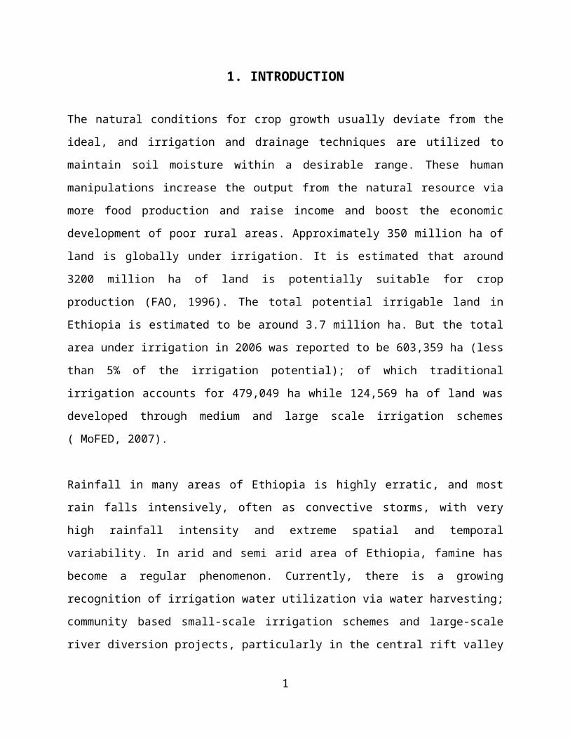
ABSTRACT

Designing, establishing and managing irrigation projects, and scheduling irrigationrequires estimating a crop seasonal water requirement. One way of achieving this isthrough the use of reference crop evapotranspiration and crop coefficient approach.However, this information is not available for many crops in the country. Thisexperiment was aimed at determining the seasonal crop evapotranspiration (ETc) andcrop coefficient (Kc) of hot pepper variety called Melka-awase for different developmentstages at Melkassa. Two rectangular drainage type lysimeters with dimension of 2 m ×1 m × 2m were used to determine the daily ETc of hot pepper. Crop coefficient (Kc) wasdetermined for each growth stages as the ratio of crop evapotranspiration (ETc) to thatof reference crop evapotranspiration (ETo).The ETc was determined by soil waterbalance equation and ETo was computed by CROPWAT 8 software version 4.2 using FAOPenman-Monteith equation. The average seasonal ETc was found to be 526.06 mm with42.3 mm, 127.7 mm, 255.9 mm and 100.7 mm of water calculated for initial, cropdevelopment, mid-season and late season stages, respectively. The calculated value ofreference crop evapotranspiration was 110.77 mm, 158.32 mm, 223.52 mm and 120.93mm, for initial, crop development, mid-season and late-season stages, respectively. Themeasured average crop coefficient (Kc) values were 0.38, 0.81, 1.14 and 0.86 for therespective growth stages with an end Kc value of 0.82. Some of the crop coefficientvalues found in this experiment differed slightly from the average of FAO estimation butsome lie in the range put for different environment. Thus, the observed differenceindicate that there is a need to develop Kc values for a given local climate conditions

xiv

and cultivars. Some crop yield and growth parameters were also collected in a sage-wise. The maximum plant height was 61.55 cm and 41.5 branches per plant wereobtained at the mid-season stage which was the highest from the four growth stages.The highest number of fruits per plant was 58.9 on average. The average maximum dryfruit weight per plant was 1.99 g with 1.34 tons of dry yield per hectare.

xv

1. INTRODUCTION

The natural conditions for crop growth usually deviate from the

ideal, and irrigation and drainage techniques are utilized to

maintain soil moisture within a desirable range. These human

manipulations increase the output from the natural resource via

more food production and raise income and boost the economic

development of poor rural areas. Approximately 350 million ha of

land is globally under irrigation. It is estimated that around

3200 million ha of land is potentially suitable for crop

production (FAO, 1996). The total potential irrigable land in

Ethiopia is estimated to be around 3.7 million ha. But the total

area under irrigation in 2006 was reported to be 603,359 ha (less

than 5% of the irrigation potential); of which traditional

irrigation accounts for 479,049 ha while 124,569 ha of land was

developed through medium and large scale irrigation schemes

( MoFED, 2007).

Rainfall in many areas of Ethiopia is highly erratic, and most

rain falls intensively, often as convective storms, with very

high rainfall intensity and extreme spatial and temporal

variability. In arid and semi arid area of Ethiopia, famine has

become a regular phenomenon. Currently, there is a growing

recognition of irrigation water utilization via water harvesting;

community based small-scale irrigation schemes and large-scale

river diversion projects, particularly in the central rift valley

1

areas. Besides, in view of the limited water resources, the

search for water saving technique is the utmost important issue

in the areas (FAO, 1996). As the industrial and domestic need of

water is drastically increasing, in the future agriculture will

get more less water. To ensure the highest crop production with

the least water use, it is important to know the water

requirement of the crops (Tyagi et al., 2000). Rejisberman (2003)

has also predicted that water would be major constraints for

agriculture in the coming decades particularly in Asia and

Africa, and recommended focusing on increasing overall water

productivity to address water scarcity.

One way of water management would be to evaluate the seasonal

crop water consumption of agricultural crops which would enhance

the proper allocation of the available water resources. This

mainly depends on the weather parameters, crop development,

growing season and local conditions. The determination of crop

water requirement would help in designing appropriate irrigation

scheduling, which should lead to improvements in the yields and

incomes, and, it also has a positive impacts on soil and ground

water. However, it is astounding how little effort is sometimes

put into estimation of crop water requirement determination for

design and management of irrigation systems involving capital

costs in the range of tens or hundreds of thousands of dollars

(Cuenca, 1989).

2

Different methods with different input requirements and output

precisions have been developed to estimate the seasonal ETc of

agricultural crops. Experimental or empirical methods can be used

to estimate evapotranspiration of a given crop, of which

experimental method gives most accurate result. ETc can be

measured experimentally by weighing or non-weighing type

lysimeters. Weighing lysimeters could provide ETc values for

short periods but their installation and operation cost is quite

high. Short-term ETc data is not that much useful for irrigation

project planning; therefore, non weighing type lysimeter is well

suited for measuring long-term ETc data such as weekly, in decade

or monthly which can be used in planning and management of

irrigation systems (Allen et al., 1998). Empirical methods can also

be used to estimate ETc from climatic data. However, to

extrapolate the measurement of ETc for irrigation planning Kc

which is the ratio of ETc to ETo is often required. The Kc

reflects the effect of crop on the crop water requirement and can

be calculated at research sites by relating the measured crop

evapotranspiration using lysimeters with the calculated ETo from

climatic data.

The ETo is defined as the rate at which water would be removed

from bare soil and plant surface of a specific crop, arbitrarily

called a reference crop. ETo determines the loss of water from a

standardized vegetated surface, which helps in fixing the base

value of ET specific to a site. Typical reference crops are

3

grasses or alfalfa. The only factors which affect ETo are climate

such us sun shine hours, wind speed, relative humidity and

maximum and minimum temperatures, which are inputs to calculate

ETo. According to Allen et al. (1998) ETo is a representation of

the demand of atmosphere, independent of crop growth and

management factors. Different methods have been developed to

estimate ETo. Pan evaporation coupled with the use of a

calibrated pan coefficient (Kp) to relate ETo with the standard

vegetative surface, can provide good estimates of ETo, provided

that soil water is readily available to the crop (James, 1988).

Alternatively ETo can be estimated from meteorological data using

empirical and semi-empirical equations. Numerous empirical

methods have been developed to estimate evapotranspiration from

different climatic variables. Examples of such methods include

Penman-Monteith (Monteith, 1965) and Blaney-Criddle (Blaney and

Criddle, 1950). One of the most important factors governing the

selection of a method is the data availability. For instance,

Blaney-Criddle only requires the temperature data while the

Penman-Monteith requires additional parameters such as wind

speed, humidity and solar radiation. In addition, since the

Blaney-Criddle method is used to calculate monthly Kc values as

compared to daily, less data is needed for this method.

Several studies have been conducted over the years to evaluate

the accuracy of different ETo methods. Most of these studies have

concluded that Penman-Monteith equation in its different forms

4

provides the best ETo estimates under most conditions. Therefore,

the Food and Agricultural Organization (FAO) recommended FAO-

Penman Monteith method as the sole standard method for

computation of ETo (Allen et al., 1998).

Various crop coefficient values were suggested for different

crops under different climate and soil conditions. Doorenbos and

Pruitt (1977), suggested a strong need for local calibration of

crop coefficients under a given climatic conditions due to the

varying results from place to place. The Kc has not been

determined for many globally important crops (Kashyap and Panda,

2001). Many research results also suggested that the crop

coefficient values need to be derived empirically for each crop

based on lysimetric data and local climatic conditions (Allen et

al., 1998; Cuenca, 1989). Adopting a Kc values developed

elsewhere for new environments may lead to improper irrigation

scheduling and crop water requirement determination, inaccurate

planning and design of irrigation projects and mismanagement of

water resources. Therefore, determining the Kc for a particular

crop in a particular environment is vital to have an accurate and

reliable irrigation schedules and management of water resources

especially for high value crops which uses intensive inputs.

Pepper (green and red) is among high valued cash crops which are

being produced by small holder and commercial growers for

domestic and export. Pepper is the most indispensable part of the

5

daily dishes of the Ethiopian people. In Ethiopia, pepper grows

under warm and humid weather conditions and the best fruit is

obtained in a temperature 21-270C during the daytime and 15-200C

at night (EARO, 2004). It is extensively grown in most parts of

the country, with the major production areas concentrated at an

altitude of 1100 to 1800 m.a.s.l. (MoARD, 2009). Most peppers

varieties are grown in soils with a pH range of 7-8.5. Peppers

prefer well drained, moisture holding loam or sandy loam

containing some organic matter (Lemma, 1998). As a food, pepper

are used eaten raw in salads, in numerous cooked preparations

including salsa, as raw material and as dehydrated and powdered

products. This crop is an excellent source of vitamins A, C and a

good source of vitamin B2, potassium, phosphorus and calcium

(Bosland and Votava, 2000). Pepper production increased worldwide

from 11 million metric tons in 1990 to 23.2 million metric tons

in 2003 (FAO, 2004). Ethiopia is considered as one of the source

of pepper diversity (Hearth and Lemma, 1992). In Ethiopia 4,783

ha of land was covered by green pepper in 2005 and the production

was 442,729 quintals under rainfall production during the main

season (CSA, 2005). The average yield was 92.56 q/ha. In 2007 the

area coverage of green pepper has increased to 6,886.19 hectare

while the production was 374,683.34 quintals. The yield in 2007

was 54.50 q/ha (CSA, 2007). This shows the decreasing trend of

average green pepper yield from time to time in the country. On

the other hand the average World pepper production is increasing

from time to time (FAO, 2004). The main bottleneck for the

6

productivity of hot pepper in Ethiopia are traditional and

backward production methods, lack of proper irrigation methods,

erratic rain fall and inadequate inputs and many other problems

(Alemu and Ermias, 2000). Therefore, estimating the ETc and the

Kc for this crop for a particular environment is necessary to

have a proper and timely irrigation schedules.

Irrigation scheduling can usefully be based on ETc and values

from measured ETo adjusted by typical Kc of pepper in a

particular environmental conditions. Therefore, experimental

determination of seasonal ETc and Kc is useful for proper water

management and irrigation scheduling to optimize yield and net

benefit from pepper production. Therefore, this research was

undertaken:

To evaluate the seasonal crop water requirement (ETc)

and crop coefficient (Kc) of hot pepper under Melkassa

climatic and soil condition

2. LITERATURE REVIEW

2.1. Crop Evapotranspiration

Crop Evapotranspiration (ETc) is defined as the depth of water

needed to meet the water loss through evapotranspiration of a

disease-free crop growing in a large field under non restricting7

soil condition including soil water and fertility and achieving a

full production potential under a given growing environment

(Allen et al., 1998). It comprises of the water lost through

evaporation from cropped field, water transpired and

metabolically used by the crop plants. The actual crop water use

depends on climatic factors, crop type and crop growth stage.

For the determination of crop water requirement, the effect of

climate on crop water requirement, which is the potential crop

evapotranspiration (ETo) and the effect of crop coefficient (Kc)

are important (Doorenbos and Pruitt, 1977).

Different ETc results have been reported from different areas of

the world which supports the advantages of local estimation of

crop ET for different environments. According to Iwena (2002),

hot pepper requires 1000 to 1500 mm of water during the growing

season. Huguez and Philippe (1998) has also indicated that the

total water requirements of hot pepper were 750 mm to 900 mm and

up to 1250 mm for long growing periods and several pickings. On

the other hand Allen et al. (1998) reported that seasonal crop

water use of pepper ranges from 600 mm to 900 mm. From these

experimental results it can be seen that water requirement of a

crop varies from place to place depending on the growing

environmental conditions as well length of growing period of the

crop and the same was true for hot pepper results from different

areas.

8

2.2. Methods of Estimating Crop Evapotranspiration

Different methods of estimating ETc are employed to determine the

seasonal water use of crops. Crop ET is determined by direct

measurement or calculated from crop and climatic data. Direct

measurement technique involves isolating a portion of crop from

its surrounding and determining ET by measurement. Several

theoretical and empirical equations have been developed to

compute crop ETc. These equations are used to estimate ET for

crops and locations where measured ET data are not available

(James, 1988).

2.2.1. Direct measurement of evapotranspiration

2.2.1.1. Field water balance technique

According to Hansen et al. (1979) in irrigated regions the

capacity of the soil to store available water for use of growing

crops is of special importance and interest, because the depth of

water to apply at each irrigation and the interval between

irrigation are both influenced by water storage capacity of the

soil. This is the most widely used direct measurement technique

without the use of lysimeters.

2.2.1.2. Lysimeter

9

By isolating the crop root zone from its environment and

controlling the processes that are difficult to measure, the

different terms in the soil water balance equation can be

determined with greater accuracy. This is done in lysimeters

where the crop grows in isolated tanks filled with either

disturbed or undisturbed soil. Lysimeters are large containers

filled with soil, located in the field so as to represent the

field environment and it is hydrologically isolated from the

nearby soil environment to avoid some of the inflow and outflow

moisture dynamics but its surfaces are indistinguishable from the

surrounding so as to represent the original soil condition. With

a bare soil or vegetated surface it can be used for determining

the evapotranspiration (ETc) of a growing crop or evaporation

from bare soils (Aboukhaled et al., 1982).

Lysimeters have been made following numerous designs, each based

on specific requirements that might be dictated by crop, soil,

climate, availability of materials and technology, skilled users

and cost involved (Khan et al., 1993). This method consists of

monitoring the incoming and outgoing water flux into and from the

crop root zone respectively over growing periods (Allen et al.,

1998). When lysimeters are employed to measure actual

evapotranspiration, it is desirable that they should contain

undisturbed representative of soil profile. Because in disturbed

soil profile moisture retention and root distribution is likely

to be different from that of the original profile and measurement

10

may not be accurate. But when lysimeters are used to measure

reference evapotranspiration (ETo) the physical condition of the

soil is of less importance and disturbed soil profile can be used

to measure ETo.

As discussed in Abdulmumin and Misari (1990), crop water

requirements of some crops are determined using hydraulic

weighing lysimeters; these crops were sorghum, cotton, maize,

groundnut and millet. Crop water requirement of pepper was

determined by Fernandez et al. (2000) using two drainage

lysimeters for one week period in the region of Almeria, Spain.

Crop water consumption of any crop increases linearly as the crop

grew and shows a slight reduction at maturity. As the researched

result of pepper showed that the seasonal crop water requirements

of pepper were 362 mm. The result of this research was out of the

range put by Allen et al. (1998) and this asserted the strong need

of local estimation of crop ET for different environments.

Samson (2005), determined stage wise and seasonal water

requirements of Haricot bean at Melkassa with four non-weighing

type lysimeters and he get the average measured ETc values of

36.5, 111.0, 234.7 and 65.8 mm for the initial, development, mid-

season and late season stages respectively for the cropping

period of 21 November to 7 February 2005. The total seasonal ETc

was found to be 447.1 mm. In the value of bean seasonal ET

estimated by FAO Allen et al (1998) the amount of water to be

11

consumed by this crop ranged from 300 mm to 500 mm and the result

reported by Samson (2005) agrees with the range of FAO.

Therefore, this and those results discussed above supported the

need of local ET estimations of different crops.

2.2.2. Indirect methods

2.2.2.1. Crop Evapotranspiration computed from weather data

Under standard conditions ETc refers to the evaporative demands

of a crop that are grown in large fields under optimum soil

water, good management and environmental conditions, and

achieving full production potential under the given climatic

conditions. Different crops have different water requirement for

different environmental conditions due to the variability of

weather elements, as a result, the accuracy of the result is

subject to error unless it is collected with greater follow up.

Owing to the difficulty of getting accurate field results, ET is

measured from weather data. Several equations with different

approaches and data requirements were developed in the past three

decades (Allen et al., 1998).

2.2.2.2. Crop coefficient approach

Crop coefficient is a parameter which reflects the effect of

crops on ETc and it can be computed by dividing the ETc by the

ETo. The FAO land and water development division has played a12

significant role in developing and promoting guidelines and

methodologies on crop water management at field level that have

become widely used standards (Doorenbos and Pruitt, 1977).

Reference evapotranspiration: ETo is defined as the rate at which

water would be removed from bare soil and plant surface of a

specific crop, arbitrarily called a reference crop. Typical

reference crops are grasses and alfalfa. The crop is assumed to

be well watered, with a full canopy cover, no disease and pest

effect and with no limitation in environmental inputs. As (Allen

et al., 1998), stated that, the reference surface is a

hypothetical grass reference crop with assumed crop height of

0.12 m, a fixed surface resistance of 70 s/m and an albedo of

0.2. The fixed surface resistance of 70 s/m implies a moderately

dry soil surface resulting from about from a weekly irrigation

frequency. The methods for calculating evapotranspiration from

meteorological data require various climatological and physical

parameters; some of the data are measured directly in weather

stations. Other parameters are related to commonly measured data

and can be derived with the help of direct or empirical

relationships (Allen et al., 1998). Different meteorological

parameters are common which affects crop evapotranspiration of

which the principal weather parameters are solar radiation, air

temperature, relative humidity and wind speed which will be

measured from meteorological stations.

13

Determining reference evapotranspiration: Various methods with

different input requirement, degree of accuracy, time scale

required and resource available have been developed by different

researchers to determine the reference crop evapotranspiration.

According to Allen et al. (1998), a large number of more or less

empirical methods have been developed over the last 5 decades by

different scientists and specialists worldwide to estimate

reference crop evapotranspiration from different climatic

variables. To evaluate the performance of these and other

estimation procedures under different climatological conditions,

a major study was undertaken under the auspices of the committee

on irrigation water requirement of the American Society of Civil

Engineers (ASCE). The evaluation of ASCE analyzed the performance

of 20 different methods using detailed procedures to assess the

validity of the methods compared to a set of screened lysimeter

data from 11 locations with varying climatic conditions. The

output or result of the study showed that there is a varying

performance of these methods under differing climatic conditions.

The European research institute has also evaluated the

performance of various evapotranspiration measurement methods

using different data from Europe gathered from various lysimetric

study. These studies have revealed that different results are

observed from different methods of evapotranspiration measurement

methods, and this shows the adaptation of each method to

different local conditions (Jensen et al., 1990). A possible

14

exception is the Hargreve’s method, (Hargreves et al, 1985), which

has shown reasonable reference evapotranspiration results with a

global validity in the year 1985. Out of the many different ETo

estimation methods the FAO Penman-Monteith equation is considered

to be the sole model which gives the best result. This method

gives the best result with coefficient of determination (R2 =

0.91). Consequently, ETo is a climatic parameter and can be

computed from weather data.

2.3. FAO Penman-Monteith Method

According to Allen et al. (1998), FAO Penman-Monteith method was

developed by defining the reference crop as a hypothetical crop

closely resembling an extensive surface of green grass, with

uniform height, actively growing and with no short of water. This

method overcomes the minor anomalies seen in the original penman

method and provides values which are more consistent with the

actual crop evapotranspiration data worldwide. The FAO penman-

Monteith is developed from the original Penman equation and from

the equation of aerodynamic and surface resistance to estimate

the reference crop evapotranspiration.

2.4. Factors Affecting Crop Evapotranspiration

The water requirement of plants vary with weather parameters,

crop characteristics, growth stages and environmental aspects

which directly or indirectly affects the evaporation and

transpiration which together called evapotranspiration of crops

15

(Andreas an Karen, 2002; Allen et al., 1998; Doorenbos and Pruitt,

1977 ).

2.4.1. Climate factors

The principal weather elements affecting crop water requirements

are: solar radiation, air temperature, relative humidity and wind

speed. Several procedures have been developed to assess the

evaporation rate using these parameters. The evaporative power of

the atmosphere is expressed by ETo. The reference or potential

crop evapotranspiration represents the evapotranspiration from a

standardized vegetated surface, which is free from soil moisture

stress and not affected by disease, pest and fertility status of

the soil (Doorenbos and Pruitt, 1977).

Solar radiation: Water to be removed from plants and water bodies

first it needs to be changed to vapor and the energy that

provides the latent heat for the vaporization of water is

provided by solar radiation. The evapotranspiration process is

determined by the amount of energy available to vaporize water.

Solar radiation is the largest energy source and is able to

change large quantities of liquid water into water vapor. The

potential amount of radiation that can reach the evaporating

surface is determined by its location and time of the year. Due

to differences in the position of the sun, the potential

radiation differs at various latitudes and in different seasons

(Doorenbos and Pruitt, 1977). 16

Air temperature: According to Allen et al. (1998) the solar

radiation absorbed by the atmosphere and the heat emitted by the

earth increase the air temperature. The sensible heat of the

surrounding air transfers energy to the crop and exerts as such a

controlling influence on the rate of evapotranspiration. In

sunny, warm weather the loss of water by evapotranspiration is

greater than in cloudy and cool weather.

Air humidity: While the energy supply from the sun and

surrounding air is the main driving force for the vaporization of

water, the difference between the water vapor pressure at the

evaporating surface and the surrounding air is the determining

factor for the vapor removal. Well-watered fields in hot dry arid

regions consume large amounts of water due to the abundance of

energy and the desiccating power of the atmosphere. In humid

tropical regions, notwithstanding the high energy input, the high

humidity of the air will reduce the evapotranspiration demand. In

such an environment, the air is already close to saturation, so

that less additional water can be stored and hence the

evapotranspiration rate is lower than in arid regions (Andreas

and Karen, 2002).

Wind speed: The process of vapor removal depends to a large

extent on wind and air turbulence which transfers large

quantities of air over the evaporating surface. When water

17

vaporized, the air above the evaporating surface becomes

gradually saturated with water vapor. If this air is not

continuously replaced with drier air, the driving force for water

vapor removal and the evapotranspiration rate decreases. The

evapotranspiration demand is high in hot dry weather due to the

dryness of the air and the amount of energy available as direct

solar radiation and latent heat (Andreas and Karen, 2002).

2.4.2. Crop factors

Different crops have different response to the prevailing

environment, therefore, the crop type, variety and development

stages should be considered when assessing the evapotranspiration

from crops grown in large, well managed fields. Differences in

resistance to transpiration, crop height, crop roughness,

reflection, ground cover and crop rooting characteristics result

in different evapotranspiration levels in different types of

crops under identical environmental conditions (Paul, 2001).

2.4.3. Management and environmental factors

Factors such as soil salinity, poor land fertility, and limited

application of fertilizers, the presence of hard or impenetrable

soil horizons, the absence of control of diseases and pests and

poor soil management may limit the crop development and reduce

the evapotranspiration. Other factors to be considered when

assessing ET are ground cover, plant density and the soil water

18

content. The effect of soil water content on ET is conditioned

primarily by the magnitude of the water deficit and the type of

soil. On the other hand, too much water will result in water

logging which might damage the root and limit root water uptake

by inhibiting respiration. When assessing the ET rate, additional

consideration should be given to the range of management

practices that act on the climatic and crop factors affecting the

ET process. The use of mulches, especially when the crop is

small, is another way of substantially reducing soil evaporation.

Anti-transpirants, such as stomata-closing, film-forming or

reflecting material, reduce the water losses from the crop and

hence the transpiration rate (Andreas and Karen, 2002; Allen et

al., 1998).

2.5. Factors Determining the Crop Coefficient (Kc)

The Kc integrates the effect of crop characteristics on ETc that

distinguishes a typical field crop from the grass reference,

which have a constant appearance and a complete ground cover.

Consequently, different crops will have different Kc values. The

changing characteristics of the crop over the growing season also

affect the Kc value. Finally, as evaporation is an integrated

part of crop evapotranspiration, conditions affecting soil

evaporation will also have an effect on Kc. The crop type,

climate, soil evaporation and crop growth stages are those

19

parameters which directly or indirectly affect the Kc (Andreas

and Karen, 2002; Allen et al., 1998; Doorenbos and Pruitt, 1977).

Crop type: Due to differences in albedo, crop height, aerodynamic

properties, and leaf and stomata properties, the

evapotranspiration from full grown, well-watered crops differs

from ETo. The close spacing’s of plants and taller canopy height

and roughness of many fully grown agricultural crops cause these

crops to have Kc factors that are larger than one. The Kc factor

is often 5-10% higher than the reference (where Kc = 1.0), and

even 15-20% greater for some tall crops such as maize, sorghum or

sugar cane. Crops such as pineapples, that close their stomata

during the day, have very small crop coefficients. In most

species, however, the stomata open as irradiance increases.

Species with stomata on only the lower side of the leaf and/or

large leaf resistances will have relatively smaller Kc values.

This is the case for citrus and most deciduous fruit trees.

Transpiration control and spacing of the trees, providing only

70% ground cover for mature trees, may cause the Kc of those

trees, if cultivated without a ground cover crop, to be smaller

than one (Allen et al., 1998).

Climate: Variations in wind alter the aerodynamic resistance of

the crops and hence their crop coefficients, especially for those

crops that are substantially taller than the hypothetical grass

reference. The effect of the difference in aerodynamic properties

20

between the grass reference surface and agricultural crops is not

only crop specific. It also varies with the climatic conditions

and crop height. Because aerodynamic properties are greater for

many agricultural crops as compared to the grass reference, the

ratio of ETc to ETo (i.e., Kc) for many crops increases as wind

speed increases and as relative humidity decreases. More arid

climates and conditions of greater wind speed will have higher

values for Kc. More humid climates and conditions of lower wind

speed will have lower values for Kc (Andreas and Karen, 2002).

Soil evaporation: Differences in soil evaporation and crop

transpiration between field crops and the reference surface are

integrated within the crop coefficient. The Kc value for full-

cover crops primarily reflects differences in transpiration as

the contribution of soil evaporation is relatively small. After

rainfall or irrigation, the effect of evaporation is predominant

when the crop is small and scarcely shades the ground. For such

low-cover conditions, the Kc value is determined largely by the

frequency with which the soil surface is wetted. Where the soil

is wet for most of the time from irrigation or rain, the

evaporation from the soil surface will be considerable and Kc may

exceed one. On the other hand, where the soil surface is dry,

evaporation is restricted and Kc will be small and might even

drop to as low as 0.1 (Allen et al., 1998; Doorenbos and Pruitt,

1977).

21

Growth stages: The duration of the total growing season has an

enormous influence on the seasonal ETc. The differences in

percent ground cover and the effects of each growth stages on ETc

and Kc are varies from stage to stages (Andreas and Karen, 2002;

Allen et al., 1998; Doorenbos and Pruitt, 1977). The different

growth stages are as below:

Initial stage: This refers to the time from planting

to the time of 10% ground cover. The crop type, the

crop variety, planting date and weather parameters

determines the length of this stage. At this stage

evaporation is higher than that of transpiration due

to less canopy cover and exposure of the bare soil to

direct sun light. Here, ET is predominantly satisfied

from evaporation. The Kc is taken as initial Kc (Kc

in) and it is high when the soil became wet and low

when the bare soil surface dry up (Andreas and Karen,

2002)

Crop development stage: This is the stage starting

from end of initial stage to the time of effective

full cover that was 70 to 80 percent ground cover.

Effective full cover is attained at the initiation of

flowering. For crops like potato, maize, sugar beets

and beans which are grown in rows effective full cover

is defined when the leaves of the adjacent crops

22

became intermingled to one another and the space

between crops are completely avoided from direct sun

light, or when plants reach nearly full size if no

intermingling of the adjacent leaves occur (Andreas

and Karen, 2002).

Mid-season stage: The stage from effective full cover

to the start of maturity is termed as mid-season

stage. This was the longest stage perennials and for

many annuals, but it may be relatively short for

vegetable crops that are harvested fresh for their

green vegetation. The maximum Kc is attained at this

stage. The Kc of the mid-season stage is symbolized by

Kcmid and it is the binging of senescence of leaves,

yellowing and leaf drop and hence reduction of ET as a

whole the overall activities of crops (Andreas and

Karen, 2002).

Late season stage: The stage starting from the end of

mid-season stage to complete maturity or harvest was

termed as late season stage. The Kc at this stage is

assigned as Kcend and the ETc of the crop is highly

reduced due to the decline in transpiration by the

senescence and loss of leaves. The calculation of Kc

and ET is presumed to end when the crop reaches full

senescence, experience leaf drop or dry-out naturally

23

without any environmental constraints (Andreas and

Karen, 2002).

2.6. Description of the Target Crop

Pepper (Capsicum annuum L.) is a new world crop that belongs to

the solanaceae family. The genus capsicum is the second most

important vegetable crop of the family next to tomato (Rubatzky

and Yamuguchi, 1997). Pepper is with erect sometimes prostrate

growth habit that may vary in certain characteristics depending

on type of the species (Bosland and Votova, 2000).

Pepper is grown in many parts of the world and its production for

culinary and vegetable uses has been increased from time to time.

According to FAO (2002) report world production of pepper was 21,

719, 000 metric tons on 1.59 ha of land, of which Africa

contributed 2,027, 000 metric tons which is 9.3% of the total

production on 0.264 ha of land. According to the Ethiopian

Agricultural Sample Enumeration (EASE, 2002), Private peasants

produced 41716.5 metric tons of green pepper and 77, 962.4 metric

tons of red pepper on 4, 672 and 56, 202 ha of land respectively.

Pepper is a national spice of Ethiopia. Though no documented

information is available, it was introduced to Ethiopia probably

by Portuguese in the 17th century (Hafnagel, 1961). He also

reported that Ethiopia was one of a few developing countries that

have been producing paprika and capsicum oleoresins for export

markets.24

Pepper as that of any crops need an optimum environmental inputs

and climate for a good production potential. Temperature controls

plant development including morphogenesis, yield and quality of

pepper. These processes make it a major growth factor. The

productivity of capsicum is constrained by adverse effect of high

and low temperatures. Capsicum flourishes in warm, sunny

conditions and requires 3-5 months within a temperature ranges of

18-300C below 50C frost kills the plant at any growth stage

(Wein, 1997). A seedbed temperature of 20-280C is optimum for

germination which will slow down out of these range and ceases

below 150C and above 300C. The slower growth rate attributed to a

reduced production of leaf area (Wein, 1997). The rate of plant

growth is also influenced by the air temperature, which affects

both the dry matter production and the partitioning of assimilate

in to leaf tissue (Miller et al., 1982).

3. MATERIALS AND METHODS

3.1. Description of the Study Area

The experiment was conducted from 13 November 2010 to 23 March

2011 at Melkassa Agricultural Research Center using two drainage

type lysimeters. The Center is located 16 km south-east of Adama

town in the semi-arid region of the Central Rift Valley of

25

Ethiopia (8° 24'N latitude and 39° 12'E longitude and at an

elevation of 1550 m above sea level). The area receives 768 mm

mean annual rainfall but with much variation in distribution and

amount, 70% of which occurs between the months of May and

September. Late onset of rains, intermittent periodic dry spells

and early cessation of rain are common causes of fluctuating

annual production with occasional drastic reduction in crop

yields. The mean annual maximum and minimum temperatures are 28.6

ºC and 10.8 ºC, respectively (Tilahun et al., 2004).

According to Ministry of Agriculture (MoA, 1998) the agro-

ecology of the area is characterized under sub moist, mountain

and plateau, tepid to cool (SM-2) based on the growing season,

temperature and altitude of the area. Occasional strong wind and

high evapotranspiration due to high temperature that is normally

above 25oC during the rainy season exacerbate the problem. The

average bulk density (BD) of the site was 1.16 g/cm3. The

dominant soil texture of the experimental area was found to be

Clay loam (Table 5). 3.2. Experimental Materials and Management

Two non-weighing lysimeters were used in the experiment to

determine the crop water use and crop coefficient of pepper

cultivar Melka-awase during 2010/11 growing season. The

dimensions of the two lysimeters were 2 m by 1 m each and with 2

m in depth and each having an access tube installed at the center26

where the neutron probe was lowered to take measurement at each

15 cm intervals up to 90 cm. As the construction of the lysimeter

was considered to avoid underground water recharge at the bottom

it was cemented. The cemented basement was a little bit tilted to

the drainage collection box to help the excess water drain

easily. Aeration tube was inserted to the lysimeter depth which

helps the air bubbles to come out from the soil and facilitate

drainage process. To control surface and subsurface runoff, the

lysimeter area was separated from the surrounding soil with a

thin ceramic. This ceramic is protruded up to the surface soil to

protect the surface runoff water that will come from rainfall or

any other source. In the experimental progress each time when

drainage was observed in the drainage collection box it was

measured with a graduated cylinder and recorded and used in the

water balance components. The different growth stages were

monitored according to FAO irrigation and drainage paper number

56 procedures (Allen et al., 1998).

3.3. Data Collected

3.3.1. Soil analysis

Soil samples were collected up to 90 cm soil depth of the

experimental area (inside and outside of the lysimeter) and used

to analyze different soil physical properties of the experimental

area like soil texture, bulk density, field capacity and

permanent wilting point. The particle size distribution was

27

analyzed by hydrometer method and the texture groups were

determined by USDA textural triangle chart. Bulk density was

determined by taking soil sample using core sampler and dried in

an oven for 24 hr at 105 0C and weighed to obtain the mass of dry

soil. The dry bulk density was obtained by dividing the dry mass

of the soil with the volume of the ring which is same as volume

of the same soil. Mathematically it is expressed as:

BD=

WdVr

(1)

where, BD = bulk density, g/cm3

Wd = weight of oven dry soil, g

Vr = volume of ring, cm3

The soil moisture content at field capacity (FC) and permanent

wilting point (PWP) were also determined for the soil of

experimental area. Pressure-plate apparatus and pressure membrane

apparatus were used to get the moisture content at 1/3 bar and 15

bar, respectively. The collected samples were dried and crashed

to a tiny sizes and soaked in a pure water for an overnight to

saturate it and then the saturated soil was put on 1/3 and 15

bars of ceramic plates with replicated rubber rings and exposed

to 1/3 and 15 bars of pressure to suck the water from respective

soils for 24 hours and then weighed on a petri dish to take the

28

fresh weight and put in an oven with 105 oC for 24 hours and

reweighed. Then the water holding capacity of the experimental

soil was identified per each 15 cm depths up to 90 cm. Finally

the field capacity and permanent wilting point of the soil was

determined interms of volumetric soil water content as:

FC=

Ww−WdWd

×BD×100

(2)

where, FC = field capacity, % by volume

Ww = weight of wet soil, g

Wd = weight of dry soil, g

BD = bulk density, g/cm3

The permanent wilting point was also computed in the same way

using the soil sample from the 15 bar pressure plate apparatus.

Field capacity and permanent wilting point were used to calculate

the total available water (TAW) found in the root zone of each

lysimeter area using the following formula;

TAW=

(FC−PWP)100

×Drz

(3) where, TAW = total available water in the root zone, cm

FC = field capacity, % by volume

29

PWP = permanent wilting point, % by volume

and

Drz = depth of root zone, cm

3.3.2. Neutron probe calibration

The neutron probe was used to monitor the soil moisture content

inside the lysimeter and it was calibrated following the

procedures given in the user manual. Prior to the measurement of

soil moisture from the lysimeter area 15 days data were collected

from wet and dry area near the lysimeter to calibrate the probe.

The need of establishing wet and dry points during the

calibration was to obtain wide ranges of moisture and to make

possible for the probe to read these ranges. Each time before

reading was taken from these two areas, standard count was taken

from the atmosphere near to the installed access tube in the wet

and dry areas. After the neutron probe was calibrated (the

appropriate linear equation fed) following the procedures given

in the user manual soil moisture measurement was started from the

lysimeter area. Access tube was installed to the depth of 1 meter

were the probe was lowered to take readings by emitting radiation

in a fixed radius and to determine the moisture content in the

soil.

As the probe was calibrated for the plot using gravimetric soil

moisture content and average bulk density, then the moisture

30

content in centimeter of water per 15 cm soil depth (CPC) was

calculated as:

cm of water per 15 cm =Ww−WdWd

×BD×15 cm

(4)

where, Ww = wet weight of the soil, g

Wd = dry weight of the soil, g

BD = bulk density of the soil, g/cm3

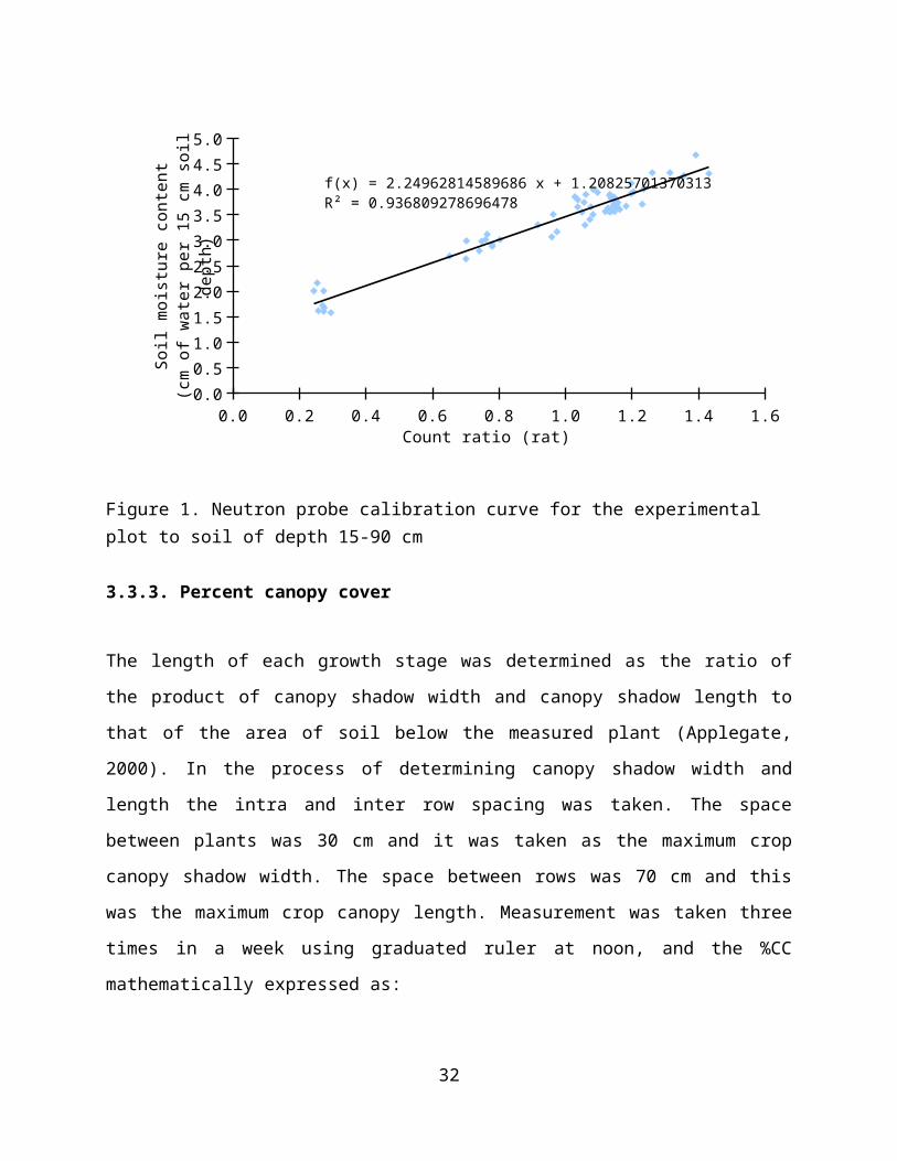
The probe reading in rat versus the volume samples in cm per 15cm

was plotted and produced a linear equation. The linear equation

was expressed as:

Y = A (ratio) + B (5)

where, Y = soil moisture in cm per 15 cm

A = slope

Ratio = count Ratio (count/standard count) and

B = intercept

The coefficients, A and B were obtained from the equation

produced and the required coefficients were fed to the probe and

the soil moisture was given in unit of cm per 15 cm soil depth.

The developed equation and the graph are shown in Figure 1.

31

0.0 0.2 0.4 0.6 0.8 1.0 1.2 1.4 1.6

0.00.51.01.52.02.53.03.54.04.55.0

f(x) = 2.24962814589686 x + 1.20825701370313R² = 0.936809278696478

Count ratio (rat)

Soil

moi

stur

e co

nten

t(c

m of

wat

er p

er 1

5 cm

soi

l de

pth)

Figure 1. Neutron probe calibration curve for the experimental plot to soil of depth 15-90 cm

3.3.3. Percent canopy cover

The length of each growth stage was determined as the ratio of

the product of canopy shadow width and canopy shadow length to

that of the area of soil below the measured plant (Applegate,

2000). In the process of determining canopy shadow width and

length the intra and inter row spacing was taken. The space

between plants was 30 cm and it was taken as the maximum crop

canopy shadow width. The space between rows was 70 cm and this

was the maximum crop canopy length. Measurement was taken three

times in a week using graduated ruler at noon, and the %CC

mathematically expressed as:

32

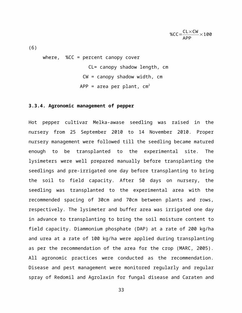
%CC=

CL×CWAPP

×100

(6)

where, %CC = percent canopy cover

CL= canopy shadow length, cm

CW = canopy shadow width, cm

APP = area per plant, cm2

3.3.4. Agronomic management of pepper

Hot pepper cultivar Melka-awase seedling was raised in the

nursery from 25 September 2010 to 14 November 2010. Proper

nursery management were followed till the seedling became matured

enough to be transplanted to the experimental site. The

lysimeters were well prepared manually before transplanting the

seedlings and pre-irrigated one day before transplanting to bring

the soil to field capacity. After 50 days on nursery, the

seedling was transplanted to the experimental area with the

recommended spacing of 30cm and 70cm between plants and rows,

respectively. The lysimeter and buffer area was irrigated one day

in advance to transplanting to bring the soil moisture content to

field capacity. Diammonium phosphate (DAP) at a rate of 200 kg/ha

and urea at a rate of 100 kg/ha were applied during transplanting

as per the recommendation of the area for the crop (MARC, 2005).

All agronomic practices were conducted as the recommendation.

Disease and pest management were monitored regularly and regular

spray of Redomil and Agrolaxin for fungal disease and Caraten and

33

Celecron for insect pest control were used in a weekly interval

when symptoms of the diseases were observed. All agronomic

activities were done to keep the crop free from biotic and

abiotic stress.

3.3.5. Application of irrigation water

Irrigation water was applied when 30% of the TAW depleted from

the effective root zone (Allen et al., 1998). Since the water was

applied to the furrows with a can application efficiency of 90 %

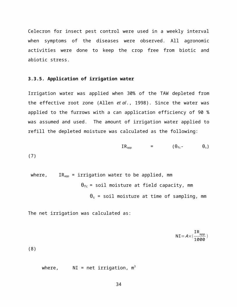
was assumed and used. The amount of irrigation water applied to

refill the depleted moisture was calculated as the following:

IRapp = (θfc- θs)

(7)

where, IRapp = irrigation water to be applied, mm

θfc = soil moisture at field capacity, mm

θs = soil moisture at time of sampling, mm The net irrigation was calculated as:

NI=A×(

IRapp1000

)

(8)

where, NI = net irrigation, m3

34

IRapp = irrigation water to be applied, mm

A = lysimeter area, m2

Gross irrigation was calculated as:

GI=NI

Ea

(9)

where, GI = gross irrigation, m3

NI = net irrigation, m3

Ea = application efficiency, %

The applied water in to the lysimeter and buffer area was

calculated as:

IRapp = GI × 1000

(10)

where, IRapp = applied irrigation water, lit

GI = gross irrigation, m3

Irrigation water was applied using a known volume of graduated

can by converting the calculated depleted water to liter.

Refilling of the depleted amount of moisture to the effective

root zone was done following the root development of the crop

which varies from 50 cm to 100 cm (Allen et al., 1998). In each

35

stage of growth the root growth has been monitored by uprooting

the crop in each stages approximated. From each lysimeter area

soil moisture was measured in each alternate days using neutron

probe for 15 cm to 90 cm soil depth and gravimetric method for

the top 0-15 cm depth to determine the change in soil moisture

content (∆S) which was an important input to determine ETc and to

apply the depleted amount of water that would bring the soil

moisture back to field capacity. Irrigation water application was

terminated when the pepper started to mature and senescence of

leaves observed.

3.4. Crop data collected

Some agronomic data were collected from the lysimeter and buffer

area excluding the border rows and the rest of all response

variables were recorded and presented. Plant height (cm)

measurement was made from the soil surface to the top most growth

points of above ground plant part. The measurement was taken as

the average of five Plants where two from the lysimeter area and

three plants from the border plants of each plot at each growth

stages. Numbers of primary, secondary and tertiary branches per

stem of five randomly selected plants were counted at each growth

stages. Leaf area index (LAI) is defined as the average total

area of leaves (one side) per unit area of ground surface and

measured directly by harvesting all green healthy leaves from

representative plants in the buffer area using a leaf area meter

(Allen et al., 1998). 36

From yield and yield related parameters the total number of

fruits per plant was counted from five randomly selected plants

from the two lysimeter and the average was taken as mean maximum

fruits number per plant. The mean number of red ripe fruits of

five randomly selected plants from central rows and

lysimeter area and weight of pods per plant for each plot at

each harvest was recorded. The total yield of each lysimeterwas also recorded and the total yield was put as the average of

the two lysimeter in a hectare basis. The number of days from

transplanting to the date of maturity and each period of pickings

(harvest) was recorded.

3.5. Determination of crop evapotranspiration

Evapotranspiration of pepper was measured using the soil water

balance of the soil water content changes in the lysimeter area,

rainfall; irrigation water applied and drainage from the

lysimeter area were used as input. For each growth stages the

crop evapotranspiration was calculated. The estimated

evapotranspiration by water balance equation was considered as

the seasonal crop evapotranspiration. In each successive day the

water balance was calculated using the soil moisture measured in

each day. The water balance equation mathematically expressed as:

37

ETc = R+I-D ± ∆S

(11)

where ETc is crop evapotranspiration, I is irrigation water

applied, R is rainfall, D is drained water collected and ∆S is

change in storage of soil moisture and all are in mm. Change in

soil moisture (∆S) is the difference in moisture content of each

consecutive days and it was calculated by deducting the moisture

content obtained today from previous day in each alternate days

starting from transplanting up to the last harvest.

3.5.2. Calculation of reference crop evapotranspiration

The reference crop evapotranspiration was calculated according to

the FAO Penman Monteith method using CROPWAT 8 windows version

4.2. Since the only factors that affect reference crop

evapotranspiration were weather parameters, reference crop

evapotranspiration was computed from climatic data which was

obtained from the nearby meteorology station (Allen et al., 1994).

The FAO Penman Monteith equation requires air temperature,

relative humidity, wind speed and sunshine hours which were

collected from weather stations (Appendix Table 2). The FAO

penman equation is expressed as:

38

ETo=

0.408Δ (RR ((Rn−G)+γ900T+273

u2(es−ea )

Δ+γ(1+0.34u2) (12)

Where, ETo = Reference evapotranspiration, mm day-1

Rn = Net radiation at the crop surface ,

MJ m-2 day-1

G = Soil heat flux density ,, MJ m-2 day-1

T = Air temperature at 2 m height , °C

u2 = Wind speed at 2 m height , m s-1

es = Saturation vapour pressure , kPa

ea = Actual vapour pressure , kPa

es - ea = Saturation vapour pressure deficit ,

kPa

∆ = Slope vapour pressure curve , kPa °C-1

and

γ = Psychrometric constant, kPa °C-1

3.5.3. Calculation of crop coefficient

Crop coefficient (Kc) was defined as the ratio of crop

evapotranspiration to the reference crop evapotranspiration and

calculated by single and dual crop methods (Jenson et al., 1990;

Allen et al., 1998). In the case of this experiment the Kc was

calculated by single crop method as the ratio of crop

evapotranspiration obtained from water balance expression (eq.

39

24) to that of reference crop evapotranspiration obtained from

FAO Penman Monteith equation (eq. 7) which uses CROPWAT 8 windows

4.2 software, as the following:

Kc=ETc

ETo

(13)

where, ETc and ETo are crop evapotranspiration and reference crop

evapotranspiration at the various growth stages (initial,

development, mid-season and late-seasons).

4. RESULTS AND DISCUSSION

4.1. Soil Characteristics of the Experimental Site

40

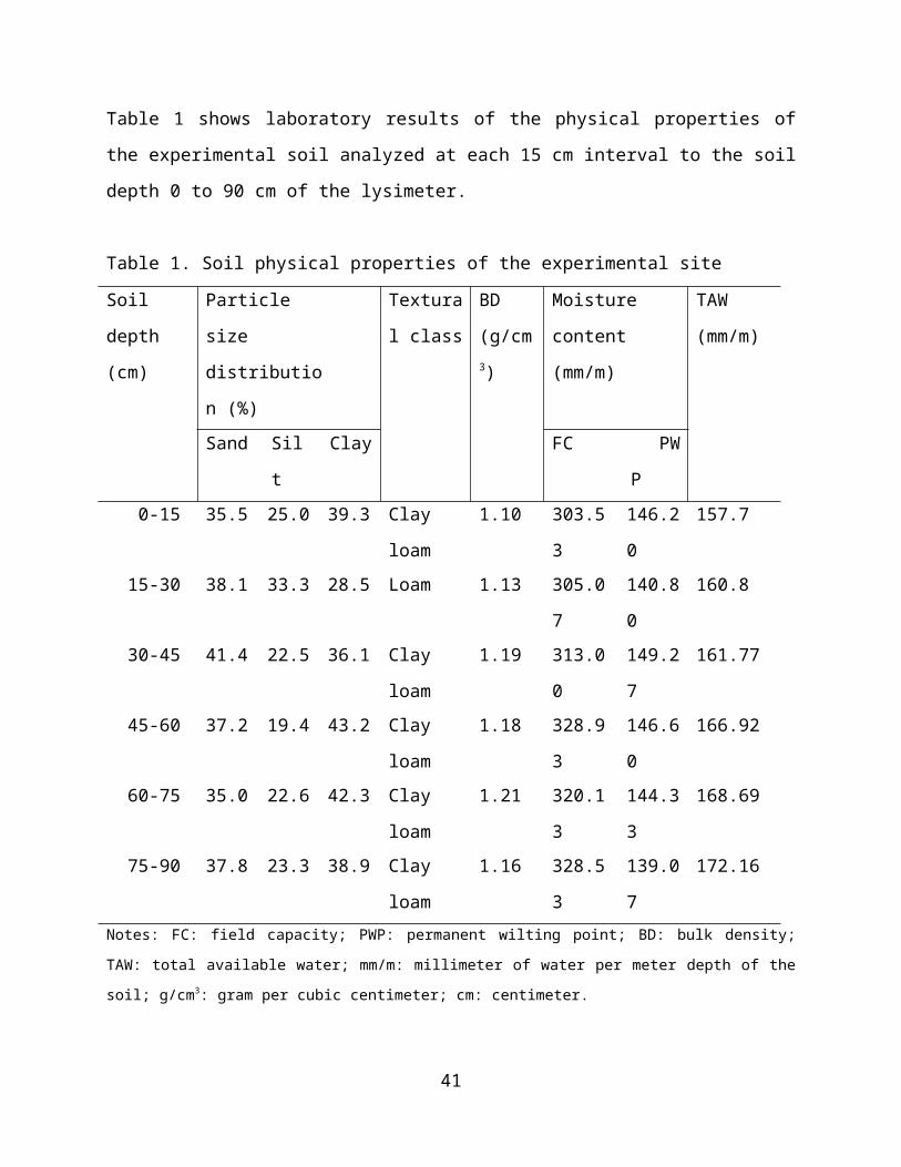
Table 1 shows laboratory results of the physical properties of

the experimental soil analyzed at each 15 cm interval to the soil

depth 0 to 90 cm of the lysimeter.

Table 1. Soil physical properties of the experimental site

Soil

depth

(cm)

Particle

size

distributio

n (%)

Textura

l class

BD

(g/cm3)

Moisture

content

(mm/m)

TAW

(mm/m)

Sand Sil

t

Clay FC PW

P 0-15 35.5 25.0 39.3 Clay

loam

1.10 303.5

3

146.2

0

157.7

15-30 38.1 33.3 28.5 Loam 1.13 305.0

7

140.8

0

160.8

30-45 41.4 22.5 36.1 Clay

loam

1.19 313.0

0

149.2

7

161.77

45-60 37.2 19.4 43.2 Clay

loam

1.18 328.9

3

146.6

0

166.92

60-75 35.0 22.6 42.3 Clay

loam

1.21 320.1

3

144.3

3

168.69

75-90 37.8 23.3 38.9 Clay

loam

1.16 328.5

3

139.0

7

172.16

Notes: FC: field capacity; PWP: permanent wilting point; BD: bulk density;

TAW: total available water; mm/m: millimeter of water per meter depth of the

soil; g/cm3: gram per cubic centimeter; cm: centimeter.

41

The estimated total available water holding capacity of the

experimental soil is 172.16 mm/m. The amount of moisture

increased from the most top layer to the bottom of the lysimeter.

The averaged field capacity and permanent wilting point of the

soil is 316.53 mm/m and 144.38 m/m, respectively. Field capacity

increases from the surface of the lysimeter to the bottom. The

average bulk density is 1.16 g/cm3 with an increasing trend down

to the lysimeter. Bulk density refers to the compactedness or

looseness of a soil; it shows an increased compaction down to the

soil profile. The type of soil under which the crop is grown has

a greater influence on the availability of water to the crop. The

textural class of soil which dominates the experimental lysimeter

is clay loam (Table 1). Crop evapotranspiration is satisfied by

the amount of water that is held around the transpiring crop and

the evaporating surface.

The average particle size distribution of the lysimeter is 37.5%

sand, 24.35% silt and 38.05% clay in the depth of 0-95 cm soil

layer except in the second layer which is loam. The difference in

texture of the layer 15 to 30 cm may be due to sampling.

4.2. Percent Canopy Cover and Leaf Area Index

The amount of moisture transpired by the crop and evaporated from

bare soil to satisfy the demand of the atmosphere is associated

with the leaf area development and canopy cover which increases

or decreases the area that will be exposed to direct sun light.

The relationship between percent canopy cover and leaf area index42

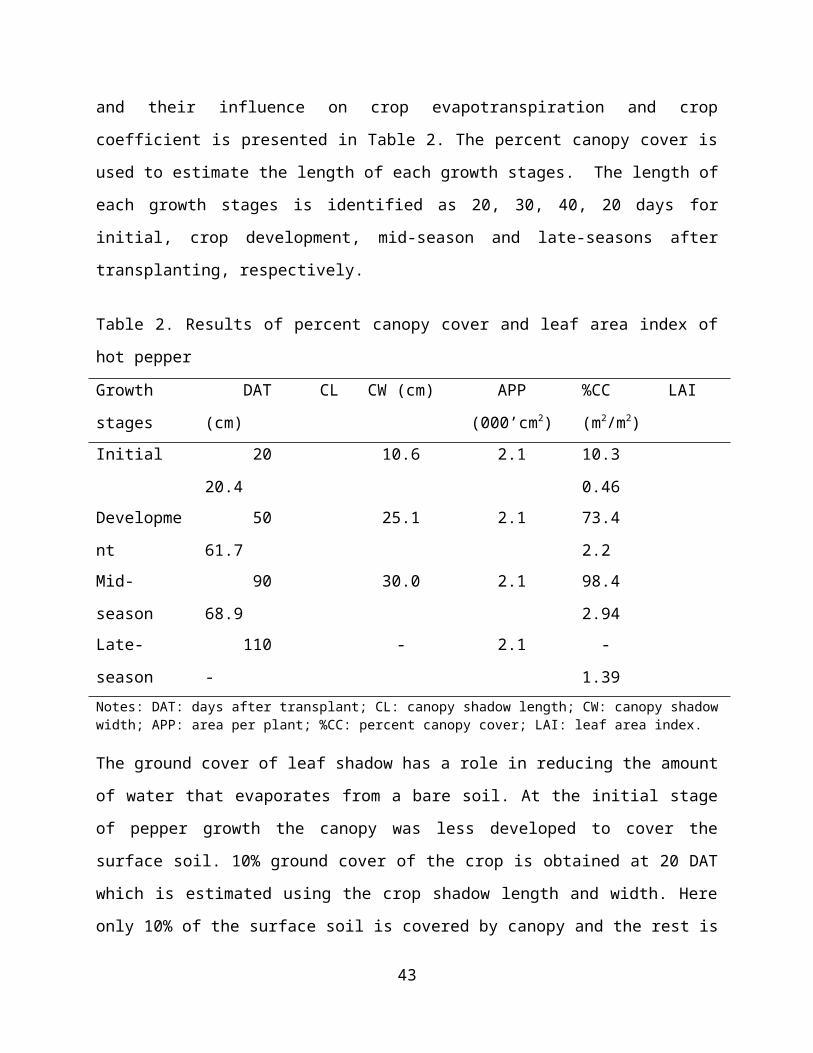
and their influence on crop evapotranspiration and crop

coefficient is presented in Table 2. The percent canopy cover is

used to estimate the length of each growth stages. The length of

each growth stages is identified as 20, 30, 40, 20 days for

initial, crop development, mid-season and late-seasons after

transplanting, respectively.

Table 2. Results of percent canopy cover and leaf area index of

hot pepper

Growth

stages

DAT CL

(cm)

CW (cm) APP

(000’cm2)

%CC LAI

(m2/m2)Initial 20

20.4

10.6 2.1 10.3

0.46Developme

nt

50

61.7

25.1 2.1 73.4

2.2Mid-

season

90

68.9

30.0 2.1 98.4

2.94Late-

season

110

-

- 2.1 -

1.39Notes: DAT: days after transplant; CL: canopy shadow length; CW: canopy shadowwidth; APP: area per plant; %CC: percent canopy cover; LAI: leaf area index.

The ground cover of leaf shadow has a role in reducing the amount

of water that evaporates from a bare soil. At the initial stage

of pepper growth the canopy was less developed to cover the

surface soil. 10% ground cover of the crop is obtained at 20 DAT

which is estimated using the crop shadow length and width. Here

only 10% of the surface soil is covered by canopy and the rest is

43

exposed to direct sun light. This indicates the crop

evapotranspiration at this stage is mostly satisfied from soil

evaporation. Allen et al., (1998), has also indicated that at

transplanting nearly 100% of ET comes from evaporation, while at

full crop cover (mid-season stage) more than 90% of ET comes from

transpiration.

As Kc is the ratio of ETc to ETo, at this stage crop coefficient

values are less as compared to the other stages. At 50 DAT the

second stage of growth is estimated which is the stage that shows

maximum vegetative growth and the space between crops are likely

to be avoided from direct sun light. At the crop development

stage there is more crop water use than the former stage. Crop

coefficient value is constantly rising at this stage due to an

increased crop evapotranspiration which resulted from increment

of leaf area of the transpiring leaf. During mid-season stage the

crop attained peak value of leaf area index and canopy cover.

These increased the proportion of leaf area exposed to direct sun

light, as a result it raised the ETc and Kc of the crop. Late-

season stage is the stage where decline of every activities are

observed. At this stage ETc of the crop is slowing down due to

senescence and aging of the transpiring leaves. Finally, since

application of irrigation water is terminated ETc and Kc became

declined.

44

Leaf area and canopy cover are directly related to each other and

to the amount of crop evapotranspiration and crop coefficient of

hot pepper. As leaf area increased from 0.46 m2/m2 to 2.2 m2/m2

the proportion of soil exposed to direct sun light decreased from

around 90% to less than 15%. The maximum ETc and Kc of hot pepper

is obtained at mid-season stage (60 to 90 DAT) and the value of

leaf area and canopy cover is also the highest (Table 2). The

size of canopy has a direct influence on evapotranspiration of

crops (Steyn, 1997). The rate of water vapour loss from a crop

and the underlying soil depends on the physical and physiological

properties of the crop, the relative heat flux to the crop and

the soil and the water content of the soil. The physiological

nature of the plant and the availability of water in the soil

play an important role in evapotranspiration. The LAI of a crop

is used to define the effective surface area for water loss from

the crop and the amount of shading of the ground surface below.

(Paul et al., 2005). As the leaf area index increased from initial

stage to mid-season stage the values of ETc and Kc is also

increasing and it declined at late-season stage when LAI

decreased.

4.3. Crop Evapotranspiration

Lysimeter data was calculated and presented in a decade interval

(Table 3). During the experimental period rainfall data was

45

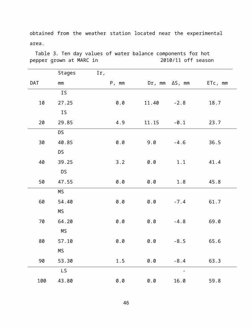
obtained from the weather station located near the experimental

area.

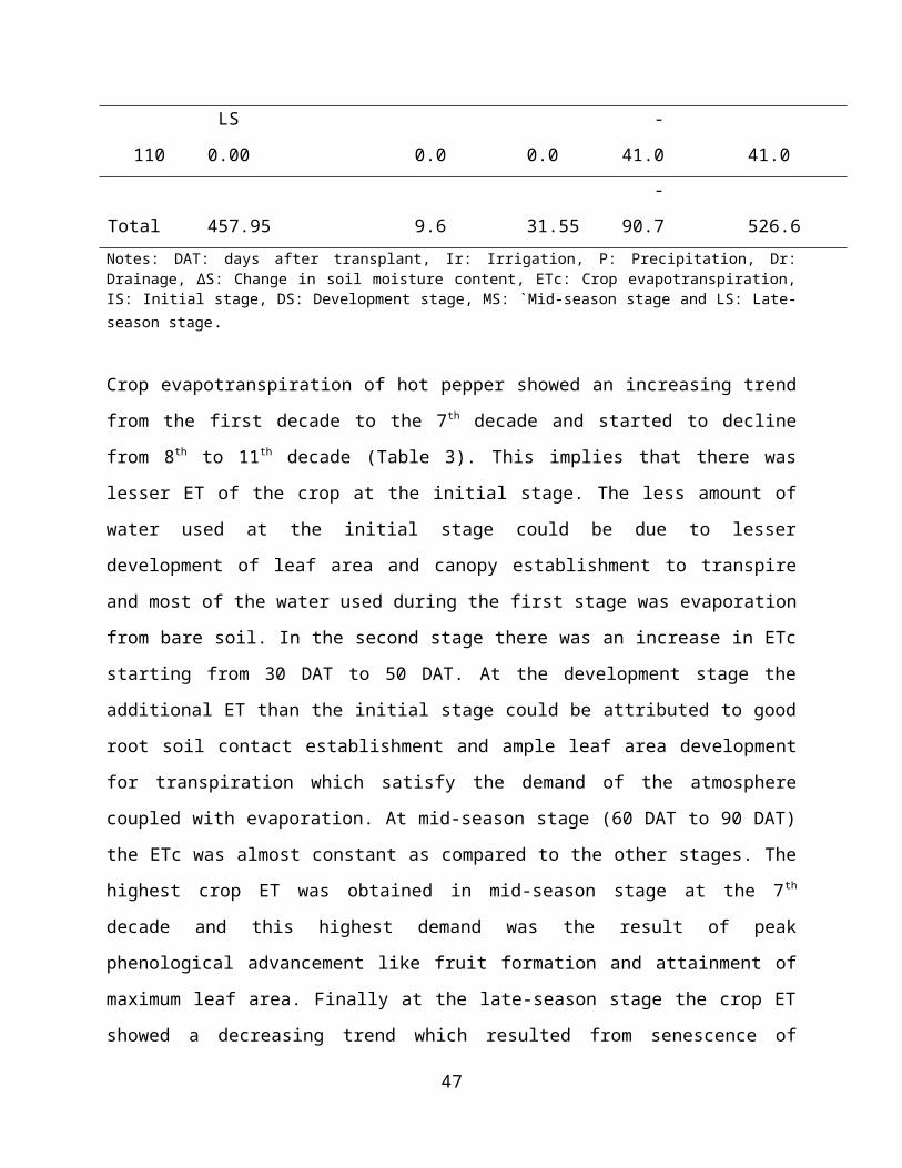
Table 3. Ten day values of water balance components for hot pepper grown at MARC in                  2010/11 off season

DAT

Stages Ir,

mm P, mm Dr, mm ΔS, mm ETc, mm

10

IS

27.25 0.0 11.40 -2.8 18.7

20

IS

29.85 4.9 11.15 -0.1 23.7

30

DS

40.85 0.0 9.0 -4.6 36.5

40

DS

39.25 3.2 0.0 1.1 41.4

50

DS

47.55 0.0 0.0 1.8 45.8

60

MS

54.40 0.0 0.0 -7.4 61.7

70

MS

64.20 0.0 0.0 -4.8 69.0

80

MS

57.10 0.0 0.0 -8.5 65.6

90

MS

53.30 1.5 0.0 -8.4 63.3

100

LS

43.80 0.0 0.0

-

16.0 59.8

46

110

LS

0.00 0.0 0.0

-

41.0 41.0

Total

457.95 9.6 31.55

-

90.7 526.6Notes: DAT: days after transplant, Ir: Irrigation, P: Precipitation, Dr:Drainage, ΔS: Change in soil moisture content, ETc: Crop evapotranspiration,IS: Initial stage, DS: Development stage, MS: `Mid-season stage and LS: Late-season stage.

Crop evapotranspiration of hot pepper showed an increasing trend

from the first decade to the 7th decade and started to decline

from 8th to 11th decade (Table 3). This implies that there was

lesser ET of the crop at the initial stage. The less amount of

water used at the initial stage could be due to lesser

development of leaf area and canopy establishment to transpire

and most of the water used during the first stage was evaporation

from bare soil. In the second stage there was an increase in ETc

starting from 30 DAT to 50 DAT. At the development stage the

additional ET than the initial stage could be attributed to good

root soil contact establishment and ample leaf area development

for transpiration which satisfy the demand of the atmosphere

coupled with evaporation. At mid-season stage (60 DAT to 90 DAT)

the ETc was almost constant as compared to the other stages. The

highest crop ET was obtained in mid-season stage at the 7th

decade and this highest demand was the result of peak

phenological advancement like fruit formation and attainment of

maximum leaf area. Finally at the late-season stage the crop ET

showed a decreasing trend which resulted from senescence of

47

leaves and it was the sign of maturity and declining of growth

and development of the crop.

From the stage wise crop ET the averaged maximum water use was

259.7 mm at the mid-season stage while development stage showed

the second in crop ET which was 123.7 mm. Late-season and initial

stages hold the third and least crop ET, respectively. With

respect to stage wise crop ET of pepper Osei-Bonsu et al. (2010)

have shown that 32.95 mm, 115.84 mm, 343.78 mm and 94.91 mm for

each stage, respectively, with 587.48 mm water use per a growing

season. The highest ETc of hot pepper cultivar Melka-awase was

found to be 6.6 mm/day which was recorded at 80 DAT. The

cumulative ETc calculated in a given environment is a function of

plant height and length of the growing season (Allen et al.,

1998).

The whole water balance components of the lysimeters are

presented in Appendix Table 3 and 4, respectively. The value of

the seasonal ETc found in this research was a little bit lower

than the ranges put by Allen et al. (1998) for hot pepper, which

varies from 600 mm to 900 mm, depending on the region, climate

and variety. Growing conditions, climate and cultivar differences

may have contributed to the observed differences between the

present results and those of FAO estimations. Agodzo et al. (2003)

indicated that the crop water requirement of hot pepper ranged

between 300 mm – 700 mm depending on the climatic condition and

48

the season of the crop and the location in which this variation

showed strong need of local calibration of crop

evapotranspiration for different environments. Grimes and

Williams (1990) have also reported that water requirement for hot

pepper per growing season ranges between 400 mm and 500 mm

depending on the season of planting (the climatic conditions

prevailing in the area). As Yibekal et al. (2009) indicated that

the seasonal crop water use of hot pepper cultivar long slim was

577 mm for South Africa condition with simulated ETc ranged from

390 mm to 546 mm for different cultivars used in the research.

Variability in the water requirements of hot pepper was a

function of environmental conditions. According to FAO reports

(Allen et al., 1998) apart from the water availability in the

topsoil, the evaporation from a cropped soil was mainly

determined by the fraction of the solar radiation reaching the

soil surface. This fraction decreases over the growing period as

the crop develops and the crop canopy shades more and more of the

ground area. When the crop was small, water was predominately

lost by soil evaporation and transpiration lesser, but once the

crop was well developed and completely covers the soil,

evapotranspiration became the main process.

4.4. Reference Crop Evapotranspiration

Reference crop evapotranspiration (ETo) is a parameter which

reflects the effect of climate on the crop evapotranspiration. As49

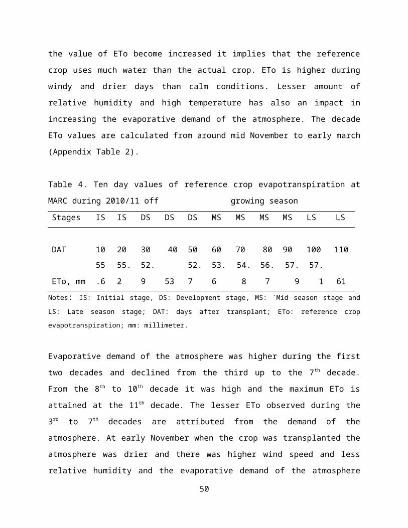
the value of ETo become increased it implies that the reference

crop uses much water than the actual crop. ETo is higher during

windy and drier days than calm conditions. Lesser amount of

relative humidity and high temperature has also an impact in

increasing the evaporative demand of the atmosphere. The decade

ETo values are calculated from around mid November to early march

(Appendix Table 2).

Table 4. Ten day values of reference crop evapotranspiration at

MARC during 2010/11 off               growing season

Stages IS IS DS DS DS MS MS MS MS LS LS

DAT 10 20 30 40 50 60 70 80

90

100 110

ETo, mm

55

.6

55.

2

52.

9

53

52.

7

53.

6

54.

8

56.

7

57.

9

57.

1 61Notes: IS: Initial stage, DS: Development stage, MS: `Mid season stage andLS: Late season stage; DAT: days after transplant; ETo: reference crop

evapotranspiration; mm: millimeter.

Evaporative demand of the atmosphere was higher during the first

two decades and declined from the third up to the 7th decade.

From the 8th to 10th decade it was high and the maximum ETo is

attained at the 11th decade. The lesser ETo observed during the

3rd to 7th decades are attributed from the demand of the

atmosphere. At early November when the crop was transplanted the

atmosphere was drier and there was higher wind speed and less

relative humidity and the evaporative demand of the atmosphere

50

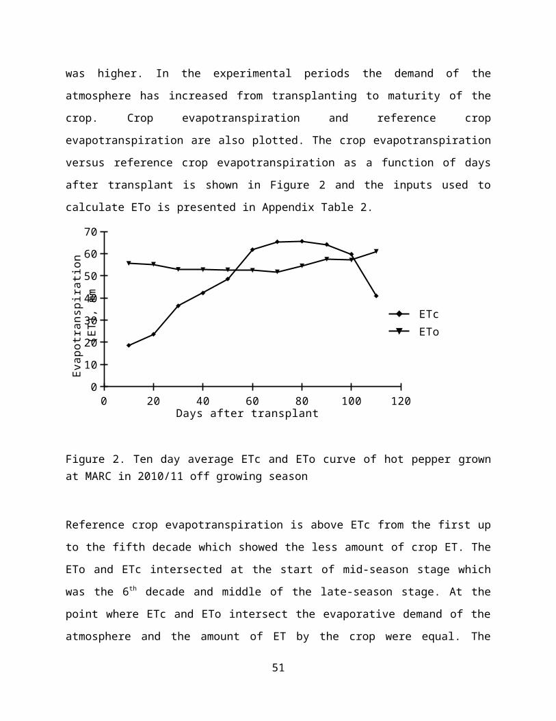
was higher. In the experimental periods the demand of the

atmosphere has increased from transplanting to maturity of the

crop. Crop evapotranspiration and reference crop

evapotranspiration are also plotted. The crop evapotranspiration

versus reference crop evapotranspiration as a function of days

after transplant is shown in Figure 2 and the inputs used to

calculate ETo is presented in Appendix Table 2.

0 20 40 60 80 100 1200

10

20

30

40

50

60

70

ETc ETo

Days after transplant

Evap

otra

nspi

rati

on

(ET)

, mm

Figure 2. Ten day average ETc and ETo curve of hot pepper grownat MARC in 2010/11 off growing season

Reference crop evapotranspiration is above ETc from the first up

to the fifth decade which showed the less amount of crop ET. The

ETo and ETc intersected at the start of mid-season stage which

was the 6th decade and middle of the late-season stage. At the

point where ETc and ETo intersect the evaporative demand of the

atmosphere and the amount of ET by the crop were equal. The

51

maximum value of ETo recorded showed the highest evaporative

demand of the atmosphere and there was a much more crop ET at

this period.

The result of decade ETo (Figure 4) showed that the values were

almost similar starting from 30 DAT up to 70 DAT while there was

an increase at the 8th decade to 10th decades. The highest value

of ETo was observed at the 11th decade which indicated the

maximum evaporative demand of the atmosphere. FAO reported that

crop ET and ETo were higher for crops with longer growing season

than for those with shorter ones. In the case of this research

the pepper crop variety used has shorter growing periods than the

other varieties of this crop. ETo and ETc were also more during

the dry season and windy days than rainy and humid season. FAO

(2005) reported that crops grown in the dry season need more

water than those grown during the rainy season. Under standard

conditions the ET of a reference crop was estimated to be 4-6

mm/day for arid and semi arid climatic regions (Allen et al.,

1998), where the result of Melkassa ETo lies in this range.

The stage wise values of ETo for Melkassa in 2010/11 off growing

season has raised from 110.77 mm at initial stage to 158.32 mm at

development stage (Table 4). The highest value of ETo at mid-

season stage (223.52 mm) implies the maximum evaporative demand

of the atmosphere. The total length of hot pepper growth stage

and the climatic conditions under which the crop growth stages

reaches has affected the evaporative demand of the atmosphere.52

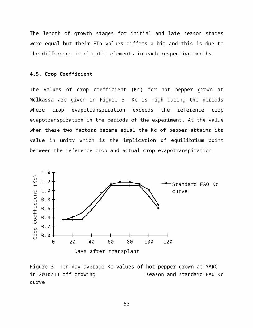
The length of growth stages for initial and late season stages

were equal but their ETo values differs a bit and this is due to

the difference in climatic elements in each respective months.

4.5. Crop Coefficient

The values of crop coefficient (Kc) for hot pepper grown at

Melkassa are given in Figure 3. Kc is high during the periods

where crop evapotranspiration exceeds the reference crop

evapotranspiration in the periods of the experiment. At the value

when these two factors became equal the Kc of pepper attains its

value in unity which is the implication of equilibrium point

between the reference crop and actual crop evapotranspiration.

0 20 40 60 80 100 1200.00.20.40.60.81.01.21.4

Standard FAO Kc curve

Days after transplant

Crop

coe

ffic

ient

(Kc

)

Figure 3. Ten-day average Kc values of hot pepper grown at MARC in 2010/11 off growing                 season and standard FAO Kccurve

53

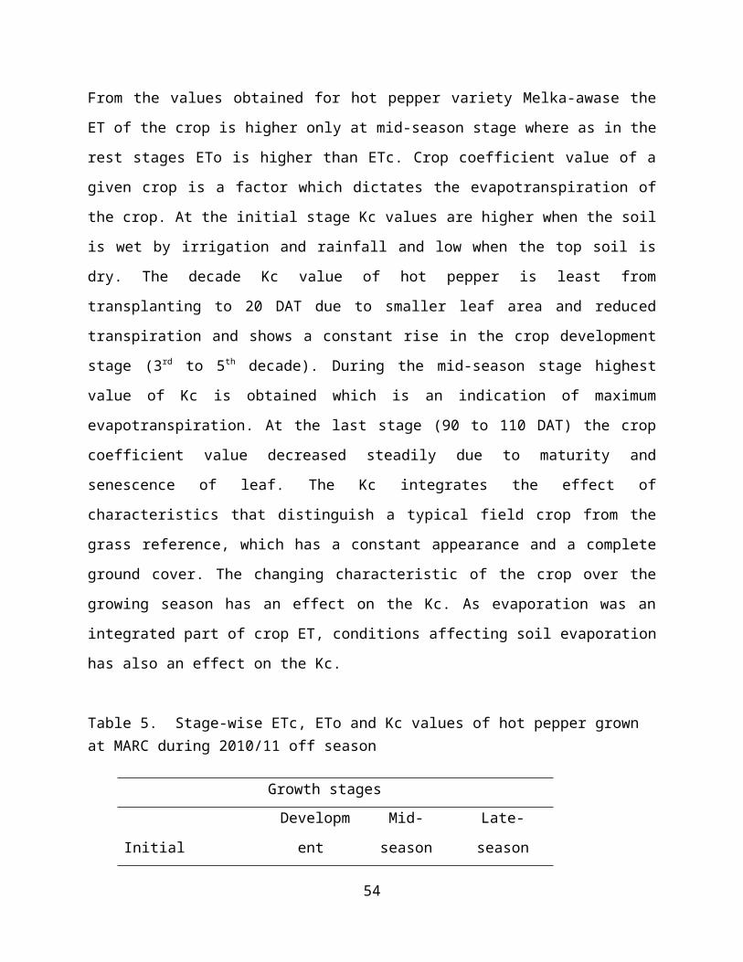
From the values obtained for hot pepper variety Melka-awase the

ET of the crop is higher only at mid-season stage where as in the

rest stages ETo is higher than ETc. Crop coefficient value of a

given crop is a factor which dictates the evapotranspiration of

the crop. At the initial stage Kc values are higher when the soil

is wet by irrigation and rainfall and low when the top soil is

dry. The decade Kc value of hot pepper is least from

transplanting to 20 DAT due to smaller leaf area and reduced

transpiration and shows a constant rise in the crop development

stage (3rd to 5th decade). During the mid-season stage highest

value of Kc is obtained which is an indication of maximum

evapotranspiration. At the last stage (90 to 110 DAT) the crop

coefficient value decreased steadily due to maturity and

senescence of leaf. The Kc integrates the effect of

characteristics that distinguish a typical field crop from the

grass reference, which has a constant appearance and a complete

ground cover. The changing characteristic of the crop over the

growing season has an effect on the Kc. As evaporation was an

integrated part of crop ET, conditions affecting soil evaporation

has also an effect on the Kc.

Table 5. Stage-wise ETc, ETo and Kc values of hot pepper grown at MARC during 2010/11 off season

Growth stages

Initial

Developm

ent

Mid-

season

Late-

season

54

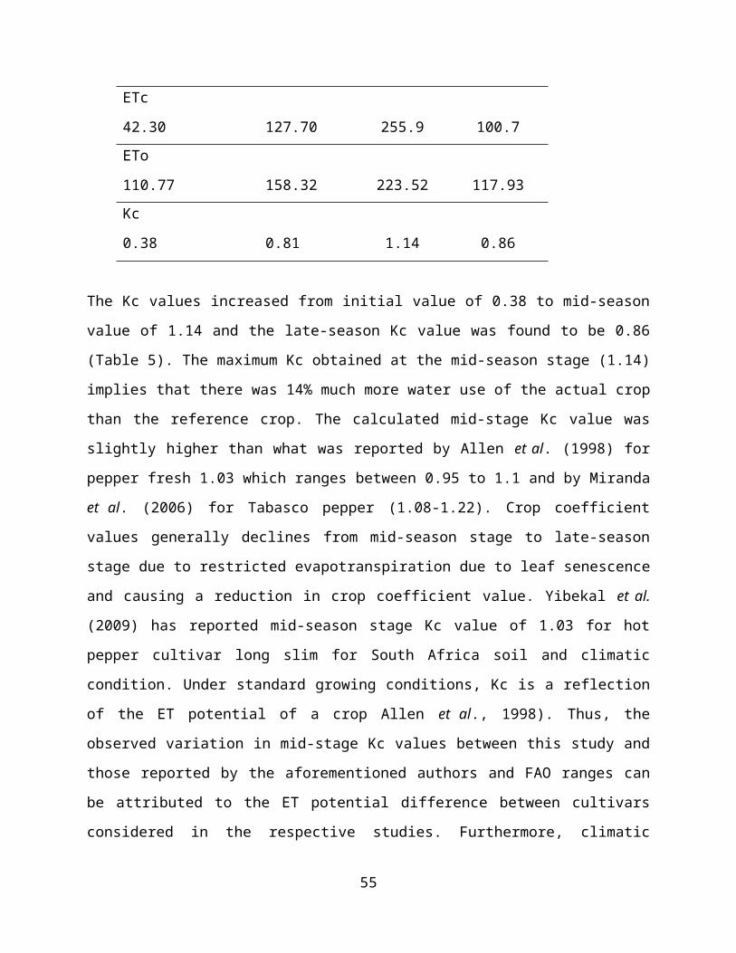
ETc

42.30

127.70 255.9 100.7ETo

110.77

158.32 223.52 117.93Kc

0.38

0.81 1.14 0.86

The Kc values increased from initial value of 0.38 to mid-season

value of 1.14 and the late-season Kc value was found to be 0.86

(Table 5). The maximum Kc obtained at the mid-season stage (1.14)

implies that there was 14% much more water use of the actual crop

than the reference crop. The calculated mid-stage Kc value was

slightly higher than what was reported by Allen et al. (1998) for

pepper fresh 1.03 which ranges between 0.95 to 1.1 and by Miranda

et al. (2006) for Tabasco pepper (1.08-1.22). Crop coefficient

values generally declines from mid-season stage to late-season

stage due to restricted evapotranspiration due to leaf senescence

and causing a reduction in crop coefficient value. Yibekal et al.

(2009) has reported mid-season stage Kc value of 1.03 for hot

pepper cultivar long slim for South Africa soil and climatic

condition. Under standard growing conditions, Kc is a reflection

of the ET potential of a crop Allen et al., 1998). Thus, the

observed variation in mid-stage Kc values between this study and

those reported by the aforementioned authors and FAO ranges can

be attributed to the ET potential difference between cultivars

considered in the respective studies. Furthermore, climatic

55

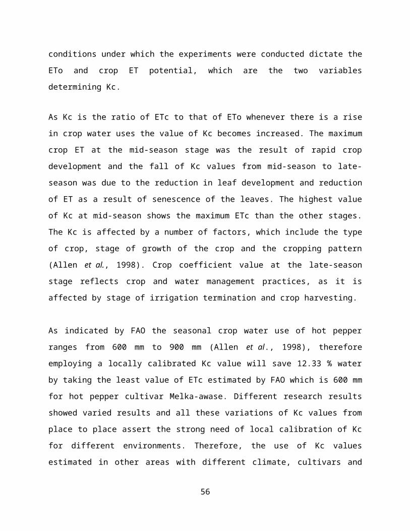
conditions under which the experiments were conducted dictate the

ETo and crop ET potential, which are the two variables

determining Kc.

As Kc is the ratio of ETc to that of ETo whenever there is a rise

in crop water uses the value of Kc becomes increased. The maximum

crop ET at the mid-season stage was the result of rapid crop

development and the fall of Kc values from mid-season to late-

season was due to the reduction in leaf development and reduction

of ET as a result of senescence of the leaves. The highest value

of Kc at mid-season shows the maximum ETc than the other stages.

The Kc is affected by a number of factors, which include the type

of crop, stage of growth of the crop and the cropping pattern

(Allen et al., 1998). Crop coefficient value at the late-season

stage reflects crop and water management practices, as it is

affected by stage of irrigation termination and crop harvesting.

As indicated by FAO the seasonal crop water use of hot pepper

ranges from 600 mm to 900 mm (Allen et al., 1998), therefore

employing a locally calibrated Kc value will save 12.33 % water

by taking the least value of ETc estimated by FAO which is 600 mm

for hot pepper cultivar Melka-awase. Different research results

showed varied results and all these variations of Kc values from

place to place assert the strong need of local calibration of Kc

for different environments. Therefore, the use of Kc values

estimated in other areas with different climate, cultivars and

56

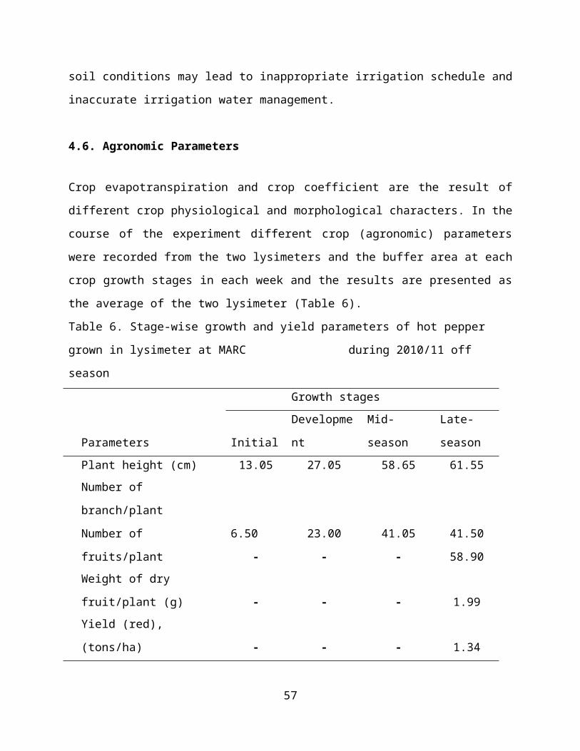
soil conditions may lead to inappropriate irrigation schedule and

inaccurate irrigation water management.

4.6. Agronomic Parameters

Crop evapotranspiration and crop coefficient are the result of

different crop physiological and morphological characters. In the

course of the experiment different crop (agronomic) parameters

were recorded from the two lysimeters and the buffer area at each

crop growth stages in each week and the results are presented as

the average of the two lysimeter (Table 6).

Table 6. Stage-wise growth and yield parameters of hot pepper

grown in lysimeter at MARC               during 2010/11 off

season

Growth stages

Parameters

Initial

Developme

nt

Mid-

season

Late-

seasonPlant height (cm) 13.05 27.05 58.65 61.55Number of

branch/plant

Number of

fruits/plant

6.50

-

23.00

-

41.05

-

41.50

58.90Weight of dry

fruit/plant (g) - - - 1.99Yield (red),

(tons/ha) - - - 1.34

57

Plant height increased from initial stage of 13.05 cm to 27.05 cm

at mid-season stage. The maximum rise in plant height was

observed from mid to late season which was assumed as the stage

of maximum crop morphological advancement. In this cultivar the

maximum plant height was found to be 61.55 cm and it was in line

with the works of MARC (2005). Similarly the highest number of

branches per plant was recorded at mid-season stage and there was

no much more branches obtained at late-season stage. In the case

of fruit number and weight of dry fruits per plant, 58.9 and 1.99

g were recorded, respectively. The average dry yield of cultivar

Melka-awase was 1.34 tons/ha (Table 6).

5. SUMMARY, CONCLUSION AND RECOMENDATION

58

5.1. Summary

For most crops grown in the country locally estimated ETc and Kc

values are not available. Determining ETc and Kc of agricultural

crops helps to have appropriate irrigation schedule, wise

management of irrigation water and designing and managing

irrigated projects. This research aimed at establishing stage

wise ETc and Kc value of hot pepper cultivar Melka-awase under

Melkassa climatic and soil condition. The experiment was

undertaken at Melkassa Agricultural Research Center to determine

the seasonal crop water requirement (ETc) and crop coefficient

(Kc) of hot pepper cultivar Melka-awase for the different growth

stages. Two rectangular drainage type lysimeters were employed to

determine the seasonal water use of hot pepper. ETc was

calculated using water balance equation and ETo was determined by

FAO-Penman Monteith equation. The ratio of ETc to that of the ETo

was taken as Kc of the crop at each respective growth stages and

the sum of each stages ETc were taken as seasonal ETc of hot

pepper cultivar Melka-awase.

The length of the four growth stages was estimated by calculating

the canopy development and soil coverage of the shadow. The

length of each growth stages were identified as 20, 30, 40 and 20

for initial, crop development, mid-season and late season stages,

respectively. From the results of this research the averaged

seasonal ETc of hot pepper cultivar Melka-awase is 526.06 mm with

the average ETc for initial, development, mid-season and late-

59

season being 42.3, 127.7, 255.9 and 100.7 mm, respectively. The

values of reference crop evapotranspiration of Melkassa during

the pepper growing periods were also calculated as 110.77,

152.32, 223.52 and 117.93 mm, respectively. With respect to Kc it

is estimated to be 0.38, 0.81, 1.14 and 0.86 for initial,

development, mid-season and late-season stages, respectively, and

the Kc end was 0.82. Some agronomic parameters related to the

crop were also measured during the experimental period from the

two lysimeters and buffer area and the uniformity between the two

areas were also monitored accordingly. Plant height, number of

branches and fruits per plant, weight of dry fruit and dry fruit

yield were determined at each respective stages.

5.2. Conclusions and Recommendations

The ETc and Kc of pepper cultivar Melka-awase was estimated. The

values of ETc and Kc found in this experiment slightly differed

from other areas results and this shows the strong need of local

calibration of crop ETc and Kc for specific climate and soil

condition. The result found in this research can be used for

appropriate irrigation planning and to have accurate irrigation

schedule of hot pepper cultivar Melka-awase at Melkassa and areas

with similar climate and soil condition. Since ETc and Kc are a

function of crop characteristics, irrigation water management,

climate conditions, local and agricultural practices, they should

be localized.

60

Due to variability of ETc and Kc results with locations, crop

varieties used, soil types and local climatic condition the

following things could be considered for future studies:

Since ETc and Kc values of agricultural crops are highly

influenced by crop varieties, climate and soil and growing

length of crops they should be determined for each

condition separately.

Determination of ETc and Kc should be done for different

crops produced by irrigation in different parts of the

country to their respective environments.

As seasonal crop ET is highly related to the lengths of

crop growth stage and since there is intra and inter

cultivar difference in seasonal ET in different

environmental conditions, ETc and Kc must be determined

separately for each crops and cultivars.

The ETc and Kc could also be evaluated for different soil

types and irrigation methods at different locations.

The values of seasonal ETc and Kc estimated for hot pepper

cultivar Melka-awase is for off season and it should also

be estimated during the main growing season due to

variability of climatic elements which influence ETo.

Determination of crop evapotranspiration using lysimeter

doesn’t have a long history in the country; therefore more

attention needs to be given to this area.

61

6. REFERENCES

Abdulmumin, S, and S. M. Misari, 1990. Crop coefficient of somemajor crops of Nigerian semi arid tropics. Agricultural WaterManagement, Nigeria, Abuja.

Aboukhaled, A., A. Alfaro and M. Smith, 1982. Lysimeters,Irrigation and Drainage. Food and Agricultural Organization,Number 39, Rome, Italy.

Agodzo, S. K., F. P. Huibers, F. Chenini, J. B. van Lier and A.Duran, 2003. Use of wastewater in irrigated agriculture. Countrystudies from Bolivia, Ghana and Tunisia, Vol. 2, Ghana.Wageningen, pp. 36.

Alemu Hailiye and Ermias Abate, 2000. Horticultural crops

production and associated constraints in Northwest Ethiopia.

Working Paper. Agricultural Economics Research Division.

Agricultural Research Center, Adet. pp. 18

Allen, R., L. Pereira, D. Raes and M. Smith, 1998. Crop

evapotranspiration; guidelines for computing crop water

requirements. Food and Agricultural Organization, Irrigation and

Drainage Paper No. 56, Rome, Italy.

Allen, R. G., R. W. Hill, and S. Vemulapali, 1994.

Evapotranspiration Parameters for Variably-Sized Wetlands. Paper

presented at the 1994 Summer Meeting of ASAE. No- 942132:`P. 24.

62

Andreas, P. S. and K. Frenken, 2002. Crop water requirements and

irrigation schedule. Water resource development and management

officers. FAO sub regional office for East and Southern Africa,

Harare, 2002.

Applegate, J. R.,`2000. A comparison of techniques for estimating

overstory crop canopy. Master of Science Thesis. The University

of Montana.

Blaney, H. F. and W. D. Criddle, 1950. Determining water

requirements in irrigated areas from

climatological and irrigation data. USDA Soil Conserv. Serv. SCS-

TP96. P. 44.

Bosland, P.W. and E. J. Votava, 2000. Peppers, Vegetables and

Spices Capsicum. CABI Publishing. New York. pp. 198.

CSA (Central Stastical Agency), 2007. Agricultural sample survey

2006/7. Report on area and production of crops (Private peasant

holdings, meher season). Addis Ababa, Ethiopia.

CSA (Central Stastical Agency), 2005. Agricultural sample survey

2004/5. Report on area and production of crops (Private peasant

holdings, meher season). Addis Ababa, Ethiopia.

[Cuenca, R. H., 1989. Irrigation system design. An engineering

approach prentices. Hall Inc, New jersey, USA. PP. 115-116.

63

Doorenbos, J. and W. O. Pruitt, 1977. Guidelines for computing

crop water requirements. Food and Agricultural Organization.

Irrigation and Drainage Paper No-24. Rome, Italy.

EASE (Ethiopian Agricultural Sample Enumeration), 2002. Ethiopian

Agricultural Sample Enumeration 2001/2002, Central Statistical

Authority, Addis Ababa, Ethiopia.

EARO (Ethiopian Agricultural research Organization), 2004.

Released crop varieties and their recommended cultural practices.

Progress report. Addis Ababa, Ethiopia

FAO (Food and Agriculture Organization), 2005. Irrigation water

requirements: Irrigation Potential in Africa: A Basin Approach,

Chapter 5, FAO Corporate Document Repository, FAO, Rome, Italy.

FAO (Food and Agricultural Organization), 2004. FAOSTAT database

result for chilies and peppers.http://apps.fao.org/cgi-bin/nph-db.pl.

Accessed on 3/10/2008.

FAO (Food and Agricultural Organization), 2002. Deficient

Irrigation practice. Food and Agriculture organization of the

united nation. Water reports. No. 22. Rome, Italy.

FAO (Food and Agricultural Organization), 1996. Food, Agriculture

and Food security: Developments since the World Food Conference

64

and Prospects. World Food Summit Technical Background Document 1,

Rome, Italy.

Fernandez, M., D. M. Gallardo, S. Bonachella, F. Orgaz and E.

Fereres, 2000. Crop coefficient of a pepper crop grown in plastic

green house in Almeria, Proc. 3rd IS on irrigation. Horticultural

corps: PP. 461-465.

Grattan, S. R., W. Bowers, A. Drong, R. L. Snyder, J. J. Carroll,

and W. George. 1998. Crop coefficient: The key to improving crop

yield. Irrigation Journal. July/August 1998.

Grimes, D.W. and L. E. Williams, 1990. Irrigation effects on

plant. Water relations and Seedless grapevines. 30: PP. 255-260.

Hafnagel, H. P., 1961. Agriculture in Ethiopia. Food and

Agricultural Organization of United Nations, Rome, Italy.

Haman, W. Z., R. T. Pritchard, A. G. Smajistrla and F. S. Zazuet,

1997. Evapotranspiration and crop coefficients for young

blueberries in Florida. ASAE.13 (2): PP. 2009-2016.

Hansen, V. E., O. W. Israelson and G. E. Stringham, 1979.

Irrigation principles and practices John Wiley and Sons. New

York.

Hargreaves, G. L., G. H. Hargreaves, and J. P. Riley, 1985.

Agricultural benefits for Senegal River Basin. Journal of Irrigation

65

and Drainage Engineers. American Society of Civil Engineers: PP. 113-

124.

Hearth, E. and Lemma Desalegn, 1992. Horticulture research and

development in Ethiopia. Proceedings of the 2nd National

Horticultural workshop of Ethiopia. 1-3 December 1992. IAR.Addis

Ababa. pp. 24.

Huguez, D. and P. Phillipe, 1998. Ways of Water, Run-off,

Irrigation and Drainage, 4th Edition. Imperimie Guyot Braine-le-

Chateau, Belgium.

IAR (Institute of Agricultural Research), 1992. Horticultural

research and development in Ethiopia. Addis Abeba, Ethiopia.

P.139.

Iwena O. A., 2002. Essential Agricultural Science for Senior

Secondary Schools. Tonad Publishers Ltd, Ikeja: PP. 55-63.

James, L.G., 1988. Principles of farm irrigation systems, design

and operation. John willey and sons. New York.

Jensen, M. E., R. D. Burman and R. G. Allen, 1990.

Evapotranspiration and Irrigation Water Requirements. American

Society of Civil Engineers Manuals and Reports on Engineering

Practices No. 70. New York: pp. 360.

66

Kashyap, P. S. and R. K. Panda, 2001. Evaluation of

evapotranspiration estimation methods and development of crop

coefficient for potato crop in sub humid regions. Agricultural Water

Management, 26 (1993): PP. 67-80.

Lemma Dessalegne, 1998. Seed production guideline for tomatoes,

onion and hot pepper. IAR. Addis Ababa. Ethiopia. pp. 65.

Khan, B. R., M. Minuddin and M. N. Molla, 1993. Design,

Construction and testing of a lysimeter for a study of

evapotranspiration of different crops. Agricultural water

management, 23 (1993): PP. 183-187. Management and regulatory

Department, Addis Ababa, Ethiopia

MARC (Melkassa Agricultural Research Center), 2005. Progress

Report on Completed Activities: PP. 1- 7.

MARC (Melkassa Agricultural Research Center), 1996. Melkassa

Agricultural Research Center Profile, Melkassa, Ethiopia.

Michael, A.M., 1989. Irrigation theory and practices.Indian

Agricultural Research Inistitute.New Delhi. Vikas Publishing

House Pvt Ltd.

Miller, N. F., L. E. Hinesley and F. A. Blazich, 1982.

Propagation of Fraser fir by stem cuttings: Effects of type of

67

cutting, length of cutting, and genotype. Horticultural Science,

17(5):

Miranda, F. R., R. S. Gondim and C. A. G. Costa, 2006.

Evapotranspiration and crop coefficients for Tabasco pepper

(Capscium frutescens L.). Agricultural Water Management: PP. 237-246.

MoA (Ministry of Agriculture), 1998. Agro-ecological Zones of

Ethiopia. Natural Resources Management and Regulatory Department

(with support of German Agency for technical cooperation (GTZ),

Ministry of Agriculture, Addis Ababa, Ethiopia.

MoARD(Ministry of Agriculture and Rural Development), 2009.

Variety Register. Issue No. 9. June 2006. Addis Ababa, Ethiopia.

MoFED (Ministry of Finance and Economic Development), 2007.

Annual Report on Macroeconomic Developments, Addis Abeba,

Ethiopia.

Monteith, J. L., 1965. Evaporation and Environment. 19th

Symposium of the Society for Experimental Biology, University

Press, Cambridge, 19:205-234.

Osei-Bonsu, P., J. D. Owusu - Sekyere and P. Asante, 2010. Water

requirement, deficit irrigation and crop coefficient of hot

pepper (Capsicum frutescens) using irrigation interval of four

(4) days. ARPN Journal of Agricultural and Biological Science, 5 (5).

68

Paul, E., 2001. Regulated deficit irrigation and partial root

zoning. Land and water. Australia. PP: 85-87.

Paul, E. D., W. S. Meyer and A. Barton, 2005. A Review of

Methods to Estimate Irrigated

Reference Crop Evapotranspiration across Australia. Cooperative

Research Center for Irrigation Futures/CSIRO Land and Water.

Technical Report No. 04/05 April 2005. Australia.

Rejisberman, F. R., 2003. Water Scarcity; fact or fiction?

Agricultural Water Management. 80: PP.5-12.

Rubatzky, V. E. and M. Yamaguchi, 1997. World vegetables:

principles, production and nutritive values, 2nd edition, Chapman

and Hall International, Thomson Publishing, New York, P. 843.

Samson Laike, 2005. Determination of crop water requirement and

crop coefficient of Haricot bean. An M.Sc Thesis presented to the

school of graduate studies of Haramaya University.

Sepaskhah, A. R. and M. Andam, 2001. Crop coefficient of sesame

in a semi arid region of I.R. Iran. Agricultural Water Management 49

(1): PP. 51-63.

Steyn, J. M., 1997. Response of potato genotypes to different

water regimes. Ph.D. Thesis, University of Pretoria, South

Africa.

69

Tilahun, H., Yusuf, K., and Mesfine, M., 2004. Response of tomato

to different irrigation schedules under melkassa conditions. pp

202-203. Kibebew, A., and Lijalem K. (eds) 2006. Proceedings of

the Tewelfth Annual Conference of the Crop Science Society of

Ethiopia. Addis Ababa, Ethiopia

Taygi, N.K., D.K. Sharma and S. K. Luthra, 2000. Determination of

evapotranspiration and crop

coefficients of rice and sunflower with lysimeter. Agricultural

Water management 45(2000).

Wein, H. C. 1997. Peppers. The physiology of Vegetable Crops.CAB

International Oxon, United Kingdom. PP. 259-293.

Yibekal Alemayehu, J. M. Steyn and J. G. Annandale, 2009. FAO-

type crop factor determination for irrigation scheduling of hot

pepper (Capsicum annuum L.) cultivars. Department of plant

production and soil science, University of Pretoria. South Africa

Journal of Plant Soil 2009, 26(3), Pretoria, South Africa.

70

7. APENDICES

71

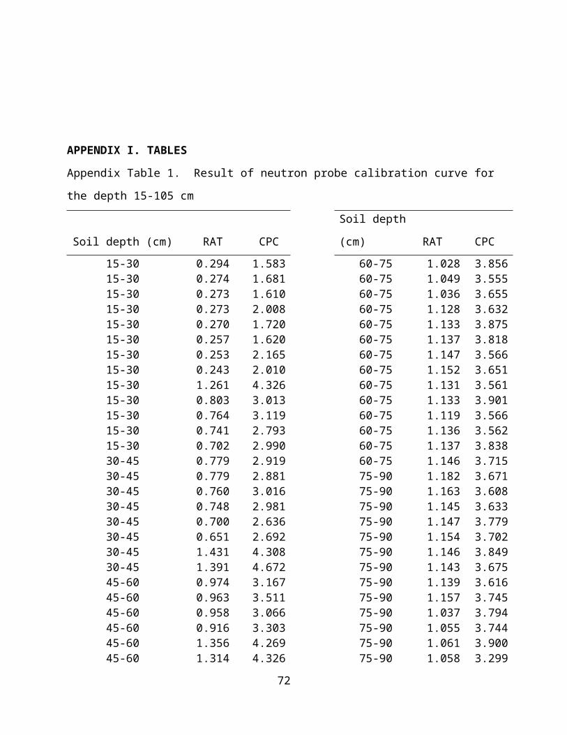
APPENDIX Ι. TABLES

Appendix Table 1. Result of neutron probe calibration curve for

the depth 15-105 cm

Soil depth (cm) RAT CPC

Soil depth

(cm) RAT CPC 15-30 0.294 1.583 60-75 1.028 3.85615-30 0.274 1.681 60-75 1.049 3.55515-30 0.273 1.610 60-75 1.036 3.65515-30 0.273 2.008 60-75 1.128 3.63215-30 0.270 1.720 60-75 1.133 3.87515-30 0.257 1.620 60-75 1.137 3.81815-30 0.253 2.165 60-75 1.147 3.56615-30 0.243 2.010 60-75 1.152 3.65115-30 1.261 4.326 60-75 1.131 3.56115-30 0.803 3.013 60-75 1.133 3.90115-30 0.764 3.119 60-75 1.119 3.56615-30 0.741 2.793 60-75 1.136 3.56215-30 0.702 2.990 60-75 1.137 3.83830-45 0.779 2.919 60-75 1.146 3.71530-45 0.779 2.881 75-90 1.182 3.67130-45 0.760 3.016 75-90 1.163 3.60830-45 0.748 2.981 75-90 1.145 3.63330-45 0.700 2.636 75-90 1.147 3.77930-45 0.651 2.692 75-90 1.154 3.70230-45 1.431 4.308 75-90 1.146 3.84930-45 1.391 4.672 75-90 1.143 3.67545-60 0.974 3.167 75-90 1.139 3.61645-60 0.963 3.511 75-90 1.157 3.74545-60 0.958 3.066 75-90 1.037 3.79445-60 0.916 3.303 75-90 1.055 3.74445-60 1.356 4.269 75-90 1.061 3.90045-60 1.314 4.326 75-90 1.058 3.299

72

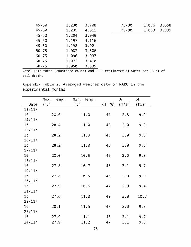
45-60 1.230 3.708 75-90 1.076 3.65845-60 1.235 4.011 75-90 1.083 3.99945-60 1.204 3.94945-60 1.197 4.11645-60 1.198 3.92160-75 1.082 3.50660-75 1.096 3.93760-75 1.073 3.41060-75 1.050 3.335

Note: RAT: ratio (count/std count) and CPC: centimeter of water per 15 cm of soil depth.

Appendix Table 2. Averaged weather data of MARC in the experimental months

DateMax. Temp. (oC)

Min. Temp. (oC) RH (%)

U2

(m/s) SH (hrs)

13/11/10 28.6 11.0 44 2.8 9.914/11/10 28.4 11.0 46 3.0 9.815/11/10 28.2 11.9 45 3.0 9.616/11/10 28.2 11.0 45 3.0 9.817/11/10 28.0 10.5 46 3.0 9.818/11/10 27.8 10.7 46 3.1 9.719/11/10 27.8 10.5 45 2.9 9.920/11/10 27.9 10.6 47 2.9 9.421/11/10 27.6 11.0 49 3.0 10.722/11/10 28.1 11.5 47 3.0 9.323/11/10 27.9 11.1 46 3.1 9.724/11/ 27.9 11.2 47 3.1 9.5

73

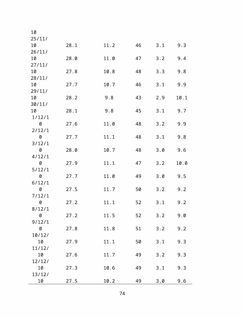
1025/11/10 28.1 11.2 46 3.1 9.326/11/10 28.0 11.0 47 3.2 9.427/11/10 27.8 10.8 48 3.3 9.828/11/10 27.7 10.7 46 3.1 9.929/11/10 28.2 9.8 43 2.9 10.130/11/10 28.1 9.8 45 3.1 9.71/12/1

0 27.6 11.0 48 3.2 9.92/12/1

0 27.7 11.1 48 3.1 9.83/12/1

0 28.0 10.7 48 3.0 9.64/12/1

0 27.9 11.1 47 3.2 10.05/12/1

0 27.7 11.0 49 3.0 9.56/12/1

0 27.5 11.7 50 3.2 9.27/12/1

0 27.2 11.1 52 3.1 9.28/12/1

0 27.2 11.5 52 3.2 9.09/12/1

0 27.8 11.8 51 3.2 9.210/12/

10 27.9 11.1 50 3.1 9.311/12/

10 27.6 11.7 49 3.2 9.312/12/

10 27.3 10.6 49 3.1 9.313/12/

10 27.5 10.2 49 3.0 9.6

74

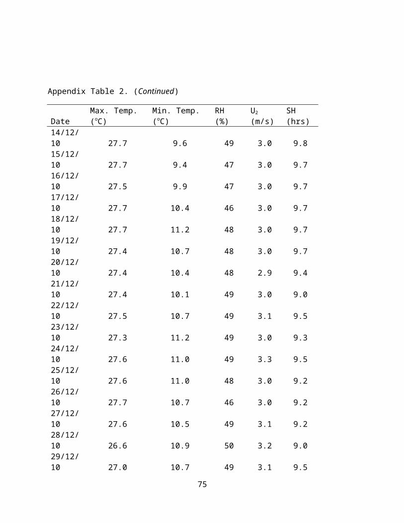
Appendix Table 2. (Continued)

DateMax. Temp. (oC)

Min. Temp. (oC)

RH (%)

U2

(m/s)

SH (hrs)

14/12/10 27.7 9.6 49 3.0 9.815/12/10 27.7 9.4 47 3.0 9.716/12/10 27.5 9.9 47 3.0 9.717/12/10 27.7 10.4 46 3.0 9.718/12/10 27.7 11.2 48 3.0 9.719/12/10 27.4 10.7 48 3.0 9.720/12/10 27.4 10.4 48 2.9 9.421/12/10 27.4 10.1 49 3.0 9.022/12/10 27.5 10.7 49 3.1 9.523/12/10 27.3 11.2 49 3.0 9.324/12/10 27.6 11.0 49 3.3 9.525/12/10 27.6 11.0 48 3.0 9.226/12/10 27.7 10.7 46 3.0 9.227/12/10 27.6 10.5 49 3.1 9.228/12/10 26.6 10.9 50 3.2 9.029/12/10 27.0 10.7 49 3.1 9.5

75

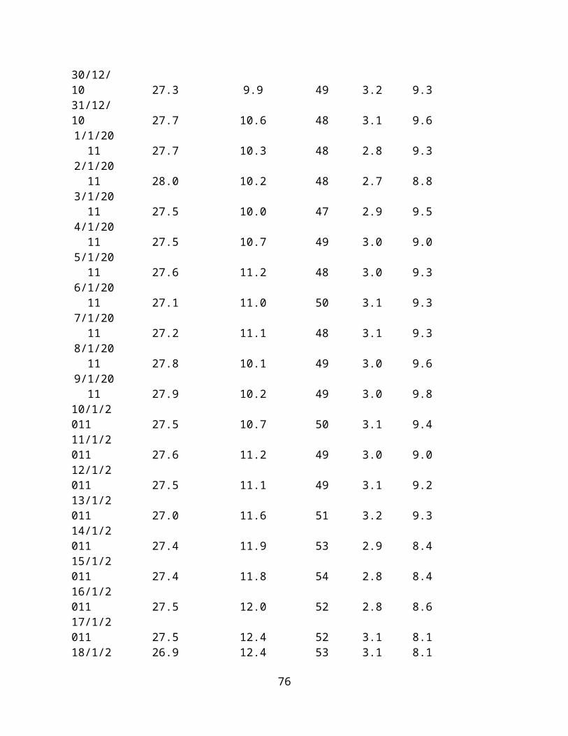
30/12/10 27.3 9.9 49 3.2 9.331/12/10 27.7 10.6 48 3.1 9.61/1/20

11 27.7 10.3 48 2.8 9.32/1/20

11 28.0 10.2 48 2.7 8.83/1/20

11 27.5 10.0 47 2.9 9.54/1/20

11 27.5 10.7 49 3.0 9.05/1/20

11 27.6 11.2 48 3.0 9.36/1/20

11 27.1 11.0 50 3.1 9.37/1/20

11 27.2 11.1 48 3.1 9.38/1/20

11 27.8 10.1 49 3.0 9.69/1/20

11 27.9 10.2 49 3.0 9.810/1/2011 27.5 10.7 50 3.1 9.411/1/2011 27.6 11.2 49 3.0 9.012/1/2011 27.5 11.1 49 3.1 9.213/1/2011 27.0 11.6 51 3.2 9.314/1/2011 27.4 11.9 53 2.9 8.415/1/2011 27.4 11.8 54 2.8 8.416/1/2011 27.5 12.0 52 2.8 8.617/1/2011 27.5 12.4 52 3.1 8.118/1/2 26.9 12.4 53 3.1 8.1

76

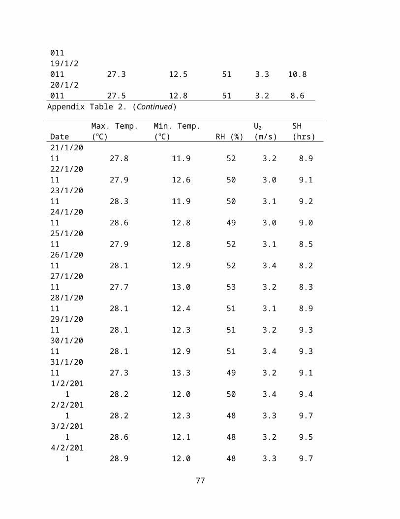
01119/1/2011 27.3 12.5 51 3.3 10.820/1/2011 27.5 12.8 51 3.2 8.6Appendix Table 2. (Continued)

DateMax. Temp. (oC)

Min. Temp. (oC) RH (%)

U2

(m/s)

SH (hrs)

21/1/2011 27.8 11.9 52 3.2 8.922/1/2011 27.9 12.6 50 3.0 9.123/1/2011 28.3 11.9 50 3.1 9.224/1/2011 28.6 12.8 49 3.0 9.025/1/2011 27.9 12.8 52 3.1 8.526/1/2011 28.1 12.9 52 3.4 8.227/1/2011 27.7 13.0 53 3.2 8.328/1/2011 28.1 12.4 51 3.1 8.929/1/2011 28.1 12.3 51 3.2 9.330/1/2011 28.1 12.9 51 3.4 9.331/1/2011 27.3 13.3 49 3.2 9.11/2/201

1 28.2 12.0 50 3.4 9.42/2/201

1 28.2 12.3 48 3.3 9.73/2/201

1 28.6 12.1 48 3.2 9.54/2/201

1 28.9 12.0 48 3.3 9.7

77

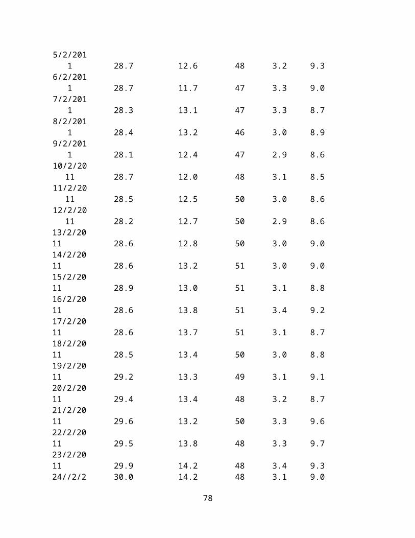
5/2/2011 28.7 12.6 48 3.2 9.3

6/2/2011 28.7 11.7 47 3.3 9.0

7/2/2011 28.3 13.1 47 3.3 8.7

8/2/2011 28.4 13.2 46 3.0 8.9

9/2/2011 28.1 12.4 47 2.9 8.6

10/2/2011 28.7 12.0 48 3.1 8.5

11/2/2011 28.5 12.5 50 3.0 8.6

12/2/2011 28.2 12.7 50 2.9 8.6

13/2/2011 28.6 12.8 50 3.0 9.014/2/2011 28.6 13.2 51 3.0 9.015/2/2011 28.9 13.0 51 3.1 8.816/2/2011 28.6 13.8 51 3.4 9.217/2/2011 28.6 13.7 51 3.1 8.718/2/2011 28.5 13.4 50 3.0 8.819/2/2011 29.2 13.3 49 3.1 9.120/2/2011 29.4 13.4 48 3.2 8.721/2/2011 29.6 13.2 50 3.3 9.622/2/2011 29.5 13.8 48 3.3 9.723/2/2011 29.9 14.2 48 3.4 9.324//2/2 30.0 14.2 48 3.1 9.0

78

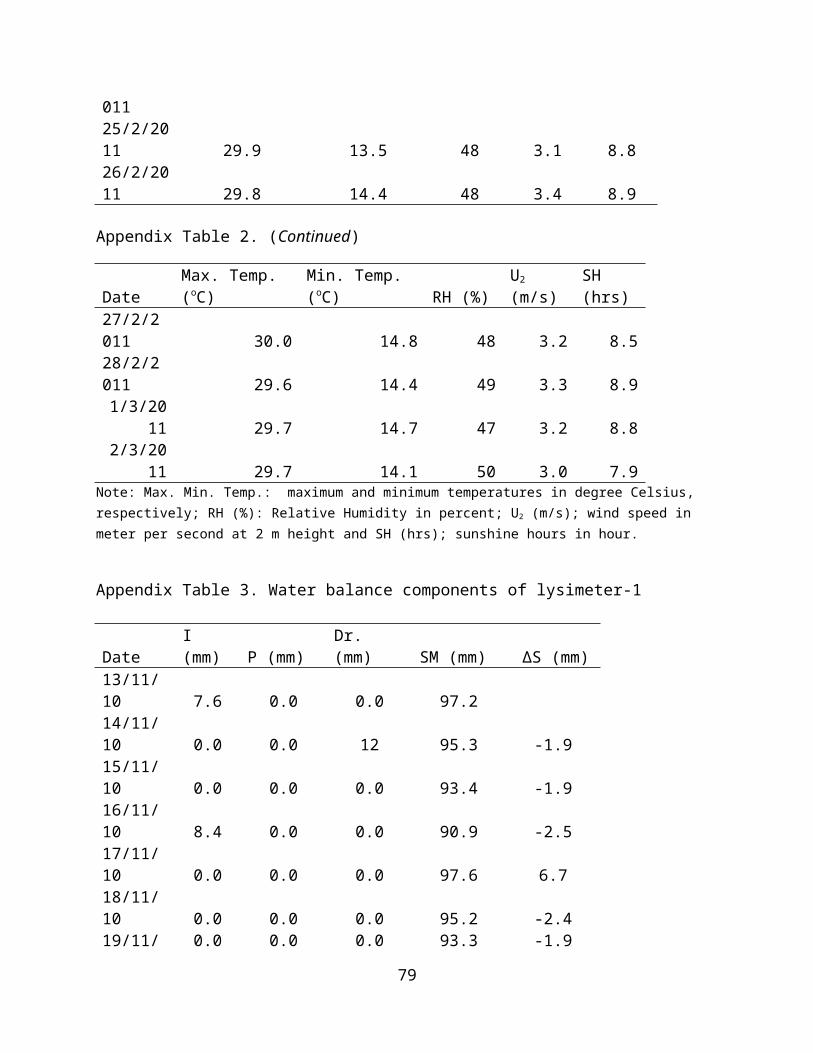
01125/2/2011 29.9 13.5 48 3.1 8.826/2/2011 29.8 14.4 48 3.4 8.9

Appendix Table 2. (Continued)

DateMax. Temp. (oC)

Min. Temp. (oC) RH (%)

U2

(m/s)

SH (hrs)

27/2/2011 30.0 14.8 48 3.2 8.528/2/2011 29.6 14.4 49 3.3 8.91/3/20

11 29.7 14.7 47 3.2 8.82/3/20

11 29.7 14.1 50 3.0 7.9Note: Max. Min. Temp.: maximum and minimum temperatures in degree Celsius, respectively; RH (%): Relative Humidity in percent; U2 (m/s); wind speed in meter per second at 2 m height and SH (hrs); sunshine hours in hour.

Appendix Table 3. Water balance components of lysimeter-1

Date

I (mm) P (mm)

Dr. (mm) SM (mm) ΔS (mm)

13/11/10 7.6 0.0 0.0 97.214/11/10 0.0 0.0 12 95.3 -1.915/11/10 0.0 0.0 0.0 93.4 -1.916/11/10 8.4 0.0 0.0 90.9 -2.517/11/10 0.0 0.0 0.0 97.6 6.718/11/10 0.0 0.0 0.0 95.2 -2.419/11/ 0.0 0.0 0.0 93.3 -1.9

79

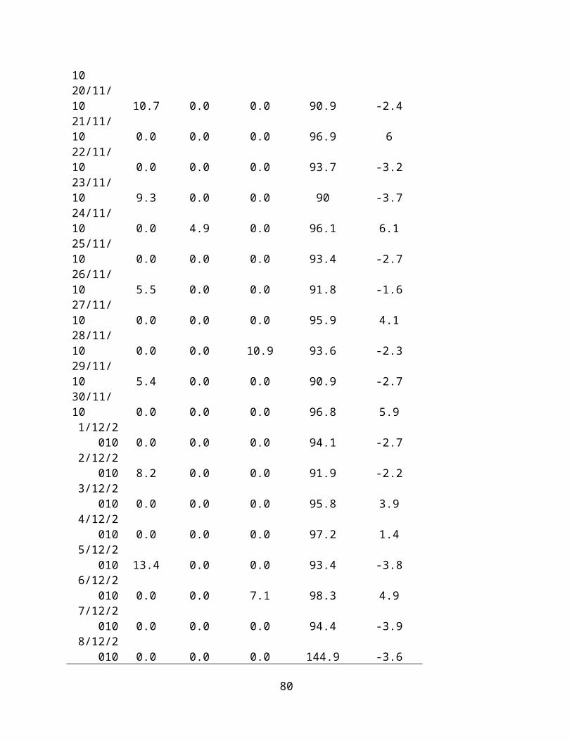
1020/11/10 10.7 0.0 0.0 90.9 -2.421/11/10 0.0 0.0 0.0 96.9 622/11/10 0.0 0.0 0.0 93.7 -3.223/11/10 9.3 0.0 0.0 90 -3.724/11/10 0.0 4.9 0.0 96.1 6.125/11/10 0.0 0.0 0.0 93.4 -2.726/11/10 5.5 0.0 0.0 91.8 -1.627/11/10 0.0 0.0 0.0 95.9 4.128/11/10 0.0 0.0 10.9 93.6 -2.329/11/10 5.4 0.0 0.0 90.9 -2.730/11/10 0.0 0.0 0.0 96.8 5.91/12/2

010 0.0 0.0 0.0 94.1 -2.72/12/2

010 8.2 0.0 0.0 91.9 -2.23/12/2

010 0.0 0.0 0.0 95.8 3.94/12/2

010 0.0 0.0 0.0 97.2 1.45/12/2

010 13.4 0.0 0.0 93.4 -3.86/12/2

010 0.0 0.0 7.1 98.3 4.97/12/2

010 0.0 0.0 0.0 94.4 -3.98/12/2

010 0.0 0.0 0.0 144.9 -3.6

80

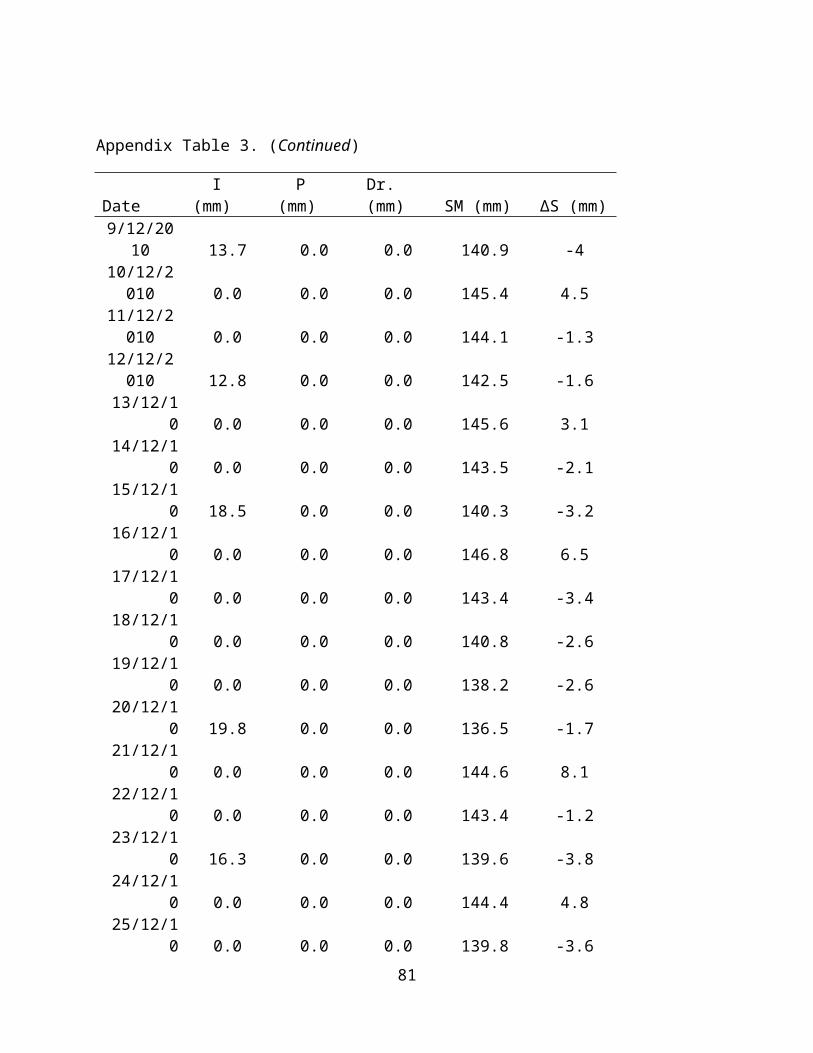
Appendix Table 3. (Continued)

Date

I (mm)

P (mm)

Dr. (mm) SM (mm) ΔS (mm)

9/12/2010 13.7 0.0 0.0 140.9 -4

10/12/2010 0.0 0.0 0.0 145.4 4.5

11/12/2010 0.0 0.0 0.0 144.1 -1.3

12/12/2010 12.8 0.0 0.0 142.5 -1.6

13/12/10 0.0 0.0 0.0 145.6 3.1

14/12/10 0.0 0.0 0.0 143.5 -2.1

15/12/10 18.5 0.0 0.0 140.3 -3.2

16/12/10 0.0 0.0 0.0 146.8 6.5

17/12/10 0.0 0.0 0.0 143.4 -3.4

18/12/10 0.0 0.0 0.0 140.8 -2.6

19/12/10 0.0 0.0 0.0 138.2 -2.6

20/12/10 19.8 0.0 0.0 136.5 -1.7

21/12/10 0.0 0.0 0.0 144.6 8.1

22/12/10 0.0 0.0 0.0 143.4 -1.2

23/12/10 16.3 0.0 0.0 139.6 -3.8

24/12/10 0.0 0.0 0.0 144.4 4.8

25/12/10 0.0 0.0 0.0 139.8 -3.6

81

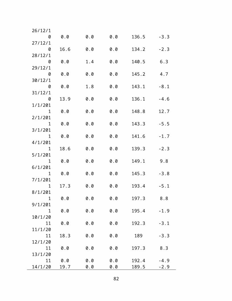
26/12/10 0.0 0.0 0.0 136.5 -3.3

27/12/10 16.6 0.0 0.0 134.2 -2.3

28/12/10 0.0 1.4 0.0 140.5 6.3

29/12/10 0.0 0.0 0.0 145.2 4.7

30/12/10 0.0 1.8 0.0 143.1 -8.1

31/12/10 13.9 0.0 0.0 136.1 -4.6

1/1/2011 0.0 0.0 0.0 148.8 12.7

2/1/2011 0.0 0.0 0.0 143.3 -5.5

3/1/2011 0.0 0.0 0.0 141.6 -1.7

4/1/2011 18.6 0.0 0.0 139.3 -2.3

5/1/2011 0.0 0.0 0.0 149.1 9.8

6/1/2011 0.0 0.0 0.0 145.3 -3.8

7/1/2011 17.3 0.0 0.0 193.4 -5.1

8/1/2011 0.0 0.0 0.0 197.3 8.8

9/1/2011 0.0 0.0 0.0 195.4 -1.9

10/1/2011 0.0 0.0 0.0 192.3 -3.1

11/1/2011 18.3 0.0 0.0 189 -3.3

12/1/2011 0.0 0.0 0.0 197.3 8.3

13/1/2011 0.0 0.0 0.0 192.4 -4.9

14/1/20 19.7 0.0 0.0 189.5 -2.9

82

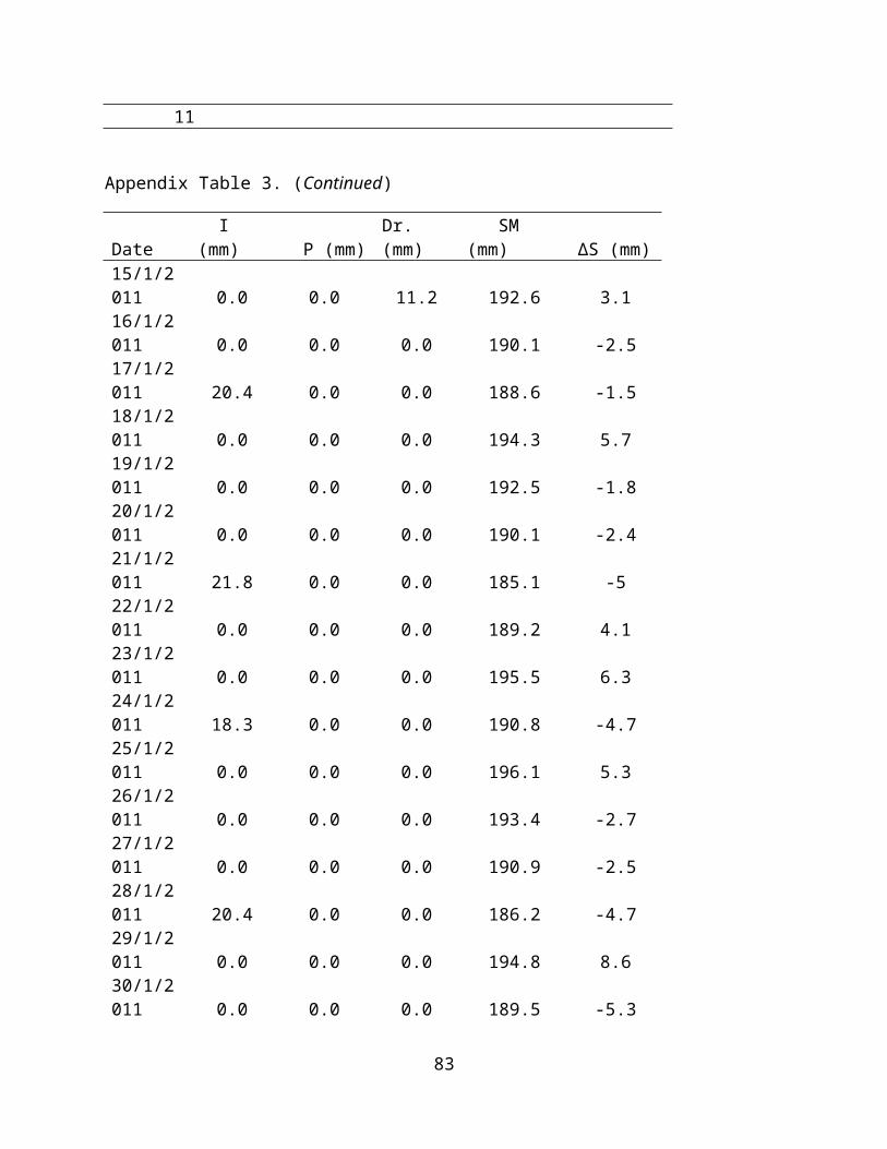
11

Appendix Table 3. (Continued)

Date I (mm) P (mm)

Dr. (mm)

SM (mm) ΔS (mm)

15/1/2011 0.0 0.0 11.2 192.6 3.116/1/2011 0.0 0.0 0.0 190.1 -2.517/1/2011 20.4 0.0 0.0 188.6 -1.518/1/2011 0.0 0.0 0.0 194.3 5.719/1/2011 0.0 0.0 0.0 192.5 -1.820/1/2011 0.0 0.0 0.0 190.1 -2.421/1/2011 21.8 0.0 0.0 185.1 -522/1/2011 0.0 0.0 0.0 189.2 4.123/1/2011 0.0 0.0 0.0 195.5 6.324/1/2011 18.3 0.0 0.0 190.8 -4.725/1/2011 0.0 0.0 0.0 196.1 5.326/1/2011 0.0 0.0 0.0 193.4 -2.727/1/2011 0.0 0.0 0.0 190.9 -2.528/1/2011 20.4 0.0 0.0 186.2 -4.729/1/2011 0.0 0.0 0.0 194.8 8.630/1/2011 0.0 0.0 0.0 189.5 -5.3

83

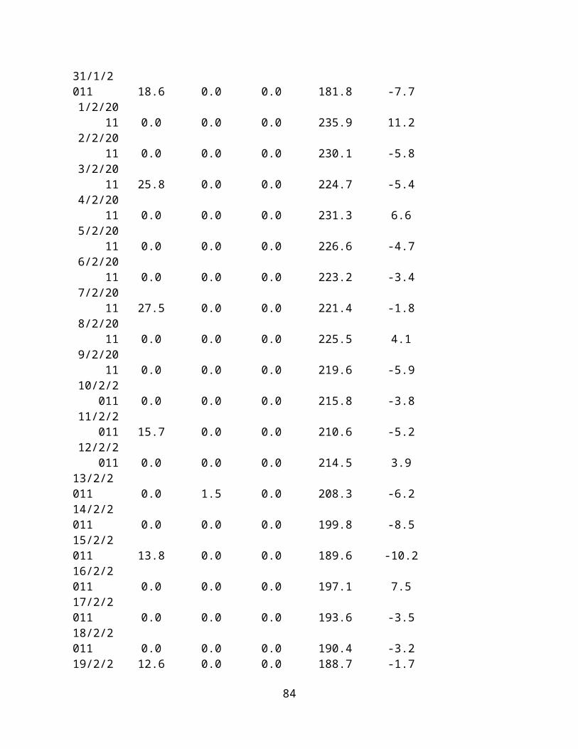
31/1/2011 18.6 0.0 0.0 181.8 -7.71/2/20

11 0.0 0.0 0.0 235.9 11.22/2/20

11 0.0 0.0 0.0 230.1 -5.83/2/20

11 25.8 0.0 0.0 224.7 -5.44/2/20

11 0.0 0.0 0.0 231.3 6.65/2/20

11 0.0 0.0 0.0 226.6 -4.76/2/20

11 0.0 0.0 0.0 223.2 -3.47/2/20

11 27.5 0.0 0.0 221.4 -1.88/2/20

11 0.0 0.0 0.0 225.5 4.19/2/20

11 0.0 0.0 0.0 219.6 -5.910/2/2

011 0.0 0.0 0.0 215.8 -3.811/2/2

011 15.7 0.0 0.0 210.6 -5.212/2/2

011 0.0 0.0 0.0 214.5 3.913/2/2011 0.0 1.5 0.0 208.3 -6.214/2/2011 0.0 0.0 0.0 199.8 -8.515/2/2011 13.8 0.0 0.0 189.6 -10.216/2/2011 0.0 0.0 0.0 197.1 7.517/2/2011 0.0 0.0 0.0 193.6 -3.518/2/2011 0.0 0.0 0.0 190.4 -3.219/2/2 12.6 0.0 0.0 188.7 -1.7

84

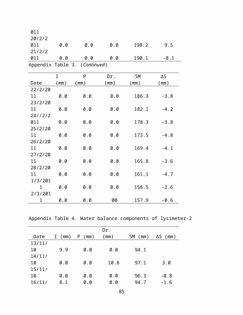
01120/2/2011 0.0 0.0 0.0 198.2 9.521/2/2011 0.0 0.0 0.0 190.1 -8.1Appendix Table 3. (Continued)

DateI (mm)

P (mm)

Dr. (mm)

SM (mm)

ΔS (mm)

22/2/2011 0.0 0.0 0.0 186.3 -3.823/2/2011 0.0 0.0 0.0 182.1 -4.224//2/2011 0.0 0.0 0.0 178.3 -3.825/2/2011 0.0 0.0 0.0 173.5 -4.826/2/2011 0.0 0.0 0.0 169.4 -4.127/2/2011 0.0 0.0 0.0 165.8 -3.628/2/2011 0.0 0.0 0.0 161.1 -4.71/3/201

1 0.0 0.0 0.0 158.5 -2.62/3/201

1 0.0 0.0 00 157.9 -0.6

Appendix Table 4. Water balance components of lysimeter-2

Date I (mm) P (mm)Dr. (mm) SM (mm) ΔS (mm)

13/11/10 9.9 0.0 0.0 94.114/11/10 0.0 0.0 10.8 97.1 3.015/11/10 0.0 0.0 0.0 96.3 -0.816/11/ 8.1 0.0 0.0 94.7 -1.6

85

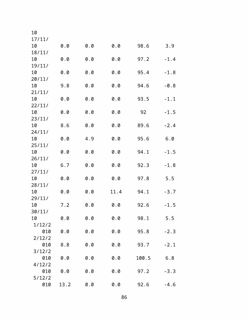
1017/11/10 0.0 0.0 0.0 98.6 3.918/11/10 0.0 0.0 0.0 97.2 -1.419/11/10 0.0 0.0 0.0 95.4 -1.820/11/10 9.8 0.0 0.0 94.6 -0.821/11/10 0.0 0.0 0.0 93.5 -1.122/11/10 0.0 0.0 0.0 92 -1.523/11/10 8.6 0.0 0.0 89.6 -2.424/11/10 0.0 4.9 0.0 95.6 6.025/11/10 0.0 0.0 0.0 94.1 -1.526/11/10 6.7 0.0 0.0 92.3 -1.827/11/10 0.0 0.0 0.0 97.8 5.528/11/10 0.0 0.0 11.4 94.1 -3.729/11/10 7.2 0.0 0.0 92.6 -1.530/11/10 0.0 0.0 0.0 98.1 5.51/12/2

010 0.0 0.0 0.0 95.8 -2.32/12/2

010 8.8 0.0 0.0 93.7 -2.13/12/2

010 0.0 0.0 0.0 100.5 6.84/12/2

010 0.0 0.0 0.0 97.2 -3.35/12/2

010 13.2 0.0 0.0 92.6 -4.6

86

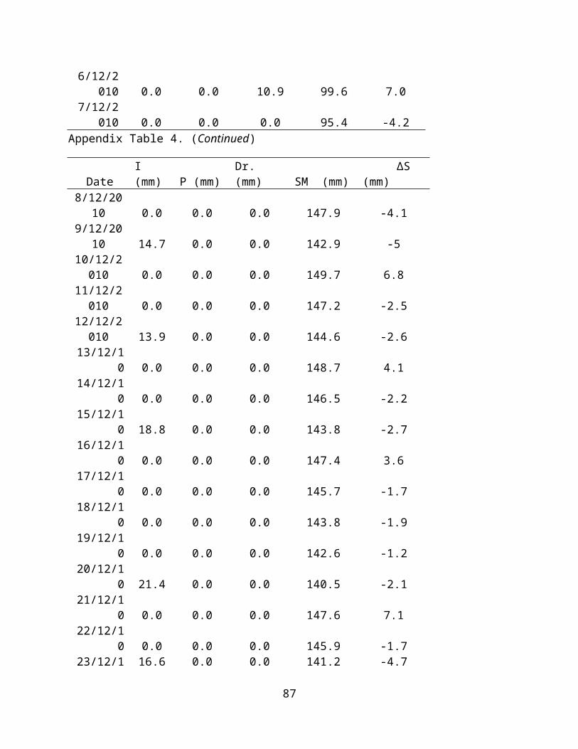
6/12/2010 0.0 0.0 10.9 99.6 7.0

7/12/2010 0.0 0.0 0.0 95.4 -4.2

Appendix Table 4. (Continued)

DateI (mm) P (mm)

Dr. (mm) SM (mm)

ΔS (mm)

8/12/2010 0.0 0.0 0.0 147.9 -4.1

9/12/2010 14.7 0.0 0.0 142.9 -5

10/12/2010 0.0 0.0 0.0 149.7 6.8

11/12/2010 0.0 0.0 0.0 147.2 -2.5

12/12/2010 13.9 0.0 0.0 144.6 -2.6

13/12/10 0.0 0.0 0.0 148.7 4.1

14/12/10 0.0 0.0 0.0 146.5 -2.2

15/12/10 18.8 0.0 0.0 143.8 -2.7

16/12/10 0.0 0.0 0.0 147.4 3.6

17/12/10 0.0 0.0 0.0 145.7 -1.7

18/12/10 0.0 0.0 0.0 143.8 -1.9

19/12/10 0.0 0.0 0.0 142.6 -1.2

20/12/10 21.4 0.0 0.0 140.5 -2.1

21/12/10 0.0 0.0 0.0 147.6 7.1

22/12/10 0.0 0.0 0.0 145.9 -1.7

23/12/1 16.6 0.0 0.0 141.2 -4.7

87

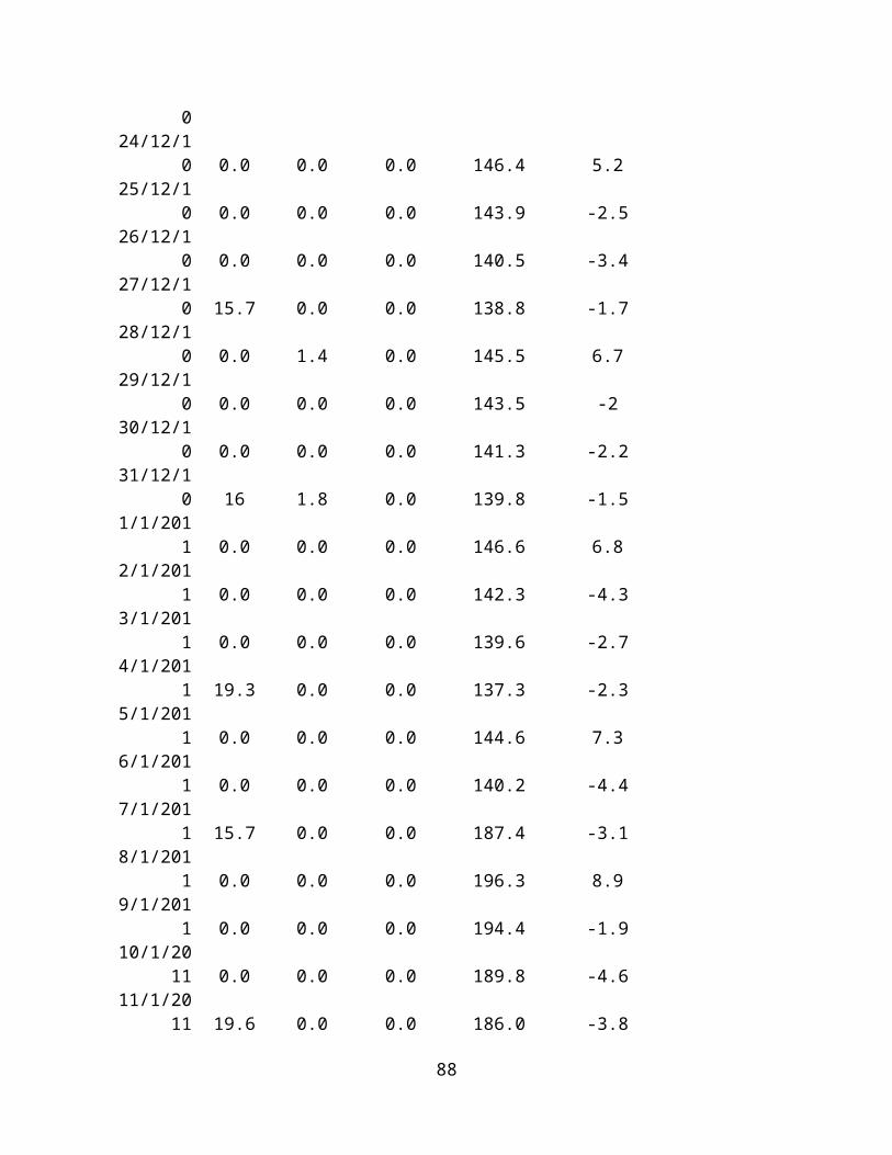
024/12/1

0 0.0 0.0 0.0 146.4 5.225/12/1

0 0.0 0.0 0.0 143.9 -2.526/12/1

0 0.0 0.0 0.0 140.5 -3.427/12/1

0 15.7 0.0 0.0 138.8 -1.728/12/1

0 0.0 1.4 0.0 145.5 6.729/12/1

0 0.0 0.0 0.0 143.5 -230/12/1

0 0.0 0.0 0.0 141.3 -2.231/12/1

0 16 1.8 0.0 139.8 -1.51/1/201

1 0.0 0.0 0.0 146.6 6.82/1/201

1 0.0 0.0 0.0 142.3 -4.33/1/201

1 0.0 0.0 0.0 139.6 -2.74/1/201

1 19.3 0.0 0.0 137.3 -2.35/1/201

1 0.0 0.0 0.0 144.6 7.36/1/201

1 0.0 0.0 0.0 140.2 -4.47/1/201

1 15.7 0.0 0.0 187.4 -3.18/1/201

1 0.0 0.0 0.0 196.3 8.99/1/201

1 0.0 0.0 0.0 194.4 -1.910/1/20

11 0.0 0.0 0.0 189.8 -4.611/1/20

11 19.6 0.0 0.0 186.0 -3.8

88

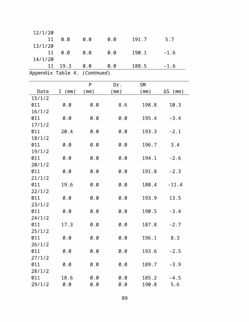
12/1/2011 0.0 0.0 0.0 191.7 5.7

13/1/2011 0.0 0.0 0.0 190.1 -1.6

14/1/2011 19.3 0.0 0.0 188.5 -1.6

Appendix Table 4. (Continued)

Date I (mm) P (mm)

Dr. (mm)

SM (mm) ΔS (mm)

15/1/2011 0.0 0.0 8.6 198.8 10.316/1/2011 0.0 0.0 0.0 195.4 -3.417/1/2011 20.4 0.0 0.0 193.3 -2.118/1/2011 0.0 0.0 0.0 196.7 3.419/1/2011 0.0 0.0 0.0 194.1 -2.620/1/2011 0.0 0.0 0.0 191.8 -2.321/1/2011 19.6 0.0 0.0 180.4 -11.422/1/2011 0.0 0.0 0.0 193.9 13.523/1/2011 0.0 0.0 0.0 190.5 -3.424/1/2011 17.3 0.0 0.0 187.8 -2.725/1/2011 0.0 0.0 0.0 196.1 8.326/1/2011 0.0 0.0 0.0 193.6 -2.527/1/2011 0.0 0.0 0.0 189.7 -3.928/1/2011 18.6 0.0 0.0 185.2 -4.529/1/2 0.0 0.0 0.0 190.8 5.6

89

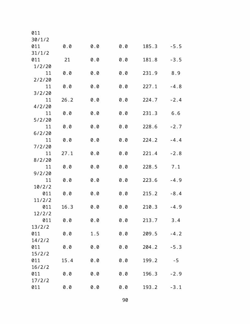
01130/1/2011 0.0 0.0 0.0 185.3 -5.531/1/2011 21 0.0 0.0 181.8 -3.51/2/20

11 0.0 0.0 0.0 231.9 8.92/2/20

11 0.0 0.0 0.0 227.1 -4.83/2/20

11 26.2 0.0 0.0 224.7 -2.44/2/20

11 0.0 0.0 0.0 231.3 6.65/2/20

11 0.0 0.0 0.0 228.6 -2.76/2/20

11 0.0 0.0 0.0 224.2 -4.47/2/20

11 27.1 0.0 0.0 221.4 -2.88/2/20

11 0.0 0.0 0.0 228.5 7.19/2/20

11 0.0 0.0 0.0 223.6 -4.910/2/2

011 0.0 0.0 0.0 215.2 -8.411/2/2

011 16.3 0.0 0.0 210.3 -4.912/2/2

011 0.0 0.0 0.0 213.7 3.413/2/2011 0.0 1.5 0.0 209.5 -4.214/2/2011 0.0 0.0 0.0 204.2 -5.315/2/2011 15.4 0.0 0.0 199.2 -516/2/2011 0.0 0.0 0.0 196.3 -2.917/2/2011 0.0 0.0 0.0 193.2 -3.1

90

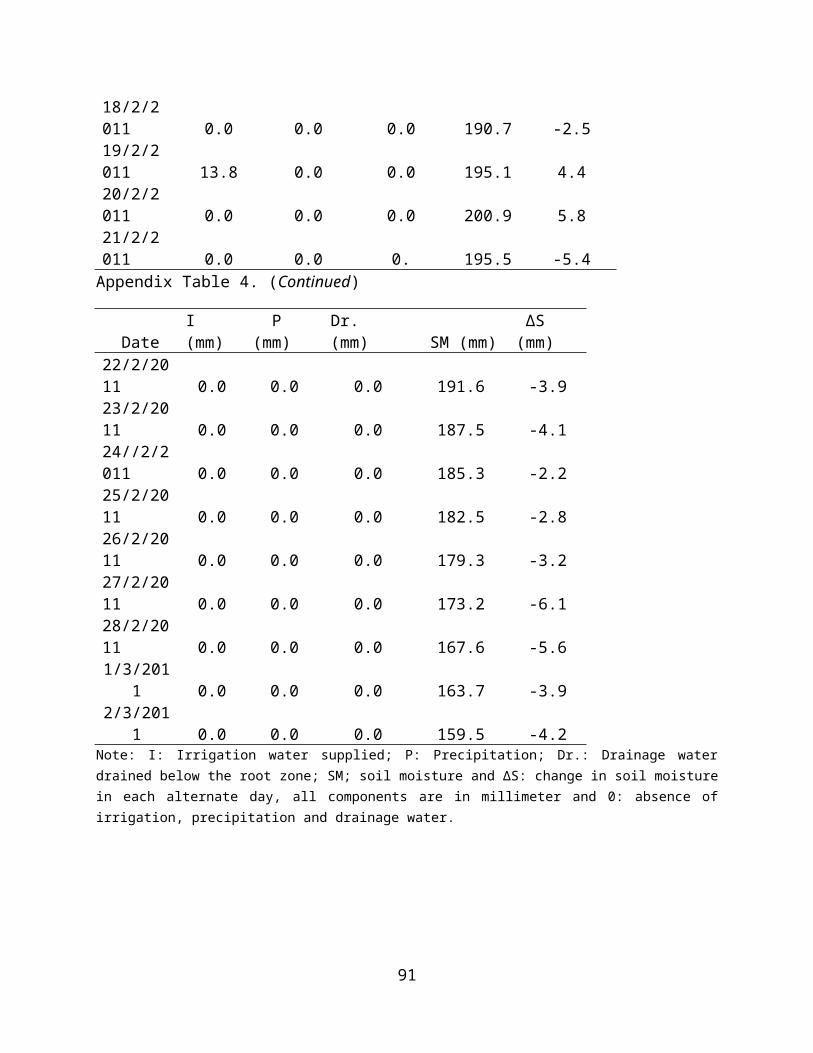
18/2/2011 0.0 0.0 0.0 190.7 -2.519/2/2011 13.8 0.0 0.0 195.1 4.420/2/2011 0.0 0.0 0.0 200.9 5.821/2/2011 0.0 0.0 0. 195.5 -5.4Appendix Table 4. (Continued)

DateI (mm)

P (mm)

Dr. (mm) SM (mm)

ΔS (mm)

22/2/2011 0.0 0.0 0.0 191.6 -3.923/2/2011 0.0 0.0 0.0 187.5 -4.124//2/2011 0.0 0.0 0.0 185.3 -2.225/2/2011 0.0 0.0 0.0 182.5 -2.826/2/2011 0.0 0.0 0.0 179.3 -3.227/2/2011 0.0 0.0 0.0 173.2 -6.128/2/2011 0.0 0.0 0.0 167.6 -5.61/3/201

1 0.0 0.0 0.0 163.7 -3.92/3/201

1 0.0 0.0 0.0 159.5 -4.2Note: I: Irrigation water supplied; P: Precipitation; Dr.: Drainage waterdrained below the root zone; SM; soil moisture and ΔS: change in soil moisturein each alternate day, all components are in millimeter and 0: absence ofirrigation, precipitation and drainage water.

91

92