Field distribution in stator core end packages of hydropower ...

16001

Examensarbete 30 hpFebruari 2016

Field distribution in stator core end packages of hydropower generators

William Johnsson

Teknisk- naturvetenskaplig fakultet UTH-enheten Besöksadress: Ångströmlaboratoriet Lägerhyddsvägen 1 Hus 4, Plan 0 Postadress: Box 536 751 21 Uppsala Telefon: 018 – 471 30 03 Telefax: 018 – 471 30 00 Hemsida: http://www.teknat.uu.se/student

Abstract

Field distribution in stator core end packages ofhydropower generators

William Johnsson

Hydropower has during the last century been known for its high reliability and efficiency. To refine and develop the technology has kept engineers and researchers busy during most of the 20th century and is still a subject of interest. With a lot of different companies involved, widely spread around the world, different design characteristics exists. A matter where opinions of designers and engineers can differ is what design action to use for reduction of the end heating, caused by the axial magnetic flux.

In this thesis the two most common design actions, stepping of the stator core end and reduction of the rotor magnetic length are investigated. The results shows that both of the design features provides a significant effect of about the same reduction.

16001Examinator: Mikael BergkvistÄmnesgranskare: Urban LundinHandledare: Urban Lundin, Bo Hernnäs, Andreas Solum

Acknowledgment

Special thanks for excellent guidance and rewarding conversations are addressedto Dr. Urban Lundin, Uppsala University, Dr. Bo Hernnas, Voith Hydro ABand Andreas Solum, Voith Hydro AB. Bjorn Hellstrom, Johan Malmberg andMarcus Svanberg of Voith Hydro AB are also acknowledged for their guidance.

3

Contents

1 Introduction 61.1 End effects . . . . . . . . . . . . . . . . . . . . . . . . . . . . . . 71.2 Background . . . . . . . . . . . . . . . . . . . . . . . . . . . . . . 71.3 Outline . . . . . . . . . . . . . . . . . . . . . . . . . . . . . . . . 7

2 Theory 82.1 End effects . . . . . . . . . . . . . . . . . . . . . . . . . . . . . . 82.2 Sources of axial flux . . . . . . . . . . . . . . . . . . . . . . . . . 8

2.2.1 Fringing flux . . . . . . . . . . . . . . . . . . . . . . . . . 82.2.2 Stator end-winding current . . . . . . . . . . . . . . . . . 9

2.3 Design philosophies . . . . . . . . . . . . . . . . . . . . . . . . . . 92.3.1 Stepping . . . . . . . . . . . . . . . . . . . . . . . . . . . . 92.3.2 Shortening of the poles . . . . . . . . . . . . . . . . . . . 10

2.4 Power losses . . . . . . . . . . . . . . . . . . . . . . . . . . . . . . 112.4.1 Anisotropy . . . . . . . . . . . . . . . . . . . . . . . . . . 112.4.2 Steinmetz model . . . . . . . . . . . . . . . . . . . . . . . 11

2.4.2.1 Hysteresis loss . . . . . . . . . . . . . . . . . . . 112.4.2.2 Classical loss (eddy current) . . . . . . . . . . . 122.4.2.3 Excess loss . . . . . . . . . . . . . . . . . . . . . 12

2.4.3 Rotational field . . . . . . . . . . . . . . . . . . . . . . . . 122.4.4 Mechanical processing . . . . . . . . . . . . . . . . . . . . 12

3 Method 133.1 Simulations . . . . . . . . . . . . . . . . . . . . . . . . . . . . . . 13

3.1.1 No-load operation . . . . . . . . . . . . . . . . . . . . . . 133.1.2 Saturation . . . . . . . . . . . . . . . . . . . . . . . . . . . 153.1.3 End-winding driven flux . . . . . . . . . . . . . . . . . . . 163.1.4 Power losses . . . . . . . . . . . . . . . . . . . . . . . . . . 16

3.2 Experiment . . . . . . . . . . . . . . . . . . . . . . . . . . . . . . 163.2.1 Measuring system . . . . . . . . . . . . . . . . . . . . . . 17

3.3 Cost analysis . . . . . . . . . . . . . . . . . . . . . . . . . . . . . 17

4 Results 194.1 Simulation results . . . . . . . . . . . . . . . . . . . . . . . . . . 19

4.1.1 Fringing flux . . . . . . . . . . . . . . . . . . . . . . . . . 194.1.2 End-winding driven flux . . . . . . . . . . . . . . . . . . . 224.1.3 Effects of saturation . . . . . . . . . . . . . . . . . . . . . 234.1.4 Power losses . . . . . . . . . . . . . . . . . . . . . . . . . . 23

4.2 Experimental results . . . . . . . . . . . . . . . . . . . . . . . . . 254.3 Cost model . . . . . . . . . . . . . . . . . . . . . . . . . . . . . . 25

4

5 Discussion 265.1 Method . . . . . . . . . . . . . . . . . . . . . . . . . . . . . . . . 26

5.1.1 Power losses . . . . . . . . . . . . . . . . . . . . . . . . . . 265.2 Results . . . . . . . . . . . . . . . . . . . . . . . . . . . . . . . . . 27

5.2.1 Power losses . . . . . . . . . . . . . . . . . . . . . . . . . . 275.2.2 Fringing flux . . . . . . . . . . . . . . . . . . . . . . . . . 275.2.3 Saturation effects . . . . . . . . . . . . . . . . . . . . . . . 285.2.4 End-winding driven flux . . . . . . . . . . . . . . . . . . . 285.2.5 Experimental result . . . . . . . . . . . . . . . . . . . . . 295.2.6 Cost analysis . . . . . . . . . . . . . . . . . . . . . . . . . 29

6 Conclusion 30

7 Future work 31

Bibliography 33

5

1 Introduction

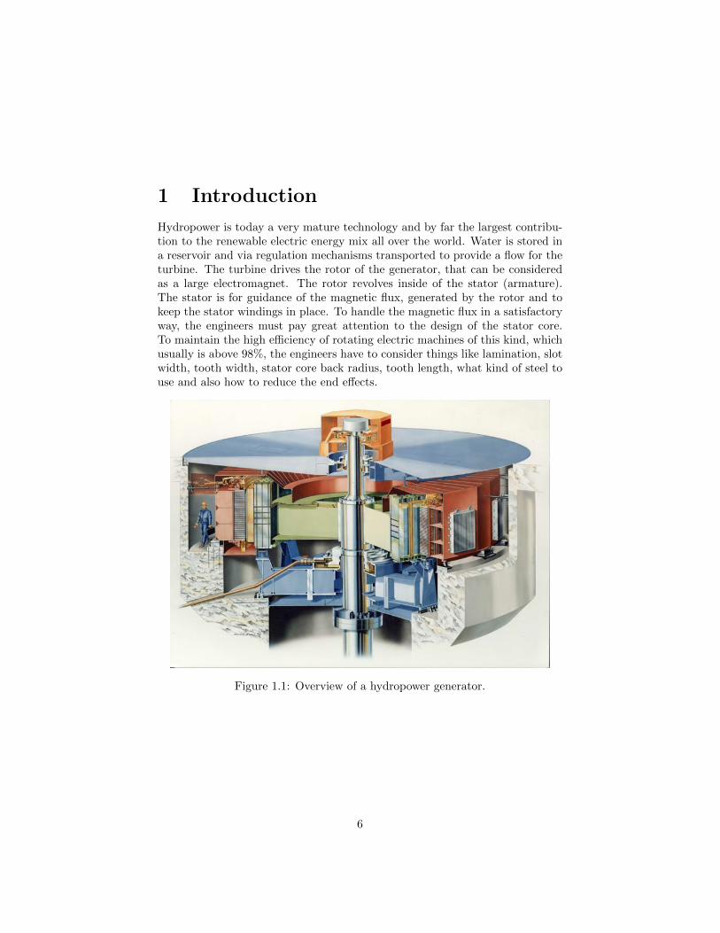
Hydropower is today a very mature technology and by far the largest contribu-tion to the renewable electric energy mix all over the world. Water is stored ina reservoir and via regulation mechanisms transported to provide a flow for theturbine. The turbine drives the rotor of the generator, that can be consideredas a large electromagnet. The rotor revolves inside of the stator (armature).The stator is for guidance of the magnetic flux, generated by the rotor and tokeep the stator windings in place. To handle the magnetic flux in a satisfactoryway, the engineers must pay great attention to the design of the stator core.To maintain the high efficiency of rotating electric machines of this kind, whichusually is above 98%, the engineers have to consider things like lamination, slotwidth, tooth width, stator core back radius, tooth length, what kind of steel touse and also how to reduce the end effects.

Figure 1.1: Overview of a hydropower generator.

6

1.1 End effects

End effects of the magnetic field in the stator core have been a well-knownproblem since the beginning of the 20th century. Most of the previous workhas considered turbogenerators and it is not as highlighted when it comes togenerators for hydropower applications.There are existing methods for decreasing the effects of the magnetic field distri-bution of the stator core end, where two are more prominent than others. Oneof them is stepping of the stator core, where the manufacturer is profiling thestator core end package in a staircase pattern. The other one is shortening ofthe rotor poles, where the axial distance between the top segment of the statorcore and the pole face is increased. Both of the methods forces a redistributionof the magnetic flux. The stepping design increases the reluctance radially atthe very end of the stator core. A greater amount of the flux then travels intothe stator core further away from the end. In the pole shortening design theincreased length ratio of the stator core and the pole allows for more flux totravel radially.

1.2 Background

At Voith Hydro AB, an operating unit within the global company Voith Hydro,there is a need for further understanding of the two design philosophies men-tioned above. This is because questions regarding the performance and costs ofthe different designs occasionally are raised, both by customers and designers.To be able to provide qualitative answers, this thesis contains:

• Simulations for the various designs using FEM tools

• Measurements for validation of the simulations

• Calculations of the losses

• A cost comparison model regarding the different designs

• Suggested development for design guidelines

1.3 Outline

In this thesis, two common design actions to prevent end heating are presentedand evaluated. One commercial machine, that was built with one of the de-signs, was used as reference through out the work. In chapter 3, brief theoryis presented, necessary for the reader to understand the results. In chapter 4,selected results that was obtained is presented. In chapter 5, the method andthe results are discussed. In chapter 6 and 7, conclusions and suggestions onfuture work is presented.

7

2 Theory

2.1 End effects

When investigating the field distribution in the stator core end, it is convenientto consider the magnetic flux density B and its effects. The magnetic fluxdensity is by definition, the magnetic flux perpendicular to the surface, per unitarea. The magnetic flux can then be related to B according to eq: 2.1.

Φ =

∫∫S

B dS (2.1)

If B reaches a value that is too high for the stator core, heating occurs andlocal hotspots can become of a problem. This can occur during abnormal oper-ation or if the machine is poorly designed. To prevent this, necessary cooling isincreased and the overall loss increases. If there is not enough cooling provided,the temperatures can become of critical magnitudes and cause serious damageto the machine.

When one look at the machine in cylindrical coordinates, the useful fluxthat creates the wanted MMF is, clearly the radial component that travelsperipherally and then links back to the opposite pole. Due to the finite lengthof the machine and because of the air gap in the magnetic circuit, there willbe a fringing (stray) flux due to the increased reluctance. The fringing flux,together with the end-winding driven flux will enter the stator core axially. Toreach the rated voltage in steady state, a certain amount of radial flux has to belinked to the stator core. This results in a value of B, that is still in the lineararea of the BH-curve, but closer to saturation. If there is additional, axial fluxpresent, high values of B can be reached and hot spots can occur. To deal withthis problem, without over dimensioning the stator core, the stator core endpackage can be stepped or the poles can be shortened with respect to the statorcore. This increases the reluctance along the flux paths in the axial direction.[1]

2.2 Sources of axial flux

2.2.1 Fringing flux

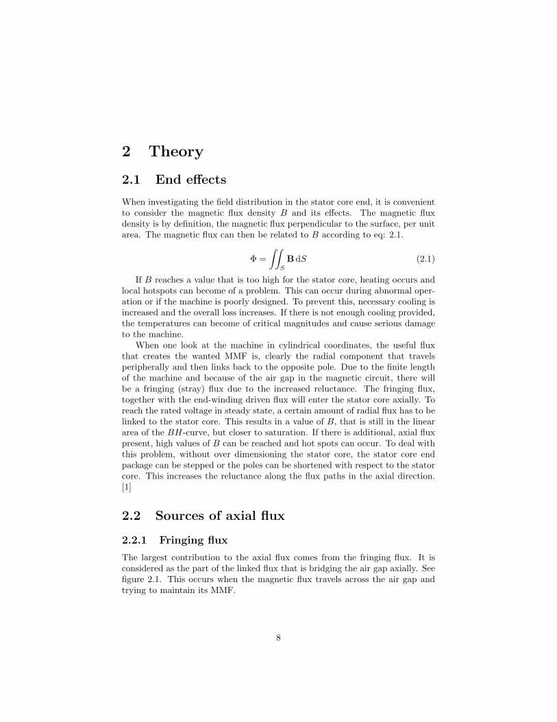
The largest contribution to the axial flux comes from the fringing flux. It isconsidered as the part of the linked flux that is bridging the air gap axially. Seefigure 2.1. This occurs when the magnetic flux travels across the air gap andtrying to maintain its MMF.

8

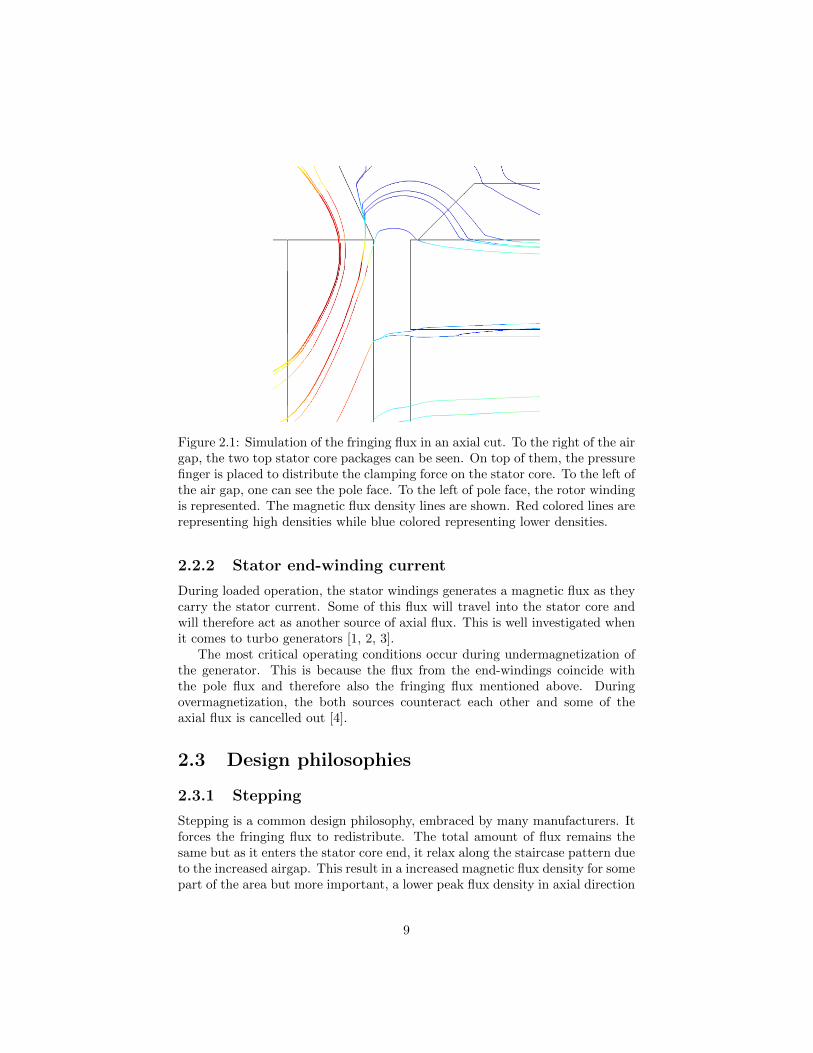
Figure 2.1: Simulation of the fringing flux in an axial cut. To the right of the airgap, the two top stator core packages can be seen. On top of them, the pressurefinger is placed to distribute the clamping force on the stator core. To the left ofthe air gap, one can see the pole face. To the left of pole face, the rotor windingis represented. The magnetic flux density lines are shown. Red colored lines arerepresenting high densities while blue colored representing lower densities.

2.2.2 Stator end-winding current

During loaded operation, the stator windings generates a magnetic flux as theycarry the stator current. Some of this flux will travel into the stator core andwill therefore act as another source of axial flux. This is well investigated whenit comes to turbo generators [1, 2, 3].

The most critical operating conditions occur during undermagnetization ofthe generator. This is because the flux from the end-windings coincide withthe pole flux and therefore also the fringing flux mentioned above. Duringovermagnetization, the both sources counteract each other and some of theaxial flux is cancelled out [4].

2.3 Design philosophies

2.3.1 Stepping

Stepping is a common design philosophy, embraced by many manufacturers. Itforces the fringing flux to redistribute. The total amount of flux remains thesame but as it enters the stator core end, it relax along the staircase pattern dueto the increased airgap. This result in a increased magnetic flux density for somepart of the area but more important, a lower peak flux density in axial direction

9

[1]. There are various designs when it comes to stepping. The one consideredhere consists of 3 smaller radii, where the one at the top, is decreased with theradius of 1 airgap.

Figure 2.2: To the right of the air gap, one can see the stator core top packageswith the stepping design. To the left, one can see the rotor pole with its poleface. The enclosed area represents the rotor winding.

2.3.2 Shortening of the poles

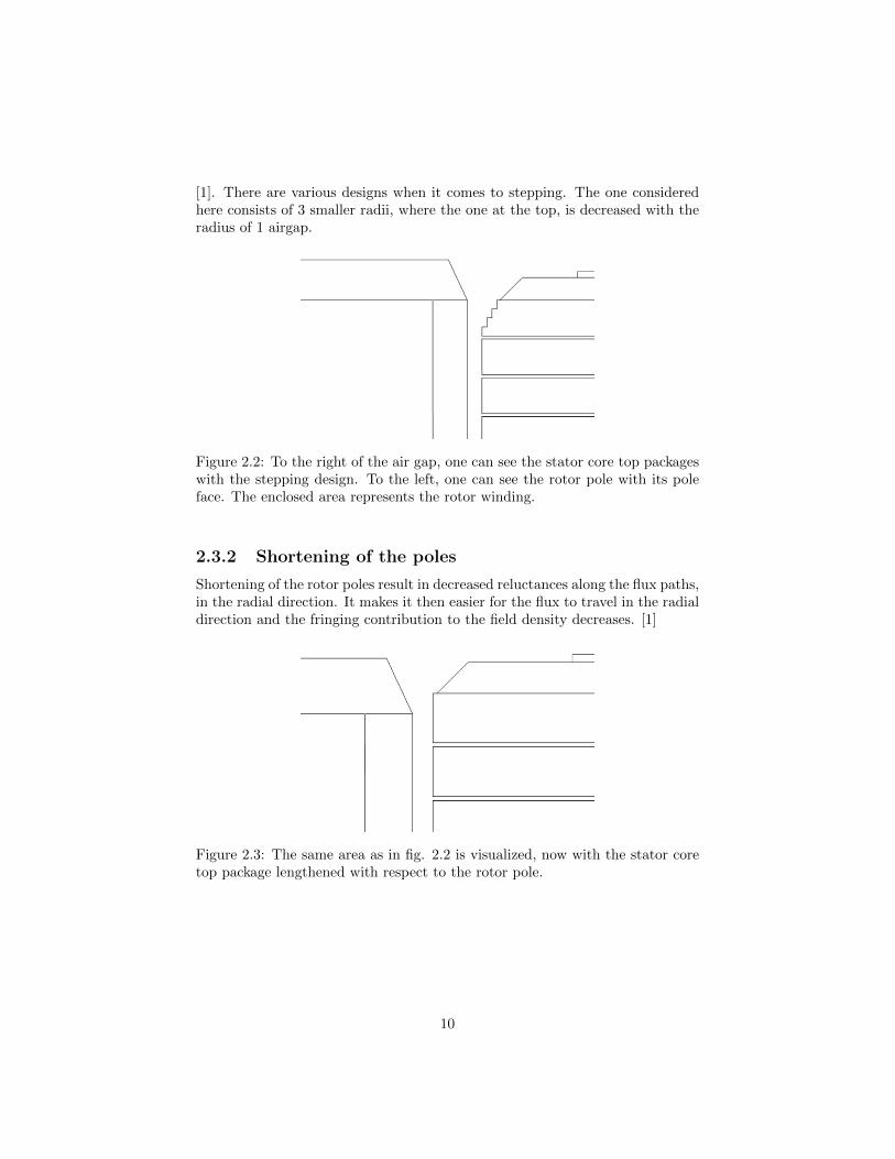
Shortening of the rotor poles result in decreased reluctances along the flux paths,in the radial direction. It makes it then easier for the flux to travel in the radialdirection and the fringing contribution to the field density decreases. [1]

Figure 2.3: The same area as in fig. 2.2 is visualized, now with the stator coretop package lengthened with respect to the rotor pole.

10

2.4 Power losses

The power loss that occur in electrical steel during no-load operation can bedivided into different components depending on physical origin. Some of thephenomenons have to be considered on a microscopic scale and some have amacroscopic dependence. Here the most influential are briefly described.

2.4.1 Anisotropy

Losses due to magnetic anisotropy have an important influence on the loss pre-diction. The problem origins from the atomic structure where there is magne-tocrystaline anisotropy, meaning the iron lattice have a preferable direction formagnetization. The crystal structure of the iron is body-centered cubic (BCC).The paths along the cube axis of the lattice is considered to be the direction thatrequires the least energy to magnetize. In literature referred to as a easy-axis.[5, 6]

2.4.2 Steinmetz model

The loss prediction model used was a 3-component, Steinmetz equation seenin 2.2. The 3 terms corresponds to hysteresis losses, the classical losses (eddy-currents) and the excess losses [5]. The losses is given as the time average ofthe specific loss [W/kg]. It assumes an alternating flux density waveform.

Ploss = kHB2f + kcB

2f2 + keB1.5f1.5 (2.2)

Where

• kH = the hysteresis coefficient

• B = the maximum B for each node

• f = the fundamental frequency

• kc = the classical loss coefficient

• kE = the excess loss coefficient

2.4.2.1 Hysteresis loss

The loss corresponds to the enclosed area of the hysteresis loop, per unit volumeand cycle. It is, on a more microscopic scale, a consequence of the anisotropywhere several easy-axis occurs along the cubic axis of the lattice. Also the originof the loss is, on a more macroscopic scale, because of movement and shape of thedomain walls. Due to the characteristics of the material such as impurities, grainsize and grain orientation the domain walls gets pinned. The domain wall thengets snapped away from its pinning site, micro eddy currents are induced andhysteresis occurs as heat. The hysteresis exponent is in this case approximated

11

by 2. There are improved Steinmetz models that accounts for saturation anduses a variable hysteresis exponent as a function of B. A hysteresis exponent of2 is a good approximation in the linear area on the hysteresis curve. [5, 6]

2.4.2.2 Classical loss (eddy current)

According to Faraday’s Law, currents are induced when a conducting materialgets exposed to an alternating magnetic field. According to Lenz’s law thiscurrent will create a magnetic field, in the opposing direction of the field that itorigins from. This leads to heat losses. This is more pronounced considering theaxial flux. As the magnetic field enters a wider surface the circulating currentscan travel further.

2.4.2.3 Excess loss

The excess (sometimes refereed to as anomalous) loss occurs because of inducedcurrents that origins from changes in the micro structure of the iron. Its depen-dency can be derived from statistical theory [7].

2.4.3 Rotational field

The conventional loss prediction models assumes a alternating flux density wave-form as it is a function of only f and Bmax. Previous work shows that thewaveform of the magnetic flux is strongly dependent of the polarization stateand unidirectional flux is present. It is shown that a conventional loss model as2.2 stated above, accounts for about only half of the total losses. This is mostlydue to the neglected influence of the rotational field. [8, 7]

2.4.4 Mechanical processing

In hydropower generators, non orientated steel is often used. It is processed insome ways to reduce the losses mentioned above. To reduce eddy currents thestator core is stacked by sheets with interlaminar insulation. The iron is usuallyalloyed with some percentages of silicon, to increase the resistivity and reducethe induction of eddy currents. [9]

12

3 Method

3.1 Simulations

The two design concepts was simulated and evaluated together with a designwhere no action was performed. In this case the rotor pole was of the samelength as the stator core that was of the same radius throughout its length.This is referred to as the no action design.

3.1.1 No-load operation

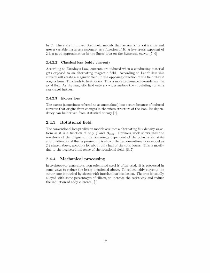
Simulations of the magnetic environment in the stator core end was performed.3D FEM calculations of the magnetic field was carried out in a simplified modelof a reference machine, namely the ”Stornorrfors G2”. It is installed in one ofthe largest hydropower plants in Sweden. The apparent power of the generatoris 155 MVA. It runs on 235 rpm, using a Francis turbine with a head of 75 m.

A cross section of the upper half with 1 pole pair and 17 slots was consid-ered, as seen in fig. 3.1. The geometry was drawn using SolidWorks and laterimported to COMSOL Multiphysics V.5.1 for magnetostatic simulations. Thenumber of elements was 638434 for the pole shortening design, 855728 for thestepping design and 637893 for the no action. COMSOL Multiphysics built-in,default solver MUMPS (Multifrontal massively parallel sparse direct solver) wasused for all simulations.

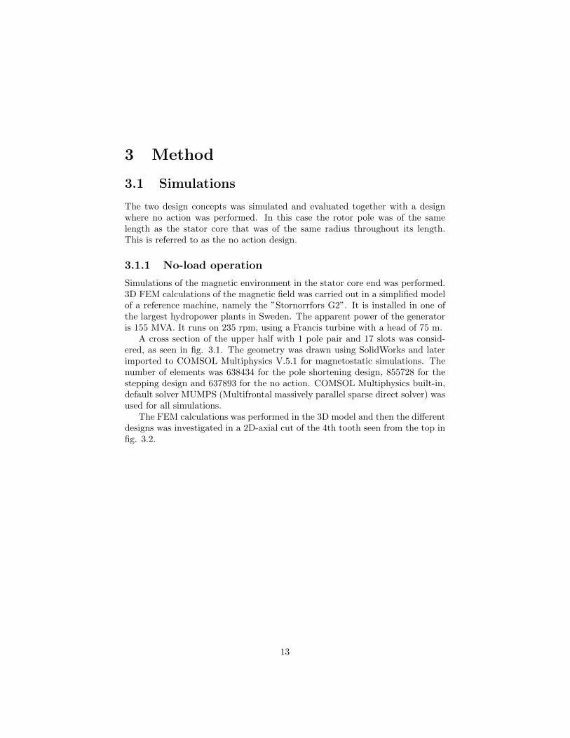
The FEM calculations was performed in the 3D model and then the differentdesigns was investigated in a 2D-axial cut of the 4th tooth seen from the top infig. 3.2.

13

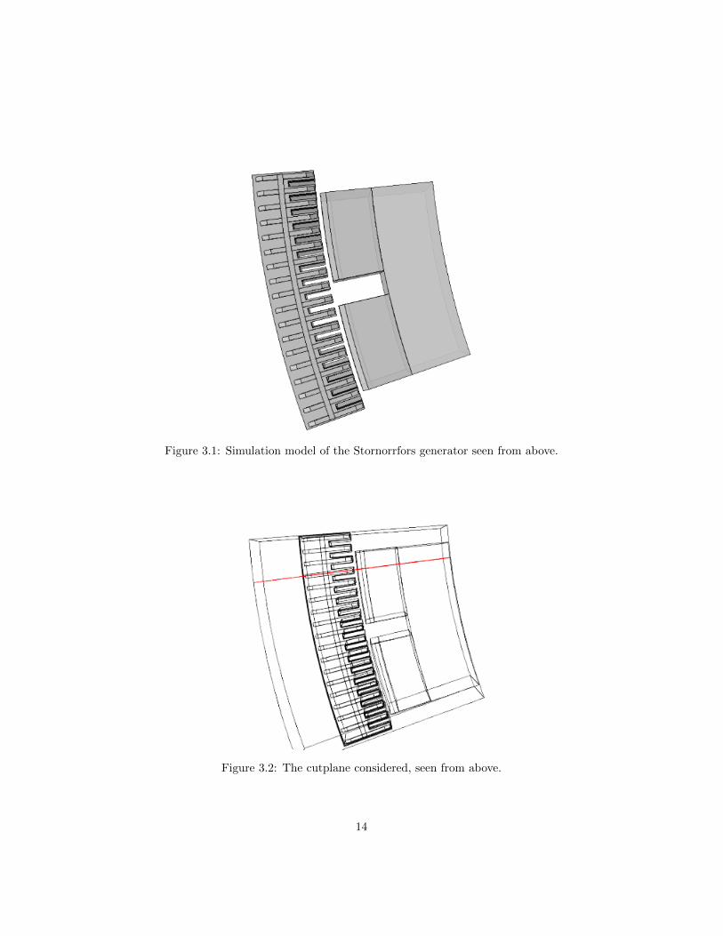
Figure 3.1: Simulation model of the Stornorrfors generator seen from above.

Figure 3.2: The cutplane considered, seen from above.

14

The magnetization of the poles was tuned in to satisfy the average fluxdensity in the air gap, according to the original design criteria. The materialswas set with user defined BH-relations, supplied from the manufacturer. The2D axial cut considered can be seen in fig. 3.3.

Figure 3.3: The full cutplane considered seen from the front, here with the noaction design.

The magnetic environment was investigated and evaluated along a statortooth, at the extreme core end, see fig. 3.4.

Figure 3.4: The red line along the x-axis is referred to as the extreme core end,for the different designs.

3.1.2 Saturation

Additional simulations were carried out to investigate the different effects ofsaturation in the stator core, using the different designs. This was to investigatehow the saturation will affect the magnetic flux in the stator core end. Onlythe no-load operation was investigated during this simulation.

The same setup as in 3.1.1 was used except a linear BH-relation was nowconsidered. A relative permeability of µr = 740 was used.

15

3.1.3 End-winding driven flux

A simple 2D model, an axial cut of a stator tooth with the end-winding wasdrawn in COMSOL Multiphysics v5.1. The current source (end-winding axialcut) was directed out of the plane. This was to evaluate the effect of the end-winding driven flux, on the different designs. The case where there was noacion, as considered in the no-load operation, was intentionally left out. Thisbecause there is no significant difference compared to the pole shortening caseon this matter. Rated current was considered. The penetration depth, theaverage surface flux density and the average flux density at the extreme coreend along the tooth was investigated. 4250 and 5540 elements was used forthe pole shortening design and the stepping design respectively. Stationarysimulations was carried out.

3.1.4 Power losses

To calculate the power losses, equation 2.2 was used. As stated above, 2.2 is asimplified loss prediction model and therefore underestimates the total losses.The simulation model does not account for anisotropy, due to the use of thesame BH-relation through out the entire geometry. In this thesis though, itis considered accurate enough for comparison of the different designs. The B-values from the simulation data was used as input. The frequency was set to50Hz. The loss coefficients stated below was solved from curve fitting of thetotal losses of the stator iron, given by the manufacturer [10] .

• kH = 0.0130439 [W/kg]

• kc = 9.17113e-05 [W/kg]

• kE = 0.00048401 [W/kg]

Equation 2.2 was evaluated for each mesh node and multiplied with thedensity of the material. The result was then integrated over the entire volumeof the stator, seen on its general form in 3.1. The result was then scaled torepresent the actual stator core.∫∫∫

Ploss ∗ ρfe dx dy dz (3.1)

3.2 Experiment

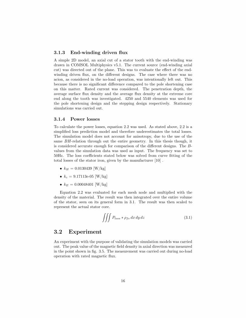
An experiment with the purpose of validating the simulation models was carriedout. The peak value of the magnetic field density in axial direction was measuredin the point shown in fig. 3.5. The measurement was carried out during no-loadoperation with rated magnetic flux.

16

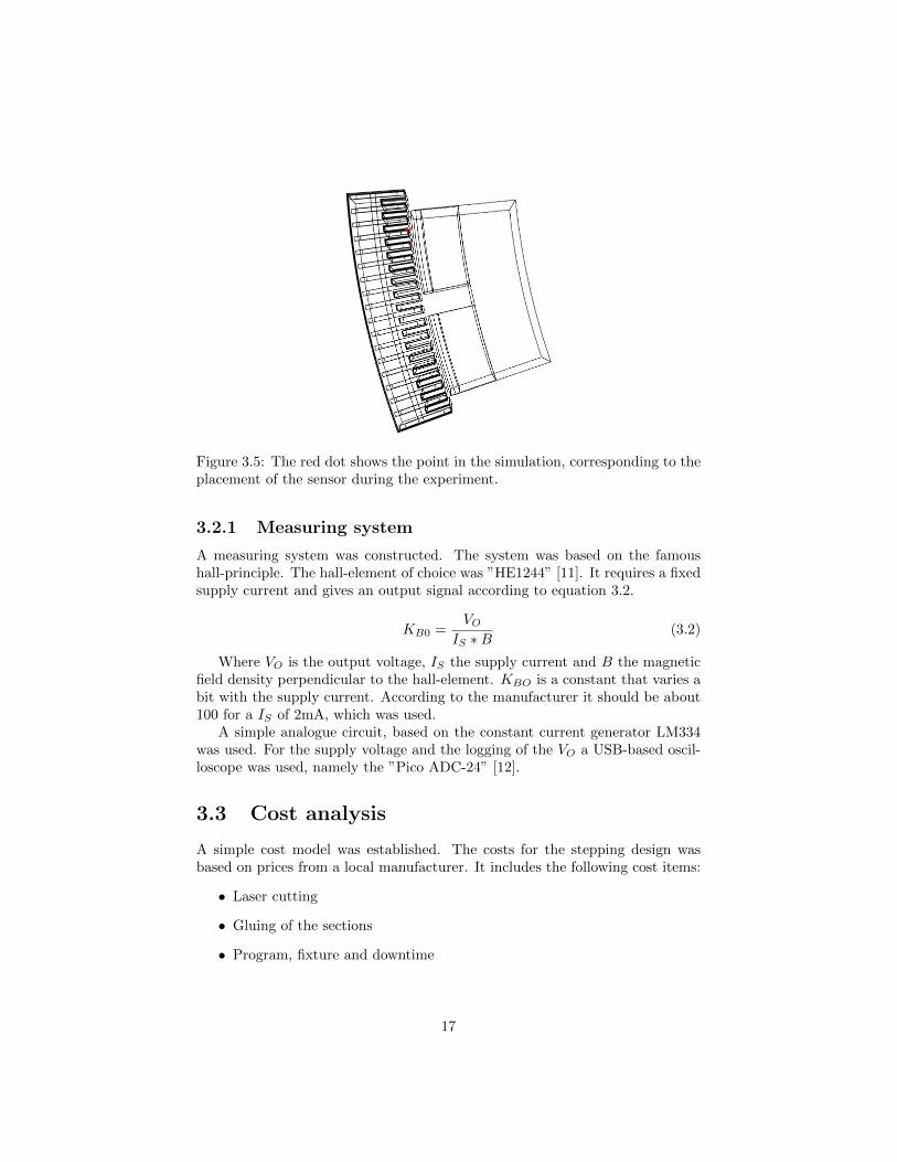
Figure 3.5: The red dot shows the point in the simulation, corresponding to theplacement of the sensor during the experiment.

3.2.1 Measuring system

A measuring system was constructed. The system was based on the famoushall-principle. The hall-element of choice was ”HE1244” [11]. It requires a fixedsupply current and gives an output signal according to equation 3.2.

KB0 =VO

IS ∗B(3.2)

Where VO is the output voltage, IS the supply current and B the magneticfield density perpendicular to the hall-element. KBO is a constant that varies abit with the supply current. According to the manufacturer it should be about100 for a IS of 2mA, which was used.

A simple analogue circuit, based on the constant current generator LM334was used. For the supply voltage and the logging of the VO a USB-based oscil-loscope was used, namely the ”Pico ADC-24” [12].

3.3 Cost analysis

A simple cost model was established. The costs for the stepping design wasbased on prices from a local manufacturer. It includes the following cost items:

• Laser cutting

• Gluing of the sections

• Program, fixture and downtime

17

The additional costs of the pole shortening design was considered as thestator length was increased, assuming the same rotor length. The cost itemsis the extra laminations and the additional cost that comes with longer statorwindings.

The costs depends mostly on the number of sections and laminations. Therule of thumb for lengthening the stator is to increase the length with 1 airgap.This makes the number of extra laminations a function of the length of the airgap. Due to the variance of these parameters, 11 different commercial machinesfrom Sweden was investigated. The design criterias and cost estimations ofVoith Hydro AB was used [13]. The features of the machines investigated canbe seen in table 3.1.

Machine Air gap [mm] Segments Diameter [mm] Power [MVA] Speed [RPM]1 10 24 7000 16 93.752 12 24 8000 24 93.753 14.5 24 7000 25 1254 15 24 7150 60 1255 18 27 7950 90 166.76 19 24 7030 39 136.47 19 26 9740 100 115.48 20 24 8860 90 1259 22 18 5180 69 272.710 23 36 11740 170 107.111 25 36 10380 155 125

Table 3.1: Features of the 11 different machines that was investigated.

18

4 Results

4.1 Simulation results

4.1.1 Fringing flux

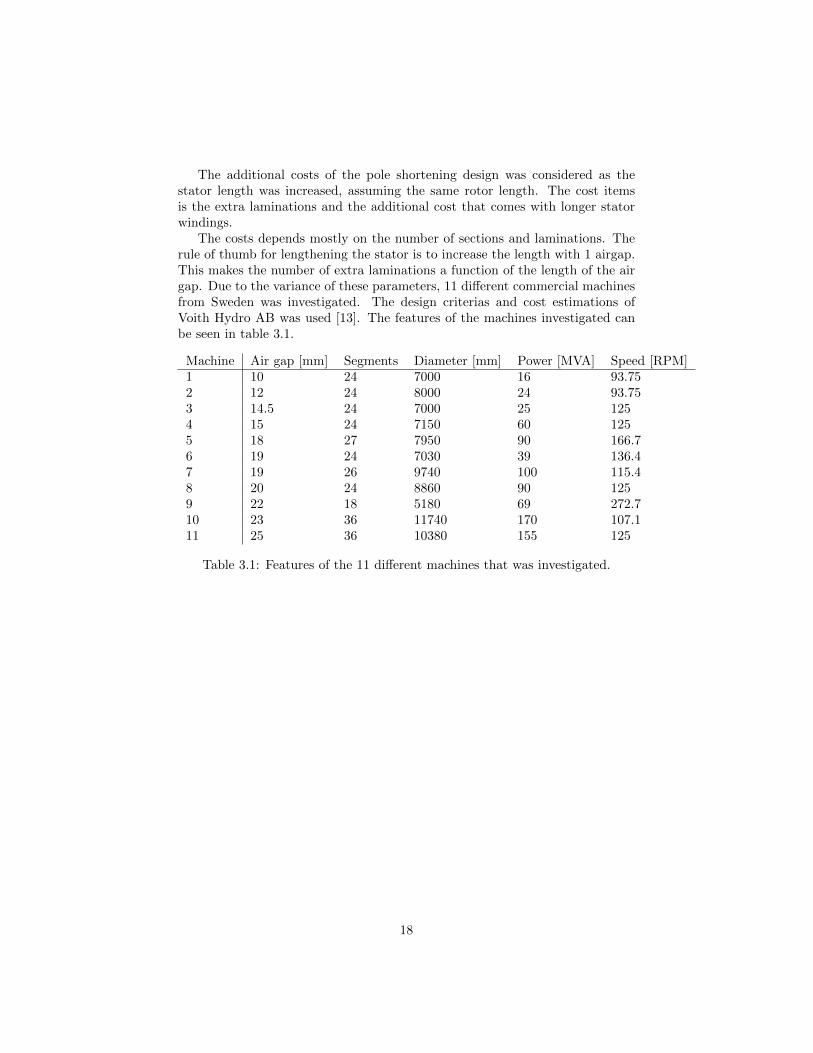
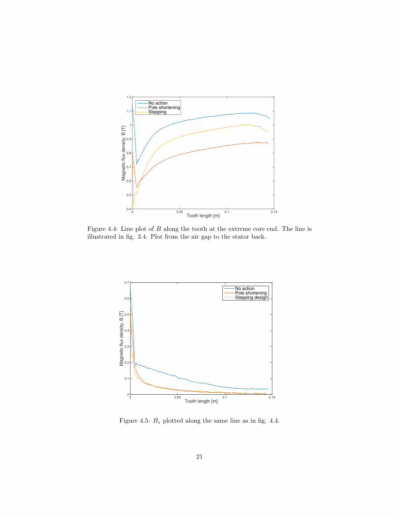
The magnetic field density B is the interesting parameter of the problem. Itis later used as input to the loss prediction model. The norm of the B-fieldand the axial component (referred to as Bz) was investigated in the 2D axialcut mentioned above. In fig. 4.4 one can see the relative differences betweenthe effects of Stepping and Shortening of the poles, about 0.5mm from the topsheet. As one can see the shortening of the pole case starts of a bit higherbut reaches lower values out through the tooth. In fig 4.5, one can evaluatethe simulated values of Bz along the chosen line. It clearly shows on a greatreduction for both designs compared to the no action case. The stepping startsof a bit higher. The average values can be seen in table 4.1.

Bavg [T] Bz,avg [mT]No action 0.997 117.4Pole shortening 0.774 60.60Stepping 0.848 58.50

Table 4.1: Magnetic field densities along the tooth, at the extreme core end.

Figure 4.1: Surface- and streamline plot of B, no action. The grading to theleft corresponds to the surface plot while the one to the right corresponds tothe streamlines. Values are given in Tesla [T].

19

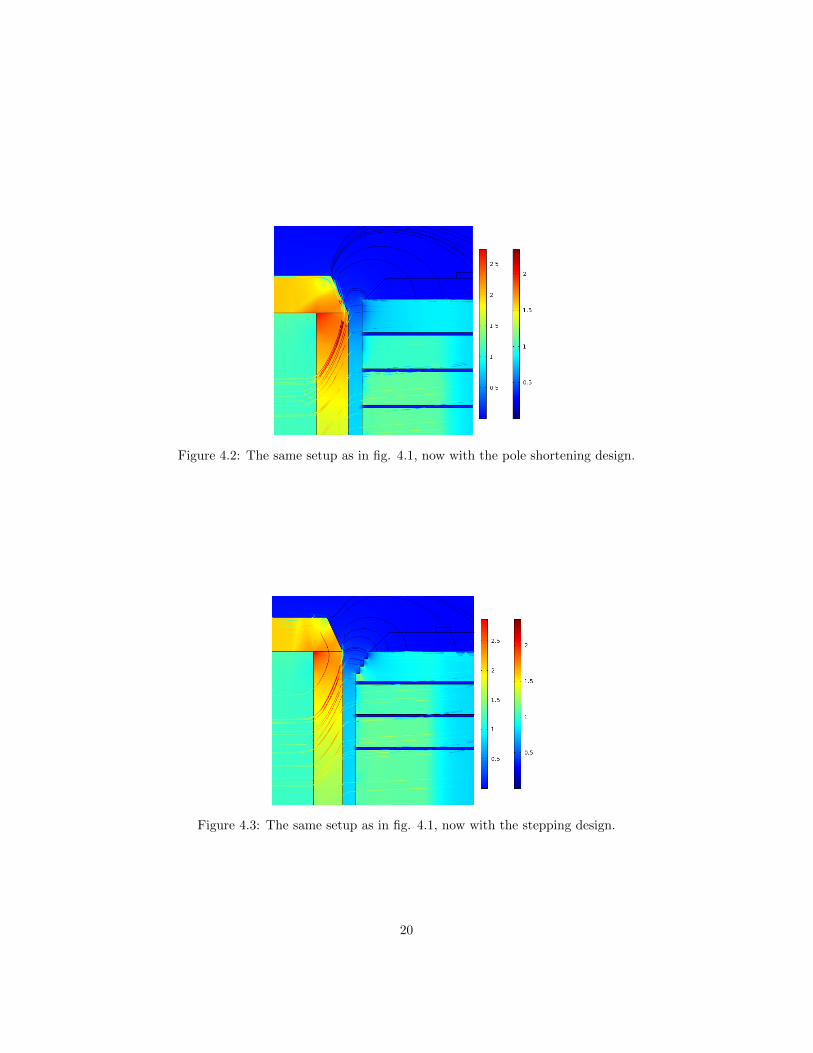
Figure 4.2: The same setup as in fig. 4.1, now with the pole shortening design.

Figure 4.3: The same setup as in fig. 4.1, now with the stepping design.

20

Tooth length [m]0 0.05 0.1 0.15

Ma

gn

etic f

lux d

en

sity, B

[T

]

0.4

0.5

0.6

0.7

0.8

0.9

1

1.1

1.2

No actionPole shorteningStepping

Figure 4.4: Line plot of B along the tooth at the extreme core end. The line isillustrated in fig. 3.4. Plot from the air gap to the stator back.

Tooth length [m]0 0.05 0.1 0.15

Magnetic flu

x d

ensity, B

[T

]

0

0.1

0.2

0.3

0.4

0.5

0.6

0.7

No actionPole shorteningStepping design

Figure 4.5: Bz plotted along the same line as in fig. 4.4.

21

4.1.2 End-winding driven flux

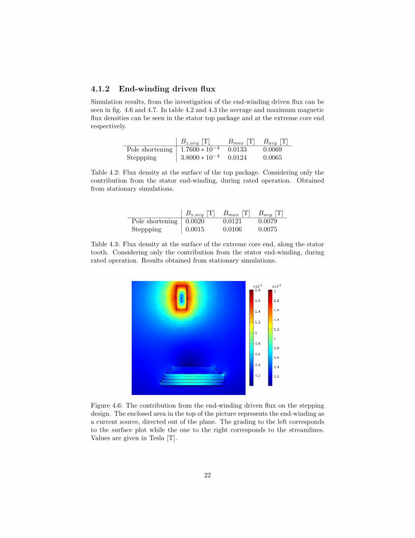
Simulation results, from the investigation of the end-winding driven flux can beseen in fig. 4.6 and 4.7. In table 4.2 and 4.3 the average and maximum magneticflux densities can be seen in the stator top package and at the extreme core endrespectively.

Bz,avg [T] Bmax [T] Bavg [T]Pole shortening 1.7600 ∗ 10−4 0.0133 0.0069Steppping 3.8000 ∗ 10−4 0.0124 0.0065

Table 4.2: Flux density at the surface of the top package. Considering only thecontribution from the stator end-winding, during rated operation. Obtainedfrom stationary simulations.

Bz,avg [T] Bmax [T] Bavg [T]Pole shortening 0.0020 0.0121 0.0079Steppping 0.0015 0.0106 0.0075

Table 4.3: Flux density at the surface of the extreme core end, along the statortooth. Considering only the contribution from the stator end-winding, duringrated operation. Results obtained from stationary simulations.

Figure 4.6: The contribution from the end-winding driven flux on the steppingdesign. The enclosed area in the top of the picture represents the end-winding asa current source, directed out of the plane. The grading to the left correspondsto the surface plot while the one to the right corresponds to the streamlines.Values are given in Tesla [T].

22

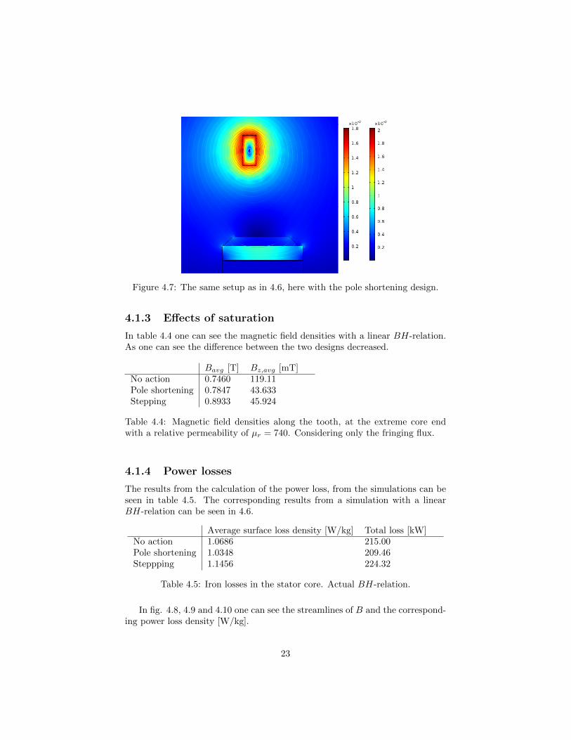
Figure 4.7: The same setup as in 4.6, here with the pole shortening design.

4.1.3 Effects of saturation

In table 4.4 one can see the magnetic field densities with a linear BH-relation.As one can see the difference between the two designs decreased.

Bavg [T] Bz,avg [mT]No action 0.7460 119.11Pole shortening 0.7847 43.633Stepping 0.8933 45.924

Table 4.4: Magnetic field densities along the tooth, at the extreme core endwith a relative permeability of µr = 740. Considering only the fringing flux.

4.1.4 Power losses

The results from the calculation of the power loss, from the simulations can beseen in table 4.5. The corresponding results from a simulation with a linearBH-relation can be seen in 4.6.

Average surface loss density [W/kg] Total loss [kW]No action 1.0686 215.00Pole shortening 1.0348 209.46Steppping 1.1456 224.32

Table 4.5: Iron losses in the stator core. Actual BH-relation.

In fig. 4.8, 4.9 and 4.10 one can see the streamlines of B and the correspond-ing power loss density [W/kg].

23

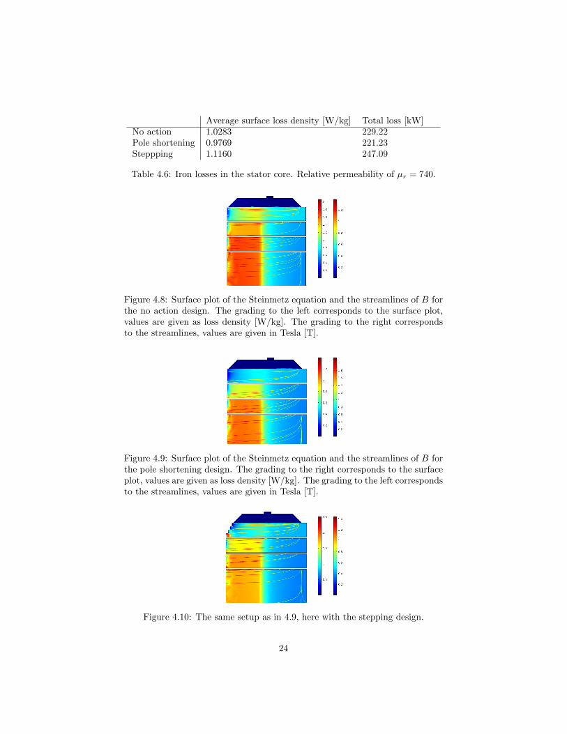
Average surface loss density [W/kg] Total loss [kW]No action 1.0283 229.22Pole shortening 0.9769 221.23Steppping 1.1160 247.09

Table 4.6: Iron losses in the stator core. Relative permeability of µr = 740.

Figure 4.8: Surface plot of the Steinmetz equation and the streamlines of B forthe no action design. The grading to the left corresponds to the surface plot,values are given as loss density [W/kg]. The grading to the right correspondsto the streamlines, values are given in Tesla [T].

Figure 4.9: Surface plot of the Steinmetz equation and the streamlines of B forthe pole shortening design. The grading to the right corresponds to the surfaceplot, values are given as loss density [W/kg]. The grading to the left correspondsto the streamlines, values are given in Tesla [T].

Figure 4.10: The same setup as in 4.9, here with the stepping design.

24

4.2 Experimental results

The peak value of the Bz was measured to be 80.0mT at the given point duringno-load operation. At the same point in the simulation data set, Bz was about100mT.

4.3 Cost model

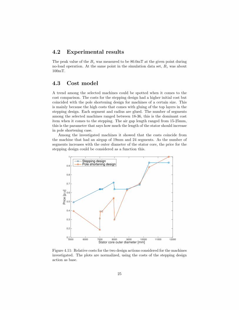
A trend among the selected machines could be spotted when it comes to thecost comparison. The costs for the stepping design had a higher initial cost butcoincided with the pole shortening design for machines of a certain size. Thisis mainly because the high costs that comes with gluing of the top layers in thestepping design. Each segment and radius are glued. The number of segmentsamong the selected machines ranged between 18-36, this is the dominant costitem when it comes to the stepping. The air gap length ranged from 15-25mm,this is the parameter that says how much the length of the stator should increasein pole shortening case.

Among the investigated machines it showed that the costs coincide fromthe machine that had an airgap of 19mm and 24 segments. As the number ofsegments increases with the outer diameter of the stator core, the price for thestepping design could be considered as a function this.

Stator core outer diameter [mm]5000 6000 7000 8000 9000 10000 11000 12000

Price

[p

.u]

0.1

0.2

0.3

0.4

0.5

0.6

0.7

0.8

0.9

1

Stepping designPole shortening design

Figure 4.11: Relative costs for the two design actions considered for the machinesinvestigated. The plots are normalized, using the costs of the stepping designaction as base.

25

5 Discussion

Through out the process simplifications and assumptions was made, as men-tioned in the method. The method and the results are discussed here. A lot ofthe references used include previous work that considers turbogenerators. Thereare a lot of differences, most of all the speed and the shape of the machine. It isstill assumed that trends of the problems are the same. In turbogenerators it ismore of a problem and it has therefore been of greater interest in the industryand academia [2].

5.1 Method

Due to limited computer capacity, lamination of the stator core was neglectedand only solid stator packages was considered. With laminated sheets the mag-netic field would probably correspond more accurate to the actual machine.

Non-magnetic pressure fingers were assumed. This is probably not the casein the actual machine. This can underestimate the amount of axial flux enter-ing the stator core due to its shielding effects [14]. Also some of the remainingpressure details such as the clamping plate was neglected.

The same BH-curve was used for all directions in the materials specifications.In this manner magnetic anisotropy is neglected. This gives a bit inaccurateresults when it comes to the amount of flux entering the stator core axially.

Since the no-load and the loaded case is investigated separately, the effect ofthem both coincide is not investigated in the simulations but in theory.

Due to a smaller radius in the stepping design, the data sets are not exactly thesame when investigating the area of the extreme core end, during the no-loadoperation. They are chosen because they are considered to be the most criticalareas and therefore comparable for the different designs.

5.1.1 Power losses

The power losses were calculated to get comparable results from the differentdesigns. One should know that it is not the main point to reduce the power lossof the entire stator with these actions, but to prevent axial magnetic flux andhence end-heating.

A conventional Steinmetz loss prediction model was used. It assumes aalternating magnetic flux wave form, without rotation in the stator core. Thisunderestimates the losses from about 1.5 to 2 times the actual values [8, 14].

26

As mentioned above anisotropy was neglected, also mechanical processing wasnot taken into account. There are improved loss prediction models based onthe conventional Steinmetz that accounts for both rotational flux, anisotropyand mechanical processing. These models often come from the industry and arederived from statistical methods and experimental results.

5.2 Results

5.2.1 Power losses

The pole shortening design showed reduction in the power loss meanwhile thestepping design showed on somewhat increasement. The pole shortening designhad a slightly lower total power loss than the stepping design. This is, clearlybecause of the overall lower B-values through out the stator core. The Bavg

for the pole shortening design was about 11.5% lower than the stepping designmeanwhile the total power loss was about 6.62% lower.

Since the power loss is based on the Bmax in each domain, the effects of thedifferent designs becomes a bit misleading, only considering the power loss. Be-cause of the axial lamination, axial flux cause more eddy-currents than in-planeflux. Using the conventional classical-loss coefficient, derived from an Epstein-test, this is not accounted for.

Because of the simplifications made due to limited computer capacity and possi-ble unphysical effects close to the extreme edges, the results should be consideredwith caution.

5.2.2 Fringing flux

The simulation results says that stepping of the stator reduces the average axialflux density Bz,avg, along the tooth at the considered height with about 50%.The reduction of the average axial flux density Bz,avg for the comparable dataset was about 48% in the pole shortening design.

In the pole shortening case, Bavg decreased with about 22%. In the steppingcase it decreased with 15%. This resulted in that Bavg ended up higher in thestepping case while Bavg,z became slightly lower.

This is probably due to different saturation conditions in the stator core anda redistribution of the field, this is further discussed below.

27

5.2.3 Saturation effects

Due to a redistributed magnetic flux in the stator core, the different designsreduces the saturation. This makes it easier for the axial flux to turn into theplane and travel towards the stator back. This isolate the effect of the axial fluxtowards a more narrow area of the stator core end. This is considered by someauthors, to be the largest benefit from from the designs.

As one can see from the results in section 4.1.3, there was no significantdifference in Bavg meanwhile the Bz,avg increased in both cases. One can assumethat this is because of saturation effects at the extreme core end. Using a linearBH-relation would then allow for more axial flux.

This could be considered as a trade-off. With increased saturation in thestator core end, the amount of axial flux seems to be reduced. Previous work[1] shows also that a lower degree of saturation makes it easier for the axial fluxto turn in-plane and hence reduces the negative effects of the axial flux.

5.2.4 End-winding driven flux

As one can see from the results in section 4.1.2, the end-winding driven fluxcaused a higher Bz,avg at the extreme core end with the stepping design. Theopposite effect occurred when one looked to the entire top stator core package.This may be an effect of the smaller surface, the end-winding is facing whenthe radius of the extreme core end is decreased. In [1] similar behaviour isdiscovered on turbo-generators. The values from the 2D-simulations was verylow though, making it difficult to come up with a conclusion. The part of theend-winding investigated during the simulations, was the very top. This wasbecause the current in this part, is directed straight out of the 2D-model. This isthe part of the end-winding that is on the longest distance from the stator coreend though. Closer to the stator core end, the end-winding is no longer parallelto the stator core but the distance is smaller. This part will give a highercontribution because B will increase with the inverse square of the distance.This can be expressed with Bio-Savart law on the form seen in eq. 5.1.

dB =µ0

4π

Idlsin(θ)

r2(5.1)

In eq. 5.1 an element of the magnetic field density dB is axpressed as therelation between an element of the current Idl and the position r where dB isdetermined. The angle θ is between Idl and r.

28

5.2.5 Experimental result

The experimental data deviated with about 20% from the results obtained inthe simulations. It can depend on a lot of different reasons, some mentionedbelow.

• The hall-element was not satisfactory mounted on the stator core end.It was not completely flat against the surface because of the attachment.This results in measurements of not only the axial component.

• The wiring that was used for measuring the hall-voltage was to long. Thisresulted in a voltage drop over the wires that weakened the signal. Usingthis long wires needs some kind of amplification device, such as a repeater.Because of this, the peak of Bz was underestimated.

• The wires had no screen for grounding. Measuring a signal of this ampli-tude makes it very sensitive to external signals. With no screen and weakinsulation, the signal will be distorted.

5.2.6 Cost analysis

The increased costs for the two different designs are estimations. The costs forthe stepping design are based on prices from one local manufacturer. It shouldcorrespond to the prices on the market, good enough for this issue. If one shoulddo a more thorough investigation, for a large scale production, several suppliershad to be taken into account. The costs for lengthening of the stator are basedon in-house guidelines, neglecting some cost items that is hard to predict.

Based on this, it seems that it would be more beneficial to increase the statorlength than stepping for a slowly rotating machine with a large outer diameter.This is a typical northern machine, because of sites with low head and high flow.

29

6 Conclusion

Literature-studies has been carried out. It was concluded that very little previ-ous work had been published. The necessary theory are presented. The methodof choise and the results has been thoroughly described.

FEM-simulations have been performed for understanding of the magnetic envi-ronment and the behaviour of the different designs.

Experiment was performed on the reference machine for validation of the simu-lation models. The deviation of the measured values compared to the simulatedsays that the simulation can be considered as good enough.

A simplified cost analysis was performed. The result depended strongly onthe shape of the machine.

The drawbacks of the method and possible sources of errors have been dis-cussed.

30

7 Future work

To really be able to make some general conclusions about which design is moreeffective, extended studies has to be made. Time dependent FEM-calculations,considering a variety of machines, running on all possible operation points hasto be investigated. Fully coupled 3D models This should also, to some extentbe verified with experimental data.

To be able say more about the costs, one need access to data from severalmachines, using the different designs. It is hard to estimate and make anygeneral conclusions because of the fact that every machine is custom made.

31

Bibliography

[1] B. Mecrow, A. Jack, and C. Cross, “Electromagnetic design of turbogenera-tor stator end regions,” IEE PROCEEDINGS, vol. 136, no. 6, pp. 361–372,Nov. 1989.

[2] B. Mecrow, A. Jack, and K. Cowan, “Stator core end heating in air andhydrogen indirectly cooled turbogenerators,” in Electrical Machines andDrives, 1991. Fifth International Conference on (Conf. Publ. No. 341).

[3] R. Singleton, P. Marshall, and J. Steel, “Axial magnetic flux in synchronousmachines: the effect of operating conditions,” IEEE Transaction on PowerApparatus and Systems, vol. PAS-100, no. 3, pp. 3200–3206, Mar. 1981.

[4] B. Marcusson and U. Lundin, “Axial magnetic fields at the ends of a syn-chronous generator at different points of operation,” IEEE Transaction onMagnetics, vol. 51, no. 2, Feb. 2015, Article: 8100208.

[5] G. Bertotti, “General properties of power losses in soft ferromagnetic ma-terials,” IEEE Trans. Magn., vol. 24, no. 1, pp. 621–630, Jan. 1988.

[6] P. Beckley, “Modern steels for transformers and machines,” Power Engi-neering Journal, vol. 13, no. 4, pp. 190–200, Aug. 1999.

[7] G. Traxler-Samek and G. Ardley, “Iron losses in salient-pole synchronousmachines considering unidirectional and elliptic magnetization,” in 8th In-ternational Symposium on Advanced Electromechanical Motion System &Electric Drives Joint Symposium, 2009. Electromotion, 2009. IEEE, Jul.2009, pp. 1–6.

[8] M. Ranlof, A. Wolfbrandt, J. Lidenholm, and U. Lundin, “Core loss predic-tion in large hydropower generators: Influence of rotational fields,” IEEETransaction on Magnetics, vol. 45, no. 8, pp. 3200–3206, Aug. 2009.

[9] P. M. Carlberg, Mjukmagnetiska material for elektroindustrin - Elektroplatoch amorfa material, Surahammars Bruks AB Std., 1987.

[10] Cogent Surahammars Bruks AB. (2008, Jun.) Typical data forSURA M250-50A. Visited on 2015-11-14. [Online]. Available: http://cogent-power.com/cms-data/downloads/m250-50a.pdf

[11] Asensor Technology AB. (2015, apr) HE244 series Analog Hall sensor.Visited on 2015-11-16. [Online]. Available: http://www.asensor.eu/productdata/Datasheet-HE244X.pdf

32

[12] Pico Technology. (2013) ADC-20/ADC-24 High-Resolution Data LoggersUser’s Guide. Visited on 2015-11-16. [Online]. Available: https://www.picotech.com/download/manuals/adc20.en-5.pdf

[13] A. Solum, Private comunication, 2015, Voith Hydro AB.

[14] M. M. Znidarich, “Hydro generator stator cores part 1 - constructionalfeatures and core losses,” 2008, pp. 1–8.

33