Adaptive Predictive Control by Open-Loop- Feedback-Optimal Controller for Cultivation Processes by Meijie Li A Thesis submitted in partial fulfillment of the requirements for the degree of Doctor of Philosophy in Biochemical Engineering Approved Dissertation Committee Supervisor: Prof. Dr. Mathias Winterhalter (Jacobs University Bremen) Supervisor: Prof. Dr.-Ing. Volker C. Hass (Hochschule Furtwangen University) Reviewer: Prof. Dr. h. c. Roland Benz (Jacobs University Bremen) Reviewer: Dr. Florian Kuhnen (Hochschule Bremen) Date of Defense: 16.10.2015

Welcome message from author
This document is posted to help you gain knowledge. Please leave a comment to let me know what you think about it! Share it to your friends and learn new things together.
Transcript

Adaptive Predictive Control by Open-Loop-
Feedback-Optimal Controller for Cultivation
Processes
by
Meijie Li
A Thesis submitted in partial fulfillment
of the requirements for the degree of
Doctor of Philosophy
in Biochemical Engineering
Approved Dissertation Committee
Supervisor:
Prof. Dr. Mathias Winterhalter
(Jacobs University Bremen)
Supervisor:
Prof. Dr.-Ing. Volker C. Hass
(Hochschule Furtwangen University)
Reviewer:
Prof. Dr. h. c. Roland Benz
(Jacobs University Bremen)
Reviewer:
Dr. Florian Kuhnen
(Hochschule Bremen)
Date of Defense: 16.10.2015

Statutory Declaration
I, Meijie Li hereby declare that I have written this PhD thesis independently, unless where clearly state
otherwise. I have used only the sources, the data and the support that I have clearly mentioned. This
PhD thesis has not been submitted for conferral of degree elsewhere.
I confirm that no rights of third parties will be infringed by the publication of this thesis.
Bremen, August 20, 2015
Signature __________________

i
Acknowledgements
The work presented in this thesis, was performed during my engagement as a research associate
at the Institute of Environmental and Biotechnology at the University of Applied Sciences
Bremen (Hochschule Bremen). Having this opportunity, I would like to express my deepest
gratitude to the people who have provided me with professional advices and moral support.
First of all, I would like to thank Prof. Dr. Matthias Winterhalter, who has offered excellent
mentoring, many suggested improvements of this thesis and participated in the evaluation of
this work. Next, I would like to thank Prof. Dr. Volker Hass, who has provided me the
opportunity to work with his outstanding research group and many inspirational insights
throughout my research work. Many thanks to Prof. Dr. Roland Benz for reviewing my thesis
and being a member of my dissertation committee. A special thanks to Dr. Florian Kuhnen,
who has provided me with continuously guidance and participated in numerous fruitful
discussions in the research area.
I would also like to thank all of my colleagues who have been very helpful and provided a good
working atmosphere at the institute.
Last but not least I would like to thank my family and friends, for their unwavering support
during the many long days which went into this endeavor.

ii
Abstract
The development of a safe and resource efficient production process is probably the most
important step in the value chain starting from a biomolecular product to a final market product.
Commonly, bioprocess optimization requires numerous experiments, which can be time and
material costly. Predictions based on calculations can reduce the manufacturing experimental
costs, assist in reaching the production of the desired product to a high concentration with high
productivity and yield. Process description, optimization and control using mathematical
models are an innovative and efficient approach in the process development.
On the other hand, the development of mathematical models is also time and cost consuming.
The use of a highly adaptive general model for bio-processes can reduce the time for model
development. Because it takes only the adjustment of model parameters to achieve the
adaptation of a process model to a new organism or product. Development of a general process
model with high adaptability was one of the main goals of the project "ProTool"*. A general
process model is not bound to a certain cell line and microorganism, but adapts itself to a variety
of organisms and different scenarios. This process model will be used for data interpretation,
process monitoring, recipe optimization and the verification of control concepts as well as the
basis of a virtual representation of the process (i.e. training simulator).
Correspondingly, the development of an advanced controller to achieve an optimized process
control adapting the general model, which is named as the open-loop-feedback-optimal
(OLFO) controller, was another main goal of the project "ProTool". The development of the
OLFO controller is the core task of my dissertation. A structured model consisting of four
biomass compartments is working as the general model which is able to describe the cultivation
of different organisms. Based on this model, online parameter identification is carried out
periodically with the actual process data collected from the plant and laboratory analysis. And
the new estimated process parameters and the updated process state variables are used in
calculating an optimal control profile. The model parameters are updated at desired period
using the extended database to reduce the plant model mismatch to improve the performance
of the optimizer.
* This work is funded by the BMBF within the cluster project BioKatalyse2021, item 0315169(A-E) Catalyse 2021.
iii
This work outlines the advantages to apply the OLFO controller in fermentation processes.
First, it can be used to work with the virtual bioreactor as a training tool for students and staffs
in industry to gain insights into fermentation processes and process control strategies which
can significantly shorten the training cycle and training cost. Second, the OLFO can provide
calculated optimized result for the real fermentation process to reach its maximum productivity
and high standards of product purity with minimum development and production cost. Finally,
the OLFO controller also shows the potential to function as a software observer to detect the
key processes state variables, e.g. biomass, substrate and product concentration, which are
normally measured offline by using the most commonly selected process variables, e.g. pH
values, O2 and CO2 composition in off gas flow etc., which can be readily measured online
using standard sensors. The results obtained in both simulation and real processes show the
efficiency of the OLFO controller for online fermentation process control.

iv
Contents
1 Introduction 1
1.1 Motivation and objective 2
1.2 State of art 4
1.2.1 Development of yeast fermentation technologies 4
1.2.2 Development of control strategies for fermentation processes 5
1.2.3 Soft Sensors 10
2 Laboratory set-up 14
2.1 Organisms and media 14
2.2 The Bioreactor 14
2.3 An overview of the variables system 16
2.3.1 Direct inputs to the fermentation unit 17
2.3.2 Measured quantities of the fermentation unit 18
2.4 Technical aspects of the OLFO embedding 19
2.4.1 Establishment of the OLFO controller structure 20
2.4.2 Options of communication with the process control system 21
3 The OLFO controller 22
3.1 General process model 22
3.1.1 The biological submodel 25
3.2 Basic theory of parameter identification 29
3.3 Optimization criterion 31
3.4 Work flow of the OLFO controller 33
4 Research results and application examples of OLFO in fed-batch processes 36
4.1 Basic research on parameter identification and optimization 36
4.1.1 Different sampling time of offline measurements 37
v
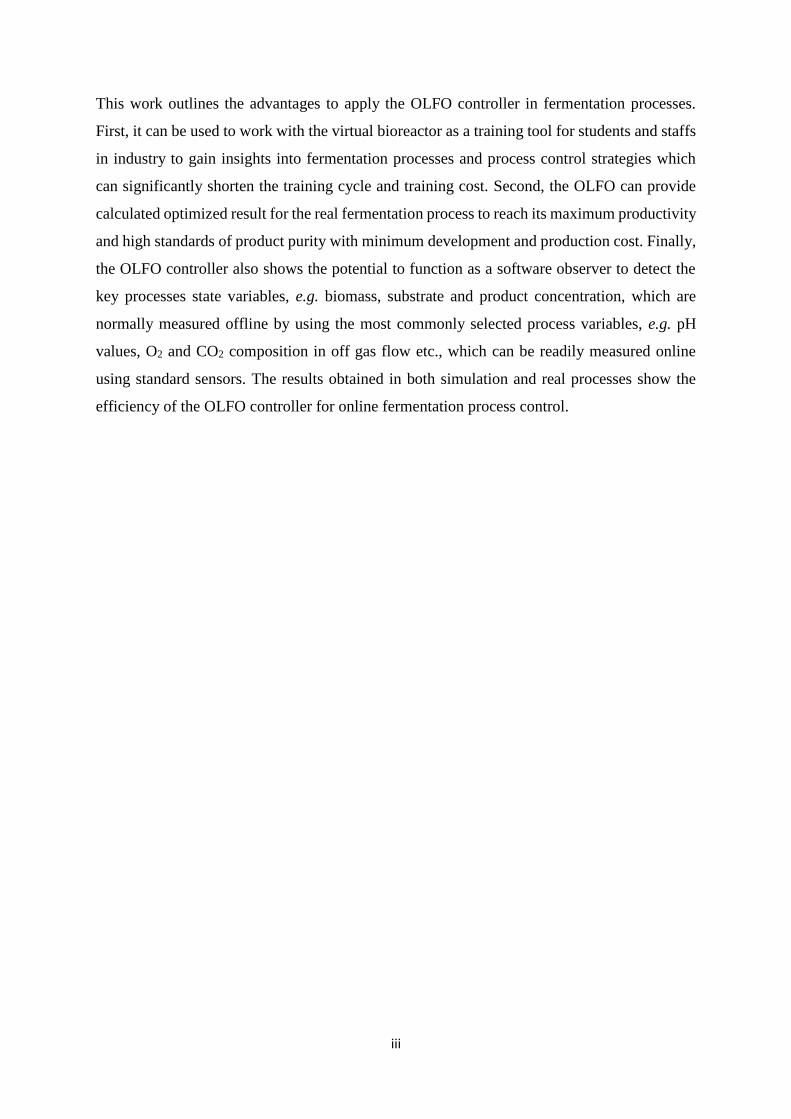
4.1.2 Different weighting factors 39
4.1.3 Absence of partial measurements 40
4.1.4 Different initial values and boundaries 41
4.1.5 Influence of each parameter on the optimization 41
4.1.6 The performance of the OLFO controller 42
4.2 OLFO works with the virtual bioreactor 43
4.3 OLFO application for yeast fed-batch cultivation 48
4.4 Software observer 58
5 Summary and Outlook 63
5.1 Summary of the overall work 63
5.2 Perspective on future OLFO controller developments and
applications
64
Appendix 1: Performance of parameter identification when lack of partial
measurements
65
Appendix 2: Performance of the OLFO controller as a software observer 67
Appendix 3: Data processing toolbox with OpenOffice 72
References 78

vi
List of Figures
Figure Description Page
1.1. Scheme of the soft sensor as defined in reference (Luttmann et al., 2012). The
figure depicts only one hardware sensor, although in reality there can be several
of those.
11
1.2. Schematic depiction of the soft sensor implementation as described in reference
(Warth et al., 2010).
13
2.1. Instrument of a laboratory stirrer tank bioreactor. Adapted from reference (B.
Braun Biotech International GmbH).
15
2.2. Cultivation system in laboratory (includes a stirred tank bioreactor, a computer
with the OLFO embedding in process control system and a control unit).
16
2.3. A scheme depicting the variables of the whole system. 17
3.1. Basic structure of the OLFO controller. Three elements: a process model, a model
parameter identification and an optimization part. )(ˆ)( txCtCx is minimized
to estimate the parameters. Based on the identified model, optimal control profiles
are calculated in the optimization part and transferred to the bioreactor and
process system. Adapted from reference (B. Frahm et al., 2002).
23
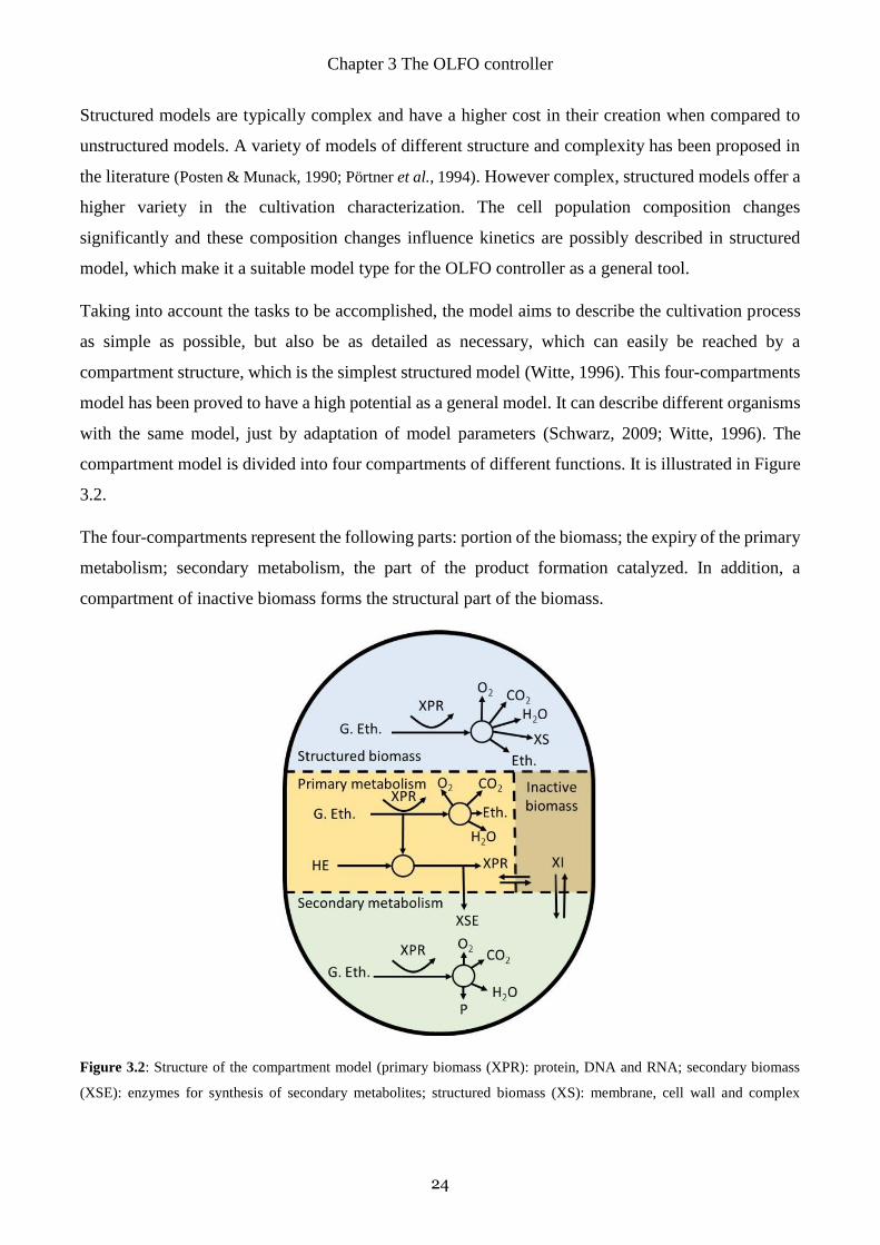
3.2. : Structure of the compartment model (primary biomass (XPR): protein, DNA
and RNA; secondary biomass (XSE): enzymes for synthesis of secondary
metabolites; structured biomass (XS): membrane, cell wall and complex
polysaccharide; inactive biomass (XI): defect enzyme, DNA and RNA; G:
glucose; Eth: ethanol; O2: oxygen; CO2: carbon dioxide; HE: yeast extract; P:
product.). The figure was redrawn from reference (Witte, 1996).
24
3.3. The substrate flux is the key element of the "Lyx" process model. A total substrate
consumption rate rS limits the speed of all subsequent reactions. Distribution
functions describe the substrate flux flows into different metabolic pathways,
depending on the actual state.
25
3.4. A scheme of the transition function. 27
3.5. Work flow of the OLFO controller. When new data becomes available from the
bioreactor, an automated parameter identification takes place, and then the
optimization part calculates the optimal control profiles based on the
34
vii
identification model. Finally, the control profiles are transferred to the direct
control level.
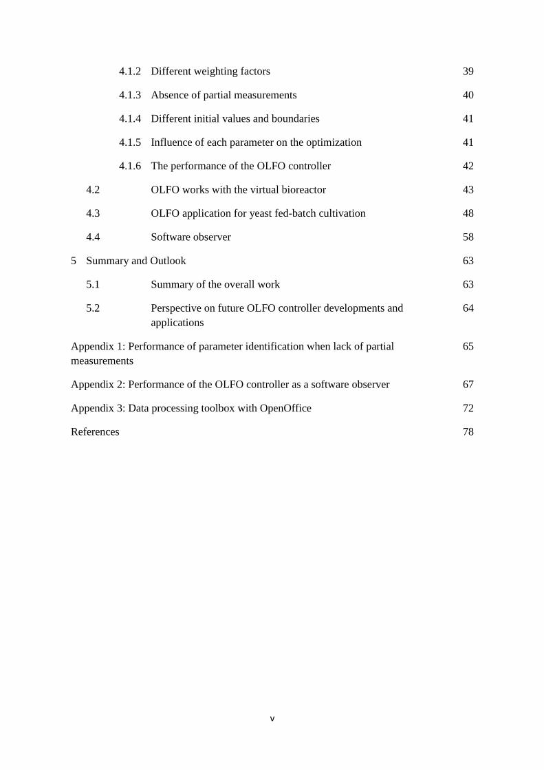
4.1 Parameter identification result with different sampling time. S-exp. is the
experimentally measured substrate concentration, S-sim. is the related parameter
estimation result. P and X are the product and biomass concentrations
respectively. There are three groups of simulation results shown here: the first
group simulation with P, X, S every 30 minutes by thickest lines, the second
group simulation with P, X, S every 60 minutes and the third group simulation
with P, X every 60 minutes, S every 180 minutes by thinnest lines. All of the
simulation results fit the measurements well, without significant difference.
38
4.2 The parameter identification result without individual weighting factors. The
experimental data (referred to as pixels) are connected with the corresponding -
best matching - model data (solid as lines) are shown together. The upper part
shows S: substrate, P: product and X: biomass; the lower part shows the
corresponding simulation and experimental data of off gas composition. Without
appropriate weighting factors, the model cannot fit the measurements.
39
4.3 The best parameter identification result with suitable individual weighting
factors: 2CO : 0.1,
2O : 0.1, S : 0.001, P : 1.0, X : 1.0. is the weighting
factor for each individual variable which depends on its dimension and reliability.
The experimental data (referred to as pixels) are connected with the
corresponding - best matching - model data (solid as lines) are shown together.
The upper part shows S: substrate, P: product and X: biomass; the lower part
shows the corresponding simulation and experimental data of off gas
composition. By putting the appropriate weight on certain state variables renders
an obviously better description of parameter identification.
40
4.4 The graphical user interface of the virtual bioreactor. 44
4.5 The user interface of the virtual bioreactor to set the interval of sampling, the
interval to generate the measurement and the beginning of the real process time.
45
4.6 (Left) Parameter identification graphs with 2.5 hours interval, with corresponding
(right) optimization of the estimated models (upper) and the optimal feeding
profile (lower). Substrate (S), product (P) and biomass (X) concentrations are
further labeled based on their generated source virtual bioreactor (experimental)
or OLFO (simulated).
47
4.7 Precalculated optimization results based on the calibrated model from a previous
fermentation experiment. The upper part shows the optimized feeding rate fS and
49
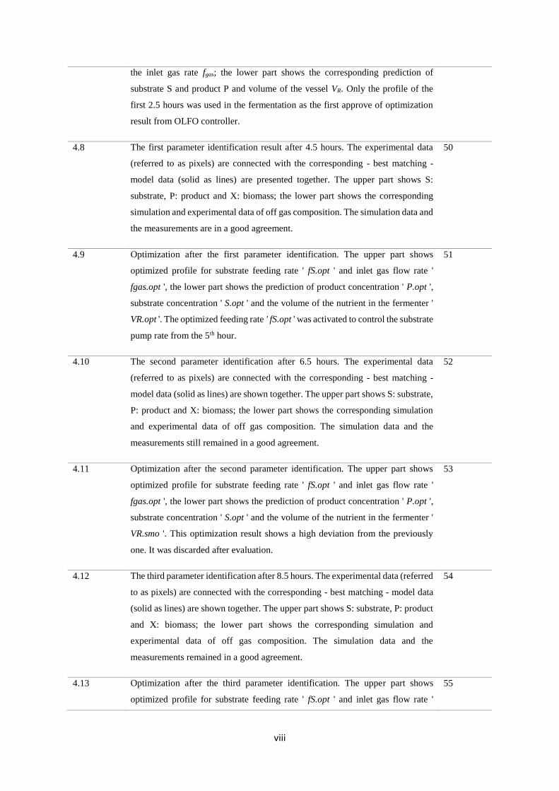
viii
the inlet gas rate fgas; the lower part shows the corresponding prediction of
substrate S and product P and volume of the vessel VR. Only the profile of the
first 2.5 hours was used in the fermentation as the first approve of optimization
result from OLFO controller.
4.8 The first parameter identification result after 4.5 hours. The experimental data
(referred to as pixels) are connected with the corresponding - best matching -
model data (solid as lines) are presented together. The upper part shows S:
substrate, P: product and X: biomass; the lower part shows the corresponding
simulation and experimental data of off gas composition. The simulation data and
the measurements are in a good agreement.
50
4.9 Optimization after the first parameter identification. The upper part shows
optimized profile for substrate feeding rate ' fS.opt ' and inlet gas flow rate '
fgas.opt ', the lower part shows the prediction of product concentration ' P.opt ',
substrate concentration ' S.opt ' and the volume of the nutrient in the fermenter '
VR.opt '. The optimized feeding rate ' fS.opt ' was activated to control the substrate
pump rate from the 5th hour.
51
4.10 The second parameter identification after 6.5 hours. The experimental data
(referred to as pixels) are connected with the corresponding - best matching -
model data (solid as lines) are shown together. The upper part shows S: substrate,
P: product and X: biomass; the lower part shows the corresponding simulation
and experimental data of off gas composition. The simulation data and the
measurements still remained in a good agreement.
52
4.11 Optimization after the second parameter identification. The upper part shows
optimized profile for substrate feeding rate ' fS.opt ' and inlet gas flow rate '
fgas.opt ', the lower part shows the prediction of product concentration ' P.opt ',
substrate concentration ' S.opt ' and the volume of the nutrient in the fermenter '
VR.smo '. This optimization result shows a high deviation from the previously
one. It was discarded after evaluation.
53
4.12 The third parameter identification after 8.5 hours. The experimental data (referred
to as pixels) are connected with the corresponding - best matching - model data
(solid as lines) are shown together. The upper part shows S: substrate, P: product
and X: biomass; the lower part shows the corresponding simulation and
experimental data of off gas composition. The simulation data and the
measurements remained in a good agreement.
54
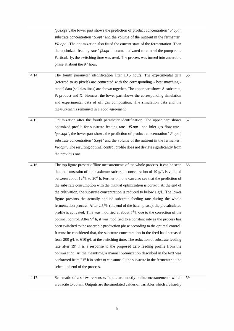
4.13 Optimization after the third parameter identification. The upper part shows
optimized profile for substrate feeding rate ' fS.opt ' and inlet gas flow rate '
55
ix
fgas.opt ', the lower part shows the prediction of product concentration ' P.opt ',
substrate concentration ' S.opt ' and the volume of the nutrient in the fermenter '
VR.opt '. The optimization also fitted the current state of the fermentation. Then
the optimized feeding rate ' fS.opt ' became activated to control the pump rate.
Particularly, the switching time was used. The process was turned into anaerobic
phase at about the 9th hour.
4.14 The fourth parameter identification after 10.5 hours. The experimental data
(referred to as pixels) are connected with the corresponding - best matching -
model data (solid as lines) are shown together. The upper part shows S: substrate,
P: product and X: biomass; the lower part shows the corresponding simulation
and experimental data of off gas composition. The simulation data and the
measurements remained in a good agreement.
56
4.15 Optimization after the fourth parameter identification. The upper part shows
optimized profile for substrate feeding rate ' fS.opt ' and inlet gas flow rate '
fgas.opt ', the lower part shows the prediction of product concentration ' P.opt ',
substrate concentration ' S.opt ' and the volume of the nutrient in the fermenter '
VR.opt '. The resulting optimal control profile does not deviate significantly from
the previous one.
57
4.16 The top figure present offline measurements of the whole process. It can be seen
that the constraint of the maximum substrate concentration of 10 g/L is violated
between about 12th h to 20th h. Further on, one can also see that the prediction of
the substrate consumption with the manual optimization is correct. At the end of
the cultivation, the substrate concentration is reduced to below 1 g/L. The lower
figure presents the actually applied substrate feeding rate during the whole
fermentation process. After 2.5th h (the end of the batch phase), the precalculated
profile is activated. This was modified at about 5th h due to the correction of the
optimal control. After 9th h, it was modified to a constant rate as the process has
been switched to the anaerobic production phase according to the optimal control.
It must be considered that, the substrate concentration in the feed has increased
from 200 g/L to 610 g/L at the switching time. The reduction of substrate feeding
rate after 19th h is a response to the proposed zero feeding profile from the
optimization. At the meantime, a manual optimization described in the text was
performed from 21th h in order to consume all the substrate in the fermenter at the
scheduled end of the process.
58
4.17 Schematic of a software sensor. Inputs are mostly online measurements which
are facile to obtain. Outputs are the simulated values of variables which are hardly
59

x
or costly to obtain. The parameter identification part of the OLFO controller here
can function as a software observer.
4.18 The parameter estimation results around anaerobic phase. In the upper part shows
S: substrate, P: product and X: biomass; in the lower part shows the
corresponding simulation and experimental data of off gas composition. The
figures of the left sides show the original parameter estimation results. On the
figures of the right sides, the offline measurements for aerobic phase, the product
and substrate measurements for anaerobic phase are not involved in the
calculation of the parameter estimation. They are presented here as a reference,
to show how effective the OLFO controller is when it is used as a software
observer.
61
4.19 The final parameter estimation result with online measurements and biomass
concentration in anaerobic phase (12th - 25th hour). The other parts of the offline
measurements as on the figure of the right side are used as reference, not involved
in the simulation. In the upper part shows S: substrate, P: product and X: biomass;
in the lower part shows the corresponding simulation and experimental data of
off gas composition.
62

xi
List of Tables
Figure Description Page
2.1. Online measurements of laboratory bioreactor Biostat C. 15
2.2. Composition of the laboratory equipment used in bioreactor Biostat C (B:
container, V: valve, P: pump; M: Motor).
16
3.1 Description of the variables in the biological submodel. 26
The stoichiometric coefficients of the biological submodel. 27
4.1 Influence of different parameters on optimization. 42
4.2 Comparison between different fermentation processes. 43
List of Abbreviations
ANN Artificial Neural Network
CSTR Continuous Stirred Tank Reactor
FDA Food and Drug Administration
GMV Generalized Minimum Variance
HPLC High Performance Liquid Chromatography
MPC Model (based) Predictive Control
OLFO Open-Loop-Feedback-Optimal
PAT Process Analytical Technology
PCA Principal Component Analysis
PID Proportional-Integral-Derivative
PLS Partial Least Square

1. Introduction
Fermentation processes have been around for many millennia. Cooking, bread making, and wine
making are some of the fermentation processes that humans rely upon for survival and pleasure (Cinar
et al., 2003). Although fermentation operations are abundant and important in industries and academia,
high costs associated with many fermentation processes have become the bottleneck for further
development and application of the products. Developing an economically and environmentally
sound optimal cultivation method becomes the primary objective of fermentation process research
nowadays.
There are three types of fermentation operational modes: batch, fed-batch and continuous processes.
In this work, we focus on the fed-batch operation mode, since it offers a great opportunity for process
control when manipulating the feed rate profile which affects the productivity and the yield of the
desired product (Lee et al., 1999). From the concept of its implementation, the substrate concentration
can be maintained in the culture liquid at arbitrarily desired levels (in most cases at low levels). The
unfavorable effects, such as substrate inhibition, crabtree effect and catabolite repression can be
avoided. In addition, the favorable effects such as high cell density and extension of operation time
can be pursued. Furthermore, fed-batch fermentations can be the best option for some systems in
which the nutrients or any other substrates are only sparingly soluble or are too toxic to add the whole
requirement for a batch process at the start (Carrillo-Ureta, 2003).
In fed-batch fermentation operations, the substrate feeding profiles are adjusted to maximize an
appropriate performance objective with minimum experimental effort. Normally a fed-batch process
begins as a batch process but with only about 30-50% of the final volume of medium and specified
cells being inoculated (Hass & Pörtner, 2009). Until a given optimal initial biomass is reached or
substrate in the medium is consumed, the substrate is continuously fed into the bioreactor during the
fermentation period without withdrawing any fermentation broth until the reactor maximum volume
or setting goal/time is reached. In such way, the substrate concentration can be maintained at a fairly
low level.
For fed-batch systems, a practically relevant goal is to follow a predetermined trajectory for the
controlled variable which maximizes (or minimizes) a particular performance objective. It is also
known as open loop control strategy. In this context, a particular fed-batch process may aim at
maximizing cell production or target product concentration at the end of the cultivation. Proper
Chapter 1 Introduction
2
control could ensure high yield of pure product at reduced manufacturing costs. However,
determining an optimal control policy to produce the maximum yield is a challenging task, as the
dynamic governing equations are often nonlinear and include some particular physical constraints.
Nowadays, due to a lack of appropriate models and controllers, the substrate feeding profiles are
mostly adjusted based on heuristics and operational experience, which normally doesn't lead to an
optimal result. In industry automated control is essentially established by developing a reference
profile for substrate feed rate based on operational experience. The reference profile is then
implemented in the plant with suitable adjustments to account for the actual conditions of the
bioreactor. This approach is empirical in nature and operator dependent, and therefore leading to
variations in the product yield (Srinivasa & Moreshwar, 2009).
An alternative, to the current industrial approach, is to develop a mathematical model of the
fermentation processes which can facilitate calculation of the optimum substrate flow rate profile to
maximize the product yield in an actual fermentation. Normally model based control is superior to
the conventional empirical approach, since the use of a model enforces the formulation of quantitative
hypothesis on the process, which can be quantitatively checked by experiments.
However, modelling of fermentation processes is still not a totally resolved problem and
consequently, troublesome to monitor and control. Generally, this kind of processes is nonlinear. The
involved biological mechanisms are far from being well understood, and the available online sensors
are usually very expensive and/or inaccurate. Typically, such models are developed by conducting
offline identification experiments on the process. These experiments for identification often result in
inaccurate model parameter estimates. However, the performance of the control system depends on
the accuracy of the identified model. Since fermentation processes can be highly nonlinear and vary
temporally in their behavior, the model parameters and states should be updated online, to minimize
the plant model mismatch. This scheme of parameter estimation and optimization is carried out
periodically online based on the plant measurements and laboratory analysis results. This ensures that
the model used in the optimization calculations is close to the behavior of the real fermentation
process.
1.1 Motivation and objective
Due to the fact that the use of process models requires a certain level of knowledge and specialization,
numerical models have not been widely used in industry, but mostly remain in the research state.

Chapter 1 Introduction
3
Especially small and medium size enterprises still apply predominantly empirical methods of process
development. A general process model with a finite parameterization can greatly simplify the task of
model adaptation to a certain organism and creates a great value for the task of process design. Since
the adaptation of a process model to a new organism or product can be achieved by the adjustment of
parameters only. A general process model with high adaptability is one of the main goals of the project
"ProTool". A general process model is not bound to a certain cell line and microorganism, but adapts
to the variety of organisms and different situations. This process model will be used for data
interpretation, recipe optimization and the verification of control concepts as well as the basis of a
virtual representation of the process (training simulator). Accordingly, the development of an
advanced controller to achieve optimized process control for the general model, which is so called
the open-loop-feedback-optimal (OLFO) controller, is another main goal of "ProTool".
Consequently, such a model will significantly enlarge the possibility for industry especially for small
and medium size enterprises to benefit from model based process development.
The aim of my work is to develop the OLFO controller with a general model as a software tool which
facilitates the use of bio-technological models to support the maximum level of productivity in
process design. The OLFO controller takes benefit of the process model. In this control scheme, the
process model can be identified online. Based on a sufficiently accurate model calibration, the
optimization process is implemented to provide optimal control profiles (Munack, 1986; Witte, 1996).
Various theoretical and experimental publications show the high potential of this strategy (Frahm et
al., 2003; Luttmann et al., 2012; Munack, 1986; Witte, 1996). However, all of these OLFO controller
applications are designed for a single process. Here, my task was to shed light on how the parameter
identification and optimization in OLFO controller perform in the context of a general model.
The work in this thesis is organized within five chapters. The rest of the first chapter presents the
motivation of this work and state of art. Chapter 2 covers materials and methods that are used for the
work. Chapter 3 demonstrates the basic structure and elements of the OLFO controller. Chapter 4 is
divided into four sections to show the application examples of the OLFO controller for the fed-batch
processes. The first section presents the basic research results of this work. The second section
presents how the OLFO controller works with the virtual bioreactor. The third section formulates the
OLFO application for yeast fed-batch cultivation with the aim to produce maximum amount of
ethanol. The experimental procedure is also highlighted in this section. The last section details the
OLFO controller used as software sensor for detecting biomass, substrate and ethanol concentration
in aerobic phase and for detecting substrate and ethanol concentration in anaerobic phase. Chapter 5
contains the general summary and the perspectives emerging from this work.
Chapter 1 Introduction
4
1.2 State of art
1.2.1 Development of Yeast fermentation technologies
Saccharomyces cerevisiae (S. cerevisiae) or common yeast, is probably the oldest domestic organism
known to the human kind. Through the past several millennia, yeast was frequently utilized for
carrying fermentation processes in food and beverage preparation (Alba-Lois & Segal-Kischinevzky,
2010; Branduardi & Porro, 2012). Nowadays it is not exactly known at what point in human history
yeast was first time utilized to carry fermentation processes, however the oldest reported
archeological artifacts of jars containing remains of wine date to 5400 B.C. (McGovern, 2009). The
ancient cultures in Summeria and Babylonia are probably best known as the oldest to utilize yeast for
beer production (Damerow, 2012; Hornsey, 2003). Ancient Egyptians are known to be the first culture
to have used yeast for dough leavening (Redford, 2001).
Although yeast was frequently utilized, its unicellular eukaryotic nature and its role in fermentation
processes became better understood only in the course of the past 150 years. First attempts to describe
the microscopic appearance of yeast, date back to 1680 when van Leeuwenhoek observed yeast under
microscope (Dobell & Leeuwenhoek, 1932). However, these observations were not sufficient to
characterize yeast as a living matter. The developments in microscopy at the beginning of the 19th
century, allowed more detailed observation of yeast cells. This led to the discovery of Cagnaird de la
Tour in 1835 that during the fermentation process yeast cells reproduce by gemmation (budding)
(Branduardi & Porro, 2012). Further studies, published in the next few years by T. Schwann, F. Ktzing
and C. Exleben, showed that “the globular, or oval, corpuscles which float so thickly in the yeast as
to make it muddy” were living organisms (Barnett, 1998). Although these observations could
associate fermentation with the presence of yeast, the correlation between the fermentation and the
yeast metabolism was revealed by Louis Pasteur in 1857 (Pasteur, 1857). This remarkable notion,
became the foundation of the work of Eduard Buchner who in late 1880s showed that yeast ”extracts”
contain functional molecules, that can carry fermentation processes (Barnett & Lichtenthaler, 2001).
Buchner first coined the term enzyme, while his contribution in the field earned the Noble Prize in
chemistry in 1907.
Resolving the metabolic pathways in yeast presented a difficult challenge in biochemistry until the
second half of the twentieth century. Nowadays it is well-understood that glucose uptake by the yeast
cell follows the glycolysis pathway which leads to the formation of pyruvic acid. Abundance of
oxygen in the culture medium, facilitates the respiratory pathway in which pyruvic aid is further
decomposed in order to generate the energy necessary for the growth of the organism. On the other

Chapter 1 Introduction
5
hand, scarcity of oxygen or anaerobic conditions facilitate the conversion of pyruvic acid to ethanol
and carbon dioxide (Nelson et al., 2008).
When the obtained products of the alcoholic fermentation (e.g. ethanol) are present above a particular
threshold in the fermenting medium, they begin to exhibit toxicity towards the yeast cells (Gray,
1941). The threshold usually varies between 10 - 15 vol. %, however considering all varieties of yeast
strands, the range may vary from 5 - 21 vol. % of ethanol.
When designing large scale fermentation processes, the direct mapping from large scale events to
molecular scale metabolic pathways may not be practically accessible. This is because the cell
cultures vary in terms of strength, efficiency of conversion, tolerance towards toxic levels of materials
etc. The interest to develop accurate models of the fermentation process and to introduce control over
the process has been highly desirable in order to have efficient processes in terms of product yield
and time. This motivation has led to laborious research and development of process control and
monitoring fermentation technologies during the past decades. Part of this research relevant for this
thesis is summarized in the next sections of this chapter.
1.2.2 Development of control strategies for fermentation processes
Nowadays, the industry scale fermentation processes are frequently adopting mathematical model
driven techniques for process control in order to achieve cost efficient product manufacturing.
However, this practice is still relatively new practice, as at earlier stages, many industry scale
bioprocesses were typically designed and operated based on state trajectories obtained from previous
successful process campaigns. The data was aggregated on a computer and holistically analyzed for
understanding trends (Albert & Kinley, 2001). Thus, in a new process operation, the data is typically
traced using an open-loop control and it is then used as an offline reference for process monitoring
and fault detection. Sometimes, this approach may have run time-predictive capability. However, it
is often argued that the offline approach may not always lead to optimal control (see for more details
section 1.2.3) (Chu & Constantinides, 1988; Ponnuswamy et al., 1987; Soroush & Valluri, 1994).
Designing optimal control based on online calculated inputs is very challenging. Some of these
challenges include: (a) lack of accurate models that describe cell growth and product formation; (b)
the bioprocess dynamics is highly non-linear; (c) slow process response; (d) deficiency of reliable
online sensors for quantification of state variables. Some of the former challenges have been
successfully addressed with various high performance model based control algorithms. These control

Chapter 1 Introduction
6
algorithms such as: the optimal adaptive feedback control, optimal predictive control and the Open-
Loop-Feedback Optimal control are addressed in the next sections (Shimizu, 1993; Stanke &
Hitzmann, 2013).
a) Optimal adaptive feedback control
Modak and Lim presented a system systematic analysis to identify the optimal mode of operation of
two different objectives, namely maximizing the yield and productivity (Modak & Lim, 1992). In
their work, the yield is the production per unit of substrate fed to the reactor, expressed as the ratio
between the harvested amount of product and the added amount of substrate. In addition the
productivity is the production per unit of time, expressed as the ratio between the harvested amount
of product and the duration of the process operation.
Many processes are characterized by a conflict between yield and productivity, for a given amount of
substrate, the productivity is an increasing function of substrate concentration and yield is a decrease
function of substrate concentration. The optimization problem is to find the optimized amount of
substrate and optimized substrate concentration from the statistics of measurement which correspond
to the best tradeoff between yield and productivity (Jadot, Bastin, & Van Impe, 1998; Shimizu, 1993).
Modak and Lim reported an optimization study of the fed-batch process, and also proposed feedback
linearization control law to track the calculated substrate concentration (Modak & Lim, 1987).
Van Impe and coworkers introduced optimal adaptive feedback control strategy for biotechnological
processes (Bastin & van Impe, 1995; Jadot et al., 1998). The strategy combines the advantages of
both the optimal control and adaptive control approaches. The authors also adopted the feedback
linearization control law, but under the form of an adaptive regulator, which is designed by using of
Lyapunov theory. In this control structure, the biomass concentration is provided by a model based
observer. The controllers derived in this way combine a nearly optimal performance with good
robustness properties against modeling uncertainties and process disturbances.
Bošković and coworkers suggested a stable adaptive control, whose parameter are adjusted using only
one of the output errors rather than both in the previous method. Thus the convergence of the output
error to zero is guaranteed and yields the acceptable performance (Bošković, 1995; Bošković, 1996).
Alternately to the above optimal strategy on optimizing yield and productivity conflict, some
advanced mathematical algorithms are developed to calculate optimal feeding strategies for complex

Chapter 1 Introduction
7
models (Carrasco & Banga, 1997; Tholudur & Ramirez, 1996; Tremblay et al., 1992). The relatively
simple bioreactor systems which are expressed in differential equation models the optimization
problem can be solved analytically from the Hamiltonian function (Van Breusegem & Bastin, 1990).
In other studies singular arc properties were used to solve the optimal control problem (Chikkula &
Lee, 2000; Park & Ramirez, 1988; Van Impe & Bastin, 1998). However, the approaches from these
studies become too complicated when the number of state and control variables increases and the
complexity of the systems grows.
In 2007 Pan and coworkers reported the lazy learning-based online identification and adaptive
Proportional-Integral-Derivative (PID) control for Continuous Stirred Tank Reactor (CSTR)
processes (Pan et al., 2007). The developed method consists of two-layer supervised algorithm. The
lower layer consists of a conventional PID controller and a plant process, while the upper layer is
composed of identification and tuning modules. Using a lazy learning algorithm, a locally valid linear
model denoting the current state of system is automatically exacted for adjusting the PID controller
parameters based on input/output data. This scheme can adjust the PID parameters in an online
manner even if the system has nonlinear properties. In this online tuning strategy, the concepts of
generalized minimum variance (GMV) and quadratic program with constraints are also considered.
The scheme has been tested on a CSTR chemical process from an AAS platform and showed a good
control system performance.
Zeng and coworkers adopted model reference adaptive control for fermentation process (Zeng &
Dahhou, 1993). The control objective is to get the state of the system to track the state of a given
reference model despite the disturbances and system parameter uncertainties. With the adaptive state
estimator, the states and parameters are updated using Lyapunov technique. The structure of the
adaptive controller is determined by the requirement to obtain stable reference model tracking.
b) Optimal predictive control
In recent years, predictive control has been accepted as a useful advanced industrial control technique
(Frahm et al., 2003). The control task is to give a series of control signals minimizing a quadratic
deviation between a reference signal and the system output in a given prediction horizon. According
to the preceding horizon strategy, only the first control value is applied and the procedure is repeated.
In predictive control methods, all controller configurations are based on a forecast of the process
output signal, using a predefined mathematical model.
Chapter 1 Introduction
8
Several nonlinear predictive control algorithms have been presented by various researches. Most of
these approaches adopt the complex physical models of the system and solve a constrained nonlinear
programming problem subject to the system dynamic equation constraints in addition to the state and
the input constraints.
Flatness-based predictive control scheme have been adopted for fed-batch fermentation process
(Mahadevan et al., 2001). The idea of differential flatness was first introduced by Fliess and
coworkers (Fliess et al., 1995). This allowed an alternate representation of the system where trajectory
planning and nonlinear controller design is straightforward. With this approach, the optimization is
transformed into low dimensional nonlinear problem through the use of flat outputs. The optimization
approach is demonstrated in the repeated optimization of nonlinear dynamic systems under the
parameter feedback which is similar to nonlinear model predictive control. Here, the biomass and
production optimization are successfully solved. The proposed scheme is also used in conjunction
with a nonlinear Luenberger observer to generate the optimal trajectories under parametric
uncertainty. Rodrigues and Filho have presented a same approach for product optimization in fed-
batch penicillin production process with predictive controller and achieved successful result
(Rodrigues & Filho, 1999).
Dahhou and coworkers presented the adaptive predictive control for continuous stirred tank reactor
(CSTR) (Dahhou et al., 1992). A discrete adaptive controller using online estimation is developed.
The new estimation algorithm formulated consists of two estimation steps: the estimation of the
specific growth rate and the attribution of the latter variations to growth and feed effects. Good
simulation results have been obtained in regulation and tracking, disturbance rejection, showing the
efficiency of this adaptive predictive control scheme.
Roux et al. reported the four approaches adaptive predictive control with empirical models (Karra et al.,
2008). The empirical model (ARMA) scheme is used as process model. The two-tier modeling scheme is
designed in which the deterministic and stochastic components of the model are updated online by two
separate recursive pseudo linear regression schemes. The deterministic and stochastic components of the
model are then combined to form a linear time varying state-space model, which is then used to formulate
the predictive control problem at each sampling instant.
Foss and coworkers decomposed the operation process into a set of operation regimes, and simple local
state-space model structures are developed for each regime (Foss et al., 1995). These are combined into
a global model structure using an interpolation method. Unknown local model parameters axe identified
using empirical data. The control problem is solved using a model predictive controller based on this

Chapter 1 Introduction
9
model representation. The performance of the model-based controller is comparable to that of the exact
process model and linear model. It is experienced that a non-linear model with good prediction
capabilities can be constructed using elementary and qualitative process knowledge combined with a
sufficiently large amount of process data.
In 2009 Ashoori et al. reported Model Predictive Control (MPC) based on a detailed unstructured model
for penicillin production in a fed-batch fermenter (Ashoori et al., 2009). The novel approach used here
is to use the inverse of penicillin concentration as a cost function instead of a common quadratic
regulating one in an optimization block. Moreover, to avoid high computational cost, the nonlinear model
is substituted with neuro-fuzzy piecewise linear models obtained from a method called locally linear
model tree (LoLiMoT). The acceptable performance is shown in the experimental result.
Zhang and Lennox investigates the partial least squares (PLS) modelling approach in the operation of
fed-batch fermentation processes (Zhang & Lennox, 2004). The modeling approach can be integrated
within a standard model predictive control to regulate the growth of biomass within the fermenter. It is
shown that models developed using PLS can be used to provide accurate inference of quality variables
that are difficult to measure on-line, such as biomass concentration. Additionally the proposed model
can be used to provide fault detection and isolation capabilities. This model predictive controller is shown
to provide its own monitoring capabilities that can be used to identify faults within the process and also
within the controller itself. Finally it is demonstrated that the performance of the controller can be
maintained in the presence of fault conditions within the process.
A new robust Model based Predictive Control (MPC) uses a finite horizon is used in fermentation process
(Eaton & Rawlings, 1992). Solving the optimization problem allows the optimal set of controllers to be
calculated efficiently by minimizing the resulting upper bound of the worst-case infinite-horizon control
cost. This approach has the advantage of guarantee the stability of algorithm.
c) The Open-Loop-Feedback Optimal (OLFO) control
Open-loop optimal feedback control uses current measurement data, the feedback policy which uses
all past measurement data and control signal of last stage. The adaptive process control with the
OLFO-method has been successfully applied to control warm water floor heating (Munack, 1986)
and in controlling the flying trajectories of unmanned aerial vehicles considering infrequent
battlefield information updates (Shen et al., 2010). In 1985 Luttmann performed early simulation
studies based on this method (Luttmann et al., 1985). In addition, the OLFO control was implemented
Chapter 1 Introduction
10
in cultivation of Cyathus striatus (Witte, 1996). A model based, adaptive process control strategy for
animal cell cultures was developed on the basis of the OLFO by Frahm. The yield of production of
monoclonal antibodies has been improved by 70% only by change of process control strategy with
the OLFO controller (Frahm et al., 2003). A model based, adaptive process control strategy for animal
cell cultures was developed on the basis of the OLFO by Frahm (Frahm et al., 2002)
Detailed description on OLFO and its implementation in control of yeast fermentation processes is
provided in Chapter 3.
1.2.3 Soft Sensors
In 2011, the Food and Drug Administration (FDA) released recommendations for development and
implementation of analytical tools that can improve the manufacturing efficiency and the process
quality in the industry (U.S. Department of Health and Human Services Food and Drug
Administration). Implementation of these recommendations, requires that the industry lowers process
expenses and losses with an aim to make many pharmaceuticals cost-efficient (Glassey et al., 2011).
As biotechnology is involved in pharmaceutical manufacturing, these recommendations have
triggered development of novel approaches in the process monitoring and quality control.
Software sensors or also referred to as soft sensors (Figure 1.1) represent synergistic combination of
precise and reliable analyzers with estimation algorithms, i.e. software (Kadlec et al., 2009; Luttmann
et al., 2012; Mandenius & Gustavsson, 2015). In the context of the Process Analytical Technology
(PAT) recommendations, soft sensors can be applied to estimate variables that are challenging to be
measured online (Chopda et al., 2016; Glassey et al., 2011). For fermentation processes one such
problem is the monitoring of biomass in real time (Wechselberger et al., 2013). In this respect, online
quantification of biomass can be inaccurate as protein expression during the induction phase impacts
cells’ morphology and physiology, while frequent offline quantification is time-consuming (leading
to delayed data accumulation) and it increases the risk for contamination.
Soft-sensors have actual applications in the industrial lypophilisation (freeze-drying) processes and
in wastewater treatment, while they are rarely used for monitoring industry scale fermentations
(Goldrick et al., 2015; Warth et al., 2010). The perspective to apply soft-sensors in fermentation
processes dates back since to the mid 1980’s (Luttmann et al., 2012), when the respiratory quotient
(i.e. the ration of the rates of carbon dioxide production and oxygen consumption) in S. cerevisiae
was monitored and used to forecast the biomass evolution and the substrate concentration (Graindorge

Chapter 1 Introduction
11
et al., 1994; Bellgardt et al., 1986; Stephanopoulos & San, 1984).
The accuracy and the efficiency of the soft sensors is directly related to the compatibility of the two
parts (hardware and software) and on the nature of the fermentation processes. In this context, soft
sensors relay on developed analytical tools for monitoring of a particular variable and on software for
modeling and calculation of the evolution of the bioprocess through time.
Figure 1.1: Scheme of the soft sensor as defined in reference (Luttmann et al., 2012). The figure depicts only one
hardware sensor, although in reality there can be several of those.
The predictions carried by the software unit of the soft sensors can be data-driven or (mathematical)
model-driven (Luttmann et al., 2012). Data driven soft sensors are often based on chemometric
techniques which allow extraction of information from large dataset obtained from previous
experiments and statistical process control. Data driven soft sensors currently are very attractive to
industry as they have been traditionally used there. In the pharmaceutical industry, partial least square
(PLS) and principal component analysis (PCA) (Luttmann et al., 2012), artificial neural networks
(ANN) (Bolf & Jerbic, 2006) neuro-fuzzy systems and support vector machines (Kadlec et al., 2009),
are commonly used as chemometric techniques. Although these techniques allow fast predictions
once significantly large database is created for a particular fermentation process, they are limited in
bringing understanding of the observed correlations.
The mathematical models can address the steady-state or the dynamic system (Luttmann et al., 2012).
Steady-state models address mass and component balances, mass or heat transfer and elementary
balances. On the other hand, the dynamic models address the kinetics of the state variables. This
kinetics and thus yields can be affected by the count and the physiology of the involved organisms.
Thus dynamic models which capture this complexity are referred to as structured models and they
have changing yield coefficients. However, such mathematical models are computationally
expensive. On the other hand, dynamical unstructured models approximate the organism complexity
Chapter 1 Introduction
12
and use constant yield coefficients. This approach leads to lower computational costs then the
structured models and therefore makes the unstructured dynamic models more attractive for sensor
applications (Pörtner et al., 1994).
Considering the strengths and weaknesses of both data and model driven software components, it has
been recommended to develop approaches that allow combination of macroscopic correlations and
mathematical models (Teixeira et al., 2007). Such attempts in principle lead towards development of
hybrid semi-parametric models, or so called ”grey-box” models, which exhibit flexible frameworks
of heterogeneous databases of different layers of information about the cell and the process (Kadlec
et al., 2009).
Regardless of method employed in carrying the predictions, the software algorithms also require to
adopt filtering of the input experimental data prior processing, as the experimental noise and the
potential outliers can lead to poorly predicted process trajectories. Processing such uncertainties of
the incoming online measurements is typically done by using the Kalman filter for linear systems and
extended Kalman filter for non-linear systems (Bellgardt et al., 1986).
The monitoring of one or several experimental variables can be performed by various types of probes,
sensors, analyzers, spectroscopic instruments or even chromatographs (See Figure 1.2). However,
one typical approach to describe the used hardware is on the basis if the sampling and analysis occurs
in the fermentor (in situ) or outside the fermentor (ex situ). In this context in-situ hardware that are
placed in the fermentation medium after proper sterilization. This category includes many probes that
record temperature, pressure, pH, volumetric or mass flow rates and weights. Paramagnetic oxygen
analyzers (O2) and infrared adsorption photometers (CO2), electronic noses (e.g. for ethanol, sulfides
etc.) are typically used for quantification of the components of the off-gas mixture (Van Impe &
Bastin, 1998), Raman spectrometers have been effectively used as a tool to follow the glucose
concentrations (Berry et al., 2016). Biological analysis of the cell cultures can be also provided by in
situ microscopy (Havlik et al., 2013), or by applications of near infrared spectroscopy (Gustavsson et
al., 2015). Ex situ hardware (sometimes referred to as at-line) requires utilization of sterile barrier
between the analytical system and the fermentation medium. This category includes sophisticated gas
chromatographs (e.g. HPLC), mass spectrometers and flame ionization detectors. In these techniques
the withdrawal of a sample may exploit methods for bioprocess stream analysis either in closed or in
open bypass flow procedures (Kaiser et al., 2007; Peuker et al., 2004). Contamination in at-line
systems is commonly solved by utilization of filtration modules (Warth et al., 2010), or alternatively
catheter probes (Olsson et al., 1998).

Chapter 1 Introduction
13
Figure 1.2: Schematic depiction of the soft sensor implementation as described in reference (Warth et al., 2010).
From the perspective of soft sensor design, in-situ sensors seem more attractive than ex situ sensors
as they do not contribute to the contamination risk and allow faster data measurements. Currently
many already available ex situ instruments allow better precision and much larger sets that can be
measured. However, considering the advances in fluorescence microscopy, other techniques for in
situ monitoring may become commonly applied for bioprocess monitoring in near future (Ohadi et
al., 2015; Ödman et al., 2009).

2. Laboratory set up
2.1 Organisms and media
The choice of the organism for our experiments is the bacteria Escherichia coli (E.coli) and the
common yeast S. cerevisiae. E.coli was chosen on the ground that it is commonly studied organism
in industry, genetics and pathology. S. cerevisiae was chosen on the ground that it is commonly
studied eukaryotic model organisms in molecular and cell biology, much like E.coli as the model
bacterium. Since most of the studies are based the fed-batch fermentation of S. cerevisiae, so only the
procedure of S. cerevisiae fed-batch fermentation is presented here. S. cerevisiae was used to establish
an application of the OLFO controller to test the adaptive, model-based fed-batch process control.
500.0 ml of cultivation medium consisting of 10.0 g/L dextrose, 5.0 g/L pep-tone, 3.0 g/L malt extract
and 3.0 g/L yeast extract was prepared. Small culture of S. cerevisiae (ca. 0.10 g/L) is added and the
medium is inserted into a humidified incubator (30 °C) with a rotator shaker (150-180 rpm) for 18
hours. At the end of this period, the preculture medium reaches 2.58 g/L substrate, 0.11 g/L ethanol
and 0.70 g/L biomass concentration, as determined as offline measurements (vide infra). This is a
typical procedure for a preculture preparation in our laboratory.
2.2 The Bioreactor
The cultivation is performed in a 15.0 L bioreactor, three six-blade stirrers (Sartorius stedim biotech,
Germany). The reactor with its complementary parts is depicted on Figure 2.1 while description of
the used abbreviations is provided in Tables 2.1 and 2.2. The reactor is equipped with online sensors
and controllers, namely: motor rotation speed, aeration rate, temperature, pH, oxygen concentration
and foam level controllers of the fermentation media. Prior use, the pH and dissolved oxygen pO2
sensors were calibrated. To avoid contamination, the bioreactor was sterilized with hot steam (120
°C) for about 20 minutes. The previously preculture medium was transferred to the bioreactor which
already contains 6.5 L fermentation medium with a glucose concentration of about 3.0 g/L. Once the
initial glucose depleted, further glucose medium was pumped into the reactor.
The laboratory bioreactor is supplemented by a computer with the OLFO embedding, a control unit
and many transmission lines (see Figure 2.2). The whole fermentation process lasted until a prefixing

Chapter 2 Laboratory set up
15
process time 25 hours. At that time, the desired ethanol concentration was also achieved by using the
optimized feed rate profiles generated by the OLFO controller.
Figure 2.1: Instrument of a laboratory stirrer tank bioreactor. Adapted from reference (B. Braun Biotech International
GmbH).
Table 2.1: Online measurements of laboratory bioreactor Biostat C.
No. PLT Measurement type
101 QIC pH-measurement
102 FI Gas flow measurement
103 QIC Rotation speed
104 TIC Temperature measurement
105 QIC Dissolved oxygen measurement
106 LA+ Substrate flow rate measurement
108 LA+ Conductivity measurement
109 LA+ Conductivity measurement

Chapter 2 Laboratory set up
16
Table 2.2: Composition of the laboratory equipment used in bioreactor Biostat C (B: container, V: valve, P: pump; M:
Motor).
No. Equipment Apparatus
107 V Harvest valve
117 V Drain valve
118 V Valve for cooling and heating jacket
113 P Inlet air dosage
114 P Acid dosage, peristaltic pump
115 P Base dosage, peristaltic pump
116 P Substrate, peristaltic pump
111 Tachogenerator
112 M Agitator motor
Figure 2.2: Cultivation system in laboratory (includes a stirred tank bioreactor, a computer with the OLFO embedding in
process control system and a control unit).
2.3 An overview of the variables system
During the actual experiment, several offline and online parameters are monitored, analyzed and
controlled in parallel. In this context, online parameters such as temperature, pH, pO2 etc. are
predominantly automatically controlled, while others such as foams levels require manual assistance.

Chapter 2 Laboratory set up
17
Offline parameters are obtained in particular timer intervals and they are analyzed manually. In the
following two subsections, details on the reactor maintenance and sample analysis are provided.
Variables of the whole system are shown in Figure 2.3. It shows all the measurements, input, output
flow, controller variables and actuating variables in the whole system.
Figure 2.3: A scheme depicting the variables of the whole system.
2.3.1 Direct inputs to the fermentation unit
The fermentation unit consist of vessels, equipped with several valves to control the flow patterns of
process gas, with a motor driven stirrer as well as with pumps for the control of substrate, base, acid
and antifoam input.
All those agitators are under direct control of a control unit. The control unit may be controlled by
hand via input of setpoints for certain vital state quantities or for the operation level of some of the
agitators. Alternatively, the control unit can be operated by a computer using a serial interface
protocol.

Chapter 2 Laboratory set up
18
2.3.2 Measured quantities of the fermentation unit
By default, the fermentation unit offers the online measurement of several state variables to get some
insight into the process state. These online quantities may be supplemented by some offline quantities.
The vessel and devices give a feedback of the operational settings (e.g. stirrer frequency or air flow
rate). Then some of the state quantities inside the fermentation fluid are observed (pH, redox potential,
temperature, dissolved oxygen content). In addition, the oxygen and the carbon dioxide content of the
cultivation exhaust gas is observed online.
1) Control and monitoring of online variables
The online variables are updated every minutes (adjustable due to different needs).
pH value: The pH controller automatically adjusts the flow rate of sodium hydroxide solution
to maintain the fermenter pH at a desired value. If the pH becomes lower than a certain
threshold, the controller switches on the pump which adds sodium hydroxide to the fermenter.
When enough sodium hydroxide is added and the pH returned to the set value, the pump is
switched off. For the experiments in this thesis, the pH was always maintained at 7.0.
Temperature: The temperature of the medium was maintained at 37 °C to ensure the optimal
growth of the cells by a thermal equilibration external jacket filled with water. As the
temperature of the medium is not constant (the fermentation process dissipates energy) the
temperature of the external jacket has to be regulated.
Dissolved oxygen pO2: The oxygen from the inlet air is absorbed at the gas-liquid interface.
The dissolved concentration is automatically controlled by a self-developed PID controller
implemented in the process control. The dissolved oxygen concentration is maintained at 60%
air saturation and it can be controlled by three variables such as: stirring frequency, aeration
rate and oxygen concentration coming from the inlet air flow. Typical aeration rates for our
system are 2.5 L/min and 5.0 L/min inlets of room air. Stirring rates are set in the range of
100 - 800 rpm. Vigorous stirring over the later boundary is not recommended since it can
cause damage to the studied species. In cases of high culture density or specific organism
characteristics (e.g. high shear sensitivity in animal cells), the desired oxygen concentrations
may be difficult to reach. Under such circumstances, the oxygen concentrations are controlled
by increasing oxygen's partial pressure in the inlet air flow.
Off gas content: The volume concentrations of CO2 and O2 in the off gas are monitored by
extractive gas analyzer S700 (SICK MAIHAK GmbH). This at-line tool extracts certain

Chapter 2 Laboratory set up
19
portion of the off -gas which is then supplied continuously to the gas analyzer. Prior supplying
the extracted portion to the gas analyzer, the gas is pretreated with liquid separators to remove
condensable components such as water. The detection and quantification of CO2 content is
carried by the installed FINOR analyzed module which is based on non-dispersive infrared
absorption measurements of the sampled gas. On the other hand, quantification of the O2
content is carried by the OXOR - analyzed module which is based on the paramagnetic
properties of the O2 molecules (or OXOR-E/electrochemical cell).
Foam formation: It is common that during the fermenting process, foam formation occurs.
To avoid foam formation, 2.0 ml of antifoam suppression agent is added manually to the
fermenting medium prior the fermentation. During the fermentation process, foam formation
is manually controlled by addition of antifoam agent.
2) Sampling and analysis of the offline variables
Offline measurements are performed periodically by sampling aliquots of ca. 5.0 - 10.0 mL from the
reactor medium every 30 minutes. The sampling interval can be further adjusted to the evolving
scenarios. Prior analysis, the samples must be treated with Carrez reagent, in order to stop metabolic
reactions by inhibiting the activity of the active enzymes. Three parameters are recorded using simple
light spectroscopy methods:
Cell concentration: this parameter is determined through measuring the optical density (OD)
of the dry biomass. The OD of each sample was measured at 600nm wavelength with a
spectrophotometer (Biomate 3, USA).
Glucose concentration: by using d-glucose enzymatic UV-method (R-Biopharm AG,
Germany).
Ethanol concentration: by using oxidation enzymatic UV method (R-BiopharmAG,
Germany).
2.4 Technical aspects of the OLFO embedding
Two main aspects govern the technical boundaries of the OLFO algorithm. First, the practical
relevance of the OLFO controller must be proven. This can be done by application of the algorithm
for the control of a real fermentation experiment. In the research lab, a biostat C laboratory
fermentation unit, being controlled by the process control system WinErs* is used. Consequently, the
OLFO controller has to be designed to operate along that system.
*WinErs is manufactured by the engineering consultant Ingenieurbüro Dr.-Ing Schoop GmbH, www.schoop.de.

Chapter 2 Laboratory set up
20
A second aspect of software design of the OLFO components is its potential use as the part in a
commercial software suite. Independent of how this software suite will be designed, it will for sure be
implemented within or along some process control system, performing the primary control of the
cultivation process.
Consequently, the algorithm can only use those measured quantities which are delivered by the process
control system. Further, it can only manipulate on the standard inputs of the fermentation unit.
2.4.1 Establishment of the OLFO controller structure
The OLFO controller is realized using a program package which is based on the programming
language C++ along with the industrial process control system WinErs, which is set up to control a
biostat C laboratory fermenter.
The process control system embeds a process model, which can be switched to serve as the virtual
counterpart of the fermenter. At an experiment, process data recorded online and offline will be
collected by the control system. During the experiment, the process data will be exported in a suitable
format for the exchange with the process model. This allows for a rapid data interpretation in the light
of the numerical model.
In order to perform an estimation of model parameters based on a cultivation process, the complete
information about the cultivation (state variables and the complete history of control settings) must be
passed to the estimation algorithm. This at least affords some defined data format and if later on, the
parameter estimation has to run online, some sort of communication between the parameter estimation
algorithm and the process control system should be set up.
The commercial process control system WinErs offers two interfaces for communication with devices
or external software. The common property of these interfaces is their binding to the operation cycle
of the system. That means, that these interfaces are designed to obtain a set of inputs each cycle,
returning an output each cycle. These interfaces are not designed to transmit a set of data vectors from
time to time. Since model calibration plus control optimization usually takes longer than one process
cycle, it would be very helpful, to achieve a decoupling from the process cycle. Actually, the
engineering company Dr-Ing. Schoop GmbH implemented a driver for the export of experimented
data and the import of control quantities. The present implementation of the OLFO is based on that
driver.

Chapter 2 Laboratory set up
21
2.4.2 Options of communication with the process control system
Since the OLFO later on will compute the optimal control pattern, a way must be found to transfer this
information to the process control system. However in the context of a commercial software tool, it is
helpful if the parameter estimation and thus the optimization would run based on the online
measurements only.
The DLL* interface allows to send 32 floating point and 32 binary quantities to user defined
functionality and return 32 floating point and 32 binary quantities each cycle.
The driver offers the same functionality in principle, with the difference, that the number of inputs and
outputs is significantly restricted. The trade-off is the fact, that the floating point variables are
transmitted in a lower digital resolution. This affords to restrict their range in order not to lose
numerical precision, which is especially important, when parameter estimations have to be performed
based on that data. A little exaggerated demonstration may underline the problem. In a hypothetical
scenario, when substrate concentrations in the range of 0.0 – 50.0 g/L are expected, the reuiered
precession is 1.0 g/l. If the associate process variable is defined to have a range of 0.0 g/L to 1.0 ∙ 105
g/L with an 8 bit digital resolution, then the minimal difference between two numbers is given by
LgLgy /16.392/255
100.1 5
which is above the desired precision. If the range definitions on the device side and on the control side
are different, a false translation of the transmitted values will be performed.
In principle, WinErs offers the functionality to implement the OLFO-loop. Online measurements and
control settings can be transmitted each operation cycle and the optimized control pattern can also be
transmitted each cycle.
* DLL is an abbreviation for the term Dynamic Link Library. It is an implementation of run time loadable computer
libraries specific for the MS-Windows operating system.

3. The OLFO controller
The OLFO controller is an adaptive, model-based, long-term-predictive controller (Frahm & Pörtner,
2002; Frahm et al., 2002a; Frahm et al., 2002b; Hass et al., 2002). It helps to find a quick pathway to an
optimal process recipe. The basic structure of the OLFO controller is shown in Figure 3.1. Major
elements of the OLFO controller are: a process model, a model parameter identification process and
an optimization process. Within the OLFO controller, the process model is calibrated online based on
online process data and offline laboratory data at runtime of the experiment to reduce the mismatch
between the process model and the actual fermentation process. The updated calibrated model is used
for the process optimization to generate the optimum substrate feed rate. According to the evaluation
result, the optimum substrate feed rate will be implemented in the process control system or discarded.
The cycle of parameter identification, optimization and the implementation of the optimum result are
repeated periodically in real time. The interval of the cycle should be set at the beginning of the
process. It can also be adjusted during the process according to the practical situation.
3.1 General process model
A general process model serves as core element of the tool set. The result of the OLFO controller relies
heavily on the process model. Since it is very difficult to develop models which take into account the
numerous factors influencing the parameters which characterize the microorganism growth. Moreover,
since the process involves living organisms, the process dynamics is strongly nonlinear and time
varying. In this respect, choosing an adequate process model and model structure applicable to the
OLFO controller is essential (Li et al., 2012).
In general, the bioprocesses can be modelled as structured or unstructured models. Unstructured
models consider only the physiology of the cells due to changes in their environment, such as the
concentrations of the main substrates and metabolites. These models neither recognize nor represent
the composition or what we call the quality of the biophase. The advantage of using simple
unstructured models is that, these models have only a few model parameters and are easily to be
controlled. However, the unstructured models exhibit several weaknesses. They do not show any lag

Chapter 3 The OLFO controller
23
phase and do not provide with any insight into the variables which influence growth. Further, they do
not make attempt to utilize or recognize knowledge about cellular metabolism and regulation.
Figure 3.1: Basic structure of the OLFO controller. Three elements: a process model, a model parameter identification and
an optimization part. )(ˆ)( txCtCx is minimized to estimate the parameters. Based on the identified model, optimal
control profiles are calculated in the optimization part and transferred to the bioreactor and process system. Adapted from
reference (B. Frahm et al., 2002).
Chapter 3 The OLFO controller
24
Structured models are typically complex and have a higher cost in their creation when compared to
unstructured models. A variety of models of different structure and complexity has been proposed in
the literature (Posten & Munack, 1990; Pörtner et al., 1994). However complex, structured models offer a
higher variety in the cultivation characterization. The cell population composition changes
significantly and these composition changes influence kinetics are possibly described in structured
model, which make it a suitable model type for the OLFO controller as a general tool.
Taking into account the tasks to be accomplished, the model aims to describe the cultivation process
as simple as possible, but also be as detailed as necessary, which can easily be reached by a
compartment structure, which is the simplest structured model (Witte, 1996). This four-compartments
model has been proved to have a high potential as a general model. It can describe different organisms
with the same model, just by adaptation of model parameters (Schwarz, 2009; Witte, 1996). The
compartment model is divided into four compartments of different functions. It is illustrated in Figure
3.2.
The four-compartments represent the following parts: portion of the biomass; the expiry of the primary
metabolism; secondary metabolism, the part of the product formation catalyzed. In addition, a
compartment of inactive biomass forms the structural part of the biomass.
Figure 3.2: Structure of the compartment model (primary biomass (XPR): protein, DNA and RNA; secondary biomass
(XSE): enzymes for synthesis of secondary metabolites; structured biomass (XS): membrane, cell wall and complex

Chapter 3 The OLFO controller
25
polysaccharide; inactive biomass (XI): defect enzyme, DNA and RNA; G: glucose; Eth: ethanol; O2: oxygen; CO2: carbon
dioxide; HE: yeast extract; P: product.). The figure was redrawn from reference (Witte, 1996).
A flexible process model which describes the cultivation process in a laboratory setting was developed
based on the compartment model in our group. This model should be a structured model consisting of
four biomass compartments. At first, the developed model is a single compartment (unstructured)
model representing cell growth, substrate uptake, product formation, oxygen consumption and carbon
dioxide formation. The model is able to describe the cultivation of different organisms. Its capability
to describe fed-batch cultivations of S. cerevisiae and E.coli has been confirmed (Schwarz, 2009;
Schwarz et al., 2010). The substrate concentration has inhibitory effect over the cell grow rate and
production formation rate. However this inhibitory effect is not included in the current general model
yet. Its ability to describe other organism cultivations is still in development (Schwarz, 2009).
Consequently the new model already fulfils some very important claims concerning its handling, but
still needs to be expanded to be able to describe the cultivations better.
3.1.1 The biological submodel
The biological submodel describes a general bio technological cultivation process. In the cultivation
process, the model provides three metabolic pathways of substrate consumption: biomass growth,
product formation and energy generation (See Figure 3.3). The substrate consumption through the cell
membrane is described by higher order kinetics. The flow of the substrate into these different metabolic
pathways is described by distribution functions. With this structure, the metabolism of the cell can be
formally written to adapt different conditions. A version of this model, which is named "Lyx" was used
in this work (Schwarz et al., 2010). The development of the procedure for model-based process
optimization and optimal control are done based on this process model. In addition, a structured model
with increasing complexity is constantly under development.

Chapter 3 The OLFO controller
26
Figure 3.3: The substrate flux is the key element of the "Lyx" process model. A total substrate consumption rate rS limits
the speed of all subsequent reactions. Distribution functions describe the substrate flux flows into different metabolic
pathways, depending on the actual state.
The consumption of substrate in different metabolic pathways is the main idea to construct the process
model "Lyx". The key functions of the biological submodel are defined by turning model variables
which depend on the physiological state. The submodel is governed by several components as listed
below.
The core variables, parameters and stoichiometric coefficients that are used in this
biological submodel are listed in Table 3.1 and Table 3.2. YanXPX , YaeSXP , YaeXlo, YaeXhi,
KS and rSmax are parameters to be estimated in the OLFO controller.
The substrate consumption rate is SS ry .
The total substrate uptake is described by a monod type expression:
𝑟𝑆 = 𝑟𝑆𝑚𝑎𝑥∙
𝑆
𝐾𝑆 + 𝑆+ 𝑆𝑤𝐴𝑛
While rS is reduced in case of anaerobic growth.
A modulation function controls the switch between aerobic and anaerobic uptake of substrate S:
)( 5021
1anslan KPOK
rsanrSan
e
KKSwAn
Table 3.1: Description of the variables in the biological submodel.

Chapter 3 The OLFO controller
27
Variables Descriptions
rSmax Maximum glucose consumption rate per biomass (under aerobic conditions).
rS The substrate uptake rate.
KS The Monod constant of glucose consumption (when substrate concentration converges
to KS, then the glucose consumption rate is reduced to 1/2 of the maximum value.
KrSan
Coefficient, the maximum glucose consumption rate decreases under anaerobic
condition (which means when pO2 = 0, the maximum glucose consumption rate is:
rSmax ∙ KrSan).
rXPX Glucose consumption for biomass growth.
rXPP Glucose consumption for product formation.
rSE Glucose consumption for energy generation.
YSXP describes the proportion of glucose consumption which does not go in the part for
power generation.
YanSXP boundary of YSXP when pO2 converges to 0.
YaeSXP boundary of YSXP when pO2 converges to 1.
Kslan determines the gradient of this transition function.
Table 3.2: The stoichiometric coefficients of the biological submodel.
Stoichiometric coefficients Values Core parameters Values
yOX 0 Kslan 1
yCOX 0 KSlcr 20
yOP 0 K50an 5
yCOP 2 KrSan 1
yOE 6 K50cr 0.45
yCOE 6
yS 180
yXX 120
With properties
rSanpO
KSwAn 02
lim
and
0.1lim2
SwAnpO
which under anaerobic conditions reduces the maximum substrate uptake rate to
rSanS Kr max
Half of the transition function:

Chapter 3 The OLFO controller
28
2
1)(
2
1maxmax SrSanS rKr
The transition function represents the glucose consumption rate under different dissolved oxygen
levels as in Figure 3.4.
Figure 3.4: A scheme of the transition function.
The fraction, the yield factors under aerobic and anaerobic conditions:
aeSXPSXPPO
anSXPSXPPO
KPOK
anSXPaeSXPanSXPSXP
YYYY
e
YYYY
anslan
22
502
lim,lim
1
0
)(
of the total substrate uptake goes into growth and product formation while the reaction (1-YSXP ) goes
into the energy formation:
SSXPSE rYr )1(
The part of the substrate uptake rate that goes not into energy generation
SXPS Yr
splits into a fraction YXPX that serves biomass growth and a faction
)1( XPXY
that serves product formation.
aeXPXXPXPO
anXPXXPXPO
K
anXPXaeXPXanXPXXPX
YYYY
e
YYYY
anKPOslan
22
)502(
lim,lim
1
0
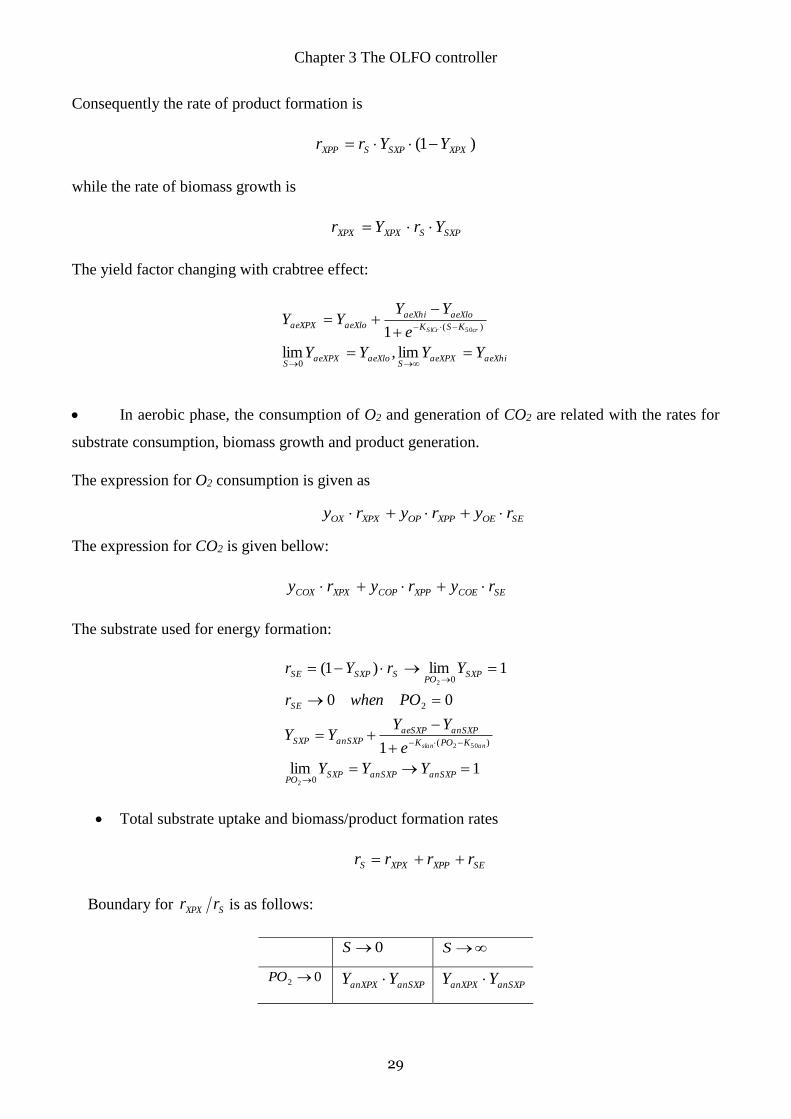
Chapter 3 The OLFO controller
29
Consequently the rate of product formation is
)1( XPXSXPSXPP YYrr
while the rate of biomass growth is
SXPSXPXXPX YrYr
The yield factor changing with crabtree effect:
aeXhiaeXPXS
aeXloaeXPXS
KSK
aeXloaeXhiaeXloaeXPX
YYYY
e
YYYY
crSlCr
lim,lim
1
0
)( 50
In aerobic phase, the consumption of O2 and generation of CO2 are related with the rates for
substrate consumption, biomass growth and product generation.
The expression for O2 consumption is given as
The expression for CO2 is given bellow:
SECOEXPPCOPXPXCOX ryryry
The substrate used for energy formation:
1lim
1
00
1lim)1(
0
)(
2
0
2
502
2
anSXPanSXPSXPPO
KPOK
anSXPaeSXPanSXPSXP
SE
SXPPO
SSXPSE
YYY
e
YYYY
POwhenr
YrYr
anslan
Total substrate uptake and biomass/product formation rates
SEXPPXPXS rrrr
Boundary for SXPX rr is as follows:
0S S
02 PO anSXPanXPX YY anSXPanXPX YY
SEOEXPPOPXPXOX ryryry

Chapter 3 The OLFO controller
30
2PO aeSXPaeXlo YY aeSXPaeXhi YY
The yield is given as:
SS
XPXXX
rY
rY
producedegluofamount
producedbiomassofamount
cos
It presents the practical circumstances of the cultivation process.
3.2 Basic theory of parameter identification
Factors such as variations in the quality of raw materials, characteristics of the initial charge media,
disturbances in process conditions and the time varying behavior of the fermentation process lead to
mismatch between the model and the actual plant, leading to deterioration in the performance of the
fermenter optimization system. The success of a feedback control scheme depends heavily on the
reliability of the parameters of the model. Consequently the model parameters need to be updated
online to reduce the model mismatch. Also the optimal trajectories should be recalculated based on
the updated model and state information to maximize the product yield.
The model parameters could be adapted to the experimental data so that the course of biomass and
product formation, glucose utilization, waste gas composition and dissolved oxygen concentration of
the experiments show very good agreement. The measured values of the state variables are compared
with the model predicting values of the same state variables. The model parameters should be well
estimated by a certain identification method to minimize the cost function J, which includes weighted
least squares:
2
1 1
exp
,, )()(
n
i
m
j
ji
sim
jiij yywpJ
where p is parameter vector, i is index of measured variable, j is index point of time, m is number of
measurements, n is number of measured variable, w is weighting factor, exp
, jiy is measurement data of
the data set i at points of time j, and sim
jiy , is model output of data set i at points of time j.
In principle, all products of the factors i and j are summed with individual weighting. However, it can
be assumed that the measurement errors are uncorrelated, both among the different measurements and
also among the various time points. Then the weighting matrix has only diagonal elements.

Chapter 3 The OLFO controller
31
More rational form with weighting factors is:
2
1 1
exp
,,
2
1 1
exp
,,, )(
n
i
m
j i
ji
sim
jin
i
m
j
ji
sim
jiji
yyyywSSR
where i is the weighting factor used in the OLFO controller. It is used to define the different roles
that each experimental variable plays in the calculation of the residuals. Their values are determined
based on the magnitude of relative experimental errors. That is the form used in this work.
Based on the great dynamic of the model parameters, a stable parameter identification should be
provided, which fulfilled the following requirements:
1. The parameter identification process must be fast, so that the parameter identification can be
implemented online.
2. The parameter identification process must be robust and stable, for the purpose to adapt the
general process model. Estimation results must be reasonable, and therefore one has to enable
the possibility that the user can define the boundary conditions of parameters. In addition, the
identified parameters should be precise enough to perform the optimization based on the last
calibrated model.
The differential equations of the model can be solved by DASSL algorithm (Brenan et al., 1995) or 4th
order Runge Kutta algorithm (Press et al., 2007) with variable step size. Parameter identification part
can be done by the robust Nelder-Mead algorithm (Nelder & Mead, 1965) or Gradient algorithm
(Snyman, 2005), and the optimization part can be done with the same algorithm. Different algorithms
are set as control pattern within the OLFO controller, which can be chosen freely by the operator
according to the practical circumstances. The model parameters are estimated with the following
measurements:
1. The values of the concentration of biomass, product and substrate in the broth are measured
through lab analysis every hour or few hours. The sampling interval can be adjusted according
to practical situation;
2. The composition of vent gas and dissolved oxygen concentration from the control system are
measured every few minutes. The measuring interval is adjustable according to practical
situation.

Chapter 3 The OLFO controller
32
3.3 Optimization criterion
After parameter identification, an estimated model is ready for the optimization. The models which
can be used in the optimization process must have sufficiently good prediction quality. A virtual
validation of the quality of parameter identification is done manually. After successful parameter
identification, an estimated model is ready for the optimization. Based on the prediction of the adapted
model and a suitable optimization criterion, a performance functional Jopt can be formed to get an
optimum reference value. Nelder-Mead algorithm or Gradient algorithm is used to minimize the cost
function to get an optimal substrate feed rate for the remaining part of the fermentation.
A suitable optimization criterion can be a maximum time-space yield, maximum income of the whole
process, a good medium utilization, to keep a certain growth rate or to maintain a constant substrate
feed rate etc. An optimum of this performance functional Jopt can be calculated by Pattern Search
Algorithms, e.g. Nelder-Mead algorithm, genetic algorithm etc. This optimum is saved as 'Control
Pattern', i.e. the optimal reference value of substrate feed profile, temperature, pH value, dissolved O2
concentration or combination of those optimal set points.
While conducting this work, the optimization of substrate feed rate is chosen as the 'Control Pattern'.
During the feed optimization part, input for the predictive algorithm is not artificially preset data for
optimization, but experimental data, the model, the set of previously identified parameters, a set of
feed flow starting values, and the optimization time interval. Output is an optimized set of feeding
profiles that best fulfills the optimization criterion provided by the model prediction.
Normally the fed-batch cultures are operated either at a constant feed rate, at a linearly increasing feed
rate or at an exponentially increasing feed rate. This process is operated in an aerobic growth phase
and an anaerobic production phase. In the growth phase one observes that the biomass grows
exponentially. During the production phase, the biomass growth slows down considerably.
Accordingly, the substrate feeding profile can be divided into exponential feeding stage and constant
feeding stage. The substrate feeding profile is modified by four optimization variables: the switching
time from aerobic phase to anaerobic phase tS; the initial pumping rate f0; the exponential factor for
the increase of the pumping rate α and the constant pumping rate for the anaerobic part f1. The substrate
feeding profile is defined as follows:
FS
SII
tttf
tttttff
;
));(exp(
1
0

Chapter 3 The OLFO controller
33
The optimal control is based on the concept that one can obtain an optimum ethanol yield when the
ideal switching point from the aerobic biomass growth phase to the anaerobic ethanol formation phase
is found. The feeding rate functions are defined by four optimization variables which are generated by
the optimization process. The switching time tS is defined as:
)(1 IFIS tttt
where tF and tI define the final and initial process time.
The initial value of the feeding rate is limited by the maximum feeding rate.
max20 ff
The exponential factor of the feeding is between zero and a maximum value.
max3
The constant feeding rate in the anaerobic phase is then limited by the maximum feeding rate.
max41 ff
The four optimization variables 321 ,, and 4 defined the substrate feed rate functions. They all
vary between 0 and 1.
The following boundary conditions are considered as constraints of the optimization: maximum
working volume of the fermenter; the substrate supply is finite and the maximum pumping capacity
maxf is limited.
This optimization pattern is used in most of our experiments related with the OLFO controller. The
number of optimization variables is low, so the optimization only occupies limited amount of the
computing power of the system.
3.4 Workflow of the OLFO controller
The work flow of the OLFO controller is illustrated by Figure 3.5. The typical steps to implement
the OLFO controller are as follows:
1. The fed-batch fermentation process is started by charging the media into the fermentation
reactor, starting the agitator and initiating the air ow through the broth.

Chapter 3 The OLFO controller
34
2. All the plant operating parameters like air flow rate, pH value, temperature, agitation rate etc.
are measured. Their initial values are stored in the OLFO controller and available for the
calculations.
3. Periodically, the broth samples are collected and analyzed in the lab for the concentration of
substrate, product and biomass. The analysis results are transformed into suitable form and
stored in the OLFO controller.
4. With the initial conditions (broth volume, biomass concentration, product concentration,
substrate concentration), the optimal substrate feeding rate profiles are calculated.
5. While the fed-batch fermentation is in progress, the following steps are implemented:
(a) Once the predetermined schedule of the initial stage of fermentation is done, an online
parameter identification process is carried out based on the actual process data collected
from the plant and laboratory analysis. The parameters are estimated by minimizing the
error between the measured and simulation values for concentration of biomass, product,
substrate, dissolved oxygen in the broth and composition (O2 and CO2) of off gas flow. A
nonlinear optimization technique, e.g. Nelder-Mead method or Gradient algorithm is used
to minimize the plant model mismatch.
(b) The new identified parameters and the updated process state variables are used in
calculating the optimal substrate feed rate.
(c) The optimization part predicts the future course of process states using the model and its
new adapted parameters. A control profile is precalculated based on an optimization
criterion (e.g. controlling substrate concentration at a certain level, maximizing time-space-
yield etc.). With the approval from the evaluation, the updated control profiles are
transferred to the process control system and fermenter.
(d) The aforementioned steps a, b and c are executed at every optimization calculation period
using the updated database. This periodic re-estimation of the model parameters and update
of the state variables while the fed-batch is in progress as it helps in reducing the plant-
model mismatch leading to improved performance of the optimizer.
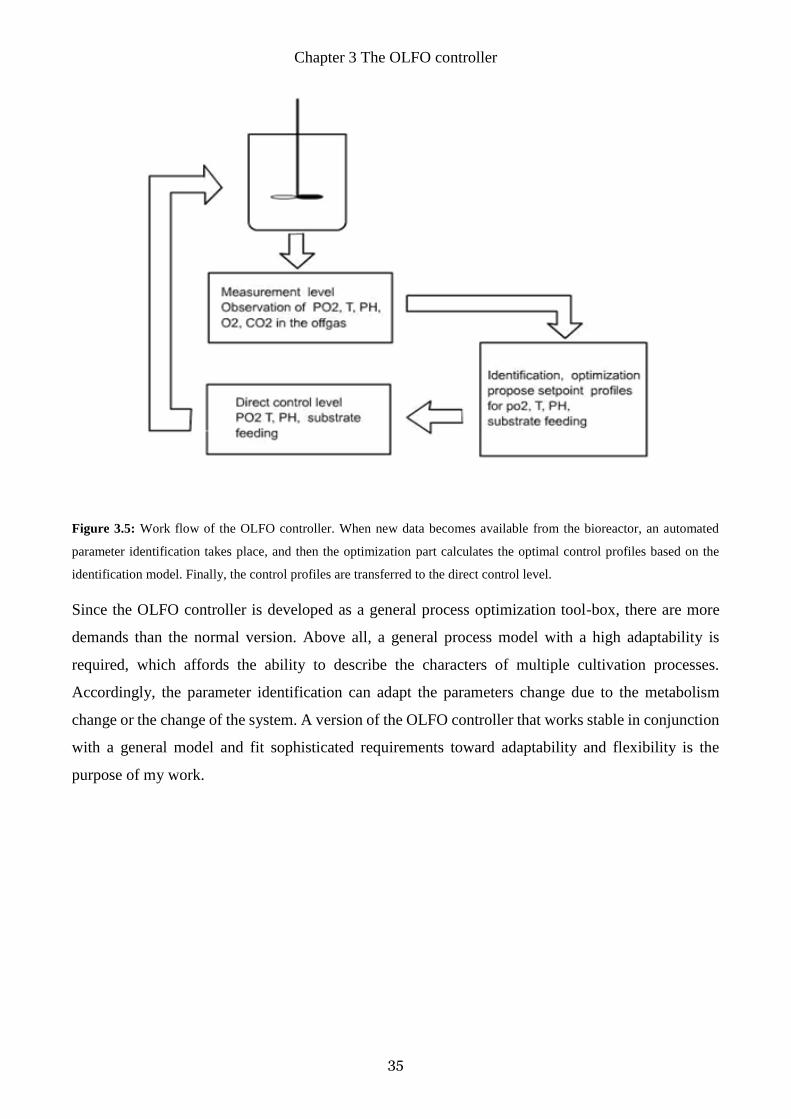
Chapter 3 The OLFO controller
35
Figure 3.5: Work flow of the OLFO controller. When new data becomes available from the bioreactor, an automated
parameter identification takes place, and then the optimization part calculates the optimal control profiles based on the
identification model. Finally, the control profiles are transferred to the direct control level.
Since the OLFO controller is developed as a general process optimization tool-box, there are more
demands than the normal version. Above all, a general process model with a high adaptability is
required, which affords the ability to describe the characters of multiple cultivation processes.
Accordingly, the parameter identification can adapt the parameters change due to the metabolism
change or the change of the system. A version of the OLFO controller that works stable in conjunction
with a general model and fit sophisticated requirements toward adaptability and flexibility is the
purpose of my work.
4. Research results and application examples of
OLFO in fed batch processes
In this chapter, a compartment model is used to present the evolution of fermentation processes. The
Gradient algorithm is formulated to calculate the process model mismatch at each interval to update
the model parameters. The Nelder-Mead method is used to optimize the objective function dynamically
throughout the course of the fed-batch fermentation process.
At the first stage, the result of the OLFO controller was not used in the real fermentation. The
experimental data from the fermentation was used for the evaluation of the performance and
characteristics of the parameter identification part and optimization part. During this research, some
illuminated features of the OLFO controller are discovered. Those results are summarized in the first
section of this chapter. Those discovers are the basis of the design of the subsequent experiments.
At the advanced stage, as a software tool which facilitates the use of biotechnological models, the
OLFO controller is mainly used in the following ways. First, the OLFO can combine with the virtual
bioreactor to be used as a training tool set in academia and industry. Second, the OLFO provides
optimized feed rate profiles for the real fermentation processes. Third, the OLFO can be used also as
a software observer for the process variables which are difficult or costly to obtain.
4.1 Basic research on parameter identification and optimization
With suitable weighting factors for measurements, the parameter identification can achieve a satisfying
result and is relatively insensitive to different initial values and boundaries. The scheme of parameter
identification is carried out online periodically based on the plant measurements and laboratory
analysis results. This ensures a model of higher accuracy used in calculating the optimum feed rate.
Particular constraints that may largely influence the parameter estimation result, such as weighting
factors on state variables, initial values and boundaries of parameters etc. must be taken into account.
To ensure a successful parameter identification, a series of simulation experiments have been
accomplished to evaluate the significance of the constraints and their proper use. The most relevant
results are presented in this thesis.

Chapter 4 Research results and application examples of OLFO in fed batch processes
37
A series of simulations have been carried out to demonstrate the influence of the following constraints
on the parameter identification process:
1. The density of offline measurements (different sampling time of offline measurements);
2. Different weighting factors;
3. Different initial values of parameters;
4. Different boundaries of the parameters;
5. Absence of partial measurements;
6. With more online measurements, less offline measurements.
4.1.1 Different sampling time of offline measurements
The rate to take the samples has some effects on the fermentation process. To take a sample, it increases
the probability of contamination and also changes the volume of the broth in the reactor as the volume
of the sample is difficult to be taken into account precisely. It is advisable to take samples as less as
possible. Therefore it is necessary to learn about the minimum amount of offline measurements which
is requisite for the accuracy of parameter estimation.
Normally, the concentration of product, biomass and substrate can only be measured offline, whereby
the results are available for control purposes only after some delay. The delay to get the measurements
of biomass concentration is about a few minutes. The delay for the product measurements varies.
However it costs at least half an hour to get the measurements of substrate concentration.
Following this, it becomes evident to determine if it is feasible to reach the accuracy of parameter
estimation by taking the samples in a longer interval. With a long sampling interval, it can reduce not
only the probability of contamination but also the manpower and costs on the analysis of the samples
which leads to the cost reduction of the whole process.
In this investigation, three different conditions are set up:
1. Measurements of product, biomass and substrate concentration are sampled every 30 minutes;
2. Measurements of product, biomass and substrate concentration are sampled every 60 minutes;

Chapter 4 Research results and application examples of OLFO in fed batch processes
38
3. Measurements of product and biomass concentration are offered every 60 minutes, the substrate
concentration every 180 minutes.
In order to reduce the risks of contamination, sampling costs and time, three different sampling
strategies were used and their effect on the parameter identification performance was evaluated (see
Figure 4.1). From the results of this investigation, all of the simulation results fit the measurements
well, without significant difference. As a reference, an accurate parameter identification was obtained
for sampling intervals of 30 minutes for P, X and S. Reducing the sampling intervals for P and X to
60 minutes and for S to 180 minutes, did not affect significantly the parameter identification results
which appeared to be in the difference range of -1.3% to 2.0% from the reference simulation. The good
agreement with the reference simulation showed that longer sampling intervals could be applied for
the further studies.
Figure 4.1: Parameter identification result with different sampling time. S-exp. is the experimentally measured substrate
concentration, S-sim. is the related parameter estimation result. P and X are the product and biomass concentrations
respectively. There are three groups of simulation results shown here: the first group simulation with P, X, S every 30
minutes by thickest lines, the second group simulation with P, X, S every 60 minutes and the third group simulation with
P, X every 60 minutes, S every 180 minutes by thinnest lines. All of the simulation results fit the measurements well,
without significant difference.
From the subsequent investigation described in Chapter 4.4 Software observer, the OLFO controller
can simulate the fermentation well even without the offline measurements on aerobic phase. For

Chapter 4 Research results and application examples of OLFO in fed batch processes
39
anaerobic phase, the success of parameter estimation still requires one of the offline measurements.
To overcome this problem, the amount of gas produced could be used as an online measurement. This
investigation also demonstrates that the density of the offline measurements makes slight difference
on the parameter estimation result.
4.1.2 Different weighting factors
Proper weighting factors of process variables are essential to ensure a successful parameter
identification. The objective function without weighting factors might lead to neglect the magnitude
distance between different variables, which means the measurements of high magnitude are
overweighed.
From the results of this investigation (Figures 4.2 and 4.3), we observe that, the weighting factors of
parameters have great influence on the result of parameter identification. By putting the appropriate
weight on certain state variables renders an obviously better description of parameter estimation.
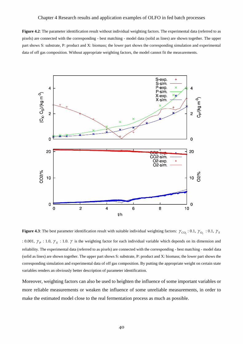
Chapter 4 Research results and application examples of OLFO in fed batch processes
40
Figure 4.2: The parameter identification result without individual weighting factors. The experimental data (referred to as
pixels) are connected with the corresponding - best matching - model data (solid as lines) are shown together. The upper
part shows S: substrate, P: product and X: biomass; the lower part shows the corresponding simulation and experimental
data of off gas composition. Without appropriate weighting factors, the model cannot fit the measurements.
Figure 4.3: The best parameter identification result with suitable individual weighting factors: 2CO : 0.1,
2O : 0.1, S
: 0.001, P : 1.0, X : 1.0. is the weighting factor for each individual variable which depends on its dimension and
reliability. The experimental data (referred to as pixels) are connected with the corresponding - best matching - model data
(solid as lines) are shown together. The upper part shows S: substrate, P: product and X: biomass; the lower part shows the
corresponding simulation and experimental data of off gas composition. By putting the appropriate weight on certain state
variables renders an obviously better description of parameter identification.
Moreover, weighting factors can also be used to heighten the influence of some important variables or
more reliable measurements or weaken the influence of some unreliable measurements, in order to
make the estimated model close to the real fermentation process as much as possible.

Chapter 4 Research results and application examples of OLFO in fed batch processes
41
4.1.3 Absence of partial measurements
The purpose of this evaluation is to figure out how the parameter identification evolves in the absence
of partial online measurements or offline measurements at some time range as a result of technical
malfunction, such as a temporary defect in the measuring device.
From the simulation results, we observe that the absence of particular online measurement has
significant influence on the parameter identification, especially for the parameter YaeXhi & rSmax. In
this example, the deviation of the parameter rSmax is about 14% and of YaeXhi is about 91% (See
Appendix 1). Therefore one should pay closer attention to the accuracy of the online measurements
especially the percentage of CO2 and O2 in the off gas. The OLFO controller is less sensitive to offline
measurements as manifested by the low mean deviation of about 2% with the same example in this
research. There one can note, online measurements play more important roll compared with offline
measurements in the parameter identification process. The accuracy of online measurements should
be more regarded.
4.1.4 Different initial values and boundaries
From the results of the research, with appropriate weighting factors of state variables, the different
initial values have nearly no influence on the parameter identification result except the value of YaeXlo
in the first time range. On the other hand, the optimization result is relatively stable to the change of
YaeXlo (see the optimization result analysis with the change of parameters). We can notice that, the
identified parameters are relatively insensitive to the different initial values of state variables in the
'step by step' case which is the way how the OLFO controller works. For the 'one step' parameter
identification, the result is extremely sensitive to the initial values. The simulation can fit the
measurement well only with very good initial values.
We can conclude from the simulation results, the boundaries of the parameters have very little
influence on the result of parameter identification, which can be ignored for the optimization.
Nevertheless, a parameter identification with a reasonable variables boundaries is still advisable, since
the variables make sense only when they are within operating boundaries which are set according to
the actual physical conditions.
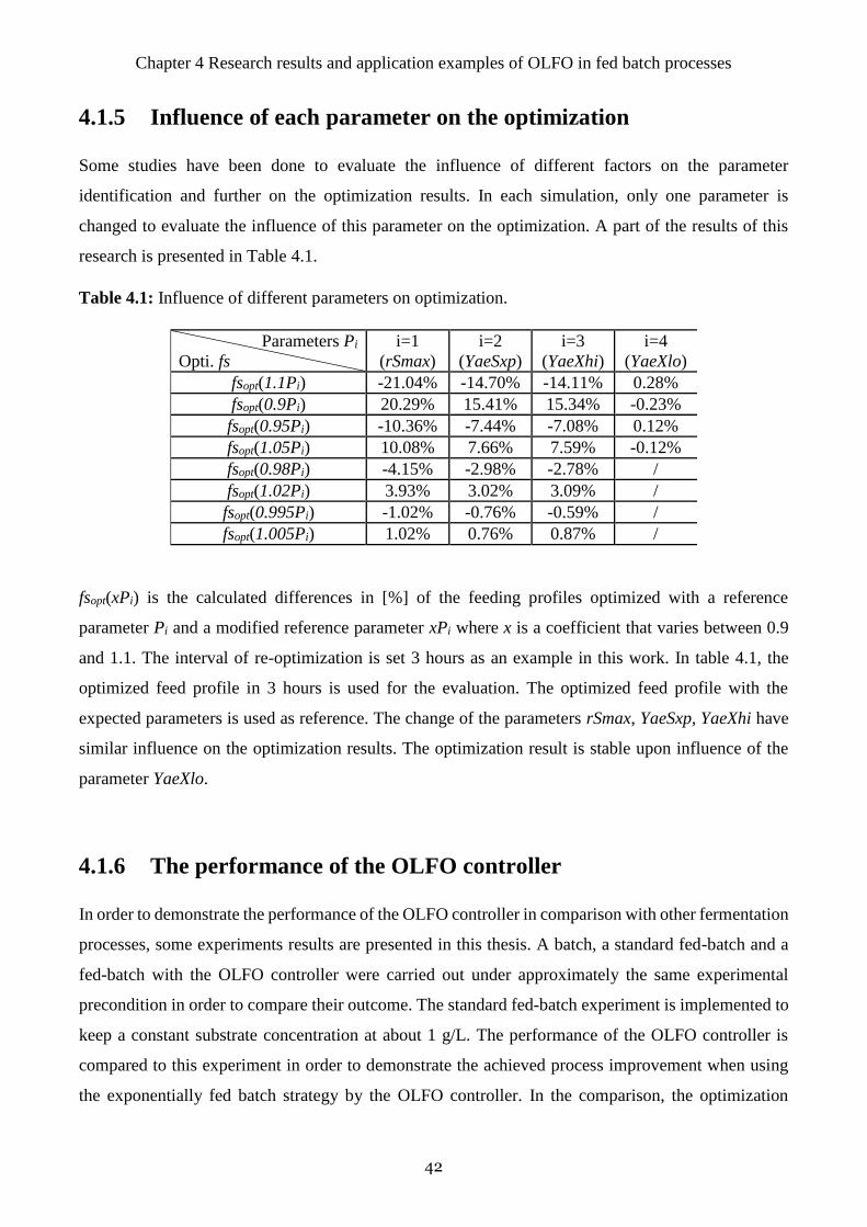
Chapter 4 Research results and application examples of OLFO in fed batch processes
42
4.1.5 Influence of each parameter on the optimization
Some studies have been done to evaluate the influence of different factors on the parameter
identification and further on the optimization results. In each simulation, only one parameter is
changed to evaluate the influence of this parameter on the optimization. A part of the results of this
research is presented in Table 4.1.
Table 4.1: Influence of different parameters on optimization.
Parameters Pi
Opti. fs
i=1
(rSmax)
i=2
(YaeSxp)
i=3
(YaeXhi)
i=4
(YaeXlo)
fsopt(1.1Pi) -21.04% -14.70% -14.11% 0.28%
fsopt(0.9Pi) 20.29% 15.41% 15.34% -0.23%
fsopt(0.95Pi) -10.36% -7.44% -7.08% 0.12%
fsopt(1.05Pi) 10.08% 7.66% 7.59% -0.12%
fsopt(0.98Pi) -4.15% -2.98% -2.78% /
fsopt(1.02Pi) 3.93% 3.02% 3.09% /
fsopt(0.995Pi) -1.02% -0.76% -0.59% /
fsopt(1.005Pi) 1.02% 0.76% 0.87% /
fsopt(xPi) is the calculated differences in [%] of the feeding profiles optimized with a reference
parameter Pi and a modified reference parameter xPi where x is a coefficient that varies between 0.9
and 1.1. The interval of re-optimization is set 3 hours as an example in this work. In table 4.1, the
optimized feed profile in 3 hours is used for the evaluation. The optimized feed profile with the
expected parameters is used as reference. The change of the parameters rSmax, YaeSxp, YaeXhi have
similar influence on the optimization results. The optimization result is stable upon influence of the
parameter YaeXlo.
4.1.6 The performance of the OLFO controller
In order to demonstrate the performance of the OLFO controller in comparison with other fermentation
processes, some experiments results are presented in this thesis. A batch, a standard fed-batch and a
fed-batch with the OLFO controller were carried out under approximately the same experimental
precondition in order to compare their outcome. The standard fed-batch experiment is implemented to
keep a constant substrate concentration at about 1 g/L. The performance of the OLFO controller is
compared to this experiment in order to demonstrate the achieved process improvement when using
the exponentially fed batch strategy by the OLFO controller. In the comparison, the optimization

Chapter 4 Research results and application examples of OLFO in fed batch processes
43
criterion JF (tf ) = 15 S(tf ) X(tf ) P (tf ) was used in the OLFO controller. The comparison of the outcome
of different experiments is presented in Table 4.2.
Table 4.2: Comparison between different fermentation processes.
Biomass conc.
[g/L]
Substrate conc.
[g/L]
Ethanol conc.
[g/L] JF(tf )
Batch 5.9 0 4.8 -10.7
Standard fed-batch 8.6 0.1 4.8 -11.9
Fed-batch with OLFO 7.8 0.1 6 -12.3
Note: Experiments were carried out in a 20.0 L stirred bioreactor (virtual bioreactor), 60% pO2 at the
beginning, after 6th hour, ca. 10% pO2, 32 °C. The biomass concentration in the inoculum (200.0 ML)
was 25.0 g/L. Substrate concentration in medium (5.0 L) was 2.5 g/L for fed-batch fermentation, 20.0
g/L for batch fermentation. The fed-batch fermentations last 10 hours, the batch fermentation takes 6
hours.
4.2 OLFO works with the virtual bioreactor
A reliable process model is served as the plant and embedded in a self-constructed software namely
virtual bioreactor. This process model is developed by Prof. V. Hass and has been verified in his work
group during long years of experiments (Hass, 2005). However due to its complexity, it does not fit as
the general model in the OLFO controller. The general process model "Lyx" as mentioned in section
3.1 is different from the process model which is embedded in the virtual bioreactor. Training with
virtual bioreactor leads to improved operating capability with laboratory cultivations for the groups
who have obtained such training in comparison to the groups who have not (Gerlach et al., 2014). The
combination of virtual bioreactor and the OLFO controller can be used as a training tool for academia
and industry with an aim to offer the user insights into fermentation process control.
The implementation of a model calibration requires a data set with characteristic measured variables
of the process. A model calibration can be implemented successfully only when all the control
variables that have influences on the process are available. Those data must be synchronized with time.
The subsequent optimization generates optimized control profiles. These profiles can be applied to the
process.
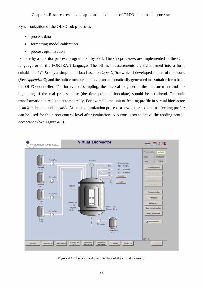
Chapter 4 Research results and application examples of OLFO in fed batch processes
44
Synchronization of the OLFO sub processes
process data
formatting model calibration
process optimization
is done by a monitor process programmed by Perl. The sub processes are implemented in the C++
language or in the FORTRAN language. The offline measurements are transformed into a form
suitable for WinErs by a simple tool-box based on OpenOffice which I developed as part of this work
(See Appendix 3); and the online measurement data are automatically generated in a suitable form from
the OLFO controller; The interval of sampling, the interval to generate the measurement and the
beginning of the real process time (the time point of inoculate) should be set ahead. The unit
transformation is realized automatically. For example, the unit of feeding profile in virtual bioreactor
is ml/min, but in model is m3/s. After the optimization process, a new generated optimal feeding profile
can be used for the direct control level after evaluation. A button is set to active the feeding profile
acceptance (See Figure 4.5).
Figure 4.4: The graphical user interface of the virtual bioreactor

Chapter 4 Research results and application examples of OLFO in fed batch processes
45
Events-sequence of the virtual bioreactor with
the OLFO controller is as follows:
1. New data are acquired;
2. Update of the four parameters by
minimizing the sum of squares;
3. Calculation of a new optimal feeding
profile (from now until Tf );
4. Verification and release of the new profile;
5. Replacement of the old feeding profile
(from the current point in time).
An example of the optimal control of a virtual yeast cultivation is described to exhibit the basic
procedure of the OLFO controller:
1. The coupling with WinErs is realized as follows:
(a) The measurements from the cultivation can be exported via a special driver;
(b) The OLFO controller works as an external analysis software to calibrate the model;
(c) The OLFO controller is used to create optimal control profile;
(d) After evaluation and approval, the driver imports the updated optimal control profile for
the direct control level to be applied in the process.
2. The control of the OLFO controller includes:
(a) To trigger the OLFO controller, the reference time for the fermentation process (after
inoculation) and the interval for the automatic data export should be set;
(b) The activation of an optimized control profile.
3. Calibration of the following four model parameters:
(a) rSmax: maximum substrate uptake rate.
(b) YaeSxp: maximal yield under aerobic condition.
Figure 4.5: The user interface of the virtual
bioreactor to set the interval of sampling, the
interval to generate the measurement and the
beginning of the real process time.

Chapter 4 Research results and application examples of OLFO in fed batch processes
46
(c) YaeXlo: maximal yield of biomass when substrate concentration is low.
(d) YaeXhi: maximal yield of biomass when substrate concentration is high.
4. Exponential substrate supply is parameterized.
5. )()()(15)( ffftF tPtXtSJf
is formulated as the cost function aiming at consuming all the
substrate in the fermenter and producing biomass and product as much as possible at the end of
the process. The numbers before the variables stand for the weight that you want to put on the
variables. Bigger number stands for more weight. This cost function is randomly set and only
used as a demonstration.
The complete experiment runs for 10 "virtual" hours (speed-up is possible) and depicts a fermentation
unit in the aerobic phase. During this demonstration, parameter identification is performed every 2.5
hours and implemented with the new generated input data by the virtual bioreactor. Based on the
updated estimated model of the virtual fermentation process, OLFO controller generates optimal
feeding profiles for the remaining time of the process. This profile is then used as a feedback for the
virtual fermentation process (Figure 4.6). The parameter identification as part of the whole procedure
is demonstrated in a stepwise manner (Figure 4.6.A). Based on the parameter identification results, the
simulation of the prediction of the estimated model (Figure 4.6.B, upper diagrams) and the newly
generated optimal feed rate profiles (Figure 4.6.B, lower diagrams) are plotted for each interval. The
current general model does not contain any inhibition function that accounts for cases of substrate
inhibition. However the OLFO controller, implements a penalty factor that sets in control once a high
level of substrate concentration is present. In this example, the penalty factor is manually set to 1000.
This means that once the substrate concentration is over the 4 g/L threshold value, the penalty factor
will be activated which will lead to a subsequent reduction on the substrate feeding rates. As shown in
Figure 4.6, at a time point near the 6th hour, the substrate concentration which is reaching the threshold
value, suddenly starts to deplete. This is due to the penalty function which is activated at this point.
On the other hand, the biomass grew faster and also consumed the substrate faster, which also led to
the rapid depletion of the substrate concentration.
The current tandem system combines several advantages. The tandem system offers an alternative to
learn and gain experience through "trial and error" without using fermentation material. Moreover, the
simulation can be accelerated in order to shorten the training process which makes it a very efficient
toolbox considering that the real fermentation processes are very time consuming.

Chapter 4 Research results and application examples of OLFO in fed batch processes
47
Figure 4.6: (Left) Parameter identification graphs with 2.5 hours interval, with corresponding (right) optimization of the
estimated models (upper) and the optimal feeding profile (lower). Substrate (S), product (P) and biomass (X) concentrations
are further labeled based on their generated source virtual bioreactor (experimental) or OLFO (simulated).

Chapter 4 Research results and application examples of OLFO in fed batch processes
48
4.3 OLFO application for yeast fed-batch cultivation
A cultivation of yeast cells with the aim to produce maximum amount of ethanol was supported by the
OLFO controller. The parameter estimation are based on the model "Lyx" as mentioned in section 3.1.
The optimization calculations are based on each updated calibrated model. For a better comparability,
the process optimization is always carried out with identical boundary conditions. These constraints
are related to the duration of cultivation, the initial concentrations and operational limits of the
instrumentation (e.g. maximum flow rate of the pump). The only variable that can potentially cause
fluctuations on the model parameters is the updated measurements.
The evaluation of process quality is determined by the choice of the corresponding cost parameters
so as to maximize the benefit at the end of the process. It depends on the market price of the product
(in this case ethanol) eP, mass specific substrate costs eS and volume specific costs of product isolation
eI. Substrate mass is the initial concentration in the vessel and the additional feed solution being
pumped in during fermentation. Product is contained in the final volume of the vessel, where the
maximum volume has been reached. Consequently, this function evaluates as
)()( ,
00
2 mvapPRPOHRI
t
t
in
SSRSPRP HCVTCVedtfCCVeCVeBF
I
∆T describes the temperature increase from the fermentation temperature to the boiling point. Using
vaporization factor of molar enthalpy mvapH , , the energy lost by the distillation of ethanol
evaporation can be estimated.
In this experiment, eS and eI were set 0, which means cost function was set to maximize the ethanol
concentration at the end of the process.
As mentioned before, as the process model is formulated without substrate inhibition, a penalty factor
is set to control the situation with high substrate concentration. In this example, the penalty factor is
set 1000. The maximum substrate concentration of 10.0 g/L is used as a constraint in the optimization.
A violation of this boundary condition produces a high punitive contribution to the quality criterion
to reduce the substrate feeding rate.
There are all in total nine parameters set free: initial concentration for substrate, biomass and product,
KS for substrate uptake, rSmax for substrate uptake, and four yield coefficients: YaeSxp, YaeXlo,
YaeXhi, YanXpx (active for anaerobic phase). The weighting factors for different measurements were
set according to the measurements density. After the batch fermentation part, the parameter
identification and optimization is implemented every 2 hours.

Chapter 4 Research results and application examples of OLFO in fed batch processes
49
The measured concentration of substrate, biomass and product at the beginning of batch are 2.6g/L,
0.7g/L and 0.0g/L respectively. The other settings of the process were basically identical to those in
chapter 2. Laboratory set-up. After about 2.5 hours, the substrate was about to deplete which means
the end of the batch phase. At that moment, the OLFO controller was activated.
1. Based on the model calibration of a previous fermentation experiment, an optimal control was
calculated for the process. The precalculated optimization result (Figure 4.7) was used between
the 2.5th-5th hours.
Figure 4.7: Precalculated optimization results based on the calibrated model from a previous fermentation experiment.
The upper part shows the optimized feeding rate fS and the inlet gas rate fgas; the lower part shows the corresponding
prediction of substrate S and product P and volume of the vessel VR. Only the profile of the first 2.5 hours was used in the
fermentation as the first approve of optimization result from OLFO controller.
2. Considering the time delay for parameter identification, optimization and evaluation for both
part, the implementation of the first parameter identification based on the current measurements
occurred after 4.5 hours. The simulation data and the measurements are in a good agreement
(Figure 4.8 ). From the optimization result (Figure 4.9), an exponential substrate feeding profile
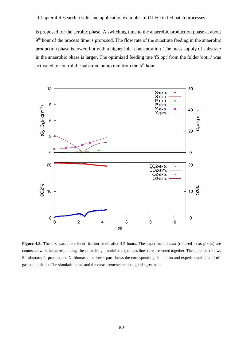
Chapter 4 Research results and application examples of OLFO in fed batch processes
50
is proposed for the aerobic phase. A switching time to the anaerobic production phase at about
9th hour of the process time is proposed. The flow rate of the substrate feeding in the anaerobic
production phase is lower, but with a higher inlet concentration. The mass supply of substrate
in the anaerobic phase is larger. The optimized feeding rate 'fS.opt' from the folder 'opti1' was
activated to control the substrate pump rate from the 5th hour.
Figure 4.8: The first parameter identification result after 4.5 hours. The experimental data (referred to as pixels) are
connected with the corresponding - best matching - model data (solid as lines) are presented together. The upper part shows
S: substrate, P: product and X: biomass; the lower part shows the corresponding simulation and experimental data of off
gas composition. The simulation data and the measurements are in a good agreement.

Chapter 4 Research results and application examples of OLFO in fed batch processes
51
Figure 4.9: Optimization after the first parameter identification. The upper part shows optimized profile for substrate
feeding rate ' fS.opt ' and inlet gas flow rate ' fgas.opt ', the lower part shows the prediction of product concentration '
P.opt ', substrate concentration ' S.opt ' and the volume of the nutrient in the fermenter ' VR.opt '. The optimized feeding
rate ' fS.opt ' was activated to control the substrate pump rate from the 5th hour.
3. The second parameter identification was implemented after 6.5 hours. The simulation data and
the measurements still remained in a good agreement (Figure 4.10). However the system
reported a convergence error of the algorithm by minimizing the sum of squares. This does not
necessarily mean that the updated model parameters must be discarded. But one should be
cautious about using the follow up optimization result based on this calibrated model. This
updated optimal control profile (Figure 4.11) showed a high deviation from the previously one.
The new optimized feeding profile 'fS.opt' from the folder 'opti2' was discarded. The previously
calculated control profile was continued.
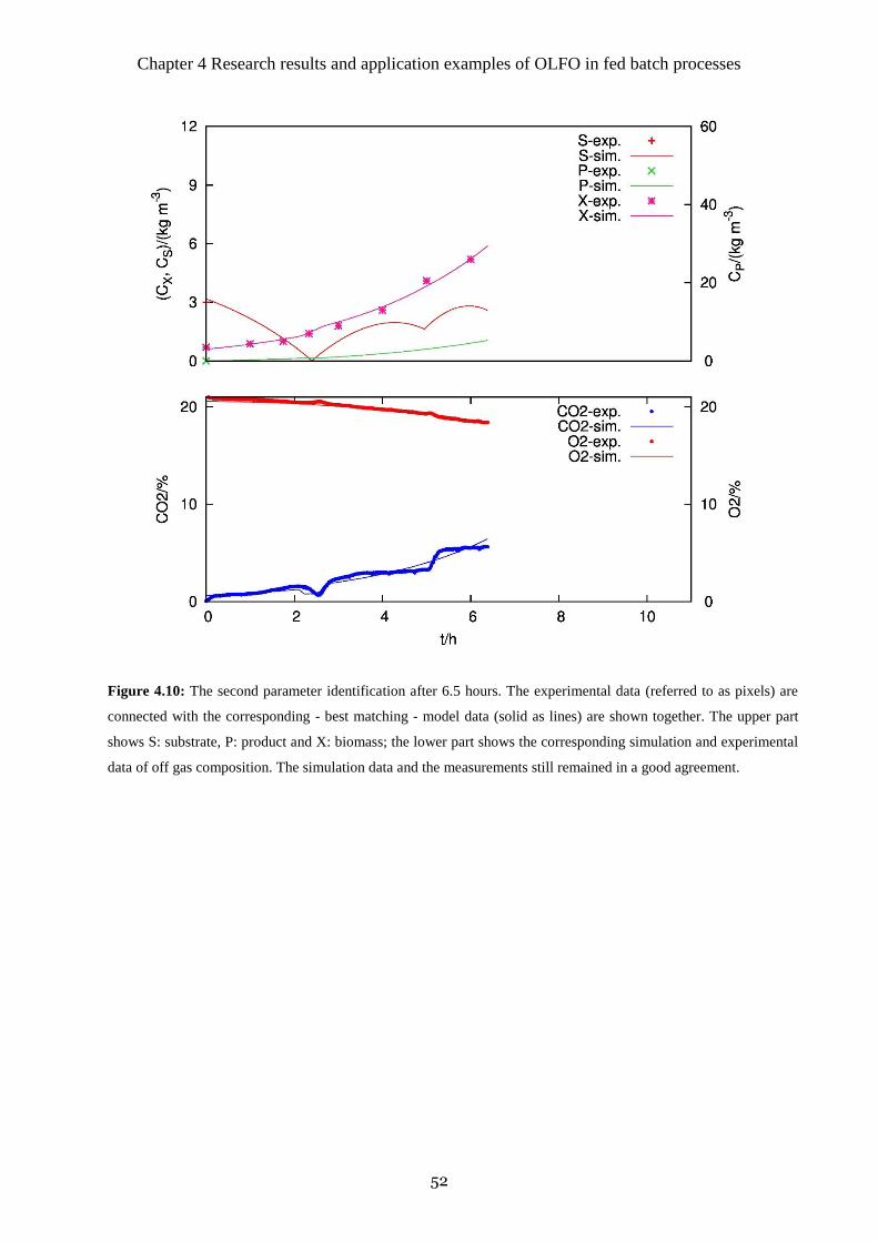
Chapter 4 Research results and application examples of OLFO in fed batch processes
52
Figure 4.10: The second parameter identification after 6.5 hours. The experimental data (referred to as pixels) are
connected with the corresponding - best matching - model data (solid as lines) are shown together. The upper part
shows S: substrate, P: product and X: biomass; the lower part shows the corresponding simulation and experimental
data of off gas composition. The simulation data and the measurements still remained in a good agreement.
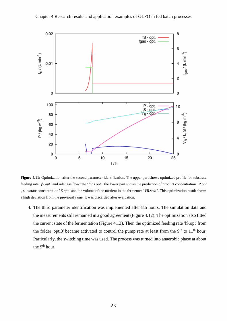
Chapter 4 Research results and application examples of OLFO in fed batch processes
53
Figure 4.11: Optimization after the second parameter identification. The upper part shows optimized profile for substrate
feeding rate ' fS.opt ' and inlet gas flow rate ' fgas.opt ', the lower part shows the prediction of product concentration ' P.opt
', substrate concentration ' S.opt ' and the volume of the nutrient in the fermenter ' VR.smo '. This optimization result shows
a high deviation from the previously one. It was discarded after evaluation.
4. The third parameter identification was implemented after 8.5 hours. The simulation data and
the measurements still remained in a good agreement (Figure 4.12). The optimization also fitted
the current state of the fermentation (Figure 4.13). Then the optimized feeding rate 'fS.opt' from
the folder 'opti3' became activated to control the pump rate at least from the 9th to 11th hour.
Particularly, the switching time was used. The process was turned into anaerobic phase at about
the 9th hour.

Chapter 4 Research results and application examples of OLFO in fed batch processes
54
Figure 4.12: The third parameter identification after 8.5 hours. The experimental data (referred to as pixels) are connected
with the corresponding - best matching - model data (solid as lines) are shown together. The upper part shows S: substrate,
P: product and X: biomass; the lower part shows the corresponding simulation and experimental data of off gas
composition. The simulation data and the measurements remained in a good agreement.
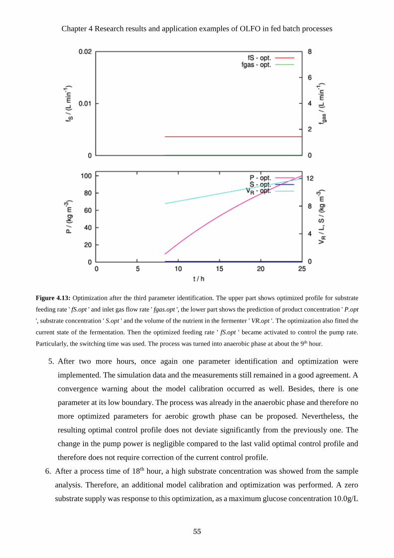
Chapter 4 Research results and application examples of OLFO in fed batch processes
55
Figure 4.13: Optimization after the third parameter identification. The upper part shows optimized profile for substrate
feeding rate ' fS.opt ' and inlet gas flow rate ' fgas.opt ', the lower part shows the prediction of product concentration ' P.opt
', substrate concentration ' S.opt ' and the volume of the nutrient in the fermenter ' VR.opt '. The optimization also fitted the
current state of the fermentation. Then the optimized feeding rate ' fS.opt ' became activated to control the pump rate.
Particularly, the switching time was used. The process was turned into anaerobic phase at about the 9th hour.
5. After two more hours, once again one parameter identification and optimization were
implemented. The simulation data and the measurements still remained in a good agreement. A
convergence warning about the model calibration occurred as well. Besides, there is one
parameter at its low boundary. The process was already in the anaerobic phase and therefore no
more optimized parameters for aerobic growth phase can be proposed. Nevertheless, the
resulting optimal control profile does not deviate significantly from the previously one. The
change in the pump power is negligible compared to the last valid optimal control profile and
therefore does not require correction of the current control profile.
6. After a process time of 18th hour, a high substrate concentration was showed from the sample
analysis. Therefore, an additional model calibration and optimization was performed. A zero
substrate supply was response to this optimization, as a maximum glucose concentration 10.0g/L
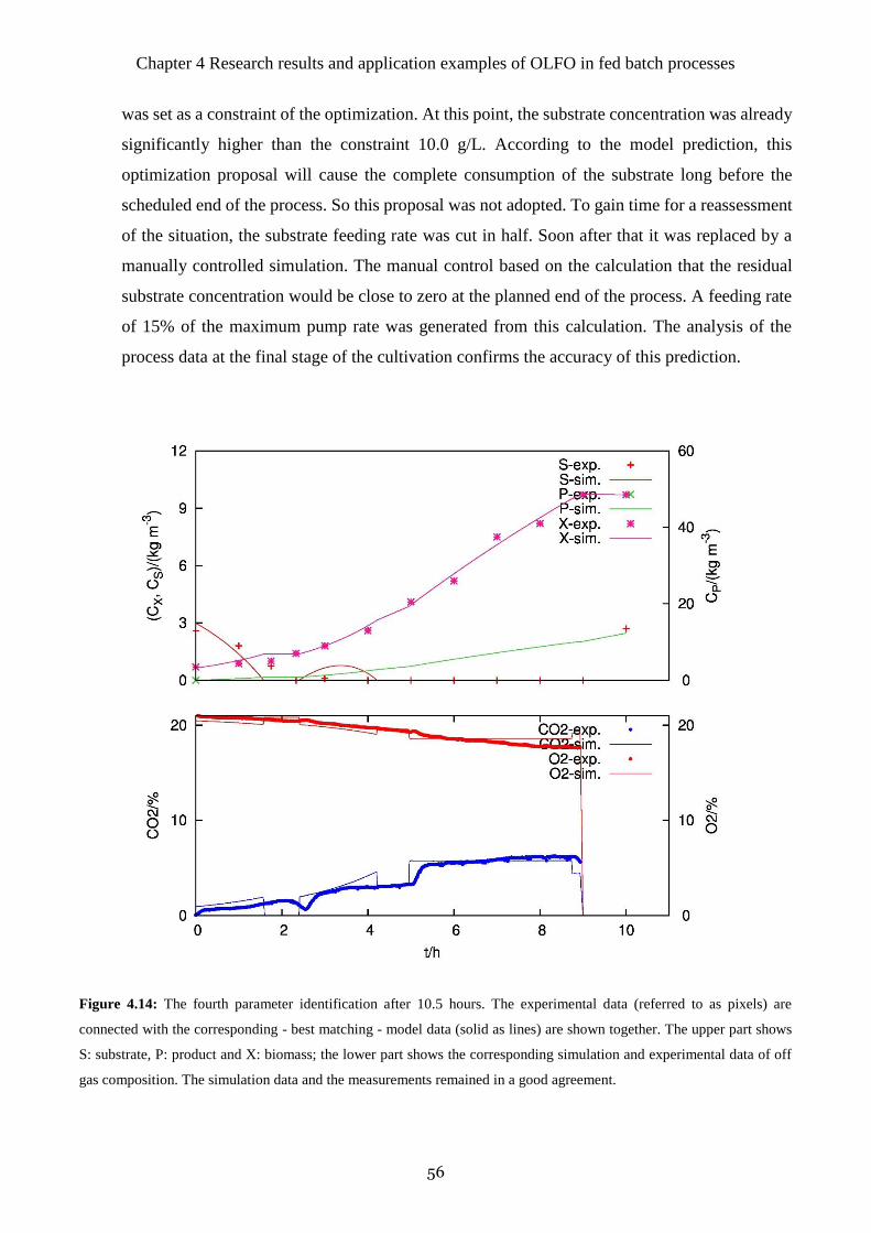
Chapter 4 Research results and application examples of OLFO in fed batch processes
56
was set as a constraint of the optimization. At this point, the substrate concentration was already
significantly higher than the constraint 10.0 g/L. According to the model prediction, this
optimization proposal will cause the complete consumption of the substrate long before the
scheduled end of the process. So this proposal was not adopted. To gain time for a reassessment
of the situation, the substrate feeding rate was cut in half. Soon after that it was replaced by a
manually controlled simulation. The manual control based on the calculation that the residual
substrate concentration would be close to zero at the planned end of the process. A feeding rate
of 15% of the maximum pump rate was generated from this calculation. The analysis of the
process data at the final stage of the cultivation confirms the accuracy of this prediction.
Figure 4.14: The fourth parameter identification after 10.5 hours. The experimental data (referred to as pixels) are
connected with the corresponding - best matching - model data (solid as lines) are shown together. The upper part shows
S: substrate, P: product and X: biomass; the lower part shows the corresponding simulation and experimental data of off
gas composition. The simulation data and the measurements remained in a good agreement.

Chapter 4 Research results and application examples of OLFO in fed batch processes
57
Figure 4.15: Optimization after the fourth parameter identification. The upper part shows optimized profile for substrate
feeding rate ' fS.opt ' and inlet gas flow rate ' fgas.opt ', the lower part shows the prediction of product concentration ' P.opt
', substrate concentration ' S.opt ' and the volume of the nutrient in the fermenter ' VR.opt '. The resulting optimal control
profile does not deviate significantly from the previous one.
7. At the 24th hour, we reached an ethanol concentration of 87.8 g/L, which has reached our set aim
for this experiment. This yeast fed-batch cultivation ended at about the 25th hour with an ethanol
concentration of 85.5 g/L. The development of the whole process and the actually applied
substrate feeding rate during the whole fermentation process are summarized at Figure 4.16.
We can see from Figure 4.16 that the prediction of the substrate consumption is correct. All the
substrate in the fermenter is consumed at the scheduled end of the process. The optimal feeding profile
generated by OLFO led the process to reach the set aim for this experiment. As the process is less
operator-dependent in comparison to conventional control techniques, the result can be easily
reproduced using similar conditions.
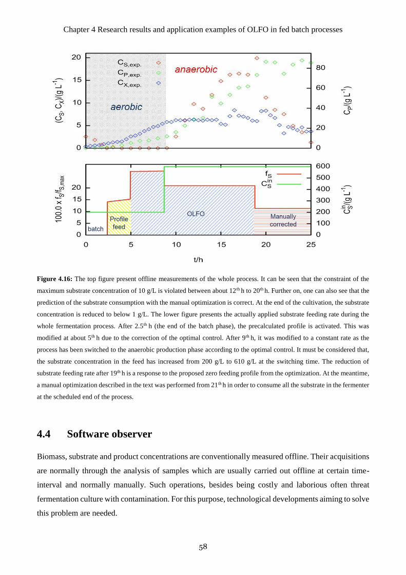
Chapter 4 Research results and application examples of OLFO in fed batch processes
58
Figure 4.16: The top figure present offline measurements of the whole process. It can be seen that the constraint of the
maximum substrate concentration of 10 g/L is violated between about 12th h to 20th h. Further on, one can also see that the
prediction of the substrate consumption with the manual optimization is correct. At the end of the cultivation, the substrate
concentration is reduced to below 1 g/L. The lower figure presents the actually applied substrate feeding rate during the
whole fermentation process. After 2.5th h (the end of the batch phase), the precalculated profile is activated. This was
modified at about 5th h due to the correction of the optimal control. After 9th h, it was modified to a constant rate as the
process has been switched to the anaerobic production phase according to the optimal control. It must be considered that,
the substrate concentration in the feed has increased from 200 g/L to 610 g/L at the switching time. The reduction of
substrate feeding rate after 19th h is a response to the proposed zero feeding profile from the optimization. At the meantime,
a manual optimization described in the text was performed from 21th h in order to consume all the substrate in the fermenter
at the scheduled end of the process.
4.4 Software observer
Biomass, substrate and product concentrations are conventionally measured offline. Their acquisitions
are normally through the analysis of samples which are usually carried out offline at certain time-
interval and normally manually. Such operations, besides being costly and laborious often threat
fermentation culture with contamination. For this purpose, technological developments aiming to solve
this problem are needed.

Chapter 4 Research results and application examples of OLFO in fed batch processes
59
Software observers are suitable for online monitoring of those offline measurements. They are an
alternative to the conventional sample-based analysis. It is used for automatic online calculation of
estimated values for process variables. A software observer is not a real analysis unit but is
implemented as a software. It uses online measurements which are available on any bioreactor, for
example outlet gas flow, to estimate those variables which are difficult to get online. These estimated
values can then be used for monitoring or control, as if they came from a real measuring device.
Application of the software observer holds some advantages: it reduces sampling and laboratory cost
and possibility for contamination; it has no time delay in acquiring the offline parameters: substrate,
biomass and product concentration; monitoring the culture course (online monitoring), which also lead
to early detection of possible defects and deviations. In general, it provides better chance to prevent
loses in the process and it facilitates the cell growth rate control, automatic control of time point of
innoculation or harvest. In general, it increases the possibility to apply automatic strategies for process
control.
The OLFO controller shows the potential to function as a software observer in a way to observe the
states of offline variables. A general scheme of the software observer implemented within the OLFO
controller is provided in Figure 4.17. Here one can notice that, the online measurements are used for
the calculation with the OLFO controller to get the simulated values for biomass, substrate and product
concentrations. The calculations are based on the period updated calibrated process model.
The simulation of the following example was based on the measurements from the yeast fed batch
fermentation December 2011 in our group. The basic settings of this experiment is the same as the
other experiments described in this thesis. When the OLFO controller is used as a software observer,
it works in the same way as it is used for the process optimization. Only the initial values but no latter
measured values of the observed variables are provided in the individual data set which is used for the
parameter estimation.
Figure 4.17: Schematic of a software sensor. Inputs are mostly online measurements which are facile to obtain. Outputs
are the simulated values of variables which are hardly or costly to obtain. The parameter identification part of the OLFO
controller here can function as a software observer.
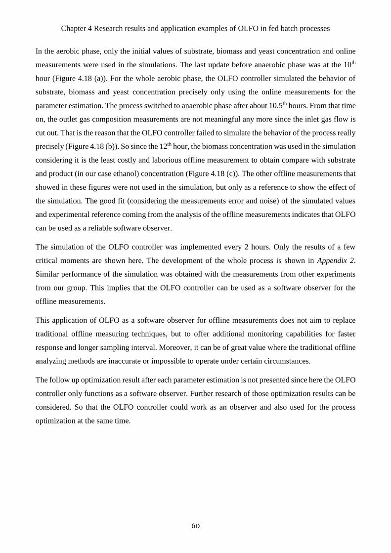
Chapter 4 Research results and application examples of OLFO in fed batch processes
60
In the aerobic phase, only the initial values of substrate, biomass and yeast concentration and online
measurements were used in the simulations. The last update before anaerobic phase was at the 10th
hour (Figure 4.18 (a)). For the whole aerobic phase, the OLFO controller simulated the behavior of
substrate, biomass and yeast concentration precisely only using the online measurements for the
parameter estimation. The process switched to anaerobic phase after about 10.5th hours. From that time
on, the outlet gas composition measurements are not meaningful any more since the inlet gas flow is
cut out. That is the reason that the OLFO controller failed to simulate the behavior of the process really
precisely (Figure 4.18 (b)). So since the 12th hour, the biomass concentration was used in the simulation
considering it is the least costly and laborious offline measurement to obtain compare with substrate
and product (in our case ethanol) concentration (Figure 4.18 (c)). The other offline measurements that
showed in these figures were not used in the simulation, but only as a reference to show the effect of
the simulation. The good fit (considering the measurements error and noise) of the simulated values
and experimental reference coming from the analysis of the offline measurements indicates that OLFO
can be used as a reliable software observer.
The simulation of the OLFO controller was implemented every 2 hours. Only the results of a few
critical moments are shown here. The development of the whole process is shown in Appendix 2.
Similar performance of the simulation was obtained with the measurements from other experiments
from our group. This implies that the OLFO controller can be used as a software observer for the
offline measurements.
This application of OLFO as a software observer for offline measurements does not aim to replace
traditional offline measuring techniques, but to offer additional monitoring capabilities for faster
response and longer sampling interval. Moreover, it can be of great value where the traditional offline
analyzing methods are inaccurate or impossible to operate under certain circumstances.
The follow up optimization result after each parameter estimation is not presented since here the OLFO
controller only functions as a software observer. Further research of those optimization results can be
considered. So that the OLFO controller could work as an observer and also used for the process
optimization at the same time.

Chapter 4 Research results and application examples of OLFO in fed batch processes
61
Figure 4.18: The parameter estimation results around anaerobic phase. In the upper part shows S: substrate, P: product
and X: biomass; in the lower part shows the corresponding simulation and experimental data of off gas composition. The
figures of the left sides show the original parameter estimation results. On the figures of the right sides, the offline
measurements for aerobic phase, the product and substrate measurements for anaerobic phase are not involved in the
calculation of the parameter estimation. They are presented here as a reference, to show how effective the OLFO controller
is when it is used as a software observer.

Chapter 4 Research results and application examples of OLFO in fed batch processes
62
Figure 4.19: The final parameter estimation result with online measurements and biomass concentration in anaerobic phase
(12th - 25th hour). The other parts of the offline measurements as on the figure of the right side are used as reference, not
involved in the simulation. In the upper part shows S: substrate, P: product and X: biomass; in the lower part shows the
corresponding simulation and experimental data of off gas composition.
5. Summary and Outlook
5.1 Summary of the overall work
Nowadays a large variety of products are manufactured in batch and fed-batch fermentation processes.
In comparison to the batch fermentation processes, fed-batch commonly exhibits higher efficiency.
However, the process control in fed-batch fermentation processes is complex as it depends on
understanding the specific cell culture properties. Development and validation of mathematical models
for fed-batch processes are cumbersome and time consuming, since the cell cultures exhibit complex
dynamics with unpredictable changes in the process parameters. To address such challenges and to
insure optimized process control, a new OLFO controller - a general model with an advanced controller
is developed and presented throughout this thesis.
In this work, fundamentals of the OLFO controller and the establishment of the OLFO controller
structure are firstly presented. Subsequently, coupling of the OLFO with the industrial process control
system "WinErs", was set to control on a biostatic laboratory fermenter. Both Nelder-Mead and
Gradient algorithm can be used for the parameter identification. Consistently with a related cost
function, the algorithm is also applied in the optimization part to calculate an optimal exponential feed
rate profile. In this context, several simulations with the OLFO controller have been performed to
evaluate the influences of various factors on the parameter identification and the subsequent
optimization. The results of those investigations are used as instructions for the later applications of
the OLFO controller (Li et al., 2012).
Several applications of the OLFO controller have been presented in the last part. First, it has been
developed and presented that the OLFO controller can generate an optimal feed rate profile for the
fed-batch fermentation process in the virtual fermenter. This, in principle can be used to run some
virtual experiments of process optimization with different setups. The application allows savings in
terms of experimental costs, which are appreciated for employing new cell lines. Further on, the
application can serve as training simulator for academia and industry. Second, application of the OLFO
controller in real fermentation laboratory scale processes has been validated. OLFO control over the
fermentation processes appears to be stable (Figure 4.16), even in cases when some deviation from the
normal behavior of cultivation occurs. In comparison with the conventional way of fermentation
process control, the OLFO controller is less operator dependent, and therefore leads to lower variations

Chapter 5 Summary and Outlook
64
influencing the product yield. The advantages of the OLFO controller are remarkable when one
encounters a less experienced operator or a new cell line. At last, the OLFO controller was presented
to exhibit function as a reliable software observer to estimate the offline measurements which are
usually obtained and analyzed manually. The results have been verified with our own process data and
satisfying results have been obtained (Figure 4.19).
5.2 Perspective on future OLFO controller developments and
applications
Developing the OLFO controller into an actual industrial multifunctional toolbox for fermentation
processes is probably the ultimate goal of this technology nowadays. In this context, one can identify
two areas which require more development e orts. The first is the general model, which currently lacks
substrate inhibition function, leading to an optimization result with a penalty function which is not the
real optimal result but a suboptimal outcome. The development of the OLFO controller is greatly
dependent on the development of the general model and therefore future efforts into improving the
general model is essential.
The current graphical user interface (GUI) for the OLFO controller is another area which needs
improvement. In general, GUI should be able to provide more user friendly embedding, which can
easily gain the OLFO controller wider research popularity and application. The current GUI version
does not allow facile access to some important settings, such as checking parameter identification and
optimization results in both figure and digital form in the context of real time analysis.
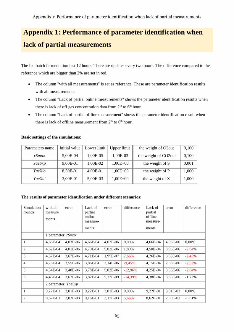
Appendix 1: Performance of parameter identification when lack of partial measurements
65
Appendix 1: Performance of parameter identification when
lack of partial measurements
The fed batch fermentation last 12 hours. There are updates every two hours. The difference compared to the
reference which are bigger than 2% are set in red.
The column "with all measurements" is set as reference. These are parameter identification results
with all measurements.
The column "Lack of partial online measurements" shows the parameter identification results when
there is lack of off gas concentration data from 2th to 6th hour.
The column "Lack of partial offline measurement" shows the parameter identification result when
there is lack of offline measurement from 2th to 6th hour.
Basic settings of the simulations:
Parameters name Initial value Lower limit Upper limit the weight of O2out 0,100
rSmax 5,00E-04 1,00E-05 1,00E-03 the weight of CO2out 0,100
YaeSxp 9,00E-01 1,00E-02 1,00E+00 the weight of S 0,001
YaeXlo 8,50E-01 4,00E-01 1,00E+00 the weight of P 1,000
YaeXhi 3,00E-01 5,00E-03 1,00E+00 the weight of X 1,000
The results of parameter identification under different scenarios:
Simulation
rounds
with all
measure
ments
error Lack of
partial
online
measure-
ments
error difference Lack of
partial
offline
measure-
ments
error difference
1.parameter: rSmax
1. 4,66E-04 4,03E-06 4,66E-04 4,03E-06 0,00% 4,66E-04 4,03E-06 0,00%
2. 4,62E-04 4,01E-06 4,70E-04 5,02E-06 1,80% 4,50E-04 3,96E-06 -2,64%
3. 4,37E-04 3,67E-06 4,71E-04 1,95E-07 7,66% 4,26E-04 3,63E-06 -2,45%
4. 4,26E-04 3,55E-06 3,86E-04 3,14E-06 -9,45% 4,15E-04 2,38E-06 -2,52%
5. 4,34E-04 3,48E-06 3,78E-04 5,02E-06 -12,96% 4,25E-04 3,56E-06 -2,04%
6. 4,46E-04 3,62E-06 3,82E-04 5,32E-09 -14,39% 4,38E-04 3,68E-06 -1,72%
2.parameter: YaeSxp
1. 9,22E-01 3,01E-03 9,22E-01 3,01E-03 0,00% 9,22E-01 3,01E-03 0,00%
2. 8,67E-01 2,02E-03 9,16E-01 3,17E-03 5,66% 8,62E-01 2,30E-03 -0,61%
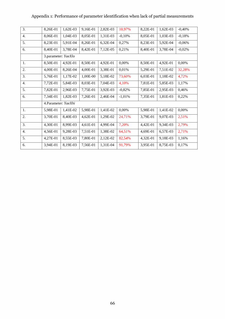
Appendix 1: Performance of parameter identification when lack of partial measurements
66
3. 8,26E-01 1,62E-03 9,16E-01 2,82E-03 10,97% 8,22E-01 1,62E-03 -0,40%
4. 8,06E-01 1,04E-03 8,05E-01 1,31E-03 -0,10% 8,05E-01 1,03E-03 -0,18%
5. 8,23E-01 5,91E-04 8,26E-01 6,32E-04 0,27% 8,23E-01 5,92E-04 -0,06%
6. 8,40E-01 3,78E-04 8,42E-01 7,12E-05 0,21% 8,40E-01 3,78E-04 -0,02%
3.parameter: YaeXlo
1. 8,50E-01 4,92E-01 8,50E-01 4,92E-01 0,00% 8,50E-01 4,92E-01 0,00%
2. 4,00E-01 8,26E-04 4,00E-01 3,38E-01 0,01% 5,29E-01 7,51E-02 32,28%
3. 5,76E-01 1,17E-02 1,00E-00 5,18E-02 73,60% 6,03E-01 1,18E-02 4,72%
4. 7,72E-01 5,84E-03 8,03E-01 7,04E-03 4,10% 7,81E-01 5,85E-03 1,17%
5. 7,82E-01 2,96E-03 7,75E-01 3,92E-03 -0,82% 7,85E-01 2,95E-03 0,46%
6. 7,34E-01 1,82E-03 7,26E-01 2,46E-04 -1,01% 7,35E-01 1,81E-03 0,22%
4.Parameter: YaeXhi
1. 5,98E-01 1,41E-02 5,98E-01 1,41E-02 0,00% 5,98E-01 1,41E-02 0,00%
2. 3,70E-01 8,40E-03 4,62E-01 1,29E-02 24,71% 3,79E-01 9,07E-03 2,51%
3. 4,30E-01 8,99E-03 4,61E-01 4,99E-04 7,20% 4,42E-01 9,34E-03 2,79%
4. 4,56E-01 9,28E-03 7,51E-01 1,38E-02 64,51% 4,69E-01 6,57E-03 2,71%
5. 4,27E-01 8,55E-03 7,80E-01 2,12E-02 82,54% 4,32E-01 9,18E-03 1,16%
6. 3,94E-01 8,19E-03 7,56E-01 1,31E-04 91,79% 3,95E-01 8,75E-03 0,17%

Appendix 2: Performance of the OLFO controller as a
software observer
In the following section, the results of parameter estimation with the measurements from the yeast cultivation
of december 2011 are shown here. Before anaerobic phase, parameter estimation was implemented only with
online measurements. The offline measurements on the figures of the right side are used as reference, not
involved in the simulation. After the switching time, the anaerobic phase was settled. The biomass concentration
measurements were also involved in the simulation, as the use of the vent gas composition measurements and
dissolved oxygen concentration from that moment was not meaningful anymore.
The following figures show the parameter estimation results every two hours real time along the cultivation
process. The figures on the left side are the original results. On the right side, the offline measurements which
are not shown on the left side are plotted here as an object of reference in order to show the effect of the OLFO
controller when it is used as a software observer. For aerobic phase, the OLFO controller simulates the behavior
of biomass, substrate and product concentration real time only with online measurements, most important of all
the measurements of off gas composition. The simulation of all those offline measurements and the
measurements themselves show really good agreement. For anaerobic phase, the biomass measurements are
used as well for the parameter estimation since the measurements of off gas composition do not make sense at
this stage. The simulations also fit with the measurements all along.

Appendix 2: Performance of the OLFO controller as a software observer
68

Appendix 2: Performance of the OLFO controller as a software observer
69

Appendix 2: Performance of the OLFO controller as a software observer
70

Appendix 2: Performance of the OLFO controller as a software observer
71
Figure A1: Parameter estimation results with only online measurements for aerobic phase; with online measurements and
biomass measurements for anaerobic phase. The upper part of each figure shows S: substrate, P: product and X: biomass;
the lower part shows the corresponding simulation and measured values of off gas composition. The figures of the left
sides show the original parameter estimation results of the whole process. The parameter estimation updates every two
hours until the end of the process. On the figures of the right sides, the offline measurements for aerobic phase, the product
and substrate measurements for anaerobic phase are not involved in the calculation of the parameter estimation. They are
presented here as a reference, to show how effective the OLFO controller is when it is used as a software observer.

Appendix 3: Data processing toolbox with OpenOffice
72
Appendix 3: Data processing toolbox with OpenOffice
In order to deal with the measurements to create individual documents for every required variables
automatically, a data processing toolbox based on a free open source office suite, namely OpenOffice, was
developed during my PhD. The instruction of how to set up this toolbox and the source code of this toolbox is
explained in this section.
1. Initial settings of OpenOffice toolbox
a) In the Tools browser, get a hierarchical view of the contents by clicking
Macros Organize Macros OpenOffice org Basic, then you get the following window as
Figure A2:
Figure A2: After opening the Macros, one can select the library that contains Module 1
b) Select the library that contains the macro Module 1 new.

Appendix 3: Data processing toolbox with OpenOffice
73
c) Insert BASIC source, select the last version → open → save. Then you have a window as Figure A3:
Import Dialog → open dialog 1 → open dialog2 → save. Then you have a window as Figure A4:
Figure A3: Importing BASIC source files
Figure A4: Importing dialog files
Until here, the toolbox is ready to be used.

Appendix 3: Data processing toolbox with OpenOffice
74
2. Toolbox User's Guide
a) In the Tools browser, get a hierarchical view of the contents by clicking Macros → Run Macros.
b) Select the library that contains the macro Module 1 (Figure A5).
Figure A5: Selecting the library that contains macro Module 1.
Select the macro Offline and then klick Run (Figure A6). Then you get the following window: The
corresponding data can be filled in as needed:
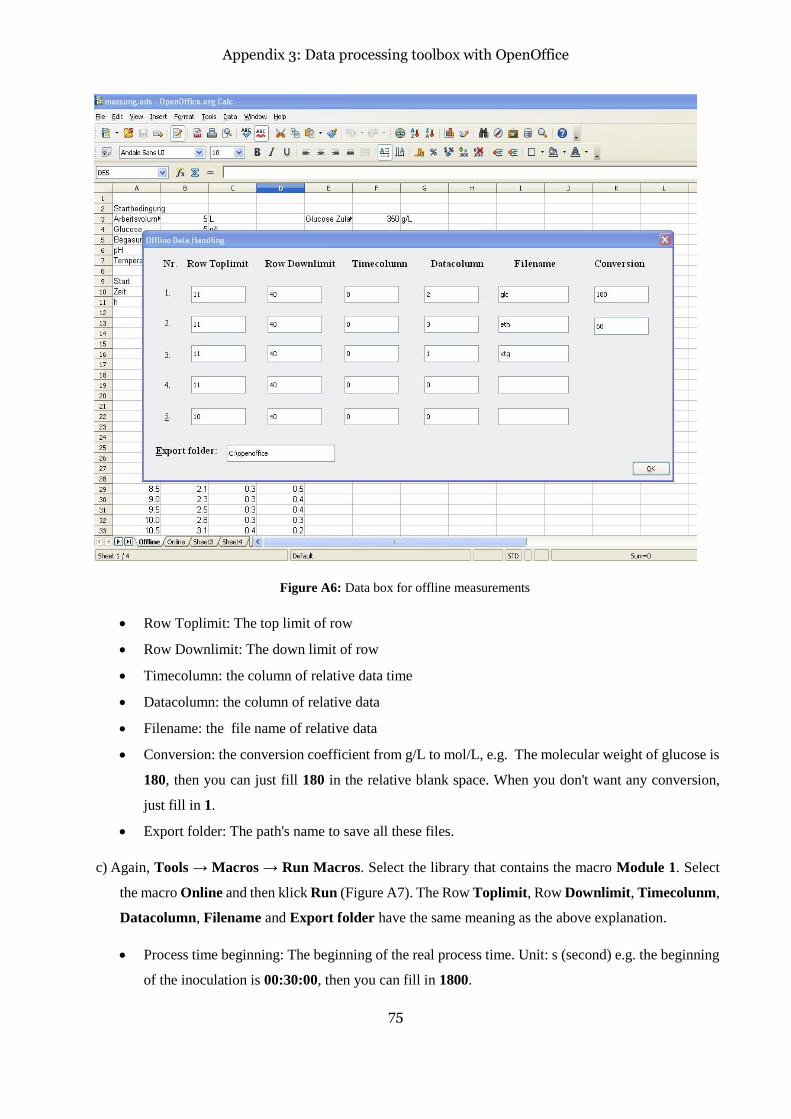
Appendix 3: Data processing toolbox with OpenOffice
75
Figure A6: Data box for offline measurements
Row Toplimit: The top limit of row
Row Downlimit: The down limit of row
Timecolumn: the column of relative data time
Datacolumn: the column of relative data
Filename: the file name of relative data
Conversion: the conversion coefficient from g/L to mol/L, e.g. The molecular weight of glucose is
180, then you can just fill 180 in the relative blank space. When you don't want any conversion,
just fill in 1.
Export folder: The path's name to save all these files.
c) Again, Tools → Macros → Run Macros. Select the library that contains the macro Module 1. Select
the macro Online and then klick Run (Figure A7). The Row Toplimit, Row Downlimit, Timecolunm,
Datacolumn, Filename and Export folder have the same meaning as the above explanation.
Process time beginning: The beginning of the real process time. Unit: s (second) e.g. the beginning
of the inoculation is 00:30:00, then you can fill in 1800.

Appendix 3: Data processing toolbox with OpenOffice
76
Interval: The interval to reduce the online data. E.g., to extract a data point for every three data
points, you should just fill 3 in the blank space.
Figure A7: Data box for online measurements.
Additional Information:
a) The beginning of the row number and column number are 0.
b) The unit of time in offline data sheet is automatically transferred from hour to second; the unit of time
in online data sheet is transferred from hh:mm:ss to second.
c) Sheet1 is set for offline measurement, sheet2 is set for online measurement.
d) Sheet3 and Sheet4 are reserved to save the inputs of the dialogs.
References
77
References
Alba-Lois, L., & Segal-Kischinevzky, C. (2010). Yeast fermentation and the making of beer and wine. Retrieved from
http://www.nature.com/scitable/topicpage/yeast-fermentation-and-the-making-of-beer-14372813.
Albert, S., & Kinley, R. D. (2001). Multivariate statistical monitoring of batch processes: An industrial case study of
fermentation supervision. Trends in Biotechnology, 19(2), 53-62.
Ashoori, A., Moshiri, B., Khaki-Sedigh, A., & Bakhtiari, M. R. (2009). Optimal control of a nonlinear fed-batch
fermentation process using model predictive approach. Journal of Process Control, 19(7), 1162-1173.
B. Braun Biotech International GmbH.Biostat C betriebshandbuch. BADC - Rev. 2.4 - 0600 SW 4.1:148-150.
Barnett, J. A. (1998). A history of research on yeasts 1: Work by chemists and biologists 1789–1850. Yeast, 14(16),
1439-1451.
Barnett, J. A., & Lichtenthaler, F. W. (2001). A history of research on yeasts 3: Emil Fischer, Eduard Buchner and their
contemporaries, 1880–1900. Yeast, 18(4), 363-388.
Bellgardt, K. H., Kuhlmann, W., Meyer, H. D., Schügerl, K., & Thoma. M. (1986). Application of an extended Kalman
filter for state estimation of a yeast fermentation. IEE Proceedings D - Control Theory and Applications, 133(5), 226-
234.
Bastin, G., & van Impe, J. F. (1995). Optimal adaptive control of fed-batch fermentation processes. Control Eng Pract,
3(7), 939-954.
Berry, B. N., Dobrowsky, T. M., Timson, R. C., Kshirsagar, R., Ryll, T., & Wiltberger, K. (2016). Quick generation of
raman spectroscopy based in-process glucose control to influence biopharmaceutical protein product quality during
mammalian cell culture. Biotechnology Progress, 32(1), 224-234.
Bolf, N., & Jerbic, I. (2006). Application of artificial neural networks for process identification and control. Kemija u
Industriji, 55(11), 457-468.
Bošković, J. D. (1995). Stable adaptive control of a class of nonlinearly parametrized bioreact or processes. Proceedings
of the American Control Conference, 1995, 3, 1795-1799.
Bošković, J. D. (1996). Stable adaptive control of a class of continuous-flow bioreactors. AIChE Journal, 42(1), 176-186.
Branduardi, P., & Porro, D. (2012). Yeasts in biotechnology. Yeast (pp. 347-370) Wiley-VCH Verlag GmbH & Co.
KGaA.
Brenan, K., Campbell, S., & Petzold, L. (1995). Numerical solution of initial-value problems in differential-algebraic
equations. Society for Industrial and Applied Mathematics.
Carrasco, E. F., & Banga, J. R. (1997). Dynamic optimization of batch reactors using adaptive stochastic algorithms.
Industrial & Engineering Chemistry Research, 36(6), 2252-2261.
Carrillo-Ureta, G. E. (2003). Optimal control of fermentation processes. PhD Thesis, City University London.
Chikkula, Y., & Lee, J. H. (2000). Robust adaptive predictive control of nonlinear processes using input-output models.
Ind. Eng. Chem. Res., 39, 2010-2023.
Chopda, V. R., Gomes, J., & Rathore, A. S. (2016). Bridging the gap between PAT concepts and implementation: An
integrated software platform for fermentation. Biotechnology Journal, 11(1), 164-171.
Chu, W. B. Z., & Constantinides, A. (1988). Modeling, optimization, and computer control of Cephalosporin C
fermentation process. Biotechnol. Bioeng., 32(3), 277-288.

References
78
Cinar, A., Parulekar, S., Ündey, C., & Birol, G. (2003). Batch fermentation: Modelling, monitoring, and control. CRC
Press, New York.
Dahhou, B., Roux, G., & Chamilothoris, G. (1992). Modelling and adaptive predictive control of a continuous
fermentation process. Applied Mathematical Modelling, 16(10), 545-552.
Damerow, P. (2012). Sumerian beer: The origins of brewing technology in ancient Mesopotamia. Cuneiform Digital
Library Journal, 2, 1-20.
Dobell, C., & Leeuwenhoek, A. v. (1932). Antony van Leeuwenhoek and his little animals. Dover Publications Inc.
Eaton, J. W., & Rawlings, J. B. (1992). Model-predictive control of chemical processes. Chemical Engineering Science,
47(4), 705-720.
Fliess, M., Lévine, J., Martin, P., & Rouchon, P. (1995). Flatness and defect of nonlinear systems: Introductory theory
and examples. Int. J. Control, 61(6), 1327-1361.
Foss, B. A., Johansen, T. A., & Sørensen, A. V. (1995). Nonlinear predictive control using local models — applied to a
batch fermentation process. Control Engineering Practice, 3(3), 389-396.
Frahm, B., & Pörtner, R. (2002). Messung und Simulation des Kohlendioxidausstoßes von Zellkulturprozessen. Chemie
Ingenieur Technik, 74(5) 702.
Frahm, B., Blank, H., Cornand, P., Oelssner, W., Guth, U., Lane, P., Pörtner, R. (2002a). Determination of dissolved CO2
concentration and CO2 production rate of mammalian cell suspension culture based on off-gas measurement. Journal of
Biotechnology, 99(2), 133-148.
Frahm, B., Lane, P., Märkl, H., & Pörtner, R. (2003). Improvement of a mammalian cell culture process by adaptive,
model-based dialysis fed-batch cultivation and suppression of apoptosis. Bioprocess and Biosystems Engineering, 26(1),
1-10.
Frahm, B., Lane, P., Atzert, H., Munack, A., Hoffmann, M., Hass, V. C., & Pörtner, R. (2002b). Adaptive, model-based
control by the open-loop-feedback-optimal (OLFO) controller for the effective fed-batch cultivation of hybridoma cells.
Biotechnology Progress, 18(5), 1095-1103.
Gerlach, I., Brüning, S., Gustavsson, R., Mandenius, C., & Hass, V. C. (2014). Operator training in recombinant protein
production using a structured simulator model. Journal of Biotechnology, 177, 53-59.
Glassey, J., Gernaey, K. V., Clemens, C., Schulz, T. W., Oliveira, R., Striedner, G., & Mandenius, C. (2011). Process
analytical technology (PAT) for biopharmaceuticals. Biotechnology Journal, 6(4), 369-377.
Goldrick, S., Ştefan, A., Lovett, D., Montague, G., & Lennox, B. (2015). The development of an industrial-scale fed-
batch fermentation simulation. Journal of Biotechnology, 193, 70-82.
Graindorge, P., Charbonnier, S., Magnin, J. P., Mauvy, C., & Cheruy, A. (1994). A software sensor of biological activity
based on a redox probe for the control of thiobacillus ferrooxidans cultures. Journal of Biotechnology, 35(1), 87-96.
Gray, W. D. (1941). Studies on the alcohol tolerance of yeasts. Journal of Bacteriology, 42(5), 561-574.
Gustavsson, R., Lukasser, C., & Mandenius, C. (2015). Control of specific carbon dioxide production in a fed-batch
culture producing recombinant protein using a soft sensor. Journal of Biotechnology, 200, 44-51.
Hass, V. C. (2005). Verbesserung der bioverfahrenstechnischen Ausbildung durch einen „Virtuellen bioreaktor”. Chemie
Ingenieur Technik, 77(1-2), 161-167.
Hass, V. C., Lane, P., Hoffmann, M., Frahm, B., Schwabe, J. -., Pörtner, R., & Munack, A. (2002). Model-based control
of hybridoma cell cultures. Computer applications in biotechnology 2001 : Modelling, monitoring and control of
References
79
biotechnological processes ; a Proceedings volume from the 8th IFAC international conference, Québec City, Canada,
24 - 27 june 2001 (pp. 323-329) Published for the International Federation of Automatic Control by Pergamon.
Hass, V. C., & Pörtner, R. (2009). Praxis der Bioprozesstechnik mit virtuellem Praktikum. Springer Spektrum
Akademischer Verlag.
Havlik, I., Lindner, P., Scheper, T., & Reardon, K. F. (2013). On-line monitoring of large cultivations of microalgae and
cyanobacteria. Trends in Biotechnology, 31(7), 406-414.
Hornsey, I. S. (2003). A history of beer and brewing. The Royal Society of Chemistry.
Jadot, F., Bastin, G., & Van Impe, J. F. (1998). Optimal adaptive control of a bioprocess with yield–productivity conflict.
Journal of Biotechnology, 65(1), 61-68.
Kadlec, P., Gabrys, B., & Strandt, S. (2009). Data-driven soft sensors in the process industry. Computers & Chemical
Engineering, 33(4), 795-814.
Kaiser, C., Carvell, J. P., & Luttmann, R. (2007). A sensitive, compact, in situ biomass measurement system controlling
and monitoring microbial fermentations using radio-frequency impedance. BioProcess International, 5(Suppl. 1), 52-55.
Karra, S., Shaw, R., Patwardhan, S. C., & Noronha, S. (2008). Adaptive model predictive control of multivariable time-
varying systems. Industrial & Engineering Chemistry Research, 47(8), 2708-2720.
Lee, J., Lee, S. Y., Park, S., & Middelberg, A. P. J. (1999). Control of fed-batch fermentations. Biotechnology Advances,
17(1), 29-48.
Li, M., Kuhnen, F., Pörtner, R., & Hass, V. C. (2012). Modellgestützte Optimalsteuerung von biotechnischen
Kultivierungen – Möglichkeiten und Grenzen. Chemie Ingenieur Technik, 84(8) 1339-1340.
Luttmann, R., Bracewell, D. G., Cornelissen, G., Gernaey, K. V., Glassey, J., Hass, V. C., Keiser, C., Preusse, C.,
Steiedner G., Mandenius, C. F. (2012). Soft sensors in bioprocessing: A status report and recommendations.
Biotechnology Journal, 7(8), 1040-1048.
Luttmann, R., Munack, A., & Thoma, M. (1985). Mathematical modelling, parameter identification and adaptive control
of single cell protein processes in tower loop bioreactors. Agricultural feedstock and waste treatment and engineering
(pp. 95-205). Springer Berlin Heidelberg.
Mahadevan, R., Agrawal, S. K., & III, F. J. D. (2001). Differential flatness based nonlinear predictive control of fed-
batch bioreactors. Control Engineering Practice, 9(8), 889-899.
Mandenius, C., & Gustavsson, R. (2015). Mini-review: Soft sensors as means for PAT in the manufacture of bio-
therapeutics. Journal of Chemical Technology & Biotechnology, 90(2), 215-227.
McGovern, P. E. (2009). Uncorking the past: The quest for wine, beer, and other alcoholic beverages. University of
California Press.
Modak, J. M., & Lim, H. C. (1987). Feedback optimization of fed-batch fermentation. Biotechnology and
Bioengineering, 30(4), 528-540.
Modak, J. M., & Lim, H. C. (1992). Optimal mode of operation of bioreactor for fermentation processes. Chemical
Engineering Science, 47(15), 3869-3884.
Munack, A. (1986). Application of receding horizon adaptive control to an underfloor heating system. IFAC Conference
on Simulation of Control Systems. 263-268.
Nelder, J. A., & Mead, R. (1965). A simplex method for function minimization. The Computer Journal, 7(4), 308-313.
Nelson, D. L., Lehninger, A. L., & Cox, M. M. (2008). Lehninger principles of biochemistry. New York: W.H. Freeman.
References
80
Ödman, P., Johansen, C. L., Olsson, L., Gernaey, K. V., & Lantz, A. E. (2009). On-line estimation of biomass, glucose
and ethanol in Saccharomyces cerevisiae cultivations using in-situ multi-wavelength fluorescence and software sensors.
Journal of Biotechnology, 144(2), 102-112.
Ohadi, K., Legge, R. L., & Budman, H. M. (2015). Development of a soft-sensor based on multi-wavelength
fluorescence spectroscopy and a dynamic metabolic model for monitoring mammalian cell cultures. Biotechnology and
Bioengineering, 112(1), 197-208.
Olsson, L., Schulze, U., & Nielsen, J. (1998). On-line bioprocess monitoring – an academic discipline or an industrial
tool? TrAC Trends in Analytical Chemistry, 17(2), 88-95.
Pan, T., Li, S., & Cai, W. (2007). Lazy learning-based online identification and adaptive PID control: A case study for
CSTR process. Industrial & Engineering Chemistry Research, 46(2), 472-480.
Park, S., & Ramirez, F.,W. (1988). Optimal production of secreted protein in fed-batch reactors. AIChE Journal, 34(9),
1550-1558.
Pasteur, L. (1857). Mémoire sur la fermentation alcoolique. Comptes Rendus De l'Académie Des Sciences, 45, 1032-
1036.
Peuker, T., Riedel, M., Kaiser, C., Ellert, A., Lenz, K., Elsholz, O., & Luttmann, R. (2004). At-line determination of
glucose, ammonia, and acetate in high cell density cultivations of Escherichia coli. Engineering in Life Sciences, 4(2),
138-143.
Ponnuswamy, S. R., Shah, S. L., & Kiparissides, C. A. (1987). Computer optimal control of batch polymerization
reactors. Industrial & Engineering Chemistry Research, 26(11), 2229-2236.
Pörtner, R., Bohmann, A., Lüdemann, I., & Märkl, H. (1994). Animal cell culture estimation of specific glucose uptake
rates in cultures of hybridoma cells. Journal of Biotechnology, 34(3), 237-246.
Posten, C., & Munack, A. (1990). Improved modeling of plant cell suspension cultures by optimum experiment design.
Preprints of the 11th IFAC world congress 1990 (pp. 268-273)
Press, W. H., Teukolsky, S. A., Vetterling, W. T., & Flannery, B. P. (2007). Numerical recipes 3rd edition: The art of
scientific computing. New York, NY, USA: Cambridge University Press.
Redford, D. B. (2001). The Oxford encyclopedia of ancient Egypt Oxford University Press, Oxford Univ.
Rodrigues, J. A. D., Zaiat, M., & Filho, R. M. (1999). State estimation and parameter identification in a fed-batch
penicillin production process. Brazilian Journal of Chemical Engineering, 16(1), 41-52.
Schwarz, S. (2009). Modellgestützte prozessoptimierung von escherichia coli kultivierungen. Master thesis, University of
Applied Sciences Bremen.
Schwarz, S., Kuhnen, F., & Hass, V. C. (2010). Development of a general process model for optimisation of
biotechnological cultivations - a case study with Escherichia coli and Saccharomyces cerevisiae. CHISA 2010 & ECCE 7
(http://www.chisa.cz/).
Shen, D., Chen, G., Cruz, J., Jose B., Pham, K., Blasch, E., & Lynch, R. (2010). Cooperative controls with intermittent
communication. Proc. SPIE. 7691, Space Missions and Technologies, 76910D-76910D-11.
Shimizu, K. (1993). An overview on the control system design of bioreactors. Measurement and control (pp. 65-84).
Springer Berlin Heidelberg.
Snyman, J. (2005). An introduction to basic optimization theory and classical and new gradient-based algorithms.
Springer US.
References
81
Soroush, M., & Valluri, S. (1994). An approach to optimization and control of batch processes. American Control
Conference,1, 490-494.
Srinivasa, B. B., & Moreshwar, J. M. (2009). Method for on-line optimization of a fed-batch fermentation unit to
maximize the product yield. Patent US20090117647 A1.
Stanke, M., & Hitzmann, B. (2013). Automatic control of bioprocesses. Advances in Biochemical
Engineering/Biotechnology, 132, 35-63.
Stephanopoulos, G., & San, K. (1984). Studies on online bioreactor identification. I. Theory. Biotechnology and
Bioengineering, 26(10), 1176-1188.
Teixeira, A. P., Carinhas, N., Dias, J. M. L., Cruz, P., Alves, P. M., Carrondo, M. J. T., & Oliveira, R. (2007). Hybrid
semi-parametric mathematical systems: Bridging the gap between systems biology and process engineering. Journal of
Biotechnology, 132(4), 418-425.
Tholudur, A., & Ramirez, W. F. (1996). Optimization of fed-batch bioreactors using neural network parameter function
models. Biotechnology Progress, 12(3), 302-309.
Tremblay, M. d., Perrier, M., Chavarie, C., & Archambault, J. (1992). Fed-batch culture of hybridoma cells: Comparison
of optimal control approach and closed loop strategies. Bioprocess Engineering, 7(5), 229-234.
U.S. Department of Health and Human Services Food and Drug Administration.Guidance for industry: Process
validation: General principles and practices. Retrieved from
http://www.fda.gov/downloads/Drugs/.../Guidances/UCM070336.pdf
Van Breusegem, V., & Bastin, G. (1990). Optimal control of biomass growth in a mixed culture. Biotechnology and
Bioengineering, 35(4), 349-355.
Van Impe, J. F., & Bastin, G. (1998). Optimal adaptive control of fed-batch fermentation processes. In Van Impe, Jan F.
M., P. A. Vanrolleghem & D. M. Iserentant (Eds.), Advanced instrumentation, data interpretation, and control of
biotechnological processes (pp. 401-435). Dordrecht, The Netherlands: Springer Netherlands.
Warth, B., Rajkai, G., & Mandenius, C. (2010). Evaluation of software sensors for on-line estimation of culture
conditions in an Escherichia coli cultivation expressing a recombinant protein. Journal of Biotechnology, 147(1), 37-45.
Wechselberger, P., Sagmeister, P., & Herwig, C. (2013). Real-time estimation of biomass and specific growth rate in
physiologically variable recombinant fed-batch processes. Bioprocess and Biosystems Engineering, 36(9), 1205-1218.
Witte, V. C. (1996). Mathematische modellierung und adaptive prozesssteuerung der kultivierung von cyathus striatus.
PhD thesis, Technische Universität Hamburg-Harburg.
Zeng, F. Y., & Dahhou, B. (1993). Adaptive control of a nonlinear fermentation process via MRAC technique. Appl.
Math. Modelling, 17, 58-69.
Zhang, H., & Lennox, B. (2004). Integrated condition monitoring and control of fed-batch fermentation processes.
Journal of Process Control, 14(1), 41-50.
Related Documents