NEAR-OPTIMAL FEEDBACK GUIDANCE FOR AN ACCURATE LUNAR LANDING by JOSEPH PARSLEY RAJNISH SHARMA, COMMITTEE CHAIR MICHAEL FREEMAN KEITH WILLIAMS A THESIS Submitted in partial fulfillment of the requirements for the degree of Master of Science in the Department of Aerospace Engineering in the Graduate School of The University of Alabama TUSCALOOSA, ALABAMA 2012

Welcome message from author
This document is posted to help you gain knowledge. Please leave a comment to let me know what you think about it! Share it to your friends and learn new things together.
Transcript

NEAR-OPTIMAL FEEDBACK GUIDANCE
FOR AN ACCURATE
LUNAR LANDING
by
JOSEPH PARSLEY
RAJNISH SHARMA, COMMITTEE CHAIRMICHAEL FREEMAN
KEITH WILLIAMS
A THESIS
Submitted in partial fulfillment of the requirementsfor the degree of Master of Science
in the Department of Aerospace Engineeringin the Graduate School of
The University of Alabama
TUSCALOOSA, ALABAMA
2012

Copyright Joseph Parsley 2012ALL RIGHTS RESERVED

ii
ABSTRACT
This research presents a novel guidance method for a lunar landing problem. The method
facilitates efficiency and autonomy in a landing. The lunar landing problem is posed as a finite-
time, fixed-terminal, optimal control problem. As a key finding of this work, the method of
solution that is applied to construct the guidance mechanism employs a new extension of the
State-Dependent Riccati Equation (SDRE) technique for constrained nonlinear dynamical
systems in finite time. In general, the solution procedure yields a closed-loop control law for a
dynamical system with point terminal constraints. Being a closed-loop solution, this SDRE
technique calculates corrections for unpredicted external inputs, hardware errors, and other
anomalies. In addition, this technique allows all calculations to be performed in real time,
without requiring that gains be calculated a priori. This increases the flexibility to make changes
to a landing in real time, if required.
The new SDRE-based feedback control technique is thoroughly investigated for
accuracy, reliability, and computational efficiency. The pointwise linearization of the underlying
SDRE methodology causes the new technique to be considered a suboptimal solution. To
investigate the efficiency of the solution method, various numerical experiments are performed,
and the results are presented. In addition, to validate the methodology, the new technique is
compared with two other methods of solution: the Approximating Sequence of Riccati Equations
(ASRE) technique and an indirect variational method, which provides the benchmark optimal
open-loop solution.

iii
ACKNOWLEDGMENTS
I would like to thank the faculty members, friends, and family members who have helped me
with this research project. Especially, I would like to thank Dr. Rajnish Sharma, the chairperson
of this thesis, for his guidance and for sharing his expertise in control theory. I would also like to
thank my other committee members, Dr. Michael Freeman and Dr. Keith Williams, for their
valuable input.

iv
CONTENTS
ABSTRACT.................................................................................................................................... ii
ACKNOWLEDGMENTS ............................................................................................................. iii
LIST OF TABLES........................................................................................................................ vii
LIST OF FIGURES ..................................................................................................................... viii
CHAPTER 1. INTRODUCTION .................................................................................................. 1
CHAPTER 2. LITERATURE SURVEY....................................................................................... 4
2.1 Apollo Guidance........................................................................................................... 4
2.2 Optimal Control Techniques ........................................................................................ 9
2.2.1 Techniques for Linear Systems ............................................................................. 9
2.2.1.1 LQR Technique ............................................................................................... 9
2.2.1.2 Fixed-Final-State LQ Control ....................................................................... 10
2.2.1.3 Indirect Variational Method .......................................................................... 12
2.2.2 Techniques for Nonlinear Systems ..................................................................... 14
2.2.2.1 SDRE Technique........................................................................................... 14
2.2.2.2 Fixed-Final-State SDRE Technique.............................................................. 17
2.2.2.3 ASRE Technique........................................................................................... 19

v
CHAPTER 3. DESCRIPTION OF THE LUNAR LANDING PROBLEM ............................... 22
CHAPTER 4. A NEW GUIDANCE METHOD FOR A LUNAR LANDING........................... 24
4.1 Solution Description ................................................................................................... 24
4.2 Phase 1........................................................................................................................ 25
4.2.1 Nondimensionalization of the Problem............................................................... 26
4.2.2 Fixed-Final-State SDRE Solution for Phase 1 .................................................... 29
4.2.3 ASRE Solution for Phase 1 ................................................................................. 32
4.2.4 Indirect Variational Solution for Phase 1............................................................ 33
4.3 Phase 2........................................................................................................................ 35
CHAPTER 5. NUMERICAL RESULTS .................................................................................... 37
5.1 Phase 1 Results ........................................................................................................... 37
5.1.1 Experiment 1 ....................................................................................................... 37
5.1.2 Experiment 2 ....................................................................................................... 39
5.1.3 Experiment 3 ....................................................................................................... 41
5.1.4 Experiment 4 ....................................................................................................... 43
5.1.5 Comparison of the Techniques............................................................................ 45
5.2 Phase 2 Results ........................................................................................................... 56
CHAPTER 6. CONCLUSIONS .................................................................................................. 58
REFERENCES ............................................................................................................................. 60

vi
APPENDIX A. DESCRIPTION OF CONTROL SYSTEMS AND OPTIMAL CONTROL..... 63
APPENDIX B. DERIVATION OF THE DYNAMICAL SYSTEM .......................................... 66

vii
LIST OF TABLES
Table 1. Initial and final conditions for Phase 1 ..................................................................... 26
Table 2. Constants of the problem .......................................................................................... 27
Table 3. Variables of the problem........................................................................................... 27
Table 4. Nondimensional variables of the problem ................................................................ 28
Table 5. Results of Experiment 1............................................................................................ 38
Table 6. Results for the first part of Experiment 2.................................................................. 40
Table 7. Results for the second part of Experiment 2 ............................................................. 41
Table 8. Results for the first part of Experiment 3.................................................................. 42
Table 9. Results for the second part of Experiment 3 ............................................................. 43
Table 10. Matrices investigated in Experiment 4.................................................................... 44
Table 11. Results of Experiment 4.......................................................................................... 45
Table 12. Results of the three solutions .................................................................................. 46
Table 13. Data for Phase 2 ...................................................................................................... 57
Table 14. Results of Phase 2 ................................................................................................... 57

viii
LIST OF FIGURES
Fig. 1. Apollo lunar landing diagram showing the various elements of a landing ................... 5
Fig. 2. Apollo lunar landing phases .......................................................................................... 6
Fig. 3. Trajectory of a simulated Apollo landing ...................................................................... 8
Fig. 4. Process for fixed-final-state LQ control ...................................................................... 12
Fig. 5. Process of the SDRE technique ................................................................................... 16
Fig. 6. Process of the fixed-final-state SDRE technique......................................................... 18
Fig. 7. Diagram illustrating the simulation time steps ............................................................ 19
Fig. 8. Process of the ASRE technique ................................................................................... 21
Fig. 9. Schematic of the lunar landing problem...................................................................... 22
Fig. 10. The new landing sequence......................................................................................... 25
Fig. 11. Phase 1 landing trajectories of the various solutions................................................. 47
Fig. 12. Phase 1 landing trajectories of the various solutions, with thrust vectors ................. 48
Fig. 13. Terminus of Phase 1 trajectories................................................................................ 49
Fig. 14. Terminus of Phase 1 trajectories, with thrust vectors................................................ 50
Fig. 15. Plot of r for the three solutions .................................................................................. 50
Fig. 16. Plot of u for the three solutions.................................................................................. 51
Fig. 17. Plot of v for the three solutions.................................................................................. 51
Fig. 18. Plot of θ for the three solutions.................................................................................. 52
Fig. 19. Plot of λr for the three solutions................................................................................. 53

ix
Fig. 20. Plot of λu for the three solutions................................................................................. 53
Fig. 21. Plot of λv for the three solutions................................................................................. 54
Fig. 22. Plot of λθ for the three solutions................................................................................. 54
Fig. 23. Plot of U for the three solutions................................................................................. 55
Fig. 24. Plot of the angle of U, , for the three solutions........................................................ 55
Fig. 25. Plot of cost-to-go, J, for the three solutions............................................................... 56
Fig. 26. Diagram of a system .................................................................................................. 63
Fig. 27. Diagram of an open-loop control system................................................................... 64
Fig. 28. Diagram of a closed-loop control system .................................................................. 64

1
CHAPTER 1
INTRODUCTION
Recently, there has been increased interest in returning to the Moon. However, it has been
nearly forty years since humans have gone there. The last manned mission was in 1972, during
the Apollo program. Since that time, a limited amount of research has been conducted to
improve the landing methodology. A few research papers written on this matter are included in
the References [1-6].
The Apollo missions had many limitations and had to overcome many challenges while using
primitive computer technology. Landing sites were hazardous because they contained rocks and
craters. Astronauts had to be able to adjust the landing point to avoid these hazards. This meant
that the trajectory profile and the orientation of the lander had to allow the astronauts to observe
the landing site. Moreover, due to the limitations of the computers, control systems were
simplified as much as possible. These restrictions added inefficiency to the landings, thus
resulting in wasted effort and fuel.
Apollo was successful in landing men on the Moon and returning them safely to the Earth.
However, with the greater speed and power of present-day computer technology, it is highly
desired to find an improved control method for landing on the Moon. Lunar stations of the near
future will require a precise and efficient landing system that does not necessitate extensive
training. The method investigated in this research could be the basis of such a desired system,

2
wherein a craft is allowed to perform all calculations in real time and is driven to a soft landing
at a desired location while consuming a minimal amount of fuel. To achieve the autonomous
goals of the new guidance method, lunar stations of the future would need to be clear of hazards
and have very precise navigational aids. This would eliminate the need for astronauts to make
course corrections and adjustments.
This research presents a novel guidance method for a lunar landing problem that is formulated
as an optimal control problem. To obtain the feedback control law, the method of solution is
presented using a new closed-loop feedback control technique for nonlinear systems with
constraints. By performing various numerical experiments, the new guidance scheme is tested
for its accuracy, efficiency, and robustness, and it is investigated with respect to computational
burden. Through numerical simulations, the results for final location and velocity are compared
with the desired values to determine the trajectory error and the precision of the control law.
Validity of the solution is verified by comparing the results of this new technique with the results
of two other optimal control solutions.
The research for this thesis is presented in the next five chapters. Chapter 2 is a literature
survey, which covers the background material. In the first section of the chapter, the Apollo
lunar landings are described. The second section discusses various common techniques for
solving optimal control problems for linear and nonlinear systems. Finally, a new terminally
constrained optimal control technique for nonlinear systems is presented.
Chapter 3 describes the modeling of the lunar landing problem. The chapter elaborates on all
of the variables used in this research and includes a schematic of the problem. It also presents
the equations of motion for the problem.

3
Chapter 4 describes a new guidance method. This chapter presents the complete sequence
involved in the solution and describes the two phases of the method. Then it presents the new
control technique along with other techniques applied in this new landing methodology.
Chapter 5 presents the results of simulations of the new guidance method. A thorough
numerical analysis is demonstrated for various experiments with respect to different possible
cases with the SDRE method. In addition, results comparing the SDRE method with two other
methods are presented. Conclusions and future scope of this work are included in Chapter 6.

4
CHAPTER 2
LITERATURE SURVEY
This chapter covers background material for the problem considered in this research. The
first section describes the Apollo lunar landing method, which includes the sequence of phases
and the guidance solution used during a landing. The second section presents an overview of
various optimal control techniques applied to solve linear and nonlinear systems. In this thesis,
these techniques are respectively referred to as linear and nonlinear optimal control techniques,
with respect to the dynamical system.
2.1 Apollo Guidance
The Apollo lunar landings were accomplished from 1969 to 1972, when computer technology
was very primitive. The limitations of the computers made it impossible to utilize the advanced
guidance techniques used today. Fig. 1 shows the overall landing procedure used by Apollo [7-
10]. The lunar module (LM) separates from the command and service module (CSM) while in
the parking orbit of approximately 60-nm in altitude. At a predetermined orbit position, the LM
performs a Hohmann-type transfer maneuver [11]. The resulting elliptical orbit efficiently
places the LM close to the Moon’s surface in preparation for landing. At perilune, the LM fires
its thrusters and begins the landing sequence.

Fig. 1. Apollo lunar landing diagram showing the various elements of a landing
The landing sequence for Apollo consisted of three phases.
braking phase (P63), the approach phase (P64), and the terminal descent phase (P66).
5
lunar landing diagram showing the various elements of a landing
g sequence for Apollo consisted of three phases. As shown in Fig.
braking phase (P63), the approach phase (P64), and the terminal descent phase (P66).
lunar landing diagram showing the various elements of a landing
Fig. 2, these are the
braking phase (P63), the approach phase (P64), and the terminal descent phase (P66).

P63 slows the LM from orbital speed. It typically begins at a 492
landing site and transfers the LM to the required initial conditions for P64.
immediately at the terminus of P63. Its
above the landing site. In addition, it provides continuous visibility of the lunar surface and of
the landing location. This was
landing point to avoid hazards.
provides velocity control but no position control. Forward and lateral velocit
produce a vertical approach to the landing site. The descent rate
value that can be adjusted by the astronauts.
The trajectories for P63 and P64
ground-based computers were required to make the calculations.
from a Taylor series expansion of
polynomial [7] as
6
Fig. 2. Apollo lunar landing phases
P63 slows the LM from orbital speed. It typically begins at a 492-km slant range from the
landing site and transfers the LM to the required initial conditions for P64.
immediately at the terminus of P63. Its objective is to deliver the LM to a point almost directly
above the landing site. In addition, it provides continuous visibility of the lunar surface and of
was a requirement in case the astronauts had to redesignate the
landing point to avoid hazards. P66 typically begins automatically at a 30
velocity control but no position control. Forward and lateral velocit
produce a vertical approach to the landing site. The descent rate is controlled to a reference
be adjusted by the astronauts.
for P63 and P64 were calculated prior to the Moon landings
based computers were required to make the calculations. These trajectories
from a Taylor series expansion of the position function and are represented by a
km slant range from the
landing site and transfers the LM to the required initial conditions for P64. P64 begins
a point almost directly
above the landing site. In addition, it provides continuous visibility of the lunar surface and of
to redesignate the
automatically at a 30-m altitude. It
velocity control but no position control. Forward and lateral velocities are nulled to
s controlled to a reference
calculated prior to the Moon landings, because large
trajectories were derived
and are represented by a quartic

7
2 3 4
( ) ( ) ( ) ( )2 6 24C C C
C
T T TRRG RTG VTG T ATG JTG STG (2.1)
where RRG is the position vector on the reference trajectory at current negative time TC. RTG,
VTG, ATG, JTG, and STG are the target position, velocity, acceleration, jerk, and snap vectors in
guidance coordinates. P63 and P64 used separate sets of target values (calculated from a ground-
based targeting program) to define their trajectories.
A quadratic guidance equation [7] was derived from Eq. (2.1). It is given as
2 2
2
2 2
( )36 24 24 18
12 6 6 6 1
P P P P
C C C C C C
P P P P
C C C C C
T T T TRTG RG VTGACG
T T T T T T
T T T TVGATG
T T T T T
(2.2)
where ACG, VG, and RG are the commanded acceleration, current velocity, and current position.
TP is the predicted target-referenced time [7] defined as
P CT T Leadtime (2.3)
where Leadtime is the transport delay due to computation and command execution.
The current negative time TC, or time-to-go, was calculated to satisfy the downrange Z-
component of jerk. With a desired value for downrange jerk, JTGZ, the following equation [7]
was numerically solved for TC:
3 26 18 6 24 0Z C Z C Z Z C Z ZJTG T ATG T VTG VG T RTG RG (2.4)
The calculated value for TC was then used in Eq. (2.2) to determine the commanded acceleration
required. Using Eq. (2.2) and target data for the Apollo 14 landing [10], a sample Apollo
landing is simulated for this research. The resulting trajectory is shown in Fig. 3 and is shown in

8
the results of Chapter 5 for comparison with the other guidance techniques. The coordinate
system shown in Fig. 3 is located at the center of the Moon.
Fig. 3. Trajectory of a simulated Apollo landing
The Apollo program was successful in landing men on the Moon using the limited computers
of the day. With today’s advanced technology, a much better method can be employed. This
would make it possible to land more precisely while being safer and more efficient. The method
investigated in this research looks promising as being one that could be used to accomplish this
goal.
This research is based on the use of optimal control theory to formulate a solution for the
lunar landing problem. Appendix A presents background material on control systems and
provides more details on optimal control. The appendix also gives the equation of a system in
standard matrix form and shows diagrams of different types of systems. Further sections of this
chapter cover various techniques for using optimal control theory for synthesizing the feedback
control schemes. Some of these techniques form the basis for the research of this thesis.
-5 -4 -3 -2 -1 0
x 105
1.6
1.65
1.7
1.75
1.8
1.85x 10
6
z (m)
x(m
)
Moon surface
Apollo trajectorylanding
start point
landingsite

9
2.2 Optimal Control Techniques
There are many techniques for solving optimal control problems (OCP), depending on
whether the system is linear or nonlinear. Linear systems are easier to solve, and their solutions
are well developed. Nonlinear systems are more difficult, and their solution techniques are not
as mature. Some solutions for nonlinear systems are just now becoming realized, as computers
are becoming powerful enough to be used in these systems effectively. The following sections
describe some of the techniques used for linear and nonlinear dynamical systems.
2.2.1 Techniques for Linear Systems
To solve optimal control problems for linear systems, some of the popular techniques are the
linear quadratic regulator (LQR) [12-17], the fixed-final-state linear quadratic (LQ) control
method [13, 14], indirect variational methods [13, 14], and dynamic programming [12-14].
Since they are applied later in this thesis, LQR, fixed-final-state LQ control, and an indirect
variational method are described in the following subsections.
2.2.1.1 LQR Technique
The linear quadratic regulator (LQR) technique gets its name from the fact that it operates on
a linear system and a quadratic cost functional. The linear system has the state-space form [17]
given as
x Ax Bu (2.5)
With an LQR approach to obtain a closed-loop system, the control input mu , for full state
feedback [17], is defined as
u Kx (2.6)

10
where K is the matrix of gains, and nx is the state vector. The cost functional [17] is
expressed as
T T
0
1( )
2J dt
x Qx u Ru (2.7)
The solution to an LQR problem is found by first solving the algebraic Riccati equation
(ARE) [17] for the P matrix prior to actually using the control system. The ARE for a linear
system is given as
T 1 T0 A P PA Q PBR B P (2.8)
The P matrix, the solution of Eq. (2.8), is then used to calculate gain K with
1 TK R B P (2.9)
Then, this gain matrix K is used in Eq. (2.6) to compute control input u at every sample time.
2.2.1.2 Fixed-Final-State LQ Control
Considering a soft constraint at the fixed-final-state with a linear system, the quadratic cost
functional, or performance index [14], can be given as
0
T T T1 1( ) ( ) ( ) ( )
2 2
T
tJ T T T dt x S x x Qx u Ru (2.10)
subject to
( ) ( )T TCx r (2.11)
where C is a constant coefficient matrix, and x(T) is the vector of final states. The states of a
system are driven to a set of desired final values r(T) over a fixed amount of time, while
minimizing the cost J.
11
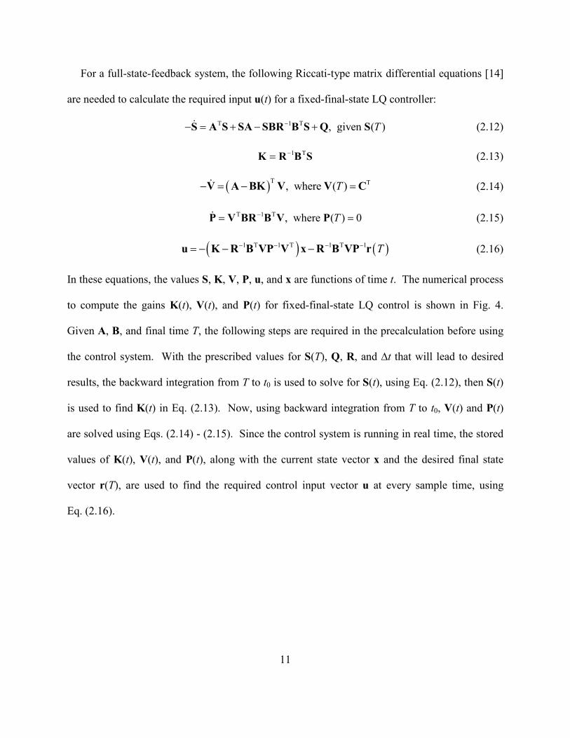
For a full-state-feedback system, the following Riccati-type matrix differential equations [14]
are needed to calculate the required input u(t) for a fixed-final-state LQ controller:
T 1 T , given ( )T S A S SA SBR B S Q S (2.12)
1 TK R B S (2.13)
T T, where ( )T V A VBK V C (2.14)
T 1 T , wher ( )e 0T P V BR B PV (2.15)
1 T 1 T 1 T 1 T u K R B VP V x R B VP r (2.16)
In these equations, the values S, K, V, P, u, and x are functions of time t. The numerical process
to compute the gains K(t), V(t), and P(t) for fixed-final-state LQ control is shown in Fig. 4.
Given A, B, and final time T, the following steps are required in the precalculation before using
the control system. With the prescribed values for S(T), Q, R, and ∆t that will lead to desired
results, the backward integration from T to t0 is used to solve for S(t), using Eq. (2.12), then S(t)
is used to find K(t) in Eq. (2.13). Now, using backward integration from T to t0, V(t) and P(t)
are solved using Eqs. (2.14) - (2.15). Since the control system is running in real time, the stored
values of K(t), V(t), and P(t), along with the current state vector x and the desired final state
vector r(T), are used to find the required control input vector u at every sample time, using
Eq. (2.16).

Fig. 4
2.2.1.3 Indirect Variational Method
In an indirect variational method, the calculus of variations
Lagrange equations and the optimality conditions for solving optimal control problems.
results of this method are considered
conditions for optimality.
For a fixed-final-state problem with a system described as
a cost functional for a variational method
12
4. Process for fixed-final-state LQ control
Indirect Variational Method
In an indirect variational method, the calculus of variations approach is used to derive
the optimality conditions for solving optimal control problems.
results of this method are considered optimal, subject to satisfying the second order necessary
state problem with a system described as
( , , )tx f x u
a variational method [14] has the form
0
( ), , ,T
tJ T T L t dt x x u
approach is used to derive Euler-
the optimality conditions for solving optimal control problems. The
, subject to satisfying the second order necessary
(2.17)
(2.18)

13
where represents the soft constraint that includes a weighting function on the final state at the
final time, and L is a function of state and input at intermediate times along the trajectory to be
considered for optimization. The terminal constraint [14] is defined as
( ), 0T T ψ x (2.19)
with being zero-valued expressions for the final state. A Hamiltonian equation [14] can be
constructed as
T( , , ) ( , , ) ( , , )H t L t t x u x u λ f x u (2.20)
where is the set of Lagrange multipliers, also known as costates. The first order necessary
conditions for optimality are used to derive the differential equations for costate, stationarity
condition, and transversality condition [14]. Respectively, these are given as
H
λ
x (2.21)
0H
u
(2.22)
TT T( ) 0t t
TT
dx T H dT x xψ ν λ ψ ν (2.23)
These three equations, with the given initial conditions on the states, create a two-point boundary
value problem (TPBVP). The solution of the TPBVP can be attempted by starting with initial
guesses for (0) and and then using a shooting method [18, 19] to solve for the values of (t)
and , which satisfy the boundary conditions of the problem. From (t) and expressions derived
from Eq. (2.22), the required input u(t) can be calculated.
There are some negative aspects to this technique. It is an open-loop control law, and all the
input values u(t) have to be calculated prior to using the control system. Also, the shooting

14
method for solving the TPBVP is problematic. If the initial guesses are poor, then accurate
results may not be produced, or convergence of the solution may not occur at all for nonlinear
systems.
2.2.2 Techniques for Nonlinear Systems
There are various techniques used to solve optimal control problems for nonlinear systems.
Some of these are the State-Dependent Riccati Equation (SDRE) method [20-34], the
Approximating Sequence of Riccati Equations (ASRE) technique [25, 35, 36], indirect
variational methods, and nonlinear programming (NLP) techniques [13, 37].
This research focuses on application of SDRE for finite time optimal control problems and
compares the solution process with ASRE and an indirect variational method. Basic descriptions
of SDRE and ASRE are given in the following subsections.
2.2.2.1 SDRE Technique
The State-Dependent Riccati Equation (SDRE) technique is a relatively new solution method
for solving nonlinear optimal control problems. The most common use of the technique is as a
regulator based on the LQR methodology described in Section 2.2.1.1, using a quadratic cost
functional such as Eq. (2.7).
The goal of the method is to solve nonlinear optimal control problems in feedback form by
approximating the system as linear at each sample time. The linear system at each of these
points in time is based on the current states at that time. At each sample time, the problem is
solved using common LQR techniques. The assumption of pointwise linearization creates a
suboptimal solution, but it facilitates in solving a difficult nonlinear system for a feedback

15
control. Moreover, with enough sample points along the trajectory, the suboptimal solution can
be made to be very close to optimal.
The heart of the SDRE strategy is to factor the nonlinear model into a linear-like form [20] as
( , , ) ( ) ( ) ( ) ( )t t t x f x u A x x B x u (2.24)
In this form, A and B are functions of x, and their numerical values change throughout the
trajectory of x. There are many possibilities for the form of A(x) and B(x). For example, the
system
2
/
c dc
d d c d
x
can be factored into
1
1/ 1
d c
d d
A x
or
2
2
1 / 0
/ /
d c c
dd c c d
Ax
The forms for A(x) and B(x) have to be decided to give the desired results. If the best matrix
forms are not known in advance, then a variety of these matrices can be tested in simulations in
order to facilitate the decision. Moreover, before distinct A(x) and B(x) matrices are used in the
SDRE formulation, they should be tested for controllability [12, 16, 17] over the entire state
trajectory. A(x) and B(x) are controllable if
2 1n B AB A B A B (2.25)
has full rank of n for all applicable values of state x. If A(x) and B(x) are not controllable over
the entire state trajectory, then the form of the matrices should be changed. After the final

choices for these matrices have been decided
calculate required control input u
Fig.
Fig. 5 shows a diagram of the SDRE technique. At each sample time, the following
procedure is accomplished. First, the current state vector
for A(x) and B(x). Then, using the LQR equations,
calculated and applied to the system. This procedure is then
For the SDRE technique, the ARE is solved at every
and B(x). This causes the nonlinear system to be approximated as a series of linear systems.
Therefore, shorter time increments increase the accuracy of the control law, because this
decreases the amount of time that each
16
or these matrices have been decided, they can be used in the SDRE technique
u(t) in real time.
Fig. 5. Process of the SDRE technique
shows a diagram of the SDRE technique. At each sample time, the following
procedure is accomplished. First, the current state vector x is used to calculate numerical
). Then, using the LQR equations, P and K are calculated. Input
calculated and applied to the system. This procedure is then repeated at the next sample time.
, the ARE is solved at every sample time for each new value of
). This causes the nonlinear system to be approximated as a series of linear systems.
Therefore, shorter time increments increase the accuracy of the control law, because this
decreases the amount of time that each approximation is applied.
SDRE technique to
shows a diagram of the SDRE technique. At each sample time, the following
is used to calculate numerical values
are calculated. Input u is then
at the next sample time.
for each new value of A(x)
). This causes the nonlinear system to be approximated as a series of linear systems.
Therefore, shorter time increments increase the accuracy of the control law, because this

17
Because of its approximating nature, the SDRE technique is considered a suboptimal solution.
However, with the proper choices for the A(x) and B(x) matrices, and with the proper amount of
sample times, the SDRE technique can provide a very adequate solution.
For this research, a new form of the SDRE technique is formulated for the finite-time OCP
posed with terminal constraints. The details of this new terminally constrained technique are
given next.
2.2.2.2 Fixed-Final-State SDRE Technique
This new technique is derived from the aforementioned SDRE method. The normal SDRE
method is most commonly used to control nonlinear systems over an infinite horizon, as
described above. The new SDRE technique described in this section can be used to solve finite-
horizon, terminally constrained, optimal control problems.
This reformulated SDRE technique combines the common SDRE method with the linear
fixed-final-state LQ control solution of Section 2.2.1.2. This produces a fixed-final-state SDRE
solution for nonlinear optimal control.
In general, the new technique operates the same as that of the more common SDRE regulator.
At every sample time, it recalculates the A(x) and B(x) matrices and then calculates the input
based on current states. The exception is that, instead of using the LQR strategy and solving the
algebraic Riccati equation, the new technique uses the fixed-final-state LQ control strategy. Like
the fixed-final-state LQ control technique, the values for S(T), Q, and R have to be chosen to
give the best desired results. In addition, a value for the time increment ∆t should be properly
chosen. A value of ∆t that is too long will reduce the accuracy of the control law, but one that is
too short could over burden the system.

Fig. 6. Process of the fixed
Fig. 6 describes how this new
occur at every sample time while the control system is running. First, at the current time
matrices A(x) and B(x) are calculated from the current state
V(t), and P(t) are calculated using Eqs.
T to current time tc. The values
current state vector x(tc) and the desired final state vector
u(tc) for the current sample time. The input
sample time. At the next sample time, a n
repeated. The iterations continue until the final time
This new SDRE formulation could be altered in many ways. One alteration would be to use a
variable sampling rate. The sampling rate could start slow and then get faster over time. This
18
. Process of the fixed-final-state SDRE technique
describes how this new control law works. As the figure shows, the following steps
occur at every sample time while the control system is running. First, at the current time
) are calculated from the current state x(tc). Next, the values for
) are calculated using Eqs. (2.12) - (2.15), with backward integration from final time
. The values K(tc), V(tc), and P(tc) are used in Eq. (2.16)
) and the desired final state vector r(T), to calculate the required input
) for the current sample time. The input u(tc) is then applied to the system until the next
sample time. At the next sample time, a new value for x(tc) is measured, and the process is
repeated. The iterations continue until the final time T has been reached.
This new SDRE formulation could be altered in many ways. One alteration would be to use a
variable sampling rate. The sampling rate could start slow and then get faster over time. This
control law works. As the figure shows, the following steps
occur at every sample time while the control system is running. First, at the current time tc, the
). Next, the values for S(t), K(t),
, with backward integration from final time
), along with the
), to calculate the required input
) is then applied to the system until the next
) is measured, and the process is
This new SDRE formulation could be altered in many ways. One alteration would be to use a
variable sampling rate. The sampling rate could start slow and then get faster over time. This

could reduce computational burden on the system. Another alteration
and record all of the K(t), V(t), and
values could then be used to make a much faster control system. In addition, an open
system could be created by recording all of t
2.2.2.3 ASRE Technique
The Approximating Sequence of Riccati E
solving nonlinear optimal control problems
constrained optimal control problems over a fixed amount of time.
As with the SDRE technique, ASRE first factors the nonlinear system into the linear
of Eq. (2.24). However, ASRE is an iterative solution that changes the linear
[ ] [ 1] [ ] [ 1] [ ]( ) ( ) ( ) ( ) ( )i i i i it t t t tx A x x B x u
where i represents the current iteration number.
control. It has a cost functional like
Prior to using the control system, a precalculation has to be performed. This precalculation is
an iterative approach that involves a
T] is divided into a determined amount of
u(t), x(t), and the time steps.
Fig. 7. Diagram illustrating the simulation time steps
19
could reduce computational burden on the system. Another alteration could be to precalculate
), and P(t) values in an SDRE simulation. These recorded gain
values could then be used to make a much faster control system. In addition, an open
system could be created by recording all of the calculated input values in an SDRE simulation.
Approximating Sequence of Riccati Equations (ASRE) technique is another solution for
near optimal control problems iteratively. It can be used to solve terminally
d optimal control problems over a fixed amount of time.
As with the SDRE technique, ASRE first factors the nonlinear system into the linear
is an iterative solution that changes the linear-like form into
[ ] [ 1] [ ] [ 1] [ ]( ) ( ) ( ) ( ) ( )i i i i it t t t t x A x x B x u
represents the current iteration number. The technique is based on fixed
a cost functional like Eq. (2.10), and it utilizes the Eqs. (2.12) - (2
Prior to using the control system, a precalculation has to be performed. This precalculation is
approach that involves a simulation of the system, where the simulation time
a determined amount of time steps. Fig. 7 shows the relationships between
. Diagram illustrating the simulation time steps
could be to precalculate
) values in an SDRE simulation. These recorded gain
values could then be used to make a much faster control system. In addition, an open-loop
he calculated input values in an SDRE simulation.
is another solution for
used to solve terminally
As with the SDRE technique, ASRE first factors the nonlinear system into the linear-like form
like form into [25]
(2.26)
ed-final-state LQ
2.16).
Prior to using the control system, a precalculation has to be performed. This precalculation is
the simulation time t [t0,
shows the relationships between t,

20
Fig. 8 shows a diagram of how the ASRE technique works. The first part of the precalculation is
to calculate A(x) and B(x) using the initial state vector x0. The resulting values A0 and B0 are
then used at every time step. The next part begins the iteration loop of the technique. The A and
B values from every time step are used with Eqs. (2.12) - (2.15) and backward integration from
S(T), V(T), and P(T) to calculate S, K, V, and P for every time step. Then, by using Eq. (2.16)
with a simulation of the system, u and x are calculated for every time step. The values for x are
then used to calculate new values for A and B at every time step. The new values for A and B
are now used in the next iteration of the loop. The loop is iterated a fixed number of times or
until the final state error reaches a value below a set threshold. The calculated gain values K(t),
V(t), and P(t) of the final iteration are recorded. These recorded gains can then be used in the
closed-loop control system to calculate required input u, as shown in Fig. 8. Or, by storing the
input values u(t) of the final iteration of the precalculation, an open-loop control system can be
created.

Fig.
The ASRE technique, like SDRE, can be used to find a good suboptimal solution to a difficult
nonlinear problem. It is noticed in this research that the
easier to implement than the indirect
require very close guess values, and it con
21
Fig. 8. Process of the ASRE technique
, like SDRE, can be used to find a good suboptimal solution to a difficult
It is noticed in this research that the ASRE technique is more reliable and is
easier to implement than the indirect variational technique of Section 2.2.1.3.
require very close guess values, and it converges reliably within only a few iterations.
, like SDRE, can be used to find a good suboptimal solution to a difficult
is more reliable and is
. ASRE does not
verges reliably within only a few iterations.

DESCRIPTION OF THE LUNAR LANDING PRO
This chapter describes the lunar landing problem that is investigated in this research.
illustrates the variables used in the lunar landing problem
a clockwise orbit around the Moo
coordinate reference frames used in the landing solution. RF
Moon, and RF2 is located at the landing site.
represented by r, and the positional angle is represented by
velocities of the lander are depicted as
applied thrust. Ur and Ut are the radial and tang
angle of U from the z-axis is represented by
Fig. 9
22
CHAPTER 3
DESCRIPTION OF THE LUNAR LANDING PROBLEM
This chapter describes the lunar landing problem that is investigated in this research.
the lunar landing problem. The lander is shown as a
Moon, represented by the large circle. RF1 and RF
coordinate reference frames used in the landing solution. RF1 is located at the center of
is located at the landing site. The radial distance from RF1
, and the positional angle is represented by θ. The radial and tangential
are depicted as u and v, respectively. U is the input acceleration due to
are the radial and tangential components of this input acceleration. The
axis is represented by .
9. Schematic of the lunar landing problem
This chapter describes the lunar landing problem that is investigated in this research. Fig. 9
. The lander is shown as a black dot in
and RF2 are the two
is located at the center of the
1 to the lander is
adial and tangential
input acceleration due to
acceleration. The
23
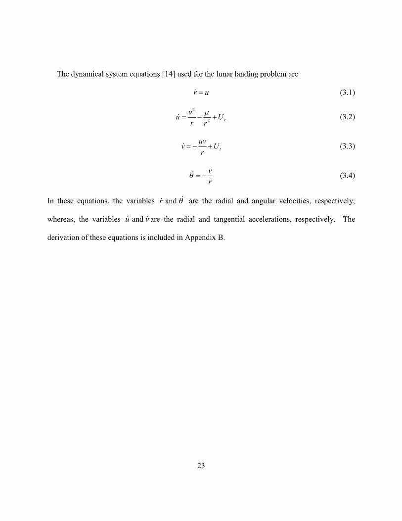
The dynamical system equations [14] used for the lunar landing problem are
r u (3.1)
2
2 r
vu U
r r
(3.2)
t
uvv U
r (3.3)
v
r (3.4)
In these equations, the variables andr are the radial and angular velocities, respectively;
whereas, the variables andu v are the radial and tangential accelerations, respectively. The
derivation of these equations is included in Appendix B.

24
CHAPTER 4
A NEW GUIDANCE METHOD FOR A LUNAR LANDING
This chapter describes the method of solution used to solve the lunar landing problem. It
illustrates and defines the phases of the landing, and it describes optimal control techniques
applied in the solution procedure of the guidance method.
4.1 Solution Description
The solution procedure is constructed in two phases, Phase 1 and Phase 2. The initial and
final conditions for the two phases are chosen to match the Apollo missions closely. Phase 1, as
the lander decelerates from orbit, utilizes a nonlinear optimal control technique. It minimizes
fuel consumption as it works to stop the lander at a target point 30 meters above the landing
location. This target point acts as a safety zone that allows for some small error in the nonlinear
control. Phase 2 reformulates the dynamical system for the final portion of the landing into an
approximate linear system and then uses linear optimal control to drive the vehicle down to a soft
pinpoint landing.
Fig. 10 shows a schematic of the landing sequence. For solving the nonlinear Phase 1 portion
of the problem, various nonlinear optimal control techniques are considered. For this research, it
is decided to use a new form of the SDRE technique, as described in Section 2.2.2.2. The results
of this new technique are compared to those obtained from the ASRE and variational methods
described previously. All three of these solutions are simulated, and the resulting numerical data

is presented for comparison. The Apollo technique i
the trajectories of the other three solutions.
4.2 Phase 1
Phase 1 covers the first portion of the landing, where orbital velocity and distance from the
Moon cause significant nonlinearity in the system. It takes the spacecraft from orbit and brings it
to rest 30 meters above the desired landing point on
uses the RF1 reference frame shown in
Table 1 shows the initial and final conditions used by
for a 15-km initial altitude, the value
calculated for a 492-km initial slant range to the landing site.
25
arison. The Apollo technique is also simulated to compare its trajectory to
the trajectories of the other three solutions.
Fig. 10. The new landing sequence
covers the first portion of the landing, where orbital velocity and distance from the
Moon cause significant nonlinearity in the system. It takes the spacecraft from orbit and brings it
to rest 30 meters above the desired landing point on the Moon, as shown in Fig.
reference frame shown in Fig. 9.
shows the initial and final conditions used by Phase 1. The value for
km initial altitude, the value rf is determined for a 30-m final altitude, and
km initial slant range to the landing site.
also simulated to compare its trajectory to
covers the first portion of the landing, where orbital velocity and distance from the
Moon cause significant nonlinearity in the system. It takes the spacecraft from orbit and brings it
Fig. 10. This phase
. The value for r0 is determined
m final altitude, and θ0 is

26
Table 1. Initial and final conditions for Phase 1
Parameter Description Value Units
t0 Initial time 0 (min)
tf Final time 11 (min)
r0 Initial radial distance 1752100 (m)
rf Final radial distance 1737000 (m)
u0 Initial radial velocity 0 (m/s)
uf Final radial velocity 0 (m/s)
v0 Initial tangential velocity 1673 (m/s)
vf Final tangential velocity 0 (m/s)
θ0 Initial position angle 1.85362 (radians)
θf Final position angle π/2 (radians)
For this research, a Moon radius rm of 1,737 km, a Moon mass of 73.48 × 10²¹ kg, and a
Moon gravitational parameter μ of 4903 km3/s2 are used [11]. In addition, for thrust calculations,
a lander mass of 16,430 kilograms is estimated.
4.2.1 Nondimensionalization of the Problem
For Phase 1 of the lunar landing problem, it is beneficial to nondimensionalize the system.
Nondimensionalization is the process of removing all units of measure from the equations by
multiplying and dividing various constants. For problems that contain large numerical values,
nondimensionalization can bring about dramatic improvement in calculation time. Sometimes, it
can make a problem solvable, where before it was not. Nondimensionalization improves the
results of this research. The process on how this is performed is given below.
First, two constants are chosen to be the basis for nondimensionalizing the problem. These
are shown, along with their units, in Table 2. They are chosen because of their large values.

27
Table 2. Constants of the problem
Constant Description Units
μ Gravitational Parameter (m3/s2)
rm Radius of the Moon (m)
The variables of the problem are then identified, along with their units. These are shown in
Table 3.
Table 3. Variables of the problem
Variable Description Units
r Radial Distance (m)
u Radial Velocity (m/s)
v Tangential Velocity (m/s)
θ Positional Angle (radians)
t Time (s)
U Input Acceleration (m/s2)
Nondimensional representations of these variables are then formulated using the constants of
Table 2. These new nondimensional forms are shown in Table 4.
28
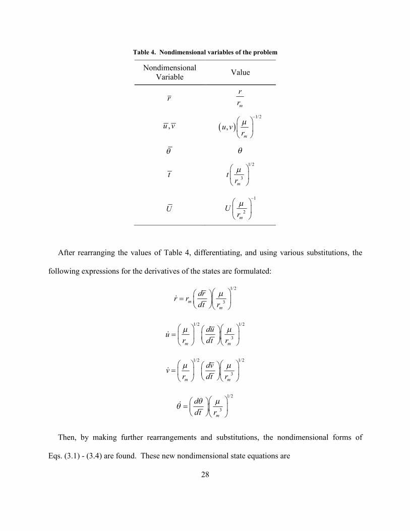
Table 4. Nondimensional variables of the problem
NondimensionalVariable
Value
rm
r
r
,u v 1/2
,m
u vr
t
1/2
3m
tr
U
1
2m
Ur
After rearranging the values of Table 4, differentiating, and using various substitutions, the
following expressions for the derivatives of the states are formulated:
1/2
3m
m
drr r
dt r
1/2 1/2
3m m
duu
r dt r
1/2 1/2
3m m
dvv
r dt r
1/2
3m
d
dt r
Then, by making further rearrangements and substitutions, the nondimensional forms of
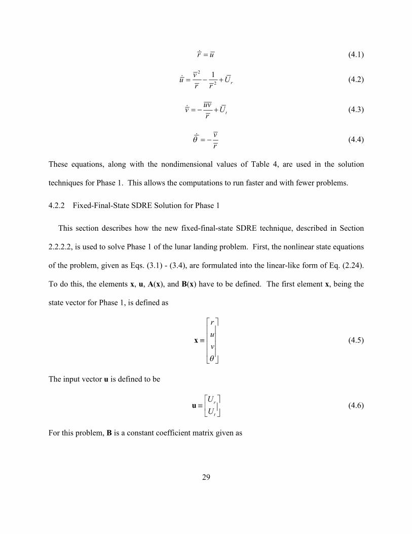
Eqs. (3.1) - (3.4) are found. These new nondimensional state equations are
29
r u (4.1)
2
2
1r
vu U
r r (4.2)
t
uvv U
r (4.3)
v
r (4.4)
These equations, along with the nondimensional values of Table 4, are used in the solution
techniques for Phase 1. This allows the computations to run faster and with fewer problems.
4.2.2 Fixed-Final-State SDRE Solution for Phase 1
This section describes how the new fixed-final-state SDRE technique, described in Section
2.2.2.2, is used to solve Phase 1 of the lunar landing problem. First, the nonlinear state equations
of the problem, given as Eqs. (3.1) - (3.4), are formulated into the linear-like form of Eq. (2.24).
To do this, the elements x, u, A(x), and B(x) have to be defined. The first element x, being the
state vector for Phase 1, is defined as
r
u
v
x (4.5)
The input vector u is defined to be
r
t
U
U
u (4.6)
For this problem, B is a constant coefficient matrix given as

30
0 0
1 0
0 1
0 0
B (4.7)
Defining A(x) is a little more difficult. Given that there are many possibilities for this matrix,
various forms have to be evaluated in order to make the decision. The evaluated matrices are
first tested for controllability. Then, several of the controllable forms are separately used in a
simulation to see which gives the best results. Experiment 1, in Section 5.1.1, shows the results
of simulations using various A(x) matrices. From the results of the evaluations, it is decided to
use the form
3
0 1 0 0
0 0
( )0 0 0
10 0 0
v
r r
v
r
r
A x (4.8)
Section 5.1.1 provides an explanation for this decision.
The nondimensional form of the A(x) matrix, corresponding to nondimensional state
equations of Eqs. (4.1) - (4.4), is defined as
3
0 1 0 0
1/ 0 / 0( )
0 / 0 0
0 0 1/ 0
r v r
v r
r
A x (4.9)
Next, the values for the weighting matrices S(T), Q, and R are defined. For the Phase 1
solution, it is determined to use the values

31
0 0 0 0 0 0 0 0
0 0 0 0 0 0 0 0 1 0( ) , ,
0 0 0 0 0 0 0 0 0 1
0 0 0 0 0 0 0 0
T
S Q R
The zero values for S(T) and Q mean that the final states and the intermediate states along the
trajectory are not minimized. For this particular problem, all states are being driven to fixed final
values; therefore, there is no need to minimize them. The R weighting matrix is used to
minimize the input u along the trajectory. It is decided that the unit matrix given to R, as shown,
will suffice for this research.
The desired final states of Phase 1 are shown in Table 1. The vector r(T), for these desired
final states, includes all of the elements of the final state vector x(T). Therefore, r(T) is given as
1737000 m
0 m/s( ) ( )
0 m/s
/2 radians
f
f
f
f
r
uT T
v
r x (4.10)
Therefore, the value of matrix C, in Eq. (2.11), has to be the unit matrix given as
1 0 0 0
0 1 0 0
0 0 1 0
0 0 0 1
C (4.11)
This C matrix defines V(T) in Eq. (2.14).
The values given above, along with the initial state values shown in Table 1, are used with the
new fixed-final-state SDRE technique of Section 2.2.2.2 to formulate a solution for Phase 1.
During the process, the relationships of Table 4 are used to nondimensionalize the desired final
state vector r(T), the current state vector x(tc), the final time T, and the time increment ∆t. A
32
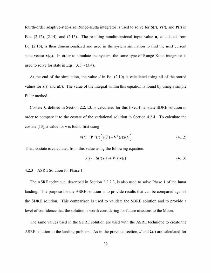
fourth-order adaptive-step-size Runge-Kutta integrator is used to solve for S(t), V(t), and P(t) in
Eqs. (2.12), (2.14), and (2.15). The resulting nondimensional input value u, calculated from
Eq. (2.16), is then dimensionalized and used in the system simulation to find the next current
state vector x(tc). In order to simulate the system, the same type of Runge-Kutta integrator is
used to solve for state in Eqs. (3.1) - (3.4).
At the end of the simulation, the value J in Eq. (2.10) is calculated using all of the stored
values for x(t) and u(t). The value of the integral within this equation is found by using a simple
Euler method.
Costate λ, defined in Section 2.2.1.3, is calculated for this fixed-final-state SDRE solution in
order to compare it to the costate of the variational solution in Section 4.2.4. To calculate the
costate [13], a value for ν is found first using
1 T( ) ( ) ( ) ( ) ( )t t T t t ν P r V x (4.12)
Then, costate is calculated from this value using the following equation:
( ) ( ) ( ) ( ) ( )t t t t t λ S x V ν (4.13)
4.2.3 ASRE Solution for Phase 1
The ASRE technique, described in Section 2.2.2.3, is also used to solve Phase 1 of the lunar
landing. The purpose for the ASRE solution is to provide results that can be compared against
the SDRE solution. This comparison is used to validate the SDRE solution and to provide a
level of confidence that the solution is worth considering for future missions to the Moon.
The same values used in the SDRE solution are used with the ASRE technique to create the
ASRE solution to the landing problem. As in the previous section, J and λ(t) are calculated for

33
this solution in the same manner. All of the results of simulations using this solution are
included in Chapter 5 for comparison with the SDRE results.
4.2.4 Indirect Variational Solution for Phase 1
An indirect variational technique is also used for Phase 1, and its results are considered
optimal. As with ASRE, the variational solution provides results that are used to compare with
those from SDRE. This adds yet another level of confidence to the SDRE solution.
This variational solution uses the technique described in Section 2.2.1.3. The cost functional
for this solution is the same as Eq. (2.10). Using this cost functional form with the optimality
equations of the technique, the optimal control law equations [14] for this solution are
formulated to be
T
fλ λ Qx
x (4.14)
0T
fRu λ
u(4.15)
The state equations of the system, Eqs. (3.1) - (3.4), are used with Eq. (4.14) to create the
following costate equations:
2
2 3 2 2
2r u v
v uv v
r r r r
(4.16)
u r v
v
r
(4.17)
2 1v u v
v u
r r r
(4.18)
0 (4.19)

34
Equation (4.15) is then used to formulate equations for input u. These are calculated to be
r uU (4.20)
t vU (4.21)
The vector of zero-valued expressions for the final state is defined as
1737000
2
f
f
f
f
r
u
v
ψ (4.22)
This is used in Eq. (2.23) to give the following expression:
1
2
3
4
( )
( )
( )
( )
r
u
v
T
T
T
T
λ (4.23)
It is extremely difficult to find proper guess values for λ(0) and ν. Without proper guess
values, the solver will not produce good results. To simplify the process, the values for λ(0) and
ν calculated from the SDRE solution are used for the guess values in the variational solution.
Using the initial values for the states and the guess values mentioned above, a numerical
solver is used to solve the state equations, solve the costate equations, and find the values of λ(0)
and ν that drive the final state conditions to the desired values. The state and costate equations
are then integrated using the initial state values and the calculated initial costate values to find
x(t) and λ(t). Then, the input u(t) is calculated from λu(t) and λv(t) using Eqs. (4.20) and (4.21).
As with the solutions of the previous two sections, the cost value J is calculated in the same
manner for this solution. This J value is included in the results of Chapter 5.
35
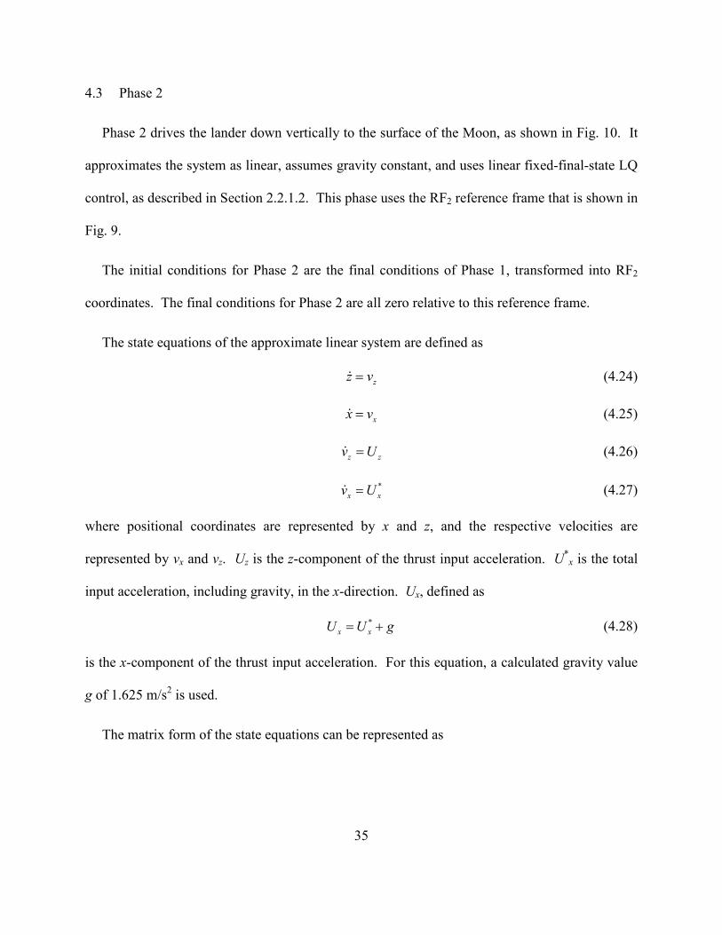
4.3 Phase 2
Phase 2 drives the lander down vertically to the surface of the Moon, as shown in Fig. 10. It
approximates the system as linear, assumes gravity constant, and uses linear fixed-final-state LQ
control, as described in Section 2.2.1.2. This phase uses the RF2 reference frame that is shown in
Fig. 9.
The initial conditions for Phase 2 are the final conditions of Phase 1, transformed into RF2
coordinates. The final conditions for Phase 2 are all zero relative to this reference frame.
The state equations of the approximate linear system are defined as
zz v (4.24)
xx v (4.25)
z zv U (4.26)
*x xv U (4.27)
where positional coordinates are represented by x and z, and the respective velocities are
represented by vx and vz. Uz is the z-component of the thrust input acceleration. U*x is the total
input acceleration, including gravity, in the x-direction. Ux, defined as
*x xU U g (4.28)
is the x-component of the thrust input acceleration. For this equation, a calculated gravity value
g of 1.625 m/s2 is used.
The matrix form of the state equations can be represented as

36
*
0 0 1 0 0 0
0 0 0 1 0 0
0 0 0 0 1 0
0 0 0 0 0 1
z
z z x
x x
z z
x x U
v v U
v v
x
xA B
(4.29)
The C constant coefficient matrix and the vector of desired final states r(T) for Phase 2 are
defined to be
0 m 1 0 0 0
0 m 0 1 0 0( ) ,
0 m/s 0 0 1 0
0 m/s 0 0 0 1
f
f
zf
xf
z
xT
v
v
r C
Also, the S(T), Q, and R matrices are given as
0 0 0 0 0 0 0 0
0 0 0 0 0 0 0 0 1 0( ) , ,
0 0 0 0 0 0 0 0 0 1
0 0 0 0 0 0 0 0
T
S Q R
All of these values are used with the technique of Section 2.2.1.2 to find the necessary u(t) that
drives the lander to a soft pinpoint landing at the surface of the Moon.
Phase 2 is used to complete the landing sequence for this research and to help validate the
overall approach. Since the technique used for this phase is common and well known, and since
this final portion of the landing is only a small part of the sequence, less emphasis is placed on
Phase 2. However, the results for this phase are included in Chapter 5.

37
CHAPTER 5
NUMERICAL RESULTS
This chapter shows the results of simulations of the lunar landing method investigated in this
research. Various numerical experiments are conducted on the new fixed-final-state SDRE
solution for Phase1. These experiments are described in this chapter, and their results are
presented. In addition to these experiments, the results of the various solutions for Phase 1 are
compared together to add validity to the fixed-final-state SDRE solution. The results of the
Phase 2 solution are also shown in this chapter.
5.1 Phase 1 Results
The following subsections describe the numerical simulations that are performed for Phase 1.
The results of each experiment are also given within the corresponding subsections.
5.1.1 Experiment 1
As discussed in Section 2.2.2.1, the A(x) matrix, for the factored system form given by
Eq. (2.24), can be constructed in many ways. In this experiment, various forms of the A(x)
matrix for the fixed-final-state SDRE solution, shown in Section 4.2.2, are used in separate
simulations to compare their results. The purpose of this is to show how changing the form of
the A(x) matrix affects the results of the solution. The results are studied to decide which A(x)
matrix to use for the remainder of the research.
The following A(x) matrices are investigated in this experiment:

38
3
1
0 1 0 0
/ 0 / 0( )
0 / 0 0
0 0 1/ 0
r v r
v r
r
A x (5.1)
2 2 3
2
0 1 0 0
/ / 0 0 0( )
0 / 0 0
0 0 1/ 0
v r r
v r
r
A x (5.2)
3
3
0 1 0 0
/ 0 / 0( )
0 0 / 0
0 0 1/ 0
r v r
u r
r
A x (5.3)
2 2 3
4
0 1 0 0
/ / 0 0 0( )
0 0 / 0
0 0 1/ 0
v r r
u r
r
A x (5.4)
These matrices are separately used in simulations of the fixed-final-state SDRE solution. The
results of the simulations are shown in Table 5.
Table 5. Results of Experiment 1
MatrixRun Time
(min)Max Thrust
(N)J
(m2/s3)Position Error
(m)Velocity Error
(m/s)
A(x)1 1.443 56,317.39 2,752.53 0.00000320 0.00000934
A(x)2 1.267 54,755.46 2,755.50 0.00000301 0.00000879
A(x)3 0.970 56,230.35 2,757.50 0.00000304 0.00000885
A(x)4 1.076 54,550.60 2,760.95 0.00000286 0.00000834
For each A(x) matrix investigated, this table shows the simulation run time, the maximum thrust
applied, the final cost J, and the final position and velocity errors. The simulation run times,

39
though difficult to measure accurately, show that different A(x) matrices can cause the
calculations to run quicker or slower. This difference is more severe in some situations and is
something that should be taken into consideration in the design of a controller. There is no
significant difference in the final error in this experiment. However, there are differences in the
values for maximum thrust and J. These differences should also be taken into consideration
when designing a controller, depending on that which is more important.
From the results of this experiment, it is decided to use A(x)1 for the Phase 1 solution over the
remainder of this research. This is because A(x)1 produces a lower J value, which means less
fuel consumption.
5.1.2 Experiment 2
This experiment tests various initial conditions for Phase 1. The purpose of this is to see how
different initial conditions affect the results and the behavior of the system. In the first part of
the experiment, the values for initial range are varied to investigate how they affect the terminal
states of Phase 1. The second part of the experiment investigates various values for initial
altitude. The values tested in both parts are ±1%, ±2%, ±3%, ±4%, and ±5% of the nominal
values. The results are shown in Table 6 and Table 7.
Table 6 shows the results for various values of initial range. All of the simulations reach the
target values within an acceptable small amount of numerical error. The table shows that
decreasing the initial range increases the values for maximum applied thrust and J, and
increasing the initial range has the opposite effect. This means that starting a landing with a
shorter range causes the control system to exert more energy to accomplish the landing.

40
However, the table also shows that an increased initial range causes slightly higher final error in
position and velocity, and a decreased initial range has the opposite effect.
Table 6. Results for the first part of Experiment 2
% Difference inInitial Range
Max Thrust(N)
J(m2/s3)
Position Error(m)
Velocity Error(m/s)
-5% 61,849.79 2,840.51 0.00000266 0.00000775
-4% 60,741.85 2,820.94 0.00000276 0.00000804
-3% 59,634.59 2,802.36 0.00000286 0.00000835
-2% 58,528.06 2,784.76 0.00000297 0.00000867
-1% 57,422.31 2,768.15 0.00000308 0.00000899
0% (nominal) 56,317.39 2,752.53 0.00000320 0.00000933
+1% 55,213.36 2,737.90 0.00000332 0.00000969
+2% 54,110.30 2,724.26 0.00000345 0.00001006
+3% 53,008.26 2,711.61 0.00000358 0.00001043
+4% 51,907.34 2,699.95 0.00000371 0.00001082
+5% 50,807.62 2,689.28 0.00000385 0.00001123
In the second part of the experiment, as the initial altitude is varied, the velocity is adjusted to
produce a circular orbit for each particular initial altitude. The purpose of this is to produce a
more realistic situation. Therefore, the results for this part of the experiment are partially due to
the changes in velocity.
Table 7 shows the results for the second part of this experiment. As before, all of the
simulations reach the target values within an acceptable small amount of error, with the error
increasing slightly with increased initial altitude. However, the initial altitude causes different
effects on maximum applied thrust and J. Smaller values of initial altitude causes slightly larger
values for maximum applied thrust and slightly smaller values for J, and larger values of initial
altitude has the opposite effect. Therefore, starting the landing at a lower altitude reduces fuel
consumption and final error, but it increases the required amount of thrust.

41
Table 7. Results for the second part of Experiment 2
% Difference inInitial Altitude
Max Thrust(N)
J(m2/s3)
Position Error(m)
Velocity Error(m/s)
-5% 56,336.27 2,751.05 0.00000317 0.00000924
-4% 56,332.43 2,751.34 0.00000318 0.00000927
-3% 56,328.62 2,751.64 0.00000318 0.00000928
-2% 56,324.84 2,751.93 0.00000319 0.00000930
-1% 56,321.10 2,752.23 0.00000319 0.00000932
0% (nominal) 56,317.39 2,752.53 0.00000320 0.00000933
+1% 56,313.70 2,752.83 0.00000320 0.00000935
+2% 56,310.06 2,753.13 0.00000321 0.00000937
+3% 56,306.44 2,753.44 0.00000322 0.00000939
+4% 56,302.85 2,753.74 0.00000322 0.00000940
+5% 56,299.30 2,754.05 0.00000323 0.00000942
Numerical experiments as shown in this section can be used to determine the optimal initial
conditions for a landing. In addition, the results of this experiment add a level of confidence to
the solution. The results show that, if the initial conditions are not exactly equal to the nominal
conditions, the controller will still drive the lander to the desired final state, in the desired
amount of time. However, of course, there will be limits based on the thrust capabilities of the
lander and on the amount of fuel available.
5.1.3 Experiment 3
This experiment records the gain values from a simulation of Phase 1 using the fixed-final-
state SDRE technique. It then uses these recorded gains in subsequent simulations to keep from
having to calculate the gains in real time. The first purpose of this experiment is to test the
robustness of the fixed-final-state SDRE technique. The second purpose is to demonstrate an
alternate way of implementing the technique.

42
In this experiment, all of the cases of Experiment 2 are investigated again. However, this time
all of the cases are investigated using recorded gain values of the nominal case. All of the K(tc),
V(tc), and P(tc) values are calculated along the trajectory for the nominal case and are recorded.
These recorded values are then used for all of the other cases to find u(t) using Eq. (2.16)
The first part of this experiment investigates various values of initial range. The results are
shown in Table 8. Even though the K(tc), V(tc), and P(tc) values are only calculated for the
nominal case, all of the simulations still reach the target values within an acceptable small
amount of error. It is somewhat surprising that the final error values are so small in every case.
Moreover, it is interesting to see that all values decrease with increasing initial range.
Table 8. Results for the first part of Experiment 3
% Difference inInitial Range
Max Thrust(N)
J(m2/s3)
Position Error(m)
Velocity Error(m/s)
-5% 61,849.79 2,842.40 0.00000420 0.00001224
-4% 60,741.85 2,822.47 0.00000404 0.00001180
-3% 59,634.59 2,803.52 0.00000387 0.00001128
-2% 58,528.06 2,785.55 0.00000367 0.00001070
-1% 57,422.31 2,768.55 0.00000345 0.00001005
0% (nominal) 56,317.39 2,752.53 0.00000320 0.00000933
+1% 55,213.36 2,737.49 0.00000294 0.00000856
+2% 54,110.30 2,723.43 0.00000265 0.00000775
+3% 53,008.26 2,710.36 0.00000236 0.00000690
+4% 51,907.34 2,698.27 0.00000207 0.00000605
+5% 50,807.62 2,687.17 0.00000180 0.00000525
The second part of this experiment investigates various values of initial altitude. The results
are shown in Table 9. Again, all of the simulations reach the target values within an acceptable
small amount of error. This, again, is surprising. The difference with this part of the experiment

43
is that, with increasing initial altitude, the maximum applied thrust and the J values increase, but
the final error values decrease.
Table 9. Results for the second part of Experiment 3
% Difference inInitial Altitude
Max Thrust(N)
J(m2/s3)
Position Error(m)
Velocity Error(m/s)
-5% 56,287.46 2,751.15 0.00000332 0.00000968
-4% 56,293.40 2,751.43 0.00000330 0.00000962
-3% 56,299.35 2,751.70 0.00000327 0.00000955
-2% 56,305.34 2,751.98 0.00000325 0.00000947
-1% 56,311.35 2,752.25 0.00000322 0.00000940
0% (nominal) 56,317.39 2,752.53 0.00000320 0.00000933
+1% 56,323.45 2,752.81 0.00000318 0.00000926
+2% 56,329.54 2,753.09 0.00000315 0.00000919
+3% 56,335.65 2,753.37 0.00000313 0.00000912
+4% 56,341.79 2,753.66 0.00000310 0.00000904
+5% 56,347.95 2,753.94 0.00000308 0.00000898
The results of this experiment show that the technique is very robust, and that the calculated
K(t), V(t), and P(t) matrices are good over a wide range of state values. This adds another level
of confidence to the fixed-final-state SDRE technique. This experiment also shows that by
storing the K(t), V(t), and P(t) matrices from a simulation, an alternate form of the technique can
be implemented wherein the gains do not have to be calculated in real time.
5.1.4 Experiment 4
This experiment demonstrates a variation of the fixed-final-state SDRE technique. Velocity is
removed from the fixed-end conditions, and the weighting matrix S(T) is formulated
appropriately in order to minimize the magnitude of the final velocity. The values of r(T) and C
change to the following forms:

44
1737130 m 1 0 0 0( ) ,
/2 radians 0 0 0 1
f
f
rT
r C
The S(T) matrix, from Eq. (2.10), changes to the form
0 0 0 0
0 0 0( )
0 0 0
0 0 0 0
u
v
nT
n
S
in order to minimize the two velocity states. In this matrix, the n values are the “weights” that
govern the amount of effort used to minimize the u and v velocities.
For this experiment, it is decided to define the matrix as
0 0 0 0
0 0 0( )
0 0 0
0 0 0 0
nT
n
S (5.5)
where the weighting values for both u and v are the same value n. Ten different values of n are
used to form ten different S(T) matrices. Table 10 shows the values of n that are used, along
with the names of the corresponding S(T) matrices. These matrices, along with the values of
r(T) and C above, are investigated in simulations to see how they affect the results of the fixed-
final-state SDRE solution.
Table 10. Matrices investigated in Experiment 4
S(T): S(T)1 S(T)2 S(T)3 S(T)4 S(T)5 S(T)6 S(T)7 S(T)8 S(T)9 S(T)10
n value: 1 10 102 103 104 105 106 107 108 109
The results of this experiment are shown in Table 11. The choice of S(T) affects all the values
in the table. As the table shows, the position error is not affected significantly. However, when

45
n is small, such as in S(T)1, the velocity error is large. When n is large, such as in S(T)8, the
velocity error is small. Increasing n more, as in S(T)9 and S(T)10, seems to increase the error
slightly and decrease the maximum thrust by a small amount.
Table 11. Results of Experiment 4
S(T)Run Time
(min)Max Thrust
(N)J
(m2/s3)Position Error
(m)Velocity Error
(m/s)
S(T)1 1.085 67,008.52 71,925.87 0.0002761 373.739135
S(T)2 1.105 60,538.74 139,704.65 0.0002034 165.743612
S(T)3 1.100 56,894.67 34,477.11 0.0001273 25.217778
S(T)4 1.121 56,370.86 6,281.12 0.0001046 2.659470
S(T)5 1.199 56,316.18 3,108.52 0.0000167 0.267123
S(T)6 1.272 56,310.54 2,786.64 0.0001508 0.026147
S(T)7 1.337 56,310.08 2,754.74 0.0001667 0.002105
S(T)8 1.253 56,310.12 2,753.47 0.0000883 0.000433
S(T)9 1.316 56,310.05 2,777.38 0.0001298 0.000705
S(T)10 1.391 56,309.93 3,079.61 0.0001596 0.000809
For this technique, it seems to take trial and error to decide on a value for S(T) that produces
the desired results. From results of this experiment, it seems that S(T)8 is the best choice. It
produces low error for both position and velocity, and it produces the lowest J value.
The results of this experiment show that using S(T) to minimize the magnitude of the final
value of certain states is an alternative way to design the controller. Depending on the desired
performance of the controller, this technique should be considered.
5.1.5 Comparison of the Techniques
This section compares the fixed-final-state SDRE solution, the ASRE solution, and the
optimal variational solution for Phase 1 of the lunar landing. In the trajectory plots, a simulated

46
Apollo landing is also included. The purpose of these comparisons is to validate the fixed-final-
state SDRE solution as a viable option for Phase 1.
Table 12 shows the results of the three solutions described previously for Phase 1. For each
of the solutions, it lists the simulation run time, the maximum applied thrust, the cost value J,
and the final error for position and velocity. All three solutions reach the target values within an
acceptable small amount of error. The simulation run time for the SDRE solution is much less
than an actual eleven-minute mission, so computational burden should not be a problem for a
real mission. The maximum applied thrust values and the J values are very similar for the three
solutions. The higher J values for the SDRE and ASRE solutions reflect the fact that these
solutions are suboptimal. The approximating nature of these two techniques results in this higher
cost, as would be expected.
Table 12. Results of the three solutions
SolutionRun Time
(min)Max Thrust
(N)J
(m2/s3)Position Error
(m)Velocity Error
(m/s)
SDRE 1.443 56,317.39 2,752.53 0.00000320 0.00000934
ASRE 5.386 54,950.55 2,741.71 0.00000232 0.00000662
Optimal 0.118 54,372.93 2,734.53 0.00000000 0.00000000
Fig. 11 and Fig. 12 show the trajectories of the three solutions for Phase 1. Included in these
plots is the trajectory for a simulated Apollo landing. The coordinate system for these plots is
located at the center of the Moon.

47
Fig. 11. Phase 1 landing trajectories of the various solutions
-5-4
-3-2
-10
x10
5
1.6
1.6
5
1.7
1.7
5
1.8
1.8
5x
10
6
z(m
)
x(m)
Mo
on
surf
ace
ori
gin
alo
rbit
SD
RE
tra
jecto
ry
AS
RE
tra
jecto
ry
op
tim
alt
raje
cto
ry
sim
ula
ted
Ap
ollo
tra
jecto
ry
Mo
on
surf
ace
lan
din
gst
art
po
int
lan
din
gsi
te

48
Fig. 12. Phase 1 landing trajectories of the various solutions, with thrust vectors
-5-4
-3-2
-10
x10
5
1.6
1.6
5
1.7
1.7
5
1.8
1.8
5x
10
6
z(m
)
x(m)
Mo
on
surf
ace
lan
din
gst
art
po
int
lan
din
gsi
te
thru
stv
ecto
rs

49
The trajectories in Fig. 11 show that all of the solutions, including that for Apollo, produce
very similar results. The included thrust vectors in Fig. 12 show that the thrust profiles of all the
solutions are very much alike.
With the coordinate system located at the center of the Moon, Fig. 13 and Fig. 14 show the
terminal ends of the trajectories for Phase 1. These figures show how all of the solutions reach
the intended target point. The ASRE trajectory is almost directly in line with the simulated
Apollo trajectory. Again, the thrust vectors of Fig. 14 show the similarities of the thrust profiles.
Fig. 13. Terminus of Phase 1 trajectories
-600 -500 -400 -300 -200 -100 0 100
1.7371
1.7372
1.7372
1.7373
1.7373
1.7373
1.7374
1.7374x 10
6
z (m)
x(m
)
Moon surface
SDRE trajectoryASRE trajectory
optimal trajectory
simulated Apollo trajectory
Moon surface
landingsite
target pointfor Phase 1

50
Fig. 14. Terminus of Phase 1 trajectories, with thrust vectors
Fig. 15 - Fig. 18 show plots of the states for the three optimal control solutions. The plots for
r and u are very similar, but the plots for v and θ are identical.
Fig. 15. Plot of r for the three solutions
-600 -500 -400 -300 -200 -100 0 100
1.7371
1.7372
1.7372
1.7373
1.7373
1.7373
1.7374
1.7374x 10
6
z (m)
x(m
)
Moon surface
target pointfor Phase 1
thrustvectors
0 100 200 300 400 500 600 7001.736
1.738
1.74
1.742
1.744
1.746
1.748
1.75
1.752
1.754
1.756x 10
6
t (seconds)
r(m
ete
rs)
SDRE
ASRE
optimal

51
Fig. 16. Plot of u for the three solutions
Fig. 17. Plot of v for the three solutions
0 100 200 300 400 500 600 700-70
-60
-50
-40
-30
-20
-10
0
10
20
30
t (seconds)
u(m
/s)
SDRE
ASRE
optimal
0 100 200 300 400 500 600 700-200
0
200
400
600
800
1000
1200
1400
1600
1800
t (seconds)
v(m
/s)
SDRE
ASRE
optimal

52
Fig. 18. Plot of θ for the three solutions
Fig. 19 - Fig. 22 show plots of the costates of the solutions. Section 2.2.1.3 gives a
description of costate. Sections 4.2.2, 4.2.3, and 4.2.4 give explanations on how it is calculated.
In these figures, the plots for the SDRE solution are closer than those are for the ASRE solution
to matching the plots of the optimal solution. However, the differences between the costates of
all three solutions are small.
Fig. 23 and Fig. 24 show plots of the input accelerations calculated for the three solutions.
Fig. 23 shows plots for the input magnitude U, and Fig. 24 shows plots for the input angle .
These plots are very similar for the three solutions. This is especially true for the plots of the
input angle, which are almost identical.
0 100 200 300 400 500 600 7001.5
1.55
1.6
1.65
1.7
1.75
1.8
1.85
1.9
t (seconds)
(r
adia
ns)
SDRE
ASRE
optimal

53
Fig. 19. Plot of λr for the three solutions
Fig. 20. Plot of λu for the three solutions
0 100 200 300 400 500 600 700-1.5
-1
-0.5
0
0.5
1
1.5
2
2.5
3
3.5
4
t (seconds)
r
SDRE
ASREoptimal
0 100 200 300 400 500 600 700-1.6
-1.4
-1.2
-1
-0.8
-0.6
-0.4
-0.2
0
0.2
t (seconds)
u
SDRE
ASRE
optimal

54
Fig. 21. Plot of λv for the three solutions
Fig. 22. Plot of λθ for the three solutions
0 100 200 300 400 500 600 700-0.5
0
0.5
1
1.5
2
2.5
t (seconds)
v
SDRE
ASRE
optimal
0 100 200 300 400 500 600 700-3
-2.5
-2
-1.5
-1
-0.5
0
t (seconds)
SDRE
ASREoptimal

55
Fig. 23. Plot of U for the three solutions
Fig. 24. Plot of the angle of U, , for the three solutions
0 100 200 300 400 500 600 7002.5
2.6
2.7
2.8
2.9
3
3.1
3.2
3.3
3.4
3.5
t (seconds)
U(m
/s2)
SDRE
ASRE
optimal
0 100 200 300 400 500 600 700-4
-3
-2
-1
0
1
2
3
4
t (seconds)
Angle
of
U,
(radia
ns)
SDRE
ASREoptimal

56
Reversing the values of J with respect to time gives values of cost-to-go. Plots of cost-to-go
are shown in Fig. 25. The plots for the three solutions are almost identical. As would be
expected, the cost-to-go for all three solutions continually decreases over time.
Fig. 25. Plot of cost-to-go, J, for the three solutions
5.2 Phase 2 Results
Phase 2, as described in Section 4.3, approximates the system as linear and then uses the
linear fixed-final-state LQ control technique to finish the landing sequence. The final conditions
of Phase 1 become the initial conditions for Phase 2. The controller then works to drive the
lander to a soft landing on the lunar surface.
Table 13 lists the data from a simulation of this phase. For the thirty-second descent, the table
shows position and velocity data in two-second intervals. It shows that the controller takes the
lander from thirty meters above the landing site to a pinpoint soft landing at the surface.
0 100 200 300 400 500 600 7000
500
1000
1500
2000
2500
3000
t (seconds)
J(m
2/s
3)
SDRE
ASRE
optimal

57
Table 13. Data for Phase 2
Time(seconds)
HorizontalPosition(meters)
VerticalPosition(meters)
HorizontalVelocity
(m/s)
VerticalVelocity
(m/s)
0 0.000 30.000 0.000 0.000
2 0.052 29.615 -0.001 -0.376
4 0.051 28.532 -0.001 -0.698
6 0.048 26.859 -0.002 -0.966
8 0.044 24.704 -0.002 -1.180
10 0.040 22.176 -0.002 -1.340
12 0.035 19.382 -0.003 -1.445
14 0.029 16.430 -0.003 -1.497
16 0.024 13.429 -0.003 -1.495
18 0.019 10.486 -0.003 -1.439
20 0.014 7.707 -0.002 -1.330
22 0.009 5.201 -0.002 -1.168
24 0.006 3.073 -0.002 -0.952
26 0.003 1.428 -0.001 -0.684
28 0.001 0.371 -0.001 -0.365
30 0.000 0.000 0.000 0.000
Table 14 shows the final error for position and velocity. These values are satisfactory and
show that the linear assumption for Phase 2 is valid.
Table 14. Results of Phase 2
Final Position Error(m)
Final Velocity Error(m/s)
0.00000000466 0.0000000528

58
CHAPTER 6
CONCLUSIONS
This research presents a new control method for landing on the Moon. The method divides
the landing into two phases. The first phase uses a newly formulated technique for solving
nonlinear problems, and the second phase uses a familiar technique for solving linear problems.
The new nonlinear technique is the fixed-final-state SDRE method. Simulations of the two
landing phases take a lander from lunar orbit to a gentle landing on the Moon’s surface. The
lander reaches the desired landing point in the desired amount of time, with pinpoint accuracy.
This is accomplished without having to calculate the trajectory in advance.
Two other nonlinear optimal control techniques are also used to solve Phase 1. These are the
ASRE technique and the indirect variational technique. The purpose of these additional
solutions is to provide results that can be compared with those obtained from the fixed-final-state
SDRE solution.
As the results show in Chapter 5, the new technique used for Phase 1 is accurate, reliable, and
robust to the desired precision. Being a closed-loop feedback control technique, it has the ability
to counteract unpredicted external inputs. It has a large degree of design flexibility because of
the many choices for such things as the A(x) matrix, weighting matrices, time increment, and
terminal constraints. In addition, the initial conditions and the target point for Phase 1 can be
adjusted to create different trajectory profiles. In fact, the target point could be changed during a

59
landing, and the system would still be able to land accurately. For these reasons, this new
technique should be considered for future missions to the Moon.
There are many possible experiments that could be performed in future research on the lunar
landing method. One possibility is to have a craft to fly from one landing site to another. This
may involve having a phase that would take the craft from the surface of the Moon to a
determined altitude and then a second phase that would take the craft to the desired landing
location. Another possibility for future investigation is variable sampling rate. Even though the
simulations for this research use constant sampling rate, it should be easy to alter the method to
vary the sample time increments over the course of the landing. If the system were to start the
landing with long sample time increments and then make them shorter as the lander approaches
the target point, this would require less computational burden and would result in a more
efficient control routine.

60
REFERENCES
[1] Bishop, R. H., and Azimov, D. M., 2008, "Enhanced Apollo Targeting for Lunar Landing,"New Trends in Astrodynamics and Applications V, Anonymous The University of Texas atAustin.
[2] Chomel, C. T., and Bishop, R. H., 2009, "Analytical Lunar Descent Guidance Algorithm,"Journal of Guidance, Control, and Dynamics, 32(3) pp. 915-926.
[3] Chomel, C. T., 2007, "Development of an Analytical Guidance Algorithm for LunarDescent".
[4] Christensen, D., and Geller, D., 2009, "Terrain-Relative and Beacon-Relative Navigation forLunar Powered Descent and Landing," American Astronautical Society, AAS 09-057,Springfield, VA.
[5] Guo, J., and Han, C., 2009, "Design of Guidance Laws for Lunar Pinpoint Soft Landing,"American Astronautical Society, AAS 09-431, Springfield, VA.
[6] Sostaric, R. R., 2007, "Powered Descent Trajectory Guidance and Some Considerations forHuman Lunar Landing," 30th Annual AAS Guidance and Control Conference, AnonymousAmerican Astronautical Society, San Diego, CA, AAS 07-051.
[7] Klumpp, A.R., 1971, "Apollo Lunar-Descent Guidance," MIT Charles Stark DraperLaboratory, R-695, Cambridge, MA.
[8] Bennett, F.V., 1972, "Apollo Experience Report- Mission Planning for Lunar ModuleDescent and Ascent," National Aeronautics and Space Administration, NASA TN D-6846,Washington, D.C.
[9] Hoag, D.G., 1969, "Apollo Navigation, Guidance, and Control Systems," MITInstrumentation Laboratory, E-2411, Cambridge, MA.
[10] Nemeth, S., 2006, "Revisiting Apollo: Lunar Landing Guidance," AIAA-Houston AnnualTechnical Symposium, Anonymous United Space Alliance, LLC.
[11] Curtis, H.D., 2005, "Orbital Mechanics for Engineering Students," Elsevier Ltd.,Burlington, MA, pp. 673.
[12] Brogan, W.L., 1991, "Modern Control Theory," Prentice Hall, Englewood Cliffs, N.J., pp.653.
[13] Bryson, A.E., and Ho, Y., 1975, "Applied Optimal Control : Optimization, Estimation, andControl," Hemisphere Pub. Corp., Washington, D.C., pp. 481.
[14] Lewis, F.L., 1986, "Optimal Control," Wiley, New York, pp. 362.

61
[15] Nelson, R.C., 1998, "Flight Stability and Automatic Control," McGraw-Hill, Boston, MA,pp. 441.
[16] Palm, W.J., 1983, "Modeling, Analysis, and Control of Dynamic Systems," Wiley, NewYork, pp. 740.
[17] Stevens, B.L., and Lewis, F.L., 2003, "Aircraft Control and Simulation," Wiley, Hoboken,NJ, pp. 664.
[18] Holsapple, R., Venkataraman, R., and Doman, D.B., 2002, "A Modified Simple ShootingMethod for Solving Two-Point Boundary-Value Problems," Air Force Research Laboratory,AFRL-VA-WP-TP-2002-327, Wright-Patterson Air Force Base, OH.
[19] Trent, A., Venkataraman, R., and Doman, D. B., 2004, "Trajectory Generation Using aModified Simple Shooting Method," 2004 IEEE Aerospace Conference, Anonymous IEEE, BigSky, MT, 4, pp. 2723-2729.
[20] Cloutier, J. R., 1997, "State-Dependent Riccati Equation Techniques: An Overview,"American Control Conference, Anonymous pp. 932-936.
[21] Cloutier, J. R., and Stansbery, D. T., 2002, "The Capabilities and Art of State-DependentRiccati Equation-Based Design," American Control Conference, Anonymous pp. 86-91.
[22] Mracek, C. P., and Cloutier, J. R., 2000, "Full Envelope Missile Longitudinal AutopilotDesign using the State-Dependent Riccati Equation Method," Nonlinear Problems in Aviationand Aerospace, 11pp. 57-76.
[23] Mracek, C. P., and Cloutier, J. R., 1998, "Control Designs for the Nonlinear BenchmarkProblem Via the State-Dependent Riccati Equation Method," International Journal of Robust andNonlinear Control, 8pp. 401-433.
[24] Cimen, T., 2008, "State-Dependent Riccati Equation (SDRE) Control: A Survey," 17th
World Congress of the International Federation of Automatic Control, Anonymous ROKETSANMissiles Industries Inc, Ankara, Turkey.
[25] Cimen, T., 2006, "Recent Advances in Nonlinear Optimal Feedback Control Design," 9th
WSEAS International Conference on Applied Mathematics, Anonymous ROKETSAN MissilesIndustries Inc, Ankara, Turkey.
[26] Banks, H.T., Lewis, B.M., and Tran, H.T., 2003, "Nonlinear Feedback Controllers andCompensators: A State-Dependent Riccati Equation Approach," North Carolina State University,Center for Research in Scientific Computation, Raleigh, NC.
[27] Beeler, S. C., Tran, H. T., and Banks, H. T., 2000, "Feedback Control Methodologies forNonlinear Systems," Journal of Optimization Theory and Applications, 107(1) pp. 1-33.
[28] Beeler, S.C., Tran, H.T., and Banks, H.T., 2000, "State Estimation and Tracking Control ofNonlinear Dynamical Systems," North Carolina State University, Center for Research inScientific Computation, Raleigh, NC.
[29] Bracci, A., Innocenti, M., and Pollini, L., 2006, "Estimation of the Region of Attraction forState-Dependent Riccati Equation Controllers," Journal of Guidance, Control, and Dynamics,29(6) pp. 1427-1430.

62
[30] Bradley, S.A., and Tsiotras, P., 2010, "A State-Dependent Riccati Equation Approach toAtmospheric Entry Guidance," American Institute of Aeronautics and Astronautics, AIAA 2010-8310.
[31] Menon, P. K., Lam, T., Crawford, L. S., 2002, "Real-Time Computational Methods forSDRE Nonlinear Control of Missiles," American Control Conference, Anonymous OptimalSynthesis Inc, Los Altos, CA.
[32] Shamma, J. S., and Cloutier, J. R., 2003, "Existence of SDRE Stabilizing Feedback," IEEETransactions on Automatic Control, 48(3) pp. 513-517.
[33] Yedavalli, R.K., Shankar, P., and Doman, D.B., 2003, "Combining State Dependent RiccatiEquation Approach with Dynamic Inversion: Application to Control of Flight Vehicles," AirForce Research Laboratory, AFRL-VA-WP-TP-2003-300, Wright-Patterson Air Force Base,OH.
[34] Zhang, Y., Agrawal, S. K., Hemanshu, P. R., 2005, "Optimal Control using State DependentRiccati Equation (SDRE) for a Flexible Cable Transporter System with Arbitrarily VaryingLengths," 2005 IEEE Conference on Control Applications, Anonymous IEEE, Toronto, Canada,pp. 1063-1068.
[35] Cimen, T., and Banks, S. P., 2004, "Global Optimal Feedback Control for GeneralNonlinear Systems with Nonquadratic Performance Criteria," Systems & Control Letters, 53(5)pp. 327-346.
[36] Cimen, T., and Banks, S. P., 2004, "Nonlinear Optimal Tracking Control with Applicationto Super-Tankers for Autopilot Design," Automatica, 40pp. 1845-1863.
[37] Betts, J.T., 2001, "Practical Methods for Optimal Control Using Nonlinear Programming,"Society for Industrial and Applied Mathematics, Philadelphia, PA, pp. 190.
[38] Ginsberg, J.H., 2008, "Engineering Dynamics," Cambridge University Press, Cambridge,New York, pp. 726.

DESCRIPTION OF CONTROL SYSTEMS AND
This section describes control systems
of this material is to provide reference informatio
A continuous-time dynamical system can be represented in a state space form
where nx is a vector of the system states,
This can be described in matrix form
where n nA and n mB are coefficient matrices. The diagram in
representation of Equation (A.2)
A control system utilizes a control law to affect the input vector
the state vector x toward a desired set of values. In addition, the control law is designed to keep
the system stable.
63
APPENDIX A
DESCRIPTION OF CONTROL SYSTEMS AND OPTIMAL CONTROL
This section describes control systems [12, 15-17] and optimal control [13, 14]
of this material is to provide reference information.
time dynamical system can be represented in a state space form
( , , )tx f x u
is a vector of the system states, mu is a vector of the inputs, and
This can be described in matrix form [12] to be
x Ax Bu
n m are coefficient matrices. The diagram in Fig. 26
and a dynamical system.
Fig. 26. Diagram of a system
A control system utilizes a control law to affect the input vector u in such a way as to drive
toward a desired set of values. In addition, the control law is designed to keep
OPTIMAL CONTROL
[13, 14]. The purpose
time dynamical system can be represented in a state space form [12] as
(A.1)
is a vector of the inputs, and t is time.
(A.2)
26 is a graphical
in such a way as to drive
toward a desired set of values. In addition, the control law is designed to keep

A control system can be either open
control law that is preprogrammed and generates
control system cannot compensate for unexpected disturbances.
general open-loop control system.
Fig. 27
A closed-loop control system uses a control law that is based on time and state
system, shown in Fig. 28, can compensate for unpredicted disturbances and other uncertainties.
Fig. 28
Optimal control is a control law that seeks to achieve prescribed optimality goals. Typically,
it works to minimize a cost function
defined by the quadratic functional
64
A control system can be either open-loop or closed-loop. An open-loop system contains a
control law that is preprogrammed and generates u values based only on time. This type of
control system cannot compensate for unexpected disturbances. Fig. 27 shows a diagram of a
loop control system.
27. Diagram of an open-loop control system
loop control system uses a control law that is based on time and state
, can compensate for unpredicted disturbances and other uncertainties.
28. Diagram of a closed-loop control system
Optimal control is a control law that seeks to achieve prescribed optimality goals. Typically,
it works to minimize a cost functional J. For a finite-time system, t [t0, T
functional [14] given as
loop system contains a
nly on time. This type of
shows a diagram of a
loop control system uses a control law that is based on time and state x. This type of
, can compensate for unpredicted disturbances and other uncertainties.
Optimal control is a control law that seeks to achieve prescribed optimality goals. Typically,
T], cost J can be

65
0
T T T1 1( ) ( ) ( ) ( )
2 2
T
tJ T T T dt x S x x Qx u Ru (A.3)
with S(T) ≥ 0, Q ≥ 0, and R > 0. The variables S(T), Q, and R are weighting matrices that can be
chosen to achieve desired results. S(T) can be used to minimize the final state vector x(T), Q can
be used to minimize the states x(t) along the trajectory, and R can be used to minimize the
control input u(t) along the trajectory.
For an infinite-time system, t [t0, ∞), cost J can be defined by the quadratic functional [17]
given as
T T
0
1( )
2J dt
x Qx u Ru (A.4)
In this functional, Q and R are the same as defined above.

66
APPENDIX B
DERIVATION OF THE DYNAMICAL SYSTEM
This section shows the derivation of the applicable state equations used in the lunar landing
problem of this research. For simplicity, the mass of the lander is assumed constant. Also, the
landing problem is modeled in only two spatial dimensions. However, this is realistic because
most of the action of a lunar landing occurs in a single plane. The unit vectors ir, iθ, and iz, for a
cylindrical coordinate system, are used in the derivation.
To derive the state equations, first the position vector is defined as
rrr i (B.1)
Differentiating this with respect to time gives the expression for velocity to be
rr r
dd drr r
dt dt dt
iV r i i (B.2)
Knowing that [38]
rr
d
dt
iω i
the following expression can be created:
rr
dr r
dt
iω i ω r
This changes the velocity expression in Equation (B.2) to
rr V i ω r (B.3)

67
The radial velocity u and the tangential velocity v are now defined as
andrr u i v ω r
Therefore
r ru ri i (B.4)
Differentiating the velocity expression in Equation (B.3) with respect to time gives an expression
for acceleration as
r rr r a V i ω i ω r ω r
Expanding this gives
2r rr r a i ω i ω r ω ω r
which can be represented as
2r z r z r z z ru u r r a i i i i i i i i (B.5)
With the tangential velocity vector v shown to be
z rv r r v i i i i
and angular velocity defined as , the following expression can be formed:
/v r (B.6)
Now, Equation (B.5) can be simplified in terms of u and v to give
22r r
uv uv vu v
r r r
a i i i i
This shows that radial acceleration can be given as
2
r r
va a u
r i (B.7)
and tangential acceleration can be given as

68
t
uva a v
r i (B.8)
For an orbital body, the total radial acceleration depends on the radial distance r, the
gravitational parameter μ, and the radial input acceleration Ur by the expression [11]
2r ra Ur
Combining this with Equation (B.7) gives
2
2 r
vu U
r r
(B.9)
Tangential acceleration can be equated to be the tangential input acceleration as
t ta U
Combining this with Equation (B.8) gives
t
uvv U
r (B.10)
From Eqs. (B.4), (B.6), (B.9), and (B.10), the nonlinear set of state equations for the dynamical
system are obtained to be
r u (B.11)
2
2 r
vu U
r r
(B.12)
t
uvv U
r (B.13)
v
r (B.14)
Related Documents