FDTD simulation of Radio-wave propagation in wireless channels with guiding effects - in analogy to Waveguide Components & Tee Junctions A report submitted in partial fulfillment of the requirements for the degree of Master of Science in Electrical Engineering Aakash Sahai June 2005 1

Welcome message from author
This document is posted to help you gain knowledge. Please leave a comment to let me know what you think about it! Share it to your friends and learn new things together.
Transcript

FDTD simulationof Radio-wave propagation in wireless channels with
guiding effects- in analogy to Waveguide Components & Tee Junctions
A report submitted in partial fulfillment of the requirements for the degree ofMaster of Science in Electrical Engineering
Aakash Sahai
June 2005
1
Contents
1 Introduction 3
1.1 Objective . . . . . . . . . . . . . . . . . . . . . . . . . . . . . . . . . . . . . . . . . . 3
1.2 Background . . . . . . . . . . . . . . . . . . . . . . . . . . . . . . . . . . . . . . . . 3
1.3 Governing equations and Staggered-Leapfrog Discretization scheme . . . . . . . 5
2 Code development and CPML implementation 10
3 Validation of Numerical Solution 15
3.1 Analytical solution for waveguide with PEC walls . . . . . . . . . . . . . . . . . . 15
3.2 FDTD solution for waveguide with PEC walls . . . . . . . . . . . . . . . . . . . . 18
4 FDTD solution of Waveguide with High-conductivity boundaries 24
5 Exciting higher-order modes in Waveguide using Coaxial probes 30
6 Copper sphere suspended in the Waveguide 37
6.1 Excitation at just above the waveguide cut-off frequency - Copper sphere sus-pended in the Waveguide . . . . . . . . . . . . . . . . . . . . . . . . . . . . . . . . 37
6.2 Excitation at 2.5×waveguide cut-off frequency - Copper sphere suspended in theWaveguide . . . . . . . . . . . . . . . . . . . . . . . . . . . . . . . . . . . . . . . . . 45
7 Exploring with FDTD 52
7.1 Boundaries of decreasing Conductivity . . . . . . . . . . . . . . . . . . . . . . . . 52
7.2 Dielectric Boundary with brick material . . . . . . . . . . . . . . . . . . . . . . . . 61
8 Radio-wave propagation in Guided channels 65
8.1 Model description . . . . . . . . . . . . . . . . . . . . . . . . . . . . . . . . . . . . . 65
8.2 T structure with PEC boundary . . . . . . . . . . . . . . . . . . . . . . . . . . . . . 66
8.3 Source at the center of main-arm . . . . . . . . . . . . . . . . . . . . . . . . . . . . 66
8.4 Source at the center of side-arm (end of the main-arm touching the side-arm) . . 72
8.5 Source at the end of main-arm (opposite to side-arm) . . . . . . . . . . . . . . . . 77
8.6 Source at an end of the side-arm . . . . . . . . . . . . . . . . . . . . . . . . . . . . 77
2

1 Introduction
1.1 Objective
To model the propagation of Electric and Magnetic fields within a waveguide (WR-90 2.286 ×1.016 cm2, X-band waveguide specified by EIA for frequencies between 8.2 GHz and 12.4GHz) by simulating their temporal evolution using Finite-Difference Time-Domain (FDTD)method. The computational solutions are validated by comparing them against the analyticalsolutions in the cross-section (across dimensions bounded by walls, forming spatial mode) ofthe waveguide. To observe the propagation of fields in waveguide when a copper sphere issuspended into it. To excite different modes using hard-sourced probes and to analyze theresulting modes using spatial Fourier transformation.
Secondly, to model the radio-wave propagation in Wireless channels with guiding effectson the propagating radio-waves. A start is made with an endeavor to determine the powerfall-off rate in indoor hallways and at their junctions. A hallway can be represented as arectangular waveguide with dielectric boundaries of finite thickness. An attempt is made usingthis abstraction to arrive at a solution of Maxwell’s equations in indoor hallways and theirjunctions. We create the E-Tee and H-Tee junctions and test their properties with application towireless-channels.
To study the above, a 3D FDTD code is developed in C with Finite Difference equivalentof Maxwell’s equations in an isotropic, homogeneous, linear and non-dispersive media andPerfectly Matched Layer - Absorbing Boundary Conditions (PML-ABC) are inserted on all theboundaries using the Convolutional PML (CPML) algorithm.
1.2 Background
Modeling of communication systems has been essential for furthering the development of effi-cient communications architecture. During early days in communications with electromagneticwaves, in-availability of good models made it hard to realize that the system capacity was notjust limited by power but also by the bandwidth available for transmission of the signal carryingthe information. Again, it was not until C. E. Shannon proposed information theoretic model ofcommunications that it came to be accepted that not just noise and unwanted signals but also theinformation to be transmitted and the communication channel could be analyzed using theoryof probability. The Wireless communication channels have been a subject of intensive study; asit is hard to exercise control over their properties and they exhibit unique effects. Radio-waveswhen propagating in a wireless channel undergo dynamic effects depending upon their envi-ronment and thereby do not generally behave like guided waves as in tethered communication.However, there are situations where man-made structures can be modeled as having a guidingeffect on the propagating radio-waves. This report deals with the study undertaken towardsexploring Wireless channels with guiding-effect on radio-waves in more detail following thebasic structure established in [1][2].
Radio-wave propagation modeling techniques used for effective wireless communicationscan be classified into two broad categories [3]: Deterministic Channel models and StochasticChannel models. Stochastic channel models for Radio propagation assume the strength of apropagating signal to be a random process and establish the received signal characteristicsin terms of their probability distribution function and statistical moments. As the channel
3

in a Wireless propagation scenario is completely dependent upon the surrounding scattererswhich are unique to the environment, stochastic modeling is an efficient strategy to describerandom phenomenon within a given error. Deterministic models on the other hand are moreenvironment specific and use mathematical methods specific to radio wave propagation tomodel signal characteristics. However, the modeling methods used in the two models are notindependent and the delineating boundary is fuzzy.
Stochastic models are always based upon repeatable channel measurements obtained bywell designed experiments. Other than showing common underlying characteristics the ex-perimentally determined statistical parameters differ significantly depending upon size andstructure of coverage area. The subsets of propagation environment that have comparableradio propagation properties have been broadly grouped as Macrocell, Microcell and Picocell.These subsets usually need relatively different communication system architecture. Determin-istic models are based upon mathematics of wave propagation ranging from geometrical opticsto electromagnetics, to express received signal characteristics in terms of known parameters.However the higher the number of scatterers in a propagation environment being determinis-tically modeled the harder it is to generalize a deterministic model.
The need for higher data rates demands efficient system development which largely dependsupon accuracy of channel models. There are instances where requirement of accuracy cannot besatisfied by Stochastic models. On the other extreme solving the governing equations of radio-energy propagation can provide high accuracy but can apply only to specific wireless media.Thus, deterministic modeling is more applicable to a picocell environment where the geometryof scatterers can be relatively easily simplified by assumptions. As the radio waves followthe fundamental laws of electromagnetism described by Maxwell’s Equations it is possible tosolve these equations under appropriate boundary conditions and excitation with reasonableassumptions to arrive at more accurate models of radio-wave propagation.
Methods that have evolved for solution of Maxwell’s equations broadly fall into Analyticaland Numerical techniques. Analytical methods produce mathematical expressions by direct solu-tions of equations, whereas Numerical techniques use indirect methods to arrive at satisfactorysolutions. Computational (discretization) and semi-analytical (method of moments etc.) methodsare two prominent numerical methods of obtaining solutions to Maxwell’s equations. Theunderstanding of solution’s behavior through numerical methods can also assist in obtaininganalytical solutions with more complicated mathematics which may not be possible directly.
Deterministic models have not commonly used electromagnetic techniques to obtain de-scription of radio wave propagation because it is not easy to solve Maxwell’s equations forcomplicated geometry or distribution of scatterers. Most deterministic models thereby followtechniques such as ray-tracing[5][6], uniform and geometrical theory of diffraction[7][8]. How-ever, modeling of radio wave propagation in generic building structures such as tunnels[9],street canyons[8] and hallways in buildings[2] have been obtained using methods in electro-magnetism. Analytical solution is ideal for channel modeling because this method of solutioncan be subsequently utilized for geometries that have different scales or different materialproperties.
Therefore, a good propagation model would be one that can deterministically express thesignal strength and depend upon statistical parameters to account for the simplifying assump-tions that are unaccounted during derivation of the deterministic solution. This strategy hasbeen successfully deployed in [1][2] to explain the propagation of radio-waves in indoor hall-ways. However, this model can be extended with the help of computational electromagnetic
4

techniques to explain the radio propagation around a corner, encountered at junctions of hall-ways thereby making the model more complete.
1.3 Governing equations and Staggered-Leapfrog Discretization scheme
Maxwell’s equations: Governing equations of ElectromagneticsMaxwell’s equations in differential form are as in eq.(1),
∇ × E(x, y, z, t) = M(x, y, z, t) −∂B(x, y, z, t)
∂t
∇ ×H(x, y, z, t) = J(x, y, z, t) +∂D(x, y, z, t)
∂t∇ ·D(x, y, z, t) = ρ(x, y, z, t)∇ · B(x, y, z, t) = 0
(1)
The current densities in the above equations can be expressed as, J = Jsource + σE and M =Msource + σ∗H. In the above expressions Jsource and Msource are sources of energy independentof energy stored in E and H fields. σ (S/m) is the electric conductivity and σ∗ (Ω/m) is themagnetic conductivity loss. E(x, y, z, t) in Volts/m is the electric field intensity vector, H(x, y, z, t)in Amperes/m is the magnetic field intensity vector, D(x, y, z, t) in Coulombs/m2 is the electricdisplacement vector, B(x, y, z, t) in Webers/m2 (Tesla) is the magnetic induction vector, J(x, y, z, t)in Amperes/m2 is the electric current density, ρ(x, y, z, t) in Coulombs/m3 is the electric chargedensity and M(x, y, z, t) in Volts/m2 is the magnetic current density. J(x, y, z, t) comprises ofconduction and diffusion current densities.
In physical reality the quantity M(x, y, z, t) does not exist but it is exploited to insert thePML-ABC into the computational domain to create numerical artifact of absorption of wavesto produce the effect of an infinite dimension in the desired directions.
In free-space there are no free-charges, equivalently no charge-densityρ(x, y, z, t) and therebyno conduction and diffusion currents (these need physical flow of charges), J(x, y, z, t) due toflow of charges driven by existing potential differences.
For a linear, isotropic, non-dispersive medium, electric flux density and field intensity arerelated as, D(x, y, z, t) = εE(x, y, z, t); magnetic flux density and field intensity are related as,B(x, y, z, t) = µH(x, y, z, t). The continuity equation in differential form is as in eq.(2),
∇ · J(x, y, z, t) = −∂ρ
∂t(2)
Maxwell’s equations in eq.(1) can be transformed into Integral form using the Divergenceand Stoke’s theorems as in eq.(3),
5

∮∂S
E · dl = −
∫ ∫S
∂B∂t· dS +
∫ ∫S
M · dS∮∂S
H · dl =
∫ ∫S
∂D∂t· dS +
∫ ∫S
J · dS∫ ∫∂V
D · dS =
∫ ∫ ∫VρdV∫ ∫
∂VB · dS = 0
(3)
The continuity equation in integral form in eq.(4) is obtained from eq.(2) using the Divergencetheorem, ∫ ∫
SJ · dS = −
∫ ∫ ∫V
∂ρ
∂tdV (4)
Centered-difference discretization of equationsThe centered-time centered-space algorithm which is also called the staggered-grid time-leapfrog algorithm is used for discretization of the Maxwell’s equations. The discretizationnaturally follows for Maxwell’s equations in differential form and can be easily shown to beequivalent to Maxwell’s equation in Integral form as well. The finite difference method evalu-ates all the fields at closely-spaced discrete grid of points over the geometry within which thefield components need to be evaluated.
The derivative operation is discretized by evaluating the Taylor series at the mid-pointof the incremental length between any two closest discrete points of the grid leading to anapproximation of the derivative. The error in this approximation decreases with the secondpower of incremental length ∆x. Thereby, centered differencing can be implemented where theaccuracy requirements are of the second-order of the incremental length ∆x.
Therefore, to evaluate the derivative at x + ∆x2 , we can use the central difference formula
eq.(5) for the approximation of derivative.
lim∆x→0
(f (x + ∆x) − f (x − ∆x)
2∆x
)= f (1)(x +
∆x2
) =d f (x + ∆x
2 )dx
;
error =∆x2
2
3!f (3)(x +
∆x2
) +∆x2
4
5!f (5)(x +
∆x2
) + · · ·
(5)
From the process described in eq.(5) of discretizing derivatives using finite-differnce ap-proximation, we can also obtain the derivative with respect to time and thereby obtain theFinite Difference Time Domain (FDTD) equivalent of Maxwell’s equations.The standard notations used in FDTD are,space point in a cartesian grid: (i, j, k) = (i ∆x, j ∆y, k ∆z)function modeled on the grid points : f (i ∆x, j ∆y, k ∆z,n ∆t) = f n
i, j,k
The spatial variables are incremented forward and backward from the observation pointonly by ∆x
2 as in eq.(5) and the Hn± 12 and En fields are leapfrogged in time. The semi-explicit
formulation of Finite Difference equations comes about due to the leap-frogging approach of
6

evaluation of E and H field vectors and use of local averaging for obtaining a intermittent fieldvalue.
The second order accurate centered-difference spatial (w.r.t x,y or z) and temporal partialderivatives (w.r.t t) of a function at any point within the grid is expressed in eq.(6),
∂ f (i ∆x, j ∆y, k ∆z,n ∆t)∂x
=
f ni+ 1
2 , j,k− f n
i− 12 , j,k
∆x+ O[(∆x)2] (6)
∂ f (i ∆x, j ∆y, k ∆z,n ∆t)∂t
=f n+ 1
2i, j,k − f n− 1
2i, j,k
∆t+ O[(∆t)2] (7)
Substituting the partial derivatives in differential form of Maxwell’s equation with corre-sponding difference equations evaluated over a cubic unit cell, applying the approximationsin eq.(6) and eq.(7), and with suitable local averaging, we get the discretized expressions ofMaxwell’s equations as expressed in equations (8) to (13),
Hn+ 12
xi, j+ 1
2 ,k+ 12
=
1 −
σ∗i, j+ 1
2 ,k+ 12
∆t
2µi, j+ 1
2 ,k+ 12
1 +σ∗
i, j+ 12 ,k+ 1
2∆t
2µi, j+ 1
2 ,k+ 12
Hn− 12
yi, j+ 1
2 ,k+ 12
+
∆t
µi, j+ 1
2 ,k+ 12
1 +σ∗
i, j+ 12 ,k+ 1
2∆t
2µi, j+ 1
2 ,k+ 12
×
Enz
i, j+1,k+ 12
− Enz
i, j,k+ 12
∆y−
Eny
i, j+ 12 ,k+1− En
yi, j+ 1
2 ,k
∆z
−Mnsource x
i, j+ 12 ,k+ 1
2
)(8)
Hn+ 12
yi− 1
2 , j+1,k+ 12
=
1 −
σ∗i− 1
2 , j+1,k+ 12
∆t
2µi− 1
2 , j+1,k+ 12
1 +σ∗
i− 12 , j+1,k+ 1
2∆t
2µi− 1
2 , j+1,k+ 12
Hn− 12
yi− 1
2 , j+1,k+ 12
+
∆t
µi− 1
2 , j+1,k+ 12
1 +σ∗
i− 12 , j+1,k+ 1
2∆t
2µi− 1
2 , j+1,k+ 12
×
Enx
i− 12 , j+1,k+1
− Enx
i− 12 , j+1,k
∆z−
Enz
i, j+1,k+ 12
− Enz
i−1, j+1,k+ 12
∆x
−Mnsource y
i, j+1,k+ 12
)(9)
7

Hn+ 12
zi− 1
2 , j+12 ,k+1
=
1 −
σ∗i− 1
2 , j+12 ,k+1
∆t
2µi− 1
2 , j+12 ,k+1
1 +σ∗
i− 12 , j+
12 ,k+1
∆t
2µi− 1
2 , j+12 ,k+1
Hn− 12
zi− 1
2 , j+12 ,k+1
+
∆t
µi− 1
2 , j+12 ,k+1
1 +σ∗
i− 12 , j+
12 ,k+1
∆t
2µi− 1
2 , j+12 ,k+1
×
Eny
i, j+ 12 ,k+1− En
yi−1, j+ 1
2 ,k+1
∆x−
Enx
i− 12 , j+1,k+1
− Enx
i− 12 , j,k+1
∆y
−Mnsource y
i− 12 , j+
12 ,k+1
)(10)
En+1x
i− 12 , j+1,k+1
=
1 −
σi− 1
2 , j+1,k+1∆t
2 εi− 1
2 , j+1,k+1
1 +σ
i− 12 , j+1,k+1
∆t
2 εi− 1
2 , j+1,k+1
Enx
i− 12 , j+1,k+1
+
∆t
εi− 1
2 , j+1,k+1
1 +σ
i− 12 , j+1,k+1
∆t
2 εi− 1
2 , j+1,k+1
×
Hn+ 1
2y
i− 12 , j+1,k+ 3
2
−Hn+ 12
yi− 1
2 , j+1,k+ 12
∆z−
Hn+ 12
zi− 1
2 , j+32 ,k+1−Hn+ 1
2z
i− 12 , j+
12 ,k+1
∆y
−Jnsource x
i− 12 , j+1,k+1
)(11)
En+1y
i, j+ 12 ,k+1
=
1 −
σi, j+ 1
2 ,k+1∆t
2 εi, j+ 1
2 ,k+1
1 +σ
i, j+ 12 ,k+1
∆t
2 εi, j+ 1
2 ,k+1
Eny
i, j+ 12 ,k+1
+
∆t
εi, j+ 1
2 ,k+1
1 +σ
i, j+ 12 ,k+1
∆t
2 εi, j+ 1
2 ,k+1
×
Hn+ 1
2z
i+ 12 , j+
12 ,k+1−Hn+ 1
2z
i− 12 , j+
12 ,k+1
∆x−
Hn+ 12
xi, j+ 1
2 ,k+ 32
−Hn+ 12
xi, j+ 1
2 ,k+ 12
∆z
−Jnsource y
i, j+ 12 ,k+1
)(12)
8

En+1z
i, j+1,k+ 12
=
1 −
σi, j+1,k+ 1
2∆t
2 εi, j+1,k+ 1
2
1 +σ
i, j+1,k+ 12
∆t
2 εi, j+1,k+ 1
2
Enx
i, j+1,k+ 12
+
∆t
εi, j+1,k+ 1
2
1 +σ
i, j+1,k+ 12
∆t
2 εi, j+1,k+ 1
2
×
Hn+ 1
2x
i, j+ 32 ,k+ 1
2
−Hn+ 12
xi, j+ 1
2 ,k+ 12
∆y−
Hn+ 12
yi+ 1
2 , j+1,k+ 12
−Hn+ 12
yi− 1
2 , j+1,k+ 12
∆x
−Jnsource z
i, j+1,k+ 12
)(13)
Equations from eq.(8) to eq.(13) form the fundamental basis of the FDTD method of solvingMaxwell’s equation on any pre-defined geometry. These equations can be implemented ona computer and are used to calculate the field vectors for many complicated electromagneticproblems with a few suitable modifications.
In the cases of simple media, constitutive parameters have a small number of different val-ues, so it is useful to define the updating coefficients for each field component over all pointsas shown in equation (14) for the z-components of fields.
CaEzi, j+1,k+ 1
2
=
1 −
σi, j+1,k+ 1
2∆t
2 εi, j+1,k+ 1
2
1 +σ
i, j+1,k+ 12
∆t
2 εi, j+1,k+ 1
2
CbEz
i, j+1,k+ 12
=
∆t
εi, j+1,k+ 1
2
1 +σ
i, j+1,k+ 12
∆t
2 εi, j+1,k+ 1
2
DaHz
i− 12 , j+
12 ,k+1
=
1 −
σ∗i− 1
2 , j+12 ,k+1
∆t
2µi− 1
2 , j+12 ,k+1
1 +σ∗
i− 12 , j+
12 ,k+1
∆t
2µi− 1
2 , j+12 ,k+1
DbHz
i− 12 , j+
12 ,k+1
=
∆t
µi− 1
2 , j+12 ,k+1
1 +σ∗
i− 12 , j+
12 ,k+1
∆t
2µi− 1
2 , j+12 ,k+1
(14)
The FDTD implementation uses one set of discretized Maxwell’s equations to evaluateelectromagnetic field components over the whole geometry. The different materials presentwithin the geometry can be mapped into the update coefficients before evaluating the fieldcomponents. The updating coefficients defined over the grid points can be thought of as a mask,laid on top of the space over which electromagnetic field components are to be evaluated. Note:The update coefficient Da is redundant in most cases because there are virtually no applicationswhere magnetic conductivity plays any role.
9
2 Code development and CPML implementation
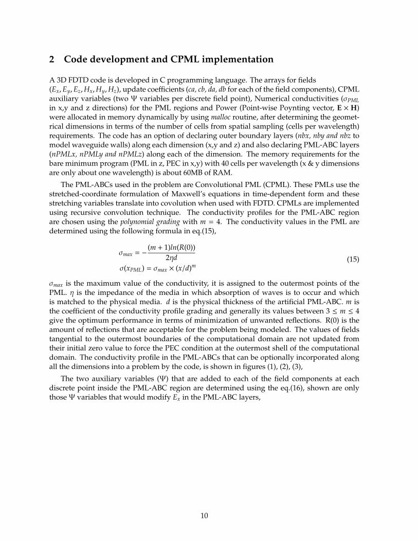
A 3D FDTD code is developed in C programming language. The arrays for fields(Ex,Ey,Ez,Hx,Hy,Hz), update coefficients (ca, cb, da, db for each of the field components), CPMLauxiliary variables (two Ψ variables per discrete field point), Numerical conductivities (σPMLin x,y and z directions) for the PML regions and Power (Point-wise Poynting vector, E × H)were allocated in memory dynamically by using malloc routine, after determining the geomet-rical dimensions in terms of the number of cells from spatial sampling (cells per wavelength)requirements. The code has an option of declaring outer boundary layers (nbx, nby and nbz tomodel waveguide walls) along each dimension (x,y and z) and also declaring PML-ABC layers(nPMLx, nPMLy and nPMLz) along each of the dimension. The memory requirements for thebare minimum program (PML in z, PEC in x,y) with 40 cells per wavelength (x & y dimensionsare only about one wavelength) is about 60MB of RAM.
The PML-ABCs used in the problem are Convolutional PML (CPML). These PMLs use thestretched-coordinate formulation of Maxwell’s equations in time-dependent form and thesestretching variables translate into covolution when used with FDTD. CPMLs are implementedusing recursive convolution technique. The conductivity profiles for the PML-ABC regionare chosen using the polynomial grading with m = 4. The conductivity values in the PML aredetermined using the following formula in eq.(15),
σmax = −(m + 1)ln(R(0))
2ηdσ(xPML) = σmax × (x/d)m
(15)
σmax is the maximum value of the conductivity, it is assigned to the outermost points of thePML. η is the impedance of the media in which absorption of waves is to occur and whichis matched to the physical media. d is the physical thickness of the artificial PML-ABC. m isthe coefficient of the conductivity profile grading and generally its values between 3 ≤ m ≤ 4give the optimum performance in terms of minimization of unwanted reflections. R(0) is theamount of reflections that are acceptable for the problem being modeled. The values of fieldstangential to the outermost boundaries of the computational domain are not updated fromtheir initial zero value to force the PEC condition at the outermost shell of the computationaldomain. The conductivity profile in the PML-ABCs that can be optionally incorporated alongall the dimensions into a problem by the code, is shown in figures (1), (2), (3),
The two auxiliary variables (Ψ) that are added to each of the field components at eachdiscrete point inside the PML-ABC region are determined using the eq.(16), shown are onlythose Ψ variables that would modify Ex in the PML-ABC layers,
10

Figure 1: σPMLx for PML-ABCs shown in a x-z section
11

Figure 2: σPMLy for PML-ABCs shown in a y-z section
12

Figure 3: σPMLz for PML-ABCs shown in a x-z section. This is implemented in the problem toabsorbs the waves propagating outwards in z-direction
13

ai =σi
(σiκi + κ2i αi)
(e−(σiκi
+αi) ∆tε − 1.0)
bi = e−(σiκi
+αi) ∆tε , (i = x, y or z)
Ψn+ 1
2exy
i− 12 , j+1,k+1
= byΨn− 1
2exy
i− 12 , j+1,k+1
+ ay(Hn+ 1
2z
i− 12 , j+
32 ,k+1−Hn+ 1
2z
i− 12 , j+
12 ,k+1
∆y)
Ψn+ 1
2exz
i− 12 , j+1,k+1
= bzΨn− 1
2exz
i− 12 , j+1,k+1
+ az(Hn+ 1
2y
i− 12 , j+1,k+ 3
2
−Hn+ 12
yi− 1
2 , j+1,k+ 12
∆z)
(16)
The variables κi and αi are used to absorb the evanescent/transient waves more effectively.PMLs are chosen to be sufficiently far away from the source such that the evanescent/transientmodes have negligibly small reflections from the PML-ABCs. Thereby, the values of κi = 1 andαi = 0 are chosen. The resultant equations for ai and bi in the PML thereby become relativelysimple as in eq.(17),
ai = (e−σi∆tε − 1.0)
bi = ai + 1 (i = x, y or z) (17)
The Ex field component inside PML-ABC thereby is implemented as in eq.(18),
En+1x
i− 12 , j+1,k+1
=
1 −
σi− 1
2 , j+1,k+1∆t
2 εi− 1
2 , j+1,k+1
1 +σ
i− 12 , j+1,k+1
∆t
2 εi− 1
2 , j+1,k+1
Enx
i− 12 , j+1,k+1
+
∆t
εi− 1
2 , j+1,k+1
1 +σ
i− 12 , j+1,k+1
∆t
2 εi− 1
2 , j+1,k+1
×
Hn+ 1
2y
i− 12 , j+1,k+ 3
2
−Hn+ 12
yi− 1
2 , j+1,k+ 12
∆z+ Ψ
n+ 12
exzi− 1
2 , j+1,k+1
−
Hn+ 1
2z
i− 12 , j+
32 ,k+1−Hn+ 1
2z
i− 12 , j+
12 ,k+1
∆y+ Ψ
n+ 12
exyi− 1
2 , j+1,k+1
−Jn
source xi− 1
2 , j+1,k+1
)
(18)
14

3 Validation of Numerical Solution
3.1 Analytical solution for waveguide with PEC walls
Analytical solution of waveguide modes (TEz and TMz) for Perfectly Electric Conducting (PEC)boundaries is obtained easily by using separation of variables method and assuming a standingwave solution (cosine and sine functions of spatial variables) in the directions that are boundedby PEC boundaries (two parallel y − z planes bind x-dimension and two parallel x − z planesbind y-dimension) and a traveling wave solution (variation in time as well as space, simplestbeing a complex exponential) in the direction of propagation (parallel to z-axis). The boundarycondition for electric fields is that those components tangential to the PEC are zero at theboundaries because no potential gradient can exist even momentarily in a material with infiniteconductivity as it will be instantaneously nullified by infinite current. This enforcement of PECwalls on a waveguide supports only those field distributions that are zero at least twice withinthe largest dimension of the waveguide cross-section (resonates with nodes at boundary walls).
Thereby, the lowest frequency that can exist and propagate without decaying in a PECboundary waveguide is that which has the distance between 0 and 180 phase points (half itswavelength) equal to the larger of the two transverse dimensions of the cavity and these pointslie on the PEC walls.
Let a and b be the two transverse dimensions of the waveguide such that a ≥ b, then thelowest cut-off frequency ( fc)10 = 1
2a√εµ corresponds to (λc)10 = 1
2a . The first of the modes toappear in a waveguide is TE10 mode and it has only a first order resonance with the larger ofthe two dimensions of the waveguide. The modes in a waveguide (being a structure boundedin two dimensions) denoted by m and n are the integer values that are used to represent theinfinitely many eigenvalues that satisfy the eigenfunctions in the bounded x and y directionsrespectively.
The analytical solutions for TE+zmn mode (Ez = 0) for propagation in +z-direction is given in
equation (19), (here the harmonic time-variation e jωt of field components is dropped)
E+x = Amn
βy
εcos(βxx)sin(βyy)e− jβzz
E+y = −Amn
βx
εsin(βxx)cos(βyy)e− jβzz
E+z = 0
H+x = Amn
βxβz
ωµεsin(βxx)cos(βyy)e− jβzz
H+y = Amn
βyβz
ωµεcos(βxx)sin(βyy)e− jβzz
H+z = − jAmn
β2c
ωµεcos(βxx)cos(βyy)e− jβzz
(19)
The analytical solutions for TM+zmn mode (Hz = 0) for propagation in +z-direction is given in
equation (20),(here the harmonic time-variation e jωt of field components is dropped)
15

E+x = −Bmn
βxβz
ωµεcos(βxx)sin(βyy)e− jβzz
E+y = −Bmn
βyβz
ωµεsin(βxx)cos(βyy)e− jβzz
E+z = − jBmn
β2c
ωµεsin(βxx)sin(βyy)e− jβzz
H+x = Bmn
βy
µsin(βxx)cos(βyy)e− jβzz
H+y = −Bmn
βx
µcos(βxx)sin(βyy)e− jβzz
H+z = 0
(20)
The eigenfunctions are derived from the boundary conditions where the tangential componentsof electric field go to zero. From the eigenfunction we get the eigenvalues that are shown inequation (21),
eigenvalues : βx =mπa
: m = 0, 1, 2 · · ·
eigenvalues : βy =nπb
: n = 0, 1, 2 · · ·(21)
The expression for analytical solutions were used in MATLAB R© to observe the solutions.Analytical solution is obtained for waveguide dimension of 2.286 × 1.016 cm2. Using this wefind that the cutoff frequency of this waveguide is ( fc)10 = 6.56 GHz. Figure 4 shows the cross-sectional field distribution for TE10 mode with PEC boundary layers. An excitation angularfrequency of ω = 2π × 1.0 × 1010rad/s is used.
It can be seen that for the dominant mode, TEz10 only Ey, Hx and Hy are non-zero.
16

Figure 4: TE10 mode distribution within WR-90 waveguide; visualization of analytical solu-tion. Note: used 400 points per wavelength when visualizing the analytical solution usingMATLAB R©.
17

3.2 FDTD solution for waveguide with PEC walls
To be able to check the validity of the code PEC walls are implemented on the x-z and y-z planes, the x-y cross-section of 2.286 × 1.016cm2 (corresponding to WR-90) is chosen. Anexcitation signal is applied to Ey field, over the geometry of a line that is placed in the centerof the waveguide (to not expose the PMLs to high evanescent/transient fields that develop inphysical problems such as Copper walls). The source has a sin(ωt) variation in time and is fixedat a frequency of 10.0 GHz for dominant mode as there will be no hinderance due to onset ofhigher order modes.
The waveguide length for FDTD is ' 4.0 wavelengths long. Figures 5 and 6 show thefield and power distribution in the cross-section about 0.4 ns after switching on the excitation.It is observed that by this time a steady-state is reached and the only variations in the fieldmagnitudes are on the order of those due to sinusoidal variation.
Comparing the FDTD solution of waveguide with PEC walls (figures 5 and 6) to the ana-lytical solutions (figure 4) it is clearly seen that the two are very closely matching each other.An exact comparison can be made by choosing an appropriate value for Amn in the analyticalsolution. Thereby, using the evidence from this comparison it can concluded that the FDTDcode is validated at least for the case of waveguide with PEC walls.
Figures (7), (8), (9) show a longitudinal section of the waveguide and the evolution of fieldsalong the propagating direction can be observed.
18

Figure 5: FDTD solution for fields with PEC boundary layers after about 0.4 ns from Ey linefield excitation switch on.
19

Figure 6: Pointwise Poynting vector on the x-y cross-section 0.4 ns after Ey line field excitationswitch on.
20
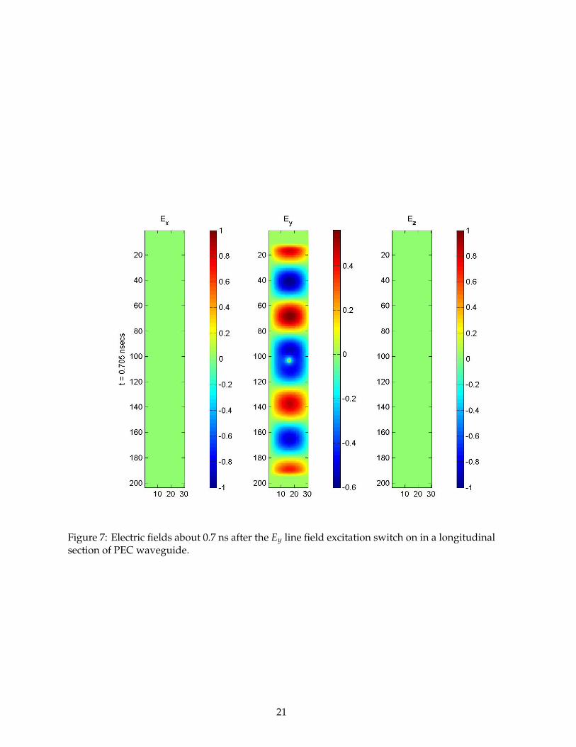
Figure 7: Electric fields about 0.7 ns after the Ey line field excitation switch on in a longitudinalsection of PEC waveguide.
21

Figure 8: Magnetic fields about 0.7 ns after the Ey line field excitation switch on in a longitudinalsection of PEC waveguide.
22

Figure 9: Power about 0.7 ns after the Ey line field excitation switch on in a longitudinal sectionof PEC waveguide.
23

4 FDTD solution of Waveguide with High-conductivity boundaries
FDTD solution to waveguide with high-conductivity metal boundary layers is obtained insteadof forcing the tangential fields to remain zero on the outermost shell of the free-space grid, bynot updating them from their initial zero value as done for PEC case. However, in addition tohaving the copper boundary layers and CPML layers, the PEC layers are still maintained onthe outermost shell of the computational domain (this is done by not updating the tangentialfield components for respective walls). The cross-section dimensions of the waveguide cavitycontaining air were not changed (2.286 × 1.016cm2) in terms of grid points.
The metal chosen for the boundary layers of the waveguide is Copper as it has an electricalconductivity, σ = 5.80 × 10⁷ S/m and a metal with such high conductivity is expected to have
a negligibly small skin depth δ =
ω√µε (12
[√1 + ( σωε )2 − 1
]) 12
−1
meters, for good conductors
( σωε )2 1 thereby δ '
√2ωµσ and as σ 1 we get δ ' 0 ) and thereby a resulting field and power
configuration that is closely equivalent to the analytical solution. Figures 10 and 11 show thefield and power distribution in a waveguide with copper boundary layers about 0.4 ns after theEy line field excitation turn on.
Comparing the analytical solution (figure 4) and FDTD solution for PEC boundary layers(figures 5 and 6) with FDTD solution for Copper boundary layers wall (figures 12, 13 and 14) it isobserved that there are evanescent/transient fields that are orders of magnitude weaker than themain field components (evanescent/transient E-fields are about seven orders of magnitude lesserand evanescent/transient H-field is about sixteen-seventeen orders of magnitude lesser). Theevanescent/transient fields also decay with distance, very rapidly compared to resonant fieldsbecause these fields are not naturally resonant with the waveguide cross-section dimensions.The evanescent/transient fields are sometimes useful to provide coupling between two pointsin a waveguide even though their spatial frequencies are not for the particular waveguide.
The evanescent/transient fields that are orders of magnitude (8 orders of magnitude smallerin the fields) weaker than the main field could also be purely computational artifacts. Theassumption that these are evanescent/transient fields is due to the fact that the fields are excitedby a single cell thick line source which has several higher-order modes. However, we havenot done a Fourier analysis to determine the spatial mode structure in the vicinity of the linesource. We plan to later explore and to solve with a higher-order solver, ticker line-source or amore fine-grid to see if that makes a difference to the order of magnitude of the fields that aredifferent from the analytical solutions.
The power flowing in the forward direction contained in the steady-state fields behavessimilar to the power in a waveguide with PEC boundary layers as there is negligible power losswith distance propagated down the waveguide (along z-axis).
24

Figure 10: FDTD solution for fields in a waveguide with Copper boundary layers sourced froman Ey line field sinusoidal excitation placed in the center. It can be observed that in this case thesolution develops some evanescent/transient fields.
25

Figure 11: Pointwise Poynting vector on the x-y cross-section of a waveguide with copperboundary layers sourced using Ey line field sinusoidal excitation.
26
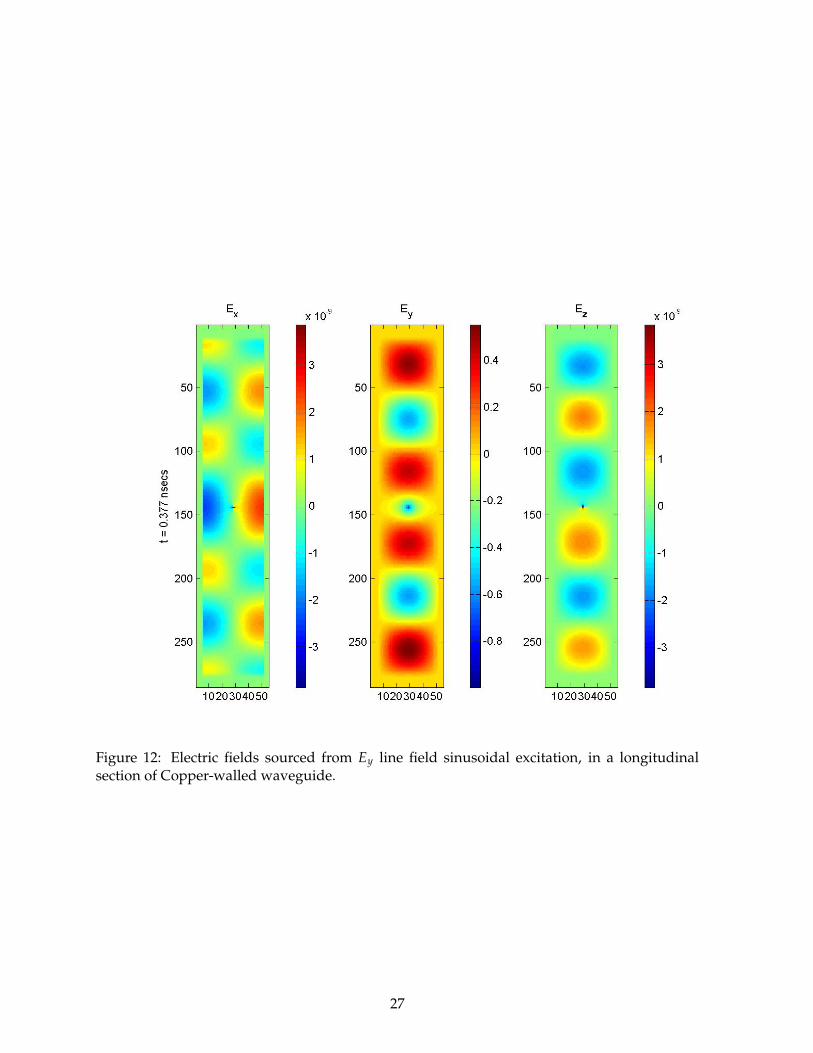
Figure 12: Electric fields sourced from Ey line field sinusoidal excitation, in a longitudinalsection of Copper-walled waveguide.
27

Figure 13: Magnetic fields sourced from Ey line field sinusoidal excitation, in a longitudinalsection of Copper-walled waveguide.
28
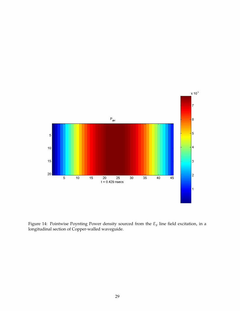
Figure 14: Pointwise Poynting Power density sourced from the Ey line field excitation, in alongitudinal section of Copper-walled waveguide.
29

5 Exciting higher-order modes in Waveguide using Coaxial probes
In previous parts of the problem Ey field in the geometry of a line located at the center ofthe computational grid was used to excite sinusoidal fields in the waveguide. This methodexcites the dominant mode TE10 when the excitation is within the specified frequency range ofoperation of the waveguide.
In this section we selectively excite higher-order modes of the parallel plate waveguide.Since, TEq0 is the first natural mode it is excited in the waveguide naturally and the fundamental-mode fields dominate the power partitioning. The TE20 mode is therefore selectively excitedusing two line sources of Ey fields which are out-of phase. Here, one full wave is seen to beresonating with the x-dimension confirming the generation of TE20 field. Fields excited usingout of phase sinusoidal excitations in Ey placed at (1/3) and (2/3) lengths of the x-dimension ofthe waveguide.
We carry our this analysis with Copper boundaries (σ = 5.80 × 10⁷ S/m). To determine thelosses to the wall for higher-order modes. In addition to looking at the spatial field profiles wealso look at the longitudinal propagation of fields and power in this rectangular waveguideselectively carrying a higher-order mode.
Analyzing the results of FDTD and comparing it to the analytical solution we see from thefield and power characteristics that a TE20-mode is excited.
30

Figure 15: TE20 mode distribution within WR-90 waveguide; visualization of analytical solu-tion. Note: used 400 points per wavelength when visualizing the analytical solution usingMATLAB R©.
31

Figure 16: FDTD solution for fields with Copper (σ = 5.80× 10⁷ S/m) boundary layers, showingthe fields in the cross-section of a physical waveguide. Fields are excited using two lines ofEy fields that are fed sinusoidally out-of-phase. Here, one full wave is seen to be resonatingwith the x-dimension confirming the generation of TE20 field. Fields excited using out of phasesinusoidal excitations in Ey placed at (1/3) and (2/3) lengths of the x-dimension of the waveguide.
32

Figure 17: FDTD solution for power with Copper boundary layers, showing the power in thecross-section of physical waveguide.
33

Figure 18: FDTD solution for Electric fields with Copper boundary layers, showing the fieldsin the cross-section of physical waveguide.
34
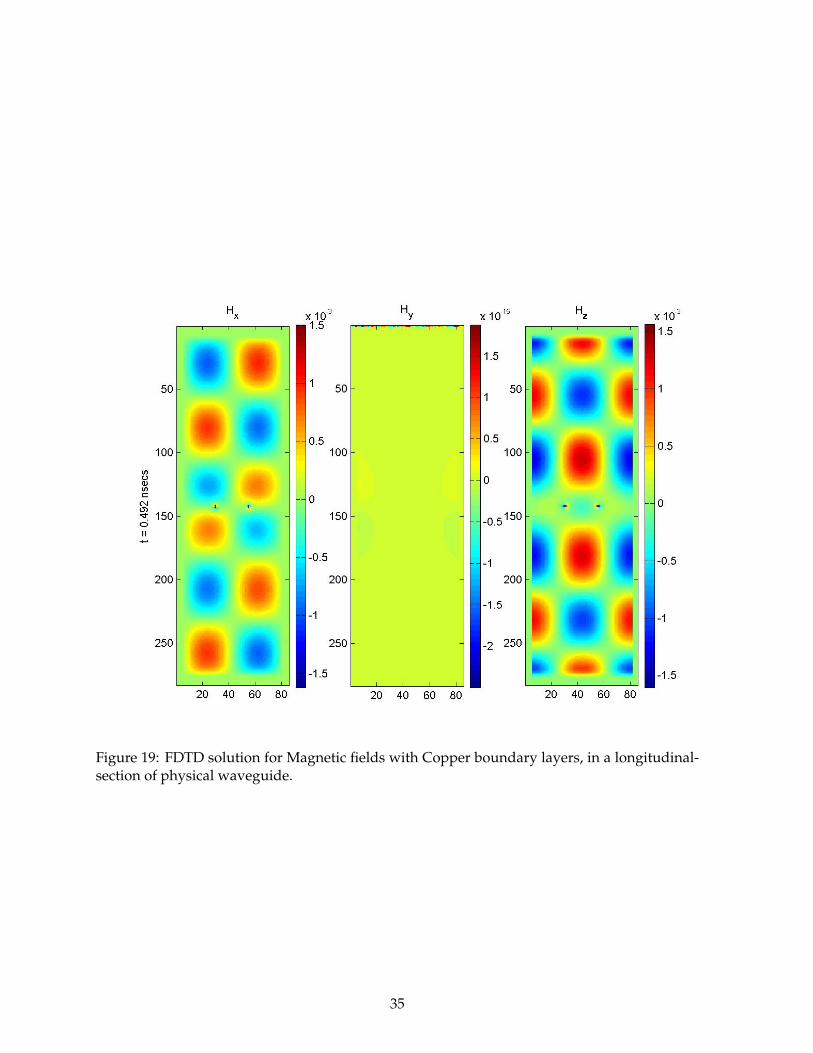
Figure 19: FDTD solution for Magnetic fields with Copper boundary layers, in a longitudinal-section of physical waveguide.
35

Figure 20: FDTD solution for Pointwise Poynting Power density with Copper boundary layers,in a longitudinal-section of physical waveguide.
36

6 Copper sphere suspended in the Waveguide
To analyze a problem which is very hard to model analytically and to explore the limitationof modeling curved surface with a mesh we setup a sphere freely suspended in a rectangularwaveguide. We look at the field profiles created in the vicinity of the sphere. We also look atthe power flow.
Analyzing the results we qualitatively find several interesting characteristics. The sphere asexpected distorts the TE10 mode in its vicinity. There is mode coupling from the fundamentalmode to higher order modes as seen from the field profiles in Fig.28 far away from the longi-tudinal location of the sphere. Whereas the fields not part of the TE10-mode were 8 orders ofmagnitude smaller here we see the higher-order modes are only 3 orders of magnitude smallerfrom the fundamental mode. At the location of the sphere in Fig.30 there is strong mode cou-pling to all the other fields and even the fundamental mode is completely distorted. The fieldsin components not present in TE10 are of the same order as the fundamental mode.
However, the more interesting observations are computational. The limit of the grid usedto model the problem shows that the sphere surface has sharp points and as a result the fieldsdevelop unphysical profiles at the sharp edges.
We note that there is a scope for very interesting future work of using non-uniform meshes.In the Adaptive Mesh Refinement (AMR) methods it is possible to grid the surface of the spherewith a number of cells that is many times higher than rest of the region of the problem underconsideration, namely the rectangular waveguide. By using cell-size which is smaller at theradial surface of the sphere we can reduce the computational problem of unphysical fields atsharp-edges.
6.1 Excitation at just above the waveguide cut-off frequency - Copper sphere sus-pended in the Waveguide
37
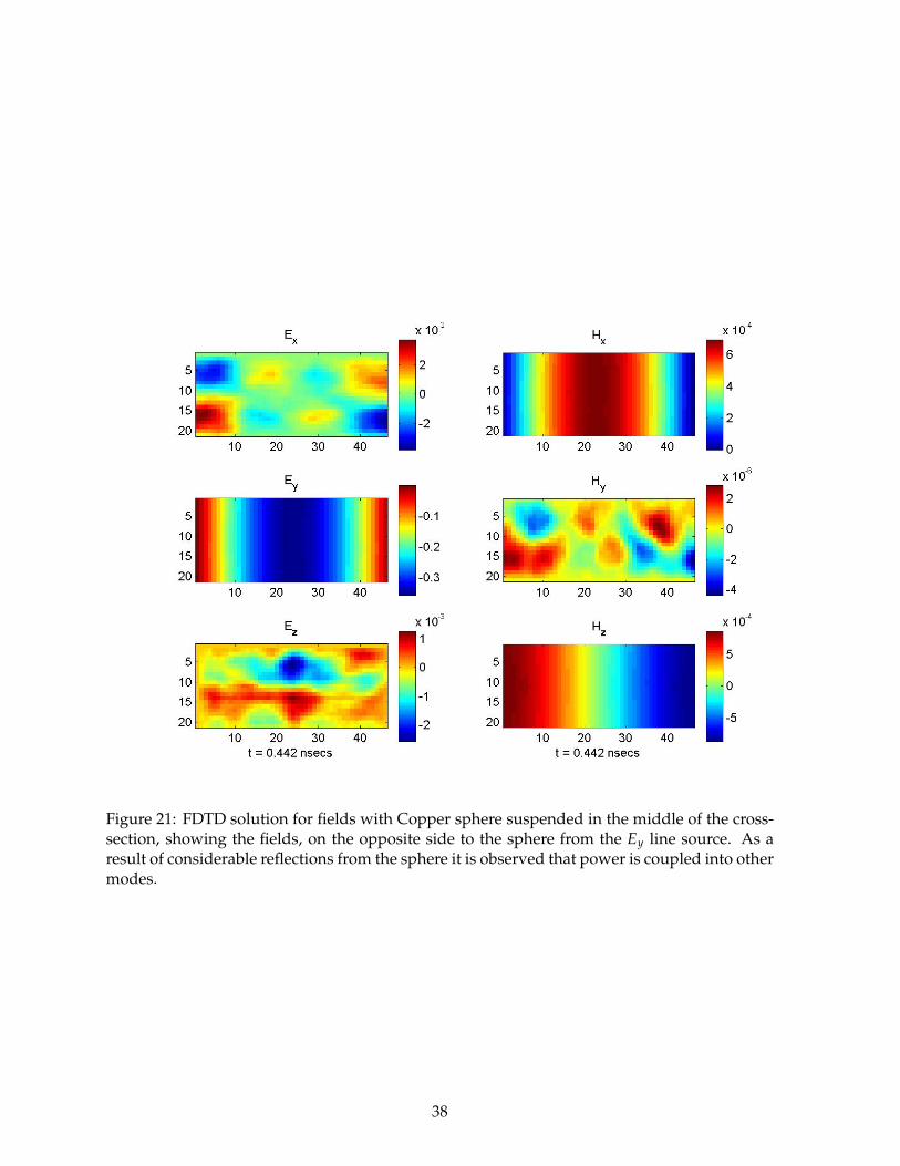
Figure 21: FDTD solution for fields with Copper sphere suspended in the middle of the cross-section, showing the fields, on the opposite side to the sphere from the Ey line source. As aresult of considerable reflections from the sphere it is observed that power is coupled into othermodes.
38

Figure 22: FDTD solution for Power with Copper sphere suspended in the middle of thecross-section, showing the power, on the opposite side to the sphere from the Ey line source.
39

Figure 23: FDTD solution for fields with Copper sphere suspended in the middle of the cross-section, showing the fields in the cross-section taken through the middle of the sphere.
40
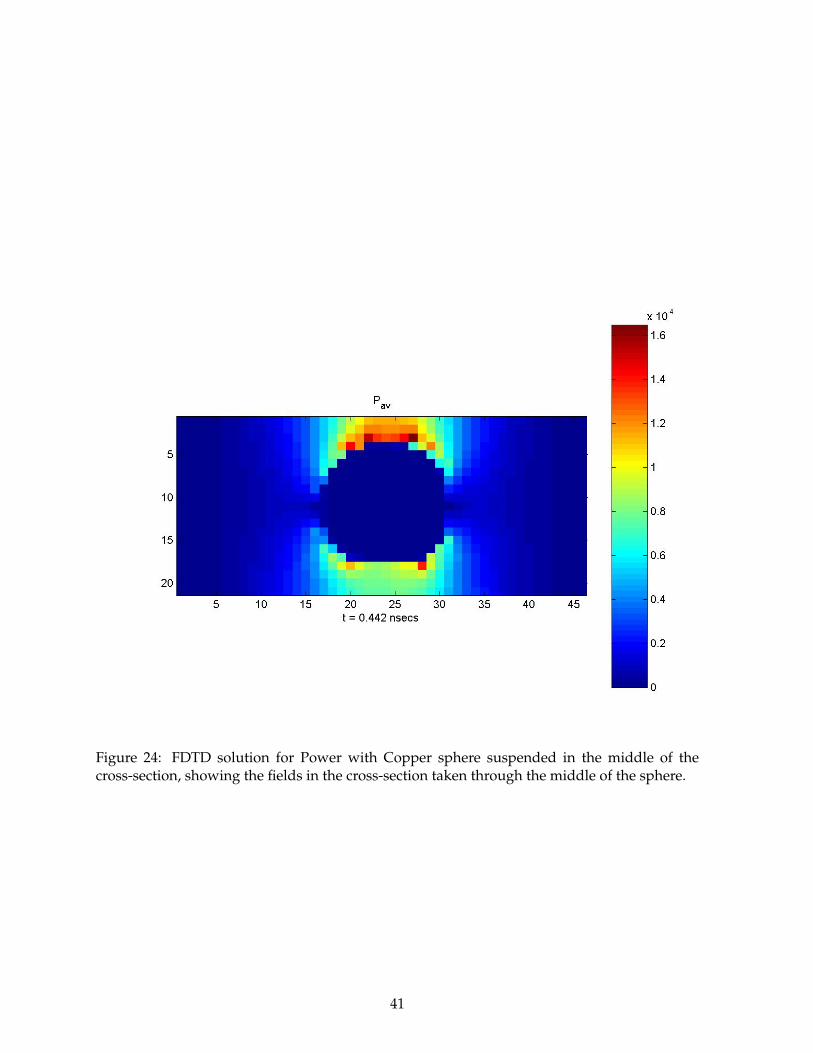
Figure 24: FDTD solution for Power with Copper sphere suspended in the middle of thecross-section, showing the fields in the cross-section taken through the middle of the sphere.
41

Figure 25: FDTD solution for Electric fields with Copper sphere suspended in the middle of thecross-section 30 grid points from the source, in a longitudinal-section of physical waveguide.
42

Figure 26: FDTD solution for Magnetic fields with Copper sphere suspended in the middle ofthe cross-section 30 grid points from the source, in a longitudinal-section of physical waveguide.
43

Figure 27: FDTD solution for Power with Copper sphere suspended in the middle of thecross-section 30 grid points from the source, in a longitudinal-section of physical waveguide.
44

6.2 Excitation at 2.5× waveguide cut-off frequency - Copper sphere suspended inthe Waveguide
We change the frequency of excitation to 2.5 × f 10c and determine the effect of the finite grid
cell-size.
Figure 28: FDTD solution for fields with Copper sphere suspended in the middle of the cross-section, showing the fields, on the opposite side to the sphere from the Ey line source. Thesourcing sinusoidal frequency is 2.5 × fc10 in this case. As a result of considerable reflectionsfrom the sphere it is observed that power is coupled into other modes.
45

Figure 29: FDTD solution for Power with Copper sphere suspended in the middle of the cross-section, showing the power, on the opposite side to the sphere from the Ey line source. Thesourcing sinusoidal frequency is 2.5 × fc10 in this case.
46

Figure 30: FDTD solution for fields with Copper sphere suspended in the middle of the cross-section, showing the fields in the cross-section taken through the middle of the sphere. Thesourcing sinusoidal frequency is 2.5 × fc10 in this case.
47

Figure 31: FDTD solution for Power with Copper sphere suspended in the middle of the cross-section, showing the fields in the cross-section taken through the middle of the sphere. Thesourcing sinusoidal frequency is 2.5 × fc10 in this case.
48

Figure 32: FDTD solution for Electric fields with Copper sphere suspended in the middle of thecross-section 30 grid points from the source, in a longitudinal-section of physical waveguide.The sourcing sinusoidal frequency is 2.5 × fc10 in this case.
49
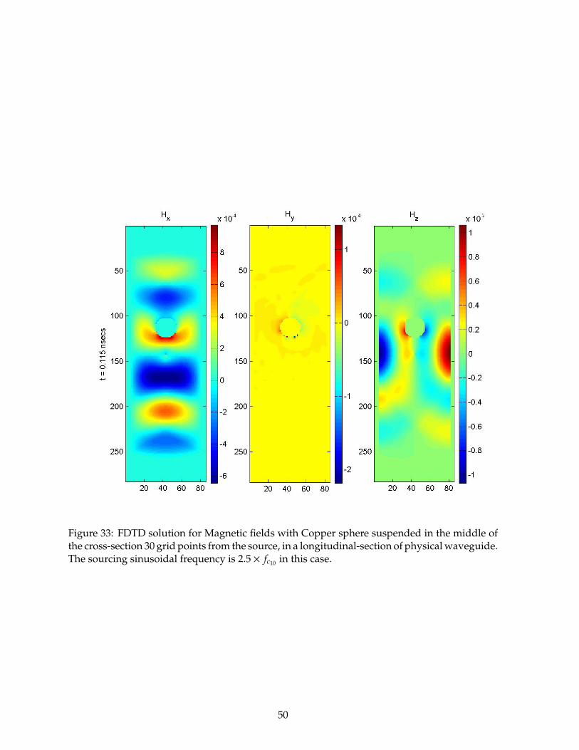
Figure 33: FDTD solution for Magnetic fields with Copper sphere suspended in the middle ofthe cross-section 30 grid points from the source, in a longitudinal-section of physical waveguide.The sourcing sinusoidal frequency is 2.5 × fc10 in this case.
50

Figure 34: FDTD solution for Power with Copper sphere suspended in the middle of thecross-section 30 grid points from the source, in a longitudinal-section of physical waveguide.
51

7 Exploring with FDTD
7.1 Boundaries of decreasing Conductivity
It is observed that in boundaries with lower conductivities, the penetration of fields into theboundary layers increases and the field distribution that is observed with high conductivityboundaries is distorted when boundaries have low conductivities. There is also a highercoupling of the modal fields into the evanescent/transient fields. A PEC outer boundary ismaintained for the boundary layers of the waveguide.
When compared to the field distribution in the waveguide for boundaries with coppermaterial, significant differences were observed when boundaries with a σ = 1000 S/m materialare used. Figures 35 and 36 show the field and power distribution in a plane transverse to thedirection of propagation (x − y plane) at a distance of 1.8 cm from the source and 0.53 ns afterthe Ey line field excitation turn on.
Figure 35: FDTD solution with σ = 1000 S/m boundary layers, fields at 1.8 cm, 0.53 ns after Eyline field excitation turn on.
For boundary layers with a conductivity of σ = 100 S/m, Figures 37 and 38 show the fieldand power distribution in a plane transverse (x − y plane) to the direction of propagation at adistance of ' 11 cm, 0.53 ns after the Ey line field excitation turn on. With lower conductivitiesthere is less attenuation to the fields that are penetrating into the boundary layers and thereby
52

Figure 36: FDTD solution with σ = 1000 S/m boundary layers, power at 1.8 cm, 0.53 ns after Eyline field excitation turn on.
there is a possibility of the fields striking the outer boundary of dielectric layers.
To get a feel for power loss down the waveguide due to low-conductivity of σ = 100 in theboundaries, reproduced in Figures 39 and 40 is the field and power distribution at steady state;at ' 17 cm from the source as compared to 1.8 cm, 0.83 ns after Ey line field excitation turn on.At this distance, we can observe a fall in power for the steady state fields.
The effect of fields striking and forming patterns due to the outer boundary of the lowconductivity boundary layers is more evident when we use layers with a conductivity of σ = 10S/m. Figures 41 and 42 show the field and power distribution in a plane transverse to thedirection of propagation at 1.8 cm, 0.18 ns after the Ey line field excitation is turned on.
To get a feel for power loss in the waveguide due to low-conductivity of σ = 10 S/m inthe boundaries, reproduced in Figure 43 is the power distribution at ' 7.3 cm from the sourceas compared to 1.8 cm, 0.39 ns after Ey line field excitation turn on. At this distance, we canobserve a fall in power in steady state fields.
53
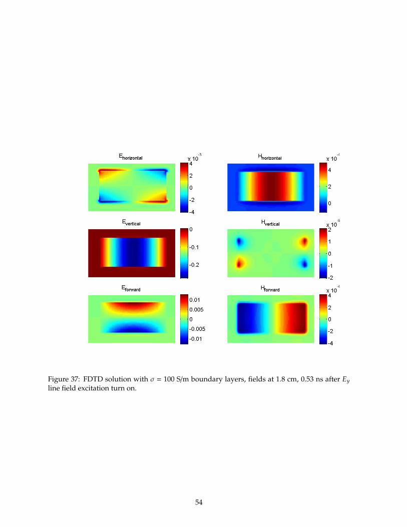
Figure 37: FDTD solution with σ = 100 S/m boundary layers, fields at 1.8 cm, 0.53 ns after Eyline field excitation turn on.
54
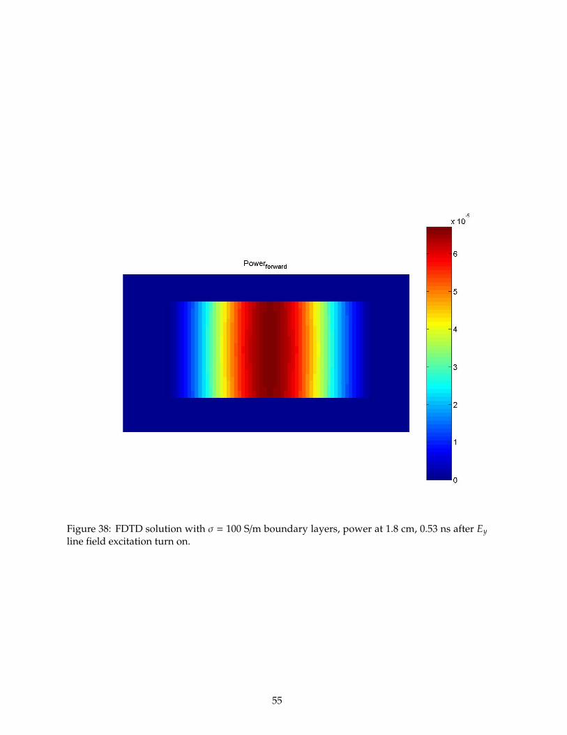
Figure 38: FDTD solution with σ = 100 S/m boundary layers, power at 1.8 cm, 0.53 ns after Eyline field excitation turn on.
55

Figure 39: FDTD solution with σ = 100 S/m boundary layers, fields at 17 cm, 0.83 ns after Ey linefield excitation turn on. Here a comparison is made with the field distribution at a distance of1.8 cm (along z-axis) from the source and a drop is observed in the steady state field strength.
56
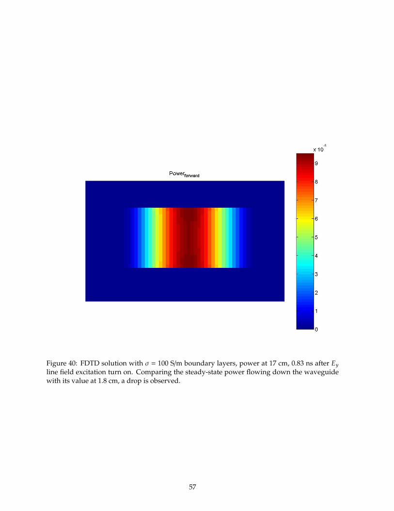
Figure 40: FDTD solution with σ = 100 S/m boundary layers, power at 17 cm, 0.83 ns after Eyline field excitation turn on. Comparing the steady-state power flowing down the waveguidewith its value at 1.8 cm, a drop is observed.
57

Figure 41: FDTD solution with σ = 10 S/m boundary layers, fields at 1.8 cm, 0.18 ns after Ey linefield excitation turn on.
58

Figure 42: FDTD solution with σ = 10 S/m boundary layers, power at 1.8 cm, 0.18 ns after Eyline field excitation turn on.
59
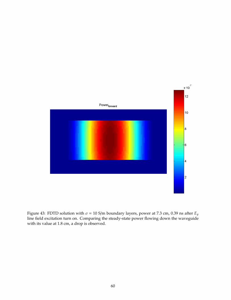
Figure 43: FDTD solution with σ = 10 S/m boundary layers, power at 7.3 cm, 0.39 ns after Eyline field excitation turn on. Comparing the steady-state power flowing down the waveguidewith its value at 1.8 cm, a drop is observed.
60

Figure 44: FDTD steady-state field solution for brick boundary layers with σ = 0.01 S/m and εr= 4.44, fields at ' 22 cm, 2.96 ns after Ey line field excitation turn on.
7.2 Dielectric Boundary with brick material
The properties of brick material were used directly from [1]. This material is used in theboundary layers to simulate the effect of walls in indoor hallways. Brick material has a dielectricconstant of εr = 4.44 and the conductivity of σ = 0.01 S/m. When using the brick material for theboundary layers their width is increased (doubled compared to conducting boundary layersused in section 4.1) to avoid significant reflections from the PEC termination that is used at theouter edge of dielectric boundaries (thicker the boundaries the larger is the distance that thefields have to penetrate before striking the outer PEC walls). The waveguide cavity dimensionsof cross-section containing air were not changed (2.286 × 1.016cm2). Figures 44 and 45 showthe steady state field and power distribution at a distance of ' 22 cm, 2.96 ns after the Ey linesource is turned on.
Figures 46 and 47 show the steady state field and power distribution at a distance of' 22 cm,3.1 ns after the Ey line source is turned on. These figures are included to show the attainmentof steady state by the field components (only sinusoidal variations with time are present) asindicated by the fixed spatial pattern observed.
61

Figure 45: FDTD steady-state power solution for brick boundary layers with σ = 0.01 S/m andεr = 4.44, power at ' 22 cm, 2.96 ns after Ey line field excitation turn on.
62

Figure 46: FDTD steady-state field solution for brick boundary layers with σ = 0.01 S/m and εr= 4.44, fields at ' 22 cm, 3.1 ns after Ey line field excitation turn on. This figure illustrates theattainment of steady state fields wherein fields achieve a steady spatial pattern and only varysinusoidally with time due to the source.
63

Figure 47: FDTD steady-state power solution for brick boundary layers with σ = 0.01 S/m andεr = 4.44, power at ' 22 cm, 3.1 ns after Ey line field excitation turn on.
64

8 Radio-wave propagation in Guided channels
8.1 Model description
The modeling of radio-wave propagation in wireless channels with guiding effects (Indoorhallways, Street canyons etc.) is investigated by first understanding behavior of the funda-mental modes using waveguide and T-junctions. These propagation effects take significancebecause the carrier wavelengths are smaller or comparable to the structure dimensions in thepresent wireless technology implementations. However, we note that since in real channels thestructure dimension is many times the cm-scale wavelengths the propagation in a Cell-phoneor WiFi channel has multiple modes. Multiple modes can be modeled by later parallelizing thecode and solving over the full geometry - however that requires matrices of size 108 to 109 andis beyond the scope of the current work.
The progress made since initial development of the FDTD code (numerical solution method-ology to solve Maxwell’s partial differential equations, used in this work) is two-fold, as follows:
1) An analysis of field components, average power per unit area (pointwise Poynting vector,℘) and energy propagation (ε, integrating pointwise Poynting vector over infinitesimally smalltime increments, limdt→0 Σ℘ dt '
∫℘ dt = ε, pointwise energy per unit area integrated upto
the current time) as the waves propagate down a standard waveguide geometry continuouslyexcited by a sinusoidal line source (Ey component is excited at center coordinates over a linealong the vertical dimension), is done for different boundary materials.
2) An analysis of a T-shaped structure with cross-sectional dimensions of the standardwaveguide that is continuously excited by a sinusoidal line source (Ey component at the centercoordinates over a line along the vertical dimension) is done. A profile of energy fall-off aswaves propagate around the corner (junction of the two perpendicular arms of the T structure)is obtained. The change in the field mode-configuration as waves propagate around a corner isalso observed.
The source frequency (10.0 GHz) in these simulation is chosen such that only the dominantmode TEz
10 (first order Ey, Hx and Hz field components) is excited in an ideal waveguide withPEC walls, simplifying the analysis of numerical solution with respect to analytical solution.
An analysis of the Electric and Magnetic field mode-configuration (in the x-y cross-sectionalplane) resulting from simulations was earlier done in the code-development stages and itwas found in complete agreement with analytical solutions (fact that solutions exist and arerelatively simple for ideal PEC boundary conditions was used for the validation of code).
The numerical solution from simulation results for propagation characterisitics of waves(Space-Time variation of electromagnetic fields) are presented in the sections that follow.
65

8.2 T structure with PEC boundary
The standard waveguide (WR-90) dimensions were used to implement a structure in the shapeof a T. This structure has two arms one of which is longer (this is where the field excitationis placed) and a shorter (side) arm (about half of the size of the main arm). The two armsintersect each other at right angles towards an end of the longer (main) arm. The results fromthis numerical solution can be divided into three depending upon the position of the sinusoidalexcitation, these are as follows:
1) center of the main-arm
2) center of the side-arm (main-arm end touching the side-arm)
3) end of the main-arm (opposite to side-arm location)
4) an end of the side-arm
8.3 Source at the center of main-arm
The figures fig.48 to fig.52 show the variation in the field components as they propagate fromthe source into the geometry of the T-structure. The source in this case is placed in the centerof the longer arm.
We can observe from the figures that the y-component of the electric field that sourcesthe T structure, Ey which has a −sin(βxx)cos(βyy) variation in x-y cross-section plane whenpropagating down a waveguide does not change its mode configuration when it propagatesaround a corner (fig.48).
The x-component of magnetic field, Hx which manifests as sin(βxx)cos(βyy) in the longer armchanges its x-y variation to cos(βxx)cos(βyy) mode configuration in the x-y cross-section whenpropagating around the corner (fig.49).
Similarly, the z-component of magnetic field, Hz which manifests as cos(βxx)cos(βyy) in thelonger arm changes its x-y variation to sin(βxx)cos(βyy) in the x-y cross-section when propagatinginto the side arm going around the corner (fig.50).
66
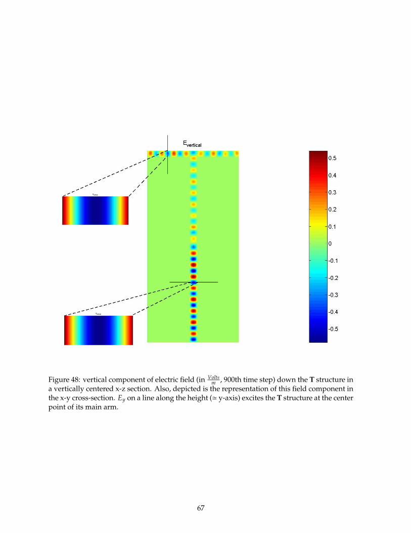
Figure 48: vertical component of electric field (in Voltsm , 900th time step) down the T structure in
a vertically centered x-z section. Also, depicted is the representation of this field component inthe x-y cross-section. Ey on a line along the height (' y-axis) excites the T structure at the centerpoint of its main arm.
67

Figure 49: horizontal component (x-axial) of magnetic field (in Amperesm , 900th time step) down
the T structure in a vertically centered x-z section. Also, depicted is the representation of thisfield component in the x-y cross-section. This field component is observed to switch its modeconfiguration as it goes around a corner. Ey on a line along the height (' y-axis) excites the Tstructure at the center point of its main arm.
68
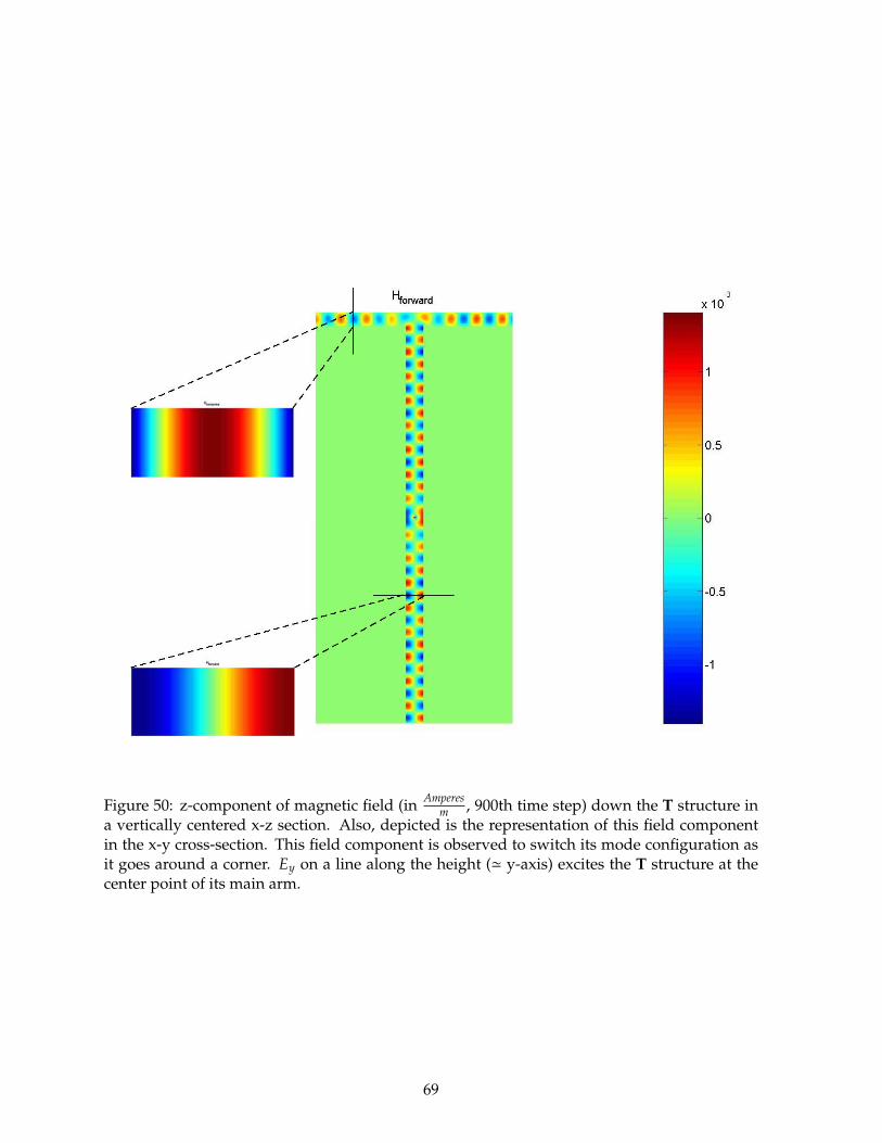
Figure 50: z-component of magnetic field (in Amperesm , 900th time step) down the T structure in
a vertically centered x-z section. Also, depicted is the representation of this field componentin the x-y cross-section. This field component is observed to switch its mode configuration asit goes around a corner. Ey on a line along the height (' y-axis) excites the T structure at thecenter point of its main arm.
69

Figure 51: pointwise Poynting vector ( Wattsm2 , 900th time step) down the T strcture in a vertically
centered x-z section. Also, depicted is the representation of this field component in the x-ycross-section. Ey on a line along the height (' y-axis) excites the T structure at the center pointof its main arm.
70

Figure 52: y-axis: pointwise energy in Joulesm2 down the T structure (900th time step), x-axis: 0 to
nz (number of field evaluation points in z-direction). Ey on a line along the height (' y-axis)excites the T structure at the center point of its main arm.
71

Figure 53: y-component of electric field (in Voltsm , 1400th time step) down the T structure in a
vertically centered x-z section. Ey on a line along the height (' y-axis) excites the T structure atthe center point of its side-arm.
8.4 Source at the center of side-arm (end of the main-arm touching the side-arm)
The figures fig.53 to fig.57 show the variation in the field components as they propagate fromthe source into the geometry of the T-structure when the source is placed in the center of theside arm.
The observation in this case is similar to above wherein the sourced component of fieldsie. y-component of the electric field, Ey that sources the T structure, does not change itspropagating mode when it propagates around a corner (figure 53), whereas the x-componentof magnetic field, Hx and the z-component of magnetic field, Hz (fig.54 and fig.55) change theirmode configuration when propagating around the corner into the side-arm from the main-arm.
72
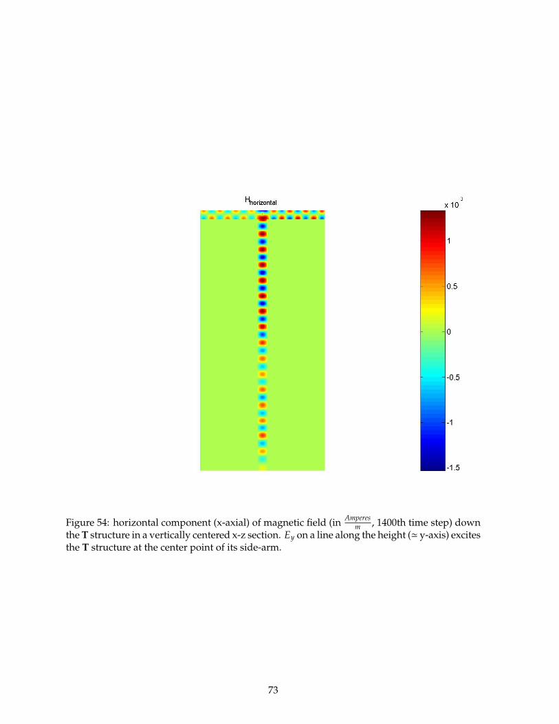
Figure 54: horizontal component (x-axial) of magnetic field (in Amperesm , 1400th time step) down
the T structure in a vertically centered x-z section. Ey on a line along the height (' y-axis) excitesthe T structure at the center point of its side-arm.
73
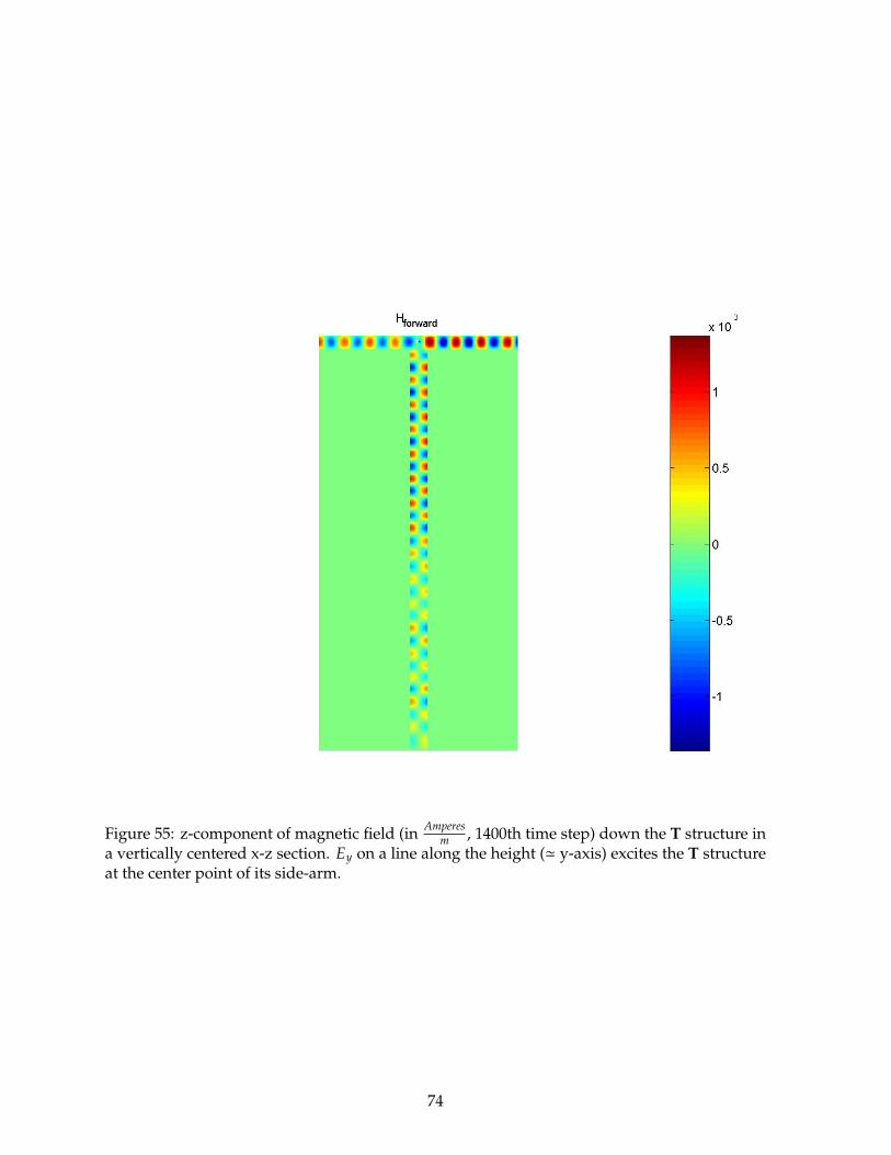
Figure 55: z-component of magnetic field (in Amperesm , 1400th time step) down the T structure in
a vertically centered x-z section. Ey on a line along the height (' y-axis) excites the T structureat the center point of its side-arm.
74
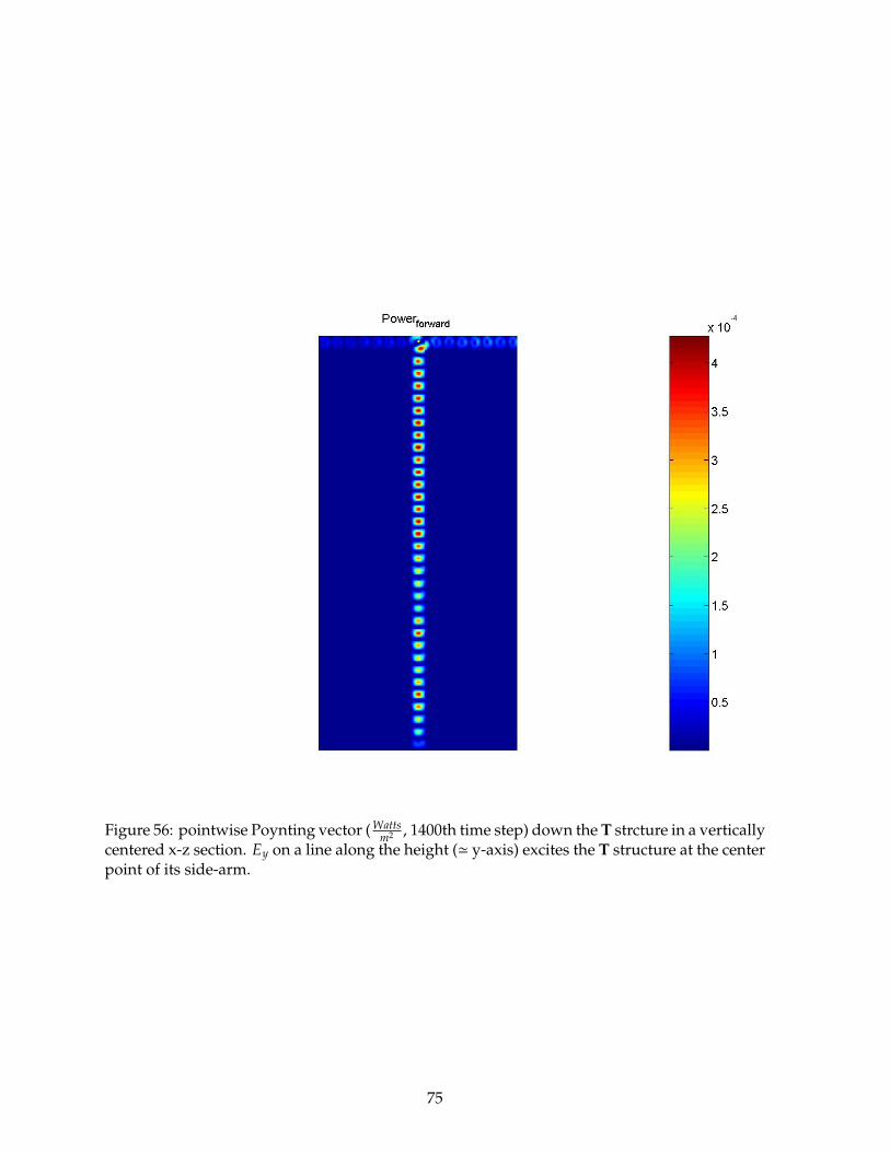
Figure 56: pointwise Poynting vector ( Wattsm2 , 1400th time step) down the T strcture in a vertically
centered x-z section. Ey on a line along the height (' y-axis) excites the T structure at the centerpoint of its side-arm.
75
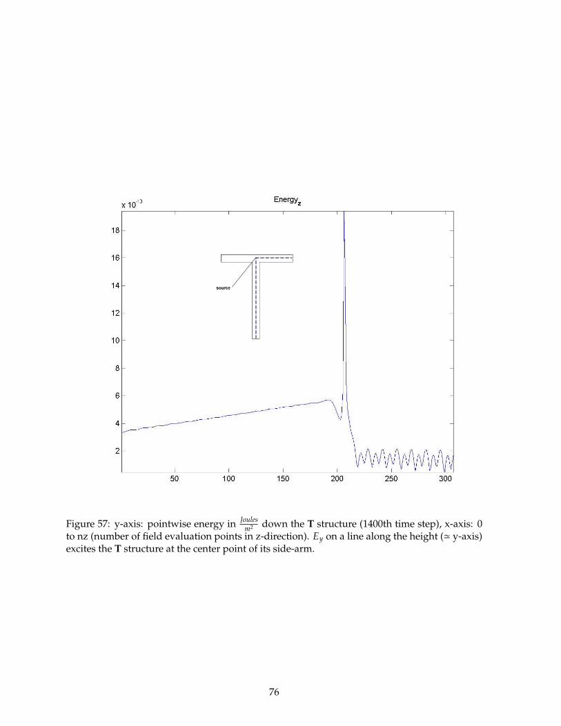
Figure 57: y-axis: pointwise energy in Joulesm2 down the T structure (1400th time step), x-axis: 0
to nz (number of field evaluation points in z-direction). Ey on a line along the height (' y-axis)excites the T structure at the center point of its side-arm.
76
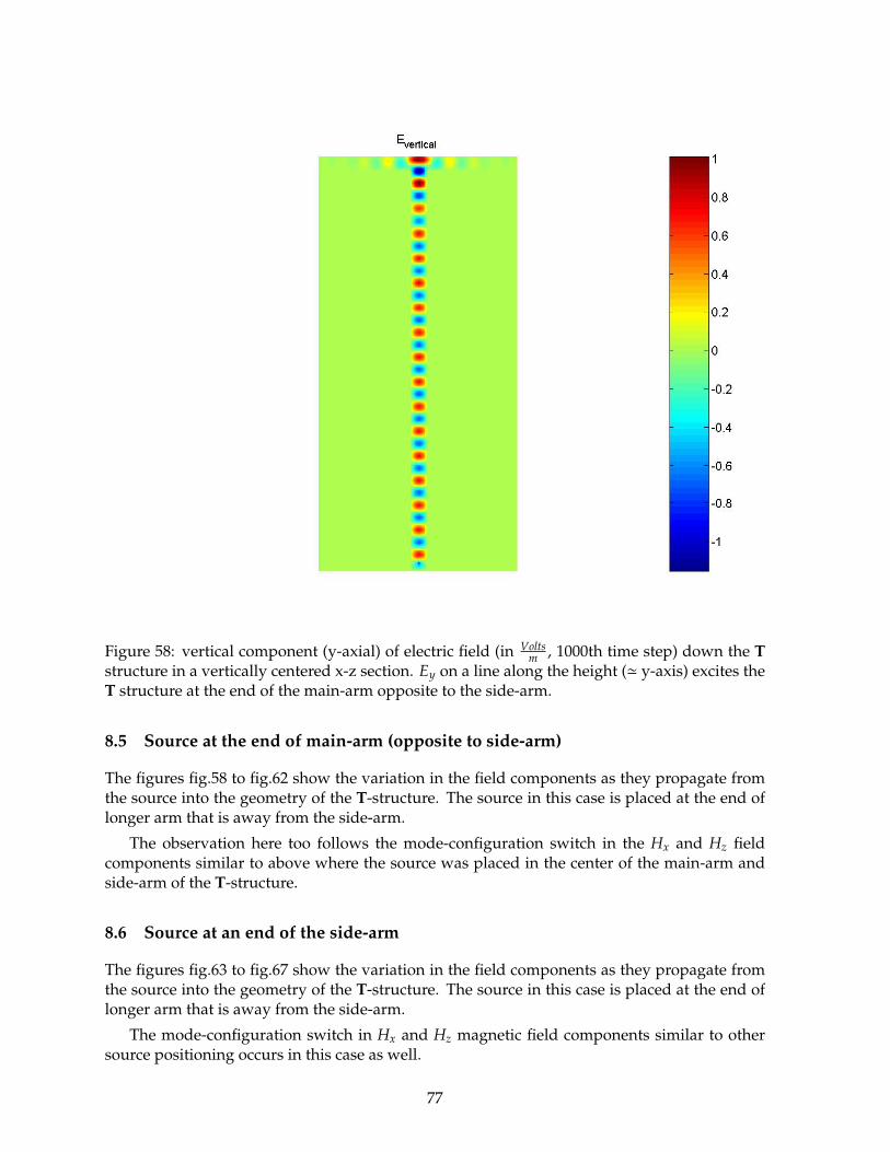
Figure 58: vertical component (y-axial) of electric field (in Voltsm , 1000th time step) down the T
structure in a vertically centered x-z section. Ey on a line along the height (' y-axis) excites theT structure at the end of the main-arm opposite to the side-arm.
8.5 Source at the end of main-arm (opposite to side-arm)
The figures fig.58 to fig.62 show the variation in the field components as they propagate fromthe source into the geometry of the T-structure. The source in this case is placed at the end oflonger arm that is away from the side-arm.
The observation here too follows the mode-configuration switch in the Hx and Hz fieldcomponents similar to above where the source was placed in the center of the main-arm andside-arm of the T-structure.
8.6 Source at an end of the side-arm
The figures fig.63 to fig.67 show the variation in the field components as they propagate fromthe source into the geometry of the T-structure. The source in this case is placed at the end oflonger arm that is away from the side-arm.
The mode-configuration switch in Hx and Hz magnetic field components similar to othersource positioning occurs in this case as well.
77

Figure 59: horizontal component (x-axial) of magnetic field (in Amperesm , 1000th time step) down
the T structure in a vertically centered x-z section. Ey on a line along the height (' y-axis) excitesthe T structure at the end of the main-arm opposite to the side-arm.
78

Figure 60: z-component of magnetic field (in Amperesm , 1000th time step) down the T structure in
a vertically centered x-z section. Ey on a line along the height (' y-axis) excites the T structureat the end of the main-arm opposite to the side-arm.
79
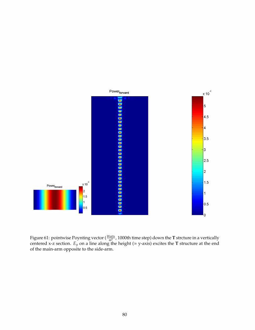
Figure 61: pointwise Poynting vector ( Wattsm2 , 1000th time step) down the T strcture in a vertically
centered x-z section. Ey on a line along the height (' y-axis) excites the T structure at the endof the main-arm opposite to the side-arm.
80

Figure 62: y-axis: pointwise energy in Joulesm2 down the T structure (1000th time step), x-axis: 0
to nz (number of field evaluation points in z-direction). Ey on a line along the height (' y-axis)excites the T structure at the end of the main-arm opposite to the side-arm.
81

Figure 63: vertical component of electric field (in Voltsm , 1200th time step) down the T structure in
a vertically centered x-z section. Ey on a line along the height (' y-axis) excites the T structureat an end of the side-arm.
82
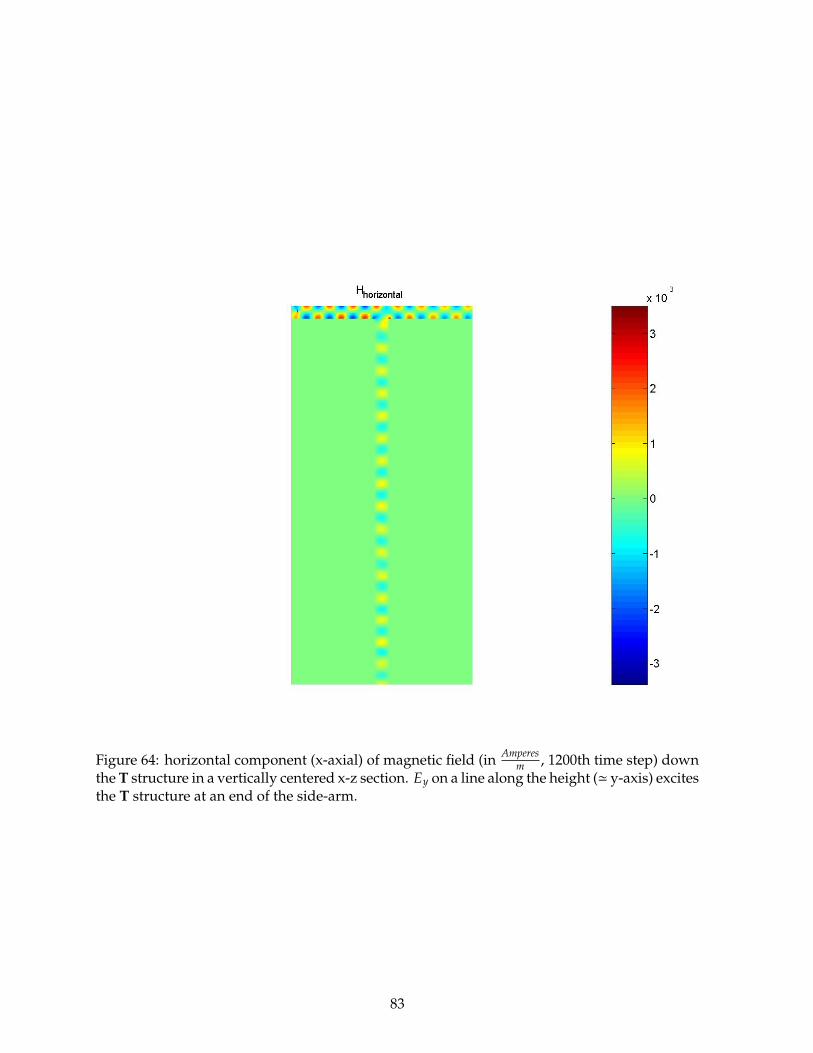
Figure 64: horizontal component (x-axial) of magnetic field (in Amperesm , 1200th time step) down
the T structure in a vertically centered x-z section. Ey on a line along the height (' y-axis) excitesthe T structure at an end of the side-arm.
83

Figure 65: z-component of magnetic field (in Amperesm , 1200th time step) down the T structure in
a vertically centered x-z section. Ey on a line along the height (' y-axis) excites the T structureat an end of the side-arm.
84

Figure 66: pointwise Poynting vector ( Wattsm2 , 1200th time step) down the T strcture in a vertically
centered x-z section. Ey on a line along the height (' y-axis) excites the T structure at an end ofthe side-arm.
85

Figure 67: y-axis: pointwise energy in Joulesm2 down the T structure (1200th time step), x-axis: 0
to nz (number of field evaluation points in z-direction). Ey on a line along the height (' y-axis)excites the T structure at an end of the side-arm.
86

References
[1] Dana Porrat, Radio Propagation in Hallways and Streets for UHF Communications, Adissertation submitted to department of Electrical Engineering, Stanford University in partialfulfillment of requirements for the degree of Doctor of Philosophy, December 2002.
[2] Dana Porrat, Donald C. Cox, UHF Propagation in Indoor Hallways, IEEE transactions onWireless Communications vol.3, no.4, 1188-1198, July, 2004.
[3] Andersen J. B., Rappaport T. S., Yoshida S., Propagation measurements and models forWireless Communications channels, IEEE Communications magazine, 42-49, January, 1995.
[4] Saleh A. A. M., Valenzuela R. A., A Statistical model for Indoor Multipath Propagation,IEEE Journal on selected areas in communications vol.SAC-5, no.2, 128-137, February, 1987.
[5] Bertoni H. L., Honcharenko W.,et.al., UHF Prediction for Wireless Personal Communica-tion, Proceedings of IEEE vol.82, no.9, 1333-1359, September, 1994.
[6] Liang G., Bertoni H. L., A new approach to 3-D ray-tracing for propagation prediction incities, IEEE transactions on Antennas and Propagation vol.46, no.6, 853-863, June, 1998.
[7] Honcharenko W., Bertoni H. L.,et.al., Mechanisms governing UHF propagation on singlefloors in modern office buildings, IEEE transactions on Vehicular Technology vol.41, no.4,496-504, November, 1992.
[8] Lee J., Bertoni H. L., Coupling at Cross, T, and L junctions in tunnels and urban streetcanyons, IEEE transactions on Antennas and Propagation vol.51, no.5, 926-935, May, 2003.
[9] Emslie A. G., Lagace R. L., Strong P. F., Theory of the propagation of UHF radio waves incoal mine tunnels, IEEE transcations on Antennas and Propagation vol.AP-23, no.2, 192-205,March, 1975.
[10] Taflove A., Hagness S. C., Computational Electrodynamics: The Finite Difference TimeDomain method, Artech House Inc., 2nd ed., 2000.
[11] Taflove A., Brodwin M. E., Numerical solution of steady-state electromagnetic scatteringproblems using time dependent Maxwell’s equations, IEEE transactions on Microwave theoryand techniques vol.MTT-23, no.8, 623-630, August, 1975.
[12] Yee K. S., Numerical solution of Initial boundary value problems involving Maxwell’sequations in Isotropic media, IEEE transactions on Antennas and Propagation vol.AP-14,no.3, 302-307, May 1966.
[13] Booton Jr. R. C., Computational methods for Electromagnetics and Microwaves, WileySeries in Microwave and Optical engineering, 1992.
[14] Jurgens T. G.,Taflove A.,Umashankar K.,Moore T. G., Finite-Difference Time-Domain mod-elling of curved surfaces, IEEE transactions on Antennas and Propagation vol.40, no.4, 357-366,April, 1992.
[15] Lee J. F. , Palandech R., Mittra R., Modelling three-dimensional discontinuities in waveg-uides using nonorthogonal FDTD algorithm, IEEE transactions on Microwave theory andtechniques vol.40, no.2, 346-352, February, 1992.
87

[16] Jurgens T. G., Taflove A., Three-Dimensional Contour FDTD modeling of scattering fromsingle and multiple bodies, IEEE transcations on Antennas and Propagation vol.82, no.12,1703-1708, December 1993.
88
Related Documents