Photoacoustic wave propagation simulations using the FDTD method with Berenger's perfectly matched layers

Photoacoustic Wave Propagation Simulations Using the FDTD Method with Berenger’s Perfectly Matched Layers

Yae-Lin Sheua, Chen-Wei Weia, Chao-Kang Liaoa, and Pai-Chi Lia,b

aDepartment of Electrical Engineering, National Taiwan University, Taipei, Taiwan bInstitute of Biomedical Electronics and Bioinformatics, National Taiwan University, Taipei, Taiwan

Tel.: +886-2-33663551, Fax: +886-2-83691354 E-mail: [email protected]

ABSTRACT

Several photoacoustic (PA) techniques, such as photoacoustic imaging, spectroscopy, and parameter sensing, measure quantities that are closely related to optical absorption, position detection, and laser irradiation parameters. The photoacoustic waves in biomedical applications are usually generated by elastic thermal expansion, which has advantages of nondestructiveness and relatively high conversion efficiency from optical to acoustic energy. Most investigations describe this process using a heuristic approximation, which is invalid when the underlying assumptions are not met. This study developed a numerical solution of the general photoacoustic generation equations involving the heat conduction theorem and the state, continuity, and Navier-Stokes equations in 2.5D axis-symmetric cylindrical coordinates using a finite-difference time-domain (FDTD) scheme. The numerical techniques included staggered grids and Berenger’s perfectly matched layers (PMLs), and linear-perturbation analytical solutions were used to validate the simulation results. The numerical results at different detection angles and durations of laser pulses agreed with the theoretical estimates to within an error of 3% in the absolute differences. In addition to accuracy, the flexibility of the FDTD method was demonstrated by simulating a photoacoustic wave in a homogeneous sphere. The performance of Berenger’s PMLs was also assessed by comparisons with the traditional first-order Mur’s boundary condition. At the edges of the simulation domain, a 10-layer PML medium with polynomial attenuation grading from zero to 5×106 m3/kg/s was designed to reduce the reflection to as low as –60 and –32 dB in the axial and radial directions, respectively. The reflections at the axial and radial boundaries were 32 and 7 dB lower, respectively, for the 10-layer PML absorbing layer than for the first-order Mur’s boundary condition.

Keywords: photoacoustic signal, finite-difference time-domain, FDTD, absorption coefficient

1. INTRODUCTION

Photoacoustic techniques in biomedical field combines laser irradiation and ultrasound detection and offers advantage of visualizing optical properties (for example, the optical absorption) with less susceptibility to light scattering as compared with all-optical techniques. For nondestructiveness and noninvasiveness, most biomedical applications utilize photoacoustic waves generated by the thermal expansion process. In the thermal expansion process, the temperature changes is due to local heating controlled by energy absorption and deposition in the medium, which is often given by the laser irradiation. The stress field that subsequently propagates through the sample results from the inhomogeneous temperature distribution. Most of the theories of the generation and propagation of a photoacoustic wave are derived from intuitive concepts of the processes related to this effect. Rigorous analysis of the phenomenon, which involves solving a nonstationary thermoelasticity problem, was performed by Gusev and Karabutov [1]. Deriving the answer from the governing equations for the general case is tedious, especially for a complicated energy distribution

Photons Plus Ultrasound: Imaging and Sensing 2008: The Ninth Conference on BiomedicalThermoacoustics, Optoacoustics, and Acousto-optics, edited by Alexander A. Oraevsky, Lihong V. Wang,

Proc. of SPIE Vol. 6856, 685619, (2008) · 1605-7422/08/$18 · doi: 10.1117/12.764416

Proc. of SPIE Vol. 6856 685619-12008 SPIE Digital Library -- Subscriber Archive Copy

geometry. The use of numerical methods falls between rigorous theoretical mathematical derivations, which are usually limited to simple geometries of energy deposition due to the assumptions necessary to make the task feasible, and experiments, in which the photoacoustic signals are generally small and suffer from unavoidable noise interference, such that considerable effort using advanced devices is required to ensure the accuracy of results when the data cannot be estimated theoretically. To this end, we employed a numerical finite-difference time-domain (FDTD) method to directly solve the governing equations of the photoacoustic wave.

In the simulation domain the boundary conditions need to be specified. Generally, the first-order Mur’s boundary condition is used for free space simulation. [2] However, in practice the first-order Mur’s boundary condition is poor in eliminating reflected waves from truncated edges, and causes errors in simulation. We overcame this shortcoming by using Berenger’s perfectly matched layers (PMLs) to minimize the interference. The concept of Berenger’s PMLs is to use a damping factor in the boundary region, containing several grids, which is called layers. When the incoming wave arrives, the wave would attenuate accordingly if the impedance of both the simulation region and the PMLs are matched. Therefore no reflected wave is going backward. In this study, the numerical results were validated according to the analytical solution derived by solving the linear-perturbation equations with the Laplace transform for several detection angles and different laser-source parameters [1]. The performance of the boundary was evaluated, and compared with other types of boundary conditions that were commonly used, including the second-order Mur’s boundary condition, and the Bayless-Turkel operator of order two.

2. FORMULATION

The following heat conduction, continuity, Navier-Stokes, and state equations proposed by Gusev and Karabutov [1] describe a thermally generated photoacoustic wave:

STtsT

v⋅∇−′∇κ⋅∇=

∂′∂

ρ 00 , (1a)

sCT

pCT

TVP

′+′ρβ

=′ 0

0

0 , (1b)

sCTc

ABccp

P′β

ρ+ρ′ρ

+ρ′=′ 0200

2

0

202

0 2, (1c)

( )( ) 00 =ρ′+ρ⋅∇+∂ρ′∂ ut

v , (1d)

)(3

))(()( 200 uuuup

tu vvvvv

⋅∇∇⎟⎠⎞

⎜⎝⎛ η

+ξ+∇η+∇⋅ρ′+ρ−=′∇+∂∂

ρ′+ρ . (1e)

The heat conduction theorem in Eq. (1a) describes the temporal diffusion of energy in the sample, stating that the net energy flowing in equals the applied energy, which is the Umov-Poynting vector S

v of the incident laser source

averaged over the electromagnetic oscillation. The divergence of the radiation intensity in the medium (i.e., the energy distribution) is commonly described by the Beer-Lambert law when the sample is assumed to be homogeneous. The states, namely the pressure deviation per unit mass ( p′ ) and the temperature deviation (T ′ ), are associated with other states (density deviation ρ′ and entropy deviation per unit mass s′ ) by Maxwell relations (i.e., Eqs. (1b) and (1c)). Constants 0ρ , 0c , and 0T correspond to the ambient density, velocity, and temperature, respectively, while κ , β ,

PC , VC , and AB / are the coefficients of thermal conductivity, thermal expansion, specific heat at constant pressure, specific heat at constant volume, and nonlinear acoustic parameter of the medium, respectively. Eqs. (1a)–(1c) describe the generation of an optical signal. According to the conservation of mass and momentum (Eqs. (1d) and (1e), respectively), the generated photoacoustic wave will propagate outward and be subject to diffraction, nonlinear distortion,

Proc. of SPIE Vol. 6856 685619-2

PML region ('rcy;)

and dissipation. Here uv is the vibration velocity of the particles in the medium, while ξ and η are the bulk and shear viscosities of the medium, respectively.

A staggered mesh is adopted in the FDTD discretization. The spatial grid size is commonly chosen to be one-tenth

of the minimum wavelength of the photoacoustic wave (i.e., { }Lc τα−0

1,min101 ). The temporal grid size is then

determined by Courant’s criterion for ensuring stability. A 2.5D axis-symmetric cylindrical-coordinates system (with the z-axis parallel to the direction of irradiation) is employed so as to reduce the memory required for computation. The simulation configuration is depicted in Fig. 1. The boundary condition at the surface of the incident irradiation ( 0=z ) is set to be rigid, which indicates that 0=uv . There is a free boundary condition (i.e., 0=p ) at the interface.

Fig. 1: Simulation configuration. The direction of light irradiation was along the symmetric axis z , and the interface at 0=z was rigid. The simulation domain was enclosed by the PMLs (region denoted by dashed lines) for free-space boundaries.

For the free-space simulation, Berenger’s PMLs were designed to eliminate artificial reflections of incoming waves induced at the truncated edges [3]. A PML medium is a perfect simulation of free space, in that a plane wave does not change its direction of propagation or its speed when it propagates from free space into a PML medium. The idea behind a PML boundary condition is to define a nonphysical set of equations in the PML region that exhibit large attenuation whilst simultaneously producing no reflections for a wave propagating into the PML region from an adjoining lossless acoustic region. Berenger’s method requires splitting the nonvector variables such as ρ′ manually into two additive components: zr ρ′+ρ′=ρ′ . Parameters rσ and zσ are the artificial attenuations in the PMLs for rρ′ and zρ′ ,

respectively, while *rσ and *

zσ are those for ru and zu . Perfect matching at the interface between the simulation medium and PMLs is achieved by ensuring that

( ) rr c σρ=σ 20

20

* / , (2a)

( ) zz c σρ=σ 20

20

* / . (2b) However, numerical reflections arise due to finite spatial sampling when implementing the PML as a single step discontinuity of zr ,σ and *

,zrσ in the FDTD lattice. To overcome this problem, Berenger proposed that the PML losses along the direction normal to the interface should gradually increase from zero [4]. The polynomial grading adopted is simply

max,))/(()( rm

rr Lrr σ∆=σ , (3a)

max,))/(()( zm

zz Lzz σ∆=σ , (3b)

where m is the polynomial order, L is the number of the PMLs, and r∆ and z∆ are the spatial grid sizes in the r and z directions, respectively. The PML parameters can be readily determined for a given reflection factor of the

Proc. of SPIE Vol. 6856 685619-3

boundary )(φR (where φ is the incident angle of the wave at the truncated boundary):

LcRm

zrzr

,00max,max, )/(2

)0(ln)1(,∆ρ

+−=σσ . (4)

In aqueous media such as water, where the relaxation of the thermal field is generally slower than that of the photoacoustic wave transiting the heated region, Eq. (1a) does not cause significant reflection along the truncated edges, especially at boundaries far from where the wave is generated. The boundary condition for Eq. (1a) can simply be the first-order Mur’s boundary.

3. RESULTS

The accuracy of the simulation was evaluated by the analytical solution of Eqs. (1a)–(1e) whilst only retaining linear-perturbation terms (and hence neglecting acoustic dissipation). The problem could then be easily solved by the spectral method by introducing the scalar potential of the velocity field. According to Gusev and Karabutov [1], the analytical solution could be derived from the spectral form as

[ ]

[ ]⎪⎪⎭

⎪⎪⎬

⎫

⎪⎪⎩

⎪⎪⎨

⎧

τα−τττα−τ+τα−ττ−τα−α−

τα+τττατ−τα+ττ−ταα

⋅πρβ

=τ

)2//()exp()/1()2//(1)exp(

)2//()exp()/1()2//(1)exp(

16),(

00

000

00

000

0

0

LLL

LL

LLL

LL

P

cGccerfcc

cGccerfcc

CW

Ruv

, (5)

where 0/ cRtv

−=τ is the retarded time, ∫∞

∞−⋅= tf(t)IπRαW D d0

20 is the total absorbed energy, and )(tG is the

Gaussian function. Note that the profile of 22zr uuu += is similar to that of the pressure.

For arbitrary detection angle when the laser pulse duration is short, an effective Gaussian light pulse of duration

0* /sin cRDL θ=τ . (6)

is used to modify Eq. (5). The FDTD results and the analytical solution obtained by Eq. (5) are compared in Fig. 2. In each graph, the solid

and dashed lines indicate the numerical and theoretical results, respectively. The error (indicated by each dashed-dotted line) was calculated as the absolute difference between the simulation result and analytical solution. The laser pulse durations for Fig. 2(a) and 2(b) were Lτ = 5 ns and Lτ = 50 ns, respectively. It is evident that Lτ = 50 ns does not fulfill stress confinement as is usually assumed in heuristic approximations. Fig. 2(a) and 2(b) indicate that the results from the numerical simulation agreed with Eq. (5) within average errors of 2.78% and 4%, respectively. The maximum error occurred at the rarefaction peak of the photoacoustic wave, and was 16% and 13% for the short- and long-pulse cases, respectively.

Proc. of SPIE Vol. 6856 685619-4

mean error: 2.78%maximum error: 16.25%

Analytical SolutionPA Simulation

— — - Error Function

-1.2-0.5 -0.3 -0.1 0.1 0.3 0.5

ktS

>,

0e>eta0-VeNaE0z

>,

0a)>a)ta)0-Va)Na)E0z

ktS

moan!I

Analytical Solution— PA Simulation

0.8 ---- Error Function

8 0.4>

-0.4 0: 8.12

-0.8

-1.2-0.5 -0.3 -0.1 0.1 0.3 0.5

18h/

01 00102 03 04

(a) (b) Fig. 2: Forward photoacoustic (PA) wave computed by the FDTD method (solid lines) and using Eq. (6) (dashed lines) for Lτ =5ns (a)

and Lτ =50 ns (b). The absolute error is indicated by the dashed-dotted lines. The simulation results for an off-axis photoacoustic wave are shown in Fig. 3(a) and 3(b) for θ = 8.12o, θ = 15.94o, θ = 22.60o, and θ = 31.97o, respectively. The average errors between the simulations and analytical solution using Eqs. (5) and (6) were 1.25%, 1.86%, 2.41%, and 2.58%, respectively. The maximum error, of around 12%, was located at the most negative part of each wave. The error rose when the off-axis angle increased, for that Eq. (6) is not a suitable modification when the angle is large. [1] For the maximum error, one possible reason for this is that the far-distance assumption when deriving the temporal form analytical solution from its spectrum oversimplified the diffraction phenomenon. However, the closed-form equation could not be defined without making this assumption. The deviation in the exponentially rising part of the wave is due to the accumulated errors when using finite differences to estimate a fast-rising function. The numerical experiments for the first case demonstrated that FDTD method was capable of solving a system of partial differential equations and that the results were consistent with those derived theoretically.

(a) (b)

Proc. of SPIE Vol. 6856 685619-5

mum error 1264%

-0.3 -0.2 -0.1 0 0.1 0.2 0.3

mum error 1622% V

-0.3 -0.2 -0.1 0 0.1 0.2 0.3

(c) (d) Fig. 3: Off-axis PA wave computed by the FDTD method (solid line) and using Eqs. (5) and (6) (dashed line) for θ = 8.12o (a), θ=

15.94o (b), θ = 22.60o (c), and θ = 31.97o (d). The absolute error is indicated by the dashed-dotted lines.

4. DISCUSSIONS

Reflection errors from truncated boundaries are evaluated by the normalized boundary reflection error function, defined as [3]

∫∫ −

= TBBtrue

Ttrue

dttzrp

dttzrptzrpzrerror

0

20

2

10),,(

),,(),,(log10),( , (7)

where T is the total simulation interval. Interval T was chosen to be 130 times the duration of laser irradiation, where waves reflected from edges r and z have not yet arrived at the symmetrical axis and the rigid interface, respectively. The uncontaminated field, truep , was computed by executing the FDTD code on a larger area. The power was normalized relative to the time-integrated power at ),( BB zr , which are the coordinates of the maximum wave incident at the z boundary.

The error functions for different types of boundary conditions are displayed in Fig. 4. In Fig. 4(a), where there is no absorbing boundary but instead total reflection at the r and z boundaries, the maximum errors were 2.35 and 0.04 dB at the r and z boundaries, respectively. Both z boundaries in Fig. 4(b) and 4(c) have the first-order Mur’s condition, and the maximum error was about –24 dB. The r boundary in Fig. 4(c) was improved by about 4 dB by applying the first-order Bayliss-Turkel condition rather than the first-order Mur’s condition in Fig. 4(b). However, the boundary reflection by the second-order Mur’s condition is -18.53dB, and did not improve the error. This is because that the operator of the second-order Mur’s condition is designed to eliminate the wave in Cartesian coordinate, but not in the cylindrical coordinate. The maximum error in r boundary in this case remained the same.

The boundary condition for Fig. 4(e) is the 10-layer PML condition. At the r boundary, the reflection error from the PML was similar to that from the first-order Bayliss-Turkel condition, while in the z direction the maximum error in the PML was 25 dB lower than that of the first-order Mur’s boundary. Moreover, the performance in the z direction was consistent for different incident angles of the wave, where the maximum reflection in Fig. 4(b) and 4(c) occurred near to a grid index of 400 pixels. The average reflection error of the PML was about -60 dB, and although this was 32 dB lower than that of the first-order Mur’s boundary, it did not meet the design value of -100 dB. This was due to the discretization error dominating when max,zσ was too large, and the actual reflection error was potentially orders of magnitude higher than that predicted by Eq. (4). The optimal choice for max,zσ that balances reflection from the outer boundary of the

Proc. of SPIE Vol. 6856 685619-6

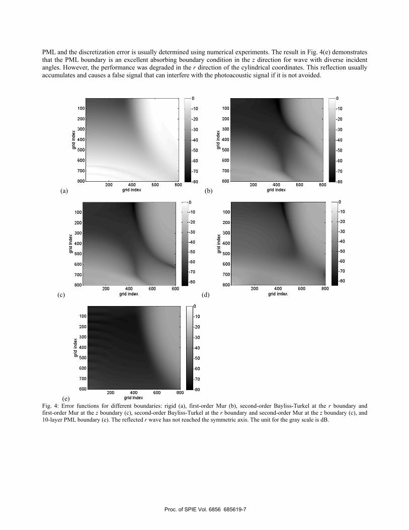
400grid index

0

-10

-20

-30

-40

-50

-60

-70

-80400

grid index

0

-10

-20

-30

-40

-50

-60

-70

-80

400grid index

0

-10

-20

-30

-40

-50

-60

-70

-80

AUU

grid index

400grid index

0

-10

-20

-30

-40

-50

-60

-70

-80

PML and the discretization error is usually determined using numerical experiments. The result in Fig. 4(e) demonstrates that the PML boundary is an excellent absorbing boundary condition in the z direction for wave with diverse incident angles. However, the performance was degraded in the r direction of the cylindrical coordinates. This reflection usually accumulates and causes a false signal that can interfere with the photoacoustic signal if it is not avoided.

(a) (b)

(c) (d)

(e) Fig. 4: Error functions for different boundaries: rigid (a), first-order Mur (b), second-order Bayliss-Turkel at the r boundary and first-order Mur at the z boundary (c), second-order Bayliss-Turkel at the r boundary and second-order Mur at the z boundary (c), and 10-layer PML boundary (e). The reflected r wave has not reached the symmetric axis. The unit for the gray scale is dB.

Proc. of SPIE Vol. 6856 685619-7

According to the numerical experiments, the performance of Berenger’s PMLs is better than the traditional

boundary conditions. Error improvement is little by higher order boundary conditions and sometimes worse, however, it could be achieved by adding layers of the PMLs. The performance of the boundary conditions in the radial direction is restricted by the cylindrical coordinate form used in this study, since the Berengers’ PMLs are carried out in the Cartesian coordinate. Modified forms are required if lower reflection in the radial reflection is to be achieved.

5. CONCLUSIONS

In this paper, the general thermally induced photoacoustic wave equations were solved using an FDTD scheme in a 2.5D axis-symmetric cylindrical-coordinates domain. The simulation results are evaluated by the analytical equation solved from the original equations. For free space simulation, the 10-layer PML was designed to produce the lowest reflection error for commonly used boundary conditions.

6. ACKNOWLEDGMENTS

Financial supports from National Science Council (grant# NSC 96-2221-E-002 -030), National Health Research Institutes, NTU Center for Genomic Medicine, and NTU Nano Center for Science and Technology are gratefully acknowledged.

REFERENCES

1. V. Gusev and A. Karabutov, Laser Optoacoustics, Chap 2, pp. 45-48. American Institute of Physics, New York (1993). 2. D. Huang, C. Liao, C. Wei, and P. Li, “Simulations of optoacoustic wave propagation in light-absorbing media using a finite-difference time-domain method,” J. Acoust. Soc. Am. 117, pp. 2795-2801 (2005) 3. X. Yuan, D. Borup, J. Wiskin, M. Berggren, R. Eidens, and S. Johnson, “Formulation and validation of Berenger’s PML absorbing boundary for the FDTD simulation of acoustic scattering,” IEEE Trans. Ultrason. Ferroelectr. and Freq. Control 44, pp. 816-822 (1997). 4. J. Berenger, “A perfectly matched layer for the absorption of electromagnetic waves,” J. Comput. Phys. 114, pp. 185-200 (1994).

Proc. of SPIE Vol. 6856 685619-8