Fastfood – Approximating Kernel Expansions in Loglinear …vgg/rg/slides/le__icml2013__fastfood... · Fastfood – Approximating Kernel Expansions in Loglinear Time Quoc Le, Tamas

Fastfood – Approximating Kernel Expansions in Loglinear Time

Quoc Le, Tamas Sarlos, and Alex Smola

Presenter: Shuai Zheng (Kyle)

Large Scale Problem: ImageNet Challenge

• Large scale data

– Number of training examples m = 1,200,000 in ILSVRC1000 dataset.

– Dimensions of encoded features for most algorithm, d is more than 20,000. (You can get better performance with bigger dictionary dimension, but you might have memory limit issue.)

– Number of support vectors: usually n > 0.1*m

SVM Tradeoffs Linear Kernel Non-linear Kernel

Training speed Very fast Very slow

Training scalability Very high Low

Testing speed Very fast Very slow

Testing accuracy Lower Higher

How to get all yellow characteristics? Additive Kernels (e.g. Efficient Additive Kernels via Explicit Feature Maps, PAMI 2011). New direction: Approximate Kernel with fake random Gaussian Matrices (Fastfood).

When Kernel Methods meet Large Scale Problem

• In kernel methods, for large scale problems, computing the decision function is expensive, especially at prediction time.

• So shall we give up nonlinear kernel methods at all? – No, we have better approximation solution.

– Turn to linear SVM + (features + complicated encoding(LLC, Fisher coding, group saliency coding) + sophisticated pooling (max pooling, average pooling, learned pooling)), and now neural network.

High-dimensional Problem vs Kernel approximation

CPU Training RAM Training CPU Test RAM Test

Naive O(𝑚2𝑑) O(md) O(md) O(md)

Reduced set O(𝑚2𝑑) O(md) O(nd) O(nd)

Low rank O(𝑚𝑛𝑑) O(𝑛𝑑) O(nd) O(nd)

Random Kitchen Sinks (RKS)

O(𝑚𝑛𝑑) O(𝑛𝑑) O(nd) O(nd)

Fastfood O(𝑚𝑛 log𝑑) O(𝑛 log𝑑) O(𝑛 log𝑑)

O(n)

𝑑 is the input feature dimension,

𝑛 is the number of nonlinear basis functions

𝑚 is the number of samples.

𝑓 𝑥 = 𝑤, 𝜙(𝑥) = 𝛼𝑖

𝑛

𝑖=1

𝜙 𝑥𝑖 𝜙(𝑥) = 𝛼𝑖𝑘(𝑥𝑖 , 𝑥)

𝑚

𝑖=1

Kernel expansion

CPU Training RAM Training CPU Test RAM Test

Naive O(𝑚2𝑑) O(md) O(md) O(md)

Reduced set O(𝑚2𝑑) O(md) O(nd) O(nd)

Low rank O(𝑚𝑛𝑑) O(𝑛𝑑) O(nd) O(nd)

Random Kitchen Sinks (RKS)

O(𝑚𝑛𝑑) O(𝑛𝑑) O(nd) O(nd)

Fastfood O(𝑚𝑛 log𝑑) O(𝑛 log𝑑) O(𝑛 log𝑑)

O(n)

High-dimensional Problem vs Fastfood

𝑑 is the input feature dimension, e.g. d= 20,000. 𝑛 is the number of nonlinear basis functions, e.g. n = 120,00.

𝑚 is the number of samples, e.g. m = 1,200,000.

Kernel expansion 𝑓 𝑥 = 𝑤, 𝜙(𝑥) = 𝛼𝑖

𝑛

𝑖=1

𝜙 𝑥𝑖 𝜙(𝑥) = 𝛼𝑖𝑘(𝑥𝑖 , 𝑥)

𝑚

𝑖=1

Random Kitchen Sinks (Rahimi & Recht, NIPS 2007)

• Given a training set 𝑥𝑖 , 𝑦𝑖 𝑖=1𝑚 , the task is to fit a

decision function 𝑓: 𝜒 → ℝ that minimize the empirical risk

𝑅𝑒𝑚𝑝 𝑓 =1

𝑚 𝑙 𝑓 𝑥𝑖 , 𝑦𝑖

𝑚

𝑖=1

Where𝑙(𝑓 𝑥𝑖 , 𝑦𝑖) denotes the loss function, e.g. Hinge loss, etc. Decision function is

𝑓 𝑥 = 𝑤, 𝜙(𝑥) = 𝛼𝑖

n

𝑖=1

𝜙 𝑥𝑖 𝜙(𝑥) = 𝛼𝑖𝑘(𝑥𝑖 , 𝑥)

𝑚

𝑖=1

Random Kitchen Sinks (Rahimi & Recht, NIPS 2007)

• Most algorithm produce an approximate minimizer of the empirical risk by optimize over:

min𝑤1,…𝑤𝑛

𝑅𝑒𝑚𝑝 ( 𝛼 𝑤𝑗 𝜙(𝑥; 𝑤𝑗)

𝑗

)

Random Kitchen Sinks (Rahimi & Recht, NIPS 2007)

• RKS attempts to approximate the decision function 𝑓 via

𝑓 𝑥 = 𝛼𝑗𝜙 (𝑥; 𝑤𝑗)

𝑚

𝑗=1

Where 𝜙 (𝑥; 𝑤𝑗) is a feature function obtained

via randomization.

Random Kitchen Sinks (Rahimi & Recht, NIPS 2007)

• Rather than computing Gaussian RBF kernel, 𝑘 𝑥, 𝑥′ = exp(− 𝑥 − 𝑥′ 2/(2𝜎2))

• This method compute𝑘 𝑥, 𝑥′ = exp(𝑖 𝑍𝑥 𝑗)

by drawing 𝑧𝑖 from a normal distribution.

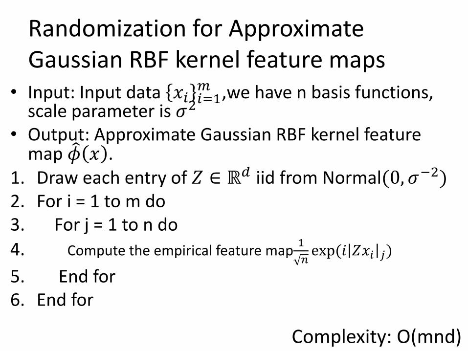
Randomization for Approximate Gaussian RBF kernel feature maps

• Input: Input data 𝑥𝑖 𝑖=1𝑚 ,we have n basis functions,

scale parameter is 𝜎2 • Output: Approximate Gaussian RBF kernel feature

map 𝜙 𝑥 . 1. Draw each entry of 𝑍 ∈ ℝ𝑑 iid from Normal(0, 𝜎−2) 2. For i = 1 to m do 3. For j = 1 to n do

4. Compute the empirical feature map1

𝑛exp(𝑖 𝑍𝑥𝑖 𝑗)

5. End for 6. End for

Complexity: O(mnd)

Fastfood

• The dimension of feature is d.

• The number of basis functions is n.

• Gaussian matrix cost O(nd) per multiplication.

• Assume 𝑑 = 2𝑙 (Pad the vector with zeros until 𝑑 = 2𝑙 holds), The goal is to approximate Z via a product of diagonal and simple matrices:

𝑍 =1

𝜎 𝑑𝑆𝐻𝐺Π𝐻𝐵

Fastfood

• Assume 𝑑 = 2𝑙 (Pad the vector with zeros until 𝑑 = 2𝑙 holds), The goal is to approximate Z via a product of diagonal and simple matrices:

𝑍 =1

𝜎 𝑑𝑆𝐻𝐺Π𝐻𝐵

S random diagonal scaling matrix H Walsh-Hadamard matrix admitting O(d log(d)) multiply

𝐻2𝑑 = ,𝐻𝑑 𝐻𝑑

𝐻𝑑 −𝐻𝑑- and 𝐻1 = 1, 𝐻2 = ,

1 11 −1

-

G random diagonal Gaussian matrix Π ∈ −1,1 𝑑×𝑑 permutation matrix B a matrix which has random*−1,1+ entries on its diagonal Multiplication now is O(d log d), storage is O(d). Draw independent blocks. n

d

Fastfood

• When 𝑛 > 𝑑, We replicate

𝑍 =1

𝜎 𝑑𝑆𝐻𝐺Π𝐻𝐵

• for 𝑛/𝑑 independent random amtrics 𝑍𝑖 and

stack them via 𝑍 𝑇 = ,𝑍 1, 𝑍 2, … , 𝑍 𝑛/𝑑- until we

have enough dimensions.

Walsh-Hadamard transform

The product of a Boolean function and a Walsh matrix is its Walsh spectrum[wiki]: (1,0,1,0,0,1,1,0) * H(8) = (4,2,0,−2,0,2,0,2)

Fast Walsh-Hadamard transform

Fast Walsh–Hadamard transform This is a faster way to calculate the Walsh spectrum of (1,0,1,0,0,1,1,0).

Key Observations 1. When combined with diagonal Gaussian matrices,

Hadamard matrices exhibit very similar to dense

Gaussian random matrices.

2. Hadamard matrices and diagonal matrices are

inexpensive to multiply and store.

Key Observations

Code:

• For C++/C user , a library called

provides extremely fast Fast Hadamard transform.

• For Matlab user, one line code y = fwht(x,n,ordering)

1. When combined with diagonal Gaussian matrices,

Hadamard matrices exhibit very similar to dense

Gaussian random matrices.

2. Hadamard matrices and diagonal matrices are

inexpensive to multiply (O(dlog(d)) and store O(d).

Experiments

d n Fastfood RKS Speedup RAM

1024 16384 0.00058s 0.0139s 24x 256x

4096 32768 0.00136s 0.1224s 90x 1024x

8192 65536 0.00268s 0.5360s 200x 2048x

Runtime, speed, and memory improvements of Fastfood

relative to random kitchen sinks (RKS).

d -input feature dimension, e.g. CIFAR-10, a tiny image

32*32*3 has 3072 dimensions.

n –n nonlinear basis functions.

Summary

• It is possible to compute n nonlinear basis functions in 𝑂(nlog 𝑑)time.

• Kernel methods become more practical for problems that have large datasets and/or require real-time prediction.

• With Fastfood, we would be able to compute nonlinear feature map for large-scale problem.