Fast Hankel Transform Algorithms for Optical Beam · PDF fileFast Hankel Transform Algorithms for Optical Beam Propagation ARL-TR-2492 December 2001 Timothy M. Pritchett Approved for

Fast Hankel Transform Algorithmsfor Optical Beam Propagation

ARL-TR-2492 December 2001

Timothy M. Pritchett

Approved for public release; distribution unlimited.

The findings in this report are not to be construed as anofficial Department of the Army position unless sodesignated by other authorized documents.

Citation of manufacturer’s or trade names does notconstitute an official endorsement or approval of the usethereof.

Destroy this report when it is no longer needed. Do not return it tothe originator.

ARL-TR-2492 December 2001

Army Research LaboratoryAdelphi, MD 20783-1197

Fast Hankel Transform Algorithmsfor Optical Beam PropagationTimothy M. Pritchett Sensors and Electron Devices Directorate

Approved for public release; distribution unlimited.

Abstract

Essential for the development of low-f-number eye and sensor protectionsystems is an accurate model for the propagation of a widely diverginglaser beam through a nonlinear medium. This problem may be solved nu-merically with the well-known “split-step” procedure, in which the effectsof propagation are computed separately from those arising from nonlinearabsorption and refraction. For a cylindrically symmetric beam, the prop-agation phase of each step in the process is most conveniently calculatedin the Hankel transform domain; each step thus requires numerical com-putation of a discrete Hankel transform followed by an inverse transform.Accordingly, we seek an algorithm for efficient numerical computation ofthe Hankel transform that preserves the transform’s invertibility. This re-port summarizes the relevant properties of the Hankel transform and ofthe closely related Fourier transform, it reviews existing fast Hankel trans-form algorithms (proposing several modest improvements in one), and itevaluates those methods in terms of their suitability for the beam propaga-tion application of interest.

ii

Contents

1 Introduction 1

2 Definition 2

3 A Word About Fourier Transforms 3

3.1 Conventions . . . . . . . . . . . . . . . . . . . . . . . . . . . . 3

3.2 Relation Between Hankel and Fourier Transforms . . . . . . 3

3.3 The Correlation Theorem . . . . . . . . . . . . . . . . . . . . . 4

4 The Hankel Transform in Optical Beam Propagation 5

5 The Effect of Finite Domains 7

5.1 “Top Hat” Input Function . . . . . . . . . . . . . . . . . . . . 7

5.2 Uniform Annular Input Function . . . . . . . . . . . . . . . . 8

5.3 Parabolic Input Function . . . . . . . . . . . . . . . . . . . . . 9

6 Survey of Fast Numerical Methods 11

6.1 The ”Quasi-Fast Hankel Transform” . . . . . . . . . . . . . . 11

6.1.1 Original Formulation of Siegman . . . . . . . . . . . . 12

6.1.2 Improved Formulations by the Author . . . . . . . . 12

6.2 The “High-accuracy Fast Hankel Transform” of Magni et al. 14

6.3 Other Fast Hankel Transform Methods . . . . . . . . . . . . . 15

7 Assessment of the High-Accuracy Fast Hankel Transform Algo-rithm 17

7.1 “Top Hat” Input Function . . . . . . . . . . . . . . . . . . . . 17

7.2 Parabolic Input Function . . . . . . . . . . . . . . . . . . . . . 18

References 19

Distribution 21

Report Documentation Page 23

iii

Figures

1 Results of successive operations of Hankel transform followedby inverse Hankel transform on a unit “top hat” input . . . . . . 8

2 Hankel transform followed by inverse Hankel transform of aunit annular input function . . . . . . . . . . . . . . . . . . . . . 9

3 Hankel transform followed by inverse Hankel transform of theparabola f(x) = x2 . . . . . . . . . . . . . . . . . . . . . . . . . . 10

4 High-accuracy numerical Hankel transform followed by inverseHankel transform on a unit “top hat” input . . . . . . . . . . . . 17

5 Comparison of the analytic Hankel transform of f(x) = x2 withthe high-accuracy numerical transform . . . . . . . . . . . . . . 18

6 High-accuracy numerical Hankel transform followed by numer-ical inverse Hankel transform on a parabolic input . . . . . . . 18

iv

1. Introduction

Applications of the Fourier-Bessel transform, commonly known as the Han-kel transform, arise in a variety of fields, including signal processing, op-tics, acoustics, geophysics, and molecular biology. In optics, the Hankeltransform appears in many contexts, not the least of which is the propaga-tion of cylindrically symmetric laser beams. The wide utility of the Hankeltransform has ensured a continuing interest in the development of efficientmethods for its numerical computation, and a variety of “fast Hankel trans-form” algorithms has emerged over the past quarter-century [1–5]. This re-port aims to evaluate these methods in terms of their utility in calculationsinvolving the propagation of optical beams.

This report is organized as follows. In the following section, we define theHankel transform and inverse transform of a function. The Hankel trans-form is intimately related to its better known cousin, the Fourier transform,and in section 3, we remind the reader of several properties of the Fouriertransform that will prove necessary in our later development. Section 4 ofthis report describes the particular application to optical beam propaga-tion that motivates our interest in fast Hankel transform algorithms. Anynumerical proccedure for computing a Hankel transform will necessarilyinvolve a domain of integration that is only finite in extent, and section 5examines the implications of this for the invertibility of the numerical trans-form. Section 6 reviews several methods for efficient numerical computa-tion of Hankel transforms, and section 7 evaluates the most promising ofthese for use in our particular application.

1

2. Definition

The standard Hankel transform of order � of a function f(r) on the half-line0 < r <∞ is defined as

g(ρ) = H�[f ](ρ) = 2π∫ ∞0

rf(r)J�(2πρ r) d r , (1)

where J�(x) is the Bessel function of the first kind of order �. The variablein the transform domain, ρ, may be thought of as a “spatial frequency,” i.e.,the quantity κ = 2πρ is a wavenumber. The inverse transform is given by

f(r) = H−1� [g](r) = 2π

∫ ∞0

ρg(ρ)J�(2π ρ r)d ρ . (2)

Hankel’s integral formula [6] may be obtained from the above definitionsby using (1) to substitute for g(ρ) in (2). This important result is valid forany real � ≥ −1/2 so long as (a) f and its first derivative are sectionally con-tinuous on each bound interval, (b) r1/2f(r) is absolutely integrable fromzero to infinity, and (c) f is defined as its mean value at each point of dis-continuity. From Hankel’s integral formula, we deduce the following “or-thogonality relation” for Bessel functions on the half line:∫ ∞

0uJ�(u v)J�(u v′) d u =

δ(v − v′)v

(3)

Equation (3) ensures the invertibility of the Hankel transform, i.e., guaran-tees that the successive operations of Hankel transform followed by inverseHankel transform reproduce the original input function.

2

3. A Word About Fourier Transforms

The Hankel transform is closely related to the two-dimensional (2-D)Fourier transform of a cylindrically symmetric function. Since the Fouriertransform will itself play an important role in the particular application tooptics that this report is intended to addresss, we pause here to briefly ex-amine the Fourier transform and its relationship to the Hankel transformand to remind the reader of some properties of the Fourier transform thatwe will require.

3.1 Conventions

Several conventions are commonly used to define the Fourier trans-form; ours follow. Let F (⇀x) be a function, in general complex, on the n-dimensional real space Rn. We define the Fourier transform of F (⇀x), de-noted F [G](⇀κ), as

G(⇀κ) = F [F ](⇀κ) =∫ ∞−∞

F (⇀x)ei⇀x ·⇀κ dnx (4)

and we define the inverse transform as

F (⇀x) = F−1[G](⇀x) = (2π)−n∫ ∞−∞

G(⇀κ)ei⇀x ·⇀κ dnκ . (5)

3.2 Relation Between Hankel and Fourier Transforms

In two dimensions, we may express the integral (4) in plane polar coordi-nates,

G(κ, φ) =∫ ∞0

∫ 2π

0rF (r, θ)ecos(θ−φ)κrd θd r ,

where κ = [κ2x + κ2

y]1/2 is the wavenumber. At this point, we specialize to

the case of a transforming function of the form F (r, θ) = f(r)eim θ, wherem is an integer. Employing the identity

ei x sin θ =∞∑

n=−∞Jn(x)ei n θ ,

we can in this case perform the integration over θ and so obtain

G(κ, φ) = 2πimeimφ∫ ∞0

rf(r)Jm(κ r)d r .

Setting κ = 2πρ, we see that the 2-D Fourier transform of F (r, θ) = f(r)eim θ

is related to the mth-order Hankel transform of the “radial function” f(r)by

G(2πρ, φ) = F [F ](2πρ, φ) = imeimφHm[f ](ρ) ,

3

where Hm[f ](ρ) is the Hankel transform of f as defined in (1). In much thesame way, one may start from the definition of the inverse Fourier trans-form (5) and show that in two dimensions the inverse transform of a func-tion of the form G(2πρ, φ) = g(ρ)e−imφ is given by

F (r, θ) = 2π(−i)me−im θ∫ ∞0

ρg(ρ)Jm(2πρr) d ρ ,

or, comparing the integral on the right-hand side with that in (2),

F−1[G](r, θ) = (−i)me−im θH−1m [g](r),

whereH−1m [g](r) is the mth-order inverse Hankel transform of g(ρ).

In optics, we are primarily interested in the case m = 0, which correspondsto a cylindrically symmetric function F (r). As we have just seen, such afunction’s Fourier transform in two dimensions is identical to its Hankeltransform. Similarly, the inverse Fourier transform in two dimensions of acircularly symmetric G(κ) is identical to the inverse Hankel transform.

3.3 The Correlation Theorem

The cross-correlation of two functions α(⇀x) and β(⇀x) is defined by the in-tegral

corr[α, β](⇀x) =∫ ∞−∞

α(⇀x + ⇀u)β(⇀u) dnu .

If we consider now the Fourier transform (4) of corr[α, β],

F [corr[α, β]](⇀κ) =∫ ∞−∞

∫ ∞−∞

α(⇀x + ⇀u)β(⇀u) ei

⇀x ·⇀κ dnu dnx ,

we can, simply by interchanging the order of the integrations and makinga change of variable, prove the well-known correlation theorem:

F [corr[α, β]](⇀κ) =∫ ∞−∞

α(⇀w)ei⇀w ·⇀κ dnw

∫ ∞−∞

β(⇀u) e−i⇀u ·⇀κ dnu

= F [α](⇀κ)F [β](−⇀κ) .

This theorem, in combination with well-known fast Fourier transform (FFT)algorithms, will be applied to efficiently compute the sums that arise in adiscrete analog of the Hankel transform.

4

4. The Hankel Transform in Optical Beam Propagation

Our interest in fast Hankel transform algorithms arises from the need tocalculate the effects of laser beam propagation through a variety of media.Some of these materials exhibit an optical response that is linear even forbeams of extremely high intensity, while others provide a response that ishighly nonlinear. Frequently, the optical systems into which these mediaare incorporated are characterized by a low f-number. In such systems, theusual simplifying assumption of beam paraxiality is invalid. Choosing thez-axis parallel to the primary direction of propagation of the beam, one typ-ically writes the electric field of a single-frequency component of the beamin terms of a spatial envelope ψ(⇀x, z) thus: E(⇀x, z, t) = ψ(⇀x, z) exp[i(kz −ωt)]. In a low-f-number system, the spatial envelope ψ(⇀x, z) satisfies thenonparaxial wave equation, which, in the case of a linear medium, reducesto the following form:(

∂

∂z− i

2k∂2

∂z2

)ψ(⇀x, z) =

i

2k∇T 2ψ(⇀x, z) . (6)

Here,∇T 2 is the transverse Laplacian.

∇T 2 =∂2

∂x2+

∂2

∂y2=

∂2

∂r2+

1r

∂

∂r+

1r

∂2

∂φ2

(In the paraxial approximation, one drops the term in (6) involving the sec-ond derivative with respect to z.)

The nonparaxial propagation operator,

P = exp

[iz∇T 2

k +√

k2 +∇T 2

],

generates from the “initial value” ψ(⇀x, z = 0) an exact solution to (6),ψ(⇀x, z) = Pψ(⇀x, 0), as one may easily verify by direct substitution [7, 8]. Inorder to implement the operator P, it is convenient use (5) to write ψ(⇀x, 0)in terms of its Fourier representation. Then

ψ(⇀x, z) = Pψ(⇀x, 0) =1

(2π)2

∫ ∞−∞

∫ ∞−∞

d2κ exp

[−izκ2

k +√

k2 − κ2

]F [ψ|z=0](

⇀κ)e−i

⇀κ ·⇀x , (7)

whereF [ψ|z=0](⇀κ) is the Fourier transform of ψ(⇀x, 0) and κ = [κx 2+κy

2]1/2

is the transverse wavenumber. For a cylindrically symmetric beam, the en-velope function’s Fourier transform and its zero-order Hankel transformare identical:F [ψ|z=0](

⇀κ) = H[ψ|z=0](κ). (In order to make the notation less

cumbersome, when no confusion can result, we frequently suppress the

5

subscript “m” in “Hm[·]” in the case of an order m = 0 transform.) Assum-ing a cylindrically symmetric beam, we write the integral over the κ-planein polar coordinates and integrate over the angular variable, obtaining aBessel function in the process. The result is

ψ(r, z) =12π

∫ ∞0

d κκ exp

[−izκ2

k +√

k2 − κ2

]H[ψ|z=0](κ)J0(κr) .

Noting that the above integral is simply the inverse Hankel transform oforder zero and switching the variable in the transform domain from κ to ρ,we write this as

ψ(r, z) = H−1

[exp

[−iz(2πρ)2

k +√

k2 − (2πρ)2

]H[ψ|z=0]

]. (8)

Alternately, (8) may also be derived from the following representation forψ(⇀x, 0) in terms of zero-order Hankel transforms

ψ(r, 0) = H−1[H[ψ|z=0]](r) = 2π∫ ∞0

ρH[ψ|z=0](ρ)J0(2πρr)dρ .

(This is none other than the Hankel integral formula, to which we alludedin sect. 2.) Now, with a transverse Laplacian reflecting the assumption ofcircular symmetry,

∇T 2J0(2πρr) =

(∂2

∂r2+

1r

∂

∂r

)J0(2πρr) = −(2πρ)2J0(2πρr) ,

where the last equality follows from Bessel’s equation of order zero. Thus,

Pψ(r, 0) = 2π∫ ∞0

ρH[ψ|z=0](ρ) exp

[−iz(2πρ)2

k +√

k2 − (2πρ)2

]J0(2πρr)dρ ,

and (8) follows.

The solution (8) is exact only for linear media. For the propagation of opti-cal beams through nonlinear media, (8) is applied repeatedly for very smallz in the split-step procedure introduced in optics by Feit and Fleck [9].Each step involves a Hankel transform followed, after multiplication bythe propagation operator P as represented in the ρ-domain, by an inversetransform. The solution generated by this procedure after a large number ofpropagation steps is reliable only to the extent that the numerical methodused to compute the Hankel transform preserves the transform’s invertibil-ity. Put another way, if successive operations of Hankel transform followedby inverse transform fail to reproduce the original input function with rea-sonable accuracy, then any solution obtained from a multi-step procedurewill after only a few steps have become so inaccurate as to be virtually use-less.

Our particular application demands an approximate numerical procedurethat will, to the greatest extent possible, preserve the invertibility of theHankel transform; computational efficiency, while important, is a secondaryconcern.

6

5. The Effect of Finite Domains

In situations of physical interest, the function f(r) may typically be takento be non-vanishing only for r less than some maximum value b. Real opti-cal systems are always characterized by an effective aperture of some sort,and even in the absence of an aperture, a function f(r) arising in a physi-cal problem will generally decrease sufficiently rapidly with distance thatits effects at large r are negligibly small. Although it is less obvious, onemay, in the same way, take the spatial frequency to have an upper bound,the maximum bandwidth β. The upper limit of integration in (1) is thusreplaced by b, and in (2) by β. In such a case, it is convenient to introducethe dimensionless spatial variable x = r/b and the dimensionless trans-form variable y = ρ/β and to work with functions f(x) and g(y) definedon the unit interval. Defining γ = bβ, the space-bandwidth product of thetransformation, we rewrite the Hankel transform (1) as

g(y) = 2πγb

β

∫ 1

0xf(x)J�(2πγxy)dx , (9)

and the inverse transform (2) as

f(x) = 2πγβ

b

∫ 1

0yg(y)J�(2πγxy)dy . (10)

We observe that, despite appearances, the ratio b/β is not dimensionless butcarries units of length squared.

In order to assess the extent to which the imposition of cutoffs in the spa-tial and spatial frequency domains limits the invertibility of the transform,we turn now to some examples for which the Hankel transform may becomputed analytically. In each case, we numerically compute the inversetransform integral (10) by Gaussian quadrature and compare the result tothe original function.

5.1 “Top Hat” Input Function

Students of optics are familiar with the zero-order Hankel transform of theunit step function, Θ(b− r), which arises in the problem of Fresnel diffrac-tion from a uniformly illuminated circular aperture of radius b. In this case,f(x) is simply equal to unity and (9) can be performed analytically with theresult:

g(y) =2πγb

β

∫ 1

0xJ0(2πγxy)dx =

bJ1(2πyγ)yβ

. (11)

We now numerically evaluate the inverse transform (10) using adaptiveGaussian quadrature with error estimation based on evaluation at Kronrodpoints; the numerical results are accurate to six decimal digits. Figure 1

7

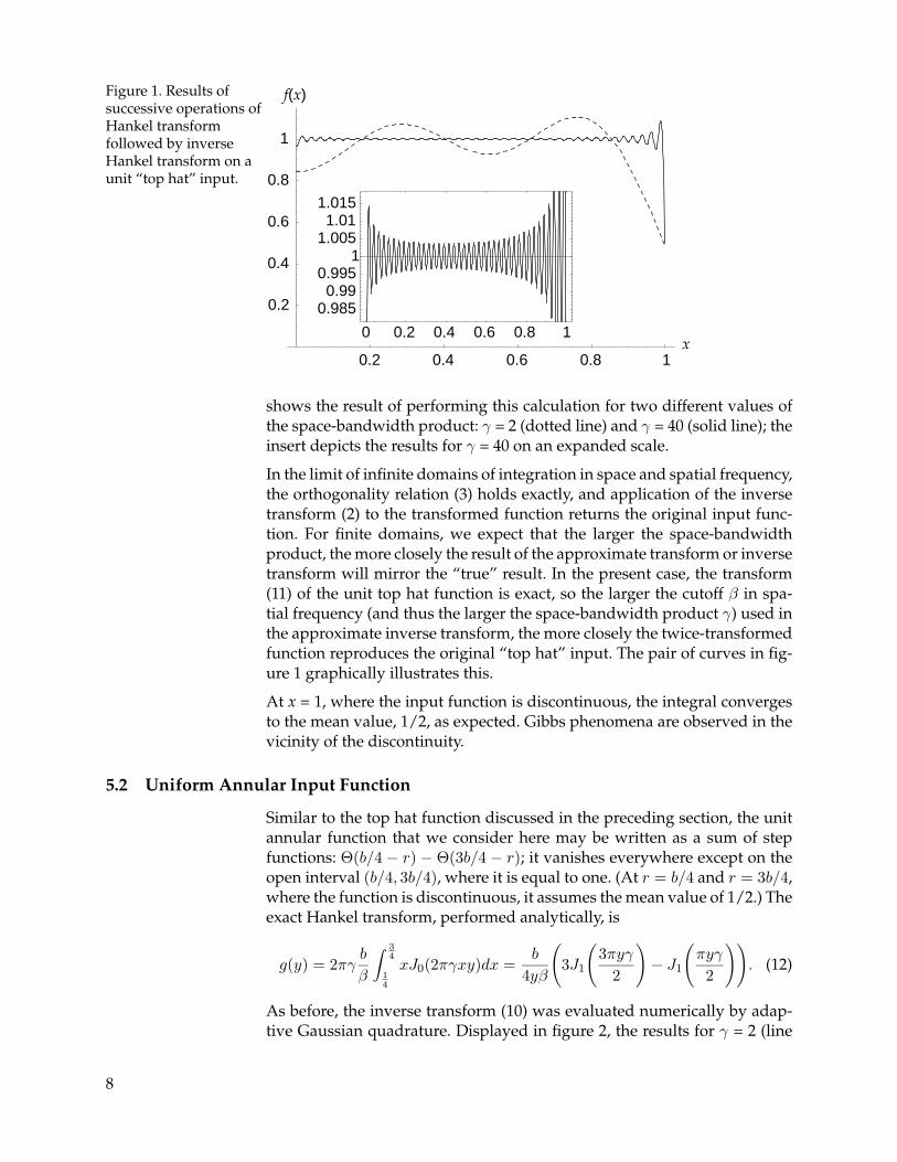
Figure 1. Results ofsuccessive operations ofHankel transformfollowed by inverseHankel transform on aunit “top hat” input.

0.2 0.4 0.6 0.8 1

0.2

0.4

0.6

0.8

1

0 0.2 0.4 0.6 0.8 1

0.9850.99

0.9951

1.0051.01

1.015

x

f(x)

shows the result of performing this calculation for two different values ofthe space-bandwidth product: γ = 2 (dotted line) and γ = 40 (solid line); theinsert depicts the results for γ = 40 on an expanded scale.

In the limit of infinite domains of integration in space and spatial frequency,the orthogonality relation (3) holds exactly, and application of the inversetransform (2) to the transformed function returns the original input func-tion. For finite domains, we expect that the larger the space-bandwidthproduct, the more closely the result of the approximate transform or inversetransform will mirror the “true” result. In the present case, the transform(11) of the unit top hat function is exact, so the larger the cutoff β in spa-tial frequency (and thus the larger the space-bandwidth product γ) used inthe approximate inverse transform, the more closely the twice-transformedfunction reproduces the original “top hat” input. The pair of curves in fig-ure 1 graphically illustrates this.

At x = 1, where the input function is discontinuous, the integral convergesto the mean value, 1/2, as expected. Gibbs phenomena are observed in thevicinity of the discontinuity.

5.2 Uniform Annular Input Function

Similar to the top hat function discussed in the preceding section, the unitannular function that we consider here may be written as a sum of stepfunctions: Θ(b/4 − r) − Θ(3b/4 − r); it vanishes everywhere except on theopen interval (b/4, 3b/4), where it is equal to one. (At r = b/4 and r = 3b/4,where the function is discontinuous, it assumes the mean value of 1/2.) Theexact Hankel transform, performed analytically, is

g(y) = 2πγb

β

∫ 34

14

xJ0(2πγxy)dx =b

4yβ

(3J1

(3πyγ

2

)− J1

(πyγ

2

)). (12)

As before, the inverse transform (10) was evaluated numerically by adap-tive Gaussian quadrature. Displayed in figure 2, the results for γ = 2 (line

8

Figure 2. Hankeltransform followed byinverse Hankeltransform of a unitannular input function.

0 0.2 0.4 0.6 0.8 1x

0

0.2

0.4

0.6

0.8

1

1.2

f(x)

Space-BandwidthProduct

2840

of short dashes), γ = 8 (line of long dashes), and γ = 40 (solid line) clearly il-lustrate how the accuracy of the approximate (finite) tranform (10) dependson the space-bandwidth product γ.

5.3 Parabolic Input Function

As a final example, we examine the parabolic input function f(x) = x2,as is done in [5]. The fact that the upper limit of integration in the Hankeltransform defined by (9) is 1, not infinity, effectively “clips” the input func-tion to the unit interval; the effective input function used here is thus an“apertured parabola,” equal to x2 on the interval 0 ≤ x < 1, vanishing forx > 1, and assuming the mean value of 1/2 at the point of discontinuity,x = 1. Indeed, the “true” Hankel transform, equation (1), of the functionf(x) = x2, defined on the entire positive real axis, does not even exist, sincethe integral of x3 from zero to infinity diverges! However, there is no suchdifficulty with the finite Hankel transform integral (9), which may be per-formed analytically, yielding

g(y) =2πγb

β

∫ 1

0x3J0(2πγxy)dx =

b

2yβ(J1(2πyγ)− J3(2πyγ)) . (13)

For completeness, we introduce η = 2πγy and use the well-known identi-ties relating Bessel functions of adjacent orders [10] to rewrite (13) as

g(η) =2bπγ(2ηJ0(η) + (η2 − 4)J1(η))

βη3,

analogous to equation (12) of reference [5].

Performing the inverse transform (10) numerically using the methods de-scribed before, we obtain the results shown in figure 3 for γ = 2 (line ofshort dashes), γ = 8 (line of longer dashes), and γ = 40 (solid line). Theseresults reinforce the points made previously: namely, that the fidelity of thetransform increases with the space-bandwidth product γ and that at points

9

Figure 3. Hankeltransform followed byinverse Hankeltransform of theparabola f(x) = x2.

0.2 0.4 0.6 0.8 1x

–0.2

0.2

0.4

0.6

0.8

1

1.2

f(x)

Space-BandwidthProduct

2

8

40

of discontinuity, the transform assumes the mean value of the function forevery value of γ.

We turn now to a brief survey of various available methods for computingHankel transforms numerically.

10

6. Survey of Fast Numerical Methods

We wish to compute a numerical approximation to the Hankel transformintegral (9) at a series of N spatial frequencies ym, m = 0, 1, . . . N − 1. Theproblem is immediately apparent: Naively sampling at N values {xn} ofthe normalized spatial variable and N normalized spatial frequencies {ym},m,n = 0, 1, . . . N − 1, and then computing the integral (9) by a finite suminvolves N2 multiplications! Fortunately, we can do considerably better.

6.1 The ”Quasi-Fast Hankel Transform”

Central to both the so-called “quasi-fast Hankel transform” methods de-scribed in this section and the “high-accuracy fast Hankel transform” ofthe following section (the names are due to Siegman [1] and Magni [5], re-spectively) is the exponential change of variables employed by Gardiner[11]:

r = r0eαu, ρ = ρ0e

αv. (14)

With this change of variables, the Hankel transform integral (1) takes theform of a cross-correlation:

g(v) =∫ ∞−∞

f(u) j(u + v)du ,

where g(v) = ρ0eαvg(ρ0e

αv), f(u) = r0eαuf(r0e

αu), and j(u + v) = 2παr0ρ0

eα(u+v)J�(2πr0ρ0eα(u+v)). The correlation theorem, which we discussed in

section 3.3, guarantees that a cross-correlation such as the one above isequal to the inverse Fourier transform of the product of the Fourier trans-forms of the functions in the correlation integral. Since discrete Fouriertransforms can be computed with extremely high efficiency via the FFTmethods that came into widespread use in the mid-1960s, the fact that onecan recast the Hankel transform as a correlation is very fortuitous indeed.

The discrete Fourier transform of a function f(u) is computed from a list offunction values at evenly spaced values of u. Because the change of vari-able (14) between u and r is exponential, sampling at regular intervals in uimplies geometric sampling in r, that is, in “real” space. While nonuniformsampling creates its own set of problems for certain applications, for ourparticular application to optics, it is actually something of an advantage.This happy state of affairs arises from the fact that the intensity of a laserbeam is typically highest in the center of the beam and decreases as the dis-tance r from the beam center increases. The geometric sampling in r leadsto an increased density of grid points in the region of highest intensity, andsince it is in this region that the optical properties of the medium would beexpected to vary most rapidly with distance, it is precisely here that a finergrid is most desirable.

11

6.1.1 Original Formulation of Siegman

Among the earliest of the fast Hankel transform methods in current useis the “quasi-fast Hankel transform” introduced by Siegman [1]. Siegmanchooses sampling points as a geometric series,

ρm = ρ0eαm, rn = r0e

αn, for m, n = 0, 1, . . . N − 1 , (15)

so that the resulting sum,

g(ρm) =2πα

ρm

N−1∑n=0

φn jm+n , (16)

takes the form of a cross-correlation between discretely sampled functions:

φn = rnf(rn)jm+n = ρmrnJ�(2πρmrn) = ρ0r0e

α(m+n)J�(2πρ0r0eα(m+n)) .

If the number of sampling points N is chosen to be a power of 2, the discretecross-correlation (16) may be computed very efficiently via a series of three2 N-term fast Fourier transforms, each requiring only 2 N log2(2 N) mul-tiplications. An end correction term suggested by Agrawal and Lax [12],πr0

2f(r0), may be added to (16) to account for the contribution to the Han-kel transform integral from the excluded region 0 ≤ r < r0. The parametersα, r0, and ρ0 are arbitrary.

6.1.2 Improved Formulations by the Author

We have developed two related formulations of the quasi fast Hankel trans-form that apply specifically to the “windowed” Hankel transform (9) andof which the latter is modestly more accurate than Siegman’s original for-mulation. We now describe these new formulations.

Approximation by “Right-hand Rectangles.” We begin by defining sam-pling points as a geometric series on the unit interval 0 ≤ x, y ≤ 1:

xn = yn = eα(n−N), n = 1, 2, . . . N

This corresponds to taking r0 = beα(1−N) and ρ0 = βeα(1−N) in (15). Thechoice of identical sampling points in the spatial (x) and spatial frequency(y) domains is intended to facilitate inversion of the transform. The win-dowed Hankel transform integral (9) is then approximated by the sum

g(ym) = 2πγb

β

N∑n=1

xnf(xn)J�(2πγxnym)(xn − xn−1) , (17)

in which

xn − xn−1 ={

x1, n = 1xn(1− e−α), n = 2, 3, . . . N

12

In effect, we are approximating the integrand in (9) by a series of rectan-gles, the height of each equal to the value of the integrand at the right-handedge of the rectangle. One might expect that a better approximation to (9)could be obtained by choosing the height of each rectangle equal to thevalue of the integrand at the center of each rectangle, and this is indeed thecase. We will develop an improved formulation based on “centered rect-angles” in a moment. To conclude the present discussion, we observe thatour choice of sampling points allows the sum in (17) to be evaluated as thecross-correlation

g(ym) = 2πγb

β

N∑n=1

φnjm+n , (18)

between the discretely sampled functions:

φn ={

x12f (x1) , n = 1

x12f (xn) (1− e−α), n = 2, 3, . . . N

and

jm+n = J�(2πγeα(m+n−2N)), m, n = 1, 2, . . . N .

Approximation by “Centered Rectangles.” In order to develop an improvedformulation in the manner indicated previously, we define

ξ0 = 0ξn = eα(n−N), n = 1, 2, . . . N, (19)

i.e., we take each ξn for n ≥ 1 to be the same as the sampling point xn usedin the previous formulation. The points {ξn}, n = 0, 1, . . . N , divide the unitinterval into N subintervals, the lengths of which are given above. We nowselect a new set of sampling points:

xn = yn = x0eαn , for m, n = 0, 1, . . . N − 1, (20)

and we choose the parameter x0 so that, with the exception of the first,each of the sampling points lies at the center of its respective interval; thisgives x0 = (eα − 1)e−αN/2. The sum approximating the Hankel transformintegral (9) is now given by

g(ym) = 2πγb

β

N−1∑n=0

xnf(xn)J�(2πγxnym)(ξn+1 − ξn) .

This sum is a discrete cross-correlation of the same form as (18) but withthe following functions.

φn ={

x0e−αNf (x0) , n = 0

x0eα(n−N)f (xn) (1− e−α), n = 1, 2, . . . N − 1

jm+n = J�(2πγx02eα(m+n)) , m, n = 0, 1, . . . N − 1

13

After the cross-correlation sum is computed by FFT methods, one could, ifdesired, add an end correction term to the sum to reflect the fact that thefirst rectangle is not “centered.”

(correction)m =12e−2αN{(e2α − 1)f(x0)J�(2πγx0ym) + e2αf(ξ1/2)J�(2πγξ1ym)}

In both formulations, the parameter α is arbitrary. One should choose αso that the minimum grid spacing corresponds to the minimum separationin space (or spatial frequency) that one could resolve in an experimentalmeasurement.

6.2 The “High-accuracy Fast Hankel Transform” of Magni et al.

Magni et al. [5] developed a method specifically for the evaluation of win-dowed Hankel transforms of order zero. This so-called “high-accuracy fastHankel transform” bears many similarities to the “centered rectangle” for-mulation of the quasi-fast Hankel transform described in the precedingparagraphs. In both approaches, one divides the unit interval into the sameN subintervals ξn ≤ x, y < ξn+1, n = 0, 1, . . . N − 1, with endpoints ξndefined in (19), and one chooses the same set of sampling points {xn} ac-cording to (20) so that there is exactly one point per subinterval and eachpoint except the first lies at the midpoint of its subinterval. Where the twoapproaches differ is in the function that one approximates as a series of“centered rectangles,” i.e., the function that one takes to be a constant overeach subinterval. In the quasi-fast Hankel transform, one approximates byrectangles the entire integrand of the windowed Hankel transform integral(9), whereas in the high-accuracy fast Hankel transform, one approximatesonly the input function f. In the latter approach, one proceeds by perform-ing the integration over each subinterval analytically.

2πγb

β

∫ ξn+1

ξnf(xn)J0(2πγyu)udu =

bf(xn)yβ

(J1(2πγyξn+1)ξn+1 − J1(2πγyξn)ξn)

Summing this result over the N intervals, one obtains a discrete approxi-mation to the Hankel transform (9):

g(ym) =b

βym

N−1∑n=0

(f(xn)− f(xn+1))ξn+1J1(2πγymξn+1)

where f(xN ) is defined to be zero. Because the sampling points lie in geo-metric progression, this sum can be computed as the cross-correlation

g(ym) =b

βym

N−1∑n=0

φnjm+n

14

between the discretely sampled functions:

φn ={

(f (x0)− f (x1)) eα(−N) × (end correction), for n = 0(f (xn)− f (xn+1)) eα(n+−N), for n = 1, 2, . . . N − 1

jm+n = J1(2πγx0eα(m+n+1−N))

The end correction factor in the expression for φ0 is equal to (2eα+ e2α)[1+eα]−2/(1− e−2α) and arises from the integral over the first subinterval.

As in the previous formulations, the parameter α is arbitrary. Magni et al.report that best results are obtained by choosing the value of α so as tomake the first and last subintervals of equal width [5].

The attempt to further improve the accuracy of this approach by approxi-mating the input function f not by a series of rectangles but by a series oftrapezoids, i.e., by approximating f on the interval ξn,≤ x < ξn+1 by

f(x) = f(ξn) +(

f(ξn+1)− f(ξn)ξn+1 − ξn

)(x− ξn)

is frustrated by the complexity of the expression obtained upon integration.

6.3 Other Fast Hankel Transform Methods

Oppenheim, Frisk, and Martinez [2] propose a number of methods basedon the “projection-slice theorem,” from which it follows that the Hankeltransform is equal to the one-dimensional Fourier transform of the projec-tion p(x) of a 2-D function onto the x-axis:

p(x) =∫ ∞−∞

f(x, y)dy =∫ ∞x

f(r)√r2 − x2

d(r2) .

Unfortunately, the inherent complexity of these methods, as well as thelengthy computations that they entail, make them less than satisfactory.

The hybrid approach of Candel [3] computes the Hankel transform viaa pair of companion algorithms, one for the low-order components andthe other for the remaining orders. The combination can be shown to con-verge to the true transform to within a specified error. Unfortunately, thisapproach is limited by the individual shortcomings of its component al-gorithms: the first is not particularly fast, and the second, relying on theapproximate representation of the Bessel function by a truncated series ex-pansion, is not particularly accurate.

The clever 2-D fast Hankel transform algorithm of Murphy and Gallagher[4] is based on the result discussed in section 3.2 that the Hankel trans-form is the 2-D Fourier transform of a circularly symmetrical function. TheMurphy-Gallagher procedure is superior to Siegman’s implementation ofthe quasi-fast Hankel transform for many applications, particularly thosein which the input data are already in a 2-D form or when one requiresa 2-D output format. For our purposes, however, it is redundant; if we

15

were willing to endure the increased storage requirements associated withsolving our nonparaxial beam propagation problem on a 2-D grid, then wewould simply employ the propagation operator in the form (7) and woulduse 2-D FFT methods throughout the process.

16

7. Assessment of the High-Accuracy Fast Hankel TransformAlgorithm

In this section, we evaluate the merits of the high-accuracy fast Hankeltransform method just described by employing it to numerically computethe Hankel transforms and inverse transforms of a variety of functions, toinclude the ”top hat” function examined in section 5.1. We abstain froma similar assessment of the quasi-fast Hankel transform methods of sec-tion 6.1, since Siegman’s implementation of this algorithm was shown byMagni et al. to be generally inferior to the high-accuracy fast Hankel trans-form method [5].

7.1 “Top Hat” Input Function

The high-accuracy fast Hankel transform method gives the exact transformof a constant function, as is obvious from the description of section 6.2; thenumerical transform of the top hat input f(x) = 1 is thus identical to the an-alytic result (11). Using the high-accuracy method to numerically transformthe top hat input for a given value of the frequency-bandwidth product γ,and then to compute the inverse transform at the identical value of γ, oneobtains the results shown in figure 4 for γ = 10 (dotted line) and γ = 40(solid line). Both the transform and the inverse transform were performedwith 256 sampling points. The reader may verify from the expanded scaleinsert that the curve for γ = 10 displays exacts ten maxima, while that forγ = 40 displays exactly 40 such “humps.”

Figure 4. High-accuracynumerical Hankeltransform followed byinverse Hankeltransform on a unit “tophat” input.

0.2 0.4 0.6 0.8 1x

0.2

0.4

0.6

0.8

1

f(x)

0 0.2 0.4 0.6 0.8 1

0.96

0.98

1

1.02

1.04

17

7.2 Parabolic Input Function

We conclude with an example of a function whose numerical high-accuracyfast Hankel transform is not exact; we consider the windowed Hankel trans-form of the parabolic input function f(x) = x2 for space-bandwidth prod-uct γ = 10. The solid gray line in figure 5 depicts the analytic result (13),while the black dotted line shows the numerical results obtained with thehigh-accuracy fast Hankel transform with 256 sampling points.

In order to assess the degree to which the numerical procedure preservesthe invertibility of the Hankel transform, we employ the high-accuracy fastHankel transform method to numerically transform the parabolic input fora given value of γ and then to perform the inverse transform at the iden-tical value of γ. Figure 6 illustrates the results of performing this sequenceof operations with 256 sampling points for γ = 4 (dotted line), and with1,048 sampling points for γ = 40 (solid line). The thick gray line shows theoriginal input function.

These results, along with others not reported here, lead us to believe thatthe fast Hankel transform algorithm of [5] is more than adequate for therepetitive use required of it in a split-step beam propagation calculation.

Figure 5. Comparison ofthe analytic Hankeltransform of f(x) = x2

with the high-accuracynumerical transform.

0.2 0.4 0.6 0.8 1y

–5

5

10

15

H[x2](y)

0 0.2 0.4 0.6 0.8 1–1.5

–1–0.5

00.5

11.5

Figure 6. High-accuracynumerical Hankeltransform followed bynumerical inverseHankel transform on aparabolic input .

0.2 0.4 0.6 0.8 1x

0.2

0.4

0.6

0.8

1 input: f(x) = x2

H–1°H[ f ], γ = 4

H–1°H[ f ], γ = 40

18

References

1. A. E. Siegman, “Quasi fast Hankel transform,” Opt. Lett. 1(1), 13–15(1977).

2. Alan V. Oppenheim, George V. Frisk, and David R. Martinez, “Com-putation of the Hankel transform using projections,” J. Acoust. Soc.Am. 68(2), 523–529 (1980).

3. Sebastien M. Candel, “Dual algorithms for fast calculation of theFourier-Bessel transform,” IEEE Trans. ASSP-29(5), 963–972 (1981).

4. Patricia K. Murphy and Neal C. Gallagher, “Fast algorithm for thecomputation of the zero-order Hankel transform,” J. Opt. Soc. Am.73(9), 1130–1137 (1983).

5. Vittorio Magni, Giulio Cerullo, and Sandro De Silvestri, “High accu-racy fast Hankel transform for optical beam propagation,” J. Opt. Soc.Am A 9(11), 2031–2033 (1992).

6. Ruel V. Churchill, Fourier Series and Boundary Value Problems, 2nd Ed.,(McGraw-Hill: New York, 1969), p. 188.

7. M. D. Feit and J. A. Fleck, Jr., “Light propagation in graded-index op-tical fibers,” Appl. Opt 17(24), 3990–3998 (1978).

8. M. D. Feit and J. A. Fleck, Jr., “Beam nonparaxiality, filament forma-tion, and beam breakup in the self-focusing of optical beams,” J. Opt.Soc. Am. B 5(3), 633–640 (1988).

9. M. D. Feit and J. A. Fleck, Jr., “Time-dependent propagation of higenergy laser beams through the atmosphere,” Appl. Phys. 10, 129–160(1976).

10. See, for instance, J. D. Jackson, Classical Electrodynamics, 2nd Ed., (Wi-ley: New York, 1975), p. 105.

11. D. G. Gardner, J. C. Gardner, G. Lausch, and W. W. Meinke, “Methodfor the analysis of multi-component exponential decays,” J. Chem.Phys. 31, 987 (1959).

12. G. P. Agrawal and M. Lax, “End correction in the quasi-fast Han-kel transform for optical propagation problems,” Opt. Lett 6, 171–173(1981).

19

21

Distribution

AdmnstrDefns Techl Info CtrATTN DTIC-OCP8725 John J Kingman Rd Ste 0944FT Belvoir VA 22060-6218

DARPAATTN S Welby3701 N Fairfax DrArlington VA 22203-1714

Ofc of the Secy of DefnsATTN ODDRE (R&AT)The PentagonWashington DC 20301-3080

AMCOM MRDECATTN AMSMI-RD W C McCorkleRedstone Arsenal AL 35898-5240

US Army Rsrch Physics DivATTN AMXRO-PH D SkatrudPO Box 12211Research Triangle Park NC 27709-2211

US Army Rsrch LabATTN AMSRL-RO-PP M CiftanPO Box 12211Research Triangle Park NC 27709-2211

US Army TRADOCBattle Lab Integration & Techl DirctrtATTN ATCD-BFT Monroe VA 23651-5850

CECOM NVESDATTN AMSEL-RD-NV-STD B AhnFT Belvoir VA 22060-5677

US Military AcdmyMathematical Sci Ctr of ExcellenceATTN MADN-MATH MAJ M JohnsonThayer HallWest Point NY 10996-1786

Natick Rsrch and Dev CtrATTN SSCNC-IT M NakashimaNatick MA 01760-5019

Dir for MANPRINTOfc of the Deputy Chief of Staff for PrsnnlATTN J HillerThe Pentagon Rm 2C733Washington DC 20301-0300

SMC/CZA2435 Vela Way Ste 1613El Segundo CA 90245-5500

TECOMATTN AMSTE-CLAberdeen Proving Ground MD 21005-5057

US Army ARDECATTN AMSTA-AR-TDBldg 1Picatinny Arsenal NJ 07806-5000

US Army Info Sys Engrg CmndATTN AMSEL-IE-TD F JeniaFT Huachuca AZ 85613-5300

US Army Natick RDEC Acting Techl DirATTN SBCN-T P BrandlerNatick MA 01760-5002

US Army Natick Rsrch & Dev CtrATTN SSCNC-II B De CristofanoNatick MA 01760-5019

US Army Simulation Train & InstrmntnCmnd

ATTN AMSTI-CG M MacedoniaATTN J Stahl12350 Research ParkwayOrlando FL 32826-3726

US Army Tank-Automtv & Armaments CmndATTN AMSTA-TR-R-MS-263 R GoedertWarren MI 48379-5000

US Army Tank-Automtv Cmnd RDECATTN AMSTA-TR J ChapinWarren MI 48397-5000

Distribution (cont’d)

22

US Military Acdmy Dept of PhysicsATTN T Pritchett (10 copies)West Point NY 10996

Nav Air Warfare CtrATTN J Sheehy48110 Shaw Rd Unit 5 Bldg 2187 Ste 1280Patuxent River MD 20670-1906

Nav Rsrch LabATTN Code 6336 G Mueller4555 Overlook Ave SWWashington DC 20375-5000

Nav Rsrch LabATTN Code 5613 J Shirk4555 Overlook Ave SWWashington DC 20375-5345

Nav Surfc Warfare CtrATTN Code B07 J Pennella17320 Dahlgren Rd Bldg 1470 Rm 1101Dahlgren VA 22448-5100

AFRL/MLPJATTN S Guha3005 P Stret Bldg 651 Ste 1Wright-Patterson aFB OH 45433-7702

WL/MLPJATTN C Ristich3005 P Stret Ste 1 Bldg 651Wright Patterson AFB OH 45433-7702

United States Military AcademyDept of Elect Engrg & Computer SciPhotonics Rsrch Ctr (10 copies)West Point NY 10996

Hicks & Assoc IncATTN G Singley III1710 Goodrich Dr Ste 1300McLean VA 22102

Palisades Inst for Rsrch Svc IncATTN E Carr1745 Jefferson Davis Hwy Ste 500Arlington VA 22202-3402

DirectorUS Army Rsrch LabATTN AMSRL-RO-D JCI ChangATTN AMSRL-RO-EN W D BachATTN AMSRL-RO-P H EverittPO Box 12211Research Triangle Park NC 27709

US Army Rsrch LabATTN AMSRL-D D R SmithATTN AMSRL-DD J M MillerATTN AMSRL-CI-IS-R Mail & Records MgmtATTN AMSRL-CI-IS-T Techl Pub (2 copies)ATTN AMSRL-CI-OK-TL Techl Lib (2 copies)ATTN AMSRL-SE J PellegrinoATTN AMSRL-SE-E H Pollehn (3 copies)ATTN AMSRL-SE-E J MaitATTN AMSRL-SE-E W ClarkATTN AMSRL-SE-EO A Mott (10 copies)ATTN AMSRL-SE-EO G Wood (10 copies)ATTN AMSRL-SE-EO J GoffATTN AMSRL-SE-EO M FerryATTN AMSRL-SE-EO M MillerAdelphi MD 20783-1197

1. AGENCY USE ONLY

8. PERFORMING ORGANIZATION REPORT NUMBER

7. PERFORMING ORGANIZATION NAME(S) AND ADDRESS(ES)

12a. DISTRIBUTION/AVAILABILITY STATEMENT

10. SPONSORING/MONITORING AGENCY REPORT NUMBER

5. FUNDING NUMBERS4. TITLE AND SUBTITLE

6. AUTHOR(S)

REPORT DOCUMENTATION PAGE

3. REPORT TYPE AND DATES COVERED2. REPORT DATE

11. SUPPLEMENTARY NOTES

14. SUBJECT TERMS

13. ABSTRACT (Maximum 200 words)

Form ApprovedOMB No. 0704-0188

(Leave blank)

9. SPONSORING/MONITORING AGENCY NAME(S) AND ADDRESS(ES)

Public reporting burden for this collection of information is estimated to average 1 hour per response, including the time for reviewing instructions, searching existing data sources,gathering and maintaining the data needed, and completing and reviewing the collection of information. Send comments regarding this burden estimate or any other aspect of thiscollection of information, including suggestions for reducing this burden, to Washington Headquarters Services, Directorate for Information Operations and Reports, 1215 JeffersonDavis Highway, Suite 1204, Arlington, VA 22202-4302, and to the Office of Management and Budget, Paperwork Reduction Project (0704-0188), Washington, DC 20503.

12b. DISTRIBUTION CODE

15. NUMBER OF PAGES

16. PRICE CODE

17. SECURITY CLASSIFICATION OF REPORT

18. SECURITY CLASSIFICATION OF THIS PAGE

19. SECURITY CLASSIFICATION OF ABSTRACT

20. LIMITATION OF ABSTRACT

NSN 7540-01-280-5500 Standard Form 298 (Rev. 2-89)Prescribed by ANSI Std. Z39-18298-102

Fast Hankel Transform Algorithms for Optical BeamPropagation

December 2001 Summary, Jan 2001 to Mar 2001

Essential for the development of low-f-number eye and sensor protection systems is an accuratemodel for the propagation of a widely diverging laser beam through a nonlinear medium. Thisproblem may be solved numerically with the well-known “split-step” procedure, in which theeffects of propagation are computed separately from those arising from nonlinear absorptionand refraction. For a cylindrically symmetric beam, the propagation phase of each step in theprocess is most conveniently calculated in the Hankel transform domain; each step thus requiresnumerical computation of a discrete Hankel transform followed by an inverse transform.Accordingly, we seek an algorithm for efficient numerical computation of the Hankel transformthat preserves the transform’s invertibility. This report summarizes the relevant properties of theHankel transform and of the closely related Fourier transform, it reviews existing fast Hankeltransform algorithms (proposing several modest improvements in one), and it evaluates thosemethods in terms of their suitability for the beam propagation application of interest.

Hankel transform, optical beam propagation, nonlinear optics

Unclassified

ARL-TR-2492

1NE3AA611102.H44

AH44

61102A

ARL PR:AMS code:

DA PR:

PE:

Approved for public release; distributionunlimited.

28

Unclassified Unclassified UL

2800 Powder Mill RoadAdelphi, MD 20783-1197

U.S. Army Research LaboratoryAttn: AMSRL- SE-EO Tim Pritchett/arl@arl

U.S. Army Research Laboratory

23

Timothy M. Pritchett

email:2800 Powder Mill RoadAdelphi, MD 20783-1197