Fast Cycle Canceling Algorithms for Minimum Cost Submodular Flow*

Fast Cycle Canceling Algorithms for

Minimum Cost Submodular Flow ∗

Satoru Iwata † S. Thomas McCormick ‡ Maiko Shigeno §

August, 1999; August, 2000

Abstract

This paper presents two fast cycle canceling algorithms for the submodular flow

problem. The first uses an assignment problem whose optimal solution identifies

most negative node-disjoint cycles in an auxiliary network. Canceling these cy-

cles lexicographically makes it possible to obtain an optimal submodular flow in

O(n4h log(nC)) time, which almost matches the current fastest weakly polynomial

time for submodular flow (where n is the number of nodes, h is the time for com-

puting an exchange capacity, and C is the maximum absolute value of arc costs).

The second algorithm generalizes Goldberg’s cycle canceling algorithm for min cost

flow to submodular flow to also get a running time of O(n4h log(nC)). We show

how to modify these algorithms to make them strongly polynomial, with running

times of O(n6h logn), which matches the fastest strongly polynomial time bound for

submodular flow. We also show how to extend both algorithms to solve submodular

flow with separable convex objectives.

∗An extended abstract of a preliminary version of part of this paper appeared in [22].†Department of Mathematical Engineering and Information Physics, University of Tokyo, Tokyo 113-

8656, Japan ([email protected]). Research supported in part by a Grant-in-Aid of the Min-

istry of Education, Science, Sports and Culture of Japan.‡Faculty of Commerce and Business Administration, University of British Columbia, Vancouver, BC

V6T 1Z2 Canada. Research supported by an NSERC Operating Grant. Part of this research was done

during a sabbatical leave at Cornell SORIE.§Institute of Policy and Planning Sciences, University of Tsukuba, Tsukuba, Ibaraki 305, Japan.

Research supported in part by a Grant-in-Aid of the Ministry of Education, Science, Sports and Culture

of Japan.

1

1 Introduction

The submodular flow problem, introduced by Edmonds and Giles [4], is one of the most

important frameworks of efficiently solvable combinatorial optimization problems. It

includes the minimum cost flow, the graph orientation, the polymatroid intersection,

and the directed cut covering problems as its special cases. Other frameworks named

independent flows [10] and polymatroid network flows [18, 28] are equivalent to submod-

ular flows. These three are collectively called neoflows in [11]. Section 2 formalizes our

notation for submodular flow.

To be able to talk about running times, define n and m as the number of nodes and

arcs in an instance of submodular flow, C as the largest absolute value of the arc costs,

and U as the largest absolute value of any bound. A number of combinatorial algorithms

have been proposed for submodular flow, all of which rely on an oracle for exchange

capacities, as generalizations of minimum cost flow algorithms. Define h as the time

for computing an exchange capacity. Cunningham and Frank [3] developed a primal-

dual algorithm and its cost scaling version, which is the first combinatorial algorithm

with weakly polynomial time complexity. This algorithm solves O(m log C) maximum

submodular flow problems. In [24] we show how to speed this up to an O(n4h log C)

algorithm, the current fastest submodular flow algorithm when C is not too big.

One reasonable strategy for designing submodular flow algorithms is to extend the

capacity scaling minimum cost flow algorithm due to Edmonds and Karp [5]. Since round-

ing a submodular function may destroy its submodularity, we need something more than

a straightforward scaling scheme. Iwata [20] shows that adding a small but strictly sub-

modular function before rounding makes it possible to get a weakly polynomial capacity

scaling algorithm for the submodular flow problem. This scaling scheme calls a maximum

submodular flow subroutine O(n4h log U) times, which is slower than the Cunningham–

Frank algorithm. This algorithm is, however, the first polynomial algorithm for sub-

modular flow with separable convex costs. In [23] we develop a cut canceling algorithm

that is the dual of Tight Arc Cycle Canceling algorithm of this paper, in the sense that

they both come from extensions of a dual pair of min cost flow algorithms from [33].

The paper [6] shows how to improve the capacity scaling algorithm to an O(n4h log U)

algorithm, which can also be seen as an improvement of the algorithm in [23].

The first strongly polynomial algorithm for the submodular flow problem is due to

Frank and Tardos [8]. This is an application of simultaneous Diophantine approximation

and substantially generalizes the first strongly polynomial minimum cost flow algorithm

of Tardos [34]. A more direct generalization of the Tardos algorithm to the submodular

2

flow problem is described by Fujishige, Rock, and Zimmermann [12]. The latter algorithm

combined with the improved primal-dual algorithm in [24] runs in O(n6h log n) time,

which is currently the best strongly polynomial bound.

The strategy of this paper is to extend cycle canceling algorithms for min cost flow

(see [33] for a survey) to submodular flow. Cui and Fujishige [2] extended the minimum-

mean cycle canceling algorithm of Goldberg and Tarjan [15], but the running time is

only pseudopolynomial. Wallacher and Zimmermann [36] improved a pseudopolynomial

minimum ratio cycle canceling algorithm of Zimmermann [37] to obtain the time bound

O(n8h log(nCU)).

Section 3 develops two fast polynomial cycle canceling algorithms for submodular

flow. The first is Tight Arc Cycle Canceling, which is an extension of our relaxed

most negative disjoint family of cycles canceling algorithm for minimum cost flow [33].

The second is Negative Arc Cycle Canceling, which is an extension of Goldberg’s cycle

canceling algorithm [14].

Both algorithms use Goldberg and Tarjan’s generic successive approximation frame-

work [16] where we scale a relaxation parameter. The key idea for the first algorithm is

to use an assignment subproblem whose optimal solution corresponds to a most negative

family of node-disjoint cycles in an auxiliary network. Given an optimal dual solution

of the assignment problem, we extract the tight arcs, and repeatedly cancel cycles of

those arcs. Lexicographical ordering makes it possible to obtain an optimal submodular

flow in a polynomial number of cancellations. The key idea for the second algorithm is

to cancel cycles in the subnetwork of negative reduced cost arcs until it is acyclic. At

this point we can make a change to dual variables that removes at least one node from

participating in future negative cycles. Both algorithms achieve a running time bound

O(n4h log(nC)), nearly matching the fastest current weakly polynomial bound.

Next, Section 4 shows that we can modify these algorithms using the standard tech-

nique of canceling a min mean cycle every O(log n) scaling phases so that they become

strongly polynomial. The running times in this case are O(n6h log n), matching the

fastest current bound.

Finally, Section 5 considers a further extension of our algorithms to submodular flows

with separable convex objectives. It is not apparent how to straightforwardly extend the

primal-dual algorithm to this case, since it is not clear what the bit scaling of a convex

function means. Scaling in the separable convex case fits in much more naturally with

the cycle canceling algorithms of this paper since here it is necessary only to scale the

relaxation parameter. We show that our algorithms have polynomial convergence for

this case.

3

2 Submodular Flow

Let V be a finite set. A pair of subsets X and Y of V is said to be crossing if X ∩Y 6= ∅,

X − Y 6= ∅, Y − X 6= ∅, and X ∪ Y 6= V . A family F ⊆ 2V is called a crossing family if

X ∩ Y ∈ F and X ∪ Y ∈ F hold for any crossing pair of X and Y in F .

Let F ⊆ 2V be a crossing family with ∅, V ∈ F . A function f : F → R is said to be

submodular if it satisfies

f(X) + f(Y ) ≥ f(X ∪ Y ) + f(X ∩ Y )

for any crossing pair of X and Y in F . For a submodular function f on F with f(∅) = 0,

the base polyhedron B(f) in RV is defined by

B(f) = {x | x(V ) = f(V ), ∀X ∈ F : x(X) ≤ f(X)}.

A vector in B(f) is called a base. Note that the base polyhedron B(f) may possibly be

empty. The bi-truncation algorithm of Frank–Tardos [9] efficiently finds a base if exists,

and proves emptiness otherwise (see also Naitoh–Fujishige [29]).

For any base x ∈ B(f) and distinct v,w ∈ V , we define the exchange capacity

r(x, v,w) by

r(x, v,w) = max{α | x + α(χv − χw) ∈ B(f)}.

We can equivalently write this as

r(x, v,w) = min{f(X) − x(X) | v ∈ X ∈ F , w /∈ X}.

Computing an exchange capacity is a submodular function minimization on a distributive

lattice, which can be done via the ellipsoid method [17] or by combinatorial methods [21,

32] in strongly polynomial time. As is often the case with combinatorial algorithms for

the submodular flow problem, we assume in this paper that an oracle for computing

exchange capacities is available, with running time h.

The directed graph Dx = (V,Ex) with the arc set Ex = {(w, v) | r(x, v,w) > 0}

is called the exchangeability graph. An arc in Ex is sometimes called a jumping arc.

The following lemmas are fundamental for developing combinatorial submodular flow

algorithms.

Lemma 2.1 ([11, Lemma 4.5]) Let (v1, w1), (v2, w2), · · · , (vq, wq) be node-disjoint arcs

in Dx for x ∈ B(f) such that i < j implies (vi, wj) /∈ Ex. If α > 0 satisfies α ≤ r(x,wi, vi)

for i = 1, 2, · · · , q, then the vector y = x + α∑q

i=1(χwi− χvi

) is also in B(f).

4

Lemma 2.2 Suppose y ∈ B(f) is obtained from x ∈ B(f) by y = x + α(χv − χw) with

0 < α ≤ r(x, v,w) and that (s, t) ∈ Ey in spite of (s, t) /∈ Ex. Then (w, t) ∈ Ex if t 6= w,

and (s, v) ∈ Ex if s 6= v.

Proof. Since (s, t) /∈ Ex and (s, t) ∈ Ey, there exists an X ∈ F such that t ∈ X, s /∈ X,

w ∈ X, v /∈ X and x(X) = f(X). If t 6= w and (w, t) /∈ Ex, there exists a Y ∈ F such

that t ∈ Y , w /∈ Y , v /∈ Y and x(Y ) = f(Y ). Thus X ∩ Y 6= ∅ and X ∪ Y 6= V . By the

submodularity of f , we have y(X ∩ Y ) = x(X ∩ Y ) = f(X ∩ Y ). Since t ∈ X ∩ Y and

s /∈ X ∩ Y , this implies (s, t) ∈ Ex, a contradiction. Similarly, if s 6= v and (s, v) /∈ Ex,

there exists a Z ∈ F such that v ∈ Z, s /∈ Z, w ∈ Z and x(Z) = f(Z). Thus X ∩ Z 6= ∅

and X ∪Z 6= V . By the submodularity of f , we have y(X ∪Z) = x(X ∪Z) = f(X ∪Z).

Since t ∈ X ∪ Z and s /∈ X ∪ Z, this implies (s, t) ∈ Ex, a contradiction.

Let G = (V,A) be a directed graph with a node set V of cardinality n and an arc set

A of cardinality m. We assume no parallel arcs, so that m = O(n2). For a node v ∈ V ,

we denote by δ+v and δ−v, respectively, the set of arcs leaving v and those entering v.

The boundary ∂ϕ of a function ϕ : A → R on node v ∈ V is defined by

∂ϕ(v) =∑

a∈δ+v

ϕ(a) −∑

a∈δ−v

ϕ(a),

which is the net flow leaving v. We are given upper and lower capacities (or bounds)

u : A → R and l : A → R, respectively, costs c : A → Z, and a submodular function

f : F → R with f(∅) = f(V ) = 0. Then the submodular flow problem is:

Minimize∑

a∈A

c(a)ϕ(a)

subject to l(a) ≤ ϕ(a) ≤ u(a) (a ∈ A)

∂ϕ ∈ B(f).

Given a base in B(f), we can efficiently check the feasibility of this problem [7, 35, 13].

In particular, a variant of the Fujishige–Zhang algorithm [13, 24] runs in O(n3h) time.

Let a denote the reversal of a. We associate with a feasible flow ϕ : A → R an

auxiliary network Nϕ = (Gϕ, rϕ, c), where Gϕ = (V,Aϕ) is a directed graph with the

node set V and the arc set Aϕ = Fϕ ∪ Bϕ ∪ E∂ϕ given by

Fϕ = {a | a ∈ A,ϕ(a) < u(a)},

Bϕ = {a | a ∈ A,ϕ(a) > l(a)},

E∂ϕ = {(w, v) | r(∂ϕ, v,w) > 0}.

5

The arcs in Fϕ ∪ Bϕ are collectively called residual arcs. The residual capacity function

rϕ : Aϕ → R and cost function c : Aϕ → Z are defined by

rϕ(a) =

u(a) − ϕ(a) (a ∈ Fϕ),

ϕ(a) − l(a) (a ∈ Bϕ),

r(∂ϕ, v,w) (a = (w, v) ∈ E∂ϕ),

and

c(a) =

c(a) (a ∈ Fϕ),

−c(a) (a ∈ Bϕ),

0 (a ∈ E∂ϕ).

The cost of a cycle Q in Gϕ is c(Q) =∑

a∈Q c(a), and we call Q a negative cycle

if c(Q) < 0. We denote by ∂+a and ∂−a, respectively, the tail and head of the arc

a. Given a set of node potentials p ∈ RV , define the reduced cost of arc a w.r.t. p as

cp(a) = c(a)+p(∂+a)−p(∂−a). If there are no negative cycles in Gϕ then we can compute

shortest path distances p ∈ RV such that cp(a) ≥ 0 for all a ∈ Aϕ. It is well-known

that a flow in a min cost flow network is optimal if and only if there are no negative cost

directed cycles in its residual network. A similar statement holds true for submodular

flow:

Theorem 2.3 ([11, Theorem 5.3]) A submodular flow ϕ is optimal if and only if

c(Q) ≥ 0 for all directed cycles Q in Gϕ, which is true if and only if there exist node

potentials p ∈ RV such that cp(a) ≥ 0 for all a ∈ Aϕ.

3 Two Fast Cycle-Canceling Algorithms

3.1 Overview

This section presents two fast cycle-canceling algorithm for submodular flow problems.

Both algorithms use the Successive Approximation framework of Goldberg–Tarjan [16].

In this framework we relax some aspect of an optimality condition for the problem by a

parameter ε, here that cp(a) ≥ 0 for all a ∈ Aϕ. Flow ϕ satisfying the relaxed condition

is called ε-optimal. In these cases we can start with ε = O(C) (not too large), and

once ε < 1/n (reasonably small) we know we are optimal. To make this idea work, it

is necessary to invent a Refine subroutine that will take as input a 2ε-optimal solution

and which will output an ε-optimal solution. One call to Refine is an ε-scaling phase,

and now we can halve ε and repeat. Thus we will have O(log(nC)) scaling phases. Since

the two algorithms share many ideas, we present them in parallel instead of serially.

6

The two algorithms use different relaxations. The first notion is a generalization of

an idea from the relaxed cycle canceling algorithm from our min cost flow paper [33]:

Use an assignment problem with scaled and rounded costs that is a relaxation of the

(NP Hard) problem of finding a most negative augmenting cycle to find a most negative

family of cycles, and cancel the resulting cycles. Since each canceled cycle consists of tight

arcs, we call this relaxation Tight Arc Cycle Canceling. The second is a generalization

of an idea from Goldberg’s cycle canceling algorithm for min cost flow [14]. It more

straightforwardly relaxes the condition cp(a) ≥ 0 to cp(a) ≥ −ε for all a ∈ Aϕ. We call

this relaxation Negative Arc Cycle Canceling.

Both algorithms generate a subgraph of Gϕ in which we must cancel cycles until the

subgraph is acyclic. We use the same Cycle Cancel subroutine in both cases, which

will take O(n3h) time. At this point the acyclicity of the subgraph implies that we are

able to update the dual variables so as to make progress. For Tight Arc Cycle Canceling

the value of the assignment problem increases by at least ε at each dual update; since

the initial assignment value is at least −2nε, we call Cycle Cancel O(n) times per

phase, giving us O(n4h) work per scaling phase. For Negative Arc Cycle Canceling, each

dual update removes at least one node from the set of nodes which are the heads of arcs

with reduced cost less than −ε, so we again call Cycle Cancel O(n) times per phase,

giving us O(n4h) work per scaling phase. Thus the total time bound for both algorithms

is O(n4h log(nC)).

3.2 The Two Relaxations

3.2.1 Tight Arc Cycle Canceling

We construct a bipartite graph Gϕ = (V +, V −;Hϕ). The node sets V + and V − are

copies of V . We denote the two copies of v ∈ V by v+ ∈ V + and v− ∈ V −. The edge

set Hϕ is given by Hϕ = Aϕ ∪H±, where H± = {(v+, v−) | v ∈ V } and a = (v,w) ∈ Aϕ

is now regarded as an edge (v+, w−). We denote by AP(ϕ) the assignment problem on

Gϕ with edge cost c(a) for a ∈ Aϕ and zero for a ∈ H±. A perfect matching in Gϕ

corresponds to a (possibly empty) node-disjoint family of cycles in Gϕ. Note that the

optimal value of AP(ϕ) is non-positive, because H± gives a perfect matching of cost

zero. When Theorem 2.3 is specialized to this case it becomes:

Theorem 3.1 A submodular flow ϕ is optimal if and only if the optimal value of AP(ϕ)

is zero.

7

For a parameter ε > 0, let AP(ϕ, ε) denote the assignment problem on Gϕ obtained

from AP(ϕ) by replacing the edge cost c(a) by cε(a) = εbc(a)/εc + ε for every a ∈ Aϕ.

The linear programming dual to AP(ϕ, ε) is

Maximize∑

v∈V

p(v+) +∑

w∈V

p(w−)

subject to p(v+) + p(w−) ≤ cε(a) (a = (v,w) ∈ Aϕ),

p(v+) + p(v−) ≤ 0 (v ∈ V ),

which we denote by DAP(ϕ, ε). Given a feasible solution p for DAP(ϕ, ε) of negative

objective value, we construct a subgraph G◦ϕ = (V,A◦

ϕ) of Gϕ with the arc set A◦ϕ that

corresponds to the set of tight arcs, i.e.,

A◦ϕ = {a | a = (w, v) ∈ Aϕ, p(w+) + p(v−) = cε(a)}.

The Tight Arc Cycle Canceling will cancel cycles in G◦ϕ until the optimal value of AP(ϕ, ε)

is zero. We say that ϕ is TA ε-optimal if AP(ϕ, ε) has no negative-cost assignment, which

is a relaxed version of the optimality condition given in Theorem 3.1. If the optimal value

of DAP(ϕ, ε) is zero, the optimal solution p proves the TA ε-optimality of ϕ.

We define F ◦ϕ = A◦

ϕ ∩ Fϕ, B◦ϕ = A◦

ϕ ∩ Bϕ, and E◦∂ϕ = A◦

ϕ ∩ E∂ϕ.

3.2.2 Negative Arc Cycle Canceling

Let G−ϕ = (V,A−

ϕ ) denote the subgraph of Gϕ with the arc set A−ϕ that consists of

the negative reduced cost residual arcs and the zero reduced cost jumping arcs in Gϕ.

Namely, A−ϕ = F−

ϕ ∪ B−ϕ ∪ E−

∂ϕ where

F−ϕ = {a | a ∈ Fϕ, cp(a) < 0},

B−ϕ = {a | a ∈ Bϕ, cp(a) < 0},

E−∂ϕ = {a | a = (w, v) ∈ E∂ϕ, p(w) = p(v)}.

We say that ϕ is NA ε-optimal if there is a potential p such that p(v) is an integer

multiple of ε for every v ∈ V , every residual arc a ∈ Fϕ ∪ Bϕ satisfies cp(a) ≥ −ε, and

p(w) ≥ p(v) holds for every jumping arc (w, v) ∈ E∂ϕ. Negative Arc Cycle Canceling

will cancel cycles in G−ϕ until we get an ε-optimal submodular flow ϕ.

3.3 Canceling Admissible Cycles

To avoid duplication, we use the shorthand Gϕ to stand for G◦

ϕ or G−ϕ , and similarly

E∂ϕ, etc. The proof of the following lemma is similar to [1, Lemma 10.2].

8

Lemma 3.2 Any submodular flow is both TA and NA C-optimal, and a submodular flow

ϕ is optimal if ϕ is TA or NA ε-optimal for ε < 1/n.

A pair of arcs is said to be consecutive if the head of one arc coincides with the tail

of the other. In both cases we need to avoid consecutive jumping arcs.

Lemma 3.3 There is no consecutive pair of jumping arcs in E◦∂ϕ.

Proof. Suppose, to the contrary, (z, v) ∈ E◦∂ϕ and (v,w) ∈ E◦

∂ϕ. Then p satisfies

p(z+) + p(v−) = ε, p(v+) + p(w−) = ε, and p(v+) + p(v−) ≤ 0. Therefore we have

p(z+) + p(w−) ≥ 2ε. It follows from the feasibility of p for DAP(ϕ, ε) that (z,w) /∈ E∂ϕ,

which means there exists X ∈ D with z /∈ X, w ∈ X, and f(X) = ∂ϕ(X). This

contradicts either (z, v) ∈ E∂ϕ or (v,w) ∈ E∂ϕ, according to v ∈ X or v /∈ X.

We call a cycle in G−ϕ legal if it contains no consecutive jumping arcs. The following

lemma implies that if there is no legal cycle then G−ϕ is acyclic.

Lemma 3.4 If (z, v) ∈ E−∂ϕ and (v,w) ∈ E−

∂ϕ, then (z,w) ∈ E−∂ϕ.

Proof. Since p(z) = p(v) = p(w), it suffices to prove that (z,w) ∈ E∂ϕ. Suppose

to the contrary that (z,w) /∈ E∂ϕ. Then there exists X ∈ D with z /∈ X, w ∈ X, and

f(X) = ∂ϕ(X). This contradicts either (z, v) ∈ E∂ϕ or (v,w) ∈ E∂ϕ, according to v ∈ X

or v /∈ X.

We say an AP potential p ∈ RV +∪V −is TA feasible for x ∈ B(f) if it satisfies

p(w+) + p(z−) ≤ ε for every (w, z) ∈ Ex and p(v+) + p(v−) ≤ 0 for every v ∈ V , i.e., if p

is feasible for the jumping arcs and H± arcs of DAP. We say a potential p ∈ RV is NA

feasible for x ∈ B(f) if it satisfies p(w) ≥ p(z) for every (w, z) ∈ Ex. To avoid special

cases in the subsequent lemmas, we use Ex to represent E

x plus the set of self-loops,

i.e., Ex = E

x ∪ {(v, v) | v ∈ V }.

Lemma 3.5 Suppose p is TA (resp. NA) feasible for x ∈ B(f) and let y = x+α(χv−χw)

with 0 < α ≤ r(x, v,w) for (w, v) ∈ E◦x (resp. E−

x ). Then p is TA (resp. NA) feasible for

y. If (s, t) ∈ Ey in spite of (s, t) /∈ E

x , then (w, t) ∈ Ex and (s, v) ∈ E

x .

Proof. Suppose that (s, t) ∈ Ey while (s, t) /∈ Ex. It follows from Lemma 2.2 that

(w, t) ∈ Ex or w = t and that (s, v) ∈ Ex or s = v.

For the case of TA feasible, since p is feasible for x, we have p(w+) + p(t−) ≤ ε and

p(s+)+p(v−) ≤ ε, which together with p(w+)+p(v−) = ε imply p(s+)+p(t−) ≤ ε. Thus

9

p is feasible for y. If we further suppose (s, t) ∈ E◦y , we must have p(w+)+p(t−) = ε and

p(s+) + p(v−) = ε, which imply (w, t) ∈ E◦x ⊆ E

◦x and (s, v) ∈ E◦

x ⊆ E◦x.

For the case of NA feasible, since p is feasible for x, we have p(w) ≥ p(t) and p(s) ≥

p(v), which together with p(w) = p(v) imply p(s) ≥ p(t). Thus p is feasible for y. If we

further suppose (s, t) ∈ E−y , we must have p(w) = p(t) and p(s) = p(v), which imply

(w, t) ∈ E−x and (s, v) ∈ E

−x .

A cycle Q in G◦ϕ, or a legal cycle in G−

ϕ , is called admissible if it allows a numbering

(w1, v1), (w2, v2), · · · , (wq, vq) of the arcs in Q∩E∂ϕ such that i < j implies (wi, vj) /∈ E

∂ϕ.

We cancel an admissible cycle Q by computing the step length α = min{rϕ(a) | a ∈ Q}

and modifying ϕ as

ϕ′(a) =

ϕ(a) + α (a ∈ Q ∩ Fϕ )

ϕ(a) − α (a ∈ Q ∩ Bϕ )

ϕ(a) (otherwise).

Lemma 3.6 If ϕ′ is obtained from ϕ by canceling an admissible cycle Q in Gϕ , then

Fϕ′ ⊆ F

ϕ and Bϕ′ ⊆ B

ϕ hold.

Proof. For the G◦ϕ case, suppose to the contrary that a = (w, v) /∈ F ◦

ϕ ∪ B◦ϕ and

a ∈ F ◦ϕ′ ∪ B◦

ϕ′ . Then a ∈ Q ⊆ A◦ϕ, which implies p(v+) + p(w−) = εbc(a)/εc + ε. Since

p(w+) + p(w−) ≤ 0 and p(v+) + p(v−) ≤ 0, we have p(w+) + p(v−) ≤ εdc(a)/εe − ε <

εbc(a))/εc + ε, a contradiction to a ∈ F ◦ϕ′ ∪ B◦

ϕ′ .

For the G−ϕ case, suppose to the contrary that a /∈ F−

ϕ ∪ B−ϕ and a ∈ F−

ϕ′ ∪ B−ϕ′ .

Then a ∈ Q ⊆ A−ϕ , which implies cp(a) < 0, and hence cp(a) > 0, a contradiction to

a ∈ F−ϕ′ ∪ B−

ϕ′ .

Lemma 3.7 Suppose ϕ′ is obtained from ϕ by canceling an admissible cycle Q in G◦ϕ

(resp. G−ϕ ). Then ϕ′ is a submodular flow, and p remains TA feasible (resp. NA feasible).

Proof. Since Q is admissible, there is a numbering (w1, v1), (w2, v2), · · · , (wq, vq) of

the arcs in Q∩E∂ϕ such that i < j implies (wi, vj) /∈ E

∂ϕ. These arcs in Q∩E◦∂ϕ (resp.

Q ∩ E−∂ϕ) are node-disjoint by Lemma 3.3 (resp. by legality).

For the TA feasible case, note that p(w+) + p(v−) = ε holds for every arc (w, v) ∈

E◦∂ϕ. If p(w+

i ) > p(w+j ), we have p(w+

i ) + p(v−j ) > ε, which implies (wi, vj) /∈ E∂ϕ by

the TA feasibility of p. Therefore we can renumber those arcs so that i < j implies

p(w+i ) ≥ p(w+

j ) in addition to (wi, vj) /∈ E◦∂ϕ.

If p(w+i ) > p(w+

j ), we have shown (wi, vj) /∈ E∂ϕ. On the other hand, if p(w+i ) =

p(w+j ) and (wi, vj) /∈ E◦

∂ϕ, then we have (wi, vj) /∈ E∂ϕ from the definition of E◦∂ϕ. Thus

i < j implies (wi, vj) /∈ E∂ϕ.

10

Therefore yk = ∂ϕ + α∑k

i=1(χvi− χwi

) ∈ B(f) holds for k = 1, · · · , q by Lemma 2.1.

Hence ϕ′ is a submodular flow. It follows from repeated applications of Lemma 3.5 that

p is TA feasible for ∂ϕ′, which together with the proof of Lemma 3.6 implies that p is

feasible to DAP(ϕ′, ε).

For the NA feasible case, note that p(w) = p(v) holds for every arc (w, v) ∈ E−∂ϕ. If

p(wi) < p(wj), we have p(wi) < p(vj), which implies (wi, vj) /∈ E∂ϕ by the NA feasibility

of p. Therefore we may renumber those arcs so that i < j implies p(wi) ≤ p(wj) in

addition to (wi, vj) /∈ E−∂ϕ.

If p(wi) < p(wj), we have shown (wi, vj) /∈ E∂ϕ. On the other hand, if p(wi) = p(wj)

and (wi, vj) /∈ E−∂ϕ, then we have (wi, vj) /∈ E∂ϕ from the definition of E−

∂ϕ. Thus i < j

implies (wi, vj) /∈ E∂ϕ.

Therefore yk = ∂ϕ + α∑k

i=1(χvi− χwi

) ∈ B(f) holds for k = 1, · · · , q by Lemma 2.1.

Hence ϕ′ is a submodular flow. It follows from repeated applications of Lemma 3.5 that

p is NA feasible for ∂ϕ′, which together with the proof of Lemma 3.6 implies that p is

feasible for G−ϕ′ .

3.4 Eligible Cycles

Following an idea of Cui and Fujishige [2], suppose that we have a fixed numbering of

the nodes, i.e., V = {1, · · · , n}. This induces the numbering of the arcs of Aϕ defined by

η(a) =

{0 (a ∈ F

ϕ ∪ Bϕ )

∂−a (a ∈ E∂ϕ).

This in turn induces a different numbering of the nodes defined by

ρϕ(v) = min{η(a) | ∂+a = v and a belongs to a (legal) cycle in Gϕ },

where we put ρϕ(v) = n + 1 if there is no cycle through v. Note that ρϕ(v) changes as

the algorithm proceeds, while η(a) does not. A cycle Q in Gϕ is called an eligible cycle

if ρϕ(∂+a) = η(a) holds for every arc a ∈ Q. An eligible cycle can be found efficiently

by depth-first search. For a cycle Q and nodes v,w on Q, we denote the path on Q from

v to w by Q[v,w] .

Lemma 3.8 An eligible cycle Q in Gϕ is admissible.

Proof. Suppose to the contrary that Q is not admissible. Then there exists {(wj , vj) |

j = 1, · · · , q} ⊆ Q∩E∂ϕ such that (wj , vj+1) ∈ E

∂ϕ, where vq+1 = v1. Adding (wj , vj+1)

11

to Q[vj+1, wj ], we obtain a cycle for each j = 1, · · · , q. Then from the eligibility of Q, we

have vj < vj+1 for j = 1, · · · , q, which implies v1 < v1, a contradiction.

Thus the definition of eligible cycles provides a systematic way of selecting admissible

cycles to be canceled. We now show that this selection rule leads to a polynomial

bound on the number of cancellations. The following lemma will be used in the proof

of Theorem 3.10, which is the key in the complexity analysis of our cycle canceling

algorithm.

Lemma 3.9 Suppose ϕ′ is obtained from ϕ by canceling an eligible cycle Q in Gϕ . If

(s, t) ∈ E∂ϕ′ in spite of (s, t) /∈ E

∂ϕ, there exist (wb, vb) and (wd, vd) in Q ∩ E∂ϕ such

that (wb, t) ∈ E∂ϕ and (s, vd) ∈ E

∂ϕ with wb = t, vd = s, or vd ≤ vb.

Proof. According to Lemmas 3.7 and 3.8, there is a numbering (w1, v1), (w2, v2), · · · , (wq, vq)

of the arcs in Q∩E∂ϕ such that yk = ∂ϕ + α

∑ki=1(χvi

− χwi) ∈ B(f) for k = 1, 2, · · · , q.

We will show by induction on k that if (s, t) ∈ Eyk

in spite of (s, t) /∈ E∂ϕ then there

exist b and d such that (wb, t) ∈ E∂ϕ and (s, vd) ∈ E

∂ϕ with wb = t, vd = s, or vd ≤ vb.

Suppose (s, t) ∈ Eyk

in spite of (s, t) /∈ E∂ϕ. If (s, t) ∈ E

x for x = yk−1, the statement

holds by the inductive assumption. Hence we consider the case of (s, t) /∈ Ex . Then by

Lemma 3.5 we have (s, vk) ∈ Ex and (wk, t) ∈ E

x .

We now suppose that s 6= vi for any i and claim that there exists an arc (wd, vd) ∈

Q ∩ E∂ϕ such that (s, vd) ∈ E

∂ϕ and vd ≤ vk. If (s, vk) ∈ E∂ϕ, the claim is obvious.

If (s, vk) /∈ E∂ϕ, there exist d and j such that (s, vd) ∈ E

∂ϕ and (wj , vk) ∈ E∂ϕ with

vd ≤ vj by the inductive assumption. From the eligibility of Q, we have vj ≤ vk, and

hence vd ≤ vk.

Similarly, if t 6= wi for any i, there exists an arc (wb, vb) ∈ Q ∩ E∂ϕ such that

(wb, t) ∈ E∂ϕ and vk ≤ vb. Therefore, we have (wb, t) ∈ E

∂ϕ and (s, vd) ∈ E

∂ϕ with

wb = t, vd = s, or vd ≤ vk ≤ vb.

Theorem 3.10 Suppose ϕ′ is obtained from ϕ by canceling an eligible cycle Q in Gϕ .

Then ρϕ′(w) ≥ ρϕ(w) for every node w ∈ V . Moreover, there exists a residual arc

a ∈ Fϕ ∪ B

ϕ that disappears in Gϕ′ or a node u ∈ V such that ρϕ′(u) > ρϕ(u).

Proof. Suppose ρϕ′(s0) = η(a0) with ∂+a0 = s0 and that a0 belongs to a cycle Q′

in Gϕ′ . We now prove that η(a0) ≥ ρϕ(s0). If all the arcs in Q′ are in A

ϕ , then this

inequality is clear from the eligibility of Q′. Hence we may assume that a /∈ Aϕ for some

a ∈ Q′. Note that a /∈ Aϕ and a ∈ A

ϕ′ imply a ∈ E∂ϕ′ by Lemma 3.6.

12

uu

uu

uu

uu uu

uu uu

wdvb

vdwb

t0s0

s1t2

t1s2

wivj

viwj

a0

Q

Q′

' $' $

%&%&

@@

@@

@R��

��

��

?

6

6

? ��

��>ZZ

ZZ~

-

6?

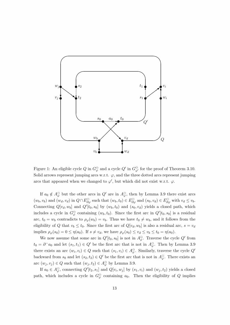
Figure 1: An eligible cycle Q in Gϕ and a cycle Q′ in G

ϕ′ for the proof of Theorem 3.10.

Solid arrows represent jumping arcs w.r.t. ϕ, and the three dotted arcs represent jumping

arcs that appeared when we changed to ϕ′, but which did not exist w.r.t. ϕ.

If a0 /∈ Aϕ but the other arcs in Q′ are in A

ϕ , then by Lemma 3.9 there exist arcs

(wb, vb) and (wd, vd) in Q∩E∂ϕ such that (wb, t0) ∈ E

∂ϕ and (s0, vd) ∈ E∂ϕ with vd ≤ vb.

Connecting Q[vd, wb] and Q′[t0, s0] by (wb, t0) and (s0, vd) yields a closed path, which

includes a cycle in Gϕ containing (wb, t0). Since the first arc in Q′[t0, s0] is a residual

arc, t0 = wb contradicts to ρϕ(wb) = vb. Thus we have t0 6= wb, and it follows from the

eligibility of Q that vb ≤ t0. Since the first arc of Q[vd, wb] is also a residual arc, s = vd

implies ρϕ(s0) = 0 ≤ η(a0). If s 6= vd, we have ρϕ(s0) ≤ vd ≤ vb ≤ t0 = η(a0).

We now assume that some arc in Q′[t0, s0] is not in Aϕ . Traverse the cycle Q′ from

t0 = ∂−a0 and let (s1, t1) ∈ Q′ be the first arc that is not in Aϕ . Then by Lemma 3.9

there exists an arc (wi, vi) ∈ Q such that (s1, vi) ∈ Aϕ . Similarly, traverse the cycle Q′

backward from s0 and let (s2, t2) ∈ Q′ be the first arc that is not in Aϕ . There exists an

arc (wj , vj) ∈ Q such that (wj , t2) ∈ Aϕ by Lemma 3.9.

If a0 ∈ Aϕ , connecting Q′[t2, s1] and Q[vi, wj ] by (s1, vi) and (wj , t2) yields a closed

path, which includes a cycle in Gϕ containing a0. Then the eligibility of Q implies

13

ρϕ(s0) ≤ η(a0).

If a0 /∈ Aϕ , it follows from Lemma 3.9 that there exist arcs (wb, vb) and (wd, vd) in

Q∩E∂ϕ such that (wb, t0) ∈ E

∂ϕ and (s0, vd) ∈ E∂ϕ with s0 = vd, t0 = wb, or vd ≤ vb, see

Figure 1. Then connecting Q[vi, wb] and Q′[t0, s1] by (wb, t0) and (s1, vi) yields a closed

path, which includes a cycle in Gϕ containing (wb, t0). Since the first arc in Q′[t0, s1] is

a residual arc, we have t0 6= wb. Hence we have vb ≤ t0 from the eligibility of Q. On the

other hand, connecting Q[vd, wj ] and Q′[t2, s0] by (s0, vd) and (wj , t2) similarly brings

a cycle in Gϕ containing (s0, vd). Since the first arc of Q[vd, wj ] is also a residual arc,

s = vd implies ρϕ(s0) = 0 ≤ η(a0). If s 6= vd, we have ρϕ(s0) ≤ vd, which together with

vd ≤ vb and vb ≤ t0 implies ρϕ(s0) ≤ t0.

When we cancel Q, there is an arc a ∈ Q that disappears in Gϕ′ . If a is a jumping

arc, w = ∂+a satisfies ρϕ′(w) > ρϕ(w).

We are now ready to present an outline of our cycle canceling algorithms. The sub-

routine Cycle Cancel repeatedly finds and cancels eligible cycles until Gϕ becomes

acyclic. Theorem 3.10 says that we need at most O(n2 + m) = O(n2) cancellations. Cy-

cle Cancel does not construct Gϕ explicitly, but instead computes exchange capacities

using a depth-first search to find an eligible cycle. Once a node v ∈ V turns out not to

have a cycle through v, i.e., ρϕ(v) = n+1, Theorem 3.10 says that we can ignore v in the

subsequent depth-first searches until Gϕ becomes acyclic. Cycle Cancel finds such a

node or an eligible cycle after computing exchange capacities O(n) times. Thus Cycle

Cancel takes O(n3h) time. Cycle Cancel is repeatedly called in the procedure Re-

fine which obtains an ε-optimal submodular flow starting from a 2ε-optimal submodular

flow. The following subsections describe the procedure Refine in the TA and the NA

cases.

3.4.1 Refine for Tight Arc Cycle Canceling

This subsection describes the procedure Refine that transforms a TA 2ε-optimal sub-

modular flow into a TA ε-optimal submodular flow. Given an initial feasible flow ϕ,

we solve AP(ϕ, ε) to obtain an optimal dual solution p whose components are integer

multiples of ε. If the optimal value is zero, then ϕ is a TA ε-optimal submodular flow.

Otherwise, we call Cycle Cancel.

When G◦ϕ becomes acyclic, there is no perfect matching that consists of tight arcs in

Gϕ, which means p is no longer optimal to DAP(ϕ, ε). Since the weight of every edge

in Gϕ is an integer multiple of ε, the optimal value of AP(ϕ, ε) has increased by at least

ε. We repeat this process until AP(ϕ, ε) has an optimal value zero, and then ϕ is a TA

14

ε-optimal submodular flow.

Refine for Tight Arc Cycle Canceling

Step 1: Solve AP(ϕ, ε) to obtain an optimal solution p for DAP(ϕ, ε).

Step 2: While AP(ϕ, ε) has a negative-cost assignment, do the following:

(2-1) Call Cycle Cancel.

(2-2) Update p into an optimal solution for DAP(ϕ, ε).

Lemma 3.11 The initial optimal value of AP(ϕ, ε) is at least −2nε.

Proof. Since cε(a) ≥ c2ε(a)−2ε, the initial reduced cost of any edge of AP(ϕ, ε) w.r.t.

an optimal dual solution p∗ to the final assignment problem of the 2ε-scaling phase is at

least −2ε. Since the objective value of p∗ is zero, the cost of any assignment is the same

if we replace cost by reduced cost. Thus the cost of any assignment is at least −2nε.

Each time G◦ϕ becomes acyclic, the optimal value of AP(ϕ, ε) increases by at least ε,

so G◦ϕ becomes acyclic O(n) times per scaling phase. We must re-solve AP(ϕ, ε) to get

a new p, but this can be done via a Dijkstra shortest path update, which also happens

O(n) times per phase, so this is not a bottleneck. It requires one call to Cycle Cancel

to make G◦ϕ acyclic, requiring O(n3h) time. Thus this Refine takes O(n4h) time.

3.4.2 Refine for Negative Arc Cycle Canceling

This subsection describes the procedure Refine that transforms an NA 2ε-optimal sub-

modular flow ϕ and a potential p that proves 2ε-optimality of ϕ into an NA ε-optimal

submodular flow and a potential that proves NA ε-optimality of ϕ. Given such a pair

of ϕ and p, we call an arc a ∈ Aϕ improvable if cp(a) < −ε. A node v ∈ V is called

improvable if v is the head of an improvable arc.

Given such an initial NA 2ε-optimal submodular flow ϕ and a potential p, we con-

struct G−ϕ and call Cycle Cancel. These cycle cancellations do not produce any new

improvable arcs. Then select an improvable node v, find the set W of nodes reachable

from v in G−ϕ , and put p(w) := p(w) − ε for w ∈ W . This Cut-Relabel(v) operation

does not violate the NA feasibility of p nor produce a new improvable arc. Furthermore,

it eliminates all the improvable arcs entering v. That is, v is no longer an improvable

node. We repeat this process until G−ϕ has no more improvable nodes. If G−

ϕ has no

improvable nodes, then it is obvious that ϕ is an NA ε-optimal submodular flow.

15

Refine for Negative Arc Cycle Canceling

Step 1: Call Cycle Cancel.

Step 2: While there still exist improvable nodes, do the following:

(2-1) Select an improvable node v and call Cut-Relabel(v).

(2-2) Call Cycle Cancel.

Since one iteration eliminates one improvable node, it is clear that we need at most

n iterations. Thus this Refine also takes O(n4h) time.

3.5 Successive Approximation

We now apply the successive approximation technique of Goldberg and Tarjan [16] to

our cycle canceling algorithms. The algorithms start with ε = 2dlog2 Ce and scale the

parameter ε. Each scaling phase uses Refine to find an ε-optimal submodular flow.

When the algorithm terminates, after performing O(log(nC)) scaling phases, it obtains

a submodular flow ϕ that is of minimum cost due to Lemma 3.2.

Algorithm Successive Approximation

Step 0: Find a feasible submodular flow ϕ.

Step 1: Compute ε := 2dlog2 Ce.

Step 2: While ε ≥ 1/n, do the following.

(2-1) Put ε := ε/2.

(2-2) Find an ε-optimal submodular flow ϕ∗ by Refine starting from ϕ.

(2-3) Put ϕ := ϕ∗.

We now compute the running time of Successive Approximation. By Lemma 3.2

there are O(log(nC)) scaling phases. We have already remarked that both versions of

Refine take O(n4h) time. Thus we have the following theorem.

Theorem 3.12 Both Tight Arc Cycle Canceling and Negative Arc Cycle Canceling run

in O(n4h log(nC)) time.

16

4 Strongly Polynomial Bounds

It is generally considered that a strongly polynomial algorithm cannot use the floor or

ceiling operation, unless the magnitude of the number is polynomially bounded. This

is because computing the floor of a ratio of real numbers can generally be accomplished

only through something like binary search. This is bad since the running time of binary

search-type algorithms definitely depends on the size of the data. Similarly, we can’t

compute dlog2 Ce in strongly polynomial time since this would involve counting the

Θ(log C) bits of C. Step 1 of Successive Approximation computes ε := 2dlog2 Ce;

since we are using real arithmetic, we can just replace this by ε := C.

Our Tight Arc Cycle Canceling uses floors in the definition of cε, so it is tricky to

extend it to be strongly polynomial. The min cost flow versions of the Tight Arc Cycle

Canceling [33] include variants which do not need to round costs. Unfortunately, we have

not been able to extend these variants to submodular flow. The main hurdle seems to

be that the argument showing that p remains TA feasible in Lemma 3.5 does not have

any slack in it, which appears to be necessary to make a more relaxed variant of the

algorithm work for this case.

Happily, a simple observation allows us to get a strongly polynomial version of the

Tight Arc Cycle Canceling despite using floors. The proof of Lemma 3.11 noted that

we can compute using reduced costs in AP(ϕ, ε) w.r.t. p∗ (the optimal node prices in

DAP at the end of the previous phase). For edge a = (v,w) this AP reduced cost is

cε(a)−p∗(v+)−p∗(w−). Note that if c(a)−p∗(v+)−p∗(w−) ≥ 2nε, then cε(a)−p∗(v+)−

p∗(w−) ≥ 2nε, implying that edge a cannot appear in any optimal solution of AP(ϕ, ε).

We can identify and delete such edges without harming strong polynomiality in O(m)

time. For the remaining edges, we can compute cε(a) − p∗(v+) − p∗(w−) using binary

search in O(log n) time each. This needs to be done only once in each scaling phase, so

it is not a bottleneck.

Our Negative Arc Cycle Canceling does not use rounding, so it does not need this

change.

Now we can apply the standard strongly polynomial machinery. We quote the prox-

imity lemma we need, which applies to both notions of ε-optimality.

Lemma 4.1 ([12, Theorem 3]) Let ϕ∗ be any optimal submodular flow, and suppose

that p proves that ϕ is ε-optimal. If cp(a) > nε, then ϕ∗(a) = l(a). If cp(a) < −nε, then

ϕ∗(a) = u(a). If p(w) > p(v) + nε, then r(∂ϕ∗, v, w) = 0.

Note that Gϕ has m′ = m + n2 = O(n2) arcs. A min mean cycle is a directed cycle

17

in Nϕ that minimizes c(Q)/|Q| over all directed cycles in Nϕ. A min mean cycle with a

minimum number of arcs can be computed in O(m′n) = O(n3) time [26]. Cui and Fu-

jishige [2, Theorem 3.2] show that such a min mean cycle is admissible, so by Lemma 3.7

we can feasibly cancel it. If Q∗ is a min mean cycle with value µ∗ = c(Q∗)/|Q∗|, then

any of the min mean cycle algorithms produces dual variables p proving that ϕ is µ∗-

optimal. We now divide the scaling phases into groups, where each group consists of

β = dlog2 n + 1e consecutive scaling phases. We then replace the first cycle cancel in

each group by canceling an admissible min mean cycle Q∗.

Our choice of β ensures that the value of ε at the end of a group is smaller than 1/n

of the min mean cycle value µ∗, which is the value of ε at the beginning of the group.

From this it follows that at least one arc a of Q∗ must satisfy one of the hypotheses

of Lemma 4.1, so that we can fix ϕ(a) to one of its bounds. That is, if a ∈ Fϕ we fix

ϕ(a) = u(a), if a ∈ Bϕ we fix ϕ(a) = l(a), and if a ∈ E∂ϕ we “fix” the flow in this

jumping arc to zero by forbidding it to be used hereafter. It can be shown as in [33] that

the flow on a was changed by canceling Q∗, so that ϕ(a) is newly fixed to a bound. After

O(m′) groups all ϕ(a)’s are fixed, so we must be optimal. This yields

Theorem 4.2 For both Tight Arc Cycle Canceling and Negative Arc Cycle Canceling,

performing scaling phases by groups with a min mean cycle cancellation at the beginning

of each group takes O(n6h log n) time overall.

Proof. Each group takes O(log n) scaling phases, each of which costs O(n4h) time, and

we need O(m′) groups to reach optimality. The cost of the min mean cycle computations

is (O(m′) computations) × (O(n3) time/computation), or O(n5) time, which is not a

bottleneck.

5 Separable Convex Objective Functions

Rockafellar’s book Network Flows and Monotropic Optimization [30] argues that it is not

really harder to optimize with a separable convex objective function than it is to optimize

with a linear objective function. Papers such as Hochbaum and Shanthikumar [19],

Karzanov and McCormick [27], and McCormick, Shigeno, and Iwata [25] have shown that

this is indeed the case for minimum cost flow algorithms based on capacity scaling, min

mean cycle canceling, and relaxed most negative cycle canceling, respectively (in all three

cases, even over totally unimodular constraints). Iwata [20] shows that capacity scaling

further extends to separable convex cost submodular flow, yielding the only previous

18

polynomial algorithm for separable convex submodular flow we know of. The concurrent

paper [23] shows a cut canceling algorithm for submodular flow also extends to separable

convex costs. This section sketches how to extend the cycle canceling algorithms of this

paper to separable convex cost submodular flow.

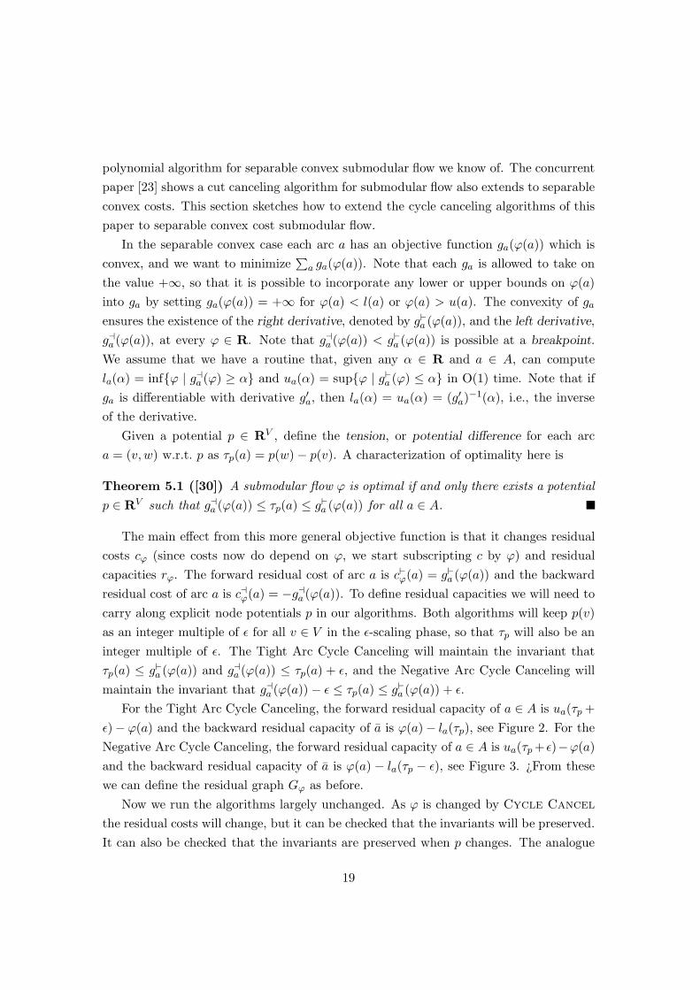
In the separable convex case each arc a has an objective function ga(ϕ(a)) which is

convex, and we want to minimize∑

a ga(ϕ(a)). Note that each ga is allowed to take on

the value +∞, so that it is possible to incorporate any lower or upper bounds on ϕ(a)

into ga by setting ga(ϕ(a)) = +∞ for ϕ(a) < l(a) or ϕ(a) > u(a). The convexity of ga

ensures the existence of the right derivative, denoted by g`a (ϕ(a)), and the left derivative,

gaa (ϕ(a)), at every ϕ ∈ R. Note that gaa (ϕ(a)) < g`a (ϕ(a)) is possible at a breakpoint.

We assume that we have a routine that, given any α ∈ R and a ∈ A, can compute

la(α) = inf{ϕ | gaa (ϕ) ≥ α} and ua(α) = sup{ϕ | g`a (ϕ) ≤ α} in O(1) time. Note that if

ga is differentiable with derivative g′a, then la(α) = ua(α) = (g′a)−1(α), i.e., the inverse

of the derivative.

Given a potential p ∈ RV , define the tension, or potential difference for each arc

a = (v,w) w.r.t. p as τp(a) = p(w) − p(v). A characterization of optimality here is

Theorem 5.1 ([30]) A submodular flow ϕ is optimal if and only there exists a potential

p ∈ RV such that gaa (ϕ(a)) ≤ τp(a) ≤ g`a (ϕ(a)) for all a ∈ A.

The main effect from this more general objective function is that it changes residual

costs cϕ (since costs now do depend on ϕ, we start subscripting c by ϕ) and residual

capacities rϕ. The forward residual cost of arc a is c`ϕ(a) = g`a (ϕ(a)) and the backward

residual cost of arc a is caϕ(a) = −gaa (ϕ(a)). To define residual capacities we will need to

carry along explicit node potentials p in our algorithms. Both algorithms will keep p(v)

as an integer multiple of ε for all v ∈ V in the ε-scaling phase, so that τp will also be an

integer multiple of ε. The Tight Arc Cycle Canceling will maintain the invariant that

τp(a) ≤ g`a (ϕ(a)) and gaa (ϕ(a)) ≤ τp(a) + ε, and the Negative Arc Cycle Canceling will

maintain the invariant that gaa (ϕ(a)) − ε ≤ τp(a) ≤ g`a (ϕ(a)) + ε.

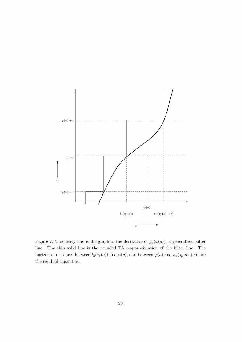
For the Tight Arc Cycle Canceling, the forward residual capacity of a ∈ A is ua(τp +

ε)− ϕ(a) and the backward residual capacity of a is ϕ(a) − la(τp), see Figure 2. For the

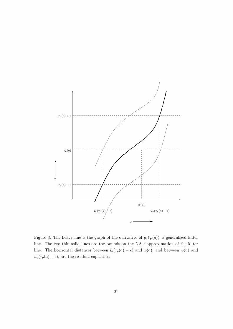
Negative Arc Cycle Canceling, the forward residual capacity of a ∈ A is ua(τp + ε)−ϕ(a)

and the backward residual capacity of a is ϕ(a) − la(τp − ε), see Figure 3. ¿From these

we can define the residual graph Gϕ as before.

Now we run the algorithms largely unchanged. As ϕ is changed by Cycle Cancel

the residual costs will change, but it can be checked that the invariants will be preserved.

It can also be checked that the invariants are preserved when p changes. The analogue

19

ϕ

τ

τp(a)

τp(a) + ε

ϕ(a)

la(τp(a)) ua(τp(a) + ε)

τp(a) − ε

Figure 2: The heavy line is the graph of the derivative of ga(ϕ(a)), a generalized kilter

line. The thin solid line is the rounded TA ε-approximation of the kilter line. The

horizontal distances between la(τp(a)) and ϕ(a), and between ϕ(a) and ua(τp(a)+ ε), are

the residual capacities.

20

ϕ

τ

ϕ(a)

τp(a)

τp(a) + ε

τp(a) − ε

la(τp(a) − ε) ua(τp(a) + ε)

Figure 3: The heavy line is the graph of the derivative of ga(ϕ(a)), a generalized kilter

line. The two thin solid lines are the bounds on the NA ε-approximation of the kilter

line. The horizontal distances between la(τp(a) − ε) and ϕ(a), and between ϕ(a) and

ua(τp(a) + ε), are the residual capacities.

21

of Lemma 3.11 for the Tight Arc Cycle Canceling is still true in this more general case.

Thus in both cases Refine still runs in O(n4h) time.

With general separable convex objective functions it is impossible to get any a priori

bound on how large we must choose the initial value of ε in Successive Approxima-

tion to ensure that our initial solution is ε-optimal. Thus we use B to stand for this

unknown initial value. Similarly, there is no way to ensure exact optimality no matter

how many scaling phases we run, so we use ι to stand for the final value of ε we use. Thus

Successive Approximation makes O(B/ι) calls to Refine, and we get the following

Theorem 5.2 For both Tight Arc Cycle Canceling and Negative Arc Cycle Canceling,

the running time in the separable convex case is O(n4h log(B/ι)).

The interested reader can consult, e.g., [27] for more details on what guarantees

are possible for ε-optimality implying that ϕ is close to some optimal ϕ∗, to see how

the algorithms can compute an exact solution in polynomial time when all the ga are

piecewise quadratic, and to see how the algorithms are strongly polynomial when all the

ga are piecewise linear.

Acknowledgment

We would like to thank an anonymous referee of [33] for suggesting that Goldberg’s

algorithm might extend to submodular flow.

References

[1] R. K. Ahuja, T. L. Magnanti, and J. B. Orlin: Network Flows — Theory,

Algorithms, and Applications, Prentice Hall (1993).

[2] W. Cui and S. Fujishige: A primal algorithm for the submodular flow problem

with minimum-mean cycle selection, J. Oper. Res. Soc. Japan, 31 (1988), 431–440.

[3] W. H. Cunningham and A. Frank: A primal-dual algorithm for submodular

flows, Math. Oper. Res., 10 (1985), 251–262.

[4] J. Edmonds and R. Giles: A min-max relation for submodular functions on

graphs, Ann. Discrete Math., 1 (1977), 185–204.

[5] J. Edmonds and R. M. Karp: Theoretical improvements in algorithmic efficiency

for network flow problems, J. ACM, 19 (1972), 248–264.

22

[6] L. Fleischer, S. Iwata, and S. T. McCormick: A faster capacity-scaling algo-

rithm for minimum cost submodular flow, Research Report 99-08, Discrete Mathe-

matics and Systems Science, Osaka University, 1999.

[7] A. Frank: Finding feasible vectors of Edmonds–Giles polyhedra, J. Combinatorial

Theory, Ser. B, 36 (1984), 221–239.

[8] A. Frank and E. Tardos: An application of simultaneous Diophantine approxi-

mation in combinatorial optimization, Combinatorica, 7 (1987), 49–65.

[9] A. Frank and E. Tardos: Generalized polymatroids and submodular flows, Math.

Programming, 42 (1988), 489–563.

[10] S. Fujishige: Algorithms for solving the independent-flow problems, J. Oper. Res.

Soc. Japan, 21 (1978), 189–204.

[11] S. Fujishige: Submodular Functions and Optimization, North-Holland, 1991.

[12] S. Fujishige, H. Rock, and U. Zimmermann: A strongly polynomial algorithm

for minimum cost submodular flow problems, Math. Oper. Res., 14 (1989), 60–69.

[13] S. Fujishige and X. Zhang: New algorithms for the intersection problem of sub-

modular systems, Japan J. Indust. Appl. Math., 9 (1992), 369–382.

[14] A. V. Goldberg: Scaling algorithms for the shortest paths problem, SIAM J.

Comput., 24 (1995), 494–504.

[15] A. V. Goldberg and R. E. Tarjan: Finding minimum-cost circulations by can-

celing negative cycles, J. ACM, 36 (1989), 873–886.

[16] A. V. Goldberg and R. E. Tarjan: Finding minimum-cost circulations by suc-

cessive approximation, Math. Oper. Res., 15 (1990), 430–466.

[17] M. Grotschel, L. Lovasz, and A. Schrijver: Geometric Algorithms and Com-

binatorial Optimization, Springer-Verlag, 1988.

[18] R. Hassin: Minimum cost flow with set-constraints, Networks, 12 (1982), 1–21.

[19] D. S. Hochbaum and J. G. Shanthikumar: Convex separable optimization is

not much harder than linear optimization, J. ACM, 37 (1990), 843–862.

[20] S. Iwata: A capacity scaling algorithm for convex cost submodular flows,

Math. Programming, 76 (1997), 299–308.

23

[21] S. Iwata, L. Fleischer, and S. Fujishige: A combinatorial, strongly

polynomial-time algorithm for minimizing submodular functions, Proceedings of

the 32nd ACM Symposium on Theory of Computing (2000), 97–106.

[22] S. Iwata, S. T. McCormick, and M. Shigeno: A faster algorithm for minimum

cost submodular flows, Proceedings of the Ninth Annual ACM/SIAM Symposium

on Discrete Algorithms (1998), 167–174.

[23] S. Iwata, S. T. McCormick, and M. Shigeno: A strongly polynomial cut

canceling algorithm for the submodular flow problem. Proceedings of the Seventh

MPS Conference on Integer Programming and Combinatorial Optimization (1999),

G. Cornuejols, R. E. Burkard, and G. J. Woeginger, eds., 259–272.

[24] S. Iwata, S. T. McCormick, and M. Shigeno: A fast cost scaling algorithm for

submodular flow, Inform. Process. Lett., 74 (2000), 123–128.

[25] S. Iwata, S. T. McCormick, and M. Shigeno: A relaxed cycle-canceling ap-

proach to separable convex optimization in unimodular linear spaces, 1999.

[26] R. M. Karp: A characterization of the minimum cycle mean in a digraph, Discrete

Math., 23 (1978), 309–311.

[27] A. V. Karzanov and S. T. McCormick: Polynomial methods for separable con-

vex optimization in totally unimodular linear spaces with applications to circulations

and co-circulations in networks, SIAM J. Comput., 26 (1997), 1245–1275.

[28] E. L. Lawler and C. U. Martel: Computing maximal polymatroidal network

flows, Math. Oper. Res., 7 (1982), 334–347.

[29] T. Naitoh and S. Fujishige: A note on the Frank–Tardos bitruncation algorithm

for crossing-submodular functions, Math. Programming, 53 (1992), 361–363.

[30] R. T. Rockafellar: Network Flows and Monotropic Optimization. Wiley Inter-

science, New York, NY (1984).

[31] P. Schonsleben: Ganzzahlige Polymatroid-Intersektions-Algorithmen, ETH

Zurich (1980).

[32] A. Schrijver: A combinatorial algorithm minimizing submodular functions in

strongly polynomial time, J. Combinatorial Theory, Ser. B, to appear.

24

[33] M. Shigeno, S. Iwata, and S. T. McCormick: Relaxed most negative cycle and

most positive cut canceling algorithms for minimum cost flow, Math. Oper. Res.,

25 (2000), 76–104.

[34] E. Tardos: A strongly polynomial minimum cost circulation algorithm, Combina-

torica, 5 (1985), 247–256.

[35] E. Tardos, C. A. Tovey, and M. A. Trick: Layered augmenting path algo-

rithms, Math. Oper. Res., 11 (1986), 362–370.

[36] C. Wallacher and U. Zimmermann: A polynomial cycle canceling algorithm for

submodular flows, Math. Programming, 86 (1999), 1–15.

[37] U. Zimmermann: Negative circuits for flows and submodular flows, Discrete

Appl. Math., 36 (1992), 179–189.

25