Deep Submodular Functions - arXiv

Deep Submodular Functions

Jeffrey A. Bilmes1,2 and Wenruo Bai1

1Department of Electrical Engineering, University of Washington, Seattle, 981952Department of Computer Science and Engineering, University of Washington, Seattle,

98195

February 1, 2017

Abstract

We start with an overview of a class of submodular functions called SCMMs (sums of concave com-posed with non-negative modular functions plus a final arbitrary modular). We then define a new classof submodular functions we call deep submodular functions or DSFs. We show that DSFs are a flex-ible parametric family of submodular functions that share many of the properties and advantages ofdeep neural networks (DNNs), including many-layered hierarchical topologies, representation learning,distributed representations, opportunities and strategies for training, and suitability to GPU-based ma-trix/vector computing. DSFs can be motivated by considering a hierarchy of descriptive concepts overground elements and where one wishes to allow submodular interaction throughout this hierarchy. Inmachine learning and data science applications, where there is often either a natural or an automati-cally learnt hierarchy of concepts over data, DSFs therefore naturally apply. Results in this paper showthat DSFs constitute a strictly larger class of submodular functions than SCMMs, thus justifying theirmathematical and practical utility. Moreover, we show that, for any integer k > 0, there are k-layerDSFs that cannot be represented by a k′-layer DSF for any k′ < k. This implies that, like DNNs, thereis a utility to depth, but unlike DNNs (which can be universally approximated by shallow networks),the family of DSFs strictly increase with depth. Despite this property, however, we show that DSFs,even with arbitrarily large k, do not comprise all submodular functions. We show this using a tech-nique that “backpropagates” certain requirements if it was the case that DSFs comprised all submodularfunctions. In offering the above results, we also define the notion of an antitone superdifferential of aconcave function and show how this relates to submodular functions (in general), DSFs (in particular),negative second-order partial derivatives, continuous submodularity, and concave extensions. To furthermotivate our analysis, we provide various special case results from matroid theory, comparing DSFs withforms of matroid rank, in particular the laminar matroid. Lastly, we discuss strategies to learn DSFs,and define the classes of deep supermodular functions, deep difference of submodular functions, and deepmultivariate submodular functions, and discuss where these can be useful in applications.

Contents1 Introduction 2

2 Background and Motivation 4

3 Sums of Concave Composed with Modular Functions (SCMMs) 43.1 Feature Based Functions . . . . . . . . . . . . . . . . . . . . . . . . . . . . . . . . . . . . . . . 6

4 Deep Submodular Functions 84.1 Recursively Defined DSFs . . . . . . . . . . . . . . . . . . . . . . . . . . . . . . . . . . . . . . 104.2 DSFs: Practical Benefits and Relation to Deep Neural Networks . . . . . . . . . . . . . . . . 11

1

arX

iv:1

701.

0893

9v1

[cs

.LG

] 3

1 Ja

n 20

17

5 Relevant Properties and Special Cases 115.1 Properties of Concave and Submodular Functions . . . . . . . . . . . . . . . . . . . . . . . . . 125.2 Antitone Maps and Superdifferentials . . . . . . . . . . . . . . . . . . . . . . . . . . . . . . . . 165.3 The Special Matroid Case and Deep Matroid Rank . . . . . . . . . . . . . . . . . . . . . . . . 195.4 Surplus and Absolute Redundancy . . . . . . . . . . . . . . . . . . . . . . . . . . . . . . . . . 21

6 The Family of Deep Submodular Functions 246.1 DSFs generalize SCMMs . . . . . . . . . . . . . . . . . . . . . . . . . . . . . . . . . . . . . . . 25

6.1.1 The Laminar Matroid Rank Case . . . . . . . . . . . . . . . . . . . . . . . . . . . . . . 266.1.2 A Non-matroid Case . . . . . . . . . . . . . . . . . . . . . . . . . . . . . . . . . . . . . 276.1.3 More General Conditions on Two-Layer Functions . . . . . . . . . . . . . . . . . . . . 28

6.2 The DSF Family Grows Strictly with the Number of Layers . . . . . . . . . . . . . . . . . . . 296.3 The Family of Submodular Functions is Strictly Larger than DSFs . . . . . . . . . . . . . . . 33

7 Applications in Machine Learning and Data Science 367.1 Learning DSFs . . . . . . . . . . . . . . . . . . . . . . . . . . . . . . . . . . . . . . . . . . . . 37

7.1.1 Training and Testing on Different Ground Sets, and Multimodal Submodularity . . . . 397.2 Deep Supermodular Functions and Deep Differences . . . . . . . . . . . . . . . . . . . . . . . 407.3 Deep Multivariate Submodular Functions . . . . . . . . . . . . . . . . . . . . . . . . . . . . . 417.4 Simultaneously Learning Hash and Submodular Functions . . . . . . . . . . . . . . . . . . . . 42

8 Conclusions and Future Work 43

9 Acknowledgments 43

References 44

A More General Conditions on Two-Layer Functions: Proofs 52

B Sums of Weighted Cardinality Truncations is Smaller than SCMMs 55

1 IntroductionSubmodular functions are attractive models of many physical processes primarily because they possess aninherent naturalness to a wide variety of problems (e.g., they are good models of diversity, information,and cooperative costs) while at the same time they enjoy properties sufficient for efficient optimization. Forexample, submodular functions can be minimized without constraints in polynomial time [46] even thoughthey lie within a 2n-dimensional cone in R2n and are parameterized, in their most general form, with acorresponding 2n independent degrees of freedom. Moreover, while submodular function maximization isNP-hard, submodular maximization is one of the easiest of the NP-hard problems since constant factorapproximation algorithms are often available — e.g., in the cardinality constrained case, the classic 1− 1/eresult of Nemhauser [113] via the greedy algorithm. Other problems also have guarantees, such as submodularmaximization subject to knapsack or multiple matroid constraints [22, 21, 88, 66, 68].

Submodular functions are becoming increasingly important in the field of machine learning. In recentyears, submodular functions have been used for representing diversity functions for the purpose of datasummarization [91], for use as structured convex norms [6], for energy functions in tree-width unconstrainedprobabilistic models [48, 82, 67, 55], useful in computer vision [79], feature [98] and dictionary selection [33],viral marketing [58] and influence modeling in social networks [77], information cascades [89] and diffusionmodeling [130], clustering [111], and active and semi-supervised learning [57], to name just a few. There alsohave been significant contributions from the machine learning community purely on the mathematical andalgorithmic aspects of submodularity. This includes algorithms for optimizing non-submodular functions viathe use of submodularity [110, 81, 71, 64], strategies for optimizing submodular functions subject to bothcombinatorial [65] and submodular level-set constraints [66], and so on.

2

One of the critical problems associated with utilizing submodular functions in machine learning and datascience contexts is selecting which submodular function to use, and given that submodular functions lie insuch a vast space with 2n degrees of freedom, it is a non-trivial task to find one that works well, if notoptimally. One approach is to attempt to learn the submodular function based on either queries of someform or based on data. This has led to results, mostly in the theory community, showing how learningsubmodularity can be harder or easier depending on how we judge what is being learnt. For example, it wasshown that learning submodularity in the PMAC setting is fairly hard [10] although in some cases thingsare a bit easier [42]. Learning can be made easier if we restrict ourselves to learn within only a subfamily ofsubmodular functions. For example, in [140, 92], it is shown empirically that one can effectively learn mixturesof submodular functions using a max-margin learning framework — here the components of the mixture arefixed and it is only the mixture parameters that are learnt, leading often to a convex optimization problem.In some cases, computing gradients of the convex problem can be done using submodular maximization [92],while in other cases, even a gradient requires minimizing a difference of two submodular functions [150].

Learning over restricted families rather than over the entire cone is desirable for the same reasons that anyform of regularization in machine learning is useful. By restricting the family over which learning occurs,it decreases the complexity of the learning problem, thereby increasing the chance that one finds a goodmodel within that family. This can be seen as a classic bias-variance tradeoff, where increasing bias canreduce variance. Up to now, learning over restricted families has apparently (to the authors’ knowledge) beenlimited to learning mixtures over fixed components. This can be limited if the components are restricted,and if not might require a very large number of components. Therefore, there is a need for a richer and moreflexible parametric family of submodular functions over which learning is not only still possible but ideallyrelatively easy. See Section 7.1 for further discussion on learning submodular functions.

In this paper, we introduce a new family of submodular functions that we term “deep submodular func-tions,” or DSFs. DSFs strictly generalize, as we show below, many of the kinds of submodular functions thatare useful in machine learning contexts. These include the so-called “decomposable” submodular functions,namely those that can be represented as a sum of concave composed with modular functions [141].

We describe the family of DSFs and place them in the context of the general submodular family. Inparticular, we show that DSFs strictly generalize standard decomposable functions, thus theoretically moti-vating the use of deeper networks as a family over which to learn. Moreover, DSFs can represent a varietyof complex submodular functions such as laminar matroid rank functions. These matroid rank functionsinclude the truncated matroid rank function [52] that is often used to show theoretical worst-case perfor-mance for many constrained submodular minimization problems. We also show, somewhat surprisingly, thatlike decomposable functions, DSFs are unable to represent all possible cycle matroid rank functions. This isinteresting in and of itself since there are laminar matroids that can not be represented by cycle matroids. Onthe other hand, we show that the more general DSFs share a variety of useful properties with decomposablefunctions. Namely, that they: (1) can leverage the vast amount of practical work on feature engineeringthat occurs in the machine learning community and its applications; (2) can operate on multi-modal data ifthe data can be featurized in the same space; (3) allow for training and testing on distinct sets since we canlearn a function from the feature representation level on up, similar to the work in [92]; and (4) are usefulfor streaming [7, 83, 23] and parallel [107, 13, 14] optimization since functions can be evaluated withoutrequiring knowledge of or access to the entire ground set. These advantages are made apparent in Section 2.

Interestingly, DSFs also share certain properties with deep neural networks (DNNs), which have becomewidely popular in the machine learning community. For example, DNNs with weights that are strictly non-negative correspond to a DSF. This suggests, as we show in Section 7.1, that it is possible to develop alearning framework over DSFs leveraging DNN learning frameworks. Unlike standard deep neural networks,which typically are trained either in classification or regression frameworks, however, learning submodularityoften takes the form of trying to adjust the parameters so that a set of “summary” data sets are offered ahigh value. We therefore extend the max-margin learning framework of [140, 92] to apply to DSFs. Ourapproach can be seen as a max-margin learning approach for DNNs but restricted to DSFs.

We offer a list of applications for DSFs in machine learning and data science in Section 7.

3

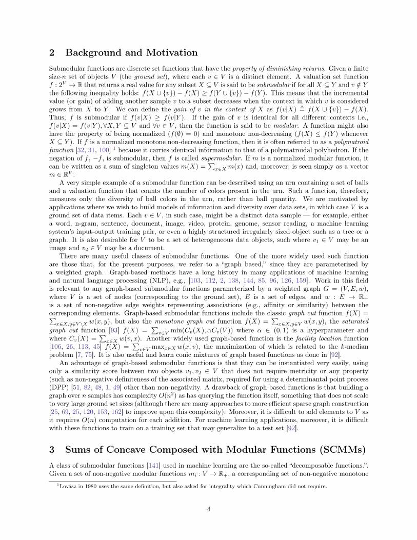
2 Background and MotivationSubmodular functions are discrete set functions that have the property of diminishing returns. Given a finitesize-n set of objects V (the ground set), where each v ∈ V is a distinct element. A valuation set functionf : 2V → R that returns a real value for any subsetX ⊆ V is said to be submodular if for allX ⊆ Y and v /∈ Ythe following inequality holds: f(X ∪ {v}) − f(X) ≥ f(Y ∪ {v}) − f(Y ). This means that the incrementalvalue (or gain) of adding another sample v to a subset decreases when the context in which v is consideredgrows from X to Y . We can define the gain of v in the context of X as f(v|X) , f(X ∪ {v}) − f(X).Thus, f is submodular if f(v|X) ≥ f(v|Y ). If the gain of v is identical for all different contexts i.e.,f(v|X) = f(v|Y ),∀X,Y ⊆ V and ∀v ∈ V , then the function is said to be modular. A function might alsohave the property of being normalized (f(∅) = 0) and monotone non-decreasing (f(X) ≤ f(Y ) wheneverX ⊆ Y ). If f is a normalized monotone non-decreasing function, then it is often referred to as a polymatroidfunction [32, 31, 100] 1 because it carries identical information to that of a polymatroidal polyhedron. If thenegation of f , −f , is submodular, then f is called supermodular. If m is a normalized modular function, itcan be written as a sum of singleton values m(X) =

∑x∈X m(x) and, moreover, is seen simply as a vector

m ∈ RV .A very simple example of a submodular function can be described using an urn containing a set of balls

and a valuation function that counts the number of colors present in the urn. Such a function, therefore,measures only the diversity of ball colors in the urn, rather than ball quantity. We are motivated byapplications where we wish to build models of information and diversity over data sets, in which case V is aground set of data items. Each v ∈ V , in such case, might be a distinct data sample — for example, eithera word, n-gram, sentence, document, image, video, protein, genome, sensor reading, a machine learningsystem’s input-output training pair, or even a highly structured irregularly sized object such as a tree or agraph. It is also desirable for V to be a set of heterogeneous data objects, such where v1 ∈ V may be animage and v2 ∈ V may be a document.

There are many useful classes of submodular functions. One of the more widely used such functionare those that, for the present purposes, we refer to a “graph based,” since they are parameterized bya weighted graph. Graph-based methods have a long history in many applications of machine learningand natural language processing (NLP), e.g., [103, 112, 2, 138, 144, 85, 96, 126, 159]. Work in this fieldis relevant to any graph-based submodular functions parameterized by a weighted graph G = (V,E,w),where V is a set of nodes (corresponding to the ground set), E is a set of edges, and w : E → R+

is a set of non-negative edge weights representing associations (e.g., affinity or similarity) between thecorresponding elements. Graph-based submodular functions include the classic graph cut function f(X) =∑x∈X,y∈V \X w(x, y), but also the monotone graph cut function f(X) =

∑x∈X,y∈V w(x, y), the saturated

graph cut function [93] f(X) =∑v∈V min(Cv(X), αCv(V )) where α ∈ (0, 1) is a hyperparameter and

where Cv(X) =∑x∈X w(v, x). Another widely used graph-based function is the facility location function

[106, 26, 113, 45] f(X) =∑v∈V maxx∈X w(x, v), the maximization of which is related to the k-median

problem [7, 75]. It is also useful and learn conic mixtures of graph based functions as done in [92].An advantage of graph-based submodular functions is that they can be instantiated very easily, using

only a similarity score between two objects v1, v2 ∈ V that does not require metricity or any property(such as non-negative definiteness of the associated matrix, required for using a determinantal point process(DPP) [51, 82, 48, 1, 49] other than non-negativity. A drawback of graph-based functions is that building agraph over n samples has complexity O(n2) as has querying the function itself, something that does not scaleto very large ground set sizes (although there are many approaches to more efficient sparse graph construction[25, 69, 25, 120, 153, 162] to improve upon this complexity). Moreover, it is difficult to add elements to V asit requires O(n) computation for each addition. For machine learning applications, moreover, it is difficultwith these functions to train on a training set that may generalize to a test set [92].

3 Sums of Concave Composed with Modular Functions (SCMMs)A class of submodular functions [141] used in machine learning are the so-called “decomposable functions.”.Given a set of non-negative modular functions mi : V → R+, a corresponding set of non-negative monotone

1Lovász in 1980 uses the same definition, but also asked for integrality which Cunningham did not require.

4

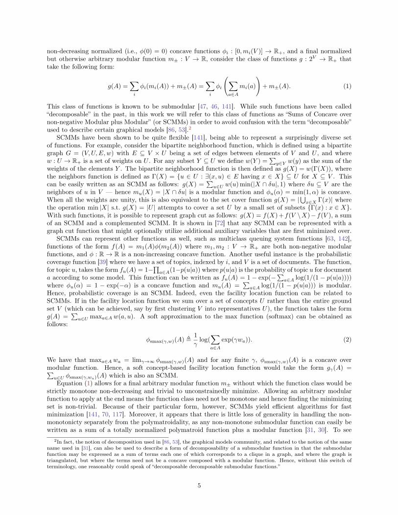
non-decreasing normalized (i.e., φ(0) = 0) concave functions φi : [0,mi(V )] → R+, and a final normalizedbut otherwise arbitrary modular function m± : V → R, consider the class of functions g : 2V → R+ thattake the following form:

g(A) =∑i

φi(mi(A)) +m±(A) =∑i

φi

(∑a∈A

mi(a)

)+m±(A). (1)

This class of functions is known to be submodular [47, 46, 141]. While such functions have been called“decomposable” in the past, in this work we will refer to this class of functions as “Sums of Concave overnon-negative Modular plus Modular” (or SCMMs) in order to avoid confusion with the term “decomposable”used to describe certain graphical models [86, 53].2

SCMMs have been shown to be quite flexible [141], being able to represent a surprisingly diverse setof functions. For example, consider the bipartite neighborhood function, which is defined using a bipartitegraph G = (V,U,E,w) with E ⊆ V × U being a set of edges between elements of V and U , and wherew : U → R+ is a set of weights on U . For any subset Y ⊆ U we define w(Y ) =

∑y∈Y w(y) as the sum of the

weights of the elements Y . The bipartite neighborhood function is then defined as g(X) = w(Γ(X)), wherethe neighbors function is defined as Γ(X) = {u ∈ U : ∃(x, u) ∈ E having x ∈ X} ⊆ U for X ⊆ V . Thiscan be easily written as an SCMM as follows: g(X) =

∑u∈U w(u) min(|X ∩ δu|, 1) where δu ⊆ V are the

neighbors of u in V — hence mu(X) = |X ∩ δu| is a modular function and φu(α) = min(1, α) is concave.When all the weights are unity, this is also equivalent to the set cover function g(X) = |⋃x∈X Γ(x)| wherethe operation min |X| s.t. g(X) = |U | attempts to cover a set U by a small set of subsets {Γ(x) : x ∈ X}.With such functions, it is possible to represent graph cut as follows: g(X) = f(X) + f(V \X)− f(V ), a sumof an SCMM and a complemented SCMM. It is shown in [72] that any SCMM can be represented with agraph cut function that might optionally utilize additional auxiliary variables that are first minimized over.

SCMMs can represent other functions as well, such as multiclass queuing system functions [63, 142],functions of the form f(A) = m1(A)φ(m2(A)) where m1,m2 : V → R+ are both non-negative modularfunctions, and φ : R → R is a non-increasing concave function. Another useful instance is the probabilisticcoverage function [39] where we have a set of topics, indexed by i, and V is a set of documents. The function,for topic u, takes the form fu(A) = 1−∏a∈A(1−p(u|a)) where p(u|a) is the probability of topic u for documenta according to some model. This function can be written as fu(A) = 1 − exp(−∑a∈A log(1/(1 − p(u|a))))where φu(α) = 1 − exp(−α) is a concave function and mu(A) =

∑a∈A log(1/(1 − p(u|a))) is modular.

Hence, probabilistic coverage is an SCMM. Indeed, even the facility location function can be related toSCMMs. If in the facility location function we sum over a set of concepts U rather than the entire groundset V (which can be achieved, say by first clustering V into representatives U), the function takes the formg(A) =

∑u∈U maxa∈A w(a, u). A soft approximation to the max function (softmax) can be obtained as

follows:

φsmax(γ,w)(A) ,1

γlog(

∑a∈A

exp(γwa)). (2)

We have that maxa∈A wa = limγ→∞ φsmax(γ,w)(A) and for any finite γ, φsmax(γ,w)(A) is a concave overmodular function. Hence, a soft concept-based facility location function would take the form gγ(A) =∑u∈U φsmax(γ,wu)(A) which is also an SCMM.Equation (1) allows for a final arbitrary modular function m± without which the function class would be

strictly monotone non-decreasing and trivial to unconstrainedly minimize. Allowing an arbitrary modularfunction to apply at the end means the function class need not be monotone and hence finding the minimizingset is non-trivial. Because of their particular form, however, SCMMs yield efficient algorithms for fastminimization [141, 70, 117]. Moreover, it appears that there is little loss of generality in handling the non-monotonicty separately from the polymatroidality, as any non-monotone submodular function can easily bewritten as a sum of a totally normalized polymatroid function plus a modular function [31, 30]. To see

2In fact, the notion of decomposition used in [86, 53], the graphical models community, and related to the notion of the samename used in [31], can also be used to describe a form of decomposability of a submodular function in that the submodularfunction may be expressed as a sum of terms each one of which corresponds to a clique in a graph, and where the graph istriangulated, but where the terms need not be a concave composed with a modular function. Hence, without this switch ofterminology, one reasonably could speak of “decomposable decomposable submodular functions.”

5

00

0.5

1

1.5

2

2.5

3

1 2 3 4 5 6 7 8 9 10

00

0.5

1

1.5

2

2.5

3

1 2 3 4 5 6 7 8 9 10

00

0.5

1

1.5

2

2.5

3

1 2 3 4 5 6 7 8 9 10

00

0.5

1

1.5

2

2.5

3

1 2 3 4 5 6 7 8 9 10

00

0.5

1

1.5

2

2.5

3

1 2 3 4 5 6 7 8 9 10

00

0.5

1

1.5

2

2.5

3

1 2 3 4 5 6 7 8 9 10

00

0.5

1

1.5

2

2.5

3

1 2 3 4 5 6 7 8 9 10

00

0.5

1

1.5

2

2.5

3

1 2 3 4 5 6 7 8 9 10

00

0.5

1

1.5

2

2.5

3

1 2 3 4 5 6 7 8 9 10

)0.5

00

0.5

1

1.5

2

2.5

3

1 2 3 4 5 6 7 8 9 10

00

0.5

1

1.5

2

2.5

3

1 2 3 4 5 6 7 8 9 10

00

0.5

1

1.5

2

2.5

3

1 2 3 4 5 6 7 8 9 10

a

d

g

(( )0.5

00

0.5

1

1.5

2

2.5

3

1 2 3 4 5 6 7 8 9 10

00

0.5

1

1.5

2

2.5

3

1 2 3 4 5 6 7 8 9 10

00

0.5

1

1.5

2

2.5

3.5

3

1 2 3 4 5 6 7 8 9 10 11 12 1313 1514

(I) (II) (III)

(IV) (V) (III)

mU (a)

= (m (a),m (a),m (a))

= (9, 0, 0)

mU (d)

= (m (d),m (d),m (d))

= (3, 3, 3)

mU (g)

= (m (g),m (g),m (g))

= (4, 3, 2)

a b c

d e f

g h i

a b c

d e f

g h i

a b c

d e f

g h i

a b c

d e f

g h i

a b c

d e f

g h i

F ({b}) =√8 +

√1 ≈ 3.8284 F ({a, b, c}) =

√8 +

√9 +

√10 ≈ 8.9907

F ({d, f, h}) = 3√9 = 9

F ({d, f, h}) =√9 +

√9 +

√9 ≈ 5.4495 F ({d, f, b}) =

√6 +

√7 +

√14 ≈ 5.9989

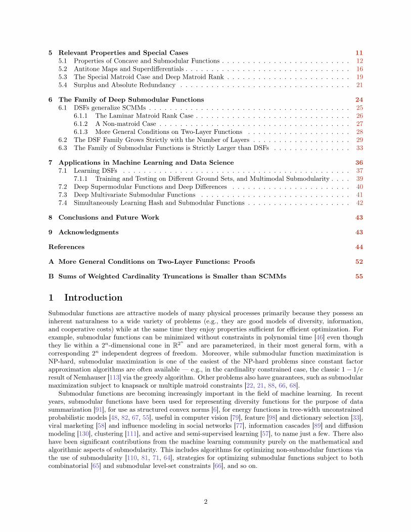
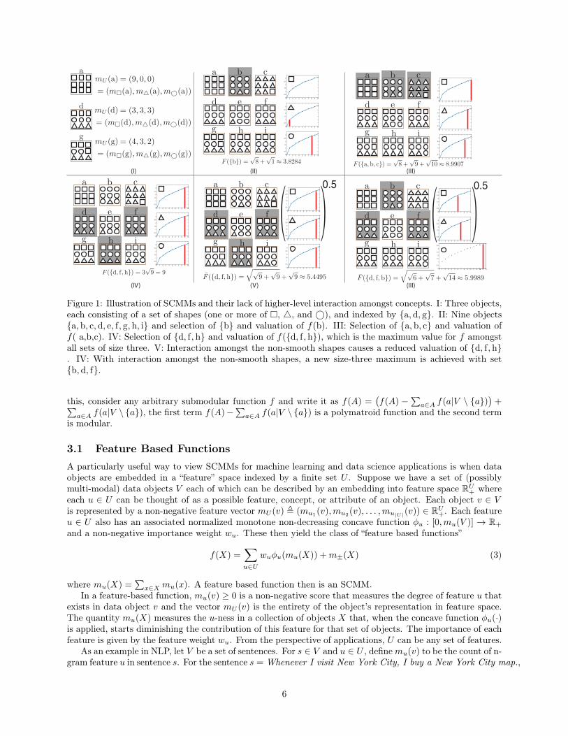
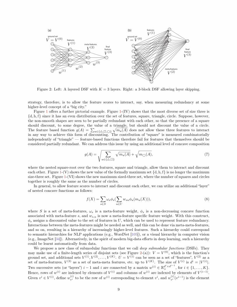
Figure 1: Illustration of SCMMs and their lack of higher-level interaction amongst concepts. I: Three objects,each consisting of a set of shapes (one or more of �, 4, and ©), and indexed by {a,d, g}. II: Nine objects{a,b, c,d, e, f, g,h, i} and selection of {b} and valuation of f(b). III: Selection of {a,b, c} and valuation off( a,b,c). IV: Selection of {d, f,h} and valuation of f({d, f,h}), which is the maximum value for f amongstall sets of size three. V: Interaction amongst the non-smooth shapes causes a reduced valuation of {d, f,h}. IV: With interaction amongst the non-smooth shapes, a new size-three maximum is achieved with set{b,d, f}.

this, consider any arbitrary submodular function f and write it as f(A) =(f(A) −∑a∈A f(a|V \ {a})

)+∑

a∈A f(a|V \ {a}), the first term f(A)−∑a∈A f(a|V \ {a}) is a polymatroid function and the second termis modular.

3.1 Feature Based FunctionsA particularly useful way to view SCMMs for machine learning and data science applications is when dataobjects are embedded in a “feature” space indexed by a finite set U . Suppose we have a set of (possiblymulti-modal) data objects V each of which can be described by an embedding into feature space RU+ whereeach u ∈ U can be thought of as a possible feature, concept, or attribute of an object. Each object v ∈ Vis represented by a non-negative feature vector mU (v) , (mu1(v),mu2(v), . . . ,mu|U|(v)) ∈ RU+. Each featureu ∈ U also has an associated normalized monotone non-decreasing concave function φu : [0,mu(V )] → R+

and a non-negative importance weight wu. These then yield the class of “feature based functions”

f(X) =∑u∈U

wuφu(mu(X)) +m±(X) (3)

where mu(X) =∑x∈X mu(x). A feature based function then is an SCMM.

In a feature-based function, mu(v) ≥ 0 is a non-negative score that measures the degree of feature u thatexists in data object v and the vector mU (v) is the entirety of the object’s representation in feature space.The quantity mu(X) measures the u-ness in a collection of objects X that, when the concave function φu(·)is applied, starts diminishing the contribution of this feature for that set of objects. The importance of eachfeature is given by the feature weight wu. From the perspective of applications, U can be any set of features.

As an example in NLP, let V be a set of sentences. For s ∈ V and u ∈ U , definemu(v) to be the count of n-gram feature u in sentence s. For the sentence s = Whenever I visit New York City, I buy a New York City map.,

6

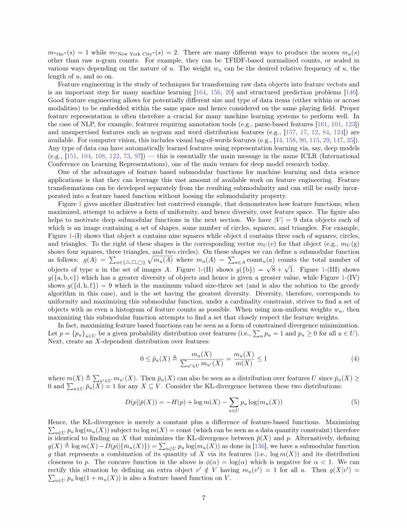
m"the"(s) = 1 while m"New York City"(s) = 2. There are many different ways to produce the scores mu(s)other than raw n-gram counts. For example, they can be TFIDF-based normalized counts, or scaled invarious ways depending on the nature of u. The weight wu can be the desired relative frequency of u, thelength of u, and so on.

Feature engineering is the study of techniques for transforming raw data objects into feature vectors andis an important step for many machine learning [164, 156, 20] and structured prediction problems [146].Good feature engineering allows for potentially different size and type of data items (either within or acrossmodalities) to be embedded within the same space and hence considered on the same playing field. Properfeature representation is often therefore a crucial for many machine learning systems to perform well. Inthe case of NLP, for example, features requiring annotation tools (e.g., parse-based features [161, 101, 123])and unsupervised features such as n-gram and word distribution features (e.g., [157, 17, 12, 84, 124]) areavailable. For computer vision, this includes visual bag-of-words features (e.g., [44, 158, 90, 115, 29, 147, 35]).Any type of data can have automatically learned features using representation learning via, say, deep models(e.g., [151, 104, 108, 122, 73, 97]) — this is essentially the main message in the name ICLR (InternationalConference on Learning Representations), one of the main venues for deep model research today.

One of the advantages of feature based submodular functions for machine learning and data scienceapplications is that they can leverage this vast amount of available work on feature engineering. Featuretransformations can be developed separately from the resulting submodularity and can still be easily incor-porated into a feature based function without loosing the submodularity property.

Figure 1 gives another illustrative but contrived example, that demonstrates how feature functions, whenmaximized, attempt to achieve a form of uniformity, and hence diversity, over feature space. The figure alsohelps to motivate deep submodular functions in the next section. We have |V | = 9 data objects each ofwhich is an image containing a set of shapes, some number of circles, squares, and triangles. For example,Figure 1-(I) shows that object a contains nine squares while object d contains three each of squares, circles,and triangles. To the right of these shapes is the corresponding vector mU (v) for that object (e.g., mU (g)shows four squares, three triangles, and two circles). On these shapes we can define a submodular functionas follows: g(A) =

∑u∈{4,�,©}

√mu(A) where mu(A) =

∑a∈A countu(a) counts the total number of

objects of type u in the set of images A. Figure 1-(II) shows g({b}) =√

8 +√

1. Figure 1-(III) showsg({a,b, c}) which has a greater diversity of objects and hence is given a greater value, while Figure 1-(IV)shows g({d,h, f}) = 9 which is the maximum valued size-three set (and is also the solution to the greedyalgorithm in this case), and is the set having the greatest diversity. Diversity, therefore, corresponds touniformity and maximizing this submodular function, under a cardinality constraint, strives to find a set ofobjects with as even a histogram of feature counts as possible. When using non-uniform weights wu, thenmaximizing this submodular function attempts to find a set that closely respect the feature weights.

In fact, maximizing feature based functions can be seen as a form of constrained divergence minimization.Let p = {pu}u∈U be a given probability distribution over features (i.e.,

∑u pu = 1 and pu ≥ 0 for all u ∈ U).

Next, create an X-dependent distribution over features:

0 ≤ pu(X) ,mu(X)∑

u′∈U mu′(X)=mu(X)

m(X)≤ 1 (4)

where m(X) ,∑u′∈U mu′(X). Then pu(X) can also be seen as a distribution over features U since pu(X) ≥

0 and∑u∈U pu(X) = 1 for any X ⊆ V . Consider the KL-divergence between these two distributions:

D(p||p(X)) = −H(p) + logm(X)−∑u∈U

pu log(mu(X)) (5)

Hence, the KL-divergence is merely a constant plus a difference of feature-based functions. Maximizing∑u∈U pu log(mu(X)) subject to logm(X) = const (which can be seen as a data quantity constraint) therefore

is identical to finding an X that minimizes the KL-divergence between p(X) and p. Alternatively, definingg(X) , logm(X)−D(p||{mu(X)}) =

∑u∈U pu log(mu(X)) as done in [136], we have a submodular function

g that represents a combination of its quantity of X via its features (i.e., logm(X)) and its distributioncloseness to p. The concave function in the above is φ(α) = log(α) which is negative for α < 1. We canrectify this situation by defining an extra object v′ /∈ V having mu(v′) = 1 for all u. Then g(X|v′) =∑u∈U pu log(1 +mu(X)) is also a feature based function on V .

7

The KL-divergence can be generalized in various ways, one of which is known as the f -divergence, or inparticular the α-divergence [137, 3]. Using the reparameteriation α = 1− 2δ [74], the α-divergence (or nowδ-divergence [165]) can be expressed as

Dδ(p, q) =1

δ(1− δ) (1−∑u∈U

pδuq1−δu ). (6)

For δ → 1 we recover the standard KL-divergence above. For δ ∈ (0, 1) we see that the optimization problemminX⊆V :m(X)≤bDδ(p, p(X)) where b is a budget constraint is the same as the constrained submodularmaximization problem maxX⊆V :m(X)≤b g(X) where g(X) =

∑u∈U p

δu(mu(X))1−δ is a feature-based function

since φu(α) = α1−δ is concave on α ∈ [0, 1] for δ ∈ (0, 1). Hence, any such constrained submodularmaximization problem can be seen as a form of α-divergence minimization.

Indeed, there are many useful concave functions one could employ in applications and that can achievedifferent forms of submodular function. Examples include the following: (1) the power functions, such asφ(α) = α1−δ that we just encountered (δ = 1/2 in Figures 1 (I)-(IV)); (2) the other non-saturating non-linearities such as φ(x) = ν−1(x) where ν(y) = y3/3 + y [4] and the log functions φγ(α) = γ log(1 + α/γ)with γ > 0 is a parameter; (3) the saturating functions such as φ(α) = 1 − exp(−α), the logistic functionφ(α) = 1/(1 + exp(−α)) and other “s”-shaped sigmoids (which are concave over the non-negative reals) suchas the hyperbolic tangent, or φ(α) =

[1− 1

ln(b) ln(

1 + exp(−α ln(b)

))]as used in [18, 78]; (4) and the hard

truncation functions such as φ(α) = min(α, γ) for some constant γ. There are also parameterized concavefunctions that get as close to the hard truncation functions as we wish, such as φa,c(x) = ((x−a+c−a)/2)−1/a

where a ≥ −1, and c > 0 are parameters — it is straightforward to show that φ−1,c(x) is linear, thatlima→∞ φa,c(x) = min(x, c), and that for −1 < a < ∞ we have a form of soft min. Also recall theparameterized soft max mentioned above in relationship to the facility location function. In other cases, isuseful for the concave function to be linear for a while before a soft or nonsaturating concave part kicks in,for example φ(α) = min(

√α/γ, α/γ) for some constant γ > 0. These all can have their uses, depending

on the application, and determine the nature of how the returns of a given feature u ∈ U should diminish.Feature based submodular functions, in particular, have been useful for tasks in speech recognition [155],machine translation [78], and computer vision [71].

We mention a final advantage of SCMMs is that they do not require the construction of a pairwisegraph and therefore do not have quadratic cost as would, say a facility location function (e.g., f(X) =∑v∈V maxx∈X wxv), or any function based on pair-wise distances, all of which have cost O(n2) to evaluate.

Feature functions have an evaluation cost of O(n|U |), linear in the ground set V size and therefore aremore scalable to large data set sizes. Finally, unlike the facility location and other graph-based functions,feature-based functions do not require the use of the entire ground set for each evaluation and hence areappropriate for streaming algorithms [7, 23] where future ground elements are unavailable at the time oneneeds a function evaluation, as well as parallel submodular optimization [107, 13, 14]. For example, thevectors mU (v) for a newly encountered object v can be computed on the fly (or in parallel) whenever theobject v is available and wherever it is located on a parallel machine.

4 Deep Submodular FunctionsWhile feature-based submodular functions are indisputably useful, their weakness lies in that features them-selves may not interact, although one feature u′ might be partially redundant with another feature u′′. Forexample, when describing a sentence via its component n-grams features, higher-order n-grams always in-clude lower-order n-grams, so some n-gram features can be partially redundant. For example, in a largecollection of documents about “New York City”, it is likely there will be some instances of “Chicago,” so thefeature functions for these two features should likely negatively covary. One way to reduce this redundancyis to subselect the features themselves, reducing them down to a subset that tends not to interact in anyway. This can only work in limited cases, however, namely when the features themselves can be reducedto an “independent” set that looses no information about the data objects, and this only happens whenredundancy is an all-or-nothing property (as in a matroid).

Most real-world features, however, involve partial redundancy. The presence of “New York City” shouldn’tcompletely remove the contributing of “Chicago”, rather it should only discount its contribution. A better

8

V = V (0)

V (1)

V (2)

V (3)

v14

v13

v12

v11

v3

v21

v22

v23

v06

v05

v04

v03

v02

v01

ground set

features

meta features�nal

feature

w(1)

w(2)

w(3)

V = V (0)

V (1)

V (2)

V (3)

v14

v13

v12

v11

v3

v21

v22

v23

v06

v05

v04

v03

v02

v01

ground set

features

meta features

�nalfeature

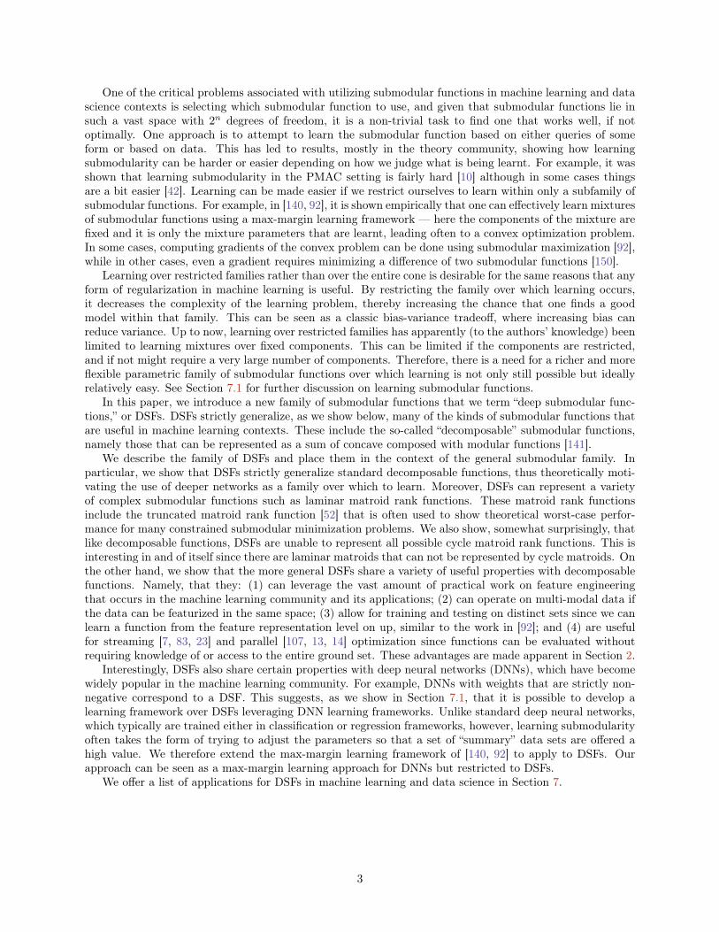
(a) (b)

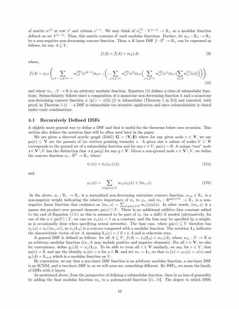
Figure 2: Left: A layered DSF with K = 3 layers. Right: a 3-block DSF allowing layer skipping.

strategy, therefore, is to allow the feature scores to interact, say, when measuring redundancy at somehigher-level concept of a “big city.”

Figure 1 offers a further pictorial example. Figure 1-(IV) shows that the most diverse set of size three is{d,h, f} since it has an even distribution over the set of features, square, triangle, circle. Suppose, however,the non-smooth shapes are seen to be partially redundant with each other, so that the presence of a squareshould discount, to some degree, the value of a triangle, but should not discount the value of a circle.The feature based function g(A) =

∑u∈{4,�,©}

√mu(A) does not allow these three features to interact

in any way to achieve this form of discounting. The contribution of “square” is measured combinatoriallyindependently of “triangle” — feature-based functions therefore fail for features that themselves should beconsidered partially redundant. We can address this issue by using an additional level of concave composition

g(A) =

√ ∑u∈{4,�}

√mu(A) +

√m©(A), (7)

where the nested square-root over the two features, square and triangle, allow them to interact and discounteach other. Figure 1-(V) shows the new value of the formally maximum set {d,h, f} is no longer the maximumsize-three set. Figure 1-(VI) shows the new maximum sized-three set, where the number of squares and circlestogether is roughly the same as the number of circles.

In general, to allow feature scores to interact and discount each other, we can utilize an additional “layer”of nested concave functions as follows:

f(X) =∑s∈S

ωsφs(∑u∈U

wsuφu(mu(X))), (8)

where S is a set of meta-features, ωs is a meta-feature weight, φs is a non-decreasing concave functionassociated with meta-feature s, and ws,u is now a meta-feature specific feature weight. With this construct,φs assigns a discounted value to the set of features in U , which can be used to represent feature redundancy.Interactions between the meta-features might be needed as well, and this can be done via meta-meta-features,and so on, resulting in a hierarchy of increasingly higher-level features. Such a hierarchy could correspondto semantic hierarchies for NLP applications (e.g., WordNet [105]), or a visual hierarchy in computer vision(e.g., ImageNet [34]). Alternatively, in the spirit of modern big-data efforts in deep learning, such a hierarchycould be learnt automatically from data.

We propose a new class of submodular functions that we call deep submodular functions (DSFs). Theymay make use of a finite-length series of disjoint sets (see Figure 2-(a)): V = V (0), which is the function’sground set, and additional sets V (1), V (2), . . . , V (K). U = V (1) can be seen as a set of “features”, V (2) as aset of meta-features, V (3) as a set of meta-meta features, etc. up to V (K). The size of V (i) is di = |V (i)|.Two successive sets (or “layers”) i − 1 and i are connected by a matrix w(i) ∈ Rd

i×di−1

+ , for i ∈ {1, . . . ,K}.Hence, rows of w(i) are indexed by elements of V (i) and columns of w(i) are indexed by elements of V (i−1).Given vi ∈ V (i), define w(i)

vi to be the row of w(i) corresponding to element vi, and w(i)vi (vi−1) is the element

9

of matrix w(i) at row vi and column vi−1. We may think of w(i)vi : V (i−1) → R+ as a modular function

defined on set V (i−1). Thus, this matrix contains di such modular functions. Further, let φvk : R+ → R+

be a non-negative non-decreasing concave function. Then, a K-layer DSF f : 2V → R+ can be expressed asfollows, for any A ⊆ V ,

f(A) = f(A) +m±(A) (9)

where,

f(A) = φvK

( ∑vK−1∈V (K−1)

w(K)

vK(vK−1)φvK−1

(. . .∑

v2∈V (2)

w(3)v3 (v2)φv2

( ∑v1∈V (1)

w(2)v2 (v1)φv1

(∑a∈A

w(1)v1 (a)

)))),

(10)

and where m± : V → R is an arbitrary modular function. Equation (9) defines a class of submodular func-tions. Submodularity follows since a composition of a monotone non-decreasing function h and a monotonenon-decreasing concave function φ (g(·) = φ(h(·))) is submodular (Theorem 1 in [93] and repeated, withproof, in Theorem 5.4) — a DSF is submodular via recursive application and since submodularity is closedunder conic combinations.

4.1 Recursively Defined DSFsA slightly more general way to define a DSF and that is useful for the theorems below uses recursion. Thissection also defines the notation that will be often used later in the paper.

We are given a directed acyclic graph (DAG) G = (V,E) where for any given node v ∈ V, we saypa(v) ⊂ V are the parents of (or vertices pointing towards) v. A given size n subset of nodes V ⊂ Vcorresponds to the ground set of a submodular function and for any v ∈ V , pa(v) = ∅. A unique “root” noder ∈ V \ V has the distinction that r /∈ pa(q) for any q ∈ V. Given a non-ground node v ∈ V \ V , we definethe concave function ψv : RV → R+ where

ψv(x) = φv(ϕv(x)), (11a)

and

ϕv(x) =∑

u∈pa(v)\V

wvuψu(x) + 〈mv, x〉. (11b)

In the above, φv : R+ → R+ is a normalized non-decreasing univariate concave function, wvu ∈ R+ is anon-negative weight indicating the relative importance of ψu to ϕv, and mv : Rpa(v)∩V → R+ is a non-negative linear function that evaluates as 〈mv, x〉 =

∑u∈pa(v)∩V mv(u)x(u). In other words, 〈mv, x〉 is a

sparse dot-product over ground elements pa(v) ∩ V . There is no additional additive bias constant addedto the end of Equation (11b) as this is assumed to be part of φv (as a shift) if needed (alternatively, forone of the u ∈ pa(V ) \ V , we can set ψu(x) = 1 as a constant, and the bias may be specified by a weight,as is occasionally done when specifying neural networks). The base case, where pa(v) ⊆ V therefore hasψv(x) = φv(〈mv, x〉), so ψv(1A) is a concave composed with a modular function. The notation 1A indicatesthe characteristic vector of set A, meaning 1A(v) = 1 if v ∈ A and is otherwise zero.

A general DSF is defined as follows: for all A ⊆ V , f(A) = ψr(1A) + m±(A), where m± : V → R isan arbitrary modular function (i.e., it may include positive and negative elements). For all v ∈ V, we alsofor convenience, define gv(A) = ψv(1A). To be able to treat all v ∈ V similarly, we say, for v ∈ V , thatpa(v) = ∅, and use the identity φv(a) = a for a ∈ R, and set mv = 1v, so that ψv(x) = ϕv(x) = x(v) andgv(A) = 1v∈A which is a modular function on V .

By convention, we say that a zero-layer DSF function is an arbitrary modular function, a one-layer DSFis an SCMM, and a two-layer DSF is, as we will soon see, something different. By DSFk, we mean the familyof DSFs with k layers.

As mentioned above, from the perspective of defining a submodular function, there is no loss of generalityby adding the final modular function m± to a polymatroid function [31, 30]. The degree to which DSFs

10

comprise a subclass of submodular functions corresponds to the degree to which gr comprise a subclass ofall polymatroid functions.

The recursive form of DSF is more convenient than the layered approach mentioned above which, in thecurrent form, would partition V = {V (0), V (1), . . . , V (K)} into layers, and where for any v ∈ V (i), pa(v) ⊆V (i−1). Figure 2-(a) corresponds to a layered graph G = (V,E) where r = v3

1 and V = {v01 , v

02 , . . . , v

06}.

Figure 2-(b) uses the same partitioning but where units are allowed to skip by more than one layer at a time.More generally, we can order the vertices in V with order σ so that {σ1, σ2, . . . , σn} = V where n = |V |,σm = r = vK where m = |V| and where σi ∈ pa(σj) iff i < j. This allows an arbitrary pattern of skippingwhile maintaining submodularity. The additional linear function in Equation (11b) is strictly not necessary(e.g., there could be paths of linearity along subsets of the φvv ∈ A for some A ⊂ V thereby achieving thesame result) but we include it to stress that at each layer there may be a modular function and a bias.

4.2 DSFs: Practical Benefits and Relation to Deep Neural NetworksThe layered definition in Equation (9) is reminiscent of feed-forward deep neural networks (DNNs) owingto its multi-layered architecture. Interestingly, if one restricts the weights of a DNN at every layer to benon-negative, then for many standard hidden-unit activation functions the DNN constitutes a submodularfunction when given Boolean input vectors. The result follows for any activation function that is monotonenon-decreasing concave for non-negative reals, such as the sigmoid, the hyperbolic tangent, and the rectifiedlinear functions. In the rectified linear case, however, the entire network would be linear so the model becomesinteresting only with hidden activations that are strictly concave (since the weights can be arbitrarily scaled,perhaps φ(x) = min(x, 1) is a reasonable concave analogy in a DSF to the rectified linear function in a DNN).More importantly, this suggests that DSFs can be trained in a fashion similar to DNNs — specifically, trainingDSFs and can take advantage of the many successful training techniques and software libraries for trainingDNNs (many of the toolkits make it easy to project weights into the positive orthant). Further discussion onthis point is given in Section 7.1. The recursive definition of DSFs, in Equation (11) is useful for the analysisin Section 5.

DSFs should be useful for many applications in machine learning. First, they retain the advantages ofSCMMs in that they require neither O(n2) computation nor access to the entire ground set for a set evalu-ation. The underlying DSF computation is matrix-vector multiplication that, like DNNs, can be performedvery quickly using modern GPU computing. Hence, DSFs can be both fast, and useful for parallel and/orstreaming applications. Second, DSFs allow for a nested hierarchy of features, similar to advantages a deepmodel has over a shallow model. For example, a one-layer DSF must construct a valuation over a set ofobjects from a large number of low-level features which can lead to fewer opportunities for feature sharingwhile a deeper network fosters distributed representations, also analogous to DNNs [15, 16]. It can be arguedthat a deep neural network is more efficient, in terms of the number of possible functions represented perweight, than a shallow neural network and perhaps DSFs share this advantage. Hence, even if the DSFand SCMM families were to be found to be same (but that Theorem 6.4 shows to be false), there couldbe advantages to applications and learning paradigms thanks to this natural hierarchical decomposition ofconcepts.

DSFs have been used occasionally in some applications. In one instance [95], a square root was applied toa subset of the right hand nodes in a bipartite neighborhood function in order to offer reduced cost for thesenodes being indirectly selected in the graph. In [155] a two-layer DSF was used to introduce higher-levelinteraction between features, an act that yielded benefits in speech data summarization. Lastly, laminarmatroid rank functions, which are instances of DSFs as shown in Section 5.3, have been used to show worstcase performance of various constrained submodular minimization problems [52, 145, 66].

5 Relevant Properties and Special CasesDSFs represent a family that, at the very least, contain the family of SCMMs. Above, we argued intuitivelythat DSFs might extend SCMMs as they allow components themselves to directly interact, and the inter-actions may propagate up a many-layered hierarchy. In this section, we start off (in Section 5.1) discussingpreliminaries regarding concave functions. Section 5.2 then covers specific properties of the multivariateconcave function associated with a DSF, in particular the antitone gradient superdifferential property which

11

is a a sufficient condition for submodularity. This section also compares this condition with the negativityof the off-diagonal Hessian matrix condition for submodular functions. Section 5.3 discusses matroid rankspecial cases, including the laminar matroid rank function which can be seen, in the light of this paper, as aform of deep matroid rank. This section also discusses special cases of the results shown later in the paper,in particular, that: (1) cycle matroid rank functions cannot represent all partition matroid rank functions;(2) laminar matroid rank functions strictly generalize partition matroid rank functions; (3) laminar matroidrank functions cannot express all cycle matroid rank functions; (4) DSFs generalize laminar matroid rankfunctions; and (5) SCMMs generalize partition matroid rank functions. Lastly, section 5.4 introduces variousanalysis tools (in particular the “surplus”) that are used later in the paper.

5.1 Properties of Concave and Submodular FunctionsMany of the results in the sections below rely on a number of properties of concave functions. Since wewish to consider non-differentiable concave functions, the theorems below consider this more general casewhere we may assume only that the concave functions have superdifferentials. It is, in general, more workto show that the properties of concave functions hold in this non-differential case, but since there seem tobe no consolidated published proofs of these properties, we offer them here in full.

Let φ : R → R be a normalized (φ(0) = 0) monotone non-decreasing concave function. In any suchfunction, there may be an initial linear part where φ(x) = γx for x ∈ [0, αφ] where γ > 0 and where αφ ≥ 0is the largest point where φ is still linear. Larger than αφ, there may be a middle part consisting of aseries of concave curves and line segments all situated to ensure concavity. Larger than this, there finallymight be a saturation point where φ(x) = c for all x ≥ αsat, where c, αsat ∈ R+ ∪ {∞}. The middle region(x ∈ [αlin, αsat]) might or might not be smooth. It is useful sometimes in applications (e.g., [71]) to formulatesubmodular functions from concave functions that have an initial linear part followed by either a saturationor by a smooth concave part.

Definition 5.1 (Superdifferential). Let φ : Rn → R be a concave function. The superdifferential of φ at xis the set of vectors defined as follows:

∂φ(x) = {s ∈ Rn : f(y)− f(x) ≤ 〈s, y − x〉,∀y ∈ Rn} (12)

The superdifferential of a concave function is guaranteed always to exist [128, 129, 60, 114]. When φ isdifferentiable at x, the superdifferential corresponds to the gradient, so that ∂φ(x) = {∇φ(x)} and otherwisemembers of ∂φ(x) are called subgradients. In general, we have the following:

Lemma 5.2. The superdifferential of a concave function is a monotone operator, i.e.,

〈u− v, x− y〉 ≤ 0,∀x, y ∈ Rn, u ∈ ∂φ(x), v ∈ ∂φ(y) (13)

Proof. We have that

f(y) ≤ f(x) + 〈u, y − x〉, and f(x) ≤ f(y) + 〈v, x− y〉 (14)

Adding the two inequalities yields monotonicity. �

This means in particular that, in the one-dimensional case when n = 1, if x ≤ y then for any u ∈ ∂φ(x)and any v ∈ ∂φ(y), we must have u ≥ v. In the below, we offer a number of properties of concavesuperdifferentials in the 1D case. While statements of these results are intuitively clear, the authors wereunable to find published proofs, so they are also included herein.

Theorem 5.3. Let φ : R → R be a continuous function. Then φ is concave if and only if for all a, b ∈ Rwith a ≤ b, and ∆ ∈ R+, we have that

φ(a+ ∆)− φ(a) ≥ φ(b+ ∆)− φ(b). (15)

Also, φ is monotone non-decreasing concave if and only if for all a, b ∈ R with a ≤ b, and ∆, ε ∈ R+, wehave that

φ(a+ ∆ + ε)− φ(a) ≥ φ(b+ ∆)− φ(b) (16)

12

Proof. The result is vacuous if a = b, or ∆ = 0 so assume a < b and ∆ > 0.If part: Assume Equation (15) is true and consider

φ(a+ ∆)− φ(a)

∆≥ φ(b+ ∆)− φ(b)

∆(17)

If φ is differentiable at a and b, then taking ∆→ 0 gives us φ′(a) ≥ φ′(b) for all a ≤ b, and this is a sufficientcondition for concavity (see Nesterov 2.13, page 54, [114]). If φ is not differentiable at either a or b, weresort to its continuity. A function is concave if and only if it is continuous and midpoint concave [116] (ormidconcave [127]), defined as for any x, y ∈ R f((x+ y)/2) ≥ (f(x) + f(y))/2). This condition is immediatefrom Equation (15) by setting x = a, y = b+ ∆, and b = a+ ∆ = (x+ y)/2.

Only if part: Assume φ is concave and a < b and ∆ > 0 are given. If φ is differentiable, then by themean value theorem, there exists an a+ with a ≤ a+ ≤ a+ ∆ and a b+ with b ≤ b+ ≤ b+ ∆ where

φ′(a+) =φ(a+ ∆)− φ(a)

∆(18)

and

φ′(b+) =φ(b+ ∆)− φ(b)

∆(19)

If a+ ∆ ≤ b then a+ ≤ b+ and hence φ′(a+) ≥ φ′(b+) by concavity (Nesterov) which immediately givesφ(a+ ∆)− φ(a) ≥ φ(b+ ∆)− φ(b). If φ is not differentiable at either a or b, then consider da ∈ ∂φ(a) anddb ∈ ∂φ(b), so that ∀ya, yb, φ(ya) ≤ φ(a)+ 〈da, ya−a〉 and φ(yb) ≤ φ(b)+ 〈db, yb− b〉. Taking ya = a+∆ andyb = b+ ∆ gives (φ(a+ ∆)− φ(a))/∆ = da ≥ db = (φ(b+ δ)− φ(b))/∆ which follows from the monotonicityof the superdifferential operator.

If a + ∆ > b then a < b < a + ∆ < b + ∆. Again when φ is differentiable, by the mean value theorem,there exists a+

b with a ≤ a+b ≤ b and a+

∆ with a+ ∆ ≤ a+∆ ≤ b+ ∆ with

φ′(a+b ) =

φ(b)− φ(a)

b− a (20)

and

φ′(a+∆) =

φ(b+ ∆)− φ(a+ ∆)

b− a , (21)

and since a+b < a+

∆, φ′(a+b ) ≥ φ′(a+

∆). This immediately gives φ(b) − φ(a) ≥ φ(b + ∆) − φ(a + ∆) orφ(a + ∆) − φ(a) ≥ φ(b + ∆) − φ(b). If φ is not differentiable, then taking supergradients da ∈ ∂φ(a) andda+∆ ∈ ∂φ(a+ ∆) again gives the result.

The second part of the theorem is immediate if we take a = b, and define δ = a + ∆ leading toφ(δ + ε) ≥ φ(δ), i.e., monotonicity. �

The above proof considers the smooth and non-smooth varieties separately where the non-smooth caseutilizes only the existence of the superdifferential of a concave function. Since the superdifferential alwaysexists for a concave function, smooth or otherwise, in the below we consider only the most general casewhere we assume only a superdifferential exists. As a result, the proofs are a bit more involved, but whenconstructing DSFs and considering the resultant submodular families in Section 6, we wish to allow for themost general class concave functions.

We next restate Theorem 1 from [93] but also provide a proof which was missing.

Theorem 5.4. Suppose that h : 2V → R is a monotone non-decreasing submodular function and φ is amonotone non-decreasing concave function. Then g(A) = φ(h(A)) is monotone non-decreasing submodular.

Proof. Consider any A ⊆ B ⊂ V and v /∈ B. Define quantities a, b,∆, ε so that: a = h(A) ≤ b = h(B),a+ ∆ + ε = h(A+ v), and b+ ∆ = h(B + b). I.e., h(v|A) = ∆ + ε ≥ h(v|B) = ∆. Then we have

φ(a+ ∆ + ε)− φ(a) ≥ φ(b+ ∆)− φ(b) (22)

13

or

φ(h(A+ v))− φ(h(A)) ≥ φ(h(B + v))− φ(h(B)). (23)

�

The slope of the linear interpolation between two points on a concave function puts a connecting re-lationship on the corresponding superdifferentials at each of the two points, as the following result shows.

Lemma 5.5. Given a concave function φ : R → R and two points a, b with a < b that define the valuedab = (φ(b)− φ(a))/(b− a). Then mind∈∂φ(a) d > dab if and only if maxd∈∂φ(b) d < dab.

Proof. From the monotonicity of the supergradient [60, 114], we always have

dmina , min

d∈∂φ(a)d ≥ dab ≥ max

d∈∂φ(b)d , dmax

b (24)

since otherwise, say if dmina < dab, then φ(a) + dmin

a (b − a) < φ(a) + dab(b − a) = φ(b) which contradictsdmina being a supergradient. We must show that the inequalities in Equation (24) can be only simultaneously

strict. Let dmina be given such that dmin

a > dab, and suppose that dmaxb = dab. Then

φ(y) ≤ φ(b) + dmaxb (y − b) (25)

= φ(b) + dmaxb (y − a+ a− b) (26)

= φ(b) + dmaxb (a− b) + dmax

b (y − a) (27)= φ(a) + dmax

b (y − a) (28)

and hence we have found a supergradient dmaxb ∈ ∂φ(a) with dmin

a > dmaxb contradicting the minimality of

dmina . Hence, we must have dmax

b < dab. A similar argument shows that dmaxb < dab and dmin

a = dab leads toa contradiction of the maximality of dmax

b . �

The next result identifies a condition that, if true, tells us about the extent of the initial linear region ofa monotone non-decreasing concave function.

Theorem 5.6. Given a monotone non-decreasing concave function φ : R→ R that is normalized (φ(0) = 0)and any a, b ∈ R+ with 0 < a ≤ b. Then φ(a + b) = φ(a) + φ(b), if and only if φ(x) is linear in the regionfrom 0 to a+ b (that is, there exists γ ∈ R with φ(x) = γx for x ∈ [0, a+ b].

Proof. If case: immediate.Only if case: Any violations of the following inequalities would violate the superdifferential property of

∂φ(y) at 0, a, b, or a+ b:

mind∈∂φ(0)

d ≥ φ(a)/a, maxd∈∂φ(a)

d ≤ φ(a)/a, (29)

mind∈∂φ(a)

d ≥ φ(b)− φ(a)

b− a , maxd∈∂φ(b)

d ≤ φ(b)− φ(a)

b− a , (30)

mind∈∂φ(b)

d ≥ φ(a+ b)− φ(b)

(a+ b)− a = φ(a)/a, maxd∈∂φ(a+b)

d ≤ φ(a)/a. (31)

This leads to the series of inequalities:

mind∈∂φ(0)

d(a)≥ φ(a)/a

(b)≥ max

d∈∂φ(a)d ≥ min

d∈∂φ(a)d ≥ φ(b)− φ(a)

b− a ≥ maxd∈∂φ(b)

d (32)

≥ mind∈∂φ(b)

d(c)≥ φ(a)/a

(d)≥ max

d∈∂φ(a+b)d (33)

From Lemma 5.5, if (a) is strict, then so is (b), leading to the contradiction φ(a)/a > φ(a)/a. Also fromLemma 5.5, if (d) is strict, then so is (c), leading to the same contradiction. Hence, all inequalities are

14

equalities. By the monotonicity of the superdifferential of a concave function, we have that for any x < y < zand dy ∈ ∂φ(y) that

mind∈∂φ(x)

d ≥ dy ≥ maxd∈∂φ(z)

d (34)

Hence, for all y ∈ [0, a + b], we have ∂φ(y) = {φ(a)/a}, meaning that φ is linear in this region withγ = φ(a)/a = φ(b)/b = φ(a+ b)/(a+ b). �

It is known that any normalized submodular function is subadditive, in that for any A ⊆ V ,∑a∈A f(a) ≥

f(A). A similar property is true of normalized monotone non-decreasing concave functions.

Theorem 5.7 (Subadditivity). Given a normalized monotone non-decreasing concave function φ, a set ofnon-negative points {xi}`i=1, xi ∈ R+, then we have∑

i

φ(xi) ≥ φ(∑i

xi) (35)

and where the inequality is strict if and only if∑i xi is past any linear part of φ.

Proof. It is sufficient to show that it is true for x1:`−1 =∑`−1i=1 xi and x` that

φ(x1:`−1) + φ(x`) ≥ φ(∑i

xi) = φ(x1:`−1 + x`) (36)

then apply it inductively with x1:`−2 =∑`−2i=1 xi and x`−1. Hence, we only need to show that φ(x1)+φ(x2) ≥

φ(x1 + x2), and we get this immediately setting a = 0, ∆ = x1, b = x2 in Equation (15).The strictness part follows from Theorem 5.6, where is states that equality in φ(x1:`−1)+φ(x`) = φ(

∑i xi)

holds if and only if φ is linear from 0 through x1:`−1 + x` =∑i xi. �

The next result shows that when an SCMM has only one term, the addition of the final modular functionm± extends the family. We in show that this is the case, even when m± is non-negative.

Theorem 5.8. The family of an SCMM with one concave over modular term is enlarged by an additionalmodular term m±.

Proof. Consider a three-element ground set V = {a,b, c} and a function g,

g(A) = min(|A|, 1) + 1c∈A, (37)

thus g is monotone non-decreasing. Suppose g(A) = φ(m(A)) for some non-negative modular function mand normalized non-decreasing concave function φ. Then by Equation (24), we have:

mind∈∂φ(m(a))

d(i)≥ φ(m(a,b))− φ(m(a))

m(a,b)−m(a)= 0

(ii)≥ max

d∈∂φ(m(a,b))d

(iii)≥ 0 (38)

where the (iii) follows since φ is monotone. Hence, (ii) is an equality and by Lemma 5.5 so is (i). Hence0 ∈ ∂φ(m(a)). Then we have that φ(y) ≤ φ(m(a,b)) + 0(y − m(a,b)). This means that φ(m(a,b, c)) ≤φ(m(a,b)) = 1 < 2 = g(a,b, c), a contradiction. �

An immediate corollary is that SCMMs are a larger class of submodular functions than just one concaveover modular function. All SCMMs, however, can be represented as a sum of modular truncations as thefollowing lemma states:

Lemma 5.9 (Sums of Modular Truncations [141]). If f is an SCMM, then f may be written as f(A) =∑i min(mi(A), βi) +m±(A) where for all i, mi is a non-negative modular function, βi ≥ 0 is a non-negative

constant, and where the sum is over a finite number of terms.

Truncating modular function is important, as it is not sufficient to truncate only cardinality functions.In other words, SCMMs also generalize the family of weighted cardinality truncations, as the next resultshows.

15

Lemma 5.10 (Sums of Weighted Cardinality Truncations). We define the class of sums of weighted cardi-nality truncations as

G =

g : ∀A, g(A) =∑B⊆V

|B|−1∑i=1

αB,i min(|A ∩B|, i), where ∀B, i, αB,i ≥ 0

. (39)

Then there exists an f ∈ SCMM that is not in G.

Lemma 5.10 is proven in Appendix B.

5.2 Antitone Maps and SuperdifferentialsThanks to concave composition closure rules [19], the root function ψr(x) : Rn → R in Eqn. (11) is amonotone non-decreasing multivariate concave function that, by the concave-submodular composition rule(Theorem 5.4) yields a submodular function ψr(1A). It is widely known that any univariate concave functioncomposed with non-negative modular functions yields a submodular function. However, given an arbitrarymultivariate concave function this is not the case. Consider, for example, any concave function ψ over R2

that offers the following evaluations: ψ(0, 0) = ψ(1, 1) = 1, ψ(0, 1) = ψ(1, 0) = 0. Then f(A) = ψ(1A)is not submodular, and hence the guarantee of submodularity when composing a concave with a linearfunction does not extend to dimensions higher than one. In this section, we discuss a limited form of such ageneralization, one that ensures submodularity and that, moreover, does not even always rely on concavityin higher dimensions. Here and below, for x, y ∈ RV , then x ≤ y ⇔ x(v) ≤ y(v),∀v ∈ V .

Definition 5.11. A concave function is said to have an antitone superdifferential if for all x ≤ y we havethat hx ≥ hy for all hx ∈ ∂ψ(x) and hy ∈ ∂ψ(y).

The antitone superdifferential is an apparently straightforward multidimensional generalization of a defin-ing characteristic of univariate concave functions. Theorem 5.12 below generalizes Theorem 5.4 when k = 1— this is because φ : R→ R being concave is, in the univariate case, synonymous with it having an antitonesuperdifferential (which is synonymous with monotone supergradients [60, 114]).

Theorem 5.12. Let ψ : Rk → R be a monotone non-decreasing concave function and let ~g : 2V → Rkbe a vector of polymatroid functions, where ~g(A) = (g1(A), g2(A), . . . , gk(A)). Then if ψ has an antitonesuperdifferential, then the set function f : 2V → R defined as f(A) = ψ(~g(A)) for all A ⊆ V is submodular.

Proof. Given two points x, y ∈ Rn with x ≤ y, then the fundamental theorem of calculus for line integralsstates that for any smooth relative path p from x to y, the integral through the vector field ∇ψ(z) yieldsψ(y)−ψ(x) =

∫p∇ψ(x+z)dz. If ψ is not differentiable, we may assume, with a slight abuse of notation, that

∇ψ(x) is any gradient map for all x ∈ Rn (i.e., ∇ψ(x) maps from x to some element within ∂φ(x)). Given anarbitrary A ⊆ B and v /∈ B, and let p(t) be any relative and parametric curve from a point ~g(A) ∈ Rk whent = 0 to a point ~g(A+ v) ∈ Rk when t = 1. Hence, ~g(A) + p(0) = ~g(A) and ~g(A) + p(1) = ~g(A+ v). Since~g is a vector of polymatroid functions, we have ~g(A) ≤ ~g(B) and ~g(A) ≤ ~g(A+ v), and hence, the path p(t)can be taken to be monotone, so that ~0 ≤ p(t1) ≤ p(t2) whenever 0 ≤ t1 ≤ t2 ≤ 1. Other than monotonicity,the path may be arbitrary. By monotonicity and submodularity, ~0 ≤ ~g(B + v) − ~g(B) ≤ ~g(A + v) − ~g(A),and hence we may choose the relative path that starts at ~0, and at some point t′ ∈ (0, 1), goes through thepoint p(t′) = ~g(B + v)− ~g(B), and ends up at p(1) = ~g(A+ v)− ~g(A). Then,

f(A+ v)− f(A) = ψ(~g(A+ v))− ψ(~g(A)) =

∫ 1

0

∇ψ(~g(A) + p(t)) · dp(t) (40)

≥∫ t′

0

∇ψ(~g(A) + p(t)) · dp(t) ≥∫ t′

0

∇ψ(~g(B) + p(t)) · dp(t) (41)

= ψ(~g(B + v))− ψ(~g(B)) = f(B + v)− f(B), (42)

where the inequality follows from the monotonicity of ψ, the pointwise antitonicity of the gradient map, thenon-negativity of the path, and by linearity of the integral. Hence, f is submodular. �

16

We also fairly quickly get a partial corollary where we need not assume that φ is monotone non-decreasing.In the below, let b ∈ RV

+ be a non-negative real vector and for any set A ⊆ V , bA is a vector such thatbA(v) = b(v) if v ∈ A and otherwise bA(v) = 0 (e.g., when b = 1 then bA = 1A is the characteristic vectorof set A).

Corollary 5.12.1. Let ψ : Rn → R be any concave function and b ∈ RV+ be a non-negative real vector.

Then if ψ has an antitone superdifferential, then the set function f : 2V → R defined as f(A) = ψ(bA) forall A ⊆ V is submodular.

Proof. The proof is practically the same as that of Theorem 5.12 except we cannot use the monotonicity ofψ. Here the path p is any relative path from a point x ∈ RV

+ with x(v) = 0 to a point x + bv. Given anarbitrary A ⊆ B and v /∈ B, we then get f(A + v) − f(A) = ψ(bA+v) − ψ(bA) =

∫p∇ψ(bA + z) · dz ≥∫

p∇ψ(bB + z) · dz = ψ(bB+v)− ψ(bB) = f(B + v)− f(B). �

Alternatively, we can set k = n in Theorem 5.12 and for all v ∈ V , set gv(A) = b(v)1v∈A which is amodular function. Then, the same relative path can be used to move from bA to bA+v as from bB to bB+v,so only antotonicity of ψ is needed in the integral.

Given the above, the following result is not surprising.

Lemma 5.13. Let ψ : Rn → R be a concave function formed by the sum of compositions of a scalar concavefunction and a linear function, i.e., ψ(x) =

∑i wiφi(〈mi, x〉) + 〈m±, x〉 where mi ∈ Rn+, wi ≥ 0 for all i,

and m± ∈ Rn (i.e., an SCMM). Then ψ(x) has an antitone superdifferential.

Proof. From the chain rule, we get that ∇ψ(x) =∑i wiφ

′i(〈mi, x〉)mT

i +mT±, and since φi is concave and mi

is non-negative, wiφ′i(〈mi, x〉)mTi is monotone non-increasing in x (mT

± is constant). In the non-differentiablecase, φi being monotone-concave implies that the same is true for any supergradient map. Closure over sumsis immediate. �

Corollary 5.13.1. Any linear function has an antitone superdifferential.

Lemma 5.14. Composition of monotone non-decreasing scalar concave and antitone superdifferential con-cave functions preserves superdifferential antitonicity.

Proof. Let φ : R → R be a monotone non-decreasing concave functions and χ : Rn → R be a monotonenon-decreasing concave function with an antitone superdifferential, and define ψ(x) = φ(χ(x)). Then by thechain rule, ∇ψ(x) = φ′(χ(x))∇χ(x). Since χ(x) is monotone non-decreasing in x, the first factor φ′(χ(x)) ismonotone non-increasing. The second factor is also monotone non-increasing, hence so is the product. �

Corollary 5.14.1. The root concave function ψr associated with a DSF has an antitone superdifferential.

Proof. The proof follows immediately from the fact that a DSF function (Equation (11)) is a recursiveapplication of composition of monotone concave functions, non-negative sums of monotone concave functions,and the addition of a final linear function associated with m±. �

While having an antitone superdifferential is sufficient to yield a submodular function, it is not necessary.Consider the following concave extension of a monotone non-decreasing submodular function [152, 113, 45],ψ(x) = minS⊆V [f(S) +

∑v∈V x(v)f(v|S)]. This function is concave and is tight f(A) = ψ(1A),∀A at the

vertices of the unit hypercube, but is not the concave closure of f [152]. The superdifferential is given by

∂ψ(x) =

{(f(v1|Sx), f(v2|Sx), . . . , f(vn|Sx)) : Sx ∈ argmin

S⊆V[f(S) +

∑v∈V

x(v)f(v|S)]

}(43)

and when evaluating at x = 1A we haveMA , argminS⊆V [f(S)+∑v∈V 1Af(v|S)] = {A}∪{A′ : A′ = A− v,∀v ∈ A}.

To have an antitone supergradient, we need ∀x ≤ y and gx ∈ ∂ψ(x), gy ∈ ∂ψ(y), that gx ≥ gy. Takingx = 1A and y = 1A+v for some v /∈ A, we can choose A ∈MA and A′ = (A+ v − v′) ∈MA+v with v′ ∈ A.In this case, we can find a monotone submodular function with f(vi|A) < f(vi|A + v − v′) which violatesantitonicity.

17

In order to explore this further, we consider the case where the function ψ is twice differentiable. In thiscase, if ψ is concave, then an antitone superdifferential means for all x ≤ y, we have for all i, ∂ψ∂xi (x) ≥ ∂ψ

∂xi(y).

Setting y = x+ ε1vj , we get for all i, j

∂2ψ

∂xi∂xj(x) = lim

ε→0

∂ψ∂xi

(x+ ε1vj )− ∂ψ∂xi

(x)

ε≤ 0, (44)

which is thus also a sufficient condition for f(A) = ψ(1A) being submodular. The condition is stricter thannecessary, however. Consider the quadratic ψ : R2 → R with ψ(x) = xT

(1 −2−2 1

)x+41Tx. Since φ(0, 0) = 0,

φ(0, 1) = 5, φ(1, 0) = 5, and φ(1, 1) = 6, f(A) = φ(1A) is monotone submodular. Here, we have ∂2ψ∂x1∂x2

= −4

but ∂2ψ∂x2i

= 2 for i ∈ {1, 2}. Being submodular does not require the non-positivity of the diagonal elements ofthe Hessian matrix. In fact, the following weaker sufficient condition for submodularity (an old result, goingback more than a hundred years [5, 38, 132, 99, 133, 148, 149]) is well established:

Theorem 5.15. Let φ : Rn → R be a twice differentiable function. If for all i 6= j we have ∂2φ/∂xi∂xj ≤ 0then the function f : 2V → R where f(A) = φ(1A) is submodular.

The above result is equivalent to ∂φ(x)/∂xj being decreasing in xi for all i 6= j. This suggests thatthe antitone superdifferential condition can also be weakened while still ensuring submodularity. Definedεiψ(x) = ψ(x + ε1vi) − ψ(x). Then an antitone superdifferential is the same as, for all x ≤ y havingdεiφ(x) ≥ dεiψ(y) for all i and ε > 0. This implies that dεjdεiψ(x) ≤ 0 for all i, j. The weaker condition asksthat dεjdεiψ(x) ≤ 0 for all i 6= j, and ε > 0, and this is the same as

ψ(x+ ε1vi) + ψ(x+ ε1vj ) ≥ ψ(x+ ε1vi + ε1vj ) + ψ(x) (45)

which essentially is a restatement of the property of submodularity but on the reals. Note that when i = j,this (and ∂2φ/∂x2

i ≤ 0 in the twice differentiable case) asks for the function to be concave in the directionof each axis, but submodularity, as Theorem 5.15 states, does not require this. Indeed, submodularity is arelationship between distinct variables, not a criterion on any one particular variable.

The weaker condition (Theorem 5.15) is also not necessary for concavity, as the aforementioned quadraticis neither concave nor convex. Concavity requires non-positive definiteness of the Hessian matrix, somethingthat antitone maps do not ensure. A map is any function h : RV → RV and is antitone if for all x, y ∈ RV ,(x − y)T (h(x) − h(y)) ≤ 0 for all x, y. Not only does an antitone map alone not ensure concavity (aresult established originally in [128, 129]), an antitone map need not be a gradient field (a property that, iftrue, would make it a conservative field). For an example related to submodular functions, the multilinearextension [119], defined as:

f(x) =∑S⊆V

f(V )∏i∈S

xi∏

j∈V \S

(1− xj) (46)

has the property that f(1A) = f(A) for all A ⊆ V . It has been used as a extension of a submodularfunction, surrogate to the true concave envelope, for use in submodular maximization problems [41, 24, 8].When f is submodular, it has ∂2f(x)/∂xi∂xj ≤ 0 for all i, j, not only abiding Theorem 5.15 but also fori = j it has ∂φ2/∂x2

i = 0 since it is multilinear. Hence, multilinear extension also has an antitone map, butis also neither convex nor concave and hence has neither a subdifferential nor a superdifferential. Indeed,concavity is not at all required for an extension of a submodular function, another well known examplebeing the Lovász extension of f : RV → R of f which is a convex, has f(A) = f(1A), is defined as f(x) =∑ni=1 xσif(σi|σ1, σ2, . . . , σi−1) where σ = (σ1, σ2, . . . , σn) is an x-dependent order ensuring xσ1

≥ xσ2≥ · · · ≥

xσn . f is not twice differentiable but it has a subgradient g ∈ ∂f(x) where g(i) = f(σi|σ1, σ2, . . . , σi−1).Given x ≤ y, a decreasing order of y can be arbitrarily different than for x implying ∂f(x) is neither antitonenor monotone, so dεidεj f(x) ≤ 0 is not a property of the Lovász extension. Also, any function defined only onthe vertices of the unit hypercube has an infinite number of both concave and convex extensions [28]. Theapproach above shows that antitone superdifferentials involves both concavity and submodular functions.Since Theorem 5.15 does not require concavity, however, this suggests that there may be a way to definesubmodular functions using generalized line integrals of antitone maps without needing concavity [131].

18

We also note that Theorem 5.15 is given as a sufficient condition, but not a necessary condition, forsubmodularity when we consider φ as a function used to produce f(A) = φ(1A). Let φ be any functionsatisfying Theorem 5.15 and χ be any other function having χ(1A) = 0 for all A ⊆ V . Then f(A) =φ(1A) + χ(1A) is submodular while φ(x) + χ(x) need not satisfy the theorem. Theorem 5.15 is typicallystated as both necessary and sufficient conditions for submodularity [38, 132, 133, 148, 149], as it is usedto define submodularity on those lattices, including the reals (and hence this is sometimes called continuoussubmodularity), where twice differentiability everywhere is well defined. For example, defining ∂if(A) =f(A∪ {i})− f(A \ {i}) for i ∈ V , we have that a function f : 2V → R is submodular if and only if for i 6= j,∂i∂jf(A) ≤ 0. This is in contrast to how we use it above, which to define a submodular function only onthe unit hypercube vertices starting from a function defined on Rn.

Getting back to DSFs, since the concave function associated with a DSF has an antitone superdifferential,and since this is sufficient but not necessary for submodularity, this suggests (but does not guarantee, sinceDSFs evaluate ψ only at hypercube vertices 1A) that the family of DSFs might not comprise all submodularfunctions. While in Section 6 we show that DSFs generalize SCMMs, and in Section 6.2 we show thatincreasing the layers in a DSF increases the size of the family, Section 6.3 shows, by giving an example, thatnot all submodular function can be represented by DSFs.

In closing this section, we state an additional potential advantage of DSFs. Ordinarily the concaveclosure of a submodular function is computationally hard to evaluate [152] and this is disappointing sincesuch a construct would be useful for relaxation schemes for maximizing submodular functions (and as resultsurrogates, such as the multilinear extension are used). In the DSF case, however, a particular concaveextension is very easy to get, namely ψr(x)+〈m±, x〉. This extension perhaps could be useful for maximizingDSFs, possibly constrainedly, using concave maximization followed by appropriate rounding methods.

5.3 The Special Matroid Case and Deep Matroid RankWe discuss in this section the special case of matroids and matroid ranks as they motivate and offer insightto the results later in the paper.

A matroid M [46] is a set system M = (V, I) where I = {I1, I2, . . .} is a set of subsets Ii ⊆ V that arecalled independent. A matroid has the property that ∅ ∈ I, that I is subclusive (i.e., given I ∈ I and I ′ ⊂ Ithen I ′ ∈ I) and that all maximally independent sets have the same size (i.e., given A,B ∈ I with |A| < |B|,there exists a b ∈ B \ A such that A + b ∈ I). The rank of a matroid, a set function r : 2V → Z+ definedas r(A) = maxI∈I |I ∩A|, is a powerful class of submodular functions. All matroids are defined uniquely bytheir rank function as I = {A : r(A) = |A|} and therefore, we can reason about if two matroids are equivalentor not based on if their ranks are equal, and vice verse. All monotone non-decreasing non-negative integralsubmodular functions can be exactly represented by grouping and then evaluating grouped ground elementsin a matroid [46].

A useful matroid in machine learning applications [94, 9] is the partition matroid, where a partition(V1, V2, . . . , V`) of V is formed, along with a set of capacities k1, k2, . . . , k` ∈ Z+. It’s rank function is definedas: r(X) =

∑`i=1 min(|X ∩ Vi|, ki) and, therefore, is an SCMM.

A cycle matroid is a different type of matroid based on a graph G = (V,E) where the rank function r(A)for A ⊆ E is defined as the size of the maximum “spanning forest” (i.e., a spanning tree for each connectedcomponent) in the edge-induced subgraph GA = (V,A). From the perspective of matroids, we can considerclasses of submodular functions via their rank. If a given type of matroid cannot represent another kind,their ranks lie in distinct families. To study where DSFs are situated in the space of all submodular functions,it is useful first to study results regarding matroid rank functions.

Lemma 5.16. There are partition matroids that are not cycle matroids.

Proof. Consider the partition matroid over |V | = 4 elements and consider a partition with one block anda capacity of two, so r(X) = min(|X|, 2), so any two elements has rank 2. For this matroid to be a cyclicmatroid, we must have a graph with 4 edges where every set of three (out of those 4) must contain a cycle.Lets name the edges a,b, c,d, then a,b, c contains a cycle and so does a,b,d, while a,b does not containa cycle ({a,b} has rank 2). The only way this can happen is if either c, d are parallel edges, or of c isparallel to one of a or b, and d is also parallel to one of a or b, or if c and d are loops. In any of the above

19

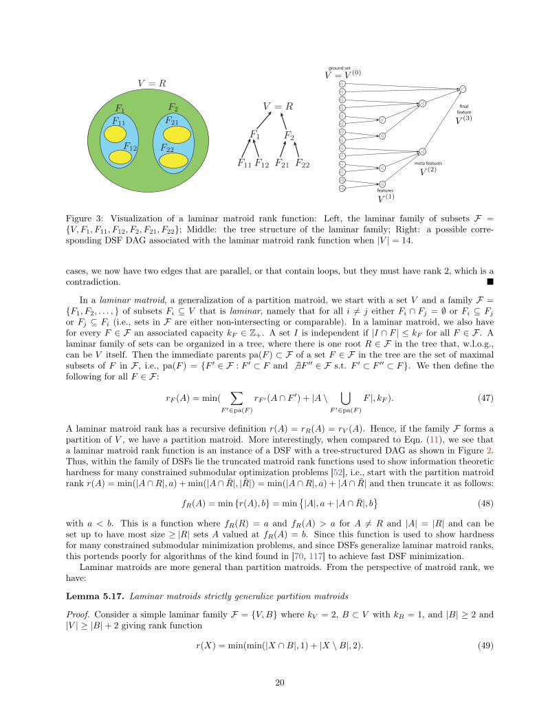
V = R

F1 F2

F11

F12

F21

F22

V = R

F1 F2

F11 F12 F21 F22

V = V (0)

V (1)

V (2)

V (3)

v14

v13

v12

v11

v3

v21

v22

v06

v07

v05

v04

v03

v02

v01

v013

v014

v012

v011

v010

v09

v08

ground set

features

meta features

�nalfeature

Figure 3: Visualization of a laminar matroid rank function: Left, the laminar family of subsets F ={V, F1, F11, F12, F2, F21, F22}; Middle: the tree structure of the laminar family; Right: a possible corre-sponding DSF DAG associated with the laminar matroid rank function when |V | = 14.

cases, we now have two edges that are parallel, or that contain loops, but they must have rank 2, which is acontradiction. �

In a laminar matroid, a generalization of a partition matroid, we start with a set V and a family F ={F1, F2, . . . , } of subsets Fi ⊆ V that is laminar, namely that for all i 6= j either Fi ∩ Fj = ∅ or Fi ⊆ Fjor Fj ⊆ Fi (i.e., sets in F are either non-intersecting or comparable). In a laminar matroid, we also havefor every F ∈ F an associated capacity kF ∈ Z+. A set I is independent if |I ∩ F | ≤ kF for all F ∈ F . Alaminar family of sets can be organized in a tree, where there is one root R ∈ F in the tree that, w.l.o.g.,can be V itself. Then the immediate parents pa(F ) ⊂ F of a set F ∈ F in the tree are the set of maximalsubsets of F in F , i.e., pa(F ) = {F ′ ∈ F : F ′ ⊂ F and 6 ∃F ′′ ∈ F s.t. F ′ ⊂ F ′′ ⊂ F}. We then define thefollowing for all F ∈ F :

rF (A) = min(∑

F ′∈pa(F )

rF ′(A ∩ F ′) + |A \⋃

F ′∈pa(F )

F |, kF ). (47)

A laminar matroid rank has a recursive definition r(A) = rR(A) = rV (A). Hence, if the family F forms apartition of V , we have a partition matroid. More interestingly, when compared to Eqn. (11), we see thata laminar matroid rank function is an instance of a DSF with a tree-structured DAG as shown in Figure 2.Thus, within the family of DSFs lie the truncated matroid rank functions used to show information theoretichardness for many constrained submodular optimization problems [52], i.e., start with the partition matroidrank r(A) = min(|A ∩R|, a) + min(|A ∩ R|, |R|) = min(|A ∩R|, a) + |A ∩ R| and then truncate it as follows:

fR(A) = min {r(A), b} = min{|A|, a+ |A ∩ R|, b

}(48)

with a < b. This is a function where fR(R) = a and fR(A) > a for A 6= R and |A| = |R| and can beset up to have most size ≥ |R| sets A valued at fR(A) = b. Since this function is used to show hardnessfor many constrained submodular minimization problems, and since DSFs generalize laminar matroid ranks,this portends poorly for algorithms of the kind found in [70, 117] to achieve fast DSF minimization.

Laminar matroids are more general than partition matroids. From the perspective of matroid rank, wehave:

Lemma 5.17. Laminar matroids strictly generalize partition matroids

Proof. Consider a simple laminar family F = {V,B} where kV = 2, B ⊂ V with kB = 1, and |B| ≥ 2 and|V | ≥ |B|+ 2 giving rank function

r(X) = min(min(|X ∩B|, 1) + |X \B|, 2). (49)

20

Suppose we are given any set of subsets {Ci}i of V and corresponding integer capacities {ki}i giving thesubmodular function:

rs(X) =∑i

min(|X ∩ Ci|, ki). (50)

and suppose that rs(X) = r(X) which means rs(X) must be a matroid rank function. Note that ki ≥ 1otherwise term i is vacuous. The Ci must be disjoint, for if not let Ci ∩ Cj 6= ∅, i 6= j and pick v ∈ Ci ∩ Cj ,which gives rs(v) ≥ 2 implying rs is not a matroid rank function. Hence the sets Ci must be disjoint and rsis a partition rank function over ∪iCi. Choose two elements b1, b2 ∈ B. If b1 ∈ Ci and b2 ∈ Cj for i 6= j thisgives rs({b1, b2}) = 2 6= r({b1, b2}) = 1. Hence, there is a unique i such that B ⊆ Ci. Thus, ki = 1 since ifnot we would get rs({b1, b2}) = 2. If there exists a v ∈ Ci \B then for any b ∈ B, rs(v, b) = 1 6= 2 = r(v, b).Hence, we must have Ci = B. Now take v1, v2 /∈ B so that r({v1, v2}) = rs({v1, v2}) = 2, but the term of rsinvolving B does not involve v1, v2 so that for b ∈ B, rs({v1, v2, b}) = 3 which is a contradiction. Hence, alaminar matroid is a strict generalization of a partition matroid. �

Since a laminar matroid generalizes a partition matroid, this augurs well for DSFs generalizing SCMMs(a result we provide in Theorem 6.4). Before considering that, we already are up against some limits oflaminar matroids, i.e.:

Lemma 5.18. Laminar matroid cannot represent all cycle matroids.

Proof. Consider the cycle matroid over edges on K4, hence M = (V, I) with |V | = 6, V being the set ofedges, where r(X) = |X| for |X| ≤ 2, r(X) = 2 when X is any 3-cycle, r(X) = 3 for any acyclic X with|X| = 3, and r(X) = 3 for |X| > 3. Consider the form of the laminar matroid in Eqn. (47) and supposerV (X) = r(X) for all X. W.l.o.g., we may assume kV = 3. Suppose ∃e ∈ V \∪F∈pa(V )F . Then consider any3-cycle C involving e, and rV (C − e) = 2 but since no element of pa(V ) contains e, there is no truncation,giving rV (C) = 3, a contradiction. Hence, V = ∪F∈pa(V )F . Given a 3-cycle C = {a,b, c}, suppose thereexists an F ∈ pa(V ) with a ∈ F and b /∈ F and c /∈ F . Since we must have rV ({b, c}) = 2 and rV ({a}) = 1,this implies rV ({a,b, c}) = 3, also a contraction. Hence, any three cycle must be in one element of pa(V ),and by transitive closure over the four intersecting three-cycles, all elements of V must be in only one memberof pa(V ). This implies that |pa(V )| = 1 and the only way to represent the 3-cycles is within that one term,rF (X). This process then is applied recursively until we are left with the base case, where the entire recursionboils down to the form rV (X) = min(rF (X), 3) = min(min(|X|, kF ), 3) = min(|X|,min(kF , 3)). This clearlycannot represent the cycle matroid rank function for any value of kF ∈ Z+. �

The proof technique is reminiscent of the back propagation method used to train DNNs and hence wecall it “backprop proof” — it recursively backpropagates required properties from the root though each layer(in a DSF sense) of a laminar matroid rank until it boils down to a partition matroid rank function, wherethe base case is clear. The proof is elucidating since it motivates the proof of Theorem 6.4 showing thatDSFs extend SCMMs. We also have the immediate corollary.

Corollary 5.18.1. Partition matroids cannot represent all cycle matroids.

5.4 Surplus and Absolute RedundancyIn this section, we introduce and study the notion of the surplus of a set as measured by a submodularfunction. The surplus is a useful concept and will be used extensively to show, in Section 6, various propertiesof the DSF family.

Definition 5.19 (Surplus and Absolute Redundancy). For a function f : 2V → R, we define Sf (A) as thesurplus (or absolute redundancy) of a set A ⊆ V by f as follows:

Sf (A) =∑a∈A

f(a)− f(A) (51)

21

We call Sf (A) the surplus of A by f . We use the term “surplus” under an interpretation where A is aset of agents that can perform their action either independently of each other, or may perform their actionsjointly and cooperatively [149]. If an agent a ∈ A performs the action independently, the cost is f(a) withan overall cost of

∑a∈A f(a), while if the agents A perform the action cooperatively, the overall cost is f(A).

The difference Sg(A) =∑a∈A f(a)−f(A) is the surplus obtained by performing the actions A cooperatively

rather than individually. When g is submodular, surplus is never negative. Hence, performing the actionsjointly leads overall to profit.3

The idea of surplus has occurred before in the field of information theory but under a different name —in this case, f(A) = H(XA) is the entropy function of a set of random variables indexed by the set A. Thequantity Sf (A) =

∑a∈AH(Xa) − H(XA) is the average bit-length penalty between optimally coding the

random variables in A separately (as if they were independent) vs. optimally coding them jointly. This can,thus, be called the absolute redundancy of the set A. For the entropy function, this idea was first definedin [102].4 Absolute redundancy is also called “total correlation” [154] and also the “multi-information” function[143]. Our notion of surplus is not the same as [118] where they define a quantity called “deficiency” thenegative of which may be considered a kind of surplus. Since there may neither be a statistical, informationtheoretic, nor economic interpretation, we actually prefer the terms “total interaction” or “combinatorialinteraction.” In the below, if only for the sake of brevity, we utilize the term “surplus,” but stress that itapplies to any submodular function whatever its interpretation. We say that the function g “gives surplus”to a set A whenever Sg(A) > 0 and otherwise A has “no surplus.”

In the below, we explore a number of properties and introduce a number of variants of surplus, all ofwhich are useful later in the paper.

Lemma 5.20 (Linearity of Surplus). Let f1, f2 be two functions and α1, α2 ∈ R+. Then for any A ⊆ V

Sα1f1+α2f2(A) = α1Sf1(A) + α2Sf2(A) (52)

Lemma 5.21 (Surplus is Immune to Modularity). Modular functions do not change surplus, i.e., whenm : V → R is a normalized modular function and f is any set function:

Sf+m(A) = Sf (A) (53)

That modular functions do not influence surplus is useful to be able to ignore the final modular functionm± in a DSF when studying its properties.

Lemma 5.22 (Non-negativity of Surplus). When f is normalized (f(∅) = 0) and submodular, then for allA ⊆ V , Sf (A) ≥ 0.

Proof. For any A ⊆ V , with A = {a1, a2, . . . , ak},

f(A) =

k∑i=1

f(ai|a1, a2, . . . , ai−1) ≤k∑i=1

f(ai) (54)

�

Thus, with a submodular function in such a context, therefore, there can never be any deficit (negativesurplus) and it is always beneficial to act cooperatively. How fairly to redistribute surplus back to theindividual agents is called the “surplus sharing problem” and is studied in [149].

Lemma 5.23 (Mixtures Preserve Surplus). Let f1, f2, . . . be a set of submodular functions and α1, α2, . . .be a set of positive real-valued weights, and define f =

∑i αifi as their conic combination. Then we have

Sf (A) > 0 if and only if ∃i with Sfi(A) > 0.

3In [149], surplus is defined as f(A)−∑

a∈A f(a) where f is a supermodular function, but the same idea still applies.4Incidentally, in 1954, [102] was also the first, to the authors knowledge, to provide inequalities on the entropy function that

are identical to the submodularity condition.

22

Proof. This follows when one considers that ∀i,Sfi(A) ≥ 0 for all A, that ∀i, αi > 0, and that Sf (A) =∑i αiSfi(A). �

The next theorem is particularly important for showing certain properties of DSFs, in particular, Corol-lary 6.23.1.

Theorem 5.24 (Concave Composition Preserves Surplus). Let h : 2V → R be a polymatroid function andφ : R → R be a normalized monotone non-decreasing concave function that is not identically zero. Defineg : 2V → R as g(A) = φ(h(A)). Then Sh(A) > 0 implies Sg(A) > 0.

Proof. Since g(·) is polymatroidal (by Theorem 5.4), Sg(A) ≥ 0 for all A. Order A arbitrarily as A =

{a1, a2, . . . , ak} with k = |A|. Then since∑ki=1 h(ai) > h(A),

k∑i=1

φ(h(ai))(a)≥ φ(

k∑i=1

h(ai))(b)≥ φ(h(A)), (55)

where (a) follows from Theorem 5.7 and (b) follows from the monotonicity of φ. If∑ki=1 h(ai) is still in the

linear part of φ(·) then (b) is strict, while if∑ki=1 h(ai) is greater than the linear part of φ(·) then, from the

second part of Theorem 5.7, (a) is strict. In either case, Sg(A) > 0. �

Proposition 5.25 (Concave Composition Increases Surplus). Let h : 2V → R be a polymatroid functionwith h(v) = 1 for all v ∈ V , and φ : R → R be a normalized monotone non-decreasing concave functionthat is not identically zero and where φ(1) = 1. Define g : 2V → R as g(A) = φ(h(A)). Then for any A,Sg(A) ≥ Sh(A).

Definition 5.26 (Grouped Surplus). We define a form of grouped surplus as follows. Given a set of mdisjoint sets A1, A2, . . . , Am ⊆ V , we define:

I(m)f (A1;A2; . . . ;Am) ,

m∑i=1

f(Ai)− f(

m⋃i=1

Ai) (56)

When f(A) = H(XA) is the entropy function, then the pairwise surplus I(2)f (A;B) is the well-known

mutual information [27] between random variable sets XA and XB . The grouped surplus can be de-fined in terms of standard surplus via I(m)

f (A1;A2; . . . ;Am) = Sf ({A1}, {A2}, . . . , {Am}) where we treateach of the sets {Ai}i as a singleton element groups in the standard surplus. Thus, for any m, we haveImf (A1;A2; . . . ;Am) ≥ 0 for any normalized submodular function f . We also have the following:

Proposition 5.27. Given a submodular function f and a set A ⊆ V , if Sf (A) = 0 then I(m)f (A1;A2; . . . ;Am) =

0 for any m and proper m-partition A1, A2, . . . , Am ⊆ A of A. Moreover, we have:

Sf (

m⋃i=1

Ai) > I(m)f (A1;A2; . . . ;Am) (57)

For example, if I(2)f (A;B) > 0 then Sf (A∪B) > 0. The converse is not true in general, i.e., we can have

I(2)f (A;B) = 0 while still having Sf (B) > 0. Of particular interest in this paper will be pairwise surplus of

the form I(2)f (e′;C) where C is a three-cycle of a graphic matroid, and e′ /∈ C. When it is clear from the

context, we will drop the superscript m and state If (A1;A2; . . . ;Am) , I(m)f (A1;A2; . . . ;Am) for any m.

Considering Proposition 5.27 and Definition 5.26, we immediately obtain the following:

Proposition 5.28 (Concave Composition Preserves Grouped Surplus). Let h : 2V → R be a polymatroidfunction and φ : R → R be a normalized monotone non-decreasing concave function that is not identicallyzero. Define g : 2V → R as g(A) = φ(h(A)). Then for any m and any set of m disjoint sets A1, A2, . . . , Am,we have I(m)

h (A1;A2; . . . ;Am) > 0 implies I(m)g (A1;A2; . . . ;Am) > 0.

23

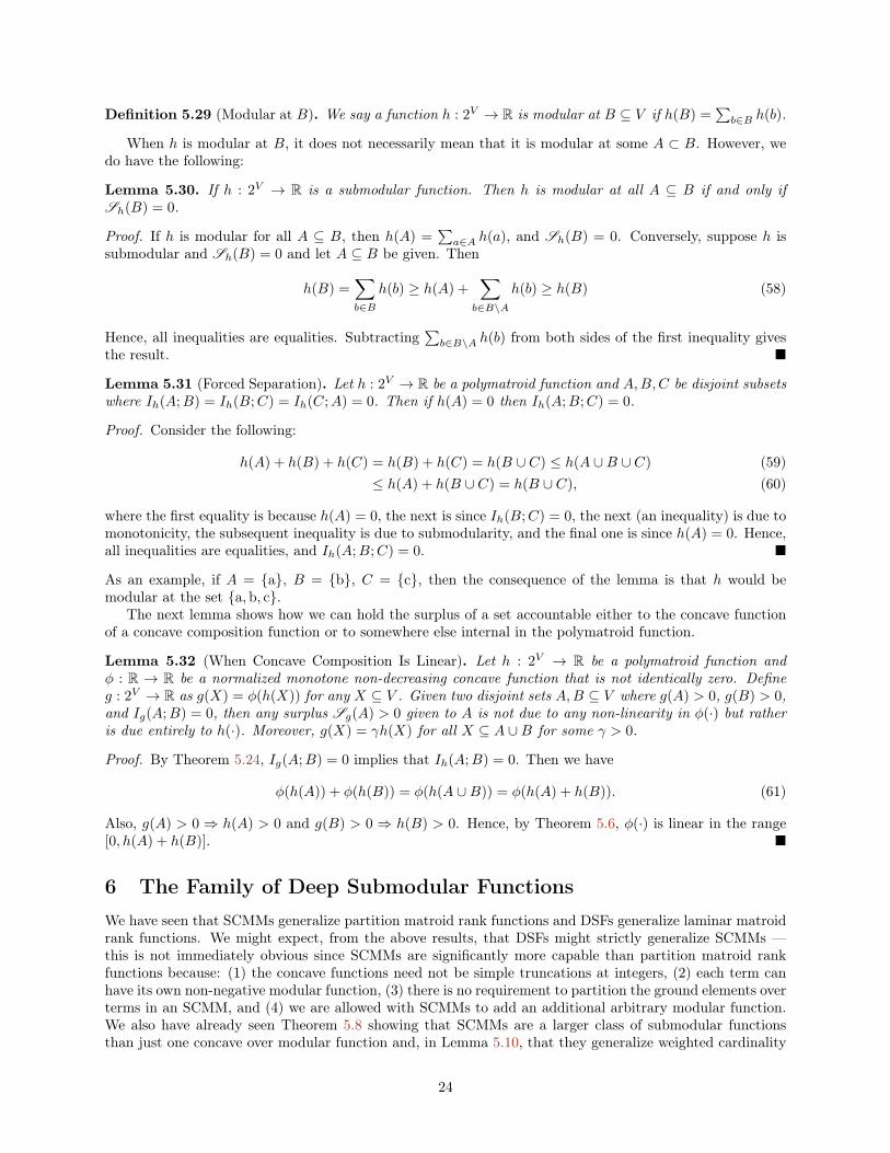
Definition 5.29 (Modular at B). We say a function h : 2V → R is modular at B ⊆ V if h(B) =∑b∈B h(b).

When h is modular at B, it does not necessarily mean that it is modular at some A ⊂ B. However, wedo have the following:

Lemma 5.30. If h : 2V → R is a submodular function. Then h is modular at all A ⊆ B if and only ifSh(B) = 0.

Proof. If h is modular for all A ⊆ B, then h(A) =∑a∈A h(a), and Sh(B) = 0. Conversely, suppose h is

submodular and Sh(B) = 0 and let A ⊆ B be given. Then

h(B) =∑b∈B

h(b) ≥ h(A) +∑

b∈B\A

h(b) ≥ h(B) (58)

Hence, all inequalities are equalities. Subtracting∑b∈B\A h(b) from both sides of the first inequality gives

the result. �

Lemma 5.31 (Forced Separation). Let h : 2V → R be a polymatroid function and A,B,C be disjoint subsetswhere Ih(A;B) = Ih(B;C) = Ih(C;A) = 0. Then if h(A) = 0 then Ih(A;B;C) = 0.

Proof. Consider the following:

h(A) + h(B) + h(C) = h(B) + h(C) = h(B ∪ C) ≤ h(A ∪B ∪ C) (59)≤ h(A) + h(B ∪ C) = h(B ∪ C), (60)

where the first equality is because h(A) = 0, the next is since Ih(B;C) = 0, the next (an inequality) is due tomonotonicity, the subsequent inequality is due to submodularity, and the final one is since h(A) = 0. Hence,all inequalities are equalities, and Ih(A;B;C) = 0. �

As an example, if A = {a}, B = {b}, C = {c}, then the consequence of the lemma is that h would bemodular at the set {a,b, c}.

The next lemma shows how we can hold the surplus of a set accountable either to the concave functionof a concave composition function or to somewhere else internal in the polymatroid function.

Lemma 5.32 (When Concave Composition Is Linear). Let h : 2V → R be a polymatroid function andφ : R → R be a normalized monotone non-decreasing concave function that is not identically zero. Defineg : 2V → R as g(X) = φ(h(X)) for any X ⊆ V . Given two disjoint sets A,B ⊆ V where g(A) > 0, g(B) > 0,and Ig(A;B) = 0, then any surplus Sg(A) > 0 given to A is not due to any non-linearity in φ(·) but ratheris due entirely to h(·). Moreover, g(X) = γh(X) for all X ⊆ A ∪B for some γ > 0.

Proof. By Theorem 5.24, Ig(A;B) = 0 implies that Ih(A;B) = 0. Then we have

φ(h(A)) + φ(h(B)) = φ(h(A ∪B)) = φ(h(A) + h(B)). (61)

Also, g(A) > 0 ⇒ h(A) > 0 and g(B) > 0 ⇒ h(B) > 0. Hence, by Theorem 5.6, φ(·) is linear in the range[0, h(A) + h(B)]. �

6 The Family of Deep Submodular FunctionsWe have seen that SCMMs generalize partition matroid rank functions and DSFs generalize laminar matroidrank functions. We might expect, from the above results, that DSFs might strictly generalize SCMMs —this is not immediately obvious since SCMMs are significantly more capable than partition matroid rankfunctions because: (1) the concave functions need not be simple truncations at integers, (2) each term canhave its own non-negative modular function, (3) there is no requirement to partition the ground elements overterms in an SCMM, and (4) we are allowed with SCMMs to add an additional arbitrary modular function.We also have already seen Theorem 5.8 showing that SCMMs are a larger class of submodular functionsthan just one concave over modular function and, in Lemma 5.10, that they generalize weighted cardinality

24

All Submodular Functions

LaminarMatroid Rank

DSFs

SCMs

PartitionMatroid Rank

CycleMatroid

Rank

Figure 4: Containment properties of the set of functions studied in this paper.

truncations. SCMMs seem therefore to be quite dexterous. The next several sections show, however, thatDSFs strictly generalize SCMMs.

More specifically, we formally place DSFs within the context of general submodular functions. We showin Section 6.1 that DSFs strictly generalize SCMMs while preserving many of their attractive attributes(i.e., featurization, multi-modal, and amenability to learning, streaming, and parallel optimization). Thenin Section 6.2, we show that the family of DSFs strictly grow with the number of layers uses. In Section 6.3,however, we show that the family of DSFs still do not comprise all submodular functions. We summarizethe results of this section in Figure 4, and that includes familial relationships amongst other classes ofsubmodular functions (e.g., various matroid rank functions mentioned in Section 5.3).

6.1 DSFs generalize SCMMsIt is clear that DSFs contain at least the class of SCMMs since any one-layer DSF is an SCMM. We nextshow that SCMM ⊂ DSF holds, or that DSFs strictly generalize SCMMs, thus providing justification forusing DSFs over SCMMs and, moreover, generalizing Lemma 5.17 to the non matroid case. The first DSF wechoose is a laminar matroid, so SCMMs are unable to represent laminar matroid rank functions even giventheir additional flexibility over partition matroid rank functions. Since DSFs generalize laminar matroidrank functions, the result follows.

It is not immediately apparent that DSFs generalize SCMMs as the following example demonstrates.Consider the DSF f : 2V → R where V = {a,b, c,d, e, f}:

f(A) = min(

min(|A ∩ {a,b, c}|, 1) + min(|A ∩ {d, e, f}|, 1), 1.5)

(62)

The reader is encouraged to ponder, for a moment, how one might represent this DSF as an SCMM. Indeed,this is one case where it is possible, as seen by the following SCMM g : 2V → R

g(A) = φ(|A ∩ {a,b, c}|) + φ(|A ∩ {d, e, f}|) + min(|A|, 0.5)− 0.5|A| (63)

where φ : R → R is concave, with φ(α) = min(α, 0.5 + 0.5α). It can be verified that g(A) = f(A)for all A ⊆ V . In fact, an even simpler SCMM does not use a modular function at all and puts g(A) =12 (min(|A∩{a,b, c}|, 1)+min(|A∩{d, e, f}|, 1)+min(|A|, 1)). From this example, one might naturally surmisethat the DSFs unable to be represented by SCMMs are obscure, contrived, and complicated. In the nexttwo sections, however, we show two fairly simple DSFs and show that no SCMM can represent them. Thenin Section 6.1.3, we provide more general conditions describing when 2-layer DSF do or do not generalizeSCMMs.

25

6.1.1 The Laminar Matroid Rank Case

Our first example DSF we choose is a simple laminar matroid on six elements. We show that SCMMs cannotexpress this laminar rank function and since DSFs generalize laminar matroid ranks, the result follows.Consider the following function f : 2V → R where V = {a,b, c,d, e, f}:

f(A) = min(

min(|A ∩ {a,b, c}|, 2) + min(|A ∩ {d, e, f}|, 2), 3)

(64)

The function is a laminar matroid rank function with F = {V, {a,b, c}, {d, e, f}} and limits kV = 3, k{a,b,c} =2, k{d,e,f} = 2.

In the following results, we assume that g : 2V → R is an SCMM of the form g(A) =∑i∈M gi(A)+m±(A)

where gi(A) = φi(mi(A)) is a normalized monotone non-decreasing concave function composed with a non-negative modular function, m±(A) is an arbitrary normalized modular function, andM is an index set. Sincef itself is normalized, then we must also have g(∅) = 0 as well. Also define B1 = {a,b, c} and B2 = {d, e, f}.

Lemma 6.1. Suppose f(A) = g(A) for all A. Then there does not exist an i ∈ M where gi offers surplusboth to B1 and B2 (i.e., there exists no i such that Sgi(B1) > 0 and Sgi(B2) > 0.

Proof. Suppose to the contrary that there exists such an i, Then both mi(B1) and mi(B2) must both bepast the last linear point of φi, say αi. We have that

mi(B1) +mi(B2) = mi({a,b, c} ∪ {d, e, f}) = mi({a,b,d} ∪ {c, e, f}) (65)= mi({a,b,d}) +mi({c, e, f}) (66)

Since mi(B1) > αi and mi(B2) > αi we must have at least one of mi({a,b,d}) > αi or mi({c, e, f}) > αi,w.l.o.g., say {a,b,d}. This implies that Sgi({a,b,d}) > 0 giving g an unrecoverable surplus which is acontradiction since Sf ({a,b,d}) = 0. �

The next result is our first instance of a DSF that cannot be represented by an SCMM.

Lemma 6.2. No SCMM can represent the DSF in Equation (64).

Proof. For clarity, we offer the proof as a series of numbered statement groups.

1. Lemma 6.1 means that we can write g as follows:

g(A) =∑i∈M1

gi(A) +∑i∈M2

gi(A) +∑i∈M0

gi(A) (67)

whereM0,M1,M2 is a partition ofM, and where for all i ∈ M1, gi gives surplus to B1 but not toB2, for all i ∈ M2, gi gives surplus to B2 but not to B1, and for all i ∈ M0, gi gives surplus neitherto B1 nor B2. Hence, for all i ∈M1 and v ∈ B1 we have gi(v) > 0, and for all i ∈M2 and v ∈ B2 wehave gi(v) > 0 by Lemma 5.31. Furthermore, since B1 and B2 are the only sets of size three that aregiven a surplus, then for all i ∈M0, Sgi(A) = 0 for all A with |A| ≤ 3.

2. We also need to have zero pairwise surplus such as:

Ig(e; {a,b, c}) = If (e; {a,b, c}) = 0 (68)

This implies that for i ∈ M, Igi(e; {a,b, c}) = 0. Since we know that mi(B1) is past the non-linearpart of φi for i ∈M1 and mi(B2) is past the non-linear part of φi for i ∈M2, the only way to achievethis (and corresponding values such as Ig(b; {d, e, f}) = 0) is if both: (1) for i ∈ M1, gi(v) = 0 whenv ∈ B2; and (2) for i ∈M2, gi(v) = 0 when v ∈ B1.

In other words, gi with i ∈ M1 not only offers no surplus for B2 but also give zero valuation for anyv ∈ B2 (and vice verse).

26

3. Consider the following set of size-four sets A = {A ⊆ V : |A ∩B1| = |A ∩B2| = 2}. Note that |A| = 9.For any A ∈ A, we have

Sf (A) = Sg(A) =∑i∈M

Sgi(A) = 1. (69)

For i ∈M1 ∪M2, we have Sgi(A) = 0 since two elements of A are given zero value to every such gi.

Hence, the only terms that can achieve Equation (69) are those i within M0 having Sgi(A) > 0,where mi(A) > αi, and where αi is the last linear part of φi. Also, to ensure no unrecoverable surplusoccurs, we must have that mi(C) ≤ αi for any C having the following properties: (1) any size-threeset; (2) any size-four set C with |C ∩ B1| = 3 and |C ∩ B2| = 1 (because Sgi(C ∩ B1) = 0 andIgi(C ∩B2;C ∩B1) = 0); and (3) any size-four set C with |C ∩B1| = 1 and |C ∩B2| = 3. For example,with A = {a,b,d, e} and C = {a,b, c,d}, we have that

mi(a,b, c,d) ≤ αi < mi(a,b,d, e) = mi(A) (70)

implying that mi(c) < mi(e).

For any A ∈ A, define A2(A) = {A′ ∈ A : |A′4A| = 2} and A4(A) = {A′ ∈ A : |A′4A| = 4}. Then|A2(A)| = 4, |A4(A)| = 4, and A = {A}∪A2(A)∪A4(A). Suppose mi(A

′) > αi where A′ ∈ A4(A). Forexample, with A = {a,b,d, e} as above, and A′ = {b, c,d, f} ∈ A4(A) , this implies that mi(d, e, f,b) ≤αi < mi(b, c,d, f) implying that mi(e) < mi(c), a contradiction with the above. Hence, we must havemi(A

′) ≤ αi.More generally, gi offering surplus to more than one member of A4(A) leads to a contradiction. Also, ifA′ ∈ A4(A), then ∃A′′ ∈ A4(A′) with A′′ 6= A and A′′ ∈ A4(A). For example, with A and A′ given asabove, A′′ = {a, c, e, f}. No more than one of this trio {A,A′, A′′} can be offered surplus by the samegi for i ∈M0. This means that we may partition the indicesM0 =

{M(0)

0 ,M(1)0 ,M(2)

0 ,M(3)0

}so that

i ∈ M(1)0 may give surplus to A, but neither A′ nor A′′, i ∈ M(2)

0 may give surplus to A′ but neitherA nor A′′, i ∈ M(3)

0 may give surplus to A′′ but neither A nor A′, and i ∈ M(0)0 gives no surplus any

of the trio.

We must then have

3 = Sf (V ) =∑

j∈{0,1,2}

∑i∈Mj

Sgi(V ) (71)

≥∑i∈M1

Sgi(B1) +∑i∈M2

Sgi(B2) +∑i∈M0

Sgi(V ) (72)

= 1 + 1 +∑

i∈M(1)0

Sgi(V ) +∑

i∈M(2)0

Sgi(V ) +∑

i∈M(3)0

Sgi(V ) (73)

≥ 2 +∑

i∈M(1)0

Sgi(A) +∑

i∈M(2)0

Sgi(A′) +

∑i∈M(3)

0

Sgi(A′′) (74)

= 2 + 1 + 1 + 1 = 5 (75)

which is a contradiction.

�

6.1.2 A Non-matroid Case

Lest one thinks it is only the matroids that give difficulty to SCMMs, consider the function f : 2V → Rwhere again V = {a,b, c,d, e, f}.

f(A) = min(

min(|A ∩ {a,b, c,d}|, 3) + min(|A ∩ {c,d, e, f}|, 3), 5)

(76)

27

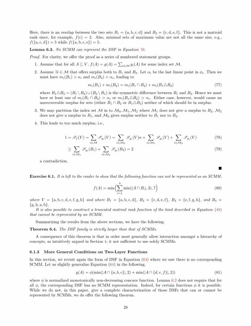
Here, there is an overlap between the two sets B1 = {a,b, c,d} and B2 = {c,d, e, f}. This is not a matroidrank since, for example, f(c) = 2. Also, minimal sets of maximum value are not all the same size, e.g.,f({a, c,d}) = 5 while f({a,b, c, e}) = 5.

Lemma 6.3. No SCMM can represent the DSF in Equation 76.

Proof. For clarity, we offer the proof as a series of numbered statement groups.

1. Assume that for all A ⊆ V , f(A) = g(A) =∑i∈M gi(A) for some index setM.

2. Assume ∃i ∈M that offers surplus both to B1 and B2. Let αi be the last linear point in φi. Then wemust have mi(B1) > αi and mi(B2) > αi, leading to

mi(B1) +mi(B2) = mi(B1 ∩B2) +mi(B14B2) (77)

where B14B2 = (B1 \B2)∪ (B2 \B1) is the symmetric difference between B1 and B2. Hence we musthave at least one of mi(B1 ∩ B2) > αi or mi(B14B2) > αi. Either case, however, would cause anunrecoverable surplus for sets (either B1 ∩B2 or B14B2) neither of which should be in surplus.

3. We may partition the index setM in toM0,M1,M2 whereM1 does not give a surplus to B2,M2

does not give a surplus to B1, andM0 gives surplus neither to B1 nor to B2.

4. This leads to too much surplus, i.e.,

1 = Sf (V ) =∑i∈M

Sgi(V ) =∑i∈M0

Sgi(V )n+∑i∈M1

Sgi(V ) +∑i∈M2

Sgi(V ) (78)

≥∑i∈M1

Sgi(B1) +∑i∈M2

Sgi(B2) = 2 (79)

a contradiction.

�

Exercise 6.1. It is left to the reader to show that the following function can not be represented as an SCMM:

f(A) = min( 4∑i=1

min(|A ∩Bi|, 3), 7)

(80)

where V = {a,b, c,d, e, f, g,h} and where B1 = {a,b, c,d}, B2 = {c,d, e, f}, B3 = {e, f, g,h}, and B4 ={g,h, a,b}.

It is also possible to construct a truncated matroid rank function of the kind described in Equation (48)that cannot be represented by an SCMM.

Summarizing the results from the above sections, we have the following.

Theorem 6.4. The DSF family is strictly larger than that of SCMMs.

A consequence of this theorem is that in order most generally allow interaction amongst a hierarchy ofconcepts, as intuitively argued in Section 4, it not sufficient to use solely SCMMs.

6.1.3 More General Conditions on Two-Layer Functions

In this section, we revisit again the form of DSF in Equation (64) where we saw there is no correspondingSCMM. Let us slightly generalize Equation (64) in the following.

g(A) = φ(min(|A ∩ {a, b, c}|, 2) + min(|A ∩ {d, e, f}|, 2)) (81)

where φ is normalized monotonically non-decreasing concave function. Lemma 6.2 does not require that forall φ, the corresponding DSF has no SCMM representation. Indeed, for certain functions φ it is possible.While we do not, in this paper, give a complete characterization of those DSFs that can or cannot berepresented by SCMMs, we do offer the following theorem.

28

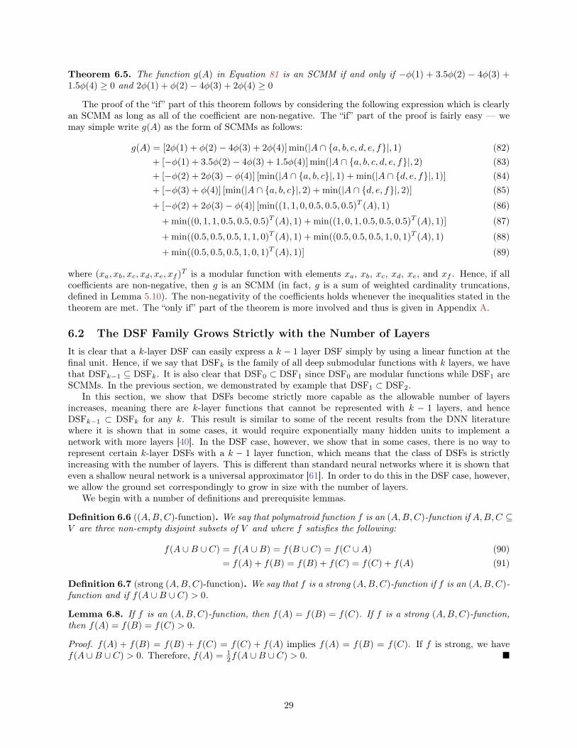
Theorem 6.5. The function g(A) in Equation 81 is an SCMM if and only if −φ(1) + 3.5φ(2) − 4φ(3) +1.5φ(4) ≥ 0 and 2φ(1) + φ(2)− 4φ(3) + 2φ(4) ≥ 0

The proof of the “if” part of this theorem follows by considering the following expression which is clearlyan SCMM as long as all of the coefficient are non-negative. The “if” part of the proof is fairly easy — wemay simple write g(A) as the form of SCMMs as follows:

g(A) = [2φ(1) + φ(2)− 4φ(3) + 2φ(4)] min(|A ∩ {a, b, c, d, e, f}|, 1) (82)+ [−φ(1) + 3.5φ(2)− 4φ(3) + 1.5φ(4)] min(|A ∩ {a, b, c, d, e, f}|, 2) (83)+ [−φ(2) + 2φ(3)− φ(4)] [min(|A ∩ {a, b, c}|, 1) + min(|A ∩ {d, e, f}|, 1)] (84)+ [−φ(3) + φ(4)] [min(|A ∩ {a, b, c}|, 2) + min(|A ∩ {d, e, f}|, 2)] (85)

+ [−φ(2) + 2φ(3)− φ(4)] [min((1, 1, 0, 0.5, 0.5, 0.5)T (A), 1) (86)

+ min((0, 1, 1, 0.5, 0.5, 0.5)T (A), 1) + min((1, 0, 1, 0.5, 0.5, 0.5)T (A), 1)] (87)

+ min((0.5, 0.5, 0.5, 1, 1, 0)T (A), 1) + min((0.5, 0.5, 0.5, 1, 0, 1)T (A), 1) (88)

+ min((0.5, 0.5, 0.5, 1, 0, 1)T (A), 1)] (89)

where (xa, xb, xc, xd, xe, xf )T is a modular function with elements xa, xb, xc, xd, xe, and xf . Hence, if allcoefficients are non-negative, then g is an SCMM (in fact, g is a sum of weighted cardinality truncations,defined in Lemma 5.10). The non-negativity of the coefficients holds whenever the inequalities stated in thetheorem are met. The “only if” part of the theorem is more involved and thus is given in Appendix A.

6.2 The DSF Family Grows Strictly with the Number of LayersIt is clear that a k-layer DSF can easily express a k − 1 layer DSF simply by using a linear function at thefinal unit. Hence, if we say that DSFk is the family of all deep submodular functions with k layers, we havethat DSFk−1 ⊆ DSFk. It is also clear that DSF0 ⊂ DSF1 since DSF0 are modular functions while DSF1 areSCMMs. In the previous section, we demonstrated by example that DSF1 ⊂ DSF2.

In this section, we show that DSFs become strictly more capable as the allowable number of layersincreases, meaning there are k-layer functions that cannot be represented with k − 1 layers, and henceDSFk−1 ⊂ DSFk for any k. This result is similar to some of the recent results from the DNN literaturewhere it is shown that in some cases, it would require exponentially many hidden units to implement anetwork with more layers [40]. In the DSF case, however, we show that in some cases, there is no way torepresent certain k-layer DSFs with a k − 1 layer function, which means that the class of DSFs is strictlyincreasing with the number of layers. This is different than standard neural networks where it is shown thateven a shallow neural network is a universal approximator [61]. In order to do this in the DSF case, however,we allow the ground set correspondingly to grow in size with the number of layers.

We begin with a number of definitions and prerequisite lemmas.

Definition 6.6 ((A,B,C)-function). We say that polymatroid function f is an (A,B,C)-function if A,B,C ⊆V are three non-empty disjoint subsets of V and where f satisfies the following:

f(A ∪B ∪ C) = f(A ∪B) = f(B ∪ C) = f(C ∪A) (90)= f(A) + f(B) = f(B) + f(C) = f(C) + f(A) (91)

Definition 6.7 (strong (A,B,C)-function). We say that f is a strong (A,B,C)-function if f is an (A,B,C)-function and if f(A ∪B ∪ C) > 0.

Lemma 6.8. If f is an (A,B,C)-function, then f(A) = f(B) = f(C). If f is a strong (A,B,C)-function,then f(A) = f(B) = f(C) > 0.

Proof. f(A) + f(B) = f(B) + f(C) = f(C) + f(A) implies f(A) = f(B) = f(C). If f is strong, we havef(A ∪B ∪ C) > 0. Therefore, f(A) = 1

2f(A ∪B ∪ C) > 0. �

29

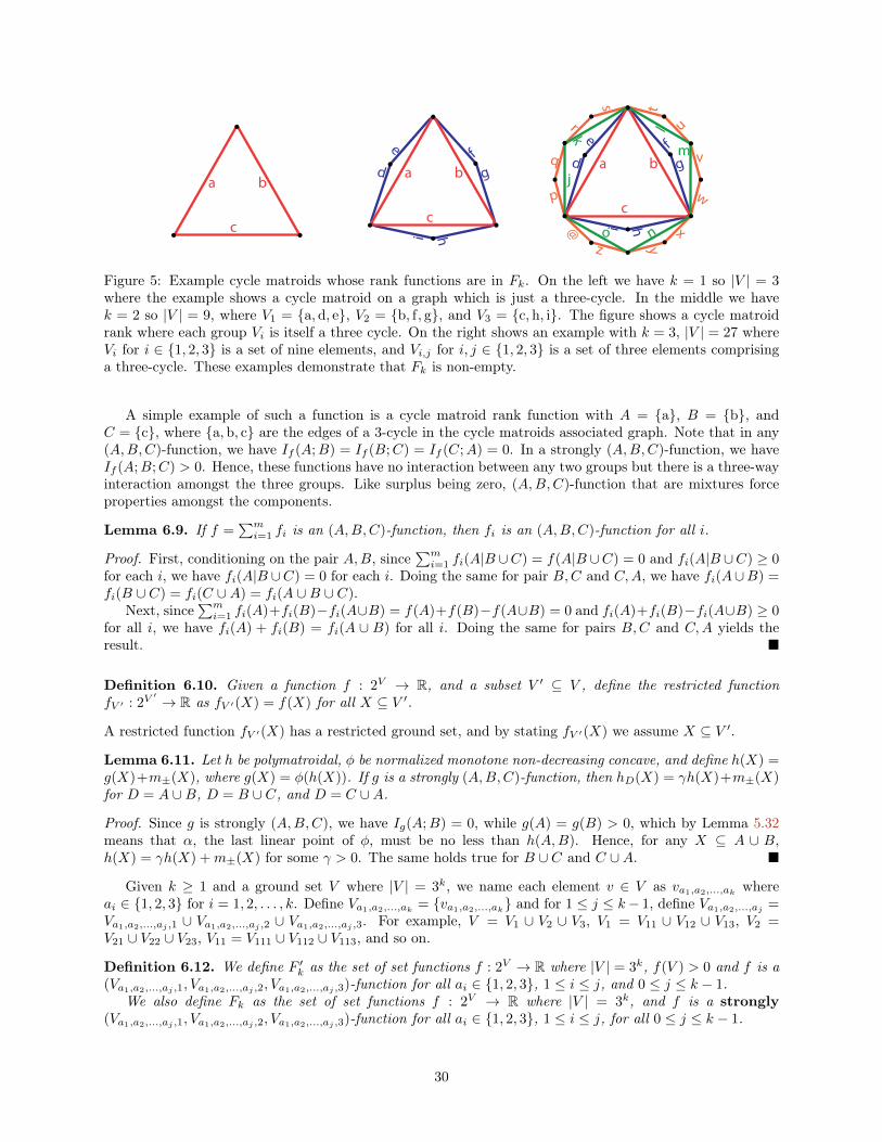
ad

e fg

hi

j

k l

m

no

p

q

r

s t

u

v

w

xyz

@

b

c

a b

c

ad

e fg

hi

b

c

Figure 5: Example cycle matroids whose rank functions are in Fk. On the left we have k = 1 so |V | = 3where the example shows a cycle matroid on a graph which is just a three-cycle. In the middle we havek = 2 so |V | = 9, where V1 = {a,d, e}, V2 = {b, f, g}, and V3 = {c,h, i}. The figure shows a cycle matroidrank where each group Vi is itself a three cycle. On the right shows an example with k = 3, |V | = 27 whereVi for i ∈ {1, 2, 3} is a set of nine elements, and Vi,j for i, j ∈ {1, 2, 3} is a set of three elements comprisinga three-cycle. These examples demonstrate that Fk is non-empty.

A simple example of such a function is a cycle matroid rank function with A = {a}, B = {b}, andC = {c}, where {a,b, c} are the edges of a 3-cycle in the cycle matroids associated graph. Note that in any(A,B,C)-function, we have If (A;B) = If (B;C) = If (C;A) = 0. In a strongly (A,B,C)-function, we haveIf (A;B;C) > 0. Hence, these functions have no interaction between any two groups but there is a three-wayinteraction amongst the three groups. Like surplus being zero, (A,B,C)-function that are mixtures forceproperties amongst the components.

Lemma 6.9. If f =∑mi=1 fi is an (A,B,C)-function, then fi is an (A,B,C)-function for all i.

Proof. First, conditioning on the pair A,B, since∑mi=1 fi(A|B ∪C) = f(A|B ∪C) = 0 and fi(A|B ∪C) ≥ 0

for each i, we have fi(A|B ∪C) = 0 for each i. Doing the same for pair B,C and C,A, we have fi(A∪B) =fi(B ∪ C) = fi(C ∪A) = fi(A ∪B ∪ C).

Next, since∑mi=1 fi(A)+fi(B)−fi(A∪B) = f(A)+f(B)−f(A∪B) = 0 and fi(A)+fi(B)−fi(A∪B) ≥ 0

for all i, we have fi(A) + fi(B) = fi(A ∪ B) for all i. Doing the same for pairs B,C and C,A yields theresult. �

Definition 6.10. Given a function f : 2V → R, and a subset V ′ ⊆ V , define the restricted functionfV ′ : 2V

′ → R as fV ′(X) = f(X) for all X ⊆ V ′.

A restricted function fV ′(X) has a restricted ground set, and by stating fV ′(X) we assume X ⊆ V ′.

Lemma 6.11. Let h be polymatroidal, φ be normalized monotone non-decreasing concave, and define h(X) =g(X)+m±(X), where g(X) = φ(h(X)). If g is a strongly (A,B,C)-function, then hD(X) = γh(X)+m±(X)for D = A ∪B, D = B ∪ C, and D = C ∪A.

Proof. Since g is strongly (A,B,C), we have Ig(A;B) = 0, while g(A) = g(B) > 0, which by Lemma 5.32means that α, the last linear point of φ, must be no less than h(A,B). Hence, for any X ⊆ A ∪ B,h(X) = γh(X) +m±(X) for some γ > 0. The same holds true for B ∪ C and C ∪A. �

Given k ≥ 1 and a ground set V where |V | = 3k, we name each element v ∈ V as va1,a2,...,ak whereai ∈ {1, 2, 3} for i = 1, 2, . . . , k. Define Va1,a2,...,ak = {va1,a2,...,ak} and for 1 ≤ j ≤ k− 1, define Va1,a2,...,aj =Va1,a2,...,aj ,1 ∪ Va1,a2,...,aj ,2 ∪ Va1,a2,...,aj ,3. For example, V = V1 ∪ V2 ∪ V3, V1 = V11 ∪ V12 ∪ V13, V2 =V21 ∪ V22 ∪ V23, V11 = V111 ∪ V112 ∪ V113, and so on.

Definition 6.12. We define F ′k as the set of set functions f : 2V → R where |V | = 3k, f(V ) > 0 and f is a(Va1,a2,...,aj ,1, Va1,a2,...,aj ,2, Va1,a2,...,aj ,3)-function for all ai ∈ {1, 2, 3}, 1 ≤ i ≤ j, and 0 ≤ j ≤ k − 1.

We also define Fk as the set of set functions f : 2V → R where |V | = 3k, and f is a strongly(Va1,a2,...,aj ,1, Va1,a2,...,aj ,2, Va1,a2,...,aj ,3)-function for all ai ∈ {1, 2, 3}, 1 ≤ i ≤ j, for all 0 ≤ j ≤ k − 1.

30

Figure 5 shows three examples of cycle matroids whose ranks are in Fk for k = 1, 2, 3 thus demonstratingthat Fk is non-empty. To show that there are DSFs who are members of Fk, consider the following example.

Example 6.13. Define fk : 2Vk → R, where |Vk| = 3k. Define f1(X) = 12 min(|X|, 2). For k ≥ 2, Vk is

partitioned into three sets Vk1, Vk2, and Vk3 where |Vk1| = |Vk2| = |Vk3| = 3k−1. The level-k function isdefined as fk(X) = 1

2 min(∑i=1,2,3 fk−1(X ∩ Vki), 2).

Hence, fk is like a [0, 1]-normalized laminar matroid rank function with the laminar family of sets Fk ={Vk, Vk1, Vk2, Vk3, Vk11, Vk12, Vk13, Vk21, . . .}. An immediate consequence is the following.

Lemma 6.14. fk ∈ Fk and fk can be expressed as a k-layer DSF.

We also note that the families Fk and F ′k are the same.

Lemma 6.15. F ′k = Fk

Proof. Immediately, we have Fk ⊆ F ′kTo show the other direction, assume there exists f ∈ F ′k and v ∈ V such that f(v) = 0 where v is

labeled as va1,a2,...,ak . Then we have f(Va1,a2,...,ak−1) = 2 × f(Va1,a2,...,ak−1,ak) = 0, f(Va1,a2,...,ak−2

) =2× f(Va1,a2,...,ak−2,ak−1) = 0, and so on until finally we have f(V ) = 0 which contradicts with the definitionof F ′k. Hence, for all f ∈ F ′k and v ∈ V , we have f(v) > 0 and by monotonicity f(A) > 0 for all A. Therefore,f ∈ Fk and F ′k ⊆ Fk. �

Lemma 6.16. Given f ∈ Fk, suppose that f =∑mi=1 fi. If fi(V ) > 0, then fi ∈ Fk for all i.

Proof. This is immediate when considering lemmas 6.9 and 6.15. �

Lemma 6.17. Given f ∈ Fk, we have γf ∈ Fk for all γ > 0. If k ≥ 2, we have fVi ∈ Fk−1, for i ∈ {1, 2, 3},where Vi is defined in Definition 6.12.

Proof. This is immediate from the definitions. �

Lemma 6.18. For all f ∈ Fk and φ be a normalized monotone non-decreasing concave function. If f =φ(f ′), then f ′Vi ∈ Fk−1, for i ∈ {1, 2, 3}.

Proof. Using Lemma 6.11, we have fVi = γf ′Vi , where γ > 0 is a constant. Also we have fVi ∈ Fk−1 accordingto second part of lemma 6.17. So f ′Vi ∈ Fk−1 according to first part of lemma 6.17. �

For any f ∈ Fk, we have that f(v|V \{v}) = 0 which follows since if v = va1,a2,...,ak−1,1, v′ = va1,a2,...,ak−1,2,and v′′ = va1,a2,...,ak−1,3, 0 = f(v|v′, v′′) ≥ f(v|V \{v}) ≥ 0. Hence, all members of Fk are totally normalizedin this sense [31, 30].

As mentioned in Section 4, a DSF allows for the use of an arbitrary final modular function m± at thetop layer. If it is the case that a given f ∈ Fk is represented as a DSF, since f is totally normalized andsince the polymatroidal part must have non-negative gain, the final m± must be non-positive as otherwisewe would have f(v|V \ {v}) > 0. Hence, in order to show that a given f ∈ Fk can not be represented by aDSF with fewer than k layers, it is sufficient to show that a function of the form f +m+, where f ∈ Fk andm+ is a non-negative modular function, can not be expressed as a k − 1 layer DSF having m± = 0. To thisend, we introduce the following class:

Definition 6.19. We define the class of functions Gk = {f +m+|f ∈ Fk,m+ ∈M+} where M+ is the setof all non-negative normalized modular functions.

The addition of a modular function to an f ∈ Fk does not change any surplus. Hence, for a g ∈ Gkwith g = f + m+ with f ∈ Fk, we have that Ig(A;B) = If (A;B) for any disjoint sets A,B, and thatSg(A) = Sf (A) for any set A.

31

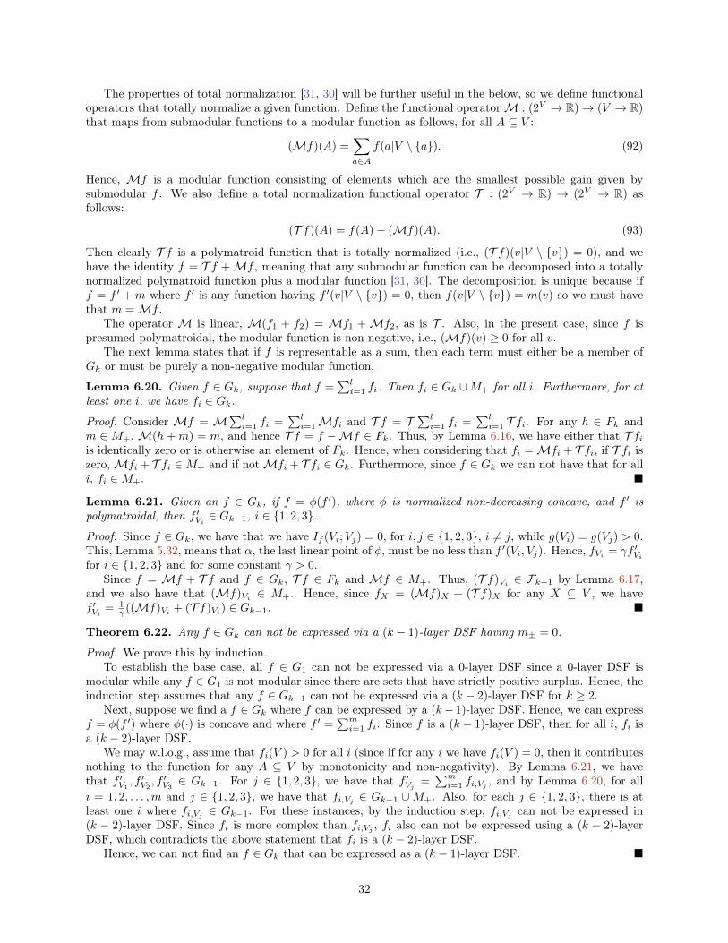
The properties of total normalization [31, 30] will be further useful in the below, so we define functionaloperators that totally normalize a given function. Define the functional operatorM : (2V → R)→ (V → R)that maps from submodular functions to a modular function as follows, for all A ⊆ V :

(Mf)(A) =∑a∈A

f(a|V \ {a}). (92)

Hence, Mf is a modular function consisting of elements which are the smallest possible gain given bysubmodular f . We also define a total normalization functional operator T : (2V → R) → (2V → R) asfollows:

(T f)(A) = f(A)− (Mf)(A). (93)

Then clearly T f is a polymatroid function that is totally normalized (i.e., (T f)(v|V \ {v}) = 0), and wehave the identity f = T f +Mf , meaning that any submodular function can be decomposed into a totallynormalized polymatroid function plus a modular function [31, 30]. The decomposition is unique because iff = f ′ + m where f ′ is any function having f ′(v|V \ {v}) = 0, then f(v|V \ {v}) = m(v) so we must havethat m =Mf .

The operator M is linear, M(f1 + f2) = Mf1 +Mf2, as is T . Also, in the present case, since f ispresumed polymatroidal, the modular function is non-negative, i.e., (Mf)(v) ≥ 0 for all v.

The next lemma states that if f is representable as a sum, then each term must either be a member ofGk or must be purely a non-negative modular function.

Lemma 6.20. Given f ∈ Gk, suppose that f =∑li=1 fi. Then fi ∈ Gk ∪M+ for all i. Furthermore, for at

least one i, we have fi ∈ Gk.Proof. Consider Mf = M∑l

i=1 fi =∑li=1Mfi and T f = T ∑l

i=1 fi =∑li=1 T fi. For any h ∈ Fk and

m ∈ M+,M(h+m) = m, and hence T f = f −Mf ∈ Fk. Thus, by Lemma 6.16, we have either that T fiis identically zero or is otherwise an element of Fk. Hence, when considering that fi =Mfi + T fi, if T fi iszero,Mfi + T fi ∈M+ and if notMfi + T fi ∈ Gk. Furthermore, since f ∈ Gk we can not have that for alli, fi ∈M+. �

Lemma 6.21. Given an f ∈ Gk, if f = φ(f ′), where φ is normalized non-decreasing concave, and f ′ ispolymatroidal, then f ′Vi ∈ Gk−1, i ∈ {1, 2, 3}.Proof. Since f ∈ Gk, we have that we have If (Vi;Vj) = 0, for i, j ∈ {1, 2, 3}, i 6= j, while g(Vi) = g(Vj) > 0.This, Lemma 5.32, means that α, the last linear point of φ, must be no less than f ′(Vi, Vj). Hence, fVi = γf ′Vifor i ∈ {1, 2, 3} and for some constant γ > 0.

Since f = Mf + T f and f ∈ Gk, T f ∈ Fk and Mf ∈ M+. Thus, (T f)Vi ∈ Fk−1 by Lemma 6.17,and we also have that (Mf)Vi ∈ M+. Hence, since fX = (Mf)X + (T f)X for any X ⊆ V , we havef ′Vi = 1

γ ((Mf)Vi + (T f)Vi) ∈ Gk−1. �

Theorem 6.22. Any f ∈ Gk can not be expressed via a (k − 1)-layer DSF having m± = 0.

Proof. We prove this by induction.To establish the base case, all f ∈ G1 can not be expressed via a 0-layer DSF since a 0-layer DSF is

modular while any f ∈ G1 is not modular since there are sets that have strictly positive surplus. Hence, theinduction step assumes that any f ∈ Gk−1 can not be expressed via a (k − 2)-layer DSF for k ≥ 2.

Next, suppose we find a f ∈ Gk where f can be expressed by a (k− 1)-layer DSF. Hence, we can expressf = φ(f ′) where φ(·) is concave and where f ′ =

∑mi=1 fi. Since f is a (k − 1)-layer DSF, then for all i, fi is

a (k − 2)-layer DSF.We may w.l.o.g., assume that fi(V ) > 0 for all i (since if for any i we have fi(V ) = 0, then it contributes

nothing to the function for any A ⊆ V by monotonicity and non-negativity). By Lemma 6.21, we havethat f ′V1

, f ′V2, f ′V3

∈ Gk−1. For j ∈ {1, 2, 3}, we have that f ′Vj =∑mi=1 fi,Vj , and by Lemma 6.20, for all

i = 1, 2, . . . ,m and j ∈ {1, 2, 3}, we have that fi,Vj ∈ Gk−1 ∪M+. Also, for each j ∈ {1, 2, 3}, there is atleast one i where fi,Vj ∈ Gk−1. For these instances, by the induction step, fi,Vj can not be expressed in(k − 2)-layer DSF. Since fi is more complex than fi,Vj , fi also can not be expressed using a (k − 2)-layerDSF, which contradicts the above statement that fi is a (k − 2)-layer DSF.

Hence, we can not find an f ∈ Gk that can be expressed as a (k − 1)-layer DSF. �

32

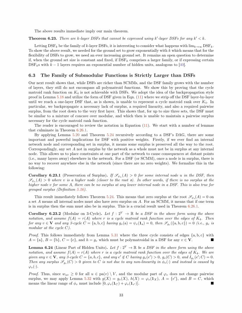
The above results immediate imply our main theorem.

Theorem 6.23. There are k-layer DSFs that cannot be expressed using k′-layer DSFs for any k′ < k.

Letting DSFk be the family of k-layer DSFs, it is interesting to consider what happens with limk→∞DSFk.To show the above result, we needed for the ground set to grow exponentially with k which means that for theflexibility of DSFs to grow, we need an ever increasing ground set. It remains an open question to determineif, when the ground set size is constant and fixed, if DSFk comprises a larger family, or if expressing certainDSFks with k − 1 layers requires an exponential number of hidden units, analogous to [40].

6.3 The Family of Submodular Functions is Strictly Larger than DSFsOur next result shows that, while DSFs are richer than SCMMs, and the DSF family grows with the numberof layers, they still do not encompass all polymatroid functions. We show this by proving that the cyclematroid rank function on K4 is not achievable with DSFs. We adopt the idea of the backpropagation styleproof in Lemma 5.18 and utilize the form of DSF given in Eqn. (11) where we strip off the DSF layer-by-layeruntil we reach a one-layer DSF that, as is shown, is unable to represent a cycle matroid rank over K4. Inparticular, we backpropagate a necessary lack of surplus, a required linearity, and also a required pairwisesurplus, from the root down to the very first layer. This shows that, for up to size three sets, the DSF mustbe similar to a mixture of concave over modular, and which then is unable to maintain a pairwise surplusnecessary for the cycle matroid rank function.

The reader is encouraged to review the notation in Equation (11). We start with a number of lemmasthat culminate in Theorem 6.26.1.

By applying Lemma 5.20 and Theorem 5.24 recursively according to a DSF’s DAG, there are someimportant and powerful implications for DSF with positive weights. Firstly, if we ever find an internalnetwork node and corresponding set in surplus, it means some surplus is preserved all the way to the root.Correspondingly, any set A not in surplus by the network as a whole must not be in surplus at any internalnode. This allows us to place constraints at one part of the network to cause consequences at distant points(i.e., many layers away) elsewhere in the network. For a DSF (or SCMM), once a node is in surplus, there isno way to recover anywhere else in the network (since there are no zero weights). We formalize this in thefollowing:

Corollary 6.23.1 (Preservation of Surplus). If Sψu(A) > 0 for some internal node u in the DSF, thenSψv (A) > 0 where v is a higher node (closer to the root r). In other words, if there is no surplus at thehigher node v for some A, there can be no surplus at any lower internal node in a DSF. This is also true forgrouped surplus (Definition 5.26).

This result immediately follows Theorem 5.24. This means that zero surplus at the root Sψr(A) = 0 ona set A means all internal nodes must also have zero surplus on A. For an SCMM, it means that if one termis in surplus then the sum must also be in surplus. This is a crucial result used in Theorem 6.26.1.

Corollary 6.23.2 (Modular on 3-Cycle). Let f : 2V → R be a DSF in the above form using the abovenotation, and assume f(A) = r(A) where r is a cycle matroid rank function over the edges of K4. Thenfor any v ∈ V and any 3-cycle C = {a,b, c} having gv(a) = ψv(1a) = 0, then Sgv ({a,b, c}) = 0 (i.e., gv ismodular at the cycle C).

Proof. This follows immediately from Lemma 5.31 where the three cycle consists of edges {a,b, c} withA = {a}, B = {b}, C = {c}, and h = gv which must be polymatroidal in a DSF for any v ∈ V. �

Lemma 6.24 (Linear Part of Hidden Units). Let f : 2V → R be a DSF in the above form using the abovenotation, and assume f(A) = r(A) where r is a cycle matroid rank function over the edges of K4. We aregiven any v ∈ V, any 3-cycle C = {a, b, c}, and any e′ /∈ C having gv(e′) > 0, gv(C) > 0, and Igv (e′;C) = 0.Then any surplus Sgv (C) > 0 given to C is not due to any non-linearity in φv(·) and instead is caused byϕv(·).Proof. Thus, since wuv ≥ 0 for all u ∈ pa(v) \ V , and the modular part of ϕv does not change pairwisesurplus, we may apply Lemma 5.32 with g(X) = gv(X), h(X) = ϕv(1X), A = {e′}, and B = C, whichmeans the linear range of φv must include [0, ϕv(1C) + ϕv(1e′)]. �

33

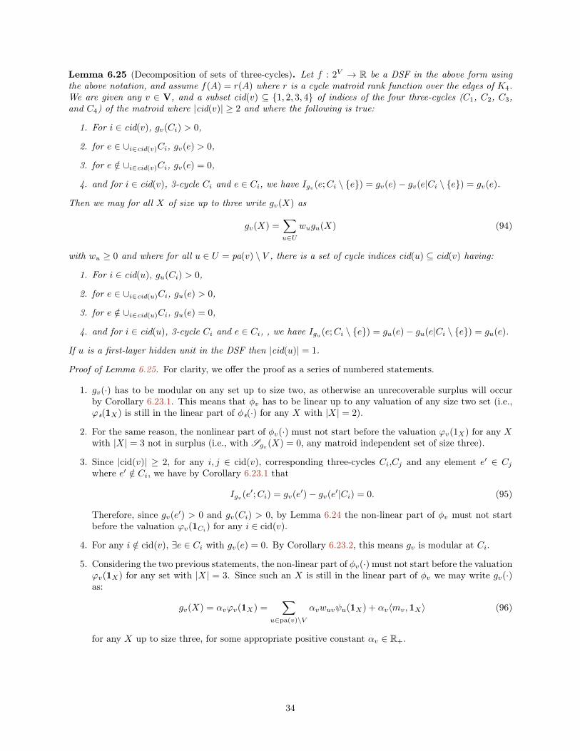
Lemma 6.25 (Decomposition of sets of three-cycles). Let f : 2V → R be a DSF in the above form usingthe above notation, and assume f(A) = r(A) where r is a cycle matroid rank function over the edges of K4.We are given any v ∈ V, and a subset cid(v) ⊆ {1, 2, 3, 4} of indices of the four three-cycles (C1, C2, C3,and C4) of the matroid where |cid(v)| ≥ 2 and where the following is true:

1. For i ∈ cid(v), gv(Ci) > 0,

2. for e ∈ ∪i∈cid(v)Ci, gv(e) > 0,

3. for e /∈ ∪i∈cid(v)Ci, gv(e) = 0,

4. and for i ∈ cid(v), 3-cycle Ci and e ∈ Ci, we have Igv (e;Ci \ {e}) = gv(e)− gv(e|Ci \ {e}) = gv(e).

Then we may for all X of size up to three write gv(X) as

gv(X) =∑u∈U

wugu(X) (94)

with wu ≥ 0 and where for all u ∈ U = pa(v) \ V , there is a set of cycle indices cid(u) ⊆ cid(v) having:

1. For i ∈ cid(u), gu(Ci) > 0,

2. for e ∈ ∪i∈cid(u)Ci, gu(e) > 0,

3. for e /∈ ∪i∈cid(u)Ci, gu(e) = 0,

4. and for i ∈ cid(u), 3-cycle Ci and e ∈ Ci, , we have Igu(e;Ci \ {e}) = gu(e)− gu(e|Ci \ {e}) = gu(e).

If u is a first-layer hidden unit in the DSF then |cid(u)| = 1.

Proof of Lemma 6.25. For clarity, we offer the proof as a series of numbered statements.

1. gv(·) has to be modular on any set up to size two, as otherwise an unrecoverable surplus will occurby Corollary 6.23.1. This means that φv has to be linear up to any valuation of any size two set (i.e.,ϕr(1X) is still in the linear part of φr(·) for any X with |X| = 2).

2. For the same reason, the nonlinear part of φv(·) must not start before the valuation ϕv(1X) for any Xwith |X| = 3 not in surplus (i.e., with Sgv (X) = 0, any matroid independent set of size three).

3. Since |cid(v)| ≥ 2, for any i, j ∈ cid(v), corresponding three-cycles Ci,Cj and any element e′ ∈ Cjwhere e′ /∈ Ci, we have by Corollary 6.23.1 that

Igv (e′;Ci) = gv(e′)− gv(e′|Ci) = 0. (95)

Therefore, since gv(e′) > 0 and gv(Ci) > 0, by Lemma 6.24 the non-linear part of φv must not startbefore the valuation ϕv(1Ci) for any i ∈ cid(v).

4. For any i /∈ cid(v), ∃e ∈ Ci with gv(e) = 0. By Corollary 6.23.2, this means gv is modular at Ci.

5. Considering the two previous statements, the non-linear part of φv(·) must not start before the valuationϕv(1X) for any set with |X| = 3. Since such an X is still in the linear part of φv we may write gv(·)as:

gv(X) = αvϕv(1X) =∑

u∈pa(v)\V

αvwuvψu(1X) + αv〈mv,1X〉 (96)

for any X up to size three, for some appropriate positive constant αv ∈ R+.

34

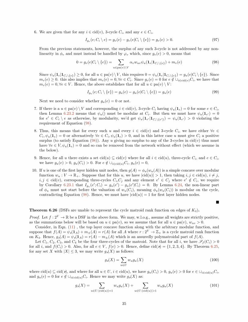
6. We are given that for any i ∈ cid(v), 3-cycle Ci, and any e ∈ Ci,Igv (e;Ci \ e) = gv(e)− gv(e|Ci \ {e}) = gv(e) > 0. (97)

From the previous statements, however, the surplus of any such 3-cycle is not addressed by any non-linearity in φv and must instead be handled by ϕv which, since gv(e) > 0, means that

0 = gv(e|Ci \ {e}) =∑

u∈pa(v)\V

αvwuvψu(1e|1Ci\{e}) +mv(e) (98)

Since ψu(1e|1Ci\{e}) ≥ 0, for all u ∈ pa(v)\V , this requires 0 = ψu(1e|1Ci\{e}) = gu(e|Ci \{e}). Sincemv(e) ≥ 0. this also implies that mv(e) = 0,∀e ∈ Ci. Since gv(e) = 0 for e /∈ ∪i∈cid(v)Ci, we have thatmv(e) = 0,∀e ∈ V . Hence, the above establishes that for all u ∈ pa(v) \ V :

Igu(e;Ci \ {e}) = gu(e)− gu(e|Ci \ {e}) = gu(e) (99)

Next we need to consider whether gu(e) = 0 or not.

7. If there is a u ∈ pa(v) \ V and corresponding i ∈ cid(v), 3-cycle Ci having ψu(1e) = 0 for some e ∈ Ci,then Lemma 6.23.2 means that ψu() must be modular at Ci. But then we must have ψu(1e′) = 0for e′ ∈ Ci \ e as otherwise, by modularity, we’d get ψu(1e′ |1Ci\{e′}) = ψu(1e′) > 0 violating therequirement of Equation (98).

8. Thus, this means that for every such u and every i ∈ cid(v) and 3-cycle Ci, we have either ∀e ∈Ci, ψu(1e) = 0 or alternatively ∀e ∈ Ci, ψu(1e) > 0, and in this latter case u must give Ci a positivesurplus (to satisfy Equation (98)). Any u giving no surplus to any of the 3-cycles in cid(v) thus musthave ∀e ∈ V, ψu(1e) = 0 and so can be removed from the network without effect (which we assume inthe below).

9. Hence, for all u there exists a set cid(u) ⊆ cid(v) where for all i ∈ cid(u), three-cycle Ci, and e ∈ Ci,we have gu(e) > 0, gu(Ci) > 0. For e /∈ ∪i∈cid(u)Ci, gu(e) = 0,

10. If u is one of the first layer hidden unit nodes, then g(A) = φu(wu(A)) is a simple concave over modularfunction wu : V → R+. Suppose that for this u, we have |cid(u)| > 1, then taking i, j ∈ cid(u), i 6= j,i, j ∈ cid(v), corresponding three-cycles Ci,Cj and any element e′ ∈ Cj where e′ /∈ Ci, we requireby Corollary 6.23.1 that Igu(e′;Ci) = gu(e′) − gu(e′|Ci) = 0. By Lemma 6.24, the non-linear partof φu must not start before the valuation of wu(Ci), meaning φu(wu(Ci)) is modular on the cycle,contradicting Equation (98). Hence, we must have |cid(u)| = 1 for first layer hidden nodes.

�

Theorem 6.26 (DSFs are unable to represent the cycle matroid rank function on edges of K4).

Proof. Let f : 2V → R be a DSF in the above form. We may, w.l.o.g., assume all weights are strictly positive,as the summations below will be based on u ∈ pa(v), so we assume that for all u ∈ pa(v), wuv > 0.

Consider, in Eqn. (11) , the top layer concave function along with the arbitrary modular function, andsuppose that f(A) = ψr(1A) +m±(A) = r(A) for all A where r : 2V → Z+ is a cycle matroid rank functionon K4. Hence, gr(A) = ψr(1A) = r(A)−m±(A) which is an assuredly polymatroidal part of f(A).

Let C1, C2, C3, and C4 be the four three-cycles of the matroid. Note that for all i, we have Sf (Ci) > 0for all i, and f(Ci) > 0. Also, for all e ∈ V , f(e) > 0. Hence, define cid(r) = {1, 2, 3, 4}. By Theorem 6.25,for any set X with |X| ≤ 3, we may write gr(X) as follows:

gr(X) =∑u∈U

wugu(X) (100)

where cid(u) ⊆ cid(r), and where for all u ∈ U , i ∈ cid(u), we have gu(Ci) > 0, gu(e) > 0 for e ∈ ∪i∈cid(u)Ci,and gu(e) = 0 for e /∈ ∪i∈cid(u)Ci. Hence we may write gr(X) as:

gr(X) =∑

u∈U :|cid(u)|=1

wugu(X) +∑

u∈U :|cid(u)|>1

wugu(X) (101)

35

For any u ∈ U with cid(u) > 1, by Theorem 6.25, we may, for any set X of size |X| ≤ 3, write it as:

gu(X) =∑u′∈U ′

wu′gu′(X) (102)

where cid(u′) ⊆ cid(u). Thus, we have

gr(X) =∑

u∈U :|cid(u)|=1

wugu(X) (103)

+∑

u′∈U ′:|cid(u′)|=1

wu′gu′(X) +∑

u′∈U ′:|cid(u′)|>1

wu′gu′(X) (104)

This process may continue recursively, applying Theorem 6.25 each time, until we reach all units in thebottom layer of the DSF. We are guaranteed termination since the DSF is itself finite size. Also, since thebottom layer consists of single concave composed with modular functions, all have cid(·) = 1. Hence, for Xwith |X| ≤ 3, the entire DSF can be expressed as:

gr(X) =∑

u∈U(`)

wugu(X) (105)

where cid(u) = 1 and where we may partition U (`) in to four disjoint sets corresponding to the four cycles,where in each index set we have surplus only of one of the cycles. This means that it is not possible toachieve, for a cycle C and e ∈ C,

Igr(e;C \ {e}) = gr(e)− gr(e|C \ {e}) = gr(e) = 1 (106)

since some of the terms in the sum are non-zero meaning gr(e|C \ {e}) > 0, thus contradicting that f(X) =r(X) for all X ⊆ V . �

The above results therefore imply the following.

Corollary 6.26.1 (SCCMs ⊂ DSFs ⊂ Submodular Functions). The family of SCMMs is smaller than thatof DSFs, and the family of DSFs is smaller than the family of all submodular functions. That is, let Cn bethe set of all submodular functions over ground set V of size n and let DSFk be the family of DSFs with klayers on V , and SCCM be the family of SCCMs on V with an arbitrary number of component functions.Then, for any k, SCCM ⊂ DSFk ⊂ Cn.

While DSFs do not comprise all submodular functions, a consequence of Theorem 5.12 is that the inputto a DSF can be any set of polymatroid functions. Let f be a DSF with k inputs and a ground setV = {1, 2, . . . , k}. Then we can consider the standard way to utilize a DSF, in the context of Theorem 5.12,as one where the ith input is a function gk(A) = 1k∈A which is modular. Theorem 5.12 allows for anypolymatroid function to be used as input to a DSF, not just an indicator function, and hence the DSF canbe used to add interactions between and perhaps improve these functions in some way. Hence, if several ofthe gk are cycle matroid rank functions, and if the DSF is learnt, the resulting family is expanded to includeat least those matroid ranks used as input. It remains an open question to see if there is a small finitefixed set of input polymatroid functions that can be cascaded into a DSF in order to achieve all submodularfunctions.

It is also worth noting that in [163] it is shown that the entropy function f(A) = H(XA) when seen as a setfunction must satisfy inequalities that are not required for an arbitrary polymatroid function, thus implyingthat entropy also does not comprise all submodular function. An additional open problem, therefore, is tocompare the family of DSFs to that of entropy functions.

7 Applications in Machine Learning and Data ScienceIn this section, we describe a number of possible DSF applications in machine learning and data science.

36

7.1 Learning DSFsAs mentioned in Section 1, recent studies [52, 11, 43, 42] show that learning submodular functions can beeasier or harder depending on the learning setting.

A general outline of various learning settings is given in [76, 43] — here, we give only a very brief overview.To start, learning may involve several families of functions F , H, and T members of which are mappingsfrom 2V to R. There is some true function f ∈ F to be learnt based on information obtained via samples ofthe form (A, f(A)) for A ⊆ V . One wishes to produce an approximation f ∈ H to f that is good in some way.Learning submodular functions has been studied under a number of possible variants. For example, there istypically a probability distribution Pr over subsets of V (i.e., Pr(S = A) ≥ 1 and

∑A⊆V Pr(S = A) = 1

where S is a random variable). A set of samples D = {(Ai, f(Ai)}i is obtained via this distribution. Thedistribution Pr might be unknown [11], or might be known (and in such case, might be assumed to beuniform [43, 42]). The quality of learning could be judged over all 2n points or over some fraction, say 1−β,of the points, for β ∈ [0, 1]. In general, there is no specificity on the particular set of points, or the particularkind of points, that should be learnt as long as at least a (probability distribution measured) fraction 1− βof them are learnt. Learning itself happens with some probability 1− δ. I.e., there is some probability δ thatthe learning will not succeed. While learning asks for a function in f ∈ H that is good, we might judge frelative only to the best function f ∈ T (the touchstone class). For example, in agnostic learning [76], weacknowledge that it might be difficult to show that learning is good relative to all of F (say due to noise)but still feasible to show that learning is good relative to the best within T . Also, there are a variety ofways to judge goodness. In [11], goodness is judged multiplicatively, meaning for a set A ⊆ V we wish thatf(A) ≤ f(A) ≤ g(n)f(A) for some function g(n), and this is typically a probabilistic condition (i.e., measuredby distribution Pr, goodness, or f(A) ≤ f(A) ≤ g(n)f(A), should happen on a fraction at least 1− β of thepoints). Alternatively, goodness may also be measured by an additive approximation error, say by a norm.I.e., defining errp(f, f) = ‖f − f‖p = (EA∼Pr[|f(A)− f(A)|p])1/p, we may wish errp(f, f) < ε for p = 1 orp = 2. In the PAC (probably approximately correct) model, we probably (δ > 0) approximately (ε > 0 org(n) > 1) learn (β = 0) with a sample or algorithmic complexity that depends on δ and g(n). In the PMAC(probably mostly approximately correct) model [11], we also “mostly” β > 0 learn. In agnostic learning,F ⊇ H = T . Let Cn be the space of all submodular functions. In some cases F ⊇ Cn = H so we wish tolearn the best submodular approximation to a non-submodular function. In other cases, F = Cn ⊆ T ⊆ Hmeaning we are allowed to deviate from submodularity as long as the error is small.

In the machine learning community, H may be a parametric family of submodular functions. For example,given a fixed set of component submodular functions, say {fi}`i=1 one may with to learn only the weights of amixture {wi}i to produce f =

∑i wifi where wi ≥ 0 for all i to ensure submodularity is preserved. What is

learnt is only the coefficients of the mixture, not the components, so the flexibility of the family is determinedby the diverseness and quantity of components used. Empirically, experiments that learn submodularity forvarious data science applications [140, 92], has been more successful than simply hand-designing a fixedsubmodular function. This is true both for image [150] and document [92] summarization tasks. Therealso has been some initial work on learnability bounds in [92]. Learning just the mixture coefficients of amixture of submodular functions, while keeping the component functions themselves fixed, is only as flexibleas the set of component functions allows, however. Given a small (or indiscriminately selected and hencepotentially redundant) number of components, the family over which one can learn might be limited. Asa result, one might need add a very large number of components before one obtains a sufficiently powerfulfamily.

An alternative approach to learning a mixture that alleviates to some extent the above problem is tolearn over a richer parametric family, and this is where DSFs hold promise. An approach to learning DSFs,therefore, is to learn within its parametric family, so H = DSFk for some finite k and where fw ∈ DSFis parameterized by the vector w that determines the topology (e.g., number and width of layers) of thenetwork, the numeric parameters (set of matrices) within that topology, and the set of concave functions{φu}u. As shown in the present paper, DSFs represent a strictly larger family than SCMMs. Therefore, evenin the mixture case above where the components may also be learnt, there are DSFs that are unachievableby SCMMs. In addition, by Theorem 5.12, a DSF rather than a mixture can be applied to a fixed set ofinput submodular components (e.g., some of which might be simple indicators of the form gu(A) = 1u∈A andothers could be cycle matroid rank functions in order to reduce any chance of the unachievability mentioned

37

in Theorem 6.26). Even in cases where a DSF can be represented by an SCMM, DSFs may be a far moreparsimonious representation of classes of submodular functions and hence a more efficient family over whichto learn, analogous to results in DNNs showing the need for exponentially many hidden units for shallownetworks to implement a network with more layers [40].

Suppose f ∈ Cn is a target submodular function, fw ∈ DSFk is a parameterized k-layer DSF, D ={(Si, yi)}i is a training set consisting of subsets Si ⊆ V and valuations yi = f(Si) for the target function andthat is drawn from distribution Pr. An empirical risk minimization (ERM), or regression, style of learningis obtained a standard way:

minw∈W

J(w) =∑i

L(yi, fw(Si)) + ‖w‖ (107)

where L(·, ·) is a loss function and ‖w‖ is a norm on the parameters. Obvious candidates for the loss wouldbe squared loss, or L1 loss, and the norm can also be chosen to prefer smaller values for w. Given theobjective J(w) one may proceed using, for example, projected stochastic gradient descent, where at eachstep we project the weights w into W which corresponds to the non-negative orthant for parameters otherthan m± to ensure submodularity is retained. Under this approach, and with an appropriate regularizer, itmay be feasible to obtain generalization bounds in some form [135] as is often found in statistical machinelearning settings. Note that, depending on the loss L used, this approach may be tolerant of noisy estimatesof the function, where, say, yi = fw(Si) + ε and where ε is noise, somewhat analogous to how it is possibleto optimize a noisy submodular function [59]. Alternatively, one could analyze it under an agnostic learningsetting.

Under many distribution assumptions, such as when Pr is the uniform distribution over 2V , then as thetraining set gets larger, we approach the case where there are O(2|V |) distinct samples, and the goal is tolearn the function at all points. For large ground sets, certain learning settings might become infeasible inpractice due to the curse of dimensionality. As mentioned above, there are learning settings that ask onlyfor a fraction 1− β of the points to be learnt, but without a mechanism to specify which fraction.

In many practical learning situations, however, access to an oracle function h(A), or training data thatutilizes h’s evaluations, might not be available. Even if h available, such a learning setting might be overkillfor certain applications, as we might not need a submodular function fw to be accurate at all points A ⊆ V .One example is in summarization applications [92, 150] where we wish to learn a submodular function fwthat, when maximized subject to a cardinality constraint, produces a set that is valuated highly by the truesubmodular function relative to other sets of that size. Such a set should be diverse and high quality. In thiscase, one does not need fw to be an accurate surrogate for f except on sets A for which f is large. Moreprecisely, instead of trying to learn f everywhere, we seek only to learn the parameters w of a function so thatif B ∈ argmaxA⊆V :|A|≤k fw(A), then h(B) ≥ αh(A∗) for some α ∈ [0, 1] where A∗ ∈ argmaxA⊆V :|A|≤k h(A).This setting puts fewer constraints on what is needing to be learnt than the regression approach and henceshould correspondingly be easier. This is somewhat analogous to discriminative learning where the entiredistribution over input and output variables is not needed and instead only a conditional distribution (or adeterministic mapping from input to output) is required.

The max-margin approach [140, 92, 150] is appropriate to this problem and is applicable to learningDSFs. Given an unknown but desired non-negative submodular function f ∈ Cn, we are given a set ofrepresentative sets S = {S1, S2, . . .}, with Si ⊆ V and where each S ∈ S is scored highly by f(·). Unlike theregression approach, we do not need the actual evaluations f(Si). It might be, for example, that the sets areselected summaries chosen by a human annotator from a larger set. A matroid analogy is to learn a matroidusing a set of independent sets of a particular size, say `. If M ′ = (V, I ′) is a matroid of rank `′ > `, thenM = (V, I) is also a matroid where I = {I ∈ I ′ : |I| ≤ `}.

In max-margin approach, we learn the parameters w of fw in an attempt to make, for all S ∈ S, fw(S)high, while for A ∈ 2V , fw(A) is lower by a given loss. More precisely, we ask that for S ∈ S and A ∈ 2V ,fw(S) ≥ fw(A) + `S(A). The loss is chosen so that `S(S) = 0, so that `S(A) is very small whenever A isclose to S (e.g., if A is also a good summary), and so that `S(A) is large when A is considered much worse(e.g. if A is a poor summary). Achieving the above is done by maximizing the loss-dependent margin, andreduces to finding parameters so that fw(S) ≥ maxA∈2V [fw(A) + `S(A)] is satisfied for S ∈ S. The task offinding the maximizing set is known as loss-augmented inference (LAI) [146, 160], which for general `(A) is

38

NP-hard. With regularization, the optimization becomes:

minw∈W

∑S∈SL(maxA∈2V

[fw(A) + `S(A)]− fw(S)

)+λ

2||w||22. (108)

where L is a classification loss function such as the logistic (L(x) = log(1 + exp(−x))) or hinge (L(x) =max(0, x)) loss. If it is the case that fw(S) is linear in w (such as when w are mixture parameters in anSCMM as was done in [140, 92, 150]), and if the maximization can is done exactly, then this constitutes aconvex minimization procedure. In general, however, there are several complications.

Firstly, the LAI problem maxA∈2V [fw(A) + `S(A)] may be hard. Given a submodular function for theloss, as was done in [92], then the greedy algorithm offers the standard 1 − 1/e approximation guaranteefor LAI. On the other hand, a submodular function is not always natural for the loss. Recall above that`S(A) should be large when A is considered a poor set relative to S (e.g. if A is a poor summary). If it isthe case that one may get an assessment of A, say via a surrogate f of the ground truth function f , thenone may use `S(A) = κ− f(A) but this, to the extent that f needs to represent f , approaches the labelingneeds of the ERM/regression approach above. If f is submodular, then κ − f is supermodular, and in thiscase solving maxA∈2V \S [f(A) + `(A)] involves maximizing the difference between two submodular functions,and the submodular-supermodular procedure [110, 64] can be used although this procedure does not haveguarantees in general.

Secondly, when fw is not linear in w, the above problem is not convex. Given the enormous success ofdeep neural networks in addressing non-convex optimization problems, however, this should not be daunting.Indeed, given an estimation to A ∈ argmaxA∈2V [fw(A) + `S(A)], we can easily obtain an approximatesubgradient of weights dw ∈ ∂w(fw(A)− fw(S) + λ/2‖w‖22) to be used in a projected stochastic subgradientdescent procedure. For a DSF, this subgradient can be easily computed using backpropagation, similar tothe approach of [121]. Like in the mixtures case, we must use projected descent to ensure w ∈ W andsubmodularity is preserved. Recall, however that the weights corresponding to m±(A) may be left negativeif they so choose. Preliminary experiments in learning DSFs in this fashion were reported in [37] and showencouraging results.

As an additional benefit, many of the concave functions mentioned in Section 3.1 are parameterizedthemselves, and these parameters may also be the target of stochastic gradient based learning. In such case,not only the weights but also the concave functions of a DSF may be learnt.

Given the ongoing research on the non-convex learning of DNNs, which have achieved remarkable resultson a plethora of machine learning tasks [87, 54], and given the similarity between DSFs and DNNs, wemay leverage the same DNN learning techniques to learn DSFs. This includes stochastic gradient descent,convolutional linear maps, momentum, dropout, batch normalization, unsupervised pre-training, learningrate scheduling such as AdaGrad/Adam, convolutional matrix patterns, mini-batching, and so on. In somecases these methods might need to be modified (e.g., stochastic projected gradient descent to ensure thefunction remains submodular). Moreover, the suitability of fast GPU computing to the matrix-matrixmultiplications necessary to evaluate DSFs should also be a benefit. Lastly, the many toolkits that supportDNN training (such as Tensorflow, Theano, Torch, Caffe, CNTK, and so on), and that include automaticsymbolic differentiation and semi-differentiation (for non-differentiable functions) for backpropagation-styleparameter learning can easily be used to train DSF. All of these techniques and software may be leveragedto DSF’s benefit, and is true both for the regression and max-margin setting.

7.1.1 Training and Testing on Different Ground Sets, and Multimodal Submodularity

In the training process in machine learning, one trains with a training set and then evaluates or tests on adistinct set having no overlap with the training set. When training submodular functions, this means thatthe training set might consist of multiple ground sets, and the test set might consist of ground sets that werenot seen during training. A data set might consist of D = {(Vi, Si, yi)}i where Vi is a ground set, Si ⊆ Viand, when available, yi = fi(Si) is an evaluation of Si by a ground-set-specific submodular function fi.Hence, there may be no instance where two ground sets are the same, so Vi 6= Vj for i 6= j, nor might therebe ground set commonality between training and test data sets. The reason this occurs can be explainedusing a document summarization example [92]. A training set consists of pairs, each of which is pile ofdocuments (comprised of a set of sentences) and a subset of those sentences corresponding to a summary.

39

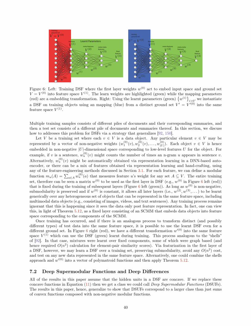
V = V (0)

V (1)

V (2)

V (4)

v24

v23

v22

v21

v4

v31

v32

v33

v16

v15

v14

v13

v12

v11

v06

v08

v09

v010

v07

v05

v04

v03

v02

v01

training ground set

features

meta features

�nalfeature

w(1)

w(0)

w(2)

w(3)

V (3)

meta meta features

V (1)

V (2)

V (4)

v24

v23

v22

v21

v4

v31

v32

v33

v16

v15

v14

v13

v12

v11

testingground set

features

meta features

�nalfeature

w(1)

w(2)

w(3)

V (3)

meta meta features

v06

v08

v07

v05

v04

v03

v02

v01

V = V (0)

w (0)

Learnt Parameters

Figure 6: Left: Training DSF where the first layer weights w(0) act to embed input space and ground setV = V (0) into feature space V (1). The learn weights are highlighted (green) while the mapping parameters(red) are a embedding transformation. Right: Using the learnt parameters (green)

{w(i)

}i>0

, we instantiatea DSF on training objects using an mapping (blue) from a distinct ground set V ′ = V ′(0) into the samefeature space V (1).

Multiple training samples consists of different piles of documents and their corresponding summaries, andthen a test set consists of a different pile of documents and summaries thereof. In this section, we discusshow to addresses this problem for DSFs via a strategy that generalizes [92, 150].

Let V be a training set where each v ∈ V is a data object. Any particular element v ∈ V may berepresented by a vector of non-negative weights (w

(0)1 (v), w

(0)2 (v), . . . , w

(0)|U |). Each object v ∈ V is hence

embedded in non-negative |U |-dimensional space corresponding to low-level features U for the object. Forexample, if v is a sentence, w(0)

u (v) might counts the number of times an n-gram u appears in sentence v.Alternatively, w(0)

u (v) might be automatically obtained via representation learning in a DNN-based auto-encoder, or there can be a mix of features obtained via representation learning and hand-crafting, usingany of the feature-engineering methods discussed in Section 3.1. For each feature, we can define a modularfunction mu(A) =

∑a∈A w

(0)u (a) that measures feature u’s weight for any set A ⊆ V . The entire training

set, therefore can be seen a matrix w(0) to be used as the first layer in DSF (e.g., w(0) in Figure 6 left (red))that is fixed during the training of subsequent layers (Figure 6 left (green)). As long as w(0) is non-negative,submodularity is preserved and if w(0) is constant, it allows all later layers (i.e., w(2), w(3), . . . ) to be learntgenerically over any heterogeneous set of objects that can be represented in the same feature space, includingmultimodal data objects (e.g., consisting of images, videos, and text sentences). Any training process remainsignorant that this is happening since it sees the data only post feature representation. In fact, one can viewthis, in light of Theorem 5.12, as a fixed layer consisting of an SCMM that embeds data objects into featurespace corresponding to the components of the SCMM.

Once training has occurred, and if there is an analogous process to transform distinct (and possiblydifferent types) of test data into the same feature space, it is possible to use the learnt DSF even for adifferent ground set. In Figure 6 right (red), we have a different transformation w′(0) into the same featurespace V (1) which can use the DSF (green) learnt during training. This process analogous to the “shells”of [92]. In that case, mixtures were learnt over fixed components, some of which were graph based (andhence required O(n2) calculation for element-pair similarity scores). Via featurization in the first layer ofa DSF, however, we may learn a DSF over a training set, preserving submodularity, avoid any O(n2) cost,and test on any new data represented in the same feature space. Alternatively, one could combine the shellsapproach and w′(0) into a vector of polymatroid functions and then apply Theorem 5.12.

7.2 Deep Supermodular Functions and Deep DifferencesAll of the results in this paper assume that the hidden units in a DSF are concave. If we replace theseconcave functions in Equation (11) then we get a class we could call Deep Supermodular Functions (DSUFs).The results in this paper, hence, generalize to show that DSUFs correspond to a larger class than just sumsof convex functions composed with non-negative modular functions.

40

In [110, 64] it was shown that any set function h : 2V → R can be represented as a difference between twosubmodular functions. If we take f1, f2 ∈ DSF then the class of functions DDSF = {h : h = f1 − f2, f1, f2 ∈ DSF}can be seen as a class of deep differences of submodular functions. Considering the class DSSUF ={h : h = f + g, f ∈ DSF, g ∈ DSUF} can be seen as a class of deep submodular plus supermodular func-tions. Given that DSFs do not comprise all submodular functions, it is unlikely that DSSUFs comprise allset functions. However, these can be useful classes of functions to learn over using, say, the deep learningmethods mentioned in Sections 7.1. A key advantage of learning over this family is that the framework neverlooses the decomposition into two submodular functions or a submodular and supermodular function. Forexample, after learning, we can utilize submodular level-set constrained submodular optimization of the kinddeveloped in [66] for optimization. Learning under such a decomposition, moreover, might reveal substitutive(via f) and complementary (via g) properties of the data.

It may also be useful to define a class of deep “cooperative-competitive” energy functions for use in aprobabilistic model. For example, one can define probability distributions p over binary vectors with p(x) =1Z exp(fw1(x) − fw2(x)) where fw1 and fw2 are both deep submodular, or p(x) = 1

Z exp(fw1(x) + gw2(x))where fw1

is deep submodular and gw2is deep supermodular. If fw1

and gw2have decomposition properties

with respect to a graph, then these could be called deep cooperative-competitive graphical models.

7.3 Deep Multivariate Submodular FunctionsSubmodular functions have been generalized in a variety of ways to domains other than just subsets of afinite set V (i.e., binary vectors). In Section 5.2, we discussed the negativity of the off-diagonal Hessian as away of defining submodular functions on lattices. Other ways to generalize submodularity considers discretegeneralizations of properties such as midpoint convexity over integer lattices [109].

In this section, we consider certain submodular generalizations to multi-argument functions. For example,a set function f(A,B) with two arguments A ⊆ V and B ⊆ V is a biset function. If the domain is of theform 22V , {(A,B) : A ⊆ V, B ⊆ V }, we may define the class of functions known as simple bisubmodular:

Definition 7.1 (Simple Bisubmodularity [139]). f : 22V → R is simple bisubmodular iff for each (A,B) ∈22V , (A′, B′) ∈ 22V with A ⊆ A′, B ⊆ B′ we have for s /∈ A′ and s /∈ B′:

f(A+ s,B)− f(A,B) ≥ f(A′ + s,B′)− f(A′, B′),

f(A,B + s)− f(A,B) ≥ f(A′, B′ + s)− f(A′, B′).

An equivalent way to define simple bisubmodularity is as follows.

Proposition 7.2. The function f : 22V → R is simple bisubmodular whenever ∀(A,B), (A′, B′) ∈ 22V ,

f(A,B) + f(A′, B′) ≥ f(A ∪A′, B ∪B′) + f(A ∩A′, B ∩B′) (109)

If the domain is of the form 3V , {(A,B) : A ⊆ V, B ⊆ V, A ∩ B = ∅}, then we can define directedbisubmodularity as follows:

Definition 7.3 (Directed Bisubmodularity [125]). Biset function f : 3V → R is directed bisubmodularwhenever

f(A,B) + f(A′, B′) ≥ f(A ∩A′, B ∩B′) + f((A ∪A′) \ (B ∪B′), (B ∪B′) \ (A ∪A′)). (110)

Directed bisubodularity functions have been generalized to what is known as k-submodular functionsin [80, 62]. More recently, simple bisubmodularity [139] has been generalized to multivariate submodularfunctions [134]. A multivariate submodular (or what we will call a k-multi-submodular) function f : (2V )k →R is defined as a function such that for all (X1, X2, . . . , Xk), (Y1, Y2, . . . , Yk) ∈ (2V )k, we have that:

f(X1, X2, . . . , Xk) + f(Y1, Y2, . . . , Yk) ≥ f(X1 ∪ Y1, X2 ∪X2, . . . , Xk ∪ Yk) + f(X1 ∩ Y1, X2 ∩X2, . . . , Xk ∩ Yk)(111)

These are not the same as k-submodular functions [62] but for k = 1 we obtain standard submodularfunctions and for k = 2 we obtain simple bisubmodular functions.

41

A DSF with k′ > k layers can be used to instantiate a k-multi-submodular function. Consider a layered-DSF with k′ layers corresponding to sets V (0), V (1), . . . , V (k′). Choose a size k subset of these layers, sayσ1, σ2, . . . , σk where σj ∈ [0, k′ − 1] for all j, σ1 = 0, and all of the σj ’s are distinct, w.l.o.g., 0 = σ1 < σ2 <· · · < σk ≤ k′ − 1. Given an f ∈ DSFk′ , we ordinarily obtain a valuation f(A) using a subset A ⊆ V (0) ofthe ground set. Now, consider f : (2V )k → R where A1 ⊆ V (σ1), A2 ⊆ V (σ2), . . . , Ak ⊆ V (σk) and the valueof f(A1, A2, . . . , Ak) is obtained as:

φvk′

( ∑vk′−1∈V (k′−1)

w(k′)

vk′(vk′−1)φvk′−1

(. . .∑

v1∈V (1)

w(2)v2 (v1)φv1

( ∑v0∈V (0)

w(1)v1 (v0)φv0

( ∑a∈V (0)

w(0)v1 (a)

))))(112)

+m(1)± (A1) +m

(2)± (A2) + · · ·+m

(k)± (Ak) (113)

where V (i) = V (i) ∩ Aσ−1i

whenever ∃j ∈ [0, k′ − 1] : i = σj and otherwise V (i) = V (i), and where m(j)± :

V (σj) → R, for each j, is an arbitrary modular function. In other words, Aj acts as a set of binary triggers toactivate a set of units at layer j in the DSF. If we hold all but layer j fixed, then Aj can be seen as the set ofunits to provide the values for the vector bAj in Corollary 5.12.1 and as a result, we get as a result that thefunction is submodular in Aj . k-multi-submodularity then follows from a generalization of Proposition 7.2to k-multi-submodularity.

Deep k-multi-submodular functions should be useful in a number of applications, for example representinginformation jointly in a set of features and data items (and could be useful for simultaneous feature/datasubset selection).

7.4 Simultaneously Learning Hash and Submodular FunctionsOne of the difficulties in training DSFs is obtaining a sufficient amount of training data. It would be usefultherefore to have an strategy to easily and cheaply obtain as much training data as desired. In the spirit ofthe empirical success of DNNs, this section suggests one strategy for doing this.

The goal is to learn a map from a vector x ∈ Rd to a b-bit vector via a function hθ : Rd → {0, 1}b, anywherehθ is parameterized by θ. The reason for doing this is to take data objects (e.g., images, documents, musicfiles, etc.) that are represented in the input space Rd and map them to binary space {−1, 1}b where b < dand, moreover, since the space is binary, operations such nearest neighbor search are faster. There areexisting approaches that can learn this mapping automatically, sometimes using neural networks (e.g., [56]).Often, hθ : Rd → {−1, 1}b rather than hθ : Rd → {0, 1}b, but this should not be of any consequence.

This section describes a strategy for learning hash functions that utilizes DSFs, the Lovász extension,and the submodular Hamming metric [50]. Let f : 2V → R be a submodular function and let f beits Lovász extension. Also, let df (A,B) = f(A4B) be the submodular Hamming metric between A and Bparameterized by submodular function f . We are given a large (and possibly unlabeled) data set D = {xi}i∈Dand a corresponding distance function between data pairs (d(xi, xj) is the distance between item xi ∈ Rd

and xj ∈ Rd). The goal is to produce a mapping hθ : Rd → {0, 1}b so that distances in the ambientspace d(xi, xj) are preserved in the binary space. One approach adjusts hθ to ensure that d(xi, xj) =∑b`=1 1hθ(xi)(`)6=hθ(xj)(`). That is, we adjust hθ(xi) so that the Hamming distance preserves the distances in

the ambient space.In general, this problem is made more difficult by the rigidity of the Hamming distance. In order to

relax this constraint, we can use a submodular Hamming metric parameterized by a DSF fw (which itself isparameterized by w). Hence, the hashing problem can be seen as finding θ and w so that the following istrue as much as possible.

d(xi, xj) = dfw(hθ(xi), hθ(xj)) (114)

The function hθ maps to binary vectors, and dfw is a function on two sets. This makes it difficult to passderivatives through these functions in a back-propagation style learning algorithm. To address this issue, wecan further relax this problem in the following way:

• Given A,B ⊆ V , the Hamming distance is |A4B| and we can represent this as (1A ⊗ (1V − 1B) +1B ⊗ (1V − 1A))(V ) where ⊗ : Rn × Rn → Rn is the vector element multiplication operator (i.e.,

42

[x⊗ y](j) = x(j)y(j)). In other words, we define a vector zA4B ∈ {0, 1}V with

zA4B = 1A ⊗ (1V − 1B) + 1B ⊗ (1V − 1A) (115)= 1A + 1B − 21A ⊗ 1B (116)

and |A4B| = zA4B(V ) =∑i∈V zA4B(i). Hence, the submodular hamming metric is f(A4B) =

f(zA4B), which holds since the Lovász extension is tight at the vertices of the hypercube.

• For two arbitrary vectors z1, z2 ∈ [0, 1]V , we can define a relaxed form of metric as follows: d(z1, z2) =

f(z1 + z2 − 2z1 ⊗ z2), and for a DSF, this can be expressed as dfw(z1, z2) = fw(z1 + z2 − 2z1 ⊗ z2).

• Let us suppose that hθ : Rd → [0, 1]b is a mapping from real vectors to vectors in the hypercube (e.g.,hθ might be expressed with a deep model with a final layer of b sigmoid units at the output to ensurethat each output is between zero and one). Then we can construct a distortion between xi and xj via

dw,θ(xi, xj) , dfw(hθ(xi), hθ(xj)) = fw(hθ(xi) + hθ(xj)− 2hθ(xi)⊗ hθ(xj)) (117)

Hence, dw,θ is a parametric family of distortion functions that uses two maps, one via the DNN hθ andanother via the DSF fw using the Lovasz extension fw.

• Assuming the original unlabeled data set D is large, and the distance function in the ambient space isaccurate, it may be possible to learn both w and θ by forming an objective function to minimize:

J(w, θ) =∑i,j∈D

‖d(xi, xj)− dw,θ(xi, xj)‖. (118)

Learning (minw,θ J(w, θ)) can utilize stochastic gradient steps and the entire arsenal of DNN trainingmethods.

The approach learns both the mapping function hθ and the submodular function fw simultaneously in away that preserves the original distances. It may therefore be that hθ can be used as a feature transformation(i.e. a way to map data objects x into feature space via hθ), and at the same time we obtain a submodularfunction fw over those features that, perhaps, can useful for summarization, all without needing labeledtraining data as in Section 7.1.

8 Conclusions and Future WorkIn this paper, we have provided a full characterization of our newly-proposed class of submodular functions,DSFs. We have introduced the antitone gradient as a way of establishing subclasses of submodular functions.We have shown that DSFs constitute a strictly larger family than the family of submodular functions obtainedby additively combining concave composed with modular functions (SCMMs). We have also shown that DSFsdo not comprise all submodular functions. This was all done in the special context of matroid rank functions,and also in a more general context.

As mentioned at various points within the paper, there are several interesting open problems associatedwith DSFs. An immediate task is to further develop practical strategies for successfully empirically learningDSFs, as was initiated in [36]. A second task is to establish generalization bounds for learning DSFs in anERM framework. A third task asks if there is a finite set of “boot” submodular functions that, when cascadedinto a DSF as in Theorem 5.12, lead to a family that comprises all polymatroid functions. And lastly, itremains to compare the DSF family with the family of all entropy functions [163].

9 AcknowledgmentsThanks to Brian Dolhansky for helping with building an initial implementation of learning DSFs that wasused in [36]. Thanks also to Reza Eghbali and Kai Wei for useful discussions, and to Jan Vondrak for

43

suggesting the use of surplus and deficit as an analysis strategy. This material is based upon work supportedby the National Science Foundation under Grant No. IIS-1162606, the National Institutes of Health underaward R01GM103544, and by a Google, a Microsoft, a Facebook, and an Intel research award. Thanks alsoto the Simons Institute for the Theory of Computing, Foundations of Machine Learning Program. This workwas supported in part by TerraSwarm, one of six centers of STARnet, a Semiconductor Research Corporationprogram sponsored by MARCO and DARPA.

References[1] A. Agarwal, Choromanska A., and K. Choromanski. Notes on using Determinantal Point Processes

for Clustering with Applications to Text Clustering. arXiv preprint arXiv: . . . , 2014.

[2] A. Alexandrescu and K. Kirchhoff. Graph-based learning for statistical machine translation. In Pro-ceedings of HLT, pages 119–127, 2009.

[3] Shun-ichi Amari and Hiroshi Nagaoka. Methods of information geometry, volume 191. AmericanMathematical Soc. and Oxford University Press, 2007.

[4] Galen Andrew, Raman Arora, Karen Livescu, and Jeff Bilmes. Deep canonical correlation analysis. InInternational Conference on Machine Learning (ICML), Atlanta, Georgia, 2013.

[5] Rudolf Auspitz and Richard Lieben. Untersuchungen über die Theorie des Preises. Duncker & Humblot,1889.

[6] F. Bach. Structured sparsity-inducing norms through submodular functions. NIPS, 2010.

[7] A. Badanidiyuru, B. Mirzasoleiman, A. Karbasi, and A. Krause. Streaming submodular maximiza-tion: Massive data summarization on the fly. In Proceedings of the 20th ACM SIGKDD internationalconference on Knowledge discovery and data mining, pages 671–680. ACM, 2014.

[8] Ashwinkumar Badanidiyuru and Jan Vondrák. Fast algorithms for maximizing submodular functions.In Proceedings of the Twenty-Fifth Annual ACM-SIAM Symposium on Discrete Algorithms, pages1497–1514. Society for Industrial and Applied Mathematics, 2014.

[9] Wenruo Bai, Jeffrey Bilmes, and William S. Noble. Bipartite matching generalizations for peptideidentification in tandem mass spectrometry. In 7th ACM Conference on Bioinformatics, ComputationalBiology, and Health Informatics (ACM BCB), ACM SIGBio, Seattle, WA, October 2016. ACM, ACMSIGBio.

[10] M. Balcan and N. Harvey. Learning submodular functions. Technical report, arXiv:1008.2159, 2010.

[11] Maria-Florina Balcan and Nicholas JA Harvey. Learning submodular functions. In Proceedings of theforty-third annual ACM symposium on Theory of computing, pages 793–802. ACM, 2011.

[12] M. Bansal and D. Klein. Coreference semantics from web features. In Proceedings of ACL, pages389–398, 2012.

[13] Rafael Barbosa, Alina Ene, Huy L Nguyen, and Justin Ward. The power of randomization: Distributedsubmodular maximization on massive datasets. In International Conference on Machine Learning,pages 1236–1244, 2015.

[14] Rafael Da Ponte Barbosa, Alina Ene, Huy L Nguyen, and Justin Ward. A new framework for dis-tributed submodular maximization. In Foundations of Computer Science (FOCS), 2016 IEEE 57thAnnual Symposium on, pages 645–654. IEEE, 2016.

[15] Y. Bengio. Learning Deep Architectures for AI. Foundations and Trends R© in Machine Learning,2(1):1–127, 2009.

44

[16] Y. Bengio, A. Courville, and P. Vincent. Representation Learning: A Review and New Perspectives.IEEE Transactions on Pattern Analysis and Machine Intelligence, 35(8):1798–1828, 2013.

[17] S. Bergsma, E. Pitler, and D. Lin. Creating robust supervised classifiers via web-scale n-gram data.In Proceedings of ACL, pages 865–874, 2010.

[18] E. Biçici and D. Yuret. Instance selection for machine translation using feature decay algorithms. InProceedings of the 6th Workshop on Statistical Machine Translation, pages 272–283, 2011.

[19] S.P. Boyd and L. Vandenberghe. Convex optimization. Cambridge Univ Pr, 2004.

[20] Jason Brownlee. Discover feature engineering, how to engineer features and how to get good at it,2014. Machine Learning Process.

[21] Niv Buchbinder, Moran Feldman, Joseph Seffi Naor, and Roy Schwartz. Submodular maximizationwith cardinality constraints. In Proceedings of the Twenty-Fifth Annual ACM-SIAM Symposium onDiscrete Algorithms, pages 1433–1452. Society for Industrial and Applied Mathematics, 2014.

[22] Gruia Calinescu, Chandra Chekuri, Martin Pál, and Jan Vondrák. Maximizing a monotone submodularfunction subject to a matroid constraint. SIAM Journal on Computing, 40(6):1740–1766, 2011.

[23] Chandra Chekuri, Shalmoli Gupta, and Kent Quanrud. Streaming algorithms for submodular functionmaximization. In International Colloquium on Automata, Languages, and Programming, pages 318–330. Springer, 2015.

[24] Chandra Chekuri, Jan Vondrák, and Rico Zenklusen. Submodular function maximization via themultilinear relaxation and contention resolution schemes. SIAM Journal on Computing, 43(6):1831–1879, 2014.

[25] J. Chen, H.-R. Fang, and Y. Saad. Fast approximate kNN graph construction for high dimensionaldata via recursive Lanczos bisection. JMLR, 10:1989–2012, 2009.

[26] G. Cornuéjols, M. Fisher, and G.L. Nemhauser. On the uncapacitated location problem. Annals ofDiscrete Mathematics, 1:163–177, 1977.

[27] Thomas M Cover and Joy A Thomas. Elements of information theory. John Wiley & Sons, 2012.

[28] Yves Crama and Peter L Hammer. Boolean functions: Theory, algorithms, and applications. CambridgeUniversity Press, 2011.

[29] Gabriella Csurka, Christopher Dance, Lixin Fan, Jutta Willamowski, and Cédric Bray. Visual cat-egorization with bags of keypoints. In Workshop on statistical learning in computer vision, ECCV,volume 1, pages 1–2. Prague, 2004.

[30] W. H. Cunningham. Testing membership in matroid polyhedra. J Combinatorial Theory B, 36:161–188,1984.

[31] William H Cunningham. Decomposition of submodular functions. Combinatorica, 3(1):53–68, 1983.

[32] William H Cunningham. Optimal attack and reinforcement of a network. Journal of the ACM (JACM),32(3):549–561, 1985.

[33] A. Das and D. Kempe. Submodular meets spectral: Greedy algorithms for subset selection, sparseapproximation and dictionary selection. In ICML, 2011.

[34] Jia Deng, Wei Dong, Richard Socher, Li-Jia Li, Kai Li, and Li Fei-Fei. Imagenet: A large-scalehierarchical image database. In Computer Vision and Pattern Recognition, 2009. CVPR 2009. IEEEConference on, pages 248–255. IEEE, 2009.

45

[35] Thomas Deselaers, Lexi Pimenidis, and Hermann Ney. Bag-of-visual-words models for adult imageclassification and filtering. In Pattern Recognition, 2008. ICPR 2008. 19th International Conferenceon, pages 1–4. IEEE, 2008.

[36] Brian Dolhansky and Jeff Bilmes. Deep submodular functions: Definitions & learning. In NeuralInformation Processing Society (NIPS), 2016.

[37] Brian Dolhansky and Jeff Bilmes. Deep submodular functions: Definitions and learning. In NeuralInformation Processing Society (NIPS), Barcelona, Spain, December 2016.

[38] F. Y. Edgeworth. The pure theory of monopoly. Giornale degli Economisti, 1887. Reprinted inEDGEWORTH, F. Y. Papers relating to political economy. London: Macmillan, 1925.

[39] Khalid El-Arini, Gaurav Veda, Dafna Shahaf, and Carlos Guestrin. Turning down the noise in the blo-gosphere. In Proceedings of the 15th ACM SIGKDD international conference on Knowledge discoveryand data mining, pages 289–298. ACM, 2009.

[40] Ronen Eldan and Ohad Shamir. The power of depth for feedforward neural networks. CoRR,abs/1512.03965, 2015. http://arxiv.org/abs/1512.03965.

[41] Uriel Feige, Vahab S Mirrokni, and Jan Vondrak. Maximizing non-monotone submodular functions.SIAM Journal on Computing, 40(4):1133–1153, 2011.

[42] V. Feldman and J. Vondrák. Optimal bounds on approximation of submodular and XOS functions byjuntas. CoRR, abs/1307.3301, 2013.

[43] Vitaly Feldman, Pravesh Kothari, and Jan Vondrák. Representation, approximation and learning ofsubmodular functions using low-rank decision trees. In COLT, pages 711–740, 2013.

[44] David Filliat. A visual bag of words method for interactive qualitative localization and mapping. InRobotics and Automation, 2007 IEEE International Conference on, pages 3921–3926. IEEE, 2007.

[45] M.L. Fisher, G.L. Nemhauser, and L.A. Wolsey. An analysis of approximations for maximizing sub-modular set functions— II. Polyhedral combinatorics, pages 73–87, 1978.

[46] S. Fujishige. Submodular Functions and Optimization. Number 58 in Annals of Discrete Mathematics.Elsevier Science, 2nd edition, 2005.

[47] Satoru Fujishige and Satoru Iwata. Minimizing a submodular function arising from a concave function.Discrete Applied Mathematics, 92(2):211–215, 1999.

[48] J. Gillenwater, A. Kulesza, and B. Taskar. Near-optimal MAP inference for determinantal pointprocesses. In NIPS, 2012.

[49] Jennifer Gillenwater. Approximate Inference for Determinantal Point Processes. PhD thesis, U. Penn,2014.

[50] Jennifer Gillenwater, Rishabh Iyer, Bethany Lusch, Rahul Kidambi, and Jeff Bilmes. Submodularhamming metrics. In Neural Information Processing Society (NIPS), Montreal, Canada, December2015.

[51] Jennifer Gillenwater, Alex Kulesza, and Ben Taskar. Near-optimal MAP inference for determinantalpoint processes. Advances in Neural Information . . . , pages 1–9, 2012.

[52] M.X. Goemans, N.J.A. Harvey, S. Iwata, and V. Mirrokni. Approximating submodular functionseverywhere. In SODA, pages 535–544, 2009.

[53] Martin Charles Golumbic. Algorithmic graph theory and perfect graphs, volume 57. Elsevier, 2004.

[54] Ian Goodfellow, Yoshua Bengio, and Aaron Courville. Deep learning. MIT Press, 2016.

46

[55] Alkis Gotovos, S. Hamed Hassani, and Andreas Krause. Sampling from probabilistic submodularmodels. In Neural Information Processing Systems (NIPS), December 2015.

[56] Kristen Grauman and Rob Fergus. Learning binary hash codes for large-scale image search. InMachinelearning for computer vision, pages 49–87. Springer, 2013.

[57] Andrew Guillory and Jeff Bilmes. Active semi-supervised learning using submodular functions. InUncertainty in Artificial Intelligence (UAI), Barcelona, Spain, July 2011. AUAI.

[58] Jason Hartline, Vahab Mirrokni, and Mukund Sundararajan. Optimal marketing strategies over socialnetworks. In Proceedings of the 17th international conference on World Wide Web, pages 189–198.ACM, 2008.

[59] Avinatan Hassidim and Yaron Singer. Submodular optimization under noise. arXiv preprintarXiv:1601.03095, 2016.

[60] Jean-Baptiste Hiriart-Urruty and Claude Lemaréchal. Convex analysis and minimization algorithmsI: fundamentals, volume 305. Springer science & business media, 1993.

[61] Kurt Hornik. Approximation capabilities of multilayer feedforward networks. Neural networks,4(2):251–257, 1991.

[62] Anna Huber and Vladimir Kolmogorov. Towards minimizing k-submodular functions. CoRR,abs/1309.5469, 2013.

[63] Toshinari Itoko and Satoru Iwata. Computational geometric approach to submodular function min-imization for multiclass queueing systems. In International Conference on Integer Programming andCombinatorial Optimization, pages 267–279. Springer, 2007.

[64] R. Iyer and J. Bilmes. Algorithms for approximate minimization of the difference between submodularfunctions, with applications. Uncertainty in Artificial Intelligence (UAI), 2012.

[65] R. Iyer, S. Jegelka, and J. Bilmes. Fast semidifferential based submodular function optimization. InICML, 2013.

[66] Rishabh Iyer and Jeff Bilmes. Submodular optimization with submodular cover and submodularknapsack constraints. In Neural Information Processing Society (NIPS), Lake Tahoe, CA, December2013.

[67] Rishabh Iyer and Jeff Bilmes. Submodular point processes. In 18th International Conference onArtificial Intelligence and Statistics (AISTATS-2015), May 2015.

[68] Rishabh Iyer, Stefanie Jegelka, and Jeff A. Bilmes. Fast semidifferential-based submodular functionoptimization. In International Conference on Machine Learning (ICML), Atlanta, Georgia, 2013.

[69] T. Jebara, J. Wang, and S.-F. Chang. Graph construction and b-matching for semi-supervised learning.In Proceedings of ICML, pages 441–448, 2009.

[70] Stefanie Jegelka, Francis Bach, and Suvrit Sra. Reflection methods for user-friendly submodular opti-mization. In Advances in Neural Information Processing Systems, pages 1313–1321, 2013.

[71] Stefanie Jegelka and Jeff A. Bilmes. Submodularity beyond submodular energies: coupling edges ingraph cuts. In Computer Vision and Pattern Recognition (CVPR), Colorado Springs, CO, June 2011.

[72] Stefanie Jegelka, Hui Lin, and Jeff A. Bilmes. Fast approximate submodular minimization. In NeuralInformation Processing Society (NIPS), Granada, Spain, December 2011.

[73] Nal Kalchbrenner, Edward Grefenstette, and Phil Blunsom. A convolutional neural network for mod-elling sentences. In Proceedings of the 52nd Annual Meeting of the Association for ComputationalLinguistics (Volume 1: Long Papers), page 655âĂŞ665, 2014.

47

[74] Robert E Kass. Canonical parameterizations and zero parameter-effects curvature. Journal of theRoyal Statistical Society. Series B (Methodological), pages 86–92, 1984.

[75] Leonard Kaufman and Peter J Rousseeuw. Finding groups in data: an introduction to cluster analysis,volume 344. John Wiley & Sons, 2009.

[76] Michael J Kearns, Robert E Schapire, and Linda M Sellie. Toward efficient agnostic learning. MachineLearning, 17(2-3):115–141, 1994.

[77] D. Kempe, J. Kleinberg, and E. Tardos. Maximizing the spread of influence through a social network.In SIGKDD, 2003.

[78] K. Kirchhoff and J. Bilmes. Submodularity for data selection in machine translation. In Proceedingsof EMNLP, pages 131–141, 2014.

[79] V. Kolmogorov and R. Zabih. What energy functions can be minimized via graph cuts? IEEE TPAMI,26(2):147–159, 2004.

[80] Vladimir Kolmogorov. Submodularity on a tree: Unifying lˆ\ natural-convex and bisubmodular func-tions. In International Symposium on Mathematical Foundations of Computer Science, pages 400–411.Springer, 2011.

[81] Andreas Krause, Brendan McMahan, Carlos Guestrin, and Anupam Gupta. Robust submodular ob-servation selection. Journal of Machine Learning Research (JMLR), 9:2761–2801, 2008.

[82] Alex Kulesza and B Taskar. Determinantal point processes for machine learning. arXiv preprintarXiv:1207.6083, pages 1–120, 2012.

[83] Ravi Kumar, Benjamin Moseley, Sergei Vassilvitskii, and Andrea Vattani. Fast greedy algorithms inmapreduce and streaming. ACM Transactions on Parallel Computing, 2(3):14, 2015.

[84] S. Lahiri and R. Mihalcea. Using n-gram and word network features for native language identifica-tion. In Proceedings of NAACL-HLT Workshop on Innovative Use of NLP for Building EducationalApplications, 2013.

[85] J. Lang and M. Lapata. Unsupervised semantic role induction with graph partitioning. In Proceedingsof EMNLP, pages 1320–1331, 2011.

[86] Steffen L Lauritzen. Graphical models, volume 17. Clarendon Press, 1996.

[87] Y. LeCun, Y. Bengio, and G. Hinton. Deep learning. Nature, 521(7553):436–444, may 2015.

[88] Jon Lee, Vahab S Mirrokni, Viswanath Nagarajan, and Maxim Sviridenko. Non-monotone submodularmaximization under matroid and knapsack constraints. In Proceedings of the forty-first annual ACMsymposium on Theory of computing, pages 323–332. ACM, 2009.

[89] Jure Leskovec, Andreas Krause, Carlos Guestrin, Christos Faloutsos, Jeanne VanBriesen, and NatalieGlance. Cost-effective outbreak detection in networks. In Proceedings of the 13th ACM SIGKDDinternational conference on Knowledge discovery and data mining, pages 420–429. ACM, 2007.

[90] Teng Li, Tao Mei, In-So Kweon, and Xian-Sheng Hua. Contextual bag-of-words for visual categoriza-tion. Circuits and Systems for Video Technology, IEEE Transactions on, 21(4):381–392, 2011.

[91] H. Lin and J. Bilmes. A class of submodular functions for document summarization. In ACL, pages510–520, 2011.

[92] H. Lin and J. Bilmes. Learning mixtures of submodular shells with application to document summa-rization. In Uncertainty in Artificial Intelligence (UAI), Catalina Island, USA, July 2012. AUAI.

[93] Hui Lin and Jeff Bilmes. A Class of Submodular Functions for Document Summarization, 2011.

48

[94] Hui Lin and Jeff Bilmes. Word alignment via submodular maximization over matroids. In North Ameri-can chapter of the Association for Computational Linguistics/Human Language Technology Conference(NAACL/HLT-2011), Portland, OR, June 2011.

[95] Hui Lin and Jeff A. Bilmes. An application of the submodular principal partition to training data subsetselection. In Neural Information Processing Society (NIPS) Workshop, Vancouver, Canada, December2010. NIPS Workshop on Discrete Optimization in Machine Learning: Submodularity, Sparsity &Polyhedra (DISCML).

[96] Q. Liu, Z. Tu, and S. Lin. A novel graph-based compact representation of word alignment. In Pro-ceedings of ACL, pages 358–363, 2013.

[97] Xiaodong Liu, Jianfeng Gao, Xiaodong He, Li Deng, Kevin Duh, and Ye-Yi Wang. Representationlearning using multi-task deep neural networks for semantic classification and information retrieval. InProceedings of NAACL, 2015.

[98] Yuzong Liu, Kai Wei, Katrin Kirchhoff, Yisong Song, and Jeff Bilmes. Submodular feature selection forhigh-dimensional acoustic score spaces. In 2013 IEEE International Conference on Acoustics, Speechand Signal Processing, pages 7184–7188. IEEE, 2013.

[99] GG Lorentz. An inequality for rearrangements. The American Mathematical Monthly, 60(3):176–179,1953.

[100] László Lovász. Matroid matching and some applications. Journal of Combinatorial Theory, Series B,28(2):208–236, 1980.

[101] S. Massung, C. Zhai, and J. Hockenmaier. Structural parse tree features for text representation. InProceedings of IEEE Seventh Conference on Semantic Computing, 2013.

[102] William J McGill. Multivariate information transmission. Psychometrika, 19(2):97–116, 1954.

[103] R. Mihalcea. Unsupervised large-vocabulary word sense disambiguation with graph-based algorithmsfor sequence data labeling. In Proceedings of EMNLP, pages 411–418, 2005.

[104] Tomas Mikolov, Ilya Sutskever, Kai Chen, Greg S Corrado, and Jeff Dean. Distributed representa-tions of words and phrases and their compositionality. In Advances in Neural Information ProcessingSystems, page 3111âĂŞ3119, 2013.

[105] George A Miller. Wordnet: a lexical database for english. Communications of the ACM, 38(11):39–41,1995.

[106] Pitu B Mirchandani and Richard L Francis. Discrete location theory. Wiley, 1990.

[107] Baharan Mirzasoleiman, Amin Karbasi, Ashwinkumar Badanidiyuru, and Andreas Krause. Distributedsubmodular cover: Succinctly summarizing massive data. In Advances in Neural Information Process-ing Systems, pages 2881–2889, 2015.

[108] Andriy Mnih and Koray Kavukcuoglu. Learning word embeddings efficiently with noise-contrastiveestimation. In Advances in Neural Information Processing Systems 26, 2013.

[109] Kazuo Murota. Discrete convex analysis. SIAM, 2003.

[110] Mukund Narasimhan and Jeff Bilmes. A submodular-supermodular procedure with applications todiscriminative structure learning. In Uncertainty in Artificial Intelligence (UAI), Edinburgh, Scotland,July 2005. Morgan Kaufmann Publishers.

[111] Mukund Narasimhan, Nebojsa Jojic, and Jeff Bilmes. Q-clustering. In Neural Information ProcessingSociety (NIPS), Vancouver, Canada, December 2005.

49

[112] R. Navigli and M. Lapata. Graph connectivity measures for unsupervised word sense disambiguation.In Proceedings of the 20th International Joint Conference on Artificial Intelligence (IJCAI), pages1683–1688, 2007.

[113] G.L. Nemhauser, L.A. Wolsey, and M.L. Fisher. An analysis of approximations for maximizing sub-modular set functions i. Mathematical Programming, 14:265–294, 1978.

[114] Yurii Nesterov. Introductory lectures on convex optimization: A basic course. Kluwer AcademicPublishers, 2004.

[115] Tudor Nicosevici and Rafael Garcia. Automatic visual bag-of-words for online robot navigation andmapping. Robotics, IEEE Transactions on, 28(4):886–898, 2012.

[116] Constantin Niculescu and Lars-Erik Persson. Convex functions and their applications: a contemporaryapproach. Springer Science & Business Media, 2006.

[117] R. Nishihara, S Jegelka, and M. I. Jordan. On the convergence rate of decomposable submodularfunction minimization. In Advances in Neural Information Processing Systems, pages 640–648, 2014.

[118] Oystein Ore. Studies on directed graphs, i. Annals of Mathematics, pages 383–406, 1956.

[119] Guillermo Owen. Multilinear extensions of games. Management Science, 18(5-part-2):64–79, 1972.

[120] K. Ozaki, M. Shimbo, M. Komachi, and Y. Matsumoto. Using the mutual k-nearest neighbor graphsfor semi-supervised classication of natural language data. In Proceedings of CoNLL, pages 154–162,2011.

[121] W. Pei. Max-Margin Tensor Neural Network for Chinese Word Segmentation. Transactions of theAssociation of Computational Linguistics, pages 293–303, 2014.

[122] Jeffrey Pennington, Richard Socher, and Christopher Manning. Glove: Global vectors for word repre-sentation. In Proceedings of the 2014 Conference on Empirical Methods in Natural Language Processing(EMNLP), page 1532âĂŞ1543, 2014.

[123] M. Post and S. Bergsma. Explicit and implicit syntactic features for text classification. In Proceedingsof ACL, pages 866–872, 2013.

[124] D. Preotiuc-Pietro and F. Hristea. Unsupervised word sense disambiguation with n-gram features.Artificial Intelligence Review, 41(2):241–260, 2014.

[125] Liqun Qi. Bisubmodular functions. CORE Discussion Papers 1989001, Université catholique de Lou-vain, Center for Operations Research and Econometrics (CORE), 1989.

[126] M. Razmara, M. Siahbani, G. Haffari, and A. Sarkar. Graph propagation for paraphrasing out-of-vocabulary words in statistical machine translation. In Proceedings of ACL, 2013.

[127] A Wayne Roberts and Dale E Varberg. Convex functions, volume 57. Academic Press, 1974.

[128] Ralph Rockafellar. Characterization of the subdifferentials of convex functions. Pacific Journal ofMathematics, 17(3):497–510, 1966.

[129] Ralph Rockafellar. On the maximal monotonicity of subdifferential mappings. Pacific Journal ofMathematics, 33(1):209–216, 1970.

[130] Manuel Gomez Rodriguez and Bernhard Schölkopf. Submodular inference of diffusion networks frommultiple trees. arXiv preprint arXiv:1205.1671, 2012.

[131] G Romano, L Rosati, F Marotti de Sciarra, and P Bisegna. A potential theory for monotone multivaluedoperators. Quarterly of applied mathematics, pages 613–631, 1993.

[132] Paul A Samuelson. Foundations of Economic Analysis. Cambridge, Harvard University Press, 1947.

50

[133] Paul A Samuelson. Complementarity: An essay on the 40th anniversary of the hicks-allen revolutionin demand theory. Journal of Economic literature, 12(4):1255–1289, 1974.

[134] Richard Santiago and F. Bruce Shepherd. Multi-agent and multivariate submodular optimization.CoRR, abs/1612.05222, 2016.

[135] Shai Shalev-Shwartz, Ohad Shamir, Nathan Srebro, and Karthik Sridharan. Learnability, stability anduniform convergence. Journal of Machine Learning Research, 11(Oct):2635–2670, 2010.

[136] Yusuke Shinohara. A submodular optimization approach to sentence set selection. In ICASSP, pages4112–4115. IEEE, 2014.

[137] Amari Shun-ichi. Differential-geometrical methods in statistics, volume 28. Springer-Verlag, 1985.

[138] C. Silberer and S.P. Ponzetto. UHD: Cross-lingual Word Sense Disambiguation using multilingualco-occurrence graphs. In Proceedings of the 5th International Workshop on Semantic Evaluations(SemEval-2010), pages 134–137, 2010.

[139] Ajit Singh, Andrew Guillory, and Jeff Bilmes. On bisubmodular maximization. In Fifteenth Interna-tional Conference on Artificial Intelligence and Statistics (AISTAT), La Palma, Canary Islands, April2012.

[140] R. Sipos, P. Shivaswamy, and T. Joachims. Large-margin learning of submodular summarization mod-els. In Proceedings of the 13th Conference of the European Chapter of the Association for ComputationalLinguistics, pages 224–233. Association for Computational Linguistics, 2012.

[141] P. Stobbe and A. Krause. Efficient minimization of decomposable submodular functions. In NIPS,2010.

[142] Peter Stobbe. Convex Analysis for Minimizing and Learning Submodular Set Functions. PhD thesis,California Institute of Technology, 2013.

[143] Milan Studeny and Jirina Vejnarová. The multiinformation function as a tool for measuring stochasticdependence. In Learning in graphical models, pages 261–297. Springer, 1998.

[144] A. Subramanya, S. Petrov, and F. Pereira. Efficient graph-based semi-supervised learning of structuredtagging models. In Proceedings of EMNLP, pages 167–176, 2010.

[145] Zoya Svitkina and Lisa Fleischer. Submodular approximation: Sampling-based algorithms and lowerbounds. SIAM Journal on Computing, 40(6):1715–1737, 2011.

[146] Ben Taskar, Vassil Chatalbashev, Daphne Koller, and Carlos Guestrin. Learning structured predictionmodels: A large margin approach. In Proceedings of the 22nd international conference on Machinelearning, pages 896–903. ACM, 2005.

[147] Pierre Tirilly, Vincent Claveau, and Patrick Gros. Language modeling for bag-of-visual words imagecategorization. In Proceedings of the 2008 international conference on Content-based image and videoretrieval, pages 249–258. ACM, 2008.

[148] Donald M Topkis. Minimizing a submodular function on a lattice. Operations research, 26(2):305–321,1978.

[149] Donald M Topkis. Supermodularity and complementarity. Princeton university press, 1998.

[150] S. Tschiatschek, R. Iyer, H. Wei, and J. Bilmes. Learning mixtures of submodular functions forimage collection summarization. In Neural Information Processing Society (NIPS), Montreal, Canada,December 2014.

[151] Joseph Turian, Lev-Arie Ratinov, and Yoshua Bengio. Word representations: A simple and generalmethod for semi-supervised learning. In Proceedings of the 48th Annual Meeting of the Association forComputational Linguistics, page 384âĂŞ394, 2010.

51

[152] J. Vondrák. Submodularity in combinatorial optimization. PhD thesis, Charles University, 2007.

[153] J. Wang and Y. Xia. Fast graph construction using auction algorithm. arXiv preprint arXiv:1210.4917,2012.

[154] Satosi Watanabe. Information theoretical analysis of multivariate correlation. IBM Journal of researchand development, 4(1):66–82, 1960.

[155] K. Wei, Y. Liu, K. Kirchhoff, and J. Bilmes. Unsupervised submodular subset selection for speechdata. In Proc. IEEE Intl. Conf. on Acoustics, Speech, and Signal Processing, Florence, Italy, 2014.

[156] Wikipedia. Feature engineering — wikipedia, the free encyclopedia, 2016. [Online; accessed 20-November-2016].

[157] X.B. Xue and Z.H.Zhou. Distributional features for text categorization. IEEE Transactions on Knowl-edge and Data Engineering, 21(3):428–442, 2009.

[158] Jun Yang, Yu-Gang Jiang, Alexander G Hauptmann, and Chong-Wah Ngo. Evaluating bag-of-visual-words representations in scene classification. In Proceedings of the international workshop on Workshopon multimedia information retrieval, pages 197–206. ACM, 2007.

[159] R. Yong, K. Nobuhiro, N. Yoshinaga, and M. Kitsuregawa. Sentiment classification in under-resourcedlanguages using graph-based semi-supervised learning methods. IEICE TRANSACTIONS on Infor-mation and Systems, 97(4):790–797, 2014.

[160] Chun-Nam John Yu and Thorsten Joachims. Learning structural svms with latent variables. InProceedings of the 26th annual international conference on machine learning, pages 1169–1176. ACM,2009.

[161] M. Zhang, G. Zhou, and A. Aw. Exploring syntactic structured features over parse trees for relationextraction using kernel methods. Information Processing & Management, 44(2):687–701, 2008.

[162] Y.-M. Zhang, K. Huang, G. Geng, and C.-L. Liu. Fast kNN graph construction with locality sensitivehashing. In Machine Learning and Knowledge Discovery in Databases, pages 660–674, 2013.

[163] Zhen Zhang and Raymond W Yeung. A non-shannon-type conditional inequality of information quan-tities. IEEE Transactions on Information Theory, 43(6):1982–1986, 1997.

[164] Alice Zheng. Mastering Feature Engineering: Principles and Techniques for Data Scientists. O’ReillyMedia, June 2016.

[165] Huaiyu Zhu and Richard Rohwer. Information geometric measurements of generalisation. Technicalreport, Aston University, Birmingham, UK, 1995.

A More General Conditions on Two-Layer Functions: ProofsProof of Theorem 6.5. We begin with the “only if” part. In the proof, we always assume the ground setV = {a, b, c, d, e, f}.Definition A.1. Consider the bijection p : V → V . Let Ap = {p(v)|v ∈ A}. Notationally, we may writea given p as (v1, v2, . . . , vk) → (u1, u2, . . . , uk) where ui, vi ∈ V with ui = p(vi). Let PA be the set of allone-to-one maps that are an identity for v ∈ V \ A, that is p(v) = v for all v ∈ V \ A. Corresponding toTheorem 6.5, in the below, assume V = {a, b, c, d, e, f}. We next define a number of operators that allow usto study the partial permutation symmetry of a set function.

Definition A.2. For any submodular function h, let:

• EB be an operator such that EBh(A) = 1|PB | (

∑p∈PB h(Ap));

• E′ be an operator such that E′h(A) = 12 [h(A) + h(A(a,b,c,d,e,f)→(d,e,f,a,b,c)];

52

• and E be an operator such that Eh(A) = E′E{d,e,f}E{a,b,c}h(A).

Immediately, we have the following lemma.

Lemma A.3. Eg(A) = g(A) for all A ⊆ V . Also, E is a linear operation, that is E(h1 +h2) = Eh1 +Eh2.Lastly, if h is an SCMM, Eh is also an SCMM.

Lemma A.4. For any A,B ⊆ V , if [|A∩{a, b, c}| = |B ∩{a, b, c}| AND |A∩{d, e, f}| = |B ∩{d, e, f}|] OR[|A ∩ {a, b, c}| = |B ∩ {d, e, f}| AND |A ∩ {d, e, f}| = |B ∩ {a, b, c}|], then Eh(A) = Eh(B).

This means that Eh(A) is fully determined by the unordered pair {|A ∩ {a, b, c}|, |A ∩ {d, e, f}|}.Definition A.5. For any h : 2V → R, define Eh(n1, n2) = Eh(A), where n1 = |A ∩ {a, b, c}|, n2 =|A ∩ {d, e, f}|, and 0 ≤ n2 ≤ n1 ≤ 3.

Since this section shows the “only if” part of Theorem 6.5, we have g(A) is an SCMM, thus by Lemma 5.9,g(A) =

∑i min(mi(A), βi) + m±(A), where mi ≥ 0 is non-negative modular and βi > 0. Immediately, we

have

Eg(A) =∑i

Emin(mi(A), βi) + Em±(A) (119)

g(A) =∑i

Egi(A) + Em±(A) (120)

according to lemma A.3, where gi(A) = min(mi(A), βi). Moreover, we assume mi(V ) > βi > 0 for eachi; otherwise gi is modular and can be merged into the final modular term. Furthermore, we assume thatmi(v) ≤ βi for all v ∈ V and all i. If mi(v) > βi, it means that min(mi(A), βi) = βi whenever v is selectedin A. In such case, we can let mi(v) = βi which have the same function value for all A. Therefore we have

Lemma A.6. gi(v|V \ {v}) < gi(v) = mi(v) for all i and v s.t. mi(v) > 0. In other words, Igi(v;V \ v) > 0for all i with gi(v) > 0.

Proof. This follows since mi(V ) passes the linear part of gi but mi(v) does not. �

Lemma A.7. gi(a|{b, c}) = gi(a|{b, c, d, e, f}) for all i.

Proof. We have that 0 ≤ Ig(a;A) ≤ Ig(a;B) for all A ⊆ B. Hence Ig(a; {b, c, d, e, f}) = 0 impliesIg(a; {b, c}) = 0. Hence, for all i, Igi(a; {b, c, d, e, f}) = Igi(a; {b, c}) = 0, implying gi(a|{b, c}) = gi(a|{b, c, d, e, f})for all i. �

Definition A.8. We define the following functions:

• f0(A) = |A|;

• f1(A) = min(|A ∩ {a, b, c, d, e, f}|, 1);

• f2(A) = min(|A ∩ {a, b, c, d, e, f}|, 2);

• f3(A) = min(|A ∩ {a, b, c}|, 1) + min(|A ∩ {d, e, f}|, 1);

• f4(A) = min(|A ∩ {a, b, c}|, 2) + min(|A ∩ {d, e, f}|, 2);

• and f5(A) = Emin((1, 1, 0, 0.5, 0.5, 0.5)T (A), 1), where (xa, xb, xc, xd, xe, xf )T is a modular functionwith elements xa, xb, xc, xd, xe, xf .

Immediately, we notice that Efi = fi for all i.

Lemma A.9. For a normalized monotonically non-decreasing submodular h, if h({d, e, f}) = 0, then Eh isa conical combination of f0, f3, f4

Proof. Let x = 13 (h(a) + h(b) + h(c)) and y = 1

3 (h({a, b}) + h({b, c}) + h({a, c})) and z = h({a, b, c}). ThenEh can actually be written as 1

2 [(z − y)f0 + (2x− y)f3 + (2y − z − x)f4] where z − y, 2x− y, 2y − z − x ≥ 0according to submodularity. �

53

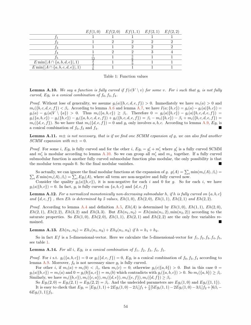
Ef(1, 0) Ef(2, 0) Ef(1, 1) Ef(2, 1) Ef(2, 2)f1 1 1 1 1 1f2 1 2 2 2 2f3 1 1 2 2 2f4 1 2 2 3 4f5

712 1 5

6 1 1Emin(|A ∩ {a, b, d, e}|, 1) 2

3 1 89 1 1

Emin(|A ∩ {a, b, c, d, e}|, 1) 56 1 1 1 1

Table 1: Function values

Lemma A.10. We say a function is fully curved if f(v|V \ v) for some v. For i such that gi is not fullycurved, Egi is a conical combination of f0, f3, f4.

Proof. Without lose of generality, we assume gi(a|{b, c, d, e, f}) > 0. Immediately we have mi(a) > 0 andmi({b, c, d, e, f}) < βi. According to lemma A.6 and lemma A.7, we have I(a; {b, c}) = gi(a)− gi(a|{b, c}) =gi(a) − gi(a|V \ {a}) > 0. Thus mi({a, b, c}) ≥ βi. Therefore 0 = gi(a|{b, c}) − gi(a|{b, c, d, e, f}) =gi({a, b, c}) − gi({b, c}) − gi({a, b, c, d, e, f}) + gi({b, c, d, e, f}) = βi −mi({b, c}) − βi + mi({b, c, d, e, f}) =mi({d, e, f}). So we have that mi({d, e, f}) = 0 and gi only involves a, b, c. According to lemma A.9, Egi isa conical combination of f0, f3 and f4. �

Lemma A.11. m± is not necessary, that is if we find one SCMM expansion of g, we can also find anotherSCMM expansion with m± = 0.

Proof. For some i, Egi is fully curved and for the other i, Egi = g′i + m′i where g′i is a fully curved SCMMand m′i is modular according to lemma A.10. So we can group all m′i and m± together. If a fully curvedsubmodular function is another fully curved submodular function plus modular, the only possibility is thatthe modular term equals 0. So the final modular vanishes. �

So actually, we can ignore the final modular functions at the expansion of g. g(A) =∑i min(mi(A), βi) =∑

iEmin(mi(A), βi) =∑iEgi(A), where all term are non-negative and fully curved now.

Consider the quality gi(a|{b, c}), it is non-negative for each i and 0 for g. So for each i, we havegi(a|{b, c}) = 0. In fact, gi is fully curved on {a, b, c} and {d, e, f}Lemma A.12. For a normalized monotonically non-decreasing submodular h, if h is fully curved on {a, b, c}and {d, e, f} , then Eh is determined by 5 values, Eh(1, 0), Eh(2, 0), Eh(1, 1), Eh(2, 1) and Eh(2, 2).

Proof. According to lemma A.4 and definition A.5, Eh(A) is determined by Eh(1, 0), Eh(1, 1), Eh(2, 0),Eh(2, 1), Eh(2, 2), Eh(3, 2) and Eh(3, 3). But Eh(n1, n2) = Eh(min(n1, 2),min(n2, 2)) according to thesaturate properties. So Eh(1, 0), Eh(2, 0), Eh(1, 1), Eh(2, 1) and Eh(2, 2) are the only free variables re-mained. �

Lemma A.13. Eh(n1, n2) = Eh1(n1, n2) + Eh2(n1, n2) if h = h1 + h2.

So in fact Ef is a 5-dimensional-vector. Here we calculate the 5-dimensional-vector for f1, f2, f3, f4, f5,see table 1.

Lemma A.14. For all i, Egi is a conical combination of f1, f2, f3, f4, f5.

Proof. For i s.t. gi({a, b, c}) = 0 or gi({d, e, f}) = 0, Egi is a conical combination of f0, f3, f4 according tolemma A.9. Moreover, f0 is not necessary since gi is fully curved.

For other i, if mi(a) + mi(b) < βi, then mi(c) = 0; otherwise gi(c|{a, b}) > 0. But in this case 0 =gi(a|{b, c}) = mi(a) and 0 = gi(b|{a, c}) = mi(b) which contradicts with gi({a, b, c}) > 0. So mi({a, b}) ≥ βi.Similarly, we have mi({b, c}),mi({c, a}),mi({d, e}),mi({e, f}),mi({d, f}) ≥ βi.

So Egi(2, 0) = Egi(2, 1) = Egi(2, 2) = βi. And the undecided parameters are Egi(1, 0) and Egi({1, 1}).It is easy to check that Egi = [Egi(1, 1) + 2Egi(1, 0)− 2βi]f1 + 1

2 [5Egi(1, 1)− 2Egi(1, 0)− 3βi]f2 + [6βi−6Egi(1, 1)]f5.

54

Next we will show that all coefficients are non-negative.

Lemma A.15. Given gi(A) = min(mi(A), βi), if mi(a) + mi(b),mi(b) + mi(c),mi(c) + mi(a),mi(d) +mi(e),mi(e) +mi(f),mi(f) +mi(d) ≥ βi, we have Egi(1, 1) + 2Egi(1, 0)−2βi ≥ 0, 5Egi(1, 1)−2Egi(1, 0)−3βi ≥ 0, Egi(1, 1) ≤ βiProof. Let xi be the weight of each elements. Without lose of generality, we assume that βi ≥ x1 ≥ xb ≥xc ≥ 0, βi ≥ xd ≥ xe ≥ xf ≥ 0 and xc ≥ xf . So xa, xb, xd, xe ≥ 1

2βi.Egi(1, 0) = 1

6

∑i xi ≥ 2

3βi and Egi(1, 1) = 19 [∑v∈{a,b,c}

∑u∈{d,e,f} gi({v, u})] = 2

3βi+19 [min(xa+xf , βi)+

min(xb + xf , βi) + min(xc + xf ), βi)] ≥ 23βi.

Therefore, Egi(1, 1) + 2Egi(1, 0)− 2βi ≥ 0 and Egi(1, 1) ≤ βi.For 5Egi(1, 1) − 2Egi(1, 0) − 3βi ≥ 0, if xc + xf ≥ βi, we have Egi(1, 1) = βi and Egi(1, 0) ≤ βi. So

5Egi(1, 1)− 2Egi(1, 0)− 3βi ≥ 0.If xc + xf ≤ βi, 5Egi(1, 1) + 2Egi(1, 0)− 3βi is growing when xf increased. So we can let xf = 0 for the

worst case. Therefore 5Egi(1, 1)+2Egi(1, 0)−2βi = 5( 23βi+

19 [xa+xb+xc])− 1

3 [xa+xb+xc+xd+xe]−3βiwhich is increasing with respect to xa, xb, xc and deceasing with respect to xd, xe. Further more, we have32βi ≤ xa + xb + xc and xd + xe ≤ 2βi. So 5Egi(1, 1) + 2Egi(1, 0)− 2βi ≥ 0

�

Therefore, we have shown that Egi is a conical combination of f1, f2, f3, f4, f5 for all i. Thereforeg =

∑iEgi is a conical combination of f1, f2, f3, f4, f5.

�

The 5-vector related to Eg is (φ(1), φ(2), φ(2), φ(3), φ(4)). So according to table 1, the unique expressionto expand g on f1, f2, f3, f4, f5 is g(A) = [2φ(1) + φ(2) − 4φ(3) + 2φ(4)]f1 + [−φ(1) + 3.5φ(2) − 4φ(3) +1.5φ(4)]f2 + [−φ(2) + 2φ(3)− φ(4)]f3 + [−φ(3) + φ(4)]f4 + 6[−φ(2) + 2φ(3)− φ(4)]f5

This expression is valid if and only if −φ(1) + 3.5φ(2)− 4φ(3) + 1.5φ(4) ≥ 0 and 2φ(1) + φ(2)− 4φ(3) +2φ(4) ≥ 0; other coefficients are always non-negative according to concavity and monotonicity.

The “if” part is straight forward according to the above expansion as we saw after the statement of thetheorem. �

B Sums of Weighted Cardinality Truncations is Smaller than SCMMs

In this section, show Lemma 5.10, namely that G = {∑B⊆V∑|B|−1i=1 αB,i min(|A∩B|, i), ∀B, i, αB,i ≥ 0} ⊂

SCMM. We assume the reader is familiar with the notation in Appendix A.

Lemma B.1. f5(A) /∈ {∑B⊆V∑|B|−1i=1 αB,i min(|A ∩B|, i)|αB,i ≥ 0}

Proof. Assume that

f5(A) =∑B⊆V

|B|−1∑i=1

αB,i min(|A ∩B|, i) =∑B⊆V

|B|−1∑i=1

αB,iEmin(|A ∩B|, i). (121)

Note that f5 is fully curved on {a, b, c} and {d, e, f}, and these hold for all terms. So for B and i, ifi ≥ |B∩{a, b, c}| or i ≥ |B∩{d, e, f}|, αB,i = 0. Therefore the remaining terms are f1, f2, f3, f4, Emin(|A∩{a, b, d, e}|, 1) and Emin(|A ∩ {a, b, c, d, e}|, 1) Therefore, for all these functions, Ef(2, 0) ≤ 9

8Ef(1, 1), butEf5(2, 0) = 6

5Ef5(1, 1) (table 1). So it is impossible to find a conical combination of min(|A ∩ B|, i) thatequals f5.

�

55