Fast Clustering leads to Fast SVM Training and More Daniel Boley

Fast Clustering leads to Fast

SVM Training and More

Daniel Boley

University of Minnesota

Supported in part by NSF

2006 Stanford Workshop on Massive Datasets. 662482 p1 of 39

Goals and Outline

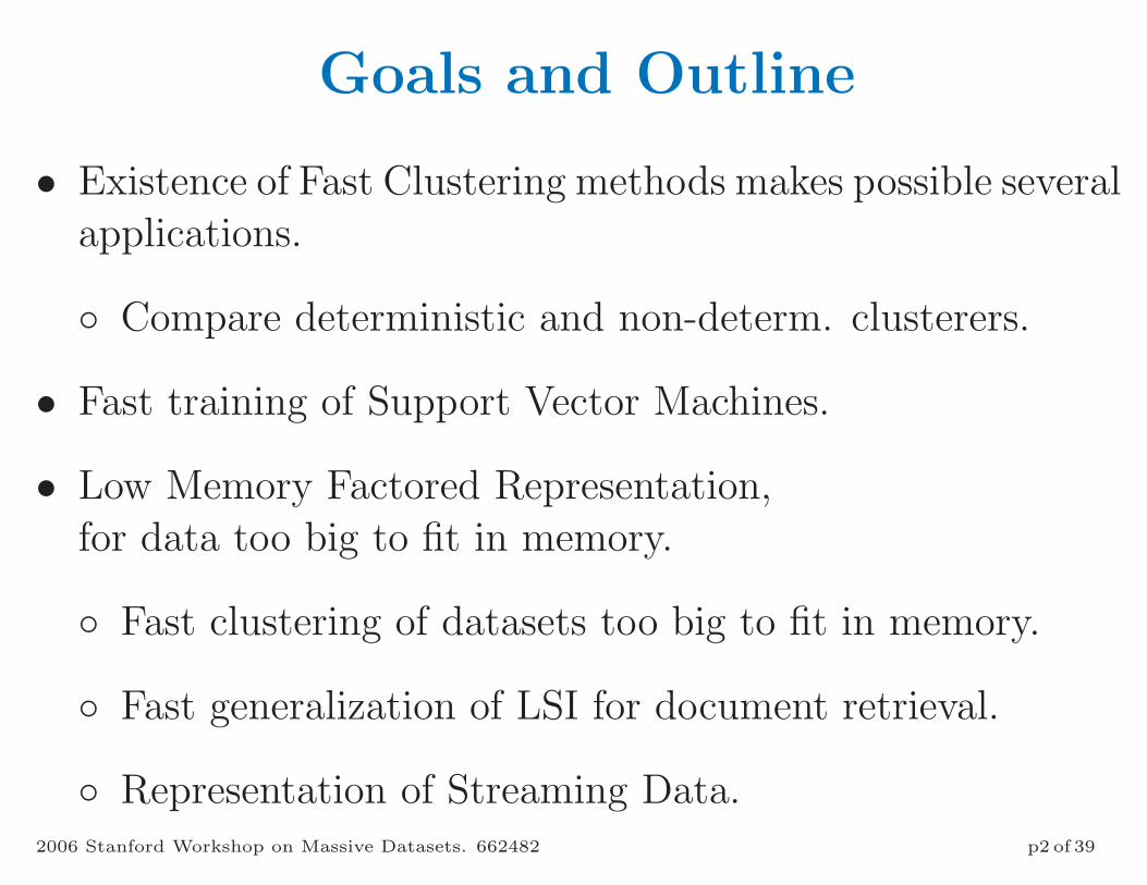
• Existence of Fast Clustering methods makes possible severalapplications.

Compare deterministic and non-determ. clusterers.

• Fast training of Support Vector Machines.

• Low Memory Factored Representation,for data too big to fit in memory.

Fast clustering of datasets too big to fit in memory.

Fast generalization of LSI for document retrieval.

Representation of Streaming Data.2006 Stanford Workshop on Massive Datasets. 662482 p2 of 39

Hierarchical Clustering

• Clustering at all levels of resolution.

• Bottom-up clustering is O(n2).

• Top-down clustering can be made O(n).

• Leads to PDDP. [basis of this talk].


Hierarchical Clustering: Get a Tree

QQ

QQ

QQ

QQ

QQ

QQ

QQ

QQQs

+

+

+

QQ

QQ

QQ

QQQs

QQ

QQ

QQ

QQQs

~

~~

~ ~ ~~

technologi

system

develop

manufactur. . .

affirm

action

employe

employ. . .

system

manufactur

engin

process. . .

patent

intellectu

properti

personnel. . .

affirm

action

minor

discrim. . .

busi

internet

electron

commerc. . .


K-means: Popular Fast Clustering

• Quality of final result depends on initialization

• Random initialization ⇒ results hard to repeat.

• Deterministic initialization - no universal strategy

• Cost: O(#iters ·m · n) ⇒ linear in n.

where n = number of data samples

m = number of attributes per sample.


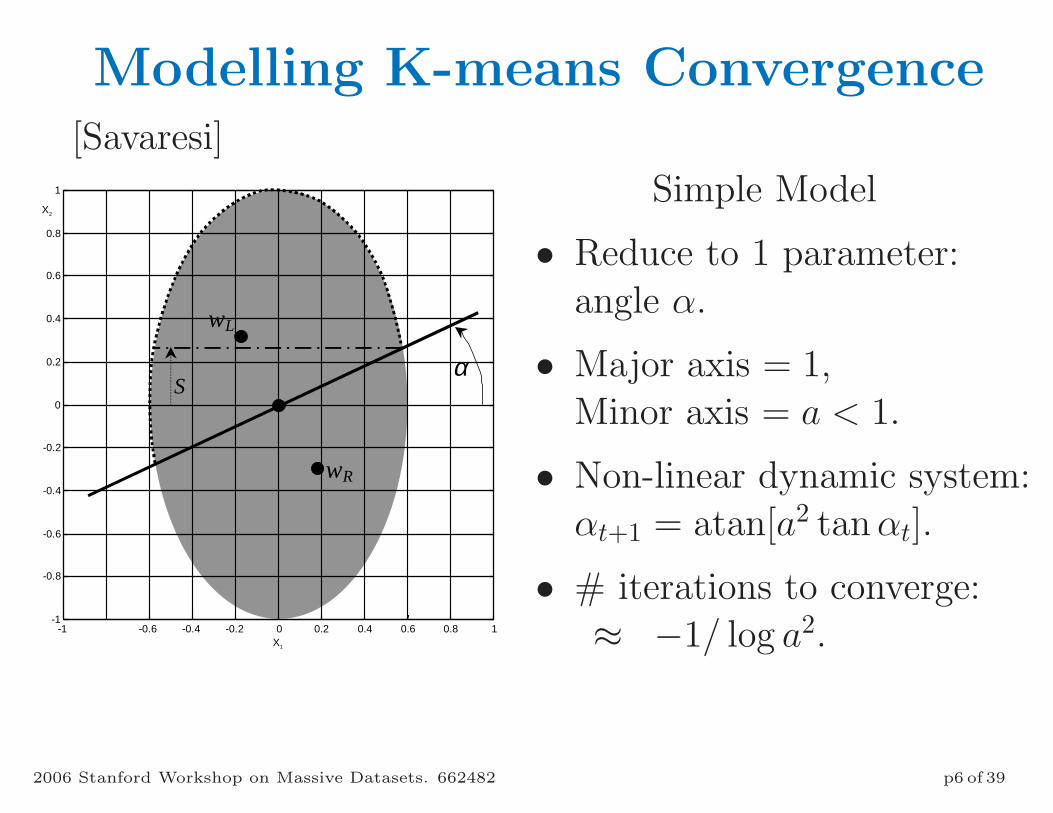
Modelling K-means Convergence

[Savaresi]

-1 -0.6 -0.4 -0.2 0 0.2 0.4 0.6 0.8 1-1

-0.8

-0.6

-0.4

-0.2

0

0.2

0.4

0.6

0.8

1

X1

X2

α

wR

S

wL

Simple Model

• Reduce to 1 parameter:angle α.

• Major axis = 1,Minor axis = a < 1.

• Non-linear dynamic system:αt+1 = atan[a2 tan αt].

• # iterations to converge:≈ −1/ log a2.


Infinitely Many Points

-0.5 0 0.5 1 1.5 2

-0.5

0

0.5

1

1.5

2

alpha(t)

alpha(t+1)

α 0

lineα t+1=α t

functionα t+1=f(α t)

K-meansmodelledas afixedpointiteration


Finite Number of Points

-0.5 0 0.5 1 1.5 2

-0.5

0

0.5

1

1.5

2

alpha(t)

alpha(t+1)

Number of data points = 15; a=0.6

(a)

Equilibriumpoints

alpha t

-0.5 0 0.5 1 1.5 2

-0.5

0

0.5

1

1.5

2

alpha(t)

alpha(t+1)

Number of data points = 100; a=0.6

(c)


Finite Number of Points

• Many equilibrium points =⇒ many local minima.

• As # points grows, local minima tend to vanish.

• As minor axis → 1, more local minina tend to appear.


PDDP vs K-means on Model Problem

• In the limit, PDDP & K-means yield same split here.[Savaresi]

-1 -0.5 0 0.5 1 1.5

-1

-0.5

0

0.5

1

1.5Bisecting K-means partition

-1 -0.5 0 0.5 1 1.5

-1

-0.5

0

0.5

1

1.5PDDP partition

(a) (b)


Starting K-means

• Empirically, PDDP is a good seed for K-means.

0 100 200 300 400 500 600 700 800 900 10000

0.2

0.4

0.6

0.8

1

Experiment #

Measure of scatter of the partition (0=best; 1=worst) – Size of the data-set N=1000

Quality of clusteringprovided by PDDP

Quality of clusteringprovided by K-means initializedwith PDDP result


Cost of K-means vs PDDP

• Both are linear in the number of samples.

• K-means often cheapest, but cost can vary a lot.

Floating points operations required to bisect a 100x1000 matrix

0,0,E+00

1,0,E+07

2,0,E+07

3,0,E+07

4,0,E+07

5,0,E+07

6,0,E+07

Min. of K-means Mean of K-means Max. of K-means PDDP PDDP + K-means


SVM via Clustering

• Motivation: Reduce trainging cost by clustering and useone representative per cluster instead of all the originaldata.

• Empirically provides good SVMs with comparable errorrates on test sets.

• Theoretically generalization error satisfies “same” boundas the SVM obtained using all the data.

• Can be made adaptable by quickly running a sequence ofSVMs, each with new data points added, to adjust andimprove SVM adaptively.


SVM via Clustering• Cluster Training Set into partitions• Train SVM using 1 representative per partition.

x2

x1

Dpos, 2

Decision boundaryd(x) = -1

: Negative class: Positive class

d(x) = 1

Dpos, 1

Dneg, 1

Dneg, 2

Dneg, 3

d(x) < -1d(x) > 1 -1< d(x)<1

l =h.y d (x)1 −

normalw

vector

measureerror


Support Vector Machine

• Minimize R (d;D, λ) = Remp(d;D)︸︷︷︸Empirical

Error

+ λ · Ω(d)︸︷︷︸Regularization/

Complexity Term

• D = xi, yin

i=1: training set.

• xi: datum w/ label yi = ±1.

• φ(x): non-linear lifting.

• d(x) = 〈w, φ(x)〉: discriminant fcn.

• λ: regularization coefficient

• Ω(d) = ‖w‖2

• Remp(d;D) = 1n

∑

(x,y)∈D

ℓhinge(d, (x, y)) = max0, 1− y · d(x)


Questions to be Resolved

• How to select representatives?

• If selection cost is O(n2)then one gains little by using representatives.

• How to adjust representatives to improve classifier quality?


Approximate SVM Methods

Choices of Clustering Method

• Use fast clustering method.

• Intuition: want to minimize distancesample point ⇔ representative in lifted space.

• =⇒ kernel K-means.

• But expensive, so approximate it with data K-means (natural choice) data PDDP (to make deterministic or to init K-means)

• Option: add potential support vectors, and repeat.


Quality of SVM – Theory

• Could apply VC dimension bounds,but we want something tighter.

• Extend Algorithmic-Stability bounds to this case.These apply specifically to learning algorithms minimizing some convex

functional, whose change is bounded when a datum is substituted.

• Assume only that representatives are centers of partitions.

• Partitions are arbitrary, so result applies even when usingdata K-means, data space PDDP, random partitioning, oreven a sub-optimal soln from kernel K-means.


Stability Bound TheoremGet theorem much like one for Exact SVM.

• For any n ≥ 1 and δ ∈ (0, 1), with confidence at least 1−δ

over the random draw of a training data set D of size n:

E(Ih(x) 6=y)

︸︷︷︸expected error

≤ 1n

∑

(x,y)∈D

ℓhinge(h,x, y)

︸︷︷︸empirical error

+ χ2

λn +(

2χ2

λ + 1) √

ln 1/δ2n

︸︷︷︸complexity/sensitivity term

.

where

h(x)def

= sign d(x) is the approximate SVM.

χ2 = maxi K(xi,xi) = max〈φ(xi), φ(xi)〉 (1 for RBF kernel).

λ corresponds to soft-margin weighting.trade-off of training error ←→ sensitivity.


Experimental Setup

• Illustrate performance of SVM with clustering on someexamples.

• We cluster in data space with PDDP;

• We compare the proposed algorithm against the standardtraining algorithm SMO [Platt, 1999], implemented inLibSVM [Chang+Lin 2001] [Fan 2005];


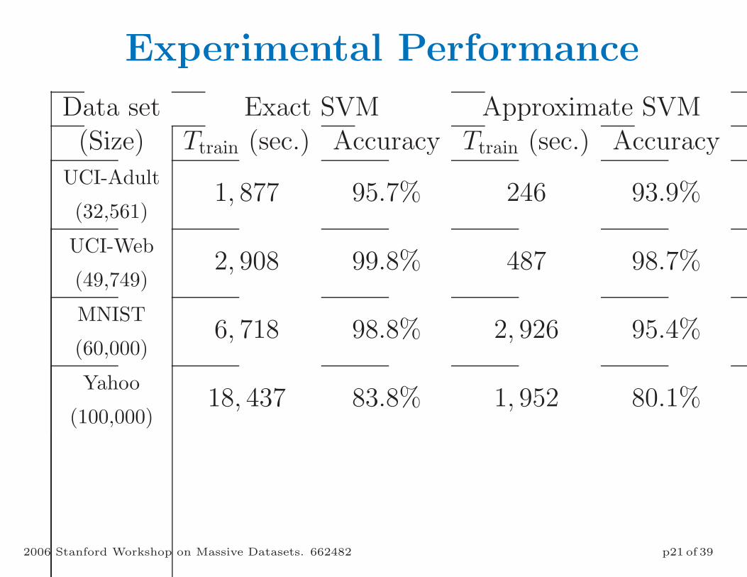
Experimental Performance

Data set Exact SVM Approximate SVM(Size) Ttrain (sec.) Accuracy Ttrain (sec.) Accuracy

UCI-Adult

(32,561)1, 877 95.7% 246 93.9%

UCI-Web

(49,749)2, 908 99.8% 487 98.7%

MNIST

(60,000)6, 718 98.8% 2, 926 95.4%

Yahoo

(100,000)18, 437 83.8% 1, 952 80.1%


Low Memory Factored Representation

• Use clustering to contruct a representation of a full massivelylarge data sets in much less space.

• Representation is not exact, but every individual samplehas its own unique representative in the approximate representation.

• In principle, would still allow detection and analysis ofoutliers and other unusual individual samples.

• Next slide has basic idea.


Low Memory Factored Representation

m

M m

n

n

C Z

.kc

. . . . . .

k

dk

kd1 2 ks

c z nonzeros per columnk

section section section section section section

section representatives

data loadings

ClusteringLeast Squares

very sparse


Fast factored representation: LMFR

[Littau]

• M = CZ by fast clustering of each section

• C = matrix of representatives

• Still have Z to individualize representation of each sample

• Make Z sparse to save space.

• linear clustering cost → linear cost to construct LMFR

• In principle, could use any fast clusterer.

• We use PDDP to make it more deterministic.


LMFR ⇒ Clustering ⇒ PMPDDP

Using PDDP on an LMFR yields Piece-Meal PDDP.

• Factored Representation ⇒ to reconstruct data

• Expensive to compute similarities between individual data.

• Want to avoid accessing individual data.

• Ideal for clusterer that depends on M× v’s

• A spectral clustering method like PDDP is a good fit.

• Experimentally, cluster quality ≈ plain PDDP.


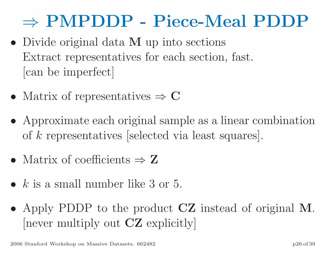
⇒ PMPDDP - Piece-Meal PDDP• Divide original data M up into sections

Extract representatives for each section, fast.[can be imperfect]

• Matrix of representatives ⇒ C

• Approximate each original sample as a linear combinationof k representatives [selected via least squares].

• Matrix of coefficients ⇒ Z

• k is a small number like 3 or 5.

• Apply PDDP to the product CZ instead of original M.[never multiply out CZ explicitly]


PMPDDP – on KDD dataset• Still Linear in size of data set.

0

1000

2000

3000

4000

5000

6000

7000

0 500000 1e+06 1.5e+06 2e+06 2.5e+06 3e+06 3.5e+06 4e+06 4.5e+06 5e+06

time

in s

econ

ds

number of samples

KDD timesPDDPCompute CZCluster CZCluster CZPMPDDP totals


PMPDDP – on KDD dataset• First 5 samples: PMPDDP cost ≈ 4 × PDDP.

0

200

400

600

800

1000

1200

100000 200000 300000 400000 500000 600000 700000 800000 900000 1e+06

time

in s

econ

ds

number of samples

first 5 KDD timesPDDPCompute CZCluster CZCluster CZPMPDDP totals4 * PDDP


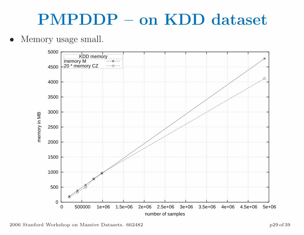
PMPDDP – on KDD dataset• Memory usage small.

0

500

1000

1500

2000

2500

3000

3500

4000

4500

5000

0 500000 1e+06 1.5e+06 2e+06 2.5e+06 3e+06 3.5e+06 4e+06 4.5e+06 5e+06

mem

ory

in M

B

number of samples

KDD memorymemory M20 * memory CZ


LMFR for Document Retrieval

• Mimic LSI, except we use factored representation CZ.

• Different from finding nearest concepts (ignoring Z)

• Can handle much larger datasets than ConceptDecomposition [full Z]

• Less time needed to achieve similar retrieval accuracy.


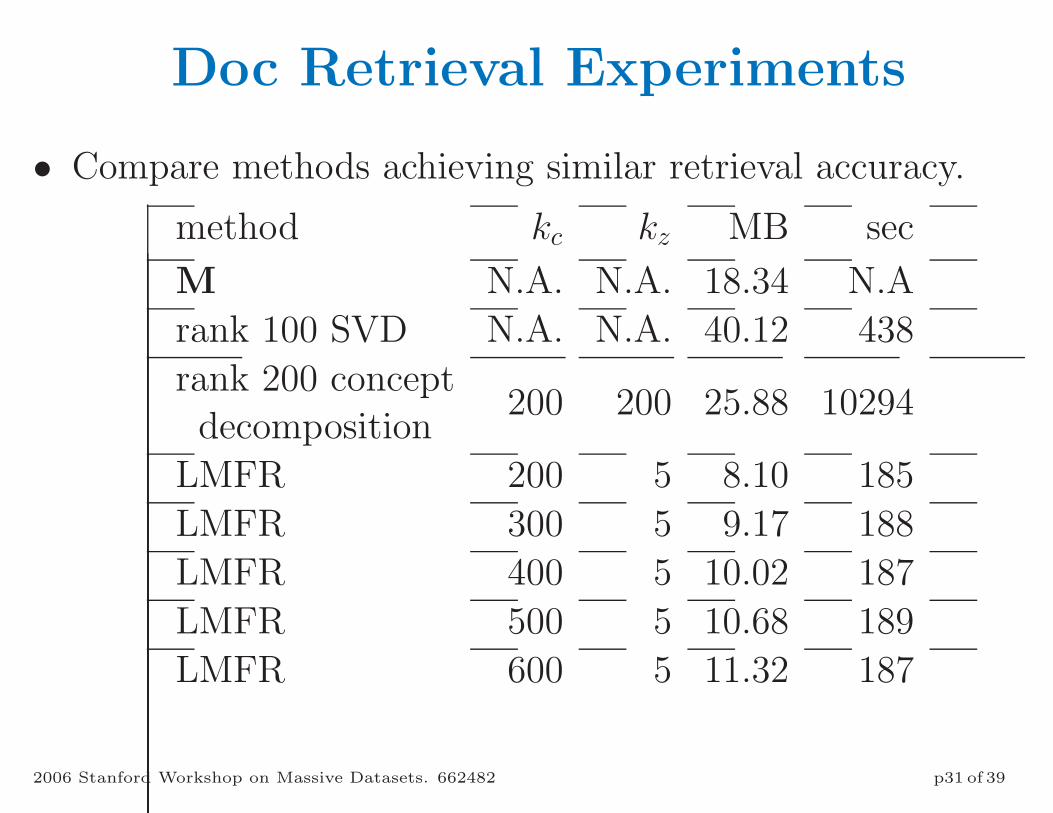
Doc Retrieval Experiments

• Compare methods achieving similar retrieval accuracy.

method kc kz MB sec

M N.A. N.A. 18.34 N.A

rank 100 SVD N.A. N.A. 40.12 438

rank 200 conceptdecomposition

200 200 25.88 10294

LMFR 200 5 8.10 185

LMFR 300 5 9.17 188

LMFR 400 5 10.02 187

LMFR 500 5 10.68 189

LMFR 600 5 11.32 187


Doc Retrieval Experiments

0 0.2 0.40

0.1

0.2

0.3

0.4

0.5

0.6

0.7

0.8

0.9

1

recall

prec

isio

n

Recall vs precision for the original representation M

0 0.2 0.40

0.1

0.2

0.3

0.4

0.5

0.6

0.7

0.8

0.9

1

recall

prec

isio

n

Recall vs precision for the rank 100 SVD

0 0.2 0.40

0.1

0.2

0.3

0.4

0.5

0.6

0.7

0.8

0.9

1

recall

prec

isio

n

Recall vs precision for the rank 200 concept decomposition

0 0.2 0.40

0.1

0.2

0.3

0.4

0.5

0.6

0.7

0.8

0.9

1

recall

prec

isio

n

Recall vs precision for the LMFR, kc=600, k

z=5


LMFR for Streaming Data

• Simple idea: collect data into sections as they arrive

• Form CZ section by section as they fill.

• Get LMFR for data, useful for any application (clustering,IR, aggregate statistics,...]

• No need to decide application in advance


LMFR for Streaming Data

• Memory for Z grows very slowly

• Memory for C grows more.

• Recursively factor C into its own CZ ⇒ less space.

• Hybrid Approach: once in a while do a completely newLMFR.


Streaming Data Results

0 0.5 1 1.5 2 2.5 3 3.5 4 4.5 5

x 106

0

100

200

300

400

500

600

number of data items

mem

ory

occu

pied

by

CG

ZG

, in

MB

Memory used for 3 Update Methods for the KDD data

rebuild CZfactor Chybrid


Streaming Data Results

0 0.5 1 1.5 2 2.5 3 3.5 4 4.5 5

x 106

0

0.02

0.04

0.06

0.08

0.1

0.12

number of data items

time

per

data

item

to c

ompu

te C

G Z

G in

sec

onds

Time Taken per data item for 3 Update Methods for the KDD data

rebuild CZfactor Chybrid


Related Work• SVM via Clustering Chunking (Boser+92, Osuna+97, Kaufman+99, Joachims99)

Low Rank Approx (Fine 01, Jordan)

Sampling (Williams+Seeger01, Achlioptas+McSherry+Scholkopf 02)

Squashing (Pavlov+Chudova+Smith 00)

Clustering (Cao+04, Yu+Yang+Han 03)

• Agglomeration on large datasets gather/scatter (Cutting+ 92)

CURE(Guha+98)

gaussian model (Fraley 99)

Heap (Kurita 91)

refinement (Karypis 99)


Related Work• K-means on large datasets Initialization (Bradley-Fayyad 1998)

kd-tree (Pelleg-Moore 1999)

Sampling (Domingos+01)

CLARANS k-medoid, spatial data (Ng+Han 94)

Birch (more sampling than k=means) (Ramakrishnan+96)

• Matrix Factorization LSI Berry 95 Deerwester 90

Sparse LowRankApprox Zhang+Zha+Simon 2002

SDD (Kolda+98) – good for outlier detection (Skillikorn+01)

Monte-Carlo sampling (Vempala+98)

Concept Decomp (Dhillon+01)


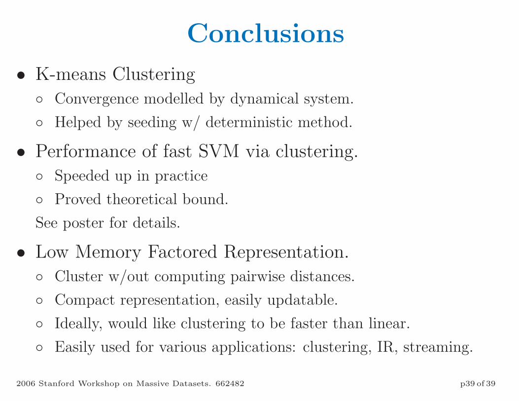
Conclusions

• K-means Clustering Convergence modelled by dynamical system.

Helped by seeding w/ deterministic method.

• Performance of fast SVM via clustering. Speeded up in practice

Proved theoretical bound.

See poster for details.

• Low Memory Factored Representation. Cluster w/out computing pairwise distances.

Compact representation, easily updatable.

Ideally, would like clustering to be faster than linear.

Easily used for various applications: clustering, IR, streaming.


Fast Clustering leads to Fast SVM Training and More Daniel Boley

Documents