Fast and accurate object detection by means of recursive monomial feature elimination and cascade of SVM

Fast and Accurate Object Detection by Means of Recursive Monomial

Feature Elimination and Cascade of SVM

Lorenzo Dal Col and Felice Andrea Pellegrino

Abstract— Support Vector Machines (SVMs) are an estab-lished tool for pattern recognition. However, their applicationto real–time object detection (such as detection of objectsin each frame of a video stream) is limited due to therelatively high computational cost. Speed is indeed crucial insuch applications. Motivated by a practical problem (handdetection), we show how second–degree polynomial SVMs intheir primal formulation, along with a recursive elimination ofmonomial features and a cascade architecture can lead to afast and accurate classifier. For the considered hand detectionproblem we obtain a speed–up factor of 1600 with comparableclassification performance with respect to a single, unreducedSVM.

I. INTRODUCTION

Since their introduction [1], Support Vector Machines

(SVMs) have been employed for visual pattern classification,

see for example [2], [3], [4], [5]. Noticeably, they lead

to accurate classifiers even when employing the simplest

feature set, namely the intensity values of the pixels of the

image to be classified [6]. When dealing with real–time

object detection, however, computational difficulties arise:

exhaustive search of an object instance within an image,

possibly in multi–scale fashion, requires a large number of

evaluations of the decision function per single frame. A great

deal of work has been done for reducing the computational

requirements of SVM in the classification phase. Most of

the literature deals with SVMs in dual formulation, where

the time taken to classify a test point is proportional to the

number N of support vectors (SVs). In [7], [8], [9], and

[10] the idea of reducing N while retaining the classification

performance is pursued either by using N ′ < N synthetic

vectors or by properly pruning the SV’s set or by rewriting

the decision function as a function of a small subset of data

points; in [11] the special case of second–degree polynomial

SVM is treated. If the primal formulation is considered,

a possibility of reducing the complexity is to reduce the

number of features by selecting the most relevant ones. In

[12] a feature selection procedure, called Recursive Feature

Elimination (RFE) is employed for linear SVM to discover

the most relevant genes to cancer diagnosis. Basically, the

features are ranked according to the magnitude of weight wi

of the decision function f(x) = wTx + b =

∑

wixi + b.Subsequently, the least relevant features are removed, the

classifier is retrained using the reduced set of feature and

Corresponding author: Felice Andrea Pellegrino. The authors are withthe Department of Industrial Engineering and Information Technology,DI3, University of Trieste, Italy ([email protected],[email protected]).

This work has been partially supported by Universita di Trieste –Finanziamento Ricerca d’Ateneo.

the procedure is repeated until a specified (minimum) level

of performance is reached. Improvements, that take into

account the classification margin, have been proposed in

[13] and [14]. A non-recursive feature reduction technique,

based on a ranking criterion different from [12], is proposed

in [15]. In addition to the mentioned general methods,

some domain–specific techniques have been proposed for

speeding–up object detection: in particular, the hierarchical

approach [16], [15], [17]. Such an approach is motivated

by the fact that, in typical applications, the large majority

of the patterns analyzed belong to the ”non–object” class

(non–object to object ratios of 3.5 × 104 and 5 × 104 are

reported respectively in [17] and [15]). Therefore, a cascade

of classifiers, having on top a simple classifier capable of

rejecting a large percentage of the non–object instances can

save a lot of computation time. In this paper, we build a

cascade of recursively reduced second–degree polynomial

SVM classifiers, each expressed in the primal formulation.

Our approach resembles that of [15], but there are some

significant differences:

• we build a cascade of nonlinear (quadratic) classifiers;

• we perform a feature reduction for each cascade level;

• the feature reduction is recursive, being the RFE applied

to a quadratic SVM;

• we do not adopt a coarse–to–fine strategy, but we feed

each classifier with a set of features extracted from the

same window.

This novel (to our knowledge) scheme yields a factor of

1600 speed–up for the considered hand detection problem

with respect to a single, unreduced SVM, while retaining

the classification performance. We report results for a hand

detection problem: detecting hands in images is a relevant

problem for gesture recognition, that is of primary impor-

tance in designing effective human–computer interfaces [18].

Ranging from surveillance to human–in–the–loop control

systems, gesture recognition has a number of automation–

related applications.

The paper is organized as follows: in Section II dual

and primal formulation of SVM are recalled; in Section

III we describe the feature reduction procedure; in Section

IV we treat the hierarchical architecture of the classifiers.

Finally, experimental results for a hand detection problem

are reported in Section V.

II. DUAL AND PRIMAL FORMULATION OF POLYNOMIAL

SVM

Denoting with x ∈ Rn the pattern to be classified, the deci-

sion function of an SVM can be written, in dual formulation,

2011 IEEE Conference on Automation Science and EngineeringTrieste, Italy - August 24-27, 2011

ThC1.1

978-1-4577-1732-1/11/$26.00 ©2011 IEEE 304

as:

f(x) =

l∑

i=1

αiyiK(xi,x) + b (1)

where l is the cardinality of the training set {(xi, yi), i =1, . . . , l}, xi ∈ R

n and yi ∈ {0, 1} are, respectively, a

training pattern and its label, and K : R2×n → R is the so–

called kernel function [19]. Given the training set, scalars αi

and b are found by solving a quadratic optimization problem

(i.e. training the SVM). The dual formulation is sparse in the

vector [α1, . . . , αl] and those training patterns corresponding

to nonzero coefficients are called Support Vectors. The kernel

function K(x,y) represents the dot product between the

images of x and y according to a feature map Φ : Rn → Rp:

K(x,y) = Φ(x)TΦ(y). (2)

The kernel implicitly defines a mapping from the input space

Rn to the (possibly infinite–dimensional) feature space R

p.

In particular, the inhomogeneous polynomial kernel

K(x,y) = (1 + xTy)d (3)

results in a finite–dimensional feature space of (weighted)

monomials, precisely all the monomials of the form xai x

bj up

to the degree d. For example, a second–degree polynomial

machine is obtained by the choice d = 2 and leads to the

feature map:

Φ(x) =[

1,√2x1, . . . ,

√2xn, x

21, . . . , x

2n, (4)

√2x1x2, . . . ,

√2xn−1xn

]T

.

In this paper we focus on second–degree polynomial SVMs

because, although relatively low–dimensional in feature

space, have been proven to be effective in many object de-

tection tasks [15]. However, the described scheme is general,

provided that one can manage the feature mapping explicitly.

In the primal formulation, the feature mapping is per-

formed explicitly, instead of implicitly through the kernel:

f(x) = wTΦ(x) + b. (5)

The i–th component wi of the vector of weights w represents

the contribution of feature Φi(x) to the decision function1.

Depending on the situation, the decision function may be

computed more conveniently using either (1) or (5). It is

clear from (1) that the number of arithmetic operations Nd

required for computing the decision function by (1) depends

on the number N of SVs and on the dimension n of the input

space. In order to compute the kernel function (3) at least

n additions and n multiplications must be computed for the

scalar product, neglecting the few operations performed on

scalars. The kernel function is computed for each SV, and

its values must be finally multiplied by the respective αi

1Equation (5) shows that the SVM is linear in the feature space. Inthat space, the decision boundary is a hyperplane, precisely the maximum–margin hyperplane, having the maximum distance to the closest points ofthe training set.

−1 −0.5 0 0.5 1−1

01

−1.5

−1

−0.5

0

0.5

1

1.5

2

2.5

3

3 features

−1 −0.5 0 0.5 1−1

−0.5

0

0.5

12 features

−1 −0.5 0 0.5 1−1

−0.5

0

0.5

12 features with retraining

Fig. 1. Example of application of the method recursive monomial

feature elimination. The original problem has three dimensions (left). Thefeature corresponding to the smallest weight is eliminated (top right). Thehyperplane separating the solution changes (bottom right) orientation afterretraining the classifier.

coefficients and added together, requiring at least 2N more

operations:

Nd = 2N(n+ 1). (6)

When using the primal formulation (5), the number of opera-

tions depends mostly on the dimension p of the feature space.

The elements of Φ(x) are obtained by n multiplications, for

the x2i terms, and nn−1

2 multiplications for the mixed terms

in (4). Finally, p additions and p multiplications are required

for the scalar product in (5)). In particular, for a second–

degree polynomial machine [19]

p =

(

n+ 2

2

)

= nn− 1

2+ 2n+ 1,

hence the number Np of required operations is

Np = nn− 1

2+ n+ 2p = 3p− 2n. (7)

In object detection tasks it may well happen that the primal

formulation is computationally preferable: this is due to the

large number of SVs, which scales roughly linearly with the

number of training samples [6]. For example, in the hand

detection task described in Section V the number of SVs is

N = 1639 and the dimension of the input space is n = 24×24 = 576, resulting in Nd = 1891406 operations for the dual

formulation. In the same case, p =(

576−22

)

= 166753 hence

the number of operations required for the primal formulation

is Np = 3p − 2n = 499107. As a consequence, the primal

formulation is preferable.

III. RECURSIVE MONOMIAL FEATURE ELIMINATION

In the following we describe the feature elimination pro-

cedure used for achieving low computational complexity

for each level of the hierarchical classifier. The procedure

of recursive feature elimination was originally proposed,

305

in data mining context, in [12] where it was applied to

linear classifiers. We deal with second–degree polynomial

SVMs in primal formulation, hence the decision function

is expressed by (5). Provided that the feature map (4) is

explicitly computed, the same procedure can be applied to

such a nonlinear SVM (treated as a linear one acting on

the computed feature vector). The monomials appearing in

(4) represent the features we want to reduce based on their

contribution to the decision function. The procedure can be

outlined as follows [12]:

1) given: a trained SVM in primal formulation, namely

the vector w ∈ Rp, the bias b and the feature map

Φ(x);2) find the index of the smallest weight j =

argmini |wi|, ∀i = 1, . . . , p, and define Φ∗(x) =[Φ1(x), . . . , Φj−1(x), Φj+1(x), . . . , Φp(x)]

T .3) train a linear SVM using the same training set and the

reduced feature map Φ∗(x). A new weight vector w∗

of dimension p∗ = p− 1 is obtained;

4) if the performance of the reduced machine is below an

established threshold, retain the previous machine and

finish, otherwise set w ← w∗ and Φ← Φ∗;

5) go to step 2.

An example of feature reduction is reported in Fig. 1, where

the original 3–feature linear SVM is reduced to a 2–feature

SVM by removing the feature having the smallest weight

and retraing the SVM. As a result of the feature reduction

procedure, the classifier

f∗(x) = w∗TΦ∗(x) + b∗ (8)

is obtained, having a small (although not necessarily min-

imal) set of monomial features and achieving a desired

performance level.

Remark 1: Notice that different criteria can be used at

step 4 for evaluating the performance. In particular, instead

of the overall accuracy of the classification, a threshold

on the true–positive rate of the obtained classifier can be

employed. Moreover, at each step, a tuning of the bias b∗

can be performed to achieve a desired false–rejection rate. As

shown in the following section, this is particularly important

when building a cascade of reduced classifiers, where the

false–rejection rate is critical for the cascade structure being

advantageous.

Remark 2: Since training SVMs is time–consuming,

achieving a small subset of features by eliminating a single

feature per step is often impractical. Indeed, in realistic

object detection tasks, p is typically as large as hundreds

of thousands. In such cases, an approximate “block–wise”

reduction can be performed by eliminating a fixed number

of least–relevant features per step.

In [15] feature reduction is applied to the last stage of

a hierarchical classifier, but not in a recursive way (no

retraining of the classifier is performed).

IV. CASCADE OF PRIMAL REDUCED SVM

In typical object detection applications, the large majority

of the patterns analyzed belong to the ”non–object” class.

Motivated by this observation, hierarchical architectures have

been proposed to speed–up the classification, see for example

the well–known paper on face detection by Viola and Jones

[17]. There, the whole classifier consists of a sequence of

linear classifiers of increasing complexity trained by means

of the AdaBoost algorithm [20]. The basic idea is to reject

most of the negative instances as soon as possible along

the cascade, in such a way that computationally expensive

classifiers evaluate a small number of negative instances

(those not rejected by the previous cascade levels). An

example of three–level cascade is depicted in Fig. 2: rejection

can occur at each level, while instances that pass through the

whole cascade are classified as positive. The detection rate

D (true positive rate) of the whole classifier depends on the

detection rate di of the single cascade levels:

D =∏

i

di. (9)

Similarly, the overall false positive rate F can be expressed

as

F =∏

fi, (10)

where fi is the false positive rate of the i–th level of the

cascade. It is clear from (9) that to get a high detection rate

(which is desirable), the classifiers composing the cascade

must have high detection rate. On the contrary, from (10) it

follows that a low overall false positive rate (which, again,

is desirable) can be achieved by rather high values of fi (see

for example Table II of the following section). Consistently

with the above observations, we build a cascade of reduced

SVMs according to the following algorithm, inspired to [17]:

1) given:

• a nested family M of m1 ⊂ m2 ⊂ · · · ⊂ mM

monomial feature sets, ordered by increasing num-

ber of features: the first feature set contains the

most relevant features (as found via RFE) while

the largest corresponds to the unreduced feature

set;

• for each cascade level i, a value fi(target) repre-

senting the maximum acceptable false positive rate

for that layer;

• an overall target of false positive rate Ftarget;

2) set the current level of the cascade to i = 1 (top level)

and the feature–set index to j = 1;

3) train a classifier based on mj and place it in the i–th

cascade level;

4) tune the bias of (8) in order to obtain a 100% detection

rate on the training set (to avoid rejection of positive

instances);

5) if the false positive rate (evaluated over the validation

set) is above the target value fi(target), increase j and

go to step 3;

6) otherwise, compute the false positive rate Fi of the

current cascade according to (10) ;

7) if Fi ≤ Ftarget the cascade is complete; otherwise

increase i, set j = 1 and go to step 3.

306

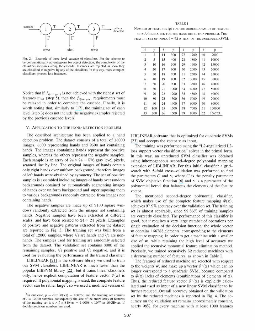
Fig. 2. Example of three–level cascade of classifiers. For the scheme tobe computationally advantageous for object detection, the complexity of theclassifiers increases along the cascade. Instances are rejected as soon theyare classified as negative by any of the classifiers. In this way, more complexclassifiers process less instances.

Notice that if fi(target) is not achieved with the richest set of

features mM (step 5), then the fi(target) requirements must

be relaxed in order to complete the cascade. Finally, it is

worth noting that, similarly to [17], the training set of each

level (step 3) does not include the negative examples rejected

by the previous cascade levels.

V. APPLICATION TO THE HAND DETECTION PROBLEM

The described architecture has been applied to a hand

detection problem. The dataset consists of a total of 15000images, 5500 representing hands and 9500 not containing

hands. The images containing hands represent the positive

samples, whereas the others represent the negative samples.

Each sample is an array of 24× 24 = 576 gray level pixels,

scanned line by line. The original images of hands contain

only right hands over uniform background, therefore images

of left hands were obtained by symmetry. The set of positive

samples is assembled including images of hands over random

backgrounds obtained by automatically segmenting images

of hands over uniform background and superimposing them

to various backgrounds randomly extracted from images not

containing hands.

The negative samples are made up of 9100 square win-

dows randomly extracted from the images not containing

hands. Negative samples have been extracted at different

scales, and have been resized to 24 × 24 pixels. Examples

of positive and negative patterns extracted from the dataset

are reported in Fig. 3. The training set was built from a

total of 12000 samples, where 1/3 are hands and 2/3 are non-

hands. The samples used for training are randomly selected

from the dataset. The validation set contains 3000 of the

remaining samples, 1/2 positive and 1/2 negative, and it is

used for evaluating the performance of the trained classifier.

LIBLINEAR [21] is the software library we used to train

our SVM classifiers. LIBLINEAR is much faster than the

popular LIBSVM library [22], but it trains linear classifiers

only, hence explicit computation of feature vector Φ(x) is

required. If polynomial mapping is used, the complete feature

vector can be rather large2, so we used a modified version of

2In our case, p = dim(Φ(x)) = 166753 and the training set consistsof l = 12000 samples, consequently the size of the entire array of featuresof the training set is p × l × 8Bytes = 1.6008 × 1010 ≃ 16 GBytes, ifdouble-precision numbers are used.

TABLE I

NUMBER OF FEATURES (p) FOR THE ORDERED FAMILY OF FEATURE

SETS M EMPLOYED FOR THE HAND DETECTION PROBLEM. THE

FEATURE SET OF INDEX i = 52 IS THAT OF THE UNREDUCED SVM.

i p i p i p i p

1 2 14 300 27 1700 40 9000

2 5 15 400 28 1800 41 10000

3 10 16 500 29 1900 42 15000

4 20 17 600 30 2000 43 20000

5 30 18 700 31 2500 44 25000

6 40 19 800 32 3000 45 30000

7 50 20 900 33 3500 46 40000

8 60 21 1000 34 4000 47 50000

9 70 22 1200 35 4500 48 60000

10 80 23 1300 36 5000 49 70000

11 90 24 1400 37 6000 50 80000

12 100 25 1500 38 7000 51 100000

13 200 26 1600 39 8000 52 166753

LIBLINEAR software that is optimized for quadratic SVMs

[23] and accepts the vector x as input.

The training was performed using the “L2-regularized L2-

loss support vector classification” solver in the primal form.

In this way, an unreduced SVM classifier was obtained

using inhomogeneous second–degree polynomial mapping

extension of LIBLINEAR. For this initial classifier a grid–

search with 5–fold cross–validation was performed to find

the parameters C and γ, where C is the penalty parameter

of SVM objective function [6] and γ is a parameter of the

polynomial kernel that balances the elements of the feature

vector.

The mentioned second–degree polynomial classifier,

which makes use of the complete feature mapping Φ(x),achieves 97.9% accuracy over the validation set. The training

set is almost separable, since 99.66% of training samples

are correctly classified. The performance of this classifier is

good, but it requires a very large number of operations per

single evaluation of the decision function: the whole vector

w contains 166753 elements, corresponding to the elements

of feature mapping. In order to get a machine with a smaller

size of w, while retaining the high level of accuracy we

applied the recursive monomial feature elimination method.

Precisely, we trained recursively 52 reduced machines with

a decreasing number of features, as shown in Table I.

The features of reduced machine are selected with respect

to the weights w, and make up a vector Φ∗(x) which can no

longer correspond to a quadratic SVM, because compared

to Φ(x) lacks of elements (combinations of elements of x).

Thus, the reduced feature vector Φ∗(x) is explicitly calcu-

lated and used as input of a new linear SVM classifier to be

further reduced. Overall accuracy obtained on the validation

set by the reduced machines is reported in Fig. 4. The ac-

curacy on the validation set remains approximately constant,

nearly 98%, for every machine with at least 1000 features

307

Fig. 3. Examples of positive patterns (left) and negative patterns (right) belonging to the dataset.

0 500 1000 1500 2000 2500 3000 3500 4000 4500 500080

82.5

85

87.5

90

92.5

95

97.5

100

Number of features (p)

Accura

cy

Fig. 4. Accuracy of the reduced primal classifiers with respect to thenumber of features they use. The performance is evaluated on the validationset for the hand detection problem. Recursive monomial feature eliminationproduces reduced classifiers with constant accuracy from 166753 to 1000features.

and even classifiers with a smaller number of features obtain

noticeable performance. Receiver Operating Characteristic

(ROC) curves for some of the reduced machines are shown

in Fig. 5.

So far, a nested family of monomial features (ordered

according to their relevance for the considered classification

problem) has been obtained by means of feature elimination.

The next step is using this information for building the

cascade of classifiers. By applying the procedure described

in Section IV, a cascade of primal SVM classifiers was built,

consisting of six levels, which are described in Table II. In

the same table, the required false positive rates fi(target),chosen to get satisfactory performance with a limited number

of cascade layers, are reported. (The detection rate achieved

on the whole validation set is 96.5% and the false–positive

rate is F = 1.5 × 10−5, that is to say about one false

0 0.05 0.1 0.15 0.2 0.25 0.3 0.35 0.4 0.45 0.50.5

0.6

0.7

0.8

0.9

1

False Positive Rate

Tru

e P

ositiv

e R

ate

1000 features

100 features

30 features

10 features

Fig. 5. ROC curves comparing some of the reduced primal classifiers.Classifiers using more that 1000 features have the same accuracy. Similarperformance is obtained by 100 and even 30–feature classifiers. A significantaccuracy decay can be seen for less than 30 features.

positive over 60000 samples. As shown in the table, the

number of features of each classifier is rather low: the first

classifier makes use of 30 features only in order to reject

nearly 60% of negative samples, while the second level

of the cascade discards almost 70% of negative samples

through 70 features and so on until the final level, which

uses 700 features and rejects 97% of negative samples. By

construction, the positive samples and the most difficult

negative samples must be evaluated by each cascade’s level,

therefore 1800 features have to be used for those samples

(30+70+200+300+500+700). The detection rate, evaluated

on the validation set, remains higher than 99% for each level

of the cascade. The average number of features used for

classifying a negative sample taken from the validation set

can be evaluated: p =∑k

i=1

(

p(i)∏i−1

h=1 fh

)

where k is the

number of levels of the cascade (6 in our case), p(i) is the

number of features used by the classifier of the i–th level and

fi is the corresponding false positive rate computed on the

308

TABLE II

NUMBER OF FEATURES, FALSE POSITIVE AND DETECTION RATE OF THE

CASCADE LEVELS EVALUATED OVER THE VALIDATION SET.

Level p fi(target) fi di Fi

1 30 0.5 0.4204 0.9974 0.4204

2 70 0.4 0.3325 0.9968 0.1398

3 200 0.3 0.2163 0.9923 0.0302

4 300 0.2 0.1861 0.9904 0.0056

5 500 0.1 0.0905 0.9948 5× 10−4

6 700 0.05 0.0302 0.9923 1.5× 10−5

TABLE III

COMPARISON OF FALSE POSITIVE AND DETECTION RATE EVALUATED

BETWEEN THE CASCADE AND UNREDUCED CLASSIFIER.

Classifier p F D Nop

Cascade (6 levels) 100 1.5× 10−5 0.965 300

Unreduced classifier 166763 2.1× 10−2 0.979 499107

validation set. For the cascade reported in Table II we obtain

p = 99.6, thus an average of 100 features is used in order to

classify a negative sample. In Table III the final performance

of the cascade is compared with that of the single unreduced

SVM classifier, which uses 166753 features. Accordingly,

300 arithmetic operations instead of 499107, are required, on

average, per instance. The comparison shows that the cascade

achieves a false positive rate of three orders of magnitude

lower than the original classifier. Furthermore, the cascade

is on average 1600 times faster then the original classifier

while achieving similar (albeit slightly lower) detection rate.

VI. CONCLUSIONS AND FUTURE WORK

In this paper we have presented a novel scheme for SVM–

based computationally efficient object detection. The binary

classifier consists of a cascade of primal second–degree poly-

nomial SVMs. At each cascade level, a recursive elimination

of monomial features is performed to achieve a prescribed

rejection rate. By applying this scheme, we reduce the com-

putation time by three orders of magnitude in the considered

hand detection problem. Applicability of this scheme to

polynomial machines of degree d > 2 depends on both the

dimension of input space and the degree of the polynomial

SVM, but is likely to become impractical due to the growth

of the feature space dimension. This can be considered a

minor problem for standard object detection tasks, where

good classification performance can be achieved by using

second–degree polynomial SVMs. However, detection tasks

having a richer input space are conceivable (for example

when the input space comprises intensity levels along with

depth information and/or other sensor’s output). In such cases

it may well happen that higher polynomial degree SVMs are

necessary for obtaining satisfactory performance. Techniques

for alleviating the problem, allowing for an application of

the proposed scheme to such cases, are a matter for future

investigation.

REFERENCES

[1] B. E. Boser, I. Guyon, and V. Vapnik, “A training algorithm for optimalmargin classifiers,” in Proceedings of the Fifth Annual Workshop on

Computational Learning Theory, A. Press, Ed., 1992, pp. 144–152.[2] M. Pontil and A. Verri, “Support vector machines for 3d object

recognition,” IEEE Transactions on Pattern Analysis and Machine

Intelligence, vol. 20, pp. 637–646, 1998.[3] C. Papageorgiou and T. Poggio, “A trainable system for object

detection,” International Journal of Computer Vision, vol. 38, pp. 15–33, June 2000.

[4] B. Heisele, P. Ho, J. Wu, and T. Poggio, “Face recognition: component-based versus global approaches,” Comput. Vis. Image Underst., vol. 91,pp. 6–21, July 2003.

[5] C. Nakajima, M. Pontil, B. Heisele, and T. Poggio, “Full-body personrecognition system,” Pattern Recognition, vol. 9, p. 36, 2003.

[6] V. N. Vapnik, The nature of statistical learning theory. Springer-Verlag New York, Inc., New York, NY, USA, 1995.

[7] C. J. C. Burges, “Simplified support vector decision rules,” in Inter-

national Conference on Machine Learning, 1996.[8] E. Osuna and F. Girosi, “Reducing the run-time complexity of support

vector machines,” in Proceedings of the 14th International Conf. on

Pattern Recognition, Brisbane, Australia, 1998.[9] T. Downs, K. E. Gates, A. Masters, N. Cristianini, J. Shaw-taylor,

R. C. Williamson, T. Downs, K. E. Gates, and A. Masters, “Exact sim-plification of support vector solutions,” Journal of Machine Learning

Research, vol. 2, p. 2001, 2001.[10] D. Nguyen and T. Ho, “An efficient method for simplifying support

vector machines,” in Proceedings of the 22nd International Conference

on Machine Learning, Bonn, Germany, 2005, pp. 617–624.[11] T. Thies and F. Weber, “Optimal reduced-set vectors for support vector

machines with a quadratic kernel,” Neural computation, vol. 16, no. 9,pp. 1769–1777, 2004.

[12] I. Guyon, J. Weston, S. Barnhill, and V. Vapnik, “Gene selection forcancer classification using support vector machines,” Mach. Learn.,vol. 46, pp. 389–422, March 2002.

[13] M. Kugler, K. Aoki, S. Kuroyanagi, A. Iwata, and A. Nugroho,“Feature subset selection for support vector machines using confidentmargin,” in International Joint Conference on Neural Networks, vol. 2,2005, pp. 907–912.

[14] Y. Aksu, D. J. Miller, G. Kesidis, and Q. X. Yang, “Margin-maximizing feature elimination methods for linear and nonlinearkernel-based discriminant functions,” IEEE Transactions on Neural

Networks, vol. 21, no. 5, pp. 701–17, 2010.[15] B. Heisele, T. Serre, S. Prentice, and T. Poggio, “Hierarchical classifi-

cation and feature reduction for fast face detection with support vectormachines,” Pattern Recognition, vol. 36, pp. 2007–2017, 2003.

[16] S. Romdhani, P. H. S. Torr, B. Scholkopf, and A. Blake, “Computa-tionally efficient face detection,” 2001, pp. 695–700.

[17] P. Viola and M. J. Jones, “Robust real-time face detection,” Interna-

tional Journal of Computer Vision, vol. 57, pp. 137–154, May 2004.[18] S. Mitra and T. Acharya, “Gesture recognition: A survey,” Systems,

Man, and Cybernetics, Part C: Applications and Reviews, IEEE

Transactions on, vol. 37, no. 3, pp. 311 –324, may 2007.[19] B. Scholkopf and A. J. Smola, Learning with kernels: support vector

machines, regularization, optimization, and beyond. MIT Press, 2002.[20] Y. Freund and R. E. Schapire, “A decision-theoretic generalization of

on-line learning and an application to boosting,” in Proceedings of

the Second European Conference on Computational Learning Theory.London, UK: Springer-Verlag, 1995, pp. 23–37.

[21] R.-E. Fan, K.-W. Chang, C.-J. Hsieh, X.-R. Wang, and C.-J. Lin,“Liblinear: A library for large linear classification,” J. Mach. Learn.

Res., vol. 9, pp. 1871–1874, June 2008.[22] C.-C. Chang and C.-J. Lin, LIBSVM: a library for

support vector machines, 2001, software available athttp://www.csie.ntu.edu.tw/ cjlin/libsvm.

[23] Y.-w. Chang, M. Ringgaard, and C.-j. Lin, “Training and TestingLow-degree Polynomial Data Mappings via Linear SVM,” Journal

of Machine Learning Research, vol. 11, pp. 1425–1444, 2010.

309