FACTORS INFLUENCING THE COMPENSATON LEVELS OF LAND GRANT UNIVERSITY EXTENSION EDUCATORS

FACTORS INFLUENCING THE COMPENSATON LEVELS OF LAND GRANT UNIVERSITY EXTENSION EDUCATORS

By

PAIGE ADELL ALEXANDER

B.S., Kansas State University, 2004

A THESIS

Submitted in partial fulfillment of the Requirements for the degree

MASTER OF SCIENCE

Department of Educational Leadership College of Education

KANSAS STATE UNIVERSITY Manhattan, Kansas

2007

Approved by:

______________________ Major Professor S. Jane Fishback

ABSTRACT

This study was influenced by the desire to better understand the factors that influence the

salary County Extension Agents in Kansas who are employed by K-State Research and

Extension. The purpose of the study was to determine factors or the correlation among factors

that influence salary compensation.

Information was retrieved regarding the 241 County Extension Agents employed in

Kansas. Demographic data was compiled on the Extension Agents as well as the ten factors that

could influence their salary compensation. The factors are as follows: 1. area within the state; 2.

county population; 3. number of agents in the county; 4. director responsibilities; 5. gender; 6.

months of Extension employment; 7. years of equivalent service outside of Kansas Extension; 8.

change of county employment within Kansas Extension; 9. position type; and 10. level of

education.

Variable selection through backward elimination was performed identifying area,

population, the number of Extension Agents in a county/district, whether the Extension Agent

was a director, previous years of experience in an equivalent position outside of K-State

Research and Extension, whether an Extension Agent was employed by K-State Research and

Extension prior to their current position, months of experience in their current position with K-

State Research and Extension, and whether an Extension Agent has a Master’s degree and if that

Master’s degree was obtained prior to the start of their current position to be the most significant

influences on salary.

Multiple regressions of the data were then performed to determine the significant

relationships among certain variables. The population-position-gender correlation was found to

be significant as well as the correlation among position types and genders.

Recommendations for further research were given including studying the affect of

performance evaluations and cost of living on salary compensation. In addition,

recommendations for further practices include an annual review of the salary gap among position

types and gender to ensure equity of salary compensation. Furthermore, recommendations were

given regarding the dispersion of the level of education and timeliness of completing a Master’s

degree salary compensation data.

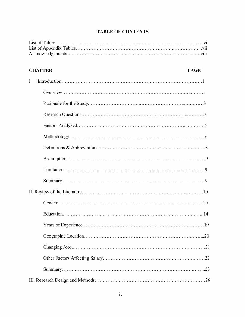
TABLE OF CONTENTS

List of Tables……………………………………………………..…………………..….…..vi List of Appendix Tables……………………………………………………..……………...vii Acknowledgements……………………………………………………………………..….viii

CHAPTER PAGE

I. Introduction…………………………………………………………………………….1 Overview………………………………………………………………….…...…….1 Rationale for the Study.…………………………..………………………...….…….3 Research Questions………………………….……………………………....……….3 Factors Analyzed…………………….……………………………………...….…….5 Methodology………………………………………………………………....……….6 Definitions & Abbreviations…………………………………………….……...…….8 Assumptions………………………………………………………………….……….9 Limitations..…………………………………………………………………....……..9 Summary….…………………………………………………………………..…..…..9 II. Review of the Literature…………………………………………………….……….…...10 Gender…………………………………………………………………….….……. .10 Education…………………………………………………………………….……....14

Years of Experience………………………………………………………….………19 Geographic Location………………………………………………………….……...20 Changing Jobs..……………………………………………………………….………21 Other Factors Affecting Salary………………………………………………….……22 Summary……………………………………………………………………….……..23

III. Research Design and Methods……………………………………………………………26

iv

Research Questions...………………………………………………………………….26 Population……….....………………………………………………………………….27 Data Collection….....………………………………………………………………….27 IV. Analysis of Data…………………………………………………………………………..30 Demographic Data....………………………………………………………………….30 Summary……..….....………………………………………………………………….48 Salary Compensation………………………………………………………………….49 Rationale for Selection of Analysis..………………………………………………….50 Summary………………………………………………………………………………55 Summary…….….....……………………………………………………………….….69 V. Summary and Conclusions Summary…….….....…………………………………………………………………..70 Data Collection & Analysis.…………………………………………………………..71 Discussion of the Findings…………………………………………………………….71 Conclusions…..….....………………………………………………………………….74 Recommendations for Further Research and Practices……………………………….76 References……………………………………………………………………………………..78 Appendices…………………………………………………………………………………….83

v

LIST OF TABLES

1. Gender of Kansas County Extension Agents………………………………………….31

2. Position Titles of Kansas Extension Agents…………………………………………..32

3. Director for Kansas Extension County/District……………………………………….33

4. Number of Kansas Extension Agents with Master’s Degrees………………………...34

5. Master’s Degree Completed Prior to Being Employed with KSRE………..…............35

6. Number of Extension Agents by the Area of the State………………………………..36

7. Number of Extension Agents in County/District Extension Office…………………...37

8. Previously Employed by Kansas State Research & Extension…...…………………...38

9. Population of Kansas Counties (by 1000)……………………………………………..39

10. Previous Years of Equivalent Non-Kansas Extension Experience…………………….41

11. Months of Kansas Extension Experience………………………………………………44

12. Salaries of Kansas State Research and Extension County Extension Agents

Frequencies…………………………………………………………………………….49

13. Summary of Backward Elimination…………………………………………………...51

14. Significant Variables at the .1000 Level………………………………………………56

vi

LIST OF APPENDICES

Appendix A – Kansas Open Records Act..……………………………………………………84 Appendix B – Table 2 Kansas County/District Extension Council Budgets for FY 2007……87

vii

ACKNOWLEDGEMENTS

There are a number of people I would like to thank for guidance and support as I worked

my way through the course work and thesis needed to complete a Master’s degree.

First, I would like to thank my major professor, Dr. Jane Fishback, for all of her words of

encouragement, patience, time and guidance. I would also like to thank my committee members,

Dr. Royce Ann Collins and Dr. Stephan Brown , their help from a distance throughout my

Master’s program has been unwavering. I also want to recognize Dr. Leigh Murray, with the

Department of Statistics at Kansas State University, for her patience and wisdom in the analysis

of data.

A big thank you goes out to my parents who taught me the true value of education and

gave me the love that I have for learning. Finally, I would like to thank my husband for his help

and dedication to the furtherance of my education. I could not have done this without the

support from my friends and family – I love you all!

viii

Chapter I

Introduction

Overview

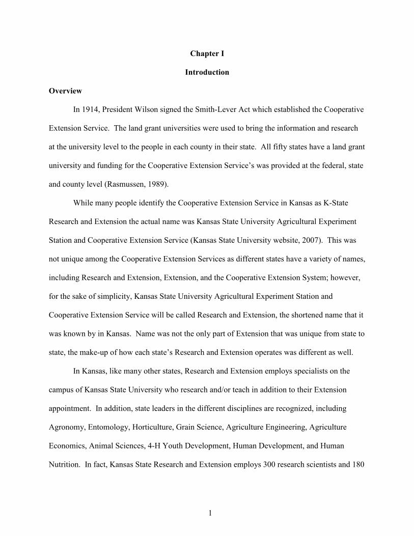
In 1914, President Wilson signed the Smith-Lever Act which established the Cooperative

Extension Service. The land grant universities were used to bring the information and research

at the university level to the people in each county in their state. All fifty states have a land grant

university and funding for the Cooperative Extension Service’s was provided at the federal, state

and county level (Rasmussen, 1989).

While many people identify the Cooperative Extension Service in Kansas as K-State

Research and Extension the actual name was Kansas State University Agricultural Experiment

Station and Cooperative Extension Service (Kansas State University website, 2007). This was

not unique among the Cooperative Extension Services as different states have a variety of names,

including Research and Extension, Extension, and the Cooperative Extension System; however,

for the sake of simplicity, Kansas State University Agricultural Experiment Station and

Cooperative Extension Service will be called Research and Extension, the shortened name that it

was known by in Kansas. Name was not the only part of Extension that was unique from state to

state, the make-up of how each state’s Research and Extension operates was different as well.

In Kansas, like many other states, Research and Extension employs specialists on the

campus of Kansas State University who research and/or teach in addition to their Extension

appointment. In addition, state leaders in the different disciplines are recognized, including

Agronomy, Entomology, Horticulture, Grain Science, Agriculture Engineering, Agriculture

Economics, Animal Sciences, 4-H Youth Development, Human Development, and Human

Nutrition. In fact, Kansas State Research and Extension employs 300 research scientists and 180

1

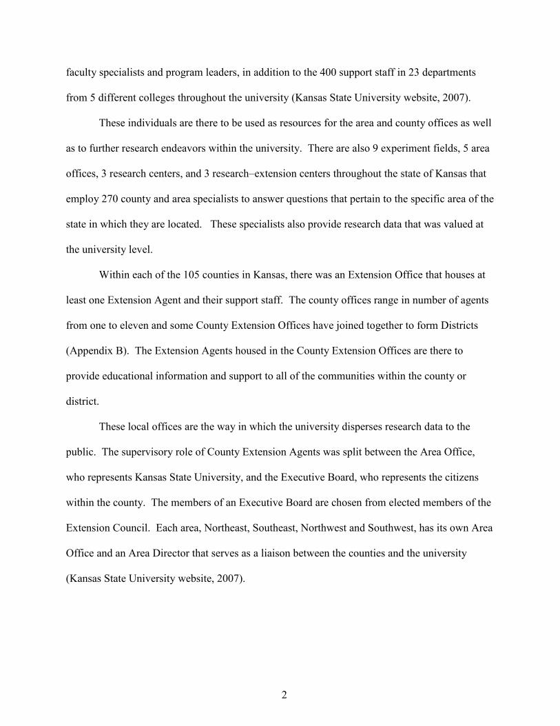
faculty specialists and program leaders, in addition to the 400 support staff in 23 departments

from 5 different colleges throughout the university (Kansas State University website, 2007).

These individuals are there to be used as resources for the area and county offices as well

as to further research endeavors within the university. There are also 9 experiment fields, 5 area

offices, 3 research centers, and 3 research–extension centers throughout the state of Kansas that

employ 270 county and area specialists to answer questions that pertain to the specific area of the

state in which they are located. These specialists also provide research data that was valued at

the university level.

Within each of the 105 counties in Kansas, there was an Extension Office that houses at

least one Extension Agent and their support staff. The county offices range in number of agents

from one to eleven and some County Extension Offices have joined together to form Districts

(Appendix B). The Extension Agents housed in the County Extension Offices are there to

provide educational information and support to all of the communities within the county or

district.

These local offices are the way in which the university disperses research data to the

public. The supervisory role of County Extension Agents was split between the Area Office,

who represents Kansas State University, and the Executive Board, who represents the citizens

within the county. The members of an Executive Board are chosen from elected members of the

Extension Council. Each area, Northeast, Southeast, Northwest and Southwest, has its own Area

Office and an Area Director that serves as a liaison between the counties and the university

(Kansas State University website, 2007).

2

Rationale for the Study

Kansas State Research and Extension was somewhat unique in that it does not require a

Master’s degree to be hired as an Extension Agent (Rasmussen, 1989). Kansas State University

encourages the furtherance of education and the base salaries set by the state reflect an increase

in salary compensation for an individual who has earned a Master’s degree. In addition, Kansas

State University offers tuition assistance, study leave (Kansas State University website, 2007),

and sabbatical leave (Kansas State University website, 2007) time to individuals wishing to

pursue a higher education.

In addition, a review of the literature suggests that a higher level of education was

rewarded through salary compensation, especially when jumping from a Bachelor’s degree to a

Master’s degree in Kansas Extension (U.S.D.A., 2006). Even with the incentives that are offered

and the literature to suggest a salary increase, there are still only 88 out of 153 (36.51%)

Extension Agents that have chosen to pursue and obtain a Master’s degree either before they

were employed by Extension or while they were an employee of Kansas State Research and

Extension.

This study will examine the demographics of Extension Agents employed by Kansas

State Research and Extension. It will also provide information regarding other factors that do

and do not have an impact on salary compensation.

Research Questions

This study will focus on the following questions:

1. What factors have an impact on salary compensation of Kansas State Research and

Extension County Extension Agents?

a. area within the state

3

b. county population

c. number of agents in the county

d. director responsibilities

e. gender

f. months of Extension employment

g. years of equivalent service outside of Kansas Extension

h. change of county employment within Kansas Extension

i. position type

j. level of education

k. timeliness of obtaining a Master’s degree

2. Which of the following factors would be significantly correlated to impact salary

compensation?

a. area within the state

b. county population

c. number of agents in the county

d. director responsibilities

e. gender

f. months of Extension employment

g. years of equivalent service outside of Kansas Extension

h. change of county employment within Kansas Extension

i. position type

j. level of education

k. timeliness of obtaining a Master’s degree

4

Factors Analyzed

Extension Agents within a county have differing position types including: 4-H Youth

Development, Agriculture and Natural Resources, Family and Consumer Sciences, and

Horticulture. In several counties, a single Extension Agent may fulfill more than one of the

position types, such as a Family and Consumer Science Agent with 4-H Youth Development

responsibility.

Gender was another factor that was analyzed. 4-H Extension Agents were primarily

female (87.50%) and 100% of the Family and Consumer Science Extension Agents were

women. However, the men were the majority in Horticulture (60%) and in Agriculture and

Natural Resources (78.57%). Female Agriculture and Natural Resources Extension Agents were

still not common and Jackson et.al, in 1999, cited this for being a reason for inequality of pay

between the genders.

The third factor analyzed was population. Population, in Kansas counties, ranged from

1,331 people in the lowest populated county to 516,731 people living in the highest populated

county (U.S. Census, n.d.). This accounts for both the extremely rural parts of Kansas and the

urban areas as well.

As stated prior, the number of Extension Agents in a County/District Extension Office

ranges from 1 to 11. As the number of Extension Agents increases, the likelihood of finding a

director with supervisory responsibilities over the other Extension Agents within the

county/district increases. Every county/district signifies a county director; however, in some

counties the county director has more responsibility than just administrative responsibility. The

county director that has both administrative responsibility and responsibilities supervising other

County Extension Agents in the county/district are the directors that were considered in this

5

study. In the 1988 study analyzed by Nobbe, it was shown that salary increased with supervisory

responsibility in the engineering field; therefore, it was hypothesized that directors earn a higher

salary when compared to Extension Agents with no supervisory roles over other Extension

Agents.

Months of experience were another factor analyzed for its impact on salary

compensation. No experience was required when applying for KSRE; therefore, both months of

experience in Research and Extension and years of experience outside of Research and

Extension were analyzed.

Changing jobs to obtain a higher salary has been done in many professions. Because

taking this approach to increase one’s salary was commonly debated upon, the study will analyze

whether changing jobs within Research and Extension, or “job-hopping” from county to county

was beneficial to salary compensation.

The final factor that was analyzed within Kansas State Research and Extension was level

of education. Extension Agents in Kansas are required to have a Bachelor’s degree, at a

minimum, and it was preferred for them to have earned a Master’s degree. Was it then beneficial

to obtain a Master’s degree before applying for Extension or if an individual was already

employed in Extension as a County Extension Agent, will it pay to go back to school to earn a

Master’s degree?

Methodology

All Kansas County Extension Agents employed by Kansas State Research and Extension,

as of September 1, 2007, were analyzed in this study (N=241). Information regarding the area

within the state was collected from the Kansas State Research and Extension home page at

www.oznet.ksu.edu. County population estimates for July 1, 2006 were found at the United

6

States Census Bureau website. The district population was found through the summation of all

counties included in the district. Information regarding the number of agents in the

county/district was collected from Table 2. Kansas County/District Extension Council Budgets

for FY 2007 received at the Southwest KSRE Annual Partnership Meeting held on January 17,

2007 (Appendix B).

Information regarding director responsibilities, gender, months of Extension

employment, years of equivalent service outside of Kansas Extension, change of county

employment within Kansas Extension, position type, and level of education were provided by

KSRE Field Operations Office, per request, with approval from Dr. Darryl Buccholz, Associate

Director of Kansas State Research and Extension. All information was gathered and figured as

of September 1, 2007.

The data was analyzed using backward elimination and multiple regressions. The

independent variables in the study were: area within the state, county population, number of

agents in the county, director responsibilities, gender, months of Extension employment, years of

equivalent service outside of Kansas Extension, change of county employment within Kansas

Extension, position type, level of education, and timeliness of obtaining a Master’s degree. The

single dependent variable used was salary. Further information regarding the research methods

used in this study can be found in Chapter III.

7

Definitions & Abbreviations

For the purpose of this study the following definitions and abbreviations were used.

4-H: 4-H Youth Development

Ag: Agriculture

FCS: Family and Consumer Sciences

Hort: Horticulture

KSRE: K-State Research and Extension, Kansas Agricultural Experiment Service and

Cooperative Extension Service. “A partnership between Kansas State University and federal,

state, and county government, with offices in every Kansas county. They conduct research

through Kansas that was then shared by Extension agents and others on their Web sites and

through numerous conferences, workshops, field days, publications, newsletters and more”

(www.oznet.ksu.edu/DesktopDefault.aspx?tabid=25).

FTE: Full-Time Equivalent, Equivalent to a full-time worker.

IT: Information Technology, as defined by the Information Technology Association of America

(ITAA), was "the study, design, development, implementation, support or management of

computer-based information systems, particularly software applications and computer

hardware."

ANR: Agriculture and Natural Resources

MBA: Master’s degree of Business Administration

BS: Bachelor’s degree

MS: Master’s degree

Ph.D.: Doctorate in Philosophy

HR: Human Resources

8

Assumptions

The information retrieved and received from the Kansas State Research and Extension

home page at www.oznet.ksu.edu, United States Census Bureau website at

http://factfinder.census.gov/servlet/GCTTable?_bm=y&-geo_id=04000US20&-

_box_head_nbr=GCT-T1&-ds_name=PEP_2006_EST&-_lang=en&-format=ST-2&-_sse=on,

Table 2. Kansas County/District Extension Council Budgets for FY 2007, and KSRE Field

Operations Office was accurate.

Limitations

1. This study was limited to the eleven factors* examined.

2. There have been position changes within KSRE since the time of data collection;

therefore, all factors are a representation of KSRE as of September 1, 2007.

*(area within the state, county population, number of agents in the county, director

responsibilities, gender, months of Extension employment, years of equivalent service

outside of Kansas Extension, change of county employment within Kansas Extension,

position type, level of education, and timeliness of obtaining a Master’s degree)

Summary

This study focused on salary compensation for County Extension Agents employed by

KSRE. The independent variables analyzed were: area within the state, county population,

number of agents in the county, director responsibilities, gender, months of Extension

employment, years of equivalent service outside of Kansas Extension, change of county

employment within Kansas Extension, position type, level of education, and timeliness of

obtaining a Master’s degree. Backward elimination and multiple regressions were used to

analyze the data.

9

Chapter II

Review of the Literature

While reviewing the literature regarding factors affecting an individual’s salary including

gender, population, number of employees in a single office setting, administrative responsibility,

years of previous experience outside of the company, years of previous experience within the

company, position type, performance and level of education it was evident that there were

several studies done regarding gender and level of education. It was more difficult; however, to

find literature that held constant factors that affected salary in regards to gender and level of

education; therefore, leaving the data to be easily misunderstood. With this in mind, the data that

was reviewed contains information that takes into consideration more than one variable.

Gender

Numerous studies have examined the relationship between compensation and gender.

Some show a greater gap between the gender’s in salary compensation than others; however,

many researchers found that if other factors were held constant, the gap would narrow.

Garvey (2004) found that women made 7.5% less than men executives in the same

position at IT companies. This was not rare and as a generalization, men still do make more than

women. In fact, it was cited that women make from $.77 (Clark, 2006) to $.91 (Isaacs, 1995) for

every $1.00 that men make, on average. However, the difference between the salaries lessens

when variables that have a direct impact on salary are held constant. For example, when years of

experience and specialty within the engineering profession were held constant there were no

salary differences between men and women. Without these constants; however, women made 13

percent less than men and had fewer years of experience. Equality in pay was found in the data

10

as the “rate at which salaries increase with experience was the same for men and women” (NSF

Study Explains, 1999).

Also, when other factors such as geographic region, educational degree, and specialty

sector are held constant, the gap between men and women decreases even more significantly.

One factor that was not accounted for by the NSF Study (1999), was the quality of program the

individuals graduated from and the quality of work the employees performed.

Another factor that directly impacts the salary earned by women was the glass ceiling

effect. In 1995, Isaacs discovered that women are not found in the highest ranks due to the fact

that somewhere along the way they ceased their way to the top. One of the reasons given for

their cease to the top included interrupted career patterns and being side-tracked when balancing

home and career; Levenson, (2006) agrees with Isaacs and states “women rise to the middle, but

they don’t easily get to the top.” The cease in getting to the top, resulted in women earning less

money, on average, than men. Even when factoring things such as years of experience,

schooling, skill level, and industry; women still earned $.91 to every $1.00 that men make

(Isaacs, 1995).

Isaacs (1995) also stated that the gap between men and women’s salaries was narrowing;

however, the researcher did cite that the difference was due to a slow down of inflation in men’s

salaries, not an increase in women’s salaries. In addition, Isaacs (1995) found that women

almost always make a lower salary, when compared to men, when they first begin their positions

in a new career. Dubeck and Borman (1997) stated that women could have equal salary

compensation to men; however, women would have to break into the “men dominated” fields to

do this. They also found that women will continue to make less than men, in terms of salaries, as

long as women entered fields that were historically known to be dominated by women.

11

Kiker, et.al, (1987) studied the National Medical Care Expenditure Survey and

formulated results from an analysis of salary and fringe benefits derived between males and

females. The study was analyzed for the significance of fringe benefits in relation to total salary

compensation and the differences in sex, education, experience, race, marital status, residence,

industry and occupation. Differences were found between men and women in wages and fringe

benefits in that they were not proportional. However, if fringe benefits were excluded or

ignored, the comparison between male and female salary was still somewhat biased towards men

but numerically the value was small.

Kicker, et.al (1987) found another factor that made an impact on salary. It was that the

value of marital status was more significant for males than females and ratio of fringe benefits to

total compensation increases with added education, especially more for males than females in

white-collar industries. Differences were found in wage and total compensation for males and

females, but the numerical values were not substantial. The tabular data also indicated that there

were differences between males and females in total compensation with more education and

additional experience.

In 2004, Koeske and Krowinski collected the results from a mail survey indicating there

had been no significant changes made in regards to salary equity in social work between men and

women since 1982. In fact, women only receive approximately 70 percent of men’s salaries.

The merit of the work performed was analyzed in this study and it only accounts for half of this

inequality, leaving 15 percent unaccounted. Even when controlling for job performance and

“other factors” (Paragraph 4), females made about $1000 less per year than their male

counterparts after three years of experience.

12

On the other hand, as years of experience increased and as the individuals were promoted

into administrative positions, men and women stayed equitable in their salaries. Other data

showed that merit factors, such as job performance, were not different for men and women;

therefore, suggesting that the basis for the salary inequality was due to discrimination. The

higher salary for men was primarily due to more years of experience thereby leading to more

opportunity for obtaining administrative positions.

The data collected in 2004 by Koeske and Krowinski was similar to the finding of Mraz

in 1990, wherein Mraz analyzed results from a survey mailed to 58,558 members of the National

Society of Professional Engineers. The findings showed salary differences between the

individuals that were surveyed for work experience, education, and geographical differences

were due to costs of living, executive level/administrative jobs, private employment versus local,

state, Federal or armed forces, gender (women in 10 of the 15 categories), longevity with a

company, and type of engineer.

The trend of men filling a higher number of upper-level positions also holds true in other

job types. In 1999, Roberts studied salary differences, among resellers, and found that while

women are moving up in the ranks with more representation in the senior sales ranks, they still

make up the majority in lower-level positions when compared to men; therefore, men are still

paid higher than women, on average.

The nursing field also holds true to the inequality found in pay between males and

females. Link (1988) found that white males earned consistently large wage premiums

comparative to female nurses. Link also noted that black individuals made significant gains in

wage over the survey period.

Gender was found to not only impact salary, but the lack of gender equality can also be

13

found in the demographic data in the Cooperative Extension Service. Seevers and Foster (2004)

found that female County Agents in the Cooperative Extension Service are under represented in

the agriculture program area and in management positions across the United States. In 2003,

women represented less than 12% of all county extension agents with agriculture responsibilities

(Seevers and Foster, 2004). Minorities were found to be even more under represented in a

system that serves all cultures, ethnicities, and gender of people.

Seevers and Foster (2004) found that the top three barriers women face include

“acceptance by peers and other males in the agricultural industry, balancing family and career,

and acceptance by administrators” (Paragraph 8). In addition to the Seevers and Foster (2004)

study, Jackson, et.al, (1999), studied the internal salaries in Extension and found the primary

difference found between faculty agents and specialists included gender as a factor that had an

impact on salary. The researchers felt that this was due to the fact that many leadership positions

were filled by males in addition to the positions in the ANR program area that were filled by

males.

The data suggests that the salary gap between males and females was not only found in

professions such as nursing, resellers and engineering, but the gap was also found in the

Cooperative Extension Service. Phenomenon’s, such as the glass ceiling effect help identify

some of the reasoning behind the gap in pay; however, it seems that equality in pay has still not

been reached.

Education

In addition to gender, education was another variable that affected salary. The ASSE

Compensation Survey (2004), completed through online and mailed questionnaires reviewed

certifications and higher education in relation to years of experience and salary. The research

14

showed that individuals with certifications made more than $12,000 more than those without any

kind of certification. Furthermore, the same relationship between education and salary existed

between college education and salary.

While earning a bachelor’s degree and some college yielded similar salaries; the

difference in salary between an associate’s degree and a bachelor’s degree was more than

$10,000 annually. The same relationship held true for Master’s degrees, Ph.D.’s and Ed.D’s

with the addition that the increase was an added increase of more than $10,000 (ASSE

Compensation Survey, 2004).

In 1994, Langer took a different approach and studied employees working in human

resource departments. Langer (1994) found that from a survey of 761 organizations, job or job

function appeared to be a key determinant for salary with other factors such as educational level

and geography having minimal influences, in most cases. One exception to this was the

compensation for those in top-level positions as opposed to those in mid- to low-level positions.

Education was more beneficial and had a greater effect on compensation in the top-level

positions, with a greater increase in salaries as the education level rose.

The other exception was for those in medical professions as they consistently had higher

salaries than other occupations. Langer (1994) found, though, that the reasoning behind the

higher salaries was primarily due to their level of education as their occupation required a higher

level of education or more professional skills.

LaPlante (1992) also found an increase in professional skills, gained through education,

was beneficial in the computer technology industry. Highly specialized computer skills were in

high demand and the supply of skilled workers with networking ability was low. This increased

salaries for those with the networking skills required for the industry.

15

In 2004, Garvey researched a study by the Ross School of Business that also showed the

value, in terms of salary compensation, of obtaining a higher level of education. The study

found that having an MBA “increased an IT exec’s compensation by 24%, while a year of extra

experience in the same position yielded an increase of just 0.2% annually” (Paragraph 2). The

study concluded that obtaining a higher education, more specifically an MBA, as an IT

professional, would allow the individual to make the most money. Francis’s (2001) study of

government agencies supported the findings regarding the correlation between level of education

and salary. Francis found that the average salary in government agencies differed by

geographical area, training, and education. Of these three factors, only education had a

consistently increasing effect on salary as the level of education increased.

In 1988, Link also found that a higher level of education did not always equal a higher

salary. Link (1988) analyzed data from the US Census in 1970 and the 1977, 1980 and 1984

National Sample Surveys of Registered Nurses. The survey utilized education, experience, hours

worked, personal demographic information, and market-place work environment variables to

produce the results.

Link (1988) found that the analysis showed minimal differences between associate and

diploma degree nurses and modest wage increases for bachelor degrees compared to associate

degrees. In some instances, attainment of higher degrees (BS or MS) resulted in more work

responsibility and, subsequently, high paying job locations, but ultimately it was location of the

high paying job that impacted salary. In addition, Link (1988) also found that education didn’t

have an impact on career advancement, especially in those with more responsibility and higher

wages.

16

Engineers were analyzed in the 1988 study completed by Nobbe using a survey from the

National Society of Professional Engineers in which 12,745 surveys were used. Components

analyzed included length of experience, education level, engineering discipline, job function,

industry or service employer, managerial responsibility and geographical region. Mean salary

for those with less than a bachelor’s degree was higher than those with bachelor’s degrees;

however, a steady increase was shown for those with master’s degrees up to a doctorate. Nobbe

found that those holding doctorate degrees earned 35.4% more than those without it.

Roberts (1999) studied salary among resellers, and found that salary was directly related

to and increased with education. Individuals with MBA’s or doctorates made 33% more than

those with four-year degrees and individuals with some college made 33% more than individuals

with a high school education. Roberts felt that this easily showed that even some college was

rewarded with a significant increase in compensation.

One challenge of obtaining a higher level of education in Extension was the fact that

Extension Agents are spread out across the state; therefore, limiting their ability to attend a

university and work towards a higher degree. A unique approach that Edwards et. al took in

2004, studied the distance programs available to Extension agents citing four individual

universities offering programs including “doc-at-a-distance,” Masters of Agriculture, workshops,

and certification programs. The programs were offered via the Internet and electronic and

printed classes. One university cited they offered programs based on the expressed interests of

the Extension agents in their state.

Extension agents interest in pursuing a higher education increased as their level of

computer competence increased. This showed a need to educate Extension agents in computer

knowledge in order to increase the number interested in pursuing a higher education. Three-

17

fourths of the Extension agents surveyed showed an interest in “pursuing additional education at

a distance” (Paragraph 13) revealing motivators including salary increase (31%), tuition

reimbursement (18%) and release time from job duties (6.7%) (Edwards et. al, 2004).

Level of education and its affect on salary was also presented in 2006 by the United

States Department of Agriculture Cooperative State Research, Education, and Extension Service.

The data compared salaries and the level of education within and among the states in the United

States and showed that Kansas Extension Agents are above average in their average pay of full

time equivalent (FTE) Extension agents, with Bachelor’s degrees, when compared to other

Cooperative Extension Services in the United States. This advantage changes; however, when

comparing salaries of Extension agents with Master’s degrees and Doctorate’s. Kansas’s

average pay for Extension agents with Master’s degrees was about $2,000 below average and

$12,000 below average for Extension agents with Doctorate degrees when compared to other

states in the United States.

Other Kansas data points that did not correlate with the data points from other states were

the comparisons of highs and lows among degrees earned. The difference in high salaries found

in regards to FTE employees with Master’s degrees versus Doctorate’s gave an advantage of

more than $27,000 to the FTE employee’s with a Master’s degree (U.S.D.A., 2006). It was

obvious that as education was increased, salary was not proportionally increased to reward the

furtherance of an individual’s higher education.

A higher level of education was shown to increase salary compensation for most careers

including IT and engineering; however, in many professions a higher level of education resulted

in more work load. Therefore, the increase in pay could not be directly linked to an increase in

education. The Cooperative Extension Service data did show an increase in salaries for

18

individuals with higher levels of education; however, the increases were not proportional to the

degrees obtained. Therefore, the data suggested there were other factors that affected salary

compensation when County Extension Agents obtained higher levels of education.

Years of Experience

In 1999, Jackson, et. al collected and analyzed data regarding the different variables that

affected salary in Extension personnel including years of experience, gender, race, performance,

base salary, leadership positions, education, title or rank, program area and district. The study

analyzed administrative and professional agents as well as faculty agents and specialists. While

Extension personnel are not on an incremental sliding scale with years of experience, Jackson

et.al (1999) found that the “best predictors of salary were found to be Years of Experience

(51%), Education (20%), Leadership Position (2.5%), and Performance (2.7%)”.

Many educational institutions and government entities pay their employees on a sliding

scale with years of experience as the main incremental factor. This was not true for all

institutions and entities and some believe that years of experience alone should not automatically

increase pay. However, Clark (2006) found that the Alabama Attorney General disagreed with

those individuals who do not value years of experience as it stands alone. In fact, he ruled that

school teachers in the public school system in Alabama should be paid for years of experience on

an every-three-year increment system up to 24 years. All increases were made on the

anniversary date of the three year increment and increases were not subject to disagreement or

discussion.

The data found in the NSF Study (1999) regarding the engineering profession, also shows

that an increase in years of experience yields an increase in salary. On average, there was a

$12,000 increase when comparing 5 to 9 years of experience with 10 to 15 years of experience

19

and a $10,000 jump from 10 to 15 years of experience to 20+ years of experience. Furthermore,

in 1994, Langer surveyed human resources departments and the data from those surveys

suggested that longevity of the employee increased salary as well.

Unlike other researchers, Linker (1988), who studied the nursing field, found that the

experience earning potential for nurses showed a flat trend indicating an unattractive return on

work experience. In Linker’s study (1988), though, the type of nurse (general versus

administrative or specific), due to experience, did offer compensation premiums.

Nobbe (1988) researched engineers and analyzed factors affecting salary. Components

analyzed included length of experience, education level, engineering discipline, job function,

industry or service employer, managerial responsibility and geographical region. Experience

level showed that those with more experience had higher mean salaries, but larger increases were

seen between years 9 to 10 and from 19 to 20.

Salary, among resellers, was also related directly to education as shown in the 1999 CRN

Reseller Salary Survey. The difference in salary still exists due to the difference in years of

experience as shown when years of experience was held constant; causing the pay gap to narrow

(Roberts, 1999).

Geographic Location

The data suggested that the Southern region was the lowest paid region in the United

States, when analyzing different fields of employment. Francis (2001) collected data from 837

online surveys sent to IT/GWAS (Geographical Information Systems) professionals throughout

the United States and Canada. Of those analyzed, 76.9% were government employees, 26.5%

were in municipal governments, and 23.5% were in county governments. There were a variety

of fringe benefits as additional compensation.

20

Overall, the lowest average regional salary was found in the southern states (Francis,

2001). A separate salary analysis done in 2006 by the United States Department of Agriculture

Cooperative State Research, Education, and Extension Service found that the lowest average

salaries, taking into account all levels of higher education, in Extension agents, could also be

found in the Southern region.

In 1988, Nobbe analyzed the salary of engineers by geographic region and found that it

had an influence on mean salary; with those in the northeast and western United States having

higher salaries than those in the central or south-eastern United States.

Changing Jobs

“Job-Hopping” was a trend that many individuals participated in for various reasons.

Garvey (2004) found that “job-hopping” was beneficial to salary and continued service with one

institution would not yield the same pay raises as obtaining new employment. Manton and van

Es (1984) stated that Agriculture agents cited that they changed jobs due to salary, benefits, and

professional growth.

Shindul (1995) studied the reasons nurses changed jobs and found that flexible schedules,

less shift rotation, salary upgrades and methods to advance up the career ladder were ways to

attract and retain nurses. The study separated the respondents into three work groups (early

stages, less than 30 years of age and 10 years experience; mid-careers, 11 to 22 years experience

and between 31 to 50 years of age; later career, more than 23 years experience and over 50 years

of age).

In the early stage group, the study found that retention was associated with having

flexible schedules. For the mid-career group, the financial aspects of the job, including salary

upgrades, appeared to have a pronounced effect in retention rates. For the later career group,

21

control over nursing practices had the most influence on retention; however, those intending on

staying 5 or more years indicated that career advancement was the incentive. It seems that no

matter what profession an individual who chooses to “job-hop” can increase their salary by doing

so.

Other Factors Affecting Salary

Was working for a bigger company always better in terms of salary potential? Langer

(1994) found that the number of employees in a firm tended to positively affect the salary of

those in HR departments with exceptions for those that were not in a supervisor or management

role. Langer also noted that the financial size of the company and longevity of the employee

increased salary.

Another factor showing an affect on salary was the level at which the individual was at

within the company. As individuals increased their position pay would normally increase as

well. Langer (1994) found that even education was more beneficial and had a greater effect on

compensation in the top-level positions. Nobbe (1988) looked at the difference in salary in

engineers if the employee’s position included a supervisory role. Those that supervised and had

more employees had a large increase in salary. Those with 3 to 9 supervisees earned a median

income of $40,000 whereas those with over 250 employees under their supervision earned an

average income of $83,500.

The type of organization also impacts salary. Garvey (2004) found that non-profit

organizations paid higher than not-for-profit organizations. Langer (1994) found that

manufacturing and extractive firms had higher salaries than educational, food and beverage and

other entities. Linker (1988) found in nursing, the type of nurse (general versus administrative or

specific), due to experience, did offer compensation premiums.

22

Performance was another factor that was noted for impacting salary; however, at the

same time, it was one factor that was commonly overlooked. Keller (2001) found that

Minnesota education officials were looking to make a change in the way they paid their teachers.

Instead of the incremental increase in salary for years of experience and higher education the

legislature was considering a pay-for-performance type of compensation. The new payment plan

would not only reward the “good” teachers, but would allow Minnesota to increase their chances

of retaining those “good” teachers as their salaries would increase quicker in a shorter amount of

time. The new approach would also reward student achievement by increasing compensation for

increased test scores in the classrooms; therefore, tying back into the performance of the

teachers.

Roberts (1999) also found job performance, among resellers, to be directly linked to

salary. The one researcher whose data disagreed with the others was that of Jackson et.al (1999).

Jackson et.al (1999) concluded that many agents who were above average in their performance

rankings were paid below average in Extension.

Summary

This literature was intended to present some of the factors that affect salary. Factors

affecting Extension agent salary were included as much applicably possible; however, many of

the factors considered had a great impact on other fields outside of Extension. Those other fields

are noted when discussed and all data considered more than one variable at a time with the hope

that the data would not be biased.

Women, on average, do make less than men in the studies researched, in fact it was cited

that women make from $.77 (Clark, 2006) to $.91 (Isaacs, 1995) for every $1.00 that men make;

however, the gap lessens when years of experience and job performance are controlled. This

23

difference was primarily due to the fewer years of experience women have (NSF Study, 1999)

and that women, on average, work fewer hours per week than men (Clark, 2006). In fact, many

studies reported that at some point in their career women cease their advancement (Isaacs, 1995);

therefore, loosing their competitive edge when vying for higher-level positions. And, it was

shown that the number of males in leadership or high-level positions was significantly greater

than women (Roberts, 1999). Isaacs (1995) found that the difference was due to women

choosing to be more family-oriented and their selection of positions that allow them to spend

more time at home and with their families. It was also shown that men receive more fringe

benefits than women in similar positions (Kiker, et al, 1987).

Generally speaking, as education increases, so did salary; however, this increase was not

always proportional to the increase in level of education (United States, 2006). Major increases

in compensation were shown when comparing individuals with bachelor’s degree to those with

an associate’s degree. Factors affecting motivation to obtain higher education include higher pay

and more flexible scheduling (Shindul, 1995).

Another factor affecting the level of salary was performance. Many fields reported that

job performance was becoming even more of a factor when determining increases; however,

some studies found that high performing employees made below average pay suggesting that all

pay scales had not yet adopted the pay-for-performance concept (Keller, 2001).

Geographic location also affected pay as individuals in the southern (Francis, 2001) and

central states (Nobbe, 1988), on average, received less compensation for the same job. The

number of years of experience was shown to increase proportionally with salary; however, in

some fields years of experience had less effect on pay than obtaining higher education.

24

Another factor shown to increase pay was job-hopping (Garvey, 2004). Individuals

moving from company to company were shown to receive higher salaries than those who

remained loyal to one corporation or company for long periods of time. Increased specialization

within a field was shown to increase pay as well as moving up the ladder of success and

embracing more responsibility within the company.

25

Chapter III

Research Design and Methods

Research Questions

This study will focus on the following questions:

1. What factors have an impact on salary compensation of Kansas State Research and

Extension County Extension Agents?

l. area within the state

m. county population

n. number of agents in the county

o. director responsibilities

p. gender

q. months of Extension employment

r. years of equivalent service outside of Kansas Extension

s. change of county employment within Kansas Extension

t. position type

u. level of education

v. timeliness of obtaining a Master’s degree

2. Which of the following factors would be significantly correlated to impact salary

compensation?

w. area within the state

x. county population

y. number of agents in the county

z. director responsibilities

26

aa. gender

bb. months of Extension employment

cc. years of equivalent service outside of Kansas Extension

dd. change of county employment within Kansas Extension

ee. position type

ff. level of education

gg. timeliness of obtaining a Master’s degree

Population

All Kansas County Extension Agents, employed by K-State Research and Extension as of

September 1, 2007, were included in the study (N=241). Only information needed for the study

was obtained in order to ensure the privacy of all of the County Extension Agents in Kansas. All

of the data was public record and obtainable due to the Kansas Open Records Act (Appendix A).

Information regarding the 241 Extension Agents employed by KSRE was obtained

through a variety of methods including retrieval of information from secure websites, retrieval of

information from a document distributed by KSRE administration, and receipt of computer

generated information regarding the demographics of Extension Agents in Kansas.

Data Collection

The information gathered included: 1. area within the state (Northeast, Southeast,

Northwest, and Southwest); 2. county population (all district populations were a summation of

the counties within the district); 3. number of agents in the county; 4. director responsibilities; 5.

gender; 6. months of Extension employment; 7. years of equivalent service outside of Kansas

Extension; 8. change of county employment within Kansas Extension; 9. position type; 10. level

of education; and 11. timeliness of obtaining a Master’s degree.

27

Retrieval of the area within the state that the Extension Agent was employed was

collected from the K-State Research and Extension home page at www.oznet.ksu.edu. The four

different areas recognized in the state are: Northeast, Southeast, Northwest, and Southwest. The

estimated county populations, from the United States Census Bureau website, for July 1, 2006,

were retrieved and documented with their respective counties. All district populations were a

summation of the counties within the district. The number of agents in each county/district was

collected from Table 2. Kansas County/District Extension Council Budgets for FY 2007 received

at the Southwest KSRE Annual Partnership Meeting held on January 17, 2007. This number

does not necessarily represent the number of agents actually employed on September 1, 2007,

when all of the data was collected, but rather the number of County Extension Agent positions

that have been appointed by the county commissioners within the county. All other pertinent

information including: director responsibilities (Yes or No), gender (Male or Female), months of

Extension employment, years of equivalent service outside of Kansas Extension, change of

county employment within Kansas Extension, position type (4-H, Ag, FCS, or Hort), level of

education (B.S. or M.S. and higher) and timeliness of obtaining a Master’s degree (prior to or

after starting their position with KSRE) were provided by the KSRE Field Operations Office, per

request, with approval from Dr. Darryl Buccholz, Associate Director for Extension and Applied

Research. All information was gathered and all data was figured as of September 1, 2007.

The data was analyzed using backwards elimination as this statistical analysis allows the

researcher to eliminate independent variables one at a time; therefore, all data was representative

of itself and does not show a significant Pr>F value due to a correlation with a factor that was

contained within the data. All Pr>F values found to be significant were less than .1 and the R

value for the data was found to be .8.

28

The independent variables in the study were: area within the state, county population,

number of agents in the county, director responsibilities, gender, months of Extension

employment, years of equivalent service outside of Kansas Extension, change of county

employment within Kansas Extension, position type, level of education, and timeliness of

obtaining a Master’s degree. The single dependent variable used was salary. All data was found

from secure websites or were received from Kansas State Research and Extension Field

Operations Office.

29

Chapter IV

Analysis of Data

This chapter will be divided into two parts. The first section corresponds to the

demographic information of Kansas County Extension Agents. The second section of the

chapter will examine the statistical analysis of the data regarding salary and the factors that affect

salary.

Demographic Data

The following information was collected: 1. area within the state; 2. county population; 3.

number of agents in the county; 4. director responsibilities; 5. gender; 6. months of Extension

employment; 7. years of equivalent service outside of Kansas Extension; 8. change of county

employment within Kansas Extension; 9. position type; 10. level of education; and 11. timeliness

of obtaining a Master’s degree. The data from this section was analyzed through multiple

regressions using the REG procedure in SAS 9.1 for Windows. Variable selection was made

from backward elimination.

30

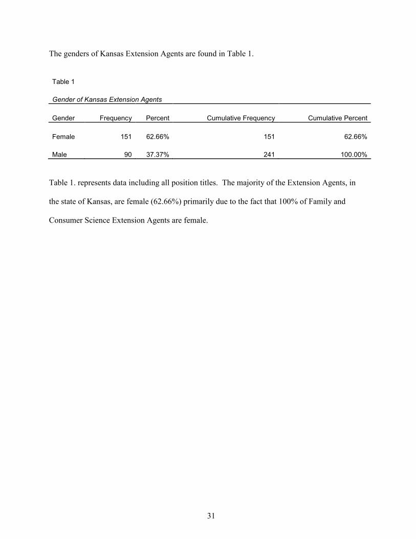
The genders of Kansas Extension Agents are found in Table 1.

Table 1

Gender of Kansas Extension Agents

Gender Frequency Percent Cumulative Frequency Cumulative Percent

Female 151 62.66% 151 62.66%

Male 90 37.37% 241 100.00%

Table 1. represents data including all position titles. The majority of the Extension Agents, in

the state of Kansas, are female (62.66%) primarily due to the fact that 100% of Family and

Consumer Science Extension Agents are female.

31

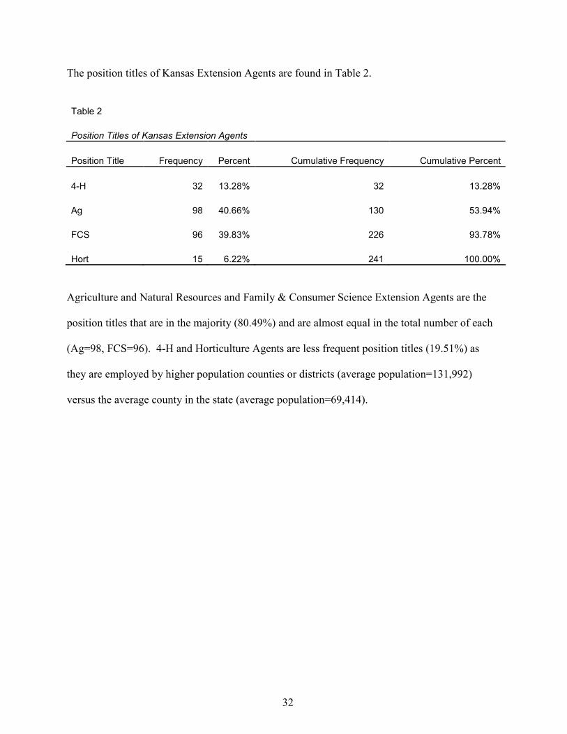
The position titles of Kansas Extension Agents are found in Table 2.

Table 2

Position Titles of Kansas Extension Agents

Position Title Frequency Percent Cumulative Frequency Cumulative Percent

4-H 32 13.28% 32 13.28%

Ag 98 40.66% 130 53.94%

FCS 96 39.83% 226 93.78%

Hort 15 6.22% 241 100.00%

Agriculture and Natural Resources and Family & Consumer Science Extension Agents are the

position titles that are in the majority (80.49%) and are almost equal in the total number of each

(Ag=98, FCS=96). 4-H and Horticulture Agents are less frequent position titles (19.51%) as

they are employed by higher population counties or districts (average population=131,992)

versus the average county in the state (average population=69,414).

32

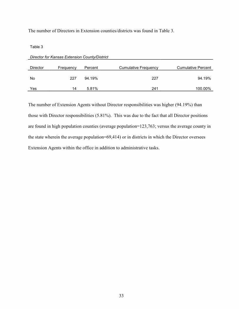
The number of Directors in Extension counties/districts was found in Table 3.

Table 3

Director for Kansas Extension County/District

Director Frequency Percent Cumulative Frequency Cumulative Percent

No 227 94.19% 227 94.19%

Yes 14 5.81% 241 100.00%

The number of Extension Agents without Director responsibilities was higher (94.19%) than

those with Director responsibilities (5.81%). This was due to the fact that all Director positions

are found in high population counties (average population=123,763; versus the average county in

the state wherein the average population=69,414) or in districts in which the Director oversees

Extension Agents within the office in addition to administrative tasks.

33

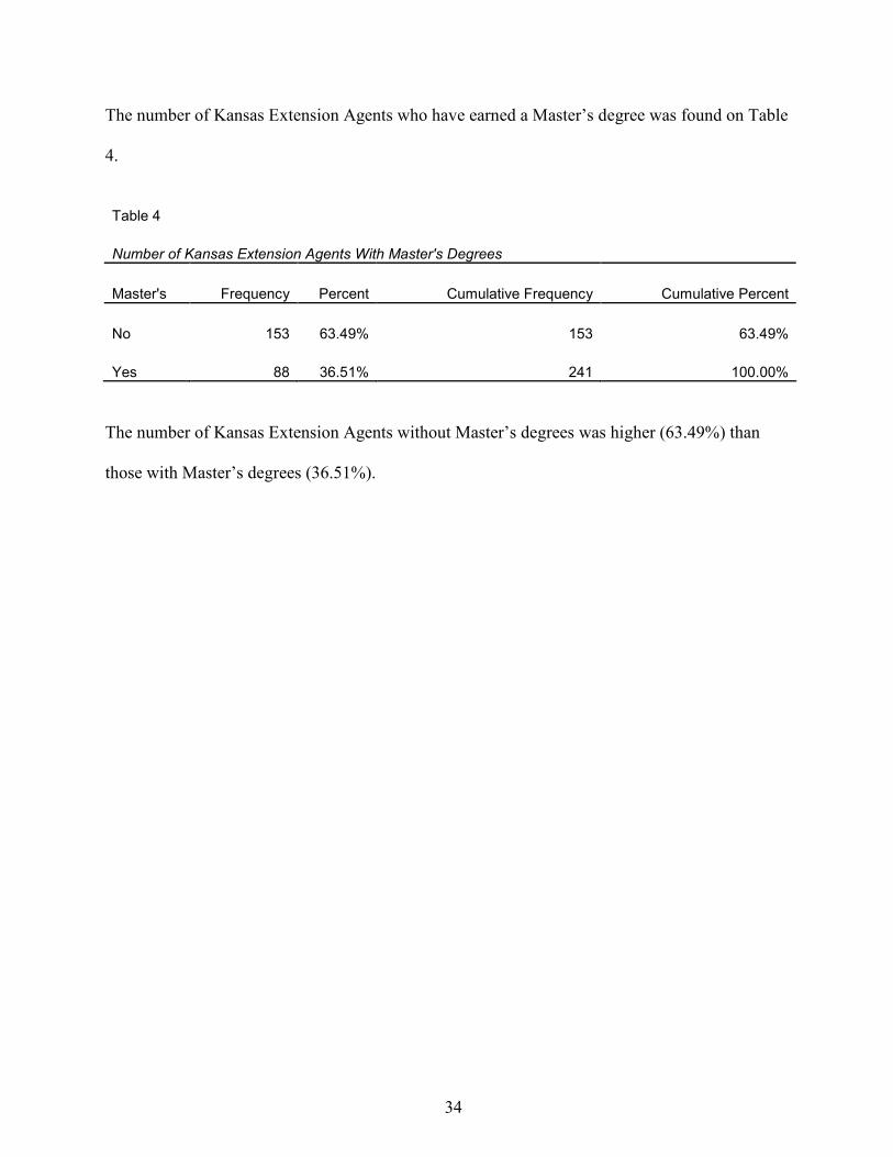
The number of Kansas Extension Agents who have earned a Master’s degree was found on Table

4.

Table 4

Number of Kansas Extension Agents With Master's Degrees

Master's Frequency Percent Cumulative Frequency Cumulative Percent

No 153 63.49% 153 63.49%

Yes 88 36.51% 241 100.00%

The number of Kansas Extension Agents without Master’s degrees was higher (63.49%) than

those with Master’s degrees (36.51%).

34

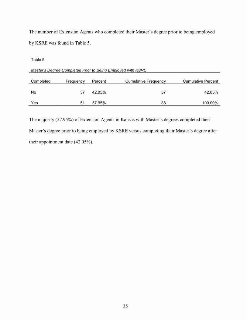
The number of Extension Agents who completed their Master’s degree prior to being employed

by KSRE was found in Table 5.

Table 5

Master's Degree Completed Prior to Being Employed with KSRE

Completed Frequency Percent Cumulative Frequency Cumulative Percent

No 37 42.05% 37 42.05%

Yes 51 57.95% 88 100.00%

The majority (57.95%) of Extension Agents in Kansas with Master’s degrees completed their

Master’s degree prior to being employed by KSRE versus completing their Master’s degree after

their appointment date (42.05%).

35

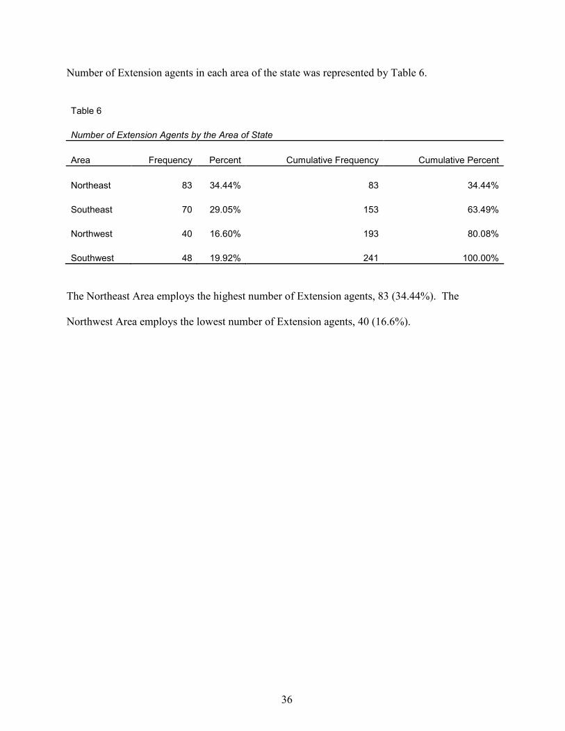
Number of Extension agents in each area of the state was represented by Table 6.

Table 6

Number of Extension Agents by the Area of State

Area Frequency Percent Cumulative Frequency Cumulative Percent

Northeast 83 34.44% 83 34.44%

Southeast 70 29.05% 153 63.49%

Northwest 40 16.60% 193 80.08%

Southwest 48 19.92% 241 100.00%

The Northeast Area employs the highest number of Extension agents, 83 (34.44%). The

Northwest Area employs the lowest number of Extension agents, 40 (16.6%).

36

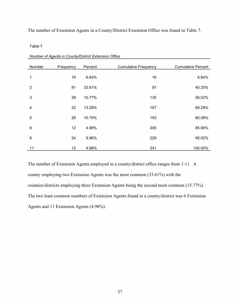
The number of Extension Agents in a County/District Extension Office was found in Table 7.

Table 7

Number of Agents in County/District Extension Office

Number Frequency Percent Cumulative Frequency Cumulative Percent

1 16 6.64% 16 6.64%

2 81 33.61% 97 40.25%

3 38 15.77% 135 56.02%

4 32 13.28% 167 69.29%

5 26 10.79% 193 80.08%

6 12 4.98% 205 85.06%

8 24 9.96% 229 95.02%

11 12 4.98% 241 100.00%

The number of Extension Agents employed in a county/district office ranges from 1-11. A

county employing two Extension Agents was the most common (33.61%) with the

counties/districts employing three Extension Agents being the second most common (15.77%).

The two least common numbers of Extension Agents found in a county/district was 6 Extension

Agents and 11 Extension Agents (4.98%).

37

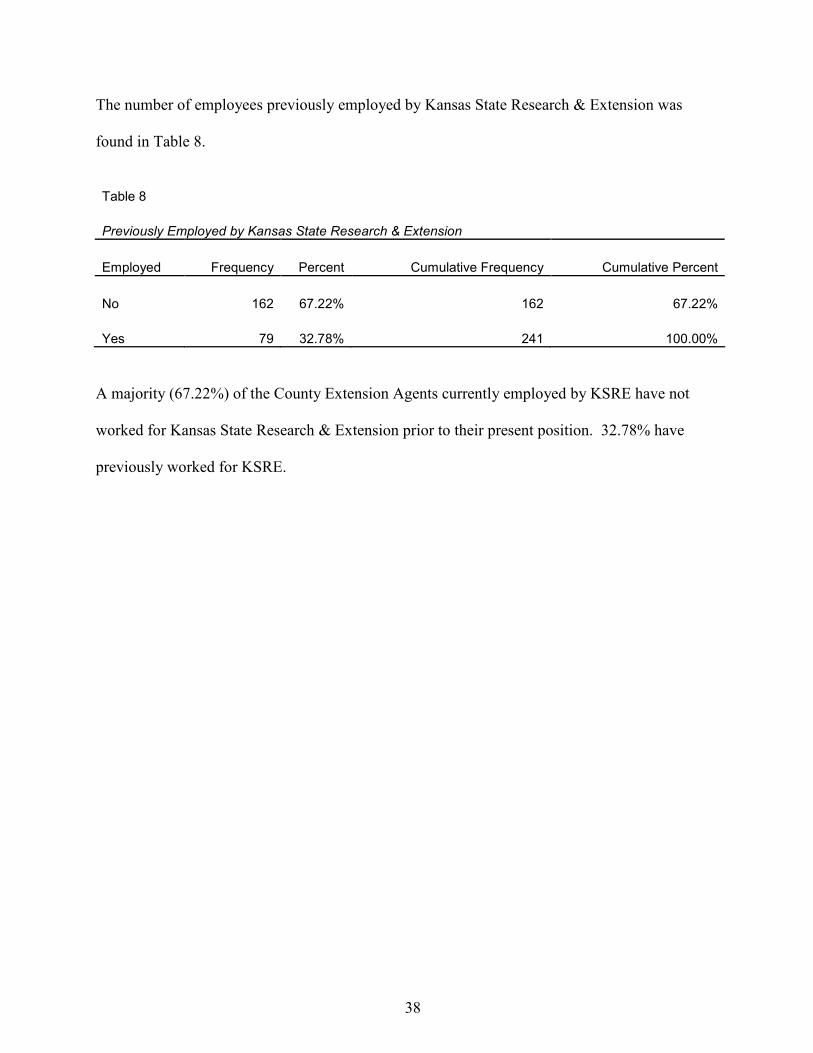
The number of employees previously employed by Kansas State Research & Extension was

found in Table 8.

Table 8

Previously Employed by Kansas State Research & Extension

Employed Frequency Percent Cumulative Frequency Cumulative Percent

No 162 67.22% 162 67.22%

Yes 79 32.78% 241 100.00%

A majority (67.22%) of the County Extension Agents currently employed by KSRE have not

worked for Kansas State Research & Extension prior to their present position. 32.78% have

previously worked for KSRE.

38

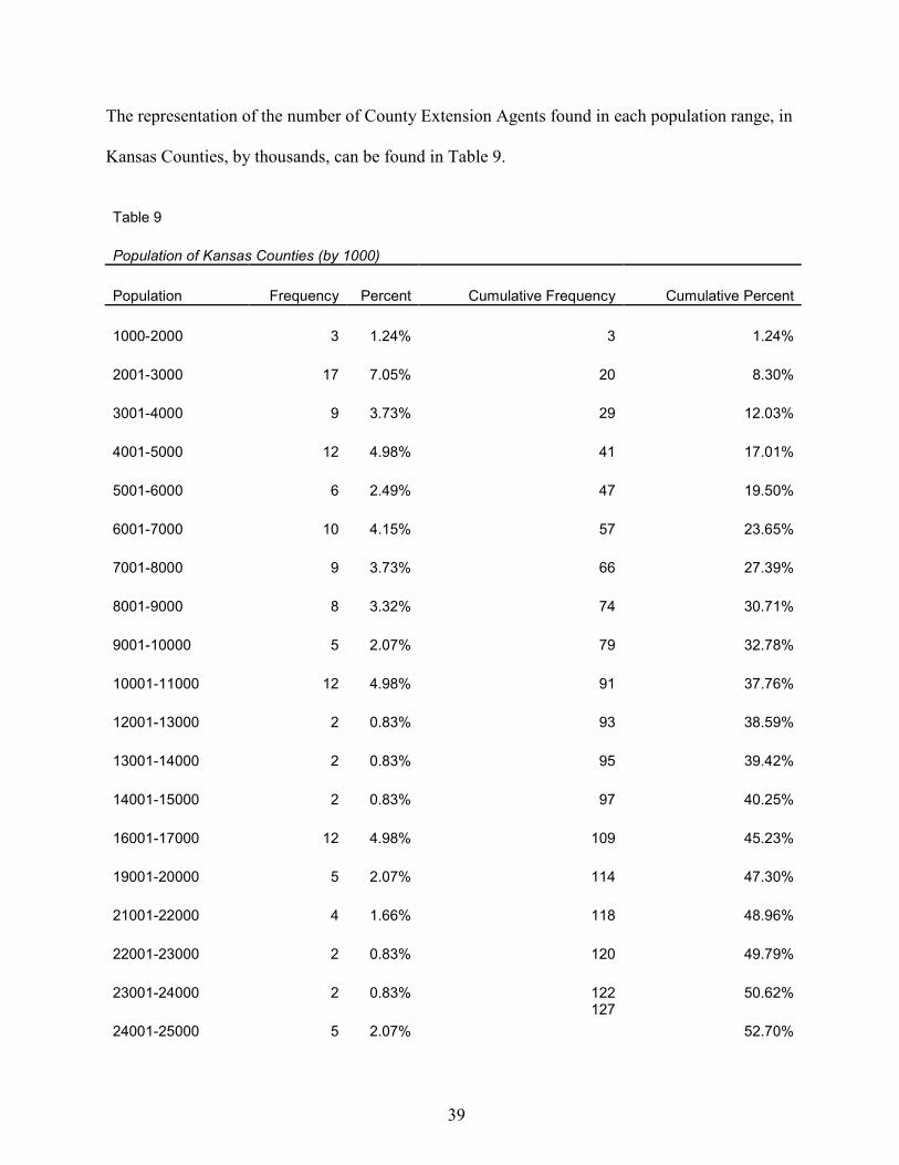
The representation of the number of County Extension Agents found in each population range, in

Kansas Counties, by thousands, can be found in Table 9.

Table 9

Population of Kansas Counties (by 1000)

Population Frequency Percent Cumulative Frequency Cumulative Percent

1000-2000 3 1.24% 3 1.24%

2001-3000 17 7.05% 20 8.30%

3001-4000 9 3.73% 29 12.03%

4001-5000 12 4.98% 41 17.01%

5001-6000 6 2.49% 47 19.50%

6001-7000 10 4.15% 57 23.65%

7001-8000 9 3.73% 66 27.39%

8001-9000 8 3.32% 74 30.71%

9001-10000 5 2.07% 79 32.78%

10001-11000 12 4.98% 91 37.76%

12001-13000 2 0.83% 93 38.59%

13001-14000 2 0.83% 95 39.42%

14001-15000 2 0.83% 97 40.25%

16001-17000 12 4.98% 109 45.23%

19001-20000 5 2.07% 114 47.30%

21001-22000 4 1.66% 118 48.96%

22001-23000 2 0.83% 120 49.79%

23001-24000 2 0.83% 122 50.62%

24001-25000 5 2.07%

127

52.70%

39

26001-27000 7 2.90% 134 55.60%

27001-28000 3 1.24% 137 56.85%

29001-30000 11 4.56% 148 61.41%

30001-31000 3 1.24% 151 62.66%

33001-34000 6 2.49% 157 65.15%

34001-35000 6 2.49% 163 67.63%

35001-36000 4 1.66% 167 69.29%

38001-39000 4 1.66% 171 70.95%

39001-40000 3 1.24% 174 72.20%

42001-43000 6 2.49% 180 74.69%

60001-61000 8 3.32% 188 78.01%

62001-63000 5 2.07% 193 80.08%

63001-64000 9 3.73% 202 83.82%

73001-74000 3 1.24% 205 85.06%

112001-113000 5 2.07% 210 87.14%

155001-156000 5 2.07% 215 89.21%

172001-173000 6 2.49% 221 91.70%

470001-471000 12 4.98% 233 96.68%

516001-517000 8 3.32% 241 100.00%

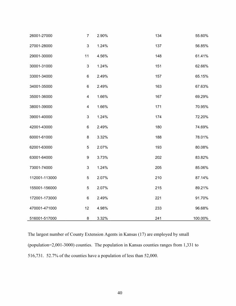
The largest number of County Extension Agents in Kansas (17) are employed by small

(population=2,001-3000) counties. The population in Kansas counties ranges from 1,331 to

516,731. 52.7% of the counties have a population of less than 52,000.

40

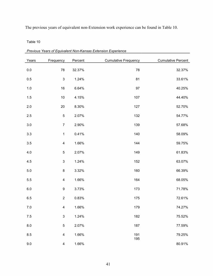
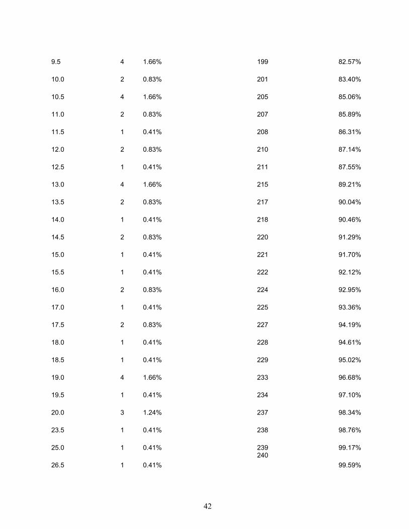
The previous years of equivalent non-Extension work experience can be found in Table 10.

Table 10

Previous Years of Equivalent Non-Kansas Extension Experience

Years Frequency Percent Cumulative Frequency Cumulative Percent

0.0 78 32.37% 78 32.37%

0.5 3 1.24% 81 33.61%

1.0 16 6.64% 97 40.25%

1.5 10 4.15% 107 44.40%

2.0 20 8.30% 127 52.70%

2.5 5 2.07% 132 54.77%

3.0 7 2.90% 139 57.68%

3.3 1 0.41% 140 58.09%

3.5 4 1.66% 144 59.75%

4.0 5 2.07% 149 61.83%

4.5 3 1.24% 152 63.07%

5.0 8 3.32% 160 66.39%

5.5 4 1.66% 164 68.05%

6.0 9 3.73% 173 71.78%

6.5 2 0.83% 175 72.61%

7.0 4 1.66% 179 74.27%

7.5 3 1.24% 182 75.52%

8.0 5 2.07% 187 77.59%

8.5 4 1.66% 191 79.25%

9.0 4 1.66%

195

80.91%

41

9.5 4 1.66% 199 82.57%

10.0 2 0.83% 201 83.40%

10.5 4 1.66% 205 85.06%

11.0 2 0.83% 207 85.89%

11.5 1 0.41% 208 86.31%

12.0 2 0.83% 210 87.14%

12.5 1 0.41% 211 87.55%

13.0 4 1.66% 215 89.21%

13.5 2 0.83% 217 90.04%

14.0 1 0.41% 218 90.46%

14.5 2 0.83% 220 91.29%

15.0 1 0.41% 221 91.70%

15.5 1 0.41% 222 92.12%

16.0 2 0.83% 224 92.95%

17.0 1 0.41% 225 93.36%

17.5 2 0.83% 227 94.19%

18.0 1 0.41% 228 94.61%

18.5 1 0.41% 229 95.02%

19.0 4 1.66% 233 96.68%

19.5 1 0.41% 234 97.10%

20.0 3 1.24% 237 98.34%

23.5 1 0.41% 238 98.76%

25.0 1 0.41% 239 99.17%

26.5 1 0.41%

240

99.59%

42

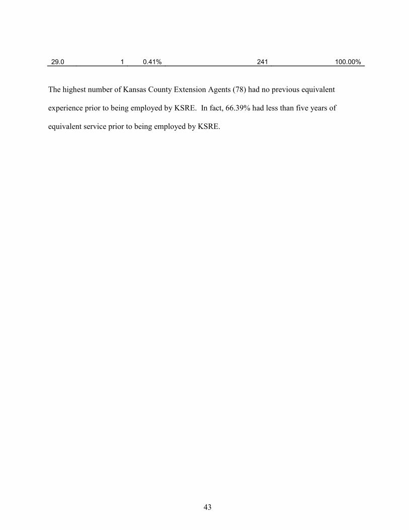
29.0 1 0.41% 241 100.00%

The highest number of Kansas County Extension Agents (78) had no previous equivalent

experience prior to being employed by KSRE. In fact, 66.39% had less than five years of

equivalent service prior to being employed by KSRE.

43

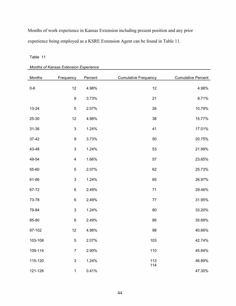
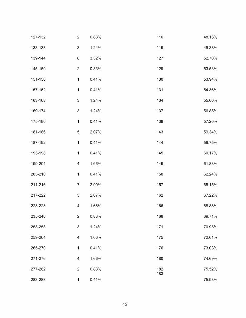
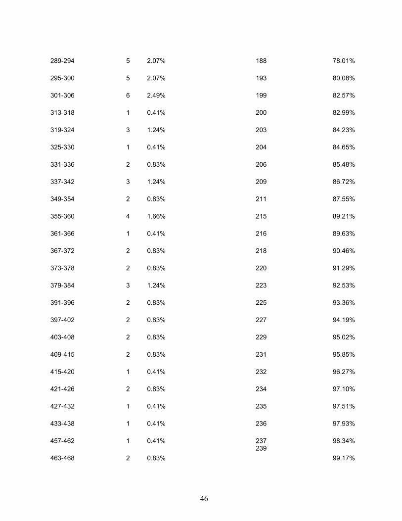
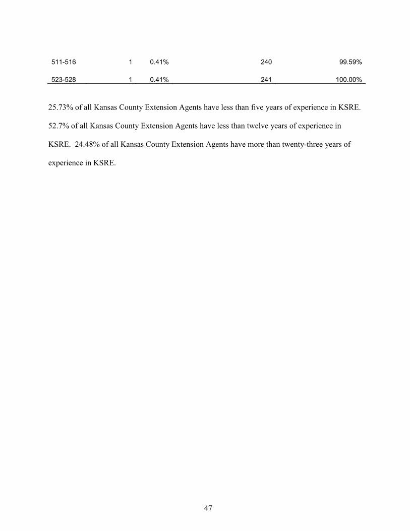
Months of work experience in Kansas Extension including present position and any prior

experience being employed as a KSRE Extension Agent can be found in Table 11.

Table 11

Months of Kansas Extension Experience

Months Frequency Percent Cumulative Frequency Cumulative Percent

0-6 12 4.98% 12 4.98%

9 3.73% 21 8.71%

13-24 5 2.07% 26 10.79%

25-30 12 4.98% 38 15.77%

31-36 3 1.24% 41 17.01%

37-42 9 3.73% 50 20.75%

43-48 3 1.24% 53 21.99%

49-54 4 1.66% 57 23.65%

55-60 5 2.07% 62 25.73%

61-66 3 1.24% 65 26.97%

67-72 6 2.49% 71 29.46%

73-78 6 2.49% 77 31.95%

79-84 3 1.24% 80 33.20%

85-90 6 2.49% 86 35.68%

97-102 12 4.98% 98 40.66%

103-108 5 2.07% 103 42.74%

109-114 7 2.90% 110 45.64%

115-120 3 1.24% 113 46.89%

121-126 1 0.41%

114

47.30%

44

127-132 2 0.83% 116 48.13%

133-138 3 1.24% 119 49.38%

139-144 8 3.32% 127 52.70%

145-150 2 0.83% 129 53.53%

151-156 1 0.41% 130 53.94%

157-162 1 0.41% 131 54.36%

163-168 3 1.24% 134 55.60%

169-174 3 1.24% 137 56.85%

175-180 1 0.41% 138 57.26%

181-186 5 2.07% 143 59.34%

187-192 1 0.41% 144 59.75%

193-198 1 0.41% 145 60.17%

199-204 4 1.66% 149 61.83%

205-210 1 0.41% 150 62.24%

211-216 7 2.90% 157 65.15%

217-222 5 2.07% 162 67.22%

223-228 4 1.66% 166 68.88%

235-240 2 0.83% 168 69.71%

253-258 3 1.24% 171 70.95%

259-264 4 1.66% 175 72.61%

265-270 1 0.41% 176 73.03%

271-276 4 1.66% 180 74.69%

277-282 2 0.83% 182 75.52%

283-288 1 0.41%

183

75.93%

45

289-294 5 2.07% 188 78.01%

295-300 5 2.07% 193 80.08%

301-306 6 2.49% 199 82.57%

313-318 1 0.41% 200 82.99%

319-324 3 1.24% 203 84.23%

325-330 1 0.41% 204 84.65%

331-336 2 0.83% 206 85.48%

337-342 3 1.24% 209 86.72%

349-354 2 0.83% 211 87.55%

355-360 4 1.66% 215 89.21%

361-366 1 0.41% 216 89.63%

367-372 2 0.83% 218 90.46%

373-378 2 0.83% 220 91.29%

379-384 3 1.24% 223 92.53%

391-396 2 0.83% 225 93.36%

397-402 2 0.83% 227 94.19%

403-408 2 0.83% 229 95.02%

409-415 2 0.83% 231 95.85%

415-420 1 0.41% 232 96.27%

421-426 2 0.83% 234 97.10%

427-432 1 0.41% 235 97.51%

433-438 1 0.41% 236 97.93%

457-462 1 0.41% 237 98.34%

463-468 2 0.83%

239

99.17%

46

511-516 1 0.41% 240 99.59%

523-528 1 0.41% 241 100.00%

25.73% of all Kansas County Extension Agents have less than five years of experience in KSRE.

52.7% of all Kansas County Extension Agents have less than twelve years of experience in

KSRE. 24.48% of all Kansas County Extension Agents have more than twenty-three years of

experience in KSRE.

47

Summary

4-H Extension Agents were primarily female (87.50%) and all Family and Consumer

Science Extension Agents were women. However, the men were the majority in Horticulture

(60%) and in Agriculture and Natural Resources (78.57%). 4-H and Horticulture Agents are less

frequent position titles (19.51%). The number of Extension Agents without Director

responsibilities was higher (94.19%) than those with Director responsibilities (5.81%).

The number of Kansas Extension Agents without Master’s degrees was higher (63.49%)

than those with Master’s degrees (36.51%). The majority (57.95%) of Extension Agents in

Kansas with Master’s degrees completed their Master’s degree prior to being employed by

KSRE versus completing their Master’s degree after their appointment date (42.05%).

The Northeast Area employs the highest number of Extension agents, 83 (34.44%). The

Northwest Area employs the lowest number of Extension agents, 40 (16.6%). The number of

Extension Agents employed in a county/district office ranges from 1-11. A county employing

two Extension Agents was the most common (33.61%). A majority (67.22%) of the County

Extension Agents currently employed by KSRE have not worked for Kansas State Research &

Extension prior to their present position.

The largest number of County Extension Agents in Kansas (17) are employed by small

(population=2,001-3000) counties. The highest number of Kansas County Extension Agents

(78) had no previous equivalent experience prior to being employed by KSRE.

48

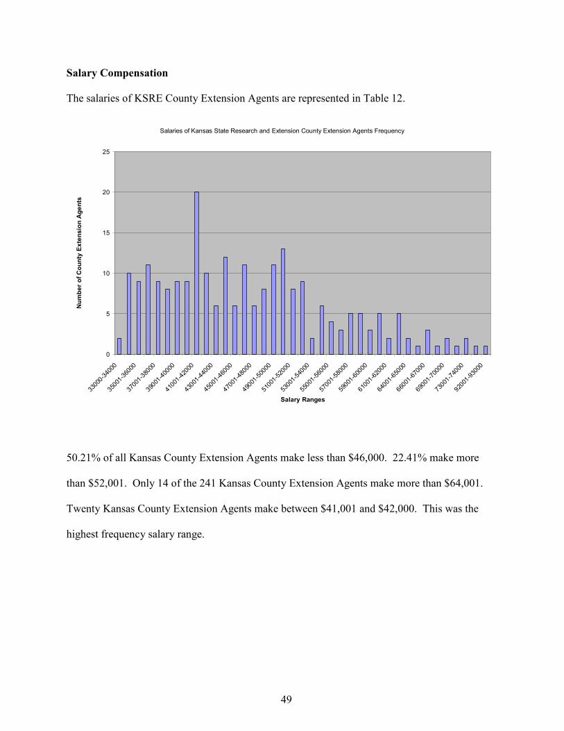
Salary Compensation

The salaries of KSRE County Extension Agents are represented in Table 12.

Salaries of Kansas State Research and Extension County Extension Agents Frequency

0

5

10

15

20

25

33000-34000

35001-36000

37001-38000

39001-40000

41001-42000

43001-44000

45001-46000

47001-48000

49001-50000

51001-52000

53001-54000

55001-56000

57001-58000

59001-60000

61001-62000

64001-65000

66001-67000

69001-70000

73001-74000

92001-93000

Salary Ranges

Number of County Extension Agents

50.21% of all Kansas County Extension Agents make less than $46,000. 22.41% make more

than $52,001. Only 14 of the 241 Kansas County Extension Agents make more than $64,001.

Twenty Kansas County Extension Agents make between $41,001 and $42,000. This was the

highest frequency salary range.

49

Rationale for Selection of Analysis

Multiple regressions with ordinary Least Squares were used to fit models for the response

variable salary as a function of demographic, geographic and other explanatory/predictor

variables. The variable selection technique of backwards elimination was used to delete non-

significant explanatory/predictor variables with an alpha-to-remove of .10. Backward

elimination was recommended over either forward selection or stepwise variable selection

techniques because it allows for examination of the full model and because estimates of the error

variance are more nearly unbiased at each step of deleting variables (Kutner et al., 2004). All

regression calculations were done with the REG procedure of SAS (SAS Institute 2004, version

9.1). Residual diagnostics were performed to check for outliers in the REG procedure and for

normality in the UNIVARIATE procedure. Residuals of the final model were normal, so that

regression coefficients, standard errors and t-statistics were reliable.

50

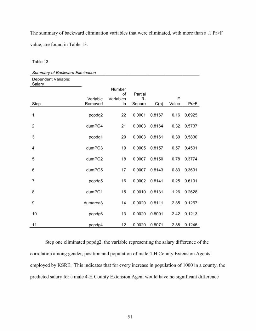
The summary of backward elimination variables that were eliminated, with more than a .1 Pr>F

value, are found in Table 13.

Table 13

Summary of Backward Elimination

Dependent Variable: Salary

Step Variable

Removed

Number of

Variables In

Partial R-

Square C(p) F

Value Pr>F

1 popdg2 22 0.0001 0.8167 0.16 0.6925

2 dumPG4 21 0.0003 0.8164 0.32 0.5737

3 popdg1 20 0.0003 0.8161 0.30 0.5830

4 dumPG3 19 0.0005 0.8157 0.57 0.4501

5 dumPG2 18 0.0007 0.8150 0.78 0.3774

6 dumPG5 17 0.0007 0.8143 0.83 0.3631

7 popdg5 16 0.0002 0.8141 0.25 0.6191

8 dumPG1 15 0.0010 0.8131 1.26 0.2628

9 dumarea3 14 0.0020 0.8111 2.35 0.1267

10 popdg6 13 0.0020 0.8091 2.42 0.1213

11 popdg4 12 0.0020 0.8071 2.38 0.1246

Step one eliminated popdg2, the variable representing the salary difference of the

correlation among gender, position and population of male 4-H County Extension Agents

employed by KSRE. This indicates that for every increase in population of 1000 in a county, the

predicted salary for a male 4-H County Extension Agent would have no significant difference

51

when compared with the baseline, male Agriculture County Extension Agent. This variable was

shown to be insignificant with a Pr>F value of .6925.

Step two eliminated the variable dumPG4, which represents the male Horticulture County

Extension Agents employed by KSRE. Therefore, there was no significant difference

(Pr>F=.5795) between the salary of male Horticulture Agents and male Agriculture Agents

(male Agriculture Agents were used as the baseline for this variable) when all other variables are

ignored.

Step three removed the variable popdg1 which represents the salary difference of the

correlation among gender, position and population of female Agriculture County Extension

Agents employed by KSRE. This indicates that for every increase in population of 1000 in a

county, the predicted salary for a female Agriculture County Extension Agent would be no

different than that of a male Agriculture County Extension Agent. This variable was shown to

be insignificant with a Pr>F value of .5830.

Step four eliminated the variable dumPG3 which represents the female 4-H County

Extension Agents employed by KSRE. Therefore, there was no significant difference

(Pr>F=.4501) between the salary of female 4-H Agents and male Agriculture Agents (male

Agriculture Agents were used as the baseline for This variable) employed by KSRE, ignoring all

other variables.

Step five eliminated the variable for male 4-H County Extension Agents employed by

KSRE, dumPG2. This means that while ignoring all other variables, there was no significant

difference found in salaries between male 4-H County Extension Agents and male Agriculture

County Extension Agents employed by KSRE. The Pr>F value for This variable that was

eliminated was .3774.

52

Step six eliminated the variable dumPG5, the variable used for female Horticulture

County Extension Agents employed by KSRE. The high Pr>F value, .3631, signifies that there

was no significant difference found between the salaries of female Horticulture County

Extension Agents and male Agriculture County Extension Agents (male Agriculture County

Extension Agents were used as the baseline for This variable) employed by KSRE, ignoring all

other variables.

Step seven eliminated the variable popdg5 which was used to represent the salary

difference of the correlation among gender, position and population of female Horticulture

County Extension Agents employed by KSRE. This indicates that for every increase in

population of 1000 in a county, the predicted salary for a female Horticulture County Extension

Agent would show no significant difference when compared with the baseline, male Agriculture

County Extension Agent (male Agriculture County Extension Agents were used as the baseline

for This variable). This variable was shown to be insignificant with a Pr>F value of .6191.

Step eight eliminated the variable representing female Agriculture County Extension

Agents employed by KSRE, dumPG1. Due to the high Pr>F value of .2628, there was no

significant difference found between the salaries made by female Agriculture County Extension

Agents and male Agriculture County Extension Agents (male Agriculture County Extension

Agents were used as the baseline for This variable) employed by KSRE.

Step nine eliminated the dumarea3 variable which was used to signify the salaries of

County Extension Agents employed by KSRE in the Northwest Area. With an insignificant

Pr>F value of .1267, the model showed that there was no significant difference between the

salaries of County Extension Agents employed in the Northwest Area of KSRE and the salaries

53

of County Extension Agents employed in the Northeast Area of KSRE (the Northeast Area was

used as the baseline for This variable).

Step ten eliminated the variable popdg6 which was used to represent the salary difference

of the correlation among gender, position and population of female Family and Consumer

Science County Extension Agents employed by KSRE (All of the FCS County Extension Agents

were female, so This variable represents all FCS County Extension Agents). This indicates that

for every increase in population of 1000 in a county, the predicted salary for a female Family and

Consumer Science County Extension Agent would show no significant difference when

compared with the baseline, male Agriculture County Extension Agent (male Agriculture County

Extension Agents were used as the baseline for This variable). This variable was shown to be

insignificant with a Pr>F value of .1213.

Step eleven eliminated the variable used to represent the salary difference of the

correlation among gender, position and population of male Horticulture County Extension

Agents employed by KSRE, popdg4. The insignificant Pr>F value of .1246 indicates that for

every increase in population of 1000 in a county, the predicted salary for a male Horticulture

County Extension Agent would show no significant difference when compared with the baseline,

male Agriculture County Extension Agent (male Agriculture County Extension Agents were

used as the baseline for This variable).

54

Summary

The independent variables that had were eliminated included: the correlation among

gender, position, and population of male 4-H County Extension Agents, male Horticulture

County Extension Agents, correlation among gender, position, and population of female

Agriculture County Extension Agents, female 4-H County Extension Agents, male 4-H County

Extension Agents, female Horticulture County Extension Agents, the correlation among gender,

position, and population of female Horticulture County Extension Agents, female Agriculture

County Extension Agents, the Northwest Area, the correlation among gender, position, and

population of female Family and Consumer Science County Extension Agents, and the

correlation among gender, position, and population of male Horticulture County Extension

Agents.

55

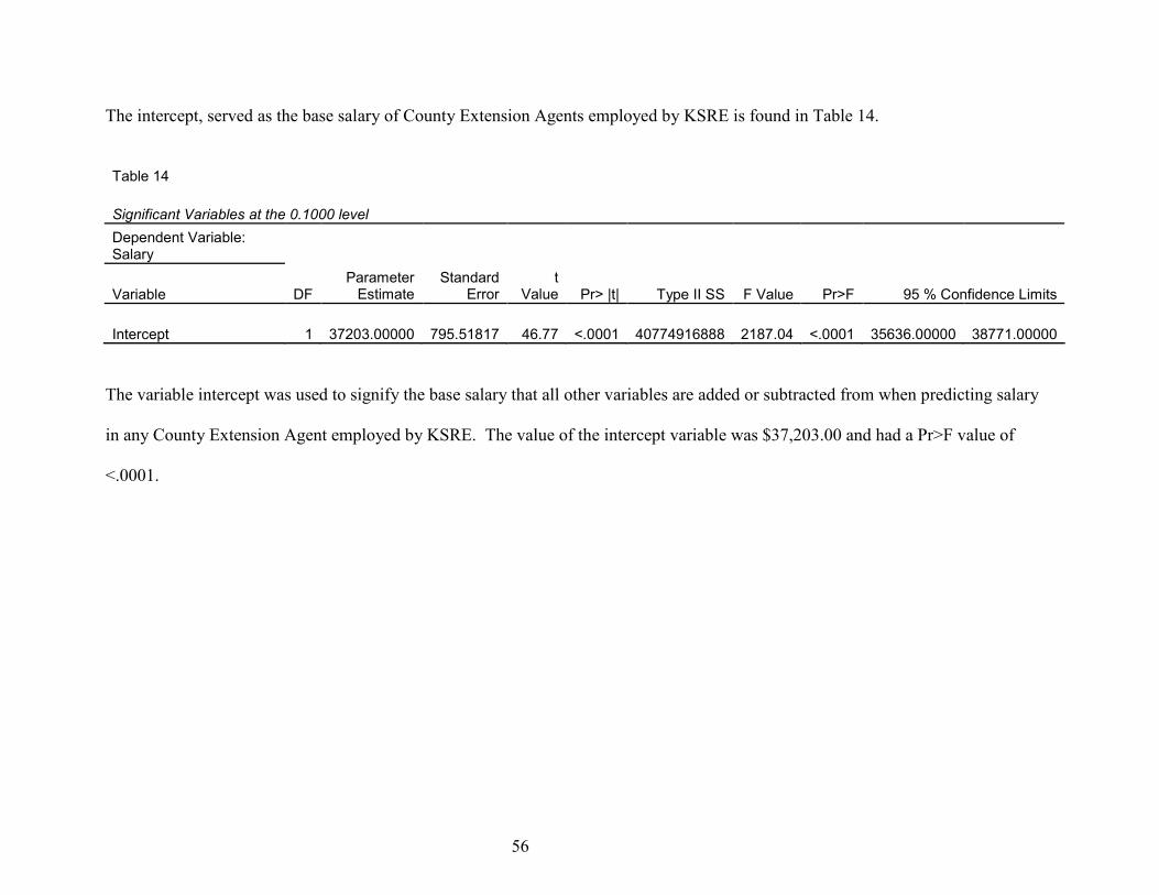
The intercept, served as the base salary of County Extension Agents employed by KSRE is found in Table 14.

Table 14

Significant Variables at the 0.1000 level

Dependent Variable: Salary

Variable DF Parameter Estimate

Standard Error

t Value Pr> |t| Type II SS F Value Pr>F 95 % Confidence Limits

Intercept 1 37203.00000 795.51817 46.77 <.0001 40774916888 2187.04 <.0001 35636.00000 38771.00000

The variable intercept was used to signify the base salary that all other variables are added or subtracted from when predicting salary

in any County Extension Agent employed by KSRE. The value of the intercept variable was $37,203.00 and had a Pr>F value of

<.0001.

56

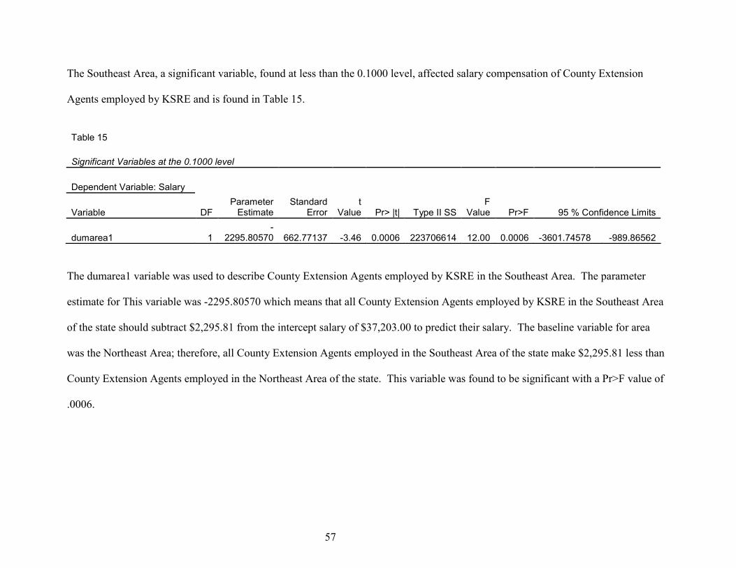
The Southeast Area, a significant variable, found at less than the 0.1000 level, affected salary compensation of County Extension

Agents employed by KSRE and is found in Table 15.

Table 15

Significant Variables at the 0.1000 level

Dependent Variable: Salary

Variable DF Parameter Estimate

Standard Error

t Value Pr> |t| Type II SS

F Value Pr>F 95 % Confidence Limits

dumarea1 1 -

2295.80570 662.77137 -3.46 0.0006 223706614 12.00 0.0006 -3601.74578 -989.86562

The dumarea1 variable was used to describe County Extension Agents employed by KSRE in the Southeast Area. The parameter

estimate for This variable was -2295.80570 which means that all County Extension Agents employed by KSRE in the Southeast Area

of the state should subtract $2,295.81 from the intercept salary of $37,203.00 to predict their salary. The baseline variable for area

was the Northeast Area; therefore, all County Extension Agents employed in the Southeast Area of the state make $2,295.81 less than

County Extension Agents employed in the Northeast Area of the state. This variable was found to be significant with a Pr>F value of

.0006.

57

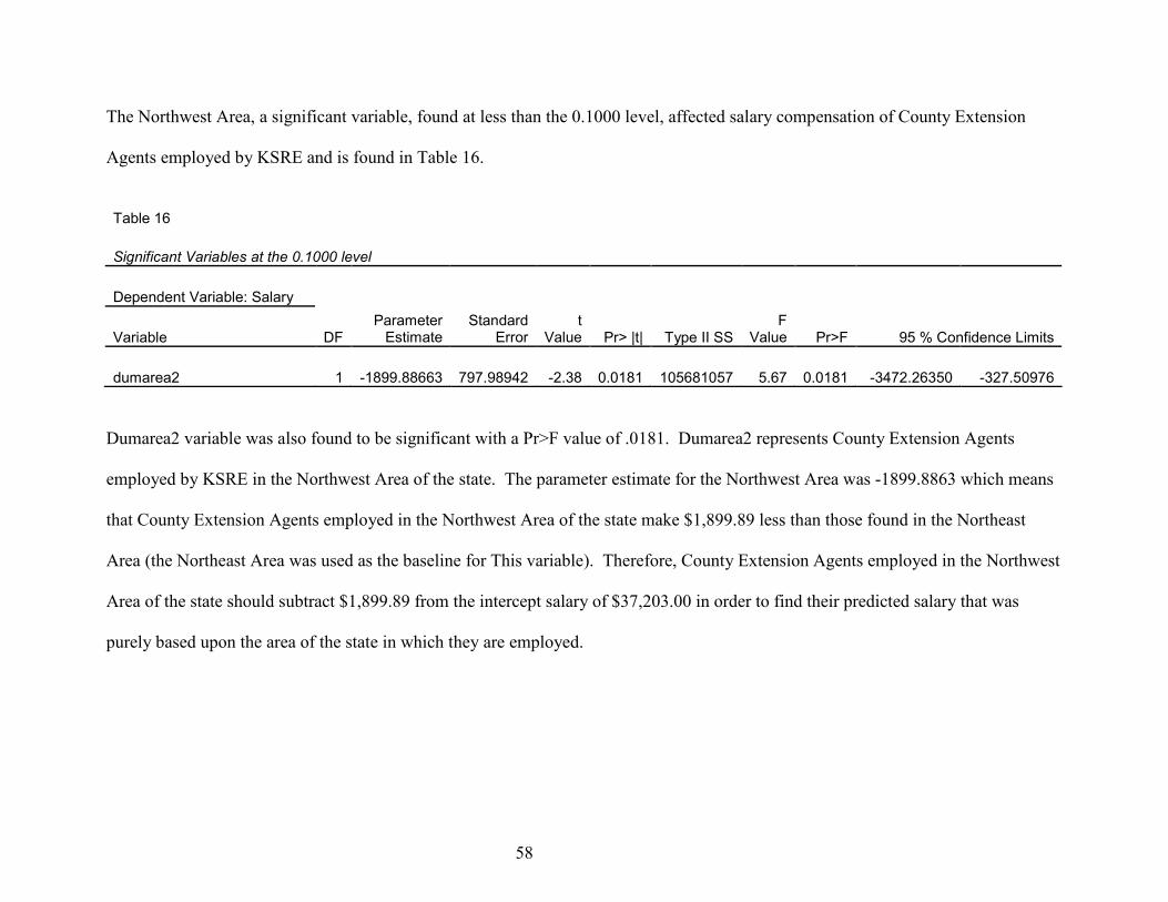
The Northwest Area, a significant variable, found at less than the 0.1000 level, affected salary compensation of County Extension

Agents employed by KSRE and is found in Table 16.

Table 16

Significant Variables at the 0.1000 level

Dependent Variable: Salary

Variable DF Parameter Estimate

Standard Error

t Value Pr> |t| Type II SS

F Value Pr>F 95 % Confidence Limits

dumarea2 1 -1899.88663 797.98942 -2.38 0.0181 105681057 5.67 0.0181 -3472.26350 -327.50976

Dumarea2 variable was also found to be significant with a Pr>F value of .0181. Dumarea2 represents County Extension Agents

employed by KSRE in the Northwest Area of the state. The parameter estimate for the Northwest Area was -1899.8863 which means

that County Extension Agents employed in the Northwest Area of the state make $1,899.89 less than those found in the Northeast

Area (the Northeast Area was used as the baseline for This variable). Therefore, County Extension Agents employed in the Northwest

Area of the state should subtract $1,899.89 from the intercept salary of $37,203.00 in order to find their predicted salary that was

purely based upon the area of the state in which they are employed.

58

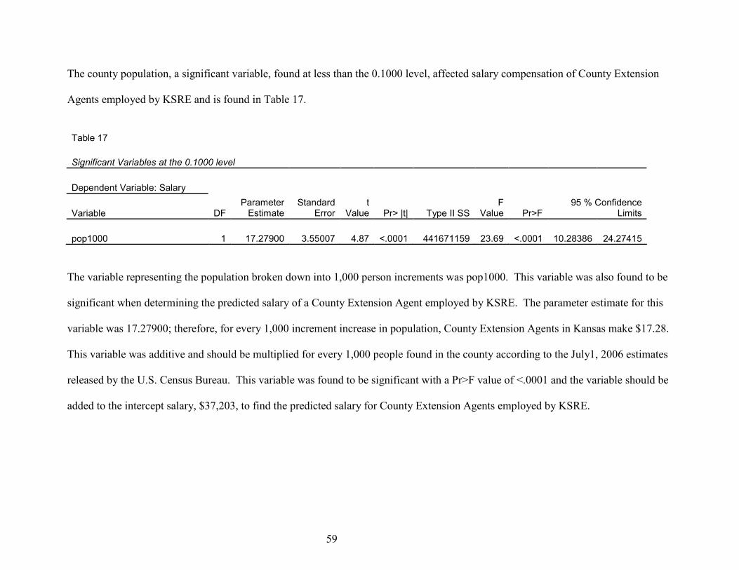
The county population, a significant variable, found at less than the 0.1000 level, affected salary compensation of County Extension

Agents employed by KSRE and is found in Table 17.

Table 17

Significant Variables at the 0.1000 level

Dependent Variable: Salary

Variable DF Parameter Estimate

Standard Error

t Value Pr> |t| Type II SS

F Value Pr>F

95 % Confidence Limits

pop1000 1 17.27900 3.55007 4.87 <.0001 441671159 23.69 <.0001 10.28386 24.27415

The variable representing the population broken down into 1,000 person increments was pop1000. This variable was also found to be

significant when determining the predicted salary of a County Extension Agent employed by KSRE. The parameter estimate for this

variable was 17.27900; therefore, for every 1,000 increment increase in population, County Extension Agents in Kansas make $17.28.

This variable was additive and should be multiplied for every 1,000 people found in the county according to the July1, 2006 estimates

released by the U.S. Census Bureau. This variable was found to be significant with a Pr>F value of <.0001 and the variable should be

added to the intercept salary, $37,203, to find the predicted salary for County Extension Agents employed by KSRE.

59

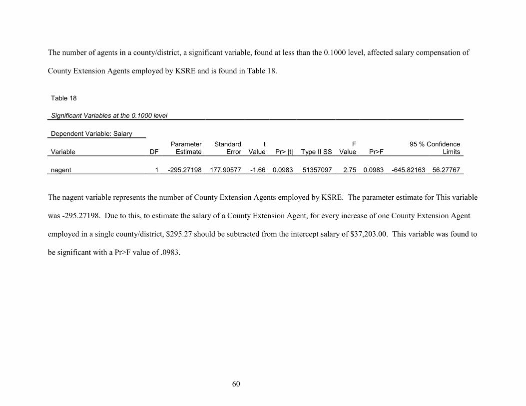
The number of agents in a county/district, a significant variable, found at less than the 0.1000 level, affected salary compensation of

County Extension Agents employed by KSRE and is found in Table 18.

Table 18

Significant Variables at the 0.1000 level

Dependent Variable: Salary

Variable DF Parameter Estimate

Standard Error

t Value Pr> |t| Type II SS

F Value Pr>F

95 % Confidence Limits

nagent 1 -295.27198 177.90577 -1.66 0.0983 51357097 2.75 0.0983 -645.82163 56.27767

The nagent variable represents the number of County Extension Agents employed by KSRE. The parameter estimate for This variable

was -295.27198. Due to this, to estimate the salary of a County Extension Agent, for every increase of one County Extension Agent

employed in a single county/district, $295.27 should be subtracted from the intercept salary of $37,203.00. This variable was found to

be significant with a Pr>F value of .0983.

60

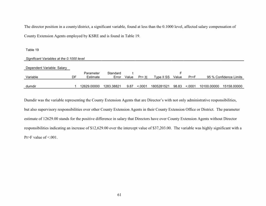
The director position in a county/district, a significant variable, found at less than the 0.1000 level, affected salary compensation of

County Extension Agents employed by KSRE and is found in Table 19.

Table 19

Significant Variables at the 0.1000 level

Dependent Variable: Salary

Variable DF Parameter Estimate

Standard Error

t Value Pr> |t| Type II SS

F Value Pr>F 95 % Confidence Limits

dumdir 1 12629.00000 1283.38821 9.87 <.0001 1805281521 98.83 <.0001 10100.00000 15158.00000

Dumdir was the variable representing the County Extension Agents that are Director’s with not only administrative responsibilities,

but also supervisory responsibilities over other County Extension Agents in their County Extension Office or District. The parameter

estimate of 12629.00 stands for the positive difference in salary that Directors have over County Extension Agents without Director

responsibilities indicating an increase of $12,629.00 over the intercept value of $37,203.00. The variable was highly significant with a

Pr>F value of <.001.

61

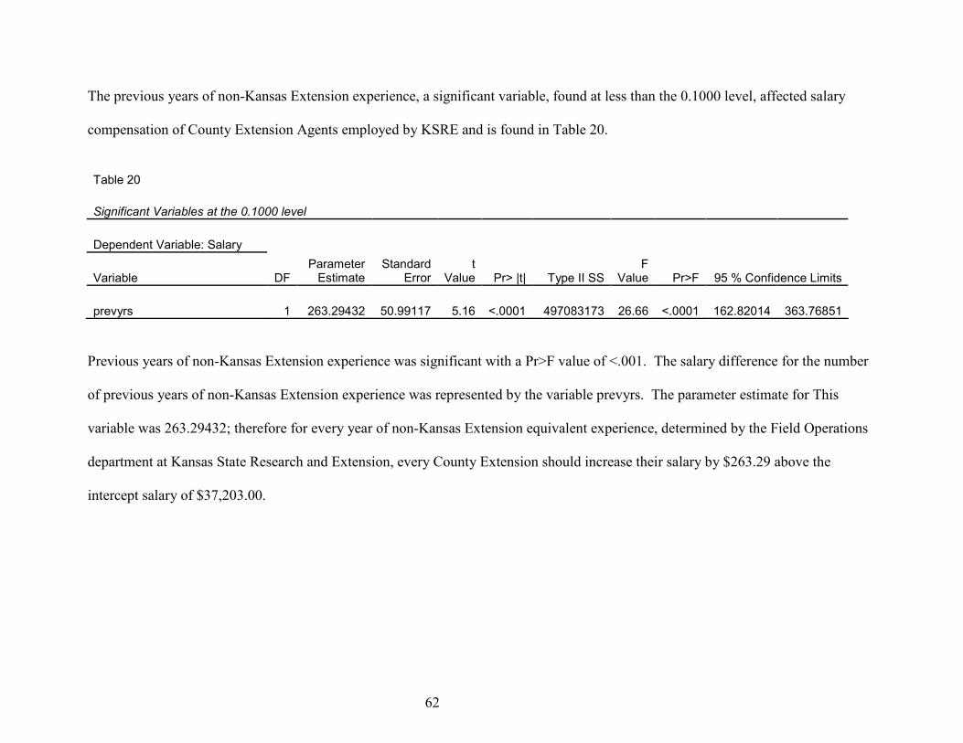
The previous years of non-Kansas Extension experience, a significant variable, found at less than the 0.1000 level, affected salary

compensation of County Extension Agents employed by KSRE and is found in Table 20.

Table 20

Significant Variables at the 0.1000 level

Dependent Variable: Salary

Variable DF Parameter Estimate

Standard Error

t Value Pr> |t| Type II SS

F Value Pr>F 95 % Confidence Limits

prevyrs 1 263.29432 50.99117 5.16 <.0001 497083173 26.66 <.0001 162.82014 363.76851

Previous years of non-Kansas Extension experience was significant with a Pr>F value of <.001. The salary difference for the number

of previous years of non-Kansas Extension experience was represented by the variable prevyrs. The parameter estimate for This

variable was 263.29432; therefore for every year of non-Kansas Extension equivalent experience, determined by the Field Operations

department at Kansas State Research and Extension, every County Extension should increase their salary by $263.29 above the

intercept salary of $37,203.00.

62

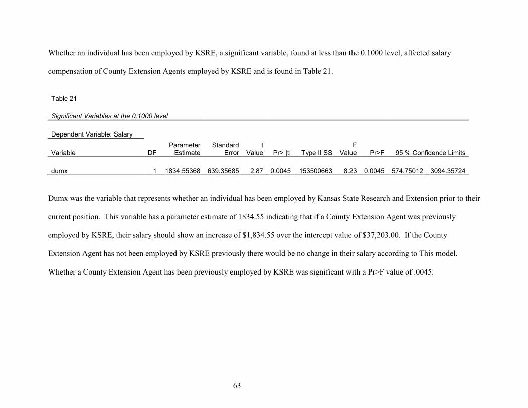
Whether an individual has been employed by KSRE, a significant variable, found at less than the 0.1000 level, affected salary

compensation of County Extension Agents employed by KSRE and is found in Table 21.

Table 21

Significant Variables at the 0.1000 level

Dependent Variable: Salary

Variable DF Parameter Estimate

Standard Error

t Value Pr> |t| Type II SS

F Value Pr>F 95 % Confidence Limits

dumx 1 1834.55368 639.35685 2.87 0.0045 153500663 8.23 0.0045 574.75012 3094.35724

Dumx was the variable that represents whether an individual has been employed by Kansas State Research and Extension prior to their

current position. This variable has a parameter estimate of 1834.55 indicating that if a County Extension Agent was previously

employed by KSRE, their salary should show an increase of $1,834.55 over the intercept value of $37,203.00. If the County

Extension Agent has not been employed by KSRE previously there would be no change in their salary according to This model.

Whether a County Extension Agent has been previously employed by KSRE was significant with a Pr>F value of .0045.

63

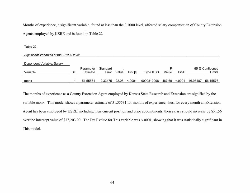
Months of experience, a significant variable, found at less than the 0.1000 level, affected salary compensation of County Extension

Agents employed by KSRE and is found in Table 22.

Table 22

Significant Variables at the 0.1000 level

Dependent Variable: Salary

Variable DF Parameter Estimate

Standard Error

t Value Pr> |t| Type II SS

F Value Pr>F

95 % Confidence Limits

monx 1 51.55531 2.33475 22.08 <.0001 9090810998 487.60 <.0001 46.95487 56.15576

The months of experience as a County Extension Agent employed by Kansas State Research and Extension are signified by the

variable monx. This model shows a parameter estimate of 51.55531 for months of experience, thus, for every month an Extension

Agent has been employed by KSRE, including their current position and prior appointments, their salary should increase by $51.56

over the intercept value of $37,203.00. The Pr>F value for This variable was <.0001, showing that it was statistically significant in

This model.

64

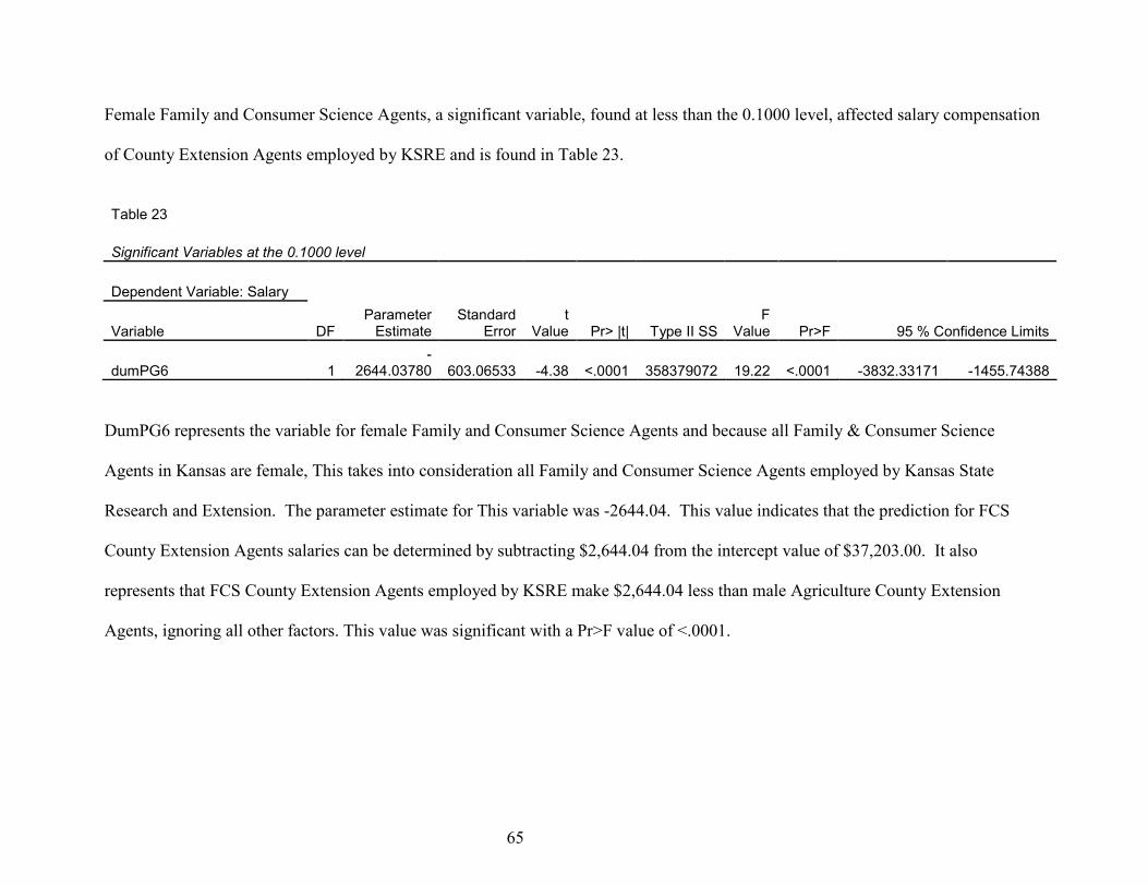
Female Family and Consumer Science Agents, a significant variable, found at less than the 0.1000 level, affected salary compensation

of County Extension Agents employed by KSRE and is found in Table 23.

Table 23

Significant Variables at the 0.1000 level

Dependent Variable: Salary

Variable DF Parameter Estimate

Standard Error

t Value Pr> |t| Type II SS

F Value Pr>F 95 % Confidence Limits

dumPG6 1 -

2644.03780 603.06533 -4.38 <.0001 358379072 19.22 <.0001 -3832.33171 -1455.74388

DumPG6 represents the variable for female Family and Consumer Science Agents and because all Family & Consumer Science

Agents in Kansas are female, This takes into consideration all Family and Consumer Science Agents employed by Kansas State

Research and Extension. The parameter estimate for This variable was -2644.04. This value indicates that the prediction for FCS

County Extension Agents salaries can be determined by subtracting $2,644.04 from the intercept value of $37,203.00. It also

represents that FCS County Extension Agents employed by KSRE make $2,644.04 less than male Agriculture County Extension

Agents, ignoring all other factors. This value was significant with a Pr>F value of <.0001.

65

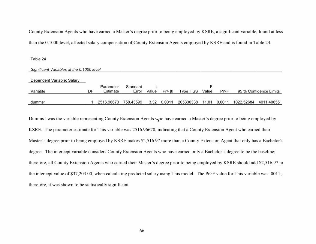
County Extension Agents who have earned a Master’s degree prior to being employed by KSRE, a significant variable, found at less

than the 0.1000 level, affected salary compensation of County Extension Agents employed by KSRE and is found in Table 24.

Table 24

Significant Variables at the 0.1000 level

Dependent Variable: Salary

Variable DF Parameter Estimate

Standard Error

t Value Pr> |t| Type II SS

F Value Pr>F 95 % Confidence Limits

dumms1 1 2516.96670 758.43599 3.32 0.0011 205330338 11.01 0.0011 1022.52684 4011.40655

Dumms1 was the variable representing County Extension Agents who have earned a Master’s degree prior to being employed by

KSRE. The parameter estimate for This variable was 2516.96670, indicating that a County Extension Agent who earned their

Master’s degree prior to being employed by KSRE makes $2,516.97 more than a County Extension Agent that only has a Bachelor’s

degree. The intercept variable considers County Extension Agents who have earned only a Bachelor’s degree to be the baseline;

therefore, all County Extension Agents who earned their Master’s degree prior to being employed by KSRE should add $2,516.97 to

the intercept value of $37,203.00, when calculating predicted salary using This model. The Pr>F value for This variable was .0011;

therefore, it was shown to be statistically significant.

5

66

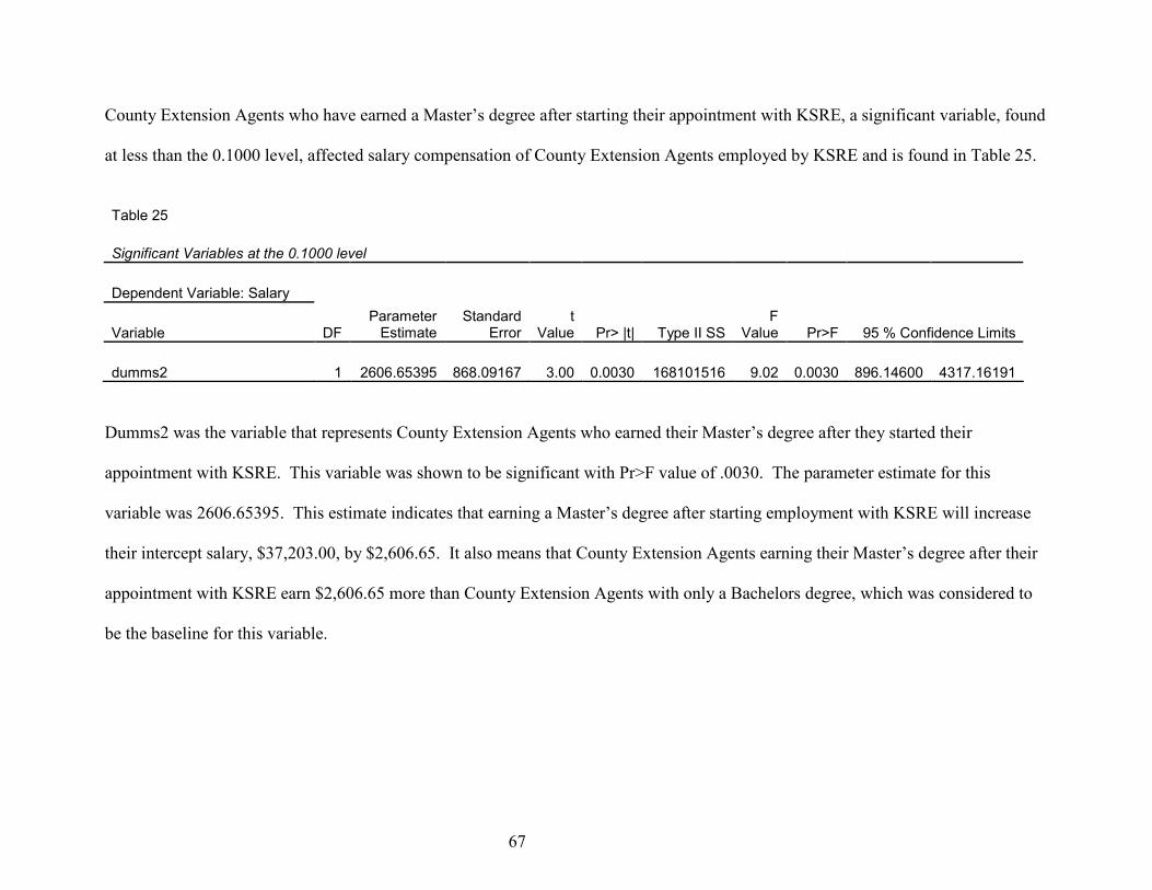
County Extension Agents who have earned a Master’s degree after starting their appointment with KSRE, a significant variable, found

at less than the 0.1000 level, affected salary compensation of County Extension Agents employed by KSRE and is found in Table 25.

Table 25

Significant Variables at the 0.1000 level

Dependent Variable: Salary

Variable DF Parameter Estimate

Standard Error

t Value Pr> |t| Type II SS

F Value Pr>F 95 % Confidence Limits

dumms2 1 2606.65395 868.09167 3.00 0.0030 168101516 9.02 0.0030 896.14600 4317.16191

Dumms2 was the variable that represents County Extension Agents who earned their Master’s degree after they started their

appointment with KSRE. This variable was shown to be significant with Pr>F value of .0030. The parameter estimate for this

variable was 2606.65395. This estimate indicates that earning a Master’s degree after starting employment with KSRE will increase

their intercept salary, $37,203.00, by $2,606.65. It also means that County Extension Agents earning their Master’s degree after their

appointment with KSRE earn $2,606.65 more than County Extension Agents with only a Bachelors degree, which was considered to

be the baseline for this variable.

67

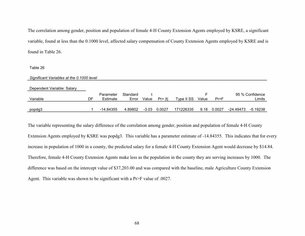
The correlation among gender, position and population of female 4-H County Extension Agents employed by KSRE, a significant

variable, found at less than the 0.1000 level, affected salary compensation of County Extension Agents employed by KSRE and is

found in Table 26.

Table 26

Significant Variables at the 0.1000 level

Dependent Variable: Salary

Variable DF Parameter Estimate

Standard Error

t Value Pr> |t| Type II SS

F Value Pr>F

95 % Confidence Limits

popdg3 1 -14.84355 4.89802 -3.03 0.0027 171226335 9.18 0.0027 -24.49473 -5.19238

The variable representing the salary difference of the correlation among gender, position and population of female 4-H County

Extension Agents employed by KSRE was popdg3. This variable has a parameter estimate of -14.84355. This indicates that for every

increase in population of 1000 in a county, the predicted salary for a female 4-H County Extension Agent would decrease by $14.84.

Therefore, female 4-H County Extension Agents make less as the population in the county they are serving increases by 1000. The

difference was based on the intercept value of $37,203.00 and was compared with the baseline, male Agriculture County Extension

Agent. This variable was shown to be significant with a Pr>F value of .0027.

68

Summary

The independent variables that were found to be significant in their impact on salary

included: the Southeast Area, the Northwest Area, population, the number of agents in a

county/district Extension Office, whether the Extension Agent was a director, previous years of

non-Kansas Extension experience, whether an Extension Agent has been employed by KSRE

prior to their current position, months of experience as an Extension Agent with KSRE, female

Family and Consumer Science agents, level of education, timeliness of obtaining a Master’s

degree, and the correlation among gender, position, and population of female 4-H County

Extension Agents.

69

Chapter V

Summary and Conclusions

A summary of the study, discussion of the findings, and conclusion and recommendations

for further research can be found in this chapter.

Summary

The purpose of this study was to identify factors affecting salary compensation for

County Extension Agents employed by Kansas State Research and Extension. The study not

only analyzed the demographic data regarding County Extension Agents, but also examined the

correlations among factors.

A review of the literature suggested a change, both positive and negative depending on

the factor, in salary when there were differences among the different aspects of a position

including: gender (Garvey, 2004; ASSE Compensation Survey, 1999; Isaacs, 1995; Kiker, et.al,

1987;Koeske and Krowinski, 2004; Seevers and Foster, 2004; Jackson, et.al, 1999; Roberts,

1999; Link, 1988), level of education (ASSE Compensation Study, 1999; Langer, 1994;

LaPlante, 1992; Garvey, 2004; Francis, 2001; United States, 2006; Link, 1988; Nobbe, 1988;

Edwards, et.al, 2004; Roberts, 1999), years of experience (Clark, 2006; Jackson, et.al, 1999;

ASSE Compensation Study, 1999; Linker, 1988; Nobbe, 1988; Roberts, 1999), geographic

location (Francis, 2001; United States, 2006; Nobbe, 1988), “job-hopping” (Garvey, 2004;

Shindul, 1995; Manton and vases, 1984), supervisory roles (Langer, 1994; Nobbe, 1988),

position type (Garvey, 2004; Langer, 1994; Linker, 1988), and job performance (Keller, 2001;

Roberts, 1999).

However, very little data was found when considering combinations of these factors

especially when analyzing Research and Extension; therefore, all of the factors listed above were

70

studied with the exception of salary and the addition of county population, number of agents in

the county/district, and timeliness of obtaining higher education.

Data Collection and Analyses

All Kansas County Extension Agents employed by Kansas State Research and Extension,

as of September 1, 2007, were studied. Demographic data collected from Kansas State Research

and Extension Field Operations Office was analyzed through multiple regressions using the REG

procedure in SAS 9.1 for Windows. Variable selection was made from backward elimination.

The independent variables considered statistically significant had a Pr>F value of .1 or less.

Discussion of the Findings

The demographic data was similar to that found by Seevers and Foster (2004) in regards

to gender as females were underrepresented in the Agriculture and Natural Resources County

Extension Agent positions. It was the opposite for Family and Consumer Sciences, though, as

100% of all Kansas County Family and Consumer Science Extension Agents were women.

Through backward elimination, the first two variables found to be statistically significant

in their impact on salary were the Southeast and Northwest Areas. The baseline for area was the

Northeast; therefore, the negative parameter estimates mean that County Extension Agents

employed in the Southeast and Northwest were paid lower than those in the Northeast Area. The

difference in pay for County Extension Agents employed in the Southeast was -$2,295.81 and

the difference in pay for County Extension Agents employed in the Northwest was -$1,899.89.

There was not a statistically significant difference in County Extension Agents employed in the

Southwest; therefore, their salary does not differ from County Extension Agents employed in the

Northeast Area.

71

The county population was another factor that was found to be statistically significant

through backward elimination of the independent variables. The model predicts that for every

increase of 1000 people in a county, the salary of that County Extension Agent was increased

$17.28. Therefore, higher populated counties, or urban counties, were higher in pay than

smaller, rural counties.

The number of County Extension Agents also impacted salary; however, it was a

negative impact. The model predicts that for every increase of one County Extension Agent

serving in a county, salary decreases by $295.27. As the number of County Extension Agents

within an Extension Office increases, so does the specialization of that agent; therefore, as

County Extension Agents become more highly specialized their pay decreased.

Unlike the negative effect that the number of agents had on pay, serving as the Director

for a County Extension Office increases pay by the highest amount. If an individual was serving

as a Director in a County Extension Office, the model predicts their salary will increase

$12,629.00 above the intercept value. This was easily understood and the salary compensation

supports the review of the literature as Directors have supervisory responsibilities over other

County Extension Agents.

Another factor positively affecting salary was previous years of non-Kansas State

Research and Extension experience. In fact, for every year of non-KSRE experience salary was

predicted to increase $263.29. Another variable related to this one was months of experience as

a KSRE County Extension Agent. This model predicts that for every month of experience a

County Extension Agent was employed by KSRE their salary will increase $51.55. At first

glance this does not seem to equal the salary compensation for non-KSRE years of experience;

however, when calculated out, the model shows that it was more advantageous, in terms of

72

salary, to be employed by KSRE rather than have experience from another organization or

company.

“Job-hopping” was analyzed by considering whether a County Extension Agent has been

previously employed by K-State Research and Extension prior to their current position. The

model predicts that “job-hopping” does have a positive impact on salary compensation. In fact,

the model predicts an increase of $1,834.55 if an Extension Agent had been previously employed

by KSRE.

Level of education as well as timeliness of obtaining a Master’s degree was also shown to

be statistically significant. When compared to a County Extension Agent without a Master’s

degree, the model predicts that those who obtained a Master’s degree prior to being employed by

KSRE increased their salary by $2,516.97 and those who have obtained their Master’s degree

after starting their employment with KSRE increased their salary by $2,606.65.

There were two factors showing salary differences involving gender. The first was

shown between gender and position for female Family and Consumer Science County Extension

Agents. All FCS Agents were female; therefore, the difference was between the baseline, male

Agriculture County Extension Agents, and Family and Consumer Science County Extension

Agents. The model predicted that female FCS Extension Agents made $2,644.04 less than their

male ANR counterparts. This was the only statistically significant variable found between

position and gender. There was no statistically significant difference found for female ANR

County Extension Agent when compared with their male counterparts.

The second variable involving gender and impacting salary compensation was also the

final factor that was shown to have an impact on salary. It was the correlation among

population, position, and gender for female 4-H County Extension Agents. The model predicted

73

that female 4-H County Extension Agents decreased their salary by $14.84 for every 1000

person increase in population. Therefore, as the county became more populated, the female 4-H

County Extension Agents decreased in their pay. No statistical significance was shown in any of

the other population, position and gender correlations.

Conclusions

The model predictions show that obtaining a Master’s degree increased salary versus

obtaining only a Bachelor’s degree. Timeliness of obtaining a Master’s degree was also

significant as the model predicts an even larger increase for County Extension Agents who

obtain their Master’s degree after being employed by Kansas State Research and Extension

versus obtaining a Master’s degree before being employed by Kansas State Research and

Extension. This was a very significant prediction as it allows individuals to feel confident in

taking advantage of tuition assistance provided by Kansas State Research and Extension while

being employed by KSRE. With the help of tuition assistance, some agents would be able to

afford to increase their level of education as they would be employed full-time while doing so.

The model also predicted lower pay for County Extension Agents employed in the

Southeast and Northwest Areas. This could be a factor when choosing which positions to apply

for within Kansas State Research and Extension. Cost of living in these areas could also

influence the lower salary compensation as well as the number of County Extension Agents in

the different areas. In the western half of the state there were significantly lower numbers of

County Extension Agents (88) versus the number of County Extension Agents employed in the

eastern half of the state (153). Tying into the number of agents in an area was the higher salary

compensation for higher population counties. This factor could also affect the decision made by

a potential applicant for a County Extension Agent position with KSRE as the cost of living in

74

urban areas could be higher than those of rural Kansas. Furthermore, if an individual considers

working in a county with a higher number of County Extension Agents, as a higher number of

agents are employed, on average, in a higher population county, the salary compensation

decreased. With this in mind, the potential employee must weigh the increase for population

with the decrease for the number of agents; then consider the salary impact of the Area in which

they are applying.

The very large increase given to individuals who are considering accepting Director

responsibilities should be another significant factor when making a career decision. With the

added responsibility of supervisory and managerial roles, it was important for a potential

candidate to know the potential salary increase. This part of the model could also help Extension

Council’s in their decisions regarding salary for a Director in their county/district.

The differences found in salary compensation for previous years of non-Kansas Research

and Extension experience versus months of experience in Kansas Research and Extension was

another significant factor affecting decision-making for potential employees. Because the

increase was greater for months of experience in Kansas Research and Extension than it was for

years of experience in non- Kansas Research and Extension positions, the model allows

individuals to weigh their potential career opportunities. If they are interested in being employed

by KSRE and a position was available they should be more inclined to apply sooner as their

experience within the organization was more valuable, in terms of salary compensation, than

experience outside of the organization.

Family and Consumer Science County Extension Agents make less than male or female

Agriculture County Extension Agents. This suggests that females can make higher salaries;

however, they must cross the line into male dominated positions to be able to achieve the higher

75

salary compensation for their work, this is supported by the findings of Dubeck and Borman

(1997) who found that women could make equal salaries when compared to men, they simply

had to enter a male-dominated field.

There was only one correlation that showed a difference in salary when taking into

consideration the interaction of population, gender and position. This was for female 4-H

County Extension Agents and it was a decrease in salary compensation. Therefore, female 4-H

County Extension Agents in smaller counties were paid higher than those in larger population

counties. This could be due to the high amount of interaction a 4-H County Extension Agent has

with the 4-H youth in the county. This interaction intensifies as the county size decreases due to

the fact that the County Extension Agent has the same amount of time for a smaller population.

When a County Extension Agent was able to spend more hours with the individuals they serve

their performance may be looked at more positively.

Recommendations for Further Research and Practices

The results of this study were intended to increase knowledge of factors affecting salary

compensation for County Extension Agents employed by Kansas State Research and Extension.

Based on these intentions, the following research and practice recommendations were made:

1. A high percentage of County Extension Agents are Family and Consumer Science Agents

(39.83%). All of these Extension Agents are female and this group was the only

statistically significant finding in the gender/position correlation. The salaries for female

Family and Consumer Science Agents should not be less than any other category when

their positions entail similar work load and responsibilities. This correlation must be

reviewed annually until the gap was narrowed among this group and the other

gender/position correlation groups studied.

76

2. The impact of performance on salary compensation was another factor that needs further

research regarding its impact on salary as its impact could further explain deviations from

the predicted model. Furthermore, performance could be directly related to salary

compensation; therefore, further explanation could be given in this study’s findings.

3. A cost of living analysis in regards to the different counties in Kansas was another factor

to be considered when evaluating the distribution of salary compensation in regards to

area as well as county population. An increase in salary compensation in a specific area

or in a county with a high population could be attributed to a high cost of living versus

area or population.

4. Dispersion of the findings from this analysis was pertinent as it will allow County

Extension Agents to make more informed decisions regarding the furtherance of their

education. Knowledge of the potential salary compensation as well as the tuition

assistance programs offered through Kansas State Research and Extension make an

increase in their level of education more economically feasible.

77

References

78

ASSE Compensation Survey. (2004, October). Professional Safety, 49, 26-27. Retrieved

June 1, 2007, from K-State electronic journals.

Clark, Hannah. (March 8, 2006). Are Women Happy Under the Glass Ceiling? Forbes.

Retrieved November 14, 2007 from http://www.forbes.com/2006/03/07/glass-ceiling-

opportunities--cx_hc_0308glass.html.

Clark, W. (2006, February). Alabama Attorney General Issues Opinion to Rep. Clark. US

Fed New Service, Wire Feed. Retrieved June 20, 2007, from K-State electronic

journals.

Dubeck, P.J., & Borman, K. (Eds.). (1997). Women and Work. New Brunswick: Rutgers

University Press.

Edwards, M.C., McLucas, B., Briers, G.E., & Rohs, F.R. (2004, February).

Educational Interests of Extension Agents: Implications for the Delivery of

Educational Programming at a Distance. Journal of Extension, 42, 1-10. Retrieved

May 28, 2007, from K-State electronic journals.

Francis, W. (2001, October). Where the Money Is. The American City & County, 116,

44-47. Retrieved June 15, 2007, from K-State electronic journals.

Garvey, M.J. (2004, November). Was an MBA Worth It?. Information Week, 1012, 31-34.

Retrieved June 7, 2007, from K-State electronic journals.

Isaacs, Ellen (1995, January). Gender Discrimination in the Workplace: A

Literature Review. Association for Computing Machinery. Communications of the

ACM, 38, 58-60. Retrieved June 20, 2007, from K-State electronic journals.

79

Jackson, D.G., Martin, R., Berry, A., Adkins, B., Johnson, L., Lindner, J.R. (1999,

June). A Summary of OSU Extension Internal Salary Study. Journal of Extension,

37, 1-32. Retrieved May 21, 2007, from K-State electronic journals.

Kansas State Research and Extension. (n.d.). About Us. (Online), Information found at

http://www.oznet.ksu.edu/DesktopDefault.aspx?tabid=25. Information retrieved on

October 19, 2007.

Kansas State University. (n.d.). Board Leadership. Retrieved October 15, 2007, from the

Kansas State University website: http://www.oznet.ksu.edu/operations/Extension_

Board_Leadership/Board_Leadership_(b&w).pdf.

Kansas State University. (n.d.). Instructions for KSU 1-9c. Retrieved October 19, 2007,

from the Kansas State University website: http://www.oznet.ksu.edu/extension

/DesktopDefault.aspx?tabid=93.

Kansas State University. (n.d.). Summary of Benefits for Faculty/Unclassified

Employees. Retrieved October 19, 2007, from the Kansas State University website:

http://www.k-state.edu/hr/benefits/benefitsunclass.htm.

Keller, B. (2001, March). Change in Schedule. Education Week, 20, 21. Retrieved June 20,

2007, from K-State electronic journals.

Kiker, B. F., Rhine, Sherrie L. W. (1987, Winter). Fringe Benefits and the Earnings

Equation – A Test of the Consistency Hyposthesis. Journal of Human Resources, 22,

126-138. Retrieved June 20, 2007, from K-State electronic journals.

Koeske G. F. & Krowinski, W.J. (2004, April). Gender-Based Salary Inequity in

Social Work: Mediators of Gender’s Effect on Salary. Social Work, 49, 309-

318. Retrieved June 21, 2007, from K-State electronic journals.

80

Kutner, M., Nachtsheim, C. and Neter, J. (2004) Applied Linear Regression Models,

Fourth edition. McGraw-Hill Irwin. Boston, MA.

Langer, S. (1994, January). Incomes Inch Up. Personnel Journal, 73, 67-71.

Retrieved June 15, 2007, from K-State electronic journals.

LaPlante, A. (1992, June). LAN/WAN Skills Sought After in WAS Shops. InfoWorld,

14, S58. Retrieved June 15, 2007, from K-State electronic journals.

Levenson, Eugenia. (October 2, 2006). 3 Big Companies Where Women Rule. Fortune

Magazine. Retrieved November 14, 2007 from http://money.cnn.com/magazines

/fortune/fortune_archive/2006/10/16/8388608/index.htm.

Link, C.R. (1988, Summer). Returns to Nursing Education: 1970-84. The Journal of

Human Resources, 23, 372-387. Retrieved June 18, 2007, from K-State electronic

journals.

Manton, L.N. & van Es, J.C. (Fall, 1984). Why Do Extension Agents Resign?

Journal of Extension, 23, 1-20. Retrieved May 28, 2007, from K-State electronic

journals.

Mraz, S.J. (1990, October). Salaries Trail Inflation in 1990. Machine Design, 62, 24-

27. Retrieved June 15, 2007, from K-State electronic journals.

NSF Study Explains Gender-Based Salary Gap. (1999, November). Civil Engineering, 69,

11. Retrieved June 21, 2007, from K-State electronic journals.

Nobbe, T.A. (1988, October). Engineers’ Salary Increases Fall Behind Inflation.

Machine Design, 60, 44-49. Retrieved June 18, 2007, from K-State electronic

journals.

Rasmussen, W.D. (1989). Taking the University to the People. Ames: Iowa State University

81

Press.

Roberts, J. (1999, May). Honest Pay for an Honest Day’s Work?. Computer Reseller News,

844, 90-91. Retrieved June 20, 2007, from K-State electronic journals.

Seevers, B.S. & Foster, B.B. (2004, December). A Profile of Female County

Agriculture Agents in Today’s CES. Journal of Extension, 42, 1-34. Retrieved May

27, 2007, from K-State electronic journals.

Shindul-Rothschild, J. (1995, June). Life-Cycle Influence on Staff Nurse Career

Expectations. Nursing Management, 26, 40-44. Retrieved June 15, 2007, from K-

State electronic journals.

United States Census Bureau. (n.d.) Kansas—County GCT-T1.2006Population Estimates.

(Online), Information found at http://factfinder.census.gov/servlet/GCTTable?_

bm=y&-geo_id=04000US20&-_box_head_nbr=GCT-T1&-ds_name=PEP_

2006_EST&-_lang=en&-format=ST-2&-_sse=on. Information retrieved on

September 28, 2007.

United States Department of Agriculture Cooperative State Research, Education,

and Extension Service (2006, December). Salary Analyswas of Cooperative

Extension Service Positions. Article found at

http://www.csrees.usda.gov/about/human_res /report.html. Reviewed by P. Alexander,

June 20, 2007.

82

Appendix A

Kansas Open Records Act

83

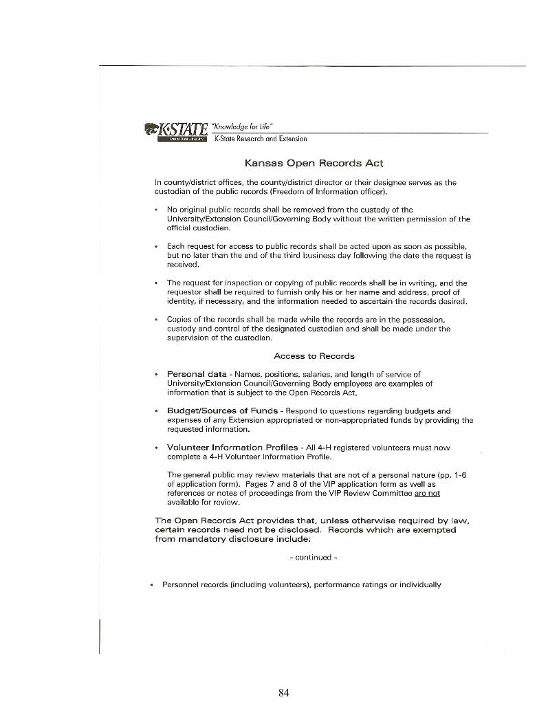
84

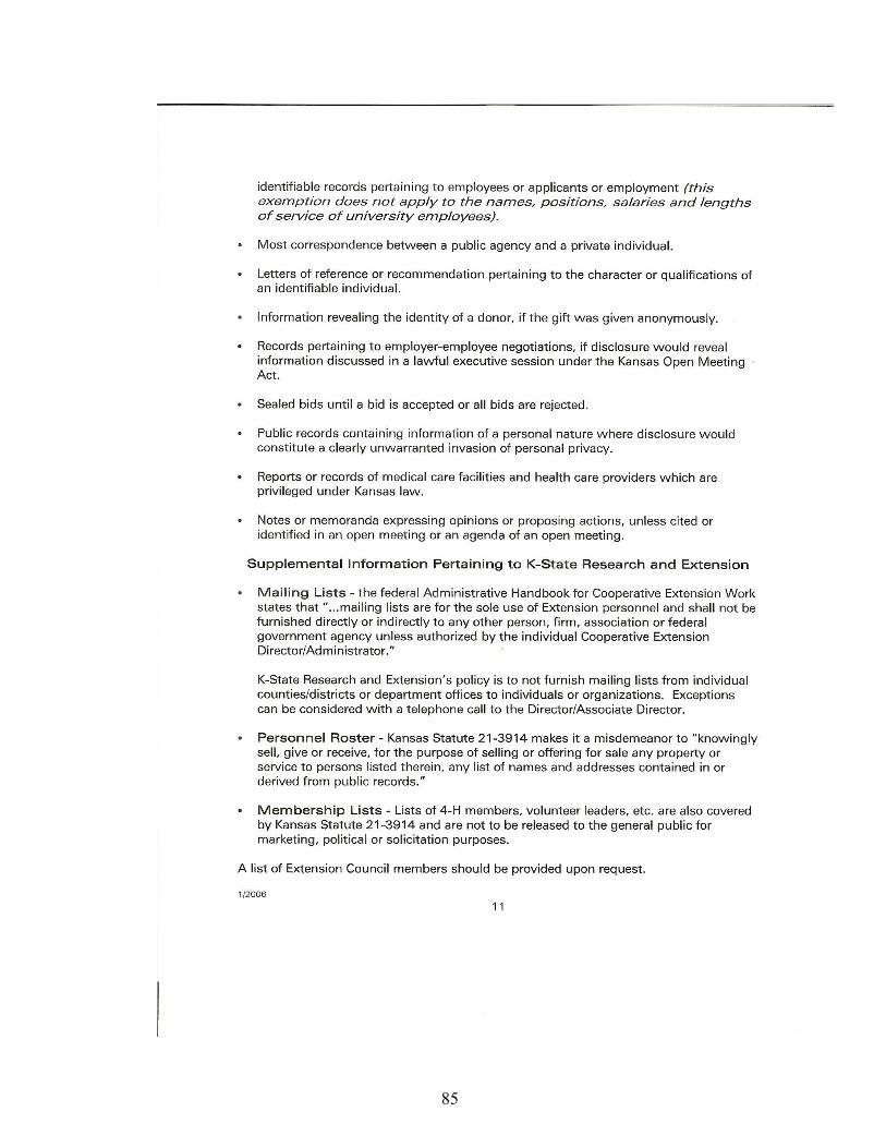
85

Appendix B

Table 2 Kansas County/District Extension Council Budgets for FY 2007

86

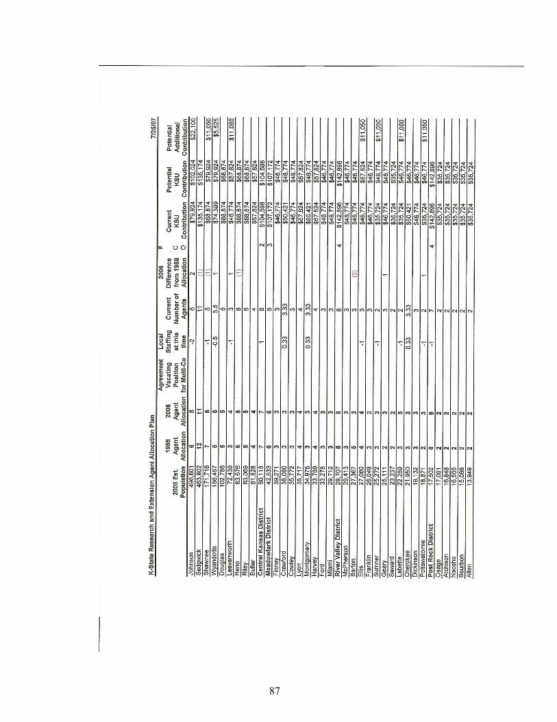
87

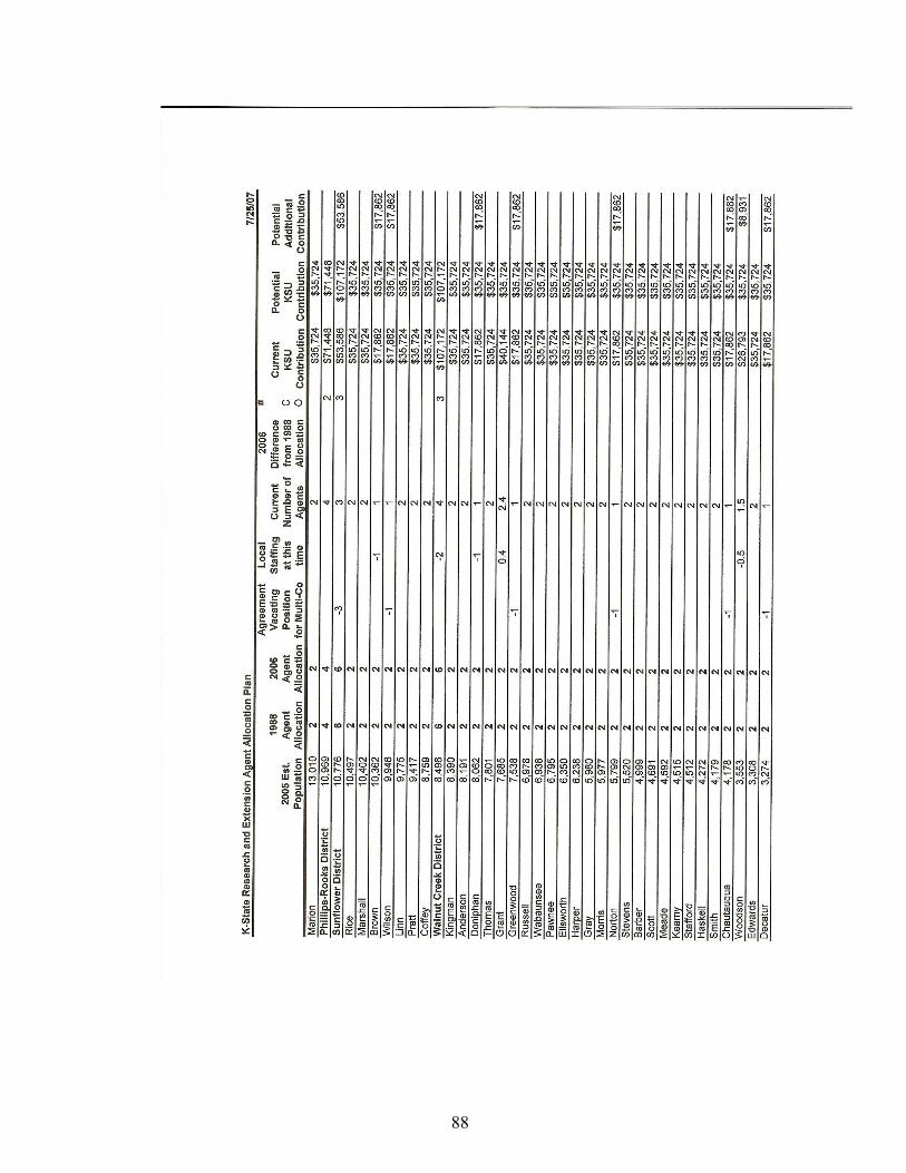
88

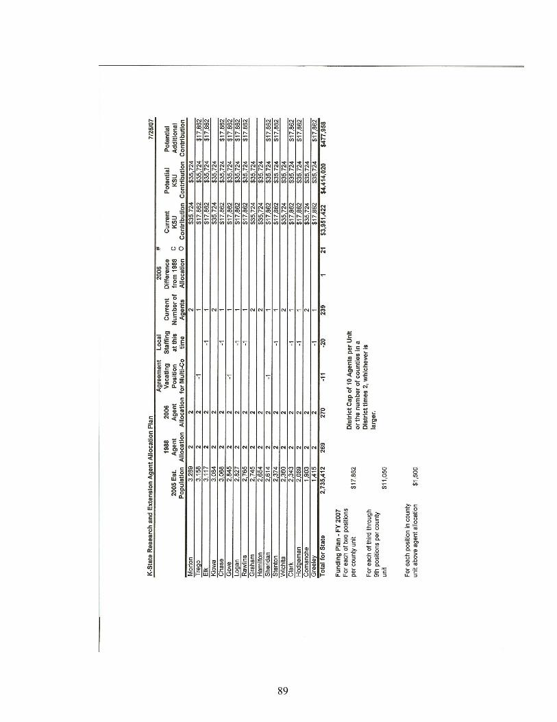
89