Factors affecting remotely sensed snow water equivalent uncertainty

www.elsevier.com/locate/rse

Remote Sensing of Environm

Factors affecting remotely sensed snow water equivalent uncertainty

Jiarui Donga,b,*, Jeffrey P. Walkerc, Paul R. Houserd

aHydrological Sciences Branch, NASA Goddard Space Flight Center, Code 974, Greenbelt, Maryland, 20771, USAbGoddard Earth Sciences and Technology Center, University of Maryland Baltimore Country, Baltimore, Maryland, 21250, USA

cDepartment of Civil and Environmental Engineering, The University of Melbourne, Parkville, Victoria, 3010 AustraliadGeorge Mason University & Center for Research on Environment and Water, Calverton, MD 20705-3106, USA

Received 22 October 2004; received in revised form 18 April 2005; accepted 24 April 2005

Abstract

State-of-the-art passive microwave remote sensing-based snow water equivalent (SWE) algorithms correct for factors believed to most

significantly affect retrieved SWE bias and uncertainty. For example, a recently developed semi-empirical SWE retrieval algorithm accounts

for systematic and random error caused by forest cover and snow morphology (crystal size — a function of location and time of year).

However, we have found that climate and land surface complexities lead to significant systematic and random error uncertainties in remotely

sensed SWE retrievals that are not included in current SWE estimation algorithms. Joint analysis of independent meteorological records,

ground SWE measurements, remotely sensed SWE estimates, and land surface characteristics have provided a unique look at the error

structure of these recently developed satellite SWE products. We considered satellite-derived SWE errors associated with the snow pack mass

itself, the distance to significant open water bodies, liquid water in the snow pack and/or morphology change due to melt and refreeze, forest

cover, snow class, and topographic factors such as large scale root mean square roughness and dominant aspect. Analysis of the nine-year

Scanning Multichannel Microwave Radiometer (SMMR) SWE data set was undertaken for Canada where many in-situ measurements are

available. It was found that for SMMR pixels with 5 or more ground stations available, the remote sensing product was generally unbiased

with a seasonal maximum 20 mm average root mean square error for SWE values less than 100 mm. For snow packs above 100 mm, the

SWE estimate bias was linearly related to the snow pack mass and the root mean square error increased to around 150 mm. Both the distance

to open water and average monthly mean air temperature were found to significantly influence the retrieved SWE product uncertainty. Apart

from maritime snow class, which had the greatest snow class affect on root mean square error and bias, all other factors showed little relation

to observed uncertainties. Eliminating the drop-in-the-bucket averaged gridded remote sensing SWE data within 200 km of open water

bodies, for monthly mean temperatures greater than �2 -C, and for snow packs greater than 100 mm, has resulted in a remotely sensed SWE

product that is useful for practical applications.

D 2005 Elsevier Inc. All rights reserved.

Keywords: Snow water equivalent (SWE); Scanning Multichannel Microwave Radiometer (SMMR); Error analysis; Uncertainty

1. Introduction

Snow cover plays an important role in governing global

energy and water budgets due to its high albedo, low thermal

conductivity, and considerable spatial and temporal varia-

bility (Cohen, 1994; Hall, 1998). Moreover, model simu-

lations demonstrate that local snow albedo feedbacks can

0034-4257/$ - see front matter D 2005 Elsevier Inc. All rights reserved.

doi:10.1016/j.rse.2005.04.010

* Corresponding author. Hydrological Sciences Branch, NASA Goddard

Space Flight Center, Code 974, Greenbelt, Maryland, 20771, USA.

E-mail address: [email protected] (J. Dong).

enhance the North American climate anomalies related to El

Nino-Southern Oscillation processes (Cohen & Entekhabi,

1999; Yang et al., 2001). Wintertime snow accumulation also

has important springtime soil moisture implications that

further enhance summer precipitation (Delworth & Manabe,

1998; Shukla & Mintz, 1982). Thus, accurate snow water

equivalent (SWE) knowledge is important for short-term

weather forecasts, climate change prediction, and hydrologic

extreme (drought and flood) forecasting.

Space-borne passive microwave remote sensors, such as

the ScanningMultichannel Microwave Radiometer (SMMR)

ent 97 (2005) 68 – 82

Table 1

J. Dong et al. / Remote Sensing of Environment 97 (2005) 68–82 69

launched in 1978, provide a capability to monitor global scale

SWE. Many investigators have carefully evaluated the

quality of SMMR-derived snow depth data, and suggested

good prairie region performance but poor boreal forest and

high latitude tundra region performance (e.g., Robinson et al.,

1993; Tait & Armstrong, 1996). To overcome these

limitations, Foster et al. (2005) derived an alternate algorithm

that made systematic error adjustments based on environ-

mental factors such as forest cover and snowmorphology (i.e.

crystal size as a function of location and time of year).

The forest cover impact on remotely sensed SWE

estimation is essentially a masking of the snow pack

microwave emission by coniferous vegetation canopy bio-

mass and the emission of vegetation canopy snow accumu-

lation (Chang et al., 1996; Hall et al., 2002). Moreover, snow

pack morphology affects the snow pack microwave emission

by changing the crystal sizes. The snow pack morphology is

strongly correlated with climate, and snow crystal size

changes caused by temperature and water vapor gradients

(Josberger & Mognard, 2002). Further, the wet snow micro-

wave response is distinctly higher than dry snow microwave

response for frequencies above 30 GHz, because water

droplets absorb and reemit rather than scatter microwave

radiation (Foster et al., 2005; Ulaby & Stiles, 1980). Previous

studies have also suggested that complex topography within a

large microwave footprint has a significant passive micro-

wave SWE retrieval influence because of the difficulty in

extracting snow signals (e.g., Matzler & Standley, 2000).

Understanding the retrieved SWE product uncertainty is

critical for its successful utilization. While Foster et al.

(2005) have developed an approach for quantitatively

estimating SWE retrieval uncertainty based on error

propagation theory, and have tested it with a Special Sensor

Microwave Imager (SSM/I) retrieval error assessment for

the period 1987 to present, the factors contributing to these

errors are only best-guess estimates. This study makes a

thorough uncertainty assessment of the Foster et al. (2005)

semi-empirical SWE retrieval algorithm, relative to Cana-

dian in-situ SWE measurements over the entire 9-year

SMMR data set. The SMMR data is used for this analysis

due to the greater SWE ground truth availability during that

time period. We consider satellite-derived SWE errors

associated with snow pack mass, distance to significant

open water bodies, liquid water in the snow pack and/or

morphology change due to melt and refreeze, forest cover,

snow class, and topographic factors such as large scale root

mean square roughness and dominant aspect.
Scanning Multifrequency Microwave Radiometer (SMMR) characteristics
Platform Nimbus-7

Period of operation October, 1978 to August, 1987

Data acquisition Every other day

Swath width 780 km

Frequency (GHz) 6.6, 10.7, 18.0, 21 and 37

Footprint resolution (km) 55�41 (18 GHz)

27�18 (37 GHz)

Polarization H and V

Orbital timing (equator crossing) Midday and midnight

2. Data

2.1. Passive microwave observations

There are currently several satellites that have made or

are making passive microwave measurements at SWE-

sensitive frequencies. These include: i) the Scanning Multi-

channel Microwave Radiometer (SMMR) which is an

imaging 5-frequency radiometer that was flown on the

Seasat and Nimbus-7 Earth satellites, providing observa-

tions from October 25, 1978 to August 20, 1987 (Table 1);

ii) the Special Sensor Microwave Imager (SSM/I) which is a

passive microwave radiometer flown aboard Defense

Meteorological Satellite Program (DMSP) satellites DMSP

F-8, F-10, F-11, F-12, and F-13, providing observations

from September 7, 1987 until present; and iii) the Advanced

Microwave Scanning Radiometer for the Earth observing

system (AMSR-E) which is a multi-frequency, dual-polar-

ized microwave radiometer flown aboard NASA’s Earth

Observing System (EOS) Aqua platform, providing obser-

vations from May 2002 until present. This paper focuses on

the 9-year SMMR data set that overlaps with more than

3000 Canadian SWE observation sites that are available

during the 1980s and early 1990s, of which 1400 sites have

at least 5 months of data for each winter season.

Several SWE estimation algorithms have been developed

for passive microwave observations. The commonly used

Chang et al. (1987) algorithm estimates SWE from the

SMMR 18 and 37 GHz or SSM/I 19 and 37 GHz brightness

temperature difference, multiplied by a constant derived

from radiative transfer theory. The 37 GHz data is sensitive

to snow pack scattering while the 18 GHz data is relatively

unaffected by snow. Foster et al. (2005) have modified this

algorithm using spatially and temporally varying constants

that account for forest cover fraction and snow crystal size

variations by

SWE ¼ F c T18 � T37ð Þ; ð1Þ

where F is the fractional forest cover factor calculated using

the International Geosphere-Biosphere Program (IGBP)

land cover map described by Loveland et al. (2000), and

c is parameterized according to the Sturm snow class

categories (Sturm et al., 1995) and time of year. T18 and T37

are the horizontally polarized brightness temperatures at 18

GHz and 37 GHz respectively. Daytime SMMR observa-

tions and T37 observations greater than 240 K were

excluded to minimize wet snow effects.

The SMMR instrument was cycled on and off every

other day due to spacecraft power limitations (Njoku, 1996),

decreasing the temporal resolution to more than 5 days.

Thus, SMMR 5-day composites include overlapping high

latitude observations and low latitude observation gaps. The

J. Dong et al. / Remote Sensing of Environment 97 (2005) 68–8270

recalibrated brightness temperature (Tb) data available for

this study were obtained from the National Snow and Ice

Data Center (NSIDC) Distributed Active Archive Center

(DAAC) at the University of Colorado (Njoku, 1996) and

had been processed onto a quarter-degree grid by using the

drop-in-the-bucket method. Overlapping data in cells from

different footprints on the same day were then averaged to

give a single brightness temperature, assumed to be located

at the center of the cell. Because SMMR footprint resolution

at 18 GHz is 55 by 41 km, which approximates to the half-

degree by half-degree resolution, it is more representative of

the actual footprint size by averaging this quarter-degree

data to half-degree. Fig. 1 shows an example of SMMR

SWE estimates when using the Foster et al. (2005)

algorithm for an individual 5-day nighttime composite.

These composites were derived by first calculating SWE

values for individual days and then averaging them over five

consecutive days, taking into account times and locations

where no data was observed.

2.2. In-situ snow observations

The Canadian Snow Water Equivalent Database (Brown,

1996) SWE estimates were derived from the Meteorological

Service of Canada (MSC) daily snow depth observation

network using an interpolated snow density from the snow

Fig. 1. An SMMR passive microwave SWE estimate for three consecutive nightti

the 5-day observation composite.

survey network specifically designed to represent local

terrain and vegetation. The resulting SWE estimates are

reported to effectively represent observed spatial and

temporal snow depth variability (Brown, 2000; Brown &

Braaten, 1998; Mote et al., 2003).

The Canadian snow observations are quite spatially

dense in the southern more populated regions and rather

sparse further to the north (Fig. 2). There are 3701 observing

stations with bi-weekly recordings from the mid-1950s to

the mid-1990s, with a pronounced active recording station

peak from 1980 to 1995. During the latter-half of the 1990s,

the number of active reporting stations declined by more

than 25% (Brown et al., 2003). The number of active

reporting stations is quite dynamic, making the observation

record length highly variable during the 1979 to 1987

SMMR timeframe. For example, 638 stations have no data,

and only 227 stations have complete data for the entire

SMMR time period (Fig. 2a). Different length in-situ station

records are combined to give an average SMMR SWE error

estimate over the observing interval, so it is important to

note that some results may be impacted by interannual

variability.

There is a recognized spatial discrepancy between the in-

situ observing station point measurements and the half-

degree by half-degree SMMR footprint (or pixel) SWE

estimates. Chang et al. (2005) suggested that 10 distributed

me overpasses on (a) March 1, (b) March 3, and (c) March 5, 1987, and (d)

Fig. 2. In-situ SWE spatial and temporal station characteristics: (a) data set

length during the 1979 to 1987 period — the numbers in the color bar show

how many stations have the indicated data length; (b) number of stations in

each half-degree grid cell — numbers in the color bar show the number of

grid cells with the indicated number of stations; (c) the 1979 to 1987

average winter season in-situ SWE data averaged to half-degree grid cells.


snow depth measurements per one-degree by one-degree

grid cell are required to produce a sampling error of 5 cm or

better. To minimize this discrepancy, we average in-situ

station SWE measurements to half-degree by half-degree

(approximately 50 km by 35 km at 50-N) pixels, which

results in 1359 pixel averages with 1 or more stations and

802 pixel averages covering 1 or more years. The number of

observing stations available for each SMMR half-degree

pixel varied widely, ranging from 1 to 60 (Fig. 2b).

However, most SMMR pixels contain fewer than 5 stations,

with only 190 having more than 5 stations. Although

northern Canada has few stations, they still provide valuable

uncertainty information for a broader environmental con-

dition range. Fig. 2c shows the 1979 to 1987 average winter

season in-situ SWE data averaged to the half-degree pixels.

3. Error assessment

The SMMR retrieved SWE uncertainty relative to in-situ

observations is investigated using root mean square (RMS)

error, relative RMS (RRMS) error, bias (BIAS) and relative

bias (RBIAS) measures. The BIAS is defined as the

difference between satellite and in-situ data. The RRMS

and RBIAS are defined as the RMS or BIAS of a given half-

degree pixel divided by the pixel mean SWE across the

SMMR 9-year timeframe. These relative calculations are

made using both the SMMR (subscript SMMR) and in-situ

observations (subscript OBS) SWE estimates.

The error statistics are calculated for the 1359 half-degree

pixels with coincident ground truth observations, for the

winter seasons (November to April) during the period of

1979 to 1987. The left column in Fig. 3 shows the RMS

error statistics spatial distribution. The most eastern regions

and some mountainous areas show the largest RMS errors

with values above 200 mm. The west near-coastal regions

have very small RMS errors with values below 25 mm. This

is due to this region’s lower snow amounts, which is

illustrated by the RRMSOBS error statistic that normalizes

for mean ground SWE amounts. These errors are over 200%

in most west coast regions and some isolated east coast

locations; errors are also above 100% in most of south-

eastern Canada, particularly near the Great Lakes and in

western mountainous areas. There are similar patterns found

in the RRMSSMMR errors statistic, but the error values are

much larger due to the general SMMR SWE under-

estimation (Fig. 3e).

The right column in Fig. 3 shows the corresponding

winter average bias errors (BIAS, RBIASOBS and

RBIASSMMR) during the 1979 to 1987 period. Most regions

show a SMMR SWE underestimation, except for a few

prairie and taiga stations (refer to Fig. 5e) with over-

estimation of less than 20 mm. Similarly, most eastern

regions and some mountainous area SMMR SWE estimates

are biased high, with some areas having more than a 50 mm

underestimation (Fig. 3b). Both east and west near-coastal

regions and regions near the Great Lakes have very small

bias errors with values below 50 mm, but their relative

biases are large, with BIASOBS above 75% and BIASSMMR

above 500% underestimation (Fig. 3d and f). RMS error

estimates reflect both bias errors and random errors. Fig. 4a

shows that a large component of the RMS error is

contributed from bias, with most stations in the west

Fig. 3. Half-degree SMMR passive microwave SWE retrieval error statistics for pixels with coincident half-degree ground truth station data: (a) root mean

square (RMS) error, (b) bias (BIAS) error, (c) root mean square errors relative to the ground truth measurements (RRMSOBS), (d) bias errors relative to the

ground truth measurements (RBIASOBS), (e) root mean square errors relative the SMMR estimates (RRMSSMMR), and (f) bias errors relative to the SMMR

estimates (RBIASSMMR).


mountainous regions and east of 95-W having more than

70% contribution of bias to the RMS error. The bias

contributions are smaller on the west coast, east coast below

50-N, and most prairie regions.

To ascertain what might be contributing to the spatial

variability of SMMR SWE error, a comparative analysis with

several environmental variables was undertaken. The

obvious tendency for higher error near significant water

bodies shown in Fig. 3 results from free water molecules

significantly increasing the brightness temperature at 37

GHz by emission rather than microwave energy scattering

(Foster et al., 2005), which can produce significant retrieval

contamination more than 100 km from the water body due to

the footprint intersection or/and signal mixing (Bellerby et

al., 1998). Fig. 4b compares the SMMR SWE seasonal bias

with distance to the nearest five significant water bodies,

defined as oceans, the Great Lakes, small lakes, Hudson Bay

and water surrounding the northern Canadian islands.

Considering the effects from the projection distortion, the

distances to nearest water body (D in kilometers) is

calculated as:

D ¼ Rp180

�

ffiffiffiffiffiffiffiffiffiffiffiffiffiffiffiffiffiffiffiffiffiffiffiffiffiffiffiffiffiffiffiffiffiffiffiffiffiffiffiffiffiffiffiffiffiffiffiffiffiffiffiffiffiffiffiffiffiffiffiffiffiffiffiffiffiffiffiffiffiffiffiffiffiffiffiffiffiffiffiffiffiffiffiffiffiffiffiffiffiffiffiffiffiffiffiffiffiffiffiffiffiffiffiffiffiffiffiffiffiffiffiffiffiffiffiffiffiffiffiffiffiffiffiffiffiffiffiffiffiffiffiffiffiffiffiffiffiffiffiffiffiLonobs�Lonwaterð Þcos Latobs þ Latwater

2I

p180

� �� 2þ Latobs � Latwaterð Þ2

s;

ð2Þ

where R is the earth radius (6371 km), Latobs and Lonobsrepresents the latitude and longitude at each in-situ station

(in unit of degree), and Latwater and Lonwater represents the

Fig. 4. Key SMMR passive microwave SWE retrieval error characteristics relative to the in-situ SWE observations: (a) the bias error to RMS error ratio, (b)

mean bias of SWE relative to distance from five different water bodies, (c) comparison of monthly mean SWE from SMMR and station data for all ground truth

pixels with monthly mean air temperature above and below indicated thresholds, and (d) the mean biases (lines) and their standard deviations (bar) calculated

from the individual bias estimates of all pixels with a given number of stations.


latitude and longitude at the center of the nearest water pixel

(in unit of degree). Doing this analysis on a half-degree grid

may distort the results by up to a quarter-degree (half pixel),

which is from the water pixel centroid to land.

There was no obvious influence from the small inland

lakes and Hudson Bay, which likely results from their

freezing and becoming snow covered during the winter

months. In contrast, the SMMR SWE data showed

significant coastal region underestimation with the mean

bias reaching about 100 mm. This is because the oceans

freeze only at much colder temperatures, so they do not

become snow covered like the Hudson Bay and inland

lakes. The Great Lakes and water surrounding the northern

Canadian islands resulted in about 50 mm of under-

estimation. This intermediary level of bias may result from

late freezing in the Great Lakes and ice effects (see Grody

& Basist, 1997; West et al., 1996) in the north. Generally,

there is a large SWE bias for regions close to large open

water bodies.

Free water and ice interact with microwave energy very

differently from snow crystals (Derksen et al., 2000).

Therefore, we consider the potential for snowmelt, the

presence of liquid water in the snow pack, or the subsequent

snow pack refreezing, as inferred from daytime air temper-

ature. A gridded half-degree monthly mean and diurnal

range temperature product generated by interpolating

directly from station observations was used for this purpose

(New et al., 2000). Fig. 4c compares the seasonal SMMR

SWE variation with the in-situ observations for daytime air

temperatures above �2 -C and below �10 -C respectively,

to highlight two extreme temperature range effects. A close

agreement was found between the remotely sensed and in-

situ SWE for temperatures below �10 -C, with some deep

snow pack underestimation caused by passive microwave

signal saturation. However, for temperatures close to or

above freezing, there was a significant SMMR SWE

underestimation with the largest difference reaching 100

mm. This is largely because wet snow and refreezing ice

significantly raise the 37 GHz microwave brightness

temperature.

Finally, to ascertain the in-situ sampling density effect

within SMMR pixels, the mean bias errors and standard

deviation (calculated from the individual bias estimates of

all pixels with a given number of stations) have been plotted

against number of stations per pixel (Fig. 4d). The mean

bias is calculated as the average of bias estimates for all

pixels. The mean bias errors show the improvement from

more than 40 mm SWE underestimation for pixels with only

1 station to less than 30 mm SWE underestimation for pixels

with 5 or more stations, and the corresponding mean


standard deviations decrease from 80 to 45 mm. The most

likely reason for this improvement is that the increased

number of stations yields an areal average estimate that is

more compatible with the remote sensor. Therefore this

analysis separately plots data for pixels with 5 or more

stations.

These findings lay the foundation to explore the distance

from water, air temperature, and related environmental

factor impact on passive microwave SWE retrieval error.

Fig. 5. Spatial maps of the environmental variables used in the SMMR passive mic

distance to ocean water and Great Lakes-ice effects are considered for Hudson Ba

ground pixel root mean square roughness, (d) half-degree ground pixel fractional fo

in the satellite retrieval algorithm, and (f) half-degree dominant topographic aspe

4. Error exploration

4.1. Environmental factors

We have analyzed the potential passive microwave SWE

retrieval error contribution from many environmental

factors, including air temperature, distance to large open

water bodies, snow class, forest cover, and topographic

factors such as large-scale root mean square roughness and

rowave SWE retrieval error analysis: (a) average January air temperature, (b)

y and northern Canadian waterways due to winter freezing, (c) half-degree

rest cover used in the satellite retrieval algorithm, (e) Sturm snow class used

ct.


dominant aspect (Fig. 5). Air temperature and distance to

water were considered for the reasons outlined above. Snow

class and forest factor were considered as they are key

inputs to the SWE algorithm and have been previously

shown to impact SWE estimation accuracy (Matzler &

Standley, 2000). The snow class indicates snow crystal size

by climate and season, which controls the passive micro-

wave scattering signal emitted by the snow surface. The

forest factor indicates forest cover fraction, which can mask

the underlying snow pack microwave signal. Roughness

controls microwave signal scattering, but only large-scale

topographic roughness (rather than micro-roughness) was

considered because it was believed to be more relevant at

the passive microwave footprint scale, and because micro-

roughness information is not available. Topographic aspect

potentially interacts with the sensor’s incidence angle,

thereby masking the lee side of steep topography. The

SMMR sensor was forward looking with a 50.3- along

track incidence angle (Madrid, 1978), indicating that

northwest and southeast facing slopes are most likely to

have aspect-related errors, which are not considered by the

SMMR SWE retrieval algorithm. Because RMS error for a

given month in each pixel is calculated through a 9-year

period sampling, the large seasonal temperature variability

rather than the interannual variability is considered in the

error statistic calculation across the 9-year SMMR time

period. Fig. 5a shows an example of monthly (January)

average temperature data derived from the 1979 to 1987

station observations.

Based on the foregoing analysis, we treated the water

body effects on SWE passive microwave retrieval as follows

(Fig. 5b). For open water bodies such as the Great Lakes

and Oceans, distance to water is simply the distance to the

closest open water body due to their infrequent wintertime

freezing. Other water bodies were given the following

special treatment: i) small lakes are assumed frozen and

therefore are ignored; and ii) the effects of Hudson Bay and

northern Canadian waterways are considered to be moder-

ate, extending inland not more than 100 and 200 km

respectively due to their wintertime freezing. The oceans

show the most significant correlation with SWE retrieval

errors, showing 100 mm underestimates within 200 km and

dropping to about 30 mm underestimates beyond 500 km.

Large-scale roughness and aspect (Fig. 5c and f) were

derived at half-degree resolution based on the GTOPO30

global 30-s digital elevation model (Gesch & Larson, 1996).

Roughness was calculated as the root mean square of the

elevation difference relative to the mean pixel elevation, and

aspect was defined as the normal direction of the maximum

slope between a half-degree pixel and its eight neighbors for

elevation differences greater than 200 m.

Half-degree resolution IGBP forest fraction derived from

1 km satellite-based land cover data (Loveland et al., 2000)

were used to investigate the overlying forest canopy

masking effects on snow pack microwave emission (Fig.

5d). Forest fraction is the fraction of each half-degree pixel

area occupied by forest land covers (including broadleaf

forests, needleleaf forests, mixed forests, woodland, and half

the area covered by wooded grassland). Comparison of total

forest area estimates from inventory and remote sensing data

provides some confidence in the remotely sensed forest

fraction data (Dong et al., 2003).

The physically based Sturm et al. (1995) snow classi-

fication (Fig. 5e) differentiates snow packs based on typical

snow layer sequence, thickness, density, crystal morphology

and grain characteristics. The six resulting snow classes are

Tundra, Taiga, Prairie, Alpine, Maritime, and Ephemeral.

4.2. Effects of environmental factors

The relationship between the average winter season

RMS error and bias and the average monthly daytime

temperature, distance to water, RMS roughness, forest

fraction, snow class, aspect, and snow pack mass are

shown in Figs. 6 and 7. The errors relative to SMMR

estimates and ground observations are also shown. The

snow pack mass has a significant relationship with passive

microwave SWE estimate error, especially for SWE above

100 mm. Due to microwave signal saturation, the SMMR

SWE algorithm is unable to reliably retrieve SWE for snow

packs deeper than 150 mm, showing 100% relative RMS

errors (Fig. 6a) that mostly result from a relative 90% SWE

underestimation bias (Fig. 7a). However, RMS errors were

small when excluding SWE values greater than 100 mm,

with the relative SWE underestimation bias being reduced

to less than 70%. Most pixels with 5 or more in-situ stations

have SWE values less than 100 mm and show lower, nearly

unbiased RMS errors (crosses in Figs. 6 and 7). Therefore,

the sampling density has significant implications on the

comparison between in-situ and remotely-sensed SWE

observations.

There is an obvious nonlinear relationship between the

relative RMS (RRMSOBS) errors and both distance to water

and temperature (Fig. 6b3 and c3). Errors consistently

decrease for cold climate stations far from water, and

sharply increase for warm climate stations close to open

water.

Snow properties are season and climate dependent,

reflecting the temperature during and after accumulation,

the precipitation or condensation rate, and wind history

(Sturm et al., 1995). Therefore, air temperature is potentially

a major passive microwave SWE retrieval uncertainty

indicator. Air temperature changes will significantly influ-

ence snow structures (density and crystal size), and thus

alter the microwave emission. An air temperature close to or

above 0 -C is a good indicator of liquid water in the snow

pack, which dramatically reduces the snow pack’s micro-

wave volume scattering. Although the RMS error and bias

are lower than 50 mm (Figs. 6b and 7b), there are larger

relative RMS errors in these high temperature regions,

which are partly contributed from the increasing bias errors.

The mean relative bias underestimation increases from less


f1 f2 f3

g1 g2 g3

Fig. 6. SMMR passive microwave SWE retrieval root mean square (RMS) error (column 1), root mean square error relative to SMMR (RRMSSMMR) estimates

(column 2), and root mean square error relative to ground truth station (RRMSOBS) data (column 3), shown relative to the in-situ SWE estimates (row a),

average monthly daytime temperature (row b), ‘‘distance’’ to water (row c), RMS roughness (row d), forest fraction (row e), snow class (row f) and ground pixel

aspect (row g). The light grey dots show all the data and dark gray dots show the data remaining after omitting pixels closer than 200 km to water and with an

average monthly daytime temperature above �2 -C; the lines show the mean values respectively. The pluses represent data for pixels including 5 or more

ground stations and the ‘‘boxes’’ (rows f and g) show plus and minus one standard deviation.


than 10% at �20 -C to over 40% above 0 -C. Because the

SMMR SWE estimates derived for a melting snow pack are

significantly underestimated and generally unreliable, we

omit all data with a monthly daytime air temperature greater

than �2 -C. Pixels with 5 or more stations are generally

located in warm regions with mean temperatures above �10

-C. The randomly distributed relative bias at a range from 0

to 100% with nearly unbiased errors suggest that RMS

errors for these pixels mostly result from the seasonal snow

mass variability rather than the systematic bias between

pixel SMMR SWE estimates and in-situ point observations.

Large passive microwave SWE retrieval errors are found

within approximately 200 km of open water that decrease

with distance from water (Figs. 6c and 7c). At approx-

imately 200 km from open water, the SWE retrieval error

sharply decreases with only slight decreases beyond 200

km. As open water bodies are obviously severely contam-

inating the passive microwave, we omit all data within 200

km of significant open water bodies in our subsequent

analysis. Even after the temperature and distance to water

truncations, some larger RMS errors are still evident that we

speculate are related to mountainous terrain or inland lakes;

we have not attempted to remove these SMMR pixels from

this analysis.

SMMR SWE errors related to topographic roughness

and aspect are almost exclusively confined to the western

Canadian mountain areas, as the central and eastern

Canadian landscape is relatively flat (Fig. 5c and f). There

are slight increases in relative RMSOBS errors and relative

bias errors associated with increasing surface roughness

(Figs. 6d and 7d), but the RMS errors and bias do not

show any obvious trend, and the omitted data distribute

randomly in different roughness ranges. Generally, the

southerly and westerly facing slopes have slightly larger

RMS and bias errors than the northerly and easterly facing

slopes, with southwest facing slopes having the largest

error (mean RMS error above 100 mm and mean bias

about 90 mm underestimation). However, the relative RMS

and bias errors do not show much difference among

different aspects (Figs. 6g and 7g). As topographical

factors do not show obvious SMMR SWE retrieval

contamination, topographical correction is not pursued

further in this analysis.

After omitting data with large water and air temperature

related errors, relative SMMR SWE RMS and bias errors do

not show any obvious trend with increasing forest fraction

factor (Figs. 6e and 7e), but some stations with large forest

fraction do have large RMS errors and bias. Again the

omitted data distribute randomly amongst the different

forest fraction ranges. The lowest errors were found in the

Prairie snow class, with the largest mean error in the

Maritime class (Figs. 6f and 7f). It was observed that

Maritime class mean relative RMS and bias errors were

reduced by nearly 50% and 10% respectively after the water

a1 a2 a3

b1 b2 b3

c1 c2 c3

d3 d2 d3

e1 e2 e3

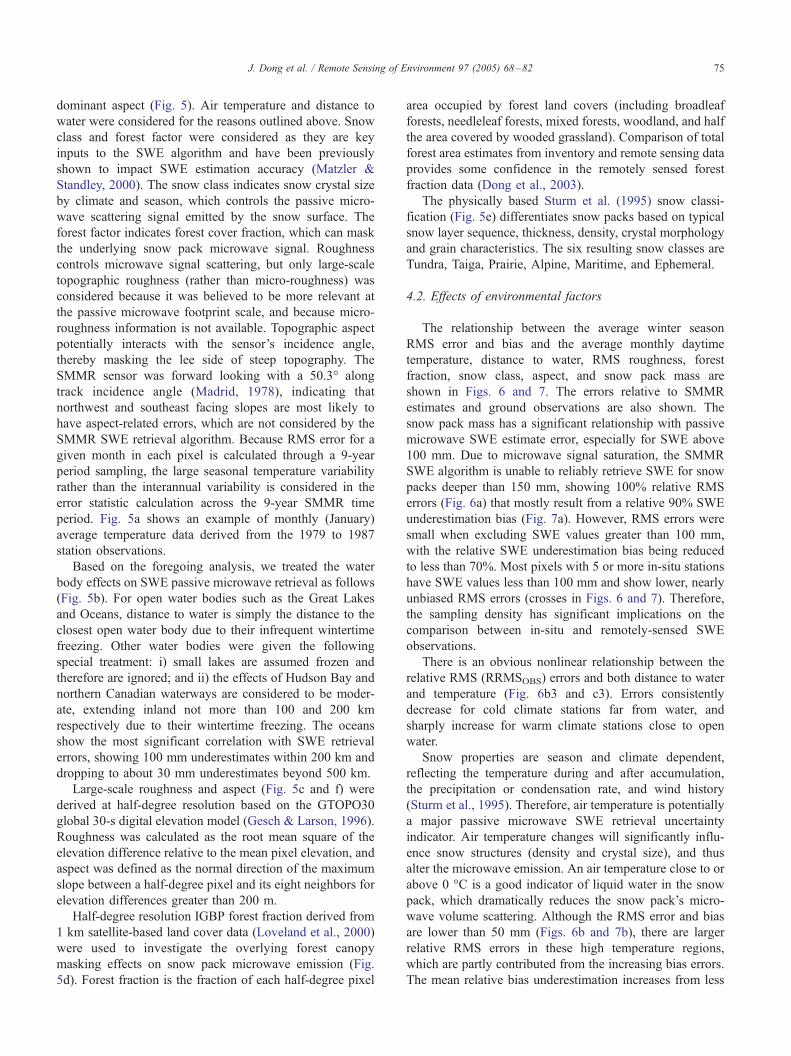
Fig. 7. As for Fig. 6 but for bias (SMMR-OBS) rather than RMS error.


f1 f2 f3

g3g2g1

Fig. 7 (continued).


and temperature related omissions, owing to the Maritime

class being in warmer climates near open water bodies (Fig.

5e). The errors from pixels with 5 or more in-situ stations

are randomly distributed beyond 200 km from the open

water and have different roughness and forest fractions

(Figs. 6c–e and 7c–e). Therefore, either the forest cover

and snow crystal size related SWE errors are small or are

mitigated by the Foster et al. (2005) retrieval algorithm, so

additional forest cover and snow crystal size corrections are

not considered.

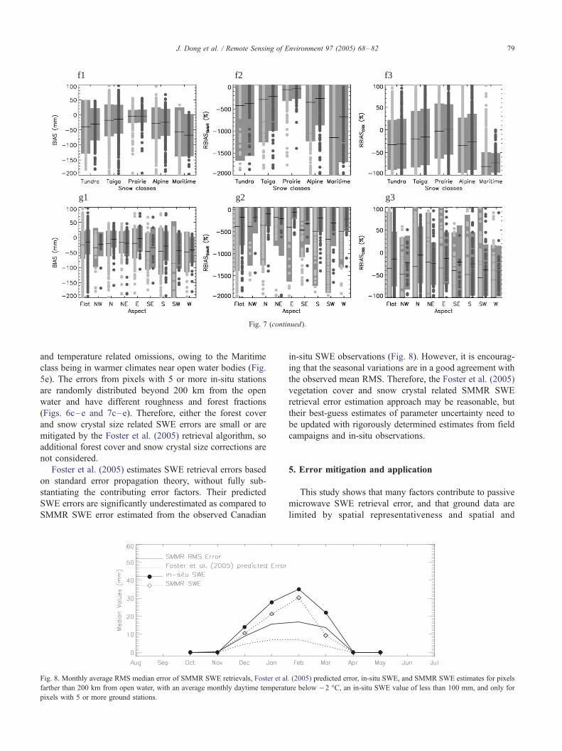
Foster et al. (2005) estimates SWE retrieval errors based

on standard error propagation theory, without fully sub-

stantiating the contributing error factors. Their predicted

SWE errors are significantly underestimated as compared to

SMMR SWE error estimated from the observed Canadian

Fig. 8. Monthly average RMS median error of SMMR SWE retrievals, Foster et al

farther than 200 km from open water, with an average monthly daytime temperat

pixels with 5 or more ground stations.

in-situ SWE observations (Fig. 8). However, it is encourag-

ing that the seasonal variations are in a good agreement with

the observed mean RMS. Therefore, the Foster et al. (2005)

vegetation cover and snow crystal related SMMR SWE

retrieval error estimation approach may be reasonable, but

their best-guess estimates of parameter uncertainty need to

be updated with rigorously determined estimates from field

campaigns and in-situ observations.

5. Error mitigation and application

This study shows that many factors contribute to passive

microwave SWE retrieval error, and that ground data are

limited by spatial representativeness and spatial and

. (2005) predicted error, in-situ SWE, and SMMR SWE estimates for pixels

ure below �2 -C, an in-situ SWE value of less than 100 mm, and only for


temporal availability. Thus remote sensing is the only

practical global SWE mapping solution. However, practical

SWE remote sensing application requires both a valid SWE

retrieval error estimate and acceptably low retrieval errors.

To eliminate the largest SMMR SWE errors, we propose

that retrievals should be omitted for i) regions within 200

km of significant open water bodies, ii) times when monthly

average air temperature is greater than �2 -C, and iii) times

and locations where SWE values are above 100 mm as the

SMMR SWE algorithm becomes insensitive. This results in

an unbiased SMMR SWE estimate whose RMS median

error varies through the season with a 20 mm seasonal

maximum when comparing pixels with 5 or more stations

(Fig. 8).

The monthly RMS median error of SMMR SWE

retrievals in Fig. 8 was obtained by first calculating the

RMS error in each pixel over the 9-year period and then

obtaining the median among the pixels including 5 or more

in-situ stations, while Foster et al. (2005) predicted errors

were based on standard error propagation theory with

empirically assigned contributing error factors for each ten

percentile of fractional forest cover and different snow

classes. The largely overlapping SMMR SWE and in-situ

SWE seasonal standard deviation ranges allow for the

filtered SMMR SWE estimate to be considered unbiased

(Table 2). The seasonally-varying SMMR SWE median

error is a function of the SMMR SWE algorithm’s reduced

sensitivity with increasing snowpack mass. While these

recommendations are specific to the Foster et al. (2005)

SMMR SWE retrieval, they may be generally applicable to

all passive microwave SWE estimates with revised distance

to water and temperature cut-off criteria.

Only omitting data within a narrow coastal region can

significantly reduce the errors in regions with temperature

above �10 -C, and only omitting data in regions with

temperature above �2 -C reduces the errors beyond the

coastal regions (Figs. 6b,c and 7b,c). By performing the two

omissions simultaneously, the relative errors related to other

environmental factors are reduced significantly (Figs. 6a3–

Table 2

Monthly average RMS median error and standard deviation of in-situ and

SMMR SWE estimates for pixels farther than 200 km from open water,

with an average monthly daytime temperature below �2 -C, an in-situ

SWE value of less than 100 mm, and only for pixels with 5 or more ground

stations (as used in Fig. 8)

Median values (mm) Standard deviation

In-situ SMMR In-situ SMMR

October 0.0 0.0 0.0 0.1

November 0.0 0.0 5.4 3.9

December 14.0 10.7 15.0 11.9

January 27.8 21.4 21.0 16.5

February 35.0 30.4 23.4 18.6

March 22.0 9.3 24.7 16.8

April 0.0 0.0 9.1 2.8

May 0.0 0.0 1.2 0.6

g3 and 7a3–g3). The relative RMS errors related to

roughness are reduced about 40%, including a 20%

reduction for the relative bias errors (Figs. 6d3 and 7d3).

The bias related to southwestern facing slopes is reduced

from a 90 mm underestimation to below 50 mm (Fig. 7g1),

and the bias related to forest fraction is reduced more than

20% (Fig. 7e1 and e3).

The SMMR SWE error related to open water contam-

ination was found to vary with distance from water, but

not with time. In contrast, SMMR SWE retrieval error

relative to air temperature was found to vary both spatially

and temporally. Fig. 9 shows how much SMMR data are

actually eliminated in order to mitigate the SMMR passive

microwave SWE retrieval error caused by distance to

water and monthly average daytime temperature. For each

pixel, we first consider the effect from open water and then

consider the effect from air temperature beyond the coastal

regions. Omitting SMMR SWE retrievals for regions

within 200 km of significant open water bodies results in

about 5% reduction of the SMMR data set with varying

fractions indicating different satellite tracks from month to

month. In practical applications, the actual monthly

average air temperature should be used. The omission of

SMMR SWE data for times when monthly average

daytime air temperature is above �2 -C significantly

reduces the SMMR data set coverage in early spring. With

the exception of coastal areas, reliable SMMR SWE

retrievals should be available for most regions in Novem-

ber, December, January, February, and March for most

years, with reduced areas in April, May, and October, and

also March in some years (e.g., in year 1980–1981) owing

to relatively high temperatures.

6. Conclusions

This study has used independent ground-based snow

water equivalent observations to investigate remotely sensed

passive microwave SWE estimation uncertainty related to

snow pack mass, distance to significant open water bodies,

daytime air temperature, forest cover, snow class, and

topographic roughness and aspect. The passive microwave

SWE retrieval error was dominated by the snow pack mass,

with secondary factors being the distance to open water and

air temperature. The SMMR SWE retrievals are sensitive to

mixed pixels that include unfrozen open water for distances

of up to 200 km from the open water. Daytime air

temperature above �2 -C were also found to be related to

satellite SWE retrieval uncertainty due to physical warm

condition snow pack structure and crystal size changes and

the presence of liquid water in the snow pack. Apart from

the maritime snow class, the other environmental variables

assessed had only slight relationships with satellite SWE

retrieval uncertainty. Omitting the drop-in-the-bucket aver-

aged gridded SMMR SWE retrievals for regions within 200

km of significant open water bodies, air temperatures above

Fig. 9. Fraction of SMMR SWE retrievals eliminated in snow season (October to May) from 1979 to 1987 for regions within 200 km of significant water

bodies (dark shading), and times when monthly average daytime air temperature is greater than �2 -C (light shading).


�2 -C, and SWE values above 100 mm, results in an

unbiased SWE estimate with seasonal maximum 20 mm

RMS median error when comparing pixels with 5 or more

stations. Imposing these rules on the SMMR SWE product

makes it useful for practical applications.

Acknowledgements

The authors wish to thank Jim Foster, Richard Kelly, and

Hugh Powell for helpful discussions during the course of

this work. This work was funded by the National


Aeronautics and Space Administration Earth Observing

System Interdisciplinary Science (NASA EOS/IDS) Pro-

gram NRA-99-OES-04.

References

Bellerby, T., Taberner, M., Wilmshurst, A., Beaumont, M., Barrett, E.,

Scott, J., et al. (1998). Retrieval of land and sea brightness temperatures

from mixed coastal pixels in passive microwave data. IEEE Trans-

actions on Geoscience and Remote Sensing, 36(6), 1844–1851.

Brown, R. D. (1996). Evaluation of methods for climatological reconstruc-

tion of snow depth and snow cover duration at Canadian meteorological

stations. Proc. Eastern Snow Conf., 53d Annual Meeting (pp. 55–65)

Williamsburg, VA.

Brown, R. D. (2000). Northern hemisphere snow cover variability and

change, 1915–97. Journal of Climate, 13, 2339–2355.

Brown, R. D., & Braaten, R. O. (1998). Spatial and temporal variability of

Canadian monthly snow depths, 1946–1995. Atmosphere-Ocean,

36(1), 37–54.

Brown, R. D., Brasnett, B., & Robinson, D. (2003). Gridded North

American monthly snow depth and snow water equivalent for GCM

evaluation. Atmosphere-Ocean, 41(1), 1–14.

Chang, A. T. C., Foster, J. L., & Hall, D. K. (1996). Effects of forest on

the snow parameters derived from microwave measurements during

the BOREAS winter field experiment. Hydrological Processes, 10,

1565–1574.

Chang, A. T. C., Foster, J. L., & Hall, D. K. (1987). Nimbus-7 derived

global snow cover parameters. Annals of Glaciology, 9, 39–44.

Chang, A. T. C., Kelly, R. E., Josberger, E. G., Armstrong, R. L., Foster,

J. L., & Mognard, N. M. (2005). Analysis of ground-measured and

passive-microwave-derived snow depth variations in midwinter across

the northern Great Plains. Journal of Hydrometeorology, 6(1), 20–33.

Cohen, J. (1994). Snow cover and climate. Weather, 49, 150–155.

Cohen, J., & Entekhabi, D. (1999). Eurasian snow cover variability and

Northern Hemisphere climate predictability. Geophysical Research

Letters, 26, 345–348.

Delworth, T. L., & Manabe, S. (1998). The influence of potential

evaporation on variabilities of simulated soil wetness and climate.

Journal of Climate, 1, 523–547.

Derksen, C., LeDrew, E., Walker, A., & Goodison, B. (2000). The influence

of sensor overpass time on passive microwave retrieval of snow cover

parameters. Remote Sensing of Environment, 73(3), 297–308.

Dong, J., Kaufmann, R. K., Myneni, R. B., Tucker, C. J., Kauppi, P. E.,

Liski, J., et al. (2003). Remote sensing of boreal and temperate forest

woody biomass: Carbon pools, sources and sinks. Remote Sensing of

Environment, 84, 393–410.

Foster, J. L., Sun, C., Walker, J. P., Kelly, R. E. J., Chang, A. T. C., Dong,

J., et al. (2005). Quantify the uncertainty in passive microwave snow

water equivalent observations. Remote Sensing of Environment, 94(2),

187–203.

Gesch, D. B., & Larson, K. S. (1996). Techniques for development of

global 1-kilometer digital elevation models. Pecora thirteen, human

interactions with the environment-perspectives from space (pp. 677–

703). South Dakota’ Sioux Falls.

Grody, N. C., & Basist, A. N. (1997). Interpretation of SSM/I measure-

ments over Greenland. IEEE Transactions on Geoscience and Remote

Sensing, 35, 360–366.

Hall, D. K. (1998). Remote sensing of snow and ice using imaging radar.

Manual of remote sensing (3rd edition) (pp. 677–703). Falls Church,

VA’ American Society for Photogrammetry and Remote Sensing.

Hall, D. K., Kelly, R. E. J., Riggs, G. A., Chang, A. T. C., & Foster, J. L.

(2002). Assessment of the relative accuracy of hemispheric-scale snow-

cover maps. Annals of Glaciology, 34, 24–30.

Josberger, E. G., & Mognard, N. M. (2002). A passive microwave snow

depth algorithm with a proxy for snow metamorphism. Hydrological

Processes, 16, 1557–1568.

Loveland, T. R., Reed, B. C., Brown, J. F., Ohler, D. O., Zhu, J., Yang, L.,

et al. (2000). Development of a global land cover characteristics dataset.

International Journal of Remote Sensing, 21, 1303–1330.

Madrid, C. R. (1978). The Nimbus 7 user’s guide, Landsat/Nimbus project.

Greenbelt, MD, USA’ Goddard Space Flight Center.

Matzler, C., & Standley, A. (2000). Relief effects for passive micro-

wave remote sensing. International Journal of Remote Sensing, 21,

2403–2412.

Mote, T. L., Grundstein, A. J., Leathers, D. J., & Robinson, D. A. (2003). A

comparison of modeled, remotely sensed, and measured snow water

equivalent in the northern Great Plains. Water Resource Research,

39(8), 1209.

New, M., Hulme, M., & Jones, P. (2000). Representing twentieth-century

space-time climate variability: Part II. Development of 1901–96

monthly grids of terrestrial surface climate. Journal of Climate,

13(13), 2217–2238.

Njoku, E. (1996). Nimbus-7 SMMR pathfinder brightness temperatures.

Boulder, CO’ National Snow and Ice Data Center.

Robinson, D. A., Dewey, K. F., & Heim, R. R. (1993). Global snow cover

monitoring: An update. Bulletin of American Meteorological Society,

74, 1689–1696.

Shukla, J., & Mintz, Y. (1982). The influence of land-surface evapotranspi-

ration on the earth’s climate. Science, 214, 1498–1501.

Sturm, M., Holmgren, J., & Liston, G. E. (1995). A seasonal snow cover

classification system for local to regional applications. Journal of

Climate, 8, 1261–1283.

Tait, A., & Armstrong, R. (1996). Evaluation of SMMR satellite-derived

snow depth using ground-based measurements. International Journal of

Remote Sensing, 17, 657–665.

Ulaby, F. T., & Stiles, W. H. (1980). Microwave radiometric observations of

snow packs, NASA CP-2153. NASA workshop on the microwave

remote sensing of snow pack properties (pp. 187–201). Ft. Collins, CO.

West, R. D., Winebrenner, D. P., Tsang, L., & Rott, H. (1996). Microwave

emission from density-stratified Antarctic firn at 6 cm wavelength.

Journal of Glaciology, 42, 63–76.

Yang, F., Kumar, A., Wang, W., Juang, H. H., & Kanamitsu, M. (2001).

Snow-albedo feedback and seasonal climate variability over North

America. Journal of Climate, 14, 4245–4248.

Factors affecting remotely sensed snow water equivalent uncertainty

Documents