Spatial interpolation of snow water equivalency using surface observations and remotely sensed images of snow-covered area

HYDROLOGICAL PROCESSESHydrol. Process. 24, 1285–1295 (2010)Published online 26 January 2010 in Wiley InterScience(www.interscience.wiley.com) DOI: 10.1002/hyp.7590

Spatial interpolation of snow water equivalency using surfaceobservations and remotely sensed images

of snow-covered area

Brian J. Harshburger,* Karen S. Humes, Von P. Walden, Troy R. Blandford, Brandon C. Mooreand Raymond J. Dezzani

Department of Geography, University of Idaho, Moscow, ID 83844-3021, USA

Abstract:

As demand for water continues to escalate in the western Unites States, so does the need for accurate monitoring of thesnowpack in mountainous areas. In this study, we describe a simple methodology for generating gridded-estimates of snowwater equivalency (SWE) using both surface observations of SWE and remotely sensed estimates of snow-covered area (SCA).Multiple regression was used to quantify the relationship between physiographic variables (elevation, slope, aspect, clear-skysolar radiation, etc.) and SWE as measured at a number of sites in a mountainous basin in south-central Idaho (Big Wood RiverBasin). The elevation of the snowline, obtained from the SCA estimates, was used to constrain the predicted SWE values.The results from the analysis are encouraging and compare well to those found in previous studies, which often utilized moresophisticated spatial interpolation techniques. Cross-validation results indicate that the spatial interpolation method producesaccurate SWE estimates [mean R2 D 0Ð82, mean mean absolute error (MAE) D 4Ð34 cm, mean root mean squared error(RMSE) D 5Ð29 cm]. The basin examined in this study is typical of many mid-elevation mountainous basins throughout thewestern United States, in terms of the distribution of topographic variables, as well as the number and characteristics of sitesat which the necessary ground data are available. Thus, there is high potential for this methodology to be successfully appliedto other mountainous basins. Copyright 2010 John Wiley & Sons, Ltd.

KEY WORDS snow water equivalency; multivariate regression; snow-covered area; spatial distribution; water resources;forecasting

Received 3 July 2007; Accepted 20 November 2009

INTRODUCTION

In the mountainous regions of the western United States,approximately 50–70% of the annual precipitation fallsas snow during the winter season and contributes torunoff during the spring (Serreze et al., 1999). Conse-quently, knowledge of the magnitude of the seasonalsnowpack [snow water equivalency (SWE)] is importantin predicting water availability (runoff). In addition, spa-tially distributed (gridded) estimates of SWE are impor-tant because some areas (e.g. portions of watersheds)contribute more runoff than others (Balk and Elder,2000). These spatial estimates also serve as an importantinput for distributed, physically based snowmelt models(Bloschl et al., 1991; Luce et al., 1998).

Recent emphasis in snow distribution modelling hasfocussed on statistical relationships between snow proper-ties (i.e. depth and SWE) and terrain characteristics (Balkand Elder, 2000). Elevation, slope, aspect, and otherlandscape characteristics have been used successfully tomodel the spatial distribution of SWE (Woo and Marsh,1978; Elder et al., 1991). In recent decades, remote sens-ing has also been used to produce spatially distributed

* Correspondence to: Brian J. Harshburger, Department of Geography,University of Idaho, Moscow, ID 83844-3021, USA.E-mail: [email protected]

estimates of SWE (McManamon et al., 1993; Cline et al.,1998; Wilson et al., 1999; Mote et al., 2003). However,these estimates are often expensive, difficult to obtain,and are not suitable for operational use in mountainousterrain (Elder et al., 1998). The interpolation of ground-based point measurements, therefore, becomes necessaryto explain and understand the spatial distribution of SWE(Balk and Elder, 2000). This has led to the use of sta-tistical and/or geostatistical methods to generate spatiallydistributed values of SWE.

At present, the most widely used ground-based esti-mates of SWE come from snow course and SNOwpackTELemetry (SNOTEL) sites. Interpolated SWE values,using these data, have been obtained using multivariatelinear regression (Chang and Li, 2000) and by regress-ing SWE with elevation (Daly et al., 2000). These stud-ies, however, did not take into account the presence orabsence of snow cover, which can lead to interpolatedSWE values (>0) in areas where snow is non-existent.As a result, remotely sensed estimates of snow-coveredarea (SCA) have been used, along with simple regressiontechniques, to obtain gridded SWE estimates (Fassnachtet al., 2003; Molotch et al., 2004). There are two typesof SCA data products, fractional and binary. Fractionalmapping techniques used by Fassnacht et al. (2003) andMolotch et al. (2004) provide information regarding the

Copyright 2010 John Wiley & Sons, Ltd.

1286 B. J. HARSHBURGER ET AL.

percentage (ranging from 0% to 100%) of each pixel thatis covered with snow. Binary mapping techniques, on theother hand, use a set of thresholds to determine whethera pixel contains snow (SCA D 100%) or no snow (SCAD 0%) (Elder et al., 1998). Although fractional SCA dataare more desirable from a spatial resolution standpoint,binary data have been available on an operational basisfor a much longer time and have been more widely vali-dated. Salomonson and Appel (2004) developed a simpleregression approach for fractional snow products, whichwas ultimately used in version 5 of the Moderate reso-lution Imaging Spectroradiometer (MODIS) operationalsnow cover products released by the National Snow andIce Data Center (NSIDC) in 2007. These data, however,were not used in this study because the data had not yetbeen widely validated. We attempted to validate thesedata for our study area, however, found the data to beinconsistent and to contain undocumented values. Giventhe maturity of the fractional versus binary products atthis time, the priority in this study was the assessment ofa new methodology for the generation of spatially dis-tributed SWE estimates using binary SCA data.

In recent years, binary regression trees have beenused successfully to obtain interpolated SWE valuesfrom surface observations (Elder et al., 1998; Balk andElder, 2000; Erxleben et al., 2002; Winstral et al., 2002;Molotch et al., 2005; Molotch and Bales, 2006), however,this method requires large amounts of data and is bettersuited for small basins (Fassnacht et al., 2003).

Kriging and cokriging methods have also been usedsuccessfully to create spatially distributed SWE esti-mates (Carroll and Cressie, 1996; Ling et al., 1996;Erxleben et al., 2002; Molotch et al., 2005). In addition,these methods have been used to interpolate the residu-als obtained using other statistical techniques (Hosangand Dettwiler, 1991; Balk and Elder, 2000; Erxlebenet al., 2002; Molotch et al., 2005). Kriging and cokrig-ing methods, however, may be inappropriate if the data

(or residuals) lack spatial dependence (Balk and Elder,2000). Furthermore, it is often difficult to fit a suitablemodel (i.e. linear and Gaussian) to the semivariogram asa result of the temporal and spatial variability in SWEdata (Fassnacht et al., 2003).

The objective of the work presented here is to evaluatethe performance of a simple multiple linear regressiontechnique to generate gridded estimates of SWE, uti-lizing data products that are widely available for mostmountainous watersheds in the western United States(snow course and SNOTEL observations of SWE, binaryremotely sensed estimates of SCA, and physiographicvariables). Cross-validation is used to assess the modelperformance in an example watershed in the intermoun-tain west.

STUDY AREA

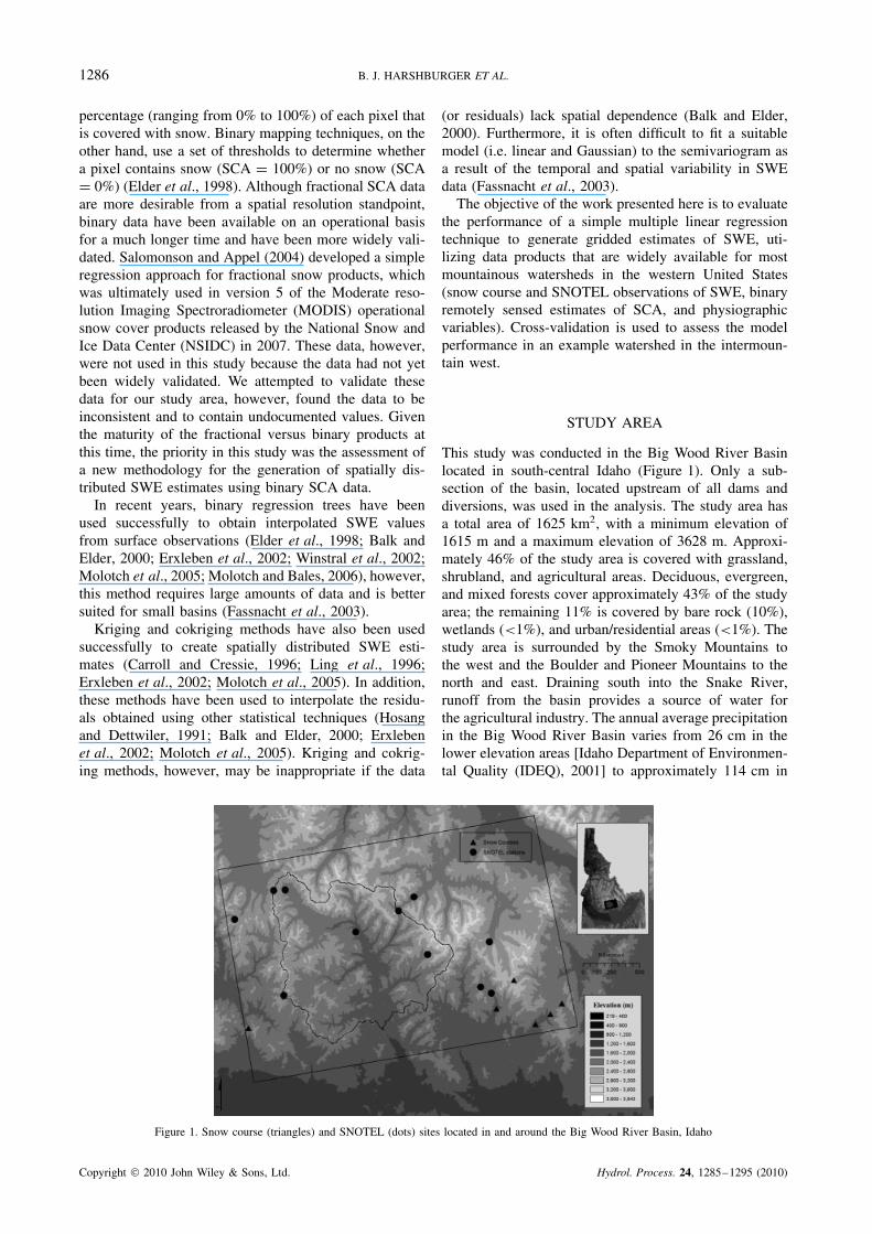
This study was conducted in the Big Wood River Basinlocated in south-central Idaho (Figure 1). Only a sub-section of the basin, located upstream of all dams anddiversions, was used in the analysis. The study area hasa total area of 1625 km2, with a minimum elevation of1615 m and a maximum elevation of 3628 m. Approxi-mately 46% of the study area is covered with grassland,shrubland, and agricultural areas. Deciduous, evergreen,and mixed forests cover approximately 43% of the studyarea; the remaining 11% is covered by bare rock (10%),wetlands (<1%), and urban/residential areas (<1%). Thestudy area is surrounded by the Smoky Mountains tothe west and the Boulder and Pioneer Mountains to thenorth and east. Draining south into the Snake River,runoff from the basin provides a source of water forthe agricultural industry. The annual average precipitationin the Big Wood River Basin varies from 26 cm in thelower elevation areas [Idaho Department of Environmen-tal Quality (IDEQ), 2001] to approximately 114 cm in

Figure 1. Snow course (triangles) and SNOTEL (dots) sites located in and around the Big Wood River Basin, Idaho

Copyright 2010 John Wiley & Sons, Ltd. Hydrol. Process. 24, 1285–1295 (2010)

SPATIAL INTERPOLATION OF SNOW WATER EQUIVALENCY 1287

the higher elevation areas. About 60% of the basin’s pre-cipitation comes in the form of snow during the monthsof November–March (IDEQ, 2001).

DATA

SWE data

The Natural Resources Conservation Service (NRCS)has conducted snow surveys in the western UnitedStates since 1935 (Chang and Li, 2000). Snow coursemeasurements are generally taken on or near the firstday of every month during the snow accumulation andmelt seasons (January–June). Measurements are takenmost frequently on March 1 and April 1, however, thefrequency of the measurements is influenced by thenature of the snowpack (snowpack condition), difficultyof access, and costs (e.g. labour, supplies, etc.). SWE dataare collected at snow courses using a snow tube and aresubjected to systematic bias because the measurementstend to underestimate SWE due to sampling difficultiesassociated with ice lenses, ground ice, and depth hoar(Carroll, 1987). The size of the sampling cutter can alsoinfluence accuracy (Goodison et al., 1981).

In 1977, the NRCS developed the SNOTEL data net-work. The SNOTEL network provides SWE measure-ments at 83 stations across the state of Idaho. Each SNO-TEL data station is equipped with automatic measuringand remote communication devices (Chang and Li, 2000).The SNOTEL network provides hourly data; however,daily SWE values were used in this study. In comparisonto snow course data, SNOTEL and SWE measurementsare obtained automatically using snow pillows (Johnsonand Schaefer, 2002; Johnson, 2004; Dressler et al., 2006).Snow pillows (typically 0Ð37 m2 in area) are envelopesof stainless steel or synthetic rubber (hypalon), whichcontain an antifreeze solution. As the snow accumulateson the pillow, pressure is exerted on the antifreeze solu-tion (caused by the weight of the overlying snowpack).Automatic measuring devices are then used to convertthe weight of the snowpack into an electrical readingof the SWE (Johnson and Schaefer, 2002). There areseveral sources of error in snow pillow measurements,however, most errors are generally attributed to snowbridging, which occurs when the snow over a snow pillowis partially or fully supported by the surrounding snow or,conversely, when the snow pillow supports some of theweight of the surrounding snow (Johnson and Schaefer,2002). In addition, errors are common during the transi-tion from subfreezing snow temperatures to an isothermalsnow cover with a temperature of 0 °C (CDWR, 1976;Johnson, 2004). The SNOTEL data, used in this study,are quality controlled, but there is no official estimate ofthe error by the NRCS. Consultation with snow surveypersonnel, familiar with the collection of data in Idaho,estimates the error at 6–8% of the measured SWE.

SWE data collected at 11 SNOTEL stations and 6 snowcourses, located within and around the study area, areused in this analysis (Figure 1). A list of the stations and

their attributes can be found in Table I. Stations wereselected to maximize at both the spatial and elevationalcoverage. SWE data collected on March 1 and April 1for 3 years (2003–2005) were used in the analysis. Thesedates (March 1 and April 1) were selected because snowcourse SWE measurements are usually taken on thesedates.

SCA data

The MOD10A1 operational MODIS daily snow coverproduct, obtained from the NSIDC, is used to constrainthe spatial interpolation of SWE to the boundary ofthe SCA. The MODIS acquires images in 36 spectralbands between 0Ð405 and 14Ð385 µm. In the MODISsnow mapping algorithm, snow is distinguished fromother surfaces using the normalized difference snowindex (NDSI) (Klein and Barnett, 2003). NDSI valuesare calculated using MODIS bands 4 (0Ð545–0Ð5Ð65 µm)and 6 (1Ð628–1Ð652 µm) from the following equation:

NDSI D(

�4 � �6

�4 C �6

)�1�

where �4 and �6 are reflectance values in bands 4 and 6.The MOD10A1 snow cover product is generated dailyfor most locations on the Earth’s surface at a spatialresolution of 500 m. SCA data are obtained for the samedates as the SWE data.

Table I. Attributes of the snow course and SNOTEL stations usedin the analysis. Stations are listed by elevation from lowest to

highest

Station Type Elevation(m)

Latitude(°N)

Longitude(°W)

Telfer Ranch Snow course 1780 43Ð53 113Ð77Iron Mine

CreekSnow course 1921 43Ð56 113Ð72

Muldoon Snow course 1927 43Ð57 113Ð91Chocolate

GulchSNOTEL 1963 43Ð77 114Ð42

Garfield R.S. SNOTEL 1999 43Ð61 113Ð93Couch

SummitSnow course 2085 43Ð52 114Ð80

Dry Fork Snow course 2201 43Ð58 113Ð68Stickney

MillSNOTEL 2265 43Ð86 114Ð21

GalenaPillow

SNOTEL 2268 43Ð88 114Ð67

Hyndman SNOTEL 2268 43Ð71 114Ð16Swede Peak SNOTEL 2329 43Ð62 113Ð97Bear Canyon SNOTEL 2408 43Ð74 113Ð94Lost-wood

DivideSNOTEL 2408 43Ð82 114Ð26

DollarhideSummit

SNOTEL 2566 43Ð60 114Ð67

GalenaSummit

SNOTEL 2676 43Ð87 114Ð71

Vienna Mine SNOTEL 2731 43Ð80 114Ð85Fishpole

LakeSnow course 2835 43Ð64 113Ð85

Copyright 2010 John Wiley & Sons, Ltd. Hydrol. Process. 24, 1285–1295 (2010)

1288 B. J. HARSHBURGER ET AL.

METHODS

The snowline elevation is determined using the MODISsnow cover grids and a digital elevation model (DEM).The DEM (30 m spatial resolution) was obtained fromthe United States Geological Survey (USGS). Since thesnowline elevation tends to be highly variable, the mediansnowline is used in this study. This methodology isconsistent with the World Meteorological Organization’s(WMO) definition, which states that the snowline is theelevation with approximately 50% snow coverage (Seidelet al., 1997; Kleindienst et al., 2000). To compute thesnowline elevation, the snow cover grid had to first beconverted to a point file. Each point then represents themiddle of each grid cell. The elevation for each pointwas then determined by sampling (overlaying) the DEM.Next, the snow cover point file was split into two separatepoint files, one for snow-covered points and the otherfor non-snow-covered points. A 600-m buffer was thencreated around each snow-covered point and all non-snow-covered points that fell within those buffers wereselected. This buffer size was selected because the snowcover imagery had a spatial resolution of 500 m and inorder to select adjacent cells the buffer size needed tobe larger than this value. Finally, the median snowlineelevation was determined using the elevations of thoseselected points. This method was used individually foreach snow cover image.

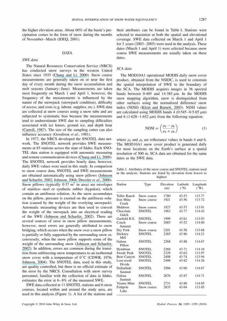
After the snowline elevation is determined, the SWEvalues are plotted against elevation. Linear regression isthen used to fit a line to the data, and the residuals areobtained. Figure 2 shows a sample regression fit for datafrom the Big Wood River Basin. This process is used toremove the elevation trend in the SWE data. The residualsare then tested for spatial dependence using Moran’s Ianalysis.

Moran’s I is one of the most common measures of spa-tial autocorrelation (dependence) and is used to describethe overall spatial relationship between individual sam-ples (Moran, 1950). Values for the Moran’s I typicallyvary between �1 and 1. A Z-value is calculated to deter-mine if the calculated I values are significant. Z valuesgreater than 1Ð96 indicate that there is significant clus-tering of the data (p D 0Ð05). On the other hand, valuesbelow �1Ð96 indicate that there is a uniform distribution(p D 0Ð05). Z values between �1Ð96 and 1Ð96 indicatethat there is a random distribution of values (completespatial randomness). For this analysis, inverse distanceweighting squared (IDW2) is used to determine the spa-tial weights for the Moran’s I analysis. Geoda, which is awidely used spatial statistics software program, was usedto calculate the Moran’s I values.

The results from the Moran’s I analysis (Table II)indicate that there was no significant spatial dependencein the residuals for any of the 6 days tested (i.e. completespatial randomness). As a result, spatial interpolationmethods that rely on spatial dependence in the sampledata (i.e. kriging, inverse distance weighting, etc.) werenot used to interpolate the residual values.

Due to the lack of spatial dependence in the detrendedresiduals, two regression equations were used to model

Table II. Results from the Moran’s I analysis for the 6 daysanalysed for the Big Wood Basin

Date Moran’s I Z value

1March 2003 �0Ð04 0Ð01 March 2004 �0Ð09 �0Ð21 March 2005 0Ð13 0Ð81 April 2003 �0Ð12 �0Ð11 April 2004 �0Ð55 �1Ð01 April 2005 0Ð21 0Ð8

Figure 2. Example plot of SWE values (snow course and SNOTEL) plotted versus elevation for the Big Wood River Basin

Copyright 2010 John Wiley & Sons, Ltd. Hydrol. Process. 24, 1285–1295 (2010)

SPATIAL INTERPOLATION OF SNOW WATER EQUIVALENCY 1289

the SWE values located above the snowline. Linearregression (elevation vs SWE) is used to estimate theSWE values between the snowline and the elevationof the station located directly above it. This step iscompleted to ensure that the interpolated SWE valuesapproach 0 cm at the snowline elevation. Stepwise mul-tivariate linear regression is then used to interpolatethe SWE values at elevations higher than the stationlocated directly above the snowline. The snowline wasnot included in the multivariate regression because it onlyhas one physiographic attribute, i.e. elevation. The step-wise multivariate linear regression was conducted usingSPSS, version 13Ð0.

The independent variables used in the multivariate lin-ear regression are: elevation, slope, degrees of northness

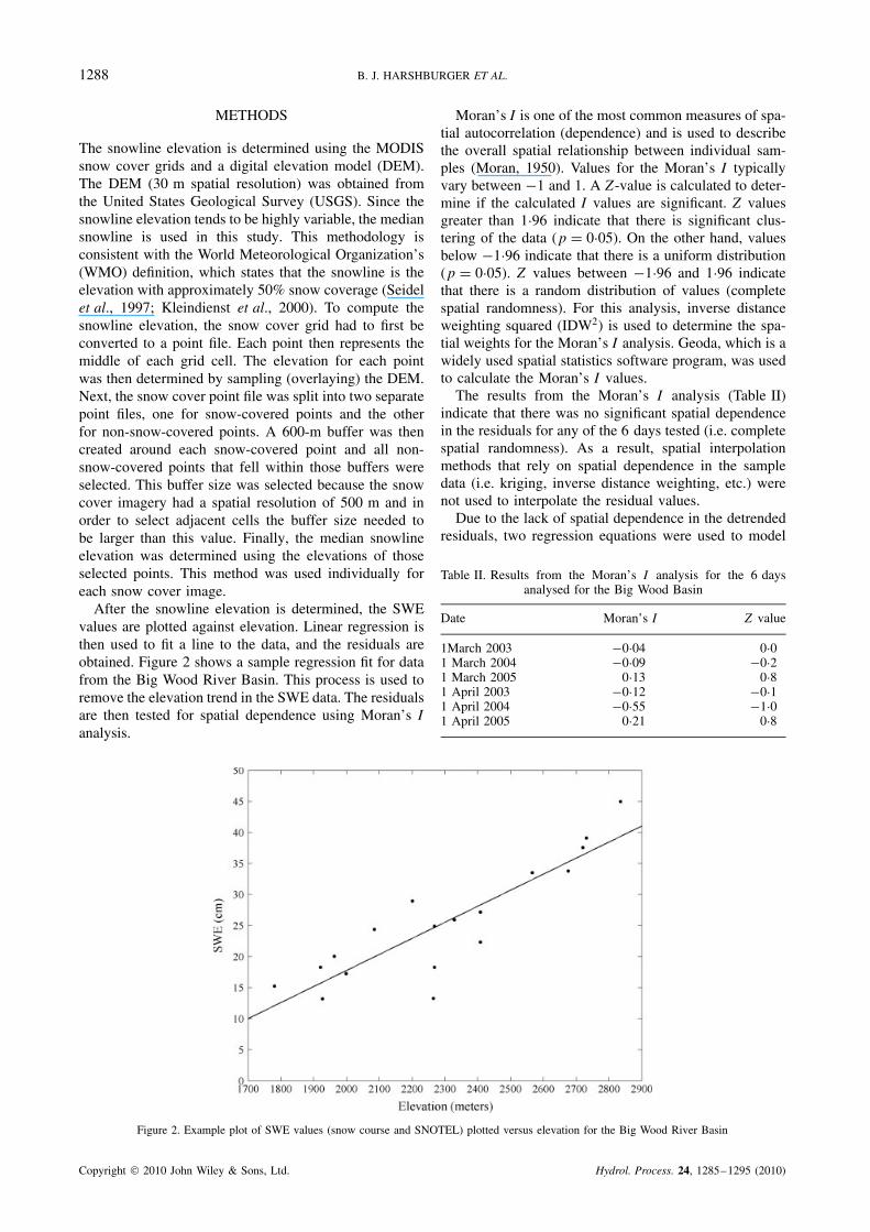
and eastness, ruggedness, latitude, longitude, clear-skysolar radiation, and vegetation cover type. Using ArcGIS9Ð0, the topographic variables, elevation (Figure 3a) andslope (Figure 3b), are obtained from the 30-m DEM. Inaddition to the elevation and slope, an aspect was alsoderived from the DEM and was used to compute thedegrees of northness and eastness. The degree of north-ness (Figure 3c) is defined as the cosine of the aspect.Values ranged from �1 to 1, with a value of �1 rep-resenting a slope facing directly south and a value of 1indicating a slope facing directly north. The degree ofeastness (Figure 3d) is defined as the sine of the aspect.Values also ranged from �1 to 1, with �1 represent-ing an east-facing slope and 1 signifying a west-facingslope.

Figure 3. Physiographic variables used in the multivariate linear regression analysis: (a) elevation (m), (b) slope (%), (c) degree of northness,(d) degree of eastness, (e) ruggedness, (f) clear-sky radiation index values, and (g) land cover

Copyright 2010 John Wiley & Sons, Ltd. Hydrol. Process. 24, 1285–1295 (2010)

1290 B. J. HARSHBURGER ET AL.

The ruggedness (Figure 3e) variable is defined as thestandard deviation of the elevation within a 0Ð21 km by0Ð21 km window. High ruggedness values are indicativeof areas with a large range in elevation. Small values arefound in areas where the elevation is relatively constant.

Clear-sky solar radiation is calculated using SolarAnalyst, which is an extension for ArcView 3Ð3. TheSolar Analyst generates an upward-looking hemisphericalviewshed (fisheye photograph) using 32 directions foreach location on a 30-m resolution DEM (Lewkowicz andEdnie, 2004). Merging the hemispherical viewsheds thatare calculated for each cell (on the DEM), Solar Analystproduces a clear-sky solar radiation density map (inMJ/m2). Average clear-sky solar radiation is calculatedfor each 30-m pixel located within the study area fromMarch 1 to April 1 for each of the 3 years used in theanalysis (Figure 3f). Finally, the values are convertedinto fractional values by dividing them by the maximumobserved clear-sky solar radiation value for that day.

The type of vegetation cover (Figure 3g) is obtainedfrom land cover data collected during the USGS NationalLand Cover Characterization Project (2001). These datawere collected across all the 50 states and Puerto Ricousing Landsat 5 and 7 data. For this study, the vegetationcover is classified as forested or non-forested becausethese were the dominant land cover types in the studyarea. A value of 1 was assigned to the forest-coveredpixels and a value of 0 was assigned to the non-forest-covered pixels.

Since a stepwise variable selection method was usedin the analysis, the variance inflation factor (VIF) wasused as a diagnostic tool to test for multicollinearity(Neter et al., 1996). The VIF measures the dependencebetween a predictor and the other independent variables(Helsel and Hirsch, 1992; Neter et al., 1996). A VIF scoregreater than 4 indicates that multicollinearity might be aproblem, however, serious problems exist when the VIFis greater than 10 (Neter et al., 1996). Additionally, acorrelation matrix (Table III) was constructed to assessthe dependence between the predictor variables. If theselected regression equation was found to violate themulticollinearity assumption then further analysis wouldbe necessary to determine which variables should beadded or removed from the equation. The residualsfrom each equation were also tested for normality. In

this study, however, the assumptions of collinearity andnormality were not violated.

Each of the steps described in the Section on Methodswas performed for each day separately. This is due to thefact that the snowline elevation changed from day to dayand the relationships between the independent variablesand dependent variable were not constant over time.

Cross-validation is used to compare the estimated(predicted) SWE values with the measured values. Thisis accomplished by removing each SWE data point andthen using the remaining observations to estimate thedata value. This procedure is repeated for every SWEobservation used to generate each multivariate linearregression equation. The predicted values were subtractedfrom the observed values to obtain the residuals. Theresulting residuals were then evaluated to assess theperformance of the models. The residuals from the cross-validation procedure were used to compute the meanMAE, root mean squared error (RMSE), and coefficientof determination (R2).

RESULTS AND DISCUSSION

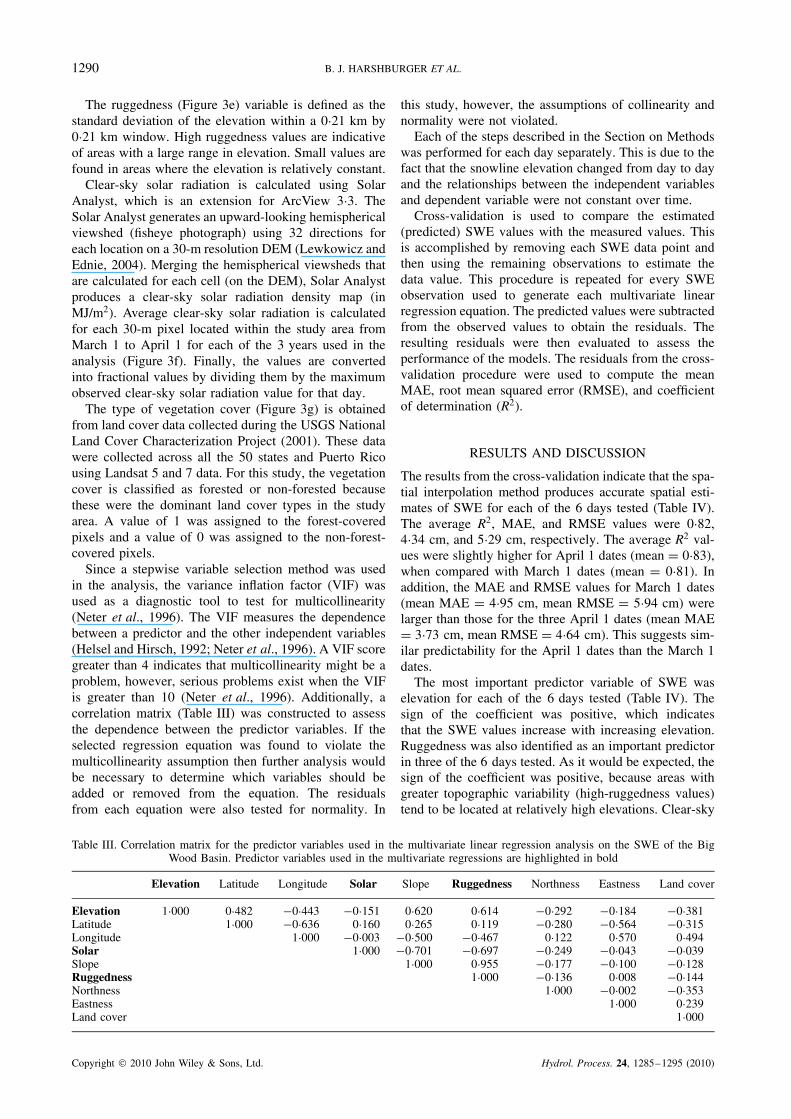
The results from the cross-validation indicate that the spa-tial interpolation method produces accurate spatial esti-mates of SWE for each of the 6 days tested (Table IV).The average R2, MAE, and RMSE values were 0Ð82,4Ð34 cm, and 5Ð29 cm, respectively. The average R2 val-ues were slightly higher for April 1 dates (mean D 0Ð83),when compared with March 1 dates (mean D 0Ð81). Inaddition, the MAE and RMSE values for March 1 dates(mean MAE D 4Ð95 cm, mean RMSE D 5Ð94 cm) werelarger than those for the three April 1 dates (mean MAED 3Ð73 cm, mean RMSE D 4Ð64 cm). This suggests sim-ilar predictability for the April 1 dates than the March 1dates.

The most important predictor variable of SWE waselevation for each of the 6 days tested (Table IV). Thesign of the coefficient was positive, which indicatesthat the SWE values increase with increasing elevation.Ruggedness was also identified as an important predictorin three of the 6 days tested. As it would be expected, thesign of the coefficient was positive, because areas withgreater topographic variability (high-ruggedness values)tend to be located at relatively high elevations. Clear-sky

Table III. Correlation matrix for the predictor variables used in the multivariate linear regression analysis on the SWE of the BigWood Basin. Predictor variables used in the multivariate regressions are highlighted in bold

Elevation Latitude Longitude Solar Slope Ruggedness Northness Eastness Land cover

Elevation 1Ð000 0Ð482 �0Ð443 �0Ð151 0Ð620 0Ð614 �0Ð292 �0Ð184 �0Ð381Latitude 1Ð000 �0Ð636 0Ð160 0Ð265 0Ð119 �0Ð280 �0Ð564 �0Ð315Longitude 1Ð000 �0Ð003 �0Ð500 �0Ð467 0Ð122 0Ð570 0Ð494Solar 1Ð000 �0Ð701 �0Ð697 �0Ð249 �0Ð043 �0Ð039Slope 1Ð000 0Ð955 �0Ð177 �0Ð100 �0Ð128Ruggedness 1Ð000 �0Ð136 0Ð008 �0Ð144Northness 1Ð000 �0Ð002 �0Ð353Eastness 1Ð000 0Ð239Land cover 1Ð000

Copyright 2010 John Wiley & Sons, Ltd. Hydrol. Process. 24, 1285–1295 (2010)

SPATIAL INTERPOLATION OF SNOW WATER EQUIVALENCY 1291

Table IV. Cross-validation results. N represents the number of stations used in each multivariate regression equation for the 6 daysanalysed for the Big Wood Basin. N/A is used to designate dates where the basin was determined to be 100% snow-covered using

the snow cover imagery

Date Snowlineelevation (m)

N R2 MAE (cm) RMSE (cm) Independent variablesand sign of coefficient

1 March 2003 1628 17 0Ð80 5Ð00 5Ð99 CElevation1 March 2004 N/A 17 0Ð91 4Ð45 5Ð14 CElevation, Cruggedness1 March 2005 N/A 17 0Ð71 5Ð39 6Ð70 CElevation1 April 2003 2011 12 0Ð90 4Ð35 5Ð28 CElevation, Cruggedness, �solar1 April 2004 2209 10 0Ð74 3Ð26 4Ð49 CElevation, Cruggedness1 April 2005 1956 14 0Ð86 3Ð59 4Ð14 CElevation

Figure 4. Gridded estimates of SWE (cm) for the Big Wood River Basin:(a) 1 March 2003 and (b) 1 April 2003

solar radiation was also identified as a predictor variablefor one of the days tested. The sign of the coefficientwas negative, which suggests that as the amount of solarradiation increased the amount of SWE decreased. Thisis because of the fact that incoming solar radiation isan important source of energy for melting the snowpack(Zuzel and Cox, 1975; Leavesley et al., 1983).

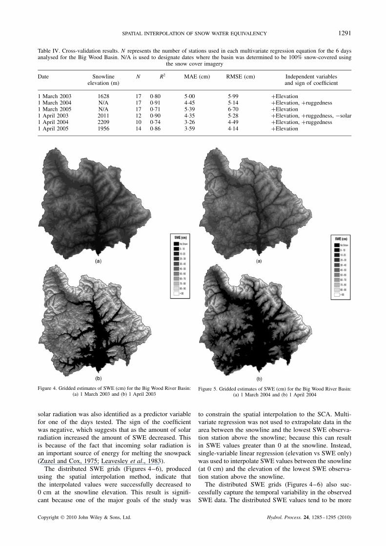
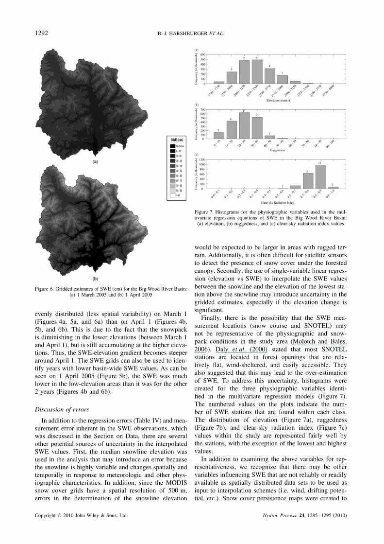
The distributed SWE grids (Figures 4–6), producedusing the spatial interpolation method, indicate thatthe interpolated values were successfully decreased to0 cm at the snowline elevation. This result is signifi-cant because one of the major goals of the study was

Figure 5. Gridded estimates of SWE (cm) for the Big Wood River Basin:(a) 1 March 2004 and (b) 1 April 2004

to constrain the spatial interpolation to the SCA. Multi-variate regression was not used to extrapolate data in thearea between the snowline and the lowest SWE observa-tion station above the snowline; because this can resultin SWE values greater than 0 at the snowline. Instead,single-variable linear regression (elevation vs SWE only)was used to interpolate SWE values between the snowline(at 0 cm) and the elevation of the lowest SWE observa-tion station above the snowline.

The distributed SWE grids (Figures 4–6) also suc-cessfully capture the temporal variability in the observedSWE data. The distributed SWE values tend to be more

Copyright 2010 John Wiley & Sons, Ltd. Hydrol. Process. 24, 1285–1295 (2010)

1292 B. J. HARSHBURGER ET AL.

Figure 6. Gridded estimates of SWE (cm) for the Big Wood River Basin:(a) 1 March 2005 and (b) 1 April 2005

evenly distributed (less spatial variability) on March 1(Figures 4a, 5a, and 6a) than on April 1 (Figures 4b,5b, and 6b). This is due to the fact that the snowpackis diminishing in the lower elevations (between March 1and April 1), but is still accumulating at the higher eleva-tions. Thus, the SWE-elevation gradient becomes steeperaround April 1. The SWE grids can also be used to iden-tify years with lower basin-wide SWE values. As can beseen on 1 April 2005 (Figure 5b), the SWE was muchlower in the low-elevation areas than it was for the other2 years (Figures 4b and 6b).

Discussion of errors

In addition to the regression errors (Table IV) and mea-surement error inherent in the SWE observations, whichwas discussed in the Section on Data, there are severalother potential sources of uncertainty in the interpolatedSWE values. First, the median snowline elevation wasused in the analysis that may introduce an error becausethe snowline is highly variable and changes spatially andtemporally in response to meteorologic and other phys-iographic characteristics. In addition, since the MODISsnow cover grids have a spatial resolution of 500 m,errors in the determination of the snowline elevation

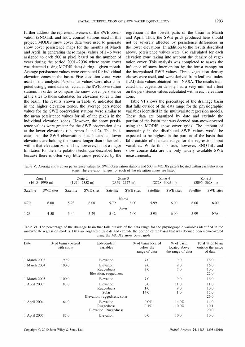
Figure 7. Histograms for the physiographic variables used in the mul-tivariate regression equations of SWE in the Big Wood River Basin:

(a) elevation, (b) ruggedness, and (c) clear-sky radiation index values

would be expected to be larger in areas with rugged ter-rain. Additionally, it is often difficult for satellite sensorsto detect the presence of snow cover under the forestedcanopy. Secondly, the use of single-variable linear regres-sion (elevation vs SWE) to interpolate the SWE valuesbetween the snowline and the elevation of the lowest sta-tion above the snowline may introduce uncertainty in thegridded estimates, especially if the elevation change issignificant.

Finally, there is the possibility that the SWE mea-surement locations (snow course and SNOTEL) maynot be representative of the physiographic and snow-pack conditions in the study area (Molotch and Bales,2006). Daly et al. (2000) stated that most SNOTELstations are located in forest openings that are rela-tively flat, wind-sheltered, and easily accessible. Theyalso suggested that this may lead to the over-estimationof SWE. To address this uncertainty, histograms werecreated for the three physiographic variables identi-fied in the multivariate regression models (Figure 7).The numbered values on the plots indicate the num-ber of SWE stations that are found within each class.The distribution of elevation (Figure 7a), ruggedness(Figure 7b), and clear-sky radiation index (Figure 7c)values within the study are represented fairly well bythe stations, with the exception of the lowest and highestvalues.

In addition to examining the above variables for rep-resentativeness, we recognize that there may be othervariables influencing SWE that are not reliably or readilyavailable as spatially distributed data sets to be used asinput to interpolation schemes (i.e. wind, drifting poten-tial, etc.). Snow cover persistence maps were created to

Copyright 2010 John Wiley & Sons, Ltd. Hydrol. Process. 24, 1285–1295 (2010)

SPATIAL INTERPOLATION OF SNOW WATER EQUIVALENCY 1293

further address the representativeness of the SWE obser-vation (SNOTEL and snow course) stations used in thisproject. MODIS snow cover data were used to generatesnow cover persistence maps for the months of Marchand April. In generating these maps, values of 1–6 wereassigned to each 500 m pixel based on the number ofyears during the period 2001–2006 where snow coverwas detected (using MODIS data) during a given month.Average persistence values were computed for individualelevation zones in the basin. Five elevation zones wereused in the analysis. Persistence values were also com-puted using ground data collected at the SWE observationstations in order to compare the snow cover persistenceat the sites to those calculated for elevation zones withinthe basin. The results, shown in Table V, indicated thatin the higher elevation zones, the average persistencevalues for the SWE observation stations were similar tothe mean persistence values for all of the pixels in theindividual elevation zones. However, the snow persis-tence values were greater for the SWE observation sitesat the lower elevations (i.e. zones 1 and 2). This indi-cates that the SWE observation sites located at lowerelevations are holding their snow longer than other cellswithin that elevation zone. This, however, is not a majorlimitation for the interpolation technique described herebecause there is often very little snow predicted by the

regression in the lowest parts of the basin in Marchand April. Thus, the SWE grids produced here shouldnot be severely affected by persistence differences inthe lower elevations. In addition to the results describedabove, persistence values were also calculated for eachelevation zone taking into account the density of vege-tation cover. This analysis was completed to assess theinfluence of snow interception by the forest canopy onthe interpolated SWE values. Three vegetation densityclasses were used, and were derived from leaf area index(LAI) data values obtained from NASA. The results indi-cated that vegetation density had a very minimal effecton the persistence values calculated within each elevationzone.

Table VI shows the percentage of the drainage basinthat falls outside of the data range for the physiographicvariables identified in the multivariate regression models.These data are organized by date and exclude theportion of the basin that was deemed non-snow-coveredusing the MODIS snow cover grids. The amount ofuncertainty in the distributed SWE values would beexpected to be highest in the portion of the basin thatfalls outside of the data range for the regression inputvariables. While this is true, however, SNOTEL andsnow course data are the only widely available SWEmeasurements.

Table V. Average snow cover persistence values for SWE observation stations and 500 m MODIS pixels located within each elevationzone. The elevation ranges for each of the elevation zones are listed

Zone 1(1615–1990 m)

Zone 2(1991–2358 m)

Zone 3(2359–2727 m)

Zone 4(2728–3095 m)

Zone 5(3096–3628 m)

Satellite SWE sites Satellite SWE sites Satellite SWE sites Satellite SWE sites Satellite SWE sites

March4Ð70 6Ð00 5Ð23 6Ð00 5Ð79 6Ð00 5Ð99 6Ð00 6Ð00 6Ð00

April

1Ð23 4Ð50 3Ð44 5Ð29 5Ð42 6Ð00 5Ð93 6Ð00 5Ð99 N/A

Table VI. The percentage of the drainage basin that falls outside of the data range for the physiographic variables identified in themultivariate regression models. Data are organized by date and exclude the portion of the basin that was deemed non-snow-covered

using the MODIS snow cover grids

Date % of basin coveredwith snow

Independentvariables

% of basin locatedbelow the

range of data

% of basinlocated above

the range of data

Total % of basinoutside the range

of data

1 March 2003 99Ð9 Elevation 7Ð0 9Ð0 16Ð01 March 2004 100Ð0 Elevation 7Ð0 9Ð0 16Ð0

Ruggedness 3Ð0 7Ð0 10Ð0Elevation, ruggedness 22Ð0

1 March 2005 100Ð0 Elevation 7Ð0 9Ð0 16Ð01 April 2003 83Ð0 Elevation 0Ð0 11Ð0 11Ð0

Ruggedness 1Ð0 9Ð0 10Ð0Solar 14Ð0 1Ð0 15Ð0

Elevation, ruggedness, solar 26Ð01 April 2004 64Ð0 Elevation 0Ð0% 14Ð0% 14Ð0

Ruggedness 0Ð1% 10Ð0% 10Ð1Elevation, Ruggedness 20Ð0

1 April 2005 87Ð0 Elevation 0Ð0 10Ð0 10Ð0

Copyright 2010 John Wiley & Sons, Ltd. Hydrol. Process. 24, 1285–1295 (2010)

1294 B. J. HARSHBURGER ET AL.

CONCLUSIONS

A new methodology was developed and tested for thecreation of gridded estimates of SWE using surface obser-vations (snow course and SNOTEL) and remotely sensedestimates of SCA. Although the methodology is rathersimple, the cross-validation results indicate that the spa-tial interpolation method produces accurate SWE esti-mates (mean R2 D 0Ð82, mean MAE D 4Ð34 cm, andmean RMSE D 5Ð29 cm). The regression model errors(MAE and RMSE) were smaller for the April 1 datesthan for the March 1 dates. Three predictor variableswere identified in the multivariate linear regression (ele-vation, ruggedness, and clear-sky solar radiation) withelevation being the most important. Visual inspection ofthe SWE grids indicates that the predicted SWE val-ues were successfully decreased to 0 cm at the snow-line elevation. Since the methodology is rather simple,and the results are similar to those found using moresophisticated spatial interpolation techniques, we believethat there is potential for this method to be success-fully applied to other mountainous basins in the west-ern United States. The simplicity of the methodologyshould also make it relatively easy for water managersand other operational forecasters (i.e. federal agencies) togenerate accurate gridded estimates of SWE in a timelymanner.

ACKNOWLEDGEMENTS

The authors thank the Natural Resources Conserva-tion Service, the National Snow and Ice Data Center,and NASA for providing us with the data required tocomplete this study. The authors thank Ryan Hruskafor downloading the snow cover data and provid-ing it to us. The authors also thank Devonee Harsh-burger for help in formatting the tables. This studywas supported by the Pacific Northwest Regional Col-laboratory as part of Raytheon Corporation’s Synergyproject, funded by NASA through NAS5-03098, TaskNo. 110.

REFERENCES

Balk B, Elder K. 2000. Combining binary recession-tree and geostatis-tical methods to estimate snow distribution in a mountain watershed.Water Resources Research 36: 13–26.

Bloschl G, Kirnbauer R, Gutknecht D. 1991. Distributed snowmeltsimulations in an alpine catchment. 2: parameter study and modelpredictions. Water Resources Research 27: 3181–3188.

Carroll T. 1987. Operational airborne measurements of snow waterequivalent and soil moisture using terrestrial gamma radiation inthe United States. In Large Scale Effects of Seasonal Snow Cover,Proceedings of the Vancouver Symposium , Goodison B, Barry R,Dozier J (eds). IAHS Publication no.166, 213–223.

Carroll SS, Cressie N. 1996. A comparison of geostatistical methodolo-gies used to estimate snow-water equivalent. Water Resources Bulletin32: 267–278.

CDWR. 1976. Snow Sensor Evaluation in the Sierra Nevada California .California Department of Water Resources, Division of Planning:Sacramento.

Chang K, Li Z. 2000. Modelling snow accumulation with a geographicinformation system. International Journal of Geographical InformationScience 14: 693–707.

Cline DW, Bales RC, Dozier J. 1998. Estimating the spatial distributionof snow in mountain basins using remote sensing and energy balancemodeling. Water Resources Research 34: 1275–1285.

Daly SF, Davis R, Ochs E, Pangburn T. 2000. An approach to spatiallydistributed snow modelling of the Sacramento and San Joaquin basins,California. Hydrological Processes 14: 3257–3271.

Dressler KA, Fassnacht SR, Bales RC. 2006. A comparison of snowtelemetry and snow course measurements in the Colorado River Basin.Journal of Hydrometeorology 7: 705–712.

Elder K, Dozier J, Michaelson J. 1991. Snow accumulation anddistribution in an alpine watershed. Water Resources Research 27:1541–1552.

Elder K, Rosenthal W, Davis RE. 1998. Estimating the spatialdistribution of snow water equivalence in a montane watershed.Hydrological Processes 12: 1793–1808.

Erxleben J, Elder K, Davis RE. 2002. Comparison of spatial interpolationmethods for estimating snow distribution in the Colorado RockyMountains. Hydrological Processes 16: 3627–3649.

Fassnacht SR, Dressler KA, Bales RC. 2003. Snow water equivalentinterpolation for the Colorado River Basin from snow telemetry(SNOTEL) data. Water Resources Research 39: 1208–1217. DOI:10.1029/2002WR001512.

Goodison BE, Ferguson HL, McKay GA. 1981. Measurement anddata analysis. In The Handbook of Snow: Principles, Processes,Management and Use, Gray DM, Male DH (eds). Pergamon Press:Toronto; 360–436.

Helsel DR, Hirsch RM. 1992. Statistical Methods in Water Resources .Elsevier Science: New York.

Hosang J, Dettwiler K. 1991. Evaluation of a water equivalent of snowcover map in a small catchment area using a geostatistical approach.Hydrological Processes 5: 283–290.

Idaho Department of Environmental Quality. 2001. The Big Wood RiverManagement Plan. IDEQ-State Office: Boise, Idaho.

Johnson JB. 2004. A theory of pressure sensor performance in snow.Hydrological Processes 18: 53–64. DOI: 10.1002/hyp.1310.

Johnson JB, Schaefer G. 2002. The influence of thermal, hydrologic,and snow deformation mechanisms on snow water equivalent pressuresensor accuracy. Hydrological Processes 16(18): 3529–3542. DOI:10.1002/hyp.1236.

Klein AG, Barnett AC. 2003. Validation of daily MODIS snow covermaps of the Upper Rio Grande River Basin for the 2000–2001 snowyear. Remote Sensing of Environment 86: 162–176.

Kleindienst H, Wunderle S, Voigt S. 2000. Snowline analysis in theSwiss Alps based on NOAA-AVHRR satellite data. Remote Sensing ofLand Ice and Snow (Proceedings of the EARSeL Workshop), Dresden,Germany; 297–307.

Leavesley GH, Lichty RW, Troutman BM, Saindon LG. 1983.Precipitation-Runoff Modeling System-Users Manual .

Lewkowicz AG, Ednie M. 2004. Probability mapping of mountainpermafrost using the BTS method, Wolf Creek, Yukon Territory,Canada. Permafrost and Periglacial Processes 15: 67–80.

Ling C, Josberger EG, Thorndike AS. 1996. Mesoscale variability of theupper Colorado River snowpack. Nordic Hydrology 27: 313–322.

Luce CH, Tarboton DG, Cooley KR. 1998. The influence of the spatialdistribution of snow on basin-averaged snowmelt. HydrologicalProcesses 12: 1671–1683.

McManamon A, Szeliga TL, Hartman RK, Day GN, Carroll TR. 1993.Gridded snow water equivalent estimation using ground-based andairborne snow data. Proceedings of the 61st Western Snow Conference,50th Eastern Snow Conference. Quebec city, Canada; 75–81.

Molotch NP, Bales RC. 2006. SNOTEL representativeness in the RioGrande headwaters on the basis of physiographics and remotely sensedsnow cover persistence. Hydrological Processes 20: 723–739. DOI:10.1002/hyp.6128.

Molotch NP, Colee MT, Bales RC, Dozier J. 2005. Estimating thespatial distribution of snow water equivalent in an alpine basinusing binary-regression tree models: the impact of digital elevationdata and independent variable selection. Hydrological Processes 19:1459–1479. DOI: 10.1002/hyp.5586.

Molotch NP, Fassnacht SR, Bales RC, Helfrich SR. 2004. Estimating thedistribution of snow water equivalent and snow extent beneath cloudcover in the Salt-Verde River basin, Arizona. Hydrological Processes18: 1595–1611.

Moran P. 1950. Notes on continuous stochastic phenomena. Biometrika37: 17–23.

Mote TL, Grundstein AJ, Leathers DJ, Robinson DA. 2003. A compari-son of modeled, remotely sensed, and measured snow water equivalentin the northern Great Plains. Water Resources Research 39: 1209.

Copyright 2010 John Wiley & Sons, Ltd. Hydrol. Process. 24, 1285–1295 (2010)

SPATIAL INTERPOLATION OF SNOW WATER EQUIVALENCY 1295

Neter J, Kutner MH, Nachtsheim CJ, Wasserman W. 1996. AppliedLinear Statistical Models . WCB McGraw-Hill: New York.

Salomonson VV, Appel I. 2004. Estimating fractional snow cover fromMODIS using the normalized difference snow index. Remote Sensingof Environment 89: 351–360.

Seidel K, Ehrler C, Martinec J, Turpin O. 1997. Derivation of statisticalsnowline from high-resolution snow cover mapping. In Remote Sensingof Land Ice and Snow (Proceedings of the EARSeL Workshop): Freiburg,Germany; 31–36.

Serreze MC, Clark MP, Armstrong RL, McGinnis DA, Pulwarty RS.1999. Characteristics of the western United States snowpack fromsnowpack telemetry (SNOTEL) data. Water Resources Research 35:2145–2160.

Wilson LL, Tsang L, Hwang JN. 1999. Mapping snow water equivalentby combining a spatially distributed snow hydrology model withpassive microwave remote-sensing data. IEEE Transactions onGeoscience and Remote Sensing 37: 690–704.

Winstral A, Elder K, Davis R. 2002. Spatial snow modeling ofwind-redistributed snow using terrain-based parameters. Journal ofHydrometeorology 3: 524–538.

Woo MK, Marsh P. 1978. Analysis of error in the determination of snowstorage for small high arctic basins. Journal of Applied Meteorology17: 1537–1541.

Zuzel JF, Cox LM. 1975. Relative importance of meteorologicalvariables in snowmelt. Water Resources Research 11: 174–176.

Copyright 2010 John Wiley & Sons, Ltd. Hydrol. Process. 24, 1285–1295 (2010)