F Universal quantum computers - Department of …mclennan/Classes/494-594-UC-F16/handouts/...F. UNIVERSAL QUANTUM COMPUTERS 169 F Universal quantum computers Hitherto we have used

F. UNIVERSAL QUANTUM COMPUTERS 169

F Universal quantum computers

Hitherto we have used a practical definition of universality: since conven-tional digital computers are implemented in terms of binary digital logic,we have taken the ability to implement binary digital logic as su�cient foruniversality. This leave open the question of the relation of quantum com-puters to the theoretical standard of computational universality: the Turingmachine. Therefore, a natural question is: What is the power of a quantumcomputer? Is it super-Turing or sub-Turing? Another question is: What isits e�ciency? Can it solve NP problems e�ciently? There are a numberof universal quantum computing models for both theoretical and practicalpurposes.

F.1 Feynman on quantum computation

F.1.a Simulating quantum systems

In 1982 Richard Feynman discussed what would be required to simulate aquantum mechanical system on a digital computer.22 First he considered aclassical probabilistic physical system. Suppose we want to use a conven-tional computer to calculate the probabilities as the system evolves in time.Further suppose that the system comprises R particles that are confined toN locations in space, and that each configuration c has a probability p(c).There are NR possible configurations, since a configuration assigns a locationN to each of the R particles (i.e., the number of functions R ! N). There-fore to simulate all the possibilities would require keeping track of a numberof quantities (the probabilities) that grows exponentially with the size of thesystem. This is infeasible.

So let’s take a weaker goal: we want a simulator that exhibits the sameprobabilistic behavior as the system. Our goal is that if we run both of themover and over, we will see the same distribution of behaviors. This we cando. You can implement this by having a nondeterministic computer that hasthe same state transition probabilities as the primary system.

Let’s try the same trick with quantum systems, that is, have a conven-tional computer that exhibits the same probabilities as the quantum system.If you do the math (which we won’t), it turns out that this is impossible.The reason is that, in e↵ect, some of the state transitions would have to have

22This section is based primarily on Feynman (1982).

170 CHAPTER III. QUANTUM COMPUTATION

510 Feynman

(a) NOT

O I

(b) CONTROLLED NOT o

b, b'

o o / o o o 1 / o l I O / l l ~ / ~ o

0, o 13 FAN OUT .I.

o ~[ 13

a ~ G' EXCHANGE b J( ~ ~( b'

(c) CONTROLLED CONTROLLED NOT

b' See Table I. c ~

Fig. 3. Reversible primitives.

Next is what we shall call the C O N T R O L L E D N O T (see Fig. 3b). There are two entering lines, a and b, and two exiting lines, a ' and b'. The a ' is always the same as a, which is the control line. If the control is activated a -= 1 then the out b' is the N O T of b. Otherwise b is unchanged, b ' = b . The table of values for input and output is given in Fig. 3. The action is reversed by simply repeating it.

The quantity b' is really a symmetric function of a and b called XOR, the exclusive or; a or b but not both. I t is likewise the sum modulo 2 of a and b, and can be used to compare a and b, giving a 1 as a signal that they are different. Please notice that this function XOR is itself not reversible. For example, if the value is zero we cannot tell whether it came from (a, b) = (0, 0) or from (1, 1) but we keep the other line a ' = a to resolve the ambiguity.

We will represent the C O N T R O L L E D N O T by putting a 0 on the control wire, connected with a vertical line to an X on the wire which is controlled.

This element can also supply us with FAN OUT, for if b = 0 we see that a is copied onto line b'. This COPY function will be important later on. It also supplies us with E X C H A N G E , for three of them used

a ..... o

b ,,, SUM

o ^ C A R R Y

Fig. 4. Adder. Figure III.38: Simple adder using reversible logic. [fig. from Feynman (1986)]

Quantum Mechanical Computers 511

0

b C

d=o '

A

C1

S I

~ C I . . . . . . (3 = 0 I s'- - - l - - - b b'

SUM c' CARRY = d'

Fig. 5. Full adder.

successively on a pair of lines, but with alternate choice for control line, accomplishes an exchange of the information on the lines (Fig. 3b).

It turns out that combinations of just these two elements alone are insufficient to accomplish arbitrary logical functions. Some element involving three lines is necessary. We have chosen what we can call the C O N T R O L L E D C O N T R O L L E D NOT. Here (see Fig. 3c) we have two control lines a, b, which appear unchanged in the output and which change the third line c to NOT c only if both lines are activated (a = 1 and b = 1). Otherwise c ' = c. If the third line input c is set to 0, then evidently it becomes 1 (c' = 1) only if both a and b are 1 and therefore supplies us with the AND function (see Table I).

Three combinations for (a, b), namely (0, 0), (0, 1), and (1, 0), all give the same value, 0, to the AND (a, b) function so the ambiguity requires two bits to resolve it. These are kept in the lines a, b in the output so the function can be reversed (by itself, in fact). The AND function is the carry bit for the sum of a and b.

From these elements it is known that any logical circuit can be put together by using them in combination, and in fact, computer science

Table I.

a b c o ' b ' ¢'

0 0 0 0 0 0 0 0 1 0 0 1 0 1 0 0 1 0 0 1 1 0 1 1 1 0 0 1 0 0 1 0 1 1 0 l 1 1 0 1 1 1 1 1 1 1 1 0

Figure III.39: Full adder using reversible logic. [fig. from Feynman (1986)]

what amount to negative probabilities, and we don’t know how to do thisclassically. We’ve seen how in quantum mechanics, probabilities can in e↵ectcancel by destructive interference of the wavefunctions. The conclusion isthat no conventional computer can e�ciently simulate a quantum computer.Therefore, if we want to (e�ciently) simulate any physical system, we needa quantum computer.

F.1.b Universal quantum computer

In 1985 Feynman described several possible designs for a universal quantumcomputer.23 He observes that NOT, CNOT, and CCNOT are su�cient forany logic gate, as well as for COPY and EXCHANGE, and therefore foruniversal computation. He exhibits circuits for a simple adder (Fig. III.38)and a full adder (Fig. III.39).

The goal is to construct a Hamiltonian to govern the operation of a quan-tum computer. Feynman describes quantum logic gates in terms of two prim-itive operations, which change the state of an “atom” (two-state system or“wire”). Letters near the beginning of the alphabet (a, b, c, . . .) are used for

23This section is based primarily on Feynman (1986).

F. UNIVERSAL QUANTUM COMPUTERS 171

data or register atoms, and those toward the end (p, q, r, . . .) for programatoms (which are used for sequencing operations). In this simple sequentialcomputer, only one program atom is set at a time.

For a single line a, the annihilation operator is defined:

a =

✓0 10 0

◆= |0ih1|.

The annihilator changes the state |1i to |0i; typically it lowers the energy ofa quantum system. Applied to |0i, it leaves the state unchanged and returnsthe zero vector 0 (which is not a meaningful quantum state). It matches|1i and resets it to |0i. The operation is not unitary (because not normpreserving). It is a “partial NOT” operation.

Its conjugate transpose it the creation operation:24

a⇤ =✓

0 01 0

◆= |1ih0|.

The creator transforms |0i to |1i, but leaves |1i alone, returning 0; typicallyis raises the energy of a quantum system. It matches |0i and sets it to |1i.This is the other half of NOT = a+ a⇤.

Feynman also defines a number operation or 1-test: Consider25

Na = a⇤a =

✓0 00 1

◆= |1ih1|.

This has the e↵ect of returning |1i for input |1i, but 0 for |0i:

Na = a⇤a = |1ih0| |0ih1| = |1ih0 | 0ih1| = |1ih1|.

Thus it’s a test for |1i. (This is a partial identity operation.)Similarly, the 0-test is defined:26

1 � Na = aa⇤ =✓

1 00 0

◆= |0ih0|.

24Note that Feynman uses a

⇤ for the adjoint (conjugate transpose) of a.25This matrix is not the same as that given in Feynman (1982, 1986), since Feynman

uses the basis |1i = (1, 0)T, |0i = (0, 1)T, whereas we use |0i = (1, 0)T and |1i = (0, 1)T.26This matrix is di↵erent from that given in Feynman (1982, 1986), as explained in the

previous footnote.

172 CHAPTER III. QUANTUM COMPUTATION

522 Feynman

There is no loss associated with the uncertainty of cursor energy; at least no loss depending on the number of calculational steps. Of course, if you want to do a ballistic calculation on a perfect machine, some energy would have to be put into the original wave, but that energy, of course, can be removed from the final wave when it comes out of the tail of the program line. All questions associated with the uncertainty of operators and the irreversibility of measurements are associated with the input and output functions.

No further limitations are generated by the quantum nature of the computer per se, nothing that is proportional to the number of com- putational steps.

In a machine such as this, there are very many other problems, due to imperfections. For example, in the registers for holding the data, there will be problems of cross-talk, interactions between one atom and another in that register, or interaction of the atoms in that register directly with things that are happening along the program line, that we did not exactly bargain for. In other words, there may be small terms in the Hamiltonian besides the ones we have written.

Until we propose a complete implementation of this, it is very difficult to analyze. At least some of these problems can be remedied in the usual way by techniques such as error correcting codes, and so forth, that have been studied in normal computers. But until we find a specific implemen- tation for this computer, I do not know how to proceed to analyze these effects. However, it appears that they would be very important, in practice. This computer seems to be very delicate and these imperfections may produce considerable havoc.

The time needed to make a step of calculation depends on the strength or the energy of the interactions in the terms of the Hamiltonian. If each of the terms in the Hamiltonian is supposed to be of the order of 0.1 electron volts, then it appears that the time for the cursor to make each step, if done in a ballistic fashion, is of the order 6 x 10 -15 sec. This does not represent

C <o ...... q

p ~ I

H : q* cp + r*c*p

+ p*c*q + p*c r

IF c = t GO p TO q AND PUT c =O

IF c =O GO p TO r AND PUT c= I

IF c = I GO r TO p AND PUT c : O

IF c =O GO q TO p AND PUT c= I

Fig. 7. Switch. Figure III.40: Switch element. 0/1 annotations on the wires show the cvalues. [fig. from Feynman (1986)]

(Feynman writes this 1 � Na because he writes 1 = I.) This has the e↵ectof returning |0i for input |0i, but 0 for |1i. This is test for |0i. (It is the restof the identity operation.)

The two operations a and a⇤ are su�cient for creating all 2⇥ 2 matrices,and therefore all transformations on a single qubit. Note that✓

w xy z

◆= waa⇤ + xa+ ya⇤ + za⇤a.

Feynman writes Aa for the negation operation applied to a. Obviously,Aa = a + a⇤ (it annihilates |1i and creates from |0i) and 1 = aa⇤ + a⇤a (itpasses |0i and passes |1i. We can prove that AaAa = 1 (Exer. III.51).

Feynman writes Aa,b for the CNOT operation applied to lines a and b.Observe, Aa,b = a⇤a(b + b⇤) + aa⇤. Notice that this is a tensor product onthe register |a, bi: Aa,b = a⇤a⌦ (b+ b⇤)+aa⇤ ⌦1. You can write this formulaNa ⌦Ab+(1�Na)⌦1. That is, if Na detects |1i, then it negates b. If 1�Na

detects |0i, then it leaves b alone.Feynman writes Aab,c for the CCNOT operation applied to lines a, b, and

c. Note that Aab,c = 1 + a⇤ab⇤b(c + c⇤ � 1) (Exer. III.52). This formula ismore comprehensible in this form:

Aab,c = 1+NaNb(Ac � 1).

One of Feynman’s universal computers is based on only two logic gates,Not and Switch (Fig. III.40). If c = |1i, then the “cursor” (locus of control)

F. UNIVERSAL QUANTUM COMPUTERS 173524 Feynman

O a

sMiNoT01tM s = b + t

I s N t N I

Fig. 8. CONTROLLED NOT by switches,

In these diagrams, horizontal or vertical lines will represent program atoms. The switches are represented by diagonal lines and in boxes we'll put the other matrices that operate on registers such as the N O T b. To be specific, the Hamiltonian for this little section of a C O N T R O L L E D NOT, thinking of it as starting at s and ending at t, is given below:

He(s, t) = s ' a s + t*a*tM + t*(b + b*) sM + s~va*s

n t- l ' a t u q- t~rs u + C.C

(The c.c means to add the complex conjugate of all the previous terms.) Although there seem to be two routes here which would possibly

produce all kinds of complications characteristic of quantum mechanics, this is not so. If the entire computer system is started in a definite state for a by the time the cursor reaches s, the atom a is still in some definite state (although possibly different from its initial state due to previous computer operations on it). Thus only one of the two routes is taken. The expression may be simplified by omitting the S * I N term and putting t u = S N.

One need not be concerned in that case, that one route is longer (two cursor sites) than the other (one cursor site) for again there is no inter- ference. No scattering is produced in any case by the insertion into a chain of coupled sites, an extra piece of chain of any number of sites with the same mutual coupling between sites (analogous to matching impedances in transmission lines).

To study, these things further, we think of putting pieces together. A piece (see Fig. 9) M might be represented as a logical unit of interacting parts in which we only represent the first input cursor site as sM and the final one at the other end as tM. All the rest of the program sites that are between sM and tM are considered internal parts of M, and M contains its registers. Only sM and t M are sites that may be coupled externally.

Figure III.41: CNOT implemented by switches. 0/1 annotations on the wiresshow the a values. [fig. from Feynman (1986)]

at p moves to q, but if c = |0i it moves to r. It also negates c in the process.It’s also reversible (see Fig. III.40).

The switch is a tensor product on |c, p, q, ri:

q⇤cp+ r⇤c⇤p+ [p⇤c⇤q + p⇤cr].

(The bracketed expression is just the complex conjugate of the first part,required for reversibility.) Read the factors in each term from right to left:(1) q⇤cp: if p and c are set, then unset them and set q.(2) r⇤c⇤p: if p is set and c is not set, the unset p and set c and r.

Fig. III.41 shows CNOT implemented by switches. This is the controlled-NOT applied to data a, b and sequenced by cursor atoms s, t (= start, ter-minate). If a = 1 the cursor state moves along the top line, and if a = 0along the bottom. If it moves along the top, then it applies b+ b⇤ to negate b(otherwise leaving it alone). In either case, the cursor arrives at the reversedswitch, where sets the next cursor atom t. We can write it

Ha,b(s, t) = s⇤Mas+ t⇤a⇤tM + t⇤M(b+ b⇤)sM + s⇤

Na⇤s+ t⇤atN + t⇤NsN + c.c,

where “c.c” means to add the complex conjugates of the preceding terms.Read the factors in each term from right to left:(1) s⇤

Mas: if s and a are set, then unset them and set sM .(4) s⇤

Na⇤s: if s is set and a in unset, then unset s and set sN and a.

(6) t⇤NsN : if sN is set, then unset it and set tN .(3) t⇤M(b+ b⇤)sM : if sM is set, then unset it, negate b and set tM .

174 CHAPTER III. QUANTUM COMPUTATION

Quantum Mechanical Computers 527

0 0 o4 sc o(, sMtMt' ,, 1 I / 0 tc

I SN 1 N It N I Fig. 12. Conditional if a = l then M, else N.

As another example, we can deal with a garbage clearer (previously described in Fig. 6) not by making two machines, a machine and its inverse, but by using the same machine and then sending the data back to the machine in the opposite direction, using our switch (see Fig. 13).

Suppose in this system we have a special flag which is originally always set to 0. We also suppose we have the input data in an external register, an empty external register available to hold the output, and the machine registers all empty (containing 0's). We come on the starting line s.

The first thing we do is to copy (using CONTROLLED NOT's) our external input into M. Then M operates, and the cursor goes on the top line in our drawing. It copies the output out of M into the external output register. M now contains garbage. Next it changes f to NOT f, comes down on the other line of the switch, backs out through M clearing the garbage, and uncopies the input again.

When you copy data and do it again, you reduce one of the registers to 0, the register into which you coied the first time. After the coying, it goes out (since f is now changed) on the other line where we restore f to 0

f

coPY I

f

i ~ NOT f IJ

Fig. 13. Garbage clearer. Figure III.42: Garbage clearer. 0/1 annotations on the wires show the fvalues. [fig. from Feynman (1986)]

(5) t⇤atN : if tN and a are set (as a must be to get here), then unset themand set t.(2) t⇤a⇤tM : if tM is set and a is unset (as it must be to get here), then reversetheir states and set t.(The t⇤NsN term can be eliminated by setting tN = sN .)

F.1.c Garbage clearer

Instead of having a separate copy of the machine to clear out the garbage,it’s possible to run the same machine backwards (Fig. III.42). An externalregister In contains the input, and the output register Out and all machineregisters are initialized to 0s. Let s be the starting program atom. The flagf is initially 0.

The f = 0 flag routes control through the reversed switch (setting f = 1)to Copy. The Copy box uses CNOTs to copy the external input into M .Next M operates, generating the result in an internal register. At the end ofthe process M contains garbage.

The f = 1 flag directs control into the upper branch (resetting f = 0),which uses CNOTs to copy the result into the external output register Out.Control then passes out from the upper branch of the switch down and backinto the lower branch, which negates f , setting it to f = 1. Control passesback into the machine through the lower switch branch (resetting f = 0), andbackwards through M , clearing out all the garbage, restoring all the registersto 0s. It passes backwards through the Copy box, copying the input backfrom M to the external input register In. This restores the internal registersto 0s. Control finally passes out through the lower branch of the left switch(setting f = 1), but it negates f again, so f = 0. It arrives at the terminal

F. UNIVERSAL QUANTUM COMPUTERS 175

program atom t. At the end of the process, everything is reset to the initialconditions, except that we have the result in the Out register. Feynman alsodiscusses how to do subroutines and other useful programming constructs,but we won’t go into those details.

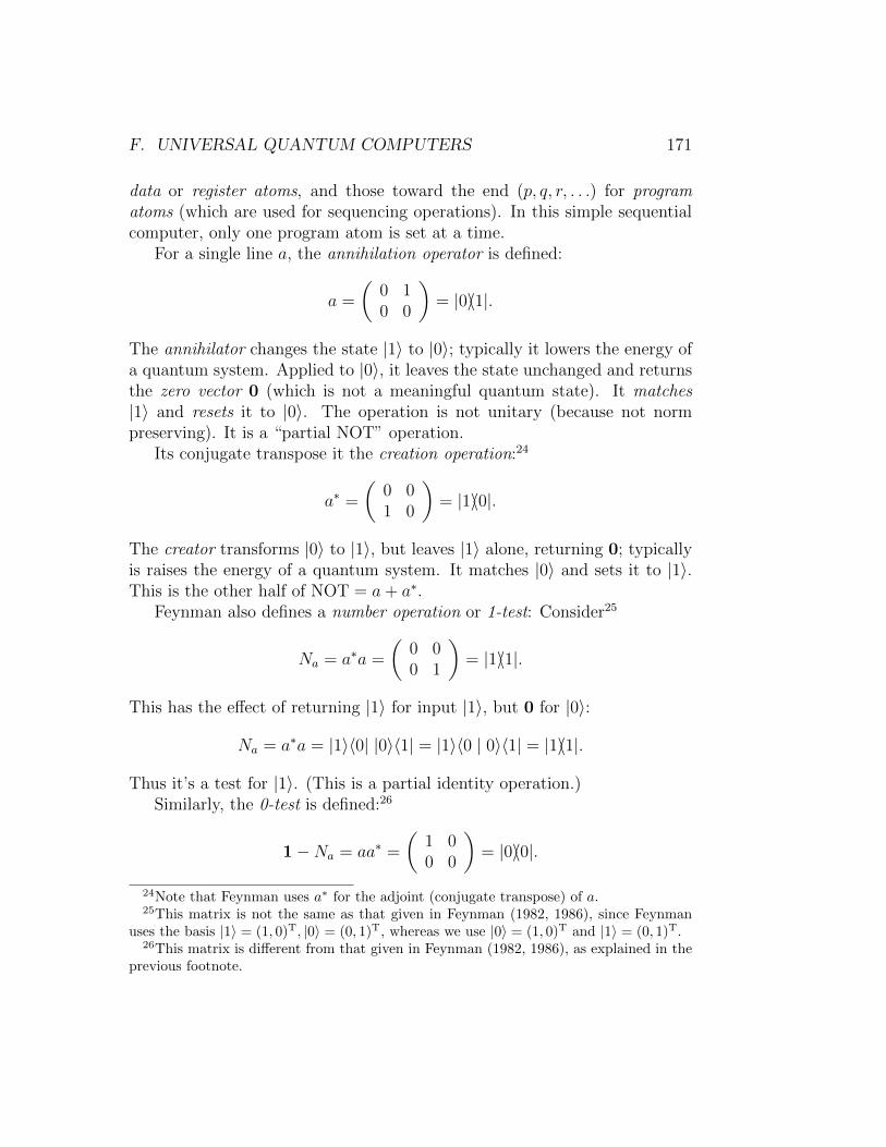
F.2 Benio↵ ’s quantum Turing machine

In 1980 Paul Benio↵ published the first design for a universal quantum com-puter, which was based on the Turing machine (Benio↵, 1980). The tapeis represented by a finite lattice of quantum spin systems with eigenstatescorresponding to the tape symbols. (Therefore, he cannot implement anopen-ended TM tape, but neither can an ordinary digital computer.) Theread/write head is a spinless system that moves along the lattice. The stateof the TM was represented by another spin system. Benio↵ defined unitaryoperators for doing the various operations (e.g., changing the tape). In 1982he extended his model to erase the tape, as in Bennett’s model (Benio↵,1982). Each step was performed by measuring both the tape state under thehead and the internal state (thus collapsing them) and using this to controlthe unitary operator applied to the tape and state. As a consequence, thecomputer does not make much use of superposition.

F.3 Deutsch’s universal quantum computer

Benio↵’s computer is e↵ectively classical; it can be simulated by a classicalTuring machine. Moreover, Feynman’s construction is not a true univer-sal computer, since you need to construct it for each computation, and it’snot obvious how to get the required dynamical behavior. Deutsch sought abroader definition of quantum computation, and a universal quantum com-puter Q.27 M binary observables are used to represent the processor, {ni}for i 2 M, where M = {0, . . . ,M � 1}. Collectively they are called n. Aninfinite sequence of binary observables implements the memory, {mi} (i 2 Z)Collectively the sequence is called m. An observable x, with spectrum Z,represents the tape position (address) of the head. The computational basisstates have the form:

|x;n;mi def

= |x;n0

, n1

, . . . , nM�1

; . . . ,m�1

,m0

,m1

, . . .i.27This section is based on Deutsch (1985).

176 CHAPTER III. QUANTUM COMPUTATION

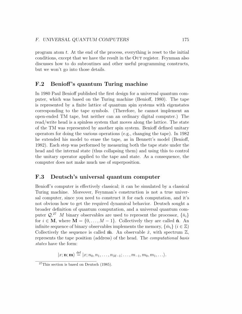
Here the eigenvectors are labeled by their eigenvalues x,n, and m.The dynamics of computation is described by a unitary operator U , which

advances the computation by one step of duration T :

| (nT )i = Un| (0)i.

Initially, only a finite number of the memory elements are prepared in anon-zero state.

| (0)i =Xm

�m|0;0;mi, whereXm

|�m|2 = 1,

That is, only finitely many �m 6= 0, and in particular �m = 0 when an infinitenumber of the m are non-zero. The non-zero entries are the program and itsinput. Note that the initial state may be a superposition of initial tapes.

The matrix elements of U (relating the new state to the current state)have the form:

hx0;n0;m0 | U | x;n;mi= [�x+1

x0 U+(n0,m0x|n,mx) + �x�1

x0 U�(n0,m0x|n,mx)]

Yy 6=x

�my

m0y.

U+ and U� represent moves to the right and left, respectively. The firsttwo � functions ensure that the tape position cannot move by more than oneposition in a step. The final product of deltas ensures that all the other tapepositions are unchanged; it’s equivalent to: 8y 6= x : m0

y = my. The U+

and U� functions define the actual transitions of the machine in terms of theprocessor state and the symbol under the tape head. Each choice defines aquantum computer Q[U+, U�].

The machine cannot be observed before it has halted, since that wouldgenerally alter its state. Therefore one of the processor’s bits is chosen as ahalt indicator. It can be observed from time to time without a↵ecting thecomputation.

Q can simulate TMs, but also any other quantum computer to arbitraryprecision. In fact, it can simulate any finitely realizable physical system toarbitrary precision, and it can simulate some physical systems that go beyondthe power of TMs (hypercomputation).