Algorithms for Quantum Computers Jamie Smith and Michele Mosca 1 Introduction Quantum computing is a new computational paradigm created by reformulating in- formation and computation in a quantum mechanical framework [ 30, 27]. Since the laws of physics appear to be quantum mechanical, this is the most relevant frame- work to consider when considering the fundamental limitations of information pro- cessing. Furthermore, in recent decades we have seen a major shift from just observ- ing quantum phenomena to actually controlling quantum mechanical systems. We have seen the communication of quantum information over long distances, the “tele- portation” of quantum information, and the encoding and manipulation of quantum information in many different physical media. We still appear to be a long way from the implementation of a large-scale quantum computer, however it is a serious goal of many of the world’s leading physicists, and progress continues at a fast pace. In parallel with the broad and aggressive program to control quantum mechan- ical systems with increased precision, and to control and interact a larger number of subsystems, researchers have also been aggressively pushing the boundaries of what useful tasks one could perform with quantum mechanical devices. These in- Jamie Smith Institute for Quantum Computing and Dept. of Combinatorics & Optimization University of Waterloo, with support from the Natural Sciences and Engineering Research Council of Canada e-mail: [email protected] Michele Mosca Institute for Quantum Computing and Dept. of Combinatorics & Optimization University of Waterloo and St. Jerome’s University, and Perimeter Institute for Theoretical Physics, with support from the Government of Canada, Ontario-MRI, NSERC, QuantumWorks, MITACS, CIFAR, CRC, ORF, and DTO-ARO e-mail: [email protected] 1 a r X i v : 1 0 0 1 . 0 7 6 7 v 2 [ q u a n t p h ] 7 J a n 2 0 1 0

Welcome message from author
This document is posted to help you gain knowledge. Please leave a comment to let me know what you think about it! Share it to your friends and learn new things together.
Transcript
8/7/2019 Algorithms for Quantum Computers
http://slidepdf.com/reader/full/algorithms-for-quantum-computers 1/48
Algorithms for Quantum Computers
Jamie Smith and Michele Mosca
1 Introduction
Quantum computing is a new computational paradigm created by reformulating in-formation and computation in a quantum mechanical framework [ 30, 27 ]. Since thelaws of physics appear to be quantum mechanical, this is the most relevant frame-work to consider when considering the fundamental limitations of information pro-cessing. Furthermore, in recent decades we have seen a major shift from just observ-ing quantum phenomena to actually controlling quantum mechanical systems. Wehave seen the communication of quantum information over long distances, the “tele-portation” of quantum information, and the encoding and manipulation of quantuminformation in many different physical media. We still appear to be a long way fromthe implementation of a large-scale quantum computer, however it is a serious goalof many of the world’s leading physicists, and progress continues at a fast pace.
In parallel with the broad and aggressive program to control quantum mechan-ical systems with increased precision, and to control and interact a larger numberof subsystems, researchers have also been aggressively pushing the boundaries of what useful tasks one could perform with quantum mechanical devices. These in-
Jamie SmithInstitute for Quantum Computing and Dept. of Combinatorics & OptimizationUniversity of Waterloo,with support from the Natural Sciences and Engineering Research Council of Canadae-mail: [email protected]
Michele MoscaInstitute for Quantum Computing and Dept. of Combinatorics & OptimizationUniversity of Waterloo and St. Jerome’s University,and Perimeter Institute for Theoretical Physics,
with support from the Government of Canada, Ontario-MRI, NSERC, QuantumWorks, MITACS,CIFAR, CRC, ORF, and DTO-AROe-mail: [email protected]
1
a r X i v : 1 0 0 1 . 0 7
6 7 v 2 [ q u a n t - p h ] 7 J a n 2 0 1 0

8/7/2019 Algorithms for Quantum Computers
http://slidepdf.com/reader/full/algorithms-for-quantum-computers 2/48
2 Jamie Smith and Michele Mosca
clude improved metrology, quantum communication and cryptography, and the im-plementation of large-scale quantum algorithms.
It was known very early on [ 27] that quantum algorithms cannot compute func-tions that are not computable by classical computers, however they might be able to
efciently compute functions that are not efciently computable on a classical com-puter. Or, at the very least, quantum algorithms might be able to provide some sortof speed-up over the best possible or best known classical algorithms for a specicproblem.
The purpose of this paper is to survey the eld of quantum algorithms, which hasgrown tremendously since Shor’s breakthrough algorithms [ 57, 58 ] over 15 yearsago. Much of the work in quantum algorithms is now textbook material (e.g. [54 ,39, 45, 43, 49] ), and we will only briey mention these examples in order to providea broad overview. Other parts of this survey, in particular, sections 4 and 5, give amore detailed description of some more recent work.
We organized this survey according to an underlying tool or approach taken, andinclude some basic applications and specic examples, and relevant comparisonswith classical algorithms.
In section 2 we begin with algorithms one can naturally consider to be basedon a quantum Fourier transform, which includes the famous factoring and discretelogarithm algorithms of Peter Shor [57 , 58]. Since this topic is covered in severaltextbooks and recent surveys, we will only briey survey this topic. We could haveadded several other sections on algorithms for generalizations of these problems,including several cases of the non-Abelian hidden subgroup problem, and hiddenlattice problems over the reals (which have important applications in number the-ory), however these are covered in the recent survey [ 52] and in substantial detail in[22] .
We continue in section 3 with a brief review of classic results on quantum search-ing and counting, and more generally amplitude amplication and amplitude esti-mation.
In section 4 we discuss algorithms based on quantum walks. We will not coverthe related topic of adiabatic algorithms, which was briey summarized in [52]; abroader survey of this and related techniques (“quantum annealing”) can be foundin [ 26] .
We conclude with section 5 on algorithms based on the evaluation of the traceof an operator, also referred to as the evaluation of a tensor network, and which hasapplications such as the approximation of the Tutte polynomial.
The eld of quantum algorithms has grown tremendously since the seminal work in the mid-1990s, and a full detailed survey would simply be infeasible for one ar-ticle. We could have added several other sections. One major omission is the de-velopment of algorithms for simulating quantum mechanical systems, which wasFeynman’s original motivation for proposing a quantum computer. This eld wasbriey surveyed in [ 52], with emphasis on the recent results in [ 13] (more recentdevelopments can be found in [ 63] ). This remains an area worthy of a comprehen-sive survey; like the many other areas we have tried to survey, it is difcult becauseit is still an active area of research. It is also an especially important area because
8/7/2019 Algorithms for Quantum Computers
http://slidepdf.com/reader/full/algorithms-for-quantum-computers 3/48
Algorithms for Quantum Computers 3
these algorithms tend to offer a fully exponential speed-up over classical algorithms,and thus are likely to be among the rst quantum algorithms to be implemented thatwill offer a speed-up over the fastest available classical computers.
Lastly, one could also write a survey of quantum algorithms for intrinsically
quantum information problems, like entanglement concentration, or quantum datacompression. We do not cover this topic in this article, though there is a very brief survey in [ 52] .
One can nd a rather comprehensive list of the known quantum algorithms (up tomid 2008) in Stephen Jordan’s PhD thesis [ 41] . We hope this survey complementssome of the other recent surveys in providing a reasonably detailed overview of thecurrent state of the art in quantum algorithms.
2 Algorithms based on the Quantum Fourier transform
The early line of quantum algorithms was developed in the “black-box” or “ora-
cle” framework. In this framework part of the input is a black-box that implementsa function f ( x), and the only way to extract information about f is to evaluate iton inputs x. These early algorithms used a special case of quantum Fourier trans-form, the Hadamard gate, in order solve the given problem with fewer black-boxevaluations of f than a classical algorithm would require.
Deutsch [27 ] formulated the problem of deciding whether a function f : 0, 1→0, 1was constant or not. Suppose one has access to a black-box that implements f reversibly by mapping x, 0 → x, f ( x); let us further assume that the black box in factimplements a unitary transformation U f that maps | x |0 →| x | f ( x) . Deutsch’sproblem is to output “constant” if f (0) = f (1) and to output “balanced” if f (0) = f (1), given a black-box for evaluating f . In other words determine f (0)⊕f (1)(where ⊕denotes addition modulo 2). Outcome “0” means f is constant and “1”means f is not constant.
A classical algorithm would need to evaluate f twice in order to solve this prob-lem. A quantum algorithm can apply U f only once to create
1√2 |0 | f (0) +
1√2 |1 | f (1) .
Note that if f (0) = f (1), then applying the Hadamard gate to the rst registeryields |0 with probability 1, and if f (0) = f (1), then applying the Hadamard gateto the rst register and ignoring the second register leaves the rst register in thestate |1 with probability 1
2 ; thus a result of |1 could only occur if f (0) = f (1).As an aside, let us note that in general, given
1
√2 |0
|ψ 0 +
1
√2 |1
|ψ 1
8/7/2019 Algorithms for Quantum Computers
http://slidepdf.com/reader/full/algorithms-for-quantum-computers 4/48
4 Jamie Smith and Michele Mosca
applying the Hadamard gate to the rst qubit and measuring it will yield “0” withprobability 1
2 + Re( ψ 0|ψ 1 ) ; this “Hadamard test” is discussed in more detail insection 5.
In Deutsch’s case, measuring a “1” meant f (0) = f (1) with certainty, and a “0”
was an inconclusive result. Even though it wasn’t perfect, it still was something thatcouldn’t be done with a classical algorithm. The algorithm can be made exact [ 24](i.e. one that outputs the correct answer with probability 1) if one assumes furtherthat U f maps | x |b → | x |b⊕f ( x) , for b
∈ 0, 1, and one sets the second qubitto 1√2 |0 − 1√2 |1 . Then U f maps
|0 + |1√2|0 −|1
√2 →(−1) f (0) |0 + ( −1) f (0)⊕ f (1) |1√2|0 −|1
√2.
Thus a Hadamard gate on the rst qubit yields the result
(−1) f (0) | f (0)⊕f (1) |0 −|1√2
and measuring the rst register yields the correct answer with certainty.The general idea behind the early quantum algorithms was to compute a black-
box function f on a superposition of inputs, and then extract a global property of f by applying a quantum transformation to the input register before measuring it. Weusually assume we have access to a black-box that implements
U f : |x |b →|x |b⊕f (x)
or in some other form where the input value x is kept intact and the second registeris shifted by f (x) is some reversible way.
Deutsch and Jozsa [28 ] used this approach to get an exact algorithm that decideswhether f : 0, 1n → 0, 1is constant or “balanced” (i.e. | f −1(0)| = | f −1(1)|),with a promise that one of these two cases holds. Their algorithm evaluated f only twice, while classically any exact algorithm would require 2 n−1 + 1 queriesin the worst-case. Bernstein and Vazirani [12 ] dened a specic class of suchfunctions f a : x →a ·x, for any a∈ 0, 1n , and showed how the same algorithmthat solves the Deutsch-Jozsa problem allows one to determine a with two evalua-tions of f a while a classical algorithm requires n evaluations. (Both of these algo-rithms can be done with one query if we have |x |b →|x |b⊕f (x) .) They furthershowed how a related “recursive Fourier sampling” problem could be solved super-polynomially faster on a quantum computer. Simon [ 59] later built on these tools todevelop a black-box quantum algorithm that was exponentially faster than any clas-sical algorithm for nding a hidden string s
∈0, 1n that is encoded in a function f : 0, 1n → 0, 1n with the property that f (x) = f (y) if and only if x = y
⊕s.
Shor [ 57, 58 ] built on these black-box results to nd an efcient algorithm fornding the order of an element in the multiplicative group of integers modulo N (which implies an efcient classical algorithm for factoring N ) and for solving the
8/7/2019 Algorithms for Quantum Computers
http://slidepdf.com/reader/full/algorithms-for-quantum-computers 5/48
Algorithms for Quantum Computers 5
discrete logarithm problem in the multiplicative group of integers modulo a largeprime p. Since the most widely used public key cryptography schemes at the timerelied on the difculty of integer factorization, and others relied on the difcultyof the discrete logarithm problem, these results had very serious practical impli-
cations. Shor’s algorithms straightforwardly apply to black-box groups, and thuspermit nding orders and discrete logarithms in any group that is reasonably pre-sented, including the additive group of points on elliptic curves, which is currentlyone of the most widely used public key cryptography schemes (see e.g. [48 ]).
Researchers tried to understand the full implications and applications of Shor’stechnique, and a number of generalizations were soon formulated (e.g. [ 15, 36] ).One can phrase Simon’s algorithm, Shor’s algorithm, and the various generaliza-tions that soon followed as special cases of the hidden subgroup problem . Considera nitely generated Abelian group G , and a hidden subgroup K that is dened bya function f : G → X (for some nite set X ) with the property that f ( x) = f ( y) if and only if x− y
∈K (we use additive notation, without loss of generality). In other
words, f is constant on cosets of K and distinct on different cosets of G . In the caseof Simon’s algorithm, G = Z n
2 and K =
0, s
. In the case of Shor’s order-nding
algorithm, G = Z and K = r Z where r is the unknown order of the element. Otherexamples and how they t in the hidden subgroup paradigm are given in [51 ].
Soon after, Kitaev [ 46] solved a problem he called the Abelian stabilizer prob-lem using an approach that seemed different from Shor’s algorithm, one based ineigenvalue estimation. Eigenvalue estimation is in fact an algorithm of independentinterest for the purpose of studying quantum mechanical systems. The Abelian sta-bilizer problem is also a special case of the hidden subgroup problem. Kitaev’s ideawas to turn the problem into one of estimating eigenvalues of unitary operators. Inthe language of the hidden subgroup problem, the unitary operators were shift op-erators of the form f ( x) →f ( x+ y). By encoding the eigenvalues as relative phaseshifts, he turned the problem into a phase estimation problem.
The Simon/Shor approach for solving the hidden subgroup problem is to rstcompute ∑ x
| x
| f ( x) . In the case of nite groups G , one can sum over all the el-
ements of G , otherwise one can sum over a sufciently large subset of G . For ex-ample, if G = Z , and f ( x) = a x mod N for some large integer N , we rst compute∑2n−1
x= 0 | x |a x , where 2 n > N 2 (we omit the “ mod N ” for simplicity). If r is the orderof a (i.e. r is the smallest positive integer such that a r ≡1) then every value x of theform x = y + kr gets mapped to a y. Thus we can rewrite the above state as
2n−1
∑ x= 0 | x |a x =
r −1
∑ y= 0
(∑ j | y+ jr ) |a y (1)
where each value of a y in this range is distinct. Tracing out the second register wethus are left with a state of the form
∑ j |
y+ jr
8/7/2019 Algorithms for Quantum Computers
http://slidepdf.com/reader/full/algorithms-for-quantum-computers 6/48
6 Jamie Smith and Michele Mosca
for a random y and where j goes from 0 to (2n −1)/ r . We loosely refer to this stateas a “periodic” state with period r . We can use the inverse of the quantum Fouriertransform (or the quantum Fourier transform) to map this state to a state of the form∑ x α x | x , where the amplitudes are biased towards values of x such that x/ 2n ≈k / r .
With probability at least4
π 2 we obtain an x such that | x/ 2n
−k / r | ≤1/ 2n+ 1
. Onecan then use the continued fractions algorithm to nd k / r (in lowest terms) andthus nd r with high probability. It is important to note that the continued fractionsalgorithm is not needed for many of the other cases of the Abelian hidden subgroupconsidered, such as Simon’s algorithm or the discrete logarithm algorithm when theorder of the group is already known.
In contrast, Kitaev’s approach for this special case was to consider the map U a :
|b → |ba x . It has eigenvalues of the form e2π ik / r , and the state |1 satises
|1 =1√r
r −1
∑k = 0 |ψ k
where
|ψ k is an eigenvector with eigenvalue e2π ik / r :
U a : |ψ k →e2π ikx/ r |ψ k .
If we consider the controlled- U a , denoted c −U a , which maps |0 |b →|0 |b and
|1 |b →|1 |ba , and if we apply it to the state (|0 + |1 ) |ψ k we get
(|0 + |1 ) |ψ k →(|0 + e2π ik / r |1 ) |ψ k .
In other words, the eigenvalue becomes a relative phase, and thus we can reduceeigenvalue estimation to phase estimation. Furthermore, since we can efcientlycompute a 2 j
by performing j multiplications modulo N , one can also efcientlyimplement c −U
a2 j and thus easily obtain the qubit |0 + e2π i2 j(k / r ) |1 for integervalues of j without performing c
−U a a total of 2 j times. Kitaev developed an ef-
cient ad hoc phase estimation scheme in order to estimate k / r to high precision, andthis phase estimation scheme could be optimized further [ 24] . In particular, one cancreate the state
(|0 + |1 )n |1 =2n−1
∑ x= 0 | x |1 =
r −1
∑k = 0
2n−1
∑ x= 0 | x |ψ k
(we use the standard binary encoding of the integers x∈ 0, 1, . . . , 2n −1as bits
strings of length n) the apply the c −U a2 j using the (n − j)th bit as the control bit,
and using the second register (initialized in |1 = ∑k |ψ k ) as the target register, for j = 0, 1, 2, . . . , n −1, to create
∑k (
|0 + e2π i2n−1 k
r
|1 )
···(
|0 + e2π i2 k
r
|1 )(
|0 + e2π i k
r
|1 )
|ψ k (2)
= ∑2n−1 x= 0 | x |a x = ∑ r −1
k = 0 ∑2n−1 x= 0 e2π ix k
r | x |ψ k . (3)
8/7/2019 Algorithms for Quantum Computers
http://slidepdf.com/reader/full/algorithms-for-quantum-computers 7/48
Algorithms for Quantum Computers 7
If we ignore or discard the second register, we are left with a state of the form∑2n−1
x= 0 e2π ixk / r | x for a random value of k ∈ 0, 1, . . . , r −1. The inverse quantumFourier transformation maps this state to a state ∑ y α y | y where most of weightof the amplitudes is near values of y such that y/ 2n ≈ k / r for some integer k .
More specically | y/ 2n
−k / r | ≤1/ 2n+ 1
with probability at least 4 / π 2; furthermore
| y/ 2n −k / r | ≤1/ 2n with probability at least 8 / π 2 . As in the case of Shor’s algo-rithm, one can use the continued fractions algorithm to determine k / r (in lowestterms) and thus determine r with high probability.
It was noted [ 24] that this modied eigenvalue estimation algorithm for order-nding was essentially equivalent to Shor’s period-nding algorithm for order-nding. This can be seen by noting that we have the same state in Equation 1 andEquation 2, and in both cases we discard the second register and apply an inverseFourier transform to the rst register. The only difference is the basis in which thesecond register is mathematically analyzed.
The most obvious direction in which to try to generalized the Abelian hid-den subgroup algorithm is to solve instances of the hidden subgroup problem fornon-Abelian groups. This includes, for example, the graph automorphism problem
(which corresponds to nding a hidden subgroup of the symmetric group). Therehas been non-trivial, but limited, progress in this direction, using a variety of al-gorithmic tools, such as sieving, “pretty good measurements” and other group the-oretic approaches. Other generalizations include the hidden shift problem and itsgeneralizations, hidden lattice problems on real lattices (which has important appli-cations in computational number theory and computationally secure cryptography),and hidden non-linear structures. These topics and techniques would take severaldozen pages just to summarize, so we refer the reader to [ 52] or [22], and leavemore room to summarize other important topics.
3 Amplitude Amplication and Estimation
A very general problem for which quantum algorithms offer an improvement is thatof searching for a solution to a computational problem in the case that a solution xcan be easily veried. We can phrase such a general problem as nding a solution x to the equation f ( x) = 1, given a means for evaluating the function f . We canfurther assume that f : 0, 1n → 0, 1.
The problems from the previous section can be rephrased in this form (or a smallnumber of instances of problems of this form), and the quantum algorithms for theseproblems exploit some non-trivial algebraic structure in the function f in order tosolve the problems superpolynomially faster than the best possible or best knownclassical algorithms. Quantum computers also allow a more modest speed-up (up toquadratic) for searching for a solution to a function f without any particular struc-ture. This includes, for example, searching for solutions to NP -complete problems.
Note that classically, given a means for guessing a solution x with probability p,one could amplify this success probability by repeating many times, and after a num-
8/7/2019 Algorithms for Quantum Computers
http://slidepdf.com/reader/full/algorithms-for-quantum-computers 8/48
8 Jamie Smith and Michele Mosca
ber of guess in O(1/ p), the probability of nding a solution is in Ω (1). Note that thequantum implementation of an algorithm that produces a solution with probability p will produce a solution with probability amplitude √ p. The idea behind quan-tum searching is to somehow amplify this probability to be close to 1 using only
O(1/ √ p) guesses and other steps.Lov Grover [ 37] found precisely such an algorithm, and this algorithm was
analyzed in detail and generalized [ 16, 17, 38, 18] to what is known as “am-plitude amplication.” Any procedure for guessing a solution with probability pcan be (with modest overhead) turned into a unitary operator A that maps |0 →√ p |ψ 1 + √1 − p |ψ 0 , where 0 = 00 . . . 0, |ψ 1 is a superposition of states encod-ing solutions x to f (x) = 1 (the states could in general encode x followed by other“junk” information) and |ψ 0 is a superposition of states encoding values of x thatare not solutions.
One can then dene the quantum search iterate (or “Grover iterate”) to be
Q = − AU 0 A−1U f
where U f : |x →(−1) f (x)
|x , and U 0 = I −2 |0 0| (in other words, maps |0 →−|0 and |x → |x for any x = 0). Here we are for simplicity assuming there areno “junk” bits in the unitary computation of f by A. Any such junk information caneither be “uncomputed” and reset to all 0s, or even ignored (letting U f act only onthe bits encoding x and applying the identity to the junk bits).
This algorithm is analyzed thoroughly in the literature and in textbooks, so weonly summarize the main results and ideas that might help understand the later sec-tions on searching via quantum walk.
If one applies Q a total of k times to the input state A|00 . . . 0 = sin (θ ) |ψ 1 +cos (θ ) |ψ 0 , where √ p = sin(θ ), then one obtains
Qk A|00 . . . 0 = sin ((2k + 1)θ ) |ψ 1 + cos ((2k + 1)θ ) |ψ 0 .
This implies that with k ≈π
4√ p one obtains |ψ 1 with probability amplitude closeto 1, and thus measuring the register will yield a solution to f ( x) = 1 with highprobability. This is quadratically better than what could be achieved by preparingand measuring A|0 until a solution is found.
One application of such a generic amplitude amplication method is for search-ing. One can also apply this technique to approximately count [ 19] the number of solutions to f ( x) = 1, and more generally to estimate the amplitude [ 18] with whicha general operator A produces a solution to f ( x) = 1 (in other words, the transitionamplitude from one recognizable subspace to another).
There are a variety of other applications of amplitude amplication that cleverlyincorporate amplitude amplication in a non-obvious way into a larger algorithm.Some of these examples are discussed in [ 52] and most are summarized at [41].
Since there are some connections to some of the more recent tools developed inquantum algorithms, we will briey explain how amplitude estimation works.
8/7/2019 Algorithms for Quantum Computers
http://slidepdf.com/reader/full/algorithms-for-quantum-computers 9/48
Algorithms for Quantum Computers 9
Consider any unitary operator A that maps some known input state, say |0 =
|00 . . . 0 , to a superposition sin (θ ) |ψ 1 + cos (θ ) |ψ 0 , 0 ≤θ ≤π / 2, where |ψ 1is a normalized superposition of “good” states x satisfying f (x) = 1 and |ψ 0 is anormalized superposition of “bad” states x satisfying f (x) = 0 (again, for simplic-
ity we ignore extra junk bits). If we measure A|0 , we would measure a “good” xwith probability sin 2(θ ). The goal of amplitude estimation is to approximate theamplitude sin (θ ). Let us assume for convenience that there are t > 0 good statesand n −t > 0 bad states, and that 0 < sin (θ ) < π / 2.
We note that the quantum search iterate Q = − AU 0 A−1U f has eigenvalues |ψ + =1√2
(|ψ 0 + i |ψ 1 ) and |ψ − = 1√2(|ψ 0 −i |ψ 1 ) with respective eigenvalues ei2θ and
e−i2θ . It also has 2 n −2 other eigenvectors; t −1 of them have eigenvalue + 1 andare the states orthogonal to |ψ 1 that have support on the states |x where f (x) = 1,and n −t −1 of them have eigenvalue −1 and are the states orthogonal to |ψ 0 thathave support on the states |x where f (x) = 0. It is important to note that A|ψ =eiθ
√2 |ψ + + e−iθ
√2 |ψ − has its full support on the two dimensional subspace spannedby |ψ + and |ψ − .
It is worth noting that the quantum search iterate Q = − AU 0 A−1
U f can also bethought of as two reections
−U A|0 U f = ( 2 A|0 0| A† − I )( I −2 ∑x| f (x)= 1
|x x|),
one which ags the “good” subspace with a −1 phase shift, and then one that agsthe subspace orthogonal to A|0 with a −1 phase shift. In the two dimensional sub-space spanned by A|0 and U f A|0 , these two reections correspond to a rotation byangle 2 θ . Thus it should not be surprising to nd eigenvalues e±2π iθ for states in thistwo dimensional subspace. (In the section on quantum walks, we’ll consider a moregeneral situation where we have an operator Q with many non-trivial eigenspacesand eigenvalues.)
Thus one can approximate sin (θ ) by estimating the eigenvalue of either
|ψ +
or |ψ − . Performing the standard eigenvalue estimation algorithm on Q with input A|0 (as illustrated in Figure 1) gives a quadratic speed-up for estimating sin 2(θ )versus simply repeatedly measuring A|0 and counting the frequency of 1s. In par-ticular, we can obtain an estimate θ of θ such that |θ −θ |< ε with high (constant)probability using O(1/ ε ) repetitions of Q , and thus O(1/ ε ) repetitions of U f , A and A−1 . For xed p, this implies that p = sin 2(θ ) satises | p − ˜ p| ∈O(ε ) with highprobability. Classically sampling requires O(1/ ε 2) samples for the same precision.One application is speeding up the efciency of the “Hadamard” test mentioned insection 5.2.3
Another interesting observation is that increasingly precise eigenvalue estimationof Q on input A|0 leaves the eigenvector register in a state that gets closer and closerto the mixture 1
2 |ψ + ψ + |+ 12 |ψ − ψ −| which equals 1
2 |ψ 1 ψ 1|+ 12 |ψ 0 ψ 0|.
Thus eigenvalue estimation will leave the eigenvector register in a state that containsa solution to f (x) = 1 with probability approaching 12 . One can in fact using this
entire algorithm as subroutine in another quantum search algorithm, and obtain an
8/7/2019 Algorithms for Quantum Computers
http://slidepdf.com/reader/full/algorithms-for-quantum-computers 10/48
10 Jamie Smith and Michele Mosca
QFT M
'&%$
!"#
QFT −1
M
r r r r L L L L r r r r L L L L
|0 ⊗m r r r r L L
L L y
... r r r r L L L L
A Q x|0 ⊗n
...
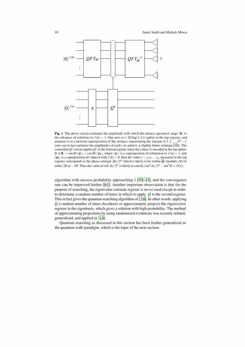
Fig. 1 The above circuit estimates the amplitude with which the unitary operator A maps |0 tothe subspace of solutions to f (x) = 1. One uses m∈Ω (log(1/ ε )) qubits in the top register, andprepares it in a uniform superposition of the strings y representing the integers 0 , 1, 2, . . . , 2m −1(one can in fact optimize the amplitudes of each y to achieve a slightly better estimate [33] ). Thecontrolled- Q y circuit applies Q y to the bottomregister when thevalue y is encoded in the top qubits.If A|0 = sin (θ ) |ψ 1 + cos (θ ) |ψ 0 , where |ψ 1 is a superposition of solutions x to f (x) = 1, and
|ψ 0 is a superposition of values x with f (x) = 0, then the value y = y1 y2 . . . ym measured in the topregister corresponds to the phase estimate 2 π y/ 2m which is likely to be within 2π
2m (modulo 2 π ) of either 2 θ or −2θ . Thus the value of sin 2 π y/ 2m is likely to satisfy |sin 2 π y/ 2m −sin2 θ |∈O(ε ).
algorithm with success probability approaching 1 [ 50, 43 ], and the convergencerate can be improved further [ 61]. Another important observation is that for thepurpose of searching, the eigenvalue estimate register is never used except in orderto determine a random number of times in which to apply Q to the second register.This in fact gives the quantum searching algorithm of [ 16] . In other words, applyingQ a random number of times decoheres or approximately projects the eigenvectorregister in the eigenbasis, which gives a solution with high probability. The methodof approximating projections by using randomized evolutions was recently rened,generalized, and applied in [14 ].
Quantum searching as discussed in this section has been further generalized inthe quantum walk paradigm, which is the topic of the next section.
8/7/2019 Algorithms for Quantum Computers
http://slidepdf.com/reader/full/algorithms-for-quantum-computers 11/48
Algorithms for Quantum Computers 11
QFT M
QFT −1 M |0 ⊗m
...
=
Q x
r r r r L L L L
r r r r L L L L
|0 ⊗n r r r r L L L L y
.
.. r r r r L L L L
Q x
r r r r L L L L
r r r r L L L L
|0 ⊗n r r r r L L L L y
... r r r r L L L L
for x∈1, 2,..., 2m −1
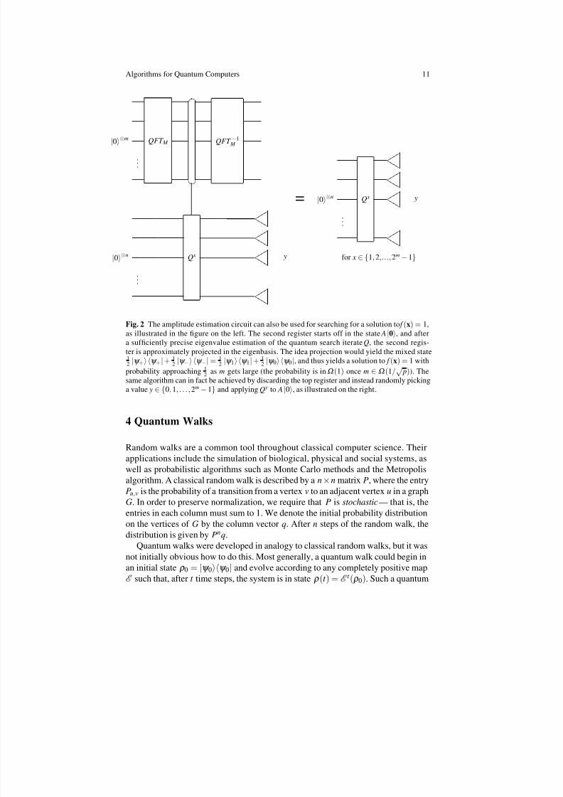
Fig. 2 The amplitude estimation circuit can also be used for searching for a solution to f (x) = 1,as illustrated in the gure on the left. The second register starts off in the state A|0 , and aftera sufciently precise eigenvalue estimation of the quantum search iterate Q , the second regis-ter is approximately projected in the eigenbasis. The idea projection would yield the mixed state12 |ψ + ψ + |+ 1
2 |ψ − ψ −|= 12 |ψ 1 ψ 1|+ 1
2 |ψ 0 ψ 0|, and thus yields a solution to f (x) = 1 withprobability approaching 1
2 as m gets large (the probability is in Ω (1) once m∈Ω (1/ √ p)). Thesame algorithm can in fact be achieved by discarding the top register and instead randomly pickinga value y∈0, 1, . . . , 2m −1and applying Q y to A|0 , as illustrated on the right.
4 Quantum Walks
Random walks are a common tool throughout classical computer science. Theirapplications include the simulation of biological, physical and social systems, aswell as probabilistic algorithms such as Monte Carlo methods and the Metropolisalgorithm. A classical random walk is described by a n×n matrix P , where the entryPu,v is the probability of a transition from a vertex v to an adjacent vertex u in a graphG . In order to preserve normalization, we require that P is stochastic — that is, theentries in each column must sum to 1. We denote the initial probability distributionon the vertices of G by the column vector q. After n steps of the random walk, thedistribution is given by P nq.
Quantum walks were developed in analogy to classical random walks, but it was
not initially obvious how to do this. Most generally, a quantum walk could begin inan initial state ρ0 = |ψ 0 ψ 0| and evolve according to any completely positive mapE such that, after t time steps, the system is in state ρ (t ) = E t (ρ0). Such a quantum
8/7/2019 Algorithms for Quantum Computers
http://slidepdf.com/reader/full/algorithms-for-quantum-computers 12/48
12 Jamie Smith and Michele Mosca
walk is simultaneously using classical randomness and quantum superposition. Wecan focus on the power of quantum mechanics by restricting to unitary walk opera-tions, which maintain the system in a coherent quantum state. So, the state at timet can be described by |ψ (t ) = U t |ψ 0 , for some unitary operator U . However, it
is not initially obvious how to dene such a unitary operation. A natural idea is todene the state space A with basis |v : v
∈V (G)and walk operator P dened by
Pu,v = Pu,v. However, this will not generally yield a unitary operator P , and a morecomplex approach is required. Some of the earliest formulations of unitary quantumwalks appear in papers by Nayak and Vishwanath [ 53], Ambainis et al. [ 8], Kempe[44] , and Aharonov et al. [2]. These early works focused mainly on quantum walkson the line or a cycle. In order to allow unitary evolution, the state space consistedof the vertex set of the graph, along with an extra “coin register.” The state of thecoin register is a superposition of |L EFT and |R IGHT . The walk then proceeds byalternately taking a step in the direction dictated by the coin register and applyinga unitary “coin tossing operator” to the coin register. The coin tossing operator isoften chosen to be the Hadamard gate. It was shown in [ 2, 6, 8, 44, 53] that the mix-ing and propagation behaviour of these quantum walks was signicantly different
from their classical counterparts. These early constructions developed into the moregeneral concept of a discrete time quantum walk, which will be dened in detail.
We will describe two methods for dening a unitary walk operator. In a discretetime quantum walk, the state space has basis vectors |u ⊗|v : u, v∈V . Roughlyspeaking, the walk operator alternately takes steps in the rst and second registers.This is often described as a walk on the edges of the graph. In a continuous timequantum walk, we will restrict our attention to symmetric transition matrices P .We take P to be the Hamiltonian for our system. Applying Schr odinger’s equation,this will dene continuous time unitary evolution in the state space spanned by
|u : u∈
V . Interestingly, these two types of walk are not known to be equivalent.We will give an overview of both types of walk as well as some of the algorithmsthat apply them.
4.1 Discrete Time Quantum Walks
Let P be a stochastic matrix describing a classical random walk on a graph G . Wewould like the quantum walk to respect the structure of the graph G , and take intoaccount the transition probabilities Pu,v. The quantum walk should be governed bya unitary operation, and is therefore reversible. However, a classical random walk isnot, in general, a reversible process. Therefore, the quantum walk will necessarilybehave differently than the classical walk. While the state space of the classical walk is V , the state quantum walk takes place in the space spanned by |u, v : u, v∈V .We can think of the rst register as the current location of the walk, and the secondregister as a record of the previous location. To facilitate the quantum walk from astate |u, v , we rst mix the second register over the neighbours of u, and then swapthe two registers. The method by which we mix over the neighbours of u must be
8/7/2019 Algorithms for Quantum Computers
http://slidepdf.com/reader/full/algorithms-for-quantum-computers 13/48
Algorithms for Quantum Computers 13
chosen carefully to ensure that it is unitary. To describe this formally, we dene thefollowing states for each u∈V :
|ψ u = |u ⊗∑v∈
V
Pvu |v (4)
|ψ ∗u = ∑v∈
V Pvu |v ⊗ |u . (5)
Furthermore, dene the projections onto the space spanned by these states:
Π = ∑u∈
V |ψ u ψ u| (6)
Π ∗= ∑u∈
V |ψ ∗u ψ ∗u |. (7)
In order to mix the second register, we perform the reection (2Π − I ). Letting Sdenote the swap operation, this process can be written as
S(2Π − I ). (8)It turns out that we will get a more elegant expression for a single step of the quan-tum walk if we dene the walk operator W to be two iterations of this process:
W = S(2Π − I )S(2Π − I ) (9)
=( 2(SΠ S) − I )(2Π − I ) (10)
=( 2Π ∗− I )(2Π − I ). (11)
So, the walk operator W is equivalent to performing two reections.Many of the useful properties of quantum walks can be understood in terms of
the spectrum of the operator W . First, we dene D , the n ×n matrix with entries Du,v =
Pu,vPv,u . This is called the discriminant matrix , and has eigenvalues in the
interval [0, 1]. In the theorem that follows, the eigenvalues of D that lie in the interval(0, 1) will be expressed as cos (θ 1),..., cos (θ k ). Let |θ 1 ,..., |θ k be the correspond-ing eigenvectors of D . Now, dene the subspaces
A = span |ψ u (12)
B = span |ψ ∗u . (13)
Finally, dene the operatorQ = ∑
v∈
V |ψ v v| (14)
andφ j = Q θ j . (15)
We can now state the following spectral theorem for quantum walks:
Theorem 1 (Szegedy, [60 ]). The eigenvalues of W acting on the space A + B can bedescribed as follows:
8/7/2019 Algorithms for Quantum Computers
http://slidepdf.com/reader/full/algorithms-for-quantum-computers 14/48
14 Jamie Smith and Michele Mosca
1. The eigenvalues of W with non-zero imaginary part are e ±2iθ 1 , e±2iθ 2 ,..., e±2iθ k
where cos (θ 1),..., cos (θ k ) are the eigenvalues of D in the interval (0, 1). Thecorresponding (un-normalized) eigenvectors of W (P ) can be written as φ j −e±2iθ j S φ j for j = 1,..., k.
2. A∩ B and A⊥∩ B⊥span the + 1 eigenspace of W. There is a direct correspon-dence between this space and the + 1 eigenspace of D. In particular, the + 1eigenspace of W has the same degeneracy as the + 1 eigenspace of D.
3. A∩ B⊥and A⊥∩ B span the −1 eigenspace of W.
We say that P is symmetric if P T = P and ergodic if it is aperiodic. Note that if P issymmetric, then the eigenvalues of D are just the absolute values of the eigenvaluesof P . It is well-known that if P is ergodic, then it has exactly one stationary distri-bution (i.e. a unique + 1 eigenvalue). Combining this fact with theorem ( 1) gives usthe following corollary:
Corollary 1. If P is ergodic and symmetric, then the corresponding walk operator W has unique + 1 eigenvector in Span ( A, B):
|ψ = 1√n ∑v∈
V |ψ v = 1√n ∑v∈
V |ψ ∗v (16)
Moreover, if we measure the rst register of |ψ , we get a state corresponding tovertex u with probability
Pr (u) =1n ∑
v∈
V Pu,v =
1n
. (17)
This is the uniform distribution, which is the unique stationary distribution for theclassical random walk.
4.1.1 The Phase Gap and the Detection Problem
In this section, we will give an example of a quadratic speedup for the problem of detecting whether there are any “marked” vertices in the graph G . First, we denethe following:
Denition 1. The phase gap of a quantum walk is dened as the smallest postivevalue 2 θ such that e±2iθ are eigenvalues of the quantum walk operator. It is denotedby ∆ (P ).
Denition 2. Let M ⊆
V be a set of marked vertices. In the detection problem , weare asked to decide whether M is empty.
In this problem, we assume that P is symmetric and ergodic. We dene the followingmodied walk P :
Puv = Puv v /∈ M 0 u = v, v∈
M
1 u = v, v∈
M .(18)
8/7/2019 Algorithms for Quantum Computers
http://slidepdf.com/reader/full/algorithms-for-quantum-computers 15/48
Algorithms for Quantum Computers 15
This walk resembles P , except that it acts as the identity on the set M . That is, if thewalk reaches a marked vertex, it stays there. Let P M denote the operator P restrictedto V \ M . Then, arranging the rows and columns of P , we can write
P = P M 0P I . (19)
By Theorem 1, if M = / 0, then P M = P = P and P M = 1. Otherwise, we have thestrict inequality P M < 1. The following theorem bounds P M away from 1:
Theorem 2. If (1 −δ ) is the absolute value of the eigenvalue of P with second largest magnitude, and | M |≥ε |V | , then P M ≤1 −δε
2 .
We will now show that the detection problem can be solved using eigenvalue esti-mation. Theorem 2 will allow us to bound the running time of this method. First,we describe the discriminant matrix for P :
D(P )uv =
Puv u, v /∈ M
1 u = v, v∈
M 0 otherwise .
(20)
Now, beginning with the state
|ψ =1√n ∑
v∈
V |ψ v =1√n ∑
v∈
V Pv,u |u |v , (21)
we measure whether or not we have a marked vertex; if so, we are done. Otherwise,we have the state
|ψ M =1
|V \ M |
∑u,v∈V \ M Pvu |u |v . (22)
If M = / 0, then this is the state |ψ dened in ( 16) , and is the + 1 eigenvector of W (P). Otherwise, by Theorem 1, this state lies entirely in the space spanned byeigenvectors with values of the form e±2iθ j , where θ j is an eigenvalue of P M . Ap-plying Theorem 2, we know that
θ ≥cos−1(1 −δ ε 2
) ≥ δ ε 2
. (23)
So, the task of distinguishing between M being empty or non-empty is equivalentto that of distinguishing between a phase parameter of 0 and a phase parameter of
at least δε 2 . Therefore, applying phase estimation to W (P ) on state |ψ M with
precision O(√δ ε ) will decide whether M is empty with constant probability. This
requires time O( 1√δε ).
8/7/2019 Algorithms for Quantum Computers
http://slidepdf.com/reader/full/algorithms-for-quantum-computers 16/48
16 Jamie Smith and Michele Mosca
By considering the modied walk operator P , it can be shown that the detectionproblem requires O( 1
δε ) time in the classical setting. Therefore the quantum algo-rithm provides a quadratic speedup over the classical one for the detection problem.
4.1.2 Quantum Hitting Time
Classically, the rst hitting time is denoted H (ρ , M ). For a walk dened by P , start-ing from the probability distribution ρ on V , H (ρ , M ) is the smallest value n suchthat the walk reaches a marked vertex v
∈ M at some time t
∈0,..., nwith constantprobability. This idea is captured by applying the modied operator P and some ntimes, and then considering the probability that the walk is in some marked statev∈ M . Let ρ M be any initial distribution restricted to the vertices V \ M . Then, attime t , the probability that the walk is in an unmarked state is P t
M ρ M 1 , where · 1denotes the L1 norm. Assuming that M is non-empty, we can see that P M < 1. So,as t →∞ , we have P t
M ρ M 1 →0. So, as t →∞ , the walk dened by P is in amarked state with probability 1. As a result, if we begin in the uniform distributionπ on V , and run the walk for some time t , we will “skew” the distribution towards M , and thus away from the unmarked vertices. So, we dene the classical hittingtime to be the minimum t such that
P t M ρ M 1 < ε (24)
for any constant ε of our choosing. Since the quantum walk is governed by a unitaryoperator, it doesn’t converge to a particular distribution the way that the classicalwalk does. We cannot simply wait an adequate number of time steps and then mea-sure the state of the walk; the walk might have already been in a state with highoverlap on the marked vertices and then evolved away from this state! Quantumsearching has the same problem when the number of solutions is unknown. We canget around this in a similar way by considering an expected value over a sufciently
long period of time. This will form the basis of our denition of hitting time. Dene
|π =1
|V \ M |∑
v∈
V \ M |ψ v . (25)
Then, if M is empty, |π is a + 1 eigenvector of W , and W t |π = |π for all t .However, if M is non-empty, then the spectral theorem tells us that |π lies in thespace spanned by eigenvectors with eigenvalues e±2iθ j for non-zero θ j. As a result,it can be shown that, for some values of t , the state W t |π is “far” from the initialdistribution |π . We dene the quantum hitting in the same way as Szegedy [ 60].The hitting time H Q (W ) as the minimum value T such that
1T + 1
T
∑t = 0 W t
|π −|π 2
≥1 −| M
||V | . (26)
8/7/2019 Algorithms for Quantum Computers
http://slidepdf.com/reader/full/algorithms-for-quantum-computers 17/48
Algorithms for Quantum Computers 17
This leads us to Szegedy’s hitting time theorem [ 60]:
Theorem 3. The quantum hitting time H Q (W ) is
O 1 1 − P M
.
Corollary 2. Applying Theorem 2 , if the second largest eigenvalue of P has mag-nitude (1 −δ ) and | M |/ |V |≥ε , then H Q (W )∈O( 1√δε
)
Notice that this corresponds to the running time for the algorithm for the detec-tion problem, as described above. Similarly, the classical hitting time is in O( 1
δ ε ),corresponding to the best classical algorithm for the detection problem.
It is also worth noting that, if there no marked elements, then the system remainsin the state |π , and the algorithm never “hits.” This gives us an alternative wayto approach the detection problem. We run the algorithm for a randomly selectednumber of steps t
∈0,..., T with T of size O( 1/ δ ε ), and then measure whetherthe system is still in the state |π ; if there are any marked elements, then we canexpect to nd some other state with constant probability.
4.1.3 The Element Distinctness Problem
In the element distinctness problem, we are given a black box that computes thefunction
f : 1,..., n →S (27)
and we are asked to determine whether there exist x, y∈ 1,..., nwith x = y and f ( x) = f ( y). We would like to minimize the number of queries made to the black
box. There is a lower bound of Ω (n2/ 3) on the number of queries, due indirectlyto Aaronson and Shi [ 1]. The algorithm of Ambainis [ 7] proves that this bound istight. The algorithm uses a quantum walk on the Johnson graph J (n, p) has vertexset consisting of all subsets of 1,..., nof size p. Let S1 and S2 be p-subsets of
1,..., n. Then, S1 is adjacent to S2 if and only if |S1 ∩S2| = p −1. The Johnsongraph J (n, p) therefore has n
p vertices, each with degree p(n − p).The state corresponding to a vertex S of the Johnson graph will not only record
which subset s1 ,..., s p⊆1,..., nit represents, but the function values of thoseelements. That is,
|S = s1 , s2 ..., s p; f (s1), f (s2),..., f (s p) . (28)
Setting up such a state requires p queries to the black box.
The walk then proceeds for t iteration, where t is chosen from the uniform dis-tribution on 0,..., T and T
∈O(1/ √δ ε ). Each iteration has two parts to it. First,
we need to check if there are distinct si, s j with f (si) = f (s j)—that is, whether the
8/7/2019 Algorithms for Quantum Computers
http://slidepdf.com/reader/full/algorithms-for-quantum-computers 18/48
18 Jamie Smith and Michele Mosca
vertex S is marked. This requires no calls to the black box, since the function valuesare stored in the state itself. Second, if the state is unmarked, we need to take a stepof the walk. This involves replacing, say, si with si , requiring one query to erase f (si) and another to insert the value f (si). So, each iteration requires a total of 2
queries.We will now bound ε and δ . If only one pair x, y exists with f ( x) = f ( y), then
there are n−2 p−2 marked vertices. This tells us that, if there are any such pairs at all,
epsilon is Ω ( p2/ n2). Johnson graphs are very well-understood in graph theory. It isa well known result that the eigenvalues for the associated walk operator are givenby:
λ j = 1 −j(n + 1 − j) p(n − p)
(29)
for 0 ≤ j ≤ p. For a proof, see [ 20]. This give us δ = n p(n− p) . Putting this together,
we nd that 1/ δ ε is O( n√ p ). So, the number of queries required is O( p + n√ p ).
In order to minimize this quantity, we choose m to be of size Θ (n2/ 3). The querycomplexity of this algorithm is O(n2/ 3), matching the lower bound of Aaronson andShi [1].
4.1.4 Unstructured Search as a Discrete Time Quantum Walk
We will now consider unstructured search in terms of quantum walks. For unstruc-tured search, we are required to identify a marked element from a set of size n. Let M denote the set of marked elements, and U denote the set of unmarked elements.Furthermore, let m = | M | and q = |U |. We assume that the number of marked el-ements, m, is very small in relation to the total number of elements n. If this werenot the case, we could efciently nd a marked element with high probability bysimply checking a randomly chosen set of vertices. Since the set lacks any structureor ordering, the corresponding walk takes place on the complete graph on n vertices.Let us dene the following three states:
|UU =1q ∑
u,v∈U |u, v (30)
|UM =1
√nq ∑u∈
U v∈
M |u, v (31)
| MU =1
√nq ∑u∈
M v∈
U |u, v . (32)
Noting that |UU , |UM , | MU is an orthonormal set, we will consider the actionof the walk operator on the three dimensional space
Γ = span |UU , |UM , | MU . (33)
8/7/2019 Algorithms for Quantum Computers
http://slidepdf.com/reader/full/algorithms-for-quantum-computers 19/48
Algorithms for Quantum Computers 19
In order to do this, we will express the spaces A and B, dened in ( 12-13 ) in termsof a different basis. First we label the unmarked vertices:
U = u0 ,..., uq−1. (34)
Then, we dene
|γ k =1√q
q−1
∑ j= 0
e2π i jk
q ψ u j (35)
and
|γ ∗k =1√q
q−1
∑ j= 0
e2π i jk
q ψ ∗u j (36)
with k ranging from 0 to q −1. Note that |γ 0 corresponds to the denition of |π in(25) . We can then rewrite A and B:
A = span |γ k (37)
B = span
|γ ∗
k . (38)
Now, note that for k = 0, the space Γ is orthogonal to |γ k and γ ∗k . Furthermore,
|γ 0 =1√n
√m |UM + √q |UU (39)
and
|γ ∗0 =1√n
√m | MU + √q |UU . (40)
Therefore, the walk operator
W = ( 2Π ∗− I )(2Π − I ) (41)
when restricted to Γ is simply
W = 2 |γ ∗0 γ ∗0 |− I 2 |γ 0 γ 0|− I . (42)
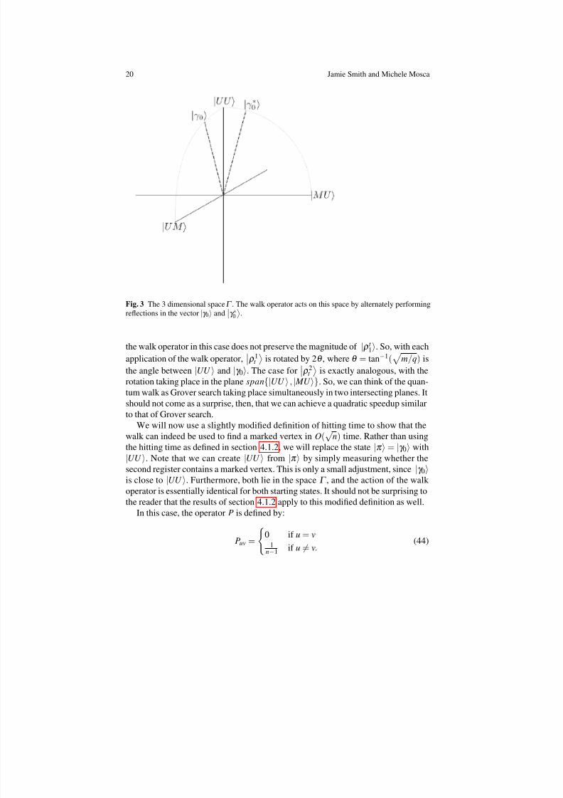
Figure 4.1.4 illustrates the space Γ which contains the vectors |γ 0 and γ ∗0 .At this point, it is interesting to compare this algorithm to Grover’s search algo-
rithm. Dene
|ρt = W t |UU . (43)
Now, dene ρ 1t and ρ 2
t to be the projection of |ρt onto span |UU , |UM and span |UU , | MU respectively. We can think of these as the “shadow” cast bythe vector |ρt on two-dimensional planes within the space Γ . Note that |γ 0 lies inthe span |UU , |UM and its projection onto span |UU , | MU is
q/ n |UU .
So, the walk operator acts on ρ1t by reecting it around the vector |γ 0 and then
around q/ n |UU . This is very similar to Grover search, except for the fact that
8/7/2019 Algorithms for Quantum Computers
http://slidepdf.com/reader/full/algorithms-for-quantum-computers 20/48
20 Jamie Smith and Michele Mosca
Fig. 3 The 3 dimensional space Γ . The walk operator acts on this space by alternately performingreections in the vector |γ 0 and γ ∗0 .
the walk operator in this case does not preserve the magnitude of |ρ t 1 . So, with each
application of the walk operator, ρ 1t is rotated by 2 θ , where θ = tan−1( m/ q) is
the angle between |UU and |γ 0 . The case for ρ 2t is exactly analogous, with the
rotation taking place in the plane span |UU , | MU . So, we can think of the quan-tum walk as Grover search taking place simultaneously in two intersecting planes. Itshould not come as a surprise, then, that we can achieve a quadratic speedup similarto that of Grover search.
We will now use a slightly modied denition of hitting time to show that thewalk can indeed be used to nd a marked vertex in O(√n) time. Rather than usingthe hitting time as dened in section 4.1.2, we will replace the state |π = |γ 0 with
|UU . Note that we can create |UU from |π by simply measuring whether thesecond register contains a marked vertex. This is only a small adjustment, since |γ 0is close to |UU . Furthermore, both lie in the space Γ , and the action of the walk operator is essentially identical for both starting states. It should not be surprising tothe reader that the results of section 4.1.2 apply to this modied denition as well.
In this case, the operator P is dened by:
Puv =0 if u = v
1n
−1 if u = v.
(44)
8/7/2019 Algorithms for Quantum Computers
http://slidepdf.com/reader/full/algorithms-for-quantum-computers 21/48
Algorithms for Quantum Computers 21
Let v0,..., vn−1 be a labeling of the vertices of G . Let x0 ,..., xn−1 denote the eigen-vectors of P , with xk
v jdenoting the amplitude on v j in xk . Then, the eigenvalues of P
are as follows: xk
v j =1
n ·e
2π i jk n . (45)
Then, x0 has eigenvalue 1, and is the stationary distribution. All the other xk haveeigenvalue −1/ (n −1), giving a spectral gap of δ = n−2
n−1 . Applying corollary 2, thisgives us quantum hitting time for the corresponding quantum walk operator W
H Q (W ) ≤ (n −1)nn −2
= O(√n). (46)
So, we run the walk for some randomly selected time t ∈0,..., T −1with T of sizeO(√n), then measure whether either the rst or second register contains a markedvertex. Applying theorem 3, the probability that neither contains a marked vertex is
1
T
T −1
∑t = 0 |
ρt
|UU
|2
≤1
T
T −1
∑t = 0 |
ρt
|UU
|= 1 −
12T
T −1
∑t = 0 |ρt −|UU 2
≤1 − | M |2 |V |
Assuming that | M | is small compared to |V |, we nd a marked vertex in either therst or second register with high probability. Repeating this procedure a constantnumber of times, our success probability can be forced arbitrarily close to 1.
4.1.5 The MNRS Algorithm
Magniez, Nayak, Roland and Santha [ 47] developed an algorithm that generalizesthe search algorithm described above to any graph. A brief overview of this al-gorithm and others is also given in the survey paper by Santha [56 ]. The MNRSalgorithm employs similar principles to Grover’s algorithm; we apply a reection in M , the space of unmarked states, followed by a reection in |π , a superposition of marked and unmarked states. This facilitates a rotation through an angle related tothe number of marked states. In the general case considered by Magniez et al., |π is the stationary distribution of the walk operator. It turns out to be quite difcult toimplement a reection in |π exactly. Rather, the MNRS algorithm employs an ap-
proximate version of this reection. This algorithm requires O 1√δ ε applications
of the walk operator, where δ is the eigenvalue gap of the operator P , and ε is the
proportion vertices that are marked. In his survey paper, Santha [ 56] outlines someapplications of the MNRS algorithm, including a version of the element distinctnessproblem where we are asked to nd elements x and y such that f ( x) = f ( y).
8/7/2019 Algorithms for Quantum Computers
http://slidepdf.com/reader/full/algorithms-for-quantum-computers 22/48
22 Jamie Smith and Michele Mosca
4.2 Continuous Time Quantum Walks
To dene a classical continuous time random walk for a graph with no loops, wedene a matrix similar to the adjacency matrix of G , called the Laplacian :
Luv =0 u = v, uv /∈ E
1 u = v, uv∈ E
−deg (v) u = v.(47)
Then, given a probability distribution p(t ) on the vertices of G , the walk is denedby
ddt
p(t ) = Lp(t ). (48)
Using the Laplacian rather than the adjacency matrix ensures that p(t ) remains nor-malized. A continuous time quantum walk is dened in a similar way. Forsimplicity,we will assume that the Laplacian is symmetric, although it is still possible to dene
the walk in the asymmetric case. Then, since the Laplacian is Hermitian, we cansimply take it to be the Hamiltonian of our system. Letting |ρ (t ) be a normalizedvector in CV , Schr odinger’s equation gives us
iddt |ρ (t ) = L |ρ (t ) . (49)
Solving this equation, we get an explicit expression for |ρ (t ) :
|ρ (t ) = e−iLt |ρ (0) . (50)
Let |λ 1 .,,, |λ n be the eigenvectors of L with corresponding values λ 1,..., λ n.We can rewrite the expression for |ρ (t ) in terms of this basis as follows:
|ρ (t ) =n
∑ j= 1
e−iλ jt λ j|ρ0 λ j . (51)
Clearly, the behaviour of a continuous time quantum walk is very closely related tothe eigenvectors and spectrum of the Laplacian.
Note that we are not required to take the Laplacian as the Hamiltonian for thewalk. We could take any Hermitian matrix we like, including the adjacency matrix,or the transition matrix of a (symmetric) Markov chain.
4.2.1 A Continuous Time Walk for Unstructured Search
For unstructured search, the walk takes place on a complete graph. First, we denethe following three states:
8/7/2019 Algorithms for Quantum Computers
http://slidepdf.com/reader/full/algorithms-for-quantum-computers 23/48
Algorithms for Quantum Computers 23
|V =1
|V |∑v∈
V |v (52)
| M =1
| M
|∑
v
∈
M |v . (53)
The Hamiltonian we will use is a slightly modied version of the Laplacian for thecomplete graph, with an extra “marking term” added:
H = |V V |+ | M M |. (54)
It is convenient to consider the action of this Hamiltonian in terms of the vectors
| M and M ⊥, where
M ⊥ =1
|V \ M |∑
v∈
V \ M |v =
1
1 − M |V 2(|S −| M M |S ). (55)
As outlined in [ 21], we let α = M |S . We can then re-write the Hamiltonian in
terms of the basis | M , M ⊥:
H = α 2 α √1 −α 2
α √1 −α 2 1 −α 2+ 1 0
0 0 (56)
= 1 00 1 + α 2 1 0
0 −1 + α 1 −α 2 0 11 0
(57)
= I + α 2σ Z + α 1 −α 2σ X (58)
= I + α ασ Z + 1 −α 2σ X (59)
where σ X and σ Z are the Pauli X and Z operators. Note that the identity term in thesum simply introduces a global phase, and can be ignored. Note that the operator
A = ασ Z + 1 −α 2σ X (60)
has eigenvalues ±1, and is therefore Hermitian and unitary. Therefore, we can write
e−iHt = e−iAα t = cos (α t ) I −i sin (α t ) A. (61)
Also note that
A|S = ασ Z + 1 −α 2σ X α | M + 1 −α 2 M ⊥ (62)
= | M . (63)
If we start with the state |S , we can now calculate the state of the system at time t :
|ρ (t ) = cos (α t ) |S −i sin(α t ) A|S (64)= cos (α t ) |S −i sin(α t ) | M . (65)
8/7/2019 Algorithms for Quantum Computers
http://slidepdf.com/reader/full/algorithms-for-quantum-computers 24/48
24 Jamie Smith and Michele Mosca
So, at time t , the probability of nding the system in a state corresponding to amarked vertex is
∑v∈
M |v
|ρ (t )
|2 =
| M
|
cos 2(α t )
|V |+
sin2(α t )
| M |(66)
= α 2 cos 2(α t )+ sin 2(α t ). (67)
At time t = 0, this is the same as sampling from the uniform distribution, as wewould expect. However, at time t = π / 2α = π / 2 · N / M , we observe a markedvertex with probability 1. Therefore, this search algorithm runs in time O( N / M ),which coincides with the running time of Grover’s search algorithm and the relateddiscrete time quantum walk algorithm.
4.2.2 Mixing in Quantum Walks and the Glued Tree Traversal Problem
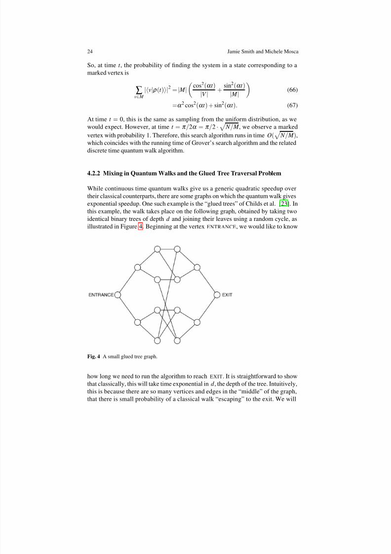
While continuous time quantum walks give us a generic quadratic speedup overtheir classical counterparts, there are some graphs on which the quantum walk givesexponential speedup. One such example is the “glued trees” of Childs et al. [23 ]. Inthis example, the walk takes place on the following graph, obtained by taking twoidentical binary trees of depth d and joining their leaves using a random cycle, asillustrated in Figure 4. Beginning at the vertex ENTRANCE , we would like to know
Fig. 4 A small glued tree graph.
how long we need to run the algorithm to reach EXIT . It is straightforward to showthat classically, this will take time exponential in d , the depth of the tree. Intuitively,this is because there are so many vertices and edges in the “middle” of the graph,that there is small probability of a classical walk “escaping” to the exit. We will
8/7/2019 Algorithms for Quantum Computers
http://slidepdf.com/reader/full/algorithms-for-quantum-computers 25/48
Algorithms for Quantum Computers 25
prove that a continuous time quantum walk can achieve an overlap of Ω (P (d )) withthe EXIT vertex in time O( 1
Q(d ) ), where Q and P are polynomials.Let V s denote the set of vertices at depth s, so that V 0 = ENTRANCE and
V 2d + 1 =
EXIT
. Taking the adjacency matrix to be our Hamiltonian, the operator
U (t ) = e−iHt acts identically on the vertices in V s for any s. Therefore, the states
|s =1
|V s|∑
v∈
V s|v (68)
form a convenient basis. We can therefore think of the walk on G as a walk on thestates |s : 0 ≤s ≤2d + 1. We also note that, if A is the adjacency matrix of G ,
A|s =
√2 |s + 1 s = 0√2 |s −1 s = 2d + 1√2 |s −1 + 2 |s + 1 s = d √2 |s + 1 + 2 |s −1 s = d + 1
√2 |s + 1 + √2 |s −1 otherwise .
(69)
Aside from the exceptions at ENTRANCE , EXIT , and the vertices in the center, thiswalk looks exactly like the walk on a line with uniform transition probabilities.
Continuous time classical random walks will eventually converge to a limitingdistribution. The time that it takes for the classical random walk to get ‘close’ tothis distribution is called the mixing time . More formally, we can take some smallconstant γ , and take the mixing time to be the amount of time time it take to comewithin γ of the stationary distribution, according to some metric. In general, weexpress the mixing time in terms of 1 / γ and n, the number of vertices in the graph.
Since quantum walks are governed by a unitary operator, we cannot expect thesame convergent behaviour. However, we can dene the limiting behaviour of quan-tum walks by taking an average over time. In order to do this, we dene Pr (u, v, T ).
If we select t ∈[0, T ] uniformly at random and run the walk for time t , beginningat vertex u, then Pr (u, v, T ) is the probability that we nd the system in state v. For-
mally, we can write this as
Pr(u, v, T ) =1T T
0v|e−iAt |u
2dt (70)
where A is the adjacency matrix of the graph. Now, if we take |λ to be theset of eigenvectors of A with corresponding eigenvalues λ , then we can rewritePr(u, v, T ) as follows:
8/7/2019 Algorithms for Quantum Computers
http://slidepdf.com/reader/full/algorithms-for-quantum-computers 26/48
26 Jamie Smith and Michele Mosca
Pr(u, v, T ) =1T T
0∑λ
e−iλ t v|λ λ |u2
dt (71)
=1
T T
0∑
λ ,λ
e−i(λ −λ )t v
|λ λ
|u v
|λ λ
|u dt (72)
= ∑λ | v|λ λ |u |2 (73)
+1T ∑
λ = λ v|λ λ |u v|λ λ |u T
0e−i(λ −λ )t dt (74)
= ∑λ | v|λ λ |u |2 (75)
+ ∑λ = λ
v|λ λ |u v|λ λ |u1 −e−i(λ −λ )T
i(λ −λ )T . (76)
In particular, we have
limT →∞
Pr(u, v, T ) = ∑λ | v|λ λ |u |2 . (77)
We will denote this value by Pr (u, v, ∞). This is the quantum analogue of thelimiting distribution for a classical random walk. We would now like to applythis to the specic case of the glued tree traversal problem. First, we will lowerbound Pr (ENTRANCE , EXIT , ∞). We will then show that Pr (ENTRANCE , EXIT , T )approaches this value rapidly as we increase T , implying that we can traverse theglued tree structure efciently using a quantum walk.
Dene the reection operator Θ by
Θ | j = |2d −1 − j (78)
This operator commutes with the adjacency matrix, and hence the walk operatorbecause of the symmetry of the glued trees. This implies that Θ can be diagonalizedin the eigenbasis of the walk operator e−iAt for any t . What is more, the eigenvaluesof Θ are ±1. As a result, if |λ is an eigenvalue of e−iAt , then
λ |ENTRANCE = ± λ |EXIT . (79)
We can apply this to (77 ), yielding
Pr(ENTRANCE , EXIT , ∞) = ∑λ | ENTRANCE |λ |4 (80)
≥1
2d + 2 ∑λ | ENTRANCE |λ |2 (81)
= 12d + 2
. (82)
8/7/2019 Algorithms for Quantum Computers
http://slidepdf.com/reader/full/algorithms-for-quantum-computers 27/48
Algorithms for Quantum Computers 27
Now, we need to determine how quickly Pr (ENTRANCE , EXIT , T ) approachesPr (ENTRANCE , EXIT , ∞)as we increase T :
|Pr(ENTRANCE , EXIT , T ) −Pr(ENTRANCE , EXIT , ∞)| (83)
= ∑λ = λ
EXIT |λ λ |ENTRANCE EXIT |λ λ |ENTRANCE1 −e−i(λ −λ )T
i(λ −λ )T (84)
≤ ∑λ = λ | λ |ENTRANCE |2 λ |ENTRANCE
2 1 −e−i(λ −λ )T
i(λ −λ )T (85)
≤2
T δ (86)
where δ is the difference between the smallest gap between any two distinct eigen-values of A. As a result, we get
Pr(ENTRANCE , EXIT , T ) ≥1
2d
−1 −
2T δ
. (87)
Childs et al. [23 ] show that δ is Ω (1/ d 3). Therefore, if we take T of size O(d 4), weget success probability O(1/ d ). Repeating this process, we can achieve an arbitrarilyhigh probability of success in time polynomial in d — an exponential speedup overthe classical random walk.
4.2.3 AND -OR Tree Evaluation
AND -OR trees arise naturally when evaluating the value of a two player combi-natorial game. We will call the players P0 and P1 . The positions in this game arerepresented by nodes on a tree. The game begins at the root, and players alternate,moving from the root towards the leaves of the tree. For simplicity, we assume thatwe are dealing with a binary tree; that is, for each move, the players have exactlytwo moves. While the algorithm can be generalizes to any approximately balancedtree, but we consider the binary case for simplicity. We also assume that every gamelasts some xed number of turns d , where a turn consists of one player making amove. We denote the total number of leaf nodes by n = 2d . We can label the leaf nodes according to which player wins if the game reaches each node; they are la-beled with a 0 if P0 wins, and a 1 if P1 wins. We can then label each node in thegraph by considering its children. If a node corresponds to P0’s turn, we take theAND of the children. For P1’s move, we take the OR of the children. The value at theroot node tells us which player has a winning strategy, assuming perfect play.
Now, since
AND ( x1 ,..., xk ) = NAND (NAND ( x1 ,..., xk )) (88)
OR ( x1 ,..., xk ) = NAND (NAND ( x1),..., NAND ( xk )) (89)
8/7/2019 Algorithms for Quantum Computers
http://slidepdf.com/reader/full/algorithms-for-quantum-computers 28/48
28 Jamie Smith and Michele Mosca
we can rewrite the AND -OR tree using only NAND operations. Furthermore, since
NOT ( x1) = NAND ( x1) (90)
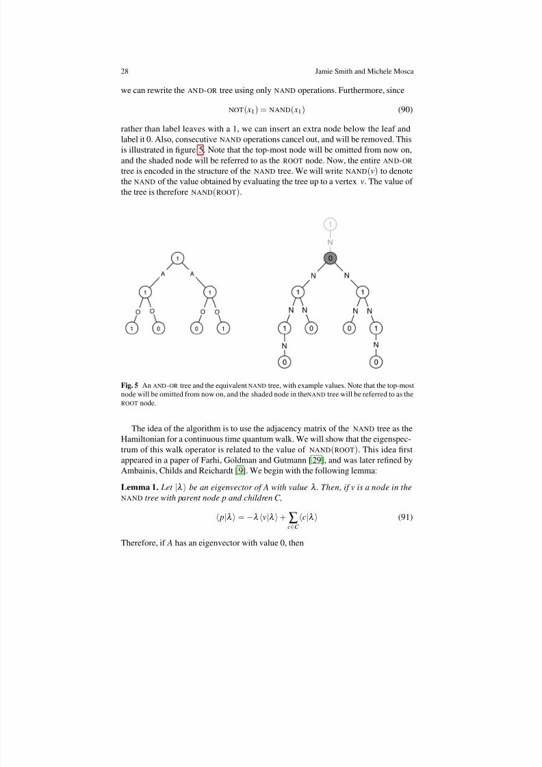
rather than label leaves with a 1, we can insert an extra node below the leaf andlabel it 0. Also, consecutive NAND operations cancel out, and will be removed. Thisis illustrated in gure 5. Note that the top-most node will be omitted from now on,and the shaded node will be referred to as the ROOT node. Now, the entire AND -OR
tree is encoded in the structure of the NAND tree. We will write NAND (v) to denotethe NAND of the value obtained by evaluating the tree up to a vertex v. The value of the tree is therefore NAND (ROOT ).
Fig. 5 An AND -OR tree and the equivalent NAND tree, with example values. Note that the top-mostnode will be omitted from now on, and the shaded node in the NAND tree will be referred to as theROOT node.
The idea of the algorithm is to use the adjacency matrix of the NAND tree as theHamiltonian for a continuous time quantum walk. We will show that the eigenspec-trum of this walk operator is related to the value of NAND (ROOT ). This idea rstappeared in a paper of Farhi, Goldman and Gutmann [ 29] , and was later rened byAmbainis, Childs and Reichardt [ 9]. We begin with the following lemma:
Lemma 1. Let |λ be an eigenvector of A with value λ . Then, if v is a node in theNAND tree with parent node p and children C,
p|λ = −λ v|λ + ∑c∈
C c|λ (91)
Therefore, if A has an eigenvector with value 0, then
8/7/2019 Algorithms for Quantum Computers
http://slidepdf.com/reader/full/algorithms-for-quantum-computers 29/48
Algorithms for Quantum Computers 29
p|λ 0 = ∑c∈
C c|λ 0 (92)
Using this fact and some inductive arguments, Ambainis, Childs and Reichardt [ 9]prove the following theorem:
Theorem 4. If NAND (ROOT ) = 0 , then there exists an eigenvector |λ 0 of A witheigenvalue 0 such that | ROOT |λ 0 |≥ 1√2
. Otherwise, if NAND (ROOT ) = 1 , then for
any eigenvector |λ of A with λ | A|λ < 12√n , we have ROOT |λ 0 = 0.
This result immediately leads to an algorithm. We perform phase estimation withprecision O(1/ √n) on the quantum walk, beginning in thestate |ROOT . If NAND (ROOT ) =0, get a phase of 0 with probability ≥ 1
2 . If NAND (ROOT ) = 1, we will never get aphase of 0. This gives us a running time of O(√n). While we have restricted ourattention to binary trees here, this result can be generalized to any m-ary tree.
It is worth noting that unstructured search is equivalent to taking the OR of nvariables. This is a AN D -OR tree of depth 1, and n leaves. The O(√n) running time of Grover’s algorithm corresponds to the running time for the quantum walk algorithm.
Classically, the running time depends not just on the number of leaves, but on thestructure of the tree. If it is a balanced m-ary tree of depth d , then the running timeis
Om−1 + √m2 + 14m + 1
4
d
. (93)
In fact, the quantum speedup is maximal when we have an n-ary tree of depth 1.This is just unstructured search, and requires Ω (n) time classically.
Reichardt and Spalek [55] generalize the AND-OR tree problem to the evalu-ation of a broader class of logical formulas. Their approach uses span programs .A span program P consists of a set of target vector t , and a set of input vectors
v01 , v1
1 ,..., v0n , v1
n ,corresponding to logical literals x1 , x1 ,..., xn , xn. The programcorresponds to a boolean function f
P:
0,1
n
→ 0
,1
such that, for σ
∈ 0
,1
n ,
f (σ ) = 1 if and only if n
∑ j= 1
vσ j j = t . [42 ]
Reichardt and Spalek outline the connection between span programs and the evalu-ation of logical formulas. They show that nding σ
∈f −1(1) is equivalent to nd-
ing a zero eigenvector for a graph GP corresponding to the span program P . In thissense, the span program approach is similar to the quantum walk approach of Childset al.— both methods evaluate a formula by nding a zero eigenvector of a corre-sponding graph.

8/7/2019 Algorithms for Quantum Computers
http://slidepdf.com/reader/full/algorithms-for-quantum-computers 30/48
30 Jamie Smith and Michele Mosca
5 Tensor Networks and Their Applications
A tensor network consists of an underlying graph G , with an algebraic object calleda tensor assigned to each vertex of G . The value of the tensor network is calculatedby performing a series of operations on the associated tensors. The nature of theseoperations is dictated by the structure of G . At their simplest, tensor networks cap-ture basic algebraic operations, such as matrix multiplication and the scalar productof vectors. However, their underlying graph structure makes them powerful tools fordescribing combinatorial problems as well. We will explore two such examples—the Tutte polynomial of a planar graph, and the partition function of a statisticalmechanical model dened on a graph. As a result, the approximation algorithm thatwe will describe below for the value of a tensor network is implicitly an algorithmfor approximating the Tutte polynomial, as well as the partition function for thesestatistical mechanics models. We begin by dening the notion of a tensor. We thenoutline how these tensors and tensor operations are associated with an underlyinggraph structure. For a more detailed account of this algorithm, the reader is referredto [10 ]. Finally, we will describe the quantum approxiamtion algorithm for the valueof a tensor network, as well as the applications mentioned above.
5.0.4 Tensors: Basic Denitions
Tensors are formally dened as follows:
Denition 3. A tensor M of rank m and dimension q is an element of C qm. Its entries
are denoted by M j1 , j2 ,..., jm , where 0 ≤ jk ≤q −1 for all jk .
Based on this denition, a vector is simply a tensor of rank 1, while a square matrixis a tensor of rank 2. We will now dene several operations on tensors, which willgeneralize many familiar operations from linear algebra.
Denition 4. Let M and N be two tensors of dimension q and rank m and n respec-tively. Then, their product, denoted M
⊗ N , is a rank m + n tensor with entries
( M ⊗ N ) j1 ,..., jm,k 1 ,...,k n = M j1 ,..., jm · N k 1 ,...,k n . (94)
This operation is simply the familiar tensor product. While the way that the entriesare indexed is different, the resulting entries are the same.
Denition 5. Let M be a tensor of rank m and dimension q. Now, take a and b with1 ≤a < b ≤m. The contraction of M with respect to a and b is a rank m −2 tensor N dened as follows:
N j1 ,..., ja
−1 , ja+ 1 ,... jb
−1 , jb+ 1 ,..., jm =
q−1
∑k = 0
M j1 ,..., ja−
1 ,k , ja+ 1 ,... jb−
1 ,k , jb+ 1 ,..., jm . (95)
8/7/2019 Algorithms for Quantum Computers
http://slidepdf.com/reader/full/algorithms-for-quantum-computers 31/48
Algorithms for Quantum Computers 31
One way of describing this operation is that each entry in the contracted tensor isgiven by summing along the “diagonal” dened by a and b. This operation general-izes the partial trace of a density operator. The density operator of two qubit systemcan be thought of as a rank 4 tensor of dimension 2. Tracing out the second qubit is
then just taking a contraction with respect to 3 and 4. It is also useful to consider thecombination of these two operations:
Denition 6. If M and N are two tensors of dimension q and rank m and n, then fora and b with 1 ≤a ≤m and 1 ≤b ≤n, the contraction of M and N is the result of contracting the product M
⊗ N with respect to a and m + b.
We now have the tools to describe a number of familiar operations in terms of tensoroperations. For example, the inner product of two vectors can be expressed as thecontraction of two rank 1 tensors. Matrix multiplication is just the contraction of 2rank 2 tensors M and N with respect to the second index of M and the rst index of N . Finally, if we take a Hilbert space H = C q , then we can identify a tensor M of dimension q and rank m with a linear operator M s,t : H ⊗t → H ⊗s where s + t = m:
M s,t
= ∑ j1 ,..., jm
M j1 ,..., jm |
j1⊗...⊗ |
js
js+ 1|⊗...⊗
jm|.
(96)
This correspondence with linear operators is essential to understanding tensor net-works and their evaluation.
5.1 The Tensor Network Representation
A tensor network T (G, M ) consists of a graph G = ( V , E ) and a set of tensors M =
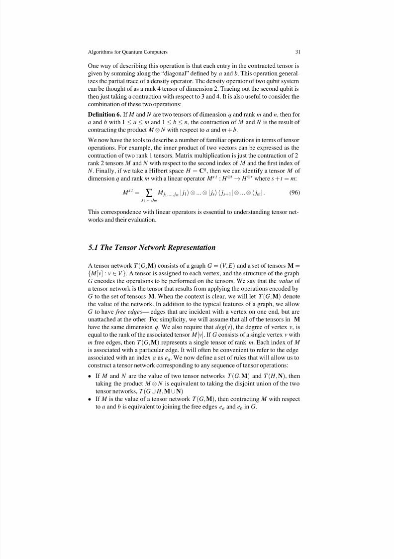
M [v] : v∈V . A tensor is assigned to each vertex, and the structure of the graphG encodes the operations to be performed on the tensors. We say that the value of a tensor network is the tensor that results from applying the operations encoded byG to the set of tensors M . When the context is clear, we will let T (G, M ) denotethe value of the network. In addition to the typical features of a graph, we allowG to have free edges — edges that are incident with a vertex on one end, but areunattached at the other. For simplicity, we will assume that all of the tensors in Mhave the same dimension q. We also require that deg (v), the degree of vertex v, isequal to the rank of the associated tensor M [v]. If G consists of a single vertex v withm free edges, then T (G, M ) represents a single tensor of rank m. Each index of M is associated with a particular edge. It will often be convenient to refer to the edgeassociated with an index a as ea . We now dene a set of rules that will allow us toconstruct a tensor network corresponding to any sequence of tensor operations:
• If M and N are the value of two tensor networks T (G, M ) and T ( H , N), thentaking the product M ⊗ N is equivalent to taking the disjoint union of the two
tensor networks, T (G∪
H , M∪
N)• If M is the value of a tensor network T (G, M ), then contracting M with respect
to a and b is equivalent to joining the free edges ea and eb in G .
8/7/2019 Algorithms for Quantum Computers
http://slidepdf.com/reader/full/algorithms-for-quantum-computers 32/48
32 Jamie Smith and Michele Mosca
• As a result, taking the contraction of M and N with respect to a and b correspondsto joining the associated edge ea from T (G, M ) and eb from T ( H , N)
Some examples are illustrated in gure 6. Applying these simple operations itera-tively allows us to construct a network corresponding to any series of products andcontractions of tensors. Note that the number of free edges in T (G, M ) is alwaysequal to the rank of the corresponding tensor M . We will be particularly interestedin tensor networks that have no free edges, and whose value is therefore a scalar.
Fig. 6 The network representation of a tensor M of rank 4, and the contraction of two rank 4tensors, M and N .
We can now consider the tensor network interpretation of a linear operator M s,t
dened in (96 ). M s,t is associated with a rank m = s + t tensor M . An equivalenttensor network could consist of a single vertex with m free edges (e1,..., em). Theoperator M s,t acts on elements of (C q)⊗t , which are rank t tensors, and can thereforebe represented a single vertex with t free edges (e1 ,..., et ). The action of M s,t on anelement N
∈(C q)⊗t is therefore represented by connecting ek to es+ k for k = 1,..., t .Figure 7 illustrates the operator M 2,2 acting on a rank 2 tensor. Note that the resultingnetwork has two free edges, corresponding to the rank of the resulting tensor.
Fig. 7 The network corresponding to the operator M 2,2 acting on a rank 2 tensor N .
We now return to the tensor networks we will be most interested in— those with
no free edges. Let us rst consider the example of an inner product of two rank 1tensors. This corresponds to a graph consisting of two vertices u and v joined by asingle edge. The value of the tensor is then
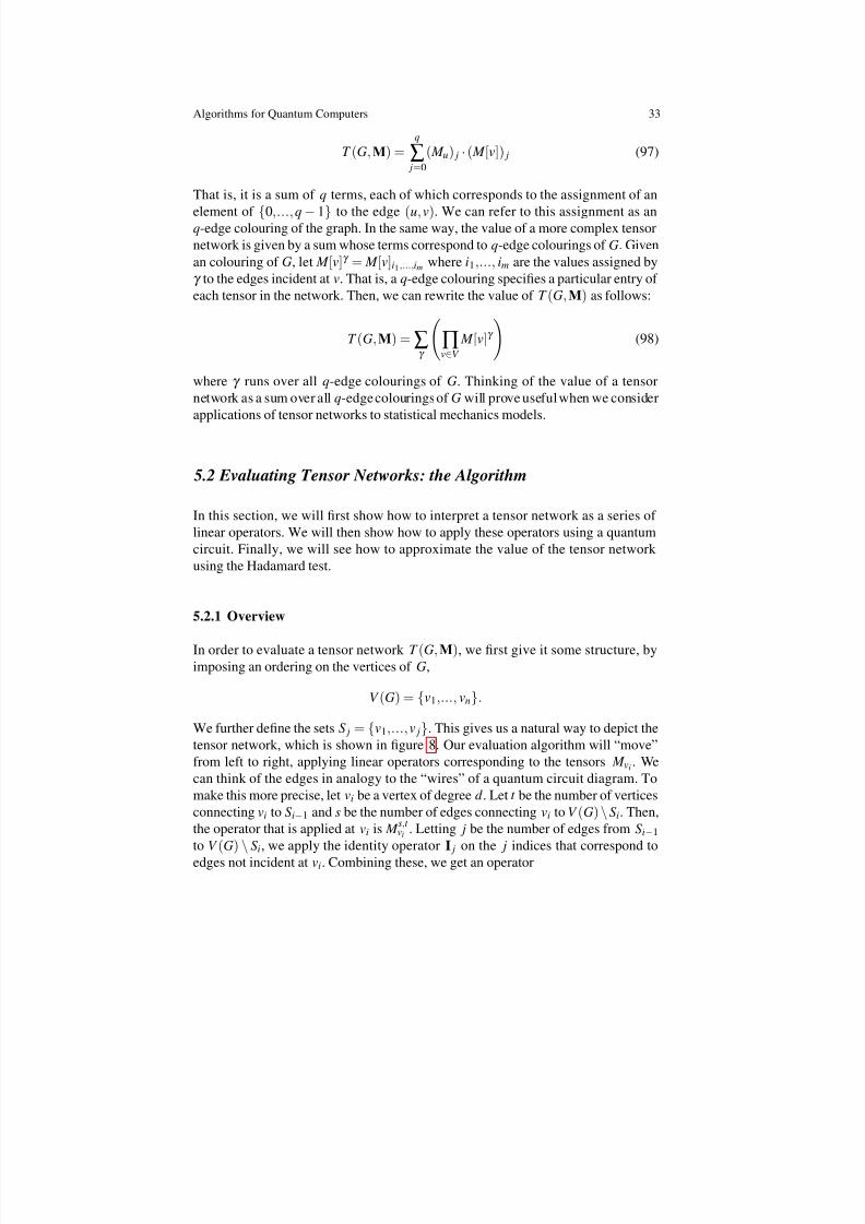
8/7/2019 Algorithms for Quantum Computers
http://slidepdf.com/reader/full/algorithms-for-quantum-computers 33/48
Algorithms for Quantum Computers 33
T (G, M ) =q
∑ j= 0
( M u) j ·( M [v]) j (97)
That is, it is a sum of q terms, each of which corresponds to the assignment of an
element of 0,..., q −1to the edge (u, v). We can refer to this assignment as anq-edge colouring of the graph. In the same way, the value of a more complex tensornetwork is given by a sum whose terms correspond to q-edge colourings of G . Givenan colouring of G , let M [v]γ = M [v]i1 ,..., im where i1 ,..., im are the values assigned byγ to the edges incident at v. That is, a q-edge colouring species a particular entry of each tensor in the network. Then, we can rewrite the value of T (G, M ) as follows:
T (G, M ) = ∑γ
∏v∈
V M [v]γ (98)
where γ runs over all q-edge colourings of G . Thinking of the value of a tensornetwork as a sum over all q-edgecolouringsof G will prove usefulwhen we considerapplications of tensor networks to statistical mechanics models.
5.2 Evaluating Tensor Networks: the Algorithm
In this section, we will rst show how to interpret a tensor network as a series of linear operators. We will then show how to apply these operators using a quantumcircuit. Finally, we will see how to approximate the value of the tensor network using the Hadamard test.
5.2.1 Overview
In order to evaluate a tensor network T (G, M ), we rst give it some structure, byimposing an ordering on the vertices of G ,
V (G) = v1 ,..., vn.
We further dene the sets S j = v1,..., v j. This gives us a natural way to depict thetensor network, which is shown in gure 8. Our evaluation algorithm will “move”from left to right, applying linear operators corresponding to the tensors M vi . Wecan think of the edges in analogy to the “wires” of a quantum circuit diagram. Tomake this more precise, let vi be a vertex of degree d . Let t be the number of verticesconnecting vi to Si−1 and s be the number of edges connecting vi to V (G) \Si . Then,the operator that is applied at vi is M s,t
vi . Letting j be the number of edges from Si−1to V (G)
\Si , we apply the identity operator I j on the j indices that correspond to
edges not incident at vi . Combining these, we get an operator
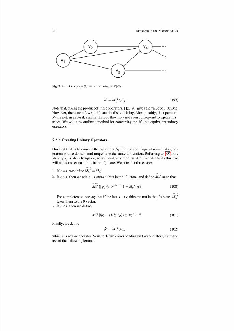
8/7/2019 Algorithms for Quantum Computers
http://slidepdf.com/reader/full/algorithms-for-quantum-computers 34/48
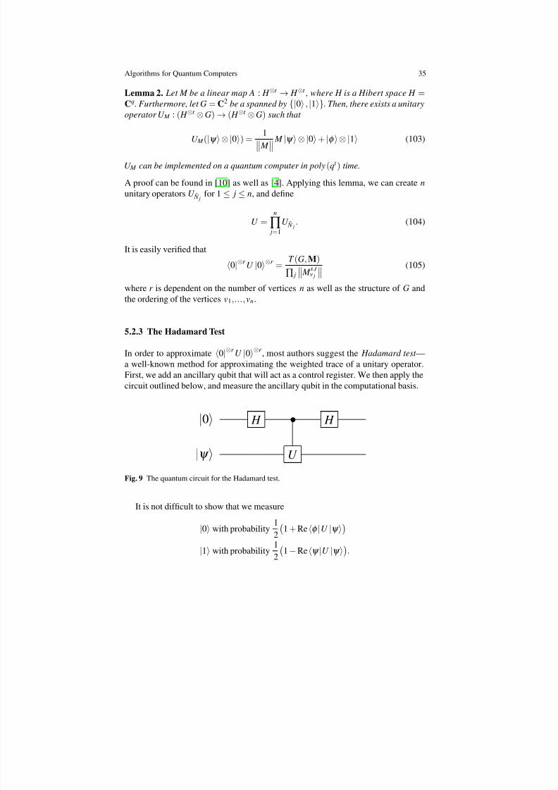
8/7/2019 Algorithms for Quantum Computers
http://slidepdf.com/reader/full/algorithms-for-quantum-computers 35/48
Algorithms for Quantum Computers 35
Lemma 2. Let M be a linear map A : H ⊗t → H ⊗t , where H is a Hibert space H =C q . Furthermore, let G = C 2 be a spanned by |0 , |1 . Then, there exists a unitaryoperator U M : ( H ⊗t
⊗G) →( H ⊗t ⊗G) such that
U M (|ψ ⊗ |0 ) =
1 M M |ψ
⊗ |0 + |φ ⊗ |1 (103)
U M can be implemented on a quantum computer in poly (qt ) time.
A proof can be found in [ 10] as well as [4]. Applying this lemma, we can create nunitary operators U ˜ N j for 1 ≤ j ≤n, and dene
U =n
∏ j= 1
U ˜ N j . (104)
It is easily veried that
0|⊗r U |0 ⊗r =T (G, M )
∏ j M
s,t v j
(105)
where r is dependent on the number of vertices n as well as the structure of G andthe ordering of the vertices v1,..., vn .
5.2.3 The Hadamard Test
In order to approximate 0|⊗r U |0 ⊗r , most authors suggest the Hadamard test —a well-known method for approximating the weighted trace of a unitary operator.First, we add an ancillary qubit that will act as a control register. We then apply thecircuit outlined below, and measure the ancillary qubit in the computational basis.
|0 H • H
|ψ U
Fig. 9 The quantum circuit for the Hadamard test.
It is not difcult to show that we measure
|0 with probability12
1 + Re φ |U |ψ
|1 with probability12 1 −Re ψ |U |ψ .
8/7/2019 Algorithms for Quantum Computers
http://slidepdf.com/reader/full/algorithms-for-quantum-computers 36/48
36 Jamie Smith and Michele Mosca
So, if we assign a random variable X such that X = 1 when we measure |0 and X = −1 when we measure |1 , then X has expected value Re ψ |U |ψ . So, in orderto approximate Re ψ |U |ψ to a precision of ε with constant probability p > 1/ 2,we require O(ε −2) repetitions of this protocol. In order to calculate the imaginary
portion, we apply the gate R = 1 0
0 −i
to the ancillary qubit, right after the rst Hadamard gate. It is important to notethat the Hadamard test gives an additive approximation of 0|⊗r U |0 ⊗r . Additiveapproximations will be examined in section 5.2.5.
5.2.4 Approximating 0|⊗r U |0 ⊗r Using Amplitude Estimation
In order to estimate 0|⊗r U |0 ⊗r , most of the literature applies the Hadamard test.However, it is worth noting that we can improve the running time by using theprocess of amplitude estimation , as outlined in section 3. Using the notation fromsection 3, we have U f = U 0 and A = U , the unitary corresponding to the tensornetwork T (G, M ). We begin in the state U |0 ⊗r , and our search iterate is
Q = −UU 0U −1U 0. (106)
In order to approximate 0|⊗r U |0 ⊗r to a precision of ε , our running time is inO(1/ ε ), a quadratic improvement over the Hadamard test.
5.2.5 Additive Approximation
Let f : S →C be a function that we would like to evaluate. Then, an additive ap- proximation A with approximation scale ∆ : S
→R is an algorithm that, on input
x∈
S and parameter ε > 0 , outputs A( x) such that
Pr | A( x) − f ( x)|≥ε∆ ( x) ≤c (107)
for some constant c with 0 ≤c < 1/ 2.If ∆ ( x) is O( f ( x)) , then A is a fully polynomialrandomized approximation scheme , or FPRAS.
We will now determine the approximation scale for the algorithm outlined above.Using amplitude estimation, we estimate
0|⊗r U |0 ⊗r =T (G, M )
∏ j M s,t v j
(108)
to within ε with time requirement in O(1/ ε ). However, the quantity we actuallywant to evaluate is T (G, M ), so we must multiply by ∏ j M s,t
v j . Therefore, ouralgorithm has approximation scale
8/7/2019 Algorithms for Quantum Computers
http://slidepdf.com/reader/full/algorithms-for-quantum-computers 37/48
Algorithms for Quantum Computers 37
∆ (G, M ) = ∏ j
M s,t v j
(109)
We apply lemma 2 to each vertex in G , and require O(1/ ε ) repetitions of the algo-rithm to approximate T (G, M ) with the desired accuracy using amplitude estima-tion. This gives an overall running time
O poly (q D(G)) ·|V (G)|·ε (110)
where D(G) is the maximum degree of any vertex in G . The algorithm is, therefore,an additive approximation of T (G, M ).
5.3 Approximating the Tutte Polynomial for Planar Graphs UsingTensor Networks
In 2000, Kitaev, Freedman, Larsen and Wang [ 32, 31] demonstrated an efcientquantum simulation for topological quantum eld theories. In doing so, they im-plied that the Jones polynomial can be efciently approximated at e2π i/ 5. This sug-gests that efcient quantum approximation algorithms might exist for a wider rangeof knot invariants and values. Aharonov, Jones and Landau developed such a Jonespolynomial for any complex value [ 5]. Yard and Wocjan’s developed a related algo-rithm for approximating the HOMFLYPT polynomial of a braid closure [ 64]. Bothof these knot invariants are special cases of the Tutte polynomial. While the tensornetwork algorithm in section 5.3.2 follows directly from a later paper of Aharonovet al. [4], it owes a good deal to these earlier results for knot invariants.
We will give a denition of the Tutte polynomial, as well as an overview of itsrelationship to tensor networks and the resulting approximation algorithm.
5.3.1 The Tutte Polynomial
The multi-variate Tutte Polynomial is dened for a graph G = ( V , E ) with edgeweights w = weand variable q as follows:
Z G (q, w) = ∑ A⊆
E qk ( A) ∏
e∈
Awe (111)
where k ( A) denotes the number of connected components in the graph induced by A. The power of the Tutte polynomial arises from the fact that it captures nearly allfunctions on graphs dened by a skein relation . A skein relation is of the form
f (G) = x · f (G/ e) + y· f (G \ e) (112)
8/7/2019 Algorithms for Quantum Computers
http://slidepdf.com/reader/full/algorithms-for-quantum-computers 38/48
38 Jamie Smith and Michele Mosca
where G/ e is created by contracting an edge e and G \ e is created by deleting e.Oxley and Welsh [ 62] show that, with a few additional restrictions on f , if f isdened by a skein relation, then computing f can be reduced to computing Z G . Itturns out that many functions can be dened in terms of a skein relation, including
1. The partition functions of the Ising and Potts models from statistical physics.2. The chromatic and ow polynomials of a graph G .3. The Jones Polynomial of an alternating link.
The exact evaluation of the Tutte polynomial, even when restricted to planar graphs,turns out to be # P -hard for all but a handful of values of q and w. An exact algo-rithm is therefore believed to be impossible for a quantum computer. Indeed, evena polynomial time FPRAS seems very unlikely for the Tutte polynomial of a gen-eral graph and any parameters q and w. The interesting question seems to be whichgraphs and parameters admit an efcient and accurate approximation. By describ-ing the Tutte polynomial as the evaluation of a Tensor network, we immediatelyproduce an additive approximation algorithm for the Tutte polynomial. However,we do not have a complete characterization of the graphs and parameters for which
this approximation is non-trivial.
5.3.2 The Tutte Polynomial as a Tensor Network
Given a planar graph G , and an embedding of G in the plane, we dene the medialgraph L G . The vertices of LG are placed on the edges of G . Two vertices of LG are joined by an edge if they are adjacent on the boundary of a face of G . If G containsvertices of degree 2, then LG will have multiple edges between some pair of vertices.Also note that LG is a regular graph with valency 4. An example of a graph and itsassociated medial graph is depicted in gure 10.
In order to describe the Tutte polynomial in terms of a tensor network, we makeuse of the generalized Temperley-Lieb algebra , as dened in [ 4]. The basis elementsof the Temperley-Lieb algebra GT L(d ) can be thought of as diagrams in which mupper pegs are joined to n lower pegs by a series of strands. The diagram mustcontain no crossings or loops. See gure 11 for an example of such an element. Twobasis elements are considered equivalent if they are isotopic to each other or if onecan be obtained from the other by ‘padding’ it on the right with a series of verticalstrands. The algebra consists of all complex weighted sums of these basis elements.Given two elements of the algebra T 1 and T 2 , we can take their product T 2 ·T 1 bysimply placing T 2 on top of T 1 and joining the strands. Note that if the number of strands do not match, we can simply pad the appropriate element with some numberof vertical strands. As a consequence, the identity element consists of any number of vertical strands. In composing two elements in this way, we may create a loop. Letus say that T 1 ·T 2 contains one loop. Then, if T 3 is the element created by removingthe loop, we dene T 1
·T 2 = dT 3 , where d is the complex parameter of GT L(d ).
We would also like this algebra to accommodate drawings with crossings. LetT 1 be such a diagram, and T 2 and T 3 be the diagrams resulting from ‘opening’ the
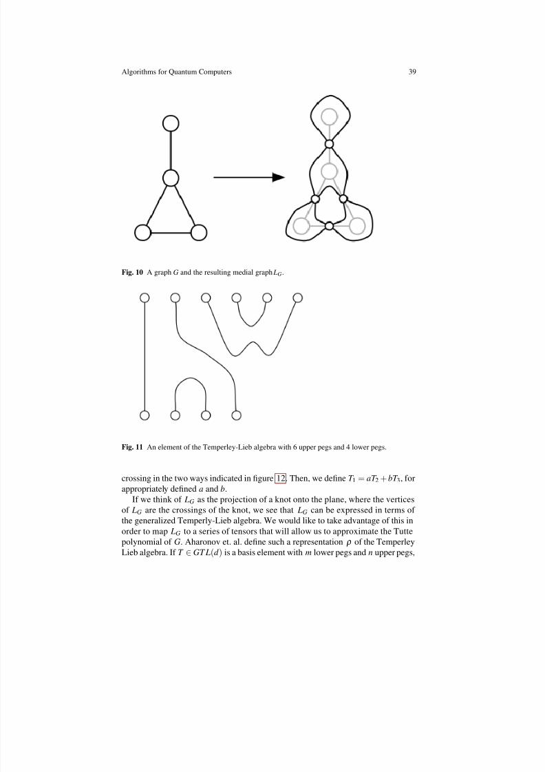
8/7/2019 Algorithms for Quantum Computers
http://slidepdf.com/reader/full/algorithms-for-quantum-computers 39/48
Algorithms for Quantum Computers 39
Fig. 10 A graph G and the resulting medial graph LG .
Fig. 11 An element of the Temperley-Lieb algebra with 6 upper pegs and 4 lower pegs.
crossing in the two ways indicated in gure 12. Then, we dene T 1 = aT 2 + bT 3 , forappropriately dened a and b.
If we think of LG as the projection of a knot onto the plane, where the verticesof LG are the crossings of the knot, we see that LG can be expressed in terms of the generalized Temperly-Lieb algebra. We would like to take advantage of this inorder to map LG to a series of tensors that will allow us to approximate the Tutte
polynomial of G . Aharonov et. al. dene such a representation ρ of the TemperleyLieb algebra. If T
∈GT L (d ) is a basis element with m lower pegs and n upper pegs,
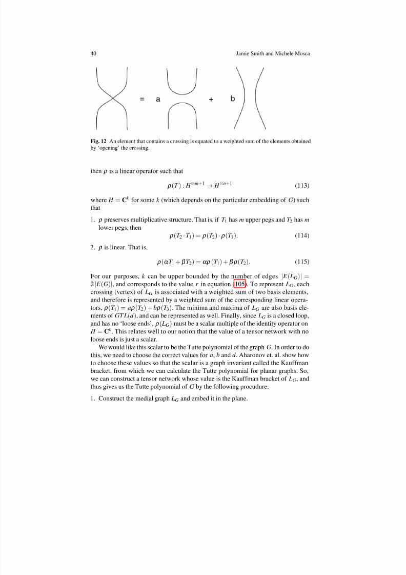
8/7/2019 Algorithms for Quantum Computers
http://slidepdf.com/reader/full/algorithms-for-quantum-computers 40/48
40 Jamie Smith and Michele Mosca
Fig. 12 An element that contains a crossing is equated to a weighted sum of the elements obtainedby ‘opening’ the crossing.
then ρ is a linear operator such that
ρ (T ) : H ⊗m+ 1 → H ⊗n+ 1 (113)
where H = Ck
for some k (which depends on the particular embedding of G) suchthat
1. ρ preserves multiplicative structure. That is, if T 1 has m upper pegs and T 2 has mlower pegs, then
ρ (T 2 ·T 1) = ρ (T 2) ·ρ (T 1). (114)
2. ρ is linear. That is,
ρ (α T 1 + β T 2) = αρ (T 1) + β ρ (T 2). (115)
For our purposes, k can be upper bounded by the number of edges | E ( LG )| =2 | E (G)|, and corresponds to the value r in equation ( 105 ). To represent LG , eachcrossing (vertex) of LG is associated with a weighted sum of two basis elements,
and therefore is represented by a weighted sum of the corresponding linear opera-tors, ρ (T 1) = aρ (T 2) + bρ (T 3). The minima and maxima of LG are also basis ele-ments of GT L(d ), and can be represented as well. Finally, since LG is a closed loop,and has no ‘loose ends’, ρ ( LG ) must be a scalar multiple of the identity operator on H = C k . This relates well to our notion that the value of a tensor network with noloose ends is just a scalar.
We would like this scalar to be the Tutte polynomial of the graph G . In order to dothis, we need to choose the correct values for a , b and d . Aharonov et. al. show howto choose these values so that the scalar is a graph invariant called the Kauffmanbracket, from which we can calculate the Tutte polynomial for planar graphs. So,we can construct a tensor network whose value is the Kauffman bracket of LG , andthus gives us the Tutte polynomial of G by the following procudure:
1. Construct the medial graph LG and embed it in the plane.
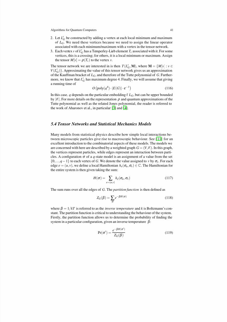
8/7/2019 Algorithms for Quantum Computers
http://slidepdf.com/reader/full/algorithms-for-quantum-computers 41/48
Algorithms for Quantum Computers 41
2. Let LG be constructed by adding a vertex at each local minimum and maximumof LG . We need these vertices because we need to assign the linear operatorassociated with each minimum/maximum with a vertex in the tensor network.
3. Each vertex v of LG has a Temperley-Lieb element T v associated with it. For some
vertices, this is a crossing; for others, it is a local minimum or maximum. Assignthe tensor M [v] = ρ (T v) to the vertex v.
The tensor network we are interested in is then T ( LG , M ), where M = M [v] : v∈V ( LG ). Approximating the value of this tensor network gives us an approximationof the Kauffman bracket of LG , and therefore of the Tutte polynomial of G . Further-more, we know that LG has maximum degree 4. Finally, we will assume that givinga running time of
O poly (q4) · | E (G)| ·ε −1 (116)
In this case, q depends on the particular embedding f LG , but can be upper boundedby | E |. For more details on the representation ρ and quantum approximations of theTutte polynomial as well as the related Jones polynomial, the reader is referred tothe work of Aharonov et al., in particular [3] and [4].
5.4 Tensor Networks and Statistical Mechanics Models
Many models from statistical physics describe how simple local interactions be-tween microscopic particles give rise to macroscopic behaviour. See [ 11] for anexcellent introduction to the combinatorial aspects of these models. The models weare concerned with here are described by a weighted graph G = ( V , E ). In this graph,the vertices represent particles, while edges represent an interaction between parti-cles. A conguration σ of a q-state model is an assignment of a value from the set
0,..., q −1to each vertex of G . We denote the value assigned to v by σ v. For eachedge e = ( u, v), we dene a local Hamiltonian he(σ u , σ v)
∈
C . The Hamiltonian forthe entire system is then given taking the sum:
H (σ ) = ∑e=( u,v)
he(σ u , σ v) (117)
The sum runs over all the edges of G . The partition function is then dened as
Z G (β ) = ∑σ
e−β H (σ ) (118)
where β = 1/ kT is referred to as the inverse temperature and k is Boltzmann’s con-stant. The partition function is critical to understanding the behaviour of the system.Firstly, the partition function allows us to determine the probability of nding thesystem in a particular conguration, given an inverse temperature β :
Pr(σ ) =e−β H (σ )
Z G (β )(119)
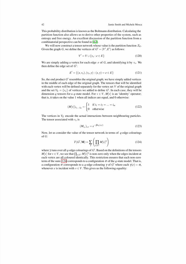
8/7/2019 Algorithms for Quantum Computers
http://slidepdf.com/reader/full/algorithms-for-quantum-computers 42/48
42 Jamie Smith and Michele Mosca
This probability distribution is known as the Boltmann distribution. Calculating thepartition function also allows us to derive other properties of the system, such asentropy and free energy. An excellent discussion of the partition function from acombinatorial perspective can be found in [ 62].
We will now construct a tensor network whose value is the partition function Z G .Given the graph G , we dene the vertices of G = ( V , E ) as follows:
V = V ∪ve : e∈ E (120)
We are simply adding a vertex for each edge e of G , and identifying it by ve . Wethen dene the edge set of G :
E = ( x, ve), (ve , y) : ( x, y) = e∈ E (121)
So, the end product G resembles the original graph; we have simply added verticesin the middle of each edge of the original graph. The tensors that will be identiedwith each vertex will be dened separately for the vertex set V of the original graphand the set V E =
ve
of vertices we added to dene G . In each case, they will be
dimension q tensors for a q-state model. For v∈
V , M [v] is an ‘identity’ operator;that is, it takes on the value 1 when all indices are equal, and 0 otherwise:
( M [v])i1 ,.., im =1 if i1 = i2 = ... = im
0 otherwise(122)
The vertices in V E encode the actual interactions between neighbouring particles.The tensor associated with ve is
( M ve )s,t = e−β he(s,t ) (123)
Now, let us consider the value of the tensor network in terms of q-edge colouringsof G:
T (G , M ) = ∑γ
∏v∈
V M [v]γ (124)
where γ runs over all q-edge colourings of G . Based on the denitions of the tensors M [v] for v
∈V , we see that ∏ v
∈V M [v]γ is non-zero only when the edges incident at
each vertex are all coloured identically. This restriction ensures that each non-zeroterm of the sum ( 124 ) corresponds to a conguration σ of the q-state model. That is,a conguration σ corresponds to a q-edge colouring γ of G where each γ (e) = σ vwhenever e is incident with v∈V . This gives us the following equality:
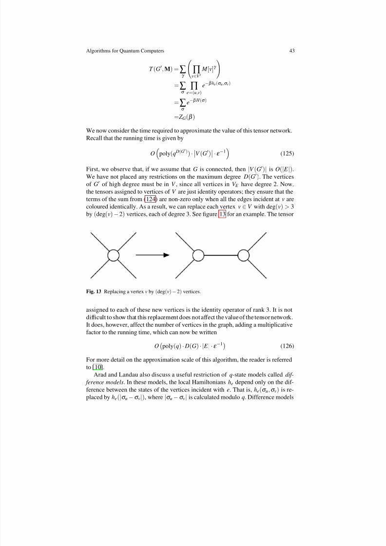
8/7/2019 Algorithms for Quantum Computers
http://slidepdf.com/reader/full/algorithms-for-quantum-computers 43/48
Algorithms for Quantum Computers 43
T (G , M ) = ∑γ
∏v∈
V M [v]γ
= ∑σ
∏e=( u,v)
e−β he(σ u ,σ v)
= ∑σ
e−β H (σ )
= Z G(β )
We now consider the time required to approximate the value of this tensor network.Recall that the running time is given by
O poly (q D(G )) · V (G ) ·ε −1 (125)
First, we observe that, if we assume that G is connected, then |V (G )| is O(| E |).We have not placed any restrictions on the maximum degree D(G ). The verticesof G of high degree must be in V , since all vertices in V E have degree 2. Now,
the tensors assigned to vertices of V are just identity operators; they ensure that theterms of the sum from ( 124) are non-zero only when all the edges incident at v arecoloured identically. As a result, we can replace each vertex v
∈V with deg (v) > 3
by (deg (v) −2) vertices, each of degree 3. See gure 13 for an example. The tensor
Fig. 13 Replacing a vertex v by (deg (v) −2) vertices.
assigned to each of these new vertices is the identity operator of rank 3. It is notdifcult to show that this replacement does not affect the value of the tensornetwork.It does, however, affect the number of vertices in the graph, adding a multiplicativefactor to the running time, which can now be written
O poly (q) · D(G) ·| E |·ε −1 (126)
For more detail on the approximation scale of this algorithm, the reader is referredto [ 10] .
Arad and Landau also discuss a useful restriction of q-state models called dif-
ference models . In these models, the local Hamiltonians he depend only on the dif-ference between the states of the vertices incident with e. That is, he(σ u , σ v) is re-placed by he(|σ u −σ v|), where |σ u −σ v| is calculated modulo q. Difference models
8/7/2019 Algorithms for Quantum Computers
http://slidepdf.com/reader/full/algorithms-for-quantum-computers 44/48
44 Jamie Smith and Michele Mosca
include the well-known Potts, Ising and Clock models. Arad and Landau show thatthe approximation scale can be improved when we restrict our attention to differencemodels.
Van den Nest et al. [25 , 40] show that the partition function for difference models
can be described as the overlap between two quantum states,
Z G = ψ G|e∈
E (G)|α e . (127)
Van den Nest uses the state |ψ G to encode the structure of the graph, while eachstate |α e encodes the strength of the local interaction at e. The actual computationof this overlap is best described as a tensor network. While this description doesnot yield a computational speedup over the direct method described above, it isan instructive way to deconstruct the problem. In the case of planar graphs, it alsorelates the partition function of a graph G and its planar dual.
Geraci and Lidar [ 34, 35] show that the Potts partition may be efciently and
exactly evaluated for a class of graphs related to irreducible cyclic cocycle codes.While their algorithm does not employ tensor networks, it is interesting to considerthe implications of their results in the context of tensor networks. Is there a class of tensor networks whose value can be efciently and exactly calculated using similartechniques?
6 Conclusion
In this chapter, we have reviewed quantum algorithms of several types: those basedon the quantum Fourier transform, amplitude amplication, quantum walks, andevaluating tensor networks. This is by no means a complete survey of quantum al-
gorithms; most notably absent are algorithms for simulating quantum systems. Thisis a particularly natural application of quantum computers, and these algorithmsoften achieve an exponential speedup over their classical counterparts.
Algorithms based on the quantum Fourier transform, as reviewed in section 2include some of the earliest quantum algorithms that give a demonstrable speedupover classical algorithms, such as the algorithms for Deutsch’s problem and Simon’sproblem. Many problems in this area can be described as hidden subgroup problems.Despite the fact that problems of this type have been well-studied, many questionsremain open. For example, there is no efcient quantum algorithm known for mostexamples of non-Abelian groups. In particular, the quantum complexity of the graphisomorphism problem remains unknown.
Similarly, the family of algorithms based on amplitude amplication and estima-tion have a relatively long history. While Grover’s original searching algorithm isthe best-known example, this approach has been greatly generalized. For example,in [18 ] it is shown how the same principles applied by Grover to searching can be
8/7/2019 Algorithms for Quantum Computers
http://slidepdf.com/reader/full/algorithms-for-quantum-computers 45/48
8/7/2019 Algorithms for Quantum Computers
http://slidepdf.com/reader/full/algorithms-for-quantum-computers 46/48
46 Jamie Smith and Michele Mosca
8. Ambainis, A., Bach, E., Nayak, A., Vishwanath, A., Watrous, J.: One-dimensional quantumwalks. In: STOC ’01: Proceedings of the thirty-third annual ACM symposium on Theory of computing, pp. 37–49. ACM, New York, NY, USA (2001). DOI http://doi.acm.org/10.1145/ 380752.380757
9. Ambainis, A., Childs, A., Reichardt, B.: Any and-or formula of size n can be evaluated in time
n1/ 2+ o(1) on a quantum computer. pp. 363–372 (2007). DOI 10.1109/FOCS.2007.5710. Arad, I., Landau, Z.: Quantum computation and the evaluation of tensor networks (2008)11. Beaudin, L., Ellis-Monaghan, J., Pangborn, G., Shrock, R.: A little statistical mechanics for
the graph theorist (2008)12. Bernstein, B.K., Vazirani, U.: Quantum complexity theory. SIAM Journal on Computing 26,
1411–1473 (1997)13. Berry, D.W., Ahokas, G., Cleve, R., Sanders, B.C.: Efcient quantum algorithms for simulat-
ing sparse hamiltonians. Communications in Mathematical Physics 270 (2007)14. Boixo, S., Knill, E., Somma, R.: Quantum state preparation by phase randomization.
arXiv:0903.165215. Boneh, D., Lipton, R.: Quantum cryptanalysis of hidden linear functions (extended abstract).
pp. 424–437 (1995)16. Boyer, M., Brassard, G., Hoyer, P., Tapp, A.: Tight bounds on quantum searching. Fortschritte
der Physik 56(5-5) , 493–505 (1998)17. Brassard, G., Hoyer, P.: An exact quantum polynomial-time algorithm for simon’s problem.
In: Proc. of Fifth Israeli Symposium on Theory of Computing and Systems (ISTCS’97), pp.12–23 (1997)18. Brassard, G., Hoyer, P., Mosca, M., Tapp, A.: Quantum Amplitude Amplication and Estima-
tion. Quantum Computation & Information, AMS Contemporary Math Series (2002)19. Brassard, G., Hoyer, P., Tapp, A.: Cryptology column —quantum algorithm for the collision
problem. ACM SIGACT News 28, 14–19 (1997)20. Brouwer, A.E.: Distance-Regular Graphs. Springer-Verlag, New York (1989)21. Childs, A.: Lecture notes on quantum algorithms (2008)22. Childs, A., van Dam, W.: Quantum algorithms for algebraic problems (to appear). Reviews of
Modern Physics (2009)23. Childs, A.M., Cleve, R., Deotto, E., Farhi, E., Gutmann, S., Spielman, D.A.: Exponential
algorithmic speedup by a quantum walk. In: STOC ’03: Proceedings of the thirty-fth annualACM symposium on Theory of computing, pp. 59–68. ACM, New York, NY, USA (2003).DOI http://doi.acm.org/10.1145/780542.780552
24. Cleve, R., Ekert, A., Macchiavello, C., Mosca, M.: Quantum algorithms revisited. In: Pro-ceedings of the Royal Society of London A, vol. 454, pp. 339–354 (1998)
25. Cuevas, G.D.l., D ur, W., Van den Nest, M., Briegel, H.J.: Completeness of classical spin mod-els and universal quantum computation (2008)
26. Das, A., Chakrabarti, B.K.: Quantum annealing and analog quantum computation. Rev. Mod.Phys. 80, 1061 (2008)
27. Deutsch, D.: Quantumtheory, the church-turing principle and the universal quantum computer.In: Proceedings of the Royal Society of London A, vol. 400, pp. 97–117 (1985)
28. Deutsch D., J.R.: Rapid solutions of problems by quantum computation. In: Proceedings of the Royal Society of London, Series A, vol. 439, pp. 553–558 (1992)
29. Farhi, E., Goldstone, J., Gutmann, S.: A quantum algorithm for the hamiltonian nand tree(2007)
30. Feynman, R.: Simulating physics with computers. International Journal of Theoretical Physics21(6,7) , 467–488 (1982)
31. Freedman, M.H., Kitaev, A., Larsen, M.J., Wang, Z.: Topological quantum computation(2001)
32. Freedman, M.H., Kitaev, A., Wang, Z.: Simulation of topological eld theories by quantum
computers (2000)33. G. M. D’Ariano W. van Dam, E.E.C.M., Mosca, M.: General optimized schemes for phase
estimation. Physical Review Letters 98(9), 090,501 (2007)
8/7/2019 Algorithms for Quantum Computers
http://slidepdf.com/reader/full/algorithms-for-quantum-computers 47/48
Algorithms for Quantum Computers 47
34. Geraci, J.: A bqp-complete problem related to the ising model partition function via a newconnection between quantum circuits and graphs (2008)
35. Geraci, J., Lidar, D.A.: On the exact evaluation of certain instances of the potts partitionfunction by quantum computers. Communications in Mathematical Physics 279 (3), 735–768(2008)
36. Grigoriev, D.: Testing shift-equivalence of polynomials by deterministic, probabilistic andquantum machines. Theor. Comput. Sci. 180 , 217–228 (1997)
37. Grover, L.: A fast quantum mechanical algorithm for database search. In: Proceedings of the 28th Annual ACM Symposium on the Theory of Computing (STOC 1996), pp. 212–219(1996)
38. Grover, L.: A framework for fast quantum mechanical algorithms. In: Proceedings of theThirtieth Annual ACM Symposium on Theory of Computing (STOC), pp. 53–62 (1998)
39. Hirvensalo, M.: Quantum computing. Series: Natural Computing Series (2001)40. H ubener, R., Van den Nest, M., D¨ ur, W., Briegel, H.J.: Classical spin systems and the quantum
stabilizer formalism: general mappings and applications (2008)41. Jordan, S.: Quantum computation beyond the circuit model. Ph.D. thesis, MIT (2008)42. Karchmer, M., Wigderson, A.: On span programs. In: Proceedings of the 8th Structures in
Complexity Conference, pp. 102–111 (1993)43. Kaye, P., Laamme, R., Mosca, M.: An Introduction to Quantum Computation. Oxford Uni-
versity Press (2007)44. Kempe, J.: Quantum random walks– an introductory overview. Contemporary Physics 44(4),
307–327 (2003)45. Kitaev, A.,Shen, A.,Vyalvi, M.: Classical and quantum computation. American Mathematical
Society (2002)46. Kitaev, A., Yu: Quantum measurements and the abelian stabilizer problem (1995)47. Magniez, F., Nayak, A., Roland, J., Santha, M.: Search via quantum walk. In: STOC ’07:
Proceedings of the thirty-ninth annual ACM symposium on Theory of computing, pp. 575–584. ACM, New York, NY, USA (2007). DOI http://doi.acm.org/10.1145/1250790.1250874
48. Menezes, A., van Oorschot, P., S., V.: Handbook of Applied Cryptography. CRC Press (1996)49. Mermin, N.D.: Quantum Computer Science: An Introduction. Cambridge University Press
(2007)50. Mosca, M.: Counting by quantum eigenvalue estimation. Theoretical Computer Science 264 ,
139–153 (2001)51. Mosca, M.: Abelian Hidden Subgroup Problem. Encyclopedia of Algorithms. Springer (2008)52. Mosca, M.: Quantum Algorithms (to appear). Encyclopedia of Complexity and Systems Sci-
ence (2009)53. Nayak, A., Vishwanath, A.: Quantum walk on the line (2000)54. Nielsen, M., Chuang, I.: Quantum Computation and Quantum Information. Cambridge Uni-
versity Press (2000)55. Reichardt, B.W., Spalek, R.: Span-program-based quantum algorithm for evaluating formulas.
In: STOC ’08: Proceedings of the 40th annual ACM symposium on Theory of computing,pp. 103–112. ACM, New York, NY, USA (2008). DOI http://doi.acm.org/10.1145/1374376.1374394
56. Santha, M.: Quantum walk based search algorithms. In: Theory and Applications of Modelsof Computation, pp. 31–46 (2008). DOI 10.1007/978-3-540-79228-4 \ 3
57. Shor, P.: Algorithms for quantum computation: Discrete logarithms and factoring. In: Pro-ceedings of the 35th Annual Symposium on Foundations of Computer Science, pp. 124–134(1994)
58. Shor, P.: Polynomial-time algorithms for prime factorization and discrete logarithms on aquantum computer. SIAM J. Computing 26, 1484 – 1509 (1997)
59. Simon, D.: On the power of quantum computation. In: Proceedings of the 35th IEEE Sympo-sium on the Foundations of Computer Science (FOCS), pp. 116–123 (1994)
60. Szegedy, M.: Quantum speed-up of markov chain based algorithms. In: FOCS ’04: Proceed-ings of the 45th Annual IEEE Symposium on Foundations of Computer Science, pp. 32–41.IEEE Computer Society,Washington, DC, USA (2004). DOI http://dx.doi.org/10.1109/FOCS.2004.53
8/7/2019 Algorithms for Quantum Computers
http://slidepdf.com/reader/full/algorithms-for-quantum-computers 48/48
48 Jamie Smith and Michele Mosca
61. Tulsi, T., Grover, L., Patel, A.: A new algorithm for xed point quantum search 6(6), 483–494(2006)
62. Welsh, D.: Complexity: Knots, Colourings and Countings. Cambridge University Press (1993)63. Wiebe, N., Berry, D.W., Hoyer, P., Sanders, B.C.: Higher order decompositions of ordered
operator exponentials (2008)
64. Wocjan, P., Yard, J.: The jones polynomial: quantum algorithms and applications in quantumcomplexity theory (2006)
Related Documents