EXTRACTION OF LANDSCAPE ELEMENTS FROM REMOTE SENSING … · BIBLIOGRAPHY MARTINOVÁ, Olga. Extraction of landscape elements from remote sensing data. Brno, 2013. 58 s., 9 s. . Master's

VYSOKÉ UČENÍ TECHNICKÉ V BRNĚ BRNO UNIVERSITY OF TECHNOLOGY

FAKULTA STAVEBNÍ ÚSTAV GEODÉZIE FACULTY OF CIVIL ENGINEERING INSTITUTE OF GEODESY

EXTRACTION OF LANDSCAPE ELEMENTS FROM REMOTE SENSING DATA EXTRAKCE KRAJINNÝCH PRVKŮ Z DAT DÁLKOVÉHO PRŮZKUMU

DIPLOMOVÁ PRÁCE MASTER'S THESIS

AUTOR PRÁCE BC. OLGA MARTINOVÁ AUTHOR

VEDOUCÍ PRÁCE doc. Ing. VLASTIMIL HANZL, CSc. SUPERVISOR

BRNO 2013

BIBLIOGRAPHY MARTINOVÁ, Olga. Extraction of landscape elements from remote sensing data. Brno, 2013. 58 s., 9 s. . Master's thesis. Brno University of Technology, Faculty of Civil Engineering, Institute of Geodesy. Supervisor doc. Ing. Vlastimil Hanzl, CSc.

MARTINOVÁ, Olga. Extrakce krajinných prvků z dat dálkového průzkumu. Brno, 2013. 58 s., 9 s. příl. Diplomová práce. Vysoké učení technické v Brně, Fakulta stavební, Ústav geodézie. Vedoucí práce doc. Ing. Vlastimil Hanzl, CSc.

ABSTRACT

In this thesis, an approach to automatically derive information about land cover from the remotely sensed data is presented. The data interpretation was done with classification process and performed in software eCognition Developer. The Object-based image analysis, which assignes the classes - for example land cover types, to clusters of pixels (=objects), was used. For the classification, products of two different data sources were combined - the orthophotos generated from aerial imagery and Normalized Digital surface model derived from LiDAR data. Five types of landscape elements were identified and classified.

ABSTRAKT

V této práci je popsán postup pro automatickou detekci krajinných prvků z dat pořízených bezkontaktními dálkovými metodami. Tato interpretace dat byla provedena v softwaru eCognition Developer prostřednictvím procesu klasifikace. Pro klasifikaci byla využita matoda obektově orientované analýzy, která dělí data takovým způsobem, že přiřazuje informaci o příslušnosti k nějaké třídě, například krajinnému typu, skupinám pixelů - objektům. Klasifikace byla provedena se současným využitím produktů dvou různých mapovacích technik - ortofot pořízených z leteckého snímkování a normalizovaného digitálního modelu povrchu, který byl určen pomocí LiDARU. Bylo identifikováno a klasikováno pět typů krajinných prvků.

Key words

classification, object-based image analysis (OBIA), Normalised digital surface model (nDSM), eCognition Developer

Klí čová slova

klasifikace, objektově orientovaná analýza (OBIA), Normalizovaný digitální model povrch (nDSM), eCognition Developer

Prohlášení:

Prohlašuji, že jsem diplomovou práci zpracoval(a) samostatně a že jsem uvedl(a) všechny použité informační zdroje.

V Brně dne 24.5.2013

………………………………………………………

podpis autora Olga Martinová

Acknowledgements:

I would like to thank my supervisor Ing. Vlastimil Hanzl, CSc. for general guidance and help and Správa Krkonošského Národního Parku and GEODIS BRNO, spol. s.r.o. for provided data.

Brno, 24.5. 2013

8

TABLE OF CONTENTS

1. INTRODUCTION ........................................................................................................ 10

2. REMOTE SENSING .................................................................................................... 11

2.1. History ................................................................................................................... 12

2.2. Physical principles ................................................................................................ 12

2.3. Image processing ................................................................................................... 15

2.4. Data fusion ............................................................................................................ 16

2.5. Airborne laser scanning (ALS) ............................................................................. 17

2.5.1. Generation of elevation models ..................................................................... 18

2.5.2. Applications ................................................................................................... 19

2.5.3. Characteristics of LiDAR data: ...................................................................... 19

2.6. Aerial imagery ....................................................................................................... 19

2.6.1. Vertical aerial photography ........................................................................... 20

2.6.2. Orthorectification ........................................................................................... 20

2.6.3. Applications of orthophotography ................................................................. 22

2.6.4. Characteristics of data .................................................................................... 22

2.7. Fusion of LiDAR data and imagery - advantages and previous uses ................... 22

3. IMAGE CLASSIFICATION ........................................................................................ 24

3.1. Supervised and unsupervised classification .......................................................... 25

3.2. Pixel - based classification .................................................................................... 25

3.3. Object based image analysis (OBIA) .................................................................... 26

4. SOFTWARE - eCognition Developer .......................................................................... 29

4.1. Analysis procedure and terminology in eCognition .............................................. 29

4.1.1. Segmentation in eCognition ........................................................................... 31

4.1.2. Features of objects ......................................................................................... 33

4.1.3. Classification in eCognition ........................................................................... 34

5. INVESTIGATION ....................................................................................................... 35

5.1. Characteristics of data ........................................................................................... 35

5.2. The investigation workflow .................................................................................. 37

5.2.1. Normalized Digital surface model (nDSM) ................................................... 38

5.2.2. Segmentation ................................................................................................. 39

9

5.2.3. Features in rule set ......................................................................................... 40

5.2.4. Classification ................................................................................................. 41

5.2.5. Evaluation ...................................................................................................... 45

5.2.6. Problems in classification, misclassifications ................................................ 50

6. CONCLUSION ............................................................................................................ 52

REFERENCES ....................................................................................................................53

LIST OF FIGURES ............................................................................................................. 57

LIST OF TABLES ............................................................................................................... 57

LIST OF APPENDICES ...................................................................................................... 58

Appendix A - nDSM generation .........................................................................................60

Appendix B - The sample-based classification ...................................................................61

Appendix C - The classification result - first region ...........................................................64

Appendix D - Evaluation - buildings ..................................................................................65

10

1. INTRODUCTION

The products of the remote sensing surveying methods are currently widely used. In comparison with the classical terrestrial surveying methods, these allow to scan large area of the Earth's surface in short time and therefore represent source of up-to-date information, which would be otherwise hard to obtain using classical methods. Remote sensing methods' products are used not only for the exploration and research of the Earth's surface and atmosphere but also in city planning and urbanism, city modelling (creation of 3D building models), monitoring damages after disasters, monitoring illegal construction activity or vegetation.

There are many methods, principles and different instruments such as camera, laser scanner, radar and laser altimeter, used for remote sensing. Depending on the chosen instrument, the data have specific characteristics and so their strong points and weak points. To improve the final products, the combination of different data sources, in which the strong points of involved data sources should be preserved, started to be used for data interpretation.

The data obtained by this technologies form in most cases a two-dimensional representation of the scanned area. Before the processing, this representation usually does not provide the information about the scanned objects. To get the information about what the data represent, the data need to be interpreted - for this the image classification is used. The main idea of classification is to ascribe all pixels in the digital image into some land cover type (or class). The classification of images can be done visually or in specialized software, which enable the analyst to automatize and speed up this process.

In this thesis is presented an approach to classify the remotely sensed data using the Object based image analysis (OBIA), which classifies the image on the level of clusters of pixels. The combination of high-resolution imagery and the laser scanner data is used for the investigation. The classification is done in the software eCognition Developer.

In the next Chapter 2 remote sensing technologies, laser scanning, photogrammetry

and their basic principles are described. The emphasis is put on the technologies which products are used in the investigation part of this thesis - Digital terrain model (DTM) and Digital surface model (DSM) from airborne laser scanner system (light detection and ranging - LiDAR) and orthophotos derived from aerial imagery. The idea of data fusion from different remote sensing technologies is also discussed.

Chapter 3 deals with the process of image classification using the specialized software and with different methods, which are used for deriving of land cover information.

Some information about the software eCognition. which was used in this approach, are given in Chapter 4. The used terminology and the brief principle of classification in this software is explained as well.

In the next Chapter 5, the investigation and evaluation of the outcomes is presented.

11

2. REMOTE SENSING

Remote sensing technologies obtain data about an object (Earth's surface) from distance - the instruments or sensors are carried on platforms and are not in contact with the target object during the measuring.

A lot of definitions of remote sensing can be found in literature: for example in [6] ''Remote sensing is the measurement and recording of the electromagnetic radiation

emanating from the Earth's environment (surface and atmosphere) by sensors mounted on a platform at a vantage point above the earth's surface.''

Or according to International society of Photogrammetry and Remote sensing (ISPRS) [20]:

''Photogrammetry and Remote Sensing is the art, science, and technology of obtaining reliable information from noncontact imaging and other sensor systems about the Earth and its environment, and other physical objects and processes through recording, measuring, analyzing and representation. ''

Three distinctive groups of techniques dealing with the processing of different non-

contactly obtained data are included in this chapter. These differ in the methods they use and provided outcomes:

• Remote sensing technologies which concentrates on the interpretation of data. • Photogrammetry - uses mathematical principles for processing and reconstruction

objects in 3D. • Laser scanning - also results in 3D representation of objects, also the information

about measured objects can be gained, using the intensity data from laser scanner. The obvious advantage of these methods of data collection over the classical surveying

ones is, that they are able to scan a huge area in short time and therefore can be efficiently used for monitoring, mapping and 3D modelling. This feature makes these technologies very popular due to the development of Geographic Information Systems (GIS) and increasing demand for up-to-date accurate geospatial information. Areas which are difficult to reach for with traditional geodetic techniques can be mapped as well.

Commonly used platforms in remote sensing data acquisition are aircraft, satellites and unmanned aerial vehicles (UAV). Many different types of instruments or sensors such as camera, laser scanner, synthetic aperture radar, multispectral and hyperspectral scanners and laser altimeters, can be mounted on these platforms.

There are several satellite systems in operation today, which collect imagery continuously - for example LANDSAT (Land Remote-Sensing Satellite) system, SPOT (Système Pour l'Observation de la Terre), IRS (Indian Remote Sensing Satellite), NOAA-AVHRR (National Oceanic and Atmospheric Administration - Advanced Very High Resolution Radiometer), RADARSAT (Radar Satellite), AVIRIS (Advanced Visible and

12

Infrared Imaging Spectrometer) and MODIS (Moderate Resolution Imaging Spectroradiometer). [19]

In the first section 2.1 of this chapter is given a very brief summary of the history and

development of the remote sensing data acquisition methods. The basic outline of the physical principles on which these technologies works follows in subchapter 2.2. Afterwards a procedure of image processing is described. Several approaches with the data fusion from different remote sensing data sources are presented in 2.4. Since this thesis deals with the combination of the products of airborne laser scanning and aerial imagery, both techniques are described in their own subchapters 2.5 and 2.6. The last subchapter 2.7 summarizes advantages of this kind of fusion and the previous works dealing with similar approaches.

2.1. History

One of the first steps towards the concept of acquisition of data remotely were taken during the 19th century - with the invention of photography (the first aerial photograph was taken in 1858 from a balloon) and discovers in electromagnetic radiation. Aerial photography was used during the First World War for military and afterwards also for civilian uses such as cartography, geology, agriculture and forestry. During the Second World War the photogrammetry development went on and the infrasensitive instruments and radar systems were developed. The 1950s brought development of high-resolution imaging radars and in the 1960s, sensors began to be placed in space. As the opening of the modern era of spaceborne remote sensing can be marked the year 1972 with the program ERTS (Earth Resources Technology Satellite) by National Aeronautics and Space Administration lately renamed Landsat-1. [34]

2.2. Physical principles

The main value, the remote data technologies work with, is the electromagnetic radiation (EMR) which is recorded using sensors. According to [6] ''Electromagnetic radiation is a form of energy transferred from one target to another through space and media.''

EMR is not used in these methods in its whole spectrum since some wavelengths are influenced by atmosphere so, that the radiation cannot pass threw it significantly. The main regions (or windows) of electromagnetic spectrum used in remote sensing are highlighted on Figure 1 and described in detail in Table 1. [6]

13

Region name Wavelength range Details

Ultraviolet (UV)

0,30-0,38 µm

Very narrow zone of electromagnetic radiation that lies between the X-ray region and visible region. It is largely scattered by atmospheric particles, thus is not readily used in remote sensing, having very specialised applications.

Visible 0,4-0,75 µm

Narrow, but well-used region since the short wavelengths are of high frequency and high energy. Comprises the three additive primaries: blue (0,4 - 0,5 µm), green (0,5 - 0,6 µm) and red (0,6 - 0,7 µm).

Near infrared (NIR)

0,75-1,5 µm Start of the region beyond the red wavelengths. Like the visible region, it is frequently used in remote sensing.

Middle infrared (MIR)

1,5-5,0 µm

Comprises two main portion: shortwave infrared (SWIR, 1,5- 3,0 µm) and MIR (3,0-5,0 µm). MIR radiation measured by sensors can comprise a mixed signal of reflected solar radiation and radiation emitted from the earth's surface.

Thermal infrared (TIR)

5,0-15 µm Comprised of long wavelengths of lower frequency and thus lower energy. Much of the thermal infrared signal is comprised of emitted radiation from the earth's surface.

Microwave 1 mm - 1m

Longest wavelengths used in remote sensing. Passive remote sensing is difficult as wavelengths have low energy, so some sensors that record microwave radiation in this region generate radiation artificially and measure radiation backscattered from the earth.

Table 1 Main regions of electromagnetic spectrum used in remote sensing [6]

Each of these regions has different characteristics, so it is suitable and used for different purpose. For example the infrared region can be used in geology and thermal region for monitoring the heat - from industrial activity or fire and for animal distribution studies. [19]

The EMR used in remote sensing comes from natural and artificial sources. According to which of these sources is used for measuring, the systems of remote data acquisition can be divided into passive and active. The passive systems use only natural sources and the active ones emit artificial radiation on their own.

The sources of natural EMR used in remote sensing are Sun and the terrestrial objects on the Earth's surface. Every object with a temperature above -273°C (absolute zero) emit EMR. The sensors can measure the radiation emitted by targets on their own (Figure 3 (b),

Figure 1 Main regions of electromagnetic spectrum used in remote sensing [6]

14

e.g. thermal infrared and passive microwave sensors) or the backscattered sun radiation after interacting with the targets (see Figure 3 (a), e.g. airborne cameras, photoelectric detectors). Objects on the Earth surface interact with the coming electromagnetic radiation in a unique way according to its physical, chemical and biological properties.[6].

There are three types of interaction between the electromagnetic energy and the target: reflection, absorption and transmission (Figure 2). The amount of reflected energy and in which part of electromagnetic spectrum it was taken depends on the properties of the material. The description of the amounts of energy reflected in particular parts of spectrum is characteristic for different materials. This response patterns (or signatures) are used for interpretation of remotely sensed imagery using computer software. [19]

In active remote sensing system the sensor produces EMR artificially. Afterwards, the

backscattered radiation is recorded - Figure 3 (c). Those are for example radar (radio detection and ranging), which emits pulses of radiation at microwave wavelengths, and LiDAR (light detection and ranging). LiDAR produces the pulses of laser light. These systems allow to record the time difference between emitting and receiving the radiation so the distance of targets from the sensor can be determined.

Below in the Table 2 is simple taxonomy of remote sensing systems.

Figure 2 Interaction between

electromagnetic energy and target [19]

Figure 3 Common remote sensing systems [19]

15

Pasive systems

Active systems Reflected sunlight

Thermal emission Infrared Microwave (radio) Visible/IR Microwave (ra dio)

Non

-imag

ing

Thermal infrared

radiometry Passive microwave

radiometry Laser

profiling

Radar altimetry

Microwave scatterometry

Imag

ing Aerial photography

Visible/near infrared imaging

Thermal infrared imaging

Passive microwave radiometry

Real aperture radar

Synthetic aperture radar

Sou

ndin

g

Ultraviolet backscatter sounding

Thermal infrared sounding

Passive microwave sounding

Lidar

Table 2 Taxonomy of remote sensing systems [34]

Table 2 - explanation of terms: ''An imaging system measures the intensity of radiation reaching it as a function of position on the Earth’s surface so that a 2-D picture of the intensity can be constructed. A non-imaging system either does not measure the intensity of radiation OR does not do so as a function of position on the Earth’s surface. A sounding system (“sounder”) measures the intensity of radiation to provide information about a particular property as a function of height in the atmosphere.'' [40]

2.3. Image processing

The data from sensors form in most cases two-dimensional representation of radiation intensity distribution (imaging system). These data are normally digital and therefore can be directly analysed in computer. Image processing is applied to raw data in order to extract information, using the values of radiation and spatial context. [34]

Image processing usually involves several steps [19]: • Image restoration - correction and calibration of images, registration in a coordinate

system (georeferencing).

• Image enhancement - modification of images - to improve and optimize their appearance, it is an important step for visual analysis.

• Image classification - interpretation of images which is usually done in specialized software, this thesis focuses on this part of image processing, is more discussed in the following chapters.

• Image transformation - mathematical processing is applied to raw data and new imagery is derived

16

Digital Image Processing's applications are used not only for the processing of remote sensing imagery, but in many other areas too - for example in medicine, surveillance and in astronomy. [16]

In recent years, there have been two trends in digital imagery - the increasing amount of produced data with broad range of different resolutions and also establishments of programmes and systems using imagery for regular surveys of Earth's surface. These regular surveys were supported by releasing satellites, such as the Landsat, SPOT and later IKONOS (1999), QuickBird (2001) or OrbView (2003), which obtain a huge amount of imagery data and allow to study Earth in global. [5]

When dealing with remote sensed imagery, the term resolution often appears. According to [14] in case of remotely sensed data four types of resolution should be considered:

• the spectral resolution (interval of the wavelengths recorded by sensor), • spatial (what area on the ground is represented by one pixel),

• radiometric (the number of possible data files values in each band), • temporal (in the case of satellite imagery - how often is particular area scanned).

2.4. Data fusion

Different techniques of remote data acquisition provides various characteristic data sets with specific strengths and weaknesses from the perspective of processing and applicability. This fact led many researchers to experiments in combining different data sources in order to get the best of involved technologies, improve the final products and increase the amount of gained information.

The fusions of different kinds of imagery were investigated - for example high resolution panchromatic images and highspectral images, or IKONOS images and multispectral images - more examples with references to research papers can be found in [44].

The combination of the imagery and laser scanner data was found highly advantageous to several applications - this issue is more discussed in Chapter 2.7.

17

2.5. Airborne laser scanning (ALS)

Laser scanner is an active sensing system, which uses the laser beam (wavelength in the range 0.8 - 1.55 μm) for sensing. In Airborne laser scanning systems, the laser scanner is mounted on an aircraft for ranging.

There are two main methods of laser scanning in range measuring - using the pulse laser beam (the majority of instruments) or continuous laser beam (continuous wave lasers).

The laser scanners enable one to determine 3D positions of a great number of points in short time (point clouds are generated). The points are measured gradually in the regular grid (horizontal and vertical angle of particular points is given), the density of points depends on the flying height and on the type and the setting of the instrument. The distance between the instrument and the individual points in pulse system is estimated using time of the flight (TOF) of the beam. TOF represents the time difference between the moment of emitting the light pulse and the receiving its backscattered echo. Some instruments record more than one echo from one emitted pulse - these are called multi-echo or multiple pulse laser or also full-waveform LiDAR system. Recording of more echoes is very useful for mapping areas where several objects emerge in the path of the beam - for example forests.

During the measuring, the optical beam is moved across the flight direction (using for example oscillating mirror, Palmer scan, glass fibers, rotating polygon, ...) and the motion forward is done by the airplane. Depending on which scanning mechanism is used for sensing, different scanning patterns are produced (zigzag, parallel lines). [42] Since the scanners determine positions of points relatively to the position of the scanner and the instrument itself is in a constant motion, the ALS system includes differential GPS (Global Positioning System) and Inertial Measurement Unit (IMU). These monitor the position of aircraft continuously and make the transformation of the measured point clouds to the known coordinate system (process known as geocoding) possible. The time synchronisation of all the devices is needed.

Besides of the position of the points, the laser scanning system register the intensity of backscattered energy from the targets too. The reflectivity differs depending on the materials and colour of the targets (examples see Table 3) and the used wavelength of the laser beam.

MATERIAL REFLECTIVITY White paper up to 100% Snow 80-90% White masonry 85% Limestone, clay up to 75% Deciduous trees typ. 60% Coniferous trees typ. 30% Concrete, smooth 24%

Table 3 Reflectivity of materials

Figure 4 Airborne laser scanning [18]

18

This information can be used for improving the filtering and classification of data and

land cover. Several approaches to use these intensity values for land cover classification were made - for example [39].

Since in this thesis investigation the Digital terrain model and Digital surface model

generated from laser scanning data are used, the elevation model generation is outlined in section 2.5.1. In 2.5.2 the common applications of airborne scanner systems are named. In the last section 2.5.3 are summarized the characteristics of LiDAR data in perspective of the potential advantages and disadvantages compared to data from imagery.

2.5.1. Generation of elevation models

The process of elevation model generation from LiDAR data is illustrated on the Figure 5.

By combining the data from the laser scanner, GPS and IMU, the coordination of points in WGS 84 are calculated and subsequently transformed to the local coordinate system (Map projection). Subsequently, the point clouds are sorted out - during this process the ground points are separated from buildings and vegetation. Filtering is applied to eliminate the wrong and redundant points. In order to reduce the amount of obtained data and a speed up the following processing of models (interpolation and visualisation), the number of points is narrowed. For generation of DTM, DSM and city models special post-processing software (which enables filtering, interpolating programs) are used. Quality of product depends on software used for processing.

Figure 5 Processing steps for laser scanner data [42]

19

2.5.2. Applications

Data from airborne laser scanner systems are used in plenty of applications in which the rapid acquisition and precise 3D information are needed:

• mapping of objects with predominant one-dimension (roads, railway tracks, waterway landscapes, electrical transmission lines and pipelines), costal areas, snow- and ice-covered areas

• monitoring of costal areas (changes, erosion), glacier monitoring, forest borders, growth monitoring in precision farming

• generation of elevation models (DTM, DSM) and 3D city models • rapid and damage assessment

2.5.3. Characteristics of LiDAR data:

• LiDAR is an active system so the data it provides do not depend nor are influenced by radiation of Sun.

• Not only the top layer of Earth surface is scanned. Threw small openings between trees, the ground under them can be mapped. Some of the systems register multiple echoes and from one emitted pulse can be than obtained more points in different distances from device.

• Points are taken in a grid, so the laser beam cannot be pointed directly on the edges of objects.

• The laser scanner data are well suited for monitoring the changes on the Earth surface over time (e.g. monitoring of illegal construction activity and damages after natural disasters) - data from different dates can be immediately compared.[11]

2.6. Aerial imagery

The acquisition of aerial imagery is passive sensing technique (2.2). The reflected electromagnetic radiation from Earth surface is recorded and since particular land covers interact differently with particular wavelengths of electromagnetic spectrum, distinction between land cover types is possible.

The orthophotos are obtained by processing of vertical aerial photography and elevation model. Therefore, the overall accuracy is derived from the image resolution, camera calibration and orientation and from elevation model. Nowadays, the overall accuracy of orthophoto depends the most on the accuracy of elevation model. [4]

Formerly, the dense DTMs/DSMs used for orthophoto processing could be obtained at low cost only by aerial photogrammetry, so these are the traditional elevation models used for generation of orthophotos. These days also LiDAR, which has higher resolution and can improve the quality of orthophoto, is used. In [4] the use of different elevation models is compared.

20

The orhophotos are derived using the traditional aerial photography, so the first section 2.6.1 deals with some basic facts about this technique. In section 2.6.2 the principle of orthorectification is explained and in 2.6.3 the applications of orthography are named. The last part 2.6.4, similarly as in the previous subchapter, summarizes some characteristics, advantages and disadvantages of this dataset in comparison with the laserscanning one.

2.6.1. Vertical aerial photography

The vertical aerial photography is taken with specialized cameras. These are mounted on the aircraft and gyro stabilized in order to stay pointed down at the Earth surface. Pictures are taken in lines with an overlap of neighbouring photos of 60- 80%. This overlap enable the surface to be stereo viewed. If more than one line is needed for mapping the target area, the neighbouring flight lines are taken with an overlap 20-30%. This should guarantee that no gaps would be present in target area. [38]

Before the aerial flight, the Ground Control Points (GCP) need to be established. The coordinates of these points in reference coordinate system are known. GCPs are identified in image coordinate system and are fundamental for transformation of data to a reference coordinate system (= georeferencing).

Because of the irregular surface of the Earth, the imagery needs to be rectified (corrected to represent planar surface). The special type of rectification is orthorectification. [14]

2.6.2. Orthorectification

The images obtained by aerial imagery provide a perspective image of reality. In the perspective projection all the projection rays pass a common perspective center - the camera focal point. The orthorectification changes the perspective projection of the image to orthographic - with the projection rays parallel and perpendicular to the plane of orthophoto. [29] In the orthorectified image, every point is displayed as being observed along a line of sight that is perpendicular to the Earth. [14] This perspectivness of the vertical images causes that the objects, which are placed in the same

Figure 6 Perspective and orthographic image geometry [27]

21

point but at different height, are also projected onto different positions. This phenomenon is called relief displacement and affects negatively the spatial accuracy of image, especially in the case of big differences in heights. The relief displacements are higher when the high of the flight is low and increases towards the edges of images. [29]

Because of the relief displacement, the scale varies across the image. Objects with lower elevation are represented at smaller scale, meanwhile the object at higher elevations at a larger scale. The orthorectification changes the position of the pixels on the photo so, the resulting image has a constant scale. Relief displacement and the effect of high differences are eliminated. [38]

The orthophoto rectification is done by reprojection - the rays from the image are reprojected onto a model of the terrain. The reprojection can be done in two ways: forward (project the source image onto terrain) and backward projection (project the pixel onto the output image to the source image). [29]

In case of larger orthophoto project, which requires more than one picture, mosaicking needs to be applied to put several source images together. According to [29] it consists of several steps:

• seamline generation - generation of lines, which illustrates the borders between images,

• colour matching - the colour characteristic should be the same for images near seamlines, so the position of the seamlines is not recognizable,

• feathering - makes a smooth cut to hide the remaining difference,

• dodging - removes radiometric differences.

True orthophoto

The conventional orthophoto cannot display correctly rapid changes in elevation, because some of relief displacements, which are so large that effect and hide the objects behind them. The true othophotos restore all hidden objects. For the restoring of obscured areas pictures of the same area from different stations can be used. [29]

Figure 7 Forward and backward projection [29]

Figure 8 Obscured areas [29]

22

2.6.3. Applications of orthophotography

The first orthophotos were produced in 1960s, but at first the production was expensive and time consuming. It was processed by optical methods and equipment. With technical development these methods were gradually replaced by computer processing. [38] Traditional analog photography was replaced by digital photography.

Nowadays, the processing software became affordable and the georeferenced digital aerial imagery is more available too. The orthophotos can be generated almost automatically, so the production takes short time and is relatively cheap. Data can be acquired frequently and after processing the up-to-date information is available.[4].

Since the resulting product of orthophoto is in digital form, it can be easily integrated into GIS. The orthophotos are used in cartography, environmental monitoring and city planning. There is demand for orthophotos also as convenient source of actual information for commercial web location services. [4]

2.6.4. Characteristics of data

• The edge points of objects are visible. • Only the ''top layer'' of the Earth surface is recorded (trees - canopy).

• Passive solar system - on images can be shadows and occlusions present. • It is necessary to process transition of the 2 dimensional images into 3D space. • The data from imagery are not as convenient for monitoring the changes as LiDAR

is, two images taken in a different time can have differences caused by geometric mismatches between them or errors in the data returns, or momentary differences within the vegetation caused by wind direction - so many ''false changes" can be an be interpreted.

2.7. Fusion of LiDAR data and imagery - advantages

and previous uses

As was already mentioned in 2.4, among the approaches of the fusion of data from different sources, the combination of the imagery and laser scanner data was found highly advantageous. This is probably because where one of the technologies lacks, it can be compensated using the data of the other technology so the two technologies complement each other well.

Light Detection and Ranging system (LiDAR) provides precise 3D coordinates - in contrast to imagery it provides direct 3D positional information. On the other hand, the horizontal precision is often worse than in the case of imagery. The boundaries of objects provided by LiDAR are not the actual ones, because with this technology the points are taken regularly in the grid independently on the position of objects. [22] These edges can

23

be obtained from aerial images to improve object shapes provided by laser scanner data. [28]

The disadvantage of using only aerial images to extract buildings, lies in the presence of shadows and occlusions and in necessity to transfer the two-dimensional images to 3D space. It scans only the top layer of the Earth surface. LiDAR enables to map the ground under the trees.

LiDAR provides good vertical accuracy while with imagery good planimetric accuracy is achieved. [22] According to [36] there are three problems where this combination of data is the most beneficial: building detection, roof plane detection and determination of roof boundaries.

A lot of papers was written on this topics using different methods and software - this method is often used for the 3D building extraction - for example in [9], [22], [25], [35] and [45].

The combination of data from laser scanner and hyperspectral imagery was also tested in close range applications - for example for modelling of building facade [7] and for geology.

24

3. IMAGE CLASSIFICATION

With the process of image classification the individual pixels in the image are assigned to classes in according to their characteristics (brightness, colour information, ...). These classes represent the types of land cover that appear in the image. The classification is done via image classification algorithms.[16]

The classification process within the specialised software is usually divided into two steps. At first is a set of criteria for sorting the pixels into different classes is created and after that the classification of all image pixels is done following this set of rules. This set of criteria or signatures is gathered and the decision rule - mathematical algorithm - is formed. The process of making a decision rule can be supervised or unsupervised (see subchapter 3.1). [14]

At first the pixel-based methods dominated the land cover classification, but in recent years it started to be replaced by object-based methods. The idea of object-based classification dates back in 1980s, but due to insufficient technological tools and computing power it was not fully developing until 1990s. The development of this method was triggered by two factors - the progress in GIS technology - most importantly the compatibility of raster and vector formats, and by the release of object-based image analysis system eCognition in early 2000s, which brought this method to broader audience. [2]

The popularity of this software inspired the rise of another similar software - such as Feature Analyst, SAGA, Envi Feature Extraction and Erdas Imagine 9.3. [5]

In the pixel-based method the affiliation to class is assigned to every pixel separately. This method is still successfully used in a lot of applications, but it has some drawbacks and limitations which are tried to be avoided by using object-based method.

The object-based classification analysis (OBIA) assign the information about class to objects (clusters of pixels), which is closer to our picture of real world. Object-based methods allow use of spectral and contextual information for identification of objects.

In the first part 3.1 of this chapter, a more detailed description of the differences

between supervised and unsupervised classification is given. The next two subchapters deal with the two methods of classification: pixel- based (subchapter 3.2) and object-based (subchapter 3.3). Since this thesis focuses on object-based classification, the subchapter 3.2 is written with an emphasis on the drawbacks of the pixel-based method which make OBIA more successful.

25

3.1. Supervised and unsupervised classification

In view of the amount of user's employment in the classification process, the methods are divided into ''supervised and ''unsupervised''.

In the supervised approach, the user has to identify examples (''training sites'') of classes that s/he wants to be distinguished in the image. The software afterwards develops the statistical characterization of the reflectance for identified classes. The pixels are than assigned to the class with which they have the most similar characteristic. [16] This method usually needs the analyst to be familiar with types of land cover that are present in the area. [14]

The unsupervised classification is done by specialised software without involvement of the analyst in the choice of training sites. The software does the classification itself and specifies the parameters of particular classes. Afterwards analyst attaches meaning to the classes. This classification is based on the groupings of pixels in the image and is sometimes called clustering. [14] The pixels in the class should have similar characteristic and different classes should be well distinguished. [16]

3.2. Pixel - based classification

The pixel-based classification assigns information about class to particular pixels. As was mentioned in the beginning of this chapter, the pixel-based classification is being replaced by object-based. This was caused by the increasing dissatisfaction of this method by users. [5]

Fisher in [15] points out, that there are some risks, which should be considered, when working with pixel as a unit for analysis. During the analysis is each pixel assigned to some land cover type though the Earth surface does not consist of rectangular homogenous units. The pixels, which contain boundaries between land cover types (or objects smaller than pixel size) cannot be analysed easily, because these could be assigned to more than one type of land cover. This results in mixed pixels phenomena.

Another drawback of pixel-based method in comparison with OBIA is emergence of 'salt and pepper effect', which develops from the fact, that pixel based classification cannot work with texture of objects. [5]

One of the main limitation of this method is the relative scale (size of pixels x size of objects), which became a problem with increasing spatial resolution of remotely sensed imagery. [5]

Figure 9 Pixel-based classification used in the land

Cover Map of Great Britain 1990 [2]

26

With such data resolution as the pixel size was coarser or similar to the size of objects of interest, this method was sufficient. When the resolution became higher, though, more objects needed to be made of several pixels. In Figure 10 Pixel-based classification, relative scale Figure 10 above can be seen that in the situations (a) and (b) the choice of object-based of pixel-based method would not influence the result much. In contrast in case of high resolution (c) the OBIA approach is more advantageous. [5] When the classified object is much larger compared with the pixel's size, some of the pixels can be classified wrong.

Some of the object-based image classifications imitates the pixel-based ones, using as a spatial scale of the object instead of pixel (the maximum likelihood classification algorithm, fuzzy classification). [2]

3.3. Object based image analysis (OBIA)

In [33] the OBIA method is summarized as:

,,OBIA, some researches called GEOBIA (geographic object-based analysis.), is a knowledge-driven method, whereby spectral, morphometric, and contextual diagnostic features of an object can be integrated based on expert knowledge. It allows the user incorporating both spectral information (tone, colour) and spatial features (size, shape, texture, pattern, relation to neighbouring objects) which is similar to human visual interpretation from images.''

The information about objects on the Earth surface is not only in the characteristics of the pixels, but also in their mutual relationships - such as information about texture and shape. These can help in classification of the images. When the spectral information (tone, colour) and spatial information (size, shape, ...) is included into decision process, it is more alike to the way how the people interpret the images.

Figure 10 Pixel-based classification, relative scale [5]

Figure 11 Object-based classification used in the Land

Cover Map 2000 (the same area as in Figure 10)[2]

27

A lot of studies, which confirmed the advantage of using this contextual information were done - for example [5], [9], [23] and [32].

In [32] is stated that OBIA (in software eCognition) has 4 components which are not

used in pixel-based approach:

• the segmentation procedure - crucial for OBIA analysis, • the nearest neighbour classifier - assigns each object to its closest class in feature

space, • the integration of expert knowledge - the nearest neighbour classifier and

membership functions (classification according spectral, shape, textural characteristics and relationships between neighbouring objects) are integrated, the probability of belonging to some class is computed,

• feature space optimization - user chooses which feature space bands should be analysed, these are afterwards sorted based on the efficiency of separation the classes

In study [32] is described a classification of land cover using imagery from ICONOS

in eCognition. The comparison of accuracy of OBIA over a pixel-based method is presented and in addition the mentioned four features are evaluated, regarding to the effect on the accuracy of classification.

The process of image segmentation results into division of an image into homogenous

clusters of pixels, which would represent the boundaries of objects. There have been hundreds of segmentation techniques defined, probably for the

reason, that there are many types of imagery with variety of landscapes and no single method was right for all the images so far. There were a lot of attempts to classify this methods - a summarization of these can be found in [31]. In this study the classification regarding the used mathematical approaches is presented - to the methods using classical or the fuzzy mathematic.

Good characterization of some segmentation algorithms can be found in [8]. This paper describes and compares the boundary-based (detect boundaries) and region-based (locate objects according similarity of pixel features) algorithms.

However, if the scale of the all objects we want to be distinguished in the picture is not

the same, it is possible to use several different scales for the segmentation (tree x forest). This is called ''multiscale segmentation / object relationship modelling''. [5]

One-level reflection (utilizes only one level) is sufficient if in the image prevail homogenous geographic features. More complex images, which do not have distinctive boundaries, can be better reflected by multi-scale segmentation. The hierarchy of levels can be created - the first level with largest objects represents only basic landscape elements. The second one is more aggregated and consists of objects at mapping level. [25]

28

OBIA builds on segmentation, edge detection, feature extraction and classification from pixel-based approach.[5] Nevertheless the results it provides are more reasonable than the one from pixel-based approach from several aspects.

It provides a connection of the concept of image analysis and vector-based Geographic information System (GIS), which are often object-related. The results are in vector format and can be directly used for spatial analysis. [5]

Object-based classification can achieve better accuracy in comparison with the pixel-based because of the risk of misclassifying individual pixels is reduced. By focussing on the real-world objects, maps produced in this way may be more recognisable and can be directly used for analysis. The analysis does not deal with the mathematical relationships only, but is more about understanding the landscapes.[1]

At first, the focus in the OBIA development was on the software and algorithms to

enable user to extract the objects. Later, the incorporation of geographic-based intelligence, which would arrange appropriate information to be assigned within a geographical context, was considered. The latest phase of development is directed towards the automation of analysis. [5]

In [5] a lot of examples of the studies about application of OBIA can be found. In this paper the result of the analysis of publications about image classification is presented. In the graph below - Figure 12, the sharp increase of usage image segmentation techniques and the usage of term OBIA can be observed. Some of the milestones in its development are showed in this image.

According to [5] the success of OBIA software lies in: ,, It met the demands of increasing spatial resolution in imagery and almost explosive amounts of geospatial data that required processing within a specific time-frame.''

Figure 12 Development of the amount of OBIA literature [5]

29

4. SOFTWARE - eCognition Developer

eCognition Developer software uses Object Based Image Analysis for image classification. It was launched in 2000 and since 2010 it is part of Trimble Navigation Ldt.

This software analyses data from various sources - laser scanner, satellite, radar, hyperspectral data or aerial photography. Both raster and vector data can be processed.

As was already mentioned in subchapter 3.3 the development of the OBIA technique was supported by the release of this software. According to study from 2010 [5] among the research papers dealing with OBIA about 50-55% employ this software. It was used for example for monitoring of slum settlements using remotely sensed data [37], shrub

encroachment [23] and mangrove forest cover [1], for comparison OBIA and pixel-based classification [32] and for oil slick classification from SAR data [30].

In the following subchapter 4.1 is briefly described the analysis procedure in eCognition. The terminology, which uses this software and which appears in the thesis, is explained.

4.1. Analysis procedure and terminology in eCognition

In this subchapter some terms which are used in eCognition software are explained, in order to understand the following investigation. The workflow of classification process is outlined and important steps and terms are described in their own sections in more detail. The contents of this subchapter was taken from eCognition User Guide [13] and Reference book [12].

The basic level of the image's information in eCognition is layer. For example, if the RGB image is loaded, 3 information layers emerge, each layer represents one colour band.

The first step in the image analysis process is segmentation, which divides the image pixels into clusters with similar characteristics. In eCogniton these clusters are called image objects. The segmentation is done using mathematical algorithm - this algorithm can be applied on the pixels or on image objects. The initial segmentation is done on the pixel level (the individual pixels are processed) and the subsequent steps are usually done on the object level. Different types of segmentations which can be applied in eCognition are further described in following section 4.1.1.

After the initial segmentation, the generated objects are undefined - no information about what they represent is given. The objects are interpreted during the classification. Classes are the types of land cover which are recognized in the image and to which the image objects can be assigned. The name and characteristics of classes are defined by user. The user chooses and arranges the segmentation and classification algorithms in sequence, in which they will be applied to the image - his/her instructions form a rule set.

30

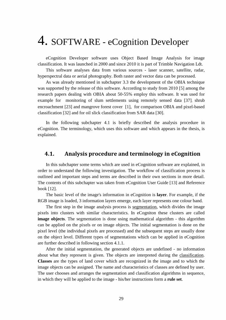
Another term used in eCognition is level. Levels should be not confused with layers - layers are imported to the software with images and levels store image objects. The new level emerges when the segmentation is executed. In this thesis, the analysis was done only on a single image object level, but with eCognition it is also possible to use multiple levels and create a hierarchy of image objects (multiscale segmentation). Each of the levels than store different resolution of image objects. The objects in the higher level are defined by the objects from the level below (Figure 13). Each of the levels should represent a meaningful structure in the image.

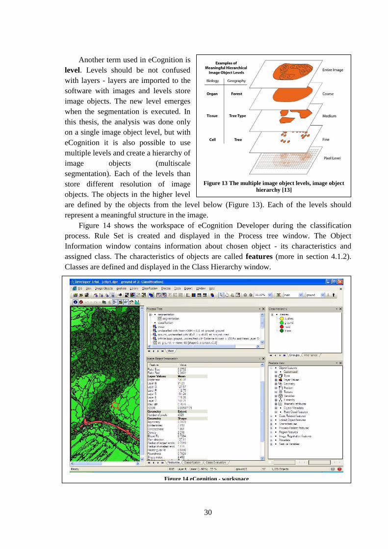
Figure 14 shows the workspace of eCognition Developer during the classification process. Rule Set is created and displayed in the Process tree window. The Object Information window contains information about chosen object - its characteristics and assigned class. The characteristics of objects are called features (more in section 4.1.2). Classes are defined and displayed in the Class Hierarchy window.

Figure 13 The multiple image object levels, image object

hierarchy [13]

Figure 14 eCognition - workspace

31

4.1.1. Segmentation in eCognition

eCognition software provides a variety of segmentation algorithms. A few of them will be presented in this section in order to illustrate the principle of segmentation. The multiresolution segmentation, which was used in investigation, is explained in more detail. Segmentation can be used not only for division of the pixels (on the pixel level) but also for division of the existing images objects (on the image level).

There are two basic segmentation principles [13]:

• top-down strategy - image is divided into smaller pieces - chessboard (Figure 15), quadtree-based, multi-threshold segmentation, ...

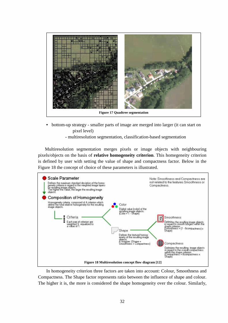
The quadtree-based segmentation results in the square image objects with different sizes. The size of the objects depends on the chosen upper limit of differences in colour within the squares. The particular squares keep on dividing, until is this homogeneity criteria met. Illustration of this process is in the Figure 16.

Figure 15 Chessboard segmentation

Figure 16 Diagram - quadree-based segmentation [13]

32

• bottom-up strategy - smaller parts of image are merged into larger (it can start on pixel level)

- multiresolution segmentation, classification-based segmentation

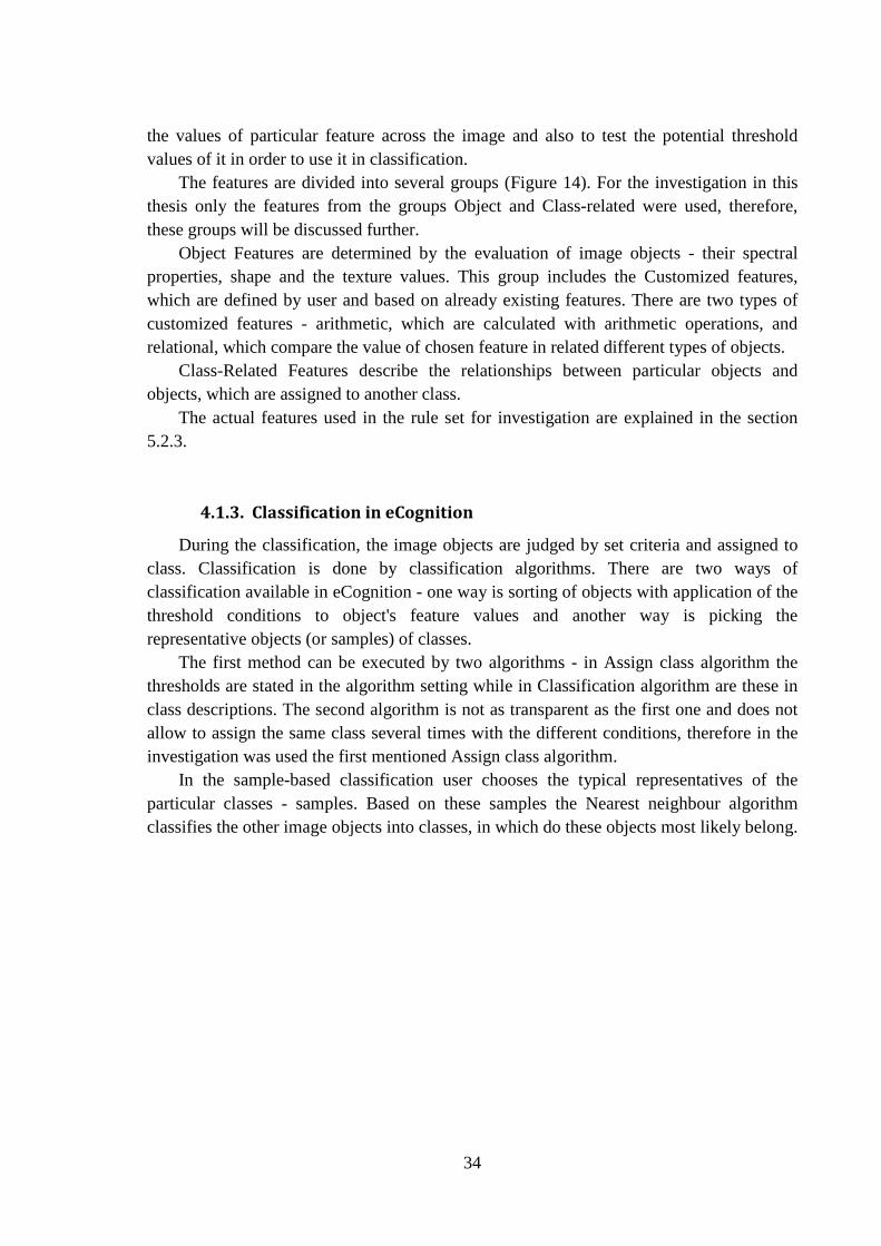
Multiresolution segmentation merges pixels or image objects with neighbouring pixels/objects on the basis of relative homogeneity criterion. This homegeneity criterion is defined by user with setting the value of shape and compactness factor. Below in the Figure 18 the concept of choice of these parameters is illustrated.

In homogeneity criterion three factors are taken into account: Colour, Smoothness and Compactness. The Shape factor represents ratio between the influence of shape and colour. The higher it is, the more is considered the shape homogeneity over the colour. Similarly,

Figure 17 Quadtree segmentation

Figure 18 Multiresolution concept flow diagram [12]

33

the Compactness factor represents ratio between compactness and smoothness. This factor optimizes image objects regarding to the shape.

Below in Table 4 several multiresolution segmentation outcomes are shown. The

particular examples differs in setting of the shape and compactness factors - In each line one of these factors remains the same, while the other one changes.

Table 4 Multiresolution segmentation, different homogeneity criterion

Besides these two factors, user adjusts the multiresolution segmentation algorithm by setting the scale parameter, which defines the size of the objects, and by selection of the image layers, which will be considered in the segmentation algorithm together with the degree of their influence.

4.1.2. Features of objects

The features represent spectral, shape and other characteristics of image objects and are necessary for the classification process. Features, which are at analyst's disposal to use for analysis, are displayed in the Feature View window (Figure 14). It is possible to display

Compactness -fixed: 0.5 Shape: 0.1 Shape: 0.5 Shape: 0.9

Shape - fixed: 0.5 Compactness: 0.1 Compactness: 0.5 Compactness: 0.9

34

the values of particular feature across the image and also to test the potential threshold values of it in order to use it in classification.

The features are divided into several groups (Figure 14). For the investigation in this thesis only the features from the groups Object and Class-related were used, therefore, these groups will be discussed further.

Object Features are determined by the evaluation of image objects - their spectral properties, shape and the texture values. This group includes the Customized features, which are defined by user and based on already existing features. There are two types of customized features - arithmetic, which are calculated with arithmetic operations, and relational, which compare the value of chosen feature in related different types of objects.

Class-Related Features describe the relationships between particular objects and objects, which are assigned to another class.

The actual features used in the rule set for investigation are explained in the section 5.2.3.

4.1.3. Classification in eCognition

During the classification, the image objects are judged by set criteria and assigned to class. Classification is done by classification algorithms. There are two ways of classification available in eCognition - one way is sorting of objects with application of the threshold conditions to object's feature values and another way is picking the representative objects (or samples) of classes.

The first method can be executed by two algorithms - in Assign class algorithm the thresholds are stated in the algorithm setting while in Classification algorithm are these in class descriptions. The second algorithm is not as transparent as the first one and does not allow to assign the same class several times with the different conditions, therefore in the investigation was used the first mentioned Assign class algorithm.

In the sample-based classification user chooses the typical representatives of the particular classes - samples. Based on these samples the Nearest neighbour algorithm classifies the other image objects into classes, in which do these objects most likely belong.

35

5. INVESTIGATION

In this chapter is described the process of rule set creation for image classification in the eCognition software. Following the aim of this thesis, the land cover types were classified from remotely sensed data - the combination of the orthophotos and DTM and DSM. The orthophotos were acquired by means of aerial photography and the elevation models were generated from LiDAR data.

In the first part 5.1 the data, and the instruments, which were used for their caption are characterized. The description of the actual process of investigation follows in 5.2.

5.1. Characteristics of data

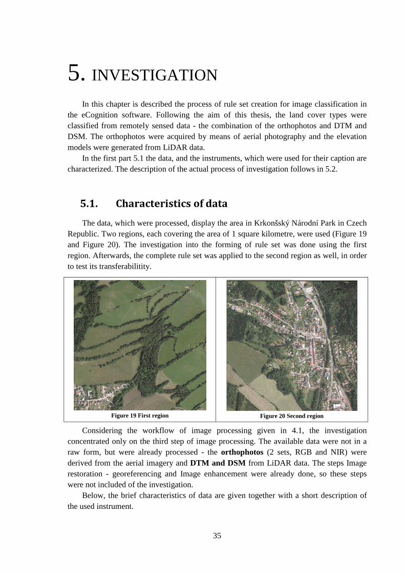
The data, which were processed, display the area in Krkonšský Národní Park in Czech Republic. Two regions, each covering the area of 1 square kilometre, were used (Figure 19 and Figure 20). The investigation into the forming of rule set was done using the first region. Afterwards, the complete rule set was applied to the second region as well, in order to test its transferabilitity.

Considering the workflow of image processing given in 4.1, the investigation concentrated only on the third step of image processing. The available data were not in a raw form, but were already processed - the orthophotos (2 sets, RGB and NIR) were derived from the aerial imagery and DTM and DSM from LiDAR data. The steps Image restoration - georeferencing and Image enhancement were already done, so these steps were not included of the investigation.

Below, the brief characteristics of data are given together with a short description of the used instrument.

Figure 19 First region

Figure 20 Second region

36

ORTHOPHOTOS - RGB + NIR

Format TIFF file (RGB - bands Red, Green, Blue NIR - CIR format - bands NIR, Green, Blue) Resolution 0,125 m Accuracy 0,300 m (standard deviation) Date of image acquisition 18 - 29.6. 2012 GPS-IMU aparature Applanix POS AV 410

elevation model used for orthorectification - LiDAR (grid) Camera Microsoft UltraCamXp Technical specifications [43]: Camera head – 13 CCDs – 9 for high resolution Pan image collection and 4 for R, G, B and NIR image collection

DTM + DSM Format ASCII file grid Resolution 1 x 1 m (grid) Accuracy of point clouds: vertical 0,087 m (standard deviation) horizontal 0,145 m (standard deviation) Date of acquisition (LiDAR) 24.7.-18.8. 2012 Aircraft Zlín Z-Z37

Classification and filtration of the point clouds and generation of elevation models was done in software: SW MicroStation V8 + MDL extension TerraScan 012.020 a TerraModeler 012.008).

Panchromatic image size 17310 x 11310

pixels

Figure 21 Microsoft UltraCamXP [41]

Panchromatic physical pixel size

6 μm

Panchromatic lens focal distance

100 mm

Color (multi-spectral capability)

4 channels - RGB & NIR

Table 5 Technical specification - Microsoft UltraCamXp [43]

37

Laser scanner Riegl LMS-Q680i

Minimum Range 30 m

Accuracy 20 mm Precision 20 mm Laser Pulse Repetition Rate Up to 400 000 Hz Laser Wavelength Near infrared Scanning mechanism Rotating polygon mirror Scan Pattern Parallel scan lines Scan Angle Range +/- 30° = 60° total Scan Speed 10-200 lines/sec

Table 6 Technical specifications - Riegl LMS-Q680i [26]

5.2. The investigation workflow

In this chapter a workflow of the investigation will be presented to make the whole process more transparent and the contents of this subchapter clearer.

I. Preparation of data for classification

In the beginning of the investigation, the data needed to be prepared for the further investigation. The Normalised Digital surface (nDSM) model was generated from DTM and DSM - the description of this process is given in the section 5.2.1. Afterwards, a testing area from the first region was chosen and cut. This part of investigation was done in the ArcMap software.

It was decided to do the investigation on a small testing area and not on the whole image, in order to speed up the investigation. The area was chosen so that it would contain all classes and problems emerging in the whole image. After the forming of rule set, the classification was applied on whole image. The testing area is shown in on the Figure 22.

II. Processing in eCognition As was mentioned in the previous paragraph, the investigation into classification was done on the small training area. Firstly, the suitable method of segmentation and the setting of its parameters was estimated (section 5.2.2). In order to investigate the different possibilities of classification in eCognition, the supervised sample-based approach was tested to see what results it would provide (Appendix

Figure 22 Testing area

38

B). The results were not as good as in the case of Assign class algorithm, so for the final classification was used the Assign class algorithm (section 5.2.4). The rule set was created and afterwards applied on the both regions. The features which were used in classification are described in section 5.2.3. After the application of the rule set on the areas was the resulting classes' borderlines exported to shape files for the Evaluation part of the investigation.

III. Evaluation In section 5.2.5.results and methodology of evaluation is described. Outcomes of classification were compared to the reference data and the confusion matrices were created. The comparison was done both on the pixel and object levels. After the evaluation the detected misclassifications and limitations of this method are discussed in 5.2.6.

5.2.1. Normalized Digital surface model (nDSM)

In order to utilize the information about the heights of the scanned objects in the target area for classification, the Normalised Digital terrain model (nDSM) was created.

nDSM is as a difference between Digital surface model and Digital terrain model. Digital surface model represents the top layer of the Earth surface as it would be seen from the space - it includes the vegetation and buildings. DSM shows the bare Earth surface, without the presence of vegetation and buildings. Consequently, the difference between DSM and DTM represents the height of the objects on the Earth surface above the ground (surface) - the vegetation and buildings. nDSM was generated in the software ArcMap - the workflow of this process is in Appendix A.

DSM - DTM = nDSM

Table 7 nDSM generation

DSM - DTM

nDSM

39

5.2.2. Segmentation

As was already mentioned, segmentation is very important step in OBIA and has a great influence on the following classification. From the number of segmentation algorithms in the eCognition, the Multiresolution segmentation was chosen as giving the best results.

In the section 4.1.1 is mentioned that with this segmentation method the layers of images, which will participate in the recognition of the borders, and the degree of their influence, can be chosen. For the segmentations were considered the layers representing the bands R, G, B and NIR of the orthophotos. The values of nDSM layer were not included, because the resolution of this model was much coarser in comparison of the orthophotos and so it could negatively influence the accuracy of formed borders (see Table 8).

Each of the chosen layers was given the same weight - 1. The different values of factors determining the homogeneity criterion were tested and in the end the values: Shape: 0,5 and Compactness: 0,6 were used.

In the rule set two multiresolution segmentations were applied. The first was applied in the beginning of the whole process on the pixel level and with the scale 30 in order to capture small details.

RGB image

RGB image x nDSM grid (light

squares)

Table 8 Ortophoto x nDSM resolution

Figure 23 Results of multiresolution segmentation - scale 30

40

The second classification was applied later with the scale factor 60. Between the first

and second segmentation the image objects were differentiated according to their height value into 3 classes. The second segmentation was executed separately for each of these classes, so the image objects with very different height value would not mix, even if these have similar spectral characteristics.

The borders of objects, which represent also the height difference (roofs), should be conserved in the level of details of 30 scale segmentation. The second segmentation was done in order to eliminate the small inconsistent objects within the same high level, which tended to be misclassified in the later steps of the classification.

One of the algorithms used in the final Rule Set is Merge region. Merge region can be understand also as one of the segmentation algorithms, because it modifies the shape of the image objects. This algorithm merges the neighbouring image objects, which were assigned to the same class, into one.

5.2.3. Features in rule set

In Table 9 are shown the features which were used for setting thresholds in the rule set.

Figure 24 Results of multiresolution segmentation - scale 60

41

OBJECT FEATURES Customized features R ... Red band (RGB image)

G ... Green band (RGB image) B ... Blue band (RGB image) IR ... Infrared band (NIR image)

Normalized difference vegetation index (NDVI) (recognition of vegetation)

Red Ratio

Layer Values nDSM (height of the objects) Layer B (intensity of band B) Geometry Area (size of the objects) Compactness (estimated with using length and width of an object, divided by

number of pixels )

CLASS-RELATED FEATURES

Relative border to class ( ratio between the length of border, which object shares with objects assigned to chosen class and the total border length of this object)

Border to class (number of pixels which the chosen object shares with chosen class)

Table 9 Features used in rule set

5.2.4. Classification

The training area and later the both whole images were classified using Assign class algorithm. A lot of threshold values for different features were tested. The final rule set is shown below in the Figure 25. The instructions in the rule set are divided into several groups to make the classification more clear.

For the classification six classes were identified to represent five types of land cover in the image (one class is empty). A short description of these classes derived after the choice of the thresholds used for the classification with their colour coding is given in the Table 10.

Class description

above is used only in the beginning of the classification process later it is divided into roof and trees class, the value of nDSM > 1.5 m do not represent a land cover type, it is not present in results of classification

roofs derived from the class above, NDVI < -0,01

trees derived from the class above, NDVI > -0,01

42

shrubs vegetation with the value of nDSM between 0.5 m and 1 m, for the evaluation, this class was assigned to one class together with ground.

ground fields and gardens, low vegetation

roads the parts of ground which display roads, NDVI < 0

Table 10 Description of classes

The first step in the rule set is segmentation I of the image on the pixel level. The

segmentations I and II are described in more detail in section 5.2.2. Afterwards, the formed image objects were classified (classification I in the rule set) accordingly to their height (the value of nDSM). The image objects were divided into three different classes or in this case ''height levels''.

nDSM value (m) class < 0.5 ground < 0.5 , 1> unclassified > 1 above

Table 11 Classification I - results

The newly created classes were segmented (segmentation II) one by one, to prevent the mixing of the different high levels.

Figure 25 Rule set

43

With the group of algorithms named as classification - trees, roofs, the class above

was divided. For the distinguishing between roofs and trees, the feature NDVI was used. Originally, the NDVI threshold was set to 0, but the value -0,01 has shown better results. In the next step were the particular image objects assigned to the class roofs merged in order to get more compact shapes. The following algorithms were executed to reduce those image objects (representing trees) which were misclassified as roofs - the objects which did not meet the threshold set for Compactness criteria and also the objects with the area < 600 pixels were assigned to the class trees. (see Table 12)

original image (RGB)

roofs identified by NDVI

roofs after merging and elimination of

noncompact objects

roofs after elimination of

objects < 600 pix

Table 12 Recognition of roofs

In the next group classification- roads were derived the roads from the class ground - again, NDVI was used. More image objects than those representing actual roads were classified and with the next step these were eliminated using the Red ratio feature. With setting the threshold for Red ratio, the objects, which was classified as a road, but represented ground - bare soil were quiet efficiently recognized and ascribed to the class ground (see Table 13).

original image (RGB)

roads after use of NDVI

roads after use of Red ratio

Table 13 Recognition of roads

44

The roads should in the most cases form the continuous landscape element, but

because of the effect of shadow, some of the small image object in the middle of the road were misclassified as a ground (Figure 26). To recognize these, the threshold of a feature Relative border to road was set and some of these problematic image objects were classified correctly. The last step in this group eliminates the isolated image objects classified as road, which because of the continuous character of the roads were likely to be missclassified.

The last group of algorithms named classification dealt with the unclassified objects - the objects with the height between 0.5-1 m. These are classified according to the value of NDVI, Mean Layer Blue and Border to roads into the classes shrubs, roads or ground. The Mean Layer Blue feature was used because it seemed to help the NDVI parameter to recognize the shrubs and represents the mean intensity value of B layer. The road image objects are merged and in the next step the objects in the class of roads with small area are assigned to the class ground.

The last group of algorithms merging was applied before the export of classes' borderlines to shape files. Some generalization of the scene was included, eliminating the small objects classified as shrubs with no border to trees, which probably represented just higher vegetation. Below in Figure 27 the classification outcome of testing area can be seen. In the Appendix C is shown the outcome the classification of whole first region.

Figure 27 Classification result - testing area

Figure 26 Roads - misclassified objects

45

5.2.5. Evaluation

When doing the accuracy assessment, the reference data, which are considered to be correct and to which the results of the investigation are compared are needed. For this purpose are usually used data measured in field. The result of such evaluation shows the overall accuracy of the whole processing - from the obtaining data to final product. In this thesis only the evaluation of classification process is done, so no measuring in the field was undertaken. To obtain the reference data, the objects were digitised from the orthophotos in software ArcGIS. The evaluation was done on a cuts of the both testing areas to limit the amount of data to be processed.

Figure 28 Evaluation - tested areas

The evaluation methods used in research papers can be divided into two groups according to the fact, if they use the thresholds to compare the detected and reference data or not. In this approach the threshold-based evaluation would not be effective since the thresholds were already used in classification. [3]

Another classification of evaluation methods is to object level and pixel level methods. The first one compares the numbers of objects and the second one compares the number of pixels or areas. [3]

In the following text are used some terms to

express the outcomes of the classification. These terms were taken from [17] and mostly refer to the areas, but are also used for the object level evaluation.

True positive (TP) - correctly classified areas - the reference object overlap the classified object.

False positive (FP) – misclassified areas - the object is detected, but it is not in the reference dataset (does not exist).

False negative (FN) – misclassified areas, the object was not detected (it is only in reference dataset).

Figure 29 Evaluation - areas

46

Evaluation approaches in this thesis:

1. Confusion matrix - shows the overlapping areas of particular classes in the reference datat and the data provided by eCognition. The diagonal of matrices represent the area which was correctly classified (true positives), the other values show the areas which was misclassified and to which class these were assigned (the predicted class in reference data is different from the classified one). Each cell represents the intersection area of respective layers.

Classification results

roofs roads trees ground

Re

fere

nce

da

ta

roofs TP FN/FP FN/FP FN/FP

roads FN/FP TP FN/FP FN/FP

trees FN/FP FN/FP TP FN/FP

ground FN/FP FN/FP FN/FP TP

Table 14 Confusion matrix

2. Pixel level evaluation - areas of the particular classes in the two datasets are compared. Several quality factors illustrating the achieved accuracy were calculated [24]using the values from the Confusion matrix:

RA .... reference area of a class/object DA .... detected area of a class/object

Detection rate: ratio between the correctly detected

area of the chosen class (true positive) and the area which this class covers in the reference dataset.

Quality rate: ratio between the true positive area and the union of detected and reference area.

Branch factor: it is the ratio between the part of reference area which was not detected (false negative)

and true positive area. Miss factor: Ratio between false positive and true

positive area.

False alarm rate: ratio of the part of the reference area which was not detected (false negative) and reference area.

3. Object level evaluation - was done only for the class representing buildings, the

actual numbers of objects was compared.

47

Digitisation

From the orthophotos were digitised these classes: roofs, roads and trees. The roofs provided the most relevant outcome of digitisation, since these are quite

well recognisable from the images. Considering that the digitisation of the roads and especially trees from orthophotos was not very reliable, the outcomes of the evaluation of classification of these objects should be considered as illustrative.

In the layer representing the roads were included not only roads, but also other man-made ground structures - the parking lots and pavements covering large area.

The trees were the most tricky class to digitise, since the position of the trees was not well recognisable in the images. Only the forests, larger groupings of trees and also a few of the most apparent single trees were digitised.

The rest of the area, where none of the mentioned three class was identified, were assigned to the class ground. The rest of the area was considered as ground (= the outcomes of ground and shrubs classification).

Confusion matrices

1. area

(85079 m2)

classification results [m2]

roofs roads trees ground

refe

ren

ce

da

ta [

m2] roofs 10785 119 147 272

roads 245 9750 519 1750

trees 0 0 6223 57

ground 670 1990 7383 45169

2. area

(40228 m2)

classification results [m2]

roofs roads trees ground

refe

ren

ce

da

ta[m

2] roofs 6775 50 34 66

roads 307 4548 158 588

trees 6 14 8591 389

ground 433 749 2941 14579

Pixel-level evaluation

In Table 15 below the comparison of the reference data areas and the classification outcome - the detected areas are shown. For each class the evaluation factors were calculated. In the end the overall accuracy was estimated.

48

class reference

area [m2]

detected area [m2]

overlap [m2]

detection rate [%]

quality rate [%]

branch factor [%]

miss factor [%]

false alarm rate [%]

1. testing area

roofs 11323 11700 10785 95,2 88,1 5,0 8,5 4,7

roads 12264 11859 9750 79,5 67,8 25,7 21,6 20,5

trees 6280 14272 6223 99,1 43,4 0,9 129,3 0,9

ground 55212 47248 45169 81,8 78,8 22,2 4,6 18,2

overall 85079 85079 71927 84,5 73,2 18,3 18,3 15,5

2. testing area

roofs 6925 7521 6775 97,8 88,4 2,2 11,0 2,2

roads 5601 5361 4548 81,2 70,9 23,2 17,9 18,8

trees 9000 11724 8591 95,5 70,8 4,8 36,5 4,54

ground 18702 15622 14579 78 73,8 28,3 7,2 22,0

overall 40228 40228 34493 85,7 75,1 16,6 14,3 Table 15 Pixel level evaluation

As was written in the beginning of this section, the most reliable evaluation results are given for the class representing buildings (roofs). The accuracy of the digitisation is indefinable, especially considering bad contrast in the pictures, quality of the digitisation is questionable.

In the case of the classes roads, trees and consequently ground, the statistics of Quality rate are low in the comparison with the class representing buildings (= roofs) and also the values of the factors are not very good. This fact should not be considered to be caused only by the classification but also by the quality of digitisation. Since the quality of digitisation seemed to be the main cause of, this numbers will not be discussed further. Visually, the classification outcomes seemed to match well with the landscape elements on the orthophotos.

The detection rate of the buildings was more than 95% in both testing areas, but there were some mismatches which caused the quality rate of the classification to drop to 88 %. The comparison between branch and miss factor values shows, that from the whole misclassified building area, more was ''overdetected'' than undetected. The reason for non-detection of buildings was mostly the shadow. The value of the branch factor was mainly caused by the fact, that only roofs of the buildings were digitised, but the whole buildings were classified. In few cases, these two borders did not match (Figure 30 Roof x buildingFigure 30) well.

During the visual evaluation of second testing area classification, the values of the thresholds did not provide such a good results as in the case of the testing area. Considering the slightly different spectral characteristics of different images, the threshold values would be needed to adjust for the particular images to improve the result.

This similar table of evaluation, was also done for the particular buildings in the testing areas - the table can be found in Appendix C.

Figure 30 Roof x building

49

Object level evaluation

In object level evaluation the comparison of the numbers of detected and digitised buildings was done. This type of evaluation was applied only for the class representing buildings, because the other object classes form a larger areas and not a number of smaller objects, which numbers could be compared and therefore were not considered to be suitable for this type of evaluation.

In Chyba! Nenalezen zdroj odkazů. the numbers and values of some factors are shown. It should be noted, that the number of detected buildings is not equal to the number of detected objects. Some of the buildings which were included into one object during the digitisation were detected not as a one object but as several smaller objects. In these cases, the corresponding objects within one reference building were counted as one. The false positives display the number of the detected buildings which do not exist and false negatives the building which were not detected. Correctness shows the ratio between the number of correctly detected buildings and the detected buildings.

1. area 2. area reference buildings 77 30 detected buildings 76 31 false positives 2 3 false negatives 3 2 overlapping buildings 74 28 reference buildings 96,1 % 93,3 % quality rate 93,6 % 84,8 % branch factor (over-detection) 2,7 % 11 % miss factor (under-detection) 4,1 % 7 % correctness 97,3 % 90%

Figure 31 Object level evaluation - 1.testing area

50

5.2.6. Problems in classification, misclassifications

The main cause for the misclassification of the objects was the effect of shadow. This problem was reduced during the forming of the rule set by applying additional threshold conditions (see 5.2.4), but it was not removed completely and some areas remained misclassified.

Figure 32 Effect of the shadow

Another problem, which occurred during the classification, was, that in some areas the nDSM did not match well with the orthophotos (see Chyba! enalezen zdroj odkazů.).

This fact did not effected the results of segmentation, since the nDSM layer was not involved in segmentation algorithm, but during the classification several objects were misclassified, because of this mismatch. An example is shown Figure 33.

In this case buildings were detected on the area displaying road. The reason for this misclassifications were the trees, which partially covered the road. The height information of the misclassified objects comes from the tree branches - from nDSM. Meanwhile, the spectral information derived from orthophoto have the NDVI value of area without vegetation. As a result, the image objects characteristics correspond to class roofs. In this case, also the influence of the segmentation should be considered.

reference area (orthophoto)

light squares - height value (nDSM)

51

Figure 33 nDSM x orthophoto misclassification

After the use of the Assign class algorithm for the classification, a possible disadvantage of this method should be mentioned. Thresholds in this investigation were chosen regarding to the best result it provided in the testing area and the involved images. In case of applying this threshold conditions to an image with a little bit different spectral distribution and characteristics, the results can be very different. For different imagery might be necessary to slightly adjust the threshold values to get the best results.

52

6. CONCLUSION

In this thesis an approach to interpret the remotely sensed imagery data using image classification was presented. The Object-based image analysis was applied to the data, which were obtained by two different remote sensing techniques, at once - the orthophotos derived from high-resolution imagery and the nDSM, which was estimated from the LiDAR point clouds. For the classification, the software eCognition Developer was used.

In the investigation area five different classes of objects, each representing particular land cover type, were identified and a rule set for recognition of these classes in the data was formed in the eCognition software.

With this rule set, the achieved overall detection rate is very good - 85%. The detection rate of the buildings, for which the evaluation approach was the most reliable is even better, about 95%.

The use of this combination of the data sources proved to be very advantageous. The to datasets complement each other well. The nDSM was used for recognition of the objects on the basis of their height - the borders of forests, buildings or vegetation with different heights were identified without the risk of misclassification caused by shadow. The Normalized difference vegetation index (NDVI) estimated from the orthophoto band's values allowed to distinguish between vegetation and man-made structures.

Still, some areas remained misclassified, mainly because of the effect of the shadow. The results could be improved by using a different indexes or by putting more thresholds for the differentiation between classes. Also the area effected by shadow could be classified separately.

53

REFERENCES [1] ABBAS, S., QAMER, F.M., HUSSAIN, N.,SALEEM, R., NITIN, K.T. National Level Assessment of

Mangrove Forest Cover in Pakistan. In ISPRS Archives: Vol. XXXVIII-8/W20 [online]. 08 November 2011, Bhopal, India. [cit. 2012-12-28]. <http://www.int-arch-photogramm-remote-sens-spatial-inf-sci.net/XXXVIII-8-W20/187/2011/isprsarchives-XXXVIII-8-W20-187-2011.pdf>

[2] APLIN, P., SMITH,G.M. Advances in Object-based Image Classification. In ISPRS Archives: Vol. XXXVII-B7 [online]. 03-11 July 2008, Beijing, China. [cit. 2012-12-30]. <http://www.isprs.org/proceedings/XXXVII/congress/7_pdf/4_WG-VII-4/45.pdf>

[3] AWRANGJEB, M., RAVANBAKHSH, M., FRASER, C.S. Automatic detenction of residential buildings using LIDAR data and multispectral imagery. ISPRS Journal of Photogrammetry and Remote Sensing [online], 2010, vol. 65 (2010), pp. 457-467 [cited 2013-02-23]. <http://www.crcsi.com.au/getattachment/bf39930f-8e39-4eb1-8fac-f95153dd75bb/.aspx>

[4] BARAZZETTI Luigi, BROVELLI Maria, SCAIONI Marco. Generation of true-orthophotos with LiDAR high resolution digital surface models. The Photogrammetric Journal of Finland [online], 2008, vol.21, No.1, pp.26-36 [cited 2013-03-10]. <http://foto.hut.fi/seura/julkaisut/pjf/pjf_e/2008/Barazzetti_et_al_2008_PJF.pdf>

[5] BLASCHKE, T. Object based image analysis for remote sensing. ISPRS Journal of Photogrammetry and Remote Sensing [online], 2010, vol. 65 (2010), pp. 2-16 [cited 2013-02-02]. <https://www1.ethz.ch/igp/photogrammetry/education/lehrveranstaltungen/RSGISFS2011/coursematerial/paperblaschke.pdf>

[6] BOYD, D.S. Geoinformatics - Vol.1- Physical Basis of Remote Sensing. Encyclopedia of life Support Systems (EOLSS) [online]. [cit. 2013-03-01]. <http://www.eolss.net/Sample-Chapters/C01/E6-64-02-01.pdf>

[7] BUCKLEY, S.J., KURZ, T.H., SCHNEIDER, D. The Benefits of Terrestrial Laser Scanning and Hyperspectral Data Fusion Products. In ISPRS Archives: Vol. XXXIX-B7 [online]. 25 August - 01 September 2012, Melbourne, Australia. [cit. 2012-12-28]. < http://www.int-arch-photogramm-remote-sens-spatial-inf-sci.net/XXXIX-B7/541/2012/isprsarchives-XXXIX-B7-541-2012.pdf>

[8] CARLEER A.P., DEBEIR O., WOLFF E.. Asessment of Very High Spatial Resolution Satellite Image Segmentations. Photogrammetric Engineering & Remote Sensing [online], 2005, vol. 71, no. 11, pp. 1285-1294[cited 2013-02-02]. < http://www.armurs.ulb.ac.be/images/8/86/PERS_Carleer_05.pdf>

[9] LIANG-CHIEN, C., TEE-ANN, T., YI-CHEN, S., YEN-CHUNG, L., JIANN-YEOU, R. Fusion of LiDAR Data and Optical Imagery for Building Modelling. In ISPRS Archives: XXXV-B4 [online]. 12 - 23 July 2004, Istanbul, Turkey. [cit. 2013-02-01]. <http://www.isprs.org/proceedings/XXXV/congress/comm4/papers/445.pdf>

[10] DEVADAS, R., DENHAM, R.J., PRINGLE, M. Support Vector Machine Classification of Object-based Data for Crop Mapping, Using Multi-temporal Landsat Imagery. In ISPRS Archives: Volume XXXIX-B7 [online], 25 August-01 September 2012, Melbourne, Australia. [cit. 2012-12-28]. <http://www.int-arch-photogramm-remote-sens-spatial-inf-sci.net/XXXIX-B7/185/2012/isprsarchives-XXXIX-B7-185-2012.pdf>

[11] DU PLESSIS, Steve. Identifying Building Change Using High Resolution Point Clouds - an Object-based Approach. In ISPRS Archives: Vol. XXXIX-B7 [online]. 25 August - 01 September 2012, Melbourne, Australia. [cit. 2012-12-27]. <http://www.int-arch-photogramm-remote-sens-spatial-inf-sci.net/XXXIX-B7/305/2012/isprsarchives-XXXIX-B7-305-2012.pdf>

[12] eCognition Developer 8.7.2. Reference book. Trimble Germany GMbH, 2012. Printed: 2012-04-23. Document Version 8.7.2.

54

[13] eCognition Developer 8.7.2. User Guide. Trimble Germany GMbH, 2012. Printed: 2012-04-23. Document Version 8.7.2

[14] ERDAS. ERDAS Field Guide [online], Atlanta (Gorgia - USA): 1999 [cit. 2013-02-01]. Fifth Edition. <http://www.gis.usu.edu/manuals/labbook/erdas/manuals/FieldGuide.pdf>

[15] FISHER P.The pixel: a snare and a delusion, International Journal of Remote Sensing Finland [online], 1996, vol.18, No.3, pp. 679-685 [cited 2013-02-02]. <http://www.smfn.unisi.it/smfn_lauree/view_matidd.php?id=832.>

[16] FURTADO, J.J., CAI, Z., XIAOBO, L. Digital Image Processing: Supervised Classification Using Genetic Algorithm in Matlab Toolbox. Report and Opinon [online], 2010, Vol. 2, Issue 6, pp. 53-61 [cited 2013-02-01]. <http://www.sciencepub.net/report/report0206/09_3172report0206_53_61.pdf>

[17] HERMOSILLA, T., RUIZ, L.A., RECIO, J.A., ESTORNELL, J. Evaluation of Automatic Building Detection Approaches Combining High Resolution Images and LiDAR Data. Remote Sensing [online], 2011, vol 3, pp. 1188-1210 [cited 2013-04-29]. < http://www.mdpi.com/2072-4292/3/6/1188/pdf>

[18] HOEFLE, B. [online]. 2010 [cit. 2013-03-05]. <http://www.laserdata.info/index.php?pageref=bericht&sid=589&fid=2143>

[19] IDRISI Guide to GIS and Image Processing Volume 1, 2006, last revision 10th April 2006 [cit. 2013-03-01]. <https://www.mtholyoke.edu/courses/tmillett/course/geog205/files/remote_sensing.pdf>

[20] ISPRS Statue-Definitions[online]. [cit. 2013-02-02]. < http://www.isprs.org/documents/statutes12.aspx>

[21] KAŠPAR, Milan. Laser Scanning in Civil engineering and land and land surveying. Prague:Vega s.r.o, 2004.

[22] KWAK, E., AL-DURGHAM, M., HABIB, A. Automatic 3D Building Model Generation from LiDAR and Image Data Using Sequential Minimum Bounding Rectangle. In ISPRS Archives: Vol. XXXIX-B3 [online]. 25 August - 01 September 2012, Melbourne, Australia. [cit. 2012-12-26].< http://www.int-arch-photogramm-remote-sens-spatial-inf-sci.net/XXXIX-B3/285/2012/isprsarchives-XXXIX-B3-285-2012.pdf>

[23] LALIBERTE A., RANGO a., HVSTAD, k., PARIS, j., BECK, R., McNEELY R. GONZALES A. Object-oriented image analysis for mapping shrub encroachment from 1937 to 2003 in southern New Mexico. Remote Sensing of Environment [online], 2004, vol.93, pp. 198-210 [cited 2013-03-06]. <http://public.gettysburg.edu/~rplatt/platt_rapoza_PG.pdf>

[24] LANDES, T., GRUSSENMEYER, P., BOULAASSAL, H., MOHAMED,M. Assessment of Three-dimensional Models Derived from Lidar and TLS Data. In ISPRS Archives: Vol. XXXIX-B2 [online]. 25 August - 01 September 2012, Melbourne, Australia. [cit. 2013-04-29]. < http://www.int-arch-photogramm-remote-sens-spatial-inf-sci.net/XXXIX-B2/95/2012/isprsarchives-XXXIX-B2-95-2012.pdf>

[25] LANG, S., BLASCHKE, T. Hierarchical Object Representation Comparative Multi-Scale Mapping of Anthropogenic and Natural Features. In ISPRS Archives: Vol. XXXIV-3/W8 [online]. 17-19 September 2003, Munich, Germany. [cit. 2012-12-30]. <http://www.isprs.org/proceedings/XXXIV/3-W8/papers/pia03_s8p1.pdf>

[26] Long-Range Airborne Laser Scanner for Full Waveform Analysis LMS-Q680i [online]. 2012, last revision 8th October 2012 [cit. 2013-05-18]. <http://www.riegl.com/uploads/tx_pxpriegldownloads/10_DataSheet_LMS-Q680i_28-09-2012.pdf>

[27] MIKHAIL, E.M., et.al. Introduction to Modern Photogrammetry. 2001. Wiley and Sons Inc.

[28] NAKANO, K., CHIKATSKU, H. On Object Extraction Using Airborne Laser Scanner Data and Digital Images for 3D Modelling. In ISPRS Archives: Vol. XXXIX-B3 [online]. 25 August - 01 September

55

2012, Melbourne, Australia. [cit. 2012-12-26]. <http://www.int-arch-photogramm-remote-sens-spatial-inf-sci.net/XXXIX-B3/53/2012/isprsarchives-XXXIX-B3-53-2012.pdf>

[29] NIELSEN, M. Ø. True Orthophoto generation [online]. Lyngby, 2004. 127 s. Master thesis - DTU. ISSN 1601-233X. [cit. 2013-03-11]. <http://www.sharpgis.net/projects/docs/imm-thesis-2004-50_web.pdf>

[30] OZKAN, C., OSMANOGLU, B., SUNAR, F., STAPLES, G., KALKAN, K., BALIK SANLI, F. Testing the Generalization Efficiency of Oil Slick Classification Algorithm using Multiple SAR Data for Deepwater Horizon Oil Spill. In ISPRS Archives: Vol. XXXIX-B7 [online]. 25 August - 01 September 2012, Melbourne, Australia. [cit. 2012-12-28]. < http://www.int-arch-photogramm-remote-sens-spatial-inf-sci.net/XXXIX-B7/67/2012/isprsarchives-XXXIX-B7-67-2012.pdf>

[31] PAL Nikhil R., PAL Sankar K. A review on image segmentation techniques, Pattern recognition [online], 1993, vol. 26, Issue.9. pp. 1277 - 1294 [cited 2013-03-01]. < http://www.sciencedirect.com/science?_ob=MiamiImageURL&_cid=272206&_user=640830&_pii=003132039390135J&_check=y&_origin=article&_zone=toolbar&_coverDate=1993-Sep-30&view=c&originContentFamily=serial&wchp=dGLbVlk-zSkWz&md5=13e9e39daeb64fa68fe722543922680d&pid=1-s2.0-003132039390135J-main.pdf >

[32] PLATT V., RAPOZA Lauren. An Evaluation of an Object-Oriented Paradigm for land Use/Land Cover classification. The Professional Geographer [online], 2008, vol 60, pp. 87-100 [cited 2013-03-07]. <http://public.gettysburg.edu/~rplatt/platt_rapoza_PG.pdf>

[33] RAU, J.Y., JHAN, J.P., LO, C.F., LIN, Y.S. Landslide Mapping Using Imagery Acquired by a Fixedd-wing UAV. In ISPRS Archives: Vol. XXXVIII-1/C22 [online]. 14-16 September 2011, Zurich, Switzerland. [cit. 2012-12-28]. <http://www.int-arch-photogramm-remote-sens-spatial-inf-sci.net/XXXVIII-1-C22/195/2011/isprsarchives-XXXVIII-1-C22-195-2011.pdf>

[34] REES, W.G., Physical principles of remote sensing (Second edition) [online]. Cambridge University Press 2001 [cit. 2012-12-28]. <http://www.google.cz/books?hl=cs&lr=&id=u17Zv45DENoC&oi=fnd&pg=PR13&dq=campbell+1996+definition+of+remote+sensing&ots=AC_DJMOg3b&sig=5izWtcWOHN5R4-BrkFRU35Um30U&redir_esc=y#v=onepage&q=campbell%201996%20definition%20of%20remote%20sensing&f=false>

[35] ROTTENSTEINER, F., BRIESE, CH. Automatic Generation of Building Models from LiDAR Data and the Intergration of Aerial images. In ISPRS Archives: XXXIV-3/W13 [online]. 8 - 10 August 2003, Dresden, Germany. [cit. 2013-02-01]. <http://www.isprs.org/proceedings/XXXIV/3-W13/papers/Rottensteiner_ALSDD2003.pdf>

[36] ROTTENSTEINER, F., TRINDER, J., CLODE, S., KUBIK, K. Fusing Airborne Laser Scanner Data and Aerial Imagery for the Automatic Extraction of Buildings in Densely Built-up Areas. In ISPRS Archives: Vol. XXXV-B3 [online]. 12 - 23 July 2004, Istanbul, Turkey. [cit. 2012-12-30]. <http://www.isprs.org/proceedings/XXXV/congress/comm3/papers/323.pdf>

[37] SHEKHAR, S. Detecting Slums from Quick Bird Data in Pune Using an Object Oriented Approach. In ISPRS Archives: Vol. XXXIX-B8 [online]. 25 August- 01 September 2012, Melbourne, Australia. [cit. 2012-12-28]. <http://www.int-arch-photogramm-remote-sens-spatial-inf-sci.net/XXXIX-B8/519/2012/isprsarchives-XXXIX-B8-519-2012.pdf>

[38] SMITH Gary S. Digital orthophotography and GIS [online]. 1996, [cit. 2013-03-10]. <http://proceedings.esri.com/library/userconf/proc95/to150/p124.html>

[39] SONG, Jeong-Heon, HAN, Soo-Hee, YU, Kiyun, KIM, Yong-Il. Assessing the Possibility of Land-cover Classification Using Lidar Intensity Data. In ISPRS Archives: Vol. XXXIV part 3 [online]. 9-13 September 2002, Graz, Austria. [cit. 2012-12-28]. <http://www.isprs.org/proceedings/XXXIV/part3/papers/paper128.pdf>

56

[40] STRONG, K., PHY 499S - Earth Observation from Space, Spring Term 2005[online], last revision 16th December 2004 [cit. 2013-05-18]. <http://www.atmosp.physics.utoronto.ca/people/strong/phy499/section4_05.pdf >

[41] UltraCam - Xp Technical Specifications [online]. last revision 4th February 2009 [cit. 2013-05-18]. <http://www.google.cz/url?sa=t&rct=j&q=parameter%20microsoft%20ultracamxp&source=web&cd=4&ved=0CE0QFjAD&url=http%3A%2F%2Fdownload.microsoft.com%2Fdownload%2F8%2F5%2FA%2F85A3648B-B4F5-46D6-80E6-C0698A2EE109%2FUCXp-Technical%2FUltraCamXp-Technical.pdf&ei=08qXUYzEA8nCPMP_gKgI&usg=AFQjCNHytKvIF5YM4jJAewV9SxQ6WV585Q&bvm=bv.46751780,d.ZWU>

[42] WEHR, A., LOHR, U. Airborne laser scanning - an introduction and overview. ISPRS Journal of Photogrammetry & Remote Sensing [online], 1999, vol.54, pp. 68-82 [cited 2013-03-06]. <http://warnercnr.colostate.edu/~lefsky/isprs/1136.pdf>

[43] Wiechert, A., Gruber, M. Vexcel Imaging GmbH – Innovating in Photogrammetry UltraCamXp, UltraCamLp and UltraMap [online]. Last revision 3rd February 2010 [cit. 2013-05-18]. <http://www.google.cz/url?sa=t&rct=j&q=microsoft%20ultracamxp%20number%20of%20lenses&source=web&cd=4&ved=0CEMQFjAD&url=http%3A%2F%2Fdownload.microsoft.com%2Fdownload%2F1%2F6%2Fa%2F16aa08fd-a0ae-4c0e-811f-29f192965b85%2FVexcelPho009_V02.pdf&ei=aMuXUduDNcfrPP-pgcgH&usg=AFQjCNHBCP5iY5kkwJk0gEIOmsFhM5edbQ&bvm=bv.46751780,d.ZWU>

[44] WU, H., LIU, C., ZHOU, X. Data Fusion with Integration of Airborne Laser Scanning Data and Ortho-aerial Photos. In ISPRS Archives: Vol. XXXVII-B1 [online]. 3 - 11 July 2008, Beijing, China. [ cited 2013-02-01]. <http://www.isprs.org/proceedings/XXXVII/congress/1_pdf/51.pdf>

[45] ZHAN, Q., LIANG, Q., WEI, C., XIAO Y. Ground Object Recognition Using Combined High Resolution Airborne Images and DSM. In ISPRS Archives: Vol. XXXIX-B3 [online]. 25 August - 01 September 2012, Melbourne, Australia. [cit. 2012-12-26]. <http://www.int-arch-photogramm-remote-sens-spatial-inf-sci.net/XXXIX-B3/573/2012/isprsarchives-XXXIX-B3-573-2012.pdf >

57

LIST OF FIGURES

Figure 1 Main regions of electromagnetic spectrum used in remote sensing [6] ................ 13 Figure 2 Interaction between electromagnetic energy and target [19] ............................... 14 Figure 3 Common remote sensing systems [19] .................................................................. 14 Figure 4 Airborne laser scanning [18] ................................................................................. 17 Figure 5 Processing steps for laser scanner data [42] .......................................................... 18 Figure 6 Perspective and orthographic image geometry [27] .............................................. 20 Figure 7 Forward and backward projection [29] ................................................................. 21 Figure 8 Obscured areas [29] ............................................................................................... 21 Figure 9 Pixel-based classification used in the land Cover Map of Great Britain 1990 [2] 25 Figure 10 Pixel-based classification, relative scale [5] ........................................................ 26 Figure 11 Object-based classification used in the Land Cover Map 2000[2] ..................... 26 Figure 12 Development of the amount of OBIA literature [5] ............................................ 28 Figure 13 The multiple image object levels, image object hierarchy [13] .......................... 30 Figure 14 eCognition - workspace ....................................................................................... 30 Figure 15 Chessboard segmentation .................................................................................... 31 Figure 16 Diagram - quadree-based segmentation [13] ....................................................... 31 Figure 17 Quadtree segmentation ........................................................................................ 32 Figure 18 Multiresolution concept flow diagram [12] ......................................................... 32 Figure 19 First region .......................................................................................................... 35 Figure 20 Second region ...................................................................................................... 35 Figure 21 Microsoft UltraCamXP [41] ................................................................................ 36 Figure 22 Testing area ......................................................................................................... 37 Figure 23 Results of multiresolution segmentation - scale 30 ............................................. 39 Figure 24 Results of multiresolution segmentation - scale 60 ............................................. 40 Figure 25 Rule set ................................................................................................................ 42 Figure 27 Classification result - testing area ....................................................................... 44 Figure 26 Roads - misclassified objects .............................................................................. 44 Figure 28 Evaluation - tested areas ...................................................................................... 45 Figure 29 Evaluation - areas ................................................................................................ 45 Figure 30 Roof x building .................................................................................................... 48 Figure 31 Object level evaluation - 1. testing area .............................................................. 49 Figure 32 Effect of the shadow ............................................................................................ 50 Figure 34 nDSM x orthophoto misclassification ................................................................. 51

LIST OF TABLES

Table 1 Main regions of electromagnetic spectrum used in remote sensing [6] ................. 13

Table 2 Taxonomy of remote sensing systems [34] ............................................................ 15 Table 3 Reflectivity of materials ......................................................................................... 17 Table 4 Multiresolution segmentation, different homogeneity criterion ............................. 33

58

Table 5 Technical specification - Microsoft UltraCamXp [43] ........................................... 36

Table 6 Technical specifications - Riegl LMS-Q680i [26] ................................................. 37

Table 7 nDSM generation .................................................................................................... 38 Table 8 Ortophoto x nDSM resolution ................................................................................ 39 Table 9 Features used in rule set .......................................................................................... 41 Table 10 Description of classes ........................................................................................... 42 Table 11 Classification I - results ........................................................................................ 42 Table 12 Recognition of roofs ............................................................................................. 43 Table 13 Recognition of roads ............................................................................................. 43 Table 14 Confusion matrix .................................................................................................. 46 Table 15 Pixel level evaluation ............................................................................................ 48

LIST OF APPENDICES

Appendix A - nDSM generation .........................................................................................60 Appendix B - The sample-based classification ...................................................................61 Appendix C - The classification result - first region ...........................................................64 Appendix D - Evaluation - buildings ..................................................................................65

LIST OF ELECTRONIC APPENDICES - CD

Appendix A - nDSM generation Appendix B - The sample-based classification Appendix C - The classification result - first region Appendix D - Evaluation - buildings Rule set - dcp. file (eCognition) Shape files - the classification results