Extended Verification Finite Element Program Plaxis · PDF file6 3. Calculation of geotechnical structural response to difference earthquake A 16‐meters thick ideal deposit of soft

1

1. Introduction

Nowadays, the seismic verification of structures has dramatically evolved. Italy is surrounded

many great earthquakes; hence it would be unwise to totally ignore the effects of earthquakes

on geotechnical structures.

The purpose of this study is to verify finite element program Plaxis and Analytical solution in

Elastodynamics by EERA for several geotechnical structures such as retaining wall, sheet pile

and embankment. These structures are examined by various homogeneous soil layers which

contents different thickness and soil stiffness parameters time history is obtained as dynamics

loads. This verification is necessary in order to investigate the vulnerability assessment in

geotechnical structures which is investigated in the master thesis.

PLAXIS is a finite element program for geotechnical applications in which soil models are used to

simulate the soil behaviour. Although a lot of testing and validation have been performed, it cannot be

guaranteed that the PLAXIS code is free of errors. Moreover, the simulation of geotechnical problems by

means of the finite element method implicitly involves some inevitable numerical and modeling errors.

The accuracy at which reality is approximated depends highly on the expertise of the user regarding the

modeling of the problem, the understanding of the soil models and their limitations, the selection of

model parameters, and the ability to judge the reliability of the computational results.

An earthquake analysis can be performed by imposing an acceleration time‐history at the base of the

FE model and solving the equations of motion in the time domain by adopting a Newmark type implicit

time integration scheme.

EERA is an analytical solution to the seismic response of viscoelastic soil layers and obtained a transfer

function of the seismic shape which stands for Equivalent‐linear Earthquake site Response Analysis. It is

a modern implementation of the well‐known concepts of the equivalent linear site response analysis

that was first implemented in the SHAKE code (Schnabel et al., 1972). The input and output are fully

integrated with the spreadsheet program MS‐Excel. This code permits to perform frequency domain

analyses for linear and equivalent linear stratified subsoils.

2

2. Geotechnical Structures Parameters

2.1 Material properties of Soil and wall

The soil material used in the model is linear elastic which is examined as homogeneous

for some cases as following below:

a) homogeneous soil:

1. case a – Shear wave velocity vs 200 m/s, density () 1.9 t/m³

2. case b – Shear wave velocity vs 500 m/s, density () 1.9 t/m³

3. case c – Shear wave velocity vs 1000 m/s, density () 1.9 t/m³

b) one‐layer system of homogeneous half‐space:

1. case d – layer: vs 200 m/s, density () 1.9 t/m³, thickness 20m; homogeneous half

space vs 1500 m/s, density () 2.3 t/m³

2. case e – layer: vs 200 m/s, density () 1.9 t/m³, thickness 50m; homogeneous half


3. case f – layer: vs 200 m/s, density() 1.9 t/m³, thickness 100m; homogeneous

half space vs 1500 m/s, density () 2.3 t/m³

4. case g – layer: vs 500 m/s, density () 1.9 t/m³, thickness 20m; homogeneous half


5. case h – layer: vs 500 m/s, density () 1.9 t/m³, thickness 50m; homogeneous half


6. case i – layer: vs 500 m/s, density () 1.9 t/m³, thickness 100m; homogeneous

half space vs 1500 m/s, density () 2.3 t/m³

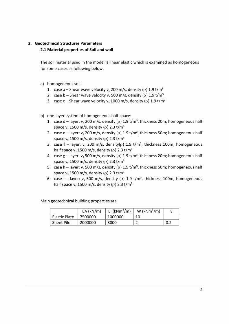
Main geotechnical building properties are

EA (kN/m) EI (kNm2/m) W (kNm3/m) v

Elastic Plate 7500000 1000000 10

Sheet Pile 2000000 8000 2 0.2

3

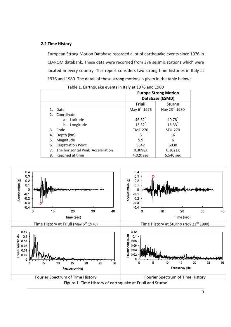
2.2 Time History

European Strong Motion Database recorded a lot of earthquake events since 1976 in

CD‐ROM databank. These data were recorded from 376 seismic stations which were

located in every country. This report considers two strong time histories in Italy at

1976 and 1980. The detail of these strong motions is given in the table below:

Table 1. Earthquake events in Italy at 1976 and 1980

Europe Strong Motion Database (ESMD)

Friuli Sturno 1. Date 2. Coordinate

a. Latitude b. Longitude

3. Code 4. Depth (km) 5. Magnitude 6. Registration Point 7. The horizontal Peak Acceleration 8. Reached at time

May 6th 1976

46.320 13.320

TMZ‐270 6 5.9 3542

0.3098g 4.020 sec

Nov 23rd 1980

40.780 15.330 STU‐270

16 6

6030 0.3021g 5.540 sec

Time History at Friuli (May 6th 1976) Time History at Sturno (Nov 23rd 1980)

Fourier Spectrum of Time History Fourier Spectrum of Time History

Figure 1. Time History of earthquake at Friuli and Sturno

4

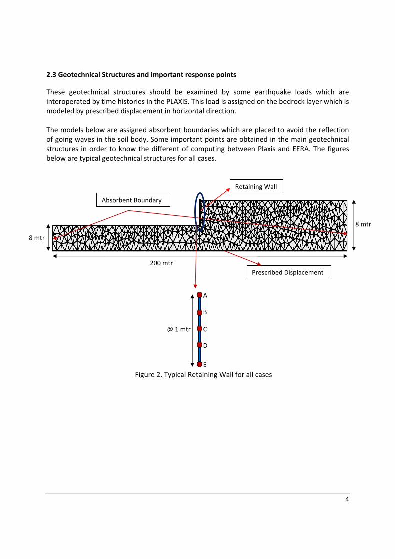
2.3 Geotechnical Structures and important response points

These geotechnical structures should be examined by some earthquake loads which are interoperated by time histories in the PLAXIS. This load is assigned on the bedrock layer which is modeled by prescribed displacement in horizontal direction. The models below are assigned absorbent boundaries which are placed to avoid the reflection of going waves in the soil body. Some important points are obtained in the main geotechnical structures in order to know the different of computing between Plaxis and EERA. The figures below are typical geotechnical structures for all cases.

Figure 2. Typical Retaining Wall for all cases

Absorbent Boundary

Prescribed Displacement

8 mtr

8 mtr

200 mtr

Retaining Wall

A

B

C

D

E

@ 1 mtr

5

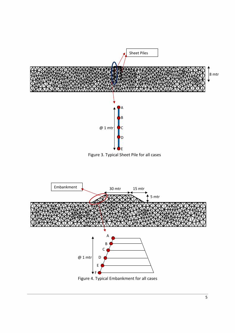
Figure 3. Typical Sheet Pile for all cases

Figure 4. Typical Embankment for all cases

Sheet Piles

Embankment 15 mtr

5 mtr

30 mtr

8 mtr

A

B

C

D

E

@ 1 mtr

A

B

C

D

E

F

@ 1 mtr

6

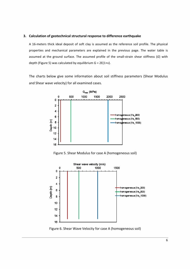
3. Calculation of geotechnical structural response to difference earthquake

A 16‐meters thick ideal deposit of soft clay is assumed as the reference soil profile. The physical

properties and mechanical parameters are explained in the previous page. The water table is

assumed at the ground surface. The assumed profile of the small‐strain shear stiffness (G) with

depth (Figure 5) was calculated by equilibrium G = 2E(1+ν).

The charts below give some information about soil stiffness parameters (Shear Modulus

and Shear wave velocity) for all examined cases.

Figure 5. Shear Modulus for case A (homogeneous soil)

Figure 6. Shear Wave Velocity for case A (homogeneous soil)

7

Figure 7. Typical Shear Modulus for case B (one‐layer system of homogeneous half‐space)

Figure 8. Typical Shear Wave Velocity for case B (one‐layer system of homogeneous half‐space)

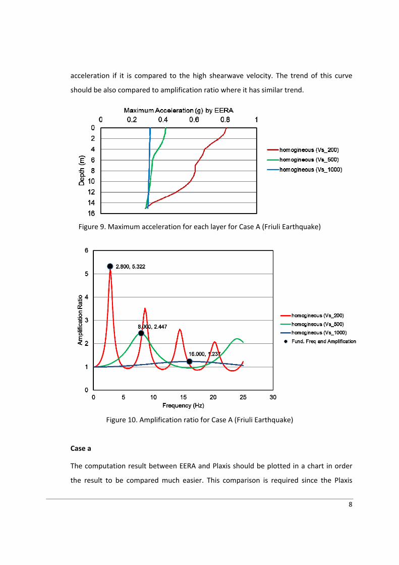
3.1 homogeneous soil in Friuli Earthquake

According to EERA computation by using time history of Friuli, the maximum

acceleration for each homogeneous stiffness parameter is illustrated in the chat below.

It can be clearly seen that the soil layer with low shearwave velocity has higher

8

acceleration if it is compared to the high shearwave velocity. The trend of this curve

should be also compared to amplification ratio where it has similar trend.

Figure 9. Maximum acceleration for each layer for Case A (Friuli Earthquake)

Figure 10. Amplification ratio for Case A (Friuli Earthquake)

Case a

The computation result between EERA and Plaxis should be plotted in a chart in order

the result to be compared much easier. This comparison is required since the Plaxis

9

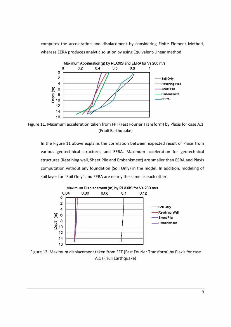
computes the acceleration and displacement by considering Finite Element Method,

whereas EERA produces analytic solution by using Equivalent‐Linear method.

Figure 11. Maximum acceleration taken from FFT (Fast Fourier Transform) by Plaxis for case A.1

(Friuli Earthquake)

In the Figure 11 above explains the correlation between expected result of Plaxis from

various geotechnical structures and EERA. Maximum acceleration for geotechnical

structures (Retaining wall, Sheet Pile and Embankment) are smaller than EERA and Plaxis

computation without any foundation (Soil Only) in the model. In addition, modeling of

soil layer for “Soil Only” and EERA are nearly the same as each other.

Figure 12. Maximum displacement taken from FFT (Fast Fourier Transform) by Plaxis for case

A.1 (Friuli Earthquake)

10

Base on figure 12 above, the maximum displacement for each geotechnical structure is

nearly constant. Actually, this value is being investigated as if time history used for this

model use SMC file, the maximum displacement value is higher than ASCII file result.

Case b

In the case B, soil stiffness parameter is modified to 500 m/s for each layer. Because of

that, the maximum acceleration is smaller than case A which has been explained above.


(Friuli Earthquake)

The trend of EERA and “Soil Only” curve are seen to be so different. It could be

happened due to the number of element used in the finite element is not sufficient or

boundary condition of geometry, hence the wave propagation does not flow as EERA.



11

In this figure 14, it can be seen that maximum displacement is nearly constant as well as

the case a.

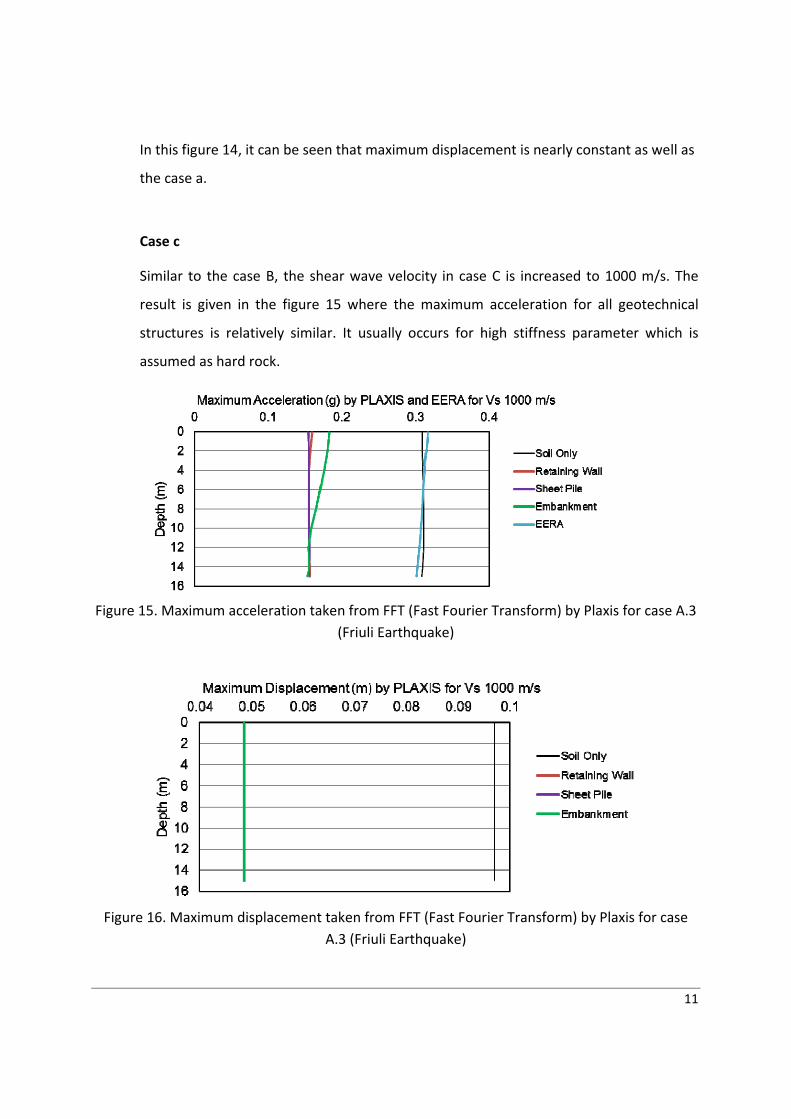
Case c

Similar to the case B, the shear wave velocity in case C is increased to 1000 m/s. The

result is given in the figure 15 where the maximum acceleration for all geotechnical

structures is relatively similar. It usually occurs for high stiffness parameter which is

assumed as hard rock.


(Friuli Earthquake)



12

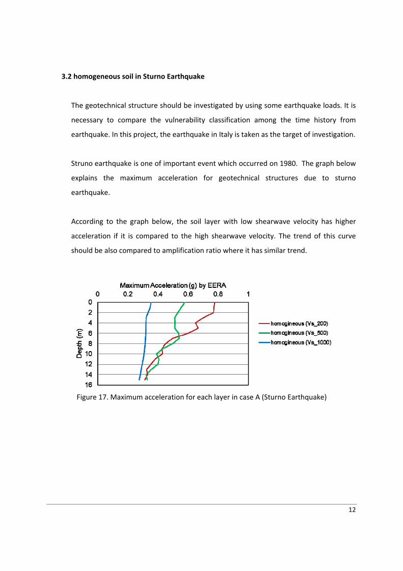
3.2 homogeneous soil in Sturno Earthquake

The geotechnical structure should be investigated by using some earthquake loads. It is

necessary to compare the vulnerability classification among the time history from

earthquake. In this project, the earthquake in Italy is taken as the target of investigation.

Struno earthquake is one of important event which occurred on 1980. The graph below

explains the maximum acceleration for geotechnical structures due to sturno

earthquake.

According to the graph below, the soil layer with low shearwave velocity has higher

acceleration if it is compared to the high shearwave velocity. The trend of this curve

should be also compared to amplification ratio where it has similar trend.

Figure 17. Maximum acceleration for each layer in case A (Sturno Earthquake)

13

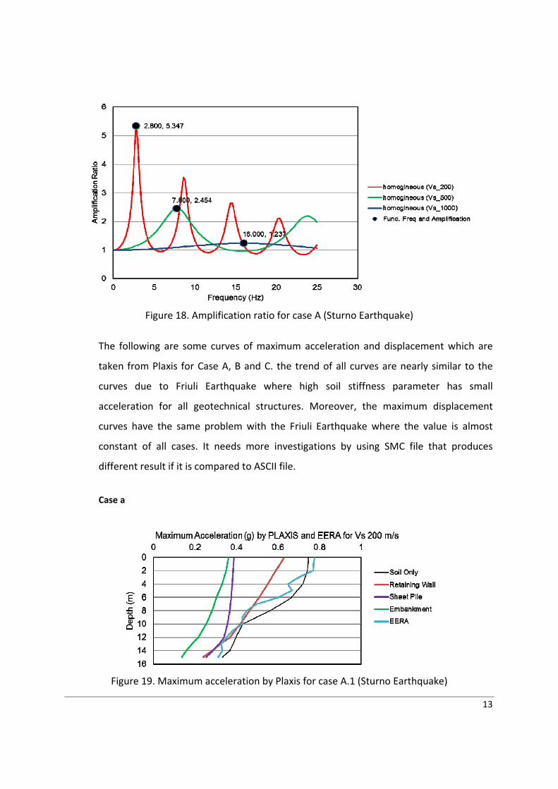
Figure 18. Amplification ratio for case A (Sturno Earthquake)

The following are some curves of maximum acceleration and displacement which are

taken from Plaxis for Case A, B and C. the trend of all curves are nearly similar to the

curves due to Friuli Earthquake where high soil stiffness parameter has small

acceleration for all geotechnical structures. Moreover, the maximum displacement

curves have the same problem with the Friuli Earthquake where the value is almost

constant of all cases. It needs more investigations by using SMC file that produces

different result if it is compared to ASCII file.

Case a

Figure 19. Maximum acceleration by Plaxis for case A.1 (Sturno Earthquake)

14

Figure 20. Maximum displacement by Plaxis for case A.1

Case b



15

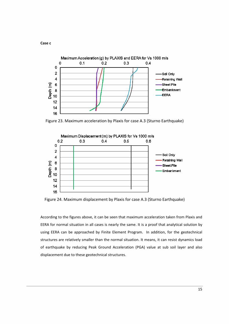
Case c


Figure 24. Maximum displacement by Plaxis for case A.3 (Sturno Earthquake)

According to the figures above, it can be seen that maximum acceleration taken from Plaxis and

EERA for normal situation in all cases is nearly the same. It is a proof that analytical solution by

using EERA can be approached by Finite Element Program. In addition, for the geotechnical

structures are relatively smaller than the normal situation. It means, it can resist dynamics load

of earthquake by reducing Peak Ground Acceleration (PGA) value at sub soil layer and also

displacement due to these geotechnical structures.

16

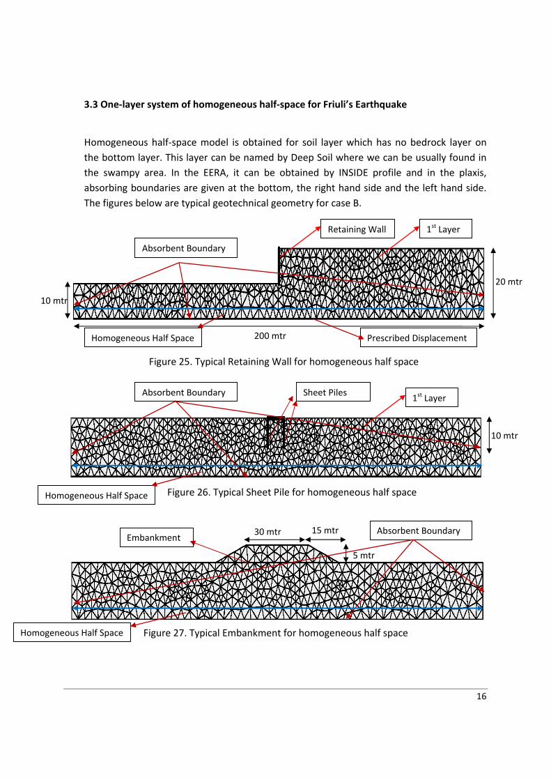
3.3 One‐layer system of homogeneous half‐space for Friuli’s Earthquake

Homogeneous half‐space model is obtained for soil layer which has no bedrock layer on

the bottom layer. This layer can be named by Deep Soil where we can be usually found in

the swampy area. In the EERA, it can be obtained by INSIDE profile and in the plaxis,

absorbing boundaries are given at the bottom, the right hand side and the left hand side.

The figures below are typical geotechnical geometry for case B.

Figure 25. Typical Retaining Wall for homogeneous half space

Figure 26. Typical Sheet Pile for homogeneous half space

Figure 27. Typical Embankment for homogeneous half space

Absorbent Boundary

Prescribed Displacement

10 mtr

20 mtr

200 mtr

Retaining Wall

Sheet Piles

Embankment 15 mtr

5 mtr

30 mtr

10 mtr

Absorbent Boundary

Absorbent Boundary

Homogeneous Half Space

1st Layer

1st Layer



17

In the case B, the exercises are divided into two groups which is dependent on the

thickness:

1. Thickness 20 meter, case a and case d

2. Thickness 50 meter, case b and case e

3. Thickness 100 meter, case c and case f

Based on the soil profile, every thickness consists of two shear wave velocity which is

comparable to the maximum acceleration at every soil layer.

The charts below are detail of maximum acceleration for each case with respect to the

depth of soil.

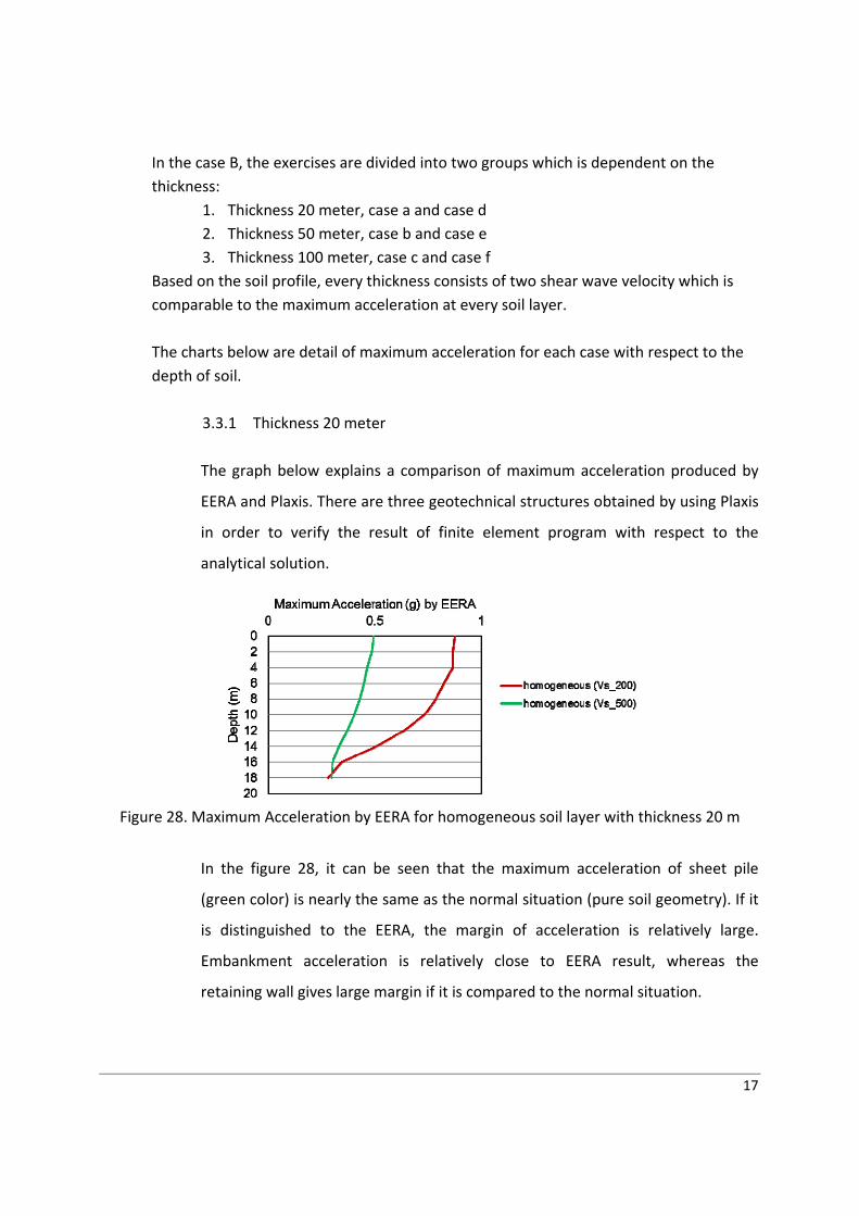
3.3.1 Thickness 20 meter

The graph below explains a comparison of maximum acceleration produced by

EERA and Plaxis. There are three geotechnical structures obtained by using Plaxis

in order to verify the result of finite element program with respect to the

analytical solution.

Figure 28. Maximum Acceleration by EERA for homogeneous soil layer with thickness 20 m

In the figure 28, it can be seen that the maximum acceleration of sheet pile

(green color) is nearly the same as the normal situation (pure soil geometry). If it

is distinguished to the EERA, the margin of acceleration is relatively large.

Embankment acceleration is relatively close to EERA result, whereas the

retaining wall gives large margin if it is compared to the normal situation.

18

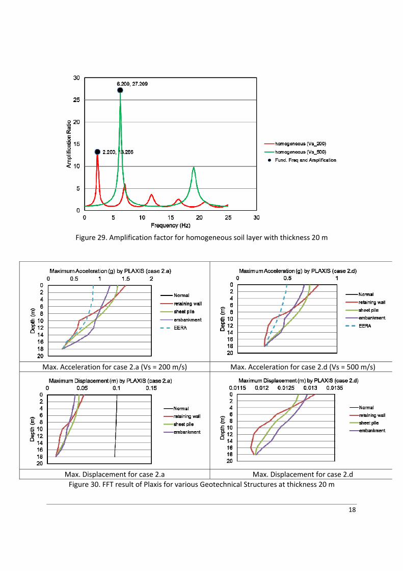
Figure 29. Amplification factor for homogeneous soil layer with thickness 20 m

Max. Acceleration for case 2.a (Vs = 200 m/s) Max. Acceleration for case 2.d (Vs = 500 m/s)

Max. Displacement for case 2.a Max. Displacement for case 2.d

Figure 30. FFT result of Plaxis for various Geotechnical Structures at thickness 20 m

19

According to figure above, the maximum displacement is relatively constant for all sub

soil layer. This displacement is required to evaluate the structures for the vulnerability

assessment which is explained in the master thesis.


Maximum acceleration for homogeneous sub soil layer with shear wave velocity 200 m/s

has no linear trend. It could be happened in this layer due to soft soil in deep layer.

There is instability of wave propagation.

Figure 31. Maximum Acceleration by EERA for homogneous soil layer with thickness 50 m


20

Max. Acceleration for case 2.b (Vs = 200 m/s) Max. Acceleration for case 2.e (Vs = 500 m/s)

Max. Displacement for case 2.b Max. Displacement for case 2.e


3.3.3 Thickness 100 meter This is also deep soil which cause instability of acceleration in the sub soil layer as well as previous thickness.


21


Max. Acceleration for case 2.c (Vs = 200 m/s) Max. Acceleration for case 2.f (Vs = 500 m/s)

Max. Displacement for case 2.c Max. Displacement for case 2.f


22

3.4 One‐layer system of homogeneous half‐space for Sterno’s Earthquake


Homogeneous soil at half‐space condition for earthquake in Sterno which is

shear wave velocity distinguished into 200 m/s and 500 m/s respectively, has

maximum acceleration nearly the same.



23

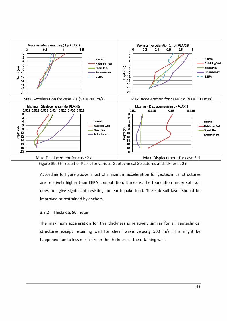
Max. Acceleration for case 2.a (Vs = 200 m/s) Max. Acceleration for case 2.d (Vs = 500 m/s)

Max. Displacement for case 2.a Max. Displacement for case 2.d

Figure 39. FFT result of Plaxis for various Geotechnical Structures at thickness 20 m According to figure above, most of maximum acceleration for geotechnical structures

are relatively higher than EERA computation. It means, the foundation under soft soil

does not give significant resisting for earthquake load. The sub soil layer should be

improved or restrained by anchors.

3.3.2 Thickness 50 meter The maximum acceleration for this thickness is relatively similar for all geotechnical

structures except retaining wall for shear wave velocity 500 m/s. This might be

happened due to less mesh size or the thickness of the retaining wall.

24



25

Max. Acceleration for case 2.b Max. Acceleration for case 2.e

Max. Displacement for case 2.b Max. Displacement for case 2.e


3.3.3 Thickness 100 meter The sub soil homogeneous half space with thickness 100 meter consist nearly constant maximum acceleration for all geotechnical structures. The figure below compares EERA computation to the Plaxis.


26


Max. Acceleration for case 2.c Max. Acceleration for case 2.f

Max. Displacement for case 2.c Max. Displacement for case 2.f


27

4 Conclusions and Recommendations

There are many computation have been conducted to verify analytical solution (EERA) and

Finite Element Program by using Plaxis software. In the case A, it can be clearly seen that

homogeneous soil layer which contains the bedrock at the bottom is able to reflect a wave

propagation as we expected where the low stiffness soil parameter will produce higher

acceleration then the high soil stiffness parameter. It is also shown in the geotechnical

structures which reduce the acceleration at sub soil layer; hence the foundation works as well

as the expected design.

On the other hand, the maximum acceleration in the homogeneous half space soil (Case B)

does not behave as well as case A. It can be caused by the characteristic of deep soil which is

not obtained bedrock at the bottom and it is assumed as non linear behavior; hence the soil

does not reflect the wave propagation properly. It will be absorbed into deep soil and will not

be reflected to the surface anymore.

The displacement FFT (Fast Fourier Transform) should be filtered in order to find a good

solution. It can be done by using Matlab which is necessary to determine vulnerability

assessment.

The geometry of geotechnical structure should be compared to some different size. It is really

difficult to distinguish the behavior between some geotechnical structures since the purpose of

the foundation is not the same. It will be recommended if each structure is analyzed by

different soil stiffness parameter or geometry size.

28

REFERENCES

Bardet J.P., Ichii K. and Lin C.H. (2000) “EERA: a computer program for Equivalent‐linear Earthquake site Response Analyses of layered soil deposits”, University of Southern California, Los Angeles.

Visone C., and Bilotta E. (2010) “Comparative Study on Frequency and Time Domain Analyses for Seismic Site Reponse”, University of Molise and University of Napoli, Italy.

Jesmani M., and Kamalzare M. (2010) “Comparative between Numerical and Analytical Solution of Dynamic Response of Circular Shallow Footing”, Imam Khomeini International University of Iran and Rensselaer Polytechnic Institute, NY, USA.

Visone C., Bilotta E. and Santucci F. “Remarks on Site Response Analysis by Using Plaxis Dynamic Module”, University of Naples and University of Molise, Italy.

Santucci F. “Some Aspects of Seismic design Methods for Flexible Earth Retaining Structures”, University of Molise, Italy.

Ricerca R. “Modellazione Numerica del Comportamento Dinamico di Gallerie Superficiali in Terreni Argillosi”, Unita Politectico di Bari, Italy.

Kramer L.S. “Geotechical Earthquake Engineering, Ground Response Analysis (1996)”, prentice‐Hall International Series, University of Washington, USA. Amorosi A., Boldini D., Elia G. “Analysis of Tunnel Behavior Under Seismic Loads Using Different Numerical Approaches (2011)”,5th International Conference on Earthquake Geotechnical Engineering, Santiago, Chile.

Georgopoulos E.C., Tsompanakis Y., Lagaros N.D, Psarropoulos P.N. “Probabilistic Analysis of Embankments Using Montecarlo Simulation (2007)”,4th International Conference on Earthquake Geotechnical Engineering, Thessaloniki, Greece.

PLAXIS version 8 Dynamics Manual.(2007)

29

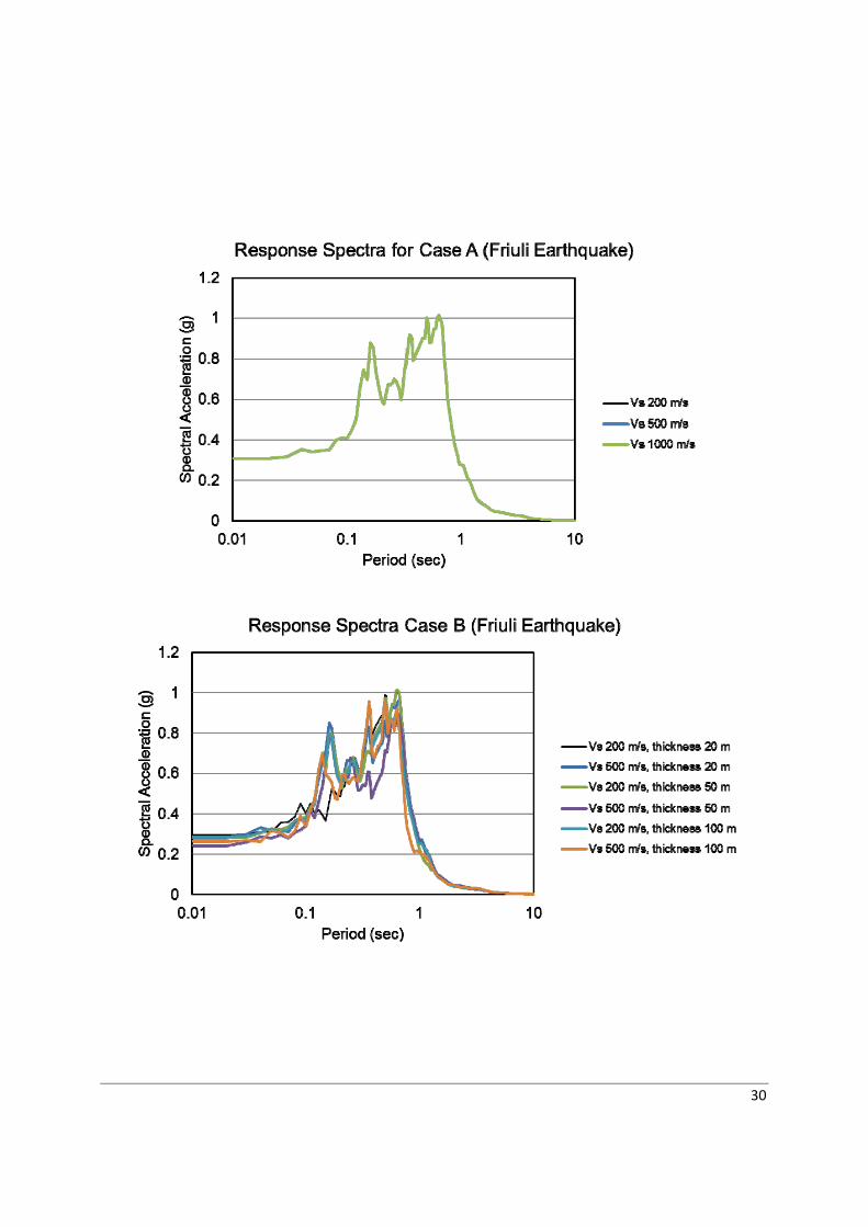
ANNEX

RESPONSE SPECTRA

30

31

Extended Verification Finite Element Program Plaxis · PDF file6 3. Calculation of geotechnical structural response to difference earthquake A 16‐meters thick ideal deposit of soft

Documents