Exploring Complex Systems in Chemical Engineering - National

Meso-scale Structure and Multi-scale Strategy in Simulating Multiphase Systems

Meso-scale Structure and Multi-scale Strategy in Simulating Multiphase Systems

Jinghai Li，Wei Ge, Wei Wang, Ning Yang, and Jingdong He

State Key Laboratory of Multi-Phase Complex SystemsInstitute of Process Engineering, Chinese Academy of Sciences

Beijing, P. R. China

NETL 2009 Workshop on Multiphase Flow Science

Mogantown, WV, April 22~23, 2009

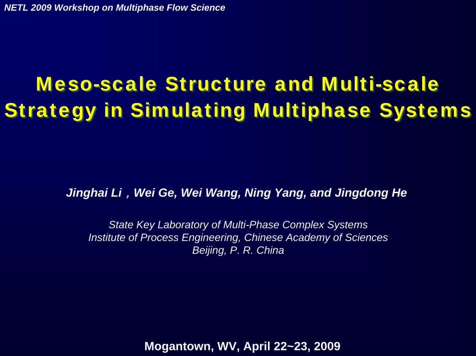
ChallengesChallenges

Modeling

Computation

Multi-scale Discrete

+ Commonnature

Software

Hardware

Multi-ScaleParallel Computation

Progresses Applications Perspectives

Similarity in structure

Meso-scale

StrategyStrategy

Outline of presentation

Low efficiencyHigh cost

1.0 Peta flops

3

Factory Environment(~100m, ~1000m )

Molecule~1A

Assembly~1 nm

Particle(~1μm)

Cell(~1mm)

Cluster(~1cm)

Component(~ 1m)

Apparatus(~10m)

Product

Bottleneck：Multi-scale structure

Multi-scale and multi-level features of process engineering

Process Material

SystemProcess

Multi-scale:

Multi-level:

4

ChallengeChallengeIn Physical ModelingIn Physical Modeling

Poor predictabilityPoor predictability

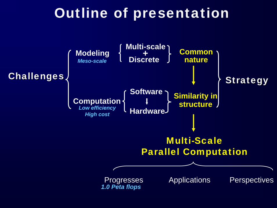
5

0.5 0.6 0.7 0.8 0.9 1.01E-3

0.01

0.1

1

10

β/β 0

Voidage, εg

Deviation between different methods

3～4 orders of difference

Mass transfer

Re

Sh 6～7 orders of difference

Drag Coefficient

Reaction

+

Almost impossible

6

EQUIPMENT SCALE

MESO-SCALE

MICRO-SCALE

Critical influence on transport

CD= 18.6 CD= 5.43

?

Axial and radial distribution

Flow, mass transfer and reaction around a particle

Process

7

Ca5(OH)(PO4)3

Tooth

Bone

?

Material: Hydroxyapatite

MACRO MICROMESO ?

8

folding

unfolding

MACRO MICROMESO ?

Material: Protein

Challenge in physicalmodeling is poor predictability

Understanding of meso-scale structure is the bottleneck

9

10

100 101 102 10310-4

10-3

10-2

10-1

100

101

102

Sc=2.51

Sh ov

r

Re0

1

3

2

5

4

7

6

8

single sphere

02

46

810

020

4060

80100

-8

-6

-4

-2

0

2

4

Ug, m/sGs, kg/m2s

log(

Shov

r)

Dong et al, Chem. Eng. Sci., 63,2008, 2798-2823

Meso-scale structure is the key to achieve high predictability:

11

ChallengesChallengesIn ComputationIn Computation

High cost & low efficiencyHigh cost & low efficiency

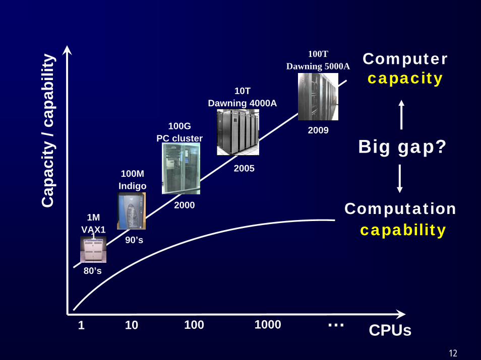
12

100MIndigo

100GPC cluster

1

1MVAX1

1

10TDawning 4000A

10 100 1000 … CPUs

Computation capability

Computer capacity

Cap

acity

/ ca

pabi

lity

Big gap?

80’s

90’s

2000

2005

2009

100TDawning 5000A

13

DisparityStructure of problems

Configuration of software

Architecture of computers:

Diversity:

Multi-scale:

Single scale

Single-scale architecture

Long-range correlation

Global communication

14

NNmodelsmodels

MMPhenomenaPhenomena

M×N algorithms

Universal

Diversity in algorithms

Hardware

Specific

?

Software

Application

Hardware

Software

Application

Low efficiency

high cost

15

StrategyStrategyIn Physical ModelingIn Physical Modeling

VarationalVarational MultiMulti--scale scale MethodolgyMethodolgy

16

“Multi-scale science ”

Glimm and Sharp, SIAM News, 1997Multi-scale Science

– the challenge of 21st century

Krumhansl, Material Science Forum, 2000Multi-scale Science

– Material Science of 21st century

“Multi-scale” OR “Multiscale” within Keywords/Title/Abstract http://isiknowledge.com/ on Nov. 14, 2008

0

500

1000

1500

2000

2500

1950 1960 1970 1980 1990 2000 2010

All FieldChemical Engineering

http://isiknowledge.com/

18

Complex system

Resolution

Description of individual scales

Mech. 1 ……Mech. 2 Mech. k

With respect to dominant mechs.

Identification of extremum tendencies of each dominant mechanisms and their compromise

Stability

Modeling

Correlation between scales

Scale 1Scale 2 Scale n…...With respect to scales

Variational multi-scale methodology

19

Equilibrium: Max. Entropy

Linear: Min. Entropy Production

Non-linear: ?Non-Equilibrium

Stability criterion

Chemical Processes

Multi-scale Structure !

Complexity science

20

The 1The 1stst practice inpractice ingas/solid systemgas/solid system

21

Insufficiency of conservation equationsInsufficiency of conservation equations

Cluster-scale

Particle-scale:in dense-phase

Stability ?

6 equations

Dilute phase

Gas velocity UcSolid velocity UpcVoidage εcVolume fraction fCluster diameter dcl

Gas velocity UfSolid velocity UpfVoidage εf

8 variablesDense phase

in dilute-phase

22

Physical Concept of Physical Concept of EMMS ModelModel

EMMSmodel

Operating Conditions

6 equations

Dilute phase

Gas velocity UcSolid velocity UpcVoidage εcVolume fraction fCluster diameter dcl


8 Variables

Densephase

Energy-minimization multi-scale

Particle-fluid compromiseWst = min|ε=min

Particle dominatedε = min

Fluid dominatedWst = min

Mathematical FormulationMathematical Formulation

max

2

3

4

5

6

( )1 1

(

( ) (1 )( ) 0

( ) (1 )( ) 0

( ) /(1 ) 0

( ) (1 ) 0

( ) (1 ) 0

( )

p p mf

p mf

mf

p p m

st mf

p f

c c i i c p f

f f f p f

f f i i c c

p pf pc

g f c

cl

U Ud U g

UN U

F m F f m F f g

F m F g

F m F m F f m F

F U U f U f

F U U f U f

F d

ε

ε ε

ρ ε

ρ ρ

ε ρ ρ

ε ρ ρ

− + ⋅− −

− +−

= + − − − =

= − − − =

= + − − =

= − − − =

= − − − =

⎡ ⎤⎢ ⎥⎣ ⎦= −

X

X

X

X

X

X

1

)1

0f

mf

gε

⋅−

=

(1- )st

stWNε ρ

=

To find：X={ Upc, Uc , εc, f , dcl , Upf, Uf, εf }

Minimizing：

23

s.t. Fi(X)=0

24

Local structural parameters

Previously:Gas velocity UcSolid velocity UpcVoidage εcVolume fraction fCluster diameter dcl


8 variables

Radial and axial distributions

Regime diagram

0.5 0.6 0.7 0.8 0.9 1.060

65

70

75

80

85

90

95

100

}FD(dilute)

900

620

500

400

300

200

Gs=100

Voidage in clusters εc

E

nerg

y co

nsum

ptio

n fo

r sus

pend

ing

and

trans

porti

ng p

artic

les

Nst (J

/kg

s)

PFC(dense)

25

Prediction of chockingGe&Li, Chem. Eng. Sci. 2002, Vol. 56; Wang et al Chem. Eng. Sci. 2007 Vol. 62

26

0.01 0.1

10

100

100018

12 108

6.0

4.0

3.0

5.0

1.52

Ug=1m/s

Gs,

kg/m

2 s

εs0

2.1

Intrinsic flow regime predicted by EMMS

Solids inventory

http://pevrc.ipe.ac.cn/emms/emmsmodel.php3

Sol

ids

flux


27

Online servicehttp://pevrc.ipe.ac.cn/emms/emmsmodel.php3


28

Discrete simulationDiscrete simulation& verification& verification

Whether or not ?

If yes, why?Nst = min ?

29

PseudoPseudo--ParticleParticle

Micro-scale description

Macro-scale phenomena

30

W(r)

aiVgV Δ+∇′−= νρk&

aii ai

aia r

W r∑=∇ 2|ρ

aii ai

ia Wr∑=Δ 2

m

2 V|V a ρ

Numerical Operators “Interactions” between “Particles”

Particles

Physical

Fluid Pseudo-particles

Macro-scale Pseudo-Particle Modeling

Mathematical

Ge & Li: CFB5, 1996; Chem. Eng. Sci., 58, 2003, 1565; Powder Tech. 137:99

31

Generating meso- and micro-scale structures with micro-phenomena:

Nst(r,t)

Nst

32

0 1 2 3 4 5 6 71

2

3

4

5

6

7

8

9

10

11

12

Nst

(J/

(kg.

s))

Time (s)

1.5 2.0 2.5 3.0 3.5 4.0 4.51

2

3

4

5

6

7

8

9

10

11

12

Nst

(J/

(kg.

s))

Time (s)

1.5 2.0 2.5 3.0 3.5 4.0 4.51

2

3

4

5

6

7

8

9

10

11

12

Nst

(J/

(kg.

s))

Time (s)

0 1 2 3 4 5 6 71

2

3

4

5

6

7

8

9

10

11

12

Nst

(J/

(kg.

s))

Time (s)

Li et al., Chem. Eng. Sci. Vol.59，2004，1687 ~ 1700

Region D Region G

min(1 )

stst

p

WNε ρ

= =−

( )1 (v) 1 (v) v min(1 )

st stV

N N dV

εε

= ⋅ ⋅ − =− ⋅ ∫

Fluid

Particle-Fluid Systems

Region D

Region G

EMMS model Radial EMMS model

globalcompromise

Point A

Point B

st

=

W min

e

=

min

temporal compromise(at any single point)

regional compromise

stW =

spatial compromise(at any single instant)

min

→ minstN→ minstN

Nst min was verified in 2004

Local (micro-scale) structure:Point A & B

Meso-scale structure:Region D

Global (macro-scale) structure:Region G

33

The 2The 2ndnd practice inpractice ingas/liquid systemgas/liquid system

34

Stability ?

3 equationsLarge

bubbles

Gas velocity Ug,S

Volume fraction fSBubble diameter dS

6 Variables

Smallbubbles

Large bubble

Small bubble

Gas velocity Ug,L

Volume fraction fLBubble diameter dL

Liquid

Insufficiency of conservation equations:Insufficiency of conservation equations:

TN

breakN

35

Liquid

Energy consumption dueto meso-scale structuralchange:

Path of energy transfer and dissipation

Small bubble

Large bubble

Liquid-dominated

Gas-dominated

Compromise

+ →turbsurf minN N

Large/Small

Turbulent Dissipation

Interface Oscillationturb min→N

surf min→N

Gas

Zhao, Ge & Li, Chem. Eng. Sci., 2007

36

Physical ModelPhysical Model

DBSmodel

Operating Conditions

Compromisebetween dominant

mechanisms

Stability ?Correlation between scales

3 equationsLargebubbles

Gas velocity Ug,SVolume fraction fSBubble diameter dS

6 Variables

Smallbubbles

Dual-bubble-size model

Large bubble

Small bubble

Gas velocity Ug,LVolume fraction fLBubble diameter dL

Stability Condition:

surf,S+L turb min .N N+ →

Liquid ?

37Yang, Chen, Zhao, Ge & Li, Chem. Eng. Sci., 2007

The jump change of flow structure

38

Extension to more systems Extension to more systems for generalizationfor generalization

minWν →

maxWte →

Viscosity

Inertia

39

Wv , Wte fluctuating Wv / Wte min

75 100 125 150 175

0.0000

0.0004

0.0008

0.0012

75 100 125 150 175

0.00004

0.00006

0.00008

temporal compromise (at any point)

spatial compromise(at any instant)

Time step

Wν

Wte

50 100 150 200 250 300 3500

5

10

15

20

25

Time step

WWteν

minWWteν →

Point A

Point B

Region G

Region G

Point A & B Region G

Extension 3: Turbulent FlowCompromise between Viscosity and Inertia

40

Lipophile

Hydrophile

minOHE →

minWTE →

3x105 4x105 5x105

20

25

30

3x105 4x105 5x105

18

24

30

minOHE =

minWTE =

minOHE =minrepulse WT OHE E E= + →

2.0x105 4.0x105

300

400

500

Region C Point ARegion C

Point B



Point A & B Region C

EWT , EOH fluctuating Erepulse min

H: Hydrophile group (red) T: Lipophile group (blue) W: Water (green) O: Oil (yellow)

Extension 4: MicroemulsionCompromise between Hydrophile and Lipophile

41

Extension 5: Granular Flow

Stream a Stream a dominantdominant

Ha , Hb fluctuating Ha+Hb min

Fa

Fb

Point A & B Region G

Region G

200 300 4000.500

0.504

0.508

0.512

Ha

t

Point B

200 300 4000.500

0.504

0.508

0.512

Hb

Point A

Ha=min

Hb=min

Ha=min



Ha+Hb min( )

Ha+

Hb

Region G

200 400 600 8000.500

0.504

0.508

0.512

t

Fb

Stream b Stream b dominantdominant

Compromise Between Two Streams of Granular Flow

42

ES , Eμ fluctuating Es/Eμ min

9000 10000 11000 1200018

20

22

24

26

E s / E μ

Time step

9000 10000 11000 12000

18

20

22

24

26

E s / E μ

Time step

0 5000 10000 1500010

20

30

40

50

E s/Eμ

Time step

Point A & B

Region G

Liquid Point A

Point B



Region G

Region G

Surface energy

Viscous dissipation

minsE →

minEμ →

Extension 6: Foam DrainageCompromise Between Surface Energy and Viscosity

43

Extension 7: Nano Gas-liquid FlowCompromise Between Interfacial Potential and Viscosity

a b c d e f g h

0 2000 4000 6000 8000 10000

1.0

1.5

2.0

1.0

1.2

1.4ϕr

ϕ r

Time t (-)

1.0

1.5

2.0

2.5

3.0

ϕ r×S/

S 0

S/S0S/S

0

r minSϕ →

Compromise

a b c d e f g h

S

∫∫∫=

A mm

AA mr

dAAVA

dAdAAVF

)()(21

)(

3ρϕ

rϕ The “cost–benefit” ratio of the energy transportation.

Interfacial area

44

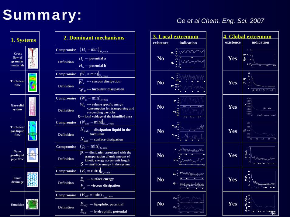
2. Dominant mechanisms

Compromise

Definition aH --- potential a

bH --- potential b

Compromise

Compromise

Compromise

Compromise

Compromise

Definition

Definition

Definition

Definition

Definition

( )b

a minmin

HH

==

te =max( min) WW =ν

teW --- turbulent dissipation

Wν --- viscous dissipation

st min( min)W ε ==

stW --- volume specific energyconsumption for transporting andsuspending particles

ε--- local voidage of the identified area

surfturb min( min) NN ==

turbN --- dissipation liquid in the turbulent

surfN --- surface dissipation

s min( min) EEμ =

=

Eμ--- viscous dissipation

sE --- surface energy

OHWT min( min) EE ==

WTE --- lipophilic potential

OHE --- hydrophilic potential

Compromise

Definition

r S min( min) ϕ ==

rϕ --- dissipation associated with the transportation of unit amount of kinetic energy across unit length

S --- surface energy in the system

1. Systems

Crossflow of

granular materials

Gas-solidsystem

Turbulentflow

Emulsion

Foamdrainage

Turbulentgas-liquid

flow

Nanogas-liquidpipe flow

3. Local extremumexistence indication

121518

21

1.0x105 2.5x1052.0x1051.5x105

EWT

369121518

1.0x105 1.5x105 2.0x105 2.5x105

EOH

No

No

No

No

No

No

No

existence indication4. Global extremum

0.00.0020.003

0.004

0.0050.006

0.007

0.008

8.0x105 1.6x106 2.4x106

Nst min

0.0 0.5 1.0 1.5 2.00.46

0.50

0.54

0.58

0.62

N st

Yes

Yes

Yes

Yes

Yes

Yes

Yes

Summary: Ge et al Chem. Eng. Sci. 2007

45

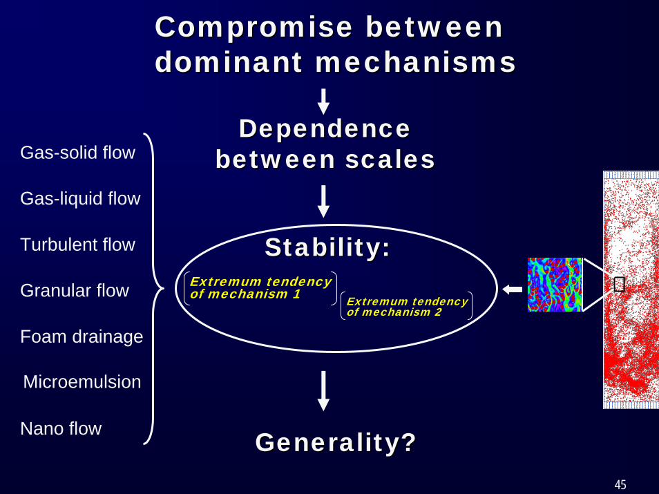
Compromise Compromise between between dominant mechanismsdominant mechanisms

Generality?Generality?

DependenceDependencebetween scalesbetween scalesGas-solid flow

Gas-liquid flow

Turbulent flow

Nano flow

Foam drainage

Microemulsion

Granular flow

Stability:Stability:Extremum tendency of mechanism 1 Extremum tendency

of mechanism 2

46

Mathematical model of complex systemsMathematical model of complex systems

J. Li et al., Chem. Eng. Sci., 2003, 58, 521- 535

Ej (X)min

s.t. Fi(X)=0, i=1, 2, …, m

X = { x1, x2, ……, xn }

… Multi-objective variational problem

Ek (X)

47

Strategy Strategy in Computationin Computation

Multi-scale structureProblems

SoftwareHardware

Similarity

48

Multi-objective variation

Ej (X)┇�

Ek (X)min

s.t. Fi(X)=0, i=1, 2, …, m

X = { x1, x2, ……, xn }

New computation approach

Different problems in engineering

Common nature

Multi-scale

Discrete

Computer

Physical model

Low cost

High efficiency

Generality

Software

49

Computer software computation

Chemical engineers

physical models software computer computation

Computer scientists

Computer scientists

Chemical engineers

Two different strategies:

50

Parallel

Computation

CPUpopular

CPU+GPUTo be optimized

PU？:

BorrowingGPU

Low cost

Structuralsimilarity

ProblemsSoftwareHardware

Ordinary hardware

Super capability

CapacityCapability

Gap between

51

Software structure

CPUMacro

GPU

Variational multi-scale

Lower scale variables

Pseuo-particle

Meso

120 T

Micro:

Computer structure

Physical structure

52

MultiMulti--scale Discrete scale Discrete Parallel ComputationParallel Computation

53

ProgressesProgresses

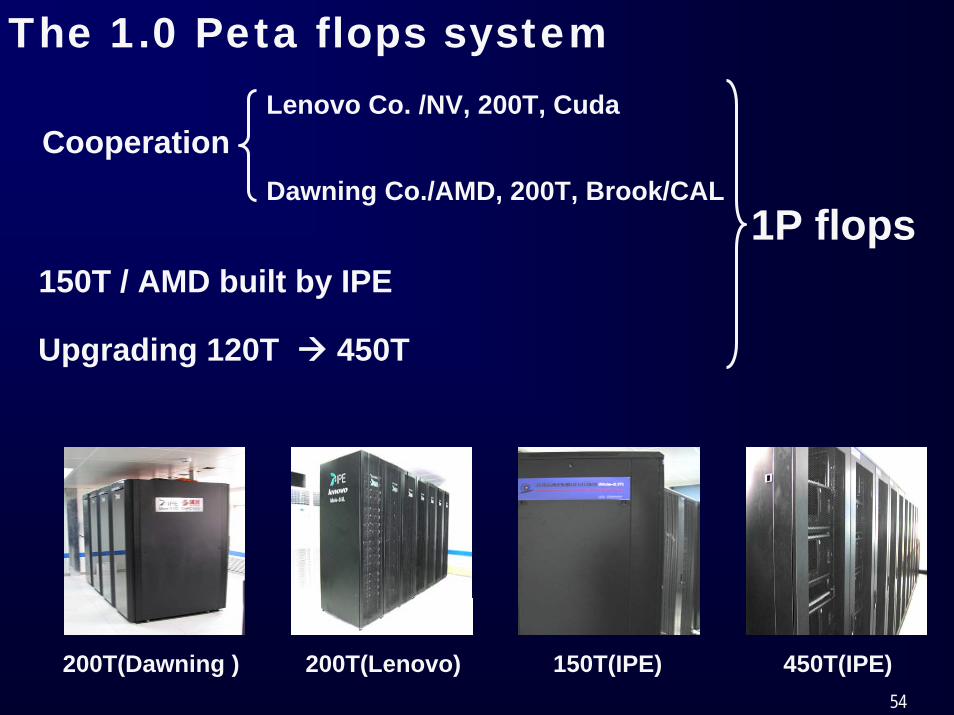
54

The 1.0 Peta flops systemLenovo Co. /NV, 200T, Cuda

Dawning Co./AMD, 200T, Brook/CAL

Cooperation

1P flops

200T(Dawning ) 200T(Lenovo) 150T(IPE) 450T(IPE)

150T / AMD built by IPE

Upgrading 120T 450T

55

CPU+mGPU

CPU+ nGPU

CPU

Equipment

System Architecture

56

Real performance in couette-cavity flow

Grooved micro-channel 1024x1024x4

Computational load

.5×1×2×5×

Performance (flops)

51T102T162T324T

Mode member

150T / AMD+

450T / NV

Efficiency

8.5%17%27%54%

57

Comparison of capability

120T (GPU)

1000T GPU

Variational multi-scale

2 Hours

2 Minutes

1 Day

Simulation of gas-solid system

59

1024 Particles

Oil-field

Sample of rock

20000 Particles

Experimental apparatus

Industrial apparatus

60

100MIndigo

100GPC cluster

100TDawing 5000A

1

1MVAX11

10TDawning 4000A

10 100 1000 … CPUs

VariationalMulti-scale

Computatio

Actual capability

Theoretical Capacity

Big gap

80’s

90’s

2000

2005

2009

Huge potential

Cap

acity

/ ca

pabi

lity

61

ApplicationsApplications

62

Direct simulation of gas/solid system

1024 Particles1024CPU

2006 2008

25 K Particles200GPU

Ma et al., Chem. Eng. Sci., 61: 7096,2006.

Ma et al., Chem. Eng. Sci., 64: 43,2008.

2.5M Particles240GPU

2009

63

GPU computation：100K Particles +200M pesudo-particles

from Systems to Particles

Direct simulation of industrial stirred tank

64

Commercial software

2D steady

This system

3D Dynamic200GPU

Parallel computation

65

Stirred Tank3D MaPM, 200 GPU

66

Stirred tank~100 M particles, 32GPU，5.5s/step，61h/round

67

Metallurgy process

2007-08：10CPU/2GPU 2009：20GPU

3D simulation of granular flow in

blast furnace

Slurry of steel

68

Coal-ash mixing in coal topping

69

Measurement

Initial condition

Flow field

DNS of flow in porous media

70

Protein folding in vivo

71

Polymer dynamics Vesicle formation

1392656 water3375 dipalmiteyl phosphatidyl choline

NPT Ensemble

1200 polyethylene chainsChain length：300 CH2

NVT Ensemble

72

Silicon crystal for solar cell

Solar cell

GPU：bulk CPU：interfance

Atom number：1010

Scale ：1μm3

Thickness on silicon film

Photon

interfance

From Angstroms to Microns:MD-PPM simulation of interactions

73

2D simulation ofliquid film rupture40nm×35nm,solid velocity 3.2m/s LJ/PP fluid at 60K, constant P & V

10000 particles,3.2G Intel CPU(1core)

Chen et al., Sci. in China,52,2008,372-380

74

3D simulation: bubble-particle in liquid0.1*0.1*0.15µm, bubble mean velocity 3m/s

LJ/PP fluid at 60K, NVT ensemble7M particles, 2 GPUs

75

On-line

Real-time CTImage Reconstruction

Off-line

CT Scanister

76

CFD+EMMSCFD+EMMS

77

Two-fluid model Smaller grid size

LimitationAverage in grid

Constitutive model

OptionsMeso-structure Correlation

Stability

7878

Two-fluid models

Local parameters Cd for local cells

Start Final

Spatial-temporal correlation

Average approach

EMMS

Structure parameters

& acceleration

79

1 10 1000.5

1.0

1.5

2.0

2.5

3.0

λ/dp

Dim

ensi

onle

ss s

lip v

eloc

ity

1 10 1003

4

5

6

7

8

Dim

ensi

onle

ss s

lip v

eloc

ity

λ/dp

0.7 0.8 0.9 1.00

2

4

6

8

10

Bed

hei

ght (

m)

Voidage

Bed

hei

ght (

m)

0.7 0.8 0.9 1.00

2

4

6

8

10

Voidage

Fine-grid TEM, big deviation from experiments

EMMS+CFD, good agreement and mesh

independent

CFD + EMMS

80

0 5 10 15 20 25 30

0

20

40

60

80

100

120

Experimental

Simulation

Output solid flux (kg/m2s)Empirical correlations+CFD

Time (s)0 5 10 15 20 25 30

0

20

40

60

80

100

120

ExperimentalSimulation

Output solid flux (kg/m2s)EMMS+CFD

Time (s)

Solid flux: comparison between experiment & simulation

Simulation:with only CFX

Simulation:CFX + EMMS

Yang, Wang, Ge & Li, Chem. Eng. J., 2003

81

0

1

2

3

4

5

6

7

8

9

0.0 0.1 0.2 0.3 0.4

Solid Volume Fraction

Hei

ght (

m)

Exp.15-3-4 Sim.15-3-4 Sim.15-3-4-100w

-0.2 -0.1 0.0 0.1 0.2

0.0

0.1

0.2

0.3

0.4

0.5

Sol

id V

olum

e Fr

actio

n

x (m)

Exp.15-3-4 Sim.15-3-4 Sim.15-3-4-100w

-0.2 -0.1 0.0 0.1 0.2

-4

-3

-2

-1

0

1

2

3

4

5

6

Solid

Vol

ume

Frac

tion

x (m)

Exp.15-3-4 Sim.15-3-4 Sim.15-3-4-100w

Comparison between experiment & simulation

0.72m

2m

4m

6.5m

7.6m

Ug = 3.5 m/s Hinit = 1.70m

82

0.0 0.3 0.6 0.9 1.2 1.5 1.8 2.1 2.4 2.7 3.00

30

60

90

120

150

180

210

240

S

olid

Flu

x (k

g/m

2 .s)

Hini (m)

Ug=3.5m/sUg=2.5m/s

83

Riser Height

0.00 0.05 0.10 0.15

100

200

300

εs0

Gs

0.01 0.1

10

100

1000

Gs Ug=18m/s 10

1.5 m/s

εs0

0.00 0.05 0.10 0.15

50

100

150

εs0

Gs

0.00 0.05 0.10 0.15

20406080

100120

εs0

2.1

Gs

2.8

Ug=4.0m/s

8

10m 20m ...

Crit

ical

poi

nt

Ug*

, Gs*

Intrinsic critical point

Riser height is a key factor !O

pera

tion

flexi

bilit

y

84

εgc, εgf, f,

dcl, ugc, ugf,

usc, usf,

ac, af, ai

Shdynamic

Shstatic

Shdilute

Shdense

Structure-dependent CD

Meso-scale

Micro-scale

Structure-dependent Sh(Ug, Gs)

EMMS/mass: Sub-grid mass transfer

Multiscale flow Multiscale mass transfer

c/c 0

r/r0

c/c 0

r/r0

85

Comparison between CFD computation and experiments

c/c 0

r/r0

Averaged flow & averaged mass transfer

Multi-scale flow &averaged mass transfer

Multi-scale flow multi-scale mass transfer

c/c 0

r/r0

c/c 0

r/r0

c/c 0

r/r0

Dong et al, Chem. Eng. Sci., 63,2008,2798-2823

86

Commercial codes of EMMS

87

Applications to Applications to industriesindustries

88

SINOPEC Stage 1 :MIP (max. iso-paraffins) process

Shade of color: concentrationShade of color: concentration

Novel FCC RiserHeight: 40 mDiameter: 1∼3.5 m

Determine design parameterDiametervelocityInventory

89

SINOPEC SINOPEC Stage 2Stage 2 ::Further optiFurther optimization of MIP processation of MIP process

90

SINOPEC GaoqiaoMIP process, 1.4 M tons/a

91

98 169 390

SINOPEC: the influence ofSINOPEC: the influence ofOrifice numberOrifice number

Distributor shapeDistributor shape

OutletsOutlets

Distributor shapeDistributor shape OutletOutletOrifice numberOrifice number

Upright SidewardArc Basin Cone

92

Before optimization

After optimization

PetroChina: slurry bed loop reactor

93

XinhuiXinhui Power plantPower plant

Solid volume fraction

Height:36.5 mWidth:15.3 mDepth:7.22 m

480t/h (150MW)CFB boiler480t/h (150MW)CFB boiler

94

Classification of ore

Dispersive particle

Slag processing in metallugry

95

Hot model with phase transition

Cool model

Coarse particle Fine particle/multi particle1 billion particles

Secondary oil recovery from fractures to oil fields

96

97

PerspectivesPerspectives

98

Astro- Sciences

Earth, Space & Oceanic Sciences

Multi-scale StructureA common challenge for different areas

ProcessNano

Molecular

Atom

Basic LawsMathematics

System Science

ResourcesEnvironment Buildings

Agriculture Life

& H

ealth

Information

Economics

ManufactureTraffic

Mat

eria

ls

Energy

Nan

o-st

ruct

ure

Multi-Scale

Mol

ecul

es

Clu

ster

s

Part

icle

s

Rea

ctor

s

Fact

ory

Ato

ms

Part

icle

s

Rea

ctor

s

Part

icle

s

99

CPU+GPUBottleneck: Application

PU？:

BorrowingGPU

Simple Hardware, Low cost

Structuralsimilarity

ApplicationSoftwareHardware

Ordinary hardware

Super capability

Breakthrough of computation capability is expected in near future

100

Classified design

Flexible design

Application-oriented

Hardware Software ApplicationUniversal

Easy to use

Application

Software Hardware

High efficiency

Common nature

Particularity

Dive

rsity

Generality

Software Hardware

High efficiencySpecial purposeHigh cost

Conditionally universal

Principles for designing variationalmulti-scale computer systems

CPU-a

CPU-b + m GPU-j

CPU-c + n GPU-k

Parameters：a,b,c,n,m,j,k

Virtual Process Engineering: Dream reality

Breakthrough in understanding meso-scale structures:

Ug=3.5m/sGs=40Kg/m2s



Acknowledgement

NSFC (Natural Science Foundation of China)

MOST (Ministry of Science and Technology)CAS (Chinese Academy of Sciences)

Supports from:

Coworkers:

104

Thanks for Thanks for your attentionyour attention ! !

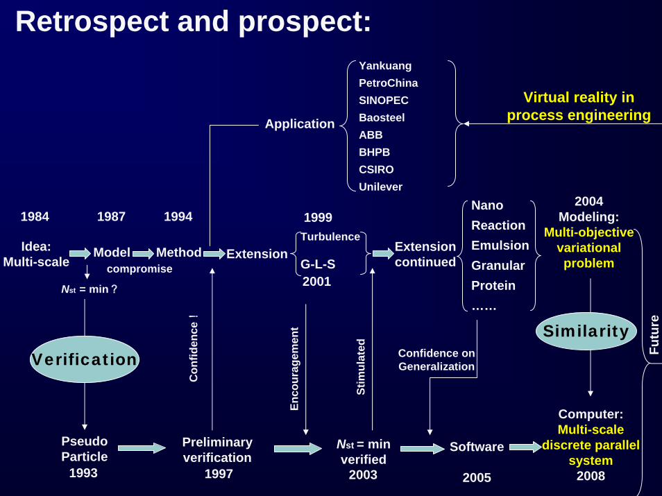
Idea: Multi-scale

Model Method ExtensionTurbulence

G-L-S

1999

2001

NanoReactionEmulsionGranularProtein……

2004Modeling:

Multi-objective variationalproblem

Software

2005

Nst = minverified

Preliminaryverification

Verification

Pseudo Particle

Nst = min？

Computer: Multi-scale

discrete parallel system

2008

Application

YankuangPetroChinaSINOPEC BaosteelABBBHPBCSIROUnilever

Con

fiden

ce！

Stim

ulat

ed Confidence on Generalization

compromise

1984 1987 1994

1993 1997

Enco

urag

emen

t

2003

Extension continued

Futu

re

Virtual reality in process engineering

Similarity

Retrospect and prospect:

Exploring Complex Systems in Chemical Engineering - National

Documents