Exploring chemical homogeneity in dwarf galaxies: a VLT ...

MNRAS 495, 2564–2581 (2020) doi:10.1093/mnras/staa1280Advance Access publication 2020 May 8

Exploring chemical homogeneity in dwarf galaxies: a VLT-MUSE study ofJKB 18

Bethan L. James ,1‹ Nimisha Kumari ,2 Andrew Emerick ,3,4 SergeyE. Koposov ,5,6 Kristen B. W. McQuinn,7 Daniel P. Stark,8 Vasily Belokurov 6

and Roberto Maiolino2

1AURA for ESA, Space Telescope Science Institute, 3700 San Martin Drive, Baltimore, MD 21218, USA2Kavli Institute for Cosmology, University of Cambridge, Madingley Road, Cambridge CB3 0HA, UK3Carnegie Observatories, Pasadena, CA 91101, USA4TAPIR, California Institute of Technology, Pasadena, CA 91125, USA5McWilliams Center for Cosmology, Carnegie Mellon University, 5000 Forbes Ave, Pittsburgh, PA 15213, USA6Institute of Astronomy, University of Cambridge, Madingley Road, Cambridge CB3 0HA, UK7Rutgers University, Department of Physics and Astronomy, 136 Frelinghuysen Road, Piscataway, NJ 08854, USA8Steward Observatory, The University of Arizona, 933 N Cherry Ave, Tucson, AZ 85721, USA

Accepted 2020 May 4. Received 2020 April 1; in original form 2019 November 8

ABSTRACTDeciphering the distribution of metals throughout galaxies is fundamental in our understandingof galaxy evolution. Nearby, low-metallicity, star-forming dwarf galaxies, in particular, canoffer detailed insight into the metal-dependent processes that may have occurred withingalaxies in the early Universe. Here, we present VLT/MUSE observations of one such system,JKB 18, a blue diffuse dwarf galaxy with a metallicity of only 12 + log(O/H)=7.6 ± 0.2(∼0.08 Z�). Using high spatial resolution integral-field spectroscopy of the entire system, wecalculate chemical abundances for individual H II regions using the direct method and deriveoxygen abundance maps using strong-line metallicity diagnostics. With large-scale dispersionsin O/H, N/H, and N/O of ∼0.5–0.6 dex and regions harbouring chemical abundances outsidethis 1σ distribution, we deem JKB 18 to be chemically inhomogeneous. We explore this findingin the context of other chemically inhomogeneous dwarf galaxies and conclude that neitherthe accretion of metal-poor gas, short mixing time-scales or self-enrichment from Wolf–Rayetstars are accountable. Using a galaxy-scale, multiphase, hydrodynamical simulation of a low-mass dwarf galaxy, we find that chemical inhomogeneities of this level may be attributableto the removal of gas via supernovae and the specific timing of the observations with respectto star formation activity. This study not only draws attention to the fact that dwarf galaxiescan be chemically inhomogeneous, but also that the methods used in the assessment of thischaracteristic can be subject to bias.

Key words: galaxies: abundances – galaxies: dwarf – galaxies: evolution – galaxies: irregu-lar – galaxies: star formation.

1 IN T RO D U C T I O N

The ‘gas regulatory’ or ‘bathtub’ chemical processing frameworksof galaxy evolution are thought to consist of four key components:star formation, chemical enrichment, outflows, and accretion (e.g.Dayal, Ferrara & Dunlop 2013; Lilly et al. 2013; Peng & Maiolino2014). Each of these components is dependent on the other,operating together in the multiphase interstellar medium (ISM) via

� E-mail: [email protected]

the exchange of energy and momentum. The metal content of themedium through which this exchange occurs can play a significantrole – both in communicating the evolutionary history of the galaxyand shaping the evolutionary future of the galaxy. Via collisionalexcitation and recombination processes, metals provide efficientmechanisms through which gas can cool, condense, and eventuallyform stars (e.g. Krumholz & Dekel 2012). As these stars formand evolve, they eject their metals into the ISM, via photosphericwinds during the asymptotic giant branch (AGB) phase or throughsupernovae driven outflows, enriching the ISM and intergalacticmedium (IGM) with chemoevolutionary signatures that depend

C© 2020 The Author(s)Published by Oxford University Press on behalf of the Royal Astronomical Society

Dow

nloaded from https://academ

ic.oup.com/m

nras/article/495/3/2564/5834563 by guest on 03 June 2022

http://orcid.org/0000-0003-4372-2006

http://orcid.org/0000-0002-5320-2568

http://orcid.org/0000-0003-2807-328X

http://orcid.org/0000-0003-2644-135X

http://orcid.org/0000-0002-0038-9584

mailto:[email protected]

Exploring chemical homogeneity in dwarf galaxies 2565

on the temperature and mass of the star. Since the winds of hotstars are driven by photon momentum transfer through metal-lineabsorption, metals also drive the momentum and velocity of thewind (Kudritzki & Puls 2000). In turn, the metal content of accretedgas, combined with the metal content of the site of subsequentlytriggered star formation, can provide important constraints onthe enrichment history and structure of the IGM surrounding thegalaxy (Putman 2017, and references therein). As such, a deep andthorough understanding of the spatial distribution of metals in thegas throughout galaxies, is imperative in furthering our insight intogalaxy evolution in general.

Given the important role of metals in deciphering global trends ofgalaxy evolution – such as the mass–metallicity relation (Lequeuxet al. 1979; Tremonti et al. 2004) and the fundamental metallicityrelation (Ellison et al. 2008; Mannucci et al. 2010) – much efforthas been spent in investigating the spatial distribution of metalsthroughout star-forming galaxies. For several decades, metallicitygradients have been found to be prevalent in galactic discs, typicallyshowing a negative relation as a function of galactic radius (e.g.Searle 1971; Pagel & Edmunds 1981; Vila-Costas & Edmunds 1992;Zaritsky, Kennicutt & Huchra 1994; van Zee et al. 1998; Moustakaset al. 2010; Werk et al. 2011) – which provided insight into processesthat regulated the growth and assembly of galaxies such as inside-out growth and/or galaxy quenching. Inverted metallicity gradientshave also been found at high redshifts (e.g. Cresci et al. 2010;Troncoso et al. 2014), which are thought to be due to an enhancedinflow of chemically pristine gas towards the centre of the galaxy.Furthermore, metallicity gradients have been characterized at ahigher level of detail during the past decade or so due to theadvent of integral field units (IFUs). Thanks to large-scale surveysof spatially resolved spectroscopy, such as CALIFA (Sanchez et al.2012), MaNGA (Bundy et al. 2015), and SAMI (Croom et al. 2012)we now know the shape of the gradient depends on the stellar massof the galaxy (Belfiore et al. 2017; Goddard et al. 2017; Poetrodjojoet al. 2018). While these works have provided significant insightinto the role of metals in galaxy evolution, by concentrating almostentirely on massive (M� > 1010 M�), disc-dominated galaxies, theyprovide a limited view on the evolutionary processes involved inthe early Universe. As discussed in Maiolino & Mannucci (2019),measurements of radial gradients are deemed virtually inefficientat early epochs of galaxy evolution due to their large, irregularmetallicity variations (most likely due to more chaotic accretionand formation processes, e.g. Forster Schreiber et al. 2018) andthus fail to represent the chemical complexity of such systems.

Since current facilities cannot provide us with the detailed spec-troscopic information required to investigate the spatial distributionof metals and chemical homogeneity of the first galaxies, we insteadrely on nearby ‘analogues’ of these complex systems. Nearby low-mass galaxies with extremely low metal content (i.e.<10 per centsolar metallicity), currently or recently undergoing periods ofintense star formation provide close representations, while alsoenabling the spatial and spectral detail that we require for suchstudies. There are of course some caveats to this approach – forexample, local extremely metal-poor (XMP, e.g. Papaderos et al.2008; Filho et al. 2015;Sanchez Almeida et al. 2016) galaxies areknown to have much lower specific star formation rates (SFRs)(0.1–1 Gyr−1, James et al. 2016) compared to star-forming systemsat z =6–10 (5–10 Gyr−1, Lehnert et al. 2015), and thus differentmassive-star populations. Also, being in the local Universe, andthus having undergone previous periods of star formation, such‘analogues’ cannot be true representatives of the first galaxies bydesign. Despite these setbacks, one such population of galaxies that

we can use to our advantage are blue diffuse dwarf (BDD) galaxies.BDD galaxies were brought to light by conducting a search on SDSSimaging data using the morphological properties of Leo P, one ofthe most metal-deficient dwarf galaxies known (∼1/34 Z�, Skillmanet al. 2013). The search uncovered ∼130 previously undetected lowsurface brightness star-forming galaxies, a sub-sample of whichwere followed-up with MMT optical long-slit spectroscopy (Jameset al. 2015, 2016). Each of these galaxies is faint, blue systems, withisolated H II regions embedded within a diffuse continuum. Opticallong-slit spectroscopy confirms that ∼25 per cent of the samplewere indeed extremely metal poor. Combined with SDSS imaging,optical spectra reveal them to be nearby systems (5–120 Mpc)with regions of ongoing and recent star formation (i.e. SFRs of∼0.03–8 × 10−2 M� yr-1, with average ages of ∼7 Myr) randomlydistributed throughout their diffuse, chemically unevolved gas. Thiscombination of pristine environments in a pre- or post-starburstera offers an opportunity to explore and understand the interplaybetween star formation and metallicity in ‘young’ star-formingenvironments that we expect to see in the high-z Universe – inexceptional detail.

Here, we present IFU observations of one such BDD, JKB 18(Fig. 1, Table 1). As presented in James et al. (2016), this is a nearby(z = 0.004), low metallicity (12 + log(O/H) = 7.56 ± 0.20) systemforming stars at an average rate of 0.20 ± 0.09 × 10−2 M� yr-1. Weestimate a distance of ∼18 Mpc and a stellar mass of ∼108 M�, al-though due to radial velocities and peculiar motions, these estimatesare subject to significant uncertainties. As shown in Fig. 1, JKB 18has an extremely interesting morphology, with numerous sites ofongoing star formation scattered in a somewhat random fashionamongst a diffuse body. In this paper, we utilize the high sensitivityand high spatial resolution of VLT-MUSE observations to performa detailed spatially resolved spectroscopic study of this system, inorder to investigate the distribution of metals throughout its ionizedgas. Our goal is to explore the chemically inhomogeneous natureof its gas and understand it in the context of evolutionary processessuch as star formation, outflows, and gas accretion.

The paper is structured as follows: In Section 2, we describethe VLT/MUSE observations and data reduction. Maps of flux,reddening, and emission-line diagnostics for JKB 18 and themethods used to create them are described in Section 3. In Section 4,we explore the chemical homogeneity of the ionized gas, includingdirect-method oxygen abundances and nitrogen-to-oxygen ratiosof individual H II regions, and metallicity maps using strong-linediagnostics. These findings are discussed in the context of otherdwarf galaxies in Section 5, and interpreted via detailed galaxy-scale simulations of a similar, XMP system. In Section 6, we drawconclusions on our findings.

2 O B S E RVAT I O N S A N D DATA R E D U C T I O N

Observations of JKB 18 (Table 1) were made using VLT-MUSE on2015 November 18 and 2016 January 10 under program 096.B–0212(A) (PI: James). Data were taken in wide-field mode, withextended wavelength coverage (4650–9300 Å) and a resolution of R∼1770–3950. The 1 × 1 arcmin field of view of MUSE fully coversJKB 18, providing 0.2 × 0.2 arcsec2 plate-scale spatial resolutionfor each of the 300 × 300 spaxels (providing 90 000 spectra intotal). Observing blocks (OBs) were broken down into 5 × 275 sand 5 × 600 s exposures, for a total of 1.2-h integration time onsource. Separate sky observations were taken for each OB and theseeing was reported to be 0.9 arcsec (∼78 pc at the distance ofJKB 18) for both sets of observations, as such it was necessary to

MNRAS 495, 2564–2581 (2020)

Dow


ic.oup.com/m


2566 B. L. James et al.

Figure 1. Color composite image of JKB 18 (α =09:21:27.173, δ =07:21:50.70) derived from the VLT-MUSE data cube, created from 100 Å channels at4700 Å (blue), 6050 Å (green), and 8000 Å (red). North is up, east is to the left.

Table 1. General properties of JKB 18, as presented inJames et al. (2016).

RA 9:21:27.173Dec. 07:21:50.70z 0.004Distance ∼18 Mpc12 + log(O/H) 7.56 ± 0.20Mass ∼108 M�

bin our data cube using a two-dimensional three-pixel boxcar kernelbefore performing emission-line fitting to avoid oversampling.

Although the MUSE data cubes had already undergone datareduction via the European Southern Obseratory (ESO)–MUSEpipeline, upon inspection the cubes were found to have poorlysubtracted sky lines. As such, the cubes were re-reduced usingthe MUSE pipeline version 2.4.2,1 with stricter constraints on thesky subtraction parameters (such as a non-modified sky subtractionto mitigate contamination of the continuum from the sky spectrum,and for the sky frames a usable pixel fraction of 40 per cent and anignore pixel fraction of 10 per cent). Specifically, we implementedthis using MUSEPACK, a python-based wrapper for ESO’s MUSEpipeline, as described in Zeidler et al. (2019). The pipeline coversflat-field removal, wavelength calibration, flux calibration, and skyremoval, finally combining the cubes from each OB into a singledata cube. The wavelength solution and line-spread function (LSF)of the MUSE instrument are very stable. Nevertheless, we used a90◦ dither pattern strategy, as suggested by the MUSE handbook,to not only remove cosmic rays and detector defects, but also toreduce possible small offsets in the wavelength and flux calibration.

1https://www.eso.org/sci/software/pipelines/〈0:italic 〉MUSE〈/0:italic〉/

Furthermore, the stability of the wavelength and LSF was checkedby fitting multiple sky lines across several sky-only regions acrossthe cube. Variation in both parameters was found to be negligible.

3 EMISSION-LINE MAPS

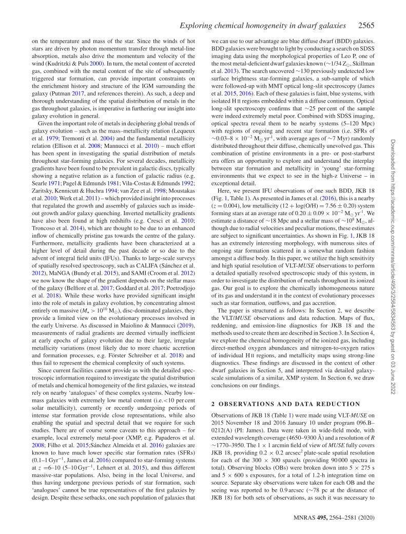
The full MUSE spectrum, integrated across JKB 18 can be seen inFig. 2. All of the strong emission lines typical of H II regions canbe seen, along with the He I series, the [S III] λ6312 auroral line,the [O II] λλ7321, 7332 doublet, and [S III] λ9071 (the companionof this doublet line, [S III] λ9531, is not covered by the MUSEwavelength range). The methodology used to fit each of theseemission lines throughout JKB 18 and the resultant emission-linemaps are described below.

3.1 Automated line fitting

For each spaxel, we performed emission-line fitting using ALFA

(Automated Line Fitting Algorithm),2 an automated line fitting tooloptimized to work on MUSE data cubes. A full description of ALFA

can be found in Wesson (2016). The tool’s novel approach consistsof constructing a synthetic spectrum to match the observations,derived from a line catalogue input from the user, then optimizingthe parameters of all the Gaussian line profiles by means of a genericalgorithm. In addition to the Gaussian parameters and uncertaintiesfor each line (estimated using the noise structure of the residuals),the tool additionally outputs the fitted spectrum and the fit to thecontinuum. It should be noted that stellar absorption features werenot seen in individual spaxel spectra. In order to estimate theeffects of any underlying stellar absorption, tests were performed

2https://www.nebulousresearch.org/codes/alfa/

MNRAS 495, 2564–2581 (2020)

Dow


ic.oup.com/m


https://www.eso.org/sci/software/pipelines/muse/

https://www.nebulousresearch.org/codes/alfa/


Figure 2. Emission-line spectrum summed overall 30 identified H II regions throughout JKB 18 (as described in Section 4). Major emission lines are labelledin red. Grey rectangles correspond to regions of poor sky subtraction.

on the highest signal-to-noise ratio (S/N) single-spaxel spectra byadditionally including Balmer-line absorption features while fitting.Accounting for the absorption had a negligible effect on the finalparameters of the emission-line fits.

3.2 Structure of the ionized gas

Fig. 3 (top panel) shows the structure of the Hα emitting gasthroughout JKB 18. The emission appears to be clumpy, with amultitude of H II regions (∼100–130 pc in size, as found by theH II region fitting algorithm described in Section 4 and resolved atthe resolution of our observations) distributed randomly across thegalaxy. This morphology is in contrast to blue compact dwarf (BCD)galaxies, which typically have a compact, central emitting region.The structure suggests little or no large-scale order, although someareas do appear to be connected as streams or arms of emission. Adetailed analysis of each H II region is described in Section 4.

Also shown in Fig. 3 are the radial velocity and velocitydispersion maps for Hα. The radial velocity map has been correctedfor the systemic velocity of 1378 km s−1, as derived from the redshiftof the Hα emission line in the integrated spectrum, and the velocitydispersion map has been corrected for the instrumental resolutionat Hα of ∼2 Å (∼88 km s−1 as measured from a selection of skylines). We can see from the radial velocity map that there is indeedsome large-scale gas structure throughout JKB 18, in that the gasappears to be rotating as a large body. The range in velocities acrossthe whole system is relatively small, of the order of ±20–30 km s−1

(although given the unknown inclination of the system, this rotationcould potentially be larger). Within this radial velocity frame, thereis one region that appears to be disconnected from the galaxy wherethere is a rapid jump to ∼−20 km s−1in the most south-westernclump of emission. The upper north-eastern ‘arm’ of emission (x =∼ − 15 arcsec,y = ∼10 arcsec) also appear to be disjoint fromthe rest of the galaxy in that all the gas is moving towards us

at a constant 30 km s−1. Conversely, the velocity dispersion mapshows a surprising lack of structure. The large majority of the gashas a dispersion between 100 and 120 km s−1. This suggests thatthere is little or no movement within the gas due to e.g. large-scalein/outflowing gas.

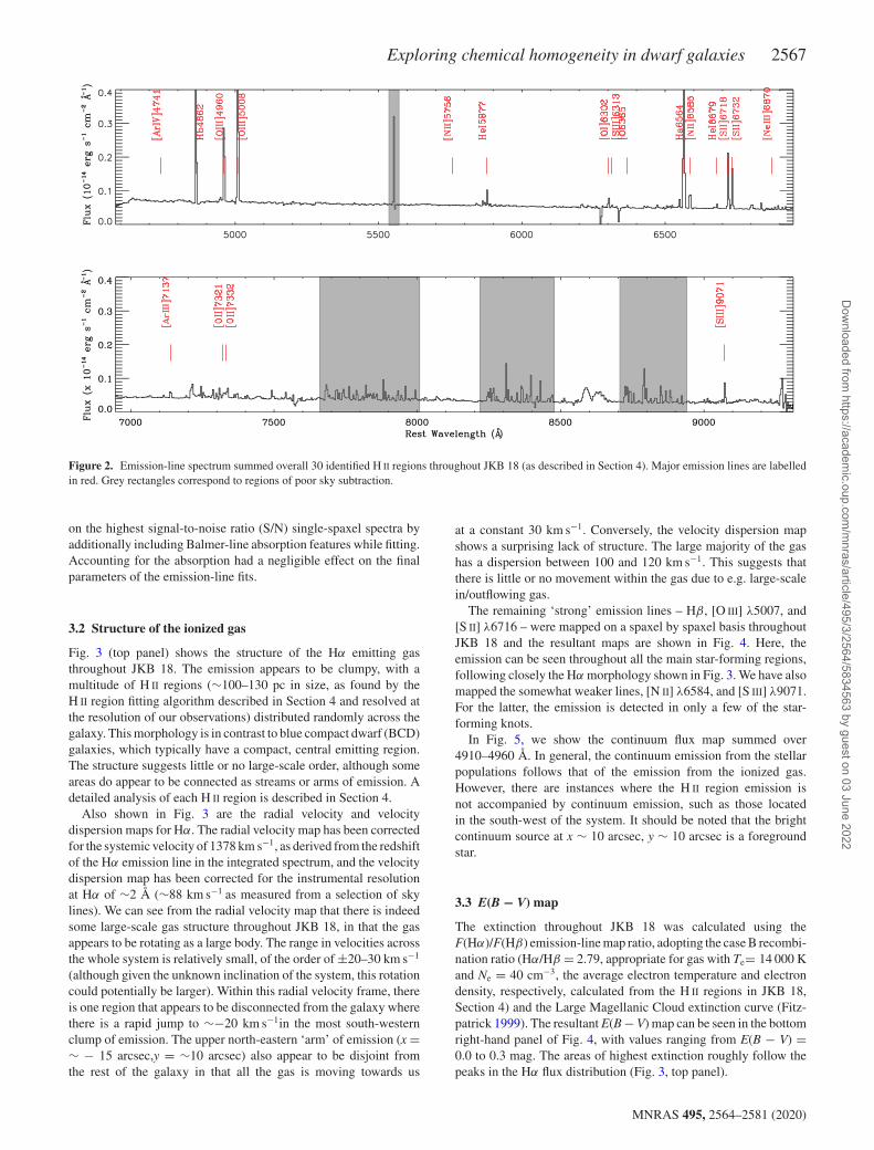
The remaining ‘strong’ emission lines – Hβ, [O III] λ5007, and[S II] λ6716 – were mapped on a spaxel by spaxel basis throughoutJKB 18 and the resultant maps are shown in Fig. 4. Here, theemission can be seen throughout all the main star-forming regions,following closely the Hα morphology shown in Fig. 3. We have alsomapped the somewhat weaker lines, [N II] λ6584, and [S III] λ9071.For the latter, the emission is detected in only a few of the star-forming knots.

In Fig. 5, we show the continuum flux map summed over4910–4960 Å. In general, the continuum emission from the stellarpopulations follows that of the emission from the ionized gas.However, there are instances where the H II region emission isnot accompanied by continuum emission, such as those locatedin the south-west of the system. It should be noted that the brightcontinuum source at x ∼ 10 arcsec, y ∼ 10 arcsec is a foregroundstar.

3.3 E(B − V) map

The extinction throughout JKB 18 was calculated using theF(Hα)/F(Hβ) emission-line map ratio, adopting the case B recombi-nation ratio (Hα/Hβ = 2.79, appropriate for gas with Te= 14 000 Kand Ne = 40 cm−3, the average electron temperature and electrondensity, respectively, calculated from the H II regions in JKB 18,Section 4) and the Large Magellanic Cloud extinction curve (Fitz-patrick 1999). The resultant E(B − V) map can be seen in the bottomright-hand panel of Fig. 4, with values ranging from E(B − V) =0.0 to 0.3 mag. The areas of highest extinction roughly follow thepeaks in the Hα flux distribution (Fig. 3, top panel).

MNRAS 495, 2564–2581 (2020)

Dow


ic.oup.com/m



Figure 3. Maps of flux, radial velocity, and velocity dispersion [full widthat half-maximum (FWHM)] of JKB 18, as measured from the Hα emissionline across the MUSE FoV. White spaxels correspond to those with <3σ

detections.

3.4 Sources of ionization across JKB 18

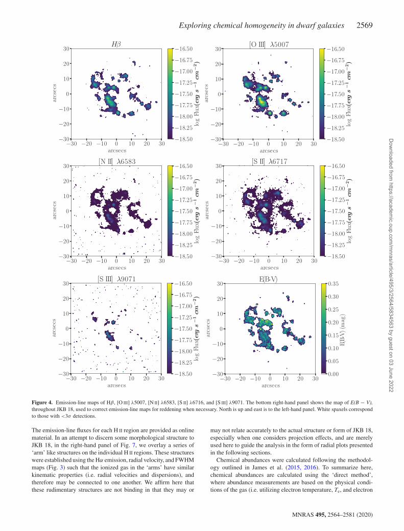
In order to explore the sources of ionization within JKB 18, inFig. 6, we show emission-line diagnostic images of the galaxy. Here,each spaxel is colour coded according to its placement within the[N II]/Hα or [S II]/Hα versus [O III]/Hβ diagram. These emission-line diagnostic diagrams or ‘BPT’ diagrams separate emission-lineratios according to the source of ionizing radiation, with the overlaid‘maximum starburst line’ from Kewley et al. (2001) separatingphotoionized gas (below the line) from harder ionizing sources

such as shocks and active galactic nuclei (above the line). Since allof the emission-line ratios from JKB 18 lie below the solid line, wecan confirm that the gas is dominated by photoionization, however,as demonstrated by Plat et al. (2019) and Kewley et al. (2013), giventhe low metallicity of the gas, contributions from shock excitationcannot be ruled out. Both diagnostics maps show an interestingionization structure – while the central star-forming region (markedas ‘X’) shows (an expected) high [O III]/Hβ, other regions of similarexcitation lie at the edges of some star-forming regions and areoffset from the areas of strongest star formation (as indicated by theoverlaid Hα contours), suggesting that the ionizing photons are notpropagating in a uniform direction from the centre of the ionized gasand instead preferentially move towards the outer boundary of theionized gas. There are clear gradients in decreasing [O III]/Hβ as youmove away from the edges of star-forming regions, an effect evenmore prominent in the [S II]/Hα versus [O III]/Hβ map. In particular,there is a region located at x = −5 arcsec, y = +5 arcsec whichshows particularly high [O III]/Hβ ratio for its [S II]/Hα ratio, veryclose to a gap in the ionized gas, with similar high values ∼3 arcseceastward. This region, along with other edge-enhanced areas couldsignify shock-excited gas due to interactions with the surroundingISM. Overall these detailed diagnostic maps reveal a complex andinhomogeneous ionization structure with widely varying levels ofradiation field hardness throughout.

4 C H E M I C A L A BU N DA N C E S

4.1 Direct method abundances of individual H II regions

Since the auroral line [S III] λ6312 was not detected at a 3σ levelon a spaxel-by-spaxel basis, it was not possible towe derive a‘direct method’ abundance map. Instead, we binned the spectraacross each of the H II regions throughout the galaxy using apublicly available PYTHON-based package IFUANAL3 and derivedirect method chemical abundances from the spectra integratedover each H II region. While this reduces our spatial resolution,the approach is deemed sufficient since temperatures derived fromintegrating over individual H II regions are good representations ofthe spatially resolved average value (e.g. Kumari et al. 2019a).

In order to identify and extract spectra of individual H II regions,we used the IFUANAL implementation of an H II region binningalgorithm that is based on the HIIEXPLORER4 algorithm (Sanchezet al. 2012; Galbany et al. 2016). Briefly, this algorithm creates atwo-dimensional continuum-subtracted flux map of Hα emissionand identifies emission peaks with flux values equal to or above aspecified minimum peak flux value in the Hα line map. Starting withthe brightest one, these emission peaks act as seeds for creating thebins, which include all pixels within a specified maximum radius,with flux values above a minimum threshold and at least 10 per centof the seed pixel flux but exclude any pixel which is already includedin a previous bin. An optimum bin size of seven pixels and minimumthreshold flux of 10−19 erg s−1 cm−2 was found to maximizethe number of H II regions in JKB 18, while also preserving asufficient S/N (�8) in each spectrum for the analysis performedhere.

Fig. 7 shows the location of the 30 individual H II regionsidentified using the above method, where their IDs (0–29) aremarked in the decreasing order of the flux of the emission peak/seed.

3https://ifuanal.readthedocs.io/en/latest/4http://www.caha.es/sanchez/HII explorer/

MNRAS 495, 2564–2581 (2020)

Dow


ic.oup.com/m


https://ifuanal.readthedocs.io/en/latest/

http://www.caha.es/sanchez/HII_explorer/


Figure 4. Emission-line maps of Hβ, [O III] λ5007, [N II] λ6583, [S II] λ6716, and [S III] λ9071. The bottom right-hand panel shows the map of E(B − V),throughout JKB 18, used to correct emission-line maps for reddening when necessary. North is up and east is to the left-hand panel. White spaxels correspondto those with <3σ detections.

The emission-line fluxes for each H II region are provided as onlinematerial. In an attempt to discern some morphological structure toJKB 18, in the right-hand panel of Fig. 7, we overlay a series of‘arm’ like structures on the individual H II regions. These structureswere established using the Hα emission, radial velocity, and FWHMmaps (Fig. 3) such that the ionized gas in the ‘arms’ have similarkinematic properties (i.e. radial velocities and dispersions), andtherefore may be connected to one another. We affirm here thatthese rudimentary structures are not binding in that they may or

may not relate accurately to the actual structure or form of JKB 18,especially when one considers projection effects, and are merelyused here to guide the analysis in the form of radial plots presentedin the following sections.

Chemical abundances were calculated following the methodol-ogy outlined in James et al. (2015, 2016). To summarize here,chemical abundances are calculated using the ‘direct method’,where abundance measurements are based on the physical condi-tions of the gas (i.e. utilizing electron temperature, Te, and electron

MNRAS 495, 2564–2581 (2020)

Dow


ic.oup.com/m



Figure 5. Continuum flux map, derived from emission-line free wavelengthrange between 4910 and 4960 Å. North is up, east is to the left. White spaxelscorrespond to those with < 10 per cent uncertainty in the continuum flux.

density, Ne) and extinction-corrected line fluxes. Each H II regionis modelled by three separate ionization zones (low, medium, andhigh), and the abundance calculations for ions within each zoneare made using the temperature within the respective zone. Werefer the reader to James et al. (2016) for further details. The onlydifference between the methods used here and that of James et al.(2016) is that due to MUSE’s restricted wavelength coverage inthe blue, here we use the [S III] λ6312 auroral line to derive theelectron temperature (Te) rather than [O III]λ4363. Despite its lesscommon usage compared to [O III], the [S III] emission-line ratio[S III] λ9071/λ6312 has been demonstrated to be more accuratein deriving electron temperatures and subsequently H II regionabundances (Berg et al. 2015). The Ne, Te, ionic, and elementaloxygen abundances, nitrogren abundances, and nitrogen-to-oxygenabundance ratios for each H II region are shown in Table 2. Forthree H II regions (IDs 11, 15, and 26), it was necessary to adoptthe Te of the closest neighbouring H II region. Despite [S III] λ6312being detected at a >3σ level in these regions, Te([S III]) valueswere found to be unfeasibly high (>30 000 K),5 which uponinvestigation may be due to [S III] λ9071 having an asymmetricline profile due to poor sky subtraction. The [S III] λ9071 lineprofile in all other H II regions were inspthat aected and foundto be uncontaminated.

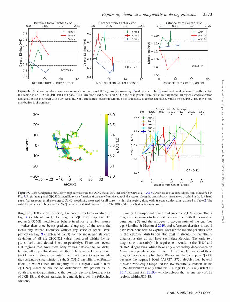
The direct method oxygen abundance calculated for each of theindividual H II regions is plotted as a function of distance from thecentral H II region in Fig. 8, where the ‘arm’ denomination refersto those shown in Fig. 7(b). Here, we only show the H II regiondirect method abundances where Te could be derived confidently(i.e.,where [S III] λ6312 was measured with 3σ significance) and,as a result, only direct method measurements for the most central,brightest, H II regions are available. Nevertheless, it can be seenthat JKB 18 harbours H II regions with a large range in oxygenabundance of 7.3 � 12 + log(O/H) � 7.9, with an average of12 + log(O/H) = 7.56 ± 0.20 (∼0.08 Z�). A variation of ∼0.6 dexis quite significant, given than most dwarf galaxies are thought to bechemically homogeneous with [O/H] variations of only 0.1–0.2 dex

5Such extremely low oxygen abundance values were not supported by the[N II]/Hα line ratio (Pettini & Pagel 2004) and weak He I lines (which shouldbe relatively strong in comparison to metal lines in the XMP regime).

(e.g. Skillman, Kennicutt & Hodge 1989; Kobulnicky & Skillman1996; Lee, Skillman & Venn 2006; Kehrig et al. 2008; Croxallet al. 2009; James, Tsamis & Barlow 2010; Berg et al. 2012; Lagoset al. 2014, 2016; Kumari et al. 2019a) and small uncertainty (i.e.σ < 0.1). Several regions have oxygen abundances outside the±1σ distribution (dotted lines) of ∼0.2 dex, all within ∼1 kpc ofthe central H II region. Only Arm 3 shows any kind of discerniblegradient in that the metallicity increases steadily with distance fromthe central H II region. In an attempt to quantify the size of thespread in oxygen abundance, we calculate an interquartile range(IQR) of 0.11.

In Fig. 8, we show the radial distribution of N/H and N/Othroughout JKB 18, as derived using the direct method. Similarlywith O/H, significant variations in both elemental abundance ratioscan be seen, with ∼0.5 dex spreads in both N/H and N/O, andaverages values of < 12 + log(N/H) > = 6.41 ± 0.14 and <N/O> = −1.95 ± 0.13. We calculate IQRs of 0.23 and 0.19 for N/Hand N/O, respectively. Along ‘Arm 3’, variations can be ∼0.3 dexin N/H and N/O. Similar sized variations are also seen, however, inO/H of the same ‘arm’ (Fig. 8), which suggests that the differencesbetween mechanisms responsible for N-production (e.g. AGB stars)and O-production (e.g. core-collapse SNe) may not be the sole causeof this variation in nitrogen.

Unfortunately, it is difficult to make any firm conclusions on thechemical homogeneity of JKB 18 with such a small number ofdirect-method abundance measurements. In the following sections,we explore the metallicity distribution using a strong-line calibrationfor metallicity, which does not rely on the detection of faintauroral lines and instead provides us with metallicity measurementsthroughout the entirety of JKB 18. While the absolute value of thestrong-line methods is somewhat dubious compared to the direct-method abundances – i.e. typically showing ∼0.7 dex offsets fromdirect-method abundances (e.g. Kewley & Ellison 2008; Moustakaset al. 2010; Lopez-Sanchez et al. 2012) – we can use strong-line calibrations to gauge relative metallicity variations within theionized gas.

4.2 Metallicity map from strong-line diagnostics

In order to explore the chemical (in)homogeneity throughoutJKB 18 on the highest possible spatial resolution afforded by thedata, we performed a spatially resolved abundance analysis usingthe O3N2 metallicity diagnostic (log [([O III]/Hβ) / ([N II]/Hα)])prescribed by Curti et al. ( 2017) following the equation:

O3N2 = 0.281 − 4.765 xO3N2 − 2.268 x2O3N2, (1)

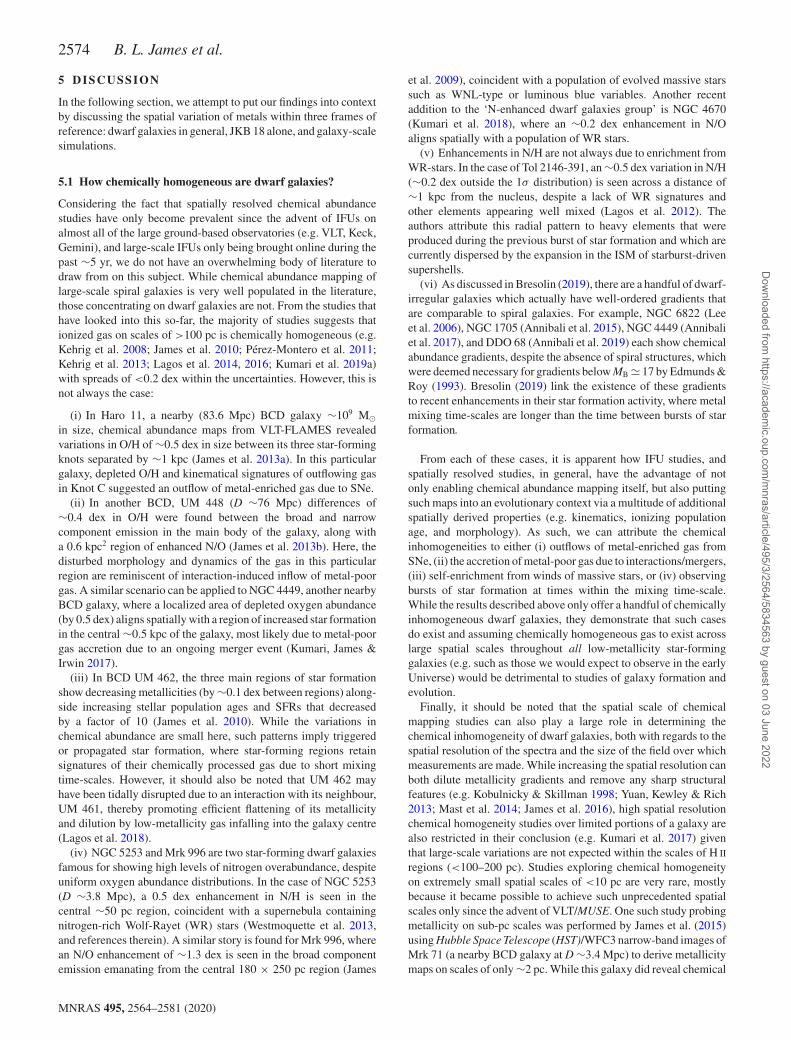
where xO3N2 is oxygen abundance normalized to the solar valuein the form 12 + log(O/H)� = 8.69 (Asplund et al. 2009). TheZ[O3N2] metallicity map is shown in Fig. 9, where the metallicitycan be seen to range between 8.1� 12 + log(O/H)� 8.6, an averagevalue of Z[O3N2] = 8.44 ± 0.08 and an IQR of 0.11. As mentionedabove, the large ∼0.7–0.8 dex systematic discrepancy between theoxygen abundances derived from the direct method and the strong-line diagnostic is to be expected (with the latter typically showinglarger abundances than the former). As such, here we focus only onthe relative values of Z[O3N2] between the H II regions, rather thanthe absolute values.

Small gradients in Z[O3N2] within the gas can be seen, althoughwith no discernible global pattern. To explore these patterns in amore quantitative context, in Fig. 9 (right-hand panel), we showthe mean Z[O3N2] value (as listed in Table 2) for each of theH II regions plotted as a function of distance from the central

MNRAS 495, 2564–2581 (2020)

Dow


ic.oup.com/m



Figure 6. Emission-line diagnostic maps of JKB 18 showing log([N II]/Hα) versus log([O III]/Hβ) (top panel) and log([S II]/Hα) versus log([O III]/Hβ) (bottompanel) derived from the line ratio images in Fig. 4 and colour-coded according to their location within the BPT diagram, shown in the inset of each panel.Overlaid contours represent the morphology of Hα emission (Fig. 3) and ‘X’ denotes the central star-forming region. The ‘maximum starburst line’ fromKewley et al. (2001) is overlaid in white. The black cross overlaid on each diagnostic diagram represents the average error for the emission-line diagnosticratio. Grey spaxels correspond to those with <3σ detections. North is up, east is to the left.

MNRAS 495, 2564–2581 (2020)

Dow


ic.oup.com/m



Figure 7. (a) Individual H II regions identified using the H II region binning algorithm described in Section 4 overlaid on the Hα emission-line map (Fig. 3,upper panel). Each of the 30 H II regions is labelled, with the blue outline denoting the ‘edge’ of the H II region, within which all spaxels are summed for theindividual H II region spectra. (b) Individual H II regions with ‘arm’ like structures overlaid. Structures were identified using the Hα flux, radial velocity, andFWHM maps shown in Fig. 3 (as discussed in Section 4). North is up and east is to the left.

Table 2. Ionic and elemental abundances for individual H II regions throughout JKB 18, derived from the emission-line measurements integrated over eachH II region (Fig. 7) and discussed in Section 4.

H II Reg ID Ne([S II]) Te([S III]) Te([O II]) O+/H+ O2 +/H+ 12 + log(O/H) log(N/O) 12 + log(N/H) 12+log(O/H)(cm−3) (K) (K) (×10−5) (×10−5) Z[Direct] Z[O3N2]

0 13 ± 7.8 15 300 ± 490 20 100 ± 586 0.70 ± 0.08 2.20 ± 0.18 7.46 ± 0.03 − 1.15 ± 0.02 6.31 ± 0.02 8.33 ± 0.051 41 ± 9.5 14 200 ± 619 18 600 ± 740 1.15 ± 0.18 2.10 ± 0.24 7.51 ± 0.04 − 1.07 ± 0.03 6.44 ± 0.03 8.43 ± 0.042 22 ± 11 12 800 ± 605 16 600 ± 723 1.26 ± 0.24 4.78 ± 0.65 7.78 ± 0.05 − 1.28 ± 0.04 6.50 ± 0.04 8.27 ± 0.053 28 ± 13 12 400 ± 668 15 900 ± 798 1.02 ± 0.25 5.65 ± 0.91 7.82 ± 0.06 − 1.27 ± 0.04 6.56 ± 0.04 8.22 ± 0.044 36 ± 14 14 400 ± 947 18 800 ± 1130 1.03 ± 0.24 2.59 ± 0.46 7.56 ± 0.06 − 1.28 ± 0.04 6.28 ± 0.04 8.34 ± 0.065 13 ± 8.8 11 300 ± 823 14 400 ± 984 2.69 ± 0.88 4.32 ± 1.02 7.85 ± 0.08 − 1.43 ± 0.06 6.41 ± 0.06 8.36 ± 0.066 36 ± 19 15100 ± 1500 19 800 ± 1790 0.70 ± 0.25 3.04 ± 0.79 7.57 ± 0.10 − 1.01 ± 0.07 6.56 ± 0.07 8.34 ± 0.057 18 ± 12 16 600 ± 1480 22 000 ± 1770 0.61 ± 0.17 1.51 ± 0.32 7.33 ± 0.08 − 1.12 ± 0.05 6.21 ± 0.05 8.37 ± 0.048 12 ± 12 <11 700 <15 000 >2.14 >2.44 >7.66 – >6.39 8.47 ± 0.059 18+18

−18 <9580 <12 000 >3.64 >11.97 >8.19 – >6.66 8.29 ± 0.0710 17 ± 10 <12 500 <16 200 >1.49 >1.08 >7.41 – >6.29 8.53 ± 0.0311 41 ± 25 16 600 ± 1480a 22 000 ± 1770 0.63 ± 0.20 1.16 ± 0.25 7.25 ± 0.08 − 1.12 ± 0.06 6.13 ± 0.06 8.41 ± 0.0412 1.7+4.3

−1.7 <11600 <14 900 >3.47 >4.78 >7.92 – >6.59 8.44 ± 0.0613 100 ± 44 <13 400 <17 500 >0.99 >2.53 >7.55 – >6.38 8.41 ± 0.0714 86 ± 27 <12 600 <16 200 >1.50 >1.82 >7.52 – >6.29 8.45 ± 0.0615 9.5+10.

−9.5 15300 ± 514a 20100 ± 614 0.75 ± 0.19 1.31 ± 0.12 7.31 ± 0.05 − 1.01 ± 0.03 6.31 ± 0.03 8.43 ± 0.0516 14 ± 13 <10 500 <13 300 >2.21 >3.42 >7.75 – >6.53 8.45 ± 0.0417 40 ± 29 <15 800 <20 900 >0.69 >1.27 >7.29 – >6.02 8.40 ± 0.0818 20 ± 19 <15 400 <20 300 >0.59 >1.57 >7.34 – >6.48 8.45 ± 0.0519 43 ± 21 <19 900 <26 700 >0.19 >0.20 >6.59 – >5.98 8.56 ± 0.0420 24 ± 19 <12 400 <16 000 >2.25 >1.38 >7.56 – >6.19 8.50 ± 0.0421 33 ± 20 <14 700 <19 300 >0.79 >1.27 >7.31 – >6.44 8.49 ± 0.0422 180 ± 71 <17800 <23 700 >0.24 >0.99 >7.09 – >6.33 8.43 ± 0.0523 59 ± 36 <15300 <20 100 >0.62 >1.14 >7.25 – >6.31 8.47 ± 0.0424 32 ± 27 <11700 <15 000 >1.43 >4.79 >7.79 – >6.69 8.36 ± 0.0425 23 ± 21 <25 000 <33 900 >0.26 >0.29 >6.74 – >5.76 8.49 ± 0.0426 180 ± 39 15100 ± 1540a 19 900 ± 1840 0.83 ± 0.34 3.50 ± 0.94 7.64 ± 0.10 − 1.09 ± 0.07 6.54 ± 0.07 8.35 ± 0.0727 23 ± 18 <11 800 <15 100 >1.40 >2.24 >7.56 – >6.62 8.50 ± 0.0428 48 ± 44 <16 300 <21 500 >0.93 >0.88 >7.26 – >5.96 8.42 ± 0.0829 17 ± 16 <16 800 <22 200 >0.16 >0.48 >6.81 – >6.43 8.29 ± 0.07

Notes. Electron density and temperatures are also listed. aElectron temperatures for which the neighbouring H II region temperature was adopted as a result of unfeasibly high electrontemperatures being measured, despite >3σ detections on the [S III] λ6312 auroral line. Z[O3N2] values correspond to H II region averages and standard deviations, as measured fromthe Z[O3N2] map shown in Fig. 9.

MNRAS 495, 2564–2581 (2020)

Dow


ic.oup.com/m



Figure 8. Direct method abundance measurements for individual H II regions (shown in Fig. 7 and listed in Table 2) as a function of distance from the centralH II region in JKB 18 for O/H (left-hand panel), N/H (middle-hand panel) and N/O (right-hand panel). Here, we show only those H II regions whose electrontemperature was measured with >3σ certainty. Solid and dotted lines represent the mean abundance and ±1σ abundance values, respectively. The IQR of thedistribution is shown inset.

Figure 9. Left-hand panel: metallicity map derived from the O3N2 metallicity indicator by Curti et al. (2017). Overlaid are the arm substructures identified inFig. 7. Right-hand panel: Z[O3N2] metallicity as a function of distance from the central H II region, along the arm substructures shown overlaid in the left-handpanel. Values represent the average Z[O3N2] metallicity measured for all spaxels within that region, along with its standard deviation, as listed in Table 2. Thesolid line represents the mean Z[O3N2] metallicity, dotted lines are ±1σ . The IQR of the distribution is shown inset.

(brightest) H II region following the ‘arm’ structures overlaid inFig. 9 (left-hand panel). Echoing the Z[O3N2] map, the H II

region Z[O3N2] metallicities behave in almost a random nature– rather than there being gradients along any of the arms, themetallicity instead fluctuates without any sense of order. Over-plotted on Fig. 9 (right-hand panel) are the mean and standarddeviation of all the Z[O3N2] values measured within the re-gions (solid and dotted lines, respectively). There are severalH II regions that have metallicity values outside the 1σ distri-bution, although the deviations themselves are relatively small(∼0.1 dex). It should be noted that if we were to also includethe systematic uncertainties on the Z[O3N2] metallicity calibratoritself (0.09 dex) then the majority of H II regions would haveZ[O3N2] values within the 1σ distribution. We present an in-depth discussion pertaining to the possible chemical homogeneityof JKB 18, and dwarf galaxies in general, in given the followingsections.

Finally, it is important to note that since the Z[O3N2] metallicitydiagnostic is known to have a dependency on both the ionizationparameter (U) and the nitrogen-to-oxygen ratio of the gas (seee.g. Maiolino & Mannucci 2019, and references therein), it wouldhave been beneficial to explore whether the inhomogeneities seenin the Z[O3N2] distribution also exist in strong-line metallicitydiagnostics that do not have such dependencies. The only twodiagnostics that satisfy this requirement would be the ‘R23’ and‘O3S2’ diagnostics, which have only a secondary dependence onU and no dependence on nitrogen. Unfortunately, neither of thesediagnostics can be applied here. We are unable to compute Z[R23]because the required [O II] λλ3727, 3729 doublet lies beyondMUSE’s wavelength range and the low-metallicity ‘branch’ of theO3S2 distribution is only valid for 12 + log(O/H) > 7.6 (Curti et al.2017; Kumari et al. 2019b), which excludes the vast majority of H II

regions within JKB 18.

MNRAS 495, 2564–2581 (2020)

Dow


ic.oup.com/m



5 D ISCUSSION

In the following section, we attempt to put our findings into contextby discussing the spatial variation of metals within three frames ofreference: dwarf galaxies in general, JKB 18 alone, and galaxy-scalesimulations.

5.1 How chemically homogeneous are dwarf galaxies?

Considering the fact that spatially resolved chemical abundancestudies have only become prevalent since the advent of IFUs onalmost all of the large ground-based observatories (e.g. VLT, Keck,Gemini), and large-scale IFUs only being brought online during thepast ∼5 yr, we do not have an overwhelming body of literature todraw from on this subject. While chemical abundance mapping oflarge-scale spiral galaxies is very well populated in the literature,those concentrating on dwarf galaxies are not. From the studies thathave looked into this so-far, the majority of studies suggests thationized gas on scales of >100 pc is chemically homogeneous (e.g.Kehrig et al. 2008; James et al. 2010; Perez-Montero et al. 2011;Kehrig et al. 2013; Lagos et al. 2014, 2016; Kumari et al. 2019a)with spreads of <0.2 dex within the uncertainties. However, this isnot always the case:

(i) In Haro 11, a nearby (83.6 Mpc) BCD galaxy ∼109 M�in size, chemical abundance maps from VLT-FLAMES revealedvariations in O/H of ∼0.5 dex in size between its three star-formingknots separated by ∼1 kpc (James et al. 2013a). In this particulargalaxy, depleted O/H and kinematical signatures of outflowing gasin Knot C suggested an outflow of metal-enriched gas due to SNe.

(ii) In another BCD, UM 448 (D ∼76 Mpc) differences of∼0.4 dex in O/H were found between the broad and narrowcomponent emission in the main body of the galaxy, along witha 0.6 kpc2 region of enhanced N/O (James et al. 2013b). Here, thedisturbed morphology and dynamics of the gas in this particularregion are reminiscent of interaction-induced inflow of metal-poorgas. A similar scenario can be applied to NGC 4449, another nearbyBCD galaxy, where a localized area of depleted oxygen abundance(by 0.5 dex) aligns spatially with a region of increased star formationin the central ∼0.5 kpc of the galaxy, most likely due to metal-poorgas accretion due to an ongoing merger event (Kumari, James &Irwin 2017).

(iii) In BCD UM 462, the three main regions of star formationshow decreasing metallicities (by ∼0.1 dex between regions) along-side increasing stellar population ages and SFRs that decreasedby a factor of 10 (James et al. 2010). While the variations inchemical abundance are small here, such patterns imply triggeredor propagated star formation, where star-forming regions retainsignatures of their chemically processed gas due to short mixingtime-scales. However, it should also be noted that UM 462 mayhave been tidally disrupted due to an interaction with its neighbour,UM 461, thereby promoting efficient flattening of its metallicityand dilution by low-metallicity gas infalling into the galaxy centre(Lagos et al. 2018).

(iv) NGC 5253 and Mrk 996 are two star-forming dwarf galaxiesfamous for showing high levels of nitrogen overabundance, despiteuniform oxygen abundance distributions. In the case of NGC 5253(D ∼3.8 Mpc), a 0.5 dex enhancement in N/H is seen in thecentral ∼50 pc region, coincident with a supernebula containingnitrogen-rich Wolf-Rayet (WR) stars (Westmoquette et al. 2013,and references therein). A similar story is found for Mrk 996, wherean N/O enhancement of ∼1.3 dex is seen in the broad componentemission emanating from the central 180 × 250 pc region (James

et al. 2009), coincident with a population of evolved massive starssuch as WNL-type or luminous blue variables. Another recentaddition to the ‘N-enhanced dwarf galaxies group’ is NGC 4670(Kumari et al. 2018), where an ∼0.2 dex enhancement in N/Oaligns spatially with a population of WR stars.

(v) Enhancements in N/H are not always due to enrichment fromWR-stars. In the case of Tol 2146-391, an ∼0.5 dex variation in N/H(∼0.2 dex outside the 1σ distribution) is seen across a distance of∼1 kpc from the nucleus, despite a lack of WR signatures andother elements appearing well mixed (Lagos et al. 2012). Theauthors attribute this radial pattern to heavy elements that wereproduced during the previous burst of star formation and which arecurrently dispersed by the expansion in the ISM of starburst-drivensupershells.

(vi) As discussed in Bresolin (2019), there are a handful of dwarf-irregular galaxies which actually have well-ordered gradients thatare comparable to spiral galaxies. For example, NGC 6822 (Leeet al. 2006), NGC 1705 (Annibali et al. 2015), NGC 4449 (Annibaliet al. 2017), and DDO 68 (Annibali et al. 2019) each show chemicalabundance gradients, despite the absence of spiral structures, whichwere deemed necessary for gradients below MB � 17 by Edmunds &Roy (1993). Bresolin (2019) link the existence of these gradientsto recent enhancements in their star formation activity, where metalmixing time-scales are longer than the time between bursts of starformation.

From each of these cases, it is apparent how IFU studies, andspatially resolved studies, in general, have the advantage of notonly enabling chemical abundance mapping itself, but also puttingsuch maps into an evolutionary context via a multitude of additionalspatially derived properties (e.g. kinematics, ionizing populationage, and morphology). As such, we can attribute the chemicalinhomogeneities to either (i) outflows of metal-enriched gas fromSNe, (ii) the accretion of metal-poor gas due to interactions/mergers,(iii) self-enrichment from winds of massive stars, or (iv) observingbursts of star formation at times within the mixing time-scale.While the results described above only offer a handful of chemicallyinhomogeneous dwarf galaxies, they demonstrate that such casesdo exist and assuming chemically homogeneous gas to exist acrosslarge spatial scales throughout all low-metallicity star-forminggalaxies (e.g. such as those we would expect to observe in the earlyUniverse) would be detrimental to studies of galaxy formation andevolution.

Finally, it should be noted that the spatial scale of chemicalmapping studies can also play a large role in determining thechemical inhomogeneity of dwarf galaxies, both with regards to thespatial resolution of the spectra and the size of the field over whichmeasurements are made. While increasing the spatial resolution canboth dilute metallicity gradients and remove any sharp structuralfeatures (e.g. Kobulnicky & Skillman 1998; Yuan, Kewley & Rich2013; Mast et al. 2014; James et al. 2016), high spatial resolutionchemical homogeneity studies over limited portions of a galaxy arealso restricted in their conclusion (e.g. Kumari et al. 2017) giventhat large-scale variations are not expected within the scales of H II

regions (<100–200 pc). Studies exploring chemical homogeneityon extremely small spatial scales of <10 pc are very rare, mostlybecause it became possible to achieve such unprecedented spatialscales only since the advent of VLT/MUSE. One such study probingmetallicity on sub-pc scales was performed by James et al. (2015)using Hubble Space Telescope (HST)/WFC3 narrow-band images ofMrk 71 (a nearby BCD galaxy at D ∼3.4 Mpc) to derive metallicitymaps on scales of only ∼2 pc. While this galaxy did reveal chemical

MNRAS 495, 2564–2581 (2020)

Dow


ic.oup.com/m



variations of 0.2–0.3 dex on scales <50 pc, the study found thatapplying strong-line metallicity diagnostics on spatial scales smallerthan an H II region can be problematic in that they may effectively‘break down’ as the diagnostic design is based on light integratedover entire or multiple H II regions.

5.2 Is JKB 18 chemically inhomogeneous?

Overall, the question of whether the gas throughout JKB 18 is chem-ically homogeneous or not, is somewhat difficult to quantify. Per-haps first the question of how we quantify chemical (in)homogeneitybecomes significant. Several previous studies have used the 1σ

distribution as a boundary beyond which any chemical variationsare considered ‘inhomogeneous’ (e.g. James et al. 2016; Kumariet al. 2017, 2019). However, the size of the 1σ distribution itselfshould also be taken into account, such that a large spread in oxygenabundances also deems gas to be chemically inhomogeneous. Ifthis were not the case, a significant fraction of shallow metallicitygradients would not be considered gradients, given the uncertaintieson the measurements. Also, using only deviations outside standarddeviation of the distribution to define inhomogeneity assumes thatdistribution is normal, or Gauassian, which is not always the case.In fact, this was indeed the test assumed in a chemical homogeneitystudy by Perez-Montero et al. (2011), where only distributions thatcould be fitted with a Gaussian function were deemed homogeneous.As such, an additional useful measure of (in)homogeneity could alsobe the IQR of the distribution in that outlier values are not takeninto consideration. In the case of JKB 18, on the one hand, a largerange in oxygen abundances of ∼0.5–0.6 dex is observed betweenindividual H II regions, using both the direct method and the O3N2strong-line metallicity indicator. However, when we consider thesevariations in the context of the mean and standard deviation ofthe oxygen abundance distribution, variations of only ∼0.1 dex areseen outside the 1 σ distribution – but the 1σ distribution in itselfis ∼0.2 dex in size. The IQR is somewhat smaller, of the orderof ∼0.1 dex, suggesting that a large number of outlier values arepresent. If we consider much smaller spatial scales, i.e. looking atspaxel-to-spaxel variations in Z[O3N2] (Fig. 9) then variations of∼0.2–0.3 dex are seen within regions the size of typical H II regions.The 1σ distribution on this spatial scale is ∼0.1 dex whereas theIQR = 0.13.

Overall, given the significant variation in oxygen abundance,both with regard to the size of the 1σ distribution and the fact thatseveral H II regions lie outside this distribution, we find JKB 18 tobe chemically inhomogeneous.

While only small temperature variations seen within JKB 18’sindividual H II regions are to be expected, what would be the causeof 0.5–0.6 dex variations in oxygen abundance between H II regions?To explore the cause of the H II region metallicity distribution ofFig. 9 further, in Fig. 10, we show the Z[O3N2] metallicities asa function of SFR. SFR values for each individual H II region arelisted in Table 3 and were calculated following the method outlinedin James et al. (2016) in that we follow the prescription of Leeet al. (2009) because all individual H II regions are below the low-luminosity threshold of L(Hα) < 2.5 × 1039 erg s−1.6 We find anaverage SFR and 1σ distribution of 0.19 ± 0.09 × 10−2 M� yr-1

6This prescription is essentially a recalibration the Kennicutt (1998) relationto account for the underprediction of SFRs by Hα compared to those fromfar-ultraviolet (FUV) fluxes within the low-luminosity regime, under theassumption that the FUV traces the SFR in dwarf galaxies more robustly.

Figure 10. Z[O3N2] as a function of SFR (as listed in Table 3). Nocorrelation can be seen between the two properties, suggesting that inflowof metal-poor gas is not the dominant mechanism influencing the metallicityof the individual H II region. The central H II region is shown in black.

Table 3. Hα luminosity and SFRs for each individual H II region identifiedthroughout JKB 18.

H II Region ID L(Hα) (×1036 erg s−1) SFR(Hα) (×10−2 M� yr−1)

0 129.46 ± 0.16 0.47 ± 0.111 91.51 ± 0.18 0.38 ± 0.092 72.99 ± 0.12 0.33 ± 0.083 82.11 ± 0.14 0.36 ± 0.084 55.30 ± 0.10 0.28 ± 0.075 78.23 ± 0.13 0.35 ± 0.086 43.97 ± 0.15 0.24 ± 0.067 57.96 ± 0.13 0.29 ± 0.078 23.00 ± 0.09 0.16 ± 0.049 28.83 ± 0.09 0.19 ± 0.0510 35.13 ± 0.10 0.21 ± 0.0511 24.66 ± 0.10 0.17 ± 0.0412 13.81 ± 0.10 0.12 ± 0.0413 13.26 ± 0.06 0.12 ± 0.0414 30.42 ± 0.13 0.19 ± 0.0515 23.29 ± 0.10 0.16 ± 0.0416 22.54 ± 0.07 0.16 ± 0.0417 17.24 ± 0.09 0.14 ± 0.0418 14.25 ± 0.13 0.12 ± 0.0419 24.39 ± 0.10 0.17 ± 0.0420 22.48 ± 0.09 0.16 ± 0.0421 19.82 ± 0.18 0.15 ± 0.0422 9.10 ± 0.05 0.09 ± 0.0323 14.38 ± 0.08 0.12 ± 0.0424 19.71 ± 0.18 0.15 ± 0.0425 14.25 ± 0.14 0.12 ± 0.0426 19.03 ± 0.11 0.14 ± 0.0427 20.40 ± 0.14 0.15 ± 0.0428 8.58 ± 0.08 0.09 ± 0.0329 21.48 ± 0.14 0.16 ± 0.04

across the 30 H II regions identified in Fig. 7. If there were inflowsof metal-poor gas affecting the metallicity of an H II region, then wewould expect to see an anticorrelation between SFR and Z[O3N2]– i.e. as metal-poor gas flows into a region, both the metal contentof the gas becomes diluted and star formation is triggered. Thiseffect is commonly seen in XMP and ‘tadpole’ galaxies, as shown

MNRAS 495, 2564–2581 (2020)

Dow


ic.oup.com/m



in Sanchez Almeida et al. (2014). In order to understand whethersuch a correlation exists here, a Pearson correlation test wasperformed on the parameters shown in Fig. 10, which resulted ina Pearson correlation coefficient of ρ = −0.43. As such, only aweak negative correlation exists between Z and SFR, suggestingthat in inflow of metal-poor gas cannot entirely be responsiblefor the decreased oxygen abundance in seen in some regions ofJKB 18.

If instead, mixing time-scales were sufficiently short enough thatthe metal content of the gas surrounding the stars reflected the evo-lutionary age of the material ejected by the star (i.e. as proposed byKobulnicky & Skillman 1997), then we would expect the metallicityof the H II region to increase with stellar age. In Fig. 11, we show thecontribution of stellar populations within each H II region, separatedin three age bins (<500 Myr, 500 Myr < Age < 5 Gyr, and >5 Gyr).The percentage contributions were calculated from the best-fittingparameters to the stellar continuum of the integrated spectrumof each H II region using STARLIGHT (Cid Fernandes et al. 2005)implemented within IFUANAL (Section 4.2). In short, the spectral-fitting code STARLIGHT allows us to fit the continuum of a spectrum(where the emission lines are masked) with a model composedof spectral components from a predefined set of 45 base spectrafrom Bruzual & Charlot 2003, corresponding to 3 metallicities and15 different ages, and outputs the light-fraction (contribution inper cent) of each base spectrum among various parameters. Thecontribution of stellar populations shown in Fig. 11 corresponds tothe sum of contribution of the base spectra corresponding to a givenstellar age bin. We find that the majority of H II regions have theirlargest percentage contribution within the 500 Myr < Age < 5 Gyrage range. There are several H II regions whose continuum mostlyindicates a young, <500 Myr population, which appear to lie mostlyin the outskirts of the galaxy. A few H II regions also contain stellarpopulations older than 5 Gyr (bottom panel) though their fractionis < 5 per cent (with the exception of the central H II region),signifying that these H II regions have gone through episodes of starformation in the past, which have resulted in an underlying olderpopulation.

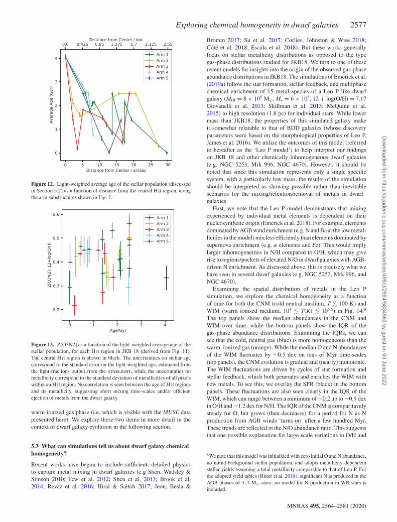
Despite the lack of metallicity gradients in JKB 18, the distri-bution of stellar population age suggests that JKB 18 may haveundergone inside-out growth, such that older stellar populations liein the centre and younger populations in the outskirts of the galaxy.This can perhaps be seen more clearly in Fig. 12, where we plotthe light-weighted average age of each H II region7 of the stellarpopulation as a function of radius from the central H II region – theaverage age of the populations within the central ∼0.5 kpc of thegalaxy are mostly �2 Gyr in age, which then plateaus into a largeage distribution ∼0.5–1.8 kpc from the centre of 0.1–2 Gyr, with theoutermost H II regions (>1.8 kpc) all with ages less than 0.5 Gyr.In Fig. 13, we plot the light-weighted average stellar populationages as a function of Z[O3N2]. Once again, we see no correlationbetween the two properties, suggesting that long mixing time-scalesand thus the evolutionary stage of the star are not affecting the metalcontent of the surrounding gas.

Finally, the increased levels of N/H and N/O seen in Fig. 8 maybe due to self-enrichment from WR stars within those particularregions (e.g. those along Arm 3). However, upon inspection of theindividual spectra, WR features at ∼4650 and ∼5800 Å were notpresent.

7Estimated via the light-fraction of base spectra output from STARLIGHT asdescribed above.

Figure 11. Age of the stellar population in each H II region, as identified inSection 4. The three panels show the percentage of light contributing to thestellar continuum from three separate age bins: <500 Myr, 500 Myr < Age<5 Gyr, and >5 Gyr.

The fluctuations in metallicity seen in Figs 8 and 9, and the lackof correlation between metallicity and SFR or stellar populationage suggest two properties about this system: (i) enrichment events(e.g. SNe or stellar ejecta) are currently ongoing and occurring atdifferent time intervals, resulting in a dispersed metal content and(ii) the metals ejected by the stars within the individual H II regionshave been removed from the galaxy and are yet to cool into the

MNRAS 495, 2564–2581 (2020)

Dow


ic.oup.com/m



Figure 12. Light-weighted average age of the stellar population (discussedin Section 5.2) as a function of distance from the central H II region, alongthe arm substructures shown in Fig. 7.

Figure 13. Z[O3N2] as a function of the light-weighted average age of thestellar population, for each H II region in JKB 18 (derived from Fig. 11).The central H II region is shown in black. The uncertainties on stellar agecorrespond to the standard error on the light-weighted age, estimated fromthe light-fractions output from the STARLIGHT, while the uncertainties onmetallicity correspond to the standard deviation of metallicities of all pixelswithin an H II region. No correlation is seen between the age of H II regionsand its metallicity, suggesting short mixing time-scales and/or efficientejection of metals from the dwarf galaxy.

warm-ionized gas phase (i.e. which is visible with the MUSE datapresented here). We explore these two items in more detail in thecontext of dwarf galaxy evolution in the following section.

5.3 What can simulations tell us about dwarf galaxy chemicalhomogeneity?

Recent works have begun to include sufficient, detailed physicsto capture metal mixing in dwarf galaxies (e.g Shen, Wadsley &Stinson 2010; Few et al. 2012; Shen et al. 2013; Brook et al.2014; Revaz et al. 2016; Hirai & Saitoh 2017; Jeon, Besla &

Bromm 2017; Su et al. 2017; Corlies, Johnston & Wise 2018;Cote et al. 2018; Escala et al. 2018). But these works generallyfocus on stellar metallicity distributions as opposed to the typegas-phase distributions studied for JKB18. We turn to one of theserecent models for insights into the origin of the observed gas-phaseabundance distributions in JKB18. The simulations of Emerick et al.(2019a) follow the star formation, stellar feedback, and multiphasechemical enrichment of 15 metal species of a Leo P like dwarfgalaxy (MHI = 8 × 105 M�, M� = 6 × 105, 12 + log(O/H) = 7.17Giovanelli et al. 2013; Skillman et al. 2013; McQuinn et al.2015) to high resolution (1.8 pc) for individual stars. While lowermass than JKB18, the properties of this simulated galaxy makeit somewhat relatable to that of BDD galaxies (whose discoveryparameters were based on the morphological properties of Leo P,James et al. 2016). We utilize the outcomes of this model (referredto hereafter as the ‘Leo P model’) to help interpret our findingson JKB 18 and other chemically inhomogeneous dwarf galaxies(e.g. NGC 5253, Mrk 996, NGC 4670). However, it should benoted that since this simulation represents only a single specificsystem, with a particularly low mass, the results of the simulationshould be interpreted as showing possible rather than inevitablescenarios for the mixing/retention/removal of metals in dwarfgalaxies.

First, we note that the Leo P model demonstrates that mixingexperienced by individual metal elements is dependent on theirnucleosynthetic origin (Emerick et al. 2018). For example, elementsdominated by AGB wind enrichment (e.g. N and Ba at the low metal-licities in the model) mix less efficiently than elements dominated bysupernova enrichment (e.g. α elements and Fe). This would implylarger inhomogeneities in N/H compared to O/H, which may giverise to regions/pockets of elevated N/O in dwarf galaxies with AGB-driven N enrichment. As discussed above, this is precisely what wehave seen in several dwarf galaxies (e.g. NGC 5253, Mrk 996, andNGC 4670).

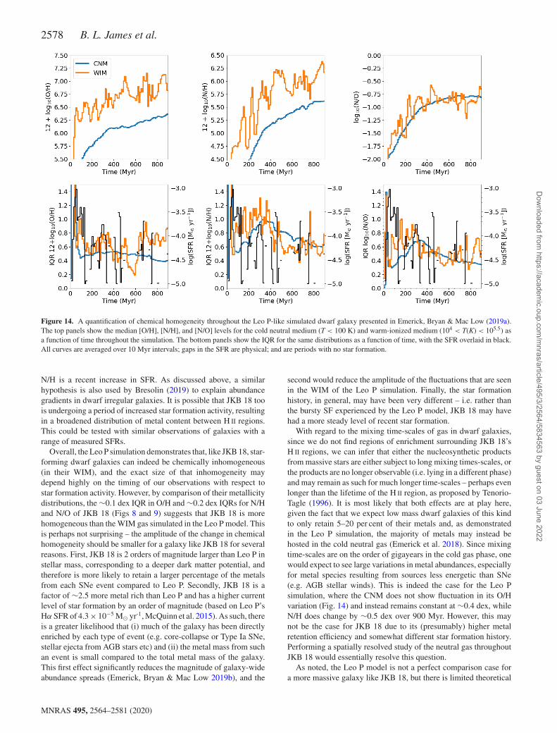
Examining the spatial distribution of metals in the Leo Psimulation, we explore the chemical homogeneity as a functionof time for both the CNM (cold neutral medium, T � 100 K) andWIM (warm ionised medium, 104 � T(K) � 105.5) in Fig. 14.8

The top panels show the median abundances in the CNM andWIM over time, while the bottom panels show the IQR of thegas-phase abundance distributions. Examining the IQRs, we cansee that the cold, neutral gas (blue) is more homogeneous than thewarm, ionized gas (orange). While the median O and N abundancesof the WIM fluctuates by ∼0.5 dex on tens of Myr time-scales(top panels), the CNM evolution is gradual and (nearly) monotonic.The WIM fluctuations are driven by cycles of star formation andstellar feedback, which both generates and enriches the WIM withnew metals. To see this, we overlay the SFR (black) in the bottompanels. These fluctuations are also seen clearly in the IQR of theWIM, which can range between a minimum of ∼0.2 up to ∼0.9 dexin O/H and ∼1.2 dex for N/H. The IQR of the CNM is comparitavelysteady for O, but grows (then decreases) for a period for N as Nproduction from AGB winds ‘turns on’ after a few hundred Myr.These trends are reflected in the N/O abundance ratio. This suggeststhat one possible explanation for large-scale variations in O/H and

8We note that this model was initialized with zero initial O and N abundance,no initial background stellar population, and adopts metallicity-dependentstellar yields assuming a total metallicity comparable to that of Leo P. Forthe adopted yield tables (Ritter et al. 2018), significant N is produced in theAGB phases of 5–7 M� stars; no model for N production in WR stars isincluded.

MNRAS 495, 2564–2581 (2020)

Dow


ic.oup.com/m



Figure 14. A quantification of chemical homogeneity throughout the Leo P-like simulated dwarf galaxy presented in Emerick, Bryan & Mac Low (2019a).The top panels show the median [O/H], [N/H], and [N/O] levels for the cold neutral medium (T < 100 K) and warm-ionized medium (104 < T(K) < 105.5) asa function of time throughout the simulation. The bottom panels show the IQR for the same distributions as a function of time, with the SFR overlaid in black.All curves are averaged over 10 Myr intervals; gaps in the SFR are physical; and are periods with no star formation.

N/H is a recent increase in SFR. As discussed above, a similarhypothesis is also used by Bresolin (2019) to explain abundancegradients in dwarf irregular galaxies. It is possible that JKB 18 toois undergoing a period of increased star formation activity, resultingin a broadened distribution of metal content between H II regions.This could be tested with similar observations of galaxies with arange of measured SFRs.

Overall, the Leo P simulation demonstrates that, like JKB 18, star-forming dwarf galaxies can indeed be chemically inhomogeneous(in their WIM), and the exact size of that inhomogeneity maydepend highly on the timing of our observations with respect tostar formation activity. However, by comparison of their metallicitydistributions, the ∼0.1 dex IQR in O/H and ∼0.2 dex IQRs for N/Hand N/O of JKB 18 (Figs 8 and 9) suggests that JKB 18 is morehomogeneous than the WIM gas simulated in the Leo P model. Thisis perhaps not surprising – the amplitude of the change in chemicalhomogeneity should be smaller for a galaxy like JKB 18 for severalreasons. First, JKB 18 is 2 orders of magnitude larger than Leo P instellar mass, corresponding to a deeper dark matter potential, andtherefore is more likely to retain a larger percentage of the metalsfrom each SNe event compared to Leo P. Secondly, JKB 18 is afactor of ∼2.5 more metal rich than Leo P and has a higher currentlevel of star formation by an order of magnitude (based on Leo P’sHα SFR of 4.3 × 10−5 M� yr-1, McQuinn et al. 2015). As such, thereis a greater likelihood that (i) much of the galaxy has been directlyenriched by each type of event (e.g. core-collapse or Type Ia SNe,stellar ejecta from AGB stars etc) and (ii) the metal mass from suchan event is small compared to the total metal mass of the galaxy.This first effect significantly reduces the magnitude of galaxy-wideabundance spreads (Emerick, Bryan & Mac Low 2019b), and the

second would reduce the amplitude of the fluctuations that are seenin the WIM of the Leo P simulation. Finally, the star formationhistory, in general, may have been very different – i.e. rather thanthe bursty SF experienced by the Leo P model, JKB 18 may havehad a more steady level of recent star formation.

With regard to the mixing time-scales of gas in dwarf galaxies,since we do not find regions of enrichment surrounding JKB 18’sH II regions, we can infer that either the nucleosynthetic productsfrom massive stars are either subject to long mixing times-scales, orthe products are no longer observable (i.e. lying in a different phase)and may remain as such for much longer time-scales – perhaps evenlonger than the lifetime of the H II region, as proposed by Tenorio-Tagle (1996). It is most likely that both effects are at play here,given the fact that we expect low mass dwarf galaxies of this kindto only retain 5–20 per cent of their metals and, as demonstratedin the Leo P simulation, the majority of metals may instead behosted in the cold neutral gas (Emerick et al. 2018). Since mixingtime-scales are on the order of gigayears in the cold gas phase, onewould expect to see large variations in metal abundances, especiallyfor metal species resulting from sources less energetic than SNe(e.g. AGB stellar winds). This is indeed the case for the Leo Psimulation, where the CNM does not show fluctuation in its O/Hvariation (Fig. 14) and instead remains constant at ∼0.4 dex, whileN/H does change by ∼0.5 dex over 900 Myr. However, this maynot be the case for JKB 18 due to its (presumably) higher metalretention efficiency and somewhat different star formation history.Performing a spatially resolved study of the neutral gas throughoutJKB 18 would essentially resolve this question.

As noted, the Leo P model is not a perfect comparison case fora more massive galaxy like JKB 18, but there is limited theoretical

MNRAS 495, 2564–2581 (2020)

Dow


ic.oup.com/m



work examining detailed metal abundances in galaxies like JKB 18.While this section aimed to provide insight into possible physicaldrivers of the observed abundance variations in JKB 18, additionalwork is required to build a definitive explanation. Examination ofthe gas-phase abundances of dwarf galaxies in existing and ongoingsimulations would be a valuable avenue of future research.

6 SU M M A RY A N D C O N C L U S I O N S

The goal of this study was to explore the chemical homogeneity ofa low-metallicity, star-forming dwarf galaxy using the high spatialresolution, wide-area coverage, IFU data afforded by VLT/MUSE.JKB 18 is a nearby, isolated BDD galaxy with an average(direct-method) metallicity of ∼0.08 Z� and an average SFR of0.20 ± 0.09 × 10−2 M� yr-1. We utilized its close proximity toperform a detailed study of its ionized gas in order to explore thedistribution of metals throughout its gas and understand the causeand effects of this distribution with the hope of providing insightinto the chemical complexity experienced by galaxies in the earlyUniverse.

Emission-line maps of Hα, Hβ, [O III], [N II], [S II], and[S III] created from the VLT/MUSE data, all revealed JKB 18 to bea system of H II regions without any discernibly ordered structure.However, Hα radial velocity maps suggested large-ordered rotationof the gas between −20 and +30 km s−1 relative to the systemicvelocity. Little or no signs of gas inflow/outflow from the H II regionswere found, with a very uniform velocity dispersion of ∼100–120 km s−1 throughout. Emission-line diagnostic maps suggesta rather complex ionization structure, with regions of highestionization lying offset from the main star-forming regions. Overall,the gas appears to be dominated by photoionization throughout,although we cannot rule out shocks due to the low-metallicity ofthe gas.

Chemical abundance calculations were performed using twomethods and the distribution of metals throughout the gas wasassessed both statistically and spatially via radial profiles. First,direct method abundances were determined for each of the 30H II regions throughout JKB 18 by integrating the spectra overthe individual regions. Secondly, oxygen abundance maps werederived using the O3N2 strong-line metallicity calibration. For the11 H II regions for which a direct method abundance was available,abundances were found to have a range of 7.3 � 12 + log(O/H)� 7.9, with an average of 12 + log(O/H)=7.6 ± 0.2. Several H II

regions were found to lie outside the 1σ distribution by ∼0.1 dex,all within 1 kpc of the central (brightest) H II region. A large spreadin O/H ∼0.5 dex was also found using the high spatial resolutionZ[O3N2] map, although without any discernible gradients or globalpattern throughout the system. Overall, considering the large sizeof the 1σ distribution, and the fact that several H II regions haveO/H values that lie beyond this distribution, we deem JKB 18 to bechemically inhomogeneous.

In an attempt to understand the cause of this inhomogeneity, wefirst reviewed similarly irregular chemical abundance distributionsfound within other dwarf galaxies and the mechanisms causingthese anomalies. No relation was found between SFR and low O/Hin JKB 18, suggesting that the accretion of metal-poor gas is not adominant factor in influencing the metal content of these regions. Inaddition to this, no correlation was found between the average ageof an H II region’s stellar population (found to be between 500 Myrand 5Gyr) and O/H, suggesting short mixing time-scales are alsonot responsible for regions of inhomogeneity.

Secondly, we assessed a high-resolution hydrodynamical galaxy-scale simulation of a low-mass XMP dwarf galaxy. This particularsimulation offers possible insight into the chemical inhomogeneityfound within JKB 18 in that it allows for ‘realistic’ chemicalevolution scenarios. From this simulation, we learn that the warmionized phase of this type of system can indeed be chemicallyinhomogeneous, with chemical abundance levels largely dependenton the SNe rate. As such, the level of chemical inhomogeneityin dwarf galaxies may be contingent upon both the level of starformation activity and the timing of our observations with respect tothat activity. Overall, the magnitude of inhomogeneity in the modelis larger than that found in JKB 18, which we attribute to JKB 18being more massive than the model and (most likely) having a highermetal retention rate, and being more metal rich and thus effectively‘diluting’ the levels of metal enrichment experienced from a givenevent. Additionally, both stellar feedback and environmental effectsare thought to play a role in the removal/redistribution of metalsfrom these systems.

Finally, this study not only highlights the fact that (contraryto popular belief) dwarf galaxies can be chemically inhomoge-neous, but also draws attention to the biases involved in deter-mining whether or not gas is chemically homogeneous. Variationsbeyond the 1σ distribution are not conducive to this decisiongiven that the size of the distribution itself is a measure ofchemical inhomogeneity. Moreover, the physical scale of suchstudies can also play a large role in this measurement, in thatsampling the entire galaxy on at least H II regions scales (∼100–200 pc) is the only way to provide the detailed, global picturethat is required. With the continued usage of large-scale IFUssuch as VLT/MUSE and Keck Cosmic Web Imager, large-scalehigh spatial resolution studies of galaxy chemical homogeneitywill hopefully be more prominent in the literature in the future,allowing us to draw firmer conclusions on the cause and effect ofmetal variations throughout star-forming galaxies. Moreover, futurespatially resolved spectroscopic studies of the rest-frame UV (e.g.using HST/COS for the nearby Universe or optical IFUs for high-redshift systems) will provide us with much-needed insight intothe metal distribution of the cold neutral ISM and a more holisiticunderstanding of the metal recycling processes ongoing in thesesystems.

AC K N OW L E D G E M E N T S

This study is based on observations collected at the European Or-ganisation for Astronomical Research in the Southern hemisphereunder ESO programme(s) 096.B-0212(A). We are grateful to theEuropean Southern Observatory time assignment committee, whoawarded time to this programme and to the staff astronomers atParanal, who conducted the observations. We thank Peter Zeidlerfor his invaluable assistance in the MUSE data reduction and forallowing us access to MUSEPACK during its development phase,and Roger Wesson for his advice on optimizing ALFA for ourline-fitting needs. We are sincerely grateful to Evan Skillman fordiscussions concerning chemical inhomogeneities, to Danielle Bergfor the assessment of anomalously low metallicity measurements,and Matthew Auger for his assistance with several of the figurespresented here. The authors would also like thank the anony-mous referee, whose insightful comments helped greatly improvethis manuscript. BLJ thanks support from the European SpaceAgency (ESA). NK thanks the Schlumberger Foundation for thefellowship supporting her postdoctoral work at the Universityof Cambridge. SK is partially supported by NSF grants AST-

MNRAS 495, 2564–2581 (2020)

Dow


ic.oup.com/m



1813881, AST-1909584 and Heising-Simon’s foundation grant2018-1030.

RE FERENCES

Annibali F., Tosi M., Pasquali A., Aloisi A., Mignoli M., Romano D., 2015,AJ, 150, 143

Annibali F. et al., 2017, ApJ, 843, 20Annibali F. et al., 2019, MNRAS, 482, 3892Asplund M., Grevesse N., Sauval A. J., Scott P., 2009, ARA&A, 47,

481Belfiore F. et al., 2017, MNRAS, 469, 151Berg D. A. et al., 2012, ApJ, 754, 98Berg D. A., Skillman E. D., Croxall K. V., Pogge R. W., Moustakas J.,

Johnson-Groh M., 2015, ApJ, 806, 16Bresolin F., 2019, MNRAS, 488, 3826Brook C. B., Stinson G., Gibson B. K., Shen S., Maccio A. V., Obreja A.,

Wadsley J., Quinn T., 2014, MNRAS, 443, 3809Bruzual G., Charlot S., 2003, MNRAS, 344, 1000Bundy K. et al., 2015, ApJ, 798, 7Cid Fernandes R., Mateus A., Sodre L., Stasinska G., Gomes J. M., 2005,

MNRAS, 358, 363Corlies L., Johnston K. V., Wise J. H., 2018, MNRAS, 475, 4868Cote B., Silvia D. W., O’Shea B. W., Smith B., Wise J. H., 2018, ApJ, 859,

67Cresci G., Mannucci F., Maiolino R., Marconi A., Gnerucci A., Magrini L.,

2010, Nature, 467, 811Croom S. M. et al., 2012, MNRAS, 421, 872Croxall K. V., van Zee L., Lee H., Skillman E. D., Lee J. C., Cote S.,

Kennicutt R. C., Jr, Miller B. W., 2009, ApJ, 705, 723Curti M., Cresci G., Mannucci F., Marconi A., Maiolino R., Esposito S.,

2017, MNRAS, 465, 1384Dayal P., Ferrara A., Dunlop J. S., 2013, MNRAS, 430, 2891Edmunds M. G., Roy J.-R., 1993, MNRAS, 261, L17Ellison S. L., Patton D. R., Simard L., McConnachie A. W., 2008, ApJ, 672,

L107Emerick A., Bryan G. L., Mac Low M.-M., Cote B., Johnston K. V., O’Shea

B. W., 2018, ApJ, 869, 94Emerick A., Bryan G. L., Mac Low M.-M., 2019a, MNRAS, 482,

1304Emerick A., Bryan G. L., Mac Low M.-M., 2019b, ApJ, 890, 175Escala I. et al., 2018, MNRAS, 474, 2194Few C. G., Courty S., Gibson B. K., Kawata D., Calura F., Teyssier R., 2012,

MNRAS, 424, L11Filho M. E., Sanchez Almeida J., Munoz-Tunon C., Nuza S. E., Kitaura F.,

Heß S., 2015, ApJ, 802, 82Fitzpatrick E. L., 1999, PASP, 111, 63Forster Schreiber N. M. et al., 2018, ApJS, 238, 21Galbany L. et al., 2016, MNRAS, 455, 4087Giovanelli R. et al., 2013, AJ, 146, 15Goddard D. et al., 2017, MNRAS, 466, 4731Hirai Y., Saitoh T. R., 2017, ApJ, 838, L23James B. L., Tsamis Y. G., Barlow M. J., Westmoquette M. S., Walsh J. R.,

Cuisinier F., Exter K. M., 2009, MNRAS, 398, 2James B. L., Tsamis Y. G., Barlow M. J., 2010, MNRAS, 401, 759James B. L., Tsamis Y. G., Barlow M. J., Walsh J. R., Westmoquette M. S.,

2013a, MNRAS, 428, 86James B. L., Tsamis Y. G., Walsh J. R., Barlow M. J., Westmoquette M. S.,

2013b, MNRAS, 430, 2097James B. L., Auger M., Aloisi A., Calzetti D., Kewley L., 2015, ApJ, 816,

40James B. L., Koposov S. E., Stark D. P., Belokurov V., Pettini M., Olszewski

E. W., McQuinn K. B. W., 2016, MNRAS, 465, 3977James B. L., Auger M., Aloisi A., Calzetti D., Kewley L., 2016, ApJ, 816,

40Jeon M., Besla G., Bromm V., 2017, ApJ, 848, 85

Kehrig C., Vılchez J. M., Sanchez S. F., Telles E., Perez-Montero E., Martın-Gordon D., 2008, A&A, 477, 813

Kehrig C. et al., 2013, MNRAS, 432, 2731Kennicutt R. C., Jr, 1998, ARA&A, 36, 189Kewley L. J., Ellison S. L., 2008, ApJ, 681, 1183Kewley L. J., Dopita M. A., Sutherland R. S., Heisler C. A., Trevena J.,

2001, ApJ, 556, 121Kewley L. J., Dopita M. A., Leitherer C., Dave R., Yuan T., Allen M., Groves

B., Sutherland R., 2013, ApJ, 774, 100Kobulnicky H. A., Skillman E. D., 1996, ApJ, 471, 211Kobulnicky H. A., Skillman E. D., 1997, ApJ, 489, 636Kobulnicky H. A., Skillman E. D., 1998, ApJ, 497, 601Krumholz M. R., Dekel A., 2012, ApJ, 753, 16Kudritzki R.-P., Puls J., 2000, ARA&A, 38, 613Kumari N., James B. L., Irwin M. J., 2017, MNRAS, 470, 4618Kumari N., James B. L., Irwin M. J., Amorın R., Perez-Montero E., 2018,

MNRAS, 476, 3793Kumari N., James B. L., Irwin M. J., Aloisi A., 2019a, MNRAS, 485,

1103Kumari N., Maiolino R., Belfiore F., Curti M., 2019b, MNRAS, 485, 367Lagos P., Telles E., Nigoche-Netro A., Carrasco E. R., 2012, MNRAS,

427, 740Lagos P., Papaderos P., Gomes J. M., Smith Castelli A. V., Vega L. R., 2014,

A&A, 569, A110Lagos P., Demarco R., Papaderos P., Telles E., Nigoche-Netro A., Humphrey

A., Roche N., Gomes J. M., 2016, MNRAS, 456, 1549Lagos P., Scott T. C., Nigoche-Netro A., Demarco R., Humphrey A.,

Papaderos P., 2018, MNRAS, 477, 392Lee H., Skillman E. D., Venn K. A., 2006, ApJ, 642, 813Lee J. C. et al., 2009, ApJ, 706, 599Lehnert M. D., van Driel W., Le Tiran L., Di Matteo P., Haywood M., 2015,

A&A, 577, A112Lequeux J., Peimbert M., Rayo J. F., Serrano A., Torres-Peimbert S., 1979,

A&A, 80, 155Lilly S. J., Carollo C. M., Pipino A., Renzini A., Peng Y., 2013, ApJ, 772,

119Lopez-Sanchez A. R., Dopita M. A., Kewley L. J., Zahid H. J., Nicholls D.

C., Scharwachter J., 2012, MNRAS, 426, 2630Maiolino R., Mannucci F., 2019, A&AR, 27, 3Mannucci F., Cresci G., Maiolino R., Marconi A., Gnerucci A., 2010,

MNRAS, 408, 2115Mast D. et al., 2014, A&A, 561, A129McQuinn K. B. W. et al., 2015, ApJ, 812, 158Moustakas J., Kennicutt R. C., Jr, Tremonti C. A., Dale D. A., Smith J.-D.

T., Calzetti D., 2010, ApJS, 190, 233Pagel B. E. J., Edmunds M. G., 1981, ARA&A, 19, 77Papaderos P., Guseva N. G., Izotov Y. I., Fricke K. J., 2008, A&A, 491, 113Peng Y.-j., Maiolino R., 2014, MNRAS, 443, 3643Perez-Montero E. et al., 2011, A&A, 532, A141Pettini M., Pagel B. E. J., 2004, MNRAS, 348, L59Plat A., Charlot S., Bruzual G., Feltre A., Vidal-Garcıa A., Morisset C.,

Chevallard J., Todt H., 2019, MNRAS, 2242Poetrodjojo H. et al., 2018, MNRAS, 479, 5235Putman M. E., 2017, in Fox A., Dave R., eds, Astrophysics and Space

Science Library, Vol. 430, Gas Accretion on to Galaxies. Springer-Verlag, Berlin, p. 1

Revaz Y., Arnaudon A., Nichols M., Bonvin V., Jablonka P., 2016, A&A,588, A21

Ritter C., Herwig F., Jones S., Pignatari M., Fryer C., Hirschi R., 2018,MNRAS, 480, 538

Sanchez Almeida J., Morales-Luis A. B., Munoz-Tunon C., Elmegreen D.M., Elmegreen B. G., Mendez-Abreu J., 2014, ApJ, 783, 45

Sanchez Almeida J., Perez-Montero E., Morales-Luis A. B., Munoz-TunonC., Garcıa-Benito R., Nuza S. E., Kitaura F. S., 2016, ApJ, 819,110

Sanchez S. F. et al., 2012, A&A, 546, A2Searle L., 1971, ApJ, 168, 327Shen S., Wadsley J., Stinson G., 2010, MNRAS, 407, 1581

MNRAS 495, 2564–2581 (2020)

Dow


ic.oup.com/m


http://dx.doi.org/10.1088/0004-6256/150/5/143

http://dx.doi.org/10.3847/1538-4357/aa7678

http://dx.doi.org/10.1093/mnras/sty2911

http://dx.doi.org/10.1146/annurev.astro.46.060407.145222

http://dx.doi.org/10.1093/mnras/stx789

http://dx.doi.org/10.1088/0004-637X/754/2/98

http://dx.doi.org/10.1088/0004-637X/806/1/16

http://dx.doi.org/10.1093/mnras/stz1947

http://dx.doi.org/10.1093/mnras/stu1406

http://dx.doi.org/10.1046/j.1365-8711.2003.06897.x

http://dx.doi.org/10.1088/0004-637X/798/1/7

http://dx.doi.org/10.1111/j.1365-2966.2005.08752.x


http://dx.doi.org/10.3847/1538-4357/aabe8f

http://dx.doi.org/10.1038/nature09451

http://dx.doi.org/10.1111/j.1365-2966.2011.20365.x

http://dx.doi.org/10.1088/0004-637X/705/1/723

http://dx.doi.org/10.1093/mnras/stw2766

http://dx.doi.org/10.1093/mnras/stt083

http://dx.doi.org/10.1093/mnras/261.1.L17

http://dx.doi.org/10.1086/527296

http://dx.doi.org/10.3847/1538-4357/aaec7d



http://dx.doi.org/10.1111/j.1745-3933.2012.01275.x

http://dx.doi.org/10.1088/0004-637X/802/2/82

http://dx.doi.org/10.1086/316293

http://dx.doi.org/10.3847/1538-4365/aadd49

http://dx.doi.org/10.1093/mnras/stv2620

http://dx.doi.org/10.1088/0004-6256/146/1/15


http://dx.doi.org/10.3847/2041-8213/aa6799

http://dx.doi.org/10.1111/j.1365-2966.2009.15172.x

http://dx.doi.org/10.1111/j.1365-2966.2009.15706.x

http://dx.doi.org/10.1093/mnras/sts004


http://dx.doi.org/10.3847/0004-637X/816/1/40


http://dx.doi.org/10.3847/0004-637X/816/1/40

http://dx.doi.org/10.3847/1538-4357/aa8c80

http://dx.doi.org/10.1051/0004-6361:20077987



http://dx.doi.org/10.1086/587500

http://dx.doi.org/10.1086/321545

http://dx.doi.org/10.1088/0004-637X/774/2/100

http://dx.doi.org/10.1086/177964

http://dx.doi.org/10.1086/304830

http://dx.doi.org/10.1086/305491

http://dx.doi.org/10.1088/0004-637X/753/1/16






http://dx.doi.org/10.1111/j.1365-2966.2012.21944.x

http://dx.doi.org/10.1051/0004-6361/201323353



http://dx.doi.org/10.1086/500568

http://dx.doi.org/10.1088/0004-637X/706/1/599

http://dx.doi.org/10.1051/0004-6361/201322630

http://dx.doi.org/10.1088/0004-637X/772/2/119

http://dx.doi.org/10.1111/j.1365-2966.2012.21145.x

http://dx.doi.org/10.1007/s00159-018-0112-2

http://dx.doi.org/10.1111/j.1365-2966.2010.17291.x

http://dx.doi.org/10.1051/0004-6361/201321789

http://dx.doi.org/10.1088/0004-637X/812/2/158

http://dx.doi.org/10.1088/0067-0049/190/2/233

http://dx.doi.org/10.1146/annurev.aa.19.090181.000453

http://dx.doi.org/10.1051/0004-6361:200810028

http://dx.doi.org/10.1093/mnras/stu1288

http://dx.doi.org/10.1051/0004-6361/201116582

http://dx.doi.org/10.1111/j.1365-2966.2004.07591.x


http://dx.doi.org/10.1051/0004-6361/201526438


http://dx.doi.org/10.1088/0004-637X/783/1/45

http://dx.doi.org/10.3847/0004-637X/819/2/110

http://dx.doi.org/10.1051/0004-6361/201219578

http://dx.doi.org/10.1086/151090

http://dx.doi.org/10.1111/j.1365-2966.2010.17047.x


Shen S., Madau P., Guedes J., Mayer L., Prochaska J. X., Wadsley J., 2013,ApJ, 765, 89

Skillman E. D., Kennicutt R. C., Hodge P. W., 1989, ApJ, 347, 875Skillman E. D. et al., 2013, AJ, 146, 3Su K.-Y., Hopkins P. F., Hayward C. C., Faucher-Giguere C.-A., Keres D.,

Ma X., Robles V. H., 2017, MNRAS, 471, 144Tenorio-Tagle G., 1996, AJ, 111, 1641Tremonti C. A. et al., 2004, ApJ, 613, 898Troncoso P. et al., 2014, A&A, 563, A58van Zee L., Salzer J. J., Haynes M. P., O’Donoghue A. A., Balonek T. J.,

1998, AJ, 116, 2805Vila-Costas M. B., Edmunds M. G., 1992, MNRAS, 259, 121Werk J. K., Putman M. E., Meurer G. R., Santiago-Figueroa N., 2011, ApJ,

735, 71Wesson R., 2016, MNRAS, 456, 3774Westmoquette M. S., James B., Monreal-Ibero A., Walsh J. R., 2013, A&A,

550, A88Yuan T.-T., Kewley L. J., Rich J., 2013, ApJ, 767, 106Zaritsky D., Kennicutt R. C., Jr, Huchra J. P., 1994, ApJ, 420, 87

Zeidler P., Nota A., Sabbi E., Luljak P., McLeod A. F., Grebel E. K., PasqualiA., Tosi M., 2019, ApJ, 158, 201

SUPPORTI NG INFORMATI ON

Supplementary data are available at MNRAS online.

Table A1. Spectroscopic line uxes and de-reddened line intensities(both relative to Hβ = 100) as measured from the individual H II

regions identified in Figure 7.

Please note: Oxford University Press is not responsible for thecontent or functionality of any supporting materials supplied bythe authors. Any queries (other than missing material) should bedirected to the corresponding author for the article.

This paper has been typeset from a TEX/LATEX file prepared by the author.

MNRAS 495, 2564–2581 (2020)

Dow


ic.oup.com/m


http://dx.doi.org/10.1088/0004-637X/765/2/89

http://dx.doi.org/10.1086/168178

http://dx.doi.org/10.1088/0004-6256/146/1/3


http://dx.doi.org/10.1086/117903

http://dx.doi.org/10.1086/423264

http://dx.doi.org/10.1051/0004-6361/201322099

http://dx.doi.org/10.1086/300647

http://dx.doi.org/10.1093/mnras/259.1.121

http://dx.doi.org/10.1088/0004-637X/735/2/71


http://dx.doi.org/10.1051/0004-6361/201220580

http://dx.doi.org/10.1088/0004-637X/767/2/106

http://dx.doi.org/10.1086/173544

http://dx.doi.org/10.1088/0004-637X/735/2/71

https://academic.oup.com/mnras/article-lookup/doi/10.1093/mnras/staa1280#supplementary-data

Exploring chemical homogeneity in dwarf galaxies: a VLT ...

Documents