Experimental and Theoretical Study of Dynamic Water Control ...

Louisiana State University Louisiana State University

LSU Digital Commons LSU Digital Commons

LSU Historical Dissertations and Theses Graduate School

1998

Experimental and Theoretical Study of Dynamic Water Control in Experimental and Theoretical Study of Dynamic Water Control in

Oil Wells. Oil Wells.

Ephim I. Shirman Louisiana State University and Agricultural & Mechanical College

Follow this and additional works at: https://digitalcommons.lsu.edu/gradschool_disstheses

Recommended Citation Recommended Citation Shirman, Ephim I., "Experimental and Theoretical Study of Dynamic Water Control in Oil Wells." (1998). LSU Historical Dissertations and Theses. 6709. https://digitalcommons.lsu.edu/gradschool_disstheses/6709

This Dissertation is brought to you for free and open access by the Graduate School at LSU Digital Commons. It has been accepted for inclusion in LSU Historical Dissertations and Theses by an authorized administrator of LSU Digital Commons. For more information, please contact [email protected].

https://digitalcommons.lsu.edu/

https://digitalcommons.lsu.edu/gradschool_disstheses

https://digitalcommons.lsu.edu/gradschool

https://digitalcommons.lsu.edu/gradschool_disstheses?utm_source=digitalcommons.lsu.edu%2Fgradschool_disstheses%2F6709&utm_medium=PDF&utm_campaign=PDFCoverPages

https://digitalcommons.lsu.edu/gradschool_disstheses/6709?utm_source=digitalcommons.lsu.edu%2Fgradschool_disstheses%2F6709&utm_medium=PDF&utm_campaign=PDFCoverPages

mailto:[email protected]

INFORMATION TO USERS

This manuscript has been reproduced from the microfilm master. UMI

films the text directly from the original or copy submitted. Thus, some

thesis and dissertation copies are in typewriter face, while others may be

from any type of computer printer.

The quality of this reproduction is dependent upon the quality of the

copy submitted. Broken or indistinct print, colored or poor quality

illustrations and photographs, print bleedthrough, substandard margins,

and improper alignment can adversely affect reproduction.

In the unlikely event that the author did not send UMI a complete

manuscript and there are missing pages, these will be noted. Also, if

unauthorized copyright material had to be removed, a note will indicate

the deletion.

Oversize materials (e.g., maps, drawings, charts) are reproduced by

sectioning the original, beginning at the upper left-hand comer and

continuing from left to right in equal sections with small overlaps. Each

original is also photographed in one exposure and is included in reduced

form at the back of the book.

Photographs included in the original manuscript have been reproduced

xerographically in this copy. Higher quality 6” x 9” black and white

photographic prints are available for any photographs or illustrations

appearing in this copy for an additional charge. Contact UMI directly to

order.

UMIA Bell & Howell Information Company

300 North Zeeb Road, Ann Arbor MI 48106-1346 USA 313/761-4700 800/521-0600

Reproduced with permission of the copyright owner. Further reproduction prohibited without permission.


EXPERIMENTAL AND THEORETICAL STUDY OF DYNAMIC WATER CONTROL IN OIL WELLS

A Dissertation

Submitted to the Graduate Faculty o f the Louisiana State University and

Agricultural and Mechanical College In partial fulfillment of the

Requirements for the degree o f Doctor of Philosophy

in

The Department of Petroleum Engineering

byEphim I. Shirman

M.S., Academy of Oil and Gas, Moscow, 1978 M.S., Louisiana State University, 1995

May 1998


UMI Num ber: 9 8 3 6 9 1 0

UMI Microform 9836910 Copyright 1998, by UMI Company. A11 rights reserved.

This microform edition is protected against unauthorized copying under Title 17, United States Code.

UMI300 North Zeeb Road Ann Arbor, MI 48103


DEDICATION

To my parents, Itsko and Ninel Shirman who have always supported and encouraged

me for new achievements.

To my kids, George and Margaret hoping they will soon appreciate the value of

creativity in enriching one’s life.

ii


ACKNOWLEDGEMENT

The author wishes to express his gratitude to his major professor, Dr. Andrew

Wojtanowicz for the guidance and supervision he has provided to this work.

The author also thanks Dr. Zaki Bassiouni for the invaluable discussions of

results and ideas relevant to this study.

Expression of gratitude is given to the LSU Department o f Petroleum

Engineering for providing financial support of my Graduate studies and to Texaco

Exploration and Production Technology Department for sponsoring the fabrication of

the experimental model.

Finally, the author would like to express appreciation to Mr. Krystian Maskos

for his help in the experimental work.

iii


TABLE OF CONTENTS

DEDICATION.................................................................................................................... ii

ACKNOWLEDGMENT.................................................................................................. iii

ABSTRACT...................................................................................................................... vii

CHAPTER1. INTRODUCTION........................................................................................................ 1

2. WATER CONING: PROBLEMS AND SOLUTIONS - LITERATUREREVIEW....................................................................................................................... 32.1 Description of Water Coning................................................................................3

2.1.1 Analytical Studies.......................................................................................32.1.2 Experimental Studies..................................................................................52.1.3 Computer Simulation Studies.................................................................... 82.1.4 Field Studies..............................................................................................11

2.2 Coning Suppression Techniques...................................................................... 122.2.1 Single, Conventional, Completion........................................................... 122.2.2 Well-to-Well Injection............................................................................. 142.2.3 Dual Completion....................................................................................... 15

3. DOWNHOLE WATER SINK TECHNOLOGY...................................................... 173.1 Principles of Downhole Water Sink (DWS) Technology................................... 173.2 Current Design of DWS Completions..................................................................193.3 Shortcoming of Current Design........................................................................... 20

4. OBJECTIVES OF THIS WORK...............................................................................22

5. PHYSICAL MODEL OF DWS COMPLETION..................................................... 245.1 Selecting a Type of Physical Model.................................................................... 245.2 Analysis of a Hele-Shaw Model Design..............................................................255.3 General Schematics of the Experimental Model.................................................295.4 Calibration of the Model...................................................................................... 31

6. TRANSFORMATION FROM LINEAR- TO RADIAL-FLOW SYSTEMS 356.1 Pressure Distribution in Models with Partially Penetrating Wells..................... 35

6.1.1 Pressure around a Well with Limited Entry in InfiniteHele-Shaw Model..................................................................................... 38

6.1.2 Infinite Line and Point Sink Cases...........................................................416.2 Pressure Distribution on Models with 100% Penetrating Wells........................426.3 Critical Rate and Critical Cone Height...............................................................43

7. GENERALIZED STEADY STATE MODEL OF DWS.......................................... 477.1 Method o f Calculations.......................................................................................48

iv


7.2 Algorithm and Computer Program......................................................................49

8. EQUILIBRIUM WATER CUT PREDICTION METHOD..................................... 558.1 Post-Breakthrough Performance o f Single Completion..................................... 55

8.1.1 Determination of the Cone Shape Factors................................................ 588.1.2 Validation o f the Method.......................................................................... 63

8.1.2.1 Radial-Flow Model....................................................................... 638.1.2.2 Hele-Shaw, Linear-Flow Model................................................... 65

8.2 Post-Breakthrough Performance of Wells with DWS........................................ 688.2.1 Effect of DWS on Critical Rate at the Top Completion......................... 688.2.2 Water Cut Isolines for the Oil Rates below the Two-Phase Flow Point 718.2.3 Water Cut Iso lines for the Oil Rates above the Two-Phase Flow Point.. 72

8.3 Maximum Production Rate in Wells with DWS.................................................778.4 Final Form of the Inflow Performance Window.................................................81

9. USE OF GENERALIZED MODEL FOR WATER-OIL INTRFACE PROFILE PREDICTION.............................................................................................................. 829.1 Calculation Method.............................................................................................. 829.2 Analytical Solution versus Numerical Simulation..............................................83

10. USE OF GENERALIZED MODEL FOR SEGREGATED-INFLOW SYSTEM DESCRIPTION............................................................................................................ 8710.1 Conventional Completion.................................................................................... 87

10.1.1 Theoretical Analysis and Example Calculation....................................... 8710.1.2 Experimental Verification of Water Coning Histeresis...........................90

10.2 Segregated Inflow in DWS Completion............................................................ 9310.2.1 Problem Definition.................................................................................... 9310.2.2 Results and Discussion..............................................................................95

10.2.2.1 Complete Isolation between Drainage and Injection Sinks 9610.2.2.2 No Isolation between Drainage and Injection Sinks..................9810.2.2.3 Isolation with Leak between the Drainage and Injection Sinks. 9910.2.2.4 No Isolation and Leak between Drainage and Injection Sinks.. 100

11. DWS VERSUS CONVENTIONAL COMPLETION: EXPERIMENTAL COMPARISON........................................................................................................ 10211.1 Water Cone Development................................................................................. 10211.2 Water Cone Suppression in Wells with DWS.................................................. 10711.3 Effect of DWS on Water Cut............................................................................ 11011.4 Effect of DWS on Oil Recovery....................................................................... 114

12. TIME DEPENDENT MODEL OF DWS..................................................................12312.1 Model Derivation...............................................................................................12412.2 Computer Program............................................................................................ 12712.3 DWS Production Schedules - MSSTM Validation......................................... 129

13 CONCLUSIONS AND RECOMENDATONS..................................................... 132

v


NOMENCLATURE......................................................................................................... 134

REFERENCES................................................................................................................. 137

APPENDIX....................................................................................................................... 143

VITA..................................................................................................................................146

vi


ABSTRACT

A dynamic water control, dubbed Downhole Water Sink (DWS) technology, is a

well completion technique for production of hydrocarbons from reservoirs with bottom

aquifer causing water coning. Typically, a DWS well is dually completed with top

completion designated mostly for hydrocarbon production and bottom completion used

for water drainage and coning control. Positions and flow rates of the completions are

the DWS performance parameters to be determined by a process designer.

This dissertation presents a theoretical and experimental study of DWS

performance for various reservoir conditions and production schedules. A new

mathematical model, developed in this work calculates steady state pressure distribution

around DWS well under two-phase inflow conditions, i.e. producing oil and water at the

top and bottom completions.

Based upon the model, computational techniques have been developed for

prediction of production rates of water and oil, calculation of water cone profile, and

performance comparison of DWS with conventional single completions. The theoretical

results show how to find a unique relationship between three performance variables of

DWS: liquid rates at the top and bottom completions, and the total water production.

The results also show DWS performance limit resulting from pressure interference

between the two completions.

Experimental part of the work has been performed with a tabletop Hele-Shaw

model. The model was calibrated and theoretically scaled-up so that the results from

this model could be transformed to the radial flow systems. Preliminary experiments

provided qualitative insight of the water coning reversal mechanism for conventional

vii


and DWS completions. Also, more detailed studies demonstrated the similarity in water

production control with DWS in the linear and radial flow systems. Also demonstrated

in this study was a minimum 30% increase in oil recovery with DWS in comparison to

conventional completions.

Also presented in this work is a mathematical model of DWS well at early

time of production when oil and water is in transient and time-dependent. The new

Moving Spherical Sink Transient Model (MSSTM) and the MSSTM computer program

was qualitatively validated by comparing with results from a numerical simulator

software of DWS system.

viii


CHAPTER 1

INTRODUCTION

The oil industry’s desire to accelerate the rate of hydrocarbon production is

limited by the “critical” flow rate. If oil production rate is above this critical value,

water breakthrough occurs. After the breakthrough, the water phase may dominate the

total production rate to the extent that further operation of the well becomes

uneconomical and the well must be shut-in. In the oil industry, this phenomenon is

referred to as coning.

Until recently, several technologies have been used by industry to fight water

breakthrough to oil perforations due to coning. These methods include: perforating as far

from the initial water-oil contact (WOC) as possible; keeping production rates below the

critical value, and creating a low- or no-permeable zone above WOC by injecting resins,

polymers or gels. However, all these conventional methods did not solve the water

breakthrough problem.

It is usually uneconomical to keep production rate in a well below the critical

rate. Benefits created by the low-permeable zone are temporary and not always

successful. In some cases after this treatment, the well could produce neither oil nor

water.

Perforating far above the WOC reduces the length of the perforations and, thus,

increases the pressure drawdown around the well. This reduction o f pressure in the

vicinity of the wellbore diminishes, if not completely overcomes the positive effect of

the increased distance from the aquifer. Thus, determination of the length of the

completed interval is an optimization problem, related to the reservoir’s geometry and

1


2

properties. A well performance depends upon the geometrical parameters of the

reservoir, such as thickness of the oil and water zones. Thus, it is impossible to assure

the optimal performance of the well while oil is being produced due to the constant

changes of thickness in the oil and water zones.

Since premature water production due to water coning reduces the oil recovery

and shortens the production life of oil wells, coning phenomenon and different

approaches to reduce its negative effect have become topics of special interest in

Petroleum Engineering technical literature. LSU Petroleum Engineering department

published results of the first theoretical studies of DWS in 1991-1994. In 1995 the first

field trial of the DWS completion was successful and received Special Meritorious

Award for technical innovation. Texaco was the first major oil company got interested in

application o f the technology and signed a cooperative agreement with LSU for its

development in 1997. To date, nine oil companies participated in the Downhole Water

Sink Initiative that was organized on the basis of the cooperative agreement with

Texaco. The members of the Initiative are Baker-Hughes, Chevron, Mobile, Pan

Canadian Petroleum Ltd., Pennzoil, Texaco, Sonat, and UNOCAL.


CHAPTER 2

WATER CONING: PROBLEMS AND SOLUTIONS - LITERATUR REVIEW

A statement made by Joshi (1991) - “Presently, no simple analytical solution

exists to calculate post-water breakthrough behavior of a vertical well,” can make an

epigraph to the literature review on the description of coning phenomenon. Only a few

analytical models that used complicated coefficient, which must be read from graphs,

are valid after water breakthrough. For example, the water-coning model, developed by

Petraru (1997), employs a formal concept of “coning radius” and a graph of

dimensionless flow rate versus dimensionless time. Parker (1977), and Byrne and

Morse (1973a) developed set of curves where WOR is presented as a function of well

penetration, horizontal-to-vertical permeability ratio and viscosity ratio. That is why

most descriptions of post-breakthrough relations are based on numerical or

experimental study.

2.1 Description of Water Coning

2.1.1. Analytical Studies

Muskat and Wyckoff (1935) were the first to develop a theory of water coning

in oil production. Muskat (1946) showed the way to determine the shape of water cones

for various pressure drops and the critical pressure drop at the onset of water coning as a

function of well penetration and oil-zone thickness for homogeneous sand formations.

The pressure gradient controls the rate of oil production and the entry of water into the

well. Muskat (1946) concluded that it is impossible to eliminate water coning when

producing from a thin oil zone unless the production rate of the well is reduced to

extremely low values or the well penetration is significantly decreased.

3


4

Arthur (1944) extended the preceding theory to include simultaneous water and

gas coning. In non-homogeneous sand, he found that coning might be restricted by

small lenses of relatively low permeability directly below the bottom of the well.

Richardson and Blackwell (1971) analyzed coning problems by assuming that one force

(viscous, gravitational, or capillary) and one-dimensional flow are involved in the rate-

limiting step, even though the flow is three-dimensional. By using such simplified

assumptions, they developed a procedure to determine if the injection of a fluid into a

well can reduce coning for a variety of coning problems. Boumazel and Jeanson (1971),

and Kuo and DesBrisay (1983) have also developed analytical relations for coning

evaluation based on physical and numerical modeling. Kuo and DesBrisay introduced

dimensionless time of breakthrough and dimensionless water cut to describe the general

form of post-breakthrough behavior of a partially penetrating well. These numerical

results indicate that for a given reservoir geometry and properties there is a unique

relationship between water cut and the value of oil recovery. Chappelear and Hirasaki

(1976) derived a coning model by assuming vertical equilibrium and segregated flow

for symmetric, homogeneous, anisotropic radial systems.

Chaperon (1986) theoretically estimated the water coning critical flow rates for

vertical and horizontal wells. The critical flow rate increases with a decrease of vertical

permeability in vertical wells. Horizontal wells may allow higher critical flow rates than

vertical wells and would have the advantage of higher production rates. Nevertheless,

we have to point out that once water breakthrough into a horizontal well occurs, it

reduces production of the well dramatically, because a big part of the completion is cut

off by the water cresting into the middle part of the completion.


5

2.1.2 Experimental Studies

Henley, Owens, and Craig (1961) conducted the first scaled-model laboratory

experiments to study oil recovery by bottom water drive. They investigated the effects

of well spacing, fluid mobilities, rate of production, capillary and gravity forces, well

penetration and well completion techniques on the oil recovery performance in

unconsolidated sand pack models with permeability ranging from 0.030 to 0.250 mD.

To obtain a wide range for the dimensionless scaling parameters, they used two

different physical models. Various oil and water solutions were used to obtain the

combination of fluid properties to represent a practical range for field situations. Their

results indicated that the ultimate sweep efficiency or the oil recovery did not vary

significantly with well penetration. The results also indicated that gravity effects could

have a major influence on sweep efficiency, while the capillary forces did not have any

significant effect over the range of conditions considered. An impermeable pancake

barrier at the bottom of the well moderately increased the oil recovery efficiency even at

high Water-Oil Ratios (WOR).

Caudle and Silberberg (1965) suggested that for designing and operating scaled

models for reservoirs with natural water drive, it is important to consider the resistance

to flow in the aquifer and its effect on the movement of water into the oil bearing zone.

They concluded that this is particularly true for high unfavorable mobility ratios and

high production rates.

Smith and Pirson (1963) were the first to make an experimental investigation to

develop a method to control water coning by injecting oil at a point below the

producing interval. They found that the WOR was reduced by fluid injection and also


6

concluded that the reduction was improved if the injected fluid was more viscous than

the reservoir oil. For a given oil production rate, the optimum point of fluid injection

was the point closest to the bottom of the producing interval that does not interfere with

the oil production. For higher oil production rates, the point of injection was at lower

positions for maximum efficiency in water coning suppression. No advantage resulted

from initiating fluid injection prior to the water coning development. According to their

study, a zone of low permeability in the vicinity of the injection point also improves

WOR in the production completion. Under test conditions, little benefit was derived

from the use of impermeable barriers or cement “pancakes.”

Karp, Lowe, and Marusov (1962) considered several factors involved in

creating, designing and locating horizontal barriers for controlling water coning. The

essential elements, which they considered for the design of a cement barrier, were the

radius, thickness, vertical position and permeability. They constructed an experimental

apparatus and conducted experiments to test the suitability of various materials as

impermeable barriers. Their experiments result in the conclusion that reservoirs

containing high-density or high-viscosity crude oils or having very low permeability or

a small oil-zone thickness are poor candidates for the barrier treatment.

Sobocinski and Cornelius (1965) developed a correlation to predict the

breakthrough time for water coning phenomenon. To generalize the applicability of

their correlation, they expressed time and cone height in dimensionless groups based on

scaling factors considered important for cone development. These factors were oil

viscosity, WOR, density difference, oil-zone thickness, porosity, oil flow rate, and oil

formation volume factor.


7

Khan (1970) and Khan and Caudle (1969) studied water encroachment in a

three-dimensional scaled laboratory model. The model contained a porous sand pack.

Analog or modeling fluids represented thin oil and water sand layers. The results of the

experiments indicated that mobility ratio had a significant influence on the value of

WOR and the severity of water coning problem at a given total production rate.

Regarding the shape of the cone, it was found that for mobility ratios less than unity, the

water cones have relatively lower profiles and greater radial spread, while for higher

mobility ratios, the water cone experiences an initial rapid rise followed by a radial

spread.

Mungan (1979) conducted a laboratory study of water coning in a layered model

when fluid saturation was tracked as a function of time and location. The seventy

micro-resistivety probes used to measure water saturation were inserted in the pie

shaped test bed of sand having permeability of 0.14 and 7.28 Darcy. He studied the

effect of oil viscosity and production rate on the behavior of the water cone. Some

experiments were conducted to examine the effect of heterogeneity in the test bed, and

the effect of injection of a polymer slug (10% pore volume) at the oil-water contact

before water injection. Two different sand packs were used; a homogeneous one and

one which contained two horizontal, low-permeability layers. The layers had 50-times

lower permeability than the rest of the matrix bulk. It was found that the layered model

resulted in lower oil recovery and higher water-oil ratio. Stratification appeared to be

detrimental to oil recovery in a coning situation, even when the oil viscosity was 13 cP.

Observations during the course of the experiment showed that in the two low

permeability layers, the water saturation was higher than in the adjacent matrix. It was


8

suggested that this variation in saturation be caused by imbibition o f water into the low

permeability layers. It was also found that high oil viscosity or a high production rate

led to lower recovery and higher water-oil ratios for the same amount of water injection.

Injection of a slag of polymer solution at the water-oil contact delayed development of

the water cone and resulted in a more efficient oil recovery.

2.1.3 Computer Simulation Studies

Several computer simulation studies of the coning phenomenon are available in

the published literature. It is not the objective here to review all of the available papers

in the field, but to briefly explain the progress made in the simulation of coning

problems. Black Oil Numerical simulator of IMPES (Implicit Pressure Explicit

Saturation) type, widely used for reservoir problems, were not found to be suitable for

coning simulations. This arises primarily from the small size of the blocks immediately

around the well bore, as a result of which, fluid pass-through over one time step in one

of these blocks may be several times the block pore volume, as was shown by Alikhan

and Farouq Ali (1985). Initial attempts to simulate coning problems were therefore

restricted to using very small time steps.

MacDonald and Coats (1970) improved upon the small time step restriction of

coning problems by making the production and transmissibility terms implicit. They

were able to use time steps 16 times larger than those used for IMPES models.

Letkeman and Ridings (1970) presented a numerical coning model based on implicit

transmissibilities, and simple techniques of linear interpolation. They were able to

obtain time step sizes of 100 to 1000 times larger than those previously possible by

IMPES simulators. However, as simulation models evolved and implicit formulations


9

became common practice, coning simulations became less difficult to handle.

Weinstein, Chappellear, and Nolen (1986) presented the results of a comparative

solutions project where eleven commercially available models were used to solve a

three-phase coning problem that can be described in a radial cross-section with one

central producing well.

It was found that over-all results from all the eleven models were in fairly good

agreement.

A number of researchers have conducted sensitivity studies to delineate the

relative importance of various parameters in coning situations. Mungan (1975)

published experimental and numerical modeling studies of water coning into an oil-

producing well under two-phase, immiscible and incompressible flow conditions.

Results obtained with the numerical coning model indicated that oil recovery is higher

and WOR is lower when the production rate, well penetration, vertical permeability and

well spacing are decreased or when the horizontal permeability and the ratio of gravity

to viscous forces are increased. When the ratio of vertical to horizontal permeability is

greater than one, closer well spacing would be required for better oil recovery. Higher

vertical permeability reduces the oil recovery due to severe coning and trapping of oil

while the opposite holds true for horizontal permeability. In an isotropic medium, oil

recovery increases with permeability at any WOR. In a non-homogeneous medium with

ky/kh = 11/60, Mungan studied the effect of a high permeability layer on oil recovery

and WOR. Most efficient oil recovery occurred when the high permeability layer was

located away from the oil-water contact and near the top o f the oil zone.


10

Byme and Morse (1973) showed that water breakthrough time decreased and

WOR increased significantly as the production rate increased but, the ultimate recovery

was not dependent on production rate. In addition, increase in well penetration depth

reduced the water-free oil production. There was no significant effect o f well bore

radius on WOR and water breakthrough time. Capillary pressure effect was not

considered important in their simulation study.

Blades and Stright (1975) performed a numerical simulation study for the water

coning behavior of undersaturated, high viscosity (up to 60 cP) crude oil reservoirs with

strong bottom water drive. Based on results of 45 simulation runs performed, they

developed a set of type curves (defined by oil zone thickness and oil viscosity) to

predict coning behavior and ultimate recovery in specific reservoirs. To get suitable

history match coning behavior in heavy oil reservoirs, which have significant oil-water

transition zone thickness, Blades and Strihgt included capillary pressure in their model.

They also conducted a sensitivity study to determine the effect of relative permeability,

horizontal permeability, anisotropy, skin effect, capillary pressure, and oil viscosity on

WOR. They concluded that an increase in horizontal permeability resulted in lower

WOR. Oil viscosity was found to have a large effect on WOR. Presence of lower

permeability layers in a reservoir reduced the WOR by retarding the water cone

development, thereby making the homogeneous predictions somewhat conservative.

Horizontal permeability and oil-water capillary pressure were the adjusted parameters

for history matching well data.

Abougoush (1979) obtained correlation from the results of a sensitivity study for

typical Lloydminster heavy oil pools (viscosity from 157 to 524 cP) where water coning


11

is a frequent problem. He reported that the correlation, which combines the important

parameters into dimensionless groups, could be derived for the heavy oil cases in a way

that a single curve is adequate to define the WOR behavior. Oil production was found to

decline rapidly and stabilize at a fraction of the initial productivity; the stabilized value

was not sensitive to the oil zone thickness.

Castaneda (1982) conducted a numerical simulation study to investigate water

movement into heavy oil reservoirs with the specific goal of developing operational

guidelines to maximum oil recovery. His conclusions were similar to those of Mungan

(1975). In addition, he reported that the aquifer thickness had very little effect on the

production characteristics of the formation and that decreasing the permeability

anisotropy (kv/kh) resulted in increasing the oil recovery.

2.1.4 Field Studies

Although coning is a problem in many field situations, there is a shortage of

field data on coning, Blades and Stright (1975) have presented limited data for a heavy

oil reservoir in southeastern Alberta where coning is a serious problem. They presented

the performance history of two wells in the Hays Lower Mannville pool. The data were

valuable in determining the economic limits of production and verifying a numerical

model, which then could be used for predicting performance of other wells. No attempt

was made to control coning in the wells for which the data were presented. Elkins

(1959) used an electrical network analog model to interpret the observations in a field

with no shale barriers to vertical flow and discussed an unconventional water flooding

method to improve the natural bottom water drive.


12

Farquharson (1985) presented experience from the Eye-hill field thermal project

of Murphy Oil Company, in the Lloydminster area of Saskatchewan. Without giving

many details, they stated that the combustion process used to recover oil in this field

was expected to play some role in impeding water coning. Probably, the authors

expected the increased temperature in-situ to reduce oil viscosity and consequently the

pressure drawdown, which causes coning.

2.2 Coning Suppression Techniques

Beside numerous descriptions and studies of the coning phenomenon some

works were aimed to develop techniques to reduce negative effect of the coning on

production performance. We sorted these techniques into three groups. The first one

includes methods applicable to single, conventional completions. In the second group

techniques using offset well are included. And the last but not the least one is the group

that includes methods using dual completions.

2.2.1 Single, Conventional, Completion

According to Alikhan and Farouq Ali (1985) in the mid-eighties, the techniques

for controlling the water production or water coning suppression basically involved

either creation of barriers to water up-flow, modification o f the mobility ratio or use of

horizontal wells to increase the production critical rate.

The creation of a flow barrier involves horizontal fracturing at the water-oil

contact and filling the fracture with cement. This technique increases the breakthrough

time. The value of the breakthrough delay depends upon the lateral extension of the

barrier and well drainage area. Pirson and Mehta (1967) after performing numerical

experiments concluded that an impermeable pancake does not provide absolute remedy


13

to the water-coning problem and can suppress a water cone only up to a certain time in

the production history. Once the radius of the water cone becomes greater than the

radius of the barrier, water overpasses the latter and breakthrough into the oil

completion occurs. The technique is applicable only for shallow completions where it is

possible to create a horizontal fracture.

Mobility control involves the use of chemical additives such as surfactants and

polymers or other gelling agents in the water phase. Mungan (1979), Paul and Stroem

(1998), and Zaitoun and Kohler (1989) proposed to inject water-soluble polymeric gels

to control the bottom water mobility. For the same purpose, Islam and Farouq Ali

(1987) suggested use of emulsions. One year later, in 1988 the same authors discussed

use of surfactant and foams to control developing of a water cone.

Cram and Redford (1977), and Racz (1985) have considered in-situ low

temperature oxidation as a possible method for blocking the upward flow of bottom

water; but, a practical way of implementation is not yet available. A more promising

technique for the control of bottom water mobility getting wide attention after

publications of Saxman (1984) and Costeron et al. (1990) is to use bacteria either for in-

situ permeability blockage or as a biosurfactant to mobilize the oil. Further research is

required before the biological methods would become economical.

Pollock and Shelton (1971) patented a method to reduce water coning by gas

injection. Their strategy involves injection of a pure gas or gas mixture having a

substantially higher solubility in oil than in water. Under these conditions, higher gas

saturation is created at the Water Oil Contact (WOC) thereby decreasing the relative

permeability to water with resulting decrease in the water production rates.


14

Use of horizontal wells became a popular completion technique to suppress

water coning. But relative advantage of horizontal wells will decrease with increased

kh/ky, as Butler (1989) showed. If the permeability along the length of the well is

variable, it may cause a problem with horizontal wells that water would be produced

prematurely from a high-permeability section and this may spoil the performance as a

whole. To date, this potential problem does not have any solution in wells completed as

an open hole or with a liner. In principle, an entire row of vertical wells can be replaced

by a single horizontal well, which results in real loss of flexibility and control.

2.2.2 Well-to-Well Injection

Luhiting and Ronaghan (1988) patented a method, for water coning suppression

through injection of a non-condensable gas at the injection well while the production

well is simultaneously produced. Idea behind this method is similar to the one proposed

by Pollock and Shelton (1971). The injected gas is more soluble in oil than in water.

That is why, as a result of the injecting, the gas establishes communication with the

production well along the oil-water interface. The layer along the interface, having

relatively higher gas saturation, establishes a gas “blanket” suppressing the water

production.

Kisman et al (1991 and 1992) patented two techniques for reducing water

coning in oil reservoir. The methods involve injection of a small slug of carrier oil

containing a water-wetting agent together with a relatively large slug of non-

condensable gas. The injection is carried out in a well offset to a producing well while it

is on production. The slug of a water-wetting agent ensures the main path of the


15

following gas slag through the water zone where it would increased gas saturation area.

Thus relative permeability to water would be reduced.

Reduction of permeability to water does not prevent water breakthrough but

only delays it and reduces water cut in the produced fluid.

2.2.3 Dual Completion

Smith and Pirson (1963), and Hoyt (1974) suggested a method to delay water

coning by injecting part of the produced fluid into formation below the production

completions. The re-circulation of the produced hydrocarbons (“Hydraulic Doublet”)

provides a pressure gradient barrier to delay coning. Pirson and Mehta (1967)

discovered that the Doublets are most efficient when ratio of injected to produced oil is

equal to 0.3. This method was not applied in the field due to the low economical

parameters of the process: at later stages of production more and more produced

hydrocarbons should be re-injected to prevent water breakthrough.

Fisher, Letkeman, and Tetreau (1970) made, probably, the first attempt of DWS

evaluation. They used a numerical simulator to conclude that dual completions can

reduce the effect of coning and in some cases eliminate them entirely. Castaneds (1982)

checked the applicability of this idea to the heavy oil reservoirs. Even though, Cramer

(1983) patented a method and apparatus to pump fluids from borehole, no field

application of this water cut reduction method has been published.

Pirson and Mehta (1967) discovered that selective production of water and oil

from their respective zones presently dubbed as Downhole Water Sink (DWS) may

reduce cone growth, but would give the same water oil ratios at all times. Swisher and

Wojtanowicz (1995a, 1995b) reported results of the first field application of DWS in


16

Nebo Hemphill field. The production rate of the well completed with DWS was 30%

higher than of a typical well. Water cut after two years of production was 0.1%

compared to 92% for a typical well in the field.

In summary, the available literature shows that water production control in

reservoirs with bottom aquifers is difficult and some of the mobility control and barrier

methods are only marginally effective. It is also evident from the literature survey that

although considerable effort has been made to understand the coning phenomenon,

there are not many reliable methods to prevent water coning in field situations. The

survey also indicates that very little work has been done to study the methods to delay

or suppress water coning.


CHAPTER 3

DOWNHOLE WATER SINK TECHNOLOGY

3.1 Principles of Downhole Water Sink (DWS) Technology

The interest of the oil industry returned to the DWS technology after

Wojtanowicz and Bassiouni (1991) proposed completion with “tailpipe water sink.”

This technology requires that an oil well be drilled through the oil-bearing zone to the

underlying aquifer. Then, the well is dually completed both in the oil and water zones. A

packer separates the oil and water perforations. Dining production, oil flows into the

conventional completion while water drains from below the initial WOC. As a result, the

produced oil is water free. Wojtanowicz and Xu (1994) used an analytical model to

show that water drainage keeps the water-oil interface (WOI) below the oil perforations

and prevents water breakthrough. Their model was based upon the substitution of the oil

and water completions with spherical sinks. The theory behind this new completion

method is relatively simple. Since water cones upward due to the pressure drop caused

by oil production, an equal pressure drop in the water zone will keep the water from

rising.

The water drained through the sink can be pumped to the surface or reinjected

either into the same aquifer or into a different zone. These two methods of handling

drained water distinguish the two ways of using DWS that are defined as Drainage-

Production and Drainage-Injection technologies. In these completion methods, an oil

well is drilled through the oil-bearing zone, to the underlying aquifer. Then, the well is

dual-completed both in the oil zone (above the Oil-Water Contact, OWC) for oil

production and below OWC for water drainage. The downhole installation includes a

17


18

submersible pump that is packed-off inside the well and placed below the drainage

perforations. During production, oil flows into the conventional completion while the

submersible pump drains the formation water from under the OWC. In case of

Drainage-Production application the water is being pumped to the surface. For

Drainage-Injection application the well has an additional completion in the zone of

injection, thus the pump takes the water from the water-drainage completion and injects

it down the well and into the injection zone.

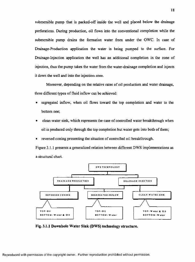
Moreover, depending on the relative rates of oil production and water drainage,

three different types o f fluid inflow can be achieved:

• segregated inflow, when oil flows toward the top completion and water to the

bottom one;

• clean-water sink, which represents the case of controlled water breakthrough when

oil is produced only through the top completion but water gets into both of them;

• reversed coning presenting the situation of controlled oil breakthrough.

Figure 3.1.1 presents a generalized relation between different DWS implementations as

a structural chart.

T O P : O i l

B O T T O M : W a t e r & O II B O T T O M : W a t e r B O T T O M : W a t e r

S E G R E G A T E D I N F L O W

D WS T E C H N O L O G Y

R E V E R S E D C O N I N G C L E A N - W A T E R S I NK

D R A I N A G E I N J E C T I O ND R A I N A G E P R O D U C T I O N

Fig. 3.1.1 Downhole Water Sink (DWS) technology structure.


19

Despite the simplicity of this new completion idea, its design and application in

the field present a real challenge to the engineer. This is due to the relatively large

number of parameters that must be considered, such as the length and position of the

perforated intervals in the oil and water zones, and the production rates of oil and water.

These facts substantiate the need for a customized design for each particular case and

the necessity of a special model describing the water coning phenomena.

3.2 Current Design of DWS Completions

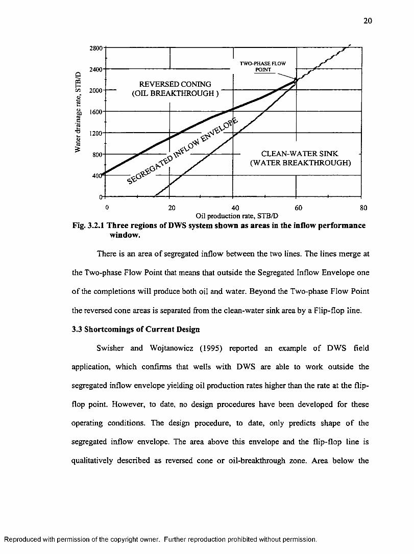
Design of a well completion with DWS for the alternatives shown in Figure

3.1.1 is based on the shape o f the dynamic Water-Oil Interface (WOI) under steady

state conditions. The WOI (water cone profile) can be predicted if the pressure

distribution around a partially penetrating well is known. Shirman (1996) developed the

Moving Spherical Sink Method (MSSM) and the Expanded Method of Images (EMI) to

predict pressure distribution around wells with limited entry to flow in multilayered

reservoirs. From the WOI, breakthrough conditions are determined both for the oil and

water completions. Finally, an inflow performance window is developed, which

determines the range of oil production and water drainage to ensure stable WOI,

(segregated inflow conditions). Figure 3.2.1 displays an example o f the inflow

performance window. There are two lines on the inflow performance window. The

topmost one presents water drainage critical rates for different oil production rates.

Thus its intercept with y-axis the critical rate for the bottom completions of DWS. The

lowest line presents critical oil rates for different rates of water drainage. Thus, the

intercept of this line with the x-axis gives the value of critical rate of the top completion

if it were completed as a single, conventional well, without the DWS.


20

2800

TWO-PHASE FLOW POINT2400------Q

m2000------

tf

REVERSED CONING (OIL BREAKTHROUGH)

1600

eoUrnT3 1200OCO£ CLEAN-WATER SINK

(WATER BREAKTHROUGH)800

0 8020 40 60Oil production rate, STB/D

Fig. 3.2.1 Three regions of DWS system shown as areas in the inflow performance window.

There is an area of segregated inflow between the two lines. The lines merge at

the Two-phase Flow Point that means that outside the Segregated Inflow Envelope one

of the completions will produce both oil and water. Beyond the Two-phase Flow Point

the reversed cone areas is separated from the clean-water sink area by a Flip-flop line.

3.3 Shortcomings of Current Design

Swisher and Wojtanowicz (1995) reported an example of DWS field

application, which confirms that wells with DWS are able to work outside the

segregated inflow envelope yielding oil production rates higher than the rate at the flip-

flop point. However, to date, no design procedures have been developed for these

operating conditions. The design procedure, to date, only predicts shape o f the

segregated inflow envelope. The area above this envelope and the flip-flop line is

qualitatively described as reversed cone or oil-breakthrough zone. Area below the


21

segregated inflow envelop and the flip-flop line describes the clean-water sink or water-

breakthrough zone. Thus, to make the design procedure complete, it is necessary:

1. to expand the procedure of production description outside o f the segregated

inflow window;

2. to be able to predict changes of the inflow performance window in time due

to the pressure transient behavior.

To ensure wide implementation of the new completion technology, it is also

important to extend MSSM for the following cases of special interest:

1. effect of water re-injection into the same aquifer (water looping) and

complications due to leaks between draining and injecting perforations

along the well casing;

2. water cone suppression in conventional wells and wells with DWS.


CHAPTER 4

OBJECTIVES OF THIS WORK

The main challenge of this work was to develop a DWS design method, which

would be valid for all the production regimes, including post-breakthrough (two-phase

flow) conditions. Accomplishing this formidable task required learning more about

different ways DWS may operate and better understanding the DWS performance,

particularly in comparison to conventional completions. Our approach was both

analytical and experimental. Following is the short list of the objectives deemed

necessary to develop a DWS design methodology.

1. Factors effecting segregated inflow DWS completions

1.1 DWS drainage-injection system with water looping (injection in the same

aquifer);

1.2 Imperfection of well integrity -- leaking between drainage and injection

perforations;

2. Mechanism of cone development and reversal in conventional and DWS

completions - theoretical and experimental studies;

3. Mathematical model of well inflow after breakthrough, i.e. two-phase inflow model;

4. Mathematical model of DWS under transient inflow conditions (MSSTM

software);

5. Procedure for prediction of steady state DWS production performance;

6. Build physical model and develop method for analysis;

6.1 Design and fabrication of DWS Hele-Shaw analog;

6.2 Mathematical model of flow in DWS Hele-Shaw analog;

22


23

6.3 Transformation from DWS analog to radial flow systems;

7. Experimentally compare performance of DWS and conventional completion

7.1 Water cut reduction performance;

7.2 Oil recovery increase performance.


CHAPTER 5

PHYSICAL MODEL OF DWS COMPLETION

Water coning behavior and post-water-breakthrough well performance have

been extensively studied with various types of experimental models. Chierici, Ciucci,

and Pizzi (1964) used a flat potentiometric model. Leverett, Lewis, and True (1941)

performed their experiments using a cylindrical sand pack while Caudle and Silberberg

(1965), VanDaalen and VanDomselaar (1972) and Hawtom (1960) prefer to

experiment on the thin rectangular sand packs.

Pie-shaped models have also been very popular in hydraulic modeling of cone

behavior. Matthews and Lefkovits (1956), Bobek and Bill (1961), Henley, Owens, and

Crig (1961), Sobocinski and Cornelius (1965), Boumazel and Jeanson (1971), Khan

(1970), Khan and Caudle (1969), Stephens, Moore, and Caudle (1963), and Mungan

(1975) -all performed their experiments on the pie-shape models. Rectangular flat

models without any porous media, Hele-Shaw models were used in the experiments of

Meyer and Searcy (1956), Schols (1972), Butler and Stephens (1981), Butler and Jiang

(1996), Greenkom, et al (1964).

5.1 Selecting a Type of Physical Model

Of the above-mentioned variety of experimental models the cylindrical and pie

shaped sand packs resemble the best geometry a real reservoir. However, they provide

poor visibility of the cone phenomenon. These models should also be cleaned after each

experimental run to return it to the initial conditions. Rectangular sand packs provide

better visibility than the previous two models, but have the same problem of frequent

cleaning. Moreover, they distort the paten; their flow in is primarily linear.

24


25

The Hele-Shaw model is not packed giving the best visibility of all above

mentioned set-ups. Also, it returns to the initial conditions without any need of

cleaning. Its main drawback, however, is high conductivity, very small capillary

pressure linearity of flow and absence o f wettability effects (fractional flow).Some of

these problems can be overcome through transformation procedures, shown in the

following sections.

The main goal of our experimental studies was visual observation of the cone

phenomena in conventional wells and wells with DWS. To get the best quality of

visualization and high repeatability o f the experiments, I chose the Hele-Shaw

transparent-plain parallel-plate cell as an experimental model. In principle, if the flow

in this model is laminar and mostly two-dimensional, it is similar to the flow in a linear

porous medium. I could not find any information concerning the principles o f the

model design in the relevant papers. To ensure that the model will be working properly,

I performed the following design analysis.

5.2 Analysis of a Hele-Shaw Model Design

For the sake of simplicity, I assumed that the reservoir to be modeled

completely penetrated (100% penetrating well.) In the Hele-Shaw model this situation

is represented by linear flow. The pressure drawdown for linear flow is described by the

following equation:

Ap = 887.3^-4 (5-2.1)k A

According to Greenkom (1964), equivalent permeability for a gap of fine clearance and

unit width is given by

k = S 2/ 12


26

Bradley (1992) presents this relation for the case, when 5 is in inches and k in Darcies,

in the following form

k = 54.4* 106 * S 2 (5.2.2)

We installed the production pumps on the outlet end of the Hele-Shaw cell in order not

to over-pressure the cell. Thus, pressure drawdown in the cell could not be higher than

14 PSIA. Substituting this value and the relation for the gap permeability into Eq. 5.2.1

we obtain the mathematical expression of this limitation

887.3 qftL 12 < 14 (5.2.3)54.4 *10 S hm5

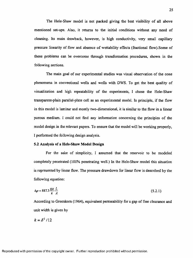
Eq. 5.2.3 requires the minimum thickness of the gap in the model to be

6 = 0.00241i f 1) (5-2.4)V hm )

0.01

0.009

0.008

0.007

0.006

0.00520 3 4 5

M odel's Iength-to-height ratio

Fig. 5.2.1 Hele-Shaw model size relation.


27

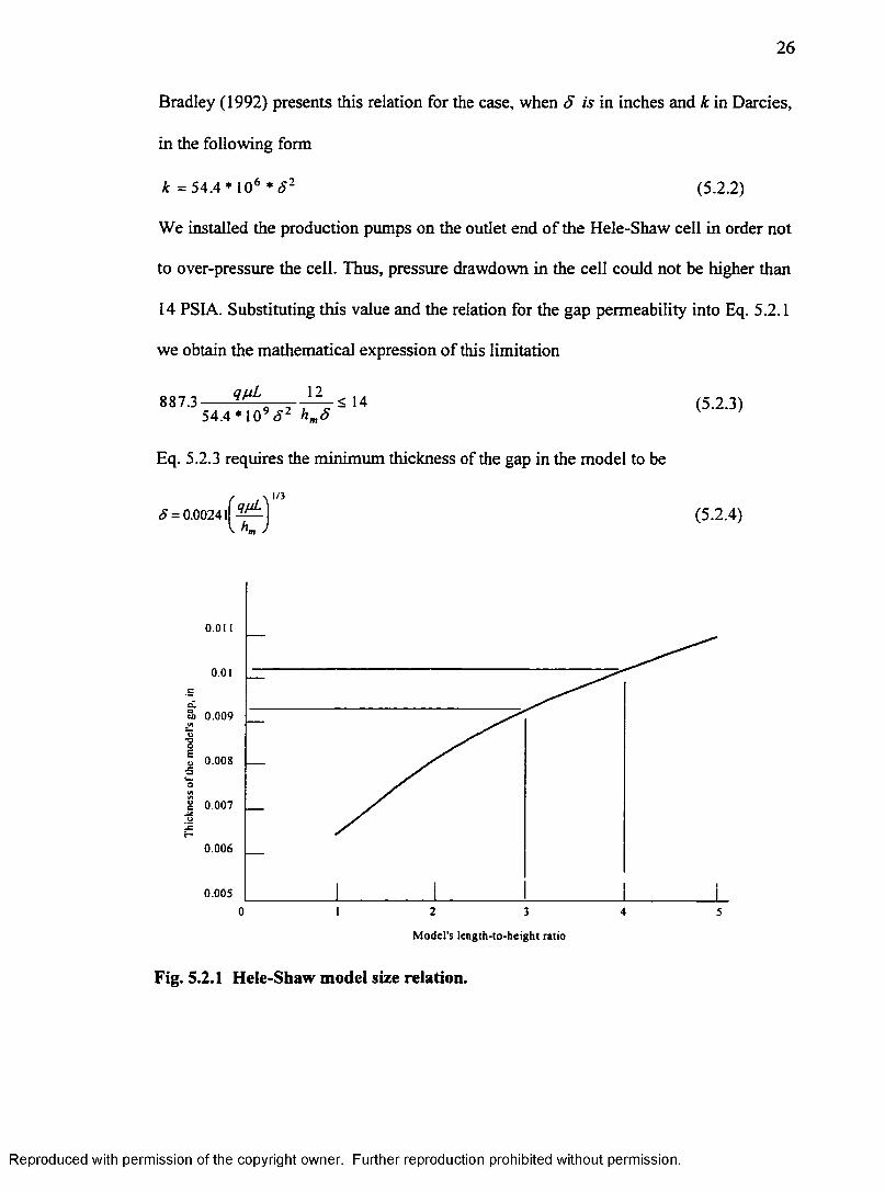
We used “Monostart” peristaltic pumps. The maximum production rate, which

can be achieved with these pumps, is 2000 cc/min of water. This production rate is

equivalent to 18.1 BWPD. Substituting this value into Eq. 5.2.4, we found that the

minimum gap size depends only on the model’s length-to-height ratio. Graphical

analysis of this relation is presented in Figure 5.2.1.

The length of the model should be at least 3-4 times its height to ensure the

presence of some stabilization zone and a zone for linear flow at the inlet side of the

model. In this range of the model size, gap thickness varies from 0.009 to 0.01 inches.

Stainless steel shims were used as spacers to create a gap. To get a gap of the estimated

size, we chose O.Olinch thick shim. The model’s length-to-height ratio was chosen to

The minimum pressure drop required to create complete water breakthrough

conditions (i.e. cone is to the top of the model) is

We may be interested in variation of the production rate (qmax/qmm) equal to a hundred.

Thus minimum rate will be 0.181 BWPD. Substituting this value into Eq. 5.2.6, we

obtain the necessary height of the model:

be 3.

b p = 0.433(/?w - p 0 )hm (5.2.5)

Substituting Eq. 5.2.2 and Eq. 5.2.5 into Eq. 5.2.1 we obtain

0-433(/?w - p 0)hm <887.3qfiL 12

54.4 * 109/im S3(5.2.6)

hm < 0.452 *10-*n = 0.452 *10"* 0.181*1*3 0 .0 13 * 0.2

= 1.3 f t (5.2.7)

Finally, we chose the height of the model to be 1 ft.


28

The flow analogy between Hele-Shaw model and porous media is valid only

when the flow is laminar. Thus, the maximum Reynolds number should not be greater

than 2100:

N Re = 111.4 p °Vde <2100 (5.2.8)

Where the equivalent diameter for a rectangular channel is,

= 4A 4 8 ^n 2(5+12 hm)

Recall that hm» S , and Eq. 5.2.9 can be simplified as follows

d e = 2 S (5.2.10)

Substituting Eq.(5.2.10) into and Eq.(5.2.8), and taking into consideration that:

v = — 12*5.615*?— = o 00078_i_24 * 3600 * ( S * h m) Sh

we obtain

= 0 .1 7 3 8 -^ - <2100 (5.2.11)A

Thus, for the chosen model sizes, condition o f laminar flow is satisfied for any

production rate in the experimental interval.

The deflection in the middle of a rectangular plate with all edges built-in under

hydrostatic pressure defined by Timoshenko and Wionwski-Krieger (1987) as

W = 0.00005A/JZ.4 / D (5.2.12)

where D = - - (5.2.13)I2(l - v 2)

For the very extreme case of a pressure drawdown of 14 PSI, we assume

acceptable change of gap size of the model to be 40%, which corresponds to a glass


29

plate deflection of 0.01*0.4/2=0.002 inches. For these conditions, it follows from Eq.

5.2.12

D = 0.00005 * 14 * 364 / 0.002 = 587865 PSI * in3

Substituting this value into Eq. 5.2.9 we obtain necessary thickness of the glass plate

112(l - v 2 )D ~ 112(l - 0.222 )587865 V E V 10.4*106

This result means that a 3/4-inch-thick glass will, probably satisfy the conditions needed

for the experiments: we are not going to create a complete vacuum in the Hele-Shaw

cell. Conditions in the model will not be exactly the same as was assumed in the

original problem to develop the method of the deflection calculation. Due to this

simplification a special experimental study should be performed to consider the effect

o f the deflections while calibrating the experimental set-up. The cell is to be built of

two 3/4-in thick, 12 x 36-inch glass plates with a gap of 0.01 inches.

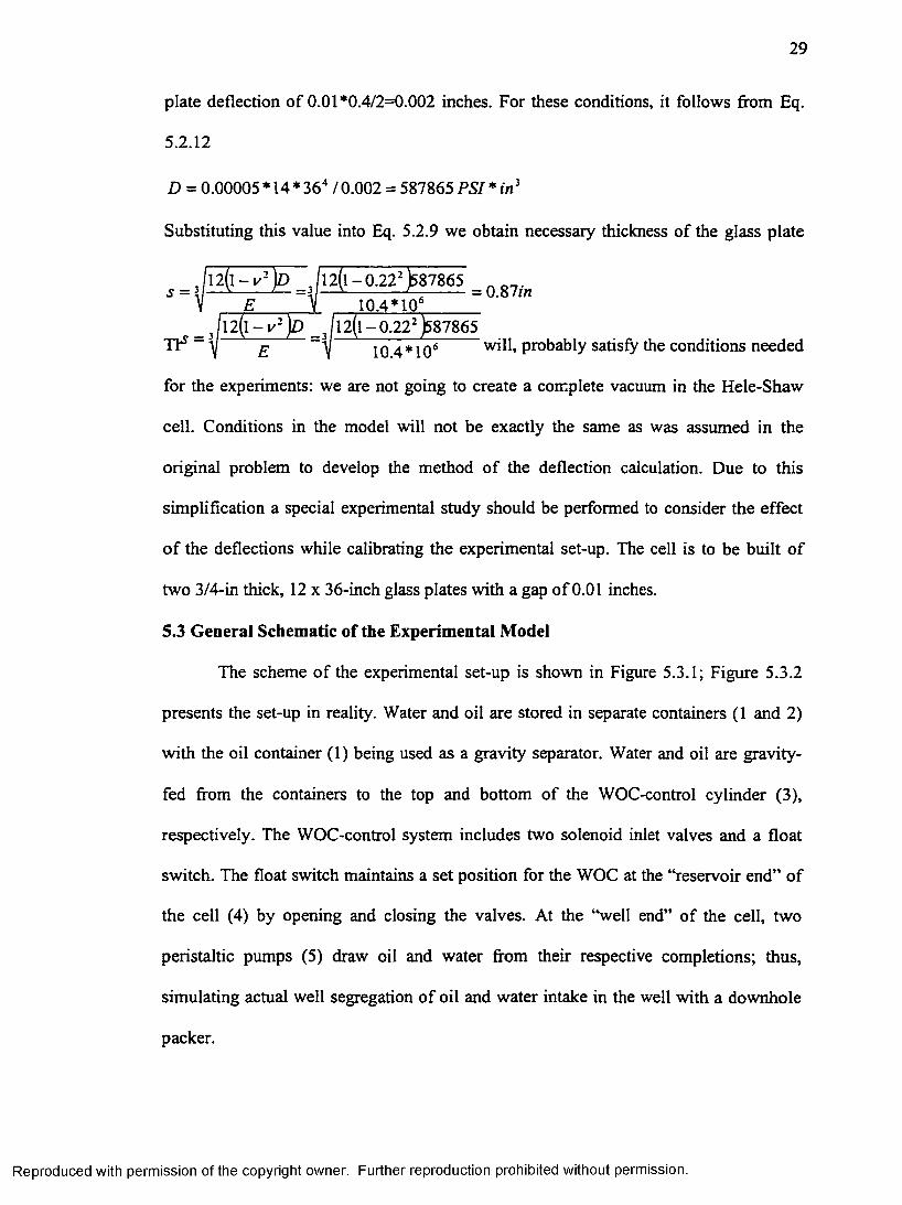
S.3 General Schematic of the Experimental Model

The scheme of the experimental set-up is shown in Figure 5.3.1; Figure 5.3.2

presents the set-up in reality. Water and oil are stored in separate containers (1 and 2)

with the oil container (1) being used as a gravity separator. Water and oil are gravity-

fed from the containers to the top and bottom of the WOC-control cylinder (3),

respectively. The WOC-control system includes two solenoid inlet valves and a float

switch. The float switch maintains a set position for the WOC at the “reservoir end” of

the cell (4) by opening and closing the valves. At the “well end” of the cell, two

peristaltic pumps (5) draw oil and water from their respective completions; thus,

simulating actual well segregation of oil and water intake in the well with a downhole

packer.


30

Through return lines (6), produced liquids return to the separator (1) so they can

be recycled in this closed-loop system. Produced liquids can also be re-directed from

the return line (6) to the fractional collector (7) in order to measure the concentration of

oil and water in the produced steam. ISCO Retriever - II was used as a fractional

collector. The retriever changes sampling tubes automatically with a variation of

sampling time from 0.1 to 999 minutes. Since the sampling time and the volume of the

sample are known, sampling becomes a tool to control production rates. The

independent way of production rate control is very important because calibration of the

peristaltic pumps is not accurate especially for two-phase flows.

c x i -w a te r v a lv e (S> ■ pressure gauge

-o il v a lv e fl

A - th re e -w a y v a lv e- s o le n o id

111000.

Fig. 5.3.1 Experimental set-up

Distilled water and white oil were used for the experimental runs. To make the

water-oil clearly visible the oil was dyed black. The total volumes of water and oil are

2.0 liters, and 1.5 liters, respectively.

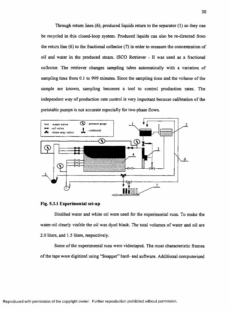
Some of the experimental runs were videotaped. The most characteristic frames

of the tape were digitized using “Snapper” hard- and software. Additional computerized


31

data processing was performed on the digitized pictures in order to read the interface

profile and sweep efficiency of the water drive.

Fig. 5.3.2 Experimental set in reality.

5.4 Calibration of the Model

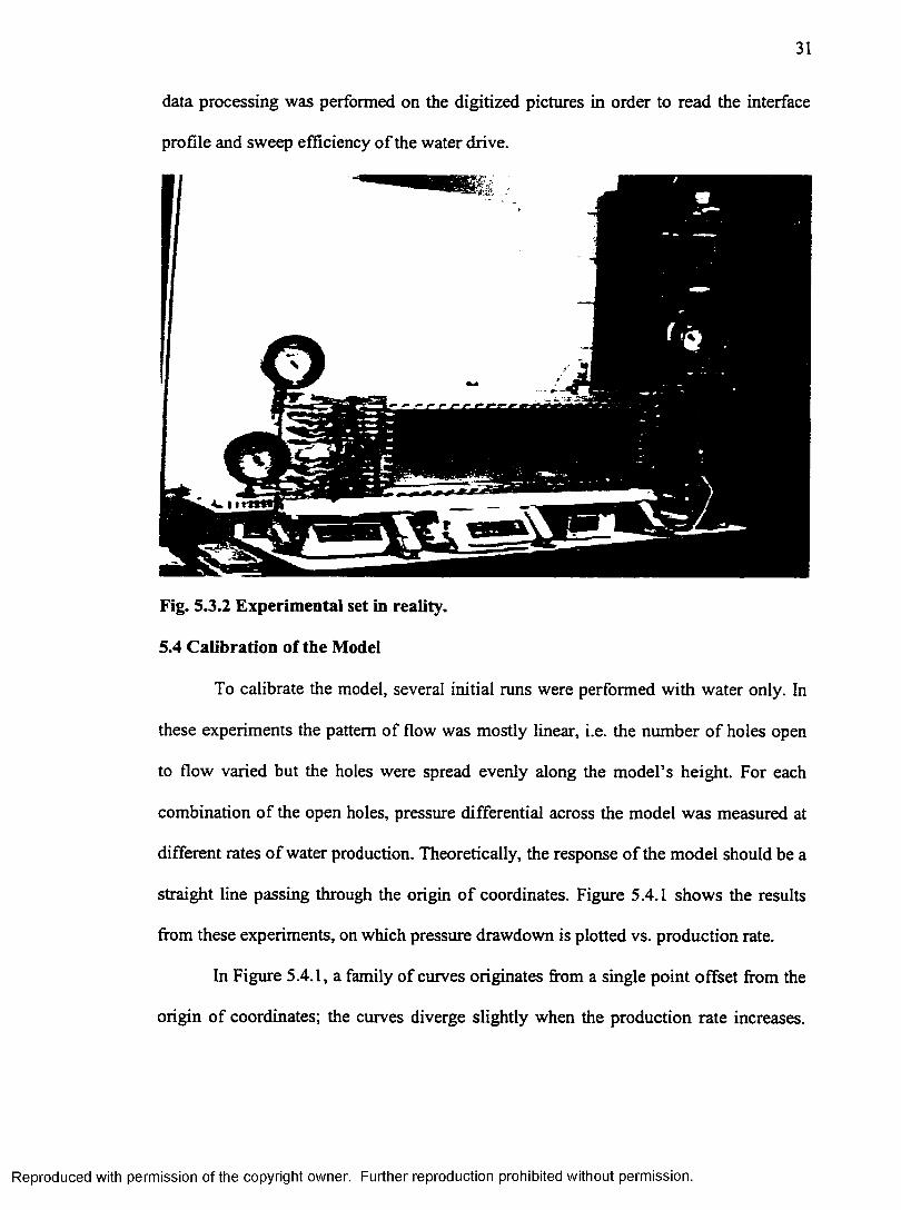
To calibrate the model, several initial runs were performed with water only. In

these experiments the pattern of flow was mostly linear, i.e. the number of holes open

to flow varied but the holes were spread evenly along the model’s height. For each

combination of the open holes, pressure differential across the model was measured at

different rates o f water production. Theoretically, the response of the model should be a

straight line passing through the origin o f coordinates. Figure 5.4.1 shows the results

from these experiments, on which pressure drawdown is plotted vs. production rate.

In Figure 5.4.1, a family of curves originates from a single point offset from the

origin of coordinates; the curves diverge slightly when the production rate increases.


32

This was not exactly the result we expected to get from the model’s calibration. The

offset, as we realized later, was resultant by the pressure differential gauge being out of

zero. Non-linear flow effects causes the deviation of the experimental points from the

theoretical, straight line, trend. Nevertheless all, the curves have a significant straight-

line sections before deviation begins. These sections were used to determine the actual

permeability of the model, because slopes of these straight lines are proportional to the

average permeability of the Hele-Shaw model corrected for number of inlet and outlet

holes open for production.

10.00

8.00

6.00

N u m b er o f holes open

4.00

2.00

0.00

2.0000.000 4.000 6.000 8.000

Production rate. BPD

Fig. 5.4.1 Pressure drop across the Hele-Shaw cell for different number of holes open to flow.

The average permeability measured in these experiments represents combined

frictional losses in the three zones having different cross-sectional areas: feed zone (12

holes open), visual zone (no restrictions to flow), well-end zone (from 2 to 12 holes

open to flow), and the end-flow effect of non-linear flow.


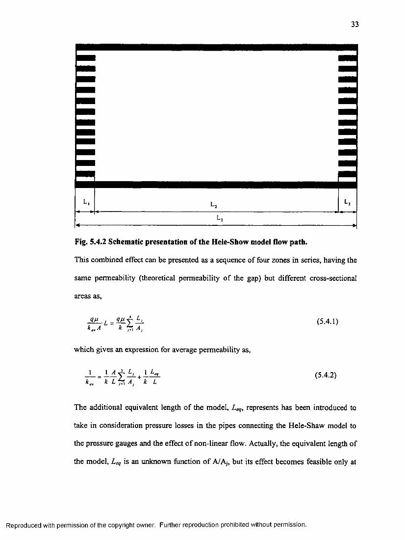
Fig. 5.4.2 Schematic presentation of the Hele-Show model flow path.

This combined effect can be presented as a sequence of four zones in series, having the

same permeability (theoretical permeability of the gap) but different cross-sectional

areas as,

(5.4.1)kavA k Ai

which gives an expression for average permeability as,

_ L = I A y i ^ + i h i . (5.4.2)kav k L f t A, k L

The additional equivalent length of the model, Leq, represents has been introduced to

take in consideration pressure losses in the pipes connecting the Hele-Shaw model to

the pressure gauges and the effect of non-linear flow. Actually, the equivalent length of

the model, Leq is an unknown function of A/Aj, but its effect becomes feasible only at


34

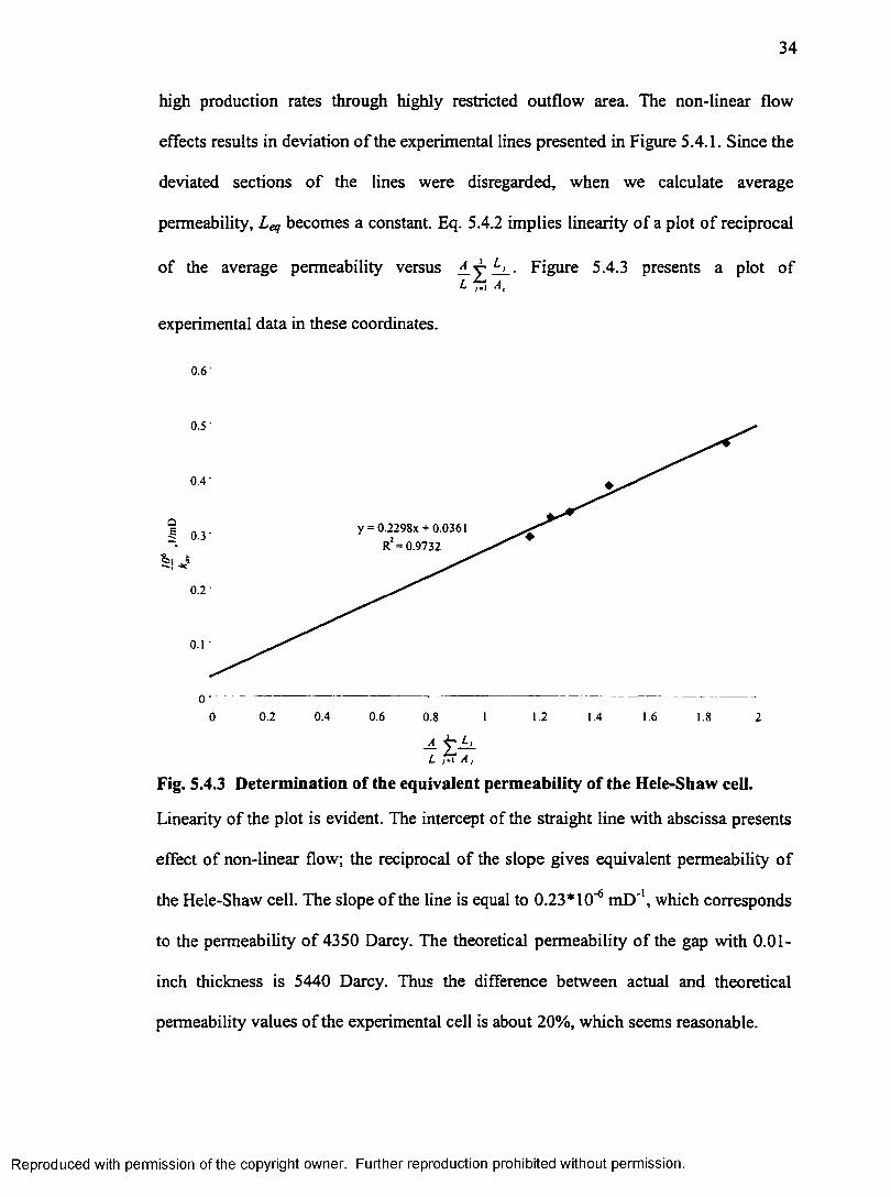
high production rates through highly restricted outflow area. The non-linear flow

effects results in deviation of the experimental lines presented in Figure 5.4.1. Since the

deviated sections of the lines were disregarded, when we calculate average

permeability, Leq becomes a constant. Eq. 5.4.2 implies linearity of a plot of reciprocal

of the average permeability versus A y L< . Figure 5.4.3 presents a plot ofl f r , a ,

experimental data in these coordinates.

0 . 6 ‘

0.4-

y = 0.2298x + 0.0361 R2= 0.9732

00 0.2 0.4 0.6 0.8 1 1.2 1.4 1.6 1.8 2

— £ —L U A ,

Fig. 5.4.3 Determination of the equivalent permeability of the Hele-Shaw cell.

Linearity of the plot is evident. The intercept of the straight line with abscissa presents

effect of non-linear flow; the reciprocal of the slope gives equivalent permeability of

the Hele-Shaw cell. The slope of the line is equal to 0.23* I O'6 mD'1, which corresponds

to the permeability of 4350 Darcy. The theoretical permeability of the gap with 0.01-

inch thickness is 5440 Darcy. Thus the difference between actual and theoretical

permeability values of the experimental cell is about 20%, which seems reasonable.


CHAPTER 6

TRANSFORMATION FROM LINEAR- TO RADIAL-FLOW SYSTEMS

Hele-Shaw models provide superior visibility and are easy to build and operate.

Their potential drawback is the lack of porous medium and two-dimensional flow

pattern. The use of these models, however, may not be limited to two-dimensional flow

problems. Aravin (1938), Efros and Allakhverdieva (1957) showed that Hele-Shaw

models can also be used to study flow phenomena with radial symmetry if the spacing

between the glass plates varies with the cubic root of the horizontal distance. Later,

Schols (1972) used a model of this type to study critical oil rate for water coning.

Although uneven glass spacing caused variation of the model’s permeability, Schols’s

results were in good agreement with correlations developed by Muskat and Wyckoff

(1935), and Mayer and Garder(1954).

To avoid inaccuracy caused by permeability variation as well as technical

difficulties of fabricating a model with a variable gap size, we decided to perform

experiments on a regular Hele Shaw model. It may seem, however, that the difference

between linear and radial flow patterns might cause the results obtained with Hele Shaw

models irrelevant. There fore, we must derive a transformation from the Hele-Shaw to

radial flow systems.

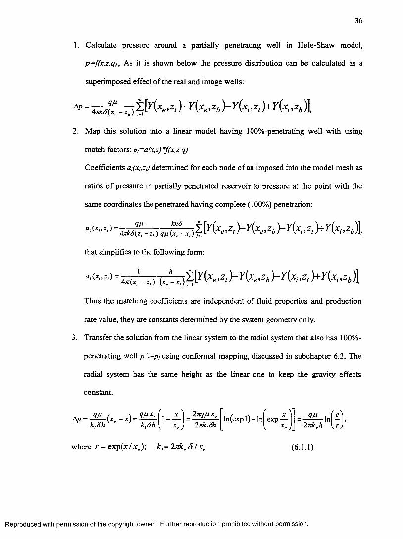
6.1 Pressure Distribution in Models with Partially Penetrating Wells

Theoretically, as shown below, linear flow can be transferred to radial flow only

when the well completely penetrates the reservoir. For partial penetration there is no

exact, analytical, transformation for pressure distribution from linear to radial flow

systems. But, there is a way to perform an approximate, numerical, transformation. The

idea of such transformation is the following:

35


36

1. Calculate pressure around a partially penetrating well in Hele-Shaw model,

p=f(x,z,q), As it is shown below the pressure distribution can be calculated as a

superimposed effect of the real and image wells:

Ap = ^ — t [ y ( x e , z , ) - H x e , z b ) - K ' c, , z , h H x , , z b ) l4nkS(zt - z b)

2. Map this solution into a linear model having 100%-penetrating well with using

match factors: p,=a(x,z)*f(x,z,q)

Coefficients aifazj) determined for each node of an imposed into the model mesh as

ratios of pressure in partially penetrated reservoir to pressure at the point with the

same coordinates the penetrated having complete (100%) penetration:

a,{xn z,)=-khS

4nkS{zt - z b) qp(xt -x,.)£f

that simplifies to the following form:

ai(xi, z l ) =

t [ r ( v , ) - Y ( x e , z l, } - y ( X i , z l ) + Y ( ^ i ) l

4<r(z ,'-z ,) (x.H- x , ) t l [ Y (Xe ’Z‘ ) ~ Y (Xe ’Zb ’z b )],

Thus the matching coefficients are independent of fluid properties and production

rate value, they are constants determined by the system geometry only.

3. Transfer the solution from the linear system to the radial system that also has 100%-

penetrating well p ’r=pi using conformal mapping, discussed in subchapter 6.2. The

radial system has the same height as the linear one to keep the gravity effects

constant.

^ k,8h e ’ k,8hl - ±

V X e J

2nqp x e2nktSh

ln(expl)-lnf \xexp —

xW

2mkh•In

\ r .

where r = exp(x / xe); k,= 2nkr 8 / xe (6 . 1. 1)


37

4. Map the results obtained at the previous step into the radial partially penetrated

system using match factors, obtained with MSSM [Shirman (1955)]:p r= p ’r/bi(ri,Zi),

where

1 h W 'T + (z, ~ zi) - In -Z, + 4 re + (Z' ~Zi)2(z, - z b) ln(re / /■) 3 -z, + 4 r< +("6 ~ z.)_ 3 + 4 r'2 + (Zf " - i ) j

From Eq. 6.1.1 it follows, that infinite number of radial systems are equivalent

to a given linear model The variety of the equivalent systems is determined by the

choice of the origin of the linear model coordinates. If the origin of coordinate is such

that xw=0, it becomes equivalent to a radial system with the following parameters:

radius of the wellbore, rw= 1; constant pressure boundary radius, re=2.72; permeability,

kr= 192.5 mD. The units of radial equivalent model should be consistent, there is no

difference whether rw is in inches, centimeters of miles as far as the re, and S are in the

same units.

To achieve the transformation according to the proposed algorithm a description

of pressure distribution around partially penetrating well in the linear system (thus

Hele-Shaw model) is needed. To get this description, we developed Moving Horizontal

Sink Method (MHSM) describing pressure distribution and OWI behavior in this Hele-

Shaw model.

To simulate a point sink in the linear-flow model, we used a horizontal sink

having length equal to the model’s thickness and radius approaching zero. Using this

initial point element we described the pressure distribution in Hele Shaw model in the

same way as it was done in the previous work to get Moving Spherical Sink Method

(MSSM). The only difference in these two methods is that the description of the


38

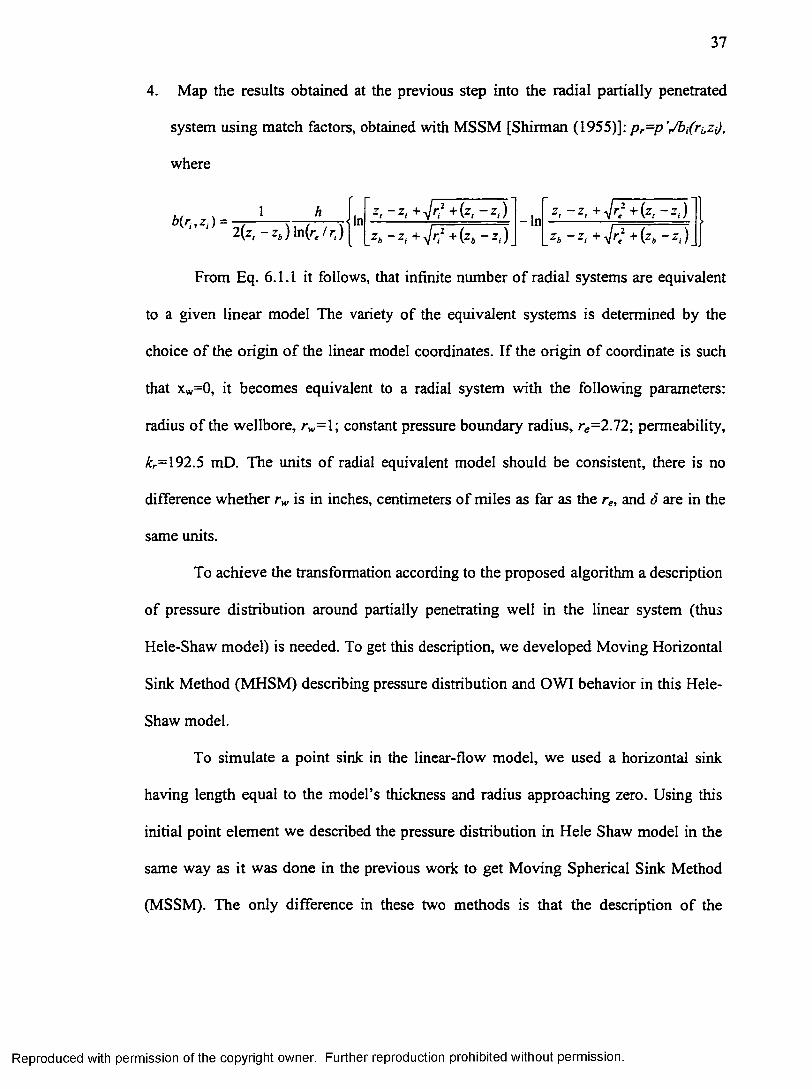
pressure distribution in the Hele-Shaw (2-D) model was derived from superposition of

several horizontal sinks, while for MSSM, the effect o f several spherical sinks was

superimposed.

6.1.1 Pressure around a Well with Limited Entry in Infinite Hele-Shaw Model

To get a general solution to the problem of pressure distribution in a Hele-Shaw

model, we begin with the following simplified case. The model is infinite in the vertical

direction and semi-infinite in horizontal direction (a right half of vertical plane is

considered) as shown in Figure 6.1.1. A finite well section having length izt-Zh) is open

to flow. The boundary conditions include constant pressure outer boundary (x=Xe) and a

uniform flux well (x=0).

O p e n to flow in terval

Z

Fig. 6.1.1.1 Infinite Hele-Shaw model with finite size completion

We remove the no-flow boundary at the well’s axis by using the method of

images, which results in doubling the well’s production rate. Also, the well is

considered a conglomerate of infinite number of horizontal sinks as Shown in figure


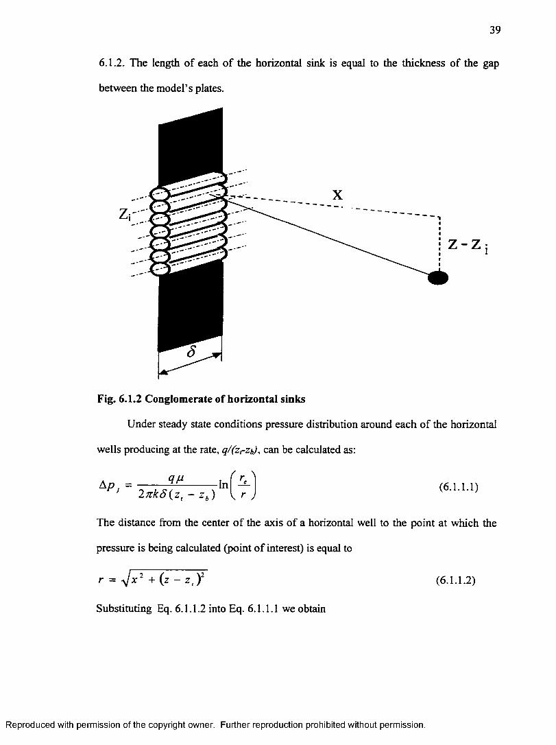
39

6.1.2. The length of each of the horizontal sink is equal to the thickness of the gap

between the model’s plates.

Zi

z-z

Fig. 6.1.2 Conglomerate of horizontal sinks

Under steady state conditions pressure distribution around each of the horizontal

wells producing at the rate, q/(zrZb), can be calculated as:

A P j =iTtkS^Z, - z b)

•In (6 . 1. 1. 1)

The distance from the center of the axis of a horizontal well to the point at which the

pressure is being calculated (point of interest) is equal to

r = V * 2 + (z “ Z' Y (6.1.1.2)

Substituting Eq. 6.1.1.2 into Eq. 6.1.1.1 we obtain


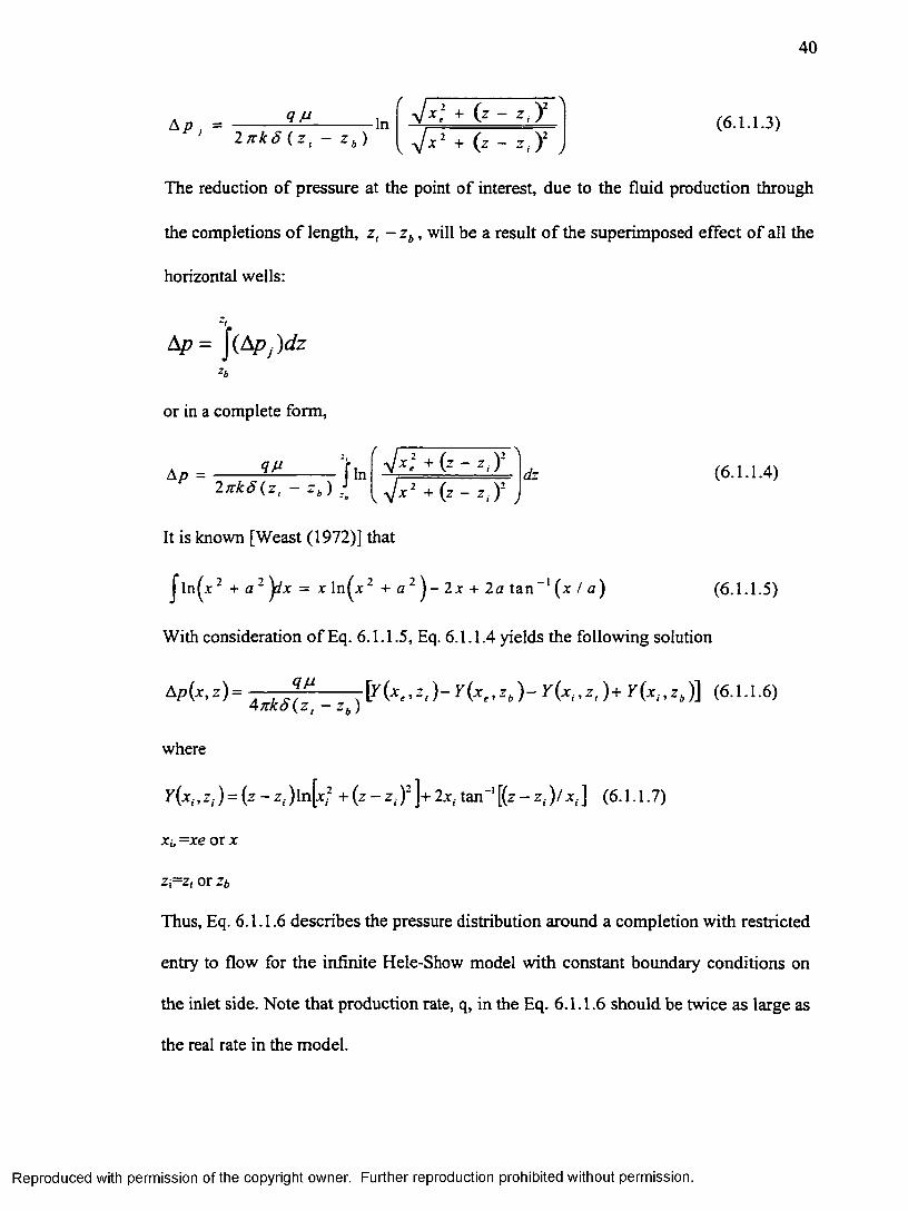
40

A P j =I n k 8 ( z , - z b )

■In yj x] + (z - z, Y

y / x 2 + (z - Zt y(6.1.1.3)

The reduction of pressure at the point of interest, due to the fluid production through

the completions o f length, z, - z b, will be a result o f the superimposed effect of all the

horizontal wells:

-t

AP = \ ( & P j ) d z

or in a complete form,

A p =Ij tkS { z t - z b) ;JIn y J X 2 + ( z - Z , . ) 2

y j x 2 + ( z - Z , ) 2dz (6.1.1.4)

It is known [Weast (1972)] that

J l n( . t 2 + a 2 y * = x In^z2 + a 2 j - 2 x + 2a tan ' ( x / a ) (6.1.1.5)

With consideration of Eq. 6.1.1.5, Eq. 6.1.1.4 yields the following solution

Ap (x , z ) = qM------- \Y( xe, z , ) - Y ( x e, z b) - Y { x t, z , ) + Y (x,., zA)] (6.1.1.6)AztkSiz, - z b)

where

.2/) = (z ~ z i ) + (z " z - )2 ]+ 2xi t a n Kz ~ z i ) / x i ] (6.1 ■ 1.7)

x„ =xe or x

Zi=z, or Zb

Thus, Eq. 6.1.1.6 describes the pressure distribution around a completion with restricted

entry to flow for the infinite Hele-Show model with constant boundary conditions on

the inlet side. Note that production rate, q, in the Eq. 6 .1.1.6 should be twice as large as

the real rate in the model.


41

6.1.2 Infinite Line and Point Sink Cases

The model developed in subchapter 6.1.1 can be verified using two extreme

cases, line source and point source.

In the case, where the well’s section opened to production is infinite, the flow in

the model becomes linear. So, if we substitute -oo and +oo for the top and bottom

coordinates of the completions into Eq. 6.1.1.6, it should yield the linear flow equation.

It follows from Eq. 6.1.1.7, after substituting infinite values for the top and

bottom coordinate of the well,

F ( x g , + 0 0 ) = ln (oo ) + 2 x en

Y ( x e ,-oo ) = ln( oo) - 2 x en

y (x ,+oo ) = ln (o o ) + 2 x 7t (6.1.2.1)

y {x ,-oo ) = ln (oo ) - 2 x k

Substitution of this system of equations into Eq. 6.1.1.6 yields

Ap = -------— --------[4^(x - *)] = ----- — ------ (.xe - x ),4n k S ( z , - z b) L Ve U kS(z, - z b) h

That is the equation of linear flow.

If the length of the completions is extremely short, only one horizontal sink

exists in the infinite Hele-Shaw model. This situation will result in pure radial flow

around the horizontal sink, and Eq. 6.1.1.6 should convert into a radial flow equation

when Zb=zt. But ifz, is substituted directly instead of z* into Eq. 6.1.1.6, the uncertainty,

0/0, occurs. To overcome this uncertainty the L’Hopital rule is used. L’Hopital rule

solves uncertainty of 0/0 and oo/oo, by substitution of function’s derivatives instead of

the function into the ratios.


Substituting the system of equations 6.4.2.2 into Eq. 6.1.1.6 yields

^ 2akS \ r )

Which is the equation of radial flow.

6.2 Pressure Distribution in Models with 100% Penetrating Wells

Laminar steady state flow of incompressible fluid is described by Laplace

equation:

d 2® d 2® d 2® n — h — h — = 0 ( 6 .2 . 1)d x 2 d y 2 d z 2

For the systems having radial symmetry, Eq. 6.2.1 may be presented in cylindrical

coordinates.

d 2® 1 d 2® d 2® n— r + r + — r = 0 (6 .2 .2)d r 2 r d y 2 d z 2

Flow between the two parallel plates is two-dimensional, thus derivative of flow

potential with respect to y-coordinate is equal to zero, which reduces Eq. 6.2.1 to the

following form:

d 2® d 2®+ — = 0 (6.2.3)d x d z

Using conformal mapping transformation of coordinates, r=exp(x), which converts a

rectangle into a sector, we can write Eq. 6.2.3 as


43

1 d2® d 2® 1 d ®t - r + X T - + “ J - = ° (6-2-4)r d z d r r d r

If d ® l d z = 0 , which represent the case of horizontal flow towards 100% penetrating

well, both Eq. 6.2.2 and Eq. 6.2.4 simplify to the same form.

d 2® 1 d ®+ = 0 (6.2.5)

dr r dr

This means that flow towards a 100%-penetrating well can be modeled in a Hele-Shaw

cell exactly. Moreover, Eq. 6.2.4 should give reasonable results for systems with partial

penetration in the zones where the flow is predominately horizontal, i.e. in the outer

reservoir area and in the close-to-the-wellbore area. One of the practical conclusions

from this fact is that Water Cut (WC) has the same value both in radial and linear

systems. For example, limiting WC defined by Eq.6.2.6 is valid both for linear and

radial systems.

WC = - m w ■ (6.2.6)M i w + h0

Thus, results of the WC development obtained in the linear models can be directly

applied to the radial systems having the same fluid properties, permeabilities, and

thickness of water and oil zones.

6.3 Critical Rate and Critical Cone Height

A simple transformation from linear to radial flow can be derived for finding

two important parameters of water coning, critical rate and cone height. The

transformation makes use of the flow equations for complete penetration in the infinite

(radial and linear) flow systems. In conventional completions, critical is the maximum

oil production rate, which does not cause water breakthrough. This rate can be


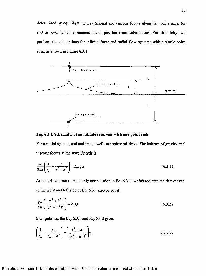
44

determined by equilibrating gravitational and viscous forces along the well’s axis, for

r=0 or x=0, which eliminates lateral position from calculations. For simplicity, we

perform the calculations for infinite linear and radial flow systems with a single point

sink, as shown in Figure 6.3.1

o w e

Fig. 6.3.1 Schematic of an infinite reservoir with one point sink

For a radial system, real and image wells are spherical sinks. The balance of gravity and

viscous forces at the wwell’s axis is

<7AInk

1r - h 2

= A pgz (6.3.1)

At the critical rate there is only one solution to Eq. 6.3.1, which requires the derivatives

of the right and left side of Eq. 6.3.1 also be equal.

+ h22jik 2 \ 2(z - h )

= Apg (6.3.2)

Manipulating the Eq. 6.3.1 and Eq. 6.3.2 gives

f 1 1zcr+h

z 2cr- h 2) 1 ( 4 - a ' F J(6.3.3)


45

Eq. 6.3.3 can be solved by trial and error for the critical cone height, zcr. Then, critical

rate can be calculated from either Eq. 6.3.1 or Eq. 6.3.2.

For a linear system, the real and image wells are reducing to horizontal sinks.

Also, we use capital letters to distinguish the similar parameters in the linear and radial

system. The force balance for the linear system is

Qp2nk5

Inr Z 2 - H i y

r T ~= A pgZ (6.3.4)

At the critical height, the Eq, 6.3.4 has only one solution for Z, thus:

QmIjikS

2 ZZ 2 - H 2

= Ap g (6.3.5)

After rearrangement of Eq. 6.3.4 and Eq. 6.3.4, we obtain the following expression,

from which the critical cone height can be determine by trial and error.

Inr z 2 - h 2^ f 2Z~ 1I ) l Z l r - H 2)

(6.3.6)

An example calculation of the critical rate for the Hele-Shaw model is presented in

Appendix. If we assume that all the reservoir and fluid properties are the same for the

linear and radial systems, we can make the following transformation for the critical

rates and critical cone heights values. The transformation formulas result from

comparing Eq. 6.3.1 with Eq. 6.3.4, and Eq. 6.3.2 with Eq. 6.3.5. The comparison gives,

Q„ S z l + h ' Z i - H >

H z l - h ' - f Z„

and,

2 Z= f c , - * 2)’ (z „ S i ? l - H ' ) z l + h 1 1 z,rRl

(6.3.7)

(6.3.8)


46

For transformation, first, Eq. 6.3.8 is used to convert the critical cone height measured

in the linear system, Zcr, into the equivalent critical cone height in radial system, zcr.

Then, the equivalent critical rate in radial flow os calculated from Eq. 6.3.1.

In conclusion we have to point out that experimental results obtained with the

Hele Shaw model can be used to make conclusions regarding coning phenomenon in

radial flow. Also, all other volumetric parameters such as Initial Oil in Place (IOP),

cumulative produced oil and water have same meaning for radial and linear flow

systems. Therefore, the conclusive results can be obtained from the Hele-Shaw

experiments.


CHAPTER 7

GENERALIZED STEADY STATE MODEL OF DWS

Current design o f DWS is based upon an analytical method developed by

Shirman (1996) for description of pressure distribution around a well with limited entry

to flow in stratified reservoirs, dubbed the Moving Spherical Sink Method (MSSM). The

method gives an analytical solution for pressure around a finite-length well completion

in an infinite homogeneous reservoir. With this solution, a homogeneous reservoir

limited from the top and the bottom by no-flow boundaries was modeled by using

method of images.

The MSSM became even more powerful when Shirman and Wojtanowicz (1996)

developed the Extended Method of Images (EMI). This method transfers stratified

reservoirs into homogeneous ones using an array of image wells producing at different

“pseudo” rates. These pseudo-rates depend upon the permeability of the neighboring

zones. The modified MSSM with EMI provided a theoretical base for a software to

calculate dynamic interface between oil and water.

The computer program compares pressure distribution in the oil zone with the

pressure distribution in the water zone to predict an interface profile. At the interface the

following condition is valid:

The assumptions used in these calculations are:

• shape of the cone does not effect the pressure distribution in the oil and water zones;

• original oil-water interface is a no-flow boundary.

47


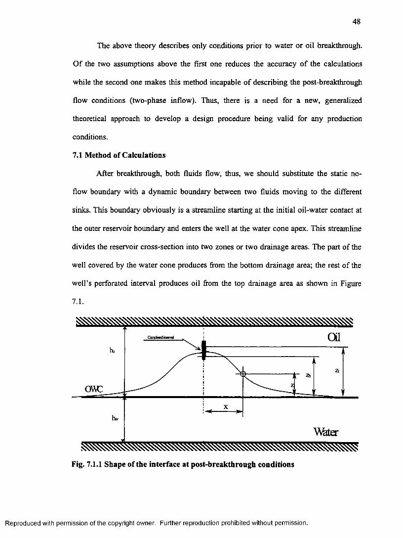
48

The above theory describes only conditions prior to water or oil breakthrough.

Of the two assumptions above the first one reduces the accuracy of the calculations

while the second one makes this method incapable of describing the post-breakthrough

flow conditions (two-phase inflow). Thus, there is a need for a new, generalized

theoretical approach to develop a design procedure being valid for any production

conditions.

7.1 Method of Calculations

After breakthrough, both fluids flow, thus, we should substitute the static no

flow boundary with a dynamic boundary between two fluids moving to the different

sinks. This boundary obviously is a streamline starting at the initial oil-water contact at

the outer reservoir boundary and enters the well at the water cone apex. This streamline

divides the reservoir cross-section into two zones or two drainage areas. The part of the

well covered by the water cone produces from the bottom drainage area; the rest of the

well’s perforated interval produces oil from the top drainage area as shown in Figure

7.1.

Fig. 7.1.1 Shape of the interface at post-breakthrough conditions


49

Pressure at any point of the reservoir can be expressed as a superimposed effect

of drawdowns created by the sections of the completion situated above and below the

dynamic interface. According to the MSSM theory, each section can be presented as a

spherical sink. In addition, we assume that when we calculate pressure drawdowns

created by either the oil (upper) or water (lower) sections of the completion, the entire

reservoir is filled with oil or water, respectively. This intuitive assumption may

introduce some inaccuracy into calculations. However, the inaccuracy disappears when

the produced water-oil ratio (WOR) approaches ultimate value. In this case, pressure

drawdowns created by the spherical sinks representing the oil and water sections of

well’s completion are:

= g ( l - W Q m *

A p w = * W C »

1 l '

a/*1 + ( z - z , ) ! '•- P . g z (7 .1. 1)

4 nk %1

\

\ x 2 + ( z - z b)2 re~ P wg z (7.1.2)

At any point, the summation of the Eq. 7.1.1 and Eq. 7.1.2 gives total pressure

drawdown at this point. Also, the difference between the Eq. 7.11 and Eq. 7.12

represents tendency of the fluid particle to move toward one of the two well sections.

Totality of the points when this difference is equal to zero is the drainage area boundary

for each section o f the completion, or the oil/water interface profile.

7.2 Algorithm and Computer Program

The following algorithm has been developed for calculation of the dynamic

oil/water interface:


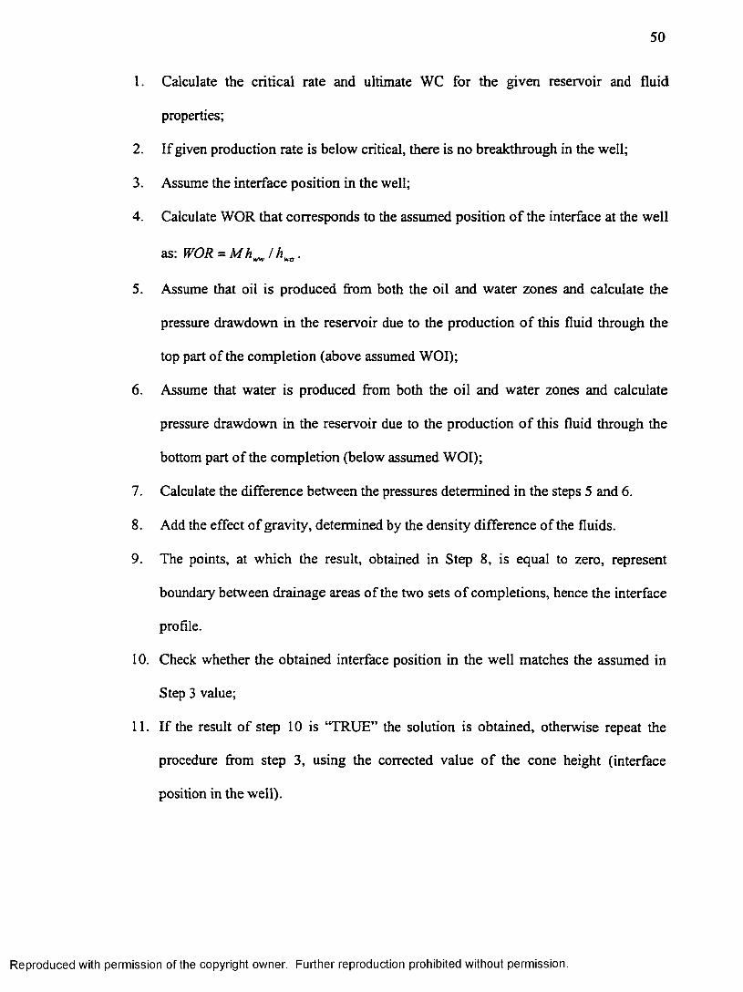
50

1. Calculate the critical rate and ultimate WC for the given reservoir and fluid

properties;

2. If given production rate is below critical, there is no breakthrough in the well;

3. Assume the interface position in the well;

4. Calculate WOR that corresponds to the assumed position of the interface at the well

as: W O R ^ M h ^ l K , .

5. Assume that oil is produced from both the oil and water zones and calculate the

pressure drawdown in the reservoir due to the production of this fluid through the

top part of the completion (above assumed WOI);

6. Assume that water is produced from both the oil and water zones and calculate

pressure drawdown in the reservoir due to the production of this fluid through the

bottom part of the completion (below assumed WOI);

7. Calculate the difference between the pressures determined in the steps 5 and 6.

8. Add the effect of gravity, determined by the density difference of the fluids.

9. The points, at which the result, obtained in Step 8, is equal to zero, represent

boundary between drainage areas of the two sets of completions, hence the interface

profile.

10. Check whether the obtained interface position in the well matches the assumed in

Step 3 value;

11. If the result of step 10 is ‘TRUE” the solution is obtained, otherwise repeat the

procedure from step 3, using the corrected value of the cone height (interface

position in the well).


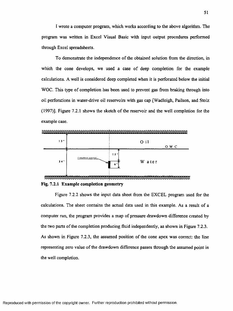
51

I wrote a computer program, which works according to the above algorithm. The

program was written in Excel Visual Basic with input output procedures performed

through Excel spreadsheets.

To demonstrate the independence of the obtained solution from the direction, in

which the cone develops, we used a case of deep completion for the example

calculations. A well is considered deep completed when it is perforated below the initial

WOC. This type of completion has been used to prevent gas from braking through into

oil perforations in water-drive oil reservoirs with gas cap [Wadleigh, Pailson, and Stolz

(1997)]. Figure 7.2.1 shows the sketch of the reservoir and the well completion for the

example case.

o w e

Fig. 7.2.1 Example completion geometry

Figure 7.2.2 shows the input data sheet from the EXCEL program used for the

calculations. The sheet contains the actual data used in this example. As a result of a

computer run, the program provides a map of pressure drawdown difference created by

the two parts of the completion producing fluid independently, as shown in Figure 7.2.3.

As shown in Figure 7.2.3, the assumed position of the cone apex was correct: the line

representing zero value of the drawdown difference passes through the assumed point in

the well completion.


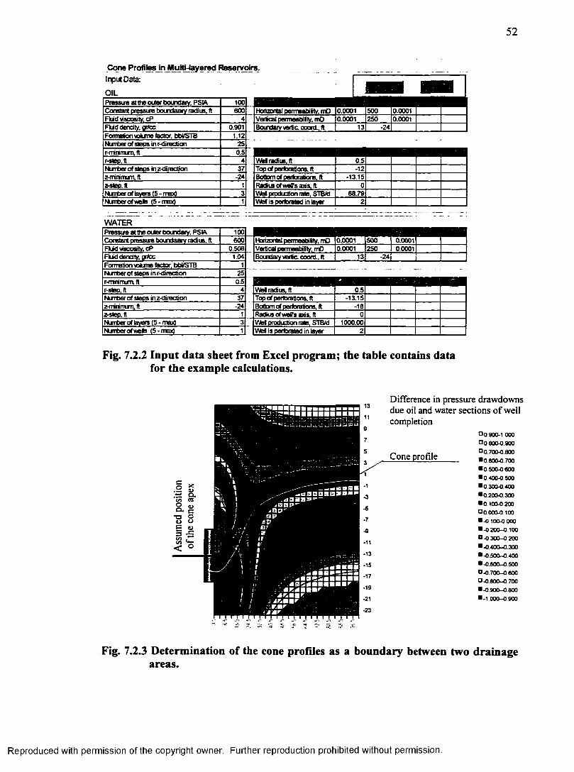
52

Cone Profiles in Multi-layered Reservoirs. Input Data:OILPressue at the outer boufoary, PSIA 100Constant pressure boundaarv rarfius, ft 600 Horizontal permeabiitv. mO 0.0001 500Fkid wscosity. cP 4 Vertical pemeabittv. mO 0.0001 250 0.0001Fkiddendty. gr/cc 0.901 Boundary vertic. coord.. It 13 -24Formation vokme factor. bbVSTB 1.12 - -Number of steps in r-direction 25 -r-mrinun.lt 0.5r-4tep.lt 4 WBlradiis.lt 0.5Nurber of steps in direction 37 TopofperibratiarB.lt -12smininun.lt -24 Bottom of perforations. It -13.15sstep.lt 1 Raditsofweffsaias.lt 0Nirnber of layers (5 - max) 3 Wb( production rate. STBAd 68.79Number of wets (5 -max) 1 WbI is perforated in layer 2

WATERPressue at the outer boundary, PSIA 100I ■ ■ ■ ■ ■ m mCorBfantpressueboirdaarytacSus.lt 600 Horizontal permeabiity. mD 0.0001 500 0.0001Fkid viscosity. cP 0.506 Vertical permeabiity. mD 0.0001 250 0.0001Fkid dencity, grfcc 1.04 Boundary vertic coord.. It 13 -24Formation vokme factor, bbi/STB 1L__________________Nurber of steps in r-direction 25r-minimun, ft 0.5r-step.lt 4 Wei radus.ft 0.5Nurber of steps in z-direction 37 Top of perforations, ft -13.15z-mirinun.lt -24 Bottom of perforations. It -18zstep.lt 1 Radius ofweffs axis, ft 0Nurber of layers (5 - max) 3 Wei production rate. STB/d 1000.00 !Nuiberofweis (5-max) 1 WbI is perforated in layer 2

Fig. 7.2.2 Input data sheet from Excel program; the table contains data for the example calculations.

Co X0)

a .CO CQOo . «

C*T3 o0) uE <U3COCO

JZ

< o

V

^daQQBBOia"*

flK illlfsr mmrJirjiir . . .

c.W.mr

13 due oil and water sections of well11

9completion

O o 900-1 0007 0 0 800-0 9005 Cone profile O 0.700-0.800

■ o 600-0 7003 /

"l■0.500-0 600■ 0 .4000 .500

-1 ■ 0 3 0 0 0 .4 0 0

-3 ■ 0 2 0 0 0 .3 0 0 ■ 0 1000 200

-5□ 0 .0 0 0 0 100

-7 ■ 0 1 0 0 0 000

-9 ■ 0 2 OO-O.IOO

-11■ 0 .3 0 0 -0 200■ 0 4 0 0 - 0 300

-13 ■ 0 5 0 0 -0 .4 0 0-15 ■ 0 .6 0 0 - 0 500

-17 ■ 0 .7 0 0 - 0 600 □ 0 .8 0 0 -0 700

-19 ■ 0 .9 0 0 -0 .8 0 0-21 ■-1 000-0.900

-23

Fig. 7.2.3 Determination of the cone profiles as a boundary between two drainage areas.


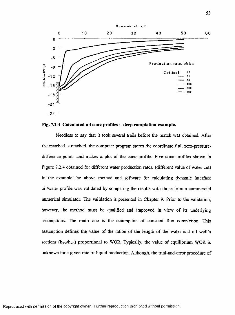
53

R e s e r v o i r r a d i u s , f t

0 10 20 30 4 0 50 6 0

0

3

6Production rate, bbl/d

-9C ritical

1 2

100 200 500

-15

18

21

-24 -

Fig. 7.2.4 Calculated oil cone profiles — deep completion example.

Needless to say that it took several trails before the match was obtained. After

the matched is reached, the computer program stores the coordinate f all zero-pressure-

difference points and makes a plot of the cone profile. Five cone profiles shown in

Figure 7.2.4 obtained for different water production rates, (different value of water cut)

in the example.The above method and software for calculating dynamic interface

oil/water profile was validated by comparing the results with those from a commercial

numerical simulator. The validation is presented in Chapter 9. Prior to the validation,

however, the method must be qualified and improved in view of its underlying

assumptions. The main one is the assumption of constant flux completion. This

assumption defines the value of the ration of the length of the water and oil well’s

sections (hww/hw0) proportional to WOR. Typically, the value of equilibrium WOR is

unknown for a given rate o f liquid production. Although, the trial-and-error procedure of


54

this method eventually gives the converged values of (hww/hWo), there is still lack of

proof that this ratio should determine the WOR value as

WOR = M Â-

Therefore, ther is a need for independent calculation of the equilibrium WOR. This

method is presented in Chapter 8, below.


CHAPTER 8

EQUILIBRIUM WATER CUT PREDICTION METHOD

8.1 Post-Breakthrough Performance of Single Completion

Equilibrium water cut represents a balanced water cone situation after

breakthrough for liquid production rates greater than critical rate but lower than ultimate

rate. For rates greater than the ultimate rate the water cut is almost constant and equal to

limiting water cut WCiim. Therefore, it follows that for each value of production rate,

qcT<q< qiim, ther is a unique value of water cut, 0<WC<WCijm.

A shortcoming of the model presented in the previous Chapter 7 is the

assumption that WOR after breakthrough is proportional to the ratio of the completion

intervals open to flow for water and oil. In this chapter we will develop a more general

approach to the problem of evaluation of post-breakthrough well performance.

We start description of post-breakthrough behavior of the wells with the

simplest case - a 100% penetrating well, which penetrates both the oil and water zones.

(Even though this case seems to have no practical meaning, it gives a basis for more

complex analysis.) For steady-state flow into this type of completion a constant

bottomhole pressure along the completion can be assumed. Thus, pressure drawdown

may be expressed as follows:

(8 .1.1)

and.

(8.1.2)

55


56

As drawdown in the oil zone should be equal to the drawdown in the water zone,

comparison of Eq. 8.1.1 and Eq.8.1.2 yields the value of limiting (ultimate) Water-Oil

Ratio (WORiim) as

The value (WOR|jm) is the maximum WOR that can be reached in the reservoir of a

given geometry for any completion’s length. Also, it follows from Eq. 8.1.3 that at any

production rate greater that qlim and for completely penetrating well, the following

relation is valid:

Now, we will study the second case of completion where a well penetrates only

the oil zone and the bottom of the well’s completion is at the initial Water-Oil Contact

(WOC). For this case the value of the drawdown will be greater comparing to the

previous case with complete penetration of oil and water zones and pure radial flow of

the oil and water. Following the idea of Boumazel and Jeanson (1971), we can use the

“cone shape factor” to match the radial flow equation for drawdown determination.

(8.1.3)

(8.1.4)

(8.1.5)

and,

(8 .1 .6)

Comparing Eq. 8.1.5 and Eq. 8.1.6 we conclude that for this type of completion the

relationship between produced water and oil can be written as


57

< l .= " O R j^ -q . (8.1.7)

The third, most general case of completion is a well partially penetrating oil

zone. For this case, according to Boumazel and Jeanson (1971), pressure drawdowns at

the well in the oil and water zones can be expressed as

Ap = Yo ^y ° 0 I nkh

/ \ rm(8 . 1.8 )

and,

/ > a n ( r 1

+ Apgzcr (8.1.9)A p w = r „ Inf— ^'* 2 * k j iw [ r wj

Where: zcr = critical cone height for water to breakthrough into the oil completion. We

extend the Boumazel and Jeanson theory and restate the water breakthrough conditions

in terms of pressure drawdown rather than the critical cone height or critical rate. An

additional drawdown needed for water breakthrough to a partially-penetrating well as

compared to a well completely penetrating oil zone. When the oil production rate is

equal to the critical value, the water rate is equal to zero and the height of the cone is

equal to the critical height, zcr, which yields

r . T Z r t * * * * ” (8-U0>2 nkoh0

Substituting Eq.8.8.10 into Eq.8.1.9 and further substracting Eq. 8.1.9 from Eq. 8.1.8,

we obtain

= Yo (<Io (8 111)


58

Thus, for a well of any penetration, there is a linear relation between the rates of the

fluid being produced and the breaking through fluid as,

q . ^ W O R j a . - q . ) (8.1. 12)7W

If the well is completed in the water zone the indices in Eq. 8.1.11 should be switched,

and Oil Water Ration (OWR) should replace WOR.

Since WORum and qCT can easily be determined from the reservoir and fluid properties,

the only unknown parameter left in the equation is the ratio of the oil and water flow

shape factors.

8.1.1 Determination of the Cone Shape Factors

To determine the unknown coefficient, which is the ratio of the two shape

factors, we compare predictions made using Eq. 8.1.12 with results obtained with a

numerical simulator. In numerical experiments all the parameters have exact,

completely determined values; thus, experimental error is not involved.

To study the effect o f the cone shape factor on WC, results presented in the

paper of Van Golf-Racht and Sonier (1994) were chosen. Van Golf-Racht and Sonier

used five different models to examine the coning behavior in fractured reservoirs. The

total pay (60 feet) and the well penetration (50%) were kept constant for all five cases.

The thickness of the oil zone, ho, was variable in the performed experiments. The

change of the oil zone thickness caused the change of the thickness of the aquifer,

because the total reservoir pay was kept constant. Oil mobility was assumed equal

unity, as Muskat and Wyckoff (1935) had made it in their calculations. Table 8.1.1.1

presents the characteristics of the five well models used in the simulation.


59

Table 8.1.1.1. Parameters of the studied cases.

Case A B C D EOil zone thickness, m 6 15 30 45 54Water Zone Thickness, m 54 45 30 15 6

Perforated Interval, m 3 7.5 15 22.5 27

1. Van Golf-Racht and Sonier presented results of the simulation runs they made in

the form of a graph showing water cut in the produced fluid after 100 days of

production versus production rate. I have rearranged these data and presented them

in water rate vs. oil rate coordinates in Figure 8.1.1.1.

y=&2B19c-63625 R?=Q9944

20000

18000

16000

14000

92000

6000

2000

0 2000 4000 8000 10000 14000 1600012000 18000 20000

CH ratal QJuriD

Fig. 8.1.1.1 Simulated post-breakthrough well performance.


60

As can be seen in Figure 8.1.1.1, experimental points for each case lay along straight

lines. The fact that the experimental data lay along the strait lines in the linear

coordinate qw vs. q0 proves the following:

2. theoretical analysis of the post-breakthrough well performance is correct;

ratio of the cone shape functions, yo/yw, remains constant regardless of the production

rate. Least square analysis performed on the data proves an almost perfect linear

relation between rates of water and oil in the produced fluid after water breakthrough

occurs. The smallest value of the R2 for all five straight lines is 0.9873 (R2=l represent

exact functional relation).

According to the Eq. 8.1.12, the slope of the straight line should be proportional

to the ultimate WOR, and the ratio of the intercept and the slope are equal to the critical

production rate. Table 8.1.1.2 displays values of the slopes and intercepts obtained as a

result of the regression analysis of the experimental data presented in Figure 8.1.1.1. In

the same table ultimate WOR and values critical rate calculated by different method are

also shown.

Table 8.1.1.2. Determination of the critical rate and ultimate WOR from the experimental data.

Case A B C D E ReferenceIntercept 636.25 979.41 1436.70 73425 508.57Slope 9280 1$71 1.050 0302 6.129Theoretical ultimate WOR 9.000 3.000 1.000 0.333 0.111 Van Golf-Racht & Sonier (1994

Critical rate, bbl/d (Intercept/Slope) 68.6 341.1 13683 2431.3 3942.4Qitical rate, bbl/d (Simulated) 45 210 1100 3000 4600 Van Golf-Racht & Sonier (1994Critical rate, bbl/d (Analytical soluti3 te l 222 1061 2647 3992 Muskat & Wjckoff (1935)

To determine the effect of the cone shape factor ratio, we have constructed a

correlation graph, where we plot theoretical values of the ultimate WOR vs. slopes of

the corresponding experimental lines, as shown in Figure 8.1.1.2.


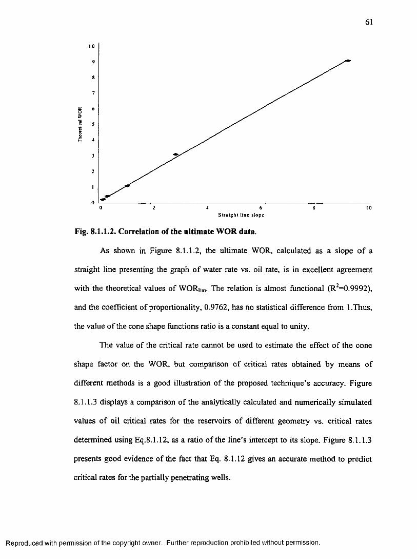
61

10

9

8

7

6

5

4

3

2

0 0 2 4 6 8 toS t r a i g h t l i ne s l o pe

Fig. 8.1.1.2. Correlation of the ultimate WOR data.

As shown in Figure 8.1.1.2, the ultimate WOR, calculated as a slope o f a

straight line presenting the graph of water rate vs. oil rate, is in excellent agreement

with the theoretical values of WOR|jm. The relation is almost functional (R2=0.9992),

and the coefficient of proportionality, 0.9762, has no statistical difference from 1 .Thus,

the value of the cone shape functions ratio is a constant equal to unity.

The value of the critical rate cannot be used to estimate the effect of the cone

shape factor on the WOR, but comparison of critical rates obtained by means of

different methods is a good illustration of the proposed technique’s accuracy. Figure

8.1.1.3 displays a comparison of the analytically calculated and numerically simulated

values of oil critical rates for the reservoirs of different geometry vs. critical rates

determined using Eq.8.1.12, as a ratio of the line’s intercept to its slope. Figure 8.1.1.3

presents good evidence of the fact that Eq. 8.1.12 gives an accurate method to predict

critical rates for the partially penetrating wells.


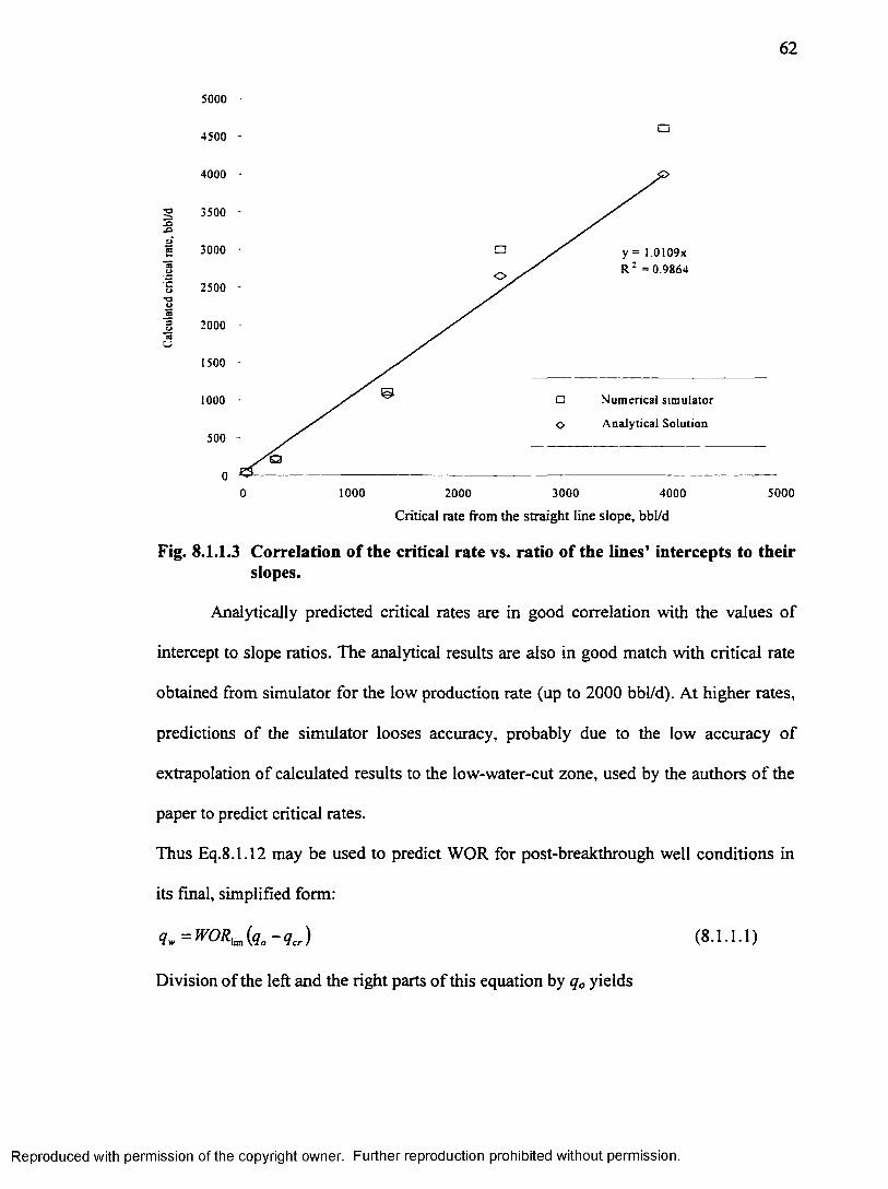
62

5000

4500 -

4000

3500.o•Ou

3000 □ceha y = l.0 I09x R 2 =0.9864Ocu 2500

■aua3UaCJ

2000

1500

Numerical sim ulator1000

Analytical Solution500

1000 3000 50000 2000 4000

Critical rate from the straight line slope, bbl/d

Fig. 8.1.1.3 Correlation of the critical rate vs. ratio of the lines’ intercepts to their slopes.

Analytically predicted critical rates are in good correlation with the values of

intercept to slope ratios. The analytical results are also in good match with critical rate

obtained from simulator for the low production rate (up to 2000 bbl/d). At higher rates,

predictions of the simulator looses accuracy, probably due to the low accuracy of

extrapolation of calculated results to the low-water-cut zone, used by the authors of the

paper to predict critical rates.

Thus Eq.8.1.12 may be used to predict WOR for post-breakthrough well conditions in

its final, simplified form:

9.= V O R im( q .- q „ ) (8.1.1.1)

Division of the left and the right parts of this equation by q0 yields


63

WOR = WO (8.1.1.2)9o

Or after taking in consideration that WC = WOR/( WOR+1), we obtain

WC = W C ,J 1— (8.1.1.3)V 9 J

8.1.2 Validation of the Method

In the previous paragraph, we established a relation between production rate and

water cut. The relation was obtained using the analitical steady state solution for

pressure destribution in the reservoir after water breakthrough. The unknown match

factor was found to be equal to unity by comparing the results from numerical

simulation with predictions of the relation. Now we are going to test the new relation

applying it to the results of the physical experiments using different model types and

fluids.

8.1.2.1 Radial Flow Model

Leverett, Lewis, and True (1942) studied the effect of production rate on water

cut on a cylindrical sand-packed model, having a one-foot inside diameter and height.

They used glycerin and S.A.E. 70 lubricating oil for the experiments. The fluids’

mobility ratio was 1.75. Thickness of the oil and glycerin zones were 16 and 8 inches

respectively. Thus, the ultimate glycerin cut (equivalent of water cut) determines as

follows:

Mk. _ ! - 7 5 . 8 . g047bm Mhw + h0 1.75*8 + 16

There is no approximation available to predict the critical rate for the completion the

authors used in their model: 2-foot length slots 5.5 feet above glycerin-oil contact. The

results of the experiments are presented in Table 8.1.2.1.1 and Figure 8.1.2.1.1.


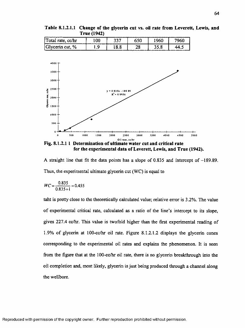
64

Table 8.1.2.1.1 Change of the glycerin cut vs. oil rate from Leverett, Lewis, and True (1942)

Total rate, cc/hr 100 337 650 1960 7960Glycerin cut, % 1.9 18.8 28 35.8 44.5

4 0 0 0 - -

3 5 0 0 - -

s 2 5 0 0 - -y » 0 8 3 5 * • 189 89

fC - 0 9 9 5 6

O 1 5 0 0 - -

1000 --

5 0 0 - -

0 500 1 000 1500 2000 2 5 0 0 3 0 0 0 3500 4 0 0 0 4 5 0 0 5 0 0 0

O il r a te , c c /h r

Fig. 8.1.2.1 1 Determination of ultimate water cut and critical ratefor the experimental data of Leverett, Lewis, and True (1942).

A straight line that fit the data points has a slope of 0.835 and intercept of -189.89.

Thus, the experimental ultimate glycerin cut (WC) is equal to

WC= 3-- =0.455 0.835+1

taht is pretty close to the theoretically calculated value; relative error is 3.2%. The value

of experimental critical rate, calculated as a ratio of the line’s intercept to its slope,

gives 227.4 cc/hr. This value is twofold higher than the first experimental reading of

1.9% of glycerin at 100-cc/hr oil rate. Figure 8.1.2.1.2 displays the glycerin cones

corresponding to the experimental oil rates and explains the phenomenon. It is seen

from the figure that at the 100-cc/hr oil rate, there is no glycerin breakthrough into the

oil completion and, most likely, glycerin is just being produced through a channel along

the wellbore.


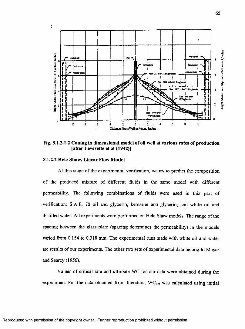
65

SmfcS n ii

fcae-237ccrtr( lSSKgtjoain)

Rac-78fiO cdr(44A i4yon i)

f ta c -1960 Gcrtr(3S8%gl)Gain)

84 1010 68 6 4 0 2Distance From Wfell in MxfeL, Inches

Fig. 8.1.2.1.2 Coning in dimensional model of oil well at various rates of production [after Leverette et al (1942)]

8.1.2.2 Hele-Shaw, Linear Flow Model

At this stage of the experimental verification, we try to predict the composition

of the produced mixture of different fluids in the same model with different

permeability. The following combinations of fluids were used in this part of

verification: S.A.E. 70 oil and glycerin, kerosene and glycerin, and white oil and

distilled water. All experiments were performed on Hele-Shaw models. The range of the

spacing between the glass plate (spacing determines the permeability) in the models

varied from 0.154 to 0.318 mm. The experimental runs made with white oil and water

are results of our experiments. The other two sets of experimental data belong to Mayer

and Searcy (1956).

Values of critical rate and ultimate WC for our data were obtained during the

experiment. For the data obtained from literature, WC|jm was calculated using initial


Hei

ght

Abo

ve

Free

G

lycc

rine

-Oil

Con

tact

, In

ches

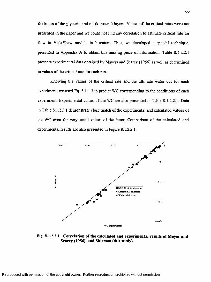
66

thickness of the glycerin and oil (kerosene) layers. Values of the critical rates were not

presented in the paper and we could not find any correlation to estimate critical rate for

flow in Hele-Shaw models in literature. Thus, we developed a special technique,

presented in Appendix A to obtain this missing piece of information. Table 8.1.2.2.1

presents experimental data obtained by Mayers and Searcy (1956) as well as determined

in values of the critical rate for each run.

Knowing the values of the critical rate and the ultimate water cut for each

experiment, we used Eq. 8.1.1.3 to predict WC corresponding to the conditions o f each

experiment. Experimental values of the WC are also presented in Table 8.1.2.2.1. Data

in Table 8.1.2.2.1 demonstrate close match of the experimental and calculated values of

the WC even for very small values of the latter. Comparison of the calculated and

experimental results are also presented in Figure 8.1.2.2.1.

0.0001 0.001 0.01

0 .01

■ SAK 70 oil & glycerine ♦ Kerosene & glycerine ▲ W hite oil & water

0.001

0.0001

Fig. 8.1.2.2.1 Correlation of the calculated and experimental results of Meyer and Searcy (1956), and Shirman (this study).


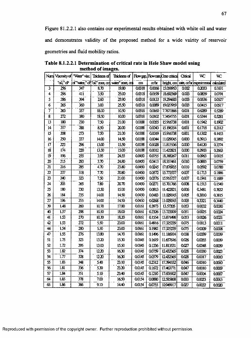
67

Figure 81.2.2.1 also contains our experimental results obtained with white oil and water

and demonstrates validity of the proposed method for a wide vairity of reservoir

geometries and fluid mobility ratios.

Table 8.1.2.2.1 Determination of critical rate in Hele Shaw model usingmethod of images.

Mm Visccstycf "Wta',visc. Thickness cf Thickness of Flowgp, FfovnteGbneoitka Qitical WC WC"ofl,"cP cf"wafa;"cf "nil" Tme, nr watef'2HE.cni cm ccftr height, an iate,ccftr pxppiingta caknlafrri

3 256 347 870 19.80 00318 00066 15.050953 0002 02033 016314 296 411 350 25.00 00318 00199 18(92369 0003 00839 007915 286 39* 260 25.90 00318 00133 1929*603 0003 00536 OQ5276 265 360 3.00 2550 OQ318 00089 19.027919 0.003 00*15 005177 263 357 1800 1050 OGB18 00160 7.7671866 Q001 06289 052898 272 380 1850 1Q00 QQ318 00102 72454755 0001 05244 0528113 180 230 750 21.00 00188 00055 15.916738 0001 01942 0190214 217 288 850 2000 00188 00043 15.196354 aooi 01718 0211215 208 273 750 21.00 00188 00019 15.916738 0001 01302 0145316 250 337 14.00 1450 00188 00044 11.0290*5 QOOO 0390 0389217 223 296 13.00 1550 00188 00028 11.813536 QOOO 04120 0337418 174 220 1350 15.00 00188 00012 11.422821 aooo 02903 0266319 196 255 3.95 2455 00450 00755 18288267 aon 00963 0093520 215 283 3.70 24.80 00450 00*13 18557461 ooio 00885 Q075921 216 285 4.70 23.80 00450 OQ245 17.876935 aoio 00592 0078022 237 318 7.70 2Q80 00450 00572 15.773537 0007 0170 0188623 240 323 750 21.00 00150 Q0376 15516737 0007 019*1 0168924 203 265 7.80 2070 00450 00271 15.701766 0008 0150 0154025 180 230 1350 15.00 00150 0080 11.422821 0006 03481 0383226 184 235 14.00 1450 0.0150 00183 11.029045 0005 03810 0381527 196 255 14.00 1450 00450 00268 11.0290*5 0005 03321 0344039 1.48 260 1Q70 17.80 00161 0L3973 057205 0053 00032 0003040 157 298 1050 1800 00161 02326 0.722009 0051 00025 0002441 153 270 1030 1820 00161 01554 0.871498 0053 00006 0002142 153 272 550 23.00 00161 04916 17225229 0075 OOOO Q001144 154 280 550 23.00 00161 01982 17225229 0075 00009 0000847 155 276 0.80 1470 00161 01496 11.186924 0038 00039 0003951 1.75 323 020 1520 00145 01619 11.657616 0026 00055 0003952 1.72 295 0.00 1550 00145 0036 11.813531 0027 00048 0003953 1.82 374 1220 1630 00145 00759 12432365 0028 OOOBO 0002354 1.77 328 1220 1630 00145 00379 12432365 0028 00017 Q001055 1.83 348 5.40 23.10 00145 02312 1729*552 0016 aooio aooio56 1.81 336 520 2320 00145 01672 17.463771 0047 aooio 0000957 1.8* 351 5.10 2140 00145 01210 17.601902 0017 OOOO* 000076* 1.85 378 7.00 1650 00154 00680 12585868 0033 00023 0001365 1.86 386 9.10 14.40 00154 00755 109*9917 0027 00032 00020


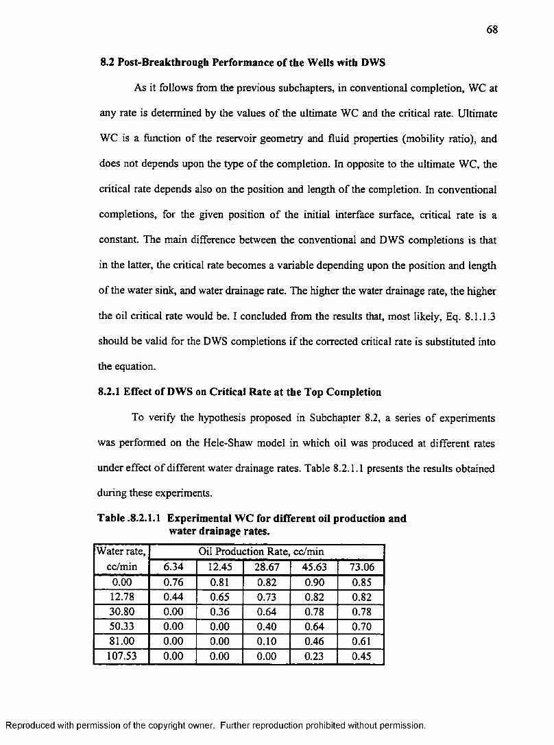
68

8.2 Post-Breakthrough Performance of the Wells with DWS

As it follows from the previous subchapters, in conventional completion, WC at

any rate is determined by the values of the ultimate WC and the critical rate. Ultimate

WC is a function of the reservoir geometry and fluid properties (mobility ratio), and

does not depends upon the type of the completion. In opposite to the ultimate WC, the

critical rate depends also on the position and length of the completion. In conventional

completions, for the given position of the initial interface surface, critical rate is a

constant. The main difference between the conventional and DWS completions is that

in the latter, the critical rate becomes a variable depending upon the position and length

of the water sink, and water drainage rate. The higher the water drainage rate, the higher

the oil critical rate would be. I concluded from the results that, most likely, Eq. 8.1.1.3

should be valid for the DWS completions if the corrected critical rate is substituted into

the equation.

8.2.1 Effect of DWS on Critical Rate at the Top Completion

To verify the hypothesis proposed in Subchapter 8.2, a series of experiments

was performed on the Hele-Shaw model in which oil was produced at different rates

under effect of different water drainage rates. Table 8.2.1.1 presents the results obtained

during these experiments.

Table .8.2.1.1 Experimental WC for different oil production and water drainage rates.

Water rate, cc/min

Oil Production Rate, cc/min6.34 12.45 28.67 45.63 73.06

0.00 0.76 0.81 0.82 0.90 0.8512.78 0.44 0.65 0.73 0.82 0.8230.80 0.00 0.36 0.64 0.78 0.7850.33 0.00 0.00 0.40 0.64 0.7081.00 0.00 0.00 0.10 0.46 0.61107.53 0.00 0.00 0.00 0.23 0.45


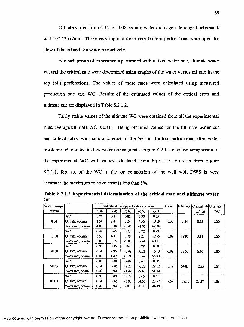
69

Oil rale varied from 6.34 to 73.06 cc/min; water drainage rate ranged between 0

and 107.53 cc/min. Three very top and three very bottom perforations were open for

flow of the oil and the water respectively.

For each group of experiments performed with a fixed water rate, ultimate water

cut and the critical rate were determined using graphs of the water versus oil rate in the

top (oil) perforations. The values of these rates were calculated using measured

production rate and WC. Results of the estimated values of the critical rates and

ultimate cut are displayed in Table 8.2.1.2.

Fairly stable values of the ultimate WC were obtained from all the experimental

runs; average ultimate WC is 0.86. Using obtained values for the ultimate water cut

and critical rates, we made a forecast of the WC in the top perforations after water

breakthrough due to the low water drainage rate. Figure 8.2.1.1 displays comparison of

the experimental WC with values calculated using Eq.8.1.13. As seen from Figure

8.2.1.1, forecast o f the WC in the top completion of the well with DWS is very

accurate: the maximum relative error is less than 8%.

Table 8.2.1.2 Experimental determination of the critical rate and ultimate water cutWale drainage,

cc/minTotal rate at the top perforations, cc/min Slope Intercept Critical rati

cc/minUltimate

WC6.34 1145 28.67 45.63 73.06

0.00WCOil rate, cc/min Water rate, cc/min

0.761.544.81

0.8114110.04

0.825.2423.43

0.904.56

41.06

0.8510.696136

6.30 3.34 0.53 0.86

1178WCOil rate, cc/min Water rate, cc/min

0.443.53181

0.654.318.15

0.737.79

20.88

0.828.21

37.41

0.82119560.11

6.09 18.91 3.11 0.86

30.80WCOil rate, cc/min Water rate, cc/rrrin

0.006340.00

0.367.964.49

0.6410.4218.24

0.7810.2135.42

0.7816.1356.93

6.02 38.53 6.40 0.86


0.006.340.00

0.0011450.00

0.4017.2011.47

0.6416.2229.40

0.70210251.04

5.17 64.87 1155 0.84


0.006.340.00

0.0011450.00

0.1025.80187

0.4624.6520.98

0.6128.5744.49

7.67 179.16 23.37 0.88


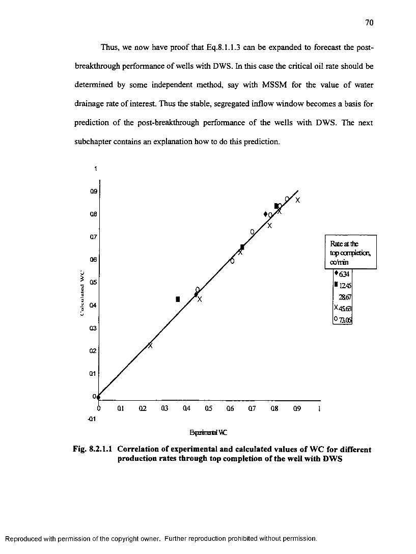
70

Thus, we now have proof that Eq.8.1.1.3 can be expanded to forecast the post

breakthrough performance of wells with DWS. In this case the critical oil rate should be

determined by some independent method, say with MSSM for the value of water

drainage rate of interest. Thus the stable, segregated inflow window becomes a basis for

prediction of the post-breakthrough performance of the wells with DWS. The next

subchapter contains an explanation how to do this prediction.

1

Q9

Q7

06jt 053

3

03

02

-01

Rate at thetopcarpletion,cc/rrin

*63A■1245

2867

X 45.63

07106

BpsmutaiWI

Fig. 8.2.1.1 Correlation of experimental and calculated values of WC for different production rates through top completion of the well with DWS


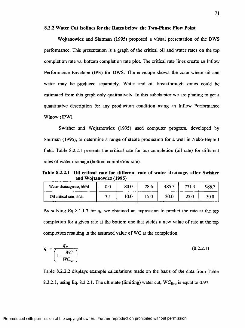
71

8.2.2 Water Cut Isolines for the Rates below the Two-Phase Flow Point

Wojtanowicz and Shirman (1995) proposed a visual presentation of the DWS

performance. This presentation is a graph of the critical oil and water rates on the top

completion rate vs. bottom completion rate plot. The critical rate lines create an Inflow

Performance Envelope (IPE) for DWS. The envelope shows the zone where oil and

water may be produced separately. Water and oil breakthrough zones could be

estimated from this graph only qualitatively. In this subchapter we are planing to get a

quantitative description for any production condition using an Inflow Performance

Winow (IPW).

Swisher and Wojtanowicz (1995) used computer program, developed by

Shirman (1995), to determine a range of stable production for a well in Nebo-Hephill

field. Table 8.2.2.1 presents the critical rate for top completion (oil rate) for different

rates of water drainage (bottom completion rate).

Table 8.2.2.1 Oil critical rate for different rate of water drainage, after Swisher and Wojtanowicz (1995)

Water drainagerate, bbl/d 0.0 80.0 28.6 485.3 771.4 986.7

Oil critical rate, bbl/d 7.5 10.0 15.0 20.0 25.0 30.0

By solving Eq 8.1.1.3 for qt, we obtained an expression to predict the rate at the top

completion for a given rate at the bottom one that yields a new value of rate at the top

completion resulting in the assumed value of WC at the completion.

' • - r X c \ (8'2'2 1 >

Table 8.2.2.2 displays example calculations made on the basis of the data from Table

8.2.2.1, using Eq. 8.2.2.1. The ultimate (limiting) water cut, WC|,m, is equal to 0.97.


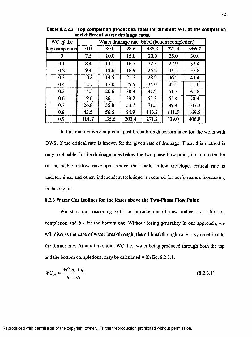
72

Table 8.2.2.2 Top completion production rates for different WC at the completion and different water drainage rates.

W C@ the top completion

Water drainage rate, bbl/d (bottom completion)0.0 80.0 28.6 485.3 771.4 986.7

0 7.5 10.0 15.0 20.0 25.0 30.00.1 8.4 11.1 16.7 22.3 27.9 33.40.2 9.4 12.6 18.9 25.2 31.5 37.80.3 10.8 14.5 21.7 28.9 36.2 43.40.4 12.7 17.0 25.5 34.0 42.5 51.00.5 15.5 20.6 30.9 41.2 51.5 61.80.6 19.6 26.1 39.2 52.3 65.4 78.40.7 26.8 35.8 53.7 71.5 89.4 107.30.8 42.5 56.6 84.9 113.2 141.5 169.80.9 101.7 135.6 203.4 271.2 339.0 406.8

In this manner we can predict post-breakthrough performance for the wells with

DWS, if the critical rate is known for the given rate of drainage. Thus, this method is

only applicable for the drainage rates below the two-phase flow point, i.e., up to the tip

of the stable inflow envelope. Above the stable inflow envelope, critical rate is

undetermined and other, independent technique is required for performance forecasting

in this region.

8.2.3 Water Cut Isolines for the Rates above the Two-Phase Flow Point

We start our reasoning with an introduction of new indices: t - for top

completion and b - for the bottom one. Without losing generality in our approach, we

will discuss the case of water breakthrough; the oil breakthrough case is symmetrical to

the former one. At any time, total WC, i.e., water being produced through both the top

and the bottom completions, may be calculated with Eq. 8.2.3.1.

WCto, = WC,q‘ +- b- (8.2.3.1)<1, +<lb


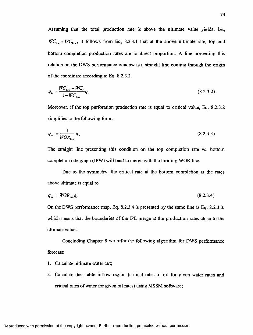
73

Assuming that the total production rate is above the ultimate value yields, i.e.,

WCtot ~ WC]im, it follows from Eq, 8.2.3.1 that at the above ultimate rate, top and

bottom completion production rates are in direct proportion. A line presenting this

relation on the DWS performance window is a straight line coming through the origin

of the coordinate according to Eq. 8.2.3.2.

WC -W Cq = ---- —------- -q (8.2.3.2)

l ~ w c um

Moreover, if the top perforation production rate is equal to critical value, Eq. 8.2.3.2

simplifies to the following form:

q „ = ---- qb (8.2.3.3)WORlimVi

The straight line presenting this condition on the top completion rate vs. bottom

completion rate graph (IPW) will tend to merge with the limiting WOR line.

Due to the symmetry, the critical rate at the bottom completion at the rates

above ultimate is equal to

qcr ~ WORiimqt (S.2.3.4)

On the DWS performance map, Eq. 8.2.3.4 is presented by the same line as Eq. 8.2.3.3,

which means that the boundaries of the IPE merge at the production rates close to the

ultimate values.

Concluding Chapter 8 we offer the following algorithm for DWS performance

forecast:

1. Calculate ultimate water cut;

2. Calculate the stable inflow region (critical rates of oil for given water rates and

critical rates of water for given oil rates) using MSSM software;


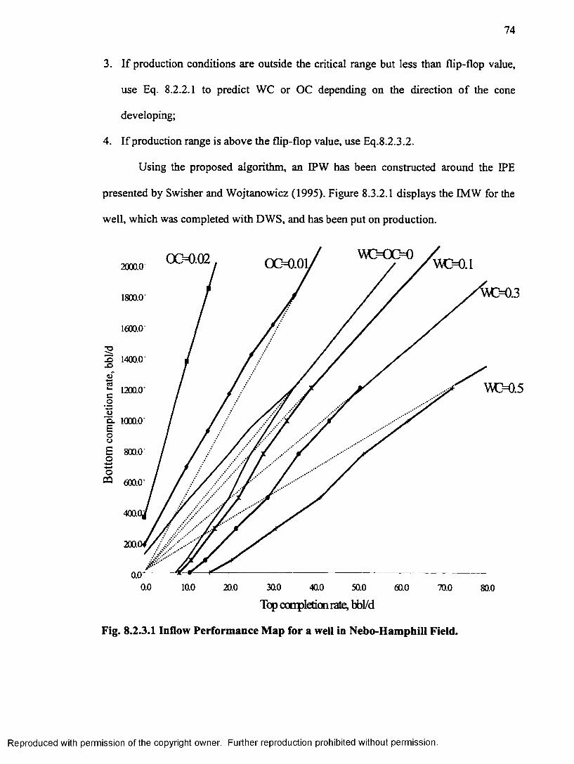
74

3. If production conditions are outside the critical range but less than flip-flop value,

use Eq. 8.2.2.1 to predict WC or OC depending on the direction of the cone

developing;

4. If production range is above the flip-flop value, use Eq.8.2.3.2.

Using the proposed algorithm, an IPW has been constructed around the IPE

presented by Swisher and Wojtanowicz (1995). Figure 8.3.2.1 displays the IMW for the

well, which was completed with DWS, and has been put on production.

0 0 0 .0 2 00=0.012000.0

1800.0

1600.0

;o3 1400.0X)

S 1200.0c_o

"5. 1000.0EoZJE 800.0 o

600.0'

200.1

0.0'0.0 10.0 30.020.0 40.0 50.0 60.0 70.0 80.0

Top completion rate, bbl/d

Fig. 8.2.3.1 Inflow Performance Map for a well in Nebo-Hamphill Field.


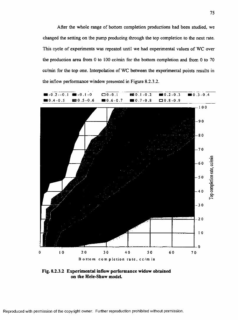
75

After the whole range of bottom completion productions had been studied, we

changed the setting on the pump producing through the top completion to the next rate.

This cycle of experiments was repeated until we had experimental values of WC over

the production area from 0 to 100 cc/min for the bottom completion and from 0 to 70

cc/min for the top one. Interpolation of WC between the experimental points results in

the inflow performance window presented in Figure 8.2.3.2.

I-0.2--0.1 S - 0 . 1 - 0 □0- 0 . 1 S O . 1-0.2 S O . 2-0.310.4-0.5 S O . 5-0.6 S O . 6-0.7 S O . 7-0.8 0 0 . 8 - 0 . 9

1 0 20 30 40 50 60Bot tom complet ion rate, cc/min

10.3-0.4

1 00

70

Fig. 8.2.3.2 Experimental inflow performance widow obtained on the Hele-Shaw model.

Reproduced with permission of the copyright owner. Further reproduction prohibited without permission

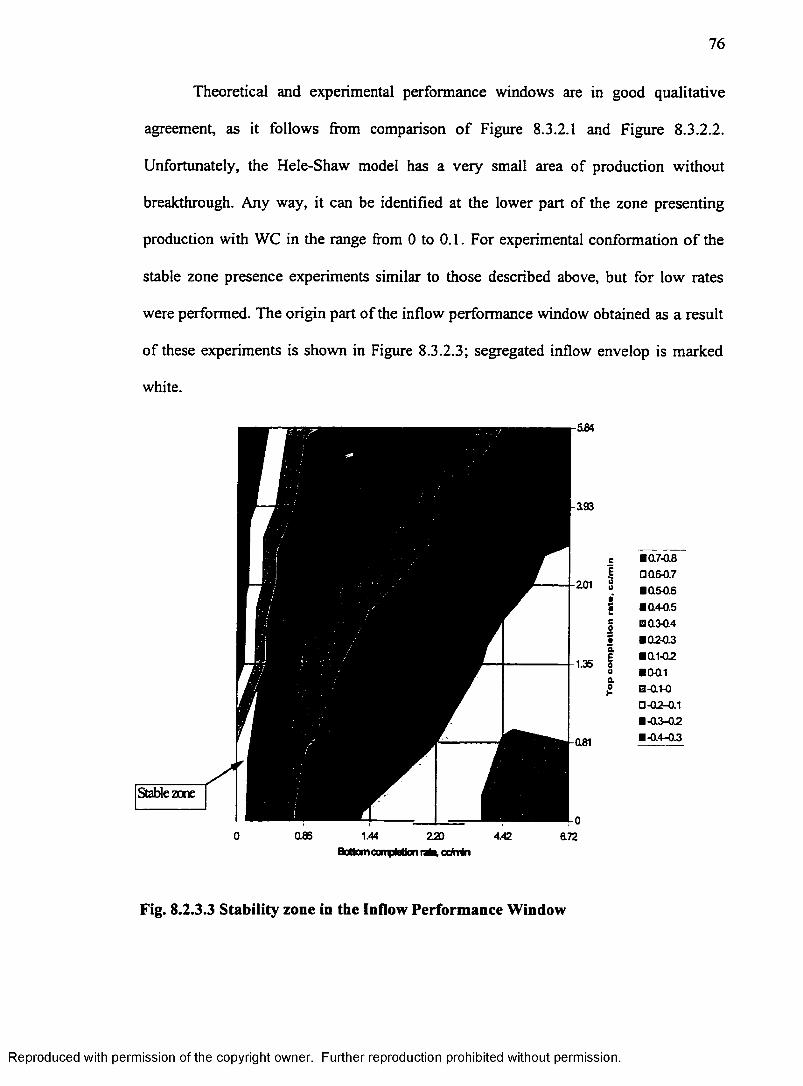
76

Theoretical and experimental performance windows are in good qualitative

agreement, as it follows from comparison o f Figure 8.3.2.1 and Figure 8.3.2.2.

Unfortunately, the Hele-Shaw model has a very small area of production without

breakthrough. Any way, it can be identified at the lower part of the zone presenting

production with WC in the range from 0 to 0.1. For experimental conformation of the

stable zone presence experiments similar to those described above, but for low rates

were performed. The origin part of the inflow performance window obtained as a result

of these experiments is shown in Figure 8.3.2.3; segregated inflow envelop is marked

white.

■ 07-08□ Q&0.7■ 0.50.6■ Q4-0.5□ 0 5 0 .4

■ 0 2 0 .3■ 01-02■ 00L1 Q -0.1-0 0 -0 2 -0 .1 ■ -03 -02■ -0 4 -0 3

Bonoro conpwuon ccmin

Fig. 8.2.3.3 Stability zone in the Inflow Performance Window


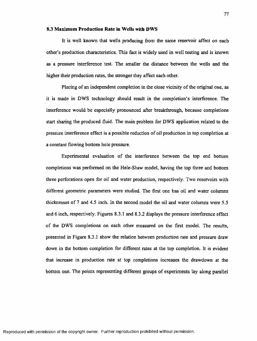
77

8.3 Maximum Production Rate in Wells with DWS

It is well known that wells producing from the same reservoir affect on each

other’s production characteristics. This fact is widely used in well testing and is known

as a pressure interference test. The smaller the distance between the wells and the

higher their production rates, the stronger they affect each other.

Placing of an independent completion in the close vicinity of the original one, as

it is made in DWS technology should result in the completion’s interference. The

interference would be especially pronounced after breakthrough, because completions

start sharing the produced fluid. The main problem for DWS application related to the

pressure interference effect is a possible reduction of oil production in top completion at

a constant flowing bottom hole pressure.

Experimental evaluation of the interference between the top end bottom

completions was performed on the Hele-Shaw model, having the top three and bottom

three perforations open for oil and water production, respectively. Two reservoirs with

different geometric parameters were studied. The first one has oil and water columns

thicknesses of 7 and 4.5 inch. In the second model the oil and water columns were 5.5

and 6 inch, respectively. Figures 8.3.1 and 8.3.2 displays the pressure interference effect

of the DWS completions on each other measured on the first model. The results,

presented in Figure 8.3.1 show the relation between production rate and pressure draw

down in the bottom completion for different rates at the top completion. It is evident

that increase in production rate at top completions increases the drawdown at the

bottom one. The points representing different groups of experiments lay along parallel


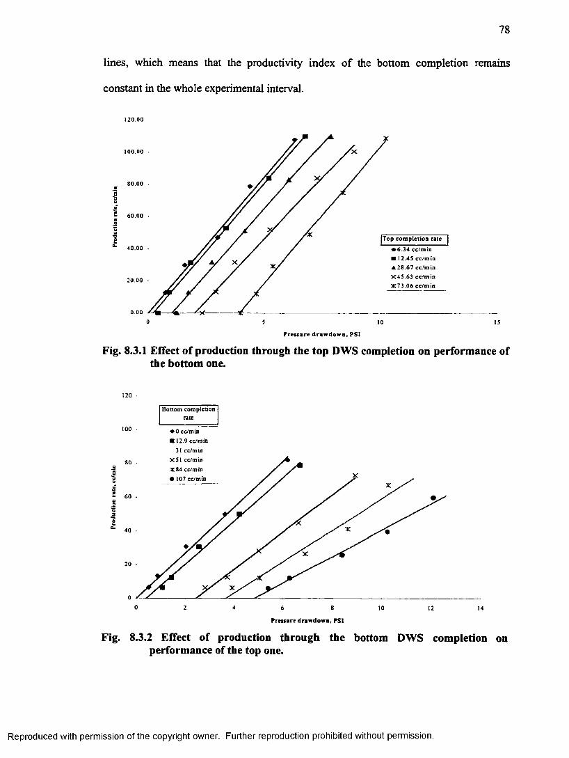
78

lines, which means that the productivity index of the bottom completion remains

constant in the whole experimental interval.

120.00

100.00 •

80.00 .sBw2 60.00 •eoua

Top comple tion rate£40.00 • ♦ 6.34 cc/m in

■ 12.45 cc/m in ▲ 28.67 cc/m in X 45 .63 cc/m in X 73 .06 cc/m in

20.00 •

0.00

0 5 10

Pressure d raw dow n, PSI

Fig. 8.3.1 Effect of production through the top DWS completion on performance of the bottom one.

120 -

Bottom completion rate

♦ 0 cc/min ■ 12.9 cc/min

31 cc/minX S l cc/mtn X84 cc/min • 107 cc/mtn

30

60

40

20

00 4 86 10 12 14

Pressure draw dow n, PSI

Fig. 8.3.2 Effect of production through the bottom DWS completion on performance of the top one.


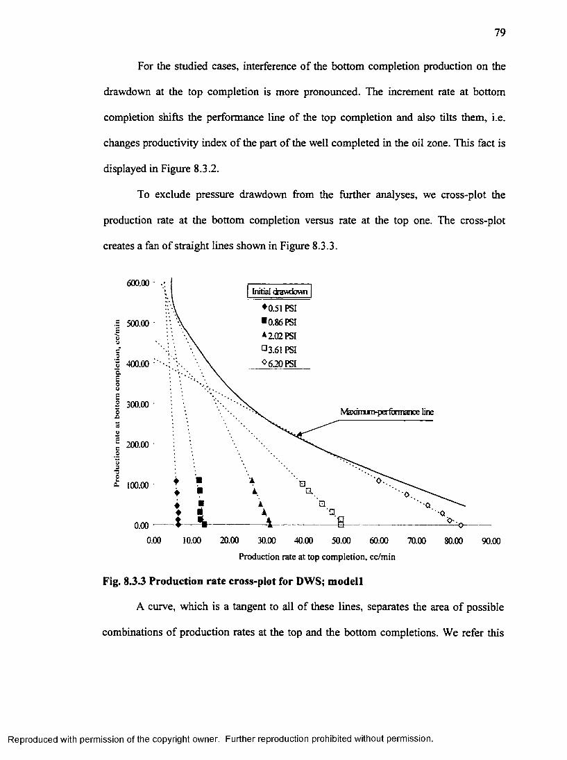
79

For the studied cases, interference of the bottom completion production on the

drawdown at the top completion is more pronounced. The increment rate at bottom

completion shifts the performance line of the top completion and also tilts them, i.e.

changes productivity index of the part of the well completed in the oil zone. This fact is

displayed in Figure 8.3.2.

To exclude pressure drawdown from the further analyses, we cross-plot the

production rate at the bottom completion versus rate at the top one. The cross-plot

creates a fan of straight lines shown in Figure 8.3.3.

600.00

♦0.51 PSI ■0.86 PSI *2.02 PSI °3.61 PSI <>620 PSI

cS"N.

500.00uu

I 400.00 ; "5.Eo

3 300.00 -o&3

Max3mjrr>perfoniiance line

V

“ 200.00Jjo3

■3O£ 100.00

<>-.0.0020.000.00 10.00 30.00 40.00 60.0050.00 70.00 80.00 90.00

Production rate at top completion, cc/min

Fig. 8.3.3 Production rate cross-plot for DWS; modell

A curve, which is a tangent to all of these lines, separates the area of possible

combinations of production rates at the top and the bottom completions. We refer this


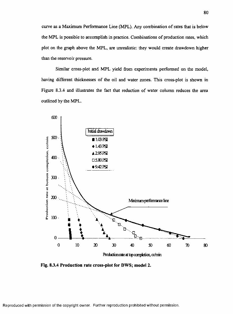
80

curve as a Maximum Performance Line (MPL). Any combination of rates that is below

the MPL is possible to accomplish in practice. Combinations of production rates, which

plot on the graph above the MPL, are unrealistic: they would create drawdown higher

than the reservoir pressure.

Similar cross-plot and MPL yield from experiments performed on the model,

having different thicknesses of the oil and water zones. This cross-plot is shown in

Figure 8.3.4 and illustrates the fact that reduction of water column reduces the area

outlined by the MPL.

600

■ l.CSPSE♦ 1.43 PSI 1295PSI □ 5.80 PSI• 9.42 PSI

s 400-

200Nfejnunperfamance line

200 10 30 40 50 60 8070

ftodbcticnrEle at top ccrrpleticn, ocfain

Fig. 8.3.4 Production rate cross-plot for DWS; model 2.


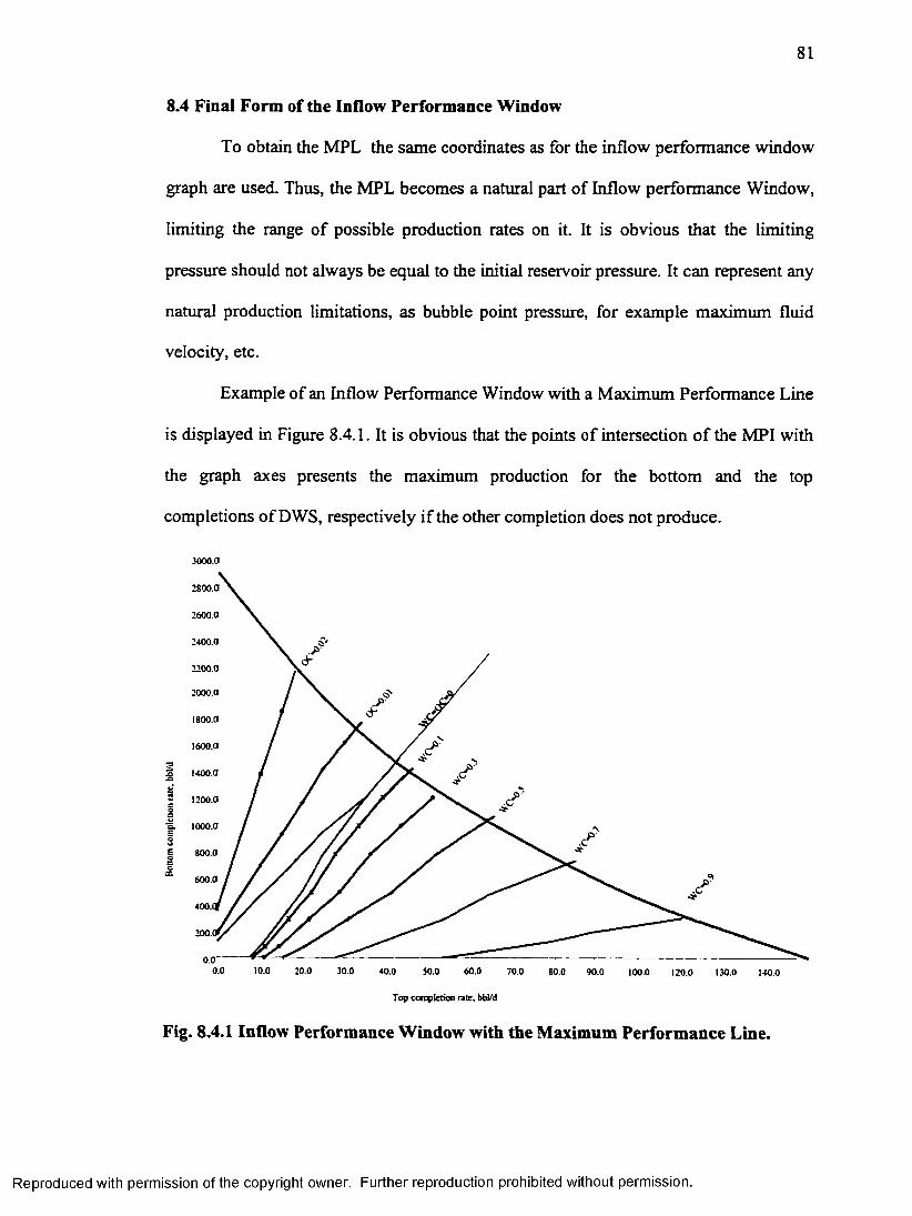
81

8.4 Final Form of the Inflow Performance Window

To obtain the MPL the same coordinates as for the inflow performance window

graph are used. Thus, the MPL becomes a natural part of Inflow performance Window,

limiting the range of possible production rates on it. It is obvious that the limiting

pressure should not always be equal to the initial reservoir pressure. It can represent any

natural production limitations, as bubble point pressure, for example maximum fluid

velocity, etc.

Example of an Inflow Performance Window with a Maximum Performance Line

is displayed in Figure 8.4.1. It is obvious that the points of intersection of the MPI with

the graph axes presents the maximum production for the bottom and the top

completions of DWS, respectively if the other completion does not produce.

3000.0

2400.0

2200.0

2000.0

2oso■aw

1000.0a.EouEo8©CD

800.0

400.(

200.1

0.0~"0.0 10.0 30.020.0 50.0 60.0 70.040.0 80.0 90.0 100.0 130.0120.0 140.0

Top completion rate, bbl/d

Fig. 8.4.1 Inflow Performance Window with the Maximum Performance Line.


CHAPTER 9

USE OF GENERALIZED MODEL FOR OIL-WATER INTERFACE PROFILE PREDICTION

9.1 Calculation Method

Algorithm described in Chapter 7 has a limitation that the assumed WOR is

proportional to the ratio of the areas open to water and oil. As we have shown, the WC

depends also on the shape of the cone, which creates a problem with two independent

unknowns. The fact that we can predict the equilibrium WC at a given production rate

using Eq. 8.1.1.3 is very helpful in reducing the number of unknown parameters. Use of

Eq. 8.1.1.3 makes the position of the cone in the well completion to be the only

unknown parameter. A corrected algorithm to determine the interface profile is

constructed as follows:

1. Calculate critical rate and ultimate WC for the given reservoir and fluid

properties;

2. If given production rate is below critical, there is no breakthrough in the well;

3. Otherwise use Eq. 8.1.1.3. to calculate WC;

4. Assume the interface position in the well;

5. Assume that oil is produced from both the oil and water zones and calculate the

pressure drawdown in the reservoir due to the production of this fluid through

the top part o f the completion (above assumed WOI);

6. Assume that water is produced from both the oil and water zones and calculate

pressure drawdown in the reservoir due to the production of this fluid through

the bottom part of the completion (below assumed WOI);

7. Calculate the difference between the pressures determined in the steps 5 and 6.

82


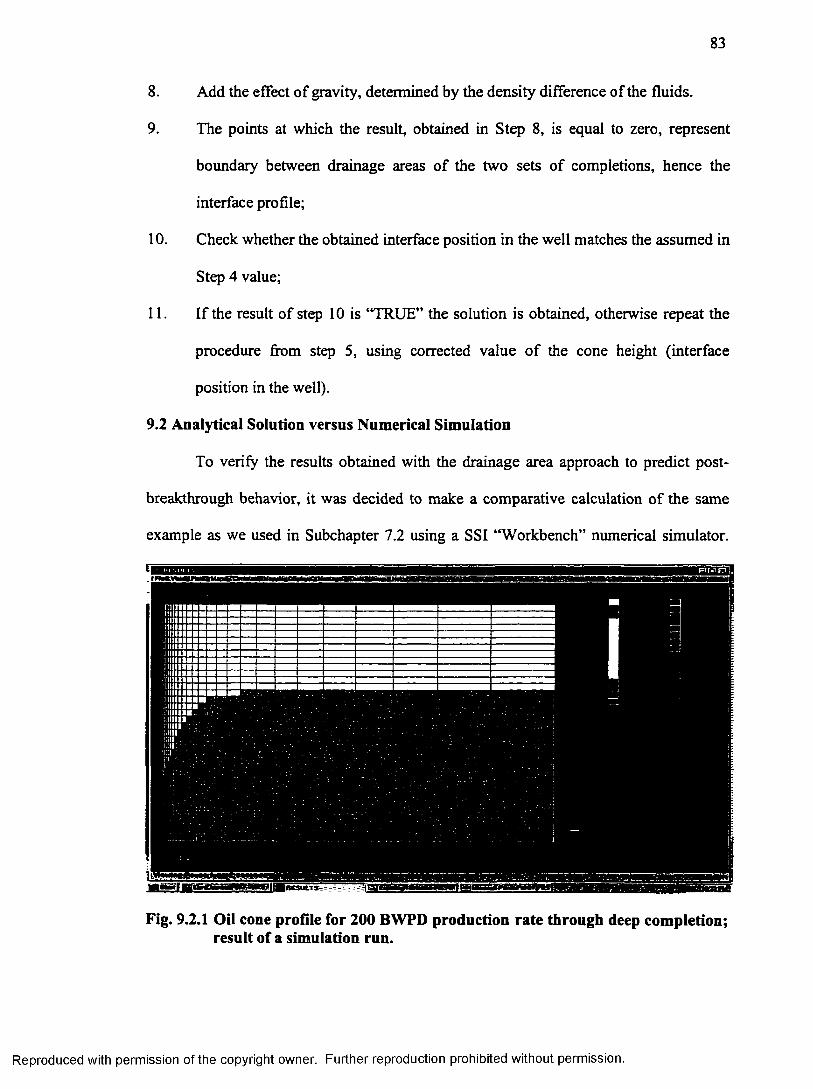
83

8. Add the effect of gravity, determined by the density difference of the fluids.

9. The points at which the result, obtained in Step 8, is equal to zero, represent

boundary between drainage areas of the two sets of completions, hence the

interface profile;

10. Check whether the obtained interface position in the well matches the assumed in

Step 4 value;

11. If the result of step 10 is “TRUE” the solution is obtained, otherwise repeat the

procedure from step 5, using corrected value of the cone height (interface

position in the well).

9.2 Analytical Solution versus Numerical Simulation

To verify the results obtained with the drainage area approach to predict post-

breakthrough behavior, it was decided to make a comparative calculation of the same

example as we used in Subchapter 7.2 using a SSI “Workbench” numerical simulator.

MHaaiwariirr ■iwin—niiMBcautTs r -- -jiawa

Fig. 9.2.1 Oil cone profile for 200 BWPD production rate through deep completion; result of a simulation run.


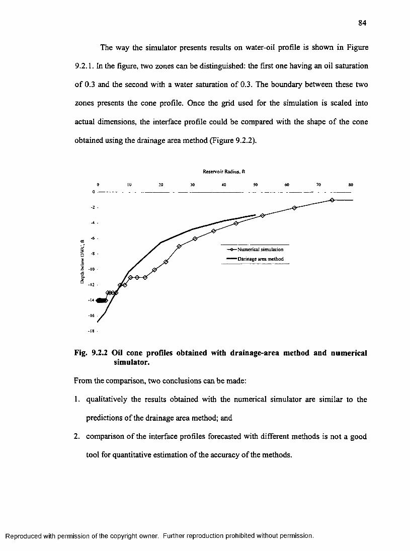
84

The way the simulator presents results on water-oil profile is shown in Figure

9.2.1. In the figure, two zones can be distinguished: the first one having an oil saturation

of 0.3 and the second with a water saturation of 0.3. The boundary between these two

zones presents the cone profile. Once the grid used for the simulation is scaled into

actual dimensions, the interface profile could be compared with the shape of the cone

obtained using the drainage area method (Figure 9.2.2).

R e se rv o ir R a d iu s , ft

0 to 20 30 40 50 60 70 80

0 ----

<r

- ❖ —N u m erica l s im u la tio n

D arin ag e a re a m e th o d

1xc.X

-14

-18

Fig. 9.2.2 Oil cone profiles obtained with drainage-area method and numerical simulator.

From the comparison, two conclusions can be made:

1. qualitatively the results obtained with the numerical simulator are similar to the

predictions of the drainage area method; and

2. comparison of the interface profiles forecasted with different methods is not a good

tool for quantitative estimation of the accuracy of the methods.


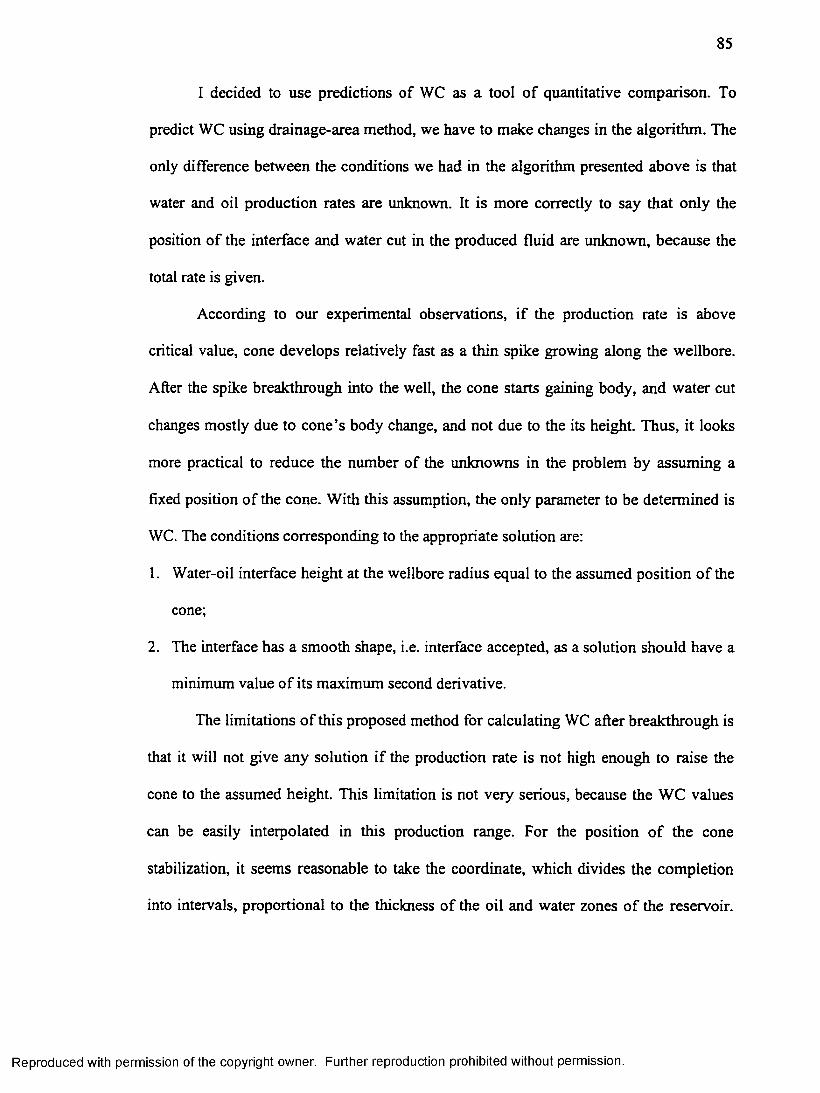
85

I decided to use predictions of WC as a tool of quantitative comparison. To

predict WC using drainage-area method, we have to make changes in the algorithm. The

only difference between the conditions we had in the algorithm presented above is that

water and oil production rates are unknown. It is more correctly to say that only the

position of the interface and water cut in the produced fluid are unknown, because the

total rate is given.

According to our experimental observations, if the production rate is above

critical value, cone develops relatively fast as a thin spike growing along the wellbore.

After the spike breakthrough into the well, the cone starts gaining body, and water cut

changes mostly due to cone’s body change, and not due to the its height. Thus, it looks

more practical to reduce the number of the unknowns in the problem by assuming a

fixed position of the cone. With this assumption, the only parameter to be determined is

WC. The conditions corresponding to the appropriate solution are:

1. Water-oil interface height at the wellbore radius equal to the assumed position of the

cone;

2. The interface has a smooth shape, i.e. interface accepted, as a solution should have a

minimum value of its maximum second derivative.

The limitations of this proposed method for calculating WC after breakthrough is

that it will not give any solution if the production rate is not high enough to raise the

cone to the assumed height. This limitation is not very serious, because the WC values

can be easily interpolated in this production range. For the position of the cone

stabilization, it seems reasonable to take the coordinate, which divides the completion

into intervals, proportional to the thickness of the oil and water zones of the reservoir.


86

The estimation of the WC made with this simplified method is presented in Figure 9.2.3.

The same figure displays the results obtained for the same case using a numerical

simulator and simplified an analytical model described in Chapter 8. It is evident that all

three methods describe the oil cut development in drained water in a similar way. The

maximum difference in the value of the oil cut predicted by the analytical model and by

the other two methods are not greater than 0.01.

o .i —

0 . 0 9 ------

0 . 0 8 ------

0 . 0 7

0 . 0 6 ------

= 0 . 0 5 ------ /

° 0 . 0 4 A. [ 2 .

0 . 0 3 ------

A N u n e r i c a l s im u l a t o r

^ D r a i n a g e a r e a m e t h o d

A n a l v t i c a l m o d e l ______

0 . 0 2 -----

0.01 1

1000 200 3 0 0 4 0 0 5 0 0 6 0 0

Wate r d r a i na ge rate, bbl /d

Fig. 9.2.3 Oil cut in reversed cone at different rate of water drainage.

It seems reasonable to use the drainage area method to predict interface profiles for

post-breakthrough conditions. There is no need to use complicated techniques such as

numerical simulators or the drainage area method to calculate stabilized fluid saturation

in the production stream; the analytical Eq. 8.2.2.1 derived in Chapter 8 gives

reasonable results.


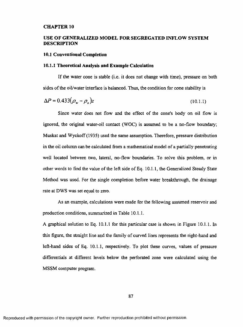
CHAPTER 10

USE OF GENERALIZED MODEL FOR SEGREGATED INFLOW SYSTEM DESCRIPTION

10.1 Conventional Completion

10.1.1 Theoretical Analysis and Example Calculation

If the water cone is stable (i.e. it does not change with time), pressure on both

sides of the oil/water interface is balanced. Thus, the condition for cone stability is

Since water does not flow and the effect of the cone's body on oil flow is

ignored, the original water-oil contact (WOC) is assumed to be a no-flow boundary;

Muskat and Wyckoff (1935) used the same assumption. Therefore, pressure distribution

in the oil column can be calculated from a mathematical model of a partially penetrating

well located between two, lateral, no-flow boundaries. To solve this problem, or in

other words to find the value of the left side of Eq. 10.1.1, the Generalized Steady State

Method was used. For the single completion before water breakthrough, the drainage

rate at DWS was set equal to zero.

As an example, calculations were made for the following assumed reservoir and

production conditions, summarized in Table 10.1.1.

A graphical solution to Eq. 10.1.1 for this particular case is shown in Figure 10.1.1. In

this figure, the straight line and the family of curved lines represents the right-hand and

left-hand sides of Eq. 10.1.1, respectively. To plot these curves, values of pressure

differentials at different levels below the perforated zone were calculated using the

MSSM computer program.

( 10. 1.1)

87


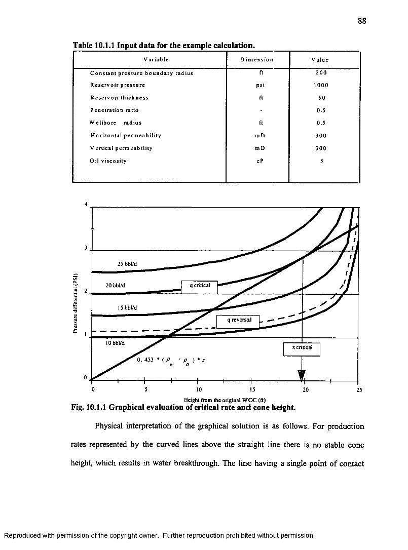
88

Table 10.1.1 Input data for the example calculation.V a r i a b l e D i m e n s i o n V a lu e

C o n s t a n t p r e s s u r e b o u n d a r y r ad ius ft 2 00

R e s e rv o i r p r e s su re ps i 1000

R e s e r v o i r t h i c k n e s s ft 50

Pen e t r a t i o n rat io - 0.5

W e l l b o r e r ad iu s ft 0.5

H or i z o n t a l p e r m e a b i l i t y m D 30 0

V er t i c a l p e r m e a b i l i t y m D 3 0 0

Oi l v i s cos i t y cP 5

4

3

25 bbl/d

q critical2

15 bbl/d

q reversal

10 bbl/dz critical

00 5 10 15 20 25

Height from the original W OC (ft)Fig. 10.1.1 Graphical evaluation of critical rate and cone height

Physical interpretation of the graphical solution is as follows. For production

rates represented by the curved lines above the straight line there is no stable cone

height, which results in water breakthrough. The line having a single point of contact


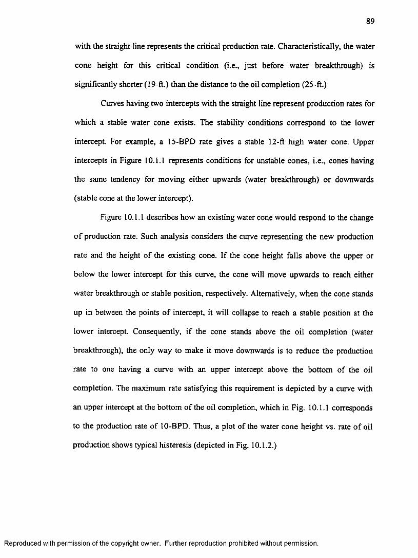
89

with the straight line represents the critical production rate. Characteristically, the water

cone height for this critical condition (i.e., just before water breakthrough) is

significantly shorter (19-ft.) than the distance to the oil completion (25-ft.)

Curves having two intercepts with the straight line represent production rates for

which a stable water cone exists. The stability conditions correspond to the lower

intercept. For example, a 15-BPD rate gives a stable 12-ft high water cone. Upper

intercepts in Figure 10.1.1 represents conditions for unstable cones, i.e., cones having

the same tendency for moving either upwards (water breakthrough) or downwards

(stable cone at the lower intercept).

Figure 10.1.1 describes how an existing water cone would respond to the change

o f production rate. Such analysis considers the curve representing the new production

rate and the height of the existing cone. If the cone height falls above the upper or

below the lower intercept for this curve, the cone will move upwards to reach either

water breakthrough or stable position, respectively. Alternatively, when the cone stands

up in between the points of intercept, it will collapse to reach a stable position at the

lower intercept. Consequently, if the cone stands above the oil completion (water

breakthrough), the only way to make it move downwards is to reduce the production

rate to one having a curve with an upper intercept above the bottom of the oil

completion. The maximum rate satisfying this requirement is depicted by a curve with

an upper intercept at the bottom of the oil completion, which in Fig. 10.1.1 corresponds

to the production rate of 10-BPD. Thus, a plot of the water cone height vs. rate of oil

production shows typical histeresis (depicted in Fig. 10.1.2.)


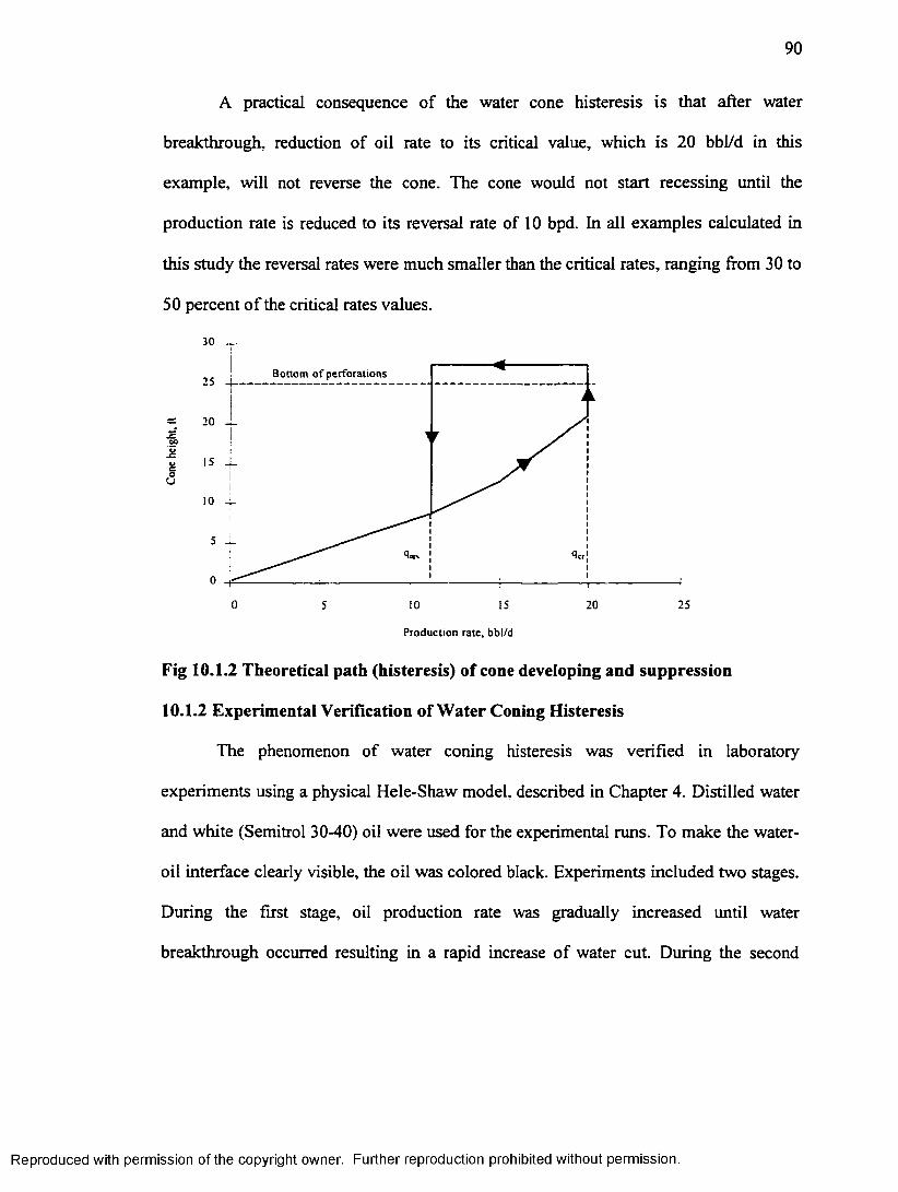
90

A practical consequence of the water cone histeresis is that after water

breakthrough, reduction of oil rate to its critical value, which is 20 bbl/d in this

example, will not reverse the cone. The cone would not start recessing until the

production rate is reduced to its reversal rate of 10 bpd. In all examples calculated in

this study the reversal rates were much smaller than the critical rates, ranging from 30 to

50 percent of the critical rates values.

30 —

Bottom o f perforations

20 -L

■a1ueoU

0 IS 20 255 !0

Production rate, bbl/d

Fig 10.1.2 Theoretical path (histeresis) of cone developing and suppression

10.1.2 Experimental Verification of Water Coning Histeresis

The phenomenon of water coning histeresis was verified in laboratory

experiments using a physical Hele-Shaw model, described in Chapter 4. Distilled water

and white (Semitrol 30-40) oil were used for the experimental runs. To make the water-

oil interface clearly visible, the oil was colored black. Experiments included two stages.

During the first stage, oil production rate was gradually increased until water

breakthrough occurred resulting in a rapid increase of water cut. During the second


91

stage, the production rate was reduced step-wise until the water cone visibly collapsed

and there was no water in the produced liquid.

An example of typical results from an experimental run is shown in Table

10.1.2.1 and Figure 10.1.2.1. The reservoir - well system simulated in this experiment

was characterized by a critical rate of 0.85 ml/min and a cone reversal rate of 0.6

ml/min. Also, the critical size of the water cone was 12.5 cm or 2.0 cm below the

bottom of the oil completion. The plot in Figure 10.1.2.1 clearly demonstrates histeresis

of water cone development and reversal.

Table 10.1.2.1 Water cone buildup and reversalP r o d u c t i o n r a t e

( c c / m i n )C o n e h e i g h t

( c m )W a t e r c u t ( f r a c t i o n )

0 . 6 I 0 . 5 0 0 . 0 00 . 7 1 1 . 9 0 0 . 0 0

00o

1 2 . 5 0 0 . 0 00 . 9 1 4 . 5 0 0 . 0 7

I I 5 . 0 0 0 . 1 30 . 9 1 5 . 2 0 0 . 1 30 . 8 1 4 . 9 0 0 . 1 10 . 7 1 4 . 9 0 0 . 0 90 . 6 1 0 . 3 0 0 . 0 0

16.00 t

14.00 - -EO

“ 12.00ucoU

10.00 —

8.00

Bottom of perforations

0.5

I

♦♦

tiii

I

♦ ys '

- experiment- histeresis path

0.6 0.79rev

0.8 0.9 l.i

Production rate, cc/min

Fig. 10.1.2.1 Experimental results on position of the cone apex during cone developing and reversal.


92

In conclusion, I would like to point out the following results of the study made in

Subchapter 10.1

1. Theoretically, for each rate of oil production below the critical rate there are two

equilibrium positions of the top of the water cone: stable (lower equilibrium point),

and unstable (upper equilibrium point). When production rate is increased, the water

cone builds up and assumes an equilibrium position at the lower equilibrium point.

The positioning of a water cone at or around the upper equilibrium point is only

possible when the rate of production is lowered during the process of cone buildup.

2. Reversal of water coning requires knowledge of the relationship between production

rates and upper equilibrium points for a given well-reservoir flow system. The

reversing can be made during water cone development or after water breakthrough.

Reversal of a developing water cone requires that the upper equilibrium point for

the reduced rate be located above the present cone height so that the water cone will

be reversed; otherwise, the cone will continue upwards until water breakthrough

occurs.

3. Reversing water cones after breakthrough requires lowering the rate o f production

to or below the value o f the cone reversal rate, q^y. The cone reversal rate is

defined as such that its upper equilibrium point coincides with the bottom of the oil

completion above OWC. Typically, values of cone reversal rates are smaller by 50-

30 percent than critical rates for the well-reservoir flow systems.

It seems feasible that in some cases of wells with acceptable values of critical rates,

cone reversal might be needed and could be accomplished without entirely shutting-in

the well for a long time.


93

10.2 Segregated Inflow in DWS Completion

This subchapter deals with a special type of DWS - Downhole Drain-Injection

System (DDIS). The objective of this study was to determine the effect of hydraulic communication

between the water drainage and injection zones. Such communication may reduce the area of water

drainage under the oil-producing perforations and make the system inefficient. Computation of this effect

should be included in the well completion design, optimization of oil production, and the diagnosis of

inflow problems.

The downhole drainage injection was mathematically modeled as a system of

three sinks operating under steady state flow conditions in a multilayered porous

medium. An isolating stratum having a zero vertical permeability separated the water

drainage and injection zones. Specifically, this study targets the issue o f a faulty

subsurface isolation between hydraulic components of the drainage-injection system

because the actual field systems are likely to operate under conditions of partial

hydraulic communication between their components. That is why, a leaking wellbore

cement sheath was modeled as a linear channel of finite conductivity. Therefore, our

approach for this study was to develop an analytical tool and to qualify the effect of

imperfect isolation on the performance of the drainage-injection systems.

10.2.1 Problem Definition

The drainage-injection system is a conglomerate of three sinks of finite size

within four no-flow planar boundaries. Figure 10.2.1.1 shows the nomenclature for the

mathematical treatment of this system. The following assumptions have been made:

1 Each of the three areas of flow, the oil zone, the aquifer, and the injection zone,

is laterally homogeneous (kx= ky = kh) with a different vertical permeability

(kv*kh), and a constant-pressure outer boundary.


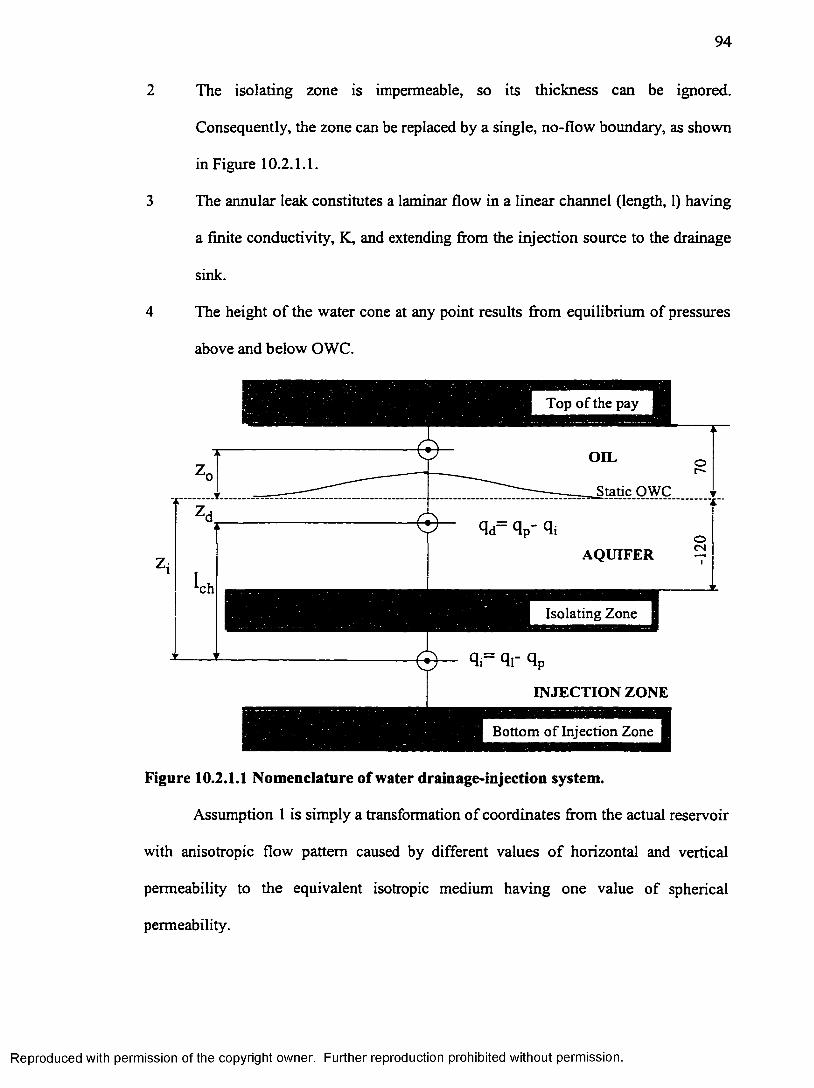
94

The isolating zone is impermeable, so its thickness can be ignored.

Consequently, the zone can be replaced by a single, no-flow boundary, as shown

in Figure 10.2.1.1.

The annular leak constitutes a laminar flow in a linear channel (length, 1) having

a finite conductivity, K, and extending from the injection source to the drainage

sink.

The height of the water cone at any point results from equilibrium of pressures

above and below OWC.

Top of the pay

OIL

Static OWC

AQUIFER

Isolating Zone

Mi nl” Qp

INJECTION ZONE

Bottom of Injection Zone

Figure 10.2.1.1 Nomenclature of water drainage-injection system.

Assumption 1 is simply a transformation of coordinates from the actual reservoir

with anisotropic flow pattern caused by different values of horizontal and vertical

permeability to the equivalent isotropic medium having one value of spherical

permeability.


95

Assumption 3 implies that the leak flow can be expressed by the formula

_ 2nrvK o (z ,r , ) <t>(zd rw)

z i ~ zd [ K kd

where 0(z,r) are the flow potentials around injecting and draining wells. Values of the

flow potentials were determined using MSSM. To simplify the analysis, spherical

sources or sinks modeled all the wells.

The effect of annular leak is introduced in the mathematical model using a

simple material balance illustrated in Fig. 10.2.1.1 which modifies the water drainage

and injection flow rates, respectively, as follows:

10.2.2 Results and Discussion

From numerous computations, we identified several regularities regarding the

way drainage injection systems operate under a variety of conditions. These regularities

may constitute principles for designing the system for a specific reservoir. Below we

will present these principles using an example oil reservoir. Table 7.2.1 shows reservoir

properties and the well geometry data.

Table 10.2.2.1 Well data properties.

Parameter Zo Zs Zd rw re kh kv P° fiw P o Pw

Units ft Ft ft ft Ft mD mD cP cP g/cc g/cc

Value 45 i o -10 0.25 1300 236 23 2.4 0.87 0.81 1.15

The results of simulation runs reveal principal relationships between the

reservoir engineering factors (fluid mobility, configuration of geological strata, and the


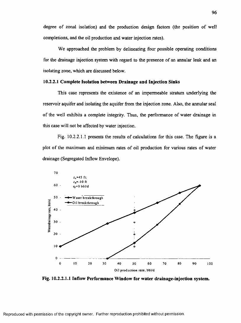
96

degree of zonal isolation) and the production design factors (the position of well

completions, and the oil production and water injection rates).

We approached the problem by delineating four possible operating conditions

for the drainage injection system with regard to the presence of an annular leak and an

isolating zone, which are discussed below.

10.2.2.1 Complete Isolation between Drainage and Injection Sinks

This case represents the existence of an impermeable stratum underlying the

reservoir aquifer and isolating the aquifer from the injection zone. Also, the annular seal

of the well exhibits a complete integrity. Thus, the performance of water drainage in

this case will not be affected by water injection.

Fig. 10.2.2.1.1 presents the results of calculations for this case. The figure is a

plot o f the maximum and minimum rates of oil production for various rates of water

drainage (Segregated Inflow Envelope).

70z„=45 ft; zd= - l0 ft

60

Water breakthrough Oil breakthrough

so

0 10 20 30 60 70 8040 50 90 100Oil p roduct ion ra te , bbl/d

Fig. 10.2.2.1.1 Inflow Performance Window for water drainage-injection system.


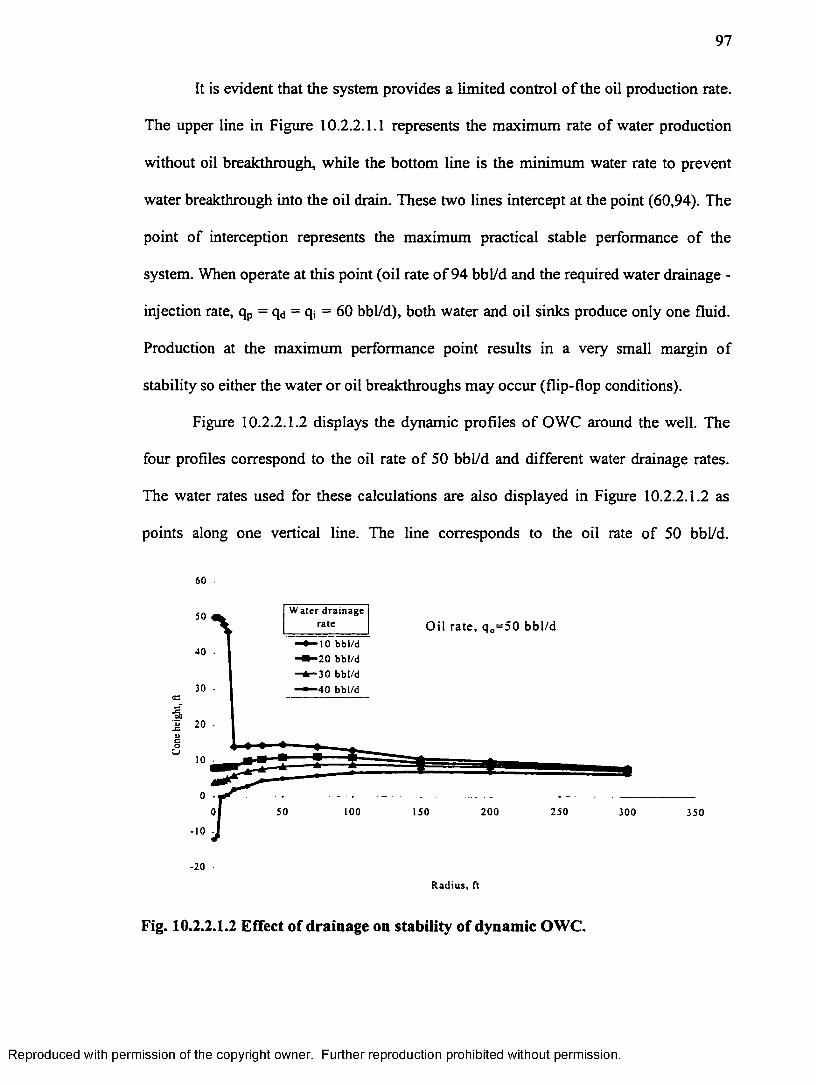
97

It is evident that the system provides a limited control of the oil production rate.

The upper line in Figure 10.2.2.1.1 represents the maximum rate of water production

without oil breakthrough, while the bottom line is the minimum water rate to prevent

water breakthrough into the oil drain. These two lines intercept at the point (60,94). The

point of interception represents the maximum practical stable performance of the

system. When operate at this point (oil rate o f 94 bbl/d and the required water drainage -

injection rate, qp = qd = qi = 60 bbl/d), both water and oil sinks produce only one fluid.

Production at the maximum performance point results in a very small margin of

stability so either the water or oil breakthroughs may occur (flip-flop conditions).

Figure 10.2.2.1.2 displays the dynamic profiles of OWC around the well. The

four profiles correspond to the oil rate of 50 bbl/d and different water drainage rates.

The water rates used for these calculations are also displayed in Figure 10.2.2.1.2 as

points along one vertical line. The line corresponds to the oil rate of 50 bbl/d.

60

W a t e r d r a i n a g e r a t e

50Oil rate, qo=50 bbl/d

■10 b b l / d

■20 b b l / d

■30 b b l / d

■40 b b l / d

40

30

20

10

05 0 100 2 5 0150 200 3 0 0 3 5 0

10

-20

R a d i u s , ft

Fig. 10.2.2.1.2 Effect of drainage on stability of dynamic OWC.


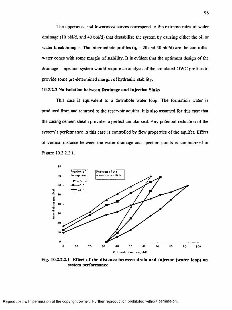
98

The uppermost and lowermost curves correspond to the extreme rates of water

drainage (10 bbl/d, and 40 bbl/d) that destabilize the system by causing either the oil or

water breakthroughs. The intermediate profiles (q<j = 20 and 30 bbl/d) are the controlled

water cones with some margin o f stability. It is evident that the optimum design of the

drainage - injection system would require an analysis of the simulated OWC profiles to

provide some pre-determined margin of hydraulic stability.

10.2.2.2 No Isolation between Drainage and Injection Sinks

This case is equivalent to a downhole water loop. The formation water is

produced from and returned to the reservoir aquifer. It is also assumed for this case that

the casing cement sheath provides a perfect annular seal. Any potential reduction of the

system’s performance in this case is controlled by flow properties of the aquifer. Effect

of vertical distance between the water drainage and injection points is summarized in

Figure 10.2.2.2.1.

80

P o s i t i o n o f th e i n j e c t o r

P o s i t i o n o f t h e w a t e r d r a i n - 10 ft70

in f i n i t e

-4 5 ft

-2 5 ft

6 0

^ 50 •S2V=0eoc 4 0

2-a

a=S20

0 10 20 4 0 5030 60 70 80 9 0 100

O i l p r o d u c t i o n r a te , bb l /d

Fig. 10.2.2.2.1 Effect of the distance between drain and injector (water loop) on system performance


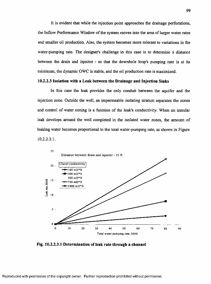
99

It is evident that while the injection point approaches the drainage perforations,

the Inflow Performance Window of the system moves into the area of larger water rates

and smaller oil production. Also, the system becomes more tolerant to variations in the

water-pumping rate. The designer’s challenge in this case is to determine a distance

between the drain and injector - so that the downhole loop's pumping rate is at its

minimum, the dynamic OWC is stable, and the oil production rate is maximized.

10.2.2.3 Isolation with a Leak between the Drainage and Injection Sinks

In this case the leak provides the only conduit between the aquifer and the

injection zone. Outside the well, an impermeable isolating stratum separates the zones

and control of water coning is a function of the leak's conductivity. When an annular

leak develops around the well completed in the isolated water zones, the amount of

leaking water becomes proportional to the total water-pumping rate, as shown in Figure

10.2.2.3.1.

25

D istan ce b e tw een d ra in and in jec to r - 35 ft

C h a n e l c o n d u c t i v i t y20

► -100 m D * f t

► -300 m D * f t

5 0 0 m D * f t

♦“ 7 5 0 m D ' f t

< - 1 0 0 0 m D * f t

15

10

5

00 10 20 30 5 04 0 6 0 70 8 0 9 0

T o t a l w a t e r p u m p i n g r a t e , b b l / d

Fig. 10.2.2.3.1 Determination of leak rate through a channel


100

Therefore, a reduction in the system's performance caused by the leak depends

only on the leak's conductivity. The reduced performance can be estimated using the

predicted rate o f leakage (Figure 10.2.2.3.1) and the Performance Window plot

(Fig. 10.2.2.1.1). In this case, the effect of the leak reduces the actual rate of water

drainage by the value of the leak flow rate. Thus, the Performance Window without the

leak can be modified and used to predict the reduced performance with the leak. For

example, an annular leak having conductivity K = 1 D - ft would reduce the actual

water drainage and oil production rates from 45 bbl/d to 31 bbl/d and from 80 bbl/d to

67 bbl/d, respectively. Also, it seems that the drainage-injection systems may tolerate

small annular leaks by suppressing their effect with increased drainage rates.

10.2.2.4 No Isolation and Leak between Drainage and Injection Sinks

This case considers the effect of an annular leak and the absence of an isolating

stratum. The downhole loop circulates water within the aquifer. However, the flow is

diverted between the annular leak and the aquifer's rock. In this case, the combined

effects of the leak's conductivity and the aquifer's properties control the system's

performance.

Figure 10.2.2.4.1 shows the destabilizing effect of an annular leak on the

theoretically optimized production program. In the figure, the bottom curve is a stable

OWC profile corresponding to optimized rates of oil production and water drainage and

injection. The upper curves show that the development of an annular leak quickly

destabilized the system, causing water encroachment and breakthrough. The hydraulic

connection between water drainage and injection completion through the leack reduces

the amount of water produced through the drainage completion. Thus the pressure


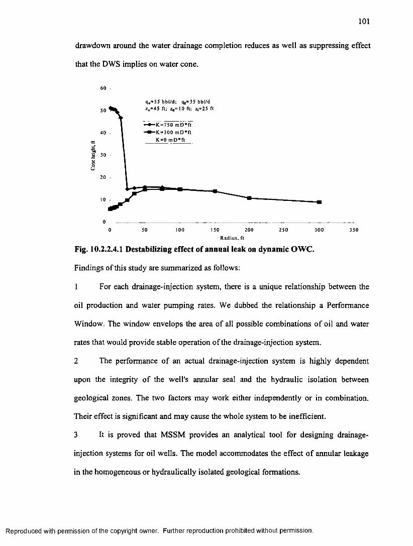
101

drawdown around the water drainage completion reduces as well as suppressing effect

that the DWS implies on water cone.

60

q„=55 bbl/d; <i,= 35 bbl/dz 0= 4 5 ft; Zt= 10 ft; Zj=25 ft50

K = 7 5 0 m D * f t

K = 3 0 0 m D * f t

K = 0 m D * f t

U-Cu

0 . _ .-------------0 50 1 0 0 150 2 0 0 2 5 0 3 0 0 3 5 0

R a d i u s , ft

Fig. 10.2.2.4.1 Destabilizing effect of annual leak on dynamic OWC.

Findings of this study are summarized as follows:

1 For each drainage-injection system, there is a unique relationship between the

oil production and water pumping rates. We dubbed the relationship a Performance

Window. The window envelops the area of all possible combinations of oil and water

rates that would provide stable operation of the drainage-injection system.

2 The performance of an actual drainage-injection system is highly dependent

upon the integrity of the well's annular seal and the hydraulic isolation between

geological zones. The two factors may work either independently or in combination.

Their effect is significant and may cause the whole system to be inefficient.

3 It is proved that MSSM provides an analytical tool for designing drainage-

injection systems for oil wells. The model accommodates the effect o f annular leakage

in the homogeneous or hydraulically isolated geological formations.


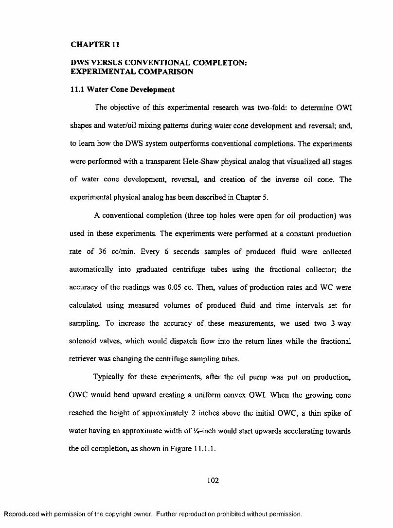
CHAPTER 11

DWS VERSUS CONVENTIONAL COMPLETON:EXPERIMENTAL COMPARISON

11.1 Water Cone Development

The objective of this experimental research was two-fold: to determine OWI

shapes and water/oil mixing patterns during water cone development and reversal; and,

to learn how the DWS system outperforms conventional completions. The experiments

were performed with a transparent Hele-Shaw physical analog that visualized all stages

of water cone development, reversal, and creation of the inverse oil cone. The

experimental physical analog has been described in Chapter 5.

A conventional completion (three top holes were open for oil production) was

used in these experiments. The experiments were performed at a constant production

rate of 36 cc/min. Every 6 seconds samples of produced fluid were collected

automatically into graduated centrifuge tubes using the fractional collector; the

accuracy of the readings was 0.05 cc. Then, values of production rates and WC were

calculated using measured volumes of produced fluid and time intervals set for

sampling. To increase the accuracy of these measurements, we used two 3-way

solenoid valves, which would dispatch flow into the return lines while the fractional

retriever was changing the centrifuge sampling tubes.

Typically for these experiments, after the oil pump was put on production,

OWC would bend upward creating a uniform convex OWI. When the growing cone

reached the height of approximately 2 inches above the initial OWC, a thin spike of

water having an approximate width of ‘/4-inch would start upwards accelerating towards

the oil completion, as shown in Figure 11.1.1.

102


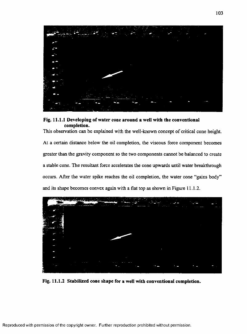
103

Fig. 11.1.1 Developing of water cone around a well with the conventional completion.

This observation can be explained with the well-known concept of critical cone height.

At a certain distance below the oil completion, the viscous force component becomes

greater than the gravity component so the two components cannot be balanced to create

a stable cone. The resultant force accelerates the cone upwards until water breakthrough

occurs. After the water spike reaches the oil completion, the water cone “gains body”

and its shape becomes convex again with a flat top as shown in Figure 11.1.2.

Fig. 11.1.2 Stabilized cone shape for a well with conventional completion.


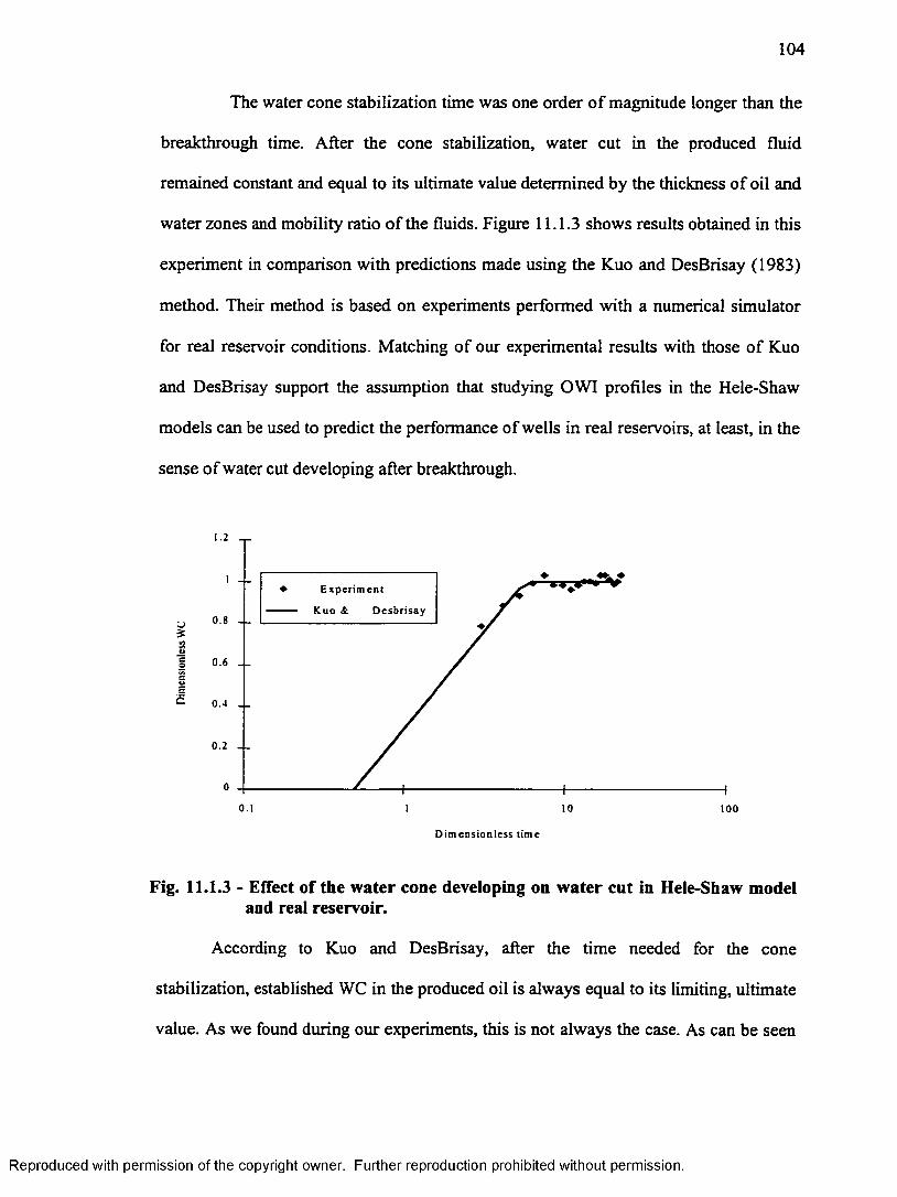
104

The water cone stabilization time was one order of magnitude longer than the

breakthrough time. After the cone stabilization, water cut in the produced fluid

remained constant and equal to its ultimate value determined by the thickness of oil and

water zones and mobility ratio of the fluids. Figure 11.1.3 shows results obtained in this

experiment in comparison with predictions made using the Kuo and DesBrisay (1983)

method. Their method is based on experiments performed with a numerical simulator

for real reservoir conditions. Matching of our experimental results with those of Kuo

and DesBrisay support the assumption that studying OWI profiles in the Hele-Shaw

models can be used to predict the performance of wells in real reservoirs, at least, in the

sense of water cut developing after breakthrough.

1.2

E x p e r i m e n t

D e s b r i s a yK u o &0.8

0.6

0 .4

0.2

00.1 10 100

D i m e n s i o n l e s s t i m e

Fig. 11.1.3 - Effect of the water cone developing on water cut in Hele-Shaw model and real reservoir.

According to Kuo and DesBrisay, after the time needed for the cone

stabilization, established WC in the produced oil is always equal to its limiting, ultimate

value. As we found during our experiments, this is not always the case. As can be seen


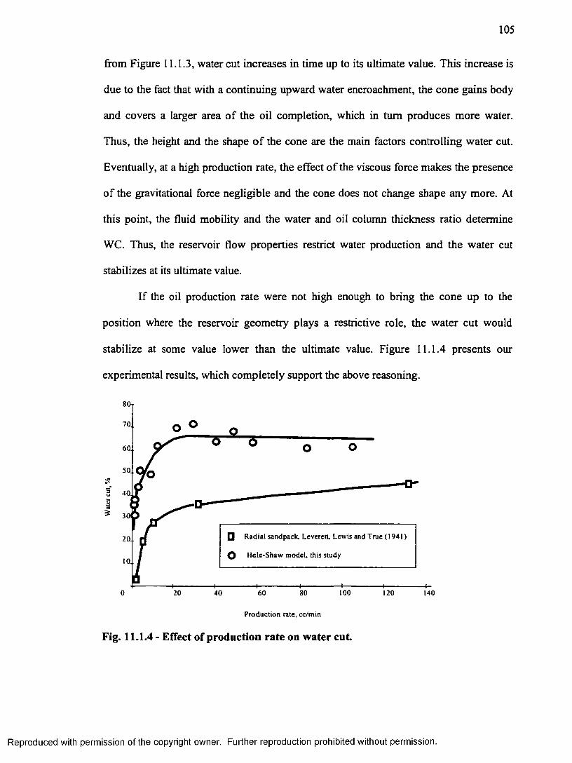
105

from Figure 11.1.3, water cut increases in time up to its ultimate value. This increase is

due to the fact that with a continuing upward water encroachment, the cone gains body

and covers a larger area of the oil completion, which in turn produces more water.

Thus, the height and the shape o f the cone are the main factors controlling water cut.

Eventually, at a high production rate, the effect o f the viscous force makes the presence

of the gravitational force negligible and the cone does not change shape any more. At

this point, the fluid mobility and the water and oil column thickness ratio determine

WC. Thus, the reservoir flow properties restrict water production and the water cut

stabilizes at its ultimate value.

If the oil production rate were not high enough to bring the cone up to the

position where the reservoir geometry plays a restrictive role, the water cut would

stabilize at some value lower than the ultimate value. Figure 11.1.4 presents our

experimental results, which completely support the above reasoning.

80t

70.

60.

3Uu

40.

C3£

Q R a d i a l s a n d p a c k . L evere t t , L e w is an d T r u e ( 19 4 1)20 .

O H e l e - S h a w m o d e l , th is s tu d y

1000 20 60 80 120 14040

Production rate, cc/min

Fig. 11.1.4 - Effect of production rate on water cut


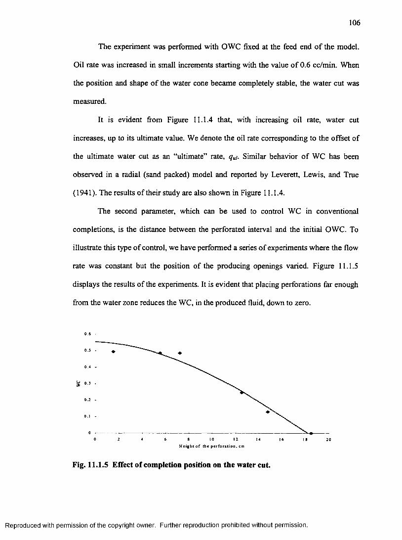
106

The experiment was performed with OWC fixed at the feed end of the model.

Oil rate was increased in small increments starting with the value of 0.6 cc/min. When

the position and shape of the water cone became completely stable, the water cut was

measured.

It is evident from Figure 11.1.4 that, with increasing oil rate, water cut

increases, up to its ultimate value. We denote the oil rate corresponding to the offset of

the ultimate water cut as an “ultimate” rate, qui. Similar behavior of WC has been

observed in a radial (sand packed) model and reported by Leverett, Lewis, and True

(1941). The results of their study are also shown in Figure 11.1.4.

The second parameter, which can be used to control WC in conventional

completions, is the distance between the perforated interval and the initial OWC. To

illustrate this type of control, we have performed a series of experiments where the flow

rate was constant but the position of the producing openings varied. Figure 11.1.5

displays the results of the experiments. It is evident that placing perforations far enough

from the water zone reduces the WC, in the produced fluid, down to zero.

0 . 6 -

0.5

0 . 4

0.3

0 .2

0.1

00 122 4 6 8 10 14 16 I 8 20

H e i g h t o f t h e p e r f o r a t i o n , c m

Fig. 11.1.5 Effect of completion position on the water cut.


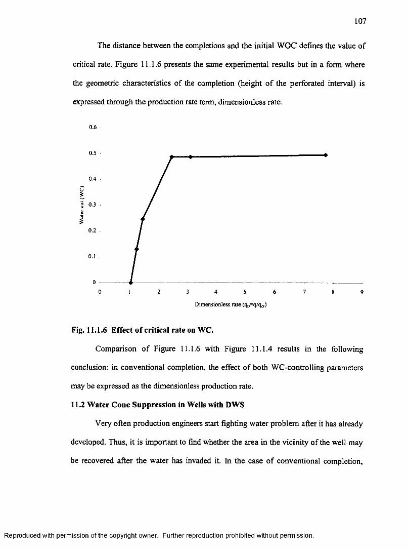
107

The distance between the completions and the initial WOC defines the value of

critical rate. Figure 11.1.6 presents the same experimental results but in a form where

the geometric characteristics of the completion (height of the perforated interval) is

expressed through the production rate term, dimensionless rate.

0.6

0.5

0.4

0.3

0.2

0.1

00 2 3 5 6 74 8 9

Dimensionless rate (qD=q/qa )

Fig. 11.1.6 Effect of critical rate on WC.

Comparison of Figure 11.1.6 with Figure 11.1.4 results in the following

conclusion: in conventional completion, the effect of both WC-controlling parameters

may be expressed as the dimensionless production rate.

11.2 Water Cone Suppression in Wells with DWS

Very often production engineers start fighting water problem after it has already

developed. Thus, it is important to find whether the area in the vicinity of the well may

be recovered after the water has invaded it. In the case of conventional completion,


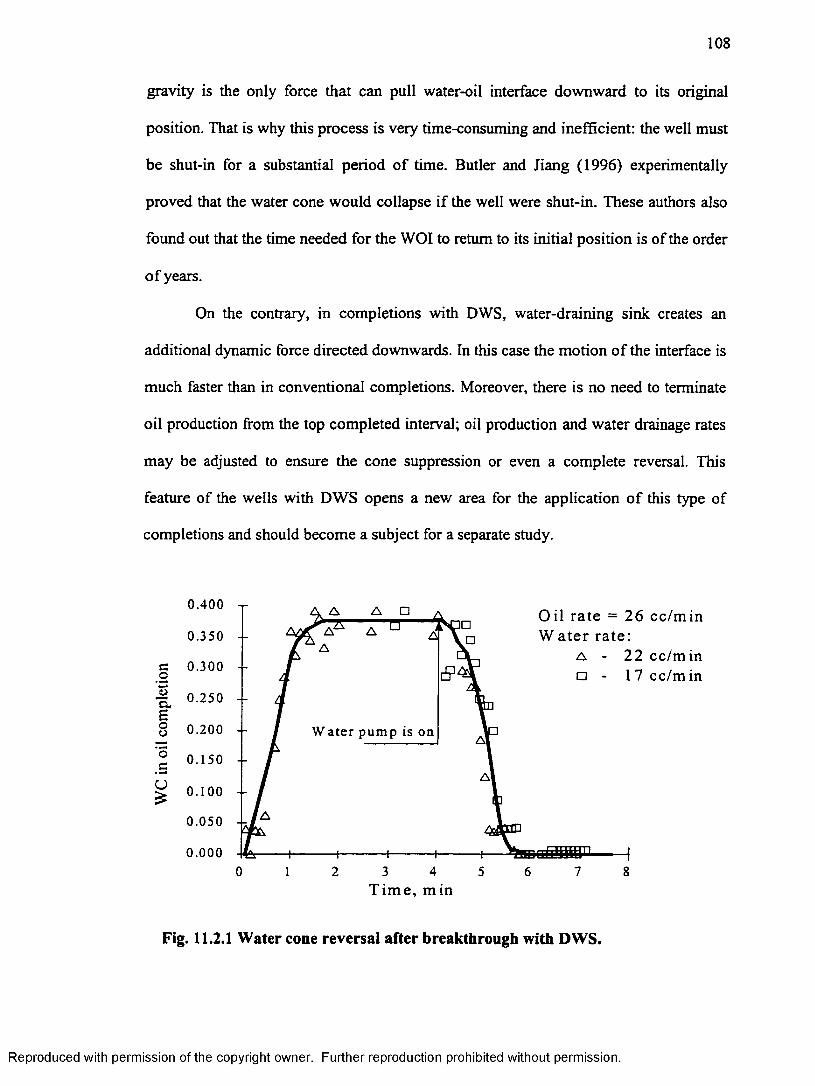
108

gravity is the only force that can pull water-oil interface downward to its original

position. That is why this process is very time-consuming and inefficient: the well must

be shut-in for a substantial period of time. Butler and Jiang (1996) experimentally

proved that the water cone would collapse if the well were shut-in. These authors also

found out that the time needed for the WOI to return to its initial position is of the order

o f years.

On the contrary, in completions with DWS, water-draining sink creates an

additional dynamic force directed downwards. In this case the motion of the interface is

much faster than in conventional completions. Moreover, there is no need to terminate

oil production from the top completed interval; oil production and water drainage rates

may be adjusted to ensure the cone suppression or even a complete reversal. This

feature of the wells with DWS opens a new area for the application of this type of

completions and should become a subject for a separate study.

0.400 A A D

0.350 a a a LJO il ra te = 26 cc/m in W a te r rate :

Aa - 22 cc/m in □ - 17 cc/m inc 0.300o

! 0.250B8 0.200 Water pump is on

.£ 0 1 5 0 0.100

0.050

0.0000 2 3 4 5 6

17 8

T ime, min

Fig. 11.2.1 Water cone reversal after breakthrough with DWS


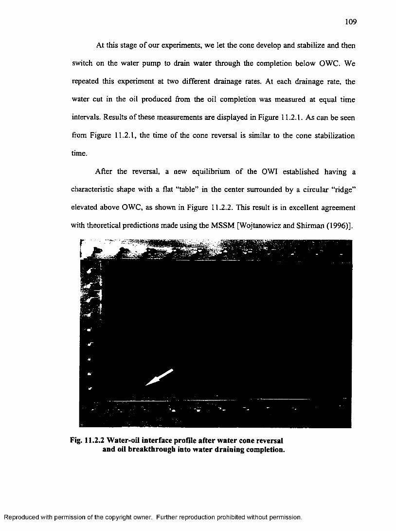
109

At this stage o f our experiments, we let the cone develop and stabilize and then

switch on the water pump to drain water through the completion below OWC. We

repeated this experiment at two different drainage rates. At each drainage rate, the

water cut in the oil produced from the oil completion was measured at equal time

intervals. Results of these measurements are displayed in Figure 11.2.1. As can be seen

from Figure 11.2.1, the time of the cone reversal is similar to the cone stabilization

time.

After the reversal, a new equilibrium of the OWI established having a

characteristic shape with a flat “table” in the center surrounded by a circular “ridge”

elevated above OWC, as shown in Figure 11.2.2. This result is in excellent agreement

with theoretical predictions made using the MSSM [Wojtanowicz and Shirman (1996)].

Fig. 11.2.2 Water-oil interface profile after water cone reversal and oil breakthrough into water draining completion.


110

We also observed that in all cases of cone reversal there was oil breakthrough

into the water completion, which resulted in an additional amount of oil produced as

“oil cut” in the drained water.

Physical modeling of water coning control with DWS completion demonstrates the

feasibility and hydromechanics of this process and leads to the following observations:

1. water cone reversal eliminates water cut in oil production by removing water from

the area around and below oil completion;

2. productivity o f a “watered out” well can be recovered to give a significant increase

in the production of oil; and

3. duration of the reversal time is comparable with the cone stabilization time and is

about an order of magnitude longer than water breakthrough time.

11.3 Effect of DWS on Water Cut

One of the most frequently asked question related to the DWS applications is

whether the new technology reduces the WC in the produced oil. Theoretical study of

this problem is presented in Chapter 5. Here we present some experimental results on

the subject. Figure 11.3.1 shows well production history obtained on the Hele-Shaw

model. For the first six minutes the well produced as a conventional one; the downhole

water sink was shut in. At these production conditions, the average value of WC was

0.31.

At 6.5 minutes after putting the well on production, the pump at the bottom

completion was switched on. As a result of the water drainage, the water cone was

suppressed, which is indicated by the reduction of WC in the fluid produced through


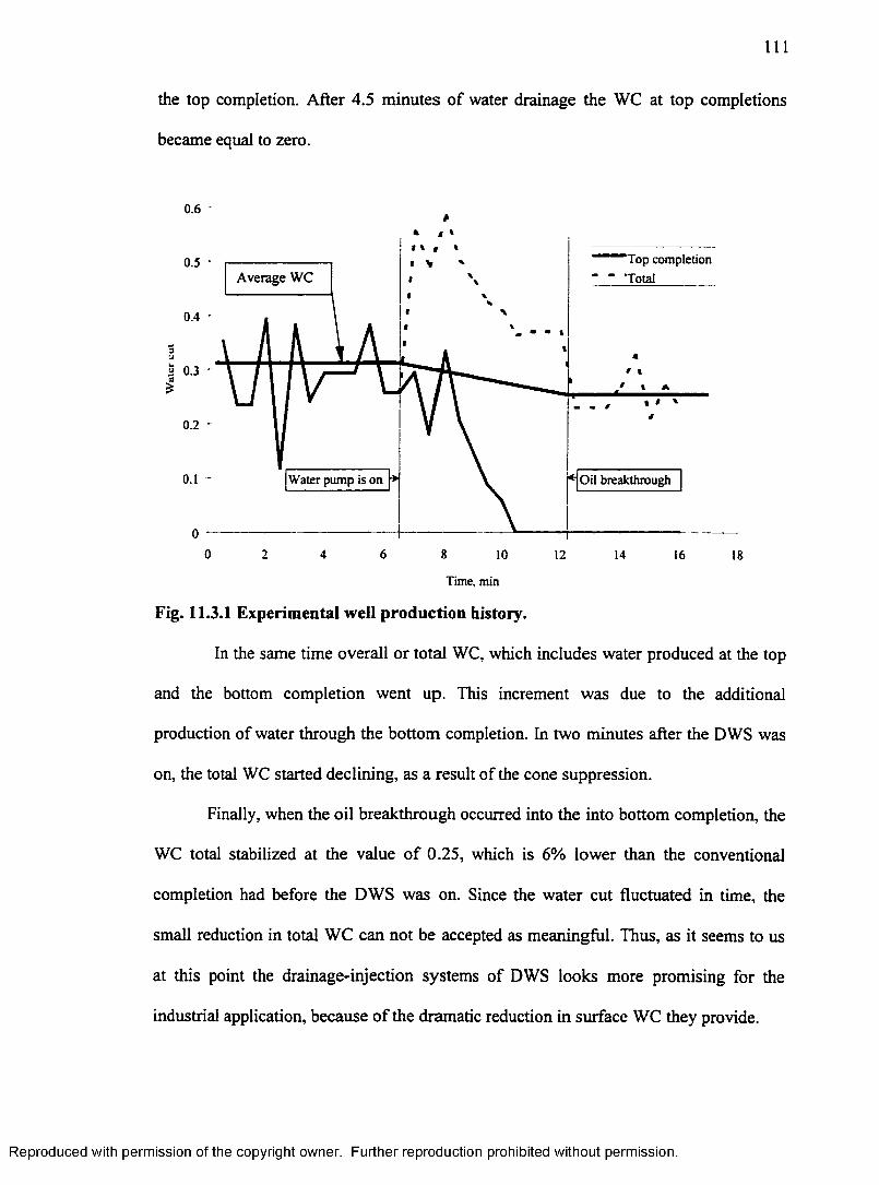
I l l

the top completion. After 4.5 minutes of water drainage the WC at top completions

became equal to zero.

'Top completionAverage WC " ~ 'Total

0.4 *

uya

Water pump is on Oil breakthrough

0 2 6 84 10 12 14 16 18

Time, min

Fig. 11.3.1 Experimental well production history.

In the same time overall or total WC, which includes water produced at the top

and the bottom completion went up. This increment was due to the additional

production of water through the bottom completion. In two minutes after the DWS was

on, the total WC started declining, as a result of the cone suppression.

Finally, when the oil breakthrough occurred into the into bottom completion, the

WC total stabilized at the value of 0.25, which is 6% lower than the conventional

completion had before the DWS was on. Since the water cut fluctuated in time, the

small reduction in total WC can not be accepted as meaningful. Thus, as it seems to us

at this point the drainage-injection systems of DWS looks more promising for the

industrial application, because of the dramatic reduction in surface WC they provide.


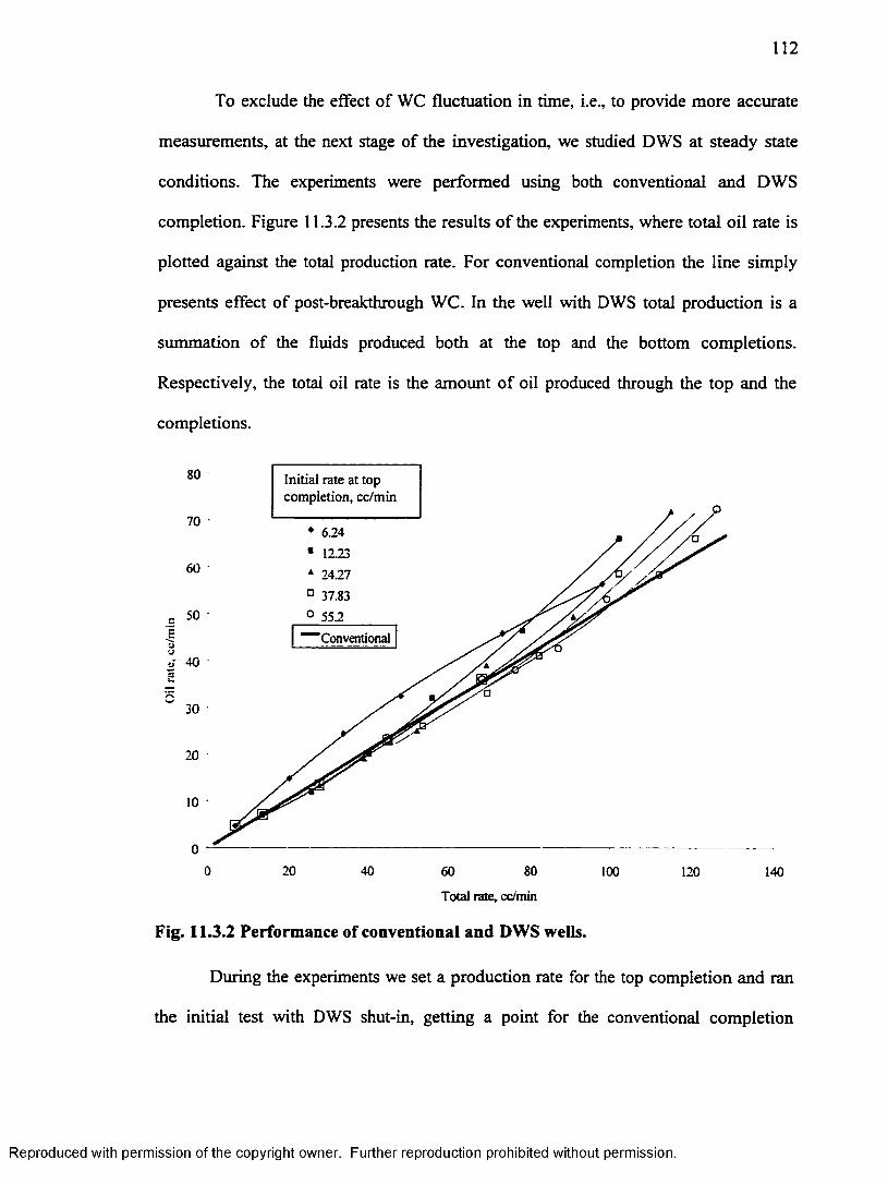
112

To exclude the effect of WC fluctuation in time, i.e., to provide more accurate

measurements, at the next stage of the investigation, we studied DWS at steady state

conditions. The experiments were performed using both conventional and DWS

completion. Figure 11.3.2 presents the results of the experiments, where total oil rate is

plotted against the total production rate. For conventional completion the line simply

presents effect of post-breakthrough WC. In the well with DWS total production is a

summation of the fluids produced both at the top and the bottom completions.

Respectively, the total oil rate is the amount of oil produced through the top and the

completions.

80 Initial rate at top completion, cc/min

70♦ 6.24

■ 12.23

* 2427 D 37.83 0 552

60

50Conventional

40

30

20

10

00 20 40 8060 100 120 140

Total rate, cc/min

Fig. 11.3.2 Performance of conventional and DWS wells.

During the experiments we set a production rate for the top completion and ran

the initial test with DWS shut-in, getting a point for the conventional completion


113

performance line. Then, without changing production at the top completion we varied

rate at the bottom one. In Figure 11.3.2 lines having different graphical style presents

experimental conditions with a constant production rate at the top completion.

Two different types of the oil rate trends were observed during experiments. As it

is seen from Figure 11.3.2, if the production at top completion is above 10 cc/min,

produced oil is the same as in conventional completion until increment of bottom

completion rate causes reversal of the cone. After the cone reversal, additional oil is

being produced at the bottom completion

At top completion rate equal to 6.24 cc/min, which is below the ultimate rate, oil

breakthrough occurred at the slightest rates of water drainage at the bottom completion.

As it was shown in the previous chapters, the reduction of the rate below the ultimate

value yields a disproportional reduction in WC. That is why initially sharp increment in

the oil rate was achieved. It is interesting to note that this oil rate trend has a maximum

at total rate of about 60 cc/min. If the total rate is above this rate, amount of additional

oil rate (compare to the rate of the conventional completion) reduces. The reduction of

WC in the top completion is, probably, due to the pressure interference from the bottom

completion, becomes lower than the relative increment of water drainage at the bottom

completion.

Plotting the total WC versus ratio of the rate at the top completion to the well’s

total rate, we discover the optimum bottom completion rate that yields the minimum

overall WC. The similar minimums exist for each production rate at the top completion.

Figure 11.3.3 illustrates this DWS behavior. DWS produces with the maximum WC

when the water cone is fully developed and at maximum Oil Cut (OC=l-WC) if oil


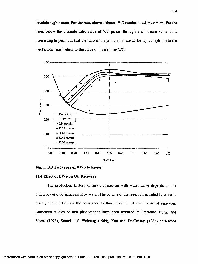
114

breakthrough occurs. For the rates above ultimate, WC reaches local maximum. For the

rates below the ultimate rate, value of WC passes through a minimum value. It is

interesting to point out that the ratio of the production rate at the top completion to the

well’s total rate is close to the value of the ultimate WC.

0.60

Rate at top conviction

♦ 6.24 cc/min ■ 12.23 cc/min

0.10 a 24.47 cc/minx 37.83 cc/min x 5520 cc/min

0.000.00 0.10 0.20 0.30 0.40 0.50 0.60 0.70 0.80 0.90 1.00

qtOfVqtotal

Fig. 11.3.3 Two types of DWS behavior.

11.4 Effect of DWS on Oil Recovery

The production history of any oil reservoir with water drive depends on the

efficiency of oil displacement by water. The volume of the reservoir invaded by water is

mainly the function of the resistance to fluid flow in different parts of reservoir.

Numerous studies of this phenomenon have been reported in literature. Byme and

Morse (1973), Settari and Weinaug (1969), Kuo and DesBrisay (1983) performed


115

simulation study of oil recovery. Caudle and Silberberg (1965), and Henley, Owens,

and Craig (1961) performed experiments on the scaled models. The numerical results

indicate that for a given reservoir geometry and properties there is a unique relationship

between water cut and value of oil recovery. Kuo and DesBrisay (1983) introduced

dimensionless time of breakthrough and dimensionless water cut to describe the general

form of post-breakthrough behavior of a partially penetrating well. Henley, Owens, and

Craig (1961) noticed the relation between reciprocal of sweep efficiency and WOR is

linear for the 2<WOR<20 and proposed a simple correlation based on this observation.

Two coefficients used in the correlation are taken from the special set o f graphs, which

is an obvious drawback for the proposed approach. Due to the fact that recovery

efficiency is in functional relation with WOR, application of DWS could significantly

improve oil recovery by reducing the WOR.

To study the effect of DWS on oil recovery a special set of experiments was

performed. The experiments model oil production from a reservoir overlaying aquifer.

The float switch controlling the position of the WOC during the steady state

experiments was disconnected. Thus, the inflow of additional oil from the storage

container was closed. At the same time, the solenoid valve controlling the influx of the

water remained open. Sampling of the outlet streams on the fractional collector

provided measurements of the production rates at the top and the bottom completions.

Three top openings (#1, #2, and #3) simulated the top completion and one

opening (#10) - bottom one. Experiments were performed at five different

combinations of production rates at the top and the bottom completions. Table 11.4.1

presents production conditions related to the studied cases.


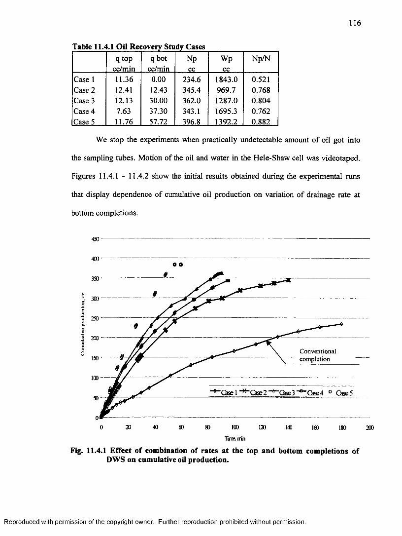
116

Table 11.4.1 Oil Recovery Study Casesq top

cc/minq bot

cc/minNpcc

Wpcc

Np/N

Case 1 11.36 0.00 234.6 1843.0 0.521Case 2 12.41 12.43 345.4 969.7 0.768Case 3 12.13 30.00 362.0 1287.0 0.804Case 4 7.63 37.30 343.1 1695.3 0.762Case 5 11.76 57.72 396.8 1392.2 0.882

We stop the experiments when practically undetectable amount of oil got into

the sampling tubes. Motion of the oil and water in the Hele-Shaw cell was videotaped.

Figures 11.4.1 - 11.4.2 show the initial results obtained during the experimental runs

that display dependence of cumulative oil production on variation of drainage rate at

bottom completions.

450 -----------------------------------------------------------------------------------------------------------------------------------------------------

400 -----------------------------------------------o o

350

U•J 300 -----eu

250 ^c.EJ>I 2003E Conventional

completionC 150 —

100

~^~Case 1 Case 2*"*"* Case 3 ~e~Case4 0 Case 5

20 60 1000 80 120 140 160 180 200

HnE,nin

Fig. 11.4.1 Effect of combination of rates at the top and bottom completions of DWS on cumulative oil production.


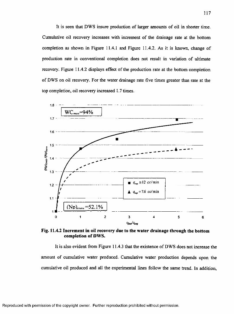
117

It is seen that DWS insure production of larger amounts of oil in shorter time.

Cumulative oil recovery increases with increment of the drainage rate at the bottom

completion as shown in Figure 11.4.1 and Figure 11.4.2. As it is known, change of

production rate in conventional completion does not result in variation of ultimate

recovery. Figure 11.4.2 displays effect of the production rate at the bottom completion

of DWS on oil recovery. For the water drainage rate five times greater than rate at the

top completion, oil recovery increased 1.7 times.

W C maY= 94%1.7

1.6

1.5 4

1.4

1.3

1.2

1.1

(NpVnnv=52.1%1

20 1 3 4 5 6bot fltop

Fig. 11.4.2 Increment in oil recovery due to the water drainage through the bottom completion of DWS.

It is also evident from Figure 11.4.3 that the existence of DWS does not increase the

amount of cumulative water produced. Cumulative water production depends upon the

cumulative oil produced and all the experimental lines follow the same trend. In addition,


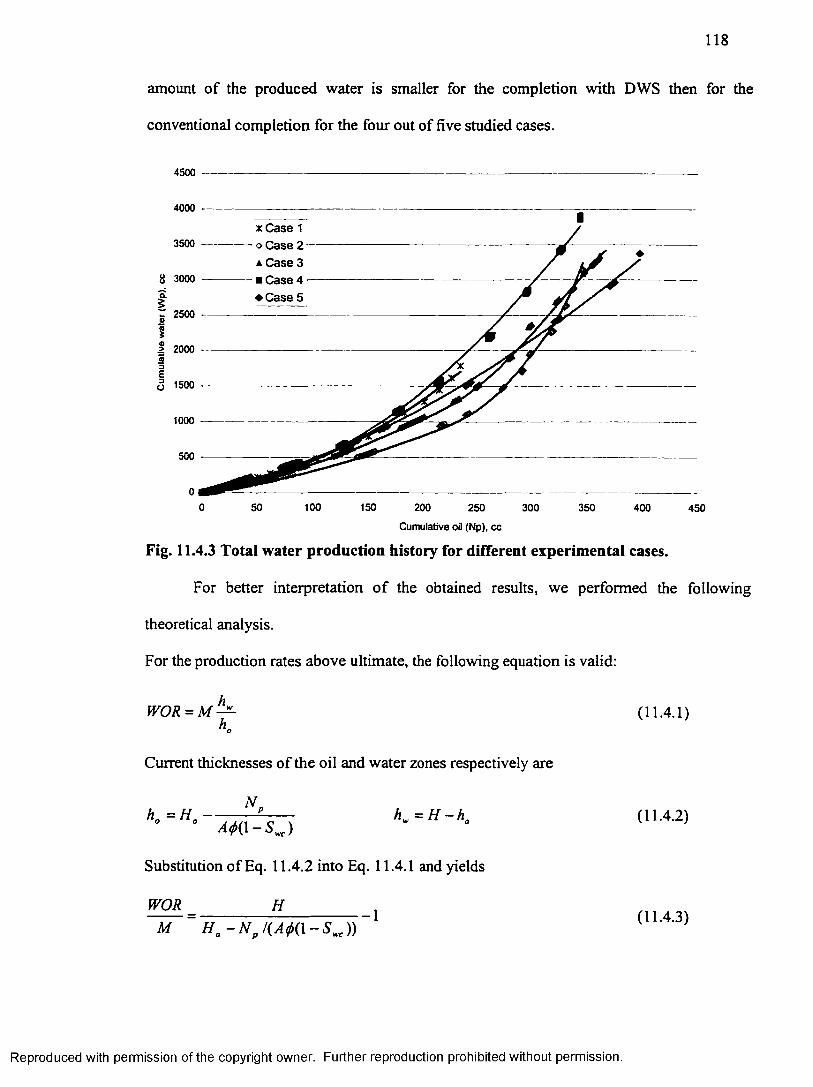
118

amount of the produced water is smaller for the completion with DWS then for the

conventional completion for the four out of five studied cases.

4500

4000 -

3500 -x Case 1o Case 2a, Case 3

3000 - Case 4♦ Case 5

Q 1500

0 50 100 150 200 250 300 350 400 450

Cumulative oil (Np), cc

Fig. 11.4.3 Total water production history for different experimental cases.

For better interpretation of the obtained results, we performed the following

theoretical analysis.

For the production rates above ultimate, the following equation is valid:

WOR = M — h

Current thicknesses of the oil and water zones respectively are

(11.4.1)

h = H a ---------- ------ h = H - K (11.4.2)

Substitution of Eq. 11.4.2 into Eq. 11.4.1 and yields

WOR HM Ha - N Swe))

-1 (11.4.3)


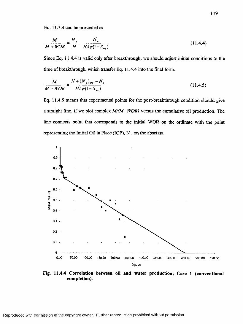
119

Eq. 11.3.4 can be presented as

M Hn N„(11.4.4)

M + WOR H HA<t>{\-Swc)

Since Eq. 11.4.4 is valid only after breakthrough, we should adjust initial conditions to the

time o f breakthrough, which transfer Eq. 11.4.4 into the final form.

M Af + (N )BT — N-------------= ----------— p- (11.4.5)M + WOR HA<f>(\-Swe)

Eq. 11.4.5 means that experimental points for the post-breakthrough condition should give

a straight line, if we plot complex M/(M+WOR) versus the cumulative oil production. The

line connects point that corresponds to the initial WOR on the ordinate with the point

representing the Initial Oil in Place (IOP), N , on the abscissa.

0.9

s0.4 -

0.3 -

0.2 -

0.1

50.00 100.00 150.00 200.00 250.00 300.00 350.00 400.00 450.00 500.00 550.000.00

Np, cc

Fig. 11.4.4 Correlation between oil and water production; Case 1 (conventional completion).


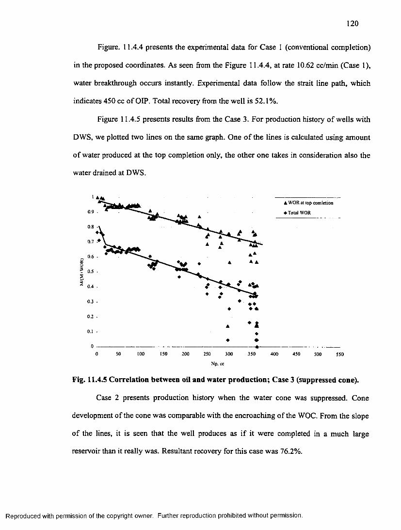
120

Figure. 11.4.4 presents the experimental data for Case 1 (conventional completion)

in the proposed coordinates. As seen from the Figure 11.4.4, at rate 10.62 cc/min (Case 1),

water breakthrough occurs instantly. Experimental data follow the strait line path, which

indicates 450 cc of OEP. Total recovery from the well is 52.1%.

Figure 11.4.5 presents results from the Case 3. For production history of wells with

DWS, we plotted two lines on the same graph. One o f the lines is calculated using amount

of water produced at the top completion only, the other one takes in consideration also the

water drained at DWS.

0.7

A AxO£s

♦0.3 ♦ ♦0.2 -

0.1 -

0 -

50

A WOR at top comietion

♦ Total WOR

A

♦

♦ ♦

♦ I♦

100 150 200 250 300

Np, cc

350 400 450 500 550

Fig. 11.4.5 Correlation between oil and water production; Case 3 (suppressed cone).

Case 2 presents production history when the water cone was suppressed. Cone

development of the cone was comparable with the encroaching of the WOC. From the slope

of the lines, it is seen that the well produces as if it were completed in a much large

reservoir than it really was. Resultant recovery for this case was 76.2%.


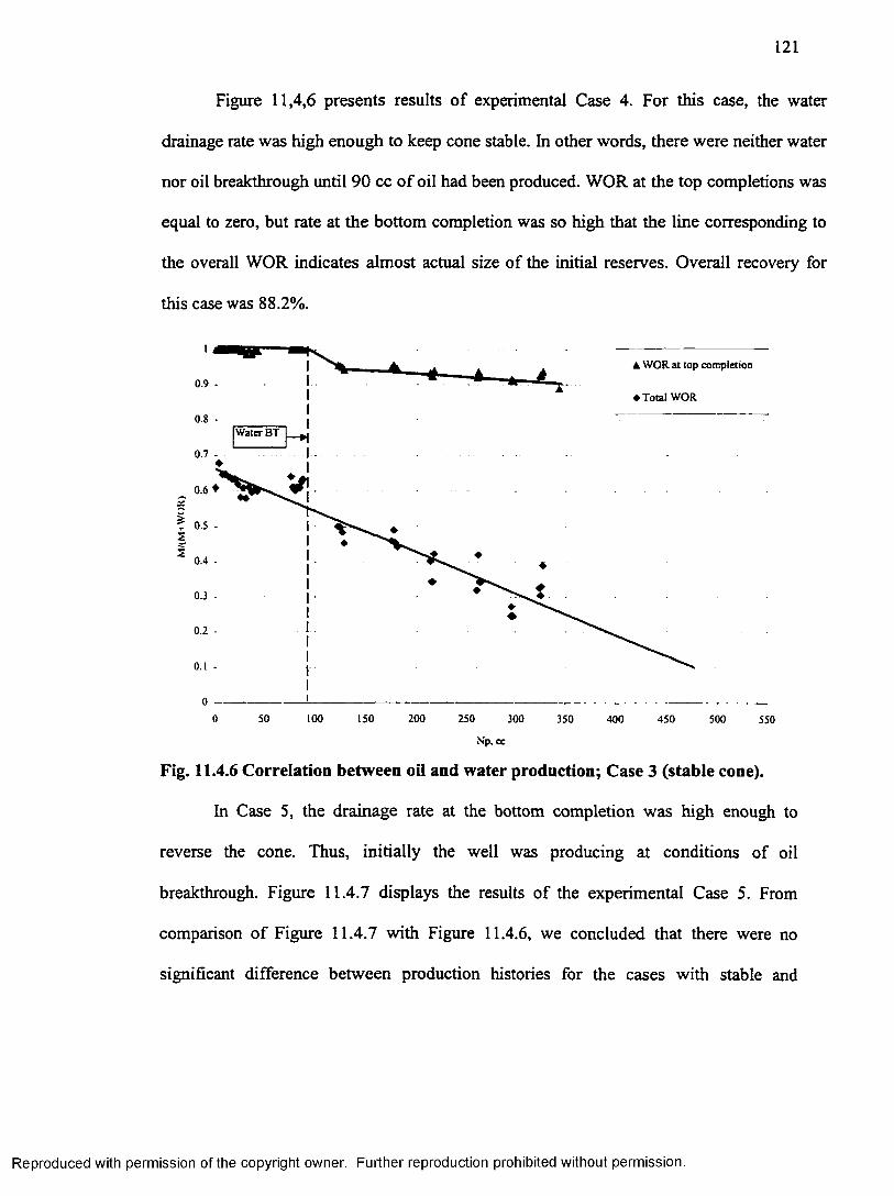
121

Figure 11,4,6 presents results of experimental Case 4. For this case, the water

drainage rate was high enough to keep cone stable. In other words, there were neither water

nor oil breakthrough until 90 cc of oil had been produced. WOR at the top completions was

equal to zero, but rate at the bottom completion was so high that the line corresponding to

the overall WOR indicates almost actual size of the initial reserves. Overall recovery for

this case was 88.2%.

▲ WOR at top completion

♦ Total WOR

Water BT

0.6 ♦

00 50 100 150 200 250 300 350 400 450 500 550

Np, cc

Fig. 11.4.6 Correlation between oil and water production; Case 3 (stable cone).

In Case 5, the drainage rate at the bottom completion was high enough to

reverse the cone. Thus, initially the well was producing at conditions of oil

breakthrough. Figure 11.4.7 displays the results of the experimental Case 5. From

comparison of Figure 11.4.7 with Figure 11.4.6, we concluded that there were no

significant difference between production histories for the cases with stable and


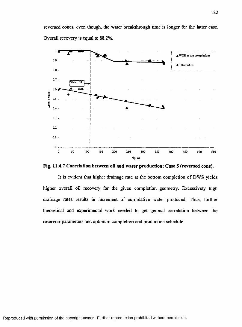
122

reversed cones, even though, the water breakthrough time is longer for the latter case.

Overall recovery is equal to 88.2%.

▲ WOR at top completions0.9 -

♦ Total WOR

0.8 -

W ater BT

0.6a£Oi

0.4 -

00 50 100 150 200 250 300 350 400 450 500 550

Np, cc

Fig. 11.4.7 Correlation between oil and water production; Case 5 (reversed cone).

It is evident that higher drainage rate at the bottom completion of DWS yields

higher overall oil recovery for the given completion geometry. Excessively high

drainage rates results in increment of cumulative water produced. Thus, further

theoretical and experimental work needed to get general correlation between the

reservoir parameters and optimum completion and production schedule.


CHAPTER 12

TIME DEPENDENT MODEL OF DWS

MSSM was developed to describe the pressure distribution around partially

penetrating wells. To model the behavior of a partially penetrating well, Shirman (1996)

substituted well’s perforated interval with an infinite number of spherical sinks. Thus,

the pressure distribution around a partially penetrating well is equal to the superimposed

effect of the all sinks and their images. To calculate this effect, steady state equation of

spherical flow was integrated along the completed interval. This integral yields a steady

state solution for the well with restricted entry to flow.

Evidently, strict steady-state conditions are virtually impossible to attain, since

these provisions are abstractions of the mind not the properties of the system. From the

practical standpoint, this fact does not exclude application of steady-state relations,

because in many cases they are closely approximated. So-called readjustment time, tr,

determines the extend of transient behavior [Chatas (1966)]. In spherical reservoir

systems readjustment time is approximated by Eq. 12.1

0.000264 fa c r;2k { ]

Evidently, the readjustment time depends on the properties of the system. If these

properties yield large readjustment time, transient, unsteady-state mechanics should be

used in the system. In a strict sense virtually all flow phenomena associated with

reservoir systems are unsteady state. Transient behavior of this phenomenon should be

considered. To do so a special time-dependent model of pressure distribution in

partially penetrated reservoirs should be developed.

123


124

12.1 Model Derivation

The fundamental differential equation of flow in spherical coordinates can be written as:

+ —— = (12 .,.!,dr2 r dr k dt

Effect of gravity in Eq. 12.1.1 is neglected.

Define some dimensionless variables as:

rD = — ( 12. 1.2)rw

0.000264kt' d = — -----7— (12.1.3)

<t>Mcrw'

„ t \ _ Pi ~ P d (*£> ’1D ) / n 1 /l\P d ~ P d v d ^ d ) ~ /. \ (12.1.4)

P i - P o v U J

tec denotes dimensionless time the system needs to achieve steady-state conditions.

Substitution of the equations 12.1.2, 12.1.3, 12.1.4 into Eq. 12.1.1 result in

dimensionless form of the differential equation of flow.

(12.1.5)drD‘ r drD dtD

In solving Eq. 12.1.5 the classical approach is illustrated by Carslaw and Jaeger

(1959),and Chatas (1966). The approach consists of introducing a new variable, b, as a

product of dimensionless time and pressure. This transformation reduces Eq 12.1.5 to

the following form.

d 2b db( 1 2 1 6 )drD otD

The general solution of Eq. 12.1.6 can be written as:


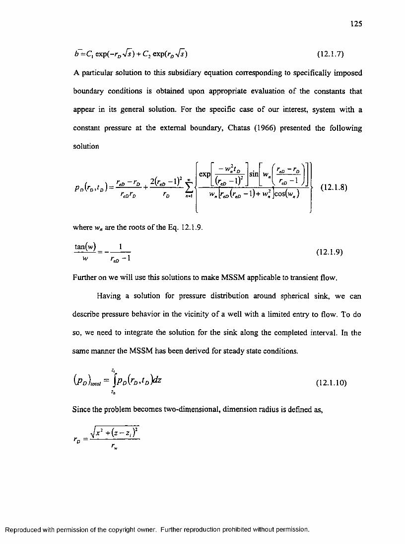
125

b = C x cxp(-rDJ s ) + C2 exp(rD^ ) (12.1.7)

A particular solution to this subsidiary equation corresponding to specifically imposed

boundary conditions is obtained upon appropriate evaluation of the constants that

appear in its general solution. For the specific case of our interest, system with a

constant pressure at the external boundary, Chatas (1966) presented the following

solution

„ (r t ) reD ~ rD , VP d V D ‘> ^ D / ~ _ / .

exp sin reD~rD V reD~\ y

reDrD fls| VcD f a > “ l ) + K ]C 0S(W „ )( 12.1.8)

where wn are the roots of the Eq. 12.1.9.

tan(w) _ 1w -1

(12.1.9)

Further on we will use this solutions to make MSSM applicable to transient flow.

Having a solution for pressure distribution around spherical sink, we can

describe pressure behavior in the vicinity o f a well with a limited entry to flow. To do

so, we need to integrate the solution for the sink along the completed interval. In the

same manner the MSSM has been derived for steady state conditions.

“f

( P D \o ta l I p d ^ d ^ d ) ^ 2 ( 1 2 .1 .1 0 )zb

Since the problem becomes two-dimensional, dimension radius is defined as,

ro =


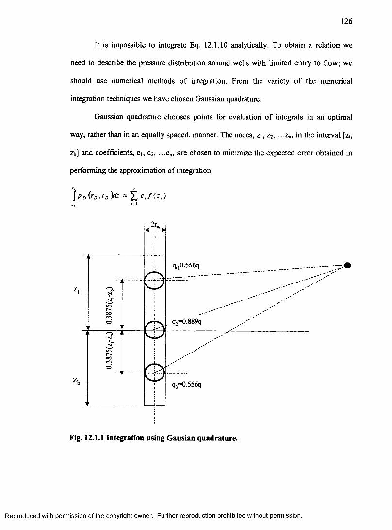
126

It is impossible to integrate Eq. 12.1.10 analytically. To obtain a relation we

need to describe the pressure distribution around wells with limited entry to flow; we

should use numerical methods of integration. From the variety o f the numerical

integration techniques we have chosen Gaussian quadrature.

Gaussian quadrature chooses points for evaluation of integrals in an optimal

way, rather than in an equally spaced, manner. The nodes, zi, z2, .. .Zn, in the interval [zt,

Zb] and coefficients, C j , c2, . . .C n , are chosen to minimize the expected error obtained in

performing the approximation of integration.

2' nJ P o O W d )dZ ~ X CJ ( Zi)

OOm

oo

i

Fig. 12.1.1 Integration using Gausian quadrature.


127

Presence of n arbitrary selected points and n coefficients, q, gives 2n parameters to

choose from. A polynomial degree at most (2n-l) also contains 2n parameters. This,

then, is the largest polynomial for which it is possible to expect the formula to be exact.

Thus, accuracy of Gaussian quadrature improves with the increment of the root number

used for the evaluation. Values for the constants and roots are tabulated and can be

found in Strout and Secrest (1966).

To approximate Eq. 12.1.10 we used three-point approximation. Practically it

means that we substituted the well’s completion with three spherical sinks, as shown in

Figure 12.1.1.

12.2 Computer Program

Numerical integration of Eq 12.1.8 yields the description of the pressure

distribution around a well with the limited entry in the infinite system with a cylindrical

constant pressure boundary. To model the effect of layers of different permeability and

horizontal no-flow boundaries an expanded method of images is used as explained in

Shirman and Wojtanowicz (1996). The resulting mathematical model, Multiple

Spherical Sink Transient Model (MSSTM) involves extensive numerical procedure so

that a computer program was written in EXCEL Visual Basic to perform computations.

To validate the MSSTM program, we compared pressure transient behavior in a 100%

penetrating well with the solution obtained using exponential integral. The difference in

the predictions was smaller than 2%.

To demonstrate the way the program works a case with a conventional partially

penetrating well was modeled. The input data for the example calculation is presented

in Figure 12.2.1


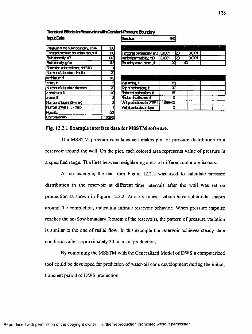
128

Trare^BfecteinFteenorewthOTEtrtfte s u e Bairfary InpiDtta ifcmhw aa

Ftesarecttteaiff banday, PSA -IOCGrEtatpressuebourferyracfus, ft 10CFUdMsooaty.cP 13l8Fhid density, g fe Q8Rsmndicnvckrnefectcr, db/STB 1NLrrbercf steps in r-drecfcn 2CH hrim inft 0 5r-stepttt 5Mrrbercf steps in zdredian Xzm nrninft ■4)zêp, It 3NLrrbercf layers (5 -rraO 3Mrrbercfwels (5-rra<) 1Fbroaty, 0 2Grrpresatifity 1.9DEGE

Hataotci paTTGEtifity, rrO Q0001 20 aoooiVertical pemBEbfity, itO aoooi 20 aoooiBandayvatic cocnl, ft 2D 4

m—

Tcpof periadicns, ft 20Etitamcf perfcrsticns, ft 15Ffeduscfwefl'saas.ft 0V\a podLdicn rata STBM 4.06&00V\aits pafcêd in laye- 2

Fig. 12.2.1 Example interface data for MSSTM software.

The MSSTM program calculates and makes plot o f pressure distribution in a

reservoir around the well. On the plot, each colored area represents value of pressure in

a specified range. The lines between neighboring areas of different color are isobars.

As an example, the dat from Figure 12.2.1 was used to calculate pressure

distribution in the reservoir at different time intervals after the well was set on

production as shown in Figure 12.2.2. At early times, isobars have spheroidal shapes

around the completion, indicating infinite reservoir behavior. When pressure impulse

reaches the no-flow boundary (bottom of the reservoir), the pattern of pressure variation

is similar to the one of radial flow. In this example the reservoir achieves steady state

conditions after approximately 20 hours of production.

By combining the MSSTM with the Generalized Model of DWS a computerized

tool could be developed for prediction of water-oil cone development during the initial,

transient period o f DWS production.


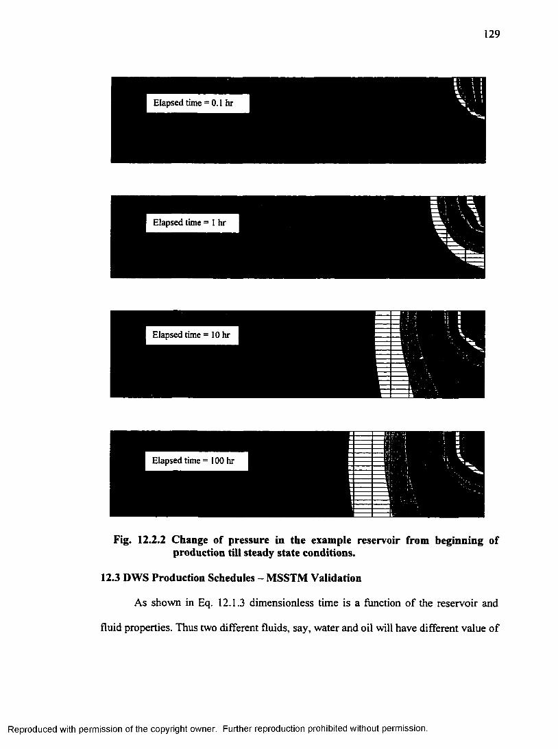
129

Elapsed time = 0.1 hr

Elapsed time = 1 hr

Elapsed time = 10 hr

Elapsed time = 100 hr

Fig. 12.2.2 Change of pressure in the example reservoir from beginning of production till steady state conditions.

12.3 DWS Production Schedules - MSSTM Validation

As shown in Eq. 12.1.3 dimensionless time is a function of the reservoir and

fluid properties. Thus two different fluids, say, water and oil will have different value of


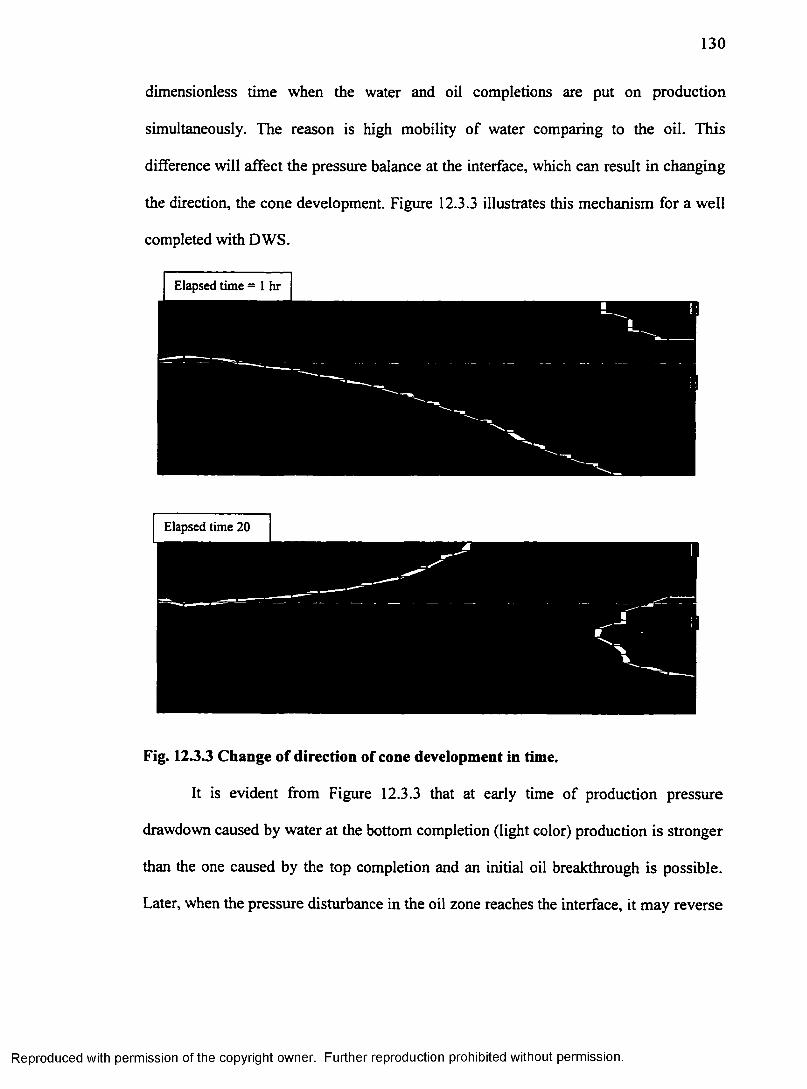
130

dimensionless time when the water and oil completions are put on production

simultaneously. The reason is high mobility of water comparing to the oil. This

difference will affect the pressure balance at the interface, which can result in changing

the direction, the cone development. Figure 12.3.3 illustrates this mechanism for a well

completed with DWS.

Elapsed tune = 1 hr

Elapsed tune 20

Fig. 12.3.3 Change of direction of cone development in time.

It is evident from Figure 12.3.3 that at early time of production pressure

drawdown caused by water at the bottom completion (light color) production is stronger

than the one caused by the top completion and an initial oil breakthrough is possible.

Later, when the pressure disturbance in the oil zone reaches the interface, it may reverse


131

the oil cone by pulling it upwards, which may eventually lead to the water

breakthrough. Similar results were obtained by the means of numerical simulator.

To eliminate this “flip-flop” cone behavior during the initial period of

production in wells with DWS, a special schedule of putting completions on production

should be developed. The schedule should have a delay in the starting of production o f

less viscous fluid. The delay period can be determined using developed software.


CHAPTER 13

CONCLUSIONS AND RECOMMENDATIONS

The main objective of this work was to develop a design procedure for wells

completed with DWS, which is valid for all production regimes, including post

breakthrough conditions. The following conclusions are drawn:

1. For conventional completions, water cone reversal requires reduction of production

rate much below the critical rate (50 - 70% of critical rate).

2. In conventional completions at equilibrium steady state production, water cut may

be in the range from zero up to limiting water cut value. A mathematical formula for

water cut prediction for any given production rate has been developed theoretically

and verified with experimental and simulated data.

3. In conventional completions at steady state flow conditions, rate of water production

is a linear function of oil production rate. Parameters of the straight line (slope and

intercept) give limiting water cut and the critical rate. Thus a complete description

of coning, based upon production history, can be made without knowing reservoir

flow properties.

4. For DWS completions, water cut in the production steams of the top and bottom

completions can be predicted using the Modified Inflow Performance Window

(MIPW) procedure, described in this work. MIPW describes the DWS performance

through the well qtop - qbonom domain.

5. The top and bottom completions of DWS interfere with each other. This

interference determines the limit of maximum performance for a given DWS

completion system.

132


133

6. For a linear flow, such as the one in Hele-Shaw model, water cut response is the

same as that for radial flow in conclusion 1.

7. A new analytical method has been developed to predict post breakthrough well

performance for both conventional and DWS completions. The method gives

analitical description pressure distribution at any point of the reservoir. It also uses

this distribution to predict dynamic oil-water interface.

8. For each production rate at the top completion unique rate at bottom completion can

be found to ensure a minimum overall water cut in the producing streams. We

observed up to twofold reduction in overall water cut compare to conventional

completions.

9. At the optimal conditions, DWS can provide additional oil recovery' (up to 30%

increment).

10. Pressure transient effects may create flip-flop cone behavior at shortly after the

DWS completions were put on production. A new analytical model was developed

to describe development of the pressure impulse around partially penetrating wells.

Time of stabilization can be predicted with the proposed model.

11. To eliminate transient flip-flop water cone behavior, it is recommended to put the

bottom completion on production with a time delay after the top completions have

been producing. The period of the delay can be determined using developed

software.


NOMENCLATURE

Unless otherwise noted within the body of the text immediately following

presentation of the mathematical expressions, the following nomenclature applies

through this work:

A cross-sectional area

B - formation volume factor

c = compressibility

E = Young’s modulus

g = gravity constant

H = initial zone thickness

h = zone thickness, height o f the well above WOC

k = permeability

L = length

M = mobility ratio

N = initial oil in place

Np = produced oil

Nrc = Reynolds number

P - pressure

q = production rate

r - radius

s = glass plate thickness

S = saturation

t — time

134


135

V = velocity

Wp = produced water

w c = water cut

WOR = water-oil ratio

x,y,z = coordinates

Y = cone shape factor

8 = gap thickness

<D = flow potential

♦ = porosity

P = dynamic viscosity

n = perimeter

n = 3.14....

P = density

Subscripts

av = average

b = bottom

cr = critical

d = drain

D = dimensionless

e = outer boundary

eq = equivalent

i = point at well’s completion; injector

j = index


136

1 = linear

lim = limiting, ultimate

m = model

o = oil

r - radial

t = top

total = total

w = water, well

wc = connate water


REFERENCES

Aboughoush, M.S.: “Correlation for Performance Prediction of Heavy Oil Pools, Lloydminster Area,” Proceedings o f the I UNITAR Conference, Edmonton, Alberta, June 4-12,1979

Alikhan, A.A., and Farouq Ali, S.M., State of-the-art of Water Coning Modeling and Operation; Soc. Pet. Eng. Paper No. 13744, Bahrain, March 11-14, 1985.

Allen, T.O., and Roberts, A.P., Production Operations-Well Completions, Workover and Stimulation, Vol.2, Chapter 1, Oil & Gas Consultants Int. Inc. Tulsa, Oklahoma, 1982.

Arthur, M.G., Fingering and Coning of Water and Gas in Homogeneous Oil Sand; Trans. AIME, Vol. 155, 154-201, 1944.

Blades, D.N., and Stright, D.H.: “Predicting High Volume Lift Performance in Wells Coning Water,” JCPT, Vol. 14, No.4, Oct.-Dec. 1975, 62-70.

Bobek, J.E. and Bil, P.T.: “Model Study of Oil Displacement from Thin Sands by Vertical Water Influx from Adjacent Shales,” JPT, Sept., 1961, 950-954.

Boumazel, C. and Jeanson, B.: “Fast Water-Coning Evaluation Method,” paper SPE 3628 presented at 1971 Fall Meeting, New Orleans, LA, Oct 1971.

Butler, R.M.: “The Potential for Horizontal Wells for Petroleum Production,” JCPT, Vol. 28, No. 3, 39-47, May-June 1989.

Butler, R.M. and Stephens, D.J.: “The Gravity Drainage of Steam-Heated Heavy Oil to Parallel Horizontal Well,” JCPT, April-June, 1981, 90-96.

Byme, W.B. Jr. and Morse, R.A.: ‘The Effects of Various Reservoir and Well Parameters on Water Coning Performance,” paper SPE 4287, presented at the Third Numerical Simulation Symposium of reservoir Performance, Houston, TX, Jan., 10-12, 1973a.

Byme, W.B. and Morse, R.A.: “Water Coning May not be Harmful,” Oil and Gas J., 66-70, Sept. 1973b.

Castaneda F.: “Mathematical Simulation Effect of Selective Water Encroachment in Heavy Oil Reservoirs,” Proceedings of the II UNITAR Conference, Caracas, Venezuela, Feb. 7-17, 1982.

Carslaw, H.S. and Jaeger, J.C.: Conduction o f Heat in Solids, second edition, Oxford at the Clarendon Press, Oxford, England, 1959

Caudle, B.H. and Silberberg, I.H.: “Laboratory Models of Oil Reservoirs Produced by Natural Water Drive,” SPEJ, March, 25-36, 1965.

137


138

Chatas, A.T.: “Unsteady Spherical Flow in Petroleum Reservoirs,” SPEJ, June 1966,102-114.

Chaperon, I.: “Theoretical Study of Coning Toward Horizontal and Vertical Wells in Anisotropic Formations: Subcritical and Critical Rates; SPE. 15377, New Orleans, Louisiana, Oct. 5-8, 1986

Chappellear, J.E. and Hirasaki, G.J.: “ A Model of Oil-Water Coning for Two-Dimensional Areal Reservoir Simulation; Soc. Pet. Eng. J„ pp. 65-7Z April 1976.

Chierici, G.L., Ciucci, G.M., and Pizzi, G.: “A Systematic Study of Gas and Water Coning by Potentiometric Models,” JPT, August, 1964, 923-929.

Costeron, J.W., et al.: “Bacterial to Control Conformance of a Waterflood,” Paper No. 6-21, AOSTRA Oil-Sands 2000, Edmonton, Alberta, March 26-28, 1990.

Cramer, R.L.: “Method and Apparatus for Pumping Fluids from Bore Holes,” Canadian Patent No.l, 140, 459, Feb. 1, 1983.

Cram, P.J., and Redford, D.A.: “Low Temperature Oxidation Process for the Recovery of Bitumen,” JCPT, Vol. 16, No.3, July-Sept. 1977, 72-83.

Elkins, L.P.: “Fosterton Field - An Unusual Problem of Bottom Water Coning and Volumetric Water Invasion Efficiency,” Trans, AIME, Vol.216, 1959, 130-137.

Farouharson, R.G., Leseons from Eyehill; Pet. Soc. of CIM Meeting, Paper No.5, Regina, Sept. 15-17, 1985.

Hawthorne, R.G.: “Two-Phase Flow in Two-Dimensional Systems - Effect of Rate, Viscosity and Density of Fluid Displacement in Porous Media,” Transactions AIME, Vol. 219, 81-87, 1960.

Henley, D.H., Owens, W.W., and Craig, F.F.: “ A Scale-Model Study of Bottom-Water Drives,” JPT Jan, 90-98, 1961.

Hoyt, D.L.: “Gradient Barrier in a Secondary Recovery Operation to Inhibit Water Coning,” U.S. Patent No.3, 825,070, July23, 1974.

Islam, R., and Farouq Ali, S.M.: “Mobility Control in Water-flooding Oil Reservoirs with a Bottom-Water Zone,” JCPT, Vol 26, No.6, Nov.-Dee. 1987, 40-53.

Islam, R., and Farouq Ali, S.M.: “An Experimental and Numerical Study of Blocking of a Mobile Water Zone by an Emulsion,” Paper No. 133, Proceedings of the IV UNITAR/UNDP Int. Conf. on Heavy Crude and Tar Sands, Edmonton, Alberta,Vol. 4, 1988, 303-321.


139

Karp, J.C., Lowe, D.K. and Marusov, N.: “ Horizontal Barriers for Controlling Water Coning; Trans. AIME, Vol.225, 783-790,1962.

Khan, A.R.: “A Scaled Model Study of Water Coning,” JPT, June, 1970, 771-776.

Khan, A.R. and Caudle, B.H.: “Scaled Model Studies of Thin Oil Columns Produced by Natural Water Drive,” SPEJ, Sept., 1969,317-322.

Kisman, K.E., et al: “Water-wetting Treatment for Reducing Water Coning in an Oil Reservoir; U.S. Patent No.5,060,730, Oct.29,1991.

Kisman, K.E., et al.: ‘Treatment for Reducing Water Coning in an Oil Reservoir,” U.S. Patent No.5,062,483, Nov. 5, 1992.

Kuo, M.C.T. and DesBrisay, C.L.: "A simplified Method of Water ConingPredictions," SPE 12067, presented at the 1983 Annual Conference and Exhibition, San Francisco, CA, Oct. 5-8.

Letkeman J.P. and Ridings, R.L.: “A Numerical Coning Model,” SPEJ, Dec. 1970, 416- 422

Leverett, M.C. Jr., Lewis, W.B., and True, M.E.: “Dimensional -model Studies of Oil -field Behavior,” Proceedings of 1941 Meeting, Dallas, TX, Oct., 157-193.

Lunhning, R.W. and Ronaghan, K.R.: “Method for Controlling Water Coning in Oil Wells; Canadian Patent No. 1,239,088, July 12, 1988.

MacDonald, R.C., and Coats, K.H.: “Methods for Numerical Simulation of Water and Gas Coning; SPEJ, 425-436, Dec. 1970.

Matthews, C.S and Lefkovits, H.C.: “Gravity Drainage Performance of Depletion -Type Reservoir in the Stripper Stage,” Transactions AIME, Vol. 207, 1956, 265-274.

Meyer, H.I. and Searcy, D.F.: “Analog Study of Water Coning”, Trans. 207, 1956, 302- 305.

Mungan, N.: “A Theoretical and Experimental Coning Study,” SPEJ, June, 1975.

Mungan, N.: “Laboratory Study of Water Coning in a Layered Model,” JCPT, VoL 18,No. 3, July-Sept. 1979, 60-70.

Muskat, M.: The Flow o f Homogeneous Fluids Through Porous Media, J.W. Edwards Inc., Attn Arbor, Michigan, 1946, 480-506.

Muskat, M., and Wyckoff, R.D.: “An Approximate Theory o f Water-coning in Oil Production,” Trans. AIME, Vol. 114, 1935,144-163.


140

Parker, R.K.: “Water Coning - A System for Predicting WOR Performance,” SPE 6978, unsolicited, 1977.

Paul, J.M., and Strom, E.T.: “Oil Reservoir Permeability Control using Polymeric Gels,” Canadian Patent No.1,264,856, Dec.20, 1988.

Pietraru, V.: “New Water/Gas Coning Solution for Vertical/Horizontal Wells,” World Oil J., Jan 1997, 55-62.

Pollock, C.B., and Shelton, J.L.: “Method for Decreasing Water production by Gas Injection in a Single Well Operation,” Canadian Patent No.866, 573, March 23, 1971.

Pirson, S.J. and Mehta, M.M.: “A study of Remedial Measures for Water-Coning by Means of a Two-Dimensional Simulator,” SPE 1808, 42th SPE Meeting, Houston, TX, Oct. 1-4, 1967.

Racz, D.: “Development and Application of a Thermocatalytic 'In Situ' Combustion Process in Hungary,” Proc. m European Mtg. Imp. Oil Rec., Rome, Italy, April 16, 1985, 431-440.

Richardson, J.G., and Blackwell, R.J., Use of Simple Mathematical Models for Predicting Reservoir Behavior; JPT, Sept. 1971, 1145-1154.

Saxman, D.B.: “Biotechnology and Enhanced Petroleum Production,” SPE 13146, 59th Annual Conf. and Exhibition, Houston, Texas, Sept. 16,1984.

Schols, R.S.: “Water Coning - An Empirical Formula for the Critical Oil-Production Rate,” Erdoel-Ergas-Zeitshrift, 88 Jg, Jan. 1972, 6-11.

Settari, A. And Aziz, K.: “A Computer Model for Two-Phase Coning Simulation,” SPEJ, June, 1974, 221-236.

Shirman E.I.: An Analytical Model of 3-D Flow Near a Limited-Entry Wellbore in Multilayered Heterogeneous Strata - Theory and Applications, Master Thesis, Louisiana State University, Baton Rouge, LA, Aug. 1995 64.

Shirman E.I.: “A Well Completion Design Model for Water-Free Production from Reservoirs Overlaying Aquifers,” International Student Paper Contest, Proceedings, SPE Annual Technical Conference and Exhibition, Denver, CO, October 6-9 1996, Vol. n , 853-860.

Shirman E.I and Wojtanowicz, A.K.: “Analytical Modeling of Crossflow into Wells in Stratified Reservoirs: Theory and Field Application,” Proceedings vol II, 7th International Scientific-Technical Conference, Cracow, June 20-21, 1996.


141

Smith, C.R., and Pirson, S J .: “ Water Coning Control in Oil Wells by Fluid Injection,” SPEJ, Vol.3, No.4, 314-326, 1963.

Sobocinski, D.P. and Cornelius A.J.: “A Correlation for Predicting Water Coning Time,” JPT, May, 594-600, 1965.

Stephens, A.C., Moore, T.F., and Caudle, B.H.: "Some Model Studies of Bottom Water Driven Reservoirs,” paper SPE 561 presented at 1963 Production Research Symposium, Norma, OK, April 29-30.

Stroud, A.H. and Secrest, D.: Gaussian Qudrature Formulas. Prentice Hall, Englewood Cliffs, N.J. 1966, 374.

Swisher, M.D. and Wojtanowicz, A.K.: “In Situ-Segregated Production of Oil and Water - A production Method with Environmental Merit: Field Application,” SPE 29693 SPE/EPA Exploration & Production Environmental Conference, Houston, TX, March 27-29,1995a.

Swisher, M.D. and Wojtanowicz, A.K.: “New Dual Completion Method Eliminates Bottom Water Cining,” SPE 30697, SPE Annual Technical Conference and Exhibition, Dallas, TX, Oct. 22-25, 1995b.

Timoshenko, S and Wionwski-Krieger, S: Theory of plates and shells, Mc.Craw-Hill Book Co., 1987, 202-204.

VanDaalen, F. and VanDomselaar, H.R.: “Scaled Fluid-Flow Models with Geometry Differing from that of Prototype,” SPEJ, June, 1972, 220-228.

Van Golf-Racht, T.D. and Sonier, F.: “ Water Coning in Fractured Reservoir,” SPE 28572, 69th Annual Technical Conference and Exhibition, New Orleans, Sept. 25-28, 1994.

Wadleigh, E.E., Paulson, C.I., and Stolz, R.P.: “Deep Completions Really Lower Water-Oil Ratios!” SPE 37763, Middle East Oil Show and Conference, Manama, Bahrain, March 15-18, 1997.

Weast, R.C.: Handbook of Chemistry and Physics, The Chemical Rubber Co., Cleveland Ohio, 1972,4-152.

Weinsein, H.G., Chappelear, J.E., and Nolen, J.S.: “Second Comparative Solution Project: A Three-Phase Coning Study,” JPT, Vol.38, No.3, 1986, 345-353.

Wojtanowicz, A.K. and Bassiouni, Z.: “Oilwell Coning Control Using Completion with Tailpipe Water Sink,” SPE 21654, SPE Prod. Org. Symp., Oklahoma City, OK, April 7-9. 1991.


142

Wojtanowicz, A.K., Xu, H. and Bassiouni, Z.: “Segregated Production Method for Oil with Active Water Coning,” JPSE, Vol. II, No.l, April, 1994.

Zaitoun, A., and Kohler, N.: “Modification of Water/Oil and Water/Gas Relative Permeability After Polymer Treatment of Oil or Gas Wells; In Situ, Vol 13, No. 1-2, 1989, 55-78.


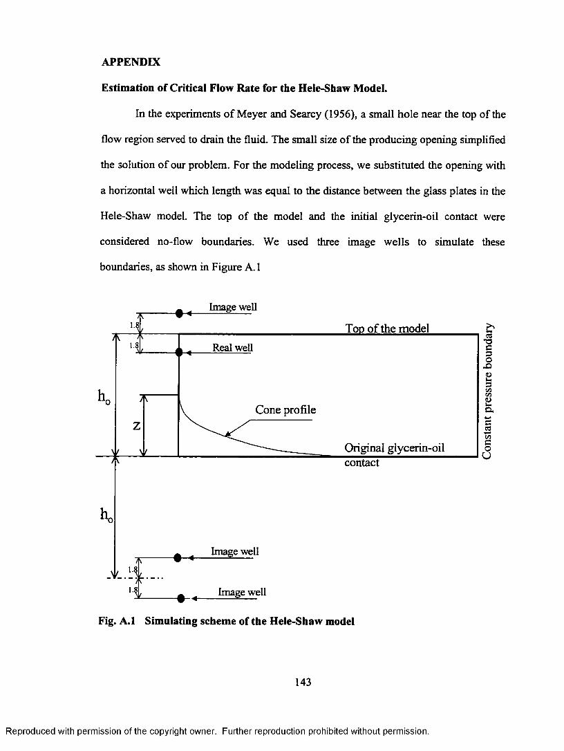
APPENDIX

Estimation of Critical Flow Rate for the Hele-Shaw Model.

In the experiments o f Meyer and Searcy (1956), a small hole near the top of the

flow region served to drain the fluid. The small size of the producing opening simplified

the solution of our problem. For the modeling process, we substituted the opening with

a horizontal well which length was equal to the distance between the glass plates in the

Hele-Shaw model. The top of the model and the initial glycerin-oil contact were

considered no-flow boundaries. We used three image wells to simulate these

boundaries, as shown in Figure A. 1

Image well

Top o f the model

Real well

U

Cone profile a.

Original glycerin-oilcontact

Image well

Image well

Fig. A.1 Simulating scheme of the Hele-Shaw model

143


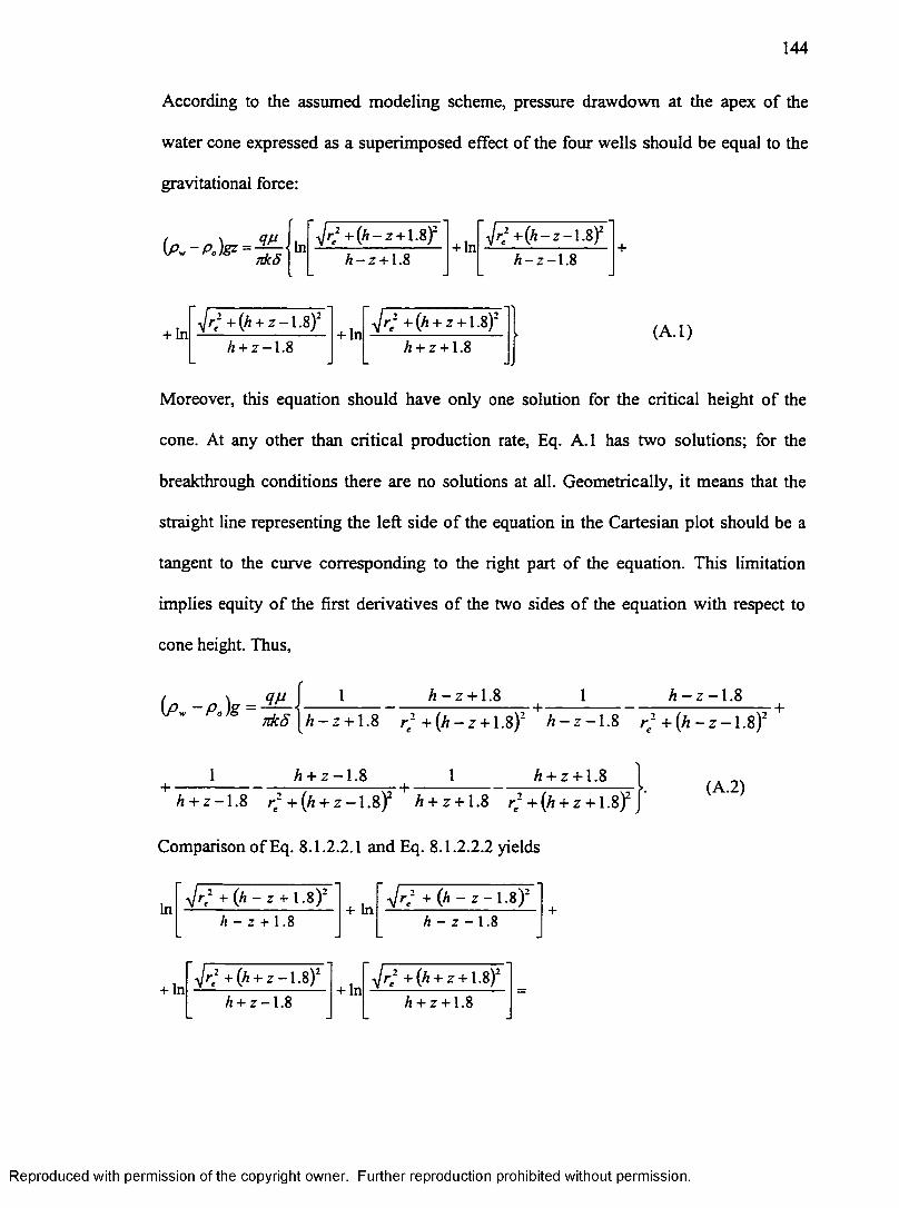
144

According to the assumed modeling scheme, pressure drawdown at the apex of the

water cone expressed as a superimposed effect of the four wells should be equal to the

gravitational force:

■ <InVr/ +0*-z + 1.8)2 + ln yjr; + (h - z - l .8 f

nkS h - z + 1.8 1

1 N 1 00 I

+ ln■\jr~ +{h + z — 1.8)

+ lnJr* +{h + z + 1.8)2

A + z-1.8 h + z +1.8(A.l)

Moreover, this equation should have only one solution for the critical height of the

cone. At any other than critical production rate, Eq. A.l has two solutions; for the

breakthrough conditions there are no solutions at all. Geometrically, it means that the

straight line representing the left side of the equation in the Cartesian plot should be a

tangent to the curve corresponding to the right part of the equation. This limitation

implies equity of the first derivatives of the two sides of the equation with respect to

cone height. Thus,

( a , -P o )s =h — z + 1.8 1 h - z - 1.8

n k S [ h - z + \.8 r* + ( h - z + \.8 )2 h - z - 1.8 r * + ( h - z - 1.8)2• +

h + z -1.8 h + z +1.8h + z - 1.8 re2 + {h + z —1.8)2 h + z + 1.8 r^+{h + z + \.^ f

Comparison of Eq. 8.1.2.2.1 and Eq. 8.1.2.2.2 yields

(A.2)

In

+ In

■\Jrc + {h - z + 1.8)2~ h - z + 1.8

•Jr* + (h + z — 1.8)/i + z-1.8

+ InVr/ + (h - z - 1.8);~

h - z -1.8

+ lnVr; + (/i + z + 1.8)2

h + z +1.8


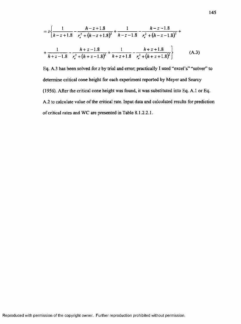
145

[ 1 h - z + 1.8 1_________h - z - 1.8 |~ [ h - z + 1.8 r ; + { h - z + \ . 8 f + h - z - 1 . 8 r 2 + { h - z - 1.8)2 +

1 h + z —1.8 1 h + z + 1.8+ h + z - l . 8 ~ r ;+( h + z - l . 8 f h + z + \ . 8~ r 2+{h + z + \ . 8f

Eq. A.3 has been solved for z by trial and error; practically I used “excel’s” “solver” to

determine critical cone height for each experiment reported by Meyer and Searcy

(1956). After the critical cone height was found, it was substituted into Eq. A.1 or Eq.

A.2 to calculate value of the critical rate. Input data and calculated results for prediction

of critical rates and WC are presented in Table 8.1.2.2.1.

(A.3)


VITA

Ephim I. Shirman is a native of Moscow, Russia, where he obtained his Diploma

with Honors in Mechanical Engineering from the Academy (Institute) of Oil and Gas in

1978. After graduation he worked in the Research Institute of Petroleum Equipment as

engineer and researcher. In 1993 he enrolled in Petroleum Engineering graduate

program of Louisiana State University, where he earned Master of Science degree in

Petroleum Engineering in 1995.

While in the graduate school, Ephim published five papers in technical books

and journals. He also won first places in SPE Gulf Cost Regional and SPE International

student paper contests in 1996. The main area of his technical interest is in well

completion and production.

146


DOCTORAL EXAMINATION AND DISSERTATION REPORT

Candidate: Ephim I. Shirman

Major Field: Petroleum Engineering

Title of Dissertation: Experimental and Theoretical Study of DynamicWater Control in Oil Wells

Approved:

Major Professor and Chairman

f the Graduate SchoolDe<

EXAMINING COMMITTEE:

Date of Examination:

4 / 1 4 / 9 8


IMAGE EVALUATIONTEST TARGET (Q A -3 )

1.0

l.l

1.25

Lb1^ m1- HIMb:i.u .L. 1 2.0i_ =====

1m1.4 | 1.6

150mm

IIW IG E . In c1653 East Main Street Rochester. NY 14609 USA Phone: 716/482-0300 Fax: 716/288-5989


Experimental and Theoretical Study of Dynamic Water Control ...

Documents