experimental and numerical investigation of a heat recovery ...

EXPERIMENTAL AND NUMERICAL INVESTIGATION OF A HEAT RECOVERY

VENTILATION UNIT WITH PHASE CHANGE MATERIAL FOR BUILDING FACADES

A Thesis Submitted to the Graduate School of Engineering and Sciences of

İzmir Institute of Technology in Partial Fulfillment of the Requirements for the Degree of

DOCTOR OF PHILOSOPHY

in Architecture

by Tuğçe PEKDOĞAN

December 2021 İZMİR

ACKNOWLEDGMENTS

It is my pleasure to acknowledge the roles of several individuals who were

instrumental in completing my Ph.D. research.

First of all, I am grateful to my supervisor, Prof. Dr. Tahsin Başaran, whose

expertise, understanding, generous guidance, and support encouraged me to work on a

topic of great interest.

I am grateful to TÜBİTAK for the financial support throughout this study. And I

would like to give special thanks to my dissertation committee. To Assoc. Prof. Dr. Ayça

Tokuç, I thank her for her untiring support and guidance throughout my journey. I would

like to thank Assoc. Prof. Dr. Mehmet Akif Ezan and Assoc. Prof. Dr. Mustafa Emre İlal

for their support, helpful critics and suggestions throughout the development of this

thesis. I would also like to thank other jury members, Prof. Dr. Zehra Tuğçe Kazanasmaz

and Assoc. Prof. Dr. Ziya Haktan Karadeniz, for their guiding comments, valuable ideas

and suggestions.

To my friends, thank you for listening to me, offering me advice, and supporting

me through this entire process. Special thanks to Fulya Atarer, Emre İpekci and Ersin

Alptekin for their friendship, technical and moral support.

Dear Mom and Dad, thank you for your endless support and encouragement. This

diploma is just as much yours as it is mine.

ABSTRACT

EXPERIMENTAL AND NUMERICAL INVESTIGATION OF A HEAT RECOVERY VENTILATION UNIT WITH PHASE CHANGE

MATERIAL FOR BUILDING FACADES

This thesis presents a wall-integrated HRV unit design that stores latent heat

thermal energy (LHTES). The system’s performance is tracked through experimental and

numerical studies. The experimental tests of the unit took place in a controlled

environment, where two HRV units are inside two wall-integrated ducts. The wall divides

two conditioned spaces that represent indoors and outdoors. In one set of experiments,

the commercially available system that stores sensible heat thermal energy (SHTES) with

ceramic block. On another set of experiments, the newly designed LHTES system with

the staggered tube bundle that contains phase change material (PCM). SHTES system

shows the best performance in 2-minute, supply efficiency is 82% and exhaust efficiency

is 67%. LHTES system shows the best performance in 20-minute and supply efficiency

is 55% and exhaust efficiency is 30%.

Numerical parametric studies on the HRV systems use the commercial CFD

software ANSYS-FLUENT. These studies include the detailed flow and heat transfer

analyses and the optimum operating times for two systems. As a result of these studies,

the CFD results show good agreement with the experimental results. At the end of the

thesis, the ability to increase the capacity of the HRV unit with PCM was investigated. In

addition, the simulations for different climatic data were studied. According to the results,

12mm longitudinal, 12mm transverse pitch size for the ∅4.76mm tube is the most

efficient system with total heat capacity of 45.77kJ. In addition, for different climates

simulations, LHTES unit can be used throughout the year in Singapore.

iii

ÖZET

BİNA CEPHELERİ İÇİN FAZ DEĞİŞİM MALZEMELİ BİR ISI GERİ KAZANIM ÜNİTESİNİN DENEYSEL VE SAYISAL İNCELENMESİ

Bu tez, duyulur ısıl enerji depolama (DIED) yerine gizli ısıl enerji depolama

(GIED) özelliğini kullanan duvara entegre bir ısı geri kazanım (IGK) ünitesinin ısı ve akış

performansının incelenmesi üzerinedir. Sistemlerin performansı deneysel ve sayısal

parametrik çalışmalarla incelenmiştir. Deneysel kısımda, laboratuvar ortamında

şartlandırılan iki mekân arasına örülen duvarda bulunan iki adet kanal içerisine IGK

havalandırma sistemleri yerleştirilerek kontrollü parametrik incelemeler yürütülmüştür.

Bu iki kanala yerleştirilen, birbirleriyle eş zamanlı çalışan ünitelerin ısı ve akış

performansları elde edilmiştir. Birinci deney setinde, piyasada bulunan DIED seramik

bloklu sistem için parametrik çalışmalar gerçekleştirilmiştir. İkinci deney setinde ise,

GIED sağlayan IGK ünitesi şaşırtmalı tüp demeti şeklinde tasarlanmış ve tüplerin içine

faz değişim malzemesi (FDM) yerleştirilerek, ünite içerisindeki sıcaklık değişimleri ve

erime/katılaşma süreçleri belirlenmiştir. DIED sisteminde 2 dakika, GIED sisteminde ise

20 dakika boyunca çalıştığında, birim zaman başına en yüksek enerji depolama

görülmektedir. Deneysel sonuçlara göre en yüksek verim; DIED için besleme verimi

%82, egzoz verimi %67’dir. GIED sisteminde ise besleme verimi %55, egzoz verimi

%30’dur.

İki IGK sistemi üzerindeki sayısal parametrik çalışmalar, ANSYS-FLUENT

aracılığıyla yapılmıştır. Yapılan çalışmalar neticesinde HAD sonuçları deneysel

sonuçlarla uyumludur. HAD çalışmaları kapsamında; sistemler üzerinde detaylı akış ve

ısı transferi analizleri ile optimum çalışma süreleri değerlendirilmiştir. Ayrıca daha

yüksek performansa sahip GIED ünitesi için kapasite geliştirme çalışmaları araştırılmış

ve farklı iklim verileri için simülasyonlar yapılmıştır. Elde edilen sonuçlara göre, 4.76mm

çapındaki tüp için 12mm enine 12mm boyuna hatve ölçüsüne sahip olan tasarım 45.77kJ

toplam ısı kapasitesi ile en verimli sistemdir. Farklı iklimlerde yapılan simülasyon

sonuçlarına göre Singapur'da bu sistemin yıl boyunca kullanılabileceği görülmüştür.

iv

TABLE OF CONTENTS

LIST OF FIGURES ....................................................................................................... x

LIST OF TABLES .................................................................................................... xvii

LIST OF ABBREVATIONS ...................................................................................... xix

LIST OF NOMENCLATURE ..................................................................................... xx

CHAPTER 1. INTRODUCTION ......................................................................................... 1

1.1. Research Area and Context................................................................... 1

1.2. Purpose of the Study............................................................................. 5

1.3. Research Methodology ......................................................................... 6

1.4. Contents of the Study ........................................................................... 8

CHAPTER 2. DEFINITIONS AND LITERATURE REVIEW .........................................9

2.1. Indoor Environment ............................................................................. 9

2.1.1. Indoor Air Quality .............................................................................. 10

2.1.2. Thermal Comfort ................................................................................ 12

2.2. International Standards and Local Regulations ................................... 15

2.2.1. Indoor Air Quality Requirements ................................................. 15

2.2.2. Thermal Comfort Requirements ................................................... 19

2.2.3. Energy Recovery Requirements ................................................... 23

2.3. HVAC Systems .................................................................................. 24

2.3.1. Classification of HVAC Systems ................................................. 25

2.3.1.1. Centralized Systems ........................................................... 25

2.3.1.1.1. All-air Systems ....................................................... 26

2.3.1.1.2. All-water Air Conditioning Systems ........................ 27

2.3.1.1.3. Hybrid (Air-Water) Air Handling Units ................... 28

2.3.1.1.4. Refrigerant-based Systems ...................................... 29

2.3.1.2. Decentralized Systems ........................................................ 30

v

2.3.1.3. Decentralized Ventilation and Centralized Ventilation

Systems .............................................................................. 31

2.3.2. Ventilation ................................................................................... 33

2.3.3. Heat Recovery System Solutions.................................................. 35

2.3.3.1. Recuperative Systems ......................................................... 36

2.3.3.2. Regenerative Systems ......................................................... 36

2.3.4. Review of Heat Recovery Systems ............................................... 37

2.4. Thermal Energy Storage Using in Buildings ....................................... 38

2.4.1. Sensible Heat Storage .................................................................. 39

2.4.2. Latent Heat Storage...................................................................... 40

2.4.2.1. Potential of Using Latent Heat Storage with Solid-Liquid

Phase Change ..................................................................... 42

2.4.3. Sensible and Latent Energy Storage HRV Systems ...................... 42

2.4.4. Temperature Control .................................................................... 44

2.5. Phase Change Materials...................................................................... 45

2.5.1. Classification ............................................................................... 45

2.5.2. Potential of PCMs Applications ................................................... 46

2.5.2.1. Use of PCM and LHTES with PCM ................................... 48

2.5.2.2. Performance of LHTES Systems Containing PCM ............. 50

2.6. Market Research for Decentralized HRV ............................................ 51

CHAPTER 3. EXPERIMENTAL METHOD .............................................................. 53

3.1. Research Framework .......................................................................... 53

3.1.1. Physical Model ............................................................................ 54

3.1.2. Test Chamber ............................................................................... 54

3.1.3. Wall Structure .............................................................................. 56

3.1.4. Duct Setup ................................................................................... 57

3.2. Ceramic Heat Recovery Ventilation System ....................................... 59

3.3. Design of the Tube Bundled Prototype With PCM Heat Recovery

Ventilation System ............................................................................. 62

3.4. Experimental Procedure ..................................................................... 64

3.5. Experimental Setup Measurement Devices ......................................... 66

3.5.1. Temperature Measurements ......................................................... 66

3.5.2. Evaluation of the Fan Characteristics ........................................... 68

vi

3.5.2.1. Air Velocity Measurements ................................................ 68

3.5.2.2. Pressure Drop Measurements ............................................. 71

3.5.2.3. Fan Characteristics ............................................................. 74

3.6. Usage of Thermal Energy Storage Material in Prototype .................... 75

3.7. Calibration Process ............................................................................. 76

3.8. Uncertainty Analysis .......................................................................... 78

3.9. Summary ............................................................................................ 80

CHAPTER 4. NUMERICAL ANALYSES ................................................................. 81

4.1. Theory and Background ..................................................................... 81

4.2. CFD Modeling Procedure ................................................................... 82

4.3. Governing Equations .......................................................................... 83

4.4. Physical Domain ....................................................................................... 84

4.5. Mesh Generation ....................................................................................... 85

4.6. Mesh Quality ............................................................................................. 85

4.7. Simulation Details of the HRV Units ...................................................... 87

4.7.1. Problem Identification .................................................................. 87

4.7.1.1. Ceramic System for Sensible Thermal Energy Storage ....... 88

4.7.1.2. Tube Bundle System for Latent Thermal Energy Storage.... 89

4.8. Numerical Approach ................................................................................. 90

4.8.1. Mesh Generation .......................................................................... 91

4.8.1.1. Grid Independence Study ................................................... 91

4.8.1.1.1. Ceramic System Mesh Structure Decision ............... 93

4.8.1.1.2. Tube Bundle System Mesh Structure Decision ........ 95

4.8.2. Boundary Conditions ................................................................... 98

4.8.3. Solution Method ........................................................................ 100

4.8.4. Model Verification and Validation ............................................. 100

4.8.4.1. Verification of Method with Reference Study ................... 101

4.8.4.2. Validation of Model for Ceramic Heat Recovery System .. 102

4.8.4.3. Validation of Model for Tube Bundle Heat Recovery

System ............................................................................. 103

4.9. Summary .................................................................................................. 104

vii

CHAPTER 5. RESULTS AND DISCUSSION .......................................................... 105

5.1. Experimental Results ........................................................................ 105

5.1.1. Charging and Discharging Experiments for SHTES ................... 106

5.1.2. Charging and Discharging Experiments for LHTES ................... 112

5.1.3. Data Reduction .......................................................................... 116

5.1.3.1. Data Reduction for SHTES ............................................... 116

5.1.3.2. Data Reduction for LHTES .............................................. 118

5.1.4. Comparison of Mean Heat Transfer Rate ................................... 120

5.1.5. Calculation of Heat Recovery Efficiency.................................... 121

5.2. Simulation Results .................................................................................. 123

5.2.1. Simulation Results of SHTES .................................................... 123

5.2.2. Simulation Results of LHTES .................................................... 129

5.2.3. Data Reduction for Simulation Results ....................................... 136

5.3. Refinement of the Tube Bundle Prototype Facade Unit ....................... 138

5.3.1. The prototype of the decentralized HRV system with PCM ........ 140

5.3.2. (1) The Alteration of Tube Diameter and Geometry ................... 142

5.3.2.1. (1-1) 3mm Tube Diameter ................................................ 143

5.3.2.1.1. (1-1-1) 14mm Longitudinal and 14mm

Transverse Pitches................................................. 143

5.3.2.1.2. (1-1-2) 12 mm Longitudinal and 14 mm






5.3.2.2. (1-2) 4.76 Mm Tube Diameter .......................................... 151

5.3.2.2.1. (1-2-1) 16 Mm Longitudinal And 16 Mm




5.3.3. (2) The Alteration of Tube Shape: Oval Tubes ........................... 155

5.3.4. (3) Analysis of Changes of Air Velocity ..................................... 158

5.3.4.1. (3-1) 0.2 m/s ..................................................................... 159

5.3.4.2. (3-2) 0.5 m/s ..................................................................... 161

viii

5.3.4.3. (3-3) 1 m/s ........................................................................ 162

5.3.5. (4) Combination of PCM at Different Melting Temperatures...... 164

5.3.5.1. (4-1) Combination 1: RT27 and RT24 .............................. 165

5.3.5.2. (4-2) Combination 2: RT27, RT26, and RT24 .................. 167

5.3.6. (5) The Case Combination with different PCM and Pitch Size ... 169

5.3.7. Cross Analysis of the Tube Bundle Unit..................................... 171

5.4. Simulations of Prototype Using Different Climatic Data ................... 173

5.4.1. Tube bundle prototype ............................................................... 173

5.4.2. Climatic data .............................................................................. 174

5.4.2.1. Continental Climate: Erzurum .......................................... 175

5.4.2.2. Mild Climate: Izmir .......................................................... 180

5.4.2.3. Tropic Climate: Singapore ................................................ 185

5.4.3. Data Reduction .......................................................................... 191

5.5. Summary .......................................................................................... 193

CHAPTER 6. CONCLUSIONS AND RECOMMENDATIONS ............................... 196

REFERENCES.......................................................................................................... 203

APPENDICES

APPENDIX A. THE AIR VELOCITY METER CALIBRATION RESULTS ........... 221

APPENDIX B. THE FAN MANUFACTURER DOCUMENT/ FAN

CHARACTERISTICS ...................................................................... 225

APPENDIX C. THE MULTICHANNEL DATALOGGER TEMPERATURE

CALIBRATION RESULTS ............................................................. 226

ix

LIST OF FIGURES

Figure Page

Figure 1.1. The relationship between CO2 and ventilation rates (converted to

SI unit). .....................................................................................................2

Figure 1.2. The flowchart of the studies to calculate heat recovery unit performance ..7

Figure 2.1. The pathway from the built environment to health effects ....................... 10

Figure 2.2. Air velocity is required to offset the increase in temperature ................... 21

Figure 2.3. Thermal comfort and overheating criteria ................................................ 22

Figure 2.4. Classification of Centralized Systems ..................................................... 26

Figure 2.5. Schematic diagram of all air systems....................................................... 27

Figure 2.6. Schematic diagram of all water systems .................................................. 28

Figure 2.7. Schematic diagram of air-water systems.................................................. 29

Figure 2.8. Decentralized HVAC System types (Seyam 2018) .................................. 30

Figure 2.9. Different Types of Thermal Energy Storage (Konstantinidou 2010). ....... 39

Figure 2.10. Heat storage as sensible heat leads to a temperature increase when the

heat is stored ........................................................................................... 40

Figure 2.11. Commercially available PCMs and water volumetric heat storage

capacity .................................................................................................. 41

Figure 2.12. Working principle of the phase change of a PCM .................................... 45

Figure 2.13. Phase Change Materials Classification. ................................................... 46

Figure 2.14. Illustration of peak load offset and peak load reduction ........................... 47

Figure 3.1. The experimental setup; I: aerated concrete wall, II: indoor

environment, III: outdoor environment, VI: constant temperature bath,

VII: cooling group .................................................................................. 54

Figure 3.2. Plan and section of the experimental setup (not in scale) ......................... 55

Figure 3.3. I: aerated concrete wall, II: indoor environment, III: outdoor

environment, V: air ducts ........................................................................ 56

Figure 3.4. Externally insulated multilayer wall, which is numbered I in

Figure 3.3. .............................................................................................. 56

Figure 3.5. Ducts’ location in simulation rooms with temperature (red dot) and

velocity (blue dot) measurement points ................................................... 57

Figure 3.6. Duct setup with the HRV units for sensible and latent energy storage ..... 58

x

Figure Page

Figure 3.7. Overview of the ceramic material for sensible energy storage in HRV

unit ......................................................................................................... 59

Figure 3.8. Thermocouple placement (mentioned with bold square) and geometric

details of the ceramic unit ....................................................................... 60

Figure 3.9. 3D views of the ceramic heat recovery system ........................................ 61

Figure 3.10. Overview of the tube bundle unit for latent energy storage in HRV unit .. 63

Figure 3.11. Section of the tube bundle prototype ....................................................... 63

Figure 3.12. 3D views of the tube bundle heat recovery system .................................. 64

Figure 3.13. HIOKI LR 8402-20 datalogger overview ................................................ 66

Figure 3.14. Thermocouple layout inside the ceramic material (not in scale) ............... 67

Figure 3.15. Thermocouple placement inside the prototype of the decentralized

HRV system with PCM ........................................................................... 68

Figure 3.16. Blitz Sens VS-C2-1-A air velocity transmitter and in-channel

measurement ........................................................................................... 69

Figure 3.17. HK Instruments DPT-R8 Differential Pressure Transmitter ..................... 71

Figure 3.18. The pressure difference at the inlet and outlet of the systems while the

fan operates in exhaust and supply modes for different running times

for the ceramic unit ................................................................................. 72

Figure 3.19. The pressure difference at the inlet and outlet of the systems while the fan

operates in exhaust and supply modes for different running times for

the tube bundle unit ................................................................................. 73

Figure 3.20. Calculated normalized air velocity .......................................................... 74

Figure 3.21. Constant temperature bath ....................................................................... 76

Figure 3.22. Thermocouples with datalogger .............................................................. 77

Figure 4.1. Schematic of CFD solution process ......................................................... 82

Figure 4.2. Ideal and Skewed Triangles and Quadrilaterals ....................................... 86

Figure 4.3. Simplified section for duct and dimensions ............................................. 88

Figure 4.4. a) Overview of the 3D ceramic heat recovery system and b) 2D views

designed in the Design Modeler module .................................................. 89

Figure 4.5. a) Overview of the 3D tube bundle heat recovery system and b) 2D

views designed in the Design Modeler module ........................................ 90

Figure 4.6. Three different modules for meshes (a) fine, (b) medium, (c) coarse

for ceramic unit ....................................................................................... 94

xi

Figure Page

Figure 4.7. Calculated pressure as a function of the number of cells at the

x=13.5cm ................................................................................................ 94

Figure 4.8. Three different modules for meshes (a) fine, (b) medium, (c) coarse

for tube bundle unit ................................................................................. 96

Figure 4.9. Calculated pressure as a function of the number of cells at the

x=13.5cm ................................................................................................ 97

Figure 4.10. Computational domain and boundary conditions of a) ceramic and

b) tube bundle system ............................................................................. 99

Figure 4.11. Verification of the method for a flow analysis of the numerical

calculation results and the reference study (Yıldırım et al. 2017;

Maheshwari, Chhabra and Biswas 2006). .............................................. 101

Figure 4.12. Verification of the method for a flow analysis of the experimental

results and numerical calculation results for ceramic system ................. 102

Figure 4.13. Verification of the method for a flow analysis of the experimental

results numerical calculation results for tube bundle system .................. 103

Figure 5.1. Ceramic thermocouple placement (in cm) ............................................. 107

Figure 5.2. Heat recovery system operating for 10 minutes with 1-minute cycles

in simulated winter conditions for Duct 1 and 2 .................................... 108

Figure 5.3. Heat recovery system operating for 6 minutes with 2-minute cycles in

simulated winter conditions for Duct 1 and 2 ........................................ 108



Figure 5.5. Heat recovery system operating for 15 minutes with 7.5-minute cycles


Figure 5.6. Heat recovery system operating for 15 minutes with 7.5-minute cycles

in simulated summer conditions for Duct 1 and 2 .................................. 110

Figure 5.7. Heat recovery system operating for 10-minute in simulated winter

conditions for Duct 1 and 2 ................................................................... 111

Figure 5.8. Heat recovery system operating for 10-minute in simulated summer

conditions for Duct 1 and 2 ................................................................... 111

Figure 5.9. Heat recovery system operation for 30 min, with 15 min cycles in

summer conditions for Duct 1 (D1) and Duct 2 (D2) ............................. 113

xii

Figure Page

Figure 5.10. Heat recovery system operating for 40 min with 20 min cycles in

summer conditions for Duct (D1) and Duct 2 (D2) ................................ 114


in summer conditions for Duct 1 (left) and Duct 2 (right) ...................... 115

Figure 5.12. Temperature distribution for rows at the end of an operation cycle in

supply mode ......................................................................................... 116

Figure 5.13. Comparison of mean heat transfer rates of ceramic and tube bundle

systems ................................................................................................. 120

Figure 5.14. Efficiency results for heat recovery systems according to different time

steps...................................................................................................... 122

Figure 5.15. Cyclic results for 1-minute operating time for winter condition ............. 124



Figure 5.18. Temperature change in the system for 150 s operating time in a

different time step charging and discharging processes.......................... 126

Figure 5.19. Cyclic results for 7.5-minute operating time for winter condition .......... 127

Figure 5.20. Cyclic results for 10-minute operating time for winter condition ........... 127

Figure 5.21. Cyclic results for 7.5-minute operating time for summer condition ....... 128

Figure 5.22. Cyclic results for 10-minute operating time for summer condition ........ 129

Figure 5.23. Cyclic results for 15-minute operating time ........................................... 130

Figure 5.24. Melting/ solidification results for 15-minute operating time .................. 131

Figure 5.25. Temperature change in the system for the 15-minute operating time

in a different time step .......................................................................... 131









Figure 5.32. Comparison of mean heat transfer rates of ceramic and tube bundle

systems ................................................................................................. 138

xiii

Figure Page

Figure 5.33. Refinement of the prototype classification............................................. 139

Figure 5.34. Overview of the tube bundle heat recovery system ................................ 140

Figure 5.35. The prototype tube bundle system geometry ......................................... 141

Figure 5.36. 14 mm for the transverse and longitudinal pitches 3 mm tube diameter

system cross-section.............................................................................. 144

Figure 5.37. Cyclic results for ∅3 mm tube with 14 mm longitudinal, 14 mm

transverse pitches .................................................................................. 144

Figure 5.38. Melting/ solidification results for ∅3 mm tube with 14 mm

longitudinal, 14 mm transverse pitches.................................................. 145

Figure 5.39. 12 mm longitudinal, 14 mm transverse pitches for 3 mm tube diameter






Figure 5.42. 10 mm longitudinal, 14 mm transverse pitches for 3 mm tube

diameter system cross-section ............................................................... 148







Figure 5.46. Cyclic results for ∅3 mm tube with 10 mm longitudinal and 10 mm


Figure 5.47. Melting/ solidification results for ∅3 mm tube with 10 mm longitudinal

and 10 mm transverse pitches................................................................ 151

Figure 5.48. 16 mm for the transverse and longitudinal pitches 4.76 mm tube


Figure 5.49. Cyclic results for ∅4.76 mm tube with 16 mm longitudinal, 16 mm


xiv

Figure Page

Figure 5.50. Melting/ solidification results for ∅4.76 mm tube with 16 mm


Figure 5.51. 12 mm for the transverse and longitudinal pitches 4.76 mm tube




Figure 5.53. Melting/ solidification results for ∅4.76 mm tube with 12 mm


Figure 5.54. 14 mm for the transverse and longitudinal pitches 4.5 mm (major axis)

tube diameter system cross-section........................................................ 156

Figure 5.55. Cyclic results for ∅4.5 mm (major axis) oval tube ................................. 157

Figure 5.56. Melting/ solidification results for ∅4.5 mm (major axis) oval tube ........ 158

Figure 5.57. Cyclic results for ∅4.76 mm tube with 0.2 m/s ...................................... 160

Figure 5.58. Melting/ solidification results for ∅4.76 mm tube with 0.2 m/s.............. 160

Figure 5.59. Cyclic results for ∅4.76 mm tube with 0.5 m/s ...................................... 161

Figure 5.60. Melting/ solidification results for ∅4.76 mm tube with 0.5 m/s.............. 162

Figure 5.61. Cyclic results for ∅4.76 mm tube with 1 m/s ......................................... 163

Figure 5.62. Melting/ solidification results for ∅4.76 mm tube with 1 m/s ................ 164

Figure 5.63. The prototype tube bundle system geometry with two different PCM .... 165

Figure 5.64. Cyclic results for ∅4.76 mm tube with the combination of RT27 and

RT24 .................................................................................................... 166

Figure 5.65. Melting/ solidification results for ∅4.76 mm tube with the combination

of RT27 and RT24 ................................................................................ 167

Figure 5.66. The prototype tube bundle system geometry with three different

PCM ..................................................................................................... 167

Figure 5.67. Cyclic results for ∅4.76 mm tube with the combination of RT27,

RT26, and RT24 ................................................................................... 168

Figure 5.68. Melting/ solidification results for ∅4.76 mm tube with the combination

of RT27, RT26, and RT24 .................................................................... 169

Figure 5.69. The prototype tube bundle system geometry with three different PCM

with 12 mm longitudinal, 12 mm transverse pitches .............................. 169

xv

Figure Page

Figure 5.70. Cyclic results for ∅4.76 mm tube with the combination of RT27,

RT26, and RT24 with 12 mm longitudinal, 12 mm transverse pitches ... 170

Figure 5.71. Melting/ solidification results for ∅4.76 mm tube with the

combination of RT27, RT26, and RT24 with 12 mm longitudinal,

12 mm transverse pitches ...................................................................... 171

Figure 5.72. Plan of the tube bundle prototype for climate simulations ..................... 173

Figure 5.73. Erzurum's highest and lowest temperatures throughout the year

(2005-2016) .......................................................................................... 175

Figure 5.74. Monthly average of the daily temperature distribution of Erzurum ........ 176

Figure 5.75. Daily simulation results for January in Erzurum .................................... 177

Figure 5.76. Erzurum, melting/solidification results for January in Erzurum ............. 178

Figure 5.77. Daily simulation results for February in Erzurum .................................. 179

Figure 5.78. Erzurum, melting/solidification results for February in Erzurum ........... 179

Figure 5.79. İzmir highest and lowest temperatures throughout the year

(2005-2016) .......................................................................................... 180

Figure 5.80. Monthly average of the daily temperature distribution of Izmir in the

summer season ...................................................................................... 181

Figure 5.81. Daily simulation results for June in İzmir .............................................. 182

Figure 5.82. İzmir, melting/solidification results for June in İzmir ............................ 183

Figure 5.83. Daily simulation results for July in İzmir .............................................. 184

Figure 5.84. İzmir, melting/solidification results for July in İzmir ............................. 184

Figure 5.85. Singapore highest and lowest temperatures throughout the year

(2005-2016) .......................................................................................... 185

Figure 5.86. Monthly average of the daily temperature distribution of Singapore

for January, April, and July ................................................................... 186

Figure 5.87. Daily simulation results for January in Singapore .................................. 187

Figure 5.88. Singapore, melting/solidification results for January in Singapore ......... 188

Figure 5.89. Daily simulation results for April in Singapore ..................................... 188

Figure 5.90. Singapore, melting/solidification results for April in Singapore ............. 189

Figure 5.91. Daily simulation results for July in Singapore ....................................... 190

Figure 5.92. Singapore, melting/solidification results for July in Singapore .............. 190

Figure 5.93. Total heat capacity of the tube bundle unit according to a monthly

average of the daily data ....................................................................... 192

xvi

LIST OF TABLES

Table Page

Table 2.1. Environmental Variables according to summer and winter ........................ 13

Table 2.2. Comparison shares of deaths, outdoor air pollution, Annual CO₂

emissions tons and, Contributions to the total amount of publications on

IAQ according to the given countries ........................................................ 16

Table 2.3. The primary IAQ standards and guidelines are stipulated by WHO and

some national agencies .............................................................................. 18

Table 2.4. The primary Thermal Comfort standards and guidelines ............................ 19

Table 2.5. The Thermal Sensation Scale of the PMV and PPD index ......................... 20

Table 2.6. The building energy performance directive, standards, and guidelines

from some national/international agencies. ................................................ 23

Table 2.7. Comparison of Centralized and Decentralized Systems ............................. 25

Table 2.8. Filter Types ............................................................................................... 35

Table 2.9. Comparison of different kinds of PCMs .................................................... 46

Table 2.10. Commercially available wall integrated decentralized heat recovery

ventilation systems and their features ........................................................ 52

Table 3.1. Information of test instruments .................................................................. 65

Table 3.2. Duct 1 fan supply (out to in) and exhaust (in to out) characteristic test

results for air velocity in m/s for ceramic HRV unit ................................... 70

Table 3.3. Duct 1 fan supply (out to in) and exhaust (in to out) characteristic test

results for air velocity in m/s for tube bundle HRV unit ............................. 71

Table 3.4. Physical properties of RT27, air, and copper ............................................. 75

Table 3.5. Measurement results at 42°C ..................................................................... 77

Table 3.6. Uncertainty values of each independent variable measured in the

experimental studies .................................................................................. 79

Table 4.1. Range of skewness values and corresponding cell quality .......................... 87

Table 4.5. Mesh properties ......................................................................................... 95

Table 4.6. Grid convergence index results for x=13.5 cm ........................................... 95

Table 4.7. Mesh properties ......................................................................................... 98

Table 4.8. Grid convergence index results for x=13.5 cm ........................................... 98

Table 4.9. Boundary definitions ................................................................................. 99

xvii

Table Page

Table 5.1. Experiments and conditions ..................................................................... 106

Table 5.2. Experiments and conditions ..................................................................... 112

Table 5.3. Air energy change of the unit on Duct 2 for different cycles .................... 117

Table 5.4. Total heat capacity of the unit on Duct 2 in certain periods at different

time steps ................................................................................................ 118

Table 5.5. Air energy change of the latent HRV prototype ....................................... 119

Table 5.6. Energy changes in the units according to simulations .............................. 137

Table 5.7. Total heat capacity of the units for all cases ............................................. 172

Table 5.8. Basic features of Köppen-Geiger climate classification ........................... 174

xviii

LIST OF ABBREVATIONS

AHU Air Handling Unit

ASHRAE American Society of Heating, Refrigerating and Air-Conditioning

Engineers

EPBD Energy Performance of Buildings Directive

AECB Association for Environment Conscious Building

BEP Basic Energy Plan

BEP-TR Building Energy Performance Turkey

BREEAM Building Research Establishment Environmental Assessment Method

CFD Computational Fluid Dynamics

CVS Centralized Ventilation System

DIN Deutsches Institut für Normung

DVS Decentralized Ventilation System

EN European Standards

EPA Environmental Protection Agency

GEMS Greenhouse and Energy Minimum Standards

HRV Heat Recovery Ventilation

HTF Heat Transfer Fluid

HVAC Heating, Ventilation, and Air Conditioning

IAQ Indoor Air Quality

LHTES Latent Heat Thermal Energy Storage

LEED Leadership in Energy and Environmental Design

MOHURD The Ministry of Housing and Urban-Rural Development

PCM Phase Change Material

PMV Predicted Mean Vote

PPD Predicted Percentage of Dissatisfied

SHTES Sensible Heat Thermal Energy Storage

WHO World Health Organization

xix

LIST OF NOMENCLATURE

A area (m2)

β thermal expansion

cp specific heat capacity (J/kg°C)

ℎ𝑠𝑠𝑠𝑠 latent heat of fusion (J/kg)

h height (m)

H total volumetric enthalpy

f friction factor

Fs safety factor

g gravity

m mass (kg)

�̇�𝑚 mass flow rate (kg/s)

Ƞ efficiency

N total number of the cell

Nu Nusselt number (hD/k)

Q thermal energy (J)

�̇�𝑄 heat transfer rate (W)

p pressure (Pa)

ρ density (kg/m3)

R total uncertainty of the value

Re Reynolds number

T temperature (℃)

t time (s, min)

∆T temperature difference (℃)

∆P pressure drop (Pa)

∆t time difference (s)

x1 independent variables

V volume (m3)

v velocity

WR uncertainty in the independent variables

xx

CHAPTER 1

INTRODUCTION

1.1. Research Area and Context

Today, people spend more than 90% of their time indoors, either in the office or

home (EPA 2018). Therefore, buildings should provide adequate accommodation and

create a healthier environment. Such studies have increased recently considering the

COVID-19 pandemic, which has raised concerns about indoor air quality (IAQ) (Afshari

2020). In an attempt to slow or stop the transmission of the virus, scientists and

government officials have focused on implementing infectious disease prevention

measures such as asking people to stay at home. Such recommendations have increased

interest in ensuring IAQ and related mechanical ventilation systems.

On the other hand, since the building sector consumes more energy than the

industry and transportation sectors (Köktürk and Tokuç 2017), many studies focus on the

effect of building energy use on the environment and methods to reduce this energy use.

Many countries have implemented compulsory measures to decrease energy consumption

while maintaining thermal comfort in response to environmental concerns. The most

common criteria include properly insulating the building envelope and reducing

infiltration loads (Chandel and Agarwal 2017). However, this creates airtight buildings

that are not well-ventilated and lead to decreased IAQ. This can lead to health problems,

and disturbances called Sick Building Syndrome, Building-Related Diseases, and

Building-Related illness, directly caused by the indoor environment and air.

Air pollution can result from both natural causes as well as human activities. In

addition, building materials can also be critical interior pollutants and affect indoor air

quality. Carbon dioxide is a significant indoor air pollutant, and its concentration is

usually considered an indicator for IAQ and adequate ventilation. Although indoor CO2

concentrations vary from country to country, 1000 ppm CO2 concentrations are

considered the threshold for the IAQ (ASHRAE Standard 62.1 2016). If the amount of

CO2 is lower than this level, the indoor air is of acceptable indoor air quality. CO2 is not

a toxic gas, but when the concentration value exceeds 35000 ppm, the central breathing

receptors are triggered and lead to inadequate breathing, and the central nervous system

cannot function due to the lack of oxygen (Işık and Çibuk 2015). Clean air is essential for

human health, and acceptable CO2 levels can be ensured by using CO2 sensors with

ventilation systems.

Figure 1.1 shows the relationship between the levels of CO2 in one area and

ventilation rates. As can be seen at the point of demand control based on CO2, it is thought

that energy costs can be reduced by meeting the ventilation needs of the area more

accurately. CO2 concentration is appropriate to take place in the open air at around 400

ppm. However, a ventilation rate of about 10 L/s per person is required when the outdoor

level is 500 ppm, while a good fresh airflow can be achieved with a ventilation rate of 7

L/s, even if the outdoor level is 700 ppm. The American Society of Heating, Refrigerating

and Air-Conditioning Engineers recommends a ventilation rate of 7-10 L/s per person in

ASHRAE Standard 62.1 (2016).

Figure 1.1. The relationship between CO2 and ventilation rates (converted to SI unit). (Source: Bas 2003)

2

In addition, previous studies have reported that the impact of ventilation rate on

sick building syndrome symptoms has been concluded to be often substandard, and it is

not unusual to find CO2 levels above less than 1000 ppm in classrooms and offices

(Persily 2017; Özdamar and Umaroğulları 2017; Çotuker and Menteşe 2017; Bulut 2011;

Ekren et al. 2017). Good ventilation systems not only provide thermal comfort, but they

should also distribute adequate fresh air to occupants and remove pollutants.

Understanding and controlling building ventilation can improve the air quality and

reduce the risk of indoor health concerns, including preventing the virus that causes

COVID-19 from spreading indoors (WHO 2020). Depending on the climate and

conditions, unique solutions and building components are used to ensure fresh air inflow

from the outside. Ventilation is a concept related to the exchange of air in an enclosed

space and has brought with it the quality and comfort criteria frequently mentioned in

architecture in recent years. Yeang (2006) summarizes the purposes of ventilation as:

• To keep the oxygen concentration of the air in a particular range and prevent it

from decreasing,

• To prevent the excessive increase of CO2, moisture, cigarette smoke content in

the closed air,

• To remove or control the air pollutants from the area,

• To remove the heat and humidity increases caused by the users, lighting, and

machines,

• To keep the temperature and humidity at the comfort level,

• To remove toxic gases and dust from the environment,

• To reduce the number of harmful microorganisms and bacteria

Good ventilation is essential for a healthy and efficient building and indoor

environment. So, a top priority is to understand the building’s HVAC system that needs

the building occupants throughout the day. Natural and mechanical ventilation methods

can help provide fresh air inside the buildings. The pressure difference between the indoor

and outdoor environment is the driving force for natural ventilation. However,

mechanical ventilation systems are preferred if the wind-driven ventilation and stack

effect are insufficient or cannot be controlled. When the differences between mechanical

and natural ventilation in terms of indoor air pollutants were compared, occupants living

in mechanically ventilated houses had a better health status, and their health was

significantly improved (Cuce and Riffat 2015). Healthcare units' IAQ results indicate that

3

adequate control of CO2 concentration and relative humidity balance effectively reduces

the risk of infection through the air using mechanical ventilation systems (Shao, Riffat

and Gan 1998). When ventilation rates investigated the air quality in schools, the

concentrations of pollutants in low-energy school buildings were lower than naturally

ventilated (Mardiana-Idayu and Riffat 2011). Comparing mechanically ventilated

buildings with naturally ventilated buildings can better understand the IAQ of buildings

because different ventilation systems can have other effects on indoor particle

concentrations. Considering IAQ conditions, mechanical ventilation can reduce indoor

particle concentrations in residential buildings (Zeng, Liu and Shukla 2017). Also, some

publications have discussed and examined mechanical ventilation systems’ energy use

potential in different climates (Wallner et al. 2017; Fonseca et al. 2019).

Advanced designs of new buildings are beginning to have mechanical systems

that bring outdoor air into the indoor environment. Some of these designs include energy-

efficient heat recovery ventilators to improve IAQ (EPA 2018). Heat recovery ventilation

(HRV) systems ensure the efficient use of energy by transferring heat from the exhaust

air to the fresh air supply (Verriele et al. 2016). There are various methods to recover heat

from exhaust air for mechanical system applications (Park, Jee and Jeong 2014), and these

systems typically recover 60-95% of the energy in the exhaust air, thereby significantly

improving buildings’ energy performance (Kim and Baldini 2016; Pekdogan et al. 2021a;

Pekdogan et al. 2021b). Although several studies on HRVs, shortcomings remain in the

research and development of using recovery systems in building applications and wall-

integrated systems (Merzkirch et al. 2016).

Considering heat recovery effectiveness, fan and pump energy consumptions are

limited (Wallner et al. 2017) and decentralized ventilation systems (DVSs) have lower

pressure losses (Fonseca et al. 2019) when DVSs and centralized ventilation systems

(CVSs) are compared. Also, the large volume requirements of a CVS (Etheridge and

Sandberg 1996) can be avoided by using a DVS and embedding HRV systems into the

building wall. HRV systems that store sensible heat (SHTES) are commercially available

in this scope. However, wall integrated HRV systems can only meet the fresh air

requirement of relatively small spaces by using multiple units because of the low capacity

of their SHTES units and small fans. These wall integrated HRV systems usually involve

electronically driven two-way fans. The indoor air expelled to the outdoors flows through

a ceramic material and transfers its thermal energy to the ceramic block and occurring

sensible heat storage corresponds to the temperature variations within the ceramic block.

4

After completing the expelling process, the fan transfers fresh outdoor air indoors in the

opposite direction. Removable filters in the system control the outdoor contaminants and

two units running simultaneously prevent indoor pressure imbalances.

The commercially available wall-integrated DVSs generally consist of an air

supply grill, an air filter, an axial fan, and a ceramic HRV unit. These products can

provide different fresh air flow rates depending on their fan capacities and the selected

control levels. The fans usually work in one direction for 70 seconds. The number and

placement of units inside a space depend on the size of the space to be ventilated, the

desired air change rate, and the homogeneous fresh air distribution. In addition to

considering aesthetic value in architectural designs, DVSs are easier to control and

generate less noise than CVSs.

However, the proper design, selection, and implementation of energy-efficient

ventilation systems require a holistic approach to the buildings and users. According to

ASHRAE Standard 62.1 2016, the sensible effectiveness of air-to-air energy recovery

equipment for the room-based DVS installed in the exterior walls is typically 80% to

90%. Also, HRV systems that store latent heat (LHTES) with phase change materials

(PCM) are possible in condensing conditions (i.e., heating mode). LHTES is frequently

used today in the heating and cooling sector due to its energy-saving and high efficiency

(Khudhair, Razack and Al-Hallaj 2004; Promoppatum et al. 2017). Therefore, heat

recovery DVSs can achieve higher thermal energy storage capacities by using latent heat

in addition to sensible heat.

1.2. Purpose of the Study

In the previous research, many energy-efficient systems have been developed and

evaluated to recover waste heat energy from buildings. Several studies mentioned wall

integrated HRV systems, a new concept DVS, and evaluated their potential applications

for residential ventilation. However, these studies only mention and evaluate units that

store sensible energy.

Based on the literature review, there are no numerical and experimental studies

into the energy and flow analysis of a decentralized wall integrated HRV system with

PCM. Thus, this dissertation's purpose is to design a wall integrated HRV unit with PCM

to achieve more thermal energy storage capacity than the sensible energy storage solution.

5

Therefore, in this study, two different types of decentralized HRV units are investigated

experimentally and numerically. These two systems are named ceramic HRV unit and

tube bundle HRV unit. Both systems' thermal performance and airflow behaviors are

evaluated experimentally and numerically.

Several items can be provided to characterize the current dissertation's objectives:

• To thermally characterize decentralized HRV units (with ceramic HRV unit

(SHTES) and tube bundle HRV unit (LHTES) working under controlled conditions in a

real-scale experimental setup).

• To investigate experimentally how the different cycle periods affect the energy

consumption of HRV units.

• To suggest appropriate solutions to evaluate the parameters affecting airflow and

energy performance on different tube bundle unit designs via conducting numerical

studies on LHTES.

• To guide the designer in selecting the wall integrated ventilation system in

different climates by analyzing the energy performance of the tube bundle prototype

under three different climatic conditions.

1.3. Research Methodology

This study will approach the problems described above in a systematic way. First,

a thorough analysis and a literature review on related subjects are undertaken. The major

area of published research reviewed focuses on current and in-development decentralized

and centralized heat recovery devices. Following this, all measurements are tested under

laboratory conditions. All measuring instruments are calibrated by an accredited

calibration laboratory for accurate and traceable measurements. Despite this, all

measurements have uncertainty caused by sources such as repeatability, calibration, and

the environment. Thus, the uncertainty of the measurements is calculated as well.

Computational Fluid Dynamics (CFD) is used for the 2D flow analysis. The CFD model

can produce data about the airflow through the heat recovery device and the temperature

change used. The data generated from the CFD model is validated against real-scale

experiments. Then results of the decentralized ventilation units are analyzed and the

conclusions on the performance of these units are given. Finally, the answer to the

question of how to improve the produced prototype is searched with the different

6

refinement of the LHTES unit. Figure 1.2. shows the flowchart of the main steps of this

study.

Figure 1.2. The flowchart of the studies to calculate heat recovery unit performance.

Experimental results of the SHTES unit

Refinement of the LHTES unit Alteration of the tube diameter,

Tube banks pattern, Air velocity, Tube shape,

Differences of climates

Conclusions and Recommendation of this thesis

SHTES unit

LHTES unit

Experimental results of the LHTES unit

Numerical results of the SHTES unit

Numerical results of the LHTES unit

SHTES unit

LHTES unit

Wall integrated heat recovery ventilation units’ analysis

Overview of the past research

Experimental analysis Charging/Discharging

experiments, Data reduction

Measurements in laboratory conditions Indoor temperature, Outdoor temperature,

HRV unit temperature distribution, Air temperature at ducts, Air velocity, Pressure drop, Calibration of the

measurements and Uncertainty analysis

Numerical analysis Charging/Discharging

simulations, Data reduction

7

1.4. Contents of the Study

This thesis contains six main chapters. These sections are organized according to

the underlying objectives based on the classification of the research problem and the

method of the study.

Chapter 1 is an introduction to the study. This chapter covers the background of

the research, the purpose of the study, the research methodology, and the organization of

the thesis.

Chapter 2 covers the literature of the study that discusses thermal comfort and

indoor air quality and reviews the thermal energy storage used in buildings and the

classification and application of different PCMs. This chapter also deals with HVAC

systems using several methods.

Chapter 3 demonstrates the methodology and research framework, experimental

setup, and measurement devices. The calibration process and uncertainty analysis of the

measurements is included as well.

Chapter 4 shows the computational fluid dynamics modeling solution for two

types of decentralized HRV systems.

Chapter 5 presents the results of each type of HRV system, including experimental

results and simulation results. And also, this chapter provides the perspectives of

refinement of the tube bundle prototype facade unit with different scenarios and the

simulation studies on the prototype with different climate data.

Chapter 6 concludes based on the results of the investigations. This chapter also

details the results and discussions from the CFD analysis and the prototype experiments.

Appendix 1 provides the air velocity calibration results and Appendix 2 provides

the fan characteristics manufacturer document. Appendix 3 shows the thermocouple

calibration results in the different temperature ranges.

8

CHAPTER 2

DEFINITIONS AND LITERATURE REVIEW

2.1. Indoor Environment

A good indoor environment, essential for successful building design, has not only

a significant impact on energy consumption but also provides occupant comfort. Built

environments consist of various functions, sizes, and forms. The diversity and availability

of building materials also reflect basic factors such as climate and culture. Different

thermal conditioning is applied according to each climate to provide indoor and thermal

comfort according to the outdoor weather conditions. While cooler conditions are

provided in hot climates, a warmer environment is desired in cold climates. Controlling

thermal comfort and other aspects of the indoor environment is associated with using and

applying climate control technologies (Maroni, Seifert, and Lindvall 1995). Indoor

environments often contain various toxic or hazardous substances and biologically

sourced pollutants. Due to some biological pollutants, diseases have been seen frequently

in human history. In developed countries, concerns have increased over the last few

decades about indoor pollutants and potential exposure risks, including ambient air

pollution, water pollution, hazardous waste (Godish 2016).

Indoor environmental quality (IEQ) and occupant comfort are closely related.

Current indoor environmental assessment includes four aspects, namely thermal comfort

(TC), indoor air quality (IAQ), visual comfort (VC), and aural comfort (AC) (Clausen

and Wyon 2008; Wong, Mui and Hui 2008). Frontczak et al. (2012) identified the effect

of indoor environmental quality studies on building occupants’ satisfaction. And the

result of this review found that these aspects, visual, thermal, acoustics, and IAQ,

contributed to occupant satisfaction. Astolfi and Pellerey (2008) found that the indoor

environment was associated with thermal, acoustic, visual, and air quality satisfaction.

However, indoor environmental quality is affected by chemical, biological, and

psychological factors. The characteristics of the built environment are defined IEQ, such

as building materials, furnishing, building design, mechanical systems, etc. Ultimately,

this can lead to health effects (Fig. 2.1.) (Wu et al. 2007).

9

Figure 2.1. The pathway from the built environment to health effects. (Source: Wu et al. 2007)

However, achieving improved indoor environmental quality involves multiple

stakeholders. But according to occupants’ satisfaction, thermal comfort is important than

air quality and much higher than visual comfort (Frontczak et al. 2012).

So, the following section focuses on the thermal comfort and IAQ definitions and

the applicability of the indoor environment. The literature background is divided into two

sections. The first is definitions of comfort and parameters, and the second is international

standards and local regulations for thermal comfort, IAQ, and energy recovery

requirements.

2.1.1. Indoor Air Quality

IAQ refers to the quality of air in and around buildings and structures, especially

in terms of the health and comfort of occupants of buildings (EPA 2018). Health can be

influenced by the quality of indoor air, which is a result of outdoor and indoor air

contaminants, thermal comfort, and sensory loads (odors, "freshness” (McDowall 2007).

Monitoring common contaminants contained indoors will help us reduce the risk of

concerns about indoor health (EPA 2018). To ensure sufficient IAQ, continuous

ventilation of occupied spaces is essential. The decrease in IAQ is directly related to Sick

Building Syndrome. The levels of the pollutants such as CO2, CO within the indoor air

Sources -Building design -Building materials -Mechanical systems -Furnishing -Cleaning Products -External sources -Smoking -Wastes

Chemical -Asbestos -Inorganic fibers -Tobacco smoke -Volatile compounds -Pesticides

Biological -Viruses, bacteria -Fungi, mold

Physical -Heat/cold -Humidity Noise -Lights -Radon

Users -Occupant characteristics -Medical history -External exposures -Lifestyle -Environmental factors -Building maintenance

Diseases -Injuries -Asthma -Allergic disorders -Infection -Mucosal irritation -Nervous effects -Psychiatric disorders (depression etc.) -Cardiovascular diseases -Cancer

10

affect the IAQ. Various government agencies, organizations, and researchers have

prepared guidelines for assessing the IAQ.

The appropriate application of three techniques is required to maintain satisfactory

IAQ. The essential way to keep indoor air quality at a safe level is to control contaminants

and pollutant sources. The other method is to remove contaminants from the air. Choosing

a filter is important for balancing initial purchase, operating, and effectiveness

requirements. And also, the third essential method is dilution. The standard method of

controlling general pollutants in buildings and the methods and quantities necessary is

dilution ventilation (Megahed and Ghoneim 2020).

Megahed and Ghoneim (2020) reviewed the design strategies in post-pandemic

architecture, which is the management of IAQ related to the COVID-19. This research

aims to show architects the increased risk of disease transmission by providing solutions

to understand the health and environmental issues of COVID-19. This study provides a

conceptual model based on this issue that discusses the integration of engineering

controls, design methods, and techniques for air disinfection to achieve a better IAQ.

Buildings include a holistic IAQ management strategy for human-centered designs that

requires adequate ventilation system, air filtration, regulation of humidity, and control of

temperature.

Mentese et al. (2020) studied 121 homes in Çanakkale, Turkey, collected data

throughout a year. Especially, some air pollutants like; CO2, VOCs, temperature, and

humidity were monitored. Finally, the SBS symptoms varied seasonally and some

diseases occurred frequently. The frequency of SBS symptoms, the calculated IAQ

parameters, and personal factors is correlated (p < 0.05).

Ma et al. (2021) proposed an analytical model and its variables of IAQ related to

thermal comfort and health. The first part of this paper has the thermal comfort model

and its variables. The second part of this paper focuses on indoor air pollutants and their

relationship to ventilation requirements. And the final part of this paper explains the

factors required for thermal comfort and IAQ to be expected. To sum up, factors such as

outdoor/indoor temperature, wind velocity, outdoor/indoor relative humidity, physical

features of the room, natural/mechanical ventilation, the number of occupants, and air

exchange rate were determined to define health, IAQ, and thermal comfort.

Zender (2020) analyzed the office building using a DVS to improve IAQ. The

object of the research carried out was to determine the efficiency of the wall-integrated

ventilation unit for pollution reduction. The DVS works 2 min, 4 min, and 10 min cycles

11

with supply and exhaust mode in this study. The experimental research was conducted

using the tracer gas method to determine the air change rate. As a result, the DVS

embedded in the wall sufficiently reduces the concentration of air pollutants. The cyclic

air supply and exhaust provide an adequate rate of hourly air change to dilute emissions.

Kozielska et al. (2020) measured indoor air pollutants in a residential building in

Poland. The samples were collected outside and inside of the buildings includes kitchens,

living rooms, and bedrooms. According to results, CO2 concentrations increased with

many people living in the home and a lower volume of rooms. NO2 (Nitrogen dioxide)

concentrations increased during cooking activities in the kitchen. Results indicated that

occupants are particularly exposed to PM4 (with an aerodynamic diameter ≤of 4 μm)

which can be dangerous for their health. Because of poor ventilation, some pollutants

concentration levels were high.

Seppänen and Fisk (2001) reviewed ventilation systems and the effect systems

had on occupant health and instances of SBS symptoms. Compared to natural ventilation

systems, mechanical systems face a higher risk of pollution but have a significantly higher

level of temperature, humidity, and ventilation control. In contrast to more simple

mechanical ventilation, air-conditioned buildings were found to have the highest rates of

SBS symptom levels.

As seen in the literature, controlling the IAQ is important to reduce SBS

symptoms. Continuous ventilation of the indoor environment is sufficient to maintain the

IAQ below the recommended pollutant limits. However, the air quality perception and

ventilation rates are correlated with each other. So, adequate ventilation should be a major

focus of design or remediation efforts.

2.1.2. Thermal Comfort

Comfort conditions vary concerning an occupied residence's function, but

physiological characteristics such as ventilation, humidity, cooling, and heating are

primary qualities in offering comfort standards. Thermal comfort is when a building

occupant is content with the ambient conditions within a building. It is subjective and

personal, and there is no single condition that can be defined at any time as comfortable

for all occupants. In practice, there is a temperature range where most occupants will feel

comfortable. Generally, there are many conditions, such as a range of temperature groups,

12

where the great majority of people will feel acceptably comfortable (CIBSE-TM52 2013).

According to Fanger Model (Fanger 1970), thermal comfort, the same comfort

conditions, can be applied worldwide. However, personal variables are also important in

determining and interpreting perceived thermal comfort conditions. Also, parameters

identified as climatic comfort conditions designate the comfort value of any indoor space.

These parameters are categorized under two main groups as personal and environmental

variables (Fanger 1970).

• Environmental Variables: Air Temperature, Mean Radiant Temperature,

Relative Air Velocity, Air Humidity,

• Personal Variables: Activity level, Clothing type, Expectation.

A list of values suggested for indoor spaces is as given below (Özbalta and

Çakmanus 2008);

Table 2.1. Environmental Variables according to summer and winter. (Source: ASHRAE Standard 62.1 2016)

Environmental Variables Summer Winter Air Temperature 23-26℃ 20-22℃ Relative Humidity 30%<RH<60% 30%<RH<50% Air Velocity 0.1-0.2 m/s 0.05-0.1 m/s

Mean Radiant Temperature 20-22℃ 16-18℃

Over time, people may adapt to the changes in the conditions, although it depends

on the rate of change of adaptation conditions. For example, a sudden hot air may feel

uncomfortably warm in April, while similar temperatures can be tolerated on average in

July. Similarly, a room may feel extremely hot when entering from the outside first, but

it may feel quite comfortable after a while. The consideration of overheating can be

defined as aiming to minimize the discomfort rather than aiming for the idealized comfort

level (CIBSE-TM52 2013).

Although several factors affect thermal comfort or discomfort, overheating is

usually attributed to high temperatures. In addition to these, overheating concerns

conditions in which people experience thermal disturbances and cannot be adequately

identified by a single measurable temperature value. Temperature increase rate, duration

13

of high temperature are all important factors (CIBSE-TM52 2013). For example, a very

rapid increase in temperature will result in a higher degree of thermal discomfort and thus

a more gradual increase in temperature and an overheating sensation.

Thermal comfort also depends on climate conditions. The Köppen-Geiger

classification is a simple system that separates only four basic types. This classification

is based on the nature of human thermal problems (Szokolay 2012).

As people adjust to changing conditions, the comfort temperature in the non-air-

conditioned buildings will change according to the outdoor temperature and person to

person. In recent studies, it is considered that due to climate change, a significant change

in the outside air temperature may occur in a much shorter period than the monthly

intervals, as some of the sudden hot spells have occurred over recent springs and

summers. For this reason, comfort temperature is evaluated according to the recent

average outdoor temperatures.

“Overheating as the condition when the actual indoor temperature for any given

day exceeds the upper limit of the comfort temperature band for that day by enough to

make people feel uncomfortable (CIBSE-TM52 2013).”

If an example is given according to this definition; In a room temperature where

the upper limit of the daily average comfort temperature is 26°C, it can be disturbing that

the indoor temperature, which is 28°C for most of the day, rises to 30°C in a very short

time.

Lai et al. (2018) investigated natural and mechanical ventilation systems in China.

This study addressed the effect of thermal comfort on ventilation behavior. They

monitored the apartments for a year according to environmental parameters: indoor air

temperature, relative humidity, CO2, PM2.5, VOCs in different climate regions. As a

result, thermal comfort directly influences ventilation behavior. A mechanical ventilation

system causes less thermal discomfort than natural ventilation.

Sassi (2017) studied thermal comfort in super-insulated housing with natural and

DVS (decentralized ventilation systems) s in the south of the UK. Eight decentralized and

naturally ventilated, highly insulated homes were monitored for one year according to air

pollutants and environmental parameters in line with the adaptive thermal comfort model,

such as CO2, CO, NO2, VOCs, and relative humidity and temperature etc. As a result,

centrally mechanical ventilated buildings are not providing personal control of the indoor

temperature. And, in decentralized systems, the occupants have the benefit of being able

to change their indoor environment to make it comfortable. With these systems, the room-

14

controlled heating/ cooling sources provide a different thermal zone within an apartment

that responds to different users’ requests.

Baranova et al. (2017) researched the correlation between energy efficiency and

thermal comfort on natural and mechanical ventilation strategies. They compared indoor

air overheating and energy consumption which depends on ventilation types. The results

show that mechanical ventilation is an effective north-facing room with a 50% window-

to-wall ratio.

This information influences thermal comfort by temperature, relative humidity,

and perceived air quality (National Research Council 2007). Therefore, for thermal

comfort, the operation of buildings systems for heating, ventilation, and air conditioning

(HVAC) must consider (Albatayneh et al. 2019).

2.2. International Standards and Local Regulations

IAQ, lighting, acoustics, and thermal comfort are important for mental and

physical well-being to create good indoor environmental quality. Although indoor air

quality in buildings can be affected by outdoor air pollution, some other factors adversely

affect indoor environments and the health of occupants of the building. Many national

organizations and international bodies have set new building standards, rules, policies,

regulations, and guidelines to provide good indoor environmental quality. These

standards provide thermal comfort in indoor environments and ensure that people

exposed to these indoor environments are healthy.

2.2.1. Indoor Air Quality Requirements

Poor IAQ is detrimental to health and comfort and can adversely affect office, school,

and healing performance in healthcare settings (Albatayneh et al. 2019). There are

worldwide recommended concentration guidelines and standards specifically for indoor

air pollutants. The research on IAQ was undertaken based on the regulations and

standards provided in different countries. Table 2.2 shows the global distribution of

deaths from outdoor air pollution, annual CO2 emissions, and the relative percentage

contribution of publications in some countries IAQ field European Union including,

Australia, Canada, China, Japan, India, Norway, Singapore, South Korea, Switzerland,

15

Russia, Turkey, United Kingdom and the United States and their regulations are also

included. The table shows the share of annual deaths attributed to outdoor air pollution

worldwide. These data show between 1990 and 2017. Most of the deaths due to outdoor

air pollution occur in India, Turkey ranked 2. with 36%, China is in 3, with a 30% increase

(OurWorldInData 2016). And also, this table has the growth of global emissions from the

mid-18th century through 2018. The highest absolute change emissions of CO2 in 9.84

billion tons in China and followed the United States with 5.27 billion tons of emissions

today.

Referring to Turkey's result, there has been a change with 425.18 million tons of CO2

emissions, of 283% increase. The contribution to literature about IAQ, a search using the

keyword "indoor air quality" in the Scopus literature database, resulted in a total of 12.200

publications between 2012 and 2021. (Search executed on 15 January 2021). Looking at

the table, the highest contribution was made by the United States 25.09% and China

14.05%, while the United Kingdom, Canada, and South Korea followed with 5.13%,

4.58%, 4.31%. Also, Turkey contributes the publication 0.77%.

Table 2.2. Comparison shares of deaths, outdoor air pollution, Annual CO₂ emissions tons and, Contributions to the total amount of publications on IAQ according to the given countries (Source: OurWorldInData 2016).

Share of deaths from

door air pollution (person)

Annual CO₂ emissions tonnes

Contributions to the total amount of

publications on IAQ

National/ International bodies involved in setting

air quality guidelines and

standards

Country Start

in 1990

End in

2017

Relative Change

%

Start in

~1800s

End in 2018

Relative Change

%

2012-2021 %

Austria 5.16 4.31 -16 168,544 t.

68.87 m.t. 40,762 63 0.54

Australia 4.33 2.86 -34 62,288 t.

417.04 m.t. 669,637 285 2.42 NHMRC

Belgium 6.20 4.65 -25 6.40 m.t.

97.56 m.t. 1,425 124 1.05 AIVC, SHC

Bulgaria 6.52 5.78 -11 0 t. 44.51 m.t. 9 0.08

Canada 4.13 2.84 -31 3,664 t. 571.14 m.t.

15,587,751 507 4.31 Health Canada

China 7.59 9.85 30 0 t. 9.84 b.t. 9.84 b.t. 1652 14.05 AIVC, SQSIQA, SEPA

Croatia 5.26 5.30 <1 5.23 m.t.

18.60 m.t. 255 9 0.08

Cyprus 7.36 6.55 -11 267,472 t. 7.49 m.t. 2,701 26 0.22

(cont. on next page)

16

Table 2.2. (cont.)

Czechia 7.37 5.74 -22 92.87 m.t.

105.95 m.t. 14 95 0.81

Denmark 5.76 4.43 -23 135,568 t.

34.81 m.t. 25,577 342 2.91 DICL

Estonia 3.01 2.22 -26 32,976 t.

19.56 m.t. 59,213 29 0.25

Finland 3.72 2.03 -45 36,640 t.

46.99 m.t. 128,145 279 2.37 FISIAQ

France 4.31 3.31 -23 2.24 m.t.

337.91 m.t. 14,994 478 4.07 ANSES, OQAI

Germany 6.03 4.44 -26 468,992 t.

759.00 m.t. 161,737 409 3.48 UBA

Greece 6.45 5.84 -9 168,544 t.

73.89 m.t. 43,738 164 1.4 AIVC member

Hungary 4.76 5.17 9 113,584 t.

49.86 m.t. 43,794 50 0.43

India 4.39 8.26 88 0 t. 2.46 b.t. 346 2.94 NAAQS, ISHRAE

Ireland 5.53 3.59 -35 395,712 t.

38.93 m.t. 9,738 27 0.23 HSE WELs, AIVC

Italy 5.85 4.78 -18 29,312 t.

338.03 m.t.

1,153,103 476 4.05

Japan 4.93 3.67 -26 10,992 t. 1.16 b.t. 10,571,0

53 405 3.45 MHLW

Latvia 5.39 4.58 -15 10,992 t. 7.19 m.t. 65,317 26 0.22

Lithuania 6.40 4.90 -23 11.95 m.t.

13.55 m.t. 13 33 0.28

Luxembourg 5.30 3.85 -27 25,648 t. 9.58 m.t. 37,258 2 0.02

Malta 6.76 5.46 -19 245,488 t. 1.58 m.t. 545 7 0.06

Netherlands 6.26 4.49 -28 2.87 m.t.

161.62 m.t. 5,534 209 1.78 NSL

Norway 4.06 2.78 -32 10,992 t.

44.33 m.t. 403,160 80 0.68 NIPH

Poland 6.48 5.71 -12 406,704 t.

343.54 m.t. 84,369 223 1.9

Portugal 3.59 3.72 4 21,984 t.

50.93 m.t. 231,548 352 2.99

Romania 4.69 4.47 -5 0 t. 74.06 m.t. 98 0.83

Russia 6.65 5.43 -18 852.61 m.t. 1.71 b.t. 101 24 0.2

Singapore 7.31 6.69 -8 1.73 m.t.

40.58 m.t. 2,246 150 1.28 NEA

Slovakia 7.62 5.74 -25 29.69 m.t.

36.03 m.t. 21 64 0.54

Slovenia 4.91 4.31 -12 3.98 m.t.

14.43 m.t. 262 26 0.22

Spain 4.68 4.11 -12 3,664 t. 268.23 m.t.

7,320,692 181 1.54 AIVC member

South Korea 5.77 5.9 2 3,664 t. 640.58 m.t.

17,483,114 539 4.58 KOC

Sweden 3.70 2.44 -34 32,976 t.

41.03 m.t. 124,314 221 1.88 IVL

Switzerland 5.45 3.60 -34 146,50 t. 36.87m.t. 25,059 103 0.88

Turkey 7.43 10.12 36 150,2 t. 428.1m.t. 284,927 91 0.77 AQAMR United

Kingdom 5.85 4.08 -30 9.35 m.t.

379.04 m.t. 3,954 603 5.13 HSE WELs, AQS,

COMEAP

United States 4.93 3.84 -22 0 t. 5.27 b.t. 2949 25.09 ASHRAE, ACGIH, EPA

17

There are many standards for IAQ in the world. National regulations and

international standards have been used in some countries. In some countries, air quality

guidelines have been developed or suggested as an alternative for national use. Generally,

European Community follows the same regulations, such as WHO and EPA. According

to WHO indications, this constant and increasing attention to IAQ has shown, over time,

a fundamental cultural change to develop and increase sanitation actions (Settimo,

Manigrasso and Avino 2020). At the European Community level, the resolution of 13

March 2019 advocates clean air for all (Mitova et al. 2020). It is of great concern to

government, regional and worldwide health organizations because of its impact on human

health. In this respect, the European community has invited member states to take and

implement measures to struggle with air pollution. Also, many countries’ national

organizations and World Health Organizations (WHO) have stipulated standards and

guidelines. These standards and guidelines are applied to limit human exposure to certain

breathing air pollutants (Ahmed Abdul–Wahab et al., 2015). International organizations

that establish the air quality guides and standards are listed in Table 2.3. The standards

and guidelines of the indoor air contaminants are summarized in this table. For the IAQ,

WHO and the different organizations globally have suggested different limit values for

indoor air pollutants. In IAQ, CO2 is of great importance and is also used as a proxy

ventilation rate (Fisk 2017). IAQ acceptability, air exchange rates, and whether sufficient

fresh air is provided to the indoor area in buildings are indicated by CO2 concentrations

(Apte 2000). So, the concentration of CO2 level in an indoor environment for ASHRAE

is no more than 700 ppm (mg/m3) above outdoor concentration and 600 ppm (high level

of comfort), for OSHA 600-1000 ppm (preferred), for EPA 800 ppm (acceptable), for

CIBSE 1000 ppm and WHO 1000 ppm (2005).

Table 2.3. The primary IAQ standards and guidelines are stipulated by WHO and some

national agencies. Organization

American Society of Heating, Refrigerating and Air Conditioning Engineer (ASHRAE Standard-55)

Occupational Safety and Health Administration (OSHA)

US Environmental Protection Agency (EPA)

Chartered Institution of Building Services Engineers (CIBSE)

World Health Organization (WHO)

18

2.2.2. Thermal Comfort Requirements

Providing comfort conditions depends on certain factors that influence the

perception and experience of thermal comfort of the occupants. Air temperature, relative

humidity, mean radiant temperature, and air velocity parameters affect indoor thermal

comfort. Furthermore, these parameters are coupled with two personal factors: the

clothing of the occupants (i.e., thermal resistance) and the level of activity (i.e., metabolic

rate). Some organizations and institutions are studied on thermal comfort. And they have

focused on defining commonly accepted criteria and parameters that have been different

international standards. ISO 7730 Standard in Europe, ASHRAE Standard 55 (2010) in

the USA, and CIBSE (2013) from the UK have guided the thermal comfort (Table 2.4).

Table 2.4. The primary Thermal Comfort standards and guidelines.

Organization

International Organization for Standardization Ergonomics of the thermal environment (ISO 7730)

American Society of Heating, Refrigerating and Air Conditioning Engineer (ASHRAE-55)

Chartered Institution of Building Services Engineers (CIBSE)

ISO 7730 is a standard that moderate thermal environments and determination of

the PMV (Predicted Mean Vote) and PPD (Predicted Percentage of Dissatisfied) -were

developed from Fanger in (1970) indices and specification of the conditions for thermal

comfort. Iso thermal comfort standards are valid, reliable, and usable data with sufficient

practical application. The aim of the ISO 7730 is comfort evaluation in moderate

environments. For airspeeds greater than 0.2 m/s, the PMV calculations employ the

elevated airspeed method, which calculates and reports the cooling effect of the air

movement ASHRAE Standard-55 (2010). PMV is calculated based on four measurable

quantities (air velocity, air temperature, mean radiant temperature, and relative humidity)

and two expected parameters (clothing and metabolism rate) (Gilani, Khan and Pao

2015). According to these standards, PMV is kept between ranges of ±0.5 for a good

standard of comfort. A score that corresponds to the Thermal Sensation Scale is given by

the PMV equation (Table 2.5) (Olesen and Parsons 2002).

19

Table 2.5. The Thermal Sensation Scale of the PMV and PPD index.

Category Thermal state of the body as a whole PPD (%) PMV

I <6 -0.2<PMV<+0.2 II <10 -0.5<PMV<+0.5 III <15 -0.7<PMV<+0.7

In this table, these categories of buildings are defined according to occupants’

level of expectations. Category I is the high-level expectation, Category II represents the

normal level of expectation, and Category III is an acceptable, moderate level of

expectation (Grignon-Massé, Adnot, and Rivière 1993).

The ISO 7730 and ASHRAE-55 (2010) include a diagram to estimate the air

velocity required to offset any increase in temperature (Fountain and Ares 1993). The

operative temperature is a simplified measure of human thermal comfort derived from air

temperature, mean radiant temperature, and air velocity. According to the comfort-

adaptive approach, the comfort limits for operative temperature are based on an indoor

air velocity of 0.2 m/s. And according to ISO 7730, the operative temperature is 24.5°C

in the summer and 22°C in the winter. The relationship between air velocity and operating

temperature upper limit is shown in Figure 2.2. It has been observed that the increase in

operative temperature cannot be above the comfort zone values of 3.0°C, and the rising

air velocity should not be greater than 0.8 m/s (Abdeen et al. 2019).

20

Figure 2.2. Air velocity is required to offset the increase in temperature. (Source: ASHRAE Standard-55 2010; Olesen and Parsons 2002)

The purpose of ASHRAE Standard-55 (2010) is to determine acceptable thermal

environmental conditions for 80% or more of those living in an indoor environment. Here,

temperature, thermal radiation, humidity, and air velocity are examined as environmental

factors, while personal factors are activity and clothing (Markov 2003).

Figure 2.3. shows the comparison of adaptive thermal comfort standards like

equations, envelopes, boundaries, and limits of applicability (Lomas and Giridharan

2012). According to adaptive comfort theory, the ideal indoor operative temperature for

occupants who can interact with the building and its equipment is determined by outdoor

environmental conditions (Carlucci et al. 2018). The three standards present very similar

envelopes of thermal acceptability shown in Figure 2.3. The first is the CIBSE TM36

standard (2005) for climate change and the indoor environment, published by the

Chartered Institution Building Services Engineers (CIBSE). This standards' subsequent

one is the CIBSE TM52 (2013) points out that the operative temperature of predominantly

mechanically ventilated rooms in summer should not exceed 26°C. The other is the

CIBSE TM59 (2017), which states that between 10:00 p.m. and 7:00 a.m., the operative

temperature in bedrooms should not exceed 26°C. The ANSI/ASHRAE Standard 55

21

(2010), on the other hand, specifies the acceptable operative temperature ranges for

natural conditions. The last one is the European Standard EN 15251 (2007), the maximum

indoor temperature for residential mechanically cooled buildings is 26°C (Guo et al.

2020). In this figure, the calculated maximum running mean (Trm) temperatures for the

derived typical and extreme years fall in June, July, or August and are, for the Test

Reference Year (TRY) and Design Summer Year (DSY) are for 2005 19.5°C and 22.9°C;

for the 2030s–21.1°C and 24.4°C; for 2050s–21.5°C and 26.6°C; for 2080s–22.6°C and

28.6°C (Lomas and Giridharan 2012).

Figure 2.3. Thermal comfort and overheating criteria. (Source: Lomas and Giridharan 2012)

The ASHRAE 55 standard (2010) defines internal thermal conditions for normal

healthy adults. The method is applicable when the occupants are free to adapt their

clothes. There are conflicts with the situation of some of the patients here. The method

allows an internal operative temperature envelope with upper and lower bounds

increasing with average monthly ambient air temperature. The CIBSE Guide provides an

envelope acceptable indoor operative temperature, increasing with the daily running

mean of the mean ambient air temperature. Also, it is stated that the envelope is related

22

to normal healthy individuals. The new European Standard BSEN15251 (2007) offers a

more holistic approach to other methods. The most important difference is, the standard's

scope includes hospitals and methods for a long-term evaluation of the indoor

environment, and the envelope width depends on the category of the space under

consideration.

2.2.3. Energy Recovery Requirements

In recent years, zero energy buildings, energy efficiency, and sustainability have

become the agenda of the building industry worldwide. Most countries have adopted new

building standards, codes, policies, regulations, and guidelines (Table 2.6). For instance,

the Energy Performance of Buildings Directive (EPBD) (2010) was adopted to improve

the energy performance of buildings, emphasizing the development of a common

framework for energy savings in the construction sector across Europe. According to this

directive, the annual energy balance of buildings is expected to be zero by using low

primary energy and producing energy and selling excess energy they produce. Many

countries have developed building design standards by setting different guidelines.

Table 2.6. The building energy performance directive, standards, and guidelines from some national/international agencies.

Directives Country References

Energy Performance of Building Directive (EPBD) European Union (EPBD 2010)

Energy Performance of Building Directive (EPBD) United Kingdom (EPBD 2010)

Association for Environment Conscious Building (AECB) United Kingdom (AECB 2015)

Building Research Establishment Environmental Assessment Method (Breeam)

United Kingdom (BREEAM 2015)

Passivhaus Germany (Passivhaus 2008) Leadership in Energy and Environmental Design (LEED) USA (LEED 2020) Basic Energy Plan (BEP) Japan (BEP 2011) Greenhouse and Energy Minimum Standards (GEMS) Australia (GEMS 2012) The Ministry of Housing and Urban-Rural Development (MOHURD) China (MOHURD, n.d.)

Building Energy Performance (BEP-TR) Turkey (BEP-TR 2008)

23

Also, standards have been introduced for residential and non-residential uses,

setting minimum standards for energy efficiency of building components, including

building envelope, heating, ventilation, HVAC systems. All these policies, standards, and

tools will encourage building design and services to use energy-efficient building

materials, adopt new technologies, and at the same time ensure that adequate ventilation

systems are considered to save energy (Ahmad and Riffat 2020).

2.3. HVAC Systems

Heating, Ventilation, and Air Conditioning (HVAC) systems provide comfortable

conditions in homes, offices, and commercial facilities by controlling indoor air

throughout the year. When HVAC systems are properly controlled, they make human

lives healthier and more efficient. In some countries, residential, institutional,

commercial, and industrial buildings have a controlled environment with HVAC systems

throughout the year.

The energy used in HVAC systems is a major proportion of the total energy used

in Europe (Teke and Timur 2014). The energy usage of a building is related directly to

the HVAC system's energy demands. Research shows that air conditioning is responsible

for 10% to 60% of overall building energy usage, depending on the building type (Ellis

and Mathews 2002). HVAC systems have the largest final energy use in both the

residential and non-residential sectors. According to studies conducted in developed

countries, HVAC systems are the most energy-consuming devices and constitute

approximately 10-20% of energy use (Pérez-Lombard, Ortiz and Pout 2008). In buildings,

HVAC systems dominate the total energy consumption. The indoor environment

conditioning is the cause of most of the total energy use, but still provides an important

possibility for reducing energy use with new technologies. For an efficient HVAC system,

all components must work effectively and efficiently. Therefore, decisions regarding the

selection and design of HVAC systems are extremely important for overall energy

savings (Ali 2013).

24

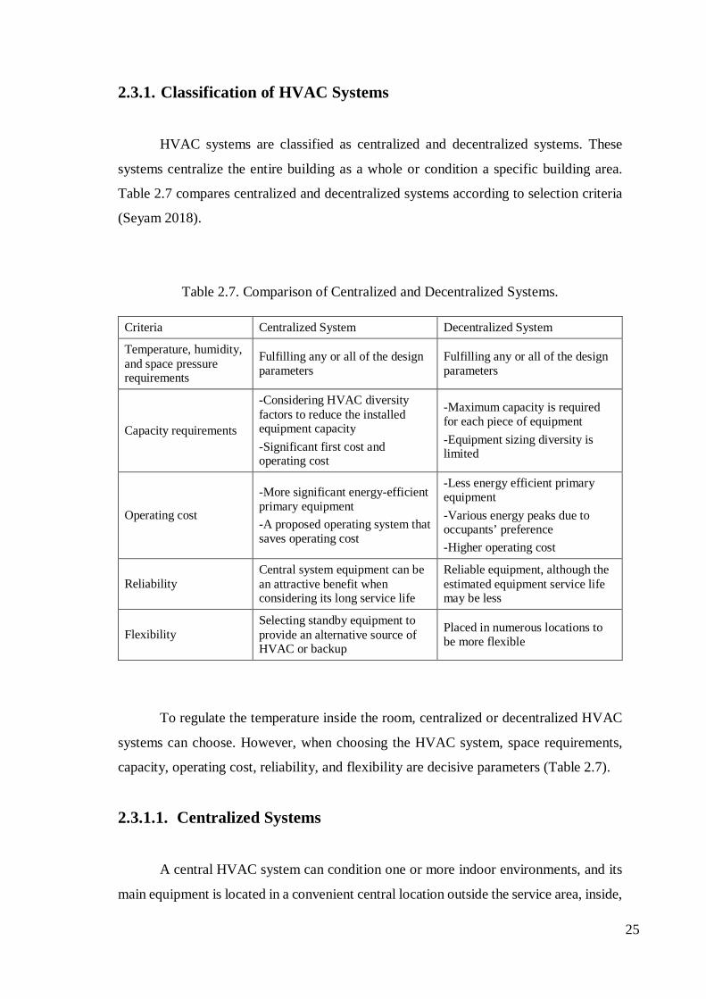
2.3.1. Classification of HVAC Systems

HVAC systems are classified as centralized and decentralized systems. These

systems centralize the entire building as a whole or condition a specific building area.

Table 2.7 compares centralized and decentralized systems according to selection criteria

(Seyam 2018).

Table 2.7. Comparison of Centralized and Decentralized Systems.

Criteria Centralized System Decentralized System

Temperature, humidity, and space pressure requirements

Fulfilling any or all of the design parameters

Fulfilling any or all of the design parameters

Capacity requirements

-Considering HVAC diversity factors to reduce the installed equipment capacity -Significant first cost and operating cost

-Maximum capacity is required for each piece of equipment -Equipment sizing diversity is limited

Operating cost

-More significant energy-efficient primary equipment -A proposed operating system that saves operating cost

-Less energy efficient primary equipment -Various energy peaks due to occupants’ preference -Higher operating cost

Reliability Central system equipment can be an attractive benefit when considering its long service life

Reliable equipment, although the estimated equipment service life may be less

Flexibility Selecting standby equipment to provide an alternative source of HVAC or backup

Placed in numerous locations to be more flexible

To regulate the temperature inside the room, centralized or decentralized HVAC

systems can choose. However, when choosing the HVAC system, space requirements,

capacity, operating cost, reliability, and flexibility are decisive parameters (Table 2.7).

2.3.1.1. Centralized Systems

A central HVAC system can condition one or more indoor environments, and its

main equipment is located in a convenient central location outside the service area, inside,

25

on top, or adjacent to the building (ASHRAE Standard-55 2010). Indoor environment

mediums with their equal thermal load must be conditioned by centralized systems. As

seen in Figure 2.4, the zones used in the control system to provide thermal energy sub-

classify the central HVAC system (Seyam 2018).

Figure 2.4. Classification of Centralized Systems. (Source: Seyam 2018)

2.3.1.1.1. All-air Systems

HVAC equipment is centrally located. All air systems are cooled by sending the

cooled and dehumidified air to the conditioned room, and heating is done by sending the

heated air to the conditioned room. All air systems can filter air and provide fresh air

(Figure 2.5).

Centralized System

All-Air Systems

Single Zone

Multi Zone

Terminal Reheat

Dual duct

Variable Air Voulme

Air-Water SystemsFan Coil Units

Induction Units

All-Water SystemsFan Coil Units

Refrigerant based Systems

26

Figure 2.5. Schematic diagram of all air systems. (Source: Seyam 2018; Goetzler et al. 2016)

The all-air systems have some advantages and disadvantages. It usually includes

the cheapest equipment, but due to the size of ducting required and the cost of installation,

it is not always easy or cheap to install in a building. It can be difficult to maintain proper

temperature control, and the system may be inefficient. These systems can be adapted to

all air conditioning systems for comfort. And it is applied in schools, hospitals,

laboratories, hotels, etc., which require individual control of room conditions. The

essential distinctiveness is to supply fresh air. AHU always supplies adequate fresh air to

maintain IAQ. Here, the return air is balanced in proportion by the rule Supply Air =

Return Air + Fresh Air.

2.3.1.1.2. All-water Air Conditioning Systems

These systems are completely water systems (Figure 2.6). Hot water and cold

water prepared in one center are sent to fan-coil devices distributed in the building. Hot

water is supplied by a hot water boiler, while cold water is produced in the cooling

(chiller) group. Fan-Coil devices are devices containing a fan and coil. Heated or cooled

Exhaust

Return air

Cooling coil Heating coil Supply air duct with fan

Humidifier

H

T

Conditioned space

Return air duct with fan

Fresh air D

D

D

D: Damper H: Humidstat T: Thermostat

27

air is taken from the room with the help of the fan and passed over the serpentines, and is

given to the room again. If cold water passes through the coil, cooling takes place, and if

hot water passes, heating takes place. The pump is used for water circulation. These

systems are usually hotels, hospitals, and offices. Fan-Coil units are usually placed in

front of windows or suspended ceilings (Seyam 2018; Yılmaz 1997; Zhang Wright and

Hanby 2006)

.

Figure 2.6. Schematic diagram of all water systems.

(Source: Seyam 2018; Goetzler et al. 2016)

2.3.1.1.3. Hybrid (Air-Water) Air Handling Units

There is no ventilation in conventional fan-coil systems in these systems (Figure

2.7). Only heating and cooling are done. In these fan-coil systems, fresh air deficiency is

eliminated by applying different applications. One of the applications; each of the fan-

coil units is supplied with fresh air from the outside via its duct connection. And the fresh

air with heat recovery and pre-conditioning, the quantity determined by the automation

system, is provided with the central air conditioning system (Seyam 2018; Yılmaz 1997;

Zhang Wright and Hanby 2006).

Conditioned space-1

Return water line

Heating/cooling coil

Supply water line

PRV

Pump

PRV: Pressure Reducing Valve FCV: Flow control valves

Conditioned space-2

FCV FCV

28

Figure 2.7. Schematic diagram of air-water systems. (Source: Seyam 2018; Goetzler et al. 2016)

With this system, much space is saved, and heating and cooling are possible. As

air-water systems require relatively low air flow rates, the cross-sectional areas of the

required air supply and extract ducts are reduced considerably. The air supply is generally

constant volume and provides outside clean air for ventilation.

2.3.1.1.4. Refrigerant-based Systems

All air conditioning systems are designed to offer thermal comfort to building

occupants. A broad range of air conditioning systems are available, from basic window-

fitted units to small-split systems, medium-scale package units, large-chilled water

systems, and, most recently, variable refrigerant flow (VRF) systems. These systems use

refrigerants to create cool air compared to a typical HVAC system that uses water to cool

air. VRF systems come from a central heat exchanger-compressor unit and associated

internal units. With its advanced automation features, many interior units can be operated

in different comfort conditions for summer and work as heat pumps in winter to meet

their heating needs. Each interior unit of the energy recovery type systems can

independently operate in heating or cooling mode in the same season (Seyam 2018;

Goetzler et al. 2016). There is a heat recovery system that can be installed for that purpose.

Besides these types of Air Conditioning Systems, The Air Handling Units are the

devices that can perform the air conditioning processes such as ventilation, heating,

Central plant for secondary

water

Central plant for primary air

Room unit

Primary + Secondary air

Secondary air

Primary air ducts

Secondary water lines

29

cooling, humidification, dehumidification, filtering, and heat recovery under the control

of automation (Küçüka 2005).

Figure 2.8. Decentralized HVAC System types. (Source: Seyam 2018)

2.3.1.2. Decentralized Systems

It is applied for small projects without a central plant with low initial cost and

simplified installation. These systems are also installed in office buildings, shopping

malls, schools, health facilities, hotels, apartments, research labs, computer rooms, and

other multi-person residences (ASHRAE Standard-55 2010). Decentralized systems are

connected to a refrigeration cycle, heating source and one or more individual HVAC units

with direct or indirect outdoor air ventilation Components of these units consist of a

package containing fans, filters, heating source, cooling coil, refrigerant compressor (s),

controls, and condenser (ASHRAE Standard-55 2010). There are many decentralized

systems, as represented in Figure 2.8 (Seyam 2018).

Decentralized System

Heating Systems

Cooling Systems

Air-conditioning Systems

Window Air-conditioner

Unitary Air-conditioner

Packaged Rooftop Air-conditionerVentilation Systems

Split Systems

HRV Systems

Sensible

Latent

30

2.3.1.3. Decentralized Ventilation and Centralized Ventilation Systems

Choosing the best system is essential for practical reasons and ensuring the

people's comfort in the building. Choosing a centralized and decentralized system is the

main issue in selecting air conditioning systems for buildings. Higher energy efficiency

and improved load-management capabilities are two major advantages of centralized air

conditioning systems. It's also less difficult to maintain. On the other hand, a decentralized

air conditioning system offers lower initial costs. It has minimum installation and space

requirements. Also, the most essential distinction is that decentralized systems have

separate zone controls allowing users to change the IAQ easily.

In this section, DVS, according to different climatic conditions, are compared with

centralized systems, and as a result, it has been determined that DVSs can cause lower

pressure losses, and these systems provide much more energy savings. These articles have

been examined experimentally and numerically (Merzkirch et al. 2016; Mikola, Simson

and Kurnitski 2019; Zemitis et al. 2016; Baldini, Kim and Leibundgut 2014; Mahler and

Himmler 2008) and numerically (Bonato, D’Antoni and Fedrizzi 2020; Carbonare et al.

2019; Manz et al. 2000) according to different climatic conditions (Bonato, D’Antoni and

Fedrizzi 2020; Zemitis et al. 2016) or building usage types offices (Carbonare et al. 2019;

Mahler and Himmler 2008) and residential building ( Murgul et al. 2014; Berkel et al.

2014).

Merzkirch et al. (2016) compared CVS and DVS and presented the findings of a

comprehensive field study on ventilation systems in residential buildings. They examined

20 CVS and 60 DVS in Luxembourg, and they discussed differential pressure, specific

fan power, and heat recovery efficiency. As a result, the heat recovery efficiency of DVS

is determined to be higher than CVS.

Mikola, Simson, and Kurnitski (2019) simulated pressure differences using field

measurements and IDA-ICE software to evaluate the performance of DVS units and

analyze pressure differences in a multi-story building in Estonia. The laboratory measured

the recuperative and regenerative performances of two types of ventilation units, and their

indoor air changes were evaluated with simulations. Thus, by using wall integrated units,

correct design recommendations can be given by determining the pressure differences to

provide a satisfactory thermal comfort and heat recovery.

31

Bonato, D’Antoni, and Fedrizzi (2020) examine the performance of the DVS unit

integrated into the facade and its potential to reduce HVAC energy consumption in office

spaces located on the perimeter of the building. Numerical simulations with TRNSYS

software were analyzed according to the climatic conditions of three European countries.

As a result, based on the analyzed climate and building, it has been concluded that DVS

can effectively reduce energy consumption and save 65% electricity compared to CVS,

while cooling demand can be reduced by 35% -70%.

Carbonare et al.'s (2019) study is simulation-based research examining DVSs. A

demand-controlled ventilation scheme was studied with a co-simulation method, using

EnergyPlus and Modelica programs, and a mathematical approach to user comfort (i.e.

quadratic for relative humidity and exponential for CO2). As a result, while thermal

comfort has increased, 10% energy saving has been achieved.

Zemitis et al. (2016) evaluated ventilation solutions for nZEB (near-zero energy

buildings) multi-story buildings in three European geographic clusters. The concept of

geographic cluster indicates transnational areas with strong similarities in climate,

culture, construction typologies, and other factors. Studies have been conducted for

Denmark, Estonia, Latvia, and Portugal, and technical and economic comparison of

ventilation systems for nZEB buildings in these countries has been made. Within the

scope of the H2020 project, it has been concluded that heat recovery mechanical supply

and exhaust ventilation units are economically efficient.

Baldini, Kim, and Leibundgut (2014) examined the performance of DVS for hot

and humid climates such as Singapore. DVSs, which have great potential to reduce

pressure losses, can reduce exergy loss and energy savings with radiant cooling. A

modified design of a DVS unit including a 3-stage heat exchanger is examined in detail

in this study.

Murgül et al. (2014) conducted a study on DVS, which are applied especially in

residential buildings. It has been shown that an effective way to reduce energy losses due

to heating and ventilation in residences can be achieved by applying DVS with heat

recovery units to achieve thermal balance.

Berkel et al.'s (2014) article review the existing residential ventilation by focusing

on three main areas. These; distribution systems, ventilation control, and energy recovery

technology. Wall-integrated heat recovery ventilation systems, which are a new concept

especially for DVS, were also mentioned, and potential applications for residential

ventilation were evaluated.

32

In the experimental study of Mahler and Himmler (2008), DVSs were evaluated

for office buildings, and the long-term results were obtained; air temperature and

humidity measurements, airflow measurements, noise emission, and user surveys are also

included in this study.

Manz et al. (2000) investigated the effect of air leaks on the performance of DVS

units with heat recovery. According to the numerical study, it has been observed that air

leaks can significantly reduce the performance of ventilation units in terms of ventilation

efficiency, and as a result, it is seen that energy savings are achieved with these systems.

2.3.2. Ventilation

Today, in many countries, the ventilation of buildings is a challenge. In COVID-

19, the importance of good IAQ is once more emphasized (Afshari 2020). It can control

ventilation, air temperature, relative humidity, and pollutant concentrations. A ventilation

system must be sized adequately to meet the welfare needs of the owners. For this reason,

ventilation and well-being are closely linked to each other. Modern technologies enable

us to build more heat-insulated buildings with airtight casing effectively. However, the

buildings become unlivable when there is no proper ventilation system due to the low

IAQ. With the increased atmospheric pollution in our cities, opening only the window

does not provide a good solution. Because there is no control over the concentration of

pollutants in the room by the amount of renewed air by natural ventilation, for this reason,

ventilation systems are often the most appropriate solution. Natural ventilation of

buildings is achieved by creating openings in the building’s exterior: chimneys, windows,

and openings in the roof, atriums, and ventilation towers, etc. In old buildings, low U

value windows provide renewal of the inside air, while new buildings are known to have

much more restricted airflow due to the more efficient windows used to reduce thermal

losses. Natural ventilation has many disadvantages (Gheorghe and Ion 2011):

• The amount of regenerated air cannot be controlled,

• Energy losses in cold seasons,

• The weather is very hot in summer and very cold in winter,

• There is more noise in the room due to opened windows,

• No control of the quality of the air taken in (pollution),

• Regional high air velocity

33

Therefore, mechanical systems are becoming widespread to provide adequate

indoor air requirements. To provide good airflow control - which lacks natural ventilation

- a mechanical air handling system can be designed to ensure proper ventilation. In such

systems, the airflow is provided by one or more fans, ducted or not. Systems without

ducts consist of one or more fans on the walls or ceiling. The simplest solution is to use

one or more extraction fans and several openings to allow fresh air to enter the room. This

solution is common in industrial environments. In residential and commercial

environments, duct systems are preferred, the fans can be placed in a remote location,

which removes noise from the room. Mechanical ventilation systems have the following

advantages (Mardiana-Idayu and Riffat 2011):

• Controlled air flows,

• Controlled air streams,

• No external noise and limited running noise,

• Controlled air quality,

• Reduced thermal losses,

• Optional energy recovery using heat exchangers.

With a better understanding of indoor pollutants, new and effective measures have

been developed, including the development of indoor air filters (Sublett 2011). Air

filtration is often proposed as a component of environmental control measures. However,

while HVAC systems offer an opportunity for all indoor filtration, poorly maintained or

contaminated systems can increase the risk of asthma and other allergic symptoms. These

filters grouped under "air conditioning" or HVAC are the primary means of improving

IAQ. As a major element in air conditioning systems, the air filter plays a significant

purpose. The addition of a proper air filter to an air conditioner is a perfect solution for

removing 98% of airborne contaminants (Elsaid and Ahmed 2021). It is now believed

that "sick building syndrome" is a possible air conditioning problem that can be improved

with better filtration (Sutherland 2008). Different filtration systems remove airborne

particles from supply air systems and enclosed spaces. Filter panels are placed in front of

blower fans in HVAC systems and ventilation units (AHU) in heating and cooling

systems. According to Elsaid and Ahmed (2021), appropriate ventilation, good air

filtration technologies, humidity adjustment, and temperature control enhance the indoor

air quality for airborne infectious illnesses, including COVID-19.

34

HEPA air filters in air conditioners should be replaced with nanofibrous air filters

or enhanced electrostatic air filters, according to the findings of this study. These panes

may include glass, cellulose, or polymeric fibers ranging in diameter from 1 to 100 μm.

Filter mats vary in density and depth, with pores ranging from 70 to 99%. Due to

differences in fiber diameters and mat densities, the filters differ in their ability to capture

airborne particles (Godish and Fu 2019). Filters designed for the treatment of air fall

broadly into three categories (Table 2.8) (Sutherland 2008).

Table 2.8. Filter Types. (Source: Godish and Fu 2019, El Fouih et al. 2012)

Filter Categories Efficiency Size Air Velocity Features Materials

Dry-type panel filters

High porosities and low dust spot efficiencies.

Collect large particles (5-10 microns in size)

Capable of working with relatively high airflow velocities

Fiberglass, open-cell foams, nonwoven textile cloths, and cellulose fibers.

Extended-surface dry-type filters

Finer media for trapping and retaining finer particles.

Collect smaller particles (0.5-5 microns in size)

Air velocities are generally low, of the order of 0.12 m/s or less.

Cellulose, glass fiber, wool felt.

Viscous-media panel filters

Ultra-fine or final stage filters yield very high efficiencies.

Collect sub-micrometer particles (99.95% or better).

Air velocity, in this case, is limited to about 0.03 m/s.

Different fabrics of synthetic fibers.

Indoor air pollution is among the top five environmental health risks (EPA 2018).

The best way to address this risk is to control or eliminate the sources of pollutants and

ventilate an indoor with clean outdoor air. However, the indoor air should be limited by

weather conditions or undesirable contaminants in outdoor air with natural ventilation.

Also, these methods are insufficient, so a mechanical system is useful for the indoor

environment.

2.3.3. Heat Recovery System Solutions

The heat recovery ventilation (HRV) principle is to recover the heat from the

exhaust air and transfer it via a heat exchanger into the supply air. With the increasing

35

share of ventilation, heating/cooling loads, heat recovery through mechanical ventilation

systems reduces heat losses and saves energy (El Fouih et al. 2012).

Heat recovery systems are necessary for designing air conditioning systems with

minimum energy consumption (Yılmaz 1997). These systems are divided into two main

groups: Recuperative and Regenerative systems.

2.3.3.1. Recuperative Systems

Plate Heat Recovery the conditioned air is passed through a heat exchanger so that

the fresh air is not mixed with the heat exchanger.

2.3.3.2. Regenerative Systems

Run Around Heat Recovery conditioned return air and fresh air through two

separate heat exchangers with water inside to provide heat recovery.

Heat Pipe Heat Recovery is a type of heat recovery by utilizes the principle of

evaporation and condensation of the refrigerant in a single two-part heat exchanger placed

in the conditioned air and fresh air.

Rotary Drum Heat Recovery with the help of a rotary type of heat exchanger, heat

recovery between fresh air and indoor air with temperature and humidity difference is

performed (Yılmaz 1997).

In this context, all central air systems can be used in shopping malls, concert halls,

etc., where many people are together, even though the initial investment cost is high and

much space is occupied. On the other hand, in the case of all water air conditioning

systems, the fresh air requirement can be met using heat recovery systems. Thus, heat

recovery systems are more useful than all-air systems, with low initial investment cost,

with efficient use in terms of IAQ and user comfort.

Many studies in the literature about ventilation systems, especially heat recovery

systems. In residential buildings, ventilation losses, in general, can be 35-40 kWh/m2-

year, and up to 90% of this can be recovered with HRV, depending on the buildings'

airtightness and insulation (Tommerup and Svendsen 2006). Many studies have searched

the effect of HRV on the energy use of buildings. Heat recovery ventilation systems

ensure the efficient use of energy due to transferring the heat from exhaust air to the fresh

36

air supplied indoors (Cuce and Riffat 2015). These systems typically recover

approximately 60% to 95% of the energy in the exhaust air and significantly improve the

energy performance of buildings (Mardiana-Idayu and Riffat 2011). Although there are

several studies on heat recovery systems, there are still shortcomings in the research and

development of the use of recovery systems in building applications (Zeng, Liu and

Shukla 2017; Van Berkel, Pressnail and Touchie 2014)

However, CVS requires large volume requirements within the space (Etheridge

and Sandberg 1996). According to building typologies, many studies examine the

performance and energy consumption reduction potential of the DVS unit integrated into

the facade in office spaces (Mahler and Himmler 2008) and articles containing

experimental and field study results on existing residential ventilation systems. Wouters,

Barles and Blomsterberg 2001; Hekmat, Feustel and Modera 1986; Jokisalo et al. 2003).

In several studies, wall integrated HRV systems, which are a new concept especially for

DVS, was also mentioned, and potential applications for residential ventilation were

evaluated (Merzkirch et al. 2016; Mikola, Simson and Kurnitski 2019; Van Berkel,

Pressnail and Touchie 2014).

2.3.4. Review of Heat Recovery Systems

Some mechanical systems store latent heat in heat recovery ventilation and the

studies that store sensible heat. The following publications are comprehensive reviews of

heat exchangers, air conditioners, and solutions for building envelopes with latent heat

storage and include experimental studies:

Xu Riffat and Zhang (2019) offer current developments in four heat recovery

systems for residential applications. The systems are categorized as recuperative and

regenerative. While recuperative systems are fixed plate and heat pipe, regenerative

systems are run around and rotary drum types. The emphasis of this study is on pressure,

air leakage, economic analysis, and combining heat pipe systems with other sustainable

technologies. Consequently, the results show that the integration of regenerative heat

recovery can achieve heat recovery ranging from 64.6% to 70%.

Balci, Ezan, and Turhan (2019) propose a new heat exchanger with PCM to

recover waste heat from the flue gas of a boiler. The thermal energy recovered from the

flue gas is stored in the heat exchanger for later use while the combi operates in central

37

heating mode. They also developed a mathematical model to examine the behavior of the

PCM in detail. As a result, PCM increases the water temperature, and with the use of

PCM, the efficiency of the boiler increases while energy consumption decreases.

Asker et al. (2018) integrate PCM on a wall to increase the energy efficiency of a

building and examine the thermal behavior of this wall. They developed a time-dependent

one-dimensional heat transfer model using ANSYS-Fluent software. They compared four

different walls and found that a 1 cm PCM application was insufficient to keep the indoor

and outdoor temperature at the desired temperature range. Yet, the heat transfer was

significantly reduced by applying 2 cm PCM. Thus, the use of PCM in the building

envelope is an option to reduce the energy consumption for air conditioning.

Alizadeh and Sadrameli (2016) focus on and review free cooling in residential and

commercial buildings. They highlight the advantages and disadvantages of cooling

systems. They study the cooling, technical, geographical, and economic differences and

performance evaluation criteria and application of PCMs.

Soares et al. (2013) examine how and where PCMs are used in latent heat thermal

energy storage (LHTES) systems. Besides, they explore the relationship between

buildings solutions and their energy performance. They also investigated the integration

of PCM into structural elements, methods to measure thermal properties, numerical

modeling, and latent heat storage system containing PCM.

2.4. Thermal Energy Storage Using in Buildings

Thermal energy storage technologies have been commonly used during the past

decades. Different type of thermal energy systems has been developed to facilitate the

use of thermal energy in different needed scales. Storing energy and using it in-demand

times is crucial in building energy efficiency. The stored energy, whether cold or heat,

can reduce cooling or heating loads and reduce the temperature fluctuations in interior

spaces (Konstantinidou 2010). External surfaces of the building are the link between the

building as a thermodynamic organization, and external thermal loads include outdoor

different climatic conditions, primarily temperature, wind, and solar radiation. And we

can control the effect of outdoor conditions on indoor spaces by improving envelope

thermal properties as a function of the capacity of the envelope and the building structures

to store heat. Thermal energy storage in buildings mainly occurs through a change in the

38

internal energy of a material as sensible heat or latent heat or a combination of both. A

diagrammatic overview of major techniques for thermal energy storage using solar

radiation as the most potential infinite source of energy is shown in Fig. 2.9 (Malekzadeh

2015).

Figure 2.9. Different Types of Thermal Energy Storage. (Source: Konstantinidou 2010)

2.4.1. Sensible Heat Storage

In the type of sensible heat storage, thermal energy is absorbed and stored with an

increase in the temperature of solid or liquid material, in which the standard building

materials such as bricks and concrete are used on the exterior/interior walls, on the floor.

The heat capacity of the SHS materials is dependent on the specific heat, the temperature

variations, and the amount of storage material, and as a result, the storage process is

followed by an increase in the material temperature during the process (Lane 2018).

Large-scale thermal energy storage is widely accepted as sensible heat. The choice of

environment is usually dependent on the heat capacity of the environment, the range of

temperatures that the store will operate, and the space available for it (Figure 2.10). Figure

2.10 shows the materials’ specific heat, density, and thermal conductivity graphs, which

are the main thermal properties of sensible heat storage materials. In particular, many

studies use the sensible heat storage calculation method for the thermal insulation

properties of walls (Pekdogan and Basaran 2017; Pekdogan 2015).

TES in Buildings

Sensible Heat

Ground

Concrete

Sand

Water

Latent Heat

Gas-Liquid

Solid-Liquid

Organics Inorganics

Eutectics

Solid-Gas

Solid-Solid

39

Figure 2.10. Heat storage as sensible heat leads to a temperature increase when the heat is stored (Source: Li 2016).

The heat capacity is given by the amount of material, volume, or mass. It is then

called molar, volumetric, or mass-specific heat capacity. The specific heats of

incompressible substances depend on temperature only. Therefore, the change in the

internal energy of solids and liquids can be expressed as;

𝑄𝑄𝑑𝑑 = 𝑚𝑚 ∙ 𝑐𝑐𝑎𝑎𝑎𝑎𝑎𝑎 ∙ ∆𝑇𝑇 Eq. (2.1)

As shown in Equation 2.1. The ratio of stored heat Qd to the temperature rise ∆T, m

is the system's mass, and cavg is the average specific heat evaluated at the average

temperature. To be effective as a thermal mass, we need materials with high heat capacity,

moderate heat conductivity, medium density, and high emissivity (Çengel 2018).

2.4.2. Latent Heat Storage

Latent heat is the heat released or absorbed by a body or a thermodynamic system

during a constant temperature process. The phase transition period is when the

temperature of the system remains constant despite the system's absorption (or release)

of heat. Latent heat storage can be obtained by solid-solid, solid-liquid, solid-gas, and

liquid-gas phase changes (Shukla 2015). The material used to store the latent heat

absorbed by the material during the phase change is called the "Phase Change Material"

40

(Konstantinidou 2010; Abhat 1983). LHTES material has substantially higher thermal

energy absorption and spreading capacity than SHTES materials.

For this reason, by incorporating the LHTES system in a small amount, more heat

storage systems are obtained instead of SHTES in the buildings. When a larger volume

container is considered to create sufficient space for the phase change process, it results in

melting and solidifying the storage material at a constant temperature. When the storage

material absorbs heat during the melting process, the material temperature remains constant

at the melting temperature, also referred to as the phase change temperature.

Figure 2.11 shows the relationship between the volumetric latent heat density and

the market's melting temperature of commercially available PCMs. Sensible heat storage

in water at different temperatures for heating and cooling is shown as a reference (yellow

line). The volumetric latent heat density of commercially available inorganic materials in

the area shaded in blue in Figure 2.11 ranges from 150 to 430 MJ/m3. On the other hand,

the red-colored area represents organic materials. These materials' volumetric latent heat

capacity belongs to a lower range between 100 and 250 MJ/m3. The water that can be

used as a reference has a capacity ranging from 63 to 250 MJ/m3 for sensible heat storage,

cooling, and heating, respectively.

Figure 2.11. Commercially available PCMs and water volumetric heat storage capacity. (Source: Vakhshouri 2020)

41

Phase transformation happens when the temperature of the storage medium

reaches the phase change temperature, as opposed to sensible heat storage. Until the

storage medium absorbs a certain amount of thermal energy, its temperature remains at

the phase change temperature. When the internal energy of the medium is increased by

the value of the latent heat of fusion, the medium achieves a complete phase change

(Dincer and Ezan 2018). It appears that the thermal energy absorbed or released by the

unit phase change per mass is much higher than the energy stored by increasing the

temperature. (Equation 2.2).

𝑄𝑄𝑎𝑎 = 𝑚𝑚𝑃𝑃𝑃𝑃𝑃𝑃𝑥𝑥∆ℎ Eq. (2.2)

As a result, latent heat is calculated from the enthalpy difference (Δh) between the

material phases. In the case of solid-liquid phase change, it is called solid-liquid phase-

change enthalpy, melting enthalpy, or heat of fusion (Çengel 2018).

2.4.2.1. Potential of Using Latent Heat Storage with Solid-Liquid Phase

Change

First, the heat absorbance by these solid-liquid PCMs is similar to that of

conventional SHS materials, increasing their temperature at their heat absorption.

However, PCMs absorb and release thermal energy at a nearly constant temperature.

Although the volume of the heat storage is small, the sensibility is higher than the heat

storage capacity. The thermal storage capacities of the unit masses of these materials,

called PCM, are quite high. They can store 5 to 14 times more heat per unit volume than

SHS materials such as water, concrete, and rock (Abhat 1983; Buddhi and Sawhney

1994). For this reason, it can be said that latent heat storage is more advantageous than

other energy storage techniques.

2.4.3. Sensible and Latent Energy Storage HRV Systems

In addition to these studies aimed at analyzing and solving problems related to

fluid behavior by using algorithms such as CFD analysis through computer simulations,

empirical analysis and important studies on CVSs and DVSs are also available in the

42

literature. The articles summarized below generally include sensible and latent energy

storage heat exchangers as well as CFD analysis.

Zeng et al. (2017) review the recent development of air-to-air heat and mass

recovery technologies. Extensive research was conducted on passive systems, mechanical

ventilation systems, defrosting methods, dehumidification systems, and heat and mass

exchangers integrated into the energy-efficient systems of buildings. The applications,

advantages, disadvantages, and basic performance criteria of each system are detailed. As

a result of this study, it was stated that the use of heat exchangers caused insufficient

airflow. Also, heat and mass exchanger solutions can cause air losses and leaks in

mechanical ventilation systems. Finally, there is an overheating problem during

dehumidification in heat and mass exchangers.

Kim and Baldini (2016) compiled extensive research on energy analysis in a DVS

compared CVS in European climatic conditions. As a result, DVSs cause lower pressure

losses. The fan speed and airflow rate can be adjusted simply and effectively depending

on indoor climate and thermal conditions. A radiant panel with a DVS was found to have

the lowest energy consumption for heating, ventilation, and air conditioning.

In Cuce and Rıffat's (2015) study, information is given about applications related

to the development of heat recovery systems. In general, terms describe heat recovery

systems, their working principles, system components, and the typical heat recovery

technologies, including building applications with theoretical, experimental, and

simulation studies. In addition, the environmental impacts of heat recovery systems are

also evaluated. According to this study, the highest efficiency is seen in rotary drum heat

recovery systems. Besides, the results obtained from the literature show that heat recovery

systems have the potential to reduce the energy demand of buildings and, therefore,

greenhouse gas emissions in the atmosphere.

Culha et al. (2015) examine heat exchangers in wastewater source heat pump

applications, classify wastewater heat exchangers in detail based on many features,

including their utilization and construction methodology. According to these studies, they

concluded that the prevention of biological contamination is an important area to be

considered and that in most commercial applications, custom-designed shell and tube heat

exchangers are used.

Russell and Sherman (2007) explore existing and potential ventilation

technologies following the ASHRAE 62.2 Standard for residential buildings in the North

American climate. Various mechanical systems, natural ventilation, and passive

43

ventilation systems are among the studied technologies. The main parameters related to

each system include operating costs, installation costs, ventilation rates, and heat recovery

potential.

As can be seen in the articles mentioned above, a wide variety of energy-efficient

systems have been developed for buildings, and studies to recover waste energy of

buildings are also considered within this scope.

2.4.4. Temperature Control

The thermal energy can be stored or released in a phase change material without

significant temperature variation. For this reason, the use of PCM as heat storage material

in building components can reduce temperature fluctuations within the building material

and prevent high surface temperatures (Mehling and Cabeza 2008).

Figure 2.12 shows the different phases of a phase change process (Wang et al.

2007). Generally, phase-changing materials have four types: solid-solid, solid-liquid,

solid-gas, and liquid–gas. (Akeiber et al. 2016). PCMs are substances that absorb or

release large amounts of latent heat when they change phase. This phase change occurs

in a heating or cooling process as soon as the material reaches the temperature of the

specific phase change. During latent heat absorption or latent heat release, the temperature

of the PCM remains constant. (Pause 2018). In this process, PCM has sensible and latent

heat regions. In the initial phase, the heat transfer increases the temperature of the material

until the melting temperature of the specific phase changes. In the melting region, PCM

transforms into liquid without any temperature change. The solid material absorbs the

latent heat of fusion to turn into a liquid. The reverse of this process occurs when the heat

is rejected from the material again (Dincer and Ezan 2018).

44

Figure 2.12. Working principle of the phase change of a PCM. (Source: Malekzadeh 2015)

2.5. Phase Change Materials

“A suitable material is having all the desired properties of a phase change material

and having its melting point in the required temperature range.” (Shukla 2015). PCMs

regulate temperature flows in a range defined by latent heat storage.

2.5.1. Classification

Depending on the phase change situation, PCMs are divided into solid-solid

PCMs, solid-liquid PCMs, and liquid-gas PCMs. Among them, solid-liquid PCM's are

the most suitable for thermal energy storage. PCMs are divided into three categories

depending on their composition - organic PCMs, inorganic PCMs, and eutectic PCMs, as

shown in Figure 2.13.

PCM liquid phase

Melting temperature

Freezing temperature

PCM solid phase

Releasing thermal energy

Releasing thermal energy

Absorbing thermal energy

Absorbing thermal energy

Liquid-to-Solid

Solid-to-Liquid

45

Figure 2.13. Phase Change Materials Classification. (Source: Sharma et al. 2009)

Comparing these different PCM types is listed in Table 2.9 (Sharma et al. 2009).

The main characteristics of each group of PCM are compared in this table. The advantages

and disadvantages of these materials are shown in Table 2.9.

Table 2.9. Comparison of different kinds of PCMs. (Source: Sharma et al. 2009)

Classifications Advantages Disadvantages

Organic PCMs

Availability in a large temperature range Low thermal conductivity

The high heat of fusion Relatively large volume change Good compatibility with other materials No supercooling

Inorganic PCMs High thermal conductivity Supercooling Low volume change Corrosion Availability in low cost

Eutectics Sharp melting temperature Lack of currently available test High volumetric thermal storage density

2.5.2. Potential of PCMs Applications

With the development of PCM technology, applications are common in both

domestic and industrial applications. Some of these are the conditioning of buildings, the

cooling of electricity and heat, transportation of blood and hot-cold therapies, waste heat

Phase Change Materials

Organic Compounds

Fatty Acids

Paraffin

Inorganic Compounds

Metallics

Salt Hydrates

Eutectics

Inorganic-Organic

Organic-Organic

Inorganic-Organic

46

recovery, heating, and cooling water, incorporation of textiles for human comfort, solar

energy facilities, spacecraft thermal systems, etc. In buildings, the addition of phase

change materials to building elements and the provision of thermal comfort conditions

using less energy is a wide working area (Agyenim et al. 2010) have been compiled and

compared the heat transfer and phase change problem formulations used in latent heat

storage applications in buildings and according to these studies, it is seen that it is

generally realized between 0 and 60°C in buildings. The most commonly used phase

change materials in this temperature range are paraffin and salt hydrates.

Thermal comfort can be defined by operating temperatures that vary at different

times of the year. According to ASHRAE Standard-55 (2010), the normally

recommended room temperature is 23.5-25.5℃ in summer and 21.0-23.0℃ in winter.

PCMs with phase change temperatures (18-30°C) are preferred in building applications

to meet thermal comfort requirements.

Another important advantage of utilizing PCMs is the ability to shift the amount

of energy required at peak times from 14:00 to 17:00. And also, the indoor air temperature

is reduced with the use of PCM. At this point, PCMs make more effective indoor climates

with daily temperature fluctuations. The usage of PCMs can both reduce and shift the

peak, as shown in Figure 2.14.

Figure 2.14. Illustration of peak load offset and peak load reduction.

(Source: Mehling and Cabeza 2008)

00:0

0

22:0

0

20:0

0

18:0

0

16:0

0

14:0

0

12:0

0

10:0

0

08:0

0

06:0

0

04:0

0

02:0

0

00:0

0

Energy savings

Peak

load

offset

Indo

or te

mpe

ratu

re

Peak load reduction

Time (h)

47

Also, this shows that PCM changes regular buildings into a regenerative

organization that reuses excessive heat (during the day), which usually is removed using

cooling systems at a time (during the night) it is needed. This time lag leads to efficient

use of the cooling system in the nighttime when the outdoor temperature drops and the

HVAC system runs more efficiently and reduces total building energy consumption

(Kalnæs and Jelle 2015).

2.5.2.1. Use of PCM and LHTES with PCM

The articles above summarize the principles of using PCMs in ventilation and the

advantages and disadvantages of such systems. Many studies calculate the performance

of these systems and analyze them with computational fluid dynamics software, while

some studies carry out experiments.

Hu et al. (2020) experimentally and numerically examined a solar air heat

exchanger integrated PCM into a ventilated window. This system heated the fresh air with

solar energy before ventilating the indoor environment. The system aimed to increase

IAQ with solar energy storage and continuous air supply.

Metin et al. (2019) The effects of the inlet temperature and velocity of the heat

transfer fluid on the system's performance in the spherical capsules in a row in the LHTES

unit were analyzed with ANSYS-FLUENT software. The method applied was controlled

by comparing it with the numerical results in the literature, and it was found that the

deviation was less than 10%. Consequently, increasing the inlet temperature and air

velocity is directly proportional to the melting time.

Ezan et al. (2018) worked on photovoltaic panels and PCM, and the difference

that highlights this study in the literature is that the convection in the PCM is also

analyzed using a numerical code. As a result, as the thickness of the PCM increases, the

difference between conduction and convection models reaches 50%, based on

photovoltaic panel temperature.

Stritih et al. (2018) conducted experimental and numerical studies on the use of

latent heat storage with an air solar energy collector mounted on the facade of an office

building in Ljubljana. They used the experimental results to validate the TRNSYS

software. According to the required heat for covering ventilation losses without an

additional system, the highest energy savings of the system were in April and October.

48

Tokuç et al. (2017) study the use of PCM on a roof to provide indoor comfort

conditions. In this study, they evaluate the decrease in cooling load depending on the

amount of PCM for four different climatic regions in Turkey and remark upon the

significance of the relationship between melting-solidifying of PCM, climate, and PCM

type.

Tokuç et al. (2015) studied the thickness of PCM in roof layers for Istanbul. This

study includes experimental and numerical methods, and time-dependent simulations for

summer conditions were evaluated according to Istanbul climate conditions. As a result,

it has been observed that 2 cm of PCM thickness is suitable for flat roofs in Istanbul.

Yıldırım et al. (2017), in this study, 2D numerical analyzes of the flow module of

an LHTES system were performed. The high-temperature water obtained from the solar

collector flows over the spherical capsules in the storage tank, and the PCM inside the

capsule’s melts. The time-dependent change of the PCM in the capsule was analyzed

using ANSYS-FLUENT software. As a result, significant differences were observed

between the sphere close to the inlet and the other spheres in heat transfer rate.

Fiorentini et al. (2015) presented an experimental analysis of a new solar-powered

HVAC system designed for UOW (University of Wollongong Australia) Solar Decathlon

House, the winner of the Solar Decathlon China 2013 competition. This HVAC system

consisted of an air-based photovoltaic-thermal system and a channel with PCM integrated

with a heat pump. The focus was on the optimization of position-velocity-time modes and

the discussion of results from experimental tests. As a result, the system’s efficiency was

relatively higher than a commercial air conditioning system.

Murray et al. (2015) aimed to experimentally develop a small capacity fan coil

unit with heat recovery. The unit consists of two rotor-type sensible and latent heat

exchangers, cooling coil, supply, and exhaust fans. It is designed for air conditioning in

the Singapore climate. Consequently, the heat recovery wheel provided latent cooling for

space rather than the sensible loads.

Weinlader et al. (2014) studied a ceiling cooling system with PCM. The

experimental results indicate that this system has achieved a temperature drop of up to

2°C compared to the control group that does not have a cooling system.

Arkar and Medved (2007) conducted experimental and numerical research on the

cooling efficiencies of two systems in a low-energy building. One system used

mechanical ventilation with two latent heat storages to cool the fresh supply air and the

49

recirculated indoor air. Thus, they determined the most suitable PCM melting temperature

for free cooling for Ljubljana, Slovenia.

2.5.2.2. Performance of LHTES Systems Containing PCM

Experimental and numerical studies examine the heat recovery performance in

ventilation systems with latent heat storage using PCM in the literature.

Promoppatum et al. (2017) conducted controlled laboratory experiments by

placing PCMs with different melting temperatures in a real-size heat exchanger consisting

of staggered tubes. They created a mathematical model of the system with the ANSYS-

Fluent software and extensively examined the PCM's time-dependent temperature and

liquid percentage changes in the pipe for the store/reuse cycles.

Diallo et al. (2017) presented a numerical investigation of the energy performance

of an energy-efficient ventilation system that can be integrated into a building facade. The

system has a modular heat recovery unit with latent heat storage. The performance

calculations using TRNSYS software examined five different climate conditions in

Europe. Hence, the energy savings using this system was in the range of 16.5–23.5%.

El Mankibi (2015) presented experimental and numerical study results of a heat

exchanger with PCM designed to provide IAQ. Numerical simulations were carried out

for one month in winter to investigate the most suitable design criteria by changing the

heat exchanger dimensions, the amount of PCM, and PCM properties.

Liu et al. (2017) designed a heat recovery unit containing PCMs with different

melting temperatures and numerically examined the effect of this unit's operation and

design parameters on energy consumption.

Stathopoulos et al. (2017) characterized different PCMs for use in a heat recovery

device containing PCM capsules in the form of a rectangular prism. The model was

compared with experimental data and accurately predicted the heat exchanger unit

performance under different air flow rates and inlet air temperature.

Although many scientific studies on the PCM heat recovery application of

ventilation systems, O'Connor et al. (2016) emphasized a lack of commercial products.

In this study, O'Connor et al. (2016), who made a brief introduction of the heat recovery

system with PCM produced by the Cool-Phase company, emphasized that this product

has the potential to reduce energy consumption by up to 90% compared to conventional

50

HVAC systems. As a result, more thermal energy storage capacity can be provided in a

more compact geometry than the ceramic solution by using less amount of material with

the use of PCM.

El Fouih et al. (2012) used the TRNSYS software to model and characterized the

annual performance of a heat recovery unit in residential and low-energy commercial

buildings. The model also compared the unit’s performance with a standard ventilation

system. Thus, the dependencies for the efficiency of the heat recovery ventilation system

were the heating load, ventilation device characteristics, and building type.

To have IAQ, thermal comfort, and also to provide heat recovery, correct design

suggestions can be given with wall embedded units. It is seen that with this approach, the

energy consumption of ventilation units can be effectively reduced. In addition, wall-

integrated DVSs can be minimized the amount of volume.

2.6. Market Research for Decentralized HRV

To control the IAQ and sufficient ventilation, appropriate filters should be used in

the system, and the airflow should be controlled. These systems generally consist of an

air supply grill, an air filter, an axial fan, and a ceramic HRV unit, from outdoors to

indoors. These products can provide different fresh air flow rates depending on their fan

capacities and the selected control levels. There are many different wall integrated heat

recovery systems on the market. Table 2.10 summarizes the features of commercially

available wall integrated DVS. Here, the product information is compiled from the

catalogs of the companies. In particular, 25 heat recovery systems belonging to 15

companies that store sensible energy have been examined according to airflow rate, size,

alternative cycle, and speed control modes. In general terms, it is seen that the flow rate

range of the products is a minimum of 8 m3/h, a maximum of 115 m3/h. However, on

average, it is within the range of 15-50 m3/h. The fans usually work in one direction for

70 seconds. The number and placement of units inside a space depend on the size of the

space to be ventilated, the desired air change rate, and the homogeneous fresh air

distribution. In addition to giving aesthetic value to architectural designs, these DVSs are

easier to control and generate less noise than CVSs. However, the proper design,

selection, and implementation of energy-efficient ventilation systems require a holistic

approach to the buildings and the users.

51

The most important factor when calculating the fan capacity is the calculation of

the room volume and the desired air change per hour. According to the report of the

European Commission, the minimum accepted air change rate is determined as 0.5-1

ACH (Air Change per Hour) on average. As seen in Table 2.10, the products vary in

airflow rates depending on the fan performance. Considering the airflow rates depending

on the speed control modes, it is seen that it is generally 15-50 m3/h. The products selected

in Table 2.10 on the market vary between 2 and 5 modes for all products.

Table 2.10. Commercially available wall integrated decentralized heat recovery ventilation systems and their features.

Firms Products Airpower level (m3/h)

Casing dimension HxWxD

Fan Reverse

Cycle (sec)

Control level

Ventomaxx (Ventomaxx, 2020)

Z-WRG Rondo IQ 17-43 200x200 70 Z-WRG RONDO PLUS LAW 15-75 280x218 70 5

Z-WRG RONDO PLUS LAL 280x218 70

AVE (AVE, 2020) VNRD150EC 335x390 Vortice (Vortice, 2020)

VORT HRW MONO 10-40

Blauberg (Blauberg, 2020)

VENTO Expert 8-25 284x234 70 3 Fresher 50 20-50

STIEBEL ELTRON (Stiebel Eltron, 2020)

LT50 14-54 3 VLR 70 S 10-70 285x360 3

envirovent (Envirovent, 2020) HEATSAVA

Inverter (Inverter, 2020) iV14R/V 24-55

Lunos (Lunos, 2020)

NEXXT K 15-115 510x510 4 NEXXT G 15-90 510x510 4 eGO 16-38 4 e2 16,5-26 55-70 4

Orca (Orca, 2020) pico 50 14-28-54 PRANA (Prana, 2020) PRANA 150 25-115 200 70

SEVI (Sevi, 2020) SEVI 17-21-29-41/90 210x210 70 4

RDZ (RDZ, 2020) WHR 60 14-28-54

Vents (Vents, 2020) TwinFresh R-50 22-58 70 2 TwinFresh S-60 35-58 2 TwinFresh RA1-50 25-50 70 2

Fantini Cosmi/aspira (Fantini Cosmi, 2020)

ASPIRVELO AIR ECOCOMFORT 25-50 35-200 2

aiolos air (Aiolos air, 2020)

Smartair 16-22-30-43 190x214 50-70 4 Pleasentair 18-28-38-46 4

52

CHAPTER 3

EXPERIMENTAL METHOD

Experimental research is the oldest form of quantitative research. Quantitative

research is an approach to testing objective theories by examining the relationship

between variables. This research approach begins with a theory (or hypothesis) that is

tested to determine whether or not it is supported (Neuman 2013). These variables can

typically be measured on instruments to analyze numbered data using statistical

procedures. Quantitative purists have assumptions about testing theories deductively,

controlling for alternative explanations, and generalizing and replicating the findings

(Creswell 2003). They have a post-positivist worldview, experimental design, and pretest

and posttest measures of attitudes. This research type deals with the objects of empirical

research for achieving posterior knowledge by conducting three main steps: experimental

design, testing measurement methods, implementation of experimentation of experiments

for testing validity of hypothesis (Creswell and Guetterman 2019; Bernold and Lee 2010).

The difference between experimental research in pure science and experimental research

in social science is that research can be carried out in a laboratory where it is relatively

easy to control the environment (Moore 2006).

The following sections introduce the experimental studies carried out as part of

this work. The experimental testing validated the CFD analysis detailed in Chapter 4. This

chapter provides an overview of the experiment design and the parameters of the

experiment. The experimental methodology covered in the chapter detail the design of

the heat recovery ventilation system, prototyping the test chamber and DVSs, and

measurement of the experiment properties. Also, this chapter includes information about

TES material, calibration, and uncertainty details.

3.1. Research Framework

The performance of the wall-integrated single-room ventilation units is studied.

Firstly, the on-site measurements are performed in laboratory conditions. The next step

is to calibrate the laboratory measurements according to the measured temperature, air

53

velocity, and pressure difference values. In experimental studies, uncertainties affect the

accuracy of the data. So, the uncertainty calculations are made. Then the fan performance

and heat recovery unit performance are calculated according to all calibrated and

measured data. Following this, CFD models are produced.

3.1.1. Physical Model

The real-scale experiments were carried out in the Building Physics Laboratory of

the Faculty of Architecture, Izmir Institute of Technology. An experimental chamber was

previously used for the thermal study of a double-skin façade (Inan, Başaran and Ezan

2016; Inan, Basaran, and Erek, 2017; Başaran and Inan 2016) redesigned and prepared

for this study. The experimental setup includes two spaces that simulate indoor and

outdoor temperature conditions. An insulated aerated concrete wall separates them.

Parametric studies have been carried out to determine the performance of two wall

integrated HRV systems (Figure 3.1).

Figure 3.1. The experimental setup; I: aerated concrete wall, II: indoor environment, III:

outdoor environment, VI: constant temperature bath, VII: cooling group.

3.1.2. Test Chamber

The experimental setup shown in Figure 3.2 consists of eight main parts: The

aerated concrete wall (I) separates the simulated indoor (II) and outdoor (III)

I II

III

VI

VII

54

environments. The simulated indoor environment (II) dimensions are 2.7 m depth, 1.5 m

width, and 3 m height, and it has 10 cm thick insulated panel walls. The simulated outdoor

environment (III) has 2 m depth, 1.5 m width, and 3 m height measurements. The

experimental two HRV systems stored internal and latent thermal energy (IV) for

individual experiments separately are mounted inside the two air ducts (V), which are

positioned outside of the wall for being accessible while taking measurements inside the

units the ducts insulated against heat transfer. The heating/cooling constant temperature

bath (VI) with a flowmeter condition the indoor (II), while a cooling group (VII) and a

thermostat-controlled heater (VIII) condition the outdoor (III) environment. The

heating/cooling systems use wall-hung serpentines to condition the air, as shown in

Figure 3.2. Thermocouples (shown as T) continuously measure temperatures from the

points shown schematically in Figure 3.2.

Figure 3.2. Plan and section of the experimental setup (not in scale)

55

3.1.3. Wall Structure

The outside of the experimental setup created within the scope of the project and both

simulated rooms are given in Figure 3.3. In this study, the wall with a very low total heat

transfer coefficient is considered to determine the wall thickness and material. The wall that

separates the indoor and outdoor environments from each other consists of two layers of

aerated concrete. For the externally insulated condition, a multi-layer wall structure is

constructed with a 10 cm mineral-based aerated concrete heat insulation board as an

insulation material on the 20 cm aerated concrete block wall as a body element (Figure 3.4).

Figure 3.3. I: aerated concrete wall, II: indoor environment, III: outdoor environment, V:

air ducts

Figure 3.4. Externally insulated multilayer wall, which is numbered I in Figure 3.3.

Aerated Concrete (0.2m)

Mineral-based Aerated Concrete Heat Insulation (0.1m)

56

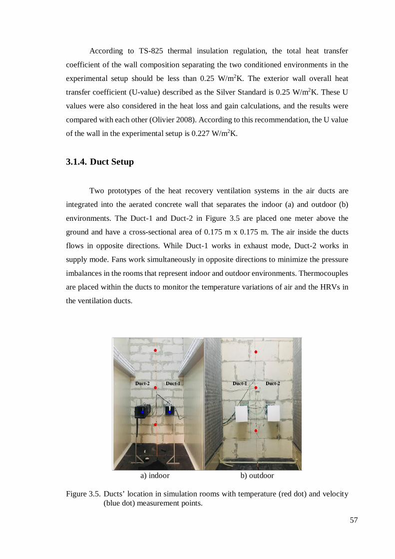
According to TS-825 thermal insulation regulation, the total heat transfer

coefficient of the wall composition separating the two conditioned environments in the

experimental setup should be less than 0.25 W/m2K. The exterior wall overall heat

transfer coefficient (U-value) described as the Silver Standard is 0.25 W/m2K. These U

values were also considered in the heat loss and gain calculations, and the results were

compared with each other (Olivier 2008). According to this recommendation, the U value

of the wall in the experimental setup is 0.227 W/m2K.

3.1.4. Duct Setup

Two prototypes of the heat recovery ventilation systems in the air ducts are

integrated into the aerated concrete wall that separates the indoor (a) and outdoor (b)

environments. The Duct-1 and Duct-2 in Figure 3.5 are placed one meter above the

ground and have a cross-sectional area of 0.175 m x 0.175 m. The air inside the ducts

flows in opposite directions. While Duct-1 works in exhaust mode, Duct-2 works in

supply mode. Fans work simultaneously in opposite directions to minimize the pressure

imbalances in the rooms that represent indoor and outdoor environments. Thermocouples

are placed within the ducts to monitor the temperature variations of air and the HRVs in

the ventilation ducts.

a) indoor b) outdoor

Figure 3.5. Ducts’ location in simulation rooms with temperature (red dot) and velocity

(blue dot) measurement points.

57

For all experiments, indoor and outdoor environment temperatures were

monitored until the system reached representative temperature conditions while the inlet

and outlet sections of the ducts were sealed with covers. A thermostat-controlled electric

heater or direct expansion evaporator was used to stabilize the outdoor environment

temperature. When the desired temperature was reached, the ducts cover was opened, and

the experiments started. During the experiments, two systems installed at each duct

worked in synchrony. While one system exhausted air from the inside, the other supplied

fresh air from the outside through the ducts. Thermocouples within the ducts monitor air

temperature variations and the ceramic unit and PCM in the tubes.

For the measurements, thermocouples located at the inlet and outlet constantly

measure the temperature changes of the airflow inside the ducts, and a datalogger records

these measurements. The duct section and measurement points are given in Figures 3.6a,

which is the ceramic unit, and 3.6b, which is the tube bundle unit. Two air velocity

transmitters which are shown in Figures 3.5a, 3.6a, and 3.6b, placed in the room that simulates

the indoor environment measures air velocities in both ducts. Moreover, a differential

pressure meter placed before and after the energy storage units records pressure drops for the

exhaust and supply conditions of the units (Figure 3.6a, 3.6b). In the exhaust mode, laminar

flow and hydrodynamically fully developed close to the outlet. Therefore, air velocity is

measured close to the outlet from different points at the cross-section of the ducts. Meanwhile,

the velocity measurement is taken from the specified point in supply mode. Besides, a

thermocouple near the duct outlet measures the air temperature for calculating the mass flow

rate of the air considering the density variation with temperature.

a. Duct setup and measurement points for ceramic (not to scale)

(b) Duct setup and measurement points for tube bundle (not to scale)

Figure 3.6. Duct setup with the HRV units for sensible and latent energy storage.

58

3.2. Ceramic Heat Recovery Ventilation System

To control the IAQ, proper filters should be used in the system, and the airflow

should be controlled, in addition to adequate ventilation. These systems include an air

supply grill, an air filter, an axial fan, and a ceramic HRV system from the outside to the

indoors. These systems can provide different fresh air flow rates depending on their fan

capacity and control settings. On the market, there are several wall-integrated heat

recovery systems. In these experiments, the characteristics of the ceramic material have

a relatively high specific heat storage capability and are closed-pore surfaces easy to

clean, as shown in Figure 3.7.

Figure 3.7. Overview of the ceramic material for sensible energy storage in HRV unit.

There are approximately 1600 cells in total in its 15 cm-by-15 cm structure (Figure

3.7). The dimensions of the cells are 4.3 mm on the outer line and 3 mm by 3 mm on the

inner parts. The cell wall thickness is 0.6 mm. The outer wall is 2 mm (Figure 3.7). As

seen in Figures 3.7 and 3.8, 8 thermocouples, 4 of each, are placed to give the average

temperature of the ceramic material. Specific heat is the amount of heat required to change

the temperature of a substance's unit mass, and the differential scanning calorimeter

method is used to measure specific heat. This method measures the amount of energy

absorbed or released while the sample taken from the ceramic material is heated and

59

cooled for a few cycles between 5℃ and 35℃. The specific heat value of the ceramic

material was measured to have an average value of 0.725 kJ/kg℃.

Figure 3.8. Thermocouple placement (mentioned with bold square) and geometric details

of the ceramic unit.

Figure 3.9a shows the isometric view of the HRV system, and Figure 3.9b shows

the front view of the ventilation system with a ceramic HRV unit consisting of covers for

inside (1) and for outside (2), filter (3), fan (4), and HRV unit (5).

60

a) isometric view

b) front view

Figure 3.9. 3D views of the ceramic heat recovery system.

1

2

3 4

5

1

2

3 4

5

61

3.3. Design of the Tube Bundled Prototype With PCM Heat Recovery

Ventilation System

In literature, three different TES systems can be defined as sensible, latent, and

thermochemical. Thermal energy is stored in sensible heat as a result of the change in

temperature of the storage material, while latent heat is stored as a result of the phase

change process of the storage material, and in thermochemical storage as a reversible

chemical reaction between the two substances (Gasia et al. 2017). Sensible TES systems,

as mentioned in Chapter 2, have a disadvantage: To obtain enough thermal storage

capacity, significant changes in the temperature of the system are necessary because of

the low heat capacity of the materials (Campos‐Celador et al. 2020). However, LHTES

has high storage densities and narrow operating temperatures (Mehling and Cabeza

2008).

Mehling and Cabeza (2008) studied design criteria for sensible and latent heat

storage systems. And in this study, four main LHTES systems are compared to each other.

These are direct contact, modular, slurry, and HRV unit. All units are filled with PCM.

As a result, the HRV system has a high storage density.

Shröder et al. (2014) investigated the different types of HRV units, which are

double pipes, shell-and-tube HRV units with baffles in stretched and U-shape alignment,

and plate HRV units. As a result, according to energy efficiency, investment costs, and

cleaning purposes, U-shaped shell and tube HRV units are preferred.

Permana et al. (2019) compared the heat transfer coefficient between a single tube

and a multi-tube with the same heat transfer surface. The single-tube dimension is 40 cm

in length and 9.5 cm diameters, while multi tubes HRV unit consists of ten tubes which

are 40 cm length 0.95 cm diameters. The ambient temperature, outlet, and inlet air are

recorded via a T-type thermocouple. As a result, the heat transfer coefficient of a multi-

tubes HRV unit is 26.6% higher than a single tube HRV unit.

In the light of these studies, a tubular HRV unit is designed in this study. The

experimental, decentralized ventilation unit with heat recovery uses an HRV unit to

transmit heat from the exhaust air to the supply air and can be installed directly on a

facade. Figure 3.10 shows the overview of the tube bundle prototype. The tube bundle

consists of 100 copper staggered tubes in its 15 cm-by-15 cm structure filled with PCM

at the airflow direction.

62

Figure 3.10. Overview of the tube bundle unit for latent energy storage in HRV unit.

The height of one tube is 15 cm, and its outer diameter is 4.76 mm. Liquid PCM

was poured into the tubes having 0.3 mm wall thickness. The tube arrangement in the

bundle is designed as 1.4 cm for the transverse pitch and 1.4 cm for the longitudinal pitch.

The prototype measured the diagonal pitch between tube centers is measured as 1.565 cm

in the prototype (Figure 3.11).

Figure 3.11. Section of the tube bundle prototype.

Figure 3.12a shows the isometric view of the HRV system, and Figure 3.12b

shows the front view of the ventilation system with a tube bundle prototype, which

consists of covers for inside (1) and for outside (2), filter (3), fan (4), and HRV unit (5).

The air taken from outside passes through the filter before reaching the indoor

environment.

63

a) isometric view

b) front view

Figure 3.12. 3D views of the tube bundle heat recovery system.

3.4. Experimental Procedure

The experimental procedure is divided into three processes: the preparation

process, the data collection process, and analyzing and interpreting the data process.

(1) The preparation process is to reach and maintain the representative

temperature conditions for the inlet and outlet sections of two HRV systems that are

closed during this period by controlling the temperature of the indoor and outdoor rooms.

64

• For sensible HRV system which is the ceramic unit; (22±1°C) and outdoor

(35±1°C) room for summer condition and indoor (20±1°C) and outdoor (5±1°C) for

winter condition.

• For latent HRV system which is tube bundle unit (22±1°C) and outdoor

(35±1°C) room for summer condition.

Indoor and outdoor temperature values were chosen based on the thermal comfort

condition (ASHRAE Standard-55 2010) and Turkish State Meteorological Service 1991-

2020 measurements as the average temperatures maximum 33.2°C and minimum 5.7°C

in İzmir (MGM-TR 2021).

(2) After adjusting the system, two HRV units (ceramic and tube bundle) are used

alternatively in exhaust/supply modes in certain periodic cycles. The thermal energy

stored by the units is monitored during these periodic cycles. Throughout the experiments,

indoor and outdoor temperatures, temperatures at the inlet and outlet sections of the units,

temperature changes in the units, air velocity at the ducts where units integrated, as well

as the pressure differences between indoor and outdoor environments and between inlet

and outlet sections of the units are measured (Table 3.1). These experimental data

measured by the instruments (mentioned in Table 3.1) are recorded with a datalogger in

time steps of 5 seconds during the experiments. During the experiment, this 64-duct data

logger, temperature, air velocity, and differential pressure measurements taken from

different points of the experimental setup are recorded.

(3) The reliability of the test results is determined by the uncertainty analysis

given in the following section. Using the measurement results, the thermal energy storage

capacity of HRV systems is calculated for different operating times.

Table 3.1. Information of test instruments.

Test parameters Test instruments Test instrument places Number of the test instrument

Temperature T-type thermocouples

Indoor and outdoor environments

5 indoor 3 outdoor

Inlet and outlet sections of the HRV units

3 both sections (twice for Duct 1 and 2)

In the HRV units 8 (twice for Duct 1 and 2)

Air velocity Blitz Sens VS-C2-1-A Air velocity transmitter

Inlet and outlet sections of the ducts 1 (twice for Duct 1 and 2)

Differential pressure

HK Instruments DPT-R8 Analog manometer

Indoor and outdoor environments

1 instrument for 2 points differentials

Inlet and outlet sections of the HRV units

1 instrument for 2 points differentials

65

3.5. Experimental Setup Measurement Devices

For calculating and describing the variation of the experimental setup, ambient

temperature, air velocity, pressure drop measurements play a decisive role in significantly

determining temperature, flow rates, and pressure differences changes. The air velocity

measurement and pressure drop results are also important factors for the fan

characteristics. In this section, air velocity and pressure drop measurement devices and

their results are explained under the sub-heading of evaluation of fan characteristics.

These data are stored in the HIOKI LR 8402-20 datalogger for evaluation

throughout all experiments. During the experiment, these measurements taken from

different points of the experimental setup are recorded with this datalogger with 64

channels. Figure 3.13 shows the HIOKI LR 8402-20 datalogger and control checkpoint.

Figure 3.13. HIOKI LR 8402-20 datalogger overview.

3.5.1. Temperature Measurements

Nickel-based thermocouples (K type thermocouples) and copper constantan

thermocouples (T type thermocouples) are used for temperature measurements from

many points of the experimental setup. Measurement ranges for these thermocouple types

are -200 to + 1200°C for K type and -200 to + 350°C for T type (Goodfellow and Wang

2021).

The positions of thermocouples inside the test rooms are shown in Figure 3.5. The

number and placement of thermocouples are as follows; one thermocouple measures the

laboratory environment, in which the experimental setup is placed, five thermocouples

66

provide the temperature values of the indoor environment, and three thermocouples

represent temperature for the outdoor environment. In the indoor environment, one

thermocouple is placed at the midpoint of the exit sections of the two ducts to measure the

air temperature inside the duct for determining the air density. In the outdoor environment,

for each duct, three thermocouples measure the system inlet temperature in front of the

filter, and three thermocouples measure the system outlet temperature (Figure 3.6).

There are two different installations of thermocouples for two different HRV units

stored sensible and latent energy. As shown in Figure 3.16, a total of eight thermocouples

are placed in the ceramic HRV units to investigate the sensible energy storage in each

duct to measure temperature changes along the ducts and mean temperatures of each

ceramic material. Thermocouple positions within the ceramic HRV units are indicated as

Group 1 and Group 2 and numbered from 1 to 4 for Duct-1 and Duct-2, respectively.

Figure 3.14. Thermocouple layout inside the ceramic material (not in scale).

For the experimental studies of the heat stored latent energy, the critical

measurements in the system are the determination of the solid and liquid phases (Ezan,

Ozdogan and Erek 2011). The temperature measurements of the medium are used for

monitoring the melting and solidification process. Besides this measurement, eight

thermocouples are placed in the tube bundle prototype with PCM in each duct. Their

placement is shown in Figure 3.16. These locations are selected to give the average

temperature gradient in the PCM. And these thermocouples are placed into the tubes in

the direction of flow to the depth of 3.5 cm, 7 cm, and 10.5 cm from top to bottom, as

shown in Figure 3.17.

67

Figure 3.15. Thermocouple placement inside the prototype of the decentralized HRV

system with PCM

3.5.2. Evaluation of the Fan Characteristics

The axial fan, installed inside the ventilation unit, can work in two flow directions.

The fans of commercial products have limited speed, and their exhaust-supply times are

also limited. Therefore, a fan control system is developed in the current study. This

interface controls the fans' desired velocity and working period on the heat recovery

system. The capacity of fans to produce a needed air volume flow rate against an expected

system resistance to flow, or pressure, is taken into account while choosing them. Fans

for wall-integrated ventilation systems available in the market have limited speeds and

directions and charging-discharging times. This study selects the most suitable fan for the

system, and the fan characteristics are investigated in this section. The air velocity

measurement and pressure drop results are also important factors for the fan

characteristics.

3.5.2.1. Air Velocity Measurements One of the key parameters to evaluate the functional capacity of an HVAC system

is the volumetric flow rate of air. A parabolic velocity profile occurs inside the duct

68

section due to the viscous fluid flow within the ducts; therefore, measurement of air

velocity at a single point is not sufficient to determine the mean velocity value of the

duct’s cross-section. Different standards can be used to measure the airflow rate

accurately. DIN EN 12599 is used in Germany, and most of Europe; DIN EN 16211 and

ASHRAE Standard-111 (2008) can also be used. The common point of all these standards

is that measurement points must be distributed inside the cross-section of the duct. DIN

EN 12599 recommends using the Trivial linear equation solution method while

measuring the air velocity in these air ducts. According to this method, the first step is to

divide the velocity field in the duct section into equal-sized measurement areas. Then,

measurements are taken from the midpoint of each section, and finally, the resultant

arithmetic means value represents the result.

Blitz Sens VS-C2-1-A air velocity transmitter (Figure 3.16) is used to measure the

air velocity inside the ducts at specified positions. The measurement range of this device

is 0-1m/s. This thermal anemometer, also called a velocity meter, works to measure the

airspeed and volumetric flow via heating and cooling of the sensor by electricity

(Goodfellow and Wang 2021). Its highly precise thin-film sensor is 180 mm long and

produced in narrow spaces. The air velocity measurement probe, Blitz Sens VS-C2-1-A

air velocity transmitter, was calibrated in a wind tunnel by a comparison method in which

the reference sensor and the test instrument were placed in the test section of the tunnel.

The uncertainty of the measurement value of the test instrument was calculated by using

5 data in a series measured in 30 seconds. Detailed calibration result for air velocity

transmitter is in appendix 1.

Figure 3.16. Blitz Sens VS-C2-1-A air velocity transmitter and in-channel measurement

69

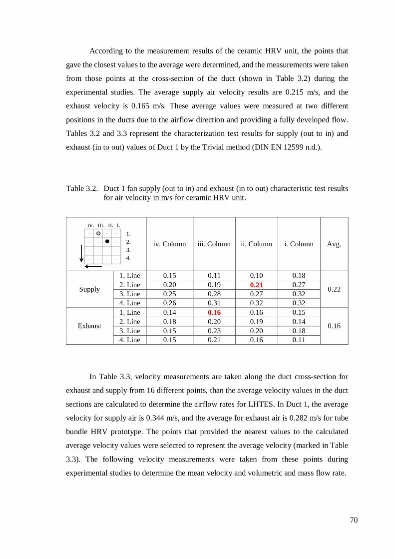
According to the measurement results of the ceramic HRV unit, the points that

gave the closest values to the average were determined, and the measurements were taken

from those points at the cross-section of the duct (shown in Table 3.2) during the

experimental studies. The average supply air velocity results are 0.215 m/s, and the

exhaust velocity is 0.165 m/s. These average values were measured at two different

positions in the ducts due to the airflow direction and providing a fully developed flow.

Tables 3.2 and 3.3 represent the characterization test results for supply (out to in) and

exhaust (in to out) values of Duct 1 by the Trivial method (DIN EN 12599 n.d.).

Table 3.2. Duct 1 fan supply (out to in) and exhaust (in to out) characteristic test results for air velocity in m/s for ceramic HRV unit.

iv. Column iii. Column ii. Column i. Column Avg.

Supply

1. Line 0.15 0.11 0.10 0.18

0.22 2. Line 0.20 0.19 0.21 0.27 3. Line 0.25 0.28 0.27 0.32 4. Line 0.26 0.31 0.32 0.32

Exhaust

1. Line 0.14 0.16 0.16 0.15

0.16 2. Line 0.18 0.20 0.19 0.14 3. Line 0.15 0.23 0.20 0.18 4. Line 0.15 0.21 0.16 0.11

In Table 3.3, velocity measurements are taken along the duct cross-section for

exhaust and supply from 16 different points, than the average velocity values in the duct

sections are calculated to determine the airflow rates for LHTES. In Duct 1, the average

velocity for supply air is 0.344 m/s, and the average for exhaust air is 0.282 m/s for tube

bundle HRV prototype. The points that provided the nearest values to the calculated

average velocity values were selected to represent the average velocity (marked in Table

3.3). The following velocity measurements were taken from these points during

experimental studies to determine the mean velocity and volumetric and mass flow rate.

1. 2. 3. 4.

iv. iii. ii. i.

70

Table 3.3. Duct 1 fan supply (out to in) and exhaust (in to out) characteristic test results for air velocity in m/s for tube bundle HRV unit.

iv. Column iii. Column ii. Column i. Column Avg.

Supply

1. Line 0.270 0.341 0.320 0.350

0.344 2. Line 0.306 0.345 0.371 0.403 3. Line 0.280 0.380 0.38 0.415 4. Line 0.271 0.300 0.35 0.370

Exhaust

1. Line 0.390 0.252 0.199 0.242

0.282 2. Line 0.395 0.251 0.225 0.278 3. Line 0.306 0.225 0.282 0.281 4. Line 0.270 0.281 0.283 0.347

3.5.2.2. Pressure Drop Measurements

The differential pressure measurement is monitored with an analog manometer

from two points in the experimental setup. Two separate measurements are taken to

measure the pressure difference between the indoor and outdoor environments and the

pressure difference between the systems on the two ducts with fans working in exhaust

and supply modes. HK Instruments DPT-R8 Differential Pressure Transmitters (Figure

3.17) are used for these measurements. This transmitter is mainly used in HVAC systems

to control and monitor the fan airflow and pressure. This differential pressure

measurement system is arranged to operate in the range of 0-25 Pa. The data are stored

for evaluation in the HIOKI LR 8402-20 datalogger.

Figure 3.17. HK Instruments DPT-R8 Differential Pressure Transmitter.

1.2.3.4.

iv. iii. ii. i.

71

Figure 3.18 shows the pressure difference values between the indoor and outdoor

environment of the ceramic units, which is operated for 1-minute, 2-minute, 5-minute,

and 7.5-minute in winter conditions. The system, which works during specified times,

first operates Duct 1 exhaust, while Duct 2 supplies and then works in the opposite

direction. Respectively, in the system running for 1-minute, the fan produces an average

pressure difference of 4.82 Pa, 4.90 Pa in 2-minute, 5.10 Pa when it runs for 5-minute,

and 4.82 Pa when it lasts for 7.5-minute.


operates in exhaust and supply modes for different running times for the ceramic unit

Figure 3.19 shows the cases when the fan is working in exhaust and supply mode

for cycles of 15-minute, 20-minute, and 30-minute. While Duct 2 operates in the exhaust

mode, Duct 1 is in supply mode. When the system runs for 15-minute, the fan produces

an average pressure difference of 8.20 Pa. A difference of 8.07 Pa is the average value

when moving air from inside to outside for 20-minute. Meanwhile, the fan-produced

average pressure difference is 8.02 Pa for both units running together for 30-minute.

During the airflow from the outdoor to the indoor environment, the pressure difference

72

between two fans for 15-minute, 20-minute, and 30-minute is 9.74 Pa, 9.78 Pa, and 9.57

Pa, respectively.


operates in exhaust and supply modes for different running times for the tube bundle unit

Koper, Palmowska and Myszkowska (2020) measured airflow rates for different

pressure drops, namely 0, 4, and 7 Pa, using a single room decentralized heat recovery

unit in winter conditions. For 7 Pa, the volume flow rate was 22 m3/h in supply mode and

6 m3/h in exhaust mode. A regenerative heat exchanger effectiveness was calculated

experimentally in the study of Zemitis et al. (2016). The results showed that for a 10 Pa

differential pressure, fresh air deviations could range from 30% to 100% for the nominal

flow rate of 30 m3/h. Regarding these references, for the current experimental setup, the

average pressure loss in this system is approximately 10 Pa (Figure 3.19), and the volume

flow rate is 28 m3/h in supply mode and 22 m3/h in exhaust mode. So, the fan

performances of the current study were quite better than the other studies (Zemitis et al.

2016; Koper, Palmowska and Myszkowska 2020) for the same and similar pressure drops.

73

And also, the tube structure affects the pressure drop. Kumar and Prabu (2015)

compared the three different tube bundles for HRV units. The first is the smooth tube, the

second is a micro fin-tube, and the last is a corrugated type of tube. According to pressure

drop results, the smooth tube is better than the others. However, according to

effectiveness results, the corrugated tube bundle gives more effectiveness. So, the

pressure drop is related to the structural consideration.

3.5.2.3. Fan Characteristics

Before running the experiments, the fan characteristic of the system is obtained,

and the common points in the direction of supply and exhaust are determined according

to the normalized air velocity and the pulse width modulation (PWM). Also, it is seen

that from Figure 3.20, the fan operates with 47% efficiency. The manufacturer fan

characteristics result in appendix 2.

Figure 3.20. Calculated normalized air velocity

74

3.6. Usage of Thermal Energy Storage Material in Prototype

The most common PCMs are paraffin and salt hydrates. Phase change materials

(PCM) are widely used in LHTES applications, and several studies have been conducted

in the literature to review the applications of TES systems containing PCM in different

applications (Dardir et al. 2019). Because of their high storage densities and latent heat

properties, PCMs are frequently used for more energy storage in many applications for

residential buildings (Bland et al. 2017). Pagkalos et al. (2020) compared the sensible

heat storage and a latent heat storage medium with CFD. It was found that PCM can store

4.1 times more energy than water for the same volume of the storage tank. And the

charging process duration of PCM is 3.9 or 3.0 times longer than water for the same

volume of the storage tank, also depending on the tube length (Pagkalos et al. 2020).

All these studies are taken into account, in this experimental study, the tubes in

the LHTES unit are filled with PCM to store thermal energy better for the same volume

of the sensible energy storage unit. According to the climatic conditions of the

experiment, RT27 is chosen. RT27, which is paraffin that changes phase at around 27℃,

was placed in copper tubes in liquid form. The tube bundle consists of 100 copper

staggered tubes filled with PCM at the airflow direction. Liquid PCM was poured into

the tubes. The inner volume of a tube is 2.04 cm3, and the total empty weight of the tube

bundle is 906 grams. When the copper tube bundle is filled with liquid PCM, it weighs

1065 grams and 1062 grams when the PCM solidifies due to the difference in solid-liquid

density. Therefore, on average, 1.6 grams of RT27 PCM (2016) can be added into a tube.

The properties of the RT27 injected into the tubes and the physical properties of the air

and copper are shown in Table 3.4. Studies by (Tokuç, Başaran and Yesügey 2015;

Durakovic and Torlak 2017) are taken as the reference for the physical properties of PCM,

and values for air and copper refer to (ASHRAE Standard-55 2010) for Table 3.4.

Table 3.4. Physical properties of RT27 (Tokuç, Yesügey and Başaran 2017; Rubitherm

Technologies 2016), air, and copper (ASHRAE Standard-55 2010).

Name Unit RT27 Air Copper Ceramic Density, Solid-phase (15℃) kg/m3 880 1.188 8900 ~2200 Density, Liquid-phase (40℃) kg/m3 760 - - - Specific Heat kJ/kgK 2.4 1.0064 0.386 0.725 Latent Heat kJ/kg 184 - - - Thermal Conductivity W/mK 0.2 0.024 400 1.4-1.5

75

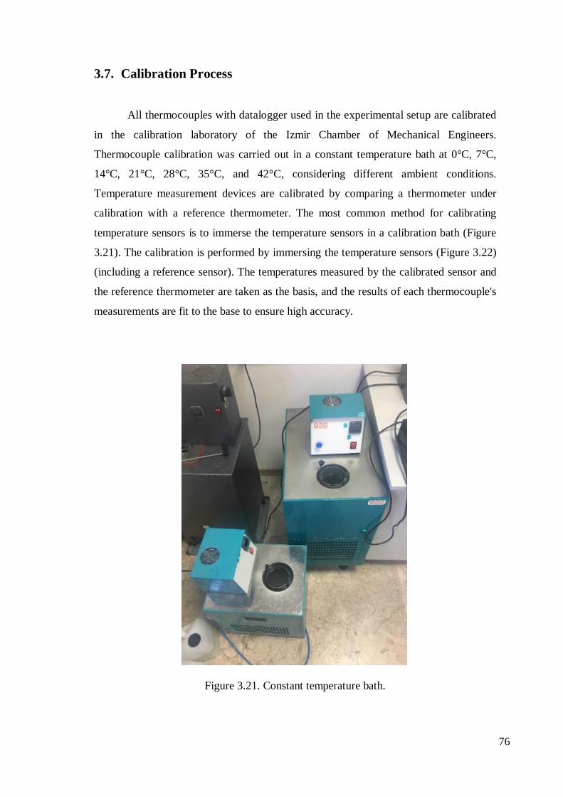
3.7. Calibration Process

All thermocouples with datalogger used in the experimental setup are calibrated

in the calibration laboratory of the Izmir Chamber of Mechanical Engineers.

Thermocouple calibration was carried out in a constant temperature bath at 0°C, 7°C,

14°C, 21°C, 28°C, 35°C, and 42°C, considering different ambient conditions.

Temperature measurement devices are calibrated by comparing a thermometer under

calibration with a reference thermometer. The most common method for calibrating

temperature sensors is to immerse the temperature sensors in a calibration bath (Figure

3.21). The calibration is performed by immersing the temperature sensors (Figure 3.22)

(including a reference sensor). The temperatures measured by the calibrated sensor and

the reference thermometer are taken as the basis, and the results of each thermocouple's

measurements are fit to the base to ensure high accuracy.

Figure 3.21. Constant temperature bath.

76

Figure 3.22. Thermocouples with datalogger

The calibration process consists of reference instruments, test instruments,

deviation, and uncertainty mean.

Reference instrument: To obtain correct measurement results, it is important to

compare the devices with a fixed reference value with the constant case. A reference

instrument is the same conditions as the system to be calibrated.

Test instrument: Represents the device to be calibrated.

Deviation: The value shows how much the measurement results deviate from the

reference instrument measurement. This value is calculated using various statistical

model methods. Table 3.5 shows the calibration results performed by comparing the

temperature values measured from the reference instrument’s measurement values with

test instrument measurement values.

Table 3.5. Measurement results at 42°C.

Measured Unit Reference°C Test°C Deviation°C Uncertainty°C UNIT-1-1 42.00 42.10 0.10 0.17 UNIT-1-2 42.00 42.20 0.20 0.17 UNIT-2-1 42.00 42.24 0.24 0.17 UNIT-2-2 42.00 42.15 0.15 0.17 UNIT-4-1 42.00 42.07 0.07 0.17 UNIT-4-2 42.00 42.19 0.19 0.17

77

Uncertainty: It refers to the measurement range by the test device. For instance, If

the uncertainty of a test system calibrated at 42°C is ±0.17°C, we expect this system to

measure 42°C between 41.83°C and 42.17°C. Measurement uncertainties are given in

Table 3.5. The uncertainties with confidence probability value represent the standard

uncertainty multiplied by the coverage factor k=2 providing about 95% confidence

interval for the normal distribution. Detailed calibration results for thermocouples are in

appendix 3.

3.8. Uncertainty Analysis

In experimental studies, some uncertainties affect the accuracy of the data.

Uncertainty calculations were made within the scope of the method followed by Holman

(2012) and Tokuc et al. (2015), which is also provided in ISO “Guide to the Expression

of Uncertainty in Measurement” as the uncertainty analysis method for errors caused by

an experimental set and measurement tools (Willink 2013). For a measurement with n

variables, the result R is a function of the independent variables x1, x2, x3…xn, whereas w1,

w2, w3…wn are uncertainties in the independent variables. R-value is expressed based on

independent variables as

𝑅𝑅 = 𝑅𝑅(𝑥𝑥1,𝑥𝑥2,𝑥𝑥3 … 𝑥𝑥𝑛𝑛) Eq. (3.1)

If wR is defined as the uncertainty value in the result, the uncertainty of all

independent variables are given with the same odds, then Eq. (3.2) is used;

𝑊𝑊𝑅𝑅 = [� 𝜕𝜕𝑅𝑅𝜕𝜕𝜕𝜕1

𝑤𝑤1�2

+ � 𝜕𝜕𝑅𝑅𝜕𝜕𝜕𝜕2

𝑤𝑤2�2

+ � 𝜕𝜕𝑅𝑅𝜕𝜕𝜕𝜕3

𝑤𝑤3�2

+ ⋯+ � 𝜕𝜕𝑅𝑅𝜕𝜕𝜕𝜕𝑛𝑛

𝑤𝑤𝑛𝑛�2]1/2 Eq. (3.2)

For the experimental studies, the uncertainty analysis of the mass flow rate (Eq.

(3)) and heat transfer rate (Eq. (4)) in the duct were calculated. Accordingly;

�̇�𝑚 = 𝜌𝜌𝑎𝑎𝐴𝐴𝑐𝑐𝑉𝑉𝑎𝑎 Eq. (3.3)

�̇�𝑄 = �̇�𝑚𝑐𝑐𝑝𝑝∆𝑇𝑇 Eq. (3.4)

78

The uncertainty in Eq. (3.3) is caused by the density of the air (ρa), the cross-

sectional surface area through which the air passes (Ac), and the average velocity of the

air (Va). The heat transfer rate uncertainty value in Eq. (3.4) depends on the mass flow

rate (�̇�𝑚), the specific heat of air at constant pressure (𝑐𝑐𝑝𝑝) and temperature difference (∆T).

Accordingly, parameters affecting the mass flow rate and the heat transfer rate for the air

in the equations are defined as

�̇�𝑚 = 𝑓𝑓(𝜌𝜌𝑎𝑎 ,𝐴𝐴𝑐𝑐 ,𝑉𝑉𝑎𝑎) Eq. (3.5)

�̇�𝑄 = 𝑓𝑓(�̇�𝑚, 𝑐𝑐𝑝𝑝,∆𝑇𝑇) Eq. (3.6)

The uncertainty values of each independent variable are given in Table 3.6. The

uncertainty of the mass flow rate is calculated according to the parameters defined in Eq.

(3.5). For the measured air velocity values obtained in the experiments, the uncertainty

value was taken from the catalog value of the manufacturer. And later, it was determined

to be approximate ~5.94% by interpolation. The uncertainty of the mass flow rate of air

calculated for each independent variable given in Table 3.6 is ~6.27%.

Table 3.6. Uncertainty values of each independent variable measured in the experimental studies.

Variables Value Uncertainty Specifications

Air density, ρa 1.184kg/m3

@25℃ ±0.02%

Air velocity, Va 0-1m/s ±5.94% Manufacturer: BLITZSENS, Type: VS-C2-1-A, (2pcs)

The cross-sectional area which the air passes, Ac

0.0225m2 ±2%

Temperature, T 0-42℃ ±1% Datalogger manufacturer: HIOKI, Type: LR8402-20 (K/T), (37pcs of Thermocouples)

Specific heat of air, cp 1007 J/kgK

@25℃ ±0.02%

The uncertainty of heat transfer rate during the experiments is calculated based on

the parameters defined in Equation 3.6. The total uncertainty value of thermocouples with

79

datalogger was evaluated in accordance with the uncertainty of the devices used during

the calibration. And the uncertainty of heat transfer rate is calculated as ~6.35% based on

the mass flow rate, specific heat, and temperature uncertainty values.

3.9. Summary

This chapter presents the experimental methods of wall integrated HRV Systems.

Firstly, the on-site measurements are represented. The next step is to calibrate the

laboratory measurements according to the measured temperature, air velocity and

pressure difference values. Also, in this chapter, the uncertainty values for measurement

tools are detailed. The real-scale experiments were carried out in this study. The

experimental setup consists of 8 main parts, which are the aerated concrete wall,

simulated indoor and outdoor environments, HRV systems are integrated inside the two

air ducts, and the heating/cooling constant temperature bath with a flowmeter condition

the indoor, while a cooling group and a thermostat-controlled heater condition the outdoor

environment. Air velocity, pressure drop, and temperature data play a critical role in

estimating and characterizing the variation of the experimental setup flow rates, pressure

differences, and temperature changes. This chapter also shares the procedure of these

measurements, measuring devices used, and the uncertainty results. The average supply

air velocity results are 0.215 m/s, and the exhaust velocity is 0.165 m/s for the ceramic

unit. And the average velocity for supply air is 0.344 m/s, and the average for exhaust air

is 0.282 m/s for tube bundle HRV prototype. For the SHTES, the fan produces an average

pressure difference of 4.9 Pa, for the LHTES, 9.7 Pa. The total uncertainty of

thermocouples with dataloggers was calculated using the devices' uncertainty during

calibration. Based on the mass flow rate, specific heat, and temperature uncertainty

values, the heat transfer rate uncertainty is ~6.35%.

80

CHAPTER 4

NUMERICAL ANALYSES

Numerical studies of the heat recovery units with phase change material (PCM)

and ceramic material are carried out with the help of the ANSYS-FLUENT package

program. Within the scope of the numerical study, temperature distributions and flow

analysis in three-dimensional and two-dimensional flow geometries are investigated

depending on time. The heat recovery units' geometric variables and operating parameters

are differentiated, and design alternatives are created in this context. In addition, the

system has been evaluated considering constraints such as thermal performance and

pressure drop. Details of the numerical studies conducted are shared below.

4.1. Theory and Background

Fluid mechanics is a fundamental field that is the basis of many important industry

and research topics, and fluid flow is studied experimentally, analytically, and

numerically (Zhai 2006). In recent years, computational fluid dynamics (CFD) has been

used frequently in research to predict the flow numerically developed by the analytical

base. Besides, the advantage of experimental analysis is to it provides good resources to

verify and validate different theories and models. However, most physical experiments

can be expensive to implement, and limited data can be collected. On the other hand, most

theoretical analysis in fluid mechanics can only be done for simple or simplified cases

such as steady and one-dimensional problems. Numerical analysis solves complicated

problems and equations. This approach has many advantages to solve the problems. The

analysis with the computer takes a short period of time. And it can be simulated as real

conditions. Also, the cost of the CFD is almost negligible when compared experimental

approach. However, the most important disadvantage of this method is accuracy. It is

very important to determine the boundary conditions for the accuracy of the results of the

problems.

Along with the governing equations for velocity, the solution of mass, momentum,

energy conservation equations, and 2D and 3D scales are also used in CFD programs.

81

CFD is used for many industrial areas such as HVAC, electronics, chemicals, etc. In the

last years, CFD has played an important role in building designs, energy efficiency,

indoor air quality, and thermal comfort in the built environment (Averfalk, Ingvarsson

and Persson 2014). Thermal comfort and indoor air quality are affected by operating

conditions, control strategies of HVAC systems. With CFD, the HVAC systems'

efficiency can study by changing system control, supply, and exhaust air conditions. Also,

the CFD can assist the natural ventilation strategies by modeling and optimizing building

sites and indoor layouts (Zhai 2006).

4.2. CFD Modeling Procedure

The most important element in CFD, abstracting, simplifying from the real world

into the simulation model with accurate solutions. To a successful CFD model, it is

important to define sufficient details. When defining the problem, the flow characteristics

to be simulated (steady/unsteady flow, laminar or turbulent flow, etc.) should be

determined based on specific simulation goals and interests. After defining the problem,

the material's physical properties are specified in CFD software. And then, boundary and

initial condition setup is an important step in the simulation. To model fluid flow motions

for momentum, mass, and energy transfer, the discretization and grid generation of the

domain can give an adequate solution to the problem. Before running the CFD engine,

the numerical control parameters specification such as convergence criteria and iteration

number allowed maximum residues before running the CFD engine. Figure 4.1 shows the

overview of the computational solution procedure for CFD problems (Ezan 2011).

Figure 4.1. Schematic of CFD solution process. (Source:Averfalk, Ingvarsson and Persson 2014)

Governing partial differential equations (mass, momentum and energy) & Boundary and initial conditions

Basic derivations of finite volume or finite difference equations

System of algebraic equations

Numerical methods

Approximate solutions of field variables

Discretization approaches (finite volume or finite differences)

82

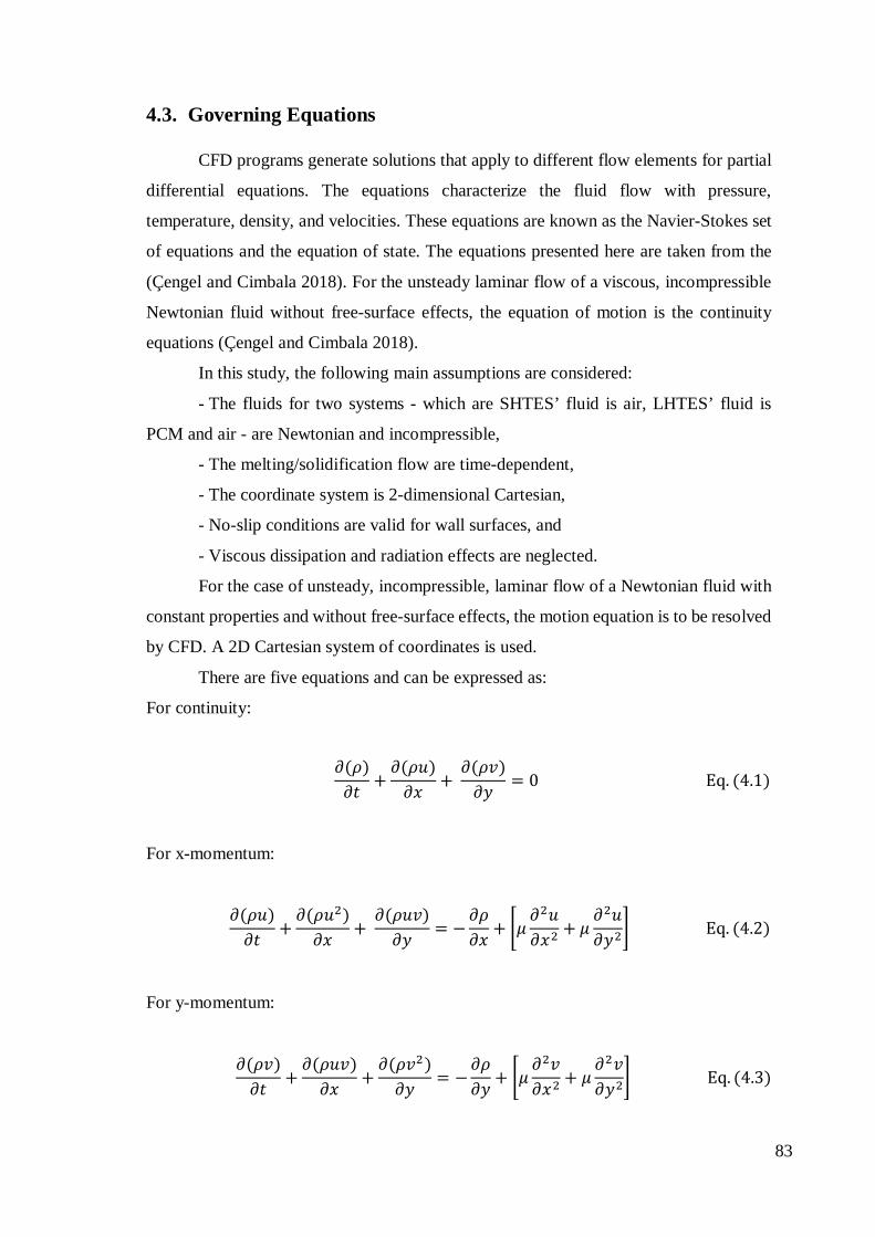
4.3. Governing Equations

CFD programs generate solutions that apply to different flow elements for partial

differential equations. The equations characterize the fluid flow with pressure,

temperature, density, and velocities. These equations are known as the Navier-Stokes set

of equations and the equation of state. The equations presented here are taken from the

(Çengel and Cimbala 2018). For the unsteady laminar flow of a viscous, incompressible

Newtonian fluid without free-surface effects, the equation of motion is the continuity

equations (Çengel and Cimbala 2018).

In this study, the following main assumptions are considered:

- The fluids for two systems - which are SHTES’ fluid is air, LHTES’ fluid is

PCM and air - are Newtonian and incompressible,

- The melting/solidification flow are time-dependent,

- The coordinate system is 2-dimensional Cartesian,

- No-slip conditions are valid for wall surfaces, and

- Viscous dissipation and radiation effects are neglected.

For the case of unsteady, incompressible, laminar flow of a Newtonian fluid with

constant properties and without free-surface effects, the motion equation is to be resolved

by CFD. A 2D Cartesian system of coordinates is used.

There are five equations and can be expressed as:

For continuity:

𝜕𝜕(𝜌𝜌)𝜕𝜕𝜕𝜕 +

𝜕𝜕(𝜌𝜌𝜌𝜌)𝜕𝜕𝑥𝑥 +

𝜕𝜕(𝜌𝜌𝜌𝜌)𝜕𝜕𝜕𝜕 = 0 Eq. (4.1)

For x-momentum:

𝜕𝜕(𝜌𝜌𝜌𝜌)𝜕𝜕𝜕𝜕 +

𝜕𝜕(𝜌𝜌𝜌𝜌2)𝜕𝜕𝑥𝑥 +

𝜕𝜕(𝜌𝜌𝜌𝜌𝜌𝜌)𝜕𝜕𝜕𝜕 = −

𝜕𝜕𝜌𝜌𝜕𝜕𝑥𝑥 + �𝜇𝜇

𝜕𝜕2𝜌𝜌𝜕𝜕𝑥𝑥2 + 𝜇𝜇

𝜕𝜕2𝜌𝜌𝜕𝜕𝜕𝜕2

� Eq. (4.2)

For y-momentum:

𝜕𝜕(𝜌𝜌𝜌𝜌)𝜕𝜕𝜕𝜕 +

𝜕𝜕(𝜌𝜌𝜌𝜌𝜌𝜌)𝜕𝜕𝑥𝑥 +

𝜕𝜕(𝜌𝜌𝜌𝜌2)𝜕𝜕𝜕𝜕 = −

𝜕𝜕𝜌𝜌𝜕𝜕𝜕𝜕 + �𝜇𝜇

𝜕𝜕2𝜌𝜌𝜕𝜕𝑥𝑥2 + 𝜇𝜇

𝜕𝜕2𝜌𝜌𝜕𝜕𝜕𝜕2

� Eq. (4.3)

83

For energy:

𝜕𝜕(𝐻𝐻)𝜕𝜕𝜕𝜕 +

𝜕𝜕(𝜌𝜌𝐻𝐻)𝜕𝜕𝑥𝑥 +

𝜕𝜕(𝜌𝜌𝐻𝐻)𝜕𝜕𝜕𝜕 =

𝜕𝜕𝜕𝜕𝑥𝑥 �𝑘𝑘

𝜕𝜕𝑇𝑇𝜕𝜕𝑥𝑥� +

𝜕𝜕𝜕𝜕𝜕𝜕 �𝑘𝑘

𝜕𝜕𝑇𝑇𝜕𝜕𝜕𝜕� Eq. (4.4)

x and y are the horizontal and vertical coordinates, and the velocities are u and v,

respectively. ρ is the density, k is the thermal conductivity in equations. An enthalpy-

porosity technique is used in ANSYS-FLUENT for modeling the solidification/melting

process (ANSYS-Fluent, 2021). In this technique, the regions where such liquid and solid

fraction of material coexist is called mushy zone. The liquid fraction lies between 0 and

1 in mushy zones. In the mushy zone, the porosity of 0 indicates the material is fully

solidified, whereas 1 indicates the material is melted. The energy equation for PCM

converted enthalpy definitions into the temperature-based form for LHTES. In Eq. 4.5,

the H is the total volumetric enthalpy value. Total volumetric enthalpy is the sum of

sensible and latent heat of the PCM, which is;

𝐻𝐻 = ℎ + 𝜌𝜌𝐿𝐿𝑓𝑓ℎ𝑠𝑠𝑠𝑠 Eq. (4.5)

where h is the sensible enthalpy, 𝜌𝜌𝐿𝐿 is the density of liquid PCM, 𝑓𝑓 is the melting fraction

and ℎ𝑠𝑠𝑠𝑠 is the latent heat of fusion.

ℎ = ℎ𝑟𝑟𝑟𝑟𝑠𝑠 + � 𝜌𝜌𝑐𝑐𝜌𝜌𝑇𝑇𝑇𝑇

𝑇𝑇𝑟𝑟𝑟𝑟𝑟𝑟 Eq. (4.6)

The sensible enthalpy’ components are the density of PCM is 𝜌𝜌, specific heat which is 𝑐𝑐

and 𝜌𝜌𝑇𝑇is the temperature of the PCM (Ezan 2011).

4.4. Physical Domain

The geometry used for flow analysis has to be generated and imported for

processing using CFD tools. This step in this current study is the 3D modeling step of the

heat recovery system with ceramic and PCM tube bundle. The geometric model includes

the design of the whole system with the other apparatus. In the "Design Modeler" tool of

84

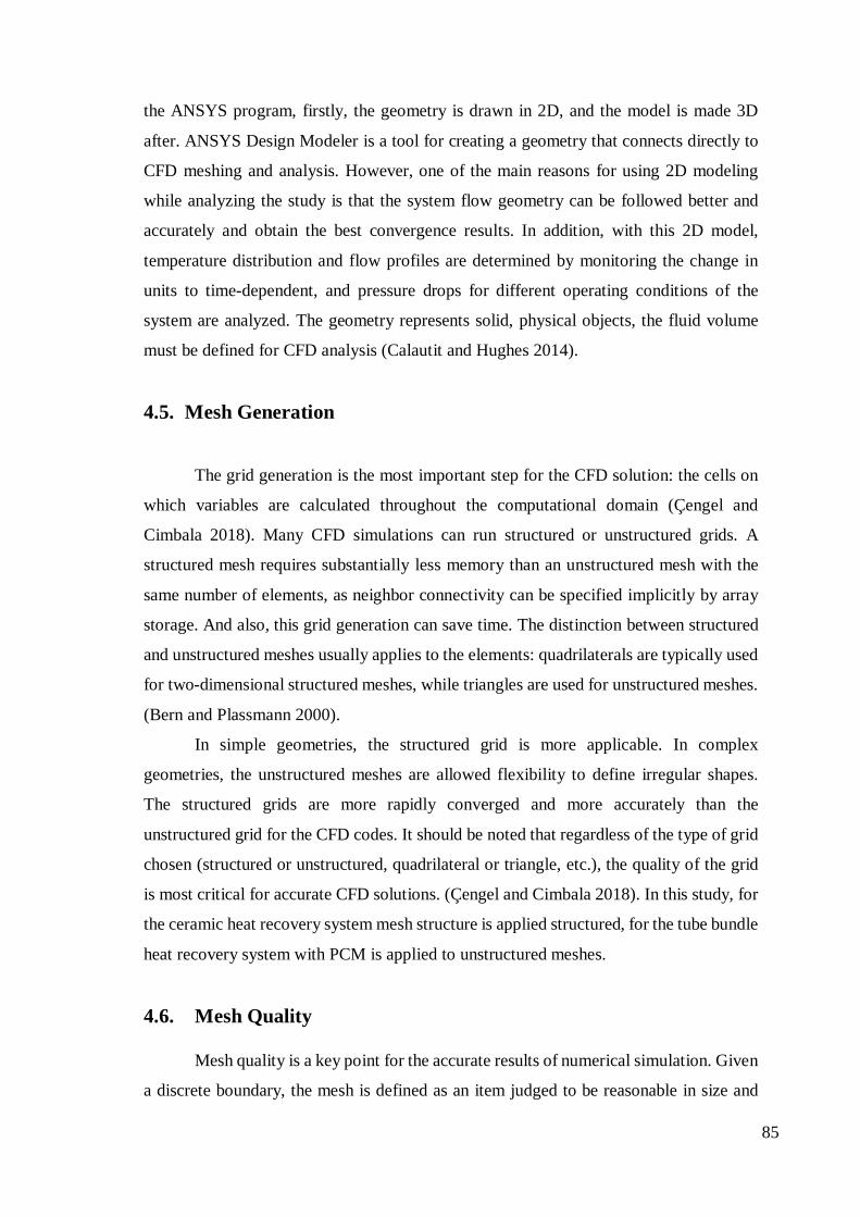
the ANSYS program, firstly, the geometry is drawn in 2D, and the model is made 3D

after. ANSYS Design Modeler is a tool for creating a geometry that connects directly to

CFD meshing and analysis. However, one of the main reasons for using 2D modeling

while analyzing the study is that the system flow geometry can be followed better and

accurately and obtain the best convergence results. In addition, with this 2D model,

temperature distribution and flow profiles are determined by monitoring the change in

units to time-dependent, and pressure drops for different operating conditions of the

system are analyzed. The geometry represents solid, physical objects, the fluid volume

must be defined for CFD analysis (Calautit and Hughes 2014).

4.5. Mesh Generation

The grid generation is the most important step for the CFD solution: the cells on

which variables are calculated throughout the computational domain (Çengel and

Cimbala 2018). Many CFD simulations can run structured or unstructured grids. A

structured mesh requires substantially less memory than an unstructured mesh with the

same number of elements, as neighbor connectivity can be specified implicitly by array

storage. And also, this grid generation can save time. The distinction between structured

and unstructured meshes usually applies to the elements: quadrilaterals are typically used

for two-dimensional structured meshes, while triangles are used for unstructured meshes.

(Bern and Plassmann 2000).

In simple geometries, the structured grid is more applicable. In complex

geometries, the unstructured meshes are allowed flexibility to define irregular shapes.

The structured grids are more rapidly converged and more accurately than the

unstructured grid for the CFD codes. It should be noted that regardless of the type of grid

chosen (structured or unstructured, quadrilateral or triangle, etc.), the quality of the grid

is most critical for accurate CFD solutions. (Çengel and Cimbala 2018). In this study, for

the ceramic heat recovery system mesh structure is applied structured, for the tube bundle

heat recovery system with PCM is applied to unstructured meshes.

4.6. Mesh Quality

Mesh quality is a key point for the accurate results of numerical simulation. Given

a discrete boundary, the mesh is defined as an item judged to be reasonable in size and

85

quality (shape). The size relates to the greater or lesser thickness of the boundary

discretization and continues to be properly defined within the domain. Quality is related

to element aspect ratios (Borouchaki and George 2000).

Skewness is one of the main methods of measuring the quality of the mesh.

Compared to an idealized cell, either triangular or quadrilateral, skewness measures the

accuracy of a cell. The Fluent Meshing User’s Guide (2020) defines the skewness of how

close to ideal (equilateral or equiangular) a face or cell is (Figure 4.2). Highly skewed

faces and cells are unacceptable, as the equations assume that cells are relatively

equilateral/equiangular.

Figure 4.2. Ideal and Skewed Triangles and Quadrilaterals. (Source: Borouchaki and George 2000)

Two methods can be used to measure skewness; the first is based on the equilateral

volume, which is only for triangles and tetrahedral, and the second is based on the

deviation from a normalized equilateral angle, which is for pyramids and prisms. In the

equilateral volume deviation method, skewness is defined as Eq.4.7.

𝑆𝑆𝑘𝑘𝑆𝑆𝑤𝑤𝑆𝑆𝑆𝑆𝑆𝑆𝑆𝑆 = 𝑂𝑂𝑂𝑂𝜕𝜕𝑂𝑂𝑚𝑚𝑂𝑂𝑂𝑂 𝐶𝐶𝑆𝑆𝑂𝑂𝑂𝑂 𝑆𝑆𝑂𝑂𝑆𝑆𝑆𝑆 − 𝐶𝐶𝑆𝑆𝑂𝑂𝑂𝑂 𝑆𝑆𝑂𝑂𝑆𝑆𝑆𝑆

𝑂𝑂𝑂𝑂𝜕𝜕𝑂𝑂𝑚𝑚𝑂𝑂𝑂𝑂 𝐶𝐶𝑆𝑆𝑂𝑂𝑂𝑂 𝑆𝑆𝑂𝑂𝑆𝑆𝑆𝑆 Eq. (4.7)

Equilateral triangle Highly skewed triange

Equiangular quad Highly skewed quad

86

According to The Fluent Meshing User’s Guide (2020), for mesh quality, the

skewness value is approximately 0.1 for 2D and 0.4 for 3D. Table 4.1 shows the range of

skewness values and corresponding cell quality. When between 0.25 and 0.5 is good

quality mesh according to the skewness range, the 0-0.25 is excellent, and the 0.75-0.9

range is considered fair. 0.9 and above values are classified as poor and bad quality. As

the equations assume that the cells are equilateral, cells are classified as bad, and

degenerate are unacceptable.

Table 4.1. Range of skewness values and corresponding cell quality.

Value of Skewness Cell Quality 1 Degenerate 0.9-<1 Bad 0.75-0.9 Poor 0.5-0.75 Fair 0.25-0.5 Good >0-0.25 Excellent 0 Equilateral

4.7. Simulation Details of the HRV Units

The CFD model is designed according to a real-scale laboratory experiment. This

CFD model is analyzed as the same room and equipment and indoor and outdoor

environmental conditions. In the CFD model, the dimensions of all parts of the HRV units

and duct in the experimental setup are designed the same. This part includes problem

identification, mesh generation, mesh quality and mesh verification, and boundary

conditions for the CFD model.

4.7.1. Problem Identification

In Chapter 3, the experimental setup of the system and the experiments for two

separate HRV systems are in detail. In CFD, the duct has the same dimensions as the

experiments. The duct has a fully developed laminar flow area of 1.5 meters after the

HRV unit to the outlet. A 15 cm by 15 cm HRV unit is placed inside this duct, which has

87

a section of 15 cm by 15 cm. The distance between the unit and the inlet is 0.06 m. As

seen in the experimental setup, there is a filter and a fan. However, filter and fan are not

defined in the CFD model, and only boundary conditions are assigned to the surfaces.

Figure 4.3 shows the CFD model in general terms. In the simplified drawing, there are

general dimensions of the model. First, experiments were carried out with the ceramic

system available in the market in the area reserved for the HRV unit, and then experiments

and CFD analyzes were carried out on the prototype. As shown in Figure 4.3, the system

consists of 3 main parts. In the system design, area I is the inlet section where the fresh

air will be transferred to the indoor environment, area number II is the tube bundle where

the HRV unit is located, and number III is the conditioned air outlet transferred to the

indoor environment.

Figure 4.3. Simplified section for duct and dimensions.

4.7.1.1. Ceramic System for Sensible Thermal Energy Storage

The project shown in Figures 4.4a and 4.4b are 2D and 3D images of ceramic heat

recovery systems modeled in the Design Modeler tool. While the area I have seen in

Figures 4.4a and 4.4b represents the region from the outlet to the HRV unit, the area

where the ceramic HRV unit is located is indicated as II. Simulations to be made will

continue over only one cell ceramic.

88

a)

b)

Figure 4.4. a) Overview of the 3D ceramic heat recovery system and b) 2D views

designed in the Design Modeler module

4.7.1.2. Tube Bundle System for Latent Thermal Energy Storage

Tube bundle system placed in the duct in the area indicated in figure 4.5. The project

shown in Figures 4.5a and 4.5b is 2D and 3D images of the tube bundle system designed in

the Design Modeler tool. As seen in Figure 4.5b, a symmetrical region which name is the

computational domain, has been chosen in the 2D model to be simulated. Future analysis will

continue through this zone. The 0.135 m represents the area in the middle of the 5th and 6th

tube from the inlet indicated in this figure. Grid convergence and static pressure, as well as

velocity values calculated in the following sections, are detailed on this surface.

1.5m 0.15m 0.06m

0.15m

0.15m

89

a)

b)

Figure 4.5. a) Overview of the 3D tube bundle heat recovery system and b) 2D views designed in the Design Modeler module

4.8. Numerical Approach

CFD is a computer-based engineering method and a numerical approach in which

detailed calculations can be done (Karaçavuş and Aydın 2017). CFD is performed to

investigate the heat transfer performance and fluid flow characteristics. First, the model

is primarily divided into mesh within the Fluent program. Then, flow analysis is obtained

with the ANSYS-Fluent tool.

1.5m 0.15m 0.06m

0.15m

0.15m

Computational domain

90

4.8.1. Mesh Generation

For the study of the CFD model, the generation of the computational mesh from

the fluid volumes is provided. In defining the accuracy of a solution, mesh quality is an

important factor, and thus many designers spend a considerable amount of time ensuring

that the mesh is suitable for the simulations. For each geometry, the individual mesh is to

be created before simulations. With the system's design, a mesh structure is created,

regions are defined as solid and liquid, and boundary conditions are determined. There

are some points to be considered in defining mesh. The size and type of the elements are

important to obtain the most accurate result. Because the use of more elements causes

both excessive calculation time and an increase in error rate. The boundary layer is a thin

region that is close to the fluid. And to accurate results would be placed as many gird

points as possible to the wall. Also, attention should be paid to deformities that may occur

in the elements. It is important not to exceed the 0.9 value given as the maximum value

for the coefficient of skewness not to give calculation errors in the FLUENT program.

The automatic mesh generation should not be done when analyzing complex geometries.

A few other analytical analyses need to be done before generating the meshes. It

is controlled according to grid independence on the specified plane's residuals and

temperature, pressure, and velocity values. The total number of cells is determined in

three different models: coarse, medium, and fine grids, and the results are compared. If

the residues reach a certain value and no longer change, we assume it converges (Werner

2016).

4.8.1.1. Grid Independence Study

The mesh resolution can affect the result of a CFD simulation. A grid

independence study is performed in the study. Besides the mesh resolution, convergence

can influence the result as well. Accordingly, mesh independence is obtained with the

grid convergence index. The term grid convergence index (GCI) compares the numerical

results of the same problem belonging to different mesh structures. Different mesh sizes

are based on the same boundary conditions as all other models (Roache 1994). A grid

convergence study is a necessary test in any CFD simulations (Zhao and Su 2019). The

solution is in the asymptotic range of convergence when the GCI value for the meshes

91

used in the simulation is small. The mesh is refined at least three times, each time solving

and getting results until an asymptotically converged solution is obtained.

Many cases estimate meshes for the GCI method in the literature (Roache 1994;

Hirt and Nichols 1981; Karimi et al. 2012). Celik and Hu (2004) demonstrated an error

transport equation to quantify the discretization error. To calculate the GCI, there are

three steps to define this value.

Step 1. First, the mesh size "h" (Eq.4.13) assigned to the 2-D geometry is

calculated on the representative cell.

h = [1𝑁𝑁�

(∆𝐴𝐴𝑖𝑖)]𝑁𝑁

𝑖𝑖=1

1/2

(Eq. (4.13)

where ∆Ai is the area of the ith cell and N is the total number of the cells.

Step 2. After the defined grid refinement factor between specified meshes, the

second step is to calculate the apparent order p of the method using the expression. p is

the formal order of accuracy of the algorithm, and which can be computed using Eq 14.14

𝑂𝑂 =1

ln (𝑟𝑟23) ln ��𝑟𝑟23

𝑝𝑝 − 1�𝑆𝑆12𝑟𝑟12𝑝𝑝 − 1)𝑆𝑆23

� Eq. (4.14)

where r23 and r12 represent ratios of the h value of the meshes. The third grid is the

“coarse” mesh size, the second grid is the “medium” mesh size, and the first grid is the

“fine” mesh size. Here, e is the analysis result for the specified variables, and e12 and e23

represent the differences between variables. The variables used in this calculation are

pressure, temperature, and velocity for the specified plane, which is 13.5 cm from the

inlet.

Step 3. The third step is the calculation of GCI along with the apparent order p.

(Gümüş, Seven and Şimşek 2020).

𝐺𝐺𝐶𝐶𝐺𝐺23𝑠𝑠𝑖𝑖𝑛𝑛𝑟𝑟 = 𝐹𝐹𝑠𝑠

|𝐸𝐸23|𝑟𝑟23𝑝𝑝 − 1

Eq. (4.15)

92

where E23 expresses the fluid's velocity, pressure, and temperature values at the point

determined in fine mesh resolutions 1, medium mesh resolutions 2, and coarse mesh

resolutions 3. And the Fs is a safety factor. Roache (1994) recommended a range of 1.25

≤ Fs ≤ 3 for the safety factor. This factor is a statistical analysis for a large number of

samples based on analytical or numerical benchmarks (Xing and Stern 2010). Also is used

to convert the best error estimate into a 95% confidence interval, uncertainty estimate.

The selection of the magnitude of this factor depends on the intended accuracy (Karimi

et al. 2012). In this calculation, the safety factor is taken as 1.25.

In light of this information, mesh independence studies for ceramics and tube

bundle systems are shared in this section. Six different meshes have been simulated for

ceramic and tube bundle systems.

4.8.1.1.1. Ceramic System Mesh Structure Decision

Three different modules have been generated on the ceramic unit's mesh tool,

shown in Figure 4.6. These are fine, medium, and coarse modules. This figure shows the

boundary layer effect on the ceramic edges; an appropriate mesh density is preferred in

these areas. In this study, a mesh structure is created using quadrilateral elements with

edge sizing and face meshing features.

The ceramic system boundary condition is the same with experiments. For

ceramic systems, the outdoor temperature is 5°C, and the indoor temperature is kept 20°C.

According to air velocity measurements, the average supply air velocity results are 0.215

m/s. In this study, six different grid densities of unstructured quadrilateral grids are

generated for ceramic HRV units with 7204, 31812, 55944, 88000, 136136, and 264660

nodes, respectively shown in Figure 4.7. All the parameters for the six simulation runs

are kept the same.

93

(a)

(b)

(c) Figure 4.6. Three different modules for meshes (a) fine, (b) medium, (c) coarse for

ceramic unit

Figure 4.7. Calculated pressure as a function of the number of cells at the x=13.5 cm

94

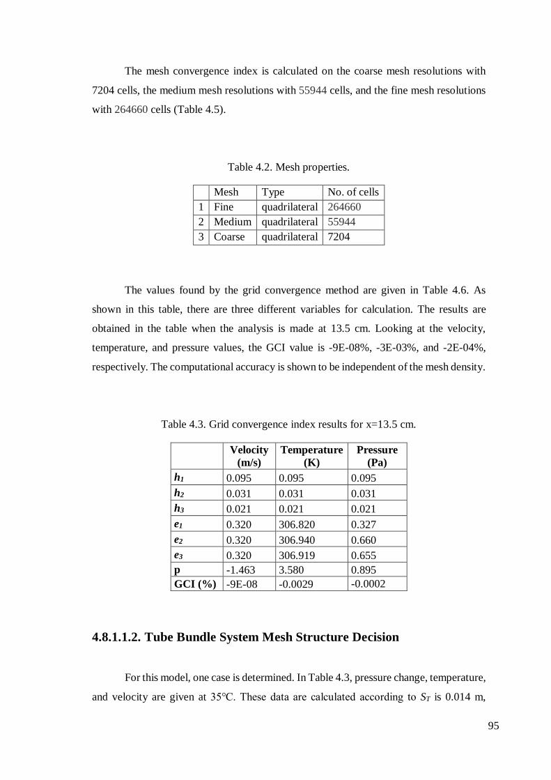
The mesh convergence index is calculated on the coarse mesh resolutions with

7204 cells, the medium mesh resolutions with 55944 cells, and the fine mesh resolutions

with 264660 cells (Table 4.5).

Table 4.2. Mesh properties.

Mesh Type No. of cells 1 Fine quadrilateral 264660 2 Medium quadrilateral 55944 3 Coarse quadrilateral 7204

The values found by the grid convergence method are given in Table 4.6. As

shown in this table, there are three different variables for calculation. The results are

obtained in the table when the analysis is made at 13.5 cm. Looking at the velocity,

temperature, and pressure values, the GCI value is -9E-08%, -3E-03%, and -2E-04%,

respectively. The computational accuracy is shown to be independent of the mesh density.

Table 4.3. Grid convergence index results for x=13.5 cm.

Velocity (m/s)

Temperature (K)

Pressure (Pa)

h1 0.095 0.095 0.095 h2 0.031 0.031 0.031 h3 0.021 0.021 0.021 e1 0.320 306.820 0.327 e2 0.320 306.940 0.660 e3 0.320 306.919 0.655 p -1.463 3.580 0.895 GCI (%) -9E-08 -0.0029 -0.0002

4.8.1.1.2. Tube Bundle System Mesh Structure Decision

For this model, one case is determined. In Table 4.3, pressure change, temperature,

and velocity are given at 35℃. These data are calculated according to ST is 0.014 m,

95

velocity is 0.345 m/s as a measured value in experiments. The height of one tube is 15

cm, and its outer diameter is 4.76mm. Liquid PCM is poured into the tubes having 0.3

mm wall thickness. Those calculations are solved according to Zukauskas's (1972)

Method. And according to this velocity, the Reynolds number is 152.472. It can be seen

that the assumption of laminar flow valid is here. The geometry is created according to

these values. Three different modules have been generated on the mesh tool, shown in

Figure 4.8. As shown in Figure 4.8, since the boundary layer effect will occur on the tube

walls, an appropriate mesh density is preferred in these zones. The sensitivity of the

solution has been increased by using a mesh structure in the zone where the tubes where

the PCM is located. This type of mesh structure is extremely important for the accuracy

of the solution results. In this study, a mesh structure is created using triangle and

quadrilateral elements.

(a)

(b)

(c) Figure 4.8. Three different modules for meshes (a) fine, (b) medium, (c) coarse for tube

bundle unit.

96

Before calculating the grid convergence index, many cases have compared each

other according to a calculated static pressure value. Many mesh structures have been

analyzed, and these can be classified as very coarse, coarse, medium, fine, very fine, ultra-

fine. Figure 4.9 is the calculated static pressure x=13.5 cm (the middle of the HRV unit)

from the inlet in the Fluent analysis program. The various grid resolution cases in the

entrance flow region of duct flow function of the number of cells. The number of cells

Case 1 is 5x103 the data for pressure is 0.2045 Pa, Case 2 is the 20x103 which is 0.1739

Pa, Case 3 has 50x103 cells, and for this case, the result is 0.1778 Pa, Case 4 is the

200x103, and the result is 0.1802 Pa, Case 5 has 250x103 cells, Case 6 has 300x103 cells,

and the calculated data are 0.1801 Pa and 0.1808 Pa, respectively.

Figure 4.9. Calculated pressure as a function of the number of cells at the x=13.5 cm.

The mesh convergence index is calculated on the coarse mesh resolutions with

22781 cells, the medium mesh resolutions with 54185 cells, and the fine mesh resolutions

with 189539 cells (Table 4.7).

97

Table 4.4. Mesh properties.

Mesh Type No. of cells Max_skewness 1 Fine quadrilateral, triangle 189539 0.81769 2 Medium quadrilateral, triangle 54185 0.62852 3 Coarse quadrilateral, triangle 22781 0.50002

The values found by the grid convergence method are given in Table 4.8. Here are

the results obtained from 3 different mesh structures. The results are obtained when the

analysis is made at 13.5 cm in the table. Looking at the velocity, temperature, and pressure

values, the GCI value is 0.0002% in the velocity analysis, -0.000042% in the temperature

analysis, and 0.0097% in the pressure differences for 13.5 cm from the inlet. As a result,

it is concluded that the computational accuracy is independent of the mesh density. The

fine mesh is chosen for the study as it is accurate enough and more efficient.

Table 4.5. Grid convergence index results for x=13.5 cm.

Velocity (m/s)

Temperature (K)

Pressure (Pa)

h1 0.029 0.029 0.029 h2 0.024 0.024 0.024 h3 0.018 0.018 0.018 e1 0.346 307.990 0.174 e2 0.344 307.990 0.178 e3 0.343 308.000 0.180 p 7.598 -19.683 3.591 GCI (%) 0.0002 -0.000042 0.0097

4.8.2. Boundary Conditions

The next step in generating the mesh is to determine the appropriate limits of

initial boundary conditions for the surfaces affecting the fluid flow to complete the

effective simulation and solution of a CFD model. The boundary conditions of this study

should also represent the experimental conditions. Computational domain, boundary, and

initial conditions used in numerical modeling are given in Figures 4.10a and 4.10b. As

seen in these figures, there are physical boundaries of inlet, outlet, symmetry, and wall.

The symmetry condition prevents flow from crossing the boundary but allows the flow

to move along the boundary (Albatayneh, Alterman and Page 2018). The experiment

determines the horizontal velocity component as the inlet boundary condition, and the

98

uniform velocity inlet is defined as 0.34 m/s for the tube bundle and 0.21 m/s for the

ceramic, while the vertical velocity component is taken as 0. All simulations for ceramics

were made on one cell. However, here, unlike the velocity value measured at the duct

inlet, the velocity value for a single cell is recalculated over the flow rate, and the air

velocity flow through a single cell is 0.32 m/s.

a)

b) Figure 4.10. Computational domain and boundary conditions of a) ceramic and b) tube

bundle system.

The required boundary conditions are shown in Table 4.9. The physical

boundaries comprise inlet, outlet, symmetry, and wall. It is assumed that the whole

domain is initially at the ambient temperature. Temperature and velocity are fixed values

at the inlet and the tube wall during initialization. There is a no-slip condition for walls

to achieve realistic velocity profiles close to walls. And on the symmetry the velocity

component and the gradients are zero (Maheshwari, Chhabra and Biswas 2006).

Table 4.6. Boundary definitions.

Inlet Velocity Inlet

x = 0 ⇾ T = Tinlet x = 0 ⇾ 𝜌𝜌x = Uinlet x = 0 ⇾ 𝜌𝜌y = 0

Outlet Pressure x = L ⇾ Poutlet = 0 (gage)

Body surfaces Symmetry

∂T/∂y = 0 𝜌𝜌y = 0 ∂𝜌𝜌y /∂y = 0 ∂𝜌𝜌x /∂y = 0

Tubes No-slip 𝜌𝜌 = 0

99

4.8.3. Solution Method

The Ansys Fluent software has 2 different solvers: the pressure-based and density-

based coupled solver. For the tube bundle prototype, the pressure-based solver can be

used for forced flow conditions included melting and solidification problems (Al-Abidi

et al. 2013). This solver uses an algorithm in which the conservation of mass of the

velocity field is obtained by solving a pressure equation (Chorin 1968). Also, the first-

order upwind, power-law and second-order upwind schemes are widely used for

solidification and melting problems. Convective terms in momentum equations, energy

equations are discretized using a second-order upwind interpolation scheme, and

turbulent equations are first-order upwind interpolation schemes. The SIMPLE algorithm

does the pressure-velocity coupling for interpolation. The material physical properties are

related to the problem, and the materials’ density, heat capacity, thermal conductivity,

viscosity can be changed. The user can define individual component properties (Chapter

3-Table 3.2).

Convergence is obtained when the residual of the continuity, momentum, and

energy equations are reduced to less than 10-6, 10-6, and 10-8, respectively, and the iteration

number used is 1000 for each time step to generate better convergence criteria (Gürel

2020; Driels and Shin 2004) The time step is set as 0.1s for tube bundle and ceramic heat

recovery system. In this study, these HRV units LHTES and SHTES are solved in a 2D

plane. All solution methods are the same for tube bundle and ceramic heat recovery

systems.

4.8.4. Model Verification and Validation

In this work, the flow model replicates the computer and experimental models to

identify and eliminate errors. For the verification process, the model is implemented of

the computer model. This model is a numerical procedure for solving equations

prescribed in the mathematical model with a computer code.

100

4.8.4.1. Verification of Method with Reference Study

In Figure 4.11, the analysis of Reynolds and Nusselt number results are compared

to find the accuracy of the Fluent settings and mesh structure in a single sphere on the

duct. In this analysis, water is used instead of air, and the accuracy of the established

Fluent and mesh structure is compared with the reference study (Yıldırım et al. 2017;

Maheshwari, Chhabra and Biswas 2006). Nusselt number changes obtained in numerical

and reference studies are compared for a single sphere. In these analyzes, the Reynolds

number is taken as 1, 5, 10, 50, and 100. As a result, it is seen that the Nusselt number

increases while the Reynolds number increases. In other words, Re and Nu numbers

increase in direct proportion. The Nusselt numbers obtained in the present study and the

values in the reference article, and the numerical data are coherent (Maheshwari, Chhabra

and Biswas 2006). To calculate the Nusselt number, the total surface heat flux value is

taken from simulation results and Eq. 4.9 is applied. While calculating the Reynolds

number, the inlet velocity is important.

Figure 4.11. Verification of the method for a flow analysis of the numerical calculation

results and the reference study (Source: Yıldırım et al. 2017; Maheshwari, Chhabra and Biswas 2006).

101

4.8.4.2. Validation of Model for Ceramic Heat Recovery System

After verifying the numerical method of the model, experimental validation

outcomes and numerical outcomes have compared each other. Time-dependent variations

of computed temperature and experimental results are compared in Figure 4.12 and

Figure 4.13. For validation, a physical experiment is conceived and designed. The study

is solved in a 2D plane. Figure 4.12 is the verification of the method for a flow analysis

of the experimental results for ceramic HRV units. As shown in this figure, the charging

and discharging process is 2-minute. The experimental data measured by the instruments

are recorded with a datalogger in time steps of 5 seconds during the experiments. In CFD,

the time step size is 0.1 s. According to this figure, the average temperature values

standard deviation for the charging process is 0.65%, for the discharging process, it is

1.59% compared with CFD and experimental study results.

Figure 4.12. Verification of the method for a flow analysis of the experimental results

and numerical calculation results for ceramic system.

102

4.8.4.3. Validation of Model for Tube Bundle Heat Recovery System

The other verification study for the tube bundle system. The experiments are

conducted with LHTES HRV units using RT27 for the PCM and air for the HTF. Figure

4.13 has a charging and discharging process for both analysis models for 15-minute

results. During the charging and discharging process in the experiment, the data is

recorded at 5-second intervals. For the numerical analysis time, the step size is 0.1. The

information about the measured points is given in Chapter 3, and the average temperature

of the tubes and the result obtained from the numerical study are compared in this graph.

As a result, while the average temperature values standard deviation for the charging

process is 1.32%, for the discharging process, it is 1.38% compared with numerical

solutions and experimental study results. In this study, it has been shown that the

numerical model can be used to examine melting and heat transfer in LHTES systems

with different geometries.

Figure 4.13. Verification of the method for a flow analysis of the experimental results

numerical calculation results for tube bundle system

103

4.9. Summary

This chapter is provided the theoretical background of the CFD for modeling and

simulation. The geometry modeling, mesh structure, solvers, and equations used for CFD

model results to be accurate and reliable are mentioned. The GCI is calculated according

to pressure change, temperature, and velocity to accurate results. And also, before

calculating the grid convergence index, many cases have compared each other according

to a calculated static pressure value to minimize the effect of such errors and uncertainties.

Using the knowledge gained from the CFD analysis, many different

configurations of tube bundle heat recovery systems with PCM are modeled and

analyzed. Their boundary conditions and some of the geometries are changed. Each

system is modeled and analyzed with varying tubes, inlet, and outlet temperatures. The

flow properties of the two types of heat recovery systems, especially the prototype heat

recovery system, are investigated by reproducing the conditions observed in the

experiments with the CFD model.

104

CHAPTER 5

RESULTS AND DISCUSSION

The following chapter details the experimental results and CFD simulations

results for decentralized heat recovery systems with two different concepts of TES. The

decentralized HRV systems store

• sensible energy into ceramic material and

• latent energy into the tube bundle containing PCM.

The boundary conditions are defined for the CFD according to experimental

measurements. The CFD simulations are validated using the results of the experiments

given in Chapter 4. Therefore, the accuracy and reliable solutions of the numerical

analysis are suitable for different arrangements and configurations.

In the context of this study, the thermal energy storage performance of the HRV

systems is firstly evaluated by the experiments. Two decentralized HRV systems work in

synchrony one by one during the experiments. At the same time, one system exhausts air

from the inside, the other supplies fresh air from the outside.

This chapter contains 4 subtitles. The first section is the experimental results, the

second section is the numerical results, the third section is the refinement of the tube

bundle HRV system, and the fourth section is the simulations made in different climates.

In this chapter, the charging and discharging results are shared for both experiments and

numerical studies. In addition, after the experiments and numerical studies, different

refinement cases are simulated for the LHTES HRV unit, and the results are examined.

Besides these refinement simulations, analyzes are made in different climatic conditions

the energy performance of the tube bundle prototype is produced.

5.1. Experimental Results

Experimental setup detailed in Chapter 3, the real-scale experiments are carried

out in the Building Physics Laboratory of the Izmir Institute of Technology, Faculty of

Architecture. Controlled parametric studies are carried out experimental testing of the

ceramic HRV unit and the tube bundled HRV unit. During these experiments, the systems

105

placed in the two ducts work synchronously. In one experimental set, HRV units with

SHTES and in another set of HRV units with LHTES are experimentally investigated

under different operating conditions. In this section, the results are shared in detail.

5.1.1. Charging and Discharging Experiments for SHTES

In this study, seven experiments are detailed for two decentralized heat recovery

units operating simultaneously, the duct and the simulation rooms were monitored until

steady-state conditions were attained before recording measurements for each experiment.

For the simulation of summer conditions, the indoor environment is kept at around 20℃,

and the outdoor environment is kept at approximately 35℃, while in winter conditions, the

indoor environment is kept constant at around 20℃ and the outdoor environment

approximately at 5℃. The heat recovery units were operated for specific cycles of; 1-

minute, 2-minute, 5-minute, 7.5-minute, and 10-minute, as given in Table 5.1.

Table 5.1. Experiments and conditions.

Investigated Parameter

Conditions Constant Parameters Variables

Time

Winter

1-minute -Indoor Temperature (20°C) -Outdoor Temperature for winter (5°C), for summer (35°C) -Supply Velocity (0.21 m/s) -Exhaust Velocity (0.16 m/s)

-Duct Inlet Temperature - Duct Outlet Temperature -Ceramic Temperature - Pressure Difference -Velocity

2-minute 5-minute 7.5-minute 10-minute

Summer 7.5-minute

10-minute

The depths of the thermocouples are coded as follows; 1-1 and 2-1 represent the

thermocouples at 12 cm, while 1-2 and 2-2 at 9 cm, 1-3 and 2-3 at 6 cm, 1-4, and 2-4

represent the thermocouples at 3 cm depth for D1 and D2, respectively, in Figures 5.1.

These four thermocouples are also mentioned as two groups numbered G1 and G2

separately. Tinside and Toutside given in Figures 5.1 are indoor temperature and outdoor

temperature, respectively. The average of the three thermocouples placed before the filter

in the unit and the average of the three thermocouples placed after the ceramic HRV unit

is coded as D1Tin and D2Tin, D1Tout, and D2Tout, in D1 and D2, respectively (Figure 5.1).

106

Figure 5.1. Ceramic thermocouple placement (in cm).

The temperature measurements of thermocouples in ceramics are given in Figures

5.2-5.8. The graphs on the left side of Figures 5.2-5.8 belong to Duct 1 (D1), and the

graphs on the right side belong to Duct 2 (D2). These graphs show the temperature

distribution when two units are operated simultaneously for different time periods defined

above. Values from the thermocouples placed in 3cm, 6cm, 9cm, and 12cm depths inside

the ceramic material show a temperature gradient inside the HRV unit during the

experiments. Figure 5.2 shows the temperature data taken from the thermocouples in the

ceramic HRV units from the two ducts for the experiment conducted in simulated winter

conditions operating for 10 minutes with 1-minute cycles. In other words, each 1-minute,

the operating direction is changed via the fan controller interface. During the experiment,

the indoor average temperature (Tinside) was measured from five points and was kept

around 20°C, while the outside average temperature (Toutside) was calculated at

approximately 3°C by using data from three thermocouples. Average air temperatures

measured by the three thermocouples placed at the inlets (Tin) and the outlets (Tout) of the

heat recovery system fluctuated by as much as 3°C during the experiment because of the

thermal inertia of the ceramic HRV units. Ceramic materials were heated by indoor air,

and their temperatures increased between 1°C and 3°C, depending on the position of the

thermocouples in the ceramics. Temperatures of the inside part of the ceramic materials

close to the indoor environment had a relatively higher temperature increase, therefore

they stored more thermal energy. On the other hand, temperatures of the outer part of the

material were close to the outside temperature, and their fluctuations were about 1°C,

with less thermal energy storage, yet all of the energy stored in the system was discharged

at the end of each cycle.

107


simulated winter conditions for Duct 1 and 2.

Figure 5.3 gives the results for the simulated winter conditions, and the values of

the units working for 6 minutes with a 2-minute cycle can be seen. Inside and outside

temperatures were almost constant during the experiment, and the two ventilation systems

worked synchronously but with different airflow directions. Since the working period was

changed to a 2-minute cycle, temperatures of the ceramic materials increased by up to

7°C, depending on the measurement positions. The material temperatures were close to

the outside temperature at the outer part of the ceramic, and the temperature fluctuations

were less than the inner part of the ceramic. The 2-minute cycles also showed that the

thermal energy-charged could be discharged from the ceramic material.



108

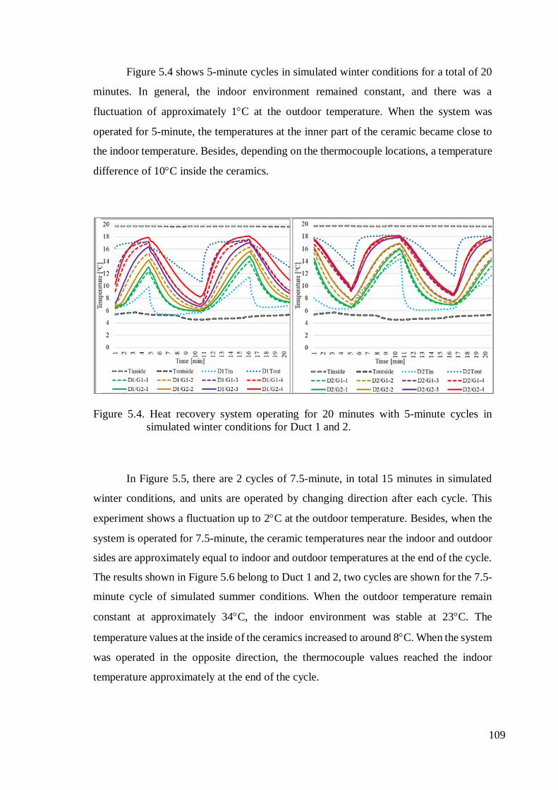
Figure 5.4 shows 5-minute cycles in simulated winter conditions for a total of 20

minutes. In general, the indoor environment remained constant, and there was a

fluctuation of approximately 1°C at the outdoor temperature. When the system was

operated for 5-minute, the temperatures at the inner part of the ceramic became close to

the indoor temperature. Besides, depending on the thermocouple locations, a temperature

difference of 10°C inside the ceramics.



In Figure 5.5, there are 2 cycles of 7.5-minute, in total 15 minutes in simulated

winter conditions, and units are operated by changing direction after each cycle. This

experiment shows a fluctuation up to 2°C at the outdoor temperature. Besides, when the

system is operated for 7.5-minute, the ceramic temperatures near the indoor and outdoor

sides are approximately equal to indoor and outdoor temperatures at the end of the cycle.

The results shown in Figure 5.6 belong to Duct 1 and 2, two cycles are shown for the 7.5-

minute cycle of simulated summer conditions. When the outdoor temperature remain

constant at approximately 34°C, the indoor environment was stable at 23°C. The

temperature values at the inside of the ceramics increased to around 8°C. When the system

was operated in the opposite direction, the thermocouple values reached the indoor

temperature approximately at the end of the cycle.

109

Figure 5.5. Heat recovery system operating for 15 minutes with 7.5-minute cycles in


Figure 5.6. Heat recovery system operating for 15 minutes with 7.5-minute cycles in

simulated summer conditions for Duct 1 and 2.

In Figures 5.7 and 5.8, the units were operated for 10-minute, in simulated winter

and summer conditions, respectively. The indoor environment is generally stable at 20°C

and the outdoor environment varies between 3°C to 5°C in Figure 5.7. Considering

temperature distribution inside the ceramic at the end of the cycle process, almost all the

temperature values are equal to the outdoor or indoor temperature, depending on the airflow

direction. Figure 5.8 shows that the outdoor temperature fluctuates up to 2°C, and the indoor

temperature is generally stable at 21°C. There is a decrease or increase of approximately

12°C in the ceramic’s temperatures during the 10-minute cycles. Temperature values at the

ceramics change significantly in the first part of the periods. After that, there were no

110

remarkable temperature alterations in the ceramic material, indicating that the thermal

energy storage rate decreased gradually during a 10-minute cycle.

Figure 5.7. Heat recovery system operating for 10-minute in simulated winter conditions

for Duct 1 and 2.

Figure 5.8. Heat recovery system operating for 10-minute in simulated summer

conditions for Duct 1 and 2.

111

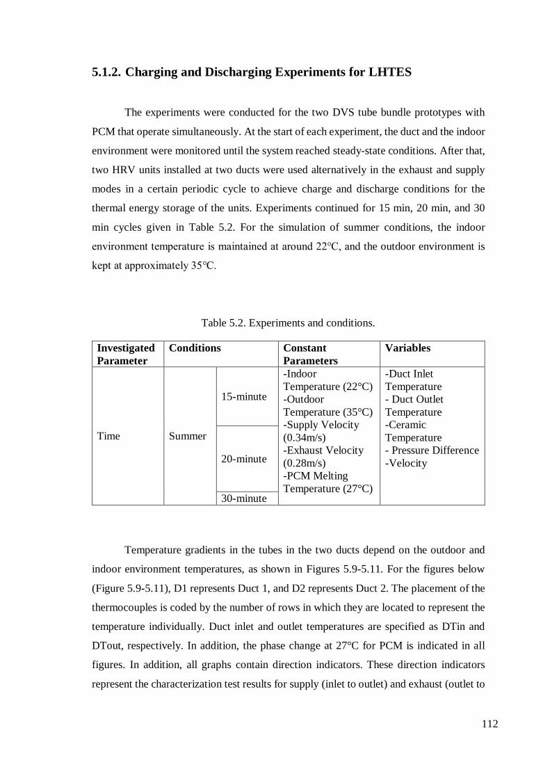
5.1.2. Charging and Discharging Experiments for LHTES

The experiments were conducted for the two DVS tube bundle prototypes with

PCM that operate simultaneously. At the start of each experiment, the duct and the indoor

environment were monitored until the system reached steady-state conditions. After that,

two HRV units installed at two ducts were used alternatively in the exhaust and supply

modes in a certain periodic cycle to achieve charge and discharge conditions for the

thermal energy storage of the units. Experiments continued for 15 min, 20 min, and 30

min cycles given in Table 5.2. For the simulation of summer conditions, the indoor

environment temperature is maintained at around 22℃, and the outdoor environment is

kept at approximately 35℃.

Table 5.2. Experiments and conditions.

Investigated Parameter

Conditions Constant Parameters

Variables

Time Summer

15-minute

-Indoor Temperature (22°C) -Outdoor Temperature (35°C) -Supply Velocity (0.34m/s) -Exhaust Velocity (0.28m/s) -PCM Melting Temperature (27°C)

-Duct Inlet Temperature - Duct Outlet Temperature -Ceramic Temperature - Pressure Difference -Velocity 20-minute

30-minute

Temperature gradients in the tubes in the two ducts depend on the outdoor and

indoor environment temperatures, as shown in Figures 5.9-5.11. For the figures below

(Figure 5.9-5.11), D1 represents Duct 1, and D2 represents Duct 2. The placement of the

thermocouples is coded by the number of rows in which they are located to represent the

temperature individually. Duct inlet and outlet temperatures are specified as DTin and

DTout, respectively. In addition, the phase change at 27°C for PCM is indicated in all

figures. In addition, all graphs contain direction indicators. These direction indicators

represent the characterization test results for supply (inlet to outlet) and exhaust (outlet to

112

inlet) of ducts. Meanwhile, Tinside and Toutside are indoor temperature and outdoor

temperature, respectively.

The experiment in Figures 5.9-5.11 is for the simulated summer conditions.

Temperature changes when both units run simultaneously for Duct 1 (D1) and Duct 2

(D2). Thereby, the charging and discharging of the PCM can be monitored by following

the temperature change in the thermocouples. The system operates for 15 min in one

direction, then, afterward it operates in the opposite direction for another 15 min (Figure

5.9).

Duct 1 first takes supply air from the outside, and the PCM melts between 26℃

and 28℃. Later, the solidification process begins when the system operates in the reverse

direction (Figure 5.9-D1). Temperature fluctuations occur in the outdoor environment

due to the thermostat of the experimental setup. When the ambient temperature rises

above or sinks below ±1°C, the thermostat activates and either stops or starts the heating

system. Since the outdoor environment has a smaller volume, heat losses have a higher

impact and cause faster cool down.

Figure 5.9. Heat recovery system operation for 30 min, with 15 min cycles in summer

conditions for Duct 1 (D1) and Duct 2 (D2)

Thus, the fluctuation in the outdoor environment occurs mainly due to the

thermostat-controlled heater. As seen in Figure 5.9, when the systems in Ducts 1 and 2

are operated for 15 min, the PCMs in the temperature trend inside the tubes of the first

three rows do not reach 27°C, thus they are not fully melted. The other measured rows

113

have temperatures higher than 27°C, which shows that the PCMs are melting, and the

fastest melting tube rows are the 8th and 10th. Duct 1 and Duct 2 work in opposite

directions. Duct 2 is in the exhaust, while Duct 1 is in the supply. In Duct 2, the fastest

solidifying tube row is the PCMs inside the first two tubes. So, this figure shows that

there is not enough time to stabilize the temperature distribution of the PCMs inside all

the tubes. For this reason, the system must operate for a while for the PCM to melt or

solidify. Hence, the system was operated for different operation times, and Figures 5.10

and 5.11 give the results.

Figure 5.10 shows the results of 20 min of operation for summer. At the beginning

of the experiment, while the fan in Duct 1 supplies air, the fan in Duct 2 exhausts air from

the indoor environment. The average indoor temperature is 22℃, and the outdoor

temperature is around 35℃. While one cycle duration is 40 min, Figure 5.10 shows two

20-min exhaust and supply modes for D1 and D2. The figure shows that the melting and

solidification process sufficiently occurs in the PCM tubes. Looking at the rows one by

one, the ones with the lowest temperatures in exhaust mode are the first two rows in D1.

In the supply mode, in D2, the fastest melting row is the 5th and 9th. Then it is 8th, 10th,

6th, 3rd, 1st, and 2nd, respectively. Moreover, when the system operates for 20 min, the

temperature increases inside the tube bundle, and the melting and solidification process

of the PCM performs better than the 15 min cycle presented in Figure 5.9.

Figure 5.10. Heat recovery system operating for 40 min with 20 min cycles in summer

conditions for Duct (D1) and Duct 2 (D2).

114

Figure 5.11 gives the results of operation for 30 min of exhaust and 30 min of

supply modes. Thus, the cycle is 60 min in total. On average, the indoor temperature is

21±1°C, while the outdoor temperature is around 33℃. As can be seen, PCM completely

melts in Duct 2 and completely solidifies in Duct 1 in 30 min. Then, the temperatures of

the thermocouples increase. This indicates that sensible heat storage follows LHTES.

Thus, the temperatures of these thermocouples get very close to the indoor or outdoor

environment when the system operates for 30 min.

When Duct 1 is in exhaust mode, the first two rows solidify first. And then 3rd,

9th, 5th, 6th, 8th, and 10th are solidifying, respectively. While Duct 2 operates in supply

mode, the first row of melting tubes is the 5th and 9th row. Then the rows of tubes 8th, 6th,

3rd, 10th, 1st, and 2nd, are melted, respectively.


summer conditions for Duct 1 (left) and Duct 2 (right)

Figure 5.12 shows the melting process of the PCM inside the tubes while working

in the supply mode. This color chart represents the temperatures measured in the tubes

from blue to red. Red is the 35°C which is the row of tubes with the highest temperature,

while blue represents 27°C is the row of tubes that have not completely melted, which is

the mushy zone. When the system operates for 15 min, the first three rows are not fully

melted. And in all operation time, the last three rows have the highest temperature.

115

Figure 5.12. Temperature distribution for rows at the end of an operation cycle in supply

mode

5.1.3. Data Reduction

In this section, calculations have been made based on the data obtained in the

experiment, first for the ceramic HRV unit (SHTES) and then the examination of the tube

bundle HRV unit with PCM (LHTES) is presented.

5.1.3.1. Data Reduction for SHTES

The amount of heat stored in/released from the ceramics embedded in the

decentralized heat recovery systems of the experimental setup is calculated by using Eq.

(5.1),

𝑄𝑄 = 𝑚𝑚𝑐𝑐𝑝𝑝𝜌𝜌𝑇𝑇 Eq. (5.1)

116

where Q is the thermal energy (J), m is the mass of the ceramic (kg), cp is the specific heat

capacity of the ceramic (J/kg℃), and dT is the change in temperature (℃) of the ceramic

material. Specific heat is the amount of heat required to change the temperature of a

substance's unit mass, and the differential scanning calorimeter method is used to measure

specific heat. This method measures the amount of energy absorbed or released while the

sample taken from the ceramic material is heated and cooled for a few cycles between

5℃ and 35℃. The specific heat value of the ceramic material was measured to have an

average value of 0.725 kJ/kg℃.

The heat recovery ventilation system results with a ceramic HRV unit for D2 are

tabulated in Table 5.3. These results are for a working cycle when the system operated

from the indoor to the outdoor environment and from the outdoor to the indoor

environment. Table 5.3 indicates that the result of the air energy change obtained from

the weighted averages of D2-Tin and D2-Tout data and air velocity data measure during

different time steps.

Table 5.3. Air energy change of the unit on Duct 2 for different cycles.

Time

[min]

D2-Tin_Avg [℃]

D2-Tout_Avg

[℃]

D2-Air_Vel [m/s]

Std. Dev. of Velocity

Energy Change [kJ]

Winter

1 16.22 4.87 0.27 0.055 5.098 2 13.76 2.15 0.27 0.023 10.607 5 16.52 6.63 0.26 0.049 20.732

7.5 16.97 8.91 0.29 0.013 29.281 10 17.64 6.69 0.28 0.003 36.532

Summer 7.5 24.45 29.09 0.21 0.044 12.556 10 23.09 30.58 0.25 0.005 30.855

The maximum possible heat transfer capacity, Qmax, is defined in Table 5.4 for the

given set of operating conditions, and it is calculated by using Eq. (5.2) as;

𝑄𝑄𝑚𝑚𝑎𝑎𝜕𝜕 = (�̇�𝑚∆𝜕𝜕)𝑐𝑐𝑝𝑝𝜌𝜌𝑇𝑇 Eq. (5.2)

where �̇�𝑚 is the mass flow rate of air (kg/s), cp is the air specific heat capacity (J/kg℃), dT is

the temperature change of air (℃), and the dt is the cycle period in second. Table 5.6 gives

the results for the thermal energy storage in the ceramic and the energy from the fan and

the maximum energy values that can be stored. According to the Ebm-papst fan

117

manufacturer's catalog data, power consumption is 3.4 Watt when the nominal voltage is

12.0 Volts. Therefore, there is an energy gain/loss of approximately 0.2-2 kJ from the fan

during a cycle period. When the data from Duct 2 are calculated, while the system is

operated in winter conditions for 1-minute from outdoor environment to indoor

environment, 4.478 kJ heat release occurs, when it is operated for 2-minute, 10.762 kJ

energy is released.

Table 5.4. Total heat capacity of the unit on Duct 2 in certain periods at different time steps

Time

[min] Tinside_Avg

[℃] Toutside_Avg

[℃] D2-in to out [kJ]

D2-out to in [kJ]

Fan [kJ]

Qmax [kJ]

Winter

1 19.69 4.32 4.478 4.240 0.20 7.142 2 19.66 2.76 10.762 10.583 0.41 15.451 5 19.72 6.26 21.832 20.682 1.02 29.819

7.5 19.50 5.08 23.853 22.711 1.53 51.762 10 20.39 4.75 24.120 21.520 2.04 73.571

Summer 7.5 23.10 34.16 17.730 16.890 1.53 27.699 10 21.32 34.08 24.552 21.855 2.04 52.134

As seen in Table 5.4, as the system's operating time increases, heat transfer also

increases. However, when looking at the storage per unit time, the best performance can

be seen by operating the system for 2-minute. When the fan runs for a long time period,

the cost of electrical energy increases. The fan is more advantageous when the system

operates in a short period.

5.1.3.2. Data Reduction for LHTES

Table 5.5 shows the results of the tube bundle HRV system with PCM obtained

from experimental data and calculations. In sensible heat storage systems, the variables

that determine the amount of energy stored are the amount of material used, the specific

heat of the material, and the temperature change during the heat storage. The amount of

heat stored in/released from the PCM to the air is calculated by using Eq. 5.3;

𝑄𝑄 = �̇�𝑚𝑐𝑐𝑝𝑝𝜌𝜌𝑇𝑇𝜌𝜌𝜕𝜕 Eq. (5.3)

118

where �̇�𝑚 is the mass flow rate of air (kg/s), cp is the air specific heat capacity (J/kg℃),

dT is the temperature change of air (℃), and dt is the running time period (s). The results

of the experiments are presented in Table 5.5. The air energy change is obtained according

to the weighted averages of three thermocouples (Tin) placed before the filter in the unit

and the average of the three thermocouples (Tout) placed after the prototype and air

velocity data measurements during specified time steps.

Table 5.5. Air energy change of the latent HRV prototype.

Time [min]

Direction [in: inlet,

out: outlet]

D2-Tin_Avg [℃]

D2-Tout_Avg

[℃]

D2-Air_Vel

[m/s]

Std. Dev. of

Vel.

Energy Change

[kJ]

Avg. Storage

Rate (Watt)

15 in to out 32.10 29.85 0.35 0.025 16.12 17.9 out to in 26.02 24.29 0.30 0.010 14.68 16.3

20 in to out 30.46 28.34 0.32 0.056 27.24 22.7 out to in 25.56 23.97 0.29 0.012 22.13 18.4

30 in to out 32.01 30.05 0.35 0.025 34.12 19.0 out to in 24.17 23.39 0.32 0.027 19.88 11.0

The PCM, which is RT27, can store latent heat and is used in the prototype to add

more energy storage capacity according to the temperature and phase changes in the

material. So, when calculating the internal energy change in the PCM during the

experiment, both the physical processes of heat storage, sensible heat and latent heat occur

and need interpretation. Sensible heat is related to the temperature change of a substance,

while latent heat depends on the phase change of the material, namely liquid to solid or

solid to liquid phases in this study. Since phase change enthalpy is used to overcome the

molecular attraction of particles, it has many times more energy storage capacity than

sensible heat (Rubitherm Tech 2016).

Furthermore, air energy changes shown in Table 5.5 are used to investigate the

performance of the heat recovery system. The storage rate per unit time is an important

parameter for evaluation rather than the actual running period of the system. According

to Table 5.5, when the system operates for 20 min, the system performs better than 15

and 30 min. Also, when looking at the calculation of the average storage rate per unit

time, the best performance can be seen by operating the system for 20-minute. The

thermal energy stored in the system from the previous cycle or waiting for the time

119

variations between the cycles are the reasons for the difference in supply and exhaust

values for heat transfer rates.

5.1.4. Comparison of Mean Heat Transfer Rate

According to the mean heat transfer rates in Figure 5.13, the best result was

observed when the system was operated for a 2-minute cycle for the ceramic system. The

reason for the difference in the exhaust (in to out) and supply (out to in) values for heat

transfer rates is due to the thermal energy stored in the ceramic from the previous cycle

or waiting for the time differences between the cycles. According to the tube bundle HRV

system in supply and exhaust mode, a 20-minute cycle gives the best result according to

the mean heat transfer rate value. In addition to these, when the fan runs for a long period,

electrical energy cost increases. So, the fan is more advantageous when the system

operates for a short period. The calculations are based on air energy changes depending

on Tables 5.3 and 5.5.

Figure 5.13. Comparison of mean heat transfer rates of ceramic and tube bundle systems

120

5.1.5. Calculation of Heat Recovery Efficiency

In literature, there are many studies about heat recovery efficiency. And some of

these are decentralized heat exchanger systems. According to Merzkirch et al. (2016), the

heat recovery efficiency is reduced 8-22% because of the wind or stack effect. According

to this study, the heat exchanger unit’s efficiency is dependent on the pressure difference.

And the result is, if the pressure differences are 10-20 Pa, the efficiency is between 20-

50%. Filis, Kolarik and Smith (2021) validated an average of 62% sensible heat recovery

efficiency with simulations at a 5.2 Pa negative pressure difference. In addition, the

present study provides 25%-55% efficiency compared to a place where this system is not

used at all.

The best possible thermal efficiency cannot always be achieved due to

experimental uncertainties and errors, and poor setup or breakdown during operation. To

obtain the efficiency of the unit, it is calculated according to the following procedures

described in European Standard EN 13141-8:2014 for non-ducted units to measure the

temperature ratio on the supply air side. The heat recovery efficiency rate used in the

calculations is the supply air side temperature ratio (Eq. 5.4).

Ƞ =1

𝜕𝜕𝑐𝑐𝑐𝑐𝑐𝑐𝑐𝑐𝑟𝑟 [ � (

𝑇𝑇21 − 𝑇𝑇22𝑇𝑇21 − 𝑇𝑇22) + (𝑇𝑇22 − 𝑇𝑇11

𝑡𝑡𝑐𝑐𝑐𝑐𝑐𝑐𝑐𝑐𝑟𝑟

𝑡𝑡 ) 𝜌𝜌𝜕𝜕] 𝑥𝑥 100 Eq. (5.4)

where;

T21 = supply inlet temperature (°C)

T22 = supply outlet temperature (°C)

T11 = inside temperature (°C)

Ƞ defines the effectiveness of a decentralized heat recovery prototype. The values

of the supply operating regime period have been calculated by calculating each

measurement point. The measurements are measured at 5-second intervals (dt), and tcycle

represents the specified operating time. For ceramic HRV, there are five winter condition

results and two summer condition results included. In winter condition; 1-minute, 2-

minute, 5-minute, also in winter and summer condition; 7.5-minute and 10-minute. For

tube bundle HRV unit, 15-minute, 20-minute, and 30-minute cycles and efficiencies are

calculated according to specified operating time.

121

According to Eq. 5.4, for the ceramic HRV unit, the supply efficiency for 2-minute

operation time is 82%, 5-minute result is 76%, the 7.5-minute result is 73%, and the

winter condition average result is 77%, and exhaust efficiency is 65%. For summer

conditions, the unit is operated 7.5-minute, the supply efficiency result is 89%, and the

10-minute exhaust efficiency result is 45%.

For the tube bundle HRV unit, the supply efficiency results are 51.6% for 15 min,

54.9% for 20 min, and 46.7% for 30-minute. And exhaust efficiency results are 23.3%,

29.8% and 24.6%, respectively. Figure 5.14 shows the efficiency results according to

different time steps.

Figure 5.14. Efficiency results for heat recovery systems according to different time steps

Comparing the studies mentioned above, different combinations, tube bundle

designs, and PCMs that melt at different temperatures should be simulated. And it should

be considered that the efficiency of the tube bundle HRV unit should be increased with

different design solutions. To obtain total internal energy per unit time, it will be possible

to shorten the melting/solidification time and achieve the ceramic system's heat transfer

rate. And to develop the system, parametric analyses are simulated with ANSYS Fluent.

In the next section, the studies in the CFD results and the experimental analysis results

are compared.

122

5.2. Simulation Results

As alluded to in the previous chapter, the simulation of HRV systems investigated

and tested the potential to identify temperature, liquid fraction issues. In these simulations for

this study, the ceramic and tube bundle systems are simulated in FLUENT. ANSYS is used

to simulate the control system, provide the necessary boundary conditions required by the

FLUENT model, and calculate the energy requirements of the systems. With these results,

simulations of operating conditions are examined, and the ability of a building simulation tool

to provide modeling and performance prediction of these systems is tested.

Many boundary conditions affect the results of the CFD model. One of them is

the wall boundary conditions. The k-omega models (std and sst) are available as low

Reynolds number models. To ensure that the predicted temperature changes are not

affected by the initial temperature distributions, the analysis has been analyzed with at

least 50 consecutive cycles. In this way, a cyclical behavior regarding temperature

changes is obtained. The reason for doing this loop is to achieve a cyclic steady-state and

eliminate boundary condition effects by providing airflow from the outlet and inlet. While

the system operates from outdoor to indoor and from indoor to outdoor, stability has been

achieved in cycles, and the difference between the last two cycles is only 2%.

5.2.1. Simulation Results of SHTES

The CFD simulations are modeled according to a real-scale laboratory

experiment. These are analyzed as the same room and equipment and at the same indoor

and outdoor environmental conditions. In the CFD model, the dimensions of all parts of

the HRV units and duct in the experimental setup are designed the same. The simulations

are detailed on one cell of the ceramic unit, which is explained in detail in Chapter 4. In

transient state simulation, two operating phases are considered charging and discharging

phases. During the charging phase, it is considered that the ceramic is subjected to the

thermal influence of the cooling heat transfer fluid in winter conditions. And discharging

process, the ceramic is subjected to the heating heat transfer fluid in winter conditions.

Discharging of ceramic storage material is initiated by exhausting heat transfer fluid

(HTF) through the discharging tubes at 5°C. Also, the charging of ceramic is initiated by

123

supplying HTF through the charging ceramic at 20°C. The temperature of the storage

material varies with time.

Variation of volume average ceramic and air temperature with time is shown in

Figure 5.15. It is seen from this figure that initially, the rise in the volume average

temperature of ceramic and air is rapid and decreases with time. This is because of the

higher driving force for conduction during the initial period of the charging cycle, and

this driving force reduces with time as the ceramic is fast due to the high capacity and

low thermal conductivity. In this figure, the charging and discharging process takes 1-

minute cycles. 1-minute operation time is not enough to charge and discharge processes.

Figure 5.15. Cyclic results for 1-minute operating time for winter condition.

Figure 5.16 shows the charging and discharging cycle of the ceramic system. The

inlet temperature is 5°C, and the outlet temperature, which is indoor temperature, is 20°C.

At the same time, the inlet temperature rises to a maximum of 17°C, the fluid inside the

ceramic and ceramic rises to 19°C. The outlet temperature drops to 6°C while the system

operates from outdoor to indoor.

124


Figure 5.17 represents the 5-minute operating time for the winter condition of the

ceramic system. Discharging process and charging process follow each other. It can be

noticed that the temperature rise of ceramic is rapid first 150 s due to the high driving

force for conduction and discharging curve becoming flat as time progresses after the 150

s. HTF receives the heat from the charged ceramic resulting in the decrease of the ceramic

temperature and increase of HTF temperature along with the system.

Figure 5.18 through the temperature contours at different intervals of the charging

and discharging cycle. The total charging and discharging in these figures are 150 s. In

charging, the material’s temperature reaches a definite rise in temperature ∆T. Here, the

temperature distribution is seen throughout the 15 cm ceramic cell.

In winter conditions, with a temperature of 5°C from the outside environment, the

system reaches the same temperature as the outdoor temperature in the 150s when the

system is in the exhaust. The same is recognized for supply. Ceramic stores heat with the

air absorbs into the system at 20°C from the indoor environment. As time increases, the

temperature also increases during charging, through which energy is getting stored in the

SHS ceramic. And also the amount of thermal energy recovered from the ceramic at the

particular discharging time. As time increases, the temperature decreases during the

discharge process, and energy is recovered from the SHS ceramic.

125


Figure 5.18. Temperature change in the system for 150 s operating time in a different

time step charging and discharging processes.

The cyclic results for the 7.5-minute operating time for winter condition of the

ceramic HRV unit are seen in Figure 5.19. Here, after the 150s, the charging and

discharging curve becomes flat. The average system temperature reaches the inlet and

outlet temperature in discharging and charging process.

Charging

Inlet Outlet

Discharging

126

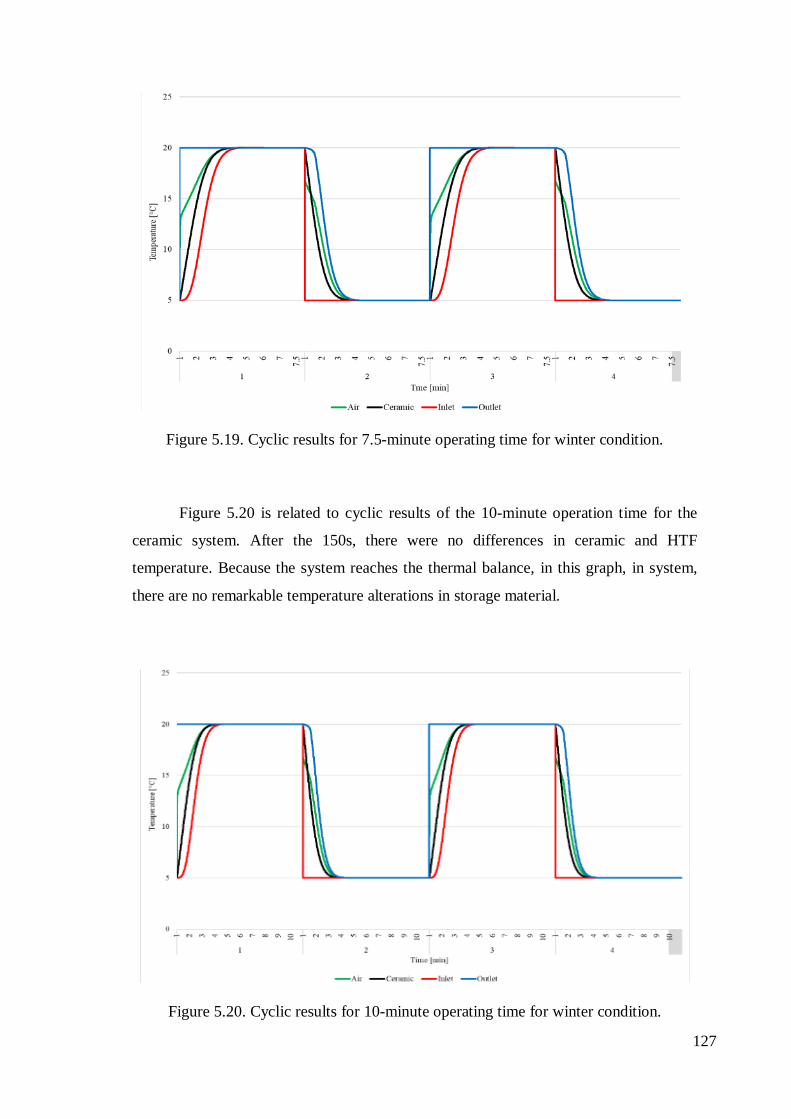
Figure 5.19. Cyclic results for 7.5-minute operating time for winter condition.

Figure 5.20 is related to cyclic results of the 10-minute operation time for the

ceramic system. After the 150s, there were no differences in ceramic and HTF

temperature. Because the system reaches the thermal balance, in this graph, in system,

there are no remarkable temperature alterations in storage material.


127

Figure 5.21 belongs to the ceramic system cycle for 7.5-minute of summer

condition. When the outdoor temperature is 34°C, the indoor environment is stable at

20°C. At the end of the cycle process, the temperature distribution inside the ceramic is

almost equal to the outdoor or the indoor temperature, depending on the airflow direction.

Figure 5.21. Cyclic results for 7.5-minute operating time for summer condition.

In figure 5.22, there are 2 cycles of 10-minute, in total 20 minutes in simulated

summer conditions, and units are operated by charging and discharging processes. The

indoor and outdoor temperatures remained constant at 20°C and 34°C, respectively. There

is a decrease in discharging increase for charging approximately 14°C in the ceramic

temperature during the 10-minute cycles.

128

Figure 5.22. Cyclic results for 10-minute operating time for summer condition.

5.2.2. Simulation Results of LHTES

In Chapter 3, the experimental setup of the system and the experiments for two

separate HRV systems are given in detail. In CFD, the duct has the same dimensions as

the experiments explained in Chapter 4. CFD is performed to investigate the heat transfer

performance and fluid flow characteristics. First, the model is primarily divided into mesh

within the Fluent program. Then, flow analysis is obtained with the ANSYS-Fluent tool.

According to the verification and validation process, the simulations are employed in this

part.

The simulated model is correlated with the experimental temperatures measured

by thermocouples. The simulation results that surface temperature increases when the

discharge current increases. As shown in related figures, the difference was observed by

operating the system for 15-minute, 20-minute, and 30-minute. It was observed that the

PCMs inside the tubes close to the outlet melted later. Figure 5.23 shows the cycle results

for the system with PCM operating in the last 2 cycles for 60 minutes. By keeping the

indoor and outdoor temperatures constant, the temperature changes of the PCMs inside

the tubes are observed. In this Figure, the inlet temperature is 34°C, and the outlet

129

temperature, which is indoor temperature, is 21°C. As can be seen in this graph, in the

exhaust mode, the PCMs inside the tubes close to the inlet reaches the outside temperature

faster and cannot reach after the 5th tube.

Figure 5.23. Cyclic results for 15-minute operating time.

Figure 5.24 represents the time-related melting and solidifying graphs for 15-

minute operating. In addition, when the PCM tube bundle is compared with the

experiments, it is seen that the PCMs inside the tubes close to the inlet are melted first.

And also, while the 1st, 2nd, 3rd, 4th, 5th tubes completely melted and, in the 6th, 7th, 8th, 9th,

and 10th tubes, complete melting is not observed. In addition, the solidification process

works have a reverse situation. The tubes that solidified first are 10th, 9th, 8th, and the

remaining tubes are not completely solidified.

130

Figure 5.24. Melting/ solidification results for 15-minute operating time.

Figure 5.25, which is created based on Figure 5.24, shows the temperature

distribution at 1.5 min., 3 min., 5 min., 7 min., 9 min., 11 min., 13, and 15 min. This figure

shows the exhaust mode for the HRV system operating for 15-minute.

Figure 5.25. Temperature change in the system for the 15-minute operating time in a

different time step.

Inlet Outlet

131

Figure 5.26, 5.27, and 5.28 belongs to the 20-minute operating time for the tube

bundle HRV system. Figure 5.26 shows the cyclic results of the tube bundle system. Here,

the outdoor environment is 34°C, the indoor environment is 21°C. And while the PCMs

in 4 tubes reached outdoor temperature, the others remained below this value. In supply

mode, only 3 tubes reached the indoor temperature. Tube-8 remained at 27°C, the melting

point of PCM. Tube-7 could only rise to 28°C. However, compared to 15-minute, it is

seen that all tubes exceed the melting temperature of 27°C after 15-minute. In supply

mode, the remaining tubes, except for 1st, 7th, 8th, 9th, and 10th, did not drop below the

melting temperature.


Unlike the results of 15-minute, PCMs in all tubes melt and solidify except for

only 2 tubes. These are Tube 7 and 8. According to supply mode, the solidification

process is not completely occurred. When the fan operates indoor to the outdoor

environment, the 8th, 9th, and 10th tubes are completely solidified. Looking at the 3rd, 4th,

5th tubes, it is seen that only half of them are solidified (Figure 5.27).

132


Figure 5.28 defines the system temperature change for 20-minute of operating

time. In this figure, 1.5 min., 3 min., 5 min., 7 min., 9 min., 11 min., 13 min., 15 min., 18-

and 20-min. results are found. The red color represents 34°C, while the blue color

represents 25°C. In the system operating in exhaust mode, almost all tubes melted in the

20th minute. Only 3 tubes are not completely melted, and the 6th 7th, and 8th tubes also

reached the melting temperature of 27°C.

133


different time step.

Figures 5.29, 5.30, and 5.31 refer to the 30-minute operating time for the tube

bundle HRV system. Figure 5.29 shows all-tube PCM in each tube melts and solidifies.

Almost all tubes reach the outdoor temperature of 34°C, and only the 7th tube remains at

30°C. The phase change temperature of 27°C is exceeded by PCM in all tubes.

Figure 5.30 presents the 30-minute operation time liquid fraction and time graph.

All PCM melted in the system. However, not all tubes solidify completely in case of

solidification. The graph shows that the 4th tube solidifies 80% while the 2nd, 3rd, and 6th

tubes solidify 90%.

Inlet Outlet

134



135

Figure 5.31 shows the temperature change of the tube bundle system at specific

times. For 30-minute, the system was observed periodically. The indicator below shows

the values of the colors. Here, blue represents 25°C which is indoor temperature, and red

represents 34°C which is the outdoor temperature. As can be seen, all the tubes reached

the outside temperature, only the internal temperature of the 7th tube could not reach 34°C

completely.


different time step

5.2.3. Data Reduction for Simulation Results

Sensible heat storage and Latent heat storage units’ thermal models for charging

and discharging characteristics have been developed with ANSYS Fluent software. The

Inlet Outlet

136

number of charging and discharging has been optimized according to experimental data.

The predicted results matched well with the data of the SHS and LHS units’ experiments.

The simulation results are summarized in Table 5.6, here air domain, PCM average

temperature, ceramic temperature, inlet, outlet temperature, and HRV materials stored

released energy results in terms of kJ. For the ceramic HRV unit 1-min., 2-min., 5-min.,

7.5-min., and 10-min. cyclic results and for tube bundle units 15-min., 20-min., and 30-

min. cyclic results have been shown.

The air energy change in the ceramic unit is given in Table 5.3 above, and the air

energy change for the tube bundle is given in Table 5.5. Table 5.6 shows the results

obtained from the simulations. Here, the energy changes in the units are shared, and there

is a difference of 1-10% on average from the experimental results.

Table 5.6. Energy changes in the units according to simulations.

Time Air_temp Ceramic_temp Inlet Outlet Ceramic (kJ) 1min 15.11 10.40 6.25 20.00 5.11 2min 16.57 13.73 9.66 20.00 10.32 5min 18.57 17.42 15.63 20.00 21.20 7.5min 19.11 18.44 17.41 20.00 30.91 10min 19.33 18.83 18.05 20.00 34.22 7.5min 32.22 32.01 34.00 28.67 16.14 10min 32.90 33.08 34.00 32.36 29.66 Air_temp PCM_temp Inlet Outlet PCM (kJ) 15min 30.67 29.45 34.00 28.90 25.94 20min 30.87 30.00 34.00 29.05 34.82 30min 31.45 30.14 34.00 30.15 41.94

Figure 5.32 represents the mean heat transfer rates of the SHTES and LHTES

HRV unit results related to Table 5.6. According to the results, the 1-minute and 2-minute

mean heat transfer rate results are very close to each other for ceramic HRV units. Also,

according to the tube bundle HRV system, 15-minute cycle and 20-minute cycle mean

heat transfer rate results are very similar. In addition to these, when the fan runs for a long

period, electrical energy cost increases. So, the fan is more advantageous when the system

operates for a short period.

137

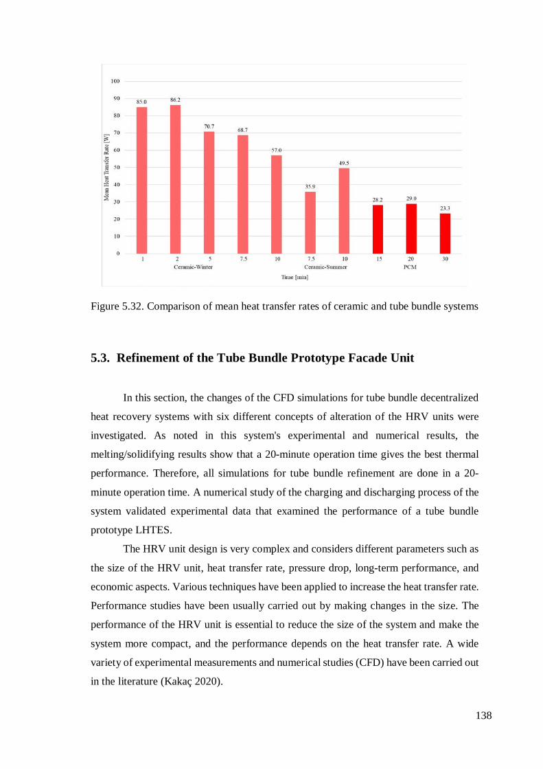
Figure 5.32. Comparison of mean heat transfer rates of ceramic and tube bundle systems

5.3. Refinement of the Tube Bundle Prototype Facade Unit

In this section, the changes of the CFD simulations for tube bundle decentralized

heat recovery systems with six different concepts of alteration of the HRV units were

investigated. As noted in this system's experimental and numerical results, the

melting/solidifying results show that a 20-minute operation time gives the best thermal

performance. Therefore, all simulations for tube bundle refinement are done in a 20-

minute operation time. A numerical study of the charging and discharging process of the

system validated experimental data that examined the performance of a tube bundle

prototype LHTES.

The HRV unit design is very complex and considers different parameters such as

the size of the HRV unit, heat transfer rate, pressure drop, long-term performance, and

economic aspects. Various techniques have been applied to increase the heat transfer rate.

Performance studies have been usually carried out by making changes in the size. The

performance of the HRV unit is essential to reduce the size of the system and make the

system more compact, and the performance depends on the heat transfer rate. A wide

variety of experimental measurements and numerical studies (CFD) have been carried out

in the literature (Kakaç 2020).

138

According to the literature, heat transfer can be enhanced with many different

modifications of the HRV unit by using a tube bundle which is the object of this thesis.

To obtain the best performance from the PCM tubes, the diameter of the tubes, pitch size

of the tubes, different PCM solidification/melting temperature, tube shape, air velocity is

studied through the CFD simulations (Figure 5.33). This model of the ANSYS-Fluent

19.0 package is used to develop the system. In this figure, the ST means transverse pitch

size, and SL means longitudinal pitch size. For the 3mm tube, the transverse pitch size has

been taken as 14 mm, and the longitudinal pitch has been changed. For 4.76 mm, both

longitudinal pitch and transverse pitch sizes have been altered. And for the tube shape,

air velocity, PCM combination, and case combination cases, the experimental setup tube

bundle system is simulated separately, as shown in Figure 5.33.

Figure 5.33. Refinement of the prototype classification.

Refinement of the prototype

(1) Tube Diameter and geometry

(1-1) 3 mm

(1-1-1) L: 14 mm, T:14 mm

(1-1-2) L: 12 mm, T:14 mm

(1-1-3) L: 10 mm, T:14 mm

(1-1-4) L: 10 mm, T:10 mm

(1-2) 4.76 mm(1-2-1) L: 16 mm, T:16 mm

(1-2-2) L: 12 mm, T:12 mm

(2) Tube Shape Oval

(3) Air Velocity

(3-1) 0.2 m/s

(3-2) 0. 5m/s

(3-3) 1 m/s

(4) PCM Combination(4-1) RT27+RT24

(4-2) RT27+RT26+RT24

(5) Case CombinationL: 12 mm, T:12 mmRT27+RT26+RT24

139

In the light of these cases, a tubular HRV unit is changed in the following studies.

Figure 5.34 shows the overview of the ventilation system with a tube bundle prototype.

The numbers represent the covers for inside (1) and for outside (2), filter (3), fan (4), and

HRV unit (5). In this decentralized ventilation unit with a heat recovery system, different

simulations were made by changing the tube bundle dimensions [case (1)], changing the

shapes of the tubes [case (2)], changing the fan speed [case (3)], and changing the PCM

material used [case (4 and 5)].

Figure 5.34. Overview of the tube bundle heat recovery system.

5.3.1. The prototype of the decentralized HRV system with PCM

The experimental studies of the HRV unit, introduced in Chapter 3, have 10 by 10

rows and consist of 100 copper staggered tubes filled with PCM, and this system is

investigated under defined simulation conditions in this subsection. This tube bundle unit

occupied with PCM acts as an HRV unit made up of copper tubes. This prototype consists

of 100 copper staggered tubes filled with PCM at the airflow direction. The units’ outer

diameter is 4.76 mm. The tube arrangement in the bundle is designed as 1.4 cm for the

transverse pitch and 1.4 cm for the longitudinal pitch. The prototype measured the

diagonal pitch between tube centers as 1.565 cm in the prototype.

140

Figure 5.35 present the schematic diagram of the plan of the tube bundle system.

The air is taken from outside (inlet), passes through the tubes and reaches the indoor

environment (outlet).

Figure 5.35. The prototype tube bundle system geometry.

This computational domain is given in Figure 5.35, with boundary and initial

conditions are used in numerical modeling. The physical boundaries for this domain,

inlet, outlet, symmetry, and wall. In this case, temperature and velocity are fixed values

at the inlet and the outlet's reverse situation. In Figure 5.35, each row has 1 or 2 full tubes.

Half tubes are alternately placed along the top and bottom walls of the test model to

simulate an infinite tube bundle and reduce the wall boundary layer. The coordinate

system and important geometrical parameters are also shown in this figure. The origin of

the coordinate system is determined at the center of the row's middle tube. The transverse

and longitudinal directions are denoted by x and y, respectively. The direction pointing

out is given to the z-axis, which is not displayed. The 2D modeling of the computational

domain has been performed in ANSYS FLUENT 19.0. CFD programs generate solutions

that apply to different elements of the flow for partial differential equations. The

equations characterize the fluid flow with pressure, temperature, density, and velocities.

The geometry that may be utilized for flow analysis must be created and imported before

CFD tools can process it. The geometric model covers the overall system design and the

other equipment. The geometry is initially created in 2D in the ANSYS program's

"Design Modeler" tool. The important thing for utilizing 2D modeling to analyze the

research is that the system flow geometry can be followed more precisely, producing the

best convergence results. Furthermore, by monitoring the change in units to time-

dependent, this 2D model determines temperature distribution and flow profiles, and

pressure drops for various operating conditions are studied.

Inlet

Outlet (0,0)

1.4 cm

1.565 cm 1.4 cm

d

ST

SL 4.76 mm

Symmetry

Symmetry

141

Indoor and outdoor temperatures have been kept constant, and the indoor

temperature is 21°C, and the outdoor temperature is 34°C. According to the

melting/solidifying findings for the tube bundle system, 20-minute of operating time

provides the optimum thermal performance for maintaining a comfortable indoor

temperature with the least amount of energy consumption according to the storage rate.

For this reason, 20-minute was taken as a reference for subsequent simulations.

According to most of the earlier experimental and numerical studies on flows in

the tube bundles, focused on making changes in the dimensions of the tubes, the shape of

the tubes, the system inlet air velocity, the PCM combinations used in the system. In the

present study, the impact of the changes in the system is simulated and modeled, and the

results are shared in this section.

5.3.2. (1) The Alteration of Tube Diameter and Geometry

Many studies have been done in the literature by changing tube sizes and pitch

sizes, and according to these studies, the tube bundle has been simulated by making

changes in the system 1, 3, 5, 6, and 7 are studied pitch ratios. Also, 1, 2, 3, and 4 are

analyzed by changing the tube arrangement. Besides these, 1, 2, 3, 4, and 6 are worked

numerically. 3rd and 7th studies set up the experimental setup for the tube bundle.

1 Erguvan and Macphee (2019) researched the energy and exergy analysis for tube

banks. The CFD simulations are analyzed the different numbers of inline tubes, inlet

velocity, pitch ratios. It was found that energy efficiency decreased with increasing pitch

ratios. And increasing the number of inline tubes increased the energy efficiency because

of high convective heat transfer.

2 Park et al. (2020) analyzed eight different tube arrays. The melting

characteristics, energy density, liquid fraction and temperature distributions, heat transfer

rate, and melting time are analyzed. The number of tubes affects the melting rate and the

energy density. And also, the tube arrangements affect the required melting time.

3 Sakhaei et al. (2020) examined the effects of tube arrangement and pitch on the

performance of a single-row tube bundle. This bundle arranges three different schemas,

which are flat, inclined A, and V frames are investigated. Flat bundles showed greater

pressure drops of up to 60% and heat transfer rates of 30% than their inclined

counterparts.

142

4 Mahant et al. (2013) simulated flow performance with tube bundle, and the

pressure drop of tube bundles with 30, 45, and 60° arrays are analyzed with ANSYS-

Fluent. The results show that the pressure drop of the 60° array is less than at 45°.

5 Gugulothu et al. (2017) reviewed heat transfer enhancement techniques of heat

exchangers. This research paper is to study the enhancement of heat transfer using passive

techniques like Reynolds number, Nusselt number, friction factor, pitch ratio, pressure

drop, and sizing, etc. in 6 Kongkaitpaiboon et al. (2010) study examined the pitch ratio

and found that the heat transfer rate increases with the decreasing pitch ratio. 7 Bas and

Ozceyhan (2012) experimented with twist ratios and clearance ratios. They investigated

that heat transfer enhancement is greater for lower clearance ratio and lower twist ratio.

After the literature review, the heat transfer enhancement during charging and

discharging of PCM is numerically analyzed according to the above studies. The tube

diameter alteration parameters, size of the HRV unit, the boundary conditions, and the

initial and final conditions of these cases are kept the same for performance comparison.

At the starting of the charging, the PCM is considered a solid phase with a value of the

liquid fraction of 0.00 at a temperature of indoor temperature, which is 21°C. On the other

hand, liquid PCM will release thermal energy in discharge. In this case, the outer diameter

is 3 mm. The tube arrangement in the bundle is designed as three different transverse

pitches and longitudinal pitches. And then, for the 4.76 mm tube, the tube arrangement is

changed as a 16 mm and 12 mm pitch size.

5.3.2.1. (1-1) 3mm Tube Diameter

In this tube bundle arrangement, the tubes in the system are replaced with tubes

with a diameter of 3 mm. Four different pitch sizes are simulated with these 3 mm tubes,

and the results are explained separately below.

The simulation results, which have been processed under subheadings, are given

below, and the evaluation has been made according to the changed dimensions.

5.3.2.1.1. (1-1-1) 14mm Longitudinal and 14mm Transverse Pitches

The 3 mm diameter tubes are arranged 14 mm for the transverse pitch and

longitudinal pitches. Figure 5.36 shows the 3 mm diameter tube bundle system. In this

143

arrangement, only the diameters of the tubes have changed, and the tubes that were

previously 4.76 mm are 3 mm in this arrangement. However, the layout in Figure 5.36

remained the same as the pitch sizes experimental prototype.

Figure 5.36. 14 mm for the transverse and longitudinal pitches 3 mm tube diameter

system cross-section.

Figures 5.37 and 5.38 illustrate the contours of temperature changes and liquid

fraction of PCM for 20-minute of operation time starting melting. In this system, there

are 100 tubes. The effect of pitch size and tube diameter on heat transfer enhancements

of PCM varies with the distance between the tube arrays. Figure 5.37 shows the results

of the temperature of tubes and inlet and outlet temperature. When looking at the 20-

minute results, all PCMs are reached outdoor temperature, which is 34°C.

Figure 5.37. Cyclic results for ∅3 mm tube with 14 mm longitudinal, 14 mm transverse

pitches.

Inlet

Outlet

ST

SL/2

d

1.4 cm 0.7 cm

3 mm

144

Figure 5.38 illustrates the melting/ solidification of a 3 mm tube with a 14 mm

pitch size of the prototype. Initially, the domain is fully occupied by the solid PCM,

therefore, the value of the liquid fraction is zero (0.00), and this value increases as the

charging time and decreases as the discharging time and becomes one (1.00) when the

PCM is completely melted. All PCMs in the systems are completely melted; however,

tube 4 is not completely solidified for 20-minute of operation time.

Figure 5.38. Melting/ solidification results for ∅3 mm tube with 14 mm longitudinal, 14

mm transverse pitches.

5.3.2.1.2. (1-1-2) 12 mm Longitudinal and 14 mm Transverse Pitches

The tube pitch size is 12 mm for 3 mm tube diameter in this arrangement. In this

configuration, in the HRV unit, there are 120 tubes. And in one row, there are 6 tubes.

Figure 5.39 shows the arrangement of the 3 mm tube. It shows the arrangement designed

for the 3 mm tube. Here, unlike the above case, the tubes are multiplied by tightening the

space between the tubes. And as seen in the figure, there are 12 tubes in a row in the flow

direction.

145



Initially, all PCMs are at 21°C in the solid phase. In 20-minute operation time, all

PCMs are reached 34°C. In discharging process, the PCM inside the tubes acts as a heat

source to melt the solid PCM. Figure 5.40 shows the contours of the temperature of tubes

which increases and decreases. As a result, the solidifying process is not completely done

after one cycle. PCM-5 and PCM-6 are not completely solidified.


pitches.

Outlet

Inlet ST

SL/2

d

1.2 cm 0.7 cm 3 mm

146

The contours are shown in Figure 5.41, phase change from solid to liquid and

liquid to the solid phase of PCM. It has been found that the value of liquid fraction at

system becomes done (1.00) before 20-minute. The amount of PCM to be melted and

solidified within an allowable time. But charging time and discharging time are different

from each other. Charging time is shorter than discharging time in this arrangement. As

a result, the 15 min. and 17 min. the liquid fraction became almost one for this case but

solidifying process, all PCMs inside the tubes are not fully solidified.




With this arrangement, there are 140 tubes. In these cases, there are 14 rows of

tubes in the streamwise airflow direction and 10 tubes per row in y, which is the spanwise

direction. The longitudinal tube pitch (ST) is 1 cm, and the transverse pitch size is (SL) 1.4

cm. In Figure 5.42, the computational domain is taken as SL/2 because of the geometric

symmetry of the tube bundle HRV system.

147


system cross-section

In Figure 5.43, phase change takes place over a temperature interval. The phase

change temperatures 27°C. Inlet air temperature is 34°C, and the indoor air temperature

is 21°C. The temperature profile of each PCM node during 20-minute in the solidification

and melting process is shown in Figures 5.43 and 5.44.


pitches.

The transient evolution of the PCM liquid-fraction profiles and the average

temperature profiles are illustrated in Figure 5.44. It can be realized that all PCMs in the

system are melted and solidified except the 6th tube. According to Figure 5.44, the best

melting rate is that the PCM completes the melting before 20-minute.

Outlet

Inlet ST

SL/2 d

1 cm 0.7 cm 3 mm

148




In this case, there are 10 mm longitudinal and 10 mm transverse pitch sizes and a

total of 3 mm diameter 196 tubes. Figure 5.45 shows the 10 mm-by-10 mm pitches size

case for the tube bundle HRV system. The figure also shows the inlet and outlet of the

model. In this case, SL/2 is 0.5 cm.



Outlet

Inlet ST

SL/2 d

1 cm 0.5 cm 3 mm

149

As in all simulations, in this case, the charging and discharging cycles of the

system are simulated with 20-minute cycles. As seen in Figure 5.46, the temperature

distribution of the thermocouples in 14 tubes can be seen. While the 14th tube reaches a

maximum of 29°C, the 10 tubes of the system reach the outdoor temperature completely.

Figure 5.46. Cyclic results for ∅3 mm tube with 10 mm longitudinal and 10 mm

transverse pitches.


minute operating. In addition, all PCM inside the tubes except the 11th and 12th tubes are

completely melted. And the solidification process works have a reverse situation. The

first solidified tubes were those close to the outlet. While the system is operating from

indoor to outdoor environment, in supply mode since the measured air velocity in the

experiments is less than the exhaust mode, there is no reaching the environment

temperature as much as in the exhaust direction. However, the 5 tubes completely solidify

and reach the indoor temperature in supply mode.

150

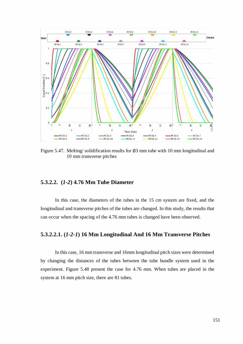
Figure 5.47. Melting/ solidification results for ∅3 mm tube with 10 mm longitudinal and

10 mm transverse pitches

5.3.2.2. (1-2) 4.76 Mm Tube Diameter

In this case, the diameters of the tubes in the 15 cm system are fixed, and the

longitudinal and transverse pitches of the tubes are changed. In this study, the results that

can occur when the spacing of the 4.76 mm tubes is changed have been observed.

5.3.2.2.1. (1-2-1) 16 Mm Longitudinal And 16 Mm Transverse Pitches

In this case, 16 mm transverse and 16mm longitudinal pitch sizes were determined

by changing the distances of the tubes between the tube bundle system used in the

experiment. Figure 5.48 present the case for 4.76 mm. When tubes are placed in the

system at 16 mm pitch size, there are 81 tubes.

151

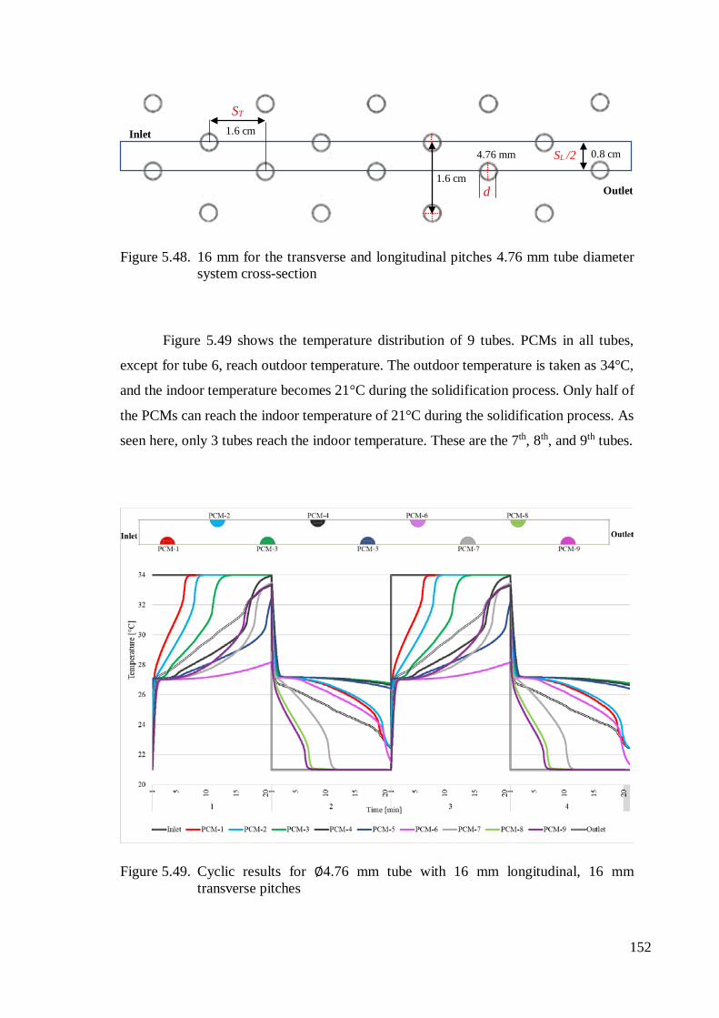
Figure 5.48. 16 mm for the transverse and longitudinal pitches 4.76 mm tube diameter

system cross-section

Figure 5.49 shows the temperature distribution of 9 tubes. PCMs in all tubes,

except for tube 6, reach outdoor temperature. The outdoor temperature is taken as 34°C,

and the indoor temperature becomes 21°C during the solidification process. Only half of

the PCMs can reach the indoor temperature of 21°C during the solidification process. As

seen here, only 3 tubes reach the indoor temperature. These are the 7th, 8th, and 9th tubes.


transverse pitches

Inlet

Outlet

SL /2

d

0.8 cm

1.6 cm

ST

4.76 mm

1.6 cm

152

In Figure 5.50, the liquid fraction “f L” can be evaluated on each tube to monitor

the evaluation of the changing phase in the PCM enclosure. This figure gives the

evaluation of the solid domain in 20-minute of operation time. The melting process begins

from 1st to 9th except for the 6th tube. The solidification at the outlet shows the fastest rate.

The rate of solidification 2nd, 3rd, and 4th rows is approximately 0.4. Only 60% of these

tubes solidified.

Figure 5.50. Melting/ solidification results for ∅4.76 mm tube with 16 mm longitudinal,

16 mm transverse pitches.


In this case, the tubes have 12 mm longitudinal and 12 mm transverse pitches. The

tubes diameter is 4.76 mm, and there are 144 tubes in the system. The arrangement of

tubes for this case is present in Figure 5.51. In this case, the spacing between the tubes

has decreased, and there are 12 tubes in each row, as seen in the domain.

153

Figure 5.51. 12 mm for the transverse and longitudinal pitches 4.76 mm tube diameter


Figures 5.52 and 5.53 belong to 20-minute operating time for the tube bundle

HRV system. Here, the outdoor environment is 34°C, the indoor environment is 21°C.

And while the PCMs in 7 tubes reached outdoor temperature, the others remained below

this value. In supply mode, only 4 tubes fully reached the indoor temperature.


transverse pitches.

Figure 5.53 shows the liquid fraction distribution of this system over time. In this

figure, the charging and discharging process take 20-minute cycles. In general, 100%

Outlet

Inlet

ST

SL /2 d

1.2 cm 0.6 cm 4.76 mm

154

melting is seen, while the 9th PCM melts at 60%, the PCM inside the 8th tube melts at

85%, the 10th, 11th, and 12th tube melts at 95%. HTF receives the heat from the charged

PCM tubes resulting in the decrease of the PCM tubes temperature and increase of HTF

temperature along with the system.

Figure 5.53. Melting/ solidification results for ∅4.76 mm tube with 12 mm longitudinal,

12 mm transverse pitches

5.3.3. (2) The Alteration of Tube Shape: Oval Tubes

There are several experimental and numerical studies available for oval tube shape

as an alternative for round tube in the literature.

Myong et al. (2021) tested generic heat exchangers having oval tubes and round

tubes for comparison. According to the findings of this research, the oval tube samples

with a smaller diameter tube had the highest performance. Furthermore, the oval tube

samples with a larger diameter tube had relatively low performance due to the significant

pressure drops.

Li et al. (2018) studied experimentally heat transfer and pressure drop of the

twisted oval tube bundle in crossflow with the staggered layout. The result is that the

155

performance of this twisted oval tube bundle is larger than that of the round tube bundle

with the same layout. Also, the twisted oval tube bundle has an advantage in airside

convection heat transfer over the round tube bundle with the same arrangement in

crossflow.

Khan, Zou and You (2021) investigated the oval tube bundle with CFD. This study

shows that the oval tube bundle provides better heat transfer enhancement with higher

pressure drop than the traditional round tube.

Kim et al. (2014) investigated experimentally oval tubes and round tubes under

wet and dry conditions. The experiments were conducted on sine wave fin and tube heat

exchangers. According to the result of this paper, the heat transfer coefficients of oval

tube samples are lower than the heat transfer coefficients of round tube samples. Oval

tube pressure drops, on the other hand, are even smaller than round tube pressure drops.

Tan et al. (2013) investigated experimentally improving the heat transfer

coefficient and decreasing the pressure drop with the twisted oval tube heat exchanger

system. This study shows that the heat transfer coefficient of the twisted oval tube heat

exchanger is higher, and the pressure drop is lower than the rod baffle heat exchanger.

And the overall performance of the twisted oval tube Works more effectively at a low

tube side flow rate and high shell-side flow rate.

According to these papers, in this case, the effect of the tube shape on the melting

and solidifying process of PCM is presented. The charging-discharging process is

observed by operating the system for 20-minute with oval copper tube bundles, which are

confirmed to provide better heat transfer than the cylindrical copper tube. Figure 5.54

shows the oval tubes are the smallest copper tubes available in the market and which

major axis is 4.5mm minor axis is 3mm. In this case, there are 100 tubes in the system.

Figure 5.54. 14 mm for the transverse and longitudinal pitches 4.5 mm (major axis) tube

diameter system cross-section

Outlet

Inlet ST

SL /2

d

1.4 cm 0.7 cm 4.5 mm

156

In this case, the charging and discharging efficiency are observed in Figures 5.55

and 5.56. When using oval tubes, the 5 tubes are completely melted in the charging

process.

Figure 5.55. Cyclic results for ∅4.5 mm (major axis) oval tube.

Figure 5.57 shows the melting and solidification process of the oval tube case for

the HRV system. The oval profile is found to be effective for the melting process except

for the 8th and 7th tubes. While 80% of the 8th tube melts, 90% of the 7th tube melts.

Looking at the solidification process, only 40% of the 3rd tube, 60% of the 2nd and 4th

tube, and 80% of the 6th and 7th tubes solidify.

157

Figure 5.56. Melting/ solidification results for ∅4.5 mm (major axis) oval tube.

5.3.4. (3) Analysis of Changes of Air Velocity

The authors discovered that higher fluid velocity results in higher heat transfer,

reducing associated irreversibility. Many researchers are interested in the performance of

circular tube bundles and finned tube bundles.

Jang and Yang (1998) studied experimental and numeric ways for different values

of inlet velocity ranging from 2 to 7 m/s. This paper showed that the average heat transfer

coefficient of elliptic finned tubes is 35-50% of the corresponding circular finned tube

having the same tube perimeter, while the pressure drop for elliptic finned-tube banks is

only 25-30% of the circular finned-tube bank configuration.

Taufiq et al. (2007) present a second law analysis for the optimal geometry of fin

array by forced convection. It has been shown that increasing the crossflow fluid velocity

improves the heat transfer rate and reduces the irreversibility of heat transfer.

Erguvan and MacPhee (2019) investigated transient crossflow tube banks' first

and second law efficiencies. The model was performed numerically. Because the

thermophysical characteristics of the fluid are mostly dependent on the mean temperature,

the inlet temperature of HTF was shown to have the highest effect on overall efficiency

158

in this study. In addition, because it depends on density and viscosity, the HTF's velocity

varies as the temperature changes.

Jeebori (2008) studied to find the best tubes design regarding entropy generation.

This study analyzes the effect of tube diameter, tube length, and pitch ratios. And the

result showed that the higher air velocities and larger dimensionless pitch ratios improve

the system performance. And small tube diameter is better performance for compact tube

banks.

Most of the aforementioned studies focus on heat transfer, pressure drop, and flow

velocity. To increase the system's overall performance, the authors optimized their design

and increased or decreased some parameters like flow velocity. It was observed here that

the system's performance increases with the increase of flow velocity. So, according to

the literature, 0.2 m/s, 0.5 m/s, and 1 m/s case are simulated and compared in this part.

To see the difference here, the inlet velocity changes on the setup used in the experiment.

According to the air velocity measurements mentioned in Chapter 3, the average velocity

for supply air is 0.34 m/s, and the average for exhaust air is 0.28 m/s.

5.3.4.1. (3-1) 0.2 m/s

The first case is the 0.2 m/s for supply air and exhaust air. Figure 5.57 illustrates

the temperature distribution of tubes and inlet temperature of 34°C and outlet temperature

of 21°C. It is obvious from the figures that there is a difference in the temperature of the

tubes. The difference can be seen clearly in Figures 5.57 and 5.58. As can be seen, only

the 1st, 2nd, 3rd, 4th tubes reach the outdoor temperature of 34°C, while the 5th tube reaches

32°C and the remaining tubes reach 27-28°C. In the case of exhaust, the 7th 8th 9th and

10th tubes have reached the indoor temperature.

Figure 5.58 shows the liquid fraction distribution of this system, and the charging

and discharging process take 20-minute cycles. In general, 100% melting is seen in 1st 2nd

3rd 4th, and 5th while the 9th PCM melts at 80%, the PCM inside the 6th 8th, and 10th tube

melts at 75%, the 7th tube melts at 50%.

159

Figure 5.57. Cyclic results for ∅4.76 mm tube with 0.2 m/s.

Figure 5.58. Melting/ solidification results for ∅4.76 mm tube with 0.2 m/s.

160

5.3.4.2. (3-2) 0.5 m/s

Figures 5.59 and 5.60 show the simulation results of 0.5 m/s inlet and outlet fluid

velocities. This figure represents the PCM melting interfaces by 10 tubes with lines. And

two of them are inlet and outlet temperature as constant. In Figure 5.59, almost all tubes

reached outdoor temperature, only the 7th and 9th tubes remained at 29°C. 0.5 m/s is not

enough in 20-minute for the whole system to reach the inlet or outlet temperature in

supply/exhaust mode. With an increase in the heat transfer fluid velocity, the amount of

energy stored in the LHTES in a system, and hence the amount of PCM melted, increases.

As expected, there is more heat transferred to the tubes found closer to the inlet in supply

mode.

Figure 5.59. Cyclic results for ∅4.76 mm tube with 0.5 m/s.

Figure 5.60 shows the liquid fraction of PCM at a different time step. In this figure,

the region of liquid fraction between 0 and 1 indicates the solid-liquid interface region. 0

means solid, 1 is liquid. The solid-liquid interface differs due to air velocity inside the

161

system. The melting process is seen in every tube except the 7th and 9th tubes. The inlet

part of the tube bundle system starts to melt rapidly.

Figure 5.60. Melting/ solidification results for ∅4.76 mm tube with 0.5 m/s.

5.3.4.3. (3-3) 1 m/s

In this model, the velocity of air, both inlet and outlet, are changed. The fluid

velocity value is 1 m/s. The melting and solidification time and the temperature

distribution of these simulations are shown in Figure 5.61 and Figure 5.62. Looking at

Figure 5.61, it is seen that the PCM in all the tubes reaches the outdoor temperature within

the specified period and reaches 21°C, which is determined as the indoor temperature in

exhaust mode. It can be noticed that the temperature rise of the PCM is rapid first 10

minutes due to the high driving force for conduction and discharging curve becomes flat

as time progresses after the 10 minutes. HTF receives the heat from the charged PCM.

162

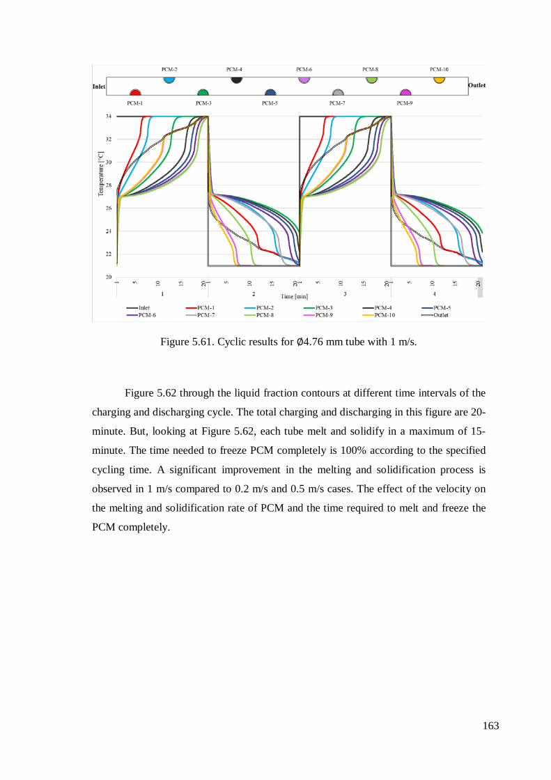
Figure 5.61. Cyclic results for ∅4.76 mm tube with 1 m/s.

Figure 5.62 through the liquid fraction contours at different time intervals of the

charging and discharging cycle. The total charging and discharging in this figure are 20-

minute. But, looking at Figure 5.62, each tube melt and solidify in a maximum of 15-

minute. The time needed to freeze PCM completely is 100% according to the specified

cycling time. A significant improvement in the melting and solidification process is

observed in 1 m/s compared to 0.2 m/s and 0.5 m/s cases. The effect of the velocity on

the melting and solidification rate of PCM and the time required to melt and freeze the

PCM completely.

163

Figure 5.62. Melting/ solidification results for ∅4.76 mm tube with 1 m/s.

5.3.5. (4) Combination of PCM at Different Melting Temperatures

According to research, the multi-PCM design improves the dynamic performance

of the LHTES by increasing the charging and discharging rate.

Elsanusi and Nsofor (2021) investigated different arrangements of the multiple

PCMs' performances of heat exchangers. As a result, natural convection has a positive

effect on heat transfer. The parallel arrangement enhances conduction and, in multiple

PCMs, reduces complete melting time compared with the single PCM arrangement.

Talukdar et al. (2019) evaluated the solidification /melting behavior of the LHTES

solar cold storage unit with the CFD model. With this model, the numerical analysis of

charging /discharging of PCM is analyzed for PCM pack thickness and evaporator

arrangements. PCM pack sizes are 100 cm x 76 cm x (4.5 cm to 7 cm) and evaporator

arrangement of 0, 5, 8, 10 and 12 aluminum fins. The 6.5 cm thick pack with 12 aluminum

fins gives the best charging/discharging time.

Aldoss and Rahman (2014) investigated the TES using spherical capsules filled

with PCMs of the different melting points at different sections along the bed. Single-PCM

design and multi-PCM design of two and three phases are investigated. The results show

164

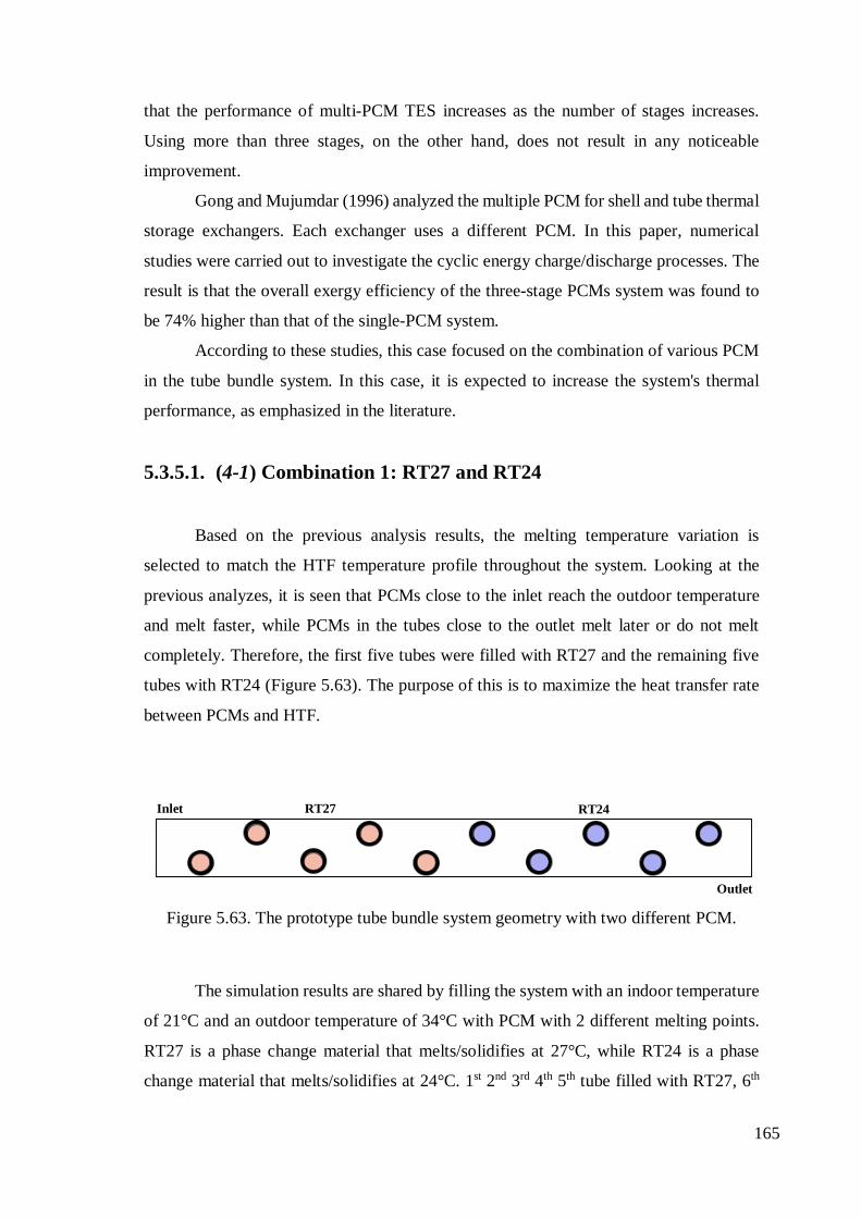
that the performance of multi-PCM TES increases as the number of stages increases.

Using more than three stages, on the other hand, does not result in any noticeable

improvement.

Gong and Mujumdar (1996) analyzed the multiple PCM for shell and tube thermal

storage exchangers. Each exchanger uses a different PCM. In this paper, numerical

studies were carried out to investigate the cyclic energy charge/discharge processes. The

result is that the overall exergy efficiency of the three-stage PCMs system was found to

be 74% higher than that of the single-PCM system.

According to these studies, this case focused on the combination of various PCM

in the tube bundle system. In this case, it is expected to increase the system's thermal

performance, as emphasized in the literature.

5.3.5.1. (4-1) Combination 1: RT27 and RT24

Based on the previous analysis results, the melting temperature variation is

selected to match the HTF temperature profile throughout the system. Looking at the

previous analyzes, it is seen that PCMs close to the inlet reach the outdoor temperature

and melt faster, while PCMs in the tubes close to the outlet melt later or do not melt

completely. Therefore, the first five tubes were filled with RT27 and the remaining five

tubes with RT24 (Figure 5.63). The purpose of this is to maximize the heat transfer rate

between PCMs and HTF.

Figure 5.63. The prototype tube bundle system geometry with two different PCM.

The simulation results are shared by filling the system with an indoor temperature

of 21°C and an outdoor temperature of 34°C with PCM with 2 different melting points.

RT27 is a phase change material that melts/solidifies at 27°C, while RT24 is a phase

change material that melts/solidifies at 24°C. 1st 2nd 3rd 4th 5th tube filled with RT27, 6th

Outlet

Inlet RT27 RT24

165

7th 8th 9th and 10th tubes filled with RT24. All tubes melt in the charging process and reach

the outdoor temperature. However, Figure 5.64 shows that the tubes filled with RT24 do

not reach the indoor temperature during the discharging process.

Figure 5.64. Cyclic results for ∅4.76 mm tube with the combination of RT27 and RT24.

Figure 5.65 shows the melting fraction versus time of the PCM during the

charging period (melting) and discharging period (solidification). As seen here, PCMs

filled with RT27 melt and solidified at full capacity, while tubes filled with RT24 operate

at 60% capacity. During the charging period, all tubes melt in the first 10-minute except

PCM-4 and PCM-5 tubes.

166

Figure 5.65. Melting/ solidification results for ∅4.76 mm tube with the combination of

RT27 and RT24

5.3.5.2. (4-2) Combination 2: RT27, RT26, and RT24

In this case, looking at the simulation results with RT27 and RT24, it is seen that

especially PCM-4 and PCM-5 melt and solidify later. For this reason, faster melting and

solidification are expected in the system by filling the 4th tube and 5th tube with RT26.

The 1st 2nd 3rd tubes will be filled with RT27, while the 4th and 5th RT26 will be simulated

by filling the remaining tubes with RT24 (Figure 5.66). Tubes are the same as the

measurements used in the experiment. The diameter of the tubes is 4.76 mm. And the

longitudinal and transverse pitches size is 14 mm.

Figure 5.66. The prototype tube bundle system geometry with three different PCM.

Outlet

Inlet RT27 RT24 RT26

167

Figure 5.67 shows the temperature distribution for 10 tubes. It is seen that all tubes

melt in the charging process. In addition, the curve continues until it changes phase

according to the melting temperatures of the PCMs in the tubes and reaches the outdoor

temperature. In the discharging process, there are 3 different solidification points.

Figure 5.67. Cyclic results for ∅4.76 mm tube with the combination of RT27, RT26, and

RT24.

Figure 5.68 shows the melting solidification process for 10 tubes. It is seen that

all the tubes melt in the charging process. Especially the shortening of the charging period

is an important difference according to the other PCM combination case. It is seen that

the tubes in the whole system melt in just 10-minute. PCM-6 solidifies 40% of the

discharging process, 3rd 4th 5th 7th tubes 60%, the remaining PCM-1, PCM-2, PCM-8,

PCM-9, and PCM-10 100% solidify.

168


RT27, RT26, and RT24.

5.3.6. (5) The Case Combination with different PCM and Pitch Size

This simulation study, it is aimed to see the results by combining two different

cases. The combination of the case with 3 different PCMs where faster melting and

solidification is seen and the combination of 12 mm longitudinal and 12 mm transverse

pitch size cases in a 4.76 mm tube is simulated. The first 6 tubes are filled with RT27, the

next two with RT26, and the last 4 tubes near the outlet with RT24. In this case, the first

six tubes were filled with RT27, the next two with RT26, and the last four tubes near the

outlet with RT24 (Figure 5.69).

Figure 5.69. The prototype tube bundle system geometry with three different PCM with 12 mm longitudinal, 12 mm transverse pitches.

Outlet

Inlet RT27 RT24 RT26

169

It is seen in Figure 5.70 that when 3 different PCMs with 3 different melting points

are used in the system, all tubes reach the outdoor temperature in the charging process,

which is 34°C. However, in the discharging process, the tubes cannot reach 21°C, which

is the indoor temperature, except for tubes 10, 11, and 12. The 1st and 9th tubes drop to

23°C, the 7th and 8th tubes drop to 26°C, and the remaining tubes to 27°C.

Figure 5.70. Cyclic results for ∅4.76 mm tube with the combination of RT27, RT26, and

RT24 with 12 mm longitudinal, 12 mm transverse pitches.

Figure 5.71 shows the simulation results when the system, consisting of tubes with

a diameter of 4.76 mm and has a 12 mm longitudinal 12 mm transverse pitch size, is filled

with 3 different PCMs. Tube-1 and tube-2 melt within the first minutes. Then the PCM

in the 3rd tube changes phase. The 3rd tube is followed by PCM-10, 11, and 12. After the

10th minute, the 4th tube, 9th tube, 7th 5th 8th, and 6th tube melt, respectively. In exhaust

mode, while 100% of the 10th 11th, and 12th tubes solidify, the 2nd tube, 1st tube 8th tube,

9th tube 7th tube 6th tube 5th tube 4th tube, and finally 3rd tube solidify respectively.

170


RT27, RT26, and RT24 with 12 mm longitudinal, 12 mm transverse pitches

5.3.7. Cross Analysis of the Tube Bundle Unit

During the liquid to solid or solid to liquid phase changes in the PCM, latent heat

hsf (kJ/kg) is stored/released per unit mass are different from each other. While RT27

heat of fusion is 184 kJ/kg, RT26’s heat storage capacity is 180 kJ/kg, and RT24 is 160

kJ/kg. So, all calculations are the result of the entire system. Calculated according to the

PCM mass in all the tubes in the system.

Table 5.7 shows the results of the cases calculation results of energy

stored/released, and also the other important parameter for the HRV unit is pressure drop.

In all cases, the operating time is 20-minute. And all cases are operated simultaneously

in summer conditions. It was determined as the indoor environment (21°C) and outdoor

environment (34°C) in exhaust and supply mode. In the first study, 4 different pitch sizes

(Case 1) are investigated on a 3 mm diameter tube. It is calculated that the heat transfer

increase is greater in the 4th simulation with a lower pitch size. When the tube shape is

changed (Case 2), it appears to be a promising technique for heat transfer enhancement

compared to conventional cylindrical tubes. In the experiments, the measured velocity

171

value is 0.34m/s from the inlet, 0.28 m/s from the outlet. So, in Case 3, the air velocity

value has changed both inlet and outlet. As velocity increases, heat transfer increases. In

Case 4 and 5, that can be seen the series arrangement compared to the single PCM

enhances the solidification and melting performance. As seen in the 5th simulation, the

heat transfer increases or decreases in direct proportion to the PCM mass in the system.

According to these results, the values of exhaust and supply, unlike the

experiments, are the same (or very close); It is related to the fact that the fan has the same

performance in both directions in the simulations. The HTC increases as the inlet velocity

increases due to the increased convective effect and turbulence. (Swain and Das 2016) In

addition to this result, as seen in the parametric velocity values in Table 5.7, the parameter

that has the most effect on energy storage is the change in velocity. In this table, the

comparison of the airside pressure drops of 14 simulations made on five different cases

is also available in Table 5.7.

Table 5.7. Total heat capacity of the units for all cases.

Cases Exhaust (kJ)

Supply (kJ)

Pressure Drop (Pa)

(1) Tube Diameter

(1-1) (3mm)

(1-1-1) L: 14 mm, T:14 mm 19.71 19.68 10.75 (1-1-2) L: 12 mm, T:14 mm 25.06 25.06 29.40 (1-1-3) L: 10 mm, T:14 mm 27.70 27.71 27.43 (1-1-4) L: 10 mm, T:10 mm 34.53 34.51 25.97

(1-2) (4.76 mm)

(1-2-1) L: 16 mm, T:16 mm 32.80 32.81 22.41 (P) L: 14mm, T:14mm 34.80 34.82 34.35 (1-2-2) L: 12 mm, T:12 mm 45.77 45.77 38.40

(2) Tube Shape Oval 30.26 30.26 16.61

(3) Air Velocity (3-1) 0.2 m/s 30.50 30.50 17.27 (3-2) 0.5 m/s 40.48 40.40 40.65 (3-3) 1 m/s 48.81 48.81 80.72

(4) PCM Combination

(4-1) (L: 14 mm, T:14 mm) + RT27+RT24 25.21 25.21 34.41

(4-2) (L: 14 mm, T:14 mm) + RT27+RT26+RT24 28.60 28.60 34.39

(5) Case Combination (L: 12 mm, T:12 mm) + (RT27+RT26+RT24) 37.9 37.9 38.41

*P: Prototype results

172

5.4. Simulations of Prototype Using Different Climatic Data

The tube bundle prototype produced within the scope of this thesis is analyzed the

energy performance in three different climatic conditions aimed to guide the designer in

selecting the wall integrated ventilation system in different climates. The heat recovery

system operated based on the monthly average daily temperature in 20-minute cycles with

the same inlet and outlet velocity. Erzurum is selected as the pilot city for the continental

climate, İzmir is selected as the pilot city for the mild climate, and Singapore is selected

as the pilot city for the tropical climate. In this section, the tube bundle is briefly

summarized, then the climate choices and analyses on the 3 selected cities are detailed.

5.4.1. Tube bundle prototype

The height of the one tube is 15 cm, and the tube's outer diameter is 4.76 mm.

Also, these tube bundle transverse and longitudinal pitch is 1.4 cm. The diagonal pitch

size is 1.565 cm in these simulations. As seen in Figure 5.72, there are physical boundaries

between inlet and outlet. The inlet side is the outdoor environment, and the outlet side

represents the indoor environment. The inlet velocity is defined as 0.34 m/s, and the outlet

velocity from the outlet is 0.28 m/s. All simulations are solved in a 2D plane. To ensure

that the predicted temperature changes are not affected by the initial conditions, the

analysis has been analyzed for at least 27 hours. All results are for 24 hours a day.

Figure 5.72. Plan of the tube bundle prototype for climate simulations.

Inlet

Outlet (0,0)

1.4 cm

1.565 cm 1.4 cm

d

ST

SL 4.76 mm

Symmetry

Symmetry

173

5.4.2. Climatic data

This thesis selected cities based on their climates according to Köppen type

climate zones (Table 5.8). The mean value of meteorological events such as humidity, air

movement, and solar radiation is referred to as climatic temperature. Physical variables

that influence climate include geographical location, altitude above sea level, atmospheric

layer quality, and surface cover. These are the data that may be used to save energy and

improve the comfort of a building (Pekdogan 2015). For the climatic Wladimir, Köppen’s

classification is the most popular one of all the others. According to this system, there are

5 main climate groups (tropical, dry, mild, continental, and polar).

Table 5.8. Basic features of Köppen-Geiger climate classification. (Source: Ma et al. 2021)

Climate Groups Basic features Tropical Tmin ≥ 18°C Dry Pthreshold x10 > Pmean annual precipitation

Mild Tmax≥ 10°C 18°C >Tmin >0°C

Continental Tmax > 10°C Tmin ≤ 0°C

Polar Tmax < 10°C

According to the classification, 3 main climate types have been determined in

Turkey. The widest distribution is the mid-climate type. The second most common

climate type is characterized as a continental climate. another is the dry climate, which

corresponds to the areas with the lowest precipitation in Turkey. (Yılmaz and Çiçek 2018)

In terms of this standard, Erzurum is selected as the pilot city for the continental climate

zone (Eastern Anatolia Region), İzmir is selected as the pilot city for the mild climate

zone (Aegean Region), and Singapore is selected as the pilot city for tropical climate

zone. In addition, these climates were determined by considering the temperature

distributions during the day and yearly. Although a PCM that will operate throughout the

year is not possible for Erzurum and İzmir, it shows the system's operating performance

in climates that dominate summer conditions for İzmir and winter conditions for Erzurum.

174

Since Singapore has similar climatic conditions throughout the year, the system's

performance has been examined.

5.4.2.1. Continental Climate: Erzurum

In a continental climate zone, the temperature point to below 0°C, generally in

winters. In this zone, the lowest average temperature is approximate -20°C. During the

summer, precipitation comes in the form of rain, while it comes in snow during the winter.

Snow usually begins to fall in October and continues until the middle of May, but the

summer season is short and cool. And the wind's effect makes already difficult weather

conditions much tougher. This study which is selected Erzurum city from the continental

climate zone. With 39° 9' latitude, 41° 3' longitude, and 1757 m above sea level, Erzurum

province is one of Turkey's highest and coldest provinces. Figure 5.73 shows the

temperature distribution whole year for Erzurum. And the highest on average in August,

and January is the coldest month of the year.

Figure 5.73. Erzurum's highest and lowest temperatures throughout the year (2005-2016)

Month of the year

175

For the outdoor temperature, simulations are made over two different months.

These are January and February. Figure 5.74 shows the monthly average of the daily

temperature distribution of Erzurum from 2005 to 2016. Although three months are

shared in this graph, simulations are made for January and February because December

and February temperature distributions are similar. These data are developed using

Photovoltaic Geographical Information System (PVGIS). These interactive maps

represent all countries and continents (Pekdogan and Başaran 2017).

Figure 5.74. Monthly average of the daily temperature distribution of Erzurum.

The possible melting and solidifying process depend on the outdoor climate.

These simulations are made according to the prototype used in the experiment and are

simulated in winter conditions for Erzurum. The phase change material’s melting and a

solidification point of 15°C is chosen for Erzurum, and the indoor temperature is assumed

to be 20°C. Different indoor temperatures are considered for each season since the

comfort room temperature changes throughout the year. In January, February, March,

November, and December, the comfort temperature is expected to be 20°C, 22°C in April,

May, September, and October, and 24°C in June, July, and August (Arıcı et al. 2020).

176

For Erzurum, January, and February are simulated. Figure 5.75 shows the heat

recovery system operates based on the monthly average of daily temperature in 20-minute

cycles for January. The melting and solidifying temperature is 15°C, and the indoor

temperature 20°C. The PCM appears to have completely solidified and completely melted

in January. PCM's melt solidification cycle occurs every 20-minute. All tubes reach the

inlet and outlet temperature in discharging and charging process.

Figure 5.75. Daily simulation results for January in Erzurum.

Figure 5.76 shows the charging and discharging cycle of the heat recovery system

for Erzurum in January. The inlet temperatures are the monthly average of the daily

temperature, and the outlet temperature, which is indoor temperature, is 20°C.

Discharging process and charging process follow each other. PCMs in all tubes change

phase. It can be noticed that the temperature rise of the PCM melts and solidifies before

20-minute. When looking at Figure 5.76, after approximately 10-minute the charging and

the discharging curve becomes flat.

177

Figure 5.76. Erzurum, melting/solidification results for January in Erzurum.

Figure 5.77 is related to 24 hours operation time in February. The February

average temperature is almost the same as in January in Erzurum. And still subzero cold

and which is approximate -3°C. Also, the average low temperature is -9°C. Same as the

January result, after the 10 minutes, there are no differences in PCM temperature. Because

the system reaches the thermal balance, after 10 minutes in the system, PCMs are not

melting or solidifying. In the simulation, the outdoor temperature is assigned a different

value for each second. According to the change in outdoor temperature, all PCMs in the

system reaches that temperature and reach 20°C, which is given as the indoor

temperature, while the system is in supply mode.


minute operating according to Erzurum outdoor temperature daily data. It is seen that the

PCMs inside the tubes close to the inlet is melted first. In exhaust mode and supply mode,

the melting and solidification process has completely occurred approximately 10 minutes.

178

Figure 5.77. Daily simulation results for February in Erzurum.

Figure 5.78. Erzurum, melting/solidification results for February in Erzurum.

179

5.4.2.2. Mild Climate: Izmir

The climate of Izmir is temperate/mild. The most significant characteristics of

mild climate are intense rainfall, high humidity ratio, and hot weather. The temperature

difference between winter and summer is negligible. There is more heavy rainfall during

the winter months than in the summer months. Izmir, with temperature in the range of an

average high of 30°C. In June, the average low temperature is 20°C. The average sunshine

in Izmir is a minimum of 11 hours a day. İzmir province is located at 38º 4' latitude, 27º

2' longitude, and 25 meters above sea level. Figure 5.79 shows the temperature

distribution whole year for Izmir. And the highest on average in July and January is the

coldest month of the year.

Figure 5.79. İzmir highest and lowest temperatures throughout the year (2005-2016).

Using this climate data as input, simulations were carried out for June and July.

Figure 5.80 shows the monthly average of the daily temperature distribution of İzmir. As

seen in Figure 5.80, the hottest month on average in July. In June, with temperature in the

Month of the year

180

range of an average high of 30°C and an average low of 20°C. With an average high

temperature of 33°C and an average low temperature of 22°C in July. Last month of the

summer in İzmir, August average high temperature is 32°C, and the average low

temperature is 22°C. Although 3 months are shared in this graph, simulations were made

for June and July, since the temperature distribution in July and August is similar. And in

these three months the temperature, which increases especially after 07.00, falls below

27°C after 18.00. Also, the average length of the day is approximately 12 hours in June,

July, and August.

Figure 5.80. Monthly average of the daily temperature distribution of Izmir in the

summer season.

All PCMs in the system completely melting degree is 27°C. So, during the day

when its temperature reaches 27°C it starts to melt and after the completion of the melting

process, its temperature will reach outdoor temperature. In accordance with the

assumption, its temperature starts to decrease at midnight. This decrease continues till it

reaches indoor temperature which is 24°C and after the completion of the freezing point,

its temperature decreases to 20°C. For the Izmir, all PCMs in the systems completely melt

at 27°C. So, during the day when its temperature reaches 27°C it starts to melt and after

the completion of the melting process, its temperature will reach outdoor temperature.

181

Following the assumption, its temperature starts to decrease at midnight. This decrease

continues till it reaches completely solidifying.

With the increase in outdoor temperature, the system starts operating again and

works all day long. Figure 5.81 is related to June the tube bundle system temperature

results and Figure 5.83 represents the July results for İzmir. Also, Figures 5.82 and 5.84

show the liquid fraction results of the tube bundle system for the İzmir summer season.

Based on the indoor temperature of 24°C, looking at the June results, the time interval

when the PCM in the system exceeds 27°C and changes phase is between 08.00 and

17.00. Especially between 12:00 and 13:00, the PCM inside the tubes in the system

reaches 30°C. However, there is no phase change in the remaining hours and the

temperature drops down to 20°C, which is the outdoor temperature.

Figure 5.81. Daily simulation results for June in İzmir.

Figure 5.82 shows the melting/solidification results for the monthly average of

daily temperature for June in İzmir. When the melting solidification process is examined,

while full melting and solidification take place in the 1st, 2nd, and 3rd tube, a phase change

of 60% is observed in the 4th and 10th tubes, and 20% in the 5th, 6th, 7th, 8th, and 9th tubes.

182

In general, the most efficient time of the system is between 10:00 and 16:00. While

melting and solidification are observed in all tubes between the specified hours, no phase

change is observed in some at other hour intervals.

Figure 5.82. İzmir, melting/solidification results for June in İzmir.

Figures 5.83 and 5.84 refer to 24 hours operating time for the tube bundle HRV

system July results for İzmir. Figure 5.83 shows the PCM chosen for İzmir melts and

solidifies at 27°C. As seen in this graph, while melting and solidification are observed in

certain time intervals, the temperature of the PCMs inside the tubes changes along with

the outside temperature in the remaining times. Phase change starts after 07:00 in the

morning and continues until 21:00. The melting and solidification of PCM in all tubes are

only observed between 12:00 and 13:00.

Figure 5.84 shows the July melting and solidification results for İzmir. As seen in

this graph, the phase changes of the tubes start at 08:00 in the morning and continue until

22:00. While a phase change of a maximum of 40% is observed in the morning hours, the

phase change is observed in almost all tubes from 12:00 until 19:00. Especially 1st, 2nd,

3rd tubes change phase more efficiently than others.

183

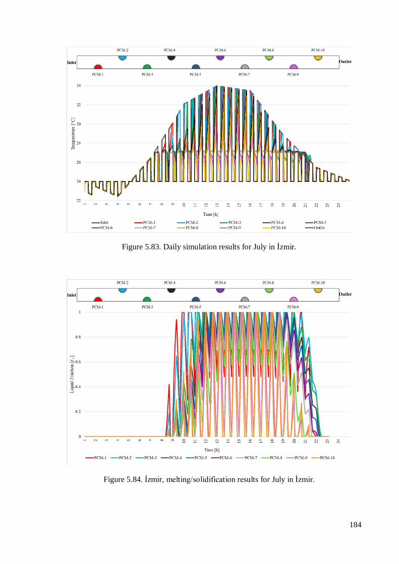
Figure 5.83. Daily simulation results for July in İzmir.

Figure 5.84. İzmir, melting/solidification results for July in İzmir.

184

5.4.2.3. Tropic Climate: Singapore

Due to Singapore's proximity to the Equator, there is only one season. The climate

type seen in Singapore is the tropical climate type. All seasons of the year are quite hot

and humid. The average temperature is between 25°C and 31°C. April is the warmest

month and January is the coolest month in Singapore. The daytime length in Singapore

remains 12 hours in all seasons. The latitude of Singapore is 1°.3’, and the longitude is

103°.8’. So, this city-state is located just 1-degree north of the equator. Because of this,

the Singapore climate is tropical. Figure 5.85 shows the yearly variation of the Singapore

climate. And the temperatures in Singapore are very little from month to month and

generally, the minimum degree is 25°C, the maximum degree is 31°C. December and

January are the coolest months of the year. May, June, and July have the highest average

of the monthly temperature data.

Figure 5.85. Singapore highest and lowest temperatures throughout the year (2005-2016)

Three months have been selected according to the monthly highest and coldest

average temperature values given in Figure 5.85, as shown in Figure 5.86. These

simulations are tried in 3 different months and are simulated in January, April, and July.

Month of the year

185

Figure 5.86 shows the monthly average of the daily data for selected months. It drops

below 25 °C only between 17.00 and 23.00 in January and usually starts to rise at 00.00

and reaches its highest level at 05.00. The lowest level is seen at 20.00 hours. However,

looking at the graph, the temperature values for April and July are almost the same. It is

observed that there is a 2°C difference with January.

Figure 5.86. Monthly average of the daily temperature distribution of Singapore for

January, April, and July.

PCM melting at 24°C is chosen considering the average temperature of Singapore.

According to Vimalanathan and Babu (2014), The ideal indoor temperature at 21°C

enhanced Singapore's office workers' productivity and health. So, simulations are carried

out by assuming a constant indoor temperature of 21°C. Complete melting and

solidification are not seen in every tube throughout the day, but the system operates all

day and night. Figure 5.87 represents the heat recovery system operating based on the

monthly average daily temperature for January. According to 21°C indoor temperature

and transient outdoor temperature, the system works daily. When looking at the tubes, it

reaches more indoor and outdoor temperatures in the morning hours, while the PCM in

any tube does not reach the outdoor temperature in the evening, especially between 18.00

and 23.00.

186

Figure 5.87. Daily simulation results for January in Singapore.

In Figure 5.88, the melting and solidification results are examined. The PCM in

all the tubes has the highest percentage between 05.00-10.00 hours. The lowest

melting/solidification ratio is observed in the evening hours. Especially 1st tube 2nd tube

3rd tube has the highest melting rate. While 8th, 9th, and 10th tubes change phase %40, 4th,

5th, 6th, and 7th tubes change phase %60. After 17.00, the liquid fraction decreases below

0.2 in all tubes except the 1st tube. The most fluctuation is seen in the 1st and 2nd tubes

throughout the day.

The average temperature in April is 27°C. The highest temperature is 31°C while

the lowest is 24°C. Here, eight hours of sunshine each day for April. In Figure 5.89, more

melting and solidification are observed during the hours when the air temperature is the

highest, while less energy is stored or released in the system in the evening hours. The

phase change material melts at 24°C which melts and solidifies around all day. The PCM

in each tube does not reach the indoor and outdoor temperatures all day. As shown in the

graph, the 1st 2nd 3rd tube melts and solidifies the most, while the 4th 5th 6th 7th tube

reaches the outdoor temperature between 05.00-12.00. After 12.00, there is no fully

melting and solidification in these tubes. In addition, tube 8, 9, and 10 reach a level 1°C

lower than the outdoor temperature between 05.00-12.00.

187

Figure 5.88. Singapore, melting/solidification results for January in Singapore.

Figure 5.89. Daily simulation results for April in Singapore.

188

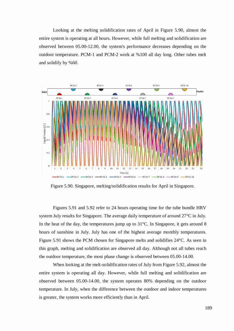
Looking at the melting solidification rates of April in Figure 5.90, almost the

entire system is operating at all hours. However, while full melting and solidification are

observed between 05.00-12.00, the system's performance decreases depending on the

outdoor temperature. PCM-1 and PCM-2 work at %100 all day long. Other tubes melt

and solidify by %60.

Figure 5.90. Singapore, melting/solidification results for April in Singapore.

Figures 5.91 and 5.92 refer to 24 hours operating time for the tube bundle HRV

system July results for Singapore. The average daily temperature of around 27°C in July.

In the heat of the day, the temperatures jump up to 31°C. In Singapore, it gets around 8

hours of sunshine in July. July has one of the highest average monthly temperatures.

Figure 5.91 shows the PCM chosen for Singapore melts and solidifies 24°C. As seen in

this graph, melting and solidification are observed all day. Although not all tubes reach

the outdoor temperature, the most phase change is observed between 05.00-14.00.

When looking at the melt-solidification rates of July from Figure 5.92, almost the

entire system is operating all day. However, while full melting and solidification are

observed between 05.00-14.00, the system operates 80% depending on the outdoor

temperature. In July, when the difference between the outdoor and indoor temperatures

is greater, the system works more efficiently than in April.

189

Figure 5.91. Daily simulation results for July in Singapore.

Figure 5.92. Singapore, melting/solidification results for July in Singapore.

190

5.4.3. Data Reduction

Figure 5.93 shows the results of the tube bundle HRV system with PCM obtained

from simulations according to different climatic data. The red lines show the supply

values in this figure, and the blue ones show the exhaust values. Here, two months are

chosen from the winter conditions for Erzurum: January and February. Simulation has

been made according to summer conditions for Izmir and the results of June and July are

seen. For Singapore, simulations are made for 3 different months above, and April and

July are shared here. Since the temperature distribution in Singapore is similar throughout

the year, the results are expected to be the same all year.

This figure shows the calculation results of energy stored/released. The

simulations are made according to the inlet and outlet velocity values obtained in the

experiments. These are 0.34 m/s for inlet and 0.28 m/s for outlet. Outdoor temperatures

are simulated using climate data. Indoor temperatures are selected differently for each

city. While PCM melting at 15°C is chosen for Erzurum, the indoor temperature is

accepted as 20°C. PCM melting at 27°C is chosen for Izmir, and the indoor temperature

is determined as 24°C. For Singapore, the indoor temperature is 21°C with PCM melting

at 24°C. While the average heat storage capacity is 38 kJ for Erzurum, it is 15 kJ for Izmir

during the operating hours. And for Singapore, the average value is 21 kJ. It is seen that

the system works all day long in winter conditions for Erzurum. For Singapore, the

highest release rate of stored heat occurred between 00.00 and 09.00 hours. For İzmir,

only the system stored/ released heat between 08:00 and 18:00. The highest storage values

for Erzurum are observed between 00.00 and 03.00 when the outdoor temperature is the

lowest. For İzmir, the system stores or releases heat at the highest outdoor temperature.

191

Erzurum results for January Erzurum results for February

İzmir results for June İzmir results for July

Singapore results for April Singapore results for July

Stored energy [kJ] Released energy [kJ]

Figure 5.93. Total heat capacity of the tube bundle unit according to a monthly average

of the daily data

192

5.5. Summary

This chapter contains 4 subtitles. The first section is the experimental results, the

second section is the numerical results, the third section is the refinement of the tube

bundle HRV system, and the fourth section is the simulations made in different climates.

In this chapter, both ceramic systems stored sensible energy and tube bundle system

stored latent energy were tested experimentally and analytically. After experimental and

numerical results, six alternative cases were simulated to improve the total heat capacity.

In addition, the thermal behavior of the system in 3 different climates was investigated.

In the first section, experimental results were explained. These units tested

charging-discharging cycles to identify the temperature characteristics and evaluate the

heat exchangers' energy capacity and losses. In order to evaluate the method of charging-

discharging cycle test, the SHS module and LHS module have been experimented with

in the laboratory. Then the detailed results in transient state different operation times for

two systems were analyzed and discussed from the quantitative way. The efficiency

results were shared for both systems by comparing.

In this case of the studied heat recovery ventilation units, the airflow generated

large differences in the supply and exhaust efficiency. Also, the pressure differences are

affected by the airflow rates in this ventilation system. And the higher-pressure rise is

affected by the airflow balance difference of the unit with an axial fan. So, this resulted

in the change in heat recovery system efficiency because of the stack effect pressure.

Also, experimental studies all have some limitations. To more accurate temperature

distribution in the heat exchanger materials could be observed by taking more

measurements while the system is working.

In the second section, numerical results were represented. For the ceramic system,

the simulation results and experimental results show that in winter conditions, the heat

transfer rate was the best result when the system was operated for the 2-minute cycle. In

addition, the best performance according to efficiency results is the 2-minute operation

time.

For the tube bundle system, according to the experiments, the melting/solidifying

results show that 20-minute of operation time gives the best thermal performance for

maintaining a comfortable indoor temperature with the least energy consumption

193

according to the storage rate. When looking at the numerical results 15-minute and 20-

minute mean heat transfer rates are very close to each other.

The third section discusses the CFD simulations' modifications for tube bundle

decentralized heat recovery systems with six alternative HRV unit alteration approaches.

Several alternative HRV unit changes can improve tube bundle heat transfer, according

to the literature. To get the best performance out of the PCM tubes, the diameter, pitch

size, various PCM solidification/melting temperatures, tube geometry, and air velocity

are all examined using CFD modeling. Most previous experimental and computational

research on flows in tube bundles concentrated on changing the size of the tubes, the form

of the tubes, the system inlet air velocity, and the PCM combinations utilized in the

system. The effect of system modifications was simulated and modeled in this study, and

the results were reported in this section. The heat transfer has been calculated from the

measured temperatures, inlet and outlet fluid temperatures, and pressure drops. The

following conclusions were obtained from the simulations:

Unlike the experiments, the values of exhaust and supply are the same (or very

close) in these results; this is due to the fact that the fan has the same performance in both

directions in the simulations.

According to pressure drop results, the oval tube bundle has an advantage in

airside convection heat transfer than the round tube bundle with the same arrangement in

crossflow.

The heat transfer for staggered tube bundles is not independent of the pitch, at

least an extended longitudinal pitch.

The heat transfer increases with the transverse row number for the tube bundle.

And the heat transfer decreases with an increasing transverse pitch size.

The heat transfer in the system increases or decreases in direct proportion to the

PCM mass. As the number of tubes increases, the amount of PCM that changes phase

increases, so the heat transfer increases.

Pressure drop and heat transfer are directly proportional to increasing velocity. As

seen in Table 1, 0.2 m/s, 0.5 m/s, and 1m/s results increase or decrease depending on the

velocity.

As a result, the tube bundle performance evaluation criterion variations with the

transverse and longitudinal tube pitches indicate that better performances can be achieved

by reducing the tube pitch. This section shows that different geometries give different

results at different flow conditions. The selection of the appropriate geometry for the tube

194

bundle does not always depend on the size, but the thermodynamic properties of the

PCMs are just as important.

In the fourth section, the simulations were made under three different climatic

conditions. In this section, according to the Köppen climate standard, Erzurum, Izmir,

and Singapore are selected as the pilot city for continental climate, mild climate, and

tropical climate, respectively. The analysis of the present study shows:

Decentralized HRV systems that store the latent heat energy in the tube bundle

containing the PCM and the PCM with a fixed melting point are unsuitable for ventilation

energy savings in some climatic zones.

Erzurum's heating load is more than the cooling load. On the other hand, in İzmir,

the cooling load is higher than the heating load. So, this system is effective when used in

Erzurum during the winter months and when used in İzmir during the summer months.

Therefore, the designers need to consider the prevailing loads for efficient utilization of

the latent HRV system.

Although the system cannot be used every month for Erzurum and İzmir, this wall

integrated LHTES tube bundle HRV unit can be used every month in Singapore. because

the temperature difference throughout the year in Singapore is low. This system is more

efficient in Singapore than the other cities Thus, it is suitable for tropical climate.

195

CHAPTER 6

CONCLUSIONS AND RECOMMENDATIONS

This study investigated two different types of decentralized HRV units

experimentally and numerically. These two systems are ceramic HRV unit and tube

bundle HRV unit. A decentralized wall integrated HRV system with PCM, which has

more energy storage capacity as an alternative to the system with ceramic units on the

market, was designed and prototyped, and energy and flow numerical and experimental

analyses were performed. For this purpose, the real-scale experiments were carried out in

the Building Physics Laboratory of the Faculty of Architecture, Izmir Institute of

Technology. The experimental tests of the ceramic HRV unit and tube bundle HRV unit

took place in a controlled environment in different cases, where two HRV units were

inside two wall integrated ducts for controlled parametric studies. The wall divides

conditioned spaces that represent the indoors and the outdoors. During these experiments,

the systems placed inside two ducts run synchronously. In an experimental set, the

performance of the HRV units with SHTES and in another experimental set LHTES and

their axial fan was experimentally investigated under different operating conditions.

Afterward, ventilation performances for supply and exhaust were also analyzed to provide

new experimental data under controlled ambient conditions.

The main findings for the ceramic HRV unit can be listed as follows:

For experimental results:

• The average supply air velocity results are 0.215 m/s, and the exhaust velocity

is 0.165 m/s. These average values were measured at two different positions in the ducts

due to the airflow direction because of providing a fully developed flow.

• The fan produces an average pressure difference of 4.82 Pa when the system is

operating for 1-minute, 4.90 Pa when it is operating for 2-minute, 5.10 Pa when it is

operating for 5-minute, and 4.82 Pa when it is operating for 7.5-minute.

• It is observed that the temperature of the ceramic materials increased between

1°C and 3°C depending on the position of the thermocouples in the ceramics during the

1-minute operating time. The air energy change of the unit for a 1-minute cycle is 5.098

kJ.

196

• When the operating time was the 2-minute cycle, the temperatures of the

ceramic materials increased by up to 7°C depending on the measuring locations. The air

energy change of the unit for a 2-minute cycle is 10.607 kJ.

• When the system was operated for 5-minute, the temperature of the interior of

the ceramic approached the indoor temperature. In addition, a temperature difference of

10°C occurs in ceramics depending on the thermocouple positions. The air energy change

of the unit for a 5-minute cycle is 20.732 kJ.

• The ceramic is approximately equal to both indoor and outdoor temperatures

when the system is operated for 7.5-minute. The temperature value of the thermocouples

in the ceramic showed an increase of a maximum of 11°C. The air energy change of the

unit for a 7.5-minute cycle is 29.281 kJ.

• During the 10-minute cycle, there is a decrease or increase in the temperature

of the ceramic materials of approximately 12°C. The high-temperature variation in the

ceramic indicates that the most energy storage is achieved during a 10-minute cycle. The

air energy change of the unit for a 10-minute cycle is 36.532 kJ.

On the other hand, by evaluating the experimental results, considering the average

heat transfer rate instead of the total heat capacity of the unit in certain periods at different

time steps; It has been seen that the HRV unit performs best in 2-minute cycles out of 1,

5, 7.5 and 10-minute cycles.

• For 1 min, 2 min, 5 min, 7.5 min, and 10 min operating time for winter

conditions for ceramic HRV unit, the supply efficiency results are 75%, 82%, 76%, 73%,

and 77%, and the exhaust efficiency results are 73%, 67%, 73%, 58%, and 62%

respectively. And the average result is 77% for supply efficiency, and exhaust efficiency

is 65%.

• For summer conditions, the unit is operated 7.5-minute, the supply efficiency

result is 89%, exhaust efficiency is 61%, for 10-minute operating time results are 81%

and 45% supply and exhaust efficiency, respectively.

The main findings for the tube bundle HRV unit can be listed as follows:

For experimental results:

• The average velocity for supply air is 0.344 m/s, and the average for exhaust

air is 0.282 m/s for the tube bundle HRV prototype. The points that provided the nearest

values to the calculated average velocity values were selected to represent the average

velocity.

197

• The pressure difference between two fans for 15-minute, 20-minute, and 30-

minute airflow from the outdoor to the indoor environment is 9.74 Pa, 9.78 Pa, and 9.57

Pa, respectively.

• When the system is operated for 15 min, all PCMs in the temperature trend

inside the tubes do not reach 27°C, which is the melting/solidifying temperature, thus

they are not fully melted. There is not enough time to stabilize the temperature distribution

of the PCMs inside all the tubes. The air energy change of the latent HRV prototype for

a 15-minute cycle in supply mode is 16.12 kJ.

• When the system operates for 20 min, the temperature increases inside the tube

bundle, and the melting and solidification process of the PCM performs better than the

15 min cycle. The air energy change of the latent HRV prototype for a 20-minute cycle

in supply mode is 27.24 kJ.

• PCM completely melts and completely solidifies 30 min. after fully

melting/solidifying, the temperatures of the thermocouples increase. This indicates that

SHTES follows LHTES. Thus, the temperatures of these thermocouples get very close to

the indoor or outdoor environment when the system operates for 30 min. Air energy

change of the latent HRV prototype for a 30-minute cycle in supply mode is 34.12 kJ.

According to experimental results, the mean heat transfer rate for tube bundle

HRV system for 20-minute cycle gives the best result in supply mode is 22.7 W and

exhaust mode is 18.4 W.

• For 15 min, 20 min, and 30 min operating time for summer conditions for tube

bundle HRV unit, the supply efficiency results are 51%, 54%, and 46%, and the exhaust

efficiency results are 23%, 29%, and 24% respectively. And the average result is 50% for

supply efficiency, and exhaust efficiency is 25%.

ANSYS was used to simulate the control system, provide the necessary boundary

conditions required by the FLUENT model, and calculate the energy requirements of the

systems. With these results, simulations of operating conditions were examined, and the

ability of a building simulation tool to provide modeling and performance prediction of

these systems was tested. The ceramic and tube bundle systems were simulated in these

simulations for this study. The fluids for the two systems are Newtonian and

incompressible, and the Boussinesq approximation is utilized to account for the buoyancy

term in the momentum equation. The flow is time-dependent, and the cartesian coordinate

198

system is 2D, no-slip conditions are valid for all boundaries, also viscous dissipation and

radiation effects are neglected.

The mesh resolution can affect the result of a CFD simulation. So, many mesh

structures were analyzed, and these can be classified as very coarse, coarse, medium, fine,

very fine, ultra-fine. To provide the cyclic steady-state and eliminate the boundary

condition that affects the simulations were analyzed with at least 50 consecutive cycles.

While the system was operated from outdoor to indoor and from indoor to outdoor,

stability was achieved in cycles, and the difference between the last two cycles is only

2%.

The main findings for the ceramic HRV unit can be listed as follows:

For numerical results:

• A mesh structure was created by using quadrilateral elements with edge sizing

and face meshing features for a ceramic cell.

• The average temperature values standard deviation for the charging process is

0.65%, for the discharging process, it is 1.59% compared with CFD and experimental

study results.

• For a 1-minute cycle, initially, the rise in the average volume temperature of

ceramic and air was rapid and decreases with time. And the inlet temperature and ceramic

reach a maximum of 15°C. The outlet temperature drops to 11°C. 1-minute operation

time is not enough to charge and discharge processes. The energy change of the unit for

a 1-minute cycle is 5.11 kJ.

• For a 2-minute operating time, the inlet temperature rises to a maximum of

17°C, the fluid inside the ceramic and ceramic rises to 19°C. The outlet temperature drops

to 7°C while the system operates from outdoor to indoor. The energy change of the unit

for a 2-minute cycle is 10.32 kJ.

• For 5 min, 7.5 min, and 10 min cycles, the temperature rise of ceramic is rapid

first 150 s due to the high driving force for conduction, and discharging curve becomes

flat as time progresses after the 150 s. The average system temperature reaches the inlet

and outlet temperature in discharging and charging process. The energy change of the

unit for 5 min, 7.5 min, and 10 min cycle results are 21.20 kJ, 30.91 kJ, and 30.91 kJ,

respectively.

The main findings for the tube bundle HRV unit can be listed as follows:

199

For numerical results:

• A mesh structure was created by using quadrilateral and triangular elements

with edge sizing and face meshing features for the tube bundle computational domain.

• As a result, while the average temperature values standard deviation for the

charging process is 1.32%, for the discharging process, it is 1.38% compared with

numerical solutions and experimental study results.

• PCM has no fully melting and solidifying process in the time-related melting

and solidifying graphs for 15-minute operating. The energy change of the latent HRV unit

for a 15-minute cycle is 26.94 kJ.

• For the 20-minute cyclic result, unlike the results of 15-minute, PCMs in all

tubes melt and solidify except only 2 tubes. According to supply mode, the solidification

process is not completely occurred. The energy change of the latent HRV unit for a 20-

minute cycle is 31.99 kJ.

• During the 30-minute operating time, all PCM melted in the system and

solidified except only 2 tubes. All the tubes reached the outside temperature. The energy

change of the latent HRV unit for a 30-minute cycle is 41.94 kJ.

This thesis dissertation made different simulations by changing the LHTES HRV

unit tube bundle dimensions, the tubes' shapes, air velocity, and the PCM material used

for enhanced heat transfer.

For numerical results of refinement of the prototype:

• 1st case: 4 different pitch sizes were investigated on a tube diameter of 3 mm.

In the simulation with 10 mm longitudinal and 10 mm transverse pitch sizes, it was

calculated that the heat transfer increase is greater with a lower pitch size. According to

the simulation results on the same tube diameter, the heat capacity increases as the

longitudinal and transverse pitch size decreases. Also, the pressure drop increases.

• 2nd case: When the tube shape is changed, it appears to be a promising

technique for heat transfer enhancement, especially the pressure drop results are

compared to conventional cylindrical tubes.

• 3rd case: In the experiments, the measured velocity value is 0.34 m/s from the

inlet, 0.28 m/s from the outlet. So, in case 3, the air velocity value has changed both inlet

and outlet. 0.2 m/s, 0.5 m/s, and 1 m/s were simulated. As a result, heat transfer and the

pressure drop increase if velocity increases.

200

• 4th case: In cases 4 and 5, it can be seen that the series arrangement improves

solidification and melting performance compared to a single PCM. However, the heat

storage capacities of the PCMs used in this case are different from each other. Therefore,

there is a lower total heat storage capacity when compared.

• 5th case: The heat transfer increases or decreases in direct proportion to the

PCM mass in the system. So, PCM's thermal energy storage capacity depends on the

amount of PCM.

The tube bundle prototype produced within the scope of this thesis was analyzed

the energy performance in three different climatic conditions was aimed to guide the

designer in the selection of the wall integrated ventilation system in different climates.

The heat recovery system operated based on the monthly average daily temperature in

20-minute cycles with the same inlet and outlet velocity. Erzurum is selected as the pilot

city for the continental climate zone, İzmir is selected as the pilot city for the mild climate

zone, and Singapore is selected as the pilot city for the tropical climate zone.

For numerical results of different climatic conditions:

• For Erzurum: the outdoor temperature simulations are made over two different

months. These are January and February. The phase change material’s

melting/solidification point of 15°C is chosen, and the indoor temperature is assumed to

be 20°C. The average outdoor temperature is -5°C. The PCM was completely solidified

and completely melted in January and February. All tubes reached the inlet and outlet

temperature in discharging and charging process. The average heat storage capacity is 38

kJ for Erzurum, according to simulation results.

• For Izmir: the simulations were carried out for June and July. The PCM melting

and a solidification temperature is 27°C, and the indoor temperature is assumed to be

24°C. The average outdoor temperature for June and July is 30°C. For June, the system

operated between 08:00 and 18:00. For July, the phase changes of the tubes start at 08:00

in the morning and continue until 22:00. While melting/solidification was observed in all

tubes between the specified hours, no phase change was observed at other hour intervals.

The average heat storage capacity is 15 kJ for Izmir during operating hours.

• For Singapore: these simulations were carried out in 3 different months and are

simulated in January, April, and July. PCM melting at 24°C is chosen considering the

average temperature of Singapore. And the indoor temperature is 21°C as a constant. The

201

melting and solidification were observed all day and all year. The average heat storage

capacity value is 21 kJ.

This thesis contributes to the studies on the integration of PCMs and thus latent

heat storage materials into HRV equipment used in the facades of buildings. The

prototype proposed in the study was analyzed both experimentally and numerically. It is

an alternative to the wall integrated sensible heat recovery ventilation systems available

in the market. Such a wall integrated latent heat recovery ventilation system has no

example in the literature. The proposed unit has a flexible model adaptable to different

climatic conditions. It is also a system that can be developed and changed.

Some of the possible future work on this prototype is to consider different fans for

more efficient ventilation performance, experimentally test it in different indoor and

outdoor conditions, as well as experimentally and numerically investigate changes in the

levels of IAQ variables, including relative humidity and CO2 levels.

202

REFERENCES

Abdeen, Ahmed, Ahmed A Serageldin, Mona GE Ibrahim, Abbas El-Zafarany, Shinichi Ookawara, and Ryo Murata. 2019. "Solar chimney optimization for enhancing thermal comfort in Egypt: An experimental and numerical study." Solar Energy 180: 524-536.

Abduljalil, A, and Sohif Bin Mat Al-abidi. 2013. "K. Sopian, MY Sulaiman and

Abdulrahman Th. Mohammed, CFD applications for latent heat thermal energy storage: a review." Renewable and sustainable energy reviews 20: 353-363.

Abdul-Wahab, Sabah Ahmed, Stephen Chin Fah En, Ali Elkamel, Lena Ahmadi, and

Kaan Yetilmezsoy. 2015. "A review of standards and guidelines set by international bodies for the parameters of indoor air quality." Atmospheric Pollution Research 6 (5): 751-767.

Abhat, A. 1983. "Low temperature latent heat thermal energy storage: heat storage

materials." Solar energy 30 (4): 313-332. Afshari, Reza. 2020. Indoor air quality and severity of COVID-19: where communicable

and non-communicable preventive measures meet. Mashhad University of Medical Sciences.

Agyenim, Francis, Neil Hewitt, Philip Eames, and Mervyn Smyth. 2010. "A review of

materials, heat transfer and phase change problem formulation for latent heat thermal energy storage systems (LHTES)." Renewable and sustainable energy reviews 14 (2): 615-628.

Ahmad, Mardiana Idayu, and Saffa Riffat. 2020. Energy Recovery Technology for

Building Applications. Springer. Akeiber, Hussein, Payam Nejat, Muhd Zaimi Abd Majid, Mazlan A Wahid, Fatemeh

Jomehzadeh, Iman Zeynali Famileh, John Kaiser Calautit, Ben Richard Hughes, and Sheikh Ahmad Zaki. 2016. "A review on phase change material (PCM) for sustainable passive cooling in building envelopes." Renewable and Sustainable Energy Reviews 60: 1470-1497.

Albatayneh, Aiman, Dariusz Alterman, and Adrian Page. 2018. "Adaptation the use of

CFD modelling for building thermal simulation." Proceedings of the 2018 International Conference on Software Engineering and Information Management.

Albatayneh, Aiman, Dariusz Alterman, Adrian Page, and Behdad Moghtaderi. 2019.

"The significance of the adaptive thermal comfort limits on the air-conditioning loads in a temperate climate." Sustainability 11 (2): 328.

Aldoss, Taha K, and Muhammad M Rahman. 2014. "Comparison between the single-

PCM and multi-PCM thermal energy storage design." Energy conversion and management 83: 79-87.

203

Ali, Muzaffar, and Mukhtar Hussain Sahir. 2013. "Optimization of Heating, Ventilation, and Air-Conditioning (HVAC) System Configurations." Thesis, University of Engineering & Technology, Taxila.

Alizadeh, M, and SM Sadrameli. 2016. "Development of free cooling based ventilation

technology for buildings: Thermal energy storage (TES) unit, performance enhancement techniques and design considerations–A review." Renewable and Sustainable Energy Reviews 58: 619-645.

Al-Jeebori, Abbas AS. 2008. "Thermal Design of Tube Banks in Cross Flow Based on

Minimum Thermodynamic Losses." Al-Qadisiyah Journal for Engineering Sciences 1 (2): 133-143.

Anderson, Brian. 2006. "Energy performance of buildings directive." BRE, April. Apte, Michael G. 2000. "Associations between indoor CO2 concentrations and sick

building syndrome symptoms in US office buildings: an analysis of the 1994-1996 BASE study data." Indoor air 10 (4).

Arıcı, Müslüm, Feyza Bilgin, Sandro Nižetić, and Hasan Karabay. 2020. "PCM integrated

to external building walls: An optimization study on maximum activation of latent heat." Applied Thermal Engineering 165: 114560.

Arkar, C, and S Medved. 2007. "Free cooling of a building using PCM heat storage

integrated into the ventilation system." Solar energy 81 (9): 1078-1087. ASHRAE. ANSI/ASHRAE STANDARD 111-2008 Measurement, Testing, Adjusting, and

Balancing of Building HVAC Systems; 2008. Asker, Mustafa, Ersin Alptekin, Ayça Tokuç, Mehmet Akif Ezan, and Hadi Ganjehsarabi.

2018. "Numerical Simulation of Building Wall Integrated with Phase Change Material: A Case Study of a Mediterranean City Izmir, Turkey." In The Role of Exergy in Energy and the Environment, 757-768. Springer.

Association for Environment Conscious Building (AECB),

http://www.aecb.net/goldstandardpdf.php. Astolfi, Arianna, and Franco Pellerey. 2008. "Subjective and objective assessment of

acoustical and overall environmental quality in secondary school classrooms." The Journal of the Acoustical Society of America 123 (1): 163-173.

Averfalk, Helge, Paul Ingvarsson, Urban Persson, Mei Gong, and Sven Werner. 2017.

"Large heat pumps in Swedish district heating systems." Renewable and Sustainable Energy Reviews 79: 1275-1284.

Balci, Ozan M, Mehmet A Ezan, and Kutbettin Z Turhan. 2019. "A heat recovery unit

with phase change material for combi‐boilers." Energy Storage 1 (5): e81.

204

Baldini, Luca, Moon Keun Kim, and Hansjürg Leibundgut. 2014. "Decentralized cooling and dehumidification with a 3 stage LowEx heat exchanger for free reheating." Energy and buildings 76: 270-277.

Baranova, Daria, Daniil Sovetnikov, Daria Semashkina, and Anatolijs Borodinecs. 2017.

"Correlation of energy efficiency and thermal comfort depending on the ventilation strategy." Procedia Engineering 205: 503-510.

Bas, Halit, and Veysel Ozceyhan. 2012. "Heat transfer enhancement in a tube with twisted

tape inserts placed separately from the tube wall." Experimental Thermal and Fluid Science 41: 51-58.

Başaran, Tahsin, and Tuğba İnan. 2016. "Experimental investigation of the pressure loss

through a double skin facade by using perforated plates." Energy and Buildings 133: 628-639.

Benyahia, Nabil, Mohamed Aksouh, Amina Mataoui, and Hakan F Oztop. 2020.

"Coupling turbulent natural convection-radiation-conduction in differentially heated cavity with high aspect ratio." International Journal of Thermal Sciences 158: 106518.

Bern, Marshall W, and Paul E Plassmann. 2000. Mesh Generation. Vol. 6. Bernard, H Russell, and Harvey Russell Bernard. 2013. Social research methods:

Qualitative and quantitative approaches. Sage. Bernold, Leonhard E, and Tai Sik Lee. 2010. "Experimental research in

construction." Journal of Construction Engineering and Management 136 (1): 26-35.

Bland, Ashley, Martin Khzouz, Thomas Statheros, and Evangelos I Gkanas. 2017. "PCMs

for residential building applications: A short review focused on disadvantages and proposals for future development." Buildings 7 (3): 78.

Bonato, Paolo, Matteo D'Antoni, and Roberto Fedrizzi. 2020. "Modelling and simulation-

based analysis of a façade-integrated decentralized ventilation unit." Journal of Building Engineering 29: 101183.

Buddhi, D, and RL Sawhney. 1994. "Proc: Thermal energy storage and energy

conversion." School of Energy and Environmental Studies, Devi Ahilya University, Indore, India.

Bulut, Hüsamettin. 2011. "Havalandırma ve iç hava kalitesi açısından CO2 miktarının

analizi." Ulusal Tesisat Mühendisliği Kongresi: 13-16. Building Energy Performance (BEP) (in Turkish).

https://www.mevzuat.gov.tr/mevzuat?MevzuatNo=13594&MevzuatTur=7&MevzuatTertip=5. (Accessed 10.09.2018).

205

Building Research Establishment Environmental Assessment Method (BREEAM), BRE Global Ltd. What Is BREEAM? www.breeam.org/about.jsp?id=66 2015.

BS EN 15251. BS EN 15251. 2007. Indoor Environ. input parameters Des. Assess.

energy Perform. Build. Calautit, John Kaiser, and Ben Richard Hughes. 2014. "Integration and application of

passive cooling within a wind tower for hot climates." HVAC&R Research 20 (7): 722-730.

Campos‐Celador, Álvaro, Gonzalo Diarce, Pello Larrinaga, and Ane Miren García‐

Romero. 2020. "A simple method for the design of thermal energy storage systems." Energy Storage 2 (6): e140.

Capeluto, Isaac Guedi, and Boris Plotnikov. 2017. "A method for the generation of

climate-based, context-dependent parametric solar envelopes." Architectural Science Review 60 (5): 395-407.

Carbonare, N, T Pflug, C Bongs, and A Wagner. 2019. "Comfort-oriented control

strategies for decentralized ventilation using co-simulation." IOP Conference Series: Materials Science and Engineering.

Carlucci, Salvatore, Lujian Bai, Richard de Dear, and Liu Yang. 2018. "Review of

adaptive thermal comfort models in built environmental regulatory documents." Building and Environment 137: 73-89.

Celik, Ismail, and Gusheng Hu. 2004. "Single grid error estimation using error transport

equation." J. Fluids Eng. 126 (5): 778-790. Cengel, Yunus A. 2010. Fluid mechanics. Tata McGraw-Hill Education. Cengel, Yunus A, and Afshin J Ghajar. 2007. "Heat and mass transfer." A practical

approach. Chandel, SS, and Tanya Agarwal. 2017. "Review of cooling techniques using phase

change materials for enhancing efficiency of photovoltaic power systems." Renewable and Sustainable Energy Reviews 73: 1342-1351.

Chorin, Alexandre Joel. 1968. "Numerical solution of the Navier-Stokes

equations." Mathematics of computation 22 (104): 745-762. CIBSE, TM36. 2005. "Climate change and the indoor environment: impacts and

adaptation." Chartered Institution of Building Services Engineers, London. CIBSE, TM52. 2013. "Environmental Design." Chartered Institution of Building Services

Engineers, London. CIBSE, TM59. 2013. "Assess Overheating Risk in Homes." Chartered Institution of

Building Services Engineers, London.

206

Clausen, Geo, and David P Wyon. 2008. "The combined effects of many different indoor environmental factors on acceptability and office work performance." HVAC&R Research 14 (1): 103-113.

Coley, David, Tristan Kershaw, and Matt Eames. 2012. "A comparison of structural and

behavioural adaptations to future proofing buildings against higher temperatures." Building and Environment 55: 159-166.

Collyer, Anna. 2019. "Independent review of the Greenhouse and Energy Minimum

Standards (GEMS) Act 2012." Comite'Europe'en de Normalisation, CEN. 2007. "Indoor environmental input parameters

for design and assessment of energy performance of buildings addressing indoor air quality, thermal environment, lighting and acoustics." EN 15251.

Council, National Research, and Green Schools. 2007. "Attributes for health and

learning." National Academy of Sciences USA, Washington. Creswell, John W. 2002. Educational research: Planning, conducting, and evaluating

quantitative. Prentice Hall Upper Saddle River, NJ. Creswell, John W, and J David Creswell. 2017. Research design: Qualitative,

quantitative, and mixed methods approaches. Sage publications. Cuce, Pinar Mert, and Saffa Riffat. 2015. "A comprehensive review of heat recovery

systems for building applications." Renewable and Sustainable Energy Reviews 47: 665-682.

Culha, Oguzhan, Huseyin Gunerhan, Emrah Biyik, Orhan Ekren, and Arif Hepbasli.

2015. "Heat exchanger applications in wastewater source heat pumps for buildings: A key review." Energy and Buildings 104: 215-232.

Daisey, Joan M, William J Angell, and Michael G Apte. 2003. "Indoor air quality,

ventilation and health symptoms in schools: an analysis of existing information." Indoor air 13 (LBNL-48287).

Dardir, Mohamed, Karthik Panchabikesan, Fariborz Haghighat, Mohamed El Mankibi,

and Yanping Yuan. 2019. "Opportunities and challenges of PCM-to-air heat exchangers (PAHXs) for building free cooling applications—A comprehensive review." Journal of Energy Storage 22: 157-175.

Diallo, Thierno MO, Xudong Zhao, Antoine Dugue, Paul Bonnamy, Francisco Javier

Miguel, Asier Martinez, Theodoros Theodosiou, Jing-Sheng Liu, and Nathan Brown. 2017. "Numerical investigation of the energy performance of an Opaque Ventilated Façade system employing a smart modular heat recovery unit and a latent heat thermal energy system." Applied energy 205: 130-152.

Dincer, Ibrahim, and Mehmet Akif Ezan. 2018. Heat storage: A unique solution for

energy systems. Springer.

207

DIN EN 12599-Ventilation for buildings-Test procedures and measurement methods to hand over air conditioning and ventilation systems.

DIN EN 16211-Ventilation for buildings. Measurement of air flows on site. Methods. Driels, Morris R, and Young S Shin. 2004. Determining the number of iterations for

Monte Carlo simulations of weapon effectiveness. Duffield, John S, and Brian Woodall. 2011. "Japan's new basic energy plan." Energy

Policy 39 (6): 3741-3749. Durakovic, Benjamin, and Muris Torlak. 2017. "Experimental and numerical study of a

PCM window model as a thermal energy storage unit." International Journal of Low-Carbon Technologies 12 (3): 272-280.

Eiamsa-ard, Smith, Chinaruk Thianpong, and Pongjet Promvonge. 2006. "Experimental

investigation of heat transfer and flow friction in a circular tube fitted with regularly spaced twisted tape elements." International Communications in Heat and Mass Transfer 33 (10): 1225-1233.

El Fouih, Younness, Pascal Stabat, Philippe Rivière, Phuong Hoang, and Valérie

Archambault. 2012. "Adequacy of air-to-air heat recovery ventilation system applied in low energy buildings." Energy and Buildings 54: 29-39.

El Mankibi, Mohamed, Nikolaos Stathopoulos, Niousha Rezai, and Amine Zoubir. 2015.

"Optimization of an Air-PCM heat exchanger and elaboration of peak power reduction strategies." Energy and Buildings 106: 74-86.

Ellis, MW, and EH Mathews. 2002. "Needs and trends in building and HVAC system

design tools." Building and environment 37 (5): 461-470. Elsaid, Ashraf Mimi, and M Salem Ahmed. 2021. "Indoor Air Quality Strategies for Air-

Conditioning and Ventilation Systems with the Spread of the Global Coronavirus (COVID-19) Epidemic: Improvements and Recommendations." Environmental Research: 111314.

Elsanusi, Omer S, and Emmanuel C Nsofor. 2021. "Melting of multiple PCMs with

different arrangements inside a heat exchanger for energy storage." Applied thermal engineering 185: 116046.

ElSorady, Dalia A, and Sahar M Rizk. 2020. "LEED v4. 1 operations & maintenance for

existing buildings and compliance assessment: Bayt Al-Suhaymi, Historic Cairo." Alexandria Engineering Journal 59 (1): 519-531.

Energy Performance of Buildings Directive. Struct. Surv. 2005.

https://doi.org/10.1108/ss.2005.11023aab.001. Energy Performance of Buildings Directive. Struct. Surv. 2010.

208

EN 13141-8:2014. Ventilation for buildings. Performance testing of components/products for residential ventilation. Performance testing of un-ducted mechanical supply and exhaust ventilation units (including heat recovery) for mechanical ventilation systems intended for a2014.

Erdem, IŞIK, and Serkan Çibuk. 2015. "Yemekhaneler ve kantinlerde iç hava kalitesi ile

ilgili ölçüm sonuçları ve analizi-Tunceli Üniversitesi örneği." Dicle Üniversitesi Mühendislik Fakültesi Mühendislik Dergisi 6 (1): 39-50.

Erguvan, Mustafa, and David W MacPhee. 2019. "Second law optimization of heat

exchangers in waste heat recovery." International Journal of Energy Research 43 (11): 5714-5734.

Ezan, Mehmet Akif. 2011. "Experimental and numerical investigation of cold thermal

energy storage systems." DEÜ Fen Bilimleri Enstitüsü. Ezan, Mehmet Akif, Muhammet Ozdogan, and Aytunç Erek. 2011. "Experimental study

on charging and discharging periods of water in a latent heat storage unit." International Journal of Thermal Sciences 50 (11): 2205-2219.

Ezan, Mehmet Akif, Ceren Yüksel, Ersin Alptekin, and Ahmet Yılancı. 2018.

"Importance of natural convection on numerical modelling of the building integrated PVP/PCM systems." Solar Energy 159: 616-627.

Fanger, Poul O. 1970. "Thermal comfort. Analysis and applications in environmental

engineering." Thermal comfort. Analysis and applications in environmental engineering.

Filis, Vasileios, Jakub Kolarik, and Kevin Michael Smith. 2021. "The impact of wind

pressure and stack effect on the performance of room ventilation units with heat recovery." Energy and Buildings 234: 110689.

Fiorentini, Massimo, Paul Cooper, and Zhenjun Ma. 2015. "Development and

optimization of an innovative HVAC system with integrated PVT and PCM thermal storage for a net-zero energy retrofitted house." Energy and Buildings 94: 21-32.

Fisk, William J. 2017. "The ventilation problem in schools: literature review." Indoor

Air 27 (6): 1039-1051. Fluent, ANSYS. 2011. "Ansys fluent theory guide." ANSYS Inc., USA 15317: 724-746. Fonseca, Ana, Isabel Abreu, Maria João Guerreiro, Cristina Abreu, Ricardo Silva, and

Nelson Barros. 2019. "Indoor Air Quality and Sustainability Management—Case Study in Three Portuguese Healthcare Units." Sustainability 11 (1): 101.

Fountain, M, and Edward A Arens. 1993. "Air movement and thermal comfort." ASHRAE

journal 35 (8): 26-30.

209

Frontczak, Monika, Stefano Schiavon, John Goins, Edward Arens, Hui Zhang, and Pawel Wargocki. 2012. "Quantitative relationships between occupant satisfaction and satisfaction aspects of indoor environmental quality and building design." Indoor air 22 (2): 119-131.

Gasia, Jaume, Jan Diriken, Malcolm Bourke, Johan Van Bael, and Luisa F Cabeza. 2017.

"Comparative study of the thermal performance of four different shell-and-tube heat exchangers used as latent heat thermal energy storage systems." Renewable Energy 114: 934-944.

George, PL, and H Borouchaki. 2000. "Quality mesh generation." Comptes Rendus de

l'Académie des Sciences Paris 328: 505-518. Gheorghe, Iuliana Florentina, and Barbu Ion. 2011. "The effects of air pollutants on

vegetation and the role of vegetation in reducing atmospheric pollution." The impact of air pollution on health, economy, environment and agricultural sources: 241-280.

Godish, Thad. 2016. Indoor environmental quality. CRC press. Godish, Thad, Wayne T Davis, and Joshua S Fu. 2014. Air quality. CRC Press. Goetzler, William, Matt Guernsey, Jim Young, Jay Fujrman, and Amar Abdelaziz.

2016. The future of air conditioning for buildings. Navigant Consulting, Burlington, MA (United States).

Gong, Zhen-Xiang, and Aran S Mujumdar. 1996. "Finite element analysis of a multistage

latent heat thermal storage system." Numerical Heat Transfer, Part A Applications 30 (7): 669-684.

Goodfellow, Howard D, and Esko Tahti. 2001. Industrial ventilation design guidebook.

Academic press. Greenhouse and Energy Minimum Standards Act 2012.

https://www.legislation.gov.au/Details/C2018C00454. (Accessed 10.09.2018). Grignon-Massé, Laurent, Jérôme Adnot, and Philippe Rivière. 2008. "Towards Adaptive

PMV/PPD Indices for European Climates…." Scaling up: building tomorrow's solutions-Proceedings from the ACEEE 2008 Summer Study on Energy Efficiency in Buildings.

Guide, A. 2006. "Environmental design." Chartered Institute of Building Services

Engineers (CIBSE). Gümüş, Veysel, Seven, Alaattin, and Şimşek, Oğuz. "Eğimli kritik altı açık kanal

akımının sayısal modellemesi." Gümüşhane Üniversitesi Fen Bilimleri Enstitüsü Dergisi 11 (1): 73-90.

210

Guo, Haibo, Lu Huang, Wenjie Song, Xinyue Wang, Hongnan Wang, and Xinning Zhao. 2020. "Evaluation of the summer overheating phenomenon in reinforced concrete and cross laminated timber residential buildings in the cold and severe cold regions of China." Energies 13 (23): 6305.

Gupta, Naveen Kumar, Arun Kumar Tiwari, and Subrata Kumar Ghosh. 2018. "Heat

transfer mechanisms in heat pipes using nanofluids–A review." Experimental Thermal and Fluid Science 90: 84-100.

Gürel, Barış. 2020. "A numerical investigation of the melting heat transfer characteristics

of phase change materials in different plate heat exchanger (latent heat thermal energy storage) systems." International Journal of Heat and Mass Transfer 148: 119117.

Hekmat, Dariusch, Helmut E Feustel, and Mark P Modera. 1986. "Impacts of ventilation

strategies on energy consumption and indoor air quality in single-family residences." Energy and Buildings 9 (3): 239-251.

Holman, Jack Philip. 2012. "Experimental methods for engineers." Hu, Yue, Per Kvols Heiselberg, Hicham Johra, and Rui Guo. 2020. "Experimental and

numerical study of a PCM solar air heat exchanger and its ventilation preheating effectiveness." Renewable Energy 145: 106-115.

İnan, Tuğba, Tahsin Başaran, and Aytunç Erek. 2017. "Experimental and numerical

investigation of forced convection in a double skin façade." Energies 10 (9): 1364. İnan, Tuğba, Tahsin Başaran, and Mehmet Akif Ezan. 2016. "Experimental and

numerical investigation of natural convection in a double skin facade." Applied Thermal Engineering 106: 1225-1235.

Incropera, Frank P, David P DeWitt, Theodore L Bergman, and Adrienne S Lavine. 2007.

"heat and mass transfer-Incropera 6e." Fundamentals of Heat and Mass Transfer 997.

Jang, Jiin-Yuh, and Jyh-Yau Yang. 1998. "Experimental and 3-D numerical analysis of

the thermal-hydraulic characteristics of elliptic finned-tube heat exchangers." Heat Transfer Engineering 19 (4): 55-67.

Jokisalo, Juha, Jarek Kurnitski, Mika Vuolle, and Antti Torkki. 2003. "Performance of

balanced ventilation with heat recovery in residential buildings in a cold climate." International Journal of Ventilation 2 (3): 223-236.

Kakac, Sadik, Hongtan Liu, and Anchasa Pramuanjaroenkij. 2002. Heat exchangers:

selection, rating, and thermal design. CRC press. Kalnæs, Simen Edsjø, and Bjørn Petter Jelle. 2015. "Phase change materials and products

for building applications: A state-of-the-art review and future research opportunities." Energy and Buildings 94: 150-176.

211

Karaçavuş, Berrin, And Kadir Aydın. 2017. "Boru Demetleri Üzerinde Çapraz Akışta Nusselt Sayısının Nümerik İncelenmesi." TESKON.

Karimi, Mohsen, G Akdogan, KH Dellimore, and SM Bradshaw. 2012. "Quantification

of numerical uncertainty in computational fluid dynamics modelling of hydrocyclones." Computers & Chemical Engineering 43: 45-54.

Khan, Muhammad Hammad, and William Pao. 2015. "Thermal comfort analysis of PMV

model prediction in air conditioned and naturally ventilated buildings." Energy Procedia 75: 1373-1379.

Kim, Moon Keun, and Luca Baldini. 2016. "Energy analysis of a decentralized ventilation

system compared with centralized ventilation systems in European climates: Based on review of analyses." Energy and Buildings 111: 424-433.

Kim, Nae-Hyun, Kang-Jong Lee, and Yeong-Bin Jeong. 2014. "Airside performance of

oval tube heat exchangers having sine wave fins under wet condition." Applied thermal engineering 66 (1-2): 580-589.

Köktürk, G, and A Tokuç. 2017. "Vision for wind energy with a smart grid in

Izmir." Renewable and Sustainable energy reviews 73: 332-345. Konstantinidis, Christine Vasiliki. 2010. "Integration of thermal energy storage in

buildings." Koper, Piotr, Agnieszka Palmowska, and Agnieszka Myszkowska. 2019. "Research of

single room decentralized heat recovery unit." Architecture Civil Engineering Environment 12 (4).

Kozielska, Barbara, Anna Mainka, Magdalena Żak, Dorota Kaleta, and Walter Mucha.

2020. "Indoor air quality in residential buildings in Upper Silesia, Poland." Building and Environment 177: 106914.

Krainer, A. Passivhaus Contra Bioclimatic Design. Bauphysik 2008.

https://doi.org/10.1002/bapi.200810051. Küçüka, Serhan. 2005. "Isı geri kazanım cihazlarının bazı şehirlerdeki yıllık toplam

ısıtma ve soğutma kazançları." Ulusal Tesisat Mühendisliği Kongresi 1 (7): 46. Kumar, D Arun, and R Prabu ME. "Investigation of Comparison of Three Different Tube

Bundles of Heat Exchanger." Lai, Dayi, Yue Qi, Junjie Liu, Xilei Dai, Lei Zhao, and Shen Wei. 2018. "Ventilation

behavior in residential buildings with mechanical ventilation systems across different climate zones in China." Building and Environment 143: 679-690.

Lane, George A. 2018. Solar Heat Storage: Volume II: Latent Heat Material. CRC press. Li, Gang. 2016. "Sensible heat thermal storage energy and exergy performance

evaluations." Renewable and Sustainable Energy Reviews 53: 897-923.

212

Li, Hui, Xu Liu, and Guiyin Fang. 2010. "Preparation and characteristics of n-nonadecane/cement composites as thermal energy storage materials in buildings." Energy and Buildings 42 (10): 1661-1665.

Li, Xiuzhen, Dongsheng Zhu, Yingde Yin, Shijie Liu, and Xun Mo. 2018. "Experimental

study on heat transfer and pressure drop of twisted oval tube bundle in cross flow." Experimental Thermal and Fluid Science 99: 251-258.

Liu, Shuli, Muriel Iten, and Ashish Shukla. 2017. "Numerical study on the performance

of an air—multiple PCMs unit for free cooling and ventilation." Energy and Buildings 151: 520-533.

Ma, Nan, Dorit Aviv, Hongshan Guo, and William W Braham. 2021. "Measuring the

right factors: A review of variables and models for thermal comfort and indoor air quality." Renewable and Sustainable Energy Reviews 135: 110436.

Maheshwari, A, RP Chhabra, and G Biswas. 2006. "Effect of blockage on drag and heat

transfer from a single sphere and an in-line array of three spheres." Powder technology 168 (2): 74-83.

Mahler, B, and R Himmler. 2008. "Results of the evaluation study DeAL Decentralized

facade integrated ventilation systems." Malekzadeh, Fatemeh Malek. 2015. "Integration of phase change materials in commercial

buildings for thermal regulation and energy efficiency." The University of Arizona.

Manz, H, H Huber, A Schälin, A Weber, M Ferrazzini, and M Studer. 2000. "Performance

of single room ventilation units with recuperative or regenerative heat recovery." Energy and Buildings 31 (1): 37-47.

Mardiana-Idayu, A, and Saffa B Riffat. 2011. "An experimental study on the performance

of enthalpy recovery system for building applications." Energy and Buildings 43 (9): 2533-2538.

Markov, Detelin. 2002. "Standards in thermal comfort." Annual International Course:

Ventilation and Indoor Climate, Sofia: 147-157. Maroni, Marco, Bernd Seifert, and Thomas Lindvall. 1995. Indoor air quality: a

comprehensive reference book. Elsevier. McDowall, Robert. 2007. Fundamentals of HVAC systems: SI edition. Academic Press. Megahed, Naglaa A, and Ehab M Ghoneim. 2020. "Indoor Air Quality: Rethinking rules

of building design strategies in post-pandemic architecture." Environmental Research: 110471.

Mehling, Harald, and Luisa F Cabeza. 2008. Heat and cold storage with PCM. Vol. 308.

Springer.

213

Mentese, Sibel, Nihal Arzu Mirici, Tolga Elbir, Elif Palaz, Deniz Tasdibi Mumcuoğlu, Osman Cotuker, Coskun Bakar, Sibel Oymak, and Muserref Tatman Otkun. 2020. "A long-term multi-parametric monitoring study: Indoor air quality (IAQ) and the sources of the pollutants, prevalence of sick building syndrome (SBS) symptoms, and respiratory health indicators." Atmospheric Pollution Research 11 (12): 2270-2281.

Merzkirch, Alexander, Stefan Maas, Frank Scholzen, and Daniele Waldmann. 2016.

"Field tests of centralized and decentralized ventilation units in residential buildings–Specific fan power, heat recovery efficiency, shortcuts and volume flow unbalances." Energy and buildings 116: 376-383.

Metin, Cagri, Servet Giray Hacipasaoglu, Ersin Alptekin, and Mehmet Akif Ezan. 2019.

"Implementation of enhanced thermal conductivity approach to an LHTES system with in‐line spherical capsules." Energy Storage 1 (1): e39.

Mikola, Alo, Raimo Simson, and Jarek Kurnitski. 2019. "The impact of air pressure

conditions on the performance of single room ventilation units in multi-story buildings." Energies 12 (13): 2633.

Mishra, Akanksha, A Shukla, and Atul Sharma. 2015. "Latent heat storage through phase

change materials." Resonance 20 (6): 532-541. Mitova, Maya I, Camille Cluse, Catherine G Goujon-Ginglinger, Samuel Kleinhans,

Michel Rotach, and Manuel Tharin. 2020. "Human chemical signature: Investigation on the influence of human presence and selected activities on concentrations of airborne constituents." Environmental Pollution 257: 113518.

Moore, Nick. 2006. How to do research: a practical guide to designing and managing

research projects. Facet publishing. Murgul, Vera, Dusan Vuksanovic, Nikolay Vatin, and Viktor Pukhkal. 2014.

"Decentralized ventilation systems with exhaust air heat recovery in the case of residential buildings." Applied Mechanics and materials.

Murray, Portia, Adam M Rysanek, Jovan Pantelic, Matthias Mast, and Arno Schlueter.

2015. "On decentralized air-conditioning for hot and humid climates: Performance characterization of a small capacity dedicated outdoor air system with built-in sensible and latent energy recovery wheels." Energy Procedia 78: 3471-3476.

Myong, Ji-Hyun, Byung-Nam Choi, Min-Geon Go, and Nae-Hyun Kim. 2021.

"Experimental investigation on the airside heat transfer and pressure drop of the fin-and-tube heat exchangers having oval tubes." Experimental Heat Transfer: 1-16.

Nichols, BD, CW Hirt, and RS Hotchkiss. 1981. "Volume of fluid (VOF) method for the

dynamics of free boundaries." Journal of Computational Physics 39 (1): 201-225.

214

Nicol, Fergus. 2013. The Limits of Thermal Comfort: Avoiding Overheating in European Buildings: CIBSE TM52, 2013. Cibse.

No, Compilation. 2008. "National Greenhouse and Energy Reporting (Measurement)

Determination 2008." O’Connor, Dominic, John Kaiser S Calautit, and Ben Richard Hughes. 2016. "A review

of heat recovery technology for passive ventilation applications." Renewable and Sustainable Energy Reviews 54: 1481-1493.

Olesen, Bjarne W, and KC Parsons. 2002. "Introduction to thermal comfort standards and

to the proposed new version of EN ISO 7730." Energy and buildings 34 (6): 537-548.

Olivier, David. 2008. "The carbonlite energy performance standards." AECB 15th

Conference. Özbalta, T, and İ Çakmanus. 2008. "Binalarda Sürdürülebilirlik: Ömür boyu maliyete

ilişkin yaklaşımlar." Doğa Sektörel Yayınları, İstanbul. Özdamar, Melek, and Umaroğullari, Filiz. 2017. "Bir Ofis Yapısı Örneğinde Isıl Konfor

ve İç Hava Kalitesinin İncelenmesi." Megaron 12 (1). Pagkalos, Christos, George Dogkas, Maria K Koukou, John Konstantaras, Kostas

Lymperis, and Michail Gr Vrachopoulos. 2020. "Evaluation of water and paraffin PCM as storage media for use in thermal energy storage applications: A numerical approach." International Journal of Thermofluids 1: 100006.

Park, JS, N‐Y Jee, and J‐W Jeong. 2014. "Effects of types of ventilation system on indoor

particle concentrations in residential buildings." Indoor Air 24 (6): 629-638. Park, Seong Hyun, Yong Gap Park, and Man Yeong Ha. 2020. "A numerical study on the

effect of the number and arrangement of tubes on the melting performance of phase change material in a multi-tube latent thermal energy storage system." Journal of Energy Storage 32: 101780.

Pause, B. 2010. "Phase change materials and their application in coatings and laminates

for textiles." In Smart Textile Coatings and Laminates, 236-250. Elsevier. Pekdoğan, Tugce. 2015. "An investigation of transient thermal behaviors of building

external walls." İzmir Institute of Technology. Pekdogan, Tugce, and Tahsin Basaran. 2017. "Thermal performance of different exterior

wall structures based on wall orientation." Applied Thermal Engineering 112: 15-24.

Pekdogan, Tugce, Ayça Tokuç, Mehmet Akif Ezan, and Tahsin Başaran. 2021a.

"Experimental investigation of a decentralized heat recovery ventilation system." Journal of Building Engineering 35: 102009.

215

Pekdogan, Tugce, Ayça Tokuç, Mehmet Akif Ezan, and Tahsin Başaran. 2021b. "Experimental investigation on heat transfer and air flow behavior of latent heat storage unit in a facade integrated ventilation system." Journal of Energy Storage 44: 103367.

Pérez-Lombard, Luis, José Ortiz, and Christine Pout. 2008. "A review on buildings

energy consumption information." Energy and buildings 40 (3): 394-398. Permana, Ikhwan, Tri Ayodha Ajiwiguna, and Mukhammad Ramdlan Kirom. 2019.

"Comparison of heat transfer coefficient on single tube and multi tube heat exchanger." Journal of Physics: Conference Series.

Persily, Andrew, and Lilian de Jonge. 2017. "Carbon dioxide generation rates for building

occupants." Indoor air 27 (5): 868-879. Prior, J. 1993. "Building research establishment environmental assessment

method." BREEAM) Version 1: 93. Promoppatum, Patcharapit, Shi-Chune Yao, Thomas Hultz, and Dave Agee. 2017.

"Experimental and numerical investigation of the cross-flow PCM heat exchanger for the energy saving of building HVAC." Energy and Buildings 138: 468-478.

Qi, MW, XF Li, LB Weschler, and J Sundell. 2014. "CO2 generation rate in Chinese

people." Indoor Air 24 (6): 559-566. Rehm, Bill, Jerome Schubert, Arash Haghshenas, Amir Saman Paknejad, and Jim

Hughes. 2013. Managed pressure drilling. Elsevier. Republic of Turkey General Directorate of State Meteorological Service.

https://www.mgm.gov.tr/veridegerlendirme/il-ve-ilceler-istatistik.aspx?k=H (Accessed 18. 09. 2021).

Roache, Patrick J. 1993. "A method for uniform reporting of grid refinement

studies." ASME-PUBLICATIONS-FED 158: 109-109. Roy, Uttam, and Pranab Kanti Roy. 2020. "Advances in heat intensification techniques

in shell and tube heat exchanger." In Advanced Analytic and Control Techniques for Thermal Systems with Heat Exchangers, 197-207. Elsevier.

Rubitherm Technologies GmbH. Rubitherm GmbH. Rubitherm GmbH. 2016. Russell, Marion, Max Sherman, and Armin Rudd. 2007. "Review of residential

ventilation technologies." Hvac&R Research 13 (2): 325-348. Sakhaei, Mehryar, I Ashtiani Abdi, Farhad Sabri, and Kamel Hooman. 2020.

"Experimental and numerical analysis of transient heat transfer from inclined tube bundles." Journal of Thermal Analysis and Calorimetry 140 (3): 1413-1426.

216

Sandberg, M, and B Moshfegh. 1996. "Investigation of fluid flow and heat transfer in a vertical channel heated from one side by PV elements, part II-Experimental study." Renewable Energy 8 (1-4): 254-258.

Sassi, Paola. 2017. "Thermal comfort and indoor air quality in super-insulated housing

with natural and decentralized ventilation systems in the south of the UK." Architectural Science Review 60 (3): 167-179.

Schröder, Elisabeth, Klaus Neumaier, Fabian Nagel, and Christian Vetter. 2014. "Study

on heat transfer in heat exchangers for a new supercritical organic Rankine cycle." Heat transfer engineering 35 (18): 1505-1519.

Seppanen, Olli, and William J Fisk. 2001. "Association of ventilation system type with

SBS symptoms in office workers." Settimo, Gaetano, Maurizio Manigrasso, and Pasquale Avino. 2020. "Indoor air quality:

A focus on the European legislation and state-of-the-art research in Italy." Atmosphere 11 (4): 370.

Seyam, Shaimaa. 2018. "Types of HVAC systems." HVAC System: 49-66. Shah, Karnav N, Priyank D Patel, Kush V Mahant, and Chetan O Yadav. 2013. "CFD

analysis of heat exchanger over a staggered tube bank for different angle arrangement of tube bundles." Int J Eng 2: 1-5.

Shao, L, SB Riffat, and G Gan. 1998. "Heat recovery with low pressure loss for natural

veltilation." Energy and Buildings 28 (2): 179-184. Sharma, Atul. 2009. "Tyagi, VV Chen, CR Buddhi, D." Renewable and Sustainable

Energy Reviews 13: 318-45. Soares, Nelson, José J Costa, Adélio Rodrigues Gaspar, and Paulo Santos. 2013. "Review

of passive PCM latent heat thermal energy storage systems towards buildings’ energy efficiency." Energy and buildings 59: 82-103.

Ekren, Orhan, Ziya Haktan Karadeniz, Ibrahim Atmaca, Tugba Ugranli-Cicek, Sait C.

Sofuoglu, and Macit Toksoy. "Assessment and improvement of indoor environmental quality in a primary school." Science and Technology for the Built Environment 23, no. 2 (2017): 391-402. Stathopoulos, N, M El Mankibi, and Mattheos Santamouris. 2017. "Numerical calibration and experimental validation of a PCM-Air heat exchanger model." Applied Thermal Engineering 114: 1064-1072.

Stritih, U, VV Tyagi, R Stropnik, H Paksoy, F Haghighat, and M Mastani Joybari. 2018.

"Integration of passive PCM technologies for net-zero energy buildings." Sustainable cities and society 41: 286-295.

Sublett, James L. 2011. "Effectiveness of air filters and air cleaners in allergic respiratory

diseases: a review of the recent literature." Current allergy and asthma reports 11 (5): 395-402.

217

Sutherland, Ken, and George Chase. 2011. Filters and filtration handbook. Elsevier. Swain, Abhilas, and Mihir Kumar Das. 2016. "Convective heat transfer and pressure drop

over elliptical and flattened tube." Heat Transfer—Asian Research 45 (5): 462-481.

Szokolay, Steven. 2012. Introduction to architectural science. Routledge. Talukdar, Shaon, Hasan Mohammad Mostafa Afroz, Md Anowar Hossain, MA Aziz, and

Md Monir Hossain. 2019. "Heat transfer enhancement of charging and discharging of phase change materials and size optimization of a latent thermal energy storage system for solar cold storage application." Journal of Energy Storage 24: 100797.

Tan, Zhi‐Zhong, Ling Zhou, and Da‐feng Luo. 2015. "Resistance and capacitance of 4×

n cobweb network and two conjectures." International Journal of Circuit Theory and Applications 43 (3): 329-341.

Taufiq, BN, Haji Hassan Masjuki, TMI Mahlia, Rahman Saidur, MS Faizul, and E Niza

Mohamad. 2007. "Second law analysis for optimal thermal design of radial fin geometry by convection." Applied Thermal Engineering 27 (8-9): 1363-1370.

Teke, Ahmet, and Oğuzhan Timur. 2014. "Assessing the energy efficiency improvement

potentials of HVAC systems considering economic and environmental aspects at the hospitals." Renewable and Sustainable Energy Reviews 33: 224-235.

The Ministry of Housing and Urban-Rural Development (MOHURD)

http://english.www.gov.cn/state_council/2014/09/09/content_281474986284089.htm. (Accessed 10.09.2018).

Tokuç, Ayça, Tahsin Başaran, and S Cengiz Yesügey. 2015. "An experimental and

numerical investigation on the use of phase change materials in building elements: The case of a flat roof in Istanbul." Energy and buildings 102: 91-104.

Tommerup, Henrik, and Svend Svendsen. 2006. "Energy savings in Danish residential

building stock." Energy and buildings 38 (6): 618-626. Vakhshouri, Amir Reza. 2020. "Paraffin as phase change material." Paraffin Overview:

1-23. Van Berkel, S, KD Pressnail, and MF Touchie. 2014. "Residential ventilation: a review

of established systems and a preliminary laboratory investigation of an innovative fine wire heat recovery ventilator." Proc. 14th CCBST, Toronto, Canada: 381-390.

Verriele, M, Coralie Schoemaecker, Benjamin Hanoune, N Leclerc, Sébastien Germain,

V Gaudion, and N Locoge. 2016. "The MERMAID study: indoor and outdoor average pollutant concentrations in 10 low‐energy school buildings in France." Indoor Air 26 (5): 702-713.

218

Vimalanathan, Komalanathan, and Thangavelu Ramesh Babu. "The effect of indoor office environment on the work performance, health and well-being of office workers." Journal of environmental health science and engineering 12, no. 1 (2014): 1-8.

Wallner, Peter, Peter Tappler, Ute Munoz, Bernhard Damberger, Anna Wanka, Michael

Kundi, and Hans-Peter Hutter. 2017. "Health and wellbeing of occupants in highly energy efficient buildings: A field study." International journal of environmental research and public health 14 (3): 314.

Wang, Chun-Yan, Akihiro Isoda, Mao-Song Li, and Dao-Long Wang. 2007. "Growth

and eco-physiological performance of cotton under water stress conditions." Agricultural Sciences in China 6 (8): 949-955.

Weinläder, Helmut, Werner Körner, and Birgit Strieder. 2014. "A ventilated cooling

ceiling with integrated latent heat storage—monitoring results." Energy and buildings 82: 65-72.

Willink, R, and R Willink. 2013. "Guide to the Expression of Uncertainty in

Measurement." Measurement Uncertainty and Probability; Cambridge University Press: Cambridge, UK: 237-244.

Wong, Ling Tim, Kwok Wai Mui, and PS Hui. 2008. "A multivariate-logistic model for

acceptance of indoor environmental quality (IEQ) in offices." Building and environment 43 (1): 1-6.

Wouters, P, P Barles, Å Blomsterberg, P Bulsing, W De Gids, Ch Delmotte, JC Faÿsse,

C Filleux, P Hardegger, and V Leal. 2001. "Towards improved performances of mechanical ventilation systems." Joule TIP-Vent project.

Wu, Felicia, David Jacobs, Clifford Mitchell, David Miller, and Meryl H Karol. 2007.

"Improving indoor environmental quality for public health: impediments and policy recommendations." Environmental health perspectives 115 (6): 953-957.

Xing, Tao, and Frederick Stern. 2010. "Factors of safety for Richardson

extrapolation." Journal of Fluids Engineering 132 (6). Xu, Qi, Saffa Riffat, and Shihao Zhang. 2019. "Review of heat recovery technologies for

building applications." Energies 12 (7): 1285. Yeang, Ken. 2006. "Ecodesign: A manual for ecological design." Yıldırım, Nazım Haydar, Emre Kahraman, Ahmet Berk Yılmaz, Ersin Alptekin, Ayça

Tokuç, Mehmet Akif Ezan, And Aytunç Erek. 2017. "Bir Gizli Isıl Enerji Depolama Tankının Akış Modülünün 2 Boyutlu Sayısal İncelenmesi.". TESKON.

Yılmaz, Erkan, and İhsan Çiçek. 2018. "Detailed Köppen-Geiger climate regions of

Turkey Türkiye’nin detaylandırılmış Köppen-Geiger iklim bölgeleri." Journal of Human Sciences 15 (1): 225-242.

219

Yılmaz, Tuncay. "Isı Geri Kazanım Sistemleri." Zemitis, Jurgis, Anatolijs Borodinecs, Aleksandrs Geikins, Targo Kalamees, and Kalle

Kuusk. 2016. "Ventilation system design in three European geo cluster." Energy Procedia 96: 285-293.

Zender–Świercz, Ewa. 2020. "Improvement of indoor air quality by way of using

decentralized ventilation." Journal of Building Engineering 32: 101663. Zeng, Cheng, Shuli Liu, and Ashish Shukla. 2017. "A review on the air-to-air heat and

mass exchanger technologies for building applications." Renewable and Sustainable Energy Reviews 75: 753-774.

Zhai, Zhiqiang. 2006. "Application of computational fluid dynamics in building design:

aspects and trends." Indoor and built environment 15 (4): 305-313. Zhang, Yi, Jonathan A Wright, and Vic I Hanby. 2006. "Energy aspects of HVAC system

configurations—problem definition and test cases." HVAC&R Research 12 (S3): 871-888.

Zhukauskas, A. 1972. "Heat transfer from a single tubes and banks of tubes in

crossflow." Advances in Heat Transfer 8: 843-865.

220

APPENDICES

APPENDIX A

THE AIR VELOCITY METER CALIBRATION RESULTS

221

222

223

224

APPENDIX B

THE FAN MANUFACTURER DOCUMENT/ FAN

CHARACTERISTICS

225

APPENDIX C

THE MULTICHANNEL DATALOGGER TEMPERATURE

CALIBRATION RESULTS

APPENDIX C.1. 0-7℃ Range

226

227

228


229

230

231


232

233

234

APPENDIX C.4. 42℃

235

236

237

VITA PERSONAL Surname Name: Pekdoğan Tuğçe EDUCATION Ph.D. İzmir Institute of Technology. The Graduate School. Department of

Architecture (2016-2022) Thesis “Experimental and Numerical Investigation of a Heat Recovery

Ventilation Unit with Phase Change Material for Building Facades” M.Sc. İzmir Institute of Technology. The Graduate School. Department of

Architecture (2013-2016) Thesis “An Investigation of Transient Thermal Behaviours of Building External

Walls” B.Arch. Eastern Mediterranean University. Faculty of Architecture (2008-2013) ACADEMIC EXPERIENCES İzmir Institute of Technology. Department of Architecture (2014-2022) Adana Alparslan Türkeş Science and Technology University. Department of Architecture (2014-ongoing) PUBLICATIONS Pekdogan, Tugce, Ayça Tokuç, Mehmet Akif Ezan, and Tahsin Başaran. "Experimental investigation on heat transfer and air flow behavior of latent heat storage unit in a facade integrated ventilation system." Journal of Energy Storage 44 (2021): 103367. Pekdogan, Tugce, Ayça Tokuç, Mehmet Akif Ezan, and Tahsin Başaran. "Experimental investigation of a decentralized heat recovery ventilation system." Journal of Building Engineering 35 (2021): 102009. Pekdogan, Tugce, Sedat Akkurt, and Tahsin Basaran. "A full 34 factorial experimental design for the low energy building’s external wall." Thermal Science 24, no. 2 Part B (2020): 1261-1273. Pekdogan, Tugce, and Tahsin Basaran. "Thermal performance of different exterior wall structures based on wall orientation." Applied Thermal Engineering 112 (2017): 15-24.

238

experimental and numerical investigation of a heat recovery ...

Documents