Exact Control of the Linear Korteweg-de Vries Equation

Exact Control of theLinear Korteweg-de Vries Equation

Derek L. SmithGSCubed Seminar

University of California, Santa Barbara2 September 2015

Abstract

Consider a system which evolves in time according to somephysical law. Often in applications, a ‘user’ can alter a portionof the system with the intention of achieving a desired result.For example, though you are able to adjust the intensity ofyour stove top, the soup still obeys the heat equation.

This talk first motivates the control theory of PDEs with anexample from numerical simulation. We then prove an exactcontrollability result for the linear Korteweg-de Vries equation.That is, how to construct a forcing function so as to guide thecorresponding solution from a given initial state v0 to a desiredterminal state vT in time T > 0.

Table of Contents

Control of PDE in the Abstract

A Motivating Detour

The Korteweg-de Vries Equation

A Class of Volume Preserving Controls

Null Controllability of the Linear KdV Equation

Evolution Equations

Let A be a linear differential operator (think A = ∂3x ). Then apartial differential equation of the form

∂tu + Au = 0

can be classified as a linear evolution equation. The solutionu = u(x , t) often represents the state of a physical system. Acommon mathematical question is to determine the solution u tothe above equation which matches a given initial state

u(x , 0) = u0(x).

Exact and Null Controllability

In this talk, we focus on the forced equation

∂tu + Au = F .

While the operator ∂t + A encapsulates the dynamical laws of thesystem, the function F = F (x , t) represents some user input.

The Exact Control Problem Given a time T > 0 and two statesu0 and uT , construct a control F such that the correpsondingsolution to the above equation satisfies

u(x , 0) = u0(x) and u(x ,T ) = uT (x).

The Null Control Problem Simply take u0 = 0 in the exactcontrol problem.

Equivalence of Exact and Null Controllability

From the definitions, exact implies null controllability.

Conversely, suppose we are given two states u0 and uT and a timeT > 0. If the system is time reversible and null controllable, thenthen there exist two controls and two solutions u1, u2 so that

∂tuj + Auj = Fj , (j = 1, 2)

and

u1(x , 0) = 0, u1(x ,T ) = uT

u2(x , 0) = u0, u2(x ,T ) = 0.

Therefore, by linearity the system is exactly controllable:

∂t(u1 + u2) + A(u1 + u2) = F1 + F2.

Table of Contents

Control of PDE in the Abstract

A Motivating Detour

The Korteweg-de Vries Equation

A Class of Volume Preserving Controls

Null Controllability of the Linear KdV Equation

Weather Modelling

Consider a global weather model which runs very 12 hours,forecasting out to six days with 20km horizontal resolution.Current models simulate the full dynamical equations of motion,using approximations for sub-scale processes (like convection) orphenomenon on large time scales (e.g. air-ocean coupling).

The physics of a modern weather model is very good!

What are some options for improving performance?

I Increase resolution (O(n3) in space).

I Increase quality/quantity of observations (expensive).

I Work with what you got (data assimilation).

Data Assimilation

Figure : Data assimilation combines observations with previous modelruns to create a more accurate initial condition for the next run.

Data Assimilation for Abstract Evolution Equations

Suppose we have observations u = u(x , t) of a system over thetime period [0,T ]. To model the system for t > T , we mustdetermine the state of the system at t = T .

The idea is choose u0 so as to

minimize ‖u − u‖,

where the norm ‖ · ‖ is unspecified and u = u(x , t) solves{∂tu + Au = 0

u(x , 0) = u0(x).

The dynamical laws are used as a constraint to determine u(·,T ).

Table of Contents

Control of PDE in the Abstract

A Motivating Detour

The Korteweg-de Vries Equation

A Class of Volume Preserving Controls

Null Controllability of the Linear KdV Equation

The Korteweg-de Vries (KdV) Equation

The initial value problem for the KdV equation on the line is{∂tu + ∂3xu + u∂xu = 0, x , t ∈ R,u(x , 0) = u0(x).

This equation models the propagation of long waves in a narrowchannel over a shallow bottom.

One interesting property of the KdV equation is the existence ofrightward-travelling wave solutions

u(x , t) =3

2c · sech2

(√c

2(x − ct)

)called solitons. Note the wave velocity dx

dt = c .

Soliton in a Narrow Channel

Figure : Recreating Scott Russell’s soliton. Heriot-Watt University

The Linear KdV Equation on T

Consider the initial value problem on a periodic domain∂tv + ∂3xv = 0, x ∈ T, t ≥ 0,

v(x , 0) = v0(x)

∂kx v(0, t) = ∂kx v(2π, t), k = 0, 1, 2.

A Special SolutionFor v0(x) = cos(kx), k ∈ Z, the above problem has solution

v(x , t) = cos(kx + k3t),

whose velocity dxdt = −k2 indicates leftward dispersion. Note that

the velocity increases unbounded with the frequency. Moreover,the solution exhibits no dissipation.

Fourier Analysis of Linear KdV

Expanding the initial condition as a Fourier series

v0(x) =∑k∈Z

vkeikx ,

then the function

v(x , t) =∑k∈Z

vkei(kx+k3t) =: e−t∂

3x v0(x)

solves the the linear homogeneous problem∂tv + ∂3xv = 0, x ∈ T, t ≥ 0,

v(x , 0) = v0(x)

∂kx v(0, t) = ∂kx v(2π, t), k = 0, 1, 2.

Conservation of Volume

The solution v = v(x , t) to the equation ∂tv + ∂3xv = 0 representsthe displacement of a fluid from its average height. Integratingboth sides of the equation shows

0 =

∫ 2π

0∂tv(x , t) dx +

∫ 2π

0∂3xv(x , t) dx

=d

dt

∫ 2π

0v(x , t) dx + ∂2xv

∣∣∣x=2π

x=0

=d

dt

∫ 2π

0v(x , t) dx .

The volume of the fluid is constant in time.

Table of Contents

Control of PDE in the Abstract

A Motivating Detour

The Korteweg-de Vries Equation

A Class of Volume Preserving Controls

Null Controllability of the Linear KdV Equation

A Closed Loop Control

Focus on the forced equation

∂tv + ∂3xv = F , x ∈ T, t ≥ 0,

with closed loop control

F = −κ(v(x , t)− 1

2π

∫ 2π

0v(y , t) dy

), κ > 0.

The quantity in parenthesis is:

I positive when v(x , t) is greater than its average value;

I negative when v(x , t) is less than its average value.

This control acts as a restoring force.

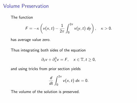
Volume Preservation

The function

F = −κ(v(x , t)− 1

2π

∫ 2π

0v(y , t) dy

), κ > 0.

has average value zero.

Thus integrating both sides of the equation

∂tv + ∂3xv = F , x ∈ T, t ≥ 0,

and using tricks from prior section yields

d

dt

∫ 2π

0v(x , t) dx = 0.

The volume of the solution is preserved.

A Localized Closed Loop Control

We can localize this control to an interval a ≤ x ≤ b by defining

g(x) =1

b − aχ[a,b](x)

and then defining

F = g(x)

(v(x , t)− 1

2π

∫ 2π

0g(y)v(y , t) dy

).

Since∫ 2π0 g(y) dy = 1, this control still preserves the volume of

the solution. Furthermore, “this sort of control can be realized,approximately, by a distributed pumping action.” [2]

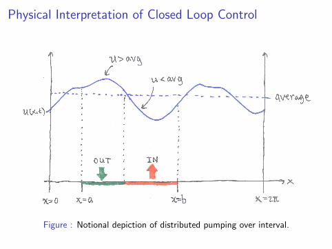
Physical Interpretation of Closed Loop Control

Figure : Notional depiction of distributed pumping over interval.

Stabilization

If we study the closed loop system

∂tv + ∂3xv = −κg(x)

(v(x , t)− 1

2π

∫ 2π

0g(y)v(y , t) dy

),

then exact controllability cannot be attained.

Instead, the solution decays exponentially to a constant:

v(x , t) −→∫ 2π

0g(y)v0(y) dy

as t →∞ (in an L2-sense). This stabilization result is found in [3].

Table of Contents

Control of PDE in the Abstract

A Motivating Detour

The Korteweg-de Vries Equation

A Class of Volume Preserving Controls

Null Controllability of the Linear KdV Equation

Null Controllability of Linear KdV

Goal: Given any T > 0 and a terminal state vT ∈ L2(0, 2π) withaverage value zero, construct F = F (x , t) so that the solution to

∂tv + ∂3xv = F , x ∈ T, t ≥ 0,

v(x , 0) = 0

∂kx v(0, t) = ∂kx v(2π, t), k = 0, 1, 2

satisfies

I preservation of volume ddt

∫ 2π0 v(x , t) dx = 0;

I v(x ,T ) = vT (x) for all x ∈ T.

This result was established by Russell and Zhang [3].

Outline of Proof of Null Controllability

1. Express vT in terms of forcing F .

2. Restrict to volume-preserving control F = Gh.

3. Determine h in terms of vT (hard part).

4. Check that construction works (omitted).

An Important Lemma

Suppose we have a solution v = v(x , t) to the problem∂tv + ∂3xv = F , x ∈ T, t ≥ 0,

v(x , 0) = 0

∂kx v(0, t) = ∂kx v(2π, t), k = 0, 1, 2

For any T > 0 the Fourier coefficients of v(x ,T )

vk =1

2π

∫ 2π

0v(x ,T ) exp(−ikx) dx

satisfy

vk =1

2π

∫ T

0exp(−ik3(T − τ))

∫ 2π

0F (x , τ) exp(−ikx) dxdτ.

This gives v(x ,T ) in terms of F !But how to solve for F in terms of v(x ,T )?

A Proof of the Important Lemma

By Duhamel’s forumla, the solution to the forced equation

∂tv + ∂3xv = F

may be written as

v(x , t) = e−t∂3x v0(x) +

∫ t

0exp(−(t − τ)∂3x )F (x , τ) dτ.

But v0 ≡ 0. Applying the Fourier transform in the x-variable andinterchanging the integrals yields the result.

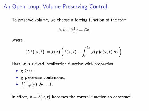
An Open Loop, Volume Preserving Control

To preserve volume, we choose a forcing function of the form

∂tv + ∂3xv = Gh,

where

(Gh)(x , t) := g(x)

(h(x , t)−

∫ 2π

0g(y)h(y , t) dy

).

Here, g is a fixed localization function with properties

I g ≥ 0;

I g piecewise continuous;

I∫ 2π0 g(y) dy = 1.

In effect, h = h(x , t) becomes the control function to construct.

Properties of Gh

The operator G defined by

(Gh)(x) := g(x)

(h(x)−

∫ 2π

0g(y)h(y) dy

)possesses the following properties:

I G : L2(0, 2π)→ L2(0, 2π);

I G is linear;

I G is self-adjoint;

I G preserves volume, that is,∫ 2π0 Gh dx = 0.

Choice of Control

We now make the clever guess

h(x , t) =∑j∈Z

hjqj(t)(Gφj)(x),

where

I the coeffcients hj are to be determined;

I the qj form a special basis for L2(0,T );

I φj(x) = 1√2π

exp(ijx).

Substituting this guess into our important lemma yields

vk =1

2πhke−ik3T‖Gφk‖2L2(0,2π),

completing the construction.

Extension to Nonlinear Problem

Russell and Zhang [4] also proved exact controllability of thenonlinear KdV equation

∂tv + ∂3xv + v∂xv = F , x ∈ T, t ≥ 0,

v(x , 0) = v0

∂kx v(0, t) = ∂kx v(2π, t), k = 0, 1, 2

The approach use for the linear siutation breaks down almostimmediately; exact and null controllability are no longer equivalentand Fourier analysis isn’t directly applicable.

But all is not lost. A contraction mapping technique allows one toapply the linear theory to the nonlinear problem. Smoothing effectsinherent in the equation are necessary to close this argument.

[1] A. K. Griffith and N. K. Nichols, Data Assimilation Using Optimal ControlTheory (1994), available athttps://www.reading.ac.uk/web/FILES/maths/10-94.pdf.

[2] D. L. Russell, Computational study of the Korteweg-de Vries equation withlocalized control action, Distributed parameter control systems(Minneapolis, MN, 1989), Lecture Notes in Pure and Appl. Math., vol. 128,Dekker, New York, 1991, pp. 195–203. MR1108858 (92c:65113)

[3] D. L. Russell and B. Y. Zhang, Controllability and stabilizability of thethird-order linear dispersion equation on a periodic domain, SIAM J.Control Optim. 31 (1993), no. 3, 659–676, DOI 10.1137/0331030.MR1214759 (94g:93018)

[4] , Exact controllability and stabilizability of the Korteweg-de Vriesequation, Trans. Amer. Math. Soc. 348 (1996), no. 9, 3643–3672, DOI10.1090/S0002-9947-96-01672-8. MR1360229 (96m:93025)