Exact analytical solutions for the Poiseuille and Couette-Poiseuille flow of third grade fluid between parallel plates

Commun Nonlinear Sci Numer Simulat 17 (2012) 1089–1097

Contents lists available at SciVerse ScienceDirect

Commun Nonlinear Sci Numer Simulat

journal homepage: www.elsevier .com/locate /cnsns

Short communication

Exact analytical solutions for the Poiseuille and Couette–Poiseuille flowof third grade fluid between parallel plates

Mohammad Danish, Shashi Kumar, Surendra Kumar ⇑Department of Chemical Engineering, Indian Institute of Technology Roorkee, Roorkee 247667, Uttarakhand, India

a r t i c l e i n f o

Article history:Received 22 April 2011Received in revised form 14 July 2011Accepted 24 July 2011Available online 10 August 2011

Keywords:Non-Newtonian fluidPoiseuille flowCouette–Poiseuille flowExact solution

1007-5704/$ - see front matter � 2011 Elsevier B.Vdoi:10.1016/j.cnsns.2011.07.037

⇑ Corresponding author. Tel.: +91 1332 285714; fE-mail address: [email protected] (S. Kumar).

a b s t r a c t

Exact analytical solutions for the velocity profiles and flow rates have been obtained inexplicit forms for the Poiseuille and Couette–Poiseuille flow of a third grade fluid betweentwo parallel plates. These exact solutions match well with their numerical counter partsand are better than the recently developed approximate analytical solutions. Besides,effects of various parameters on the velocity profile and flow rate have been studied.

� 2011 Elsevier B.V. All rights reserved.

1. Introduction

In general, many engineering fluids, e.g. slurries, pastes, polymer solutions, etc. are characterized by non-Newtonian flu-ids. Unlike their Newtonian fluids, these fluids exhibit numerous strange features, e.g. shear thinning/thickening and displayof elastic effects etc. Hence, the classical Navier–Stokes equations become redundant in describing their rheological behav-iour properly. Various rheological models have been proposed to portray their non-Newtonian flow behaviour [1–4]. Onesuch type of rheological model is the differential type fluid model and third grade fluid is one of the subclass of these dif-ferential type fluid models. Due to its ability in successfully capturing various non-Newtonian effects, it has been the subjectof many investigations covering various facets, e.g. thermodynamical aspects [5–7], existence and uniqueness of solutions[8–10], some basic flow situations [7,11–16], etc.

Recently, some of the newly developed approximate analytical tools, e.g. ADM (Adomian decomposition method), HPM(homotopy perturbation method) and HAM (homotopy analysis method) have been employed by various researchers to solveseveral basic flow problems of third grade fluid, and the approximate solutions were found for the velocity profiles [15–19].However, no solution expressions were obtained for the flow rate which unlike velocity profile, is convenient to measure.

In this work, exact solutions for the velocity profiles and flow rates have been obtained for the Poiseuille and Couette–Poiseuille flow of a third grade fluid between two parallel plates. Effects of various parameters on the velocity profilesand flow rates have also been discussed. Pure Couette flow of third grade fluid is not considered, since the exact solutionis already available [18].

2. Mathematical model

Mathematical model of the present flow problem is given by the following equations and the details of their derivationscan be found elsewhere [11,18,19].

. All rights reserved.

ax: +91 1332 273560.

Nomenclature

a velocity of the plate (m/s)A dimensionless velocity of the plate, A ¼ a= � dp

dy

� �h2

l

B dimensionless parameter considered in [18]C1, C2 constants of integration2h separation between the two plates (m)K1, K2, K3 constantsp pressure (N/m2)p modified pressure (N/m2)q fluid flow rate per unit width of the plate (m2/s)Q dimensionless fluid flow rate per unit width of the plateT constant termU dimensionless fluid velocityU0 dimensionless maximum fluid velocityux, uy, uz fluid velocity in the x, y & z coordinates, respectively (m/s)X dimensionless distance in x directionX⁄ dimensionless distance where maximum fluid velocity occursx, y, z distances in x, y & z directions, respectively (m)

Greek Symbolsai, bi material moduli (kg/m, kg.s/m)b dimensionless parameterl fluid viscosity (kg/m.s)q fluid density (kg/m3)

1090 M. Danish et al. / Commun Nonlinear Sci Numer Simulat 17 (2012) 1089–1097

@p@x¼ @

@xð2a1 þ a2Þ

@uy

@x

� �2" #

ð1aÞ

@p@y¼ l @

2uy

@x2 þ 6b3@uy

@x

� �2@2uy

@x2 ð1bÞ

@p@z¼ 0 ð1cÞ

By defining a modified pressure p ¼ p� ð2a1 þ a2Þ @uy

@x

� �2[11,17,18], the above equations can be simplified into the following

forms:

@p@x¼ 0 ð2aÞ

@p@y¼ l @

2u@x2 þ 6b3

@u@x

� �2@2u@x2 ð2bÞ

@p@z¼ 0 ð2cÞ

It should be noted that the Eqs. (2a)–(2c) remain unchanged while portraying the different flow situations arising in the flowpresent problem. However, the allied BCs differ for each of the situations and thus give rise to different solution expressions.

3. Exact solutions

3.1. Case 1: Pure Poiseuille flow of 3rd grade fluid between two stationary parallel plates

In this situation, the movement of fluid is solely due to the pressure gradient and the flow is governed by Eq. (2b) alongwith the following BCs:

BC I : uðhÞ ¼ 0 at x ¼ h ðupper stationary plateÞ ð3aÞ

BC II : uð�hÞ ¼ 0 at x ¼ �h ðlower stationary plateÞ ð3bÞ

M. Danish et al. / Commun Nonlinear Sci Numer Simulat 17 (2012) 1089–1097 1091

Introducing the following dimensionless variables,

Fig. 1.numeri

X ¼ xh; b ¼ b3 �

dpdy

� �2 h2

l3 ; U ¼ u

� dpdy

� �h2

l

the Eqs. (2b), (3a) and (3b) are transformed into the following dimensionless forms:

d2U

dX2 þ 6bdUdX

� �2 d2U

dX2 ¼ �1 ð4aÞ

BC I : UðX ¼ 1Þ ¼ 0 ðupper stationary plateÞ ð4bÞBC II : UðX ¼ �1Þ ¼ 0 ðlower stationary plateÞ ð4cÞ

One of the BCs (say BC II) can be replaced with the following equivalent BC II0, i.e.

BC II0 :dUdX¼ 0 at X ¼ 0 ðmiddle of the two platesÞ ð4c0Þ

By using the transformation dUdX ¼ f ðUÞ, where f(U) is some unknown function of U [20], the Eq. (4a) is rendered into the fol-

lowing form:

w0ð1þ 6bwÞ ¼ �2 ð5Þ

where w = f 2(U) and w0 ¼ dwdU. Eq. (5) is amenable to the following exact solution:

wþ 3bw2 ¼ 2U þ C1 ð6Þ

C1 is the constant of integration and by using BC II’ it is found to be C1 = 2U0. U0 is the unknown dimensionless velocity at thecenterline, i.e. U0 = U(X = 0) and can be found by using BC I. Substituting C1 in Eq. (6) and solving the quadratic equation for w,one obtains the following expression:

w ¼ f ðUÞ2 ¼ dUdX¼ ðU0Þ2 ¼ �1�

ffiffiffiffiffiffiffiffiffiffiffiffiffiffiffiffiffiffiffiffiffiffiffiffiffiffiffiffiffiffiffiffiffiffiffiffi1þ 24bðU0 � UÞ

p6b

ð7Þ

To avoid the imaginary value of U0, the negative sign of radical is dropped, and the following dual valued expression is ob-tained for U0:

U0 ¼ dUdX¼ �

ffiffiffiffiffiffiffiffiffiffiffiffiffiffiffiffiffiffiffiffiffiffiffiffiffiffiffiffiffiffiffiffiffiffiffiffiffiffiffiffiffiffiffiffiffiffiffiffiffiffiffiffiffi�1þ

ffiffiffiffiffiffiffiffiffiffiffiffiffiffiffiffiffiffiffiffiffiffiffiffiffiffiffiffiffiffiffiffiffiffiffiffi1þ 24bðU0 � UÞ

p6b

sð8Þ

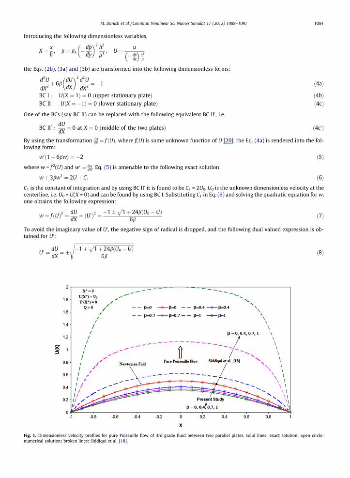
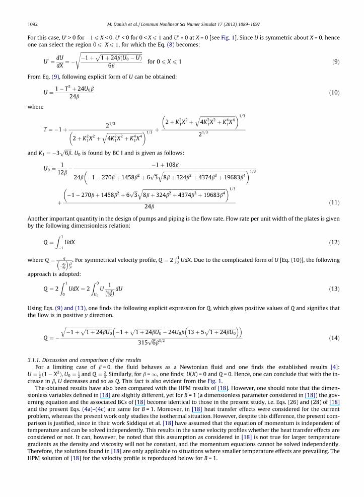
Dimensionless velocity profiles for pure Poiseuille flow of 3rd grade fluid between two parallel plates, solid lines: exact solution; open circle:cal solution; broken lines: Siddiqui et al. [18].

1092 M. Danish et al. / Commun Nonlinear Sci Numer Simulat 17 (2012) 1089–1097

For this case, U0 > 0 for �1 6 X < 0, U0 < 0 for 0 < X 6 1 and U0 = 0 at X = 0 [see Fig. 1]. Since U is symmetric about X = 0, henceone can select the region 0 6 X 6 1, for which the Eq. (8) becomes:

U0 ¼ dUdX¼ �

ffiffiffiffiffiffiffiffiffiffiffiffiffiffiffiffiffiffiffiffiffiffiffiffiffiffiffiffiffiffiffiffiffiffiffiffiffiffiffiffiffiffiffiffiffiffiffiffiffiffiffiffiffi�1þ

ffiffiffiffiffiffiffiffiffiffiffiffiffiffiffiffiffiffiffiffiffiffiffiffiffiffiffiffiffiffiffiffiffiffiffiffi1þ 24bðU0 � UÞ

p6b

sfor 0 6 X 6 1 ð9Þ

From Eq. (9), following explicit form of U can be obtained:

U ¼ 1� T2 þ 24U0b24b

ð10Þ

where

T ¼ �1þ 21=3

2þ K21X2 þ

ffiffiffiffiffiffiffiffiffiffiffiffiffiffiffiffiffiffiffiffiffiffiffiffiffiffiffiffiffiffi4K2

1X2 þ K41X4

q� �1=3 þ2þ K2

1X2 þffiffiffiffiffiffiffiffiffiffiffiffiffiffiffiffiffiffiffiffiffiffiffiffiffiffiffiffiffiffi4K2

1X2 þ K41X4

q� �1=3

21=3

and K1 ¼ �3ffiffiffiffiffiffi6b

p. U0 is found by BC I and is given as follows:

U0 ¼1

12b� �1þ 108b

24b �1� 270bþ 1458b2 þ 6ffiffiffi3p ffiffiffiffiffiffiffiffiffiffiffiffiffiffiffiffiffiffiffiffiffiffiffiffiffiffiffiffiffiffiffiffiffiffiffiffiffiffiffiffiffiffiffiffiffiffiffiffiffiffiffiffiffiffiffiffiffiffiffiffiffiffiffiffiffiffiffiffiffiffiffi

8bþ 324b2 þ 4374b3 þ 19683b4q� �1=3

þ�1� 270bþ 1458b2 þ 6

ffiffiffi3p ffiffiffiffiffiffiffiffiffiffiffiffiffiffiffiffiffiffiffiffiffiffiffiffiffiffiffiffiffiffiffiffiffiffiffiffiffiffiffiffiffiffiffiffiffiffiffiffiffiffiffiffiffiffiffiffiffiffiffiffiffiffiffiffiffiffiffiffiffiffiffi

8bþ 324b2 þ 4374b3 þ 19683b4q� �1=3

24bð11Þ

Another important quantity in the design of pumps and piping is the flow rate. Flow rate per unit width of the plates is givenby the following dimensionless relation:

Q ¼Z 1

�1UdX ð12Þ

where Q ¼ q

�dpdy

� �h3l

. For symmetrical velocity profile, Q ¼ 2R 1

0 UdX. Due to the complicated form of U [Eq. (10)], the following

approach is adopted:

Q ¼ 2Z 1

0UdX ¼ 2

Z 0

U0

U1dUdX

� � dU ð13Þ

Using Eqs. (9) and (13), one finds the following explicit expression for Q, which gives positive values of Q and signifies thatthe flow is in positive y direction.

Q ¼ �

ffiffiffiffiffiffiffiffiffiffiffiffiffiffiffiffiffiffiffiffiffiffiffiffiffiffiffiffiffiffiffiffiffiffiffiffiffiffiffiffi�1þ

ffiffiffiffiffiffiffiffiffiffiffiffiffiffiffiffiffiffiffiffiffiffiffi1þ 24bU0

pq�1þ

ffiffiffiffiffiffiffiffiffiffiffiffiffiffiffiffiffiffiffiffiffiffiffi1þ 24bU0

p� 24U0b 13þ 5

ffiffiffiffiffiffiffiffiffiffiffiffiffiffiffiffiffiffiffiffiffiffiffi1þ 24bU0

p� �� �315

ffiffiffi6p

b3=2 ð14Þ

3.1.1. Discussion and comparison of the resultsFor a limiting case of b = 0, the fluid behaves as a Newtonian fluid and one finds the established results [4]:

U ¼ 12 ð1� X2Þ;U0 ¼ 1

2 and Q ¼ 23. Similarly, for b =1, one finds: U(X) = 0 and Q = 0. Hence, one can conclude that with the in-

crease in b, U decreases and so as Q. This fact is also evident from the Fig. 1.The obtained results have also been compared with the HPM results of [18]. However, one should note that the dimen-

sionless variables defined in [18] are slightly different, yet for B = 1 (a dimensionless parameter considered in [18]) the gov-erning equation and the associated BCs of [18] become identical to those in the present study, i.e. Eqs. (26) and (28) of [18]and the present Eqs. (4a)–(4c) are same for B = 1. Moreover, in [18] heat transfer effects were considered for the currentproblem, whereas the present work only studies the isothermal situation. However, despite this difference, the present com-parison is justified, since in their work Siddiqui et al. [18] have assumed that the equation of momentum is independent oftemperature and can be solved independently. This results in the same velocity profiles whether the heat transfer effects areconsidered or not. It can, however, be noted that this assumption as considered in [18] is not true for larger temperaturegradients as the density and viscosity will not be constant, and the momentum equations cannot be solved independently.Therefore, the solutions found in [18] are only applicable to situations where smaller temperature effects are prevailing. TheHPM solution of [18] for the velocity profile is reporduced below for B = 1.

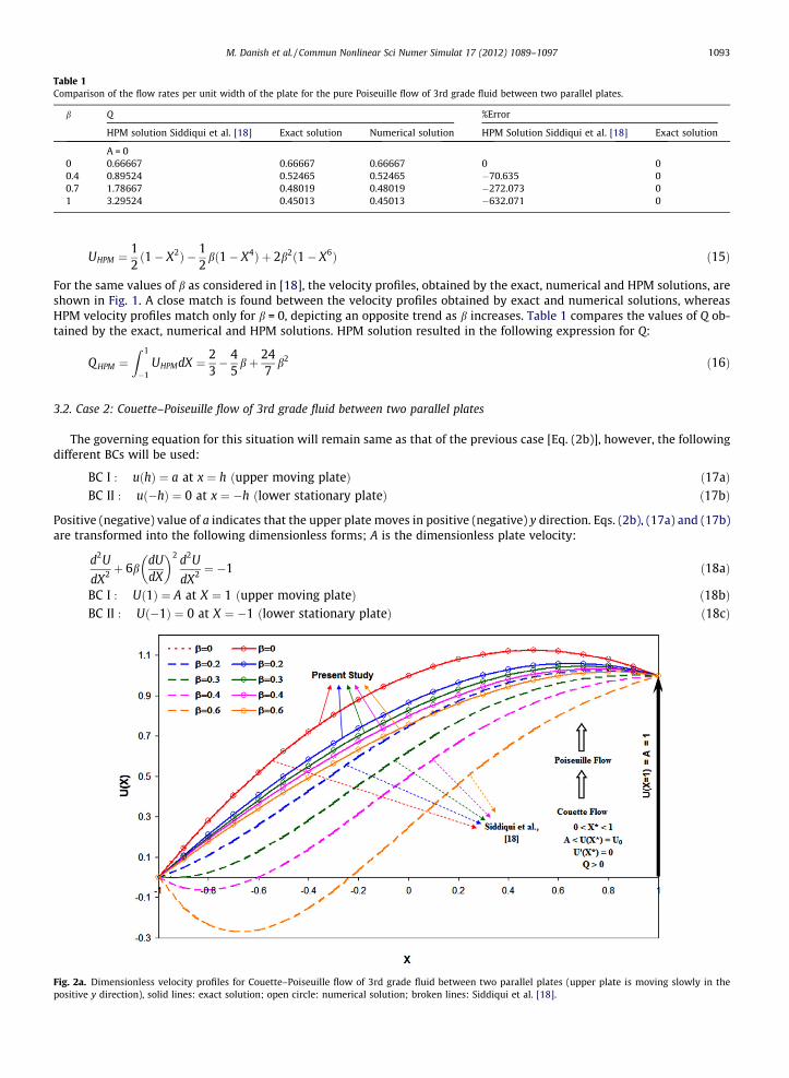
Table 1Comparison of the flow rates per unit width of the plate for the pure Poiseuille flow of 3rd grade fluid between two parallel plates.

b Q %Error

HPM solution Siddiqui et al. [18] Exact solution Numerical solution HPM Solution Siddiqui et al. [18] Exact solution

A = 00 0.66667 0.66667 0.66667 0 00.4 0.89524 0.52465 0.52465 �70.635 00.7 1.78667 0.48019 0.48019 �272.073 01 3.29524 0.45013 0.45013 �632.071 0

Fig. 2a.positive

M. Danish et al. / Commun Nonlinear Sci Numer Simulat 17 (2012) 1089–1097 1093

UHPM ¼12ð1� X2Þ � 1

2bð1� X4Þ þ 2b2ð1� X6Þ ð15Þ

For the same values of b as considered in [18], the velocity profiles, obtained by the exact, numerical and HPM solutions, areshown in Fig. 1. A close match is found between the velocity profiles obtained by exact and numerical solutions, whereasHPM velocity profiles match only for b = 0, depicting an opposite trend as b increases. Table 1 compares the values of Q ob-tained by the exact, numerical and HPM solutions. HPM solution resulted in the following expression for Q:

Q HPM ¼Z 1

�1UHPMdX ¼ 2

3� 4

5bþ 24

7b2 ð16Þ

3.2. Case 2: Couette–Poiseuille flow of 3rd grade fluid between two parallel plates

The governing equation for this situation will remain same as that of the previous case [Eq. (2b)], however, the followingdifferent BCs will be used:

BC I : uðhÞ ¼ a at x ¼ h ðupper moving plateÞ ð17aÞBC II : uð�hÞ ¼ 0 at x ¼ �h ðlower stationary plateÞ ð17bÞ

Positive (negative) value of a indicates that the upper plate moves in positive (negative) y direction. Eqs. (2b), (17a) and (17b)are transformed into the following dimensionless forms; A is the dimensionless plate velocity:

d2U

dX2 þ 6bdUdX

� �2 d2U

dX2 ¼ �1 ð18aÞ

BC I : Uð1Þ ¼ A at X ¼ 1 ðupper moving plateÞ ð18bÞBC II : Uð�1Þ ¼ 0 at X ¼ �1 ðlower stationary plateÞ ð18cÞ

Dimensionless velocity profiles for Couette–Poiseuille flow of 3rd grade fluid between two parallel plates (upper plate is moving slowly in they direction), solid lines: exact solution; open circle: numerical solution; broken lines: Siddiqui et al. [18].

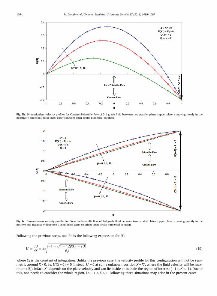
Fig. 2b. Dimensionless velocity profiles for Couette–Poiseuille flow of 3rd grade fluid between two parallel plates (upper plate is moving slowly in thenegative y direction), solid lines: exact solution; open circle: numerical solution.

Fig. 2c. Dimensionless velocity profiles for Couette–Poiseuille flow of 3rd grade fluid between two parallel plates (upper plate is moving quickly in thepositive and negative y directions), solid lines: exact solution; open circle: numerical solution.

1094 M. Danish et al. / Commun Nonlinear Sci Numer Simulat 17 (2012) 1089–1097

Following the previous steps, one finds the following expression for U0:

U0 ¼ dUdX¼ �

ffiffiffiffiffiffiffiffiffiffiffiffiffiffiffiffiffiffiffiffiffiffiffiffiffiffiffiffiffiffiffiffiffiffiffiffiffiffiffiffiffiffiffiffiffiffiffiffiffiffiffiffiffiffiffi�1þ

ffiffiffiffiffiffiffiffiffiffiffiffiffiffiffiffiffiffiffiffiffiffiffiffiffiffiffiffiffiffiffiffiffiffiffiffiffiffi1þ 12bðC1 � 2UÞ

p6b

sð19Þ

where C1 is the constant of integration. Unlike the previous case, the velocity profile for this configuration will not be sym-metric around X = 0, i.e. U0(X = 0) – 0. Instead, U0 = 0 at some unknown position X = X⁄, where the fluid velocity will be max-imum (U0). Infact, X⁄ depends on the plate velocity and can lie inside or outside the region of interest (�1 6 X 6 1). Due tothis, one needs to consider the whole region, i.e. �1 6 X 6 1. Following three situations may arise in the present case:

M. Danish et al. / Commun Nonlinear Sci Numer Simulat 17 (2012) 1089–1097 1095

(i) Upper plate moves in positive y direction but A < U0 or 0 < X⁄ < 1 [see Fig. 2a]. However, if the upper plate moves in thenegative y direction but with U0 > 0, then �1 < X⁄ < 0 [see Fig. 2b]. In both these situations, U0(X⁄) = 0.

(ii) Upper plate moves in the positive y direction but with a velocity higher enough that U0 = A. Thus X⁄ = 1. However,U0(X⁄ = 1) > 0 [see Fig. 2c].

(iii) Upper plate moves in the negative y direction but with a velocity higher enough that U0 = 0. Hence, X⁄ = �1 andU0(X⁄ = �1) < 0 [see Fig. 2c].

3.2.1. Case 2(a): Upper plate moves with a slow velocity in any direction (jAj is small)Solution of this can be obtained by the same methodology of case 1. However, for brevity we present the solutions and the

details may be obtained from the authors.

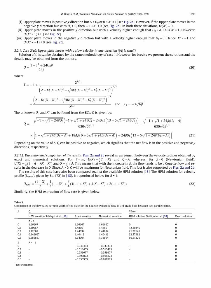
Table 2Compar

b

00.20.30.40.6

b00.20.30.40.6

- Not e

U ¼ 1� T2 þ 24U0b24b

ð20Þ

where

T ¼� 1þ 21=3

2þ K21ðX � X�Þ2 þ

ffiffiffiffiffiffiffiffiffiffiffiffiffiffiffiffiffiffiffiffiffiffiffiffiffiffiffiffiffiffiffiffiffiffiffiffiffiffiffiffiffiffiffiffiffiffiffiffiffiffiffiffiffiffiffiffiffiffiffiffi4K2

1ðX � X�Þ2 þ K41ðX � X�Þ4

q� �1=3

þ2þ K2

1ðX � X�Þ2 þffiffiffiffiffiffiffiffiffiffiffiffiffiffiffiffiffiffiffiffiffiffiffiffiffiffiffiffiffiffiffiffiffiffiffiffiffiffiffiffiffiffiffiffiffiffiffiffiffiffiffiffiffiffiffiffiffiffiffiffi4K2

1ðX � X�Þ2 þ K41ðX � X�Þ4

q� �1=3

21=3 and K1 ¼ �3ffiffiffiffiffiffi6b

p

Q ¼�

ffiffiffiffiffiffiffiffiffiffiffiffiffiffiffiffiffiffiffiffiffiffiffiffiffiffiffiffiffiffiffiffiffiffiffiffiffiffiffiffi�1þ

ffiffiffiffiffiffiffiffiffiffiffiffiffiffiffiffiffiffiffiffiffiffiffi1þ 24bU0

pq�1þ

ffiffiffiffiffiffiffiffiffiffiffiffiffiffiffiffiffiffiffiffiffiffiffi1þ 24bU0

p� 24U0b 13þ 5

ffiffiffiffiffiffiffiffiffiffiffiffiffiffiffiffiffiffiffiffiffiffiffi1þ 24bU0

p� �� �630

ffiffiffi6p

b3=2 þ

ffiffiffiffiffiffiffiffiffiffiffiffiffiffiffiffiffiffiffiffiffiffiffiffiffiffiffiffiffiffiffiffiffiffiffiffiffiffiffiffiffiffiffiffiffiffiffiffiffiffiffiffiffi�1þ

ffiffiffiffiffiffiffiffiffiffiffiffiffiffiffiffiffiffiffiffiffiffiffiffiffiffiffiffiffiffiffiffiffiffiffi1þ 24bðU0 � AÞ

pq630

ffiffiffi6p

b3=2

� 1�ffiffiffiffiffiffiffiffiffiffiffiffiffiffiffiffiffiffiffiffiffiffiffiffiffiffiffiffiffiffiffiffiffiffiffi1þ 24bðU0 � AÞ

pþ 18Ab 6þ 5

ffiffiffiffiffiffiffiffiffiffiffiffiffiffiffiffiffiffiffiffiffiffiffiffiffiffiffiffiffiffiffiffiffiffiffi1þ 24bðU0 � AÞ

p� �þ 24bU0 13þ 5

ffiffiffiffiffiffiffiffiffiffiffiffiffiffiffiffiffiffiffiffiffiffiffiffiffiffiffiffiffiffiffiffiffiffiffi1þ 24bðU0 � AÞ

p� �h ið21Þ

Depending on the value of A, Q can be positive or negative, which signifies that the net flow is in the positive and negative ydirections, respectively.

3.2.1.1. Discussion and comparison of the results. Figs. 2a and 2b reveal an agreement between the velocity profiles obtained byexact and numerical solutions. For b =1: UðXÞ ¼ A

2 ð1þ XÞ and Q = A, whereas, for b = 0 (Newtonian fluid):UðXÞ ¼ 1

2 ð1þ Aþ AX � X2Þ and Q ¼ 23þ A. This means that with the increase in b, the flow tends to be a Couette flow and re-

sults in the decrease in Q. Since, A > 0, Q will be maximum for Newtonian fluid. This fact is also supported by Figs. 2a and 2b.The results of this case have also been compared against the available HPM solution [18]. The HPM solution for velocity

profile (UHPM), given by Eq. (72) in [18], is reporduced below for B = 1:

UHPM ¼ð1þ XÞ

2þ 1

2ð1� X2Þ þ b

4ð3ð�1þ X2Þ þ 4ðX � X3Þ þ 2ð�1þ X4ÞÞ ð22Þ

Similarly, the HPM expression of flow rate is given below:

ison of the flow rates per unit width of the plate for the Couette–Poiseuille flow of 3rd grade fluid between two parallel plates.

Q %Error

HPM solution Siddiqui et al. [18] Exact solution Numerical solution HPM solution Siddiqui et al. [18] Exact solution

A = 11.66667 1.66667 1.66667 0 01.30667 1.4866 1.4866 12.10346 01.12667 1.44032 1.44032 21.77641 00.946667 1.40413 1.40413 32.57982 00.586667 1.34904 1.34904 56.51226 0

A = �1– �0.333333 �0.333333 – 0– �0.513405 �0.513405 – 0– �0.559677 �0.559677 – 0– �0.595873 �0.595873 – 0– �0.650963 �0.650963 – 0

valuated.

1096 M. Danish et al. / Commun Nonlinear Sci Numer Simulat 17 (2012) 1089–1097

QHPM ¼Z 1

�1UHPMdX ¼ 5

3� 9

5b ð23Þ

Discrepancies in UHPM and QHPM are visible in Fig. 2a and Table 2, respectively.

3.2.2. Case 2(b): Upper plate moves in positive y direction with a high velocity (A > 0 and A is large)For this case, one finds the following explicit relation for U.

U ¼ 1� T2 þ 12C1b24b

ð24Þ

where

T ¼ �1þ 3ð2Þ1=3

K3 þffiffiffiffiffiffiffiffiffiffiffiffiffiffiffiffiffiffiffiffiffiffiffiffiffiffiffi�2916þ K2

3

q� �1=3 þKþ3

ffiffiffiffiffiffiffiffiffiffiffiffiffiffiffiffiffiffiffiffiffiffiffiffiffiffiffi�2916þ K2

3

q� �1=3

3ð2Þ1=3 ;

K1 ¼ �3ffiffiffiffiffiffi6b

p;

K2 ¼ffiffiffiffiffiffiffiffiffiffiffiffiffiffiffiffiffiffiffiffiffiffiffiffiffiffiffiffiffiffiffiffiffiffiffiffiffiffiffiffi�1þ

ffiffiffiffiffiffiffiffiffiffiffiffiffiffiffiffiffiffiffiffiffiffi1þ 12C1b

pq2þ

ffiffiffiffiffiffiffiffiffiffiffiffiffiffiffiffiffiffiffiffiffiffi1þ 12C1b

p� �and

K3 ¼ 54þ 27K21 þ 54K1K2 þ 27K2

2 þ 54K21X þ 54K1K2X þ 27K2

1X2:

Unknown constants can be found from the BCs, and Q is given as follows:

Q ¼�

ffiffiffiffiffiffiffiffiffiffiffiffiffiffiffiffiffiffiffiffiffiffiffiffiffiffiffiffiffiffiffiffiffiffiffiffiffiffiffiffi�1þ

ffiffiffiffiffiffiffiffiffiffiffiffiffiffiffiffiffiffiffiffiffiffi1þ 12C1b

pq�1þ

ffiffiffiffiffiffiffiffiffiffiffiffiffiffiffiffiffiffiffiffiffiffi1þ 12C1b

p� 12C1b 13þ 5

ffiffiffiffiffiffiffiffiffiffiffiffiffiffiffiffiffiffiffiffiffiffi1þ 12C1b

p� �� �630

ffiffiffi6p

b3=2 þ

ffiffiffiffiffiffiffiffiffiffiffiffiffiffiffiffiffiffiffiffiffiffiffiffiffiffiffiffiffiffiffiffiffiffiffiffiffiffiffiffiffiffiffiffiffiffiffiffiffiffiffiffiffiffiffiffiffi�1þ

ffiffiffiffiffiffiffiffiffiffiffiffiffiffiffiffiffiffiffiffiffiffiffiffiffiffiffiffiffiffiffiffiffiffiffiffiffiffiffi1þ 12C1b� 24Ab

pq630

ffiffiffi6p

b3=2

� �1þffiffiffiffiffiffiffiffiffiffiffiffiffiffiffiffiffiffiffiffiffiffiffiffiffiffiffiffiffiffiffiffiffiffiffiffiffiffiffi1þ 12C1b� 24Ab

p� 12C1b 13þ 5

ffiffiffiffiffiffiffiffiffiffiffiffiffiffiffiffiffiffiffiffiffiffiffiffiffiffiffiffiffiffiffiffiffiffiffiffiffiffiffi1þ 12C1b� 24Ab

p� �� 18Ab 6þ 5

ffiffiffiffiffiffiffiffiffiffiffiffiffiffiffiffiffiffiffiffiffiffiffiffiffiffiffiffiffiffiffiffiffiffiffiffiffiffiffi1þ 12C1b� 24Ab

p� �h ið25Þ

Since A > 0, Q > 0 and corresponds to the net flow in the positive y direction.

3.2.2.1. Discussion of results. Fig. 2c shows that the velocity profiles obtained by the exact and numerical solutions are in agood agreement. Limiting values of b(=1,0) yield the same expressions of U and Q as those in subcase 2(a).

3.2.3. Case 2(c): Upper plate moves in negative y direction with a high velocity (A < 0 and jAj is large)For this subcase, the following explicit relation for U is obtained:

U ¼ 1� T2 þ 12C1b24b

ð26Þ

where

T ¼ �1þ 3ð2Þ1=3

K3 þffiffiffiffiffiffiffiffiffiffiffiffiffiffiffiffiffiffiffiffiffiffiffiffiffiffiffi�2916þ K2

3

q� �1=3 þKþ3

ffiffiffiffiffiffiffiffiffiffiffiffiffiffiffiffiffiffiffiffiffiffiffiffiffiffiffi�2916þ K2

3

q� �1=3

3ð2Þ1=3 ;

K1 ¼ �3ffiffiffiffiffiffi6b

p; K2 ¼

ffiffiffiffiffiffiffiffiffiffiffiffiffiffiffiffiffiffiffiffiffiffiffiffiffiffiffiffiffiffiffiffiffiffiffiffiffiffiffiffi�1þ

ffiffiffiffiffiffiffiffiffiffiffiffiffiffiffiffiffiffiffiffiffiffi1þ 12C1b

pq2þ

ffiffiffiffiffiffiffiffiffiffiffiffiffiffiffiffiffiffiffiffiffiffi1þ 12C1b

p� �and

K3 ¼ 54þ 27K21 � 54K1K2 þ 27K2

2 þ 54K21X � 54K1K2X þ 27K2

1X2

The unknown constants can be found from the BCs and Q is given by:

Q ¼

ffiffiffiffiffiffiffiffiffiffiffiffiffiffiffiffiffiffiffiffiffiffiffiffiffiffiffiffiffiffiffiffiffiffiffiffiffiffiffiffi�1þ

ffiffiffiffiffiffiffiffiffiffiffiffiffiffiffiffiffiffiffiffiffiffi1þ 12C1b

pq�1þ

ffiffiffiffiffiffiffiffiffiffiffiffiffiffiffiffiffiffiffiffiffiffi1þ 12C1b

p� 12C1b 13þ 5

ffiffiffiffiffiffiffiffiffiffiffiffiffiffiffiffiffiffiffiffiffiffi1þ 12C1b

p� �� �630

ffiffiffi6p

b3=2 �

ffiffiffiffiffiffiffiffiffiffiffiffiffiffiffiffiffiffiffiffiffiffiffiffiffiffiffiffiffiffiffiffiffiffiffiffiffiffiffiffiffiffiffiffiffiffiffiffiffiffiffiffiffiffiffiffiffi�1þ

ffiffiffiffiffiffiffiffiffiffiffiffiffiffiffiffiffiffiffiffiffiffiffiffiffiffiffiffiffiffiffiffiffiffiffiffiffiffiffi1þ 12C1b� 24Ab

pq630

ffiffiffi6p

b3=2

� �1þffiffiffiffiffiffiffiffiffiffiffiffiffiffiffiffiffiffiffiffiffiffiffiffiffiffiffiffiffiffiffiffiffiffiffiffiffiffiffi1þ 12C1b� 24Ab

p� 12C1b 13þ 5

ffiffiffiffiffiffiffiffiffiffiffiffiffiffiffiffiffiffiffiffiffiffiffiffiffiffiffiffiffiffiffiffiffiffiffiffiffiffiffi1þ 12C1b� 24Ab

p� �� 18Ab 6þ 5

ffiffiffiffiffiffiffiffiffiffiffiffiffiffiffiffiffiffiffiffiffiffiffiffiffiffiffiffiffiffiffiffiffiffiffiffiffiffiffi1þ 12C1b� 24Ab

p� �h ið27Þ

Negative Q obtained by Eq. (27) signifies that the net flow is in negative y direction.

3.2.3.1. Discussion of results. Fig. 2c validates the velocity profiles obtained by the exact solution. Limiting values of b(=1,0)gives the same expressions of U and Q as in the subcase 2(a). Since A < 0, Q < 0 for b =1. However for b = 0, Q > 0 or Q < 0depending on the magnitude of A. As A < 0; jQ j ¼ 2

3þ A � �

will be minimum for Newtonian fluid.

M. Danish et al. / Commun Nonlinear Sci Numer Simulat 17 (2012) 1089–1097 1097

4. Conclusions

Exact explicit expressions for the velocity profiles and the flow rates have been obtained for the Poiseuille and Couette–Poiseuille flow of a third grade fluid between two parallel plates, which match well with the numerical solutions and arebetter than the HPM solutions [18]. It is found that the Couette flow features dominate as b and/or jAj are increased. Fora given A, the Poiseuille flow effects are more pronounced in the case of Newtonian fluid (b = 0).

Appendix A. Supplementary data

Supplementary data associated with this article can be found, in the online version, at doi:10.1016/j.cnsns.2011.07.037.

References

[1] Oldroyd JG. On the formulation of rheological equations of state. Proc R Soc Lond A 1950;200:523–41.[2] Rivlin RS, Ericksen JL. Stress-deformation relations for isotropic materials. J Ration Mech Anal 1955;3:323–425.[3] Bird RB, Armstrong RC, Hassager O. Dynamics of polymeric liquids. In: Fluid mechanics. New York: Wiley-Interscience; 1987. vol. 1.[4] Bird RB, Stewart WE, Lightfoot EN. Transport phenomena. 2nd ed. New York: John Wiley & Sons; 2002.[5] Fosdick RL, Rajagopal KR. Thermodynamics and stability of fluids of third grade. Proc R Soc Lond A 1980;339:351–77.[6] Rajagopal KR. On the stability of third grade fluids. Arch Ration Mech Anal 1980;32:867–75.[7] Patria MC. Stability questions for a third-grade fluid in exterior domains. Int J Nonlinear Mech 1989;24:451–7.[8] Bellout H, Necas J, Rajagopal KR. On the existence and uniqueness of flows of multipolar fluids of grade 3 and their stability. Int J Eng Sci

1999;37:75–96.[9] Passerni A, Patria MC. Existence, uniqueness and stability of steady flows of second and third grade fluids in an unbounded ‘‘pipe-like’’ domain. Int J

Nonlinear Mech 2000;35:1081–103.[10] Vajravelu K, Cannon JR, Rollins D, Leto J. On solutions of some nonlinear differential equations arising in third grade fluid flows. Int J Eng Sci

2002;40:1791–805.[11] Rajagopal KR, Sciubba E. Pulsating Poiseuille flow of a non-Newtonian fluid. Math Comput Simul 1984;26:276–88.[12] Majhi SN, Nair VR. Pulsatile flow of third grade fluids under body acceleration-modelling blood flow. Int J Eng Sci 1994;32:839–46.[13] Akyildiz FT, Bellout H, Vajravelu K. Exact solutions of nonlinear differential equations arising in third grade fluid flows. Int J Nonlinear Mech

2004;39:1571–8.[14] Hayat T, Ellahi R, Mahomed FM. Exact solutions for thin film flow of a third grade fluid down an inclined plane. Chaos Solitons Fract 2008;38:1336–41.[15] Sajid M, Hayat T. The application of homotopy analysis method to thin film flows of a third grade fluid. Chaos Solitons Fract 2008;38:506–15.[16] Siddiqui AM, Mahmood R, Ghori QK. Homotopy perturbation method for thin film flow of a third grade fluid down an inclined plane. Chaos Solitons

Fract 2008;35:140–7.[17] Ayub M, Rasheed A, Hayat T. Exact flow of a third grade fluid past a porous plate using homotopy analysis method. Int J Eng Sci 2003;41:2091–103.[18] Siddiqui AM, Zeb A, Ghori QK, Benharbit AM. Homotopy perturbation method for heat transfer flow of a third grade fluid between parallel plates. Chaos

Solitons Fract 2008;36:182–92.[19] Siddiqui AM, Hameed M, Siddiqui BM, Ghori QK. Use of Adomian decomposition method in the study of parallel plate flow of a third grade fluid.

Commun Nonlinear Sci Numer Simul 2010;15:2388–99.[20] Rice RG, Do DD. Applied mathematics and modeling for chemical engineers. New York: John Wiley & Sons Inc.; 1994.