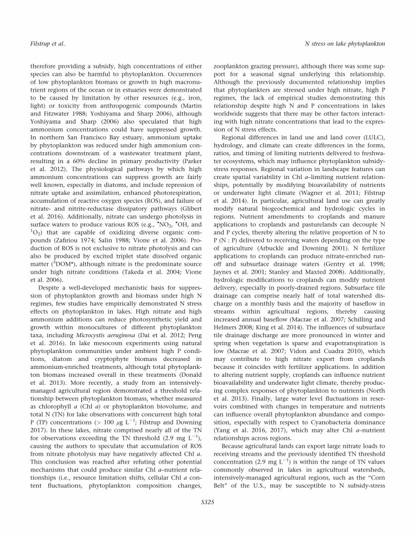
Evidence for regional nitrogen stress on chlorophyll a in lakes across large landscape and climate gradients Christopher T. Filstrup , 1 * Tyler Wagner, 2 Samantha K. Oliver , 3 Craig A. Stow , 4 Katherine E. Webster, 5 Emily H. Stanley, 3 John A. Downing 1 1 Large Lakes Observatory and Minnesota Sea Grant, University of Minnesota Duluth, Duluth, Minnesota 2 U.S. Geological Survey, Pennsylvania Cooperative Fish and Wildlife Research Unit, Pennsylvania State University, University Park, Pennsylvania 3 Center for Limnology, University of Wisconsin, Madison, Wisconsin 4 Great Lakes Environmental Research Laboratory, National Oceanic and Atmospheric Administration, Ann Arbor, Michigan 5 Department of Fisheries and Wildlife, Michigan State University, East Lansing, Michigan Abstract Nitrogen (N) and phosphorus (P) commonly stimulate phytoplankton production in lakes, but recent observations from lakes from an agricultural region suggest that nitrate may have a subsidy-stress effect on chlorophyll a (Chl a). It is unclear, however, how generalizable this effect might be. Here, we analyzed a large water quality dataset of 2385 lakes spanning 60 regions across 17 states in the Northeastern and Mid- western U.S. to determine if N subsidy-stress effects on phytoplankton are common and to identify regional landscape characteristics promoting N stress effects in lakes. We used a Bayesian hierarchical modeling frame- work to test our hypothesis that Chl a–total N (TN) threshold relationships would be common across the central agricultural region of the U.S. (“the Corn Belt”), where lake N and P concentrations are high. Data aggregated across all regions indicated that high TN concentrations had a negative effect on Chl a in lakes with concurrent high total P. This large-scale pattern was driven by relationships within only a subset of regions, however. Eight regions were identified as having Chl a–TN threshold relationships, but only two of these regions located within the Corn Belt clearly demonstrated this subsidy-stress relationship. N stress effects were not consistent across other intense agricultural regions, as we hypothesized. These findings sug- gest that interactions among regional land use and land cover, climate, and hydrogeology may be important in determining the synergistic conditions leading to N subsidy-stress effects on lake phytoplankton. The Law of the Minimum states that plant growth depends on the availability of the nutrient that is scarcest relative to the plant’s need (van der Ploeg et al. 1999). In 1899, Karl Brandt was the first to apply this concept to algal biomass regulation by hypothesizing that algal growth in the oceans was nitrogen (N) limited (de Baar 1994). Whereas N commonly limits phytoplankton growth in the open ocean (Vitousek and Howarth 1991), phosphorus (P) com- monly limits phytoplankton growth in inland freshwaters (Dillon and Rigler 1974; Jones et al. 1976), which has led to the P paradigm for mitigating cultural eutrophication of aquatic ecosystems (Schindler 1977). Historically, far less attention has been paid to the role of N in limiting primary productivity in lakes (but see Scott and McCarthy 2010), despite the documented occurrence of N and P co-limitation in some aquatic ecosystems (Elser et al. 1990; Bracken et al. 2015). Whether or not a resource has a positive effect on pri- mary production also depends on the abundance of that resource, however. Certain resources can have a stimulatory effect on primary productivity until a threshold concentra- tion is reached, beyond which that resource negatively affects primary productivity, thereby displaying a “subsidy- stress gradient” (sensu Odum et al. 1979). For example, phy- toplankters require adequate light to perform photosynthe- sis, although too much light, especially ultraviolet radiation, can inhibit their photosynthetic machinery and impede growth (Marwood et al. 2000; Staehr et al. 2016). In addition to light, N may switch from serving as a sub- sidy to a stress on phytoplankton depending on its absolute concentration and its speciation. While both ammonium and nitrate are assimilated into phytoplankton biomass, *Correspondence: fi[email protected] Additional Supporting Information may be found in the online version of this article. S324 LIMNOLOGY and OCEANOGRAPHY Limnol. Oceanogr. 63, 2018, S324–S339 V C 2017 Association for the Sciences of Limnology and Oceanography doi: 10.1002/lno.10742

Welcome message from author
This document is posted to help you gain knowledge. Please leave a comment to let me know what you think about it! Share it to your friends and learn new things together.
Transcript
Evidence for regional nitrogen stress on chlorophyll a in lakes acrosslarge landscape and climate gradients
Christopher T. Filstrup ,1* Tyler Wagner,2 Samantha K. Oliver ,3 Craig A. Stow ,4
Katherine E. Webster,5 Emily H. Stanley,3 John A. Downing1
1Large Lakes Observatory and Minnesota Sea Grant, University of Minnesota Duluth, Duluth, Minnesota2U.S. Geological Survey, Pennsylvania Cooperative Fish and Wildlife Research Unit, Pennsylvania State University,University Park, Pennsylvania
3Center for Limnology, University of Wisconsin, Madison, Wisconsin4Great Lakes Environmental Research Laboratory, National Oceanic and Atmospheric Administration, Ann Arbor, Michigan5Department of Fisheries and Wildlife, Michigan State University, East Lansing, Michigan
Abstract
Nitrogen (N) and phosphorus (P) commonly stimulate phytoplankton production in lakes, but recent
observations from lakes from an agricultural region suggest that nitrate may have a subsidy-stress effect on
chlorophyll a (Chl a). It is unclear, however, how generalizable this effect might be. Here, we analyzed a
large water quality dataset of 2385 lakes spanning 60 regions across 17 states in the Northeastern and Mid-
western U.S. to determine if N subsidy-stress effects on phytoplankton are common and to identify regional
landscape characteristics promoting N stress effects in lakes. We used a Bayesian hierarchical modeling frame-
work to test our hypothesis that Chl a–total N (TN) threshold relationships would be common across the
central agricultural region of the U.S. (“the Corn Belt”), where lake N and P concentrations are high. Data
aggregated across all regions indicated that high TN concentrations had a negative effect on Chl a in lakes
with concurrent high total P. This large-scale pattern was driven by relationships within only a subset of
regions, however. Eight regions were identified as having Chl a–TN threshold relationships, but only two of
these regions located within the Corn Belt clearly demonstrated this subsidy-stress relationship. N stress
effects were not consistent across other intense agricultural regions, as we hypothesized. These findings sug-
gest that interactions among regional land use and land cover, climate, and hydrogeology may be important
in determining the synergistic conditions leading to N subsidy-stress effects on lake phytoplankton.
The Law of the Minimum states that plant growth
depends on the availability of the nutrient that is scarcest
relative to the plant’s need (van der Ploeg et al. 1999). In
1899, Karl Brandt was the first to apply this concept to algal
biomass regulation by hypothesizing that algal growth in
the oceans was nitrogen (N) limited (de Baar 1994). Whereas
N commonly limits phytoplankton growth in the open
ocean (Vitousek and Howarth 1991), phosphorus (P) com-
monly limits phytoplankton growth in inland freshwaters
(Dillon and Rigler 1974; Jones et al. 1976), which has led to
the P paradigm for mitigating cultural eutrophication of
aquatic ecosystems (Schindler 1977). Historically, far less
attention has been paid to the role of N in limiting primary
productivity in lakes (but see Scott and McCarthy 2010),
despite the documented occurrence of N and P co-limitation
in some aquatic ecosystems (Elser et al. 1990; Bracken et al.
2015). Whether or not a resource has a positive effect on pri-
mary production also depends on the abundance of that
resource, however. Certain resources can have a stimulatory
effect on primary productivity until a threshold concentra-
tion is reached, beyond which that resource negatively
affects primary productivity, thereby displaying a “subsidy-
stress gradient” (sensu Odum et al. 1979). For example, phy-
toplankters require adequate light to perform photosynthe-
sis, although too much light, especially ultraviolet radiation,
can inhibit their photosynthetic machinery and impede
growth (Marwood et al. 2000; Staehr et al. 2016).
In addition to light, N may switch from serving as a sub-
sidy to a stress on phytoplankton depending on its absolute
concentration and its speciation. While both ammonium
and nitrate are assimilated into phytoplankton biomass,
*Correspondence: [email protected]
Additional Supporting Information may be found in the online versionof this article.
S324
LIMNOLOGYand
OCEANOGRAPHY Limnol. Oceanogr. 63, 2018, S324–S339VC 2017 Association for the Sciences of Limnology and Oceanography
doi: 10.1002/lno.10742
therefore providing a subsidy, high concentrations of either
species can also be harmful to phytoplankton. Occurrences
of low phytoplankton biomass or growth in high macronu-
trient regions of the ocean or in estuaries were demonstrated
to be caused by limitation by other resources (e.g., iron,
light) or toxicity from anthropogenic compounds (Martin
and Fitzwater 1988; Yoshiyama and Sharp 2006), although
Yoshiyama and Sharp (2006) also speculated that high
ammonium concentrations could have suppressed growth.
In northern San Francisco Bay estuary, ammonium uptake
by phytoplankton was reduced under high ammonium con-
centrations downstream of a wastewater treatment plant,
resulting in a 60% decline in primary productivity (Parker
et al. 2012). The physiological pathways by which high
ammonium concentrations can suppress growth are fairly
well known, especially in diatoms, and include repression of
nitrate uptake and assimilation, enhanced photorespiration,
accumulation of reactive oxygen species (ROS), and failure of
nitrate- and nitrite-reductase dissipatory pathways (Glibert
et al. 2016). Additionally, nitrate can undergo photolysis in
surface waters to produce various ROS (e.g., •NO2, •OH, and1O2) that are capable of oxidizing diverse organic com-
pounds (Zafiriou 1974; Salin 1988; Vione et al. 2006). Pro-
duction of ROS is not exclusive to nitrate photolysis and can
also be produced by excited triplet state dissolved organic
matter (3DOM*), although nitrate is the predominate source
under high nitrate conditions (Takeda et al. 2004; Vione
et al. 2006).
Despite a well-developed mechanistic basis for suppres-
sion of phytoplankton growth and biomass under high N
regimes, few studies have empirically demonstrated N stress
effects on phytoplankton in lakes. High nitrate and high
ammonium additions can reduce photosynthetic yield and
growth within monocultures of different phytoplankton
taxa, including Microcystis aeruginosa (Dai et al. 2012; Peng
et al. 2016). In lake mesocosm experiments using natural
phytoplankton communities under ambient high P condi-
tions, diatom and cryptophyte biomass decreased in
ammonium-enriched treatments, although total phytoplank-
ton biomass increased overall in these treatments (Donald
et al. 2013). More recently, a study from an intensively-
managed agricultural region demonstrated a threshold rela-
tionship between phytoplankton biomass, whether measured
as chlorophyll a (Chl a) or phytoplankton biovolume, and
total N (TN) for lake observations with concurrent high total
P (TP) concentrations (> 100 lg L21; Filstrup and Downing
2017). In these lakes, nitrate comprised nearly all of the TN
for observations exceeding the TN threshold (2.9 mg L21),
causing the authors to speculate that accumulation of ROS
from nitrate photolysis may have negatively affected Chl a.
This conclusion was reached after refuting other potential
mechanisms that could produce similar Chl a–nutrient rela-
tionships (i.e., resource limitation shifts, cellular Chl a con-
tent fluctuations, phytoplankton composition changes,
zooplankton grazing pressure), although there was some sup-
port for a seasonal signal underlying this relationship.
Although the previously documented relationship implies
that phytoplankters are stressed under high nitrate, high P
regimes, the lack of empirical studies demonstrating this
relationship despite high N and P concentrations in lakes
worldwide suggests that there may be other factors interact-
ing with high nitrate concentrations that lead to the expres-
sion of N stress effects.
Regional differences in land use and land cover (LULC),
hydrology, and climate can create differences in the forms,
ratios, and timing of limiting nutrients delivered to freshwa-
ter ecosystems, which may influence phytoplankton subsidy-
stress responses. Regional variation in landscape features can
create spatial variability in Chl a–limiting nutrient relation-
ships, potentially by modifying bioavailability of nutrients
or underwater light climate (Wagner et al. 2011; Filstrup
et al. 2014). In particular, agricultural land use can greatly
modify natural biogeochemical and hydrologic cycles in
regions. Nutrient amendments to croplands and manure
applications to croplands and pasturelands can decouple N
and P cycles, thereby altering the relative proportion of N to
P (N : P) delivered to receiving waters depending on the type
of agriculture (Arbuckle and Downing 2001). N fertilizer
applications to croplands can produce nitrate-enriched run-
off and subsurface drainage waters (Gentry et al. 1998;
Jaynes et al. 2001; Stanley and Maxted 2008). Additionally,
hydrologic modifications to croplands can modify nutrient
delivery, especially in poorly-drained regions. Subsurface tile
drainage can comprise nearly half of total watershed dis-
charge on a monthly basis and the majority of baseflow in
streams within agricultural regions, thereby causing
increased annual baseflow (Macrae et al. 2007; Schilling and
Helmers 2008; King et al. 2014). The influences of subsurface
tile drainage discharge are more pronounced in winter and
spring when vegetation is sparse and evapotranspiration is
low (Macrae et al. 2007; Vidon and Cuadra 2010), which
may contribute to high nitrate export from croplands
because it coincides with fertilizer applications. In addition
to altering nutrient supply, croplands can influence nutrient
bioavailability and underwater light climate, thereby produc-
ing complex responses of phytoplankton to nutrients (North
et al. 2013). Finally, large water level fluctuations in reser-
voirs combined with changes in temperature and nutrients
can influence overall phytoplankton abundance and compo-
sition, especially with respect to Cyanobacteria dominance
(Yang et al. 2016, 2017), which may alter Chl a–nutrient
relationships across regions.
Because agricultural lands can export large nitrate loads to
receiving streams and the previously identified TN threshold
concentration (2.9 mg L21) is within the range of TN values
commonly observed in lakes in agricultural watersheds,
intensively-managed agricultural regions, such as the “Corn
Belt” of the U.S., may be susceptible to N subsidy-stress
Filstrup et al. N stress on lake phytoplankton
S325

relationships. Here, we analyzed a large dataset of lakes from
diverse regions in the Northeastern and Midwestern U.S. (1)
to determine if evidence consistent with subsidy-stress rela-
tionships exists along TN gradients across regions, (2) to
determine whether these relationships are region-specific or
widespread, and (3) to identify regional landscape character-
istics promoting these effects if they are region-specific. We
hypothesized that N stress effects would be detected in pre-
dominantly agricultural regions throughout the study
extent, in which elevated N and P concentrations driven by
these practices would contribute to phytoplankton stress
responses. By examining empirical relationships between
Chl a and nutrients across diverse regions at large spatial
extents, we gain insight into the mechanisms responsible for
producing N subsidy-stress relationships in lakes. Because N
subsidy-stress relationships have never been explored at this
scale, and given the evidence that various geophysical fea-
tures within regions can alter Chl a–nutrient relationships,
we also hypothesized that landscape features that can
enhance nutrient delivery (e.g., geology, hydrology) or accu-
mulation of ROS in the water column (e.g., nutrient and
water pulses, intervals between storm events) would favor
regional subsidy-stress responses.
Materials
Dataset description
To test our hypotheses, we analyzed the LAke multi-
scaled GeOSpatial and temporal database (LAGOS-NE), as
described by Soranno et al. (2015a), which is a sub-
continental scale, integrated database of lake ecosystems. For
our analyses, we used the following two modules: LAGOS-
NE-GEO v1.05, which contained geospatial data (e.g., climate,
LULC, hydrology, geology) on � 50,000 lakes with surface
areas>4 ha across 17 states in the Northeastern and Mid-
western U.S., and LAGOS-NE-LIMNO v1.054.1, which con-
tained water quality data on � 10,000 of these lakes (Fig. 1;
Soranno et al. 2017). The spatial extent of the database cov-
ers large gradients in LULC, climate, and geology, making it
ideal for testing our hypotheses. Additionally, the database
includes lakes from the intensively managed, row-crop agri-
cultural region of the U.S., also known as the “Corn Belt,”
where N amendments to croplands contribute to high N
export rates from receiving streams (Fig. 1; Howarth et al.
1996). Regions within southwestern Minnesota, Iowa, Illi-
nois, Indiana, and Ohio have been documented as the great-
est contributors of nitrate to the Gulf of Mexico (David et al.
2010).
To maintain consistency with a previous study that dem-
onstrated a Chl a–TN threshold relationship using some of
the data included in this analysis, we used data from individ-
ual sampling events, rather than summarizing data by lake-
year or by lake, despite potential concerns about sample
independence. Filstrup and Downing (2017) commented
that aggregating data by either season or by lake could
obscure nonlinear Chl a responses to TN, which require
numerous extreme TN observations to be adequately mod-
eled and to maintain the statistical power to do so.
Fig. 1. Spatial extent of study region displaying number of observations per lake (circles) and approximate boundaries of the Corn Belt region(yellow).
Filstrup et al. N stress on lake phytoplankton
S326

Additionally, summary statistics, such as sample averages,
calculated from samples of differing sizes will have differing
variances, requiring differential weighting in most common
statistical analyses. The dataset was restricted to samples
with concurrent measures of TN, TP, Chl a, and Secchi
depth. In addition to TN concentrations reported by data
providers, where data on individual N components were
available, TN was calculated by summing total Kjeldahl
nitrogen and nitrate 1 nitrite concentrations. The final data-
set included observations from the upper mixed layer of the
water column (i.e., epilimnion) recorded from May to Sep-
tember during 1990–2013, totaling 19,341 observations
across 2385 lakes, with a median of two observations per
lake (range: 1–407 observations; Fig. 1). In general, lakes
with 201 observations were sampled semi-monthly to
monthly throughout the growing season for a portion of the
dataset’s temporal range, although several of the most fre-
quently sampled lakes had sub-weekly observations poten-
tially from different sampling locations within large natural
and constructed lakes, such as reservoirs in Missouri. Lakes
with the most observations tended to be concentrated in
Missouri, New York, and Iowa. Lakes were distributed across
60 regions defined by U.S. Geological Survey 4-digit hydro-
logic units (HU-4) boundaries within the study extent.
The dataset we analyzed was constructed to answer ques-
tions on broad-scale regional controls on N stress across a
larger and more geographically diverse spatial extent than
that explored in Filstrup and Downing (2017). For example,
the LAGOS-NE-LIMNO dataset (v1.054.1) included observa-
tions within 60 HU-4s within the Northeastern and Midwest-
ern U.S. study extent, including seven overlapping Iowa
state boundaries. The Iowa data included in our analyses
comprised 105 lakes sampled between 2001 and 2009
(n 5 1531 sampling events). These data were a subset of the
more extensive dataset on 139 Iowa lakes representing a lon-
ger monitoring period (2001–2014) and more sampling
events (n 5 4561) analyzed by Filstrup and Downing (2017).
Further, the availability of attributes, such as nitrate and
ammonium concentrations, mixing depth, and phytoplank-
ton and zooplankton biomass and composition, not avail-
able for all lakes in the LAGOS-NE database allowed Filstrup
and Downing (2017) to address more focused mechanistic
questions regarding relationships between Chl a and lake
nutrients within a predominantly agricultural landscape.
Identifying stress responses and regions
To explore potential stress responses, we created contour
plots to visualize Chl a response to both TN and TP follow-
ing procedures used by Filstrup and Downing (2017). Local
polynomial smoothing (2nd-degree polynomial) was used to
grid irregularly-spaced data in Surfer 8 software (Golden Soft-
ware, Golden, Colorado, U.S.A.). Data were not filtered to
remove or summarize “duplicates” (i.e., independent obser-
vations occupying the same x, y-coordinates) prior to
analysis, which allowed for all Chl a values to be considered
by smoothing algorithms. Contours were not extrapolated
beyond the range of the dataset.
As we hypothesized that not all regions within our study
extent would display subsidy-stress relationships, we first
developed a method to exclude these “non-stress” regions
from subsequent analyses so they did not bias our estimation
of N stress thresholds. Because Chl a–nutrient relationships
tend to be sigmoidal (McCauley et al. 1989; Prairie et al.
1989; Filstrup et al. 2014), we were concerned that modeling
threshold responses for individual regions could differ
depending on whether regions primarily had low or high
nutrients; for the former, the threshold would likely occur at
the bottom inflection point (i.e., acceleration phase sensu
Filstrup et al. 2014), whereas the upper asymptote (i.e.,
deceleration phase) would serve as the threshold in the lat-
ter. To ensure that we were only comparing the upper
threshold across regions, we first used Bayesian model selec-
tion to preliminarily identify regions as “stress regions” to be
considered in subsequent subsidy-stress analyses.
The Bayesian choice model identified whether or not a
change point model (i.e., a hockey stick model), which
resembles a subsidy-stress relationship, would better describe
Chl a–TN relationships for each region compared to a linear
model. The hockey stick model was as follows:
yi5b11b2 xi2/ð Þ1�i if xi < /
b11 b21dð Þ xi2/ð Þ1�i if xi � /
((1)
where yi is log10-transformed Chl a, xi is the predictor vari-
able (log10-transformed TN), b1 and b2 are the intercept and
slope prior to the change point /ð Þ, d is the change in the
slope after the change point, and �i is the error term inde-
pendently and identically distributed as N 0; r2� �
. The linear
model was:
yi5a1 cxi1�i (2)
where yi and xi are as defined above, a is the intercept, c is the
slope, and �i is as defined above. Diffuse normal priors were used
for bx, d, a, and c, and uniform priors were used for r and /.
We used Markov chain Monte Carlo simulations within
the program WinBUGS version 1.4 (Spiegelhalter et al. 2003)
to compare the two models. Two parallel Markov chains
with different starting values were simulated, in which the
first 25,000 samples from a total of 40,000 iterations were
excluded as burn-in. For the remaining samples, every other
sample was retained. Model convergence was evaluated
using the Gelman-Rubin convergence statistic (r̂Þ, where val-
ues<1.1 indicate convergence. Additionally, we visually
inspected trace plots and density plots of model parameters
to further assess convergence.
Bayesian model selection was employed to select between
the two candidate models. Model selection was achieved by
Filstrup et al. N stress on lake phytoplankton
S327
introducing a model indicator z to select either model 1, the
linear model (z 5 1), or model 2, the threshold model (z 5 0).
The introduction of the indicator variable allowed for the
posterior frequency of selecting model 1 (f 5 P(z 5 1|data),
where a large value of f indicates preference for model 1. A
Bernoulli prior was used for z, where z � Bernoulli(0.5). We
performed this analysis for each region separately.
For a region to be considered a potential stress region for
subsequent analyses, the following a priori criteria had to be
satisfied. (1) The posterior frequency (f) of selecting the lin-
ear model over the change point model had to be<0.40.
Although this posterior frequency criterion was somewhat
arbitrary, the selection process was largely insensitive to this
value as nearly all retained regions had much stronger pref-
erence for the change point model (f<0.15). (2) The TN
threshold had to be>1 mg L21 to avoid identifying regions
in which the threshold could occur at the lower inflection
point of a sigmoidal Chl a–TN relationship, as previously
mentioned. (3) The post-threshold slope had to be negative
to identify regions in which TN concentrations were stressful
(i.e., had a negative effect) on Chl a. We were conservative
in excluding regions where the post-threshold slope was
smaller, but still positive, compared to the pre-threshold
slope, which could have simply indicated shifting resource
limitation. (4) At least 10% of observation within a region
had to be greater than the regional TN threshold to system-
atically discard regions in which a small number of observa-
tions were driving the negative post-threshold slope (i.e.,
exclude potentially coincidental relationships).
Identifying landscape characteristics promoting N stress
For regions identified as stress regions by Bayesian model
selection, we subsequently modeled Chl a–TN relationships
using a Bayesian hierarchical threshold model, in which all
model parameters were allowed to vary across regions. The
hierarchical threshold model allowed for subsidy-stress rela-
tionships to be quantified at the population level (i.e., across
all regions and considering all observations) and at the
regional level (i.e., within each individual region). The
Bayesian hierarchical threshold model was as follows:
yi � N aj i½ �1bj i½ �xi1dj i½ � xi2/j i½ �
� �1; r2
� �for i51 . . . ;n (3)
aj
bj
dj
/j
0BBBBBBB@
1CCCCCCCA� MVN l;Rð Þ for j51 . . . J (4)
l5 �a; �b; �d; �/� �
(5)
where yi is log10-transformed Chl a, xi is the predictor vari-
able (log10-transformed TN), and the spatially-varying
(region-specific) parameters include the intercepts aj
� �,
regression slopes prior to the change point ðbjÞ, change in
regression slopes after the change points dj
� �, and the change
points ð/jÞ. The index j i½ � indexes region j for observation i.
The term ðxi2/j i½ �Þ1 is equal to ðxi2/j i½ �Þ if xi > /j, and 0 other-
wise. The parameters �a; �b; �d; �/ describe the threshold
response across all regions (i.e., the population-average
response). Diffuse normal priors were used for �a; �b; �d; �/, and
diffuse uniform prior for r, and R was modeled using the
scaled inverse-Wishart distribution (Gelman and Hill 2007).
The model was fit using the program Just Another Gibbs Sam-
pler (Plummer 2012). Three parallel Markov chains with differ-
ent starting values were simulated from a total of 1,000,000
iterations, of which the first 850,000 samples were excluded as
burn-in. For the final 150,000 iterations, every fourth sample
was retained. Model convergence was evaluated using r̂ , trace
plots, and density plots of posterior distributions.
We considered LULC categories and climate and hydrogeol-
ogy metrics to identify regional landscape characteristics pro-
moting N stress in regions. Although we originally intended to
predict regional threshold model parameters (i.e., threshold
and post-threshold slope) as a function of landscape characteris-
tics, the low number of stress regions did not provide the statis-
tical power needed to do so. Therefore, we qualitatively
compared landscape characteristics between “stress” and “non-
stress” regions. Because water quality data were from 1990 to
2013, where possible, landscape characteristics were selected to
correspond to this temporal range. Percent row-crop agricul-
ture, pasture, and wetlands (woody 1 herbaceous) within
regions were evaluated because of their previously documented
influences on regional Chl a–nutrient relationships (Wagner
et al. 2011; Filstrup et al. 2014). LULC data were obtained from
the 2001 National Land Cover Dataset (Homer et al. 2007),
which represented LULC characteristics most closely corre-
sponding to the midpoint of our dataset’s duration. Regional
precipitation was represented as 30-yr normals (1981–2010)
using PRISM data (PRISM Climate Group, Oregon State Univer-
sity, http://www.prism.oregonstate.edu, created 2004 February
04). Regional average runoff data were obtained from the U.S.
Geological Survey (https://water.usgs.gov/GIS/metadata/
usgswrd/XML/runoff.xml). We also considered atmospheric
deposition of TN and nitrate because of its importance in deter-
mining nutrient limitation in some lakes, especially those
removed from intense watershed modification and human
activities (Bergstr€om and Jansson 2006; Elser et al. 2009).
Regional TN and nitrate deposition data from 2000 were
obtained from the National Atmospheric Deposition Program
(http://nadp.sws.uiuc.edu/ntn/annualmapsByYear.aspx). Data
sources and LAGOS-NE-GEO database development are
described in Soranno et al. (2015a).
Results
Identifying stress responses and regions
For individual sampling events, water quality conditions
within the study extent spanned a broad trophic gradient,
Filstrup et al. N stress on lake phytoplankton
S328

with individual observations ranging widely in Chl a (< 0.1–
743 lg L21), TN (0.06–20.57 mg L21), and TP (0.4–1623.0 lg
L21). Consequently, average water quality conditions within
regions ranged from low nutrient, low productivity regions
to high nutrient, high productivity regions (Supporting
Information Table 1). Median regional Chl a (18.4 lg L21),
TN (0.8 mg L21), and TP (50.3 lg L21) concentrations sug-
gest that a large proportion of lakes were eutrophic in a
majority of regions. Due to regional differences in nutrient
concentrations, average phytoplankton growth conditions
ranged from stoichiometrically balanced to P-deficient
growth conditions (TN : TP by atoms: 30.8–170.9), with
most regions (n 5 46 of 60 regions) displaying P-deficient
growth conditions (Supporting Information Table 1).
When considering all lakes across the study’s spatial
extent, the relationship between Chl a and TN and TP
diverged depending on the relative availability of these
nutrients. At TP<100 lg L21 (2.0 as log10-transformed
value), Chl a did not respond to changing TN across a two
order-of-magnitude TN gradient, as demonstrated by the
nearly vertical Chl a contours (Fig. 2). In contrast, increased
TN was accompanied by increased Chl a when TP exceeded
100 lg L21. The highest Chl a concentrations were not
found for observations with the highest TP and TN concen-
trations, as predicted by N and P co-limitation paradigms,
but rather occurred when TP was high and TN moderate.
When TP exceeded 100 lg L21, Chl a displayed a unimodal
response to TN, in which Chl a was positively related to TN
at low TN intervals and negatively related to TN at high TN
intervals (Fig. 2).
We used Bayesian model selection to identify potential
stress regions defined by those for which change point mod-
els better fitted regional Chl a–TN relationships compared to
linear models. Of the 60 regions included in this study, only
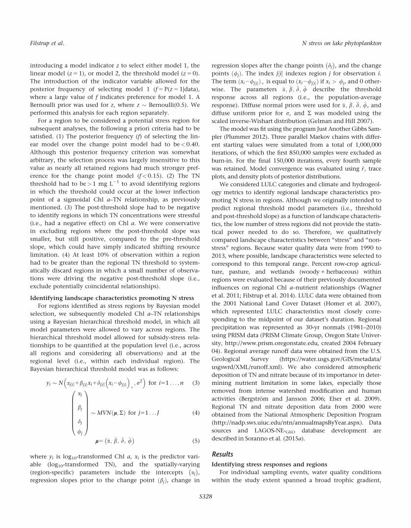
eight were identified as stress regions (Fig. 3). These regions
had strong preferences for the change point model compared
to the linear model, with linear model preference values
below 0.15 for seven regions. In these seven regions, the per-
centage of observations greater than or equal to regional TN
thresholds ranged from 13.5% to 63.0%, with two regions in
Iowa having the highest percentages. Due to a small sample
size, it was more difficult to discern between the two models
(linear model preference 5 0.28) for the other potential stress
region (HU4_50), in which only six observations had TN
concentrations greater than the regional TN threshold. Over-
all, these eight regions were preliminarily classified as stress
regions and were retained in subsequent analyses.
Identifying landscape characteristics promoting N stress
When aggregating observations across the eight stress
regions, Chl a displayed a threshold relationship with TN
(Fig. 4), with concentrations increasing with TN below the
TN threshold, but decreasing above 1.81 mg L21 (0.26 as
log10-transformed value). This TN threshold estimate had
95% credible intervals (CI) of 0.87–3.82 mg L21. Population
average pre- and post-threshold slopes were estimated at
1.44 (95% CI: 0.99, 1.88) and 20.58 (95% CI: 21.21, 20.01),
respectively. Overall, 24.2% (n 5 906) of observations had TN
concentrations equal to or exceeding this population average
TN threshold.
When examining individual region parameter estimates,
Chl a–TN relationships were weaker for most of these eight
regions and TN thresholds varied from 1.05 mg L21 to
3.66 mg L21 (0.0–0.6 as log10-transformed values; Supporting
Information Table 2; Fig. 5). Due to a small number of total
observations or a low percentage of observations above
Fig. 2. Chl a (lg L21) contour plot on TN (mg L21) vs. TP (lg L21) space. Contours were created using 2nd-degree local polynomial smoothing ofindividual sample observations. All variables were log10-transformed.
Filstrup et al. N stress on lake phytoplankton
S329
regional thresholds for most regions, uncertainty in modeled
relationships was often high either across the entire TN
range (e.g., Fig. 5c) or across TN concentrations greater than
regional TN thresholds (e.g., Fig. 5b). Additionally, three
regions (Fig. 5b,c,f) had 95% CI for post-threshold slope esti-
mates overlapping zero (Supporting Information Table 2). In
contrast, two regions (Fig. 5d,e) had tighter confidence inter-
vals across their entire TN ranges, including those for their
post-threshold slope estimates (Supporting Information
Table 2), due to a more equitable distribution of observations
before and after regional TN thresholds. TN thresholds were
2.06 mg L21 and 1.85 mg L21 for these two regions, respec-
tively. These findings suggest that although eight regions
were preliminarily identified as potential stress regions, for
the remaining six, we either have not captured high TN
events and could not obtain precise parameter estimates, or
high TN events did not occur in these regions and neither
the change point model nor the linear model was an appro-
priate approximation of Chl a–TN relationships. Only two
regions appeared to be driving the Chl a–TN relationships at
the population level (i.e., across all stress regions; Fig. 4).
Both of these regions had>300 observations (n 5 313 and
314, respectively) of high TN concentrations exceeding the
estimated change point that contributed to the increased
precision of the post-change point slope for the population-
average estimate compared to the region-specific estimates.
Additionally, relationships from these two regions suggest
that TN concentrations exceeding 2 mg L21 (0.30 as log10-
transformed value) may negatively influence Chl a
concentrations.
The eight stress regions were restricted to the western por-
tion of our study extent and were located along the entire
north-south gradient of this study (Fig. 6). These regions dif-
fered widely in their LULC characteristics for row-crop agri-
culture (4.5–73.7%), pasturelands (4.7–27.1%), and wetlands
(1.3–26.2%). Counter to our hypothesis, stress regions were
located within some, but not all, of the regions with the
highest row-crop agriculture land use (Fig. 6a). Because of
the different LULC characteristics for stress regions, average
nutrient concentrations for lakes within the stress regions
varied from medium to high (Fig. 7). With the exception of
the southern-most stress region, average regional TN concen-
trations in stress regions ranged from 0.96 mg L21 to
4.24 mg L21, but stress regions were not exclusive to the
Fig. 3. Chl a–TN relationships for each region located within this study’s spatial extent. For regions that met the criteria of stress regions, vertical lines
representing the TN change point and values (lower left corner) indicating preference for the linear model (low values 5 change point model prefer-ence) are displayed. Markers representing individual lake observations are transparent, so darker clusters represent overlapping markers. Variables were
log10-transformed.
Filstrup et al. N stress on lake phytoplankton
S330

highest TN regions (Supporting Information Table 1; Fig.
7a). Similarly, stress regions were not restricted to the high-
est TP regions (Fig. 7b). Average regional TP concentrations
in stress regions ranged from 50.5 lg L21 to 443.1 lg L21,
although they fell within the upper half of regional TP con-
centrations across all regions (median: 50.3 lg L21; Support-
ing Information Table 1).
Regional landscape characteristics varied less for the two
regions that demonstrated the strongest subsidy-stress rela-
tionships. These regions had two of the six highest percen-
tages for row-crop agriculture (66.6% and 69.7%),
percentages of pasturelands within the upper 50th percentile
(7.5% and 12.3%), and low percentages of wetlands (< 3.0%
each) compared to the other six “stress” regions and all
other regions (Fig. 6). Average nutrient concentrations like-
wise were high for these two regions (Fig. 7), with average
TN concentrations>4.00 mg L21, ranking 2nd and 3rd over-
all, and average TP concentrations>98 lg L21 (Supporting
Information Table 1). Despite relatively high TP concentra-
tions, these regions had the two highest TN : TP ratios of
any region included in this study (Supporting Information
Table 1; Fig. 7c). In contrast, other regions with high TP con-
centrations commonly had low TN : TP ratios (c.f., Fig. 7b,c).
Because the spatial distribution of stress regions countered
hypotheses based solely on LULC, we also considered
regional variability in climate, hydrology, and atmospheric
N deposition as potential factors promoting N stress regions.
Excluding the southern-most stress region, stress regions
were located within medium to low precipitation regions
compared to other regions within the study extent, with the
two distinct stress regions having low mean annual precipi-
tation (Fig. 8a). Because variability in annual runoff rates
largely followed that of mean annual precipitation, these
two stress regions also had among the lowest annual runoff
rates. Atmospheric deposition of TN was commonly lowest
along the western portion of our study extent, where our
stress regions occurred, and greatest further east into Michi-
gan, Ohio, Pennsylvania, and New York (Fig. 8b). Atmo-
spheric deposition of nitrate followed similar spatial
patterns, but tended to make up an increasing percentage of
TN deposition moving from west to east.
Discussion
In this study, we found evidence consistent with N
subsidy-stress effects on Chl a within individual regions
across a broad spatial extent. Counter to expectations, how-
ever, subsidy-stress relationships were not widespread in agri-
cultural regions, but were limited to two of the most intense
agricultural regions considered in this study, which included
the study extent of Filstrup and Downing (2017). Because
these two regions contributed a majority of high nutrient
lake observations, patterns between Chl a and nutrients were
similar between the two studies, with Chl a displaying little
response to TN when TP concentrations were below 100 lg
L21 and a unimodal response to TN when TP exceeded 100
lg L21 in this study (Fig. 2). Overall, this general pattern
between Chl a and nutrients agrees with Liebig’s Law of the
Minimum and nutrient limitation theory by demonstrating
that N concentrations have little effect on phytoplankton
biomass when P concentrations are likely to be limiting. Fur-
ther, this finding suggests that Chl a predictive models can
be improved by including TN and TN : TP in addition to TP,
as has been previously demonstrated (Smith 1982; Canfield
1983; Prairie et al. 1989), although the importance and
direction of their effect on Chl a may depend on the abso-
lute concentrations of both N and P. Additionally, the TN
threshold of 1.81 mg L21 found in this study was slightly
lower, but of similar order-of-magnitude, to the previously-
demonstrated threshold (2.93 mg L21; Filstrup and Downing
2017), likely resulting from the majority of high nutrient
observations being from regions contained within the over-
lapping spatial extent of the two studies.
In contrast to previous empirical studies demonstrating
either log-linear or log-sigmoidal relationships between Chl
a and TN (Sakamoto 1966; Canfield 1983; Prairie et al.
1989), our study demonstrated a Chl a threshold response to
TN (Fig. 4). The variation in the form of these empirical rela-
tionships may be due to differences in the ranges and distri-
butions of TN concentrations considered in each study, as
well as the manner in which data were aggregated. For
Fig. 4. Population-level change point model of Chl a–TN relationshipfor lakes across the eight regions identified as stress regions. Black linerepresents the median change point model fit to lake observations (indi-
vidual markers). Gray shaded region represents 95% credible region.Solid vertical black line is the population-level average TN threshold,
whereas dashed vertical black lines are the 95% confidence intervalsaround the threshold estimate. Markers are transparent, so darker clus-ters represent overlapping markers. Chl a (lg L21) and TN (mg L21)
were log10-transformed.
Filstrup et al. N stress on lake phytoplankton
S331
example, the two studies displaying log-linear relationships
had lower TN concentration gradients, achieving maximum
TN concentrations of 5–6 mg L21 (Sakamoto 1966; Canfield
1983), whereas the studies displaying nonlinear relationships
on log-log scales had maximum TN concentrations exceed-
ing 10 mg L21 (Prairie et al. 1989; this study). While the
dataset analyzed by Prairie et al. (1989) only contained one
observation exceeding 10 mg L21 TN, the dataset analyzed
here contained 136 observations with TN greater than 10 mg
L21 and the upper quartile of TN concentrations exceeding
1 mg L21. The rarity of high TN data in the former study
likely resulted from aggregating data by lake-wide averages,
whereas using observational data (this study) may be
required to produce enough high TN observations to identify
N stress effects. Although the TN threshold was estimated at
1.81 mg L21 with TN concentrations commonly exceeding
this threshold in regions throughout the study extent (Figs.
3, 4), this inter-study comparison suggests that numerous
observations with high TN conditions (> 10 mg L21) are
required to reveal N stress effects on Chl a (i.e., model the
negative arm of the threshold model). Further, the two stress
regions that most clearly displayed threshold relationships
had the largest proportions of observations beyond their
regional TN thresholds, as well as having the highest num-
ber of high TN observations (Fig. 5d,e). The rarity of high
TN observations from other agricultural regions may be one
of the reasons why N stress regions were not as common as
we anticipated.
Additionally, the occurrence of N stress regions was not
simply a question of agricultural land use, as we originally
hypothesized. N subsidy-stress effects on Chl a were not
common within other predominantly agricultural regions
Fig. 5. Region-specific change point models of Chl a–TN relationships for lakes across the eight regions identified as stress regions. Regions are (a)
HU4_32, (b) HU4_33, (c) HU4_50, (d) HU4_56, (e) HU4_57, (f) HU4_60, (g) HU4_61, and (h) HU4_67. Black line represents the median change pointmodel fit to lake observations (individual markers). Gray shaded region represents 95% credible region. Markers are transparent, so darker clusters rep-
resent overlapping markers. Chl a (lg L21) and TN (mg L21) were log10-transformed.
Filstrup et al. N stress on lake phytoplankton
S332

Fig. 6. Percent LULC by region for (a) row crop agriculture, (b) pas-turelands, and (c) woody and herbaceous wetlands. Black boundariesrepresent individual regions. Red boundaries identify regions selected as
stress regions by the Bayesian choice model, whereas thick red bound-aries identify the two regions that strongly demonstrated subsidy-stress
relationships. Values were categorized by quintiles for mapping.
Fig. 7. Regional average concentrations for (a) TN (mg L21) and (b) TP (lgL21) and (c) regional average ratios of TN-to-TP (TN : TP; by atoms). Black
boundaries represent individual regions. Red boundaries identify regionsselected as stress regions by the Bayesian choice model, whereas thick redboundaries identify the two regions that strongly demonstrated subsidy-
stress relationships. Values were categorized by quintiles for mapping.
Filstrup et al. N stress on lake phytoplankton
S333

located within the Corn Belt (Fig. 6a), although the two
regions that were primarily responsible for creating the Chl
a–TN threshold relationship observed across all eight stress
regions had high proportions of agricultural land use (Figs.
4, 5). Combined with the fact that these two stress regions
had the 2nd and 3rd greatest regional average TN concentra-
tions, these findings suggest that rather than simply examin-
ing proportional coverage of agricultural practices, more
detailed information on the practices themselves, along with
a greater number of observations per lake collected through-
out the growing season, are required to detect the effect of
high N concentrations on Chl a. For example, the form of
dissolved inorganic N (DIN) is also important if N stress
effects on phytoplankton result from accumulation of
nitrate-derived ROS in the water column (Takeda et al. 2004;
Vione et al. 2006), as was hypothesized by Filstrup and
Downing (2017). In regions where anhydrous ammonia
amendments to croplands are large, lakes can have high
nitrate concentrations within the water column due to oxi-
dation of ammonia within soils and receiving waters,
whereas high urea concentrations may be more common in
lakes where manure or other urea-based fertilizer applica-
tions predominate (Glibert et al. 2006). For example, Cooke
and Prepas (1998) found that nitrate dominated DIN compo-
sition in cropland watersheds compared to dominance of
ammonium in mixed agricultural watersheds. Although high
ammonium concentrations can also suppress phytoplankton
growth (Glibert et al. 2016), high TN concentrations in the
two stress regions were almost exclusively driven by nitra-
te 1 nitrite (Filstrup and Downing 2017).
The occurrence of Chl a–TN threshold relationships under
concurrent high TP regimes (> 100 lg L21) suggests that TN
and TP were interacting to determine whether high N con-
centrations provided a subsidy or induced a stress in phyto-
plankters (Fig. 2). Different types of agriculture can have
differing effects on natural biogeochemical cycles, thereby
modifying the relative export of N and P to receiving
streams. For example, lakes in watersheds dominated by
row-crop agriculture tend to have high TN : TP ratios,
whereas lakes in watersheds dominated by pasturelands tend
to have low TN : TP ratios (Downing and McCauley 1992;
Arbuckle and Downing 2001). Despite having amongst the
highest TP concentrations, the two stress regions maintained
the two highest TN : TP ratios of any region included in this
study (Supporting Information Table 1; Fig. 7c), indicating
that anhydrous ammonia applications were outpacing P
export from croplands (Dinnes et al. 2002). In contrast,
other regions with medium to high TP concentrations
located within the Corn Belt commonly had relatively low
TN : TP ratios (c.f., Fig. 7b,c). This finding implies that N
serves as a subsidy to phytoplankters when systems are
under balanced or N-deficient growth conditions because N
is in short supply relative to P and therefore is assimilated
into phytoplankton biomass, whereas under strict P-deficient
growth conditions, N is present in excess relative to growth
requirements and therefore can accumulate in the water col-
umn. The regional average TN : TP ratios for the two stress
regions (171 and 155 by atoms) were more than triple the
threshold value demarcating P-deficient growth conditions
(50 by atoms; Guildford and Hecky 2000). This finding sug-
gests that regions where N amendments to croplands result
in high nitrate concentrations in receiving water that also
have high enough N : P to maintain strict P-deficient growth
conditions are most susceptible to displaying N stress effects.
Combined with surplus nutrients on croplands, the move-
ment of nutrients from the landscape to receiving streams,
which can be influenced by interactions among LULC, cli-
matic patterns, and hydrology, may be important in
Fig. 8. Regional values for (a) mean annual precipitation (mm yr21)
and (b) atmospheric TN deposition for the year 2000 (kg ha21). Blackboundaries represent individual regions. Red boundaries identify regions
selected as stress regions by the Bayesian choice model, whereas thickred boundaries identify the two regions that strongly demonstratedsubsidy-stress relationships. Values were categorized by quintiles for
mapping.
Filstrup et al. N stress on lake phytoplankton
S334
identifying N stress regions. Previous studies have demon-
strated the importance of lake landscape position, hydrogeo-
morphology, and watershed permeability in helping
determine lake water quality responses to watershed LULC
and anthropogenic activities (Martin and Soranno 2006; Bre-
migan et al. 2008; Fraterrigo and Downing 2008; Soranno
et al. 2015b). Clustering of the eight stress regions with
respect to an east-west precipitation gradient, rather than a
strict LULC gradient (Figs. 6, 8a), suggests that runoff and
lake hydrologic connectivity contributed to the spatial distri-
bution of N stress regions. Because most stress regions were
also located within medium to low atmospheric TN deposi-
tion regions (Fig. 8b), high TN concentrations likely origi-
nated from N export from the surrounding terrestrial
landscape. Counterintuitive to these claims, most N stress
regions had medium to low mean annual precipitation rates
for our study region (Fig. 8a), possibly suggesting that the
intensity, frequency, or timing of nutrient delivery or all
three may contribute to mechanisms underlying N stress.
Experimental studies have previously demonstrated that
pulsed delivery of nutrients modify phytoplankton commu-
nity responses to nutrients compared to steady-state delivery
(Sommer 1985; Suttle et al. 1987). In regions with highly
permeable landscapes, such as intensively-managed agricul-
tural regions with tile drainage (Fraterrigo and Downing
2008), infrequent pulses of high nitrate loads to lakes may
create conditions conducive to accumulation of ROS and
resulting stress responses by phytoplankters: rapid increases
in nitrate to high water column concentrations may undergo
photolysis to produce ROS, which accumulate in the water
column and react with dissolved organic matter (DOM) and
phytoplankton for extended periods before the next flushing
event. Alternatively, water level fluctuations resulting from
large runoff events can alter phytoplankton biomass and
composition (Yang et al. 2016, 2017), potentially modifying
phytoplankton response to N stress. These findings may also
indicate that the timing of high nitrate pulses, which often
coincide with spring storms following fertilizer and herbicide
applications (Gaynor et al. 1992; Becher et al. 2001), could
decouple Chl a response to high TN concentrations through
negative effects of herbicides on phytoplankton (DeNoyelles
et al. 1982; Bester et al. 1995). Further evidence would be
needed to support these hypotheses, however.
Although six stress regions did not have enough observa-
tions with high TN concentrations to clearly define potential
Chl a–TN threshold relationships, the remaining two stress
regions may provide insight into the optimal combination
of conditions that make systems vulnerable to N stress. Large
N amendments to croplands that are heavily tile drained can
result in pulses of high nitrate concentrations to receiving
streams and lakes (Gentry et al. 1998; Jaynes et al. 2001;
David et al. 2010). These high nitrate loads help maintain
strict P-deficient growth conditions despite high P concen-
trations in lakes, which allows high nitrate concentrations to
be maintained in the water column for extended periods.
Concurrently, high P concentrations stimulate phytoplank-
ton productivity that may increase interactions among vari-
ous ROS and phytoplankters, potentially allowing them to
interact for extended periods between storm-driven flushing
events. In lakes within these two stress regions, DOM pri-
marily originates from autochthonous sources (A. Morales-
Williams pers. comm.), potentially supporting the hypothe-
sis that either Chl a or phytoplankton cell lysis can result
from interactions with ROS. These same factors may also
reduce the duration in which N is stressful to phyto-
plankters. DOM has been demonstrated to be an effective
scavenger of ROS (Brezonik and Fulkerson-Brekken 1998), so
ROS would be increasingly scavenged as more phytoplank-
ton cells are lysed. Additionally, droughts can cause some
systems in agricultural watersheds to shift to N-limitation
(Hayes et al. 2015), which is hypothesized to cause nitrate to
shift from a stress to a subsidy with increasing time since the
last flushing event. Combined with chlorophyll’s protective
systems against oxidative stress (Salin 1988), these opposing
mechanisms suggest that N stress effects are ephemeral and
highly dynamic in both space and time, and therefore
require further study.
In addition to considering stress induced by accumulation
of nitrate-derived ROS as a potential mechanism underlying
these relationships, we tested whether seasonal effects based
on phytoplankton phenology could be influencing the high
nutrient, low Chl a region. Filstrup and Downing (2017)
found that high TN concentrations occurred more frequently
in early summer, potentially occurring before phytoplankton
biomass was able to develop under more favorable tempera-
ture and light conditions in mid- to late summer. In agricul-
tural regions, fertilizer applications in spring can lead to
high N concentrations in receiving streams, especially when
followed by large runoff events (Becher et al. 2001). Because
we lacked comprehensive data on phytoplankton composi-
tion and therefore could not directly evaluate phytoplankton
seasonal succession, we compared cumulative frequency dis-
tributions of sampling events among regions. If this mecha-
nism was primarily responsible for producing the high
nutrient, low Chl a region, then sampling events for N stress
regions would be expected to begin earlier in the year than
other regions. Cumulative frequency distributions of sam-
pling events do not support this mechanism (Supporting
Information Fig. 1). Sampling events for stress regions began
around the same time of year as those for other regions, and
the two strongest stress regions had sampling that started
later in the year than most other regions. Additionally, sam-
pling for these two regions concluded before most other
regions, meaning that their sampling timeframe was more
compressed than for other regions. As a result, phytoplank-
ton communities would be expected to show a weaker sea-
sonal signal in the strongest stress regions, especially
compared to higher latitude regions. Despite the compressed
Filstrup et al. N stress on lake phytoplankton
S335

timeframe, these two regions had observational data extend-
ing through late August, which likely covered the period for
which peak Chl a concentrations would be observed. These
findings suggest that phytoplankton phenology was not
driving the N subsidy-stress effects observed in this study.
Finally, this study highlights important lessons to be con-
sidered when performing macrosystems ecology research or
large empirical analyses using secondary datasets. Had we
examined Chl a–nutrient relationships by aggregating all
data, we would have incorrectly concluded that stress
regions were common throughout our study extent, when in
fact they were largely driven by relationships within two
regions (c.f., Fig. 2 vs. Fig. 5). By interrogating these overall
relationships at the regional scale, we were able to constrain
estimates of TN thresholds and develop a more accurate
model of landscape characteristics promoting N stress first
by comparing the eight regions preliminarily identified as
stress regions by Bayesian model selection to all other
regions and subsequently by comparing the two strongest
stress regions to the other six weaker stress regions. Several
recent studies have demonstrated the importance of incorpo-
rating regional-scale drivers, as well as regional-scale land-
scape heterogeneity, when examining water quality
relationships and ecosystem functioning at broad spatial
extents (e.g., Filstrup et al. 2014; Cheruvelil et al. 2017; Lap-
ierre et al. 2017).
Conclusions
Our findings suggest that N can switch from providing a
subsidy to inducing a stress in phytoplankton from nutrient-
rich lake regions at N concentrations that are commonly
observed in worldwide lakes, but interactions among LULC,
climate, and hydrogeology may influence whether or not N
stress effects occur within a particular region. Because N
stress effects were rare within our study extent, we were able
to deduce the regional landscape characteristics under which
N stress effects are likely to occur, which seem to align with
anticipated conditions under various global change scenar-
ios. Agricultural intensification, especially increased N
amendments to croplands, to meet growing global demand
for food, fiber, and shelter is likely to increase nitrate export
to receiving waters (Cooke and Prepas 1998; Jaynes et al.
2001), thereby supplying the high nitrate concentrations
needed to foster ROS accumulation in the water column.
Because reduced P loading rates can contribute to excess
nitrate accumulating in the water column of some lakes (Fin-
lay et al. 2013) and would further encourage strict P-
deficient growth conditions in lakes, current P-only manage-
ment strategies may also exacerbate N stress occurrence in
the future. Because stress regions were located within low
mean annual precipitation regions, counter to expectations,
we hypothesized that the temporal dynamics of nutrient
delivery may influence N stress effects. Increased storm
intensity is anticipated to create “flashier” systems, especially
for those with existing subsurface tile drainage networks in
the Corn Belt (Jaynes et al. 2001; David et al. 2010).
Although N stress effects may be diminished during
extended drought periods, buildup of inorganic and organic
N in soils could result in large nitrate pulses to receiving
waters during the next storm event (Gentry et al. 1998). For
regions sharing landscape characteristics with the stress
regions identified in this study, management agencies might
want to consider strategies to reduce N and P export from
watersheds and hydrologic modifications in watersheds to
slow the delivery of large nutrient pulses to receiving waters.
Additionally, our findings indicate that monitoring programs
relying largely on Chl a or water transparency (i.e., Secchi
depth) to characterize water quality in these regions may
give a false sense of improved water quality. Instead, man-
agement agencies might want to consider additionally moni-
toring N, P, and nitrate concentrations frequently
throughout the growing season and incorporating these
results into water quality assessments.
References
Arbuckle, K. E., and J. A. Downing. 2001. The influence of
watershed land use on lake N:P in a predominantly agri-
cultural landscape. Limnol. Oceanogr. 46: 970–975. doi:
10.4319/lo.2001.46.4.0970
Becher, K. D., S. J. Kalkhoff, D. J. Schnoebelen, K. K. Barnes,
and V. E. Miller. 2001. Water-quality assessment of the
eastern iowa basins-nitrogen, phosphorus, suspended sedi-
ment, and organic carbon in surface water, 1996-98. U.S.
Geological Survey.
Bergstr€om, A. K., and M. Jansson. 2006. Atmospheric nitro-
gen deposition has caused nitrogen enrichment and
eutrophication of lakes in the northern hemisphere. Glob.
Chang. Biol. 12: 635–643. doi:10.1111/j.1365-
2486.2006.01129.x
Bester, K., H. Huhnerfuss, U. Brockmann, and H. J. Rick.
1995. Biological effects of triazine herbicide contamina-
tion on marine phytoplankton. Arch. Environ. Contam.
Toxicol. 29: 277–283. doi:10.1007/BF00212490
Bracken, M. E. S., and others. 2015. Signatures of nutrient
limitation and co-limitation: Responses of autotroph
internal nutrient concentrations to nitrogen and phos-
phorus additions. Oikos 124: 113–121. doi:10.1111/
oik.01215
Bremigan, M. T., P. A. Soranno, M. J. Gonzalez, D. B.
Bunnell, K. K. Arend, W. H. Renwick, R. A. Stein, and M.
J. Vanni. 2008. Hydrogeomorphic features mediate the
effects of land use/cover on reservoir productivity and
food webs. Limnol. Oceanogr. 53: 1420–1433. doi:
10.4319/lo.2008.53.4.1420
Brezonik, P. L., and J. Fulkerson-Brekken. 1998. Nitrate-
induced photolysis in natural waters: Controls on
Filstrup et al. N stress on lake phytoplankton
S336

concentrations of hydroxyl radical photo-intermediates
by natural scavenging agents. Environ. Sci. Technol. 32:
3004–3010. doi:10.1021/es9802908
Canfield, Jr., D. E. 1983. Prediction of chlorophyll a concen-
trations in Florida lakes: The importance of phosphorus
and nitrogen. J. Am. Water Resour. Assoc. 19: 255–262.
doi:10.1111/j.1752-1688.1983.tb05323.x
Cheruvelil, K. S., and others. 2017. Creating multithemed
ecological regions for macroscale ecology: Testing a flexi-
ble, repeatable, and accessible clustering method. Ecol.
Evol. 7: 3046–3058. doi:10.1002/ece3.2884
Cooke, S. E., and E. E. Prepas. 1998. Stream phosphorus and
nitrogen export from agricultural and forested watersheds
on the Boreal Plain. Can. J. Fish. Aquat. Sci. 55: 2292–
2299. doi:10.1139/f98-118
Dai, G. Z., J. L. Shang, and B. S. Qiu. 2012. Ammonia may
play an important role in the succession of cyanobacterial
blooms and the distribution of common algal species in
shallow freshwater lakes. Glob. Chang. Biol. 18: 1571–
1581. doi:10.1111/j.1365-2486.2012.02638.x
David, M. B., L. E. Drinkwater, and G. F. McIsaac. 2010.
Sources of nitrate yields in the Mississippi River Basin. J.
Environ. Qual. 39: 1657–1667. doi:10.2134/jeq2010.0115
de Baar, H. J. W. 1994. von Liebig’s law of the minimum
and plankton ecology (1899–1991). Prog. Oceanogr. 33:
347–386. doi:10.1016/0079-6611(94)90022-1
DeNoyelles, F., W. D. Kettle, and D. E. Sinn. 1982. The
responses of plankton communities in experimental ponds
to atrazine, the most heavily used pesticide in the United
States. Ecology 63: 1285–1293. doi:10.2307/1938856
Dillon, P. J., and F. H. Rigler. 1974. The phosphorus-
chlorophyll relationship in lakes. Limnol. Oceanogr. 19:
767–773. doi:10.4319/lo.1974.19.5.0767
Dinnes, D. L., D. L. Karlen, D. B. Jaynes, T. C. Kaspar, J. L.
Hatfield, T. S. Colvin, and C. A. Cambardella. 2002.
Review and interpretation: Nitrogen management strate-
gies to reduce nitrate leaching in tile-drained midwestern
soils. Agron. J. 94: 153–171. doi:10.2134/agronj2002.0153
Donald, D. B., M. J. Bogard, K. Finlay, L. Bunting, and P. R.
Leavitt. 2013. Phytoplankton-specific response to enrich-
ment of phosphorus-rich surface waters with ammonium,
nitrate, and urea. PLoS One 8: e53277. doi:10.1371/
journal.pone.0053277
Downing, J. A., and E. McCauley. 1992. The nitrogen:phos-
phorus relationship in lakes. Limnol. Oceanogr. 37: 936–
945. doi:10.4319/lo.1992.37.5.0936
Elser, J. J., E. R. Marzolf, and C. R. Goldman. 1990. Phospho-
rus and nitrogen limitation of phytoplankton growth in
the freshwaters of North America: A review and critique
of experimental enrichments. Can. J. Fish. Aquat. Sci. 47:
1468–1477. doi:10.1139/f90-165
Elser, J. J., and others. 2009. Shifts in lake N:P stoichiometry and
nutrient limitation driven by atmospheric nitrogen deposi-
tion. Science 326: 835–837. doi:10.1126/science.1176199
Filstrup, C. T., T. Wagner, P. A. Soranno, E. H. Stanley, C. A.
Stow, K. E. Webster, and J. A. Downing. 2014. Regional
variability among nonlinear chlorophyll–phosphorus rela-
tionships in lakes. Limnol. Oceanogr. 59: 1691–1703. doi:
10.4319/lo.2014.59.5.1691
Filstrup, C. T., and J. A. Downing. 2017. Relationship of
chlorophyll to phosphorus and nitrogen in nutrient-rich
lakes. Inland Waters. doi:10.1080/20442041.2017.1375176
Finlay, J. C., G. E. Small, and R. W. Sterner. 2013. Human
influences on nitrogen removal in lakes. Science 342:
247–250. doi:10.1126/science.1242575
Fraterrigo, J. M., and J. A. Downing. 2008. The influence of
land use on lake nutrients varies with watershed transport
capacity. Ecosystems 11: 1021–1034. doi:10.1007/s10021-
008-9176-6
Gaynor, J. D., D. C. MacTavish, and W. I. Findlay. 1992. Sur-
face and subsurface transport of atrazine and alachlor
from a Brookston clay loam under continuous corn pro-
duction. Arch. Environ. Contam. Toxicol. 23: 240–245.
doi:10.1007/BF00212282
Gelman, A., and J. Hill. 2007. Data analysis using regression
and multilevel/hierarchical models. Cambridge Univ.
Press.
Gentry, L. E., M. B. David, K. M. Smith, and D. A. Kovacic.
1998. Nitrogen cycling and tile drainage nitrate loss in a
corn/soybean watershed. Agric. Ecosyst. Environ. 68: 85–
97. doi:10.1016/S0167-8809(97)00139-4
Glibert, P. M., J. Harrison, C. Heil, and S. Seitzinger. 2006.
Escalating worldwide use of urea - a global change con-
tributing to coastal eutrophication. Biogeochemistry 77:
441–463. doi:10.1007/s10533-005-3070-5
Glibert, P. M., and others. 2016. Pluses and minuses of
ammonium and nitrate uptake and assimilation by phyto-
plankton and implications for productivity and commu-
nity composition, with emphasis on nitrogen-enriched
conditions. Limnol. Oceanogr. 61: 165–197. doi:10.1002/
lno.10203
Guildford, S. J., and R. E. Hecky. 2000. Total nitrogen, total
phosphorus, and nutrient limitation in lakes and oceans:
Is there a common relationship? Limnol. Oceanogr. 45:
1213–1223. doi:10.4319/lo.2000.45.6.1213
Hayes, N. M., M. J. Vanni, M. J. Horgan, and W. H. Renwick.
2015. Climate and land use interactively affect lake phy-
toplankton nutrient limitation status. Ecology 96: 392–
402. doi:10.1890/13-1840.1
Homer, C., and others. 2007. Completion of the 2001
National Land Cover Dataset for the conterminous United
States. Photogramm. Eng. Remote Sensing 73: 337–341.
Howarth, R. W., and others. 1996. Regional nitrogen budgets
and riverine N & P fluxes for the drainages to the North
Atlantic Ocean: Natural and human influences. Biogeo-
chemistry 35: 75–139. doi:10.1007/BF02179825
Jaynes, D. B., T. S. Colvin, D. L. Karlen, C. A. Cambardella,
and D. W. Meek. 2001. Nitrate loss in subsurface drainage
Filstrup et al. N stress on lake phytoplankton
S337

as affected by nitrogen fertilizer rate. J. Environ. Qual. 30:
1305–1314. doi:10.2134/jeq2001.3041305x
Jones, J. R., B. P. Borofka, and R. W. Bachmann. 1976. Fac-
tors affecting nutrient loads in some Iowa streams. Water
Res. 10: 117–122. doi:10.1016/0043-1354(76)90109-3
King, K. W., N. R. Fausey, and M. R. Williams. 2014. Effect
of subsurface drainage on streamflow in an agricultural
headwater watershed. J. Hydrol. 519: 438–445. doi:
10.1016/j.jhydrol.2014.07.035
Lapierre, J.-F., D. A. Seekell, C. T. Filstrup, S. M. Collins, C. E.
Fergus, P. A. Soranno, and K. S. Cheruvelil. 2017. Continental-
scale variation in controls of summer CO2 in United States
lakes. J. Geophys. Res. Biogeosci. 122: 1–11. doi:10.1002/
2016JG003525
Macrae, M. L., M. C. English, S. L. Schiff, and M. Stone.
2007. Intra-annual variability in the contribution of tile
drains to basin discharge and phosphorus export in a
first-order agricultural catchment. Agric. Water Manag.
92: 171–182. doi:10.1016/j.agwat.2007.05.015
Martin, J. H., and S. E. Fitzwater. 1988. Iron deficiency limits
phytoplankton growth in the north-east Pacific subarctic.
Nature 331: 341–343. doi:10.1038/331341a0
Martin, S. L., and P. A. Soranno. 2006. Lake landscape posi-
tion: Relationships to hydrologic connectivity and land-
scape features. Limnol. Oceanogr. 51: 801–814. doi:
10.4319/lo.2006.51.2.0801
Marwood, C. A., R. E. H. Smith, J. A. Furgal, M. N. Charlton,
K. R. Solomon, and B. M. Greenberg. 2000. Photoinhibi-
tion of natural phytoplankton assemblages in Lake Erie
exposed to solar ultraviolet radiation. Can. J. Fish. Aquat.
Sci. 57: 371–379. doi:10.1139/f99-258
McCauley, E., J. A. Downing, and S. Watson. 1989. Sigmoid
relationships between nutrients and chlorophyll among
lakes. Can. J. Fish. Aquat. Sci. 46: 1171–1175. doi:
10.1139/f89-152
North, R. L., J. G. Winter, and P. J. Dillon. 2013. Nutrient indi-
cators of agricultural impacts in the tributaries of a large
lake. Inland Waters 3: 221–234. doi:10.5268/IW-3.2.565
Odum, E. P., J. T. Finn, and E. H. Franz. 1979. Perturbation
theory and the subsidy-stress gradient. Bioscience 29:
349–352. doi:10.2307/1307690
Parker, A. E., R. C. Dugdale, and F. P. Wilkerson. 2012. Ele-
vated ammonium concentrations from wastewater dis-
charge depress primary productivity in the Sacramento
River and the Northern San Francisco Estuary. Mar. Pollut.
Bull. 64: 574–586. doi:10.1016/j.marpolbul.2011.12.016
Peng, G., Z. Fan, X. Wang, and C. Chen. 2016. Photosyn-
thetic response to nitrogen source and different ratios of
nitrogen and phosphorus in toxic cyanobacteria, Microcys-
tis aeruginosa FACHB-905. J. Limnol. 75: 560–570. doi:
10.4081/jlimnol.2016.1458
Plummer, M. 2012. JAGS Version 3.3.0 user manual. http://
iweb.dl.sourceforge.net/project/mcmc-jags/Manuals/3.x/
jags_user_manual.pdf
Prairie, Y. T., C. M. Duarte, and J. Kalff. 1989. Unifying
nutrient–chlorophyll relationships in lakes. Can. J. Fish.
Aquat. Sci. 46: 1176–1182. doi:10.1139/f89-153
Sakamoto, M. 1966. Primary production by phytoplankton
community in some Japanese lakes and its dependence
on lake depth. Arch. Hydrobiol. 62: 1–28.
Salin, M. L. 1988. Toxic oxygen species and protective sys-
tems of the chloroplast. Physiol. Plant. 72: 681–689. doi:
10.1111/j.1399-3054.1988.tb09182.x
Schilling, K. E., and M. J. Helmers. 2008. Effects of subsur-
face drainage tiles on streamflow in Iowa agricultural
watersheds: Exploratory hydrograph analysis. Hydrol. Pro-
cess. 22: 4497–4506. doi:10.1002/hyp.7052
Schindler, D. W. 1977. Evolution of phosphorus limitation in
lakes. Science 195: 260–262. doi:10.1126/science.195.4275.260
Scott, J. T., and M. J. McCarthy. 2010. Nitrogen fixation may
not balance the nitrogen pool in lakes over timescales rel-
evant to eutrophication management. Limnol. Oceanogr.
55: 1265–1270. doi:10.4319/lo.2010.55.3.1265
Smith, V. H. 1982. The nitrogen and phosphorus depen-
dence of algal biomass in lakes: An empirical and theoret-
ical analysis. Limnol. Oceanogr. 27: 1101–1112. doi:
10.4319/lo.1982.27.6.1101
Sommer, U. 1985. Comparison between steady state and
non-steady state competition: Experiments with natural
phytoplankton. Limnol. Oceanogr. 30: 335–346. doi:
10.4319/lo.1985.30.2.0335
Soranno, P. A., and others. 2015a. Building a multi-scaled
geospatial temporal ecology database from disparate data
sources: Fostering open science and data reuse. Giga-
science 4: 28. doi:10.1186/s13742-015-0067-4
Soranno, P. A., K. S. Cheruvelil, T. Wagner, K. E. Webster,
and M. T. Bremigan. 2015b. Effects of land use on lake
nutrients: The importance of scale, hydrologic connectiv-
ity, and region. PLoS One 10: e0135454. doi:10.1371/
journal.pone.0135454
Soranno, P. A., and others. 2017. LAGOS-NE: A multi-scaled
geospatial and temporal database of lake ecological con-
text and water quality for thousands of U.S. lakes. Giga-
Science, gix101. doi:10.1093/gigascience/gix101
Spiegelhalter, D., A. Thomas, N. Best, and D. Lunn. 2003.
WinBUGS user manual, Version 1.4. MRC Biostatistics
Unit.
Staehr, P. A., L. S. Brighenti, M. Honti, J. Christensen, and K.
C. Rose. 2016. Global patterns of light saturation and
photoinhibition of lake primary production. Inland
Waters 6: 593–607. doi:10.5268/IW-6.4.888
Stanley, E. H., and J. T. Maxted. 2008. Changes in the dissolved
nitrogen pool across land cover gradients in Wisconsin
streams. Ecol. Appl. 18: 1579–1590. doi:10.1890/07-1379.1
Suttle, C. A., J. G. Stockner, and P. J. Harrison. 1987. Effects
of nutrient pulses on community structure and cell size of
a freshwater phytoplankton assemblage in culture. Can. J.
Fish. Aquat. Sci. 44: 1768–1774. doi:10.1139/f87-217
Filstrup et al. N stress on lake phytoplankton
S338

Takeda, K., H. Takedoi, S. Yamaji, K. Ohta, and H. Sakugawa.
2004. Determination of hydroxyl radical photoproduction
rates in natural waters. Anal. Sci. 20: 153–158. doi:
10.2116/analsci.20.153
van der Ploeg, R. R., W. B€ohm, and M. B. Kirkham. 1999.
On the origin of the theory of mineral nutrition of plants
and the Law of the Minimum. Soil Sci. Soc. Am. J. 63:
1055–1062. doi:10.2136/sssaj1999.6351055x
Vidon, P., and P. E. Cuadra. 2010. Impact of precipitation
characteristics on soil hydrology in tile-drained land-
scapes. Hydrol. Process. 24: 1821–1833. doi:10.1002/
hyp.7627
Vione, D., and others. 2006. Sources and sinks of hydroxyl
radicals upon irradiation of natural water samples. Envi-
ron. Sci. Technol. 40: 3775–3781. doi:10.1021/es052206b
Vitousek, P. M., and R. W. Howarth. 1991. Nitrogen limita-
tion on land and in the sea: How can it occur? Biogeo-
chemistry 13: 87–115. doi:10.1007/BF00002772
Wagner, T., P. A. Soranno, K. E. Webster, and K. S.
Cheruvelil. 2011. Landscape drivers of regional variation
in the relationship between total phosphorus and chloro-
phyll in lakes. Freshw. Biol. 56: 1811–1824. doi:10.1111/
j.1365-2427.2011.02621.x
Yang, J., H. Lv, J. Yang, L. Liu, X. Yu, and H. Chen. 2016.
Decline in water level boosts cyanobacteria dominance in
subtropical reservoirs. Sci. Total Environ. 557–558: 445–
452. doi:10.1016/j.scitotenv.2016.03.094
Yang, J. R., H. Lv, A. Isabwe, L. Liu, X. Yu, H. Chen, and J.
Yang. 2017. Disturbance-induced phytoplankton regime
shifts and recovery of cyanobacteria dominance in two
subtropical reservoirs. Water Res. 120: 52–63. doi:
10.1016/j.watres.2017.04.062
Yoshiyama, K., and J. H. Sharp. 2006. Phytoplankton
response to nutrient enrichment in an urbanized estuary:
Apparent inhibition of primary production by overeutro-
phication. Limnol. Oceanogr. 51: 424–434. doi:10.4319/
lo.2006.51.1_part_2.0424
Zafiriou, O. C. 1974. Sources and reactions of OH and
daughter radicals in seawater. J. Geophys. Res. 79: 4491–
4497. doi:10.1029/JC079i030p04491
Acknowledgments
We thank members of the CSI Limnology Collaboration (www.csilim-nology.org) for helpful comments during the framing, analysis, and
drafting of this manuscript. Funding was provided by the National Sci-ence Foundation Macrosystems Biology Program through a collaborativegrant to JAD (EF-1065649), EHS (EF-1065818), and Patricia A. Soranno
(EF-1065786). SKO was funded by the University of Wisconsin GraduateSchool. Any use of trade, firm, or product names is for descriptive pur-poses only and does not imply endorsement by the U.S. Government.
GLERL contribution number 1864.
Conflict of Interest
None declared.
Submitted 30 May 2017
Revised 29 September 2017
Accepted 04 October 2017
Associate editor: Yong Liu
Filstrup et al. N stress on lake phytoplankton
S339
Related Documents