Evaluation of the potential of the common cockle (Cerastoderma edule L.) for the ecological risk assessment of estuarine sediments: bioaccumulation and biomarkers

Evaluation of the potential of the common cockle (Cerastodermaedule L.) for the ecological risk assessment of estuarine sediments:bioaccumulation and biomarkers

Jorge Lobo • Pedro M. Costa • Sandra Caeiro •

Marta Martins • Ana M. Ferreira • Miguel Caetano •

Rute Cesario • Carlos Vale • Maria H. Costa

Accepted: 4 August 2010 / Published online: 18 August 2010

� Springer Science+Business Media, LLC 2010

Abstract Common cockles (Cerastoderma edule, L.

1758, Bivalvia: Cardiidae) were subjected to a laboratory

assay with sediments collected from distinct sites of the

Sado Estuary (Portugal). Cockles were obtained from a

mariculture site of the Sado Estuary and exposed through

28-day, semi-static, assays to sediments collected from

three sites of the estuary. Sediments from these sites

revealed different physico-chemical properties and levels

of metals and organic contaminants, ranging from unim-

pacted (the reference site) to moderately impacted, when

compared to available sediment quality guidelines. Cockles

were surveyed for bioaccumulation of trace elements (Ni,

Cu, Zn, As, Cd and Pb) and organic contaminants (PAHs,

PCBs and DDTs). Two sets of potential biomarkers were

employed to assess toxicity: whole-body metallothionein

(MT) induction and digestive gland histopathology. The

bioaccumulation factor and the biota-to-soil accumulation

factor were estimated as ecological indices of exposure to

metals and organic compounds. From the results it is

inferred that C. edule responds to sediment-bound contam-

ination and might, therefore, be suitable for biomonitoring.

The species was found capable to regulate and eliminate

both types of contaminants. Still, the sediment contami-

nation levels do not account for all the variation in bio-

accumulation and MT levels, which may result from the

moderate metal concentrations found in sediments, the

species’ intrinsic resistance to pollution and from yet

unexplained xenobiotic interaction effects.

Keywords Cerastoderma edule � Sado estuary �Sediment contaminants � BAF and BSAF �Metallothionein � Histopathology

Introduction

Marine bivalve mollusks are mainly sedentary filter-feed-

ers characterised by their very high capability to bioaccu-

mulate chemical substances dissolved in the water or

bound to suspended particles (Machreki-Ajmi et al. 2008;

Sole et al. 2009). These substances can be organic com-

pounds or metallic elements (essential or not), both with

potential to cause toxic effects. Due to their fast response to

environmental changes, bivalves are therefore considered

good bioindicators for the assessment of environmental

quality (Cajaraville et al. 2000; Hedouin et al. 2007).

The assessment of polluted environments based only on

chemical analyses is difficult, particularly the assessment

of polluted sediments due to the complex nature of the

sediment matrix and the potential for exposure of aquatic

organisms to in-place contaminants via several routes (Del

Valls et al. 1998). For such reasons, the use of biomarkers

has been considered to provide reliable measures of the

impact of toxicity (Huggett et al. 1992; Peakall and Shugart

1993). In recent years, biomarkers that may provide

information on the effects of xenobiotics in organisms have

J. Lobo (&) � P. M. Costa � S. Caeiro � M. H. Costa

IMAR-Instituto do Mar, Departamento de Ciencias e Engenharia

do Ambiente, Faculdade de Ciencias e Tecnologia da

Universidade Nova de Lisboa, 2829-516 Monte de Caparica,

Portugal

e-mail: [email protected]

S. Caeiro

Departamento de Ciencias Exactas e Tecnologicas, Universidade

Aberta, Rua da Escola Politecnica, 141, 1269-001 Lisbon,

Portugal

M. Martins � A. M. Ferreira � M. Caetano � R. Cesario � C. Vale

IPIMAR-INRB, Instituto Nacional dos Recursos Biologicos,

Avenida de Brasılia, 1449-006 Lisbon, Portugal

123

Ecotoxicology (2010) 19:1496–1512

DOI 10.1007/s10646-010-0535-7

received considerable attention and many of them have

been validated in bivalves, such as, for instance, metallo-

thionein induction and oxidative stress-related enzymes

(Geret et al. 2003; Bergayou et al. 2009). Mussels and

oysters are the marine bivalves most often used in pollution

monitoring. However, other species have been studied

because of their importance for human consumption or

their close contact with sediment (Amiard et al. 2006).

Some of these species have been widely employed for

toxicity assessment and biomarker techniques have already

been validated (Livingstone 2001; Sole et al. 2009).

Translocation of bivalves between areas with different

levels of water and sediment contamination has long been

employed for standard biomonitoring of aquatic ecosys-

tems. These procedures have been proved to provide

valuable information on the mollusks’ responses and

defences against contamination, with especial respect to

the kinetics of xenobiotic uptake and elimination (see De

Kock and Kramer 1994, for a thorough review).

The common cockle (Cerastoderma edule, Bivalvia:

Cardiidae) is widely distributed from north-east Norway to

West Africa. It lives buried in the few upper centimeters of

the sediment, frequently exhibiting high populational

densities, in marine and estuarine environments. High

inter-individual variability of reproduction stage, parasite

load, metallothionein (MT) concentration, etc. is generally

observed in C. edule populations (Baudrimont et al. 2006).

It is highly tolerant to environmental variations of physico-

chemical parameters such as sediment grain size and

salinity, and may thus be employed as an indicator

organism along an estuarine gradient. In the Sado Estuary,

for instance, this cockle colonizes all intertidal sediments,

from the sand beach of Troia Peninsula close to the estu-

arine mouth to the mudflats in the channel of Aguas de

Moura located upstream. C. edule has been tested in recent

toxicological studies (e.g. Jung et al. 2006) but despite its

characteristics, there are very few ecotoxicological studies

with this bivalve.

The response to sediment-bound contamination and the

capability to regulate and eliminate both organic and

metallic contaminants are reflected in biomarkers, as MT

induction and histopathological alterations. Metallothio-

neins are small cytosolic proteins involved in metal accu-

mulation, transport and elimination. In many bivalves, MT

induction has been linked to increased levels of pollution

(Marie et al. 2006; Serafim and Bebianno 2009). Histopa-

thological lesions in bivalves have already been related to

soft-tissue concentrations of contaminants (Gold-Bouchot

et al. 1995). In general, the gills and digestive glands are, in

mollusks, the major target organs for pollution studies

(Gold-Bouchot et al. 1995; Syasina et al. 1997; Zaldibar

et al. 2007, 2008). Still, histopathology studies in C. edule

are absent.

The Sado Estuary, located on the west coast of the

Iberian Peninsula, is the second largest in Portugal with an

area of approximately 24,000 ha. The estuary comprises

the Northern and the Southern Channels, partially sepa-

rated by intertidal sandbanks. Water exchange is conducted

mainly through the Southern Channel, which reaches a

maximum depth of 25 m, whereas the maximal depth of

the Northern Channel is generally 10 m. Part of the estuary

is classified as a natural reserve, with a weighty ecological

and landscape value. The region equally plays an important

role for leisure and recreation, and therefore is important

for the local and national economies. The city of Setubal

located in the North edge of Sado Estuary, has a large

resident population and an important heavy-industry in the

adjacent area. The estuary is an important fishing area and

many aquaculture facilities have been settled during the

past few years. The southernmost section of the estuary is

mainly characterized by an important tourism-based

economy. The major sources of anthropogenic contami-

nants are mainly the pyrite mines along the river basin; the

industries that produce paper pulp, pesticides, fertilizers,

animal feeds; the shipyards along the north shore of the

lower estuary and the runoffs from extensive agriculture

grounds located upstream, besides urban discharges from

the city of Setubal, heavy shipping and a thermoelectrical

power plant. The results of previous studies indicate that

anthropogenic sources play a major role on the elemental

composition of the Sado estuarine sediments (Cortesao and

Vale 1995). Still, the estuary has a low contamination level

with some local hotspots and a moderate potential for

observing adverse biological effects (Caeiro et al. 2005).

The present work intends to evaluate effects and

responses to sediment-bound metallic and organic toxi-

cants in mariculture-brooded C. edule and to investigate

the species’ potential as an indicator organism by simu-

lating sediment translocation assays under controlled lab-

oratory conditions to minimize environmental background

noise. Specifically, this study was aimed (i) to analyze two

sets of different biomarkers, MT induction and histopa-

thological alterations, yet little investigated in bivalves; (ii)

to assess bioaccumulation through a bioaccumulation fac-

tor approach to allow integration of data with sediment

parameters and (iii) to relate the cockles’ responses to the

physico-chemical characteristics of the tested sediments

and also the cockles’ mariculture sediment.

Materials and methods

Experimental assay

The tested sediments were collected with a dredge from

three different sites (S1, S2, and S3) of the Sado Estuary

Ecological risk assessment of estuarine sediments 1497

123

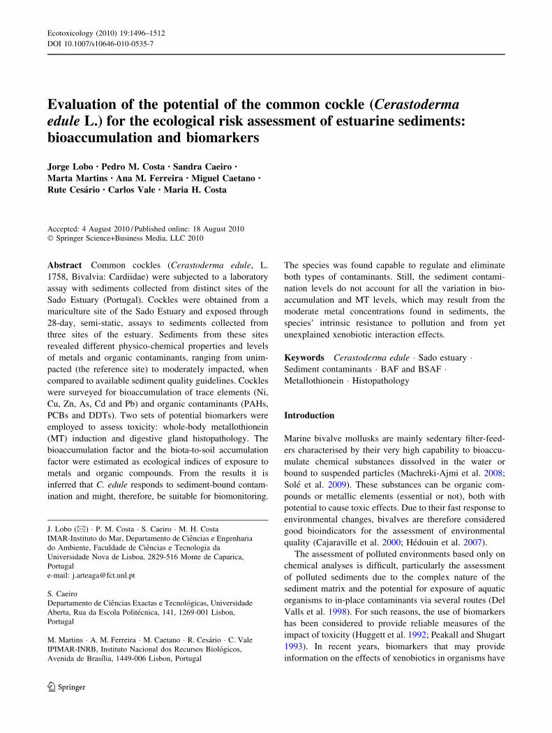
(Fig. 1) on November 2006, selected on the basis of their

potentially different levels of metallic and organic con-

tamination. Site S1 (the reference site) is located near an

environmentally protected area (the Sado Estuary Natural

Reserve) and is the most distant from sources of contam-

ination. Due to its location in the south channel of estuary,

this site is more influenced by oceanic hydrodynamism and

has lower water residence time (Caeiro et al. 2005). Site S2

is located near the port of Setubal and site S3 in the

industrial zone near factories for the production of fertil-

izers, pesticides and others (such as paper mill, a thermo-

electric power plant, shipyards, etc.), identified as potential

sources of pollution (Caeiro et al. 2005). Sites S2 and S3

are both located in areas of low hydrodynamism, which

facilitates the retention of contaminants and fine particles

of sediment from the upper estuary. The cockles were

cultured and collected from a distinct site (site CS), located

near aquaculture and small-scale fishery grounds, consist-

ing of a confined area with low hydrodynamism. Site CS is

the only one located in the intertidal zone and is also the

only located inside the Natural Reserve Protected Area and

distant from local pollution sources; all the other sites (S1,

S2 and S3) are located in the subtidal zone.

Cockles (28 ± 1.6 mm shell length, 8.0 ± 1.4 g whole-

body wet weight [ww]) were collected on November 2006

and acclimatized to laboratory conditions (temperature of

18�C and salinity of 34) in clean sand and seawater for

48 h. The bivalves were exposed to the sediments (S1, S2

and S3) directly after collection for 28 days through a

semi-static arrangement of bioassays (performed in

duplicate). Each replicate consisted of a tank (24 9 11 9

39 cm) with 2 l of sediment and 5 l of clean seawater.

Forty randomly-selected animals were distributed per

tank. Aeration was continuous and set to avoid sediment

disturbance. The animals were fed daily with pulverized

commercial fish food. Salinity, dissolved oxygen,

ammonia, pH and temperature were monitored weekly. A

50% water change was enforced on a weekly basis to

ensure constancy of water parameters with minimum

removal of xenobiotics. The animals were collected and

sacrificed for analysis at days, 14 (T14) and 28 (T28) in

order to determine the bioaccumulation of metallic and

organic contaminants, metallothionein induction and his-

topathological alterations of the digestive gland. For

each test and sampling time, 20 individuals were used

to determine the organic contaminants, 10 individuals

to determine the metals and metallothioneins and 10 to

examine the histopathology. Animals collected at

T0 consisted of 15 individuals collected directly from the

acclimatization tanks and should reflect the conditions of

the culture site, CS.

Sediment analyses

Physico-chemical characterization

Sediment redox potential (Eh) was measured immediately

after collection, using an Orion model 20A meter with a

H3131 Pt electrode and a Ag/AgCl reference electrode

(Orion Research Inc.). For the determination of the organic

matter, the sediment was previously dried at 60–80�C and

combusted at 500 ± 25�C for 4 h. The content of organic

matter (extrapolated from total combustible carbon, TOM)

is given in percent sediment dry weight (dw). Fine fraction

(particle size \63 lm) was determined by sieving after

treating the samples with hydrogen peroxide and disag-

gregation with pyrophosphate.

Contaminant determination

The sediments were analysed for the metals nickel (Ni),

copper (Cu), zinc (Zn), cadmium (Cd) and lead (Pb) and

for the metalloid arsenic (As). Sediment samples

(&100 mg dw) were mineralized completely with 6 cm3 of

HF (40%) and 1 mL of Aqua Regia (36% HCl : 65%

HNO3; 3:1) in closed Teflon vials at 100�C during 1 h.

Contents were evaporated to near dryness redissolved in

1 mL of HNO3 and 5 mL of Milli-Q water, heated for

20 min at 75�C and diluted to 50 mL with Milli-Q grade

ultrapure water (Caetano et al. 2007). The metal concen-

trations were determined in a Thermo Elemental XSeries

quadropole ICP-MS (inductively coupled plasma mass

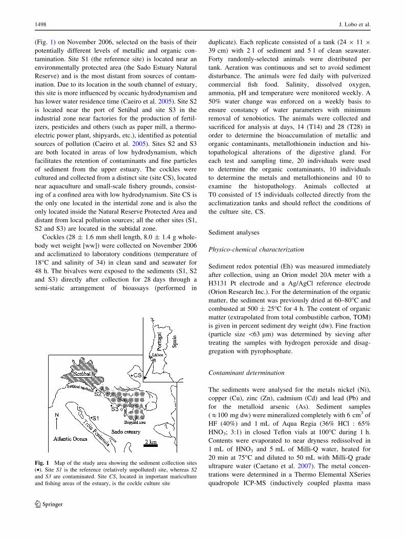
Fig. 1 Map of the study area showing the sediment collection sites

(•). Site S1 is the reference (relatively unpolluted) site, whereas S2and S3 are contaminated. Site CS, located in important mariculture

and fishing areas of the estuary, is the cockle culture site

1498 J. Lobo et al.

123

spectrometer) equipped with a Peltier Impact bead spray

chamber and a concentric Meinhard nebulizer. MESS-2,

PACS-2 and MAG-1 were the reference materials used to

validate the procedure and were found within the certified

range. Results are given in mg kg-1 sediment dw.

The determination of PAHs (polycyclic aromatic

hydrocarbons) was performed on a GCQ Trace Finnigan

gas chromatography-mass spectrometry (GC–MS) system

with a 30 m 9 0.25 mm 9 0.25 lm film thickness DB-5

MS column (Argilent, USA) in selected ion mode (Martins

et al. 2008). Seventeen three- to six-ring PAHs were

quantified. For PCB (polychlorinated biphenyls) and DDT

(dichloro-diphenyl-trichloroethane) plus metabolites anal-

yses, dry sediment samples were Soxhlet extracted with

n-hexane for 16 h. The extracts were cleaned up with

Florisil and sulfuric acid (Ferreira et al. 2003). Eighteen

PCB congeners and DDTs (ppDDD, ppDDE and ppDDT)

were analysed by GC–MS using a Hewlett-Packard 6890

apparatus. The SMR 1941b reference sediment (NIST,

USA) was used to validate the analysis and the results were

found within the certified range. The detection limit was

0.01 ng g-1. All concentrations are expressed in ng g-1

sediment dw.

The probable effects level quotient (PEL-Q) was cal-

culated to evaluate the potential for observing adverse

biological effects of the tested sediments. This quotient is

based on the published guideline values for coastal waters,

namely the threshold effects level (TEL) and the probable

effects level (PEL; MacDonald et al. 1996). These guide-

lines have been largely used in estuarine sediment eco-

logical risk assessment studies. This index was calculated

for all contaminants of each sediment as given by the

formula (Long and MacDonald 1998):

PEL - Qi ¼Ci

PELð1Þ

where PEL is the guideline value for the contaminant i and

Ci the measured concentration of the contaminant in the

surveyed sediment. The sediment quality guideline

quotient (SQG-Q) was calculated to compare the four

sites impacted by mixtures as described by Long and

MacDonald (1998):

SQG - Q ¼

Pn

i¼1

PEL� Qi

nð2Þ

where PEL-Qi is the index deriving from (1) for the con-

taminant i and n the number of contaminants under anal-

ysis. Stations were scored according to the overall potential

of sediments to produce adverse biological effects, as

proposed by MacDonald et al. (2004): SQG-Q \ 0.1

– unimpacted; 0.1 B SQG-Q \ 1 – moderately impacted;

SQG C 1 – highly impacted.

Organism analyses

Bioaccumulation

For the analysis of metals, whole soft-body individual

samples (0.025 ± 0.003 g dw) were dried in borosilicate,

lead free, glass vials at 60�C for 5 days and then digested

in Teflon vials by adding 5 ml 65% nitric acid and incu-

bated for 24 h at room temperature. The vials were then

placed in a water bath at 95�C during 4 h, after which 1 ml

hydrogen peroxide (30% v/v) was added, followed by

another hour at 95�C in a water bath (Clesceri et al. 1999).

Finally, the samples were stored in HDPE plastic bottles

after elution with Milli-Q water and kept at 4�C until

element quantification. The quantification of trace elements

(Ni, Cu, Zn, Cd, Pb and As) was performed by ICP-MS

using the same equipment described above. The organic

contaminants were determined in the same sample by GC–

MS after Soxhlet extraction (three- to six-ring PAHs, 18

PCB congeners and DDTs: ppDDD, ppDDE and ppDDT).

Quantification was carried out similarly to the procedure

described for the sediments, adapted to biological tissue

(Martins et al. 2008).

Metallothionein induction

Metallothionein induction was determined by the quanti-

fication of thiols in whole soft tissue samples as described

by Diniz et al. (2007) and Costa et al. (2008). In brief:

samples were homogenized in Tris–HCl 0.02 M buffer (pH

8.6). Homogenates were centrifuged at 30,000 9 g at 4�C

for 1 h. The supernatant was heated in a water bath at 80�C

for 10 min to denature non-heat stable proteins and then

centrifuged as previous. Thiols were quantified from heat-

treated cytosols by differential pulse polarography with a

static mercury-drop electrode (DPP-SMDE) using a 693

VA processor and a 694 VA stand (Metrohm, Herisau,

Switzerland). In absence of a commercial form of bivalve

MT, Rabbit MT isoforms I & II (Sigma, St Louis, MO,

USA) was used for the standard addition method, as vali-

dated in bivalves by Diniz et al. (2007).

Histopathology

Cockles’ digestive glands were fixed in Bouin-Holland’s

solution (27% formaldehyde, 7% acetic acid, and picric

acid until saturation) for approximately 48 h at room

temperature. Afterwards, the samples were washed with

water for 24 h to remove the excess picric acid, dehydrated

in a progressive series of ethanol and intermediately

embedded with xylene (&100%). Samples were then

embedded in paraffin for about 12 h. Sections (5 lm thick)

were stained with haematoxylin and eosin (H & E) and


123

mounted with DPX resin (BDH, Poole, UK). The proce-

dure was adapted from Martoja and Martoja (1967). The

slides were qualitatively analysed as a first attempt to

identify exposure-induced lesions and alterations to the

digestive gland of the species. A DMLB model bright-field

microscope (from Leica Microsystems) was employed in

the analyses.

Bioaccumulation and biota-to-soil accumulation factors

The bioaccumulation factor (BAF) and the biota-to-soil

accumulation factor (BSAF) were measured regarding the

trace elements (Ni, Cu, Zn, Cd, Pb and As) and organic

contaminants (PAHs, PCBs and DDTs). The BAF was

calculated according to the formula (Lee 1992):

BAF ¼ Co

Cs

ð3Þ

where Co was contaminant concentration in organism

expressed in mg kg-1 dry weight of tissue and Cs is the

contaminant concentration in sediment expressed in

mg kg-1 dry weight of sediment. The BSAF is

essentially the BAF normalized to the organic carbon

content (TOM, given in % relatively to sediment dw) of the

sediment (adapted from USEPA 1995):

BSAF ¼ Co

Cs

TOM

� � ð4Þ

Statistical analysis

The non-parametric tests Kruskall–Wallis H and Mann–

Whitney U were employed to assess global and pairwise

statistical differences, respectively. The chi-square pre-

dicted 9 observed test was applied to assess significant

differences between the concentrations of organic con-

taminants (for sediments and organisms). The non-para-

metric Spearman’s rank order correlation q statistic was

used to assess the correlation between BAFs/BSAFs and

metallothionein concentrations. A significance level of 5%

was set for all analyses. All the statistics were performed

with Statistical Package for Social Sciences (SPSS Inc.,

Chicago, IL, USA).

Results

The assay’s parameters (monitored weekly) were found to

be constant throughout the assay: salinity = 34 ± 1, dis-

solved oxygen = 42 ± 2%, ammonia & 0 mg l-1, pH =

7.8 ± 0.1, and temperature = 18 ± 1�C. Overall mortality

was low for all tests (3%, 4% and 11% for S1, S2 and S3

exposures, respectively).

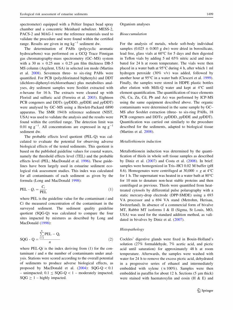
Physico-chemical characterization of sediments

Fine fraction (FF) and TOM was lowest in the reference

sediment (S1). Sediment fine fraction was highest in sedi-

ments S2 and in the culture sediment (CS), representing

98% and 94%, respectively, of the total sediment dry

weight. Sediments S2 and CS also had high organic matter

content (11.8% and 12.4%, respectively). Sediments S2

and S3 were found the most reduced/anoxic sediments,

presenting lowest Eh. CS is the only intertidal sediment

and it is the less reduced. The results are summarized in

Table 1. A linear relation was observed between FF and

TOM content in sediments from the four sites (FF = 6.4,

TOM ? 20.7; r2 = 0.96).

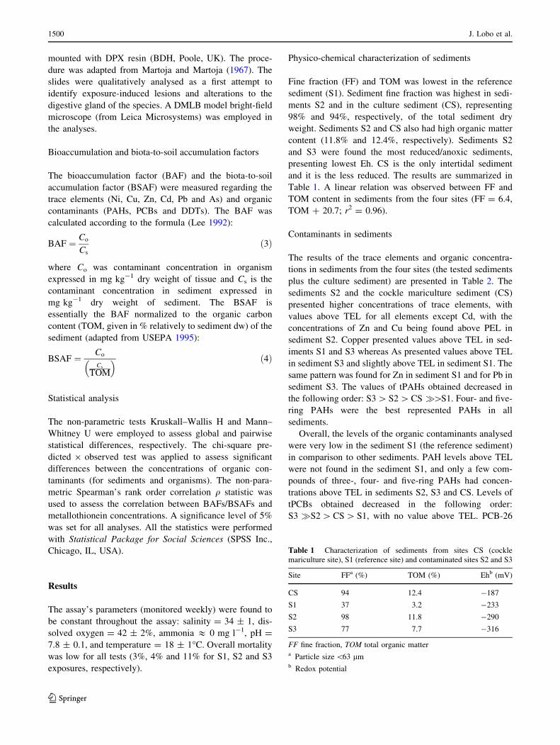
Contaminants in sediments

The results of the trace elements and organic concentra-

tions in sediments from the four sites (the tested sediments

plus the culture sediment) are presented in Table 2. The

sediments S2 and the cockle mariculture sediment (CS)

presented higher concentrations of trace elements, with

values above TEL for all elements except Cd, with the

concentrations of Zn and Cu being found above PEL in

sediment S2. Copper presented values above TEL in sed-

iments S1 and S3 whereas As presented values above TEL

in sediment S3 and slightly above TEL in sediment S1. The

same pattern was found for Zn in sediment S1 and for Pb in

sediment S3. The values of tPAHs obtained decreased in

the following order: S3 [ S2 [ CS �[S1. Four- and five-

ring PAHs were the best represented PAHs in all

sediments.

Overall, the levels of the organic contaminants analysed

were very low in the sediment S1 (the reference sediment)

in comparison to other sediments. PAH levels above TEL

were not found in the sediment S1, and only a few com-

pounds of three-, four- and five-ring PAHs had concen-

trations above TEL in sediments S2, S3 and CS. Levels of

tPCBs obtained decreased in the following order:

S3 �S2 [ CS [ S1, with no value above TEL. PCB-26

Table 1 Characterization of sediments from sites CS (cockle

mariculture site), S1 (reference site) and contaminated sites S2 and S3

Site FFa (%) TOM (%) Ehb (mV)

CS 94 12.4 -187

S1 37 3.2 -233

S2 98 11.8 -290

S3 77 7.7 -316

FF fine fraction, TOM total organic mattera Particle size \63 lmb Redox potential

1500 J. Lobo et al.

123

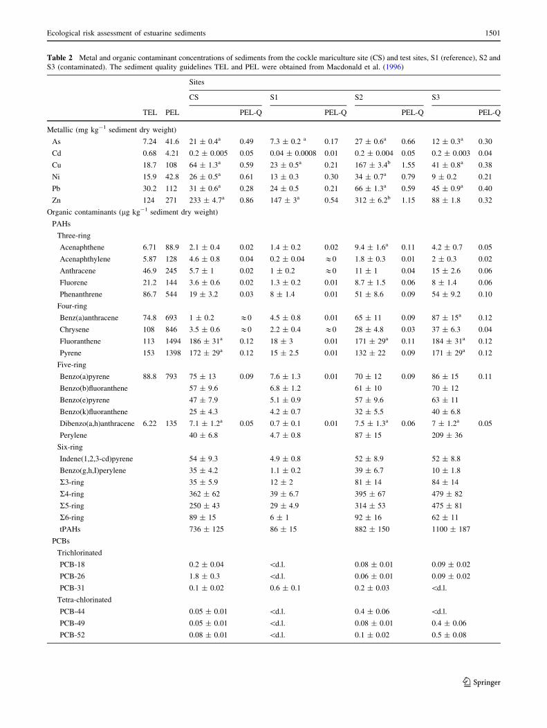
Table 2 Metal and organic contaminant concentrations of sediments from the cockle mariculture site (CS) and test sites, S1 (reference), S2 and

S3 (contaminated). The sediment quality guidelines TEL and PEL were obtained from Macdonald et al. (1996)

Sites

CS S1 S2 S3

TEL PEL PEL-Q PEL-Q PEL-Q PEL-Q

Metallic (mg kg-1 sediment dry weight)

As 7.24 41.6 21 ± 0.4a 0.49 7.3 ± 0.2 a 0.17 27 ± 0.6a 0.66 12 ± 0.3a 0.30

Cd 0.68 4.21 0.2 ± 0.005 0.05 0.04 ± 0.0008 0.01 0.2 ± 0.004 0.05 0.2 ± 0.003 0.04

Cu 18.7 108 64 ± 1.3a 0.59 23 ± 0.5a 0.21 167 ± 3.4b 1.55 41 ± 0.8a 0.38

Ni 15.9 42.8 26 ± 0.5a 0.61 13 ± 0.3 0.30 34 ± 0.7a 0.79 9 ± 0.2 0.21

Pb 30.2 112 31 ± 0.6a 0.28 24 ± 0.5 0.21 66 ± 1.3a 0.59 45 ± 0.9a 0.40

Zn 124 271 233 ± 4.7a 0.86 147 ± 3a 0.54 312 ± 6.2b 1.15 88 ± 1.8 0.32

Organic contaminants (lg kg-1 sediment dry weight)

PAHs

Three-ring

Acenaphthene 6.71 88.9 2.1 ± 0.4 0.02 1.4 ± 0.2 0.02 9.4 ± 1.6a 0.11 4.2 ± 0.7 0.05

Acenaphthylene 5.87 128 4.6 ± 0.8 0.04 0.2 ± 0.04 &0 1.8 ± 0.3 0.01 2 ± 0.3 0.02

Anthracene 46.9 245 5.7 ± 1 0.02 1 ± 0.2 &0 11 ± 1 0.04 15 ± 2.6 0.06

Fluorene 21.2 144 3.6 ± 0.6 0.02 1.3 ± 0.2 0.01 8.7 ± 1.5 0.06 8 ± 1.4 0.06

Phenanthrene 86.7 544 19 ± 3.2 0.03 8 ± 1.4 0.01 51 ± 8.6 0.09 54 ± 9.2 0.10

Four-ring

Benz(a)anthracene 74.8 693 1 ± 0.2 &0 4.5 ± 0.8 0.01 65 ± 11 0.09 87 ± 15a 0.12

Chrysene 108 846 3.5 ± 0.6 &0 2.2 ± 0.4 &0 28 ± 4.8 0.03 37 ± 6.3 0.04

Fluoranthene 113 1494 186 ± 31a 0.12 18 ± 3 0.01 171 ± 29a 0.11 184 ± 31a 0.12

Pyrene 153 1398 172 ± 29a 0.12 15 ± 2.5 0.01 132 ± 22 0.09 171 ± 29a 0.12

Five-ring

Benzo(a)pyrene 88.8 793 75 ± 13 0.09 7.6 ± 1.3 0.01 70 ± 12 0.09 86 ± 15 0.11

Benzo(b)fluoranthene 57 ± 9.6 6.8 ± 1.2 61 ± 10 70 ± 12

Benzo(e)pyrene 47 ± 7.9 5.1 ± 0.9 57 ± 9.6 63 ± 11

Benzo(k)fluoranthene 25 ± 4.3 4.2 ± 0.7 32 ± 5.5 40 ± 6.8

Dibenzo(a,h)anthracene 6.22 135 7.1 ± 1.2a 0.05 0.7 ± 0.1 0.01 7.5 ± 1.3a 0.06 7 ± 1.2a 0.05

Perylene 40 ± 6.8 4.7 ± 0.8 87 ± 15 209 ± 36

Six-ring

Indene(1,2,3-cd)pyrene 54 ± 9.3 4.9 ± 0.8 52 ± 8.9 52 ± 8.8

Benzo(g,h,I)perylene 35 ± 4.2 1.1 ± 0.2 39 ± 6.7 10 ± 1.8

R3-ring 35 ± 5.9 12 ± 2 81 ± 14 84 ± 14

R4-ring 362 ± 62 39 ± 6.7 395 ± 67 479 ± 82

R5-ring 250 ± 43 29 ± 4.9 314 ± 53 475 ± 81

R6-ring 89 ± 15 6 ± 1 92 ± 16 62 ± 11

tPAHs 736 ± 125 86 ± 15 882 ± 150 1100 ± 187

PCBs

Trichlorinated

PCB-18 0.2 ± 0.04 \d.l. 0.08 ± 0.01 0.09 ± 0.02

PCB-26 1.8 ± 0.3 \d.l. 0.06 ± 0.01 0.09 ± 0.02

PCB-31 0.1 ± 0.02 0.6 ± 0.1 0.2 ± 0.03 \d.l.

Tetra-chlorinated

PCB-44 0.05 ± 0.01 \d.l. 0.4 ± 0.06 \d.l.

PCB-49 0.05 ± 0.01 \d.l. 0.08 ± 0.01 0.4 ± 0.06

PCB-52 0.08 ± 0.01 \d.l. 0.1 ± 0.02 0.5 ± 0.08


123

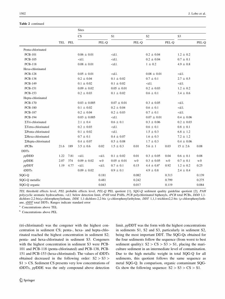
(tri-chlorinated) was the congener with the highest con-

centration in sediment CS; penta-, hexa- and hepta-chlo-

rinated reached the highest concentration in sediment S2;

penta- and hexa-chlorinated in sediment S3. Congeners

with the highest concentration in sediment S3 were PCB-

101 and PCB-118 (penta-chlorinated) and PCB-138, PCB-

151 and PCB-153 (hexa-chlorinated). The values of tDDTs

obtained decreased in the following order: S2 [ S3 [S1 [ CS. Sediment CS presents very low concentrations of

tDDTs, ppDDE was the only compound above detection

limit. ppDDT was the form with the highest concentrations

in sediments S1, S2 and S3, particularly in sediment S2,

being the most important DDT. The SQG-Qs obtained for

the four sediments follow the sequence (from worst to best

sediment quality): S2 [ CS [ S3 [ S1, placing the mari-

culture sediment in an intermediate level of contamination.

Due to the high metallic weight in total SQG-Q for all

sediments, this quotient follows the same sequence as

metal SQG-Q. In comparison, organic contaminant SQG-

Gs show the following sequence: S2 [ S3 [ CS [ S1.

Table 2 continued

Sites

CS S1 S2 S3

TEL PEL PEL-Q PEL-Q PEL-Q PEL-Q

Penta-chlorinated

PCB-101 0.06 ± 0.01 \d.l. 0.2 ± 0.04 1.2 ± 0.2

PCB-105 \d.l. \d.l. 0.2 ± 0.04 0.7 ± 0.1

PCB-118 0.08 ± 0.01 \d.l. 1 ± 0.2 4.9 ± 0.8

Hexa-chlorinated

PCB-128 0.05 ± 0.01 \d.l. 0.08 ± 0.01 \d.l.

PCB-138 0.2 ± 0.04 0.1 ± 0.02 0.7 ± 0.1 2.7 ± 0.5

PCB-149 0.1 ± 0.02 0.1 ± 0.02 \d.l. \d.l.

PCB-151 0.09 ± 0.02 0.05 ± 0.01 0.2 ± 0.03 1.2 ± 0.2

PCB-153 0.2 ± 0.03 0.1 ± 0.02 0.6 ± 0.1 3.4 ± 0.6

Hepta-chlorinated

PCB-170 0.03 ± 0.005 0.07 ± 0.01 0.3 ± 0.05 \d.l.

PCB-180 0.1 ± 0.02 0.2 ± 0.04 0.6 ± 0.1 \d.l.

PCB-187 0.2 ± 0.04 0.2 ± 0.03 0.7 ± 0.1 \d.l.

PCB-194 0.03 ± 0.005 \d.l. 0.07 ± 0.01 0.4 ± 0.06

RTri-chlorinated 2.1 ± 0.4 0.6 ± 0.1 0.3 ± 0.06 0.2 ± 0.03

RTetra-chlorinated 0.2 ± 0.03 \d.l. 0.6 ± 0.1 0.8 ± 0.1

RPenta-chlorinated 0.1 ± 0.02 \d.l. 1.5 ± 0.3 6.8 ± 1.2

RHexa-chlorinated 0.7 ± 0.1 0.4 ± 0.07 1.6 ± 0.3 7.2 ± 1.2

RHepta-chlorinated 0.4 ± 0.07 0.5 ± 0.08 1.7 ± 0.3 0.4 ± 0.06

tPCBs 21.6 189 3.5 ± 0.6 0.02 1.5 ± 0.3 0.01 5.6 ± 1 0.03 15 ± 2.6 0.08

DDTs

ppDDD 1.22 7.81 \d.l. \d.l. 0.1 ± 0.02 0.01 0.3 ± 0.05 0.04 0.6 ± 0.1 0.08

ppDDE 2.07 374 0.09 ± 0.02 &0 0.05 ± 0.01 &0 0.3 ± 0.05 &0 0.7 ± 0.1 &0

ppDDT 1.19 4.77 \d.l. \d.l. 0.7 ± 0.1 0.15 4.4 ± 0.8a 0.92 1.2 ± 0.2 0.25

tDDTs 0.09 ± 0.02 0.9 ± 0.1 4.9 ± 0.8 2.4 ± 0.4

SQG-Q 0.181 0.082 0.313 0.139

SQG-Q metallic 0.481 0.242 0.799 0.275

SQG-Q organic 0.043 0.017 0.119 0.084

TEL threshold effects level, PEL probable effects level, PEL-Q PEL quotient [1], SQG-Q sediment quality guideline quotient [2], PAHpolycyclic aromatic hydrocarbons, \d.l. below detection limit, tPAH total PAHs, PCB polychlorinated biphenyls, tPCB total PCBs, DDD 1,1-

dichloro-2,2-bis(q-chlorophenyl)ethane, DDE 1,1-dichloro-2,2-bis (q-chlorophenyl)ethylene, DDT 1,1,1-trichloro2,2-bis (q-chlorophenyl)eth-

ane, tDDT total DDTs. Ranges indicate standard errora Concentrations above TELb Concentrations above PEL

1502 J. Lobo et al.

123

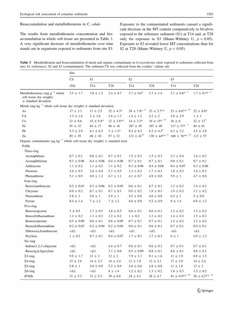
Bioaccumulation and metallothioneins in C. edule

The results from metallothionein concentration and bio-

accumulation in whole soft tissue are presented in Table 3.

A very significant decrease of metallothioneins over time

stands out in organisms exposed to sediments from site S3.

Exposure to the contaminated sediments caused a signifi-

cant decrease in the MT content comparatively to bivalves

exposed to the reference sediment (S1) at T14 and, at T28

only for exposure to S3 (Mann–Whitney U, p \ 0.05).

Exposure to S3 revealed lower MT concentrations than for

S2 at T28 (Mann–Whitney U, p \ 0.05).

Table 3 Metallothionein and bioaccumulation of metal and organic contaminants in Cerastoderma edule exposed to sediments collected from

sites S1 (reference), S2 and S3 (contaminated). The sediment CS was collected from the cockles’ culture site

Site

CS S1 S2 S3

(T0) T14 T28 T14 T28 T14 T28

Metallothioneins (mg g-1 whole

soft tissue dry weight)

± standard deviation

3.5 ± 1.7 3.8 ± 1.2 2.4 ± 0.7 2.7 ± 0.6� 2.7 ± 1.4 2.1 ± 0.8*, � 1.7 ± 0.7*, �

Metals (mg kg-1 whole soft tissue dry weight) ± standard deviation

As 17 ± 3.3 17 ± 2.5 22 ± 4.3* 24 ± 7.4*, � 23 ± 2.7** 23 ± 6.6**, �� 22 ± 6.8*

Cd 1.3 ± 1.6 2 ± 1.6 1.6 ± 1.3 1.4 ± 1.2 2.2 ± 2 2.8 ± 2.9 1 ± 1

Cu 21 ± 8.6 15 ± 9.4* 12 ± 3.8** 14 ± 3.3* 34 ± 15*, �� 16 ± 6 22 ± 13�

Ni 91 ± 32 84 ± 17 96 ± 16 107 ± 45 107 ± 40 117 ± 37*, � 84 ± 61

Pb 5.3 ± 2.9 6.1 ± 6.3 3 ± 1.2* 8.2 ± 8.2 6.2 ± 4.3� 6.3 ± 3.2 4.5 ± 2.8

Zn 85 ± 29 68 ± 10 97 ± 21 112 ± 41�� 130 ± 44**, � 160 ± 76**, �� 113 ± 57

Organic contaminants (lg kg-1 whole soft tissue dry weight) ± standard error

PAHs

Three-ring

Acenaphthene 0.7 ± 0.1 0.8 ± 0.1 0.7 ± 0.1 1.5 ± 0.3 1.5 ± 0.3 2.3 ± 0.4 1.6 ± 0.3

Acenaphthylene 0.3 ± 0.06 0.4 ± 0.06 0.4 ± 0.06 0.7 ± 0.1 0.7 ± 0.1 0.8 ± 0.1 0.7 ± 0.1

Anthracene 1.1 ± 0.2 1.1 ± 0.2 1.1 ± 0.2 0.3 ± 0.06 0.4 ± 0.06 0.4 ± 0.07 0.3 ± 0.06

Fluorene 2.6 ± 0.5 2.6 ± 0.4 2.7 ± 0.5 1.3 ± 0.2 1.7 ± 0.3 1.8 ± 0.3 1.6 ± 0.3

Phenanthrene 5.1 ± 0.9 6.8 ± 1.2 6.7 ± 1.1 4.1 ± 0.7 4.9 ± 0.8 5.9 ± 1 4.7 ± 0.8

Four-ring

Benz(a)anthracene 0.2 ± 0.03 0.3 ± 0.06 0.3 ± 0.05 0.6 ± 0.1 0.7 ± 0.1 1.2 ± 0.2 1.4 ± 0.2

Chrysene 0.9 ± 0.2 0.7 ± 0.1 0.7 ± 0.1 0.9 ± 0.2 1.9 ± 0.3 1.9 ± 0.3 1.1 ± 0.2

Fluoranthene 5.8 ± 1 5.8 ± 1 5.9 ± 1 4.5 ± 0.8 4.6 ± 0.8 6.2 ± 1 5 ± 0.9

Pyrene 8.4 ± 1.4 7 ± 1.2 7 ± 1.2 4.6 ± 0.8 5.2 ± 0.9 8 ± 1.4 6.8 ± 1.2

Five-ring

Benzo(a)pyrene 3 ± 0.5 2.7 ± 0.5 2.8 ± 0.5 0.6 ± 0.1 0.6 ± 0.1 1.2 ± 0.2 1.3 ± 0.2

Benzo(b)fluoranthene 1.2 ± 0.2 1.3 ± 0.2 1.2 ± 0.2 1 ± 0.2 1.2 ± 0.2 1.4 ± 0.3 1.5 ± 0.3

Benzo(e)pyrene 0.5 ± 0.09 0.6 ± 0.1 0.6 ± 0.09 0.7 ± 0.1 0.7 ± 0.1 1.2 ± 0.2 1.2 ± 0.2

Benzo(k)fluoranthene 0.2 ± 0.03 0.2 ± 0.04 0.2 ± 0.04 0.6 ± 0.1 0.6 ± 0.1 0.7 ± 0.1 0.9 ± 0.1

Dibenzo(a,h)anthracene \d.l. \d.l. \d.l. \d.l. \d.l. \d.l. \d.l.

Perylene 1 ± 0.2 0.7 ± 0.1 0.4 ± 0.07 1.7 ± 0.3 1.7 ± 0.3 6 ± 1 6.9 ± 1.2

Six-ring

Indene(1,2,3-cd)pyrene \d.l. \d.l. 4.4 ± 0.7 0.6 ± 0.1 0.6 ± 0.1 0.7 ± 0.1 0.7 ± 0.1

Benzo(g,h,I)perylene \d.l. \d.l. 3.7 ± 0.6 0.5 ± 0.09 0.8 ± 0.1 0.8 ± 0.1 0.8 ± 0.1

R3-ring 9.9 ± 1.7 12 ± 2 12 ± 2 7.9 ± 1.3 9.1 ± 1.6 11 ± 1.9 8.9 ± 1.5

R4-ring 15 ± 2.6 14 ± 2.3 14 ± 2.4 11 ± 1.8 12 ± 2.1 17 ± 2.9 14 ± 2.4

R5-ring 5.8 ± 1 5.6 ± 0.9 5.2 ± 0.9 4.6 ± 0.8 4.8 ± 0.8 11 ± 1.8 12 ± 2

R6-ring \d.l. \d.l. 8 ± 1.4 1.2 ± 0.2 1.3 ± 0.2 1.6 ± 0.3 1.5 ± 0.2

tPAHs 31 ± 5.3 31 ± 5.3 39 ± 6.6 24 ± 4.1 28 ± 4.7 41 ± 6.9**, �� 36 ± 6.2**, ��


123

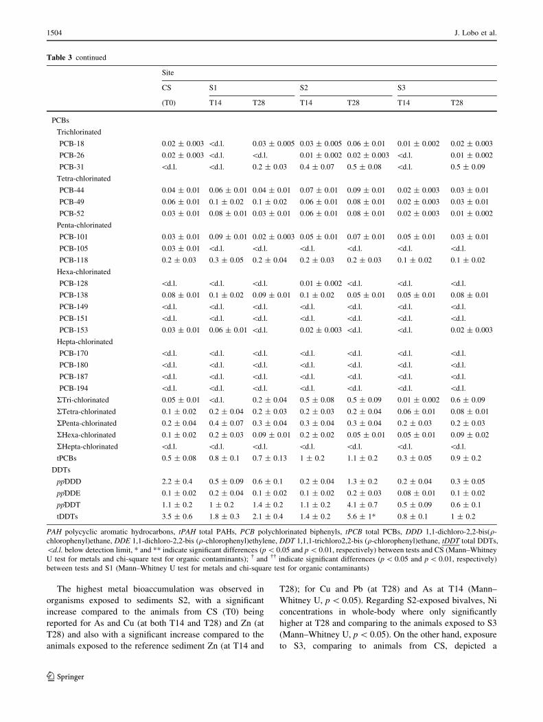
The highest metal bioaccumulation was observed in

organisms exposed to sediments S2, with a significant

increase compared to the animals from CS (T0) being

reported for As and Cu (at both T14 and T28) and Zn (at

T28) and also with a significant increase compared to the

animals exposed to the reference sediment Zn (at T14 and

T28); for Cu and Pb (at T28) and As at T14 (Mann–

Whitney U, p \ 0.05). Regarding S2-exposed bivalves, Ni

concentrations in whole-body where only significantly

higher at T28 and comparing to the animals exposed to S3

(Mann–Whitney U, p \ 0.05). On the other hand, exposure

to S3, comparing to animals from CS, depicted a

Table 3 continued

Site

CS S1 S2 S3

(T0) T14 T28 T14 T28 T14 T28

PCBs

Trichlorinated

PCB-18 0.02 ± 0.003 \d.l. 0.03 ± 0.005 0.03 ± 0.005 0.06 ± 0.01 0.01 ± 0.002 0.02 ± 0.003

PCB-26 0.02 ± 0.003 \d.l. \d.l. 0.01 ± 0.002 0.02 ± 0.003 \d.l. 0.01 ± 0.002

PCB-31 \d.l. \d.l. 0.2 ± 0.03 0.4 ± 0.07 0.5 ± 0.08 \d.l. 0.5 ± 0.09

Tetra-chlorinated

PCB-44 0.04 ± 0.01 0.06 ± 0.01 0.04 ± 0.01 0.07 ± 0.01 0.09 ± 0.01 0.02 ± 0.003 0.03 ± 0.01

PCB-49 0.06 ± 0.01 0.1 ± 0.02 0.1 ± 0.02 0.06 ± 0.01 0.08 ± 0.01 0.02 ± 0.003 0.03 ± 0.01

PCB-52 0.03 ± 0.01 0.08 ± 0.01 0.03 ± 0.01 0.06 ± 0.01 0.08 ± 0.01 0.02 ± 0.003 0.01 ± 0.002

Penta-chlorinated

PCB-101 0.03 ± 0.01 0.09 ± 0.01 0.02 ± 0.003 0.05 ± 0.01 0.07 ± 0.01 0.05 ± 0.01 0.03 ± 0.01

PCB-105 0.03 ± 0.01 \d.l. \d.l. \d.l. \d.l. \d.l. \d.l.

PCB-118 0.2 ± 0.03 0.3 ± 0.05 0.2 ± 0.04 0.2 ± 0.03 0.2 ± 0.03 0.1 ± 0.02 0.1 ± 0.02

Hexa-chlorinated

PCB-128 \d.l. \d.l. \d.l. 0.01 ± 0.002 \d.l. \d.l. \d.l.

PCB-138 0.08 ± 0.01 0.1 ± 0.02 0.09 ± 0.01 0.1 ± 0.02 0.05 ± 0.01 0.05 ± 0.01 0.08 ± 0.01

PCB-149 \d.l. \d.l. \d.l. \d.l. \d.l. \d.l. \d.l.


PCB-153 0.03 ± 0.01 0.06 ± 0.01 \d.l. 0.02 ± 0.003 \d.l. \d.l. 0.02 ± 0.003

Hepta-chlorinated





RTri-chlorinated 0.05 ± 0.01 \d.l. 0.2 ± 0.04 0.5 ± 0.08 0.5 ± 0.09 0.01 ± 0.002 0.6 ± 0.09

RTetra-chlorinated 0.1 ± 0.02 0.2 ± 0.04 0.2 ± 0.03 0.2 ± 0.03 0.2 ± 0.04 0.06 ± 0.01 0.08 ± 0.01

RPenta-chlorinated 0.2 ± 0.04 0.4 ± 0.07 0.3 ± 0.04 0.3 ± 0.04 0.3 ± 0.04 0.2 ± 0.03 0.2 ± 0.03

RHexa-chlorinated 0.1 ± 0.02 0.2 ± 0.03 0.09 ± 0.01 0.2 ± 0.02 0.05 ± 0.01 0.05 ± 0.01 0.09 ± 0.02

RHepta-chlorinated \d.l. \d.l. \d.l. \d.l. \d.l. \d.l. \d.l.

tPCBs 0.5 ± 0.08 0.8 ± 0.1 0.7 ± 0.13 1 ± 0.2 1.1 ± 0.2 0.3 ± 0.05 0.9 ± 0.2

DDTs

ppDDD 2.2 ± 0.4 0.5 ± 0.09 0.6 ± 0.1 0.2 ± 0.04 1.3 ± 0.2 0.2 ± 0.04 0.3 ± 0.05

ppDDE 0.1 ± 0.02 0.2 ± 0.04 0.1 ± 0.02 0.1 ± 0.02 0.2 ± 0.03 0.08 ± 0.01 0.1 ± 0.02

ppDDT 1.1 ± 0.2 1 ± 0.2 1.4 ± 0.2 1.1 ± 0.2 4.1 ± 0.7 0.5 ± 0.09 0.6 ± 0.1

tDDTs 3.5 ± 0.6 1.8 ± 0.3 2.1 ± 0.4 1.4 ± 0.2 5.6 ± 1* 0.8 ± 0.1 1 ± 0.2

PAH polycyclic aromatic hydrocarbons, tPAH total PAHs, PCB polychlorinated biphenyls, tPCB total PCBs, DDD 1,1-dichloro-2,2-bis(q-

chlorophenyl)ethane, DDE 1,1-dichloro-2,2-bis (q-chlorophenyl)ethylene, DDT 1,1,1-trichloro2,2-bis (q-chlorophenyl)ethane, tDDT total DDTs,

\d.l. below detection limit, * and ** indicate significant differences (p \ 0.05 and p \ 0.01, respectively) between tests and CS (Mann–Whitney

U test for metals and chi-square test for organic contaminants); � and �� indicate significant differences (p \ 0.05 and p \ 0.01, respectively)

between tests and S1 (Mann–Whitney U test for metals and chi-square test for organic contaminants)

1504 J. Lobo et al.

123

significantly higher accumulation of As at both T14 and

T28 and of Ni and Zn at T14 and, comparing to animals

exposed to the reference sediment, a significantly higher

accumulation of As, Ni, Zn at T14 and Cu at T28 was

observed (Mann–Whitney U, p \ 0.05). Nevertheless, an

overall lower metal bioaccumulation was observed in

organisms exposed to S3 than S2. Cadmium bioaccu-

mulation was, in general, very low and no significant

differences between tests and sampling times were

found.

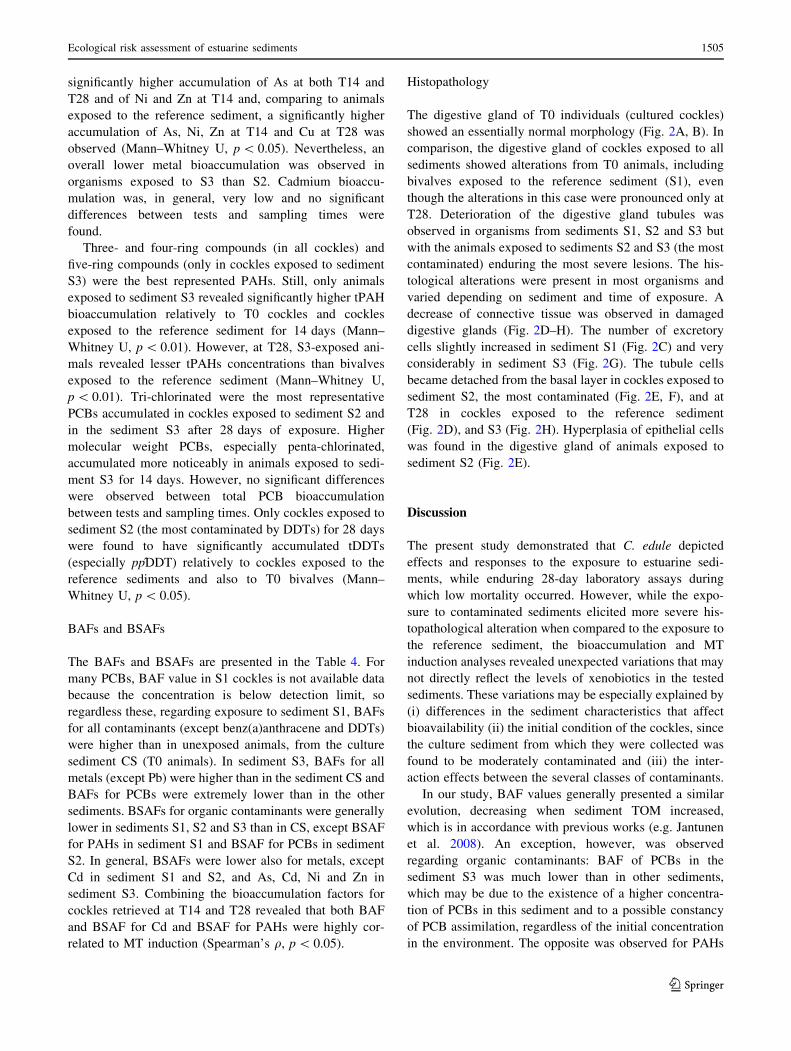
Three- and four-ring compounds (in all cockles) and

five-ring compounds (only in cockles exposed to sediment

S3) were the best represented PAHs. Still, only animals

exposed to sediment S3 revealed significantly higher tPAH

bioaccumulation relatively to T0 cockles and cockles

exposed to the reference sediment for 14 days (Mann–

Whitney U, p \ 0.01). However, at T28, S3-exposed ani-

mals revealed lesser tPAHs concentrations than bivalves

exposed to the reference sediment (Mann–Whitney U,

p \ 0.01). Tri-chlorinated were the most representative

PCBs accumulated in cockles exposed to sediment S2 and

in the sediment S3 after 28 days of exposure. Higher

molecular weight PCBs, especially penta-chlorinated,

accumulated more noticeably in animals exposed to sedi-

ment S3 for 14 days. However, no significant differences

were observed between total PCB bioaccumulation

between tests and sampling times. Only cockles exposed to

sediment S2 (the most contaminated by DDTs) for 28 days

were found to have significantly accumulated tDDTs

(especially ppDDT) relatively to cockles exposed to the

reference sediments and also to T0 bivalves (Mann–

Whitney U, p \ 0.05).

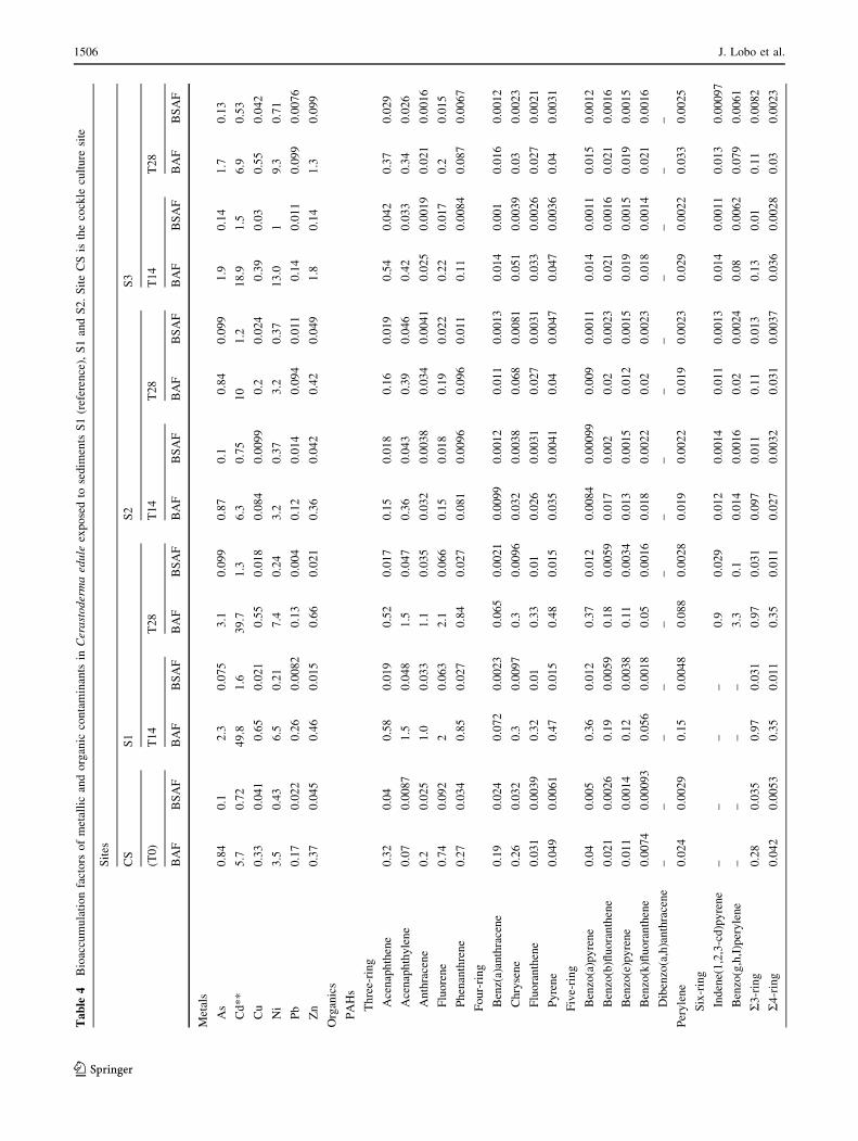
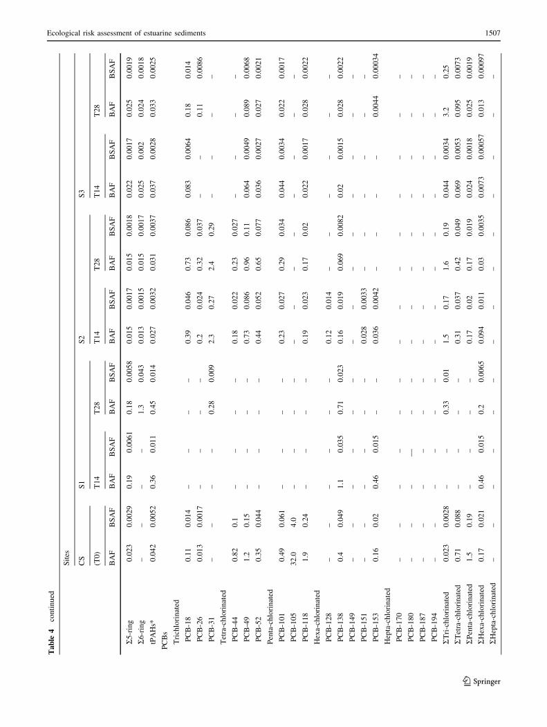
BAFs and BSAFs

The BAFs and BSAFs are presented in the Table 4. For

many PCBs, BAF value in S1 cockles is not available data

because the concentration is below detection limit, so

regardless these, regarding exposure to sediment S1, BAFs

for all contaminants (except benz(a)anthracene and DDTs)

were higher than in unexposed animals, from the culture

sediment CS (T0 animals). In sediment S3, BAFs for all

metals (except Pb) were higher than in the sediment CS and

BAFs for PCBs were extremely lower than in the other

sediments. BSAFs for organic contaminants were generally

lower in sediments S1, S2 and S3 than in CS, except BSAF

for PAHs in sediment S1 and BSAF for PCBs in sediment

S2. In general, BSAFs were lower also for metals, except

Cd in sediment S1 and S2, and As, Cd, Ni and Zn in

sediment S3. Combining the bioaccumulation factors for

cockles retrieved at T14 and T28 revealed that both BAF

and BSAF for Cd and BSAF for PAHs were highly cor-

related to MT induction (Spearman’s q, p \ 0.05).

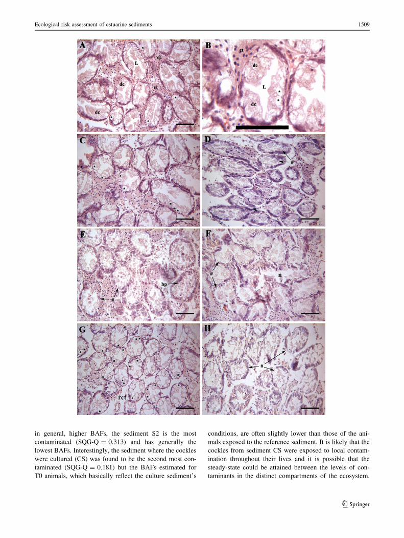
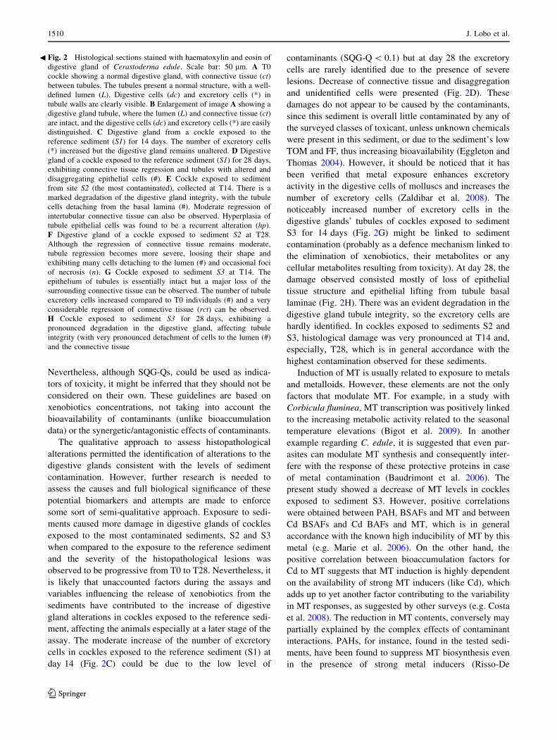
Histopathology

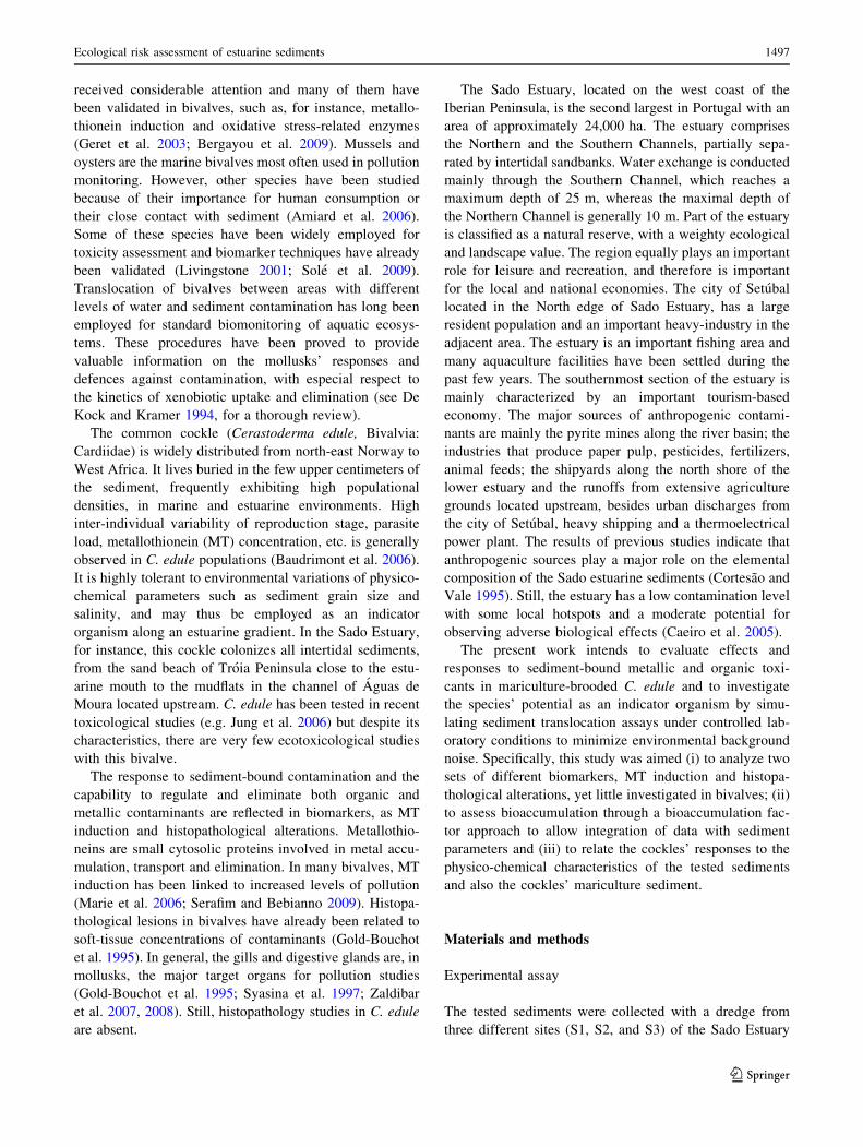
The digestive gland of T0 individuals (cultured cockles)

showed an essentially normal morphology (Fig. 2A, B). In

comparison, the digestive gland of cockles exposed to all

sediments showed alterations from T0 animals, including

bivalves exposed to the reference sediment (S1), even

though the alterations in this case were pronounced only at

T28. Deterioration of the digestive gland tubules was

observed in organisms from sediments S1, S2 and S3 but

with the animals exposed to sediments S2 and S3 (the most

contaminated) enduring the most severe lesions. The his-

tological alterations were present in most organisms and

varied depending on sediment and time of exposure. A

decrease of connective tissue was observed in damaged

digestive glands (Fig. 2D–H). The number of excretory

cells slightly increased in sediment S1 (Fig. 2C) and very

considerably in sediment S3 (Fig. 2G). The tubule cells

became detached from the basal layer in cockles exposed to

sediment S2, the most contaminated (Fig. 2E, F), and at

T28 in cockles exposed to the reference sediment

(Fig. 2D), and S3 (Fig. 2H). Hyperplasia of epithelial cells

was found in the digestive gland of animals exposed to

sediment S2 (Fig. 2E).

Discussion

The present study demonstrated that C. edule depicted

effects and responses to the exposure to estuarine sedi-

ments, while enduring 28-day laboratory assays during

which low mortality occurred. However, while the expo-

sure to contaminated sediments elicited more severe his-

topathological alteration when compared to the exposure to

the reference sediment, the bioaccumulation and MT

induction analyses revealed unexpected variations that may

not directly reflect the levels of xenobiotics in the tested

sediments. These variations may be especially explained by

(i) differences in the sediment characteristics that affect

bioavailability (ii) the initial condition of the cockles, since

the culture sediment from which they were collected was

found to be moderately contaminated and (iii) the inter-

action effects between the several classes of contaminants.

In our study, BAF values generally presented a similar

evolution, decreasing when sediment TOM increased,

which is in accordance with previous works (e.g. Jantunen

et al. 2008). An exception, however, was observed

regarding organic contaminants: BAF of PCBs in the

sediment S3 was much lower than in other sediments,

which may be due to the existence of a higher concentra-

tion of PCBs in this sediment and to a possible constancy

of PCB assimilation, regardless of the initial concentration

in the environment. The opposite was observed for PAHs


123

Ta

ble

4B

ioac

cum

ula

tio

nfa

cto

rso

fm

etal

lic

and

org

anic

con

tam

inan

tsin

Cer

ast

od

erm

aed

ule

exp

ose

dto

sed

imen

tsS

1(r

efer

ence

),S

1an

dS

2.

Sit

eC

Sis

the

cock

lecu

ltu

resi

te

Sit

es

CS

S1

S2

S3

(T0

)T

14

T2

8T

14

T2

8T

14

T2

8

BA

FB

SA

FB

AF

BS

AF

BA

FB

SA

FB

AF

BS

AF

BA

FB

SA

FB

AF

BS

AF

BA

FB

SA

F

Met

als

As

0.8

40

.12

.30

.07

53

.10

.09

90

.87

0.1

0.8

40

.09

91

.90

.14

1.7

0.1

3

Cd

**

5.7

0.7

24

9.8

1.6

39

.71

.36

.30

.75

10

1.2

18

.91

.56

.90

.53

Cu

0.3

30

.04

10

.65

0.0

21

0.5

50

.01

80

.08

40

.00

99

0.2

0.0

24

0.3

90

.03

0.5

50

.04

2

Ni

3.5

0.4

36

.50

.21

7.4

0.2

43

.20

.37

3.2

0.3

71

3.0

19

.30

.71

Pb

0.1

70

.02

20

.26

0.0

08

20

.13

0.0

04

0.1

20

.01

40

.09

40

.01

10

.14

0.0

11

0.0

99

0.0

07

6

Zn

0.3

70

.04

50

.46

0.0

15

0.6

60

.02

10

.36

0.0

42

0.4

20

.04

91

.80

.14

1.3

0.0

99

Org

anic

s

PA

Hs

Th

ree-

rin

g

Ace

nap

hth

ene

0.3

20

.04

0.5

80

.01

90

.52

0.0

17

0.1

50

.01

80

.16

0.0

19

0.5

40

.04

20

.37

0.0

29

Ace

nap

hth

yle

ne

0.0

70

.00

87

1.5

0.0

48

1.5

0.0

47

0.3

60

.04

30

.39

0.0

46

0.4

20

.03

30

.34

0.0

26

An

thra

cen

e0

.20

.02

51

.00

.03

31

.10

.03

50

.03

20

.00

38

0.0

34

0.0

04

10

.02

50

.00

19

0.0

21

0.0

01

6

Flu

ore

ne

0.7

40

.09

22

0.0

63

2.1

0.0

66

0.1

50

.01

80

.19

0.0

22

0.2

20

.01

70

.20

.01

5

Ph

enan

thre

ne

0.2

70

.03

40

.85

0.0

27

0.8

40

.02

70

.08

10

.00

96

0.0

96

0.0

11

0.1

10

.00

84

0.0

87

0.0

06

7

Fo

ur-

rin

g

Ben

z(a)

anth

race

ne

0.1

90

.02

40

.07

20

.00

23

0.0

65

0.0

02

10

.00

99

0.0

01

20

.01

10

.00

13

0.0

14

0.0

01

0.0

16

0.0

01

2

Ch

ryse

ne

0.2

60

.03

20

.30

.00

97

0.3

0.0

09

60

.03

20

.00

38

0.0

68

0.0

08

10

.05

10

.00

39

0.0

30

.00

23

Flu

ora

nth

ene

0.0

31

0.0

03

90

.32

0.0

10

.33

0.0

10

.02

60

.00

31

0.0

27

0.0

03

10

.03

30

.00

26

0.0

27

0.0

02

1

Py

ren

e0

.04

90

.00

61

0.4

70

.01

50

.48

0.0

15

0.0

35

0.0

04

10

.04

0.0

04

70

.04

70

.00

36

0.0

40

.00

31

Fiv

e-ri

ng

Ben

zo(a

)py

ren

e0

.04

0.0

05

0.3

60

.01

20

.37

0.0

12

0.0

08

40

.00

09

90

.00

90

.00

11

0.0

14

0.0

01

10

.01

50

.00

12

Ben

zo(b

)flu

ora

nth

ene

0.0

21

0.0

02

60

.19

0.0

05

90

.18

0.0

05

90

.01

70

.00

20

.02

0.0

02

30

.02

10

.00

16

0.0

21

0.0

01

6

Ben

zo(e

)py

ren

e0

.01

10

.00

14

0.1

20

.00

38

0.1

10

.00

34

0.0

13

0.0

01

50

.01

20

.00

15

0.0

19

0.0

01

50

.01

90

.00

15

Ben

zo(k

)flu

ora

nth

ene

0.0

07

40

.00

09

30

.05

60

.00

18

0.0

50

.00

16

0.0

18

0.0

02

20

.02

0.0

02

30

.01

80

.00

14

0.0

21

0.0

01

6

Dib

enzo

(a,h

)an

thra

cen

e–

––

––

––

––

––

––

–

Per

yle

ne

0.0

24

0.0

02

90

.15

0.0

04

80

.08

80

.00

28

0.0

19

0.0

02

20

.01

90

.00

23

0.0

29

0.0

02

20

.03

30

.00

25

Six

-rin

g

Ind

ene(

1,2

,3-c

d)p

yre

ne

––

––

0.9

0.0

29

0.0

12

0.0

01

40

.01

10

.00

13

0.0

14

0.0

01

10

.01

30

.00

09

7

Ben

zo(g

,h,I

)per

yle

ne

––

––

3.3

0.1

0.0

14

0.0

01

60

.02

0.0

02

40

.08

0.0

06

20

.07

90

.00

61

R3

-rin

g0

.28

0.0

35

0.9

70

.03

10

.97

0.0

31

0.0

97

0.0

11

0.1

10

.01

30

.13

0.0

10

.11

0.0

08

2

R4

-rin

g0

.04

20

.00

53

0.3

50

.01

10

.35

0.0

11

0.0

27

0.0

03

20

.03

10

.00

37

0.0

36

0.0

02

80

.03

0.0

02

3

1506 J. Lobo et al.

123

Ta

ble

4co

nti

nu

ed

Sit

es

CS

S1

S2

S3

(T0

)T

14

T2

8T

14

T2

8T

14

T2

8

BA

FB

SA

FB

AF

BS

AF

BA

FB

SA

FB

AF

BS

AF

BA

FB

SA

FB

AF

BS

AF

BA

FB

SA

F

R5

-rin

g0

.02

30

.00

29

0.1

90

.00

61

0.1

80

.00

58

0.0

15

0.0

01

70

.01

50

.00

18

0.0

22

0.0

01

70

.02

50

.00

19

R6

-rin

g–

––

–1

.30

.04

30

.01

30

.00

15

0.0

15

0.0

01

70

.02

50

.00

20

.02

40

.00

18

tPA

Hs*

0.0

42

0.0

05

20

.36

0.0

11

0.4

50

.01

40

.02

70

.00

32

0.0

31

0.0

03

70

.03

70

.00

28

0.0

33

0.0

02

5

PC

Bs

Tri

chlo

rin

ated

PC

B-1

80

.11

0.0

14

––

––

0.3

90

.04

60

.73

0.0

86

0.0

83

0.0

06

40

.18

0.0

14

PC

B-2

60

.01

30

.00

17

––

––

0.2

0.0

24

0.3

20

.03

7–

–0

.11

0.0

08

6

PC

B-3

1–

––

–0

.28

0.0

09

2.3

0.2

72

.40

.29

––

––

Tet

ra-c

hlo

rin

ated

PC

B-4

40

.82

0.1

––

––

0.1

80

.02

20

.23

0.0

27

––

––

PC

B-4

91

.20

.15

––

––

0.7

30

.08

60

.96

0.1

10

.06

40

.00

49

0.0

89

0.0

06

8

PC

B-5

20

.35

0.0

44

––

––

0.4

40

.05

20

.65

0.0

77

0.0

36

0.0

02

70

.02

70

.00

21

Pen

ta-c

hlo

rin

ated

PC

B-1

01

0.4

90

.06

1–

––

–0

.23

0.0

27

0.2

90

.03

40

.04

40

.00

34

0.0

22

0.0

01

7

PC

B-1

05

32

.04

.0–

––

––

––

––

––

–

PC

B-1

18

1.9

0.2

4–

––

–0

.19

0.0

23

0.1

70

.02

0.0

22

0.0

01

70

.02

80

.00

22

Hex

a-ch

lori

nat

ed

PC

B-1

28

––

––

––

0.1

20

.01

4–

––

––

–

PC

B-1

38

0.4

0.0

49

1.1

0.0

35

0.7

10

.02

30

.16

0.0

19

0.0

69

0.0

08

20

.02

0.0

01

50

.02

80

.00

22

PC

B-1

49

––

––

––

––

––

––

––

PC

B-1

51

––

––

––

0.0

28

0.0

03

3–

––

––

–

PC

B-1

53

0.1

60

.02

0.4

60

.01

5–

–0

.03

60

.00

42

––

––

0.0

04

40

.00

03

4

Hep

ta-c

hlo

rin

ated

PC

B-1

70

––

––

––

––

––

––

––

PC

B-1

80

––

––

––

––

––

––

––

–

PC

B-1

87

––

––

––

––

––

––

––

PC

B-1

94

––

––

––

––

––

––

––

RT

ri-c

hlo

rin

ated

0.0

23

0.0

02

8–

–0

.33

0.0

11

.50

.17

1.6

0.1

90

.04

40

.00

34

3.2

0.2

5

RT

etra

-ch

lori

nat

ed0

.71

0.0

88

––

––

0.3

10

.03

70

.42

0.0

49

0.0

69

0.0

05

30

.09

50

.00

73

RP

enta

-ch

lori

nat

ed1

.50

.19

––

––

0.1

70

.02

0.1

70

.01

90

.02

40

.00

18

0.0

25

0.0

01

9

RH

exa-

chlo

rin

ated

0.1

70

.02

10

.46

0.0

15

0.2

0.0

06

50

.09

40

.01

10

.03

0.0

03

50

.00

73

0.0

00

57

0.0

13

0.0

00

97

RH

epta

-ch

lori

nat

ed–

––

––

––

––

––

––

–


123

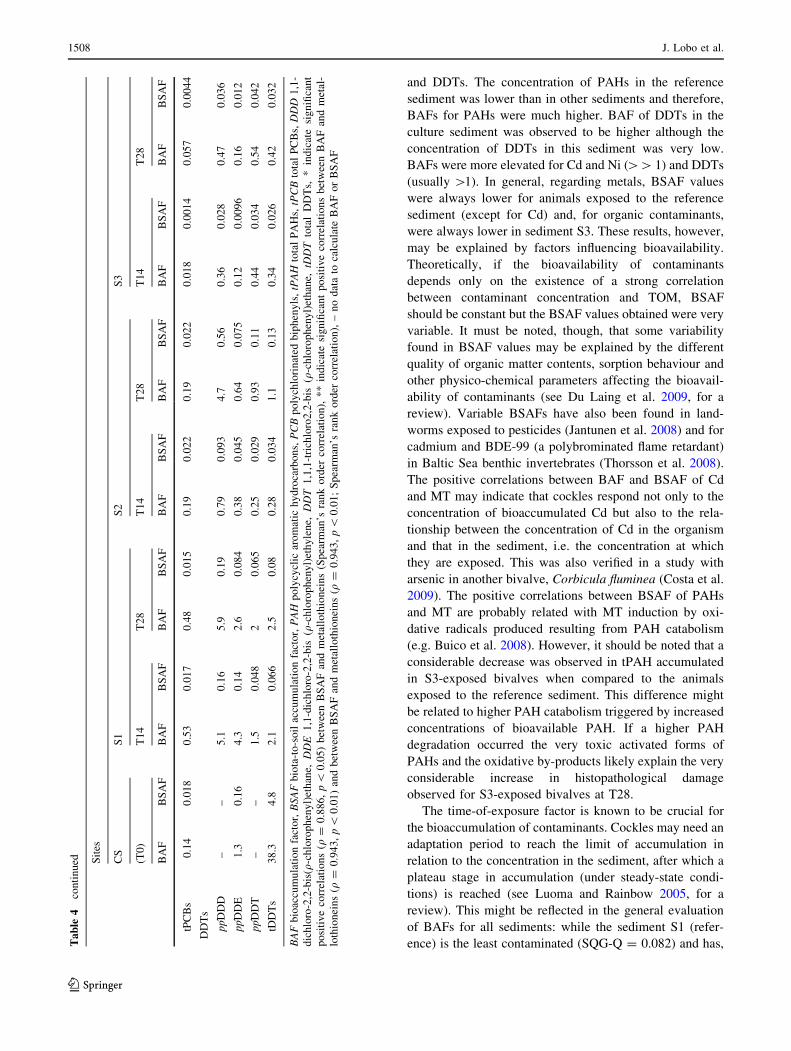
and DDTs. The concentration of PAHs in the reference

sediment was lower than in other sediments and therefore,

BAFs for PAHs were much higher. BAF of DDTs in the

culture sediment was observed to be higher although the

concentration of DDTs in this sediment was very low.

BAFs were more elevated for Cd and Ni ([[ 1) and DDTs

(usually [1). In general, regarding metals, BSAF values

were always lower for animals exposed to the reference

sediment (except for Cd) and, for organic contaminants,

were always lower in sediment S3. These results, however,

may be explained by factors influencing bioavailability.

Theoretically, if the bioavailability of contaminants

depends only on the existence of a strong correlation

between contaminant concentration and TOM, BSAF

should be constant but the BSAF values obtained were very

variable. It must be noted, though, that some variability

found in BSAF values may be explained by the different

quality of organic matter contents, sorption behaviour and

other physico-chemical parameters affecting the bioavail-

ability of contaminants (see Du Laing et al. 2009, for a

review). Variable BSAFs have also been found in land-

worms exposed to pesticides (Jantunen et al. 2008) and for

cadmium and BDE-99 (a polybrominated flame retardant)

in Baltic Sea benthic invertebrates (Thorsson et al. 2008).

The positive correlations between BAF and BSAF of Cd

and MT may indicate that cockles respond not only to the

concentration of bioaccumulated Cd but also to the rela-

tionship between the concentration of Cd in the organism

and that in the sediment, i.e. the concentration at which

they are exposed. This was also verified in a study with

arsenic in another bivalve, Corbicula fluminea (Costa et al.

2009). The positive correlations between BSAF of PAHs

and MT are probably related with MT induction by oxi-

dative radicals produced resulting from PAH catabolism

(e.g. Buico et al. 2008). However, it should be noted that a

considerable decrease was observed in tPAH accumulated

in S3-exposed bivalves when compared to the animals

exposed to the reference sediment. This difference might

be related to higher PAH catabolism triggered by increased

concentrations of bioavailable PAH. If a higher PAH

degradation occurred the very toxic activated forms of

PAHs and the oxidative by-products likely explain the very

considerable increase in histopathological damage

observed for S3-exposed bivalves at T28.

The time-of-exposure factor is known to be crucial for

the bioaccumulation of contaminants. Cockles may need an

adaptation period to reach the limit of accumulation in

relation to the concentration in the sediment, after which a

plateau stage in accumulation (under steady-state condi-

tions) is reached (see Luoma and Rainbow 2005, for a

review). This might be reflected in the general evaluation

of BAFs for all sediments: while the sediment S1 (refer-

ence) is the least contaminated (SQG-Q = 0.082) and has,Ta

ble

4co

nti

nu

ed Sit

es

CS

S1

S2

S3

(T0

)T

14

T2

8T

14

T2

8T

14

T2

8

BA

FB

SA

FB

AF

BS

AF

BA

FB

SA

FB

AF

BS

AF

BA

FB

SA

FB

AF

BS

AF

BA

FB

SA

F

tPC

Bs

0.1

40

.01

80

.53

0.0

17

0.4

80

.01

50

.19

0.0

22

0.1

90

.02

20

.01

80

.00

14

0.0

57

0.0

04

4

DD

Ts

ppD

DD

––

5.1

0.1

65

.90

.19

0.7

90

.09

34

.70

.56

0.3

60

.02

80

.47

0.0

36

ppD

DE

1.3

0.1

64

.30

.14

2.6

0.0

84

0.3

80

.04

50

.64

0.0

75

0.1

20

.00

96

0.1

60

.01

2

ppD

DT

––

1.5

0.0

48

20

.06

50

.25

0.0

29

0.9

30

.11

0.4

40

.03

40

.54

0.0

42

tDD

Ts

38

.34

.82

.10

.06

62

.50

.08

0.2

80

.03

41

.10

.13

0.3

40

.02

60

.42

0.0

32

BA

Fb

ioac

cum

ula

tio

nfa

cto

r,B

SA

Fb

iota

-to

-so

ilac

cum

ula

tio

nfa

cto

r,P

AH

po

lycy

clic

aro

mat

ich

yd

roca

rbo

ns,

PC

Bp

oly

chlo

rin

ated

bip

hen

yls

,tP

AH

tota

lP

AH

s,tP

CB

tota

lP

CB

s,D

DD

1,1

-

dic

hlo

ro-2

,2-b

is(q

-ch

loro

ph

eny

l)et

han

e,D

DE

1,1

-dic

hlo

ro-2

,2-b

is(q

-ch

loro

ph

eny

l)et

hy

len

e,D

DT

1,1

,1-t

rich

loro

2,2

-bis

(q-c

hlo

rop

hen

yl)

eth

ane,

tDD

Tto

tal

DD

Ts,

*in

dic

ate

sig

nifi

can

t

po

siti

ve

corr

elat

ion

s(q

=0

.88

6,

p\

0.0

5)

bet

wee

nB

SA

Fan

dm

etal

loth

ion

ein

s(S

pea

rman

’sra

nk

ord

erco

rrel

atio

n),

**

ind

icat

esi

gn

ifica

nt

po

siti

ve

corr

elat

ion

sb

etw

een

BA

Fan

dm

etal

-

loth

ion

ein

s(q

=0

.94

3,

p\

0.0

1)

and

bet

wee

nB

SA

Fan

dm

etal

loth

ion

ein

s(q

=0

.94

3,

p\

0.0

1;

Sp

earm

an’s

ran

ko

rder

corr

elat

ion

),–

no

dat

ato

calc

ula

teB

AF

or

BS

AF

1508 J. Lobo et al.

123

in general, higher BAFs, the sediment S2 is the most

contaminated (SQG-Q = 0.313) and has generally the

lowest BAFs. Interestingly, the sediment where the cockles

were cultured (CS) was found to be the second most con-

taminated (SQG-Q = 0.181) but the BAFs estimated for

T0 animals, which basically reflect the culture sediment’s

conditions, are often slightly lower than those of the ani-

mals exposed to the reference sediment. It is likely that the

cockles from sediment CS were exposed to local contam-

ination throughout their lives and it is possible that the

steady-state could be attained between the levels of con-

taminants in the distinct compartments of the ecosystem.


123

Nevertheless, although SQG-Qs, could be used as indica-

tors of toxicity, it might be inferred that they should not be

considered on their own. These guidelines are based on

xenobiotics concentrations, not taking into account the

bioavailability of contaminants (unlike bioaccumulation

data) or the synergetic/antagonistic effects of contaminants.

The qualitative approach to assess histopathological

alterations permitted the identification of alterations to the

digestive glands consistent with the levels of sediment

contamination. However, further research is needed to

assess the causes and full biological significance of these

potential biomarkers and attempts are made to enforce

some sort of semi-qualitative approach. Exposure to sedi-

ments caused more damage in digestive glands of cockles

exposed to the most contaminated sediments, S2 and S3

when compared to the exposure to the reference sediment

and the severity of the histopathological lesions was

observed to be progressive from T0 to T28. Nevertheless, it

is likely that unaccounted factors during the assays and

variables influencing the release of xenobiotics from the

sediments have contributed to the increase of digestive

gland alterations in cockles exposed to the reference sedi-

ment, affecting the animals especially at a later stage of the

assay. The moderate increase of the number of excretory

cells in cockles exposed to the reference sediment (S1) at

day 14 (Fig. 2C) could be due to the low level of

contaminants (SQG-Q \ 0.1) but at day 28 the excretory

cells are rarely identified due to the presence of severe

lesions. Decrease of connective tissue and disaggregation

and unidentified cells were presented (Fig. 2D). These

damages do not appear to be caused by the contaminants,

since this sediment is overall little contaminated by any of

the surveyed classes of toxicant, unless unknown chemicals

were present in this sediment, or due to the sediment’s low

TOM and FF, thus increasing bioavailability (Eggleton and

Thomas 2004). However, it should be noticed that it has

been verified that metal exposure enhances excretory

activity in the digestive cells of molluscs and increases the

number of excretory cells (Zaldibar et al. 2008). The

noticeably increased number of excretory cells in the

digestive glands’ tubules of cockles exposed to sediment

S3 for 14 days (Fig. 2G) might be linked to sediment

contamination (probably as a defence mechanism linked to

the elimination of xenobiotics, their metabolites or any

cellular metabolites resulting from toxicity). At day 28, the

damage observed consisted mostly of loss of epithelial

tissue structure and epithelial lifting from tubule basal

laminae (Fig. 2H). There was an evident degradation in the

digestive gland tubule integrity, so the excretory cells are

hardly identified. In cockles exposed to sediments S2 and

S3, histological damage was very pronounced at T14 and,

especially, T28, which is in general accordance with the

highest contamination observed for these sediments.

Induction of MT is usually related to exposure to metals

and metalloids. However, these elements are not the only

factors that modulate MT. For example, in a study with

Corbicula fluminea, MT transcription was positively linked

to the increasing metabolic activity related to the seasonal

temperature elevations (Bigot et al. 2009). In another

example regarding C. edule, it is suggested that even par-

asites can modulate MT synthesis and consequently inter-

fere with the response of these protective proteins in case

of metal contamination (Baudrimont et al. 2006). The

present study showed a decrease of MT levels in cockles

exposed to sediment S3. However, positive correlations

were obtained between PAH, BSAFs and MT and between

Cd BSAFs and Cd BAFs and MT, which is in general

accordance with the known high inducibility of MT by this

metal (e.g. Marie et al. 2006). On the other hand, the

positive correlation between bioaccumulation factors for

Cd to MT suggests that MT induction is highly dependent

on the availability of strong MT inducers (like Cd), which

adds up to yet another factor contributing to the variability

in MT responses, as suggested by other surveys (e.g. Costa

et al. 2008). The reduction in MT contents, conversely may

partially explained by the complex effects of contaminant

interactions. PAHs, for instance, found in the tested sedi-

ments, have been found to suppress MT biosynthesis even

in the presence of strong metal inducers (Risso-De

Fig. 2 Histological sections stained with haematoxylin and eosin of

digestive gland of Cerastoderma edule. Scale bar: 50 lm. A T0

cockle showing a normal digestive gland, with connective tissue (ct)between tubules. The tubules present a normal structure, with a well-

defined lumen (L). Digestive cells (dc) and excretory cells (*) in

tubule walls are clearly visible. B Enlargement of image A showing a

digestive gland tubule, where the lumen (L) and connective tissue (ct)are intact, and the digestive cells (dc) and excretory cells (*) are easily

distinguished. C Digestive gland from a cockle exposed to the

reference sediment (S1) for 14 days. The number of excretory cells

(*) increased but the digestive gland remains unaltered. D Digestive

gland of a cockle exposed to the reference sediment (S1) for 28 days,

exhibiting connective tissue regression and tubules with altered and

disaggregating epithelial cells (#). E Cockle exposed to sediment

from site S2 (the most contaminated), collected at T14. There is a

marked degradation of the digestive gland integrity, with the tubule

cells detaching from the basal lamina (#). Moderate regression of

intertubular connective tissue can also be observed. Hyperplasia of

tubule epithelial cells was found to be a recurrent alteration (hp).

F Digestive gland of a cockle exposed to sediment S2 at T28.

Although the regression of connective tissue remains moderate,

tubule regression becomes more severe, loosing their shape and

exhibiting many cells detaching to the lumen (#) and occasional foci

of necrosis (n). G Cockle exposed to sediment S3 at T14. The

epithelium of tubules is essentially intact but a major loss of the

surrounding connective tissue can be observed. The number of tubule

excretory cells increased compared to T0 individuals (#) and a very

considerable regression of connective tissue (rct) can be observed.

H Cockle exposed to sediment S3 for 28 days, exhibiting a

pronounced degradation in the digestive gland, affecting tubule

integrity (with very pronounced detachment of cells to the lumen (#)

and the connective tissue

b

1510 J. Lobo et al.

123

Faverney et al. 2000). It should also not be discarded that

gene expression and protein synthesis is impaired in tissue

damage by exposure to toxicants, as histologically deter-

mined the digestive glands of the cockles exposed to the

most contaminated sediments.

This study revealed notable responses in cockles to

different levels of contamination, hence, it is suggested that

C. edule responds to sediment-bound contamination. For

some contaminants, bioaccumulation decreased, which can

be due to the observed deterioration of digestive gland

tissue and subsequent impairment of responses to xenobi-

otics. Still, the species revealed to be robust to endure both

the contamination profiles and the testing procedures.

Bioaccumulation and histopathology were successfully

integrated and provided valuable information of what

happens in estuarine sediments even when complex inter-

action of different types of contaminants is involved.

Therefore, this cockle might be suitable for biomonitoring,

even though it is clear that the effects of contaminant

interactions on biomarkers and indicators of exposure need

yet much research. These include further development on

the histopathological biomarkers here qualitatively

screened in the digestive gland such as deterioration of

tubules, excretory cell alterations, epithelia and connective

tissue and detachment of tubular epithelia. On the other

hand, it must be noticed that caution is mandatory when

testing bivalves cultured in natural sediments since the

levels of contaminants of the culture sediments are likely

capable of influencing the results, as suspected from the

present study.

Acknowledgments The present research was approved by the

Portuguese Science and Technology Foundation (FCT) and POCTI

(Programa Operacional Ciencia, Tecnologia e Inovacao, research

project ref. POCTI/AMB 57281/104) and financed by FEDER

(European Fund for Regional Development). The authors would also

like to thank APSS (Administracao dos Portos de Setubal e Sesimbra,

SA) and RNES (Reserva Natural do Estuario do Sado) for the logistic

support and Mr Manuel Ribeiro for the offer of the cockles.

References

Amiard J-C, Amiard-Triquet C, Barka S, Pellerin J, Rainbow PS

(2006) Metallothioneins in aquatic invertebrates: their role in

metal detoxification and their use as biomarkers. Aquat Toxicol

76:160–202

Baudrimont M, de Montaudouin X, Palvadeau A (2006) Impact of

digenean parasite infection on metallothionein synthesis by the

cockle (Cerastoderma edule): a multivariate field monitoring.

Mar Pollut Bull 52:494–502

Bergayou H, Mouneyrac C, Pellerin J, Moukrim A (2009) Oxidative

stress responses in bivalves (Scrobicularia plana, Cerastodermaedule) from the Oued Souss estuary (Morocco). Ecotox Environ

Safe 72:765–769

Bigot A, Doyen P, Vasseur P, Rodius F (2009) Metallothionein

coding sequence identification and seasonal mRNA expression

of detoxification genes in the bivalve Corbicula fluminea. Ecotox

Environ Safe 72:382–387

Buico A, Cassino C, Dondero F, Vergani L, Osella D (2008) Radical

scavenging metallothionein isoforms: an ESR study. J Inorg

Biochem 102:921–927

Caeiro S, Costa MH, Ramos TB, Fernandes F, Silveira N, Coimbra A,

Medeiros G, Painho M (2005) Assessing heavy metal contam-

ination in Sado Estuary sediment: an index analysis approach.

Ecol Indic 5:151–169

Caetano M, Fonseca N, Cesario R, Vale C (2007) Mobility of Pb in

salt marshes recorded by total content and stable isotopic

signature. Sci Total Environ 380:84–92

Cajaraville MP, Bebianno MJ, Blasco J, Porte C, Sarasquete C,

Viarengo A (2000) The use of biomarkers to assess the impact of

pollution in coastal environments of the Iberian Peninsula: a

practical approach. Sci Total Environ 247:295–311

Clesceri LS, Greenberg AE, Eaton AD (1999) Standard methods for

examination of water & wastewater, 20th edn. American Public

Health Association, Baltimore

Cortesao C, Vale C (1995) Metals in sediments of the Sado Estuary,

Portugal. Mar Pollut Bull 30:34–37

Costa PM, Repolho T, Caeiro S, Diniz ME, Moura I, Costa MH

(2008) Modelling metallothionein induction in the liver of

Sparus aurata exposed to metal-contaminated estuarine sedi-

ments. Ecotox Environ Safe 71:117–124

Costa PM, Santos HM, Peres I, Costa MH, Alves S, Capelo-Martinez

JL, Diniz MS (2009) Toxicokinetics of waterborne trivalent

arsenic in the freshwater bivalve Corbicula fluminea. Arch

Environ Con Tox 57:338–347

De Kock WC, Kramer KJM (1994) Active biomonitoring (ABM) by

translocation of bivalve molluscs. In: Kramer KJM (ed)

Biomonitoring of coastal waters and estuaries. CRC Press, Boca

Raton, pp 51–84

Del Valls TA, Forja JM, Gomez-Parra A (1998) The use of

multivariate analysis to link sediment contamination and toxicity

data to establish sediment quality guidelines: an example in the

Gulf of Cadiz (Spain). Cienc Mar 24:127–154

Diniz M, Santos HM, Costa PM, Peres I, Costa MH, Capelo JL (2007)

Metallothionein responses in the Asiatic clam (Corbiculafluminea) after exposure to trivalent arsenic. Biomarkers

12:589–598

Du Laing G, Rinklebe J, Vandecasteele B, Meers E, Tack FMG

(2009) Trace metal behaviour in estuarine and riverine flood-

plain soils and sediments: a review. Sci Total Environ

407:3972–3985

Eggleton J, Thomas KV (2004) A review of factors affecting the

release and bioavailability of contaminants during sediment

disturbance events. Environ Int 30:973–980

Ferreira AM, Martins M, Vale C (2003) Influence of diffuse sources

on levels and distribution of polychlorinated biphenyls in the

Guadiana River estuary, Portugal. Mar Chem 89:175–184

Geret F, Serafim A, Bebianno MJ (2003) Antioxidant enzyme

activities, metallothioneins and lipid peroxidation as biomarkers

in Ruditapes decussatus. Ecotoxicology 12:417–426

Gold-Bouchot G, Sima-Alvarez R, Zapata-Perez O, Guemez-Ricalde

J (1995) Histopathological effects of petroleum hydrocarbons

and heavy metals on the American oyster (Crassostrea virginica)

from Tabasco, Mexico. Mar Pollut Bull 31:4–12

Hedouin L, Pringault O, Metian M, Bustamante P, Warnau M (2007)

Nickel bioaccumulation in bivalves from the New Caledonia

lagoon: seawater and food exposure. Chemosphere

66:1449–1457

Huggett RJ, Kimerle RA, Mehrle PM, Bergman HL (eds) (1992)

Biomarkers: biochemical, physiological, and histological mark-ers of anthropogenic stress. Lewis Publishers, Boca Raton, FL


123

Jantunen APK, Tuikka A, Akkanen J, Kukkonen JVK (2008)

Bioaccumulation of atrazine and chlorpyrifos to Lumbriculusvariegatus from lake sediments. Ecotox Environ Safe

71:860–868

Jung K, Stelzenmuller V, Zauke G-P (2006) Spatial distribution of heavy

metal concentrations and biomass indices in Cerastoderma eduleLinnaeus (1758) from the German Wadden Sea: an integrated

biomonitoring approach. J Exp Mar Biol Ecol 338:81–95

Lee H (1992) Models, muddles, and mud: predicting bioaccumulation

of sediment associated pollutants. In: Burton AG (ed) Sediment

toxicity assessment. CRC, Boca Raton, FL, pp 267–293

Livingstone DR (2001) Contaminant-stimulated reactive oxygen

species production and oxidative damage in aquatic organisms.

Mar Pollut Bull 42(8):656–666

Long ER, MacDonald DD (1998) Recommended uses of empirically

derived, sediment quality guidelines for marine and estuarine

ecosystems. Hum Ecol Risk Assess 4:1019–1039

Luoma S, Rainbow P (2005) Why is metal bioaccumulation so

variable? Biodynamics as a unifying concept. Environ Sci

Technol 39:1921–1931

MacDonald DD, Carr S, Calder F, Long E, Ingersoll C (1996)

Development and evaluation of sediment quality guidelines for

Florida coastal waters. Ecotoxicology 5:253–278

MacDonald DD, Carr RS, Eckenrod D, Greening H, Grabe S,

Ingersoll CG, Janicki S, Janicki T, Lindskoog RA, Long ER,

Pribble R, Sloane G, Smorong DE (2004) Development,

evaluation, and application of sediment quality targets for

assessing and managing contaminated sediments in Tampa Bay,

Florida. Arch Environ Cont Tox 46:147–161

Machreki-Ajmi M, Ketata I, Ladhar-Chaabouni R, Hamza-Chaffai A

(2008) The effect of in situ cadmium contamination on some

biomarkers in Cerastoderma glaucum. Ecotoxicology 17:1–11

Marie V, Baudrimont M, Boudou A (2006) Cadmium and zinc

bioaccumulation and metallothionein response in two freshwater

bivalves (Corbicula fluminea and Dreissena polymorpha) trans-

planted along a polymetallic gradient. Chemosphere 65:609–617

Martins M, Ferreira AM, Vale C (2008) The influence of Sarcocorniafruticosa on retention of PAHs in salt marshes sediments (Sado

estuary, Portugal). Chemosphere 71:1599–1606

Martoja R, Martoja M (1967) Initiation aux tecniques de l’histologie

animal. Masson & Cie, Paris, p 345

Peakall DB, Shugart LR (eds) (1993) Biomarkers research and

application in the assessment of environmental health. Springer-

Verlag, Berlin, Heidelberg

Risso-de Faverney C, Lafaurie M, Girard J-P, Rahmani R (2000)

Effects of heavy metals and 3-methylcholanthrene on expression

and induction of CYP1A1 and metallothionein levels in trout

(Oncorhynchus mykiss) hepatocyte cultures. Environ Toxicol

Chem 19:2239–2248

Serafim A, Bebianno MJ (2009) Metallothionein role in the kinetic

model of copper accumulation and elimination in the clam

Ruditapes decussates. Environ Res 109:390–399

Sole M, Kopecka-Pilarczyk J, Blasco J (2009) Pollution biomarkers in

two estuarine invertebrates, Nereis diversicolor and Scrobicu-laria plana, from a Marsh ecosystem in SW Spain. Environ Int

35:523–531

Syasina IG, Vaschenko MA, Zhadan PM (1997) Morphological

alterations in the digestive diverticula of Mizuhopecten yesso-ensis (Bivalvia: Pectinidae) from polluted areas of Peter the

Great Bay, Sea of Japan. Mar Environ Res 44:85–98

Thorsson MH, Hedman JE, Bradshaw C, Gunnarsson JS, Gilek M

(2008) Effects of settling organic matter on the bioaccumulation

of cadmium and BDE-99 by Baltic Sea benthic invertebrates.

Mar Environ Res 65:264–281

United States Environmental Protection Agency (1995) CRITFC

exposure study. Water quality criteria and standards Newsletter.

USEPA, Washington, DC

Zaldibar B, Cancio I, Soto M, Marigomez I (2007) Digestive cell

turnover in digestive gland epithelium of slugs experimentally

exposed to a mixture of cadmium and kerosene. Chemosphere

70:144–154

Zaldibar B, Cancio I, Soto M, Marigomez I (2008) Changes in cell-

type composition in digestive gland of slugs and its influence in

biomarkers following transplantation between a relatively

unpolluted and a chronically metal-polluted site. Environ Pollut

156:367–379

1512 J. Lobo et al.

123

Evaluation of the potential of the common cockle (Cerastoderma edule L.) for the ecological risk assessment of estuarine sediments: bioaccumulation and biomarkers

Documents