Europe's offshore winds assessed from SAR, ASCAT and WRF

1

Europe’s offshore winds assessed from SAR, ASCAT and WRF Charlotte B. Hasager1, Andrea N. Hahmann1, Tobias Ahsbahs1, Ioanna Karagali1, Tija Sile2, Merete Badger1, Jakob Mann1 1Department of Wind Energy, Technical University of Denmark, Frederiksborgvej 399, 4000 Roskilde, Denmark 5 2Department of Physics, University of Latvia, Jelgavas iela 3, Riga, LV-1004, Latvia

Correspondence to: Charlotte B. Hasager ([email protected])

Abstract. Europe’s offshore wind resource mapping is part of the New European Wind Atlas (NEWA) international

consortium effort. This study presents the results of analysis of Synthetic Aperture Radar (SAR) ocean wind maps based on

Envisat and Sentinel-1 with a brief description of the wind retrieval process and Advanced SCATterometer (ASCAT) ocean 10

wind maps. The wind statistics at 10m and 100m height using an extrapolation procedure involving simulated long-term

stability over oceans is presented for both SAR and ASCAT. Furthermore, the Weather Research and Forecasting (WRF)

offshore wind atlas of NEWA is presented. This has 3 km grid resolution with data every 30 minutes during 30 years from

1989 to 2018, while ASCAT has 12.5 km and SARhas 2 km resolution. Offshore mean wind speed maps at 100m height from

ASCAT, SAR, WRF and ERA5 at a European scale are compared. A case study on offshore winds near Crete compares SAR 15

and WRF for flow from north, west and all directions.

The paper highlights the ability of the WRF model to simulate the overall European wind climatology and the near coastal

winds constrained by the resolution of the coastal topography in the WRF model simulations.

1 Introduction

The extraction of energy from wind is part of the clean energy transition. It supports society to reach the objectives of the Paris 20

Climate Change agreement and the Sustainable Development Goals. Wind energy in Europe provided 14% of total electricity

consumption in 2018. This share will increase in coming years. By the end of 2018, the installed offshore capacity reached

18.5 GW, which is approximately 10% of Europe’s total wind energy capacity (Wind Europe, 2019).

Beyond the beneficial impact on reducing carbon dioxide emissions, the offshore wind energy industry is a significant 25

economical factor. According to the Organisation for Economic Co-operation and Development (OECD, 2016), the total of

all ocean-based industries globally will double from USD 1.5 in 2010 to 3 trillion by 2030. Offshore wind energy has the

highest relative growth rate of the ocean-based industries. In Europe alone, the investments in 2018 in new offshore wind

amounted to €10.3bn, a 37% increase from 2017 (Wind Europe, 2019).

30

https://doi.org/10.5194/wes-2019-38Preprint. Discussion started: 19 July 2019c© Author(s) 2019. CC BY 4.0 License.

2

Many countries in Europe have operating offshore wind farms. The North Sea accounts for 70% of all installed offshore wind

capacity in Europe, followed by the Irish Sea (16%), the Baltic Sea (12%), and the Atlantic Ocean (2%). The longest distance

from shore of operating wind turbines exceeds 100 km while permits are given for installation as far as 200 km offshore (Wind

Europe, 2019). The expectation is that offshore wind energy will expand to more European seas and that new wind farms are

erected in clusters, which already exist in parts of the North Sea already (4C Offshore, 2019). 35

The New European Wind Atlas (NEWA) project focused on experimental campaigns across Europe in different terrain types.

These experiments provide unique data for validation of wind models (Petersen et al., 2014; Mann et al., 2017; Witze, 2017).

Two of the field experiments are relevant for offshore wind resource mapping. The first is the coastal experiment RUNE with

a floating lidar system, three long-range horizontally scanning wind lidars and several vertical wind profiling lidars installed 40

at the North Sea coastline (Floors et al., 2016) nearby the tall meteorological masts at Høvsøre in Denmark (Peña et al., 2015).

The second is the wind profiling lidar installed at the ferry link between Kiel and Klaipeda in the Baltic Sea (Gottschall et al.,

2018). The two experiments had a duration of around six months. In addition to the dedicated experiments, several years of

meteorological observations from tall offshore masts all located in the Northern European Seas are used in preparation of the

NEWA offshore wind atlas. 45

The NEWA project (2015-2019) produced the novel state of the art offshore wind atlas for European Seas covering a minimum

distance up to 100 km offshore and the entire North Sea and Baltic Sea, excluding Iceland. In addition to the entire wind atlas

simulated using the Weather, Research and Forecasting (WRF) model (Hahmann et al. in prep.), also satellite Synthetic

Aperture Radar (SAR) and Advanced Scatterometer (ASCAT) ocean winds are processed and analyzed for wind resource 50

assessment.

The overall objective of the study is to present the new European Offshore Wind Atlas and to examine the similarities and

differences of wind maps based on ASCAT, SAR and the WRF model. The study focuses on how to use satellite observations

for model comparison beyond single cases, and specifically to investigate how different are the 100m mean winds based on 55

ASCAT, SAR and WRF.

2 Background

In the planning phase of a wind farm project there is need for information on the wind resource (Emeis, 2012; Landberg, 2012;

Petersen and Troen, 2012). The methodologies for offshore wind resource assessment rely on wind observations from offshore 60

meteorological masts, wind lidar, SODAR (sound detection and ranging), satellite images and modelling (Sempreviva et al.,

2008). The first atlas of the European wind resource covered only land (Troen and Petersen, 1989) and was later extended to


3

offshore (Petersen, 1992). Modelling of wind resources has a long tradition starting with the above-mentioned wind atlas.

Recent offshore model-based wind atlases for the European seas include the German Bight (Jimenez et al., 2006), the

Mediterranean Sea (Lavignini et al., 2006), the UK (UK Renewables Atlas, 2008), the North Sea (Berge et al., 2009), the 65

European Seas (EEA, 2009), the South Baltic Sea (Peña et al., 2011) and the Baltic and North Sea (Hahmann et al., 2015).

Offshore wind resource assessment based on in situ meteorological wind observations in the Baltic and North Sea (see review

in Sempreviva et al., 2008), Italy (Casale et al., 2010) and Malta (Farrugia and Sant, 2016) provide local information.

Furthermore, the meteorological observations are useful for comparison to model results to select suitable atmospheric model 70

setup and to assess the model performance (Jimenez et al., 2006; Berge et al., 2009; Hahmann et al., 2015).

Satellite remote sensing used to assess offshore wind resources for the European Seas include scatterometer and SAR

measurements. Scatterometer estimates have been validated for the Mediterranean Sea with buoy data (Furevik et al., 2011)

and for the Northern European Seas with meteorological mast data (Karagali et al., 2013a; Karagali et al., 2014; Karagali et 75

al. 2018a). Soukissian et al. (2017) used a blended satellite product based on six different satellites for the Mediterranean Sea

and compared to buoy data.

Satellite SAR was used for resource assessment for the North Sea (Hasager et al., 2005; Christiansen et al., 2006; Badger et

al., 2010) and the Baltic Sea (Hasager et al., 2011; Badger et al., 2016) and was compared to meteorological mast data. Coastal 80

mast data and mesoscale model results were compared to SAR-based wind resource estimates for the Icelandic waters,

(Hasager et al., 2015a). Scatterometer data (ASCAT) was also compared to WRF mesoscale model results in the entire

European Seas (Karagali et al. 2018a, 2018b).

There is potential to also compare model results and satellite data to wind profiling lidar (light detection and ranging) data at 85

offshore platforms (Hasager et al., 2013) and floating wind profile lidar systems (OWA 2018; Bischoff et al., 2018). These

are local point data similar to buoy data and meteorological mast data. Recently, new technological advancements provide

opportunities for horizontal spatial data comparison. Three such types are horizontally scanning lidar, long row of turbines

providing SCADA (Supervisory Control And Data Acquisition) data, and ship-mounted vertical profiling lidar.

90

Recently, offshore winds observed with long-range scanning lidar at a coastal site at the North Sea (Floors et al., 2016) were

compared to SAR winds and showed good comparison within 2 to 5 km from the North Sea coastline. The good agreement

was unexpected because the Geophysical Model Function (GMF) used to retrieve winds from SAR is valid in open-ocean and

not near the coast. The conclusion of the study is that SAR winds are mapped well as close as 2 km from the coastline at the

site investigated (Ahsbahs et al., 2017). Documentation at more complex coastline remains open. 95


4

Another recent study found that the SAR-based winds compare slightly better than mesoscale model results to the wind speed

observed at 20km long row of turbines. The turbines are operating in an area with a strong horizontal wind gradient along the

coast (Ahsbahs et al., 2018).

100

The third novel spatial comparison method was based on a vertical profiling lidar installed on-board a ferry sailing daily across

the Baltic Sea for several hundred kilometers; measurements compared well to mesoscale model results (Gottschall et al.,

2018). Data near the harbors were excluded from the analysis. The WRF mesoscale model results generally are better offshore

than near coastlines due to the differences between land and sea influencing the atmospheric flow (Hahmann et al., 2010;

Hahmann et al., 2015; Floors et al., 2018). 105

The presentation of methodology for wind mapping based on ASCAT, SAR and WRF is given in Section 3. Section 4 presents

the results for the entire European Seas from ASCAT, SAR and WRF, their inter-comparisons and cross-comparison to ERA5.

Section 5 is a case study of offshore winds around Western Crete using SAR and WRF; thus, provides insight to specific details

on the two types of data. Section 6 covers a discussion and perspectives regarding the results, followed by conclusions in 110

Section 7.

3 Methodology

3.1 Area of interest and time period

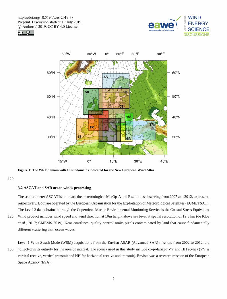
The offshore part of NEWA covers the European Union, associated states, and Turkey from the coastline and at least 100 km

offshore. For the WRF model, the simulations are done for 10 separate subdomains, which are later merged into one domain 115

(Figure 1). The WRF modelling covers 30 years from 1989 to 2018. For the satellite data collection, processing and analysis,

it is convenient to select an area of interest within latitudes (here 33.5° to 72.2°) and longitudes (here 19.4°W to 47°E).


5

Figure 1: The WRF domain with 10 subdomains indicated for the New European Wind Atlas.

120

3.2 ASCAT and SAR ocean winds processing

The scatterometer ASCAT is on-board the meteorological MetOp-A and B satellites observing from 2007 and 2012, to present,

respectively. Both are operated by the European Organisation for the Exploitation of Meteorological Satellites (EUMETSAT).

The Level 3 data obtained through the Copernicus Marine Environmental Monitoring Service is the Coastal Stress Equivalent

Wind product includes wind speed and wind direction at 10m height above sea level at spatial resolution of 12.5 km (de Kloe 125

et al., 2017; CMEMS 2019). Near coastlines, quality control omits pixels contaminated by land that cause fundamentally

different scattering than ocean waves.

Level 1 Wide Swath Mode (WSM) acquisitions from the Envisat ASAR (Advanced SAR) mission, from 2002 to 2012, are

collected in its entirety for the area of interest. The scenes used in this study include co-polarized VV and HH scenes (VV is 130

vertical receive, vertical transmit and HH for horizontal receive and transmit). Envisat was a research mission of the European

Space Agency (ESA).


6

Level 1 Extra Wide (EW) and Interferometric Wide (IW) mode acquisitions from the Sentinel-1A mission (2014-present) and

Sentinel-1B (2016-present) are collected in its entirety for the area of interest. The scenes used in this study include EW and 135

IW mode and VV and HH polarization. Sentinel-1A/B are parts of Copernicus, the European Commission’s monitoring

program. Table 1 lists the source data from ASCAT, Envisat and Sentinel-1.

ASCAT, Envisat and Sentinel-1 are polar orbiting satellites. The number of samples of ocean wind data in any pixel (grid cell)

depend upon the data recordings during time and space. For Envisat this was inhomogeneous due to various research priorities 140

in the beginning of the mission. During later years (2008 to 2012), recording was high and consistent in the area of interest.

ASCAT-A/B and Sentinel-1A/B are operational monitoring satellites and have frequent coverage in the entire domain since

launch. For all satellites, there are more samples available at higher latitudes due to the polar-orbital paths.

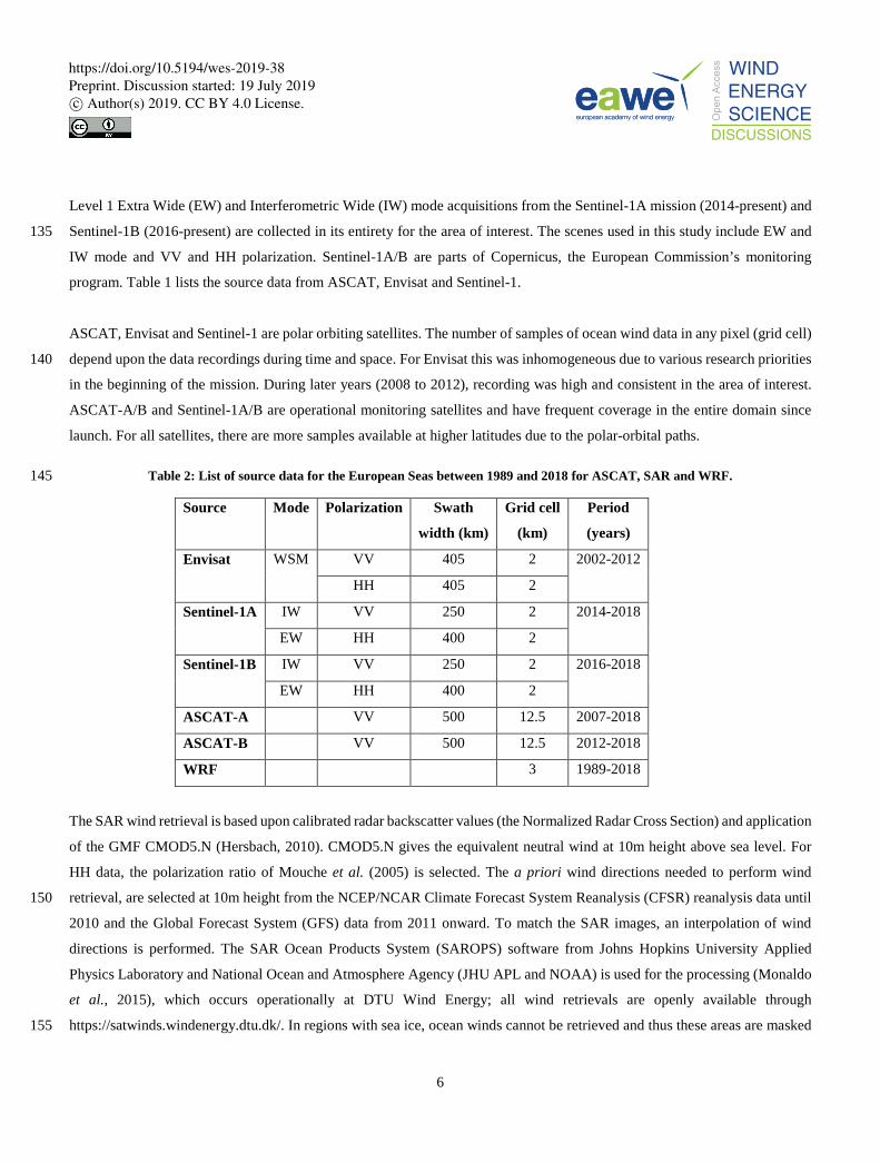
Table 2: List of source data for the European Seas between 1989 and 2018 for ASCAT, SAR and WRF. 145

Source Mode Polarization Swath

width (km)

Grid cell

(km)

Period

(years)

Envisat WSM VV 405 2 2002-2012

HH 405 2

Sentinel-1A IW VV 250 2 2014-2018

EW HH 400 2

Sentinel-1B IW VV 250 2 2016-2018

EW HH 400 2

ASCAT-A VV 500 12.5 2007-2018

ASCAT-B VV 500 12.5 2012-2018

WRF 3 1989-2018

The SAR wind retrieval is based upon calibrated radar backscatter values (the Normalized Radar Cross Section) and application

of the GMF CMOD5.N (Hersbach, 2010). CMOD5.N gives the equivalent neutral wind at 10m height above sea level. For

HH data, the polarization ratio of Mouche et al. (2005) is selected. The a priori wind directions needed to perform wind

retrieval, are selected at 10m height from the NCEP/NCAR Climate Forecast System Reanalysis (CFSR) reanalysis data until 150

2010 and the Global Forecast System (GFS) data from 2011 onward. To match the SAR images, an interpolation of wind

directions is performed. The SAR Ocean Products System (SAROPS) software from Johns Hopkins University Applied

Physics Laboratory and National Ocean and Atmosphere Agency (JHU APL and NOAA) is used for the processing (Monaldo

et al., 2015), which occurs operationally at DTU Wind Energy; all wind retrievals are openly available through

https://satwinds.windenergy.dtu.dk/. In regions with sea ice, ocean winds cannot be retrieved and thus these areas are masked 155


7

out using the National Ice Center's Interactive Multi-sensor Snow and Ice Mapping System (IMS) with daily data at 4 km

resolution (National Ice Center, 2008).

Satellite winds retrieved at 10m height are averaged into wind resource statistics using the software for SAR-based wind

resource assessment (Hasager et al., 2008, Hasager et al., 2011, Ahsbahs et al., 2019) and for ASCAT using the methodology 160

presented in (Karagali et al., 2018b). Wind turbines offshore operate at around 100m height. Therefore, an extrapolation of

wind speed from 10m to 100m height is applied. Previous investigations show that applying a long-term stability correction is

superior to neutral logarithmic wind profile in the Baltic Sea (Badger et al., 2016) and in the North Sea (Karagali et al., 2018a).

For the NEWA offshore wind atlas, the extrapolation is done similar to Karagali et al. (2018a, 2018b) using 10-years of WRF

model simulations from Nuño Martinez et al. (2018) for the long-term stability correction. 165

3.3 Mesoscale modelling

The WRF model (Skamarock et al., 2008) used for the production run of the New European Wind Atlas is a limited area

weather forecast model. The WRF model is a public domain, open-source modelling system, which has previously been used

to produce wind atlas for South Africa (Hahmann et al., 2014), the North Sea and Baltic Sea (Hahmann et al., 2015), Denmark 170

(Peña and Hahmann, 2017) and wind statistics for Europe (Nuño Martines et al., 2018).

The production run for NEWA was computed on the HPC cluster MareNostrum at the Barcelona Supercomputing Center and

on HPC Cluster EDDY at the University of Oldenburg. In order to determine optimal model scheme and forcing, surface input

and land surface model, a series of sensitivity tests were conducted and compared to tall meteorological mast data masts in 175

northern Europe and the North Sea. No setting was optimal for all, so a compromise was taken, which provided the best

verification statistics (see Witha et al., 2019 for more details). In brief, the production run was setup for 10 separate WRF

domains, which shared the same outer domain and map projection, and later merged provide one unified atlas

(http://www.neweuropeanwindatlas.eu/). The WRF model used was a modified version of 3.8.1, setup with the MYNN

Planetary Boundary Layer (Nakanishi and Niino, 2009) and Monin-Obukhov surface layer (Monin and Obukhov, 1954) 180

schemes. Forcing for the simulations was from ERA5 reanalysis (ERA5, 2017) at 0.3° x 0.3° resolution and OSTIA Sea

Surface Temperature (Donlon et al. 2012) at 1/20° resolution. The CORINE land cover data at 100 m resolution was used to

define the land use classes, except for areas it does not cover, then ESA CCI data is used. The NOAH land surface model and

icing WSM5 plus ice code and sum of cloud and ice humidity. The WRF simulations used three nested domains at 27 km, 9

km and 3 km and 61 vertical layers, with 8-day overlapping runs using spectral nudging with 24-hour spin-up (see Hahmann 185

et al., 2015 for details on the technique). The years covered and spatial resolution are listed in Table 1.


8

4 Offshore wind speed assessment for Europe

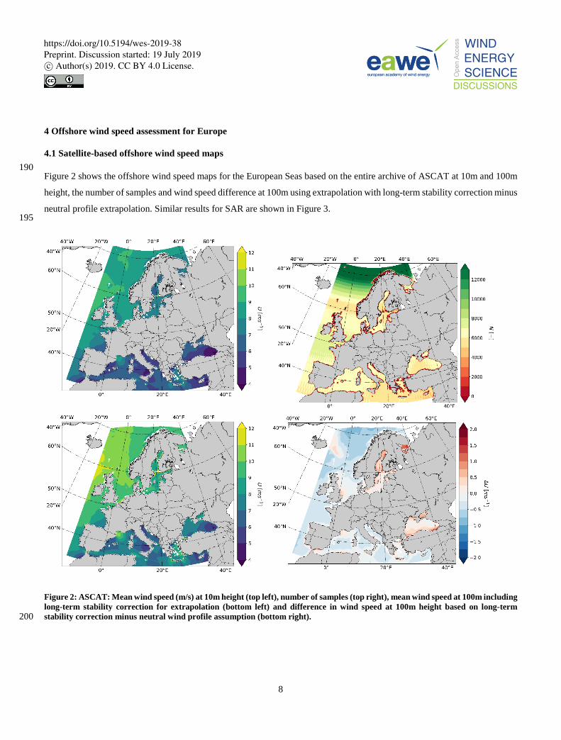
4.1 Satellite-based offshore wind speed maps 190 Figure 2 shows the offshore wind speed maps for the European Seas based on the entire archive of ASCAT at 10m and 100m

height, the number of samples and wind speed difference at 100m using extrapolation with long-term stability correction minus

neutral profile extrapolation. Similar results for SAR are shown in Figure 3.

195

Figure 2: ASCAT: Mean wind speed (m/s) at 10m height (top left), number of samples (top right), mean wind speed at 100m including long-term stability correction for extrapolation (bottom left) and difference in wind speed at 100m height based on long-term stability correction minus neutral wind profile assumption (bottom right). 200


9

205

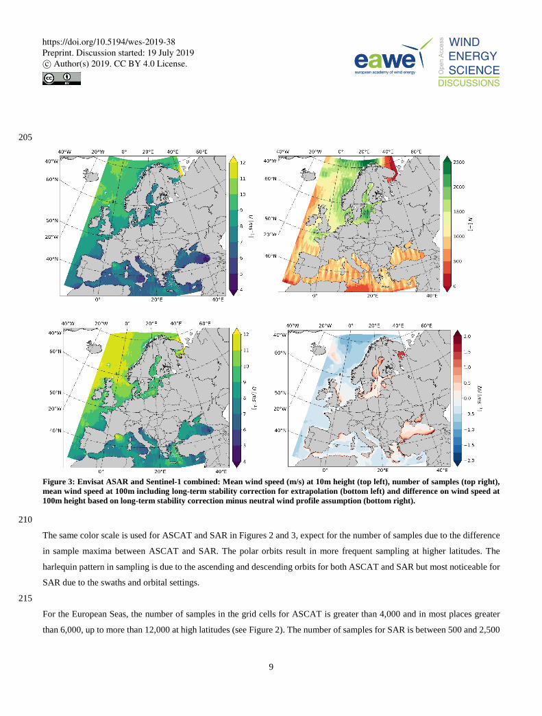
Figure 3: Envisat ASAR and Sentinel-1 combined: Mean wind speed (m/s) at 10m height (top left), number of samples (top right), mean wind speed at 100m including long-term stability correction for extrapolation (bottom left) and difference on wind speed at 100m height based on long-term stability correction minus neutral wind profile assumption (bottom right).

210

The same color scale is used for ASCAT and SAR in Figures 2 and 3, expect for the number of samples due to the difference

in sample maxima between ASCAT and SAR. The polar orbits result in more frequent sampling at higher latitudes. The

harlequin pattern in sampling is due to the ascending and descending orbits for both ASCAT and SAR but most noticeable for

SAR due to the swaths and orbital settings.

215

For the European Seas, the number of samples in the grid cells for ASCAT is greater than 4,000 and in most places greater

than 6,000, up to more than 12,000 at high latitudes (see Figure 2). The number of samples for SAR is between 500 and 2,500


10

(see Figure 3). For the WRF model, the number is constant at all locations covered with 525,912 samples (every 30 minutes

from 1989 to 2018).

220

The mean wind speed consistently shows higher values for the 100m height than 10m height both in ASCAT and SAR. The

wind speed difference maps at 100m based on long-term stability correction minus neutral wind profile assumption shows

very similar spatial patterns between ASCAT and SAR, as expected. The variation is up to ±2 m/s with high positive values

in the Baltic Sea and Black Sea and with high negative values in the Norwegian Sea. Positive values occur for stable conditions.

The continental climate dominating the flow in the Baltic Sea and the Black Sea cause the variations. Negative values occur 225

for unstable conditions prevalent in global oceans (Kara et al., 2008) and here noted in the Norwegian Sea. In the North Sea,

a gradient is observed with slightly negative values along the continental coast and positive values along the UK coast. This

corresponds well with the average stability over the North Sea (Peña and Hahmann, 2012), where unstable conditions prevail

along the continental coast and stable conditions near the UK. The Mediterranean Sea has mixed wind speed difference

variations dominated by moderately negative values in the central part and positive values in the Greek archipelago and the 230

French Riviera.

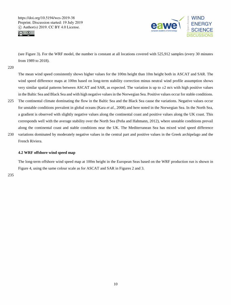
4.2 WRF offshore wind speed map

The long-term offshore wind speed map at 100m height in the European Seas based on the WRF production run is shown in

Figure 4, using the same colour scale as for ASCAT and SAR in Figures 2 and 3.

235


11

Figure 4: WRF New European Wind Atlas production run mean wind speed (m/s) at 100m height for 1989 to 2018 with 3 km spatial resolution.

ASCAT and WRF have many similarities in the spatial wind sped patterns and the range of mean wind speeds at 100m height. 240

The SAR mean wind speed at 100m height appears to be higher than ASCAT and WRF. Furthermore, SAR shows more fine-

scale spatial variations than both ASCAT and WRF.

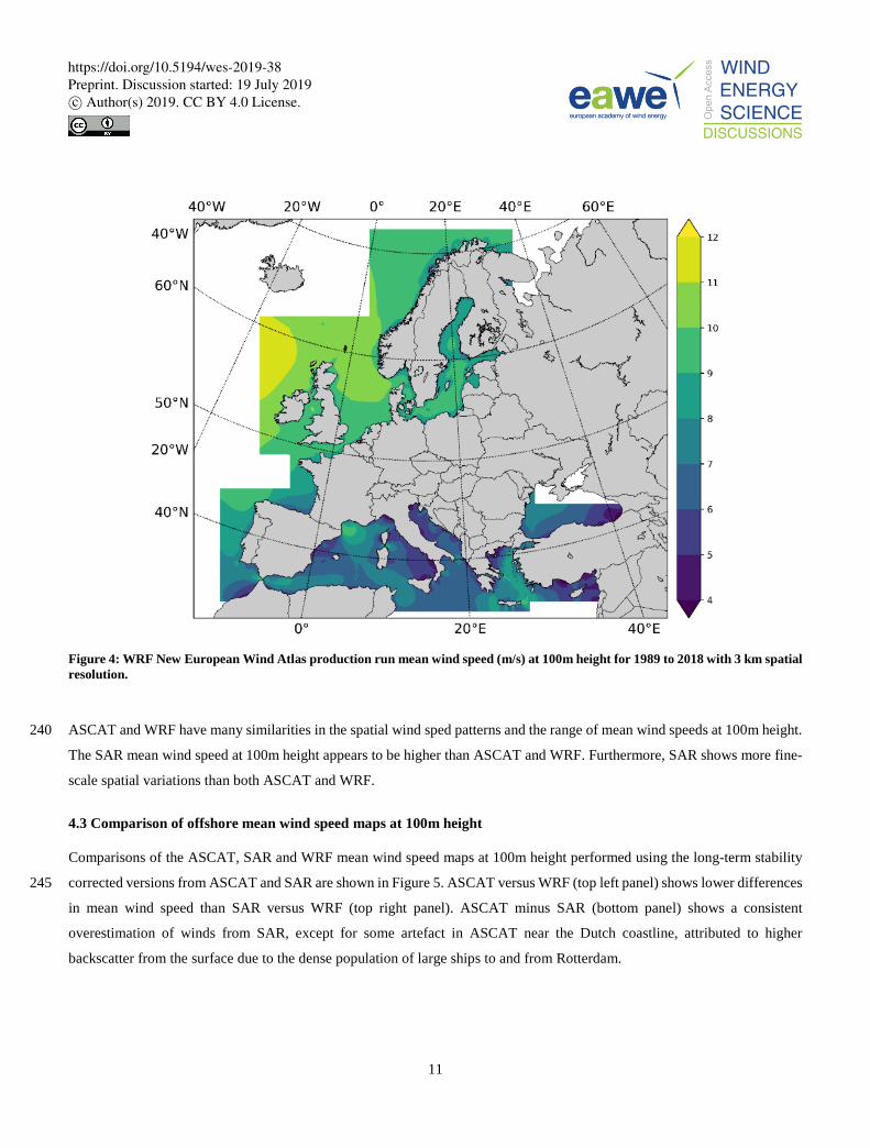
4.3 Comparison of offshore mean wind speed maps at 100m height

Comparisons of the ASCAT, SAR and WRF mean wind speed maps at 100m height performed using the long-term stability

corrected versions from ASCAT and SAR are shown in Figure 5. ASCAT versus WRF (top left panel) shows lower differences 245

in mean wind speed than SAR versus WRF (top right panel). ASCAT minus SAR (bottom panel) shows a consistent

overestimation of winds from SAR, except for some artefact in ASCAT near the Dutch coastline, attributed to higher

backscatter from the surface due to the dense population of large ships to and from Rotterdam.


12

showu

Figure 5: Comparison of mean wind speed (m/s) at 100m height: ASCAT minus WRF (top left), SAR minus WRF (top right), ASCAT 250 minus SAR (bottom left).

The ERA5 mean wind speed at 100m height is included for comparison with WRF (Figure 6). The mean wind speed difference

map of ERA5 minus WRF shows relatively large variations. There are both large positive and large negative values in the 255

Mediterranean Sea. The differences are smaller in the Northern European Seas. Along several coastlines such as the Norwegian

Sea, the Atlantic Sea and the Mediterranean Seas large differences are found between the two datasets. These are attributed to

the lack of ability in ERA5 to properly resolve the coastal atmospheric flow phenomena..


13

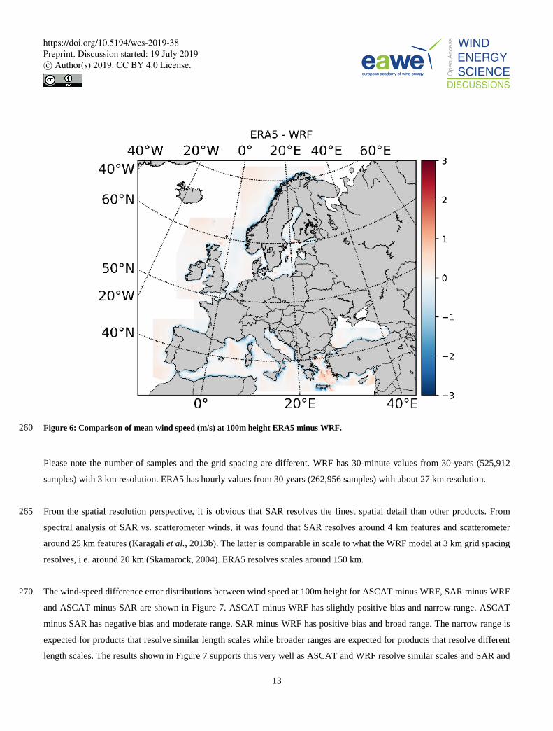
Figure 6: Comparison of mean wind speed (m/s) at 100m height ERA5 minus WRF. 260

Please note the number of samples and the grid spacing are different. WRF has 30-minute values from 30-years (525,912

samples) with 3 km resolution. ERA5 has hourly values from 30 years (262,956 samples) with about 27 km resolution.

From the spatial resolution perspective, it is obvious that SAR resolves the finest spatial detail than other products. From 265

spectral analysis of SAR vs. scatterometer winds, it was found that SAR resolves around 4 km features and scatterometer

around 25 km features (Karagali et al., 2013b). The latter is comparable in scale to what the WRF model at 3 km grid spacing

resolves, i.e. around 20 km (Skamarock, 2004). ERA5 resolves scales around 150 km.

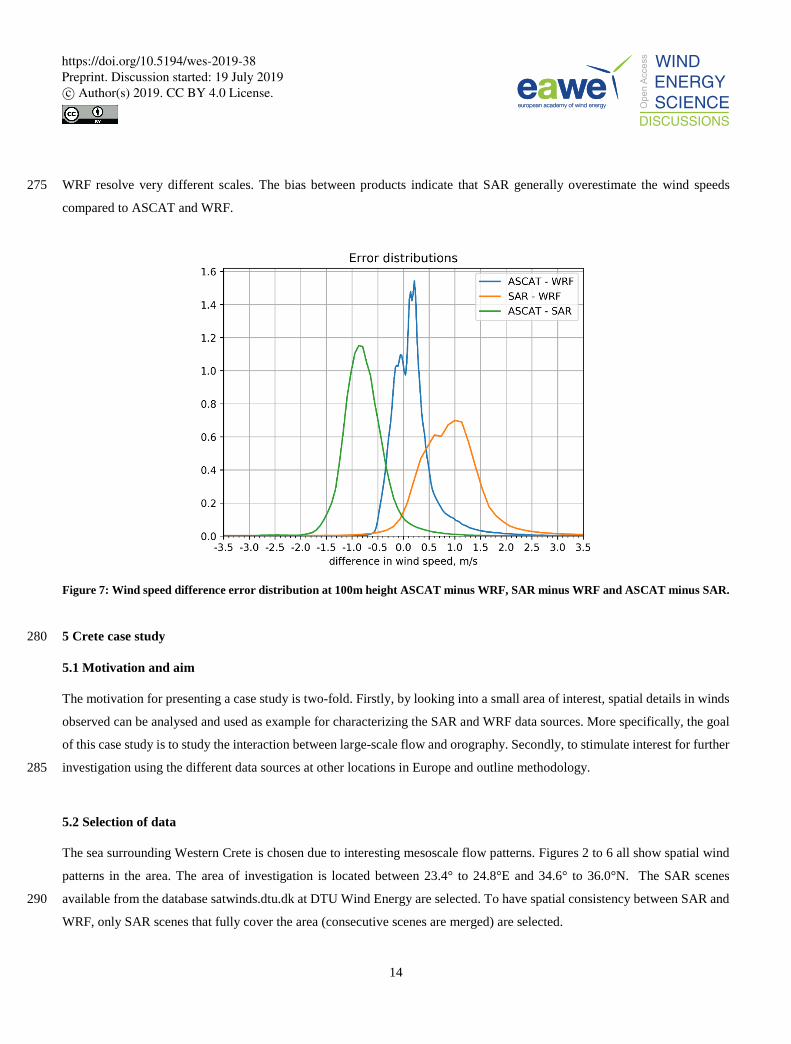
The wind-speed difference error distributions between wind speed at 100m height for ASCAT minus WRF, SAR minus WRF 270

and ASCAT minus SAR are shown in Figure 7. ASCAT minus WRF has slightly positive bias and narrow range. ASCAT

minus SAR has negative bias and moderate range. SAR minus WRF has positive bias and broad range. The narrow range is

expected for products that resolve similar length scales while broader ranges are expected for products that resolve different

length scales. The results shown in Figure 7 supports this very well as ASCAT and WRF resolve similar scales and SAR and


14

WRF resolve very different scales. The bias between products indicate that SAR generally overestimate the wind speeds 275

compared to ASCAT and WRF.

Figure 7: Wind speed difference error distribution at 100m height ASCAT minus WRF, SAR minus WRF and ASCAT minus SAR.

5 Crete case study 280

5.1 Motivation and aim

The motivation for presenting a case study is two-fold. Firstly, by looking into a small area of interest, spatial details in winds

observed can be analysed and used as example for characterizing the SAR and WRF data sources. More specifically, the goal

of this case study is to study the interaction between large-scale flow and orography. Secondly, to stimulate interest for further

investigation using the different data sources at other locations in Europe and outline methodology. 285

5.2 Selection of data

The sea surrounding Western Crete is chosen due to interesting mesoscale flow patterns. Figures 2 to 6 all show spatial wind

patterns in the area. The area of investigation is located between 23.4° to 24.8°E and 34.6° to 36.0°N. The SAR scenes

available from the database satwinds.dtu.dk at DTU Wind Energy are selected. To have spatial consistency between SAR and 290

WRF, only SAR scenes that fully cover the area (consecutive scenes are merged) are selected.


15

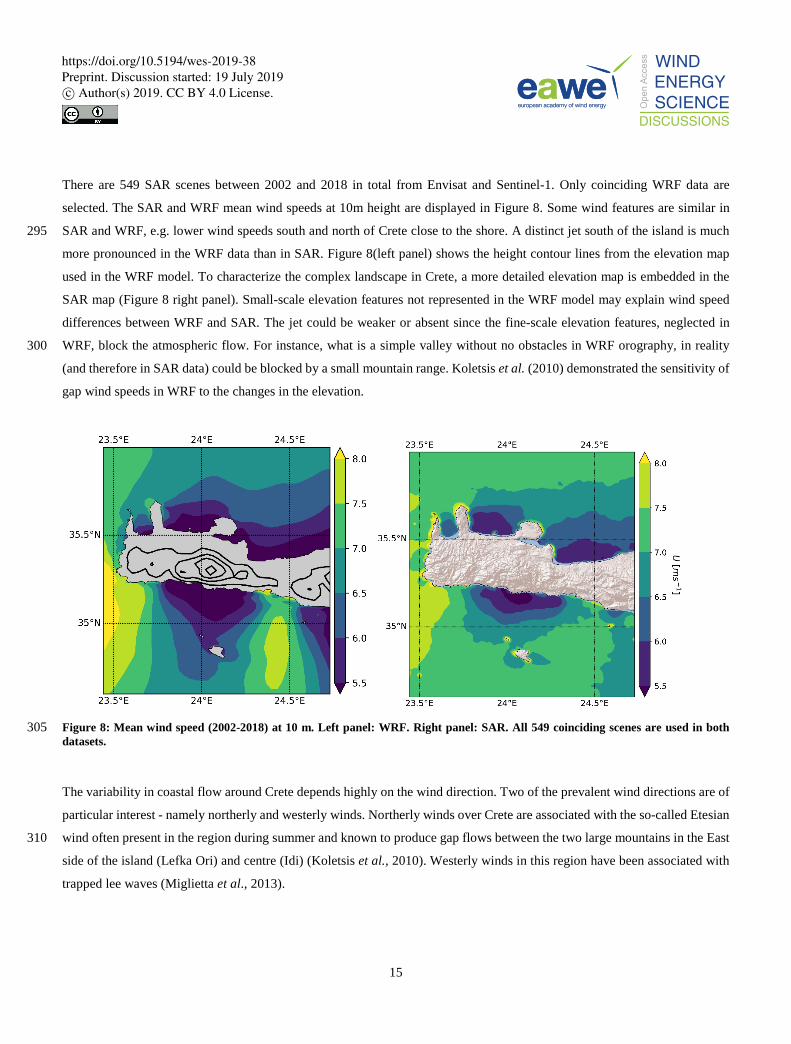
There are 549 SAR scenes between 2002 and 2018 in total from Envisat and Sentinel-1. Only coinciding WRF data are

selected. The SAR and WRF mean wind speeds at 10m height are displayed in Figure 8. Some wind features are similar in

SAR and WRF, e.g. lower wind speeds south and north of Crete close to the shore. A distinct jet south of the island is much 295

more pronounced in the WRF data than in SAR. Figure 8(left panel) shows the height contour lines from the elevation map

used in the WRF model. To characterize the complex landscape in Crete, a more detailed elevation map is embedded in the

SAR map (Figure 8 right panel). Small-scale elevation features not represented in the WRF model may explain wind speed

differences between WRF and SAR. The jet could be weaker or absent since the fine-scale elevation features, neglected in

WRF, block the atmospheric flow. For instance, what is a simple valley without no obstacles in WRF orography, in reality 300

(and therefore in SAR data) could be blocked by a small mountain range. Koletsis et al. (2010) demonstrated the sensitivity of

gap wind speeds in WRF to the changes in the elevation.

Figure 8: Mean wind speed (2002-2018) at 10 m. Left panel: WRF. Right panel: SAR. All 549 coinciding scenes are used in both 305 datasets.

The variability in coastal flow around Crete depends highly on the wind direction. Two of the prevalent wind directions are of

particular interest - namely northerly and westerly winds. Northerly winds over Crete are associated with the so-called Etesian

wind often present in the region during summer and known to produce gap flows between the two large mountains in the East 310

side of the island (Lefka Ori) and centre (Idi) (Koletsis et al., 2010). Westerly winds in this region have been associated with

trapped lee waves (Miglietta et al., 2013).


16

As already stated, the goal of this case study is to demonstrate the interaction between large-scale flow and orography. It is

necessary to choose situations where the upwind flow conditions are simple. This is to avoid wind conditions such as low 315

wind speed with poorly defined direction, anti-cyclonic situations and local flows, e.g. sea breezes that could create a

complicated wind field, that would be difficult to interpret. Therefore, the wind speeds should be sufficiently high, and the

wind direction should be representative for the entire domain.

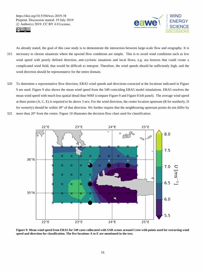
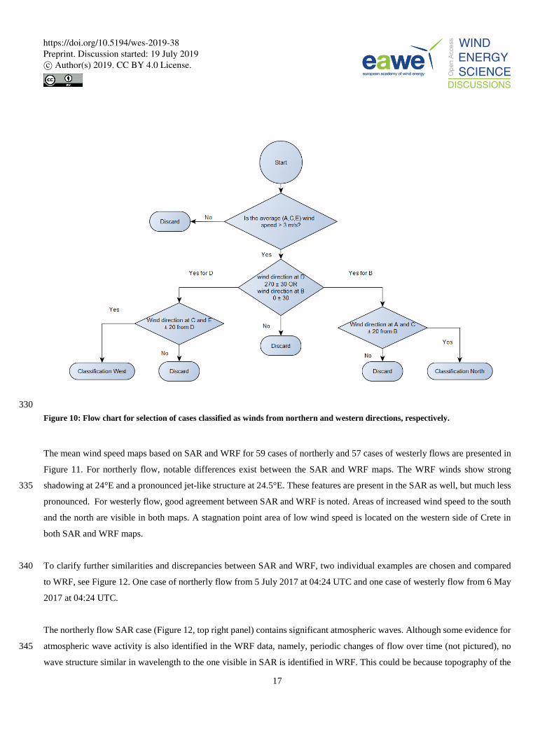
To determine a representative flow direction, ERA5 wind speeds and directions extracted at the locations indicated in Figure 320

9 are used. Figure 9 also shows the mean wind speed from the 549 coinciding ERA5 model simulations. ERA5 resolves the

mean wind speed with much less spatial detail than WRF (compare Figure 9 and Figure 8 left panel). The average wind speed

at three points (A, C, E) is required to be above 3 m/s. For the wind direction, the centre location upstream (B for northerly, D

for westerly) should be within 30° of that direction. We further require that the neighbouring upstream points do not differ by

more than 20° from the centre. Figure 10 illustrates the decision flow chart used for classification. 325

Figure 9: Mean wind speed from ERA5 for 549 cases collocated with SAR scenes around Crete with points used for extracting wind speed and direction for classification. The five locations A to E are mentioned in the text.


17

330 Figure 10: Flow chart for selection of cases classified as winds from northern and western directions, respectively.

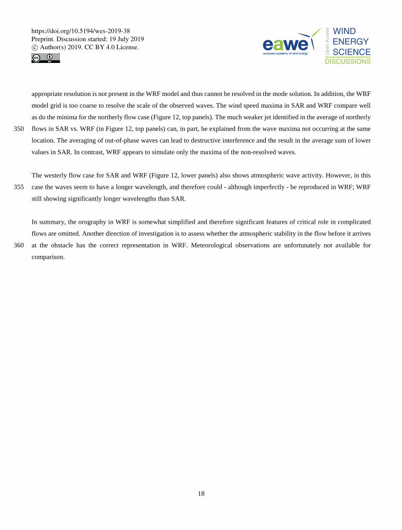
The mean wind speed maps based on SAR and WRF for 59 cases of northerly and 57 cases of westerly flows are presented in

Figure 11. For northerly flow, notable differences exist between the SAR and WRF maps. The WRF winds show strong

shadowing at 24°E and a pronounced jet-like structure at 24.5°E. These features are present in the SAR as well, but much less 335

pronounced. For westerly flow, good agreement between SAR and WRF is noted. Areas of increased wind speed to the south

and the north are visible in both maps. A stagnation point area of low wind speed is located on the western side of Crete in

both SAR and WRF maps.

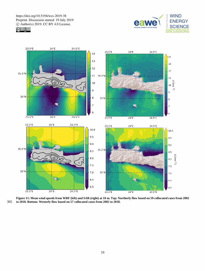
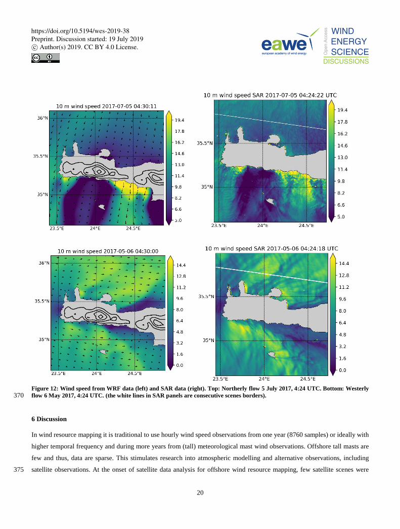
To clarify further similarities and discrepancies between SAR and WRF, two individual examples are chosen and compared 340

to WRF, see Figure 12. One case of northerly flow from 5 July 2017 at 04:24 UTC and one case of westerly flow from 6 May

2017 at 04:24 UTC.

The northerly flow SAR case (Figure 12, top right panel) contains significant atmospheric waves. Although some evidence for

atmospheric wave activity is also identified in the WRF data, namely, periodic changes of flow over time (not pictured), no 345

wave structure similar in wavelength to the one visible in SAR is identified in WRF. This could be because topography of the


18

appropriate resolution is not present in the WRF model and thus cannot be resolved in the mode solution. In addition, the WRF

model grid is too coarse to resolve the scale of the observed waves. The wind speed maxima in SAR and WRF compare well

as do the minima for the northerly flow case (Figure 12, top panels). The much weaker jet identified in the average of northerly

flows in SAR vs. WRF (in Figure 12, top panels) can, in part, be explained from the wave maxima not occurring at the same 350

location. The averaging of out-of-phase waves can lead to destructive interference and the result in the average sum of lower

values in SAR. In contrast, WRF appears to simulate only the maxima of the non-resolved waves.

The westerly flow case for SAR and WRF (Figure 12, lower panels) also shows atmospheric wave activity. However, in this

case the waves seem to have a longer wavelength, and therefore could - although imperfectly - be reproduced in WRF; WRF 355

still showing significantly longer wavelengths than SAR.

In summary, the orography in WRF is somewhat simplified and therefore significant features of critical role in complicated

flows are omitted. Another direction of investigation is to assess whether the atmospheric stability in the flow before it arrives

at the obstacle has the correct representation in WRF. Meteorological observations are unfortunately not available for 360

comparison.


19

Figure 11: Mean wind speeds from WRF (left) and SAR (right) at 10 m. Top: Northerly flow based on 59 collocated cases from 2002 to 2018. Bottom: Westerly flow based on 57 collocated cases from 2002 to 2018. 365


20

Figure 12: Wind speed from WRF data (left) and SAR data (right). Top: Northerly flow 5 July 2017, 4:24 UTC. Bottom: Westerly flow 6 May 2017, 4:24 UTC. (the white lines in SAR panels are consecutive scenes borders). 370

6 Discussion

In wind resource mapping it is traditional to use hourly wind speed observations from one year (8760 samples) or ideally with

higher temporal frequency and during more years from (tall) meteorological mast wind observations. Offshore tall masts are

few and thus, data are sparse. This stimulates research into atmospheric modelling and alternative observations, including

satellite observations. At the onset of satellite data analysis for offshore wind resource mapping, few satellite scenes were 375


21

available. Pioneering work (Barthelmie and Pryor, 2003; Pryor et al., 2005) had focus on the number of samples relevant for

assessing the mean wind speed, the Weibull scale and shape parameters and the energy density. Furthermore, the non-random

sampling in time of sun-synchronous satellites that for ASCAT A/B are local times around 9:30 am/pm, Envisat around 10:30

am/pm and Sentinel-1 A/B around 06:00 am/pm potentially may bias the wind resource statistics, in the case of diurnal wind

speed variations. The passive microwave wind observations with several more local observation times did not show much 380

variation in diurnal cycle wind speeds in the central North Sea (Hasager at al., 2016) but near coastlines land-sea breezes

prevail causing systematic diurnal wind speed variations.

Methods to deal with few satellite samples include the hybrid method (Badger et al., 2010) and the gap-filling method during

periods with lack of data due to sea ice (Doubrawa et al., 2015). The adjustment for few samples and for uneven diurnal or 385

seasonal sampling only makes sense to perform for local sites or regions (Ahsbahs et al., 2019) rather than for the entire

European Seas. In case meteorological observations are accessible, these can be useful for comparison and adjustment.

At the European scale, the SAR wind speed archive may be improved for future analysis, using the novel inter-calibration

method proposed by Badger et al. (2019) and applied for SAR-based wind resource assessment along the US East Coast 390

(Ahsbahs et al., 2019). The tendency in this inter-calibration is to decrease the SAR wind speeds. This obviously would make

the comparison to both ASCAT and WRF agree better in the European Seas. Further validation of the offshore WRF winds

with masts and lidar observations at around 100m AMSL in the North Sea show smaller biases than those identified in Figures

5 (Garcia-Bustamante et al. 2019), which substantiates this hypothesis. It could furthermore be interesting to consider SAR

and ASCAT inter-calibration such that coherent satellite data sets could be the foundation for further inter-comparison to e.g. 395

WRF model results. ASCAT and WRF test run comparisons (Karagali et al., 2018a; 2018b) have proved valuable, as well as

inter-comparison of WRF test runs and meteorological observations.

For planning of wind farms, statistics on wind speed and direction are crucial for optimal design of turbine layout within the

tender areas. ASCAT provides observations of wind speed and wind direction, thus wind roses based on ASCAT are fully 400

independent observations (e.g. Karagali et al., 2018b). SAR only provides observations of wind speed, and for direction based

upon the interpolated wind directions from global models (e.g. Badger et al., 2010; Ahsbahs et al., 2019). Thus, wind roses

from SAR are mixed from satellite data and modelling. WRF provides modelled wind speeds and wind directions. ERA5 is a

valuable data set, even though ERA5 resolves lesser spatial detail in offshore winds than the WRF production run, but ERA5

wind directions could be an alternative to CFSR and GFS wind directions as input for SAR wind retrieval. It could potentially 405

result in more homogenous SAR-based wind data set for the European Seas.

The opportunities for further investigations and analysis based on the New European Wind Atlas offshore are numerous. They

include long-term wind speed and wind direction trends, future wind climate, comparison to various new wind data sources,


22

high fidelity modelling of winds, extreme winds, seasonal dependencies in winds, wind farm cluster effects between large 410

offshore wind farms, wind energy production variability, new perspectives on marine boundary layer flows physics, processes

and meteorological parameters, air-sea interactions, among other topics. It is the beginning of a new era in offshore wind

energy research and applications.

7 Conclusion

The hitherto most comprehensive wind atlas for the European Seas has been published based on Envisat ASAR and Sentinel-415

1 A/B SAR satellite scenes, ASCAT A/B scatterometer satellite scenes and WRF mesoscale model production run results.

The WRF model covers 1989 - 2018 (30 years) with spatial resolution 3 km and results every 30 minutes (in total 525,912

samples). The SAR wind archive covers from 2002 to 2018 with spatial resolution 2 km in total around 500 to 2,500 samples

during the years. The ASCAT wind archive covers from 2007 to 2018 with spatial resolution 12.5 km in total around 5,000 to 420

12,000 samples during the years.

Comparison results between SAR and WRF for the Crete case study reveal fine-scale flow structures in SAR not fully captured

in WRF. However, overall ASCAT and WRF produce similar results of the mean wind speed across the European Seas at

100m height while SAR appears consistently too high. It is expected this bias may be diminished or removed using inter-425

calibration method for SAR.

Acknowledgements

The authors acknowledge the funding provided to the New European Wind Atlas project, in part funded by the European

Commission’s ERANET+, the Danish Energy Agency, and grants for supercomputers PRACE and EDDY. ASCAT data is

from the EUMETSAT, KNMI & the Copernicus CMEMS service. Envisat ASAR data is from ESA. Sentinel-1 data is from 430

EC Copernicus. The SAR processing is based on the SAROPS software from JHU APL and NOAA. T.S. acknowledges the

financial support of the project “Mathematical modelling of weather processes - development of methodology and applications

for Latvia (1.1.1.2/VIAA/2/18/261)”. The authors gratefully acknowledge the good collaboration with the WP3 partners of the

NEWA project.

435

Author contributions

C.B.H. wrote the article and coordinated offshore wind atlas. A.N.H. coordinated the WRF modelling and T.S. assisted in

WRF modelling and comparison. T.A. and T.S analysed the Crete case study. I.K. analysed ASCAT. T.S. prepared the


23

graphics. M.B. analysed SAR. J.M. coordinated NEWA experiments and project. All contributed to discussion of and writing

of the article. 440

References

4C Offshore 2019. Available online: https://www.4coffshore.com/ (last accessed 17 June 2019)

Ahsbahs, T., Badger, M., Karagali, I. and Larsén, X.G.: Validation of Sentinel-1A SAR Coastal Wind Speeds Against Scanning

LiDAR. Remote Sensing, 9(6), 552, 2017.

Ahsbahs, T., Badger, M., Volker, P., Hansen, K.S. and Hasager, C.B.: Applications of satellite winds for the offshore wind 445

farm site Anholt. Wind Energy Science, https://doi.org/10.5194/wes-2018-2, 2018.

Ahsbahs, T., Maclaurin, G., Draxl, C., Jackson, C., Monaldo, F. and Badger, M.: US East Coast synthetic aperture radar wind

atlas for offshore wind energy, Wind Energ. Sci. Discuss., https://doi.org/10.5194/wes-2019-16, in review, 2019.

Badger, M., Ahsbahs, T., Maule, P. and Karagali, I.: Inter-calibration of SAR data series for offshore wind resource assessment,

Remote Sensing of Environment, (in review), 2019. 450

Badger, M., Badger, J., Nielsen, M., Hasager, C.B. and Peña, A.: Wind class sampling of satellite SAR imagery for offshore

wind resource mapping, J. App. Meteor.Climatol., 49, 2474–2491. doi: 10.1175/2010JAMC2523.1, 2010.

Badger, M., Peña. A., Hahmann, A.N., Mouche, A. and Hasager, C.B.: Extrapolating satellite winds to turbine operating

heights. Journal of Applied Meteorology and Climatology, doi:10.1175/JAMC-D-15-0197, 2016.

Barthelmie, R. J. and Pryor, S. C.: Can satellite sampling of offshore wind speeds realistically represent wind speed 455

distributions, J. Appl. Meteorol., 42, 1, 83–94, 2003.

Berge, E., Byrkjedal, O., Ydersbond, Y. and Kindler, D.: Modelling of offshore wind resources. Comparison of a meso-scale

model and measurements from FINO1 and North Sea oil rigs. Scientific Proceedings EWEC'09 Marseille, France, 2009.

Bischoff, O., Yu, W., Gottschall, J. and Cheng, P. W.: Validating a simulation environment for floating lidar systems. The

Science of Making Torque from Wind (TORQUE 2018) IOP Publishing. IOP Conf. Series: Journal of Physics: Conf. Series 460

1037, 052036, doi :10.1088/1742-6596/1037/5/052036, 2018.

Casale, C., Lembo, E., Serri, L. and Viani, S.: Italy’s Wind Atlas:Offshore Resource Assessment Through On-The-Spot

Measurements, Wind Engineering, 34, 1, 17–28, 2010.

Christiansen, M.B., Koch, W., Horstmann, J., Hasager, C.B. and Nielsen, M.: Wind resource assessment from C-band SAR.

Remote Sens. Environ., 105, 68-81, 2016. 465

CMEMS 2019, Copernicus Marine Environmental Monitoring Service, http://marine.copernicus.eu/ (last accessed 17 June

2019)

De Kloe, J., Stoffelen, A. and Verhoef, A.: Improved Use of Scatterometer Measurements by Using Stress-Equivalent

Reference Winds. IEEE J. Sel. Topics Appl. Earth Observ. in Remote Sens., 10, 5, 2340-2347, 2017.


24

Donlon, C. J., M. Martin, J. D. Stark, J. Roberts-Jones, E. Fiedler, and W. Wimmer: The operational sea surface temperature 470

and sea ice analysis (OSTIA). Remote Sens. Environ., 116, doi:10.1016/j.rse.2010.10.017, 2012.

Doubrawa, P., Barthelmie, R. J., Pryor, S. C., Hasager, C. B., Badger, M. and Karagali, I.: Satellite winds as a tool for offshore

wind resource assessment: The Great Lakes Wind Atlas. Remote Sensing of Environment, 168, 349–359.

10.1016/j.rse.2015.07.008, 2015.

EEA 2009: Europe’s onshore and offshore wind energy potential. An assessment of environmental and economic constrains. 475

EEA Technical Report No 6/2009, pp. 90, 2009.

Emeis, S.: Wind Energy Meteorology: Atmospheric Physics for Wind Power Generation (Green Energy and Technology).

Springer, pp 198, 2012.

ERA5: Copernicus Climate Change Service (C3S): ERA5: Fifth generation of ECMWF atmospheric reanalyses of the global

climate . Copernicus Climate Change Service Climate Data Store (CDS), https://cds.climate.copernicus.eu/cdsapp#!/home, 480

(last accessed 17 June 2019), 2017.

Farrugia, R. N. and Sant, T.: A wind resource assessment at Aħrax Point: A node for central Mediterranean offshore wind

resource evaluation. Wind Engineering, 40, 5, 438 –446, 2016.

Floors, R. R., A. N. Hahmann, and A. Peña: Evaluating Mesoscale Simulations of the Coastal Flow Using Lidar Measurements.

J. of Geophys. Research: Atmospheres. 123, DOI: 10.1002/2017JD027504, 2018. 485

Floors, R., Peña, A., Lea, G., Vasiljević, N., Simon, E. and Courtney, M.: The RUNE Experiment—A 250 Database of

Remote-Sensing Observations of Near-Shore Winds. Remote Sens., 8, 884, 251, https://doi.org/10.3390/rs8110884, 2016.

Furevik, B. R., Sempreviva, A. M., Cavaleri, L., Lefèvre, J.-M. and Transerici, C.: Eight years of wind measurements from

scatterometer for wind resource mapping in the Mediterranean Sea. Wind Energy, 14, 3, 355-372,

https://doi.org/10.1002/we.425, 2011. 490

Garcia-Bustamante, E. et al.: Report on uncertainty quantification, NEWA Deliverable D4.4 (in preparation).

Gottschall, J., Catalano, E., Dörenkämper, M. and Witha, B.: The NEWA Ferry Lidar Experiment: Measuring Mesoscale

Winds in the Southern Baltic Sea. Remote Sens., 10, 1620. https://doi.org/10.3390/rs10101620, 2018.

Hahmann, A. N., Lennard, C., Badger, J., Vincent, C. L., Kelly, M. C., Volker, P. J. H. and Refslund, J.: Mesoscale modeling

for the Wind Atlas of South Africa (WASA) project. DTU Wind Energy. DTU Wind Energy E, No. 0050, 2015. 495

Hahmann, A.N., Rostkier-Edelstein, D., Warner, T.T., Vandenberghe, F., Liu, Y., Babarsky, R. and Swerdlin, S.P.:

A reanalysis system for the generation of mesoscale climatographies. J. Appl. Meteorol. Climatol., 49, 5, 954-972, 2010.

Hahmann A. N., Vincent C. L., Peña A., Lange J. and Hasager C. B.: Wind climate estimation using WRF model output:

Method and model sensitivities over the sea. International Journal of Climatology, 35, 3422-3439. DOI: 10.1002/joc.4217,

2015. 500

Hasager, C. B., Astrup, P., Zhu, R., Chang, R., Badger, M. and Hahmann, A. N.: Quarter-Century Offshore Winds from SSM/I

and WRF in the North Sea and South China Sea. Remote Sens., 8, 769, https://doi.org/10.3390/rs8090769, 2016.


25

Hasager, C. B., Badger, M., Nawri, N., Furevik, B. R., Petersen, G. N., Björnsson, H. and Clausen, N.-E.: Mapping offshore

winds around Iceland using satellite Synthetic Aperture Radar and mesoscale model simulations. IEEE Journal of Selected

Topics in Applied Earth Observations and Remote Sensing, 10.1109/JSTARS.2015.2443981, 2015a. 505

Hasager, C. B., Badger, M., Peña, A. and Larsén, X. G.: SAR–based wind resource statistics in the Baltic Sea. Remote Sensing,

3, 1, 117–144, doi:10.3390/rs301011, 2011.

Hasager, C. B., Mouche, A., Badger, M., Bingöl, F., Karagali, I., Driesenaar, T., Stoffelen, A., Peña, A. and Longépé, N.:

Offshore wind climatology based on synergetic use of Envisat ASAR, ASCAT and QuikSCAT. Remote Sensing of

Environment, 156, 247-263, DOI 10.1016/j.rse.2014.09.030, 2015b. 510

Hasager, C. B., Nielsen, M., Astrup, P., Barthelmie, R. J., Dellwik, E., Jensen, N.O.; Jørgensen, B.H.; Pryor, S.C.; Rathmann,

O.; Furevik, B.R. Offshore wind resource estimation from satellite SAR wind field maps. Wind Energy 2005, 8, 403-419

Hasager, C. B., Peña, A., Christiansen, M. B., Astrup, P-, Nielsen, M., Monaldo, F., Thompson, D. and Nielsen, P.: Remote

sensing observation used in offshore wind energy. IEEE Journal of Selected Topics in Applied Earth Observations and Remote

Sensing, 1, 1, 67-79, 2008. 515

Hasager, C. B., Stein, D., Courtney, M., Peña, A., Mikkelsen, T., Stickland, M. and Oldroyd, A.: Hub height ocean winds over

the North Sea observed by the NORSEWInD lidar array: Measuring techniques, quality control and data management. Remote

Sensing, 5, 9, 4280-4303, doi:10.3390/rs5094280, 2013.

Hersbach, H.: Comparison of C-Band Scatterometer CMOD5.N Equivalent Neutral Winds with ECMWF. J. Atmos. and

Ocean. Technol., 27, 4, 721–736, 2010. 520

Jimenez, B., Durante, F., Lange, B., Kreutzer, T. and Tambke, J.: Offshore Wind Resource Assessment with WAsP and MM5:

Comparative Study for the German Bight. Wind Energ., 10, 121–134, 2007.

Kara, A. B., Wallcraft, A. J. and Bourassa, M. A. J Geophys Res 113 C04009, 2008.

Karagali, I., Badger, M., Hahmann, A. N., Peña, A., Hasager, C. B. and Sempreviva, A. M.: Spatial and temporal variability

in winds in the Northern European Seas. Renewable Energy, 57, 200–210, doi:10.1016/j.renene.2013.01.017, 2013a. 525

Karagali, I., Badger, M. and Hasager, C. B.: ASCAT winds used for offshore wind energy applications. Proceedings for the

2018 EUMETSAT Meteorological Satellite Conference, 17-21 September 2018, Tallinn, Estonia, 2018a.

Karagali, I., Hahmann, A. N, Badger, M., Hasager, C. B. and Mann, J.: New European Wind Atlas offshore, Proceedings for

The Science of Making Torque from Wind (TORQUE 2018), IOP Conference Series: Journal of Physics: Conference Series

1037, 5, 2018b. 530

Karagali, I., Larsén, X. G., Badger, M., Peña, A. and Hasager, C. B.: Spectral Properties of ENVISAT ASAR and QuikSCAT

Surface Winds in the North Sea. Remote Sensing, 5, 11, 6096-6115, 2013b.

Karagali, I., Peña, A., Badger, M. and Hasager, C. B.: Wind characteristics in the North and Baltic Seas from the QuikSCAT

satellite. Wind Energy, 17, 1, 123–140, http://dx.doi.org/10.1002/we.1565, 2014.

Koletsis, I., Lagouvardos, K., Kotroni, V. and Bartzokas, A.: The interaction of northern wind flow with the complex 535

topography of Crete Island–Part 2: Numerical study. Natural Hazards and Earth System Sciences, 10, 6, 1115-1127, 2010.


26

Landberg, L.: Meteorology for wind energy: An introduction. Wiley, pp 224, 2015.

Lavagnini A., Sempreviva, A. M., Transerici, C., Accadia, C., Casaioli, M., Mariani, S. and Speranza, A.: Offshore Wind

Climatology over the Mediterranean Basin. Wind Energy, 9, 3, 251–266, 2006.

Mann, J, et al.: Complex terrain experiments in the New European Wind Atlas. Philosophical Transactions of the Royal Society 540

A: Mathematical, Physical and Engineering Sciences, 375, 2091, 20160101, 2017.

Miglietta, M. M., Zecchetto, S. and De Biasio, F.: A comparison of WRF model simulations with SAR wind data in two case

studies of orographic lee waves over the Eastern Mediterranean Sea. Atmospheric research, 120, 127-146, 2013.

Monaldo F., Jackson C., Li, X. and Pichel, W. G.: Preliminary evaluation of Sentinel-1A wind speed retrievals. IEEE J Selected

Topics Applied Earth Observation in Remote Sensing, 9, 6, 2638-42, doi:10.1109/JSTARS.2015.2504324, 2015. 545

Monin, A. S., and A. M. Obukhov: Basic laws of turbulent mixing in the surface layer of the atmosphere. Contrib. Geophys.

Inst. Acad. Sci. USSR, 151, 163–187, 1954.

Mouche, A., Hauser, D., J., Daloze, J. and Gueri, C.: Dual-polarization measurements at C-band over the ocean: Results from

airborne radar observations and comparison with ENVISAT ASAR data. IEEE Transactions on Geoscience and Remote

Sensing, 43, 4, 753–769, 2005. 550

Nakanishi, M., and H. Niino: Development of an improved turbulence closure model for the atmospheric boundary layer. J.

Meteor. Soc. Japan, 87, 895–912, doi:10.2151/jmsj.87.895, 2009.

National Ice Center 2008: IMS daily Northern Hemisphere snow and ice analysis at 4 km and 24 km resolution. Boulder,

Colorado USA: National Snow and Ice Data Centerhttp://dx.doi.org/10.7265/N52R3PMC, 2008.

Nuño Martinez, E., Maule, P., Hahmann, A. N., Cutululis, N. A., Sørensen, P. E. and Karagali, I.: Simulation of 555

transcontinental wind and solar PV generation time series. Renewable Energy, 118, 425-436, doi:

10.1016/j.renene.2017.11.039, 2018.

OECD 2016: The Ocean Economy. OECD Publishing http://www.oecd.org/sti/the-ocean-economy-in-2030-9789264251724-

en.htm, (last accessed 17 June 2019), 2016.

OWA 2018: Offshore Wind Accelerator: Floating LiDAR Roadmap Update Deployments of Floating LiDAR Systems. Carbon 560

Trust. pp 99, https://www.carbontrust.com/media/677598/uflr_d04_floatinglidarrepository_210318_final-feb19_2.pdf (last

accessed 17 June 2019), 2018.

Peña, A. and Hahmann, A. N.: Atmospheric stability and turbulence fluxes at Horns Rev—an intercomparison of sonic, bulk

and WRF model data, Wind Energy,15, 5, 717-731. https://doi.org/10.1002/we.500, 2012.

Peña, A. and Hahmann, A. N.: 30-year mesoscale model simulations for the “Noise from wind turbines and risk of 565

cardiovascular disease” project. DTU Wind Energy E, vol. 0055, 2017.

Peña, A., Hahmann, A. N., Hasager, C. B., Bingöl, F., Karagali, I., Badger, J., Badger, M. and Clausen, N.-E.: South Baltic

Wind Atlas: South Baltic Offshore Wind Energy Regions Project. Risø-R-1775(EN), Risø National Laboratory for Sustainable

Energy, Technical University of Denmark, 1-66, 2011.


27

Peña, A., Floors, R. R., Sathe, A., Gryning, S.-E., Wagner, R., Courtney, M., Larsén, X. G., Hahmann, A. N. and Hasager, C. 570

B.: Ten Years of Boundary-Layer and Wind-Power Meteorology at Høvsøre, Denmark. Boundary-Layer Meteorology.

10.1007/s10546-015-0079-8, 2015.

Petersen, E. L.: Wind resources of Europe (the offshore and coastal resources). EWEA special topic conference ’92, 8–11

September 1992, Herning, Denmark, 1992.

Petersen, E. L. and Troen, I.: Wind conditions and resource assessment. Wiley Interdisciplinary Reviews: Energy and 575

Environment, 1, 206-217, https://doi.org/10.1002/wene.4, 2012.

Petersen, E. L., Troen, I., Jørgensen, H. E. and Mann, J.: The new European wind atlas. Energy Bulletin, 17, 34-39, 2014.

Pryor, S. C., Nielsen, M., Barthelmie, R. J. and Mann, J.: Can satellite sampling of offshore wind speeds realistically represent

wind speed distributions? Part II Quantifying uncertainties associated with sampling strategy and distribution fitting methods,

J. Appl. Meteorol., 43, 739–750, 2004. 580

Sempreviva, A. M., Barthelmie, R. J. and Pryor, S. C.: Review of Methodologies for Offshore Wind Resource Assessment in

European Seas. Surveys in Geophysics, 29, 6, 471-497, https://doi.org/10.1007/s10712-008-9050-2, 2008.

Skamarock, W. C.: Evaluating mesoscale NWP models using kinetic energy spectra. Mon. Wea. Rev., 132, 3019-3032, 2004.

Skamarock, W. C. et al.,: A Description of the Advanced Research WRF Version 3. NCAR Technical Note NCAR/TN-

475+STR, doi:10.5065/D68S4MVH, 2008. 585

Soukissian, T., Karathanasi, F. and Axaopoulos, P.: Satellite-Based Offshore Wind Resource Assessment in the Mediterranean

Sea. IEEE Journal of Oceanic Engineering , 42, 1, 7491216, 2017.

Troen, I. and Petersen, E. L.: European Wind Atlas. Risø National Laboratory, Roskilde, 1989.

UK Renewables Atlas 2008: https://www.renewables-atlas.info/explore-the-atlas/ (last accessed 17 June 2019), 2008.

Wind Europe 2019: Offshore Wind in Europe. Key trends and statistics 2018. Available online: https://windeurope.org/wp-590

content/uploads/files/about-wind/statistics/WindEurope-Annual-Offshore-Statistics-2018.pdf (last accessed 17 June 2019),

2018.

Witha, B., Hahmann, A. N., Sile, T., Dörenkämper, M,, Ezber, Y,, Bustamante, E. G., Gonzalez-Rouco, J. F., Leroy, G. and

Navarro, J.: Report on WRF model sensitivity studies and specifications for the mesoscale wind atlas production runs:

Deliverable D4.3. vol. D4.3, NEWA - New European Wind Atlas. https://doi.org/10.5281/zenodo.2682604, 2019. 595

Witze, A.: World's largest wind-mapping project spins up in Portugal. Nature, 542, 282—283, 2017.


Europe's offshore winds assessed from SAR, ASCAT and WRF

Documents