Matching ASCAT and QuikSCAT winds

Matching ASCAT and QuikSCAT winds

Abderrahim Bentamy,1 Semyon A. Grodsky,2 James A. Carton,2 Denis Croizé-Fillon,1

and Bertrand Chapron1

Received 29 July 2011; revised 5 December 2011; accepted 7 December 2011; published 7 February 2012.

[1] Surface winds from two scatterometers, the Advanced scatterometer (ASCAT),available since 2007, and QuikSCAT, which was available through November 2009, showpersistent differences during their period of overlap. This study examines a set of collocatedobservations during a 13-month period November 2008 through November 2009, toevaluate the causes of these differences. A difference in the operating frequency of thescatterometers leads to differences that this study argues depend on rain rate, wind velocity,and SST. The impact of rainfall on the higher frequency QuikSCAT introduces biasesof up to 1 m s�1 in the tropical convergence zones and along the western boundarycurrents even after rain flagging is applied. This difference fromASCAT is reduced by some30% to 40% when data for which the multidimensional rain probabilities > 0.05 is alsoremoved. An additional component of the difference in wind speed seems to be the result ofbiases in the geophysical transfer functions used in processing the two data sets and isparameterized here as a function of ASCAT wind speed and direction relative to themid-beam azimuth. After applying the above two corrections, QuikSCAT wind speedremains systematically lower (by 0.5 m s�1) than ASCAT over regions of cold SST < 5°C.This difference appears to be the result of temperature-dependence in the viscous dampingof surface waves which has a greater impact on shorter waves and thus preferentiallyimpacts QuikSCAT. The difference in wind retrievals also increases in the storm trackcorridors as well as in the coastal regions where the diurnal cycle of winds is aliased bythe time lag between satellites.

Citation: Bentamy, A., S. A. Grodsky, J. A. Carton, D. Croizé-Fillon, and B. Chapron (2012), Matching ASCATand QuikSCAT winds, J. Geophys. Res., 117, C02011, doi:10.1029/2011JC007479.

1. Introduction

[2] Many meteorological and oceanic applications requirethe high spatial and temporal resolution of satellite winds[e.g., Grima et al., 1999; Grodsky and Carton, 2001; Blankeet al., 2005; Risien and Chelton, 2008]. Many of thesestudies also require consistent time series spanning the life-time of multiple satellite missions, of which there have beenseven since the launch of the first European Remote Sensingsatellite (ERS-1) in August 1991. Creating consistent timeseries requires accounting for changes in individual missionbiases, most strikingly when successive scatterometers operatein different spectral bands [e.g., Bentamy et al., 2002; Ebuchiet al., 2002]. This paper presents a comparative study ofwinds derived from the matching of two such scatterometers:the C-band Advanced SCATterometer (ASCAT) on boardMetop-A and the higher frequency Ku-band SeaWindsscatterometer onboard QuikSCAT.

[3] Scatterometers measure wind velocity indirectlythrough the impact of wind on the amplitude of capillary ornear-capillary surface waves. This wavefield is monitored bymeasuring the strength of Bragg scattering of an incidentmicrowave pulse. If a pulse of wave number kR impinges onthe surface at incidence angle q relative to the surface themaximum backscatter will occur for surface waves of wavenumber kB = 2kR sin(q) whose amplitude, in turn, reflectslocal wind conditions [e.g., Wright and Keller, 1971]. Thefraction s0 of transmitted power that returns back to thesatellite is thus a function of local wind speed and direction(relative to the antenna azimuth), and q.[4] To date, the most successful conversions of scat-

terometer measurements into near-surface wind rely onempirically derived geophysical model functions (GMFs)augmented by procedures to resolve directional ambiguitiesresulting from uncertainties in the direction of wave propa-gation. Careful tuning of the GMFs is currently providingestimates of 10 m neutral wind velocity with errors estimatedto be around� 1 m s�1 and� 20° [e.g., Bentamy et al., 2002;Ebuchi et al., 2002]. However, systematic errors are alsopresent. For example, Bentamy et al. [2008] have shown thatASCAT has a systematic underestimation of wind speed thatincreases with wind speed, reaching 1 m s�1 for winds of20 m s�1.

1Institut Francais pour la Recherche et l’Exploitation de la Mer,Plouzane, France.

2Department of Atmospheric andOceanic Science, University ofMaryland,College Park, Maryland, USA.

Copyright 2012 by the American Geophysical Union.0148-0227/12/2011JC007479

JOURNAL OF GEOPHYSICAL RESEARCH, VOL. 117, C02011, doi:10.1029/2011JC007479, 2012

C02011 1 of 15

http://dx.doi.org/10.1029/2011JC007479

[5] The GMFs and other parameters must change if thefrequency band used by the scatterometer changes. Histori-cally scatterometers have used two different frequency bands.U.S. scatterometers as well as the Indian OCEANSAT2 usefrequencies in the 10.95–14.5 GHz Ku-band. In contrast theEuropean Remote Sensing satellite scatterometers have alladopted the 4–8 GHz C-band to allow for reduced sensitivityto rain interference [Sobieski et al., 1999; Weissman et al.,2002]. To avoid spurious trends and variability in a com-bined multiscatterometer data set, the bias in wind and itsvariability between different scatterometers needs to beremoved. This paper doesn’t consider adjustment of windvariability.[6] There have been numerous efforts to construct a com-

bined multisatellite data set of winds [Milliff et al., 1999;Zhang et al., 2006; Bentamy et al., 2007, Atlas et al., 2011].These efforts generally rely on utilizing a third referenceproduct such as passive microwave winds or reanalysiswinds to which the individual scatterometer data sets can becalibrated. In contrast to such previous efforts, this currentstudy focuses on directly matching scatterometer data. Weillustrate the processes by matching the current ASCAT andthe recent QuikSCAT winds (following Bentamy et al.[2008]). This matching exploits the existence of a 13 monthperiod November 2008 to November 2009 when both mis-sions were collecting data and when ASCAT processing usedthe current CMOD5N GMF [Verspeek et al., 2010] to derive10 m neutral wind.

2. Data

[7] This study relies on data from two scatterometers,the SeaWinds Ku-band (13.4 GHz, 2.2 cm) scatterometeronboard QuikSCAT (referred to as QuikSCAT or QS, Table 1)which was operational June, 1999 to November, 2009 andthe C-band ASCAT onboard the European MeteorologicalSatellite Organization (EUMESAT) MetOp-A (http://www.eumetsat.int/Home/Main/DataProducts/Atmosphere/index.htm)(5.225 GHz, 5.7 cm) launched October, 2006 (referred to asASCAT or AS).[8] QuikSCAT uses a rotating antenna with two emitters:

the H-pol inner beam with an incidence angle q = 46.25° andthe V-pol outer beam with an incidence angle of q = 54°.Observations from these two emitters have swaths of1400 km and 1800 km, respectively which cover around 90%of the global ocean daily. These observations are then binnedinto Wind Vector Cells (WVC). QuikSCAT winds used inthis study are the 25-km Level 2b data produced and dis-tributed by NASA/Jet Propulsion Laboratory, product ID isPODAAC-QSX25-L2B0 (http://podaac.jpl.nasa.gov/dataset/QSCAT_LEVEL_2B?ids=Measurement&values=Ocean%20Winds) [Dunbar et al., 2006]. These data are estimated

with the empirical QSCAT-1 GMF and the Maximum Like-lihood Estimator which selects the most probable winddirection. To improve wind direction estimates in the middleof the swath an additional Direction Interval Retrieval withThreshold Nudging algorithm is applied. The winds pro-duced by this technique show RMS speed and direction dif-ferences from concurrent in situ buoy and ship data ofapproximately 1 m s�1 and 23°, and temporal correlations inexcess of 0.92 [e.g., Bentamy et al., 2002; Ebuchi et al., 2002;Bourassa et al., 2003].[9] The QuikSCAT wind product includes several rain

flags determined directly from scatterometer observationsand from collocated radiometer rain rate measurements fromother satellites. The impact of rain on QuikSCAT data isindicated by two rain indices: a rain flag and a multidimen-sional rain probability (MRP). All QuikSCAT retrievalsidentified as contaminated by rain are removed using the rainflag associated with each WVC. Additional rain selection isbased on MRP index provided by the Impact-based Multi-dimensional Histogram technique. Employing MRP enhan-ces rain selection since ‘rain free’ pixels identified with therain flag index not always have MRP = 0. Recently the JPL/PODAAC has reprocessed QuikSCAT data using the newKu-2011 GMF [Ricciardulli and Wentz, 2011] (see alsowww.ssmi.com/qscat/qscat_Ku2011_tech_report.pdf ). Pre-liminary analysis of this product indicates improvements inthe tropical rainfall detection, but major differences betweenQuikSCAT and ASCATwinds reported below do not changemuch.[10] ASCAT has an engineering design that is quite dif-

ferent from QuikSCAT. Rather than a rotating antenna it hasa fixed three beam antenna looking 45° (fore-beam), 90°(mid-beam), 135° (aft-beam) of the satellite track, whichtogether sweep out two 550 km swaths on both sides of theground track. The incidence angle varies in the range 34°–64° for the outermost beams and 25°–53° for the mid-beam,giving Bragg wavelengths of 3.2–5.1 cm and 3.6–6.8 cm,respectively. Here we use Level 2b ASCAT near real-time data (version 1.10) distributed by EUMETSAT and byKNMI at 25 � 25 km2 resolution. Comparisons to indepen-dent mooring and shipboard observations by Bentamy et al.[2008] and Verspeek et al. [2010] show that ASCAT windspeed and direction has accuracies similar to QuikSCAT.[11] Rain contamination in the C–band, used by ASCAT,

is weaker than in the Ku-band [e.g. Tournadre and Quilfen,2003]. The selection of ASCAT retrievals is based on thequality control flag associated with each WVC. All qualityflag bits, including rain flag but excluding strong wind(>30 m s�1) and weak wind (<3 m s�1) flags, are checkedto be 0.[12] To reevaluate wind accuracy we use a variety of

moored buoy measurements including wind velocity, SST,air temperature, and significant wave height. These areobtained from Météo-France and U.K. MetOffice (Europeanseas) [Rolland and Blouch, 2002], the NOAA NationalData Buoy Center (NDBC, U.S. coastal zone) [Meindl andHamilton, 1992], and the tropical moorings of the TropicalAtmosphere Ocean Project (Pacific), the Pilot ResearchMoored Array (Atlantic), and Research Moored Array forAfrican-Asian-Australian Monsoon Analysis and Predictionproject (Indian Ocean) [McPhaden et al., 1998; Bourlèset al., 2008; McPhaden et al., 2009]. Hourly averaged

Table 1. Orbital Parameters

Satellite QuikSCAT METOP-A

Recurrent period 4 days 29 daysOrbital period 101 min 101 minEquator crossing local Sun time

at ascending node6:30 A.M. 9:30 A.M.

Altitude above equator 803 km 837 kmInclination 98.62° 98.59°

BENTAMY ET AL.: MATCHING ASCAT AND QUIKSCAT WINDS C02011C02011

2 of 15

post-processed (off-line) buoy measurements of windvelocity, sea surface and air temperatures, and humidityare converted to neutral wind at 10 m height using theCOARE3.0 algorithm of Fairall et al. [2003]. Although thisalgorithm allows for the use of surface wave and currentsdata, we do not include the corrections since these data arenot available for most buoys.[13] Quarter-daily 10 m winds, as well as SST and air

temperatures, are also obtained from the European Centre forMedium Weather Forecasts (ECMWF) operational analysis.These are routinely provided by the Grid for Ocean Diag-nostics, Interactive Visualization and Analysis (GODIVA)project (http:// behemoth.nerc-essc.ac.uk/ncWMS/godiva2.html) on a regular grid of 0.5° in longitude and latitude.

3. Collocated Observations

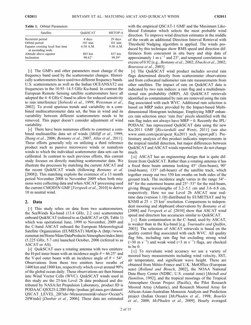
[14] Both satellites are in quasi sun-synchronous orbits,with the QuikSCAT local equator crossing time at theascending node (6:30 A.M.) leading the ASCAT localequator crossing time (9:30 A.M.) by 3 h. This differenceimplies that data precisely collocated spatially are availableonly with a few hours time difference at low latitudes(Figure. 1) [Bentamy et al., 2008]. Here we accept forexamination data pairs collocated in space and time whereQuikSCAT WVC is collected within 0 < t < 4 h and 50 kmof each valid ASCAT WVC. For the thirteen month periodNovember 2008 through November 2009 this collocationselection procedure produces an average 2800 collocatedpairs of data in each 1°� 1° geographical bin. The data countis somewhat less in the regions of the tropical convergencezones due to the need to remove QuikSCAT rain flaggeddata. The data count increases with increasing latitude as aresult of the near-polar orbits, but decreases again at veryhigh latitudes due to the presence of ice. At shorter lags of t <3 h collocated data coverage is still global, but the number

of match-ups is reduced by a factor of two. At lags of t <1 h collocated data is only available in the extra tropics(Figure 1).[15] Systematic difference in times of QuikSCAT and

ASCAT overpasses may project on the diurnal variations ofwinds, and thus may result in nonzero time mean wind dif-ference between the two satellites. This possible difference isaddressed by examining sub-sampled buoy and ECMWFanalysis data. Results of this examination are explained, butnot shown, below. In midlatitudes, where the characteristictime separation between collocated ASCAT and QuikSCATdata is less than 2 h, we examine wind measurements fromNDBC buoys. We subsample the original buoy data based onthe timing of the nearest ASCAT (subsample 1, ‘ASCAT’)and QuikSCAT (subsample 2, ‘QuikSCAT’) overpasses. Thetime mean bias between wind speed subsamples at theseextra-tropical NDBC mooring locations is close to zero withan RMS difference of less than 1 m s�1, and a temporalcorrelation > 0.95. Time mean difference (bias) in windspeed between these ‘QuikSCAT’ and ‘ASCAT’ subsamplesdoes not depend on wind strength and/or buoy location, andvaries between �0.1 m s�1 in 92% of cases. This negligibletime mean bias suggests that time mean differences betweencollocated satellite wind fields (if any) are the result of dif-ferences in the satellite wind estimates rather than the timelag between samples. Similar results are found in a compar-ison of ‘QuikSCAT’ and ‘ASCAT’ subsamples of the tropi-cal moorings (assuming t < 4 h). Again we find no meanbias, RMS differences of 1.2 m s�1, and temporal correla-tions > 0.92. Finally we examine the impact of our choice ofcollocation ranges by simulating the space and time samplingof ASCAT and QuikSCAT with ECMWF analysis surfacewinds during the period November 20, 2008 throughNovember 19, 2009. This sampling study confirms that thetime lag between the two satellites doesn’t produce any sig-nificant geographical patterns of wind speed bias. (A report is

Figure 1. Number of collocated QuikSCAT and ASCAT data on a 1° � 1° grid during November 2008–2009 for time separations less than that shown in the top left corner.


3 of 15

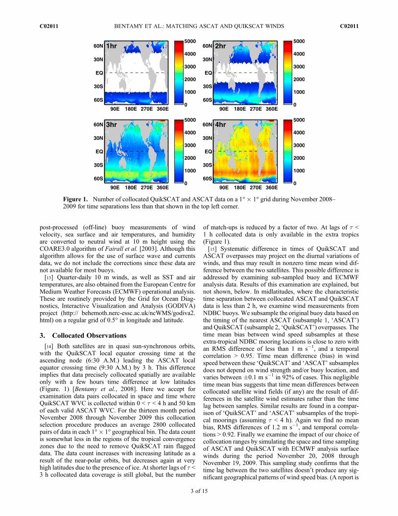
available at http://coaps.fsu.edu/scatterometry/meeting/docs/2011/cal_val/Bentamy_Grodsky_IOVWST_2011.pdf.)[16] Temporal correlation of satellite and the tropical buoy

winds is high for all of our accepted time lags (Figure 2). It isclose to 0.8 at t = 4 h (3–4 h is the most frequent time lag forASCAT-QuikSCAT collocations in the tropics), but exceeds0.9 at zero lag. At higher latitudes, where the winds havelonger synoptic timescales, the collocated satellite-buoy timeseries have even higher correlations (0.89 at t = 4 h, and 0.96at t < 0.5 h, not shown).

4. Results

4.1. Global Comparisons

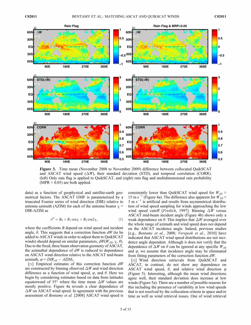
[17] Time mean difference between collocated QuikSCATand ASCAT wind speed (DW = WQS � WAS, Figure 3) isgenerally less than 1 m s�1, but contains some planetary-scale patterns. In general, DW > 0 at tropical to midlatitudeswhere it exhibits a pattern of values in the range of 0.40–0.80 m s�1, exceeding the bias found by Bentamy et al.[2008] between ASCAT and buoy winds, and resemblingthe spatial pattern of tropical and midlatitude storm trackprecipitation. This spatial pattern suggests that even afterapplying the rain flag to exclude rain-contaminated obser-vations there is a residual impact of rainfall on QuikSCATwind retrievals, as previously noted by, e.g.,Weissman et al.[2002]. Enhancing rain flagging by removing cases withMRP > 0.05 (5% of QuikSCAT data) decreases the fre-quency of positive differences in the tropical precipitationzones by some 30% to 40% and reduces the number of largedifferences ∣DW ∣ > 1 m s�1 by 38% (Figures 3a and 3b).However, the RMS variability of DW doesn’t change withthe enhanced rain flagging. Both with and without additionalrain flagging RMS(DW) has a maximum of up to 3 m s�1 inthe zones of the midlatitude storm tracks of both hemispheres

and approaches 1.8 m s�1 in the tropical convergence zones(Figures 3c and 3d). These maxima in inter-instrument vari-ability reflect a combination of still unaccounted impactsof rain events, and impacts of strong transient winds in themidlatitude storm tracks, as well as deep convection eventsin the tropics. Still, because it removes extreme differences,this enhanced rain flagging is applied to all QuikSCAT datashown below.[18] In contrast to the tropics or midlatitudes, time mean

DW is negative at subpolar and polar latitudes. This is par-ticularly noticeable at southern latitudes where the differencemay exceed �0.5 m s�1. This striking high latitude inter-scatterometer difference remains even after applying theenhanced rain flagging mentioned above (Figures 3a and 3b).[19] Despite these time-mean differences the temporal

correlation of QuikSCAT and ASCAT winds is high (>0.9)over much of the global ocean (Figures 3e and 3f ). Itdecreases to 0.7 (0.5 at some locations) in the tropical con-vergence zones at least in part because of the relatively largenoise compared to the wind signal (sampling errors dueto unresolved tropical convection, weak winds variability)results in reduced correlation [Bentamy et al., 2008]. Anadditional factor is the presence of mesoscale wind dis-turbances due to transient deep convective systems. Thelimited spatial scales of transient winds associated withthe tropical convection approach the scale of a single radarfootprint while their temporal scales approach the time lagbetween the two satellites [Houze and Cheng, 1977]. Incontrast, the correlation at mid and high latitudes is highbecause winds there have long multiday synoptic timescalesand large spatial scales.

4.2. Effect of Geophysical Model Function

[20] In this section we attempt to parameterize observedDW (after applying enhanced rain flagging to the QuikSCAT

Figure 2. Lagged correlation of collocated satellite and buoy winds as a function of time separationbetween satellite and buoy data. Solid line shows the median value and vertical bars are bounded by25th and 75th percentiles of correlation for different buoys.


4 of 15

data) as a function of geophysical and satellite-earth geo-metrical factors. The ASCAT GMF is parameterized by atruncated Fourier series of wind direction (DIR) relative toantenna azimuth (AZIM) for each of the antenna beams c =DIR-AZIM as

s0 ¼ B0 þ B1 coscþ B2 cos2c; ð1Þ

where the coefficients B depend on wind speed and incidentangle, q. This suggests that a correction function dW (to beadded to ASCATwinds in order to adjust them to QuikSCATwinds) should depend on similar parameters, dW(WAS, c, q).Due to the fixed, three beam observation geometry of ASCAT,the azimuthal dependence of dW is reduced to dependenceon ASCAT wind direction relative to the ASCAT mid-beamazimuth, 8 = DIRAS � AZIM1.[21] Empirical estimates of this correction function dW

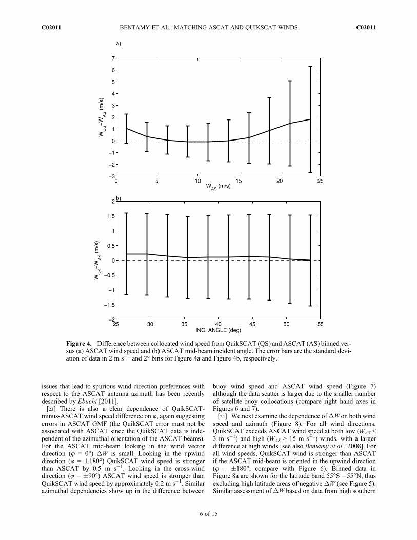
are constructed by binning observed DW and wind directiondifference as a function of wind speed, 8, and q. Here webegin by considering estimates based on data from latitudesequatorward of 55° where the time mean DW values aremostly positive. Figure 4a reveals a clear dependence ofDW on ASCAT wind speed. In agreement with the previousassessment of Bentamy et al. [2008] ASCAT wind speed is

consistently lower than QuikSCAT wind speed for WAS >15 m s�1 (Figure 4a). The difference also apparent forWAS <3 m s�1 is artificial and results from asymmetrical distribu-tion of wind speed sampling for winds approaching the lowwind speed cutoff [Freilich, 1997]. Binning DW versusASCAT mid-beam incident angle (Figure 4b) shows only aweak dependence on q. This implies that DW averaged overthe whole range of azimuth and wind speed does not dependon the ASCAT incidence angle. Indeed, previous studies[e.g., Bentamy et al., 2008; Verspeek et al., 2010] haveindicated that ASCAT wind speed distributions are not inci-dence angle dependent. Although it does not verify that thedependence of DW on q can be ignored at any specific WAS

and 8, we assume that incidence angle may be eliminatedfrom fitting parameters of the correction function dW.[22] Wind direction retrievals from QuikSCAT and

ASCAT, in contrast, do not show any dependence onASCAT wind speed, q, and relative wind direction 8(Figure 5). Interesting, although the mean wind directionsagree well, their standard deviation does increase at lowwinds (Figure 5a). There are a number of possible reasons forthis including the presence of variability at low wind speedsthat is not resolved by the collocation criteria in space and/ortime as well as wind retrieval issues. One of wind retrieval

Figure 3. Time mean (November 2008 to November 2009) difference between collocated QuikSCATand ASCAT wind speed (DW), their standard deviation (STD), and temporal correlation (CORR).(left) Only rain flag is applied to QuikSCAT, and (right) rain flag and multidimensional rain probability(MPR < 0.05) are both applied.


5 of 15

issues that lead to spurious wind direction preferences withrespect to the ASCAT antenna azimuth has been recentlydescribed by Ebuchi [2011].[23] There is also a clear dependence of QuikSCAT-

minus-ASCAT wind speed difference on 8, again suggestingerrors in ASCAT GMF (the QuikSCAT error must not beassociated with ASCAT since the QuikSCAT data is inde-pendent of the azimuthal orientation of the ASCAT beams).For the ASCAT mid-beam looking in the wind vectordirection (8 = 0°) DW is small. Looking in the upwinddirection (8 = �180°) QuikSCAT wind speed is strongerthan ASCAT by 0.5 m s�1. Looking in the cross-winddirection (8 = �90°) ASCAT wind speed is stronger thanQuikSCAT wind speed by approximately 0.2 m s�1. Similarazimuthal dependencies show up in the difference between

buoy wind speed and ASCAT wind speed (Figure 7)although the data scatter is larger due to the smaller numberof satellite-buoy collocations (compare right hand axes inFigures 6 and 7).[24] We next examine the dependence ofDW on both wind

speed and azimuth (Figure 8). For all wind directions,QuikSCAT exceeds ASCAT wind speed at both low (WAS <3 m s�1) and high (WAS > 15 m s�1) winds, with a largerdifference at high winds [see also Bentamy et al., 2008]. Forall wind speeds, QuikSCAT wind is stronger than ASCATif the ASCAT mid-beam is oriented in the upwind direction(8 = �180°, compare with Figure 6). Binned data inFigure 8a are shown for the latitude band 55°S �55°N, thusexcluding high latitude areas of negative DW (see Figure 5).Similar assessment of DW based on data from high southern

Figure 4. Difference between collocated wind speed fromQuikSCAT (QS) and ASCAT (AS) binned ver-sus (a) ASCAT wind speed and (b) ASCAT mid-beam incident angle. The error bars are the standard devi-ation of data in 2 m s�1 and 2° bins for Figure 4a and Figure 4b, respectively.


6 of 15

latitudes only (south of 55°S) has similar dependence onwind speed and azimuth but stronger negative DW at windsbelow 15 m s�1 (Figure S1 in the auxiliary material).1

[25] Most of collocated data are collected at moderatewinds between 5 m s�1 and 15 m s�1, at which number ofdata in each bin exceeds n = 105/bin (Figure 8a). It decreasesto n = 104/bin at WAS < 5 m s�1 and drops below n = 103/binat high winds WAS > 20 m s�1. Because of limited samples,binned DW are noisy at high winds and are not symmetricalin azimuth (Figure 8a). To mitigate the impact of sampling

errors we represent dW by its mean and first three symmet-ric harmonics

dW ¼Xm¼3

m¼0

Pm5 WASð Þ cos m8ð Þ; ð2Þ

where the coefficients P5m(WAS) are assumed to be fifth order

polynomials of ASCAT wind speed. The polynomial coef-ficients in turn are estimated by least squares minimization(Table 2).[26] To evaluate the usefulness of this approximation we

compare its time mean structure to that of the time mean of

Figure 5. Difference between collocated wind direction from QuikSCAT (QS) and ASCAT (AS) binnedversus (a) ASCAT wind speed, (b) ASCAT mid-beam incident angle, and (c) ASCAT wind direction rel-ative to the mid-beam azimuth (zero corresponds to wind direction coinciding with the mid-beam azimuth).The error bars are the standard deviation of binned data.

1Auxiliary materials are available in the HTML. doi:10.1029/2011JC007479.


7 of 15

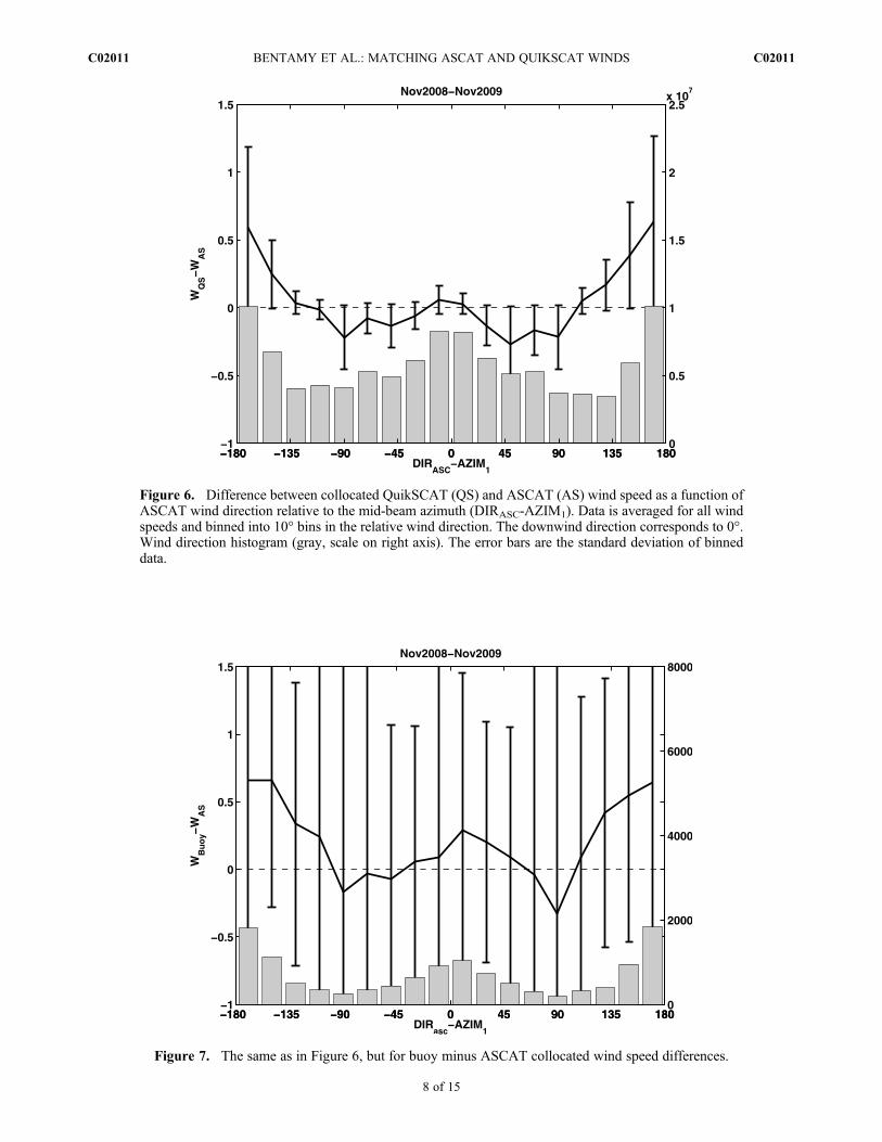
Figure 6. Difference between collocated QuikSCAT (QS) and ASCAT (AS) wind speed as a function ofASCAT wind direction relative to the mid-beam azimuth (DIRASC-AZIM1). Data is averaged for all windspeeds and binned into 10° bins in the relative wind direction. The downwind direction corresponds to 0°.Wind direction histogram (gray, scale on right axis). The error bars are the standard deviation of binneddata.

Figure 7. The same as in Figure 6, but for buoy minus ASCAT collocated wind speed differences.


8 of 15

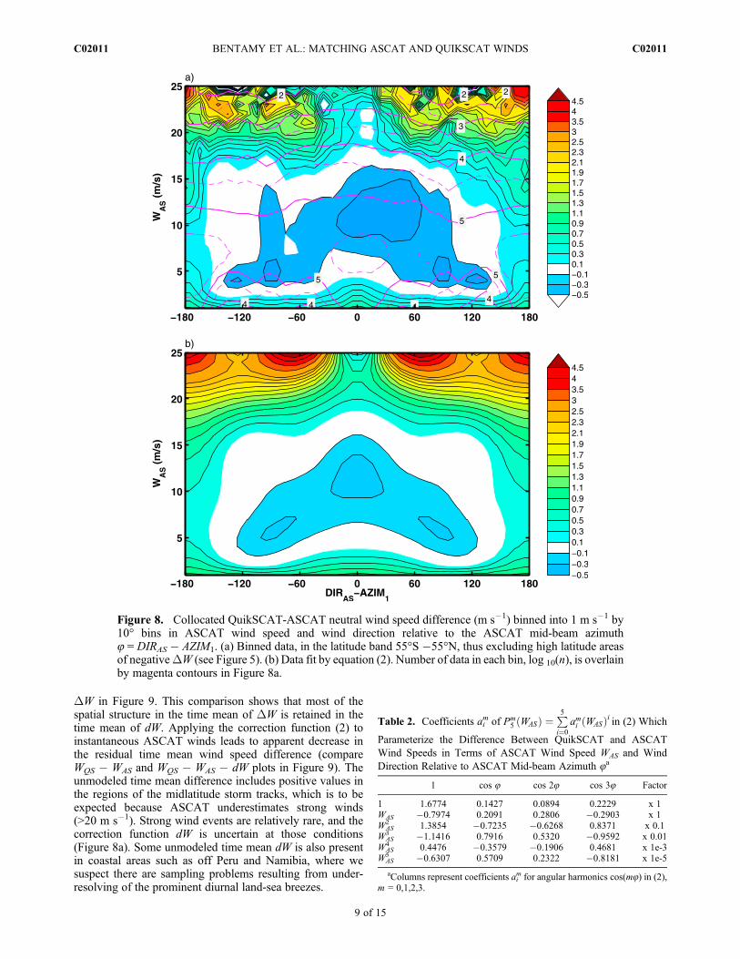
DW in Figure 9. This comparison shows that most of thespatial structure in the time mean of DW is retained in thetime mean of dW. Applying the correction function (2) toinstantaneous ASCAT winds leads to apparent decrease inthe residual time mean wind speed difference (compareWQS � WAS and WQS � WAS � dW plots in Figure 9). Theunmodeled time mean difference includes positive values inthe regions of the midlatitude storm tracks, which is to beexpected because ASCAT underestimates strong winds(>20 m s�1). Strong wind events are relatively rare, and thecorrection function dW is uncertain at those conditions(Figure 8a). Some unmodeled time mean dW is also presentin coastal areas such as off Peru and Namibia, where wesuspect there are sampling problems resulting from under-resolving of the prominent diurnal land-sea breezes.

Figure 8. Collocated QuikSCAT-ASCAT neutral wind speed difference (m s�1) binned into 1 m s�1 by10° bins in ASCAT wind speed and wind direction relative to the ASCAT mid-beam azimuth8 = DIRAS � AZIM1. (a) Binned data, in the latitude band 55°S �55°N, thus excluding high latitude areasof negativeDW (see Figure 5). (b) Data fit by equation (2). Number of data in each bin, log 10(n), is overlainby magenta contours in Figure 8a.

Table 2. Coefficients aim of Pm

5 ðWASÞ ¼P5

i¼0ami ðWASÞi in (2) Which

Parameterize the Difference Between QuikSCAT and ASCATWind Speeds in Terms of ASCAT Wind Speed WAS and WindDirection Relative to ASCAT Mid-beam Azimuth 8a

1 cos 8 cos 28 cos 38 Factor

1 1.6774 0.1427 0.0894 0.2229 x 1WAS �0.7974 0.2091 0.2806 �0.2903 x 1WAS

2 1.3854 �0.7235 �0.6268 0.8371 x 0.1WAS

3 �1.1416 0.7916 0.5320 �0.9592 x 0.01WAS

4 0.4476 �0.3579 �0.1906 0.4681 x 1e-3WAS

5 �0.6307 0.5709 0.2322 �0.8181 x 1e-5

aColumns represent coefficients aim for angular harmonics cos(m8) in (2),

m = 0,1,2,3.


9 of 15

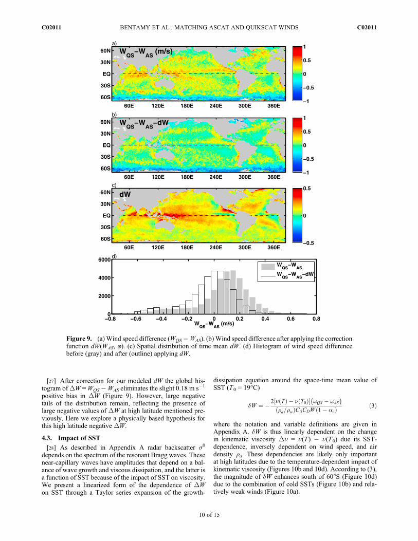
[27] After correction for our modeled dW the global his-togram ofDW =WQS �WAS eliminates the slight 0.18 m s�1

positive bias in DW (Figure 9). However, large negativetails of the distribution remain, reflecting the presence oflarge negative values of DW at high latitude mentioned pre-viously. Here we explore a physically based hypothesis forthis high latitude negative DW.

4.3. Impact of SST

[28] As described in Appendix A radar backscatter s0

depends on the spectrum of the resonant Bragg waves. Thesenear-capillary waves have amplitudes that depend on a bal-ance of wave growth and viscous dissipation, and the latter isa function of SST because of the impact of SST on viscosity.We present a linearized form of the dependence of DWon SST through a Taylor series expansion of the growth-

dissipation equation around the space-time mean value ofSST (T0 = 19°C)

dW ¼ � 2 n Tð Þ � n T0ð Þ½ � wQS � wAS

� �

ra=rwð ÞCbCDW 1� acð Þ ð3Þ

where the notation and variable definitions are given inAppendix A. dW is thus linearly dependent on the changein kinematic viscosity Dn = n(T ) � n(T0) due its SST-dependence, inversely dependent on wind speed, and airdensity ra. These dependencies are likely only importantat high latitudes due to the temperature-dependent impact ofkinematic viscosity (Figures 10b and 10d). According to (3),the magnitude of dW enhances south of 60°S (Figure 10d)due to the combination of cold SSTs (Figure 10b) and rela-tively weak winds (Figure 10a).

Figure 9. (a) Wind speed difference (WQS�WAS). (b) Wind speed difference after applying the correctionfunction dW(WAS, 8). (c) Spatial distribution of time mean dW. (d) Histogram of wind speed differencebefore (gray) and after (outline) applying dW.


10 of 15

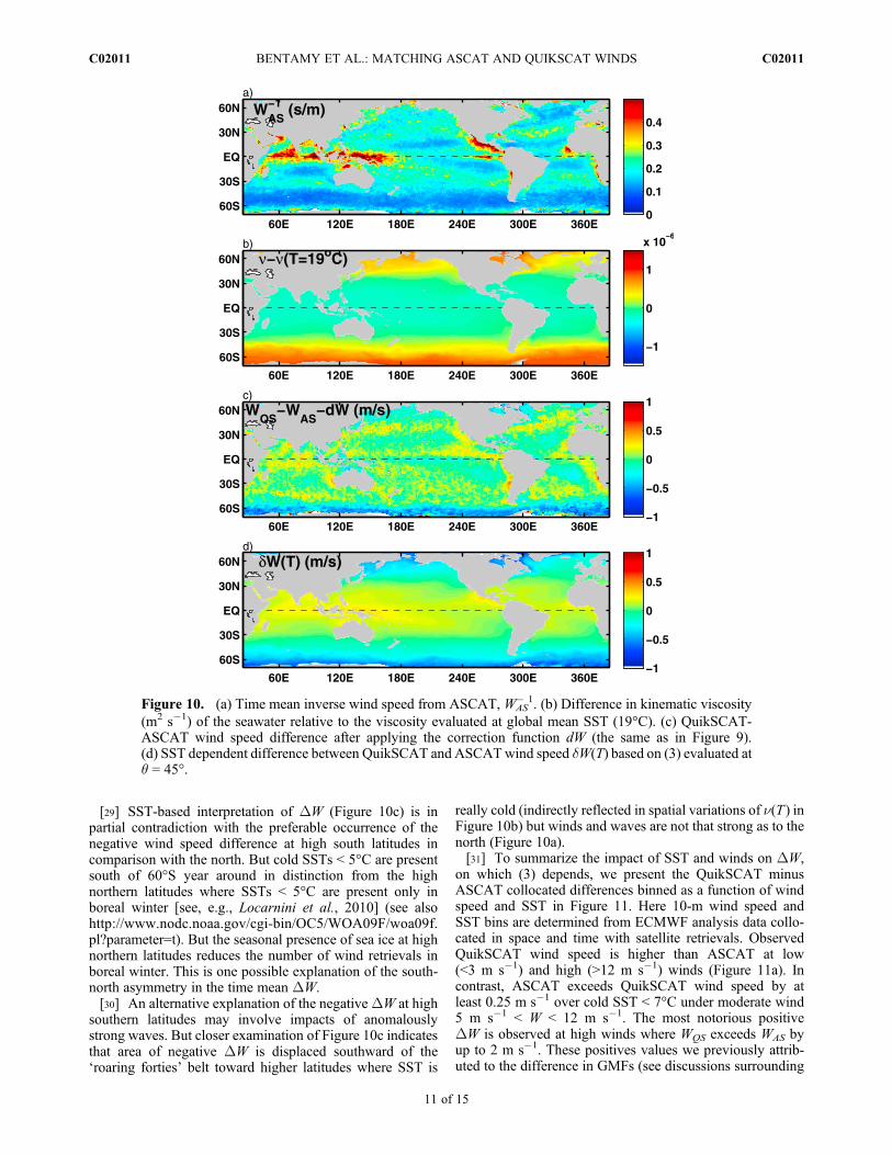
[29] SST-based interpretation of DW (Figure 10c) is inpartial contradiction with the preferable occurrence of thenegative wind speed difference at high south latitudes incomparison with the north. But cold SSTs < 5°C are presentsouth of 60°S year around in distinction from the highnorthern latitudes where SSTs < 5°C are present only inboreal winter [see, e.g., Locarnini et al., 2010] (see alsohttp://www.nodc.noaa.gov/cgi-bin/OC5/WOA09F/woa09f.pl?parameter=t). But the seasonal presence of sea ice at highnorthern latitudes reduces the number of wind retrievals inboreal winter. This is one possible explanation of the south-north asymmetry in the time mean DW.[30] An alternative explanation of the negativeDW at high

southern latitudes may involve impacts of anomalouslystrong waves. But closer examination of Figure 10c indicatesthat area of negative DW is displaced southward of the‘roaring forties’ belt toward higher latitudes where SST is

really cold (indirectly reflected in spatial variations of n(T ) inFigure 10b) but winds and waves are not that strong as to thenorth (Figure 10a).[31] To summarize the impact of SST and winds on DW,

on which (3) depends, we present the QuikSCAT minusASCAT collocated differences binned as a function of windspeed and SST in Figure 11. Here 10-m wind speed andSST bins are determined from ECMWF analysis data collo-cated in space and time with satellite retrievals. ObservedQuikSCAT wind speed is higher than ASCAT at low(<3 m s�1) and high (>12 m s�1) winds (Figure 11a). Incontrast, ASCAT exceeds QuikSCAT wind speed by atleast 0.25 m s�1 over cold SST < 7°C under moderate wind5 m s�1 < W < 12 m s�1. The most notorious positiveDW is observed at high winds where WQS exceeds WAS byup to 2 m s�1. These positives values we previously attrib-uted to the difference in GMFs (see discussions surrounding

Figure 10. (a) Time mean inverse wind speed from ASCAT, WAS� 1. (b) Difference in kinematic viscosity

(m2 s�1) of the seawater relative to the viscosity evaluated at global mean SST (19°C). (c) QuikSCAT-ASCAT wind speed difference after applying the correction function dW (the same as in Figure 9).(d) SST dependent difference between QuikSCAT and ASCATwind speed dW(T) based on (3) evaluated atq = 45°.


11 of 15

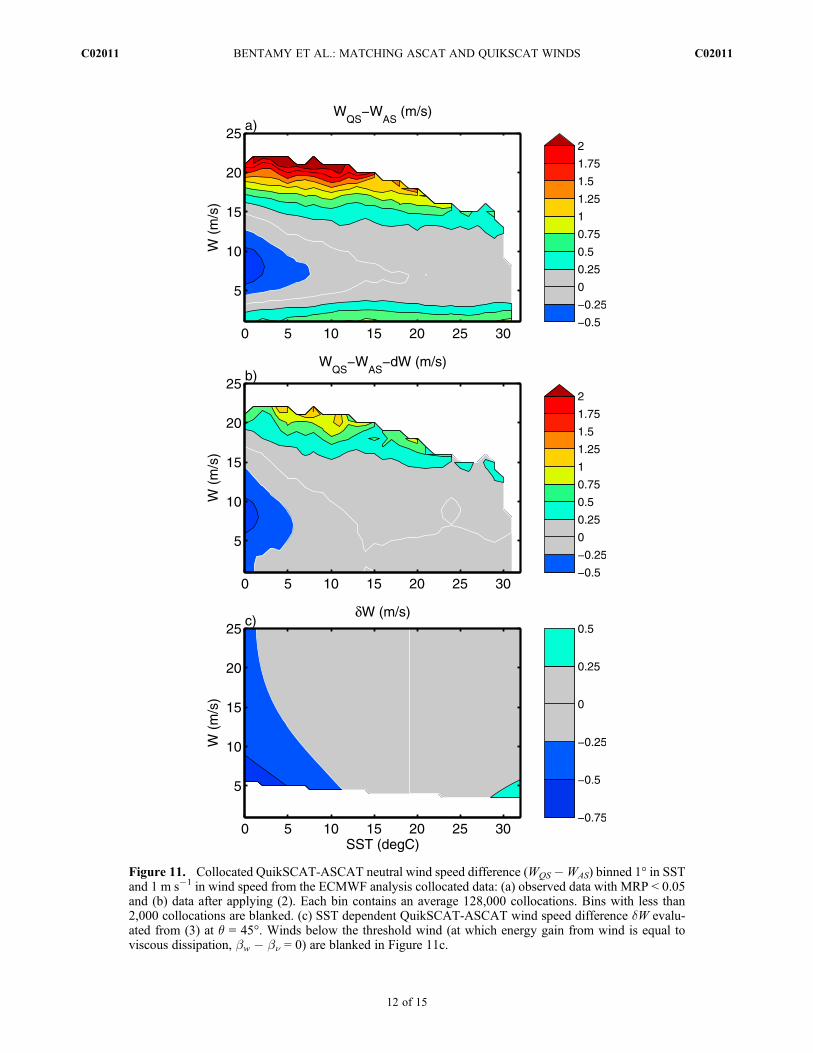
Figure 11. Collocated QuikSCAT-ASCAT neutral wind speed difference (WQS �WAS) binned 1° in SSTand 1 m s�1 in wind speed from the ECMWF analysis collocated data: (a) observed data with MRP < 0.05and (b) data after applying (2). Each bin contains an average 128,000 collocations. Bins with less than2,000 collocations are blanked. (c) SST dependent QuikSCAT-ASCAT wind speed difference dW evalu-ated from (3) at q = 45°. Winds below the threshold wind (at which energy gain from wind is equal toviscous dissipation, bw � bn = 0) are blanked in Figure 11c.


12 of 15

Figure 8) are not explained by (3). Correction of ASCATwind speed by (2) reduces DW at high winds but doesn’teliminate the deviation completely (compare Figures 11a and11b). The strongest negative wind speed difference betweenthe scatterometers is found at cold SST < 5°C. In contrast tothe simple model in (3) comparison of Figures 11b and 11cshows that the negative difference between QuikSCAT andASCAT wind speeds rises in magnitude for moderate windswhile (3) implies that the strongest negative values shouldoccur for weak winds. Examination of this discrepancy likelyrequires an improved parameterization of the wind-wavegrowth parameter and a more detailed radar imaging model.In particular we note that weak winds may act to dissipaterather than strengthen the centimeter-scale waves (seeKudryavtsev et al. [2005] for further details).

5. Summary

[32] The end of the QuikSCAT mission in 2009 and thelack of available and continuous Ku-band scatterometerretrievals has made it a high priority to ensure the compati-bility of QuikSCAT and the continuing C-band ASCATmission measurements. Yet examination of collocatedobservations during a 13 month period of mission overlapNovember 2008–November 2009 shows that there are sys-tematic differences in the 10 m neutral wind estimates fromthe two missions. This study is an attempt to identify andmodel these differences in order to produce a consistentscatterometer-based wind record spanning the period 1999to present.[33] The basic data set we use to identify the differences

and develop corrections is the set of space-time collocatedsatellite wind observations from the two missions and triplycollocated satellite-satellite-buoy observations during the13 month period of overlap. Since the scatterometers havedifferent orbits the first part of the study explores theacceptable range of spatial and temporal lags for comparisonstudy. We find a high temporal correlation (≥0.8) for timelags of up to 4 h and thus 4 h was determined to be themaximum acceptable time separation for winds stronger than3.5 m/s. Requiring shorter time lags severely limits thenumber of collocated observations at lower latitudes. Simi-larly, spatial separations of up to 50 km were determined tobe acceptable.[34] The second part of the study examines the collocated

winds for systematic differences. An examination of thecollocated winds shows a high degree of agreement indirection, but reveals systematic differences in speed thatdepend on rain rate, the strength of the wind, and SST. Wefind that the impact of rainfall on the higher frequency of thetwo scatterometers, QuikSCAT, introduces biases of up to1 m s�1 in the tropical convergence zones and the high pre-cipitation zones of the midlatitude storm tracks even afterrain flagged data are removed. This 1 m s�1 bias is cut in halfby removing QuikSCAT wind retrievals with multidimen-sional rain probabilities > 0.05 even though this additionalrain flagging reduces data amount by only 5%. For this rea-son we recommend the additional rain flagging.[35] We next examine the causes of the differences in

collocated wind speed remaining after removing QuikSCATwinds with MRP > 0.05. Data shown in Figures 3–6 suggestthat QuikSCAT and ASCAT wind directions are consistent.

Wind speed difference from the two instruments is a functionof ASCATwind speed and direction relative to the mid-beamazimuth, but it is virtually independent of the ASCAT inci-dent angle, a dependence strongly suggesting bias in theASCAT geophysical model function. We model this depen-dence based on our analysis of the collocation data, and isthen remove the dependence. Use of this bias model reducescollocated differences by 0.5 m s�1 in the tropics where it haslarge scale patterns related to variability of wind speed anddirection.[36] After applying the above two corrections, a third

source of difference is evident in that QuikSCAT wind speedremains systematically lower (by 0.5 m s�1) than ASCATwind speed at high latitudes where SST < 5°C. An exami-nation of the physics of centimeter-scale wind waves impli-cates the SST-dependence of wave dissipation, an effectwhich is enhanced for shorter waves. Again, the higher fre-quency scatterometer, QuikSCAT, will be more sensitive tothis effect.[37] Two additional sources of differences in the collo-

cated observations are also identified. Differences in windretrievals occur in storm track zones due to underestimationof infrequent strong wind events (>20 m s�1) by ASCAT.Differences in wind speed estimates are also evident in thePeruvian and Namibian coastal zones where diurnal land-seabreezes are poorly resolved by the time delays between suc-cessive passes of the two scatterometers (up to 4 h in thisstudy). Thus these latter differences seem to be a result of thelimitations of the collocated data rather than indicating errorin the scatterometer winds.

Appendix A: Impact of SST on the BraggScattering

[38] The purpose of this appendix is to evaluate deviationin retrieved scatterometer wind speed due to changes in SST.This evaluation is done for the pure Bragg scattering andusing simplified model of the Bragg wave spectrum.[39] Radar backscatter, s0, is mostly affected by energy of

the resonant Bragg wave component. According to Donelanand Pierson [1987] for the pure Bragg scattering regimeradar backscatter s0 is a positive definite function of thespectrum of the resonant Bragg wave component whoseenergy depends on the balance of wind wave growthparameter bw and viscous dissipation bn that is a function ofSST, s0 = F(bw � bn). For simplicity, we next considerwaves aligned with wind and use the Plant [1982] parame-terization bw = ra /rwCb(u*/c)

2 where c is the Bragg wavephase speed, ra /rw is the air to water density ratio, Cb = 32 isan empirical constant, u� ¼

ffiffiffiffiffiffiCD

pW is the friction velocity in

the air, CD is the neutral drag coefficient that is parameterizedfollowing Large and Yeager [2009]. This bw works overwide range of u*/c but fails at small values corresponding tothreshold winds [Donelan and Pierson, 1987]. It should bealso corrected by a factor (1 � ac), where ac is the wind-wave coupling parameter to account for the splitting of totalwind stress in the wave boundary layer into wave-inducedand turbulent components [Makin and Kudryavtsev, 1999;Kudryavtsev et al., 1999)

bw ¼ ra=rwCb u�=cð Þ2 1� acð Þ; ðA1Þ


13 of 15

[40] Viscous dissipation, bn = 4nk2w�1, depends on thewave number, k, and frequency, w, of the Bragg component.It also depends on the water temperature, T , through thekinematic viscosity, n(T ), that explains temperature behaviorof the wind-wave growth threshold wind speed [Donelan andPierson, 1987; Donelan and Plant, 2009]. We also assumethat scatterometer calibration, s0(W), corresponds to theglobally and time mean sea surface temperature T0 = 19°C.Then an expected error in retrieved wind speed ~W due todeviation of local temperature from T0, DT = T � T0, iscalculated by differentiating along b(T , W) = const, i.e.,SST-induced changes in radar backscatter, ∂ s0/∂ b * ∂ b/∂ T * DT, are interpreted as changes in retrieved wind speed�∂s0=∂b � ∂b=∂W � ~W :

~W ðkÞ ¼ � ∂b=∂T∂b=∂W

DT ¼ Dra=rabw �Dbn

∂bw=∂W; ðA2Þ

where it is assumed/used that air temperature equals SST,only ra in (A1) depends on temperature, and ∂ bn /∂ W = 0.The first term in (A2) accounts for changes in retrieved windspeed due to changes in the air density [Bourassa et al.,2010]. For chosen bw parameterization (A1) this termdoesn’t depend on k, thus doesn’t contribute to the winddifference between Ku- and C-band. Temperature dependentdifference between QS and AS winds is explained by theviscous term in (A2)

dW ¼ ~W kQS� �� ~W kASð Þ ¼ � 2Dn wQS � wAS

� �

ra=rwð ÞCbCDW 1� acð Þ ; ðA3Þ

where Dn = n(T ) � n(T0).

[41] Acknowledgments. This research was supported by the NASAInternational Ocean Vector Wind Science Team (NASA NNXIOAD99G).We thank Vladimir Kudryavtsev for comments on the manuscript, andJ. F. Piollé and IFREMER/CERSAT for data processing support. The authorsare grateful to ECMWF, EUMETSAT, CERSAT, GODIVA, JPL, Météo-France, NDBC, O&SI SAF, PMEL, and UK MetOffice for providing buoy,numerical, and satellite data used in this study. Comments and suggestionsprovided by anonymous reviewers were helpful and stimulating.

ReferencesAtlas, R., R. N. Hoffman, J. Ardizzone, S. M. Leidner, J. C. Jusem, D. K.Smith, and D. Gombos (2011), A cross-calibrated, multiplatform oceansurface wind velocity product for meteorological and oceanographicapplications, Bull. Am. Meteorol. Soc., 92, 157–174, doi:10.1175/2010BAMS2946.1.

Bentamy, A., K. B. Katsaros, M. Alberto, W. M. Drennan, and E. B. Forde(2002), Daily surface wind fields produced by merged satellite data, inGas Transfer at Water Surfaces, Geophys. Monogr. Ser., vol. 127, editedby M. A. Donelan et al., pp. 343–349, AGU, Washington, D. C.,doi:10.1029/GM127p0343.

Bentamy, A., H.-L. Ayina, P. Queffeulou, and D. Croize-Fillon (2007),Improved near real time surface wind resolution over the MediterraneanSea, Ocean Sci., 3, 259–271, doi:10.5194/os-3-259-2007.

Bentamy, A., D. Croize-Fillon, and C. Perigaud (2008), Characterization ofASCAT measurements based on buoy and QuikSCAT wind vector obser-vations, Ocean Sci., 4, 265–274, doi:10.5194/os-4-265-2008.

Blanke, B., S. Speich, A. Bentamy, C. Roy, and B. Sow (2005), Modelingthe structure and variability of the southern Benguela upwelling usingQuikSCAT wind forcing, J. Geophys. Res., 110, C07018, doi:10.1029/2004JC002529.

Bourassa, M. A., D. M. Legler, J. J. O’Brien, and S. R. Smith (2003),SeaWinds validation with research vessels, J. Geophys. Res., 108(C2),3019, doi:10.1029/2001JC001028.

Bourassa, M. A., E. Rodriguez, and R. Gaston (2010), NASA’s OceanVector Winds science team workshops, Bull. Am. Meteorol. Soc., 91,925–928, doi:10.1175/2010BAMS2880.1.

Bourlès, B., et al. (2008), The Pirata program: History, accomplishments,and future directions, Bull. Am. Meteorol. Soc., 89, 1111–1125,doi:10.1175/2008BAMS2462.1.

Donelan, M. A., and W. J. Pierson Jr. (1987), Radar scattering and equilib-rium ranges in wind-generated waves with application to scatterometry,J. Geophys. Res., 92, 4971–5029, doi:10.1029/JC092iC05p04971.

Donelan, M. A., and W. J. Plant (2009), A threshold for wind-wave growth,J. Geophys. Res., 114, C07012, doi:10.1029/2008JC005238.

Dunbar, S., et al. (2006), QuikSCAT science data product user manual,version 3.0, Doc. D-18053—Rev A, Jet Propul. Lab., Pasadena, Calif.[Available at ftp://podaac-ftp.jpl.nasa.gov/allData/quikscat/L2B/docs/QSUG_v3.pdf.]

Ebuchi, N. (2011), Self-consistency of marine surface wind vectors observedby ASCAT, IEEE Trans. Geosci. Remote Sens., 99, 1–8, doi:10.1109/TGRS.2011.2160648, in press.

Ebuchi, N., H. C. Graber, and M. J. Caruso (2002), Evaluation of wind vec-tors observed by QuikSCAT/SeaWinds using ocean buoy data, J. Atmos.Oceanic Technol., 19, 2049–2062, doi:10.1175/1520-0426(2002)019<2049:EOWVOB>2.0.CO;2.

Fairall, C. W., E. F. Bradley, J. E. Hare, A. A. Grachev, and J. B. Edson(2003), Bulk parameterization of air-sea fluxes: Updates and verificationfor the COARE algorithm, J. Clim., 16, 571–591, doi:10.1175/1520-0442(2003)016<0571:BPOASF>2.0.CO;2.

Freilich, M. H. (1997), Validation of vector magnitude data sets: Effectsof random component errors, J. Atmos. Oceanic Technol., 14, 695–703,doi:10.1175/1520-0426(1997)014<0695:VOVMDE>2.0.CO;2.

Grima, N., A. Bentamy, K. Katsaros, and Y. Quilfen (1999), Sensitivity ofan oceanic general circulation model forced by satellite wind stress fields,J. Geophys. Res., 104, 7967–7989, doi:10.1029/1999JC900007.

Grodsky, S. A., and J. A. Carton (2001), Coupled land/atmosphere interac-tions in the West African monsoon, Geophys. Res. Lett., 28, 1503–1506,doi:10.1029/2000GL012601.

Houze, R. A., and C.-P. Cheng (1977), Radar characteristics of tropicalconvection observed during GATE: Mean properties and trends overthe summer season, Mon. Weather Rev., 105, 964–980, doi:10.1175/1520-0493(1977)105<0964:RCOTCO>2.0.CO;2.

Kudryavtsev, V., V. Makin, and B. Chapron (1999), Coupled sea surface-atmosphere model: 2. Spectrum of short wind waves, J. Geophys. Res.,104, 7625–7639, doi:10.1029/1999JC900005.

Kudryavtsev, V., D. Akimov, J. Johannessen, and B. Chapron (2005), Onradar imaging of current features: 1. Model and comparison with observa-tions, J. Geophys. Res., 110, C07016, doi:10.1029/2004JC002505.

Large, W. G., and S. G. Yeager (2009), The global climatology of aninterannually varying air-sea flux data set, Clim. Dyn., 33, 341–364,doi:10.1007/s00382-008-0441-3.

Locarnini, R. A., A. V. Mishonov, J. I. Antonov, T. P. Boyer, H. E. Garcia,O. K. Baranova, M. M. Zweng, and D. R. Johnson (2010), World OceanAtlas 2009, vol. 1, Temperature, NOAA Atlas NESDIS, vol. 68, NOAA,Silver Spring, Md.

Makin, V., and V. Kudryavtsev (1999), Coupled sea surface–atmospheremodel: 1. Wind over waves coupling, J. Geophys. Res., 104, 7613–7623,doi:10.1029/1999JC900006.

McPhaden, M. J., et al. (1998), The tropical ocean–global atmosphereobserving system: A decade of progress, J. Geophys. Res., 103,14,169–14,240, doi:10.1029/97JC02906.

McPhaden, M. J., et al. (2009), RAMA: The Research Moored Array forAfrican-Asian-Australian Monsoon Analysis and Prediction, Bull. Am.Meteorol. Soc., 90, 459–480, doi:10.1175/2008BAMS2608.1.

Meindl, E. A., and G. D. Hamilton (1992), Programs of the National DataBuoy Center, Bull. Am. Meteorol. Soc., 4, 984–993.

Milliff, R. F., W. G. Large, J. Morzel, G. Danabasoglu, and T. M. Chin(1999), Ocean general circulation model sensitivity to forcing fromscatterometer winds. J. Geophys. Res., 104(C5), 11,337–11,358,doi:10.1029/1998JC900045

Plant, W. J. (1982), A relationship between wind stress and wave slope,J. Geophys. Res., 87(C3), 1961–1967, doi:10.1029/JC087iC03p01961.

Ricciardulli, L., and F. Wentz (2011), Reprocessed QuikSCAT (V04) windvectors with Ku-2011 geophysical model function, Tech. Rep. 043011,Remote Sens. Syst., Santa Rosa, Calif.

Risien, C. M., and D. B. Chelton (2008), A global climatology of surfacewind and wind stress fields from eight years of QuikSCAT scatterometerdata, J. Phys. Oceanogr., 38, 2379–2413, doi:10.1175/2008JPO3881.1.

Rolland, J., and P. Blouch (2002), Les bouées météorologiques, Meteorol.39, Meteo France, Paris. [Available at http://documents.irevues.inist.fr/bitstream/handle/2042/36252/meteo_2002_39_83.pdf.]

Sobieski, P. W., C. Craeye, and L. F. Bliven (1999), Scatterometric signa-tures of multivariate drop impacts on fresh and salt water surfaces, Int.J. Remote Sens., 20, 2149–2166, doi:10.1080/014311699212164.


14 of 15

Tournadre, J., and Y. Quilfen (2003), Impact of rain cell on scatterometerdata: 1. Theory and modeling, J. Geophys. Res., 108(C7), 3225,doi:10.1029/2002JC001428.

Verspeek, J., A. Stoffelen, M. Portabella, H. Bonekamp, C. Anderson, andJ. F. Saldana (2010), Validation and calibration of ASCAT usingCMOD5.n, IEEE Trans. Geosci. Remote Sens., 48, 386–395,doi:10.1109/TGRS.2009.2027896.

Weissman, D. E., M. A. Bourassa, and J. Tongue (2002), Effects of rain rateand wind magnitude on SeaWinds scatterometer wind speed errors,J. Atmos. Oceanic Technol., 19, 738–746, doi:10.1175/1520-0426(2002)019<0738:EORRAW>2.0.CO;2.

Wright, J. W., andW. C. Keller (1971), Doppler spectra in microwave scatter-ing from wind waves, Phys. Fluids, 14, 466–474, doi:10.1063/1.1693458.

Zhang, H.-M., J. J. Bates, and R. W. Reynolds (2006), Assessment of com-posite global sampling: Sea surface wind speed, Geophys. Res. Lett., 33,L17714, doi:10.1029/2006GL027086.

A. Bentamy, B. Chapron, and D. Croizé-Fillon, Institut Francais pour laRecherche et l’Exploitation de la Mer, Plouzane F-29280, France.J. A. Carton and S. A. Grodsky, Department of Atmospheric and Oceanic

Science, University of Maryland, College Park, MD 20742, USA.([email protected])


15 of 15

Matching ASCAT and QuikSCAT winds

Documents