Estudio Numérico y Experimental de Flujo Rayleigh-Bénard en ...

Estudio Numérico y Experimental de Flujo Rayleigh-Bénard en

Cavidades Cúbicas para Régimen Transitorio y Turbulento

Presentado por Leonardo Valencia Merizalde

Para optar al grado de doctor en Ingeniería Química Tarragona, octubre de 2005

© 2005 Leonardo Valencia Merizalde

UNIVERSITAT ROVIRA I VIRGILIESTUDIO NUMÉRICO Y EXPERIMENTAL DE FLUJO RAYLEIGH-BÉRNARD EN CAVIDADES CÚBICAS PARA RÉGIMEN TRANSITORIO Y TURBULENTO.Leonardo Valencia Merizalde ISBN: 978-84-690-8297-3 / D.L: T. 1482-2006

El Dr. Jordi Pallarès Curto, Profesor Titular de Mecánica de Fluidos de la Escuela Técnica Superior de Ingeniería Química de la Universidad Rovira i Virgili y el Dr. Ildefonso Cuesta, Director del Departamento de Ingeniería Mecánica de la Escuela Técnica Superior de Ingeniería Química de la Universidad Rovira i Virgili Hacen constar: Que el presente trabajo, con el título:

“Estudio Numérico y Experimental de Flujo Rayleigh-Bénard en Cavidades Cúbicas para Régimen Transitorio y Turbulento” que presenta Leonardo Valencia Merizalde para optar al grado de doctor en Ingeniería Química, se realizó bajo nuestra inmediata dirección y que todos los resultados obtenidos son fruto de los experimentos y análisis realizados por el mencionado doctorando.

Y para que se haga saber y tenga los efectos que corresponden, firmamos este certificado

Tarragona, 1 de julio de 2005

Dr. Jordi Pallares Curto Dr. Ildefonso Cuesta Romeo


ÍNDICE Resumen iii Lista de Publicaciones iv Agradecimientos v Nomenclatura vi 1. Introducción 1

1.1. Reseña histórica 1 1.2. Justificación y objetivos 4

2. Análisis Teórico 6

2.1. Introducción 6 2.2. Modelo físico 6 2.3. Modelo matemático 9

2.3.1. Condiciones de contorno y condiciones iniciales 11 2.3.2. Caracterización de la transferencia de calor 11

2.4. Esquema numérico 12 3. Metodología experimental 14

3.1. Célula de convección 14 3.1.1. Controlador digital PID 16

3.2. Sistema de medición de velocidades – Método PIV 16 3.2.1. Adquisición de Imágenes 17

3.2.1.1. Selección del intervalo de tiempo entre imágenes 18 3.3. Cálculo de las velocidades en el plano medio vertical de la cavidad 19 3.4. Validación del método PIV 21

4. Resumen de las publicaciones 24

4.1. Resumen de la publicación 1 – Anexo A1 24 Valencia L. Pallares J., Cuesta I. y Grau F. X. “Numerical simulation of non-Boussinesq effects in laminar and turbulent Rayleigh-Bénard convection of water in a perfectly conducting cubical cavity”. Proceedings del CHT-04: International Symposium on Advances in Computational Heat Transfer III, Eds. Graham de Vahl Davis y Eddie Leonardi. Noruega, paper CHT-04-102, 2004 4.2. Resumen de la publicación 2 – Anexo A2 27 Valencia L. Pallares J., Cuesta I. y Grau F. X. “Rayleigh-Bénard convection of water in a perfectly conducting cubical cavity: effects of temperature-dependent physical properties in laminar and turbulent regimes”. Numerical Heat Transfer, Part A Applications Vol. 47 (5) pp.333-352, 2005. 4.3. Resumen de la publicación 3 – Anexo B1 29 Valencia L. Pallares J., Cuesta I. y Grau F. X. “Numerical and experimental study of turbulent Rayleigh-Bénard convection of water in a cubical cavity”. Proceedings del ICCHMT: International Conference on Computational Heat and Mass Transfer IV, Ed. Rachid Bennacer Co-Eds: Abdulmajeed Abid Mohamad, Mohammed El Ganaoui y Jean Sicard. París Francia. Vol. 1, pp. 83-88, 2005. 4.4. Resumen de la publicación 4 – Anexo B2 32 Valencia L. Pallares J., Cuesta I. y Grau F. X. “Turbulent Rayleigh-Bénard convection of water in cubical cavities: Numerical study and experimental validation”, 2005. Para ser sometido a publicación en revista.

i


5. Conclusiones 35 Referencias 37 Anexos A Anexo A1: Publicación 1 Anexo A2: Publicación 2 Anexos B: Anexo B1: Publicación 3 Anexo B2: Publicación 4

ii


RESUMEN El presente trabajo estudia la convección Rayleigh-Bénard en cavidades cúbicas sin inclinación con respecto a la horizontal y calentadas por debajo para números de Rayleigh tanto dentro del estado estacionario como dentro del régimen turbulento. Inicialmente se estudian los efectos que tiene la variación de las propiedades físicas con la temperatura sobre la estructura de flujo, el mecanismo de transporte y la transferencia de calor para dos números de Rayleigh bajos en los que el flujo es laminar y estacionario y para un Rayleigh dentro del régimen turbulento. Para este estudio numérico se utilizó agua como fluido convectivo y se supuso que las paredes laterales de la cavidad eran perfectamente conductoras. Posteriormente se han identificado numéricamente las estructuras de flujo promedio temporal para cinco números de Rayleigh dentro del régimen turbulento. Debido a la similitud de cuatro de estas estructuras sólo dos de ellas fueron verificadas experimentalmente. Para los cálculos se asumió la aproximación de Boussinesq debido a que las diferencias de temperatura en la experimentación eran suficientemente bajas como para considerar propiedades físicas constantes de acuerdo con los resultados obtenidos en el análisis anterior. Con el fin de reproducir al máximo las condiciones experimentales, los resultados numéricos fueron obtenidos teniendo presente la conductividad térmica del vidrio de las paredes laterales. La visualización de las estructuras de flujo y la medición de los campos de velocidad en el plano vertical medio de la cavidad se realizó con el método PIV. Estos resultados nos permitieron validar los resultados obtenidos con las simulaciones, comparándose tanto las topologías del flujo como los valores de velocidad puntuales en perfiles dentro del plano analizado. De los resultados numéricos se encontró que aun con porcentajes de variación de las propiedades físicas del fluido entre las paredes fría y caliente muy por encima del criterio normalmente utilizado tanto en régimen laminar como turbulento, las estructuras de flujo y las condiciones de transporte de calor, no se ven afectadas considerablemente por esta variación. Por otro lado las estructuras de flujo promedio temporal y los valores de velocidad obtenidos numéricamente concuerdan significativamente con las correspondientes medidas experimentales para los números de Rayleigh analizados.

iii


LISTA DE PUBLICACIONES Esta Tesis para optar al grado de Doctor en Ingeniería Química se basa en las siguientes publicaciones incluidas en los Anexos de este documento: Publicación 1 (Anexo A1): Valencia L. Pallares J., Cuesta I. y Grau F. X. “Numerical simulation of non-Boussinesq effects in laminar and turbulent Rayleigh-Bénard convection of water in a perfectly conducting cubical cavity”. Proceedings del CHT-04: International Symposium on Advances in Computational Heat Transfer III, Eds. Graham de Vahl Davis y Eddie Leonardi. Noruega, paper CHT-04-102, 2004. Publicación 2 (Anexo A2): Valencia L. Pallares J., Cuesta I. y Grau F. X. “Rayleigh-Bénard convection of water in a perfectly conducting cubical cavity: effects of temperature-dependent physical properties in laminar and turbulent regimes”. Numerical Heat Transfer, Part A Applications Vol. 47 (5) pp.333-352, 2005. Publicación 3 (Anexo B1): Valencia L. Pallares J., Cuesta I. y Grau F. X. “Numerical and experimental study of turbulent Rayleigh-Bénard convection of water in a cubical cavity”. Proceedings del ICCHMT: International Conference on Computational Heat and Mass Transfer IV, Ed. Rachid Bennacer Co-Eds: Abdulmajeed Abid Mohamad, Mohammed El Ganaoui y Jean Sicard. París Francia. Vol. 1, pp. 83-88, 2005. Publicación 4 (Anexo B2): Valencia L. Pallares J., Cuesta I. y Grau F. X. “Turbulent Rayleigh-Bénard convection of water in cubical cavities: Numerical study and experimental validation”. Para ser sometido a publicación en revista Este documento se ha dividido en dos partes. En la primera parte se presenta una introducción y una revisión bibliográfica del problema que se aborda y se describen las principales características de los métodos utilizados en la Tesis. También se incluye una breve discusión de los resultados más importantes, así como las conclusiones más relevantes del trabajo. La segunda parte contiene las publicaciones listadas anteriormente donde se puede encontrar una descripción y discusión detallada de los resultados.

iv


AGRADECIMIENTOS Este trabajo fue realizado en el grupo de investigación ECOMMFIT de la Escuela Técnica Superior de Ingeniería Química de la Universitat Rovira i Virgili, bajo la dirección conjunta de los Dr. Jordi Pallarès Curto e Ildefonso Cuesta Romeo. Agradezco al Dr. Jordi Pallarès, al Dr. Ildefonso Cuesta y al Dr. Francesc Xavier Grau por aceptar la dirección de esta tesis y por permitirme desarrollar mi Tesis de doctorado en su grupo de investigación. Además me gustaría agradecerles principalmente por su dirección, su soporte y el conocimiento adquirido por medio de sus enseñanzas y consejos a lo largo de la tesis. Agradezco especialmente la ayuda económica recibida por el Departamento de Ingeniería Química de la Universitat Rovira i Virgili durante los cuatro primeros años del doctorado mediante la Beca URV para la realización de la Tesis y por las recibidas durante el quinto año de doctorado por el departamento de Ingeniería Mecánica y el grupo de Investigación ECOMMFIT con el fin de dar una correcta finalización de mi Tesis de doctorado. Agradezco la ayuda económica otorgada por el grupo de Investigación ECOMMFIT y por el departamento de Ingeniería Mecánica de la Universitat Rovira y Virgili para la participación en el congreso “ICCHMT: Fourth International Conference on Computational Heat and Mass Transfer” llevado a cabo en París, Francia, en mayo de 2005. También debo agradecer la ayuda económica dada por la Sección de Proyectos, Becas y Ayudas de la Universitat Rovira i Virgili por la Beca de Movilidad de tercer ciclo para la participación al congreso “CHT-04: International Symposium on Advances in Computational Heat Transfer” llevado a cabo en Noruega en abril de 2004 Por último agradezco a los miembros del tribunal Dr. Francesc Xavier Grau, Dr. Josep Anton Ferré, Dr. Mª Pilar Arroyo, Dr. Josep Bonet Ávalos y Dr. Immaculada Iglesias por aceptar juzgar este trabajo.

v


NOMENCLATURA BFS “Boussinesq Fluid Simulation” cálculo asumiendo la aproximación de

Boussinesq Br número de Brinkmann, v2µ/k(TH-T0) g aceleración gravitacional (m/s2) h coeficiente de transferencia de calor convectivo (W/m2×K) k conductividad térmica (W/m×K) K Ganancia (control PID) L dimensión vertical de la cavidad (m) N número de nodos de malla NBFSµ “Non-Boussines Fluid Simulation” con la viscosidad y la conductividad

térmica dependientes de la temperatura NBFSβ “Non-Boussines Fluid Simulation” con el coeficiente de expansión

térmica dependiente de la temperatura NBFSµβ “Non-Boussines Fluid Simulation” con la viscosidad, la conductividad

térmica y el coeficiente de expansión térmica dependientes de la temperatura

Nu número de Nusselt, hL/k p presión (N/m2) Pr número de Prandtl, ν/α q Eficiencia de reflexión de las partículas en el fluido Ra número de Rayleigh, gβ∆TL3/να t tiempo (s) T temperatura (K) u,v,w componentes de la velocidad (m/s) x,y,z coordenadas cartesianas (m) Greek letters α difusividad térmica (m2/s) β coeficiente de expansión térmica (1/K) δij delta de Kronecker ∆ incremento λ2 segundo mayor valor propio del tensor de gradiente de velocidad µ viscosidad dinámica (kg/m×s) ν viscosidad cinemática (m2/s) ρ densidad (kg/m3) σ desviación estándar de la velocidad (root-mean square – RMS) τ tiempo característico del controlador (integral o derivativo) T tiempo o escala integral Superscripts and subscripts * unidades adimensionales c controlador D derivativo I integral s cantidad media de superficie

vi


C placa fría H placa caliente 0 valor de referencia a la temperatura media t valor total w pared

vii


1. INTRODUCCIÓN La convección natural se genera, normalmente, en fluidos en presencia de un campo gravitatorio debido a diferencias de densidad las cuales se producen por la existencia de diferencias de temperatura o de concentración en el seno del fluido. Aunque pueden existir también movimientos de convección natural en fluidos con propiedades eléctricas y/o magnéticas sometidos a campos eléctricos y/o magnéticos. El movimiento de fluidos debido a este fenómeno se puede encontrar tanto en la naturaleza como en procesos industriales. En la naturaleza se presenta en las diferencias de temperaturas que enfrentan las nubes gaseosas en su interior y los vientos geostróficos generados en la atmósfera terrestre, en el proceso de mezclado de las aguas oceánicas y se estudia a fondo su relación con la dinámica de los materiales del manto y su influencia en el movimiento de las placas tectónicas en la corteza terrestre. Las aplicaciones ingenieriles en la industria son numerosas. En el diseño de convertidores solares la convección natural debe tenerse en cuenta para minimizar las pérdidas energéticas que resulten de los intercambios por conducción, convección y radiación. Dentro de los equipos electrónicos un factor importante es el aprovechamiento de la convección natural para la disipación de calor y en la ventilación, calefacción y aislamiento de edificios, ventanas y todo tipo de espacios cerrados dispuestos a ser acondicionados a temperaturas constantes. En la investigación básica, estos procesos de transferencia de calor convectivos en geometrías simples son también de gran importancia ya que permiten el estudio de la dinámica del flujo y de la transferencia de calor generados en estos sistemas así como el entendimiento de la descripción matemática de dichos flujos. En los últimos años los investigadores en este tema se encuentran especialmente interesados debido a que los resultados tanto experimentales como computacionales, han mostrado una diversidad de topologías de flujo y una gran complejidad en los procesos transitorios, en los cuales, se observan cambios de estructuras de flujo con mayor o menor estabilidad, además de la relación directa que se puede observar entre estas estructuras de flujo con la cantidad de calor transferido entre los puntos más calientes hasta los puntos más fríos del fluido. La convección natural Rayleigh-Bénard es un tipo de flujo convectivo en espacios confinados que se produce por la estratificación inestable de la densidad en dirección vertical asociada a gradientes de temperatura en el fluido. La convección en cavidad cúbica calentada por debajo ha sido el tema de un gran número de estudios tanto experimental como teórico ya que es de gran interés el hecho de que la dirección de la gravedad es la única dirección preferida para el movimiento del fluido; por otro lado, ha sido ampliamente usado en la validación de códigos computacionales de dinámica de fluidos (CFD) debido a su simplicidad geométrica y a la diversidad de flujos complejos que pueden generarse.

1.1. RESEÑA HISTÓRICA

En el trascurso de la historia científica son muchos los estudios realizados de este fenómeno, ya sea experimental como de predicción numérica con el fin de describir y entender la ciencia que envuelve el proceso convectivo.

1


El primero en estudiar la convección natural de fluidos confinados en una capa de fluido calentada por la parte inferior y el gradiente de temperaturas paralelo al vector gravedad fue Henry Bénard (1901) el cual demostró por primera vez de forma experimental la evidencia de un régimen permanente estable en el movimiento de líquidos por convección natural y determinó todos los elementos geométricos, cinemáticos y dinámicos para este régimen de flujo. Después de él, Lord Rayleigh (1916) determinó teóricamente y explicó satisfactoriamente la existencia de un incremento de temperaturas crítico por debajo del cual no puede existir movimiento convectivo en el fluido para una determinada altura de la capa del fluido, esto debido a que el efecto de la viscosidad y la difusividad térmica amortiguan cualquier inicio de movimiento producido por una perturbación exterior. Después de Bénard y Rayleigh son muchos los trabajos que se han realizado sobre la convección natural en fluidos confinados y sería casi imposible mencionarlos todos. Los siguientes son los estudios más relevantes relacionados directamente con el tipo de sistema estudiado en el presente trabajo. Batchelor (1954) mencionó que la solución del problema de la convección natural en una cavidad depende de tres parámetros adimensionales independientes: la relación de geometría de la cavidad, el número de Prandtl (Pr=ν/α) que caracteriza las propiedades físicas del fluido y el número de Rayleigh que da la relación entre las fuerzas de empuje o flotación y las viscosas (Ra= gβ∆TL3/να). El número de Rayleigh crítico caracteriza el punto a partir del cual cualquier perturbación en el sistema inicia el movimiento convectivo en el fluido. Muchos autores han encontrado el valor del Ra crítico (RaC) para sistemas particulares, Jeffreys (1926) determinó por primera vez el número de Rayleigh crítico para el caso de placas infinitas (RaC=1708), algunos años después Davis (1967), Catton (1970, 1972a,1972b), Heitz y Westwater (1971) y Stork y Müller (1972) mostraron resultados teóricos y experimentales de valores de números de RaC para diferentes geometrías con diferentes conductividades de las paredes laterales. Otros han realizado trabajos con aire y el gradiente de temperaturas entre placas verticales como Eckert (1961) que midió el campo de temperaturas para este caso a diferentes gradientes de temperatura y Elder (1965a, 1965b) que construyó una cavidad lo suficientemente grande en la tercera dimensión para considerar el flujo bidimensional, Bohn (1983,1984) estableció que el límite hasta el cual se puede considerar el flujo como laminar es de Ra=7×1010, este experimento se hizo en una cavidad cúbica con agua (Pr=5) y con el gradiente de temperaturas entre paredes laterales. Después Schmidt (1986) tuvo como objetivo la determinación experimental de las características del flujo en una cavidad con una relación geométrica de 2. Cuatro de las 6 paredes fueron aisladas térmicamente y las otras dos (laterales) colocadas en lugares opuestos y mantenidas constantemente a dos temperaturas diferentes. Las velocidades del fluido fueron medidas con un sistema de anemometría láser. Concluyó que dentro de la cavidad hay un flujo primario que se mueve cerca de las paredes, ascendente en la pared caliente y descendente en la pared fría. Junto con este flujo coexiste un flujo secundario, situado en medio del primario, y un núcleo central que permanece prácticamente quieto. Entre los estudios de cavidades con gradiente de temperatura entre las placas horizontales se encuentra el de Deardorff (1965) que estudió la convección natural del aire entre las dos placas haciendo que estas sean más grandes que la distancia que las separa. Azíz y Hellmuns (1967) estudiaron por primera vez la convección de Rayleigh-Bénard en el interior de una cavidad cúbica. Simularon numéricamente el movimiento convectivo en el interior de una cavidad cúbica con paredes laterales adiabáticas a

2


números de Ra próximos al crítico (Ra=3.5×103, Pr=1). A pesar de las mallas utilizadas en este trabajo (11×11×11 nodos) los resultados indicaron la existencia de una circulación en forma de rollo con eje orientado perpendicularmente a dos aristas verticales de la cavidad diagonalmente opuestas. Después Ozoe et al. (1977) retomaron los cálculos de Aziz y Hellmuns (1967) y utilizando un código mejorado encontraron dos configuraciones de flujo estable, circulación diagonal y circulación de rollo simple con el eje orientado perpendicularmente a dos paredes laterales opuestas. Un resultado muy importante es el de Kim y Viskanta (1984) que demostraron que omitir la interacción entre la convección dentro de la cavidad y la conducción en las paredes, mediante la utilización de condiciones de contorno ideales, no constituye una buena aproximación, ya que en la realidad la conducción en las paredes es un fenómeno inevitable. Kessler (1987) y Kirchartz y Oertel (1988) comenzaron a estudiar numérica y experimentalmente la estructura tridimensional de los rollos formados dentro de la cavidad en estado estacionario y en regímenes no estacionarios en cavidades rectangulares. Hernández y Frederick (1994) utilizando un código con formulación de volúmenes finitos de segundo orden reportaron una nueva estructura de flujo a Ra=8×103 y Pr=0.71 en la cavidad cúbica, previamente observada experimentalmente por Stork y Müller (1972) en una cavidad con paredes laterales adiabáticas y relación ancho-alto de 2×2×1. Esta circulación consistía en un rollo de forma toroidal que presentaba una corriente ascendente a lo largo del eje vertical de simetría de la cavidad y corrientes descendentes fluyendo paralelas a las cuatro paredes paralelas. Dabiri y Gharib (1996) estudiaron la convección en una cavidad cúbica aplicando calor en forma sinusoidal en una de sus paredes laterales. Utilizaron la velocimetría y termometría de imagen de partícula como método de medición del campo de temperatura y de velocidades dentro de la cavidad y obtuvieron resultados experimentales confiables. Dentro de los últimos trabajos se encuentra el de Pallares et al. (1996) que con el código 3DINAMICS (Cuesta, 1993) caracterizaron las topologías de flujo y la transferencia de calor de las tres estructuras de flujo previamente obtenidas, en régimen laminar y estacionario. Estos autores también describieron una nueva estructura que consiste en un rollo simple similar a la reportada por Ozoe et al. (1977) pero con una topología más alargada hacia dos aristas horizontales diagonalmente opuestas y con características de calor diferentes. Las cuatro estructuras eran estables en el rango 3.5×103≤Ra≤104 y Pr=0.71. Pallares et. al. (2001) encontraron experimentalmente una gama de 7 estructuras de flujo para Ra moderados ≤ 8×104 y número de Pr=130. Además determinaron el campo de velocidad de los flujos usando velocimetría de imagen de partícula (PIV por Particle Image Velocimetry), y obtuvieron resultados acordes con simulaciones hechas con el código 3DINAMICS antes mencionado. Pallares et. al. (2002) encontraron que a Ra=106 y Ra=108 y Pr=0.71, en los que el flujo es turbulento, los campos de velocidad y temperatura instantáneas presentaban grandes fluctuaciones con respecto a los valores promedio de los mismos e identificaron en el campo de velocidades promedio temporal dos estructuras toroidales cercanas a las paredes horizontales. Otros trabajos han centrado su estudio en la determinación del número de Nusselt con el fin de caracterizar la transferencia de calor en el sistema. Leong et. al. (1999) reportaron medidas experimentales de valores del número de Nusselt para Pr=0.71 a diferentes números de Ra, sin embargo no reportaron las estructuras en ninguno de los casos. Por otro lado, el efecto de la variación de las propiedades físicas con la temperatura en la convección natural ha sido ampliamente estudiada. La simulación exacta de las

3


ecuaciones de movimiento tendría un costo computacional bastante alto sino se hicieran algunas suposiciones. En los cálculos de fluidos sometidos a flotación es usualmente utilizada la aproximación de Boussinesq, la cual consta de tres suposiciones principales:

1. La densidad se considera constante excepto cuando causa fuerzas de flotación (dependencia lineal con la temperatura)

2. Todas las otras propiedades del fluido se consideran constantes. 3. Los términos de disipación viscosa se asumen despreciables.

Con el fin de crear un criterio para considerar válida la aproximación de Boussinesq, Gray y Giorgini (1976) fijaron una variación máxima del 10% de las propiedades físicas entre las placas isotérmicas. En su trabajo reportaron para una temperatura media de 15ºC que la diferencia de temperatura máxima en el agua podría ser de 1.25ºC y para aire de 28.6ºC con el fin de no sobrepasar una variación del 10% en el coeficiente de expansión térmica y la densidad, respectivamente. Aplicando este criterio en el presente trabajo, para agua a temperatura media de 26ºC entre paredes fría y caliente, la suposición de propiedades físicas constantes queda limitada a una diferencia de temperatura máxima de 2.9ºC (10% de variación del coeficiente de expansión térmica). Otros estudios considerando propiedades físicas variables se enfocan en grandes variaciones de viscosidad del fluido y se refieren principalmente a simulaciones numéricas de la convección en el manto terrestre (Solomatov (1995), Moresi y Solomatov (1995), Trompert y Hansen (1998) y Manga et al. (2001). En estas condiciones las diferencias de viscosidad dentro del fluido son suficientemente grandes para producir una capa de fluido estática cerca de la pared fría superior de la cavidad, y por lo tanto con un valor elevado de viscosidad, a través de la cual la transferencia de calor se produce solo por conducción.

1.2. JUSTIFICACIÓN Y OBJETIVOS Este trabajo se divide en dos partes. El objetivo principal de la primera parte es estudiar el criterio fijado por Gray y Giorgini (1976) (variación máxima del 10% de las propiedades físicas entre las placas isotérmicas) para considerar la validez de la aproximación de Boussinesq (supone el término de disipación viscosa despreciable y todas las propiedades físicas del fluido constantes exceptuando la densidad en el término de empuje) y así descubrir la aplicabilidad real de dicho criterio para flujos laminares y turbulentos. De hecho la mayor parte de estudios numéricos existentes en la literatura asumen esta aproximación cuando la variación de las propiedades físicas con la temperatura es un efecto inevitable experimentalmente. Para esto se analizará mediante simulaciones numéricas la influencia que tiene sobre la transferencia de calor y las estructuras de flujo al someter agua (Pr=5.9) a una alta variación de sus propiedades físicas dentro de una cavidad cúbica calentada por debajo y paredes perfectamente conductoras para regímenes laminar (Ra=104 y Ra=5×104) y turbulento (Ra=107). Este análisis constituye un primer paso para la determinación del efecto de la variación de las propiedades físicas en una situación experimental real similar que se aborda en la segunda parte de este estudio. También se muestran los resultados numéricos así como el análisis de los mismos. En este análisis se describen las topologías de flujo para los diferentes números de Rayleigh, se identifican las diferencias que existen en la transferencia de calor, en los campos de velocidad y de temperatura y entre los mecanismos de movimiento entre las simulaciones a propiedades físicas variables y las simulaciones con la aproximación de Boussinesq.

4


En la segunda parte del trabajo se analizan resultados experimentales y numéricos propios en régimen turbulento con el fin de validar las simulaciones. Particularmente se comparan el campo de velocidades promedio temporal y la desviación estándar de la velocidad vertical en el plano medio de la cavidad obtenidos numéricamente para régimen turbulento a números de Rayleigh Ra=107, Ra=7×107 y Ra=108. También se reportan las estructuras de flujo, las características de transferencia de calor y los efectos sobre estos al considerar la conducción de calor a través de las paredes laterales de la cavidad, con una conductividad térmica correspondiente a la de los experimentos, para números de Rayleigh altos (Ra=107, Ra=3×107, Ra=5×107, Ra=7×107 y Ra=108). Además se estudian las estructuras de flujo medias y la transferencia de calor a los números de Rayleigh estudiados. Se hace una comparación para Ra=107 entre las simulaciones considerando paredes parcialmente conductoras y perfectamente conductoras y se comparan los resultados experimentales obtenidos con PIV (por Particle Image Velocimetry) y los obtenidos numéricamente considerando conductividad térmica finita en las paredes.

5


2. ANÁLISIS TEÓRICO 2.1. INTRODUCCIÓN Acerca del estudio experimental del flujo de un fluido confinado en una cavidad cúbica de paredes rígidas e inmóviles, con la pared inferior a una temperatura mayor que la superior, se sabe que es un sistema potencialmente inestable debido a la generación del gradiente de densidad asociado a esta diferencia de temperaturas, estando el fluido más caliente y ligero en la parte inferior y el fluido más frío y pesado en la parte superior. Si el incremento de temperaturas es suficientemente pequeño, el calor se transmite de la placa inferior a la superior por conducción sin observarse movimiento macroscópico en el fluido. Todas las perturbaciones que se puedan realizar sobre el sistema se amortiguan por efecto de la viscosidad y de la difusividad térmica, y el sistema al cabo de un tiempo después que la perturbación desaparece, vuelve a su estado de reposo inicial. El número de Rayleigh (Ra= gβ∆TL3/να) caracteriza el punto crítico del sistema a partir del cual cualquier perturbación inicia el movimiento convectivo en el fluido. Este número adimensional que depende de las propiedades físicas relevantes del fluido (β, ν y α), del incremento de temperaturas (∆T=TH-TC) y de la distancia entre las placas caliente y fría (L), indica la importancia relativa de las fuerzas de flotación respecto de las fuerzas viscosas en el seno del fluido. La transferencia de calor en el sistema se puede establecer como una funcionalidad del número de Nusselt, el número de Rayleigh, el número Prandtl y la geometría. El número adimensional Nusselt (Nu=hL/k) es un coeficiente de transferencia de calor adimensional que proporciona una medida de la transferencia de calor por convección que ocurre en el sistema. Este número adimensional relaciona la transferencia de calor por convección con la establecida en el mismo sistema si sólo existiera conducción. Valores de Nu del orden de la unidad indican que la transferencia de calor se produce esencialmente por conducción. Por último el número de Prandtl (Pr=ν/α) relaciona la facilidad de difundir cantidad de movimiento con la de difundir calor. Se ha observado el movimiento convectivo del fluido en condiciones moderadamente por encima del valor crítico (Ra>RaC) y en cavidades con relaciones ancho-alto pequeñas (entre 1 y 5), adopta un patrón regular y periódico de corrientes calientes ascendentes alternadas con corrientes frías descendentes que forman circulaciones de fluido denominadas rollos convectivos. La variedad de estructuras topológicamente diferentes y con características de transporte diferenciadas que pueden desarrollarse en la amplia gama de cavidades tridimensionales posibles es un aspecto todavía no del todo conocido.

2.2. MODELO FÍSICO La geometría de las cavidades cúbicas utilizadas en la simulación, así como el sistema de referencia se muestran en la Figura 1. Las características de los sistemas que se estudian en este trabajo son:

6


X

Z

Y

Pared CalientePared Fría

Paredes Laterales

TC

TH

g L

X

Z

YPared Caliente (TH)

Pared Fría (TC)

g

FluidoParedes de vidrio

Figura 1. Geometría y sistema coordenado para (a) cavidad con paredes perfectamente conductoras y (b) conductividad finita en las paredes laterales.

(b) (a)

Anexos A: Paredes perfectamente conductoras (Ra=104, Ra=5×104 y Ra=107, Pr=5.9):

- Cavidad cúbica con las dos paredes horizontales isotérmicas y las cuatro paredes laterales perfectamente conductoras (Figura 1.a.)

- Se desprecian los efectos de compresibilidad y disipación viscosa - La densidad del fluido se considera constante con la temperatura exceptuando en

el término de flotación, en el cual se modeliza una dependencia lineal con la temperatura

- Se suponen constantes las demás propiedades físicas del fluido para las simulaciones con aproximación de Boussinesq (BFS-Boussinesq Fluid Simulation)

- Para los cálculos NBFS (Non Boussinesq Fluid Simulation) no se supone la aproximación de Boussinesq ya que no se desprecia la dependencia de algunas propiedades físicas con la temperatura.

La variación máxima de las propiedades físicas del agua para el incremento de temperatura usado en esta parte del trabajo (∆T = 17.5ºC) se muestra en la Tabla 1.

Tabla 1. Variación de las propiedades físicas del agua para una diferencia de temperatura de 17.5ºC entre

las paredes fría y caliente referido a la temperatura media (T0=26.0ºC) (

0100*)( TTT nnnn

CH% −= )

%β %µ %k %Cp %ρ 62.1 40.0 4.8 0.6 0.4

De acuerdo con Gray y Giorgini (1976) la aproximación de Boussinesq debe aplicarse para diferencias menores al 10% en las propiedades físicas del fluido. De acuerdo con este criterio, para agua a T0=26ºC las variaciones de temperatura máximas permitidas para poder aplicar la aproximación de Boussinesq serían ∆T ≤ 2.9ºC para el coeficiente de expansión térmica, ∆T ≤ 4.5ºC para la viscosidad y ∆T ≤ 35.7ºC para la conductividad térmica. Así pues, la diferencia de temperaturas de 17.5ºC es lo bastante

7


grande (6 veces mayor para la propiedad física más crítica) y por tanto los presentes resultados pueden ser considerados fuera de la aproximación de Boussinesq. En este trabajo, los cálculos a propiedades físicas variables fueron considerados de la siguiente manera: NBFSµ: solo la viscosidad y la conductividad térmica estarán en función de la temperatura, NBFSβ: dependencia con la temperatura del coeficiente de expansión térmica para analizar la influencia individual en el flujo y el campo de temperatura y por ultimo, NBFSµβ: en el que se consideran tanto la viscosidad, la conductividad térmica y el coeficiente de expansión térmica dependientes de la temperatura para obtener la influencia conjunta de las propiedades físicas que más varían en el agua y así poder comparar con los resultados a propiedades físicas constantes (BFS). Anexos B: Paredes con conductividad térmica finita (Ra=107, Ra=3×107, Ra=5×107, Ra=7×107 y Ra=108):

El número de Prandtl es diferente entre los números de Rayleigh Ra=107, Ra=3×107, Ra=5×107 y Ra=7×107 comparado con Ra=108. Para los primeros se considera Pr≈6.0 mientras que para el Rayleigh más alto se adopta Pr=5.35. Esta diferencia se debe a que experimentalmente, con temperatura media de 26ºC (Pr=6.0), no era posible suministrar la energía necesaria para obtener el Ra=108. Por lo tanto, fue necesario fijar el valor de la temperatura media en 30.3ºC donde la diferencia de temperaturas podía ser menor con el fin de alcanzar al valor de Ra=108 deseado. Al igual que en el caso anterior las simulaciones numéricas consideran la cavidad cúbica con las dos paredes horizontales isotérmicas pero en este caso se tiene en cuenta la conducción de calor en las paredes laterales de acuerdo con las condiciones experimentales (ver Figura 1.b). Los efectos de compresibilidad y disipación viscosa se desprecian. Los cálculos considerando paredes parcialmente conductoras fueron realizados con dos fines primordiales. En primer lugar encontrar las estructuras de flujo medias para validar experimentalmente los campos de velocidad por medio de la técnica PIV y, en segundo lugar, para compararlas con los resultados anteriores con paredes laterales perfectamente conductoras. La Tabla 2 muestra los valores de las propiedades físicas a la temperatura media así como la variación de las mismas entre paredes fría y caliente respecto a la temperatura media para cada número de Rayleigh estudiado en el presente apartado. De acuerdo con los resultados obtenidos con paredes perfectamente conductoras, reportados en el Anexo A, las variaciones del 62% del coeficiente de expansión térmica no influyen considerablemente en la estructura de flujo y las velocidades a Ra=107. Por esto a pesar de tener variaciones del 18% en el coeficiente de expansión térmica (Ver Tabla 2), los cálculos con paredes parcialmente conductoras fueron realizados asumiendo la aproximación de Boussinesq. La variación de las propiedades físicas restantes entre las temperaturas máxima y mínima utilizadas en los experimentos es menor que el criterio del 10% máximo (Gray y Giorgini, 1976) y por tanto se consideran propiedades físicas constantes.

8


Tabla 1.

Valores de las propiedades físicas a la temperatura media y sus variaciones con la temperatura expresadas como (

0100*)( TTT nnnn

CH% −= )

1 Incropera y DeWitt (1996)

Ra β01

kg/m s %β µ02

kg/m s %µ k03

W/m K %k Cp03

J/kg K %Cp ρ03

kg/m3 %ρ

107 2.64×10-4 15.4 8.7×10-4 9.7 0.61 1.2 4160 0.14 996.2 0.103×107 2.61×10-4 7.6 8.8×10-4 4.7 0.61 0.6 4157 0.07 996.3 0.055×107 2.61×10-4 12.6 8.8×10-4 7.9 0.61 1.0 4157 0.11 996.3 0.087×107 2.59×10-4 18.0 8.8×10-4 11.2 0.61 1.4 4160 0.16 996.4 0.11

108 3.04×10-4 17.5 8.0×10-4 12.1 0.62 1.5 4163 0.17 995.2 0.14

2 Potter y Wiggert (1998) 3 Holman (1976) 2.3. MODELO MATEMÁTICO Las ecuaciones que gobiernan el fenómeno de la convección natural de acuerdo con las características antes mencionadas, en forma adimensional, en coordenadas cartesianas y notación tensorial se muestran a continuación para los resultados del anexo A: ecuación de continuidad

0*

*

=∂∂

i

i

xu , (1)

ecuaciones de movimiento

( ) 12**

00*

*

*

**

*0*

*

*

**

*

* )(i

i

j

j

i

jij

iji TBTrPRaxu

xu

xrP

xp

xuu

tu

δµ ⋅++

∂

∂+

∂∂

∂∂

+∂∂

−=∂

∂+

∂∂

, (2)

y la ecuación de energía

∂∂

∂∂

=∂∂

+∂∂

*

**

**

**

*

*

iiii x

Tkxx

TutT , (3)

Las escalas de referencia para la longitud, velocidad, tiempo y presión son: L, α0/L, L2/α0 y ρ0α0

2/L2, respectivamente. La temperatura adimensional se define respecto a la diferencia de temperaturas entre las placas caliente y fría, ∆T=(TH-TC), de acuerdo con (T-T0)/ ∆T, donde T0 es la temperatura media, T0=(TH+TC)/2. En las ecuaciones para los cálculos con propiedades físicas variables y paredes perfectamente conductoras (NBFS), se generan los números adimensionales µ*=µ/µ0 y k*=k/k0 (Ecuaciones (2) y (3)) donde µ0 y k0 son la viscosidad y la conductividad térmica del fluido a la temperatura promedio T0. Además la ecuación de movimiento en la dirección vertical queda en función del cuadrado de la temperatura debido a la dependencia del coeficiente de expansión térmica con la temperatura y aparece un nuevo término, que para agua a T0=26ºC puede escribirse como B=9.38x10-6∆T/2β0 donde β0 es el coeficiente de expansión térmica a T0 (Ecuación 2). Para los cálculos con la aproximación de Boussinesq µ*=k*=1.0 y el término de empuje depende

9


linealmente con la temperatura (i.e. B=0 en la Ecuación (2)) y consecuentemente para los cálculos con BFS las Ecuaciones (2) y (3) quedan: ecuaciones de movimiento asumiendo BFS

1*

002*

*2

0*

*

*

**

*

* )(i

j

i

ij

iji TrPRax

urP

xp

xuu

tu

δ+∂

∂+

∂∂

−=∂

∂+

∂∂

, (4)

ecuación de energía para BFS

2*

*2

*

**

*

*

iii x

TxTu

tT

∂∂

=∂∂

+∂∂ (5)

Las ecuaciones utilizadas para obtener los resultados con paredes parcialmente conductoras mostrados en el Anexo B se muestran a continuación: ecuación de continuidad:

0*

*

=∂∂

i

i

xu

, (6)

ecuaciones de movimiento:

1*

002*

*2

0*

*

*

**

*

* )(i

j

i

ij

iji TrPRax

urP

xp

xuu

tu

δ+∂

∂+

∂∂

−=∂

∂+

∂∂

, (7)

ecuación de transporte de energía en el fluido:

2*

*2

*

**

*

* )(

ii

i

xT

xTu

tT

∂∂

=∂

∂+

∂∂

, (8)

y la ecuación de transporte de energía a través de las paredes laterales:

2*

*2*

*

*

ixT

tT

∂∂

=∂∂ α , (9)

En la Ecuación (9) aparece el término α*=αg/αf donde αg y αf son las difusividades térmicas del vidrio y del agua a T0, respectivamente. Los términos fuente de la ecuación de conservación de la energía correspondientes a la disipación viscosa (Φ) no se han incluido en el modelo matemático. Cálculos efectuados del número de Brinkmann (Br=v2µ/k(TH-T0)) el cual multiplica los términos de disipación viscosa, muestran que es del orden de 5×10-16 en el caso más extremo de las condiciones experimentales y numéricas de este trabajo. La transferencia de calor por radiación fue despreciada. De acuerdo a la ley de Stefan-Boltzmann y suponiendo la placa inferior (pared caliente) como una superficie real, el flujo de calor por radiación puede expresarse como E=εσ(TH

4-TC4). La emisividad para el cobre, material utilizado para la construcción de

las paredes horizontales de las cavidades, es de ε=0.03 y la constante de Stefan-Boltzmann σ=5.67x10-8 W/m2.K4. Para el caso más extremo en las simulaciones, se tiene un gradiente de temperatura de 17.5ºC para Ra=107 y cavidad de longitud L=0.05m. Para estas condiciones la potencia emitida por radiación desde la pared caliente a la pared fría es de 0.008W mientras que la potencia debida a la transferencia de calor por conducción y convección es aproximadamente de 9.2W, esto es un 0.09% de la energía total transferida.

10


2.3.1. Condiciones de contorno y condiciones iniciales Las seis paredes de la cavidad son rígidas e inmóviles (u*=0, v*=0, w*=0). En las paredes horizontales la temperatura es constante y uniforme (TH*=0.5 en la pared inferior y TC*=-0.5 en la pared superior). En las paredes verticales se considera perfil lineal de temperatura (T*=-x*+0.5) para los cálculos con paredes perfectamente conductoras (Anexos A). Para las simulaciones considerando conductividad térmica finita (Anexos B) se calcula la conducción de calor por las paredes tomando la conductividad térmica del vidrio (kg=0.78 W/m ºC), material con el cual fueron construidas las paredes de las cavidades para los experimentos. Para las condiciones de frontera entre las paredes de vidrio y el aire alrededor de la cavidad se calculó la variación de la temperatura en la superficie externa de las paredes calculando el coeficiente de transferencia convectivo a partir de una correlación típica para convección natural del aire en superficies planas verticales para Ra<109: h=1.42(∆T/L)1/4 (Holman, 1976). Donde ∆T es la diferencia entre la temperatura de la pared y la temperatura del aire y L la altura de la pared. Suponiendo la temperatura del aire circundante igual a la temperatura de la placa caliente (T∞=TH) como el caso más desfavorable que incrementa las pérdidas de calor a través de las paredes laterales, se obtuvo un valor de h=4.3 W/m2 ºC para la cavidad L=0.05m (Ra=107 dentro de la cavidad) y h=4.0 W/m2 ºC para la cavidad L=0.092m a las condiciones de trabajo más extremas (Ra=108 dentro de la cavidad). Se encontró que la variación de la temperatura normal a las paredes laterales cerca del aire era menor de 0.014ºC para L=0.05m y 0.03ºC para L=0.092m en la región donde la convección del aire sería más crítica, es decir, cerca de la placa horizontal superior. Debido a la baja variación de la temperatura en la dirección normal a las superficies exteriores de la cavidad se consideraron condiciones adiabáticas para los contornos laterales pared-aire. Las condiciones iniciales de los resultados para paredes perfectamente conductoras de los resultados en los Anexos A, asumen que el fluido está en reposo (ui*=0) con una distribución lineal de temperaturas conductiva (T*=-x*+0.5). Las simulaciones de los anexos B comienzan a partir de un campo de velocidades y de temperatura instantáneos obtenido a Ra=107 con paredes perfectamente conductoras y la distribución de temperaturas en las paredes comienza con una distribución lineal entre las placas caliente y fría. 2.3.2. Caracterización de la transferencia de calor La transferencia de calor entre el fluido y cualquiera de las seis paredes de la cavidad puede caracterizarse mediante el número adimensional de Nusselt (Nu) que indica la razón entre el transporte total de calor convectivo y el que existiría si hubiera un perfil puramente conductivo de temperaturas. Es posible definir el flujo adimensional de calor local según la expresión:

*

**

nTkNu

∂∂

= (10)

donde n es la dirección normal a la pared y k* es igual a 1 en las simulaciones donde se considera conductividad térmica constante con la temperatura. A partir de las distribuciones del número de Nusselt local se define el número de Nusselt medio Nu que indica el transporte de calor medio en toda la superficie (S*) de la pared o placa,

11


∫=SNudS

SNu *

1 (11)

2.4. ESQUEMA NUMÉRICO Las ecuaciones de transporte adimensionales con las condiciones iniciales y de contorno mencionadas anteriormente se resolvieron numéricamente con el código de cálculo 3DINAMICS (Cuesta, 1993) previamente modificado para trabajar con viscosidad, conductividad térmica y coeficiente de expansión térmica dependientes de la temperatura. Este código se ha aplicado satisfactoriamente en la simulación de flujos en cavidades en regímenes de convección forzada (pared superior móvil) y convección natural (calentamiento lateral), así como en la simulación de combustores (Cuesta et. al. 1996) 3DINAMICS está basado en la discretización del espacio en volúmenes de control (Patankar, 1980). La variación de las variables dependientes (ui*, p*, T*), respecto a las variables independientes (xi*, t*) fue aproximada con formulación de segundo orden mediante un esquema centrado tanto para los términos difusivos como para los convectivos. El código utiliza el esquema explícito Adams–Bashforth respecto al tiempo. El acoplamiento de los campos de velocidad y presión se resuelve con el método SMAC (Amsden y Harlow, 1970) y la ecuación de Poisson para la presión resultante, mediante un algoritmo eficiente de gradiente conjugado (Koshla y Rubin, 1981). Una descripción detallada del método de cálculo y de las características del código se puede encontrar en Cuesta (1993) y Cuesta et. al. (1996). El dominio de cálculo cubre toda la extensión del fluido dentro de la cavidad cúbica para los resultados con paredes perfectamente conductoras (Anexos A). Se eligieron mallas de cálculo uniformes de 413 puntos en los casos de régimen laminar (Ra=104 y Ra=5×104). De acuerdo con Pallares et. al (1997) el aumento en el número de puntos de 313 a 413 para Ra=6×104 y Pr=0.71 no influía considerablemente en los resultados de Nusselt medio en la pared fría. Para números de Rayleigh altos tanto en los resultados de los anexos A como B se eligieron mallas de cálculo de 81×61×61 no uniformes y la conducción de calor por las paredes (Anexos B) fue calculada usando 8 puntos adicionales en la dirección perpendicular de cada pared lateral para Ra=107, Ra=3×107 y Ra=5×107 y 5 nodos adicionales para Ra=7×107 y Ra=108. Los 81 puntos en la coordenada vertical son debido a que la escala de valores de velocidades ascendentes y descendentes es mayor que en las otras dos dimensiones debido al proceso convectivo entre las paredes inferior y superior (caliente y fría respectivamente), así como a la existencia de la capa límite térmica en las paredes horizontales. Según medidas realizadas por Belmonte et. al. (1994) el grueso de la capa límite térmica en flujos turbulentos de convección natural puede expresarse como δ=1/(2Nu). De acuerdo con esto, la malla de 81×61×61 nodos presenta 3 nodos dentro de la capa límite térmica en el rango de fluctuación del Nusselt medio (Nu±σ(Nu)) en las paredes horizontales para el Rayleigh más elevado estudiado en el presente trabajo, Ra=108. En las simulaciones del flujo turbulento no se ha utilizado ningún modelo de subescala. Con el fin de verificar la bondad de esta aproximación se realizaron simulaciones de gran escala (LES

12


por Large-eddy simulation) a Ra=108 utilizando el mismo modelo de subescala reportado en Pallares et al. (2002) y una malla de 81×61×61 puntos. Estas simulaciones muestran que el valor promedio temporal de la relación entre la viscosidad de subescala y la viscosidad molecular alcanza valores máximos de tan solo el 0.1% con una desviación estándar de 0.2%. Por lo tanto se ha considerado innecesario el costo computacional adicional que conlleva el cálculo de las viscosidades y difusividades térmicas de subescala para todos los cálculos realizados en el presente trabajo.

13


3. METODOLOGÍA EXPERIMENTAL En este apartado se presentan los aspectos más relevantes del montaje, del procedimiento experimental y del sistema de medida de velocidades utilizado. La metodología experimental se divide básicamente en tres partes principales, la célula de convección, el sistema de adquisición de imágenes, el sistema óptico y de iluminación y finalmente el análisis de imágenes y cálculo de las velocidades con el PIV. Adicionalmente se añade a este numeral el procedimiento de validación de la técnica de velocimetría por medio de la generación de imágenes artificiales a partir de campos obtenidos numéricamente. 3.1. CÉLULA DE CONVECCIÓN Para los resultados experimentales se fabricaron 2 cavidades cúbicas, una de longitud interior de 50 mm para los resultados a Ra=107 y otra de 92 mm para los resultados a números de Ra=7×107 y Ra=108. Las cavidades se construyeron con paredes laterales de vidrio de 4 mm de espesor y placas horizontales de cobre de 5 mm de espesor. Las 4 paredes laterales fueron construidas a las dimensiones especificadas y pegadas entre sí por la empresa Afora. Las paredes de cobre fueron pegadas a las de vidrio con Loctite 3106. Estas cavidades se ponían entre dos bloques de cobre de 25 mm y 15mm de grueso que se mantenían a temperatura constante. Las cavidades podían ser fácilmente intercambiables entre los bloques de enfriamiento y calentamiento. La unión entre los bloques de cobre y la cavidad se hacia con una capa de pasta térmica para asegurar un buen contacto entre las superficies y una buena conducción de calor desde y hacia la cavidad. El bloque inferior se calentaba con una fuente de alimentación y una resistencia eléctrica controlada por un controlador digital PID (Proporcional-Integral-Derivativo) desarrollado para este trabajo (ver sección 3.1.1). El bloque superior se mantenía a temperatura constante recirculando agua desde un baño termostático. La estabilidad del incremento de temperaturas que este sistema proporcionaba a lo largo del tiempo es de ∆T±0.02ºC. Tres RTD PT100 conectadas a lo largo de la diagonal de cada uno de los bloques horizontales median el gradiente de temperatura. La temperatura de las paredes horizontales se calculaba tomando la media entre los tres sensores de cada bloque de cobre y la diferencia entre las mediciones de los medidores de temperatura del mismo bloque estaba en el rango de ±0.02ºC. La resistencia de este sistema de sensores se medía con un equipo de adquisición de datos HP 34970A. El suministro de energía máximo entregado por la fuente de alimentación era de 12W. La Figura 2 muestra el montaje experimental completo de la técnica PIV y del sistema de refrigeración y calefacción. Se puede ver la cámara y el láser así como el sistema de refrigeración y calefacción de las placas caliente y fría (fuente de alimentación manipulada por el control digital PID y baño termostático con recirculación de agua de refrigeración). La Figura 3 muestra el detalle del montaje de la cavidad entre los bloques de cobre indicado en la Figura 2 con el número (5). En la Figura 3 se puede ver la cavidad de tamaño L=0.05m puesta entre los bloques de cobre de calentamiento y de enfriamiento así como las mangueras de entrada y salida del agua de refrigeración al intercambiador de enfriamiento, También se muestra la posición de la resistencia eléctrica y de dos de los seis medidores de temperatura distribuidos en los bloques de cobre superior e inferior.

14


(7)

(6)(5)

(4)

(3)

(2)

(1)

Figura 2. Montaje experimental de la técnica PIV y del sistema de refrigeración y calefacción,(1) Ordenador de toma de imágenes, registro de temperaturas de la placa fría y control de latemperatura de la placa caliente. (2) baño termostático y sistema de recirculación del agua derefrigeración (3) equipo de adquisición de temperaturas HP 34970A (4) cámara CCD (5)montaje de la cavidad entre las placas de cobre de refrigeración y calefacción (6) fuente dealimentación de corriente para la resistencia eléctrica del control de temperatura de la placacaliente. (7) equipo de luz Láser

(5)

(5) (4)

(3)

(2)(1)

(b)

(a)

Figura 3. (a) Detalle del montaje experimental de la cavidad (ver número (5) en la Figura 2.). (1)Cavidad con paredes laterales de vidrio de dimensión L=0.05m (2) mangueras de entrada y deretorno del agua de refrigeración del baño termostático (3) intercambiador de calor y bloque decobre, mantienen la temperatura de la placa fría uniforme en toda la superficie (4) Resistenciaeléctrica del bloque de cobre de calentamiento (5) medidores de temperatura (los cuatrorestantes se encuentran en la parte posterior). (b) Cavidades cúbicas de dimensiones L=0.05m yL=0.092m

15


3.1.1. Controlador Digital PID

Con el fin de asegurar una temperatura constante en el tiempo (T±0.01ºC) en cada uno de los sensores de la placa caliente se desarrolló un controlador digital Proporcional-Integral-Derivativo (PID) con un algoritmo del tipo Ideal usando el programador gráfico LabView 6.0. Para la transferencia de señal entre el ordenador y el proceso se utilizó una tarjeta de adquisición de datos GPIB-NI488.2. El diagrama de flujo de la malla de control se muestra en la Figura 4. Los parámetros de entrada eran la temperatura de referencia o valor deseado de la temperatura en la placa caliente (Tref), la ganancia del controlador (Kc), el tiempo integral (τI) y el tiempo derivativo (τD). Para la determinación de los tres parámetros del controlador (Kc, τI y τD), se utilizó el método de la curva de reacción de Ziegler-Nichols (Smith y Corripio, 1991). En este método se supone que el proceso (en nuestro caso el último bloque del diagrama de flujo mostrado en la Figura 4.) puede describirse con un modelo de primer orden más tiempo muerto y mediante un procedimiento experimental a lazo abierto es posible obtenerse una versión linealizada cuantitativa de este modelo. A partir de un punto de operación en estado estacionario, el procedimiento experimental consiste en aplicar un escalón en la señal de entrada al proceso (Watios) y registrar la respuesta de la salida (T placa caliente) hasta que el proceso se estabilice en el nuevo punto de operación. A partir de la curva de respuesta de la temperatura es posible obtener los parámetros del controlador óptimos para el sistema. Para el presente trabajo estos valores fueron: Kc=250%, τI=15 seg y τD=2 seg. El objetivo del método Ziegler-Nichols es alcanzar como máximo una razón de asentamiento (disminución gradual) de ¼ entre dos oscilaciones sucesivas de la variable controlada (TH) en el momento de alcanzar el valor de referencia. Con los valores de Kc, τI y τD encontrados con este método se obtuvo un valor de en la razón de asentamiento de la temperatura al llegar a un valor de operación típico en el sistema, lo cual es bastante aceptable para contrarrestar las perturbaciones del proceso que en este caso serían causadas por el proceso convectivo.

41

8.

Figura 4. Diagrama de flujo del sistema de control utilizado para el control de la temperatura dela placa caliente.

0-12W

Temperatura Real Placa Caliente (TH)

Perturbaciones del Proceso Convectivo

Resistenciaeléctrica +

RTD

Fuente de alimentación

Entrada de Parámetros:

Tref, Kc, τI y τD Controlador PID + Tarjeta adquisición datos GPIB

3.2. SISTEMA DE MEDICIÓN DE VELOCIDADES – MÉTODO PIV Las velocidades del fluido se han medido mediante la técnica PIV (por Particle Image Velocimetry). Este apartado explica el proceso completo para el cálculo del promedio temporal de la distribución de velocidades en un plano vertical de la cavidad. El

16


procedimiento se divide en dos partes, la primera parte explica el proceso para obtener las imágenes y los criterios que se tuvieron en cuenta para su adquisición. En la segunda parte del proceso de medición de velocidad se explican los parámetros que se tuvieron en cuenta para el cálculo de las velocidades a partir de las imágenes obtenidas en la primera parte. 3.2.1. Adquisición de imágenes: El método de medición de velocidades PIV permite la medida simultánea de las dos componentes de la velocidad (u* y w* ó u* y v*) en un plano del fluido en el que se encuentran partículas en suspensión. Esta técnica consta de dos etapas, la primera etapa consiste en adquirir diversas imágenes del fluido en movimiento y en la segunda etapa se analizan las imágenes para determinar el desplazamiento que han tenido las partículas entre imágenes consecutivas. Una vez conocido el desplazamiento en diferentes puntos del plano iluminado y teniendo en cuenta el tiempo transcurrido entre las imágenes se pueden determinar las componentes de la velocidad contenidas en el plano de fluido iluminado. La Figura 5 muestra la distribución experimental de los equipos utilizados para la primera etapa de la medición de las velocidades con la técnica PIV. La fuente de luz láser y el sistema óptico a la salida del haz de luz permiten la iluminación de las partículas presentes en el plano de fluido de interés y la cámara CCD adquiere la secuencia de imágenes y son enviadas y grabadas en el ordenador. El láser utilizado en los experimentos fue un Diode-Pumped Solid-State Laser (DPSSL) con pulsos de 532nm monocromático, de 80mW de potencia con una frecuencia de hasta 1 Khz. El máximo espesor del plano de luz era de 2mm para los casos de alto número de Rayleigh. Las partículas utilizadas eran de poliamida 12 con una distribución de tamaño entre 1-10µm y densidad levemente superior a la del agua a la temperatura media de los experimentos. Para equilibrar la densidad entre las partículas y el fluido y así evitar la deposición de las partículas en el fondo de la cavidad durante el tiempo de duración de los experimentos que podía ser de hasta 13 horas, se disolvió K2SO4 en el agua a concentraciones bajas. Esto permitió mantener una concentración de partículas razonable en las imágenes correspondientes a los últimos estadios de los experimentos con una duración más larga. La variación de las propiedades físicas de la solución de K2SO4 no variaba más del 1% respecto a las del agua. La primera etapa del proceso de medición de las velocidades consistió en adquirir diversas imágenes del fluido en movimiento. Las imágenes fueron tomadas con una cámara digital CCD (Motion Scope PCI 1000 S) monocromo con una resolución de 480×420 píxeles. El intervalo de tiempo óptimo entre cada par de imágenes fue de 10 imágenes por segundo para los tres números de Rayleigh estudiados experimentalmente, Ra=107, Ra=7×107 y Ra=108 tal como se describe en el siguiente apartado. El tamaño de las imágenes fue igual al tamaño de la cavidad en cada caso (420 píxeles/50mm para Ra=107 y 420píxeles/92mm para Ra=7×107 y Ra=108) y el diámetro de las partículas oscilaba entre 1-2 píxeles entre todos los casos (2 píxeles en las zonas del fluido con aglomeración de partículas). Inicialmente se situaba la cavidad entre las dos placas de cobre a temperatura ambiente. Después se ponían en funcionamiento los controladores y se fijaban los valores del punto de control a la temperatura correspondiente de cada placa horizontal (TC y TH) para obtener el Rayleigh deseado y se esperaba hasta alcanzar el estado estacionario. De acuerdo con pruebas previas, después de 30 minutos de alcanzar temperaturas constantes se podía asegurar que las velocidades del fluido se encontraban dentro de los rangos de valores característicos para dicho número de Rayleigh. A partir de los 30 minutos de estado estable se procedía a tomar las imágenes las cuales se tomaban

17


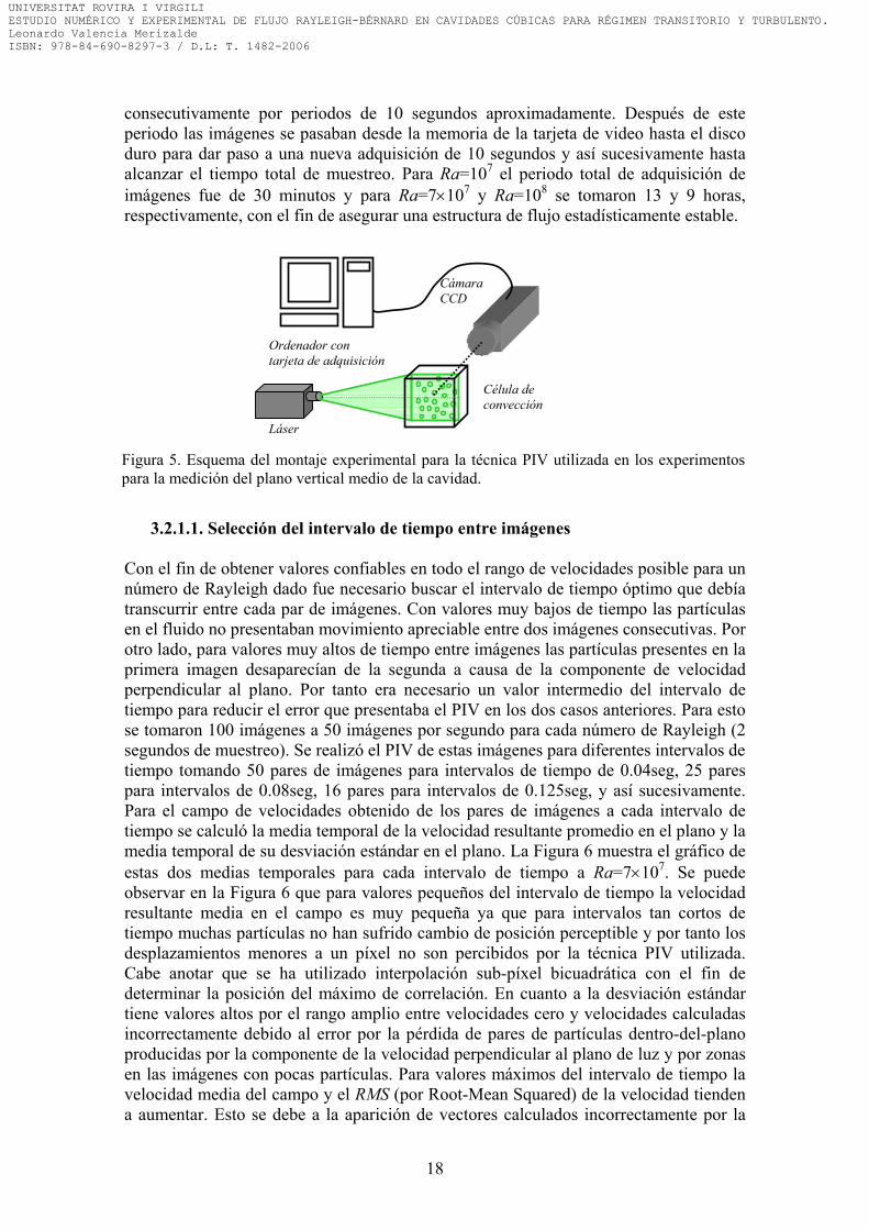
consecutivamente por periodos de 10 segundos aproximadamente. Después de este periodo las imágenes se pasaban desde la memoria de la tarjeta de video hasta el disco duro para dar paso a una nueva adquisición de 10 segundos y así sucesivamente hasta alcanzar el tiempo total de muestreo. Para Ra=107 el periodo total de adquisición de imágenes fue de 30 minutos y para Ra=7×107 y Ra=108 se tomaron 13 y 9 horas, respectivamente, con el fin de asegurar una estructura de flujo estadísticamente estable.

Láser

Célula de convección

Cámara CCD

Ordenador con tarjeta de adquisición

Figura 5. Esquema del montaje experimental para la técnica PIV utilizada en los experimentospara la medición del plano vertical medio de la cavidad.

3.2.1.1. Selección del intervalo de tiempo entre imágenes Con el fin de obtener valores confiables en todo el rango de velocidades posible para un número de Rayleigh dado fue necesario buscar el intervalo de tiempo óptimo que debía transcurrir entre cada par de imágenes. Con valores muy bajos de tiempo las partículas en el fluido no presentaban movimiento apreciable entre dos imágenes consecutivas. Por otro lado, para valores muy altos de tiempo entre imágenes las partículas presentes en la primera imagen desaparecían de la segunda a causa de la componente de velocidad perpendicular al plano. Por tanto era necesario un valor intermedio del intervalo de tiempo para reducir el error que presentaba el PIV en los dos casos anteriores. Para esto se tomaron 100 imágenes a 50 imágenes por segundo para cada número de Rayleigh (2 segundos de muestreo). Se realizó el PIV de estas imágenes para diferentes intervalos de tiempo tomando 50 pares de imágenes para intervalos de tiempo de 0.04seg, 25 pares para intervalos de 0.08seg, 16 pares para intervalos de 0.125seg, y así sucesivamente. Para el campo de velocidades obtenido de los pares de imágenes a cada intervalo de tiempo se calculó la media temporal de la velocidad resultante promedio en el plano y la media temporal de su desviación estándar en el plano. La Figura 6 muestra el gráfico de estas dos medias temporales para cada intervalo de tiempo a Ra=7×107. Se puede observar en la Figura 6 que para valores pequeños del intervalo de tiempo la velocidad resultante media en el campo es muy pequeña ya que para intervalos tan cortos de tiempo muchas partículas no han sufrido cambio de posición perceptible y por tanto los desplazamientos menores a un píxel no son percibidos por la técnica PIV utilizada. Cabe anotar que se ha utilizado interpolación sub-píxel bicuadrática con el fin de determinar la posición del máximo de correlación. En cuanto a la desviación estándar tiene valores altos por el rango amplio entre velocidades cero y velocidades calculadas incorrectamente debido al error por la pérdida de pares de partículas dentro-del-plano producidas por la componente de la velocidad perpendicular al plano de luz y por zonas en las imágenes con pocas partículas. Para valores máximos del intervalo de tiempo la velocidad media del campo y el RMS (por Root-Mean Squared) de la velocidad tienden a aumentar. Esto se debe a la aparición de vectores calculados incorrectamente por la

18


pérdida de pares de partículas fuera-del-plano. Este error en el cálculo se presenta en flujos tridimensionales como el estudiado en el presente trabajo debido a que la componente de la velocidad perpendicular al plano es significativa. Como muestra la Figura 6, para valores intermedios del intervalo de tiempo tanto el promedio de la velocidad como su RMS presentan valores esencialmente constantes y por lo tanto independientes del valor del intervalo de tiempo entre imágenes. El intervalo de tiempo seleccionado e indicado en la Figura 6 se encuentra en ∆t=0.2 seg, esto son 10 imágenes por segundo. A Ra=108 se mantuvo el valor de 10 imágenes/seg indicando que no era necesario aumentar el intervalo de tiempo para contrarrestar el aumento de velocidades a este número de Rayleigh. Para Ra=107 se esperaría un intervalo de tiempo menor que para los números de Rayleigh altos, sin embargo, el valor de 10 imágenes/seg también resultó ser adecuado ya que la relación en píxel/mm de las imágenes para Ra=107 es aproximadamente el doble que para Ra=7×107 y Ra=108 y este aumento en fidelidad de las imágenes (i.e. mayor valor del número de píxeles por mm) contrarresta la disminución de las velocidades.

∆t (seg)

<V re

s>s,

RMS(

V res) s

0.05 0.10 0.15 0.20 0.25 0.30

0.5

1.0

1.5

2.0

2.5

3.0

<Vres>s (mm/s)RMS(Vres)s (mm/s)

10 imágenes/seg

Figura 6. Gráfico de la media temporal de la velocidad resultante media en el plano y la mediatemporal de su desviación estándar en el plano contra varios intervalos de tiempo entre imágenespara Ra=7×107

3.3. CÁLCULO DE LAS VELOCIDADES EN EL PLANO MEDIO VERTICAL DE LA CAVIDAD

Las imágenes obtenidas con la cámara generalmente contenían reflejos de las paredes de vidrio. Debido a que estos reflejos distorsionan los resultados obtenidos por el PIV, se utilizó el método descrito en detalle por Usera et al. (2005) con el cual se eliminan los reflejos y se puede realizar el PIV con imágenes que contienen solo píxeles iluminados por las partículas en suspensión. La Figura 7(a) muestra como la influencia de los reflejos se presenta principalmente cerca de las paredes. Digitalmente, cada imagen es una matriz de 420 filas×420columnas con valores entre 0 (píxeles de color negro) y 255 (píxeles de iluminación máxima o blancos). La imagen media es una media numérica del valor de intensidad de cada posición de la imagen en el tiempo obteniéndose una imagen resultante en la cual los píxel con valores máximos son debidos a los reflejos.

19


Este método consiste en restar a cada imagen la media eliminando así los reflejos de cada una de ellas para realizar posteriormente un PIV más confiable. La Figura 7(a) muestra una imagen tomada por la cámara sin tratamiento alguno, la Figura 7(b) muestra la imagen media de todas las imágenes utilizadas durante un experimento concreto y la imagen de la Figura 7(c) muestra la diferencia entre la imagen de la Figura 7(a) y la imagen media (Figura 7(b)). Adicionalmente la imagen resultante se normalizó para valores de intensidad de los píxeles entre 0 y 255. Después de obtener la imagen media comenzaba el proceso de análisis para determinar el desplazamiento que han sufrido las partículas entre dos imágenes consecutivas. Para esto, las imágenes de 420×420 píxeles se dividieron en 27×27 ventanas de interrogación superpuestas de 30×30 píxeles cada ventana (3.57×3.57 mm para la cavidad con L=50 mm y 6.57×6.57 mm para la cavidad con L=92 mm) la cual contenía una media de 8 y 12 partículas para las cavidades de tamaño L=50mm y L=92mm, respectivamente. La auto-correlación se realizaba con ventanas de 60×60 píxeles de la segunda imagen (tomando 15 píxeles más a cada lado de la ventana de interrogación de la primera imagen). El tamaño de las ventanas fue elegido de acuerdo con las recomendaciones de Keane y Adrian (1990) que indican, de manera orientativa, los tamaños mínimos y máximos de las áreas de interrogación y los tiempos de exposiciones o imágenes según el rango de velocidades a medir y la concentración de partículas presente para que la correlación sea significativa y la velocidad medida representativa. El tiempo de exposición de la cámara, 20.4ms, es suficientemente pequeño para las velocidades máximas medidas, del orden de 3.5mm/s. La auto-correlación entre cada par de imágenes para calcular el desplazamiento medio de las partículas dentro de cada ventana de interrogación se realizó con un código propio desarrollado en Matlab. Finalmente, con el campo de velocidades obtenido de cada par de imágenes se empieza el proceso de obtención del campo o estructura de flujo media en el plano de medida. Para esto se eliminan los vectores calculados incorrectamente por el PIV para que no entren en el cálculo de la media temporal. En las regiones del plano en las que el PIV no puede obtener un valor razonable de desplazamiento (debido a la pérdida de partículas fuera-del-plano, la pérdida de partículas dentro-del-plano o a regiones con pocas partículas) se generan vectores con dirección diferente a los vectores de su entorno y magnitud muy por encima de la media de velocidad de los vectores del campo. Para eliminarlos, se calcula la media en el plano de la velocidad resultante y los vectores con valores de 3mm/s para Ra=107 y 5mm/s para Ra=7×107 y Ra=108 por encima de la media eran descartados y no entraban en el cálculo de la estructura de flujo media.

50 100 150 200 250 300 350 400 450

50

100

150

200

250

300

350

400

0

50

100

150

200

250

50 100 150 200 250 300 350 400 450

50

100

150

200

250

300

350

400

50

100

150

200

250

50 100 150 200 250 300 350 400 450

50

100

150

200

250

300

350

400

0

50

100

150

200

250

(b) (c) (a) Figura 7. (a)imagen obtenida con la cámara CCD sin ningún tratamiento. (b) Imagen media (c)imagen mostrada en (a) después de restarle la imagen media.

20


3.4. VALIDACIÓN DEL MÉTODO PIV Con el fin de validar y analizar los posibles errores causados por el método de medición de velocidades PIV, se generaron diversos pares de imágenes de partículas a partir de un campo de velocidades instantáneo proveniente de una simulación numérica. El código de generación de imágenes de partículas a partir de simulaciones numéricas fue desarrollado en Matlab. Dicho código toma en cuenta el desplazamiento de las partículas en las 3 dimensiones de acuerdo con el campo de velocidades obtenido numéricamente y el tiempo entre imágenes utilizado en la experimentación. La distribución de intensidad de las partículas esta descrito por una distribución Gaussiana de acuerdo con la siguiente ecuación:

−−−−

=2

20

20

)8/1()()(

0),( dyyxx

eIyxI (12) Donde (x0,y0) es el centro de la imagen de la partícula y d está definido como el diámetro de la partícula. En la Ecuación 12, I0 es la intensidad máxima calculada en función de la posición de la partícula, z0, en la dirección perpendicular al plano de luz. Para un plano de luz centrado en z=0 con una distribución de intensidad Gaussiana, el valor de I0 se expresó con la siguiente ecuación:

∆−

=2

0

2

)8/1(0 )( z

z

qezI (13) Donde ∆z0 es el espesor del plano de luz y q es la eficiencia con la cual la partícula refleja la luz incidente del láser. Con fines prácticos, este valor se consideró como el valor máximo posible de intensidad que se puede obtener en las imágenes del laboratorio, esto es q=255. Para los cálculos de las imágenes generadas se supuso un diámetro de partícula medio de 2 píxeles y 10000 partículas dispuestas en la primera imagen de forma aleatoria. En los casos de superposición de partículas se supuso suma de intensidades. Con el fin de obtener similitud entre imágenes experimentales y generadas se añadió ruido aleatorio en todo el plano con distribución normal y el centro de la campana en intensidad de píxel q=50. La Figura 8(a) muestra una imagen típica de los experimentos para Ra=107 después de eliminar los reflejos y la Figura 8(b) es una imagen generada con el procedimiento antes descrito para el mismo número de Rayleigh a partir de un campo numérico instantáneo. La similitud de estas imágenes da credibilidad al proceso de validación del método PIV que se explica en este apartado. A modo de ejemplo, la Figura 9(a) muestra el campo de velocidades calculado numéricamente para Ra=107 a partir del cual se han generado las imágenes con el método descrito en el presente apartado. En la Figura 9(b) se puede ver el campo de velocidades obtenido con el método PIV a partir de las imágenes generadas digitalmente. Ambos campos muestran una gran similitud cualitativa. Cabe señalar que los resultados obtenidos para otros pares de imágenes generadas muestran una concordancia similar entre las velocidades numéricas y las obtenidas con PIV a la que muestran las Figuras 9(a) y 9(b). En la Figura 10 se puede comparar perfiles de velocidad vertical (u) y horizontal (v) para los resultados del campo numérico de la Figura 9(a) y para los obtenidos con la técnica PIV a partir de las imágenes generadas (Figura 9(b)). En los perfiles horizontales se grafica la velocidad vertical (y vs. u), los

21


resultados numéricos se muestran con la línea continua y los del PIV con círculos. Ambos perfiles son cuantitativamente muy cercanos excepto en los valores máximos (6mm<y<8mm) los cuales pierden fidelidad debido a la pérdida de partículas fuera-del-plano en los resultados calculados a partir de imágenes generadas. Los perfiles verticales de la velocidad horizontal (x vs. v) se muestran como línea discontinua y cuadrados para resultados computacionales y obtenidos por velocimetría respectivamente. Las diferencias principales se encuentran en las velocidades menores a 1.2 mm/s (ej. x<16mm). Esto se debe a que el PIV percibe un desplazamiento mínimo de 1 píxel que equivale a 0.12mm en la cavidad de longitud L=50mm (utilizada a Ra=107). Ya que el intervalo de tiempo entre las imágenes es de 0.2 segundos, la velocidad mínima que puede percibir esta técnica de medición de velocidad a estas condiciones será de 0.12mm/0.2s=0.6mm/s aproximadamente (ver Figura 10 para 5mm<x<8mm). El siguiente valor de velocidad posible sería el obtenido con un desplazamiento de 2 píxeles el cual en este caso equivale aproximadamente a 1.2mm/s (ver Figura 10 para x=4mm). Y por tanto, valores intermedios de velocidad entre estos valores no son posibles a causa de las limitaciones de la técnica de medición. Sin embargo, la técnica PIV es bastante confiable para la medición de rangos amplios de velocidad y las Figuras 9 y 10 muestran que en términos generales es posible confiar en los resultados de velocidad y más aun cuando se consideran velocidades medias en el tiempo.

50 100 150 200 250 300 350 400

50

100

150

200

250

300

350

400

0

50

100

150

200

250

50 100 150 200 250 300 350 400

50

100

150

200

250

300

350

400

0

50

100

150

200

250

(a) (b) Figura 8. (a) Imagen experimental para Ra=107 después del proceso de eliminación de reflejos.(b) Imagen generada a partir de un campo numérico instantáneo para Ra=107.

22


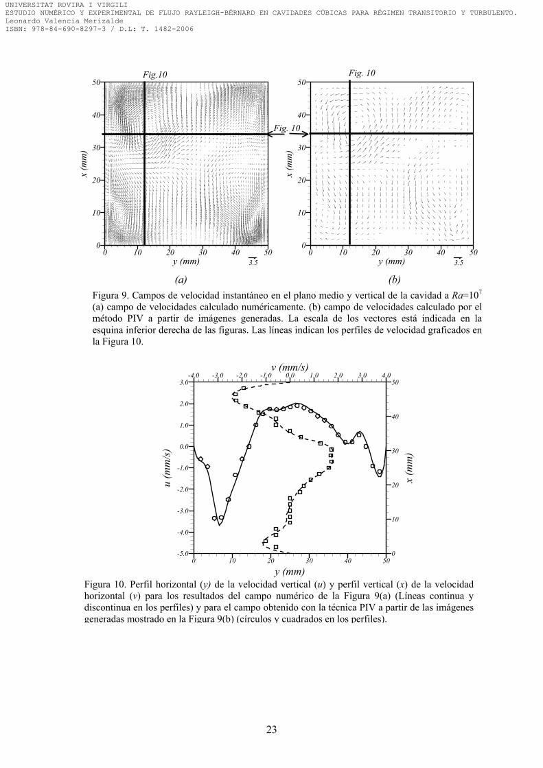
Figura 10. Perfil horizontal (y) de la velocidad vertical (u) y perfil vertical (x) de la velocidadhorizontal (v) para los resultados del campo numérico de la Figura 9(a) (Líneas continua ydiscontinua en los perfiles) y para el campo obtenido con la técnica PIV a partir de las imágenesgeneradas mostrado en la Figura 9(b) (círculos y cuadrados en los perfiles).

y (mm)

v (mm/s)

u(m

m/s

)

x(m

m)

0 10 20 30 40 50

-4.0 -3.0 -2.0 -1.0 0.0 1.0 2.0 3.0 4.0

-5.0

-4.0

-3.0

-2.0

-1.0

0.0

1.0

2.0

3.0

0

10

20

30

40

50

y (mm)

x(m

m)

0 10 20 30 40 500

10

20

30

40

50

3.5 y (mm)

x(m

m)

0 10 20 30 40 500

10

20

30

40

50

3.5

Fig. 10

Fig. 10 Fig.10

(a) (b) Figura 9. Campos de velocidad instantáneo en el plano medio y vertical de la cavidad a Ra=107

(a) campo de velocidades calculado numéricamente. (b) campo de velocidades calculado por elmétodo PIV a partir de imágenes generadas. La escala de los vectores está indicada en laesquina inferior derecha de las figuras. Las líneas indican los perfiles de velocidad graficados enla Figura 10.

23


4. RESUMEN DE LAS PUBLICACIONES En esta sección se resumen las publicaciones que son la base de la tesis y que se encuentran incluidas en los anexos del presente escrito. Las publicaciones están presentadas en orden cronológico. Para cada publicación, se dará una breve explicación de los objetivos y las motivaciones que movieron a la realización de este trabajo, así como los resultados y conclusiones más importantes. Dos principales problemas fueron considerados en las publicaciones para flujos Rayleigh-Bénard en cavidades cúbicas calentadas por debajo. Las incluidas en el anexo A (Anexos A1 y A2) se centran en la influencia que tiene una alta variación de las propiedades físicas en las estructuras de flujo y la transferencia de calor usando agua como fluido convectivo. También se estudian los efectos que tiene esta variación sobre el mecanismo de flujo tanto en régimen laminar como turbulento mediante la inspección de la contribución de los diferentes térmicos de los balances de cantidad de movimiento en la dirección vertical. Las dos publicaciones de los anexos B están dirigidas a la validación experimental de resultados numéricos en régimen turbulento y al análisis de las estructuras de flujo obtenidas para valores de número de Rayleigh altos. Es importante resaltar que los resultados de los artículos de los anexos A2 y B2 son mejoras de resultados presentados en las publicaciones A1 y B1, respectivamente. 4.1. RESUMEN DE LA PUBLICACIÓN 1 – ANEXO A1 En el primera publicación se hace un estudio numérico en el cual se analizan los efectos que tienen los cálculos sin la aproximación de Boussinesq para convección Rayleigh-Bénard en una cavidad cúbica con paredes laterales perfectamente conductoras. Este análisis se realiza a números de Rayleigh bajos en el que el flujo es laminar y estacionario y a Ra=107 para el que el flujo es turbulento considerando agua como fluido convectivo (Pr=5.9). El modelo físico y matemático se encuentran, respectivamente, descritos en los apartados 2.2 y 2.3 de este documento. Las simulaciones numéricas se efectuaron para dos casos diferentes. En el primer caso se consideró la aproximación de Boussinesq y en el segundo caso se consideró la dependencia de la viscosidad y la conductividad térmica del agua en función de la temperatura. Trabajos previos, como el de Gray y Giorgini (1976), recomiendan que la diferencia de temperatura entre la pared caliente y la fría debe ser menor que 4.5ºC con el fin de obtener variaciones en la viscosidad menores del 10%. Según estos autores este es el límite de variación de las propiedades físicas con la temperatura para considerar válida la aproximación de Boussinesq. Los cálculos sin la aproximación de Boussinesq llevados a cabo en el presente trabajo fueron calculados con una variación del 40% en la viscosidad entre las placas fría y caliente. Para los números de Rayleigh Ra=104 y Ra=5×104 el análisis se centra en el efecto de la variación de la viscosidad del agua con la temperatura en las dos estructuras de flujo en estado estacionario más estables de las siete estructuras encontradas en estudios previos (Pallares et al. 2001). A modo de ejemplo, la Figura 11 muestra la topología de una de estas dos estructuras estables mediante una isosuperficie de valor negativo del segundo valor propio del tensor gradiente de velocidad, siguiendo el método propuesto por Jeong y Hussain (1995) para detectar las regiones del espacio ocupadas por vórtices. La Figura 11 también muestra trayectorias de partículas de fluido que indican el sentido de rotación del rollo. Se puede observar en la Figura 11 que la estructura consiste en un rollo convectivo con el eje de rotación perpendicular a dos paredes laterales opuestas. A

24


Ra=104 y Ra=5×104 la topología general de las estructuras de flujo permanecen prácticamente iguales a las calculadas con los efectos de variación de la viscosidad y la conductividad térmica con la temperatura. Sin embargo, los resultados obtenidos considerando estas variaciones muestran, en comparación con las simulaciones realizadas con propiedades físicas constantes, un incremento en las velocidades ascendentes debido a la menor viscosidad del fluido caliente y una disminución de las velocidades descendientes debido a la mayor viscosidad de las corrientes descendentes. Este aumento de velocidades ascendentes produce una disminución del área de paso por el que el flujo asciende y un aumento del área por el que el fluido desciende. Con el fin de ilustrar este fenómeno en la Figura 12 se muestran los contornos de la componente vertical de velocidad en el plano medio horizontal de la cavidad, correspondiente a la estructura de la Figura 11 para el caso de viscosidad constante (Fig. 12.a) y para el caso en que se considera la variación de la viscosidad con la temperatura (Fig. 12.b). Cabe tener en cuenta que la variación de la conductividad térmica con la temperatura es tan solo del 4.8% como muestra la Tabla 1 y por tanto este efecto es mayoritariamente atribuible a la variación de la viscosidad con la temperatura. Para Ra=107 y Pr=5.9 en el que el flujo es turbulento se analizan en detalle los efectos de la variación de la viscosidad con la temperatura y se comparan las estructuras de flujo y los flujos de transferencia de calor con los disponibles en la literatura para Pr=0.71. Para Ra=107 los campos de flujo instantáneo muestran grandes desviaciones respecto al campo de velocidades media el cual consiste en dos vórtices en forma de anillo localizados cerca de las placas horizontales como muestra la Figura 13. A este elevado número de Rayleigh tanto instantáneamente como en promedio temporal los gradientes de temperatura y, por tanto, las variaciones de viscosidad están localizadas cerca de las paredes dentro de la capa límite térmica con un espesor característico de 0.03L a Ra=107. El flujo fuera de estas capas es esencialmente isotérmico y por lo tanto con un valor de viscosidad constante, correspondiente a la temperatura media (T0). Esto causa que la topología del campo de flujo medio en el tiempo correspondiente a las simulaciones con y sin la aproximación de Boussinesq no esté en gran medida afectada por los efectos de la variación de la viscosidad y la conductividad térmica con la temperatura. El análisis de la contribución de los diferentes términos del balance de cantidad de movimiento en la dirección vertical en condiciones de viscosidad constante y en condiciones de viscosidad variable tampoco muestran grandes diferencias en régimen laminar y son prácticamente idénticos en régimen turbulento. Cabe señalar que los números de Nusselt promedio en las paredes horizontales para ambos casos son, en las condiciones estudiadas, también insensibles a la variación de viscosidad. Las diferencias en régimen laminar son inferiores al 3% mientras que no son significativas en régimen turbulento. De acuerdo con estos resultados el límite de variación de viscosidad del 10% utilizado normalmente para la adopción de la aproximación de Boussinesq resulta, para las condiciones estudiadas, excesivamente restrictivo, en particular cuando el flujo es turbulento.

25


X

YZ

Contornos Figs. 12(a) y 12(b)

Figura 11. Topología de flujo de la estructura S1 a Ra=104 en términos de la isosuperficie delsegundo valor propio del tensor gradiente de velocidad (λ2/|λ2,max|=-0.12)

-2-6

-10

-14

02

610

14

y*

z*

0 0.2 0.4 0.6 0.8 10

0.2

0.4

0.6

0.8

1 0.

0. 0. 0.

2

10

-14

-10

-6

-2 0

14

6

y*

z*

0 0.2 0.4 0.6 0.8 10

2

4

6

8

1

(a) (b)

Figura 12. Contornos de la velocidad vertical (u*) en el plano horizontal medio de la cavidad (x*=0.5) a Ra=104 para (a) Simulación con la aproximación de Boussinesq (BFS) y (b) Simulación con viscosidad y conductividad térmica en función de la temperatura(NBFSµ) respectivamente

26


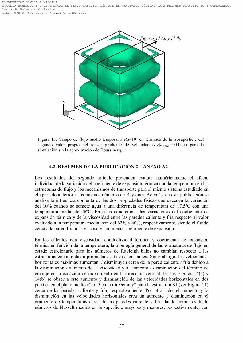
Figura 13. Campo de flujo medio temporal a Ra=107 en términos de la isosuperficie delsegundo valor propio del tensor gradiente de velocidad (λ2/|λ2,max|=-0.017) para lasimulación sin la aproximación de Boussinesq.

X

Z

Y

Figuras 17 (a) y 17 (b) 4.2. RESUMEN DE LA PUBLICACIÓN 2 – ANEXO A2 Los resultados del segundo artículo pretenden evaluar numéricamente el efecto individual de la variación del coeficiente de expansión térmica con la temperatura en las estructuras de flujo y los mecanismos de transporte para el mismo sistema estudiado en el apartado anterior a los mismos números de Rayleigh. Además, en esta publicación se analiza la influencia conjunta de las dos propiedades físicas que exceden la variación del 10% cuando se somete agua a una diferencia de temperatura de 17.5ºC con una temperatura media de 26ºC. En estas condiciones las variaciones del coeficiente de expansión térmica y de la viscosidad entre las paredes caliente y fría respecto al valor evaluado a la temperatura media, son del 62% y 40%, respectivamente, siendo el fluido cerca a la pared fría más viscoso y con menor coeficiente de expansión. En los cálculos con viscosidad, conductividad térmica y coeficiente de expansión térmica en función de la temperatura, la topología general de las estructuras de flujo en estado estacionario para los números de Rayleigh bajos no cambian respecto a las estructuras encontradas a propiedades físicas constantes. Sin embargo, las velocidades horizontales máximas aumentan / disminuyen cerca de la pared caliente / fría debido a la disminución / aumento de la viscosidad y al aumento / disminución del término de empuje en la ecuación de movimiento en la dirección vertical. En las Figuras 14(a) y 14(b) se observa este aumento y disminución de las velocidades horizontales en dos perfiles en el plano medio z*=0.5 en la dirección y* para la estructura S1 (ver Figura 11) cerca de las paredes caliente y fría, respectivamente. Por otro lado, el aumento y la disminución en las velocidades horizontales crea un aumento y disminución en el gradiente de temperaturas cerca de las paredes caliente y fría dando como resultado números de Nusselt medios en la superficie mayores y menores, respectivamente, con

27


28

y*

v*

0 0.2 0.4 0.6 0.8 1

0

2

4

6

8

y*

v*

0 0.2 0.4 0.6 0.8 1

-6

-4

-2

0

Placa caliente – S1 Placa fría – S1

BFSNBFSµ

NBFSβ

NBFSµβ

Figura 14. Perfiles de velocidad de la estructura S1 a Ra=104 para las simulaciones sin laaproximación de Boussinesq y las simulaciones con propiedades físicas constantes. (a) perfilhorizontal (y*) de la componente horizontal de la velocidad (v*) cerca de la placa caliente a lolargo de la línea x*=0.064, z*=0.5. (b), perfil horizontal (y*) de la componente horizontal de lavelocidad (v*) cerca de la placa fría a lo largo de la línea x*=0.94, z*=0.5.

(a) (b)

respecto al obtenido con la aproximación de Boussinesq. Por ejemplo para la estructura consistente en un rollo, que muestra la Figura 11 el número de Nusselt en la pared inferior / superior es un 3% mayor / menor, en comparación a los resultados con propiedades físicas constantes. Para Ra=107 las propiedades medias en el tiempo del flujo turbulento no están afectadas significativamente por la dependencia de las propiedades físicas con la temperatura. El número de Nusselt en las placas horizontales solo varía un 1% respecto a los cálculos con la aproximación de Boussinesq. La Figura 15 muestra la contribución de los diferentes términos más importantes de la ecuación de movimiento en la dirección vertical (x*) en un perfil vertical cerca de la pared y*=0, sobre el plano medio z*=0.5. Cabe resaltar que este perfil está situado dentro de la capa límite térmica generada por la distribución de temperaturas lineal impuesta en las paredes laterales y por lo tanto la variación de temperatura a lo largo del perfil, y por tanto de propiedades físicas, es significativa. Se puede observar en la Figura 15 que las diferencias en la contribución de los términos de la ecuación de movimiento son menores en todas las simulaciones, incluso dentro de la capa límite térmica y de velocidad donde los efectos de la viscosidad son importantes. Se puede ver también que la influencia individual de la variación de µ y β con la temperatura en los términos difusivos se cancela cuando se considera la influencia conjunta de ambas propiedades físicas y por tanto la contribución de los términos difusivos para BFS y NBFSµβ es muy similar. Tal como muestran estos resultados el límite del 10% de variación máxima de las propiedades físicas del fluido para poder aplicar la aproximación de Boussinesq resulta demasiado estricto especialmente en flujos turbulentos en los cuales el gradiente de temperatura y por tanto la variación de las propiedades físicas está restringida al interior de la delgada capa límite térmica.


Balance ecn. movimiento en x*

x*

-0.4 -0.2 0 0.2 0.40

0.2

0.4

0.6

0.8

1Presión

Empuje

Difusivos

BFSNBFSµ

NBFSβ

NBFSµβ

Figura 15. Perfil vertical en y*=0.012, z*=0.5 del balance de los principales términos de la ecuación de movimiento en la dirección x a Ra=107 calculado con propiedades físicas constantes (BFS) y sin la aproximación de Boussinesq (NBFSµ, NBFSβ y NBFSµβ)

4.3. RESUMEN DE LA PUBLICACIÓN 3 – ANEXO B1 En la tercera publicación se validan experimentalmente los resultados numéricos encontrados para números de Rayleigh altos (Ra=107 y Ra=7×107) en la cavidad cúbica calentada por debajo usando agua como fluido convectivo. Las principales características del montaje experimental utilizado así como el modelo físico y matemático considerados en las simulaciones se encuentran descritos en los apartados 2 y 3 de este documento. Con el fin de asegurar una buena reproducción numérica de los resultados experimentales, se consideran las paredes laterales parcialmente conductoras usando un valor típico de la conductividad térmica del vidrio que es el material utilizado en la fabricación de las paredes laterales de las cavidades experimentales. Debido a las bajas diferencias de temperatura usadas en los experimentos se considera la aproximación de Boussinesq en los cálculos numéricos. Para la medición de las dos componentes de la velocidad en un plano del fluido se utilizó la técnica PIV Tanto numéricamente como experimentalmente Se observan dos estructuras de flujo medias diferentes a Ra=107 y Ra=7×107. Para Ra=107 la estructura de flujo media es muy similar a la encontrada en los cálculos con paredes perfectamente conductoras que consiste esencialmente en dos vórtices en forma de anillo paralelos y cercanos a las paredes horizontales (ver Figura 13), mientras que para Ra=7×107 la estructura presenta una corriente principal ascendente a lo largo de una arista vertical de la cavidad y otra descendente a lo largo de la arista diagonalmente opuesta. En la Figura 16 se puede ver esta estructura en términos de dos isosuperficies de dos valores de la componente vertical de la velocidad (un valor positivo y por lo tanto correspondiente a flujo ascendente y otro negativo que indica flujo descendente). Esta estructura puede entenderse como consistente en un solo rollo con el eje de rotación horizontal y en dirección diagonal a dos aristas verticales de la cavidad. Por otro lado, se observa que al considerar las paredes parcialmente conductoras en los cálculos numéricos, los campos de velocidad medios en el plano medio de la cavidad presentan la misma estructura y

29


valores locales en concordancia con los medidos experimentalmente para ambos números de Rayleigh. Las Figuras 17 (a) y 17 (b) muestran una similitud cualitativa entre los campos de velocidad medio temporal (numérico y experimental, respectivamente) en el plano medio de la cavidad a Ra=107. La Figura 18 muestra los perfiles de velocidad vertical indicados en las Figuras 17 (a) y 17 (b) para los resultados experimentales, para los cálculos con paredes parcialmente conductoras y para los resultados numéricos con paredes perfectamente conductoras. A pesar de no encontrarse diferencias significativas entre las estructuras de flujo media calculadas con paredes perfectamente conductoras y con conductividad térmica finita a Ra=107, se observan diferencias hasta del 110% entre los valores de velocidad media locales (ver por ejemplo la Figura 18 en z≈13mm y z≈36mm). La causa de estas diferencias se puede explicar con la Figura 19, en la cual se muestra el perfil de temperaturas vertical dentro de las paredes de la cavidad en el plano medio (y*=0.5) para ambos cálculos (paredes perfectamente conductoras y parcialmente conductoras). Se puede observar que en la zona media inferior de la cavidad (x*<0.5) las temperaturas para el caso con paredes perfectamente conductoras son mayores que para el caso con conductividad térmica finita. Esto genera valores de empuje mayores en la ecuación de movimiento de la dirección vertical creando corrientes ascendentes y por tanto descendentes mayores cuando se considera el perfil lineal de temperaturas en las paredes. Por esto se puede concluir que los cálculos considerando paredes parcialmente conductoras son una buena aproximación para predecir los resultados experimentales obtenidos para las condiciones del sistema estudiados en este trabajo.

Figura 16. Campo de velocidad medio temporal para un tiempo total de integración de tt* =0.16(156 min) en términos de isosuperficies de dos valores de la velocidad vertical u*=1000 y u*=-1000 a Ra=7×107.

X

YZ

u*=1000 Fluido Ascendente

u*=-1000 Fluido Descendente

Contornos Figura 19(c)

30


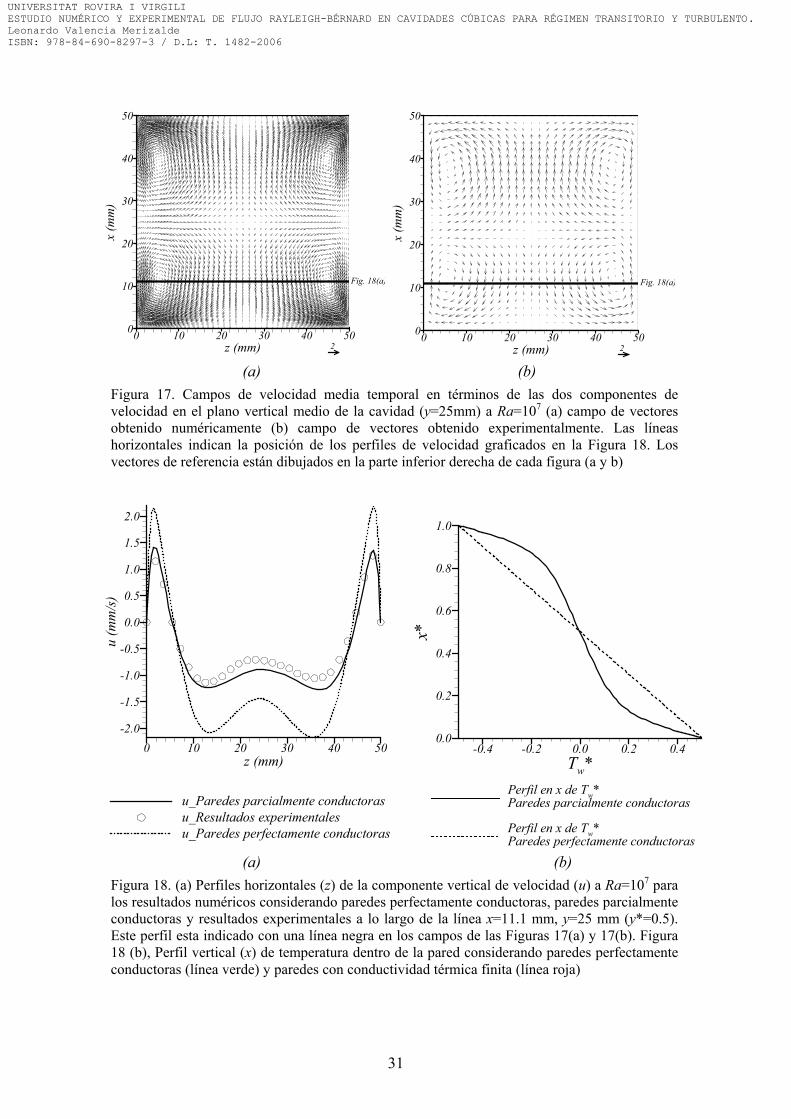
z (mm)

x(m

m)

0 10 20 30 40 500

10

20

30

40

50

2

Fig. 18(a)

z (mm)

x(m

m)

0 10 20 30 40 500

10

20

30

40

50

2

Fig. 18(a)

(a) (b)

Figura 17. Campos de velocidad media temporal en términos de las dos componentes develocidad en el plano vertical medio de la cavidad (y=25mm) a Ra=107 (a) campo de vectoresobtenido numéricamente (b) campo de vectores obtenido experimentalmente. Las líneashorizontales indican la posición de los perfiles de velocidad graficados en la Figura 18. Losvectores de referencia están dibujados en la parte inferior derecha de cada figura (a y b)

Perfil en x de Tw*Paredes perfectamente conductoras

Perfil en x de Tw*Paredes parcialmente conductoras

z (mm)

u(m

m/s

)

0 10 20 30 40 50-2.0

-1.5

-1.0

-0.5

0.0

0.5

1.0

1.5

2.0

u_Paredes parcialmente conductorasu_Resultados experimentalesu_Paredes perfectamente conductoras

Tw*

x*

-0.4 -0.2 0.0 0.2 0.40.0

0.2

0.4

0.6

0.8

1.0

Figura 18. (a) Perfiles horizontales (z) de la componente vertical de velocidad (u) a Ra=107 paralos resultados numéricos considerando paredes perfectamente conductoras, paredes parcialmenteconductoras y resultados experimentales a lo largo de la línea x=11.1 mm, y=25 mm (y*=0.5).Este perfil esta indicado con una línea negra en los campos de las Figuras 17(a) y 17(b). Figura18 (b), Perfil vertical (x) de temperatura dentro de la pared considerando paredes perfectamenteconductoras (línea verde) y paredes con conductividad térmica finita (línea roja)

(a) (b)

31


4.4. RESUMEN DE LA PUBLICACIÓN 4 – ANEXO B2 En la presente publicación se muestran los resultados de las estructuras de flujo media calculadas para números de Rayleigh Ra=3×107, Ra=5×107 y Ra=108. Adicionalmente se reportan cálculos del promedio temporal de las estructuras a los números de Rayleigh reportados en el artículo anterior (Ra=107 y Ra=7×107) con mayor tiempo de muestro con el fin de obtener estructuras de flujo medias estadísticamente estables en el tiempo. Por otro lado, se reportan nuevos resultados experimentales para Ra=108. En los resultados numéricos se observa que en el rango 3×107≤Ra≤108 las estructuras de flujo permanecen estables un cierto periodo de tiempo en la estructura encontrada y descrita en la publicación anterior para Ra=7×107 (ver Figura 16). Sin embargo, al aumentar el tiempo de cálculo, se observa que la estructura cambia de dirección a través del cambio de orientación del eje de rotación del rollo permaneciendo periodos de tiempo indefinidos en una posición determinada. Para ilustrar esta variación de baja frecuencia en la estructura la Figura 19(b) muestra la evolución temporal de la velocidad vertical en el punto indicado en la Figura 19(a). En esta evolución temporal se observa una alternancia de muy baja frecuencia entre valores positivos y negativos de la velocidad que corresponden a las cuatro diferentes posiciones posibles encontradas en el tiempo de la estructura media que muestra la Figura 19(c) mediante contornos de la velocidad vertical en el plano medio horizontal. Las letras (A), (B), (C) o (D) indicadas sobre el eje x de la evolución temporal de la Figura 19(b) indican la posición en que se encuentra la estructura de flujo (ver Figura 19(c)) y el paréntesis bajo la letra indica el periodo de tiempo que permanece en dicha posición. Cabe anotar que a Ra=3×107, Ra=5×107 y Ra=108 también se encontró una evolución temporal similar con cambios de posición de la estructura básica mostrada en la Figura 16. Los resultados estadísticos muestran que el tiempo de muestro utilizado (t t*) es mucho mayor que el tiempo integral (T*) (274<t

t*/T *<1111) si este último se calcula con la velocidad horizontal media temporal en x*=0.5, y*=0.75 y z*=0.5 (ver Fig. 19(a)) o con la media temporal del Nusselt medio en la pared horizontal. Sin embargo, la escala integral calculada con u* o T* en el mismo punto da como resultado valores de t t*/T * entre 4 y 9. Esto significa que para definir si una estructura esta estadísticamente convergida debe evaluarse, como mínimo, la escala integral de alguna de las variables con menores frecuencias (tiempos integrales altos). Los resultados experimentales para Ra=7×107 y Ra=108, no presentan este cambio de baja frecuencia en la estructura. Se observa que la estructura de flujo no cambia de posición en el tiempo conservando la misma orientación durante todo el tiempo de muestreo. Esto puede atribuirse a las inevitables imperfecciones en las condiciones de contorno de los experimentos, especialmente en la distribución de temperaturas en las paredes de la cavidad, o bien a la pequeña pero también inevitable desviación de la cavidad respecto la perfecta horizontalidad. Estos efectos pueden ser los causantes de la inhibición del cambio de orientación de la estructura observado en las simulaciones numéricas con condiciones de contorno ideales y llevadas a cabo suponiendo una perfecta horizontalidad de la cavidad. Sin embargo, es importante resaltar que las estructuras de flujo medias y los contornos de la desviación estándar de la velocidad vertical obtenidos experimentalmente son cualitativamente similares a aquellos obtenidos numéricamente para un periodo de tiempo en el cual la estructura media permanece en la misma posición (A), (B), (C) o (D), indicando que la estructura de flujo experimental corresponde a una determinada orientación de la estructura obtenida numéricamente. Como ejemplo, la Figura 20 muestra los perfiles de velocidad vertical y horizontal comparativos entre las simulaciones y los experimentos para Ra=7×107. Se

32


puede observar en la Figura 20 que existe concordancia entre los valores de velocidad locales obtenidos numéricamente y los experimentales.

X

Z

Y

y*=0.75

x*=0.5

z*=0.5

2300

17001000

400

0

-400

400

-400

-1000-1700

-2300

y*

z*

0 0.2 0.4 0.6 0.8 10

0.2

0.4

0.6

0.8

1

-2300

-1700

-1000-400

0

400

1000

17002300

400

-400

y*

z*

0 0.2 0.4 0.6 0.8 10

0.2

0.4

0.6

0.8

1

-2300-1700

-1000-400

0

400

10001700

2300

400

-400

y*

z*

0 0.2 0.4 0.6 0.8 10

0.2

0.4

0.6

0.8

1

2000

1700

1000

400

0-400

-1000-1700

-2000

-400

400

y*

z*

0 0.2 0.4 0.6 0.8 10

0.2

0.4

0.6

0.8

1

Posición de la serie temporal graficada en la Fig. 19(b)

(B) (C)

(D) (A)

(c)

(a) (b)

(D) (A) (B) (A)(D)(A)(B)(C)

Figure 19. (a) Posición del punto x*=0.5, y*=0.75 y z*=0.5, punto de análisis de la evolucióntemporal de algunas variables, (b) evolución temporal de la componente vertical de la velocidaden la posición indicada, las letras (A), (B), (C) o (D) sobre el eje horizontal indican la posiciónen que se encuentra la estructura de flujo y el periodo de tiempo que permanece en dichaposición está indicado por el paréntesis bajo la letra. (c) Contornos de la velocidad vertical en elplano medio horizontal para las cuatro posibles posiciones de la estructura encontrada aRa=7×107 (posición (A), (B), (C) o (D)). Contornos con líneas continuas/discontinuascorresponden a valores positivos/negativos de la velocidad. El punto negro en los contornosmuestra la posición señalada en (a).

33


uvuv

Simulacion con paredesparcialmente conductoras

Resultados experimentales

z (mm)

w (mm/s)

u(m

m/s

)

x(m

m)

0 20 40 60 80

-2.0 -1.0 0.0 1.0 2.0

-4.0

-3.0

-2.0

-1.0

0.0

1.0

2.0

3.0

4.0

0

20

40

60

80

Figura 20. Perfiles de velocidad de la estructura a Ra=7×107, perfiles vertical/horizontal de lacomponente de velocidad horizontal/vertical (v/u) a lo largo de la línea z=16.5mm/x=65.8mm,y=46 mm (y*=0.5).

34


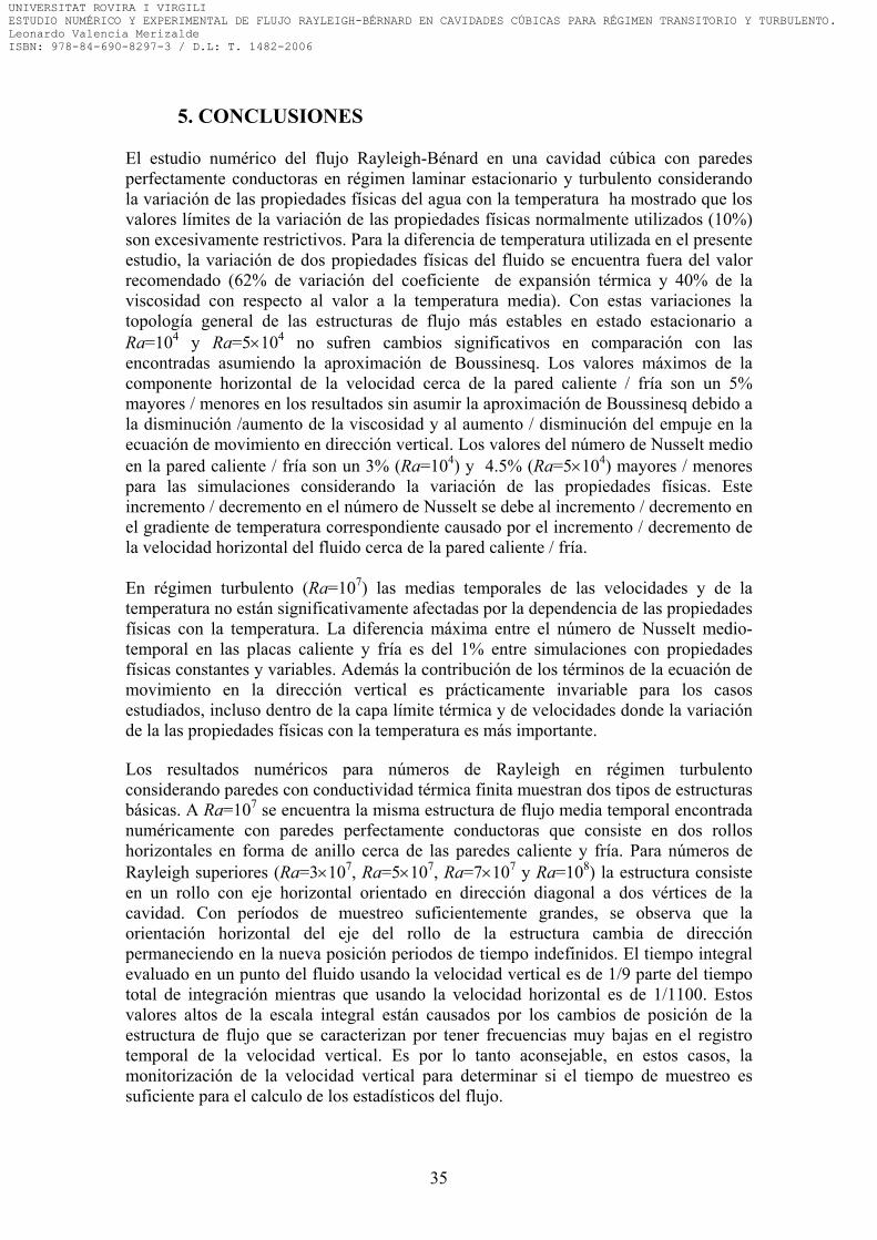
5. CONCLUSIONES El estudio numérico del flujo Rayleigh-Bénard en una cavidad cúbica con paredes perfectamente conductoras en régimen laminar estacionario y turbulento considerando la variación de las propiedades físicas del agua con la temperatura ha mostrado que los valores límites de la variación de las propiedades físicas normalmente utilizados (10%) son excesivamente restrictivos. Para la diferencia de temperatura utilizada en el presente estudio, la variación de dos propiedades físicas del fluido se encuentra fuera del valor recomendado (62% de variación del coeficiente de expansión térmica y 40% de la viscosidad con respecto al valor a la temperatura media). Con estas variaciones la topología general de las estructuras de flujo más estables en estado estacionario a Ra=104 y Ra=5×104 no sufren cambios significativos en comparación con las encontradas asumiendo la aproximación de Boussinesq. Los valores máximos de la componente horizontal de la velocidad cerca de la pared caliente / fría son un 5% mayores / menores en los resultados sin asumir la aproximación de Boussinesq debido a la disminución /aumento de la viscosidad y al aumento / disminución del empuje en la ecuación de movimiento en dirección vertical. Los valores del número de Nusselt medio en la pared caliente / fría son un 3% (Ra=104) y 4.5% (Ra=5×104) mayores / menores para las simulaciones considerando la variación de las propiedades físicas. Este incremento / decremento en el número de Nusselt se debe al incremento / decremento en el gradiente de temperatura correspondiente causado por el incremento / decremento de la velocidad horizontal del fluido cerca de la pared caliente / fría. En régimen turbulento (Ra=107) las medias temporales de las velocidades y de la temperatura no están significativamente afectadas por la dependencia de las propiedades físicas con la temperatura. La diferencia máxima entre el número de Nusselt medio-temporal en las placas caliente y fría es del 1% entre simulaciones con propiedades físicas constantes y variables. Además la contribución de los términos de la ecuación de movimiento en la dirección vertical es prácticamente invariable para los casos estudiados, incluso dentro de la capa límite térmica y de velocidades donde la variación de la las propiedades físicas con la temperatura es más importante. Los resultados numéricos para números de Rayleigh en régimen turbulento considerando paredes con conductividad térmica finita muestran dos tipos de estructuras básicas. A Ra=107 se encuentra la misma estructura de flujo media temporal encontrada numéricamente con paredes perfectamente conductoras que consiste en dos rollos horizontales en forma de anillo cerca de las paredes caliente y fría. Para números de Rayleigh superiores (Ra=3×107, Ra=5×107, Ra=7×107 y Ra=108) la estructura consiste en un rollo con eje horizontal orientado en dirección diagonal a dos vértices de la cavidad. Con períodos de muestreo suficientemente grandes, se observa que la orientación horizontal del eje del rollo de la estructura cambia de dirección permaneciendo en la nueva posición periodos de tiempo indefinidos. El tiempo integral evaluado en un punto del fluido usando la velocidad vertical es de 1/9 parte del tiempo total de integración mientras que usando la velocidad horizontal es de 1/1100. Estos valores altos de la escala integral están causados por los cambios de posición de la estructura de flujo que se caracterizan por tener frecuencias muy bajas en el registro temporal de la velocidad vertical. Es por lo tanto aconsejable, en estos casos, la monitorización de la velocidad vertical para determinar si el tiempo de muestreo es suficiente para el calculo de los estadísticos del flujo.

35


Las topologías de flujo promedio temporal obtenidas numéricamente considerando paredes laterales de la cavidad parcialmente conductoras se obtienen también experimentalmente a Ra=107, Ra=7×107 y Ra=108. Los campos de velocidad calculados y medidos usando la técnica PIV concuerdan tanto cualitativa como cuantitativamente. La técnica PIV utilizada no puede medir con la misma exactitud las velocidades altas y las bajas en flujos tridimensionales como el estudiado en el presente trabajo. Esto se debe a que para velocidades bajas el intervalo de tiempo entre imágenes debe ser muy largo para poder obtener un desplazamiento mínimo de las partículas entre imágenes consecutivas pero para velocidades altas y con una componente de la velocidad perpendicular al plano iluminado importante los intervalos de tiempo altos entre imágenes las partículas salen del plano de luz y no es posible medir su desplazamiento. No se encontraron diferencias apreciables entre la topología general de las estructuras de flujo calculadas con paredes parcialmente conductoras y perfectamente conductoras a Ra=107. Sin embargo se encontraron diferencias de hasta un 110% entre valores locales de la velocidad vertical de ambas simulaciones. Las comparaciones cualitativas y cuantitativas realizadas entre los resultados experimentales y los obtenidos numéricamente considerando conductividad térmica finita de las paredes laterales y con los cálculos con condiciones de contorno de paredes perfectamente conductoras, muestran que los resultados experimentales están mejor reproducidos por las simulaciones cuando éstas consideran paredes parcialmente conductoras

36


REFERENCIAS Amsden A. A. Y Harlow F. H. (1970) The SMAC method: A numerical technique for calculating incompressible fluid flows, Los Alamos Scientific Laboratory of the University of California, LA-4370 Aziz K. y Hellmuns J.D. (1967) Numerical solutions of the three-dimensional equations of motion for laminar natural convection, Phys. of Fluids. Vol. 10, pp. 314-324. Batchelor, G.K. (1954). Heat transfer for free convection across a closed cavity between vertical boundaries at different temperatures. Quaterly of applied mathematics. Vol. 12, pp. 209-233. Belmonte A. Tigner A. y Libchaber A. (1994) Temperature and velocity boundary layers in turbulent convection, Phys. Rev. E. Vol. 50, pp.269-279 Bénard M.H. (1901). Les tourbillons callulaires dans une nappe liquide transportant de la chaleur par convection en régime permanent. Ann. Chim. Phys. Vol. 23, pp.62-144. Bohn, M. S. (1983). Experimental study of Tree-dimensional natural convection al high Rayleigh number. Rep. Solar Energy Reserch Institute no. SERI/TR-252-1912, pp.46. Bohn, M. S. (1984). Experimental study of Tree-dimensional natural convection al high Rayleigh number. J. Heat Transfer. Vol. 106, pp. 339-345. Catton I (1970) convection in a closed rectangular region: the onset of motion, J. Heat Transfer. C92, pp. 186-188. Catton I (1972a) The effect of insulating vertical walls on the onset of motion in a fluid heated from below. Int. J. Heat Mass Transfer. Vol. 15, pp. 665-672. Catton I (1972b) Effect of wall conduction on the stability of a fluid in a rectangular region heated from below. J. Heat Transfer. pp. 446-458. Cuesta I. (1993) Estudi numèric de fluxos laminars i turbulents en una cavitat cúbica, Tesis Doctoral, Universitat Rovira i Virgili, Tarragona. Cuesta I., GrauF. X., y Giralt F. (1996) Simulación numérica de flujos tridimensionales no estacionarios mediante el código de segundo orden 3DINAMICS, Anales Química. Dabiri D. y Gharib M. (1996) The effects of forced boundary conditions on flow within a cubic cavity using digital particle image thermometry and velocimetry (DPITV), Experimental Thermal and fluid Science. Vol. 13, pp. 349-363. Davis S.H. (1967) convection in a box: linear theory. J. Fluid Mech. Vol. 30, pp. 465-478. Deardorff, J.W. y Willis, G.E. (1965) The effect of two-dimensionality on the suppression of thermal turbulence. J Fluid Mech. Vol. 23, pp.337-353.

37


Eckert, E.R.G. y Carlson, W.O. (1961) Natural convection in an air layer enclosed between two vertical plates with different temperatures. Int. J. Heat Mass Transfer. Vol. 2, pp. 106-120. Elder, J. W. (1965a). Laminar free convection in a vertical slot. J. Fluid Mech. Vol. 23, pp. 77-98. Elder, J. W. (1965b). Turbulent free convection in a vertical slot. J. Fluid Mech. Vol. 23, pp. 99-111. Gray D.D. y Giorgini A. (1976) The validity of the Boussinesq approximation for liquids and gases. Int. J. Heat Mass Transfer. Vol. 19, pp.545-551 Heitz W. L., y Westwater J. W. (1971) Critical Rayleigh numbers for natural convection of water confined in square cells with L/D from 0.5 to 8. J. Heat Transfer. C936, pp. 188-196. Hernández R. y Frederick R.L. (1994). Spatial and termal features of three dimensional Rayleigh-Bénard convection. Int. J. Heat Mass Transfer. Vol. 37 (3), pp. 411-424. Holman J. P. (1976). Heat Transfer. 4ª ed. Mc Graw-Hill Kogakusha Ltd. pp. 253, 507. Tokyo. Incropera F. P. y DeWitt D. P. (1996). Fundamentals of Heat and Mass Transfer. 4ª ed. John Wiley and Sons. New York. Jeffreys H. (1926) The stability of a layer of fluid heated from below, Phil. Mag. Vol. 2, pp. 833-844. Jeong J. y Hussain F. (1995). On the Identification of a Vortex, J. Fluid Mech., Vol. 285, pp. 69–80. Kean R. D. y Adrian R. J. (1990). Optimization of particle image velocimeters. Part 1: Double pulsed systems. Meas. Sci. and Tech. Vol. 1, pp.1202-1215. Kessler R. (1987) Nonlinear transition in three-dimensional convection. J. Fluid Mech. Vol. 174, pp. 357-379. Kim, D.M. y Viskanta, R. (1984). Study of the effects of wall conductance on natural convection in differently oriented square cavities. J. Fluid Mech. Vol. 144, pp 153-176. Kirchartz K. R. y Oertel H. (1988) Three-dimensional thermal cellular convection in rectangular boxes. J. Fluid Mech. Vol. 192, pp. 249-286. Koshla P. K. y Rubin S. G. (1981). A conjugate gradient iterative method. comp. Fluids. Vol. 9, pp.109-121. Leong W.H., Hollands K.G.T., Brunger A.P. (1999). Experimental Nusselt numbers for a cubical-cavity benchmark problem in natural convection. J. Heat and Mass Transfer. Vol. 42, pp.1979-1989.

38


Manga M., Weeraratne D., y Morris S. J. S. (2001). Boundary-Layer Thickness and Instabilities in Bénard Convection of a Liquid With a Temperature-Dependent Viscosity. Phys. Fluids. Vol. 13, pp. 802-805. Moresi L. N., y Solomatov V. S. (1995). Numerical Investigation of 2D Convection with Extremely Large Viscosity Variations. Phys. Fluids. Vol. 7, pp. 2154-2162. Ozoe H., Yamamoto K., Churchill S. W. y Sayama H. (1977). Three-dimensional, numerical analysis of laminar natural convection in a confined fluid heated from below. J. Heat Transfer. Vol. 98, pp. 202-207. Pallares J. Cuesta I., Grau F.X. y Giralt F. (1996). Natural convection in a cubical cavity heate4d from below at low Rayleigh numbers. Int. J. Heat Mass Transfer. Vol. 39 (15), pp. 3233-3247. Pallares J., Arroyo M. P., Grau F.X. y Giralt F. (2001) Experimental laminar Rayleigh-Bénard convection in a cubical cavity at moderate Rayleigh and Prandtl numbers. J. Experiments in fluids. Vol. 31, pp.208-218. Pallares J. Cuesta I. y Grau F.X.. (2002) Laminar and turbulent Rayleigh-Bénard convection in a perfectly conducting cubical cavity. Int. J. Heat and Fluid Flow. Vol. 23, pp. 346-358. Pallares J. (1997) Estudi numèric i experimental de fluxos Rayleigh-Bénard en una cavitat cúbica. Tesis Doctoral. Universitat Rovira i Virgili, Tarragona. Patankar S.V. (1980) Numerical heat tranfer and fluid flow. Mc Graw Hill. New York Potter M. C. y Wiggert D. C. (1998). Mecánica de Fluidos. 2ª ed. Prentice Hall. México. Rayleigh (Lord) (1916) On convection currents in a horizontal layer of fluid when the higher temperature is on the under side. Philos. Mag. Vol. 32, pp. 529-546. Schmidt, F.W. (1986). A comparison of experimental and predicted results for laminar convection in an enclosure. Int. J. Heat and Fluid Flow. Vol. 7, pp. 183-190. Smith C. A. y Corripio A. B. (1991). Control automático de procesos, teoría y práctica. Limusa. Mexico D.F. Solomatov V. S. (1995). Scaling of Temperature- and Stress-Dependent Viscosity Convection. Phys. Fluids. Vol. 7, pp. 266-274 Stork, K. y Müller, U. (1972) Convection in boxes: experiments. J. Fluid Mech. Vol. 54, pp. 599-611. Trompert R. A., y Hansen U. (1998). On the Rayleigh Number Dependence of Convection with a Strongly Temperature-Dependent Viscosity. Phys. Fluids. Vol. 10, pp. 351-360

39


Usera G., Vernet A. y Ferre J. A., (2005). Time resolved PIV measurements for validating LES of the turbulent flow within a PCB enclosure model, ETMM6, Cerdeña, Italia. Zhong Z. Y., Yang K. T. y Lloyd J. R. (1985). Variable property effects in laminar natural convection in square enclosure. J. Heat Transfer. Vol. 107, pp. 133-138

40


Anexo A1


Proceedings of CHT-04 ICHMT International Symposium on Advances in Computational Heat Transfer

April 19-24, 2004, Norway

CHT-04-102

NUMERICAL SIMULATION OF NON-BOUSSINESQ EFFECTS IN LAMINAR AND TURBULENT RAYLEIGH-BÉNARD CONVECTION OF WATER IN A PERFECTLY

CONDUCTING CUBICAL CAVITY

Leonardo Valencia, Jordi Pallares, Ildefonso Cuesta and Francesc Xavier Grau Department of Mechanical Engineering

University Rovira i Virgili, Avinguda dels Països Catalans 26, 43007, Tarragona, Spain Correspondence author: Fax:+34 977559691 Email: [email protected]

ABSTRACT The effects of a non-Boussinesq fluid are numerically studied and discussed for Rayleigh-Bénard convection in a cubical cavity with perfectly conducting sidewalls at low and high Rayleigh numbers using water as a convecting fluid (Pr=5.9). Numerical simulations at all Rayleigh numbers considered were carried out for two different cases. In the first case a Boussinesq fluid was considered (Boussinesq Fluid Simulation-BFS) and in the second case, the dependence of viscosity and thermal conductivity of water on temperature was adopted in the simulations (Non-Boussinesq Fluid Simulation-NBFS). At the low Rayleigh numbers used in this study (Ra=104 and Ra=5x104) the flow is laminar and steady and at the high Rayleigh number considered (Ra=107) the flow is turbulent. At Ra=104 and Ra=5x104 we focus our analysis on the effect of variation of the fluid viscosity with temperature on the more stable flow structures from the set of seven different topologies reported in previous studies. At Ra=107 and Pr=5.9 the non-Boussinesq effects on the turbulent flow are analysed in detail and the flow structures and heat transfer rates compared with those available in the literature at Pr=0.71. Previous works recommend that temperature difference should be less than 4.5ºC in order to obtain less than 10% of variation in the viscosity. Non-Boussinesq simulations in the present work were calculated with a viscosity variation of 40% between cold and hot plates. The numerical simulations at high and low Rayleigh numbers were conducted with a second order finite volume code without any turbulence model because the time-steps and grid sizes used are adequate for the time and spatial resolution requirements reported in previous direct numerical simulations of Rayleigh-Bénard flows. The structure of the flow topologies at Ra=104 and Ra=5x104 are not significantly affected by the effects of the variation of viscosity and thermal conductivity with temperature. However, results obtained with a NBFS show an increase of the ascending flow velocities compared with those obtained with the Boussinesq approximation according to the decrease of viscosity with increasing temperature. At Ra=107 the instantaneous flow shows large deviations with respect to the time-average flow field that consists in two counter rotating vortex rings located near the horizontal plates. The temperature gradients and, thus the viscosity variation are located close to the walls within the thermal boundary layers. This causes that the time-averaged flow field topologies corresponding to BFS and NBFS are not greatly affected by the effects of the variation of viscosity and thermal conductivity with temperature.


NOMENCLATURE

BT Buoyancy term CT convective term DT diffusive term FVST fluctuating viscous stresses terms L vertical dimension of the cube (m) n arbitrary variable N number of grid points PT pressure gradient term TT turbulent transport terms Greek letters β thermal expansion coefficient (K-1) λ thermal boundary layer thickness (m) λ2 second largest eigenvalue of the velocity gradient tensor δij Kronecker delta ∆ increment σ standard deviation (root-mean square – RMS) θ autocorrelation function T integral scale (s) Superscripts and subscripts s surface averaged quantity * non-dimensional quantity C cold plate H hot plate 0 reference value at mean temperature m average or mean value t total integrating values ‘ fluctuating value i initial value

average value V volume average

INTRODUCTION Natural convection flows are generated by density differences within the fluid. These density differences can be produced by temperature or concentration gradients. Rayleigh-Bénard convection is a type of natural convection that is produced by an unstable vertical density stratification in a bounded horizontal fluid layer. Natural convection in parallelepipedic cavities, heated from below has been the topic of numerous experimental and theoretical studies. Because of their geometrical simplicity, and the diversity of complex flow structures these systems have been used as benchmarks for testing Computational Fluid Dynamic codes [1]. Particularly, flows in cubical cavities are of interest because the direction of gravity is the only preferred direction of flow motion. Leong et al. [2] reported experimental natural convection averaged Nusselt numbers at the cold face of a cubical cavity filled with air with two opposite isothermal faces at different


temperatures. The rest of the faces had a linear variation of temperature from the cold to the hot plate temperatures (i.e. perfectly conducting walls). The Rayleigh numbers studied were 104, 105, 106, 107 and 108. Measurements were performed for three angles of inclination of the isothermal faces. Pallares et al. studied numerically [3] and experimentally [4] the Rayleigh-Bénard convection in a cubical cavity heated from below at low Rayleigh numbers (Ra≤8x104) and three Prandtl numbers. They considered both, perfectly conducting sidewalls and adiabatic lateral walls. They identified seven different structures in the steady and laminar regime and discussed the heat transfer characteristics of this topologies. In this simulations the Boussinesq approximation was assumed. Large –Eddy simulations of Rayleigh-Bénard convection of a Boussinesq fluid with Prandtl number 0.71 in a perfectly conducting cubical cavity were performed by Pallares et. al [5] at Ra=106 and Ra=108. They reported the time-averaged velocity and temperature fields and relatively low subgrid-scale contributions for the grid resolution used. Most of the studies in convection of fluids with a temperature-dependent viscosity which are related mainly with simulations of the planetary mantle convection [6,7,8,9] consider a strong difference of viscosity between fluid close to the top cold and bottom hot walls. In this cases the viscosity difference is sufficiently large and the cold fluid near the top of the enclosure is stagnant and the heat is transferred only by conduction. This study is focused in the analysis of the numerical simulations of Rayleigh Bénard convection using water as a convecting fluid (Pr=5.9) in the laminar (Ra=104 and Ra=5x104) and turbulent regimes (Ra=107) in a cubical cavity heated from below with perfectly conducting sidewalls to determine the differences between Boussinesq fluid simulation (BFS) and Non-Boussinesq fluid simulation (NBFS) results.

MODEL

The physical model of the cubical cavity and the coordinate system adopted are shown in Figure 1. The cavity is assumed to be full of water (Pr=5.9) and the walls of the cavity are immobile and rigid. The two horizontal walls are isothermal and the four lateral walls are perfectly conducting (i.e. constant vertical linear temperature profile from the bottom to the top). Compressibility effects and viscous dissipation are neglected and the density of fluid is considered constant with the exception of the buoyancy term in which a linear temperature variation is considered. All other physical properties are assumed constant in the BFS. The last three assumptions are known as the Boussinesq approximation [10]. Results for the NBFS are calculated with a dependence of the viscosity and the thermal conductivity with temperature corresponding to water in the range 10ºC<T<35ºC:

( ) 310543 1018.51001.21004.11089.1 TTLnTT ⋅×−⋅⋅×+⋅×−×= −−−−µ (1) 1326 1067.5108.1102 −−− ×+⋅×+⋅×−= TTk (2)

Where µ is in Kg m-1 s-1, k in W m-1 ºC-1 and T in ºC. Equations (1) and (2) are correlations developed by the authors based on experimental data obtained from reference [11] for viscosity and [12] for thermal conductivity. Gray and Giorgini [10] fixed the maximum temperature differences within the fluid to consider the Boussinesq approximation as those producing a 10% variation of the physical properties. For water at T0=26ºC, the maximum temperature differences according to this criterion are ∆T ≤ 2.9ºC for the variation of thermal expansion coefficient with temperature, ∆T ≤ 4.5ºC for the variation of viscosity with temperature and ∆T ≤ 35.7ºC for the variation of thermal conductivity with temperature. Despite the relative importance of the variation of the thermal expansion coefficient, as a first step to determine the individual effects of the physical properties dependence on temperature on the Rayleigh-Bénard convection, in this study only the variation of viscosity and thermal conductivity with temperature is considered. This work is presently being extended to the


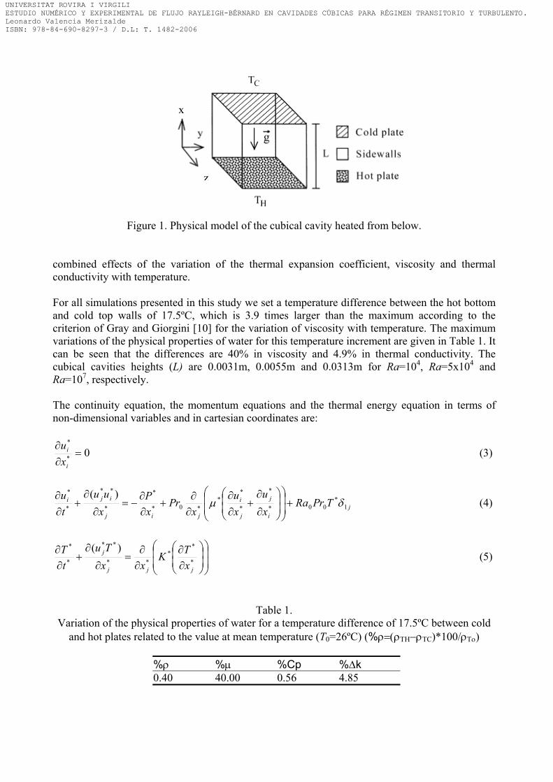
z

x

Figure 1. Physical model of the cubical cavity heated from below. combined effects of the variation of the thermal expansion coefficient, viscosity and thermal conductivity with temperature.

For all simulations presented in this study we set a temperature difference between the hot bottom and cold top walls of 17.5ºC, which is 3.9 times larger than the maximum according to the criterion of Gray and Giorgini [10] for the variation of viscosity with temperature. The maximum variations of the physical properties of water for this temperature increment are given in Table 1. It can be seen that the differences are 40% in viscosity and 4.9% in thermal conductivity. The cubical cavities heights (L) are 0.0031m, 0.0055m and 0.0313m for Ra=104, Ra=5x104 and Ra=107, respectively. The continuity equation, the momentum equations and the thermal energy equation in terms of non-dimensional variables and in cartesian coordinates are:

0*

*

=∂∂

i

i

xu (3)

ji

j

j

i

jij

iji TrPRaxu

xu

xrP

xP

xuu

tu

1*

00*

*

*

**

*0*

*

*

**

*

* )(δµ +

∂

∂+

∂∂

∂∂

+∂∂

−=∂

∂+

∂∂ (4)

∂∂

∂∂

=∂

∂+

∂∂

*

**

**

**

*

* )(

jjj

j

xTK

xxTu

tT (5)

Table 1. Variation of the physical properties of water for a temperature difference of 17.5ºC between cold

and hot plates related to the value at mean temperature (T0=26ºC) (%ρ=(ρΤΗ−ρTC)*100/ρΤο)

%ρ %µ %Cp %∆k 0.40 40.00 0.56 4.85


Where µ*=µ(T)/µ0 and k*= k(T)/k0 according to the fitting functions of Equations (1) and (2). The reference scales for length, velocity, time and pressure are, respectively, L, α0/L, L2/α0 and α0

2ρ0/L2. The non-dimensional temperature is defined as T*=(T-T0)/∆T where ∆T=(TH-TC) and T0 is the mean temperature T0=(TH+TC)/2. All the physical properties in the Ra and Pr numbers are evaluated at T0. The six walls are assumed to be rigid and static (ui

*=0) and the thermal conditions at the hot and cold plates are TH=0.5 and TC=-0.5 respectively. A linear temperature profile between hot plate and cold plate is imposed at the vertical walls (T*=-X*+0.5). In calculations with the Boussinesq approximation µ*=k*=1.0 and Equation (4) becomes

j

j

i

ij

iji TrPRax

urP

xP

xuu

tu

1*

002*

*2

0*

*

*

**

*

* )(δ+

∂

∂+

∂∂

−=∂

∂+

∂∂

(6)

The local and average Nusselt number in the hot and cold plates were computed with second order accuracy and are defined as,

10**

*

orxxTNu

=∂∂

= (7)

and

(8) **1

0

1

0dzdyNuNus ∫ ∫=

Equations (3), (4) and (5) and the corresponding boundary conditions have been solved numerically with the control volume 3DINAMICS code. In this second order accuracy code, the diffusive and convective fluxes are discretized in a staggered grid using a central scheme. The code performs the time-marching procedure with an explicit Adams–Bashforth scheme. The coupling between the pressure and velocity field is computed using a predictor–corrector scheme involving a Poisson equation that is solved with the conjugate gradient method. The details of the complete mathematical formulation and the description of the numerical methods can be found in Cuesta [13]. Uniform grids of 413 nodes have been used for the low Rayleigh number simulations (Ra=104 and Ra=5x104). Pallares et al. [4] showed that this grid resolution is adequate for describing these flows. They successfully compared numerical velocity distributions of the different flow structures at Ra≤8×104 and Pr=130 computed using the same grid resolution with the corresponding PIV measured distributions. At Ra=8×104 and Pr=130 the difference on average Nusselt numbers using uniform grids of 413 and 813 nodes was 2.5%. Table 2 shows the computational details of the numerical simulations at low Rayleigh numbers (Ra=104 and Ra=5x104). Numerical simulations at Ra=107 and Pr=5.9 were conducted without any turbulence model with grid sizes of Nx=81, Ny=61 and Nz=61 nodes and ∆t*=5x10-7 for BFS and ∆t*=10-7 for NBFS. According to the LES reported by Pallares et. al [5], Ra=106, the use of time steps of ∆t*=1.2x10-6 and non-uniform grids of 613 nodes the ratio between the SGS viscosity and the molecular viscosity is only 0.5%. Grötzbach [14] deduced criteria to predict grid sizes for accurate direct numerical simulations of Rayleigh-Bénard turbulent flows. These criteria are based on wavelength considerations, boundary layer thickness estimates, and on a simplified theoretical model to calculate the coefficient of a subgrid-scale heat flux model. The mean grid widths used in this work agree with those corresponding to the criteria reported by Grötzbach [14] (see Table 3). The grid used at Ra=107 has at least 8 grid nodes within the thermal boundary layers near the horizontal walls as shown in Figure 2. Table 4 shows the computational details of the numerical


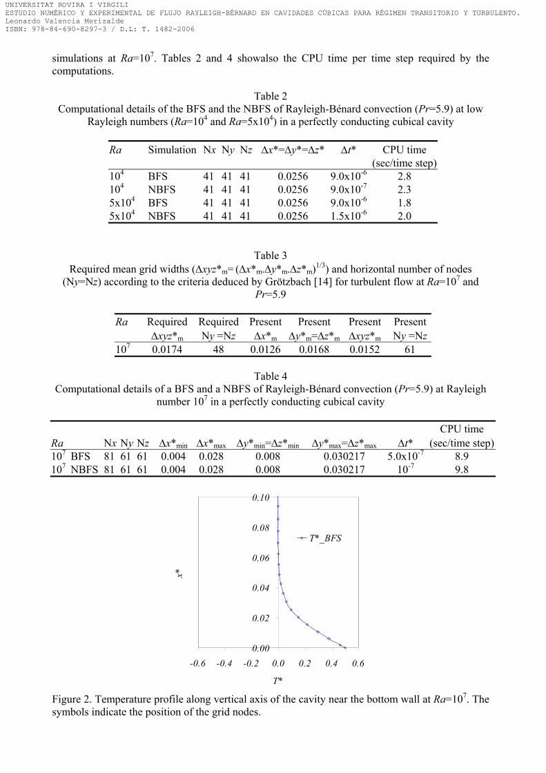
simulations at Ra=107. Tables 2 and 4 showalso the CPU time per time step required by the computations.

Table 2

Computational details of the BFS and the NBFS of Rayleigh-Bénard convection (Pr=5.9) at low Rayleigh numbers (Ra=104 and Ra=5x104) in a perfectly conducting cubical cavity

Ra Simulation Nx Ny Nz ∆x*=∆y*=∆z* ∆t* CPU time (sec/time step) 104 BFS 41 41 41 0.0256 9.0x10-6 2.8 104 NBFS 41 41 41 0.0256 9.0x10-7 2.3 5x104 BFS 41 41 41 0.0256 9.0x10-6 1.8 5x104 NBFS 41 41 41 0.0256 1.5x10-6 2.0

Table 3 Required mean grid widths (∆xyz*m= (∆x*m.∆y*m.∆z*m)1/3) and horizontal number of nodes

(Ny=Nz) according to the criteria deduced by Grötzbach [14] for turbulent flow at Ra=107 and Pr=5.9

Ra Required Required Present Present Present Present ∆xyz*m Ny =Nz ∆x*m ∆y*m=∆z*m ∆xyz*m Ny =Nz 107 0.0174 48 0.0126 0.0168 0.0152 61

Table 4

Computational details of a BFS and a NBFS of Rayleigh-Bénard convection (Pr=5.9) at Rayleigh number 107 in a perfectly conducting cubical cavity

CPU time Ra Nx Ny Nz ∆x*min ∆x*max ∆y*min=∆z*min ∆y*max=∆z*max ∆t* (sec/time step) 107 BFS 81 61 61 0.004 0.028 0.008 0.030217 5.0x10-7 8.9 107 NBFS 81 61 61 0.004 0.028 0.008 0.030217 10-7 9.8

0.00

0.02

0.04

0.06

0.08

0.10

-0.6 -0.4 -0.2 0.0 0.2 0.4 0.6

T*

x*

T*_BFS

Figure 2. Temperature profile along vertical axis of the cavity near the bottom wall at Ra=107. The symbols indicate the position of the grid nodes.


RESULTS AND DISCUSSION In this section the influences of the variations of viscosity and thermal conductivity with temperature are presented for the flow structures at low (Ra=104 and Ra=5x104) and high (Ra=107) Rayleigh numbers for water at T0=26ºC (Pr=5.9). Laminar flow: Non-Boussinesq effects at low Rayleigh numbers We investigate the effects of the dependence of viscosity and thermal conductivity on temperature for two stable, steady and laminar flow structures. These flow structures are depicted in Figure 3 in terms of velocity vectors in two vertical planes and isosurfaces of the second largest eigenvalue of the velocity gradient tensor following the method of Jeong and Hussain [15] to detect the occurrence of vortex cores. The first structure, named S1 according to the nomenclature proposed by Pallares et al. [16], is a single roll with its axis parallel to two of the lateral walls. The cold fluid descends parallel to one sidewall (y*=0) and hot fluid rises by the opposite wall (y*=1) (see Figures 3(a), 3(b) and 3(c)). The second structure, named S5 and shown in Figures 3(d), 3(e) and 3(f), consists in four recirculating motions in planes nearly parallel to the four lateral walls. These motions produce two ascending currents of hot fluid along two diagonally opposite vertical edges and two descending currents near the other vertical edges of the cavity. Despite the large variation of viscosity considered, there are no significant differences in the main characteristics of structures S1 and S5 shown in Figure 3 which correspond to NBFS. However a more detailed comparison of the velocity profiles obtained with a NBFS shows a clear increase of the ascending flow velocities compared with those obtained with the Boussinesq approximation. Figures 4(a) and 4(c) show the profiles of the horizontal velocity component (v*) close to the hot wall along the horizontal y* direction for NBFS and BFS for structure S1 at Ra=104 and S5 at Ra=5x104 respectively and Figures 4(b) and 4(d) show the vertical profiles of u* close to the corresponding ascending wall along the vertical x* direction for NBFS and BFS for structure S1 at Ra=104 and S5 at Ra=5x104 respectively. It can be seen in Figures 4 (a) (S1) and 4(c) (S5) that the absolute values of the horizontal velocity components near the bottom hot wall are increased in the NBFS in comparison with the BFS in agreement with the fact that the viscosity decreases with the increase of temperature. This velocity increase in the NBFS directly affects vertical velocities in the ascending flow near the corresponding vertical wall. Close to the cold wall the viscosity is larger for NBFS causing a decrease of horizontal velocity compared with BFS. This causes a decrease of the vertical velocities in the descending flow near the opposite side wall. The effects of the viscosity-temperature dependence in structure S5 at Ra=5x104 are similar to those of S1.


Z

X

YX

YZ Fig. 4(e)

Vector plot of Vector plot of Fig. 4(b) Fig. 4(f) Vector plot of Fig. 4(c) Vector plot of

(a) (d) (b) (e)

y*

x*

0 0.2 0.4 0.6 0.8 10

0.2

0.4

0.6

0.8

1

y*

x*

0 0.2 0.4 0.6 0.8 10

0.2

0.4

0.6

0.8

1

5010

(c) (f)

z*

x*

0 0.2 0.4 0.6 0.8 10

0.2

0.4

0.6

0.8

1

10 z*

x*

0 0.2 0.4 0.6 0.8 10

0.2

0.4

0.6

0.8

1

50

Figure 3. (a), (b) and (c) Flow topology of structure S1 at Ra=104, (d), (e) and (f) of structure S5 at Ra=5x104. (a) and (d), surface of constant value of λ2/|λ2,max|=-0.12 and λ2/|λ2,max|=-0.47 respectively. (b) and (e), velocity field in the vertical midplane z*=0.5 and z*=0.17 respectively, (c) and (f), velocity field in the vertical midplane y*=0.5. These planes are indicated in (a) and (d). The reference vectors are depicted near the bottom right corner of (b), (c), (e) and (f).


0.0

0.2

0.4

0.6

0.8

1.0

0 5 10 15 20u*

x*

u*_BFS u*_NBFS

-2

0

2

4

6

8

10

0.0 0.2 0.4 0.6 0.8 1.0

y*

v*

v*_BFS v*_NBFS

(a) (b)

-25

-20

-15

-10

-5

0

5

10

15

0.0 0.2 0.4 0.6 0.8 1.0

y*

v*

v*_BFS v*_NBFS

0.0

0.2

0.4

0.6

0.8

1.0

-20 0 20 40 60u*

x*

u*_BFS u*_NBFS

(c) (d) Figure 4. (a) and (b) are velocity profiles of structure S1 (Ra=104), (a) is the horizontal (y*) profiles of the horizontal velocity component (v*) close to the hot plate along the line x*=0.064, z*=0.5 and (b) is the vertical profile (x*) of the vertical velocity component (u*) close to the lateral wall (y*=1) along the line y*=0.75, z*=0.5. (c) and (d) are velocity profiles of structure S5 (Ra=5x104), (c) shows the horizontal profile of the horizontal velocity component (v*) close to the hot plate along the line x*=0.064, z*=0.17 and (d) shows the vertical profile of the vertical velocity component (u*) close to the vertical edge (y*=0, z*=0) along the line y*=0.17, z*=0.17. Figure 5 shows vertical velocity contours in the horizontal midplane (x*=0.5) for structures S1 and S5 for the BFS and the NBFS. Note that maximum ascending velocities (u*>0) are larger in the NBFS (Fig. 5(b)) than in the BFS (Fig. 5(a)). Correspondingly, the absolute value of the descending velocities in the BFS are larger in comparison with the NBFS for the S1 topology at Ra=104. This difference is equilibrated with the decrease of the area used by the fluid to ascend and the increase of the area where the cold fluid descends in the NBFS. In the BFS both areas are the same. At


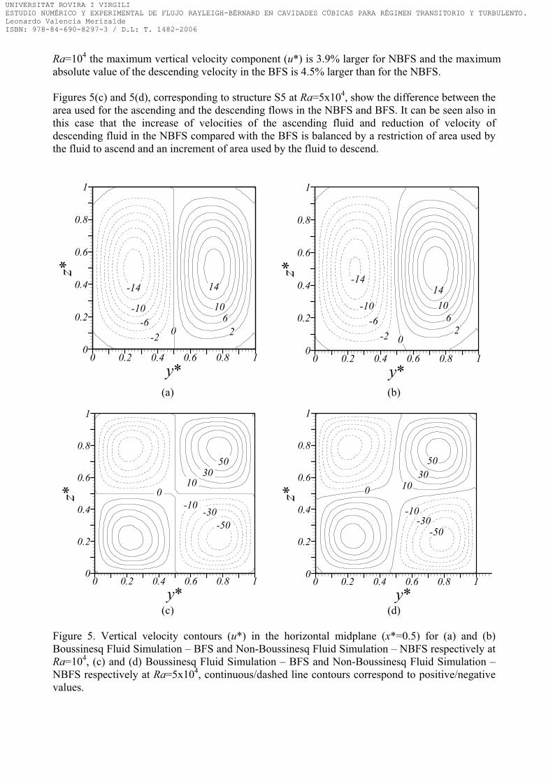
5030

100

-50-30

-10

y*

z*

0 0.2 0.4 0.6 0.8 10

0.2

0.4

0.6

0.8

1

5030

100

-50-30

-10

y*

z*

0 0.2 0.4 0.6 0.8 10

0.2

0.4

0.6

0.8

1

14

106

2

-14

-10-6

-2 0

y*

z*

0 0.2 0.4 0.6 0.8 10

0.2

0.4

0.6

0.8

1

-2-6

-10

-14

02

610

14

y*

z*

0 0.2 0.4 0.6 0.8 10

0.2

0.4

0.6

0.8

1

Ra=104 the maximum vertical velocity component (u*) is 3.9% larger for NBFS and the maximum absolute value of the descending velocity in the BFS is 4.5% larger than for the NBFS. Figures 5(c) and 5(d), corresponding to structure S5 at Ra=5x104, show the difference between the area used for the ascending and the descending flows in the NBFS and BFS. It can be seen also in this case that the increase of velocities of the ascending fluid and reduction of velocity of descending fluid in the NBFS compared with the BFS is balanced by a restriction of area used by the fluid to ascend and an increment of area used by the fluid to descend. (a) (b) (c) (d) Figure 5. Vertical velocity contours (u*) in the horizontal midplane (x*=0.5) for (a) and (b) Boussinesq Fluid Simulation – BFS and Non-Boussinesq Fluid Simulation – NBFS respectively at Ra=104, (c) and (d) Boussinesq Fluid Simulation – BFS and Non-Boussinesq Fluid Simulation – NBFS respectively at Ra=5x104, continuous/dashed line contours correspond to positive/negative values.


Concerning heat transfer rates, Table 5 compares the averaged Nusselt numbers in the horizontal walls at low Ra numbers. When the Boussinesq approximation is considered the surface averaged values of the Nusselt numbers on the top and bottom walls are the same because the velocity and temperature fields are antisymmetric with respect the centre of the cavity (x*=0.5, y*=0.5, z*=0.5). The values at Ra=104 and Pr=5.9 are in agreement with that measured by Leong et. al. [2] at Pr=0.71. The average Nu numbers at the cold/hot wall of the NBFS are about 1% at Ra=104 and 3% at Ra=5x104 larger/smaller than the corresponding to BFS. Considering the maximum variation of the thermal conductivity (4%), these differences can be attributed to the variation of the viscosity with temperature (up to 40%) on the thermal and velocity fields. Structure S1, with the axis of rotation parallel to the z* direction, produces non-zero average heat flux through the lateral walls y*=0 and y*=1. The average Nu numbers at these walls are Nus,y*=0= Nus,y*=1=0.390 for the BFS and Nus,y*=0=0.380, Nus,y*=1=0.394 for the NBFS. As shown in Figure 5(b) the ascending/descending current of the S1 structure flows parallel to the y*=1/y*=0 sidewall. The differences between the average Nusselt numbers at y*=1 and y*=0 for the NBFS agree with the increase/decrease of the vertical velocity component produced by the viscosity dependence on temperature. (for example, compare Figs. 5(a) and 5(b)). Structures S1 and S5 do not produce any net heat flux on the lateral walls perpendicular to the axis of their rolling motion because the heat flux to the sidewall generated by the ascending current is the same that the heat flux from the wall caused by the descending current. To determine the effects of the viscosity and thermal conductivity variation with temperature on the mechanisms of the flow motion we analysed the different terms of the vertical momentum equation for NBFS and BFS. The vertical momentum budget can be written as

*

**1

1*

*1

*

*

*1*

**1

* )(1110j

jj

j

jj xuu

rRaPT

xu

xu

xRaxP

rRaP ∂

∂−+

∂

∂+

∂∂

∂∂

+∂∂

−= δµ (9)

(PT) (DT) (BT) (CT) Pressure gradient term Diffusive term Buoyancy term Convective term Note that all terms of the x-momentum equation (Eq. (4)) have been displaced to the right hand side and divided by RaPr. Figure 6 shows the horizontal profiles of the different terms of Equation (9) along the line x*=0.5, z*=0.5 for structure S1 at Ra=104 (Fig.6(a)) and along the line x*=0.5, z*=0.17 for structure S5 at Ra=5x104 (Fig 6(b)). It can be seen that in NBFS and BFS the fluid ascends and descends mainly due to a balance between the buoyancy, the pressure gradient and the viscous terms in the vertical momentum equation. The convective terms do not contribute significantly to the balance. Figure 6 shows that there is no significant difference in the contribution of the viscous terms between NBFS and BFS. The difference can be observed, for structures S1 and S5, in the contribution of the buoyancy and the pressure gradient terms. There is an increase of the buoyancy term for the NBFS in the region of ascending fluid (y*>0.5 for S1, Fig. 6(a) and y*<0.5 for S5, Fig. 6(b)), which is balanced by an increase of the pressure gradient term. In the region where the fluid descends (y*<0.5 for S1 and y*>0.5 for S5) the opposite situation is encountered (i.e. the decrease of the buoyancy is balanced by the decrease of the gradient pressure term).


Table 5 Average Nusselt numbers at the horizontal walls at low Ra numbers

Ra 104 (S1) 5x104 (S5) Pr=0.71 NusC [2] 1.246±0.013 (2.018 at Ra=4x104) Pr=5.9 BFS NusC 1.246 2.676 NusH 1.246 2.676 NBFS NusC 1.263 2.755 NusH 1.224 2.595

Turbulent Flow: BFS and NBFS at Ra=107 The effect of the viscosity variation with temperature on the turbulent Rayleigh-Bénard flow is analyzed at Ra=107 using water as a convecting fluid at T0=26ºC (Pr=5.9). The NBFS were performed with a temperature difference between the hot and cold plates of 17.5ºC. This temperature increment produces a variation of viscosity of 40% (see Table 1). Figure 7 shows the time averaged flow field for the NBFS in terms of velocity vectors in the vertical symmetry planes of the cavity and in terms of an isosurface of the of the second largest eigenvalue of the velocity gradient tensor [15]. It can be seen that the averaged flow structure consists in two main counter rotating vortex rings located near the horizontal walls and four small vortex tubes following the y-edges and the z-edges of the cavity (see Figure 7(a)). The topology is symmetric with respect to the horizontal and vertical midplanes of the cavity. The vortex rings can be understood as a combination of four z-rolls (with vorticity aligned with the z-direction) and four y-rolls (with vorticity aligned with the y-direction).

-0,20

-0,15

-0,10

-0,05

0,00

0,05

0,10

0,15

0,20

0,0 0,2 0,4 0,6 0,8 1,0y*

x-m

omen

tum

bud

get

-0,20

-0,15

-0,10

-0,05

0,00

0,05

0,10

0,15

0,20

0,0 0,2 0,4 0,6 0,8 1,0y*

x-m

omen

tum

bud

get

CT_BFS CT_NBFS PT_BFS PT_NBFSBT_BFS BT_NBFS DT_BFS DT_NBFS

(a) (b) Figure 6. Profiles along the y-direction of the terms of the x-momentum budgets (Eq. 9) for NBFS and BFS. (a), y-profile at x*=0.5, z*=0.5 at Ra=104 for structure S1 (b) y-profile at x*=0.5, z*=0.17 at Ra=5x104 for structure S5.


The cross sections of the z- and y-rolls are shown in Figures 7.(b) and 7.(c), respectively. This time averaged flow structure is similar to that reported by Pallares et. al. [5] at Ra=106 (Pr=0.71). The flow structure and velocity fields for the BFS are not shown in Figure 7 because there are no significant differences with those for the NBFS. The flow at Ra=107 presents large fluctuations in the velocity and temperature fields with respect to the time averaged values. Table 6 shows the values of the integral scale, the number of integral scales sampled (t t*/ T *) and the time averaged fluctuations of the surface averaged Nusselt number on the cold plate (NuC) and u*, v* and T* at the position x*=0.5, y*=0.75 and z*=0.5. The flow statistics discussed in this section were obtained by sampling the statistically developed velocity and thermal fields during 0.071 non-dimensional time units.

Z

X

Y

y*

x*

0 0.2 0.4 0.6 0.8 10

0.2

0.4

0.6

0.8

1

Vector plot of Vector plot of Fig. 7(b) Fig. 7(c) (a) (b) (c)

z*

x*

0 0.2 0.4 0.6 0.8 10

0.2

0.4

0.6

0.8

1

2500 2500

Figure 7. Time average flow fields at Ra=107 for the non-Boussinesq fluid simulation. (a) surface of constant value of λ2/|λ2,max|= -0.017. (b) velocity field in the vertical midplane z*=0.5 and (c) velocity field in the vertical midplane y*=0.5. The reference vector is depicted near the bottom right corner of (b) and (c).


Table 6 Integral scale (T *), number of integral scales sampled (t t*/ T *) and *'n for average Nusselt

number in the cold plate (NuC) and for u*, v* and T* in the point x*=0.5, y*=0.75 and z*=0.5 with a total integration time of t t* =0.071

Ra=107_BFS Integral scale (T *) (t t*/ T *) 'n NuC 2.2x10-3 32.3 1.8x10-14 u* 8.3 x10-4 85.5 1.0x10-14 v* 4.4 x10-3 16.1 -6.3x10-15 T* 8.3 x10-4 85.5 -5.4x10-16 Ra=107_NBFS Integral scale (T *) (t t*/ T *) 'n NuC 5.1 x10-4 139.2 1.2x10-15 u* 1.2 x10-3 59.2 1.2x10-14 v* 3.5 x10-3 20.3 7.8x10-15 T* 1.8 x10-3 39.4 -7.6x10-15

It can be seen in Table 6 that the total integration time ranges from 16-139 times the integral scale and that the number of data taken to calculate the time averaged values is enough to assure that variables are statistically steady as indicated by the low values of the time averaged fluctuations of the variables analysed. Considering the averaged modulus of the velocity vector as a typical velocity scale of the flow, the distance covered by a fluid particle during the sampling time is about 32 times the cavity height. Table 7 shows that the averaged Nusselt number at the cold plate and the corresponding RMS value are almost the same in the NBFS and BFS. The volume averaged modulus of the velocity vector are 451.9 and 449.9 non-dimensional velocity units for BFS and NBFS, respectively. The standard deviations of the quantities sampled at the position x*=0.5, y*=0.75, z*=0.5 and their volume averaged values do not show significant differences for the NBFS and BFS. The time-averaged vertical x-momentum and horizontal y-momentum budgets can be written as

jj

j

j

jj

jj

j

jj

Txuu

rRaPxuu

rRaPxu

xu

xRaxu

xu

xRaxP

rRaP 1*

*

**1

*

**1

*1

*

*

*1*

**1

*

*

*1*

**1

* )''(1)(1'''1110 δµµ +∂

∂−

∂

∂−

∂

∂+

∂∂

∂∂

+

∂

∂+

∂∂

∂∂

+∂∂

−= (10)

(PTx) (DTx) (FVSTx) (CTx) (TTx) (BT) and

*

**2

*

**2

*2

*

*

*2*

**2

*

*

*2*

**2

* )''(1)(1'''1110j

j

j

jj

jj

j

jj xuu

rRaPxuu

rRaPxu

xu

xRaxu

xu

xRaxP

rRaP ∂

∂−

∂

∂−

∂

∂+

∂∂

∂∂

+

∂

∂+

∂∂

∂∂

+∂∂

−= µµ (11)

(PTy) (DTy) (FVSTy) (CTy) (TTy) respectively. The different terms of Equations (10) and (11) are, from left to right, the pressure gradient term (PT), the diffusive terms (DT), the fluctuating viscous stresses terms (FVST), the convective terms (CT), and the turbulent transport terms (TT). The subscripts indicate if the term correspond to the x or the y-momentum equation. The last term in Equation (10) is the buoyancy term (BT).


Figure 8(a) shows the different terms of Equation (10) along the vertical line (y*=0.012, z*=0.5) near the sidewall (y*=0). The contributions of the terms of the y-momentum equation (Eq. 11) are depicted in Figure 8(b) along the line (x*=0.0062, z*=0.5), located near the hot bottom wall (x*=0). These lines have been selected to identify differences between NBFS and BFS because they are located within the corresponding thermal and momentum boundary layers where the contributions of the viscous terms to the budgets are important. For the sake of clarity, the convective terms and the turbulent transport terms have been omitted in Figure 8 because their contributions to the momentum budgets along the selected lines are very small in comparison with those of the pressure gradient terms, the diffusive terms and the buoyancy term. The fluctuating viscous stresses have been included in Figure 8 to show their small relative importance in the momentum budgets. It can be seen in Figure 8(a) that the main terms in the vertical momentum budget along the line y*=0.012, z*=0.5 are the buoyancy term, the pressure gradient term and the diffusive terms. Near the vertical wall y*=0 the fluid ascends/descends from the hot/cold plate (see Fig. 7(b)) due to the buoyancy term which is mainly balanced by the diffusive term. The contribution of the pressure gradient term agrees with the increases and decreases of the x-momentum near the vertical wall y*=0.

Table 7 Statistical values for average Nusselt number, vertical and horizontal velocities and temperature at

the position (x*=0.5, y*=0.75, z*=0.5) at Ra=107

Ra=107_BFS Mean value, n RMS, σ RMS V

NuC 16.80 0.72 u* 29.6 374.4 202.9 v* -496.1 198.2 135.7 T* -2.2x10-3 0.06 0.0434 Ra=107_NBFS Mean value, n RMS, σ RMS V NuC 16.84 0.67 u* 184.2 383.8 203.0 v* -472.5 203.5 136.2 T* 2.2x10-2 0.06 0.0431


0,0

0,2

0,4

0,6

0,8

1,0

-0,6 -0,4 -0,2 0,0 0,2 0,4 0,6x-momentum budget

x*

FVSTx_BFS PTx_BFS BTx_BFS DTx_BFSFVSTx_NBFS PTx_NBFS BTx_NBFS DTx_NBFS

(a)

-0,10

-0,06

-0,02

0,02

0,06

0,10

0,0 0,2 0,4 0,6 0,8 1,0y*

y-m

omen

tum

bud

get

FVSTy_BFS PTy_BFS DTy_BFSFVSTy_NBFS PTy_NBFS DTy_NBFS

(b) Figure 8. x- and y-momentum equation budgets at Ra=107 calculated for NBFS and BFS (a) vertical x-profile at y*=0.012, z*=0.5 and (b) horizontal y-profile at x*=0.0062, z*=0.5.


Figure 8(a) shows also that the vertical component of the pressure gradient is favourable (dP*/dx*<0) for the ascending flow near x*=0.1. Correspondingly, the pressure gradient is favourable (dP*/dx*>0) for the descending flow near x*=0.9. This term acts as a sink in the vertical momentum equation near the horizontal walls and near the horizontal midplane of the cavity (x*=0.5). Figure 8(b) shows the main terms of the y-momentum equation (Eq. 11) along the line x*=0.0062, z*=0.5 which is located within the thermal and momentum boundary layers developed near the bottom wall. The flow impingement towards the bottom wall (see Figs. 7(b) and 7(c)) produces a maximum of pressure located at the centre of the wall. It can be seen in Figure 8(b) that the horizontal currents near the horizontal walls are produced by a favourable pressure gradient along the y-direction and that the pressure gradient term is mainly balanced by the viscous terms. Finally, Figure 8 shows that in general the contributions of the different terms in the near-wall momentum budgets are not greatly affected by the changes in viscosity. However Figure 8(a) shows small differences in the viscous terms for NBFS and BFS. In the NBFS the ascending/descending flow has smaller/larger viscosity (i.e. lower/higher viscous term contribution) than in the BFS. This difference in the contribution of the viscous terms for the NBFS and BFS is balanced by the vertical pressure gradient term.

CONCLUSIONS Laminar and turbulent Rayleigh-Bénard convection of water (T0=26ºC, Pr=5.9) in a perfectly conducting cavity have been simulated considering both constant and variable viscosity. We considered a temperature increment of 17.5ºC between the bottom hot wall and the top cold wall. This maximum temperature difference produces variations of 40% in the viscosity and variations of only 4.5% in the thermal conductivity of water, with respect to the corresponding values at the reference temperature (T0=26ºC). The variation of the viscosity is well above the limit of 10% usually considered for the adoption of the Boussinesq approximation. At low Rayleigh numbers (Ra=104 and Ra=5x104) the variation of viscosity produces an increase/decrease of the fluid horizontal component velocities of about 10% near the hot/cold plate due to the decrease/increase of viscosity with temperature. When the viscosity and thermal conductivity variation with temperature are considered, the averaged Nusselt numbers on the cold/hot wall are about 1% (Ra=104) and 3% (Ra=5x104) larger/smaller in comparison with the corresponding values obtained with constant physical properties. At Ra=107 the time-averaged properties of the turbulent flow are not significantly affected by the viscosity and thermal conductivity dependence on temperature. The volume averaged modulus of the velocity is only 0.8% greater in the BFS than in NBFS. The averaged Nusselt numbers at the horizontal plates is the same for both simulations. There are also no significant differences in the contribution of the different terms of the momentum budgets within the vertical and horizontal thermal and momentum boundary layers, where the viscous terms are important and thus the variation of viscosity with temperature is not negligible. It can be concluded that, for the flow conditions analysed in this work, a variation of 40% of the viscosity has a very limited influence on the flow. Thus the limit of 10% variation in all physical properties suggested by Gray and Giorgini [10] reveals to be too restrictive in the case of temperature dependence viscosity. This study will be completed with the analysis of the effect of temperature variations in the thermal expansion coefficient.


REFERENCES 1. Pepper, D.W. and Hollands, K.G.T., Summary of Benchmark Numerical Studies for 3-D

Natural Convection in an Air-Filled Enclosure, Num. Heat Transf.Part A, Vol. 42, pp. 1-11, 2002.

2. Leong, W.H., Hollands K.G.T. and Brunger A.P., Experimental Nusselt Numbers for a Cubical-Cavity Benchmark Problem in Natural Convection, Int. J. Heat and Mass Transfer, Vol. 42, No. 11, pp.1979-1989, 1999.

3. Pallares, J., Grau, F.X. and Giralt, F., Flow Transitions in Laminar Rayleigh-Bénard Convection in a Cubical Cavity at Moderate Rayleigh Numbers, Int. J. Heat and Mass Transfer, Vol. 42, pp 753-769, 1999.

4. Pallares, J., Arroyo, M.P., Grau, F.X. and Giralt, F., Experimental Laminar Rayleigh-Bénard Convection in a Cubical Cavity at Moderate Rayleigh and Prandtl numbers, Exp. Fluids, Vol. 31, No. 2, pp 208-218, 2001.

5. Pallares, J., Cuesta, I. and Grau, F.X., Laminar and Turbulent Rayleigh-Bénard convection in a Perfectly Conducting Cubical Cavity, Int. J. Heat and Fluid Flow, Vol. 23, pp 346-358, 2002.

6. Manga, M., Weeraratne, D. and Morris, S.J.S., Boundary-Layer Thickness and Instabilities in Bénard Convection of a Liquid With a Temperature-Dependent Viscosity, Phys. Fluids, Vol. 13, pp 802-805, 2001.

7. Trompert, R.A. and Hansen, U., On the Rayleigh Number Dependence of Convection with a Strongly Temperature-Dependent Viscosity, Phys. Fluids, Vol. 10, pp 351-360, 1998.

8. Moresi, L.N. and Solomatov, V.S., Numerical Investigation of 2D Convection with Extremely Large Viscosity Variations, Phys. Fluids, Vol. 7, pp 2154-2162, 1995.

9. Solomatov, V.S., Scaling of Temperature- and Stress-Dependent Viscosity Convection, Phys. Fluids, Vol. 7, pp 266-274, 1995.

10. Gray, D.D. and Giorgini, A., The Validity of the Boussinesq Approximation for Liquids and Gasses, Int. J. Heat Mass Transfer, Vol. l9, pp 545-551, 1976.

11. Potter, M.C. and Wiggert, D.C., Mecánica de Fluidos, Second Edition, Prentice Hall, México, 1998.

12. Holman, J.P., Heat Transfer, Fourth Edition, Mc Graw-Hill Kogakusha, Ltd., Tokyo, 1976.

13. Cuesta, I., Estudi Numéric de Fluxos Laminars i Turbulents en una Cavitat Cúbica. Ph.D Thesis, Universitat Rovira i Virgili, Tarragona, 1993.

14. Grötzbach G., Spatial Resolution Requirements for Direct Numerical Simulation of the Rayleigh-Bénard Convection, J. of Computational Physics, Vol. 49, pp 241-264, 1983.

15. Jeong, J. and Hussain, F., On the Identification of a Vortex, J. Fluid Mech., Vol. 285, pp. 69–80, 1995.


16. Pallares J., Cuesta I., Grau F.X. and Giralt F., Natural convection in a cubical cavity heated from below at low Rayleigh numbers, Int. J. Heat Mass Transfer, Vol. 39, pp. 3233-3247, 1996.


Anexo A2


RAYLEIGH-BENARD CONVECTION OF WATER INA PERFECTLY CONDUCTING CUBICAL CAVITY: EFFECTSOF TEMPERATURE-DEPENDENT PHYSICAL PROPERTIESIN LAMINAR AND TURBULENT REGIMES

L. Valencia, J. Pallares, I. Cuesta, and F. X. GrauDepartment of Mechanical Engineering, University Rovira i Virgili,Avinguda dels Paısos Catalans, Tarragona, Spain

The effects of a non-Boussinesq fluid are discussed for Rayleigh-Benard convection in

a cubical cavity with perfectly conducting side walls at low and high Rayleigh numbers

using water as a convecting fluid. Non-Boussinesq simulations were calculated with a vari-

ation of 62% and 40% of the thermal expansion coefficient and viscosity, respectively,

between cold and hot plates. These variations are well above the 10% usually accepted to

consider the Boussinesq approximation. The overall laminar and turbulent flow topologies

obtained are not significantly affected by the effects of the physical properties variation

with temperature.

INTRODUCTION

Natural-convection flows are generated by density differences within the fluid.These density differences can be produced by temperature or concentration gradi-ents. Rayleigh-Benard convection is a type of natural convection that is producedby an unstable vertical density stratification in a bounded horizontal fluid layer.Natural convection in parallelepipedic cavities heated from below has been the topicof numerous experimental and theoretical studies because of their geometric sim-plicity and the diversity of complex flow structures that may develop. These flowconfigurations have been used extensively as benchmarks for testing computationalfluid dynamics (CFD) codes [1]. Particularly, flows in cubical cavities are of interestbecause the direction of gravity is the only preferred direction of flow motion. Leonget al. [2] reported experimental averaged Nusselt numbers at the cold face of a per-fectly conducting cubical cavity filled with air with two opposite isothermal faces atdifferent temperatures. The measurements were performed in the range104�Ra� 108 for three angles of inclination of the cavity. Rayleigh-Benard convec-tion of a Boussinesq fluid in a cubical cavity heated from below at low Rayleigh

Received 30 July 2004; accepted 10 September 2004.This study was financially supported by the Spanish Ministry of Science of Technology under

projects DPI2003-06725-C02-01 and VEM2003-20048.A preliminary version of this article was presented at CHT-04: An ICHMT International

Symposium on Advances in Computational Heat Transfer, April 2004, G. de Vahl Davis and E. Leonardi

(eds.), CD-ROM Proceedings, ISBN 1-5670-174-2, Begell House, New York, 2004.Address correspondence to Leonardio Valencia, Department of Mechanical Engineering, Univer-

sity Rovira i Virgili, Avinguda dels Paısos Catalans 26, 43007 Tarragona, Spain. E-mail: lvalencia@

etseq.urv.es

333

Numerical Heat Transfer, Part A, 47: 333–352, 2005

Copyright # Taylor & Francis Inc.

ISSN: 1040-7782 print=1521-0634 online

DOI: 10.1080/10407780590889130


numbers (Ra� 8� 104), and three Prandtl numbers has been studied numerically [3]and experimentally [4]. These authors considered perfectly conducting side walls andadiabatic lateral walls and they identified seven different structures in the steady andlaminar regime. Large-eddy simulations of Rayleigh-Benard convection of a Boussi-nesq fluid with a Prandtl number of 0.71 in a perfectly conducting cubical cavitywere performed by Pallares et al. [5] at Ra ¼ 106 and Ra ¼ 108. They reported thetime-averaged velocity and temperature fields and a relatively small subgrid-scalecontribution for the grid resolution used. Most of the existing studies in natural con-vection of fluids with temperature-dependent physical properties are focused onlarge viscosity variations and are related mainly to simulations of the planetarymantle convection [6–9]. Under these conditions the viscosity difference within thefluid is sufficiently large to produce a stagnant fluid layer near the top cold wallof the enclosure in which the heat is transferred only by conduction.

The present study is focused on the analysis of the numerical simulations ofRayleigh-Benard convection using water as a convecting fluid (Pr ¼ 5.9) in the lami-nar (Ra ¼ 104 and Ra ¼ 5� 104) and turbulent regimes (Ra ¼ 107). The flow ina cubical cavity heated from below with perfectly conducting side walls is considered

NOMENCLATURE

BFS Boussinesq fluid simulation

BT buoyancy term

CT convective term

DT diffusive term

FVST fluctuating viscous stresses terms

g gravitational acceleration, m=s2

h convective heat transfer coefficient,

W=m2K

k thermal conductivity, W=mK

L vertical dimension of the cavity, m

N number of grid points

NBFSb Non-Boussinesq fluid simulation

with dependence on temperature of

the thermal expansion coefficient

NBFSm Non-Boussinesq fluid simulation

with dependence on temperature of

the viscosity and thermal

conductivity

NBFSmb Non-Boussinesq fluid simulation

with the combined effect of the

dependence on temperature of the

viscosity, thermal conductivity, and

thermal expansion coefficient

Nu Nusselt number (¼hL=k)

p pressure, N=m2

Pr Prandtl number (¼n=a)PT pressure gradient term

Ra Rayleigh number (¼gbDTL3=na)t time, s

T temperature, K

TT turbulent transport terms

u, v, w velocity components, m=s

x, y, z Cartesian coordinates, m

a thermal diffusivity, m2=s

b thermal expansion

coefficient, 1=K

dij Kronecker delta

D increment

h autocorrelation function

k2 second largest eigenvalue of the

velocity gradient tensor

m dynamic viscosity, kg=ms

n kinematic viscosity, m2=s

q density, kgm3

r standard deviation (root-mean

square, RMS)

T integral time scale, s

Superscripts and Subscripts

i initial value

C cold plate

H hot plate

s surface-averaged quantity

t total value

V volume average

0 reference value at mean temperature� nondimensional quantity

‘ fluctuating value� average value

334 L. VALENCIA ET AL.


to determine the differences between the Boussinesq fluid simulation (BFS) and the non-Boussinesq fluid simulations (NBFSs) with variations of the thermal expansion coef-ficient, the viscosity, and the thermal conductivity with temperature.

MODEL

The physical model of the cubical cavity and the coordinate system adopted areshown in Figure 1. The cavity is assumed to be full of water (Pr ¼ 5.9), and the wallsof the cavity are immobile and rigid. The two horizontal walls are isothermal and thefour lateral walls are perfectly conducting (i.e., constant vertical linear temperatureprofile from the bottom wall to the top wall). Radiation heat transfer, compress-ibility effects, and viscous dissipation are neglected, and the density of fluid isconsidered constant with the exception of the buoyancy term, in which a lineartemperature variation is considered. All other physical properties are assumedconstant, following the Boussinesq approximation [10]. Results for the NBFSs arecalculated with a dependence of the thermal expansion coefficient, the viscosity, andthe thermal conductivity with temperature corresponding to water in the range10�C < T < 35�C according to Eqs. (1), (2), and (3) respectively:

b ¼ 9:38� 10�6 � T þ 2:02� 10�5 ð1Þ

m ¼ 1:89� 10�3 � 1:04� 10�4 � T þ 2:01� 10�5 � T � ln Tð Þ � 5:18� 10�10 � T3 ð2Þ

k ¼ �2� 10�6 � T2 þ 1:8� 10�3 � T þ 5:67� 10�1 ð3Þ

In Eqs. (1)–(3), b is in �C�1, m is in kg=ms, k is in W=m�C, and T is in �C. Theseequations fit well the experimental data from Incropera and DeWitt [11] for thermal

Figure 1. Configuration and coordinates of the cubical cavity heated from below.

RAYLEIGH-BENARD CONVECTION IN A CUBICAL CAVITY 335


expansion coefficient, from Potter and Wiggert [12] for viscosity, and from Holman[13] for thermal conductivity.

Gray and Giorgini [10] fixed the maximum temperature differences within thefluid to consider the Boussinesq approximation valid as those producing a variationof 10% of the physical properties. For water at T0 ¼ 26.0�C, the maximum tem-perature differences according to this criterion are DT� 2.9�C for the thermal expan-sion coefficient, DT� 4.5�C for the viscosity, and DT� 35.7�C for the thermalconductivity. In this study, the variation of viscosity and thermal conductivity withtemperature is first considered to determine the differences with the constant physi-cal properties simulation. The variation of the thermal expansion coefficient withtemperature is also considered to determine its individual effect on the flow and tem-perature fields, and finally, the combined effects of the variation of the three physicalproperties are studied and compared with the BFS.

The maximum variation of the physical properties of water for the temperatureincrement used in this study (DT ¼ 17.5�C ) are given in Table 1. It can be seen thatthe differences for the thermal expansion coefficient and viscosity are well abovethe 10% proposed by Gray and Giorgini [10]. Note that the temperature incrementis six times larger than the maximum suggested by these authors for the variation ofthermal expansion coefficient with temperature. The cubical cavity heights (L)are 0.0031, 0.0055, and 0.0313m for Ra ¼ 104, Ra ¼ 5� 104, and Ra ¼ 107,respectively.

The continuity equation, the momentum equations, and the thermal energyequation in terms of nondimensional variables and in Cartesian coordinates are

qu�iqx�i

¼ 0 ð4Þ

qu�iqt�

þqðu�j u�i Þqx�j

¼�qp�

qx�iþPr0

qqx�j

m�qu�iqx�j

þqu�j@x�i

!" #þRa0 Pr0ðT� þBT�2Þdi1 ð5Þ

and

qT�

qt�þ u�i

qT�

qx�i¼ qqx�i

k�qT�

qx�i

� �� ð6Þ

respectively.In Eqs. (5) and (6), m� ¼ m(T )=m0, k� ¼ k(T )=k0, and B ¼ 9.38� 10�6DT=2b0

according to the fitting functions of Eqs. (1), (2), and (3). The reference scales forlength, velocity, time, and pressure are, respectively, L, a0=L, L

2=a0, and a02q0=L

2.

Table 1. Variation of physical properties of water for a temperature difference of

17.5�C between cold and hot plates in comparison to their values at the mean

temperature (T0 ¼ 26:0�C) ð%q ¼ ðqTH � qTCÞ100=qToÞ

%b %m %k %Cp %q

62.1 40.0 4.8 0.6 0.4



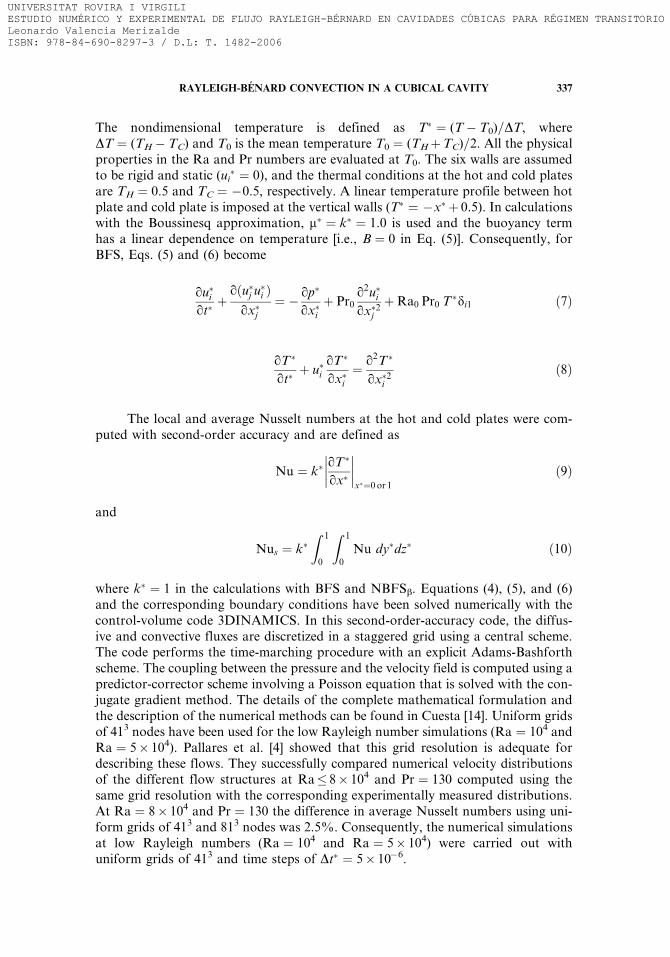
The nondimensional temperature is defined as T� ¼ (T� T0)=DT, whereDT ¼ (TH � TC) and T0 is the mean temperature T0 ¼ (THþTC)=2. All the physicalproperties in the Ra and Pr numbers are evaluated at T0. The six walls are assumedto be rigid and static (ui

� ¼ 0), and the thermal conditions at the hot and cold platesare TH ¼ 0.5 and TC ¼ �0.5, respectively. A linear temperature profile between hotplate and cold plate is imposed at the vertical walls (T� ¼ �x� þ 0.5). In calculationswith the Boussinesq approximation, m� ¼ k� ¼ 1.0 is used and the buoyancy termhas a linear dependence on temperature [i.e., B ¼ 0 in Eq. (5)]. Consequently, forBFS, Eqs. (5) and (6) become

qu�iqt�

þqðu�j u�i Þqx�j

¼ � qp�

qx�iþ Pr0

q2u�iqx�2j

þRa0 Pr0 T�di1 ð7Þ

qT�

qt�þ u�i

qT�

qx�i¼ q2T�

qx�2ið8Þ

The local and average Nusselt numbers at the hot and cold plates were com-puted with second-order accuracy and are defined as

Nu ¼ k�qT�

qx�

��x�¼0 or 1

ð9Þ

and

Nus ¼ k�Z 1

0

Z 1

0

Nu dy�dz� ð10Þ

where k� ¼ 1 in the calculations with BFS and NBFSb. Equations (4), (5), and (6)and the corresponding boundary conditions have been solved numerically with thecontrol-volume code 3DINAMICS. In this second-order-accuracy code, the diffus-ive and convective fluxes are discretized in a staggered grid using a central scheme.The code performs the time-marching procedure with an explicit Adams-Bashforthscheme. The coupling between the pressure and the velocity field is computed using apredictor-corrector scheme involving a Poisson equation that is solved with the con-jugate gradient method. The details of the complete mathematical formulation andthe description of the numerical methods can be found in Cuesta [14]. Uniform gridsof 413 nodes have been used for the low Rayleigh number simulations (Ra ¼ 104 andRa ¼ 5� 104). Pallares et al. [4] showed that this grid resolution is adequate fordescribing these flows. They successfully compared numerical velocity distributionsof the different flow structures at Ra� 8� 104 and Pr ¼ 130 computed using thesame grid resolution with the corresponding experimentally measured distributions.At Ra ¼ 8� 104 and Pr ¼ 130 the difference in average Nusselt numbers using uni-form grids of 413 and 813 nodes was 2.5%. Consequently, the numerical simulationsat low Rayleigh numbers (Ra ¼ 104 and Ra ¼ 5� 104) were carried out withuniform grids of 413 and time steps of Dt� ¼ 5� 10�6.



Numerical simulations at Ra ¼ 107 and Pr ¼ 5.9 were conducted with directnumerical simulation (DNS) with nonuniform grids of Nx ¼ 81, Ny ¼ 61, andNz ¼ 61 nodes and time steps of about Dt� ¼ 5� 10�7. According to the large-eddysimulation (LES) reported by Pallares et al. [5], at Ra ¼ 106, the use of time stepsof Dt� ¼ 1.2� 10�6, and nonuniform grids of 613 nodes produces averagedratios between the subgrid-scale viscosity and the molecular viscosity of only 0.5%.Grotzbach [15] deduced criteria to predict grid sizes for accurate direct numericalsimulations of Rayleigh-Benard turbulent flows. These criteria are based on wave-length considerations, boundary-layer-thickness estimates, and on a simplified theo-retical model to calculate the coefficient of a subgrid-scale heat flux model. The meangrid widths used in this work agree with the minimum corresponding to the criteriareported by Grotzbach [15] (see Table 2). The grid used at Ra ¼ 107 has at least 8grid nodes within the thermal boundary layers near the horizontal walls, as shownin Figure 2. Table 3 shows the computational details of the numerical simulationsat Ra ¼ 107.

RESULTS AND DISCUSSION

In this section the influences of the variation of thermal expansion coefficient,viscosity, and thermal conductivity with temperature are presented for the flowstructures at low (Ra ¼ 104 and Ra ¼ 5� 104) and high (Ra ¼ 107) Rayleigh num-bers for water at T0 ¼ 26.0�C (Pr ¼ 5.9).

Laminar Flow: Non-Boussinesq Effects at Low Rayleigh Numbers

We investigate the individual and the combined effects of the dependence of thephysical properties of the fluid on temperature, for two stable, steady, and laminarflow structures. The different cases analyzed are

1. Effects of viscosity and thermal conductivity variation with temperature(NBFSm).

2. Effects of thermal expansion coefficient variation with temperature(NBFSb).

3. Combined effects of viscosity, thermal conductivity, and thermal expansioncoefficient variation with temperature (NBFSmb).

The flow structures are depicted in Figure 3 in terms of isosurfaces of thesecond largest eigenvalue of the velocity gradient tensor (Figures 3a and 3d), follow-ing the method to detect the occurrence of vortex cores [16] and in terms of velocity

Table 2. Required mean grid widths (Dxyz�m ¼ (Dx�mDy�mDz�m)1=3) and horizontal number of nodes

(Ny ¼ Nz) according to the criteria deduced by Grotzbach [15] for turbulent flow at Ra ¼ 107 and Pr ¼ 5.9

Required Required Present Present Present Present

Ra Dxyz�m Ny ¼ Nz Dx�m Dy�m ¼ Dz�m Dxyz�m Ny ¼ Nz

107 0.0174 48 0.0126 0.0168 0.0152 61



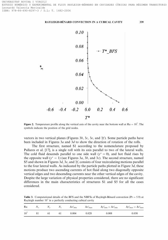
vectors in two vertical planes (Figures 3b, 3c, 3e, and 3f ). Some particle paths havebeen included in Figures 3a and 3d to show the direction of rotation of the rolls.

The first structure, named S1 according to the nomenclature proposed byPallares et al. [17], is a single roll with its axis parallel to two of the lateral walls.The cold fluid descends parallel to one side wall (y� ¼ 0), and hot fluid rises bythe opposite wall (y� ¼ 1) (see Figures 3a, 3b, and 3c). The second structure, namedS5 and shown in Figures 3d, 3e, and 3f, consists of four recirculating motions parallelto the four lateral walls. As indicated by the particle paths plotted in Figure 3d, thesemotions produce two ascending currents of hot fluid along two diagonally oppositevertical edges and two descending currents near the other vertical edges of the cavity.Despite the large variation of physical properties considered, there are no significantdifferences in the main characteristics of structures S1 and S5 for all the casesconsidered.

Table 3. Computational details of the BFS and the NBFSs of Rayleigh-Benard convection (Pr ¼ 5.9) at

Rayleigh number 107 in a perfectly conducting cubical cavity

Ra Nx Ny Nz Dx�min Dx�max Dy�min ¼ Dz�min Dy�max ¼ Dz�max

107 81 61 61 0.004 0.028 0.008 0.030

Figure 2. Temperature profile along the vertical axis of the cavity near the bottom wall at Ra ¼ 107. The

symbols indicate the position of the grid nodes.



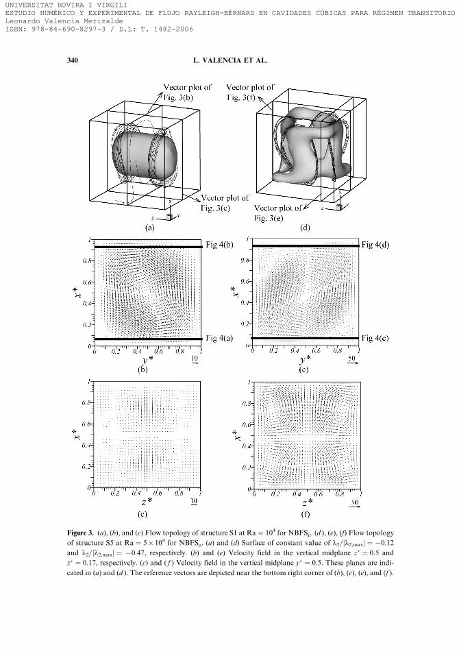
Figure 3. (a), (b), and (c) Flow topology of structure S1 at Ra ¼ 104 for NBFSm. (d ), (e), (f) Flow topology

of structure S5 at Ra ¼ 5� 104 for NBFSm. (a) and (d) Surface of constant value of k2=jk2,maxj ¼ �0.12

and k2=jk2,maxj ¼ �0.47, respectively. (b) and (e) Velocity field in the vertical midplane z� ¼ 0.5 and

z� ¼ 0.17, respectively. (c) and ( f ) Velocity field in the vertical midplane y� ¼ 0.5. These planes are indi-

cated in (a) and (d ). The reference vectors are depicted near the bottom right corner of (b), (c), (e), and (f ).



Figures 4a and 4c show the profiles of the horizontal velocity component (v�)close to the hot wall along the horizontal y� direction for the NBFSs and for the BFSfor structure S1 at Ra ¼ 104 and S5 at Ra ¼ 5� 104, respectively. The horizontalvelocity component (v�) close to the cold wall along the horizontal y� direction isplotted in Figures 4b and 4d.

It can be seen in Figures 4a (S1) and 4c (S5) that, near the hot plate, the absolutevalues of the horizontal velocity components are increased in the NBFSm in comparisonwith the BFS, in agreement with fact that the viscosity decreases with increase of tem-perature. In the NBFSb, the variation of b with temperature (i.e., quadratic dependenceof the buoyancy term on temperature) affects the buoyancy term only close to the hotand cold walls, where the extreme values of temperature occur. As expected, the veloci-ties are generally increased=reduced near the bottom hot walls, in comparison with theBFS (see, for example, y� > 0.4 in Figure 4a and 0.32 > y� > 0.65 in Figure 4c), becauseof the increase=decrease of the buoyancy term near the horizontal walls. It can be seen inFigure 4 that the combined effect of the variation of viscosity, thermal conductivity, andthermal expansion coefficient is basically the addition of the individual effects of thevariation of viscosity and thermal expansion coefficient.

Figure 5 shows the vertical velocity contours in the horizontal midplane(x� ¼ 0.5) of structures S1 and S5 for the BFS and the NBFSs. It can be seen thatfor structure S1 the maximum ascending velocities (u� > 0) are larger in the NBFSm(Figure 5b) than in the BFS (Figure 5a). Correspondingly, the absolute value of thedescending velocities in the BFS are larger in comparison with the NBFSs for struc-ture S1 at Ra ¼ 104. These differences in the absolute values of the velocities in theNBFSm are counterbalanced by the decrease of the area used by the fluid to ascendand the increase of the area where the cold fluid descends. Note that in the BFS bothareas are the same. As shown in Figure 5a, at Ra ¼ 104 the maximum vertical velo-city component (u�) is 3.9% larger for NBFSm, in comparison with BFS, and themaximum absolute value of the descending velocity in the BFS is 4.5% larger com-pared with that of the NBFSm. In the vertical velocity contour of structure S1 corre-sponding to the NBFSb (Figure 5c), the difference between the absolute values of theascending and descending velocities is not significant, considering that the tempera-ture of the fluid is close to the mean temperature (T�

0 ¼ 0) and the effect of thevariation of b with temperature for the NBFSb is very similar than that for theBFS. Figure 5d shows that for the NBFSmb the combined effect of the variation ofall the physical properties is produced mainly by the viscosity variation with tem-perature (i.e., the contours shown in Figures 5b and 5d are very similar).

Figures 5e, 5f, and 5g, corresponding to structure S5 at Ra ¼ 5� 104, show thedifferences between the areas used for the ascending and the descending flows in theBFS, NBFSm, and NBFSb, respectively. It can be seen that the global increase=decrease of the ascending=descending velocities of NBFSs (Figures 5f, 5g, and 5h)in comparison with BFS (Figure 5e) also produces different areas for the ascendingand descending currents.

Table 4 compares the surface-averaged Nusselt numbers in the horizontal andvertical walls of structures S1 and S5 at Ra ¼ 104 and Ra ¼ 5� 104, respectively.When the Boussinesq approximation is considered, the surface-averaged values ofthe Nusselt numbers on the top and bottom walls are the same because the velocityand temperature fields for these flow structures are antisymmetric with respect to the



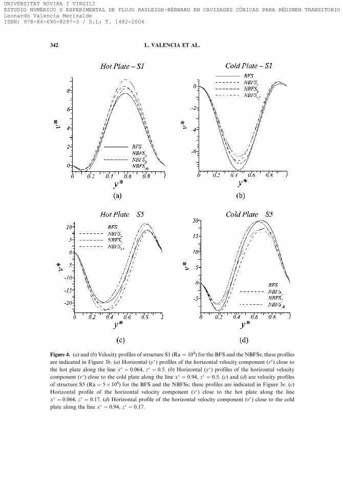
Figure 4. (a) and (b) Velocity profiles of structure S1 (Ra ¼ 104) for the BFS and the NBFSs; these profiles

are indicated in Figure 3b. (a) Horizontal (y�) profiles of the horizontal velocity component (v�) close to

the hot plate along the line x� ¼ 0.064, z� ¼ 0.5. (b) Horizontal (y�) profiles of the horizontal velocity

component (v�) close to the cold plate along the line x� ¼ 0.94, z� ¼ 0.5. (c) and (d) are velocity profiles

of structure S5 (Ra ¼ 5� 104) for the BFS and the NBFSs; these profiles are indicated in Figure 3e. (c)

Horizontal profile of the horizontal velocity component (v�) close to the hot plate along the line

x� ¼ 0.064, z� ¼ 0.17. (d) Horizontal profile of the horizontal velocity component (v�) close to the cold

plate along the line x� ¼ 0.94, z� ¼ 0.17.



Figure

5.Verticalvelocity

contours

(u� )

inthehorizontalmidplane(x

�¼

0.5)for(a)BFS,(b)NBFSm,(c)NBFSb,and(d)NBFSmbatRa¼

104,andfor(e)BFS,(f)

NBFSm,(g)NBFSb,and(h)NBFSmbatRa¼

5�104.Continuous=dashed

linecontours

correspondto

positive=negativevalues.

343


center of the cavity (x� ¼ 0.5, y� ¼ 0.5, z� ¼ 0.5). The macroscopic thermal energybalance for all simulations considered in the present work is fulfilled within 0.3%with respect to the heat flux through the cold plate. As shown in Table 4, the valuesof the surface-averaged Nusselt number at Ra ¼ 104 and Pr ¼ 5.9 are in agreementwith those measured by Leong et al. [2] at Pr ¼ 0.71. The averaged Nusselt numbersat the cold=hot wall of the NBFSm at Ra ¼ 104 are only 1.1%=0.6% smaller=largerthan the corresponding to the BFS. Considering the maximum variation of the ther-mal conductivity (4%), these differences can be attributed to the decrease=increaseof the horizontal velocities of the fluid close to the cold=hot plates in the NBFSm,in comparison with the BFS as shown in Figure 4a. At Ra ¼ 5� 104 the averagedNusselt numbers in the horizontal walls are even less affected by the viscosity vari-ation. The difference is 0.4%=0.7% larger=smaller at the cold=hot wall for NBFSm incomparison with the BFS. The Nusselt numbers for the NBFSb and the NBFSmb aresmaller=larger than those calculated with the Boussinesq approximation and thesedifferences agree with the decrease=increase of the horizontal velocities close tothe cold=hot plates. The increase=decrease of the averaged Nusselt number in thehot=cold plate for the combined effect of the variation of all the physical propertiesis 2.5%=2.9% at Ra ¼ 104 and 4.3%=4.4% at Ra ¼ 5� 104 compared with the BFS.Structure S1, with the axis of rotation parallel to the z� direction, produces a signifi-cant average heat flux through the lateral walls parallel to the axis of rotation of theroll y� ¼ 0 and y� ¼ 1. The average Nusselt numbers at these lateral walls are shownin Table 4. The larger=smaller values of Nus,y� ¼1=Nus,y� ¼0 for NBFSs comparedwith the BFS agree with the increase=decrease of the vertical velocities close to thevertical wall y� ¼ 1=y� ¼ 0 for the NBFSs in comparison with the BFS as shownin Figures 4a and 4b and Figures 5b and 5d.

Table 4. Average Nusselt numbers at the horizontal and vertical walls at low Ra numbers

Ra 104 (S1) 5� 104 (S5)

Pr ¼ 0.71 NusC [2] 1.246� 0.013 —

Pr ¼ 5.9 BFS NusC 1.246 2.676

NusH 1.246 2.676

Nus,y� ¼0 0.390 —

Nus,y� ¼1 0.390 —

NBFSm NusC 1.232 2.687

NusH 1.253 2.658

Nus,y� ¼0 0.381 —

Nus,y� ¼1 0.394 —

NBFSb NusC 1.222 2.536

NusH 1.269 2.820

Nus,y� ¼0 0.374 —

Nus,y� ¼1 0.404 —

NBFSmb NusC 1.215 2.560

NusH 1.282 2.795

Nus,y� ¼0 0.369 —

Nus,y� ¼1 0.413 —



Structures S1 and S5 do not produce any net heat flux on the lateral wallsperpendicular to the axis of their rolling motions in the case of constant physical pro-perties because the heat flux to the side wall generated by the ascending current isthe same as the heat flux from the wall caused by the descending current.

To determine the effects of viscosity, thermal conductivity, and thermal expan-sion coefficient variation with temperature on the mechanisms of the flow, we ana-lyzed the different terms of the vertical momentum equation for the three NBFSsand the BFS. The vertical momentum budget can be written as

0 ¼� 1

RaPr

qp�

qx�1þ 1

Ra

qqx�j

m�qu�1qx�j

þqu�jqx�1

!" #þ ðT� þ BT�2Þ � 1

RaPr

qðu�1u�j Þqx�j

ðPTÞ ðDTÞ ðBTÞ ðCTÞPressure Diffusive term Buoyancy Convective

gradient term term

term ð11Þ

Note that all terms of the x-momentum equation [Eq. (5)] have been displaced to theright-hand side and divided by RaPr to obtain Eq. (11).

Figure 6 shows the horizontal profiles of the different terms of Eq. (11) alongthe line x� ¼ 0.5, z� ¼ 0.5 for structure S1 at Ra ¼ 104 (Figure 6a) and along the linex� ¼ 0.5, z� ¼ 0.17 for structure S5 at Ra ¼ 5� 104 (Figure 6b). These lines havebeen selected to show the x-momentum budget across a horizontal profile of the roll-ing motion. It can be seen in Figure 6 that in the NBFSs and BFS the fluid ascendsand descends mainly due to a balance between the buoyancy, the pressure gradient,and the viscous terms in the vertical momentum equation. Because of the lowRayleigh number, the convective terms do not contribute significantly to the balanceand have been omitted in Figure 6. Figure 6a shows that there is no significant dif-ference in the contribution of the viscous terms between the NBFSs and BFS forstructure S1. The difference can be observed in the contribution of the buoyancyand the pressure gradient terms. For the simulations considering the dependenceof viscosity on temperature (NBFSm and NBFSmb), there is an increase of the buoy-ancy term in the region of ascending fluid ( y� > 0.5, see Figure 6a) which is balancedby an increase of the contribution of the pressure gradient term. In the region wherethe fluid descends ( y� < 0.5, see Figure 6a), the opposite situation occurs (i.e., thedecrease of the buoyancy is balanced by the decrease of the gradient pressure term).The differences between the BFS and the NBFSb in the x-momentum budget are notsignificant at Ra ¼ 104 as shown in Figure 6a because T � is close to T�

0 ¼ 0 inthe horizontal middle plane. Similarly to structure S1, the differences between thex-motion equation budget of the BFS and NBFSs for structure S5 are encounteredin the buoyancy, the pressure gradient, and the diffusive terms. The increase of thebuoyancy term in the region of ascending fluid ( y� < 0.5, see Figure 6b), is balancedby an increase=decrease of the pressure gradient term and by a decrease=increaseof the diffusive terms in the NBFSm=NBFSb. It can be seen in Figure 6 that thecombined effect of the variation of m and b produce larger=smaller contributionsof the buoyancy term for the ascending=descending flows in comparison with



the Boussinesq simulation. In the region of descending fluid, the situation is theopposite to that in the ascending region.

BFS and NBFS of Turbulent Flow at Ra=107

The effect of the variation of m, b, and k with temperature on turbulentRayleigh-Benard flow is analyzed at Ra ¼ 107 using water as a convecting fluid atT0 ¼ 26.0�C (Pr ¼ 5.9). The NBFSs were performed with a temperature differencebetween the hot and cold plates of 17.5�C, which corresponds to a cavity height ofL ¼ 0.031m. This temperature increment produces a variation of b and m of 62%and 40%, respectively (see Table 1).

Figure 7 shows the time-averaged flow field for the NBFSm in terms of anisosurface of the second largest eigenvalue of the velocity gradient tensor [16] (Figure7a) and in terms of velocity vectors in the vertical symmetry planes of the cavity(Figures 7b and 7c). It can be seen that the averaged flow structure consists oftwo main counterrotating vortex rings located near the horizontal walls and eightsmall vortex tubes near the vertices of the cavity (see Figure 7a). The time-averagedtopology is symmetric with respect to the horizontal and vertical midplanes of thecavity. The vortex rings can be understood as a combination of four z rolls (with vor-ticity aligned with the z direction) and four y rolls (with vorticity aligned with the ydirection). The cross sections of the z and y rolls are shown in Figures 7b and 7c,respectively. This time-averaged flow structure is similar to that reported by Pallares

Figure 6. Profiles along the y direction of the terms of the x-momentum budgets [Eq. (9)] for the BFS and

NBFSs. (a) y Profile at x� ¼ 0.5, z� ¼ 0.5 at Ra ¼ 104 for structure S1. (b) y Profile at x� ¼ 0.5, z� ¼ 0.17

at Ra ¼ 5� 104 for structure S5.



et al. [5] at Ra ¼ 106 (Pr ¼ 0.71). The flow structure and velocity fields for the Bous-sinesq simulation and the other non-Boussinesq simulations (NBFSb and NBFSmb)are very similar to those shown in Figure 7 corresponding to NBFSm and conse-quently have been omitted.

The flow at Ra ¼ 107 presents large fluctuations in the velocity and tempera-ture fields with respect to the time-averaged values. Table 5 shows the values ofthe integral scale, the number of integral scales sampled (t�t =T �), and the time-averaged fluctuations of the surface-averaged Nusselt number on the cold plate(NuC) and u�, v�, and T� at the position x� ¼ 0.5, y� ¼ 0.75, and z� ¼ 0.5. The flowstatistics discussed in this section were obtained by sampling the statisticallydeveloped velocity and thermal fields during t�t ¼ 0:071 nondimensional time units.

Figure 7. Time-average flow fields at Ra ¼ 107 for the NBFSm. (a) Surface of constant value of

k2=jk2,maxj ¼ �0.017. (b) Velocity field in the vertical midplane z� ¼ 0.5 and (c) Velocity field in the

vertical midplane y� ¼ 0.5. These midplanes are indicated in (a). The reference vector is depicted near

the bottom right corner of (b) and (c).



It can be seen in Table 5 that the total integration time ranges from 16 to 146times the integral scale and that the number of data taken to calculate the time-averaged values is enough to assure that variables are statistically steady as indicatedby the low values of the time-averaged fluctuations of the variables analyzed. Con-sidering the averaged modulus of the velocity vector as a typical velocity scale of theflow, the distance covered by a fluid particle during the sampling time is about 32times the cavity height. Table 6 shows that the averaged Nusselt number at the coldplate is about 2% smaller for the NBFSm and NBFSmb in comparison with the BFSand NBFSb. This trend produced by the larger viscosity near the cold top is alsoobserved for structure S1 at Ra ¼ 104 in Table 4. The root-mean-square (RMS)values of the Nusselt numbers at Ra ¼ 107 at the horizontal walls are almost thesame in the NBFSs and the BFS. Table 6 shows that the averaged Nusselt numberat the cold plate and the corresponding RMS value are almost the same in theNBFSs and the BFS. The volume-averaged modulus of the velocity vector is 451.9nondimensional velocity units for the BFS, 449.9 for the NBFSm, 455.2 for theNBFSb, and 458.0 for the NBFSmb. The standard deviations of the quantitiessampled at position x� ¼ 0.5, y� ¼ 0.75, z� ¼ 0.5 and their volume-averaged valuesin the averaged flow field do not show significant differences between the BFSand the NBFSs.

Table 5. Integral scale (T �), number of integral scales sampled (t�t=T �Þ and n�0 for average Nusselt number

in the cold plate NuC and for u�; v�; and T� at the point x� ¼ 0:5; y� ¼ 0:75; and z� ¼ 0:5 with a total

integration time of t�t ¼ 0:071

Integral scale (T �) (t�t=T �) n�0

Ra ¼ 107 BFS

NuC 2.1� 10�3 33 8.2� 10�15

u� 7.9� 10�4 90 1.3� 10�15

v� 4.3� 10�3 16 8.5� 10�16

T� 8.1� 10�4 87 �3.4� 10�14

Ra ¼ 107 NBFSm

NuC 5.1� 10�4 138 1.2� 10�15

u� 1.2� 10�3 58 1.2� 10�14

v� 3.5� 10�3 20 7.8� 10�15

T� 1.8� 10�3 39 �7.6� 10�15

Ra ¼ 107 NBFSb

NuC 5.5� 10�4 128 �3.2� 10�15

u� 8.7� 10�4 81 �1.4� 10�15

v� 5.4� 10�4 131 �4.9� 10�16

T� 2.0� 10�3 35 �2.4� 10�16

Ra ¼ 107 NBFSmb

NuC 4.8� 10�4 146 �1.2� 10�14

u� 9.1� 10�4 78 1.8� 10�14

v� 1.5� 10�3 47 1.4� 10�14

T� 9.7� 10�4 73 �7.9� 10�15



The time-averaged vertical x-momentum budget can be written as

0 ¼ � 1

RaPr

qpqx�1

þ 1

Ra

qqx�j

m�qu�1qx�j

þqu�jqx�1

!" #þ 1

Ra

qqx�j

m�0qu�01qx�j

þqu�0jqx�1

!24

35

ðPTÞ ðDTÞ ðFVSTÞ

� 1

RaPr

qðu�1 u�j Þqx�j

� 1

RaPr

qðu�10u�j

0Þqx�j

þ T� þ B � T�2� �

ðCTÞ ðTTÞ ðBTÞ ð12Þ

The terms of Eq. (12) are, from left to right, the pressure gradient term (PT), the dif-fusive terms (DT), the fluctuating viscous stresses terms (FVST), the convectiveterms (CT), the turbulent transport terms (TT), and the buoyancy term (BT).

Figure 8 shows the different terms of Eq. (10) along the vertical line (y� ¼ 0.012,z� ¼ 0.5) near the side wall y� ¼ 0. This line has been selected to identify differencesbetween the NBFSs and BFS because it is located within the corresponding thermaland momentum boundary layers, where the influence of the variation of the physicalproperties is expected to be important. For the sake of clarity, the convective terms,

Table 6. Statistical values for average Nusselt number, vertical and horizontal velocities, and temperature

at the position (x� ¼ 0.5, y� ¼ 0.75, z� ¼ 0.5) at Ra ¼ 107

Mean value, �nn RMS, r RMSv

Ra ¼ 107 BFS

NuC 16.82 0.72 —

u� 29.6 374.4 202.9

v� �496.1 198.2 135.7

T� �2.2� 10�3 0.06 0.0434

Ra ¼ 107 NBFSm

NuC 16.43 0.67 —

u� 184.2 383.8 203.0

v� �472.5 203.5 136.2

T� 2.2� 10�2 0.06 0.0431

Ra ¼ 107 NBFSb

NuC 16.75 0.75 —

u� 50.5 374.6 199.4

v� �518.0 175.8 134.3

T� 5.8� 10�3 0.06 0.0431

Ra ¼ 107 NBFSmb

NuC 16.44 0.65 —

u� 28.41 394.5 201.9

v� �468.5 197.9 135.9

T� 1.5� 10�2 0.05 0.0431



the turbulent transport terms, and the fluctuating viscous stresses terms have beenomitted in Figure 8 because their contributions to the momentum budget alongthe selected line are very small in comparison with those of the pressure gradientterms, the diffusive terms, and the buoyancy term.

It can be seen in Figures 7b and 8 that, near the vertical wall y� ¼ 0, the fluidascends=descends from the hot=cold plate due to the buoyancy term which is mainlybalanced by the diffusive term. The contribution of the pressure gradient term agreeswith the increase and decrease of the x momentum near the vertical wall y� ¼ 0 gen-erated by the rolling motions (Figure 7b). Figure 8 shows that the vertical compo-nent of the pressure gradient is favorable (dP�=dx� < 0) for the ascending flownear x� ¼ 0.1. Correspondingly, the pressure gradient is favorable (dP�=dx� > 0)for the descending flow near x� ¼ 0.9. This term acts as a sink in the vertical momen-tum equation near the horizontal walls and near the horizontal midplane of thecavity (x� ¼ 0.5). It can be seen in Figure 8 that, in general, the contributions ofthe different terms in the near-wall momentum budgets are not greatly affected bythe changes in viscosity, thermal conductivity, and thermal expansion coefficient.However, this figure shows small differences in the viscous terms for the NBFSsand BFS. In the NBFSm, the ascending=descending flow has smaller=larger viscosity(i.e., lower=higher viscous term contribution) than in the BFS. This difference in thecontribution of the viscous terms for the NBFSm and BFS is balanced by the verticalpressure gradient term. In the NBFSb, the temperature of the fluid is larger=smaller

Figure 8. Vertical x profile at y� ¼ 0.012, z� ¼ 0.5 of the x-momentum equation budget at Ra ¼ 107

calculated for the BFS and the NBFSs. This profile is indicated in Figure 7b.



in the lower=higher half of the cavity, and this produces a decrease=increase of thebuoyancy term in comparison with the Boussinesq simulation. These changes inthe buoyancy term are mainly counterbalanced by the corresponding changes ofthe diffusive term. In the NBFSmb, the changes of the buoyancy term in comparisonwith the BFS are similar to those obtained in the NBFSb. However, these changesare balanced by changes in the gradient pressure term as in the NBFSm. It can be seenin Figure 8 that the individual influence of the dependence of m and b on temperaturein the diffusive terms is cancelled when the variation of both physical properties isconsidered and the contributions of the diffusive terms of BFS and NBFSmb are verysimilar.

CONCLUSIONS

Laminar and turbulent Rayleigh-Benard convection of water (T0 ¼ 26.0�C,Pr ¼ 5.9) in a perfectly conducting cavity have been studied considering constantphysical properties, variable viscosity and thermal conductivity, variable thermalexpansion coefficient, and the combined influence of the simultaneous variation ontemperature of these three properties. We considered a temperature increment of17.5�C between the bottom hot wall and the top cold wall. This maximum tempera-ture difference produces variations of 62% in thermal expansion coefficient, 40% inthe viscosity, and variations of only 4.5% in the thermal conductivity of water, withrespect to the corresponding values at the reference temperature (T0 ¼ 26.0�C). Thevariation of the thermal expansion coefficient and viscosity is well above the limit of10% usually considered for the adoption of the Boussinesq approximation. At lowRayleigh numbers (Ra ¼ 104 and Ra ¼ 5� 104), the variation of viscosity and ther-mal expansion coefficient produce an increase=decrease of the maximum horizontalvelocity of about 5% near the hot=cold plate due to the decrease=increase ofviscosity with temperature and the increase=decrease of the buoyancy term in thex-momentum equation. When the variations of viscosity, thermal conductivity,and thermal expansion coefficient with temperature are considered, the averagedNusselt numbers on the cold=hot wall are about 3% (Ra ¼ 104) and 4.5%(Ra ¼ 5� 104) larger=smaller in comparison with the corresponding values obtainedwith constant physical properties. At Ra ¼ 107 the time-averaged properties of theturbulent flow are not significantly affected by the dependence on temperature ofthe physical properties analyzed. The volume-averaged modulus of the velocity isonly 1.3% greater in the NBFSmb than in the BFS. The maximum differences inthe averaged Nusselt numbers at the horizontal plates is 1% for the four simulationscarried out at this Rayleigh number. There are also no significant differences in thecontribution of the different terms of the momentum budget within the vertical ther-mal and momentum boundary layer, where the viscous terms are important and thusthe variation of viscosity with temperature is not negligible. It can be concluded that,for the flow conditions analyzed in this work, a variation of 62% of the thermalexpansion coefficient and 40% of the viscosity have very limited influence on theflow. Consequently, the limit of a variation of 10% in the physical properties forthe applicability of the Boussinesq approximation suggested by Gray and Giorgini[10] can be considered too restrictive, especially for turbulent flows in which the



temperature gradients, and thus the effects of the variation of the physical properties,are restricted to the thin thermal boundary layers.

REFERENCES

1. D. W. Pepper and K. G. T. Hollands, Summary of Benchmark Numerical Studies for3-D Natural Convection in an Air-Filled Enclosure, Numer. Heat Transfer A, vol. 42,pp. 1–11, 2002.

2. W. H. Leong, K. G. T. Hollands, and A. P. Brunger, Experimental Nusselt Numbers for aCubical-Cavity Benchmark Problem in Natural Convection, Int. J. Heat Mass Transfer,vol. 42, no. 11, pp. 1979–1989, 1999.

3. J. Pallares, F. X. Grau, and F. Giralt, Flow Transitions in Laminar Rayleigh-BenardConvection in a Cubical Cavity at Moderate Rayleigh Numbers, Int. J. Heat Mass Trans-fer, vol. 42, pp. 753–769, 1999.

4. J. Pallares, M. P. Arroyo, F. X. Grau, and F. Giralt, Experimental Laminar Rayleigh-Benard Convection in a Cubical Cavity at Moderate Rayleigh and Prandtl Numbers,Exp. Fluids, vol. 31, no. 2, pp. 208–218, 2001.

5. J. Pallares, I. Cuesta, and F. X. Grau, Laminar and Turbulent Rayleigh-Benard Convec-tion in a Perfectly Conducting Cubical Cavity, Int. J. Heat Fluid Flow, vol. 23, pp. 346–358, 2002.

6. M. Manga, D. Weeraratne, and S. J. S. Morris, Boundary-Layer Thickness and Instabil-ities in Benard Convection of a Liquid with a Temperature-Dependent Viscosity, Phys.Fluids, vol. 13, pp. 802–805, 2001.

7. R. A. Trompert and U. Hansen, On the Rayleigh Number Dependence of Convectionwith a Strongly Temperature-Dependent Viscosity, Phys. Fluids, vol. 10, pp. 351–360,1998.

8. L. N. Moresi and V. S. Solomatov, Numerical Investigation of 2D Convection withExtremely Large Viscosity Variations, Phys. Fluids, vol. 7, pp. 2154–2162, 1995.

9. V. S. Solomatov, Scaling of Temperature- and Stress-Dependent Viscosity Convection,Phys. Fluids, vol. 7, pp. 266–274, 1995.

10. D. D. Gray and A. Giorgini, The Validity of the Boussinesq Approximation for Liquidsand Gasses, Int. J. Heat Mass Transfer, vol. 19, pp. 545–551, 1976.

11. F. P. Incropera and D. P. DeWitt, Fundamentals of Heat and Mass Transfer, 4th ed.,pp. 846–847, Wiley, New York, 1996.

12. M. C. Potter and D. C. Wiggert, Mec�aanica de Fluidos, 2d ed., pp. 754–755, Prentice Hall,Mexico, 1998.

13. J. P. Holman, Heat Transfer, 4th ed., p. 503, McGraw-Hill Kogakusha, Tokyo, 1976.14. I. Cuesta, Estudi Numeric de Fluxos Laminars i Turbulents en una Cavitat Cubica, Ph.D.

thesis, Universitat Rovira i Virgili, Tarragona, Spain, pp. 40–64, 1993.15. G. Grotzbach, Spatial Resolution Requirements for Direct Numerical Simulation of the

Rayleigh-Benard Convection, J. Comput. Phys., vol. 49, pp. 241–264, 1983.16. J. Jeong and F. Hussain, On the Identification of a Vortex, J. Fluid Mech, vol. 285,

pp. 69–80, 1995.17. J. Pallares, I. Cuesta, F. X. Grau, and F. Giralt, Natural Convection in a Cubical Cavity

Heated from Below at Low Rayleigh Numbers, Int. J. Heat Mass Transfer, vol. 39,pp. 3233–3247, 1996.



Anexo B1


4thInternational Conference on Computational Heat and Mass Transfer

Proceedings of 4th ICCHMT May 17-20, 2005, Paris-Cachan, FRANCE

ICCHMT’05 - 333

NUMERICAL AND EXPERIMENTAL STUDY OF TURBULENT RAYLEIGH-BÉNARD CONVECTION OF WATER IN A CUBICAL CAVITY

Leonardo Valencia, Jordi Pallares, Ildefonso Cuesta and Francesc Xavier Grau

Department of Mechanical Engineering University Rovira i Virgili, Avinguda dels Països Catalans 26, 43007, Tarragona, Spain

Correspondence author: Fax:+34 977559691 Email: [email protected]

ABSTRACT Experimental measurements and numerical simulations of natural convection in a partially conducting cubical cavity heated from below and cooled from above are reported at turbulent Rayleigh numbers (Ra=107 and Ra=7×107) and water as a convective fluid (Pr=6.0). The numerical simulations were carried out with a second order finite volume code without any turbulence model because the time-steps and grid sizes used are adequate for the time and spatial resolution requirements reported in previous direct numerical simulations of Rayleigh-Bénard flows. The Boussinesq approximation was considered in the simulations according to the thermal conditions and the dimensions of the cavities used in the experiments. The Particle Image Velocimetry (PIV) technique was used to measure the two velocity components parallel to a vertical mid-plane of the cavity. If the heat conduction through the sidewalls is considered in the simulations, there is a general agreement between the predicted time averaged local velocities and those experimentally measured in the vertical mid-planes. NOMENCLATURE L vertical dimension of the cavity (m) N number of grid points d thickness of the sidewalls Greek letters β thermal expansion coefficient (1/K) δij Kronecker delta ∆ increment λ2 second largest eigenvalue of the velocity

gradient tensor σ standard deviation (root-mean square –

RMS) θ autocorrelation function T integral time scale (s)

Superscripts and subscripts S surface averaged quantity * non-dimensional quantity C cold plate H hot plate f fluid g glass walls t total value of integration 0 reference value at the mean temperature

time average value V volume averaged value W wall INTRODUCTION Numerical simulations of natural convection flows have been extensively performed and analysed in the laminar and turbulent regimes. Some authors have identified different flow structures in a cubical cavity heated from below. For example, at low Rayleigh numbers, Ozoe et al. [1], predicted a single roll structure (ascending and descending flows close to two opposed lateral walls) and Hernandez and Frederick [2] reported the toroidal roll which consists of four ascending currents of flow close to the vertical edges of the cavity and a single descending one along the vertical symmetry axis of the cavity. At turbulent Rayleigh numbers Pallares et al. [3] reported the time-averaged velocity and temperature fields of large–eddy simulations of Rayleigh-Bénard convection of a Boussinesq fluid with a Prandtl number of 0.71 in a perfectly conducting cubical cavity at Ra=106 and Ra=108. Valencia et al. [4] studied the effects of a non-Boussinesq fluid in a cubical cavity with perfectly conducting sidewalls at Ra=107 using water as a convecting fluid. Non-Boussinesq simulations were calculated with a variation of 62% and 40% of the thermal expansion coefficient and viscosity respectively between cold and hot plates. These authors found that the overall turbulent flow



topology and the average Nusselt number in the cold plate were not significantly affected by the effects of the physical properties variation with temperature. These variations were well above the 10% of the usually accepted value to consider the Boussinesq approximation (Gray and Giorgini [5]). Leong et al. [6] measured the averaged Nusselt numbers at the cold plate of a perfectly conducting cubical cavity filled with air and with isothermal horizontal walls. These authors studied the range 104≤Ra≤108 and three angles of inclination of the cavity. The objective of the present study is to compared and validate the calculated averaged-velocity field considering partially conducting lateral walls at the turbulent Rayleigh numbers 107 and 7×107 with those measured experimentally with the PIV technique for a cubical cavity heated from below. EXPERIMENTAL The experimental set-up used in the present work to measure the velocity field is similar to that used by Arroyo and Savirón [7]. Two cubical cavities were constructed (Lx= Ly= Lz=50 mm at Ra=107 and Lx= Ly= Lz=92 mm at Ra=7×107) with 4-mm-thick glass lateral walls and horizontal copper plates. Table 1 shows the experimental conditions used in the experiments for the two cavities. During the experiments the copper blocks were kept at constant temperatures within ±0.01ºC. The top block was cooled by recirculating water from a thermostatic bath and the bottom block was heated with an electrical resistance controlled by a Proportional – Integral - Derivative (PID) digital control. The lateral thermal boundary conditions of the experiments are fixed by the thickness and the material (glass) of the side walls. These conditions can be characterized by the conductance defined by

**gg

fLk

1dkLkC == (1)

Equation 1 shows that for small thickness (L* 0) or small thermal conductivity of the wall (k* 0) insulation is obtained (C ∞) while values of C close to zero indicates a perfectly conducting condition. Under the thermal conditions of the experiments the values of conductance are C=9.6 and C=17.7 for the cavities with dimensions L=50 mm and L=92 mm, respectively. These values are not as great/small to consider adiabatic/perfectly conducting walls.

Particle Image Velocimetry (PIV): The velocity fields were measured with the PIV method. This technique allows the simultaneous measurement of two components of the velocity in an illuminated plane of the flow. The cross-correlation between two images of the fluid seeded with particles was carried out with an in-house Matlab code. The images were acquired with a digital CCD camera (Motion Scope PCI 1000 S). The appropriate time intervals chosen between images were 5/10 frames per second at Ra=107/ Ra=7×107 to obtain maximum particle displacements of about 1.8 mm (3-15 pixels). The size of the images were 50 × 50 mm to keep the size of the particles (2-3 pixels of diameter) in the images of all the experiments. The images with a resolution of 420×420 pixels were divided into 27×27 overlapped interrogation windows of 32×32 pixels (3.81×3.81 mm). More details of the experimental technique can be found in Raffel et al. [8].

Table 1. Operation Conditions of the Experiments

Exp.Nº

Cavity size L (m)

∆T=TC-TH (ºC)

T0 (ºC) Ra0 Pr0

1 0.050 4.3 26.0 107 6.0 2 0.092 5.0 25.5 7×107 6.0

NUMERICAL METHOD The physical model consists in a cubical cavity full of water (Pr=6.0) with rigid glass lateral walls of thickness dg=4mm and thermal conductivity kg=0.78 W/m ºC. A sketch of the cell and the coordinate system adopted are shown in Figure 1. The two horizontal walls are also rigid and isothermal. Radiation heat transfer, compressibility effects and viscous dissipation are neglected. The Boussinesq approximation was adopted according to Valencia [4]. The maximum variation of the relevant physical properties is 18%/15% for β and 11%/9.7% for µ at Ra=7×107/ Ra=107. The three-dimensional governing dimensionless equations in Cartesian coordinates are: The continuity equation:

0*

*

=∂∂

i

i

xu (2)

The momentum equations:

*

*

*

**

*

* )(

ij

iji

xp

xuu

tu

∂∂−=

∂∂

+∂∂



1

*002*

*2

0 i

j

i TrPRax

urP δ+∂

∂+ (3)

and the thermal energy equation:

2*

*2

*

**

*

*

iii x

TxTu

tT

∂∂=

∂∂+

∂∂ (4)

And the thermal energy equation for the walls is

2*

*2*

*

*

ixT

tT

∂∂=

∂∂ α (5)

where α*=αg/αf, is the relation between thermal diffusivity of the glass and thermal diffusivity of water (αg=3.4×10-7 m2/s and αf=1.4×10-7 m2/s)[9]. For normalization we use the cavity length L for distance, α0/L for velocity, L2/α0 for time and α0

2ρ0/L2 for pressure. The non-dimensional temperature is defined as T*=(T-T0)/∆T where ∆T=(TH-TC) and T0 is the mean temperature T0=(TH+TC)/2. All physical properties are evaluated at T0. The six walls are assumed to be rigid and static (ui

*=0) and the thermal conditions at the hot and cold plates are TH=0.5 and TC=-0.5, respectively. A typical constant convective heat transfer coefficient for air in vertical walls (h=3.64 W/m2 ºC) [9] was considered to set the boundary condition on the outer surface of the lateral walls and the temperature for the surrounding air is assumed to be T0. According to the low value of this heat transfer coefficient, a perfect adiabatic boundary condition was used in the outer surface of the sidewalls for the simulations. Computations of Equations (2), (3), (4) and (5) and the corresponding boundary conditions have been solved numerically with the second order accuracy control volume code 3DINAMICS. The details of the complete mathematical formulation and the description of the numerical methods can be found in Cuesta [12]. Direct numerical simulations at the Rayleigh numbers considered in this study, were conducted with non-uniform grids and time steps of about ∆t*=3×10-7.

Figure 1. Sketch showing the configuration and coordinates

of the cubical cell

The grid resolution used has at least 7 grid nodes within the thermal boundary layers near the horizontal walls for the Rayleigh numbers studied. Table 2 shows the computational details of the numerical simulations at Ra=107 and Ra=7×107. RESULTS AND DISCUSSION The numerical results of the time-averaged flow structures and the averaged Nusselt numbers in the horizontal cold plate and the measured and numerically predicted time-averaged velocity field in a vertical mid-plane of the cavity are reported in this section at Rayleigh numbers Ra=107 and Ra=7×107. As initial conditions for the simulations, an instantaneous velocity and thermal field at Ra=107 and Pr=5.9 in a cavity with perfectly conducting lateral walls computed by Valencia et al. [4] was used. The time averaged flow structures found at Ra=107 and Ra=7×107 are shown in Figure 2 in terms of isosurfaces of the second largest eigenvalue of the velocity gradient tensor following the method to detect the occurrence of vortex cores proposed by Jeong and Hussein [13] and in terms of velocity vectors in the vertical mid-plane (z*=0.5 and y*=0.5) of the cavity. At Ra=107, the averaged flow structure is very similar to that reported by Valencia et al. [4] at the same Rayleigh number for a cavity with a perfectly conducting lateral walls. It consists in two main counter rotating vortex rings located near the horizontal walls and eight small vortex tubes near the vertices of the cavity (see Figure 2(a)). The time-averaged topology is symmetric with respect to the horizontal and vertical mid-planes of the cavity. The vortex rings can be understood as a combination of four z-rolls (with vorticity aligned with the z-direction) and four y-rolls (with vorticity aligned with the y-direction). The numerically predicted and the measured cross section of the z-rolls are shown in Figures 2(b) and 2(c), respectively. It can be seen a good qualitative agreement between the calculated and the measured velocity fields.

Table 2.

Computational Details of the Simulations at Pr=6.0 and at Rayleigh Numbers 107 and 7×107

Nx Ny Nz ∆x*min ∆x*max ∆y*min=∆z*min

∆y*max=∆z*max

81 61 61 0.004 0.028 0.008 0.030

Cold plate

Glass walls

Hot plate



The averaged flow structure at Ra=7×107 also consists in two main counter rotating vortex rings located near the horizontal walls. However the rings are not symmetric with respect to the horizontal mid-plane as shown in Fig 2(e) and 2(f). This flow structure can be also understood as a combination of four z-rolls and four y-rolls, however in this case two of the diagonally opposed rolls are larger and are located further from the horizontal walls than the other two diagonally opposed rolls. On average, the two larger rolls of the top/bottom ring cause that the main descending/ascending flows occur close to two diagonally opposed vertical edges (y=0mm, z=92mm and y=92mm, z=0mm). The measured velocity vector fields of this structure, shown in Fig 2(f), were taken in two different periods of time of about 30 minutes in order to keep the same image resolution in all the experiments. It can be seen that there is also a good qualitative agreement between numerical and experimental velocity vectors indicating that the experimental flow structures are well predicted by the numerical simulations. The flow at Ra=107 and Ra=7×107 present large fluctuations in the velocity and temperature fields with respect to the time averaged values. Table 3 shows the values of the integral scale and the number of integral scales sampled (t t*/ T *) of the surface averaged Nusselt number on the cold plate (NuC) and u*, v* and T* at the position x*=0.5, y*=0.75 and z*=0.5. The flow statistics discussed in this section were obtained at Ra=107 and Ra=7×107 by sampling the statistically developed velocity and thermal fields during tt*=0.39 and tt*=0.14 non-dimensional time

units, respectively. It can be seen that the total integration time ranges from 61-631 times the integral scale and consequently the number of data taken is adequate to calculate the time averaged values. Considering the averaged modulus of the velocity vector as a typical velocity scale of the flow, the distance covered by a fluid particle during the sampling time is about 113/150 times the cavity height at the Rayleigh number 107/7×107. Table 3 also shows the mean value ( *n ) and the standard deviation (RMS (n*)) of NuC, u*, v* and T* at the position x*=0.5, y*=0.75 and z*=0.5 and the standard deviation of u*, v* and T* in the average-velocity and temperature fields ( )( *

VnRMS ). The mean value and the standard deviation of the averaged Nusselt number at the cold plate at Ra=107 are very similar to those reported by Valencia et al. [4] at the same Rayleigh number with perfectly conducting lateral walls. The mean value/standard deviation is only 1.3%/4.2% smaller/larger for the present study. However the volume averaged modulus of the velocity vector is 290 non-dimensional velocity units, a 36% smaller for the simulation with a finite value of thermal conductivity in comparison with the value reported by Valencia et al. [4] in a perfectly conducting cavity. It also can be seen in Table 3 the general increase of the mean values and RMSs at Rayleigh number 7×107 compared with 107 caused by the increase of turbulence level of the flow. Figure 3. shows the numerical and experimental velocity profiles indicated in Figures 2(b) and 2(c) at Ra=107 and in Figures 2(e) and 2(f) at Ra=7×107.

Table 3.

Integral Scale (T *), Number of Integral Scales Sampled (t t*/ T *) and Statistical Values for Average Nusselt Number in the Cold Plate (NuC) and for u*, v* and T* at the Point x*=0.5, y*=0.75 and z*=0.5.

Ra=107

(t t* =0.39) Integral scale (T *) (t t*/ T *)Mean value

( *n ) RMS (n*),

σ(n*) )( *VnRMS

NuC 6.2×10-4 631 16.6 0.75 u* 4.7×10-3 84 59.6 468.8 249.1 v* 6.5×10-3 61 -233.3 239.1 160.6 T* 6.3×10-4 624 -1.6×10-3 0.04 0.18

Ra=7×107 (t t* =0.14) Integral scale (T *) (t t*/ T *)

Mean value ( *n )

RMS (n*), σ(n*) )( *

VnRMS

NuC 1.2×10-3 117 35.1 1.12 u* 6.2×10-4 233 1151.5 1089.0 883.5 v* 1.3×10-3 109 -256.3 733.6 704.7 T* 3.5×10-4 411 5.9×10-3 0.02 0.14



y (mm)

x(m

m)

0 10 20 30 40 500

10

20

30

40

50

2

y (mm)

x(m

m)

0 10 20 30 40 500

10

20

30

40

50

2

X

YZ

z (mm)

x(m

m)

0 20 40 60 800

20

40

60

80

5

z (mm)

x(m

m)

0 20 40 60 800

20

40

60

80

5

Z

X

Y

y (mm)

u(m

m/s

)

0 10 20 30 40 50-2.0

-1.5

-1.0

-0.5

0.0

0.5

1.0

1.5

2.0

z (mm)

u(m

m/s)

0 10 20 30 40 50 60 70 80 90-3.0

-2.0

-1.0

0.0

1.0

2.0

w (mm/s)

x(m

m)

-0.5 0.0 0.5 1.0 1.5 2.00

10

20

30

40

50

60

70

80

90

v (mm/s)

x(m

m)

-0.5 0.0 0.5 1.00

10

20

30

40

50

PIV, t(min)=30.36DNS, 358800 steps, t(min)=68.53

DNS, 717000 steps, t(min)=136.95DNS, 358200 steps, t(min)=68.42

PIV, t(min)=30.45DNS, 219900 steps, t(min)=30.97

DNS, 784800 steps, t(min)=110.5

DNS, 159600 steps, t(min)=20.96DNS, 211200 steps, t(min)=29.74

DNS, Perfectly conducting lateral wallsp ( )

The velocity profiles were plotted for three/two sets of simulations at Ra=107/Ra=7×107, averaged during 30/68 minutes of time (0.11/0.07 non-dimensional time units), in order to compare with experimental data which were taken during 31/30 minutes. The profiles depicted at Ra=107 (Figures 3(a) and 3(b)) show qualitative and quantitative agreement between the experimental and the calculated velocity values. The maximum differences between the experimental and the numerical vertical velocities (Figure 3(a)) are about 30%. These differences can be observed in Fig. 3(a) close to y=25mm for the third set of the numerical simulations and can be attributed to the short integration time (30 minutes) used in the experiments at this Rayleigh number. Figure 3(a) also shows the vertical velocity profile of the time averaged flow structure in a perfectly conducting

cavity at Ra=107 reported by Valencia et al. [4]. It can be seen that velocities are about 110% larger for the perfectly conducting cavity indicating that the effect of the thermal conductivity of the walls is important in the simulations to reproduce the experimental measurements. In Figure 3(b) the horizontal velocity profiles also show that the maximum differences between experiments and simulations is found for the third set of numerical results. This difference is about 15% close to x=25 mm. The maximum difference between the numerical and the experimental horizontal velocities is lower than that found for the vertical velocity component. This can be attributed to the larger intensity of the fluctuations of the vertical velocity component in comparison with that of the horizontal velocity component as shown in the RMS values of Table 3.

Vector plot of Fig. 2(e) Vector plot of Fig. 2(b) (a) (d) Fig. 3(b) Fig. 3(d) Fig 3(c) Fig. 3(a) (b) (e) Fig. 3(b) Fig. 3(d) Fig. 3(c) Fig. 3(a) (c) (f)

Figure 2. (a), (b), (c)/ (d), (e), (f) Time average flow field at

Ra=107/ Ra=7×107 (t t* =0.39 (110.5 min) / t t* =0.14 (136.95 min)) (a) and (d) surface of constant

value of λ2/|λ2,max|=-0.02 and λ2/|λ2,max|=-0.03, respectively. (b), (e) and (c), (f) numerical and

experimental velocity fields in the vertical mid-planes. The reference vectors are depicted near the

bottom right corner of (b), (c), (e) and (f).

(a) (b) (c) (d)

Figure 3.

Velocity profiles for three sets of simulations, for the total integration time and for the experimental data. (a) and (b)/(c) and (d) velocity profiles of the average flow topology at Ra=107/ Ra=7×107. (a)

and (c), horizontal (y) profiles of the vertical velocity component (u) along the lines x=11.1 mm and x=55.7 mm. (b) and (d), vertical (x) profiles of

the horizontal velocity component (v) along the lines y=45.2 mm and z=85.4 mm.



Figures 3(c) and 3(d) show the velocity profiles indicated in Figs. 2(c) and 2(f) at Ra=7×107. The main differences between the measured velocities and the numerically predicted are found for values around zero (see Figure 3(c) in 40mm<z<60mm and Figure 3(d) in 40mm<x<60mm). This can be explained considering the large relative error of the PIV technique to measure the in-plane velocity components lower than 0.1 mm/s (i.e. 1 pixel of displacement). It should be noted that the decrease of the frame rate (i.e. increase of the time between images) leads to a reduction of the correlation between the images. This reduction is specially observed in the interrogation windows in which the velocity component perpendicular to the illuminated plane is much larger than the in-plane velocity components. CONCLUDING REMARKS The time averaged Rayleigh-Bénard flow structures at turbulent Rayleigh numbers (Ra=107 and Ra=7×107) predicted numerically are in agreement with those measured using the PIV technique. The simulations were performed considering the conduction heat transfer through the lateral glass walls of the experimental cavities. Although the overall flow structure and averaged heat transfer rates are not significantly dependent on the thermal conductivity of the walls, differences on the time averaged velocity fields of about 110% are observed between simulations in cavities with perfectly conducting sidewalls and the simulations of the cavities with glass lateral walls used in the experiments. ACKNOWLEDGMENTS This study was financially supported by the Spanish Ministry of Science of Technology under projects DPI2003-06725-C02-01 and VEM2003-20048. REFERENCES 1. Ozoe, H., Yamamoto, K., Churchill, S. W. and

Sayama, H, 1977, Three-dimensional, Numerical Analysis of Laminar Natural Convection in a Confined Fluid Heated From Below, J. Heat Transfer, 98, pp. 202-207.

2. Hernández, R. and Frederick, R. L., 1994, Spatial and Thermal Features of Three Dimensional Rayleigh-Bénard Convection, Int. J. Heat Mass Transfer 37 (3), pp. 411-424.

3. Pallares, J., Cuesta, I., and Grau, F. X., 2002, Laminar and Turbulent Rayleigh-Bénard Convection in a Perfectly Conducting Cubical Cavity, Int. J. Heat and Fluid Flow, 23, pp. 346-358.

4. Valencia, L., Pallares, J. Cuesta, I. and Grau, F. X., 2005, Rayleigh - Bénard Convection of Water in a Perfectly Conducting Cubical Cavity: Effects of Temperature - Dependent Physical Properties in Laminar and Turbulent Regimes, Numerical Heat Transfer, Part A, 47, pp. 1-20. (to appear)

5. Gray, D. D., and Giorgini, A., 1976, The Validity of the Boussinesq Approximation for Liquids and Gasses, Int. J. Heat Mass Transfer, 19, pp. 545-551.

6. Leong, W. H., Hollands, K. G. T., and Brunger, A. P., 1999, Experimental Nusselt Numbers for a Cubical-Cavity Benchmark Problem in Natural Convection, Int. J. Heat and Mass Transfer, 42 (11), pp. 1979-1989.

7. Arroyo, M. P., and Savirón, J. M., 1992, Rayleigh – Bénard Convection in a Small Box: Spatial Features and Thermal Dependence of the Velocity Field, J. Fluid Mech., 235, pp. 325-348.

8. Raffel, M., Willert C., and Kompenhans, J., 1998, Particle Image Velocimetry, 1st edition, Springer, Germany.

9. Holman, J. P., 1976, Heat Transfer, 4th edition, Mc Graw-Hill Kogakusha Ltd., Tokyo.

10. Incropera, F. P., and DeWitt, D. P., 1996, Fundamentals of Heat and Mass Transfer, 4th edition, John Wiley and Sons, New York.

11. Potter, M. C. and Wiggert, D. C., 1998, Mecánica de Fluidos, 2nd edition, Prentice Hall, México.

12. Cuesta, I., 1993, Estudi Numéric de Fluxos Laminars i Turbulents en una Cavitat Cúbica. Ph.D. thesis, Universitat Rovira i Virgili, Tarragona, Spain.

13. Jeong, J. and Hussain, F., 1995, On the Identification of a Vortex, J. Fluid Mech, 285, pp. 69–80.


Anexo B2


TURBULENT RAYLEIGH-BÉNARD CONVECTION OF WATER IN CUBICAL CAVITIES: NUMERICAL STUDY AND EXPERIMENTAL VALIDATION

Leonardo Valencia, Jordi Pallares, Ildefonso Cuesta and Francesc Xavier Grau Department of Mechanical Engineering

University Rovira i Virgili, Avinguda dels Països Catalans 26, 43007, Tarragona, Spain Correspondence author: Fax:+34 977559691 Email: [email protected]

ABSTRACT Experimental measurements and numerical simulations of natural convection in a cubical cavity heated from below and cooled from above are reported at turbulent Rayleigh numbers using water as a convective fluid (Pr=6.0). The numerical simulations were carried out, in the range 107≤Ra≤108, with a second order finite volume code without any turbulence model because the time-steps and grid sizes used are adequate for the time and spatial resolution requirements reported in previous direct numerical simulations of Rayleigh-Bénard flows. The Boussinesq approximation was considered in the simulations according to the thermal conditions and the dimensions of the cavities used in the experiments. The Particle Image Velocimetry technique was used to measure the two velocity components parallel to a vertical mid-plane of the cavity at Ra=107, Ra=7×107 and Ra=108. Both experiments and simulations show that at Ra=107 the time averaged flow structure consists in two horizontal counter-rotating vortex rings located near the horizontal walls of the cavity. At the higher Rayleigh numbers considered, the simulations predict an unsteady single roll motion in which the direction of the axis of rotation rotates in the horizontal plane with very low frequencies. This rotation produces a time averaged flow structure similar to that found at Ra=107. There is a general agreement between the predicted time averaged local velocities and those experimentally measured if the heat conduction through the sidewalls occurring in the experiments is considered in the simulations. NOMENCLATURE A heat transfer area (m2) L vertical dimension of the cavity (m) N number of grid points Greek letters β thermal expansion coefficient (1/K) δij Kronecker delta ∆ increment λ2 second largest eigenvalue of the velocity gradient tensor σ standard deviation (root-mean square – RMS) θ autocorrelation function T integral time scale (s) Superscripts and subscripts S surface averaged quantity * non-dimensional quantity C cold plate H hot plate f fluid g glass walls

1


t total value of integration 0 reference value at the mean temperature

time average value V volume averaged value W wall 1. INTRODUCTION Flows in cubical cavities have been extensively used for validation of CFD codes because of the geometrical simplicity. Although the advantages that the numerical investigation offers, it is important to note that it is essential to perform measurements of the physically-realizable numerical simulations in order to verify their accuracy and significance. Numerical simulations of natural convection flows have been extensively performed and analysed in the laminar and turbulent regimes. Some authors have identified different flow structures in a cubical cavity heated from below. For example, at low Rayleigh numbers, Ozoe et al.[1], predicted a single roll structure with ascending and descending flows close to two opposed lateral walls and Hernandez and Frederick [2] reported the toroidal roll which consists of four ascending currents of flow close to the vertical edges of the cavity and a single descending one along the vertical symmetry axis of the cavity. These structures and other two were reported and classified by Pallares et al. [3]. At turbulent Rayleigh numbers, Pallares et al.[4] reported the time-averaged velocity and temperature fields of large–eddy simulations of Rayleigh-Bénard convection of a Boussinesq fluid with a Prandtl number of 0.71 in a perfectly conducting cubical cavity at Ra=106 and Ra=108. Valencia et al. [5] studied the non-Boussinesq effects of water [6] in a cubical cavity with perfectly conducting sidewalls at Ra=107. Leong et al. [10] measured the averaged Nusselt numbers at the cold plate of a perfectly conducting cubical cavity filled with air and with isothermal horizontal walls. These authors studied the range 104≤Ra≤108 and three angles of inclination of the cavity but the flow topologies were not reported. The effect of the thermal boundary conditions of natural convection flows confined by walls of finite thickness and thermal conductivity was investigated by Kim and Viskanta [7]. These authors demonstrated that the use of ideal thermal boundary conditions that neglect the interaction between the heat transfer convection of the fluid and the thermal conduction across the walls in numerical simulations was not a good approximation to reproduce experimental flows of air in cavities with Lexan lateral walls. Ahlers [8] showed that the experimental method of substraction of the conductance of the empty cell to estimate the conductance of the sidewalls could lead to errors of 20% in the Nusselt number and an important underestimation of the exponent γ of the Rayleigh number in the correlation (Nu= Nu0Raγ). The numerical results reported by Verzicco [9], who studied the effects of a sidewall with finite thermal conductivity in a cylindrical enclosure, showed that the additional heat transfer across the lateral fluid/wall interface produces an important effect on the flow and Nusselt numbers. The objective of the present study is to compare and validate the calculated averaged-velocity field of the turbulent Rayleigh-Bénard flow structures found in a cubical cavity with partially conducting lateral walls with those measured experimentally with the Particle Image Velocimetry (PIV) technique. The experimental setup and the numerical techniques are described in Sections 2 and 3, respectively, and the results are presented and discussed in Section 4. 2. EXPERIMENTAL The experimental set-up used in the present work to measure the velocity field is similar to that used by Arroyo and Savirón [11] (Figure 1). Two cubical cavities were constructed (Lx= Ly= Lz=50mm at Ra=107 and Lx= Ly= Lz=92mm at Ra=7×107 and Ra=108) with 4-mm-thick glass lateral walls and 5-mm-thick horizontal copper plates. Table 1 shows the experimental

2


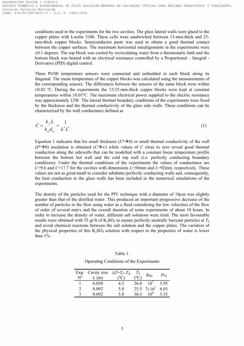
conditions used in the experiments for the two cavities. The glass lateral walls were glued to the copper plates with Loctite 3106. These cells were sandwiched between 15-mm-thick and 25-mm-thick copper blocks. Semiconductor paste was used to obtain a good thermal contact between the copper surfaces. The maximum horizontal misalignments in the experiments were ±0.1 degrees. The top block was cooled by recirculating water from a thermostatic bath and the bottom block was heated with an electrical resistance controlled by a Proportional – Integral - Derivative (PID) digital control. Three Pt100 temperature sensors were connected and embedded in each block along its diagonal. The mean temperature of the copper blocks was calculated using the measurements of the corresponding sensors. The differences between the sensors of the same block were within ±0.02 ºC. During the experiments the 15/25-mm-thick copper blocks were kept at constant temperatures within ±0.01ºC. The maximum electrical power supplied to the electric resistance was approximately 12W. The lateral thermal boundary conditions of the experiments were fixed by the thickness and the thermal conductivity of the glass side walls. These conditions can be characterized by the wall conductance defined as

**

1Lkdk

LkC

gg

f == (1)

Equation 1 indicates that for small thickness (L* 0) or small thermal conductivity of the wall (k* 0) insulation is obtained (C ∞) while values of C close to zero reveal good thermal conduction along the sidewalls that can be modelled with a constant linear temperature profile between the bottom hot wall and the cold top wall (i.e. perfectly conducting boundary conditions). Under the thermal conditions of the experiments the values of conductance are C=9.6 and C=17.7 for the cavities with dimensions L=50mm and L=92mm, respectively. These values are not as great/small to consider adiabatic/perfectly conducting walls and, consequently, the heat conduction in the glass walls has been included in the numerical simulations of the experiments. The density of the particles used for the PIV technique with a diameter of 10µm was slightly greater than that of the distilled water. This produced an important progressive decrease of the number of particles in the flow using water as a fluid considering the low velocities of the flow of order of several mm/s and the overall duration of some experiments of about 10 hours. In order to increase the density of water, different salt solutions were tried. The most favourable results were obtained with 55 gr/lt of K2SO4 to ensure perfectly neutrally buoyant particles at T0 and avoid chemical reactions between the salt solution and the copper plates. The variation of the physical properties of this K2SO4 solution with respect to the properties of water is lower than 1%.

Table 1.

Operating Conditions of the Experiments

Exp. Nº

Cavity sizeL (m)

∆T=TC-TH(ºC)

T0 (ºC) Ra0 Pr0

1 0.050 4.3 26.0 107 5.952 0.092 5.0 25.5 7×107 6.033 0.092 5.8 30.3 108 5.35

3


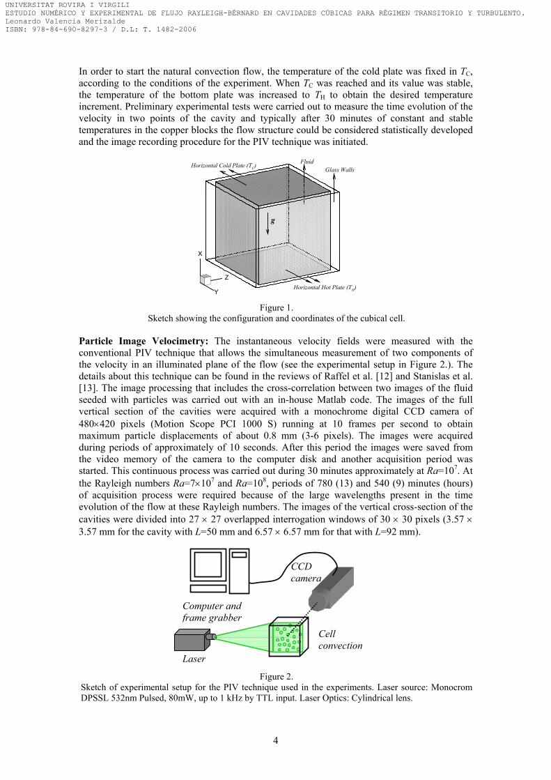
In order to start the natural convection flow, the temperature of the cold plate was fixed in TC, according to the conditions of the experiment. When TC was reached and its value was stable, the temperature of the bottom plate was increased to TH to obtain the desired temperature increment. Preliminary experimental tests were carried out to measure the time evolution of the velocity in two points of the cavity and typically after 30 minutes of constant and stable temperatures in the copper blocks the flow structure could be considered statistically developed and the image recording procedure for the PIV technique was initiated.

X

Z

YHorizontal Hot Plate (TH)

Horizontal Cold Plate (TC)

g

FluidGlass Walls

Figure 1. Sketch showing the configuration and coordinates of the cubical cell.

Particle Image Velocimetry: The instantaneous velocity fields were measured with the conventional PIV technique that allows the simultaneous measurement of two components of the velocity in an illuminated plane of the flow (see the experimental setup in Figure 2.). The details about this technique can be found in the reviews of Raffel et al. [12] and Stanislas et al. [13]. The image processing that includes the cross-correlation between two images of the fluid seeded with particles was carried out with an in-house Matlab code. The images of the full vertical section of the cavities were acquired with a monochrome digital CCD camera of 480×420 pixels (Motion Scope PCI 1000 S) running at 10 frames per second to obtain maximum particle displacements of about 0.8 mm (3-6 pixels). The images were acquired during periods of approximately of 10 seconds. After this period the images were saved from the video memory of the camera to the computer disk and another acquisition period was started. This continuous process was carried out during 30 minutes approximately at Ra=107. At the Rayleigh numbers Ra=7×107 and Ra=108, periods of 780 (13) and 540 (9) minutes (hours) of acquisition process were required because of the large wavelengths present in the time evolution of the flow at these Rayleigh numbers. The images of the vertical cross-section of the cavities were divided into 27 × 27 overlapped interrogation windows of 30 × 30 pixels (3.57 × 3.57 mm for the cavity with L=50 mm and 6.57 × 6.57 mm for that with L=92 mm).

Laser

Cell convection

CCD camera

Computer and frame grabber

Figure 2. Sketch of experimental setup for the PIV technique used in the experiments. Laser source: MonocromDPSSL 532nm Pulsed, 80mW, up to 1 kHz by TTL input. Laser Optics: Cylindrical lens.

4


3. NUMERICAL METHOD The physical model consists in a cubical cavity full of water (Pr=6.0) with rigid lateral glass walls of thickness dg=4mm and thermal conductivity kg=0.78 W/m ºC. A sketch of the cell and the coordinate system adopted are shown in Figure 1. The two horizontal walls are considered isothermal. Radiation heat transfer, compressibility effects and viscous dissipation are neglected. Table 2, shows the relevant physical properties of the fluid and the maximum variation of physical properties between the cold and hot temperatures for the present simulations and experiments. It can be seen that the maximum variation is only 18% for β at Ra=7×107. The variation of the physical properties at Rayleigh numbers 3×107 and 5×107 shown in Table 2 corresponds to a cavity with L=0.092 mm and Pr0=6.0. For the simulations at Ra=107, Ra=7×107 and Ra=108 the experimental conditions shown in Table 1 were adopted. According to previous studies [5] at Ra=107 and Pr=5.9, the differences in the flow structure and averaged Nusselt numbers are not significant between a Boussinesq simulation and a simulation considering the variation of 62%/40% in β/µ between cold and hot plates and consequently the Boussinesq approximation is adopted in the present simulations.

Table 2.

Values of the Physical Properties at the Mean Temperature and their Variation with temperature expressed as (

0100*)(% TTT nnnn

CH−= )

Ra β0 [14] kg/m s %β µ0 [15]

kg/m s %µk0 [16] W/m K %k Cp0 [16]

J/kg K %Cp ρ0 [16] kg/m3 %ρ

107 2.64×10-4 15.4 8.7×10-4 9.7 0.61 1.2 4160 0.14 996.2 0.103×107 2.61×10-4 7.6 8.8×10-4 4.7 0.61 0.6 4157 0.07 996.3 0.055×107 2.61×10-4 12.6 8.8×10-4 7.9 0.61 1.0 4157 0.11 996.3 0.087×107 2.59×10-4 18.0 8.8×10-4 11.2 0.61 1.4 4160 0.16 996.4 0.11

108 3.04×10-4 17.5 8.0×10-4 12.1 0.62 1.5 4163 0.17 995.2 0.14

Considering a Boussinesq fluid and a three-dimensional unsteady flow, the governing dimensionless equations in Cartesian coordinates are: the continuity equation:

0*

*

=∂∂

i

i

xu

, (2)

the momentum equations:

*

*

*

**

*

* )(

ij

iji

xp

xuu

tu

∂∂

−=∂

∂+

∂∂

1*

002*

*2

0 i

j

i TrPRax

urP δ+∂

∂+ , (3)

the thermal energy equation:

2*

*2

*

**

*

* )(

ii

i

xT

xTu

tT

∂∂

=∂

∂+

∂∂

, (4)

and the thermal energy equation for the walls:

2*

*2*

*

*

ixT

tT

∂∂

=∂∂ α , (5)

5


where α*=αg/αf, is the relation between thermal diffusivity of the glass and thermal diffusivity of water (αg=3.4×10-7 m2/s and αf=1.4×10-7 m2/s)[16]. The scales used for length, velocity, time and pressure are L, α0/L, L2/α0 and α0

2ρ0/L2, respectively. The non-dimensional temperature is defined as T*=(T-T0)/∆T where ∆T=(TH-TC) and T0 is the mean temperature T0=(TH+TC)/2. The six walls are assumed to be rigid and static (ui

*=0) and the thermal conditions at the hot and cold plates are TH

*=0.5 and TC*=-0.5, respectively. The lateral thermal boundary conditions for the

fluid are fixed by the dimension and the material of the lateral vertical walls of the cavities used in the experiments. According to the values of the conductance of the lateral walls, the heat thermal conduction along the walls of the cavity was calculated solving Equation 5. The physical properties of the glass at 20ºC relevant for the simulations are kg=0.78 W/m ºC, Cpg=840 J/kg ºC and ρg=2700 kg/m3 [16]. The Rayleigh number of the air around the cavities based on the height and the maximum temperature difference of the cavities is 4×107, 3×108 and 3.3×108 in experiments Nº 1, Nº 2 and Nº 3, respectively (Table 1). To set the boundary condition on the outer surface of the lateral walls a typical constant convective heat transfer coefficient for air in vertical walls (h=3.64 W/m2 ºC) [16] was considered. This value of the heat transfer coefficient produces negligible heat transfer rates between the sidewalls and the surrounding air in comparison with the heat conduction transferred across the walls from the hot plate to the cold plate and the heat transfer between the walls and the convecting fluid. Consequently, a perfectly adiabatic boundary condition was imposed at the outer surface of the sidewalls for the simulations to model the experimental thermal conditions of the lateral walls. The dimensional average heat transfer rates, integrated over the whole surface (S) of a particular horizontal wall (W), can be defined as,

=+= −− gWfWW qqq10*

*

*

orx

fWSfW

f dSxT

Sk

LT

fW=

−−

∫− ∂

∂∆−

10**

*

orx

gWSgW

g dSxT

Sk

LT

gW=

−−

∫− ∂

∂∆−

, (6)

where the first term on the right hand side is the averaged heat flux density exchanged between the horizontal walls and the fluid and the second term represents the heat flux from the horizontal walls to the lateral walls with finite thickness. It can be seen in Equation (6) that, by definition, positive values of average heat transfer indicate an average input of thermal energy from the horizontal walls to the fluid or the glass walls and negative average values indicate heat transfer from the system to the horizontal isothermal plates. The average Nusselt number in the horizontal walls can be calculated using Equation 7:

10*

**

*

* *

1

orx

fWSfW

W dSxT

SNu

fW=

−−

∫− ∂

∂= , (7)

By definition, the sum of the average heat transfer rates on the six walls of the cavity is zero for a statistically steady time-averaged flow. The global energy balance (qt

*) of the system can be written as follows:

∫−

−

=−=−−

∂∂

+∂∂

==*

*

1*,*

*

0*,*

*

** 10

fWS fWxfWxfWfW

t dSxT

xT

Sq ∫

−−

=−=−−

∂∂

+∂∂

+*

*

1*,*

*

0*,*

*

*

**

fWS fWxgWxgWfW

dSxT

xT

SAk

, (8)

where A* is the relation between heat transfer areas (A*=AW-g/AW-f with A*=2.89 for L=50mm and A*=5.19 for L=92mm) and k* the relation between the thermal conductivities of the glass and the fluid (k*=kg/kf =1.31).

6


Equations (2), (3) , (4) and (5) and the corresponding boundary conditions have been solved numerically with the control volume code 3DINAMICS. In this second order accuracy code, the diffusive and convective fluxes are discretized in a staggered grid using a central scheme. The code performs the time-marching procedure with an explicit Adams–Bashforth scheme. The coupling between the pressure and velocity field is computed following a predictor and a step corrector which involves the solution of a Poisson equation with the conjugate gradient method. The details of the complete mathematical formulation and the description of the numerical methods can be found in Cuesta [17]. Numerical simulations at the Rayleigh numbers considered in this study, were conducted with non-uniform grids of Nx=81, Ny=61 and Nz=61 nodes and the heat transfer across the lateral walls was calculated using 8 additional nodes in the perpendicular direction of each wall at Ra=107, Ra=3×107 and Ra=5×107 and 5 additional nodes at Ra=7×107 and Ra=108. The range of time steps used were from ∆t*=2×10-7 for the highest Rayleigh number (Ra=108) to ∆t*=5×10-7 for the lowest (Ra=107). Large-eddy simulations of the flow at Ra=108 and Pr0=6 were initially carried out with the dynamically localized subgrid scale (SGS) model used by Pallares et al. [4] to check the subgrid scale contribution for the computational conditions of the present study. It was found that at Pro=6, the maximum time-averaged ratios between the local subgrid-scale viscosity and the molecular viscosity in the cavity were only 0.1% with a standard deviation of 0.2%. These small contributions agree with those reported by Pallares et al. [4] at lower Prandtl number (Pr=0.7). As shown in Figure 3, the grid resolution used has 3 grid nodes within the time-average thermal boundary layers near the horizontal walls at the highest Rayleigh number studied (Ra=108). Table 3 shows the minimum and maximum grid spacing of the mesh used in the numerical simulations.

T*

x*

-0.4 -0.2 0 0.2 0.40.00

0.02

0.04

0.06

0.08

0.10Ra=107

Ra=3x107

Ra=5x107

Ra=7x107

Ra=108

Figure 3. Temperature profile along the vertical axis of the cavity near the bottom wall at Ra=107, Ra=3×107,Ra=5×107, Ra=7×107 and Ra=108. The symbols indicate the position of the grid nodes.

Table 3.

Minimum and maximum grid spacing of the mesh used in the numerical simulations at Pr=6.0 and at Rayleigh numbers 107, 3×107, 5×107, 7×107 and 108.

Nx Ny Nz ∆x*min ∆x*max ∆y*min=∆z*min ∆y*max=∆z*max 81 61 61 0.004 0.028 0.008 0.030

7


4. RESULTS AND DISCUSSION The numerical results of the time-averaged flow structures and the averaged Nusselt numbers in the horizontal cold plate are reported in this section at Ra=107, Ra=3×107, Ra=5×107, Ra=7×107 and Ra=108, and the measured and numerically predicted time-averaged velocity field in a vertical mid-plane of the cavity are compared at Rayleigh numbers Ra=107, Ra=7×107 and Ra=108. As initial conditions for the simulations, an instantaneous velocity and thermal field at Ra=107 and Pr=5.9 in a cavity with perfectly conducting lateral walls computed by Valencia et al. [5] was used. The results at higher Rayleigh numbers were obtained from instantaneous flow fields using a step change of the Ra number. Numerical and experimental results at Rayleigh number 107 The time averaged flow structure numerically obtained at Ra=107 is shown in Figure 4 in terms of isosurfaces of the second largest eigenvalue of the velocity gradient tensor following the method to detect the occurrence of vortex cores proposed by Jeong and Hussein [18] (Fig. 4.a) and in terms of two isosurfaces of the vertical velocity component (Fig. 4.b). The average flow and temperature fields and the flow statistics at Ra=107 were obtained by sampling the statistically developed velocity and thermal fields during tt*=1.61 non-dimensional time units (tt=456min of dimensional time considering a cavity of L=50mm). This sampling period was started after tt*=0.7 from the initial conditions. The time averaged flow topology at this Rayleigh number can also be seen in Figure 5 in terms of the velocity vectors field in the vertical mid-planes (z*=0.5 and y*=0.5) of the cavity (see Figures 5.a and 5.b). The averaged flow structure at Ra=107 is very similar to that reported by Valencia et al. [5] at the same Rayleigh number for a cavity with a perfectly conducting lateral walls. As shown in Figures 4.a and 4.b it consists in two main counter rotating vortex rings located near the horizontal walls and eight small vortex tubes near the vertices of the cavity. The time-averaged topology is symmetric with respect to the horizontal and vertical mid-planes of the cavity. The vortex rings can be understood as a combination of four z-rolls (with vorticity aligned with the z-direction) and four y-rolls (with vorticity aligned with the y-direction), as shown in Figures 5.a and 5.b. The numerically predicted and the measured cross section of the z-rolls are shown in Figures 5.b and 5.c, respectively. These figures show a good agreement between the calculated and the measured velocity fields and RMS values of the vertical velocity (u) contours. It can be seen that, the numerically predicted local values of the standard deviation of the vertical velocity are greater than those experimentally measured. Lecordier et al. [19] reported the standard deviation of the horizontal velocity component of homogeneous turbulence calculated from synthetic images with a conventional PIV algorithm. These authors compared the RMS values calculated with different sizes of interrogation windows with the original results obtained from direct numerical simulations and found that the greater the size of the interrogation window the lower the estimated values of the standard deviation due to the filtering of the larger velocities when the autocorrelation is calculated in large interrogation windows. The differences between the simulations and the PIV calculations of the generated images using window sizes of 32×32 were about 5%. The present results, obtained with interrogation windows of 30×30 pixels show, maximum differences obtained for the standard deviation of the vertical velocities between the simulations and the measurements of about 10% (see contours of Figs. 5.b and 5.c). The differences can be also attributed to the error introduced by the PIV technique when out-of-plane loss of pairs of particles occurs in a fully three-dimensional instantaneous flow as the one considered. It should be noted that with constant time interval between images it is not possible to obtain the same accuracy in the measurement of the maximum and minimum velocities.

8


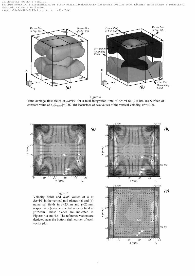
X

Z

Y

u*=300AscendingFluid

Vector Plotof Fig. 5(b)

Vector Plotof Fig. 5(a)

u*=-300DescendingFluid

X

Z

Y



Figure 4. Time average flow fields at Ra=107 for a total integration time of t t* =1.61 (7.6 hr). (a) Surface of constant value of λ2/|λ2,max|=-0.02. (b) Isosurface of two values of the vertical velocity, u*=±300.

(b) (a)

1.2

1.4

1.6

1.00.5

1.0

z (mm)

x(m

m)

0 10 20 30 40 500

10

20

30

40

50

2

Fig. 6(c)

Fig. 6(a)

Fig. 6(b)

0.5

1.0

1.2

1.40.8

0.8

z (mm)

x(m

m)

0 10 20 30 40 500

10

20

30

40

50

2

Fig. 6(c)

Fig. 6(a)

Fig. 6(b)

0.51.0

1.2

1.4

1.0 1.6

y (mm)

x(m

m)

0 10 20 30 40 500

10

20

30

40

50

2

Figure 5. Velocity fields and RMS values of u atRa=107 in the vertical mid-planes. (a) and (b)numerical fields in z=25mm and y=25mm,respectively (c) experimental velocity field iny=25mm. These planes are indicated inFigures 4.a and 4.b. The reference vectors aredepicted near the bottom right corner of eachvector plot.

(c)

(b)(a)

9


The instantaneous maximum velocities are usually associated with out-of-plane loss of particle pairs. This produces an underestimation of the measurement of the large fluctuations of the flow, which leads to the reduction of the corresponding RMS values. The comparison of the contours of the fluctuation intensities of vertical velocity component in Figures 5.b and 5.c shows that the greater the RMS values, the greater the difference between experimental and numerical results. For example, in Figures 5.b and 5.c the value of the RMS near the bottom wall is 0.5 at z=30mm and x=2mm for both the simulations and the measurements. However, the differences are clearly seen near the vertical walls where the intensities of the fluctuations attain the maximum values. As an example the RMS of the measured vertical velocity component is 1.4 and 1.6 for the simulations at z=46mm and x=22mm. The flow at the Rayleigh numbers studied presents large fluctuations in the velocity and temperature fields with respect to the time averaged values. The first six rows of Table 4 show the values of the integral scale and the number of integral scales sampled (t t*/ T *), at Ra=107, of the surface averaged Nusselt number on the cold plate (NuC), the global energy balance (qt

*) and u*, v* and T* at the position x*=0.5, y*=0.75 and z*=0.5. It can be seen that the total integration time, at this Rayleigh number, ranges from 191-2920 times the integral scale and consequently the number of data taken is adequate to calculate the time averaged values. Considering the averaged modulus of the velocity vector as a typical velocity scale of the flow, the distance covered by a fluid particle during the sampling time is about 456 times the cavity height. Table 4 also shows the mean value ( *n ) and the standard deviation (RMS (n*)) of NuC, qt

*, u*, v* and T* at the position x*=0.5, y*=0.75 and z*=0.5. It can be seen that the RMS values are significantly larger than the time averaged values for the vertical velocity component and temperature indicating an intensive turbulent transfer across the horizontal midplane. The mean value and the standard deviation of the averaged Nusselt number at the cold plate at Ra=107 are very similar to those reported by Valencia et al. [5] at the same Rayleigh number with perfectly conducting lateral walls. The mean value/standard deviation is only 1.3%/4.2% smaller/larger for the present study. Figures 6.a and 6.b show the numerical and experimental time-averaged velocity profiles indicated in Figures 5.b and 5.c at Ra=107. These profiles show qualitative and quantitative agreement between the experimental and the calculated velocity values. The maximum differences between the experimental and the numerical vertical velocities are about 20% and can be observed in Figure 6.a close to the left wall (z=2mm). This can be attributed to the error introduced by the finite size of the interrogation volumes used in the PIV technique when the velocity is measured in regions with large velocity gradients. It should be noted that the correlation between the interrogation window and the target window capture the mean displacement of the particles contained in this region. In the case of the 50mm cavity the interrogation window is 3.6×3.6mm and the calculated velocities close to the walls can range between 0.0 to 1.4 mm/s (see the numerical profiles in Fig. 6.a). As expected, the measured value is lower, approximately 1.15mm/s. In Figure 6.b the horizontal velocity profiles also show good agreement with the greater differences close to the wall velocities. This difference is about 17% close to x=2mm and x=48mm. The maximum differences between the numerical and the experimental horizontal velocities are lower than those found for the vertical velocity component at Ra=107. This can be attributed to the larger intensity of the fluctuations of the vertical velocity component in comparison with that of the horizontal velocity component as shown in the RMS values of Table 4 and to the greater velocity gradients obtained for the vertical velocities compared with those obtained for the horizontal velocities.

10


11

Table 1

Integral scale (T *), number of integral scales sampled (t t*/ T *) and statistical values for average Nusselt number in the cold plate (NuC), the global energy balance (qt

*) and for u*, v* and T* at the point x*=0.5, y*=0.75 and z*=0.5.

Ra=107 (t t* =1.61)

Integral scale (T *) (t t*/ T *)Mean value

( *n ) RMS (n*), σ(n*)

NuC 6.2×10-4 2595 16.6 0.76 u* 8.3×10-3 195 25.0 466.1 v* 4.9×10-3 331 -226.6 233.9 T* 8.5×10-3 191 -1.3×10-4 0.04 qt

* 5.5×10-4 2920 1.0×10-3 1.02

Ra=3×107 (t t* =0.85)


( *n ) RMS (n*), σ(n*)

NuC 4.1×10-4 2066 25.1 0.95 u* 6.5×10-2 13 365.8 926.4 v* 3.1×10-3 274 -207.2 470.4 T* 2.5×10-2 35 3.8×10-3 0.03 qt

* 3.7×10-4 2273 -2.8×10-3 1.35

Ra=5×107 (t t* =0.75)


( *n ) RMS (n*), σ(n*)

NuC 1.2×10-3 636 30.7 1.05 u* 1.9×10-1 4 -511.2 1147.9 v* 2.6×10-3 285 -264.17 610.4 T* 3.5×10-2 21 -4.5×10-3 0.025 qt

* 1.0×10-3 719 -2.5×10-3 1.48

Ra=7×107 (t t* =0.86)


( *n ) RMS (n*), σ(n*)

NuC 1.4×10-3 631 35.0 1.15 u* 9.7×10-2 9 121.4 1513.8 v* 7.7×10-4 1111 -266.9 734.2 T* 7.9×10-2 11 5.5×10-4 0.024 qt

* 8.7×10-4 985 7.6×10-4 1.59

Ra=108 (t t* =0.56)


( *n ) RMS (n*), σ(n*)

NuC 2.0×10-4 2822 40.4 1.19 u* 8.1×10-2 7 -645.0 1429.5 v* 5.0×10-4 1116 -329.2 831.5 T* 1.2×10-2 47 -4.1×10-3 0.022 qt

* 6.6×10-4 848 8.4×10-4 1.67 Figure 6.a also shows the vertical velocity profile of the time averaged flow structure in a perfectly conducting cavity at Ra=107 reported by Valencia et al. [5]. It can be seen that close to z=37mm velocities are about 110% larger for the perfectly conducting cavity indicating that the effect of the thermal conductivity of the walls is important in the simulations to reproduce the experimental measurements. Although the averaged Nusselt number at the horizontal walls in the present study are very similar to those calculated with perfectly conducting walls, the volume averaged modulus of the velocity vector is 290 non-dimensional velocity units. That is a


12

v_Partially Conducting Walls

v_Experimental Data

w (mm/s)

x(m

m)

-1.0 -0.5 0.0 0.5 1.00

10

20

30

40

50

u_Partially Conducting Wallsu_Experimental Datau_Conducting Walls

z (mm)

u(m

m/s

)

0 10 20 30 40 50-2.0

-1.5

-1.0

-0.5

0.0

0.5

1.0

1.5

2.0 (a) (b)

Figure 6. Velocity profiles for the simulations and for the experimental data of the average flow topology atRa=107, these profiles are indicated in Figures 5.b and 5.c. (a), horizontal (y) profiles of the verticalvelocity component (u), along the line x=11.1 mm, z=25 mm (z*=0.5). (b), vertical (x) profiles of thehorizontal velocity component (v) along the lines y=4.7 mm, z=25 mm and y=45.2 mm, z=25 mm. Thegray squares indicate the size of the interrogation window used in the experiments

36% smaller for the simulation with a finite value of thermal conductivity in comparison with the value reported by Valencia et al. [5] in a perfectly conducting cavity. This decrease of the velocity values for the present study (also shown in Figure 6.a) can be explained with Figure 7.c. This figure shows the vertical profile (y*=1.041) of the temperature inside the wall of the cavity in the mid-plane z*=0.5, for the simulations with perfectly conducting walls and for the simulations considering finite thermal conductivity in the lateral walls. Figure 7.c reveals that in the lower region of the cavity (x*<0.5), the temperatures for the perfectly conducting lateral walls are larger than simulations with partially conducting heat transfer across the walls. These larger values of temperature produce an overall increase of the buoyancy term in the vertical momentum equation in these regions and, consequently, an increase of the vertical velocities close to the lateral walls in comparison with the present results (see, for example Figure 6.a. at 46mm<z<4mm). Figure 7.a shows the time averaged temperature contour of the fluid close to the glass walls in the vertical planes y*=0.996 and z*=0.004 at Ra=107. It can be seen that the departure from the linear velocity profile of the perfectly conducting conditions is found along all the area of the lateral walls. The temperature contours in the vertical mid-plane including both, the fluid and the lateral walls indicated in Figure 7.a, are depicted in Figure 7.b. This figure shows that more than the 90% of the volume of fluid is between the range T*=–0.1 and T*=0.1 because of the good mixing produced by the mean flow and the turbulence intensities, that restricts the temperature gradients to the thin thermal boundary layers near the horizontal walls of the cavity. The temperature contours in the lateral walls shown in Figure 7.b indicate that the heat transfer in the walls is not only from the hot to the cold plates. It can be seen that the heat is also transferred from the fluid to the walls in the lower part of the cavity and from the walls to the fluid close to the top of the cavity.


13

X

Z

Y

-0.5

0.3

0.0

-0.1

-0.3

-0.15

0.1

0.05

0.15

-0.05

-0.2

0.2

Contour Plotof Fig. 7(b)

(a)

Tw*

x*

-0.4 -0.2 0.0 0.2 0.40.0

0.2

0.4

0.6

0.8

1.0

0.00.0

y*

x*

0.0 0.2 0.4 0.6 0.8 1.00.0

0.2

0.4

0.6

0.8

1.0

-0.1

0.1

0.5

Fluid/Glass WallsBoundary

-0.5Fig.7(c)

0.2

-0.2

(b) (c) Figure 7.

(a) Temperature contours of the average temperature field in the fluid close to the glass walls at Ra=107

(3.2×106 time steps) (b) Temperature contours in the vertical mid-plane. This contour plot is indicated inFigure 7.a. Figure 7(c) show vertical (y*=1.041) temperature profile indicated in the Figure 7(b) for thesimulations with perfectly conducting walls and considering finite conductivity for the heat transferacross the lateral walls.

Partiallyconducting walls

Perfectlyconducting walls

Time evolution of the flow structure at Ra=3×107, Ra=5×107, Ra=7×107 and Ra=108. The time evolution of the average flow structure and the averaged Nusselt number in the cold plate calculated at Rayleigh numbers 3×107, 5×107, 7×107 and 108 are reported in this section. Because of the similitude of the time averaged flow structures found in the range 3×107≤Ra≤108, only the topology at Ra=7×107 will be showed and analyzed in present section. Figure 8.b shows the vertical velocity (u*) as a function of time at Ra=7×107 at the position x*=0.5, y*=0.75 and z*=0.5. This position inside the cavity is indicated in Figures 8.a and 8.c. The time evolution of the vertical velocity component shown in Figure 8.b reveals very low frequencies superimposed to higher ones. These low frequencies produce large periods of time of positive instantaneous values (for example between 0.1 and 0.25 non-dimensional units of time) followed by periods in which the values are negative (for example between 0.3 and 0.5


14

non-dimensional units of time). The different time averaged flow fields obtained by averaging the instantaneous flow during the periods of time corresponding to the low frequencies can be classified into four flow configurations. These four averaged flow structures were obtained by averaging the velocity flow field during different periods of time. Each period of time could contain from 0.03 to 0.16 non-dimensional time units as shown in Table 5. In the cases in which two consecutive short averaging periods were available they usually show the same flow configuration, indicating that the transition had not occurred. However for the long average periods of time it was not possible to clearly identify the flow configurations or the transitions (see for example the period of time between 0.6 and 0.74 non-dimensional time units in the time evolution of the Figure 8.b at Ra=7×107). This periods of time were identified in Table 5 as NA (from Not Available). These four possible configurations of the average flow structure obtained at Ra=7×107 are depicted in Figure 8.c in terms of the vertical velocity contours in the horizontal mid-plane x*=0.5 and each configuration has been identified with the letters (A), (B), (C) and (D). The period of time in which each configuration occurs in the time evolution of the vertical velocity of the analyzed point is indicated above the horizontal axis of Figure 8.b. The averaged flow structure of each configuration consists in two main descending and ascending flows that occur close to two diagonally opposed vertical edges. Figure 9 shows the averaged flow structure in terms of isosurfaces of two values of the vertical velocity for configuration (C) (i.e. ascending fluid near the corner y=92mm, z=0mm and descending fluid near y=0mm, z=92mm). The time averaged flow topology of this configuration can also be seen in Figure 10 in terms of the velocity vectors field in the vertical mid-planes (z*=0.5 and y*=0.5) of the cavity (see Figures 10.a and 10.b). It can be seen that this combination of main ascending and descending flows is associated with a single rolling motion with its axis of rotation horizontally oriented and perpendicular to two diagonally opposed vertical edges of the cavity. Figure 8.c shows that the main difference between the configurations or positions of the flow topology identified in Figure 8.c is the diagonally opposed pair of corners used by the fluid to ascend from the hot plate and descend from the cold plate. For example, Figure 8.c indicates that the positive mean vertical velocities at the position x*=0.5, y*=0.75 and z*=0.5 are found in configurations (C) and (D) and the negative mean vertical velocities occur in configurations (A) and (B). The change of the sign of the instantaneous vertical velocity plotted in Figure 8.b agrees with the changes of the configuration of the structure. The changes from positive to negative mean velocity values indicate that the mean flow structure evolves from (A) to (D) or from (B) to (C) and the changes from negative to positive values, correspond to the inverse evolutions. This change of flow configuration, which has associated a very low frequency, can be understood as a progressive rotation in the horizontal plane of the rotation axis of the single roll flow structure. It can be seen in Figure 8.b that this rotation of the roll axis, or of the overall flow structure, around the vertical axis of the cavity that produces the evolution between two flow configurations can be clockwise (i.e. from (A) to (D)) or anticlockwise (i.e from (A) to (B)). It should be noted that the direct transition from (A) to (C), (C) to (A), (B) to (D) or (D) to (B) are not possible, and in fact have not observed, according to the rotation of the flow structure. The change of orientation of the averaged flow structure also occurs at Rayleigh numbers 3×107, 5×107 and 108. Table 5 shows the observed evolution of the different configurations at these Rayleigh numbers and at Ra=7×107. The series of data labeled as Transition in Table 5 correspond to long intermediate states of the flow between the previous and the subsequent configuration. The evolutions reported in Table 5 correspond to those observed after approximately 0.3 non-dimensional units of time from the step change of the Rayleigh number used as initial conditions and consequently do not include the transient until the flow is statistically fully developed. It can be seen in Table 5 that the flow evolves erratically between the different configurations and that there is not a clear relation between the Rayleigh number


15

and the time in which the flow is in a given configuration or the time needed by the flow to change between configurations.

(C) (A) (D) (A)(D)(A) (B) (B)

(a) (b)

(c)

X

Z

Y

y*=0.75

x*=0.5

z*=0.5

2300

17001000

400

0

-400

400

-400

-1000-1700

-2300

y*

z*

0 0.2 0.4 0.6 0.8 10

0.2

0.4

0.6

0.8

1

-2300

-1700

-1000-400

0

400

1000

17002300

400

-400

y*

z*

0 0.2 0.4 0.6 0.8 10

0.2

0.4

0.6

0.8

1

-2300-1700

-1000-400

0

400

10001700

2300

400

-400

y*

z*

0 0.2 0.4 0.6 0.8 10

0.2

0.4

0.6

0.8

1

2000

1700

1000

400

0-400

-1000-1700

-2000

-400

400

y*

z*

0 0.2 0.4 0.6 0.8 10

0.2

0.4

0.6

0.8

1

(A) (D)

(C) (B)

Position of the time series plotted in Fig. 8.b

Figure 8. (a) Sketch of the position x*=0.5, y*=0.75 and z*=0.5, point of analysis of the time evolution of some variables (see Fig. 8.b and Table 4), (b) Time evolution of the vertical velocity component (u*) in the position pictured in Fig. 8.a, the letters (A), (B), (C) or (D) near the x-axis indicates the configuration (see figure 8.c) of the flow structure in the period of time showed by the parenthesis. (c) Vertical velocity (u*) contours in the horizontal mid-plane for the four possible configurations of the structure found at Rayleigh7×107 (configurations (A), (B), (C) and (D)). Continuous/dashed line contours correspond to positive/negative values. The black point in the contours indicates the position depicted in Fig. 8.a.


16

The observed evolution of the flow between the different configurations in the range 3×107≤Ra≤108 implies different statistical properties of the time evolution of the different variables of the flow. Since these flow transitions, that occur at very low frequencies, can be viewed as a progressive rotation of the overall flow structure with respect to the vertical axis of the cavity, the statistical properties of the variables that are sensitive to the particular configuration of the flow are different from those that are more insensitive to the flow configuration. Table 4 shows that at the Rayleigh numbers in which the single roll is observed (3×107≤Ra≤108) the integral time scales of the vertical velocity and temperature in the horizontal mid plane of the cavity are drastically reduced in comparison with the evolutions of these variables at Ra=107 because of the important contribution of the low frequencies associated with the transition between different flow configurations in their time evolutions (see for example Fig. 8.b). On the contrary the time evolution of other quantities, as the horizontal velocity component, the averaged Nusselt number or the global energy balance, not significantly affected by the evolution between configurations, show integral time scales of the same order of magnitude as those at Ra=107. Table 4 also show that the increase of the RMS values as the Rayleigh is increased is more evident in the variables insensitive to the particular flow configuration than in the sensitive quantities. It is important to note that the influence of the low frequency evolution in the integral time scale of some specific flow quantities should be taken into account to determine adequate sampling periods for the calculation of the flow statistics. The measured average flow fields in the mid-plane at Ra=7×107 and at Ra=108 were taken for a total period of time of 13 and 8 hours respectively. The time evolution of the vertical velocity in the same point evaluated numerically (x*=0.5, y*=0.75 and z*=0.5) showed only high frequencies as opposed to the obtained with the simulations at the same Rayleigh numbers (See for example at Ra=7×107 Figure 8.b). Besides, the average flow structure of the vector field showed good agreement with the average flow configurations obtained numerically (i.e. configurations (A), (B), (C) and (D)). This indicates that the average flow structure experimentally obtained keeps one of the configurations and the change of position is not produced. In order to measure the influence of the horizontal inclination of the cavity, a

X

YZ


u*=1000AscendingFluid


u*=-1000DescendingFluid

Figure 9. Time average flow field at Ra=7×107 for the (C) configuration with a total integration time of tt*=0.16 (156 min) in terms of the isosurface of two values of the vertical velocity u*=±1000. The period of time in which this flow structure occurs can be identified in Table 5 with boldface letters


17

simulation at Ra=7×107 was carried out whit 0.1º of inclination in the y direction and 0.2º in the z direction.

Table 2 Change of configuration of the averaged flow filed at Rayleigh numbers 3×107, 5×107, 7×107

and 108. ∆t*: period of time averaged

Ra 3×107 5×107 7×107 108 ∆t* Conf. ∆t* Conf. ∆t* Conf. ∆t* Conf. 0.11 (D) 0.05 Transition 0.16 (C) 0.09 (B) 0.04 Transition 0.04 (A) 0.03 Transition 0.08 (C) 0.33 (C) 0.06 Transition 0.03 (B) 0.06 Transition 0.12 (B) 0.38 (A) 0.08 (A) 008 (B) 0.05 Transition 0.11 Transition 0.15 NA 0.04 Transition 0.07 (C) 0.11 (D) 0.04 (D) 0.03 (A) 0.06 (D) 0.10 (A) 0.17 NA 0.03 Transition 0.07 Transition 0.08 (A) 0.04 (B) 0.04 (D) 0.04 (A) 0.03 Transition 0.04 (B) 0.07 (A) 0.04 Transition 0.07 (B) 0.12 (A) tt* 0.86 0.83 0.93 0.68 tt (hr) 13.6 13.3 14.7 10.8 The average flow structure obtained with this inclination was perfectly identified as the (D) configuration and the change to another configuration was not observed. This indicates that the difference observed between the simulations of a perfectly horizontal cavity and the experiments is possibly due to the small horizontal misalignments of the experimental cavities that were estimated to be of the same order of magnitude than those introduced in this numerical simulation. As shown in Table 5, at Ra=7×107 the four possible configurations were obtained and consequently can be compared with the measurements while at Ra=108 only the velocity fields in the vertical mid-plane of the configurations (A), (B) and (C) can be compared. Because of the similitude of the time averaged flow structures found in the range 3×107≤Ra≤108, only the topology at Ra=7×107 and Ra=108 of the numerical results were validated with the experiments. Although the integrating time of the measurements were 13/9 hours at Ra=7×107/ Ra=108 only 3.5hr, 1.5hr, 2.6hr and 1.2hr / 2.9hr, 3.9hr and 1.2hr were used for the configurations (A), (B), (C) and (D) / (A), (B) and (C), respectively (tt*=0.22, tt*=0.09, tt*=0.16 and tt*=0.08 / tt*=0.19, tt*=0.25 and tt*=0.08, respectively). This was because of the maximum total time obtained for each configuration along the complete integration time. The measured velocity vector field in the mid-plane at Ra=7×107 is shown in Fig 10.c. In the Figure 10.b the (C) configuration is plotted for the numerical simulations in the mid-plane y*=0.5. This flow configuration is the first obtained in the complete integration time at this Rayleigh number as shown in the first line of Table 5. It can be seen that there is a good qualitative agreement between numerical and experimental velocity vectors and RMS values of u indicating that the experimental flow structures are well predicted by the numerical simulations. Figure 11.a show the velocity profiles indicated in Figs. 10.b and 10.c at Ra=7×107 for the (C) configuration of the averaged flow field obtained at this Rayleigh number and the corresponding for the other three configurations that have been rotated accordingly, to make the profiles comparable. Figure 11.b shows the velocity profiles at Ra=108 along the same lines used at Ra=7×107 for the three configurations obtained at this Rayleigh number ((A), (B) and


18

(C)). It can be seen that, in general, the measured velocities are within the numerically predicted velocity profiles for the different flow configurations. The agreement of the numerical and measured velocity profiles is better at Ra=7×107 than at Ra=108. Figure 11.b shows the difference between experimental and simulation data in the regions of the maximum velocities (80mm<z<mm20 for the vertical velocity profile and 25mm<x<40mm for the horizontal velocity profile). Because of the greater velocities at Ra=108 compared with Ra=7×107 the out-of-plane vectors increase causing that the measured velocity mean value becomes smaller than that of the calculations. However, the velocity profiles at Rayleigh numbers Ra=7×107 and Ra=108 depicted in Figures 11.a and 11.b show a good numerical reproduction of the experimental results. The averaged flow structure obtained from the averaging of the different flow configurations at Ra=7×107 is shown in Figure 12, in terms of isosurface of the second largest eigenvalue of the velocity gradient tensor [18] (Fig. 12a) and in terms of the velocity vectors field in a vertical mid-plane of the cavity (z*=0.5) (Fig. 12b). It can be seen that the averaging of the different orientations of the single roll, corresponding to the different flow configurations, produces the same overall two-ring flow topology observed at Ra=107 (see Fig. 4.a). This is consistent with the average flow structure that would be obtained by rotating, for example, the flow configuration shown in Figure 10.b, with respect to the vertical axis of the cavity.

0.6

1.01.1

1.4

0.9

0.9

z (mm)

x(m

m)

0 20 40 60 800

20

40

60

80

3

Fig. 11(a)

Fig. 11(a)

0.81.4

1.61.8

2.51.4

z (mm)

x(m

m)

0 20 40 60 800

20

40

60

80

3

Fig. 11(a)

Fig. 11(a)

1.6

0.81.4

1.82.5 1.4

y (mm)

x(m

m)

0 20 40 60 800

20

40

60

80

3

(a) (b)

(c)Figure 10. Velocity fields and RMS values of u atRa=7×107 in the vertical mid-planes. (a) and(b) numerical fields in z=46mm andy=46mm, respectively (c) experimentalvelocity field in y=46mm. These planes areindicated in Figure 9. The reference vectorsare depicted near the bottom right corner ofeach vector plot.


19

Figure 11. Velocity profiles of the four possible configurations obtained from the DNS and from the experiments.Vertical/horizontal profile of the horizontal/vertical velocity component (v/u) along the line y=16.5/x=65.8mm, y=46 mm (y*=0.5) (a) at Ra=7×107 and (b) at Ra=108. The horizontal axis is named as y for theconfigurations A and B, and z for the configurations C and D. The D configuration at Ra=7×107 had to berotated in order to obtain comparable velocity profiles and the horizontal axis has to be read inversely,from 92 to 0mm. At Ra=108 it was not obtained the D configuration as shown in Table 5. The profiles atRa=7×107 are indicated in Figures 10.a and 10.b. The gray squares indicate the size of the interrogationwindow used in the experiments.

y, z (mm)

w (mm/s)

u(m

m/s

)

x(m

m)

0 20 40 60 80

-4.0 -3.0 -2.0 -1.0 0.0 1.0 2.0

-5.0

-4.0

-3.0

-2.0

-1.0

0.0

1.0

2.0

3.0

4.0

0

20

40

60

80

y, z (mm)

w (mm/s)

u(m

m/s

)

x(m

m)

0 20 40 60 80

-4.0 -3.0 -2.0 -1.0 0.0 1.0 2.0

-4.0

-3.0

-2.0

-1.0

0.0

1.0

2.0

3.0

0

20

40

60

80

Ra=7×107 Ra=108

(a) (b)

Experimental resultsDNS, A configurationDNS, B configurationDNS, C configurationDNS, D configuration

X

YZ


(a) (b) y*

x*

0 0.2 0.4 0.6 0.8 10

0.2

0.4

0.6

0.8

1

2000

Figure 12. Time average flow field calculated using four average data sets of approximately 3.7×105 time steps ofeach configuration ((A), (B), (C) and (D)) at Ra=7×107 (a) in terms of the isosurface of a constant value(λ2/|λ2,max|=-0.036) of the second largest eigenvalue of the velocity gradient tensor and (b) in terms of thevelocity field in the vertical mid-plane z*=0.5.


20

5. CONCLUDING REMARKS The time average flow structures at the Rayleigh numbers Ra=107, Ra=3×107, Ra=5×107, Ra=7×107 and Ra=108 were obtained for water in a cubical enclosure heated from below and considering partially conducting lateral walls. The average flow structure obtained at Ra=107 consisted in two main counter rotating vortex rings parallel to the horizontal walls. In the range 3×107<Ra<108 the flow was characterized by a single rolling motion. The time evolution of the vertical velocity component in one point of the cavity in this range of Rayleigh numbers shows low frequencies which agree with the progressive rotation of this single roll motion around the vertical axis of the cavity. The time averaged flow topologies numerically predicted were also observed experimentally using the PIV technique at Ra=107. At Ra=7×107 and Ra=108 the rotation of the orientation of the single roll obtained numerically was not observed, probably because of the extreme sensitivity of this rotation to the horizontal misalignments of the cavity, as numerical simulations with small inclinations have shown. The concordance between the measured and calculated velocity fields was qualitative and quantitative significant. In the range 3×107<Ra<108, in which the progressive and erratically rotation of the single roll is observed, the largest values of the integral scale were obtained from the time evolution of the vertical velocity component. In these cases it is recommended to monitor the flow quantities with low frequencies (as the vertical velocity component) in order to determine the adequate sampling size to obtain a statistically stable averaged flow topology. The differences of the heat transfer and flow structure between partially conducting walls and perfectly conducting lateral walls at Ra=107 are not significant but differences in velocities can reach 110% indicating that the experimental results are better predicted when a finite thermal conductivity is considered in the calculations. ACKNOWLEDGMENTS This study was financially supported by the Spanish Ministry of Science and Technology under projects DPI2003-06725-C02-01 and VEM2003-20048. REFERENCES 1. Ozoe, H., Yamamoto, K., Churchill, S. W. and Sayama, H, 1977, Three-dimensional,

Numerical Analysis of Laminar Natural Convection in a Confined Fluid Heated From Below, J. Heat Transfer, 98, pp. 202-207.

2. Hernández, R. and Frederick, R. L., 1994, Spatial and Thermal Features of Three Dimensional Rayleigh-Bénard Convection, Int. J. Heat Mass Transfer 37 (3), pp. 411-424.

3. Pallares, J., Cuesta, I., Grau, F.X. and Giralt, F., 1996, Natural Convection in a Cubical Cavity Heated From Below at Low Rayleigh Numbers, Int. J. Heat Mass Transfer, 39 (15), pp. 3233-3247.

4. Pallares, J., Cuesta, I., and Grau, F. X., 2002, Laminar and Turbulent Rayleigh-Bénard Convection in a Perfectly Conducting Cubical Cavity, Int. J. Heat and Fluid Flow, 23, pp. 346-358.

5. Valencia, L., Pallares, J. Cuesta, I. and Grau, F. X., 2005, Rayleigh - Bénard Convection of Water in a Perfectly Conducting Cubical Cavity: Effects of Temperature - Dependent Physical Properties in Laminar and Turbulent Regimes, Numerical Heat Transfer, Part A Applications. 47 (5) pp.333-352.

6. Gray, D. D., and Giorgini, A., 1976, The Validity of the Boussinesq Approximation for Liquids and Gasses, Int. J. Heat Mass Transfer, 19, pp. 545-551.


21

7. Kim, D.M. and Viskanta, R., 1984, Study of the effects of wall conductance on natural convection in differently oriented square cavities, J. Fluid Mech, 144, pp 153-176.

8. Ahlers, G., 2000, Effect of Sidewall Conductance on Heat-transport Measurements for Turbulent Rayleigh-Bénard Convection., Physical Review E, 63, pp 015303/1-4

9. Verzicco, R., 2002, Sidewall Finite-Conductivity Effects in Confined Turbulent Thermal Convection, J. Fluid, Mech., 473, pp. 201-210.

10. Leong, W. H., Hollands, K. G. T., and Brunger, A. P., 1999, Experimental Nusselt Numbers for a Cubical-Cavity Benchmark Problem in Natural Convection, Int. J. Heat and Mass Transfer, 42 (11), pp. 1979-1989.

11. Arroyo, M. P., and Savirón, J. M., 1992, Rayleigh – Bénard Convection in a Small Box: Spatial Features and Thermal Dependence of the Velocity Field, J. Fluid Mech., 235, pp. 325-348.

12. Raffel, M., Willert, C., and Kompenhans, J., 1998, Particle Image Velocimetry, 1st edition, Springer, Germany.

13. Stanislas, M., Westerweel, J., and Kompenhans, J. (Eds.), 2004, Particle Image Velocimetry: Recent Improvements, Procedings of the EUROPIV 2 workshop, held in Zaragoza, Spain, March 31st-April 1st 2003, Springer, Germany.

14. Incropera, F. P., and DeWitt, D. P., 1996, Fundamentals of Heat and Mass Transfer, 4th edition, John Wiley and Sons, New York.

15. Potter, M. C. and Wiggert, D. C., 1998, Mecánica de Fluidos, 2nd edition, Prentice Hall, México.

16. Holman, J. P., 1976, Heat Transfer, 4th edition, Mc Graw-Hill Kogakusha Ltd., Tokyo. 17. Cuesta, I., 1993, Estudi Numéric de Fluxos Laminars i Turbulents en una Cavitat Cúbica.

Ph.D. thesis, Universitat Rovira i Virgili, Tarragona, Spain. 18. Jeong, J. and Hussain, F., 1995, On the Identification of a Vortex, J. Fluid Mech, 285, pp.

69–80.


Estudio Numérico y Experimental de Flujo Rayleigh-Bénard en ...

Documents