Estuarine Environmental Assessment and Monitoring: A National Protocol Prepared for Supporting Councils and the Ministry for the Environment Sustainable Management Fund Contract No. 5096 December 2002

Welcome message from author
This document is posted to help you gain knowledge. Please leave a comment to let me know what you think about it! Share it to your friends and learn new things together.
Transcript

Estuarine Environmental Assessment and Monitoring:
A National Protocol
Prepared for Supporting Councils and the Ministry for the Environment
Sustainable Management Fund Contract No. 5096
December 2002


Sustainable Management Contract No. 5096
National Estuary Monitoring Protocol
December 2002
i
Estuarine Environmental
Assessment and Monitoring:
A National Protocol
PART C: Application of the Estuarine Monitoring
Protocol
by
Barry Robertson, Paul Gillespie, Rod Asher, Sinnet Frisk, Nigel Keeley, Grant Hopkins,
Stephanie Thompson, and Ben Tuckey
Cawthron Institute 98 Halifax Street East
Private Bag 2 NELSON
NEW ZEALAND
Phone: +64.3.548.2319 Fax: +64.3.546.9464
Email: [email protected]
Report reviewed by: Approved for release by:
Barrie Forrest Senior Coastal Scientist
Dr Barry Robertson Coastal and Estuarine Group- Manager

Sustainable Management Contract No. 5096
National Estuary Monitoring Protocol
December 2002
ii
Recommended Citation: Robertson, B.M.; Gillespie, P.A.; Asher, R.A.; Frisk, S.; Keeley, N.B.; Hopkins,
G.A.; Thompson, S.J.; Tuckey, B.J. 2002. Estuarine Environmental Assessment and Monitoring: A National Protocol. Part A. Development, Part B. Appendices, and Part C. Application. Prepared for supporting Councils and the Ministry for the Environment, Sustainable Management Fund Contract No. 5096. Part A. 93p. Part B. 159p. Part C. 40p plus field sheets.

Sustainable Management Contract No. 5096
National Estuary Monitoring Protocol
December 2002
iii
Estuarine Environmental Assessment and Monitoring:
A National Protocol
PART C:
Application of the Estuarine Monitoring Protocol

Sustainable Management Contract No. 5096
National Estuary Monitoring Protocol
December 2002
iv
TABLE OF CONTENTS 1. INTRODUCTION 1
1.1 What is the EMP?...........................................................................................1 1.2 How was the EMP developed?.........................................................................2 1.3 Using the EMP ...............................................................................................3
2. PRELIMINARY ASSESSMENT OF ESTUARY HEALTH 4
2.1 Overview.......................................................................................................4 2.2 Methods........................................................................................................5 2.3 How much will it cost?....................................................................................7 2.4 Working With the Decision Matrix as a flexible management tool .......................7
3. BROAD-SCALE MAPPING OF INTERTIDAL HABITATS 10
3.1 Overview..................................................................................................... 10 3.2 Methods...................................................................................................... 11
Step 1: Colour aerial photography........................................................................ 11 Step 2: Rectification ........................................................................................... 11 Step 3: Classification of habitat features............................................................... 12 Step 4: Ground-truthing of habitat features .......................................................... 18 Step 5: Digitisation of habitat boundaries ............................................................. 20
3.3 Working with the GIS maps .......................................................................... 20 3.4 How much will it cost?.................................................................................. 21 3.5 Changing technology.................................................................................... 21
4. FINE-SCALE ENVIRONMENTAL MONITORING 22
4.1 Overview..................................................................................................... 22 4.2 Application of reference estuary results to the EMP......................................... 22 4.3 Methods...................................................................................................... 25
Step 1: Choose appropriate monitoring sites......................................................... 25 Step 2: Carry out the field work (between January-March).................................... 25 Step 3: Process the samples................................................................................ 33 Step 4. Carry out data analyses: .......................................................................... 34 Step 5. Interpret the data ................................................................................... 36
4.4 How often to sample and report? .................................................................. 37 4.5 How much will it cost?.................................................................................. 37
5. THE FUTURE OF THE EMP 38
5.1 The “Living Document” concept .................................................................... 38 5.2 A National estuaries database ....................................................................... 38 5.3 Continued technical support.......................................................................... 39

Sustainable Management Contract No. 5096
National Estuary Monitoring Protocol
December 2002
v
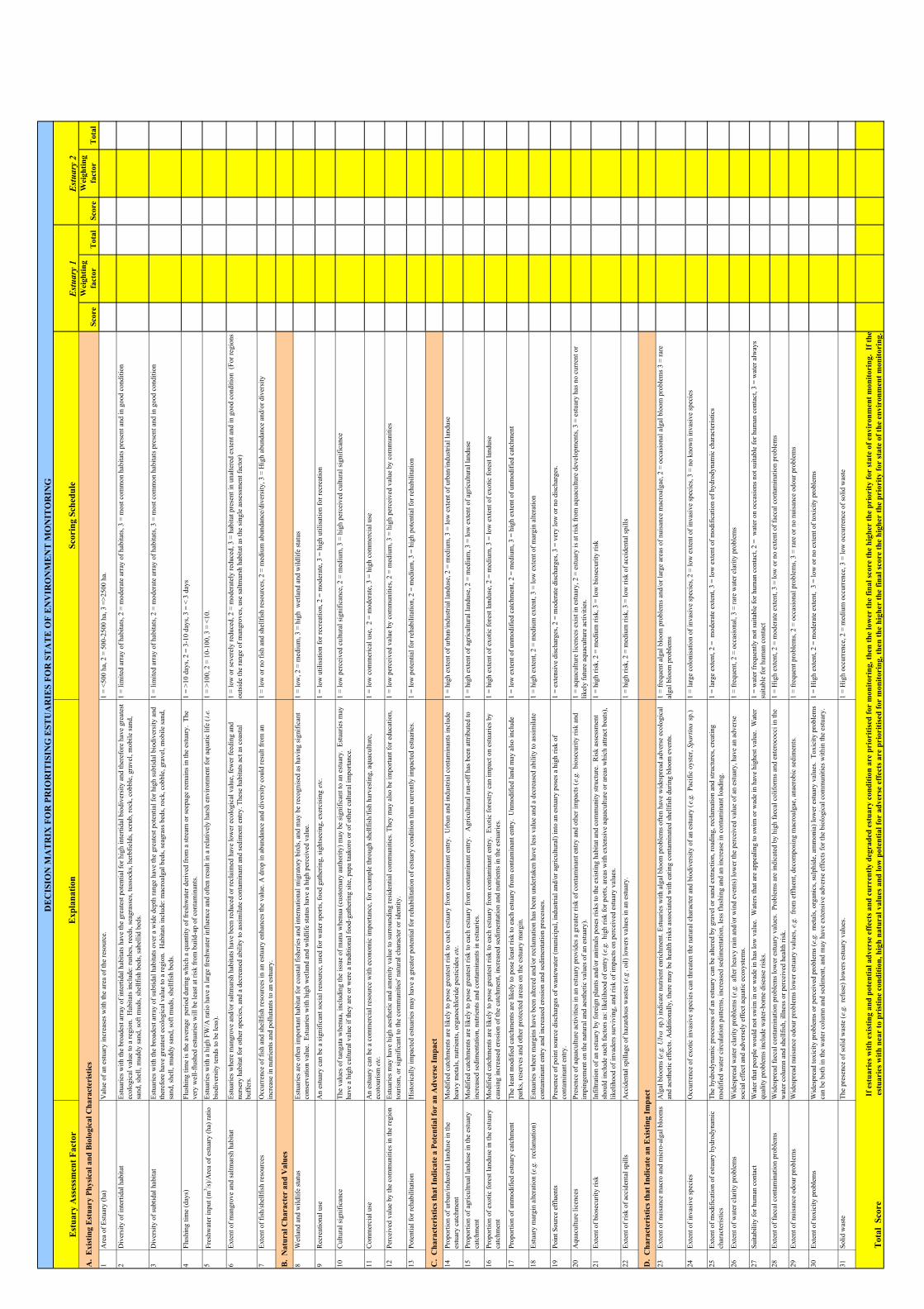
LIST OF TABLES Table 1: The Decision Matrix- a preliminary assessment of estuary condition for prioritising
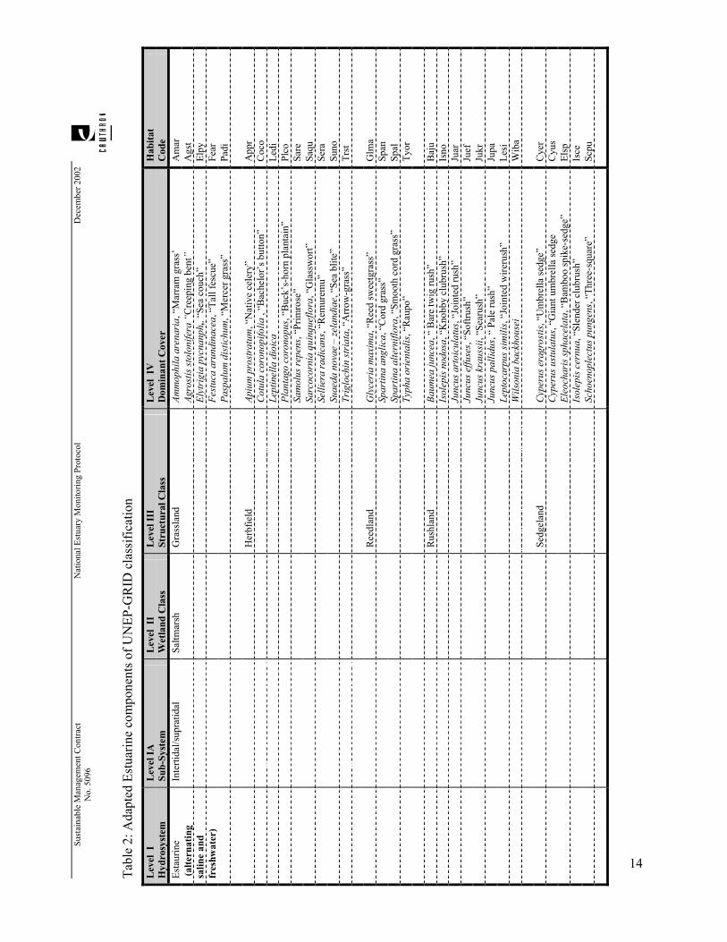
estuaries for State of the Environment monitoring. .....................................................................8 Table 2: Adapted Estuarine components of UNEP-GRID classification ..........................................14 Table 3: Checklist of expected epibiota for New Zealand estuaries..................................................30 Table 4: Approximate number of replicates required to detect specified levels of change (10-50%)
for four different levels of CV ranging from 8 to 58%..............................................................36
LIST OF FIGURES Figure 1: Locations of the nine reference estuaries with expanded inserts showing a magnified view
of each estuary. ............................................................................................................................3 Figure 2: Summary of the sampling strategy applied to each estuary, with a sampling site and
station expanded for clarity. The Avon-Heathcote Estuary is used as the example. ................27

Sustainable Management Contract No. 5096
National Estuary Monitoring Protocol
December 2002
1
1. INTRODUCTION Development of a standardised protocol for assessment and monitoring of New Zealand estuaries
has, until now, been relegated to the too-hard basket by most estuarine managers and scientists.
There are good reasons for this. Most importantly, estuaries are complex, dynamic and extremely
heterogeneous environments. Consequently, with few exceptions, it has not been possible to
identify general “indicators” of health or condition that are applicable to the full range of estuary
types and habitats that occur in New Zealand. However, because estuaries play such a pivotal role
in coastal ecosystems, and are often subjected to a wide variety of potentially conflicting uses and
related impacts, a standardised monitoring protocol is of obvious high priority.
The Ministry for the Environment (MfE) have started the process by identifying a number of
Environmental Performance Indicators (EPIs) for a variety of coastal environments (MfE 2001). A
few of these are suitable for implementation now, while most require further development. After
preliminary discussions with Andrew Fenemor (Tasman District Council) and Murray Bell
(Ministry for the Environment), and later discussions with coastal managers throughout New
Zealand, we decided that the time was right to further develop promising indicators and begin the
implementation procedure. Thus the development of the Estuarine Monitoring Protocol (EMP) was
initiated through the support of the MfE’s Sustainable Management Fund and 11 New Zealand
regional and local councils.
The present document (Part C) is the condensed form of the EMP. It gives a step-by-step
description (or recipe) of how to select an estuary for monitoring, establish a baseline of estuary
conditions and monitor change over time. The accompanying Parts A and B provide a more
detailed description of how it was developed, the rationale/justification and methodology and
complete datasets for the nine reference estuaries.
1.1 What is the EMP?
The estuary monitoring protocol is simply a standard method or approach to assess the current state
or condition of a particular estuary in order to establish a benchmark for comparison with
subsequent surveys. A major advantage of using a standard approach is that it generates an

Sustainable Management Contract No. 5096
National Estuary Monitoring Protocol
December 2002
2
integrated database that not only facilitates comparisons with successive monitoring surveys, but
also allows interpretation with respect to other estuaries/regions.
The EMP was intended to provide environmental resource managers with a set of tools to assess
and monitor the status of estuaries in their region. To achieve this, the protocol was required to be
scientifically defensible, cost-effective, practical/easy to use, and applicable to estuaries throughout
New Zealand.
1.2 How was the EMP developed?
In summary, three estuarine assessment techniques were applied to a series of reference estuaries
along the geographical/latitudinal range Northland to Southland (Figure 1). These techniques were:
1) A preliminary assessment of estuary condition for prioritising estuaries for monitoring,
2) Broad-scale mapping of intertidal habitat characteristics, and
3) Fine-scale assessment of one key representative habitat (the sand/mud, mid-low intertidal
habitat) using analyses of a suite of characteristics relevant to estuarine condition.
Following these assessments, the data were analysed, and the results used as a guide to structuring a
protocol that would adequately describe the current ‘health’ of the intertidal seabed (benthic)
environment. This included selecting appropriate characteristics to use as ‘indicators’, and
determining the number of replicate samples/analyses required for particular fine-scale analyses to
enable managers to detect change over time with statistical reliability.
Undetaking habitat mapping at the Otamatea Arm of the Kaipara Estuary during this project

Sustainable Management Contract No. 5096
National Estuary Monitoring Protocol
December 2002
3
Figure 1: Locations of the nine reference estuaries with expanded inserts showing a magnified view of each estuary.
1.3 Using the EMP
The EMP provides a stepwise approach to applying the three techniques (tools) for the assessment
of estuarine health.
For each of the three assessment methods, the following information is given:
• the equipment required (software, field equipment, chemicals etc),
• the methodology,
• estimated time/costs,
• a guide to interpreting the data,
• a guide for making management decisions based on the outputs of the assessment.

Sustainable Management Contract No. 5096
National Estuary Monitoring Protocol
December 2002
4
2. PRELIMINARY ASSESSMENT OF ESTUARY HEALTH
2.1 Overview
A preliminary characterisation and assessment of estuary health is a means of indexing estuarine
health within a region. This approach utilises a combination of information that can be acquired
easily from general literature and/or a brief site assessment, and information that is obtained from
more involved studies. The aim is NOT to derive a ‘magic’ number that will represent the state of
health of an estuary but rather to provide a flexible tool, the ‘Decision Matrix’ (DM) to give a rapid,
broad overview of the condition/status of an estuary (Table 1). The DM uses four categories of
factors to undertake the preliminary assessment; geomorphological classification, catchment use,
water and sediment quality, and resource values/uses. Each of the various factors are assigned a
score (or rating), tabulated, and an overall assessment score is assigned. By ranking estuaries based
on the combination of these factors, estuaries in the region can be evaluated, and a risk-based
approach can be made on deciding which estuaries require monitoring.
In completing the table for each of their estuaries, it is envisaged that managers will:
• become more familiar with their estuaries,
• identify knowledge gaps about their estuaries,
• identify the significant values within their estuaries,
• identify potential threats to estuarine values,
• prioritise estuary monitoring based on the current condition, potential threats, or values of
significance (e.g. ecological, cultural, recreational, and economic).
It is accepted that the DM does have limitations:
• There will be some loss of individual detail as it condenses and simplifies a large amount of
information about each estuary,
• It can not be applied to a broad comparison of estuaries outside a particular region. The
ranking factors allocated in the examples are subjective and discretionary. They can be
modified or replaced to emphasise particular features that are considered more relevant to
estuaries in a region. Although this allows the ranking process to be tailored to the concerns
and issues of the region, community or manager, it precludes its use for ranking estuaries
against those in other regions,

Sustainable Management Contract No. 5096
National Estuary Monitoring Protocol
December 2002
5
• The ranking result is only as good as the information used in its application. This could also
be seen as a strength as it will allow improvement of the result with the application of more
or higher quality information about the estuary and,
• In the case of relatively undisturbed estuaries, particularly, further consideration will be
required of the potential for future degradation of existing values; e.g. high natural
freshwater (nutrient or sediment) inflows, low flushing rate, etc.
2.2 Methods
The process of undertaking the preliminary estuary assessment involves the following steps:
Step 1: Matrix Familiarisation
Read through and become familiar with the estuary assessment factors and scoring schedule in the
DM (Table 1).
Step 2: Choose Estuaries to Prioritise
Decide on estuaries to be included in the prioritisation process. For example, this may be a cut-
down list of 6 estuaries in the region that the manager has already targeted for prioritisation or it
may be all encompassing and include all the estuaries in a region.
Requirements
- Decision matrix for prioritising estuaries for monitoring.
- Uses and values of each estuary.
- Relevant background information on the physical, chemical and
biological characteristics of estuaries in the region including
local experience.
- A background on the geology and land use characteristics of the
surrounding catchments.

Sustainable Management Contract No. 5096
National Estuary Monitoring Protocol
December 2002
6
Step 3: Score Estuary Factors
For each estuary allocate an appropriate score for each factor or item on the Decision Matrix. To
achieve this you will need to review available background information on the estuaries and their
catchments and, depending on the amount of information available and familiarity with the
estuaries, one or more site visits to each may be required.
Step 4: Assign Weightings to Estuary Factors
For each factor on the list, decide on the appropriateness of the given weighting factor (the greater
the weighting factor, the greater the priority for monitoring). Weighting factors range from a low
weighting of 1 to a high weighting of 5. To achieve this, you will firstly need to decide if
unmodified estuaries have a greater priority for monitoring in a particular region than highly
modified estuaries. If so, you will need to downgrade the pre-set weightings for C and D as they
are presently favouring factors that are characteristic of impacted or modified estuaries. For
example, Factor 19 “Point Source Effluents” would be weighted with a 1 or 2 if unmodified
estuaries were being given a high monitoring priority and a 4 or 5 if modified estuaries were being
given the highest priority.
Step 5: Total Score for Each Factor
For each factor on the matrix, add the score to the weighting factor to give a total for each factor.
Step 6: Total Score for Each Estuary
Sum each of the factor totals in the whole matrix to give an Estuary Total Score.
Step 7: Interpreting the Data
Compare totals for each estuary in your prioritisation list. Estuaries with the highest scores have the
highest priority for monitoring.
Step 8: Stakeholder Input
Ideally, the next step is to provide stakeholders with the completed decision matrices for each
estuary under consideration and to seek their input.
Step 9: Final Prioritisation
Following stakeholder input, undertake any necessary modifications to the matrix set-up and
calculations and repeat Steps 6 and 7 to prioritise estuaries for monitoring.

Sustainable Management Contract No. 5096
National Estuary Monitoring Protocol
December 2002
7
2.3 How much will it cost?
The time to undertake the initial prioritisation of estuaries for monitoring will vary depending on
the extent of existing information and the availability of local expert knowledge. If both are readily
available, then this particular aspect could be undertaken by council staff for $5,000 or less.
2.4 Working With the Decision Matrix as a flexible management
tool
It is envisaged that the primary use of the matrix will be for providing a defensible and transparent
means of prioritising estuaries for long term monitoring. In particular, it will provide a tool for
Regional Councils to use in the design of their State of Environment monitoring programmes. Once
completed, the manager can prepare a summary of the matrix approach and estuary scores for a
region which is then available as a tidy package for Council decision-makers. By periodically re-
addressing the DM, the manager will be able to evaluate the effectiveness of management decisions
and/or changing usage and values of estuarine resources.
A jointed wirerush (Leptocarpus similis) field in Whangamata Estuary

Sustainable Management Contract No. 5096
National Estuary Monitoring Protocol
December 2002
8
Table 1: The Decision Matrix- a preliminary assessment of estuary condition for prioritising estuaries for State of the Environment monitoring.
Exp
lana
tion
Scor
ing
Sche
dule
Scor
eW
eigh
ting
fact
orT
otal
Scor
eW
eigh
ting
fact
orT
otal
1A
rea
of E
stua
ry (h
a)V
alue
of a
n es
tuar
y in
crea
ses w
ith th
e ar
ea o
f the
reso
urce
.1
= <5
00 h
a, 2
= 5
00-2
500
ha, 3
=>2
500
ha.
2D
iver
sity
of i
nter
tidal
hab
itat
Estu
arie
s with
the
broa
dest
arr
ay o
f int
ertid
al h
abita
ts h
ave
the
grea
test
pot
entia
l for
hig
h in
terti
dal b
iodi
vers
ity a
nd th
eref
ore
have
gre
ates
t ec
olog
ical
val
ue to
a re
gion
. H
abita
ts in
clud
e: ru
shes
, ree
ds, s
eagr
asse
s, tu
ssoc
ks, h
erbf
ield
s, sc
rub,
rock
, cob
ble,
gra
vel,
mob
ile sa
nd,
sand
, she
ll, m
uddy
sand
, sof
t mud
s, sh
ellfi
sh b
eds,
sabe
llid
beds
.
1 =
limite
d ar
ray
of h
abita
ts, 2
= m
oder
ate
arra
y of
hab
itats
, 3 =
mos
t com
mon
hab
itats
pre
sent
and
in g
ood
cond
ition
3D
iver
sity
of s
ubtid
al h
abita
tEs
tuar
ies w
ith th
e br
oade
st a
rray
of s
ubtid
al h
abita
ts o
ver a
wid
e de
pth
rang
e ha
ve th
e gr
eate
st p
oten
tial f
or h
igh
subt
idal
bio
dive
rsity
and
th
eref
ore
have
gre
ates
t eco
logi
cal v
alue
to a
regi
on.
Hab
itats
incl
ude:
mac
roal
gal b
eds,
seag
rass
bed
s, ro
ck, c
obbl
e, g
rave
l, m
obile
sand
, sa
nd, s
hell,
mud
dy sa
nd, s
oft m
uds,
shel
lfish
bed
s.
1 =
limite
d ar
ray
of h
abita
ts, 2
= m
oder
ate
arra
y of
hab
itats
, 3 =
mos
t com
mon
hab
itats
pre
sent
and
in g
ood
cond
ition
4Fl
ushi
ng ti
me
(day
s)Fl
ushi
ng ti
me
is th
e av
erag
e p
erio
d du
ring
whi
ch a
qua
ntity
of f
resh
wat
er d
eriv
ed fr
om a
stre
am o
r see
page
rem
ains
in th
e es
tuar
y. T
he
very
wel
l-flu
shed
est
uarie
s will
be
leas
t at r
isk
from
bui
ld-u
p of
con
tam
inan
ts.
1
= >1
0 da
ys, 2
= 3
-10
days
, 3 =
< 3
day
s
5Fr
eshw
ater
inpu
t (m
3 /s)/A
rea
of e
stua
ry (h
a) ra
tioEs
tuar
ies w
ith a
hig
h FW
/A ra
tio h
ave
a la
rge
fres
hwat
er in
fluen
ce a
nd o
ften
resu
lt in
a re
lativ
ely
hars
h en
viro
nmen
t for
aqu
atic
life
(i.e
. bi
odiv
ersi
ty te
nds t
o be
less
).
1 =
>100
, 2 =
10-
100,
3 =
<10
.
6Ex
tent
of m
angr
ove
and
saltm
arsh
hab
itat
Estu
arie
s whe
re m
angr
ove
and/
or sa
ltmar
sh h
abita
ts h
ave
been
redu
ced
or re
clai
med
hav
e lo
wer
eco
logi
cal v
alue
, few
er fe
edin
g an
d nu
rser
y ha
bita
t for
oth
er sp
ecie
s, an
d a
decr
ease
d ab
ility
to a
ssim
ilate
con
tam
inan
t and
sedi
men
t ent
ry. T
hese
hab
itats
act
as c
oast
al
buff
ers.
1 =
low
or s
ever
ely
redu
ced,
2 =
mod
erat
ely
redu
ced,
3 =
hab
itat p
rese
nt in
una
ltere
d ex
tent
and
in g
ood
cond
ition
(Fo
r reg
ions
ou
tsid
e th
e ra
nge
of m
angr
oves
, use
saltm
arsh
hab
itat a
s the
sing
le a
sses
smen
t fac
tor)
7Ex
tent
of f
ish/
shel
lfish
reso
urce
s O
ccur
renc
e of
fish
and
shel
lfish
reso
urce
s in
an e
stua
ry e
nhan
ces t
he v
alue
. A d
rop
in a
bund
ance
and
div
ersi
ty c
ould
resu
lt fr
om a
n in
crea
se in
nut
rient
s and
pol
luta
nts t
o an
est
uary
.1
= lo
w o
r no
fish
and
shel
lfish
reso
urce
s, 2
= m
ediu
m a
bund
ance
/div
ersi
ty, 3
= H
igh
abun
danc
e an
d/or
div
ersi
ty
8W
etla
nd a
nd w
ildlif
e st
atus
Estu
arie
s are
ofte
n im
porta
nt h
abita
t for
coa
stal
fish
erie
s and
inte
rnat
iona
l mig
rato
ry b
irds,
and
may
be
reco
gnis
ed a
s hav
ing
sign
ifica
nt
cons
erva
tion
valu
e. E
stua
ries w
ith h
igh
wet
land
and
wild
life
stat
us h
ave
a hi
gh p
erce
ived
val
ue.
1 =
low
, 2 =
med
ium
, 3 =
hig
h w
etla
nd a
nd w
ildlif
e st
atus
9R
ecre
atio
nal u
seA
n es
tuar
y ca
n be
a si
gnifi
cant
soci
al re
sour
ce, u
sed
for w
ater
spor
ts, f
ood
gath
erin
g, si
ghts
eein
g, e
xerc
isin
g et
c.1
= lo
w u
tilis
atio
n fo
r rec
reat
ion,
2 =
mod
erat
e, 3
= h
igh
utili
satio
n fo
r rec
reat
ion
10C
ultu
ral s
igni
fican
ceTh
e va
lues
of t
anga
ta w
henu
a, in
clud
ing
the
issu
e of
man
a w
henu
a (c
usto
mar
y au
thor
ity) m
ay b
e si
gnifi
cant
to a
n es
tuar
y. E
stua
ries m
ay
have
a h
igh
cultu
ral v
alue
if th
ey a
re o
r wer
e a
tradi
tiona
l foo
d-ga
ther
ing
site
, pap
a ta
akor
o or
of o
ther
cul
tura
l im
porta
nce.
1 =
low
per
ceiv
ed c
ultu
ral s
igni
fican
ce, 2
= m
ediu
m, 3
= h
igh
perc
eive
d cu
ltura
l sig
nific
ance
11C
omm
erci
al u
seA
n es
tuar
y ca
n be
a c
omm
erci
al re
sour
ce w
ith e
cono
mic
impo
rtanc
e, fo
r exa
mpl
e th
roug
h sh
ellfi
sh/fi
sh h
arve
stin
g, a
quac
ultu
re,
ecot
ouris
m e
tc.
1 =
low
com
mer
ical
use
, 2
= m
oder
ate,
3 =
hig
h co
mm
erci
al u
se
12Pe
rcei
ved
valu
e by
the
com
mun
ities
in th
e re
gion
Estu
arie
s may
hav
e hi
gh a
esth
etic
and
am
enity
val
ue to
surr
ound
ing
resi
dent
ial c
omm
uniti
es. T
hey
may
als
o be
impo
rtant
for e
duca
tion,
to
uris
m, o
r sig
nific
ant t
o th
e co
mm
uniti
es' n
atur
al c
hara
cter
or i
dent
ity.
1 =
low
per
ceiv
ed v
alue
by
com
mun
ities
, 2 =
med
ium
, 3 =
hig
h pe
rcei
ved
valu
e by
com
mun
ities
13Po
tent
ial f
or re
habi
litat
ion
His
toric
ally
impa
cted
est
uarie
s may
hav
e a
grea
ter p
oten
tial f
or re
habi
litat
ion
of e
stua
ry c
ondi
tion
than
cur
rent
ly im
pact
ed e
stua
ries.
1 =
low
pot
entia
l for
reha
bilit
atio
n, 2
= m
ediu
m, 3
= h
igh
pote
ntia
l for
reha
bilit
atio
n
14Pr
opor
tion
of u
rban
/indu
stria
l lan
duse
in th
e es
tuar
y ca
tchm
ent
Mod
ified
cat
chm
ents
are
like
ly to
pos
e gr
eate
st ri
sk to
eac
h es
tuar
y fr
om c
onta
min
ant e
ntry
. U
rban
and
indu
stria
l con
tam
inan
ts in
clud
e he
avy
met
als,
nutri
ents
, org
anoc
hlor
ide
pest
icid
es e
tc.
1 =
high
ext
ent o
f urb
an/in
dust
rial l
andu
se, 2
= m
ediu
m, 3
= lo
w e
xten
t of u
rban
/indu
stria
l lan
duse
15Pr
opor
tion
of a
gric
ultru
al la
ndus
e in
the
estu
ary
catc
hmen
tM
odifi
ed c
atch
men
ts a
re li
kely
to p
ose
grea
test
risk
to e
ach
estu
ary
from
con
tam
inan
t ent
ry.
Agr
icul
tura
l run
-off
has
bee
n at
tribu
ted
to
incr
ease
d se
dim
enta
tion,
nut
rient
s and
con
tam
inan
ts in
est
uarie
s.1
= hi
gh e
xten
t of a
gric
ultu
ral l
andu
se, 2
= m
ediu
m, 3
= lo
w e
xten
t of a
gric
ultu
ral l
andu
se
16Pr
opor
tion
of e
xotic
fore
st la
ndus
e in
the
estu
ary
catc
hmen
tM
odifi
ed c
atch
men
ts a
re li
kely
to p
ose
grea
test
risk
to e
ach
estu
ary
from
con
tam
inan
t ent
ry.
Exot
ic fo
rest
ry c
an im
pact
on
estu
arie
s by
caus
ing
incr
ease
d er
osio
n of
the
catc
hmen
t, in
crea
sed
sedi
men
tatio
n an
d nu
trien
ts in
the
estu
arie
s.1
= hi
gh e
xten
t of e
xotic
fore
st la
ndus
e, 2
= m
ediu
m, 3
= lo
w e
xten
t of e
xotic
fore
st la
ndus
e
17Pr
opor
tion
of u
nmod
ified
est
uary
cat
chm
ent
The
leas
t mod
ified
cat
chm
ents
are
like
ly to
pos
e le
ast r
isk
to e
ach
estu
ary
from
con
tam
inan
t ent
ry.
Unm
odifi
ed la
nd m
ay a
lso
incl
ude
park
s, re
serv
es a
nd o
ther
pro
tect
ed a
reas
on
the
estu
ary
mar
gin.
1 =
low
ext
ent o
f unm
odifi
ed c
atch
men
t, 2
= m
ediu
m, 3
= h
igh
exte
nt o
f unm
odifi
ed c
atch
men
t
18Es
tuar
y m
argi
n al
tera
tion
(e.g
. re
clam
atio
n)Es
tuar
ies w
here
mar
gins
hav
e be
en a
ltere
d an
d/or
recl
amat
ion
has b
een
unde
rtake
n ha
ve le
ss v
alue
and
a d
ecre
ased
abi
lity
to a
ssim
ilate
co
ntam
inan
t ent
ry a
nd in
crea
sed
eros
ion
and
sedi
men
tatio
n pr
oces
ses.
1 =
high
ext
ent,
2 =
med
ium
ext
ent,
3 =
low
ext
ent o
f mar
gin
alte
ratio
n
19Po
int S
ourc
e ef
fluen
tsPr
esen
ce o
f poi
nt so
urce
dis
char
ges o
f was
tew
ater
(mun
icip
al, i
ndus
trial
and
/or a
gric
ultu
ral)
into
an
estu
ary
pose
s a h
igh
risk
of
cont
amin
ant e
ntry
. 1
= ex
tens
ive
disc
harg
es, 2
= m
oder
ate
disc
harg
es, 3
= v
ery
low
or n
o di
scha
rges
.
20A
quac
ultu
re li
cenc
esPr
esen
ce o
f aqu
acul
ture
act
iviti
es in
an
estu
ary
prov
ides
a g
reat
er ri
sk o
f con
tam
inan
t ent
ry a
nd o
ther
impa
cts (
e.g.
bio
secu
rity
risk
and
impi
ngem
ent o
n th
e na
tura
l and
aes
thet
ic v
alue
s of a
n es
tuar
y).
1 =
aqua
cultu
re li
cenc
es e
xist
in e
stua
ry, 2
= e
stua
ry is
at r
isk
from
aqu
acul
ture
dev
elop
men
ts, 3
= e
stua
ry h
as n
o cu
rren
t or
likel
y fu
ture
aqu
acul
ture
act
iviti
es.
21Ex
tent
of b
iose
curit
y ris
kIn
filtra
tion
of a
n es
tuar
y by
fore
ign
plan
ts a
nd/o
r ani
mal
s pos
es ri
sks t
o th
e ex
istin
g ha
bita
t and
com
mun
ity st
ruct
ure.
Ris
k as
sess
men
t sh
ould
incl
ude
such
fact
ors a
s: li
kelih
ood
of e
ntry
(e.g
. hi
gh ri
sk fo
r por
ts, a
reas
with
ext
ensi
ve a
quac
ultu
re o
r are
as w
hich
attr
act b
oats
), lik
elih
ood
of in
vade
rs su
rviv
ing,
and
risk
of i
mpa
cts o
n pe
rcei
ved
estu
ary
valu
es.
1 =
high
risk
, 2 =
med
ium
risk
, 3 =
low
bio
secu
rity
risk
22Ex
tent
of r
isk
of a
ccid
enta
l spi
lls
Acc
iden
tal s
pilla
ge o
f haz
ardo
us w
aste
s (e.
g. o
il) lo
wer
s val
ues i
n an
est
uary
.1
= hi
gh ri
sk, 2
= m
ediu
m ri
sk, 3
= lo
w ri
sk o
f acc
iden
tal s
pills
23Ex
tent
of n
uisa
nce
mac
ro a
nd m
icro
-alg
al b
loom
sA
lgal
blo
oms (
e.g.
Ulv
a sp
.) in
dica
te n
utrie
nt e
nric
hmen
t. Es
tuar
ies w
ith a
lgal
blo
om p
robl
ems o
ften
have
wid
espr
ead
adve
rse
ecol
ogic
al
and
aest
hetic
eff
ects
. Add
ition
ally
, the
re m
ay b
e he
alth
risk
s ass
ocia
ted
with
eat
ing
cont
amin
ated
shel
lfish
dur
ing
bloo
m e
vent
s.1
= fr
eque
nt a
lgal
blo
om p
robl
ems a
nd/o
r lar
ge a
reas
of n
uisa
nce
mac
roal
gae,
2 =
occ
asio
nal a
lgal
blo
om p
robl
ems 3
= ra
re
alga
l blo
om p
robl
ems
24Ex
tent
of i
nvas
ive
spec
ies
Occ
urre
nce
of e
xotic
inva
sive
spec
ies c
an th
reat
en th
e na
tura
l cha
ract
er a
nd b
iodi
vers
ity o
f an
estu
ary
(e.g
. Pa
cific
oys
ter,
Spar
tina
sp.)
1 =
larg
e co
loni
satio
n of
inva
sive
spec
ies,
2 =
low
ext
ent o
f inv
asiv
e sp
ecie
s, 3
= no
kno
wn
inva
sive
spec
ies
25Ex
tent
of m
odifi
catio
n of
est
uary
hyd
rody
nam
ic
char
acte
ristic
sTh
e hy
drod
ynam
ic p
roce
sses
of a
n es
tuar
y ca
n be
alte
red
by g
rave
l or s
and
extra
ctio
n, ro
adin
g, re
clam
atio
n an
d st
ruct
ures
, cre
atin
g m
odifi
ed w
ater
circ
ulat
ion
patte
rns,
incr
ease
d se
dim
enta
tion,
less
flus
hing
and
an
incr
ease
in c
onta
min
ant l
oadi
ng.
1 =
larg
e ex
tent
, 2 =
mod
erat
e ex
tent
, 3 =
low
ext
ent o
f mod
ifica
tion
of h
ydro
dyna
mic
cha
ract
eris
tics
26Ex
tent
of w
ater
cla
rity
prob
lem
sW
ides
prea
d w
ater
cla
rity
prob
lem
s (e.
g. a
fter h
eavy
rain
and
/or w
ind
even
ts) l
ower
the
perc
eive
d va
lue
of a
n es
tuar
y, h
ave
an a
dver
se
soci
al e
ffec
t and
adv
erse
ly e
ffec
t aqu
atic
eco
syst
ems.
1
= fr
eque
nt, 2
= o
ccas
iona
l, 3
= ra
re w
ater
cla
rity
prob
lem
s
27Su
itabi
lity
for h
uman
con
tact
Wat
er th
at p
eopl
e w
ould
not
swim
in o
r wad
e in
has
low
val
ue.
Wat
ers t
hat a
re a
ppea
ling
to sw
im o
r wad
e in
hav
e hi
ghes
t val
ue.
Wat
er
qual
ity p
robl
ems i
nclu
de w
ater
-bor
ne d
isea
se ri
sks.
1 =
wat
er fr
eque
ntly
not
suita
ble
for h
uman
con
tact
, 2 =
wat
er o
n oc
casi
ons n
ot su
itabl
e fo
r hum
an c
onta
ct, 3
= w
ater
alw
ays
suita
ble
for h
uman
con
tact
28Ex
tent
of f
aeca
l con
tam
inat
ion
prob
lem
s W
ides
prea
d fa
ecal
con
tam
inat
ion
prob
lem
s low
er e
stua
ry v
alue
s. P
robl
ems a
re in
dica
ted
by h
igh
faec
al c
olifo
rms a
nd e
nter
ococ
ci in
the
wat
er c
olum
n an
d sh
ellfi
sh, i
llnes
s or p
erce
ived
hea
lth ri
sk.
1 =
Hig
h ex
tent
, 2 =
mod
erat
e ex
tent
, 3 =
low
or n
o ex
tent
of f
aeca
l con
tam
inat
ion
prob
lem
s
29Ex
tent
of n
uisa
nce
odou
r pro
blem
s W
ides
prea
d nu
isan
ce o
dour
pro
blem
s low
er e
stua
ry v
alue
s, e.
g. f
rom
eff
luen
t, de
com
posi
ng m
acro
alga
e, a
naer
obic
sedi
men
ts.
1 =
freq
uent
pro
blem
s, 2
= oc
casi
onal
pro
blem
s, 3
= ra
re o
r no
nuis
ance
odo
ur p
robl
ems
30Ex
tent
of t
oxic
ity p
robl
ems
Wid
espr
ead
toxi
city
pro
blem
s or p
erce
ived
pro
blem
s (e.
g. m
etal
s, or
gani
cs, s
ulph
ide,
am
mon
ia) l
ower
est
uary
val
ues.
Tox
icity
pro
blem
s ca
n be
bot
h in
the
wat
er c
olum
n an
d se
dim
ent,
and
may
hav
e ex
tens
ive
adve
rse
effe
cts f
or th
e bi
olog
ical
com
mun
ities
with
in th
e es
tuar
y.
1 =
Hig
h ex
tent
, 2 =
mod
erat
e ex
tent
, 3
= lo
w o
r no
exte
nt o
f tox
icity
pro
blem
s
31So
lid w
aste
The
pres
ence
of s
olid
was
te (e
.g.
refu
se) l
ower
s est
uary
val
ues.
1 =
Hig
h oc
curr
ence
, 2 =
med
ium
occ
urre
nce,
3 =
low
occ
urre
nce
of so
lid w
aste
Tot
al S
core
If e
stua
ries
with
exi
stin
g an
d po
tent
ial a
dver
se e
ffec
ts a
nd c
urre
ntly
deg
rade
d es
tuar
y co
nditi
on a
re p
rior
itise
d fo
r m
onito
ring
, the
n th
e lo
wer
the
final
scor
e th
e hi
gher
the
prio
rity
for
stat
e of
env
iron
men
t mon
itori
ng.
If th
e es
tuar
ies w
ith n
ear
to p
rist
ine
cond
ition
, hig
h na
tura
l val
ues a
nd lo
w p
oten
tial f
or a
dver
se e
ffec
ts a
re p
rior
itise
d fo
r m
onito
ring
, the
n th
e hi
gher
the
final
scor
e th
e hi
gher
the
prio
rity
for
stat
e of
the
envi
ronm
ent m
onito
ring
.
C.
Cha
ract
eris
tics t
hat I
ndic
ate
a Po
tent
ial f
or a
n A
dver
se Im
pact
A.
Exi
stin
g E
stua
ry P
hysi
cal a
nd B
iolo
gica
l Cha
ract
eris
tics
B.
Nat
ural
Cha
ract
er a
nd V
alue
s
DE
CIS
ION
MA
TR
IX F
OR
PR
IOR
ITIS
ING
EST
UA
RIE
S FO
R S
TA
TE
OF
EN
VIR
ON
ME
NT
MO
NIT
OR
ING
Estu
ary
1Es
tuar
y 2
D.
Cha
ract
eris
tics t
hat I
ndic
ate
an E
xist
ing
Impa
ct
Est
uary
Ass
essm
ent F
acto
r

Sustainable Management Contract No. 5096
National Estuary Monitoring Protocol
December 2002
10
3. BROAD-SCALE MAPPING OF INTERTIDAL HABITATS
3.1 Overview
The aim of broad-scale habitat mapping is to describe an estuary according to different dominant
habitat types based on surface features of substrate characteristics (mud, sand, cobble, etc) and
vegetation type (mangrove, eelgrass, salt marsh species, etc), and develop a baseline habitat map.
Once a baseline map has been constructed, the distribution of the various habitats can be compared
amongst different estuaries/regions to provide a better understanding of how estuarine ecosystems
in New Zealand are structured. Changes in the position and/or size of habitats (MfE Confirmed
Indicators for the Marine Environment, ME6 2001) can then be monitored by repeating the
mapping exercise. This procedure involves the use of aerial photography together with detailed
ground-truthing and digital mapping using Geographical Information System (GIS) technology.
Equipment Required
General
- GIS software (e.g. ArcviewTM)
- Image analysis software (e.g. ERDAS)
- Colour aerial photographs of the selected estuary (taken at low tide at a maximum scale of 1:10,000)
- Scanner (capable of creating resolution of 508 dpi yielding an image resolution of 0.5 m per pixel)
Field
- 4WD vehicle
- Small boat and outboard (if necessary)
- GPS unit with data logger (e.g. Trimble Pathfinder Pro, with TD1 data logger)
- Chest-high waders
- Waterproof notebook and pencils
- Camera
- Checklist of likely dominant plant and substrate types (preferably include taxonomic keys/photographs
to enable easy identification)
- Plastic bags for any samples that may later require identification
- 6 fine tipped felt pens (3 different colours)
- Laminated colour aerial photographs of whole estuary and margins (scale 1:5000 to 1:10,000)
- Watch and tide chart

Sustainable Management Contract No. 5096
National Estuary Monitoring Protocol
December 2002
11
3.2 Methods
Step 1: Colour aerial photography The first step is to obtain aerial photographs of your estuary at low tide on a clear day. The
maximum scale should be 1:10000, based on the fact that with a broader scale you will lose some of
the detail of the estuary and it will become difficult to accurately determine changes in habitats over
time. Working with a finer scale will require more photographs, increasing the cost of the exercise.
Using the recommended scale you can achieve a resolution of 508 dots per inch (dpi), equating to
0.5 m per pixel. You may already have existing aerial photographs of your estuary. Although
historical photographs may be black and white, it may still be possible to distinguish and identify
major habitats. Aerial photographs, suitable for the mapping purposes can be obtained from various
New Zealand companies (e.g. New Zealand Aerial Mapping Ltd. (Auckland/Hastings), Air
Logistics (Auckland/Nelson).
Step 2: Rectification The second step is to rectify the images. When you join together all the aerial photographs into a
mosaic of the estuary, the photos are overlapped on a flat 2-D plane. Unavoidably, you can get
some shifting of the image, and a consequent reduction in positional accuracy. The actual
shape/area of a habitat won’t change much, but its position might.
Rectification is ideally undertaken using a minimum of six prominent landmarks per photo (e.g.
road intersections, islands, buildings, polythene markers, etc.), each of which has been visited and
its differential GPS position recorded (we use a Trimble Pathfinder Pro GPS unit). Occasionally
large homogeneous areas of the estuary are lacking in suitable landmarks for rectification. Where
this is likely to be a problem, white polythene sheets (2 m x 2 m) with overlaid black crosses should
be pegged out on the seabed immediately before the survey and removed afterward.
The individual photos should then be scanned at a resolution of 508 dpi yielding an image
resolution of 0.5 m per pixel. This is achieved by converting the landmarks to Arcview shapefiles.
ERDAS image analysis software, running under Arcview (v 3.1), can be used to register, rectify,
and mosaic the scanned photos. Positional accuracy can be calculated by documenting the root
mean square (RMS) error for each landmark. In general, RMS error should be within ± 5 m using
this procedure, however much greater accuracy can be achieved for many of the photos. With this

Sustainable Management Contract No. 5096
National Estuary Monitoring Protocol
December 2002
12
approach, the maximum summed error depends on the number of photos required (i.e. the size of
the estuary) and can range from approximately 2-15 m at any point. The actual error is often much
lower, however.
A mosaic of aerial photographs of the Havelock Estuary, Marlborough following rectification
Step 3: Classification of habitat features The classification of the features follows the proposed national classification system (with
adaptations), which is currently being developed under another SMF funded programme
(Monitoring Changes in Wetland Extent: An Environmental Performance Indicator For Wetlands)
by Lincoln Environmental, Lincoln. The classification system for wetland types is based on the
Atkinson System (Atkinson 1985) and covers 4 levels, ranging from broad to fine-scale;
• Level I: Hydrosystem (e.g. intertidal estuary)
• Level II: Wetland Class (e.g. saltmarsh)
• Level III: Structural Class (e.g. marshland)
• Level IV: Dominant Cover (e.g. Leptocarpus similis)
For this project, you will only need to use Level III (Structural Class) and Level IV (Dominant
Cover).

Sustainable Management Contract No. 5096
National Estuary Monitoring Protocol
December 2002
13
• The individual vegetation species are named by using the two first letters of their Latin
genus and species names, e.g. Pldi = ribbonwood, Plagianthus divaricatus.
• / separates canopy vegetation, e.g. Pldi/Lesi (ribbonwood is taller than jointed wire rush).
• - separates vegetation with approximately the same height, e.g. Lesi-Jukr (jointed wire rush
is the same height as searush).
• ( ) are used for subdominant species, e.g. (Pldi)/Lesi = dominant cover is jointed wire rush
and subdominant cover is ribbonwood. The use of ( ) is not based on percentage cover but
from the subjective observation of which vegetation is the dominant or subdominant species
within the patch.
• The classification always starts with the tallest vegetation type and works down, e.g.
(Pldi/Baju)/Lesi-Jukr = a patch with a dominant cover of jointed wire rush and searush
(which are of the same height) with a subdominant cover of ribbonwood and Baumea juncea
(which are taller than the dominant cover).
A list of all the classification types used in the study and their codes are given in Table 2.
Leptocarpus similis (Jointed wirerush)
Sust
aina
ble
Man
agem
ent C
ontra
ct
No.
509
6 N
atio
nal E
stua
ry M
onito
ring
Prot
ocol
Dec
embe
r 200
2
14
Tabl
e 2:
Ada
pted
Est
uarin
e co
mpo
nent
s of U
NEP
-GR
ID c
lass
ifica
tion
Lev
el I
L
evel
IA
Lev
el I
I L
evel
III
Lev
el I
V
Hab
itat
Hyd
rosy
stem
Su
b-Sy
stem
W
etla
nd C
lass
St
ruct
ural
Cla
ss
Dom
inan
t Cov
er
Cod
e Es
taur
ine
Inte
rtida
l/sup
ratid
al
Saltm
arsh
G
rass
land
Am
mop
hila
are
nari
a, “
Mar
ram
gra
ss’
Am
ar
(alte
rnat
ing
Agro
stis
stol
onife
ra “
Cre
epin
g be
nt”
Ags
t sa
line
and
El
ytri
gia
pycn
anph
,, “S
ea c
ouch
” El
py
fres
hwat
er)
Fe
stuc
a ar
undi
nace
a, “
Tall
fesc
ue”
Fear
Pa
spal
um d
istic
hum
, “M
erce
r gra
ss”
Padi
Her
bfie
ld
Apiu
m p
rost
ratu
m, “
Nat
ive
cele
ry”
App
r
C
otul
a co
rono
pifo
lia ,
“Bac
helo
r’s b
utto
n”
Coc
o
Le
ptin
ella
dio
ica
Ledi
Pl
anta
go c
oron
opus
, “B
uck’
s-ho
rn p
lant
ain”
Pl
co
Sam
olus
repe
ns, “
Prim
rose
” Sa
re
Sarc
ocor
nia
quin
quef
lora
, “G
lass
wor
t”
Saqu
Se
llier
a ra
dica
ns, “
Rem
urem
u”
Sera
Su
aeda
nov
ae –
zela
ndia
e, “
Sea
blite
” Su
no
Trig
loch
in st
riat
a, “
Arr
ow-g
rass
” Tr
st
R
eedl
and
Gly
ceri
a m
axim
a, “
Ree
d sw
eetg
rass
”
Glm
a
Sp
artin
a an
glic
a, “
Cor
d gr
ass”
Sp
an
Spar
tina
alte
rnifl
ora,
“Sm
ooth
cor
d gr
ass”
Sp
al
Typh
a or
ient
alis
, “R
aupo
” Ty
or
R
ushl
and
Baum
ea ju
ncea
, “ B
are
twig
rush
” B
aju
Isol
epis
nod
osa,
“K
nobb
y cl
ubru
sh”
Isno
Ju
ncus
art
oicu
latu
s, “J
oint
ed ru
sh”
Juar
Ju
ncus
effu
ses,
“Sof
trush
” Ju
ef
Junc
us k
raus
sii,
“Sea
rush
” Ju
kr
Junc
us p
allid
us, “
Pal
e ru
sh”
Jupa
Le
ptoc
arpu
s sim
ilis,
“Joi
nted
wire
rush
” Le
si
Wils
onia
bac
khou
sei
Wib
a
Sedg
elan
d C
yper
us e
ragr
ostis
, “U
mbr
ella
sedg
e”
Cye
r
C
yper
us u
stul
atus
, “G
iant
um
brel
la se
dge
Cyu
s
El
eoch
aris
spha
cela
ta, “
Bam
boo
spik
e-se
dge”
El
sp
Isol
epis
cer
nua,
“Sl
ende
r clu
brus
h”
Isce
Sc
hoen
ople
ctus
pun
gens
, “Th
ree-
squa
re”
Scpu
14

Sust
aina
ble
Man
agem
ent C
ontra
ct
No.
509
6 N
atio
nal E
stua
ry M
onito
ring
Prot
ocol
Dec
embe
r 200
2
15
Tabl
e 2
cont
inue
d.
Lev
el I
L
evel
IA
Lev
el I
I L
evel
III
Lev
el I
V
Hab
itat
Hyd
rosy
stem
Su
b-Sy
stem
W
etla
nd C
lass
St
ruct
ural
Cla
ss
Dom
inan
t Cov
er
Cod
e
Scru
b Av
icen
nia
mar
ina
var.
resi
nfer
a, “
Man
grov
e”
Avr
e
C
ordy
line
aust
ralis
, “C
abba
ge tr
ee”
Coa
u
C
ytis
us sc
opar
ius,
“Bro
om”
Cys
c
Le
ptos
perm
um sc
opar
ium
, “M
anuk
a”
Lesc
Pl
agia
nthu
s div
aric
atus
, “Sa
ltmar
sh ri
bbon
woo
d”
Pldi
U
lex
euro
paeu
s, “G
orse
”
Ule
u
Tuss
ockl
and
Cor
tade
ria
sp.,
“Toe
toe”
C
o sp
Ph
orm
ium
tena
x, “
New
Zea
land
flax
” Ph
te
Poa,
“Si
lver
tuss
ock”
Po
a
Pu
ccin
ella
stri
cta,
”Sa
lt gr
ass”
Pu
st
Stip
a st
ipoi
des,
“Nee
dle
tuss
ock”
St
st
Seag
rass
mea
dow
s Se
agra
ss m
eado
w
Zos
tera
nov
azel
andi
ca, “
Eelg
rass
” Zo
sp
Mac
roal
gal b
ed
Mac
roal
gal b
ed
Ente
rom
orph
a sp
. En
sp
Gra
cila
ria
chile
nsis
G
rch
Ulv
a ri
gida
, “Se
a le
ttuce
” U
lri
Mud
/san
dfla
t Fi
rm sh
ell/s
and
(<1c
m)
FS
S
Firm
sand
(<1c
m)
FS
Soft
sand
SS
M
obile
sand
(<1c
m)
M
S
Firm
mud
/san
d (0
-2cm
)
FMS
So
ft m
ud/s
and
(2-5
cm)
SM
Ver
y so
ft m
ud/s
and
(>5c
m)
V
SM
Ston
efie
ld
Gra
vel f
ield
GF
C
obbl
e fi
eld
C
F
B
ould
erfie
ld
Bou
lder
fiel
d
BF
Roc
klan
d R
ockl
and
R
F
Sh
ell b
ank
Shel
l ban
k
Shel
l
Sh
ellfi
sh fi
eld
Coc
kleb
ed
C
ockl
e
Mus
selre
ef
M
usse
l
Oys
terr
eef
O
yste
r
W
orm
fiel
d Sa
belli
d fie
ld
Sa
belli
d
Subt
idal
W
ater
W
ater
Wat
er
15

Sustainable Management Contract No. 5096
National Estuary Monitoring Protocol
December 2002
16
Level III Structural classes are defined as follows:
Cushionfield: Vegetation in which the cover of cushion plants in the canopy is 20-100% and in
which the cushion-plant cover exceeds that of any other growth form or bare ground. Cushion
plants include herbaceous, semi-woody and woody plants with short densely packed branches and
closely spaced leaves that together form dense hemispherical cushions.
Herbfield: Vegetation in which the cover of herbs in the canopy is 20-100% and in which the herb
cover exceeds that of any other growth form or bare ground. Herbs include all herbaceous and low-
growing semi-woody plants that are not separated as ferns, tussocks, grasses, sedges, rushes, reeds,
cushion plants, mosses or lichens.
Lichenfield: Vegetation in which the cover of lichens in the canopy is 20-100% and in which the
lichen cover exceeds that of any other growth form or bare ground.
Reedland: Vegetation in which the cover of reeds in the canopy is 20-100% and in which the reed
cover exceeds that of any other growth form or open water. If the reed is broken the stem is both
round and hollow – somewhat like a soda straw. The flowers will each bear six tiny petal-like
structures – neither grasses nor sedges will bear flowers, which look like that. Reeds are
herbaceous plants growing in standing or slowly-running water that have tall, slender, erect,
unbranched leaves or culms that are either hollow or have a very spongy pith. Examples include
Typha, Bolboschoenus, Scirpus lacutris, Eleocharis sphacelata, and Baumea articulata. Some
species covered by the Rushland or Sedgeland classes (below) are excluded.
Rushland: Vegetation in which the cover of
rushes in the canopy is 20-100% and in which the
rush cover exceeds that of any other growth form
or bare ground. A tall grasslike, often hollow-
stemmed plant, included in the rush growth form
are some species of Juncus and all species of
Leptocarpus. Tussock-rushes are excluded.
Sedgeland: Vegetation in which the cover of sedges in the canopy is 20-100% and in which the
sedge cover exceeds that of any other growth form or bare ground. “Sedges have edges.” Sedges
can be differentiated from grass by feeling the stem. If the stem is flat or rounded, it’s probably a
grass or a reed, if the stem is clearly triangular, it’s a sedge. Included in the sedge growth form are
many species of Carex, Uncinia, and Scirpus. Tussock-sedges and reed-forming sedges (c.f.
REEDLAND) are excluded.
Juncus krausii (searush)

Sustainable Management Contract No. 5096
National Estuary Monitoring Protocol
December 2002
17
Scrub: Woody vegetation in which the cover of shrubs and trees in the canopy is > 80% and in
which shrub cover exceeds that of trees (c.f. FOREST). Shrubs are woody plants < 10 cm diameter
at breast height (dbh).
Tussockland: Vegetation in which the cover of tussocks in the canopy is 20-100% and in which the
tussock cover exceeds that of any other growth form or bare ground. Tussocks include all grasses,
sedges, rushes, and other herbaceous plants with linear leaves (or linear non-woody stems) that are
densely clumped and > 10 cm height. Examples of the growth form occur in all species of
Cortaderia, Gahnia, and Phormium, and in some species of Chionochloa, Poa, Festuca,
Rytidosperma, Cyperus, Carex, Uncinia, Juncus, Astelia, Aciphylla, and Celmisia.
Forest: Woody vegetation in which the cover of trees and shrubs in the canopy is > 80% and in
which tree cover exceeds that of shrubs. Trees are woody plants ≥ 10 cm dbh. Tree ferns ≥ 10cm
dbh are treated as trees.
Seagrass meadows: Seagrasses are the sole marine representatives of the Angiospermae. They all
belong to the order Helobiae, in two families: Potamogetonaceae and
Hydrocharitaceae. Although they may occassionally be exposed to the
air, they are predominantly submerged, and their flowers are usually
pollinated underwater. A notable feature of all seagrass plants is the
extensive underground root/rhizome system which anchors them to
their substrate. Seagrasses are commonly found in shallow coastal
marine locations, salt-marshes and estuaries.
Macroalgal bed: Algae are relatively simple plants that live in freshwater or saltwater
environments. In the marine environment, they are often called seaweeds. Although they contain
cholorophyll, they differ from many other plants by their lack of vascular tissues (roots, stems, and
leaves). Many familiar algae fall into three major divisions: Chlorophyta (green algae), Rhodophyta
(red algae), and Phaeophyta (brown algae). Macroalgae are algae that can be seen without the use of
a microscope.
Firm mud/sand: A mixture of mud and sand, the surface appears
brown and may have a black anaerobic layer below. When walking on
the substrate you’ll sink 0-2 cm.
Soft mud/sand: A mixture of mud and sand, the surface appears brown
and may have a black anaerobic layer below. When walking on the
substrate you’ll sink 2-5 cm.
Very soft mud/sand: A mixture of mud and sand, the surface appears brown, often with a black
anaerobic layer below. When walking on the substrate you’ll sink greater than 5 cm.
Zostera novazelandica (eelgrass)
The simple way to classify mud/sand: how deep you sink

Sustainable Management Contract No. 5096
National Estuary Monitoring Protocol
December 2002
18
Mobile sand: The substrate is clearly recognised by the granular beach sand appearance and the
often rippled surface layer. Mobile sand is continually being moved by strong tidal currents and
often forms bars and beaches. When walking on the substrate you’ll sink less than 1 cm.
Firm sand: Firm sand flats may be mud-like in appearance but are granular when rubbed between
the fingers, and solid enough to support an adult’s weight without sinking more than 1-2 cm. Firm
sand may have a thin layer of silt on the surface making identification from a distance impossible.
Soft sand: Substrate containing greater than 99% sand. When walking on the substrate you’ll sink
greater than 2 cm.
Stonefield/gravelfield: Land in which the area of unconsolidated gravel (2-20 mm diameter) and/or
bare stones (20-200 mm diam.) exceeds the area covered by any one class of plant growth-form.
The appropriate name is given depending on whether stones or gravel form the greater area of
ground surface. Stonefields and gravelfields are named from the leading plant species when plant
cover of ≥ 1%.
Boulderfield: Land in which the area of unconsolidated bare boulders (> 200mm diam.) exceeds the
area covered by any one class of plant growth-form. Boulderfields are named from the leading
plant species when plant cover is ≥ 1%.
Rockland: Land in which the area of residual bare rock exceeds the area covered by any one class
of plant growth-form. Cliff vegetation often includes rocklands. They are named from the leading
plant species when plant cover is ≥1%
Cocklebed: Area that is dominated by cockle shells.
Musselreef: Area that is dominated by one or more mussel species.
Oysterreef: Area that is dominated by one or more oyster species.
Sabellid field: Area that is dominated by extensive raised beds of sabellid polychaete tubes.
Step 4: Ground-truthing of habitat features Field surveys are undertaken to verify photography, and identify dominant habitat and map
boundaries. The approach involves at least one experienced estuarine scientist plus a technician
walking over the whole estuary at low-mid tide, identifying dominant habitat and their boundaries
and recording these as codes on aerial images at a scale of between 1:5,000 and 1:10,000. For
example, approximately 25 images were used to ground-truth the New River estuary. The codes
and list of dominant habitat types, including various categories of bare and vegetated substrate, are
shown in Table 2.

Sustainable Management Contract No. 5096
National Estuary Monitoring Protocol
December 2002
19
Access
A four wheel drive vehicle is the preferred option for access to the estuary and its margins, although
for some areas a small boat and outboard may be necessary (e.g. islands). Participants in the survey
require a reasonable level of fitness particularly for those areas where deep mud conditions exist.
Participants should be trained in negotiating mud conditions prior to the survey commencing.
Flexible-leg chest waders have proven the most effective footwear for survey work within the
estuary. Adequate drinking water supplies and some snack food are essential.
Weather Conditions and Timing
This survey must be undertaken during dry weather or it becomes impossible to record habitat types
on the laminated photographs. Ideally the survey should be undertaken during the period
September through till May when most plants are still visible and have not died back.
Extent of Survey
For the purposes of the intertidal survey the upper boundary of each estuary could be set at MHWS,
however we have included supra-littoral categories in the classification system in case these are
required. The lower boundary is set at MLWS.
Identification and Recording
The aim in this survey is to coarsely map the intertidal features of the estuary. This will require the
guidance of a specialist scientist to make decisions on what features should be mapped and what
they should be called. This survey is not designed to record detail. The substrate types and their
Dr Barry Robertson undertaking ground-truthing by mapping dominant substrate/habitats onto laminated aerial photographs

Sustainable Management Contract No. 5096
National Estuary Monitoring Protocol
December 2002
20
extents are confirmed by field verification of the textural and tonal patterns identified on the aerial
photographs.
Step 5: Digitisation of habitat boundaries Vegetation and substrate features are then digitally mapped on-screen from the rectified photos
using the Arcview ‘image analysis’ extension. This procedure requires using the mouse to draw
boundaries on the computer screen, as precisely as possible, around the features identified from the
field surveys. Each drawing is then saved to a shape file or GIS layer associated with each specific
feature. To calculate the area cover for a chosen habitat type, the Arcview ‘X-tools’ extension is
used. This gives the area of any selected features in hectares. These GIS layers, along with
supplemental field information, can then be combined with the image mosaic and written to CD-
ROM.
Limitations
Mapping and classification of substrates and vegetation using colour aerial photography is labour
intensive. Degradation of images by scanning and digitising can result in a loss of information, and
the scanning, digitising and rectification increases processing costs. Any imperfections in
photographic images (e.g. uneven developing, or poor print quality) interfere with image analysis.
Aerial photography is also subject to interference from cloud cover, reflection, etc.
3.3 Working with the GIS maps
The completed GIS maps of an estuary provide a foundation of defensible information for use in
answering a variety of habitat-related questions. In particular:
• the use of habitat area ratios for comparison with other estuaries and assessing aspects of
estuarine function.
• historical comparison of specific habitats using past aerial photographs (e.g. to show what is
growing in area and what is shrinking). In this particular case, historical aerial photographs
can not be ground-truthed but often dominant vegetation types can be estimated and their
boundaries mapped.
• identification of sites for more detailed study. In particular, areas of dominant mid-low tide
habitat can be identified for fine-scale monitoring at a later date.

Sustainable Management Contract No. 5096
National Estuary Monitoring Protocol
December 2002
21
• development of cause and effect hypotheses. The survey provides an overview framework
which helps identify issues within and estuary and their likely causes. For example,
locations of muddy habitat in relation to potential sources.
• decision-making – e.g. habitat restoration.
Monitoring Frequency
We suggest that a monitoring frequency of five years would be suitable to provide input for
addressing most medium to long-term, management-related questions/strategies. Shorter term
questions, such as the rate of invasion of an exotic species, or the effects of a major hydrological
modification, may require more frequent (e.g. yearly) surveys.
3.4 How much will it cost?
As a rule of thumb, the cost to survey the broad-scale habitat of an estuary can range from $15,000
to $30,000, depending on its size and whether or not suitable aerial photographs are already
available.
3.5 Changing technology
The technologies available for broad-scale habitat mapping are advancing rapidly (e.g. satellite
imagery, GIS software, etc.). For this reason, it is essential that the resulting protocol be viewed as
an evolving document that can be updated as new and better methods become available.
A typical view of the upper Waimea Estuary, Nelson, showing a mixture of Juncus krausii (sea rush) andSarcocornia quinqueflora (glasswort) and upper littoral scrub and grass.
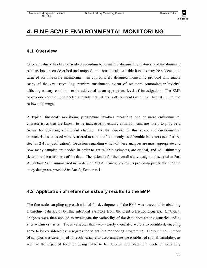
Sustainable Management Contract No. 5096
National Estuary Monitoring Protocol
December 2002
22
4. FINE-SCALE ENVIRONMENTAL MONITORING
4.1 Overview
Once an estuary has been classified according to its main distinguishing features, and the dominant
habitats have been described and mapped on a broad scale, suitable habitats may be selected and
targeted for fine-scale monitoring. An appropriately designed monitoring protocol will enable
many of the key issues (e.g. nutrient enrichment, extent of sediment contamination/toxicity)
affecting estuary condition to be addressed at an appropriate level of investigation. The EMP
targets one commonly impacted intertidal habitat, the soft sediment (sand/mud) habitat, in the mid
to low tidal range.
A typical fine-scale monitoring programme involves measuring one or more environmental
characteristics that are known to be indicative of estuary condition, and are likely to provide a
means for detecting subsequent change. For the purpose of this study, the environmental
characteristics assessed were restricted to a suite of commonly used benthic indicators (see Part A,
Section 2.4 for justification). Decisions regarding which of these analyses are most appropriate and
how many samples are needed in order to get reliable estimates, are critical, and will ultimately
determine the usefulness of the data. The rationale for the overall study design is discussed in Part
A, Section 2 and summarised in Table 7 of Part A. Case study results providing justification for the
study design are provided in Part A, Section 6.4.
4.2 Application of reference estuary results to the EMP
The fine-scale sampling approach trialled for development of the EMP was successful in obtaining
a baseline data set of benthic intertidal variables from the eight reference estuaries. Statistical
analyses were then applied to investigate the variability of the data, both among estuaries and at
sites within estuaries. Those variables that were closely correlated were also identified, enabling
some to be considered as surrogates for others in a monitoring programme. The optimum number
of samples was determined for each variable to accommodate the established spatial variability, as
well as the expected level of change able to be detected with different levels of variability

Sustainable Management Contract No. 5096
National Estuary Monitoring Protocol
December 2002
23
(~sampling precision). Parts A and B of this document contain the baseline data and describe the
development of the project and the methodologies employed.
Estuary sampling on the Waimea Inlet.
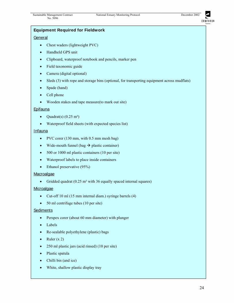
Sustainable Management Contract No. 5096
National Estuary Monitoring Protocol
December 2002
24
Equipment Required for Fieldwork
General
• Chest waders (lightweight PVC)
• Handheld GPS unit
• Clipboard, waterproof notebook and pencils, marker pen
• Field taxonomic guide
• Camera (digital optional)
• Sleds (3) with rope and storage bins (optional, for transporting equipment across mudflats)
• Spade (hand)
• Cell phone
• Wooden stakes and tape measure(to mark out site)
Epifauna
• Quadrat(s) (0.25 m²)
• Waterproof field sheets (with expected species list)
Infauna
• PVC corer (130 mm, with 0.5 mm mesh bag)
• Wide-mouth funnel (bag plastic container)
• 500 or 1000 ml plastic containers (10 per site)
• Waterproof labels to place inside containers
• Ethanol preservative (95%)
Macroalgae
• Gridded quadrat (0.25 m² with 36 equally spaced internal squares)
Microalgae
• Cut-off 10 ml (15 mm internal diam.) syringe barrels (4)
• 50 ml centrifuge tubes (10 per site)
Sediments
• Perspex corer (about 60 mm diameter) with plunger
• Labels
• Re-sealable polyethylene (plastic) bags
• Ruler (x 2)
• 250 ml plastic jars (acid rinsed) (10 per site)
• Plastic spatula
• Chilli bin (and ice)
• White, shallow plastic display tray

Sustainable Management Contract No. 5096
National Estuary Monitoring Protocol
December 2002
25
4.3 Methods
Step 1: Choose appropriate monitoring sites The choice of sites (generally a total of 2 to 4 per estuary) is made using a combination of the
knowledge collected through the broad-scale habitat mapping and on-site, specialist expertise as
follows:
• Broad-scale habitat maps and local knowledge are used to locate broad areas of unvegetated,
mid-low water, mud/sand habitat located away from river mouths (mean salinity of
overlying water > 20 ppt).
• A representative position within each of the broad areas is then chosen to locate potential
sampling sites. Areas of significant vegetation and channel areas are avoided.
• The number of sites selected for an estuary should be allocated proportionately, based on
estuary size, extent of the mud/sandflat habitat, and the number of isolated arms. Large (i.e.
>3000 ha) and/or highly branched estuaries should be allocated more sites (e.g. four), while
those that are small or less complex in shape, can be allocated fewer.
• Additional sites may be added for areas that are of particular interest or concern (i.e. consent
monitoring sites).
Step 2: Carry out the field work (between January-March) See Figure 2 for a summary diagram of the sampling strategy. Ideally you will require three trained
and reasonably fit staff to undertake the sampling.
1. A person capable of identifying estuarine epifauna.
2. A person able to operate the hand-held GPS and camera.
3. A person able to collect physical, chemical and infauna
core samples.
Each of these people should be wearing lightweight, flexible leg,
chest waders so they can easily sit and keep warm and dry in soft mud
conditions.
Sampling in the mud,demonstrating how important chest waders are!

Sustainable Management Contract No. 5096
National Estuary Monitoring Protocol
December 2002
26
Sampling can be undertaken on wet days, but ideally it should be dry. The work will need to be
carried out over the low tide period beginning approximately 1.5 hrs prior to low water. It will
usually take around two hours per site. Don’t leave the sampling till too late in the day because an
hour or two is required to sieve infauna samples before preserving. All samples should be clearly
labelled with estuary, site, station (plot), date/time and collectors (pre-labelling is a must given the
generally muddy conditions at each site). Tide (spring or neap) and weather conditions and any site
features of interest should be recorded in the field notebook.
Marking out the sites: The areal extent of the sand/mud habitat may differ considerably from one
estuary to another. Thus there may be reason to consider the use of sites proportional to the size of
the estuary or habitat. To simplify this decision, we suggest that sites of a standard size of 60 x 30
m would be suitable in most cases.
• Sites of 60 x 30 m are marked out with the aid of a tape measure for placement of wooden
stakes at each corner.
• Corner positions are recorded using differential GPS to enable subsequent repeat surveys.
• The site is then subdivided into 12 equal-sized (i.e. 15 x 10 m) plots. Plot intersections can
be marked with temporary stakes (e.g. bamboo) to provide reference points when sampling.
It is recommended that 10 of these plots be sampled on each occasion.
Fine-scale sampling at the New River Estuary, showing the collection of sediment core samples.
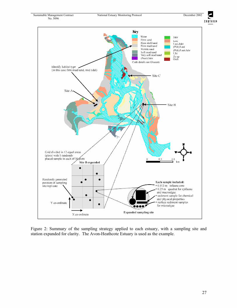
Sustainable Management Contract No. 5096
National Estuary Monitoring Protocol
December 2002
27
Figure 2: Summary of the sampling strategy applied to each estuary, with a sampling site and station expanded for clarity. The Avon-Heathcote Estuary is used as the example.

Sustainable Management Contract No. 5096
National Estuary Monitoring Protocol
December 2002
28
Photographs: Photographs are taken to provide a record of the general site appearance. If a digital
camera is available, these can easily be archived for comparison with subsequent survey results.
Sediment core profiles (and the depth of the Redox Discontinuity Layer):
• One randomly positioned 60 mm perspex core is collected to a
depth of at least 100 mm from each plot.
• The core is extruded onto a white plastic tray, split lengthwise
(vertically) into two halves and photographed along side a ruler
and a corresponding label.
• The stratification of colour and texture are described with
particular attention to the occurrence of any black (anoxic)
zones. Where these occur, the average depth of the lighter-
coloured surface layer is recorded as the depth of the Redox Discontinuity Layer (RDL).
Epifauna: (surface-dwelling animals):
• Epifauna are assessed from 10 replicate 0.25 m2 quadrats within each site (one randomly
placed within 1m of the Perspex core sample within each plot). All animals observed on the
sediment surface are identified and counted, and any visible microalgal mat development is
noted. Crab burrows may be counted as a relative indicator of mud crab populations, but the
data can not be used as a direct measure of abundance without calibration. The species,
abundance and related descriptive information are recorded on specifically designed,
Notes:
• Distinct RDLs were not observed at any of the REs. However in
highly enriched situations, the black anoxic layer may be at, or very
near, the sediment surface and a strong rotten egg odour of hydrogen
sulphide gas will be evident. In extreme situations a patchy, white
bacterial mat may be visible on the surface of the sediment. These are
the white sulphur bacteria (Beggiatoa sp.) that help to detoxify the
system by oxidising the H2S.
The perspex corer used to sample sediments.

Sustainable Management Contract No. 5096
National Estuary Monitoring Protocol
December 2002
29
waterproof field data sheets containing a checklist of expected species (see the example
provided in Table 3).
• Photographs of representative quadrats are taken and archived for future reference.
Macroalgae (seaweeds) % cover:
• Where a significant macroalgal cover exists, the percent coverage is estimated from the
epifauna quadrats, but with gridlines dividing it into 36 equally-spaced squares. The
number of grid intersections (49 in total, including the outer frame) that overlap vegetation
are counted and the result converted to a percent (i.e. No. x 2 = %). The data can be
recorded on the same field data sheets used for epifauna analyses.
Infauna (animals living buried in the sediments):
• Ten sediment cores (one randomly placed within 1 m of the
Perspex core sample within each plot) are collected from
each site using 130 mm diameter (area = 0.0133 m2) PVC
tubes with 0.5 mm nylon mesh bags affixed to the top to
act as a sieve.
• The core tubes are manually driven 150 mm into the
sediments, removed with core intact and inverted so that
the core is retained in the mesh bag.
• The contents of the core are washed through the attached sieve using seawater from a nearby
source. The remaining contents are carefully emptied into a plastic container with a
waterproof label and preservative is added. Although 4% formalin (made up in seawater) is
traditionally used as a preservative, it is a potentially dangerous chemical. We
recommend using 95% ethanol instead (enough to roughly double the volume of the
sample).
The PVC corer with 0.5 mm mesh bag attached for sampling infauna.

Sust
aina
ble
Man
agem
ent C
ontra
ct
No.
509
6 N
atio
nal E
stua
ry M
onito
ring
Prot
ocol
Dec
embe
r 200
2
30
Tabl
e 3:
Che
cklis
t of e
xpec
ted
epib
iota
for N
ew Z
eala
nd e
stua
ries
Plot
1 2
3 4
5 6
7 8
9 10
Sp
ecie
s C
omm
on n
ame
Com
inel
la g
land
iform
is
Mud
flat w
helk
C
omin
ella
mac
ulos
a Sp
otte
d W
helk
D
ilom
a su
rost
rata
M
udfla
t top
shel
l
D
ilom
a ze
land
ica
M
icre
lenc
hus h
utto
ni
Tops
hell
Zeac
uman
tus s
ubca
rinat
a Sm
all s
pire
shel
l
Ze
acum
antu
s lut
ulen
tus
Spire
shel
l
Am
phib
ola
cren
ata
Not
oacm
ea h
elm
si
Estu
arin
e lim
pet
Aust
rove
nus s
tutc
hbur
yi
cock
le
Paph
ies a
ustr
alis
pi
pi
Mac
tra
disc
ors
larg
e tro
ugh
shel
l
M
acra
ova
ta
oval
trou
gh sh
ell
Cra
ssos
trea
gig
as
Paci
fic o
yste
r
C
rab
hole
s
Hal
icar
cinu
s var
ius
Pilb
ox c
rab
Ente
rom
orph
a
Isop
od
Ed
war
dsia
tric
olor
B
urro
win
g an
emon
e
An
thop
leur
a au
reor
adia
ta
Mud
flat a
nem
one
Elm
iniu
s mod
estu
s Es
tuar
ine
barn
acle
G
raci
lari
a
Ulv
a
Equ
ipm
ent:
10
Qua
drat
s, C
ores
, (gr
ain
size
and
AFD
W) b
ags,
Pottl
es (n
utrie
nts,
org
C, m
etal
s), s
yrin
ge (m
icro
alga
e), p
hoto
s, be
nthi
c al
gae,
GPS
.
30

Sustainable Management Contract No. 5096
National Estuary Monitoring Protocol
December 2002
31
Benthic microalgae:
• Cut-off 10 cc syringe barrels (15 mm internal diameter) are used to collect sediment cores
(four per plot from within 0.5m of the epifauna quadrat).
• The top 5 mm of the cores are sliced off and mixed in a 50 ml centrifuge tube to obtain one
sediment composite per plot.
• Samples are stored on ice (in the dark) while in the field and frozen (-20oC) upon return.
Notes:
• In firm substrates, it may be necessary to remove the core by digging.
• Avoid rigorous handling of samples (especially during rinsing through
mesh) to avoid damaging organisms.
• If water for sieving the infauna samples is too far away, you may need to
use larger plastic bags (well-labelled) to transport the cores to the water
(after sampling is finished at that site). Do not pour water through the
mesh bag. Just immerse the closed end of the bag into the water and
gently agitate to wash the fine sediment through the sieve. Then transfer
the remaining contents into plastic containers (labelling and adding
preservative).
• When transporting preserved samples, care must be taken to avoid
spillage. Place containers in a large, tied-off plastic bag to minimise
leakage.
Sustainable Management Contract No. 5096
National Estuary Monitoring Protocol
December 2002
32
Physical and chemical analyses:
• Ten replicate samples (one from each plot) are collected from an area within 300 mm of the
position of the infauna cores. The top 20 mm of sediment is scraped into a clean, acid-
rinsed (see note) 250 ml plastic jar and stored on ice until processed (preferably within 12
hours).
Notes:
• The clean plastic container should be rinsed thoroughly with 10% HCl,
followed by deionised water, prior to use.
• Avoid cross-contamination of samples and any contact with metal
implements (use a plastic spatula).
• Do not place a label inside the plastic container. If necessary, cover
the outer label with Cellotape to keep dry.
Notes:
• The primary objective of benthic microalgal analyses is to identify any
major bloom occurrences that could be indicative of eutrophic (highly
enriched) conditions. Sediment chl a and phaeopigment concentrations
provide an indication of the degree of mat development
• Some species of benthic microalgae (e.g. euglenoids) and
cyanobacteria (blue green algae) may be indicative of nutrient
enrichment; particularly if they dominate the microalgal community.
However, more data is required before this can be developed as a
useful indicator. If you would like to contribute to this process, collect
one additional composite sample using the same procedure as for chl a,
but preserve it with Lugol’s Iodine solution (do not freeze).
Sustainable Management Contract No. 5096
National Estuary Monitoring Protocol
December 2002
33
Step 3: Process the samples
Epifauna
• Field notes are transferred to a spreadsheet or database for statistical analyses.
Infauna
• Samples are washed through a series of sieves (from 4.0 mm to 0.5 mm) within a fume
cabinet to roughly sort invertebrates into size classes.
• The contents of each sieve are systematically scanned, by eye or by microscope, and the
invertebrate species identified (to at least the family level), counted and recorded.
• The data is transferred to a spreadsheet or database ready for statistical analyses.
Microalgae
• Pigments are analysed as described in Part A, Table 19.
• Optional identification of dominant species may be carried out using an inverted
microscopic. These analyses require technical expertise/training.
Physical and chemical analyses
• The chilled samples are sent to an appropriate analytical laboratory, where the they are
analysed for the following characteristics (as described in Part A, Table 19):
Particle size distribution (% mud, sand, gravel)
Nutrients (total nitrogen and total phosphorus)
Ash free dry weight (AFDW) as a measure of total organic content
Common trace metal contaminants (copper, cadmium, nickel, lead, zinc and chromium).
Notes:
• Skill/experience is required for the identification of invertebrate species. There are a
variety of suitable reference texts available (refer reference list, Part A).
• It is often helpful to keep a reference collection of invertebrate species obtained from
the sediment samples.
• If formalin is used as a preservative, care should be taken to avoid inhalation of
fumes which can be hazardous to health.
Sustainable Management Contract No. 5096
National Estuary Monitoring Protocol
December 2002
34
• All data are transferred to a spreadsheet or database for statistical analyses.
Step 4. Carry out data analyses
Data Manipulation
a) Arrange data logically in a spreadsheet (replicates aligned in columns, variables in adjacent
rows, anticipate incorporating consecutive years data).
b) Check data values:
• Check that the units are appropriate (e.g. infauna core area, concentrations), convert the
data if necessary.
• Check the comparability of the sampling procedures and analytical methods,
• Check for values recorded as <detection limits. Less-than signs (<) preceding data
values often inhibit computation and the associated detection limit represents the
maximum likely value. Although not entirely accurate, assigning a value, ca. 0.5 ×
detection limit, allows the result to be included in further analyses. An indication that
the result was very low (i.e. below detection limit) is important information, despite not
knowing the exact magnitude.
• Check for anomalies or aberrant data points. Box plots may help with this. If the result
is obviously erroneous or can be attributed to interference or contamination from an
irrelevant source, it can be removed. Data should not be removed without justification.
• Check that missing data are represented by empty cells rather than zeros. Zeros in place
of missing data will erroneously lower the mean value and effect sample variability.
c) Create a secondary table where the chemical values are normalised to the % mud fraction. This
is achieved by dividing the result by the corresponding % mud value and then multiplying by
100.
Note:
• Analyses of other metals/contaminants may be included where they are
of particular concern in an estuary.
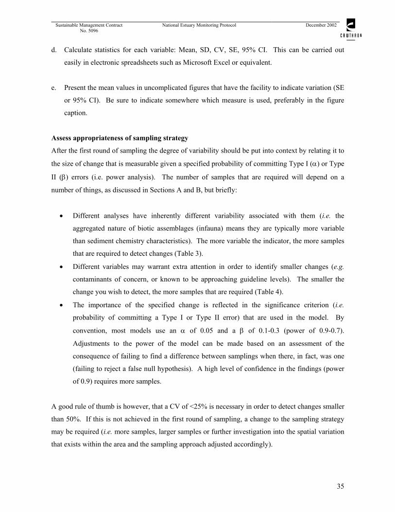
Sustainable Management Contract No. 5096
National Estuary Monitoring Protocol
December 2002
35
d. Calculate statistics for each variable: Mean, SD, CV, SE, 95% CI. This can be carried out
easily in electronic spreadsheets such as Microsoft Excel or equivalent.
e. Present the mean values in uncomplicated figures that have the facility to indicate variation (SE
or 95% CI). Be sure to indicate somewhere which measure is used, preferably in the figure
caption.
Assess appropriateness of sampling strategy
After the first round of sampling the degree of variability should be put into context by relating it to
the size of change that is measurable given a specified probability of committing Type I (α) or Type
II (β) errors (i.e. power analysis). The number of samples that are required will depend on a
number of things, as discussed in Sections A and B, but briefly:
• Different analyses have inherently different variability associated with them (i.e. the
aggregated nature of biotic assemblages (infauna) means they are typically more variable
than sediment chemistry characteristics). The more variable the indicator, the more samples
that are required to detect changes (Table 3).
• Different variables may warrant extra attention in order to identify smaller changes (e.g.
contaminants of concern, or known to be approaching guideline levels). The smaller the
change you wish to detect, the more samples that are required (Table 4).
• The importance of the specified change is reflected in the significance criterion (i.e.
probability of committing a Type I or Type II error) that are used in the model. By
convention, most models use an α of 0.05 and a β of 0.1-0.3 (power of 0.9-0.7).
Adjustments to the power of the model can be made based on an assessment of the
consequence of failing to find a difference between samplings when there, in fact, was one
(failing to reject a false null hypothesis). A high level of confidence in the findings (power
of 0.9) requires more samples.
A good rule of thumb is however, that a CV of <25% is necessary in order to detect changes smaller
than 50%. If this is not achieved in the first round of sampling, a change to the sampling strategy
may be required (i.e. more samples, larger samples or further investigation into the spatial variation
that exists within the area and the sampling approach adjusted accordingly).
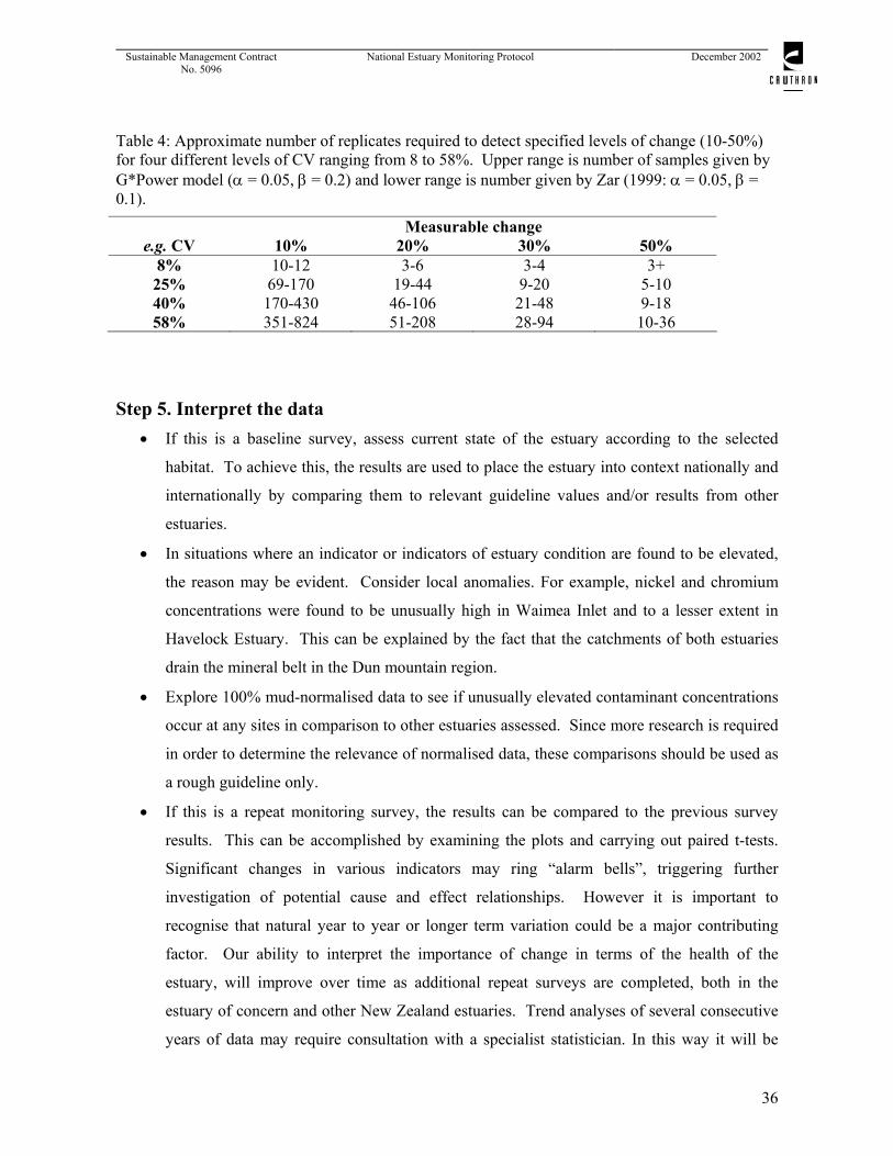
Sustainable Management Contract No. 5096
National Estuary Monitoring Protocol
December 2002
36
Table 4: Approximate number of replicates required to detect specified levels of change (10-50%) for four different levels of CV ranging from 8 to 58%. Upper range is number of samples given by G*Power model (α = 0.05, β = 0.2) and lower range is number given by Zar (1999: α = 0.05, β = 0.1).
Measurable change e.g. CV 10% 20% 30% 50%
8% 10-12 3-6 3-4 3+ 25% 69-170 19-44 9-20 5-10 40% 170-430 46-106 21-48 9-18 58% 351-824 51-208 28-94 10-36
Step 5. Interpret the data • If this is a baseline survey, assess current state of the estuary according to the selected
habitat. To achieve this, the results are used to place the estuary into context nationally and
internationally by comparing them to relevant guideline values and/or results from other
estuaries.
• In situations where an indicator or indicators of estuary condition are found to be elevated,
the reason may be evident. Consider local anomalies. For example, nickel and chromium
concentrations were found to be unusually high in Waimea Inlet and to a lesser extent in
Havelock Estuary. This can be explained by the fact that the catchments of both estuaries
drain the mineral belt in the Dun mountain region.
• Explore 100% mud-normalised data to see if unusually elevated contaminant concentrations
occur at any sites in comparison to other estuaries assessed. Since more research is required
in order to determine the relevance of normalised data, these comparisons should be used as
a rough guideline only.
• If this is a repeat monitoring survey, the results can be compared to the previous survey
results. This can be accomplished by examining the plots and carrying out paired t-tests.
Significant changes in various indicators may ring “alarm bells”, triggering further
investigation of potential cause and effect relationships. However it is important to
recognise that natural year to year or longer term variation could be a major contributing
factor. Our ability to interpret the importance of change in terms of the health of the
estuary, will improve over time as additional repeat surveys are completed, both in the
estuary of concern and other New Zealand estuaries. Trend analyses of several consecutive
years of data may require consultation with a specialist statistician. In this way it will be

Sustainable Management Contract No. 5096
National Estuary Monitoring Protocol
December 2002
37
possible to consider, not only short term impacts but also longer term trends in indicator
levels.
4.4 How often to sample and report?
It is recommended that a suitable long-term monitoring programme will include an initial period of
3-5 years of annually monitoring of the same sites, at the same time of year, in each estuary. This
will broaden the baseline by providing an indication of the inter-annual variability thus enhancing
the ability to interpret change over time. State of Environment reporting with detailed interpretation
would be undertaken say every 4 years. Reporting of results only would be undertaken in
intervening years. Once the initial yearly monitoring period is finished, the data would be used to
optimise the design to a lesser monitoring frequency (for example, every two to five years).
4.5 How much will it cost?
Estimated costs for fine scale monitoring are approximately $15,000 to $25,000 per estuary (2-4
sites).
Sleds can be handy when travelling between fine-scale sampling sites (New River Estuary shown).

Sustainable Management Contract No. 5096
National Estuary Monitoring Protocol
December 2002
38
5. THE FUTURE OF THE EMP
5.1 The “Living Document” concept
All three documents comprising the EMP should be updated periodically. The individual estuary
results provide potentially valuable datasets for managers that can be further evaluated and/or
expanded as additional data becomes available. As the protocol is applied to additional estuaries,
the expanded database will most likely extend the range of conditions within the continuum from
pristine to highly modified. It will also extend the range of estuary types and habitat types
compared.
The expanding data base will also provide opportunities for future development of various indices
of estuarine condition. For example, as the data base expands, the species and abundance of animal
communities may be used to develop biotic indices, while physico-chemical characteristics could
lead to development of companion indices (e.g. of nutrient enrichment). Ultimately, guidelines
may be recommended in order to facilitate evaluation of the state of health of estuarine habitats in
New Zealand.
Methodologies can also be improved over time (e.g. taxonomic precision), and new tools may
become available (e.g. satellite imagery, GIS software capabilities). Thus the Protocol and
supporting data should be viewed as a “living document” that will improve with use and
technological advancement.
5.2 A National estuaries database
The EMP provides coastal managers with a standardised methodology to collect a variety of data
types from various disciplines. The different data types include GIS mapping information and fine-
scale physical, chemical and biological descriptions of estuary condition. The large volumes of data
generated, particularly with regard to the fine-scale monitoring, can be difficult to manage
effectively. In order to facilitate this, we envisage the development of a database for the entry,
storage and retrieval of this information as a logical follow-on to the existing project. However,

Sustainable Management Contract No. 5096
National Estuary Monitoring Protocol
December 2002
39
rather than trying to develop and maintain a centralised database for all the information collected by
the various groups, we believe it would be more effective to develop a stand-alone version that can
be distributed (via the web) and operated by the various end-users but would still guarantee that the
data was collected and maintained in a similar format. Essentially, the National database would be
housed individually but could be incorporated into a single entity in the future if need arose.
5.3 Continued technical support
Cawthron’s Coastal and Estuarine Group are dedicated to continued support of the EMP initiative.
In some instances, councils may wish to develop and carry out their own monitoring programmes
with minimum consultation (i.e. advice only). In others, they may elect to contract some or all of
the work to an independent science provider. Cawthron would be pleased to provide support in
either capacity.
Cawthron would like to thank all participants in the Estuary Monitoring Protocol Workshop, 5 September 2002, Nelson.

Sustainable Management Contract No. 5096
National Estuary Monitoring Protocol
December 2002
40
CAWTHRON INSTITUTE
98 Halifax Street East Private Bag 2
NELSON NEW ZEALAND
Phone: +64.3.548.2319
Fax: +64.3.546.9464 Email: [email protected]
www.cawthron.org.nz
Related Documents